nonlinear criterion for the stability of molecular clouds
TRANSCRIPT

arX
iv:a
stro
-ph/
0512
629v
1 2
8 D
ec 2
005
Journal reference: THE ASTROPHYSICALJOURNAL, 635:1126–1135, 2005 December 20Preprint typeset using LATEX style emulateapj v. 12/14/05
NONLINEAR CRITERION FOR THE STABILITY OF MOLECULAR CLOUDS
RUBEN KRASNOPOLSKY ANDCHARLES F. GAMMIECenter for Theoretical Astrophysics, University of Illinois at Urbana-Champaign, Loomis Laboratory of Physics,
1110 West Green Street, Urbana, IL 61801Received by ApJ 2004 May 28, accepted 2005 July 30, published2005 December 20
ABSTRACTDynamically significant magnetic fields are routinely observed in molecular clouds, with mass-to-flux ratio
λ ≡ (2π√
G)Σ/B∼ 1 (hereΣ is the total column density andB is the field strength). It is widely believed that“subcritical” clouds withλ < 1 cannot collapse, based on virial arguments by Mestel and Spitzer and a linearstability analysis by Nakano and Nakamura. Here we confirm, using high resolution numerical models thatbegin with a strongly supersonic velocity dispersion, thatthis criterion is a fully nonlinear stability condition.All the high-resolution models withλ ≤ 0.95 form “Spitzer sheets” but collapse no further. All modelswithλ ≥ 1.02 collapse to the maximum numerically resolvable density.We also investigate other factors determin-ing the collapse time for supercritical models. We show thatthere is a strong stochastic element in the collapsetime: models that differ only in details of their initial conditions can have collapse times that vary by as muchas a factor of 3. The collapse time cannot be determined from just the velocity dispersion; it depends also onits distribution. Finally, we discuss the astrophysical implications of our results.Subject headings:star formation
1. INTRODUCTION
Molecular clouds evolve under the influence of self-gravityso as to condense part of their mass into dense cores and, ul-timately, stars. The presence of magnetic fields can preventor delay condensation. The possibility was first studied byMestel & Spitzer (1956), who noted that the magnetic energyand the gravitational energy scale in exactly the same waywith the radiusRof the cloud (∝ 1/R) if flux freezing obtains.They argued that there was therefore a critical mass belowwhich a cloud threaded by a particular field strength would beunable to collapse.
A more precise but less general argument was advanced byNakano & Nakamura (1978), who studied the linear theoryof a self-gravitating, isothermal, equilibrium sheet of plasmathreaded by a perpendicular magnetic field. They found thatmagnetic fields stabilize the sheet against gravitational col-lapse if the mass-to-flux ratio is smaller than 1/2π
√G.
These results motivate the definition of a dimensionlessmass-to-flux ratio,
λ ≡ 2π√
GΣB
, (1)
whereΣ is the column density of the sheet, andB is the mag-netic field strength. The exact coefficient used to defineλdepends somewhat on the geometry of the collapse. Herewe have chosen the coefficient most relevant to the magneticfield geometry adopted in this paper, tending to produce thinsheets, in agreement with the expectations for magneticallysupported clouds. Clouds withλ > 1 are termedsupercriti-cal, and clouds withλ < 1 are termedsubcritical.
Both the Mestel & Spitzer and the Nakano & Nakamuramodels consider exact equilibria. Molecular clouds are farfrom equilibrium, however, with near-virial, highly super-sonic velocity dispersion. These internal velocities mustarisefrom strong turbulence.1 Turbulence might change the stabil-
1 The most plausible alternative to turbulence, some type of weakly dissi-pative ordered flow, does not emerge naturally in any relevant numerical ex-periments that we are aware of. The mode-mode coupling is always strong.Even circularly polarized Alfven waves, which are exact solutions to the com-
ity properties of the cloud, either by compressing aλ < 1 flowuntil it collapses, or by providing turbulent support to a cloudwith λ > 1.
Many works have suggested that turbulence could pro-vide support to star-forming clouds. Chandrasekhar & Fermi(1953) included turbulent support in their model for interstel-lar gaseous structures. Mestel & Spitzer (1956) pointed outthat turbulence tends to decay, and that turbulence of am-plitude large enough to support a cloud against self-gravitywould decay especially quickly, although allowing the pos-sibility that a strong magnetic field might perhaps allowlonger lived turbulence. The supersonic linewidths observedin molecular clouds were attributed to radial motions insidethe cloud instead of turbulence by Goldreich & Kwan (1974).Zuckerman & Palmer (1974) argued that if this interpretationwere true for all clouds where such fluctuations are observed,the star formation rate would be too large by at least one or-der of magnitude. Arons & Max (1975) then suggested thatthe observed velocity fluctuations are due to hydromagneticwaves. By the late 1980s, this idea was widely accepted (e.g.,Shu, Adams, & Lizano 1987). In the late 1990s, however, asuccession of numerical experiments (Mac Low et al. 1998;Stone, Ostriker, & Gammie 1998; Gammie & Ostriker 1996)strongly suggested that the damping time of turbulence inmagnetized molecular clouds is close to the dynamical time.If one accepts this, then turbulent pressure can be effective insupporting self-gravitating clouds only if it is constantly re-plenished, in which case the support is perhaps more readilyidentified with the stirring mechanism than with the turbu-lence itself.
Other work has tended to emphasize the role of turbulencein initiating gravitational collapse (e.g., Mac Low & Klessen2004). Regions with a convergent velocity field will natu-rally tend to collapse sooner than regions with divergent ve-locity fields. It seems highly likely that some parts of molec-ular clouds have strongly convergent velocity fields; is thisever enough to overcome the stabilizing effects of the mag-
pressible equations of motion, suffer from a parametric instability with a dy-namical decay rate (Sagdeev & Galeev 1969; Goldstein 1978).

2 KRASNOPOLSKY ANDGAMMIE
netic field? Can a subcritical cloud be induced to collapse bysqueezing, or can a supercritical cloud be prevented from col-lapsing by the introduction of turbulence? The purpose of thispaper is to investigate these questions using a simple series ofnumerical experiments.
The plan of the paper is as follows. In§2 we describe the ex-perimental design, our numerical methods, and the diffusioncharacteristics of our code (based on the ZEUS algorithm). In§3 we describe results, including a “fiducial” run, and the in-fluence of physical and numerical parameters on the outcome.§4 summarizes and discusses astrophysical implications.
2. DESCRIPTION OF NUMERICAL EXPERIMENTS
We will consider the simplest possible system that can man-ifest sub/supercritical behavior: a two-dimensional, periodicbox containing a magnetized, self-gravitating, isothermal gas.Since we are interested in studying the effects of turbulence,we will introduce a velocity field in the initial conditionswith statistical properties similar to those found in interstel-lar clouds. We will then allow the system to evolve for manydynamical times, or until it “collapses.”
Specifically, we consider a square domain in thex−y planeof size L × L. The z direction points out of this plane; noquantity depends onz. The initial fluid density isρ , and thesound speed, which is constant in space and time, iscs. Theinitial field is B = Bxx, whereBx is constant. The strengthof the field can be characterized byλ = 2π
√GρL/Bx. We
set the initial value of〈Bz〉 = 0, because otherwise in thisz-independent geometry, asymptotically there is no collapse.
The initial velocity field is a Gaussian random field withzero divergence, constructed as in Ostriker, Gammie, & Stone(1999). The initial velocity field has a power spectrum
⟨
v2k
⟩
∝k−3 for 2π/L < k < 8(2π/L) andk ·vk = 0. This power spec-trum is consistent, in 2D, with Larson’s Lawvλ ∼ λ 1/2, whichis equivalent to an energy spectrumEk ∼ k−2 (in 3D Larson’sLaw implies
⟨
v2k
⟩
∝ k−4). The velocity is normalized so thatthe kinetic energyEK matches the desired value, and 1/3 ofthe kinetic energy is in motions perpendicular to thex− yplane of the simulation.
2.1. Spitzer sheets and simulation units
In our experiments we will frequently find that matter flowsalong magnetic field lines to form sheets normal to the field.These sheets are given coherence by the self-gravity of themedium. Spitzer (1942) was the first to consider the problemof the vertical structure of an infinite, self-gravitating,isother-mal sheet. Spitzer’s solution turns out to be highly useful inunderstanding the evolution of our simulations. Spitzer foundthat the equilibrium density profile of a sheet of surface den-sity Σ is ρ(z) = (Σ/2H)sech2(z/H) whereH = cs
2/(πGΣ).The corresponding gravitational potential and field areφS =2cs
2 log(cosh(z/H)) andg = −2πGΣ tanh(z/H).For any given Spitzer sheet formed during our simulation
the surface density parameterΣ corresponds toρLs, whereLs is the extent of the region along the fieldlines that a givensheet has collected its mass from. At late times we can assumethatLs ≈ L: most of the mass originally distributed along thefieldlines will be collected into the given sheets. This is truefor the most massive sheets in the supercritical simulations,and it is seen even more clearly in the subcritical simulations,where at late times in the simulation a single large scale, sta-ble sheet incorporates most of the mass of the system. In thefollowing we will assumeLs ≈ L andΣ = Lρ for the Spitzer
sheets we are largely interested in — those that have collectedmost mass.
We nondimensionalize our models by settingL = 1, ρ = 1,andcs = 1. The simulation time unit is thereforeL/cs, thesound crossing time. In these units, Newton’s gravitationalconstant equalsπnJ
2, the Jeans length is 1/nJ, the peak den-sity ρS of an equilibrium Spitzer sheet ofLs = L is (πnJ)
2/2,and its half-thicknessH equals(πnJ)
−2. Notice that, becauseof the periodic boundary conditions the Spitzer sheets areslightly distorted, but as long asH ≪ 1, the Spitzer solutionwill be approximately correct.
Most of the simulations presented in this paper havenJ =3. This implies that the semithickness of the Spitzer sheet is0.011, and if we are to resolve this with at least four grid zoneswe needN > 360, where the resolution of our uniform grid isN2. This rather stringent resolution requirement explains whywe have chosen to study the problem in 2D rather than 3D.
This Spitzer-sheet model is especially useful whenλ . 1inside a largely ordered magnetic field, able to channel theflow into sheets, which later might become unstable and col-lapse, through accretion, collision, and merger. This sheetmodel, however, is not useful whereλ ≫ 1 and collapse isunconstrained by the field.
Simulation units can be converted to dimensional valuesby assuming for illustrative purposes a typical densitynH2 =
102cm−3, and a typical temperatureT = 10K. Then thesound speedcs = 0.19kms−1 fixes the unit of speed, andfrom the Jeans lengthLJ = cs(π/Gρ)1/2 = 1.9pc we obtainthe unit of lengthL = nJLJ = 5.7pc for our standard valuenJ = 3; a Spitzer sheet would then have a peak density ofnH2 = 4.4×103cm−3, andH = 0.064pc. The unit of mass isgiven byρL3 = ρnJ
3LJ3 = 1.3×10³M⊙. The unit of time is
the sound crossing timets = L/cs ≈ 30Myr. A characteristicgravitational contraction time istg = LJ/cs≈ 10Myr; free-fallcollapse times are on the order of 0.3tg ≈ 3Myr, depending onthe geometry of the collapse.
The sound-crossing time of a Spitzer sheet is∼ H/cs ≈0.3Myr. From the Spitzer sheet parametersρS and H itis possible to define a characteristic “Spitzer” massMS =(πH)2Σ = cs
4/(G2Σ) = (π2nJ4)−1 in dimensionless units,
with Σ = Lρ . The factor ofπ2 is designed to capture themass inside half a wavelength of the shortest unstable modeof the sheet (Ledoux 1951; Elmegreen & Elmegreen 1978).For parameters typical of a molecular cloud,MS = 1.6M⊙,which is a suggestive result. This may be compared withthe thermal Jeans massMJ = ρLJ
3 = π3/2cs3/G3/2ρ1/2 =
nJ−3 in dimensionless units, with a typical value ofMJ =
49(T/10K)3/2(
nH2/10cm−3)−1/2
M⊙.
2.2. Ambipolar diffusion
Our simulation utilizes the ideal MHD equations, whichhave some well-known limitations. Ambipolar diffusion is ex-pected to become relevant (Kulsrud & Pearce 1969) at length-scales smaller than the damping length for Alfven waves,LAD ∼ vAtni, wherevA = B/
√4πρ, andtni = 1/(Kni), with
K ≈ 1.9×10⁻⁹cm3s−1 (Draine, Roberge, & Dalgarno 1983).The number density of ionsni may depend strongly on en-vironmental factors, such as the UV illumination and its at-tenuation by the cloud material (Ciolek & Mouschovias 1995;McKee 1989); it also depends on chemical properties, such asthe metal abundance in the gas phase. For our fiducial meandensityρ, a representative value could beni ∼ 2×10⁻⁴cm−3,

NONLINEAR STABILITY OF MOLECULAR CLOUDS 3
largely limited by an assumed metal abundancexM ≈ 10−6.For the typical peak density of a Spitzer sheetρS in our con-ditions,ni ∼ 6×10⁻⁴cm−3 for cosmic-ray dominated ioniza-tion, and about ten times larger for regions of the cloud thatare moderately well UV-illuminated.
The ambipolar diffusion lengthscaleLAD can now be com-pared with the sizeL of the computational volume, giving anestimate of the scale at which ideal MHD stops being a com-plete dynamical description of the flow. For our mean densityprofile, we find that this lengthscale isLAD ∼ L/35, muchlarger than our typical grid spacingL/512, and comparable toour typical sheet thickness 2H = L/45. However, ideal MHDis still a good description of the most important portions ofthis study; the regions where mass is collected to form densesheets. Forρ = ρS, the lengthscales areLAD ∼ L/700 for aUV-dark region, andLAD ∼ L/7000 for the more illuminatedcase. The decrease ofvA with density has contributed to thiseffect, together with the largerni .
We keep in mind, however, that densities and ionizationrates vary widely inside clouds, and so the ambipolar diffu-sion lengthscales and timescales may vary widely. Turbulentconditions inside the flow are also expected to increase the im-portance of ambipolar diffusion, even at larger lengthscales,especially near sharp velocity and magnetic gradients.
2.3. Stopping criterion
We must fix some criterion for stopping the numerical in-tegration; when the density in any zone equals or exceeds thelargest allowed by the Truelove numerical stability condition(Truelove et al. 1997) the run is terminated and classified ashaving collapsed. The Truelove condition requires that thelocal Jeans length be resolved by some algorithm-dependentnumberNT of grid zones, typically about 4. This requirementsets a maximum resolvable density ofρT = (N/nJNT)2 =1820(N/512)2 for nJ = 3 on our uniform grid ofN2 zones.We have found that further integration of Truelove-unstablemodels results in large local fluctuations in the density, whichcan produce “explosions” that corrupt the entire computa-tional domain. Runs that reacht = 2 without violating theTruelove condition are classified as stable.
We have experimented with other collapse detectionschemes, because the Truelove criterion has the deficiencythat it is resolution dependent. In the Tables described belowwe report not only the timetT at which the Truelove conditionis violated, but also the timet10 when 1% of the mass exceeds10 times the Spitzer densityρS. These times are typicallyclose to each other, and both can be considered as measures ofthe onset of gravitational instability. The timet10 has the ad-vantage of not depending explicitly on numerical resolution,but it can be fooled into producing misleadingly short col-lapse times by strong density fluctuations, particularly whenthe turbulent kinetic energy is large.
2.4. Numerical methods and tests
Our simulations are run on a fixed 2D Cartesian grid, us-ing the ZEUS algorithm (Stone & Norman 1992a,b) as im-plemented for instance in Ostriker, Gammie, & Stone (1999).ZEUS is a numerical algorithm to evolve ideal (non-resistive,non-viscous) non-relativistic MHD flows. It is operator-split, representing the fields on a (possibly moving) Eule-rian staggered mesh. The magnetic field evolution uses con-strained transport (Evans & Hawley 1988) which guaranteesthat∇·B = 0 to machine precision, combined with the method
of characteristics (Hawley & Stone 1995), which ensures ac-curate propagation of Alfven waves. ZEUS is explicit intime, and so the timestep∆t is limited by the Courant con-ditions. In our problem, usually the most stringent has been∆t < ∆x/vA , wherevA = B/
√4πρ can take very large values
in density-depleted regions. A numerical density floor,ρfloor,has been set to limit density depletion, preventing∆t from be-coming too small; we have directly tested that this tiny non-conservation of mass by the code does not alter the simulationresults regarding collapse in any way. The Poisson equation,needed to describe self-gravity, is solved by Fourier transformmethods, using the FFTW code (Frigo & Johnson 2005).
Any Eulerian scheme will cause some diffusion of the mag-netic field with respect to the mass. It is crucial for our exper-iment that this nonconservation ofλ be as small as possible.The numerical diffusivity of ZEUS is difficult to estimate be-cause, unlike a physical resistivity, it is flow dependent. Anempirical approach is therefore required.
We have studied conservation ofλ using two distinct meth-ods. In the first method we initialize a non–self-gravitatingbox using the same initial data as in our main experiments,as described above. We evolve the computation tot = 0.5and then damp the velocity field exponentially (with timescaletdamp= 0.05) untilt = 10. If there were noλ diffusion the boxwould return to a uniform density, uniform field state. Diffu-sion changesλ , so the final state consists of a unidirectionalmagnetic field with density and field strength varying onlyperpendicular to the field, from whichλ can be easily mea-sured.
In the second method we initialize a non–self-gravitatingbox using the same initial data as in our main experiments,but we evolve the computation only tot = 0.5. We then sam-ple 80 field lines chosen to lie at equal intervals of the verticalcomponent of the vector potential (equivalent to lines equally
spaced in magnetic flux). We then integrateρ/(
B2x +B2
y
)1/2
along the field line in thex−y plane,2 using linear interpola-tion to determineρ andB at each position, which immediatelyyieldsλ .
These two methods give nearly identical results. We there-fore adopt the second method exclusively, since it can be usedto probe existing numerical data without any additional, ex-pensive evolution.
One possible figure of merit for the diffusion inλ is σλ /λ0,whereσλ is the dispersion in sampled values ofλ at the finalinstant of the simulation, andλ0 is the nominal initial value(which we call simplyλ outside of this subsection). Tables1 and 2 showσλ /λ0 as a function of resolution and of timeduring a single simulation, respectively. The run shown inTable 2 has a resolution of 5122. The key points here arethat σλ /λ0 decreases as resolution increases, and that in ev-ery caseσλ /λ0 is about 10% or less, which suggests that weshould be able to measure the critical value ofλ to similaraccuracy.
Evidentlyσλ /λ0 is converging, but as≈ N−1/2 rather thanthe expectedN−1. This may be because of the existence ofunresolved regions in the flow where most of the diffusionoccurs, or it may be the result of irreducible “turbulent” dif-fusion that is present independent of the magnitude of the ef-fective numerical diffusion. The numerical diffusion is corre-lated with the amplitude of turbulence. According to Table 2,
2 This is equivalent to integratingρ/(
B2x +B2
y +B2z
)1/2along the 3D field-
line.

4 KRASNOPOLSKY ANDGAMMIE
TABLE 1MASS-TO-FLUX DIFFUSION IN ZEUS,AS A
FUNCTION OF NUMERICAL RESOLUTION
N t σλ /λ0 λmax/λ0 λmin/λ0
400 0.1 9.0 % 1.26 0.78512 0.1 8.6 % 1.31 0.78
1024 0.1 6.1 % 1.30 0.872048 0.1 4.4 % 1.10 0.86512 0.2 8.3 % 1.20 0.79
2048 0.2 4.7 % 1.12 0.85
TABLE 2MASS-TO-FLUX DIFFUSION IN ZEUS,AS A
FUNCTION OF TIME
t σλ /λ0 λmax/λ0 λmin/λ0 EK(t)
0 0 % 1 1 500.01 0.2% 1.01 0.99 370.02 0.9% 1.02 0.97 250.03 2.1% 1.05 0.92 180.04 3.6% 1.10 0.90 150.05 6.4% 1.18 0.84 160.06 8.0% 1.32 0.74 190.1 8.6% 1.31 0.78 170.2 8.3% 1.20 0.79 110.3 9.6% 1.20 0.74 8.50.34 11.1% 1.21 0.71 5.5
much of the diffusion occurs very early in the run, when therms velocity is large.
Another possible figure of merit is the total variation inλ ,that is,|λmax−λmin|/(2λ0), measuring the possible existenceof localized diffusion events in addition to the overall diffu-sivity of the code. We find in Tables 1 and 2 that this quantityis typically of the size∼ 2.4σλ , expected in the mean for thehalf-range of a sample of 80 elements randomly taken from aGaussian distribution. However, the distribution of values ofλ might not always be Gaussian, because localized numericaldiffusion could be important for some fieldlines. In our tables,this may be happening whenλmax reaches values as large as1.3λ0, even at the relatively high resolution ofN = 1024. Thelarger total variation ofλ observed in those simulations sug-gests a possible risk of masking the subcritical nature of somemodels.3 However, we also find that the total variation ofλstarts to drop at the even higher resolution ofN = 2048; nu-merical resolution seems apparently able to reduce also thismore local measure of the diffusivity of the numerical code.
It is worth noting that ambipolar diffusion in nature is likelystrong enough to dominate the diffusion measured here. Forour nominal cloud parameters, we have seen in§2.2 that thedamping length of Alfven waves is of the same order as theexpected thickness of an equilibrium sheet. Thus our modelsmay misrepresent the situation in nature by tying the fluid tooclosely to the magnetic field. The combination of ambipolardiffusion and turbulence (which can drive sharp features forthe ambipolar diffusion to act on) may be a potent driver ofvariations in mass-to-flux ratio in Galactic molecular clouds.
3. RESULTS
3.1. Fiducial run
3 As a possible example of this effect, in Table 5 one model collapsesdespite havingλ0 = 0.9; also the very low resolution models withN = 128that collapse forλ0 = 0.744.
As a guide to the dynamics of our numerical experiments,we will first describe a “fiducial” run, whose behavior is in asense typical of the other experiments. This run is supercriti-cal, withλ = 1.5, initial EK = 50 (equivalent to an rms Machnumber of 10),nJ = 3, andN = 512. The panels of Figures 1and 2 show how condensation proceeds. At first, small densityconcentrations form due to both ram pressure associated withthe supersonic velocity fluctuations in the initial conditionsand fluctuations in the magnetic pressure. These later coa-lesce into larger clumps, typically oriented perpendicular tothe magnetic field.4 We have seen that these clumps developinto fully stable Spitzer sheets in the simulations of subcriti-cal clouds; here they can be considered also as approximateSpitzer sheets, which later come unstable, as the peak den-sity of these sheets grows. This density growth takes placewhen the clumps merge or collide, and when matter accretesfrom outside the sheet. The largest density of these clumpsincreases as shown in Fig. 3; slowly at the beginning, but verysteeply close to the end of the run. The energies, on the otherhand, vary smoothly in time (Fig. 4), and are not a good pre-dictor of the time required for instability.
At a time t10 = 0.325, the fraction of matter denser than10 times the nominal Spitzer density includes more than 1%of the massρ1%(t) > 10ρS. Not long afterwards, at a timetT = 0.341 (soon after the last panel in Fig. 1) the peak densityof the simulation box exceeds the Truelove limit, forcing anend to the run. We conclude that the initial state of this fiducialrun represents an unstable cloud, able to produce dense cores.These two times are much larger than the linear e-folding timefound in Nakano (1988) (≈ 0.035 for λ = 1.5); collectingmatter into the unstable structures takes a longer time thanthe instability process, linear or nonlinear, and dominates thetotal time necessary to achieve instability in the mildly super-critical clouds. Using our nominal conversion factors fromsimulation to physical units,t10 = 9.8Myr.
3.2. The nonlinear stability criterion
To discover how precisely the criticality condition wasobeyed in the numerical experiments, we considered a seriesof runs withEK = 50 andEK = 10 while gradually varyingλ . Table 3 lists the collapse times for each of these runs. Ev-idently the criticality condition is very nearly obeyed in thenumerical evolutions, and there is no evidence of collapse in-duced by compression. Indeed, given the diffusion ofλ mea-sured in§2, it is remarkable (from a numerical standpoint) thatwe are able to reproduce the condition so accurately. Somesense of the “error bars” can be obtained by noticing that theλ = 1 model withEK = 50 does collapse, while theλ = 1.02model withEK = 10 does not. This suggests that the Nakano& Nakamura condition is the true nonlinear stability condi-tion.
Tables 4 and 5 show a clear trend to make the simulationsshorter lived asλ increases. This trend is expected from thealready observed stability criterion.5 Models withλ ≈ 1 canbe quite long lived; theλ = 1, EK = 50 model persists untilt = 0.756, or about 23Myr for our nominal cloud parameters.
The run withλ = 1.05 andEK = 10 has been done twice,with different values of the numerical density floor; the col-
4 Clumps do not tend to orient perpendicular to the field in our three di-mensional models (Gammie et al. 2003). Those runs had a resolution of 2563,however, and the supercritical runs did not haveλ as close to 1 as the modelsconsidered here.
5 The most strongly supercritical models (λ & 10) collapse very quickly,in around one free-fall time.

NONLINEAR STABILITY OF MOLECULAR CLOUDS 5
lapse times are identical up to reasonable precision. This al-lows us to trust the runs using the larger density floor, whichare much more convenient because it allows a larger timestep,largely controlled by the maximum value of the Alfven speedB/
√4πρ on the grid. From here on, we will not report the val-
ues of this purely numerical parameter in these simulations.
3.3. Influence of the turbulence energy and distribution
We have also investigated the effect of the amplitude andstructure of the initial velocity field. Table 4 shows the resultsfrom a series of runs withnJ = 3 andN = 512. The columnmarked “Seed” is the seed used to initiate the random num-ber generator used to generate the initial velocity field. Runswith the same seed but different initial kinetic energies havevelocity fields that are linearly proportional to each other.
The first series of runs with seed= 1 show a monotonicincrease in the lifetime of the cloud with kinetic energy, con-sistent with results reported elsewhere (Gammie & Ostriker1996; Ostriker, Gammie, & Stone 1999). The effect is weakat low energies but more pronounced onceEK > 50.
An even larger effect is obtained by changing the structureof the initial velocity field, i.e. by changing the seed. We findthat models that differ only in the initial seed can have col-lapse times that vary by up to a factor of 3.
To further explore this effect, we performed a series of runs,choosing sixty different values of the random seed used to setup the shape of the initial velocity distribution. In this se-ries, we have fixedλ = 1.5, EK = 50, N = 512, andnJ=3.The results can be seen in Figure 5, showing a wide distri-bution of collapse times. The total range of this sample goesfrom tT = 0.228 to tT = 0.667, equal to∼ 7 to 20Myr forthe typical cloud parameters used in§2. The mean time is〈tT〉 = 0.368 (∼ 11Myr); the median is located attT = 0.355,and the peak neartT = 0.3, showing a moderate asymmetry.This asymmetry is more pronounced in the tails:tT < 0.2 isnot observed in the sample; while a few values oftT > 0.5 (at asimilar distance from the median but in the opposite direction)are present in the distribution, corresponding to clouds lastingbetween∼ 15 and 20Myr before collapse, much longer thanthe mean lifetime value.
This stochastic variation in cloud lifetime doubtless has acounterpart in nature. The origin of this variability is clear:almost all velocity variations occur at the largest scales,andare driven by just a few Fourier modes. If these modes hap-pen to have the right amplitude and phase then collapse is has-tened. If they are unfavorable, then collapse can be delayedby as much as 12Myr for our nominal cloud parameters.
3.4. Influence of numerical parameters
The influence of the density floorρfloor has already beenshown in§3.2 to be fully negligible, provided this floor is notunreasonably large.
Numerical resolution, on the other hand, can be quite rel-evant. Any serious simulation of condensation in a nearlycritical cloud must be able to resolve the half-thicknessH ofa Spitzer sheet, requiring at the very minimumN > 1/H =(πnJ)
2. For our fiducial choice ofnJ=3, this requires a mini-mum ofN > 89, and more reasonablyN > 200; any simula-tion run at smaller resolution would not be exploring the mostbasic physics of mass condensation. However, this require-ment does not seem to take care of all the effects of numericalresolution.
Table 5 lists simulations where we have varied the num-berN of active zones in the grid on each direction. There is
TABLE 3MODELS WITH λ CLOSE TO1
λ EK ρfloor t10 tT
1.1 50 10−6 0.304 0.3761.05 50 10−4 0.387 0.5001.0 50 10−4 0.497 0.7560.95 50 10−4 > 2 > 20.9 50 10−4 > 2 > 21.1 10 10−6 0.314 0.3671.05 10 10−6 0.702 0.7411.05 10 10−4 0.702 0.7411.02 10 10−4 > 2 > 21.0 10 10−4 > 2 > 21.0 10 10−6 > 2 > 20.9 10 10−6 > 2 > 2
NOTE. — Parameters kept fixed inthese runs:nJ = 3, N = 512, randomseed= 2.
TABLE 4SUPERCRITICAL AND
SUBCRITICAL MODELS
λ EK Seed t10 tT
1.5 100 1 0.601 0.6151.5 70 1 0.521 0.5331.5 50 1 0.325 0.3411.5 20 1 0.260 0.2701.5 10 1 0.250 0.2571.5 1 1 0.259 0.2691.5 50 2 0.126 0.2111.5 20 2 0.193 0.2001.5 10 2 0.233 0.2441.5 50 3 0.510 0.5371.5 20 3 0.346 0.3601.5 10 3 0.299 0.3101.5 1 3 0.314 0.3241.2 100 1 0.715 0.7441.2 50 1 0.376 0.4001.1 100 1 0.787 0.9101.1 50 1 0.377 0.5341.1 100 2 0.314 0.3721.1 50 2 0.304 0.3761.1 10 2 0.314 0.3671.1 50 3 0.735 0.7460.8 100 2 0.216 > 20.8 10 2 > 2 > 20.8 10 3 0.664 > 20.8 1 3 > 2 > 2
NOTE. — Parameters kept fixedin these runs:nJ = 3, N = 512.
a clear tendency for the more resolved simulations to delaytT. This was in part expected, as the Truelove limit densityρT = (N/nJNT)2 depends steeply onN. This is not, however,the main reason for the observed trend. Peak densities growvery quickly in the neighborhood of the condensation time,almost nullifying in most cases the influence of the exact mag-nitude ofρT on the value oftT. The quantityt10 is expectedto be less directly dependent on resolution, having a defini-tion whereN does not appear; it still shows some dependenceon resolution, closely correlated to the dependence shown bytT, and probably due to details of the dynamics being morerevealed at higher resolutions and to reduced numerical diffu-sion.
Most of our simulations were performed atN = 512. Forcomparison purposes, a simulation run with the same initialconditions as the fiducial run, but withN = 2048, hastT =
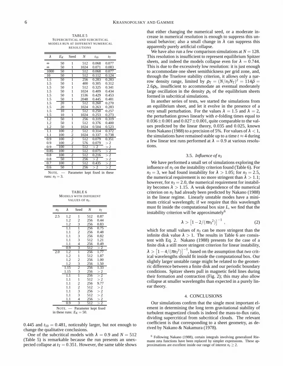
6 KRASNOPOLSKY ANDGAMMIE
TABLE 5SUPERCRITICAL AND SUBCRITICAL
MODELS RUN AT DIFFERENT NUMERICALRESOLUTIONS
λ EK Seed N t10 tT
∞ 50 1 512 0.068 0.077∞ 50 1 1024 0.071 0.0831000 50 1 512 0.068 0.07710 50 1 512 0.112 0.1241.5 50 1 256 0.283 0.2831.5 50 1 400 0.305 0.3121.5 50 1 512 0.325 0.3411.5 50 1 1024 0.409 0.4341.5 50 1 1536 0.429 0.4531.5 50 1 2048 0.445 0.4811.5 20 1 512 0.260 0.2701.5 20 1 1024 0.263 0.2831.5 10 1 512 0.250 0.2571.5 10 1 1024 0.253 0.2731.2 50 1 256 0.319 0.3191.2 50 1 512 0.376 0.4001.2 50 1 1024 0.504 0.5231.1 100 2 512 0.314 0.3721.1 100 2 1024 0.337 0.7380.9 100 2 512 0.079 0.3510.9 100 2 576 0.079 > 20.9 100 1 512 > 2 > 20.85 100 2 512 0.075 > 20.8 100 2 512 0.216 > 20.8 50 1 256 > 2 > 20.7 100 2 512 0.435 > 20.6 50 1 256 > 2 > 2
NOTE. — Parameter kept fixed in theseruns:nJ = 3.
TABLE 6MODELS WITH DIFFERENT
VALUES OF nJ.
nJ λ Seed N tT
2.5 1.2 1 512 0.871.2 2 256 0.441.2 3 256 0.831.1 1 256 0.751.1 2 256 0.481.1 3 256 0.821.1 3 512 1.211.1 4 256 0.490.9 3 512 > 2
2.0 1.2 1 256 1.771.2 1 512 1.871.2 2 256 1.001.2 3 256 1.50
1.15 2 256 1.331.15 3 256 > 21.1 1 256 > 21.1 1 512 > 21.1 2 256 9.771.1 2 512 > 21.1 3 256 > 21.1 3 512 > 21.1 4 256 > 20.9 3 512 > 2
NOTE. — Parameter kept fixedin these runs:EK = 50.
0.445 andt10 = 0.481, noticeably larger, but not enough tochange the qualitative conclusions.
One of the subcritical models withλ = 0.9 andN = 512(Table 5) is remarkable because the run presents an unex-pected collapse attT = 0.351. However, the same table shows
that either changing the numerical seed, or a moderate in-crease in numerical resolution is enough to suppress this un-usual behavior; also a small change inλ can suppress thisapparently purely artificial collapse.
We have also run a few comparison simulations atN = 128.This resolution is insufficient to represent equilibrium Spitzersheets, and indeed the models collapse even forλ = 0.744.This is due to the excessively low resolution: it is just enoughto accommodate one sheet semithickness per grid zone, and,through the Truelove stability criterion, it allows only a nar-row density range, limited byρT = (N/nJNT)2 = 114ρ =2.6ρS, insufficient to accommodate an eventual moderatelylarge oscillation in the densityρS of the equilibrium sheetsformed in subcritical simulations.
In another series of tests, we started the simulations froman equilibrium sheet, and let it evolve in the presence of avery small perturbation. For the valuesλ = 1.5 andλ = 2,the perturbation grows linearly withe-folding times equal to0.036±0.001 and 0.027±0.001, quite comparable to the val-ues predicted by the linear theory, 0.035 and 0.025, knownfrom Nakano (1988) to a precision of 5%. For values ofλ < 1,the simulations have remained stable up to a timet ≈ 4 duringa few linear test runs performed atλ = 0.9 at various resolu-tions.
3.5. Influence of nJWe have performed a small set of simulations exploring the
influence ofnJ on the instability criterion found (Table 6). FornJ = 3, we had found instability forλ > 1.05; for nJ = 2.5,the numerical requirement is no more stringent thanλ > 1.1;however, fornJ = 2.0, the numerical requirement for instabil-ity becomesλ > 1.15. A weak dependence of the numericalcriterion onnJ had already been predicted by Nakano (1988)in the linear regime. Linearly unstable modes have a mini-mum critical wavelength; if we require that this wavelengthmust fit inside the computational box sizeL, we find that theinstability criterion will be approximately6
λ >[
1−2/(πnJ2)
]−1, (2)
which for small values ofnJ can be more stringent than theinfinite disk valueλ > 1. The results in Table 6 are consis-tent with Eq. 2. Nakano (1988) presents for the case of afinite disk a still more stringent criterion for linear instability,λ >
[
1−4/(πnJ2)
]−1, based on the assumption thattwocrit-
ical wavelengths should fit inside the computational box. Ourslightly larger unstable range might be related to the geomet-ric difference between a finite disk and our periodic boundaryconditions. Spitzer sheets pull in magnetic field lines duringtheir formation and contraction (Fig. 2); this may also allowcollapse at smaller wavelengths than expected in a purely lin-ear theory.
4. CONCLUSIONS
Our simulations confirm that the single most important el-ement in determining the long term gravitational stabilityofturbulent magnetized clouds is indeed the mass-to-flux ratio,dividing supercritical from subcritical clouds. The relevantcoefficient is that corresponding to a sheet geometry, as de-rived by Nakano & Nakamura (1978).
6 Following Nakano (1988), certain integrals involving generalized Rie-mann zeta functions have been replaced by simpler expressions. These ap-proximations are excellent inside our range of interestnJ ≥ 2.

NONLINEAR STABILITY OF MOLECULAR CLOUDS 7
Turbulent energy has comparatively little influence on thepresence or absence of stability, up to Mach numbers∼ 10.Subcritical clouds will develop density concentrations due tothis turbulence, but under an ideal MHD regime, the conse-quent increase in magnetic pressure prevents further collapse.However, total turbulent energy has some influence on thelifetime of supercritical clouds, especially as the Mach num-ber becomes large enough (of the order of∼ 7 in these simu-lations).
More interesting is the fact that turbulence introduces astochastic element. The collapse time cannot be predictedwith certainty from physical parameters such as the mass andfield in the cloud, and the typical energy of the turbulence mo-tions, because the random distributions of velocity and densitycan change the lifetime by some factor, seen to be of the orderof 3 in one large sample. The resulting distribution of life-times has an asymmetric tail of unusually long-lived clouds.We suggest that the existence of such a tail may introduce abias in the observed samples of star-forming clouds. Most starformation will take place in the more frequent, shorter livedclouds, while observations of clouds will tend to focus on thefewer longer lived ones.
We have seen that the numerical resolution requirementsneeded to study cloud collapse are very stringent, and we ex-pect they will be even more stringent in 3D. There is a ne-cessity of resolving the possible equilibrium structures,suchas the Spitzer sheets, which we have seen fully formed in thesubcritical clouds, and partially formed during the run-uptoinstability of the mildly supercritical ones. The thickness ofthese sheets scale with the numbernJ of Jeans lengths asnJ
−2.Accommodating a large numbernJ of Jeans lengths inside thecomputational volume will therefore be numerically challeng-ing. IncreasingnJ by only a factor of 2 requires increasingthe space resolution by a factor of 4. Unless adaptive meshrefinement (AMR) is used, this requires increasing the simu-lation runtime by factors on the order of 64= 43 in 2D, and256= 44 in 3D. We anticipate that AMR will be used in manyof the successful simulations of core formation in the future.
Numerical stability, through the Truelove condition, setsamaximum density that can be accommodated at a given spatialresolution. Shocks in strongly turbulent flows have large com-pression ratios, sometimes requiring increasing resolution inorder to distinguish a transient density increase due to a shockfrom an authentically unstable accumulation of mass able toform a collapsed object.
We have seen that artificially enforcing numerical densityfloors, even relatively large ones, on the order of 10−4 timesthe background density, had almost no influence in the evo-lution of the collapse. This result is again not surprising,because wide regions of small density have little influenceon the dense, self-gravitating regions that undergo collapse.Density floors can significantly speed up ideal MHD simula-tions, whose Courant timestep is often limited by large Alfven
speedsB/√
4πρ in the least dense regions.This work is limited due to the periodic boundary con-
ditions. We believe this may have favored the collectionof clumps into larger clumps until the instability can takeplace. Some simulations occasionally show fast-movingclumps flowing past each other, and later merging once oneof them returns through the other side of the periodic com-putational volume. The periodic boundary conditions make itplausible that sooner or later, most of the mass in a given field-line will collect into a single clump, which then can undergoinstability if its mass is even slightly supercritical. In realclouds with ordered magnetic fields, clumps inside the samefieldline but moving in opposite directions are not expectedtomerge; however, it is improbable this will apply to all of thefieldlines and so we expect that the instability will still takeplace in a similar form, albeit with an additional stochasticfactor in the cloud lifetime.
Two-dimensionality is also a limitation of this work. It hasstrongly limited the topological possibilities for the fieldlines;it is conceivable that the consequent limitations in motionhave favored the collection of mass into massive sheets andother structures. Observations (e.g., Goodman et al. 1990;Crutcher 2004), and 3D simulations and studies (e.g., Basu2000; Gammie et al. 2003) indeed indicate that sheets alignedperpendicular to the magnetic field are not always the pre-ferred possibility for the long term development of clouds.More variety of clump shapes is expected in a 3D study. Thelarger variety in motions allowed by a 3D magnetic field isexpected to enhance the already observed stochastic effects,and perhaps might also delay mass collection into potentiallyunstable structures. However, even in 3D, the simulations per-formed by Ostriker, Stone, & Gammie (2001) suggest that thestability criterion will still be dominated by the mass-to-fluxratio.
In some of our models, artificial numerical diffusion hasturned an initially uniform mass-to-flux ratioλ into a non-uniform distribution, sometimes with striking effects on thenumerical stability. While this has a numerical origin, non-uniform distributions of mass-to-flux are also expected on as-trophysical grounds. For instance, turbulence provides struc-tures and shocks with small lengthscales and strong magneticgradients, conditions favorable to a localized, efficient am-bipolar diffusion, which can redistribute mass and magneticflux independently. Cloud collisions can also merge togetherportions of gas having different masses and magnetic fields.We plan to study directly the physical effect of a non-uniformmass-to-flux ratio in our future work.
This work was supported by NASA grant NAG 5-9180. Wethank Jon McKinney, Eve Ostriker, Zhi-Yun Li, and ChrisMatzner for comments.
REFERENCES
Arons, J., & Max, C. E. 1975, ApJ, 196, L77Basu, S. 2000, ApJ, 540, L103Chandrasekhar, S., & Fermi, E. 1953, ApJ, 118, 113Ciolek, G. E., & Mouschovias, T. Ch. 1995, ApJ, 454, 194Crutcher, R. M. 2004, in The Magnetized Interstellar Medium, eds. B.
Uyaniker, W. Reich & R. Wielebinski, (Copernicus GmbH: Katlenburg-Lindau), 123
Draine, B. T., Roberge, W. G., & Dalgarno, A. 1983, ApJ, 264, 485Elmegreen, B. G., & Elmegreen, D. M. 1978, ApJ, 220, 1051Evans, C. R., & Hawley, J. F. 1988, ApJ, 332, 659Frigo, M., & Johnson, S. G. 2005, Proc. IEEE, 93, 216
Gammie, C. F., Lin, Y.-T., Stone, J. M., & Ostriker, E. C. 2003, ApJ, 592, 203Gammie, C. F., & Ostriker, E. C. 1996, ApJ, 466, 814Goldreich, P., & Kwan, J. 1974, ApJ, 189, 441Goldstein, M. L. 1978, ApJ, 219, 700Goodman, A. A., Bastien, P., Myers, P. C., & Menard, F. 1990,ApJ, 359, 363Hawley, J. F., & Stone, J. M. 1995, Comput. Phys. Commun., 89,127Kulsrud, R., & Pearce, W. P. 1969, ApJ, 156, 445Ledoux, P. 1951, Ann. d’Astrophys. 14, 438Mac Low, M.-M., Klessen, R. S., Burkert, A., & Smith, M. D. 1998,
Phys. Rev. Lett., 80, 2754Mac Low, M.-M., & Klessen, R. S., 2004 Rev. Mod. Phys., 76, 125

8 KRASNOPOLSKY ANDGAMMIE
McKee, C. F. 1989, ApJ, 345, 782Mestel, L., & Spitzer, L., Jr. 1956, MNRAS, 116, 503Nakano, T., & Nakamura, T. 1978, PASJ, 30, 671Nakano, T. 1988, PASJ, 40, 593Ostriker, E. C., Gammie, C. F., & Stone, J. M. 1999, ApJ, 513, 259Ostriker, E. C., Stone, J. M., & Gammie, C. F. 2001, ApJ, 546, 980Sagdeev, R. Z., & Galeev, A. A. 1969, Nonlinear Plasma Theory(New York:
W. A. Benjamin)Shu, F. H., Adams, F. C., & Lizano, S. 1987, ARA&A, 25, 23
Spitzer, L., Jr. 1942, ApJ, 95, 329Stone, J. M., & Norman, M. L. 1992, ApJS, 80, 753Stone, J. M., & Norman, M. L. 1992, ApJS, 80, 791Stone, J. M., Ostriker, E. C., & Gammie, C. F. 1998, ApJ, 508, L99Truelove, J. K., Klein, R. I., McKee, C. F., Holliman, J. H., II, Howell, L. H.,
& Greenough, J. A. 1997, ApJ, 489, L179Zuckerman, B., & Palmer, P. 1974, ARA&A, 12, 279
FIG. 1.— Colormaps ofρ in the fiducial run. Snapshots at timest = 0.01, 0.02, 0.04, 0.06, 0.12, 0.18, 0.24, 0.30, and 0.34. The logarithmic colorscale goesfrom dark blue (saturating on black) to deep red, corresponding to densities going from 0.01ρS = 0.4441ρ to 10ρS = 444.1ρ , whereρS is the peak density of anequilibrium Spitzer sheet for the given parameters.

NONLINEAR STABILITY OF MOLECULAR CLOUDS 9
FIG. 2.— Field lines in the fiducial run. The figure shows snapshots at timest = 0.01, 0.02, 0.04, 0.06, 0.12, 0.18, 0.24, 0.30, and 0.34.

10 KRASNOPOLSKY ANDGAMMIE
0 0.1 0.2 0.3tT (dimensionless)
0
200
400
600
800
Max
imum
den
sity
FIG. 3.— Increase of the maximum mass densityρmax with time in the fiducial run. The run finishes whenρmax = 1820, the Truelove value, at a timet = 0.341,slightly beyond the plotted region. Some of the transient peaks shown here could have provoked a numerical instability at a resolution smaller than the valueN = 512 adopted for the fiducial run.
0 0.1 0.2 0.3tT (dimensionless)
0
10
20
30
40
50
Ene
rgie
s
EB
EK(t)
-EG
FIG. 4.— Variations in time of the turbulent kinetic energyEK , the total magnetic energyEB, and (minus) the gravitational energy−EG.

NONLINEAR STABILITY OF MOLECULAR CLOUDS 11
0 0.2 0.4 0.6 0.8 1tT (dimensionless)
0
1
2
3
4
Fre
quen
cy
0 6 12 18 24
tT (Myr)
FIG. 5.— Frequency of the different values oftT . Sixty simulations have been run with the parametersλ = 1.5, EK = 50,N = 512, and different random seeds.Each of these runs has reported a value oftT . This plot was constructed by summing 60 Gaussian profiles (with σ = 0.03ts = 0.9Myr) centered at each of thesetT values. Collapse times range from∼ 7 to 20Myr.