nonintrusive frequency analysis for variable pairing on a distillation column

ectrummethodimpactsed. This

est aremation

ISATRANSACTIONS®

ISA Transactions 44~2005! 295–303

Nonintrusive frequency analysis for variable pairingon a distillation column

Glen Hay, William Y. Svrcek, Brent R. Young*Department of Chemical and Petroleum Engineering, University of Calgary, Calgary, Alberta, Canada, T2N 1N4

~Received 10 May 2004; accepted 8 November 2004!

Abstract

This paper describes a nonintrusive plant analysis technique for variable pairing that relies on power spfrequency analysis. The development of the method is described and guidelines for the implementation of theare presented. Information gathered from the frequency analysis is used in variable pairing to ensure minimalfrom unmeasured disturbances. Specifically, the nested epsilon decomposition method for variable pairing is usnonintrusive analysis method is implemented on a pilot plant distillation column. The results of the pilot plant tused in the decoupling of a multiloop control system. © 2005 ISA—The Instrumentation, Systems, and AutoSociety.

Keywords: Frequency signal analysis; Variable pairing; Control structure; Power spectra; Predictive control

esof

a-is

lesIn

areess

ersisrol

ter-nd

sssisro-hat

x-gh-umh-pa-atin

en-e

eiednig-

isesfit

1. Introduction

Coupling of variables in multivariable processcan be problematic and often requires the usepredictive modeling for robust process controllbility @1#. When modeling of complex processescompleted for model predictive control~MPC!purposes, the issue of knowing what variabshould be included in the model always arises.addition, the pathways in which these variablesinterconnected are not always understood unlan expert on the process is readily available~e.g.,Ref. @2#!. Since this is rarely the case, this papdescribes a nonintrusive frequency analymethod that helps guide the creation of the contstructure.

Conventional process plant testing used to demine related variables involves step testing arelative gain array~RGA! @3# analysis techniques

*Corresponding author. Tel.:11-403-220-8751; fax:11-403-282-3945.Email address:[email protected]

0019-0578/2005/$ - see front matter © 2005 ISA—The Instru

~e.g., Ref.@4#!, which creates unwanted procedisturbances. The frequency used for the analymethod proposed here is imbedded into the pcess through manipulated variables at a level tis virtually hidden in the process noise.

Once the frequency is input it can then be etracted from the variable measurements throuout the process and viewed using power spectrfrequency analysis. The application of this metodology can recognize how disturbances progate through the process and can identify whvariables are strongly affected and thus neededthe final process model. The pathways thus idtified also uncover valuable information about thinterconnectivity of the variables when multiplmanipulated variables are excited by the applfrequency. This approach allows for informatioon variable interactions to be gathered without snificantly disturbing the actual process.

Even though the concepts of this analysmethod are simple, there are specific guidelinthat need to be followed to gain the most bene

mentation, Systems, and Automation Society.

ere-o-on

eanter

his-es

tioncereht,, ale.

ededillam

p-to

re-pas-g-of

inggredibleareas

ed-

o-sysss

ae-ar

e aies

-imeed

ntreen-edor

lea

ofis.

r-ld

ee

bednd

gtion.t-ec-e-es

es-

296 Hay, Svrcek, Young / ISA Transactions 44 (2005) 295–303

from an implementation. In addition, many othapplications can be introduced along with the frquency testing for gathering other beneficial prcess control knowledge. An example applicatiof this, using nested epsilon decomposition@5#, isgiven later in this paper. This application is thoverall decentralization of the control loops ofchemical processing plant, namely a pilot pladistillation column and can be applied to othmultiunit process operations.

2. Data gathering techniques

The data gathering techniques required for tmethod should be virtually nonintrusive to processes. This is due to the small magnitude necsary for the disturbance and the natural attenuathat results when using sinusoidal signals. Sininformation for which large set point changes anecessary for good results is not being sougsuch as gain relationships between variablessmall forcing signal magnitude becomes feasibIn addition, having a sinusoidal signal imposaround the regular set point for a manipulatvariable will have an averaged result that weliminate any sustained offset in the downstreprocess conditions.

The correct sinusoidal frequency must be aplied to the process for this analysis techniquegather the best data from a plant test. This fquency must be chosen specifically for each serate plant application. The first guideline in chooing the frequency is that no naturally occurrinoscillations within the plant have a similar frequency. This can be accomplished by analysisthe plant data gathered during regular operatconditions. From this analysis, naturally occurrinfrequencies can be extracted from the measuprocess variables and removed from the posstest disturbance choices. If these frequenciesused, then incorrect conclusions can be drawnto what variables are being affected by the embded frequencies.

The next issue is the period of the natural prcess attenuation. We are considering processtems, which typically act dynamically as low pafilters and are often dynamically described bysingle dominant time constant, i.e., higher frquencies are attenuated and lower frequenciesnot. Thus, in practice, process oscillations havgreater tendency to dissipate at higher frequenc

-

-

-

e

.

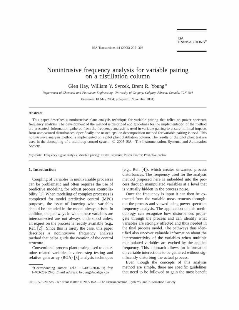
This is especially true when units within the process being analyzed have large capacities. Tconstants of approximately 45 min were observin the distillation pilot plant, Fig. 1. It was foundfrom experimental observations for this pilot plathat test signals of frequency above 6.0 mHz weattenuated and were not detectable. Test frequcies higher than 6.0 mHz were therefore avoidas a result of the implications on attenuation fthis pilot plant.

The distributed control system~DCS! sampletime interval used to collect the process variabmeasurements is also important. Too largesample interval will not capture the spectrumthe frequencies required for frequency analysWith a sampling interval of 1 min it was detemined that a frequency lower than 5.6 mHz shoube used in order to avoid aliasing problems~i.e.,assuming that an absolute minimum of thrpoints is required to define half a sinusoid!. Fil-tered and compressed data should also alwaysavoided when applying this method. Filtering ancompression of data will lead to accuracy loss apoor variable relationships being determined.

Slight drifting of the process variables durindata gathering is another issue that needs attenWhen a low forcing frequency is applied, a drifing signal causes lower values in the power sptrum to be altered and hidden. If the forcing frquency is too low the data eventually becomunreliable. Subtracting overall drift trends fromthe data is one solution to this problem, but exc

Fig. 1. Distillation pilot plant schematic.

297Hay, Svrcek, Young / ISA Transactions 44 (2005) 295–303

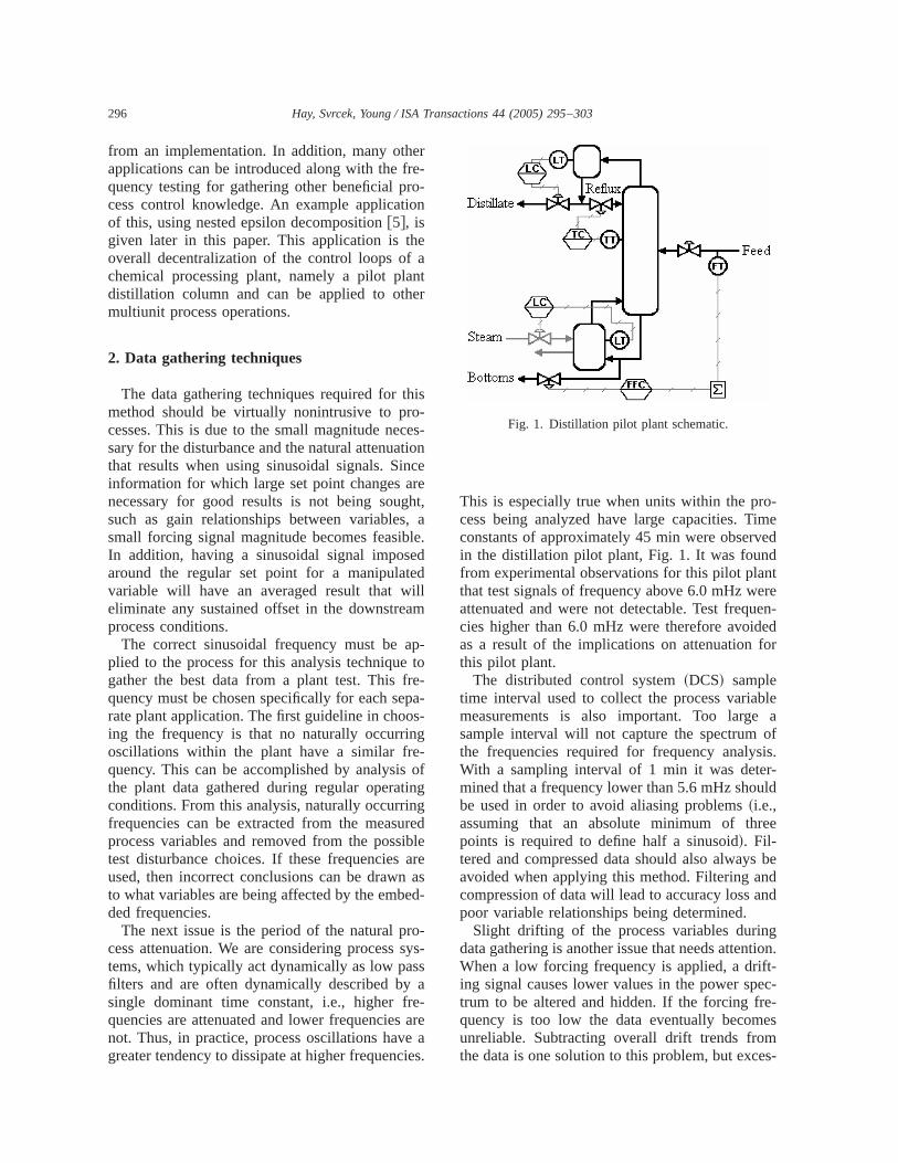
Fig. 2. Results of a simulated 0.16-Hz signal frequency analysis test.

stilnd.

omge

is-

ryallnges.nhee

theerethehe

onon-hatiso-by

theheec-re,f-

heier

rm

sive changes due to other disturbances canskew the sinusoidal signal being introduced athis skewing will lead to data of a lower qualityAs a result of considering these issues and frexperimental observations, a practical, low ranguideline of 2.7 mHz was determined for the dtillation column.

The length of the frequency test is also veimportant in that it affects accuracy of data. Smtime intervals have a higher chance of showipoor results from unexpected plant disturbancTwo hours of data were used for the distillatiocolumn and was found to be acceptable. If tlength of the test were not limited, it would also badvisable to choose a specific time span ofanalysis when no large plant disturbances wobserved. This would help improve results asgradual drifting of variable values reduces tquality of the data.

l 3. Frequency analysis

The calculations for the frequency analysisthe gathered data were performed as follows. Csider x as one measured variable data set twould be reacting to a sinusoidal signal thatapplied to a controller set point. The analysis prcess first sets the signal mean equal to zerosubtracting each element in the data set byoverall mean of that data set, which results in tderived signal having a cleaner frequency sptrum in the lower frequency ranges. Furthermoadding or subtracting a constant bias will not afect the resulting spectrum frequencies in thigher ranges, or those of interest. A fast Fourtransform ~FFT! then transforms this modifieddata. A 512-point FFT of the given data setximplements the transform and inverse transfopair for vectors of lengthN.


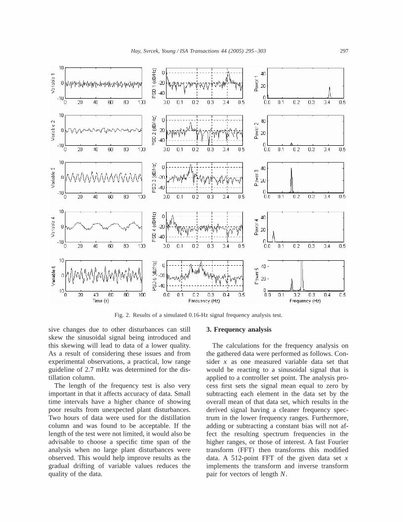
Fig. 3. MPC pathway modelling before frequency analysis results.

atheentm

m-ehe

e-to

en

atais

thed 5freedithet

ted

beo

isct

a-ig.rera-ns.ac-n-tu-nd

reaces-ndri-lso

fre-.enre

ng

cytheedal

on

atendd

Once this step has been used to process the dthe arrays of the processed data sets are tpassed to a function that multiplies each elemin each array in the processed data set by its coplex conjugate and divides this result by the nuber of points used in the FFT function. Lastly, thfrequency corresponding to each variable in toriginal data set is found and plotted.MATLAB wasused for this calculation procedure.

Fig. 2 presents an example of a simulated ‘‘zroed’’ data and the power spectrum data usedtest the program code. Also displayed, as the cter set of Fig. 2, is the ‘‘periodogram’’ functionfrom MATLAB . Even though this function wouldgive good estimates of the frequencies within dsets, the related power of specific frequenciesnot obvious. Fig. 2 also demonstrates thatsame frequency is present in variables 2, 3, anbecause a similar spike is seen at the samequency value in each plot. If the controller ushad variable 3 as its input process variable wthe 0.16-Hz sinusoidal signal applied to the spoint, variables 2 and 5 would represent relainteracting process variables.

4. Variable pairing and modeling

The completed plant power spectrum canused for process diagnosis once the analysissingle or multiple frequencies implementedcompleted. Variable pairing, or cause and effe

a,n

-

-

,-

f

relationships, is one of the key types of informtion that may be extracted from these results. F3 is an example of modeling relationships that aknown in a process including measured tempetures, pressures, flow rates, and compositioLines connecting these variables represent theknowledgement of these existing, known relatioships. This type of model structure could evenally be used as the basis for an MPC structure aany missing links would represent a possible awhere other, currently unmeasured disturbancould be introduced. In Fig. 3 five different forcing frequencies were introduced into the plant aare also shown graphically above the input vaables. The spectra for the other variables are arepresented showing the propagation of thesequencies through the related variable pathways

It can be shown that variable pairings betwethe input and output variables of this structure amissing. An example of a possible missed pairiwould be betweenflow rate 3and temperature 4.The conclusion being drawn from the frequenanalysis is that a relationship exists becauseeffect of the sinusoidal excitement is being passfrom one variable to another, as indeed a normdisturbance would be transferred. The introductiof theflow rate 3pairing directly totemperature 4,while bypassingtemperature 2andtemperature 3,can also be used if the concept of intermedivariables is implemented in the MPC structure aalgorithms @6#. Furthermore, it can be observe


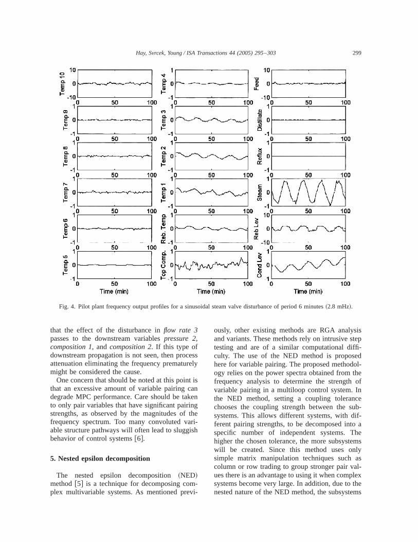
Fig. 4. Pilot plant frequency output profiles for a sinusoidal steam valve disturbance of period 6 minutes~2.8 mHz!.

esly

t isankengtheri-sh

-vi-

sistep-

edol-heof

nceub-if-o aheemslyasl-lexthems

that the effect of the disturbance inflow rate 3passes to the downstream variablespressure 2,composition 1, andcomposition 2. If this type ofdownstream propagation is not seen, then procattenuation eliminating the frequency prematuremight be considered the cause.

One concern that should be noted at this pointhat an excessive amount of variable pairing cdegrade MPC performance. Care should be tato only pair variables that have significant pairinstrengths, as observed by the magnitudes offrequency spectrum. Too many convoluted vaable structure pathways will often lead to sluggibehavior of control systems@6#.

5. Nested epsilon decomposition

The nested epsilon decomposition~NED!method@5# is a technique for decomposing complex multivariable systems. As mentioned pre

s

ously, other existing methods are RGA analyand variants. These methods rely on intrusive stesting and are of a similar computational difficulty. The use of the NED method is proposhere for variable pairing. The proposed methodogy relies on the power spectra obtained from tfrequency analysis to determine the strengthvariable pairing in a multiloop control system. Ithe NED method, setting a coupling toleranchooses the coupling strength between the ssystems. This allows different systems, with dferent pairing strengths, to be decomposed intspecific number of independent systems. Thigher the chosen tolerance, the more subsystwill be created. Since this method uses onsimple matrix manipulation techniques suchcolumn or row trading to group stronger pair vaues there is an advantage to using it when compsystems become very large. In addition, due tonested nature of the NED method, the subsyste

min


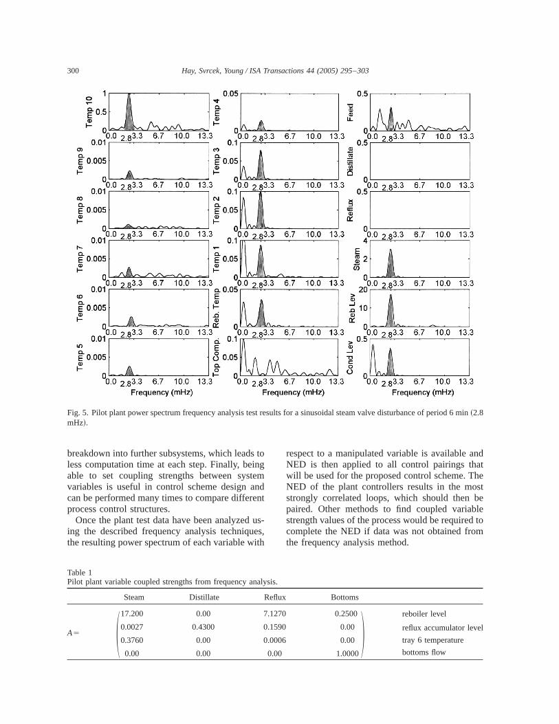
Fig. 5. Pilot plant power spectrum frequency analysis test results for a sinusoidal steam valve disturbance of period 6~2.8mHz!.

toingemndent

usesith

ndthestbeleto

m

breakdown into further subsystems, which leadsless computation time at each step. Finally, beable to set coupling strengths between systvariables is useful in control scheme design acan be performed many times to compare differprocess control structures.

Once the plant test data have been analyzeding the described frequency analysis techniquthe resulting power spectrum of each variable w

-,

respect to a manipulated variable is available aNED is then applied to all control pairings thawill be used for the proposed control scheme. TNED of the plant controllers results in the mostrongly correlated loops, which should thenpaired. Other methods to find coupled variabstrength values of the process would be requiredcomplete the NED if data was not obtained frothe frequency analysis method.

Table 1Pilot plant variable coupled strengths from frequency analysis.

Steam Distillate Reflux Bottoms

A5 S17.200 0.00 7.1270 0.2500

0.0027 0.4300 0.1590 0.00

0.3760 0.00 0.0006 0.00

0.00 0.00 0.00 1.0000

D reboiler level

reflux accumulator level

tray 6 temperature

bottoms flow


Table 2Resulting pilot plant variable coupled strengths.

eheod

osiar-

lert onties,os-

ote

icaprotheh-nter

lerthe

o-ureg

is-ydhe

z,ineranm-a-

-cybleim-r-gst.

is

er-a-le

ou-g-n-

si-re-

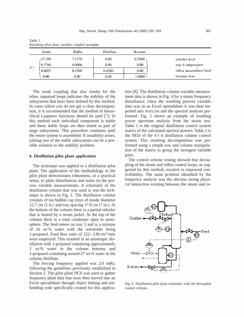
Fig. 6. Distillation pilot plant schematic with the decoupledcontrol scheme.

The weak coupling that also results for thother, unpaired loops indicates the stability of tsubsystems that have been defined by this methIn cases where you do not get a clear decomption, it is recommended that the method of hierchical Liapunov functions should be used@7#. Inthis method each individual component is staband these stable loops are then tested as palarge subsystems. This procedure continues uthe entire system is assembled. If instability arisjoining two of the stable subsystems can be a psible solution to the stability problem.

6. Distillation pilot plant application

The technique was applied to a distillation pilplant. The application of the methodology to thpilot plant demonstrates robustness, in a practsense, to plant disturbances and noise on thecess variable measurements. A schematic ofdistillation column that was used to test the tecnique is shown in Fig. 1. The distillation columconsists of ten bubble cap trays of inside diame12.7 cm~5 in.! and tray spacing 17.8 cm~7 in.!. Atthe bottom of the column there is a partial reboithat is heated by a steam jacket. At the top ofcolumn there is a total condenser open to atmsphere. The feed enters on tray 5 and is a mixtof 16 wt % water with the remainder bein1-propanol. Feed flow rates of122– 138 cm3/minwere employed. This resulted in an azeotropic dtillation with 1-propanol containing approximatel2 wt % water in the column bottoms an1-propanol containing around 27 wt % water in tcolumn distillate.

The forcing frequency applied was 2.8 mHfollowing the guidelines previously establishedSection 2. The pilot plant DCS was used to gathfrequency plant data that were then moved intoExcel spreadsheet through object linking and ebedding code specifically created for this applic

.-

fl

l-

tion @8#. The distillation column variable measurement data is shown in Fig. 4 for a steam frequendisturbance. Once the resulting process variadata was in an Excel spreadsheet it was thenported intoMATLAB and the spectral analysis peformed. Fig. 5 shows an example of resultinpower spectrum analysis from the steam teTable 1 is the original distillation control systemmatrix of the calculated spectral powers. Table 2the NED of the434 distillation column controlsystem. This resulting decomposition was pformed using a simple row and column manipultion of the matrix to group the strongest variabpairs.

The control scheme testing showed that decpling of the steam and reflux control loops, as sugested by this method, resulted in improved cotrollability. The main problem identified by thefrequency analysis was the obvious strong phycal interaction existing between the steam and


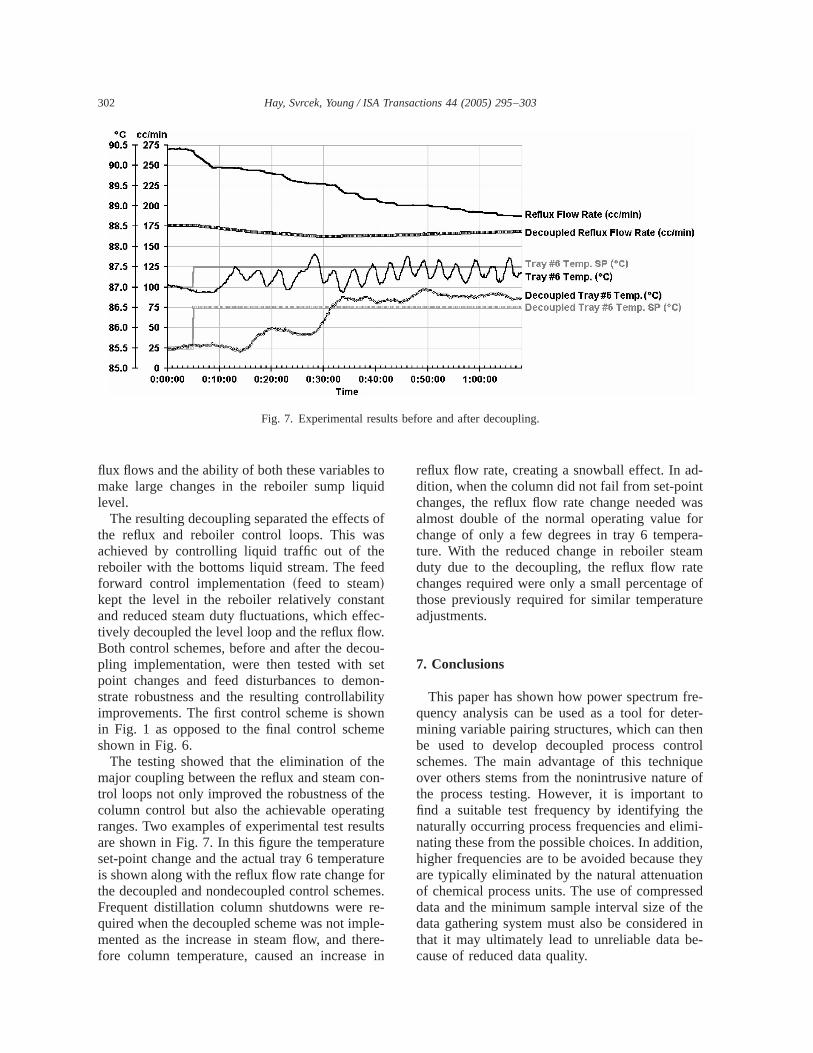
Fig. 7. Experimental results before and after decoupling.

toid

ofs

d

ntec-w.ou-etonlitywn

e

en-

hengultsre

tureores

e-le-rein

d-tas

orra-m

teof

re

re-ter-entrolueoftoei-n,

heyn

sedhed ine-

flux flows and the ability of both these variablesmake large changes in the reboiler sump liqulevel.

The resulting decoupling separated the effectsthe reflux and reboiler control loops. This waachieved by controlling liquid traffic out of thereboiler with the bottoms liquid stream. The feeforward control implementation~feed to steam!kept the level in the reboiler relatively constaand reduced steam duty fluctuations, which efftively decoupled the level loop and the reflux floBoth control schemes, before and after the decpling implementation, were then tested with spoint changes and feed disturbances to demstrate robustness and the resulting controllabiimprovements. The first control scheme is shoin Fig. 1 as opposed to the final control schemshown in Fig. 6.

The testing showed that the elimination of thmajor coupling between the reflux and steam cotrol loops not only improved the robustness of tcolumn control but also the achievable operatiranges. Two examples of experimental test resare shown in Fig. 7. In this figure the temperatuset-point change and the actual tray 6 temperais shown along with the reflux flow rate change fthe decoupled and nondecoupled control schemFrequent distillation column shutdowns were rquired when the decoupled scheme was not impmented as the increase in steam flow, and thefore column temperature, caused an increase

-

.

-

reflux flow rate, creating a snowball effect. In adition, when the column did not fail from set-poinchanges, the reflux flow rate change needed walmost double of the normal operating value fchange of only a few degrees in tray 6 tempeture. With the reduced change in reboiler steaduty due to the decoupling, the reflux flow rachanges required were only a small percentagethose previously required for similar temperatuadjustments.

7. Conclusions

This paper has shown how power spectrum fquency analysis can be used as a tool for demining variable pairing structures, which can thbe used to develop decoupled process conschemes. The main advantage of this techniqover others stems from the nonintrusive naturethe process testing. However, it is importantfind a suitable test frequency by identifying thnaturally occurring process frequencies and elimnating these from the possible choices. In additiohigher frequencies are to be avoided because tare typically eliminated by the natural attenuatioof chemical process units. The use of compresdata and the minimum sample interval size of tdata gathering system must also be considerethat it may ultimately lead to unreliable data bcause of reduced data quality.

aa-here-usn-fiedr-

tonlyc-l-

ted-nserete--

is--

g.l

utet-ust

b-

ese.

or.

Aey

-ca-

ic-anC,

v

l.


Multiple frequencies can also be applied toprocess or unit in order to complete multiple mnipulated variable cause and effect pathways. Tuse of frequency power spectra allows these fquencies to be separately extracted without caing detrimental effects on the resulting data. Umeasured disturbance sources can be identiand thus eliminated from the resulting test infomation.

It is also suggested that care be taken notoveruse the variable pairing pathways and oimplement the strongest pairings in MPC strutures. This will lead to the required strong controler action to measured disturbances.

Nested epsilon decomposition was implemenand shown to work well in conjunction with frequency analysis to define decomposition regiofor centralized controllers. Even though othtools could be applied, it was found that the stolerance brought in through nested epsilon dcomposition allowed for a more detailed decomposition of the tested plant control system.

The method developed was validated on a dtillation column pilot plant and the results provided direct guidance for control variable pairinMultiple single-input single-output contro

-

schemes were implemented, both with and withocontrol loop decoupling, showing that greater spoint ranges were achievable with resultant robcontrollability.

References

@1# Riggs, J. B., Chemical Process Control. Ferret Pulishing, Lubbock, TX, 1999.

@2# Marlin, T. E., Process Control: Designing Processand Control Systems for Dynamic PerformancMcGraw-Hill, New York, 1995, pp. 639–675.

@3# Bristol, E. H., On a new measure of interactions fmultivariable process control. IEEE Trans. AutomControl AC-11, 133–134~1966!.

@4# Svrcek, W. Y., Mahoney, D. P., and Young, B. R.,Real-Time Approach to Process Control. John Wil& Sons, West Sussex, England, 2000.

@5# Siljak, D. D., Decentralized Control of Complex Systems. Mathematics in Science and Engineering. Ademic Press, Boston, 1991, Vol. 184.

@6# Cott, B. J., The New Shell Standard for Model Predtive Control. Proceedings of the 52nd CanadiChemical Engineering Conference, Vancouver, BOctober 20–23, 2002.

@7# Ikeda, M. and Siljak, D. D., Hierarchical Liapunofunctions. J. Math. Anal. Appl.112, 110–128~1985!.

@8# Hay, G., Distillation Column Decentralized ControUniversity of Calgary, Alberta, Canada, 2003.

nonintrusive frequency analysis for variable pairing on a distillation column

Documents