arX

iv:n

ucl-

th/0

1010

61v1

26

Jan

2001

Non equilibrium effects in fragmentation

A.Chernomoretz, M. Ison, S.Ortiz and C.O.Dorso

(February 8, 2008)

Abstract

We study, using molecular dynamics techniques, how boundary conditions

affect the process of fragmentation of finite, highly excited, Lennard-Jones

systems. We analyze the behavior of the caloric curves (CC), the associated

thermal response functions (TRF) and cluster mass distributions for con-

strained and unconstrained hot drops. It is shown that the resulting CC’s for

the constrained case differ from the one in the unconstrained case, mainly in

the presence of a “vapor branch”. This branch is absent in the free expanding

case even at high energies . This effect is traced to the role played by the

collective expansion motion. On the other hand, we found that the recently

proposed characteristic features of a first order phase transition taking place

in a finite isolated system, i.e. abnormally large kinetic energy fluctuations

and a negative branch in the TRF, are present for the constrained (dilute) as

well the unconstrained case. The microscopic origin of this behavior is also

analyzed.

PACS: 25.70Mn, 05.70Fh, 02.70Ns

1

I. INTRODUCTION

The possibility of getting information about the thermodynamics of nuclear matter from

the analysis of intermediate energies heavy ion collisions has triggered a lot of interest in

this field. Starting from the pioneering work of the Purdue group, when for the first time

a power law was used to fit the mass spectra resulting from highly excited nuclear systems

and thus suggesting that a critical phenomena was taking place, it has open the study of

a rather new branch of thermodynamics i.e the study of phase transitions (liquid-vapor) in

finite systems [1].

One of the most challenging features that nuclear multi-fragmentation phenomena

presents, is that signals of phase transitions of different orders can be extracted from ex-

perimental data. On one hand, the analogy between the nuclear force and a van der Waals

interaction suggests that the nuclear equation of state should reproduce the main features

that characterize a liquid-gas phase transition. Different indications of this kind of transi-

tion have been reported [2–5]. On the other, signatures of a second order phase transition

or critical behavior have been obtained assuming Fisher-like scaling relations for fragment

distributions [6–10]. Moreover, in recent works [11,12] is suggested that the observed critical

behavior is compatible with a first order phase transition, and it is due exclusively to finite

size effects.

An important point to be kept in mind is that the above mentioned approaches to the

fragmentation problem are based on descriptions where not only the concept of thermo-

dynamical equilibrium, but also the macroscopic constraints imposed to the system play a

relevant role. For example, several statistical descriptions of the nuclear multi-fragmentation

process, e.g. the statistical multifragmentation model (SMM) [13] and the microcanonical

Metropolis Monte Carlo model (MMMC) [3], employ the concept of a freeze-out volume

inside of which the existence of a thermodynamical equilibrated ensemble of fragments is

assumed. These statistical models have been widespreadly used by the nuclear community

in a successful manner to described some experimental observations. However, from the

2

experience gained in numerical simulations, such a concept as freeze-out volume, even as an

approximation, does not seem to be completely correct. It is then important to study which

kind of differences arise as a consequence of not assumming a finite volume scenario, as it is

not a priori evident that the evolution of a fragmenting system confined in a finite volume

would produced the same macroscopic observable when compared with a non confined one,

in which an expansive motion is present as an extra collective degree of freedom.

In previous works [16,17] we have studied the fragmentation of a simple classical system

where the dynamics is governed by a Hamiltonian with a two body interaction Lennard-

Jones term. A microscopic description, employing molecular dynamics techniques, was

used in order to adequately handle the possible presence of a non equilibrium behavior.

It was shown that a fragmentation time can be defined, after which a certain degree of local

equilibrium is achieved in the system. This fact allowed us to calculate a caloric curve for

our expanding-fragmenting system, which is characterized by the absence of a vapor branch.

The aim of the present communication is to study how the restriction of a finite vol-

ume, and then the imposition of equilibration, affects some of the results obtained in the

unconstrained case. We will show that one of the main effects is seen in the behavior of

the caloric curve (CC). For the constrained system it clearly shows a vapor-branch, which

is absent in the free expanding case. This behavior is a direct consequence of the presence

of a confining volume, which destroys the velocity correlations that, in the case of the free

expanding system, build up an expansive flux that acts as a heat sink. Nevertheless for both

cases (at rather low densities for the constrained system) a local maximum and a loop in the

CC can be seen. This feature can be associated with a negative branch in the corresponding

thermal response function (TRF), that might signal a phase transition of first order. A

gradual smoothing of the mentioned indicators is observed for the confined system at higher

densities. Differences in fragment mass distributions are also reported and related to the

microscopic origin of such behavior.

This paper is organized as follows. In Section II we will describe the model used in our

simulations. A brief review of the results already obtained for the unconstrained expanding

3

system is included. Section III is devoted to the study of the caloric curves. In Section IV

we study possible choices for the freeze out volume for the constrained case. In Section V we

calculate the thermal response functions and the kinetic energy fluctuations in order to signal

the presence of possible phase transitions. A microscopic correlations study is performed

in Section VI analyzing the results of two different clusterization algorithms. Finally, in

Section VII, conclusions are drawn.

II. NUMERICAL SIMULATIONS

The system under study is composed by excited drops made up of particles interacting

via a 6-12 Lennard Jones potential, which reads:

V (r) =

4ǫ

[

(

σr

)12−

(

σr

)6−

(

σrc

)12

+(

σrc

)6]

r ≤ rc

0r¿rc

(1)

We took the cut-off radius as rc = 3σ. Energies and distances are measured in units of

the potential well (ǫ) and the distance at which the potential changes sign (σ), respectively

while the unit of time used is: t0 =√

σ2m/48ǫ. We integrated the set of classical equations

of motion using the well known Verlet algorithm [14], taking tint = 0.002t0 as the integration

time step. Initial conditions were constructed using the already presented method of cutting

spherical drops composed of 147 particles out of equilibrated and periodic 512 particles per

cell L.J. system [17].

A broad energy range was considered such that the asymptotic mass spectra of the

fragmented drops for the unconstrained system changes from a ”U shaped” pattern to an

exponentially decaying one. Somewhere in between this two extremes a power law like

spectra can be obtained.

4

A. Analysis of the unconstrained expanding case

For the sake of completeness we summarize in this section the main results obtained in

previous work for the non-constrained fragmenting system (see [17] for details).

Due to the fact that we are dealing with a non-stationary process the determination of

the time at which fragments are formed becomes one of the key ingredients in the analysis.

To accomplish this task one can use a simple and intuitive cluster definition, that is based

on correlations in configuration space: a particle i belongs to a cluster C if there is another

particle j that belongs to C and |ri − rj| ≤ rcl, where rcl is a parameter called clusterization

radius (In this work we used rcl = rcut = 3σ). The recognition algorithm introduced by this

definition is known as minimum spanning tree (MST) fragment recognition method.

In [18] it was shown that a different recognition method , the Early Cluster Formation

Model and its companion practical realization the so called Early Cluster Recognition Al-

gorithm (ECRA), outperforms the MST clusterization algorithm in the sense that it finds

the asymptotic fragmentation pattern in phase space at early stages in the evolution, when

fragments are still not observables in configuration space. At that time the system still looks

like a rather compact piece of excited matter. Instead of being defined through a proximity

criteria, the ECRA fragments are associated with the set of clusters {Ci} for which the sum

of the fragment internal energies attains its minimum value:

{Ci} =min{Ci}[E{Ci} =∑

i ECi

int]

ECi

int =∑

i

[∑

j∈Ci

Kc.m.j +

∑

j,k∈Cij≤k

Vj,k] (2)

where the first sum in ( 2) is over the clusters of the partition, Kc.m.j is the kinetic energy

of particle j measured in the center of mass frame of the cluster which contains particle j,

and Vij stands for the inter-particle potential. We dub the partition found by ECRA as the

most bound density fluctuation in phase space (MBDF) and we define as time of fragment

formation (τff ) the time at which the MBDF attain microscopic stability (see appendix for

details). In this way τff is related to the time at which the systems switches from a regime

5

dominated by fragmentation to one in which the dominant decay mode is evaporation of

light aggregates (mostly single particles) by the excited fragments. In this way the ECFM-

ECRA outperforms the MST not only in terms of the time at which fragments are detected

but also in it’s capability of unveiling the nature of fragmentation process. It shows that

fragments are formed in phase space as a consequence of correlations in both q-p space.

Once the time of fragment formation is determined it is possible to calculate several

properties of the system at fragmentation time. For this purpose the expanding system is

decomposed in concentric shells and the mean radial velocity is calculated. It can be seen

that the expansion is almost linear with the distance to the center of mass of the system,

and that a local temperature can be defined as the fluctuations of the velocity around the

local expansive collective motion. Moreover, the isotropical character of those fluctuations

supports the idea that local equilibrium is achieved [17].

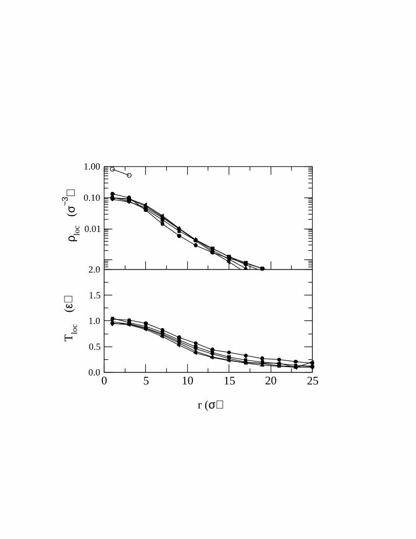
It is worth noticing that, on one hand at τff most of the system is still interacting, and

on the other the local temperature of the inner shells attain a rather constant value that can

be consistently considered as the temperature of the system at fragmentation time. This

can be seen in figure 1 where we show, for different energies, the dependence of the local

temperature, Tloc(r), and the local density, ρ(r), as a function of the distance to the center

of mass at fragmentation time.

B. Analysis of the Constrained System

In order to study the consequences of imposing a finite volume constraint to our system

we used a spherical confining ‘wall’. The considered external potential behaves like Vwall ∼

(r − rwall)−12 with a cut off distance rcut = 1σ , where it smoothly became zero along with

its first derivative. A rather broad range of values for rwall were used.

Inside this potential, a highly excited drop was initialized in the way already described

above and the corresponding equations of motion were integrated. Once the transient be-

havior was over we performed a microcanonical sampling of particle configurations every 5t0

6

up to a final time of 140000t0.

In this case the standard prescription for temperature calculation in the microcanonical

ensemble was used, i.e. the kinetic energy (K) was related to the temperature of our N -

particles system using:

T =2

3(N − 1)K

III. CALORIC CURVES

One of the thermodynamics measurements that remains useful in the small system limit

(hundred of particles) is the caloric curve, i.e. the functional relationship of the system

temperature with its excitation energy.

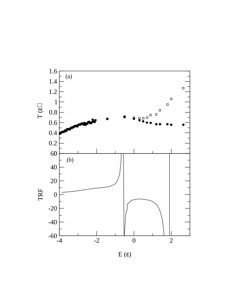
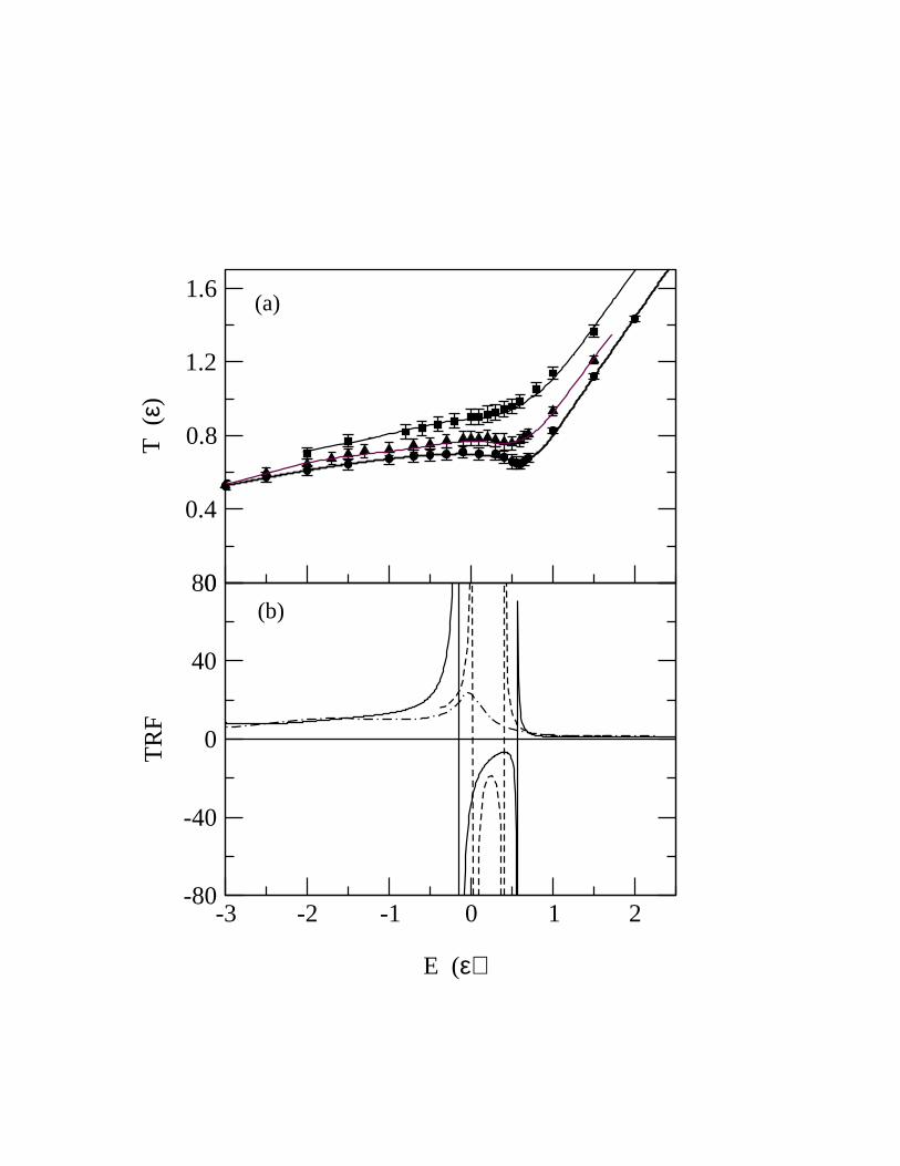
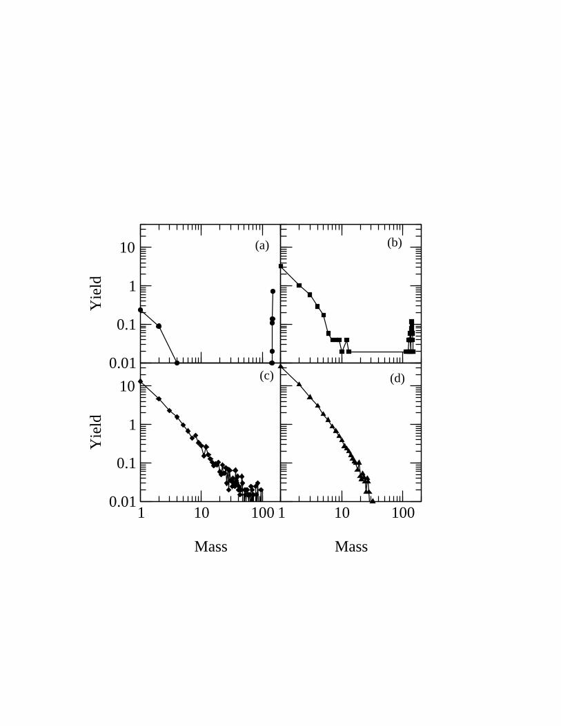
The resulting caloric curve (CC) for the unconstrained system is displayed in Fig. 2 a).

In this figure circles denote the temperature of the system, already defined in Section IIA,

as a function of the energy. On the same figure a curve denoted by squares is also present,

for this one the total kinetic energy, i.e. including both the fluctuations around the collective

motion and the collective motion itself, is used instead. Of course this is not a temperature ,

just a fraction of the total kinetic energy, but it is then obvious that collective motion begins

to be noticeable around a value of E = 0 , and it becomes dominant at around E = 2.ǫ.

Two main features are to be noticed, in first place the CC develops a maximum, and second

the CC has no ”vapor branch” but develops a rather constant behavior. These features are

in contrast with the standard expectations inherited from the thermodynamics of infinite

systems.

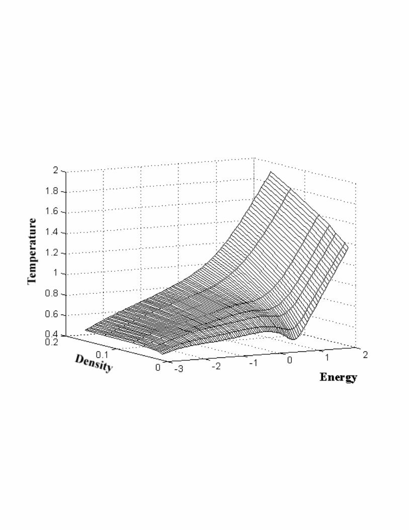
In Fig.3) we show the behavior of T (E, ρ) for the constrained system (see also Fig.4a),

where for the sake of clarity, we include just three different values of ρ).

For all density values a vapor branch is clearly observed. Moreover, comparing Fig.2a)

with Fig.3) and Fig.4a), it is clear that the vapor branch is due to the presence of the confin-

ing volume which inhibits the formation of radial collective motion that behaves like a heat

7

sink in the non constrained case. Inside the volume the emitted aggregates can do nothing

but interact among themselves, and with the constraining wall, until thermal equilibrium is

attained.

The effect of the boundaries on the CC is not important as long as the total energy in

the system is small enough, and the expansive collective motion (in the unconstrained case)

can be neglected. But this is not the case for highly excited finite systems, for which the

presence of the constraining wall prohibits the formation of the expansive radial motion. For

that range of energies the local equilibrium features that can be found in the fragmentation

of the unconstrained system are replaced by global equilibrium ones when the dynamics is

confined to finite volumes. This means that one has to be at least extremely careful if one

intends to analyze expanding systems using confining volumes or any other model that rely

on a global equilibrium hypothesis.

Another interesting feature to be notice in Fig.3) and Fig.4a) is the presence of a loop

at the beginning of the gas rise in the CC for diluted enough systems. This back-bending

behavior is gradually smeared out as the system density is increased. In Section V we will

relate this to the behavior of the thermal response function of the system and in Section VI

we will find that this can also be understood with the aid of the mass spectrum resulting

from the MST and ECRA analysis.

IV. FREEZE OUT VOLUME APPROXIMATION

As was already shown, due to the intrinsic non-equilibrium character of the fragmenta-

tion process in the non-confined case, an assumption of local equilibrium (‘mounted’ over

an expansive radial flux) instead of a global one has been found to be more appropriate.

Accordingly, distributions of density and temperature, and not unique values, are neces-

sary to described the system at fragmentation time in a rigorous way(see Fig.1). It is then

not expected to find an exact mapping in the (T, ρ) space between the constrained and

8

non-constrained dynamics.

Nevertheless if one insists on establishing such a comparison, two different criteria can

be adopted in order to choose the appropriate volume for the constrained case (which we

will call freeze-out volume, Vfo). On one hand it can be seen from Fig.1) that at τff the local

density value for the inner cells (where most of the mass is present at the time of fragment

formation) remains rather constant (ρ ∼ 0.08σ−3) for the broad energy range presented

in the figure. Accordingly, one can choose Vfo in order to attain such density value in

the constrained case. This election, that could be considered as a ‘density-guided’ choice,

corresponds to rwall ∼ 8σ and a freeze out density value of ρ+fo ∼ ρ0/10 .

For the other hand a different approach can also be adopted looking at Fig.2a)

and Fig.4a). It can be verified that for energy values where the onset of the fragmen-

tation process occurs (−2ǫ ≤ E ≤ 0ǫ) the thermal energy in the expanding system is

clearly lower than for the rwall = 8σ case in the constrained case. In fact, similar tem-

peratures can be found in the constrained case only for much diluted situations, i.e. for

rwall = 12σ. In this sense, from a ‘temperature point of view’, a different freeze out density

ρ−fo ∼ 0.02σ−3 ∼ ρ0/40 can be established.

As we mentioned above this ambiguity in the definition of a freeze out volume (or density)

is a consequence of trying to reproduce the behavior of an expanding fragmenting system

using a global equilibrium scenario.

V. THERMAL RESPONSE FUNCTION

In recent works [3,5,15] a lot of attention has been paid to the role played by the behavior

of the specific heat (or more generally speaking: the thermal response function, TRF ) as

a signal of the occurrence of a phase transition in finite systems. Moreover, it has been

shown (see [3]) that the presence of a negative branch in the TRF can be related to a first

order phase transition taking place in an isolated finite system. This kind of analysis can

straightforwardly be performed over the systems under the current study, using the already

9

calculated CC and taking into account that the respective TRF’s can be calculated as:

TRF = (∂T

∂E)−1 (3)

In Fig.2b) we show the TRF for the unconstrained system. Two poles can be seen.

The first one (E ∼ −0.5ǫ) signals the entrance of the system into the multifragmentation

regime, while the second one is related to the leveling off in the corresponding CC, and can

be related to the increasing limit imposed by the strong flux to the ’thermalization’ of the

total available energy.

Fig.4b) shows the corresponding TRF for the constrained case. We include the curves

for the two limiting cases discussed in Section IV as possible freeze out choices, i.e. ρ+fo and

ρ−fo, and an intermediate ρ0 ∼ ρ0/20 value (ρ−

fo < ρ0 < ρ+fo). We notice that two poles and

a negative branch can be observed for the ρ−fo TRF curve. In this case we can relate the

first pole with the onset of the transition, and the second one with the entrance in the gas

phase, the energy distance between them being related to the associated latent heat. For

ρ = ρ0 it can be seen that the curve exhibits a qualitatively similar behavior, the distance

between the two poles is just reduced. Nevertheless, for higher density cases, such as ρ+fo,

the two poles merge into a single ‘singularity’ limited by finite-size effects. In that case, the

TRF remains positive for all energies, showing a peak as a signature of the transition, as

a consequence of the fact that the corresponding caloric curve does not display a loop but

instead a simple change of slope (see next section for an analysis of this change of behavior).

Before leaving this section we would like to discuss, using an approach introduced in [15],

the behavior of the fluctuations in the kinetic energy as an indicator of the occurrence of a

phase transition in our finite system. In [15] it is shown that for an isolated and equilibrated

system in which the total energy can be decomposed as: E = E1 +E2 the heat capacity can

be calculated as:

C ≈C2

1

C1 − σ21/T

2(4)

10

where C1 is the heat capacity associated with the subsystem-1, σ1 is the fluctuation of

the partial energy E1, and T the temperature of the system. In this context, the presence

of poles and negative values in TRF’s can be associated to abnormally large fluctuations of

the partial energy stored in subsystem-1, i.e. σ21 ≥ C1T

2, during the phase transition.

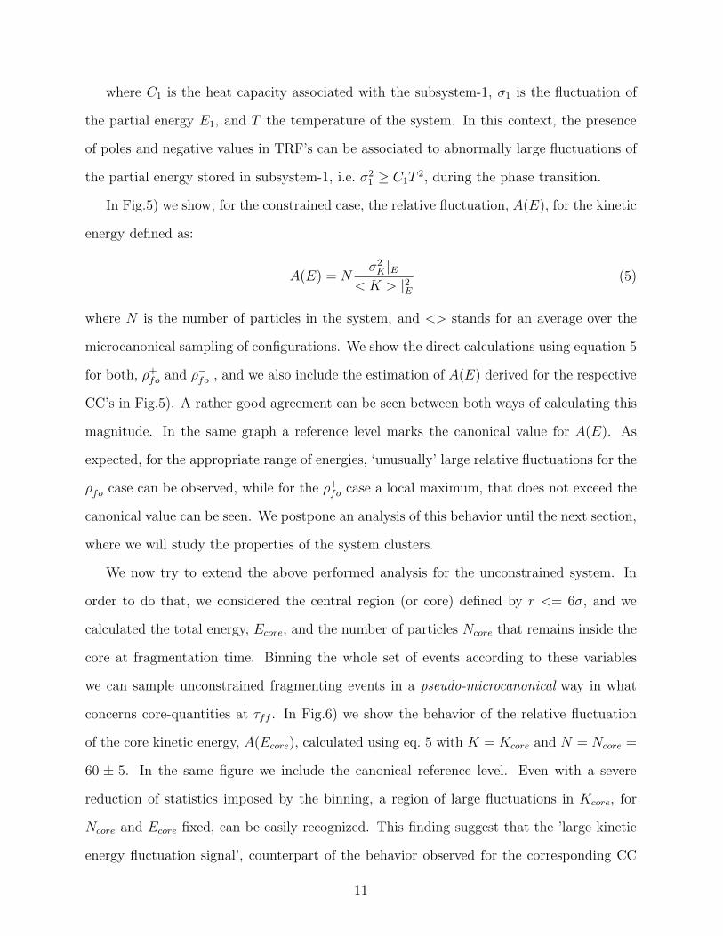
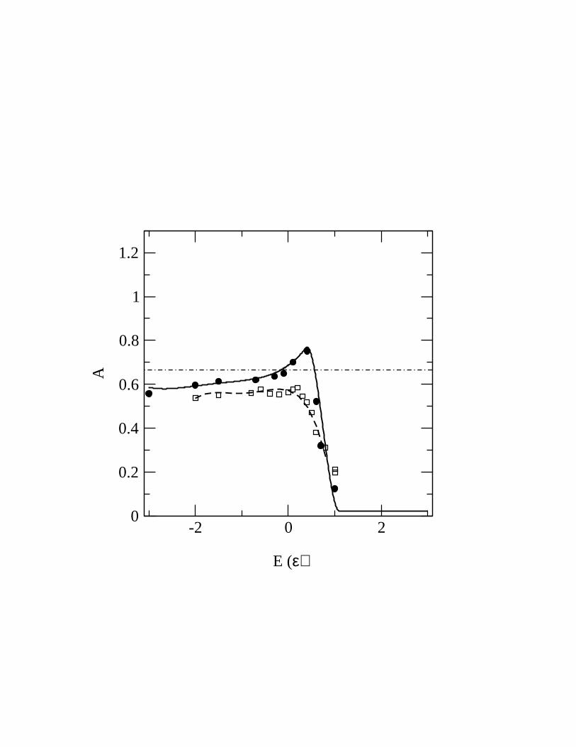
In Fig.5) we show, for the constrained case, the relative fluctuation, A(E), for the kinetic

energy defined as:

A(E) = Nσ2

K |E< K > |2E

(5)

where N is the number of particles in the system, and <> stands for an average over the

microcanonical sampling of configurations. We show the direct calculations using equation 5

for both, ρ+fo and ρ−

fo , and we also include the estimation of A(E) derived for the respective

CC’s in Fig.5). A rather good agreement can be seen between both ways of calculating this

magnitude. In the same graph a reference level marks the canonical value for A(E). As

expected, for the appropriate range of energies, ‘unusually’ large relative fluctuations for the

ρ−fo case can be observed, while for the ρ+

fo case a local maximum, that does not exceed the

canonical value can be seen. We postpone an analysis of this behavior until the next section,

where we will study the properties of the system clusters.

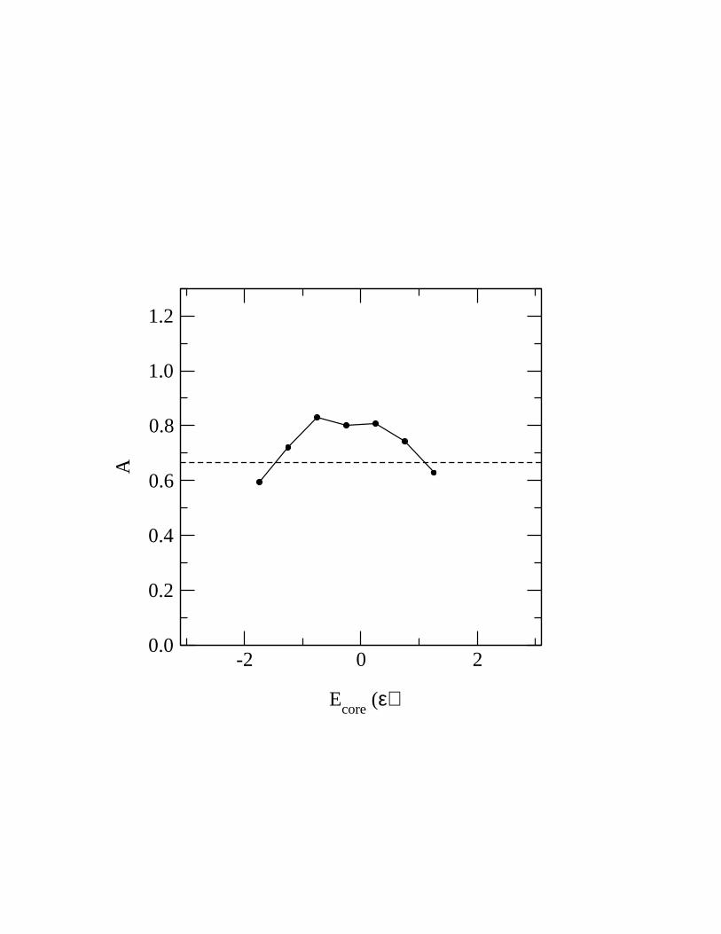
We now try to extend the above performed analysis for the unconstrained system. In

order to do that, we considered the central region (or core) defined by r <= 6σ, and we

calculated the total energy, Ecore, and the number of particles Ncore that remains inside the

core at fragmentation time. Binning the whole set of events according to these variables

we can sample unconstrained fragmenting events in a pseudo-microcanonical way in what

concerns core-quantities at τff . In Fig.6) we show the behavior of the relative fluctuation

of the core kinetic energy, A(Ecore), calculated using eq. 5 with K = Kcore and N = Ncore =

60 ± 5. In the same figure we include the canonical reference level. Even with a severe

reduction of statistics imposed by the binning, a region of large fluctuations in Kcore, for

Ncore and Ecore fixed, can be easily recognized. This finding suggest that the ’large kinetic

energy fluctuation signal’, counterpart of the behavior observed for the corresponding CC

11

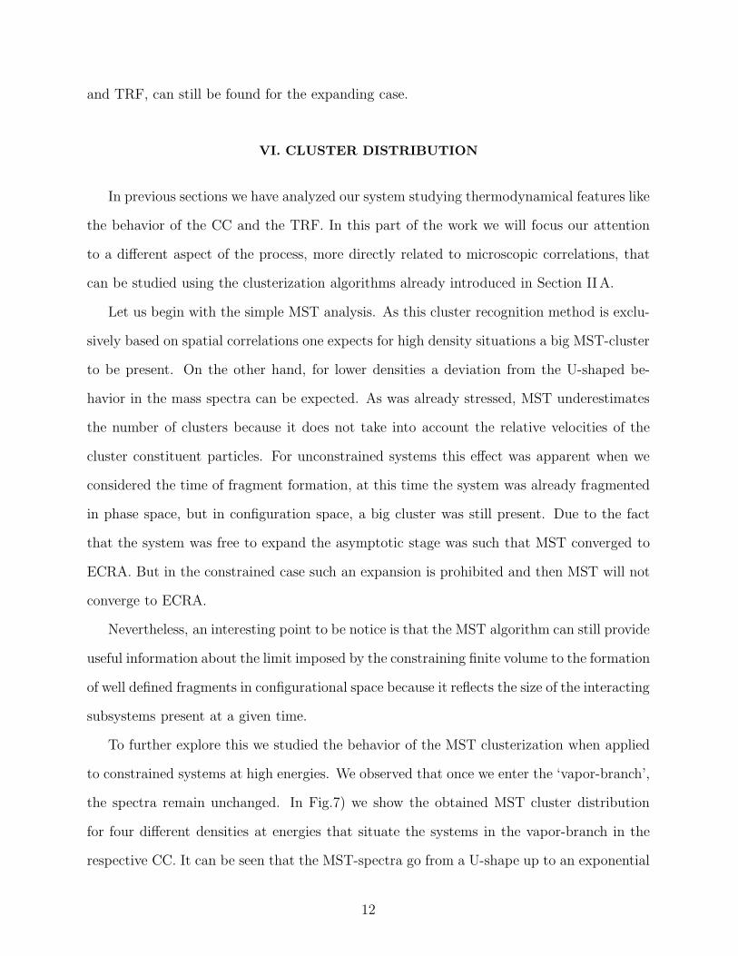
and TRF, can still be found for the expanding case.

VI. CLUSTER DISTRIBUTION

In previous sections we have analyzed our system studying thermodynamical features like

the behavior of the CC and the TRF. In this part of the work we will focus our attention

to a different aspect of the process, more directly related to microscopic correlations, that

can be studied using the clusterization algorithms already introduced in Section IIA.

Let us begin with the simple MST analysis. As this cluster recognition method is exclu-

sively based on spatial correlations one expects for high density situations a big MST-cluster

to be present. On the other hand, for lower densities a deviation from the U-shaped be-

havior in the mass spectra can be expected. As was already stressed, MST underestimates

the number of clusters because it does not take into account the relative velocities of the

cluster constituent particles. For unconstrained systems this effect was apparent when we

considered the time of fragment formation, at this time the system was already fragmented

in phase space, but in configuration space, a big cluster was still present. Due to the fact

that the system was free to expand the asymptotic stage was such that MST converged to

ECRA. But in the constrained case such an expansion is prohibited and then MST will not

converge to ECRA.

Nevertheless, an interesting point to be notice is that the MST algorithm can still provide

useful information about the limit imposed by the constraining finite volume to the formation

of well defined fragments in configurational space because it reflects the size of the interacting

subsystems present at a given time.

To further explore this we studied the behavior of the MST clusterization when applied

to constrained systems at high energies. We observed that once we enter the ‘vapor-branch’,

the spectra remain unchanged. In Fig.7) we show the obtained MST cluster distribution

for four different densities at energies that situate the systems in the vapor-branch in the

respective CC. It can be seen that the MST-spectra go from a U-shape up to an exponential

12

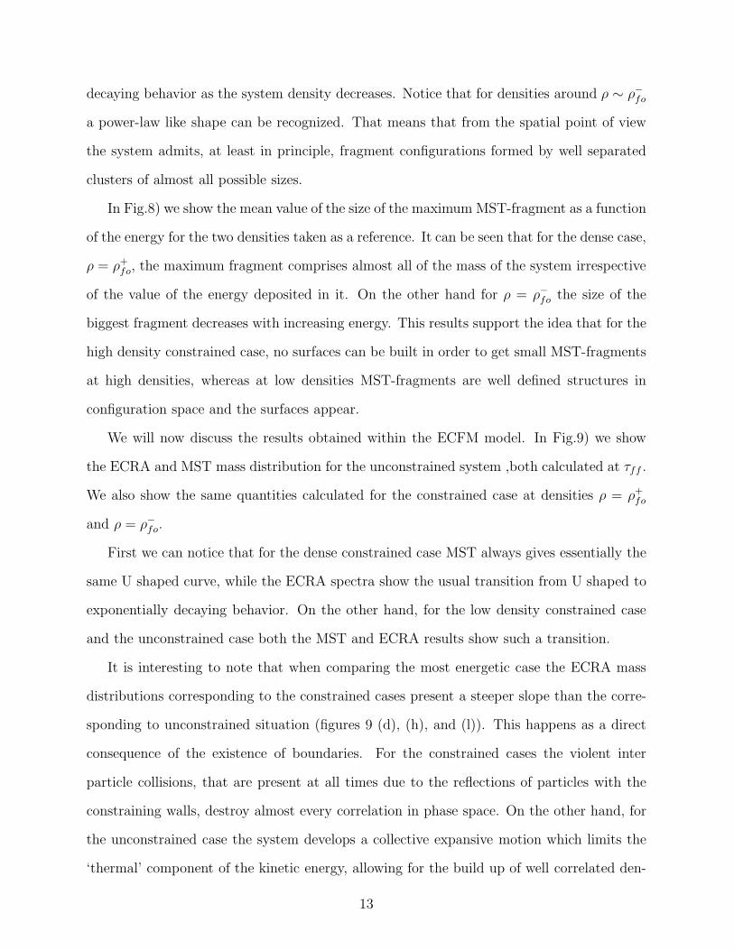
decaying behavior as the system density decreases. Notice that for densities around ρ ∼ ρ−fo

a power-law like shape can be recognized. That means that from the spatial point of view

the system admits, at least in principle, fragment configurations formed by well separated

clusters of almost all possible sizes.

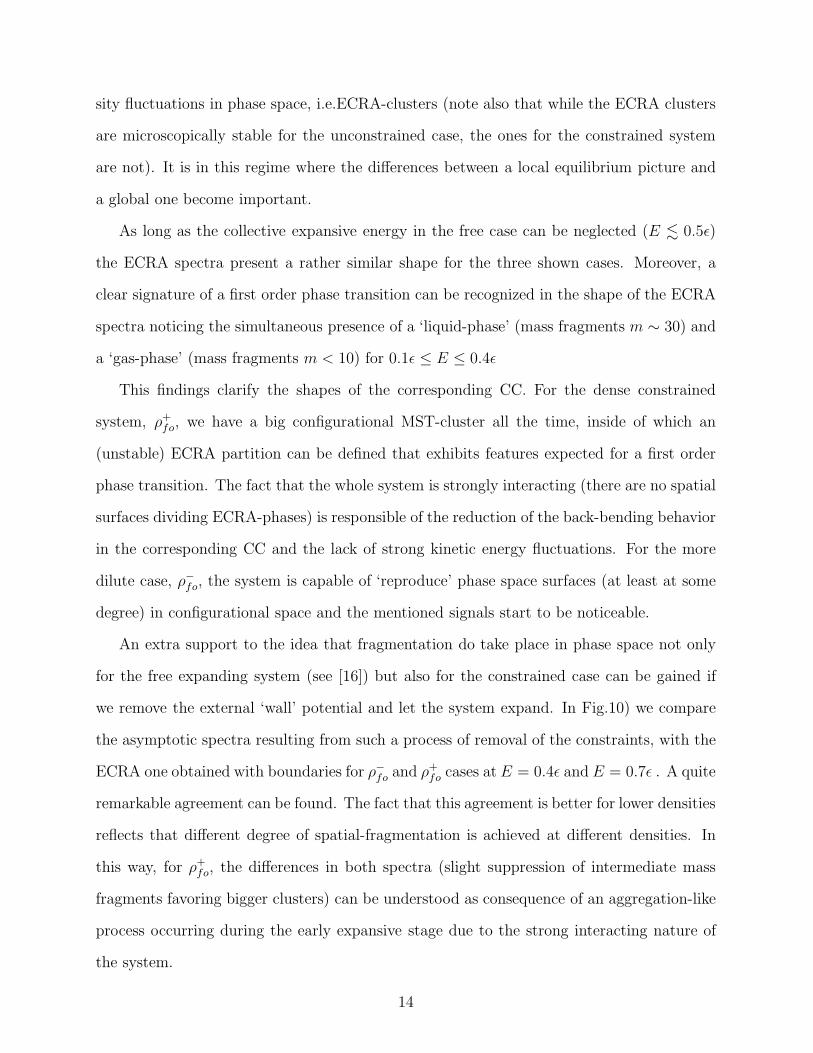
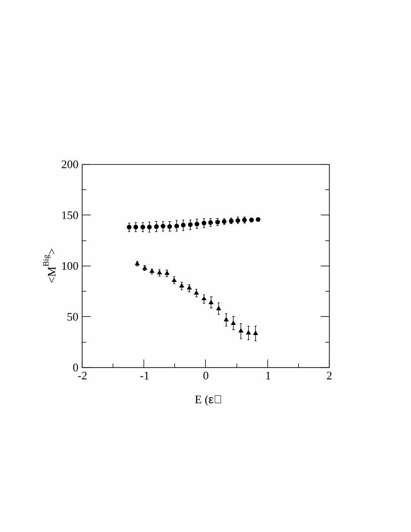
In Fig.8) we show the mean value of the size of the maximum MST-fragment as a function

of the energy for the two densities taken as a reference. It can be seen that for the dense case,

ρ = ρ+fo, the maximum fragment comprises almost all of the mass of the system irrespective

of the value of the energy deposited in it. On the other hand for ρ = ρ−fo the size of the

biggest fragment decreases with increasing energy. This results support the idea that for the

high density constrained case, no surfaces can be built in order to get small MST-fragments

at high densities, whereas at low densities MST-fragments are well defined structures in

configuration space and the surfaces appear.

We will now discuss the results obtained within the ECFM model. In Fig.9) we show

the ECRA and MST mass distribution for the unconstrained system ,both calculated at τff .

We also show the same quantities calculated for the constrained case at densities ρ = ρ+fo

and ρ = ρ−fo.

First we can notice that for the dense constrained case MST always gives essentially the

same U shaped curve, while the ECRA spectra show the usual transition from U shaped to

exponentially decaying behavior. On the other hand, for the low density constrained case

and the unconstrained case both the MST and ECRA results show such a transition.

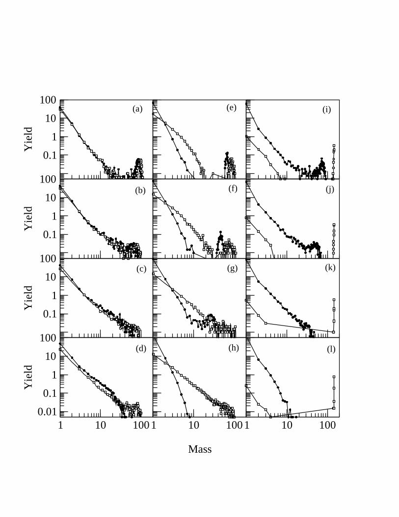
It is interesting to note that when comparing the most energetic case the ECRA mass

distributions corresponding to the constrained cases present a steeper slope than the corre-

sponding to unconstrained situation (figures 9 (d), (h), and (l)). This happens as a direct

consequence of the existence of boundaries. For the constrained cases the violent inter

particle collisions, that are present at all times due to the reflections of particles with the

constraining walls, destroy almost every correlation in phase space. On the other hand, for

the unconstrained case the system develops a collective expansive motion which limits the

‘thermal’ component of the kinetic energy, allowing for the build up of well correlated den-

13

sity fluctuations in phase space, i.e.ECRA-clusters (note also that while the ECRA clusters

are microscopically stable for the unconstrained case, the ones for the constrained system

are not). It is in this regime where the differences between a local equilibrium picture and

a global one become important.

As long as the collective expansive energy in the free case can be neglected (E . 0.5ǫ)

the ECRA spectra present a rather similar shape for the three shown cases. Moreover, a

clear signature of a first order phase transition can be recognized in the shape of the ECRA

spectra noticing the simultaneous presence of a ‘liquid-phase’ (mass fragments m ∼ 30) and

a ‘gas-phase’ (mass fragments m < 10) for 0.1ǫ ≤ E ≤ 0.4ǫ

This findings clarify the shapes of the corresponding CC. For the dense constrained

system, ρ+fo, we have a big configurational MST-cluster all the time, inside of which an

(unstable) ECRA partition can be defined that exhibits features expected for a first order

phase transition. The fact that the whole system is strongly interacting (there are no spatial

surfaces dividing ECRA-phases) is responsible of the reduction of the back-bending behavior

in the corresponding CC and the lack of strong kinetic energy fluctuations. For the more

dilute case, ρ−fo, the system is capable of ‘reproduce’ phase space surfaces (at least at some

degree) in configurational space and the mentioned signals start to be noticeable.

An extra support to the idea that fragmentation do take place in phase space not only

for the free expanding system (see [16]) but also for the constrained case can be gained if

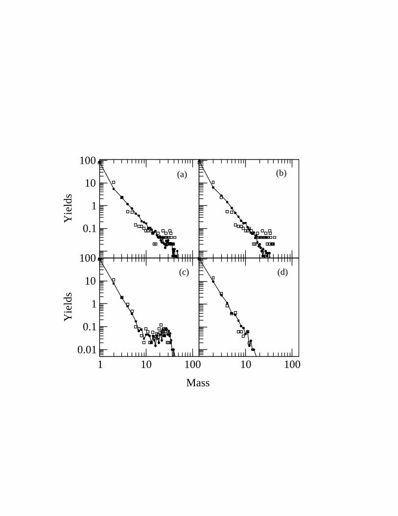
we remove the external ‘wall’ potential and let the system expand. In Fig.10) we compare

the asymptotic spectra resulting from such a process of removal of the constraints, with the

ECRA one obtained with boundaries for ρ−fo and ρ+

fo cases at E = 0.4ǫ and E = 0.7ǫ . A quite

remarkable agreement can be found. The fact that this agreement is better for lower densities

reflects that different degree of spatial-fragmentation is achieved at different densities. In

this way, for ρ+fo, the differences in both spectra (slight suppression of intermediate mass

fragments favoring bigger clusters) can be understood as consequence of an aggregation-like

process occurring during the early expansive stage due to the strong interacting nature of

the system.

14

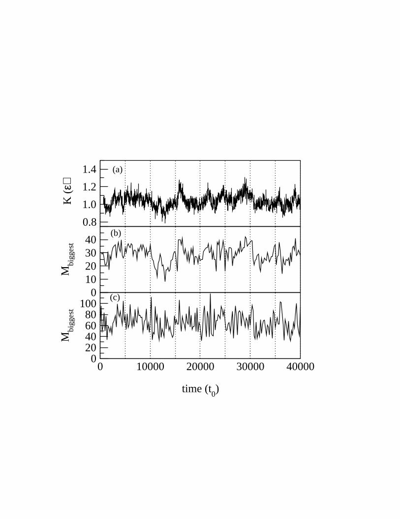
In Section V we showed for the confined system that the diverging behavior of the TRF

is related to abnormally large fluctuations of the kinetic energy. In order to understand the

origin of those fluctuations we show in Fig.11) the system kinetic energy K and the mass

of the biggest ECRA-cluster as a function of time for ρ = ρ−fo at E = 0.4ǫ. Also the mass

of the biggest MST-cluster is shown. It is clearly seen that the first two quantities are well

correlated while the MST biggest cluster is not. This indicates that from a microscopic point

of view the systems is sometimes mainly liquid (big ECRA biggest cluster) and others it is

mainly vapor (small ECRA biggest cluster). This phase alternation is the kind of coexistence

expected for finite system (see [19]).

VII. CONCLUSIONS

In this work we have presented a complete analysis of Caloric Curves, Thermal Response

Functions and MST and ECRA fragment distributions for constrained and unconstrained

excited liquid drops. We have shown that the effect of constraints is quite important, and

that its main result is to allow the system to reach thermal equilibrium. In particular the

Caloric Curves for constrained cases show a vapor branch which is clearly an ‘equilibrium

effect’ that is not present for unconstrained systems.

We have also verified, studying the behavior of ECRA-cluster mass distributions, that

fragmentation does occur in phase space in all the studied cases. Moreover, phase coexistence

can be found in all ECRA spectra at appropriate energies (we have shown that the ECRA

fragments in constrained systems correspond closely to the MST asymptotic clusters when

the constraints are removed. This reinforces the validity of the ECFM-ECRA approach to

study fragmentation phenomena occurring in finite volumes).

It is interesting to notice that for the constrained case, as the system density is increased,

the expected signals of a first order phase transition in the CC, TRF and kinetic energy

fluctuations are gradually smoothed, and eventually disappear. This can be associated

to the fact that at low densities ”internal surfaces” can be developed in the constrained

15

system allowing the transition to be traced in configurational space (i.e. MST clusters are

formed reflecting the fact that well separated aggregates appear in coordinate space). Such

a feature is not possible in the dense case, all of the time the system is composed by a big

configurational cluster that comprises more than 95% of the total mass.

Moreover for the constrained case, a relation between the fluctuations in size of the

maximum ECRA-fragment and the kinetic energy fluctuations was established. As a con-

sequence, the presence of abnormally large fluctuations in the system kinetic energy could

directly be linked with a phase coexistence phenomenon taking place in a finite system.

As a final remark we want to emphasize that, even some similarities can be found between

the behavior of low density constrained systems and unconstrained ones at low energies, such

a comparison fails at and above the energy that corresponds to the onset of the fragmentation

process, i.e. when the collective radial modes begin to drive the evolution of the system.

As we mentioned, the role of this collective motion is to behave as a heat sink, precluding

the system from developing a vapor branch, and freezing the most bound density fluctuations

in phase space allowing them to become the asymptotic clusters. This is why a ‘local’

equilibrium picture, and not a ‘global’ one, is necessary to describe the fragmentation process

correctly, i.e. taking into account the effects of the radial flux. This teaches us that when

dealing with fragmentation phenomena of the kind appearing in nuclear multifragmentation,

caloric curves which display vapor branches should be taken with caution, and consequently

the results obtained from models that display such a feature should be at least critically

reexamined.

Acknowledgment

This work was done under partial financial support from the University of Buenos Aires

via Grant No.TW98, and CONICET via Grant No. PIP 4436/96. A.Chernomoretz ac-

knowledges CONICET for financial support and the warm hospitality of the Laboratoire de

Physique Nucleaire, Departement de Physique, Universite Laval (Quebec, Canada). M.Ison

16

aknowledges finantial support from UBA via a student scholarship.

17

A. Appendix

Once the clusters have been calculated using the ECFM we have to determine the time

at which the fragmentation is over and the systems enters an evaporation regime (i.e the

fragmentation pattern is formed and the fragments undergo a simple evaporation process).

We will then define the time of fragment formation to that time at which the MBDF attain

microscopic stability. This property of the clusters has been calculated using what we call the

Short Time Persistence, in which we calculate the stability of MBDF against evaporation and

coalescence. We define the time of stabilization in the following way: Given a configuration

resulting from the ECRA analysis at a given time t we analyze the microscopic stability

of each fragment Cti of size N t

i by searching on all the fragments Ct+dtj present at time

t + dt for the biggest subset Nmax]t+dti of particles that belonged to Ct

i . We then we assign

to this fragment a value STPd =Nmax]t+dt

i

Nt

i

. In this way we are taking into account what we

call the ”evaporation process”. We also have to take into account that there can be some

realization for which cases the Nmax]t+dti does not constitute a subset of the original cluster

Cti but is embedded in a bigger fragment of mass N t+dt

i . We include this effect by defining

STPi =Nmax]t+dt

i

Nt+dt

i

(with i standing for inverse). Finally the Short time persistence reads :

STP (t, dt) =

⟨⟨

[

STPd(t, dt) + STPi(t, dt)

2

]

j

⟩

m

⟩

e

(6)

where 〈...〉m is the mass weighted average over all the fragments with size N > 3. And

〈...〉e is the average over an ensemble of fragmentation events at a given energy E.

A reference value for STP (t, dt) can be obtained considering that the fragments undergo

only a simple evaporative process. In this way we say that when STP reaches this reference

value the system goes from fragmentation to evaporation. We call this time τff .

18

REFERENCES

[1] A.Bonsera, M.Bruno. C.O.Dorso and P.F.Mastinu , Rivista del Nuovo Cimento 2(2000).

J.Lopez and C.O.Dorso ”Phase Transformations in Nuclear Matter”, World Scientific

2000.

[2] J.Pochodzalla et al., Phys.Rev.Lett 75,1040 (1995)

[3] D.H.E.Gross, Phys.Rep. 279,119 (1997)

[4] F.Gulminelli, Ph.Chomaz, V.Duflot,Europhys.Lett. 50,4,434 (2000)

[5] M.D’Agostino et al., Phys.Lett.B 473, 219,(2000)

[6] A.S.Hirsh et al., Phys.Rev.C 29,508 (1984)

[7] J.B.Elliot et al., Phys.Rev.Lett, 85 1194 (2000)

[8] P.Balenzuela, A.Chernomoretz, C.O.Dorso, Phys.Rev.C (submitted)

[9] X.Campi, H.Krivine

[10] F.Gulminelli, Ph.Chomaz, Phys.Rev.Lett 82,7,1402(1999)

[11] F.Gulminelli, Ph.Chomaz, Phys.Rev.Lett 82,7,1402(1999)

[12] J.M.Carmona, N.Michel, J.Richert, P.Wagner, Phys.Rev.C 61,037304 (2000)

[13] J.P.Bondorf, A.S.Botvina, A.S. Ijilinov, I.N.Mishustin, K.Sneppen, Phys.Rep. 257,133

(1995)

[14] D.Frenkel, B.Smit, Understanding Molecular Simulation, From Algorithms to Applica-

tions (Academic, San Diego, 1996)

[15] Ph.Chomaz, F.Gulminelli, Nuclear Physics A 647, 153 (1999)

[16] A.Strachan, C.O.Dorso, Phys.Rev.C 55, 2, 775 (1997)

[17] A.Strachan, C.O.Dorso, Phys.Rev.C 59, 1, 285 (1999)

19

[18] A.Strachan, C.O.Dorso, Phys.Rev.C 56, 2, 1 (1997)

[19] P.Labestie, R.L.Whetten, Phys.Rev.Lett.65, 1567 (1990)

20

FIGURES

FIG. 1. In the higher figure: local density at the initialization step (empty symbols) and

local density at fragmentation time (solid symbols) as a function of the center of mass distance.

In the lower figure: local temperature profile at fragmentation time as a function of the center of

mass distance. Circles denote E = 0.0ǫ, squares denote E = 0.5ǫ, up-triangles denote E = 0.7ǫ,

diamonds denote E = 0.9ǫ, and left-triangles denote E = 1.2ǫ.

FIG. 2. In figure (a): Caloric curve calculated for the expanding system (solid circles). The

empty squares correspond to an estimation of a ‘fake-temperature’ that does not take into account

in a proper way the collective motion and is calculated simply as a fraction of the total kinetic

energy (see text for details). Figure (b) shows the associated thermal response function.

FIG. 3. Temperature of the constrained system as a function of its energy and density.

FIG. 4. Caloric curve for the constrained system, figure (a), and the respective thermal

response functions, figure (b), for three different densities: ρ = ρ−fo, ρ0fo, and ρ+

fo (circle, triangle,

square symbols in figure (a), and full, dashed, dotted-dashed lines in figure (b), respectively)

FIG. 5. Relative kinetic fluctuation, A(E), for the constrained case calculated for different

densities, as a function of the total energy. The symbols correspond to direct calculations for

ρ = ρ+fo (empty squares) and for ρ = ρ−fo (solid circles). The lines correspond to A estimations

using the caloric curve (solid-line for ρ = ρ−fo, and dashed-line for ρ = ρ+fo). The dashed-dotted

line shows the canonical expectation value for A.

FIG. 6. Relative kinetic energy fluctuation, for the non constrained system, as a function of

the core-energy. The calculation includes only events with Ncore = 60± 5 particles inside the core.

FIG. 7. MST mass distribution calculated for the vapor-branch of constrained systems of den-

sities: ρ = 0.08σ−3(ρ+fo), 0.035σ3 , 0.02σ−3(ρ−fo), and 0.01σ−3 are shown in figures (a), (b), (c), and

(d) respectively.

21

FIG. 8. Mean value of the mass of the biggest MST-cluster for the constrained case. Circles

denote ρ = ρ+fo, and triangles ρ = ρ−fo

FIG. 9. ECRA (solid circles) and MST (empty squares) mass spectra calculated at frag-

mentation time τff . The first column corresponds to the free expanding case, the others to the

ρ = ρ−fo and ρ = ρ+fo confined cases respectively. The considered system energies were: E = −0.5ǫ,

E = 0.0ǫ, E = 0.5ǫ, E = 1.2ǫ, in figures (a)-(d) for the free expanding case, and E = −0.2ǫ,

E = 0.1ǫ, E = 0.4ǫ, E = 1.2ǫ in figures (e)-(f) and (i)-(l) for the constrained cases.

FIG. 10. Asymptotic mass distribution after the ‘wall’ removal (empty squares) and ECRA

spectra calculated within boundaries (solid circles) for densities ρ = ρ+fo (first raw), and ρ−fo (second

raw). Figures (a) and (c) corresponds to E = 0.4ǫ, while (b) and (d) to E = 0.7ǫ

FIG. 11. In figure (a), the system kinetic energy is shown as a function of time for the con-

strained case at ρ = ρ−fo and E = 0.4ǫ. The temporal dependence of the mass of the biggest ECRA

and MST clusters are shown in figures (b) and (c) respectively.

22

0.01

0.10

1.00

ρ loc

(σ−3

)

0 5 10 15 20 25

r (σ)

0.0

0.5

1.0

1.5

2.0

Tlo

c (

ε)

0

0.2

0.4

0.6

0.8

1

1.2

1.4

1.6

T (

ε)

-4 -2 0 2

E (ε)

-60

-40

-20

0

20

40

60

TR

F

(a)

(b)

0

0.4

0.8

1.2

1.6

T (

ε)

-3 -2 -1 0 1 2

E (ε)

-80

-40

0

40

80

TR

F

(a)

(b)

-2 0 2

E (ε)

0

0.2

0.4

0.6

0.8

1

1.2

A

-2 0 2

Ecore

(ε)

0.0

0.2

0.4

0.6

0.8

1.0

1.2

A

0.01

0.1

1

10

Yie

ld

1 10 100

Mass

0.01

0.1

1

10

Yie

ld

1 10 100

Mass

(a) (b)

(d)(c)

-2 -1 0 1 2

E (ε)

0

50

100

150

200

<M

Big

>

0.1

1

10

100

Yie

ld

0.1

1

10

100

Yie

ld

0.1

1

10

100

Yie

ld

1 10 1000.01

0.1

1

10

100

Yie

ld

1 10 100

Mass

1 10 100

(a)

(b)

(c)

(d)

(e)

(f)

(g)

(h)

(i)

(j)

(k)

(l)

0.1

1

10

100

Yie

lds

1 10 1000.01

0.1

1

10

100

Yie

lds

10 100

Mass

(a) (b)

(d)(c)

0.8

1.0

1.2

1.4

K (

ε)

010203040

Mbi

gges

t

0 10000 20000 30000 40000

time (t0)

020406080

100

Mbi

gges

t

(a)

(b)

(c)