arX

iv:c

ond-

mat

/021

2045

v1 [

cond

-mat

.mes

-hal

l] 3

Dec

200

2

A self-consistent treatment of non-equilibrium spin torques

in magnetic multilayers

Asya Shpiro, Peter M. LevyDepartment of Physics, New York University,

4 Washington Place, New York, NY 10003

Shufeng ZhangDepartment of Physics and Astronomy,

University of Missouri-Columbia,

Columbia, MO 65211

(Dated: February 1, 2008)

It is known that the transfer of spin angular momenta between current carriers and local momentsoccurs near the interface of magnetic layers when their moments are non-collinear. However, todetermine the magnitude of the transfer, one should calculate the spin transport properties farbeyond the interface regions. Based on the spin diffusion equation, we present a self-consistentapproach to evaluate the spin torque for a number of layered structures. One of the salient featuresis that the longitudinal and transverse components of spin accumulations are inter-twined fromone layer to the next, and thus, the spin torque could be significantly amplified with respect totreatments which concentrate solely on the transport at the interface due to the presence of themuch longer longitudinal spin diffusion length. We conclude that bare spin currents do not properlyestimate the spin angular momentum transferred between to the magnetic background; the spintransfer that occurs at interfaces should be self-consistently determined by embedding it in ourglobally diffuse transport calculations.

PACS numbers: 72.25.-b, 72.15.Gd, 73.23.-b

I. INTRODUCTION

The concept of using a spin polarized current to switch the orientation of a magnetic layer was developed by Slon-czewski and Berger1, and has been followed up by several others2−4. Recently, we have proposed a way to understandthis spin transfer torque by adopting the model we used to understand magnetoresistance for currents perpendicularto the plane of the layer (CPP)5. Namely, two phenomena, CPP magnetoresistance (MR) and spin torque, originatefrom the spin accumulation. The former is primarily associated with the longitudinal spin accumulation and thelatter is governed by a transverse effect. The distinguishing feature between previous treatments and the one werecently outlined lies in our focus on the spin transport for the entire CPP structure rather than for the interfaceregion alone. The specular scattering of the current at interfaces between magnetic and nonmagnetic layers that isattendant to ballistic transmission can create spin torque1,2. Here we start at the opposite extreme and consider thespin torque due to the bulk of the magnetic layers and the diffuse scattering at interfaces; as is the case for giantmagnetoresistance (GMR) reality is probably a mixture of these extreme positions.

To understand the significance of our approach, we recall the physics of CPP-MR. The resistance of the entireCPP structure comes from various sources of scattering. If one only considers scattering at an interface, one mayconcentrate on the calculation of the transmission coefficient for the interface. However, ballistic transmission acrossan interface is not the only physics of the transport in magnetic multilayers. The leads, as well as impurity scatteringin the layers, have to be included in the calculation of the resistance of the entire CPP structure. Therefore, oneshould embed the ballistic interface scattering in the framework of the diffusive scattering from the bulk of the layers,as well as the diffuse interface scattering, for a better approach to describing the transport. This is very muchthe spirit of CPP transport: the spin transport is described by macroscopic spin diffusion while the detail of theinterface scattering is treated as a boundary condition. The crossover from ballistic interface scattering to diffusivescattering has been recently studied in detail6. By analogy, we argue that the spin torque should be calculated bysolving the transport equation for the entire structure. The interface ballistic spin transfer, which is the center ofthe previous discussions, may be physically important; however it should be embedded in a larger picture, i.e., theballistic transport across an interface should be connected to the diffusive transport outside the interfacial region. Wewill show in this paper that our semi-classical formalism supplies a natural framework to incorporate this. IndeedStiles and Zangwill have done just this; however we make a key assumption, that is different from theirs. That is,we assume that a component of the spin current transverse to the magnetization exists in the magnetic layers.7 Weshould emphasize that our transport calculation does not conflict with the physics of ballistic transport at interfaces.In fact, we will see below, the ballistic component can be accommodated within our formalism.

2

θ

M M(2) (1)

0 t F

z

FM2 Sp FM1 NMy

x

d d

je

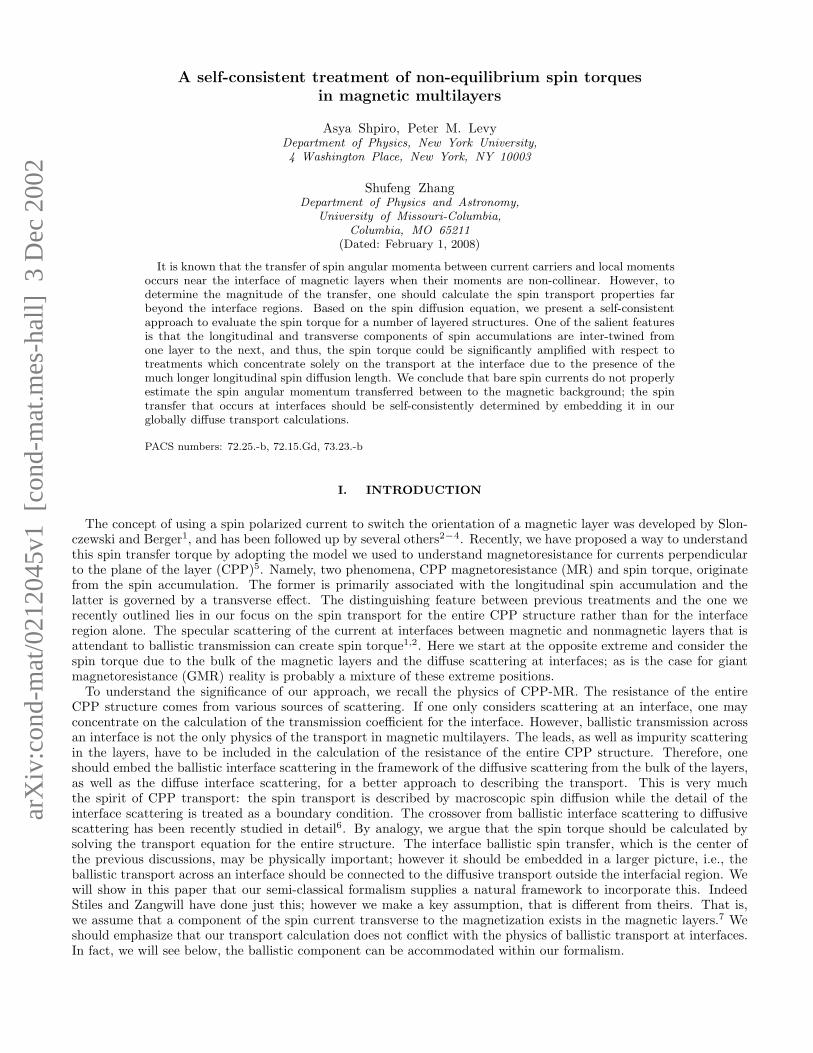
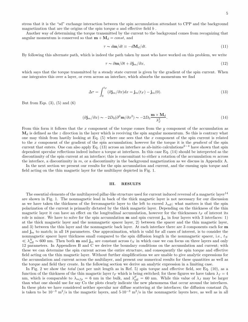
FIG. 1: Multilayered pillar-like structure used for current induced reversal of a magnetic layer. FM2 is a thick ferromagnetic

layer with the thickness exceeding λFsdl and local magnetization M

(2)d = cos θez − sin θey , Sp is a thin nonmagnetic spacer, FM1

is a thin ferromagnetic layer with the thickness tF and local magnetization M(1)d = ez, and NM is a nonmagnetic back layer.

Here we specify a model system to calculate the spin torque: a magnetic multilayer whose essential elements consistof a thick magnetic layer, whose primary role is to polarize the current, a thin magnetic layer that is to be switched,a nonmagnetic spacer layer so that there is no interlayer exchange coupling between the thick and thin layers, anda nonmagnetic layer or lead on back of the thin magnetic layer; see Fig. 1. As we show in this paper the angularmomentum transferred to a thin layer far exceeds the transverse component (to the orientation of the magnetizationof the thin layer) of the bare portion of the incoming spin polarized current, i.e., that part proportional to the electricfield; see Eq. (2) below. It is a direct consequence of the spin accumulation coming from the two primary layers, thethick magnetic and nonmagnetic back layers, that produce this buildup. The role of this accumulation in the spincurrent is given in Eq. (7) of Ref. 5; it is a consequence of considering the transport in the multilayer as a diffusiveprocess, and is in keeping with our previous treatments of transport in magnetic multilayers with the proviso thatone has to include the exchange interaction between the accumulation and the magnetic background, a.k.a. the “sd”interaction, to obtain the angular momentum transferred. It is this interaction which produces the spin transferbetween the current and the magnetic background. Among other things the parameters entering our theory aredetermined from CPP transport measurements, except for the exchange interaction between the itinerant electronsand the magnetic background.

In this paper we first review the formalism presented in Ref. 5 for calculating the torque and effective field acting ona magnetic layer. In particular we define the boundary conditions between the layers of the multilayer and point outwhat are the sources for the longitudinal and transverse spin accumulations when the magnetization of the layers arenoncollinear. In Sec. III we present our results for the spin accumulation, spin currents and the torque and effectivefield acting on the thin layer of the multilayer depicted in Fig. 1. The bulk of our results are obtained numerically,however in certain limits we are able to give analytic expressions, e.g., for the amplification of the torque and effectivefield acting on a layer due to the accumulation. In Sec. IV we present an analytic expression for the amplification, andwe indicate how recent “ab-initio” determinations of the change of spin currents across a ferromagnetic-nonmagnetic(FM/NM) interface can be incorporated at the interfaces between layers in our diffusive treatment of the transport ina multilayered structure. The impact of transverse accumulation on GMR is given in Sec. V; in particular in creatingdeviations from the simple linear dependence of the resistance with the cosine of the angle between the thick and thinlayers.

II. REVIEW OF FORMALISM

By starting with the linear response of the current to the electric field for diffusive transport5

(x) = CE(x) − D∂n

∂x, (1)

3

we find the spin or magnetization current is

jm = ReTr(σ) = 2CE(x) − 2D∂n0

∂x− 2D0

∂m

∂x, (2)

where both current (x) and field E(x) are directed along the growth direction x of the multilayer8. Here C denotes a

conductivity and D a diffusion constant; the two are related by the Einstein relation C = e2N(ǫF )D for a degenerate

metal, where N(ǫF ) is the density of states at the Fermi level. The first term on the right hand side of Eq. (2) isthe bare contribution to the spin polarized current from the electric field, the third term is the contribution fromthe spin accumulation attendant to the current across a magnetically inhomogeneous structure; although it can besubsumed as an interface contribution, as we include the diffuse interface scattering below, we will neglect the secondterm coming from charge accumulation. As we will show in magnetic multilayers the contribution of the third termto the spin current can dominate over the first.

The equation of motion for the spin accumulation is

∂m

∂t+

∂jm∂x

+ (J/~)m × Md = − m

τsf, (3)

where τsf is the spin-flip relaxation time of the conduction electron. While the last term is diffusive the spin motioninduced by the exchange interaction J is not at all diffusive in spin space; it describes a deterministic or ballisticrotation of the accumulation that itself is generated by diffusive spin-flip processes. The diffusion equation for themacroscopic variables m and jm can be derived from the Boltzmann equation for the spin distribution function in thelimit where the length scale dJ ≡ vF h/J & λmfp , i.e., when the distance an electron moves while its spin rotates by2π is greater than the mean free path9. In the opposite limit we are not able to derive such a simple relation betweenthese variables from the Boltzmann equation; nonetheless we will calculate the spin torque by using this expressionand later evaluate the significance of the results. We note that in this treatment we consider the effect of the exchangeinteraction between the itinerant electrons and the background magnetization Hint = −Jm · Md, a.k.a. the “sd”interaction, in the equation of motion for the distribution function. To write the spin current Eq. (2) in terms of theelectric current

je ≡ Re(Tr) = 2C0E(x) − 2D0∂n0

∂x− 2D · ∂m

∂x, (4)

we insert this expression in Eq. (2) to eliminate the electric field and charge density, and we obtain

jm = βjeMd − 2D0

[

∂m

∂x− ββ′Md(Md · ∂m

∂x)

]

, (5)

where we have dropped an uninteresting term proportional to the derivative of the charge accumulation ∂n0/∂x. Uponplacing this expression in Eq. (3) we find the equation of motion for the spin current is

1

2D0

∂m

∂t− ∂2m

∂x2+ ββ′Md

(

Md · ∂2m

∂x2

)

+m

λ2sf

+m × Md

λ2J

= − 1

2D0

∂

∂x(βjeMd), (6)

where β, β′ are the spin polarization parameters defined by the relations C = βC0Md, where Md is the unit vectorto represent the direction of the local magnetization and D = β′D0Md

5, and we have defined λsf ≡√

2D0τsf and

λJ ≡√

2~D0/J =√

λmfpdJ/3π where τsf is the spin flip relaxation time, and J the exchange between the itinerantelectrons and the magnetic background. The diffusion constant is D0 ∼ (1/3)v2

F τ = (1/3)vF λmfp , where vF is theFermi velocity, τ the momentum relaxation time, and λmfp the mean free path; λmfp ≡ vF τ . As we indicate later,if one interprets λmfp as that associated with the diffusive scattering at interfaces one arrives at a much smallerestimates for λJ than when one uses the mean free path arriving from scattering in the bulk of the layers.

The term on the right hand side of the time dependent diffusion equation Eq. (6) for the spin accumulation is thesource term; it is this term that drives the accumulation10. Here we will look for the steady state solutions so thatthe first term on the left hand side is zero, and the electric current je is constant throughout the multilayer. InAppendix A we discuss the source term; here we point out that this term guarantees the continuity of the spin currentjm across the interfaces, provided the accumulation is continuous. This can be immediately verified by integratingEq. (6) across an interface and using the definition of spin current Eq. (5), or by integrating Eq. (3).

We will proceed along the lines of the conventional treatment for current perpendicular to the plane of the layers(CPP) in magnetic multilayers and focus on the discontinuous variation of the background magnetization between

4

the layers. In this treatment of CPP we assume that the magnetization is uniform throughout a layer so that thesource term is confined to interfaces between layers11,12; in this case one can take into account the source terms byappropriate boundary conditions; this is the procedure usually followed when calculating the spin accumulation inmagnetic multilayers12. In this case we set the source term in Eq. (6) to zero, separate the spin accumulation intolongitudinal (parallel to the local moment) and transverse (perpendicular to the local moment) modes, and look forthe steady state solutions. We stress that the terms longitudinal and transverse are relative to the magnetization inthe individual layers, i.e., they are locally defined and have no global meaning throughout a multilayer. Equation (6) can now be written as

∂2m||∂x2

− m||λ2

sdl

= 0, (7)

where λsdl =√

1 − ββ′λsf , and

∂2m⊥∂x2

− m⊥λ2

sf

− m⊥ × Md

λ2J

= 0. (8)

The longitudinal accumulation m|| decays at the length scale of the spin diffusion length λsdl while the transverse spinaccumulation m⊥ decays as λJ . It is important to differentiate between λsdl which arises from spin flip processes,and λJ which represents the decay of transverse spin currents due to ordinary spin dependent, λmfp, but non-spin-flipscattering. For cobalt we estimate in Appendix A the transverse spin accumulation has a much shorter length scalecompared to the longitudinal one; for permalloy λJ is comparable to the spin diffusion length. We limit our presentstudy to λJ ≪ λsdl .

The boundary conditions are that the spin accumulation m and current jm are continuous across at interfaces aslong as there is no specular or diffusive interface scattering; note that it is unnecessary to invoke the delta functionsource term at the boundary of a layer (see the Appendix A) which specifies the discontinuity in ∂m/∂x. As notedabove the source of this discontinuity in the accumulation is to guarantee the continuity of the spin current (providedno torque is created at interface, see below), therefore we can simply invoke it; see Appendix C. While we could inprinciple consider the effect of specular scattering at interfaces, as we have for other problems associated with CPPtransport13, this involves considering each k vector separately which for a noncollinear multilayer is a cumbersomeproblem we will not address. Others have considered specular scattering at interfaces and have shown it gives riseto spin torque at these boundaries1,2. The presence of diffuse scattering at interfaces due to both roughness andinterdiffusion in noncollinear structures is treated in Appendix B.

Once having the spin accumulation we take a look at its influence on the background magnetization. The equationof motion for the local magnetization is

dMd

dt= −γ0Md × (He + Jm) + αMd × dMd

dt, (9)

where γ0 is the gyromagnetic ratio, He is the magnetic field including the contributions from the external field,anisotropy and magnetostatic field, the additional effective field Jm is due to coupling between the local moments(background magnetization) and the spin accumulation, and the last term is the Gilbert damping term. As seenfrom Eq. (9), the longitudinal spin accumulation has no effect on the local moment; we can re-write Eq. (9) in termsof the transverse spin accumulation only by replacing m by m⊥. As shown in Ref. 3 the two components of the

accumulation in the plane transverse to the magnetization M(1)d of the layer for which we are calculating the effect

due to the spin current are

Jm⊥ = aM(2)d × M

(1)d + bM

(2)d (10)

where M(2)d is the magnetization of the other layer; in the case we discuss in this paper (see Fig. 1) M

(1)d refers to

the thin layer which is being switched and M(2)d to the thick layer which polarizes the current and which is pinned

so that is does not rotate. By placing this form of the accumulation in the equation of motion for the backgroundmagnetization Eq. (9) we find that the transverse spin accumulation produces two effects simultaneously: the term

bM(1)d

× M(2)d

is the torque due to an “effective field” bM(2)d

, and the other is aM(1)d

× (M(2)d

×M(1)d

) which is called

the “spin torque” predicted by Slonczewski and Berger1. The first term produces a precessional motion about M(1)d ;

in this sense it acts as if the spin current creates a magnetic field on M(1)d . The second term acts so as to increase or

decrease the angle between M(1)d and M

(2)d ; also, it acts so as to assist or oppose the damping term in Eq. (9). We

5

stress that it is the “sd” exchange interaction between the spin accumulation attendant to CPP and the backgroundmagnetization that are the origins of the spin torque a and effective field b .

Another way of determining the torque transmitted by the current to the background comes from recognizing thatangular momentum is conserved so that m + Md = const, and

τ ∼ dm/dt ≡ −dMd/dt. (11)

By following this alternate path, which is indeed the path taken by most who have worked on this problem, we write

τ ∼ ∂m/∂t + ∂jm/∂x, (12)

which says that the torque transmitted by a steady state current is given by the gradient of the spin current. Whenone integrates this over a layer, or even across an interface, which absorbs the momentum we find

∆τ =

∫ tF

0

(∂jm/∂x)dx = jm(tF ) − jm(0). (13)

But from Eqs. (3), (5) and (6)

(∂jm/∂x) ∼ −2D0(∂2m/∂x2) ∼ −2D0

m × Md

λ2J

. (14)

From this form it follows that the x component of the torque comes from the y component of the accumulation asMd is defined as the z direction in the layer which is receiving the spin angular momentum. So this is contrary whatone may think from hastily looking at Eq. (5) where one sees that the x component of the spin current is relatedto the x component of the gradient of the spin accumulation; however for the torque it is the gradient of the spincurrent that enters. One can also apply Eq. (13) across an interface as ab-initio calculations2−4 have shown that spindependent specular reflections indeed induce a torque at interfaces. In this case Eq. (14) should be interpreted as thediscontinuity of the spin current at an interface; this is concomitant to either a rotation of the accumulation m acrossthe interface, a discontinuity in m, or a discontinuity in the background magnetization as we discuss in Appendix A.

In the next section we present our results for the spin accumulation and current, and the ensuing spin torque andfield acting on the thin magnetic layer for the multilayer depicted in Fig. 1.

III. RESULTS

The essential elements of the multilayered pillar-like structure used for current induced reversal of a magnetic layer14

are shown in Fig. 1. The nonmagnetic lead in back of the thick magnetic layer is not necessary for our discussionas we have taken the thickness of the ferromagnetic layer to the left to exceed λsdl; what matters is that the spinpolarization of the current is primarily dictated by the thick magnetic layer. Depending on the thickness of the thinmagnetic layer it can have an effect on the longitudinal accumulation, however for the thicknesses tF of interest itsrole is minor. We have to solve for the spin accumulation m and spin current jm in four layers with 3 interfaces: 1)at the thick magnetic layer and the nonmagnetic spacer layer, 2) between the spacer and the thin magnetic layer,and 3) between the thin layer and the nonmagnetic back layer. At each interface there are 3 components each for m

and jm to match; in all 18 parameters. One approximation, which is valid for all cases of interest, is to consider thenonmagnetic spacer layer thickness small compared to the spin diffusion length in the nonmagnetic spacer, i.e., tN≪ λN

sdl ∼ 600 nm. Then both m and jm are constant across tN in which case we can focus on three layers and only12 parameters. In Appendices B and C we derive the boundary conditions on the accumulation and current; withthese we can determine the spin current across the entire structure, and consequently the spin torque and effectivefield acting on the thin magnetic layer. Without further simplifications we are unable to give analytic expressions forthe accumulation and current across the multilayer, and present our numerical results for these quantities as well asthe torque and field they create. In the following section we derive an analytic expression in a limiting case.

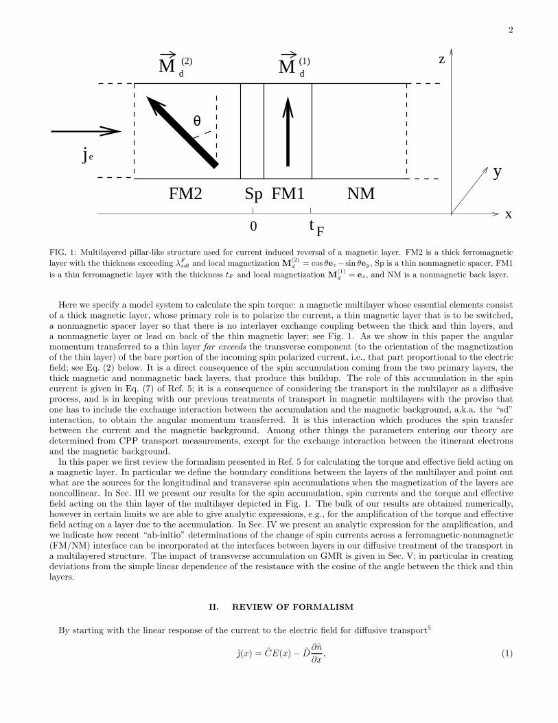
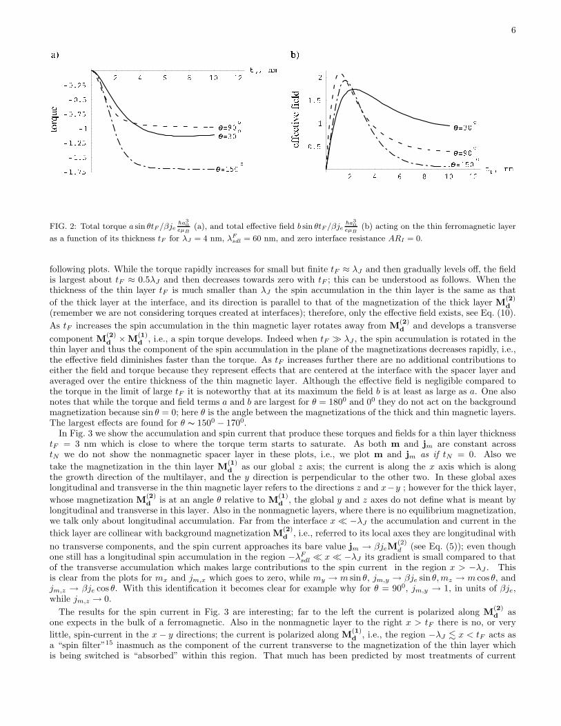
In Fig. 2 we show the total (not per unit length as in Ref. 5) spin torque and effective field, see Eq. (10), as afunction of the thickness of the thin magnetic layer tF which is being switched; for these figures we have taken λJ = 4nm, which is comparable to λmfp = 6 nm in the bulk, and λF

sdl = 60 nm. While this value of λJ may be largerthan what one should use for say Co the plots clearly indicate the new phenomena that occur around the interfaces.In these plots we have considered neither specular nor diffuse scattering at the interfaces; the diffusion constant D0

is taken to be 10−3 m2/s in the magnetic layers, and 5·10−3 m2/s in the nonmagnetic layers here, as well as in all

6

FIG. 2: Total torque a sin θtF /βje~a3

0

eµB(a), and total effective field b sin θtF /βje

~a30

eµB(b) acting on the thin ferromagnetic layer

as a function of its thickness tF for λJ = 4 nm, λFsdl = 60 nm, and zero interface resistance ARI = 0.

following plots. While the torque rapidly increases for small but finite tF ≈ λJ and then gradually levels off, the fieldis largest about tF ≈ 0.5λJ and then decreases towards zero with tF ; this can be understood as follows. When thethickness of the thin layer tF is much smaller than λJ the spin accumulation in the thin layer is the same as that

of the thick layer at the interface, and its direction is parallel to that of the magnetization of the thick layer M(2)d

(remember we are not considering torques created at interfaces); therefore, only the effective field exists, see Eq. (10).

As tF increases the spin accumulation in the thin magnetic layer rotates away from M(2)d and develops a transverse

component M(2)d × M

(1)d , i.e., a spin torque develops. Indeed when tF ≫ λJ , the spin accumulation is rotated in the

thin layer and thus the component of the spin accumulation in the plane of the magnetizations decreases rapidly, i.e.,the effective field diminishes faster than the torque. As tF increases further there are no additional contributions toeither the field and torque because they represent effects that are centered at the interface with the spacer layer andaveraged over the entire thickness of the thin magnetic layer. Although the effective field is negligible compared tothe torque in the limit of large tF it is noteworthy that at its maximum the field b is at least as large as a. One alsonotes that while the torque and field terms a and b are largest for θ = 1800 and 00 they do not act on the backgroundmagnetization because sin θ = 0; here θ is the angle between the magnetizations of the thick and thin magnetic layers.The largest effects are found for θ ∼ 1500 − 1700.

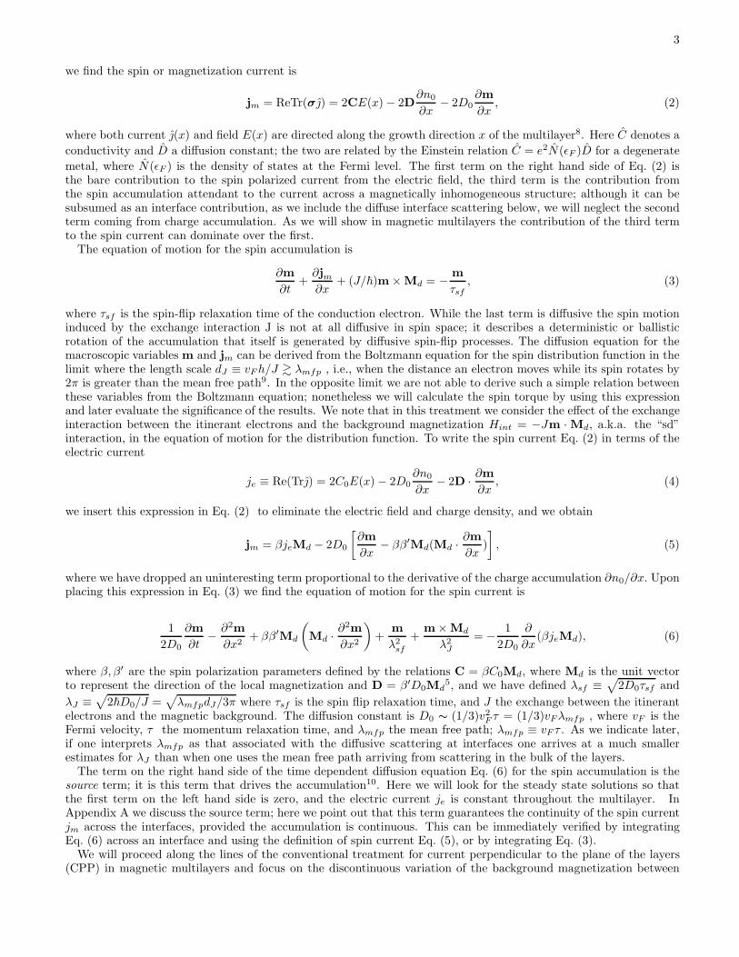
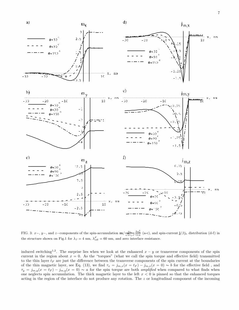
In Fig. 3 we show the accumulation and spin current that produce these torques and fields for a thin layer thicknesstF = 3 nm which is close to where the torque term starts to saturate. As both m and jm are constant acrosstN we do not show the nonmagnetic spacer layer in these plots, i.e., we plot m and jm as if tN = 0. Also we

take the magnetization in the thin layer M(1)d as our global z axis; the current is along the x axis which is along

the growth direction of the multilayer, and the y direction is perpendicular to the other two. In these global axeslongitudinal and transverse in the thin magnetic layer refers to the directions z and x−y ; however for the thick layer,

whose magnetization M(2)d is at an angle θ relative to M

(1)d , the global y and z axes do not define what is meant by

longitudinal and transverse in this layer. Also in the nonmagnetic layers, where there is no equilibrium magnetization,we talk only about longitudinal accumulation. Far from the interface x ≪ −λJ the accumulation and current in the

thick layer are collinear with background magnetization M(2)d , i.e., referred to its local axes they are longitudinal with

no transverse components, and the spin current approaches its bare value jm → βjeM(2)d (see Eq. (5)); even though

one still has a longitudinal spin accumulation in the region −λFsdl ≪ x ≪ −λJ its gradient is small compared to that

of the transverse accumulation which makes large contributions to the spin current in the region x > −λJ . Thisis clear from the plots for mx and jm,x which goes to zero, while my → m sin θ, jm,y → βje sin θ, mz → m cos θ, andjm,z → βje cos θ. With this identification it becomes clear for example why for θ = 900, jm,y → 1, in units of βje,while jm,z → 0.

The results for the spin current in Fig. 3 are interesting; far to the left the current is polarized along M(2)d as

one expects in the bulk of a ferromagnetic. Also in the nonmagnetic layer to the right x > tF there is no, or very

little, spin-current in the x − y directions; the current is polarized along M(1)d , i.e., the region −λJ . x < tF acts as

a “spin filter”15 inasmuch as the component of the current transverse to the magnetization of the thin layer whichis being switched is “absorbed” within this region. That much has been predicted by most treatments of current

7

FIG. 3: x−, y−, and z−components of the spin-accumulation m/ βje√2λJ J

~a30

eµB(a-c), and spin-current j/βje distribution (d-f) in

the structure shown on Fig.1 for λJ = 4 nm, λFsdl = 60 nm, and zero interface resistance.

induced switching1,2. The surprise lies when we look at the enhanced x − y or transverse components of the spincurrent in the region about x = 0. As the “torques” (what we call the spin torque and effective field) transmittedto the thin layer tF are just the difference between the transverse components of the spin current at the boundariesof the thin magnetic layer, see Eq. (13), we find τx = jm,x(x = tF ) − jm,x(x = 0) ∼ b for the effective field , andτy = jm,y(x = tF ) − jm,y(x = 0) ∼ a for the spin torque are both amplified when compared to what finds whenone neglects spin accumulation. The thick magnetic layer to the left x < 0 is pinned so that the enhanced torquesacting in the region of the interface do not produce any rotation. The z or longitudinal component of the incoming

8

spin current is not absorbed by the thin magnetic layer as there is no transfer of spin angular momentum along thisdirection (tF ≪ λsdl); see Fig. 3f. The slight decrease in jm,z is due to the ambient spin flip scattering in the magneticlayer which is characterized by λF

sdl ∼ 60 nm in the plots shown in Fig. 3. The much slower decrease in jm,z(x > tF )comes from the spin flip scattering in the nonmagnetic layer whose λN

sdl ∼ 600 nm ≫ λFsdl .

The large enhancement of the transverse spin currents can be understood as follows. Around x = 0, which in ourpicture contains the interfaces between the thick and thin magnetic layers, the source term for the transverse spinaccumulation is comparable to that for the longitudinal; as mentioned in the previous section the spin accumulationmakes up for the discontinuity in the “bare” spin current. At the interface between the thick and thin layers this isthe component of the spin current, coming from the bulk of the thick magnetic layer, that is perpendicular to themagnetization in the thin layer. The distance over which it is absorbed is much smaller than that for the longitudinalaccumulation λJ ≪ λF

sdl. Therefore the gradient of the transverse accumulation about x = 0 is large and as it isthe gradient that contributes to the spin current, Eq. (5), we find the unanticipated amplification of the transversecomponents of the spin current at this interface (really two interfaces). This amplification is not a maximum aboutθ = 900, because in addition to the ”bare” contribution, there is the component of the spin current that arises from

the longitudinal accumulation in the thick layer, i.e., parallel to the magnetization M(2)d . For θ = 900 this longitudinal

accumulation is quite small, see Fig. 2h, so that there’s little amplification at this angle. In the next section we presenta more quantitative reason for the enhancement.

The plots in Fig. 2 were for the case of λFsdl = 60 nm, λJ = 4 nm, tF ∼ where the torque a starts to saturate. To

determine the roles of the spin diffusion length, λFsdl (while keeping λN

sdl = 600 nm), the spin transfer length λJ , andthe interface resistance due to diffuse scattering at the interfaces ARI (see Appendix B), on these plots we have rerunour program for: λF

sdl = 30 nm, λJ = 4 nm, ARI = 0, to show effect of reduced λsdl on torques; λFsdl = 60 nm, λJ = 1

nm, ARI = 0, to show effect of smaller λJ on torques; and λFsdl = 30 − 60 nm, λJ = 1 − 4 nm, ARI 6= 0, to show

effect of interface scattering on torques. We account for this scattering in Appendix C by introducing thin “interfacialregions” in the magnetic layers which have the enhanced scattering found at interfaces, and derive the boundaryconditions on the accumulation and current in the presence of interface scattering as we let the thickness of the regiontend to zero. The amount of the scattering ARI and its spin dependence γ are taken from experimental data onCPP-MR16. While the diffuse interface scattering by itself produces sizeable discontinuities in the accumulation itdoes not create much spin torque; this is one difference between our treatment and others.

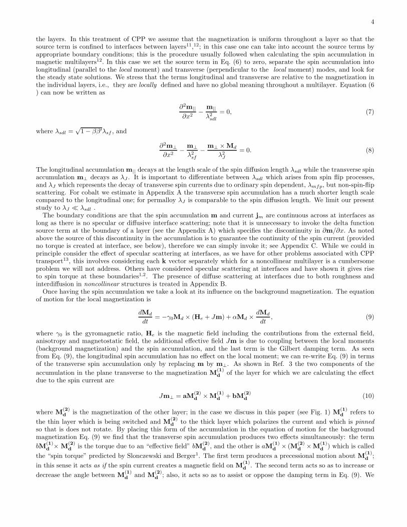
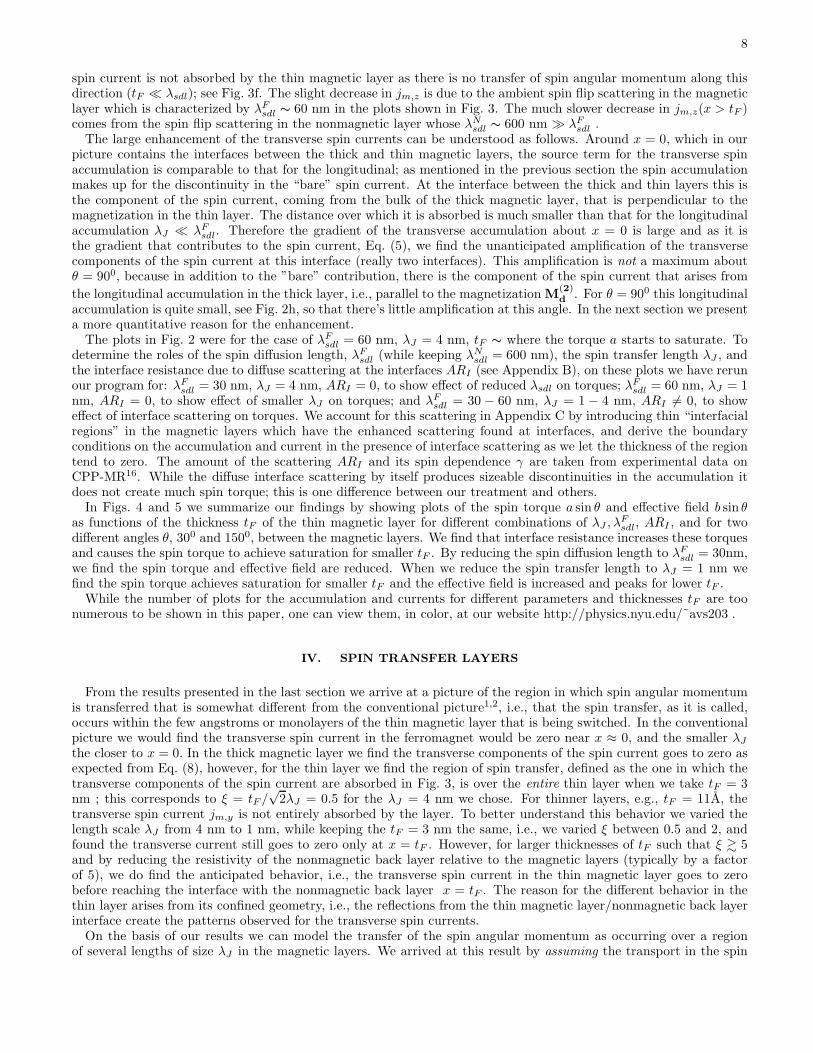
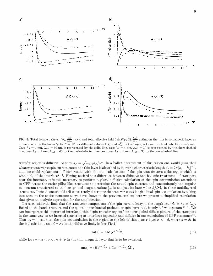
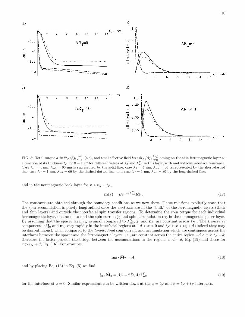
In Figs. 4 and 5 we summarize our findings by showing plots of the spin torque a sin θ and effective field b sin θas functions of the thickness tF of the thin magnetic layer for different combinations of λJ , λF

sdl, ARI , and for twodifferent angles θ, 300 and 1500, between the magnetic layers. We find that interface resistance increases these torquesand causes the spin torque to achieve saturation for smaller tF . By reducing the spin diffusion length to λF

sdl = 30nm,we find the spin torque and effective field are reduced. When we reduce the spin transfer length to λJ = 1 nm wefind the spin torque achieves saturation for smaller tF and the effective field is increased and peaks for lower tF .

While the number of plots for the accumulation and currents for different parameters and thicknesses tF are toonumerous to be shown in this paper, one can view them, in color, at our website http://physics.nyu.edu/˜avs203 .

IV. SPIN TRANSFER LAYERS

From the results presented in the last section we arrive at a picture of the region in which spin angular momentumis transferred that is somewhat different from the conventional picture1,2, i.e., that the spin transfer, as it is called,occurs within the few angstroms or monolayers of the thin magnetic layer that is being switched. In the conventionalpicture we would find the transverse spin current in the ferromagnet would be zero near x ≈ 0, and the smaller λJ

the closer to x = 0. In the thick magnetic layer we find the transverse components of the spin current goes to zero asexpected from Eq. (8), however, for the thin layer we find the region of spin transfer, defined as the one in which thetransverse components of the spin current are absorbed in Fig. 3, is over the entire thin layer when we take tF = 3nm ; this corresponds to ξ = tF /

√2λJ = 0.5 for the λJ = 4 nm we chose. For thinner layers, e.g., tF = 11A, the

transverse spin current jm,y is not entirely absorbed by the layer. To better understand this behavior we varied thelength scale λJ from 4 nm to 1 nm, while keeping the tF = 3 nm the same, i.e., we varied ξ between 0.5 and 2, andfound the transverse current still goes to zero only at x = tF . However, for larger thicknesses of tF such that ξ & 5and by reducing the resistivity of the nonmagnetic back layer relative to the magnetic layers (typically by a factorof 5), we do find the anticipated behavior, i.e., the transverse spin current in the thin magnetic layer goes to zerobefore reaching the interface with the nonmagnetic back layer x = tF . The reason for the different behavior in thethin layer arises from its confined geometry, i.e., the reflections from the thin magnetic layer/nonmagnetic back layerinterface create the patterns observed for the transverse spin currents.

On the basis of our results we can model the transfer of the spin angular momentum as occurring over a regionof several lengths of size λJ in the magnetic layers. We arrived at this result by assuming the transport in the spin

9

FIG. 4: Total torque a sin θtF /βje~a3

0

eµB(a,c), and total effective field b sin θtF /βje

~a30

eµBacting on the thin ferromagnetic layer as

a function of its thickness tF for θ = 30◦ for different values of λJ and λFsdl in this layer, with and without interface resistance.

Case λJ = 4 nm, λsdl = 60 nm is represented by the solid line, case λJ = 4 nm, λsdl = 30 is represented by the short-dashedline, case λJ = 1 nm, λsdl = 60 by the dashed-dotted line, and case λJ = 1 nm, λsdl = 30 by the long-dashed line.

transfer region is diffusive, so that λJ =√

λmfpdJ/3π. In a ballistic treatment of this region one would posit that

whatever transverse spin current enters the thin layer is absorbed by it over a characteristic length dk ≡ 2π |k↑ − k↓|−1,

i.e., one could replace our diffusive results with ab-initio calculations of the spin transfer across the region which iswithin dk of the interface2−4. Having noticed this difference between diffusive and ballistic treatments of transportnear the interface, it is still necessary to perform a global diffusive calculation of the spin accumulation attendantto CPP across the entire pillar-like structures to determine the actual spin currents and concomitantly the angularmomentum transferred to the background magnetization; jm is not just its bare value βjeMd in these multilayeredstructures. Instead, one should self-consistently determine the transverse and longitudinal spin accumulation by takinginto account the entire structure as we have shown in the previous section; here we present a simplified calculationthat gives an analytic expression for the amplification.

Let us consider the limit that the transverse components of the spin current decay on the length scale dk ≪ tF ≪ λsf .Based on the band structure and the quantum mechanical probability spin current dk is only a few angstroms2−4. Wecan incorporate this picture of interfacial thin “spin transfer regions” into our global diffuse picture of the transportin the same way as we inserted scattering at interfaces (specular and diffuse) in our calculation of CPP resistance13.That is, we posit that the spin accumulation in the region to the left of thin spacer layer x < −d, where d = dk inthe ballistic limit and d = λJ in the diffusive limit, is (see Fig.1)

m(x) = AM2ex/λF

sdl , (15)

while for tN + d < x < tN + tF in the thin magnetic layer that is to be switched,

m(x) = (Bex/λFsdl + Ce−x/λF

sdl)M1, (16)

10

FIG. 5: Total torque a sin θtF /βje~a3

0

eµB(a,c), and total effective field b sin θtF /βje

~a30

eµBacting on the thin ferromagnetic layer as

a function of its thickness tF for θ = 150◦ for different values of λJ and λFsdl in this layer, with and without interface resistance.

Case λJ = 4 nm, λsdl = 60 nm is represented by the solid line, case λJ = 4 nm, λsdl = 30 is represented by the short-dashedline, case λJ = 1 nm, λsdl = 60 by the dashed-dotted line, and case λJ = 1 nm, λsdl = 30 by the long-dashed line.

and in the nonmagnetic back layer for x > tN + tF ,

m(x) = Ee−x/λNsdlM1. (17)

The constants are obtained through the boundary conditions as we now show. These relations explicitly state thatthe spin accumulation is purely longitudinal once the electrons are in the “bulk” of the ferromagnetic layers (thickand thin layers) and outside the interfacial spin transfer regions. To determine the spin torque for each individualferromagnetic layer, one needs to find the spin current j0 and spin accumulation m0 in the nonmagnetic spacer layer.By assuming that the spacer layer tN is small compared to λN

sdl, j0 and m0 are constant across tN . The transverse

components of j0 and m0 vary rapidly in the interfacial regions at −d < x < 0 and tN < x < tN +d (indeed they maybe discontinuous), when compared to the longitudinal spin current and accumulation which are continuous across theinterfaces between the spacer and the ferromagnetic layers, i.e., are constant across the entire region −d < x < tN +d;therefore the latter provide the bridge between the accumulations in the regions x < −d, Eq. (15) and those forx > tN + d, Eq. (16). For example,

m0 · M2 = A, (18)

and by placing Eq. (15) in Eq. (5) we find

j0 · M2 = βje − 2D0A/λFsdl (19)

for the interface at x = 0. Similar expressions can be written down at the x = tN and x = tN + tF interfaces.

11

As we postulate that the transverse component of the accumulation and current is limited to a spin transfer regionof size d at the interfaces we have

dm0

dx× M1,2=

m0

d× M1,2, (20)

and as the spin current is related to the gradient of the accumulation by Eq. (5) we find that j0×M1,2=±(D0/d)m0×M1,2 is approximately valid. By using this relation along with the boundary conditions mentioned above, we arriveat the transverse current density in the spacer layer

j⊥0 = βje[sin2 θ + (2d/λsf ) cos2 θ]−1M1 × (M1 × M2) (21)

where we have taken the limit that d ≪ tF ≪ λsf . Clearly, as θ goes to zero or π, the magnitude of the spin

torque is enhanced by a factor of λsf/2d compared to the “bare” transverse current βjeM1 × (M1 × M2). This hugeenhancement comes from interplay between longitudinal and transverse accumulation; it is the result of the globalnature of the spin current even though the transverse component of the spin current and accumulation are absorbedwithin a region d of the interfaces. One should not take the limit d → 0 because the assumptions we made aboutthe spin accumulation, Eqs. (15-17) and (20) break down, i.e., in our calculation the transverse current j⊥0 cannot beabsorbed within d as it tends to zero, and the enhancement does not blow up.

There is an analogy with how one treats depletion layers in semiconductor p-n junctions; while the transport istreated by the diffusion equation the characteristics of the depletion layers themselves are determined from quantummechanics. Similarly while the matching of the Boltzmann distribution functions across interfaces are described byquantum mechanics, the overall transport in the magnetic multilayered structure is a problem of diffusive transport.

V. CORRECTIONS TO CPP RESISTANCE

The resistance of a magnetic multilayer for CPP has been extensively discussed. At first one limited oneselfto nominally collinear configurations of the magnetic layers, i.e., ferromagnetic and antiferromagnetic alignmentsθ = 0, 180011,12, and noncollinear structures were considered where we took account only of the spin dependentscattering through layer dependent self energies, but left out the effect of the background magnetization on the bandstructure, i.e., we considered conduction by free electron states17. The effect of band structure on CPP resistance hasbeen considered by Vedyayev18.

When the idea of current induced switching was proposed it was immediately recognized that the transfer of angularmomentum from the polarized current would have an effect on the voltage drop across the multilayer being studied19;since that time there have been several calculations of the CPP resistance as a function of the angle between magneticlayers2−4. Also there has been experimental data on several multilayered structures that have confirmed that thereare corrections to the simple cos2(θ/2) dependence of the CPP resistance20. However one impediment was that formultilayered structures one does not have a good knowledge of the orientation of the magnetization for the individuallayers, so that one does not have good data on the angular variation of the resistivity. Recently a study of this wasmade on an exchange biased spin valve (ESBV) so as to have a precise determination of the angular dependence ofthe CPP-MR21. The normalized angular dependence of the resistance was defined as

Rnorm =R(θ) − R(0)

R(π) − R(0)(22)

and the data was fit to

Rnorm =1 − cos2(θ/2)

1 + χ cos2(θ/2). (23)

Here we present our calculation of the angular dependence of the CPP resistance based on the spin currents wefind by using the diffusion equation for the spin accumulation in noncollinear structures; see Sec. II. By treating two“thick” magnetic layers, i.e., neglecting reflections from the outer boundaries of the layers, with the magnetizations

M(1)d = cos(θ/2)ez +sin(θ/2)ey, M

(2)d = cos(θ/2)ez − sin(θ/2)ey, where x is the direction of the electric current, with

a nonmagnetic spacer tN ≪ λNsdl, and zero interface resistance we obtain the Eq. (23) with

χ =1

λ− 1, (24)

12

where

λ =(1 − ββ′)λJ√

2λFsdl

. (25)

It should be stressed that this expression for χ is based on the assumption that λJ ≪ λFsdl . For cobalt, λJ is

of the order of 3 nm, λFsdl is about 60 nm22, taking β to be 0.516, and calculating β′ ≈ 0.9 by using the densities of

states for up and down electrons23, we estimate χ to be about 50. We are unable to compare this to data on systemscontaining cobalt; the one system that has been accurately measured has been a series of Py(t)/Cu(20nm)/Py(t)ESBV with variable permalloy thicknesses ranging from 6 − 24 nm. The best fit yielded χ = 1.17; however asλJ

∼= λFsdl for permalloy our expressions for χ are not applicable.

By taking into account the resistance of the interfaces between two FM layers and the normal metal spacer, ARI ,we obtain

χ =1

λ(1 + r)− 1 +

r

(1 + r)(1 − γγ′), (26)

where r = ARIe2N I

0 (ǫF )(1−γ′′2)/(1−γγ′), e is the electron charge, N I0 is the density of states at the interface, γ, γ′,

γ′′ are the spin polarization parameters for the conductivity, diffusion constant, and density of states at the interface(see Appendix 2). We estimate χ to be about 31 for cobalt.

VI. DISCUSSION OF RESULTS

The salient conclusion we arrive at is that the bare currents do not correctly estimate the amount of spin angularmomentum transferred from the polarized current to the background magnetization of the magnetic layers, in thelayered structures that have been studied to date. It is necessary to do a complete “globally diffusive” transportcalculation, with the possibility of interfacial ballistic inserts to account for the spin transfer there, in order toascertain the enhancement of this spin transfer by the accumulation attendant to CPP transport. The size of the spintransfer region has not been resolved, but we can circumvent this uncertainty by postulating a region d in which atransverse component of the accumulation and current exist, and we can place in this sector either results obtainedfrom ab-initio calculation2−4, or our diffusive spin transfer. Also when we consider diffuse interface scattering themean free path in the region of the spin transfer is considerably smaller, by at least one order of magnitude, than inthe bulk of the layers.

The uncertainty in the size of the spin transfer region comes from estimating the magnitude of the “sd” exchangeinteraction J . If one erroneously identifies it with the spin splitting, ∆ ∼ 1 eV found from band structure calculationswhich are limited to the diagonal spin components of the exchange-correlation potential, one would indeed find aspin transfer region no larger than dk; however it has been stressed that J ∼ kTC ∼ 0.1 eV should be identified asthe “Heisenberg-like” exchange coupling found in calculations that include the off-diagonal spin components of theexchange-correlation potential24. The one case in which one has been able to directly measure J from transmissionconduction electron spin resonance one found J = 0.106 eV (see Appendix A) for permalloy25; unfortunately no dataexists for Co26. Indeed when we use this value for J and the λmfp in the bulk of Co we find λJ ∼ 3 nm in whichcase the spin transfer region would be larger than the dk of the order of several angstroms anticipated by others2−4.However, when we use the λmfp appropriate to the interface between Co and Cu22, we find λJ ∼ 1 nm which iscomparable to the upper limit estimated from data on Co/Cu pillars27.

Our conclusion about the amplification of the spin torque is independent of the size of the spin transfer region (aslong as d is large enough so that we can consider the conduction in the semi-classical approximation) because ouroverall calculation of the diffusive transport outside the spin transfer regions remains valid, inasmuch as it is identicalto the well established theory of Valet and Fert for CPP transport. However the magnitude of the amplification of thespin torque does depends on d; see Eq. (21). The size of the spin torque transmitted to the background is primarilygoverned by: the spin dependent transport parameters of the thick magnetic layer which creates the polarized spincurrent, β, λF

sdl, the spin dependent interface scattering parameter γ, and the resistivity and spin diffusion length inthe normal back layer relative to that of the thick magnetic layer. The characteristics for the relatively thin magneticlayers tF used to observe current induced switching do not determine the overall spin accumulation and current inthe sample; other than sensing the spin polarized current through the “sd” exchange interaction they do not affectthe size of the spin torque acting on the thin layer.

In our treatment of current induced switching we considered spin transport across the entire CPP structure ratherthan for the interface region alone, i.e., we have considered the spin torque due to the bulk of the magnetic layers andthat arising from diffuse scattering at interfaces. We have not considered the problem of matching the distribution

13

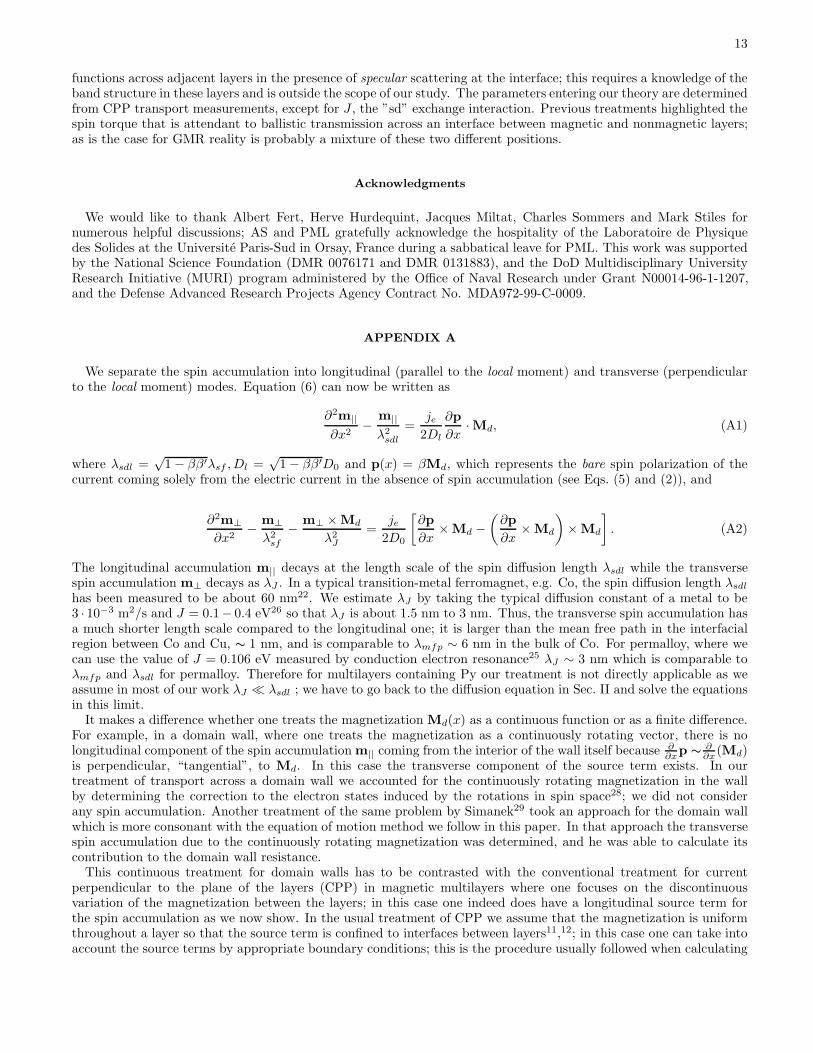
functions across adjacent layers in the presence of specular scattering at the interface; this requires a knowledge of theband structure in these layers and is outside the scope of our study. The parameters entering our theory are determinedfrom CPP transport measurements, except for J , the ”sd” exchange interaction. Previous treatments highlighted thespin torque that is attendant to ballistic transmission across an interface between magnetic and nonmagnetic layers;as is the case for GMR reality is probably a mixture of these two different positions.

Acknowledgments

We would like to thank Albert Fert, Herve Hurdequint, Jacques Miltat, Charles Sommers and Mark Stiles fornumerous helpful discussions; AS and PML gratefully acknowledge the hospitality of the Laboratoire de Physiquedes Solides at the Universite Paris-Sud in Orsay, France during a sabbatical leave for PML. This work was supportedby the National Science Foundation (DMR 0076171 and DMR 0131883), and the DoD Multidisciplinary UniversityResearch Initiative (MURI) program administered by the Office of Naval Research under Grant N00014-96-1-1207,and the Defense Advanced Research Projects Agency Contract No. MDA972-99-C-0009.

APPENDIX A

We separate the spin accumulation into longitudinal (parallel to the local moment) and transverse (perpendicularto the local moment) modes. Equation (6) can now be written as

∂2m||∂x2

− m||λ2

sdl

=je

2Dl

∂p

∂x· Md, (A1)

where λsdl =√

1 − ββ′λsf , Dl =√

1 − ββ′D0 and p(x) = βMd, which represents the bare spin polarization of thecurrent coming solely from the electric current in the absence of spin accumulation (see Eqs. (5) and (2)), and

∂2m⊥∂x2

− m⊥λ2

sf

− m⊥ × Md

λ2J

=je

2D0

[

∂p

∂x× Md −

(

∂p

∂x× Md

)

× Md

]

. (A2)

The longitudinal accumulation m|| decays at the length scale of the spin diffusion length λsdl while the transversespin accumulation m⊥ decays as λJ . In a typical transition-metal ferromagnet, e.g. Co, the spin diffusion length λsdl

has been measured to be about 60 nm22. We estimate λJ by taking the typical diffusion constant of a metal to be3 · 10−3 m2/s and J = 0.1− 0.4 eV26 so that λJ is about 1.5 nm to 3 nm. Thus, the transverse spin accumulation hasa much shorter length scale compared to the longitudinal one; it is larger than the mean free path in the interfacialregion between Co and Cu, ∼ 1 nm, and is comparable to λmfp ∼ 6 nm in the bulk of Co. For permalloy, where wecan use the value of J = 0.106 eV measured by conduction electron resonance25 λJ ∼ 3 nm which is comparable toλmfp and λsdl for permalloy. Therefore for multilayers containing Py our treatment is not directly applicable as weassume in most of our work λJ ≪ λsdl ; we have to go back to the diffusion equation in Sec. II and solve the equationsin this limit.

It makes a difference whether one treats the magnetization Md(x) as a continuous function or as a finite difference.For example, in a domain wall, where one treats the magnetization as a continuously rotating vector, there is nolongitudinal component of the spin accumulation m|| coming from the interior of the wall itself because ∂

∂xp ∼∂∂x(Md)

is perpendicular, “tangential”, to Md. In this case the transverse component of the source term exists. In ourtreatment of transport across a domain wall we accounted for the continuously rotating magnetization in the wallby determining the correction to the electron states induced by the rotations in spin space28; we did not considerany spin accumulation. Another treatment of the same problem by Simanek29 took an approach for the domain wallwhich is more consonant with the equation of motion method we follow in this paper. In that approach the transversespin accumulation due to the continuously rotating magnetization was determined, and he was able to calculate itscontribution to the domain wall resistance.

This continuous treatment for domain walls has to be contrasted with the conventional treatment for currentperpendicular to the plane of the layers (CPP) in magnetic multilayers where one focuses on the discontinuousvariation of the magnetization between the layers; in this case one indeed does have a longitudinal source term forthe spin accumulation as we now show. In the usual treatment of CPP we assume that the magnetization is uniformthroughout a layer so that the source term is confined to interfaces between layers11,12; in this case one can take intoaccount the source terms by appropriate boundary conditions; this is the procedure usually followed when calculating

14

the spin accumulation in magnetic multilayers12. By discretizing the source terms in Eqs. (A1) and (A2) we find forthe longitudinal accumulation

βje

2D0

∑

j=i±1

Mi(1 − Mi · Mj)δ(xj), (A3)

while for the transverse accumulation the source term is

βje

2D0

∑

j=i±1

Mi × (Mi × Mj)δ(xj), (A4)

where the layer we are considering is labelled i while the interfaces with the adjacent layers j = i ± 1 are at xj . Forcollinear structures we see that the transverse term is zero; the longitudinal source term at the interface between twoidentical magnetic layers is zero if they are parallel, and

βje

D0Miδ(x0) (A5)

if they are antiparallel; here x0 is the coordinate of the interface between the two magnetic layers. At the interfacebetween magnetic and nonmagnetic layers (FM/NM) only the longitudinal source term exists, irrespective of the

alignment of neighboring magnetic layers; it is

βje

2D0Miδ(x0). (A6)

When two identical magnetic layers are noncollinear there is a transverse source term given by Eq. (A4) as well as alongitudinal one Eq. (A3).

For the multilayered structure depicted in Fig. 1, which models the case studied up till now for current inducedswitching, no two magnetic layers are adjacent so the sole source term that exists is given by Eq. (A3). In this casethe boundary condition at the interfaces between adjacent FM/NM layers is given by Eq. (A6). However, as we makethe assumption that the thickness of the nonmagnetic spacer layer between the two magnetic layers is much smallerthan λN

sdl we can replace the two sets of FM/NM boundaries by one and use the conditions Eqs. (A3) and (A4).

APPENDIX B

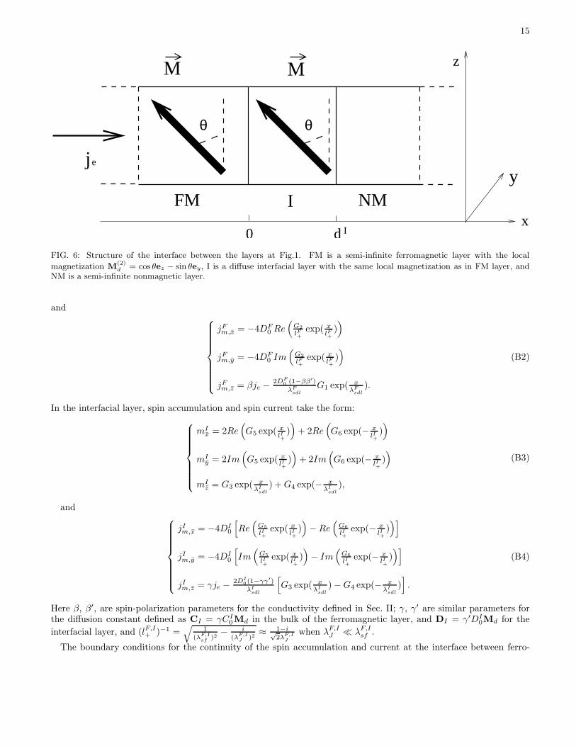
In this Appendix, we derive the boundary conditions at the interfaces between the layers in Fig. 1. To achievethis goal, we consider a sub-system shown in Fig. 6 which consists of a semi-infinite FM layer with x < 0 withthe local magnetization M = cos θez − sin θey, a diffuse interfacial layer I between 0 < x < dI with the same localmagnetization as in the FM layer, and a semi-infinite NM layer for x > dI . When dI is infinitesimally small, thissub-system represents the three FM-NM interfaces in Fig. 1, i.e., between the thick FM and spacer layers, between thespacer and thin FM layers (when spatially inverted), and between the thin FM and back NM layers. We assume thatboth spin accumulation and current are continuous at the FM-I and I-NM interfaces, and derive the relation betweenspin accumulation and current at x = 0 with the same quantities at x = dI as the thickness of the interfacial layerdI goes to zero. In this limit the parameters of the interfacial layer, such as λI

mfp, τIsf , JI , λI

J , and, most important,its resistance ARI remain constant; the latter condition implies that the diffusion constant of the interfacial layerDI

0 ∼ dI as dI → 0.We solve Eqs. (7), (8) for the spin accumulation and use Eq. (5) to find spin current in the ferromagnetic and

interfacial layers. By adopting a set of local coordinates (x, y, z) such that the local magnetization is Mz = ez thespin accumulation and current in the FM layer take the form:

mFx = 2Re

(

G2 exp( xlF+

))

mFy = 2Im

(

G2 exp( xlF+

))

mFz = G1 exp( x

λFsdl

),

(B1)

15

M M z

NMy

xFM I

0

θ θ

d

je

I

FIG. 6: Structure of the interface between the layers at Fig.1. FM is a semi-infinite ferromagnetic layer with the local

magnetization M(2)d = cos θez − sin θey, I is a diffuse interfacial layer with the same local magnetization as in FM layer, and

NM is a semi-infinite nonmagnetic layer.

and

jFm,x = −4DF

0 Re(

G2

lF+

exp( xlF+

))

jFm,y = −4DF

0 Im(

G2

lF+

exp( xlF+

))

jFm,z = βje − 2DF

0 (1−ββ′)

λFsdl

G1 exp( xλF

sdl

).

(B2)

In the interfacial layer, spin accumulation and spin current take the form:

mIx = 2Re

(

G5 exp( xlI+

))

+ 2Re(

G6 exp(− xlI+

))

mIy = 2Im

(

G5 exp( xlI+

))

+ 2Im(

G6 exp(− xlI+

))

mIz = G3 exp( x

λIsdl

) + G4 exp(− xλI

sdl

),

(B3)

and

jIm,x = −4DI

0

[

Re(

G5

lI+

exp( xlI+

))

− Re(

G6

lI+

exp(− xlI+

))]

jIm,y = −4DI

0

[

Im(

G5

lI+

exp( xlI+

))

− Im(

G6

lI+

exp(− xlI+

))]

jIm,z = γje − 2DI

0(1−γγ′)

λIsdl

[

G3 exp( xλI

sdl

) − G4 exp(− xλI

sdl

)]

.

(B4)

Here β, β′, are spin-polarization parameters for the conductivity defined in Sec. II; γ, γ′ are similar parameters forthe diffusion constant defined as CI = γCI

0Md in the bulk of the ferromagnetic layer, and DI = γ′DI0Md for the

interfacial layer, and (lF,I+ )−1 =

√

1

(λF,I

sf)2

− i

(λF,IJ

)2≈ 1−i√

2λF,IJ

when λF,IJ ≪ λF,I

sf .

The boundary conditions for the continuity of the spin accumulation and current at the interface between ferro-

16

magnetic and interfacial layer x = 0 take the form:

2ReG2 = 2ReG5 + 2ReG6

2ImG2 = 2ImG5 + 2ImG6)

G1 = G3 + G4,

(B5)

and

−4DF0 Re(G2

lF+

) = −4DI0Re(G5−G6

lI+

)

−4DF0 Im(G2

lF+

) = −4DI0Im(G5−G6

lI+

)

βje − 2DF0 (1−ββ′)

λFsdl

G1 = γje − 2DI0(1−γγ′)

λIsdl

(G3 − G4).

(B6)

To relate mF (0) to mI(dI), and jFm(0) to jIm(dI), we use the assumption that as the thickness of the interfacial layergoes to zero, other parameters of the interfacial layer, such as λI

sdl, JI , and λIJ remain constant, but the diffusion

constant DI0 goes to zero with the same rate as dI , so that dI/DI

0 = const. Then, for example, for small dI ≪ λIJ the

x-component of the spin-accumulation at x = dI may be written as

mIx(dI → 0) ≈ 2Re(G5 + G6) + 2Re

(

(G5 − G6)dI

lI+

)

. (B7)

By comparing this expression with Eqs. (B5) and (B6), we obtain a relation between the x-components of spinaccumulation and current at x = 0 and x = dI :

mIx(dI → 0) = mF

x (0) − jFm,x(0)

dI

2DI0

, (B8)

and similarly,

mIy(dI → 0) = mF

y (0) − jFm,y(0)

dI

2DI0

, (B9)

mIz(d

I → 0) = mFz (0) + je

γ

2(1 − γγ′)

dI

DI0

− jFm,z(0)

1

2(1 − γγ′)

dI

DI0

. (B10)

In a manner similar to Eq. (B7) the x-component of spin current at x = dI may be written as

jIm,x(dI → 0) ≈ −4DI

0Re

(

G5 − G6

lI+

)

− 2Re (i(G5 + G6))dIJI

~.

By comparing this expression with Eqs. (B5) and (B6), we find the continuity condition for the x-component of spincurrent:

jIm,x(dI → 0) = jF

m,x(0) − mFy (0)

dIJI

~, (B11)

and, similarly,

jIm,y(d

I → 0) = jFm,y(0) + mF

x (0)dIJI

~, (B12)

and

jIm,barz(d

I → 0) = jFm,z(0) − mF

z (0)dI

τIsf

. (B13)

17

With these relations we can now obtain the boundary conditions at the three interfaces in the multilayered structuredepicted in Fig. 1.

By using the conditions Eqs. (B8)-(B13), the boundary conditions at the interface between the thin (first) ferro-magnetic and non-magnetic (N) layers of the structure shown in Fig. 1 at x = tF may be written immediately, sincein the thin FM layer the local coordinate system (x, y, z) coincides with the global axes (x, y, z); we find

mNx (tF ) − m

(1)x (tF ) = −rj

(1)m,x(tF )

mNy (tF ) − m

(1)y (tF ) = −rj

(1)m,y(tF )

mNz (tF ) − m

(1)z (tF ) = rje

γ1−γγ′

− rj(1)m,z(tF ) 1

1−γγ′,

(B14)

and

jNm,x(tF ) − j

(1)m,x(tF ) = −m

(1)y (tF )dIJI

~

jNm,y(tF ) − j

(1)m,y(tF ) = m

(1)x (tF )dIJI

~

jNm,z(tF ) − j

(1)m,z(tF ) = −m

(1)z (tF ) dI

τIsf

,

(B15)

where r = dI/2DI0. Similarly, the boundary conditions at the interface between the non-magnetic spacer (S) and the

thin (first) FM layer at x = 0 take the form:

mSx (0) − m

(1)x (0) = rj

(1)m,x(0)

mSy (0) − m

(1)y (0) = rj

(1)m,y(0)

mSz (0) − m

(1)z (0) = −rje

γ1−γγ′

+ rj(1)m,z(0) 1

1−γγ′,

(B16)

and

jSm,x(0) − j

(1)m,x(0) = m

(1)y (0)dIJI

~

jSm,y(0) − j

(1)m,y(0) = −m

(1)x (0)dIJI

~

jSm,z(0) − j

(1)m,z(0) = m

(1)z (0) dI

τIsf

,

(B17)

Note that spin-current conservation condition at the interfaces, which means that there are no torques acting at theinterfaces, is due to the infinitely small thickness of the interfacial layers dI → 0. To write the boundary conditionsat the interface between the thick FM and NM spacer layers at x = 0, we have to change from the local coordinatesystem (x, y, z), related to the magnetization direction in the thick FM layer, to the global (x, y, z) system. Anyvector a will be transformed according to the following rule:

ax = ax

ay = ay cos θ + az sin θ

az = −ay sin θ + az cos θ.

(B18)

By applying this transformation to the conditions, Eqs. (B8)-(B13), we obtain the following boundary conditions at

18

the interface between the thick (second) FM and non-magnetic spacer (S) layers:

mSx (0) − m

(2)x (0) = −rj

(2)m,x(0)

mSy (0) − m

(2)y (0) = −rje

γ1−γγ′

sin θ − rj(2)m,y(0)1−γγ′ cos2 θ

1−γγ′

+rj(2)m,z(0) sin θ cos θ γγ′

1−γγ′

mSz (0) − m

(2)z (0) = rje

γ1−γγ′

cos θ + rj(2)m,y(0) sin θ cos θ γγ′

1−γγ′

+rj(2)m,z(0)1−γγ′ sin2 θ

1−γγ′,

(B19)

and

jSm,x(0) − j

(2)m,x(0) = −m

(2)y (0) cos θ dIJI

~− m

(2)z (0) sin θ dIJI

~

jSm,y(0) − jS

m,y(0) = m(2)x (0) cos θ dIJI

~− m

(2)y (0) sin2 θ dI

τIsf

+m(2)z (0) sin θ cos θ dI

τIsf

jSm,z(0) − j

(2)m,z(0) = m

(2)x (0) sin θ dIJI

~+ m2y(0) sin θ cos θ dI

τIsf

−m(2)z (0) cos2 θ dI

τIsf

,

(B20)

Note that as the thickness of the interfacial layer dI goes to zero, for diffuse scattering we considered one produceslarge discontinuities in the spin-accumulation (Eqs. (B14), (B16), (B19)) proportional to finite r = dI/2DI

0, but smalldiscontinuities in the spin-currents (Eqs. (B15), (B17), (B20)) proportional to dI , because JI does not increase and τI

sf

does not decrease as dI → 0. In our picture finite thickness of the interfacial layer is essential for torque productionat the interface. As we consider infinitely small interfacial thicknesses dI → 0, we obtain spin-current conservationconditions at each interface:

jNm(tF ) = j(1)m (tF ), (B21)

jSm(0) = j(1)m (0), (B22)

and

j(2)m (0) = jSm(0). (B23)

By eliminating mS(0) and jSm(0) from Eqs. (B16), (B19), (B22), and (B23), we finally obtain the boundary conditions

at the interface between thick (second) and thin (first) FM layers at x = 0 (of course there is the NM spacer in-between,however its thickness tN is irrelevant for these boundary conditions as long as tN ≪ λN

sdl):

m(1)x (0) − m

(2)x (0) = −2rj

(1)m,x(0)

m(1)y (0) − m

(2)y (0) = −rje

γ1−γγ′

sin θ − rj(1)m,y(0)2−γγ′(1+cos2 θ)

1−γγ′

+rj(1)m,z(0) sin θ cos θ γγ′

1−γγ′

m(1)z (0) − m

(2)z (0) = rje

γ1−γγ′

(1 + cos θ) + rj(1)m,y(0) sin θ cos θ γγ′

1−γγ′

−rj(1)m,z(0)2−γγ′ sin2 θ

1−γγ′,

(B24)

19

and

j(1)m (0) = j(2)m (0) (B25)

Finally, we show that parameter r = dI/2DI0 is proportional to the interface resistance ARI found from CPP

transport measurements 16. By considering the expression (4) for the electrical current in the interfacial layer,and the assumptions that DI

0 ∼ dI and λIsdl remains constant as the thickness of the interfacial layer dI → 0, we

find ARI = dI/2CI0 , or r = dI

2DI0

= ARICI

0

DI0

. The parameters CI0 and DI

0 may be related via Einstein’s relation

CI = e2NI(ǫF )DI , so that the parameter r takes the form:

r = ARIe2N I

0 (ǫF )1 − γ′′2

1 − γγ′ , (B26)

where e is the electron charge, N I0 (ǫF ) is the density of states at the interface at Fermi energy, and γ′′ is the spin

polarization parameters for the density of states at the interfaces which is defined as NI = γ′′N I0 Md.

APPENDIX C

We solve the Eqs. (7), (8) for the spin accumulation in each of three layers, and find spin currents using Eq. (5).In the thick ferromagnetic layer, spin accumulation and current take the form

m(2)x = 2Re

(

G2 exp( xl+

))

m(2)y = 2Im

(

G2 exp( xl+

))

cos θ − G1 exp( xλF

sdl

) sin θ

m(2)z = 2Im

(

G2 exp( xl+

))

sin θ + G1 exp( xλF

sdl

) cos θ,

(C1)

and

j(2)m,x = −4D0Re

(

G2

l+exp( x

l+))

j(2)m,y = −βje sin θ − 4D0Im

(

G2

l+exp( x

l+))

cos θ

+ 2D0(1−ββ′)λsdl

G1 exp( xλF

sdl

) sin θ

j(2)m,z = βje cos θ − 4D0Im

(

G2

l+exp( x

l+))

sin θ − 2D0(1−ββ′)

λFsdl

G1 exp( xλF

sdl

) cos θ.

(C2)

In the thin ferromagnetic layer

m(1)x = 2Re

(

G5 exp(− xl+

))

+ 2Re(

G6 exp(x−tF

l+))

m(1)y = 2Im

(

G5 exp(− xl+

))

+ 2Im(

G6 exp(x−tF

l+))

m(1)z = G3 exp(− x

λFsdl

) + G4 exp(x−tF

λFsdl

),

(C3)

and

j(1)m,x = 4D0

[

Re(

G5

l+exp(− x

l+))

− Re(

G6

l+exp(x−tF

l+))]

j(1)m,y = 4D0

[

Im(

G5

l+exp(− x

l+))

− Im(

G6

l+exp(x−tF

l+))]

j(1)m,z = βje + 2D0(1−ββ′)

λFsdl

[

G3 exp(− xλF

sdl

) − G4 exp(x−tF

λFsdl

)]

.

(C4)

20

where l−1+ =

√

1λ2

sf

− iλ2

J

≈ 1−i√2λJ

, and λFsdl is spin-diffusion length in FM layer. In the non-magnetic layer,

mN = A exp(−x − tFλN

sdl

), (C5)

and

jNm =2DN

0

λNsdl

A exp(−x − tF

λNsdl

). (C6)

To obtain the 12 unknown constants Ax, Ay, Az , G1, ReG2, ImG2, G3, G4, ReG5, ImG5, ReG6, ImG6, we usethe boundary conditions (see Appendix B, Eqs. (B14 ), (B24), (B21), and (B25)):

mNx (tF ) − m

(1)x (tF ) = −rj

(1)m,x(tF )

mNy (tF ) − m

(1)y (tF ) = −rj

(1)m,y(tF )

mNz (tF ) − m

(1)z (tF ) = rje

γ1−γγ′

− rj(1)m,z(tF ) 1

1−γγ′,

(C7)

and

m(1)x (0) − m

(2)x (0) = −2rj

(1)m,x(0)

m(1)y (0) − m

(2)y (0) = −rje

γ1−γγ′

sin θ − rj(1)m,y(0)2−γγ′(1+cos2 θ)

1−γγ′

+rj(1)m,z(0) sin θ cos θ γγ′

1−γγ′

m(1)z (0) − m

(2)z (0) = rje

γ1−γγ′

(1 + cos θ) + rj(1)m,y(0) sin θ cos θ γγ′

1−γγ′

−rj(1)m,z(0)2−γγ′ sin2 θ

1−γγ′,

(C8)

jNm(tF ) = j(1)m (tF ) (C9)

j(1)m (0) = j(2)m (0) (C10)

where the parameter r is proportional to the interface resistance ARI , r = ARIe2N0(1 − γ′′2)/(1 − γγ′), e is the

electron charge, N0 is the density of states at the interface, γ, γ′, γ′′ are the spin polarization parameters for theconductivity, diffusion constant, and density of states at the interfaces (see Appendix B). The other six boundaryconditions come from the conservation of spin current at the interfaces.

1 J.C. Slonczewski, J. Mag. Mag. Mater. 159, L1 (1996); J. Magn. Magn. Mater. 195, L261 (1999); J. Magn. Magn. Mater. 247,324 (2002); L. Berger, Phys. Rev. B 54, 9353 (1996); J. Appl. Phys. 89, 5521 (2001).

2 X. Waintal, E.B. Myers, P.W. Brouwer, and D.C. Ralph, Phys. Rev.B 62, 12 317 (2000). Also see, A. Brataas, Yu.V.Nazarov, and G.E.W. Bauer, Phys. Rev. Lett. 84, 2481 (2000) and D.H. Hernando, Y.V. Nazarov, A. Brataas, and G.E.W.Bauer, Phys. Rev.B 62, 5700 (2000).

3 M.D. Stiles and A. Zangwill, J.Appl. Phys. 91, 6812 (2002).4 M.D. Stiles and A. Zangwill, Phys.Rev. B 66, 014407 (2002).5 S. Zhang, P.M. Levy, and A. Fert, Phys. Rev. Lett. 88, 236601 (2002).6 Y.-N. Qi and S. Zhang, Phys. Rev. B 65, 214407 (2002).7 See Ref. 3. The differences in these two calculations are: their’s is based on band structure and specular scattering at

interface, our’s is confined to a Boltzmann description for transport in the bulk of the layers with diffuse scattering atinterfaces and assumes that transverse spin accumulation and current does exist in the ferromagnet’s bulk. Referring to Fig.3 and Eqs.14 and 18 in the above referenced paper one notes the absence of the component of the spin distribution function

21

that is transverse to the magnetization (axis of spin quantization) in the ferromagnetic layers. Indeed in a subsequent paper(Ref. 4) they have shown that the transverse component decays in a distance less than 1nm for metals that fit the Stonermodel. On the contrary we are currently in the process of further justifying the assumption that a transverse component ofthe spin accumulation exists in the 3d transition-metal ferromagnets. Aside from these differences both approaches do findan amplification in the spin torque above that one anticipates on the basis of a non-diffusive transport calculation, i.e., weboth find the angular momentum transferred from the spin current to the free magnetic layer far exceeds the bare portionof the transverse component of the spin current in the nonmagnetic layer adjacent to the free magnetic layer; M.D. Stiles,private communication.

8 In general the spinor current (x), which can be written as jeI + σ · jm, is also a vector in position space. To simplify thenotation we limit ourselves to currents along the x axis which is perpendicular to the planes of the layers.

9 G.D. Gaspari, Phys, Rev. 151, 215 (1966). In the context of ferromagnetic resonance the decay of spin polarized currentsin ferromagnetic metals with diffuse scattering has been derived from the Boltzmann equation by Gaspari; the same Blochequation as that for conduction-electron spin resonance applies to our current driven situation. From these studies we findthe steady state diffusion equation for the transverse spin accumulation m±, i.e., the magnetization swept into the secondmagnetic layer by the spin current created by the first after steady state current is achieved, is given as

D∂2m±

∂x2= {

1

τsf

+ iω0}m±,

where the diffusion constant is

D =v2

F

3{ 1τmfp

+ 1τsf

+ iω0}.

See Eqs. 26 and 27 of Gaspari; note that we have dropped the transverse field H+ as it does not exist in transport experiments,as well as the cyclotron resonance term ∽ ωcτ because for the structures we study it is small. Here m± = mx±imy, ω0 = J/~

is the rate at which spins precess in the ferromagnet, τsf is the spin flip rate, and τmfp the mean time between momentumrelaxing collisions. In all cases we consider τsf ≫ τmfp, ω−1

0 so that

∂2m±

∂x2= −

ω0

(1/3)v2F

{−i

τmfp

+ ω0}m±.

We note that there are oscillatory ω0 and decaying 1τmfp

portions to the spin accumulation. In the cases we consider in

this paper 1τmfp

≫ ω0 one can neglect the second term in the curly brackets and one arrives at an overdamped solution to

the above equation, which is just our Eq. (8) with λsf = ∞, in which the accumulation simply decays on the length scale

λJ =√

(1/3)v2F τmfp/ω0. It is just this case that was discussed in a previous publication5.

10 S. Zhang and P.M. Levy, Phys. Rev. B 65, 052409 (2002).11 H.E. Camblong, S. Zhang and P.M. Levy, Phys. Rev. B 47, 4735 (1993).12 T. Valet and A. Fert, Phys. Rev. B 48, 7099 (1993).13 S. Zhang and P.M. Levy, Phys. Rev. B 57, 5336 (1998); A. Shpiro and P.M. Levy, Phys. Rev. B 63, 014419 (2000).14 J. A. Katine, F. J. Albert, R. A. Buhrman, E. B. Myers, and D. C. Ralph, Phys. Rev. Lett. 84, 3149 (2000); F. J. Albert,

J. A. Katine, R. A. Buhrman, and D. C. Ralph, Appl. Phys. Lett. 77, 3809 (2000); J. Grollier, V. Cros, A. Hamzic, J. M.George, H. Jaffres, A. Fert, G. Faini, J. Ben Youssef, and H. Legall, Appl. Phys. Lett. 78 , 3663 (2001).

15 See Waintal et al., Ref. 2.16 J.Bass and W.P.Pratt Jr., Journal of Magnetism and Magnetic Materials 200, 274 (1999).17 H.E. Camblong, P.M. Levy, and S. Zhang , Phys. Rev. B 51, 16052 (1995).18 A.V. Vedyayev et al., Phys.Rev. B 55, 3728 (1997), Phys. Solid State 41, 1665 (1999).19 J.C. Slonczewski, see Ref. 1.20 P. Dauguet et al., Phys. Rev. B 54, 1083 (1996).21 W.P.Pratt Jr., private communication.22 L. Piraux, S. Dubois, A. Fert, and L. Belliard, Eur. Phys. J. B 4, 413 (1998); A. Fert and L. Piraux, J. Magn. Magn. Mater.

200, 338 (1999); J. Bass and W.P. Pratt Jr, J. Magn. Magn. Mater. 200, 274 (1999).23 Kuising Wang, Thesis New York University (1999); K. Wang et al., “On the calculation of magnetoresistance of tunnel

junctions with parallel paths of conduction”, submitted for publication.24 See Chapter 5 of Theory of Itinerant Electron Magnetism by Jurgen Kubler (Clarendon Press, Oxford, 2000); Also see V.P.

Antropov et al., Phys. Rev. B 54, 1019 (1996); M.V. You and Volker Heine, J. Phys. F: Met. Phys. 12, 177 (1982); L.M.Small and Volker Heine, J. Phys. F: Met. Phys. 14, 3041 (1984); D.M. Edwards, J. Mag. Mag . Mater. 45, 151 (1984).

25 R.L. Cooper and E.A. Uehling, Phys. Rev. 164, 662 (1967).26 H. Hurdequint, private communication.27 R.A. Buhrman, private communication.28 P.M. Levy and S. Zhang, Phys. Rev. Lett. 79, 5110 (1997).29 E. Simanek, Phys. Rev. B 63, 224412 (2001).