arX

iv:h

ep-p

h/97

0923

2v1

3 S

ep 1

997

PITT-97-677; CMU-HEP-97-08; LPTHE-97; DOE-ER/40682-133

NON-PERTURBATIVE QUANTUM DYNAMICS OF A NEW

INFLATION MODEL

D. Boyanovsky(a), D. Cormier(b), H. J. de Vega(c), R. Holman(b), S. P. Kumar(b)

(a) Department of Physics and Astronomy, University of Pittsburgh, Pittsburgh, PA. 15260,

U.S.A.

(b) Department of Physics, Carnegie Mellon University, Pittsburgh, PA. 15213, U. S. A.

(c) LPTHE, ∗ Universite Pierre et Marie Curie (Paris VI) et Denis Diderot (Paris VII), Tour

16, 1er. etage, 4, Place Jussieu 75252 Paris, Cedex 05, France

(September 1997)

Abstract

We consider an O(N) model coupled self-consistently to gravity in the semi-

classical approximation, where the field is subject to ‘new inflation’ type initial

conditions. We study the dynamics self-consistently and non-perturbatively

with non-equilibrium field theory methods in the large N limit. We find that

spinodal instabilities drive the growth of non-perturbatively large quantum

fluctuations which shut off the inflationary growth of the scale factor. We

find that a very specific combination of these large fluctuations plus the in-

flaton zero mode assemble into a new effective field. This new field behaves

classically and it is the object which actually rolls down. We show how this

reinterpretation saves the standard picture of how metric perturbations are

generated during inflation and that the spinodal growth of fluctuations dom-

inates the time dependence of the Bardeen variable for superhorizon modes

during inflation. We compute the amplitude and index for the spectrum of

scalar density and tensor perturbations and argue that in all models of this

type the spinodal instabilities are responsible for a ‘red’ spectrum of primor-

dial scalar density perturbations. A criterion for the validity of these models is

provided and contact with the reconstruction program is established validat-

ing some of the results within a non-perturbative framework. The decoherence

aspects and the quantum to classical transition through inflation are studied

in detail by following the full evolution of the density matrix and relating the

classicality of cosmological perturbations to that of long-wavelength matter

fluctuations.

∗Laboratoire Associe au CNRS UA280.

1

I. INTRODUCTION AND MOTIVATION

Inflationary cosmology has come of age. From its beginnings as a solution to purelytheoretical problems such as the horizon, flatness and monopole problems [1], it has growninto the main contender for the source of primordial fluctuations giving rise to large scalestructure [2–4]. There is evidence from the measurements of temperature anisotropies in thecosmic microwave background radiation (CMBR) that the scale invariant power spectrumpredicted by generic inflationary models is at least consistent with observations [5–9] and wecan expect further and more exacting tests of the inflationary power spectrum when the MAPand PLANCK missions are flown. In particular, if the fluctuations that are responsible forthe temperature anisotropies of the CMB truly originate from quantum fluctuations duringinflation, determinations of the spectrum of scalar and tensor perturbations will constraininflationary models based on particle physics scenarios and probably will validate or ruleout specific proposals [6,7,10,11]. Already current bounds on the spectrum of scalar densityperturbations seem to rule out some versions of ‘extended’ inflation [10].

The tasks for inflationary universe enthusiasts are then two-fold. First, models of inflationmust be constructed that have a well-defined rationale in terms of coming from a reasonableparticle physics model. This is in contrast to the current situation where most, if not allacceptable inflationary models are ad-hoc in nature, with fields and potentials put in for thesole purpose of generating an inflationary epoch. Second, and equally important, we must besure that the quantum dynamics of inflation is well understood. This is extremely important,especially in light of the fact that it is exactly this quantum behavior that is supposed to giverise to the primordial metric perturbations which presumably have imprinted themselves inthe CMBR. This latter problem is the focus of this paper.

The inflaton must be treated as a non-equilibrium quantum field . The simplest way tosee this comes from the requirement of having small enough metric perturbation amplitudeswhich in turn requires that the quartic self coupling λ of the inflaton be extremely small,typically of order ∼ 10−12. Such a small coupling cannot establish local thermodynamicequilibrium (LTE) for all field modes; near a phase transition the long wavelength modeswill respond too slowly to be able to enter LTE. In fact, the superhorizon sized modes willbe out of the region of causal contact and cannot thermalize. We see then that if we wantto gain a deeper understanding of inflation, non-equilibrium tools must be developed. Suchtools exist and have now been developed to the point that they can give quantitative answersto these questions in cosmology [12–16]. These methods permit us to follow the dynamics

of quantum fields in situations where the energy density is non-perturbatively large (∼ 1/λ).That is, they allow the computation of the time evolution of non-stationary states and ofnon-thermal density matrices.

Our approach is to apply non-equilibrium quantum field theory techniques to the situa-tion of a scalar field coupled to semiclassical gravity, where the source of the gravitationalfield is the expectation value of the stress energy tensor in the relevant, dynamically chang-ing, quantum state. In this way we can go beyond the standard analyses [17–20] which treatthe background as fixed.

We will mainly deal with ‘new inflation’ scenarios, where a scalar field φ evolves underthe action of a typical symmetry breaking potential. The initial conditions will be taken sothat the initial value of the order parameter (the field expectation value) is near the top of

2

the potential (the disordered state) with essentially zero time derivative.What we find is that the existence of spinodal instabilities, i.e. the fact that eventually

(in an expanding universe) all modes will act as if they have a negative mass squared, drivesthe quantum fluctuations to grow non-perturbatively large. We have the picture of an initialwave-function or density matrix peaked near the unstable state and then spreading until itsamples the stable vacua. Since these vacua are non-perturbatively far from the initial state(typically ∼ m/

√λ, where m is the mass scale of the field and λ the quartic self-coupling),

the spinodal instabilities will persist until the quantum fluctuations, as encoded in the equaltime two-point function 〈Φ(~x, t)2〉, grow to O(m2/λ).

This growth eventually shuts off the inflationary behavior of the scale factor as well asthe growth of the quantum fluctuations (this last also happens in Minkowski spacetime [12]).

The scenario envisaged here is that of a quenched or supercooled phase transition wherethe order parameter is zero or very small. Therefore one is led to ask:

a) What is rolling down?.b) Since the quantum fluctuations are non-perturbatively large ( ∼ 1/λ), will not they

modify drastically the FRW dynamics?.c) How can one extract (small?) metric perturbations from non-perturbatively large field

fluctuations?We address the questions a)-c) as well as other issues below.

II. NON-EQUILIBRIUM QUANTUM FIELD THEORY, SEMICLASSICAL

GRAVITY AND INFLATION

Our program consists of finding ways to incorporate the non-equilibrium behavior of thequantum fields involved in inflation into a framework that treats gravity self consistently,at least in some approximation. We do this via the use of semiclassical gravity [21] wherewe say that the metric is classical, at least to first approximation, whose source is theexpectation value of the stress energy tensor 〈Tµν〉 where this expectation value is takenin the dynamically determined state described by the density matrix ρ(t). This dynamicalproblem can be described schematically as follows:

1. The dynamics of the scale factor a(t) is driven by the semiclassical Einstein equations

1

8πGR

Gµν +ΛR

8πGR

gµν + (higher curvature) = −〈Tµν〉R. (2.1)

Here GR,ΛR are the renormalized values of Newton’s constant and the cosmologicalconstant, respectively and Gµν is the Einstein tensor. The higher curvature termsmust be included to absorb divergences.

2. On the other hand, the density matrix ρ(t) that determines 〈Tµν〉R obeys the Liouvilleequation

i∂ρ(t)

∂t= [H, ρ(t)] , (2.2)

where H is the evolution Hamiltonian, which is dependent on the scale factor, a(t).

3

It is this set of equations we must try to solve; it is clear that initial conditions must beappended to these equations for us to be able to arrive at unique solutions to them. Let usdiscuss some aspects of the initial state of the field theory first.

A. On the initial state: dynamics of phase transitions

As we mentioned above, the situation we consider is one in which the theory admits asymmetry breaking potential and in which the field expectation value starts its evolutionnear the unstable point. There is an issue as to how the field got to have an expectationvalue near the unstable point (typically at Φ = 0) as well as an issue concerning the initialstate of the non-zero momentum modes. The issue of initial conditions is present in anyformulation of inflation but chaotic.

Since our background is an FRW spacetime, it is spatially homogeneous and we canchoose our state ρ(t) to respect this symmetry. Starting from the full quantum field Φ(~x, t)we can extract a part that has a natural interpretation as the zero momentum, c-numberpart of the field by writing:

Φ(~x, t) = φ(t) + Ψ(~x, t)

φ(t) = Tr[ρ(t)Φ(~x, t)] ≡ 〈Φ(~x, t))〉. (2.3)

The quantity Ψ(~x, t) represents the quantum fluctuations about the zero mode φ(t) andclearly satisfies 〈Ψ(~x, t)〉 = 0.

We need to choose a basis to represent the density matrix. A natural choice consistentwith the translational invariance of our quantum state is that given by the Fourier modes,in comoving momentum space, of the quantum fluctuations Ψ(~x, t):

Ψ(~x, t) =∫

d3k

(2π)3exp(−i ~k · ~x) ψk(t). (2.4)

In this language we can state our ansatz for the initial condition of the quantum stateas follows. We take the zero mode φ(t = 0) = φ0, φ(t = 0) = 0, where φ0 will typicallybe very near the origin, while the initial conditions on the the nonzero modes ψk(t = 0)will be chosen such that the initial density matrix ρ(t = 0) describes a vacuum state (i.e.an initial state in local thermal equilibrium at a temperature Ti = 0). There are somesubtleties involved in this choice. First, as explained in [16], in order for the density matrixto commute with the initial Hamiltonian, we must choose the modes to be initially in theconformal adiabatic vacuum (these statements will be made more precise below). This choicehas the added benefit of allowing for time independent renormalization counterterms to beused in renormalizing the theory.

We are making the assumption of an initial vacuum state in order to be able to proceedwith the calculation. It would be interesting to understand what forms of the density matrixcan be used for other, perhaps more reasonable, initial conditions.

The assumptions of an initial equilibrium vacuum state are essentially the same used byLinde [17], Vilenkin [18] , as well as by Guth and Pi [20] in their analyses of the quantummechanics of inflation in a fixed de Sitter background.

4

As discussed in the introduction, if we start from such an initial state, spinodal insta-bilities will drive the growth of non-perturbatively large quantum fluctuations. In order todeal with these, we need to be able to perform calculations that take these large fluctuationsinto account. Although the quantitative features of the dynamics will depend on the initialstate, the qualitative features associated with spinodal instabilities will be fairly robust fora wide choice of initial states that describes a phase transition with a spinodal region in fieldspace.

III. THE MODEL AND EQUATIONS OF MOTION

Having recognized the non-perturbative dynamics of the long wavelength fluctuations,we need to study the dynamics within a non-perturbative framework. That is, a frame-work allowing calculations for non-perturbatively large energy densities. We require thatsuch a framework be: i) renormalizable, ii) covariant energy conserving, iii) numericallyimplementable. There are very few schemes that fulfill all of these criteria: the Hartree andthe large N approximation [18,12,14]. Whereas the Hartree approximation is basically aGaussian variational approximation [22,23] that in general cannot be consistently improvedupon, the large N approximation can be consistently implemented beyond leading order[24,25] and in our case it has the added bonus of providing many light fields (associatedwith Goldstone modes) that will permit the study of the effects of other fields which arelighter than the inflaton on the dynamics. Thus we will study the inflationary dynamics ofa quenched phase transition within the framework of the large N limit of a scalar theory inthe vector representation of O(N).

We assume that the universe is spatially flat with a metric given by

ds2 = dt2 − a2(t) d~x2 . (3.1)

The matter action and Lagrangian density are given by

Sm =∫

d4x Lm =∫

d4x a3(t)

1

2~Φ

2

(x) − 1

2

(~∇~Φ(x))2

a2(t)− V (~Φ(x))

(3.2)

V (~Φ) =λ

8N

(

~Φ2 − 2Nm2

λ

)2

+1

2ξ R ~Φ2 , (3.3)

R(t) = 6

(

a(t)

a(t)+a2(t)

a2(t)

)

, (3.4)

where we have included the coupling of Φ(x) to the scalar curvature R(t) since it will ariseas a consequence of renormalization [13].

The gravitational sector includes the usual Einstein term in addition to a higher ordercurvature term and a cosmological constant term which are necessary to renormalize thetheory. The action for the gravitational sector is therefore:

5

Sg =∫

d4x Lg =∫

d4x a3(t)

[

R(t)

16πG+α

2R2(t) −K

]

. (3.5)

with K being the cosmological constant (we use K rather than the conventional Λ/8πG todistinguish the cosmological constant from the ultraviolet cutoff Λ we introduce to regular-ize the theory; see section IV). In principle, we also need to include the terms RµνRµν andRαβµνRαβµν as they are also terms of fourth order in derivatives of the metric (fourth adia-batic order), but the variations resulting from these terms turn out not to be independentof that of R2 in the flat FRW cosmology we are considering.

The variation of the action S = Sg +Sm with respect to the metric gµν gives us Einstein’sequation

Gµν

8πG+ αHµν +Kgµν = − < Tµν > , (3.6)

where Gµν is the Einstein tensor given by the variation of√−gR, Hµν is the higher order

curvature term given by the variation of√−gR2, and Tµν is the contribution from the

matter Lagrangian. With the metric (3.1), the various components of the curvature tensorsin terms of the scale factor are:

G00 = −3(a/a)2, (3.7)

Gµµ = −R = −6

(

a

a+a2

a2

)

, (3.8)

H00 = −6

(

a

aR +

a2

a2R− 1

12R2

)

, (3.9)

Hµµ = −6

(

R + 3a

aR)

. (3.10)

Eventually, when we have fully renormalized the theory, we will set αR = 0 and keep as ouronly contribution to KR a piece related to the matter fields which we shall incorporate intoTµν .

A. The Large N Approximation

To obtain the proper large N limit, the vector field is written as

~Φ(~x, t) = (σ(~x, t), ~π(~x, t)),

with ~π an (N − 1)-plet, and we write

σ(~x, t) =√Nφ(t) + χ(~x, t) ; 〈σ(~x, t)〉 =

√Nφ(t) ; 〈χ(~x, t)〉 = 0. (3.11)

To implement the large N limit in a consistent manner, one may introduce an auxiliary fieldas in [25]. However, the leading order contribution can be obtained equivalently by invokingthe factorization [14,16]:

6

χ4 → 6〈χ2〉χ2 + constant , (3.12)

χ3 → 3〈χ2〉χ, (3.13)

(~π · ~π)2 → 2〈~π2〉~π2 − 〈~π2〉2 + O(1/N), (3.14)

~π2χ2 → 〈~π2〉χ2 + ~π2〈χ2〉, (3.15)

~π2χ→ 〈~π2〉χ. (3.16)

To obtain a large N limit, we define [14,16]

~π(~x, t) = ψ(~x, t)

N−1︷ ︸︸ ︷

(1, 1, · · · , 1), (3.17)

where the large N limit is implemented by the requirement that

〈ψ2〉 ≈ O(1) , 〈χ2〉 ≈ O(1) , φ ≈ O(1). (3.18)

The leading contribution is obtained by neglecting the O(1/N) terms in the formal limit.The resulting Lagrangian density is quadratic, with linear terms in χ and ~π. The equations ofmotion are obtained by imposing the tadpole conditions < χ(~x, t) >= 0 and < ~π(~x, t) >= 0which in this case are tantamount to requiring that the linear terms in χ and ~π in theLagrangian density vanish. Since the action is quadratic, the quantum fields can be expandedin terms of creation and annihilation operators and mode functions that obey the Heisenbergequations of motion

~π(~x, t) =∫

d3k

(2π)3

[

~ak fk(t) ei~k·~x + ~a†k f

∗k (t) e−i~k·~x

]

. (3.19)

The tadpole condition leads to the following equations of motion [14,16]:

φ(t) + 3H(t) φ(t) + M2(t) φ(t) = 0, (3.20)

with the mode functions[

d2

dt2+ 3H(t)

d

dt+

k2

a2(t)+ M2(t)

]

fk(t) = 0, (3.21)

where

M2(t) = −m2 + ξR +λ

2φ2(t) +

λ

2〈ψ2(t)〉 . (3.22)

In this leading order in 1/N the theory becomes Gaussian, but with the self-consistencycondition

〈ψ2(t)〉 =∫

d3k

(2π)3

|fk(t)|22

. (3.23)

The initial conditions on the modes fk(t) must now be determined. At this stage it provesilluminating to pass to conformal time variables in terms of the conformally rescaled fields(see [16] and section IX for a discussion) in which the mode functions obey an equation

7

which is very similar to that of harmonic oscillators with time dependent frequencies inMinkowski space-time. It has been realized that different initial conditions on the modefunctions lead to different renormalization counterterms [16]; in particular imposing initialconditions in comoving time leads to counterterms that depend on these initial conditions.Thus we chose to impose initial conditions in conformal time in terms of the conformallyrescaled mode functions leading to the following initial conditions in comoving time:

fk(t0) =1√Wk

, fk(t0) =

[

− a(t0)a(t0)

− iWk

]

fk(t0), (3.24)

with

W 2k ≡ k2 + M2(t0) −

R(t0)

6. (3.25)

For convenience, we have set a(t0) = 1 in eq. (3.25). At this point we recognize that whenM2(t0) − R(t0)/6 < 0 the above initial condition must be modified to avoid imaginaryfrequencies, which are the signal of instabilities for long wavelength modes. Thus we define

the initial frequencies that determine the initial conditions (3.24) as

W 2k ≡ k2 +

∣∣∣∣∣M2(t0) −

R(t0)

6

∣∣∣∣∣

for k2 <

∣∣∣∣∣M2(t0) −

R(t0)

6

∣∣∣∣∣, (3.26)

W 2k ≡ k2 + M2(t0) −

R(t0)

6for k2 ≥

∣∣∣∣∣M2(t0) −

R(t0)

6

∣∣∣∣∣. (3.27)

As an alternative we have also used initial conditions which smoothly interpolate frompositive frequencies for the unstable modes to the adiabatic vacuum initial conditions definedby (3.24,3.25) for the high k modes. While the alternative choices of initial conditionsresult in small quantitative differences in the results (a few percent in quantities whichdepend strongly on these low-k modes), all of the qualitative features we will examine areindependent of this choice.

In the large N limit we find the energy density and pressure density to be given by [14,16]

ε

N=

1

2φ2 +

1

2m2φ2 +

λ

8φ4 +

m4

2λ− ξ G0

0 φ2 + 6ξ

a

aφ φ

+1

2〈ψ2〉 +

1

2a2〈(∇ψ)2〉 +

1

2m2〈ψ2〉 +

λ

8[2φ2 〈ψ2〉 + 〈ψ2〉2]

− ξG00〈ψ2〉 + 6ξ

a

a〈ψψ〉, (3.28)

ε− 3p

N= −φ2 + 2m2 φ2 +

λ

2φ4 +

2m4

λ− ξGµ

µφ2 + 6ξ

(

φφ+ φ2 + 3a

aφφ)

− 〈ψ2〉 +1

a2〈(∇ψ)2〉 + 2m2 〈ψ2〉 − ξ Gµ

µ 〈ψ2〉

+λ

2[2φ2 〈ψ2〉 + 〈ψ2〉2] + 6ξ

(

〈ψ ψ〉 + 〈ψ2〉 + 3a

a〈ψψ〉

)

, (3.29)

where 〈ψ2〉 is given by equation (3.23) and we have defined the following integrals:

8

〈(∇ψ)2〉 =∫

d3k

2(2π)3k2 |fk(t)|2 , (3.30)

〈ψ2〉 =∫

d3k

2(2π)3|fk(t)|2 . (3.31)

The composite operators 〈ψψ〉 and 〈ψψ〉 are symmetrized by removing a normal orderingconstant to yield

1

2(〈ψψ〉 + 〈ψψ〉) =

1

4

∫d3k

(2π)3

d|fk(t)|2dt

, (3.32)

1

2(〈ψψ〉 + 〈ψψ〉) =

1

4

∫d3k

(2π)3

[

fk(t)f∗k (t) + fk(t)f

∗k (t)

]

. (3.33)

The last of these integrals, (3.33), may be rewritten using the equation of motion (3.21):

〈ψψ〉 = −3a

a〈 ψψ〉 − 〈(∇ψ)2〉

a2−M2〈ψ2〉 . (3.34)

It is straightforward to show that the bare energy is covariantly conserved by using theequations of motion for the zero mode and the mode functions.

IV. RENORMALIZATION

Renormalization is a very subtle but important issue in gravitational backgrounds [21].The fluctuation contribution 〈ψ2(~x, t)〉, the energy, and the pressure all need to be renor-malized. The renormalization aspects in curved space times have been discussed at lengthin the literature [21] and have been extended to the large N self-consistent approximationsfor the non-equilibrium backreaction problem in [25,16,26]. More recently a consistent andcovariant regularization scheme that can be implemented numerically has been provided[27].

In terms of the effective mass term for the large N limit given by (3.22) and defining thequantity

B(t) ≡ a2(t)(

M2(t) −R/6)

, (4.1)

M2(t) = −m2B + ξBR(t) +

λB

2φ2(t) +

λB

2〈ψ2(t)〉B , (4.2)

where the subscript B stands for bare quantities, we find the following large k behavior forthe case of an arbitrary scale factor a(t) (with a(0) = 1):

|fk(t)|2 =1

ka2(t)− 1

2k3a2(t)B(t)

+1

8k5 a2(t)

{

3B(t)2 + a(t)d

dt

[

a(t)B(t)]}

+ O(1/k7)

= S(2) + O(1/k5) , (4.3)

|fk(t)|2 =k

a4(t)+

1

2ka4(t)

[

B(t) + 2a2]

9

+1

8k3 a4(t)

{

−B(t)2 − a(t)2B(t) + 3a(t)a(t)B(t) − 4a2(t)B(t)}

+ O(1/k5)

= S(1) + O(1/k5) , (4.4)

1

2

[

fk(t)f∗k (t) + fk(t)f

∗k (t)

]

= − 1

k a2(t)

a(t)

a(t)− 1

4k3a2(t)

[

B(t) − 2a(t)

a(t)B(t)

]

+ O(1/k5) .

(4.5)

Although the divergences can be dealt with by dimensional regularization, this procedureis not well suited to numerical analysis (see however ref. [27]). We will make our subtractionsusing an ultraviolet cutoff, Λa(t), constant in physical coordinates. This guarantees that thecounterterms will be time independent. The renormalization then proceeds much in thesame manner as in reference [13]; the quadratic divergences renormalize the mass and thelogarithmic terms renormalize the quartic coupling and the coupling to the Ricci scalar. Inaddition, there is a quartic divergence which renormalizes the cosmological constant whilethe leading renormalizations of Newton’s constant and the higher order curvature couplingare quadratic and logarithmic respectively. The renormalization conditions on the mass,coupling to the Ricci scalar and coupling constant are obtained from the requirement thatthe frequencies that appear in the mode equations are finite [13], i.e:

−m2B + ξBR(t) +

λB

2φ2(t) +

λB

2〈ψ2(t)〉B = −m2

R + ξRR(t) +λR

2φ2(t) +

λR

2〈ψ2(t)〉R,

(4.6)

while the renormalizations of Newton’s constant, the higher order curvature coupling, andthe cosmological constant are given by the condition of finiteness of the semi-classicalEinstein-Friedmann equation:

G00

8πGB

+ αBH00 +KBg

00 + 〈T 0

0 〉B =G0

0

8πGR

+ αRH00 +KRg

00 + 〈T 0

0 〉R . (4.7)

Finally we arrive at the following set of renormalizations [16]:

1

8πNGR

=1

8πNGB

− 2(

ξR − 1

6

)Λ2

16π2+ 2

(

ξR − 1

6

)

m2R

ln(Λ/κ)

16π2, (4.8)

αR

N=αB

N−(

ξR − 1

6

)2 ln(Λ/κ)

16π2, (4.9)

KR

N=KB

N− Λ4

16π2+m2

R

Λ2

16π2+m4

R

2

ln(Λ/κ)

16π2, (4.10)

−m2R = −m2

B + λRΛ2

16π2+ λR m2

R

ln(Λ/κ)

16π2, (4.11)

ξR = ξB − λR

(

ξR − 1

6

)ln(Λ/κ)

16π2, (4.12)

λR = λB − λRln(Λ/κ)

16π2, (4.13)

〈ψ2(t)〉R =∫ d3k

2(2π)3

{

|fk(t)|2 −[

1

ka2(t)− Θ(k − κ)

2k3

[

M2(t) − R(t)

6

]]}

. (4.14)

10

Here, κ is the renormalization point. As expected, the logarithmic terms are consistent withthe renormalizations found using dimensional regularization [27,26]. Again, we set αR = 0and choose the renormalized cosmological constant such that the vacuum energy is zero inthe true vacuum. We emphasize that while the regulator we have chosen does not respectthe covariance of the theory, the renormalized energy momentum tensor defined in this waynevertheless retains the property of covariant conservation in the limit when the cutoff istaken to infinity.

The logarithmic subtractions can be neglected because of the coupling λ ≤ 10−12. Usingthe Planck scale as the cutoff and the inflaton mass mR as a renormalization point, theseterms are of order λ ln[Mpl/mR] ≤ 10−10, for m ≥ 109 GeV . An equivalent statement isthat for these values of the coupling and inflaton masses, the Landau pole is well beyond thephysical cutoffMpl. Our relative error in the numerical analysis is of order 10−8, therefore ournumerical study is insensitive to the logarithmic corrections. Though these corrections arefundamentally important, numerically they can be neglected. Therefore, in the numericalcomputations that follow, we will neglect logarithmic renormalization and subtract onlyquartic and quadratic divergences in the energy and pressure, and quadratic divergences inthe fluctuation contribution.

V. RENORMALIZED EQUATIONS OF MOTION FOR DYNAMICAL

EVOLUTION

It is convenient to introduce the following dimensionless quantities and definitions,

τ = mRt ; h =H

mR

; q =k

mR

ωq =Wk

mR

; g =λR

8π2, (5.1)

η2(τ) =λR

2m2R

φ2(t) ; gΣ(τ) =λ

2m2R

〈ψ2(t)〉R ; fq(τ) ≡√mR fk(t) . (5.2)

Choosing ξR = 0 (minimal coupling) and the renormalization point κ = |mR| and settinga(0) = 1, the equations of motion become:

[

d2

dτ 2+ 3h

d

dτ− 1 + η2(τ) + gΣ(τ)

]

η(τ) = 0, (5.3)

[

d2

dτ 2+ 3h

d

dτ+

q2

a2(τ)− 1 + η2 + gΣ(τ)

]

fq(τ) = 0,

fq(0) =1

√ωq

; fq(0) = [−h(0) − iωq] fq(0),

ωq =

[

q2 − 1 + η2(0) − R(0)

6m2R

+ gΣ(0)

] 1

2

for q2 > −1 + η2(0) − R(0)

6m2R

+ gΣ(0),

ωq =

[

q2 + 1 − η2(0) +R(0)

6m2R

− gΣ(0)

] 1

2

for q2 < −1 + η2(0) − R(0)

6m2R

+ gΣ(0). (5.4)

11

where

Σ(τ) =∫ ∞

0q2dq

[

|fq(τ)|2 −1

a(τ)2+

Θ(q − 1)

2q3

(

/fracM2(τ)m2R − R(τ)

6m2R

)]

.

The initial conditions for η(τ) will be specified later. An important point to noticeis that the equation of motion for the q = 0 mode coincides with that of the zero mode(5.3). Furthermore, for η(τ → ∞) 6= 0, a stationary (equilibrium) solution of the eq.(5.3) isobtained when the sum rule [12,14,16]

− 1 + η2(∞) + gΣ(∞) = 0 (5.5)

is fulfilled. This sum rule is nothing but a consequence of Goldstone’s theorem and is aresult of the fact that the large N approximation satisfies the Ward identities associatedwith the O(N) symmetry, since the term −1 + η2 + gΣ is seen to be the effective mass ofthe modes transverse to the symmetry breaking direction, i.e. the Goldstone modes in thebroken symmetry phase.

In terms of the zero mode η(τ) and the quantum mode function given by eq.(5.4) we findthat the Friedmann equation for the dynamics of the scale factor in dimensionless variablesis given by

h2(τ) = 4h20 ǫR(τ) ; h2

0 =4πNm2

R

3M2P lλR

(5.6)

and the renormalized energy and pressure are given by:

ǫR(τ) =1

2η2 +

1

4

(

−1 + η2 + gΣ)2

+

g

2

∫

q2dq

[

|fq|2 − S(1)(q, τ) +q2

a2

(

|fq|2 − Θ(q − 1) S(2)(q, τ))]

, (5.7)

(p+ ε)R(τ) =2Nm4

R

λR

{

η2

+ g∫

q2dq

[

|fq|2 − S(1)(q, τ) +q2

3a2

(

|fq|2 − Θ(q − 1) S(2)(q, τ))]}

, (5.8)

where the subtractions S(1) and S(2) are given by the right hand sides of eqns.(4.4) and (4.3)respectively.

The renormalized energy and pressure are covariantly conserved:

ǫR(τ) + 3 h(τ) (p+ ε)R(τ) = 0 . (5.9)

In order to provide the full solution we now must provide the values of η(0), η(0), andh0. Assuming that the inflationary epoch is associated with a phase transition at the GUTscale, this requires that Nm4

R/λR ≈ (1015 Gev )4 and assuming the bound on the scalarself-coupling λR ≈ 10−12−10−14 (this will be seen later to be a compatible requirement), wefind that h0 ≈ N1/4 which we will take to be reasonably given by h0 ≈ 1 − 10 (for examplein popular GUT’s N ≈ 20 depending on particular representations).

We will begin by studying the case of most interest from the point of view of describingthe phase transition: η(0) = 0 and η(0) = 0, which are the initial conditions that led topuzzling questions. With these initial conditions, the evolution equation for the zero modeeq.(5.3) determines that η(τ) = 0 by symmetry.

12

A. Early time dynamics:

Before engaging in the numerical study, it proves illuminating to obtain an estimate ofthe relevant time scales and an intuitive idea of the main features of the dynamics. Becausethe coupling is so weak (g ∼ 10−12 ≪ 1) and after renormalization the contribution fromthe quantum fluctuations to the equations of motion is finite, we can neglect all the termsproportional to g in eqs.(5.7) and (5.4).

For the case where we choose η(τ) = 0 and the evolution equations for the mode functionsare those for an inverted oscillator in De Sitter space-time, which have been studied by Guthand Pi [20]. One obtains the approximate solution

h(t) ≈ h0,

fq(t) ≈ e−3h0τ/2[

Aq Jν

(q

h0e−h0τ

)

+Bq J−ν

(q

h0e−h0τ

)]

,

ν =

√

9

4+

1

h20

, (5.10)

where J±ν(z) are Bessel functions, and Aq and Bq are determined by the initial conditionson the mode functions:

Bq = − 1√ωq

π q

2h0 sin νπ

[

iωq − 12h0

qJν

(q

h0

)

− J ′ν

(q

h0

)]

, (5.11)

Aq =1

√ωq

π q

2h0 sin νπ

[

iωq − 12h0

qJ−ν

(q

h0

)

− J ′−ν

(q

h0

)]

. (5.12)

After the physical wavevectors cross the horizon, i.e. when qe−h0τ/h0 ≪ 1 we find thatthe mode functions factorize:

fq(τ) ≈Bq

Γ(1 − ν)

(

2h0

q

)ν

e(ν−3/2)h0τ . (5.13)

This result reveals a very important feature: because of the negative mass squared termin the matter Lagrangian leading to symmetry breaking (and ν > 3/2), we see that allof the mode functions grow exponentially after horizon crossing (for positive mass squaredν < 3/2, and they would decrease exponentially after horizon crossing). This exponentialgrowth is a consequence of the spinodal instabilities which is a hallmark of the process ofphase separation that occurs to complete the phase transition. We note, in addition thatthe time dependence is exactly given by that of the q = 0 mode, i.e. the zero mode, which isa consequence of the redshifting of the wavevectors and the fact that after horizon crossingthe contribution of the term q2/a2(τ) in the equations of motion become negligible. Weclearly see that the quantum fluctuations grow exponentially and they will begin to be ofthe order of the tree level terms in the equations of motion when gΣ(τ) ≈ 1. At large times

Σ(τ) ≈ F2(h0)h20e

(2ν−3)h0τ ,

with F(h0) a finite constant that depends on the initial conditions and is found numericallyto be of O(1) [see figure (10)].

13

In terms of the initial dimensionful variables, the condition gΣ(τ) ≈ 1 translates to< ψ2(~x, t) >R≈ 2m2

R/λR, i.e. the quantum fluctuations sample the minima of the (renor-malized) tree level potential. We find that the time at which the contribution of the quantumfluctuations becomes of the same order as the tree level terms is estimated to be [14]

τs ≈1

(2ν − 3)h0

ln

[

1

g h20F2(h0)

]

=3

2h0 ln

[

1

g h20F2(h0)

]

+ O(1/h0). (5.14)

At this time, the contribution of the quantum fluctuations makes the back reaction very im-portant and, as will be seen numerically, this translates into the fact that τs also determinesthe end of the De Sitter era and the end of inflation. The total number of e-folds during thestage of exponential expansion of the scale factor (constant h0) is given by

Ne ≈1

2ν − 3ln

[

1

g h20 F2(h0)

]

=3

2h2

0 ln

[

1

g h20 F2(h0)

]

+ O(1) (5.15)

For large h0 we see that the number of e-folds scales as h20 as well as with the logarithm

of the inverse coupling. These results (5.13,5.14,5.15) will be confirmed numerically belowand will be of paramount importance for the interpretation of the main consequences of thedynamical evolution.

B. η(0) 6= 0: classical or quantum behavior?

Above we have analyzed the situation when η(0) = 0 (or in dimensionful variablesφ(0) = 0). The typical analysis of inflaton dynamics in the literature involves the classical

evolution of φ(t) with an initial condition in which φ(0) is very close to zero (i.e. the topof the potential hill) in the ‘slow-roll’ regime, for which φ ≪ 3Hφ. Thus, it is importantto quantify the initial conditions on φ(t) for which the dynamics will be determined bythe classical evolution of φ(t) and those for which the quantum fluctuations dominate thedynamics. We can provide a criterion to separate classical from quantum dynamics byanalyzing the relevant time scales, estimated by neglecting non-linearities and backreactioneffects. We consider the evolution of the zero mode in terms of dimensionless variables, andchoose η(0) 6= 0 and η(0) = 0. (η(0) 6= 0 simply corresponds to a shift in origin of time).We assume η(0)2 << 1 which is the relevant case where spinodal instabilities are important.We find

η(τ) ≈ η(0) e(ν−3

2)h0τ . (5.16)

The non-linearities will become important and eventually terminate inflation whenη(τ) ≈ 1. This corresponds to a time scale given by

τc ≈ln [1/η(0)]

(ν − 32) h0

. (5.17)

If τc is much smaller than the spinodal time τs given by eq.(5.14) then the classical evolutionof the zero mode will dominate the dynamics and the quantum fluctuations will not becomevery large, although they will still undergo spinodal growth. On the other hand, if τc ≫ τs

14

the quantum fluctuations will grow to be very large well before the zero mode reaches thenon-linear regime. In this case the dynamics will be determined completely by the quantumfluctuations. Then the criterion for the classical or quantum dynamics is given by

η(0) ≫ √g h0 =⇒ classical dynamics

η(0) ≪ √g h0 =⇒ quantum dynamics (5.18)

or in terms of dimensionful variables φ(0) ≫ H0 leads to classical dynamics and φ(0) ≪ H0

leads to quantum dynamics.However, even when the classical evolution of the zero mode dominates the dynamics,

the quantum fluctuations grow exponentially after horizon crossing unless the value of φ(t)is very close to the minimum of the tree level potential. In the large N approximation thespinodal line, that is the values of φ(t) for which there are spinodal instabilities, reaches allthe way to the minimum of the tree level potential as can be seen from the equations ofmotion for the mode functions. Therefore even in the classical case one must understandhow to deal with quantum fluctuations that grow after horizon crossing.

C. Numerics

The time evolution is carried out by means of a fourth order Runge-Kutta routine withadaptive stepsizing while the momentum integrals are carried out using an 11-point Newton-Cotes integrator. The relative errors in both the differential equation and the integration areof order 10−8. We find that the energy is covariantly conserved throughout the evolution tobetter than a part in a thousand. Figures (1–3) show gΣ(τ) vs. τ , h(τ) vs. τ and ln(|fq(τ)|2)vs. τ for several values of q with larger q′s corresponding to successively lower curves. Figures(4,5) show p(τ)/ε(τ) and the horizon size h−1(τ) for g = 10−14 ; η(0) = 0 ; η(0) = 0 and wehave chosen the representative value h0 = 2.0.

Figures (1) and (2) show clearly that when the contribution of the quantum fluctuationsgΣ(τ) becomes of order 1 inflation ends, and the time scale for gΣ(τ) to reach O(1) is verywell described by the estimate (5.14). From figure 1 we see that this happens for τ = τs ≈ 90,leading to a number of e-folds Ne ≈ 180 which is correctly estimated by (5.14, 5.15).

Figure (3) shows clearly the factorization of the modes after they cross the horizon asdescribed by eq.(5.13). The slopes of all the curves after they become straight lines in figure(3) is given exactly by (2ν−3), whereas the intercept depends on the initial condition on themode function and the larger the value of q the smaller the intercept because the amplitudeof the mode function is smaller initially. Although the intercept depends on the initialconditions on the long-wavelength modes, the slope is independent of the value of q and isthe same as what would be obtained in the linear approximation for the square of the zeromode at times long enough that the decaying solution can be neglected but short enoughthat the effect of the non-linearities is very small. Notice from the figure that when inflationends and the non-linearities become important all of the modes effectively saturate. Thisis also what one would expect from the solution of the zero mode: exponential growth inearly-intermediate times (neglecting the decaying solution), with a growth exponent given by(ν − 3/2) and an asymptotic behavior of small oscillations around the equilibrium position,which for the zero mode is η = 1, but for the q 6= 0 modes depends on the initial conditions.

15

All of the mode functions have this behavior once they cross the horizon. We have alsostudied the phases of the mode functions and we found that they freeze after horizon crossingin the sense that they become independent of time. This is natural since both the real andimaginary parts of fq(τ) obey the same equation but with different boundary conditions.After the physical wavelength crosses the horizon, the dynamics is insensitive to the valueof q for real and imaginary parts and the phases become independent of time. Again, thisis a consequence of the factorization of the modes.

The growth of the quantum fluctuations is sufficient to end inflation at a time given by τsin eq.(5.14). Furthermore figure (4) shows that during the inflationary epoch p(τ)/ε(τ) ≈ −1and the end of inflation is rather sharp at τs with p(τ)/ε(τ) oscillating between ±1 with zeroaverage over the cycles, resulting in matter domination. Figure (5) shows this feature veryclearly; h(τ) is constant during the De Sitter epoch and becomes matter dominated afterthe end of inflation with h−1(τ) ≈ 3

2(τ − τs). There are small oscillations around this value

because both p(τ) and ε(τ) oscillate. These oscillations are a result of small oscillationsof the mode functions after they saturate, and are also a feature of the solution for a zeromode.

All of these features hold for a variety of initial conditions. As an example, we show infigures (6) – (9) the plots corresponding to figs. (1) – (4) for the case of an initial Hubbleparameter of h0 = 10.

D. Zero Mode Assembly:

This remarkable feature of factorization of the mode functions after horizon crossing canbe elegantly summarized as

fk(t)|kph(t)≪H0= g(q, h0)f0(τ), (5.19)

with kph(t) = k e−H0t being the physical momentum, g(q, h0) a complex constant, and f0(τ)a real function of time that satisfies the mode equation with q = 0 and real initial conditionswhich will be inferred later. Since the factor g(q, h0) depends solely on the initial conditionson the mode functions, it turns out that for two mode functions corresponding to momentak1, k2 that have crossed the horizon at times t1 > t2, the ratio of the two mode functions attime t, (ts > t > t1 > t2) is

fk1(t)

fk2(t)

∝ e(ν−3

2)h0(τ1−τ2) > 1 .

Then if we consider the contribution of these modes to the renormalized quantum fluctuationsa long time after the beginning of inflation (so as to neglect the decaying solutions), we findthat

gΣ(τ) ≈ Ce(2ν−3)h0τ + small ,

where ‘small’ stands for the contribution of mode functions associated with momenta thathave not yet crossed the horizon at time τ , which give a perturbatively small (of order λ)contribution. We find that several e-folds after the beginning of inflation but well beforeinflation ends, this factorization of superhorizon modes implies the following:

16

g∫

q2dq |f 2q (τ)| ≈ |C0|2f 2

0 (τ), (5.20)

g∫

q2dq |f 2q (τ)| ≈ |C0|2f 2

0 (τ), (5.21)

g∫ q4

a2(τ)dq |f 2

q (τ)| ≈ |C1|2a2(τ)

f 20 (τ), (5.22)

where we have neglected the weak time dependence arising from the perturbatively smallcontributions of the short-wavelength modes that have not yet crossed the horizon, and theintegrals above are to be understood as the fully renormalized (subtracted), finite integrals.For η = 0, we note that (5.20) and the fact that f0(τ) obeys the equation of motion for the

mode with q = 0 leads at once to the conclusion that in this regime [gΣ(τ)]1

2 = |C0|f0(τ)obeys the zero mode equation of motion

[

d2

dτ 2+ 3h

d

dτ− 1 + (|C0|f0(τ))

2

]

|C0|f0(τ) = 0 . (5.23)

It is clear that several e-folds after the beginning of inflation, we can define an effectivezero mode as

η2eff(τ) ≡ gΣ(τ), or in dimensionful variables, φeff(t) ≡

[

〈ψ2(~x, t)〉R] 1

2 (5.24)

Although this identification seems natural, we emphasize that it is by no means a trivial orad-hoc statement. There are several important features that allow an unambiguous identifi-cation: i) [〈ψ2(~x, t)〉R] is a fully renormalized operator product and hence finite, ii) becauseof the factorization of the superhorizon modes that enter in the evaluation of [〈ψ2(~x, t)〉R],φeff(t) (5.24) obeys the equation of motion for the zero mode, iii) this identification is validseveral e-folds after the beginning of inflation, after the transient decaying solutions havedied away and the integral in 〈ψ2(~x, t)〉 is dominated by the modes with wavevector k thathave crossed the horizon at t(k) ≪ t. Numerically we see that this identification holdsthroughout the dynamics except for a very few e-folds at the beginning of inflation. Thisfactorization determines at once the initial conditions of the effective zero mode that can beextracted numerically: after the first few e-folds and long before the end of inflation we find

φeff(t) ≡ φeff(0) e(ν−3

2)H0t , (5.25)

where we parameterized

φeff(0) ≡ H0

2πF(H0/m)

to make contact with the literature. As is shown in fig. (10), we find numerically thatF(H0/m) ≈ O(1) for a large range of 0.1 ≤ H0/m ≤ 50 and that this quantity depends onthe initial conditions of the long wavelength modes.

Therefore, in summary, the effective composite zero mode obeys

[

d2

dτ 2+ 3h

d

dτ− 1 + η2

eff (τ)

]

ηeff (τ) = 0 ; ηeff (τ = 0) = (ν − 3

2) ηeff(0) , (5.26)

17

where ηeff(0) ≡√

λR/2

mRφeff(0) is obtained numerically for a given h0 by fitting the interme-

diate time behavior of gΣ(τ) with the growing zero mode solution.Furthermore, this analysis shows that in the case η = 0, the renormalized energy and

pressure in this regime in which the renormalized integrals are dominated by the superhori-zon modes are given by

εR(τ) ≈ 2Nm4R

λR

{1

2η2

eff +1

4

(

−1 + η2eff

)2}

, (5.27)

(p+ ε)R ≈ 2Nm4R

λR

{

η2eff

}

, (5.28)

where we have neglected the contribution proportional to 1/a2(τ) because it is effectivelyred-shifted away after just a few e-folds. We found numerically that this term is negligibleafter the interval of time necessary for the superhorizon modes to dominate the contributionto the integrals. Then the dynamics of the scale factor is given by

h2(τ) = 4h20

{1

2η2

eff +1

4

(

−1 + η2eff

)2}

. (5.29)

We have numerically evolved the set of effective equations (5.26, 5.29) by extracting theinitial condition for the effective zero mode from the intermediate time behavior of gΣ(τ).We found a remarkable agreement between the evolution of η2

eff and gΣ(τ) and between thedynamics of the scale factor in terms of the evolution of ηeff(τ), and the full dynamics of thescale factor and quantum fluctuations within our numerical accuracy. Figures (11) and (12)show the evolution of η2

eff (τ) and h(τ) respectively from the classical evolution equations(5.26) and (5.29) using the initial condition ηeff(0) extracted from the exponential fit ofgΣ(τ) in the intermediate regime. These figures should be compared to Figure (1) and (2).We have also numerically compared p/ε given solely by the dynamics of the effective zeromode and it is again numerically indistinguishable from that obtained with the full evolutionof the mode functions.

This is one of the main results of our work. In summary: the modes that becomesuperhorizon sized and grow through the spinodal instabilities assemble themselves into aneffective composite zero mode a few e-folds after the beginning of inflation. This effectivezero mode drives the dynamics of the FRW scale factor, terminating inflation when the non-linearities become important. In terms of the underlying fluctuations, the spinodal growth ofsuperhorizon modes gives a non-perturbatively large contribution to the energy momentumtensor that drives the dynamics of the scale factor. Inflation terminates when the meansquare root fluctuation probes the equilibrium minima of the tree level potential.

This phenomenon of zero mode assembly, i.e. the ‘classicalization’ of quantum mechan-ical fluctuations that grow after horizon crossing is very similar to the interpretation of‘decoherence without decoherence’ of Starobinsky and Polarski [28].

The extension of this analysis to the case for which η(0) 6= 0 is straightforward. Since

both η(τ) and√

gΣ(τ) = |C0|f0(τ) obey the equation for the zero mode, eq.(5.3), it is clearthat we can generalize our definition of the effective zero mode to be

ηeff(τ) ≡√

η2(τ) + gΣ(τ) . (5.30)

18

which obeys the equation of motion of a classical zero mode:[

d2

dτ 2+ 3h

d

dτ− 1 + ηeff(τ)

2

]

ηeff (τ) = 0 . (5.31)

If this effective zero mode is to drive the FRW expansion, then the additional condition

η2f 20 − 2ηηf0f0 + η2f0

2= 0 (5.32)

must also be satisfied. One can easily show that this relation is indeed satisfied if the modefunctions factorize as in (5.19) and if the integrals (5.20) – (5.22) are dominated by thecontributions of the superhorizon mode functions. This leads to the conclusion that thegravitational dynamics is given by eqns. (5.27) – (5.29) with ηeff (τ) defined by (5.30).

We see that in all cases, the full large N quantum dynamics in these models of inflation-ary phase transitions is well approximated by the equivalent dynamics of a homogeneous,classical scalar field with initial conditions on the effective field ηeff (0) ≥ √

gh0F(h0). Wehave verified these results numerically for the field and scale factor dynamics, finding thatthe effective classical dynamics reproduces the results of the full dynamics to within ournumerical accuracy. We have also checked numerically that the estimate for the classical toquantum crossover given by eq.(5.18) is quantitatively correct. Thus in the classical case inwhich η(0) ≫

√λ h0 we find that ηeff (τ) = η(τ), whereas in the opposite, quantum case

ηeff(τ) =√

gΣ(τ).This remarkable feature of zero mode assembly of long-wavelength, spinodally unstable

modes is a consequence of the presence of the horizon. It also explains why, despite the factthat asymptotically the fluctuations sample the broken symmetry state, the equation of stateis that of matter. Since the excitations in the broken symmetry state are massless Goldstonebosons one would expect radiation domination. However, the assembly phenomenon, i.e.the redshifting of the wave vectors, makes these modes behave exactly like zero momentummodes that give an equation of state of matter (upon averaging over the small oscillationsaround the minimum).

Subhorizon modes at the end of inflation with q > h0 eh0τs do not participate in the

zero mode assembly. The behavior of such modes do depend on q after the end of inflation.Notice that these modes have extremely large comoving q since h0 e

h0τs ≥ 1026. As discussedin ref. [16] such modes decrease with time after inflation as ∼ 1/a(τ).

VI. MAKING SENSE OF SMALL FLUCTUATIONS:

Having recognized the effective classical variable that can be interpreted as the compo-nent of the field that drives the FRW background and rolls down the classical potential hill,we want to recognize unambiguously the small fluctuations. We have argued above thatafter horizon crossing, all of the mode functions evolve proportionally to the zero mode, andthe question arises: which modes are assembled into the effective zero mode whose dynamicsdrives the evolution of the FRW scale factor and which modes are treated as perturbations?In principle every k 6= 0 mode provides some spatial inhomogeneity, and assembling theseinto an effective homogeneous zero mode seems in principle to do away with the very in-homogeneities that one wants to study. However, scales of cosmological importance today

19

first crossed the horizon during the last 60 or so e-folds of inflation. Recently Grishchuk[29] has argued that the sensitivity of the measurements of ∆T/T probe inhomogeneitieson scales ≈ 500 times the size of the present horizon. Therefore scales that are larger thanthese and that have first crossed the horizon much earlier than the last 60 e-folds of inflationare unobservable today and can be treated as an effective homogeneous component, whereasthe scales that can be probed experimentally via the CMB inhomogeneities today must betreated separately as part of the inhomogeneous perturbations of the CMB.

Thus a consistent description of the dynamics in terms of an effective zero mode plus‘small’ quantum fluctuations can be given provided the following requirements are met:a) the total number of e-folds Ne ≫ 60, b) all the modes that have crossed the horizonbefore the last 60-65 e-folds are assembled into an effective classical zero mode via φeff(t) =

[φ20(t) + 〈ψ2(~x, t)〉R]

1

2 , c) the modes that cross the horizon during the last 60–65 e-foldsare accounted as ‘small’ perturbations. The reason for the requirement a) is that in theseparation φ(~x, t) = φeff(t) + δφ(~x, t) one requires that δφ(~x, t)/φeff(t) ≪ 1. As arguedabove, after the modes cross the horizon, the ratio of amplitudes of the mode functionsremains constant and given by e(ν−

3

2)∆N with ∆N being the number of e-folds between the

crossing of the smaller k and the crossing of the larger k. Then for δφ(~x, t) to be much smallerthan the effective zero mode, it must be that the Fourier components of δφ correspond tovery large k’s at the beginning of inflation, so that the effective zero mode can grow for along time before the components of δφ begin to grow under the spinodal instabilities. Infact requirement a) is not very severe; in the figures (1-5) we have taken h0 = 2.0 whichis a very moderate value and yet for λ = 10−12 the inflationary stage lasts for well over100 e-folds, and as argued above, the larger h0 for fixed λ, the longer is the inflationarystage. Therefore under this set of conditions, the classical dynamics of the effective zeromode φeff(t) drives the FRW background, whereas the inhomogeneous fluctuations δφ(~x, t),which are made up of Fourier components with wavelengths that are much smaller than thehorizon at the beginning of inflation and that cross the horizon during the last 60 e-folds,provide the inhomogeneities that seed density perturbations.

VII. SCALAR AND TENSOR METRIC PERTURBATIONS:

A. Scalar Perturbations:

Having identified the effective zero mode and the ‘small perturbations’, we are now inposition to provide an estimate for the amplitude and spectrum of scalar metric pertur-bations. We use the clear formulation by Mukhanov, Feldman and Brandenberger [30] interms of gauge invariant variables. In particular we focus on the dynamics of the Bardeenpotential [31], which in longitudinal gauge is identified with the Newtonian potential. Theequation of motion for the Fourier components (in terms of comoving wavevectors) for thisvariable in terms of the effective zero mode is [30]

Φk +

[

H(t) − 2φeff(t)

φeff(t)

]

Φk +

[

k2

a2(t)+ 2

(

H(t) −H(t)φeff(t)

φeff(t)

)]

Φk = 0. (7.1)

We are interested in determining the dynamics of Φk for those wavevectors that cross

20

the horizon during the last 60 e-folds before the end of inflation. During the inflationarystage the numerical analysis yields to a very good approximation

H(t) ≈ H0 ; φeff(t) = φeff(0) e(ν−3

2)H0t, (7.2)

where H0 is the value of the Hubble constant during inflation, leading to

Φk(t) = e(ν−2)H0t

[

ak H(1)β

(

ke−H0t

H0

)

+ bk H(2)β

(

ke−H0t

H0

)]

; β = ν − 1 . (7.3)

The coefficients ak, bk are determined by the initial conditions.Since we are interested in the wavevectors that cross the horizon during the last 60

e-folds, the consistency for the zero mode assembly and the interpretation of ‘small pertur-bations’ requires that there must be many e-folds before the last 60. We are then consideringwavevectors that were deep inside the horizon at the onset of inflation. Mukhanov et. al.[30] show that Φk(t) is related to the canonical ‘velocity field’ that determines scalar per-turbations of the metric and which is quantized with Bunch-Davies initial conditions for thelarge k-mode functions. The relation between Φk and v and the initial conditions on v leadat once to a determination of the coefficients ak and bk for k >> H0 [30]

ak = −3

2

[

8π

3M2P l

]

φeff(0)

√

π

2H0

1

k; bk = 0 . (7.4)

Thus we find that the amplitude of scalar metric perturbations after horizon crossing isgiven by

|δk(t)| = k3

2 |Φk(t)| ≈3

2

[

8√π

3M2P l

]

φeff(0)(

2H0

k

)ν− 3

2

e(2ν−3)H0t . (7.5)

The power spectrum per logarithmic k interval is given by |δk(t)|2. The time dependenceof |δk(t)| displays the unstable growth associated with the spinodal instabilities of super-horizon modes and is a hallmark of the phase transition. This time dependence can be alsounderstood from the constraint equation that relates the Bardeen potential to the gaugeinvariant field fluctuations [30], which in longitudinal gauge are identified with δφ(~x, t).The constraint equation and the evolution equations for the gauge invariant scalar fieldfluctuations are [30]

d

dt(aΦk) =

4π

M2P l

a δφgik φ0 , (7.6)

[

d2

dt2+ 3H

d

dt+k2

a2+ M2

]

δφgik − 4 φeff Φk + 2V ′(φeff) Φk = 0 . (7.7)

Since the right hand side of (7.6) is proportional to φeff/M2P l ≪ 1 during the inflationary

epoch in this model, we can neglect the terms proportional to Φk and Φk on the left handside of (7.7), in which case the equation for the gauge invariant scalar field fluctuation isthe same as for the mode functions. In fact, since δφgi

k is gauge invariant we can evaluate

21

it in the longitudinal gauge wherein it is identified with the mode functions fk(t). Thenabsorbing a constant of integration in the initial conditions for the Bardeen variable, we find

Φk(t) ≈4π

M2P la(t)

∫ t

toa(t′) φeff(t

′) fk(t′) dt′ + O

(

1

M4P l

)

, (7.8)

and using that φ(t) ∝ e(ν−3/2)H0t and that after horizon crossing fk(t) ∝ e(ν−3/2)H0t, oneobtains at once the time dependence of the Bardeen variable after horizon crossing. Inparticular the time dependence is found to be ∝ e(2ν−3)H0t. It is then clear that the timedependence is a reflection of the spinodal (unstable) growth of the superhorizon field fluc-tuations.

To obtain the amplitude and spectrum of density perturbations at second horizon crossingwe use the conservation law associated with the gauge invariant variable [30]

ξk =2

3

Φk

H+ Φk

1 + p/ε+ Φk ; ξk = 0 , (7.9)

which is valid after horizon crossing of the mode with wavevector k. Although this conserva-tion law is an exact statement of superhorizon mode solutions of eq.(7.1), we have obtainedsolutions assuming that during the inflationary stage H is constant and have neglected theH term in Eq. (7.1). Since during the inflationary stage,

H(t) = − 4π

M2P l

φ2eff(t) ∝ H2

0

(

dηeff(τ)

dτ

)2

≪ H20 (7.10)

and φ/φ ≈ H0, the above approximation is justified. We then see that φ2eff(t) ∝ e(2ν−3)H0t

which is the same time dependence as that of Φk(t). Thus the term proportional to 1/(1 +p/ε) in Eq. (7.9) is indeed constant in time after horizon crossing. On the other hand,the term that does not have this denominator evolves in time but is of order (1 + p/ε) =−2H/3H2 ≪ 1 with respect to the constant term and therefore can be neglected. Thus, weconfirm that the variable ξ is conserved up to the small term proportional to (1 + p/ε)Φk

which is negligible during the inflationary stage. This small time dependence is consistentwith the fact that we neglected the H term in the equation of motion for Φk(t).

The validity of the conservation law has been recently studied and confirmed in differentcontexts [32,33]. Notice that we do not have to assume that Φk vanishes, which in fact doesnot occur.

However, upon second horizon crossing it is straightforward to see that Φk(tf ) ≈ 0. Thereason for this assertion can be seen as follows: eq.(7.7) shows that at long times, when theeffective zero mode is oscillating around the minimum of the potential with a very smallamplitude and when the time dependence of the fluctuations has saturated (see figure 3),Φk will redshift as ≈ 1/a(t) [16] and its derivative becomes extremely small.

Using this conservation law, assuming matter domination at second horizon crossing,and Φk(tf) ≈ 0 [30], we find

|δk(tf )| =12 Γ(ν)

√π

5 (ν − 32)F(H0/m)

(2H0

k

)ν− 3

2

, (7.11)

22

where F(H0/m) determines the initial amplitude of the effective zero mode (5.25). We cannow read the power spectrum per logarithmic k interval

Ps(k) = |δk|2 ∝ k−2(ν− 3

2). (7.12)

leading to the index for scalar density perturbations

ns = 1 − 2(

ν − 3

2

)

. (7.13)

For H0/m ≫ 1, we can expand ν − 3/2 as a series in m2/H20 in eq. (7.11). Given that

the comoving wavenumber of the mode which crosses the horizon n e-folds before the end ofinflation is k = H0e

(Ne−n) where Ne is given by (5.15), we arrive at the following expressionfor the amplitude of fluctuations on the scale corresponding to n in terms of the De SitterHubble constant and the coupling λ:

|δn(tf )| ≃9H3

0

5√

2m3(2en)m2/3H2

0

√λ

[

1 +2m2

3H20

(7

6− ln 2 − γ

2

)

+ O(

m4

H40

)]

. (7.14)

Here, γ is Euler’s constant. Note the explicit dependence of the amplitude of density per-turbations on

√λ. For n ≈ 60, the factor exp(nm2/3H2

0 ) is O(100) for H0/m = 2, while itis O(1) for H0/m ≥ 4. Notice that for H0/m large, the amplitude increases approximatelyas (H0/m)3, which will place strong restrictions on λ in such models.

We remark that we have not included the small corrections to the dynamics of theeffective zero mode and the scale factor arising from the non-linearities. We have foundnumerically that these nonlinearities are only significant for the modes that cross about 60e-folds before the end of inflation for values of the Hubble parameter H0/mR > 5. The effectof these non-linearities in the large N limit is to slow somewhat the exponential growth ofthese modes, with the result of shifting the power spectrum closer to an exact Harrison-Zeldovich spectrum with ns = 1. Since for H0/mR > 5 the power spectrum given by (7.13)differs from one by at most a few percent, the effects of the non-linearities are expected tobe observationally unimportant. The spectrum given by (7.11) is similar to that obtainedin references [6,20] although the amplitude differs from that obtained there. In addition, wedo not assume slow roll for which (ν − 3

2) ≪ 1, although this would be the case if Ne ≫ 60.

We emphasize an important feature of the spectrum: it has more power at long wave-

lengths because ν − 3/2 > 0. This is recognized to be a consequence of the spinodal insta-bilities that result in the growth of long wavelength modes and therefore in more power forthese modes. This seems to be a robust prediction of new inflationary scenarios in which thepotential has negative second derivative in the region of field space that produces inflation.

It is at this stage that we recognize the consistency of our approach for separating thecomposite effective zero mode from the small fluctuations. We have argued above that manymore than 60 e-folds are required for consistency, and that the small fluctuations correspondto those modes that cross the horizon during the last 60 e-folds of the inflationary stage.For these modes H0/k = e−H0t∗(k) where t∗(k) is the time since the beginning of inflation ofhorizon crossing of the mode with wavevector k. The scale that corresponds to the Hubbleradius today λ0 = 2π/k0 is the first to cross during the last 60 or so e-folds before theend of inflation. Smaller scales today will correspond to k > k0 at the onset of inflation

23

since they will cross the first horizon later and therefore will reenter earlier. The boundon |δk0

| ∝ ∆T/T ≤ 10−5 on these scales provides a lower bound on the number of e-foldsrequired for these type of models to be consistent:

Ne > 60 +12

ν − 32

− ln(ν − 32)

ν − 32

, (7.15)

where we have written the total number of e-folds as Ne = H0 t∗(k0) + 60. This in turn can

be translated into a bound on the coupling constant using the estimate given by eq.(5.15).The four year COBE DMR Sky Map [34] gives n ≈ 1.2 ± 0.3 thus providing an upper

bound on ν

0 ≤ ν − 3

2≤ 0.05 (7.16)

corresponding to h0 ≥ 2.6. We then find that these values of h0 and λ ≈ 10−12 − 10−14

provide sufficient e-folds to satisfy the constraint for scalar density perturbations.

B. Tensor Perturbations:

The scalar field does not couple to the tensor (gravitational wave) modes directly, andthe tensor perturbations are gauge invariant from the beginning. Their dynamical evolutionis completely determined by the dynamics of the scale factor [30,35]. Having establishednumerically that the inflationary epoch is characterized by H/H2

0 ≪ 1 and that scalesof cosmological interest cross the horizon during the stage in which this approximation isexcellent, we can just borrow the known result for the power spectrum of gravitational wavesproduced during inflation extrapolated to the matter era [30,35]

PT (k) ≈ H20

M2P l

k0 . (7.17)

Thus the spectrum to this order is scale invariant (Harrison-Zeldovich) with an amplitudeof the order m4/λM4

P l. Then, for values of m ≈ 1012 − 1014 Gev and λ ≈ 10−12 − 10−14

one finds that the amplitude is ≤ 10−10 which is much smaller than the amplitude of scalardensity perturbations. As usual the amplification of scalar perturbations is a consequenceof the equation of state during the inflationary epoch.

VIII. CONTACT WITH THE RECONSTRUCTION PROGRAM:

The program of reconstruction of the inflationary potential seeks to establish a rela-tionship between features of the inflationary scalar potential and the spectrum of scalar andtensor perturbations. This program, in combination with measurements of scalar and tensorcomponents either from refined measurements of temperature inhomogeneities of the CMBor through galaxy correlation functions will then offer a glimpse of the possible realization ofthe inflation [36,37]. Such a reconstruction program is based on the slow roll approximationand the spectral index of scalar and tensor perturbations are obtained in a perturbativeexpansion in the slow roll parameters [36,37]

24

ǫ(φ) =32φ2

φ2

2+ V (φ)

, (8.1)

η(φ) = − φ

Hφ. (8.2)

We can make contact with the reconstruction program by identifying φ above with our φeff

after the first few e-folds of inflation needed to assemble the effective zero mode from thequantum fluctuations. We have numerically established that for the weak scalar couplingrequired for the consistency of these models, the cosmologically interesting scales cross thehorizon during the epoch in which H ≈ H0 ; φeff ≈ (ν− 3/2) H0 φeff ; V ≈ m4

R/λ≫ φ2eff .

In this case we find

η(φeff) = −(ν − 3

2) ; ǫ(φeff) ≈ O(λ) ≪ η(φeff). (8.3)

With these identifications, and in the notation of [36,37] the reconstruction programpredicts the index for scalar density perturbations ns given by

ns − 1 = −2(

ν − 3

2

)

+ O(λ), (8.4)

which coincides with the index for the power spectrum per logarithmic interval |δk|2 with|δk| given by eq.(7.11). We must note however that our treatment did not assume slow rollfor which (ν− 3

2) ≪ 1. Our self-consistent, non-perturbative study of the dynamics plus the

underlying requirements for the identification of a composite operator acting as an effectivezero mode, validates the reconstruction program in weakly coupled new inflationary models.

IX. DECOHERENCE: QUANTUM TO CLASSICAL TRANSITION DURING

INFLATION

An important aspect of cosmological perturbations is that they are of quantum originbut eventually they become classical as they are responsible for the small classical metricperturbations. This quantum to classical crossover is associated with a decoherence processand has received much attention [28,38].

Recent work on decoherence focused on the description of the evolution of the densitymatrix for a free scalar massless field that represents the “velocity field” [30] associatedwith scalar density perturbations [28]. In this section we study the quantum to classicaltransition of superhorizon modes for the Bardeen variable by relating these to the fieldmode functions and analyzing the full time evolution of the density matrix of the matterfield. This is accomplished with the identification given by equation (7.8) which relatesthe mode functions of the Bardeen variable with those of the scalar field. This relationestablishes that in the models under consideration the classicality of the Bardeen variableis determined by the classicality of the scalar field modes.

In the situation under consideration, long-wavelength field modes become spinodallyunstable and grow exponentially after horizon crossing. The factorization (5.13) results inthe phases of these modes “freezing out”. This feature and the growth in amplitude entail

25

that these modes become classical. The relation (7.8) in turn implies that these featuresalso apply to the superhorizon modes of the Bardeen potential.

Therefore we can address the quantum to classical transition of the Bardeen variable(gravitational potential) by analyzing the evolution of the density matrix for the matterfield.

To make contact with previous work [28,38] we choose to study the evolution of the fielddensity matrix in conformal time, although the same features will be displayed in comovingtime.

The metric in conformal time takes the form

ds2 = C2(T )(dT 2 − d~x2). (9.1)

Upon a conformal rescaling of the field

~Φ(~x, t) = ~χ(~x, T )/C(T ), (9.2)

the action for a scalar field becomes, after an integration by parts and dropping a surfaceterm

S =∫

d3x dT{

1

2(~χ′)2 − 1

2(~∇~χ)2 − V(~χ)

}

, (9.3)

with

V(~χ) = C4(T )V

(

~χ

C(T )

)

− C2(T )R12

~χ2, (9.4)

where R = 6C ′′(T )/C3(T ) is the Ricci scalar, and primes stand for derivatives with respectto conformal time T (for more details see the appendix of ref. [16]). As we can see fromeq.(9.3), the action takes the same form as in Minkowski space-time with a modified potentialV(~χ).

The conformal time Hamiltonian operator, which is the generator of translations in T ,is given by

HT =∫

d3x{

1

2Π2

~χ +1

2(~∇~χ)2 + V(~χ)

}

, (9.5)

with ~Πχ being the canonical momentum conjugate to ~χ, ~Πχ = ~χ′. Separating the zero modeof the field ~χ

~χ(~x, T ) = χ0(T )δi,1 + ~χ(~x, T ), (9.6)

and performing the large N factorization on the fluctuations we find that the Hamiltonianbecomes linear plus quadratic in the fluctuations, and similar to a Minkowski space-timeHamiltonian with a T dependent mass term given by

M2(T ) = C2(T )

[

m2 +(

ξ − 1

6

)

R +λ

2χ2

0(T ) +λ

2〈χ2〉

]

. (9.7)

26

We can now follow the steps and use the results of ref. [13] for the conformal timeevolution of the density matrix by setting a(t) = 1 in the proper equations of that referenceand replacing the frequencies by

ω2k(T ) = ~k2 + M2(T ) . (9.8)

The expectation value in Eq.(9.7) and that of the energy momentum tensor are obtainedin this T evolved density matrix. [As is clear, we obtain in this way the self-consistentdynamics in the curved cosmological background (9.1)].

The time evolution of the kernels in the density matrix (see [13]) is determined by themode functions that obey

[

d2

dT 2+ k2 + M2(T )

]

Fk(T ) = 0. (9.9)

The Wronskian of these mode functions

W(F, F ∗) = F ′kF

∗k − FkF

′∗k (9.10)

is a constant. It is natural to impose initial conditions such that at the initial T the densitymatrix describes a pure state which is the instantaneous ground state of the Hamiltonianat this initial time. This implies that the initial conditions of the mode functions Fk(T ) bechosen to be (see [13])

Fk(To) =1

√

ωk(To); F ′

k(To) = −iωk(To) Fk(To). (9.11)

With such initial conditions, the Wronskian (9.10) takes the value

W(F, F ∗) = −2i . (9.12)

The Heisenberg field operators χ(~x, T ) and their canonical momenta Πχ(~x, T ) can nowbe expanded as:

~χ(~x, T ) =∫

d3k

(2π)3/2

[

~a~k Fk(T ) + ~a†−~kF ∗

k (T )]

ei~k·~x, (9.13)

~Πχ(~x, T ) =∫

d3k

(2π)3/2

[

~a~k F′k(T ) + ~a†

−~kF ′∗

k (T )]

ei~k·~x, (9.14)

with the time independent creation and annihilation operators ~a~k and ~a†~k obeying canonicalcommutation relations. Since the fluctuation fields in comoving and conformal time arerelated by a conformal rescaling given by eq. (9.2) it is straightforward to see that the modefunctions in comoving time t are related to those in conformal time simply as

fk(t) =Fk(T )

C(T ). (9.15)

Therefore the initial conditions given in Eq. (9.11) on the conformal time mode functionsand the choice a(t0) = C(T0) = 1 imply the initial conditions for the mode functions incomoving time given by Eq. (3.24).

27

In the large N or Hartree (also in the self-consistent one-loop) approximation, the den-sity matrix is Gaussian, and defined by a normalization factor, a complex covariance thatdetermines the diagonal matrix elements, and a real covariance that determines the mixingin the Schrodinger representation as discussed in ref. [13] (and references therein).

That is, the density matrix takes the form

ρ[Φ, Φ, T ] =∏

~k

Nk(T ) exp{

−1

2Ak(T ) ~η~k(T ) · ~η

−~k(T ) − 1

2A∗

k(T ) ~η~k(T ) · ~η−~k(T )

− Bk(T ) ~η~k(T ) · ~η−~k(T ) + i ~π~k(T ) ·

(

~η−~k(T ) − ~η

−~k(T ))}

; , (9.16)

~η~k(T ) = ~χ~k(T ) − χ0(T ) δi,1 δ(~k) ; ~ηk(T ) = ~χk(T ) − χ0(T ) δi,1 δ(~k) .

~π~k(T ) is the Fourier transform of Πχ(T , ~x). This form of the density matrix is dictated bythe hermiticity condition

ρ[Φ, Φ, T ] = ρ∗[Φ,Φ, T ] ;

as a result of this, Bk(T ) is real. The kernel Bk(T ) determines the amount of ‘mixing’ inthe density matrix since if Bk = 0, the density matrix corresponds to a pure state because itfactorizes into a wave functional depending only on Φ(·) times its complex conjugate takenat Φ(·). This is the case under consideration, since the initial conditions correspond to apure state and under time evolution the density matrix remains that of a pure state [13].

In conformal time quantization and in the Schrodinger representation in which the fieldχ is diagonal the conformal time evolution of the density matrix is via the conformal timeHamiltonian (9.5). The evolution equations for the covariances is obtained from those givenin ref. [13] by setting a(t) = 1 and using the frequencies ω2

k(T ) = k2 +M2(T ). In particular,by setting the covariance of the diagonal elements (given by equation (2.20) in [13]; see alsoequation (2.44) of [13]),

Ak(T ) = −i F′∗k (T )

F ∗k (T )

. (9.17)

More explicitly [13],

Nk(T ) = Nk(T0) exp

[∫ T

T0

AIk(T ′) dT ′

]

=Nk(T0)

√

ωk(To) |Fk(T )|,

AIk(T ) = − d

dT log |Fk(T )| = −a(t) − a(t)d

dtlog |fk(t)| ,

ARk(T ) =1

|Fk(T )|2 =1

a(t)2 |fk(t)|2, (9.18)

Bk(T ) ≡ 0 ,

where ARk and AIk are respectively the real and imaginary parts of Ak and we have usedthe value of the Wronskian (9.12) in evaluating (9.18).

The coefficients Ak(T ) and Nk(T ) in the gaussian density matrix (9.16) are completelydetermined by the conformal mode functions Fk(T ) (or alternatively the comoving timemode functions fk(t)).

28

Let us study the time behavior of these coefficients. During inflation, a(t) ≈ eh0t, andthe mode functions factorize after horizon crossing, and superhorizon modes grow in cosmictime as in Eq. (5.13):

a2(t)|fk(t)|2 ≈1

Dke(2ν−1)h0t

where the coefficient Dk can be read from eq. (5.13).We emphasize that this is a result of the full evolution as displayed from the numerical so-

lution in fig. (3). These mode functions encode all of the self-consistent and non-perturbativefeatures of the dynamics. This should be contrasted with other studies in which typicallyfree field modes in a background metric are used.

Inserting this expression in eqs.(9.18) yields,

AIk(T )t→∞= −h0 e

h0t(

ν − 1

2

)

+ O(e−h0t) ,

ARk(T )t→∞= Dk e−(2ν−1)h0t.

Since ν− 12> 1, we see that the imaginary part of the covariance AIk(T ) grows very fast.

Hence, the off-diagonal elements of ρ[Φ, Φ, T ] oscillate wildly after a few e-folds of inflation.In particular their contribution to expectation values of operators will be washed out. Thatis, we quickly reach a classical regime where only the diagonal part of the density matrix isrelevant:

ρ[Φ,Φ, T ] =∏

~k

Nk(T ) exp{

−ARk(T ) η~k(T ) η−~k(T )

}

. (9.19)

The real part of the covariance ARk(T ) (as well as any non-zero mixing kernel Bk(T )[13]) decreases as e−(2ν−1)h0t. Therefore, characteristic field configurations η~k are very large

(of order e(ν−1

2)h0t). Therefore configurations with field amplitudes up to O(e(ν−

1

2)h0t) will

have a substantial probability of occurring and being represented in the density matrix.Notice that χ ∼ e(ν−

1

2)h0t corresponds to field configurations Φ with amplitudes of order

e(ν−3

2)h0t [see eq. (9.2)]. It is the fact that ν − 3

2> 0 which in this situation is responsible

for the “classicalization”, which is seen to be a consequence of the spinodal growth of long-wavelength fluctuations.

The equal-time field correlator is given by

〈χ(~x, T ) χ(~x′, T )〉 =∫

d3k

2(2π)3|Fk(T )|2 ei~k.(~x−~x′) ,

= a(t)2∫

d3k

2(2π)3|fk(t)|2 ei~k.(~x−~x′) . (9.20)

and is seen to be dominated by the superhorizon mode functions and to grow as e(2ν−1)h0t,whereas the field commutators remain fixed showing the emergence of a classical behavior.As a result we obtain

〈χ(~x, T ) χ(~x′, T )〉 ∝ a2(t) φeff(t) φeff (t′) G(|~x− ~x′|) + small (9.21)

29

where G(|~x−~x′|) falls off exponentially for distances larger than the horizon [14] and “small”refers to terms that are smaller in magnitude. This factorization of the correlation functionsis another indication of classicality.

Therefore, it is possible to describe the physics by using classical field theory. Moreprecisely, one can use a classical statistical (or stochastic) field theory described by thefunctional probability distribution (9.19).

These results generalize the decoherence treatment given in ref. [39] for a free masslessfield in pure quantum states to the case of interacting fields with broken symmetry. Note thatthe formal decoherence or classicalization in the density matrix appears after the modes withwave vector k become superhorizon sized i.e. when the factorization of the mode functionsbecomes effective.

X. CONCLUSIONS:

It can be argued that the inflationary paradigm as currently understood is one of thegreatest applications of quantum field theory. The imprint of quantum mechanics is every-where, from the dynamics of the inflaton, to the generation of metric perturbations, throughto the reheating of the universe. It is clear then that we need to understand the quantummechanics of inflation in as deep a manner as possible so as to be able to understand whatwe are actually testing via the CMBR temperature anisotropies, say.

What we have found in our work is that the quantum mechanics of inflation is extremelysubtle. We now understand that it involves both non-equilibrium as well as non-perturbativedynamics and that what you start from may not be what you wind up with at the end!

In particular, we see now that the correct interpretation of the non-perturbative growthof quantum fluctuations via spinodal decomposition is that the background zero mode mustbe redefined through the process of zero mode reassembly that we have discovered. Whenthis is done (and only when!) we can interpret inflation in terms of the usual slow-rollapproach with the now small quantum fluctuations around the redefined zero mode drivingthe generation of metric perturbations.

We have studied the non-equilibrium dynamics of a ‘new inflation’ scenario in a self-consistent, non-perturbative framework based on a large N expansion, including the dy-namics of the scale factor and backreaction of quantum fluctuations. Quantum fluctuationsassociated with superhorizon modes grow exponentially as a result of the spinodal insta-bilities and contribute to the energy momentum tensor in such a way as to end inflationconsistently.

Analytical and numerical estimates have been provided that establish the regime ofvalidity of the classical approach. We find that these superhorizon modes re-assemble intoan effective zero mode and unambiguously identify the composite field that can be usedas an effective expectation value of the inflaton field whose classical dynamics drives theevolution of the scale factor. This identification also provides the initial condition for thiseffective zero mode.

A consistent criterion is provided to extract “small” fluctuations that will contribute tocosmological perturbations from “large” non-perturbative spinodal fluctuations. This is animportant ingredient for a consistent calculation and interpretation of cosmological pertur-bations. This criterion requires that the model must provide many more than 60 e-folds

30

to identify the ‘small perturbations’ that give rise to scalar metric (curvature) perturba-tions. We then use this criterion combined with the gauge invariant approach to obtain thedynamics of the Bardeen variable and the spectrum for scalar perturbations.

We find that during the inflationary epoch, superhorizon modes of the Bardeen poten-tial grow exponentially in time reflecting the spinodal instabilities. These long-wavelengthinstabilities are manifest in the spectrum of scalar density perturbations and result in anindex that is less than one, i.e. a “red” power spectrum, providing more power at longwavelength. We argue that this ‘red’ spectrum is a robust feature of potentials that leadto spinodal instabilities in the region in field space associated with inflation and can beinterpreted as an “imprint” of the phase transition on the cosmological background. Tensorperturbations on the other hand, are not modified by these features, they have much smalleramplitude and a Harrison-Zeldovich spectrum.

We made contact with the reconstruction program and validated the results for thesetype of models based on the slow-roll assumption, despite the fact that our study does notinvolve such an approximation and is non-perturbative.

Finally we have studied the quantum to classical crossover and decoherence of quantumfluctuations by studying the full evolution of the density matrix, thus making contact withthe concept of “decoherence without decoherence” [28] which is generalized to the interact-ing case. In the case under consideration decoherence and classicalization is a consequenceof spinodal growth of superhorizon modes and the presence of a horizon. The phases ofthe mode functions “freeze out” and the amplitudes of the superhorizon modes grow ex-ponentially during the inflationary stage, again as a result of long-wavelength instabilities.As a result field configurations with large amplitudes have non-vanishing probabilities to berepresented in the dynamical density matrix. In the situation considered, the quantum toclassical crossover of cosmological perturbations is directly related to the “classicalization”of superhorizon matter field modes that grow exponentially upon horizon crossing duringinflation. The diagonal elements of the density matrix in the Schroedinger representationcan be interpreted as a classical distribution function, whereas the off-diagonal elements arestrongly suppressed during inflation.

XI. ACKNOWLEDGEMENTS:

The authors thank J. Baacke, K. Heitman, L. Grishchuk, E. Weinberg, E. Kolb, A.Dolgov and D. Polarski, for conversations and discussions. D. B. thanks the N.S.F forpartial support through the grant awards: PHY-9605186 and INT-9216755, the PittsburghSupercomputer Center for grant award No: PHY950011P and LPTHE for warm hospitality.R. H., D. C. and S. P. K. were supported by DOE grant DE-FG02-91-ER40682. The authorsacknowledge partial support by NATO.

31

REFERENCES

[1] A. H. Guth, Phys. Rev. D23, 347 (1981).[2] “The Scalar, Vector and Tensor Contributions to CMB anisotropies from Topological

Defects”, by N. Turok, Ue-Li Pen, U. Seljak astro-ph/9706250 (1997).[3] “The case against scaling defect models of cosmic structure formation” by Andreas

Albrecht, Richard A. Battye, James Robinson, astro-ph/9707129 (1997).[4] “CMB Anisotropy Induced by Cosmic Strings on Angular Scales > 15′”, by B. Allen,

R. R. Caldwell, S. Dodelson, L. Knox, E. P. S. Shellard, A. Stebbins, astro-ph/9704160(1997).

[5] For thorough reviews of standard and inflationary cosmology see: E. W. Kolb and M.S. Turner, The Early Universe (Addison Wesley, Redwood City, C.A. 1990). A. Linde,Particle Physics and Inflationary Cosmology, (Harwood Academic Pub. Switzerland,1990). R. Brandenberger, Rev. of Mod. Phys. 57,1 (1985); Int. J. Mod. Phys. A2, 77(1987).

[6] For more recent reviews see: M. S. Turner, astro-ph/9703197; astro-ph/9703196; astro-ph/9703174; astro-ph/9703161; astro-ph/9704062; astro-ph/9704024. A. Linde, in Cur-rent Topics in Astrofundamental Physics, Proceedings of the Chalonge Erice School, N.Sanchez and A. Zichichi Editors, Nato ASI series C, vol. 467, 1995, Kluwer Acad. Publ.

[7] A. R. Liddle, astro-ph/9612093, Lectures at the Casablanc Winter School Morocco,1996.

[8] A. R. Liddle and D. H. Lyth, Phys. Rep. 231, 1 (1993).[9] G. Smoot, astro-ph/9705135; M. Sakellariadou, astro-ph/9612075, and references

therein.[10] D. H. Lyth, hep-ph/9609431 (1996).[11] S. Dodelson, W. H. Kinney and E. W. Kolb, Phys. Rev. D56, Sept. 15, 1997 (astro-

ph/9702166).[12] D. Boyanovsky, H. J. de Vega, R. Holman, D.-S. Lee and A. Singh, Phys. Rev. D51,

4419 (1995); D. Boyanovsky, H. J. de Vega, R. Holman and J. F. J. Salgado, Phys. Rev.D54, 7570, (1996); D. Boyanovsky, H. J. de Vega and R. Holman in the Proceedingsof the Erice Chalonge School on Astrofundamental Physics, p. 183-270, N. Sanchez andA. Zichichi eds., World Scientific, 1997.

[13] D. Boyanovsky, H. J. de Vega and R. Holman, Phys. Rev. D49, 2769 (1994).[14] D. Boyanovsky, D. Cormier, H. J. de Vega and R. Holman, Phys. Rev D55, 3373 (1997).[15] D. Boyanovsky, D-S. Lee, and A. Singh, Phys. Rev. D48, 800 (1993).[16] D. Boyanovsky, D. Cormier, H. J. de Vega, R. Holman, A. Singh, M. Srednicki,

Phys. Rev. D56, 1939 (1997).[17] A.D. Linde, Phys. Lett. B116, 335 (1982).[18] A. Vilenkin, Phys. Lett. B115, 91 (1982).[19] P. J. Steinhardt and M. S. Turner, Phys. Rev. D29, 2162, (1984).[20] A. Guth and S-Y. Pi, Phys. Rev. D32, 1899 (1985).[21] N. D. Birrell and P.C.W. Davies, ‘Quantum fields in curved space’ Cambridge Univ.

Press, (Cambridge, 1986).[22] O. Eboli, R. Jackiw and S-Y. Pi, Phys. Rev. D37, 3557 (1988);

M.Samiullah, O. Eboli and S-Y. Pi, Phys. Rev. D44, 2335 (1991).[23] J. Guven, B. Liebermann and C. Hill, Phys. Rev. D39, 438 (1989).

32

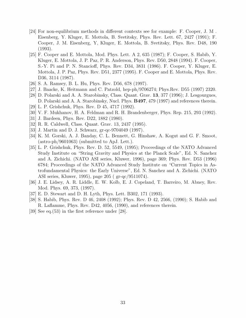
[24] For non-equilibrium methods in different contexts see for example: F. Cooper, J. M .Eisenberg, Y. Kluger, E. Mottola, B. Svetitsky, Phys. Rev. Lett. 67, 2427 (1991); F.Cooper, J. M. Eisenberg, Y, Kluger, E. Mottola, B. Svetitsky, Phys. Rev. D48, 190(1993).

[25] F. Cooper and E. Mottola, Mod. Phys. Lett. A 2, 635 (1987); F. Cooper, S. Habib, Y.Kluger, E. Mottola, J. P. Paz, P. R. Anderson, Phys. Rev. D50, 2848 (1994). F. Cooper,S.-Y. Pi and P. N. Stancioff, Phys. Rev. D34, 3831 (1986). F. Cooper, Y. Kluger, E.Mottola, J. P. Paz, Phys. Rev. D51, 2377 (1995). F. Cooper and E. Mottola, Phys. Rev.D36, 3114 (1987).

[26] S. A. Ramsey, B. L. Hu, Phys. Rev. D56, 678 (1997).[27] J. Baacke, K. Heitmann and C. Patzold, hep-ph/9706274; Phys.Rev. D55 (1997) 2320.[28] D. Polarski and A. A. Starobinsky, Class. Quant. Grav. 13, 377 (1996); J. Lesgourgues,

D. Polarski and A. A. Starobinsky, Nucl. Phys. B497, 479 (1997) and references therein.[29] L. P. Grishchuk, Phys. Rev. D 45, 4717 (1992).[30] V. F. Mukhanov, H. A. Feldman and R. H. Brandenberger, Phys. Rep. 215, 293 (1992).[31] J. Bardeen, Phys. Rev. D22, 1882 (1980).[32] R. R. Caldwell, Class. Quant. Grav. 13, 2437 (1995).[33] J. Martin and D. J. Schwarz, gr-qc-9704049 (1997).[34] K. M. Gorski, A. J. Banday, C. L. Bennett, G. Hinshaw, A. Kogut and G. F. Smoot,

(astro-ph/9601063) (submitted to ApJ. Lett.).[35] L. P. Grishchuk, Phys. Rev. D. 52, 5549, (1995); Proceedings of the NATO Advanced

Study Institute on “String Gravity and Physics at the Planck Scale”, Ed. N. Sanchezand A. Zichichi. (NATO ASI series, Kluwer, 1996), page 369; Phys. Rev. D53 (1996)6784; Proceedings of the NATO Advanced Study Institute on “Current Topics in As-trofundamental Physics: the Early Universe”, Ed. N. Sanchez and A. Zichichi. (NATOASI series, Kluwer, 1995), page 205 ( gr-qc/9511074).

[36] J. E. Lidsey, A. R. Liddle, E. W. Kolb, E. J. Copeland, T. Barreiro, M. Abney, Rev.Mod. Phys. 69, 373, (1997).

[37] E. D. Stewart and D. H. Lyth, Phys. Lett. B302, 171 (1993).[38] S. Habib, Phys. Rev. D 46, 2408 (1992); Phys. Rev. D 42, 2566, (1990); S. Habib and

R. Laflamme, Phys. Rev. D42, 4056, (1990), and references therein.[39] See eq.(53) in the first reference under [28].

33

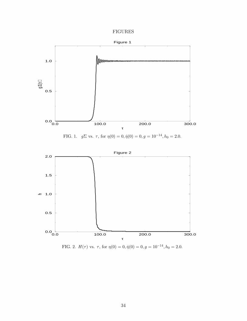
FIGURES

0.0 100.0 200.0 300.0τ

Figure 1

0.0

0.5

1.0

Σ(τ)

g

FIG. 1. gΣ vs. τ , for η(0) = 0, η(0) = 0, g = 10−14, h0 = 2.0.

0.0 100.0 200.0 300.0τ

Figure 2

0.0

0.5

1.0

1.5

2.0

h

FIG. 2. H(τ) vs. τ , for η(0) = 0, η(0) = 0, g = 10−14, h0 = 2.0.

34

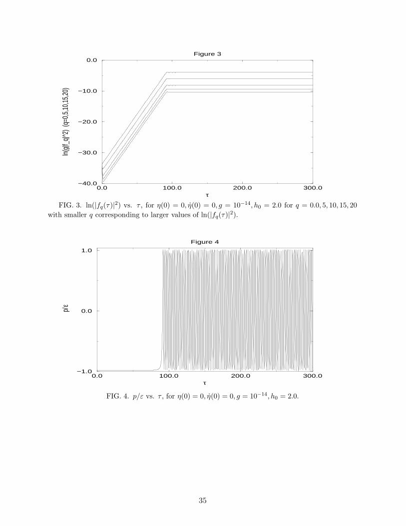
0.0 100.0 200.0 300.0τ

Figure 3

−40.0

−30.0

−20.0

−10.0

0.0ln(

g|f_q

|^2)

(q=0

,5,1

0,15

,20)

FIG. 3. ln(|fq(τ)|2) vs. τ , for η(0) = 0, η(0) = 0, g = 10−14, h0 = 2.0 for q = 0.0, 5, 10, 15, 20

with smaller q corresponding to larger values of ln(|fq(τ)|2).

0.0 100.0 200.0 300.0τ

Figure 4

−1.0

0.0

1.0

p/ε

FIG. 4. p/ε vs. τ , for η(0) = 0, η(0) = 0, g = 10−14, h0 = 2.0.

35

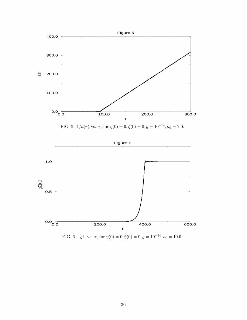
0.0 100.0 200.0 300.0τ

Figure 5

0.0

100.0

200.0

300.0

400.01/

h

FIG. 5. 1/h(τ) vs. τ , for η(0) = 0, η(0) = 0, g = 10−14, h0 = 2.0.

0.0 200.0 400.0 600.0τ

Figure 6

0.0

0.5

1.0

Σ(τ)

g

FIG. 6. gΣ vs. τ , for η(0) = 0, η(0) = 0, g = 10−14, h0 = 10.0.

36

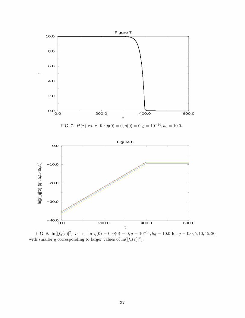
0.0 200.0 400.0 600.0τ

Figure 7

0.0

2.0

4.0

6.0

8.0

10.0h

FIG. 7. H(τ) vs. τ , for η(0) = 0, η(0) = 0, g = 10−14, h0 = 10.0.

0.0 200.0 400.0 600.0τ

Figure 8

−40.0

−30.0

−20.0

−10.0

0.0

ln(g|f

_q|^2

) (q

=0,5

,10,

15,2

0)

FIG. 8. ln(|fq(τ)|2) vs. τ , for η(0) = 0, η(0) = 0, g = 10−14, h0 = 10.0 for q = 0.0, 5, 10, 15, 20

with smaller q corresponding to larger values of ln(|fq(τ)|2).

37

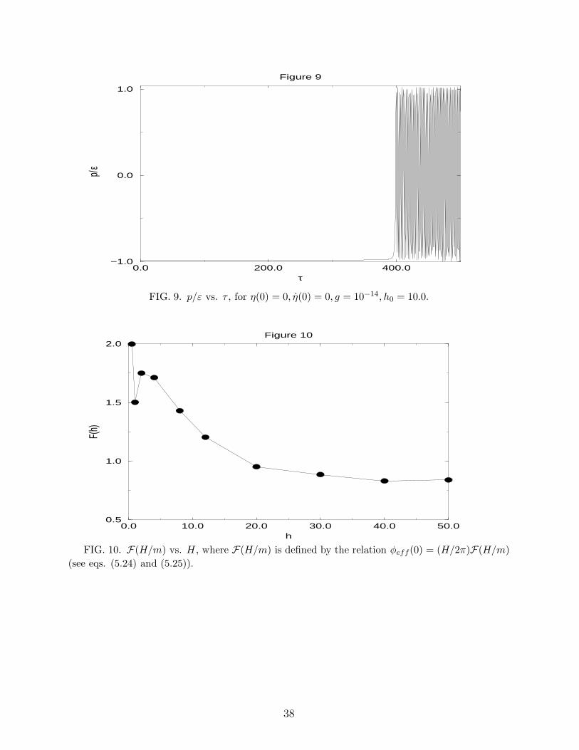
0.0 200.0 400.0τ

Figure 9

−1.0

0.0

1.0p/

ε

FIG. 9. p/ε vs. τ , for η(0) = 0, η(0) = 0, g = 10−14, h0 = 10.0.

0.0 10.0 20.0 30.0 40.0 50.0h

Figure 10

0.5

1.0

1.5

2.0

F(h)

FIG. 10. F(H/m) vs. H, where F(H/m) is defined by the relation φeff (0) = (H/2π)F(H/m)

(see eqs. (5.24) and (5.25)).

38

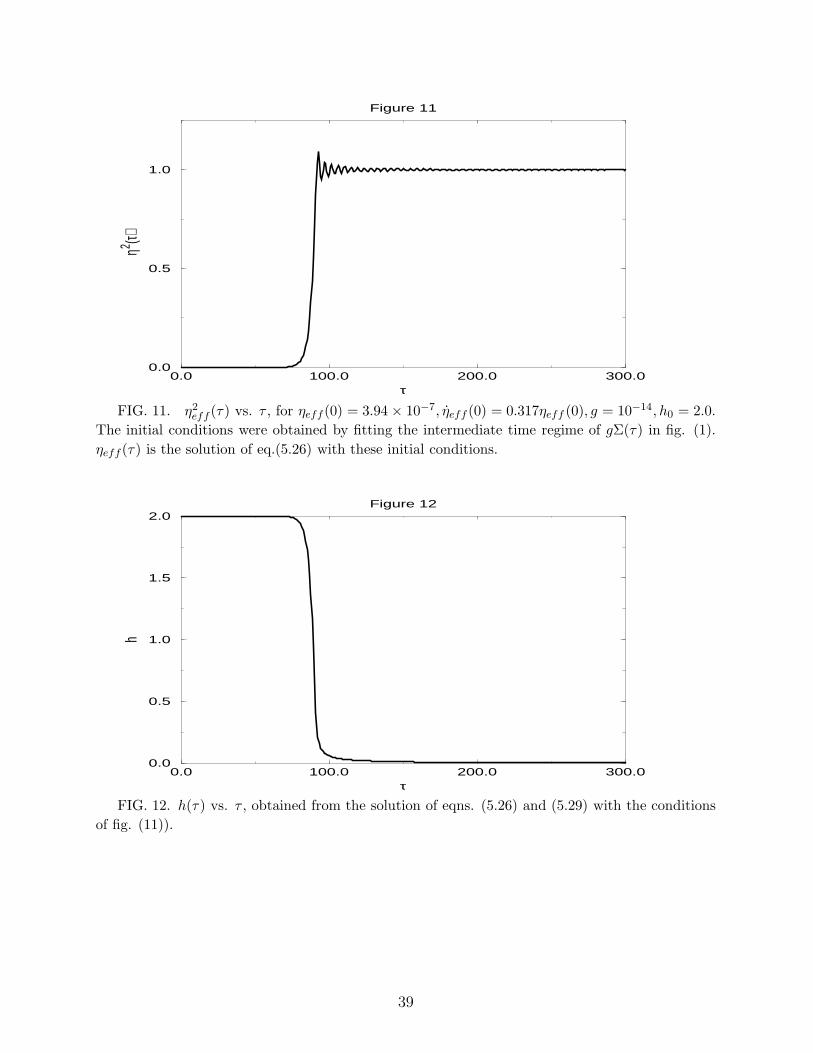
0.0 100.0 200.0 300.0τ

Figure 11

0.0

0.5

1.0

η (τ)2

FIG. 11. η2eff (τ) vs. τ , for ηeff (0) = 3.94 × 10−7, ηeff (0) = 0.317ηeff (0), g = 10−14, h0 = 2.0.

The initial conditions were obtained by fitting the intermediate time regime of gΣ(τ) in fig. (1).

ηeff (τ) is the solution of eq.(5.26) with these initial conditions.

0.0 100.0 200.0 300.0τ

Figure 12

0.0

0.5

1.0

1.5

2.0

h

FIG. 12. h(τ) vs. τ , obtained from the solution of eqns. (5.26) and (5.29) with the conditions

of fig. (11)).

39