arX

iv:p

att-

sol/9

7120

06v1

16

Dec

199

7

New Stability Results for Long–Wavelength

Convection Patterns

Anne C. Skeldon a and Mary Silber b

aDepartment of Mathematics, City University, Northampton Square, London,

EC1V 0HB UK, England

bDepartment of Engineering Sciences and Applied Mathematics, Northwestern

University, Evanston, IL 60208 USA

Abstract

We consider the transition from a spatially uniform state to a steady, spatially-periodic pattern in a partial differential equation describing long-wavelength convec-tion [1]. This both extends existing work on the study of rolls, squares and hexagonsand demonstrates how recent generic results for the stability of spatially-periodicpatterns may be applied in practice. We find that squares, even if stable to rollperturbations, are often unstable when a wider class of perturbations is considered.We also find scenarios where transitions from hexagons to rectangles can occur. Insome cases we find that, near onset, more exotic spatially-periodic planforms arepreferred over the usual rolls, squares and hexagons.

1 Introduction

Pattern forming instabilities arise in a wide number of physical and chemi-cal problems. Model partial differential equations are used to try to capturethe essential features of the observed transitions. In many interesting exam-ples such as Rayleigh-Benard convection and reaction-diffusion problems, themodel equations are invariant under all translations, rotations and reflectionsin the plane and patterns arise at a transition from a trivial solution consist-ing of no pattern. Linear stability analysis of the trivial solution leads to acritical curve describing how the wavenumber for instability, k, depends on aparameter, µ, in the problem. For parameter values below the critical curvethe trivial solution is stable. At a critical parameter, µc, instability onsets ata critical wavenumber kc.

Weakly nonlinear analysis is often used to try to predict the type of patternsobserved once the trivial solution becomes unstable. Two aspects make this

Preprint submitted to Elsevier Preprint 9 February 2008

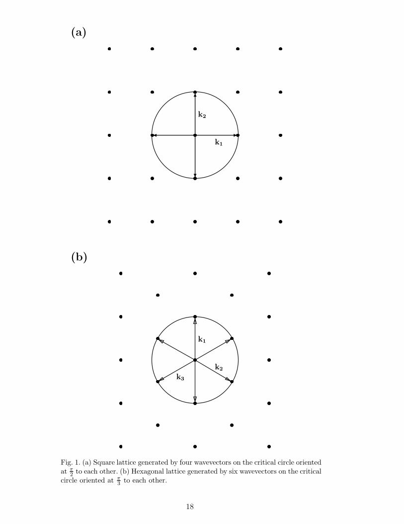
particularly difficult: firstly, the rotational invariance of the problem meansthat instability to a single wavenumber gives instability to a whole circle ofwavevectors. In other words, if the trivial solution is unstable to rolls then itis unstable to rolls with any orientation in the plane. Secondly, for µ > µc, notjust a single wavenumber but a whole band of wavenumbers is unstable. Of-ten this second problem is addressed by assuming that, sufficiently close to µc,boundaries in any real problem will select out one particular wavenumber andmodes with neighbouring wavenumbers will be suppressed. In the case of thefirst problem, a tacit assumption is often made that, for a given wavenumber,only a finite number of critical wavevectors are relevant. For example, fourcritical wavevectors oriented at π

2to each other (see figure 1(a)) are chosen or

six critical wavevectors oriented at π3

to each other are chosen (see figure 1(b)).In both cases the critical wavevectors generate a periodic lattice of points, asquare lattice in the first case and a hexagonal lattice in the second. Con-sequently, the circle of critical wavevectors is replaced by a finite set and afinite dimensional centre manifold exists for the problem, of dimension fourin the case of squares and of dimension six in the case of hexagons. If criticalwavevectors are used which do not generate a periodic lattice then there is noreason a priori why a finite dimensional centre manifold exists, since modesarbitrarily close to critical occur. While non-periodic cases have been consid-ered [2], their validity requires an additional assumption on the suppressionof these near critical modes.

Weakly nonlinear analysis using wavevectors on a square lattice or a hexagonallattice as shown in figure 1, provide a framework for examining the relativestability of either squares and rolls or hexagons and rolls respectively. In bothcases generic bifurcation equations have been derived using symmetry argu-ments [3–5]. A more complete stability analysis for rolls has been performed,for example by Brattkus and Davis [6], who consider the relative stability oftwo sets of rolls oriented at an arbitrary angle for a problem arising in crys-tal growth. Similarly, a more complete analysis can be performed for squaresand hexagons by considering families of different square and hexagonal lat-tices (for specific examples see figure 2). This problem has a high degree ofsymmetry and using group theoretic arguments, Dionne and Golubitsky showthat, for each lattice, additional branches other than hexagons, rolls or squaresbifurcate as primary bifurcations [9,10]. In spite of the fact that the Fouriertransform of the new patterns involves only one critical wavenumber, in phys-ical space they appear to have more than one lengthscale. Such “superlattice”patterns have recently been observed in the Faraday crispation experiment[7,8]. (For examples see figures 4 and 8 below.)

Using symmetry arguments, Dionne et al. derive the generic bifurcation equa-tions for the families of square and hexagonal lattices and examine the stabilityof certain primary bifurcation branches in terms of the coefficients of the bifur-cation equations [11]. This stability analysis enables two types of statement tobe made. Firstly, since each lattice problem corresponds to a subspace of the

2

original unbounded problem, and since hexagons and squares each exist on awhole family of lattices, the stability of these planforms can be considered toa countably infinite number of perturbations. While this is not equivalent tocompletely determining the stability of squares and hexagons in an unboundeddomain, it does considerably extend previous results. Secondly, each individ-ual lattice corresponds to either a square or hexagonal domain with periodicboundary conditions. For each lattice, the relative stability of the primarybranches known to exist from [9] can be calculated. These results, containedin [11], have not as yet been applied to any specific partial differential equationand it is this issue we address here.

In this paper, we re-examine the relative stability of spatially-periodic so-lutions to a partial differential equation considered by Knobloch [1]. Thisequation,

ft = αf − µ∇2f −∇4f + κ∇ · |∇f |2∇f

+β∇ · ∇2f∇f − γ∇ · f∇f + δ∇2|∇f |2, (1)

describes a number of long-wavelength partial differential equations whicharise in convection problems. For example, when κ = 1, β = δ = γ = 0 werecover the planform equation for convection in a layer between two poorlyconducting boundaries [12], and when κ = 1, γ = 0, β = −

√7

8, δ = −3

√7

8equa-

tion (1) models long-wavelength Marangoni convection [13]. Further examplesare given in [1]. For equation (1) we demonstrate, that with relatively littleadditional analysis, we can derive all the coefficients necessary to apply theresults from [11]. We thereby significantly extend Knobloch’s stability resultsby inclusion of the additional perturbations.

In section 2 we define the critical modes which generate square and hexagonallattices used here and the resulting generic bifurcation equations. The deriva-tion of the coefficients of the bifurcation equations is given in section 3. Thenin section 4 we discuss the results for two specific cases. In Case I we takeγ = 0, κ = +1. Knobloch called this Case B, the nature of our conclusionsfor his Case A are similar and we do not present them in detail. For Case I,provided β 6= δ, the coefficient of the quadratic term in the bifurcation equa-tions for the hexagonal lattices is nonzero. This quadratic term renders all ofthe primary solution branches for the hexagonal lattices unstable at bifurca-tion [14] and thus we restrict our attention to the square lattice bifurcationproblems. We divide our discussion into two parts: in section 4.1.1 we considerthe stability of squares and rolls in an unbounded domain by considering theirstability on the whole family of square lattices; in section 4.1.2 we consider theparticular example of long-wavelength Marangoni convection and show thatdifferent bifurcation scenarios can occur for different square lattices. In CaseII we consider γ/k2 = δ−β, κ = +1. This choice of parameters yields a degen-erate bifurcation problem for the hexagonal lattice since the coefficient of the

3

quadratic term in the bifurcation equations is zero. Stable primary branchesare therefore a possibility for all lattices and we consider both square andhexagonal types. We first discuss what can be deduced of the stability of rolls,hexagons and squares in an unbounded domain in section 4.2.1; then in sec-tion 4.2.2 we discuss the unfolding expected if the coefficient of the quadraticterm is non-zero but sufficiently small. Finally, in 4.2.3 we discuss the spe-cific example of Marangoni convection for different hexagonal lattices. Ourconclusions are summarised in section 5.

2 Preliminaries

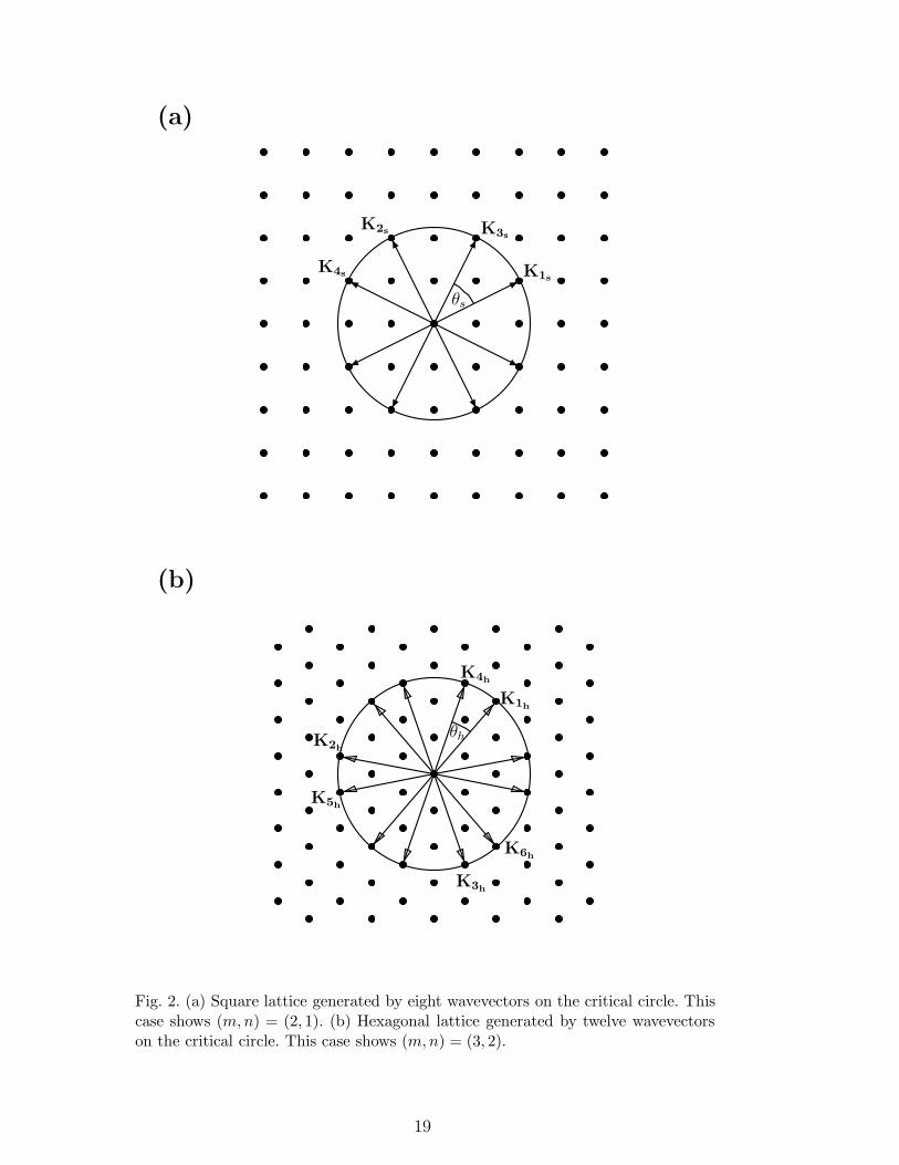
In order to apply the analysis given in [11], we consider sets of eight or twelvecritical modes whose wavevectors generate square or hexagonal lattices respec-tively, where the length of the critical wavevector is greater than the distancebetween neighbouring points on the lattice. A typical example is shown infigure 2(a) for the square lattice. This figure should be contrasted with figure1(a), which shows the wavevectors which are used conventionally in patternselection studies. In both figures, a circle representing the critical wavevectorsfor the original unbounded problem has been superimposed on the lattice. Infigure 1(a) this circle only intersects the lattice at four points and there areconsequently four critical modes, whereas in figure 2(a) the circle intersectsthe lattice at eight points and hence there are eight critical modes. Sufficientlyclose to the critical value of the parameter, µc, all other modes, representedby vectors not of length kc, will be damped. A family of finer and finer latticescan be constructed each with eight points on the critical circle. Each latticecan be encoded by a pair of integers, (m, n); for example, the lattice shown infigure 2(a) corresponds to the case (2, 1) i.e. K1s

is two squares of the latticeacross and one up. The eight wavevectors consist of two sets of four wavevec-tors, (±K1s

,±K2s) and (±K3s

,±K4s), that comprise squares and are rotated

by an angle θs relative to each other. An alternative way to specify each latticeis therefore through the lattice angle θs, where,

θs = cos−1(

2mn

m2 + n2

)

, (2)

and m > n > 0 are relatively prime positive integers that are not both odd.Reducing the circle of critical wavevectors to four critical wavevectors, asshown in figure 1(a), is equivalent to changing the original unbounded domainto a box whose side length is 1

kcand applying periodic boundary conditions.

Using eight critical wavevectors, illustrated in figure 2(a) for the case (m, n) =

(2, 1), corresponds to changing the domain to a box of side length√

m2+n2

kcand

again applying periodic boundary conditions.

4

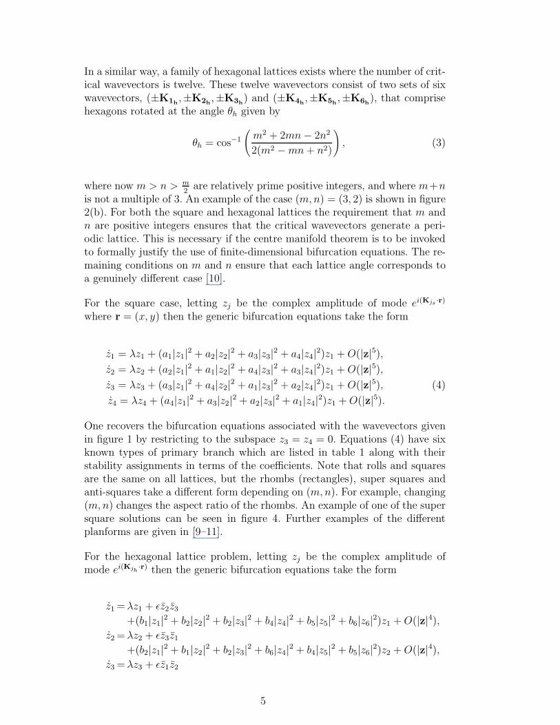
In a similar way, a family of hexagonal lattices exists where the number of crit-ical wavevectors is twelve. These twelve wavevectors consist of two sets of sixwavevectors, (±K1h

,±K2h,±K3h

) and (±K4h,±K5h

,±K6h), that comprise

hexagons rotated at the angle θh given by

θh = cos−1

(

m2 + 2mn − 2n2

2(m2 − mn + n2)

)

, (3)

where now m > n > m2

are relatively prime positive integers, and where m+nis not a multiple of 3. An example of the case (m, n) = (3, 2) is shown in figure2(b). For both the square and hexagonal lattices the requirement that m andn are positive integers ensures that the critical wavevectors generate a peri-odic lattice. This is necessary if the centre manifold theorem is to be invokedto formally justify the use of finite-dimensional bifurcation equations. The re-maining conditions on m and n ensure that each lattice angle corresponds toa genuinely different case [10].

For the square case, letting zj be the complex amplitude of mode ei(Kjs ·r)

where r = (x, y) then the generic bifurcation equations take the form

z1 = λz1 + (a1|z1|2 + a2|z2|2 + a3|z3|2 + a4|z4|2)z1 + O(|z|5),z2 = λz2 + (a2|z1|2 + a1|z2|2 + a4|z3|2 + a3|z4|2)z1 + O(|z|5),z3 = λz3 + (a3|z1|2 + a4|z2|2 + a1|z3|2 + a2|z4|2)z1 + O(|z|5), (4)

z4 = λz4 + (a4|z1|2 + a3|z2|2 + a2|z3|2 + a1|z4|2)z1 + O(|z|5).

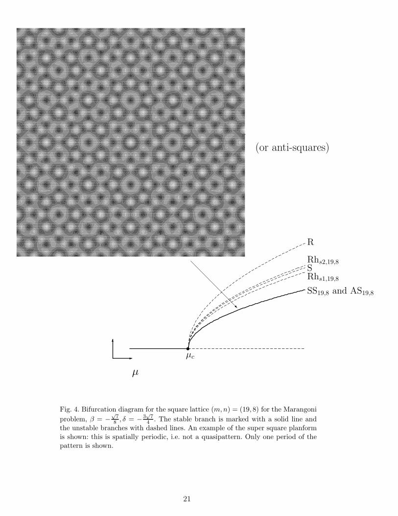
One recovers the bifurcation equations associated with the wavevectors givenin figure 1 by restricting to the subspace z3 = z4 = 0. Equations (4) have sixknown types of primary branch which are listed in table 1 along with theirstability assignments in terms of the coefficients. Note that rolls and squaresare the same on all lattices, but the rhombs (rectangles), super squares andanti-squares take a different form depending on (m, n). For example, changing(m, n) changes the aspect ratio of the rhombs. An example of one of the supersquare solutions can be seen in figure 4. Further examples of the differentplanforms are given in [9–11].

For the hexagonal lattice problem, letting zj be the complex amplitude ofmode ei(Kjh

·r) then the generic bifurcation equations take the form

z1 = λz1 + ǫz2z3

+(b1|z1|2 + b2|z2|2 + b2|z3|2 + b4|z4|2 + b5|z5|2 + b6|z6|2)z1 + O(|z|4),z2 = λz2 + ǫz3z1

+(b2|z1|2 + b1|z2|2 + b2|z3|2 + b6|z4|2 + b4|z5|2 + b5|z6|2)z2 + O(|z|4),z3 = λz3 + ǫz1z2

5

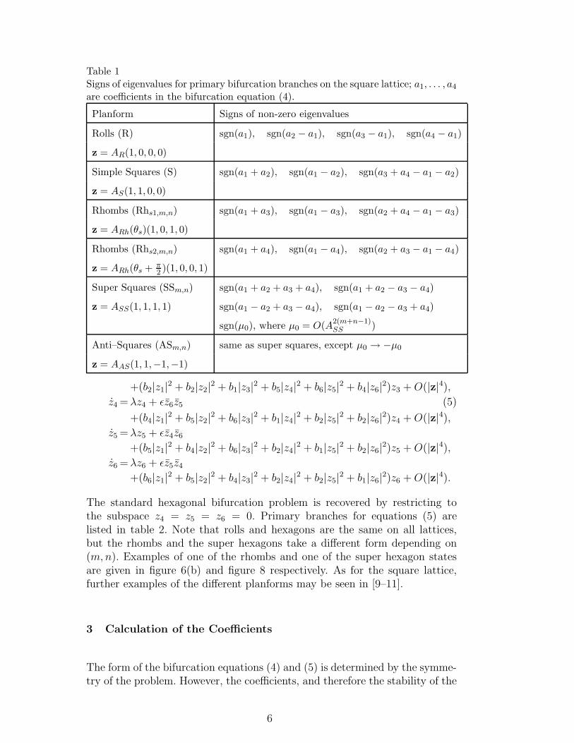
Table 1Signs of eigenvalues for primary bifurcation branches on the square lattice; a1, . . . , a4

are coefficients in the bifurcation equation (4).

Planform Signs of non-zero eigenvalues

Rolls (R) sgn(a1), sgn(a2 − a1), sgn(a3 − a1), sgn(a4 − a1)

z = AR(1, 0, 0, 0)

Simple Squares (S) sgn(a1 + a2), sgn(a1 − a2), sgn(a3 + a4 − a1 − a2)

z = AS(1, 1, 0, 0)

Rhombs (Rhs1,m,n) sgn(a1 + a3), sgn(a1 − a3), sgn(a2 + a4 − a1 − a3)

z = ARh(θs)(1, 0, 1, 0)

Rhombs (Rhs2,m,n) sgn(a1 + a4), sgn(a1 − a4), sgn(a2 + a3 − a1 − a4)

z = ARh(θs + π2 )(1, 0, 0, 1)

Super Squares (SSm,n) sgn(a1 + a2 + a3 + a4), sgn(a1 + a2 − a3 − a4)

z = ASS(1, 1, 1, 1) sgn(a1 − a2 + a3 − a4), sgn(a1 − a2 − a3 + a4)

sgn(µ0), where µ0 = O(A2(m+n−1)SS )

Anti–Squares (ASm,n) same as super squares, except µ0 → −µ0

z = AAS(1, 1,−1,−1)

+(b2|z1|2 + b2|z2|2 + b1|z3|2 + b5|z4|2 + b6|z5|2 + b4|z6|2)z3 + O(|z|4),z4 = λz4 + ǫz6z5 (5)

+(b4|z1|2 + b5|z2|2 + b6|z3|2 + b1|z4|2 + b2|z5|2 + b2|z6|2)z4 + O(|z|4),z5 = λz5 + ǫz4z6

+(b5|z1|2 + b4|z2|2 + b6|z3|2 + b2|z4|2 + b1|z5|2 + b2|z6|2)z5 + O(|z|4),z6 = λz6 + ǫz5z4

+(b6|z1|2 + b5|z2|2 + b4|z3|2 + b2|z4|2 + b2|z5|2 + b1|z6|2)z6 + O(|z|4).

The standard hexagonal bifurcation problem is recovered by restricting tothe subspace z4 = z5 = z6 = 0. Primary branches for equations (5) arelisted in table 2. Note that rolls and hexagons are the same on all lattices,but the rhombs and the super hexagons take a different form depending on(m, n). Examples of one of the rhombs and one of the super hexagon statesare given in figure 6(b) and figure 8 respectively. As for the square lattice,further examples of the different planforms may be seen in [9–11].

3 Calculation of the Coefficients

The form of the bifurcation equations (4) and (5) is determined by the symme-try of the problem. However, the coefficients, and therefore the stability of the

6

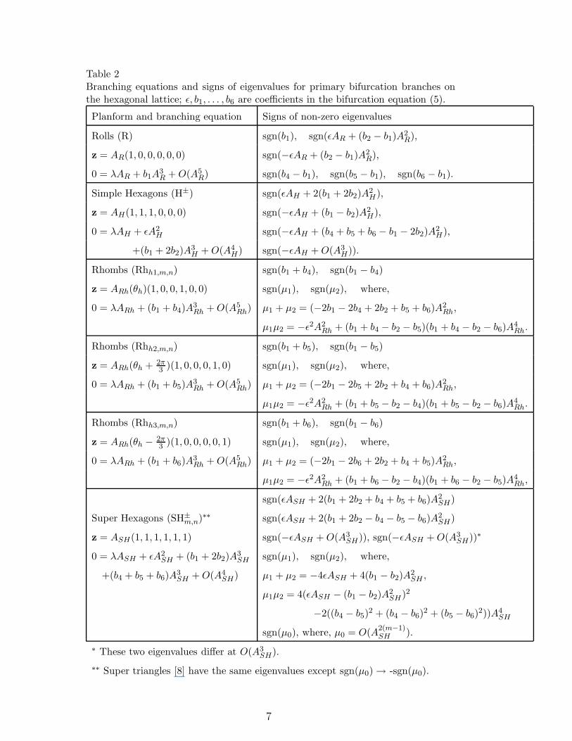
Table 2Branching equations and signs of eigenvalues for primary bifurcation branches onthe hexagonal lattice; ǫ, b1, . . . , b6 are coefficients in the bifurcation equation (5).

Planform and branching equation Signs of non-zero eigenvalues

Rolls (R) sgn(b1), sgn(ǫAR + (b2 − b1)A2R),

z = AR(1, 0, 0, 0, 0, 0) sgn(−ǫAR + (b2 − b1)A2R),

0 = λAR + b1A3R + O(A5

R) sgn(b4 − b1), sgn(b5 − b1), sgn(b6 − b1).

Simple Hexagons (H±) sgn(ǫAH + 2(b1 + 2b2)A2H),

z = AH(1, 1, 1, 0, 0, 0) sgn(−ǫAH + (b1 − b2)A2H),

0 = λAH + ǫA2H sgn(−ǫAH + (b4 + b5 + b6 − b1 − 2b2)A

2H),

+(b1 + 2b2)A3H + O(A4

H) sgn(−ǫAH + O(A3H)).

Rhombs (Rhh1,m,n) sgn(b1 + b4), sgn(b1 − b4)

z = ARh(θh)(1, 0, 0, 1, 0, 0) sgn(µ1), sgn(µ2), where,

0 = λARh + (b1 + b4)A3Rh + O(A5

Rh) µ1 + µ2 = (−2b1 − 2b4 + 2b2 + b5 + b6)A2Rh,

µ1µ2 = −ǫ2A2Rh + (b1 + b4 − b2 − b5)(b1 + b4 − b2 − b6)A

4Rh.

Rhombs (Rhh2,m,n) sgn(b1 + b5), sgn(b1 − b5)

z = ARh(θh + 2π3 )(1, 0, 0, 0, 1, 0) sgn(µ1), sgn(µ2), where,

0 = λARh + (b1 + b5)A3Rh + O(A5

Rh) µ1 + µ2 = (−2b1 − 2b5 + 2b2 + b4 + b6)A2Rh,

µ1µ2 = −ǫ2A2Rh + (b1 + b5 − b2 − b4)(b1 + b5 − b2 − b6)A

4Rh.

Rhombs (Rhh3,m,n) sgn(b1 + b6), sgn(b1 − b6)

z = ARh(θh − 2π3 )(1, 0, 0, 0, 0, 1) sgn(µ1), sgn(µ2), where,

0 = λARh + (b1 + b6)A3Rh + O(A5

Rh) µ1 + µ2 = (−2b1 − 2b6 + 2b2 + b4 + b5)A2Rh,

µ1µ2 = −ǫ2A2Rh + (b1 + b6 − b2 − b4)(b1 + b6 − b2 − b5)A

4Rh,

sgn(ǫASH + 2(b1 + 2b2 + b4 + b5 + b6)A2SH)

Super Hexagons (SH±m,n)∗∗ sgn(ǫASH + 2(b1 + 2b2 − b4 − b5 − b6)A

2SH)

z = ASH(1, 1, 1, 1, 1, 1) sgn(−ǫASH + O(A3SH)), sgn(−ǫASH + O(A3

SH))∗

0 = λASH + ǫA2SH + (b1 + 2b2)A

3SH sgn(µ1), sgn(µ2), where,

+(b4 + b5 + b6)A3SH + O(A4

SH) µ1 + µ2 = −4ǫASH + 4(b1 − b2)A2SH ,

µ1µ2 = 4(ǫASH − (b1 − b2)A2SH)2

−2((b4 − b5)2 + (b4 − b6)

2 + (b5 − b6)2))A4

SH

sgn(µ0), where, µ0 = O(A2(m−1)SH ).

∗ These two eigenvalues differ at O(A3SH).

∗∗ Super triangles [8] have the same eigenvalues except sgn(µ0) → -sgn(µ0).

7

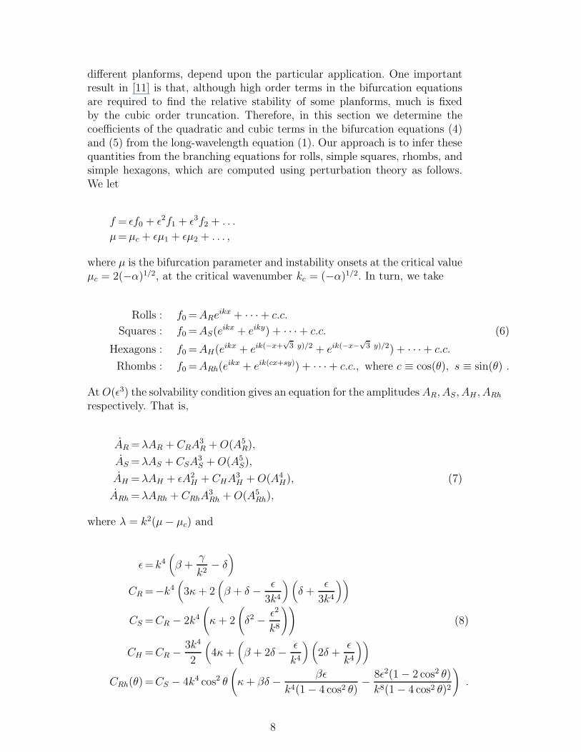
different planforms, depend upon the particular application. One importantresult in [11] is that, although high order terms in the bifurcation equationsare required to find the relative stability of some planforms, much is fixedby the cubic order truncation. Therefore, in this section we determine thecoefficients of the quadratic and cubic terms in the bifurcation equations (4)and (5) from the long-wavelength equation (1). Our approach is to infer thesequantities from the branching equations for rolls, simple squares, rhombs, andsimple hexagons, which are computed using perturbation theory as follows.We let

f = ǫf0 + ǫ2f1 + ǫ3f2 + . . .

µ= µc + ǫµ1 + ǫµ2 + . . . ,

where µ is the bifurcation parameter and instability onsets at the critical valueµc = 2(−α)1/2, at the critical wavenumber kc = (−α)1/2. In turn, we take

Rolls : f0 = AReikx + · · · + c.c.

Squares : f0 = AS(eikx + eiky) + · · ·+ c.c. (6)

Hexagons : f0 = AH(eikx + eik(−x+√

3 y)/2 + eik(−x−√

3 y)/2) + · · · + c.c.

Rhombs : f0 = ARh(eikx + eik(cx+sy)) + · · ·+ c.c., where c ≡ cos(θ), s ≡ sin(θ) .

At O(ǫ3) the solvability condition gives an equation for the amplitudes AR, AS, AH , ARh

respectively. That is,

AR = λAR + CRA3R + O(A5

R),

AS = λAS + CSA3S + O(A5

S),

AH = λAH + ǫA2H + CHA3

H + O(A4H), (7)

ARh = λARh + CRhA3Rh + O(A5

Rh),

where λ = k2(µ − µc) and

ǫ = k4(

β +γ

k2− δ

)

CR =−k4(

3κ + 2(

β + δ − ǫ

3k4

)(

δ +ǫ

3k4

))

CS =CR − 2k4

(

κ + 2

(

δ2 − ǫ2

k8

))

(8)

CH =CR − 3k4

2

(

4κ +(

β + 2δ − ǫ

k4

)(

2δ +ǫ

k4

))

CRh(θ) =CS − 4k4 cos2 θ

(

κ + βδ − βǫ

k4(1 − 4 cos2 θ)− 8ǫ2(1 − 2 cos2 θ)

k8(1 − 4 cos2 θ)2

)

.

8

Note that, as expected, CRh(π2) = CS. Also note that CRh diverges as θ → π

3

since when θ = π3

there is resonance between eikx and eik(cx+sy).

The cubic coefficients in the equivariant bifurcation equations (4) and (5)are readily expressed in terms of the branching coefficients CR, CS, CH andCRh. For instance, if (4) is restricted to the simple squares subspace z =(AS, AS, 0, 0), we find

AS = λAS + (a1 + a2)A3S. (9)

Comparing equation (9) with the appropriate branching equation from equa-tions (7) gives a1 + a2 = CS. Similarly, by restricting to subspaces for rollsand rhombs for the square lattice problems (4), we find

a1 = CR, a2 = CS − CR,

a3 = CRh(θs) − CR, a4 = CRh

(

θs +π

2

)

− CR, (10)

where θs ∈ (0, π2) takes on one of the discrete set of values (2). Similarly, re-

striction to subspaces for rolls, hexagons and rhombs for the hexagonal latticebifurcation problems (5) leads to

b1 =CR, b2 =1

2(CH − CR), b4 = CRh(θh) − CR,

b5 =CRh

(

θh +2π

3

)

− CR, b6 = CRh

(

θh − 2π

3

)

− CR, (11)

where θh ∈ (0, π3) takes on one of the values in the discrete set (3).

Note that the expressions for CR, CS, ǫ, and CH are given in [1] and, in thatpaper, are used to calculate the coefficients a1, a2, b1 and b2. The remainingexpression for CRh is the only additional calculation required to enable all theremaining coefficients in the bifurcation equations (4) and (5) to be found.

4 Stability Results

In this section we use the bifurcation equations (4) and (5) to determine therelative stability of the steady planforms which are given in section 2. Theresults depend on the parameters κ, β, δ, and γ in the long-wave equation(1). They also depend on the size of the periodic domain through the latticeparameters (m, n). We restrict our discussion to two cases and, where possible,compare and contrast our results with those given in [1].

9

The task of establishing the stability of each planform is considerably eased bythe fact that the eigenvalues determining the relative stability of each primarybranch are derived in terms of the coefficients of the Taylor expansion of thebifurcation equations in [11]. The signs of the eigenvalues are summarized intables 1 and 2 for the square and hexagonal lattices, respectively. The sign ofthe first quantity listed for each planform gives the branching direction; if thiseigenvalue is negative (positive), then the branch is supercritical (subcritical).If ǫ 6= 0 then simple hexagons and super hexagons bifurcate transcritically; allother patterns arise through pitchfork bifurcations. We distinguish betweenthe two branches of hexagons, denoted H+ and H−, which satisfy AH > 0and AH < 0, respectively. Similarly, there are two distinct branches of superhexagons, denoted by SH±

m,n. Omitted from the tables are the zero eigenvaluesassociated with translations of the patterns, and also information about themultiplicities of each eigenvalue; this information can be found in [11]. Notethat certain eigenvalues in tables 1 and 2 are not determined at cubic order inthe bifurcation equations. For instance, the relative stability of super squaresand anti-squares depends on a resonant term of O(|z|2m+2n−1). However, inthis case, if super squares and anti-squares are neutrally stable at cubic order,then, generically, exactly one of the two states is stable. There is an analogousstability result for super hexagons and triangles [8].

In the case of the square lattice, the eigenvalues that depend only on a1 and a2

can be determined by considering the restricted bifurcation problem z3 = z4 =0 in equation (4). Similarly, those results for the hexagonal lattice that dependonly on ǫ, b1 and b2 can be obtained by considering the simpler hexagonalbifurcation problem. In general, the signs of all the remaining eigenvalues aredependent on the choice of lattice. However, in the special case when ǫ = 0,we find that those eigenvalues which are unchanged on permutation of a3 anda4 are independent of θs, and those which are unchanged on permutation ofb4, b5 and b6 are independent of θh. This is due to the particularly simple θ-dependence of CRh(θ) in equation (8) when ǫ = 0. Also, in the case of thesquare lattices, results for angles close to π

6and π

3must be interpreted with

care because of the singularity in CRh(θ) at θ = π3

that occurs due to resonantinteractions.

In each of the cases we discuss below, we evaluate the signs of the eigenvaluesfor each planfrom and determine if and where they change sign. We presentthe results in the form of bifurcation sets separating different regions of sta-bility and instability for the relevant patterns. Note that along the stabilityboundaries themselves, the bifurcation problem is degenerate and the bifurca-tion equations (4) and (5) are insufficient to locally determine the bifurcationstructure. These degenerate points have been analysed by Knobloch [1].

10

4.1 Case I: γ = 0, κ = +1

In case I, solutions on the hexagonal lattices are unstable at onset unless β = δi.e. ǫ = 0 in equations (5). Thus here we focus on the square lattice problemsand defer discussion of the hexagonal cases to section 4.2.

4.1.1 The stability of squares and rolls

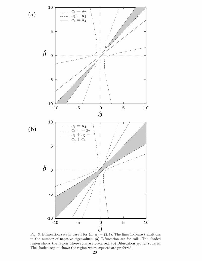
If we can show that squares or rolls are unstable on any one lattice thenthey must be unstable in the original unbounded problem sufficiently close toonset. From the hexagonal lattice result, we can immediately infer that rollsare unstable to hexagonal perturbations for β 6= δ. Here we show that squaresare also unstable unless β is sufficiently close to δ. The bifurcation sets forrolls and for squares in the (β, δ)-plane are presented in figures 3(a) and (b)respectively.

The sign of the branching eigenvalue for rolls, sgn(a1), is always negative,so rolls always bifurcate supercritically. The sign of a2 − a1 determines therelative stability of squares and rolls and the corresponding bifurcation line,a1 = a2 in figure 3(a), is identical to the line q(0) = 0 given in figure 2(b) of[1]. The relative stability of rolls and the two rhombic patterns is determinedby the signs of a3 − a1 and a4 − a1. Since a3 and a4 are dependent on θs, theprecise position of the corresponding bifurcation curves a1 = a3 and a1 = a4

depends on the choice of lattice: those shown in figure 3(a) are for the case(m, n) = (2, 1). Qualitatively the picture is the same in all cases correspondingto 0 < θs < π

4. For θs > π

4, the picture is similar except a3 − a1 and a4 − a1

switch roles. The region of stability is indicated by the shaded wedges in the(β, γ)-plane between a1 = a2 and a1 = a4 (a1 = a2 and a1 = a3 if θs > π

4).

As the lattice angle, θs, approaches π6

or π3

the region of stability of the rollsis reduced to a narrower and narrower region occurring only for large |β| and|δ|. At precisely θ = π

3(or the complementary π

6) the hexagonal lattice must

be considered.

In figure 3(b) we show the analogous bifurcation set for squares showing whereeach of the three expressions given in table 1 for the eigenvalues for squareschange sign. The lines a1 = a2 and a1 = −a2 correspond to the lines q(0) = 0and pN(0) = 0 given by Knobloch. In his study he found the squares werepreferred to rolls for the region between these two curves. However, this regionis significantly reduced when instability to super square (or anti-square) statesis included through the eigenvalue a3 + a4 − a1 − a2. The position of thecorresponding bifurcation line given by a3 + a4 = a1 + a2 is again dependenton the value of the lattice angle. As the lattice angle approaches π

6or π

3the

region of stability of the squares is reduced to a narrower and narrower region.Interestingly this narrow region always includes the line β = δ, for which the

11

hexagonal problem is degenerate. Recall that, for hexagonal lattices, it is onlyin this degenerate case that stable planforms can exist at onset. Thus, insummary, we find that there are only stable squares or rolls when β ≈ δ, thatis ǫ ≈ 0.

Knobloch also considered the case where β = δ, γ 6= 0 which he refers to as caseA. In this case we find that the region of stability for the rolls and for squaresis diminished to a narrow region about γ = 0 as the lattice angle approachesπ6

or π3. Since γ = 0 corresponds to the degenerate hexagonal problem, again

we find that squares and rolls are unstable unless ǫ ≈ 0.

4.1.2 Stability of other planforms: the example of Marangoni convection

As discussed in section 2, for each lattice, there are in fact six primary branchesknown to exist, any one of which could in principle be stable. Since many ofthe eigenvalues are dependent on the lattice angle θs, the precise region ofstability for each state is dependent on the choice of lattice, i.e. on the size ofthe domain for a box with periodic boundary conditions. Consequently, for agiven physical problem, which planforms are stable at onset, can be dependenton the size of the box. We illustrate this with the example of Marangoniconvection which corresponds to β = −

√7

8, δ = −3

√7

4and γ = 0. This lies

within the region where squares are preferred to rolls in Knobloch’s analysis.In contrast, we find that one of the following scenarios occurs:

0 < θs < 15.79o : Bistability of Rhs2,m,n and squares. e.g. (m,n)=(6,5).15.79 < θs < 18.34o : Rhs2,m,n stable. e.g. (m,n)=(11,8).18.34 < θs < 39.26o : Everything unstable, e.g. (m,n)=(2,1).39.26 < θs < 43.71o : Rhs2,m,n stable. e.g. (m,n)=(9,4).43.71 < θs < 44.67o : Super squares or anti-squares are stable. e.g. (m,n)=(19,8).44.67 < θs < 45.0o : Squares stable. e.g. (m,n)=(29,12).

The results for 450 < θs < 900 are essentially the same with Rhs1 and Rhs2

interchanged. Recall that the size of the periodic box for which these results

apply is given by√

m2+n2

kcand that the aspect ratio of the rhombs (rectangles)

is given by m−nm+n

for Rhs1,m,n and by nm

for Rhs2,m,n. In figure 4 we show anexample of the bifurcation diagram close to onset for the case (m, n) = (19, 8).We know that either super squares or anti-squares are stable and have drawnthe super square case. We have not calculated which of these two planformsis preferred at onset since this is determined at an O(2(m + n) − 1) = O(53)truncation of the bifurcation equations!

12

4.2 Case II: The degenerate case γk2

c= δ − β, κ = +1

In the degenerate case γk2

c= δ−β the quadratic coefficient, ǫ, is zero in equation

(5) and both square and hexagonal lattices can give locally stable planforms.We have therefore evaluated the signs of the eigenvalues listed in both table 1and table 2 which are determined at a cubic truncation of the bifurcationequations.

4.2.1 The stability of rolls, hexagons and squares

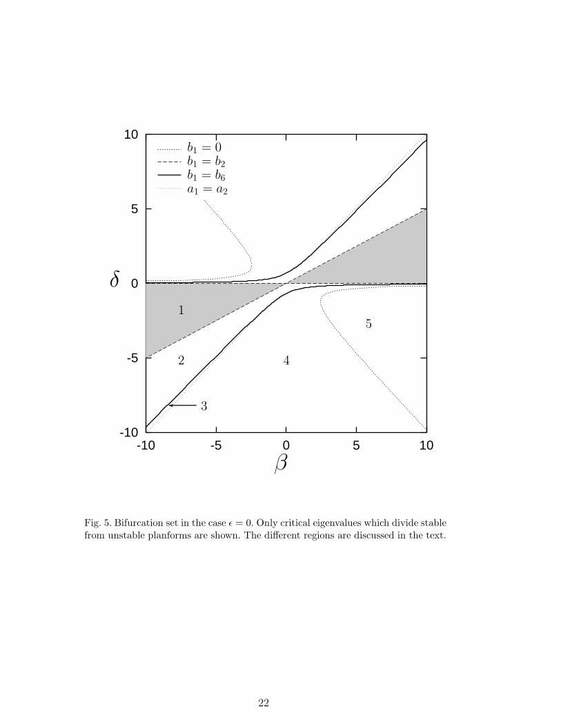
Our results are presented in the form of a bifurcation set in the (β, δ)-planeshown in figure 5.

We first recap the relative stability results given in [1] for the subspaces z4 =z5 = z6 = 0 of equation (5) and z3 = z4 = 0 of equation (4) before discussingthe results of our extended analysis. First, in the subspace of the hexagonalbifurcation problem it is found:

• Hexagons are stable in region 1.• Rolls are stable in regions 2,3 and 4.

In contrast, for the subspace of the square lattice bifurcation problem:

• Squares are stable in region 1, 2 and 3.• Rolls are stable only in region 4.

Together the results for the two lattices suggest that in regions 2 and 3, foran unbounded domain, that hexagons are unstable to rolls but that rolls areunstable to squares. However, there is no formal way of directly studying ifhexagons are unstable to squares.

In our analysis of the finer lattices the results given above are modified. Fora given hexagonal lattice we find hexagons and rhombs (Rhh3,m,n) are stablein region 1. Rhombs (Rhh3,m,n) are stable in region 2 and rolls are stableonly in regions 3 and 4. All other planforms are unstable. The position ofthe line dividing regions 2 and 3 is dependent on the choice of lattice. As thelattice angle approaches π

6, this line approaches the line a1 = a2. The rhombs

(rectangles) have aspect ratio depending on the lattice angle but lying between1√3

and 1.

For a given finer square lattice we find the stability results are unchangedfor squares and rolls, however rhombs can be stable in regions 1 and 2. Inparticular, for the rhombs, we find that rhombs, Rhs2,m,n are stable if 0 <θs < π

6and the rhombs, Rhs1,m,n are stable if π

3< θs < π

2. These have aspect

ratio dependent on θs, but again lying between 1√3

and 1. In addition, there are

13

regions of stable rhombs within region 1 which exist for π6

< θ < sin−1 1√3≈

35.30 and for π3

> θ > cos−1 1√3≈ 54.70 (aspect ratios between 1√

3and

√3−1√2

).

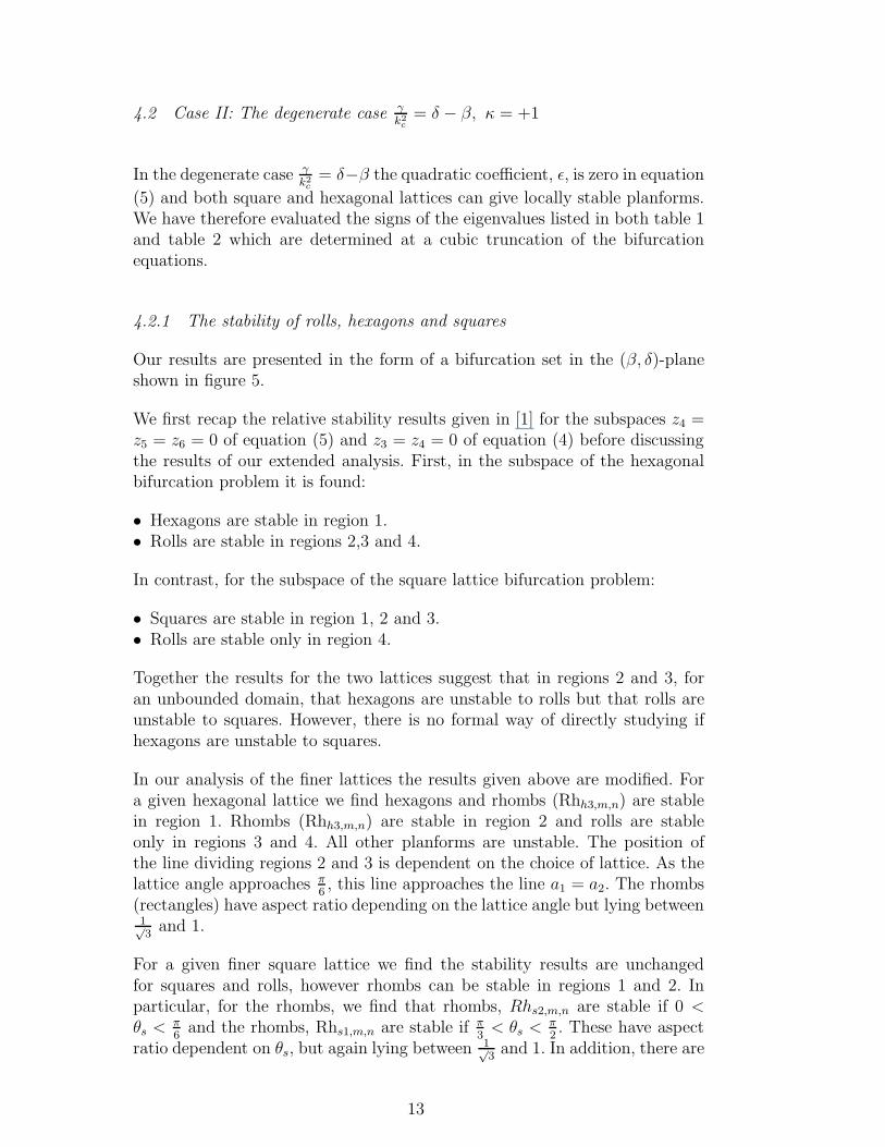
In summary, although the regions of stability of the hexagons and squares areunchanged by the extended bifurcation analysis, the inclusion of the rhombicstates allows for bistability of hexagons and rhombs of aspect ratio close toone.

4.2.2 Unfolding the degenerate problem

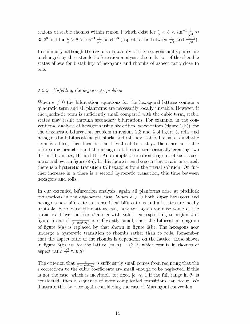
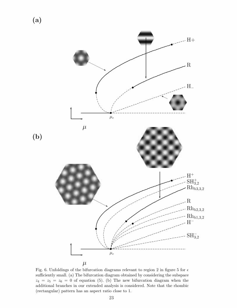
When ǫ 6= 0 the bifurcation equations for the hexagonal lattices contain aquadratic term and all planforms are necessarily locally unstable. However, ifthe quadratic term is sufficiently small compared with the cubic term, stablestates may result through secondary bifurcations. For example, in the con-ventional analysis of hexagons using six critical wavevectors (figure 1(b)), forthe degenerate bifurcation problem in regions 2,3 and 4 of figure 5, rolls andhexagons both bifurcate as pitchforks and rolls are stable. If a small quadraticterm is added, then local to the trivial solution at µc there are no stablebifurcating branches and the hexagons bifurcate transcritically creating twodistinct branches, H+ and H−. An example bifurcation diagram of such a sce-nario is shown in figure 6(a). In this figure it can be seen that as µ is increased,there is a hysteretic transition to hexagons from the trivial solution. On fur-ther increase in µ there is a second hysteretic transition, this time betweenhexagons and rolls.

In our extended bifurcation analysis, again all planforms arise at pitchforkbifurcations in the degenerate case. When ǫ 6= 0 both super hexagons andhexagons now bifurcate as transcritical bifurcations and all states are locallyunstable. Secondary bifurcations can, however, again stabilise some of thebranches. If we consider β and δ with values corresponding to region 2 offigure 5 and if ǫ

(1−cos2 θh)is sufficiently small, then the bifurcation diagram

of figure 6(a) is replaced by that shown in figure 6(b). The hexagons nowundergo a hysteretic transition to rhombs rather than to rolls. Rememberthat the aspect ratio of the rhombs is dependent on the lattice: those shownin figure 6(b) are for the lattice (m, n) = (3, 2) which results in rhombs of

aspect ratio√

32

≈ 0.87.

The criterion that ǫ(1−cos2 θh)

is sufficiently small comes from requiring that theǫ corrections to the cubic coefficients are small enough to be neglected. If thisis not the case, which is inevitable for fixed |ǫ| ≪ 1 if the full range in θh isconsidered, then a sequence of more complicated transitions can occur. Weillustrate this by once again considering the case of Marangoni convection.

14

4.2.3 Unfolding the degenerate problem: the example of Marangoni convec-

tion

Although the Marangoni problem is nondegenerate, previous studies [13] haveassumed that the quadratic term is sufficiently small and that it can legiti-mately be compared with the cubic terms. Specifically, the Marangoni prob-lem has β = −√

7/8, δ = −3√

7/4, ǫ = 5√

78

and although ǫ does not appearto be small, the cubic coefficients themselves are relatively large. For exam-ple, a1 = −1615

144and a2 = −1707

128resulting in a saddle-node bifurcation on

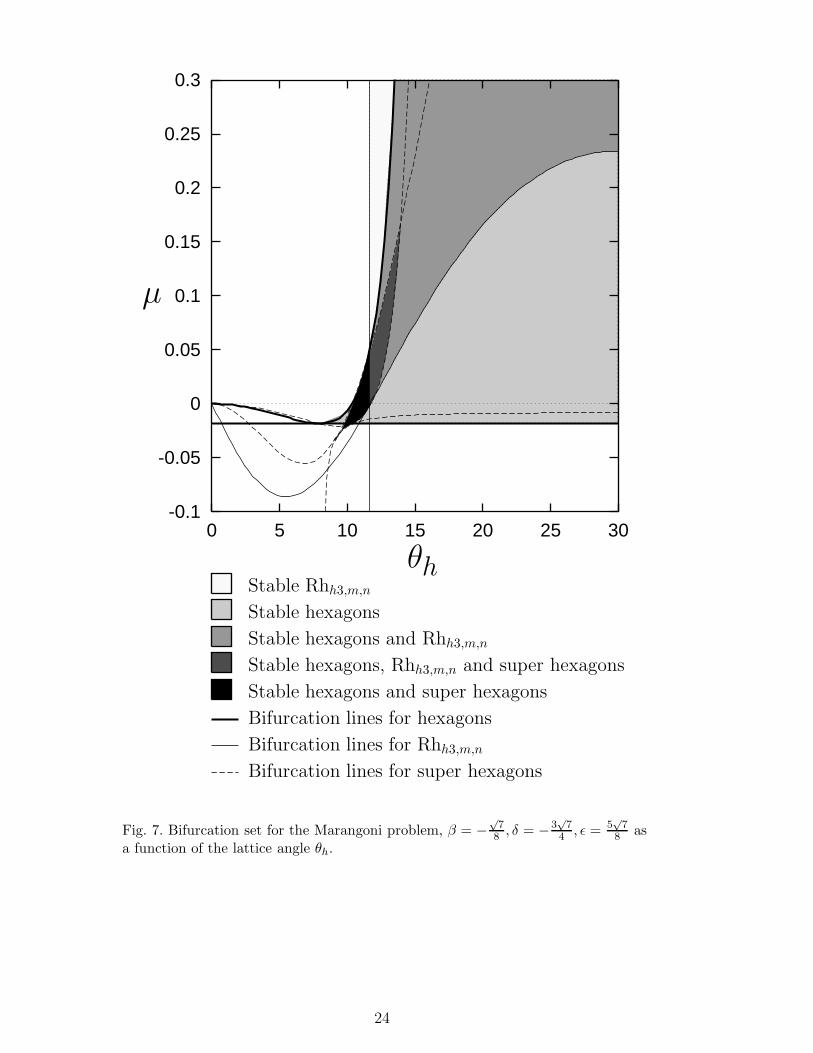
the hexagonal branch occurring at µ = −0.018. We have calculated all theeigenvalues that are determined at cubic order for the Marangoni case for thefamily of hexagonal lattices and found the corresponding bifurcation lines. Theresults are summarised in figure 7. The horizontal axis gives the lattice angle,θh. For the eigenvalues shown, this diagram is reflection symmetric about theline θh = π

6and we have therefore only shown 0 < θh < π

6. For simplicity,

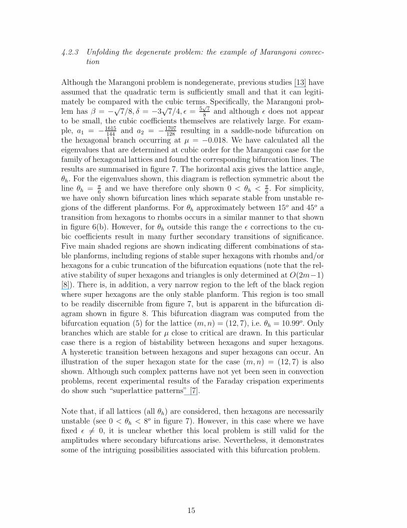
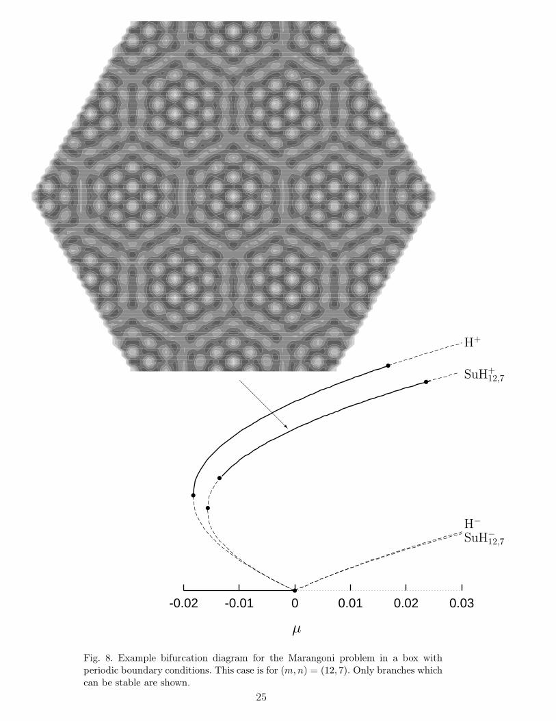
we have only shown bifurcation lines which separate stable from unstable re-gions of the different planforms. For θh approximately between 15o and 45o atransition from hexagons to rhombs occurs in a similar manner to that shownin figure 6(b). However, for θh outside this range the ǫ corrections to the cu-bic coefficients result in many further secondary transitions of significance.Five main shaded regions are shown indicating different combinations of sta-ble planforms, including regions of stable super hexagons with rhombs and/orhexagons for a cubic truncation of the bifurcation equations (note that the rel-ative stability of super hexagons and triangles is only determined at O(2m−1)[8]). There is, in addition, a very narrow region to the left of the black regionwhere super hexagons are the only stable planform. This region is too smallto be readily discernible from figure 7, but is apparent in the bifurcation di-agram shown in figure 8. This bifurcation diagram was computed from thebifurcation equation (5) for the lattice (m, n) = (12, 7), i.e. θh = 10.99o. Onlybranches which are stable for µ close to critical are drawn. In this particularcase there is a region of bistability between hexagons and super hexagons.A hysteretic transition between hexagons and super hexagons can occur. Anillustration of the super hexagon state for the case (m, n) = (12, 7) is alsoshown. Although such complex patterns have not yet been seen in convectionproblems, recent experimental results of the Faraday crispation experimentsdo show such “superlattice patterns” [7].

Note that, if all lattices (all θh) are considered, then hexagons are necessarilyunstable (see 0 < θh < 8o in figure 7). However, in this case where we havefixed ǫ 6= 0, it is unclear whether this local problem is still valid for theamplitudes where secondary bifurcations arise. Nevertheless, it demonstratessome of the intriguing possibilities associated with this bifurcation problem.

15

5 Conclusions

Standard low-dimensional bifurcation analyses of squares and hexagons giveonly a restricted stability analysis of these planforms. We have shown that,with one additional perturbation calculation, i.e. the calculation of CRh, allthe additional coefficients required to apply the extended stability analysisof [11] are determined. We have performed this calculation for the case ofthe long-wavelength convection equation (1) and analysed the results in twomain cases. In Case I we found that extending the stability results significantlyincreased the known region of instability for squares in an unbounded domain.In particular, we find that squares are only stable at onset if ǫ ≈ 0. This isinteresting given that it is already known that all solutions which are periodicon a hexagonal lattice are unstable at onset unless ǫ = 0. For a given boxwith periodic boundary conditions we found that the predicted planform atonset was strongly dependent on the size of the box: some of the more exoticplanforms such as super squares and anti-squares could be stable. In Case IIwe showed that regions of bistability of rhombs and hexagons exist. This gavea formal setting for studying the transition between hexagons and rhombs ofaspect ratio close to 1 (although not squares).

Acknowledgement

The research of MS was supported by NSF grant DMS-9404266 and by an NSFCAREER award DMS-9502266. ACS thanks the Nuffield Foundation and theRoyal Society for their support. The authors also appreciate the hospitality ofthe Hat Creek Radio Observatory, where much of the work for this paper wasdone.

16

References

[1] E. Knobloch. Pattern selection in long-wavelength convection. Physica D 41

(1990) 450–479.

[2] B.A. Malomed, A.A. Nepomnyashchii and M.I. Tribelskii. Two-dimensionalquasiperiodic structures in nonequilibrium systems. Sov. Phys. JETP 69 (1989)388–396.

[3] J.W. Swift. Bifurcation and symmetry in convection PHD Thesis (1984)University of California, Berkeley.

[4] E. Buzano and M. Golubitsky. Bifurcation on the hexagonal lattice and theplanar Benard problem. Philos. Trans. R. Soc. A 308 (1983) 617–667.

[5] M. Golubitsky, E. Knobloch and J.W. Swift. Symmetries and pattern selectionin Rayleigh-Benard convection. Physica D 10 (1984) 249–276.

[6] K. Brattkus and S.H. Davis. Cellular growth near absolute stability Phys. Rev.

B 38 (1988) 11452–60.

[7] A. Kudrolli, B. Pier and J.P. Gollub. Superlattice patterns in surface waves.preprint (1997).

[8] M. Silber and M.R.E. Proctor. Nonlinear competition between small and largehexagonal patterns. preprint (1997).

[9] B. Dionne. Spatially Periodic Patterns in Two and Three Dimensions. Ph.D.Thesis, University of Houston (1990).

[10] B. Dionne and M. Golubitsky. Planforms in two and three dimensions. Z.

Angew. Math. Phys. 43 (1992) 36–62.

[11] B. Dionne, M. Silber and A.C. Skeldon. Stability results for steady, spatially-periodic planforms. Nonlinearity 10 (1997) 321–353.

[12] M.R.E. Proctor. Planform selection by finite-amplitude thermal convectionbetween poorly conducting slabs. J. Fluid Mech. (1981) 469–485.

[13] L. Shtilman and B. Sivashinsky. Hexagonal structure of large scale Marangoniconvection. Physica D 52 (1991) 472–488.

[14] E. Ihrig and M. Golubitsky. Pattern selection with O(3) symmetry. Physica D

12 (1984) 1–33.

17

-

6

�

?

k1

k2

(a)

k1

k2

k3

(b)

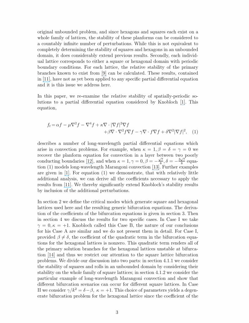
Fig. 1. (a) Square lattice generated by four wavevectors on the critical circle orientedat π

2 to each other. (b) Hexagonal lattice generated by six wavevectors on the criticalcircle oriented at π

3 to each other.

18

*

�K

Y

j

U�

�

K1s

K3s

K2s

K4s

(a)

θs

K1h

K2h

K3h

K5h

K4h

K6h

(b)

θh

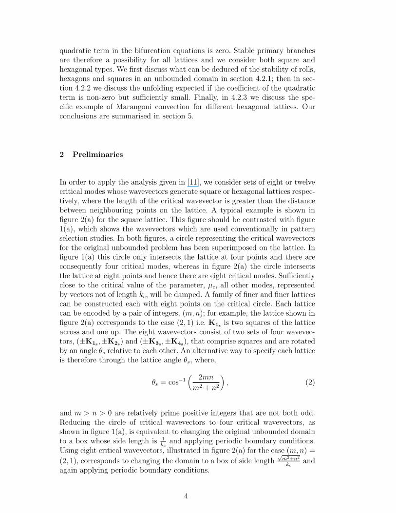
Fig. 2. (a) Square lattice generated by eight wavevectors on the critical circle. Thiscase shows (m,n) = (2, 1). (b) Hexagonal lattice generated by twelve wavevectorson the critical circle. This case shows (m,n) = (3, 2).

19

-10

-5

0

5

10

-10 -5 0 5 10

β

δ

a1 = a2a1 = a3a1 = a4

(a)

-10

-5

0

5

10

-10 -5 0 5 10

β

δ

a1 = a2a1 = −a2a1 + a2 =a3 + a4

(b)

Fig. 3. Bifurcation sets in case I for (m,n) = (2, 1). The lines indicate transitionsin the number of negative eigenvalues. (a) Bifurcation set for rolls. The shadedregion shows the region where rolls are preferred. (b) Bifurcation set for squares.The shaded region shows the region where squares are preferred.

20

R

µ

SS19,8 and AS19,8

Rhs1,19,8

SRhs2,19,8

R

-

6

(or anti-squares)

•µc

Fig. 4. Bifurcation diagram for the square lattice (m,n) = (19, 8) for the Marangoni

problem, β = −√

78 , δ = −3

√7

4 . The stable branch is marked with a solid line andthe unstable branches with dashed lines. An example of the super square planformis shown: this is spatially periodic, i.e. not a quasipattern. Only one period of thepattern is shown.

21

-10

-5

0

5

10

-10 -5 0 5 10

β

δ

b1 = 0b1 = b2

b1 = b6

a1 = a2

1

2

3

4

5

�

Fig. 5. Bifurcation set in the case ǫ = 0. Only critical eigenvalues which divide stablefrom unstable planforms are shown. The different regions are discussed in the text.

22

?

j

Y

µ

H−

R

H+

-

6 •

••

•

µc

(a)

?

j

µ

H−

R

H+

SH−3,2

SH+3,2

Rhh1,3,2

Rhh2,3,2

Rhh3,3,2

-

6 •

••

•

•

µc

(b)

Fig. 6. Unfoldings of the bifurcation diagrams relevant to region 2 in figure 5 for ǫ

sufficiently small. (a) The bifurcation diagram obtained by considering the subspacez4 = z5 = z6 = 0 of equation (5). (b) The new bifurcation diagram when theadditional branches in our extended analysis is considered. Note that the rhombic(rectangular) pattern has an aspect ratio close to 1.

23

-0.1

-0.05

0

0.05

0.1

0.15

0.2

0.25

0.3

0 5 10 15 20 25 30

θh

µ

Stable Rhh3,m,n

Stable hexagons

Stable hexagons and Rhh3,m,n

Stable hexagons, Rhh3,m,n and super hexagons

Stable hexagons and super hexagons

Bifurcation lines for hexagons

Bifurcation lines for Rhh3,m,n

Bifurcation lines for super hexagons

Fig. 7. Bifurcation set for the Marangoni problem, β = −√

78 , δ = −3

√7

4 , ǫ = 5√

78 as

a function of the lattice angle θh.

24

-0.02 -0.01 0 0.01 0.02 0.03

R

µ

H+

H−

SuH−12,7

SuH+12,7

•

••

•

••

Fig. 8. Example bifurcation diagram for the Marangoni problem in a box withperiodic boundary conditions. This case is for (m,n) = (12, 7). Only branches whichcan be stable are shown.

25