new load flow methods and techniques by ahmed mustafa
TRANSCRIPT
NEW LOAD FLOW METHODS
AND TECHNIQUES
BY
AHMED MUSTAFA MOHAMMED AL-JAALI
INDEX NO.074008
SUPERVISOR
DR. ABDUL-RAHMAN ALI KARRAR
REPORT SUBMITTED TO
University of Khartoum
In partial fulfillment of the requirement of the degree of
B.Sc. (HONS) Electrical and Electronic Engineering
(POWER SYSTEMS ENGINEERNG)
Faculty of Engineering
Department of Electrical and Electronic Engineering
September 2012

ii
DECLARATION OF ORIGINALITY
I declare that this report entitled “New Load Flow Methods and Techniques” is my
own work except as cited in the references. The report has not been accepted for any degree and
is not being submitted concurrently in candidature for any degree or other award.
Signature: _________________________
Name: ____________________________
Date: _____________________________

iii
Dedication
To the late Dr. Fayiz M. Al-Sadig, a teacher, scientist, and a true father…

iv
Acknowledgment
All praise is due to Allah Lord of all the worlds, the One God to whom praise is due
forever.
I would like to express my deep gratitude to our supervisor Dr. Abdul-Rahman Karrar,
without him, after Allah, this work wouldn‟t see the light. He was a real mentor, teacher and
close advisor. He never spared neither time nor effort to help us in our work by all means
possible.
Special thanks is for my project partner, Oday Hassan who was a real mate throughout
the project work and helped me and exhibited much of patience and cooperation.
Finally, I would like to thank the University of Khartoum for giving me the

v

vi
Abstract
Load flow Analysis is probably one of the most important studies of the performed on a
power system since it evaluates steady state operating conditions of the system. Principal
information obtained from a load flow is the voltage angle and magnitude at each bus hence the
flow of active and reactive power in each line. Load flow analysis is required by other power
system studies such as transient stability, contingency analysis and voltage stability. Numerical
analysis is the main tool used to solve the load flow problem to obtain the desired results.
A problem that faces the numerical methods is that they do not converge near the voltage
stability limit, this lead to the emergence of what‟s known as Continuation Power Flow, which is
a method that performs load flow beyond the voltage stability limit. A numerical technique is
employed to achieve this task. Continuation Power Flow employs arrives at the full PV curve
which is vital to the voltage stability analysis.
Project scope is to discover and implement new methods and techniques of load flow
that overcome the problem of Jacobian singularity and arrive at the full continuation curve.
New methods were discovered; their mathematical expressions were derived and
programmed by MATLABTM
. For the sake verification, the programs were tested on IEEE -14-
bus test system and results were compared with other results obtained by PSAT, Power System
Analysis Toolbox used on MATLABTM
and they were satisfactory.

vii
المستخلص
حث أنها تقم ربائة، الكه د كون واحدا من أهم الدراسات الت تجرى على نظام القدرةتحلل سران الحمولة ق
عند كل جهد المعلومات األساسة المستقاة من تحلل سران الحمولة ه زاوة و مقدار ال. التشغل للحالة المستقرة ظروف
: مطلوب من قبل دراسات نظم قدرة أخرى مثلتحلل سران الحمولة . التفاعلةالقدرة و ، و سران القدرة النشطة عقدة
التحلل العددي هو األداة األساسة المستخدمة لحل معادالت سران . تحلل الطوارئ و استقرار الجهداالستقرار العابر،
.الحمولة للحصول على النتائج المرغوبة
ة و ه أنها ال تتقارب بالقرب من حد استقرار الجهد ، هذا أدى إلى ظهور طرقة تحلل هنالك مشكلة تواجه الطرق العدد
تستخدم . جددة و ه تحلل استمرارة سران القدرة، و ه طرقة تؤدي تحلل سران حمولة ما بعد نقطة استقرار الجهد
الجهد الكامل و هو منحنى -صل إلى منحنى القدرةتحلل استمرارة سران القدرة . تقنة تحلل عددي لتحقق هذه المهمة
.حوي ف تحلل استقرار الجهد
نطاق المشروع هو اكتشاف و تطبق طرق و أسالب جددة لتحلل سران الحمولة تتجاوز مشكلة تفرد مصفوفة
.الجاكوبان و الوصول إلى منحنى االستمرارة الكامل
MATLABابرها الراضة و تمت برمجتها باستخدام تم اكتشاف طرق جددة، و تم اشتقاق تع TM
لغرض .
PSATو تمت مقارنة النتائج مع نتائج متحصل علها من IEEE -14-busالتأكد، تم اختبار البرامج على نظام االختبار TM
. و كانت النتائج مرضة
viii
1 Table of Contents
DECLARATION OF ORIGINALITY ....................................................................................... ii
Dedication iii
Acknowledgment ...................................................................................................................... iv
Abstract vi
vii المستخلص
1 Table of Contents .................................................................................................. viii
Chapter 1 1
1.1 Overview ......................................................................................................................1
1.2 Problem Statement ........................................................................................................1
1.3 Motivation ....................................................................................................................2
1.4 Project Objectives .........................................................................................................2
1.5 Report Layout ...............................................................................................................2
2 Chapter 2 ...................................................................................................................4
2.1 Overview ......................................................................................................................4
2.2 Load-Flow Analysis ......................................................................................................4
2.3 Newton-Raphson Method for Solution of System of Non-Linear Equations: .................4
2.4 Load-Flow Problem(Glover, Sarma, & Overbye, 2008): ...............................................6
2.5 Load-Flow Solution by Newton-Raphson:.....................................................................9
2.6 Continuation Power-Flow (Zakaria) ........................................................................... 13
2.6.1 General principle of the continuation power flow ................................................. 13
2.6.2 Formulation of the Power Flow Equations ........................................................... 14
2.6.3 Application of Continuation Algorithm ................................................................ 16
2.6.4 Predicting the Next Solution ................................................................................ 17
2.6.5 Parameterization and the Corrector Step ............................................................... 19
2.6.6 Choosing the Continuation Parameters ................................................................. 20
2.6.7 Sensing the Critical Point ..................................................................................... 20
3 Chapter 3 ................................................................................................................. 22
3.1 Introduction ................................................................................................................ 22
ix
3.2 Sin/Cos method ........................................................................................................... 22
3.3 The loading parameter (Lambda) method .................................................................... 27
3.3.1 Lambda Change Algorithm: ................................................................................. 27
3.3.2 Voltage Change Algorithm .................................................................................. 31
3.4 Impedance Load Flow ................................................................................................. 36
3.4.1 Single Injection Network Model: ......................................................................... 36
3.4.2 Starting values for admittances............................................................................. 36
3.4.3 Power and Admittance Mismatch Equations ........................................................ 37
3.4.4 Generator Reactive Power Limit Check ............................................................... 40
4 Chapter 4 ................................................................................................................. 42
4.1 Introduction ................................................................................................................ 42
4.2 The Sin Cos method results: ........................................................................................ 42
4.3 Loading Parameter method results: ............................................................................. 43
4.4 Impedance method results: .......................................................................................... 50
4.5 Results from PSAT ..................................................................................................... 51
4.6 Discussion of the results: ............................................................................................. 52
5 Chapter 5 ................................................................................................................. 53
5.1 Project Review ............................................................................................................ 53
5.2 Future Work ................................................................................................................ 54
6 Bibliography............................................................................................................ 55
8 APPENDIX A ...................................................................................................... A-1
9 APPENDIX B ....................................................................................................... B-1
10 APPENDIX C ....................................................................................................... C-1
11 Appendix D .......................................................................................................... D-1
x
List of Figure
Table of Figures
Figure 1 :Transmission Line Pi Model .........................................................................................7
Figure 2: Illustration of the Predictor-Corrector Scheme Used in the Continuation Power Flow 14
Figure 3 : Sin Cos Method algorithm ......................................................................................... 26
Figure 4: Loading Parameter method ......................................................................................... 35
Figure 5: Single Injection Network Model ................................................................................. 36
Chapter 1 Introduction
1
Chapter 1
INTRODUCTION
1.1 Overview
There is no doubt that load flow analysis is one of the most important and basic
study among other power system studies such as voltage stability and contingency
analysis. The load flow analysis problem have been formulated and clearly defined. It
gives the values of state variables updates(voltage magnitude and angle) at each bus
bar. Accordingly, it‟s important in determining the steady state Solution of the power
flow problem would have been impossible in the absence of computer system because
of the tremendous difficulty of solving this problem by hand, not only this, but as the
system grows larger and larger, solution by hand tend to be more impossible. The rise
of computer systems and rapid improvements in their technology participated primarily
in the load flow analysis by its easiness, improving the precision, and speed of the
analysis.
In the literature, many methods have been developed to define the load flow
problem and many numerical methods have been developed, each of which has its
advantages and disadvantages. Newton-Raphson method is one the most used methods
out there because it converges quickly and arrives at the solution after a few iterations.
1.2 Problem Statement
In the conventional load flow methods, there‟s a drawback, which is if we increase the
load at some bus bars, we can find the corresponding voltage. As we increase the load, we arrive
at some point where the Newton-Raphson solution does not converge at all because the Jacobian
matrix cannot be inverted. This case is called: Jacobian matrix singularity. It was found that the
Jacobian singularity occurs at the practical maximum loading point. This singularity is one of the
biggest problems encountered in the Newton-Raphson solution or any other method. This
Chapter 1 Introduction
2
problem inhibits the load flow program to continue after reaching the maximum loading point is
reached.
Jacobian singularity received great attention and was studied and methods have been
developed to continue the load flow, even beyond the maximum loading point. The most popular
one is the predictor-corrector continuation load flow, it adapts an algorithm that predicts the
solution of the next loading value using a predictor step, then a corrector step gives the exact
value.
1.3 Motivation
Load flow analysis is such an interesting challenging field of study. Computer systems
technology made it possible to study new methods and program them.
1.4 Project Objectives
Objective is to discover new methods that overcome the Jacobian singularity, develop
programs that perform the new methods, and finally test these programs on some well known
testing systems such as IEEE-14-Bus testing system.
1.5 Report Layout
The rest of this thesis is organized as follows:
Chapter 2- Literature Review: it provides the reader with the very basic knowledge
considering the project and all necessary equations and concepts that will be used along
the following chapters. It starts with the definition of load flow analysis. Solution by
numerical analysis technique, Newton-Raphson, namely is presented to serve as a tool for
the solution of the load flow problem. Next, Newton-Raphson technique is applied to the
load flow problem as steps. Finally, concept of continuation load flow is presented and
so the algorithm of solving this problem numerically.
Chapter 3- Methodology: this chapter introduces the new methods and techniques
discovered. Every method is introduced as a concept, next, an algorithm and a flow chart
is provided for each method.

Chapter 1 Introduction
3
Chapter 4- Results: Results are presented here in forms of tables and PV curves, and they
are compared with results obtained from other methods and PSAT. Those results are
obtained after implementing the methods to IEEE-14-Bus test system.
Chapter 5- Conclusion and future work: In this chapter, conclusion of the work done and
future work and recommendation are presented.
Chapter 2 Literature Review
4
2 Chapter 2
Literature Review
2.1 Overview
In this chapter, a review of load-flow analysis is presented, as well as continuation
load-flow. The chapter begins with a section about the conventional load- flow analysis, its
definition, problem formulation and numerical solution, Newton-Raphson method of solution
was chosen among different methods because it serves the problem to be solved by the project.
The next section is an overview of the continuation load-flow analysis, which is overcomes the
problem of singularity faced in the conventional load-flow and leads to plotting the full P-V
curve.
2.2 Load-Flow Analysis
The load-flow analysis is the computation of voltage magnitude and phase angle at each
bus in a power system under balanced three-phase steady-state conditions. As a by-product of
this calculation, real and reactive power flows in equipment such as transmission lines and
transformers, as well as equipment losses can be computed.
The starting point for a load-flow problem is a single line diagram of the power system,
from which the input data for computer solutions can be obtained. Input data consist of bus data,
transmission line data, and transformer data.(Glover, Sarma, & Overbye, 2008)
Load flow studies are necessary for planning, economic operation, scheduling and
exchange of power between utilities. It‟s also required for many other analysis such as transient
stability, voltage stability, contingency analysis and state estimation.(Das, 2006)
2.3 Newton-Raphson Method for Solution of System of Non-Linear
Equations:
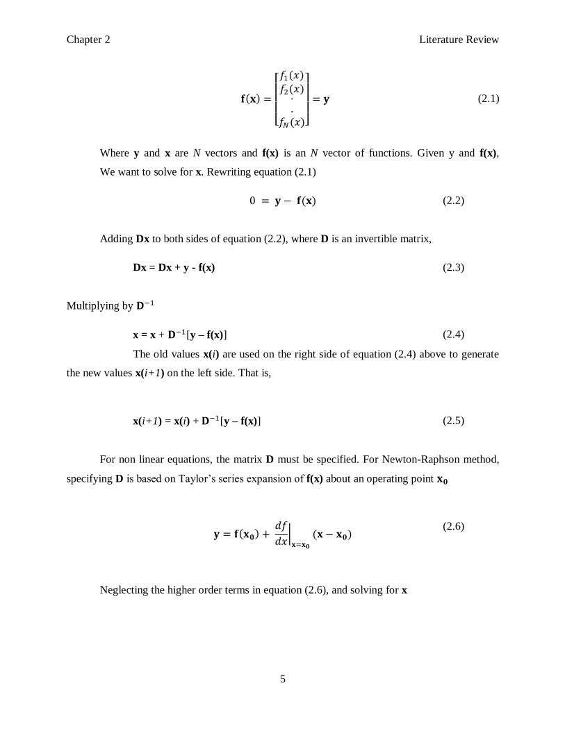
A set of nonlinear algebraic equations in matrix form is given by
Chapter 2 Literature Review
5
(2.1)
Where y and x are N vectors and f(x) is an N vector of functions. Given y and f(x),
We want to solve for x. Rewriting equation (2.1)
(2.2)
Adding Dx to both sides of equation (2.2), where D is an invertible matrix,
Dx = Dx + y - f(x)
(2.3)
Multiplying by
x = x + [y – f(x)] (2.4)
The old values x(i) are used on the right side of equation (2.4) above to generate
the new values x(i+1) on the left side. That is,
x(i+1) = x(i) + [y – f(x)]
(2.5)
For non linear equations, the matrix D must be specified. For Newton-Raphson method,
specifying D is based on Taylor‟s series expansion of f(x) about an operating point
(2.6)
Neglecting the higher order terms in equation (2.6), and solving for x
Chapter 2 Literature Review
6
(2.7)
The Newton-Raphson method replaces by the old value x(i) and x by the new value
x(i+1) in equation (2.7). Thus,
(2.8)
Where
(2.9)
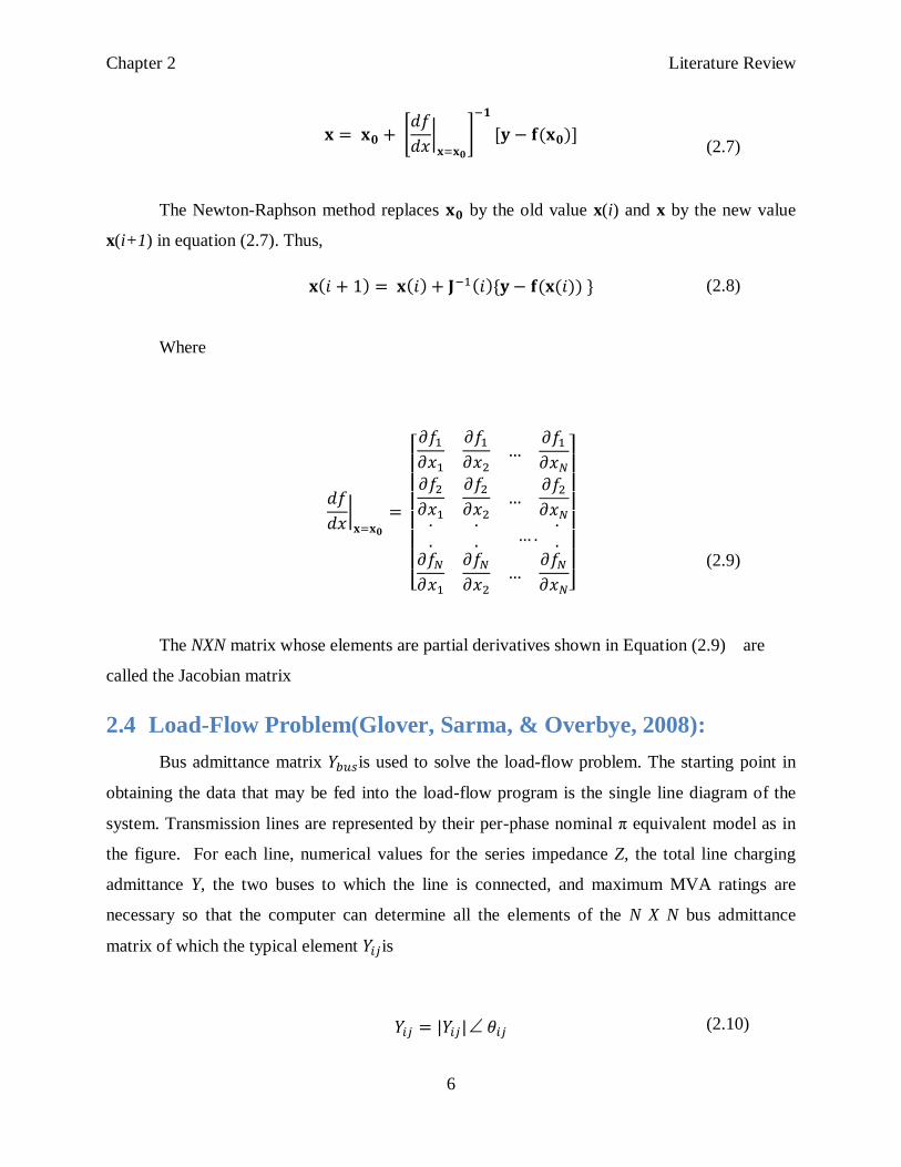
The NXN matrix whose elements are partial derivatives shown in Equation (2.9) are
called the Jacobian matrix
2.4 Load-Flow Problem(Glover, Sarma, & Overbye, 2008):
Bus admittance matrix is used to solve the load-flow problem. The starting point in
obtaining the data that may be fed into the load-flow program is the single line diagram of the
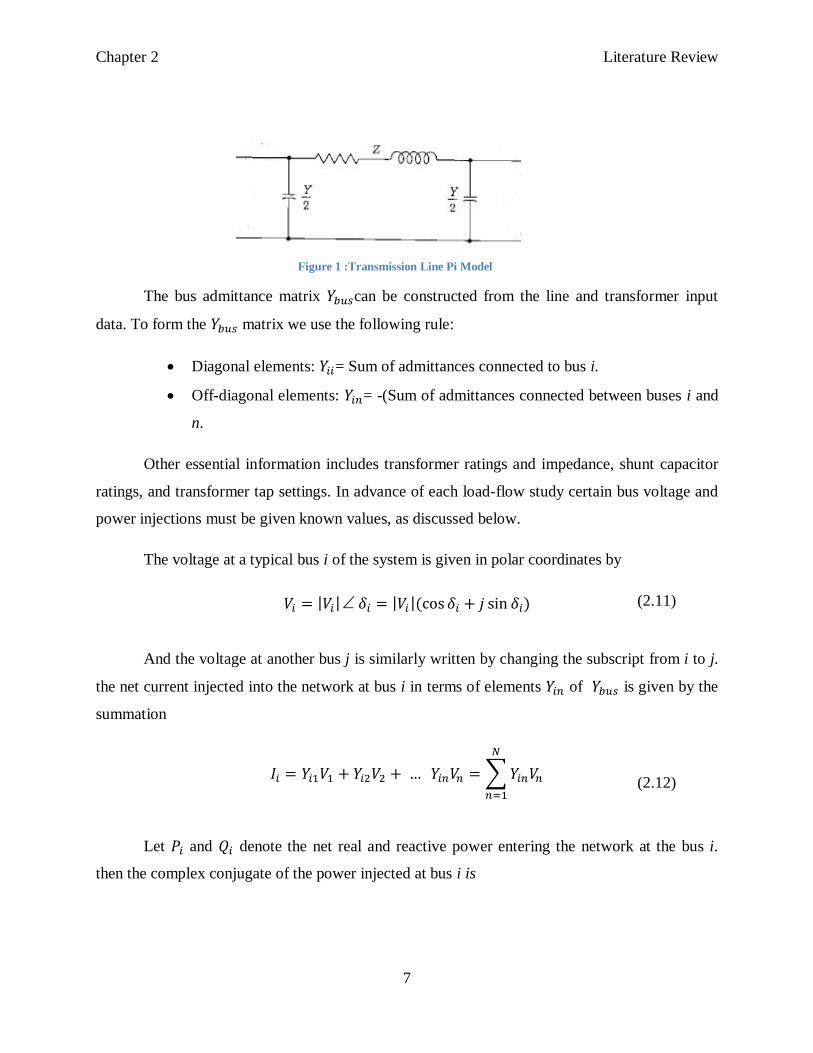
system. Transmission lines are represented by their per-phase nominal π equivalent model as in
the figure. For each line, numerical values for the series impedance Z, the total line charging
admittance Y, the two buses to which the line is connected, and maximum MVA ratings are
necessary so that the computer can determine all the elements of the N X N bus admittance
matrix of which the typical element is
(2.10)
Chapter 2 Literature Review
7
The bus admittance matrix can be constructed from the line and transformer input
data. To form the matrix we use the following rule:
Diagonal elements: = Sum of admittances connected to bus i.
Off-diagonal elements: = -(Sum of admittances connected between buses i and
n.
Other essential information includes transformer ratings and impedance, shunt capacitor
ratings, and transformer tap settings. In advance of each load-flow study certain bus voltage and
power injections must be given known values, as discussed below.
The voltage at a typical bus i of the system is given in polar coordinates by
(2.11)
And the voltage at another bus j is similarly written by changing the subscript from i to j.
the net current injected into the network at bus i in terms of elements of is given by the
summation
(2.12)
Let and denote the net real and reactive power entering the network at the bus i.
then the complex conjugate of the power injected at bus i is
Figure 1 :Transmission Line Pi Model
Chapter 2 Literature Review
8
(2.13)
In which we substitute from (2.13) to obtain
(2.14)
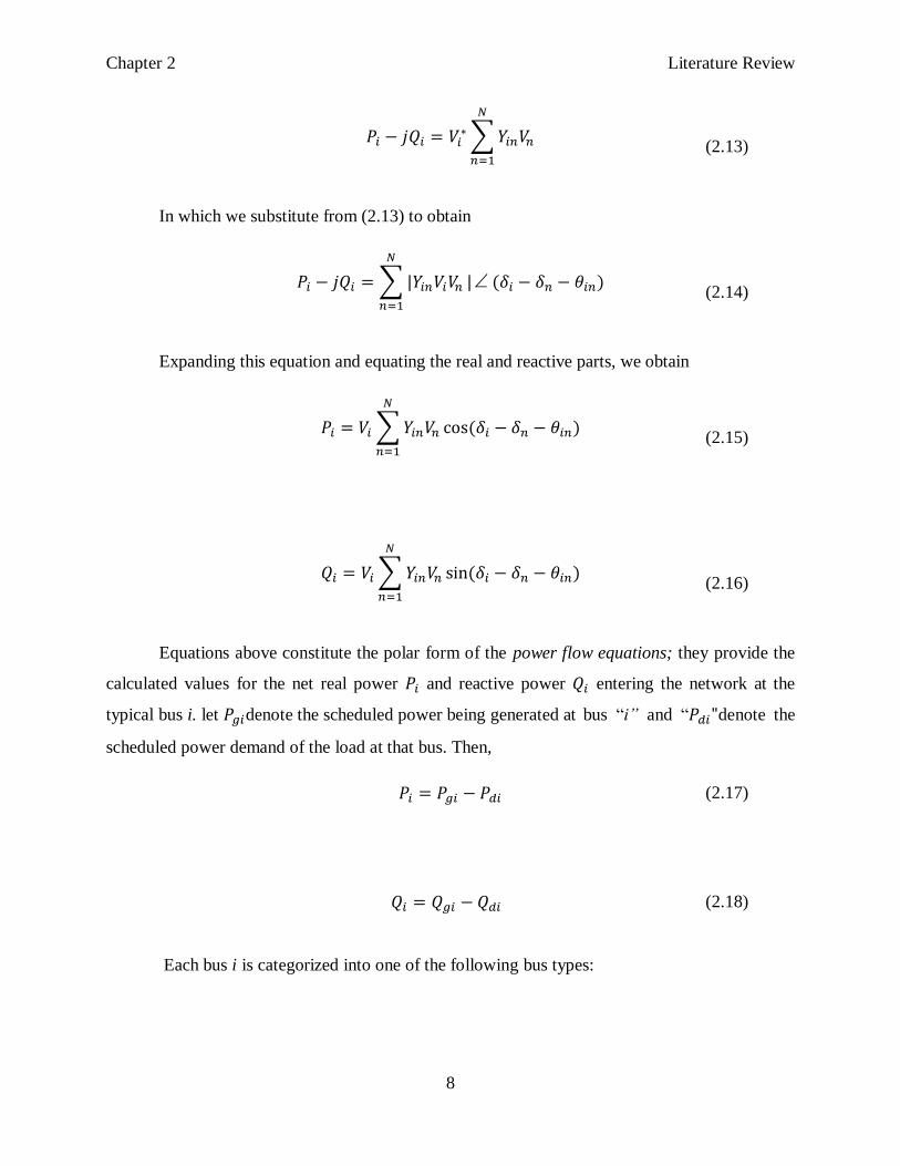
Expanding this equation and equating the real and reactive parts, we obtain
(2.15)
(2.16)
Equations above constitute the polar form of the power flow equations; they provide the
calculated values for the net real power and reactive power entering the network at the
typical bus i. let denote the scheduled power being generated at bus “i” and “ denote the
scheduled power demand of the load at that bus. Then,
(2.17)
(2.18)
Each bus i is categorized into one of the following bus types:
Chapter 2 Literature Review
9
1- Swing bus (or slack bus): there‟s only one swing bus in the system, which for
convenience is numbered bus 1. The swing bus is reference bus for which ,
per unit., is input data. Load-flow program computes and .
2- Load bus: and are input data. The load-flow program computes and . Most
buses are load buses.
3- Generator bus (Voltage controlled bus), and are input data. The power flow
program computes and . Examples are buses to which generators, switched shunt
capacitors, or static VAR systems are connected. Maximum and minimum VAR limits
that this equipment can supply are also input data.
2.5 Load-Flow Solution by Newton-Raphson:
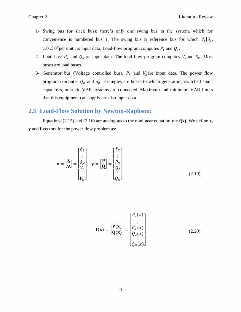
Equations (2.15) and (2.16) are analogous to the nonlinear equation y = f(x). We define x,
y and f vectors for the power flow problem as:
;
(2.19)
(2.20)
Chapter 2 Literature Review
10
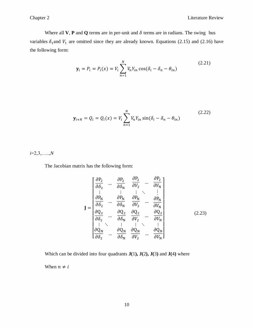
Where all V, P and Q terms are in per-unit and terms are in radians. The swing bus
variables and are omitted since they are already known. Equations (2.15) and (2.16) have
the following form:
(2.21)
(2.22)
i=2,3,…..,N
The Jacobian matrix has the following form:
(2.23)
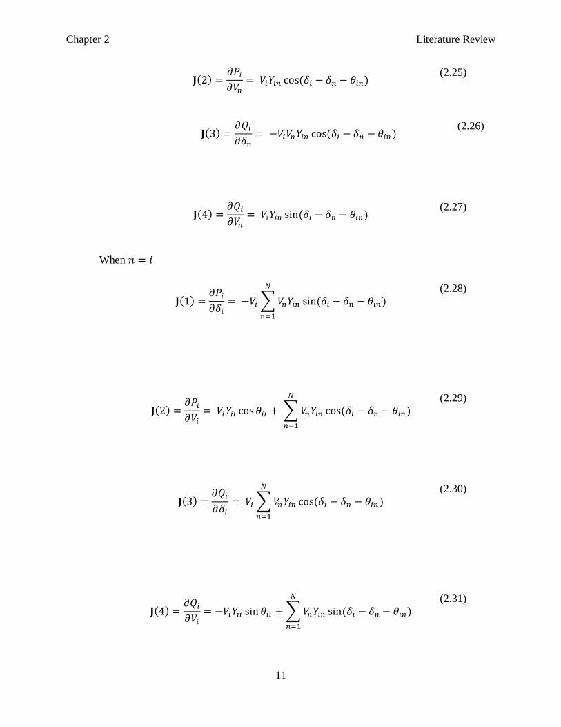
Which can be divided into four quadrants J(1), J(2), J(3) and J(4) where
When
Chapter 2 Literature Review
11
(2.25)
(2.27)
When
(2.28)
(2.29)
(2.30)
(2.31)
(2.26)
Chapter 2 Literature Review
12
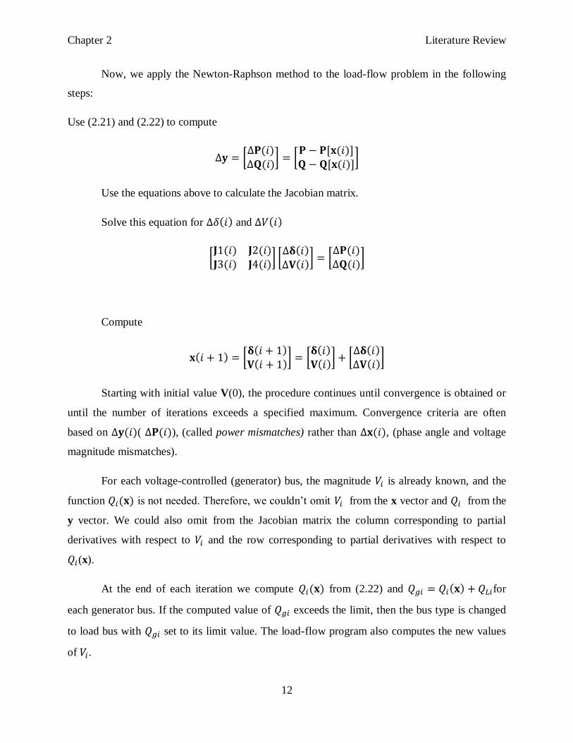
Now, we apply the Newton-Raphson method to the load-flow problem in the following
steps:
Use (2.21) and (2.22) to compute
Use the equations above to calculate the Jacobian matrix.
Solve this equation for and
Compute
Starting with initial value V(0), the procedure continues until convergence is obtained or
until the number of iterations exceeds a specified maximum. Convergence criteria are often
based on ( ), (called power mismatches) rather than , (phase angle and voltage
magnitude mismatches).
For each voltage-controlled (generator) bus, the magnitude is already known, and the
function is not needed. Therefore, we couldn‟t omit from the x vector and from the
y vector. We could also omit from the Jacobian matrix the column corresponding to partial
derivatives with respect to and the row corresponding to partial derivatives with respect to
(x).
At the end of each iteration we compute from (2.22) and for
each generator bus. If the computed value of exceeds the limit, then the bus type is changed
to load bus with set to its limit value. The load-flow program also computes the new values
of .
Chapter 2 Literature Review
13
2.6 Continuation Power-Flow (Zakaria)
The Jacobian matrix becomes singular at the voltage stability limit; consequently,
conventional load-flow algorithms are prone to convergence problems at the operating
conditions near the stability limit. The continuation power-flow analysis overcomes this problem
by reformulating the load-flow equations so that they remain well-conditioned at all possible
loading conditions. This allows the solution of the load-flow problem for stable, as well as
unstable equilibrium points (that is, for both upper and lower portions of the P-V
curve)(Kundur). The purpose of continuation power flow is to find a continuum of load flow
solutions for a given load/generation change scenario (i.e. computation direction). It‟s capable of
solving the whole PV curve. The continuation power flow finds the solution path of a set of load-
flow equations that are reformulated to include a continuation parameter.
The continuation power-flow method described here uses locally parameterized
continuation method that belong to a general class of methods for solving nonlinear algebraic
equations known as path-following methods.
2.6.1 General principle of the continuation power flow
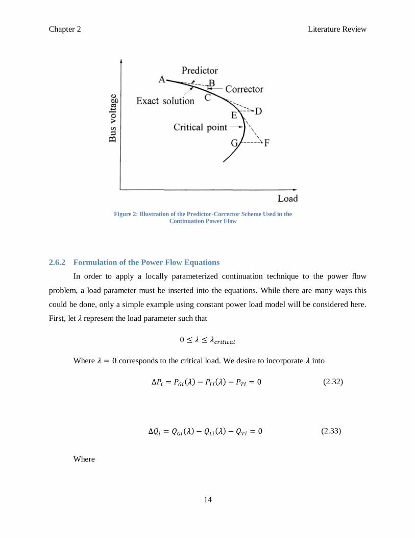
The general principle behind the continuation power flow is rather simple. It employs a
predictor-corrector scheme to find a solution path of a set of power flow equations that have been
reformulated to include a load parameter. As shown in Figure 2. Initial solution (A), a tangent
predictor is used to estimate the solution (B) for a specified pattern of load increase. The
corrector step then determines the exact solution (C) using conventional load-flow analysis with
the system load assumed to be fixed.
The voltages for a further increase in load are then predicted based on a new tangent
predictor. If the new estimated load (D) is now beyond the maximum load on the exact solution,
a corrector step with loads fixed would not converge; therefore, a corrector step with a fixed
voltage at the monitored bus is applied to find the exact solution (E). As the voltage stability
limit is reached, to determine the exact maximum load the size of load increase has to be reduced
gradually during the successive predictor steps.
Chapter 2 Literature Review
14
2.6.2 Formulation of the Power Flow Equations
In order to apply a locally parameterized continuation technique to the power flow
problem, a load parameter must be inserted into the equations. While there are many ways this
could be done, only a simple example using constant power load model will be considered here.
First, let λ represent the load parameter such that
Where corresponds to the critical load. We desire to incorporate into
(2.32)
(2.33)
Where
Figure 2: Illustration of the Predictor-Corrector Scheme Used in the
Continuation Power Flow
Chapter 2 Literature Review
15
(2.34)
(2.35)
The subscript L, G and T respectively denote bus load, generation and injection. The
voltage at bus i is and is the element of the system admittance
matrix .
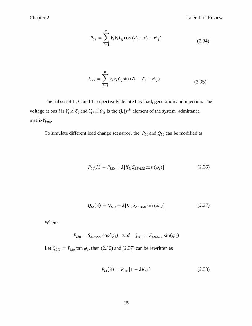
To simulate different load change scenarios, the and can be modified as
(2.36)
(2.37)
Where
Let , then (2.36) and (2.37) can be rewritten as
(2.38)
Chapter 2 Literature Review
16
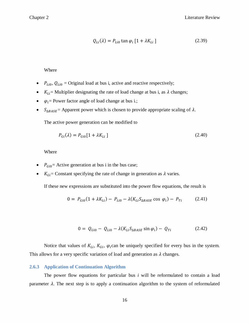
(2.39)
Where
, = Original load at bus i, active and reactive respectively;
= Multiplier designating the rate of load change at bus i, as changes;
= Power factor angle of load change at bus i.;
= Apparent power which is chosen to provide appropriate scaling of .
The active power generation can be modified to
(2.40)
Where
= Active generation at bus i in the bus case;
= Constant specifying the rate of change in generation as varies.
If these new expressions are substituted into the power flow equations, the result is
(2.41)
(2.42)
Notice that values of , , can be uniquely specified for every bus in the system.
This allows for a very specific variation of load and generation as changes.
2.6.3 Application of Continuation Algorithm
The power flow equations for particular bus i will be reformulated to contain a load
parameter . The next step is to apply a continuation algorithm to the system of reformulated
Chapter 2 Literature Review
17
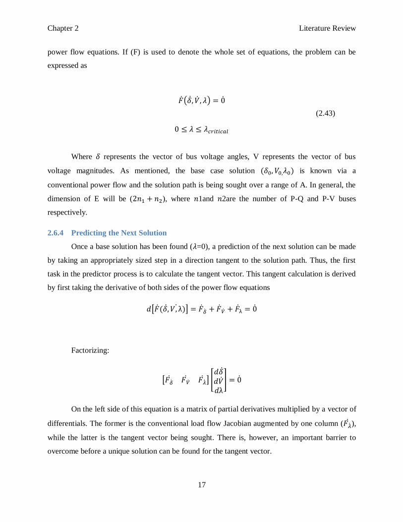
power flow equations. If (F) is used to denote the whole set of equations, the problem can be
expressed as
(2.43)
Where represents the vector of bus voltage angles, V represents the vector of bus
voltage magnitudes. As mentioned, the base case solution is known via a
conventional power flow and the solution path is being sought over a range of A. In general, the
dimension of E will be ( ), where 1and 2are the number of P-Q and P-V buses
respectively.
2.6.4 Predicting the Next Solution
Once a base solution has been found ( =0), a prediction of the next solution can be made
by taking an appropriately sized step in a direction tangent to the solution path. Thus, the first
task in the predictor process is to calculate the tangent vector. This tangent calculation is derived
by first taking the derivative of both sides of the power flow equations
Factorizing:
On the left side of this equation is a matrix of partial derivatives multiplied by a vector of
differentials. The former is the conventional load flow Jacobian augmented by one column ( ),
while the latter is the tangent vector being sought. There is, however, an important barrier to
overcome before a unique solution can be found for the tangent vector.
Chapter 2 Literature Review
18
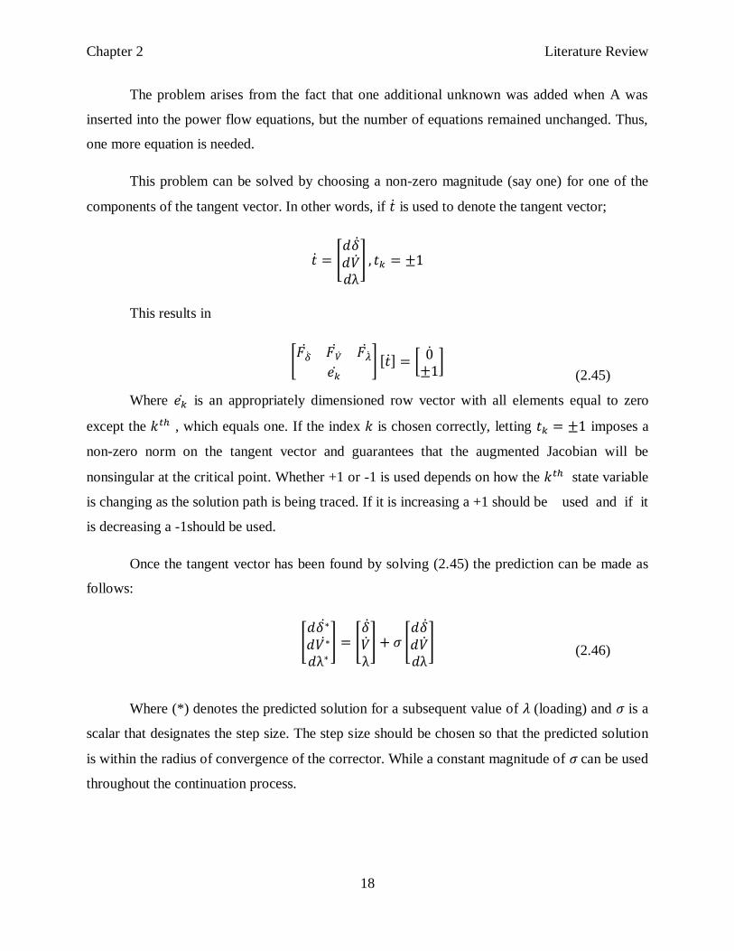
The problem arises from the fact that one additional unknown was added when A was
inserted into the power flow equations, but the number of equations remained unchanged. Thus,
one more equation is needed.
This problem can be solved by choosing a non-zero magnitude (say one) for one of the
components of the tangent vector. In other words, if is used to denote the tangent vector;
This results in
(2.45)
Where is an appropriately dimensioned row vector with all elements equal to zero
except the , which equals one. If the index is chosen correctly, letting imposes a
non-zero norm on the tangent vector and guarantees that the augmented Jacobian will be
nonsingular at the critical point. Whether +1 or -1 is used depends on how the state variable
is changing as the solution path is being traced. If it is increasing a +1 should be used and if it
is decreasing a -1should be used.
Once the tangent vector has been found by solving (2.45) the prediction can be made as
follows:
(2.46)
Where (*) denotes the predicted solution for a subsequent value of (loading) and is a
scalar that designates the step size. The step size should be chosen so that the predicted solution
is within the radius of convergence of the corrector. While a constant magnitude of can be used
throughout the continuation process.
Chapter 2 Literature Review
19
2.6.5 Parameterization and the Corrector Step
Now that a prediction has been made, a method of correcting the approximate solution is
needed. The best way to present this corrector is to expand on parameterization, which is vital to
the process.
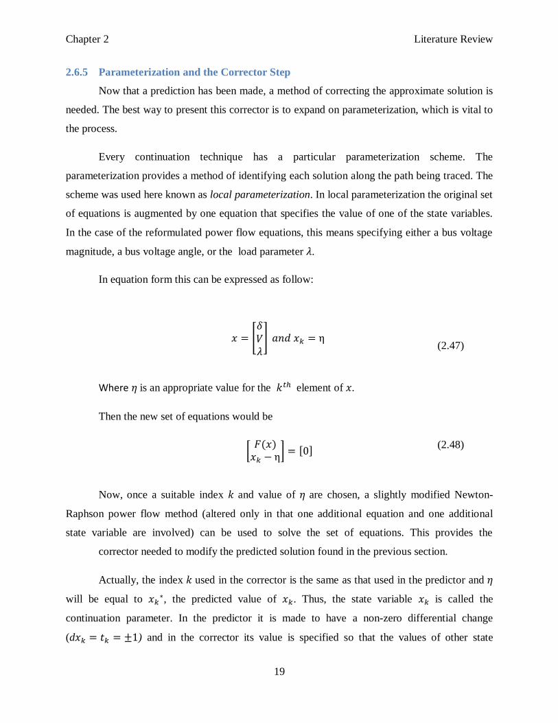
Every continuation technique has a particular parameterization scheme. The
parameterization provides a method of identifying each solution along the path being traced. The
scheme was used here known as local parameterization. In local parameterization the original set
of equations is augmented by one equation that specifies the value of one of the state variables.
In the case of the reformulated power flow equations, this means specifying either a bus voltage
magnitude, a bus voltage angle, or the load parameter .
In equation form this can be expressed as follow:
(2.47)
Where is an appropriate value for the element of .
Then the new set of equations would be
(2.48)
Now, once a suitable index and value of are chosen, a slightly modified Newton-
Raphson power flow method (altered only in that one additional equation and one additional
state variable are involved) can be used to solve the set of equations. This provides the
corrector needed to modify the predicted solution found in the previous section.
Actually, the index used in the corrector is the same as that used in the predictor and
will be equal to , the predicted value of . Thus, the state variable is called the
continuation parameter. In the predictor it is made to have a non-zero differential change
(d ) and in the corrector its value is specified so that the values of other state
Chapter 2 Literature Review
20
variables updatescan be found. How then does one know which state variable should be used as
the continuation parameter.
2.6.6 Choosing the Continuation Parameters
There are several ways of explaining the proper choice of continuation parameter
Mathematically, it should correspond to the state variable that has the largest tangent vector
component. More simply put, this would correspond to the state variable that has the greatest rate
of change near the given solution. In the case of a power system, the load parameter is
probably the best choice when starting from the base solution. This is especially true if the base
case is characterized by normal or light loading. Under such conditions, the voltage magnitudes
and angles remain fairly constant under load change. On the other hand, once the load has been
increased by a number of continuation steps and the solution path approaches the critical point,
voltage magnitudes and angles will likely experience significant change. At this point would be
a poor choice of continuation parameter since it may change only a small amount in comparison
to the other state variables. For this reason, the choice of continuation parameter should be re-
evaluated at each step. Once the choice has been made for the first step, a good way to handle
successive steps is to use
Where t is the tangent vector with a corresponding dimension, m = (2 + +1) and
index corresponds to the component of the tangent vector that is maximal. When the
continuation parameter is chosen, the sign of its corresponding tangent component should be
noted so that the proper value of +1 or -1 can be assigned to , in the subsequent tangent vector
calculation.
2.6.7 Sensing the Critical Point
The only thing left to do amid the predictor-corrector process is to check to see if the
critical point has been passed. This is easily done if one keeps in mind that the critical point is
where the loading (and therefore ) reaches a maximum and starts to decrease. Because of this,
the tangent component corresponding to X (i.e., d ) is zero at the critical point and is negative
beyond the critical point. Thus, once the tangent vector has been calculated in the predictor step,

Chapter 2 Literature Review
21
a test of the sign of the d component will reveal whether or not the critical point has been
passed.
Chapter 3 Methodology
22
3 Chapter 3
Methodology and Design
3.1 Introduction
In this chapter, we will discover, formulate and develop algorithms for new methods and
techniques of load flow analysis. The first method is just a new representation of the load flow
problem and will be solved by Newton-Raphson method. The second one is a method that
emp;oys loading parameter and is dedicated for the continuation load flow because it overcomes
the Jacobian singularity problem. Also, Newton-Raphson is used here to find the solution.
Finally, a method that converts the load into impedance representation is discovered.
For all the methods here, system data is required. For the sake of convenience, system
data was saved in two matrices: BusData and LineData. A small piece of code calculates the
matrix of the system in the form of angle and magnitude ( ) were “i” and “j” are
two buses between which the line is connected.
3.2 Sin/Cos method
Here, a different representation was given to the load flow equations. This was done by
accommodating the two state variables updates(voltage angle ( ) and voltage magnitude (Vm))
into one term. The load flow problem was then described by the following equation:
(3.1)
dY=J*dX
Where
dY: Active and reactive power mismatch matrix
and : Active and reactive power calculation mismatch respectively.
Chapter 3 Methodology
23
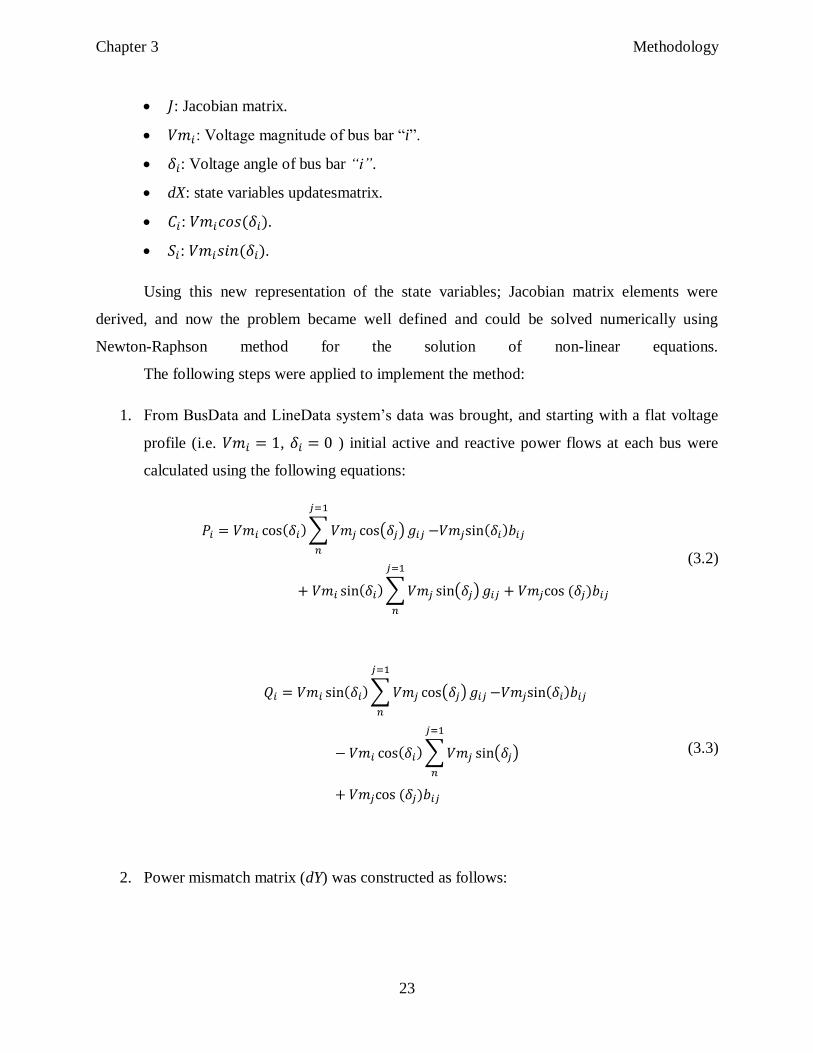
: Jacobian matrix.
: Voltage magnitude of bus bar “i”.
: Voltage angle of bus bar “i”.
dX: state variables updatesmatrix.
: .
: .
Using this new representation of the state variables; Jacobian matrix elements were
derived, and now the problem became well defined and could be solved numerically using
Newton-Raphson method for the solution of non-linear equations.
The following steps were applied to implement the method:
1. From BusData and LineData system‟s data was brought, and starting with a flat voltage
profile (i.e. , ) initial active and reactive power flows at each bus were
calculated using the following equations:
(3.2)
(3.3)
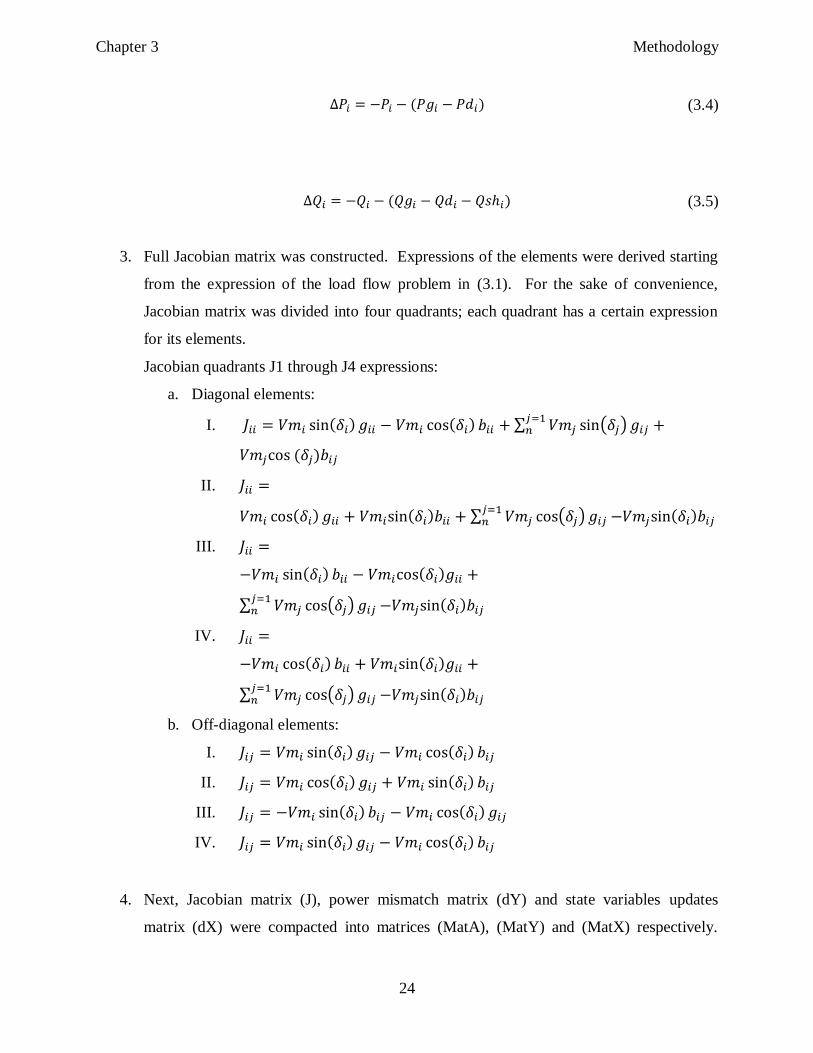
2. Power mismatch matrix (dY) was constructed as follows:
Chapter 3 Methodology
24
(3.4)
(3.5)
3. Full Jacobian matrix was constructed. Expressions of the elements were derived starting
from the expression of the load flow problem in (3.1). For the sake of convenience,
Jacobian matrix was divided into four quadrants; each quadrant has a certain expression
for its elements.
Jacobian quadrants J1 through J4 expressions:
a. Diagonal elements:
I.
II.
III.
IV.
b. Off-diagonal elements:
I.
II.
III.
IV.
4. Next, Jacobian matrix (J), power mismatch matrix (dY) and state variables updates
matrix (dX) were compacted into matrices (MatA), (MatY) and (MatX) respectively.
Chapter 3 Methodology
25
Those new matrices do not have zero rows and columns corresponding to slack P and Q
and generator Q equations. The equation dY=J*dX was changed into:
MatY=MatA*MatX.
5. Equation in (4) was solved for “ ” as follows: .
6. Voltage magnitude and angle values were updated.
7. Generator Reactive Rower Limit Check algorithm was applied.
8. New iteration of the procedure above was started.
9. The algorithm exits if the predetermined tolerance or the predetermined number of
iterations is exceeded without reaching the desired accuracy.
10. Finally, from the results of voltage angle and magnitude, active and reactive powers were
calculated for each bus.
11. Total results were tabulated for all buses. This included: voltage angle and magnitude and
active and reactive power
Chapter 3 Methodology
26
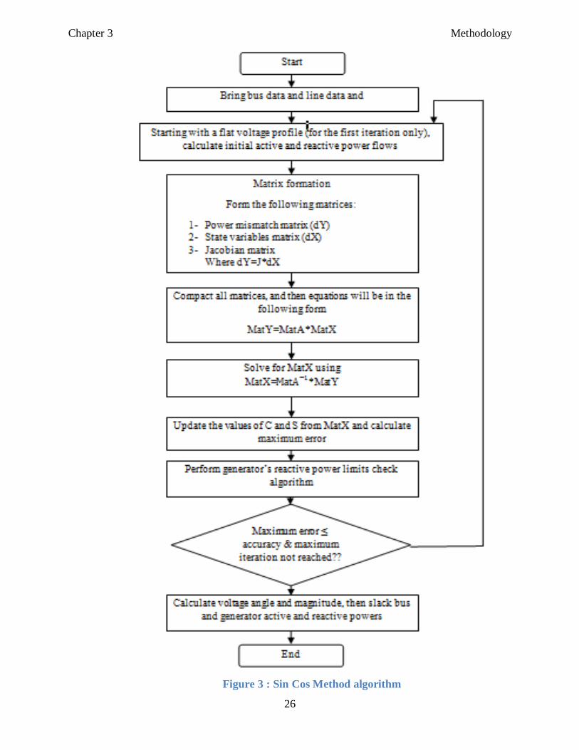
Figure 3 : Sin Cos Method algorithm
Chapter 3 Methodology
27
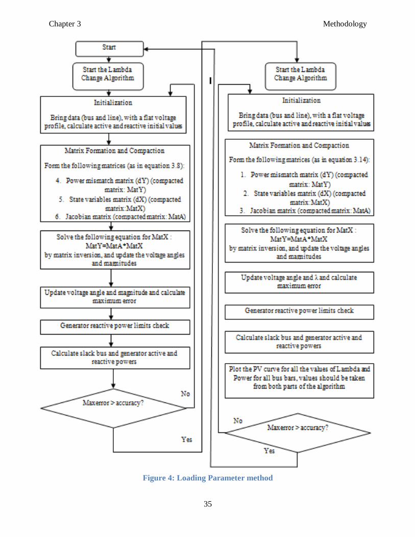
3.3 The loading parameter (Lambda) method
This method performs load analysis flow for the system; it also overcomes the maximum
loading point problem encountered before due to Jacobian singularity, hence, it gives complete
PV curves for the system‟s buses.
A loading parameter, Lambda “ ”, was defined which increased the load at each load bus
in constant steps, and then power flow was performed for each step using Newton-Raphson
method. As Lambda increased, load flow was performed and voltage at the bus decreased, until a
point where the load flow solution doesn‟t converge to a solution was reached, at this point, the
loading parameter, Lambda (which was known) and the voltage (which was unknown) were
interchanged. Here, the unknown is the Lambda and the voltage is known. Next, voltage was
increased in steps, too. At each step load flow was performed to obtain the corresponding
Lambda.
To get the continuation curve, the algorithm was divided into two parts: Lambda change
part and Voltage change part.
3.3.1 Lambda Change Algorithm:
An initial value=1 was assigned to , the algorithm was next performed, then, was
increased in by a fixed step, and the algorithm is applied again.
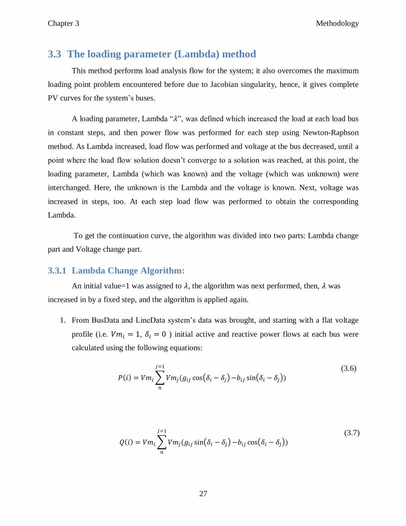
1. From BusData and LineData system‟s data was brought, and starting with a flat voltage
profile (i.e. , ) initial active and reactive power flows at each bus were
calculated using the following equations:
(3.6)
(3.7)
Chapter 3 Methodology
28
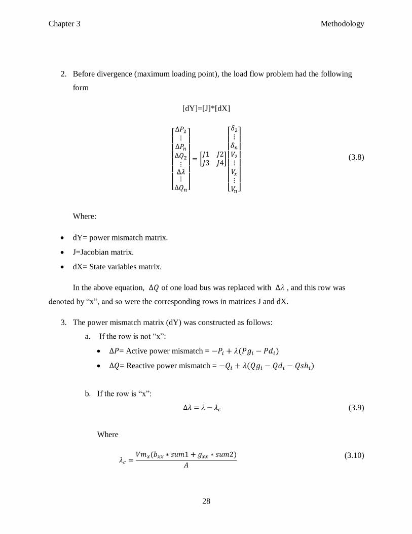
2. Before divergence (maximum loading point), the load flow problem had the following
form
[dY]=[J]*[dX]
(3.8)
Where:
dY= power mismatch matrix.
J=Jacobian matrix.
dX= State variables matrix.
In the above equation, of one load bus was replaced with , and this row was
denoted by “x”, and so were the corresponding rows in matrices J and dX.
3. The power mismatch matrix (dY) was constructed as follows:
a. If the row is not “x”:
= Active power mismatch =
= Reactive power mismatch =
b. If the row is “x”:
(3.9)
Where
(3.10)
Chapter 3 Methodology
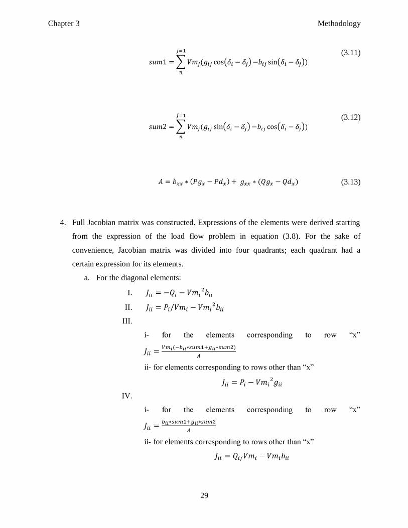
29
(3.11)
(3.12)
(3.13)
4. Full Jacobian matrix was constructed. Expressions of the elements were derived starting
from the expression of the load flow problem in equation (3.8). For the sake of
convenience, Jacobian matrix was divided into four quadrants; each quadrant had a
certain expression for its elements.
a. For the diagonal elements:
I.
II.
III.
i- for the elements corresponding to row “x”
ii- for elements corresponding to rows other than “x”
IV.
i- for the elements corresponding to row “x”
ii- for elements corresponding to rows other than “x”
Chapter 3 Methodology
30
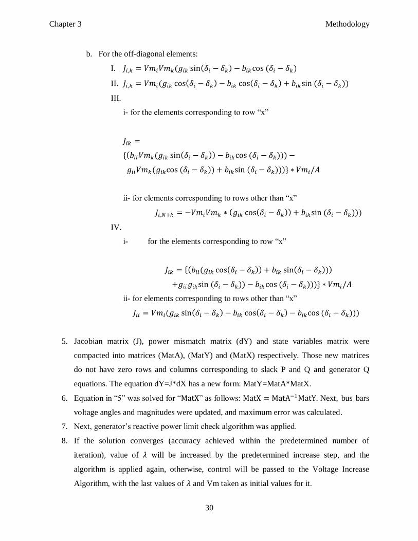
b. For the off-diagonal elements:
I.
II.
III.
i- for the elements corresponding to row “x”
ii- for elements corresponding to rows other than “x”
IV.
i- for the elements corresponding to row “x”
ii- for elements corresponding to rows other than “x”
5. Jacobian matrix (J), power mismatch matrix (dY) and state variables matrix were
compacted into matrices (MatA), (MatY) and (MatX) respectively. Those new matrices
do not have zero rows and columns corresponding to slack P and Q and generator Q
equations. The equation dY=J*dX has a new form: MatY=MatA*MatX.
6. Equation in “5” was solved for “ ” as follows: . Next, bus bars
voltage angles and magnitudes were updated, and maximum error was calculated.
7. Next, generator‟s reactive power limit check algorithm was applied.
8. If the solution converges (accuracy achieved within the predetermined number of
iteration), value of will be increased by the predetermined increase step, and the
algorithm is applied again, otherwise, control will be passed to the Voltage Increase
Algorithm, with the last values of and Vm taken as initial values for it.
Chapter 3 Methodology
31
9. Finally slack bus and generator‟s bus active and reactive powers were computed.
10. Results were plotted in the form of Lambda V.S. Vm for each bus bar.
3.3.2 Voltage Change Algorithm
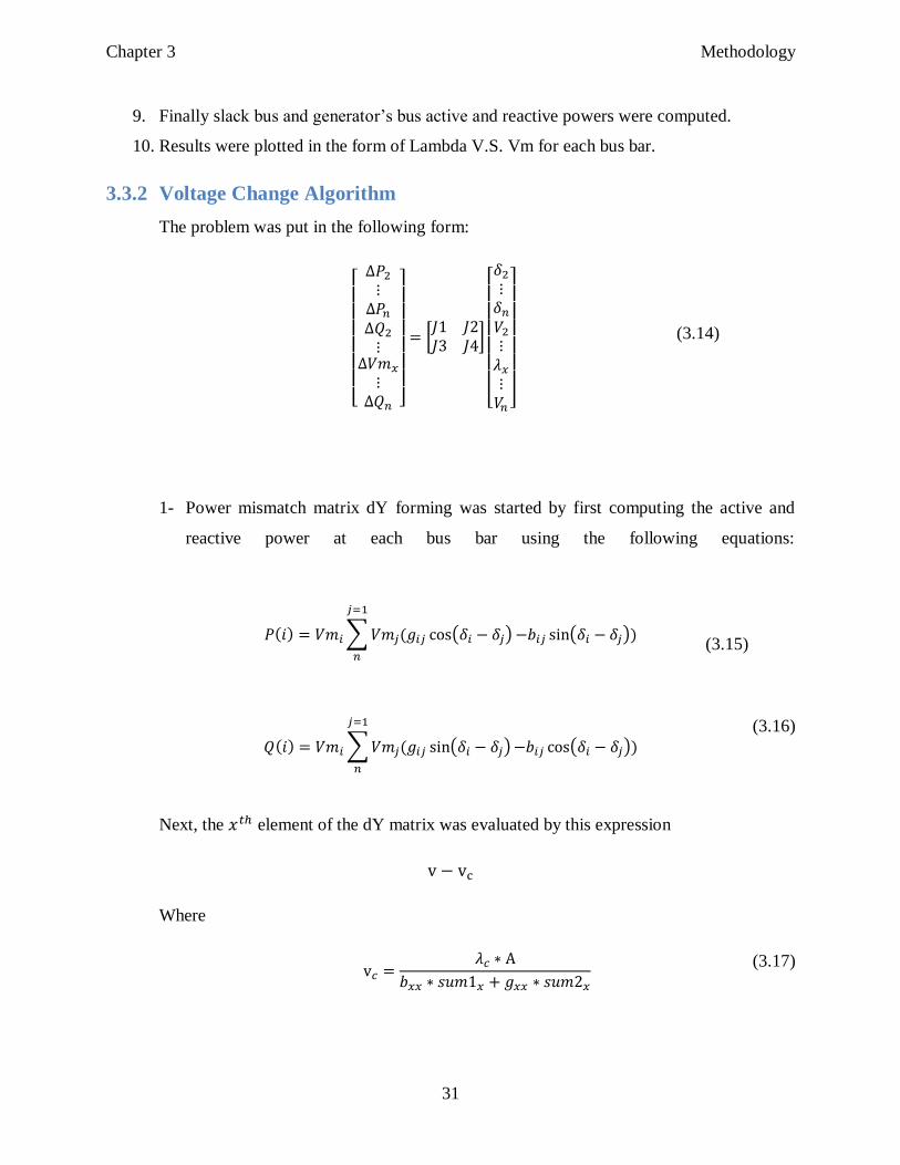
The problem was put in the following form:
(3.14)
1- Power mismatch matrix dY forming was started by first computing the active and
reactive power at each bus bar using the following equations:
(3.15)
(3.16)
Next, the element of the dY matrix was evaluated by this expression
Where
(3.17)
Chapter 3 Methodology
32
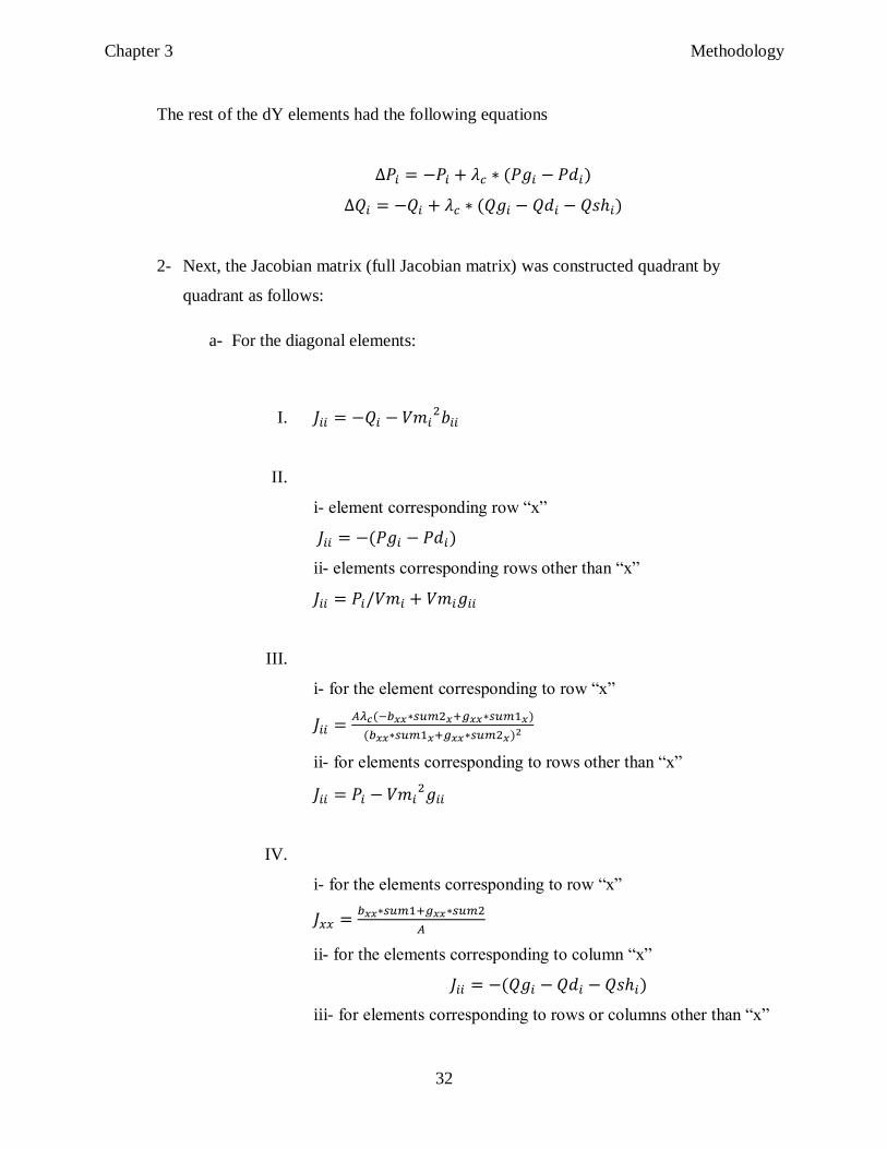
The rest of the dY elements had the following equations
2- Next, the Jacobian matrix (full Jacobian matrix) was constructed quadrant by
quadrant as follows:
a- For the diagonal elements:
I.
II.
i- element corresponding row “x”
ii- elements corresponding rows other than “x”
III.
i- for the element corresponding to row “x”
ii- for elements corresponding to rows other than “x”
IV.
i- for the elements corresponding to row “x”
ii- for the elements corresponding to column “x”
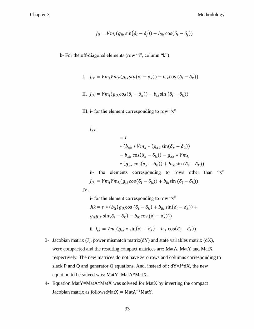
iii- for elements corresponding to rows or columns other than “x”
Chapter 3 Methodology
33
b- For the off-diagonal elements (row “i”, column “k”)
I.
II.
III. i- for the element corresponding to row “x”
ii- the elements corresponding to rows other than “x”
IV.
i- for the element corresponding to row “x”
Jik
ii-
3- Jacobian matrix (J), power mismatch matrix(dY) and state variables matrix (dX),
were compacted and the resulting compact matrices are: MatA, MatY and MatX
respectively. The new matrices do not have zero rows and columns corresponding to
slack P and Q and generator Q equations. And, instead of : dY=J*dX, the new
equation to be solved was: MatY=MatA*MatX.
4- Equation MatY=MatA*MatX was solveed for MatX by inverting the compact
Jacobian matrix as follows: .
Chapter 3 Methodology
34
5- Bus bars voltage angles and magnitudes were updated, maximum error was calculated
and was compared with the desired accuracy to decide whether the solution is close to
the right, or another iteration is required.
6- Generator reactive power limits were checked for generator bus bars using the Check
Limit algorithm.
7- If the current iteration number was larger than the maximum iteration number and yet
the maximum error is still larger than the accuracy, the algorithm would exit the
iterations, otherwise, another iteration would start from step 1 above.
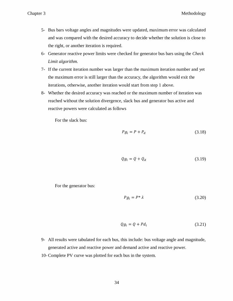
8- Whether the desired accuracy was reached or the maximum number of iteration was
reached without the solution divergence, slack bus and generator bus active and
reactive powers were calculated as follows
For the slack bus:
(3.18)
(3.19)
For the generator bus:
*
(3.20)
(3.21)
9- All results were tabulated for each bus, this include: bus voltage angle and magnitude,
generated active and reactive power and demand active and reactive power.
10- Complete PV curve was plotted for each bus in the system.
Chapter 3 Methodology
35
Figure 4: Loading Parameter method
Chapter 3 Methodology
36
3.4 Impedance Load Flow
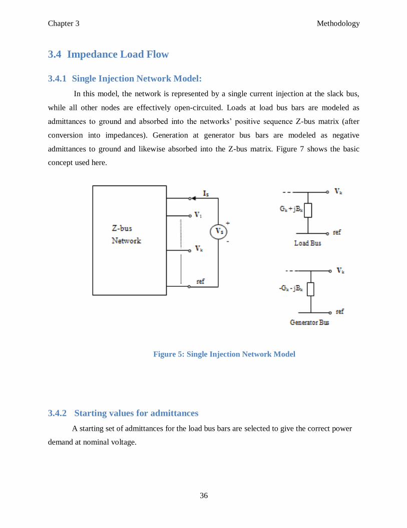
3.4.1 Single Injection Network Model:
In this model, the network is represented by a single current injection at the slack bus,
while all other nodes are effectively open-circuited. Loads at load bus bars are modeled as
admittances to ground and absorbed into the networks‟ positive sequence Z-bus matrix (after
conversion into impedances). Generation at generator bus bars are modeled as negative
admittances to ground and likewise absorbed into the Z-bus matrix. Figure 7 shows the basic
concept used here.
3.4.2 Starting values for admittances
A starting set of admittances for the load bus bars are selected to give the correct power
demand at nominal voltage.
Figure 5: Single Injection Network Model
Chapter 3 Methodology
37
2
k
dk
kV
PG ,
2
k
dkk
V
QB
(3.22)
And, since voltage is nominal;
dkk PG , dkk QB (3.23)
For the generator bus bars, the starting value for conductance will be established to
deliver the required power demand at the fixed generator nominal voltage. This conductance will
remain unchanged unless the generator voltage is regulated to limit the reactive power. The
initial susceptance will be set to give the reactive demand at the bus, if exists; otherwise it shall
be zero.
2
gk
dkgk
kV
PPG
, 2
gk
dkk
V
QB
(3.24)
The starting admittances for all load and generator bus bars are added to the networks‟
bus admittance matrix Y. The bus impedance matrix Z is obtained by inverting Y. This will be
the only time Z is obtained through inversion since all subsequent modifications are operated on
Z directly.
3.4.3 Power and Admittance Mismatch Equations
Now that we have an initial network model, we need to check for compliance with
network constraints, ie specified powers and voltages. The bus impedance equations with single
injection at the slack bus are expressed as:
0
s
kkks
skss
k
s I
ZZ
ZZ
V
V
(3.25)
Chapter 3 Methodology
38
Note that the current injections are everywhere zero except at slack bus. The slack bus
current is immediately determined asss
ss
Z
VI . The voltage at any other bus is then:
sksk IZV ss
sks
Z
VZ
(3.26)
We shall call this voltage the open circuit (i.e Thevenin‟s) voltage, THkV . The Thevenin‟s
impedance, looking into bus k, is obtained by setting the slack bus voltage to zero and
eliminating its equation from the Z-bus formation. This will result in:
ss
skkskkTHkTHkTHk
Z
ZZZjxrZ
(3.27)
Let node k be a load bus bar. Now let us add an additional admittance element,
kk BjG between node k and ground, with the objective of correcting the calculated power
at the node to match the specified demand. The equivalent impedance of the added element is
kk jxr , which is typically a large value since the admittance element is typically small.
Incorporating this impedance in the Thevenin‟s model and calculating the power consumed in it
results in:
P
xxrr
rV
kTHkkTHk
kTHk
22
2
Q
xxrr
xV
kTHkkTHk
kTHk
22
2
(3.28)
Where the power mismatches P and Q are found as
Chapter 3 Methodology
39
kTHkdk GVPP 2
kTHkdk BVQQ 2
(3.29)
Equations (6) is solved for kr by eliminating kx , which results in a quadratic equation
with solutiona
acbbrk
2
42 , where
P
QPa
2
222 THkTHkTHk VQxPrb
)( 22
THkTHk xrPc
(3.30)
The question arises whether to use the plus or minus sign in the solution for kr . We
require that the admittance corrections kG , kB vanish together with the power mismatches
P and Q upon arrival at a solution. This should take kr to infinity and can only be achieved if
we use the plus sign in the quadratic equation solution.
kx is then trivially found as krP
Q
and the admittance corrections are finally
22
kk
kk
xr
rG
22
kk
kk
xr
xB
(3.31)
Now let node k be a generator bus bar. We shall only add an additional susceptance
element, kBj between node k and ground, with the objective of correcting the reactive power
at the node to match the specified voltage. The conductance shall not be modified unless there is
a reactive power violation, forcing a voltage regulation. Adding the susceptance is equivalent to
adding a reactance kjx in series with Thevenin‟s impedance THkTHk jxr . The criteria for the
added reactance is that the voltage magnitude at node k should be equal to the specified voltage
gkV . This can be expressed as follows:
Chapter 3 Methodology
40
gk
kTHkTHk
kTHk V
xxr
xV
22
(3.32)
Or
2
22
22
gk
kTHkTHk
kTHk V
xxr
xV
(3.33)
Solving for kx
a
acbbxk
2
42 , where
22
THkgk VVa
22 gkTHk Vxb
)( 222
THkTHkgk xrVc
(3.34)
And the conditions for kx as gkTHk VV are only achieved by taking the minus
sign in the quadratic equation solution form. kB is found as before in equation (9).
3.4.4 Generator Reactive Power Limit Check
The reactive power produced in the generator is expressed as:
dkgkgk QBVQ 2
(3.35)
This should be checked against max
gkQ and min
gkQ at every iteration for limit violations. If
a limit is transgressed, then the reactive power is set at the limit, and both kG and kB are
updated using a slight modification to equation (3.29), i.e
Chapter 3 Methodology
41
kTHkdkgk GVPPP 2
kTHkdkgk BVQQQ 2max (for a maximum limit violation)
(3.36)
kG and kB are then found exactly as in equations (3.31) and (3.34) and the admittances
updated as
22
kk
kk
xr
rG
22
kk
kk
xr
xB
(3.37)
Chapter 4 Results and Discussion
42
4 Chapter 4
Implementation and Results
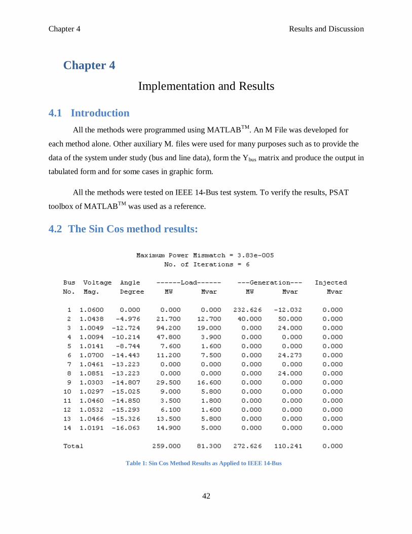
4.1 Introduction
All the methods were programmed using MATLABTM
. An M File was developed for
each method alone. Other auxiliary M. files were used for many purposes such as to provide the
data of the system under study (bus and line data), form the Ybus matrix and produce the output in
tabulated form and for some cases in graphic form.
All the methods were tested on IEEE 14-Bus test system. To verify the results, PSAT
toolbox of MATLABTM
was used as a reference.
4.2 The Sin Cos method results:
Table 1: Sin Cos Method Results as Applied to IEEE 14-Bus
Chapter 4 Results and Discussion
43
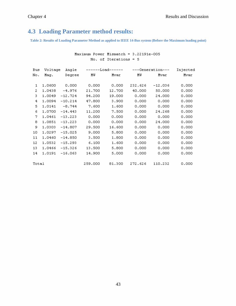
4.3 Loading Parameter method results:
Table 2: Results of Loading Parameter Method as applied to IEEE 14-Bus system (Before the Maximum loading point)
Chapter 4 Results and Discussion
44
0.5 1 1.5 2 2.5 3 3.5 4
0.4
0.5
0.6
0.7
0.8
0.9
1
1.1
loading parameter
voltages
data1
data2
data3
data4
data5
data6
data7
data8
data9
data10
data11
data12
data13
data14
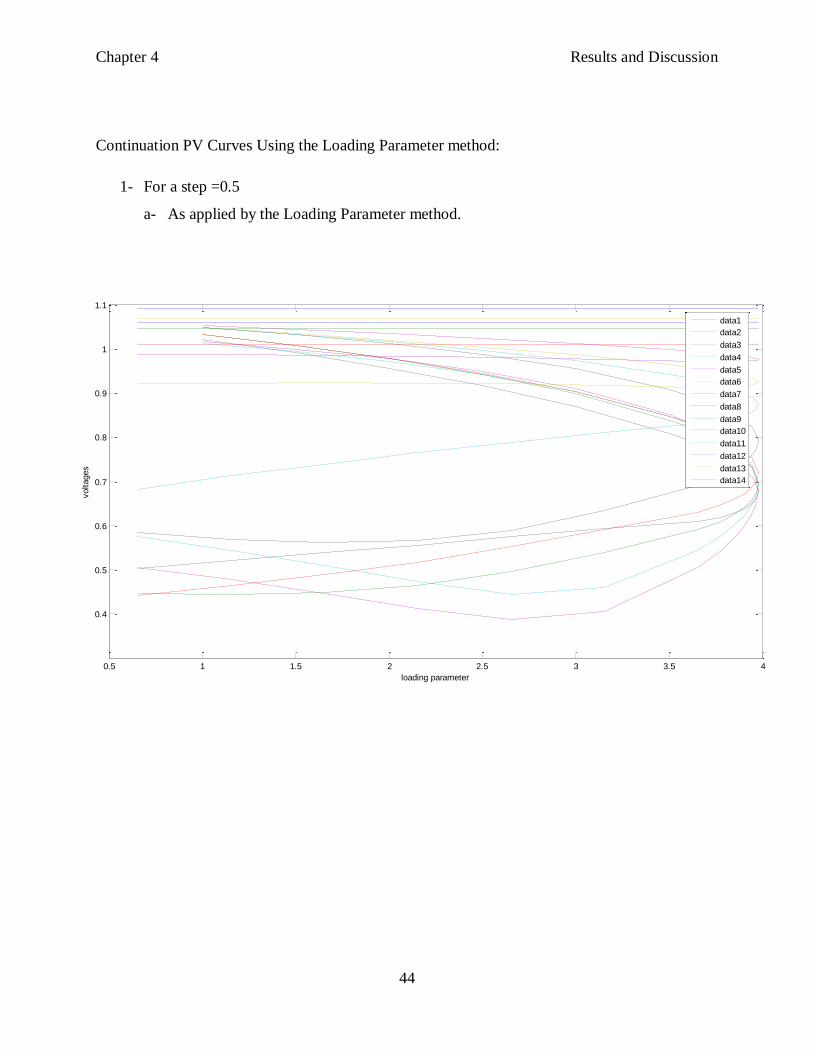
Continuation PV Curves Using the Loading Parameter method:
1- For a step =0.5
a- As applied by the Loading Parameter method.
Chapter 4 Results and Discussion
45
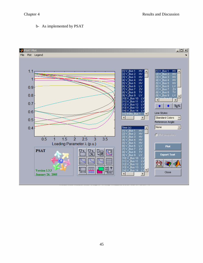
b- As implemented by PSAT
Chapter 4 Results and Discussion
46
0.5 1 1.5 2 2.5 3 3.5 4
0.4
0.5
0.6
0.7
0.8
0.9
1
1.1
loading parameter
voltages
data1
data2
data3
data4
data5
data6
data7
data8
data9
data10
data11
data12
data13
data14
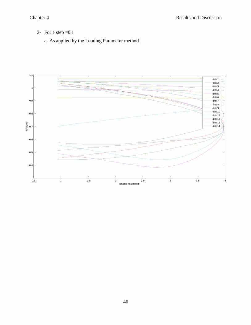
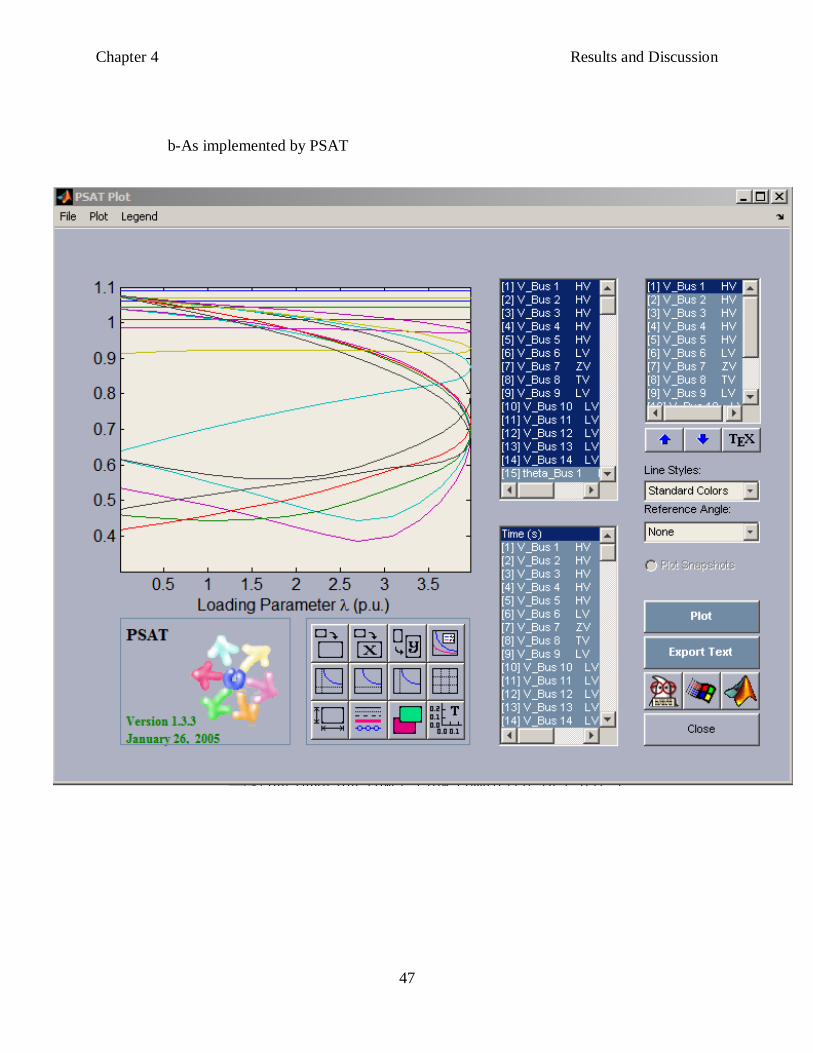
2- For a step =0.1
a- As applied by the Loading Parameter method
Chapter 4 Results and Discussion
47
b-As implemented by PSAT
Chapter 4 Results and Discussion
48
0.5 1 1.5 2 2.5 3 3.5 4
0.4
0.5
0.6
0.7
0.8
0.9
1
1.1
loading parameter
voltages
data1
data2
data3
data4
data5
data6
data7
data8
data9
data10
data11
data12
data13
data14
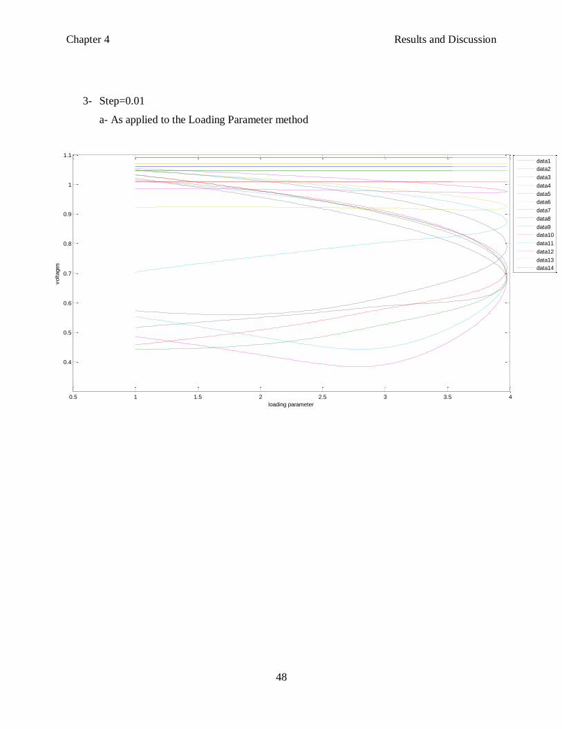
3- Step=0.01
a- As applied to the Loading Parameter method
Chapter 4 Results and Discussion
49
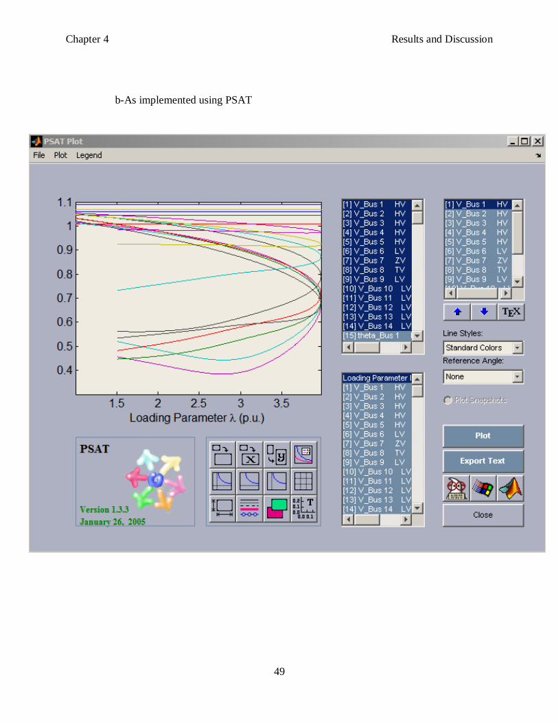
b-As implemented using PSAT
Chapter 4 Results and Discussion
50
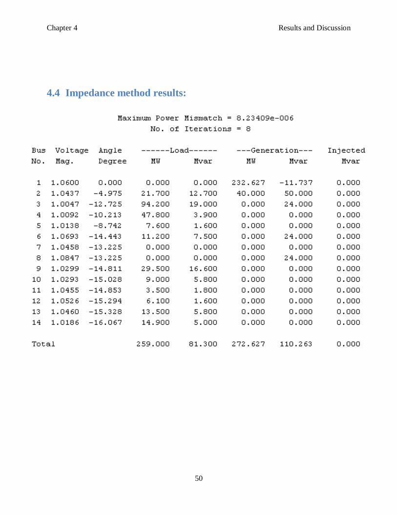
4.4 Impedance method results:
Chapter 4 Results and Discussion
51
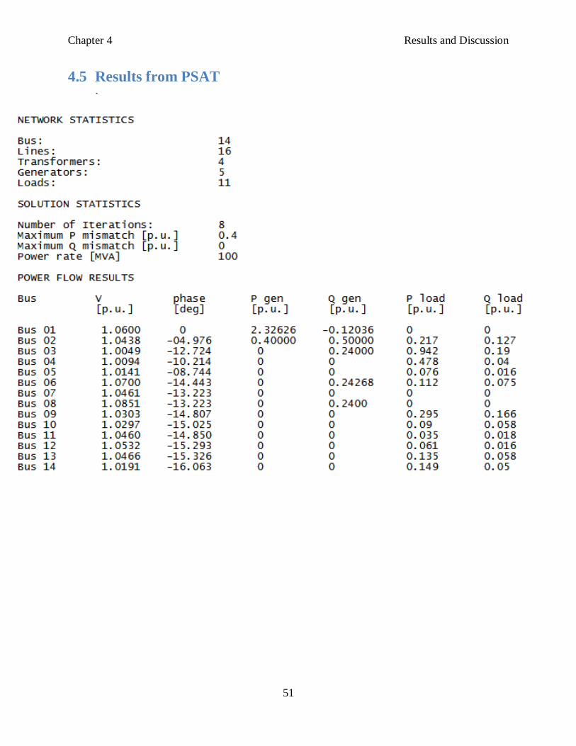
4.5 Results from PSAT

Chapter 4 Results and Discussion
52
4.6 Discussion of the results:
1- Results of all the methods were compared with the results obtained from PSAT and they
were almost typical.
2- Loading parameter method has the smallest number of iterations, next the Sin Cos
method, and finally comes the Impedance method. But, concerning the maximum error
(the maximum absolute difference between the actual power and the calculated power)
impedance method gave the smallest error, then came the Loading parameter method,
finally, Sin Cos method. This makes the Impedance method the most accurate one.
3- The Loading Parameter method gave results that were quite with the results obtained by
PSAT. The full continuation curve was also obtained for all the 14 buses.
4- Also, looking at the curves of various steps, tell us that any step can be used.
Chapter 5 Conclusion and Future Work
53
5 Chapter 5
Conclusion
5.1 Project Review
Project scope was to discover new methods and techniques for load flow analysis that
overcome the well known problem of Jacobian matrix singularity encountered in many other
conventional techniques. This problem inhibits the load flow program to function under certain
conditions, primarily voltage stability limit of the PV curve and the points beyond it.
MatLab software was used as a tool to implement the new discovered techniques to
produce the desired program that performs the algorithm quickly, easily, and efficiently as far as
time and precision is concerned.
Three methods were formulated and programmed. The first one is just another
representation of the conventional Newton-Raphson problem. But it has the same problem of
divergence near the voltage stability limit. The second method used a loading parameter that is
used to increase the load at each load bus bas, and this parameter is also accommodated in the
power mismatch matrix in the place of one of the reactive power mismatch of some load bus.
The loading parameter value started from the base case, which is „1‟. As this parameter is
increased in fixed steps, load flow was performed and results (voltage magnitude and angle) are
saved at each increase. This is repeated until the voltage stability limit is reached, then we switch
the roles between the loading parameter and its corresponding voltage magnitude, i.e., we apply
decreases to the voltage magnitude of that same bus bar, starting from its last value before
divergence and obtain the resulting voltage angle and loading parameter. Finally, we end up
having the complete continuation PV curve for each bus bar.
The validity of the methods was tested on IEEE-14-Busand the expected results were
found and compared with results from PSAT for the same system.

Chapter 5 Conclusion and Future Work
54
5.2 Future Work
For further verification of the methods, they should be tested on other testing systems
such as IEEE 30-Bus, IEEE 57-Bus and IEEE 118-Bus and compare the results with reliable
software packages such as PSAT and Etap.
And, for real utilization of the methods, after verification, they should be used in other
power system studies, such as voltage stability to evaluate the stability of the system,
contingency analysis.

55
6 Bibliography
7
Das, D. (2006). Electrical Power Systems. New Age International Publishers.
Glover, J. D., Sarma, M. S., & Overbye, T. J. (2008). Power System Analysis (Fourth Edition).
Thomson.
Kundur, P. Power System Stability and Control. McGraw-Hill, Inc.
Zakaria, A. Voltage Stability Sudy: Sudan National Grid as a Study Case, PHD.

APPENDIXA MATLAB CODE FOR SIN COS
A-1
8 APPENDIX A
MATLABTM Code for Sin Cos Method
% This program should be called by pfdata14bus (power flow 14
bus data program)
%Vm=0; delta=0;
converge=1;
busType=[];%buscode
Vm=[]; delta=[]; Pd=[]; Qd=[]; Pg=[]; Qg=[]; Qmin=[]; Qmax=[];
% Added (6-8-00)
P=[]; Q=[];; % Added (6-8-00)
J=[];dY=[];MatY=[];MatX=[];MatA=[];genBus=[];genVolts=[];
C=[]; S=[];T1=[]; T2=[];
busType=busdata(:,2); Vm=busdata(:,3); delta=busdata(:,4);
Pd=busdata(:,5)/basemva; Qd=busdata(:,6)/basemva;
Pg=busdata(:,7)/basemva; Qg=busdata(:,8)/basemva;
Qmin=busdata(:,9)/basemva; Qmax=busdata(:,10)/basemva;
Qsh=busdata(:,11)/basemva;
S=zeros(size(Vm));%Actually C(i)=Vm(i)*sin(delta(i)) but all
initial values of delta = zeros
C=Vm;%Actually C(i)=Vm(i)*cos(delta(i)) but all initial values
of delta = zeros
for i=1 : nBusbars
%busType(i+nBusbars) = busType(i);
if busType(i) == 2 %generator bus
%busType(i)=0; %in first and second quadrant of
jacobian gen bus is treated as load bus
genBus=[genBus;i];
genVolts=[genVolts;Vm(i)];
end
end
busType;
nGens=length(genBus);
%========================================================
% Start of Newton-Raphson Loadflow iterations
%========================================================
maxerror = 1; converge=1;iter = 0;
while maxerror >= accuracy & iter <= maxiter % Test for max.
power mismatch

APPENDIXA MATLAB CODE FOR SIN COS
A-2
%===========Compute power at each busbar=======
for i=1:nBusbars
T1(i) = 0;
T2(i) = 0;
for j=1 : nBusbars
T1(i) = T1(i)+C(j)*g(i,j)-S(j)*b(i,j);
T2(i) = T2(i)+S(j)*g(i,j)+C(j)*b(i,j);
end
P(i)=C(i)*T1(i)+S(i)*T2(i);
Q(i)=S(i)*T1(i)-C(i)*T2(i);
if (busType(i) ~= 1)
dY(i) = -P(i) + (Pg(i)-Pd(i)); %mismatch equation for
active power (load and generator busbars)
end
if (busType(i) ~= 1) & (busType(i) ~= 2)
dY(i+nBusbars) =-Q(i) + (Qg(i)-(Qd(i)-
Qsh(i)));%mismatch equation for reactive power (only load
busbars)
end
end
%===============================================================
==
% Construct Jacobian Matrix
%===============================================================
==
N = nBusbars;
J =zeros(N,N);
%First Quadrant
for i=1 : nBusbars
if busType(i) ~= 1
for k=1 : nBusbars
if (i ~= k)
J(i, k) =S(i)*g(i,k)-C(i)*b(i,k);
else
J(i, i) =S(i)*g(i,i)-C(i)*b(i,i)+T2(i);
end
end
end
end
%Second quadrant
for i=1 : nBusbars
if busType(i) ~= 1
for k=1 : nBusbars
if (i ~= k)

APPENDIXA MATLAB CODE FOR SIN COS
A-3
J(i, k + N) = C(i)*g(i,k)+S(i)*b(i,k);
else
J(i, i + N) = C(i)*g(i,i)+S(i)*b(i,i)+T1(i);
end
end
end
end
%Third Quadrant
for i = 1 : nBusbars
if busType(i) ~= 1 & busType(i) ~= 2
for k=1 : nBusbars
if (i ~= k)
J(i + N, k) = -S(i)*b(i,k)-C(i)*g(i,k);
else
J(i + N, i) =-S(i)*b(i,i)-C(i)*g(i,i)+T1(i);
end
end
end
end
%Fourth Quadrant
for i = 1 : nBusbars
if busType(i) ~= 1 & busType(i) ~= 2
for k=1 : nBusbars
if (i ~= k)
J(i + N, k + N) = S(i)*g(i,k)-C(i)*b(i,k);
else
J(i + N, i + N) =-C(i)*b(i,i)+S(i)*g(i,i)-T2(i);
end
end
end
end
%===============================================================
==
% End of Jacobian Matrix construction
%===============================================================
==
% Prepare Jacobian Matrix for inversion; first copy it into a
compact

APPENDIXA MATLAB CODE FOR SIN COS
A-4
% matrix that does not have zero rows and columns (corresponding
to slack
% P & Q and generator Q equations). The original equations have
the form
% dY = J * dX; The compact form is MatY= MatA*MatX
N = nBusbars;
num1=0;
for i=1 : nBusbars
if busType(i) ~= 1
num1=num1+1;
MatY(num1,1) = dY(i);
num2=0;
for j=1 : nBusbars
if busType(j) ~= 1
num2=num2+1;
MatA(num1,num2)=J(i,j);
end
end
end
end
num1=0;
for i=1 : nBusbars
if busType(i) ~= 1
num1=num1+1;
num2=nBusbars-1;
for j=1 : nBusbars
if busType(j)~= 1 & busType(j)~= 2
num2=num2+1;
MatA(num1,num2)=J(i,j+N);
end
end
end
end
num1=nBusbars-1;
for i=1 : nBusbars
if busType(i) ~= 1 & busType(i)~= 2
num1=num1+1;
MatY(num1, 1) = dY(i+nBusbars);
num2=0;
for j=1 : nBusbars
if busType(j)~= 1
num2=num2+1;
MatA(num1,num2)=J(i+N,j);
end
end

APPENDIXA MATLAB CODE FOR SIN COS
A-5
end
end
num1=nBusbars-1;
for i=1 : nBusbars
if busType(i) ~= 1 & busType(i)~= 2
num1=num1+1;
num2=nBusbars-1;
for j=1 : nBusbars
if busType(j)~= 1 & busType(j)~= 2
num2=num2+1;
MatA(num1,num2)=J(i+N,j+N);
end
end
end
end
MatX=MatA\MatY; % Solve for MatX using inverse(MatA) *
MatY
%Note: Matrices dY, dX and m contain zero rows and columns,
%corresponding to slack and generator busbars. In order to
invert m,
%it must be copied into matrix MatA, which contains no zero
rows or
%columns. Likewise dY is copied into MatY. The result of
inversion,
%MatX is expanded into matrix dX.
%==========Update C, S and calculate max error ===========
num1 = 0;
for i=1 : nBusbars
if busType(i) ~= 1
num1 = num1 + 1;
%dX(i+nBusbars) = MatX(num1, 1);
S(i) = S(i) + MatX(num1, 1);
end
end
num1=nBusbars-1;
for i=1 : nBusbars
if busType(i) == 0
num1 = num1 + 1;
% dX(i) = MatX(num1, 1);
C(i) = C(i) + MatX(num1, 1);
end
if busType(i) ==2

APPENDIXA MATLAB CODE FOR SIN COS
A-6
C(i) =Vm(i)*sqrt(1-(S(i)/Vm(i))^2);
%C(i) =Vm(i)*sin(asin(S(i)/Vm(i)));
end
end
maxerror=max(abs(MatY));
for k = 1 : nGens
i=genBus(k);
T1(i) = 0;
T2(i) = 0;
for j=1 : nBusbars
T1(i) = T1(i)+C(j)*g(i,j)-S(j)*b(i,j);
T2(i) = T2(i)+S(j)*g(i,j)+C(j)*b(i,j);
end
Vm(i) =sqrt((C(i))^2+(S(i))^2);
Q(i)=genVolts(k)/Vm(i)*(S(i)*T1(i)-C(i)*T2(i));
fprintf('%g\n',(Q(i) + Qd(i))*100),
end
%============================= Generator reactive power limits
check =====
if maxerror > accuracy & genlimits == 1 & iter > 0
for k = 1 : nGens
i=genBus(k);
T1(i) = 0;
T2(i) = 0;
for j=1 : nBusbars
T1(i) = T1(i)+C(j)*g(i,j)-S(j)*b(i,j);
T2(i) = T2(i)+S(j)*g(i,j)+C(j)*b(i,j);
end
Vm(i) =sqrt((C(i))^2+(S(i))^2);
Q(i)=genVolts(k)/Vm(i)*(S(i)*T1(i)-C(i)*T2(i));
fprintf('%g ',Vm(i)),fprintf('%g
',genVolts(k)),fprintf('%g ',(Q(i) + Qd(i))*100),
if busType(i) == 2
if Q(i) + Qd(i) > Qmax(i) + 0.01
fprintf('1 '),
Qg(i) = Qmax(i);
busType(i) = 0; % convert gen bus to load bus if
reactive power exceeds max
%Vm(i) = 1;
elseif Q(i) + Qd(i) < Qmin(i) - 0.01
fprintf('2 '),
Qg(i) = Qmin(i);
busType(i) = 0; % convert gen bus to load bus if
reactive power exceeds min
%Vm(i) = 1;
end

APPENDIXA MATLAB CODE FOR SIN COS
A-7
else
if Q(i) + Qd(i) < Qmax(i) - 0.01 & Vm(i) <
genVolts(k)
fprintf('3 '),
%Vm(i) = genVolts(k);
busType(i ) = 2; % return to gen bus if within
limits
elseif Q(i) + Qd(i) > Qmin(i) + 0.01 & Vm(i) >
genVolts(k)
fprintf('4 '),
%Vm(i) = genVolts(k);
busType(i) = 2; % return to gen bus if within
limits
end
end
fprintf('%g\n',busType(i )),
end
end
%===============================================================
=========
fprintf('\n'),
iter=iter+1;
if iter > maxiter & maxerror > accuracy
fprintf('\nWARNING: Iterative solution did not converge
after ')
fprintf('%g', iter), fprintf(' iterations.\n\n')
fprintf('Press Enter to terminate the iterations and print
the results \n')
converge = 0; pause,
end
if maxerror <= accuracy
end
%===============================
end % end of Load Flow iteration
% Calculation of Vm & delta
for i=1 : nBusbars
if busType(i) == 0
Vm(i) =sqrt((C(i))^2+(S(i))^2);
end

APPENDIXA MATLAB CODE FOR SIN COS
A-8
if busType(i) ~= 1
delta(i) = asin(S(i)/Vm(i));
end
end
%calculate slack bus and generator powers
for i=1 : nBusbars
if busType(i) == 1
Pg(i)=P(i) + Pd(i);
Qg(i)=Q(i) + Qd(i);
elseif busType(i) == 2
Qg(i)=Q(i) + Qd(i);
end
end
%==========================================

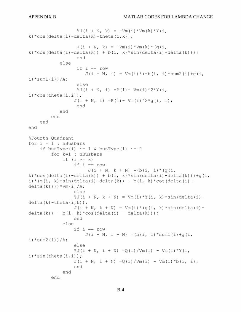
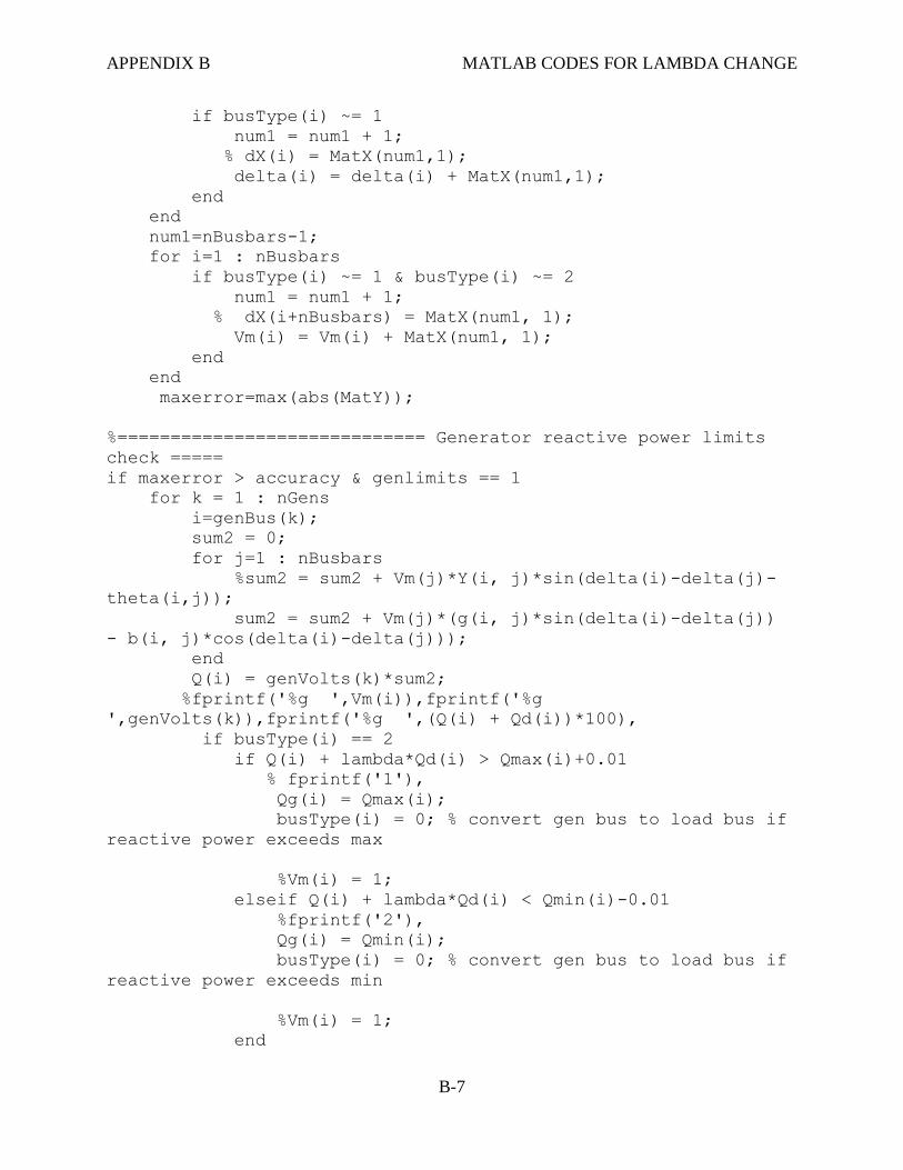
APPENDIX B MATLAB CODES FOR LAMBDA CHANGE
B-1
9 APPENDIX B
MATLABTM Code for Lambda Change
% This program should be called by pfdata14bus (power flow 14
bus data program)
Vm=0; delta=0;
converge=1;
busType=[];%buscode
Vm=[]; delta=[]; Pd=[]; Qd=[]; Pg=[]; Qg=[]; Qmin=[]; Qmax=[];
% Added (6-8-00)
P=[]; Q=[]; sum1=[]; sum2=[]; A=[]; % Added (6-8-00)
J=[];dY=[];MatY=[];MatX=[];MatA=[];genBus=[];genVolts=[];
sum1=[];sum2=[];
busType=busdata(:,2); Vm=busdata1(:,3);
delta=busdata1(:,4);
Pd=busdata(:,5)/basemva; Qd=busdata(:,6)/basemva;
Pg=busdata(:,7)/basemva; Qg=busdata(:,8)/basemva;
Qmin=busdata(:,9)/basemva; Qmax=busdata(:,10)/basemva;
Qsh=busdata(:,11)/basemva;
for i=1 : nBusbars
%busType(i+nBusbars) = busType(i);
if busType(i) == 2 %generator bus
%busType(i)=0; %in first and second quadrant of
jacobian gen bus is treated as load bus
genBus=[genBus;i];
genVolts=[genVolts;Vm(i)];
end
end
busType;
nGens=length(genBus);
A = b(row, row)*(Pg(row)-Pd(row))+g(row, row)*(Qg(row)-Qd(row));
sig=0;
%========================================================
% Start of Newton-Raphson Loadflow iterations
%=======================================================
maxerror = 1; converge=1;iter = 0;
while maxerror > accuracy & iter <= maxiter % Test for max.
power mismatch
%===========Compute power at each busbar=======
sum1 = zeros(size(Vm));
sum2 = zeros(size(Vm));
APPENDIX B MATLAB CODES FOR LAMBDA CHANGE
B-2
for i=1:nBusbars
for j=1 : nBusbars
%sum1 = sum1 + Vm(j)*Y(i, j)*cos(delta(i)-delta(j)-
theta(i,j));
%sum2 = sum2 + Vm(j)*Y(i, j)*sin(delta(i)-delta(j)-
theta(i,j));
sum1(i) = sum1(i) + Vm(j)*(g(i, j)*cos(delta(i)-
delta(j)) + b(i, j)*sin(delta(i)-delta(j)));
sum2(i) = sum2(i) + Vm(j)*(g(i, j)*sin(delta(i)-
delta(j)) - b(i, j)*cos(delta(i)-delta(j)));
end
P(i) = Vm(i) * sum1(i);
Q(i) = Vm(i) * sum2(i);
if (busType(i) ~= 1) & (busType(i) ~= 2)
if i == row
sum1(i) = sum1(i) - Vm(i)*g(i, i);
sum2(i) = sum2(i) + Vm(i)*b(i, i);
lambdac=Vm(i)*(b(i, i)*sum1(i)+g(i, i)*sum2(i))/A;
dY(nBusbars+row) = lambda - lambdac;
else
dY(i+nBusbars) = -Q(i) +lambda*(Qg(i)-(Qd(i)-
Qsh(i)));%mismatch equation for reactive power (only load
busbars)
end
end
if (busType(i) ~= 1)
dY(i) = -P(i) +lambda*(Pg(i)-Pd(i)); %mismatch equation
for active power (load and generator busbars)
end
end
%===============================================================
==
% Construct Jacobian Matrix
%===============================================================
==
N = nBusbars;
J =zeros(N,N);
%First Quadrant
for i=1 : nBusbars
if busType(i) ~= 1
for k=1 : nBusbars
if (i ~= k)
APPENDIX B MATLAB CODES FOR LAMBDA CHANGE
B-3
%J(i, k) = Vm(i)*Vm(k)*Y(i, k)*sin(delta(i)-
delta(k)-theta(i,k));
J(i, k) = Vm(i)*Vm(k)*(g(i, k)*sin(delta(i)-
delta(k)) - b(i, k)*cos(delta(i)-delta(k)));
else
%J(i, i) = -Q(i) - Vm(i)^2*Y(i,i)*sin(theta(i,
i));
J(i, i) = -Q(i) - Vm(i)^2*b(i, i);
end
end
end
end
%Second quadrant
for i=1 : nBusbars
if busType(i) ~= 1
for k=1 : nBusbars
if (i ~= k)
%J(i, k + N) = Vm(i)*Y(i,k)*cos(delta(i)-
delta(k)-theta(i,k));
J(i, k + N) = Vm(i)*(g(i, k)*cos(delta(i)-
delta(k)) + b(i, k)*sin(delta(i)-delta(k)));
else
%J(i, i + N) = P(i)/Vm(i) + Vm(i)*Y(i,
i)*cos(theta(i,i));
J(i, i + N) = P(i)/Vm(i) + Vm(i)*g(i, i);
end
end
end
end
%Third Quadrant
for i = 1 : nBusbars
if busType(i) ~= 1 & busType(i) ~= 2
for k=1 : nBusbars
if (i ~= k)
if i == row
J(i + N, k)= (b(i, i)*Vm(k)*(g(i,
k)*sin(delta(i)-delta(k)) - b(i, k)*cos(delta(i)-delta(k)))-g(i,
i)*Vm(k)*(g(i,k)*cos(delta(i)-delta(k)) + b(i, k)*sin(delta(i)-
delta(k))))*Vm(i)/A;
else
APPENDIX B MATLAB CODES FOR LAMBDA CHANGE
B-4
%J(i + N, k) = -Vm(i)*Vm(k)*Y(i,
k)*cos(delta(i)-delta(k)-theta(i,k));
J(i + N, k) = -Vm(i)*Vm(k)*(g(i,
k)*cos(delta(i)-delta(k)) + b(i, k)*sin(delta(i)-delta(k)));
end
else
if i == row
J(i + N, i) = Vm(i)*(-b(i, i)*sum2(i)+g(i,
i)*sum1(i))/A;
else
%J(i + N, i) =P(i)- Vm(i)^2*Y(i,
i)*cos(theta(i,i));
J(i + N, i) =P(i)- Vm(i)^2*g(i, i);
end
end
end
end
end
%Fourth Quadrant
for i = 1 : nBusbars
if busType(i) ~= 1 & busType(i) ~= 2
for k=1 : nBusbars
if (i ~= k)
if i == row
J(i + N, k + N) =(b(i, i)*(g(i,
k)*cos(delta(i)-delta(k)) + b(i, k)*sin(delta(i)-delta(k)))+g(i,
i)*(g(i, k)*sin(delta(i)-delta(k)) - b(i, k)*cos(delta(i)-
delta(k))))*Vm(i)/A;
else
%J(i + N, k + N) = Vm(i)*Y(i, k)*sin(delta(i)-
delta(k)-theta(i,k));
J(i + N, k + N) = Vm(i)*(g(i, k)*sin(delta(i)-
delta(k)) - b(i, k)*cos(delta(i) - delta(k)));
end
else
if i == row
J(i + N, i + N) =(b(i, i)*sum1(i)+g(i,
i)*sum2(i))/A;
else
%J(i + N, i + N) =Q(i)/Vm(i) - Vm(i)*Y(i,
i)*sin(theta(i,i));
J(i + N, i + N) =Q(i)/Vm(i) - Vm(i)*b(i, i);
end
end
end

APPENDIX B MATLAB CODES FOR LAMBDA CHANGE
B-5
end
end
%===============================================================
==
% End of Jacobian Matrix construction
%===============================================================
==
% Prepare Jacobian Matrix for inversion; first copy it into a
compact
% matrix that does not have zero rows and columns (corresponding
to slack
% P & Q and generator Q equations). The original equations have
the form
% dY = J * dX; The compact form is MatY= MatA*MatX
N = nBusbars;
num1=0;
for i=1 : nBusbars
if busType(i) ~= 1
num1=num1+1;
MatY(num1,1) = dY(i);
num2=0;
for j=1 : nBusbars
if busType(j) ~= 1
num2=num2+1;
MatA(num1,num2)=J(i,j);
end
end
end
end
num1=0;
for i=1 : nBusbars
if busType(i) ~= 1
num1=num1+1;
num2=nBusbars-1;
for j=1 : nBusbars
if busType(j)~= 1 & busType(j)~= 2
num2=num2+1;
MatA(num1,num2)=J(i,j+N);
end
end
end
end
num1=nBusbars-1;
for i=1 : nBusbars

APPENDIX B MATLAB CODES FOR LAMBDA CHANGE
B-6
if busType(i) ~= 1 & busType(i)~= 2
num1=num1+1;
MatY(num1, 1) = dY(i+nBusbars);
if i== row
deleted= num1;
end
num2=0;
for j=1 : nBusbars
if busType(j)~= 1
num2=num2+1;
MatA(num1,num2)=J(i+N,j);
end
end
end
end
num1=nBusbars-1;
for i=1 : nBusbars
if busType(i) ~= 1 & busType(i)~= 2
num1=num1+1;
num2=nBusbars-1;
for j=1 : nBusbars
if busType(j)~= 1 & busType(j)~= 2
num2=num2+1;
MatA(num1,num2)=J(i+N,j+N);
end
end
end
end
MatX=MatA\MatY; % Solve for MatX using inverse(MatA) *
MatY
%Note: Matrices dY, dX and m contain zero rows and columns,
%corresponding to slack and generator busbars. In order to
invert m,
%it must be copied into matrix MatA, which contains no zero
rows or
%columns. Likewise dY is copied into MatY. The result of
inversion,
%MatX is expanded into matrix dX.
%==========Update angles, voltages and calculate max error
===========
num1 = 0;
for i=1 : nBusbars
APPENDIX B MATLAB CODES FOR LAMBDA CHANGE
B-7
if busType(i) ~= 1
num1 = num1 + 1;
% dX(i) = MatX(num1,1);
delta(i) = delta(i) + MatX(num1,1);
end
end
num1=nBusbars-1;
for i=1 : nBusbars
if busType(i) ~= 1 & busType(i) ~= 2
num1 = num1 + 1;
% dX(i+nBusbars) = MatX(num1, 1);
Vm(i) = Vm(i) + MatX(num1, 1);
end
end
maxerror=max(abs(MatY));
%============================= Generator reactive power limits
check =====
if maxerror > accuracy & genlimits == 1
for k = 1 : nGens
i=genBus(k);
sum2 = 0;
for j=1 : nBusbars
%sum2 = sum2 + Vm(j)*Y(i, j)*sin(delta(i)-delta(j)-
theta(i,j));
sum2 = sum2 + Vm(j)*(g(i, j)*sin(delta(i)-delta(j))
- b(i, j)*cos(delta(i)-delta(j)));
end
Q(i) = genVolts(k)*sum2;
%fprintf('%g ',Vm(i)),fprintf('%g
',genVolts(k)),fprintf('%g ',(Q(i) + Qd(i))*100),
if busType(i) == 2
if Q(i) + lambda*Qd(i) > Qmax(i)+0.01
% fprintf('1'),
Qg(i) = Qmax(i);
busType(i) = 0; % convert gen bus to load bus if
reactive power exceeds max
%Vm(i) = 1;
elseif Q(i) + lambda*Qd(i) < Qmin(i)-0.01
%fprintf('2'),
Qg(i) = Qmin(i);
busType(i) = 0; % convert gen bus to load bus if
reactive power exceeds min
%Vm(i) = 1;
end
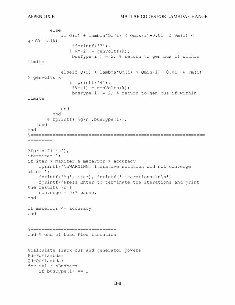
APPENDIX B MATLAB CODES FOR LAMBDA CHANGE
B-8
else
if Q(i) + lambda*Qd(i) < Qmax(i)-0.01 & Vm(i) <
genVolts(k)
%fprintf('3'),
% Vm(i) = genVolts(k);
busType(i ) = 2; % return to gen bus if within
limits
elseif Q(i) + lambda*Qd(i) > Qmin(i)+ 0.01 & Vm(i)
> genVolts(k)
% fprintf('4'),
%Vm(i) = genVolts(k);
busType(i) = 2; % return to gen bus if within
limits
end
end
% fprintf('%g\n',busType(i)),
end
end
%===============================================================
=========
%fprintf('\n'),
iter=iter+1;
if iter > maxiter & maxerror > accuracy
fprintf('\nWARNING: Iterative solution did not converge
after ')
fprintf('%g', iter), fprintf(' iterations.\n\n')
fprintf('Press Enter to terminate the iterations and print
the results \n')
converge = 0;% pause,
end
if maxerror <= accuracy
end
%===============================
end % end of Load Flow iteration
%calculate slack bus and generator powers
Pd=Pd*lambda;
Qd=Qd*lambda;
for i=1 : nBusbars
if busType(i) == 1

APPENDIX B MATLAB CODES FOR LAMBDA CHANGE
B-9
Pg(i)=P(i) + Pd(i);
Qg(i)=Q(i) + Qd(i);
elseif busType(i) == 2
Pg(i)=Pg(i)*lambda;
Qg(i)=Q(i) + Qd(i);
end
end
%==========================================

APPENDIX C MATLAB CODE FOR VOLTAGE CHANGE
C-1
10 APPENDIX C
MATLABTM Code for Voltage Change
% This program should be called by pfdata14bus (power flow 14
bus data program)
Vm=0; delta=0;
converge=1;
busType=[];%buscode
Vm=[]; delta=[]; Pd=[]; Qd=[]; Pg=[]; Qg=[]; Qmin=[]; Qmax=[];
% Added (6-8-00)
P=[]; Q=[]; sum1=[]; sum2=[]; A=[]; % Added (6-8-00)
J=[];dY=[];MatY=[];MatX=[];MatA=[];genBus=[];genVolts=[];
sum1=[];sum2=[];
busType=busdata(:,2); Vm=busdata1(:,3);
delta=busdata1(:,4);
Pd=busdata(:,5)/basemva; Qd=busdata(:,6)/basemva;
Pg=busdata(:,7)/basemva; Qg=busdata(:,8)/basemva;
Qmin=busdata(:,9)/basemva; Qmax=busdata(:,10)/basemva;
Qsh=busdata(:,11)/basemva;
for i=1 : nBusbars
%busType(i+nBusbars) = busType(i);
if busType(i) == 2 %generator bus
%busType(i)=0; %in first and second quadrant of
jacobian gen bus is treated as load bus
genBus=[genBus;i];
genVolts=[genVolts;Vm(i)];
end
end
busType;
nGens=length(genBus);
A = b(row, row)*(Pg(row)-Pd(row))+g(row, row)*(Qg(row)-Qd(row));
Vm(row)= v;
sig=0;
%========================================================
% Start of Newton-Raphson Loadflow iterations
%=======================================================
maxerror = 1; converge=1;iter = 0;
while maxerror >= accuracy & iter <= maxiter % Test for max.
power mismatch
%===========Compute power at each busbar=======
sum1 = zeros(size(Vm));

APPENDIX C MATLAB CODE FOR VOLTAGE CHANGE
C-2
sum2 = zeros(size(Vm));
for i=1:nBusbars
for j=1 : nBusbars
%sum1 = sum1 + Vm(j)*Y(i, j)*cos(delta(i)-delta(j)-
theta(i,j));
%sum2 = sum2 + Vm(j)*Y(i, j)*sin(delta(i)-delta(j)-
theta(i,j));
sum1(i) = sum1(i) + Vm(j)*(g(i, j)*cos(delta(i)-
delta(j)) + b(i, j)*sin(delta(i)-delta(j)));
sum2(i) = sum2(i) + Vm(j)*(g(i, j)*sin(delta(i)-
delta(j)) - b(i, j)*cos(delta(i)-delta(j)));
end
P(i) = Vm(i) * sum1(i);
Q(i) = Vm(i) * sum2(i);
if (busType(i) ~= 1) & (busType(i) ~= 2)
if i == row
sum1(i) = sum1(i) - v*g(i, i);
sum2(i) = sum2(i) + v*b(i, i);
vc=lambdac*A/(b(i, i)*sum1(i)+g(i, i)*sum2(i));
dY(nBusbars+row) = v-vc;
else
dY(i+nBusbars) = -Q(i) +lambdac*(Qg(i)-(Qd(i)-
Qsh(i)));%mismatch equation for reactive power (only load
busbars)
end
end
if (busType(i) ~= 1)
dY(i) = -P(i) +lambdac*(Pg(i)-Pd(i)); %mismatch equation
for active power (load and generator busbars)
end
end
%===============================================================
==
% Construct Jacobian Matrix
%===============================================================
==
N = nBusbars;
J =zeros(N,N);
%First Quadrant
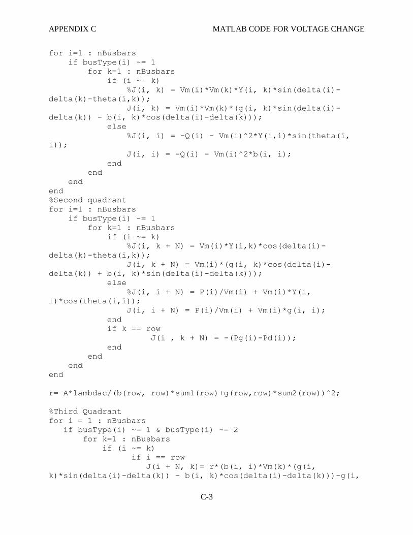
APPENDIX C MATLAB CODE FOR VOLTAGE CHANGE
C-3
for i=1 : nBusbars
if busType(i) ~= 1
for k=1 : nBusbars
if (i ~= k)
%J(i, k) = Vm(i)*Vm(k)*Y(i, k)*sin(delta(i)-
delta(k)-theta(i,k));
J(i, k) = Vm(i)*Vm(k)*(g(i, k)*sin(delta(i)-
delta(k)) - b(i, k)*cos(delta(i)-delta(k)));
else
%J(i, i) = -Q(i) - Vm(i)^2*Y(i,i)*sin(theta(i,
i));
J(i, i) = -Q(i) - Vm(i)^2*b(i, i);
end
end
end
end
%Second quadrant
for i=1 : nBusbars
if busType(i) ~= 1
for k=1 : nBusbars
if (i ~= k)
%J(i, k + N) = Vm(i)*Y(i,k)*cos(delta(i)-
delta(k)-theta(i,k));
J(i, k + N) = Vm(i)*(g(i, k)*cos(delta(i)-
delta(k)) + b(i, k)*sin(delta(i)-delta(k)));
else
%J(i, i + N) = P(i)/Vm(i) + Vm(i)*Y(i,
i)*cos(theta(i,i));
J(i, i + N) = P(i)/Vm(i) + Vm(i)*g(i, i);
end
if k == row
J(i , k + N) = -(Pg(i)-Pd(i));
end
end
end
end
r=-A*lambdac/(b(row, row)*sum1(row)+g(row,row)*sum2(row))^2;
%Third Quadrant
for i = 1 : nBusbars
if busType(i) ~= 1 & busType(i) ~= 2
for k=1 : nBusbars
if (i ~= k)
if i == row
J(i + N, k)= r*(b(i, i)*Vm(k)*(g(i,
k)*sin(delta(i)-delta(k)) - b(i, k)*cos(delta(i)-delta(k)))-g(i,
APPENDIX C MATLAB CODE FOR VOLTAGE CHANGE
C-4
i)*Vm(k)*(g(i,k)*cos(delta(i)-delta(k)) + b(i, k)*sin(delta(i)-
delta(k))));
else
%J(i + N, k) = -Vm(i)*Vm(k)*Y(i,
k)*cos(delta(i)-delta(k)-theta(i,k));
J(i + N, k) = -Vm(i)*Vm(k)*(g(i,
k)*cos(delta(i)-delta(k)) + b(i, k)*sin(delta(i)-delta(k)));
end
else
if i == row
J(i + N, i) =r*(-b(i, i)*sum2(i)+g(i,
i)*sum1(i));
else
%J(i + N, i) =P(i)- Vm(i)^2*Y(i,
i)*cos(theta(i,i));
J(i + N, i) =P(i)- Vm(i)^2*g(i, i);
end
end
end
end
end
%Fourth Quadrant
for i = 1 : nBusbars
if busType(i) ~= 1 & busType(i) ~= 2
for k=1 : nBusbars
if (i ~= k)
if i == row
J(i + N, k + N) =r*(b(i, i)*(g(i,
k)*cos(delta(i)-delta(k)) + b(i, k)*sin(delta(i)-delta(k)))+g(i,
i)*(g(i, k)*sin(delta(i)-delta(k)) - b(i, k)*cos(delta(i)-
delta(k))));
else
%J(i + N, k + N) = Vm(i)*Y(i, k)*sin(delta(i)-
delta(k)-theta(i,k));
J(i + N, k + N) = Vm(i)*(g(i, k)*sin(delta(i)-
delta(k)) - b(i, k)*cos(delta(i) - delta(k)));
end
if k==row
J(i + N, k + N) = -(Qg(i)-(Qd(i)- Qsh(i)));

APPENDIX C MATLAB CODE FOR VOLTAGE CHANGE
C-5
end
else
if i == row
J(i + N, i + N) =A/(b(i, i)*sum1(i)+g(i,
i)*sum2(i));
else
%J(i + N, i + N) =Q(i)/Vm(i) - Vm(i)*Y(i,
i)*sin(theta(i,i));
J(i + N, i + N) =Q(i)/Vm(i) - Vm(i)*b(i, i);
end
end
end
end
end
%===============================================================
==
% End of Jacobian Matrix construction
%===============================================================
==
% Prepare Jacobian Matrix for inversion; first copy it into a
compact
% matrix that does not have zero rows and columns (corresponding
to slack
% P & Q and generator Q equations). The original equations have
the form
% dY = J * dX; The compact form is MatY= MatA*MatX
N = nBusbars;
num1=0;
for i=1 : nBusbars
if busType(i) ~= 1
num1=num1+1;
MatY(num1,1) = dY(i);
num2=0;
for j=1 : nBusbars
if busType(j) ~= 1
num2=num2+1;
MatA(num1,num2)=J(i,j);
end
end
end
end
num1=0;
for i=1 : nBusbars
if busType(i) ~= 1
num1=num1+1;

APPENDIX C MATLAB CODE FOR VOLTAGE CHANGE
C-6
num2=nBusbars-1;
for j=1 : nBusbars
if busType(j)~= 1 & busType(j)~= 2
num2=num2+1;
MatA(num1,num2)=J(i,j+N);
end
end
end
end
num1=nBusbars-1;
for i=1 : nBusbars
if busType(i) ~= 1 & busType(i)~= 2
num1=num1+1;
MatY(num1, 1) = dY(i+nBusbars);
num2=0;
for j=1 : nBusbars
if busType(j)~= 1
num2=num2+1;
MatA(num1,num2)=J(i+N,j);
end
end
end
end
num1=nBusbars-1;
for i=1 : nBusbars
if busType(i) ~= 1 & busType(i)~= 2
num1=num1+1;
num2=nBusbars-1;
for j=1 : nBusbars
if busType(j)~= 1 & busType(j)~= 2
num2=num2+1;
MatA(num1,num2)=J(i+N,j+N);
end
end
end
end
MatX=MatA\MatY; % Solve for MatX using inverse(MatA) *
MatY
%Note: Matrices dY, dX and m contain zero rows and columns,
%corresponding to slack and generator busbars. In order to
invert m,
%it must be copied into matrix MatA, which contains no zero
rows or
APPENDIX C MATLAB CODE FOR VOLTAGE CHANGE
C-7
%columns. Likewise dY is copied into MatY. The result of
inversion,
%MatX is expanded into matrix dX.
%==========Update angles, voltages and calculate max error
===========
num1 = 0;
for i=1 : nBusbars
if busType(i) ~= 1
num1 = num1 + 1;
% dX(i) = MatX(num1,1);
delta(i) = delta(i) + MatX(num1,1);
end
end
num1=nBusbars-1;
for i=1 : nBusbars
if i== row
num1 = num1 + 1;
% dX(i+nBusbars) = MatX(num1, 1);
lambdac = lambdac + MatX(num1, 1);
elseif busType(i) ~= 1 & busType(i) ~= 2
num1 = num1 + 1;
% dX(i+nBusbars) = MatX(num1, 1);
Vm(i) = Vm(i)+ MatX(num1, 1);
end
end
maxerror=max(abs(MatY));
%============================= Generator reactive power limits
check =====
if maxerror > accuracy & genlimits == 1
for k = 1 : nGens
i=genBus(k);
sum2 = 0;
for j=1 : nBusbars
%sum2 = sum2 + Vm(j)*Y(i, j)*sin(delta(i)-delta(j)-
theta(i,j));
sum2 = sum2 + Vm(j)*(g(i, j)*sin(delta(i)-delta(j))
- b(i, j)*cos(delta(i)-delta(j)));
end
Q(i) = genVolts(k)*sum2;
%fprintf('%g ',Vm(i)),fprintf('%g
',genVolts(k)),fprintf('%g ',(Q(i) + Qd(i))*100),
if busType(i) == 2
if Q(i) + lambdac*Qd(i) > Qmax(i)+0.01
% fprintf('1'),
APPENDIX C MATLAB CODE FOR VOLTAGE CHANGE
C-8
Qg(i) = Qmax(i);
busType(i) = 0; % convert gen bus to load bus if
reactive power exceeds max
%Vm(i) = 1;
elseif Q(i) + lambdac*Qd(i) < Qmin(i)-0.01
%fprintf('2'),
Qg(i) = Qmin(i);
busType(i) = 0; % convert gen bus to load bus if
reactive power exceeds min
%Vm(i) = 1;
end
else
if Q(i) + lambdac*Qd(i) < Qmax(i)-0.01 & Vm(i) <
genVolts(k)
%fprintf('3'),
% Vm(i) = genVolts(k);
busType(i ) = 2; % return to gen bus if within
limits
elseif Q(i) + lambdac*Qd(i) > Qmin(i)+ 0.01 & Vm(i)
> genVolts(k)
% fprintf('4'),
%Vm(i) = genVolts(k);
busType(i) = 2; % return to gen bus if within
limits
end
end
% fprintf('%g\n',busType(i)),
end
end
%===============================================================
=========
%fprintf('\n'),
iter=iter+1;
if iter > maxiter & maxerror > accuracy
fprintf('\nWARNING: Iterative solution did not converge
after ')
fprintf('%g', iter), fprintf(' iterations.\n\n')
fprintf('Press Enter to terminate the iterations and print
the results \n')
converge = 0;% pause,
end
APPENDIX C MATLAB CODE FOR VOLTAGE CHANGE
C-9
%===============================
end % end of Load Flow iteration
%calculate slack bus and generator powers
Pd=Pd*lambdac;
Qd=Qd*lambdac;
for i=1 : nBusbars
if busType(i) == 1
Pg(i)=P(i) + Pd(i);
Qg(i)=Q(i) + Qd(i);
elseif busType(i) == 2
Pg(i)=Pg(i)*lambdac;
Qg(i)=Q(i) + Qd(i);
end
end
%==========================================
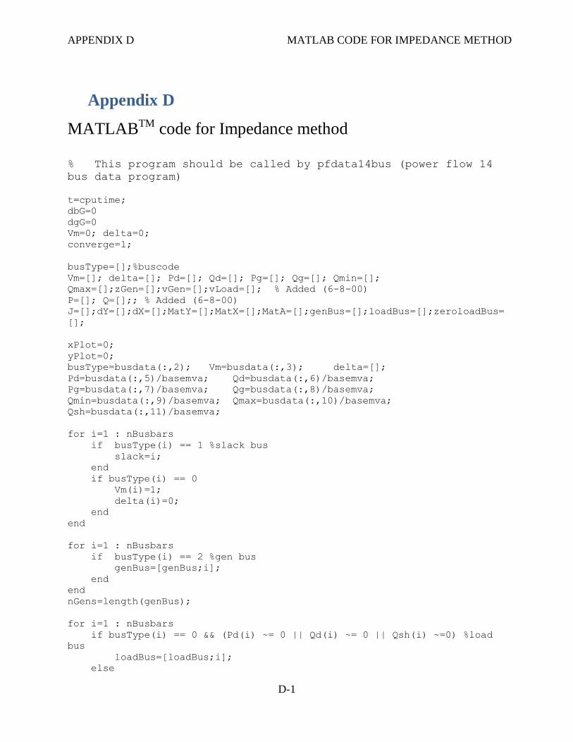
APPENDIX D MATLAB CODE FOR IMPEDANCE METHOD
D-1
11 Appendix D
MATLABTM code for Impedance method
% This program should be called by pfdata14bus (power flow 14
bus data program)
t=cputime;
dbG=0
dgG=0
Vm=0; delta=0;
converge=1;
busType=[];%buscode
Vm=[]; delta=[]; Pd=[]; Qd=[]; Pg=[]; Qg=[]; Qmin=[];
Qmax=[];zGen=[];vGen=[];vLoad=[]; % Added (6-8-00)
P=[]; Q=[];; % Added (6-8-00)
J=[];dY=[];dX=[];MatY=[];MatX=[];MatA=[];genBus=[];loadBus=[];zeroloadBus=
[];
xPlot=0;
yPlot=0;
busType=busdata(:,2); Vm=busdata(:,3); delta=[];
Pd=busdata(:,5)/basemva; Qd=busdata(:,6)/basemva;
Pg=busdata(:,7)/basemva; Qg=busdata(:,8)/basemva;
Qmin=busdata(:,9)/basemva; Qmax=busdata(:,10)/basemva;
Qsh=busdata(:,11)/basemva;
for i=1 : nBusbars
if busType(i) == 1 %slack bus
slack=i;
end
if busType(i) == 0
Vm(i)=1;
delta(i)=0;
end
end
for i=1 : nBusbars
if busType(i) == 2 %gen bus
genBus=[genBus;i];
end
end
nGens=length(genBus);
for i=1 : nBusbars
if busType(i) == 0 && (Pd(i) ~= 0 || Qd(i) ~= 0 || Qsh(i) ~=0) %load
bus
loadBus=[loadBus;i];
else
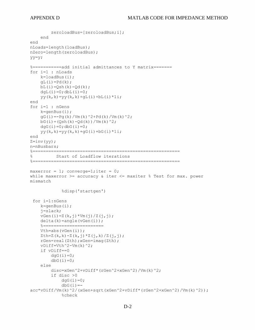
APPENDIX D MATLAB CODE FOR IMPEDANCE METHOD
D-2
zeroloadBus=[zeroloadBus;i];
end
end
nLoads=length(loadBus);
nZero=length(zeroloadBus);
yy=y;
%===========add initial admittances to Y matrix=======
for i=1 : nLoads
k=loadBus(i);
gL(i)=Pd(k);
bL(i)=Qsh(k)-Qd(k);
dgL(i)=0;dbL(i)=0;
yy(k,k)=yy(k,k)+gL(i)+bL(i)*1i;
end
for i=1 : nGens
k=genBus(i);
gG(i)=-Pg(k)/Vm(k)^2+Pd(k)/Vm(k)^2;
bG(i)=(Qsh(k)-Qd(k))/Vm(k)^2;
dgG(i)=0;dbG(i)=0;
yy(k,k)=yy(k,k)+gG(i)+bG(i)*1i;
end
Z=inv(yy);
n=nBusbars;
%========================================================
% Start of Loadflow iterations
%========================================================
maxerror = 1; converge=1;iter = 0;
while maxerror >= accuracy & iter <= maxiter % Test for max. power
mismatch
%disp('startgen')
for i=1:nGens
k=genBus(i);
j=slack;
vGen(i)=Z(k,j)*Vm(j)/Z(j,j);
delta(k)=angle(vGen(i));
%=======================
Vth=abs(vGen(i));
Zth=Z(k,k)-Z(k,j)*Z(j,k)/Z(j,j);
rGen=real(Zth);xGen=imag(Zth);
vDiff=Vth^2-Vm(k)^2;
if vDiff==0
dgG(i)=0;
dbG(i)=0;
else
disc=xGen^2+vDiff*(rGen^2+xGen^2)/Vm(k)^2;
if disc >0
dgG(i)=0;
dbG(i)=-
acc*vDiff/Vm(k)^2/(xGen+sqrt(xGen^2+vDiff*(rGen^2+xGen^2)/Vm(k)^2));
%check
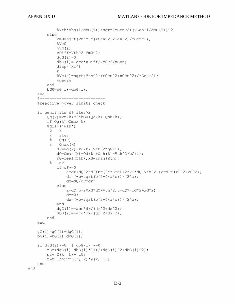
APPENDIX D MATLAB CODE FOR IMPEDANCE METHOD
D-3
%Vth*abs(1/dbG(i))/sqrt(rGen^2+(xGen-1/dbG(i))^2)
else
Vm0=sqrt(Vth^2*(rGen^2+xGen^2)/rGen^2);
%Vm0
%Vm(i)
vDiff=Vth^2-Vm0^2;
dgG(i)=0;
dbG(i)=-acc*vDiff/Vm0^2/xGen;
disp('Hi')
k
%Vm(k)=sqrt(Vth^2*(rGen^2+xGen^2)/rGen^2);
%pause
end
bG0=bG(i)+dbG(i);
end
%===========================
%reactive power limits check
if genlimits && iter>2
Qg(k)=Vm(k)^2*bG0+Qd(k)-Qsh(k);
if Qg(k)>Qmax(k)
%disp('wak')
% k
% iter
% Qg(k)
% Qmax(k)
dP=Pg(k)-Pd(k)+Vth^2*gG(i);
dQ=Qmax(k)-Qd(k)+Qsh(k)-Vth^2*bG(i);
rG=real(Zth);xG=imag(Zth);
% dP
if dP~=0
a=dP+dQ^2/dP;b=(2*rG*dP+2*xG*dQ-Vth^2);c=dP*(rG^2+xG^2);
dr=(-b+sqrt(b^2-4*a*c))/(2*a);
dx=dQ/dP*dr;
else
a=dQ;b=2*xG*dQ-Vth^2;c=dQ*(rG^2+xG^2);
dr=0;
dx=(-b+sqrt(b^2-4*a*c))/(2*a);
end
dgG(i)=-acc*dr/(dr^2+dx^2);
dbG(i)=+acc*dx/(dr^2+dx^2);
end
end
gG(i)=gG(i)+dgG(i);
bG(i)=bG(i)+dbG(i);
if dgG(i)~=0 || dbG(i) ~=0
zG=(dgG(i)-dbG(i)*1i)/(dgG(i)^2+dbG(i)^2);
piv=Z(k, k)+ zG;
Z=Z-1/piv*Z(:, k)*Z(k, :);
end
end
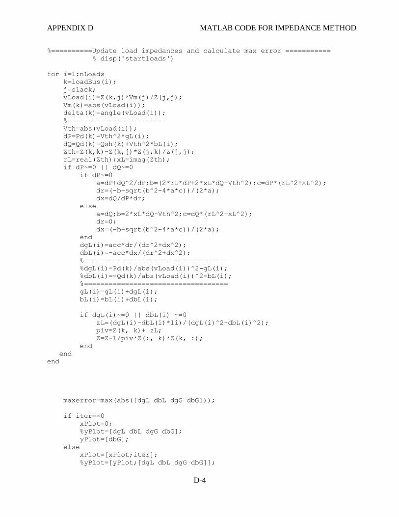
APPENDIX D MATLAB CODE FOR IMPEDANCE METHOD
D-4
%==========Update load impedances and calculate max error ===========
% disp('startloads')
for i=1:nLoads
k=loadBus(i);
j=slack;
vLoad(i)=Z(k,j)*Vm(j)/Z(j,j);
Vm(k)=abs(vLoad(i));
delta(k)=angle(vLoad(i));
%=======================
Vth=abs(vLoad(i));
dP=Pd(k)-Vth^2*gL(i);
dQ=Qd(k)-Qsh(k)+Vth^2*bL(i);
Zth=Z(k,k)-Z(k,j)*Z(j,k)/Z(j,j);
rL=real(Zth);xL=imag(Zth);
if dP~=0 || dQ~=0
if dP~=0
a=dP+dQ^2/dP;b=(2*rL*dP+2*xL*dQ-Vth^2);c=dP*(rL^2+xL^2);
dr=(-b+sqrt(b^2-4*a*c))/(2*a);
dx=dQ/dP*dr;
else
a=dQ;b=2*xL*dQ-Vth^2;c=dQ*(rL^2+xL^2);
dr=0;
dx=(-b+sqrt(b^2-4*a*c))/(2*a);
end
dgL(i)=acc*dr/(dr^2+dx^2);
dbL(i)=-acc*dx/(dr^2+dx^2);
%===================================
%dgL(i)=Pd(k)/abs(vLoad(i))^2-gL(i);
%dbL(i)=-Qd(k)/abs(vLoad(i))^2-bL(i);
%===================================
gL(i)=gL(i)+dgL(i);
bL(i)=bL(i)+dbL(i);
if dgL(i)~=0 || dbL(i) ~=0
zL=(dgL(i)-dbL(i)*1i)/(dgL(i)^2+dbL(i)^2);
piv=Z(k, k)+ zL;
Z=Z-1/piv*Z(:, k)*Z(k, :);
end
end
end
maxerror=max(abs([dgL dbL dgG dbG]));
if iter==0
xPlot=0;
%yPlot=[dgL dbL dgG dbG];
yPlot=[dbG];
else
xPlot=[xPlot;iter];
%yPlot=[yPlot;[dgL dbL dgG dbG]];

APPENDIX D MATLAB CODE FOR IMPEDANCE METHOD
D-5
yPlot=[yPlot;[dbG]];
end
if iter==2
%acc=max(abs(yPlot(1,:)))/(4/3*max(abs(yPlot(1,:))))
end
iter=iter+1;
if iter > maxiter & maxerror > accuracy
fprintf('\nWARNING: Iterative solution did not converge after ')
fprintf('%g', iter), fprintf(' iterations.\n\n')
fprintf('Press Enter to terminate the iterations and print the results
\n')
converge = 0; pause,
end
if maxerror <= accuracy
end
%===============================
end % end of Load Flow iteration
Islack=Vm(slack)/Z(slack,slack);
%calculate slack bus and generator powers
Pg(slack)=real(Vm(slack)*conj(Islack))+Pd(slack);
Qg(slack)=imag(Vm(slack)*conj(Islack))+Qd(slack);
for i=1:nGens
k=genBus(i);
Vm(k)=abs(vGen(i));
Qg(k)=Vm(k)^2*bG(i)+Qd(k)-Qsh(k);
end
for i=1:nZero
k=zeroloadBus(i);
Vm(k)=abs(Islack*Z(k,slack));
delta(k)=angle(Islack*Z(k,slack));
end
%==========================================
cpuTime=cputime-t

APPENDIX E IEEE 14-BUS DATA
E-1