new approach to satellite formation-keeping: exact solution to the full nonlinear problem

New Approach to Satellite Formation-Keeping:Exact Solution to the Full Nonlinear Problem

Hancheol Cho1 and Adam Yu2

Abstract: This paper presents a new, simple, and exact solution to the formation keeping of satellites when the relative distance betweenthe satellites is so large that the linearized relative equations of motion no longer hold. We employ a recently proposed approach, theUdwadia-Kalaba approach, which makes it possible to explicitly obtain the desired control function without making any approximationsrelated to the nonlinearities in the underlying dynamics. We use an inertial frame of reference to describe the motion of a satellite andsince no approximations are made, the results obtained apply to situations even when the distance between the satellites is arbitrarily large.The paper deals with a projected circular formation, but the methodology in this paper can be applied to any desired configuration ororbital requirements. Numerical simulations confirm the brevity and the accuracy of the analytical solution to the dynamical controlproblem developed herein.

DOI: 10.1061/�ASCE�AS.1943-5525.0000013

CE Database subject headings: Satellites; Orbits; Simulation.

Introduction

Formation flying technology has been extensively investigated asa means to get better performance than a single monolithic satel-lite. This technology guarantees a reduction in cost and has manyapplications such as the optical interferometry, distributed sens-ing, gravitational field measurements, ionospheric observation,earth observation, and 3D mapping for planetary explorers. Oneof the central problems of formation flying is the proper descrip-tion of the relative dynamics between satellites, which is the basisof formation design and control. Conventionally, linearized equa-tions of relative motion such as Hill-Clohessy-Wiltshire �HCW�equations �Hill 1878; Clohessy and Wiltshire 1960�, which arelinearized about a reference orbit or the formation center, havebeen used due to their simplicity. In the presence of perturbations,however, the formation configuration based on linearized equa-tions would be destroyed. Therefore, control forces must be ap-plied to maintain the desired configuration for a specific mission.This formation-keeping problem for multiple satellites has beenwidely investigated by various researchers. Yan et al. �2000� de-signed a pulse-based periodic controller to keep a formation usingthe HCW equations and the linear quadratic regulation technique.The main drawback to this paper is that the earth oblateness grav-ity perturbation is neglected, hence, Sparks �2000� proposed afeedback control strategy in the presence of this perturbation. Hedesigned a controller using discrete time linear quadratic regula-

1Graduate Student, Dept. of Aerospace and Mechanical Engineering,Univ. of Southern California, Los Angeles, CA 90089-1453 �correspond-ing author�. E-mail: [email protected]

2Member, Engineering Staff, F-35 JSF Program Section, NorthropGrumman Co., 1840 Century Park East, Los Angeles, CA 90067-2199.E-mail: [email protected]

Note. This manuscript was submitted on March 26, 2009; approvedon April 29, 2009; published online on May 4, 2009. Discussion periodopen until March 1, 2010; separate discussions must be submitted forindividual papers. This paper is part of the Journal of Aerospace Engi-neering, Vol. 22, No. 4, October 1, 2009. ©ASCE, ISSN 0893-1321/
2009/4-445–455/$25.00.
JOURNA

Downloaded 18 Sep 2009 to 128.125.182.13. Redistribution subject to

tor laws based on the HCW equations. Based on the HCW equa-tions, Sabol et al. �2001� investigated several satellite formationflying designs and their evolution through time. Using the varia-tion of orbital elements, they designed formation-keepingschemes in the presence of various perturbations. Armellin et al.�2004� developed a real-time control strategy that includes bothreconfiguration and formation keeping. They solved these twoproblems by generating a control sequence based on a discretiza-tion of the differential constraints and a parametrization of thecontrols. Qingsong et al. �2004� solved this formation-keepingproblem by using a low-thrust fuzzy control method. However,Yan and others �Yan et al. 2000; Sparks 2000; Sabol et al. 2001;Armellin et al. 2004; Qingsong et al. 2004� made use of thelinearized equations of relative motion, and hence the methodsthus derived are suitable only for very close formations.

Although, as pointed out earlier, there has been an extensiveliterature regarding formation flying to date, the effects that resultfrom the nonlinearities remain yet to be fully modeled. Karlgaardand Lutze �2003� approached the problem using spherical coordi-nates and perturbation techniques to extend the HCW equationsthat are correct to second order. Richardson and Mitchell �2003�obtained the solution that includes the third-order nonlinearitiesby enforcing periodic motion. Kasdin et al. �2005� used a Hamil-tonian formulation to solve the problem to include second-ordernonlinearity effects, but with J2 perturbations.

In this paper, assuming unbounded and time-varying low-thrust burns throughout the maneuver, the formation-keepingproblem is exactly and explicitly solved without any restrictionabout the distance between satellites. Also, this paper derives theexact control force to maintain the configuration of the formation.We use a new approach for constrained dynamic systems pro-posed by Udwadia and Kalaba �Udwadia 2000, 2002, 2003, 2005,2008; Kalaba and Udwadia 1993; Udwadia and Kalaba 1992,2002�, which is based on Gauss’s principle. The Udwadia-Kalabaequation unlike the Lagrange’s equation handles both holonomicand nonholonomic constraints with equal ease. This equation con-tains the generalized Moore-Penrose inverse �Udwadia and
Kalaba 1999� and has been applied to highly constrained prob-
L OF AEROSPACE ENGINEERING © ASCE / OCTOBER 2009 / 445

ASCE license or copyright; see http://pubs.asce.org/copyright

lems in various fields of study such as robotics �Peters et al. 2005�and astrodynamics �Schutte and Dooley 2005�. The major contri-bution of this paper is the ability to explicitly solve the completenonlinear dynamics and control problem as a whole without theuse of any approximations. In previous research, the linearizedequations of relative motion described in a local moving frame ortheir approximate versions �that are valid only to second or thirdorder� have been used to solve the formation-keeping problem, soit has been very challenging to obtain an exact solution.

We consider a satellite called the “chief” orbiting a centralbody, and require that a “deputy” satellite maintain a given re-quired formation relative to this chief. We employ herein the two-body equation of motion described in an inertial frame ofreference, and then incorporate the station-keeping requirementsas constraints to obtain a simple equation of motion that com-pletely captures all the nonlinearities. This equation exactly yieldsthe given constrained motion and also gives an exact control force�as an explicit function of the state and time� required to maintainthe formation. The results obtained can apply to the case evenwhen the distance between satellites is so large that the linearizedrelative equations of motion no longer hold. The dynamics oncedescribed in the inertial frame are then recast, for convenience,into a local moving frame by the use of a transformation matrix.As a practical constraint we choose the relative configuration thatis circular when projected on the local horizontal plane, which isgenerally called the projected circular orbit �PCO� �Vaddi et al.2003�. This projected circular formation is based on the solutionsto the linearized equations, and hence the nonlinear behavior ofrelative motion will break down this configuration. To avoid thisbreak down of configuration, the need to use a control forcearises, which will be solved for in detail. Also, this new approachgives a general methodology that can be easily applied to anytype of relative configuration.

The analysis in this paper is summarized as follows: in thesection Udwadia-Kalaba equation, we briefly discuss the funda-mental equation of motion for a constrained system. Next, in thesection Unconstrained motion, the acceleration for the uncon-strained motion is depicted, which also serves as a solution for therelative motion in the two-body problem. In the section Con-strained motion, the constraint equation and the exact controlforce are derived in the inertial frame which forces the deputy tomaintain the required PCO configuration. Finally, in the sectionNumerical simulations, numerical simulations are presented todemonstrate the brevity and the accuracy of the method.

Udwadia-Kalaba Equation

This section deals with the fundamental equation for a con-strained system, which we will call the Udwadia-Kalaba equation.Consider a point-mass satellite in the inertial Cartesian coordinateframe. When the initial position and velocity of the satellite areknown, the vectors of displacement and velocity are denoted bythe following:

x = �x1,x2,x3�T; x = �x1, x2, x3�T �1�

The forces impressed on the satellite are denoted by a 3 by 1vector, and denoted by

F�t� = �F1�t�,F2�t�,F3�t��T �2�

The unconstrained motion of the system can be expressed as a 3
by 1 matrix equation
446 / JOURNAL OF AEROSPACE ENGINEERING © ASCE / OCTOBER 200


Mx = F�x�t�, x�t�,t� �3�

or

x = M−1F�x�t�, x�t�,t� = a�t� �4�

where M=mI3�3=diagonal mass matrix; m=mass of the satellite;I3�3=3 by 3 identity matrix; and a�t�=acceleration at the time tof the unconstrained system. Furthermore, the system is con-strained through the application of the following set of consistentconstraint equations:

A�x�t�, x�t�,t�x = b�x�t�, x�t�,t� �5�

where the matrix A=m by 3 matrix and b=m by 1 vector, wherem is the number of constraints. The application of constraints onthe unconstrained system causes additional forces to be applied tothe unconstrained system and the equation of motion of the con-strained system becomes

Mx�t� = F�x�t�, x�t�,t� + Fc �6�

where Fc=additional constraint force vector that arises due to theapplication of the constraints. Udwadia and Kalaba proposed thefollowing equation of motion for the constrained system�uniquely described at each instant of time� �Udwadia and Kalaba2008�:

Mx = F + M1/2�AM−1/2�+�b − Aa� �7�

where the superscript “+” represents the generalized Moore-Penrose inverse. In this paper, Eq. �7� is referred to as theUdwadia-Kalaba equation. It is important to note that theUdwadia-Kalaba equation should be described in the inertialframe of reference. Then, the constraint force vector Fc�t� is de-scribed as

Fc�t� = M1/2�AM−1/2�+�b − Aa� �8�

Since the generalized Moore-Penrose inverse of a matrix isunique, the control force is uniquely and explicitly calculated byEq. �8�, regardless of whether the constraints given by Eq. �5� areholonomic or nonholonomic. It is straightforward to show that theUdwadia-Kalaba equation satisfies the constraint Eq. �5�. Usingthe fact that M=mI3�3 in this paper, as we are concerned withonly a single deputy satellite, the Udwadia-Kalaba equation canbe further simplified to �Udwadia and Kalaba 2008�

x = a + A+�b − Aa� �9�

Mx = F + MA+�b − Aa� �10�

Unconstrained Motion

The unconstrained motion represents the relative motion withoutthe application of a control force on the system of satellites. Thechief and the deputy satellites move only under the influence ofgravity, and hence we consider “unconstrained” motion and “un-controlled” motion to have the same meaning. In the case ofconstrained motion, proper control forces are needed to be ap-plied on the unconstrained system to meet the constraint require-ments. Hence, we consider “constrained” motion and “controlled”motion to also have the same meaning.

When a point-mass satellite is orbiting around the Earth, theunconstrained acceleration of the system is expressed in the iner-
tial coordinate system as follows �Prussing and Conway 1993�:
9


a = −GM

�X2 + Y2 + Z2�3/2�X

Y

Z� �11�

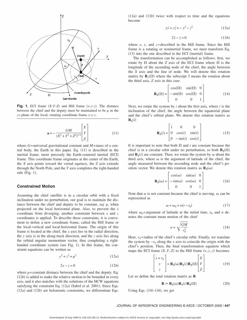
where G=universal gravitational constant and M =mass of a cen-tral body, the Earth in this paper. Eq. �11� is described in theinertial frame, more precisely the Earth-centered inertial �ECI�frame. This coordinate frame originates at the center of the Earth,the X axis points toward the vernal equinox, the Z axis extendsthrough the North Pole, and the Y axis completes the right-handedrule �Fig. 1�.

Constrained Motion

Assuming the chief satellite is in a circular orbit with a fixedinclination under no perturbation, our goal is to maintain the dis-tance between the chief and deputy to be constant, say �, whenprojected on the local horizontal plane. Also, to prevent the xcoordinate from diverging, another constraint between x and zcoordinates is applied. To describe these constraints, it is conve-nient to define a new coordinate frame, called the Hill frame orthe local-vertical and local-horizontal frame. The origin of thisframe is located at the chief, the x axis lies in the radial direction,the y axis is in the along-track direction, and the z axis lies alongthe orbital angular momentum vector, thus completing a right-handed coordinate system �see Fig. 1�. In this frame, the con-straint equations can be written as

y2 + z2 = �2 �12a�

2x − z = 0 �12b�

where �=constant distance between the chief and the deputy. Eq.�12b� is added to make the relative motion to be bounded in everyaxis, and it also matches with the solutions of the HCW equationssatisfying the constraint Eq. �12a� �Sabol et al. 2001�. Since Eqs.�12a� and �12b� are holonomic constraints, we differentiate Eqs.

Fig. 1. ECI frame �X-Y-Z� and Hill frame �x-y-z�. The distancebetween the chief and the deputy must be maintained to be � in theyz-plane of the local, rotating coordinate frame x-y-z.

JOURNA


�12a� and �12b� twice with respect to time and the equationsbecome

yy + zz = − y2 − z2 �13a�

2x − z = 0 �13b�

where x, y, and z=described in the Hill frame. Since the Hillframe is a rotating or noninertial frame, we must transform Eq.�13� into the one described in the ECI �inertial� frame.

The transformation can be accomplished as follows: first, werotate by � about the Z axis of the ECI frame where � is thelongitude of the ascending node of the chief, the angle betweenthe X axis and the line of node. We will denote this rotationmatrix by R3�� where the subscript 3 means the rotation aboutthe third axis, Z axis in this case

R3�� = � cos�� sin�� 0

− sin�� cos�� 0

0 0 1� �14�

Next, we rotate the system by i about the first axis, where i is theinclination of the chief, the angle between the equatorial planeand the chief’s orbital plane. We denote this rotation matrix asR1�i�

R1�i� = �1 0 0

0 cos�i� sin�i�0 − sin�i� cos�i�

� �15�

It is important to note that both � and i are constant because thechief is in a circular orbit under no perturbation, so both R3��and R1�i� are constant. Then, we rotate the system by � about thethird axis, where � is the argument of latitude of the chief, theangle measured between the ascending node and the chief’s po-sition vector. We denote this rotation matrix as R3��

R3�� = � cos�� sin�� 0


0 0 1� �16�

Note that � is not constant because the chief is moving. � can berepresented as

� = �0 + n�t − t0� �17�

where �0=argument of latitude at the initial time, t0, and n de-notes the constant mean motion of the chief

n =�GM

r03 �18�

Here, r0=radius of the chief’s circular orbit. Finally, we translatethe system by −r0 along the x axis to coincide the origin with thechief’s position. Then, the final transformation equation whichmaps the ECI frame �X ,Y ,Z� to the Hill frame �x ,y ,z� becomes

�x + r0

y

z� = R3��R1�i�R3��X

Y

Z� �19�

Let us define the total rotation matrix as R

R � R3��R1�i�R3�� 20�

Using Eqs. �14�–�16�, we get



R = � cos��cos�� − sin��cos�i�sin�� sin��cos�� + cos��cos�i�sin�� sin�i�sin��− cos��sin�� − sin��cos�i�cos�� cos��cos�i�cos�� − sin��sin�� sin�i�cos��

sin��sin�i� − cos��sin�i� cos�i�� 21�

The first constraint equation �Eq. �13a�� contains only y and z, so we use only the last two rows of the matrix R and define the followingmatrix:

R � − cos��sin�� − sin��cos�i�cos�� cos��cos�i�cos�� − sin��sin�� sin�i�cos��sin��sin�i� − cos��sin�i� cos�i� �22�

Differentiating the matrix R once and twice with respect to time, we get the following:

R = − n cos��cos�� + n sin��cos�i�sin�� − n cos��cos�i�sin�� − n sin��cos�� − n sin�i�sin��0 0 0

�23�

R = n2 cos��sin�� + n2 sin��cos�i�cos�� − n2 cos��cos�i�cos�� + n2 sin��sin�� − n2 sin�i�cos��0 0 0

�24�

Also, the second constraint equation �Eq. �13b�� contains only x and z, so we use only the first and third rows of the matrix R and definethe following matrix:

R � cos��cos�� − sin��cos�i�sin�� sin��cos�� + cos��cos�i�sin�� sin�i�sin��sin��sin�i� − cos��sin�i� cos�i� �25�

Differentiating the matrix R once and twice with respect to time, we get the following:

R = − n cos��sin�� − n sin��cos�i�cos�� − n sin��sin�� + n cos��cos�i�cos�� n sin�i�cos��0 0 0

�26�

R = − n2 cos��cos�� + n2 sin��cos�i�sin�� − n2 sin��cos�� − n2 cos��cos�i�sin�� − n2 sin�i�sin��0 0 0

�27�

If the chief is in an equatorial orbit, then its inclination is zero, theline of nodes does not exist, so � and � cannot be defined. In thiscase the X axis is considered as the node, therefore �=0, i=0,and � is just the angle between the X axis and the position of thechief. Hence, the transformation matrix R is simply given by

R = R3�� = � cos�� sin�� 0


0 0 1� �28�

Also

R = − sin�� cos�� 0

0 0 1 ;

R = − n cos�� − n sin�� 0

0 0 0 ;

R = n2 sin�� − n2 cos�� 0

0 0 0 �29�

and

R = cos�� sin�� 0

0 0 1 ;

R = − n sin�� n cos�� 0

0 0 0 ;

R = − n2 cos�� − n2 sin�� 0 �30�
0 0 0


Let us consider the first constraint given by Eq. �12a�. Then,from Eq. �19�, y and z components in the Hill frame are related by

y

z = R�X

Y

Z� �31�

Differentiating Eq. �31� once and twice yields the following:

y

z = R�X

Y

Z� + R�X

Y

Z� �32�

y

z = R�X

Y

Z� + 2R�X

Y

Z� + R�X

Y

Z� �33�

Eq. �13a� can be represented in a matrix form

�y z �y

z = − �y z �y

z �34�

Substituting Eqs. �31�–�33� into Eq. �34�, we get the first con-
straint equation described in the ECI frame
9


�X Y Z �RT�R�X

Y

Z� + 2R�X

Y

Z� + R�X

Y

Z�� = − �X Y Z �RT

+ �X Y Z �RT��R�X

Y

Z� + R�X

Y

Z�� 35�

Eq. �35� can be rearranged into the following:

�X Y Z �RTR�X

Y

Z� = − �X Y Z �RTR�X

Y

Z�

− 2�X Y Z �RTR�X

Y

Z�

− �X Y Z �RTR�X

Y

Z�

− 2�X Y Z �RTR�X

Y

Z�


Y

Z� �36�

Next, let us consider the second constraint Eq. �12b�. Then,from Eq. �19�, x- and z-components in the Hill frame are relatedby

x

z = R�X

Y

Z� �37�

Differentiating Eq. �37� once and twice yields the following:

x

z = R�X

Y

Z� + R�X

Y

Z� �38�

x

z = R�X

Y

Z� + 2R�X

Y

Z� + R�X

Y

Z� �39�

Eq. �13b� can be represented in a matrix form

�2 − 1 �x = 0 �40�
z
JOURNA


Inserting Eq. �39� into Eq. �40� yields the second constraint equa-tion described in the ECI frame

�2 − 1 �R�X

Y

Z� = − �2 − 1 �R�X

Y

Z� − �4 − 2 �R�X

Y

Z� �41�

The two constraint equations �Eqs. �36� and �41�� can be repre-sented in a form of Eq. �5�

A�x�t�, x�t�,t�x = b�x�t�, x�t�,t�

More specifically, we obtain the following vector equation:

A11 A12 A13

A21 A22 A23�X

Y

Z� = b1

b2 �42�

Then, each component of the matrices A and b can be written asfollows:

�A11 A12 A13 � = �X Y Z �RTR �43�

so that

A11 � X �cos��sin�� + sin��cos�i�cos��2 + sin2��sin2�i��

+ Y �cos��sin�� + sin��cos�i�cos��sin��sin��

− cos��cos�i�cos�� − sin��cos��sin2�i��

+ Z sin��sin�i�cos�i� − sin�i�cos��cos��sin��

+ sin��cos�i�cos�� 44a�

A12 � X �cos��sin�� + sin��cos�i�cos��sin��sin��

− cos��cos�i�cos�� − sin��cos��sin2�i��

+ Y �cos��cos�i�cos�� − sin��sin��2

+ cos2��sin2�i�� + Z sin�i�cos��cos��cos�i�cos��

− sin��sin�� − cos��sin�i�cos�i�� 44b�

A13 � X sin��sin�i�cos�i� − sin�i�cos��cos��sin��

+ sin��cos�i�cos�� + Y sin�i�cos��

��cos��cos�i�cos�� − sin��sin��

− cos��sin�i�cos�i�� + Z�sin2�i�cos2�� + cos2�i��

�44c�

and

�A21 A22 A23 � = �2 − 1 �R �45�

so that

A21 = 2 cos��cos�� − 2 sin��cos�i�sin�� − sin��sin�i�

�46a�

A22 = 2 sin��cos�� + 2 cos��cos�i�sin�� + cos��sin�i�

�46b�

A23 = 2 sin�i�sin�� − cos�i� �46c�



In addition

b1 = − �X Y Z �RTR�X

Y

Z� − 2�X Y Z �RTR�X

Y

Z�


Y

Z� − 2�X Y Z �RTR�X

Y

Z�


Y

Z� �47�

and

b2 = − �2 − 1 �R�X

Y

Z� − �4 − 2 �R�X

Y

Z� �48�

The generalized Moore-Penrose inverse of the matrix A can beobtained in a following closed form �Udwadia and Kalaba 2008�:

A+ = ��A1+ − �c+��c+� �49�

where

A1+ =

1

A112 + A12

2 + A132 �A11

A12

A13� �50�

� =A11A21 + A12A22 + A13A23

A112 + A12

2 + A132 �51�

c+ =1

A212 + A22

2 + A232 − �2�A11

2 + A122 + A13

2 ��A21

A22

A23� − ��A11

A12

A13��52�

Finally, substituting all these terms in the Udwadia-Kalaba equa-tion �Eq. �9��

x = a + A+�b − Aa� = −GM

�X2 + Y2 + Z2�3/2�X

Y

Z� + ��A1

+ − �c+��c+�

�b1

b2 +

GM

�X2 + Y2 + Z2�3/2 ��A1+ − �c+��c+�A11 A12 A13

A21 A22 A23

��X

Y

Z� �53�

The constraint force that is needed to satisfy our constraints can
be explicitly obtained


Fc = MA+�b − Aa� = m��A1+ − �c+��c+�b1

b2

+GMm

�X2 + Y2 + Z2�3/2 ��A1+ − �c+��c+�A11 A12 A13

A21 A22 A23�X

Y

Z��54�

where m=mass of the deputy satellite. In Eqs. �53� and �54�, A1+,

�, and c+ are explicitly given in Eqs. �50�–�52� as a closed form.

Numerical Simulations

In this section, the analytical results in the previous section areverified by numerical simulations. The radius of the chief’s orbitis assumed to be 7.0�106 m and the mean motion n is 0.001 078rad/s. The deputy is desired to be maintained the PCO with �=50 km. Since the value of � is not small, using the HCW equa-tions is not a good idea to solve this problem. �, i, and �0 of thechief are given as 30°, 80°, and 0°, respectively. Therefore theinitial condition for the chief in the ECI frame is given by

X0� = �r0 cos��

r0 sin��0

� = �6.062 � 106 m

3.5 � 106 m

0 m� ;

X0� = �− v0 cos�i�sin��

v0 cos�i�cos��v0 sin�i�

� = �− 6.553 � 102 m/s1.135 � 103 m/s7.432 � 103 m/s

� �55�

where the subscript 0 means the values at the initial time, thesuperscript � denotes the vector associated with the chief satelliteand v0 is the constant orbital speed of the chief, which is deter-mined by the vis-viva equation �Prussing and Conway 1993�

v0 =�GM

r0= 7.547 � 103 m/s �56�

Next, we must be careful when dealing with the initial condi-tion of the deputy, because the initial condition must also satisfythe constraint equations. In this paper, the constraints are holo-nomic, so both Eqs. �12� and �13� must hold. Eqs. �12� and �13�can be represented in the ECI frame as

�X Y Z �RTR�X

Y

Z� − �2 = 0,�2 − 1 �R�X

Y

Z� = 0 �57�

�X Y Z �RTR�X

Y

Z� + �X Y Z �RTR�X

Y

Z� = 0,�2 − 1 �R�X

Y

Z�

+ �2 − 1 �R�X

Y

Z� = 0 �58�

Then, the initial condition for the deputy satellite must satisfy the

9


following equations:

�X0 Y0 Z0 �R0TR0�X0

Y0

Z0� − �2 = 0,�2 − 1 �R0�X0

Y0

Z0� = 0

�59�

�X0 Y0 Z0 �R0TR0�X0

Y0

Z0� + �X0 Y0 Z0 �R0

TR0�X0

Y0

Z0

�= 0,�2 − 1 �R0�X0

Y0

Z0� + �2 − 1 �R0�X0

Y0

Z0

� = 0 �60�

For practical use, the general initial conditions that satisfy theconstraint equations �Eqs. �59� and �60�� are proposed by Vaddi etal. �2003�

x0 =�

2sin �0; y0 = � cos �0; z0 = � sin �0

x0 =�

2n cos �0; y0 = − �n sin �0; z0 = �n cos �0 �61�

where �=50 km; �0=phase angle between deputy satellites; andthe mean motion n is 0.001 078 rad/s as before. If we use �0

=0.55 rad, Eq. �61� will yield

x0 = 1.306 7 � 104 m; y0 = 4.262 6 � 104 m;

z0 = 2.613 4 � 104 m

x0 = 22.978 4 m/s; y0 = − 28.176 4 m/s; z0 = 45.956 8 m/s�62�

The initial conditions given by Eqs. �61� and �62� are designedprimarily to keep the PCO without any application of controlforces by assuming that the linearized HCW equations are valid,and so these initial conditions under this assumption lead to acircular orbit. However, we shall show that when the full nonlin-ear system is considered, the orbit no longer remains circular, andin what follows we will determine the explicit control forceneeded to get a circular orbit.

Eqs. �61� and �62� are described in the Hill frame. To use theUdwadia-Kalaba equation, we need to transform these values intothe ones in ECI frame by using Eq. �19�

X0 = �X0

Y0

Z0� = �6.082 7 � 106 m

3.490 7 � 106 m

4.651 7 � 106 m� ;

X0 = �X0

Y0

Z0

� = �− 651.304 1 m/s1,082.1 m/s7,426.4 m/s

� �63�

Also, we set three times the orbital period of the chief as thesimulation time in which the period is given by

P =2�

= 5.828 � 103 s = 1.619 h �64�
n
JOURNA


First, we simulate the unconstrained motion. The ODE solverODE45 in MATLAB was used to numerically integrate the sys-tem, and the error tolerance was set to 10−12. The position vectorof the deputy X�t� can be obtained by directly integrating Eq. �11�with the initial condition of Eq. �63�. The result is described in theECI frame. If the position vector is desired to be described in theHill frame, Eq. �19� can be used

�x

y

z� = R�X

Y

Z� − �r0

0

0� �65�

Next, we simulate the constrained motion. The ODE solverODE45 in MATLAB was again used to numerically integrate thesystem, and the error tolerance was set to 10−12 as before. Theposition vector of the deputy X�t� can be obtained by directlyintegrating Eq. �53� with the initial condition of Eq. �63�. Then,we transform the position vector in the ECI frame into that in theHill frame using Eq. �65�.

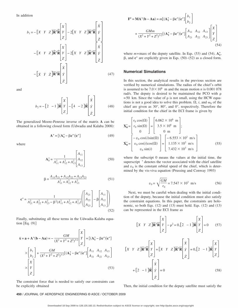
Fig. 2 shows the trajectory of the deputy projected on theyz-plane in the Hill frame without the constraint. The scale isnormalized to �, and the relative motion is unbounded and mov-ing left in the y direction, which shows the necessity of the con-straint, say, thrust. This means that the initial conditions given byEq. �61� fail to keep the desired circular orbit. This is becausethese initial conditions assume that the linear HCW equationshold, that is, that the relative distance between the deputy and thechief is small. However, since we are dealing here with the large-relative-distance case ��=50 km�, this assumption of linearity nolonger holds. In Fig. 3, the constrained motion of the deputy isshown. Also, the scale is normalized to �. The trajectory is beingmaintained very well with the relative distance of �=50 km.

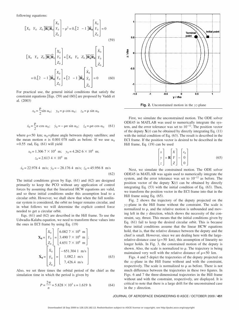
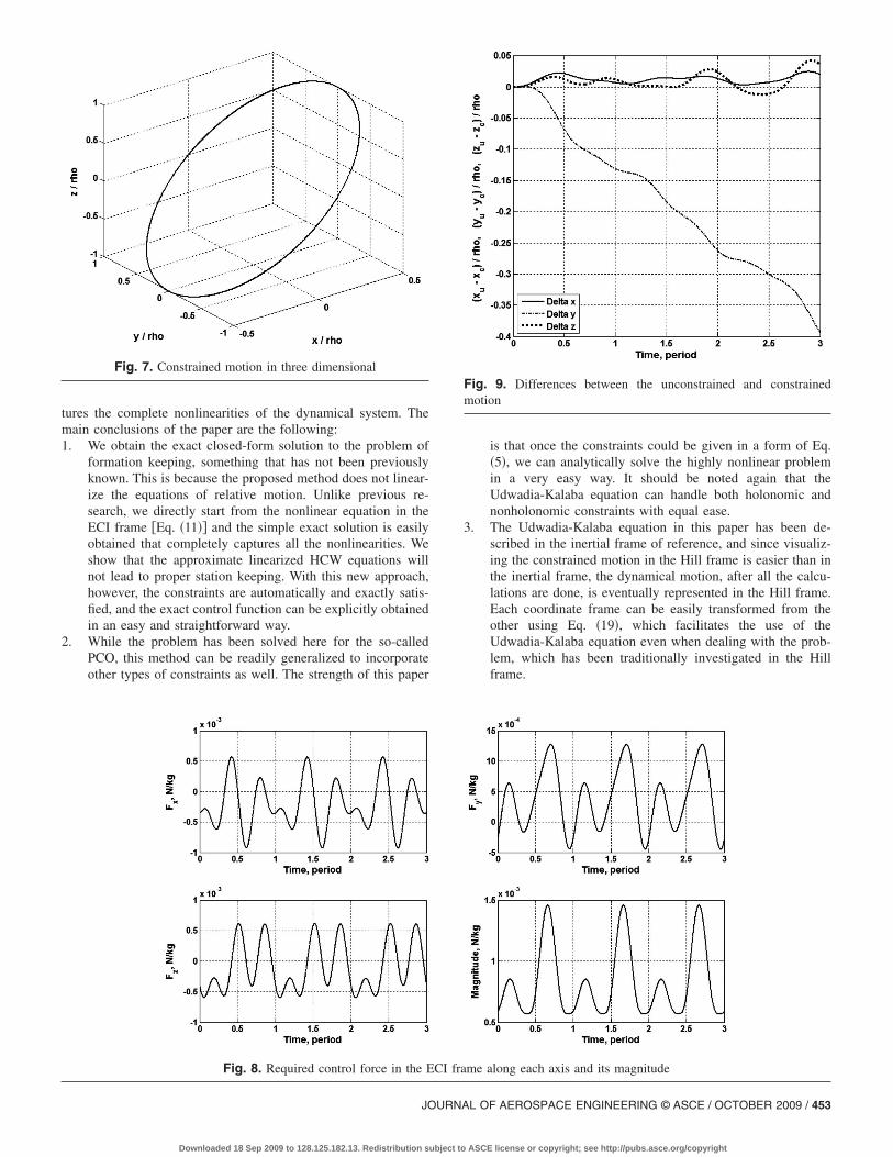
Figs. 4 and 5 depict the trajectories of the deputy projected onthe xz-plane in the Hill frame without and with the constraint,respectively. The scale is normalized to � as before. There is notmuch difference between the trajectories in these two figures. InFigs. 6 and 7 the three-dimensional trajectories in the Hill framewithout and with the constraint, respectively, are displayed. It iscritical to note that there is a large drift for the unconstrained case

Fig. 2. Unconstrained motion in the yz-plane

in the y direction.



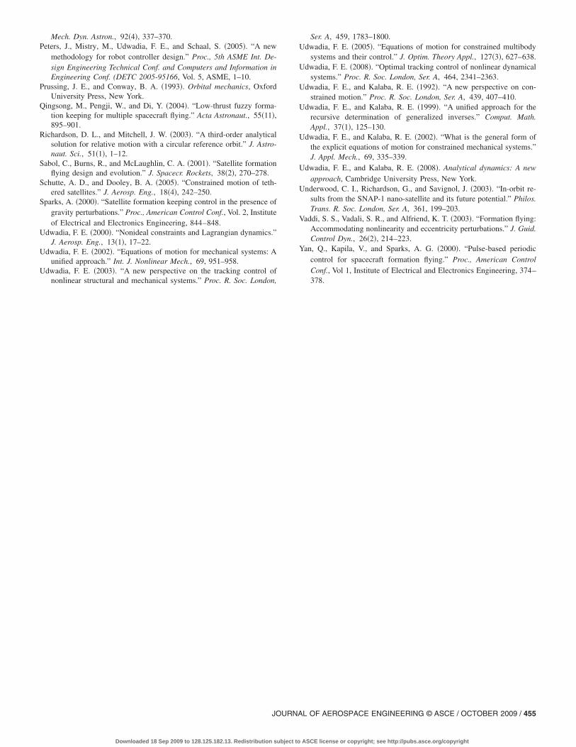
In Fig. 8 the required forces to maintain the desired formationand their total magnitude are represented. They are described inthe ECI frame and calculated using Eq. �54�. The largest thrust isin the Y direction, which dominates the total magnitude, and itcorresponds to about 1.3 mN per kg. According to Underwood etal. �2003�, the Surrey SNAP-1 nanosatellite whose mass is only6.5 kg can deliver 7.7 mN per kg. Therefore, we conclude that allof the thrusts required are attainable by even this small satellite.Fig. 9 shows the differences between the unconstrained and con-strained motion for each axis. The displacements for the uncon-strained motion are subtracted from the displacements for theconstrained motion. The time unit is normalized to the period ofthe chief. The major drift is observed in the y direction, and thismeans that without the application of a control force, the deputysatellite will lag behind as time goes by and it would eventually

Fig. 3. Constrained motion in the yz-plane

Fig. 4. Unconstrained motion in the xz-plane



fail to maintain the desired station keeping. At the final time, thedifference in the y direction approximately corresponds to 0.4��=20 km. Figs. 10–13 represent errors described by Eqs. �57�and �58�. The time unit is normalized to the period of the chief asbefore. The largest displacement error corresponds to about10−4 m or 0.1 mm. �Fig. 10� This is very small when comparedwith the relative orbit size �=50 km. Also, the largest velocityerror corresponds to only about 3.6�10−7 m /s �Fig. 12�. We seetherefore that the errors are so small that the relative orbit is beingmaintained very well as desired.

Conclusions

In this paper, a simple, new method for the formation-keepingproblem, which is not restricted to the relative size of the forma-tion, is presented. We make use of a recently proposedapproach—the Udwadia-Kalaba equation—and this method cap-

Fig. 5. Constrained motion in the xz-plane

Fig. 6. Unconstrained motion in three dimensional

9


tures the complete nonlinearities of the dynamical system. Themain conclusions of the paper are the following:1. We obtain the exact closed-form solution to the problem of

formation keeping, something that has not been previouslyknown. This is because the proposed method does not linear-ize the equations of relative motion. Unlike previous re-search, we directly start from the nonlinear equation in theECI frame �Eq. �11�� and the simple exact solution is easilyobtained that completely captures all the nonlinearities. Weshow that the approximate linearized HCW equations willnot lead to proper station keeping. With this new approach,however, the constraints are automatically and exactly satis-fied, and the exact control function can be explicitly obtainedin an easy and straightforward way.

2. While the problem has been solved here for the so-calledPCO, this method can be readily generalized to incorporateother types of constraints as well. The strength of this paper

Fig. 7. Constrained motion in three dimensional

Fig. 8. Required control force in the E

JOURNA


is that once the constraints could be given in a form of Eq.�5�, we can analytically solve the highly nonlinear problemin a very easy way. It should be noted again that theUdwadia-Kalaba equation can handle both holonomic andnonholonomic constraints with equal ease.

3. The Udwadia-Kalaba equation in this paper has been de-scribed in the inertial frame of reference, and since visualiz-ing the constrained motion in the Hill frame is easier than inthe inertial frame, the dynamical motion, after all the calcu-lations are done, is eventually represented in the Hill frame.Each coordinate frame can be easily transformed from theother using Eq. �19�, which facilitates the use of theUdwadia-Kalaba equation even when dealing with the prob-lem, which has been traditionally investigated in the Hillframe.

me along each axis and its magnitude

Fig. 9. Differences between the unconstrained and constrainedmotion

CI fra



4. The fact that we have the exact solution to the nonlineardynamics and control problem is corroborated by the numeri-cal examples that show that the formation is pretty wellmaintained, as desired, even when the relative distance be-tween the satellites is not small. The errors between the con-trolled and desired values are extremely small.

5. Finally, we note that the methodology presented in this paperdoes not include any other perturbations. Future work isplanned to consider J2 perturbations on the satellites and/orsituations where the chief is in a general elliptic �or hyper-bolic� Keplerian orbit. Then, we will be able to have a solu-tion to the formation-keeping problem that makes up for allthe weak points in the linearized HCW equations.

Fig. 10. Displacement error for the first constraint

Fig. 11. Displacement error for the second constraint



References

Armellin, R., Massari, M., and Finzi, A. E. �2004�. “Optimal formationflying reconfiguration and station keeping maneuvers using low thrustpropulsion.” Proc., 18th Int. Symp. on Space Flight Dynamics (ESASP-548), ESA Publication Division, Noordwijk, 429–434.

Clohessy, W. H., and Wiltshire, R. S. �1960�. “Terminal guidance systemfor satellite rendezvous.” J. Aerosp. Sci., 27�9�, 653–658, 674.

Hill, G. W. �1878�. “Researches in the lunar theory.” Am. J. Math., 1�1�,5–26.

Kalaba, R. E., and Udwadia, F. E. �1993�. “Equations of motion fornonholonomic, constrained dynamical systems via Gauss’s principle.”J. Appl. Mech., 60�3�, 662–668.

Karlgaard, C. D., and Lutze, F. H. �2003�. “Second-order relative motionequations.” J. Guid. Control Dyn., 26�1�, 41–49.

Kasdin, N. J., Gurfil, P., and Kolemen, E. �2005�. “Canonical modelling

Fig. 12. Velocity error for the first constraint

Fig. 13. Velocity error for the second constraint

of relative spacecraft motion via epicyclic orbital elements.” Celest.

9


Mech. Dyn. Astron., 92�4�, 337–370.Peters, J., Mistry, M., Udwadia, F. E., and Schaal, S. �2005�. “A new

methodology for robot controller design.” Proc., 5th ASME Int. De-sign Engineering Technical Conf. and Computers and Information inEngineering Conf. (DETC 2005-95166, Vol. 5, ASME, 1–10.

Prussing, J. E., and Conway, B. A. �1993�. Orbital mechanics, OxfordUniversity Press, New York.

Qingsong, M., Pengji, W., and Di, Y. �2004�. “Low-thrust fuzzy forma-tion keeping for multiple spacecraft flying.” Acta Astronaut., 55�11�,895–901.

Richardson, D. L., and Mitchell, J. W. �2003�. “A third-order analyticalsolution for relative motion with a circular reference orbit.” J. Astro-naut. Sci., 51�1�, 1–12.

Sabol, C., Burns, R., and McLaughlin, C. A. �2001�. “Satellite formationflying design and evolution.” J. Spacecr. Rockets, 38�2�, 270–278.

Schutte, A. D., and Dooley, B. A. �2005�. “Constrained motion of teth-ered satellites.” J. Aerosp. Eng., 18�4�, 242–250.

Sparks, A. �2000�. “Satellite formation keeping control in the presence ofgravity perturbations.” Proc., American Control Conf., Vol. 2, Instituteof Electrical and Electronics Engineering, 844–848.

Udwadia, F. E. �2000�. “Nonideal constraints and Lagrangian dynamics.”J. Aerosp. Eng., 13�1�, 17–22.

Udwadia, F. E. �2002�. “Equations of motion for mechanical systems: Aunified approach.” Int. J. Nonlinear Mech., 69, 951–958.

Udwadia, F. E. �2003�. “A new perspective on the tracking control of
nonlinear structural and mechanical systems.” Proc. R. Soc. London,
JOURNA


Ser. A, 459, 1783–1800.Udwadia, F. E. �2005�. “Equations of motion for constrained multibody

systems and their control.” J. Optim. Theory Appl., 127�3�, 627–638.Udwadia, F. E. �2008�. “Optimal tracking control of nonlinear dynamical

systems.” Proc. R. Soc. London, Ser. A, 464, 2341–2363.Udwadia, F. E., and Kalaba, R. E. �1992�. “A new perspective on con-

strained motion.” Proc. R. Soc. London, Ser. A, 439, 407–410.Udwadia, F. E., and Kalaba, R. E. �1999�. “A unified approach for the

recursive determination of generalized inverses.” Comput. Math.Appl., 37�1�, 125–130.

Udwadia, F. E., and Kalaba, R. E. �2002�. “What is the general form ofthe explicit equations of motion for constrained mechanical systems.”J. Appl. Mech., 69, 335–339.

Udwadia, F. E., and Kalaba, R. E. �2008�. Analytical dynamics: A newapproach, Cambridge University Press, New York.

Underwood, C. I., Richardson, G., and Savignol, J. �2003�. “In-orbit re-sults from the SNAP-1 nano-satellite and its future potential.” Philos.Trans. R. Soc. London, Ser. A, 361, 199–203.

Vaddi, S. S., Vadali, S. R., and Alfriend, K. T. �2003�. “Formation flying:Accommodating nonlinearity and eccentricity perturbations.” J. Guid.Control Dyn., 26�2�, 214–223.

Yan, Q., Kapila, V., and Sparks, A. G. �2000�. “Pulse-based periodiccontrol for spacecraft formation flying.” Proc., American ControlConf., Vol 1, Institute of Electrical and Electronics Engineering, 374–
378.


new approach to satellite formation-keeping: exact solution to the full nonlinear problem

Documents