arX

iv:h

ep-p

h/92

0929

2v1

29

Sep

1992

OUTP-92-10PSeptember 1992

Neutralino Dark Matter

in a Class of Unified Theories

S.A. Abel and S. Sarkar

Theoretical Physics,University of Oxford,

Oxford OX1 3NP, U.K.

I.B. Whittingham

Department of PhysicsJames Cook University

Townsville, Australia 4811

Abstract

The cosmological significance of the neutralino sector is studied for a class of super-symmetric grand unified theories in which electroweak symmetry breaking is seededby a gauge singlet. Extensive use is made of the renormalization group equationsto significantly reduce the parameter space, by deriving analytic expressions for allthe supersymmetry-breaking couplings in terms of the universal gaugino mass m1/2,the universal scalar mass m0 and the coupling A. The composition of the lightestsupersymmetric partner is determined exactly below the W mass, no approxima-tions are made for sfermion masses, and all particle exchanges are considered incalculating the annihilation cross-section; the relic abundance is then obtained byan analytic approximation. We find that in these models, stable neutralinos maymake a significant contribution to the dark matter in the universe.

(to appear in Nuclear Physics B)

1 Introduction

The neutralino (χ) in supersymmetric theories is a leading candidate for the constituentof the dark matter in the universe [1]. It has been demonstrated to be the lightestsupersymmetric partner (LSP), and to have a significant cosmological relic density, in boththe minimal supersymmetric standard model (MSSM) [2]-[10], and in an extended version[11] in which symmetry breaking is driven by a gauge singlet [12]-[14]. In contrast to otherdark matter candidates such as the axion or gravitino, the neutralino has a relic density ρχ

such that its contribution to the cosmological density parameter, Ωχ ≡ ρχ/ρc, is naturallyclose to unity [1]. Here ρc ≃ 1.05×10−5h2 GeV cm−3 is the critical density correspondingto a flat universe and h ≡ H0/100 km s−1 Mpc−1 is the (conventionally scaled) Hubbleparameter, which is observationally constrained to lie in the range 0.4 <∼h <∼ 1.0 [15].

The actual value of Ω is rather uncertain. Luminous matter, e.g. in the disks ofgalaxies, contributes at most Ω ∼ 0.01 while studies of dark matter in galactic halos andin groups and clusters of galaxies imply Ω ∼ 0.01−0.2 [16]. Indirect estimates of Ω basedon observations of peculiar (i.e. non-Hubble) motions on supercluster and larger scalessuggest higher values in the range ∼ 0.2 − 1 [17]. The recent observations by the COBEsatellite of angular fluctuations in the microwave background radiation has given strongsupport to the hypothesis that the universe is dominated by dark matter with a densityclose to the critical value; interpretations of these data require that for cold dark matter,Ω ∼ (0.2 − 0.5) h−1 [18]. Additionally, the product Ωh2 (∝ ρ) can be conservativelybounded from above by requiring that the age of the universe exceed the observationallower limit of ∼ 1010 yr; this yields Ωh2 <∼ 1 for h >∼ 0.4, assuming a Friedmann-Robertson-Walker cosmology [15]. Further, if one assumes that the dark matter provides the criticaldensity, then the age constraint restricts the Hubble parameter to be h <∼ 2/3, henceΩh2 <∼ 4/9. Taking all this into account, we adopt as the range of cosmological interest:

0.1 <∼Ωχ h2 <∼ 0.5 . (1)

Note that the range 0.01 <∼Ωχ h2 <∼ 0.1 would be relevant only to the dark matter ingalactic halos. Obviously the constituent of the cosmological (cold) dark matter may alsobe the constituent of the halo dark matter (but not neccessarily vice versa).

In the standard picture of the evolution of the universe [15], it is assumed that ex-pansion is adiabiatic following an early period of inflation. Massive particles ‘freeze out’of chemical equilibrium with the thermal radiation-dominated plasma when their rate ofannihilation falls behind the rate of expansion; hence their relic abundance is inversely

proportional to the thermally-averaged annihilation cross-section 〈σann v〉. In order to ex-pedite the calculation of this quantity in supersymmetric theories, most authors resortto assumptions about the values of various parameters in order to reduce the multi-dimensional parameter space (e.g. 20-dim in the case of the MSSM !). One commonassumption, motivated by grand unified theories (GUT), is that the gaugino masses arerelated by their renormalisation from a common value at an energy scale of O(1016) GeV,viz.

2

mY =5

3

(

g2Y

g22

)

m2 . (2)

One can go further and note that all the low energy couplings are then related by therenormalization group equations (RGEs) and a few model-dependent parameters. Useof this fact is however seldom made in the literature, because the RGEs are not solubleanalytically, and also because the large value suggested by experiment for the mass ofthe top quark requires its Yukawa coupling to be quite close to the unitarity limit in theMSSM, thus prohibiting any acceptable approximations.

On the other hand, attention has recently been drawn [8, 9, 10] to the importance ofusing accurate expressions for the low energy couplings when determining the relic abun-dance. The model considered in these papers was the MSSM as derived from supergravity-inspired GUTs, which has only 6 arbitrary parameters defined at the unification scale.These are the universal scalar (m0) and gaugino (m1/2) masses, the Higgs coupling (µ)and the hidden sector parameters (A and B) and the top quark mass (mt). In prin-ciple, the remaining parameters such as the Higgs vacuum expectation values (VEVs)are determined by the electroweak breaking constraints, although in practice matters arecomplicated by large radiative corrections to the effective potential from top and stopdiagrams [19].

In this paper we shall carry out a similar analysis for the ‘minimally’ extended super-symmetric standard model. Running the RGEs analytically, we have obtained polynomialapproximations for all the parameters at the weak scale in terms of their values at theGUT scale. Comparison with numerical evaluations show our solutions to be accurate tobetter than 5%, even close to the unitarity limit. This reduces the dimensionality of theparameter space to 6: m1/2, m0, A, the top quark Yukawa coupling λ2t

, and two Yukawacouplings involving the Higgs fields and gauge singlets, λ7 and λ8. Again the Higgs VEVsare determinable from the electroweak symmetry breaking requirements. In the followingsection we describe the model and introduce the dark matter candidate. Then we reviewthe prescription for analytically obtaining the relic density to an accuracy better than 5%and, using our RGE approximations, calculate its value for various choices of the HiggsVEVs. We find that the neutralino has a relic abundance Ωχ ∼ O(1) over most of theexperimentally allowed parameter space.

2 The Minimally Extended Standard Model

The model we shall consider is the MSSM extended by including a gauge singlet togive the necessary Higgs mixing and thus break SU(2)L ⊗ U(1)Y [20, 21]. The relevantsuperpotential is

W = λ1DR(D†Lh0 − U†

Lh−) + λ2UR(U†Lh0 − D†

Lh+) (3)

+λ3ER(E†Lh0 − ν†

Lh−) + λ7(h0h0 − h−h+)φ0 + λ8φ

30. (4)

3

The first three terms give masses to the (s)quarks and (s)leptons, such that λ1〈h〉, λ2〈h〉and λ3〈h〉 are the mass matrices of the down quarks, up quarks, and electrons respectively(the generation indices have been supressed). The form of eq. (3) is clearly similar tothe Standard Model superpotential, apart from the presence of the last two couplingsinvolving the gauge singlet φ0, which replace the usual quadratic Higgs coupling, andensure a satisfactory breaking of SU(2)L ⊗ U(1)Y. This model is the minimal extensionto the MSSM that contains only trilinear couplings, thus making it a natural candidateto emerge from level-one fermionic string theory. (It should be pointed out that in the‘flipped string’ models [22] no gauge singlet appears in the low-energy effective potential,because such singlets may aquire large VEVs at a scale of O(1011) GeV corresponding tothe condensation of scalars in the hidden SU(4) ⊗ SO(10) sector. We are therefore notaddressing schemes of this form.)

The phenomenology of such models has been studied extensively in the literature[12]-[14], [21]-[27], but relatively little attention has been paid to the cosmological relicabundance of the neutralinos therein. Other proposed dark matter candidates are the‘flatino’ superpartner of the massless scalar flat field (‘flaton’) after SU(5) ⊗ U(1) sym-metry breaking [26] and the integer-charged bound states (‘cryptons’) in some hiddensector [27]. The flatino/neutralino mass matrix is restricted by the amount of R-paritybreaking which is induced. This is because models with broken R-parity (such as the min-imal flipped SU(5) model considered in ref. [26]) have relic particles which are unstable.The decays of such particles into photons, charged particles or even neutrinos may violatethe astrophysical bounds obtained by analysis of the diffuse γ-ray background and datafrom underground and cosmic ray detectors [28]. Careful analysis of the diagonalisationof the neutral fermion mass matrix shows [29] that the mixing of the neutralino with theneutrino is O(mW/mGUT)2, not the generic value of O(mW/mGUT) adopted earlier [26].Assuming that flaton decay repopulates the neutralino density, we find that the neutralinolifetime is ≈ 106 − 1015 yr and falls in the region forbidden by the astrophysical bounds[28]. We are therefore forced to reject the flatino as a dark matter candidate, at least inthe form presented in ref. [26]. There are few phenomenological restrictions on cryptons atpresent since their nominal cosmological abundance would be far in excess of cosmologicallimits and must needs be substantially diluted by invoking entropy generation subsequentto freeze-out. Hence their relic density is quite uncertain [27]. Further, such particlescan also decay through non-renormalizable superpotential interactions and are thus con-strained by the aforementioned astrophysical bounds if their relic density happens to becomparable to that of the dark matter [28].

Inspired by the most general supergravity models [30], we shall break supersymmetrysoftly at a scale mX with the initial conditions of universal gaugino masses m1/2, scalarmasses m0 and trilinear scalar couplings A. For the sake of expediency we specificallyassume mX = mGUT. However, we argue that changing the particular details of themodel at high energies has only minor consequences for our analysis, and that we aretherefore addressing a large class of possible theories. Consider, for example, the casewhere mX = 10−2mGUT. Between mX and mGUT, the gauginos and squarks receivecontributions from the RGEs of ∼ 5% of their final values, so that the assumed degeneracyof the soft breaking parameters is approximately correct. Likewise, we expect the effect

4

of the deconfinement of any hidden sector to be mitigated if it happens reasonably closeto the GUT scale. In addition, we observe the following: any parameters which do notdepend on the values of the strong coupling or top quark Yukawa coupling, convergeto infra-red stable points at low energy and are therefore relatively independent of the(dimensionless) details of the model at high energies. On the other hand parameterssuch as λ7 which do depend on the strong coupling or top quark Yukawa coupling, aredominated by their (diverging) values at low energies and are thus also expected to berelatively stable to changes in the details of the model at high energy.

We shall only consider interactions relevant for neutralino masses below that of theW boson. (Above the W mass, the annihilation cross-section receives important contri-butions from processes such as χχ → W+W− [4]). Since the infra-red fixed point of λ8 isonly ∼ 0.21 [11], we expect our analysis to be valid for most of the parameter space where〈φ0〉 and m1/2 are not too large. When the neutralino mass exceeds mW, our results areonly qualitative.

If we neglect the bottom quark mass, then the squark and slepton mass matrices whichwe need are already diagonal, and are as follows:

the up and charm squarks,

m2uL

m2uR

=

m2Q − g2

Y(v2 − v2)/12 + g22(v

2 − v2)/4

m2U + g2

Y(v2 − v2)/3

, (5)

the down, strange and bottom squarks,

m2dL

m2dR

=

m2Q − g2

Y(v2 − v2)/12 − g22(v

2 − v2)/4

m2D − g2

Y(v2 − v2)/6

, (6)

the left and right handed sleptons,

m2eL

m2eR

=

m2L + g2

Y(v2 − v2)/4 − g22(v

2 − v2)/4

m2E − g2

Y(v2 − v2)/2

, (7)

and, the sneutrino,

m2νL

= m2L + g2

Y(v2 − v2)/4 + g22(v

2 − v2)/4 , (8)

where v, v and x are the VEVs of the scalar fields h0, h0 and φ0, and the rest of thenotation is as in ref. [30].

In addition we have three Higgs states, whose mass squared matrix is:

5

g2v2−(A7λ7+3λ7λ8x)vx/v (2λ27−g2)vv+(A7+3λ8x)λ7x (A7+6λ8x)λ7v+2λ2

7vx

(2λ27−g2)vv+(A7+3λ8x)λ7x g2v2−(A7λ7+3λ7λ8x)vx/v (A7+6λ8x)λ7v+2λ2

7vx

(A7+6λ8x)λ7v+2λ27vx (A7+6λ8x)λ7v+2λ2

7vx 3A8λ8x+36λ28x

2−A7λ7vv/x

(9)

where g2 = (g2Y + g2

2)/2, and we define, for future use: tan βx ≡ x/v, tanβ ≡ v/v. Finallythere are two physical states coming from the pseudoscalar mass squared matrix,

−

(A7 + 3λ8x)λ7xV 2/vv (A7λ7 − 6λ7λ8x)V

(A7λ7 − 6λ7λ8x)V (A7 + 12λ8x)λ7vv/x + 9A8λ8x

, (10)

where V 2 = (v2 + v2). The A7 and A8 are the coefficients of the λ7 and λ8 trilinear scalarcoupling terms. In order to be able to identify the Goldstone boson state in the above, wehave substituted in the minimisation conditions [11], and find the massless eigenvector tobe

G = sin βh − cos βh , (11)

as expected from consideration of current conservation. This use of the minimisationcondition has the added advantage that it enables one to avoid estimating the SUSYbreaking, gauge singlet mass-squared term, which is the most sensitive to small changesin the Yukawa couplings. As stated earlier, the remaining low energy parameters may beapproximated to better than 5% using the RGEs as follows.

We begin at mW and renormalize the Yukawa and gauge couplings to mGUT where g3

and g2 are unified. We have used 2-loop RGEs for the gauge couplings, and 1-loop RGEsfor all other parameters, as in ref. [23]. At each step in the renormalization procedure,we keep track of the parameters by expanding them in terms of the Yukawa couplings atmW. Then the supersymmetry breaking terms m1/2, A and m0 are switched on, and allthe parameters evolved back down to mW. This gives a set of polynomials in λ1, λ2, λ7,λ8, m1/2, m0 and A which we truncate at sixth order in the Yukawa couplings.

The current LEP values of the strong coupling (extracted from Z event shapes usingresummed QCD) [32] and of the weak mixing angle [31] are given by :

αs(mZ) = 0.124 ± 0.005 , sin2 θW(mZ) = 0.2325 ± 0.0007 , (12)

where both quantities are evaluated in the MS scheme, as is appropriate for our renor-malization group calculations. However, analyses of deep inelastic µ, ν scattering give asomewhat smaller value: αs(mZ) = 0.112±0.005, while analyses of τ decays and of J/Ψ, Υdecays give intermediate values, all with comparable errors [32]. Given the present uncer-tainty in determinations of αs, we prefer to perform our calculations using the ‘weightedmean’ value [32]

6

αs(mZ) = 0.118, (13)

with sin2 θW(mZ) = 0.2325, and present the corresponding results in Appendix A. (Notethat the equivalent expressions for the MSSM may be deduced by setting λ7 = λ8 = 0,replacing A7 by Bµ, and the first term in Bµ by Bm0, where B is the quadratic scalarHiggs coupling at the GUT scale.) In order to illustrate the effect of a small change inαs, we also solve the RGEs using αs = 1/8 = 0.125 in Appendix B and using αs = 0.113

in Appendix C. It should be noted that since√

53gY is still significantly below g2 at the

GUT scale, the value of mY is slight grey larger than suggested by eq. (2). In fact thecorrect relation is:

mY =

(

g22(0)

g2Y(0)

)(

g2Y

g22

)

m2. (14)

These approximations turn out to be much better than expected, again because of theconvergence of the couplings to infra-red stable points. Thus, despite the fact that theanalytic approximations diverge from the correct values during the running of the RGEstowards the GUT scale, upon returning to the weak scale we find an accuracy of betterthan 5% when compared with numerical runnings, even close to the unitarity limit. Theresults obtained are sensitive to the value of αs and the current uncertainty (±0.005) inits determination corresponds to an uncertainty of ∼ 10% in the calculated couplings.We find a discrepancy of ∼ 10% with the results obtained using one-loop expressions forthe gauge couplings (which for the first two generations reproduce the numerical valuesobtained in ref. [9]). For the case αs = 1/8, we find good agreement with the numericalresults of ref. [33], taking λ2t

= 0.31.

3 Relic Abundance of the Neutralino

The relic neutralino energy density may be computed by solution of the Boltzmann trans-port equation governing the abundance of any stable particle in the expanding universe.The exercise is greatly simplified by noting that under suitable assumptions this reducesto the continuity equation [34]

d

dt(nχR3) = −〈σann v〉

[

n2χ − (neq

χ )2]

R3 ; (15)

this simply states that the number of neutralinos (of density nχ) in a comoving volumeis governed by the competition between annihilations and creations, the latter beingdependent, by detailed balance, on the equilibrium neutralino density, neq

χ . This equationholds if the annihilating particles are non-relativistic and if both the annihilating particlesand the annihilation products are maintained in kinetic equilibrium with the backgroundthermal plasma through rapid scattering processes [35, 36]. The essential physical input isthe ‘thermally-averaged’ annihilation cross-section, which may be conveniently calculatedin the rest frame of one of the annihilating particles (i.e. the ‘lab’ frame) [36]:

7

〈σann v〉 =∫ ∞

0dǫ K(x, ǫ) σann v , (16)

K(x, ǫ) ≡ 2x

K22(x)

√ǫ (1 + 2ǫ) K1(2x

√1 + ǫ) , x ≡ mχ/T , ǫ =

s − 4m2χ

4m2χ

,

where v is the relative velocity of the annihilating neutralinos, s is the usual Mandelstamvariable, and the Kn are modified Bessel functions of order n. This 1-dim integral canbe easily evaluated numerically and is well-behaved even if σann v varies rapidly with ǫ,as near a resonance or at the opening up of a new annihilation channel. (Useful analyticapproximations have been provided for these situations in refs. [36, 37].) Outside theseproblematic regions, a simple series expansion for 〈σann v〉 is useful [36, 38]:

〈σann v〉 = a(0) +3

2a(1)x−1 +

(

9

2a(1) +

15

8a(2)

)

x−2 (17)

+(

15

16a(1) +

195

16a(2) +

35

16a(3)

)

x−3 + · · ·

where a(n) is the nth derivative of 〈σann v〉 with respect to ǫ, evaluated at ǫ = 0. We willbe interested in the value of 〈σann v〉 for very non-relativistic annihilating particles (withx ∼ 20), hence it is adequate to retain terms only upto O(x−1) if errors of a few percentare tolerable. Therefore we write

〈σann v〉 ≃ a(0) +3

2a(1)x−1. (18)

Since the neutralino (χ) is a Majorana fermion, a(0) (the S-wave part in the above) issuppressed relative to a(1) (which contains both S and P-wave pieces) due to the smallnessof the final state fermion masses [2]. As noted above, this expansion breaks down close toresonances where the value of a(1) may even be negative; however careful analysis [36, 37]shows that the true situation is not in fact pathological. We are mainly interested inidentifying the broad characteristics of parameter space, eq. (18) is therefore adequate forour purposes. The above expansion also breaks down close to particle thresholds becauseone of the denominators in a(1) decreases to zero. In our case this happens when the χmass is close to that of the bottom quark; however as we will see, such low masses formχ are in fact disallowed by experiment. Finally, we stress again that only annihilationchannels relevant for mχ

<∼mW are considered here. Above the W mass, 〈σann v〉 receivesimportant contributions from processes such as χχ → W+W−, as discussed in ref. [4].This is relevant to the present discussion only for small values of tan βx and large valuesof m1/2, where our results are only qualitative.

Most solutions to the continuity equation (15) in the literature (e.g. [15, 34, 35])have been obtained by transforming variables from t → T assuming that the product ofthe cosmic scale-factor R and the photon temperature T is constant. However, RT doeschange as the temperature in the cooling universe falls below various mass thresholds and

8

the corresponding particles annihilate and release entropy (i.e. thermalized interactingparticles) into the system, according to

dR

R= −dT

T− 1

3

dgsI

gsI

. (19)

Here gsIcounts the number of interacting degrees of freedom which determine the specific

entropy density, sI:

gsI(T ) ≡ 45

2π2

sI(T )

T 3, (20)

where, sI =∑

int

gi

∫

3m2i + 4p2

3Ei(p) Tf eq

i (p, T )d3p

(2π)3.

Here the sum is over all interacting particles, Ei ≡√

m2i + p2, gi is the number of inter-

nal (spin) degrees of freedom, and the equilibrium phase-space distribution function (forzero chemical potential) is, f eq

i (p, T ) = [exp(Ei/T ) ± 1]−1, with +/− corresponding toFermi/Bose statistics.

In addition we have to keep track of any particle species which ‘decouples’, i.e. goesout of kinetic equilibrium with the thermal plasma, while still relativistic, thus taking itsentropy content out of the ‘interacting’ sector (which defines the photon temperature).The quantity which remains truly invariant (in a comoving volume) is the total entropyS = sR3, where

s(T ) ≡ 2π2

45gs(T ) T 3 , (21)

with gs, the entropy degrees of freedom, related to gsIas [36]

gs(T ) = gsI(T )

∏

dec

[

1 +gsj

(TDj)

gsI(TDj

)

]

, (22)

The product is over all the decoupled particle species j (which decouple at T = TDj).

Such particles will not share in any subsequent entropy release hence their temperaturewill drop below that of the interacting particles. By conservation of the total entropy, weobtain [36, 38] :

Tj

T=

[

gsj(TD)

gsj(T )

gsI(T )

gsI(TD)

]1/3

. (23)

The total energy density includes, of course, all particles, decoupled or interacting, ap-propriately weighted by their respective temperatures. The energy degrees of freedom,gρ, is given by

gρ(T ) ≡ 30

π2

ρ(T )

T 4, (24)

9

where, ρ =∑

all

gk

∫

Ek(q) f eqk (p, Tk)

d3p

(2π)3.

In the present case the only particles which decouple while relativistic are massless neu-trinos, hence gs is actually the same as gsI

above the neutrino decoupling temperature ofO (MeV), and can replace the latter in eq. (19) (see e.g. ref. [38])

The continuity equation (15) can now be rewritten [36] in terms of the dimensionlessvariables Yχ ≡ nχ/s, Y eq

χ ≡ neqχ /s, and x ≡ mχ/T as

dYχ

dx= λx−2

[

(Y eqχ )2 − Y 2

χ

]

, (25)

where, λ ≡√

π

45mχ mP 〈σann v〉 g1/2

⋆ ,

and, g1/2⋆ (T ) ≡ gs(T )

√

gρ(T )

(

1 +1

3

d ln gsI(T )

d ln T

)

.

The parameter g⋆ keeps track of the changing values of both gρ (which measures thetotal energy density and thus determines the expansion rate R/R), as well as gsI

(whichdetermines the specific entropy density and consequently the value of the adiabat RT ). 1

The values of gρ(T ) and gsI(T ) have been computed in ref. [38] by explicit integration over

the particle distribution functions (using eqs. 20 and 24), and g⋆(T ) has been calculatedfrom these data in ref. [36]. There is considerable ambiguity concerning the behaviourof these quantities during the quark-hadron phase transition and the authors of ref. [38]present curves for two choices of the critical temperature, Tc, viz. 150 MeV and 400 MeV(corresponding to two choices of the ‘bag’ constant characterizing the confined hadrons).In fact the two curves merge at T >∼ 800 MeV, above which temperature it is appropriateto treat the thermal plasma as an ideal gas of non-interacting fermions and gauge bosons.As we shall see, the cosmologically interesting regions of parameter space correspondto neutralino masses which are high enough (mχ

>∼ 20 GeV) that freeze-out occurs wellabove the quark-hadron phase transition; hence their relic abundance is not particularlysensitive to the choice of Tc. To simplify the presentation of our results, we specificallyadopt the curves corresponding to Tc = 150 MeV. Another source of ambiguity concernsthe electroweak phase transition, since if the relevant critical temperature is small thenthis may alter the relic abundance of massive particles which obtain their mass at thisphase transition [39]. The LEP bounds on the Higgs mass imply that this does not happenin the minimal Standard Model [39], however in supersymmetric models, the electroweakphase transition may well be strongly supercooled. Nonetheless this ought not to affect therelic abundance of neutralinos lighter than a few hundred GeV, which is of interest in thiswork. (However, such effects ought to be taken into account for the heavier neutralinos,mχ ∼ O (TeV), considered in refs. [3, 4, 14].)

According to the continuity equation (25), the particle abundance tracks its equilib-rium value as long as the self-annihilation rate is sufficiently rapid relative to the expansion

1Warning: g⋆ is often used (e.g. [15]) to denote the energy degrees of freedom, which is called gρ here.

10

rate. When the particle becomes non-relativistic, its equilibrium abundance falls expo-nentially due to a Boltzmann factor, hence so does the annihilation rate. Eventually, theannihilation rate becomes sufficiently small that the particle abundance can no longertrack its equilibrium value but becomes constant (in a comoving volume). Hence theparameter

∆ ≡ (Yχ − Y eqχ )

Y eqχ

, (26)

grows exponentially from zero as the particle goes out of chemical equilibrium, accordingto [36]

45g

4π4

K2(x)

gs

λ ∆(∆ + 2) =K2(x)

K1(x)− 1

x

d ln gsI

d lnT, (27)

where we have used Y eqχ = (45g/4π4)[x2K2(x)/gs(T )]. This equation can be solved for the

‘freeze-out’ temperature, x = xfr corresponding to a specific choice of ∆ = ∆fr; it is foundthat the choice ∆fr = 1.5 gives a good match to numerical solutions [36]. In fact, thefirst term on the r.h.s. is ∼ 1 for non-relativistic particles, while the second term on ther.h.s. is zero and g

1/2⋆ = g−1/2

ρ if gsIis constant at the epoch of freeze-out; the freeze-out

temperature is then given by the more commonly used condition (e.g. [15]) :

xfr = ln [∆fr(2 + ∆fr)δ] −1

2ln xfr (28)

where δ =(

45

32π6

)1/2

g mχ mP〈σann v〉 g−1/2ρ .

This corresponds to the epoch when the annihilation rate, neqχ 〈σann v〉, equals the rate

of change of the particle abundance itself [34]: d lnneq/dt = xfr R/R. We find that forneutralinos, xfr ∼ 20 − 25.

After freeze-out, only annihilations are important since the temperature is now too lowfor the inverse creations to proceed; hence the asymptotic abundance, Yχ∞

≡ Yχ(t → ∞),obtains by integrating dYχ/dx = −λx−2Y 2

χ with the initial condition, Yχ(xfr) = Y eqχ (xfr)

[34]. This gives

1

Yχ∞

− 1

Yχ(xfr)=

∫ ∞

xfr

λ

x2dx (29)

=

√

45

πmP

∫ Tfr

0〈σann v〉 g1/2

∗ dT .

Since Yχ∞subsequently remains invariant, the number density of the neutralinos today

(at T = T0) is obtained by simply multiplying by the present entropy density, s(T0),which is given by eq.(21) with gs(T0) = 3.91 and T0 = 2.735± 0.02 0 K [40]. The presentneutralino energy density is thus given by

11

Ωχ h2 = 2.775 × 108 Yχ∞

(

mχ

GeV

)

. (30)

The observational error in T0 corresponds to an uncertainty of ±2% in Ωχ h2. The aboveprocedure give an accuracy of better than 5% when compared with numerical solutionsof eq.(25) (e.g. [38]).

Two further remarks are in order. We have assumed above that the neutralino, as theLSP, is absolutely stable by virtue of R-parity invariance. However, most models havebeen considered as effective theories derived from broken GUTs; in some cases (e.g theminimal flipped SU(5) model) a small amount of R-parity breaking is possible, causingthe LSP to decay via superheavy boson exchange. As noted earlier, if such metastableLSPs constitute the dark matter, then constraints from astrophysical data [28] requiretheir lifetime to be at least 106 times longer than the age of the universe, hence they maybe considered effectively stable.

We have also assumed that the neutralino is much lighter than the charginos andsleptons, so that it cannot annihilate into these particles at the epoch of freeze-out; such‘co-annihilation’ effects can greatly reduce the relic abundance [37]. In fact such effects areimportant and must be taken into account for pure Higgsino states ref. [41]. However inthe present case the neutralino is either a gaugino or a mixed state over most of parameterspace. Also, the presence of the gauge singlet ensures that there is no degeneracy betweenthe neutralino and the squark masses as argued in ref. [41] for the case of the MSSM.

4 Exploring Parameter Space

We now take the most general expression for the cross-section and composition of theLSP and analyse the parameter space in the (λ7, λ8), (m0, m1/2), (tanβ, tanβx) and(tanβ, A) planes. Below the W mass, the calculation of the cross-section is simplifiedsince the contributing diagrams are only those shown in fig. 1 (where f denotes a matterfermion). The cross section may therefore be found as a general expression involvingleft and right external fields and arbitrary internal propagators; summing over all masseigenstates and interactions yields the required quantity (which is far too cumbersome tobe presented here). We have checked that our cross sections for various pure LSP statesagree with those found in refs. [14, 38].

We restrict our attention to SUSY breaking parameters less than 500 GeV, to avoidexcessive fine-tuning in the model. 2 As discussed earlier, we look for cosmologically‘interesting’ regions in which the value of the relic density is 0.1 <∼Ωχ h2 <∼ 0.5, and excluderegions in which Ωχ h2 >∼ 1. Using recent experimental data from LEP [43] and CDF[44], we also exclude regions of parameter space where the slepton, sneutrino, chargino,(lightest) Higgs or gluino have masses which have already been excluded (or are less thanthat of the neutralino), or where the supersymmetric contribution [6, 25] to the (recentlyrevised) Z0 ‘invisible width’ [45] is excessive. In particular, we impose the following bounds(all at the 90% confidence level):

2For a model-independent survey see ref. [42].

12

ml, χ± > 45 GeV, mh > 43 GeV, mν > 40 GeV, mg > 150 GeV, (Nν − 3) < 0.11 .(31)

We also adopt mt = 120 GeV as suggested by recent analyses of high precision LEP data[46]. It is neccessary to exclude negative Higgs and pseudo-Higgs masses-squared sinceotherwise the absolute minimum of the potential would be CP-violating, as is implicit intheir mass matrices [11].

4.1 The (λ7, λ8) plane

Since the sfermion masses are independent of λ7 and λ8 to first order (see the appendices),when we look in the (λ7, λ8) plane we see the effect on the LSP relic density of the massesof the LSP, Higgs and pseudo-Higgs only. (In the two remaining planes, however, themasses of all the (s)particles in the low energy spectrum have an effect.) For a gaugino-like LSP, sfermion exchange is the important contribution to 〈σann v〉, but Z exchangebecomes increasingly important for Higgsino-like and mixed LSPs. Also, for Higgsino-likeLSPs, the sfermion exchange diagrams are suppressed by a factor of at least mb/mZ.

In contrast with previous work, it is not possible here to choose the signs of A7 andA8, in order to guarantee the positiveness of the Higgs and pseudo-Higgs masses-squared.Instead we choose the signs of the VEVs such that the experimental conditions above aresatisfied, and allow λ7 and λ8 to be both positive and negative. This translates to thefollowing constraints on the VEVs:

Sgn[v] = +1

Sgn[v] = −Sgn[λ7λ8]

Sgn[x] = +Sgn[Aλ8]. (32)

We find no other choice of parameters which consistently meet all experimental require-ments. The first condition is chosen arbitrarily, without loss of generality. Inspection ofthe neutral terms in the potential shows that under the above conditions, all the massesare invariant under the transformations λ7 → −λ7 and λ8 → −λ8. We are therefore freeto choose λ7 and λ8 to be positive.

In figs. 2a-d we show contours of the LSP mass and the relic density in the (λ7 − λ8)plane, as well as the experimentally allowed regions. (Note that λ7 and λ8 are boundedby their infra-red fixed values of 0.87 and 0.21 respectively). We choose m0 and m1/2

to be comparable and of order the Fermi scale since the changing LSP mass is then thedominant parameter in determining the relic density. For small values of λ7 and λ8, theLSP mass is small and the relic abundance large. However these regions are unlikely tosatisfy experimental bounds and we find that this is indeed so. At large λ7 and λ8, theHiggs and pseudo-Higgs masses increase and therefore do not contribute appreciably to〈σann v〉, which is then dominated by sfermion exchange. Also the LSP becomes mostlygaugino, and its mass becomes large and nearly constant. For positive A, the relic density

13

tends to a plateau (at a relatively low value) in the experimentally allowed region (seefig. 2a). (The ‘holes’ seen in the figures correspond to poles in the annihilation cross-section where the calculated relic density is neligibly small. As noted earlier, this is anartifact of the approximate series expansion eq. (18); correct thermal averaging of thecross-section at resonances shows that the dips in the relic abundance are not in fact assharp or as deep [36, 37].)

The behaviour is similar, although somewhat more complex, for negative A, but themore mixed LSP states produce a significantly lower relic density in the experimentallyallowed region. Higher values of Ωχh2 occur along the strips where λ7 ∼ 0.6, and whereλ7 ∼ 0.25, when the LSP mass is still relatively small (see fig. 2b). Because of the relationsin eq. (32), the relic density takes longer to reach its plateau at high values of the Yukawacouplings since the LSP eigenstate is dominated by the mixed higgsino/singlet.

In addition, making |A|, tanβ or m0 large causes the relic density to flatten out morequickly, and tends to increase its value in the flat region (see figs. 2c,d). We find thatthe experimentally allowed region tends to shrink for higher values of tan β and |A| andtherefore conclude that these are experimentally disfavoured. These last two observationswill be discussed in more detail below.

For the values of parameters chosen in fig. 2d (i.e. A = +1, tan β = 4, tanβx = 1/2,mt = 120 GeV, m0 = 300 GeV and m1/2 = 200 GeV), Ωχ h2 flattens out at

Ωχ h2 ≃ 0.4 , (33)

as seen in fig. 2e. In the experimentally allowed region, there is very little variation withλ8, for either positive or negative A. In this region the neutralino mass lies in the range∼ 60 − 80 GeV.

Clearly the large value of λ7 (= g2) often chosen in the literature [14] is in fact favouredby experiment; also the relic density in this region is particularly constant. The value ofλ8 ∼ g2/6 [14] however seems to be too low, and λ8 ∼ 0.2 is a better choice. (In any casethe former value was derived using smaller values of the top quark coupling, and we findthat in our case the latter value is quite natural for λ2t

of O(1) at the GUT scale.)

Henceforth, we shall choose λ7 = g2 and λ8 = 0.2, to analyse the (m0, m1/2) and (tan β,tan βx) planes, bearing in mind that when the LSP contains a significant proportion ofhiggsino or gauge singlet, the values obtained for Ωχ h2may be slight grey reduced bychoosing larger λ7.

4.2 The (m0, m1/2) plane

In figs. 3a-d we exhibit contours of the relic density, together with the experimentallyallowed region, and the mass of the LSP (which depends only on the value of m1/2).There are three easily identifiable regions in the (m0, m1/2) plane. The first is the regionclose to the origin, where the relic density is small. This is because here the sfermion,Higgs and pseudo-Higgs masses are small, causing 〈σann v〉 to be correspondingly large.The LSP mass increases linearly with m1/2, until it becomes dominated by the gaugesinglet, when it becomes constant. At this point the relic density tends to increase,

14

as the sfermion exchange contribution to 〈σann v〉 (the third diagram of fig. 1) becomessuppressed. This increase becomes more marked for larger tan β, and as a result, theregion of high m1/2 ( >∼ 300 GeV) appears to be excluded for these values. The thirdregion one can identify is where m0 is large, the LSP mass is small, and the Higgs andpseudo-Higgs masses are large. This also yields a cosmologically interesting relic densityfor m0

>∼ 200 GeV, which is relatively independent of tan β and A. This behaviour issimilar to that found for the MSSM in ref. [9]. At low m1/2 the LSP is mostly photinoand has a mass of order 2

3sin2 θWm2 + O(m2

2/mZ), in accord with ref. [14].

We find that high values of Ωχ h2 are favoured by high values of m0 and low values ofm1/2. In particular we note that for tan β >∼ 4 and negative A, there are no allowed regionswhich are cosmologically interesting. For positive A, the no-scale theories (m0 = 0) areexcluded by LEP as shown in fig. 3a. Note that since we are using the choice of VEVsgiven by eq. (32), the sign of A may instead be regarded as a choice of the sign of λ8. Fornegative A this is not the case, and we find that there exists an upper limit on the allowedm0, coming from the requirement that the vacuum not be CP-violating (see fig. 3b). Thisbound becomes more restrictive if the values of tan β or |A| are increased as seen infigs. 3c,d.

4.3 The (tanβ, tanβx) and (tan β, A) planes

Choosing the above values of λ7 and λ8, we examine the relic density in the (tanβ, tan βx)plane (figs. 4a,b) for A = ±1, m1/2 = 200 GeV, and m0 = 300 GeV. The experimentalconstraints discussed earlier now place the following limits on the allowed values of theseparameters,

0.5 <∼ tan β <∼ 5.0tanβx

<∼ 2.0,(34)

corresponding to the values of λ7 and λ8 chosen here. (Higher values of tan β considerablyshrink the experimentally allowed regions in fig. 2.) These limits are considerably lessrestrictive than those suggested in ref. [14], where the specific values chosen were λ7 = g2

and λ8 = g2/6 ≃ 0.108. In addition we find that, remarkably enough, the parameter spaceis restricted to those values of tan β and tanβx which yield Ωχ ∼ 1, and where the relicdensity is relatively uniform, especially for positive A. In fig. 5, we examine the effect ofvarying A and tan β. Now Ωχ h2 is relatively constant over the whole plane, apart fromat A = 0 where we find a jump in the relic density from Ωχ h2 ∼ 0.3 down to Ωχ h2 ∼ 0.1due to the change in the sign of v and v dictated by eq. (32). In general we conclude thatnegative values of A favour higher values of Ωχ. We can place additional limits on thetrilinear coupling,

− 3 <∼A <∼ 4, (35)

which marginally favour positive values of A.

15

5 Conclusions

Using a set of approximate analytic solutions to the RGEs, we have examined the relicdensity of the LSP in a class of unified theories in which the electroweak symmetry isbroken by a gauge singlet. We have used the most general expressions for all the sparticlemasses and for the thermally-averaged cross-section below the W mass. This is particu-larly important when the LSP is gaugino-like, in which case the dominant contribution tothe cross-section is the sfermion exchange. In addition, we stress the importance of usingaccurate expressions for the scalar and trilinear coupling terms A7 and A8, since theseare involved in determining the electroweak breaking. The unknown Yukawa couplingsλ7 and λ8 are experimentally restricted to have relatively high values,

0.2 <∼λ7<∼ 0.8

0.1 <∼λ8 < 0.21,(36)

where the last limit is a unitarity constraint, above which the naıve unification assumptionis no longer valid. For the chosen values of mt = 120 GeV, λ7 = g2, λ8 = 0.2, the valuesof the VEVs are constrained by eq. (34) and the trilinear coupling A at the GUT scaleby eq. (35). Further, positive values of A are marginally favoured by experiment andlead to a more uniform relic abundance in parameter space. We find that cosmologicallyinteresting regions exist with

250 GeV <∼m0<∼ 500 GeV. (37)

For negative A, higher values of m0 tend to be excluded by symmetry breaking require-ments. The region m1/2

>∼ 300 GeV is excluded for larger tanβ, although one should nowtake into account new processes involving W final states, and would therefore expect Ωχ h2

to be smaller than our estimates in this region. As pointed out in ref. [14], for various‘pure’ LSP states (no gaugino content) there are cosmologically interesting regions formuch higher values of m1/2, although such large masses (exceeding 1 TeV) necessitatefine tuning of at least one part in a hundred in the top quark Yukawa coupling, to obtainsatisfactory electroweak breaking [42]. (We also confirm the conclusion of ref. [10] thatfor a higgsino-like LSP (corresponding to large m1/2 and m0 and small λ8) there is no

bound on the LSP mass coming from the constraint Ωχ h2 <∼ 1.) Although computationalconstraints dictated a tree-level treatment of electroweak symmetry breaking in this work,we note that 1-loop corrections have a relatively minor effect on the relic density [14]. Wetherefore anticipate that our conclusions will remain unaltered in a more detailed analysisof this model including radiative corrections.

Acknowledgement We would like to thank Graham Ross for useful discussions.SAA was supported by a SERC fellowship.

16

Appendix A

Analytic approximations for all required parameters (at mZ) in terms of the Yukawa cou-plings (at mZ) and the supersymmetry-breaking terms m0, m1/2 and A for the minimallyextended, supersymmetric, standard model, with αs = 0.118. Note that m2

U, m2Q, m2

D, λ1

and λ2 carry suppressed generation indices. 3

A1 = Am0(1−0.78λ21−0.13λ2

2−0.31λ27+0.03λ2

1λ27−0.02λ2

2λ27+0.25λ2

7λ28)

+ m1/2(−3.85+1.69λ21+0.01λ4

1+0.28λ22+0.11λ2

7+0.04λ21λ

27−0.02λ2

2λ27+0.25λ2

7λ28)

A2 = Am0(1−0.13λ21−0.77λ2

2−0.31λ27−0.02λ2

1λ27+0.03λ2

2λ27+0.25λ2

7λ28)

+ m1/2(−3.89+0.28λ21+1.70λ2

2+0.01λ42+0.11λ2

7−0.02λ21λ

27+0.04λ2

2λ27+0.25λ2

7λ28)

A7 = Am0(1−0.39λ21−0.39λ2

2−1.23λ27−0.11λ2

1λ27−0.11λ2

2λ27−7.46λ2

8−0.52λ27λ

28)

+ m1/2(−0.58+0.85λ21+0.85λ2

2+0.43λ27−0.10λ2

1λ27−0.10λ2

2λ27−0.50λ2

7λ28)

A8 = Am0(1−1.84λ27−0.22λ2

1λ27−0.22λ2

2λ27−22.4λ2

8−3.05λ27λ

28)

+ m1/2(0.69λ27−0.21λ2

1λ27−0.21λ2

2λ27−3.01λ2

7λ28)

m2U = m2

0(1−0.77λ22−0.26A2λ2

2+0.03A2λ21λ

22+0.20A2λ4

2+0.07λ22λ

27+0.13A2λ2

2λ27)

+ Am0m1/2(1.14λ22−0.15λ2

1λ22−0.86λ4

2−0.25λ22λ

27)

+ m21/2(6.27−3.21λ2

2+0.15λ21λ

22+0.94λ4

2−0.07λ22λ

27)

m2Q = m2

0(1−0.39λ21−0.13A2λ2

1+0.10A2λ41−0.39λ2

2−0.13A2λ22+0.03A2λ2

1λ22+0.10A2λ4

2+

0.03λ21λ

27+0.06A2λ2

1λ27+0.04λ2

2λ27+0.06A2λ2

2λ27)

+ Am0m1/2(0.56λ21−0.44λ4

1+0.57λ22−0.14λ2

1λ22−0.43λ4

2−0.13λ21λ

27−0.13λ2

2λ27)

+ m21/2(6.68−1.59λ2

1+0.46λ41−1.60λ2

2+0.16λ21λ

22+0.47λ4

2−0.03λ21λ

27−0.03λ2

2λ27)

m2D = m2

0(1−0.78λ21−0.26A2λ2

1+0.20A2λ41+0.03A2λ2

1λ22+0.07λ2

1λ27+0.13A2λ2

1λ27)

+ Am0m1/2(1.13λ21−0.87λ4

1−0.14λ21λ

22−0.25λ2

1λ27)

+ m21/2(6.22−3.17λ2

1+0.93λ41+0.16λ2

1λ22−0.07λ2

1λ27)

m2E = m2

0+0.15m21/2

m2L = m2

0+0.51m21/2

mY = 0.41m1/2

m2 = 0.79m1/2

m3 = 2.77m1/2

3The equivalent expressions for the MSSM may be obtained by setting λ7 = λ8 = 0, replacing A7 byBµ and the first term in Bµ by Bm0, where B is the quadratic scalar Higgs coupling at the GUT scale.

17

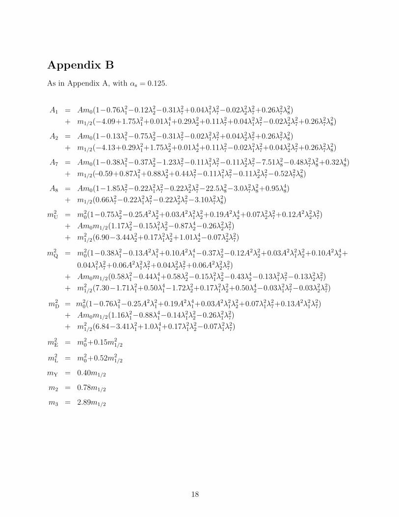
Appendix B

As in Appendix A, with αs = 0.125.

A1 = Am0(1−0.76λ21−0.12λ2

2−0.31λ27+0.04λ2

1λ27−0.02λ2

2λ27+0.26λ2

7λ28)

+ m1/2(−4.09+1.75λ21+0.01λ4

1+0.29λ22+0.11λ2

7+0.04λ21λ

27−0.02λ2

2λ27+0.26λ2

7λ28)

A2 = Am0(1−0.13λ21−0.75λ2

2−0.31λ27−0.02λ2

1λ27+0.04λ2

2λ27+0.26λ2

7λ28)

+ m1/2(−4.13+0.29λ21+1.75λ2

2+0.01λ42+0.11λ2

7−0.02λ21λ

27+0.04λ2

2λ27+0.26λ2

7λ28)

A7 = Am0(1−0.38λ21−0.37λ2

2−1.23λ27−0.11λ2

1λ27−0.11λ2

2λ27−7.51λ2

8−0.48λ27λ

28+0.32λ4

8)

+ m1/2(−0.59+0.87λ21+0.88λ2

2+0.44λ27−0.11λ2

1λ27−0.11λ2

2λ27−0.52λ2

7λ28)

A8 = Am0(1−1.85λ27−0.22λ2

1λ27−0.22λ2

2λ27−22.5λ2

8−3.0λ27λ

28+0.95λ4

8)

+ m1/2(0.66λ27−0.22λ2

1λ27−0.22λ2

2λ27−3.10λ2

7λ28)

m2U = m2

0(1−0.75λ22−0.25A2λ2

2+0.03A2λ21λ

22+0.19A2λ4

2+0.07λ22λ

27+0.12A2λ2

2λ27)

+ Am0m1/2(1.17λ22−0.15λ2

1λ22−0.87λ4

2−0.26λ22λ

27)

+ m21/2(6.90−3.44λ2

2+0.17λ21λ

22+1.01λ4

2−0.07λ22λ

27)

m2Q = m2

0(1−0.38λ21−0.13A2λ2

1+0.10A2λ41−0.37λ2

2−0.12A2λ22+0.03A2λ2

1λ22+0.10A2λ4

2+

0.04λ21λ

27+0.06A2λ2

1λ27+0.04λ2

2λ27+0.06A2λ2

2λ27)

+ Am0m1/2(0.58λ21−0.44λ4

1+0.58λ22−0.15λ2

1λ22−0.43λ4

2−0.13λ21λ

27−0.13λ2

2λ27)

+ m21/2(7.30−1.71λ2

1+0.50λ41−1.72λ2

2+0.17λ21λ

22+0.50λ4

2−0.03λ21λ

27−0.03λ2

2λ27)

m2D = m2

0(1−0.76λ21−0.25A2λ2

1+0.19A2λ41+0.03A2λ2

1λ22+0.07λ2

1λ27+0.13A2λ2

1λ27)

+ Am0m1/2(1.16λ21−0.88λ4

1−0.14λ21λ

22−0.26λ2

1λ27)

+ m21/2(6.84−3.41λ2

1+1.0λ41+0.17λ2

1λ22−0.07λ2

1λ27)

m2E = m2

0+0.15m21/2

m2L = m2

0+0.52m21/2

mY = 0.40m1/2

m2 = 0.78m1/2

m3 = 2.89m1/2

18

Appendix C

As in Appendix A, with αs = 0.113.

A1 = Am0(1−0.80λ21−0.13λ2

2−0.30λ27+0.03λ2

1λ27−0.02λ2

2λ27+0.24λ2

7λ28)

+ m1/2(−3.65+1.64λ21+0.01λ4

1+0.28λ22+0.10λ2

7+0.04λ21λ

27−0.02λ2

2λ27+0.24λ2

7λ28)

A2 = Am0(1−0.13λ21−0.79λ2

2−0.30λ27−0.02λ2

1λ27+0.03λ2

2λ27+0.24λ2

7λ28)

+ m1/2(−3.69+0.27λ21+1.65λ2

2+0.01λ42+0.10λ2

7−0.02λ21λ

27+0.04λ2

2λ27+0.24λ2

7λ28)

A7 = Am0(1−0.40λ21−0.39λ2

2−1.21λ27−0.11λ2

1λ27−0.11λ2

2λ27−7.33λ2

8−0.47λ27λ

28+0.15λ4

8)

+ m1/2(−0.57+0.82λ21+0.83λ2

2+0.42λ27−0.10λ2

1λ27−0.10λ2

2λ27−0.49λ2

7λ28)

A8 = Am0(1−1.82λ27−0.21λ2

1λ27−0.21λ2

2λ27−22.0λ2

8−2.84λ27λ

28+0.46λ4

8)

+ m1/2(0.62λ27−0.21λ2

1λ27−0.21λ2

2λ27−2.87λ2

7λ28)

m2U = m2

0(1−0.79λ22−0.26A2λ2

2+0.04A2λ21λ

22+0.20A2λ4

2+0.07λ22λ

27+0.13A2λ2

2λ27)

+ Am0m1/2(1.10λ22−0.14λ2

1λ22−0.86λ4

2−0.24λ22λ

27)

+ m21/2(5.74−2.99λ2

2+0.15λ21λ

22+0.89λ4

2−0.06λ22λ

27)

m2Q = m2

0(1−0.40λ21−0.13A2λ2

1+0.11A2λ41−0.39λ2

2−0.13A2λ22+0.03A2λ2

1λ22+0.10A2λ4

2+

0.03λ21λ

27+0.06A2λ2

1λ27+0.03λ2

2λ27+0.06A2λ2

2λ27)

+ Am0m1/2(0.55λ21−0.43λ4

1+0.55λ22−0.14λ2

1λ22−0.43λ4

2−0.12λ21λ

27−0.12λ2

2λ27)

+ m21/2(6.15−1.48λ2

1+0.44λ41−1.50λ2

2+0.15λ21λ

22+0.44λ4

2−0.03λ21λ

27−0.03λ2

2λ27)

m2D = m2

0(1−0.80λ21−0.27A2λ2

1+0.21A2λ41+0.03A2λ2

1λ22+0.07λ2

1λ27+0.13A2λ2

1λ27)

+ Am0m1/2(1.09λ21−0.86λ4

1−0.14λ21λ

22−0.24λ2

1λ27)

+ m21/2(5.70−2.97λ2

1+0.88λ41+0.15λ2

1λ22−0.06λ2

1λ27)

m2E = m2

0+0.15m21/2

m2L = m2

0+0.50m21/2

mY = 0.42m1/2

m2 = 0.79m1/2

m3 = 2.67m1/2

19

References

[1] J. Ellis, Phil. Trans. R. Soc. Lond. A336 (1991) 247, Phys. Scr. T36 (1991) 142

[2] H. Goldberg, Phys. Rev. Lett. 50 (1983) 1419;L.M. Krauss, Nucl. Phys. B227 (1983) 556;J. Ellis, J.S. Hagelin, D.V. Nanopoulos, K.A. Olive and M. Srednicki, Nucl. Phys.B238 (1984) 453K. Griest, Phys. Rev. D38 (1988) 2357

[3] K.A. Olive and M.Srednicki, Phys. Lett. 230B (1989) 78;K.A. Olive and M.Srednicki, Nucl. Phys. B355 (1991) 208;J.M. McDonald, K.A. Olive and M. Srednicki, Phys. Lett. B283 (1992) 80

[4] K. Griest, M. Kamionkowski and M.S. Turner, Phys. Rev. D41 (1990) 3565

[5] R. Barbieri, M. Frigeni and G. Giudice, Nucl. Phys. B313 (1989) 725;J. Ellis, L. Roszkowski and Z. Lalak, Phys. Lett. 245B (1990) 545

[6] L. Krauss, Phys. Rev. Lett. 64 (1990) 999;J. Ellis, D.V. Nanopoulos, D.N. Schramm and L. Roszkowski, Phys. Lett. B245 (1990)251

[7] L. Roszkowski, Phys. Lett. 262 (1991) 59, Proc. Joint Lepton-Photon Symp. & Eu-rophys. Conf. on High Energy Phys., Geneva, eds. S. Hegarty et al (World-Scientific,1992) Vol.1, p.498

[8] J.L. Lopez, K. Yuan and D.V. Nanopoulos, Phys. Lett. 267B (1991) 219;J.L. Lopez, D.V. Nanopoulos and K. Yuan, Nucl. Phys. B370 (1992) 445;S. Kelley, J.L. Lopez, D.V. Nanopoulos, H. Pois and K. Yuan, Texas preprint CTP-TAMU-56/92 (1992)

[9] J. Ellis and L. Roszkowski, Phys. Lett. 283B (1992) 252

[10] M. Drees and M.M. Nojiri, DESY preprint 92-101/SLAC preprint PUB-5860 (1992)

[11] J. Ellis, J.F. Gunion, H.E. Haber, L. Roszkowski and F. Zwirner, Phys. Rev. D39(1989) 844

[12] B.R. Greene and P.J. Miron, Phys. Lett. 168B (1986) 226

[13] R. Flores, K.A. Olive and and D. Thomas, Phys. Lett. 245B (1990) 509

[14] K.A. Olive and D. Thomas, Nucl. Phys. B355 (1991) 192

[15] E.W. Kolb and M.S. Turner, The Early Universe (Addison-Wesley, 1990)

[16] J. Binney and S. Tremaine, Galactic Dynamics (Princeton, 1988)

20

[17] N. Kaiser, Proc. Texas/ESO-CERN Conf., Brighton, ed. J. Barrow (1992) in press;O. Lahav, in After the First Three Minutes, eds. S.S. Holt et al (AIP, 1991) p.421

[18] E.L. Wright et al, Astrophys. J. 396 (1992) L13;N. Gouda and N.Sugiyama, Astrophys. J. 395 (1992) L59;G. Efstathiou, J.R. Bond and S.D.M. White, Mon. Not. R. Astr. Soc. 258 (1992) 1p

[19] J. Ellis, G. Ridolfi and F. Zwirner, Phys. Lett. 262B (1991) 477

[20] J.-P Derendinger and C.A Savoy, Nucl. Phys. B237 (1984) 307

[21] S.M. Barr, Phys. Lett. 112B (1982) 219;I. Antoniadis, J. Ellis, J.S. Hagelin and D.V. Nanopoulos, Phys. Lett. 194B (1987)231;B.A. Campbell, J. Ellis, J.S. Hagelin, D.V. Nanopoulos and R. Ticciati, Phys. Lett.198B (1987) 200

[22] I. Antoniadis, J. Ellis, J.S. Hagelin and D.V. Nanopoulos, Phys. Lett. 208B (1988)209;J.L. Lopez and D.V. Nanopoulos, Nucl. Phys. B338 (1990) 73;J.L. Lopez and D.V. Nanopoulos, Phys. Lett. 251B (1990) 73;J.L. Lopez and D.V. Nanopoulos, Phys. Lett. 268B (1991) 359

[23] J. Ellis, J.S. Hagelin, S. Kelley and D.V. Nanopoulos, Nucl. Phys. B311 (1988/89) 1

[24] F. Gabbiani and A. Masiero, Phys. Lett. 209B (1988) 289;S.M. Barr, Phys. Rev. D40 (1989) 2457;A.E. Faraggi, J.L. Lopez, D.V. Nanopoulos, Phys. Lett. 221B (1989) 337;S.A. Abel, W.N. Cottingham and I.B. Whittingham, Phys. Lett. 236B (1990) 305;J. Rizos and K. Tamvakis, Phys. Lett. 251B (1990) 369;J. Ellis, J.L. Lopez and D.V. Nanopoulos, Phys. Lett. 252B (1990) 53;S. Kelley, J.L. Lopez and D.V. Nanopoulos, Texas preprint CPT-TAMU-90/90 (1990)

[25] H. Komatsu, Phys. Lett. 177B (1986) 201;S.A. Abel, W.N. Cottingham and I.B. Whittingham, Phys. Lett. 244B (1990) 327

[26] J. Ellis, J.S. Hagelin, S. Kelley, D.V. Nanopoulos and K.A. Olive, Phys. Lett. 209B(1988) 283;M. J.McDonald, Phys. Lett. 225B (1989) 133

[27] J. Ellis, J.L. Lopez, and D.V. Nanopoulos, Phys. Lett. 247B (1990) 257

[28] J. Ellis, G.B. Gelmini and S. Sarkar, Nucl. Phys. B373 (1992) 399;P. Gondolo, G.B. Gelmini and S. Sarkar, UCLA preprint 91/TEP/31 (1991);S. Sarkar, Nucl. Phys. B (Proc. Suppl.) 28A (1992) 405

[29] S.A. Abel, Ph.D. theis, University of Bristol (1990) unpublished

21

[30] A.B. Lahanas and D.V. Nanopoulos, Phys. Rep. 145 (1987) 1

[31] H. Burkhardt and J. Steinberger, Ann. Rev. Nucl. Part. Sci. 41 (1991) 55;P. Langacker, M. Luo and A. K.Mann, Rev. Mod. Phys. 64 (1992) 87

[32] S. Bethke and S. Catani, CERN preprint TH.6484/92;S. Bethke, Proc. XXVI Intern. Conf. on High Energy Phys., Dallas (1992) in press

[33] L.E. Ibanez, C. Lopez and C. Munoz, Nucl. Phys. B256 (1985) 218

[34] B.W. Lee and S. Weinberg, Phys. Rev.Lett. 39 (1977) 165;M.I. Vysotskii, A.D. Dolgov and Ya B. Zeldovich, JETP Lett. 26 (1977) 188

[35] J. Bernstein, L.S. Brown and G. Feinberg, Phys. Rev. D32 (1985) 3261;J. Bernstein, Kinetic Theory in the Expanding Universe, (Cambridge, 1988)

[36] P. Gondolo and G. Gelmini, Nucl. Phys. B360 (1991) 145

[37] K. Griest and D. Seckel, Phys. Rev. D43 (1991) 3191

[38] M. Srednicki, R. Watkins and K.A. Olive, Nucl. Phys. B310 (1988) 693

[39] S. Dimopoulos, R. Esmailzadeh, L.J. Hall and G. Starkman, Phys. Lett. B247 (1990)601

[40] J.C. Mather et al, Astrophys. J. Lett. 354 (1990) L37;H.P. Gush, M. Halpern and E.H. Wishnow, Phys. Rev. Lett. 65(1990)537;R.B. Partridge, in Cosmology and Large-Scale Structure in the Universe, ed. R.R. deCarvalho (ASP, 1992) p.97

[41] S. Mizuta and M. Yamaguchi, Tohoku preprint TU-409 (1992)

[42] G.G. Ross and R.G. Roberts, RAL preprint 92-005 (1992)

[43] M. Davier, Proc. Joint Lepton-Photon Symp. & Europhys. Conf. on High EnergyPhys., Geneva, eds. S. Hegarty et al (World-Scientific, 1991) Vol.2, p.151

[44] A. Laasanen, Proc. Particles and Fields ’91, Vancouver (APS, 1992) in press

[45] L. Rolandi, Proc. XXVI Intern. Conf. on High Energy Phys., Dallas (1992) in press

[46] J. Ellis, G. Fogli and E. Lisi, Phys. Lett. B274 (1992) 456;F. del Aguila, M. Martınez and M. Quiros, Nucl. Phys. B381 (1992) 451

22

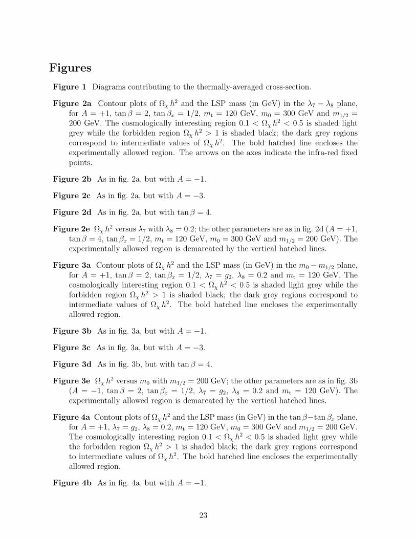
Figures

Figure 1 Diagrams contributing to the thermally-averaged cross-section.

Figure 2a Contour plots of Ωχ h2 and the LSP mass (in GeV) in the λ7 − λ8 plane,for A = +1, tanβ = 2, tan βx = 1/2, mt = 120 GeV, m0 = 300 GeV and m1/2 =200 GeV. The cosmologically interesting region 0.1 < Ωχ h2 < 0.5 is shaded lightgrey while the forbidden region Ωχ h2 > 1 is shaded black; the dark grey regionscorrespond to intermediate values of Ωχ h2. The bold hatched line encloses theexperimentally allowed region. The arrows on the axes indicate the infra-red fixedpoints.

Figure 2b As in fig. 2a, but with A = −1.

Figure 2c As in fig. 2a, but with A = −3.

Figure 2d As in fig. 2a, but with tanβ = 4.

Figure 2e Ωχ h2 versus λ7 with λ8 = 0.2; the other parameters are as in fig. 2d (A = +1,tanβ = 4, tanβx = 1/2, mt = 120 GeV, m0 = 300 GeV and m1/2 = 200 GeV). Theexperimentally allowed region is demarcated by the vertical hatched lines.

Figure 3a Contour plots of Ωχ h2 and the LSP mass (in GeV) in the m0 −m1/2 plane,for A = +1, tanβ = 2, tanβx = 1/2, λ7 = g2, λ8 = 0.2 and mt = 120 GeV. Thecosmologically interesting region 0.1 < Ωχ h2 < 0.5 is shaded light grey while theforbidden region Ωχ h2 > 1 is shaded black; the dark grey regions correspond tointermediate values of Ωχ h2. The bold hatched line encloses the experimentallyallowed region.

Figure 3b As in fig. 3a, but with A = −1.

Figure 3c As in fig. 3a, but with A = −3.

Figure 3d As in fig. 3b, but with tan β = 4.

Figure 3e Ωχ h2 versus m0 with m1/2 = 200 GeV; the other parameters are as in fig. 3b(A = −1, tan β = 2, tan βx = 1/2, λ7 = g2, λ8 = 0.2 and mt = 120 GeV). Theexperimentally allowed region is demarcated by the vertical hatched lines.

Figure 4a Contour plots of Ωχ h2 and the LSP mass (in GeV) in the tanβ−tan βx plane,for A = +1, λ7 = g2, λ8 = 0.2, mt = 120 GeV, m0 = 300 GeV and m1/2 = 200 GeV.The cosmologically interesting region 0.1 < Ωχ h2 < 0.5 is shaded light grey whilethe forbidden region Ωχ h2 > 1 is shaded black; the dark grey regions correspondto intermediate values of Ωχ h2. The bold hatched line encloses the experimentallyallowed region.

Figure 4b As in fig. 4a, but with A = −1.

23

Figure 5 Contour plots of Ωχ h2 and the LSP mass (in GeV) in the tan β − A plane,for tan βx = 1/2, λ7 = g2, λ8 = 0.2, mt = 120 GeV, m0 = 300 GeV and m1/2 = 200GeV. The cosmologically interesting region 0.1 < Ωχ h2 < 0.5 is shaded light greywhile the forbidden region Ωχ h2 > 1 is shaded black; the dark regions correspondto intermediate values of Ωχ h2. The bold hatched line encloses the experimentallyallowed region.

24