calculations of neutralino-stop coannihilation in the cmssm

hep-ph/0112113

CERN–TH/2001-339

UMN–TH–2032/01

TPI–MINN–01/50

Calculations of Neutralino-Stop Coannihilation in the CMSSM

John Ellis1, Keith A. Olive2 and Yudi Santoso2

1TH Division, CERN, Geneva, Switzerland

2Theoretical Physics Institute, University of Minnesota, Minneapolis, MN 55455, USA

Abstract

We present detailed calculations of the χt1 coannihilation channels that have the largest

impact on the relic χ density in the constrained minimal supersymmetric extension of the

Standard Model (CMSSM), in which scalar masses m0, gaugino masses m1/2 and the trilinear

soft supersymmetry-breaking parameters A0 are each assumed to be universal at some input

grand unification scale. The most important t1t∗1 and t1t1 annihilation channels are also

calculated, as well as t1 ˜ coannihilation channels. We illustrate the importance of these new

coannihilation calculations when A0 is relatively large. While they do not increase the range

of m1/2 and hence mχ allowed by cosmology, these coannihilation channels do open up new

‘tails’ of parameter space extending to larger values of m0.

CERN–TH/2001-339

November 2001

1 Introduction

A favoured candidate for cold dark matter is the lightest supersymmetric particle (LSP),

which is generally thought to be the lightest neutralino χ [1] in the minimal supersym-

metric extension of the Standard Model (MSSM). It is common to focus attention on the

constrained MSSM (CMSSM), in which all the soft supersymmetry-breaking scalar masses

m0 are required to be equal at an input superysmmetric GUT scale, as are the gaugino

masses m1/2 and the trilinear soft supersymmetry-breaking parameters A0. These assump-

tions yield well-defined relations between the various sparticle masses, and correspondingly

more definite predictions for the relic abundance Ωχh2 and observable signatures. This paper

is devoted to relic-abundance calculations including coannihilations of the lightest neutralino

χ with t1, the lighter supersymmetric partner of the top quark [2].

The range 0.1 < Ωχh2 < 0.3 is generally thought to be preferred by astrophysics and

cosmology [3]. Lower values of Ωχh2 might be possible if there is some other source of

cold dark matter, but higher values are incompatible with observation. The regions of the

m1/2, m0 plane where the relic density falls within the preferred range 0.1 < Ωχh2 < 0.3 have

generally been divided into four generic parts. There is a ‘bulk’ region at moderate m1/2

and m0 [1]. Then, extending to larger m1/2, there is a ‘tail’ of the parameter space where

the LSP χ is almost degenerate with the next-to-lightest supersymmetric particle (NLSP),

which is in this region the τ1, the lighter supersymmetric partner of the τ lepton. Along

this ‘tail’, efficient coannihilations [4, 5, 6] keep Ωχh2 down in the preferred range, even for

larger values of mχ [7, 8, 9, 10]. At larger m0, close to the boundary where electroweak

symmetry breaking is no longer possible, there is the ‘focus-point’ region where the LSP has

a larger Higgsino component and mχ is small enough for Ωχh2 to be acceptable [11]. Finally,

extending to larger m1/2 and m0 at intermediate values of m1/2/m0, there may be a ‘funnel’

of CMSSM parameter space where rapid direct-channel annihilations via the poles of the

heavier Higgs bosons A and H keep Ωχh2 in the preferred range [12, 13].

In this paper, we emphasize the significance of coannihilation of the LSP χ with t1, the

lighter supersymmetric partner of the t quark [2]. This mechanism opens up another ‘tail’

of parameter space, this time extending to larger values of m0. It is not relevant for the

small values of A0 considered in previous coannihilation calculations [8, 9, 10], but may

be important for large A0, as we demonstrate in this paper. Coannihilations of χ with t1

are important when the latter is the NLSP, just as χτ1 coannihilations are important when

the τ1 is the NLSP. In the latter case, one must also consider coannihilations with the e1

and µ1, which are not much heavier than the τ1 [7, 8, 9, 10]. There are also regions of

1

CMSSM parameter space where both the t1 and τ1 are close in mass to the LSP χ, and

t1τ1 coannihilations must also be considered. We present here detailed calculations of the

matrix elements and cross sections for all the leading χt1 and t1 ˜ coannihilation processes,

and illustrate their importance for Ωχh2 in some instances in the CMSSM when A0 6= 0.

The structure of the paper is as follows. In Section 2 we recall some important features

of LSP relic-density calculations in general, and coannihilations in particular. Then, in

Section 3 we compare the relative magnitudes of the χχ, χt1, t1t(∗)1 and t1 ˜(∗) processes

for some specific choices of the CMSSM parameters. Section 4 provides an overview of

the implications of χt1 coannihilation and related processes for the regions of the m1/2, m0

plane allowed by the constraint 0.1 < Ωχh2 < 0.3 for various choices of the other CMSSM

parameters. Relevant details of our calculations of the matrix elements are contained in an

Appendix.

2 Formalism for Annihilation and Coannihilation

The density of neutralino relics left over from the early Universe may be determined relatively

simply in terms of relevant annihilation cross sections, using the Boltzmann rate equation to

determine a freeze-out density. The relic density subsequently scales with the inverse of the

comoving volume, and hence with the entropy density. In the MSSM framework discussed

here, since neutralinos are Majorana fermions, the S-wave annihilation cross sections into

fermion-antifermion pairs are suppressed by the masses of the final-state fermions, and it is

therefore necessary to compute P -wave contributions to the cross sections [1].

The rate equation for a stable particle with density n is

dn

dt= −3

R

Rn− 〈σvrel〉(n2 − n2

eq) , (1)

where neq is the equilibrium number density and 〈σvrel〉 is the thermally averaged product of

the annihilation cross section σ and the relative velocity vrel. In the early Universe, we can

write R/R = (8πGNρ/3)1/2, where ρ = π2g(T )T 4/30 is the energy density in radiation and

g(T ) is the number of relativistic degrees of freedom. Conservation of the entropy density

s = 2π2h(T )T 4/45 implies that R/R = −T /T − h′T /3h where h′ ≡ dh/dT . Generally, we

have h(T ) ≈ g(T ). Defining x ≡ T/m and q ≡ n/T 3h, we can write

dq

dx= m

(4π3

45GNg

)−1/2 (h + 1

3mxh′

)〈σvrel〉(q2 − q2

eq) . (2)

The effect of the h′ term was discussed in detail in [14], and is most important when the

mass m is between 2 and 10 GeV. Since we only consider neutralinos that are significantly

2

more massive, we neglect it below (though it is not neglected in our calculations). In the

case of the MSSM, freeze-out occurs when x ∼ 1/20, and the final relic density is determined

by integrating (1) down to x = 0, and is given by

ρχ = mq(0)h(0)T 30 . (3)

When coannihilations are important, there are several relevant particle species i, each

with different mass, number density ni and equilibrium number density neq,i. Even in such a

situation [4], the rate equation (1) still applies, provided n is interpreted as the total number

density,

n ≡∑

i

ni , (4)

neq as the total equilibrium number density,

neq ≡∑

i

neq,i , (5)

and the effective annihilation cross section as

〈σeffvrel〉 ≡∑ij

neq,ineq,j

n2eq

〈σijvrel〉 . (6)

In (2), m is now understood as the mass of the lightest particle under consideration. For

T <∼ mi, the equilibrium number density of each species is given by [14, 15]

neq,i = gi

∫ d3p

(2π)3e−E/T

=gim

2i T

2π2K2(mi/T ) ,

= gi

(miT

2π

)3/2

exp(−mi/T )(1 +

15T

8mi

+ . . .)

, (7)

where gi is a spin and color degeneracy factor and K2(x) is a modified Bessel function.

We make the approximation of Boltzmann statistics for the annihilating particles, which is

excellent in practice.

We now recall how to compute 〈σ12vrel〉 for the process 1+2 → 3+4 in an efficient manner.

Suppose we have determined the squared transition matrix element |T |2 (summed over final

spins and averaged over initial spins) and expressed it as a function of the Mandelstam

variables s, t, u. We then express |T |2 in terms of s and the scattering angle θCM in the

center-of-mass frame, as described in [8]. We now define

w(s) ≡ 1

4

∫d3p3

(2π)3E3

d3p4

(2π)3E4

(2π)4δ4(p1 + p2 − p3 − p4) |T |2

=1

32π

p3(s)

s1/2

∫ +1

−1d cos θCM |T |2 . (8)

3

In terms of w(s), the total annihilation cross section σ12(s) is given by σ12(s) = w(s)/s1/2p1(s)1.

The above analysis is exact. To reproduce the usual partial wave expansion, we expand

|T |2 in powers of p1(s)/m1. The odd powers vanish upon integration over θCM, while the

zeroth- and second-order terms correspond to the usual S and P waves, respectively. Each

factor of p1(s) is accompanied by a factor of cos θCM, so we have∫ +1

−1d cos θCM |T |2 =

(|T |2cos θCM→+1/

√3 + |T |2cos θCM→−1/

√3

)+O(p4

1) . (9)

We can therefore evaluate the S- and P -wave contributions to w(s) simply by evaluating

|T |2 at two different values of cos θCM; no integrations are required.

The proper procedure for thermal averaging has been discussed in [14, 15] for the case of

m1 = m2, and in [16, 6] for the case of m1 6= m2, so we do not discuss it in detail here. One

finds

〈σ12vrel〉 = a12 + b12 x +O(x2) , (10)

where x ≡ T/m1 (assuming m1 < m2). In our case, we extract a12 and b12 from the transition

amplitudes listed in the Appendix for each final state. We set x = 0 to get a12, and then

compute b12 by setting x to a numerical value small enough to render the O(x2) terms

negligible. We then compute aeff and beff by performing the sum over initial states as in (6),

and integrate the rate equation (2) numerically to obtain the relic LSP abundance. To a fair

approximation, the relic density can simply be written as [1, 4]

Ωh2 ≈ 109 GeV−1

g1/2f Mpl(aeff + beffxf/2)xf

, (11)

where the freeze-out temperature Tf ∼ mχ/20, and gf is the number of relativistic degrees

of freedom at Tf .

This implies that the ratio of relic densities computed with and without coannihilations

is approximately

R ≡ Ω0

Ω≈(

σeff

σ0

)(xf

x0f

), (12)

where σ ≡ a+bx/2 and sub- and superscripts 0 denote quantities computed ignoring coanni-

hilations. The ratio x0f/xf ≈ 1+x0

fln(geffσeff/g1σ0), where geff ≡

∑i gi(mi/m1)

3/2e−(mi−m1)/T .

For the case where the t1 and χ are almost degenerate, geff ≈∑

i gi = 8 and x0f /xf ≈ 1.2.

1Our w(s) is also the same as w(s) in [14, 16, 7], which is written as W/4 in [6].

4

3 Coannihilation Rates for t1 in the MSSM

We now use the above formalism to estimate the relative importance of the t1χ coannihilation

processes, t1t∗1 and t1t1 annihilations calculated in the Appendix. We also take into account

the χ˜ coannihilations calculated previously [7, 8] and, for completeness, include the t1 ˜ and

t1 ˜∗ coannihilations also calculated in the Appendix.

To compute the effective annihilation cross sections for light sparticles in the MSSM, we

allow the index i in (4) to run over t1, t∗1, τ1, τ

∗1, eR, e∗

R, µR and µ∗

R, as well as χ. The following

is the change in σeff compared with [8], where 49 of the σij in (6) were already included:

∆σeff = 2 (σt1 t1 + σt1 t∗1)r2

t1+ 4 σχt1

rχrt1 + 8 (σt1eR+ σt1 e∗

R)rt1reR

+ 4 (σt1τ1 + σt1 τ∗1)rτ1

rt1 (13)

where ri ≡ neq,i/neq. We have taken the eR and µR (but not the τ) to be degenerate in mass,

thus accounting for the 81 possible initial state combinations. Note that we have summed

over color states in the cross sections amplitudes listed in the Appendix, and we have taken

the stop degeneracy factor gt = 3. We list in Table 1 the sets of initial and final states for

which we compute the annihilation cross sections, using the transition amplitudes given in

the Appendix. We use q to denote the four light quarks, which we have taken to be massless.

Table 1: Initial and Final States for t1 Annihilation and Coannihilation Processes

Initial State Final States

t1t∗1 gg, γg, Zg, tt, bb, qq, gh, gH, Zh, ZH, ZA, W±H∓,

hh, hH, HH, AA, hA, HA, H+H−

t1t1 ttχt1 tg, tZ, bW+, tH, th, tA, bH+

t1 ˜ t`, bν

t1 ˜∗ t¯

In the CMSSM, the diagonal entries of the squark mass matrix tend to pick up large

contributions from the gaugino masses, m2LL,RR 3 O(6)m2

1/2, thus making the squarks heavier

than the neutralinos. The off-diagonal entry for an up-type squark 2

m2LR = −mq(Aq + µ cotβ) (14)

can, however, be large, particularly for the stops, or for sbottoms at large tanβ 3. When

At is sufficiently large, the lighter stop, t1, can become degenerate with (or lighter than)2Note here our sign convention for Aq.3For down-type squarks, the factor cotβ in (14) is replaced by tanβ.

5

100 200 300 400 500

10-6

10-7

10-8

10-9

10-10

10-11

σtχ

→X

(

GeV

-2)

∼∼

m0 (GeV)

tan β = 10, A0 = 1000 GeV

^

m1/2 = 230 GeV

200 400 600 800 1000

σχχ→all

Tot

t h

t g

10-6

10-7

10-8

10-9

10-10

10-11

σtχ

→X

(

GeV

-2)

∼∼

m0 (GeV)

tan β = 10, A0 = 2000 GeV

^

^ ∼∼

m1/2 = 450 GeV

b W+

t Z

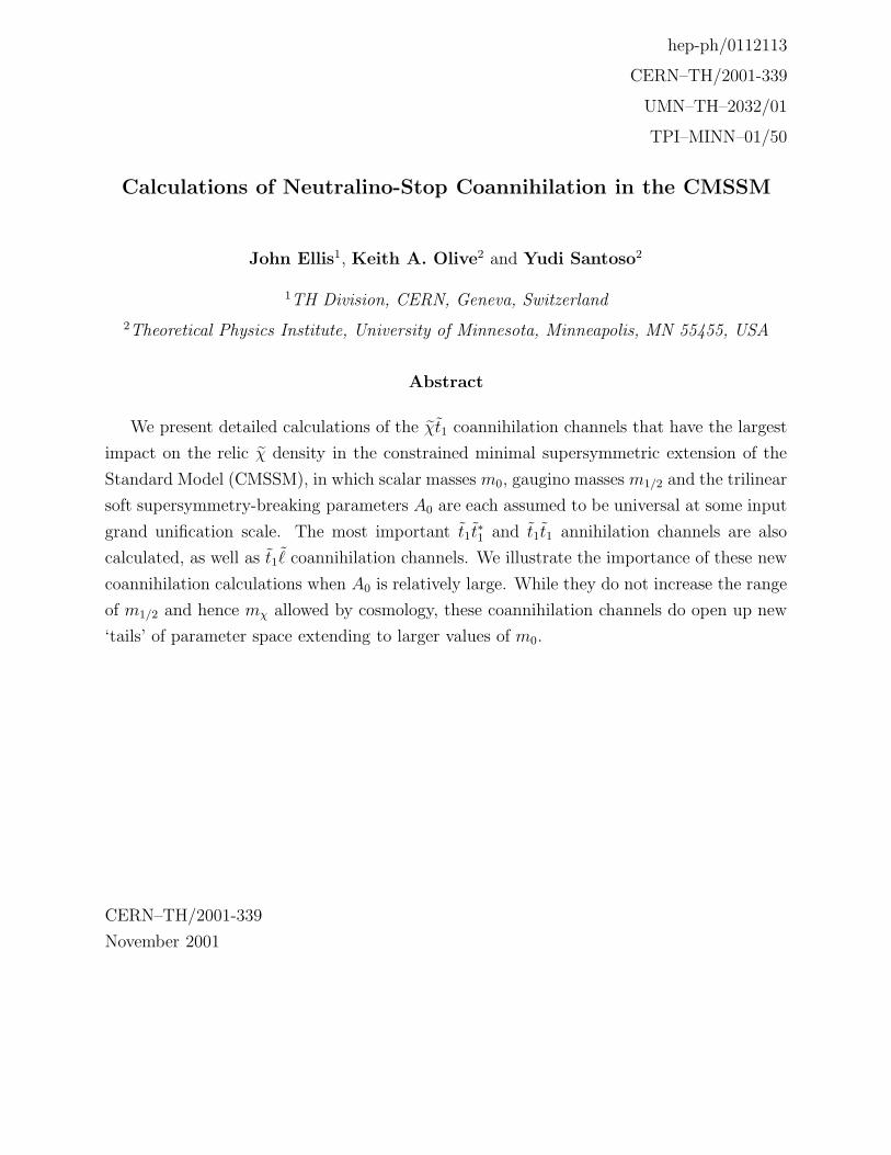
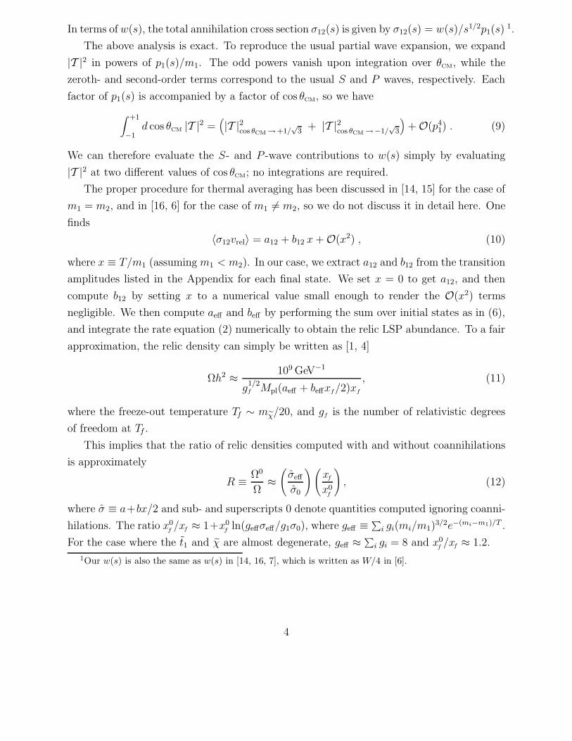
Figure 1: The separate contributions to the χt1 coannihilation cross sections σ ≡ a + 12bx

for x = T/mχ = 1/23 as functions of m0 for (a) m1/2 = 230 GeV, A0 = 1000 GeV and (b)m1/2 = 450 GeV, A0 = 2000 GeV. Also shown are the total cross section and , for comparison,the much smaller total cross section for χχ annihilation.

the neutralino. Thus, it is when A0 is large that we expect χt1 coannihilations to become

important.

It is important to distinguish between the effective low-energy parameters At, etc.,

and the high-energy input parameter A0, which are related through the running of the

renormalization-group equations. For example, for tan β = 10 and m0 = 300 GeV, t1χ

coannihilations are important when m1/2 = 200, 450,and 670 GeV and A0 = 1000, 2000,

and 3000 GeV, but these values correspond to At ' 565, 1200, and 1700 GeV respectively.

Furthermore, the values of A for the light squarks are different and typically larger than At.

We display in Fig. 1 numerical values of the contributions to σ ≡ a + bx/2 (see (11))

in χt1 coannihilation, for the representative values x = 1/23, tanβ = 10, µ > 0 and (a)

m1/2 = 230 GeV, A0 = 1000 GeV and (b) m1/2 = 450 GeV, A0 = 2000 GeV as functions of m0.

For comparison, the total cross section for χχ annihilation to all final states is also shown, as

a thick dotted line. We see that the χt1 → tg and th coannihilation cross sections dominate

by large factors over the total χχ annihilation cross section, suggesting that they may have a

greater importance than that suggested by simply comparing Boltzmann suppression factors.

The feature in Fig. 1(a) at m0 ∼ 400 GeV is due to the threshold for the production of th

final states. At smaller values of m0, this final state is kinematically forbidden.

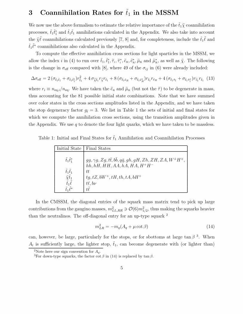
Fig. 2 displays similar plots for t1t∗1 annihilation, for the same parameter choices as in

Fig. 1. In this case, the dominant t1t∗1 annihilation cross sections are into gg and hh, and even

6

100 200 300 400 500

10-5

10-6

10-7

10-8

10-9

10-10

m0 (GeV)

tan β = 10, A0 = 1000 GeV

σtt

*→

X

(GeV

-2)

∼∼^

m1/2 = 230 GeV

200 400 600 800 1000

σχχ→all

Tot

h h

g h

b b

γ g

g g

_u u _

t t _

10-5

10-6

10-7

10-8

10-9

10-10

σtt

*→

X

(G

eV-2

) ∼∼

m0 (GeV)

tan β = 10, A0 = 2000 GeV

^

^ ∼∼

m1/2 = 450 GeV

Z g

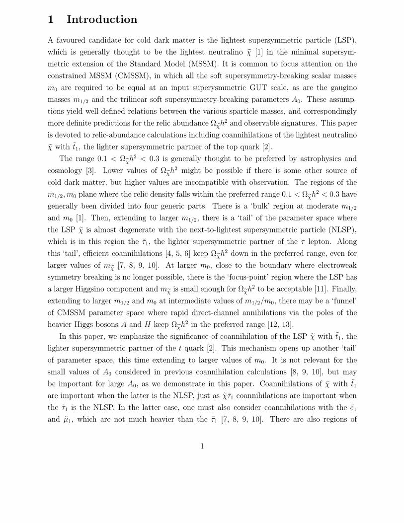
Figure 2: The separate contributions to the t1t∗1 annihilation cross sections σ ≡ a + 1

2bx

for x = T/mχ = 1/23, as functions of m0 for (a) m1/2 = 230 GeV, A0 = 1000 GeV and (b)m1/2 = 450 GeV, A0 = 2000 GeV. Also shown are the total cross section and, for comparison,the much smaller total cross section for χχ annihilation.

subdominant cross sections such as γg, Zg, gh and the various quark-antiquark channels are

far larger than the total χχ annihilation cross section. Once again, when A0 = 1000 GeV

we see thresholds, in this case corresponding to hh production at m0 ∼ 180 GeV and tt

production at m0 ∼ 330 GeV.

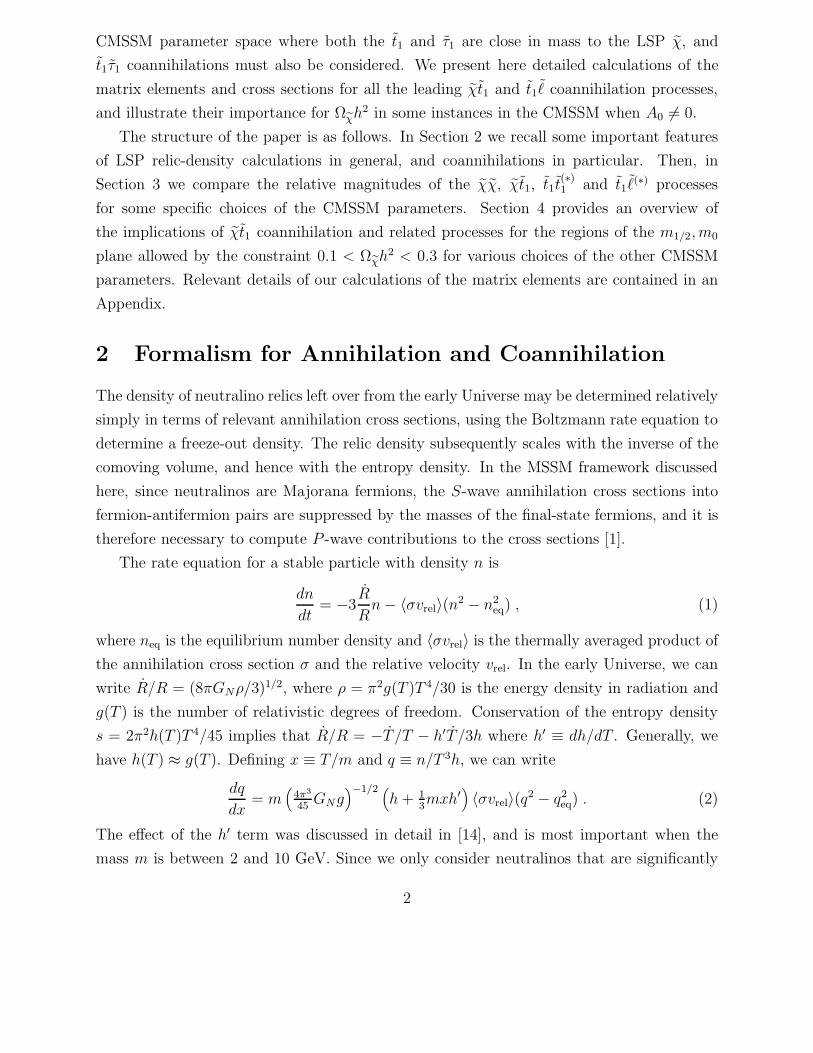
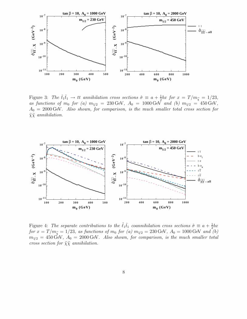
The t1t1 annihilation cross sections shown in Fig. 3 show that the cross section for anni-

hilation into the tt final state, when it is kinematically open, is also far larger than the total

χχ annihilation cross section.

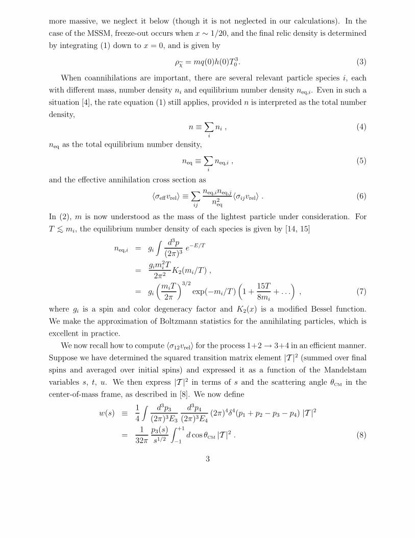
A complete study of coannihilation effects must include not only the χ˜ processes consid-

ered previously [7, 8], and the χt1 processes considered above, but also ˜1t1 coannihilations.

Accordingly, the final set of coannihilation cross sections we present are those for ˜1t1 and

˜∗1t1, shown in Fig. 4. We see that, when (a) A0 = 1000 GeV, the tτ , tτ and bνe final states

are the most important, followed by te, bντ and te, whereas (b) the tτ and te final states

are relatively much less important when A0 = 2000 GeV. In all panels of Fig. 4, there are

coannihilation cross sections much greater than the total χχ annihilation cross section, which

is also plotted.

The basic reason for the relatively small magnitude of the χχ annihilation cross section is

that it is dominated by the P -wave suppressed cross sections for χχ annihilation to fermion

pairs. This was also the basic reason why χ˜ coannihilation processes were previously found

to be so important [7, 8, 9, 10].

7

100 200 300 400 50010-11

10-7

10-8

10-9

10-10σtt

→X

(

GeV

-2)

∼∼

m0 (GeV)

tan β = 10, A0 = 1000 GeV

^

m1/2 = 230 GeV

200 400 600 800 1000

σχχ→all

t t

10-11

10-7

10-8

10-9

10-10σtt

→X

(

GeV

-2)

∼∼

m0 (GeV)

tan β = 10, A0 = 2000 GeV

^

^ ∼∼

m1/2 = 450 GeV

Figure 3: The t1t1 → tt annihilation cross sections σ ≡ a + 12bx for x = T/mχ = 1/23,

as functions of m0 for (a) m1/2 = 230 GeV, A0 = 1000 GeV and (b) m1/2 = 450 GeV,A0 = 2000 GeV. Also shown, for comparison, is the much smaller total cross section forχχ annihilation.

100 200 300 400 50010-11

10-7

10-8

10-9

10-10σtl

→X

(

GeV

-2)

∼∼

m0 (GeV)

tan β = 10, A0 = 1000 GeV

^

m1/2 = 230 GeV

200 400 600 800 1000

σχχ→all

t τ

b νe

t e

b ντ

10-11

10-7

10-8

10-9

10-10σtl

→X

(

GeV

-2)

∼∼

m0 (GeV)

tan β = 10, A0 = 2000 GeV

t e _ t τ _

^

^ ∼∼

m1/2 = 450 GeV

Figure 4: The separate contributions to the ˜1t1 coannihilation cross sections σ ≡ a + 1

2bx

for x = T/mχ = 1/23, as functions of m0 for (a) m1/2 = 230 GeV, A0 = 1000 GeV and (b)m1/2 = 450 GeV, A0 = 2000 GeV. Also shown, for comparison, is the much smaller totalcross section for χχ annihilation.

8

The contributions of the various annihilation channels to σeff are weighted by the rela-

tive abundances of the χ, t1 and ˜1. For a stop degenerate with the χ, t1t

∗1 annihilation,

t1t1 annihilation and χt1 coannihilation are clearly the dominant contributions to ∆σeff , and

hence to σeff in (6), and the final neutralino relic density is greatly reduced. As the stops

become heavier than the neutralinos, their number densities are exponentially suppressed

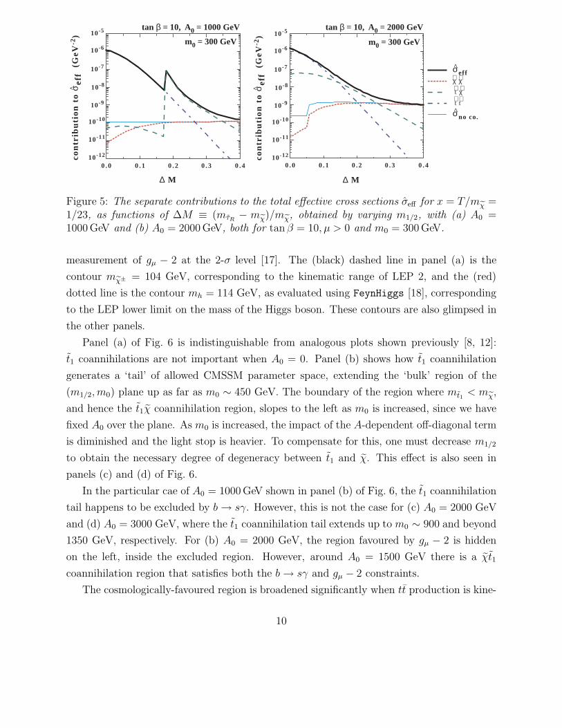
and the stop contributions to σeff become less important. Fig. 5 shows the sizes of the

separate contributions to σeff from χχ annihilation, t1χ coannihilation and t1t∗1, t1t1 anni-

hilations (combined), as functions of the mass difference between the t1 and χ. In Fig. 5,

we have fixed m0 = 300 GeV, tanβ = 10, µ > 0, A0 = (a) 1000 and (b) 2000 GeV, and

computed σeff for varying m1/2, which amounts to varying the fractional mass difference

∆M ≡ (mt1 −mχ)/mχ. For these choices, the stau mass, mτ1 , is much larger than mχ. The

thin dotted lined is the value of σ that one would compute if one ignored all coannihilation

contributions 4. Note that, in the case of close degeneracy between the χ and t1, the t1t1 and

t1t∗1 annihilations dominate σeff . However, since these contributions are suppressed by two

powers of neq,t1 , they drop rapidly with ∆M , and neutralino-stop coannihilation takes over.

For A0 = 2000 GeV, this occurs at ∆M >∼ 0.18. This contribution in turn falls with one

power of neq,t1 , and χχ annihilation re-emerges as the dominant reaction for ∆M >∼ 0.25.

When ∆M >∼ 0.35, t1 coannihilation effects can be neglected. In We see the presence of

kinematic thresholds also in Fig. 5. In panel (a), we see the threshold for producing a single

top quark in tχ coannihilations, and in panel (b) we see the threshold for producing a tt pair

in χχ annihilations.

4 Implications of t1 Coannihilations for the Region of

CMSSM Parameter Space Favoured by Cosmology

We now explore the consequences of t1 coannihilations for the region of CMSSM parameter

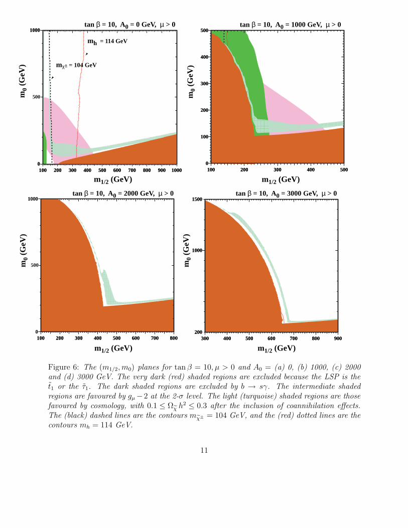
space in which 0.1 < Ωχh2 < 0.3, as favoured by cosmology. We display in Fig. 6 the

(m1/2, m0) planes for tanβ = 10 and µ > 0, for the different values of A0 = (a) 0, (b) 1000,

(c) 2000 and (d) 3000 GeV. The very dark (red) shaded regions have mτ1 or mt1 < mχ,

and hence are excluded by the very stringent bounds on charged dark matter [1]. The light

(turquoise) shaded regions correspond to the preferred relic-density range 0.1 < Ωχ h2 < 0.3.

The dark (green) shaded regions are those excluded by measurements of b → sγ. The

intermediate (pink) shaded regions in panels (a) and (b) are those favoured by the BNL

4This differs from σχχ

because of the number-density weighting factor.

9

0 . 0 0 .1 0 .2 0 .3 0 .4

con

trib

uti

on

to

σef

f (

GeV

-2)

^

10-5

10-6

10-7

10-8

10-9

10-12

10-10

10-11

∆ M

tan β = 10, A0 = 1000 GeV

m0 = 300 GeV

0. 0 0 . 1 0 . 2 0 . 3 0 . 4

con

trib

uti

on

to

σef

f (

GeV

-2) 10-5

10-6

10-7

10-8

10-9

10-12

10-10

10-11

σno co.

t t

t χ

χ χ

σeff^

^

∼ ∼∼ ∼

∆ M

∼ ∼

^

tan β = 10, A0 = 2000 GeV

m0 = 300 GeV

Figure 5: The separate contributions to the total effective cross sections σeff for x = T/mχ =1/23, as functions of ∆M ≡ (mτR

− mχ)/mχ, obtained by varying m1/2, with (a) A0 =1000 GeV and (b) A0 = 2000 GeV, both for tan β = 10, µ > 0 and m0 = 300 GeV.

measurement of gµ − 2 at the 2-σ level [17]. The (black) dashed line in panel (a) is the

contour mχ± = 104 GeV, corresponding to the kinematic range of LEP 2, and the (red)

dotted line is the contour mh = 114 GeV, as evaluated using FeynHiggs [18], corresponding

to the LEP lower limit on the mass of the Higgs boson. These contours are also glimpsed in

the other panels.

Panel (a) of Fig. 6 is indistinguishable from analogous plots shown previously [8, 12]:

t1 coannihilations are not important when A0 = 0. Panel (b) shows how t1 coannihilation

generates a ‘tail’ of allowed CMSSM parameter space, extending the ‘bulk’ region of the

(m1/2, m0) plane up as far as m0 ∼ 450 GeV. The boundary of the region where mt1 < mχ,

and hence the t1χ coannihilation region, slopes to the left as m0 is increased, since we have

fixed A0 over the plane. As m0 is increased, the impact of the A-dependent off-diagonal term

is diminished and the light stop is heavier. To compensate for this, one must decrease m1/2

to obtain the necessary degree of degeneracy between t1 and χ. This effect is also seen in

panels (c) and (d) of Fig. 6.

In the particular cae of A0 = 1000 GeV shown in panel (b) of Fig. 6, the t1 coannihilation

tail happens to be excluded by b → sγ. However, this is not the case for (c) A0 = 2000 GeV

and (d) A0 = 3000 GeV, where the t1 coannihilation tail extends up to m0 ∼ 900 and beyond

1350 GeV, respectively. For (b) A0 = 2000 GeV, the region favoured by gµ − 2 is hidden

on the left, inside the excluded region. However, around A0 = 1500 GeV there is a χt1

coannihilation region that satisfies both the b → sγ and gµ − 2 constraints.

The cosmologically-favoured region is broadened significantly when tt production is kine-

10

100 200 300 400 500 600 700 800 900 10000

1000

100 200 300 400 500 600 700 800 900 10000

1000

mh = 114 GeV

m0

(GeV

)

m1/2 (GeV)

mχ± = 104 GeV

500

tan β = 10, A0 = 0 GeV, µ > 0

100 200 300 400 5000

100

200

300

400

500

100 200 300 400 5000

100

200

300

400

500

m0

(GeV

)m1/2 (GeV)

tan β = 10, A0 = 1000 GeV, µ > 0

100 200 300 400 500 600 700 8000

1000

100 200 300 400 500 600 700 8000

1000

m0

(GeV

)

m1/2 (GeV)

tan β = 10, A0 = 2000 GeV, µ > 0

500

300 400 500 600 700 800 900200

1000

1500

300 400 500 600 700 800 900200

1000

1500

m0

(GeV

)

m1/2 (GeV)

tan β = 10, A0 = 3000 GeV, µ > 0

Figure 6: The (m1/2, m0) planes for tan β = 10, µ > 0 and A0 = (a) 0, (b) 1000, (c) 2000and (d) 3000 GeV. The very dark (red) shaded regions are excluded because the LSP is thet1 or the τ1. The dark shaded regions are excluded by b → sγ. The intermediate shadedregions are favoured by gµ−2 at the 2-σ level. The light (turquoise) shaded regions are thosefavoured by cosmology, with 0.1 ≤ Ωχ h2 ≤ 0.3 after the inclusion of coannihilation effects.The (black) dashed lines are the contours mχ± = 104 GeV, and the (red) dotted lines are thecontours mh = 114 GeV.

11

matically allowed in χχ annihilation The t-channel stop exchange contribution to this process

is significantly enhanced when t1 is relatively light: mt1 ' mχ. This feature can be seen in

Fig. 6(c) and Fig. 6(d). The t1 ˜ coannihilations are only important in the corner area near

the instep of the dark (red) shaded region where mτ1 ' mt1 ' mχ.

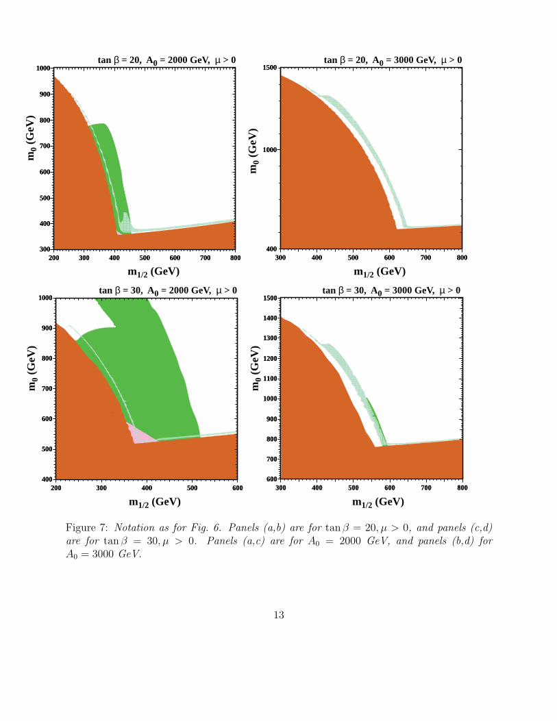
Fig. 7 shows analogous (m1/2, m0) planes for the larger values tanβ = 20 and 30, both

again for µ > 0. We see in panel (a) that the t1 coannihilation tail extends up to m0 ∼900 GeV when tanβ = 20 and A0 = 2000 GeV, beyond the region forbidden by b → sγ.

We then see in panel (b) that the t1 coannihilation tail extends beyond m0 ∼ 1400 GeV

when tan β = 20 and A0 = 3000 GeV. A similar portion of the t1 coannihilation tail that

is consistent with b → sγ is also visible in panel (c), for tanβ = 20 and A0 = 2000 GeV,

where m0 ∼ 900 GeV. For fixed A0, as tanβ is increased the b → sγ constraint becomes

more severe.

The t1 coannihilation tails do not increase the allowed range of m1/2, as was the case for

the ˜ coannihilation tail [7, 8, 9, 10], but they do add a significant filament to the CMSSM

region allowed by experiment and favoured by cosmology.

In the above illustrative examples, we have chosen the sign of A0 to be the same as that

of µ, with the effect of maximizing the stop off-diagonal mass terms, and hence minimizing

mt1 . If the sign of A0 is switched while keeping µ > 0, an analogous χt1 coannihilation

region is found only at even larger negative A0. However, the mh constraint is more severe

for A0 < 0, and also for µ < 0, excluding the region of parameter space of interest in the χt1

coannihilation context.

We have not discussed in this paper the potential constraint imposed by the absence

of colour and charge breaking (CCB) vacua, or at least the suppression of transitions to

CCB vacua. This constraint would restrict the value of A0 relative to m0 [19]. If the CCB

constraint is imposed, some of the parameter space for small m0 will be excluded, but there

will still be regions at high m0 where χt1 coannihilation is crucial. The issue of compatibity

with the potential gµ − 2 constraint would then arise. Since raising m0 suppresses the

neutralino-proton elastic scatttering cross section, χt1 coannihilation would tend to lower

the neutralino direct detection rate for the same range of mχ.

5 Conclusions and Open Issues

We have documented in this paper the potential importance of χt1 coannihilation in delin-

eating the preferred domain of CMSSM parameter space for A0 6= 0. In this paper, we have

only sctratched the surface of this subject, whose higher-dimensional parameter space merits

12

200 300 400 500 600 700 800300

400

500

600

700

800

900

1000

200 300 400 500 600 700 800300

400

500

600

700

800

900

1000

m0

(GeV

)

m1/2 (GeV)

tan β = 20, A0 = 2000 GeV, µ > 0

300 400 500 600 700 800400

1000

1500

300 400 500 600 700 800400

1000

1500

m0

(GeV

)

m1/2 (GeV)

tan β = 20, A0 = 3000 GeV, µ > 0

200 300 400 500 600400

500

600

700

800

900

1000

200 300 400 500 600400

500

600

700

800

900

1000

m0

(GeV

)

m1/2 (GeV)

tan β = 30, A0 = 2000 GeV, µ > 0

300 400 500 600 700 800600

700

800

900

1000

1100

1200

1300

1400

1500

300 400 500 600 700 800600

700

800

900

1000

1100

1200

1300

1400

1500

m0

(GeV

)

m1/2 (GeV)

tan β = 30, A0 = 3000 GeV, µ > 0

Figure 7: Notation as for Fig. 6. Panels (a,b) are for tanβ = 20, µ > 0, and panels (c,d)are for tan β = 30, µ > 0. Panels (a,c) are for A0 = 2000 GeV, and panels (b,d) forA0 = 3000 GeV.

13

more detailed exploration. The Appendix provides details of the diagrammatic calculations

that should be sufficient for our results to be verified and used by other authors. Although

applied in the context of the CMSSM, our results may also be used in more general MSSM

contexts. However, other coannihilation processes are also important in other regions of the

general MSSM parameter space. For example, in the CMSSM the sbottom mass is generally

larger than the stop mass even for large tanβ. However, if one allow non-degeneracy in

the scalar soft breaking mass term, a sbottom NLSP becomes possible [10]. A complete

calculation of the LSP relic density in the MSSM requires a careful discussion of all such

coannihilation possibilities.

Acknowledgments

We thank Toby Falk for many related discussions. The work of K.A.O. and Y.S. was sup-

ported in part by DOE grant DE–FG02–94ER–40823.

14

Appendix

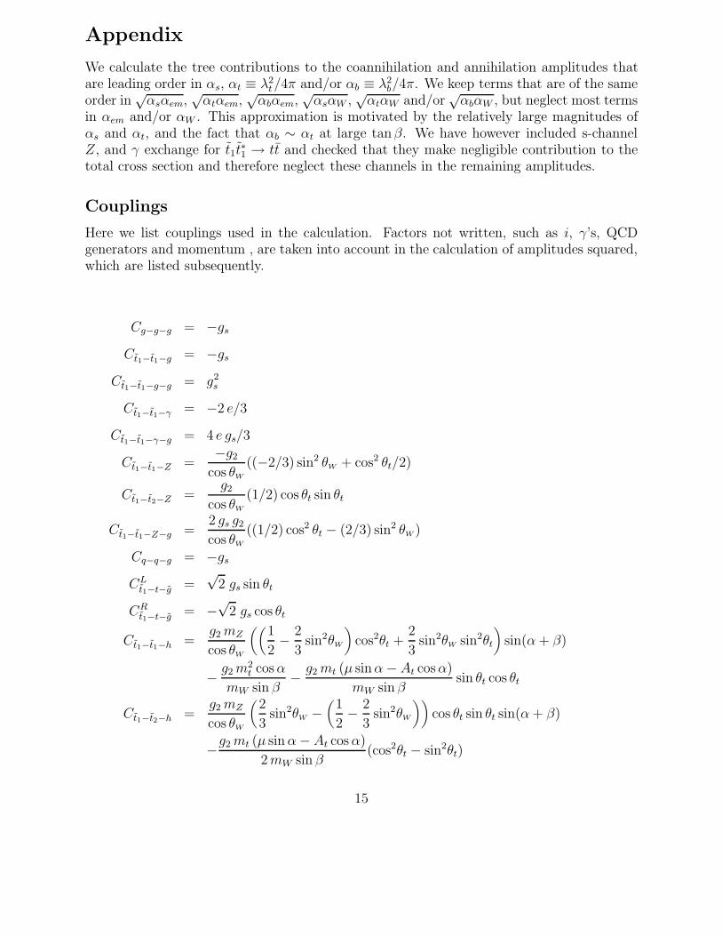
We calculate the tree contributions to the coannihilation and annihilation amplitudes thatare leading order in αs, αt ≡ λ2

t/4π and/or αb ≡ λ2b/4π. We keep terms that are of the same

order in√

αsαem,√

αtαem,√

αbαem,√

αsαW ,√

αtαW and/or√

αbαW , but neglect most termsin αem and/or αW . This approximation is motivated by the relatively large magnitudes ofαs and αt, and the fact that αb ∼ αt at large tanβ. We have however included s-channelZ, and γ exchange for t1t

∗1 → tt and checked that they make negligible contribution to the

total cross section and therefore neglect these channels in the remaining amplitudes.

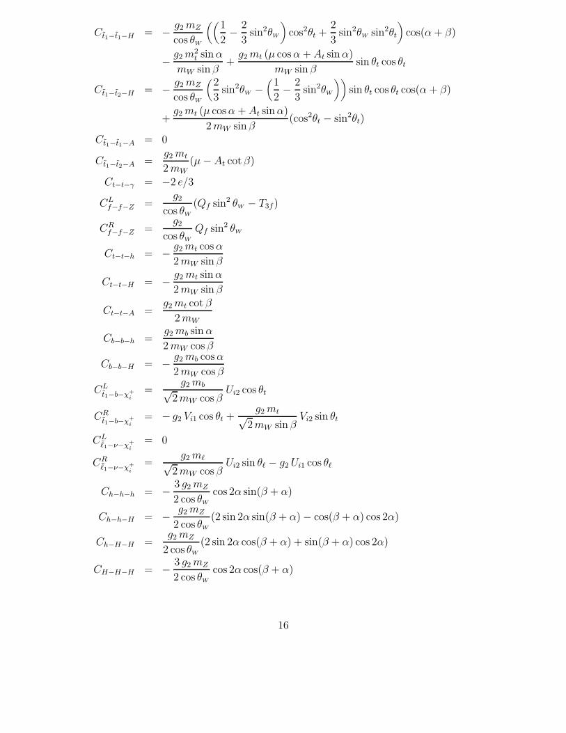
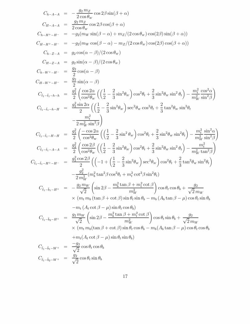
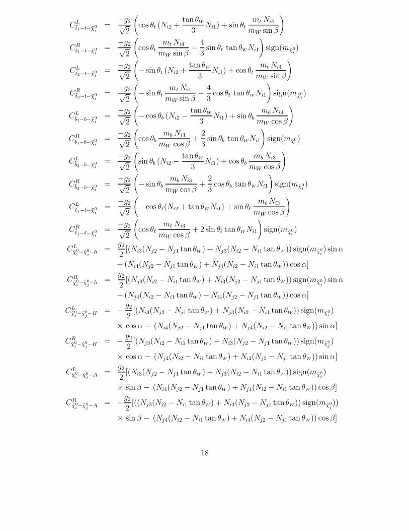
Couplings

Here we list couplings used in the calculation. Factors not written, such as i, γ’s, QCDgenerators and momentum , are taken into account in the calculation of amplitudes squared,which are listed subsequently.

Cg−g−g = −gs

Ct1−t1−g = −gs

Ct1−t1−g−g = g2s

Ct1−t1−γ = −2 e/3

Ct1−t1−γ−g = 4 e gs/3

Ct1−t1−Z =−g2

cos θW

((−2/3) sin2 θW + cos2 θt/2)

Ct1−t2−Z =g2

cos θW

(1/2) cos θt sin θt

Ct1−t1−Z−g =2 gs g2

cos θW

((1/2) cos2 θt − (2/3) sin2 θW )

Cq−q−g = −gs

CLt1−t−g =

√2 gs sin θt

CRt1−t−g = −

√2 gs cos θt

Ct1−t1−h =g2 mZ

cos θW

((1

2− 2

3sin2θW

)cos2θt +

2

3sin2θW sin2θt

)sin(α + β)

− g2 m2t cos α

mW sin β− g2 mt (µ sinα− At cos α)

mW sin βsin θt cos θt

Ct1−t2−h =g2 mZ

cos θW

(2

3sin2θW −

(1

2− 2

3sin2θW

))cos θt sin θt sin(α + β)

−g2 mt (µ sin α− At cos α)

2 mW sin β(cos2θt − sin2θt)

15

Ct1−t1−H = − g2 mZ

cos θW

((1

2− 2

3sin2θW

)cos2θt +

2

3sin2θW sin2θt

)cos(α + β)

− g2 m2t sin α

mW sin β+

g2 mt (µ cos α + At sin α)

mW sin βsin θt cos θt

Ct1−t2−H = − g2 mZ

cos θW

(2

3sin2θW −

(1

2− 2

3sin2θW

))sin θt cos θt cos(α + β)

+g2 mt (µ cos α + At sin α)

2 mW sin β(cos2θt − sin2θt)

Ct1−t1−A = 0

Ct1−t2−A =g2 mt

2 mW(µ−At cotβ)

Ct−t−γ = −2 e/3

CLf−f−Z =

g2

cos θW

(Qf sin2 θW − T3f)

CRf−f−Z =

g2

cos θW

Qf sin2 θW

Ct−t−h = − g2 mt cos α

2 mW sin β

Ct−t−H = − g2 mt sin α

2 mW sin β

Ct−t−A =g2 mt cot β

2 mW

Cb−b−h =g2 mb sin α

2 mW cos β

Cb−b−H = − g2 mb cos α

2 mW cos β

CLt1−b−χ+

i=

g2 mb√2mW cos β

Ui2 cos θt

CRt1−b−χ+

i= − g2 Vi1 cos θt +

g2 mt√2mW sin β

Vi2 sin θt

CL˜1−ν−χ+

i= 0

CR˜1−ν−χ+

i=

g2 m`√2mW cos β

Ui2 sin θ` − g2 Ui1 cos θ`

Ch−h−h = − 3 g2 mZ

2 cos θW

cos 2α sin(β + α)

Ch−h−H = − g2 mZ

2 cos θW

(2 sin 2α sin(β + α)− cos(β + α) cos 2α)

Ch−H−H =g2 mZ

2 cos θW

(2 sin 2α cos(β + α) + sin(β + α) cos 2α)

CH−H−H = − 3 g2 mZ

2 cos θW

cos 2α cos(β + α)

16

Ch−A−A = − g2 mZ

2 cos θW

cos 2β sin(β + α)

CH−A−A =g2 mZ

2 cos θW

cos 2β cos(β + α)

Ch−H+−H− = −g2(mW sin(β − α) + mZ/(2 cos θW ) cos(2β) sin(β + α))

CH−H+−H− = −g2(mW cos(β − α)−mZ/(2 cos θW ) cos(2β) cos(β + α))

Ch−Z−A = g2 cos(α− β)/(2 cos θW )

CH−Z−A = g2 sin(α− β)/(2 cos θW )

Ch−W+−H− =g2

2cos(α− β)

CH−W+−H− =g2

2sin(α− β)

Ct1−t1−h−h =g22

2

(cos 2α

cos2θW

((1

2− 2

3sin2θW

)cos2θt +

2

3sin2θW sin2 θt

)− m2

t

m2W

cos2α

sin2β

)

Ct1−t1−h−H =g22 sin 2α

2

((1

2− 2

3sin2θW

)sec2θW cos2θt +

2

3tan2θW sin2θt

− m2t

2 m2W sin2β

)

Ct1−t1−H−H =g22

2

(− cos 2α

cos2θW

((1

2− 2

3sin2 θW

)cos2θt +

2

3sin2θW sin2θt

)− m2

t

m2W

sin2α

sin2β

)

Ct1−t1−A−A =g22

2

(cos 2β

cos2θW

((1

2− 2

3sin2θW

)cos2θt +

2

3sin2θW sin2 θt

)− m2

t

m2W tan2β

)

Ct1−t1−H+−H− =g22 cos 2β

2

((−1 +

(1

2− 2

3sin2θW

)sec2θW

)cos2θt +

2

3tan2θW sin2θt

)− g2

2

2 m2W

(m2b tan2β cos2θt + m2

t cot2β sin2θt)

Ct1−b1−H+ = − g2 mW√2

(sin 2β − m2

b tan β + m2t cot β

m2W

)cos θt cos θb +

g2√2 mW

× (mt mb (tan β + cot β) sin θt sin θb −mb (Ab tan β − µ) cos θt sin θb

−mt (At cot β − µ) sin θt cos θb)

Ct1−b2−H+ =g2 mW√

2

(sin 2β − m2

b tan β + m2t cot β

m2W

)cos θt sin θb +

g2√2 mW

× (mt mb(tanβ + cotβ) sin θt cos θb −mb(Ab tan β − µ) cos θt cos θb

+mt(At cotβ − µ) sin θt sin θb)

Ct1−b1−W+ =−g2√

2cos θt cos θb

Ct1−b2−W+ =g2√2

cos θt sin θb

17

CLt1−t−χ0

i=

−g2√2

(cos θt (Ni2 +

tan θW

3Ni1) + sin θt

mt Ni4

mW sin β

)

CRt1−t−χ0

i=

−g2√2

(cos θt

mt Ni4

mW sin β− 4

3sin θt tan θW Ni1

)sign(mχ0

i)

CLt2−t−χ0

i=

−g2√2

(− sin θt (Ni2 +

tan θW

3Ni1) + cos θt

mt Ni4

mW sin β

)

CRt2−t−χ0

i=

−g2√2

(− sin θt

mt Ni4

mW sin β− 4

3cos θt tan θW Ni1

)sign(mχ0

i)

CLb1−b−χ0

i=

−g2√2

(− cos θb (Ni2 −

tan θW

3Ni1) + sin θb

mb Ni3

mW cos β

)

CRb1−b−χ0

i=

−g2√2

(cos θb

mb Ni3

mW cos β+

2

3sin θb tan θW Ni1

)sign(mχ0

i)

CLb2−b−χ0

i=

−g2√2

(sin θb (Ni2 −

tan θW

3Ni1) + cos θb

mb Ni3

mW cos β

)

CRb2−b−χ0

i=

−g2√2

(− sin θb

mb Ni3

mW cos β+

2

3cos θb tan θW Ni1

)sign(mχ0

i)

CL˜1−`−χ0

i=

−g2√2

(− cos θ`(Ni2 + tan θW Ni1) + sin θ`

m` Ni3

mW cos β

)

CR˜1−`−χ0

i=

−g2√2

(cos θ`

m` Ni3

mW cos β+ 2 sin θ` tan θW Ni1

)sign(mχ0

i)

CLχ0

i−χ0j−h =

g2

2[(Ni3(Nj2 −Nj1 tan θW ) + Nj3(Ni2 −Ni1 tan θW )) sign(mχ0

i) sin α

+ (Ni4(Nj2 −Nj1 tan θW ) + Nj4(Ni2 −Ni1 tan θW )) cos α]

CRχ0

i−χ0j−h =

g2

2[(Nj3(Ni2 −Ni1 tan θW ) + Ni3(Nj2 −Nj1 tan θW )) sign(mχ0

j) sin α

+ (Nj4(Ni2 −Ni1 tan θW ) + Ni4(Nj2 −Nj1 tan θW )) cos α]

CLχ0

i−χ0j−H = − g2


i)

× cos α− (Ni4(Nj2 −Nj1 tan θW ) + Nj4(Ni2 −Ni1 tan θW )) sin α]

CRχ0

i−χ0j−H = − g2

2[(Nj3(Ni2 −Ni1 tan θW ) + Ni3(Nj2 −Nj1 tan θW )) sign(mχ0

j)

× cos α− (Nj4(Ni2 −Ni1 tan θW ) + Ni4(Nj2 −Nj1 tan θW )) sin α]

CLχ0

i−χ0j−A =

g2


i)

× sin β − (Ni4(Nj2 −Nj1 tan θW ) + Nj4(Ni2 −Ni1 tan θW )) cos β]

CRχ0

i−χ0j−A = −g2

2[((Nj3(Ni2 −Ni1 tan θW ) + Ni3(Nj2 −Nj1 tan θW )) sign(mχ0

j))

× sin β − (Nj4(Ni2 −Ni1 tan θW ) + Ni4(Nj2 −Nj1 tan θW )) cos β]

18

CLt−b−H+ =

g2√2mW

mb tanβ

CRt−b−H+ =

g2√2mW

mt cot β

CLχ0

i−χ−j −H+ = −g2

(Ni3 Uj1 − (Ni2 + Ni1 tan θW )Uj2/

√2)

sign(mχ0i) sin β

CRχ0

i−χ−j −H+ = −g2

(Ni4 Vj1 + (Ni2 + Ni1 tan θW )Vj2/

√2)

cos β

CLχ0

i−χ0j−Z =

g2

4 cos θW

sign(mχ0j)(Ni4 Nj4 −Ni3 Nj3)

CRχ0

i−χ0j−Z = −CL

χ0i−χ0

j−Z

CLχ0

i−χ−j −W+ = g2(Ni2 Vj1 −Ni4 Vj2/√

2)

CRχ0

i−χ−j −W+ = g2(Ni2 Uj1 + Ni3 Uj2/√

2)

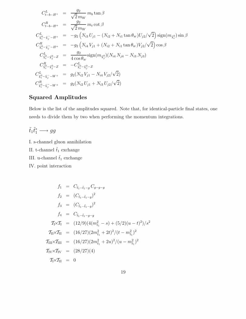
Squared Amplitudes

Below is the list of the amplitudes squared. Note that, for identical-particle final states, one

needs to divide them by two when performing the momentum integrations.

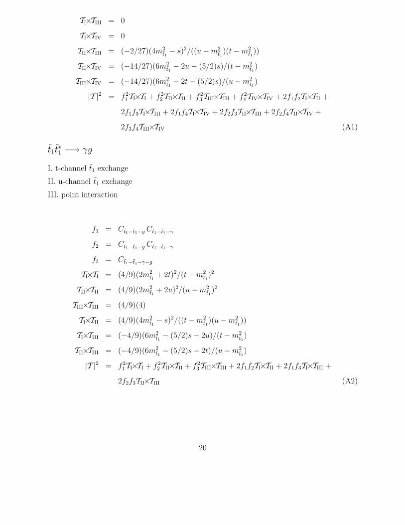
t1t∗1 −→ gg

I. s-channel gluon annihilation

II. t-channel t1 exchange

III. u-channel t1 exchange

IV. point interaction

f1 = Ct1−t1−g Cg−g−g

f2 = (Ct1−t1−g)2

f3 = (Ct1−t1−g)2

f4 = Ct1−t1−g−g

TI×TI = (12/9)(4(m2t1− s) + (5/2)(u− t)2)/s2

TII×TII = (16/27)(2m2t1

+ 2t)2/(t−m2t1)2

TIII×TIII = (16/27)(2m2t1

+ 2u)2/(u−m2t1

)2

TIV×TIV = (28/27)(4)

TI×TII = 0

19

TI×TIII = 0

TI×TIV = 0

TII×TIII = (−2/27)(4m2t1− s)2/((u−m2

t1)(t−m2

t1))

TII×TIV = (−14/27)(6m2t1− 2u− (5/2)s)/(t−m2

t1)

TIII×TIV = (−14/27)(6m2t1− 2t− (5/2)s)/(u−m2

t1)

|T |2 = f 21TI×TI + f 2

2TII×TII + f 23TIII×TIII + f 2

4TIV×TIV + 2f1f2TI×TII +

2f1f3TI×TIII + 2f1f4TI×TIV + 2f2f3TII×TIII + 2f2f4TII×TIV +

2f3f4TIII×TIV (A1)

t1t∗1 −→ γg

I. t-channel t1 exchange

II. u-channel t1 exchange

III. point interaction

f1 = Ct1−t1−g Ct1−t1−γ

f2 = Ct1−t1−g Ct1−t1−γ

f3 = Ct1−t1−γ−g

TI×TI = (4/9)(2m2t1

+ 2t)2/(t−m2t1)2

TII×TII = (4/9)(2m2t1

+ 2u)2/(u−m2t1

)2

TIII×TIII = (4/9)(4)

TI×TII = (4/9)(4m2t1− s)2/((t−m2

t1)(u−m2

t1))

TI×TIII = (−4/9)(6m2t1− (5/2)s− 2u)/(t−m2

t1)

TII×TIII = (−4/9)(6m2t1− (5/2)s− 2t)/(u−m2

t1)

|T |2 = f 21TI×TI + f 2

2TII×TII + f 23TIII×TIII + 2f1f2TI×TII + 2f1f3TI×TIII +

2f2f3TII×TIII (A2)

20

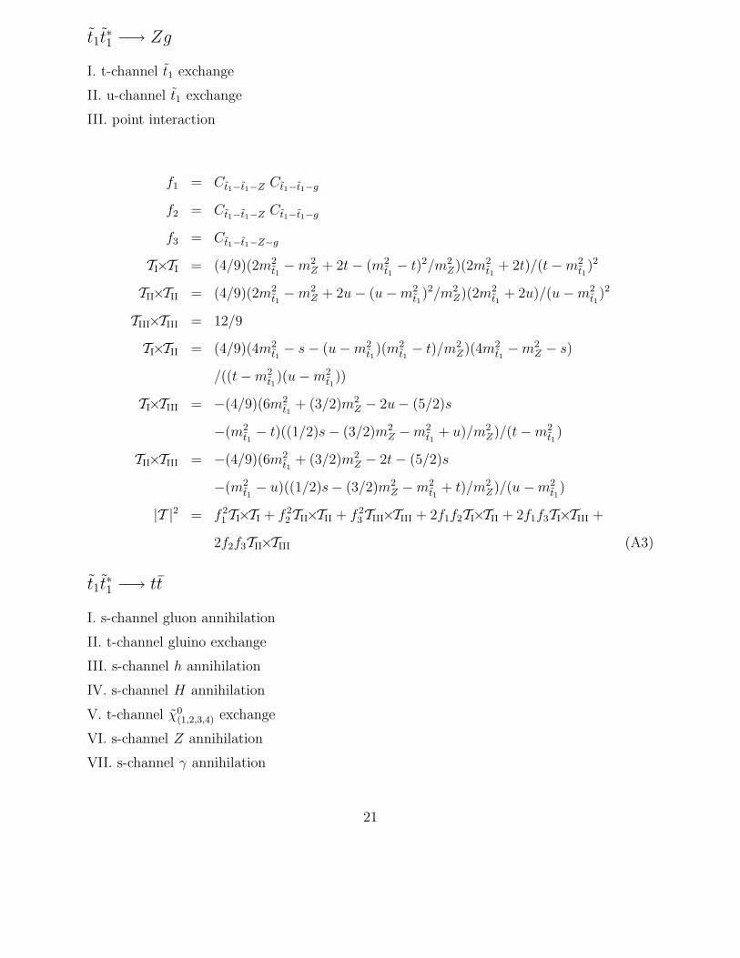
t1t∗1 −→ Zg




f1 = Ct1−t1−Z Ct1−t1−g

f2 = Ct1−t1−Z Ct1−t1−g

f3 = Ct1−t1−Z−g

TI×TI = (4/9)(2m2t1−m2

Z + 2t− (m2t1− t)2/m2

Z)(2m2t1

+ 2t)/(t−m2t1)2

TII×TII = (4/9)(2m2t1−m2

Z + 2u− (u−m2t1

)2/m2Z)(2m2

t1+ 2u)/(u−m2

t1)2

TIII×TIII = 12/9

TI×TII = (4/9)(4m2t1− s− (u−m2

t1)(m2

t1− t)/m2

Z)(4m2t1−m2

Z − s)

/((t−m2t1

)(u−m2t1

))

TI×TIII = −(4/9)(6m2t1

+ (3/2)m2Z − 2u− (5/2)s

−(m2t1− t)((1/2)s− (3/2)m2

Z −m2t1

+ u)/m2Z)/(t−m2

t1)

TII×TIII = −(4/9)(6m2t1

+ (3/2)m2Z − 2t− (5/2)s

−(m2t1− u)((1/2)s− (3/2)m2

Z −m2t1

+ t)/m2Z)/(u−m2

t1)

|T |2 = f 21TI×TI + f 2

2TII×TII + f 23TIII×TIII + 2f1f2TI×TII + 2f1f3TI×TIII +

2f2f3TII×TIII (A3)

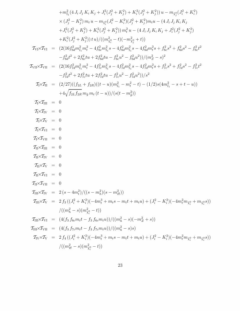
t1t∗1 −→ tt


II. t-channel gluino exchange

III. s-channel h annihilation

IV. s-channel H annihilation

V. t-channel χ0(1,2,3,4) exchange

VI. s-channel Z annihilation

VII. s-channel γ annihilation

21

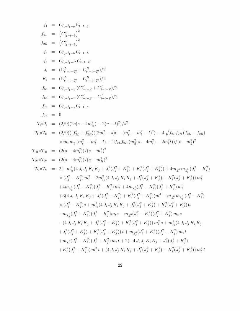
f1 = Ct1−t1−g Ct−t−g

f2L =(CL

t1−t−g

)2

f2R =(CR

t1−t−g

)2

f3 = Ct1−t1−h Ct−t−h

f4 = Ct1−t1−H Ct−t−H

Ji = (CLt1−t−χ0

i+ CR

t1−t−χ0i)/2

Ki = (CLt1−t−χ0

i− CR

t1−t−χ0i)/2

f6c = Ct1−t1−Z (CRt−t−Z + CL

t−t−Z)/2

f6d = Ct1−t1−Z (CRt−t−Z − CL

t−t−Z)/2

f7c = Ct1−t1−γ Ct−t−γ

f7d = 0

TI×TI = (2/9)(2s(s− 4m2t1)− 2(u− t)2)/s2

TII×TII = (2/9)((f 22L + f 2

2R)((2m2t − s)t− (m2

t1−m2

t − t)2)− 4√

f2Lf2R (f2L + f2R)

×mt mg (m2t1−m2

t − t) + 2f2Lf2R (m2g(s− 4m2

t )− 2m2t t))/(t−m2

g)2

TIII×TIII = (2(s− 4m2t ))/(s−m2

h)2

TIV×TIV = (2(s− 4m2t ))/(s−m2

H)2

TV×TV = 2(−m4t1

(4 Ji Jj Ki Kj + J2i (J2

j + K2j ) + K2

i (J2j + K2

j )) + 4mχ0imχ0

j(J2

i −K2i )

× (J2j −K2

j ) m2t − 2m2

t1(4 Ji Jj Ki Kj + J2

i (J2j + K2

j ) + K2i (J2

j + K2j )) m2

t

+4mχ0j(J2

i + K2i )(J2

j −K2j ) m3

t + 4mχ0i(J2

i −K2i )(J

2j + K2

j ) m3t

+3(4 Ji Jj Ki Kj + J2i (J2

j + K2j ) + K2

i (J2j + K2

j ))m4t −mχ0

imχ0

j(J2

i −K2i )

× (J2j −K2

j )s + m2t1


j + K2j ) + K2

i (J2j + K2

j ))s

−mχ0j(J2

i + K2i )(J2

j −K2j )mts−mχ0

i(J2

i −K2i )(J2

j + K2j ) mt s

−(4 Ji Jj Ki Kj + J2i (J2

j + K2j ) + K2

i (J2j + K2

j )) m2t s + m2

t1(4 Ji Jj Ki Kj

+J2i (J2

j + K2j ) + K2

i (J2j + K2

j )) t + mχ0j(J2

i + K2i )(J2

j −K2j ) mt t

+mχ0i(J2

i −K2i )(J2

j + K2j ) mt t + 2(−4 Ji Jj Ki Kj + J2

i (J2j + K2

j )

+K2i (J2

j + K2j )) m2

t t + (4 Ji Jj Ki Kj + J2i (J2

j + K2j ) + K2

i (J2j + K2

j )) m2t t

22

+m2t1


j + K2j ) + K2

i (J2j + K2

j )) u−mχ0j(J2

i + K2i )

× (J2j −K2

j ) mt u−mχ0i(J2

i −K2i )(J

2j + K2

j )mtu− (4 Ji Jj Ki Kj

+J2i (J2

j + K2j ) + K2

i (J2j + K2

j )) m2t u− (4 Ji Jj Ki Kj + J2

i (J2j + K2

j )

+K2i (J2

j + K2j )) t u)/((m2

χ0i− t)(−m2

χ0j+ t))

TVI×TVI = (2(16f 26dm

2t1m2

t − 4f 26cm

2t1s− 4f 2

6dm2t1s− 4f 2

6dm2t s + f 2

6cs2 + f 2

6ds2 − f 2

6ct2

−f 26dt

2 + 2f 26ctu + 2f 2

6dtu− f 26cu

2 − f 26du

2))/(m2Z − s)2

TVII×TVII = (2(16f 27dm

2t1m2

t − 4f 27cm

2t1s− 4f 2

7dm2t1s− 4f 2

7dm2t s + f 2

7cs2 + f 2

7ds2 − f 2

7ct2

−f 27dt

2 + 2f 27ctu + 2f 2

7dtu− f 27cu

2 − f 27du

2))/s2

TI×TII = (2/27)((f2L + f2R)((t− u)(m2t1−m2

t − t)− (1/2)s(4m2t1− s + t− u))

+4√

f2Lf2R mg mt (t− u))/(s(t−m2g))

TI×TIII = 0

TI×TIV = 0

TI×TV = 0

TI×TVI = 0

TI×TVII = 0

TII×TIII = 0

TII×TIV = 0

TII×TV = 0

TII×TVI = 0

TII×TVII = 0

TIII×TIV = 2 (s− 4m2t )/((s−m2

h)(s−m2H))

TIII×TV = 2 f3 ((J2i + K2

i )(−4m3t + mts−mtt + mtu) + (J2

i −K2i )(−4m2

t mχ0i+ mχ0

is))

/((m2h − s)(m2

χ0i− t))

TIII×TVI = (4(f3 f6cmtt− f3 f6cmtu))/((m2h − s)(−m2

Z + s))

TIII×TVII = (4(f3 f7cmtt− f3 f7cmtu))/((m2h − s)s)

TIV×TV = 2 f4 ((J2i + K2

i )(−4m3t + mts−mtt + mtu) + (J2

i −K2i )(−4m2

t mχ0i+ mχ0

is))

/((m2H − s)(m2

χ0i− t))

23

TIV×TVI = (4(f4 f6cmtt− f4 f6cmtu))/((m2H − s)(−m2

Z + s))

TIV×TVII = (4(f4 f7cmtt− f4 f7cmtu))/((m2H − s)s)

TV×TVI = (−16f6d Ki Ji m2t1m2

t − 16f6d Ji Ki m2t1m2

t − 4f6c J2i m2

t1s + 4f6d Ki Ji m

2t1s

+4f6d Ji Ki m2t1s− 4f6c K2

i m2t1s + 4f6d Ki Ji m

2t s + 4f6d Ji Ki m

2ts + f6c J2

i s2

−f6d Ki Ji s2 − f6d Ji Ki s

2 + f6c K2i s2 − 4f6c J2

i m2t t− 4f6c K2

i m2t t

−4f6c J2i mtmχ0

it + 4f6c K2

i mtmχ0it− f6c J2

i t2 + f6d Ki Ji t2 + f6d Ji Ki t

2

−f6c K2i t2 + 4f6c J2

i m2t u + 4f6c K2

i m2t u + 4f6c J2

i mtmχ0iu

−4f6c K2i mtmχ0

iu + 2f6c J2

i tu− 2f6d Ki Ji tu− 2f6d Ji Ki tu + 2f6c K2i tu

−f6c J2i u2 + f6d Ki Ji u

2 + f6d Ji Ki u2 − f6c K2

i u2)/((m2Z − s)(m2

χ0i− t))

TV×TVII = −((−4f7c J2i m2

t1s− 4f7c K2

i m2t1s + f7c J2

i s2 + f7c K2i s2 − 4f7c J2

i m2t t

−4f7c K2i m2

t t− 4f7c J2i mtmχ0

it + 4f7c K2

i mtmχ0it− f7c J2

i t2 − f7c K2i t2

+4f7c J2i m2

t u + 4f7c K2i m2

t u + 4f7c J2i mtmχ0

iu− 4f7c K2

i mtmχ0iu

+2f7c J2i tu + 2f7c K2

i tu− f7c J2i u2 − f7c K2

i u2)/(s(m2χ0

i− t)))

TVI×TVII = (2(−16f6d f7d m2t1m2

t + 4f6c f7c m2t1

s + 4f6d f7d m2t1

s + 4f6d f7d m2t s

−f6c f7c s2 − f6d f7d s2 + f6c f7c t2 + f6d f7d t2 − 2f6c f7c tu− 2f6d f7d tu

+f6c f7c u2 + f6d f7d u2))/((m2Z − s)s)

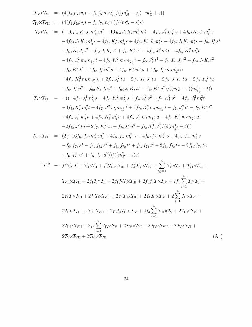
|T |2 = f 21TI×TI + TII×TII + f 2

3TIII×TIII + f 24TIV×TIV +

4∑i,j=1

TV×TV + TVI×TVI +

TVII×TVII + 2f1TI×TII + 2f1f3TI×TIII + 2f1f4TI×TIV + 2f1

4∑i=1

TI×TV +

2f1TI×TVI + 2f1TI×TVII + 2f3TII×TIII + 2f4TII×TIV + 24∑

i=1

TII×TV +

2TII×TVI + 2TII×TVII + 2f3f4TIII×TIV + 2f3

4∑i=1

TIII×TV + 2TIII×TVI +

2TIII×TVII + 2f4

4∑i=1

TIV×TV + 2TIV×TVI + 2TIV×TVII + 2TV×TVI +

2TV×TVII + 2TVI×TVII (A4)

24

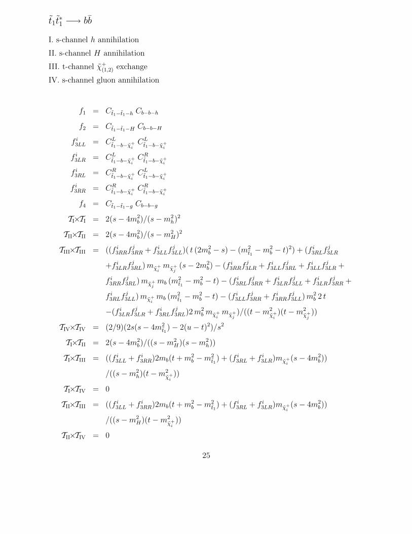
t1t∗1 −→ bb

I. s-channel h annihilation

II. s-channel H annihilation

III. t-channel χ+(1,2) exchange

IV. s-channel gluon annihilation

f1 = Ct1−t1−h Cb−b−h

f2 = Ct1−t1−H Cb−b−H

f i3LL = CL

t1−b−χ+i

CLt1−b−χ+

i

f i3LR = CL

t1−b−χ+i

CRt1−b−χ+

i

f i3RL = CR

t1−b−χ+i

CLt1−b−χ+

i

f i3RR = CR

t1−b−χ+i

CRt1−b−χ+

i

f4 = Ct1−t1−g Cb−b−g

TI×TI = 2(s− 4m2b)/(s−m2

h)2

TII×TII = 2(s− 4m2b)/(s−m2

H)2

TIII×TIII = ((f i3RRf j

3RR + f i3LLf j

3LL)( t (2m2b − s)− (m2

t1−m2

b − t)2) + (f i3RLf j

3LR

+f i3LRf j

3RL) mχ+i

mχ+j

(s− 2m2b)− (f i

3RRf j3LR + f i

3LLf j3RL + f i

3LLf j3LR +

f i3RRf j

3RL) mχ+j

mb (m2t1−m2

b − t)− (f i3RLf j

3RR + f i3LRf j

3LL + f i3LRf j

3RR +

f i3RLf j

3LL) mχ+i

mb (m2t1−m2

b − t)− (f i3LLf j

3RR + f i3RRf j

3LL) m2b 2 t

−(f i3LRf j

3LR + f i3RLf j

3RL)2 m2b mχ+

imχ+

j)/((t−m2

χ+i)(t−m2

χ+j))

TIV×TIV = (2/9)(2s(s− 4m2t1)− 2(u− t)2)/s2

TI×TII = 2(s− 4m2b)/((s−m2

H)(s−m2h))

TI×TIII = ((f i3LL + f i

3RR)2mb(t + m2b −m2

t1) + (f i

3RL + f i3LR)mχ+

i(s− 4m2

b))

/((s−m2h)(t−m2

χ+i))

TI×TIV = 0

TII×TIII = ((f i3LL + f i

3RR)2mb(t + m2b −m2

t1) + (f i

3RL + f i3LR)mχ+

i(s− 4m2

b))

/((s−m2H)(t−m2

χ+i))

TII×TIV = 0

25

TIII×TIV = 0

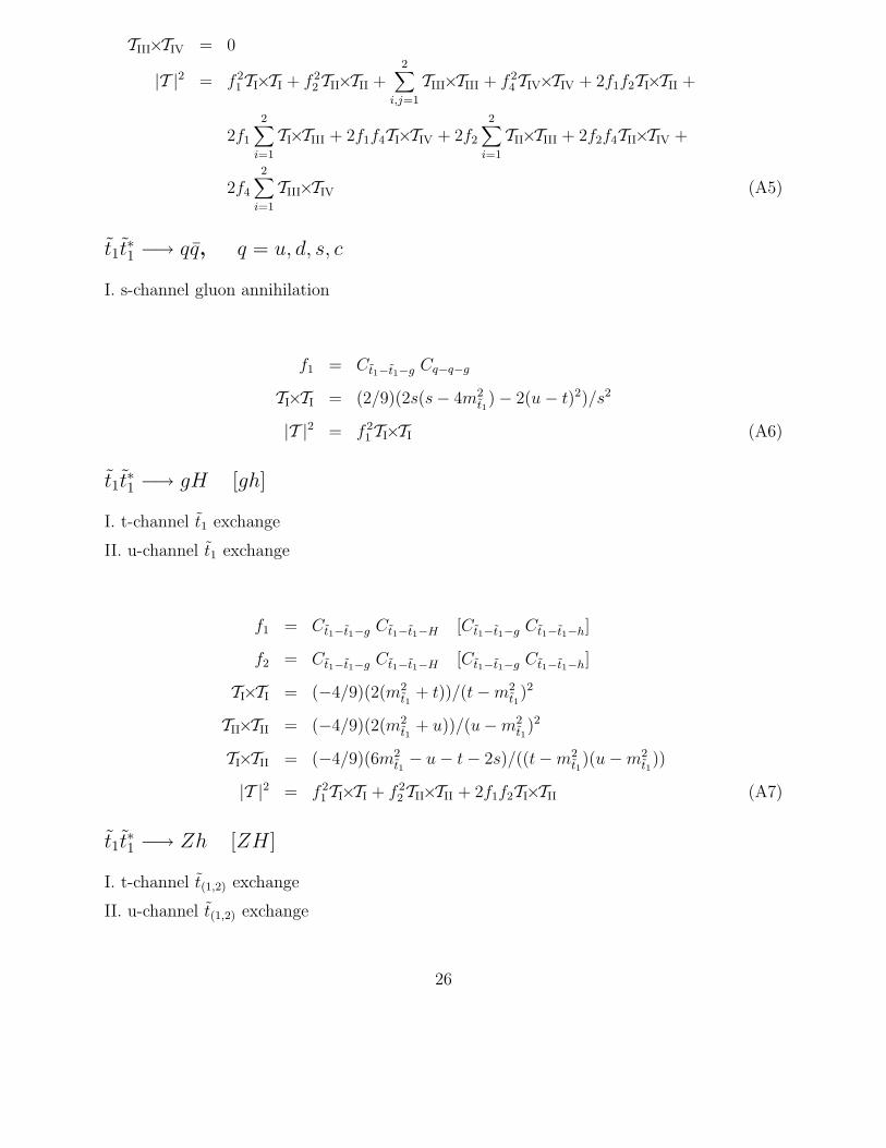
|T |2 = f 21TI×TI + f 2

2TII×TII +2∑

i,j=1

TIII×TIII + f 24TIV×TIV + 2f1f2TI×TII +

2f1

2∑i=1

TI×TIII + 2f1f4TI×TIV + 2f2

2∑i=1

TII×TIII + 2f2f4TII×TIV +

2f4

2∑i=1

TIII×TIV (A5)

t1t∗1 −→ qq, q = u, d, s, c


f1 = Ct1−t1−g Cq−q−g

TI×TI = (2/9)(2s(s− 4m2t1

)− 2(u− t)2)/s2

|T |2 = f 21TI×TI (A6)

t1t∗1 −→ gH [gh]



f1 = Ct1−t1−g Ct1−t1−H [Ct1−t1−g Ct1−t1−h]

f2 = Ct1−t1−g Ct1−t1−H [Ct1−t1−g Ct1−t1−h]

TI×TI = (−4/9)(2(m2t1

+ t))/(t−m2t1

)2

TII×TII = (−4/9)(2(m2t1

+ u))/(u−m2t1

)2

TI×TII = (−4/9)(6m2t1− u− t− 2s)/((t−m2

t1)(u−m2

t1))

|T |2 = f 21TI×TI + f 2

2TII×TII + 2f1f2TI×TII (A7)

t1t∗1 −→ Zh [ZH]

I. t-channel t(1,2) exchange

II. u-channel t(1,2) exchange

26

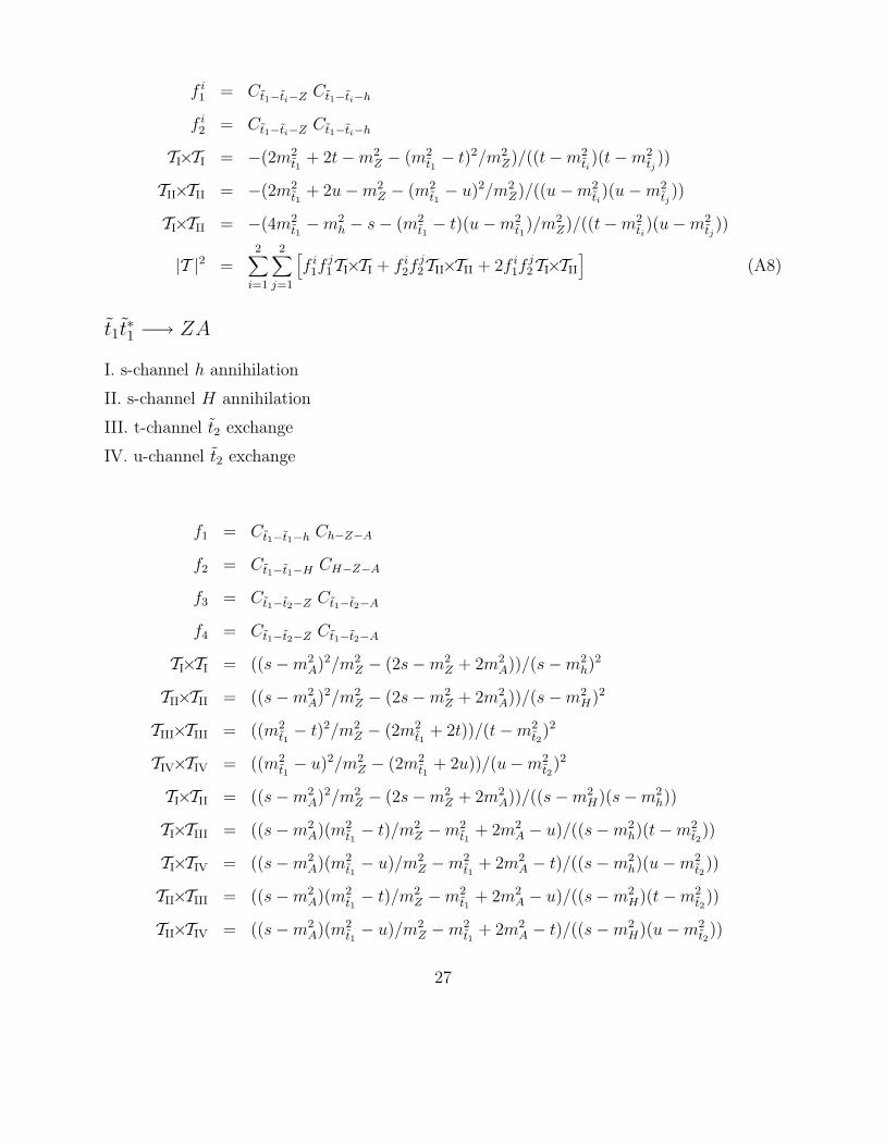
f i1 = Ct1−ti−Z Ct1−ti−h

f i2 = Ct1−ti−Z Ct1−ti−h

TI×TI = −(2m2t1

+ 2t−m2Z − (m2

t1− t)2/m2

Z)/((t−m2ti)(t−m2

tj))

TII×TII = −(2m2t1

+ 2u−m2Z − (m2

t1− u)2/m2

Z)/((u−m2ti)(u−m2

tj))

TI×TII = −(4m2t1−m2

h − s− (m2t1− t)(u−m2

t1)/m2

Z)/((t−m2ti)(u−m2

tj))

|T |2 =2∑

i=1

2∑j=1

[f i

1fj1TI×TI + f i

2fj2TII×TII + 2f i

1fj2TI×TII

](A8)

t1t∗1 −→ ZA



III. t-channel t2 exchange

IV. u-channel t2 exchange

f1 = Ct1−t1−h Ch−Z−A

f2 = Ct1−t1−H CH−Z−A

f3 = Ct1−t2−Z Ct1−t2−A

f4 = Ct1−t2−Z Ct1−t2−A

TI×TI = ((s−m2A)2/m2

Z − (2s−m2Z + 2m2

A))/(s−m2h)

2

TII×TII = ((s−m2A)2/m2

Z − (2s−m2Z + 2m2

A))/(s−m2H)2

TIII×TIII = ((m2t1− t)2/m2

Z − (2m2t1

+ 2t))/(t−m2t2)2

TIV×TIV = ((m2t1− u)2/m2

Z − (2m2t1

+ 2u))/(u−m2t2)2

TI×TII = ((s−m2A)2/m2

Z − (2s−m2Z + 2m2

A))/((s−m2H)(s−m2

h))

TI×TIII = ((s−m2A)(m2

t1− t)/m2

Z −m2t1

+ 2m2A − u)/((s−m2

h)(t−m2t2))

TI×TIV = ((s−m2A)(m2

t1− u)/m2

Z −m2t1

+ 2m2A − t)/((s−m2

h)(u−m2t2

))

TII×TIII = ((s−m2A)(m2

t1− t)/m2

Z −m2t1

+ 2m2A − u)/((s−m2

H)(t−m2t2

))

TII×TIV = ((s−m2A)(m2

t1− u)/m2

Z −m2t1

+ 2m2A − t)/((s−m2

H)(u−m2t2

))

27

TIII×TIV = ((u−m2t1)(m2

t1− t)/m2

Z − (4m2t1−m2

A − s))/((t−m2t2)(u−m2

t2))

|T |2 = f 21TI×TI + f 2


4TIV×TIV + 2f1f2TI×TII +

2f1f3TI×TIII + 2f1f4TI×TIV + 2f2f3TII×TIII + 2f2f4TII×TIV +

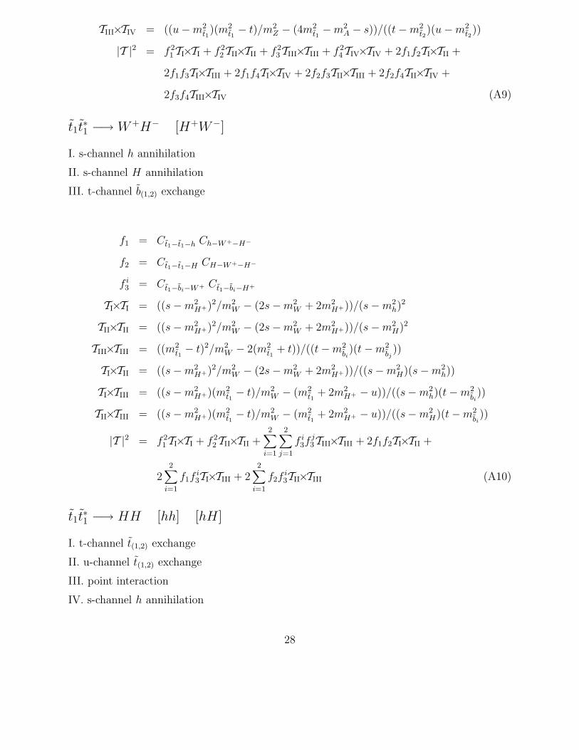
2f3f4TIII×TIV (A9)

t1t∗1 −→ W+H− [H+W−]



III. t-channel b(1,2) exchange

f1 = Ct1−t1−h Ch−W+−H−

f2 = Ct1−t1−H CH−W+−H−

f i3 = Ct1−bi−W+ Ct1−bi−H+

TI×TI = ((s−m2H+)2/m2

W − (2s−m2W + 2m2

H+))/(s−m2h)

2

TII×TII = ((s−m2H+)2/m2

W − (2s−m2W + 2m2

H+))/(s−m2H)2

TIII×TIII = ((m2t1− t)2/m2

W − 2(m2t1

+ t))/((t−m2bi)(t−m2

bj))

TI×TII = ((s−m2H+)2/m2

W − (2s−m2W + 2m2

H+))/((s−m2H)(s−m2

h))

TI×TIII = ((s−m2H+)(m2

t1− t)/m2

W − (m2t1

+ 2m2H+ − u))/((s−m2

h)(t−m2bi))

TII×TIII = ((s−m2H+)(m2

t1− t)/m2

W − (m2t1

+ 2m2H+ − u))/((s−m2

H)(t−m2bi))

|T |2 = f 21TI×TI + f 2

2TII×TII +2∑

i=1

2∑j=1

f i3f

j3TIII×TIII + 2f1f2TI×TII +

22∑

i=1

f1fi3TI×TIII + 2

2∑i=1

f2fi3TII×TIII (A10)

t1t∗1 −→ HH [hh] [hH]

I. t-channel t(1,2) exchange

II. u-channel t(1,2) exchange


IV. s-channel h annihilation

28

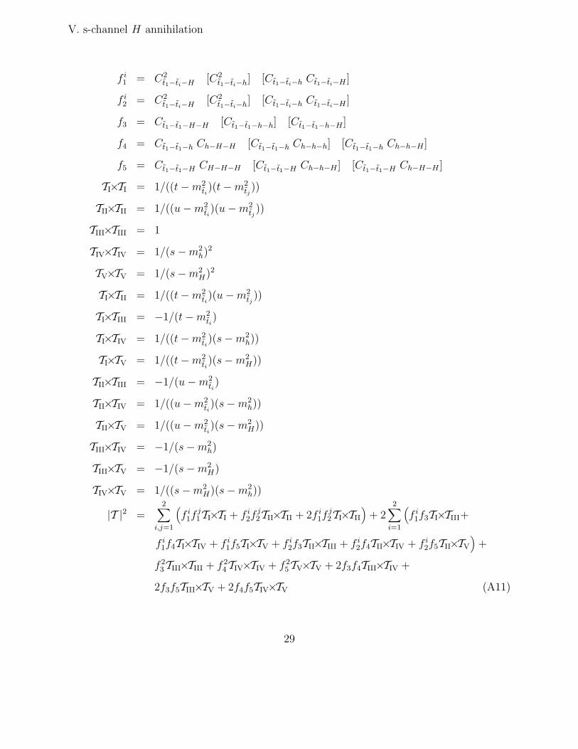
V. s-channel H annihilation

f i1 = C2

t1−ti−H [C2t1−ti−h] [Ct1−ti−h Ct1−ti−H ]

f i2 = C2

t1−ti−H [C2t1−ti−h] [Ct1−ti−h Ct1−ti−H ]

f3 = Ct1−t1−H−H [Ct1−t1−h−h] [Ct1−t1−h−H]

f4 = Ct1−t1−h Ch−H−H [Ct1−t1−h Ch−h−h] [Ct1−t1−h Ch−h−H]

f5 = Ct1−t1−H CH−H−H [Ct1−t1−H Ch−h−H] [Ct1−t1−H Ch−H−H]

TI×TI = 1/((t−m2ti)(t−m2

tj))

TII×TII = 1/((u−m2ti)(u−m2

tj))

TIII×TIII = 1

TIV×TIV = 1/(s−m2h)

2

TV×TV = 1/(s−m2H)2

TI×TII = 1/((t−m2ti)(u−m2

tj))

TI×TIII = −1/(t−m2ti)

TI×TIV = 1/((t−m2ti)(s−m2

h))

TI×TV = 1/((t−m2ti)(s−m2

H))

TII×TIII = −1/(u−m2ti)

TII×TIV = 1/((u−m2ti)(s−m2

h))

TII×TV = 1/((u−m2ti)(s−m2

H))

TIII×TIV = −1/(s−m2h)

TIII×TV = −1/(s−m2H)

TIV×TV = 1/((s−m2H)(s−m2

h))

|T |2 =2∑

i,j=1

(f i

1fj1TI×TI + f i

2fj2TII×TII + 2f i

1fj2TI×TII

)+ 2

2∑i=1

(f i

1f3TI×TIII+

f i1f4TI×TIV + f i

1f5TI×TV + f i2f3TII×TIII + f i

2f4TII×TIV + f i2f5TII×TV

)+

f 23TIII×TIII + f 2

4TIV×TIV + f 25TV×TV + 2f3f4TIII×TIV +

2f3f5TIII×TV + 2f4f5TIV×TV (A11)

29

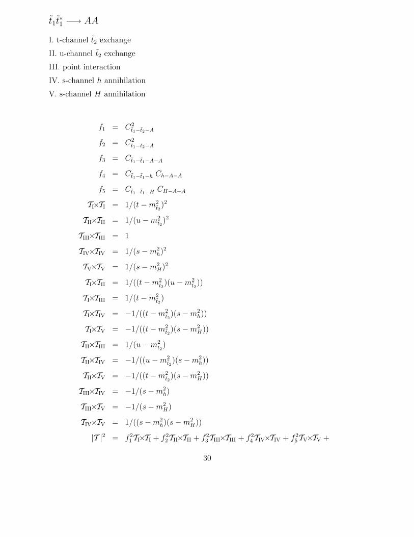
t1t∗1 −→ AA




IV. s-channel h annihilation

V. s-channel H annihilation

f1 = C2t1−t2−A

f2 = C2t1−t2−A

f3 = Ct1−t1−A−A

f4 = Ct1−t1−h Ch−A−A

f5 = Ct1−t1−H CH−A−A

TI×TI = 1/(t−m2t2)2

TII×TII = 1/(u−m2t2

)2

TIII×TIII = 1

TIV×TIV = 1/(s−m2h)

2

TV×TV = 1/(s−m2H)2

TI×TII = 1/((t−m2t2)(u−m2

t2))

TI×TIII = 1/(t−m2t2)

TI×TIV = −1/((t−m2t2

)(s−m2h))

TI×TV = −1/((t−m2t2

)(s−m2H))

TII×TIII = 1/(u−m2t2

)

TII×TIV = −1/((u−m2t2)(s−m2

h))

TII×TV = −1/((t−m2t2

)(s−m2H))

TIII×TIV = −1/(s−m2h)

TIII×TV = −1/(s−m2H)

TIV×TV = 1/((s−m2h)(s−m2

H))

|T |2 = f 21TI×TI + f 2


4TIV×TIV + f 25TV×TV +

30

2f1f2TI×TII + 2f1f3TI×TIII + 2f1f4TI×TIV + 2f1f5TI×TV +

2f2f3TII×TIII + 2f2f4TII×TIV + 2f2f5TII×TV + 2f3f4TIII×TIV +

2f3f5TIII×TV + 2f4f5TIV×TV (A12)

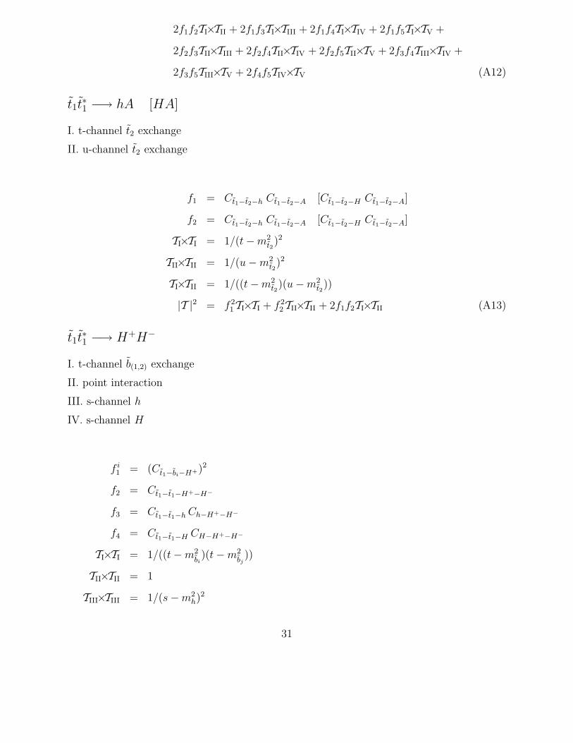
t1t∗1 −→ hA [HA]



f1 = Ct1−t2−h Ct1−t2−A [Ct1−t2−H Ct1−t2−A]

f2 = Ct1−t2−h Ct1−t2−A [Ct1−t2−H Ct1−t2−A]

TI×TI = 1/(t−m2t2

)2

TII×TII = 1/(u−m2t2)2

TI×TII = 1/((t−m2t2

)(u−m2t2))

|T |2 = f 21TI×TI + f 2

2TII×TII + 2f1f2TI×TII (A13)

t1t∗1 −→ H+H−

I. t-channel b(1,2) exchange

II. point interaction

III. s-channel h

IV. s-channel H

f i1 = (Ct1−bi−H+)2

f2 = Ct1−t1−H+−H−

f3 = Ct1−t1−h Ch−H+−H−

f4 = Ct1−t1−H CH−H+−H−

TI×TI = 1/((t−m2bi)(t−m2

bj))

TII×TII = 1

TIII×TIII = 1/(s−m2h)

2

31

TIV×TIV = 1/(s−m2H)2

TI×TII = −1/(t−m2bi)

TI×TIII = 1/((s−m2h)(t−m2

bi))

TI×TIV = 1/((s−m2H)(t−m2

bi))

TII×TIII = −1/(s−m2h)

TII×TIV = −1/(s−m2H)

TIII×TIV = 1/((s−m2h)(s−m2

H))

|T |2 =2∑

i,j=1

f i1f

j1TI×TI + f 2


4TIV×TIV + 22∑

i=1

f i1f2TI×TII +

22∑

i=1

f i1f3TI×TIII + 2

2∑i=1

f i1f4TI×TIV + 2f2f3TII×TIII + 2f2f4TII×TIV +

2f3f4TIII×TIV (A14)

t1t1 −→ tt

I. t-channel gluino exchange

II. u-channel gluino exchange

III. t-channel χ0(1,2,3,4) exchange

IV. u-channel χ0(1,2,3,4) exchange

f1L = f2L ≡ fL = (CLt1−t−g)

2

f1R = f2R ≡ fR = (CRt1−t−g)

2

Ji = (CLt1−t−χ0

i+ CR

t1−t−χ0i)/2

Ki = (CLt1−t−χ0

i− CR

t1−t−χ0i)/2

TI×TI = (2/9)((f 2L + f 2

R)m2g(s− 2m2

t )− fLfR(4m2tm

2g + 2st + 2(m2

t1−m2

t − t)2)

+√

fLfR (fL + fR) 4 mt mg(t + m2t −m2

t1))/(t−m2

g)2

TII×TII = (2/9)((f 2L + f 2

R)m2g(s− 2m2

t )− fLfR(4m2tm

2g + 2su + 2(m2

t1−m2

t − u)2)

+√

fLfR (fL + fR) 4 mt mg(u + m2t −m2

t1))/(u−m2

g)2

TIII×TIII = (−2 (4 Ji Jj Ki Kj mχ0imχ0

js + K2

i (J2j (−m4

t1− 2m2

t1m2

t + 3m4t − 4m3

t mχ0i

+4m3t mχ0

j− 4m2

t mχ0imχ0

j+ m2

t1s−m2

t s + mtmχ0is−mtmχ0

js + mχ0

imχ0

js

32

+m2t1t + 3m2

t t−mtmχ0it + mtmχ0

jt + m2

t1u−m2

t u + mtmχ0iu−mtmχ0

ju

−tu) + K2j (m

4t1

+ 2m2t1m2

t − 3m4t + 4m3

t mχ0i+ 4m3

tmχ0j− 4m2

t mχ0imχ0

j

−m2t1s + m2

t s−mtmχ0is−mtmχ0

js + mχ0

imχ0

js−m2

t1t− 3m2

t t + mtmχ0it

+mtmχ0jt−m2

t1u + m2

t u−mtmχ0iu−mtmχ0

ju + tu)) + J2

i (K2j (−m4

t1

−2m2t1m2

t + 3m4t + 4m3

tmχ0i− 4m3

tmχ0j− 4m2

t mχ0imχ0

j+ m2

t1s−m2

ts

−mtmχ0is + mtmχ0

js + mχ0

imχ0

js + m2

t1t + 3m2

t t + mtmχ0it−mtmχ0

jt

+m2t1u−m2

t u−mtmχ0iu + mtmχ0

ju− tu) + J2

j (m4t1

+ 2m2t1m2

t − 3m4t

−4m3t mχ0

i− 4m3

tmχ0j− 4m2

t mχ0imχ0

j−m2

t1s + m2

t s + mtmχ0is + mtmχ0

js

+mχ0imχ0

js−m2

t1t− 3m2

t t−mtmχ0it−mtmχ0

jt−m2

t1u + m2

tu

+mtmχ0iu + mtmχ0

ju + tu))))/((m2

χ0i− t)(−m2

χ0j+ t))

TIV×TIV = (−2(4 Ji Jj Ki Kj mχ0imχ0

js + J2

i (K2j (−m4

t1− 2m2

t1m2

t + 3m4t + 4m3

tmχ0i

−4m3t mχ0

j− 4m2

tmχ0imχ0

j+ m2

t1s−m2

ts−mtmχ0is + mtmχ0

js + mχ0

imχ0

js

+m2t1t−m2

t t−mtmχ0it + mtmχ0

jt + m2

t1u + 3m2

t u + mtmχ0iu−mtmχ0

ju− tu)

+J2j (m4

t1+ 2m2

t1m2

t − 3m4t − 4m3

t mχ0i− 4m3

tmχ0j− 4m2

tmχ0imχ0

j−m2

t1s

+m2t s + mtmχ0

is + mtmχ0

js + mχ0

imχ0

js−m2

t1t + m2

t t + mtmχ0it + mtmχ0

jt

−m2t1u− 3m2

tu−mtmχ0iu−mtmχ0

ju + tu)) + K2

i (J2j (−m4

t1− 2m2

t1m2

t

+3m4t − 4m3

t mχ0i+ 4m3

tmχ0j− 4m2

t mχ0imχ0

j+ m2

t1s−m2

t s + mtmχ0is

−mtmχ0js + mχ0

imχ0

js + m2

t1t−m2

t t + mtmχ0it−mtmχ0

jt + m2

t1u + 3m2

t u

−mtmχ0iu + mtmχ0

ju− tu) + K2

j (m4t1

+ 2m2t1m2

t − 3m4t + 4m3

tmχ0i

+4m3t mχ0

j− 4m2

t mχ0imχ0

j−m2

t1s + m2

t s−mtmχ0is−mtmχ0

js + mχ0

imχ0

js

−m2t1t + m2

t t−mtmχ0it−mtmχ0

jt−m2

t1u− 3m2

tu + mtmχ0iu + mtmχ0

ju

+tu))))/((m2χ0

i− u)(−m2

χ0j+ u))

TI×TII = (−2/27)(fLfR(2(m2t1−m2

t − u)(m2t1−m2

t − t)− 4(s− 2m2t )(m

2t1−m2

t ))

+√

fLfR (fL + fR)mt mg(t− u) + (f 2L + f 2

R)m2g(s− 2m2

t )− 4m2t tfLfR

−mtmg

√fLfR(fL + fR)(t + u)− 4m2

tm2gfLfR)/((t−m2

g)(u−m2g))

TI×TIII = 0

TI×TIV = 0

33

TII×TIII = 0

TII×TIV = 0

TIII×TIV = (8 Ji Jj Ki Kj mχ0imχ0

js + J2

i (−(K2j (2m4

t1+ 4m2

t1m2

t − 6m4t − 8m3

tmχ0i

+8m3t mχ0

j+ 8m2

tmχ0imχ0

j+ 2m2

t1s + 2m2

ts + 2mtmχ0is− 2mtmχ0

js

−2mχ0imχ0

js− s2 − 2m2

t1t− 2m2

t t + 2mtmχ0it + 2mtmχ0

jt + t2 − 2m2

t1u

−2m2t u− 2mtmχ0

iu− 2mtmχ0

ju + u2)) + J2

j (2m4t1

+ 4m2t1m2

t − 6m4t

−8m3t mχ0

i− 8m3

tmχ0j− 8m2

t mχ0imχ0

j+ 2m2

t1s + 2m2

t s + 2mtmχ0is + 2mtmχ0

js

+2mχ0imχ0

js− s2 − 2m2

t1t− 2m2

t t + 2mtmχ0it− 2mtmχ0

jt + t2 − 2m2

t1u

−2m2t u− 2mtmχ0

iu + 2mtmχ0

ju + u2)) + K2

i (K2j (2m

4t1

+ 4m2t1m2

t − 6m4t

+8m3t mχ0

i+ 8m3

tmχ0j− 8m2

tmχ0imχ0

j+ 2m2

t1s + 2m2

ts− 2mtmχ0is− 2mtmχ0

js

+2mχ0imχ0

js− s2 − 2m2

t1t− 2m2

t t− 2mtmχ0it + 2mtmχ0

jt + t2 − 2m2

t1u

−2m2t u + 2mtmχ0

iu− 2mtmχ0

ju + u2)− J2

j (2m4t1

+ 4m2t1m2

t − 6m4t

+8m3t mχ0

i− 8m3

t mχ0j+ 8m2

tmχ0imχ0

j+ 2m2

t1s + 2m2

ts− 2mtmχ0is + 2mtmχ0

js

−2mχ0imχ0

js− s2 − 2m2

t1t− 2m2

t t− 2mtmχ0it− 2mtmχ0

jt + t2 − 2m2

t1u

−2m2t u + 2mtmχ0

iu + 2mtmχ0

ju + u2)))/((m2

χ0i− t)(m2

χ0j− u))

|T |2 = TI×TI + TII×TII +4∑

i,j=1

(TIII×TIII + TIV×TIV) + 2TI×TII +

24∑

i=1

(TI×TIII + TI×TIV + TII×TIII + TII×TIV) + 24∑

i,j=1

TIII×TIV (A15)

χt1 −→ tg

I. s-channel t annihilation


f1L = CLt1−t−χ0

1Ct−t−g

f1R = CRt1−t−χ0

1Ct−t−g


1Ct1−t1−g


1Ct1−t1−g

34

TI×TI = (−4/6)((f 21L + f 2

1R)2((3m2t − s)(s + m2

χ −m2t1) + (s−m2

t )(m2χ + m2

t − t))

−8f1Lf1R mt mχ(s + m2t ))/(s−m2

t )2

TII×TII = (−4/6)(2(t + m2t1

)((f 22L + f 2

2R)(m2χ + m2

t − t)− 4mχmtf2Lf2R))/(t−m2t1

)2

TI×TII = (−4/6)((f1Lf2L + f1Rf2R)/2((m2χ + m2

t − t)(s− 2m2χ + 2m2

t1+ m2

t )

−(s + m2t )(2s− 3m2

χ − 2m2t1

+ u) + (2m2t1

+ 3m2t − 2u− s)(s + m2

χ −m2t1)

+2m2t (2s− 3m2

χ − 2m2t1

+ u))− (f1Lf2R + f1Rf2L) mt mχ(4m2t1

+ 4m2t

−2m2χ − 2u))/((s−m2

t )(t−m2t1))

|T |2 = TI×TI + TII×TII + 2TI×TII (A16)

χt1 −→ tZ

I. u-channel χ0(1,2,3,4) exchange

f iLL = CL

t1−t−χ0iCL

χ01−χ0

i−Z

f iLR = CL

t1−t−χ0iCR

χ01−χ0

i−Z

f iRL = CR

t1−t−χ0iCL

χ01−χ0

i−Z

f iRR = CR

t1−t−χ0iCR

χ01−χ0

i−Z

TI×TI = (1/2)((f iLL f j

LL + f iRR f j

RR)(((u−m2t1

+ m2t )(u + m2

χ −m2Z)− (m2

χ + m2t − t)u)

+((m2χ + m2

Z − u)/m2Z)((m2

χ −m2Z − u)(u−m2

t1+ m2

t )− (s−m2t −m2

Z)u))

+(f iLR f j

RR + f iRL f j

LL)mtmχ0i((u + m2

χ −m2Z) + (1/m2

Z)((m2χ + m2

Z − u)

× (m2χ −m2

Z − u))) + (f iLL f j

RL + f iRR f j

LR)mtmχ0j((u + m2

χ −m2Z)

+(1/m2Z)((m2

χ + m2Z − u)(m2

χ −m2Z − u)))

+(f iLR f j

LR + f iRL f j

RL)mχ0imχ0

j((t + m2

χ −m2t )

+(1/m2Z)((m2

χ + m2Z − u)(s−m2

t −m2Z)))

+(f iLL f j

RR + f iRR f j

LL)6mtmχu + (f iLL f j

LR + f iRR f j

RL)3mχ0j(u + m2

t −m2t1

)mχ

+(f iLR f j

LL + f iRL f j

RR)3mχ0i(u + m2

t −m2t1

)mχ

+(f iLR f j

RL + f iRL f j

LR)6mχ0imχ0

jmtmχ)/((t−m2

χ0i)(t−m2

χ0j))

|T |2 =4∑

i,j=1

TI×TI (A17)

35

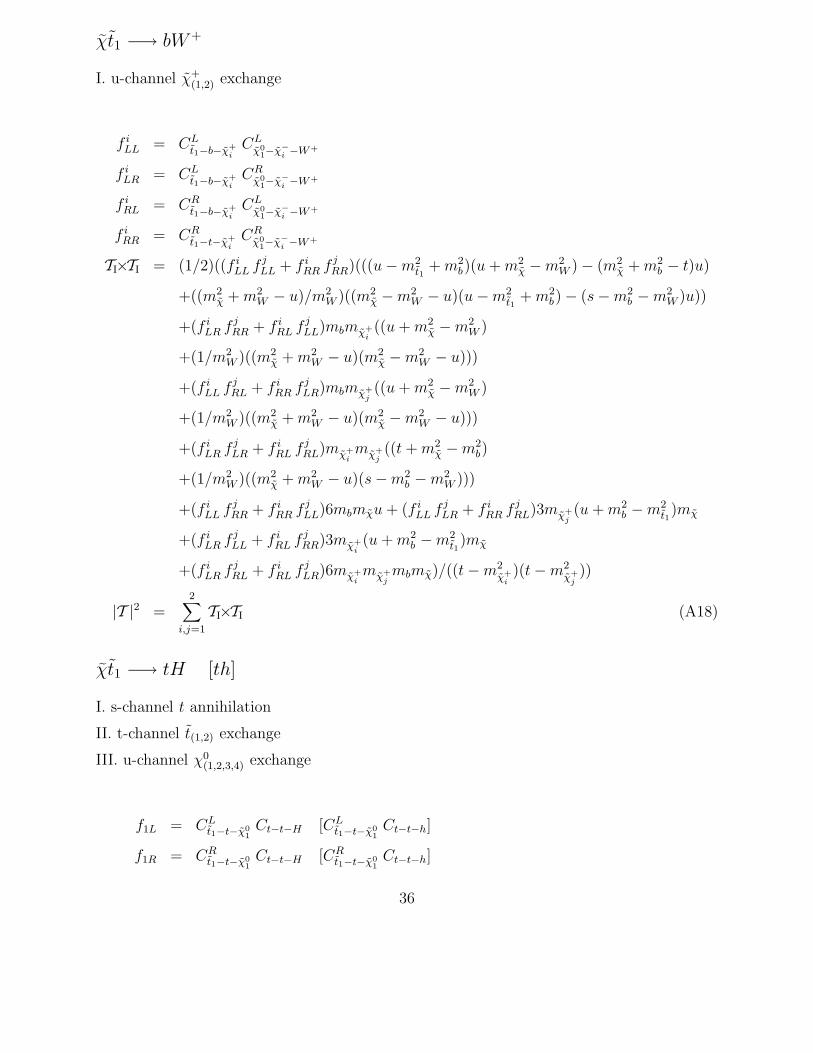
χt1 −→ bW+

I. u-channel χ+(1,2) exchange

f iLL = CL

t1−b−χ+i

CLχ0

1−χ−i −W+

f iLR = CL

t1−b−χ+i

CRχ0

1−χ−i −W+

f iRL = CR

t1−b−χ+i

CLχ0

1−χ−i −W+

f iRR = CR

t1−t−χ+i

CRχ0

1−χ−i −W+

TI×TI = (1/2)((f iLL f j

LL + f iRR f j

RR)(((u−m2t1

+ m2b)(u + m2

χ −m2W )− (m2

χ + m2b − t)u)

+((m2χ + m2

W − u)/m2W )((m2

χ −m2W − u)(u−m2

t1+ m2

b)− (s−m2b −m2

W )u))

+(f iLR f j

RR + f iRL f j

LL)mbmχ+i((u + m2

χ −m2W )

+(1/m2W )((m2

χ + m2W − u)(m2

χ −m2W − u)))

+(f iLL f j

RL + f iRR f j

LR)mbmχ+j((u + m2

χ −m2W )

+(1/m2W )((m2

χ + m2W − u)(m2

χ −m2W − u)))

+(f iLR f j

LR + f iRL f j

RL)mχ+imχ+

j((t + m2

χ −m2b)

+(1/m2W )((m2

χ + m2W − u)(s−m2

b −m2W )))

+(f iLL f j

RR + f iRR f j

LL)6mbmχu + (f iLL f j

LR + f iRR f j

RL)3mχ+j(u + m2

b −m2t1

)mχ

+(f iLR f j

LL + f iRL f j

RR)3mχ+i(u + m2

b −m2t1

)mχ

+(f iLR f j

RL + f iRL f j

LR)6mχ+imχ+

jmbmχ)/((t−m2

χ+i)(t−m2

χ+j))

|T |2 =2∑

i,j=1

TI×TI (A18)

χt1 −→ tH [th]


II. t-channel t(1,2) exchange

III. u-channel χ0(1,2,3,4) exchange


1Ct−t−H [CL

t1−t−χ01Ct−t−h]


1Ct−t−H [CR

t1−t−χ01Ct−t−h]

36

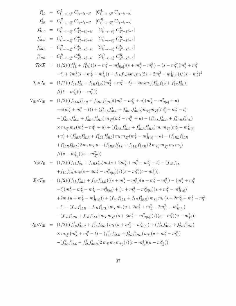
f i2L = CL

t1−t−χ01Ct1−t1−H [CL

t1−t−χ01Ct1−t1−h]

f i2R = CR

t1−t−χ01Ct1−t1−H [CR

t1−t−χ01Ct1−t1−h]

f i3LL = CL

t1−t−χ0iCL

χ01−χ0

i−H [CLt1−t−χ0

iCL

χ01−χ0

i−h]

f i3LR = CL

t1−t−χ0iCR

χ01−χ0

i−H [CLt1−t−χ0

iCR

χ01−χ0

i−h]

f i3RL = CR

t1−t−χ0iCL

χ01−χ0

i−H [CRt1−t−χ0

iCL

χ01−χ0

i−h]

f i3RR = CR

t1−t−χ0iCR

χ01−χ0

i−H [CRt1−t−χ0

iCR

χ01−χ0

i−h]

TI×TI = (1/2)((f 21L + f 2

1R)((s + m2t −m2

H[h])(s + m2χ −m2

t1)− (s−m2

t )(m2χ + m2

t

−t) + 2m2t (s + m2

χ −m2t1

))− f1Lf1R4mχmt(2s + 2m2t −m2

H[h]))/(s−m2t )

2

TII×TII = (1/2)((f i2Lf j

2L + f i2Rf j

2R)(m2χ + m2

t − t)− 2mtmχ(f i2Lf j

2R + f i2Rf j

2L))

/((t−m2ti)(t−m2

tj))

TIII×TIII = (1/2)((f i3LRf j

3LR + f i3RLf j

3RL)((m2t −m2

t1+ u)(m2

χ −m2H[h] + u)

−u(m2χ + m2

t − t)) + (f i3LLf j

3LL + f i3RRf j

3RR)mχ0imχ0

j(m2

χ + m2t − t)

−(f i3LRf j

3LL + f i3RLf j

3RR) mχ0j(m2

t −m2t1

+ u)− (f i3LLf j

3LR + f i3RRf j

3RL)

×mχ0imχ(m2

t −m2t1

+ u) + (f i3RLf j

3LL + f i3LRf j

3RR) mt mχ0j(m2

χ −m2H[h]

+u) + (f i3RRf j

3LR + f i3LLf j

3RL) mt mχ0i(m2

χ −m2H[h] + u)− (f i

3RLf j3LR

+f i3LRf j

3RL)2 mt mχ u− (f i3RRf j

3LL + f i3LLf j

3RR) 2 mχ0imχ0

jmt mχ)

/((u−m2χ0

i)(u−m2

χ0j))

TI×TII = (1/2)((f1Lf i2L + f1Rf i

2R)mt(s + 2m2χ + m2

t −m2t1− t)− (f1Rf i

2L

+f1Lf i2R)mχ(s + 3m2

t −m2H[h]))/((s−m2

t )(t−m2ti))

TI×TIII = (1/2)((f1Lf i3RL + f1Rf i

3LR)((s + m2χ −m2

t1)(u + m2

t −m2t1)− (m2

χ + m2t

−t)(m2t + m2

χ −m2t1−m2

H[h]) + (u + m2χ −m2

H[h])(s + m2t −m2

H[h])

+2mt(u + m2χ −m2

H[h])) + (f1Lf i3LL + f1Rf i

3RR) mχ0imt (s + 2m2

χ + m2t −m2

t1

−t)− (f1Lf i3LR + f1Rf i

3RL) mχ mt (u + 2m2t + m2

χ − 2m2t1−m2

H[h])

−(f1Lf i3RR + f1Rf i

3LL) mχ mχ0i(s + 3m2

t −m2H[h]))/((s−m2

t )(u−m2χ0

i))

TII×TIII = (1/2)((f j2Rf i

3LR + f j2Lf i

3RL) mt (u + m2χ −m2

H[h]) + (f j2Lf i

3LL + f j2Rf i

3RR)

×mχ0i(m2

χ + m2t − t)− (f j

2Lf i3LR + f j

2Rf i3RL) mχ (u + m2

t −m2t1)

−(f j2Rf i

3LL + f j2Lf i

3RR)2 mχ mt mχ0i)/((t−m2

tj)(u−m2

χ0i))

37

|T |2 = TI×TI +2∑

i,j=1

TII×TII +4∑

i,j=1

TIII×TIII + 22∑

i=1

TI×TII + 24∑

i=1

TI×TIII +

22∑

j=1

4∑i=1

TII×TIII (A19)

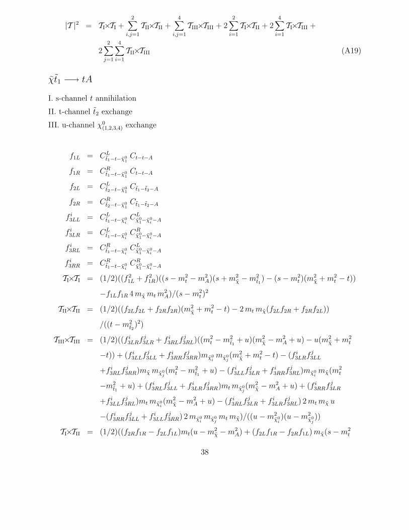
χt1 −→ tA



III. u-channel χ0(1,2,3,4) exchange


1Ct−t−A


1Ct−t−A


1Ct1−t2−A


1Ct1−t2−A

f i3LL = CL

t1−t−χ0iCL

χ01−χ0

i−A

f i3LR = CL

t1−t−χ0iCR

χ01−χ0

i−A

f i3RL = CR

t1−t−χ0iCL

χ01−χ0

i−A

f i3RR = CR

t1−t−χ0iCR

χ01−χ0

i−A

TI×TI = (1/2)((f 21L + f 2

1R)((s−m2t −m2

A)(s + m2χ −m2

t1)− (s−m2

t )(m2χ + m2

t − t))

−f1Lf1R 4 mχ mt m2A)/(s−m2

t )2

TII×TII = (1/2)((f2Lf2L + f2Rf2R)(m2χ + m2

t − t)− 2 mt mχ(f2Lf2R + f2Rf2L))

/((t−m2t2

)2)

TIII×TIII = (1/2)((f i3LRf j

3LR + f i3RLf j

3RL)((m2t −m2

t1+ u)(m2

χ −m2A + u)− u(m2

χ + m2t

−t)) + (f i3LLf j

3LL + f i3RRf j

3RR)mχ0imχ0

j(m2

χ + m2t − t)− (f i

3LRf j3LL

+f i3RLf j

3RR)mχ mχ0j(m2

t −m2t1

+ u)− (f i3LLf j

3LR + f i3RRf j

3RL)mχ0imχ(m2

t

−m2t1

+ u) + (f i3RLf j

3LL + f i3LRf j

3RR)mt mχ0j(m2

χ −m2A + u) + (f i

3RRf j3LR

+f i3LLf j

3RL)mt mχ0i(m2

χ −m2A + u)− (f i

3RLf j3LR + f i

3LRf j3RL) 2 mt mχ u

−(f i3RRf j

3LL + f i3LLf j

3RR) 2 mχ0imχ0

jmt mχ)/((u−m2

χ0i)(u−m2

χ0j))

TI×TII = (1/2)((f2Rf1R − f2Lf1L)mt(u−m2χ −m2

A) + (f2Lf1R − f2Rf1L) mχ(s−m2t

38

−m2A))/((s−m2

t )(t−mt22))

TI×TIII = (1/2)((f i3LRf1R − f i

3RLf1L)((m2χ + m2

t − t)(m2t + m2

χ −m2t1−m2

A)

−(s−m2t −m2

A)(u + m2χ −m2

A)− (u + m2t −m2

t1)(s + m2

χ −m2t1

))/2

+(f i3RRf1R − f i

3LLf1L) mχ0imt (u−m2

A −m2χ) + (f i

3LRf1L − f i3RLf1R)

×mt mχ(u−m2χ + m2

A) + (f i3RRf1L − f i

3LLf1R)mχ0imχ(m2

t + m2A − s))

/((s−m2t )(u−m2

χ0i))

TII×TIII = (1/2)((f2Rf i3LR + f2Lf i

3RL) mt (u + m2χ −m2

A) + (f2Lf i3LL + f2Rf i

3RR)

×mχ0i(m2

χ + m2t − t)− (f2Lf i

3LR + f2Rf i3RL)mχ(u + m2

t −m2t1)

−(f2Rf i3LL + f2Lf i

3RR) 2 mχ mt mχ0i)/((t−m2

t2)(u−m2

χ0i))

|T |2 = TI×TI + TII×TII +4∑

i,j=1

TIII×TIII + 2TI×TII + 24∑

i=1

TI×TIII + 24∑

i=1

TII×TIII (A20)

χt1 −→ bH+


II. t-channel χ+(1,2) exchange

III. u-channel b(1,2) exchange

f1LL = CLt−b−H+ CL

t1−t−χ01

f1LR = CLt−b−H+ CR

t1−t−χ01

f1RL = CRt−b−H+ CL

t1−t−χ01

f1RR = CRt−b−H+ CR

t1−t−χ01

f i2LL = CL

t1−b−χ+i

CLχ0

1−χ+i −H+

f i2LR = CL

t1−b−χ+i

CRχ0

1−χ+i −H+

f i2RL = CR

t1−b−χ+i

CLχ0

1−χ+i −H+

f i2RR = CR

t1−b−χ+i

CRχ0

1−χ+i −H+

f i3L = CL

bi−b−χ01Ct1−bi−H+

f i3R = CR

bi−b−χ01Ct1−bi−H+

TI×TI = (1/2)((f 21LR + f 2

1RL)((s + m2b −m2

H+)(s + m2χ −m2

t1)− s(m2

χ + m2b − u))

39

+(f 21LL + f 2

1RR)m2t (m

2χ + m2

b − u)− 2(f1LLf1LR + f1RRf1RL) mχ mt

× (s + m2b −m2

H+) + 2(f1LRf1RR + f1LLf1RL)mb mt(s + m2χ −m2

t1)

−4(f1LRf1RL)mb mχ s− 4f1LLf1RR m2t mχ mb)/(s−m2

t )2

TII×TII = (1/2)((f i2RRf j

2RR + f i2LLf j

2LL)((t + m2b −m2

t1)(t + m2

χ −m2H+)− t(m2

χ + m2b

−u)) + (f i2RLf j

2RL + f i2LRf j

2LR) mχ+i

mχ+j

(m2χ + m2

b − u)− (f i2RRf j

2RL

+f i2LLf j

2LR) mχ mχ+j

(t + m2b −m2

t1)− (f i

2RLf j2RR + f i

2LRf j2LL) mχ+

imχ

× (t−m2b −m2

t1) + (f i

2LLf j2RL + f i

2RRf j2LR) mb mχ+

j(t + m2

χ −m2H+)

+(f i2LRf j

2RR + f i2RLf j

2LL) mb mχ+i

(t + m2χ −m2

H+)− (f i2LLf j

2RR + f i2RRf j

2LL)

× 2 mb mχ t− (f i2LRf j

2RL + f i2RLf j

2LR) 2 mb mχ mχ+i

mχ+j)

/((t−m2χ+

i)(t−m2

χ+j))

TIII×TIII = (1/2)((f i3Lf j

3L + f i3Rf j

3R)(m2χ + m2

b − u)− 2 mχ mb(fi3Lf j

3R + f i3Rf j

3L))

/((u−m2bi)(u−m2

bj))

TI×TII = (1/2)((f i2RRf1LR + f i

2LLf1RL)(1/2)((t + m2b −m2

t1)(s + m2

χ −m2t1)− (m2

χ

+m2b − u)(m2

χ + m2b −m2

t1−m2

H+) + (s + m2b −m2

H+)(t + m2χ −m2

H+))

+(f i2RLf1LL + f i

2LRf1RR) mχ+i

mt (m2χ + m2

b − u)− (f i2RRf1LL + f i

2LLf1RR)

×mχ mt (t + m2b −m2

t1)− (f i

2RLf1LR + f i2LRf1RL) mχ+

imχ (s + m2

b −m2H+)

+(f i2LLf1LL + f i

2RRf1RR) mb mt (t + m2χ −m2

H+) + (f i2LRf1LR + f i

2RLf1RL)

×mb mχ+i

(s + m2χ −m2

t1)− (f i

2LLf1LR + f i2RRf1RL) mb mχ (m2

χ + m2b −m2

t1

−m2H+)− (f i

2LRf1LL + f i2RLf1RR) 2 mb mχ mt mχ+

i)/((s−m2

t )(t−m2χ+

i))

TI×TIII = (1/2)((f1LRf i3R + f1RLf i

3L) mb (s + m2χ −m2

t1) + (f1LLf i

3L + f1RRf i3R) mt

× (m2χ + m2

b − u)− (f1LRf i3L + f1RLf i

3R) mχ (s + m2b −m2

H+)− (f1LLf i3R

+f1RRf i3L) 2 mt mb mχ)/((u−m2

bi)(s−m2

t ))

TII×TIII = (1/2)((f j2LRf i

3R + f j2RLf i

3L) mb (t + m2χ −m2

H+) + (f j2LLf i

3L + f j2RRf i

3R)

×mχ+j(m2

χ + m2b − u)− (f j

2LRf i3L + f j

2RLf i3R) mχ (t + m2

b −m2t1)

−(f j2LLf i

3R + f j2RRf i

3L) 2 mχ+j

mb mχ)/((u−m2bi)(t−m2

χ+j))

|T |2 = TI×TI +2∑

i,j=1

TII×TII +2∑

i,j=1

TIII×TIII + 22∑

i=1

TI×TII + 22∑

i=1

TI×TIII +

40

22∑

i,j=1

TII×TIII (A21)

t1 ˜−→ t`

I. t-channel χ0(1,2,3,4) exchange

f iLL = CL

t1−t−χ0i

CL˜1−`−χ0

i

f iLR = CL

t1−t−χ0i

CR˜1−`−χ0

i

f iRL = CR

t1−t−χ0i

CL˜1−`−χ0

i

f iRR = CR

t1−t−χ0i

CR˜1−`−χ0

i

TI×TI = ((f iLRf j

RL + f iRLf j

LR)((m2t1−m2

t − t)(t + m2` −m2

˜1)− t(s−m2

t −m2`))

+(f iLLf j

LL + f iRRf j

RR) mχ0imχ0

j(s−m2

t −m2`)

−(f iLRf j

LL + f iRLf j

RR) m` mχ0j(m2

t1−m2

t − t)

−(f iLLf j

RL + f iRRf j

LR) m` mχ0i(m2

t1−m2

t − t)

+(f iRLf j

LL + f iLRf j

RR) mt mχ0j(t + m2

` −m2˜1)

+(f iRRf j

RL + f iLLf j

LR) mt mχ0i(t + m2

` −m2˜1)

−(f iRLf j

LR + f iLRf j

LR) mt m` 2 t− (f iRRf j

LL + f iLLf j

RR) 2 mt m` mχ0imχ0

j)

/((t−m2χ0

i)(t−m2

χ0j))

|T |2 =4∑

i,j=1

TI×TI (A22)

t1 ˜−→ bν

I. t-channel χ+(1,2) exchange

f iLL = CL

t1−b−χ+i

CL˜1−ν−χ+

i

f iLR = CL

t1−b−χ+i

CR˜1−ν−χ+

i

f iRL = CR

t1−b−χ+i

CL˜1−ν−χ+

i

f iRR = CR

t1−b−χ+i

CR˜1−ν−χ+

i

41

TI×TI = ((f iLRf j

RL + f iRLf j

LR)((m2t1−m2

b − t)(t−m2˜1)− t(s−m2

b))

+(f iLLf j

LL + f iRRf j

RR) mχ+i

mχ+j

(s−m2b)

+(f iRLf j

LL + f iLRf j

RR) mb mχ+j

(t−m2˜1)

+(f iRRf j

RL + f iLLf j

LR) mb mχ+i

(t−m2˜1))

/((t−m2χ+

i)(t−m2

χ+j))

|T |2 =2∑

i,j=1

TI×TI (A23)

t1 ˜∗ −→ t¯

I. t-channel χ0(1,2,3,4) exchange

f iLL = CL

t1−t−χ0i

CL˜1−`−χ0

i

f iLR = CL

t1−t−χ0i

CR˜1−`−χ0

i

f iRL = CR

t1−t−χ0i

CL˜1−`−χ0

i

f iRR = CR

t1−t−χ0i

CR˜1−`−χ0

i

TI×TI = ((f iLLf j

LL + f iRRf j

RR)((m2t1−m2

t − t)(t + m2` −m2

˜1)− t(s−m2

t −m2`))

+(f iLRf j

RL + f iRLf j

LR) mχ0imχ0

j(s−m2

t −m2`)

−(f iLLf j

RL + f iRRf j

LR) m` mχ0j(m2

t1−m2

t − t)

−(f iLRf j

LL + f iRLf j

RR) m` mχ0i(m2

t1−m2

t − t)

+(f iRRf j

RL + f iLLf j

LR) mt mχ0j(t + m2

` −m2˜1)

+(f iRLf j

LL + f iLRf j

RR) mt mχ0i(t + m2

` −m2˜1)

−(f iRRf j

LL + f iLLf j

RR) mt m` 2 t− (f iRLf j

RL + f iLRf j

LR) 2 mt m` mχ0imχ0

j)

/((t−m2χ0

i)(t−m2

χ0j))

|T |2 =4∑

i,j=1

TI×TI (A24)

42

References

[1] J. Ellis, J.S. Hagelin, D.V. Nanopoulos, K.A. Olive and M. Srednicki, Nucl. Phys. B

238, 453 (1984); see also H. Goldberg, Phys. Rev. Lett. 50, 1419 (1983).

[2] C. Boehm, A. Djouadi and M. Drees, Phys. Rev. D 62, 035012 (2000) [arXiv:hep-

ph/9911496].

[3] N. Bahcall, J. P. Ostriker, S. Perlmutter and P. J. Steinhardt, Science 284, 1481 (1999).

[4] K. Griest and D. Seckel, Phys. Rev. D 43, 3191 (1991).

[5] S. Mizuta and M. Yamaguchi, Phys. Lett. B 298, 120 (1993) [arXiv:hep-ph/9208251].

[6] J. Edsjo and P. Gondolo, Phys. Rev. D 56, 1879 (1997) [arXiv:hep-ph/9704361].

[7] J. Ellis, T. Falk and K.A. Olive, Phys. Lett. B 444, 367 (1998).

[8] J. Ellis, T. Falk, K.A. Olive and M. Srednicki, Astropart. Phys. 13 181 (2000).

[9] M. E. Gomez, G. Lazarides and C. Pallis, Phys. Rev. D 61, 123512 (2000) [arXiv:hep-

ph/9907261] and Phys. Lett. B 487, 313 (2000) [arXiv:hep-ph/0004028]; see also:

A. B. Lahanas, D. V. Nanopoulos and V. C. Spanos, Phys. Rev. D 62, 023515 (2000),

[arXive:hep-ph/9909497].

[10] R. Arnowitt, B. Dutta and Y. Santoso, Nucl. Phys. B 606, 59 (2001) [arXiv:hep-

ph/0102181].

[11] J. L. Feng, K. T. Matchev and T. Moroi, Phys. Rev. Lett. 84, 2322 (2000) [arXiv:hep-

ph/9908309]; J. L. Feng, K. T. Matchev and T. Moroi, Phys. Rev. D 61, 075005 (2000)

[arXiv:hep-ph/9909334]; J. L. Feng, K. T. Matchev and F. Wilczek, Phys. Lett. B 482,

388 (2000) [arXiv:hep-ph/0004043].

[12] J. R. Ellis, T. Falk, G. Ganis, K. A. Olive and M. Srednicki, Phys. Lett. B 510, 236

(2001) [arXiv:hep-ph/0102098].

[13] M. Drees and M. M. Nojiri, Phys. Rev. D 47, 376 (1993); H. Baer and M. Brhlik, Phys.

Rev. D 53, 597 (1996) and Phys. Rev. D 57, 567 (1998); H. Baer, M. Brhlik, M. A. Diaz,

43

J. Ferrandis, P. Mercadante, P. Quintana and X. Tata, Phys. Rev. D 63, 015007 (2001);

A. B. Lahanas and V. C. Spanos, hep-ph/0106345.

[14] M. Srednicki, R. Watkins and K. A. Olive, Nucl. Phys. B 310, 693 (1988).

[15] P. Gondolo and G. Gelmini, Nucl. Phys. B 360, 145 (1991).

[16] T. Falk, K. A. Olive and M. Srednicki, Phys. Lett. B 339, 248 (1994) [arXiv:hep-

ph/9409270].

[17] H. N. Brown et al. [Muon g-2 Collaboration], Phys. Rev. Lett. 86, 2227 (2001) [hep-

ex/0102017].

[18] S. Heinemeyer, W. Hollik and G. Weiglein, Comput. Phys. Commun. 124, 76 (2000)

[arXiv:hep-ph/9812320]; S. Heinemeyer, W. Hollik and G. Weiglein, Eur. Phys. J. C 9,

343 (1999) [arXiv:hep-ph/9812472].

[19] H. Baer, M. Brhlik and D. Castano, Phys. Rev. D 54 (1996) 6944; S. Abel and T. Falk,

Phys. Lett. B 444 (1998) 427.

44

calculations of neutralino-stop coannihilation in the cmssm

Documents