Int. J. Applied Decision Sciences, Vol. 7, No. 3, 2014 255

Copyright © 2014 Inderscience Enterprises Ltd.

Neural network DEA for measuring the efficiency of mutual funds

Payam Hanafizadeh* School of Management and Accounting, Allameh Tabataba’i University, Nezami Ganjavi Street, Tavanneer, Valy Asr Avenue, P.O. Box 14155-6476, Tehran, Iran Fax: +98-21-8877-0017 E-mail: hanafizadeh@gmail.com *Corresponding author

Hamid Reza Khedmatgozar Department of IT Management, Iranian Research Institute for Information Science and Technology, No. 1090, Enghelab Avenue, P.O. Box 13185-1371, Tehran, Iran Fax: +98-21-6646-2254 E-mail: h.khedmatgozar@gmail.com

Ali Emrouznejad Aston Business School, Aston University, Aston Triangle, Birmingham, B4 7ET, UK E-mail: a.emrouznejad@aston.ac.uk

Mojtaba Derakhshan Department of Financial Engineering, University of Science and Culture, Asharif Esfahani Blvd., Park Street, P.O. Box 13145-871, Tehran, Iran Fax: +98-21-4421-4750 E-mail: e.m.derakhshan@gmail.com

Abstract: Efficiency in the mutual fund (MF), is one of the issues that has attracted many investors in countries with advanced financial market for many years. Due to the need for frequent study of MF’s efficiency in short-term periods, investors need a method that not only has high accuracy, but also high speed. Data envelopment analysis (DEA) is proven to be one of the most widely used methods in the measurement of the efficiency and productivity of decision making units (DMUs). DEA for a large dataset with many inputs/outputs would require huge computer resources in terms of memory and CPU time. This paper uses neural network back-propagation DEA in measurement of mutual funds efficiency and shows the requirements, in the

256 P. Hanafizadeh et al.

proposed method, for computer memory and CPU time are far less than that needed by conventional DEA methods and can therefore be a useful tool in measuring the efficiency of a large set of MFs.

Keywords: mutual fund; data envelopment analysis; DEA; back-propagation DEA; neural network; large dataset.

Reference to this paper should be made as follows: Hanafizadeh, P., Khedmatgozar, H.R., Emrouznejad, A. and Derakhshan, M. (2014) ‘Neural network DEA for measuring the efficiency of mutual funds’, Int. J. Applied Decision Sciences, Vol. 7, No. 3, pp.255–269.

Biographical notes: Payam Hanafizadeh started his career in January 2001 at the School of Management and Accounting at the Allameh Tabataba’i University in Tehran, Iran. He was a Visiting Research Fellow at the University of Canberra, Australia in 2010 and a visiting scholar at the University of Waterloo, Canada in 2004. His research interest is on the broad area of information systems and decision science particularly decision making under uncertainty. He has written over 80 peer-reviewed research manuscripts, including 50+ journal articles, six books, six book chapters, and several conference papers and presentations.

Hamid Reza Khedmatgozar is a PhD candidate of Information Technology (IT) Management at the Iranian Research Institute for Information Science and Technology – IRANDOC, Tehran, Iran. He holds a BSc in Industrial Engineering from Yazd University, Yazd, Iran, and a Master’s degree in Financial Engineering from University of Science and Culture, Tehran, Iran. His research interests revolve around IT adoption and risk management in financial markets and digital identifier systems for information objects. He has published articles in Electronic Commerce Research, Telematics and Informatics, Iranian Journal of Management Sciences and Sharif Industrial Engineering and Management Journal.

Ali Emrouznejad is a reader in Operational Research and Management at the Aston Business School, Aston University, UK. He holds an MSc in Applied Mathematics and received his PhD in Operational Research and Systems from Warwick Business School, UK. His areas of research interest include performance measurement and management, efficiency and productivity analysis as well as data mining. He serves on the editorial board of several scientific journals; he is the Editor of Annals of Operations Research, Senior Editor and one of the founding members of the Data Envelopment Analysis Journal. He is the author of the book on Applied Operational Research with SAS.

Mojtaba Derakhshan is a graduated Master of Science in the Department of Financial Engineering at the University of Science and Culture in Tehran, Iran. He received his BSc in Industrial Engineering from Tehran Polytechnic University and pursues his research in portfolio selection and organisational diagnosis (OD). He has published some articles in journals such as the International Journal of Industrial Engineering and Product Management and accepted in the international IIE conference, among others.

Neural network DEA for measuring the efficiency of mutual funds 257

1 Introduction

Data envelopment analysis (DEA) is a linear programming technique for assessing the efficiency of decision making units (DMUs). During the last three decades DEA has gained considerable attention as a managerial tool for measuring comparative performance of both private and public organisations such as banks, airports, hospitals, universities and industries (Charnes et al., 1978). As a result, many new applications with more complicated models are being introduced (Emrouznejad et al., 2008).

Examples of DEAs applications can be seen in Burger and Moormann (2010), Cooper et al. (2011), Djema and Djerdjouri (2012), Field and Emrouznejad (2003), Heidari et al. (2012), Ho and Wu (2008), Iazzolino et al. (2013), Kthiri et al. (2011), Meenakumari et al. (2009), Staat (2006), Sufian (2007, 2010) and Van der Meer et al. (2004). Due to the complexity of DEA calculation, several software have been developed (e.g., Emrouznejad and Thanassoulis, 2005, 2010; Zhanxin et al., 2012).

In addition of the theoretical development of DEA, practitioners in many fields have recognised that DEA is a useful methodology for measuring productivity and efficiency of homogeneous DMUs. Recently, some large organisations have started using DEA for evaluation of thousands of DMUs. Application like these, need careful calculations. Even with a very fast computer it may take a long time to get the results since DEA solves one linear programming for each DMU (Emrouznejad and Shale, 2009).

This paper explores the effective factors in determining mutual funds (MFs) efficiency and uses a combined algorithm of neural network and DEA to estimates the efficiency of a large set of MFs. It is shown that this method offers considerable computational savings in terms of mass and time.

The paper is organised as follows. Section 2 describes MFs. The DEA, method of calculation in DEA and neural network algorithm for DEA (NNDEA) are explained in Section 3. Section 4 describes the assessment procedure and the use of NNDEA for assessment of MFs. This is followed by discussion of the results in Section 5. Conclusions and future direction of research are given in Section 6.

2 Mutual fund

A mutual fund (MF) is a company that collects people and companies’ financial resources and invests in a portfolio of securities. People who buy shares of an MF are the owners or shareholders. Their investments provide the capital for an MF to buy securities such as stocks and bonds. An MF can make money from its securities in two ways: a security can pay dividends or interest to the fund or a security can raise in value. A fund can also lose money and fall in value (Hanafizadeh et al., 2009).

In the USA, investment company assets consist of Mutual, Close End and Exchange Trader Funds, it has been increased from 2,955 billion dollars in 1995 to 14,647 billion dollars in 2012. During the same time, the number of MFs has been increased from 6,263 to 10,593 (resource: Investment Company Institute).

The first question that rises in the mind of each investor is the efficiency assessment “which MF does have strong efficiency and which one weak?” Because of the large number of MFs in the world wide, e.g., about 10,000 in the USA only, investors need a suitable tool in order to be able to select the best MF for their investment. Further, they need to review the efficiency of MFs on a defined time period like on a daily, weekly,

258 P. Hanafizadeh et al.

monthly or annual basis. DEA is proven to be a useful tool for helping investors to select a more efficient MF.

Examples of applications of DEA in MFs can be seen in Basso and Funari (2003), Briec et al. (2007), Chang (2004), Chen et al. (2011), Gregoriou et al. (2005), Haslem and Scheraga (2003), Joro and Na (2006), Lozano and Gutiérrez (2008), McMullen and Strong (1998), Murthi et al. (1997), Premachandra et al. (2012), Wilkens and Zhu (2001), Zhao and Wang (2007) and Zhao et al. (2011). By reviewing these studies, we can see that they generally follow two main goals:

1 improving the DEA model which is used evaluating the efficiency of MFs

2 developing the used variables (input and output) in DEA models for having a complete evaluation of MFs efficiency.

Often the investors want to know the results of the analysis very quickly, so speed is very critical parameter, but DEA needs to run one linear programming for each MF, hence the results cannot be obtained at the speed the investors need. An alternative to DEA is a method uses combined DEA and neural network (NNDEA) as developed by Emrouznejad and Shale (2009). In this paper, we propose an NNDEA assessment procedure for comparison of MFs in order to reduce the time to get the results for investors.

3 DEA and NNDEA

DEA is a method for measuring the efficiency of DMUs using linear or non-linear programming techniques by input–output vectors of each DMU. One of the main advantages of DEA is that it allows several inputs and outputs to be considered at the same time. In this case, efficiency is measured based on the value which the input/output of every DMU takes.

Consider a set of observed DMUs, {DMUj; j = 1, …, n}, associated with m inputs as, {xij; i = 1, …, m}, and s outputs as, {yrj; r = 1, …, s}. A standard constant return to scale DEA for measuring efficiency of DMUp is formulated in model 1.

3.1 Model 1: input oriented – CRS model

1 1

1

1

: 1, 2, ,

1,2, ,

0; 1, 2, ,

, 0; ,

m s

p i ri r

n

j rj r rpj

n

j ij i p ipj

j

i r

p

MinY θ ε S S

St γ S y r s

x S θ x i m

j n

S S i rθ free

− +

= =

+

=

−

=

− +

⎡ ⎤= − +⎢ ⎥

⎢ ⎥⎣ ⎦

− = =

+ = =

≥ =

≥ ∀ ∀

∑ ∑

∑

∑

……

……

……

λ

λ

λ

(1)

Neural network DEA for measuring the efficiency of mutual funds 259

where m is number of inputs, n is number of DMUs, s is number of outputs, xij is the ith input of DMUj, yrj is the rth output of DMUj, p is the DMU under evaluation and λj is the weight of DMUj during estimation.

Assume *pθ is the optimum value of the objective function, if * 1pθ = and the optimal

evaluation of iS − and rS + are zero for all i and r, then DMUp is efficient. In model (1), Si

and Sr represent slack variables. Thus, a slack in an input i, i.e., * 0,iS > represents

additional inefficiency in the use of input i. A slack in an output r, i.e., * 0,rS > represents an additional inefficiency in the production of output r.

The DEA model (1) is known as an input – oriented model because it minimises the input of DMUp within the production space. It must be solved n times, once for each DMU being evaluated, and generate n times the optimal values of * ,pθ λ* and S*.

As alternative to DEA, Emrouznejad and Shale (2009) proposed a combined NNDEA. An example of NNDEA network in measuring the efficiency of the DMUs is shown in Figure 1, this method does learning process on multi-layer neural network.

The NN inputs correspond to the attributes that can be used to measure the DEA efficiency (i.e., resources and outcome variables in DEA) and the NN output corresponds to the value that should be predicted (i.e., DEA efficiency score). The inputs are fed simultaneously into a layer of units making up the input layer. The weighted outputs of theses units are, in turn, fed simultaneously to a second layer of ‘neuron-like’ units, known as a hidden layer. The hidden layer’s weighted outputs can be input to another hidden layer, and so on. The number of hidden layers is arbitrary, although in practice, usually only one (or maximum three) is used. The weighted outputs of the last hidden layer are input to the unit making up the output layer, which produces the network’s prediction for given set of DMUs.

Figure 1 Back-propagation DEA

The multi-layer NNDEA shown in Figure 1 has one hidden layers and one output layer and therefore we refer to it as a two-layer neural network. The network is feed-forward in that none of the weights cycles back to an input unit or to an output unit of a previous

260 P. Hanafizadeh et al.

layer. In such a network, output of every units of a layer, makes the input of the next layer.

The aim in this paper is to propose a multilayer feed-forward DEA network, given sufficient hidden layers which cane be used for determination of the optimal evaluation of the efficiency of MFs with a good accuracy.

Back-propagation DEA, see Appendix, learns by iteratively processing a set of training sample, comparing the network’s prediction about efficiency amount for each sample of DMUs with estimated efficiency using standard DEA. For each training sample, the weights are corrected so as to minimise the mean squared error between the network’s prediction and the efficiency value as obtained in a conventional DEA model. These corrections are made in the ‘backwards’ direction. In Appendix, the back-propagation DEA algorithm, corresponding to Figure 1, for two layers neural network and one hidden layer that are used in this paper are shown in details.

4 An NNDEA model for measuring efficiency of MFs

The aim of using NNDEA in this paper is to select a random set of DMUs for training a neural network and to use the generated model for estimating the efficiency scores without any need to solve linear programming problems for every single MF (DMU). Since NNDEA requirements for computer memory and CPU time are far less than those which are needed by conventional methods of DEA it can be a useful tool in measuring efficiency of a large-scaled dataset such as MFs.

To set up the assessment procedure we have to decide about suitable variables, to elaborate the data and to choose an appropriate model.

4.1 Variable selection

For selecting input and output variables, having considered all previous studies in this area, it can be said that there is no agreement on the selection of variables for evaluation of MFs efficiency. However, we decided to choose the most popular variables. According to traditional financial theories and mean-variance portfolio theory (Markowitz, 1952), investors make their investment choices by considering simultaneously the returns approximated by the mathematical mean return and the risks, including both systematic and non-systematic risks, measured by the return dispersion (represented by variance or standard deviation). Recent studies enlarge the evaluation dimension to the skewness (3rd moment), and even other higher moments in order to take into account the non-normality of return distributions (see, for example, Gregoriou and Gueyie, 2003; Leland, 1999; Sortino and Price, 1994; Stutzer, 2000). Negative skewness means there is a substantial probability of a big negative return and positive skewness means that there is a greater-than-normal probability of a big positive return.

While some investors might be more concerned with central tendencies (mean, variance), others may concern more about extreme values such as skewness. Let us consider the positive preference of individuals for skewness first invoked by Arditti (1967). This implies that individuals will be willing to accept a lower expected value from their investments in portfolio A, than in portfolio B, if both portfolios have the same variance, and if portfolio A has greater positive skewness and all higher moments are the

Neural network DEA for measuring the efficiency of mutual funds 261

same. In other words, individuals attach a higher importance to the skewness than to the mean of returns.

In measuring the efficiency of MFs, Nguyen-Thi-Thanh (2004) chooses standard deviation and excess kurtosis as inputs and mean return and skewness as outputs and Briec et al. (2007) choose variance as input and mean return and skewness as outputs. Also, Joro and Na (2006) in their mean-variance-skewness (MVS) framework use variance as input and mean return and skewness as outputs. Accordingly, we include variance as input and mean return and skewness as outputs (For more detail see, Joro and Na, 2006).

4.2 Data

A large random sample would be selected to train the network before using NNDEA for assessing all the intended DMUs. Sampling theory suggests that a random sample of the dataset with this size should be a good descriptor of the underlying production technology pertaining throughout the system. Thus, the network is an excellent source of information to understand the performance of the system as a whole in transforming inputs to outputs. Troutt et al. (1996) suggest that there should be at least ten observations in the selected sample in order to avoid the problem while undergo training. Obviously, these numbers should be more in the large-scaled dataset. We delivered our approach as DMU, using random sample consist of 1,150 MFs among 10,049 MFs in the USA. In order to let our sample be a good descriptor of the whole population, we select the samples based on star grouping in morning star database. Hence, we tried to proportionate the number of any star sample with the total number of MFs with the same number of stars. For each MF, monthly returns are taken out from 2006 to the end of 2009 from Morningstar Principia [according to Morningstar Funds (2009)]. Daily returns could be selected for more accuracy or seasonal returns for more speed. Monthly returns of each MF are used for calculation of mean, variance and skewness.

4.3 Model

In the previous studies, for evaluating MFs efficiency, different models of DEA have been used. Based on Murthi et al. (1997), Basso and Funari (2001), Anderson et al. (2004) and Nguyen-Thi-Thanh (2004) studies, the original DEA model invented by Charnes, Cooper, and Rhodes (1978) (known as CCR model) is the most popular method for evaluating MFs. One concern is the type of variables, as explained in Emrouznejad and Amin (2009) if there is a ratio variable in the assessment model, then DEA may produce incorrect results. To avoid such a problem either one has to use a non-linear model as proposed by Emrouznejad and Amin (2009) or to make sure that the DMUs in the DEA assessment are about the same size to avoid convexity problem. This has been considered in the selection of 1,150 MFs among 10,049 MFs in the USA.

4.4 Assessment procedure

Generally, before training begins in any neural network, the user must decide on the network topology by specifying the number of variables in the input and output layer, the number of hidden layers, and the number of neurons in any hidden layer. In the NNDEA

262 P. Hanafizadeh et al.

we use resources and outcomes in the corresponding DEA model as variables in the input layer and DEA efficiency amount as the only variable in the output layer.

The selection of number hidden layers in feed-forward neural network topology often requires an engineering opinion, because there is not any defined rule for determining the ‘best’ number of hidden layers. Generally, the concept of ‘the more, the better’ can use as a policy for determining hidden layer numbers, since number of hidden layers and numbers of neurons within them control the flexibility of mapping in the network. However, using large numbers of hidden layers may not be suitable (for more details, see Schalkoff, 1997).

Therefore, it can be said that the number of hidden layers, which influences on network correctness, is proportional to the kind of problem and trial and error process. Thus, primary values of weights influence on obtained correctness (error rate). When network is trained and its correctness is not so important, it is recommend repeating training process with different structure of neural network.

Determination of available neuron numbers in each layer is also very important. Gaborski (1990) indicated that training time is affected by hidden layers neuron numbers. Over increase in the hidden layer neurons, leads to significant increase in the training time, in return of it, only little level of mapping correctness can be improved. To explain the function of this algorithm, a set of data contains 10,049 MFs (DMUs) is considered. A randomised sample as big as 1,150 MF, is selected among above MFs for training and testing the function of NNDEA as explained above. Then this sample was divided into two sets of 600 and 550 MFs, respectively for training and testing NNDEA. Analysis performed in two stages:

1 training NNDEA using first set

2 testing NNDEA using the second set.

Further, we compared the efficiency of MFs obtained using NNDEA with the efficiency scores obtained from conventional DEA in the test set. Estimated efficiency amount by NNDEA have been calculated by MATLAB programs.

In the first stage, i.e., NNDEA training, three networks without hidden layer, with one hidden layer and with two hidden layers were examined. To evaluate these networks, using the first group data, these three networks were trained in order to obtain a better correctness in testing and in training each of these networks, by changing Emax, our aim was minimise the error. Then, by comparing the training time and correctness in these networks, a network with one hidden layer was recognised appropriate, because it had the least error and the shorter training time.

Afterward, in the second stage, the efficiency of MFs in the second group (test set) was assessed. This was done by multiplying the obtained weights of training network in the inputs and outputs of the DEA. On the other hand, for comparison study the efficiency of MFs in second group were obtained using the DEA method.

5 Discussion and results

Comparison of scores obtained by the two methods, conventional DEA and NNDEA, is illustrated in Figure 2.

Neural network DEA for measuring the efficiency of mutual funds 263

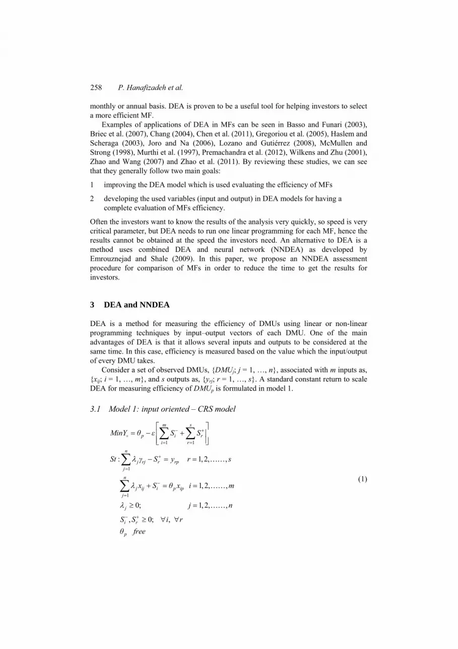
Figure 2 Comparison of the efficiency estimation, NNDEA and standard DEA (see online version for colours)

In order to validate the NNDEA model we compared the results obtained from NNDEA with those of DEA. In this procedure, we use correctness and time as two key criteria for comparing the scores.

5.1 Correctness

Figure 2 illustrates a comparison of the efficiency scores as calculated by NNDEA and the actual efficiency scores as measured by the DEA model. For further analysis, we also calculated the error as the absolute difference between NNDEA and DEA scores which is shown in Figure 3. It can be seen that the NNDEA predictions for efficiency amount appear to be a good estimate for the majority of cases.

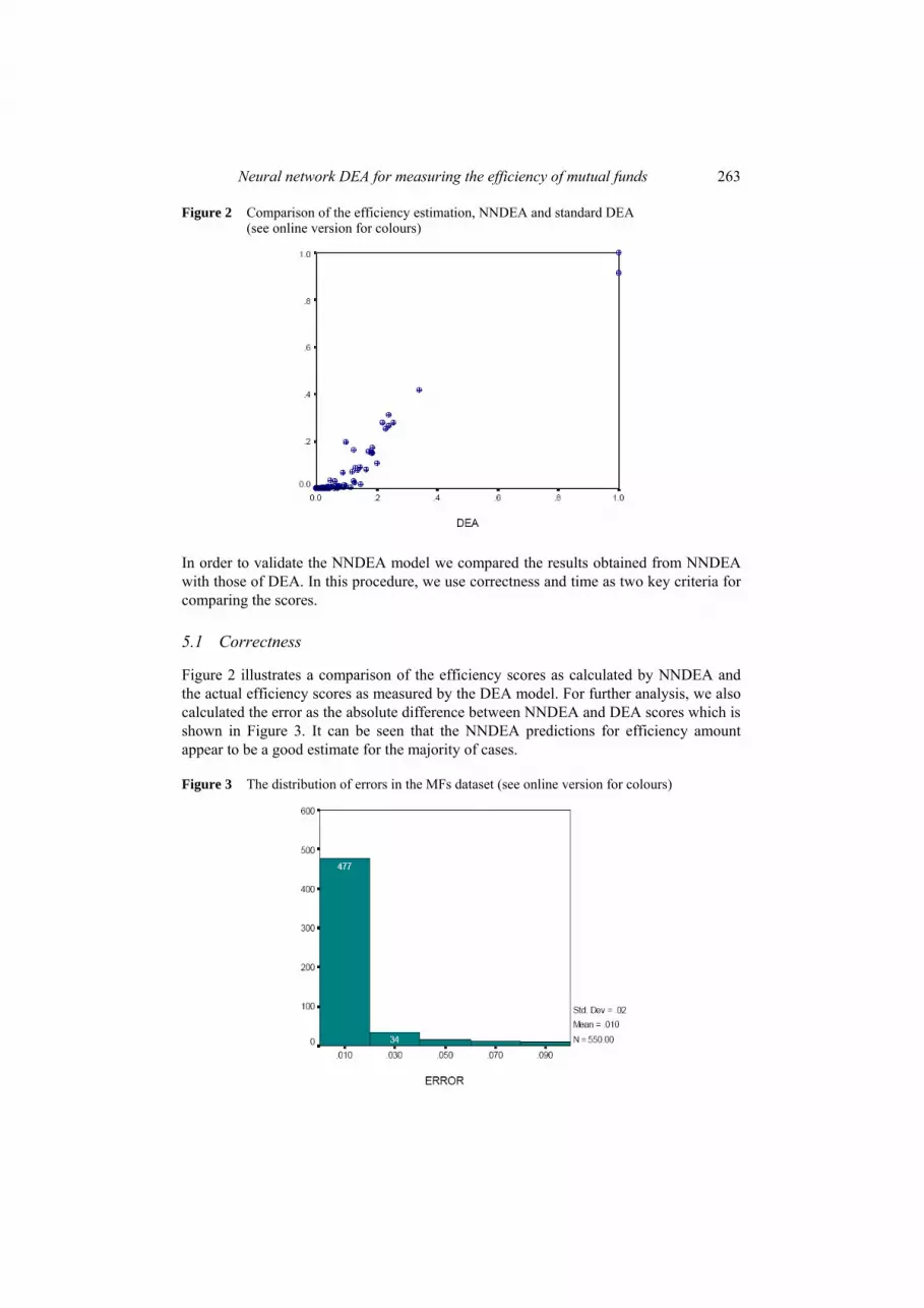
Figure 3 The distribution of errors in the MFs dataset (see online version for colours)

264 P. Hanafizadeh et al.

The first similarity criterion between obtained amounts from this model and the ones of conventional DEA model is distribution of the error estimation. As see in Figure 3, 86.7% estimated MFs efficiency have been associated with less than 0.02 error units compared to the real efficiency amounts from conventional DEA. Also, 92.9% estimated efficiency amounts have error less than 0.04 units of error.

The second criterion of similarity in the two approaches is in terms of the rank ordering of the DMUs by the two methods of the estimation. At first, this was tested by calculating Spearman’s P that evaluates the linear correlation of the measures and criterion. This analysis was done in SPSS software and the results are given in Table 1. All correlations are at 0.01 confidence level (two-tail test).

One important point in using Spearman’s ρ criterion on studying rank correlation is that this criterion only considers linear correlation of the ranks, while there may be some ranks with non-linear correlation. For solving this problem, we use Kendall’s ρ criterion which evaluate both linear and non-linear correlations. The result is reported in Table 1. The two models have rank correlation of 99% confidence level. So, we can conclude that the rank orders of DMUs are very similar in both DEA and NNDEA models. Table 1 Comparison of NNDEA and conventional DEA: Spearman’s and Kendall’s

correlation

NNDEA DEA

Kendall’s tau_b NNDEA Correlation coefficient 1.000 .487**

Sig. (two-tailed) . .000

N 550 550

DEA Correlation coefficient .487** 1.000

Sig. (two-tailed) .000 .

N 550 550

Spearmans rho NNDEA Correlation coefficient 1.000 .582**

Sig. (two-tailed) . .000

N 550 550

DEA Correlation coefficient .582** 1.000

Sig. (two-tailed) .000 .

N 550 550

Note: **Correlation is significant at the .01 level (two-tailed).

5.2 Time

As it is noted, we can obtain conventional DEA efficiency scores and estimated efficiency scores by NNDEA, through two distinctive programmes which are written in MATLAB software. Comparison of performing time of these two programmes can be a good criterion for comparing these two models from the point of speed. The time comparison is reported in Table 2. These results indicate the considerable time reduction in NNDEA in comparison to DEA. It is clear from this table that the solving time for NNDEA to estimate efficiency of 10,049 MFs is far less than corresponding conventional DEA model.

Neural network DEA for measuring the efficiency of mutual funds 265

Table 2 Time comparison of NNDEA and DEA methods

Method Time(s) Computer Software

DEA 128.0588 Intell Pentum III Processor MATLAB NNDEA 0.0886 797 MHZ 240 MB of RAM Ver: 7.3.0.267

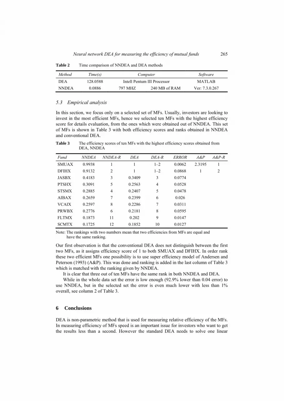
5.3 Empirical analysis

In this section, we focus only on a selected set of MFs. Usually, investors are looking to invest in the most efficient MFs, hence we selected ten MFs with the highest efficiency score for details evaluation, from the ones which were obtained out of NNDEA. This set of MFs is shown in Table 3 with both efficiency scores and ranks obtained in NNDEA and conventional DEA. Table 3 The efficiency scores of ten MFs with the highest efficiency scores obtained from

DEA, NNDEA

Fund NNDEA NNDEA-R DEA DEA-R ERROR A&P A&P-R SMUAX 0.9938 1 1 1–2 0.0062 2.3195 1 DFIHX 0.9132 2 1 1–2 0.0868 1 2 JASBX 0.4183 3 0.3409 3 0.0774 PTSHX 0.3091 5 0.2563 4 0.0528 STSMX 0.2885 4 0.2407 5 0.0478 AIBAX 0.2659 7 0.2399 6 0.026 VCAIX 0.2597 8 0.2286 7 0.0311 PRWBX 0.2776 6 0.2181 8 0.0595 FLTMX 0.1873 11 0.202 9 0.0147 SCMTX 0.1725 12 0.1852 10 0.0127

Note: The rankings with two numbers mean that two efficiencies from MFs are equal and have the same ranking.

Our first observation is that the conventional DEA does not distinguish between the first two MFs, as it assigns efficiency score of 1 to both SMUAX and DFIHX. In order rank these two efficient MFs one possibility is to use super efficiency model of Andersen and Peterson (1993) (A&P). This was done and ranking is added in the last column of Table 3 which is matched with the ranking given by NNDEA.

It is clear that three out of ten MFs have the same rank in both NNDEA and DEA. While in the whole data set the error is low enough (92.9% lower than 0.04 error) to

use NNDEA, but in the selected set the error is even much lower with less than 1% overall, see column 2 of Table 3.

6 Conclusions

DEA is non-parametric method that is used for measuring relative efficiency of the MFs. In measuring efficiency of MFs speed is an important issue for investors who want to get the results less than a second. However the standard DEA needs to solve one linear

266 P. Hanafizadeh et al.

programming for each MFs, hence it may takes some time to obtained the results of large datasets even with fast computers. This paper proposed a NNDEA model for such problem which requires far less time than standard DEA to obtain the same results.

Applicability of the proposed model is examined for evaluating efficiency of large set of MFs in USA. After applying the proposed algorithm, the validity of the model was discussed using distribution errors and correlation of the two efficiency scores. The results show that NNDEA estimates MFs’ relative efficiency with high accuracy and it is very fast compared to conventional DEA method.

The selection of variables, determination of the number of hidden layers and neurons in NNDEA are subjects of future studies.

References Andersen, P. and Petersen, N.C. (1993) ‘A procedure for ranking efficient units in data

envelopment analysis’, Management Science, Vol. 39, No. 10, pp.1261–1264. Anderson, R.I., Brockman, C.M., Giannikos, C. and McLeod, R. (2004) ‘A non-parametric

examination of real estate mutual fund efficiency’, International Journal of Business and Economics, Vol. 3, No. 3, pp.225–238.

Arditti, F.D. (1967) ‘Risk and the required return on equity’, The Journal of Finance, Vol. 22, No. 1, pp.19–36.

Basso, A. and Funari, S. (2001) ‘A data envelopment analysis approach to measure the mutual fund performance’, European Journal of Operational Research, Vol. 135, No. 3, pp.477–492.

Basso, A. and Funari, S. (2003) ‘Measuring the performance of ethical mutual funds: a DEA approach’, Journal of the Operational Research Society, Vol. 54, No. 5, pp.521–531.

Briec, W., Kerstens, K. and Jokung, O. (2007) ‘Mean-variance-skewness portfolio performance gauging: a general shortage function and dual approach’, Management Science, Vol. 53, No. 1, pp.135–149.

Burger, A. and Moormann, J. (2010) ‘Performance analysis on process level: benchmarking of transactions in banking’, International Journal of Banking, Accounting and Finance, Vol. 2, No. 4, pp.404–420.

Chang, K.P. (2004) ‘Evaluating mutual fund performance: an application of minimum convex input requirement set approach’, Computers and Operations Research, Vol. 31, No. 6, pp.929–940.

Charnes, A., Cooper, W.W. and Rhodes, E. (1978) ‘Measuring the efficiency of decision making unit’, European Journal of Operational Research, Vol. 2, No. 6, pp.429–444.

Chen, Y.C., Chiu, Y.H. and Li, M.C. (2011) ‘Mutual fund performance evaluation–application of system BCC model’, South African Journal of Economics, Vol. 79, No. 1, pp.1–16.

Cooper, W.W., Seiford, L.M. and Zhu, J. (Eds.) (2011) Handbook on Data Envelopment Analysis, Springer Science+ Business Media, New York, USA.

Djema, H. and Djerdjouri, M. (2012) ‘A two-stage DEA with partial least squares regression model for performance analysis in healthcare in Algeria’, International Journal of Applied Decision Sciences, Vol. 5, No. 2, pp.118–141.

Emrouznejad, A. and Amin, G.R. (2009) ‘DEA models for ratio data: convexity consideration’, Applied Mathematical Modelling, Vol. 33, No. 1, pp.486–498.

Emrouznejad, A. and Shale, E. (2009) ‘A combined neural network and DEA for measuring efficiency of large scale datasets’, Computers and Industrial Engineering, Vol. 56, No. 1, pp.249–254.

Emrouznejad, A. and Thanassoulis, E. (2005) ‘A mathematical model for dynamic efficiency using data envelopment analysis’, Applied Mathematics and Computation, Vol. 160, No. 2, pp.363–378.

Neural network DEA for measuring the efficiency of mutual funds 267

Emrouznejad, A. and Thanassoulis, E. (2010) Performance Improvement Management Software (PIMsoft): A User Guide [online] http://www.DEAsoftware.co.uk (accessed 20 July 2013).

Emrouznejad, A., Parker, B.R. and Tavares, G. (2008) ‘Evaluation of research in efficiency and productivity: a survey and analysis of the first 30 years of scholarly literature in DEA’, Socio-Economic Planning Sciences, Vol. 42, No. 3, pp.151–157.

Field, K. and Emrouznejad, A. (2003) ‘Measuring the performance of neonatal care units in Scotland’, Journal of Medical Systems, Vol. 27, No. 4, pp.315–324.

Gaborski, R. (1990) An Intelligent Character Recognition System Based on Neural Networks, Research Magazine, Eastman Kodak Company, Rochester, New York.

Gregoriou, G.N. and Gueyie, J.P. (2003) ‘Risk-adjusted performance of funds of hedge funds using a modified Sharpe ratio’, The Journal of wealth management, Vol. 6, No. 3, pp.77–83.

Gregoriou, G.N., Sedzro, K. and Zhu, J. (2005) ‘Hedge fund performance appraisal using data envelopment analysis’, European Journal of Operational Research, Vol. 164, No. 2, pp.555–571.

Hanafizadeh, P., Rezaei, M. and Ghafouri, A. (2009) ‘Defining strategic processes in investment companies: an exploration study in Iranian investment companies’, Business Process Management Journal, Vol. 15, No. 1, pp.20–33.

Haslem, J. and Scheraga, C. (2003) ‘Data envelopment analysis of Morningstar’s large-cap mutual funds’, Journal of Investing, Vol. 12, No. 4, pp.41–48.

Heidari, M.D., Omid, M. and Mohammadi, A. (2012) ‘Measuring productive efficiency of horticultural greenhouses in Iran: a data envelopment analysis approach’, Expert Systems with Applications, Vol. 39, No. 1, pp.1040–1045.

Ho, C-T.B. and Wu, D.D. (2008) ‘Measuring bank performance using DEA and Monte Carlo simulation’, International Journal of Management and Enterprise Development, Vol. 5, No. 6, pp.634–655.

Iazzolino, G., Bruni, M.E. and Beraldi, P. (2013) ‘Using DEA and financial ratings for credit risk evaluation: an empirical analysis’, Applied Economics Letters, Vol. 20, No. 14, pp.1310–1317.

Investment Company Institute (2012) 2012 Investment Company Fact Book [online] http://www.ici.org/pdf/2012_factbook.pdf (accessed 20 July 2013).

Joro, T. and Na, P. (2006) ‘Portfolio performance evaluation in a mean-variance-skewness framework’, European Journal of Operational Research, Vol. 175, No. 1, pp.446–461.

Kthiri, W., Emrouznejad, A., Boujelbene, Y. and Ouertani, M.N. (2011) ‘A framework for performance evaluation of employment offices: a case of Tunisia’, International Journal of Applied Decision Sciences, Vol. 4, No. 1, pp.16–33.

Leland, H.E. (1999) ‘Beyond mean-variance: Performance measurement in a nonsymmetrical world’, Financial Analysts Journal, Vol. 55, No. 1, pp.27–36.

Lozano, S. and Gutiérrez, E. (2008) ‘Data envelopment analysis of mutual funds based on second-order stochastic dominance’, European Journal of Operational Research, Vol. 189, No. 1, pp.230–244.

Markowitz, H. (1952) ‘Portfolio selection’, The Journal of Finance, Vol. 7, No. 1, pp.77–91. McMullen, P.R. and Strong, R.A. (1998) ‘Selection of mutual funds using data envelopment

analysis’, Journal of Business and Economic Studies, Vol. 4, No. 1, pp.1–12. Meenakumari, R., Kamaraj, N. and Thakur, T. (2009) ‘Measurement of relative operational

efficiency of SOEUs in India using data envelopment analysis’, International Journal of Applied Decision Sciences, Vol. 2, No. 1, pp.87–104.

Morningstar Funds (2009) [online] http://www.morningstar.com/Cover/Funds.aspx (accessed 20 July 2013).

Murthi, B.P.S., Choi, Y.K. and Desai, P. (1997) ‘Efficiency of mutual funds and portfolio performance measurement: a non-parametric approach’, European Journal of Operational Research, Vol. 98, No. 2, pp.408–418.

268 P. Hanafizadeh et al.

Nguyen-Thi-Thanh, H. (2004) ‘Hedge fund behavior: an ex-post analysis’, Communication at International Conference of the French Association of Finance, June, Paris, France.

Premachandra, I.M., Zhu, J., Watson, J. and Galagedera, D.U. (2012) ‘Best-performing US mutual fund families from 1993 to 2008: evidence from a novel two-stage DEA model for efficiency decomposition’, Journal of Banking and Finance, Vol. 36, No. 12, pp.3302–3317.

Schalkoff, R.J. (1997) Artificial Neural Networks, McGraw-Hill Higher Education, New York, USA.

Sortino, F.A. and Price, L.N. (1994) ‘Performance measurement in a downside risk framework’, The Journal of Investing, Vol. 3, No. 3, pp.59–64.

Staat, M. (2006) ‘Efficiency of hospitals in Germany: a DEA-bootstrap approach’, Applied Economics, Vol. 38, No. 19, pp.2255–2263.

Stutzer, M. (2000) ‘A portfolio performance index’, Financial Analysts Journal, Vol. 56, No. 3, pp.52–61.

Sufian, F. (2007) ‘Trends in the efficiency of Singapore’s commercial banking groups: A non-stochastic frontier DEA window analysis approach’, International Journal of Productivity and Performance Management, Vol. 56, No. 2, pp.99–136.

Sufian, F. (2010) ‘The evolution of Malaysian banking sector’s efficiency during financial duress: consequences, concerns, and policy implications’, International Journal of Applied Decision Sciences, Vol. 3, No. 4, pp.366–389.

Troutt, M.D., Rai, A. and Zhang, A. (1996) ‘The potential use of DEA for credit applicant acceptance systems’, Computers and Operations Research, Vol. 23, No. 4, pp.405–408.

Van der Meer, R.B., Quigley, J. and Storbeck, J.E. (2004) ‘Using data envelopment analysis to model the performance of UK coastguard centres’, Journal of the Operational Research Society, Vol. 56, No. 8, pp.889–901.

Wilkens, K. and Zhu, J. (2001) ‘Portfolio evaluation and benchmark selection: a mathematical programming approach’, The Journal of Alternative Investments, Vol. 4, No. 1, pp.9–19.

Zhanxin, M., Shengyun, M. and Zhanying, M. (2012) ‘Program design of DEA based on windows system’, Computer, Informatics, Cybernetics and Applications, pp.699–707, Springer, Netherlands.

Zhao, X., Lai, K.K. and Wang, S. (2011) ‘Mutual funds return and risk decomposition evaluation based on quadratic-constrained DEA models’, International Journal of Society Systems Science, Vol. 3, No. 1, pp.119–136.

Zhao, X.J. and Wang, S.Y. (2007) ‘Empirical study on Chinese mutual funds’ performance’, Systems Engineering-Theory and Practice, Vol. 27, No. 3, pp.1–11.

Appendix

Back propagation DEA algorithm (neural network with one hidden layer shown in Figure 1).

Training sample (net input) Desirable output (DEA output) x1 d1 x2 d2 · · · · xR dR

Neural network DEA for measuring the efficiency of mutual funds 269

Step 1 Initialise learning rate C > 0, maximum level of error criterion function Emax, initial amounts of weights of V, W randomly about zero. Set E = 0, r = 1, q = 1 that r: training sample counter, q: training period counter.

Step 2 Give the training sample to the network (dr → d, xr → x). Then calculate these values and compare them with related threshold and then calculate output values of each layer.

.T jjY x v=

( )j jy f Y=

.TZ y w=

( )z f Z=

vj is jth column vector of matrix V. In other words, weights lead to hidden layer of ith neuron.

Step 3 After calculating the network’s output (z) for the given sample, compute output error.

2

1

1 ( )2

l

k

E E d z=

→ + × −∑

Step 4 Calculate error signals of δy, δZ

.(1 ).( )Zδ z z d z= − −

( ) ( ). 1 . . ; 1, 2,3 ,jy j j Z jδ y y w j n= − = …δ

Step 5 Correcting the weights of output layer

. . ; 1, 2,3, ,j j Z jw w C y j n→ + = …δ

Step 6 Correcting the weights of hidden layer

. . ; 1, 2,3, , , 1,2,3, ,ij ij yj iv v C x i m j n→ + = =… …δ

Step 7 If r < R, then add one nit to r and go to 2, else go to 8.

Step 8 If E < Emax, training period is completed and show V, W, q, E in output, but if, E < Emax set E = 0, r = 1, q = q + 1 and start new training period again from step 2.