network deployment for maximal energy efficiency in ... - arxiv
TRANSCRIPT
1
Network Deployment for Maximal Energy
Efficiency in Uplink with Multislope Path Loss
Andrea Pizzo, Student Member, IEEE, Daniel Verenzuela, Student Member, IEEE,
Luca Sanguinetti, Senior Member, IEEE, Emil Björnson, Senior Member, IEEE
Abstract
This work aims to design the uplink (UL) of a cellular network for maximal energy efficiency (EE).
Each base station (BS) is randomly deployed within a given area and is equipped with M antennas to
serve K user equipments (UEs). A multislope (distance-dependent) path loss model is considered and
linear processing is used, under the assumption that channel state information is acquired by using pilot
sequences (reused across the network). Within this setting, a lower bound on the UL spectral efficiency
and a realistic circuit power consumption model are used to evaluate the network EE. Numerical results
are first used to compute the optimal BS density and pilot reuse factor for a Massive MIMO network with
three different detection schemes, namely, maximum ratio combining, zero-forcing (ZF) and multicell
minimum mean-squared error. The numerical analysis shows that the EE is a unimodal function of BS
density and achieves its maximum for a relatively small density of BS, irrespective of the employed
detection scheme. This is in contrast to the single-slope (distance-independent) path loss model, for
which the EE is a monotonic non-decreasing function of BS density. Then, we concentrate on ZF and
use stochastic geometry to compute a new lower bound on the spectral efficiency, which is then used
to optimize, for a given BS density, the pilot reuse factor, number of BS antennas and UEs. Closed-
form expressions are computed from which valuable insights into the interplay between optimization
variables, hardware characteristics, and propagation environment are obtained.
I. INTRODUCTION
KEEPING up with the ever-growing demand for higher data throughput is the major
ambition of future cellular networks [1]. An important question is how to evolve com-
munication technologies to deliver higher throughput without prohibitively increasing the power
A. Pizzo and L. Sanguinetti are with the University of Pisa, Dipartimento di Ingegneria dell’Informazione, Italy (an-
[email protected]). D. Verenzuela and E. Björnson are with the Department of Electrical Engineering (ISY), Linköping
University, Linköping, Sweden ([email protected]). L. Sanguinetti is also with the Large Systems and Networks Group
(LANEAS), CentraleSupélec, Université Paris-Saclay, 3 rue Joliot-Curie, 91192 Gif-sur-Yvette, France.
A preliminary version of this work was presented at IEEE GLOBECOM, 4–8 December, 2017, Singapore.
arX
iv:1
801.
0004
3v2
[cs
.IT
] 2
2 Ju
n 20
18
2
consumption [2]. This calls for new design mechanisms that provide the user equipments (UEs)
with high spectral efficiency at moderate energy costs. There is a broad consensus that this
wireless capacity growth can only be achieved with a substantial network densification [3] [4].
The main approaches for this densification are twofold: small-cell networks [5]–[7] and Massive
MIMO [8]–[12]. The former relies on a massive deployment of small cells that guarantees lower
propagation losses. The latter makes use of a massive number of base station (BS) antennas
to simultaneously serve a relatively large number of UEs by means of spatial multiplexing.
A combination of both has also received a lot of interest in the research literature (e.g., [13],
[14]). Despite being potentially effective in increasing spectral efficiency, both solutions tend to
increase the power consumed by the network; small cells increase the number of deployed BSs,
whereas Massive MIMO requires more hardware per BS. The aim of this work is to design a
cellular network from scratch to achieve maximal energy efficiency (EE), without any a priori
assumption on the number of BS antennas, UEs, pilot reuse or BS density.
A. Main literature
The optimal deployment of cellular networks has received great attention in the literature.
The first attempts were based on the simple Wyner model [15] wherein both BSs and UEs are
located on a line at fixed positions. Next, more complex 2D symmetric grid-based deployments
(e.g., hexagonal lattice) were considered [16]. Both approaches are not suited for modeling and
studying networks characterized by a very irregular and dense structure, as envisioned in future
cellular networks. To address this problem, advanced mathematical tools based on stochastic
geometry have been employed in the last years (e.g., [17]–[19]). Within the stochastic geometry
framework, the locations of BSs form a point process in a compact set whose cardinality is
a Poisson distributed random variable that is independent among different disjoint sets. The
performance of a cellular network can be measured in many different ways such as coverage
probability, throughput and EE [6].Earlier works on the design of EE-optimal cellular networks,
equipped with multiple antenna BSs, can be found in [9] and [20] where closed-form expressions
are derived for a single-cell scenario and numerical results are given for a multicell setting. The
EE analysis of a multicell network is developed in [6], [21], [22] by using stochastic geometry.
In [21], the optimization is done while satisfying a quality-of-service requirement per UE. In
[6], [22], the use of small-cells together with sleeping strategies is proved to be a promising
solution for increasing the EE. Generally speaking, small-cells lead to a higher EE but this gain
3
saturates quickly as the density of small cells increases. In [13], it has been shown that further
benefits can be achieved by using Massive MIMO.
As the majority of works in the literature, all the aforementioned ones use the standard path
loss model where received power decays like d−α over a distance d, where α is called the
"path loss exponent". This standard path loss model is quite idealized, and in most scenarios
α is itself a function of distance, typically an increasing one [23]. For example, three distinct
regimes could be easily identified in a practical environment [24]: a distance-independent "near-
field" where α0 = 0, a free-space like regime where α1 = 2, and finally some heavily-attenuated
regime where α2 > 2.1 What happens if densification pushes many BSs into the near-field? An
answer to this question can be found in [23], [25], [26] (among others), wherein the authors
show that the propagation environment and fading distribution play a key role in identifying
network operating regimes for which an increase, saturation, or decrease of the throughput is
observed as the network densifies. In the extreme case, ultra BS-densification may even lead
to zero throughput. Despite all this, multislope path loss models are not frequently used in
the analysis of cellular networks because, in general, they make the theoretical analysis more
demanding. This work attempts to solve this issue for the EE maximization problem at hand.
B. Contributions and outline
We consider a cellular network in which the BSs are independently and uniformly distributed
in a given area according to a homogeneous Poisson point process (H-PPP) of intensity λ. Each
BS is equipped with an arbitrary number M of antennas and serves simultaneously K UEs.
Statistical channel inversion power-control is employed in the uplink (UL) to achieve a uniform
average signal-to-noise ratio (SNR) across all the UEs. A multislope (distance-dependent) path
loss model is considered. Three different linear combining schemes, namely, maximum ratio
(MR), zero-forcing (ZF) and multicell minimum mean-squared error (M-MMSE), are used under
the assumption that channel state information is acquired by using pilots, which are reused across
the network with a factor ζ . The EE of the network is computed by using a lower bound on the
average UL spectral efficiency (valid for any combining scheme) as well as a polynomial power
consumption model, thoroughly developed in [12]. Numerical results are used to evaluate the
impact of BS density λ and pilot reuse factor ζ on the EE of a Massive MIMO network such that
1Such a situation results even with a simple 2-ray ground reflection, with α2 = 4 in that case.
4
M ≫ K ≫ 1. The results show that the EE with a multislope path loss is a unimodal2 function
of λ. Irrespective of the employed detection scheme, the optimal EE is achieved for relatively
small values of λ and ζ . This is in sharp contrast to [13] where the adoption of a single-slope
path loss model leads to the conclusion that densification is always beneficial for EE; the EE is
shown to be a monotonic increasing function of λ in [13]. The results show also that, although
the “optimal” M-MMSE combiner provides the highest EE, the three different schemes behave
similarly in terms of EE and area throughput as BS density increases.
Motivated by the above analysis, we concentrate on ZF and compute a new closed-form
lower bound on the average UL SE. This lower bound is used to analytically find in closed-
form the EE-optimal network configuration with respect to M , K and ζ while satisfying a
signal-to-interference-plus-noise ratio (SINR) constraint. The closed-form expressions reveal the
fundamental interplay between the three design parameters, which are also illustrated numerically.
It turns out that ZF allows a higher densification of the network while using a smaller pilot reuse
factor and achieving a higher EE than with MR. Both schemes employ almost the same optimal
number of antennas per BS to approximately serve the same number of UEs, with a ratio M/K
between 4 and 19 when using ZF and between 4 and 27 for MR depending on the SINR
constraint. In addition, ZF is characterized by a smoother EE function, which is more robust to
system changes and thus makes it a better choice.
Compared to the preliminary version in [27], this work: (i) provides the EE analysis for MR,
ZF and M-MMSE; (ii) is based on a multislope path loss model and aims at showing its impact
on EE when the network is densified; (iii) gives more details and insights into the effect of
network parameters and circuit power model.
The remainder of this paper is organized as follows.3 Next section introduces basic notation
and describes the cellular network with the underlying assumptions and transmission protocols.
2A function f(x) is unimodal if it is monotonically increasing for x ≤ m and decreasing for x > m for some m ∈ R.3Upper (lower) bold face letters are used for matrices (column vectors). Sans serif fonts are used for mathematical quantities
whereas times new roman fonts are used for acronyms/texts. IN is the N ×N identity matrix and 0 is the zero vector. (·)T,
(·)∗ and (·)H are the transpose, conjugate and conjugate transpose operators, respectively. We use tr(·) to denote the matrix
trace operator and ‖ · ‖ for the Euclidean norm vector operator. ⌈x⌋ is the nearest integer projector whereas P(A) indicates the
probability associated with an event A. En{·} denotes the expectation operator with respect to the random vector n, whereas
n ∼ NC(0,Rn) is the shorthand for a circularly-symmetric normal distribution with covariance matrix Rn. We use Rn, Cn,
and Nn to denote the n-dimensional real-valued, complex-valued and nonnegative integer-valued vector spaces. We denote
Γ(s;x) =∫∞x
ts−1e−t dt the upper incomplete gamma function.
5
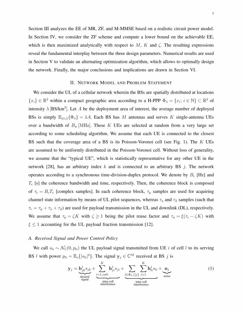
Section III analyzes the EE of MR, ZF, and M-MMSE based on a realistic circuit power model.
In Section IV, we consider the ZF scheme and compute a lower bound on the achievable EE,
which is then maximized analytically with respect to M , K and ζ . The resulting expressions
reveal the fundamental interplay between the three design parameters. Numerical results are used
in Section V to validate an alternating optimization algorithm, which allows to optimally design
the network. Finally, the major conclusions and implications are drawn in Section VI.
II. NETWORK MODEL AND PROBLEM STATEMENT
We consider the UL of a cellular network wherein the BSs are spatially distributed at locations
{xi} ∈ R2 within a compact geographic area according to a H-PPP Φλ = {xi; i ∈ N} ⊂ R2 of
intensity λ [BS/km2]. Let A be the deployment area of interest, the average number of deployed
BSs is simply E{xi}{Φλ} = λA. Each BS has M antennas and serves K single-antenna UEs
over a bandwidth of Bw [MHz]. These K UEs are selected at random from a very large set
according to some scheduling algorithm. We assume that each UE is connected to the closest
BS such that the coverage area of a BS is its Poisson-Voronoi cell (see Fig. 1). The K UEs
are assumed to be uniformly distributed in the Poisson-Voronoi cell. Without loss of generality,
we assume that the “typical UE”, which is statistically representative for any other UE in the
network [28], has an arbitrary index k and is connected to an arbitrary BS j. The network
operates according to a synchronous time-division-duplex protocol. We denote by Bc [Hz] and
Tc [s] the coherence bandwidth and time, respectively. Then, the coherence block is composed
of τc = BcTc [complex samples]. In each coherence block, τp samples are used for acquiring
channel state information by means of UL pilot sequences, whereas τu and τd samples (such that
τc = τp + τu + τd) are used for payload transmission in the UL and downlink (DL), respectively.
We assume that τp = ζK with ζ ≥ 1 being the pilot reuse factor and τu = ξ(τc − ζK) with
ξ ≤ 1 accounting for the UL payload fraction transmission [12].
A. Received Signal and Power Control Policy
We call sli ∼ NC(0, pli) the UL payload signal transmitted from UE i of cell l to its serving
BS l with power pli = Es{|sli|2}. The signal yj ∈ CM received at BS j is
yj = hjjksjk︸ ︷︷ ︸
desiredsignal
+K∑
i=1,i 6=k
hjjisji
︸ ︷︷ ︸intra-cell
interference
+∑
l∈Φλ\{j}
K∑
i=1
hjlisli
︸ ︷︷ ︸inter-cell
interference
+ nj︸︷︷︸noise
(1)
6
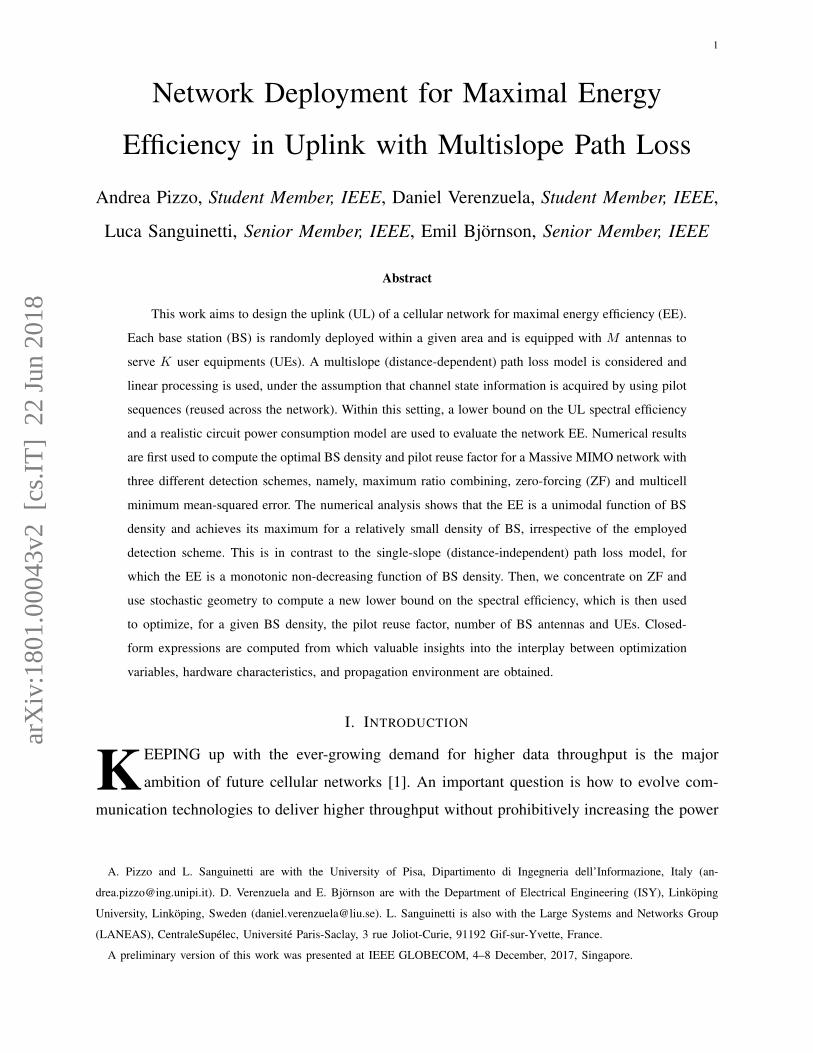
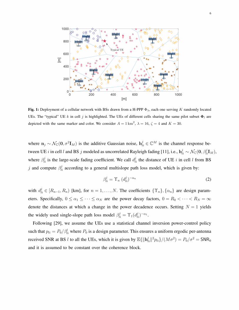
Fig. 1: Deployment of a cellular network with BSs drawn from a H-PPP Φλ, each one serving K randomly located
UEs. The “typical” UE k in cell j is highlighted. The UEs of different cells sharing the same pilot subset Φl are
depicted with the same marker and color. We consider A = 1km2, λ = 16, ζ = 4 and K = 30.
where nj ∼ NC(0, σ2IM) is the additive Gaussian noise, hj
li ∈ CM is the channel response be-
tween UE i in cell l and BS j modeled as uncorrelated Rayleigh fading [11], i.e., hjli ∼ NC(0, β
jliIM),
where βjli is the large-scale fading coefficient. We call djli the distance of UE i in cell l from BS
j and compute βjli according to a general multislope path loss model, which is given by:
βjli = Υn (djli)
−αn (2)
with djli ∈ [Rn−1, Rn) [km], for n = 1, . . . , N . The coefficients {Υn}, {αn} are design param-
eters. Specifically, 0 ≤ α1 ≤ · · · ≤ αN are the power decay factors, 0 = R0 < · · · < RN = ∞denote the distances at which a change in the power decadence occurs. Setting N = 1 yields
the widely used single-slope path loss model βjli = Υ1(d
jli)
−α1 .
Following [29], we assume the UEs use a statistical channel inversion power-control policy
such that pli = P0/βlli where P0 is a design parameter. This ensures a uniform ergodic per-antenna
received SNR at BS l to all the UEs, which it is given by E{‖hlli‖2pli}/(Mσ2) = P0/σ
2 = SNR0
and it is assumed to be constant over the coherence block.
7
B. Pilot Reuse Policy and Channel Estimation
We assume that a pilot book Φ ∈ Cτp×τp of τp mutually orthogonal UL sequences is used
for channel estimation and call φjk ∈ Cτp the pilot sequence assigned to the typical UE k in
cell j. It is assumed to have normalized UL pilot sequences, to obtain a constant power level,
and this implies that ‖φjk‖2 = 1. To avoid cumbersome pilot coordination, we assume that in
each coherence block each BS l picks a subset of K different sequences from Φ, uniformly
at random and distribute them among its served UEs. Since τp = ζK, we have that the reuse
factor is ζ = τp/K > 1. In other words, there are on average E{Φλ}/ζ cells in the network
that share the same pilot subset. This is modeled in each cell through a Bernoulli stochastic
variable al′l ∼ B(1/ζ) for l′ 6= l and all = 1. Specifically, if al′l = 1 all the UEs in cell l′ use the
same pilot subset of those in cell l and thus causes pilot contamination [12]. This occurs with
probability P(al′l = 1) = 1/ζ. Similarly, al′l = 0 indicates that there is no pilot contamination
from cell l′ to cell l and vice versa, and happens with probability P(al′l = 0) = 1− 1/ζ. To
facilitate understanding, Fig. 1 illustrates a pilot allocation snapshot where different markers and
colors identify different pilot subsets {Φl}. We call Ypj ∈ CM×τp the signal received at BS j
during pilot transmission. The vector ypjli = Yp
jφ∗li obtained by correlating Yp
j with φli takes
the form:
ypjli =
√ρ√pli h
jli
︸ ︷︷ ︸desired pilot
+∑
l′∈Φλ\{l}al′l
√ρ√pl′i h
jl′i
︸ ︷︷ ︸interfering pilots
+Npjφ
∗li
︸ ︷︷ ︸noise
(3)
where Npjφ
∗li ∼ NC(0, σ
2IM) and the power of the UL transmitted payload signal is scaled
by a factor ρ = Pp/P0 ≥ 1 to compensate for the lack of beamforming gain during channel
acquisition.
Corollary 1 (e.g. [12]). By using pli = Pp/βlli, the MMSE estimate of hj
li at BS j based on ypjli
is
hjli =
βjli√
βlli Pp
βjli
βlli
+∑
l′∈Φλ\{l}al′l
βj
l′iβl′l′i
+ 1SNRp
ypjli (4)
with SNRp = ρ SNR0. The MMSE estimate hjli and error hj
li, conditioned on a realization of al′l
for all l′, l ∈ Φλ, are independent and distributed as hjli ∼ NC(0, γ
jliIM) and hj
li ∼ NC(0, (βj
li − γjli)IM
)
8
where
γjli =
βjli
βjli
βlli+
∑l′∈Φλ\{l}
al′lβj
l′iβl′l′i
+ 1SNRp
βjli
βlli
. (5)
For notational convenience, we define the collecting of all the estimates in (4) from all UEs
in cell l to BS j as Hjl =
[hjl1 . . . hj
lK
]∈ CM×K . Note that the estimate hj
l′i of a UE i in cell
l′ using the same pilot sequence of UE i in cell l (i.e. al′l = 1) can be obtained from hjli in (4)
as
hjl′i =
√βlli
βl′l′i
βjl′i
βjli
hjli (6)
where hjl′i ∼ NC
(0, γj
l′iIM)
has variance
γjl′i =
βlli
βl′l′i
(βjl′i
βjli
)2γjli (7)
and estimation error hjl′i ∼ NC
(0, (βj
l′i − γjl′i)IM
). The expression in (6) is responsible of pilot
contamination with spatially uncorrelated channels; the inability of BS j to separate UEs that
use the same pilot [8].
III. ENERGY EFFICIENCY ANALYSIS
The EE is defined as the amount of information reliably transmitted per unit of energy4, which
is mathematically expressed as [20]:
EE =Area throughput [bit/s/km2]
Area power consumption [W/km2]
=Bw[Hz] · ASE [bit/s/Hz/km2]
APC [W/km2](8)
which is measured in [bit/Joule] and can be seen as a benefit-cost ratio, where the service
quality (area throughput) is compared with the associated cost (area power consumption). In
(8), ASE and APC are the area spectral efficiency (ASE) and area power consumption (APC),
respectively.
4A considerable number of papers on EE analysis has considered misleading EE metrics measured in bit/Joule/Hz, instead
of bit/Joule. This is pointless since one cannot make the EE bandwidth-independent: the transmit power is divided over the
bandwidth while the noise power is proportional to the bandwidth.
9
A. Area Spectral Efficiency
Since the “typical UE” is statistically representative for any other UE in the network [28],
the ASE is obtained as ASE = λK SE in [bit/s/Hz/km2] where SE denotes the average UL
spectral efficiency of the typical UE k in cell j and is obtained averaging over different UE
positions, pilot allocations and channel realizations. The multiplicative factor K accounts for the
sum spectral efficiency of all UEs in cell j and λ is the BS density per km2. A lower bound on
SE, which holds for any combining scheme, UE positions and pilot allocations is as follows.5
Theorem 1 ([12]). When the channel is obtained through the MMSE estimator in (4), the UL
average ergodic channel capacity of the typical UE k in cell j is lower bounded by
SE ≥ SE′ = ξ(1− Kζ
τc
)E{d,h,a}
{log2 (1 + SINR′)
}(9)
where SINR′ is the instantaneous SINR given by
SINR′ =pjk|vH
jkhjjk|2
vHjk
∑
l∈Φλ
K∑i=1
(l,i)6=(j,k)
plihjlih
jH
li +∑l∈Φλ
K∑i=1
pli(βjli − γj
li)IM + σ2IM
vjk
(10)
and the expectation E{d,h,a}{·} is computed with respect to UE positions, channel realizations
and pilot allocations. The pre-log factor accounts for the pilot overhead.6
The optimal vjk that maximizes (9) is given as follows.
Corollary 2 ([12]). The instantaneous UL SINR in (10) for a typical UE k in cell j is maximized
by
vM−MMSEjk =
(∑
l∈Φλ
K∑
i=1
pli
(hjli(h
jli)
H + (βjli − γj
li)IM
)+ σ2IM
)−1
pjkhjjk. (11)
Proof. The proof can be found in [12] and it is based on the Rayleigh quotient maximization.
The optimal combining vector in (11) is known as M-MMSE combiner since it can be proved
to be the vector vjk that minimizes the conditional MSE, that is E{sjk − vH
jkyj | {Hjl}, {al′,l}
}.
5Note that the UL capacity for a network (such as the one under investigation) with imperfect CSI and inter-cell interference
modeled as a shot-noise process is not known yet [30]. As a common practice in these circumstances, we resort to a lower
bound.6In each coherence block, BS j uses the first τp samples for acquiring CSI to decode the UL payload in the remaining τu
samples.
10
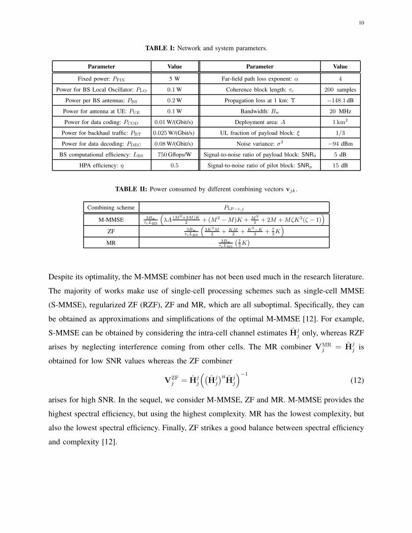
TABLE I: Network and system parameters.
Parameter Value Parameter Value
Fixed power: PFIX 5 W Far-field path loss exponent: α 4
Power for BS Local Oscillator: PLO 0.1W Coherence block length: τc 200 samples
Power per BS antennas: PBS 0.2W Propagation loss at 1 km: Υ −148.1 dB
Power for antenna at UE: PUE 0.1W Bandwidth: Bw 20 MHz
Power for data coding: PCOD 0.01W/(Gbit/s) Deployment area: A 1 km2
Power for backhaul traffic: PBT 0.025W/(Gbit/s) UL fraction of payload block: ξ 1/3
Power for data decoding: PDEC 0.08W/(Gbit/s) Noise variance: σ2 −94 dBm
BS computational efficiency: LBS 750Gflops/W Signal-to-noise ratio of payload block: SNR0 5 dB
HPA efficiency: η 0.5 Signal-to-noise ratio of pilot block: SNRp 15 dB
TABLE II: Power consumed by different combining vectors vjk .
Combining scheme PLP−c,j
M-MMSE 3BwτcLBS
(λA (M2+3M)K
2+ (M2 −M)K + M3
3+ 2M +MζK2(ζ − 1)
)
ZF 3BwτcLBS
(3K2M
2+ KM
2+ K3−K
3+ 7
3K)
MR 3BwτcLBS
(73K)
Despite its optimality, the M-MMSE combiner has not been used much in the research literature.
The majority of works make use of single-cell processing schemes such as single-cell MMSE
(S-MMSE), regularized ZF (RZF), ZF and MR, which are all suboptimal. Specifically, they can
be obtained as approximations and simplifications of the optimal M-MMSE [12]. For example,
S-MMSE can be obtained by considering the intra-cell channel estimates Hjj only, whereas RZF
arises by neglecting interference coming from other cells. The MR combiner VMRj = Hj
j is
obtained for low SNR values whereas the ZF combiner
VZFj = Hj
j
((Hj
j
)HHj
j
)−1
(12)
arises for high SNR. In the sequel, we consider M-MMSE, ZF and MR. M-MMSE provides the
highest spectral efficiency, but using the highest complexity. MR has the lowest complexity, but
also the lowest spectral efficiency. Finally, ZF strikes a good balance between spectral efficiency
and complexity [12].
11
B. Area Power Consumption
The APC can be expressed as follows:
APC = λ(η−1PTX + PCP
)[W/km2] (13)
where PTX accounts for the average power usage for UL transmission (payload and pilots) in
an arbitrary cell j with η ∈ (0, 1] being the high power amplifier (HPA) efficiency whereas PCP
is the power consumed by circuitry and can be computed as in [13], [20]. Both are evaluated
next.
Corollary 3. If τu and τp samples are respectively used in UL for data and pilot transmissions,
then the average total power used for transmission is
PTX =
(τu + ρ τp
τc
)K U (14)
where
U = P0
N∑
n=1
Υ−1n
Γ(2+αn
2;Rn
)− Γ
(2+αn
2;Rn+1
)
(πλ)αn/2(15)
with Γ(s; x) =∫∞x
ts−1e−t dt being the upper incomplete gamma function.
Proof. The BS locations are drawn from a H-PPP Φλ and the UEs are uniformly distributed
in the Poisson-Voronoi cells. Thus, the distance djjk from the typical UE k to its serving BS
j is Rayleigh distributed as djjk ∼ R(1/√2πλ) and its probability density function is given
by fd = (2πλdjjk)e−πλ(djjk)
2
for djjk > 0 [30]. Besides, Es{|sjk|2} = pjk with pjk = P0/βjjk or
pjk = Pp/βjjk, depending on wether sjk is a payload or pilot signal, respectively. Within a
coherence block, each user transmits data symbols for a fraction of τu/τc and pilot symbols
for τp/τc. This, together with Pp = ρP0, leads to PTX = τu+ρ τpτc
P0KEd{1/βjjk}. Finally, using
the path loss model in (2) we have that Ed{1/βjjk} =
N∑n=1
Υ−1n
∫ Rn
Rn−1yαn fd(y) dy from which
(15) follows by using (69) in Appendix B.
The power needed to run the circuitry of an arbitrary BS j can be modeled as follows [13],
[20]
PCP = PFIX︸︷︷︸fixedpower
+ PTC︸︷︷︸transceiver
chain
+ PC−BH︸ ︷︷ ︸coding&
backhauling
+ PCE︸︷︷︸channel
estimation
+ PLP︸︷︷︸linear
processing
(16)
where PFIX is the power consumed for site-cooling, control signaling and load-independent
backhauling, PTC for the transceiver chain, PC−BH for coding and load-dependent backhauling
12
10
2
4
8
6
8
6
10
104 20302 405060Pilot reuse factor (ζ) BS density (λ)
EE[M
bit/Joule] (ζ⋆, λ⋆,EE⋆) = (3, 5, 11)
(a) M-MMSE combining
10
2
4
8
6
8
6
10
104 20302 405060Pilot reuse factor (ζ) BS density (λ)
EE[M
bit/Joule]
(ζ⋆, λ⋆,EE⋆) = (2, 5, 9.63)
(b) ZF combining
10
2
4
8
6
8
6
10
104 20302 405060Pilot reuse factor (ζ) BS density (λ)
EE[M
bit/Joule]
(ζ⋆, λ⋆,EE⋆) = (2, 7, 6.47)
(c) MR combining
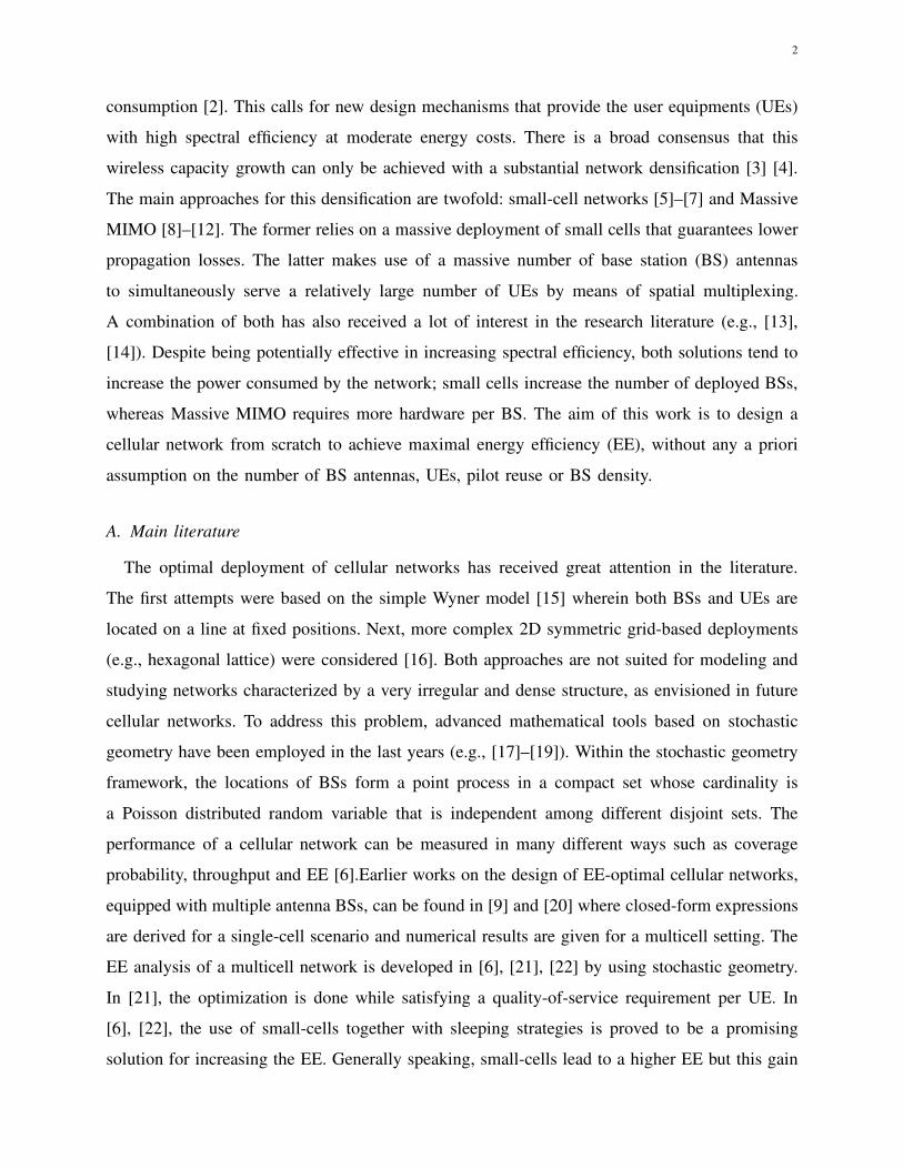
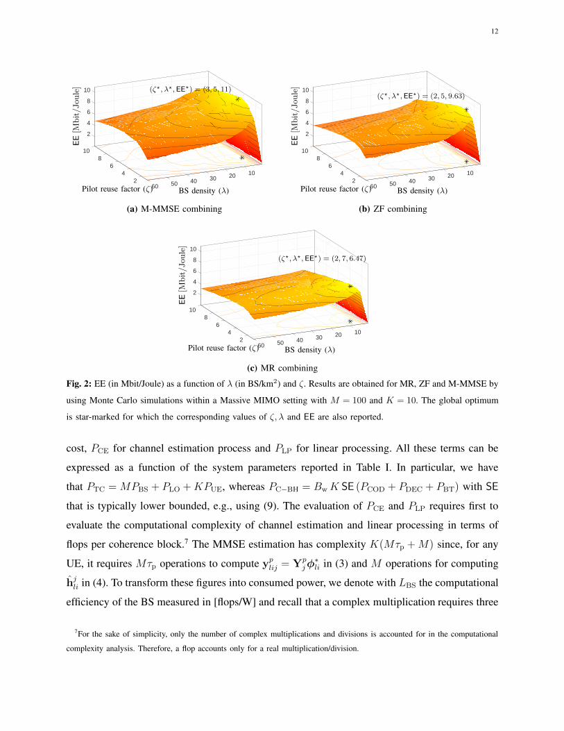
Fig. 2: EE (in Mbit/Joule) as a function of λ (in BS/km2) and ζ. Results are obtained for MR, ZF and M-MMSE by
using Monte Carlo simulations within a Massive MIMO setting with M = 100 and K = 10. The global optimum
is star-marked for which the corresponding values of ζ, λ and EE are also reported.
cost, PCE for channel estimation process and PLP for linear processing. All these terms can be
expressed as a function of the system parameters reported in Table I. In particular, we have
that PTC = MPBS + PLO +KPUE, whereas PC−BH = Bw K SE (PCOD + PDEC + PBT) with SE
that is typically lower bounded, e.g., using (9). The evaluation of PCE and PLP requires first to
evaluate the computational complexity of channel estimation and linear processing in terms of
flops per coherence block.7 The MMSE estimation has complexity K(Mτp +M) since, for any
UE, it requires Mτp operations to compute yplij = Yp
jφ∗li in (3) and M operations for computing
hjli in (4). To transform these figures into consumed power, we denote with LBS the computational
efficiency of the BS measured in [flops/W] and recall that a complex multiplication requires three
7For the sake of simplicity, only the number of complex multiplications and divisions is accounted for in the computational
complexity analysis. Therefore, a flop accounts only for a real multiplication/division.
13
0 2 4 6 8 10 15 20 25 30 35 40 45 50 55 600
2
4
6
8
10
12
BS density (λ) [BS/km2]
EE[M
bit/Joule]
M-MMSEZFMR
Single-slope
Multislope
(a) EE versus BS density (λ)
0 1 2 3 4 5 6 7 8 9 100
2
4
6
8
10
12
Area throughput [Gbit/s/km2]
EE[M
bit/Joule]
M-MMSEZFMR
(b) EE versus area throughput
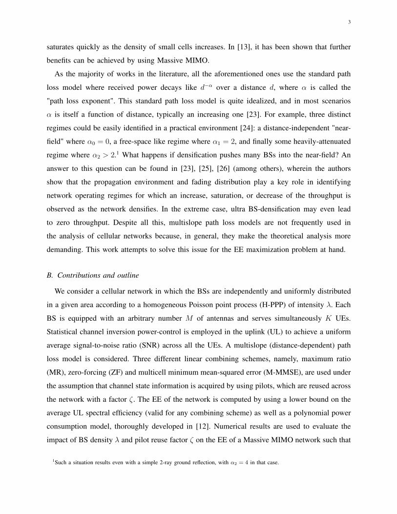
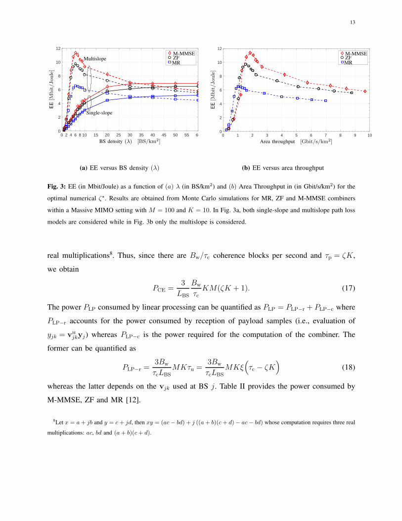
Fig. 3: EE (in Mbit/Joule) as a function of (a) λ (in BS/km2) and (b) Area Throughput in (in Gbit/s/km2) for the
optimal numerical ζ⋆. Results are obtained from Monte Carlo simulations for MR, ZF and M-MMSE combiners
within a Massive MIMO setting with M = 100 and K = 10. In Fig. 3a, both single-slope and multislope path loss
models are considered while in Fig. 3b only the multislope is considered.
real multiplications8. Thus, since there are Bw/τc coherence blocks per second and τp = ζK,
we obtain
PCE =3
LBS
Bw
τcKM(ζK + 1). (17)
The power PLP consumed by linear processing can be quantified as PLP = PLP−r + PLP−c where
PLP−r accounts for the power consumed by reception of payload samples (i.e., evaluation of
yjk = vHjkyj) whereas PLP−c is the power required for the computation of the combiner. The
former can be quantified as
PLP−r =3Bw
τcLBSMKτu =
3Bw
τcLBSMKξ
(τc − ζK
)(18)
whereas the latter depends on the vjk used at BS j. Table II provides the power consumed by
M-MMSE, ZF and MR [12].
8Let x = a+ jb and y = c+ jd, then xy = (ac− bd) + j ((a+ b)(c+ d)− ac− bd) whose computation requires three real
multiplications: ac, bd and (a+ b)(c+ d).
14
C. Numerical analysis
We now use the developed power model to design the network for maximal EE. To this end,
we adopt the parameters listed in Table I [12].9 We stress that these parameters tend to be
extremely hardware-specific and thus may take substantially different values. The Matlab code
that is available online at https://github.com/lucasanguinetti/max-EE-Multislope-Path-Loss en-
ables testing of other values. We consider a deployment area of A = 1km2 wherein E{Φλ} = λA
BSs are randomly deployed according to a H-PPP. A wrap-around topology is used to simulate
the H-PPP in the whole R2 and keep the translation invariance. Inspired by [23] and [14], a
bounded N = 3 slopes path loss model is used for the large scale fading in (2) with parameters
[α1, α2, α3] = [0, 2, α], [R1, R2] = [10, 446] [m] and [Υ1,Υ2,Υ3] = [1, 1,Υ] with α and Υ
as in Table I. The cut off distance R2 comes from a simple 2-ray ground reflection case,
with R2 ≈ 4hthr/λc where ht = 10 and hr = 1.65 are the antenna heights of BS and UE, and
λc = c/fc is the operating wavelength at a carrier frequency fc = 2GHz. A Massive MIMO
setup is considered, which is roughly characterized by an antenna-UE ratio M/K = 10 in order
to meet the channel hardening and favorable propagation conditions [12]. Within this setup, we
set M = 100 and K = 10.
Fig. 2 shows the EE of MR, ZF and M-MMSE as a function of BS density and pilot
reuse factor ζ . In particular, we consider λ ∈ L = {1, 2, . . . , 10, 20, . . . , 60} and ζ ∈ {1, . . . , 10}with an average SNR0 = 5 dB. We see that with all schemes the EE is a pseudo-concave
function and has a unique global optimizer (λ⋆, ζ⋆) at which maximum EE⋆ Mbit/Joule is
achieved. In the remainder, the superscript ⋆ is used to indicate optimal values. Each point
uniquely determines the EE-optimal network deployment configuration for the corresponding
scheme. We notice that M-MMSE provides the highest EE, followed by ZF, while MR achieves
the lowest EE. M-MMSE does not only provide the highest EE but has also the smoothest
EE around the optimum. This makes it more robust to a variation of network settings (e.g.,
pilot reuse and BS density). From Fig. 2a, we can see that the maximal EE value with M-
MMSE is EE⋆ = 11 Mbit/Joule and is achieved at (ζ⋆, λ⋆) = (3, 5). With ZF (see Fig. 2b),
we have EE⋆ = 9.63Mbit/Joule at (ζ⋆, λ⋆) = (2, 5), whereas with MR (see Fig. 2c) we obtain
EE⋆ = 6.47Mbit/Joule at (ζ⋆, λ⋆) = (2, 7). Note that, irrespective of the combining scheme, the
9The interested reader is also referred to the power consumption model developed by IMEC and available on line at the
following link http://www.imec.be/powermodel.
15
optimal EE is achieved for a pilot reuse factor between 2 and 3 and also for a relatively small
BS density (e.g., a few BSs per km2). This latter result is in contrast to [13], wherein the EE
monotonically increases as λ grows large. This was a consequence of the single-slope path loss
model adopted in [13]. Further details on this are given next.
Fig. 3a depicts the EE of MR, ZF and M-MMSE as a function of λ ∈ L for the optimal
pilot reuse factors ζ⋆, provided by Fig. 2. Comparisons are made with the EE achieved with
a single-slope path loss model with large scale fading parameters α and Υ as in Table I. As
expected, in this latter case, the EE is a monotonic non-decreasing function of λ for all schemes.
For completeness, Fig. 3b illustrates the EE with MR, ZF and M-MMSE as a function of the
corresponding average area throughput, obtained for λ ∈ L. We see that there exist operating
conditions under which it is possible to jointly increase both the area throughput and EE up to the
maximum EE point, but further increases in throughput can only come at a loss in EE. The curves
are quite smooth around the maximum EE point; thus, there is a variety of throughput values or,
equivalently, BS densities that provide nearly maximum EE with higher area throughput. With
M-MMSE, selecting λ = 9 > λ⋆ = 5 leads to a 27% increase in area throughput while the EE
is reduced by 12% only. The gain is even higher when considering MR and ZF. Specifically,
they allow a reduction of respectively 19% and 10% in EE to achieve 46% and 56% higher
area throughput.
To summarize, Figs. 2 and 3 show that the additional computational complexity of M-MMSE
processing pays off both in terms of EE and area throughput. Moreover, the analysis shows that,
for a Massive MIMO setup, reducing the cell size does not bring benefits in terms of EE; the
optimal EE is roughly achieved for the same λ for all detection schemes.
IV. ENERGY EFFICIENCY MAXIMIZATION WITH ZF
Monte Carlo simulations were used above to examine the EE of different network configu-
rations for a given pair of (M,K) and detection scheme. In the following, we look at the EE
from a different perspective: we design the network from scratch to achieve maximal EE for a
given BS density, without any a priori assumption on M and K. In doing so, we concentrate on
ZF and show how the EE maximization problem can be solved analytically, without the need
of heavy Monte Carlo simulations. Moreover, such an analysis exposes fundamental behaviors
with respect to network parameters that cannot be easily inferred from the numerical analysis.
In particular, we are interested in finding the EE-optimal tuple of parameters θ = (ζ,M,K)
16
defined over a set Θ = {θ : 1 ≤ ζ < τc/K, (M,K) ∈ N2} where the channel coherence block
length τc represents the upper limit on the pilot signaling overhead. To this end, we resort to an
alternative lower bound for the average ergodic capacity, which is called Use-and-then-Forget
(UatF) bound that is as follows.
Theorem 2 (e.g. [12]). The UL average ergodic channel capacity of the typical UE k in cell
j is lower bounded by SE ≥ ξUL
(1− Kζ
τc
)Ed {log2 (1 + SINR)} where the SINR of the typical
UE, conditioned on a realization of UEs locations, is given by
SINR =pjk|E{h,a}{vH
jkhjjk}|2
∑l∈Φλ
K∑i=1
pliE{h,a}{|vHjkh
jli|2} − pjk|E{h,a}{vH
jkhjjk}|2 + σ2E{h,a}{‖vjk‖2}
. (19)
The lower bound in Theorem 2 is less tight than the previous bound in Theorem 1 since the
instantaneous channel estimates are not utilized during signal detection [11]. However, it allows
to compute a tractable lower bound on the average UL spectral efficiency when ZF is used.
Lemma 1. When the channel is obtained through the MMSE estimator in (4), the UL powers
{pjk} are chosen as pjk = P0/βjjk and the ZF combining is chosen as in (12), a lower bound
on the UL average ergodic channel capacity of the typical UE k in cell j, computed using the
UatF bound in (19), is given by SE = ξ(1− Kζ
τc
)log2 (1 + SINR) where
SINR =M −K
INT︸︷︷︸Interference plus noise
+ (M −K)µ2/ζ︸ ︷︷ ︸Pilot contamination
(20)
with
INT =(K +
1
SNR0
)(1 +
µ1
ζ+
1
SNRp
)+
K
ζ
(µ21 + µ2
)+Kµ1
(1 +
1
SNRp
)−K
(1 +
µ2
ζ
)
(21)
and µκ for κ = 1, 2
µκ = 2N∑
n=1
Γ(2; πλR2
n−1
)− Γ
(2; πλR2
n
)
καn − 2+
2 cn(κ)
(πλ)καn2
−1
(Γ(1 +
καn
2; πλR2
n−1
)− Γ
(1 +
καn
2; πλR2
n
))(22)
with cn(κ) = −R2−καnn
καn−2+∑N
i=n+1
(Υi
Υn
)κ R2−καii−1 −R
2−καii
καi−2.
Proof. The proof is available in the Appendices and is articulated in two parts: the first part
is given in Appendix A wherein all the expectations in (19) with respect to channel and pilot
17
realizations are computed, while the second part is given in Appendix B where the expectation
with respect to both BS and UE locations is computed.
Notice that the numerator of SINR in (20) scales with M −K since each BS sacrifices K
degrees of freedom for interference suppression within the cell. The pilot contamination term
scales also with M −K and accounts for the coherent interference due to UEs that use the same
pilot sequence as the typical UE. Many of the interference terms in INT increase with K since
having more UEs leads to both more intra-cell and inter-cell interference due to the imperfect
CSI and lack of multicell processing. Comparing the above expressions with those obtained
in [13] with MR combining and a single-slope path loss model, it follows that the numerator
scales with M rather than M −K since MR combining overcome the interference and noise by
amplifying the signal of interest using the full array gain of M . The interference from other cells
is the same for both schemes except for the extra negative term in (21) given by K(1 + µ2/ζ
),
which makes ZF combining preferable to MR combining whenever the reduced interference is
more substantial than the loss in array gain. The pilot contamination term scales also with M
(as the useful signal) rather than M −K as in (20) since MR combining does not benefit from
interference suppression.
A. Problem Statement
The EE maximization problem using Lemma 1 is formulated as
θ⋆ =argmaxθ∈Θ
EE(θ) =Bw ASE(θ)
APC(θ)
subject to SINR(θ) = γ
(23)
where ASE(θ) = λK SE(θ) and γ > 0 is a design parameter, SINR(θ) is given in (20) and
APC(θ) can be obtained from (13). This constraint is imposed to avoid that the EE optimization
may lead to an optimizer with poor spectral efficiency. More details are given next. By adopting
the power consumption model developed in Section III and expanding the contribution due to
PTX in (14) and PCP in (16)–(18), the PC with ZF combining can be rewritten as:
APC(θ) = λ(C0 + C1K − ζC2K2 + C3K3 +D0M +D1MK +D2MK2
)+ABw ASE (24)
with C0 = PFIX+PLO, C1 = PUE+5Bw/(τcLBS) + U(1 + 1/τc)K, C2 = U/τc, C3 = Bw/(τcLBS),
D0 = PBS, D1 = 3Bw
(5/2 + τc
)/(τcLBS
), D2 = 9Bw/(2τcLBS) and A = PCOD + PDEC + PBT.
Note that the functional dependence of APC(θ) on λ is due to the term U given in (15), which
18
depends on the transmit power. Due to the unavoidable inter-cell interference in cellular networks,
(23) is only feasible for some values of γ. This feasible range is obtained in [13] observing that
SINR is a monotonically increasing function of M and the constraint ζ < τc/K must be satisfied,
which leads to γ < τc/(Kµ2).
B. Optimal Pilot Reuse Factor
Next, the optimal pilot reuse factor ζ⋆ for problem (23) is computed.
Lemma 2. Consider any pair of (M,K) for which the problem (23) is feasible. The SINR
equality constraint in (23) is satisfied by selecting
ζ⋆(M,K) =B1(M,K)γ
M −K −B2(K)γ(25)
where B1 : N2 → R and B2 : N → R are given by
B1(M,K) = K(µ1(1 + µ1)− µ2
)+Mµ2 +
µ1
SNR0(26)
B2(K) = K
(1
SNRp
+ µ1
(1 +
1
SNRp
))+
1 + 1SNRp
SNR0
(27)
Proof. The optimal ζ follows from the constraint (23), which parametrizes the solution set with
respect to M and K.
The above lemma provides insights into how the EE-optimal pilot reuse factor ζ⋆ depends on
the other system parameters. In particular, it shows that ζ⋆ must increase with K to guarantee
a certain average SINR equal to γ. This is intuitive since increasing ζ leads to better channel
estimation which can partially suppress the increased interference due to more UEs. Comparing
(25) with the optimal pilot reuse factor
ζ⋆MR(M,K) =B1(M,K) γ + 2Kµ2 γ
M −K γ −B2(K) γ(28)
obtained in [13] with MR combining, it follows that with MR the denominator scales with Kγ
rather than K and we have a positive extra term in the numerator. Since usually γ ≥ 1 (to ensure
reasonable average spectral efficiency constraint), it turns out that a smaller pilot reuse factor can
be used with ZF due to its interference suppression capabilities. Notice that ζ⋆ is a decreasing
function of M , SNR0 and SNRp. This is because all these parameters amplify the desired signal,
which, as a consequence, improves the channel estimation and makes the system operate in a
less noise limited regime. The pilot reuse factor ζ⋆ reduces as the path loss exponents {αn}

19
TABLE III: Optimization parameters.
Parameter Value Parameter Value
a0γτc
µ2 K2 b0
γτc
(µ1(1 + µ1) + µ2(c− 1)
)
a1γKτc
(K (µ1(1 + µ1)− µ2) +
µ1SNR0
)b1
γτcµ1
1SNR0
a2 K b2 c− 1− µ1γ(1 + 1
SNRp
)− γ
SNRp
a3 K(1 + γ
(1
SNRp+ µ1
(1 + 1
SNRp
)))+ γ
SNR0
(1 + 1
SNRp
)b3
γSNR0
(1 + 1
SNRp
)
a4 D0K +D1K2 +D2K
3 b4 C0
a5 C0 + C1K + C3K3 b5 C1 +D0c
a6 τcC2K b6 D1c
a7 — b7 C3 +D2c
a8 — b8 τcC2
increase (since B1 and B2 are reduced), which is natural since inter-cell interference decays
more quickly.
C. Optimal Number of Antennas per BS and Number of UEs
Plugging ζ⋆ as in (25) into (23), the EE maximization problem becomes
maximize(M,K)∈N2
EE(ζ⋆,M,K) =Bw ASE(ζ⋆,M,K)
APC(ζ⋆,M,K)
subject to 1 ≤ ζ⋆(M,K) ≤ τc/K.
(29)
Next, we look for the optimal values of M and K in the above problem. We start by considering
an integer-relaxed version of the original problem (29) obtained by relaxation of the domain set.
For analytic tractability, we replace M with c = M/K, i.e., the number of BS antennas per UE.
This yields:
maximize(c,K)∈R2
EE(ζ⋆, c, K) =Bw ASE(ζ⋆, c, K)
APC(ζ⋆, c, K)
subject toK
τc≤ ζ⋆(c, K)K
τc≤ 1
(30)
withζ⋆(c, K)K
τc= K
B1(c, K)γ/τcK(c− 1)−B2(K)γ
. (31)
However, this is still a non-convex problem that is hard to solve. To this end, we resort to an
iterative alternating optimization algorithm in which we optimize over one variable at a time
while the other one is kept fixed. By doing so, the objective of (29) turns out being convex in
20
each variable (M,K) and also the descent directions at each iteration can be computed in closed-
form. The integer-valued solutions are finally retrieved from the relaxed ones by projection onto
N2.
1) Optimal Number of Antennas per BS: We look for the optimal c when K is given.
Lemma 3. For any fixed K > 0 such that (30) is feasible, the EE is maximized by
c⋆ = min (max (c0, c1) , c2) (32)
with c1 =a1+a3a2−a0
, c2 =Kτc
a1+a3
a2−Kτc
a0, and
c0 =r1r0
+
√−q0q2
− q1q2
r1r0
+
(r1r0
)2
(33)
where we used r0 = a2 − a0, r1 = a1 + a3, q0 = a1a6 + a3a5, q1 = a3a4 + a0a6 − a2a5 and
q2 = a2a4, while all the auxiliary parameters {ai} are listed in Table III.
Proof. By using the notation introduced in the lemma, we begin with computing the term ζ⋆K/τc
that appears in both ASE and APC. Plugging (26) and (27) into (31) yields ζ⋆K/τc =a0 c+a1a2 c−a3
such that the objective function in (30) reduces to EE(ζ⋆, c, K) =1− a0c+a1
a2 c−a3
a4c+a5−a6a0c+a1a2c−a3
which is a
quasi-concave function of c. By taking the first derivative and equating it to zero, we obtain c0
in (33), which corresponds to the solution to the unconstrained problem. Further, the constraint
in (30) can be rewritten as 1 ≤ a0c+a1a2c−a3
≤ τcK
which implies c1 ≤ c ≤ c2. This yields the desired
result.
Notice that the constraint c ≥ c1 is active for γ ≤ τc/(µ2K). Assuming single-slope pathloss
model with typical values: α = 4, τc = 200 symbols and a very high number of UEs (worst
case) as K = 24, e.g., then we obtain γ ≤ 23, namely a gross spectral efficiency constraint of
4.6 bit/s/Hz/UE, which implies that this constraint is always active for practical cases. The second
constraint c ≤ c2 is instead active for γ ≤ τ 2c /(µ2K2), which obviously applies even more. This
lemma shows how the optimal c depends on the other system parameters. In particular, we see that
c0 increases roughly linearly with K and γ. This is reasonable since the network tends to equip
the BSs with more antennas in order to guarantee an increase of the minimum average SINR to
each UE. In contrast, the contrary happens with respect to the the circuit power parameters given
by C0 = PFIX + PSYN and C1 = PUE + 5Bw/(τcLBS) + U(1 + 1/τc). In particular, c0 depends on
the BS density as λαn/4 (since U in a5 is reduced as λ−αn/2); larger antenna arrays must be
21
used if the BS density increases. The same happens with respect to D0 = PBS since it becomes
more costly to have additional antennas when PBS increases. Finally, fewer antennas are needed
when SNR0 and SNRp are increased since the rate requirement is achieved by using a higher
transmitted power during either data transfer or channel estimation.
2) Optimal Number of UEs per cell: We now look for the optimal K when c is given.
Lemma 4. For any fixed c > 0 such that the relaxed problem (30) is feasible, the optimal number
of UEs is
K⋆ = max (K2,max (K1,1,min (K0, K1,2))) (34)
where K0 is the real root of the quintic equation5∑
i=0
pixi = 0 with p0 = 2(−m1 +m2), p1 =
n1(−m1+m2)+3m3n0, p2 = n1(−m3 + 3m1), p3 = (−m1 +m2)n3 −m3n2, p4 = 2n4(−m1+
m2), p5 = −m3n4 and we define K2 = − b1+b3/τcb0−b2/τc
and
K1,1 =−(b1 − b2)−
√(b1 − b2)2 − 4b0b32b0
(35)
K1,2 =−(b1 − b2) +
√(b1 − b2)2 − 4b0b32b0
. (36)
Proof. As already done in Lemma 3, we begin with computing the term Kζ⋆/τc, which is
given by K b0K+b1b2K−b3
, being {bi} auxiliary parameters that are listed in Table III. By doing so, the
objective function in (30) can be rewritten as
EE(ζ⋆, c, K) =−m3K
3 +m2K2 −m1K
n4K4 + n3K3 + n2K2 + n1K − n0(37)
with m1 = b3, m2 = b2 − b1, m3 = b0 and n0 = b3b4, n1 = b2b4 − b3b5, n2 = b2b5 − b3b6 − b1b8,
n3 = b2b6 − b3b7 − b0b8 and n4 = b2b7. Then, this lemma can be proved by taking the derivative
of (37) with respect to K and then considering the constraints on ζ⋆K/τc.
In particular, it is trivial to show that constraint K2 is active if and only if γ ≤ γ−12 with
γ2 =(µ21 + µ1
(2 + 1
SNRp
)+ µ2(c− 1) + 1
SNRp
)/(c− 1). Notice that there exists no generic closed-
form root expression for a quintic equation but solutions can be easily found by means of
exhaustive search over the domain set. This can be further speeded up by using for example a
bisection method over a feasible set. To gain insights into how K⋆ is affected by the system
parameters, assume that the power consumption required for linear processing due to combining
at the BS is negligible, which implies C3 = D2 ≈ 0. This is relevant as all these terms essentially
decrease with the computational efficiency LBS, which is expected to increase rapidly in the
22
future. If LBS is very large, we can further neglect other terms due to linear processing and
channel estimation, i.e. D1 ≈ 0. For the sake of tractability, we assume also that both SNR and
BS density are sufficiently large (since U reduces as λ−αn/2 we have C2 → 0 and SNR0 ≫ γ).
Then, the following result is of interest:
Corollary 4. Consider the optimization problem (30) where c = M/K and K are relaxed to
be real-valued variables. For any fixed c > 0 such that the relaxed problem is feasible, if we let
LBS → ∞10, λ ≫ 1 and SNR0 ≫ γ, the optimal number of UEs is
K⋆∞ =
C0C1 +D0c
(√1 +
b2 − b1b0
C1 +D0c
C0− 1
). (38)
Proof. If c is given, C2 = C3 = D1 = D2 = 0 and b3 = 0, then (37) reduces to
EE∞(ζ⋆, c, K) = Km2 −Km3
n1 +Kn2
(39)
which is a quasi-concave function whose maximum is achieved for (38).
The above result coincides with that in [13] and shows that, under the above circumstances,
K⋆ decreases with c⋆ as√1/c⋆. From (38), it is found that K⋆ increases with the static energy
consumption C0, while it decreases with C1 and D0. The same behavior is observed for the optimal
number of BS antennas. Therefore, we may conclude that more BS antennas and UEs per cell
can be supported only if the increase in circuit power has a marginal effect on the consumed
power. In addition, we note that K⋆ is a decreasing function of γ, since the interference increases
as more UEs are served. We later show that when using hardware parameters as in Table I and
having reasonable SNR values, the optimal K computed using Corollary 4 achieves practically
the same performance of the one in Lemma 4 that requires exhaustive search.
3) Convergence Analysis of the Alternating Optimization: To summarize, we first show in
Lemma 2 how to compute the optimal ζ⋆ for the original optimization problem (23). This leads
to (29) that is later relaxed as in (30), and then solved through the alternating method explicated
in Algorithm 1.
Lemma 5. Algorithm 1 converges to the global optimum θ⋆.
Proof. See Appendix C. Results are validated by numerical analysis in the sequel.
10Notice that in (38) and (39) the subscript ∞ is used to emphasize that the provided expressions is an asymptotic behavior.
23
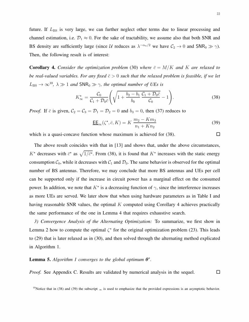
Algorithm 1 Alternating optimization for Problem (29)Set θ⋆
0 = (ζ⋆0 , c⋆0,K
⋆0 ); 0 < ε < 1; k = 1;
while ‖θ⋆k − θ⋆
k−1‖ ≥ ε do
Compute c⋆k by using Lemma 3;
Compute K⋆k by using Lemma 4 (Corollary 4);
Compute M⋆k = c⋆kK
⋆k ;
Compute ζ⋆k (M⋆k ,K
⋆k) by using Lemma 2;
Collect θ⋆k = (ζ⋆k ,M
⋆k ,K
⋆k); k = k + 1;
end while
return θ⋆ = (ζ⋆, c⋆,K⋆) = (ζ⋆k , ⌈M⋆k ⌋, ⌈K⋆
k⌋)
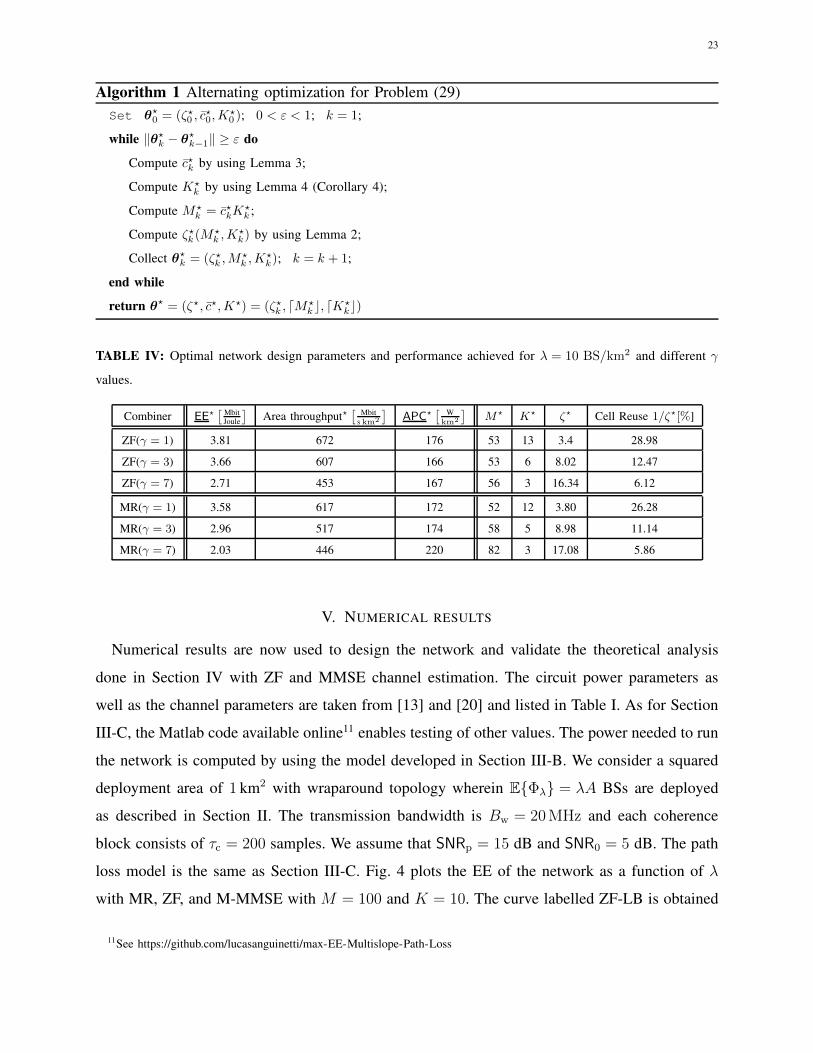
TABLE IV: Optimal network design parameters and performance achieved for λ = 10 BS/km2 and different γ
values.
Combiner EE⋆[ Mbit
Joule
]Area throughput⋆
[ Mbits km2
]APC⋆
[ Wkm2
]M⋆ K⋆ ζ⋆ Cell Reuse 1/ζ⋆[%]
ZF(γ = 1) 3.81 672 176 53 13 3.4 28.98
ZF(γ = 3) 3.66 607 166 53 6 8.02 12.47
ZF(γ = 7) 2.71 453 167 56 3 16.34 6.12
MR(γ = 1) 3.58 617 172 52 12 3.80 26.28
MR(γ = 3) 2.96 517 174 58 5 8.98 11.14
MR(γ = 7) 2.03 446 220 82 3 17.08 5.86
V. NUMERICAL RESULTS
Numerical results are now used to design the network and validate the theoretical analysis
done in Section IV with ZF and MMSE channel estimation. The circuit power parameters as
well as the channel parameters are taken from [13] and [20] and listed in Table I. As for Section
III-C, the Matlab code available online11 enables testing of other values. The power needed to run
the network is computed by using the model developed in Section III-B. We consider a squared
deployment area of 1 km2 with wraparound topology wherein E{Φλ} = λA BSs are deployed
as described in Section II. The transmission bandwidth is Bw = 20MHz and each coherence
block consists of τc = 200 samples. We assume that SNRp = 15 dB and SNR0 = 5 dB. The path
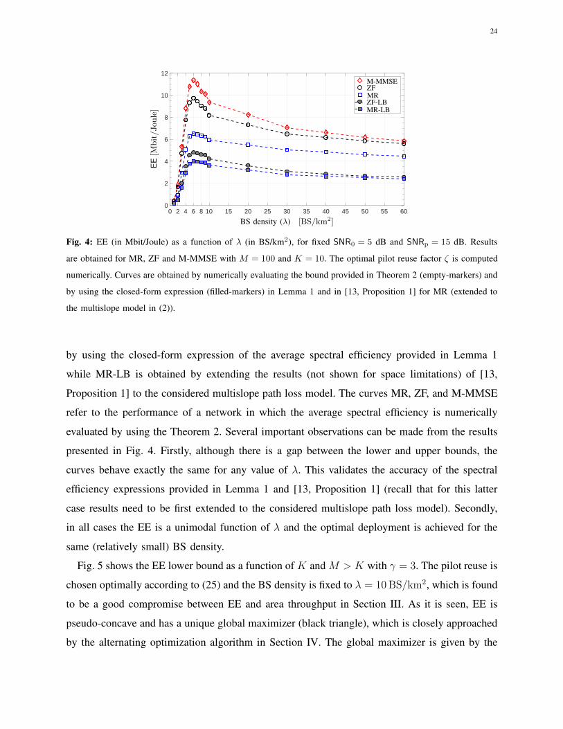
loss model is the same as Section III-C. Fig. 4 plots the EE of the network as a function of λ
with MR, ZF, and M-MMSE with M = 100 and K = 10. The curve labelled ZF-LB is obtained
11See https://github.com/lucasanguinetti/max-EE-Multislope-Path-Loss
24
0 2 4 6 8 10 15 20 25 30 35 40 45 50 55 600
2
4
6
8
10
12
BS density (λ) [BS/km2]
EE[M
bit/Joule]
M-MMSEZFMRZF-LBMR-LB
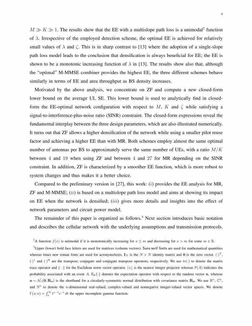
Fig. 4: EE (in Mbit/Joule) as a function of λ (in BS/km2), for fixed SNR0 = 5 dB and SNRp = 15 dB. Results
are obtained for MR, ZF and M-MMSE with M = 100 and K = 10. The optimal pilot reuse factor ζ is computed
numerically. Curves are obtained by numerically evaluating the bound provided in Theorem 2 (empty-markers) and
by using the closed-form expression (filled-markers) in Lemma 1 and in [13, Proposition 1] for MR (extended to
the multislope model in (2)).
by using the closed-form expression of the average spectral efficiency provided in Lemma 1
while MR-LB is obtained by extending the results (not shown for space limitations) of [13,
Proposition 1] to the considered multislope path loss model. The curves MR, ZF, and M-MMSE
refer to the performance of a network in which the average spectral efficiency is numerically
evaluated by using the Theorem 2. Several important observations can be made from the results
presented in Fig. 4. Firstly, although there is a gap between the lower and upper bounds, the
curves behave exactly the same for any value of λ. This validates the accuracy of the spectral
efficiency expressions provided in Lemma 1 and [13, Proposition 1] (recall that for this latter
case results need to be first extended to the considered multislope path loss model). Secondly,
in all cases the EE is a unimodal function of λ and the optimal deployment is achieved for the
same (relatively small) BS density.
Fig. 5 shows the EE lower bound as a function of K and M > K with γ = 3. The pilot reuse is
chosen optimally according to (25) and the BS density is fixed to λ = 10BS/km2, which is found
to be a good compromise between EE and area throughput in Section III. As it is seen, EE is
pseudo-concave and has a unique global maximizer (black triangle), which is closely approached
by the alternating optimization algorithm in Section IV. The global maximizer is given by the
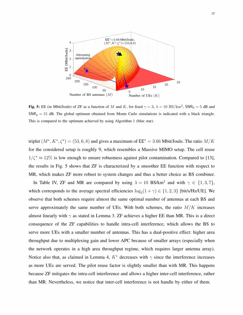
25
0250
1
200 25
2
150 20
3
15100
4
1050 5
EE
[Mbi
t/Jou
le]
Number of BS antennas (M) Number of UEs (K)
Alternatingoptimization
EE⋆=3.66Mbit/Joule,(M⋆,K⋆,ζ⋆)=(53,6,8)
Fig. 5: EE (in Mbit/Joule) of ZF as a function of M and K , for fixed γ = 3, λ = 10 BS/km2, SNR0 = 5 dB and
SNRp = 15 dB. The global optimum obtained from Monte Carlo simulations is indicated with a black triangle.
This is compared to the optimum achieved by using Algorithm 1 (blue star).
triplet (M⋆, K⋆, ζ⋆) = (53, 6, 8) and gives a maximum of EE⋆ = 3.66 Mbit/Joule. The ratio M/K
for the considered setup is roughly 9, which resembles a Massive MIMO setup. The cell reuse
1/ζ⋆ ≈ 12% is low enough to ensure robustness against pilot contamination. Compared to [13],
the results in Fig. 5 shows that ZF is characterized by a smoother EE function with respect to
MR, which makes ZF more robust to system changes and thus a better choice as BS combiner.
In Table IV, ZF and MR are compared by using λ = 10 BS/km2 and with γ ∈ {1, 3, 7},
which corresponds to the average spectral efficiencies log2(1 + γ) ∈ {1, 2, 3} [bit/s/Hz/UE]. We
observe that both schemes require almost the same optimal number of antennas at each BS and
serve approximately the same number of UEs. With both schemes, the ratio M/K increases
almost linearly with γ as stated in Lemma 3. ZF achieves a higher EE than MR. This is a direct
consequence of the ZF capabilities to handle intra-cell interference, which allows the BS to
serve more UEs with a smaller number of antennas. This has a dual-positive effect: higher area
throughput due to multiplexing gain and lower APC because of smaller arrays (especially when
the network operates in a high area throughput regime, which requires larger antenna array).
Notice also that, as claimed in Lemma 4, K⋆ decreases with γ since the interference increases
as more UEs are served. The pilot reuse factor is slightly smaller than with MR. This happens
because ZF mitigates the intra-cell interference and allows a higher inter-cell interference, rather
than MR. Nevertheless, we notice that inter-cell interference is not handle by either of them.
26
VI. CONCLUSIONS
We designed a cellular network for maximal EE with MR, ZF and M-MMSE under the
assumption of imperfect CSI and a multislope path loss model. This was formulated as an
optimization problem by using a lower bound on the spectral efficiency and a state-of-the-art
power consumption model. The variables were pilot reuse factor ζ and BS density λ for a
Massive MIMO network. The results showed that the additional computational complexity of
M-MMSE processing pays off in terms of EE and area throughput, though all the scheme behaves
substantially the same with respect to λ, that is, reducing the cell size does not bring benefits
in terms of EE. To get further insights, we concentrated on ZF and formulated the optimization
problem by using stochastic geometry and a new lower bound on the average ergodic spectral
efficiency. The variables were pilot reuse factor, number of BS antennas and UEs per BS. The
results showed that ZF allows a higher network densification and the use of a smaller pilot
reuse factor while achieving a higher EE than with MR combining. Also, it turned out that the
EE-optimal configuration resembles a Massive MIMO setup.
APPENDIX A — PROOF OF LEMMA 1
To ease understanding, the proof is articulated in two steps. The first aims at computing all
the inner expectations in (19) with respect to channel and pilot realizations, whereas the second
makes use of all these terms, together with the power allocation policy in Section II, to evaluate
the outer expectation with respect to both the BSs’ and UEs’ locations.
A.1. Computation of all the expectations in (19)
Let vjk = VZFj ek be the ZF detector for the typical UE k in cell j, with VZF
j as in (12) and
ek being the kth vector of the standard basis.
Received signal power: The useful term is computed as:
|E{h,a}{vH
jkhjjk}|2
(a)= |E{h,a}{vH
jkhjjk}|2
(b)= 1 (40)
where (a) follows from Corollary 1 and (b) comes from the ZF combining.
Noise power: The noise term is obtained as:
E{h,a}{‖vjk‖2}(a)= E{h,a}
{[((Hj
j)HHj
j
)−1]k,k
}
(a)=
1
M −KE{a}
{1
γjjk
}(41)
27
where (a) is due to the ZF combining, (b) exploits both the statistics of hjjk in Corollary 1, with
γjjk denoted in (5), and the properties of Wishart matrices (e.g., see [9, Proof of Proposition 3]
or [31] for a more general treatment).
Intra-cell interference power: Consider now the cell of interest j and let us compute the
intra-cell interference. Then, for any interferer UE i in cell j we have that
E{h,a}{|vH
jkhjji|2}
(a)= E{h,a}{tr(vjkv
H
jkhjji(h
jji)
H) + tr(vjkvH
jkhjji(h
jji)
H)}(b)= δ(i− k) + E{a}
{(βj
ji − γjji)E{h}{‖vjk‖2}
}
(c)= δ(i− k) +
1
M −K
(βjjiE{a}
{1
γjjk
}− E{a}
{γjji
γjjk
})(42)
with δ(·) as the delta Kronecker function and where (a)–(b) follow from Corollary 1 while using
ZF combining for the first term and (c) is due to (41).
Inter-cell interference power: The inter-cell interference collected by BS j from cell l,
e.g., depends on whether the UEs in that cell use the same or a different pilot subset Φl than
the one used in cell j, that is (l, i) ∈ Pj,k with Pj,k = {(l, i) ∈ Φλ \ {j} × {1, . . . , K} : alj = 1}.
Consider a UE i that does not cause pilot contamination to UE k of cell j. In that case, (l, i) /∈ Pj,k
and
E{h,a}{|vH
jkhjli|2|alj = 0} (a)
= βjliE{h,a}{‖vjk‖2|alj = 0}
(b)=
βjli
M −KE{a}
{1
γjjk
∣∣∣∣alj = 0
}(43)
where (a) follows from Corollary 1 and the fact that vjk is a function of {hjji}Ki=1, which are
statistically independent from {hjli}Ki=1 (and so {hj
ji}Ki=1) in presence of no pilot contamination,
for which (6) does not hold and (b) is due to (41). Consider an interferer UE i that cause
pilot contamination to UE k of cell j. Then, (l, i) ∈ Pj,k and using Corollary 1 leads to
E{h,a}{|vHjkh
jli|2|alj = 1}=E{h,a}{|vH
jkhjli|2|alj = 1} + E{h,a}{|vH
jkhjli|2|alj = 1}. Let us now
tackle these contributions to pilot contamination separately. The former is
E{h,a}{|vH
jkhjli|2|alj = 1} (a)
=(βj
li)2
βlliβ
jji
E{h,a}{|vH
jkhjji|2|alj = 1}
(b)=
(βjli)
2
βlliβ
jji
δ(i− k) (44)
28
where in (a) we make use of (6) that accounts for the channel estimates linearity (alj = 1) and
(b) follows from the same considerations used for (42) since conditioning has no impact here.
The latter term is computed as
E{h,a}{|vH
jkhjli|2|alj = 1} (a)
= βjliE{h,a}{‖vjk‖2|alj = 1
}− E{h,a}
{γjli ‖vjk‖2|alj = 1
}
(b)=
βjliE{a}
{1
γjjk
∣∣∣∣alj = 1
}
M −K−
E{a}
{γjli
γjjk
∣∣∣∣alj = 1
}
M −K
(c)=
βjliE{a}
{1
γjjk
∣∣∣∣alj = 1
}− (βj
li)2
βlliβ
jji
E{a}
{γjji
γjjk
∣∣∣∣alj = 1
}
M −K(45)
where (a) follows from Corollary 1 while keeping the conditioning, (b) is due to (41) and
(c) follows from (6). The inter-cell interference term can be computed by considering the
probability of having or not pilot contamination between UE i of cell l and the typical UE,
i.e., P(alj = 1) = 1/ζ and P(alj = 0) = 1− 1/ζ. Particularly, from (43) – (45) we obtain
E{h,a}{|vH
jkhjli|2}=
1∑
p=0
P(alj = p)E{h,a}{|vH
jkhjli|2|alj = p}
=1
ζ
(βjli)
2
βlliβ
jji
δ(i− k)− 1
ζ
1
M −K
(βjli)
2
βlliβ
jji
E{a}
{γjji
γjjk
∣∣∣∣alj = 1
}
+βjli
M −KE{a}
{1
γjjk
}. (46)
A.2. Computation of the lower bound on the UL SE
To begin with, let us define the following quantities
ϑ(1)ji =
∑
l∈Φλ\{j}
βjli
βlli
, ϑ(2)ji =
∑
l∈Φλ\{j}
(βjli
βlli
)2
(47)
which are then used to compute the inner expectations in (41), (42) and (46) with respect to the
pilot realizations only. Then, the following terms are of interest
E{a}
{1
γjjk
}=
1
βjjk
(1 +
ϑ(1)jk
ζ+
1
SNRp
)(48)
E{a}
{γjji
γjjk
}=
E{a}{1} = 1 if i = k
E{a}
{1
γjjk
}E{a}{γj
ji}(a)
≥ βjji
βjjk
1+ϑ(1)jkζ
+ 1SNRp
1+ϑ(1)jiζ
+ 1SNRp
if i 6= k(49)

29
where (48) follows from (5) with E{a}{alj} = 1/ζ and ϑ(1)jk ∈ R that is denoted in (47), while
in (49) we exploit the fact that UEs i and k in cell j cannot share the same pilot sequence when
i 6= k and (a) comes directly from jointly using Jensen’s inequality and (48).12 The noise term
in (19) is computed by plugging (48) into (41) as follows
βjjkE{h,a}{‖vjk‖2} =
1
M −K
(1 +
ϑ(1)jk
ζ+
1
SNRp
). (50)
The interference contribution is decomposed as the sum of three terms, i.e., the intra-cell
interference and the inter-cell interferences due to pilot and no pilot contamination:∑
l∈Φλ
K∑
i=1
βjjk
βlli
E{h,a}{|vH
jkhjli|2} =
K∑
i=1
βjjk
βjji
E{h,a}{|vH
jkhjji|2}
︸ ︷︷ ︸intra-cell interference
+∑
l∈Φλ\{j}
K∑
i=1
βjjk
βlli
1∑
p=0
P(alj = p)E{h,a}{|vH
jkhjli|2|al,j = p}
︸ ︷︷ ︸inter-cell interference
. (51)
The first term accounts for intra-cell interference from all UEs i in cell j when using (48) and
(49) into (42) becomes
K∑
i=1
βjjk
βjji
E{h,a}{|vH
jkhjji|2}≤ 1 +
K(1 +
ϑ(1)jk
ζ+ 1
SNRp
)−
K∑i=1
1+ϑ(1)jkζ
+ 1SNRp
1+ϑ(1)jiζ
+ 1SNRp
M −K. (52)
The second term accounts for the interference from all UEs i in cells l 6= j and thus it can be
computed substituting (48) – (49) into (46), which reads∑
l∈Φλ\{j}
K∑
i=1
βjjk
βlli
E{h,a}{|vH
jkhjli|2}≤
1
M −K
[(1 +
ϑ(1)jk
ζ+
1
SNRp
) K∑
i=1
ϑ(1)ji +
(M −K)
ζϑ(2)jk
− 1
ζ
K∑
i=1
ϑ(2)ji
(1 +
ϑ(1)jk
ζ+ 1
SNRp
1 +ϑ(1)ji
ζ+ 1
SNRp
)]. (53)
Plugging (40) and (50) – (53) together into (19) we have
SINR ≥ M −K(K + 1
SNR0+
K∑i=1
ϑ(1)ji
)(1 +
ϑ(1)jk
ζ+ 1
SNRp
)+ M−K
ζϑ(2)jk −
K∑i=1
(1+ϑ
(1)jk /ζ+ 1
SNRp
1+ϑ(1)ji /ζ+ 1
SNRp
)(1 +
ϑ(2)ji
ζ
)
(54)
This completes the first part of the proof.
12Hereafter we do not consider the conditioning anymore since, as we will see in a while, we lower bound this term when
averaging over the BSs and UEs locations in the outer expectation.
30
Ed
1 +
ϑ(1)jk
ζ+ 1
SNRp
1 +ϑ(1)ji
ζ+ 1
SNRp
=
Ed{1} = 1 if i = k
Ed
{1 +
ϑ(1)jk
ζ+ 1
SNRp
}Ed
1
1+ϑ(1)jiζ
+ 1SNRp
≥ 1 if i 6= k
(56)
Ed
1 +
ϑ(1)jk
ζ+ 1
SNRp
1 +ϑ(1)ji
ζ+ 1
SNRp
ϑ(2)ji
=
Ed
1+ϑ(1)jkζ
+ 1SNRp
1+ϑ(1)jkζ
+ 1SNRp
ϑ(2)jk
= Ed
{ϑ(2)jk
}if i = k
Ed
ϑ(2)ji
1+ϑ(1)jiζ
+ 1SNRp
Ed
{1 +
ϑ(1)jk
ζ+ 1
SNRp
}≥Ed
{ϑ(2)ji
}if i 6= k
(57)
APPENDIX B — PROOF OF LEMMA 1
Next, a tractable lower bound on the UL average ergodic spectral efficiency of the typical UE
is computed, where the expectation is taken with respect to the BSs and UEs locations. To begin
with, the Jensen’s inequality is applied to move the expectation inside the logarithm and obtain
Ed
{log2
(1 +
1
SINR−1
)}≥ log2
(1 +
1
Ed
{SINR−1
})
= log2(1 + SINR
)(55)
where we denote with SINR = Ed
{SINR−1
}. Before proceeding further, let us explicate some
of the terms included in (53), that is, (56) and (56), respectively, where in (56) we use the
independence between UEs distance realizations for i 6= k together with the Jensen’s inequality,
while in (57) we lower bound the expectation13. From (54), the expectation of SINR−1 can be
expanded as in (58).
SINR ≥ 1
M −K
((K +
1
SNR0
)(1 +
1
ζEd
{ϑ(1)jk
}+
1
SNRp
)
+(1 +
1
SNRp
) K∑
i=1
Ed
{ϑ(1)ji
}+
1
ζ
K∑
i=1
Ed
{ϑ(1)jkϑ
(1)ji
}
+M −K
ζEd
{ϑ(2)jk
}−K − 1
ζ
K∑
i=1
Ed
{ϑ(2)ji
}). (58)
13Let us consider one term of the sum within ϑ(1)ji at a time and denote with x = βj
li/βlli. Then we have
Ex{ x2
b+x} ≥ (Ex{x})2
b+Ex{x} ≥ Ex{x2}b+Ex{x} by applying Jensen’s inequality first (since b = 1 + 1/SNRp > 0) and Holder’s inequality
at second.
31
Now, in order to obtain the achievable lower bound in (20) we introduce the following Lemma:
Lemma 6. Assume a multislope path loss model βjlk(d
jlk) as in (2) and djlk ∈ Φλ \ {j} with djlk
being the distance between UE k in cell l and the BS in cell j (where Φλ \ {j} describes the
set of BSs distributed as an H-PPP with density λ) we have
Ed
{ϑ(κ)ji
}= Ed
∑
l∈Φλ\{j}
(βjli(d
jli)
βlli(d
lli)
)κ = µκ, (59)
Ed
{ϑ(1)jkϑ
(1)ji
}= Ed
∑
n∈Φλ\{j}
∑
l∈Φλ\{j}l 6=n
(βjnk(d
jnk)
βnnk(d
nnk)
)(βjli(d
jli)
βlli(d
lli)
)
≤ µ21 + µ2 (60)
where µκ for κ = 1, 2 is denoted in (22).
Proof. We start by considering the BSs distributed in a circular area of finite radius r and wrap
around in the radial domain to keep the translation invariance. Considering the closest BS policy
association in Section II, which tells us that there are no interfering BSs closer than the one is
serving the typical UE k in cell j, that is BS j, the average number of inter-cell interferers in
that ring is λAR with AR(r, λ) = π(r2 − Ed
{(djjk)
2})
= π(r2 − 1
πλ
). Then, (59) – (60) can
be written as [13, Appendix B]
Ed
{ϑ(κ)ji
}= λAR(r, λ)Ed
{(βjlk(d
jlk)
βllk(d
llk)
)κ}(61)
Ed{ϑ(1)jkϑ
(1)ji } ≤ λAR(r, λ)
((λAR(r, λ)− 1
)E2d
{βjlk(d
jlk)
βllk(d
llk)
}+ Ed
(βjlk(d
jlk)
βllk(d
llk)
)2
). (62)
Therefore, (61) – (62) requires computing the following term
Ed
{(βjlk(d
jlk)
βllk(d
llk)
)κ}(a)= Ed
{β(dllk)
−κ Ed
{β(djlk)
κ | dllk}}
(b)= Ed
{β(dllk)
−κ
∫ r
dllk
β(x)κ2x
r2 − (dllk)2dx
}
(c)=
N∑
n=1
(∫ Rn
Rn−1
2βn(y)−κ
r2 − y2
(∫ r
y
x β(x)κ dx
)fd(y) dy
)(63)
for κ = {1, 2} and with βn as the path loss related to the interval [Rn−1, Rn), where in (a) we
use the theorem of total expectation conditioning over dllk, (b) is due to the fact that there are no
interfering BSs closer than the jth (i.e., djlk ≥ dllk) and change of variable to polar coordinates,

32
while in (c) we use the multislope pathloss model in (2) y ∈ [Rn−1, Rn), n = 1, . . . , N and
denote with fd(djjk) the probability density function of the distance from the typical UE k to its
serving BS j. By using (2), we rewrite the term within the inner brackets in (63) as followsr∫
y
xβ(x)κ dx =
Rn∫
y
xβn(x)κ dx+
N∑
i=n+1
Ri∫
Ri−1
xβi(x)κ dx (64)
where we have used that x ≥ y for any fixed index n of the summation in (63). Then, using (2)
into (64) we obtainr∫
y
xβ(x)κ dx = Υκn
y2−καn − R2−καnn
καn − 2+
N∑
i=n+1
Υκi
R2−καii−1 − R2−καi
i
καi − 2. (65)
Plugging (65) into (63), after some rearrangements we obtain
Ed
{(βjlk(d
jlk)
βllk(d
llk)
)κ}= 2
N∑
n=1
Rn∫
Rn−1
(y2
(καn − 2)(r2 − y2)+
yκαncn(κ)
(r2 − y2)
)fd(y) dy (66)
where cn(κ) =∑N
i=n+1
(Υi
Υn
)κ R2−καii−1 −R
2−καii
καi−2− R2−καn
n
καn−2.
To account for the wrap around in R2, we let r → ∞ and obtain14
λA(r, λ)Ed
{(βjlk(d
jlk)
βllk(d
llk)
)κ}→ 2λπ
N∑
n=1
(1
καn − 2
Rn∫
Rn−1
y2fd(y) dy + cn(κ)
Rn∫
Rn−1
yκαnfd(y) dy
).
(67)
Finally, by using Corollary 3 the two integrals in (66) can be computed in closed-form as (after
simple calculus)Rn∫
Rn−1
y2fd(y) dy =Γ(2; πλR2
n−1
)− Γ
(2; πλR2
n
)
πλ(68)
Rn∫
Rn−1
yκαnfd(y) dy =Γ(
2+καn
2; πλR2
n−1
)− Γ
(2+καn
2; πλR2
n
)
(πλ)καn2
. (69)
Plugging (67) – (69) into (61) – (62) leads to (59) – (60), which completes the proof.
14Notice that the function within the integral is a fractional polynomial of second order degree that converges to a bounded
real-valued limit as r → ∞. For this reason, the bounded convergence theorem conditions are satisfied and that operation is
allowed.
33
APPENDIX C — PROOF OF LEMMA 5
We start by noticing that the mapping applied at each iteration, to compute the next point of the
algorithm, follows the gradient descent rule, which provides a stationary point with no increase
of the objective value. In [32, Theorem 3.2], convergence of a gradient descent-based alternating
method is proved given that the objective EE(c, K) is pseudo-concave in each variable and
the level set S = {(c, K) ∈ R2 : EE(c, K) ≤ EE(c0, K0)}, with respect to the the initial point
of the algorithm, is compact. The latter can be easily proved by noticing that c and K are
defined over a box (compact and closed domain) and the objective function is bounded, which is
true for any PFIX > 0. In particular, under these conditions, the alternating optimization method
introduced in Lemma 5 returns a sequence {ck, Kk} that converges to a global maximizer of
EE on R2. Thus, convergence is achieved whenever pseudo-concavity holds component-wise for
both EE(c) and EE∞(K) in (30) and (39), respectively. To this end, in [33, Proposition 2.9] it
is shown that fractional objectives in the form of r = f/g defined over a convex set X ⊆ Rn
with n ≥ 1 enjoy pseudo-concave properties when f : X → R is non-negative, differentiable,
and concave, while g : X → R is differentiable and convex (if g is affine, the non-negativity
of f can be relaxed). In particular, the former objective can be rewritten as r(c) = EE(c) with
f(c) = p1c+ p0 and g(c) = q2c2 + q1c + q0 with some parameters {pi, qi} that can be easily
related to the parameters {ai} illustrated in Table III. Here, f(c) is affine and non-negative
for c ≥ −p0p1
= a1+a3a2−a0
, which is equivalent to assume γ ≤ τcµ2K
(true in general as seen below
(30)) whereas g(c) is convex since q2 = a2a4 that are both positive quantities; see Table III.
For the latter objective r(K) = EE∞(K), we have that f(K) = −m3K2 +m2K is concave for
m3 = b0 > 0 (see Table III), while g(K) = n2K + n1 is affine over K ∈ R. This proves the
convergence of Algorithm 1.
REFERENCES
[1] J. G. Andrews, S. Buzzi, W. Choi, S. V. Hanly, A. Lozano, A. C. K. Soong, and J. C. Zhang, “What Will 5G Be?” IEEE
J. Sel. Areas Commun., vol. 32, no. 6, pp. 1065–1082, jun 2014.
[2] A. Fehske, G. Fettweis, J. Malmodin, and G. Biczok, “The global footprint of mobile communications: The ecological
and economic perspective,” IEEE Commun. Mag., vol. 49, no. 8, pp. 55–62, aug 2011.
[3] N. Bhushan, J. Li, D. Malladi, R. Gilmore, D. Brenner, A. Damnjanovic, R. T. Sukhavasi, C. Patel, and S. Geirhofer,
“Network densification: the dominant theme for wireless evolution into 5G,” IEEE Communications Magazine, vol. 52,
no. 2, pp. 82–89, February 2014.
[4] H. S. Dhillon, M. Kountouris, and J. G. Andrews, “Downlink MIMO HetNets: Modeling, ordering results and performance
analysis,” IEEE Transactions on Wireless Communications, vol. 12, no. 10, pp. 5208–5222, October 2013.
34
[5] J. Hoydis, M. Kobayashi, and M. Debbah, “Green Small-Cell Networks,” IEEE Veh. Technol. Mag., vol. 6, no. 1, pp.
37–43, mar 2011.
[6] Y. S. Soh, T. Q. S. Quek, M. Kountouris, and H. Shin, “Energy Efficient Heterogeneous Cellular Networks,” IEEE J. Sel.
Areas Commun., vol. 31, no. 5, pp. 840–850, may 2013.
[7] J. G. Andrews, “Seven ways that HetNets are a cellular paradigm shift,” IEEE Communications Magazine, vol. 51, no. 3,
pp. 136–144, March 2013.
[8] T. L. Marzetta, “Noncooperative Cellular Wireless with Unlimited Numbers of Base Station Antennas,” IEEE Trans. Wirel.
Commun., vol. 9, no. 11, pp. 3590–3600, nov 2010.
[9] Hien Quoc Ngo, E. G. Larsson, and T. L. Marzetta, “Energy and spectral efficiency of very large multiuser MIMO systems,”
IEEE Trans. Commun., vol. 61, no. 4, pp. 1436–1449, apr 2013.
[10] E. Björnson, J. Hoydis, and L. Sanguinetti, “Massive mimo has unlimited capacity,” IEEE Transactions on Wireless
Communications, vol. 17, no. 1, pp. 574–590, Jan 2018.
[11] T. L. Marzetta, E. G. Larsson, H. Yang, and H. Q. Ngo, Fundamentals of Massive MIMO. Cambridge University Press,
2016.
[12] E. Björnson, J. Hoydis, and L. Sanguinetti, “Massive MIMO networks: Spectral, energy, and hardware efficiency,”
Foundations and Trends in Signal Processing, vol. 11, no. 3-4, pp. 154–655, 2017.
[13] E. Björnson, L. Sanguinetti, and M. Kountouris, “Deploying dense networks for maximal energy efficiency: Small cells
meet Massive MIMO,” IEEE J. Sel. Areas Commun., vol. 34, no. 4, pp. 832–847, apr 2016.
[14] H. Q. Ngo, A. Ashikhmin, H. Yang, E. G. Larsson, and T. L. Marzetta, “Cell-free Massive MIMO versus small cells,”
IEEE Transactions on Wireless Communications, vol. 16, no. 3, pp. 1834–1850, March 2017.
[15] A. D. Wyner, “Shannon-theoretic approach to a Gaussian cellular multiple-access channel,” IEEE Transactions on
Information Theory, vol. 40, no. 6, pp. 1713–1727, Nov 1994.
[16] O. Somekh and S. Shamai, “Shannon-theoretic approach to a Gaussian cellular multiple-access channel with fading,” IEEE
Transactions on Information Theory, vol. 46, no. 4, pp. 1401–1425, Jul 2000.
[17] J. G. Andrews, F. Baccelli, and R. K. Ganti, “A tractable approach to coverage and rate in cellular networks,” IEEE
Transactions on Communications, vol. 59, no. 11, pp. 3122–3134, November 2011.
[18] H. S. Dhillon, R. K. Ganti, F. Baccelli, and J. G. Andrews, “Modeling and analysis of k-tier downlink heterogeneous
cellular networks,” IEEE Journal on Selected Areas in Communications, vol. 30, no. 3, pp. 550–560, April 2012.
[19] H. ElSawy, E. Hossain, and M. Haenggi, “Stochastic geometry for modeling, analysis, and design of multi-tier and cognitive
cellular wireless networks: A survey,” IEEE Communications Surveys Tutorials, vol. 15, no. 3, pp. 996–1019, Third 2013.
[20] E. Björnson, L. Sanguinetti, J. Hoydis, and M. Debbah, “Optimal design of energy-efficient multi-user mimo systems: Is
Massive MIMO the answer?” IEEE Trans. Wirel. Commun., vol. 14, no. 6, pp. 3059–3075, jun 2015.
[21] D. Cao, S. Zhou, and Z. Niu, “Optimal base station density for energy-efficient heterogeneous cellular networks,” in 2012
IEEE International Conference on Communications (ICC), June 2012, pp. 4379–4383.
[22] S. r. Cho and W. Choi, “Energy-efficient repulsive cell activation for heterogeneous cellular networks,” IEEE Journal on
Selected Areas in Communications, vol. 31, no. 5, pp. 870–882, May 2013.
[23] X. Zhang and J. G. Andrews, “Downlink cellular network analysis with multi-slope path loss models,” IEEE Transactions
on Communications, vol. 63, no. 5, pp. 1881–1894, May 2015.
[24] D. Tse and P. Viswanath, Fundamentals of Wireless Communication. New York, NY, USA: Cambridge University Press,
2005.
[25] H. Munir, S. A. Hassan, H. Pervaiz, Q. Ni, and L. Musavian, “Resource optimization in multi-tier HetNets exploiting
multi-slope path loss model,” IEEE Access, vol. 5, pp. 8714–8726, 2017.
35
[26] V. M. Nguyen and M. Kountouris, “Performance limits of network densification,” IEEE Journal on Selected Areas in
Communications, vol. 35, no. 6, pp. 1294–1308, June 2017.
[27] A. Pizzo, D. Verenzuela, L. Sanguinetti, and E. Bjoernson, “Network deployment for maximal energy efficiency in uplink
with zero-forcing,” in GLOBECOM 2017 - 2017 IEEE Global Communications Conference, Dec 2017, pp. 1–7.
[28] F. Baccelli and B. Blaszczyszyn, Stochastic Geometry and Wireless Networks: Volume I Theory. NoW Publishers, 2009,
vol. 3, no. 3-4.
[29] E. Björnson, L. Sanguinetti, and M. Kountouris, “Designing wireless broadband access for energy efficiency: Are small
cells the only answer?” in 2015 IEEE Int. Conf. Commun. Work. IEEE, jun 2015, pp. 136–141.
[30] S. Weber and J. G. Andrews, Transmission Capacity of Wireless Networks. Now Publishers, Inc., 2010, vol. 5, no. 2-3.
[31] D. Maiwald and D. Kraus, “Calculation of moments of complex Wishart and complex inverse Wishart distributed matrices,”
IEE Proc. - Radar, Sonar Navig., vol. 147, no. 4, p. 162, 2000.
[32] L. Grippof and M. Sciandrone, “Globally convergent block-coordinate techniques for unconstrained optimization,”
Optimization Methods and Software, vol. 10, no. 4, pp. 587–637, 1999.
[33] A. Zappone and E. Jorswieck, “Energy efficiency in wireless networks via fractional programming theory,” Foundations
and Trends in Communications and Information Theory, vol. 11, no. 3-4, pp. 185–396, 2015.