maximal and minimal sample coordination
TRANSCRIPT
Sankhya : The Indian Journal of Statistics2006, Volume 67, Part 3, pp 590-612c© 2006, Indian Statistical Institute
Maximal and Minimal Sample Co-ordination
Alina Matei and Yves TilleUniversity of Neuchatel, Switzerland
Abstract
For sampling design over time we are interested in maximizing/minimizingthe expected overlap between two or more samples drawn in different timepoints. For this it is necessary to compute the joint inclusion probability oftwo samples drawn in different time periods. A solution is given by usinglinear programming and more precisely by solving a transportation problem.This solution is not computationally fast. We are interested in identifyingthe conditions under which the objective function associated with an optimalsolution of the transportation problem is equal to the bound given by maxi-mizing/minimizing the expected overlap. Using these conditions we proposea new algorithm to optimize the co-ordination between two samples withoutusing linear programming. Our algorithm is based on the Iterative Propor-tional Fitting (IPF) procedure. Theoretical complexity is substantially lowerthan for transportation problem approach, because more than five iterationsof IPF procedure are not required in practice.
AMS (2000) subject classification. 62D05.Keywords and phrases. Sample survey, sample co-ordination, IPF procedure,transportation problem.
1 Introduction
It is usual to sample populations on two or more occasions in orderto obtain current estimates of a character. Sample co-ordination problemconsists in managing the overlap of two or more samples drawn in differenttime occasions. It is either positive or negative. While in the former theexpected overlap of two or more samples is maximized, in the latter it isminimized. Positive and negative co-ordination can be formulated as a dualproblem. Thus, solving positive co-ordination problem can lead us to thesolution of negative sample co-ordination and vice versa.
Various methods have been proposed in order to solve sample co-ordinationproblem. The co-ordination problem has been the main topic of interest formore than fifty years. The first papers on this subject are due to Patterson
Maximal and minimal sample co-ordination 591
(1950) and Keyfitz (1951). Other papers dated from the same period are:Kish and Hess (1959), Fellegi (1963), Kish (1963), Fellegi (1966), Gray andPlatek (1963). These first works present methods which are in general re-stricted to two successive samples or to small sample sizes. A generalizationof the problem in the context of a larger sample size has been done by Kishand Scott (1971). Mathematical programming met the domain of the sam-ple co-ordination with the books of Raj (1968) and Arthanari and Dodge(1981) and the paper of Causey et al. (1985). Brewer (1972) and Breweret.al (1972) introduced the concept of co-ordination based on PermanentRandom Numbers (PRN). Furthermore, Rosen (1997a,b) developed ordersampling, which is another approach that takes into account the concept ofPRN.
Let U = {1, . . . , k, . . . , N} be the population under study. Samples with-out replacement are selected on two distinct time periods. The time periodsare indicated by the exponents 1 and 2 in our notation. Thus, π1
k denotesthe inclusion probability of unit k ∈ U for time period 1 in the first sample.Similarly, π2
k denotes the inclusion probability of unit k ∈ U for time period2 in the second sample. Let S1,S2 be the sets of all samples in the firstoccasion and the second occasion, respectively. Our notation for a sample iss1i ∈ S1 and s2
j ∈ S2. Let also π1,2k be the joint inclusion probability of unit
k in both samples. Thus
max(π1k + π2
k − 1, 0) ≤ π1,2k ≤ min(π1
k, π2k).
Let p1i , p
2j denote the probability distributions on S1,S2, respectively. Let
|s1i ∩ s2
j | be the number of common units of both samples, let I = {k ∈U |π1
k ≤ π2k} be the set of “increasing” units, and let D = {k ∈ U |π1
k > π2k}
be the set of “decreasing” units.
Definition 1. The quantity∑
k∈U min(π1k, π
2k) is called the absolute
upper bound; the quantity∑
k∈U max(π1k + π2
k − 1, 0) is called the absolutelower bound.
Note that∑
k∈U π1,2k is the expected overlap. The expected overlap is
equal to the absolute upper bound when π1,2k = min(π1
k, π2k), for all k ∈ U.
We use in this case the terminology “the absolute upper bound is reached”.Similarly, the absolute lower bound is reached when π1,2
k = max(π1k + π2
k −1, 0), for all k ∈ U. Only a few of the already developed methods can reachthe absolute upper/lower bound.
592 Alina Matei and Yves Tille
As we have already mentioned, one point of view to solve sample co-ordination problem is to use mathematical programming and more exactlyto solve a transportation problem. The form of the sample co-ordinationproblem in the frame of a transportation problem enables us to compute thejoint inclusion probability of two samples drawn on two different occasions,s1i and s2
j , and then the conditional probability p(s2j |s1
i ). This allows to choosethe sample s2
j drawn in the second occasion given that the sample s1i was
drawn in the first. The solution given by using mathematical programmingis not computationally fast.
We call a bi-design a couple of two sampling designs for two differentoccasions. Let S = {s = (s1
i , s2j )|s1
i ∈ S1, s2j ∈ S2}. Let p(s) be a probability
distribution on S. In our notation p(s) is pij . We are interested in findingconditions when the absolute upper/lower bound is reached. We pose thisproblem because the value of the objective function in the case of an optimalsolution given by the linear programming (denoted as relative upper bound)is not necessarily equal to the absolute upper/lower bound. In the equalitycase, for positive co-ordination, we use the terminology “maximal sampleco-ordination” instead of “optimal sample co-ordination” to avoid confusionwith the optimal solution given by the linear programming. Similarly, forthe case of negative co-ordination, we talk about the “minimal sample co-ordination” when the absolute lower bound is reached.
In this article, we extend the method presented in Matei and Tille (2004).Two procedures to decide whether the absolute upper bound, respectivelythe absolute lower bound can be reached or not are developed. In the af-firmative case, we propose an algorithm to compute the probability distri-bution p(·) of a bi-design, without using mathematical programming. Theproposed algorithm is based on Iterative Proportional Fitting (IPF) proce-dure (Deming and Stephan, 1940) and it has lower complexity compared tolinear programming. The proposed methods can be applied for any type ofsampling design when it is possible to compute the probability distributionsfor both samples.
The article is organized as follows: Section 2 presents the transportationproblem in the case of sample co-ordination; Section 3 presents some caseswhere the probability distribution of a bi-design can be computed directly,and gives some conditions to reach the maximal co-ordination; Section 4presents the proposed algorithm and gives two examples of its applicationfor the positive co-ordination. In Section 5 the method is applied in the caseof negative co-ordination. Finally, in Section 6 the conclusions are given.
Maximal and minimal sample co-ordination 593
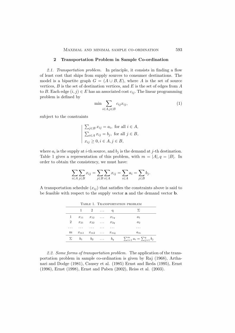
2 Transportation Problem in Sample Co-ordination
2.1. Transportation problem. In principle, it consists in finding a flowof least cost that ships from supply sources to consumer destinations. Themodel is a bipartite graph G = (A ∪ B,E), where A is the set of sourcevertices, B is the set of destination vertices, and E is the set of edges from Ato B. Each edge (i, j) ∈ E has an associated cost cij . The linear programmingproblem is defined by
min∑
i∈A,j∈B
cijxij , (1)
subject to the constraints∣∣∣∣∣∣∣∑
j∈B xij = ai, for all i ∈ A,∑i∈A xij = bj , for all j ∈ B,
xij ≥ 0, i ∈ A, j ∈ B,
where ai is the supply at i-th source, and bj is the demand at j-th destination.Table 1 gives a representation of this problem, with m = |A|, q = |B|. Inorder to obtain the consistency, we must have:∑
i∈A
∑j∈B
xij =∑j∈B
∑i∈A
xij =∑i∈A
ai =∑j∈B
bj .
A transportation schedule (xij) that satisfies the constraints above is said tobe feasible with respect to the supply vector a and the demand vector b.
Table 1. Transportation problem
1 2 . . . q Σ
1 x11 x12 . . . x1q a1
2 x21 x22 . . . x2q a2
. . . . . . . . . . . . . . . . . .
m xm1 xm2 . . . xmq am
Σ b1 b2 . . . bq
∑mi=1 ai =
∑qj=1 bj
2.2. Some forms of transportation problem. The application of the trans-portation problem in sample co-ordination is given by Raj (1968), Artha-nari and Dodge (1981), Causey et al. (1985) Ernst and Ikeda (1995), Ernst(1996), Ernst (1998), Ernst and Paben (2002), Reiss et al. (2003).
594 Alina Matei and Yves Tille
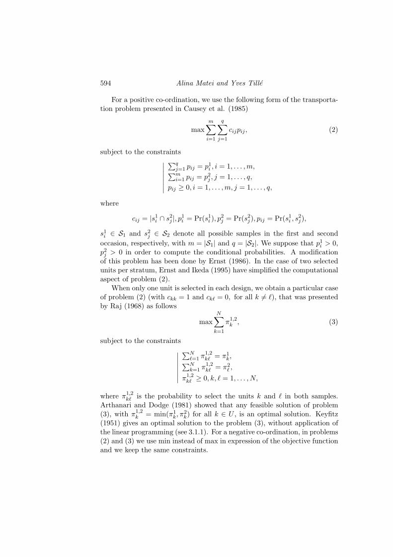
For a positive co-ordination, we use the following form of the transporta-tion problem presented in Causey et al. (1985)
maxm∑
i=1
q∑j=1
cijpij , (2)
subject to the constraints∣∣∣∣∣∣∣∑q
j=1 pij = p1i , i = 1, . . . ,m,∑m
i=1 pij = p2j , j = 1, . . . , q,
pij ≥ 0, i = 1, . . . ,m, j = 1, . . . , q,
where
cij = |s1i ∩ s2
j |, p1i = Pr(s1
i ), p2j = Pr(s2
j ), pij = Pr(s1i , s
2j ),
s1i ∈ S1 and s2
j ∈ S2 denote all possible samples in the first and secondoccasion, respectively, with m = |S1| and q = |S2|. We suppose that p1
i > 0,p2
j > 0 in order to compute the conditional probabilities. A modificationof this problem has been done by Ernst (1986). In the case of two selectedunits per stratum, Ernst and Ikeda (1995) have simplified the computationalaspect of problem (2).
When only one unit is selected in each design, we obtain a particular caseof problem (2) (with ckk = 1 and ck` = 0, for all k 6= `), that was presentedby Raj (1968) as follows
maxN∑
k=1
π1,2k , (3)
subject to the constraints∣∣∣∣∣∣∣∑N
`=1 π1,2k` = π1
k,∑Nk=1 π1,2
k` = π2` ,
π1,2k` ≥ 0, k, ` = 1, . . . , N,
where π1,2k` is the probability to select the units k and ` in both samples.
Arthanari and Dodge (1981) showed that any feasible solution of problem(3), with π1,2
k = min(π1k, π
2k) for all k ∈ U , is an optimal solution. Keyfitz
(1951) gives an optimal solution to the problem (3), without application ofthe linear programming (see 3.1.1). For a negative co-ordination, in problems(2) and (3) we use min instead of max in expression of the objective functionand we keep the same constraints.
Maximal and minimal sample co-ordination 595
3 Maximal Sample Co-ordination
In what follows, we focus attention on problem (2). Our goal is to definea method that gives an optimal solution for problem (2), without usingmathematical programming. We consider problem (2) as a two-dimensionaldistribution where only the two marginal distributions (the sums along therows and columns) are given. Information about the joint distribution isavailable by using the propositions below. It is required to compute thejoint probability values. The technique is based on IPF procedure (Demingand Stephan, 1940).
A measure of positive co-ordination is the number of common sampledunits in these two occasions. Let n12 be this number. The goal is to maximizethe expectation of n12. We have
E(n12) =∑k∈U
π1,2k =
∑k∈U
∑s1i3k
∑s2j3k
pij
=∑
s1i∈S1
∑s2j∈S2
|s1i ∩ s2
j |pij ,
which is the objective function of problem (2). Similarly, the objective func-tion of problem (3) is
N∑k=1
|{k} ∩ {k}|Pr({k}, {k}) =N∑
k=1
π1,2k .
3.1. Some cases of maximal sample co-ordination. There are threecases when the absolute upper bound equal to
∑k∈U min(π1
k, π2k) can be
reached, without solving the associated transportation problem. These casesare presented below.
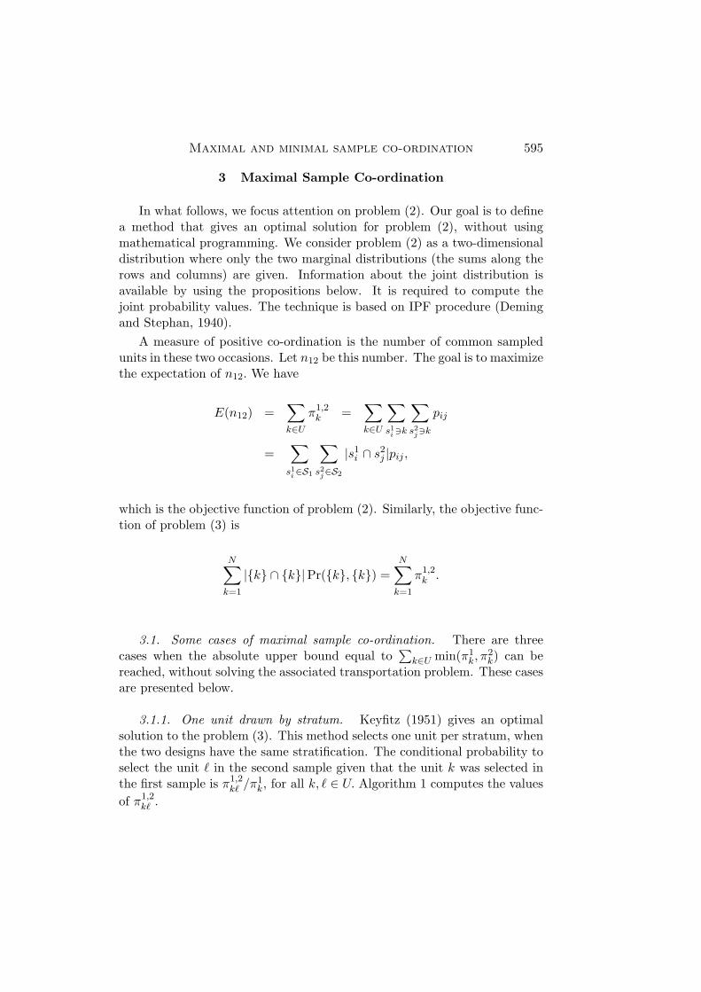
3.1.1. One unit drawn by stratum. Keyfitz (1951) gives an optimalsolution to the problem (3). This method selects one unit per stratum, whenthe two designs have the same stratification. The conditional probability toselect the unit ` in the second sample given that the unit k was selected inthe first sample is π1,2
k` /π1k, for all k, ` ∈ U. Algorithm 1 computes the values
of π1,2k` .
596 Alina Matei and Yves Tille
Algorithm 1. Keyfitz algorithm
1. for all k ∈ U do
2. π1,2k = min(π1
k, π2k),
3. end for4. if k ∈ D, ` ∈ I, k 6= ` then
5. π1,2k` = (π1
k − π2k)(π
2` − π1
` )/∑
`1∈I(π2`1− π1
`1),
6. else
7. π1,2k` = 0.
8. end if
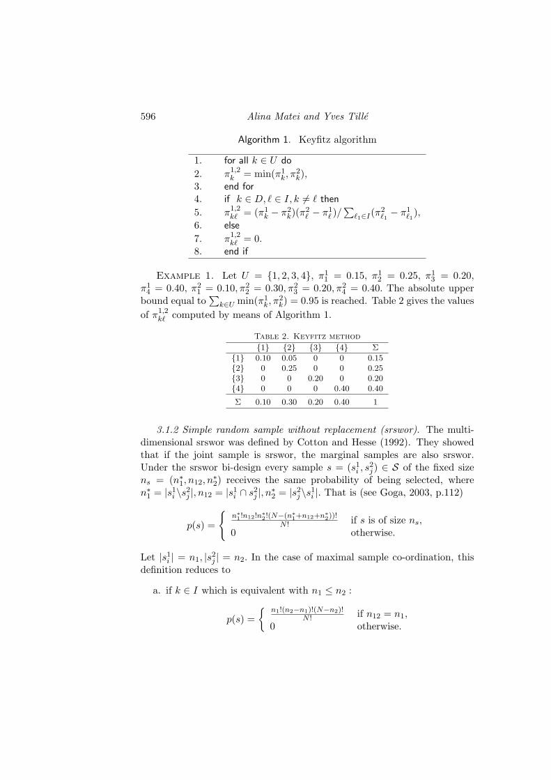
Example 1. Let U = {1, 2, 3, 4}, π11 = 0.15, π1
2 = 0.25, π13 = 0.20,
π14 = 0.40, π2
1 = 0.10, π22 = 0.30, π2
3 = 0.20, π24 = 0.40. The absolute upper
bound equal to∑
k∈U min(π1k, π
2k) = 0.95 is reached. Table 2 gives the values
of π1,2k` computed by means of Algorithm 1.
Table 2. Keyfitz method
{1} {2} {3} {4} Σ
{1} 0.10 0.05 0 0 0.15{2} 0 0.25 0 0 0.25{3} 0 0 0.20 0 0.20{4} 0 0 0 0.40 0.40
Σ 0.10 0.30 0.20 0.40 1
3.1.2 Simple random sample without replacement (srswor). The multi-dimensional srswor was defined by Cotton and Hesse (1992). They showedthat if the joint sample is srswor, the marginal samples are also srswor.Under the srswor bi-design every sample s = (s1
i , s2j ) ∈ S of the fixed size
ns = (n∗1, n12, n∗2) receives the same probability of being selected, where
n∗1 = |s1i \s2
j |, n12 = |s1i ∩ s2
j |, n∗2 = |s2j\s1
i |. That is (see Goga, 2003, p.112)
p(s) =
{n∗1!n12!n∗2!(N−(n∗1+n12+n∗2))!
N ! if s is of size ns,0 otherwise.
Let |s1i | = n1, |s2
j | = n2. In the case of maximal sample co-ordination, thisdefinition reduces to
a. if k ∈ I which is equivalent with n1 ≤ n2 :
p(s) ={
n1!(n2−n1)!(N−n2)!N ! if n12 = n1,
0 otherwise.
Maximal and minimal sample co-ordination 597
b. if k ∈ D which is equivalent with n2 < n1 :
p(s) ={
n2!(n1−n2)!(N−n1)!N ! if n12 = n2,
0 otherwise.
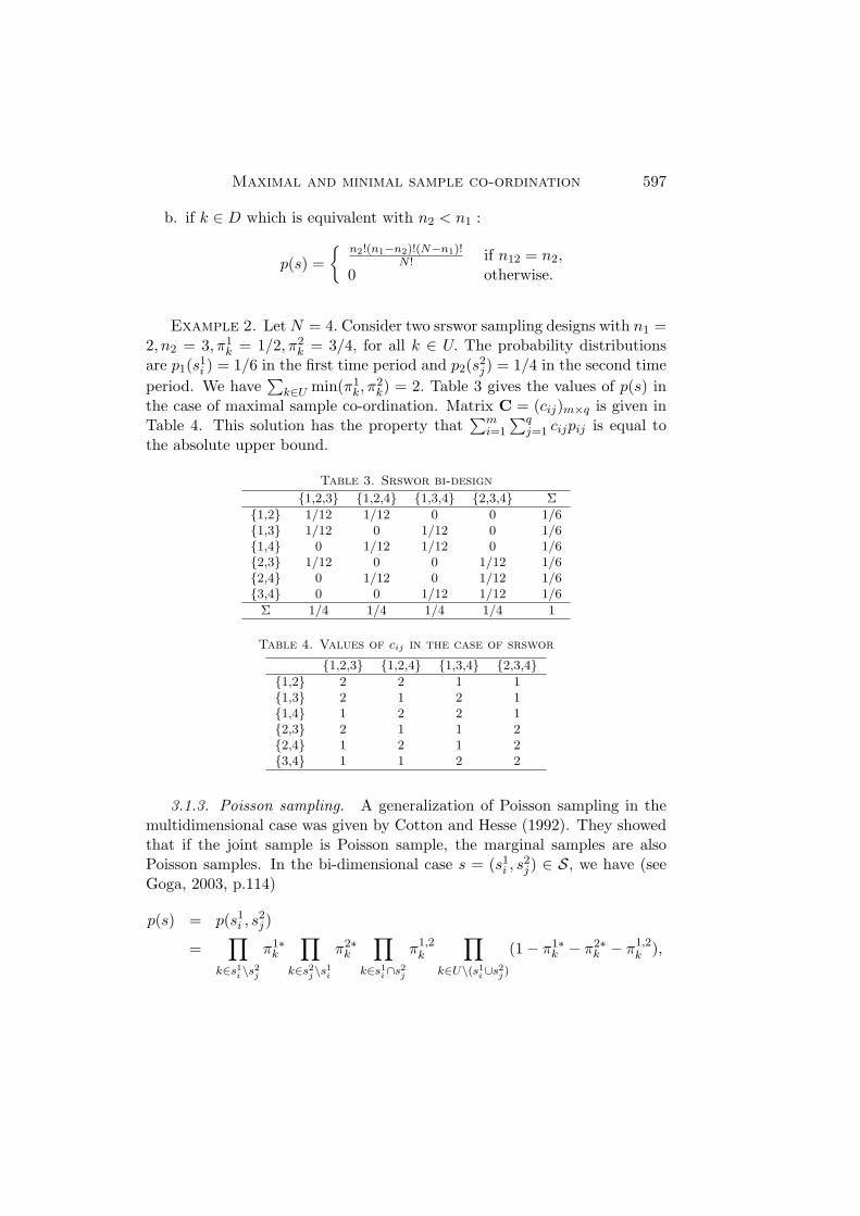
Example 2. Let N = 4. Consider two srswor sampling designs with n1 =2, n2 = 3, π1
k = 1/2, π2k = 3/4, for all k ∈ U. The probability distributions
are p1(s1i ) = 1/6 in the first time period and p2(s2
j ) = 1/4 in the second timeperiod. We have
∑k∈U min(π1
k, π2k) = 2. Table 3 gives the values of p(s) in
the case of maximal sample co-ordination. Matrix C = (cij)m×q is given inTable 4. This solution has the property that
∑mi=1
∑qj=1 cijpij is equal to
the absolute upper bound.
Table 3. Srswor bi-design
{1,2,3} {1,2,4} {1,3,4} {2,3,4} Σ
{1,2} 1/12 1/12 0 0 1/6{1,3} 1/12 0 1/12 0 1/6{1,4} 0 1/12 1/12 0 1/6{2,3} 1/12 0 0 1/12 1/6{2,4} 0 1/12 0 1/12 1/6{3,4} 0 0 1/12 1/12 1/6
Σ 1/4 1/4 1/4 1/4 1
Table 4. Values of cij in the case of srswor
{1,2,3} {1,2,4} {1,3,4} {2,3,4}{1,2} 2 2 1 1{1,3} 2 1 2 1{1,4} 1 2 2 1{2,3} 2 1 1 2{2,4} 1 2 1 2{3,4} 1 1 2 2
3.1.3. Poisson sampling. A generalization of Poisson sampling in themultidimensional case was given by Cotton and Hesse (1992). They showedthat if the joint sample is Poisson sample, the marginal samples are alsoPoisson samples. In the bi-dimensional case s = (s1
i , s2j ) ∈ S, we have (see
Goga, 2003, p.114)
p(s) = p(s1i , s
2j )
=∏
k∈s1i \s2
j
π1∗k
∏k∈s2
j\s1i
π2∗k
∏k∈s1
i∩s2j
π1,2k
∏k∈U\(s1
i∪s2j )
(1− π1∗k − π2∗
k − π1,2k ),
598 Alina Matei and Yves Tille
where π1∗k = π1
k − π1,2k , π2∗
k = π2k − π1,2
k are the inclusion probabilities fork ∈ s1
i \s2j , s
2j\s1
i , respectively. In the case of maximal sample co-ordination,this definition reduces to
p(s1i , s
2j ) =
∏k∈s1
i \s2j
(π1k −min(π1
k, π2k))
∏k∈s2
j\s1i
(π2k −min(π1
k, π2k))
∏k∈s1
i∩s2j
min(π1k, π
2k)
∏k∈U\(s1
i∪s2j )
(1−max (π1k, π
2k)).
An optimal solution for problem (2) can be obtained directly by using thedefinition above in the case of maximal sample co-ordination. This solutionhas the property that its optimal objective function is equal to the absoluteupper bound.
When the inclusion probabilities are equal for each occasion, a Poissonbi-sampling reduces to a Bernoulli bi-sampling.
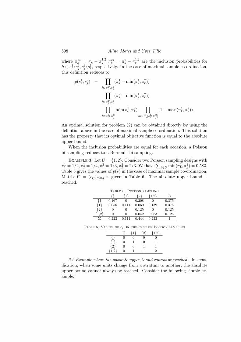
Example 3. Let U = {1, 2}. Consider two Poisson sampling designs withπ1
1 = 1/2, π12 = 1/4, π2
1 = 1/3, π22 = 2/3. We have
∑k∈U min(π1
k, π2k) = 0.583.
Table 5 gives the values of p(s) in the case of maximal sample co-ordination.Matrix C = (cij)m×q is given in Table 6. The absolute upper bound isreached.
Table 5. Poisson sampling
{} {1} {2} {1,2} Σ
{} 0.167 0 0.208 0 0.375{1} 0.056 0.111 0.069 0.139 0.375{2} 0 0 0.125 0 0.125{1,2} 0 0 0.042 0.083 0.125
Σ 0.223 0.111 0.444 0.222 1
Table 6. Values of cij in the case of Poisson sampling
{} {1} {2} {1,2}{} 0 0 0 0{1} 0 1 0 1{2} 0 0 1 1{1,2} 0 1 1 2
3.2 Example where the absolute upper bound cannot be reached. In strat-ification, when some units change from a stratum to another, the absoluteupper bound cannot always be reached. Consider the following simple ex-ample:
Maximal and minimal sample co-ordination 599
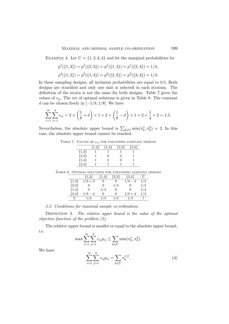
Example 4. Let U = {1, 2, 3, 4} and let the marginal probabilities be
p1({1, 3}) = p1({2, 3}) = p1({1, 4}) = p1({2, 4}) = 1/4,
p2({1, 2}) = p2({1, 4}) = p2({2, 3}) = p2({3, 4}) = 1/4.
In these sampling designs, all inclusion probabilities are equal to 0.5. Bothdesigns are stratified and only one unit is selected in each stratum. Thedefinition of the strata is not the same for both designs. Table 7 gives thevalues of cij . The set of optimal solutions is given in Table 8. The constantd can be chosen freely in [−1/8, 1/8]. We have
m∑i=1
q∑j=1
cij = 2×(
18
+ d
)× 1 + 2×
(18− d
)× 1 + 2× 1
4× 2 = 1.5.
Nevertheless, the absolute upper bound is∑
k∈U min(π1k, π
2k) = 2. In this
case, the absolute upper bound cannot be reached.
Table 7. Values of cij for stratified sampling designs
{1,2} {1,4} {2,3} {3,4}{1,3} 1 1 1 1{2,3} 1 0 2 1{1,4} 1 2 0 1{2,4} 1 1 1 1
Table 8. Optimal solutions for stratified sampling designs
{1,2} {1,4} {2,3} {3,4} Σ
{1,3} 1/8 + d 0 0 1/8− d 1/4{2,3} 0 0 1/4 0 1/4{1,4} 0 1/4 0 0 1/4{2,4} 1/8− d 0 0 1/8 + d 1/4
Σ 1/4 1/4 1/4 1/4 1
3.3. Conditions for maximal sample co-ordination.
Definition 2. The relative upper bound is the value of the optimalobjective function of the problem (2).
The relative upper bound is smaller or equal to the absolute upper bound,i.e.
maxm∑
i=1
q∑j=1
cijpij ≤∑k∈U
min(π1k, π
2k).
We havem∑
i=1
q∑j=1
cijpij =∑k∈U
π1,2k . (4)
600 Alina Matei and Yves Tille
The relative upper bound is equal to the absolute upper bound when π1,2k =
min(π1k, π
2k), for all k ∈ U. In this case, the sample co-ordination is maximal.
Proposition 1. The absolute upper bound is reached iff the followingtwo relations are fulfilled:
a. if k ∈ (s1i \s2
j ) ∩ I then pij = 0,
b. if k ∈ (s2j\s1
i ) ∩D then pij = 0,
for all k ∈ U.
Proof. Necessity: Suppose that π1,2k = min(π1
k, π2k) for all k ∈ U. For
the case where k ∈ I
π1k =
∑s1i3k
p1(s1i )
=∑s1i3k
∑s2j∈S2
p(s1i , s
2j )
=∑s1i3k
∑s2j3k
p(s1i , s
2j ) +
∑s1i3k
∑s2j 63k
p(s1i , s
2j )
= π1,2k +
∑s1i3k
∑s2j 63k
p(s1i , s
2j ).
The assumption π1k = π12
k , for all k ∈ U implies∑
s1i3k
∑s2j 63k p(s1
i , s2j ) =
pij = 0, i.e. pij = 0. A similar development can be done for the case wherek ∈ D in the condition b.
Sufficiency: Suppose that the relations a and b are fulfilled. We showthat the absolute upper bound is reached.
m∑i=1
q∑j=1
cijpij =∑k∈U
π1,2k =
∑k∈U
∑s1i3k
∑s2j3k
pij
=∑k∈U
∑s1i3k
∑s2j3k
pij +∑k∈U,
min(π1k,π2
k)=π1k
∑s1i3k
∑s2j 63k
pij +∑k∈U,
min(π1k,π2
k)=π2k
∑s1i 63k
∑s2j3k
pij
=∑k∈U,
min(π1k,π2
k)=π1k
(∑s1i3k
∑s2j3k
pij +∑s1i3k
∑s2j 63k
pij)
+∑k∈U,
min(π1k,π2
k)=π2k
(∑s2j3k
∑s1i3k
pij +∑s2j3k
∑s1i 63k
pij)
Maximal and minimal sample co-ordination 601
=∑k∈U,
min(π1k,π2
k)=π1k
∑s1i3k
∑s2j∈S2
pij +∑k∈U,
min(π1k,π2
k)=π2k
∑s2j3k
∑s1i∈S1
pij
=∑k∈U,
min(π1k,π2
k)=π1k
∑s1i3k
p1(s1i ) +
∑k∈U,
min(π1k,π2
k)=π2k
∑s2j3k
p2(s2j )
=∑k∈U,
min(π1k,π2
k)=π1k
π1k +
∑k∈U,
min(π1k,π2
k)=π2k
π2k
=∑k∈U
min(π1k, π
2k).
Proposition 1 shows that any feasible solution for problem (2), whichsatisfies the conditions a and b, has the property that its objective functionis equal to the absolute upper bound. Proposition 1 also gives a method toput zeros in the matrix P = (pij)m×q associated with an optimal solution.Note that the necessary and sufficient condition is obviously satisfied inExamples 1, 2 and 3, and is not satisfied in Example 4.
Proposition 2. Suppose that all samples have the corresponding prob-abilities strictly positive, and the relations a and b of Proposition 1 are sat-isfied. Let s1
i ∈ S1. If at least one of the following conditions is fulfilled forall s2
j ∈ S2:
1) (s1i \s2
j ) ∩ I 6= ∅,
2) (s2j\s1
i ) ∩D 6= ∅,
the two designs cannot be maximally co-ordinated. This proposition holds inthe symmetric sense, too (if s2
j is fixed and at least one of the conditions 1and 2 is fulfilled, for all s1
i ∈ S1).
Proof. Suppose, if possible, the two designs are maximally co-ordinated.Since (s1
i \s2j ) ∩ I 6= ∅, from condition a of Proposition 1 it follows that
p(s1i , s
2j ) = 0. The second relation is fulfilled similarly from condition b of
Proposition 1. We have p(s1i , s
2j ) = 0, for all s2
j ∈ S2. So p1(s1i ) = 0. We
obtain a contradiction with p1(s1i ) > 0. The proof is analogous for the other
part.
602 Alina Matei and Yves Tille
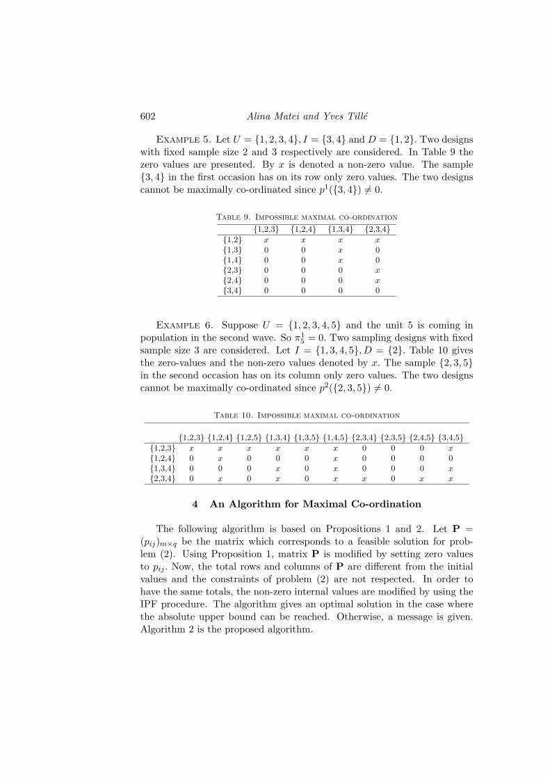
Example 5. Let U = {1, 2, 3, 4}, I = {3, 4} and D = {1, 2}. Two designswith fixed sample size 2 and 3 respectively are considered. In Table 9 thezero values are presented. By x is denoted a non-zero value. The sample{3, 4} in the first occasion has on its row only zero values. The two designscannot be maximally co-ordinated since p1({3, 4}) 6= 0.
Table 9. Impossible maximal co-ordination
{1,2,3} {1,2,4} {1,3,4} {2,3,4}{1,2} x x x x{1,3} 0 0 x 0{1,4} 0 0 x 0{2,3} 0 0 0 x{2,4} 0 0 0 x{3,4} 0 0 0 0
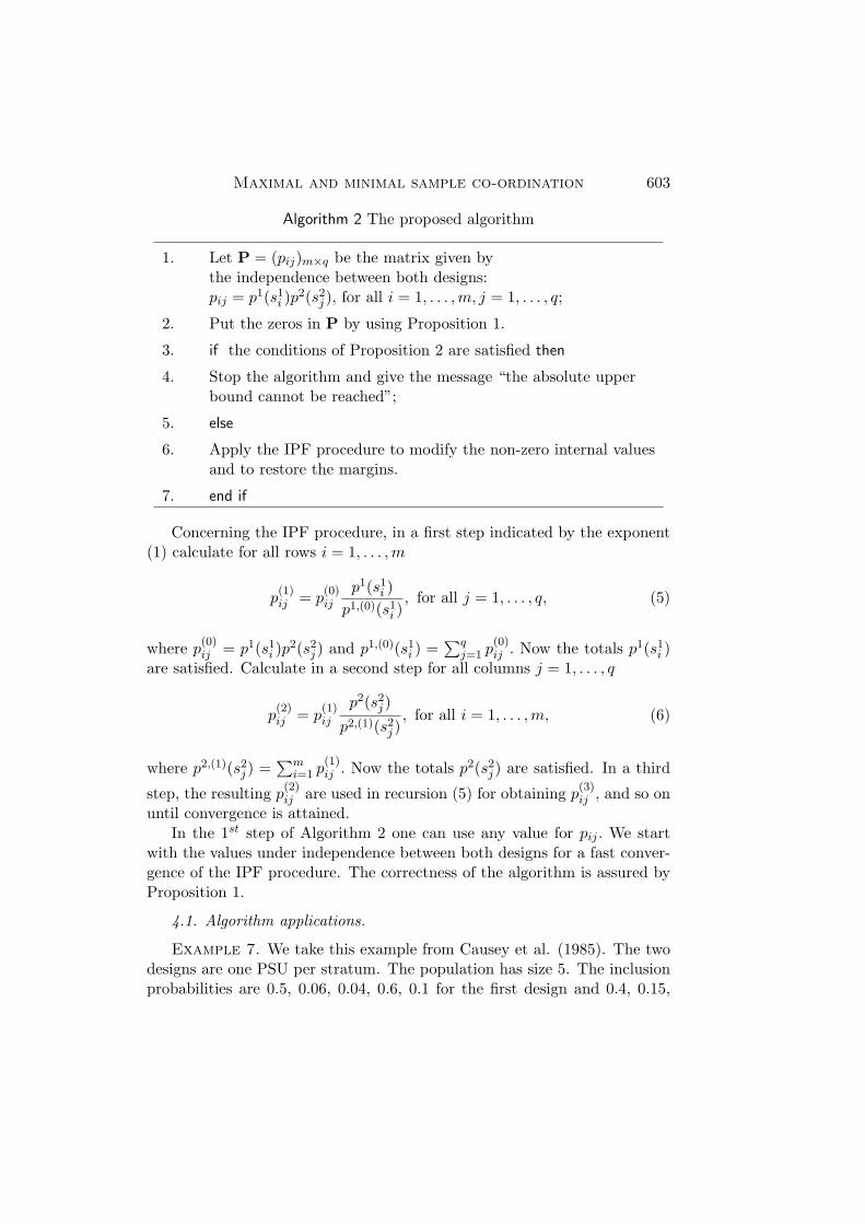
Example 6. Suppose U = {1, 2, 3, 4, 5} and the unit 5 is coming inpopulation in the second wave. So π1
5 = 0. Two sampling designs with fixedsample size 3 are considered. Let I = {1, 3, 4, 5}, D = {2}. Table 10 givesthe zero-values and the non-zero values denoted by x. The sample {2, 3, 5}in the second occasion has on its column only zero values. The two designscannot be maximally co-ordinated since p2({2, 3, 5}) 6= 0.
Table 10. Impossible maximal co-ordination
{1,2,3} {1,2,4} {1,2,5} {1,3,4} {1,3,5} {1,4,5} {2,3,4} {2,3,5} {2,4,5} {3,4,5}{1,2,3} x x x x x x 0 0 0 x{1,2,4} 0 x 0 0 0 x 0 0 0 0{1,3,4} 0 0 0 x 0 x 0 0 0 x{2,3,4} 0 x 0 x 0 x x 0 x x
4 An Algorithm for Maximal Co-ordination
The following algorithm is based on Propositions 1 and 2. Let P =(pij)m×q be the matrix which corresponds to a feasible solution for prob-lem (2). Using Proposition 1, matrix P is modified by setting zero valuesto pij . Now, the total rows and columns of P are different from the initialvalues and the constraints of problem (2) are not respected. In order tohave the same totals, the non-zero internal values are modified by using theIPF procedure. The algorithm gives an optimal solution in the case wherethe absolute upper bound can be reached. Otherwise, a message is given.Algorithm 2 is the proposed algorithm.
Maximal and minimal sample co-ordination 603
Algorithm 2 The proposed algorithm
1. Let P = (pij)m×q be the matrix given bythe independence between both designs:pij = p1(s1
i )p2(s2
j ), for all i = 1, . . . ,m, j = 1, . . . , q;
2. Put the zeros in P by using Proposition 1.
3. if the conditions of Proposition 2 are satisfied then
4. Stop the algorithm and give the message “the absolute upperbound cannot be reached”;
5. else
6. Apply the IPF procedure to modify the non-zero internal valuesand to restore the margins.
7. end if
Concerning the IPF procedure, in a first step indicated by the exponent(1) calculate for all rows i = 1, . . . ,m
p(1)ij = p
(0)ij
p1(s1i )
p1,(0)(s1i )
, for all j = 1, . . . , q, (5)
where p(0)ij = p1(s1
i )p2(s2
j ) and p1,(0)(s1i ) =
∑qj=1 p
(0)ij . Now the totals p1(s1
i )are satisfied. Calculate in a second step for all columns j = 1, . . . , q
p(2)ij = p
(1)ij
p2(s2j )
p2,(1)(s2j )
, for all i = 1, . . . ,m, (6)
where p2,(1)(s2j ) =
∑mi=1 p
(1)ij . Now the totals p2(s2
j ) are satisfied. In a third
step, the resulting p(2)ij are used in recursion (5) for obtaining p
(3)ij , and so on
until convergence is attained.In the 1st step of Algorithm 2 one can use any value for pij . We start
with the values under independence between both designs for a fast conver-gence of the IPF procedure. The correctness of the algorithm is assured byProposition 1.
4.1. Algorithm applications.
Example 7. We take this example from Causey et al. (1985). The twodesigns are one PSU per stratum. The population has size 5. The inclusionprobabilities are 0.5, 0.06, 0.04, 0.6, 0.1 for the first design and 0.4, 0.15,
604 Alina Matei and Yves Tille
0.05, 0.3,0.1 for the second design. In the first design, the first three PSU’swere in one initial stratum and the other two in a second initial stratum.There are m = 12 possible samples given in Table 12 with the correspondingprobabilities:
0.15, 0.018, 0.012, 0.24, 0.04, 0.3, 0.05, 0.036, 0.006, 0.024, 0.004, 0.12.
The second design consists of five PSU’s (q = 5). Causey et al. (1985) solvethe linear program associated with this problem and give the value 0.88 asthe optimal value for the objective function. Yet,
∑k∈U min(π1
k, π2k) = 0.9.
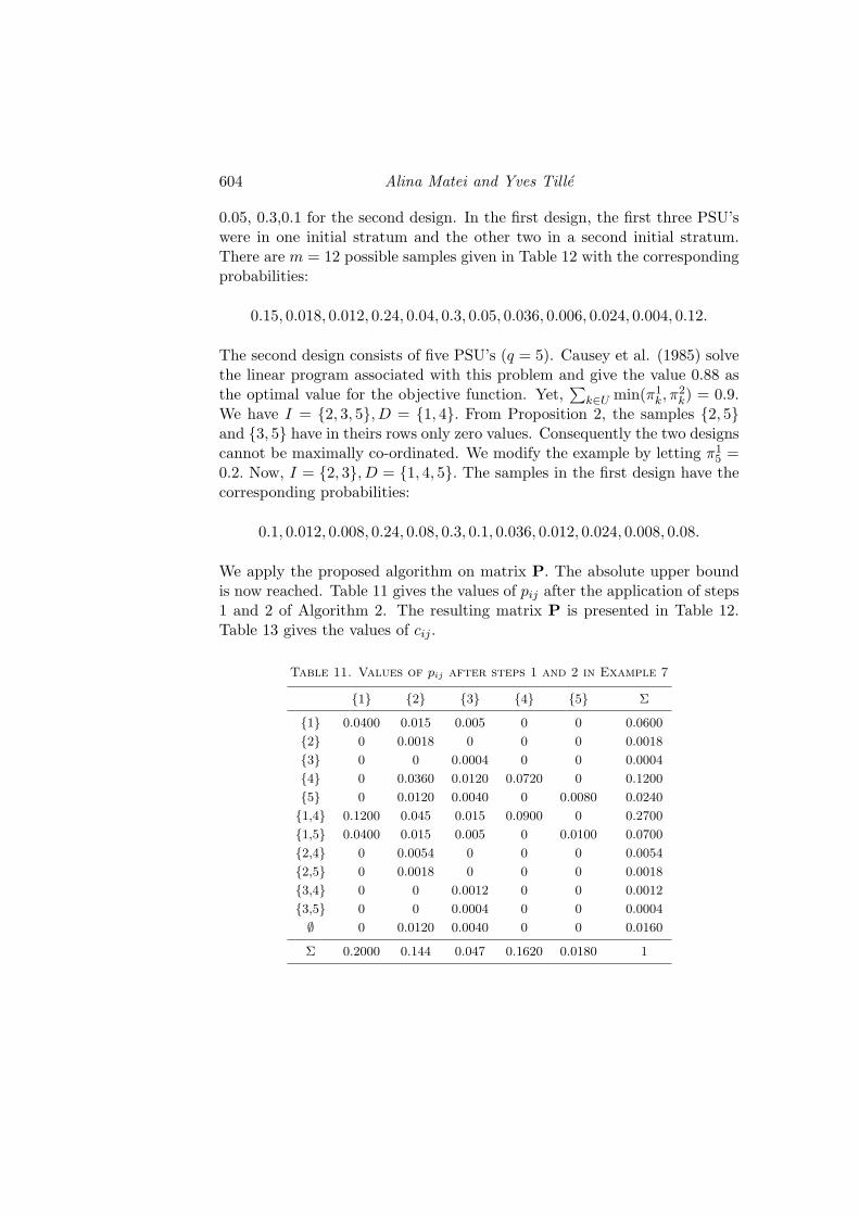
We have I = {2, 3, 5}, D = {1, 4}. From Proposition 2, the samples {2, 5}and {3, 5} have in theirs rows only zero values. Consequently the two designscannot be maximally co-ordinated. We modify the example by letting π1
5 =0.2. Now, I = {2, 3}, D = {1, 4, 5}. The samples in the first design have thecorresponding probabilities:
0.1, 0.012, 0.008, 0.24, 0.08, 0.3, 0.1, 0.036, 0.012, 0.024, 0.008, 0.08.
We apply the proposed algorithm on matrix P. The absolute upper boundis now reached. Table 11 gives the values of pij after the application of steps1 and 2 of Algorithm 2. The resulting matrix P is presented in Table 12.Table 13 gives the values of cij .
Table 11. Values of pij after steps 1 and 2 in Example 7
{1} {2} {3} {4} {5} Σ
{1} 0.0400 0.015 0.005 0 0 0.0600
{2} 0 0.0018 0 0 0 0.0018
{3} 0 0 0.0004 0 0 0.0004
{4} 0 0.0360 0.0120 0.0720 0 0.1200
{5} 0 0.0120 0.0040 0 0.0080 0.0240
{1,4} 0.1200 0.045 0.015 0.0900 0 0.2700
{1,5} 0.0400 0.015 0.005 0 0.0100 0.0700
{2,4} 0 0.0054 0 0 0 0.0054
{2,5} 0 0.0018 0 0 0 0.0018
{3,4} 0 0 0.0012 0 0 0.0012
{3,5} 0 0 0.0004 0 0 0.0004
∅ 0 0.0120 0.0040 0 0 0.0160
Σ 0.2000 0.144 0.047 0.1620 0.0180 1
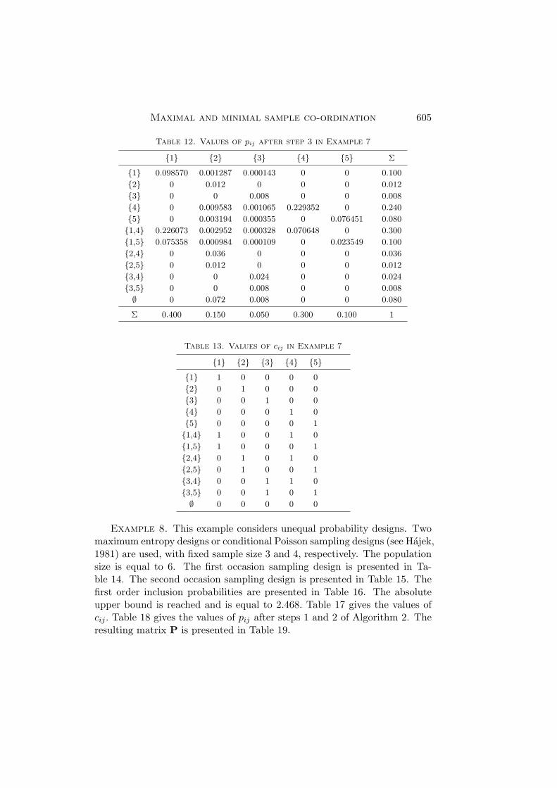
Maximal and minimal sample co-ordination 605
Table 12. Values of pij after step 3 in Example 7
{1} {2} {3} {4} {5} Σ
{1} 0.098570 0.001287 0.000143 0 0 0.100
{2} 0 0.012 0 0 0 0.012
{3} 0 0 0.008 0 0 0.008
{4} 0 0.009583 0.001065 0.229352 0 0.240
{5} 0 0.003194 0.000355 0 0.076451 0.080
{1,4} 0.226073 0.002952 0.000328 0.070648 0 0.300
{1,5} 0.075358 0.000984 0.000109 0 0.023549 0.100
{2,4} 0 0.036 0 0 0 0.036
{2,5} 0 0.012 0 0 0 0.012
{3,4} 0 0 0.024 0 0 0.024
{3,5} 0 0 0.008 0 0 0.008
∅ 0 0.072 0.008 0 0 0.080
Σ 0.400 0.150 0.050 0.300 0.100 1
Table 13. Values of cij in Example 7
{1} {2} {3} {4} {5}
{1} 1 0 0 0 0
{2} 0 1 0 0 0
{3} 0 0 1 0 0
{4} 0 0 0 1 0
{5} 0 0 0 0 1
{1,4} 1 0 0 1 0
{1,5} 1 0 0 0 1
{2,4} 0 1 0 1 0
{2,5} 0 1 0 0 1
{3,4} 0 0 1 1 0
{3,5} 0 0 1 0 1
∅ 0 0 0 0 0
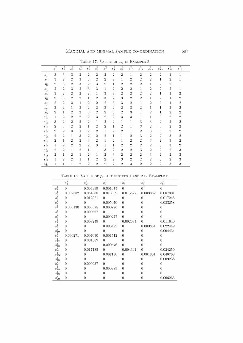
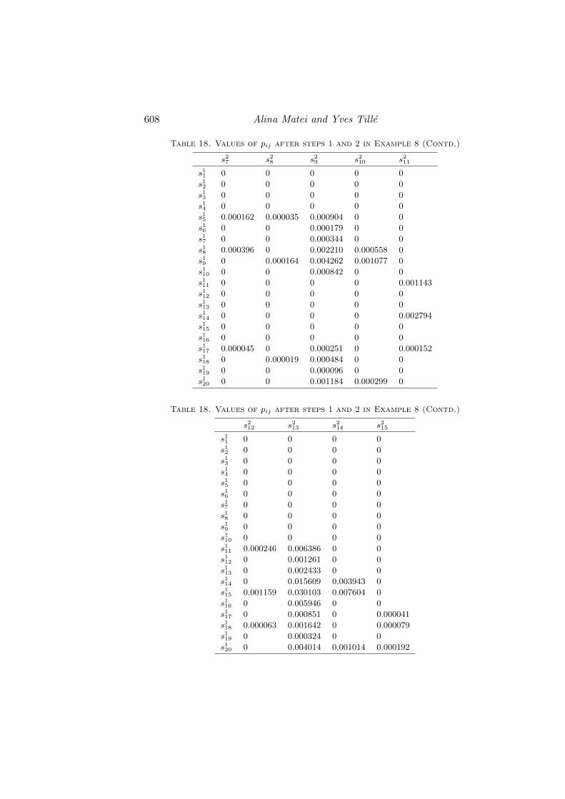
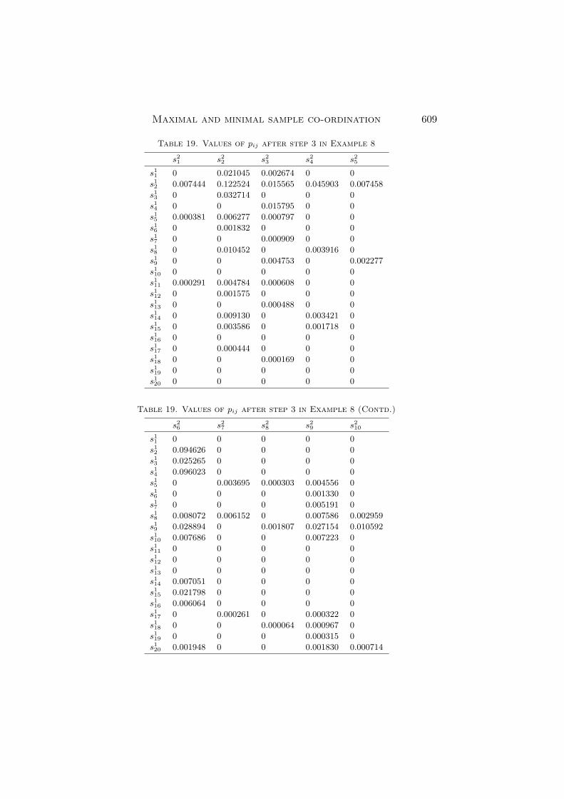
Example 8. This example considers unequal probability designs. Twomaximum entropy designs or conditional Poisson sampling designs (see Hajek,1981) are used, with fixed sample size 3 and 4, respectively. The populationsize is equal to 6. The first occasion sampling design is presented in Ta-ble 14. The second occasion sampling design is presented in Table 15. Thefirst order inclusion probabilities are presented in Table 16. The absoluteupper bound is reached and is equal to 2.468. Table 17 gives the values ofcij . Table 18 gives the values of pij after steps 1 and 2 of Algorithm 2. Theresulting matrix P is presented in Table 19.

606 Alina Matei and Yves Tille
Table 14. First occasion sampling design in Example 8
i s1i p1(s1
i ) i s1i p1(s1
i )
1 {1,2,3} 0.023719 11 {2,3,4} 0.033355
2 {1,2,4} 0.293520 12 {2,3,5} 0.006589
3 {1,2,5} 0.057979 13 {2,3,6} 0.012707
4 {1,2,6} 0.111817 14 {2,4,5} 0.081533
5 {1,3,4} 0.016010 15 {2,4,6} 0.157243
6 {1,3,5} 0.0031626 16 {2,5,6} 0.031060
7 {1,3,6} 0.006099 17 {3,4,5} 0.004447
8 {1,4,5} 0.039137 18 {3,4,6} 0.008577
9 {1,4,6} 0.07548 19 {3,5,6} 0.001694
10 {1,5,6} 0.014909 20 {4,5,6} 0.020966.
Table 15. Second occasion sampling design in Example 8
j s2j p2(s2
j ) j s2j p2(s2
j )
1 {1,2,3,4} 0.008117 9 {1,3,4,6} 0.002175
2 {1,2,3,5} 0.210778 10 {1,3,5,6} 0.056474
3 {1,2,3,6} 0.045342 11 {1,4,5,6} 0.014264
4 {1,2,4,5} 0.053239 12 {2,3,4,5} 0.034269
5 {1,2,4,6} 0.011453 13 {2,3,4,6} 0.007372
6 {1,2,5,6} 0.297428 14 {2,3,5,6} 0.191446
7 {1,3,4,5} 0.010109 15 {2,4,5,6} 0.048356
8 {3,4,5,6} 0.009182
Table 16. Inclusion probabilities in Example 8
unit k 1 2 3 4 5 6
π1k 0.641830 0.809522 0.116359 0.730264 0.261477 0.440549
π2k 0.709377 0.907798 0.575260 0.198533 0.925542 0.683490
5 Minimal Sample Co-ordination
A similar algorithm can be constructed in the case of negative co-ordination,when the expected overlap is minimized. In an analogous way, the quantity∑
k∈U max(0, π1k + π2
k − 1) is called the absolute lower bound. Retaining thesame constraints, we now seek to minimize the objective function of problem(2). In general,
m∑i=1
q∑j=1
cijpij ≥∑k∈U
max(0, π1k + π2
k − 1).
By setting max(0, π1k + π2
k − 1) = π1,2k , for all k ∈ U a proposition similar to
Proposition 1 is given next.
Maximal and minimal sample co-ordination 607
Table 17. Values of cij in Example 8
s21 s2
2 s23 s2
4 s25 s2
6 s27 s2
8 s29 s2
10 s211 s2
12 s213 s2
14 s215
s11 3 3 3 2 2 2 2 2 2 1 2 2 2 1 1
s12 3 2 2 3 3 2 2 2 1 2 2 2 1 2 1
s13 2 3 2 3 2 3 2 1 2 2 2 1 2 2 1
s14 2 2 3 2 3 3 1 2 2 2 1 2 2 2 1
s15 3 2 2 2 2 1 3 3 2 2 2 2 1 1 2
s16 2 3 2 2 1 2 3 2 3 2 2 1 2 1 2
s17 2 2 3 1 2 2 2 3 3 2 1 2 2 1 2
s18 2 2 1 3 2 2 3 2 2 3 2 1 1 2 2
s19 2 1 2 2 3 2 2 3 2 3 1 2 1 2 2
s110 1 2 2 2 2 3 2 2 3 3 1 1 2 2 2
s111 3 2 2 2 2 1 2 2 1 1 3 3 2 2 2
s112 2 3 2 2 1 2 2 1 2 1 3 2 3 2 2
s113 2 2 3 1 2 2 1 2 2 1 2 3 3 2 2
s114 2 2 1 3 2 2 2 1 1 2 3 2 2 3 2
s115 2 1 2 2 3 2 1 2 1 2 2 3 2 3 2
s116 1 2 2 2 2 3 1 1 2 2 2 2 3 3 2
s117 2 2 1 2 1 1 3 2 2 2 3 2 2 2 3
s118 2 1 2 1 2 1 2 3 2 2 2 3 2 2 3
s119 1 2 2 1 1 2 2 2 3 2 2 2 3 2 3
s120 1 1 1 2 2 2 2 2 2 3 2 2 2 3 3
Table 18. Values of pij after steps 1 and 2 in Example 8
s21 s2
2 s23 s2
4 s25 s2
6
s11 0 0.004999 0.001075 0 0 0
s12 0.002382 0.061868 0.013309 0.015627 0.003362 0.087301
s13 0 0.012221 0 0 0 0.017245
s14 0 0 0.005070 0 0 0.033258
s15 0.000130 0.003375 0.000726 0 0 0
s16 0 0.000667 0 0 0 0
s17 0 0 0.000277 0 0 0
s18 0 0.008249 0 0.002084 0 0.011640
s19 0 0 0.003422 0 0.000864 0.022449
s110 0 0 0 0 0 0.004434
s111 0.000271 0.007030 0.001512 0 0 0
s112 0 0.001389 0 0 0 0
s113 0 0 0.000576 0 0 0
s114 0 0.017185 0 0.004341 0 0.024250
s115 0 0 0.007130 0 0.001801 0.046768
s116 0 0 0 0 0 0.009238
s117 0 0.000937 0 0 0 0
s118 0 0 0.000389 0 0 0
s119 0 0 0 0 0 0
s120 0 0 0 0 0 0.006236
608 Alina Matei and Yves Tille
Table 18. Values of pij after steps 1 and 2 in Example 8 (Contd.)
s27 s2
8 s29 s2
10 s211
s11 0 0 0 0 0
s12 0 0 0 0 0
s13 0 0 0 0 0
s14 0 0 0 0 0
s15 0.000162 0.000035 0.000904 0 0
s16 0 0 0.000179 0 0
s17 0 0 0.000344 0 0
s18 0.000396 0 0.002210 0.000558 0
s19 0 0.000164 0.004262 0.001077 0
s110 0 0 0.000842 0 0
s111 0 0 0 0 0.001143
s112 0 0 0 0 0
s113 0 0 0 0 0
s114 0 0 0 0 0.002794
s115 0 0 0 0 0
s116 0 0 0 0 0
s117 0.000045 0 0.000251 0 0.000152
s118 0 0.000019 0.000484 0 0
s119 0 0 0.000096 0 0
s120 0 0 0.001184 0.000299 0
Table 18. Values of pij after steps 1 and 2 in Example 8 (Contd.)
s212 s2
13 s214 s2
15
s11 0 0 0 0
s12 0 0 0 0
s13 0 0 0 0
s14 0 0 0 0
s15 0 0 0 0
s16 0 0 0 0
s17 0 0 0 0
s18 0 0 0 0
s19 0 0 0 0
s110 0 0 0 0
s111 0.000246 0.006386 0 0
s112 0 0.001261 0 0
s113 0 0.002433 0 0
s114 0 0.015609 0.003943 0
s115 0.001159 0.030103 0.007604 0
s116 0 0.005946 0 0
s117 0 0.000851 0 0.000041
s118 0.000063 0.001642 0 0.000079
s119 0 0.000324 0 0
s120 0 0.004014 0.001014 0.000192
Maximal and minimal sample co-ordination 609
Table 19. Values of pij after step 3 in Example 8
s21 s2
2 s23 s2
4 s25
s11 0 0.021045 0.002674 0 0
s12 0.007444 0.122524 0.015565 0.045903 0.007458
s13 0 0.032714 0 0 0
s14 0 0 0.015795 0 0
s15 0.000381 0.006277 0.000797 0 0
s16 0 0.001832 0 0 0
s17 0 0 0.000909 0 0
s18 0 0.010452 0 0.003916 0
s19 0 0 0.004753 0 0.002277
s110 0 0 0 0 0
s111 0.000291 0.004784 0.000608 0 0
s112 0 0.001575 0 0 0
s113 0 0 0.000488 0 0
s114 0 0.009130 0 0.003421 0
s115 0 0.003586 0 0.001718 0
s116 0 0 0 0 0
s117 0 0.000444 0 0 0
s118 0 0 0.000169 0 0
s119 0 0 0 0 0
s120 0 0 0 0 0
Table 19. Values of pij after step 3 in Example 8 (Contd.)
s26 s2
7 s28 s2
9 s210
s11 0 0 0 0 0
s12 0.094626 0 0 0 0
s13 0.025265 0 0 0 0
s14 0.096023 0 0 0 0
s15 0 0.003695 0.000303 0.004556 0
s16 0 0 0 0.001330 0
s17 0 0 0 0.005191 0
s18 0.008072 0.006152 0 0.007586 0.002959
s19 0.028894 0 0.001807 0.027154 0.010592
s110 0.007686 0 0 0.007223 0
s111 0 0 0 0 0
s112 0 0 0 0 0
s113 0 0 0 0 0
s114 0.007051 0 0 0 0
s115 0.021798 0 0 0 0
s116 0.006064 0 0 0 0
s117 0 0.000261 0 0.000322 0
s118 0 0 0.000064 0.000967 0
s119 0 0 0 0.000315 0
s120 0.001948 0 0 0.001830 0.000714
610 Alina Matei and Yves Tille
Table 19. Values of pij after step 3 in Example 8 (Contd.)
s211 s2
12 s213 s2
14 s215
s11 0 0 0 0 0
s12 0 0 0 0 0
s13 0 0 0 0 0
s14 0 0 0 0 0
s15 0 0 0 0 0
s16 0 0 0 0 0
s17 0 0 0 0 0
s18 0 0 0 0 0
s19 0 0 0 0 0
s110 0 0 0 0 0
s111 0.011417 0.001027 0.015229 0 0
s112 0 0 0.005014 0 0
s113 0 0 0.012219 0 0
s114 0.021792 0 0.029067 0.011072 0
s115 0 0.006059 0.089856 0.034226 0
s116 0 0 0.024996 0 0
s117 0.001059 0 0.001413 0 0.000948
s118 0 0.000286 0.004243 0 0.002847
s119 0 0 0.001380 0 0
s120 0 0 0.008029 0.003058 0.005387
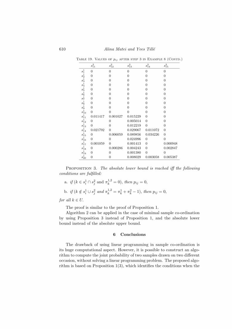
Proposition 3. The absolute lower bound is reached iff the followingconditions are fulfilled:
a. if (k ∈ s1i ∩ s2
j and π1,2k = 0), then pij = 0,
b. if (k /∈ s1i ∪ s2
j and π1,2k = π1
k + π2k − 1), then pij = 0,
for all k ∈ U.
The proof is similar to the proof of Proposition 1.Algorithm 2 can be applied in the case of minimal sample co-ordination
by using Proposition 3 instead of Proposition 1, and the absolute lowerbound instead of the absolute upper bound.
6 Conclusions
The drawback of using linear programming in sample co-ordination isits huge computational aspect. However, it is possible to construct an algo-rithm to compute the joint probability of two samples drawn on two differentoccasion, without solving a linear programming problem. The proposed algo-rithm is based on Proposition 1(3), which identifies the conditions when the

Maximal and minimal sample co-ordination 611
absolute upper bound (absolute lower bound) is reached and gives a modal-ity to determine the joint sample probabilities equal to zero. The algorithmuses the IPF procedure, which assures a fast convergence. The algorithm hasthe complexity O(m× q× number of iterations in IPF procedure), which islow compared to linear programming, and it is very easy to implement.
References
Arthanari, T. and Dodge, Y. (1981). Mathematical Programming in Statistics. Wiley,New York.
Brewer, K. (1972). Selecting several samples from a single population. Austral. J.Statist., 14, 231-239.
Brewer, K., Early, L., and Joyce, S. (1972). Selecting several samples from a singlepopulation. Austral. J. Statist., 3, 231-239.
Causey, B.D., Cox, L.H., and Ernst, L.R. (1985). Application of transportationtheory to statistical problems. J. Amer. Statist. Assoc., 80, 903-909.
Cotton, F. and Hesse, C. (1992). Tirages coordonnes d’echantillons. Documentde travail de la Direction des Statistiques Economiques E9206. Technical report,INSEE, Paris.
Deming, W. and Stephan, F. (1940). On a least square adjustment of sampled fre-quency table when the expected marginal totals are known. Ann. Math. Statist.,11, 427-444.
Ernst, L.R. (1986). Maximizing the overlap between surveys when information is in-complete. European J. Oper. Res., 27, 192-200.
Ernst, L.R. (1996). Maximizing the overlap of sample units for two designs withsimultaneous selection. J. Official Statist., 12, 33-45.
Ernst, L.R. (1998). Maximizing and minimizing overlap when selecting a large numberof units per stratum simultaneously for two designs. J. Official Statist., 14, 297-314.
Ernst, L.R. and Ikeda, M.M. (1995). A reduced-size transportation algorithm formaximizing the overlap between surveys. Survey Methodology, 21, 147-157.
Ernst, L. R. and Paben, S.P. (2002). Maximizing and minimizing overlap when select-ing any number of units per stratum simultaneously for two designs with differentstratifications. J. Official Statist., 18, 185-202.
Fellegi, I. (1963). Sampling with varying probabilities without replacement, rotationand non-rotating samples. J. Amer. Statist. Assoc., 58, 183-201.
Fellegi, I. (1966). Changing the probabilities of selection when two units are selectedwith PPS without replacement. In Proceeding of the Social Statistics Section, Amer-ican Statistical Association, Washington, 434-442.
Goga, C. (2003). Estimation de la Variance dans les Sondages a Plusieurs Echantillonset Prise en Compte de l’Information Auxiliaire par des Modeles Nonparametriques.PhD thesis, Universite de Rennes II, Haute Bretagne, France.
Gray, G. and Platek, R. (1963). Several methods of re-designing area samples utilizingprobabilities proportional to size when the sizes change significantly. J. Amer.Statist. Assoc., 63, 1280-1297.
Hajek, J. (1981). Sampling from a Finite Population. Marcel Dekker, New York.
612 Alina Matei and Yves Tille
Keyfitz, N. (1951). Sampling with probabilities proportional to size, adjustment forchanges in the probabilities. J. Amer. Statist. Assoc., 46, 105-109.
Kish, L. (1963). Changing strata and selection probabilities. In Proceeding of the SocialStatistics Section, American Statistical Association, Washington, 124-131.
Kish, L. and Hess, I. (1959). Some sampling techniques for continuing surveys opera-tions. In Proceeding of the Social Statistics Section, American Statistical Associa-tion, Washington, 139-143.
Kish, L. and Scott, A.. (1971). Retaining units after changing strata and probabilities.J. Amer. Statist. Assoc., 66, 461-470.
Matei, A. and Till, Y. (2004). On the maximal sample coordination. In Proceed-ings in Computational Statistics, COMPSTAT’04, J. Antoch (ed.), Physica-Verlag,Heidelberg, 1471-1480.
Patterson, H. (1950). Sampling on successive occasions with partial replacement ofunits. J. Roy. Statist. Soc. Ser. B, 12, 241-255.
Raj, D. (1968). Sampling Theory. McGraw-Hill, New York.
Reiss, P., Schiopu-Kratina, I., and Mach, L. (2003). The use of the transportationproblem in coordinating the selection of samples for business surveys. In Proceedingsof the Survey Methods Section, Statistical Society of Canada Annual Meeting, June2003.
Rosen, B. (1997a). Asymptotic theory for order sampling. J. Statist. Planning Infer-ence, 62, 135-158.
Rosen, B. (1997b). On sampling with probability proportional to size. J. Statist.Planning Inference, 62, 159-191.
Alina Matei and Yves Tille
Statistics Institute, University of Neuchatel,
Espace de l’Europe 4, CP 805
2002 Neuchatel, Switzerland
E-mail: [email protected]
Paper received: October 2004; revised August 2005.