Journal of Hydrology 402 (2011) 340–356

Contents lists available at ScienceDirect

Journal of Hydrology

journal homepage: www.elsevier .com/locate / jhydrol

Climate and catchment controls on the performance of regional flood simulations

Thomas Nester ⇑, Robert Kirnbauer, Dieter Gutknecht, Günter BlöschlInstitute of Hydraulic Engineering and Water Resources Management, Vienna University of Technology, Vienna, Austria

a r t i c l e i n f o s u m m a r y

Article history:Received 15 February 2011Accepted 21 March 2011Available online 12 April 2011

This manuscript was handled byK. Georgakakos, Editor-in-Chief, with theassistance of Enrique R. Vivoni, AssociateEditor

Keywords:Rainfall–runoff modellingCalibrationClimateModel performance

0022-1694/$ - see front matter � 2011 Elsevier B.V. Adoi:10.1016/j.jhydrol.2011.03.028

⇑ Corresponding author. Address: Vienna Universi13/223, A-1040 Wien, Austria. Tel.: +43 1 58801 223

E-mail address: nester@hydro.tuwien.ac.at (T. Nes

Flood runoff is simulated for 57 catchments in Austria and Southern Germany. Catchment sizes rangefrom 70 to 25,600 km2, elevations from 200 to 3800 m and mean annual precipitation from 700 to2000 mm. A semi-distributed conceptual water balance model on an hourly time step is used to examinehow model performance (both calibration and validation) is related to the hydroclimatic characteristicsof the catchments. Model performance of runoff is measured in terms of four indices, the Nash–Sutcliffemodel efficiency, the volume error, the percent absolute peak errors and the error in the timing of thepeaks. The simulation results indicate that the model performance in terms of the Nash–Sutcliffe modelefficiency has a tendency to increase with mean annual precipitation, mean annual runoff, the long-termratio of rainfall and total precipitation and catchment size. Peak errors have a tendency to decrease withclimatological variables as well as with catchment size. Catchment size is the most important control onthe model performance but also the ratio rain/precipitation is an important factor. The hydrographshapes tend to improve with the spatial scale and magnitude of the precipitation events. Calibrationand validation results are consistent in terms of these controls on model performance.

� 2011 Elsevier B.V. All rights reserved.

1. Introduction

Understanding the performance of hydrological models isimportant for a number of reasons. From a practical perspective,it is essential to know how well streamflow and flood forecasts willperform. For short lead times, streamflow and flood forecasts aremainly limited by the hydrological model (Blöschl, 2008) as theshort term forecasts are highly dependant on the observed precip-itation. From a more theoretical perspective it is also of interest tounderstand what the limits of hydrological predictability (Blöschland Zehe, 2005) are which may give guidance on selecting modelcomplexity (Sivapalan, 2003; Jakeman and Hornberger, 1993). Itis clear that model performance depends on the type and amountof data available as well as the model type (Grayson et al., 2002)but there is also evidence in the literature that the model perfor-mance depends on climate and catchment characteristics althoughthese relationships are less apparent.

Many studies have been performed on the catchment scale (e.g.,Robinson et al., 1995; Ogden and Dawdy, 2003; Vivoni et al., 2007;Merz et al., 2009) and a number of modelling studies found catch-ment size to be a major control on the performance of a model. Thestudy of Hellebrand and van den Bos (2008) performed on 18catchments in Germany ranging between 8 and 4000 km2 showedthat model performance was higher in larger catchments.

ll rights reserved.

ty of Technology, Karlsplatz13; fax: +43 1 58801 22399.ter).

Similarly, the results of Das et al. (2008) indicated that model per-formance is higher for larger sub-catchments as random errors arelikely to be cancelled out on larger scales. Oudin et al. (2008) ob-tained higher model efficiencies for the larger, ground-water dom-inated and highland catchments than the smaller catchments inthe South of France and explained the differences by averagingand storage effects. Merz et al. (2009) found that the long-termwater balance could be modelled more reliably with increasingcatchment scale and the scatter of the model performance betweencatchments decreased as well. They attributed both effects to thelarger number of climate stations in any one catchment. There isa line of argument suggesting that part of the hydrological variabil-ity averages out as one increases the catchment scale but there willalso be additional variability that needs to be captured as thecatchments become large (Sivapalan, 2003; Skøien and Blöschl,2006).

Climate is another important control on model performance.Generally, it is well accepted that catchments in dry climates seemto be more difficult to simulate than catchments in humid climates(e.g., Xiong and Guo, 2004). Braun and Renner (1992) reported thecatchments in the Swiss lowlands to be more difficult to simulatethan the alpine and high-alpine catchments. The lowlandcatchments had less mean annual precipitation (1000–1230 mm/yr) than the Alpine catchments (1490 and 2400 mm/yr). Similarly,the results of Lidén and Harlin (2000) show that the model perfor-mance decreased with increasing catchment dryness for four catch-ments evaluated in Tanzania, Zimbabwe, Bolivia and Turkey. This isconsistent with the French results of Oudin et al. (2008). One reason

T. Nester et al. / Journal of Hydrology 402 (2011) 340–356 341

for the lower model performance in arid climates may be the flashierand smaller scale rainfall patterns (Yatheendradas et al., 2008).Goodrich et al. (1997), however, related the differences in modelperformance to the more non-linear character of the rainfall–runoffrelationship in arid than in wetter regimes. Xiong and Guo (2004)state that ‘‘it is nearly impossible to establish a clear relationshipbetween the humidity/aridity of catchments and the model perfor-mance.’’ Clearly, in arid regions, runoff tends to become an ephem-eral process with threshold character (and hence nonlinear), whilefor wet climates the rainfall–runoff relationship is more linear. Inthis context, Mimikou et al. (1992) have shown in their study thatthe model efficiency is increasing with basin humidity in fivesemi-arid to humid catchments in Greece. In more general terms,predictability tends to increase as the system states move away fromthe threshold states (Zehe et al., 2007), which is the case for increas-ingly wet climates. This is also true of wetter years, as compared todrier years, as noted by Gupta et al. (1999). However, catchmentsdenoted as dry in this paper would not be considered as a dry catch-ment in most climate regions around the world but as catchmentswith moderate rainfall rates. We used the term for clarity in the con-text of the Alpine region where most catchments, in fact, have amean annual runoff of 600 mm/yr or more. We define a dry catch-ment as catchment with a mean annual runoff of around 250 mm/yr.

Snow melt is another climate related control. Snow dominatedrunoff regimes tend to be easier to model than rainfall dominatedregimes for a number of reasons. First, snow data can be used inmodel setup and calibration which gives additional informationon this part of the hydrological model (Blöschl and Kirnbauer,1991, 1992; Parajka et al., 2007). Second, and equally important,the snow dominated runoff regime tends to have a clear annualdevolution with winter low flows and spring snow melt which ismore predictable. Merz et al. (2009) found that the model perfor-mance for a model run on a daily time step significantly increasedwith the ratio of snowfall and total precipitation which they attrib-uted to the stronger seasonality of the runoff regime.

While these studies found interesting controls on the perfor-mance of hydrological models, most of them conducted the simu-lations on a daily time step and for a relatively small number ofcatchments. As Micovic and Quick (2009) noted, the model perfor-

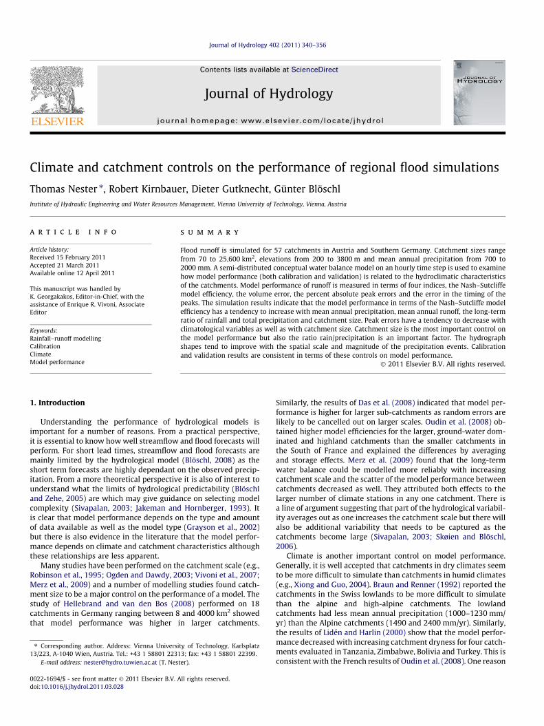
Fig. 1. Topography of Austria and parts of Southern Germany. Elevations within the mindicated by triangles, the precipitation gauges by circles. Weather radar stations are in

mance may strongly depend on the temporal resolution of themodel. It is hence of interest to examine the controls for a highertemporal resolution where routing effects become more importantand the flood peaks are more accurately represented, and to extendthe analyses to a larger number of catchments than is usually done.

The aim of this paper is to analyse the controls on the perfor-mance of a hydrological model with an hourly time resolution thatincludes channel routing processes. Specifically, we examinewhether the model performance can be related to climatic andhydrological characteristics of the catchments. We do not only fo-cus on the Nash–Sutcliffe model efficiency, but also on peak errormeasures. The rainfall runoff model used is a conceptual hydrolog-ical model (Blöschl et al., 2008) which is applied in a semi-distrib-uted mode to 57 Danube tributaries in Austria and Germany over aperiod of seven years.

The organisation of the paper is as follows: Following thedescription of the study region and data used in Section 2, a shortdescription of the model is given in Section 3. Section 4 presentsthe results found in the simulation runs, and in Section 5 theresults are discussed.

2. Study region and data

The study region is hydrologically diverse covering large partsof Austria and some parts of Bavaria (Fig. 1). The West of the regionis Alpine with elevations of up to 3800 m a.s.l. while the North andEast consist of prealpine terrain and lowlands with elevationsbetween 200 and 800 m a.s.l.

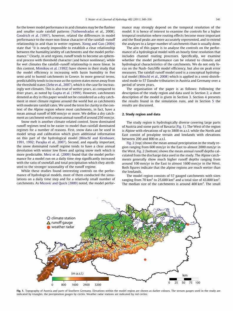
Fig. 2 (top) shows the mean annual precipitation in the study re-gion ranging from 600 mm/yr in the East to almost 2000 mm/yr inthe West. Fig. 2 (bottom) shows the mean annual runoff depths cal-culated from the discharge data used in the study. The Alpine catch-ments generally show much higher runoff depths ranging fromaround 100 mm/yr in the East to almost 1600 mm/yr in the West.Both figures indicate that the alpine regions are much wetter thanthe lowlands.

The model region consists of 57 gauged catchments with sizesranging from 70 km2 to 25,600 km2 and a total size of 43,800 km2.The median size of the catchments is around 400 km2. The small

odel region are shown as darker colours. The stream gauges used in the study aredicated by red circles.

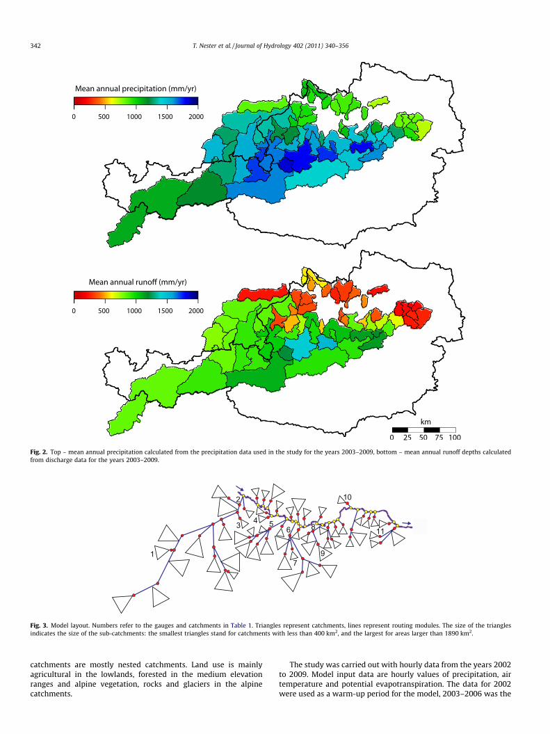
Fig. 2. Top – mean annual precipitation calculated from the precipitation data used in the study for the years 2003–2009, bottom – mean annual runoff depths calculatedfrom discharge data for the years 2003–2009.

91

2

3 4 56

7

8

10

11

Fig. 3. Model layout. Numbers refer to the gauges and catchments in Table 1. Triangles represent catchments, lines represent routing modules. The size of the trianglesindicates the size of the sub-catchments: the smallest triangles stand for catchments with less than 400 km2, and the largest for areas larger than 1890 km2.

342 T. Nester et al. / Journal of Hydrology 402 (2011) 340–356

catchments are mostly nested catchments. Land use is mainlyagricultural in the lowlands, forested in the medium elevationranges and alpine vegetation, rocks and glaciers in the alpinecatchments.

The study was carried out with hourly data from the years 2002to 2009. Model input data are hourly values of precipitation, airtemperature and potential evapotranspiration. The data for 2002were used as a warm-up period for the model, 2003–2006 was the

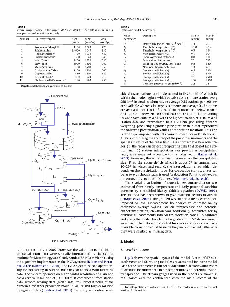
Table 1Stream gauges named in the paper. MAP and MAR (2002–2009) is mean annualprecipitation and runoff, respectively.

Number Gauge/catchment Area(km2)

MAP(mm/yr)

MAR(mm/yr)

1 Rosenheim/Mangfall 1100 1520 7702 Schärding/Inn 25,600 1040 8303 Haging/Antiesena 160 1030 4404 Fraham/Innbacha 360 940 3405 Wels/Traun 3400 1550 10406 Steyr/Enns 5900 1500 10607 Molln/Steyrling 130 1700 9558 Greimpersdorf/Ybbs 1100 1260 8409 Opponitz/Ybbs 510 1800 1140

10 Krems/Imbacha 300 720 21011 Cholerakapelle/Schwechata 180 890 250

a Denotes catchments we consider to be dry.

S3

Qby

p p byp p by(

S2

Qp

0 1 L k1 0

1 1 k1

2 2 k2

Q = Qt i

3 3 k3

EvapotranspirationT Da m

S1

L1

RoutingN K

LsSsLp

P = Ps CS

Snow

r

Fig. 4. Model scheme.

Table 2Hydrologic model parameters.

Modelparameter

Description Min inregion

Max inregion

D Degree-day factor (mm �C�1 day�1) 1.3 2.3Ts Threshold temperature (�C) �1.8 �0.4Tr Threshold temperature (�C) 0.3 1.6Tm Melt temperature (�C) 0.1 0.9CS Snow correction factor (–) 0.8 1.0LS Max. soil moisture (mm) 70 725LP Limit for pot. evaporation (mm) 9.5 360b Nonlinearity parameter (–) 1.3 4.7k0 Storage coefficient (h) 0.5 200k1 Storage coefficient (h) 10 550k2 Storage coefficient (h) 75 2500k3 Storage coefficient (h) 100 2500cp Constant percolation (mm day�1) 2.2 24

1 For interpretation of color in Figs. 1 and 3, the reader is referred to the webversion of this article.

T. Nester et al. / Journal of Hydrology 402 (2011) 340–356 343

calibration period and 2007–2009 was the validation period. Mete-orological input data were spatially interpolated by the CentralInstitute for Meteorology and Geodynamics (ZAMG) in Vienna usingthe algorithm implemented in the INCA system (Haiden and Pistot-nik, 2009; Haiden et al., 2010). The INCA system is used operation-ally for forecasting in Austria, but can also be used with historicaldata. The system operates on a horizontal resolution of 1 km andhas a vertical resolution of 100–200 m. It combines surface stationdata, remote sensing data (radar, satellite), forecast fields of thenumerical weather prediction model ALADIN, and high-resolutiontopographic data (Haiden et al., 2010). Currently, 408 online avail-

able climate stations are implemented in INCA; 169 of which liewithin the model region, which equals to one climate station every258 km2. In small catchments, on average 0.35 stations per 100 km2

are available whereas in large catchments on average 0.45 stationsare available per 100 km2. 70% of the stations are below 1000 ma.s.l., 24% are between 1000 and 2000 m a.s.l. and the remaining6% are above 2000 m a.s.l. with the highest station at 3100 m a.s.l.Station data are interpolated to a 1 � 1 km grid using distanceweighting, producing a gridded precipitation field that reproducesthe observed precipitation values at the station locations. This gridis then superimposed with data from four weather radar stations inAustria, combining the accuracy of the point measurements and thespatial structure of the radar field. This approach has two advanta-ges: (1) the radar can detect precipitating cells that do not hit a sta-tion and (2) station interpolation can provide a precipitationanalysis in areas not accessible to the radar beam (Haiden et al.,2010). However, there are two error sources on the precipitationside: First, the gauge deficit which is about 5% in summer and10–20% in winter and second, the interpolation error which de-pends on the precipitation type. For convective storms, errors canbe large even though radar is used for detection. For synoptic events,the errors are around 5–10% or less (Viglione et al., 2010a,b).

The spatial distribution of potential evapotranspiration wasestimated from hourly temperature and daily potential sunshineduration by a modified Blaney–Criddle equation (DVWK, 1996).This method has been shown to give plausible results in Austria(Parajka et al., 2003). The gridded weather data fields were super-imposed on the subcatchment boundaries to estimate hourlycatchment average values. For air temperature and potentialevapotranspiration, elevation was additionally accounted for bydividing all catchments into 500 m elevation zones. To calibrateand verify the model, hourly discharge data from 57 stream gaugeswere used. The data were checked for errors and in cases where aplausible correction could be made they were corrected. Otherwisethey were marked as missing data.

3. Model

3.1. Model structure

Fig. 3 shows the spatial layout of the model. A total of 57 sub-catchments and 58 routing modules are accounted for in the model.Each of the catchments is further divided into 500 m elevation zonesto account for differences in air temperature and potential evapo-transpiration. The stream gauges used in the model are shown asred1 points and the confluences with the main stream of the

344 T. Nester et al. / Journal of Hydrology 402 (2011) 340–356

Danube are shown as yellow points. Table 1 gives details aboutcatchments named in the paper such as area, mean annual precip-itation and runoff.

The rainfall runoff model used in this study is a conceptualhydrological model (Blöschl et al., 2008) which is applied in asemi-distributed mode. The structure is similar to that of theHBV model (Bergström, 1976) but several modifications weremade including an additional ground water storage, a bypass flow(Blöschl et al., 2008; Komma et al., 2008) and a modified routingroutine (Szolgay, 2004). Fig. 4 shows the model scheme for one500 m elevation zone of a catchment. For each elevation zone,snow processes, soil moisture processes and hill slope scale routingare simulated on an hourly time step. In the snow routine, snowaccumulation and melt are represented by a simple degree-dayconcept, involving the degree-day factor D (mm �C�1 day�1) andmelt temperature Tm (�C). Catch deficit of the precipitation gaugesis corrected by a snow correction factor, CS (–). Precipitation is con-sidered to fall as rain if the air temperature Ta (�C) is above athreshold temperature Tr (�C), as snow if Ta (�C) is below a thresh-

0

100

200

300

400

500

600

Jan Feb Mar Apr May Jun

0

5

10

15

0

100

200

300

400

500

600

0

5

10

15

Jan Feb Mar Apr May Jun

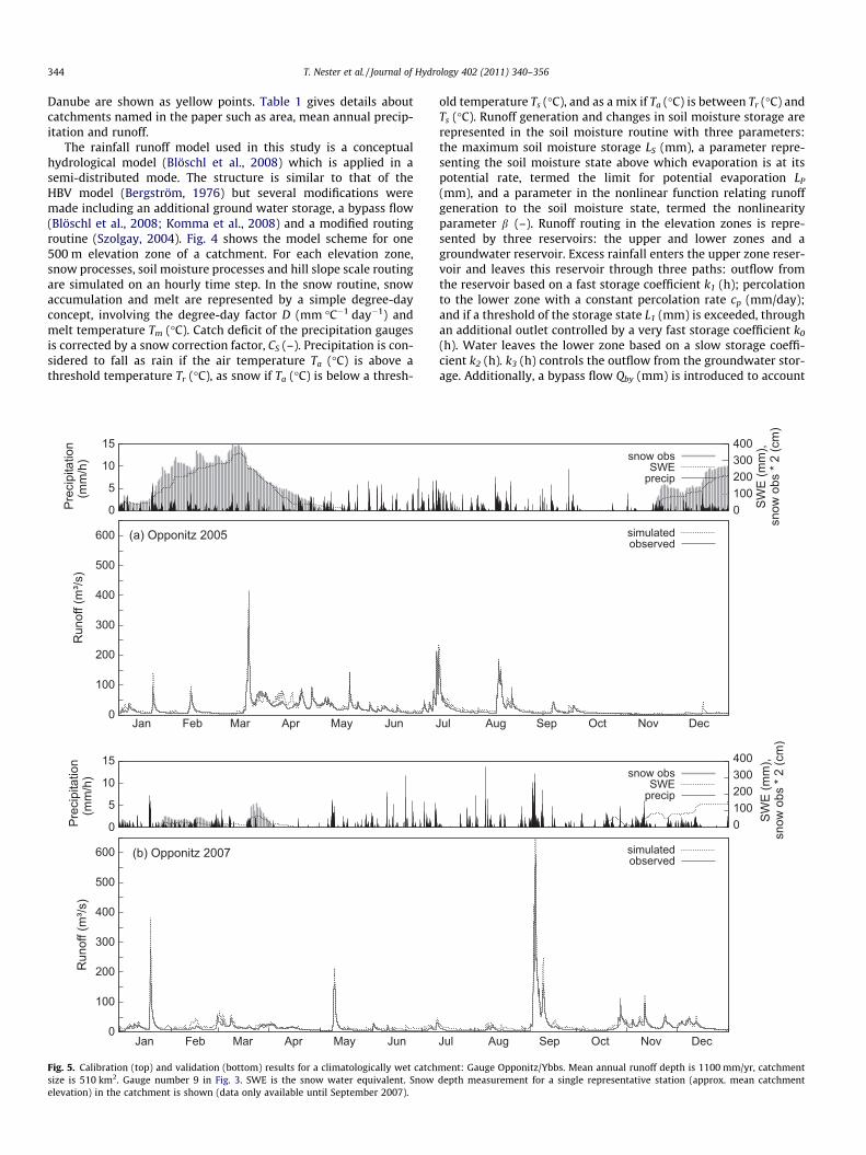
Fig. 5. Calibration (top) and validation (bottom) results for a climatologically wet catchsize is 510 km2. Gauge number 9 in Fig. 3. SWE is the snow water equivalent. Snowelevation) in the catchment is shown (data only available until September 2007).

old temperature Ts (�C), and as a mix if Ta (�C) is between Tr (�C) andTs (�C). Runoff generation and changes in soil moisture storage arerepresented in the soil moisture routine with three parameters:the maximum soil moisture storage LS (mm), a parameter repre-senting the soil moisture state above which evaporation is at itspotential rate, termed the limit for potential evaporation LP

(mm), and a parameter in the nonlinear function relating runoffgeneration to the soil moisture state, termed the nonlinearityparameter b (–). Runoff routing in the elevation zones is repre-sented by three reservoirs: the upper and lower zones and agroundwater reservoir. Excess rainfall enters the upper zone reser-voir and leaves this reservoir through three paths: outflow fromthe reservoir based on a fast storage coefficient k1 (h); percolationto the lower zone with a constant percolation rate cp (mm/day);and if a threshold of the storage state L1 (mm) is exceeded, throughan additional outlet controlled by a very fast storage coefficient k0

(h). Water leaves the lower zone based on a slow storage coeffi-cient k2 (h). k3 (h) controls the outflow from the groundwater stor-age. Additionally, a bypass flow Qby (mm) is introduced to account

Jul Aug Sep Oct Nov Dec

simulatedobserved

0100200300400

SWEprecip

simulatedobserved

0100200300400

SWEprecip

Jul Aug Sep Oct Nov Dec

ment: Gauge Opponitz/Ybbs. Mean annual runoff depth is 1100 mm/yr, catchmentdepth measurement for a single representative station (approx. mean catchment

T. Nester et al. / Journal of Hydrology 402 (2011) 340–356 345

for precipitation that bypasses the soil matrix and directly contrib-utes to the storage in the lower soil levels (Blöschl et al., 2008).Outflow from all reservoirs is then routed by a transfer functionwhich consists of a linear storage cascade with the parameters N(–; number of reservoirs) and K (h; time parameter of eachreservoir).

3.2. Model calibration

Madsen et al. (2002) have compared different methods of auto-mated and manual calibration to find that the different methodsput emphasis on different aspect of the hydrograph, but none ofthe methods were superior with respect to the performance mea-sures. However, we believe that manual calibration based onhydrological reasoning will yield model parameters that are moresuitable for the extrapolation of extreme conditions so the manualcalibration was used here as modelling floods was the main inter-est in this study. This is supported by several studies. E.g., Franchiniand Pacciani (1991) have stated that ‘‘it is apparent that betweenan automatic calibration procedure and a procedure based on suc-cessive rational attempts, the latter is preferable as it is the onlyone which makes it possible to use prior knowledge of the nature

0

50

100

150

Jan Feb Mar Apr May Jun

0

5

10

15

0

50

100

150

0

5

10

15

Jan Feb Mar Apr May Jun

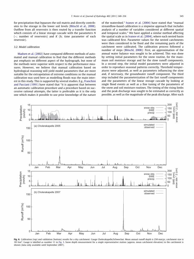
Fig. 6. Calibration (top) and validation (bottom) results for a dry catchment: Gauge Cho181 km2. Gauge is labelled as number 11 in Fig. 3. Snow depth measurement for a singshown (data only available until September 2007).

of the watershed.’’ Ivanov et al. (2004) have stated that ‘‘manualstreamflow-based calibration is a stepwise approach that includesanalysis of a number of variables considered at different spatialand temporal scales.’’ We have applied a similar method affectingthe spatial scale as in Ivanov et al. (2004), where each nested basinwas calibrated first. Parameter values for the nested catchmentswere then considered to be fixed and the remaining parts of thecatchment were calibrated. The calibration process followed anumber of steps (Blöschl, 2008): First, an approximation of theannual water balance was sought to be achieved. This was doneby setting initial parameters for the snow routine, for the maxi-mum soil moisture storage and for the slow runoff components.In a second step, the initial model parameters were adjusted inorder to reproduce seasonal patterns correctly. Threshold temper-atures were adjusted, as well as parameters influencing the slowand, if necessary, the groundwater runoff component. The thirdstep included the parameterization of the fast runoff componentsand the parameters of the linear storage cascade by looking atsingle flood events as well as a fine tuning of the parameters ofthe snow and soil moisture routines. The timing of the rising limbsand the peak discharge was sought to be estimated as correctly aspossible, as well as the magnitude of the peak discharge. After each

Jul Aug Sep Oct Nov Dec

simulatedobserved

050100150200

SWEprecip

simulatedobserved

050100150200

SWEprecip

Jul Aug Sep Oct Nov Dec

lerakapelle/Schwechat. Mean annual runoff depth is 250 mm/yr, catchment size isle representative station (approx. mean catchment elevation) in the catchment is

346 T. Nester et al. / Journal of Hydrology 402 (2011) 340–356

model run, we visualised the model simulations and evaluated theresults using statistical measures (measures used are given inAppendix A). It showed that the manual calibration had two mainadvantages. First, the structure of events in different hydrologicalsituations could be captured better by using manual calibration.Second, the timing of the rising limbs of the flood waves couldbe simulated well. Additionally, the approach has been found tobe efficient as looking at a lot of different flood events helped togain a deep insight into the runoff processes throughout thecatchments.

In the calibration process, the snow correction factor CS (–) hasbeen set to a value of 1, as an elevation-based parameterization forprecipitation is implemented in the INCA system (Haiden andPistotnik, 2009). However, in one elevation zone ranging from3250 to 3750 m a.s.l. the model results have shown that a snowcorrection factor of 1 results in a constantly increasing SWE valuefor this elevation zone. Therefore, a CS value of 0.8 has been used inthis elevation zone to yield better and more realistic results. Initialmodel parameters for the calibration of the snow routine weretaken from the literature and were adjusted in several model runs.Initial values were taken from, e.g., Seibert (1999) who has usedthreshold temperatures ranging from �1.5 to 2.5 �C and a de-gree-day factor ranging from 1 to 10 mm �C�1 day�1 for his MonteCarlo based calibration in Sweden. A temperature range from �2.0to 4.0 �C is reported in Braun (1985) where a mix of rain and snowcan occur in lowland and lower-alpine catchments in Switzerland.

0.00

0.20

0.40

0.60

0.80

1.00

10 100 1000 10000 100000

nsme

0

20

40

60

80

100

10 100 1000 10000 100000

Nash

peak

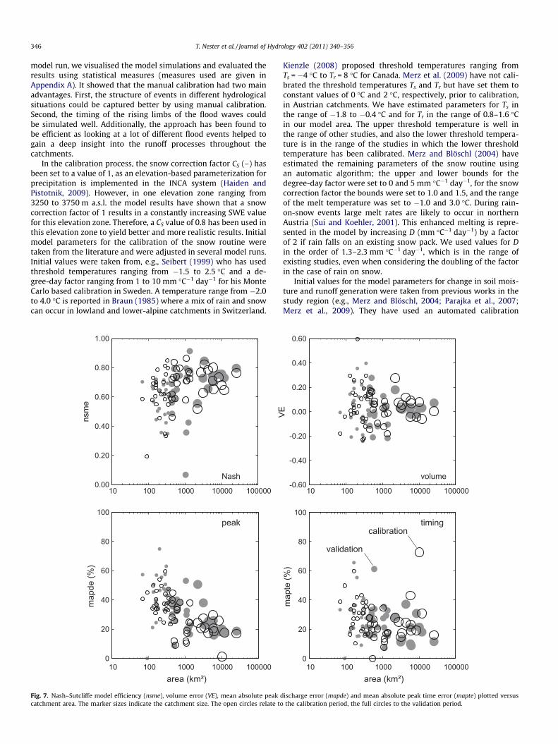
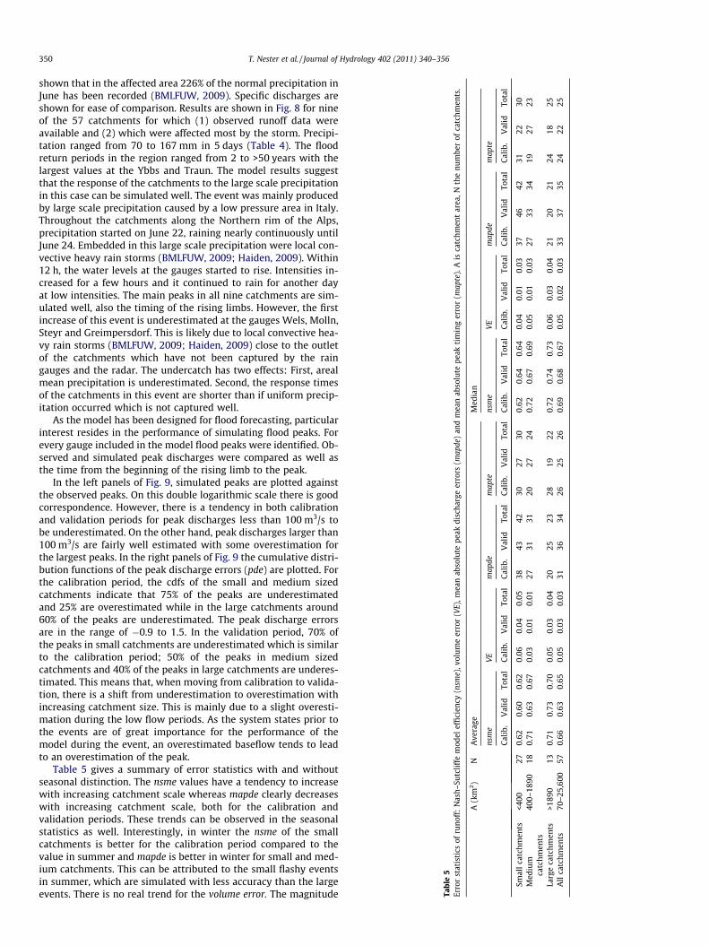
Fig. 7. Nash–Sutcliffe model efficiency (nsme), volume error (VE), mean absolute peak dcatchment area. The marker sizes indicate the catchment size. The open circles relate to

Kienzle (2008) proposed threshold temperatures ranging fromTs = �4 �C to Tr = 8 �C for Canada. Merz et al. (2009) have not cali-brated the threshold temperatures Ts and Tr but have set them toconstant values of 0 �C and 2 �C, respectively, prior to calibration,in Austrian catchments. We have estimated parameters for Ts inthe range of �1.8 to �0.4 �C and for Tr in the range of 0.8–1.6 �Cin our model area. The upper threshold temperature is well inthe range of other studies, and also the lower threshold tempera-ture is in the range of the studies in which the lower thresholdtemperature has been calibrated. Merz and Blöschl (2004) haveestimated the remaining parameters of the snow routine usingan automatic algorithm; the upper and lower bounds for thedegree-day factor were set to 0 and 5 mm �C�1 day�1, for the snowcorrection factor the bounds were set to 1.0 and 1.5, and the rangeof the melt temperature was set to �1.0 and 3.0 �C. During rain-on-snow events large melt rates are likely to occur in northernAustria (Sui and Koehler, 2001). This enhanced melting is repre-sented in the model by increasing D (mm �C�1 day�1) by a factorof 2 if rain falls on an existing snow pack. We used values for Din the order of 1.3–2.3 mm �C�1 day�1, which is in the range ofexisting studies, even when considering the doubling of the factorin the case of rain on snow.

Initial values for the model parameters for change in soil mois-ture and runoff generation were taken from previous works in thestudy region (e.g., Merz and Blöschl, 2004; Parajka et al., 2007;Merz et al., 2009). They have used an automated calibration

-0.60

-0.40

-0.20

0.00

0.20

0.40

0.60

10 100 1000 10000 100000

VE

0

20

40

60

80

100

10 100 1000 10000 100000

calibration

validation

volume

timing

ischarge error (mapde) and mean absolute peak time error (mapte) plotted versusthe calibration period, the full circles to the validation period.

),m

ean

abso

lute

peak

tim

eer

ror

(map

te)

and

abso

lute

volu

me

erro

r(|

VE|

)to

mea

nan

nual

runo

ffM

AR

(mm

yr�

1),

nter

isD

ecem

ber

toM

ay(r

unof

finfl

uenc

edby

snow

and/

orsn

owm

elt)

,sum

mer

isJu

neto

Nov

embe

r.Co

rrel

atio

n

apde

map

te|V

E|

alib

.V

alid

Tota

lC

alib

.V

alid

Tota

lC

alib

.V

alid

Tota

l

0.34

�0.

24�

0.42

�0.

37�

0.08

�0.

35�

0.23

�0.

10�

0.19

0.33

�0.

25�

0.40

�0.

42�

0.13

�0.

38�

0.09

�0.

05�

0.08

0.44

0.57

0.55

0.36

0.36

0.43

0.19

0.48

0.28

0.57

�0.

31�

0.60

�0.

22�

0.01

�0.

27�

0.08

�0.

12�

0.24

0.33

�0.

11�

0.43

�0.

140.

08�

0.17

�0.

36�

0.21

�0.

340.

33�

0.12

�0.

41�

0.24

0.04

�0.

23�

0.23

�0.

15�

0.28

0.42

0.33

0.52

0.20

0.23

0.30

0.33

0.59

0.41

0.52

�0.

19�

0.58

�0.

19�

0.02

�0.

22�

0.21

�0.

09�

0.27

0.15

�0.

05�

0.15

�0.

38�

0.17

�0.

35�

0.03

�0.

16�

0.22

0.19

�0.

10�

0.20

�0.

42�

0.17

�0.

340.

07�

0.22

�0.

110.

310.

500.

460.

390.

340.

43�

0.01

0.45

0.19

0.40

�0.

05�

0.37

�0.

35�

0.04

�0.

300.

03�

0.09

�0.

16

T. Nester et al. / Journal of Hydrology 402 (2011) 340–356 347

routine; values for the maximum soil moisture LS are in the rangeof 0–600 mm and the nonlinearity parameter b is varied in therange of 0–20 (–); values for storage parameters are in the rangeof 0–2 days for k0, 2–30 days for k1 and 30–250 days for k2 andthe percolation rate cp is varied between 0 and 8 mm day�1. Param-eters controlling the soil moisture were chosen depending oncatchment characteristics (land use, geology) which were analysedprior to the calibration. E.g., in catchments dominated by open landmedium values for the maximum soil moisture LS were used, incatchments dominated by forests, larger values of LS were used asit was assumed that the storage capacity is higher in forested areas.In alpine catchments small values of LS were chosen as the storagecapacity was assumed to be smaller due to rocks and shallow soil.The storage coefficients were chosen depending on the shape of thecatchments. E.g., the fast runoff component of a catchment which isstretched was assumed to be slower (and hence the storage coeffi-cients larger) compared to a more compact catchment which wasassumed to react quicker (and hence the storage coefficients beingsmaller). Table 2 gives an overview over the calibrated minimumand maximum parameters values in the region.

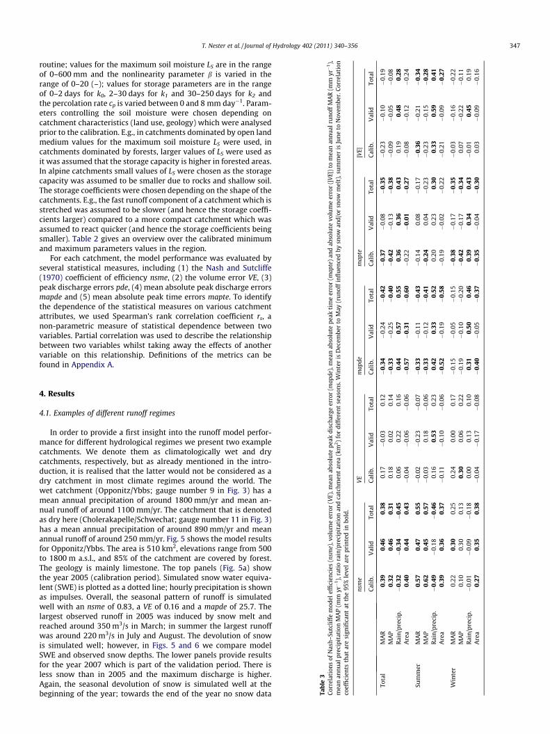
For each catchment, the model performance was evaluated byseveral statistical measures, including (1) the Nash and Sutcliffe(1970) coefficient of efficiency nsme, (2) the volume error VE, (3)peak discharge errors pde, (4) mean absolute peak discharge errorsmapde and (5) mean absolute peak time errors mapte. To identifythe dependence of the statistical measures on various catchmentattributes, we used Spearman’s rank correlation coefficient rs, anon-parametric measure of statistical dependence between twovariables. Partial correlation was used to describe the relationshipbetween two variables whilst taking away the effects of anothervariable on this relationship. Definitions of the metrics can befound in Appendix A.

Tabl

e3

Corr

elat

ions

ofN

ash–

Sutc

liffe

mod

elef

fici

enci

es(n

sme)

,vol

ume

erro

r(V

E),m

ean

abso

lute

peak

disc

harg

eer

ror

(map

dem

ean

annu

alpr

ecip

itat

ion

MA

P(m

myr�

1),

rati

ora

in/p

reci

pita

tion

and

catc

hmen

tar

ea(k

m2)

for

diff

eren

tse

ason

s.W

ico

effi

cien

tsth

atar

esi

gnifi

cant

atth

e95

%le

vel

are

prin

ted

inbo

ld.

nsm

eV

Em

Cal

ib.

Val

idTo

tal

Cal

ib.

Val

idTo

tal

C

Tota

lM

AR

0.39

0.46

0.38

0.17

�0.

030.

12�

MA

P0.

320.

460.

310.

180.

020.

14�

Rai

n/p

reci

p.�

0.32

�0.

34�

0.45

0.06

0.22

0.16

Are

a0.

400.

440.

43�

0.04

�0.

06�

0.06

�

Sum

mer

MA

R0.

570.

470.

55�

0.02

�0.

23�

0.07

�M

AP

0.62

0.45

0.57

�0.

030.

18�

0.06

�R

ain

/pre

cip.

�0.

49�

0.18

�0.

460.

160.

530.

23A

rea

0.39

0.36

0.37

�0.

11�

0.10

�0.

06�

Win

ter

MA

R0.

220.

300.

250.

240.

000.

17�

MA

P0.

100.

300.

130.

300.

060.

22�

Rai

n/p

reci

p.�

0.01

�0.

09�

0.18

0.00

0.13

0.10

Are

a0.

270.

350.

38�

0.04

�0.

17�

0.08

�

4. Results

4.1. Examples of different runoff regimes

In order to provide a first insight into the runoff model perfor-mance for different hydrological regimes we present two examplecatchments. We denote them as climatologically wet and drycatchments, respectively, but as already mentioned in the intro-duction, it is realised that the latter would not be considered as adry catchment in most climate regimes around the world. Thewet catchment (Opponitz/Ybbs; gauge number 9 in Fig. 3) has amean annual precipitation of around 1800 mm/yr and mean an-nual runoff of around 1100 mm/yr. The catchment that is denotedas dry here (Cholerakapelle/Schwechat; gauge number 11 in Fig. 3)has a mean annual precipitation of around 890 mm/yr and meanannual runoff of around 250 mm/yr. Fig. 5 shows the model resultsfor Opponitz/Ybbs. The area is 510 km2, elevations range from 500to 1800 m a.s.l., and 85% of the catchment are covered by forest.The geology is mainly limestone. The top panels (Fig. 5a) showthe year 2005 (calibration period). Simulated snow water equiva-lent (SWE) is plotted as a dotted line; hourly precipitation is shownas impulses. Overall, the seasonal pattern of runoff is simulatedwell with an nsme of 0.83, a VE of 0.16 and a mapde of 25.7. Thelargest observed runoff in 2005 was induced by snow melt andreached around 350 m3/s in March; in summer the largest runoffwas around 220 m3/s in July and August. The devolution of snowis simulated well; however, in Figs. 5 and 6 we compare modelSWE and observed snow depths. The lower panels provide resultsfor the year 2007 which is part of the validation period. There isless snow than in 2005 and the maximum discharge is higher.Again, the seasonal devolution of snow is simulated well at thebeginning of the year; towards the end of the year no snow data

0.0

0.2

0.4

0.6

0.8

22/06 24/06 26/06

Steyr/Enns2

22/06 24/06 26/06

Gr./Ybbs2

22/06 24/06 26/06

Imbach/Krems2

0.0

0.2

0.4

0.6

0.8 Fraham/Innbach2

Wels/Traun2

Molln/Steyrling2

0.0

0.2

0.4

0.6

0.8 Rosenheim/Mangfall2

Schärding/Inn2

Haging/Antiesen2

simulatedobserved

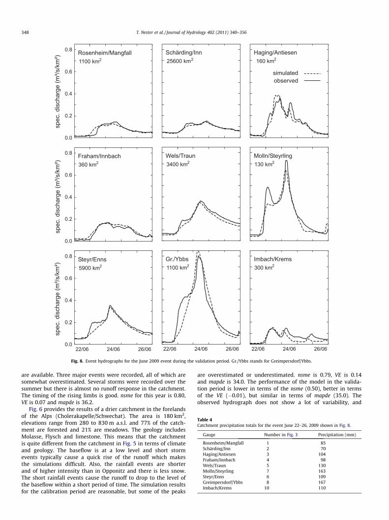
Fig. 8. Event hydrographs for the June 2009 event during the validation period. Gr./Ybbs stands for Greimpersdorf/Ybbs.

Table 4Catchment precipitation totals for the event June 22–26, 2009 shown in Fig. 8.

Gauge Number in Fig. 3 Precipitation (mm)

Rosenheim/Mangfall 1 85Schärding/Inn 2 70Haging/Antiesen 3 104Fraham/Innbach 4 98Wels/Traun 5 130Molln/Steyrling 7 163Steyr/Enns 6 109Greimpersdorf/Ybbs 8 167Imbach/Krems 10 110

348 T. Nester et al. / Journal of Hydrology 402 (2011) 340–356

are available. Three major events were recorded, all of which aresomewhat overestimated. Several storms were recorded over thesummer but there is almost no runoff response in the catchment.The timing of the rising limbs is good. nsme for this year is 0.80,VE is 0.07 and mapde is 36.2.

Fig. 6 provides the results of a drier catchment in the forelandsof the Alps (Cholerakapelle/Schwechat). The area is 180 km2,elevations range from 280 to 830 m a.s.l. and 77% of the catch-ment are forested and 21% are meadows. The geology includesMolasse, Flysch and limestone. This means that the catchmentis quite different from the catchment in Fig. 5 in terms of climateand geology. The baseflow is at a low level and short stormevents typically cause a quick rise of the runoff which makesthe simulations difficult. Also, the rainfall events are shorterand of higher intensity than in Opponitz and there is less snow.The short rainfall events cause the runoff to drop to the level ofthe baseflow within a short period of time. The simulation resultsfor the calibration period are reasonable, but some of the peaks

are overestimated or underestimated. nsme is 0.79, VE is 0.14and mapde is 34.0. The performance of the model in the valida-tion period is lower in terms of the nsme (0.50), better in termsof the VE (�0.01), but similar in terms of mapde (35.0). Theobserved hydrograph does not show a lot of variability, and

T. Nester et al. / Journal of Hydrology 402 (2011) 340–356 349

several short small-scale storms do not have a lot of influence onthe runoff. At the beginning of September a large scale precipita-tion event caused fast response. The discharge increased to110 m3/s, but the model estimated 165 m3/s. The comparison ofthe two catchments (Figs. 5 and 6) suggests that the flashierrunoff pattern in the drier catchment is more difficult to model.Small precipitation events can lead to unexpected runoffresponse, and rain-on-snow events occur in these prealpine areas(Merz and Blöschl, 2003; 2008). Alpine catchments with a largerelevation range such as Opponitz have a more distinct annualcycle related to snow melt in spring.

4.2. Effect of catchment scale on the model performance

To assess the model performance more comprehensively, themodel error measures based on hourly data of all catchments havebeen plotted in Fig. 7 against catchment area. Additionally, wehave calculated the Spearman’s rank correlation coefficients rs

between model error measures and catchment attributes for theentire period and for winter and summer seasons (Table 3). Over-all, the model performs well. The median Nash–Sutcliffe modelefficiencies (nsme) for the calibration and validation periods are0.69 and 0.67, respectively. Median nsme in the summer months(June–November) are 0.69 (calibration) and 0.71 (validation), inthe winter months (December–May) the values are 0.64 (calibra-tion) and 0.56 (validation). The distribution of the nsme in thevalidation period is similar to that in the calibration period. Inthe validation period, 80% of the nsme values are larger than 0.5

1

10

100

1000

10000

1 10 100 1000 10000

QPeak,sim(m³/s)

1

10

100

1000

10000

1 10 100 1000 10000

QPeak,sim(m³/s)

Q Peak,obs (m³/s)

calibration

validation

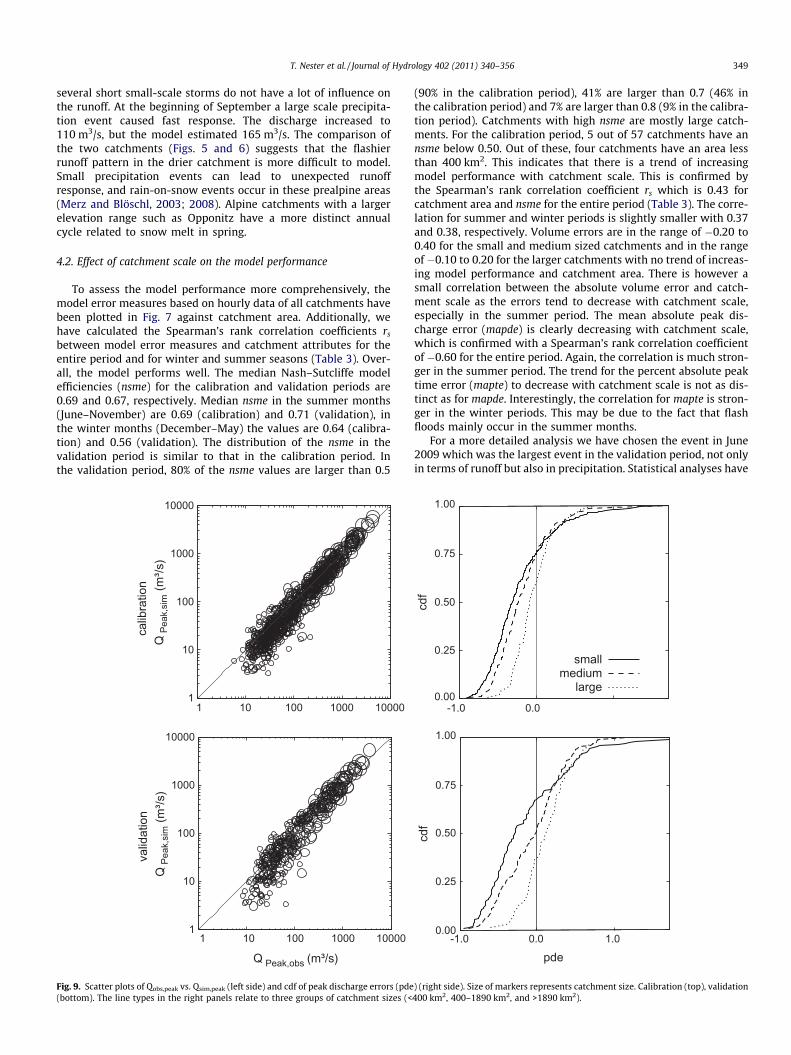
Fig. 9. Scatter plots of Qobs,peak vs. Qsim,peak (left side) and cdf of peak discharge errors (pde(bottom). The line types in the right panels relate to three groups of catchment sizes (<

(90% in the calibration period), 41% are larger than 0.7 (46% inthe calibration period) and 7% are larger than 0.8 (9% in the calibra-tion period). Catchments with high nsme are mostly large catch-ments. For the calibration period, 5 out of 57 catchments have annsme below 0.50. Out of these, four catchments have an area lessthan 400 km2. This indicates that there is a trend of increasingmodel performance with catchment scale. This is confirmed bythe Spearman’s rank correlation coefficient rs which is 0.43 forcatchment area and nsme for the entire period (Table 3). The corre-lation for summer and winter periods is slightly smaller with 0.37and 0.38, respectively. Volume errors are in the range of �0.20 to0.40 for the small and medium sized catchments and in the rangeof �0.10 to 0.20 for the larger catchments with no trend of increas-ing model performance and catchment area. There is however asmall correlation between the absolute volume error and catch-ment scale as the errors tend to decrease with catchment scale,especially in the summer period. The mean absolute peak dis-charge error (mapde) is clearly decreasing with catchment scale,which is confirmed with a Spearman’s rank correlation coefficientof �0.60 for the entire period. Again, the correlation is much stron-ger in the summer period. The trend for the percent absolute peaktime error (mapte) to decrease with catchment scale is not as dis-tinct as for mapde. Interestingly, the correlation for mapte is stron-ger in the winter periods. This may be due to the fact that flashfloods mainly occur in the summer months.

For a more detailed analysis we have chosen the event in June2009 which was the largest event in the validation period, not onlyin terms of runoff but also in precipitation. Statistical analyses have

0.00

0.25

0.50

0.75

1.00

cdf

smallmediumlarge

0.00

0.25

0.50

0.75

1.00

cdf

pde-1.0 0.0 1.0

-1.0 0.0

) (right side). Size of markers represents catchment size. Calibration (top), validation400 km2, 400–1890 km2, and >1890 km2).

Tabl

e5

Erro

rst

atis

tics

ofru

noff

:N

ash–

Sutc

liffe

mod

elef

fici

ency

(nsm

e),v

olum

eer

ror

(VE)

,mea

nab

solu

tepe

akdi

scha

rge

erro

rs(m

apde

)an

dm

ean

abso

lute

peak

tim

ing

erro

r(m

apte

).A

isca

tchm

ent

area

,Nth

enu

mbe

rof

catc

hmen

ts.

A(k

m2)

NA

vera

geM

edia

n

nsm

eV

Em

apde

map

tens

me

VE

map

dem

apte

Cal

ib.

Val

idTo

tal

Cal

ib.

Val

idTo

tal

Cal

ib.

Val

idTo

tal

Cal

ib.

Val

idTo

tal

Cal

ib.

Val

idTo

tal

Cal

ib.

Val

idTo

tal

Cal

ib.

Val

idTo

tal

Cal

ib.

Val

idTo

tal

Smal

lca

tch

men

ts<4

0027

0.62

0.60

0.62

0.06

0.04

0.05

3843

4230

2730

0.62

0.64

0.64

0.04

0.01

0.03

3746

4231

2230

Med

ium

catc

hm

ents

400–

1890

180.

710.

630.

670.

030.

010.

0127

3131

2027

240.

720.

670.

690.

050.

010.

0327

3334

1927

23

Larg

eca

tch

men

ts>1

890

130.

710.

730.

700.

050.

030.

0420

2523

2819

220.

720.

740.

730.

060.

030.

0421

2021

2418

25A

llca

tch

men

ts70

–25,

600

570.

660.

630.

650.

050.

030.

0331

3634

2625

260.

690.

680.

670.

050.

020.

0333

3735

2422

25

350 T. Nester et al. / Journal of Hydrology 402 (2011) 340–356

shown that in the affected area 226% of the normal precipitation inJune has been recorded (BMLFUW, 2009). Specific discharges areshown for ease of comparison. Results are shown in Fig. 8 for nineof the 57 catchments for which (1) observed runoff data wereavailable and (2) which were affected most by the storm. Precipi-tation ranged from 70 to 167 mm in 5 days (Table 4). The floodreturn periods in the region ranged from 2 to >50 years with thelargest values at the Ybbs and Traun. The model results suggestthat the response of the catchments to the large scale precipitationin this case can be simulated well. The event was mainly producedby large scale precipitation caused by a low pressure area in Italy.Throughout the catchments along the Northern rim of the Alps,precipitation started on June 22, raining nearly continuously untilJune 24. Embedded in this large scale precipitation were local con-vective heavy rain storms (BMLFUW, 2009; Haiden, 2009). Within12 h, the water levels at the gauges started to rise. Intensities in-creased for a few hours and it continued to rain for another dayat low intensities. The main peaks in all nine catchments are sim-ulated well, also the timing of the rising limbs. However, the firstincrease of this event is underestimated at the gauges Wels, Molln,Steyr and Greimpersdorf. This is likely due to local convective hea-vy rain storms (BMLFUW, 2009; Haiden, 2009) close to the outletof the catchments which have not been captured by the raingauges and the radar. The undercatch has two effects: First, arealmean precipitation is underestimated. Second, the response timesof the catchments in this event are shorter than if uniform precip-itation occurred which is not captured well.

As the model has been designed for flood forecasting, particularinterest resides in the performance of simulating flood peaks. Forevery gauge included in the model flood peaks were identified. Ob-served and simulated peak discharges were compared as well asthe time from the beginning of the rising limb to the peak.

In the left panels of Fig. 9, simulated peaks are plotted againstthe observed peaks. On this double logarithmic scale there is goodcorrespondence. However, there is a tendency in both calibrationand validation periods for peak discharges less than 100 m3/s tobe underestimated. On the other hand, peak discharges larger than100 m3/s are fairly well estimated with some overestimation forthe largest peaks. In the right panels of Fig. 9 the cumulative distri-bution functions of the peak discharge errors (pde) are plotted. Forthe calibration period, the cdfs of the small and medium sizedcatchments indicate that 75% of the peaks are underestimatedand 25% are overestimated while in the large catchments around60% of the peaks are underestimated. The peak discharge errorsare in the range of �0.9 to 1.5. In the validation period, 70% ofthe peaks in small catchments are underestimated which is similarto the calibration period; 50% of the peaks in medium sizedcatchments and 40% of the peaks in large catchments are underes-timated. This means that, when moving from calibration to valida-tion, there is a shift from underestimation to overestimation withincreasing catchment size. This is mainly due to a slight overesti-mation during the low flow periods. As the system states prior tothe events are of great importance for the performance of themodel during the event, an overestimated baseflow tends to leadto an overestimation of the peak.

Table 5 gives a summary of error statistics with and withoutseasonal distinction. The nsme values have a tendency to increasewith increasing catchment scale whereas mapde clearly decreaseswith increasing catchment scale, both for the calibration andvalidation periods. These trends can be observed in the seasonalstatistics as well. Interestingly, in winter the nsme of the smallcatchments is better for the calibration period compared to thevalue in summer and mapde is better in winter for small and med-ium catchments. This can be attributed to the small flashy eventsin summer, which are simulated with less accuracy than the largeevents. There is no real trend for the volume error. The magnitude

T. Nester et al. / Journal of Hydrology 402 (2011) 340–356 351

of the peak errors seems to be large. However, they are perfectly inthe range of existing studies. Senarath et al. (2000) have given val-ues for the average absolute peak discharge error in the range from32% to 66%; Reed et al. (2004) have shown that the percent abso-lute peak error (pape) is typically on the order of 30–50% for cali-brated models with much larger errors for the smallest basins.Similarly, Reed et al. (2007) report percent absolute peak errorsfrom 24% to 88% with increasing errors with decreasing catchmentsize. Modarres (2009) gives values of 11–41% for the medium abso-lute percentage error of peak discharges.

4.3. Climate effects on model performance

The results shown so far have indicated that the model perfor-mance depends on both the catchment size and the wetness of thecatchments. To provide further insights into these findings, themodel performance indices were plotted in Fig. 10 against themean annual precipitation (MAP). While there is a lot of scatterin the diagrams, they also indicate interesting patterns. The lowestnsme only occur for the driest catchments which are also amongthe smallest catchments. The correlation coefficient between nsmeand MAP is in the range of 0.31 for the entire period 2003–2009,with a larger correlation in summer (0.57) and a lower correlationin winter (0.13) (see Table 3). The VE ranges between �0.25 and0.25 with a few outliers. Correlation coefficients between VE andMAP are small. The range of VE is somewhat smaller for the catch-ments with higher mean annual precipitation, suggesting that themodel performance in these catchments is slightly better. The

0.00

0.20

0.40

0.60

0.80

1.00

0 500 1000 1500 2000

nsme

0

20

40

60

80

100

0 500 1000 1500 2000

Nash

peak

Fig. 10. Nash–Sutcliffe model efficiency (nsme), volume error (VE), mean absolute peakmean annual precipitation. The marker sizes indicate the catchment size. The open circ

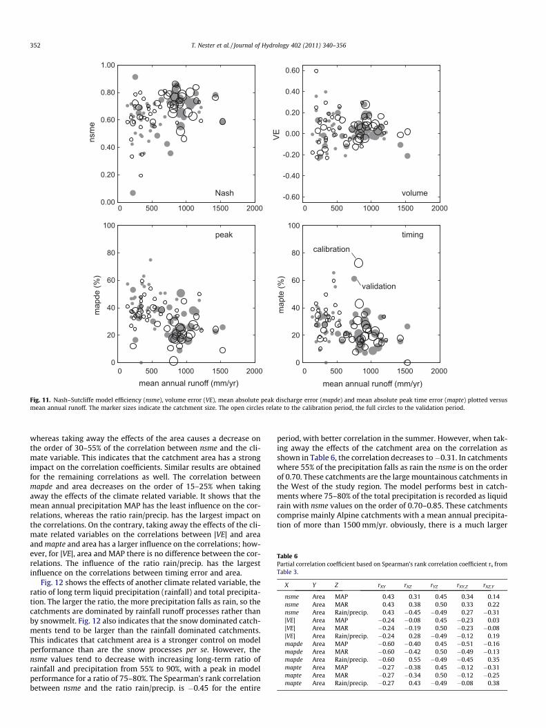
generally rather large volume errors are due to the fact that themodel calibration was guided by an attempt to simulate the peakswell, as the main purpose of the study was flood forecasting. Also,hydrologically realistic parameters were given preference overminimizing biases with a view of representing extreme eventswell. There is quite a clear tendency for the peak errors in bothterms of maximum discharge (mapde) and time to peak (mapte)to decrease with mean annual precipitation which is consistentwith the other error measures. Interestingly, correlation coeffi-cients for mapde and mapte are quite different for the winter andsummer periods. For mapte, the correlation coefficients are higherin winter, indicating that the timing of the peaks can be simulatedbetter in winter. This is no surprise as the flashier events which aremore difficult to simulate are more likely to occur in summer. Formapde, the correlation coefficients are higher in summer, indicat-ing that the peaks are simulated somewhat better in summer.For comparison, the performance measures have been plottedagainst the mean annual runoff (MAR) in Fig. 11. The patternsare similar to those in Fig. 10, and also the correlation coefficientsare similar.

As the smallest catchments also tend to be among the driercatchments and the larger catchments tend to have more snow,we have calculated the partial correlation coefficient based onthe Spearman’s rank correlation coefficient rs to separate the twoeffects. Correlation coefficients and partial correlation coefficientsvariables are summarized in Table 6. Taking away the effects ofthe climate related variable (MAP, MAR, rain/precip.) decreasesthe correlation between nsme and area on the order of 20–36%

-0.60

-0.40

-0.20

0.00

0.20

0.40

0.60

0 500 1000 1500 2000

VE

0

20

40

60

80

100

0 500 1000 1500 2000

calibration

validation

volume

timing

discharge error (mapde) and mean absolute peak time error (mapte) plotted versusles relate to the calibration period, the full circles to the validation period.

0.00

0.20

0.40

0.60

0.80

1.00

0 500 1000 1500 2000

nsme

0

20

40

60

80

100

0 500 1000 1500 2000

-0.60

-0.40

-0.20

0.00

0.20

0.40

0.60

0 500 1000 1500 2000

VE

0

20

40

60

80

100

0 500 1000 1500 2000

calibration

validation

Nash volume

peak timing

Fig. 11. Nash–Sutcliffe model efficiency (nsme), volume error (VE), mean absolute peak discharge error (mapde) and mean absolute peak time error (mapte) plotted versusmean annual runoff. The marker sizes indicate the catchment size. The open circles relate to the calibration period, the full circles to the validation period.

Table 6Partial correlation coefficient based on Spearman’s rank correlation coefficient rs fromTable 3.

X Y Z rXY rXZ rYZ rXY,Z rXZ,Y

nsme Area MAP 0.43 0.31 0.45 0.34 0.14nsme Area MAR 0.43 0.38 0.50 0.33 0.22nsme Area Rain/precip. 0.43 �0.45 �0.49 0.27 �0.31|VE| Area MAP �0.24 �0.08 0.45 �0.23 0.03|VE| Area MAR �0.24 �0.19 0.50 �0.23 �0.08|VE| Area Rain/precip. �0.24 0.28 �0.49 �0.12 0.19mapde Area MAP �0.60 �0.40 0.45 �0.51 �0.16mapde Area MAR �0.60 �0.42 0.50 �0.49 �0.13mapde Area Rain/precip. �0.60 0.55 �0.49 �0.45 0.35mapte Area MAP �0.27 �0.38 0.45 �0.12 �0.31mapte Area MAR �0.27 �0.34 0.50 �0.12 �0.25mapte Area Rain/precip. �0.27 0.43 �0.49 �0.08 0.38

352 T. Nester et al. / Journal of Hydrology 402 (2011) 340–356

whereas taking away the effects of the area causes a decrease onthe order of 30–55% of the correlation between nsme and the cli-mate variable. This indicates that the catchment area has a strongimpact on the correlation coefficients. Similar results are obtainedfor the remaining correlations as well. The correlation betweenmapde and area decreases on the order of 15–25% when takingaway the effects of the climate related variable. It shows that themean annual precipitation MAP has the least influence on the cor-relations, whereas the ratio rain/precip. has the largest impact onthe correlations. On the contrary, taking away the effects of the cli-mate related variables on the correlations between |VE| and areaand mapte and area has a larger influence on the correlations; how-ever, for |VE|, area and MAP there is no difference between the cor-relations. The influence of the ratio rain/precip. has the largestinfluence on the correlations between timing error and area.

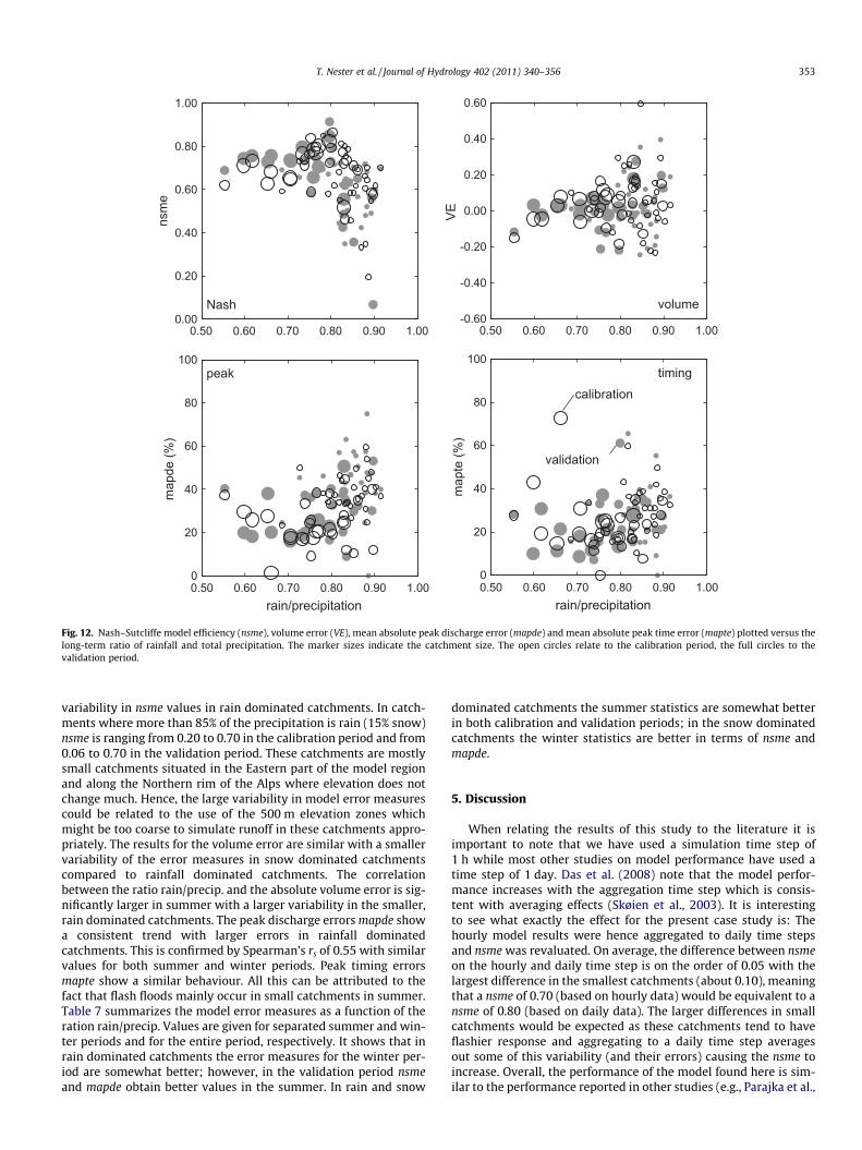
Fig. 12 shows the effects of another climate related variable, theratio of long term liquid precipitation (rainfall) and total precipita-tion. The larger the ratio, the more precipitation falls as rain, so thecatchments are dominated by rainfall runoff processes rather thanby snowmelt. Fig. 12 also indicates that the snow dominated catch-ments tend to be larger than the rainfall dominated catchments.This indicates that catchment area is a stronger control on modelperformance than are the snow processes per se. However, thensme values tend to decrease with increasing long-term ratio ofrainfall and precipitation from 55% to 90%, with a peak in modelperformance for a ratio of 75–80%. The Spearman’s rank correlationbetween nsme and the ratio rain/precip. is �0.45 for the entire

period, with better correlation in the summer. However, when tak-ing away the effects of the catchment area on the correlation asshown in Table 6, the correlation decreases to�0.31. In catchmentswhere 55% of the precipitation falls as rain the nsme is on the orderof 0.70. These catchments are the large mountainous catchments inthe West of the study region. The model performs best in catch-ments where 75–80% of the total precipitation is recorded as liquidrain with nsme values on the order of 0.70–0.85. These catchmentscomprise mainly Alpine catchments with a mean annual precipita-tion of more than 1500 mm/yr. obviously, there is a much larger

0.00

0.20

0.40

0.60

0.80

1.00

0.50 0.60 0.70 0.80 0.90 1.00

nsme

0

20

40

60

80

100

0.50 0.60 0.70 0.80 0.90 1.00rain/precipitation

-0.60

-0.40

-0.20

0.00

0.20

0.40

0.60

0.50 0.60 0.70 0.80 0.90 1.00

VE

0

20

40

60

80

100

0.50 0.60 0.70 0.80 0.90 1.00rain/precipitation

calibration

validation

Nash volume

peak timing

Fig. 12. Nash–Sutcliffe model efficiency (nsme), volume error (VE), mean absolute peak discharge error (mapde) and mean absolute peak time error (mapte) plotted versus thelong-term ratio of rainfall and total precipitation. The marker sizes indicate the catchment size. The open circles relate to the calibration period, the full circles to thevalidation period.

T. Nester et al. / Journal of Hydrology 402 (2011) 340–356 353

variability in nsme values in rain dominated catchments. In catch-ments where more than 85% of the precipitation is rain (15% snow)nsme is ranging from 0.20 to 0.70 in the calibration period and from0.06 to 0.70 in the validation period. These catchments are mostlysmall catchments situated in the Eastern part of the model regionand along the Northern rim of the Alps where elevation does notchange much. Hence, the large variability in model error measurescould be related to the use of the 500 m elevation zones whichmight be too coarse to simulate runoff in these catchments appro-priately. The results for the volume error are similar with a smallervariability of the error measures in snow dominated catchmentscompared to rainfall dominated catchments. The correlationbetween the ratio rain/precip. and the absolute volume error is sig-nificantly larger in summer with a larger variability in the smaller,rain dominated catchments. The peak discharge errors mapde showa consistent trend with larger errors in rainfall dominatedcatchments. This is confirmed by Spearman’s rs of 0.55 with similarvalues for both summer and winter periods. Peak timing errorsmapte show a similar behaviour. All this can be attributed to thefact that flash floods mainly occur in small catchments in summer.Table 7 summarizes the model error measures as a function of theration rain/precip. Values are given for separated summer and win-ter periods and for the entire period, respectively. It shows that inrain dominated catchments the error measures for the winter per-iod are somewhat better; however, in the validation period nsmeand mapde obtain better values in the summer. In rain and snow

dominated catchments the summer statistics are somewhat betterin both calibration and validation periods; in the snow dominatedcatchments the winter statistics are better in terms of nsme andmapde.

5. Discussion

When relating the results of this study to the literature it isimportant to note that we have used a simulation time step of1 h while most other studies on model performance have used atime step of 1 day. Das et al. (2008) note that the model perfor-mance increases with the aggregation time step which is consis-tent with averaging effects (Skøien et al., 2003). It is interestingto see what exactly the effect for the present case study is: Thehourly model results were hence aggregated to daily time stepsand nsme was revaluated. On average, the difference between nsmeon the hourly and daily time step is on the order of 0.05 with thelargest difference in the smallest catchments (about 0.10), meaningthat a nsme of 0.70 (based on hourly data) would be equivalent to ansme of 0.80 (based on daily data). The larger differences in smallcatchments would be expected as these catchments tend to haveflashier response and aggregating to a daily time step averagesout some of this variability (and their errors) causing the nsme toincrease. Overall, the performance of the model found here is sim-ilar to the performance reported in other studies (e.g., Parajka et al.,

Tabl

e7

Erro

rst

atis

tics

ofru

noff

:N

ash–

Sutc

liffe

mod

elef

fici

ency

(nsm

e),

volu

me

erro

r(V

E),

mea

nab

solu

tepe

akdi

scha

rge

erro

rs(m

apde

)an

dm

ean

abso

lute

peak

tim

ing

erro

rs(m

apte

).R/

Pis

the

long

-ter

mra

tio

ofra

infa

llan

dto

tal

prec

ipit

atio

n,N

isth

enu

mbe

rof

catc

hmen

ts.

R/P

(–)

NA

vera

geM

edia

n

nsm

eV

Em

apde

map

tens

me

VE

map

dem

apte

Cal

ib.

Val

idTo

tal

Cal

ib.

Val

idTo

tal

Cal

ib.

Val

idTo

tal

Cal

ib.

Val

idTo

tal

Cal

ib.

Val

idTo

tal

Cal

ib.

Val

idTo

tal

Cal

ib.

Val

idTo

tal

Cal

ib.

Val

idTo

tal

Rai

ndo

min

ated

catc

hm

ents

>0.8

517

0.60

0.56

0.57

0.00

0.03

0.00

3842

4226

2023

0.62

0.56

0.61

0.03

0.04

0.01

4043

4023

2025

Rai

nan

dsn

owdo

min

ated

catc

hm

ents

0.65

–0.8

536

0.71

0.67

0.69

0.08

0.03

0.06

2833

3125

2625

0.74

0.69

0.70

0.08

0.02

0.04

2734

3420

2122

Snow

dom

inat

edca

tch

men

ts<0

.65

40.

670.

730.

69�

0.05

�0.

02�

0.05

3029

2930

2630

0.67

0.74

0.69

�0.

040.

00�

0.04

2929

2831

2229

All

catc

hm

ents

0.55

–0.9

257

0.66

0.63

0.65

0.05

0.03

0.03

3136

3426

2526

0.69

0.68

0.67

0.05

0.02

0.03

3337

3524

2225

354 T. Nester et al. / Journal of Hydrology 402 (2011) 340–356

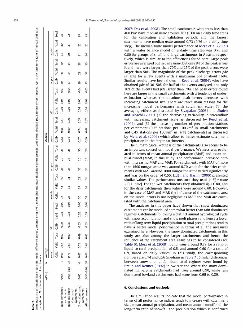
2007; Das et al., 2008). The small catchments with areas less than400 km2 have median nsme around 0.63 (0.68 on a daily time step)for the calibration and validation periods, and the largestcatchments have median nsme around 0.73 (0.76 on a daily timestep). The median nsme model performance of Merz et al. (2009)with a water balance model on a daily time step was 0.70 and0.80 for groups of small and large catchments in Austria, respec-tively, which is similar to the efficiencies found here. Large peakerrors are averaged out in daily nsme, but only 8% of the peak errorsfound here were larger than 70% and 25% of the peak errors werelarger than 50%. The magnitude of the peak discharge errors pdeis large for a few events with a maximum pde of about 160%.Similar results have been shown in Reed et al. (2004), who haveobtained pde of 30–50% for half of the events analysed, and only10% of the events had pde larger than 70%. The peak errors foundhere are larger in the small catchments with a tendency of under-estimation whereas the absolute peak errors decrease withincreasing catchment size. There are three main reasons for theincreasing model performance with catchment scale: (1) theaveraging effects as discussed by Sivapalan (2003) and Skøienand Blöschl (2006), (2) the decreasing variability in streamflowwith increasing catchment scale as discussed by Reed et al.(2004), and (3) the increasing number of precipitation stationsper catchment (0.35 stations per 100 km2 in small catchmentsand 0.45 stations per 100 km2 in large catchments) as discussedby Merz et al. (2009) which allow to better estimate catchmentprecipitation in the larger catchments.

The climatological wetness of the catchments also seems to bean important control on model performance. Wetness was evalu-ated in terms of mean annual precipitation (MAP) and mean an-nual runoff (MAR) in this study. The performance increased bothwith increasing MAP and MAR. For catchments with MAP of morethan 1500 mm/yr, nsme was around 0.70 while for the drier catch-ments with MAP around 1000 mm/yr the nsme varied significantlyand was on the order of 0.55. Lidén and Harlin (2000) presentedsimilar values. The performance measure they used is R2

V = nsme– 0.1 |nme|. For the wet catchments they obtained R2

V = 0.80, andfor the drier catchments their values were around 0.60. However,in the case of MAP and MAR the influence of the catchment areaon the model errors is not negligible as MAP and MAR are corre-lated with the catchment area.

The analyses in this paper have shown that snow dominatedcatchments can be modelled somewhat better than rain dominatedregimes. Catchments following a distinct annual hydrological cyclewith snow accumulation and snow melt phases (and hence a lowerratio of long term liquid precipitation to total precipitation) tend tohave a better model performance in terms of all the measuresexamined here. However, the snow dominated catchments in thisstudy are also among the larger catchments and hence theinfluence of the catchment area again has to be considered (seeTable 6). Merz et al. (2009) found nsme around 0.78 for a ratio ofliquid to total precipitation of 0.5, and around 0.60 for a ratio of0.9, based on daily values. In this study, the correspondingnumbers are 0.74 and 0.56 (medians in Table 7). Similar differencesbetween snow and rainfall dominated regimes were found byBraun and Renner (1992) in Switzerland where the snow domi-nated high-alpine catchments had nsme around 0.90, while raindominated lowland catchments had nsme from 0.66 to 0.80.

6. Conclusions and outlook

The simulation results indicate that the model performance interms of all performance indices tends to increase with catchmentsize, mean annual precipitation, and mean annual runoff and thelong-term ratio of snowfall and precipitation which is confirmed

T. Nester et al. / Journal of Hydrology 402 (2011) 340–356 355

by the correlation coefficients. However, the latter are mainly dueto the fact that there is a correlation between catchment size andthe climatological indices, indicating that the catchment size isthe most important control on model performance. The calibrationand validation results are consistent in terms of these controls onmodel performance.

This study is based on observed meteorological data. Additionaluncertainty will come in if rainfall forecasts are used (Blöschl,2008). As the model presented in this study has been designed asa part of an operational forecasting system the total forecastingperformance and its controls are also of interest. It is planned toexamine these in more detail in the context of ensemble floodforecasting.

Acknowledgements

We would like to thank the Hydrographic Services of LowerAustria and Upper Austria for providing the discharge data andthe Central Institute for Meteorology and Geodynamics (ZAMG)in Vienna for providing the meteorological data. The study wasperformed as part of developing an operational flood foresting sys-tem for the Austrian Danube and tributaries.

Appendix A

Statistical measures used to evaluate the model performanceinclude the Nash and Sutcliffe (1970) coefficient of efficiency(nsme):

nsme ¼ 1�Pn

i¼1ðQ sim;i � Q obs;iÞ2Pni¼1ðQ obs;i � Q obsÞ2

; ð1Þ

where Qobs,i and Qsim,i are observed and simulated runoff at hour i,respectively, and Qobs is the mean observed runoff over the calibra-tion or validation period of n hours. nsme values can range from �1to 1. A perfect match between simulation and observation impliesnsme = 1; nsme = 0 indicates that the model predictions are as accu-rate as the mean of the observed data, and nsme < 0 occurs whenthe observed mean is a better predictor than the model.

As a measure of bias the volume error, VE, was used:

VE ¼Pn

i¼1Q sim;i �Pn

i¼1Q obs;iPni¼1Q obs;i

; ð2Þ

The value can be positive or negative, with a VE of an unbiasedmodel being 0. Values larger and smaller than 0 imply over- andunderestimation, respectively.

Peak discharge errors were estimated as

pde ¼Q sim;peak � Q obs;peak

Q obs;peak; ð3Þ

where Qobs,peak and Qsim,peak are the observed and simulated peakdischarges, respectively. Based on the peak discharge errors, themean absolute peak discharge errors mapde (%) were calculated as

mapde ¼ 1m�Xm

i¼1

jpdeij � 100; ð4Þ

where m is the total number of peaks analysed for the calibration(or validation) period of the catchment. Analogue to the peak dis-charge error, peak time errors were estimated as

pte ¼ t0�peak;sim � t0�peak;obs

t0�peak;obsð5Þ

where t0-peak,obs and t0-peak,sim are the observed and simulated dura-tion of the rising limb, respectively. Based on the peak time errors,the mean absolute peak time errors mapte (%) were calculated as

mapte ¼ 1m�Xm

i¼1

jpteij � 100; ð6Þ

where m is the total number of peaks analysed for the calibration(or validation) period of the catchment.

Spearman’s rank correlation coefficient rs is calculated as

rs ¼ 1� 6 �Pn

i¼1d2i

n � ðn2 � 1Þ with di ¼ rkðxiÞ � rkðyiÞ ð7Þ

with rk(xi) as the rank of xi, where the highest value has rank 1 andthe lowest value has rank n. Spearman’s rs can vary between �1 and1, where �1 represents a completely negative correlation and 1 rep-resents a completely positive correlation. Completely uncorrelatedpairs of data have a Spearman’s rs of 0. The partial correlation coef-ficient is calculated as

rXY ;Z ¼rXY � rXZ � rYZffiffiffiffiffiffiffiffiffiffiffiffiffiffiffiffiffiffiffiffiffiffiffiffiffiffiffiffiffiffiffiffiffiffiffiffiffiffiffiffiffiffi

1� r2XZ

� �� 1� r2

YZ

� �q ð8Þ

with rXY, rXZ and rYZ as Spearman’s rank correlation coefficient be-tween variables X and Y, X and Z, and Y and Z, respectively, and rXY,Z

as the partial correlation of X and Y adjusted for Z. For rXY,Z = 0 andrXY – 0 the correlation is highly influenced by Z, for rXY,Z = rXY thethird variable Z has no influence on the correlation of X and Y.

References

Bergström, S., 1976. Development and application of a conceptual runoff model forScandinavian catchments. Dept. Water Resou. Engng, Lund Inst. Technol./Univ.Lund, Bull. Ser. A52, 134.

Blöschl, G., Kirnbauer, R., 1991. Point snowmelt models with different degrees ofcomplexity – internal processes. J. Hydrol. 129, 127–147.

Blöschl, G., Kirnbauer, R., 1992. An analysis of snow cover patterns in a small Alpinecatchment. Hydrol. Process. 6, 99–109.

Blöschl, G., Zehe, E., 2005. On hydrological predictability. Invited commentary.Hydrol. Process. 19, 3923–3929.

Blöschl, G., 2008. Flood warning – on the value of local information. InternationalJournal of River Basin Management 6 (1), 41–50.

Blöschl, G., Reszler, C., Komma, J., 2008. A spatially distributed flash floodforecasting model. Environ. Modell. Softw. 23 (4), 464–478.

BMLFUW, 2009. Das Hochwasser in Österreich vom 22. bis 30 Juni, 2009 –Beschreibung der hydrologischen Situation (in German). <http://wasser.lebensministerium.at/filemanager/download/51869/> (accessed 29.09.10).

Braun, L.N., 1985. Simulation of Snowmelt-runoff in Lowland and Lower AlpineRegions in Switzerland. Dissert. Zürcher Geographische Schriften, Heft 21. (ETH)Zürich.

Braun, L.N., Renner, C.B., 1992. Application of a conceptual runoff model in differentphysiographic regions of Switzerland/Application d’un modèle conceptuald’écoulement à différentes régions physiographiques de la Suisse. Hydrolog.Sci. J. 37 (3), 217–231.

Das, T., Bárdossy, A., Zehe, E., He, Y., 2008. Comparison of conceptual modelperformance using different representations of spatial variability. J. Hydrol. 356,106–118.

DVWK, 1996. Ermittlung der Verdunstung von Land- und Wasserflächen. DVWK-Merkblätter, Heft 238, Bonn.

Franchini, M., Pacciani, M., 1991. Comparative analysis of several conceptualrainfall–runoff models. J. Hydrol. 122, 161–219.

Goodrich, D.C., Lane, L.J., Shillito, R.M., Miller, S.N., Syed, K.H., Woolhiser, D.A., 1997.Linearity of basin response as a function of scale in a semiarid watershed. WaterResour. Res. 33 (12), 2951–2965.

Grayson, R., Blöschl, G., Western, A., McMahon, T., 2002. Advances in the use ofobserved spatial patterns of catchment hydrological response. Adv. Water Res.25, 1313–1334.

Gupta, H.V., Sorooshian, S., Yapo, P.O., 1999. Status of automatic calibration forhydrologic models: comparison with multilevel expert calibration. J. Hydrol.Eng. 4 (2), 135–143.

Haiden, T., Kann, A., Stadlbacher, K., Steinheimer, M., Wittmann, C., 2010. IntegratedNowcasting Through Comprehensive Analysis (INCA) – System Overview.ZAMG Report, 60 p. <http://www.zamg.ac.at/fix/INCA_system.doc> (accessed22.02.10).

Haiden, T., Pistotnik, G., 2009. Intensity-dependent parameterization of elevationeffects in precipitation analysis. Adv. Geosci. 20, 33–38. <www.adv-geosci.net/20/33/2009/>.

Haiden, T., 2009. Meteorologische Analyse des Niederschlags von 22–25 Juni, 2009(in German). <http://www.zamg.ac.at/docs/aktuell/2009-06-30_Meteorologische%20Analyse%20HOWA2009.pdf> (accessed 29.09.10).

356 T. Nester et al. / Journal of Hydrology 402 (2011) 340–356

Hellebrand, H., van den Bos, R., 2008. Investigating the use of spatial discretizationof hydrological processes in conceptual rainfall–runoff modelling: a case studyfor the mesoscale. Hydrol. Process. 22, 2943–2952.

Ivanov, V.Y., Vivoni, E.R., Bras, R.L., Entekhabi, D., 2004. Preserving high-resolutionsurface and rainfall data in operational-scale basin hydrology: a fully-distributed physically-based approach. J. Hydrol. 298, 80–111.

Jakeman, A.J., Hornberger, G.M., 1993. How much complexity is warranted in arainfall–runoff model? Water Resour. Res. 29, 2637–2649.

Kienzle, S.W., 2008. A new temperature based method to separate rain and snow.Hydrol. Process. 22, 2067–2085. doi:10.1002/hyp.7131.

Komma, J., Blöschl, G., Reszler, C., 2008. Soil moisture updating by Ensemble KalmanFiltering in real-time flood forecasting. J. Hydrol. 357, 228–242.

Lidén, R., Harlin, J., 2000. Analysis of conceptual rainfall–runoff modellingperformance in different climates. J. Hydrol. 238, 231–247.

Madsen, H., Wilson, G., Ammentorp, H.C., 2002. Comparison of different automatedstrategies for calibration of rainfall–runoff models. J. Hydrol. 261, 48–59.

Merz, R., Blöschl, G., 2004. Regionalisation of catchment model parameters. J.Hydrol. 287, 95–123.

Merz, R., Blöschl, G., 2008. Process controls on the statistical flood moments – a databased analysis. Hydrol. Process. 23 (5), 675–696. doi:10.1002/hyp.7168.

Merz, R., Parajka, J., Blöschl, G., 2009. Scale effects in conceptual hydrologicalmodeling. Water Resour. Res. 45, W09405. doi:10.1029/2009WR007872.

Micovic, Z., Quick, M.C., 2009. Investigation of the model complexity required inrunoff simulation at different time scales. Hydrol. Sci. J. 54, 872–885.

Mimikou, M.A., Hatjisava, P.S., Kouvopoulos, Y.S., Anagnostou, E.N., 1992. Theinfluence of basin aridity on the efficiency of runoff predicting models. Nord.Hydrol. 23, 105–120.

Modarres, R., 2009. Multi-criteria validation of artificial neural network rainfall–runoff modeling. Hydrol. Earth Syst. Sci. 13, 411–421.

Nash, J.E., Sutcliffe, J.V., 1970. River flow forecasting through conceptual models:Part I. A discussion of principles. J. Hydrol. 10, 282–290. doi:10.1016/0022-1694(70)90255-6.

Ogden, F.L., Dawdy, D.R., 2003. Peak discharge scaling in small Hortonianwatershed. J. Hydrol. Eng. 8 (2), 64–73.

Oudin, L., Andréassian, V., Perrin, C., Michel, C., Le Moine, N., 2008. Spatialproximity, physical similarity, regression and ungaged catchments: acomparison of regionalization approaches based on 913 French catchments.Water Resour. Res. 44, W03413. doi:10.1029/2007WR006240.

Parajka, J., Merz, R., Blöschl, G., 2003. Estimation of daily potentialevapotranspiration for regional water balance modeling in Austria. In: 11thInternational Poster Day and Institute of Hydrology Open Day ‘‘Transport ofWater, Chemicals and Energy in the Soil – Crop Canopy – Atmosphere System’’.Slovak Academy of Sciences, Bratislava, pp. 299–306.

Parajka, J., Merz, R., Blöschl, G., 2007. Uncertainty and multiple objective calibrationin regional water balance modeling – case study in 320 Austrian catchments.Hydrol. Process. 21, 435–446.

Reed, S., Koren, V., Smith, M., Zhang, Z., Moreda, F., Seo, D.-J., 2004.Overall distributed model intercomparison project results. J. Hydrol. 298,27–60.

Reed, S., Schaake, J., Zhang, Z., 2007. A distributed hydrologic model and thresholdfrequency-based method for flash flood forecasting at ungauged locations. J.Hydrol. 337, 402–420. doi:10.1016/j.jhydrol.2007.02.015.

Robinson, J.S., Sivapalan, M., Snell, J.D., 1995. On the relative roles ofhillslope processes, channel routing, and network geomorphology in thehydrologic response of natural catchments. Water Resour. Res. 31 (2),3089–3101.

Seibert, J., 1999. Regionalisation of parameters for a conceptual rainfall–runoffmodel. Agr. Forest Meteorol. 98–99, 279–293.

Senarath, S.U.S., Ogden, F.L., Downer, C.W., Sharif, H.O., 2000. On the calibration andverification of two-dimensional, distributed, Hortonian, continuous watershedmodels. Water Resour. Res. 36 (6), 1495–1510.

Sivapalan, M., 2003. Process complexity at hillslope scale, process simplicityat the watershed scale: is there a connection? Hydrol. Process. 17, 1037–1041.

Skøien, J.O., Blöschl, G., Western, A.W., 2003. Characteristic space scales andtimescales in hydrology. Water Resour. Res. 39 (10) (article number 1304).

Skøien, J.O., Blöschl, G., 2006. Sampling scale effects in random fields andimplications for environmental monitoring. Environ. Monit. Assess. 114 (1–3),521–552.

Sui, J., Koehler, G., 2001. Rain-on-snow induced flood events in Southern Germany. J.Hydrol. 252, 205–220.

Szolgay, J., 2004. Multilinear flood routing using variable travel-time dischargerelationships on the Hron river. J. Hydro. Hydromech. 52, 4.

Viglione, A., Chirico, G.B., Komma, J., Woods, R., Borga, M., Blöschl, G., 2010a.Quantifying space–time dynamics of flood event types. J. Hydrol. 394 (1–2),213–229. doi:10.1016/j.jhydrol.2010.05.041.

Viglione, A., Chirico, G.B., Woods, R., Blöschl, G., 2010b. Generalised synthesis ofspace–time variability in flood response: an analytical framework. J. Hydrol.394 (1–2), 198–212. doi:10.1016/j.jhydrol.2010.05.047.

Vivoni, E.R., Entekhabi, D., Bras, R.L., Ivanov, V.Y., 2007. Controls on runoffgeneration and scale dependence in a distributed hydrologic model. Hydrol.Earth Sys. Sci. 11, 1683–1701.

Xiong, L., Guo, S., 2004. Effects of the catchment runoff coefficient on theperformance of TOPMODEL in rainfall–runoff modelling. Hydrol. Process. 18,1823–1836.

Yatheendradas, S., Wagener, T., Gupta, H., Unkrich, C., Goodrich, D., Schaffner, M.,Stewart, A., 2008. Understanding uncertainty in distributed flash floodforecasting for semiarid regions. Water Resour. Res. 44, W05S19. doi:10.1029/2007WR005940.

Zehe, E., Elsenbeer, H., Lindenmaier, F., Schulz, K., Blöschl, G., 2007. Patterns ofpredictability in hydrological threshold systems. Water Resour. Res. 43,W07434. doi:10.1029/2006WR005589.