navigating the concrete jungle - diva portal
TRANSCRIPT

Magister thesis, 15 hp
Master’s programme in Human Geography with specialization in Geographical Information Systems (GIS), 60 hp
Spring term 2022
Navigating the concrete
jungle
Route planning in urban last-mile delivery
Author: Thomas Ebenspanger
Supervisor: Roger Marjavaara

Abstract
The e-commerce market has developed massively since the 1990ies. In addition to a general
change of shopping behavior, the COVID-pandemic increased the importance of online
shopping. This study is about the transportation of e-commerce parcels on the last mile in
urban areas, so called last-mile delivery. Special focus is put on innovative last mile solutions
that reduce the externalities related to last-mile delivery. There are several factors that
complicate the delivery on the last mile such as congestion, driving restrictions and meeting
time-windows for customers. This study investigates to what extent the route planning for a
fleet of vehicles can account for these various requirements and restrictions. The route
planning was conducted in the GIS software ArcGIS Pro using the vehicle routing problem.
The routes could be successfully planned and consider most of the relevant factors for last-
mile delivery operations. The results indicate that traffic and congestion in cities can be
accounted for which results in an average driving speed of 20km/h. The planned routes also
indicate that not even 20% of the vehicle’s cargo capacity was used and that 60-65% of the
total time is spent driving between orders. The study and its results are relevant to
businesses and researchers in the field of last-mile delivery as the analysis of a real-world
scenario highlights the possibilities and limitations of route planning on the last mile.
Keywords:
last-mile delivery, green last-mile, e-commerce, route planning, vehicle routing problem, GIS,
network analysis

1 Inhalt
1. INTRODUCTION........................................................................................................................................ 1
1.1. AIM & RESEARCH QUESTION ........................................................................................................................ 2
2. THEORY & PREVIOUS STUDIES ................................................................................................................. 2
2.1. E-COMMERCE DEVELOPMENT ....................................................................................................................... 3 2.2. LAST-MILE DELIVERY ................................................................................................................................... 3
2.2.1. External Costs Associated With Last-mile Delivery ....................................................................... 5 2.1 URBAN PLANNING TO REDUCE EMISSIONS ........................................................................................................ 5 2.2 INNOVATIVE LAST-MILE SOLUTIONS ................................................................................................................ 7 2.3 THE PLANNING OF ROUTES ........................................................................................................................... 9 2.4 VEHICLE ROUTING PROBLEM ...................................................................................................................... 10
3 STUDY AREA .......................................................................................................................................... 10
3.1 VIENNA, AUSTRIA ..................................................................................................................................... 10
4 METHODOLOGY ..................................................................................................................................... 12
4.1 VEHICLE ROUTING PROBLEM ...................................................................................................................... 12 4.2 ARCGIS PRO .......................................................................................................................................... 13
5 METHODS .............................................................................................................................................. 13
5.1 CASE: GREEN TO HOME ......................................................................................................................... 13 5.2 SCENARIO ............................................................................................................................................... 14 5.3 DATA ..................................................................................................................................................... 14 5.4 DATA PREPARATION .................................................................................................................................. 15
5.4.1 Network Dataset ............................................................................................................................. 15 5.4.2 Modelling the Network Dataset ...................................................................................................... 15 5.4.3 Creating Orders ............................................................................................................................... 17 5.4.4 Creating Time Windows .................................................................................................................. 18
5.5 MODELLING THE VEHICLE ROUTING PROBLEM ............................................................................................... 19 5.6 LIMITATIONS ............................................................................................................................................ 22
6 REUSLTS ................................................................................................................................................. 23
6.1 RESULTS RELATED TO ORDERS ...................................................................................................................... 23 6.2 RESULT RELATED TO ROUTES ...................................................................................................................... 26
7 DISCUSSION ........................................................................................................................................... 29
7.1 TIME WINDOWS....................................................................................................................................... 30 7.2 THE POTENTIAL OF USING CARGO BIKES ......................................................................................................... 30 7.3 UNUSED VEHICLE CAPACITY & RETURN PACKAGES .......................................................................................... 30
8 FURTHER STUDIES & CONCLUSION ........................................................................................................ 31
9 REFERENCES ........................................................................................................................................... 32
10 APPENDIX ................................................................................................................................................. I
10.1 A1: MODELLING CATALOGUE .......................................................................................................................... I 10.2 A2: ORDERS .............................................................................................................................................. IV

2 List of figures, tables and maps
Figure 1: The supply chain with first-, middle- and last mile (Zitycity, n.d.) ______________________________ 4 Figure 2: Pedestrian zone in Vienna with driving restrictions _________________________________________ 6 Figure 3: Alternative vehicles - cargo bike, drone, electric van ________________________________________ 8 Figure 4: Oneway restriction __________________________________________________________________ 29
Table 1: Time windows ______________________________________________________________________ 19 Table 2: Overview of routes ___________________________________________________________________ 26 Table 3: Evaluation of time ___________________________________________________________________ 27 Table 4: Average travel speed _________________________________________________________________ 27 Table 5: Loaded quantity of parcels and vehicle capacity ___________________________________________ 28 Table 6: Breaks _____________________________________________________________________________ 28 Table 7: Monetary costs _____________________________________________________________________ 29 Table 8: Modelling catalogue ___________________________________________________________________ i Table 9: Orders ______________________________________________________________________________ iv
Map 1: Study area __________________________________________________________________________ 12 Map 2: Creating orders ______________________________________________________________________ 18 Map 3: Time windows per district ______________________________________________________________ 19 Map 4 VRP before calculating the routes ________________________________________________________ 22 Map 5: Output of the VRP - The planned routes ___________________________________________________ 24 Map 6: Evaluation of unassigned order _________________________________________________________ 25
List of abbreviations:
GIS = Geographic Information System
UCC = Urban consolidation center
VRP = Vehicle routing problem
GTH = GREEN TO HOME

Page 1 of 31
1. Introduction The world’s population is growing rapidly, with more and more people residing in urban
areas. Urban areas require massive quantities of goods, services and resources that are
produced globally due to spatial division of labour (Smith, 2020). Therefore, transportation
becomes a central feature since it constitutes the link between sites of production and
consumption. The gods transported to urban areas are increasingly sold via the internet, so
called e-commerce (Mucowska, 2021). There has been a huge development in the e-
commerce market since the 1990ies as a result of increased access to the internet and
changed shopping behaviour (Mucowska, 2021). As of 2021 the sale of e-commerce
amounted to 4.9 trillion U.S. dollars worldwide and that is expected to grow by 50% until
2025 (Statista, 2022).
The growth of urban population, the booming of e-commerce, and changed shopping
behaviour increase the relevance to think about how goods are transported. Before e-
commerce came into play, goods were distributed in a linear channel: manufactures sold
large quantities of products to wholesalers, the wholesalers sold to retailers, who in turn
sold the products to the customers (Wang, 2021). This business form is referred to as
business-to-business transactions (B2B). This business models requires transportation of
high volumes of goods to the brick-and-mortar stores, which are the physical shops where
customers buy the products. With e-commerce, it is easier for producers to sell their
products directly to customers (B2C). This development added complexity to the distribution
system. The challenge of e-commerce transportation are the large number of small packages
that are delivered to many individual customers with relatively short distances (Deng et al.,
2021).
The distribution of goods in urban areas is often referred to as last-mile delivery (LMD)
(Ranieri et al., 2018). Last-mile delivery starts at the outskirts of cities after long-haul
transportation. Last-mile delivery of e-commerce faces challenges such as navigating
vehicles through congested city centers, finding parking spots and meeting time windows of
customers (van Heeswijk et al., 2019).
The increased demand for last-mile delivery does not come without external costs. Problems
connected to last-mile delivery include air pollution, noise pollution, climate change due to
greenhouse gas emissions and congestion (Ranieri et al., 2018). To meet the target of
decarbonization of the EU by 2050 (Ranieri et al., 2018), “The imminent need to improve the
efficiency and to reduce the environmental impact of urban freight transport” has to be
acted on by both companies and local governments (van Heeswijk et al., 2019, p. 675). The
reduction of emissions need to take place at all parts of the transport chain. However,
logistic services on the last mile are a significant contributors to increased emissions and
make up to 50% of traffic emissions in cities (Mucowska, 2021; van Heeswijk et al., 2019). In
urban planning and local governmental authorities the issues of urban last-mile delivery are
addressed amongst others through imposing vehicle-type or time window restrictions. This
has the aim to promote delivery to the city center by small eco-friendly trucks or cargo bikes
(Deng et al., 2021). From companies, the reduction of environmental impact requires to go
beyond traditional logistics and adapt innovative solutions in the last-mile delivery services
(Montecinos et al., 2021). Ranieri et al. (2018) categorizes the different kinds of innovative

Page 2 of 31
LMD solutions into: new vehicles, proximity stations or package lockers, collaborative and
cooperative urban logistics, optimization of transport management and optimized routing.
An important part of the LMD logistics is the route planning. The modelling and planning of
routes need to reflect several real-life parameters: both the constraints on the ground such
as restricted road access for certain vehicles but also special requirements of innovative LMD
business models. The LMD logistic industry is interested in efficient, fast and real-life related
tools to support this planning process (Rincon-Garcia et al., 2018). In that sense
technological support systems such as routing software can be used (Ranieri et al., 2018).
Computerized routing can optimize LMD in terms of less-driven distance, reduced fuel or
energy consumption and less vehicles on the roads. This ultimately reduces externalities of
the last-mile delivery sector and can save millions of dollars (Rincon-Garcia et al., 2018)
The so called “Vehicle Routing Problem” is the method that route planning is based on.
Vehicle route planning are algorithms to find the optimal set of routes for vehicles by
including limitations, priorities and operational considerations in the problems. There are
constantly new VRP algorithms developed to adapt to the changing realities of LMD ( Dündar
et al., 2021; Kim et al., 2015). However, the authors Guido Perboli et al. (2018) highlight that
the “VRP contributions contain very few real-world-based applications” and that results are
based on rudimentary datasets. This might be due to the fast-changing environment of last-
mile delivery.
1.1. Aim & Research Question The aim of this study is to investigate how well the constraints and requirements faced in
urban last-mile delivery can be reflected in the planning of routes. The factors to be
considered in the planning of routes have gotten more complex. The aim of this study is to
investigate to what extent these factors can be accounted for in the planning of routes.
The specific research question to be addressed is:
To what extent can increasingly important parameters of innovative urban last-mile
delivery solutions be taken into account in the planning of routes?
In this study the case of a last-miler delivery company in Vienna is used. The analyzed
scenario assumes an operational day of the company. Increasingly important parameters in
this study refer to the factors that the last-mile delivery company identified as important to
consider in the route planning.
2. Theory & Previous Studies In this chapter the theoretical concepts and previous studies that are central for this study
are presented. It departs by describing the development of the e-commerce sector. The
booming of e-commerce creates the demand for distribution of goods at the “last-leg” in the
supply chain, the last-mile delivery. After that the external costs associated with last-mile
delivery are presented. To reduce external costs, governmental regulations, urban planning
as well as various innovative solutions are discussed. The last part is about the planning of
routes and the so-called vehicle routing problem as well as technological tools supporting
this process.

Page 3 of 31
2.1. E-commerce Development The growing world’s population is coupled to urbanization as more and more people reside
in urban areas. As of 2018, 54% of the world’s population resided in urban areas, and this is
expected to increase to 66% by 2050 (Ranieri et al., 2018; van Heeswijk et al., 2019). The
urban areas require massive quantities of goods, services and resources, that are produced
all over the world. This has to be seen in the context of globalization and the liberalization of
labour markets, where one strategy is to outsource production to lower cost locations,
which creates a spatial division of labour (Smith, 2020). To link the site of production to the
site of consumption, transportation is needed. Traditionally the supply chain for distributing
goods was quite linear: manufacturers sold large quantities of goods to wholesalers,
wholesalers distributed to retailers which then in turn sold products to customers (Smith,
2020).
This changed drastically with the development of the internet and the possibility to sell
products online in the early 1990ies. Electronic commerce, better known as e-commerce,
includes any form of business activity over the internet such as selling and buying products,
services and information (Mucowska, 2021). While the top sold merchandise categories still
include books, music, movies, video games, electronics and clothing, more traditionally
retailer bound segments such as groceries are increasingly sold over the internet. Examples
of large companies that build upon the idea of e-commerce sales are Amazon, Alibaba and
eBay (Smith, 2020). In terms of the supply chain this development means that producers can
now bypass wholesalers and retailers and sell their products directly to the customers. This
enhances business to customers (B2C) transactions. That development adds complexity to
the distribution system, since new delivery concepts are required such as home delivery and
pick-up boxes for e-commerce.
For customers, e-commerce provides the possibility to shop whenever, with no after-
business hours and obtain products from wherever, with almost no restrictions by location
and distance. This change in shopping behaviour, forces retailers to adapt their business
models to include multichannel (both in store and online sales) and omnichannel retail
(order online with home delivery and pick up in store) (Wang, 2021).
The increasing availability of internet around the globe, contributes to the boom of e-
commerce. Internet usage amounts to 63.2% in 2020 worldwide, and 87.2% in Europe
(Mucowska, 2021). Accordingly, e-commerce sales figures grew with nearly 300% between
2014 and 2019, amounting to approximately 4.9 trillion U.S dollars in 2021 (Mucowska,
2021). This figure is expected to grow by 50% until 2025, reaching 7.4 trillion dollars (Statista
b, 2022). 7.4 trillion dollars equals to the combined GDP of Germany and the UK in 2020
(IMF, n.d.).
2.2. Last-mile Delivery Increasing urbanization and development of e-commerce are strong drivers for an ever-
increasing demand for last-mile delivery services. Last-mile delivery is often referred to as
the “last-leg” in the supply chain of freight or package transportation (Deng et al., 2021). Nils
Boysen et. al (2021, p. 4) define last-mile delivery as “all those logistics activities related to
the distribution of shipments, e.g., parcels with goods ordered online, to private customer
households in urban areas”. According to this understanding, last-mile delivery starts once

Page 4 of 31
the shipment has reached the urban area after long haul transportation, e.g a distribution
center in the outskirts of a city, and ends when the shipment has reached the final
destination stated by the customer (Boysen et al., 2021; see Figure 1).
Figure 1: The supply chain with first-, middle- and last mile (Zitycity, n.d.)
Companies like DHL, UPS, FedEx are major players in the parcel carrier market that organize
the complete supply chain. However, the last mile in the supply chain is especially costly and
inefficient and therefore often outsourced to smaller companies specialized in the last-mile
delivery (Gevaers et al., 2014; Mucowska, 2021). Unlike large-scale shipping, the objective is
Page 5 of 31
not to deliver high volumes to a single location. Instead, the challenge of last-mile delivery is
to deliver a large number of small packages to individual customers. This means more stops
and more complex routes (Wang, 2021). Additionally, there are different constraints met in
urban areas such as congestion and the need to find parking spots as well as requirements
from the customer such as delivering within a defined time window (Boysen et al., 2021).
This makes last-mile delivery a complex logistical challenge. All this factors contribute to the
fact that the last mile comprises up to 28% of the total delivery costs in the supply chain
(Deng et al., 2021).
2.2.1. External Costs Associated With Last-mile Delivery
The e-commerce boom and increasing demand for last-mile delivery does not come without
costs. Increasing last-mile delivery contributes to a much higher number of vehicles entering
the city centers, contributing to congestion, wear of infrastructure, negative impacts on
health, environment and safety (Boysen et al., 2021).
These negative side effects of LMD can also be termed as external costs or externalities.
External costs occur if “activities of one group of persons have an impact on another group
and when that impact is not fully accounted, or compensated for, by the first group” (Ranieri
et al., 2018, p. 2). These various externalities associated with last-mile delivery have been
pointed out by various researchers (Dündar et al., 2021; Mucowska, 2021; Ranieri et al.,
2018). These are: emissions, congestion, infrastructure wear, noise and air pollution and
traffic accidents. The literature does not indicate a hierarchy of importance but rather points
out the interconnectedness of the various externalities.
Emissions
One problem associated with last-mile delivery is air pollution and emissions caused by
fossil-fueled vehicles. The transport sector on the global level is responsible for about 30% of
the CO2 emissions (Ranieri et al., 2018). When breaking this number down to freight
transportation cities, last-mile delivery activities contribute to 50% of the city’s traffic
emissions (van Heeswijk et al., 2019). Especially in the context of sustainable development
and the objective of the European commission to be decarbonized by 2050 (80% decrease of
cO2 emissions compared to 1990), the need for green logistics is self-evident (Ranieri et al.,
2018).
Congestion & Infrastructure Wear
Externalities of last-mile delivery are furthermore caused by having more vehicles on the
roads delivering goods. Problems arise since e-commerce involves individual and time
sensitive orders of small sized items. Sellers of e-commerce engage different logistic
providers, which can lead to not fully loaded trucks and a large number of routes. City
congestion related to last-mile delivery is expected to increase by 21% until 2030
(Mucowska, 2021). The externalities of increased traffic are amongst others the wear of
infrastructure and emissions (Perboli et al., 2018; Ranieri et al., 2018).
2.1 Urban planning to reduce emissions The imminent need to reduce the negative externalities of urban last-mile delivery is
recognized by companies, policy makers and urban planners (van Heeswijk et al., 2019).

Page 6 of 31
Policy makers have the possibility to deal with the problem of transport externalities on the
national and local level. On the national level emission norms and gasoline taxes are
prominent measures (Schmutzler, 2011). In the European context, the system of emission
limits EURO 1-6 categorizes cars based on engine class emission levels which aims to reduce
cars under a certain emission standard (Adamec et al., 2011). This can contribute to change
the composition of cars in an environmentally benign way. Gasoline taxes are another
measure that momentarily incentivises the usage of fuel-efficient vehicles and the
employment of non-fossil fuel vehicles.
On the local governmental level, there has been the aim to reduce the number of vehicles in
city centers or specific zones. Urban planning can approach the problem of traffic by
imposing driving restrictions, improving infrastructure for non-motorized vehicles and
incentivizing public transport. One of those measures connected to infrastructure and
driving restrictions can come in the form of pedestrian zones, also known as car-free zones
(Schmutzler, 2011). A more general measure are price based systems to enter the city
centers, such as the congestion tax in Gothenburg, Sweden (Transportstyrelsen, 2021). This
is especially relevant in the context of European city centers with medieval characters,
where narrow streets are unfit for heavy truck transportation. The driving restrictions can
also be time-based to account for rush hours and no-peak time periods, e.g during the night
(Ranieri et al., 2018).
Figure 2: Pedestrian zone in Vienna with driving restrictions
Attractive public transport is another strategy to change the modal split to more ecologically
beneficial modes of transport. To motivate the population to use this transport mode more
often, public transport should be time-efficient and affordable. To not be slowed down by
automobile transport, own infrastructure such as separate lanes could be needed. Also

Page 7 of 31
public transport requires governmental subsidies to ensure affordability by the population
(Adamec et al., 2011).
The instruments of urban transport planning and governmental regulations outlined above,
complement each other to minimize the impact of transportation. In terms of externalities
this tackles emissions, congestion and infrastructure wear and thereby increase the air- and
life quality in cities. For last-mile delivery companies these regulations to reduce
externalities, mean additional factors to be taken into account when navigating urban areas.
Driving restrictions such as pedestrian zones complicate routing to customers which can lead
to longer walking distances between vehicle and customer. Congestion taxes on certain
types of vehicles entering city centers add to the operating costs. This might incentivize last-
mile delivery companies to adapt the business models in a more sustainable way. For
example, by employing alternative types of vehicles companies can bypass congestion taxes
(van Heeswijk et al., 2019).
2.2 Innovative Last-mile Solutions Last-mile delivery needs to be embedded in sustainable development, which requires that
the externalities of LMD operations are reduced. On the one hand, this is accomplished by
regulations of authorities and planning with the overarching goal of reducing the impact of
transportation. Last-mile delivery companies adapt to these various regulations and
restrictions. On the other hand, LMD operators need to reflect over more efficient ways of
transporting goods on the last mile. This process is driven by the intrinsic motivation for
more sustainable operations, to meet the needs of customers and to stay competitive in the
market (Perboli et al., 2018). These influences have led to various innovative solutions in
LMD. The authors Boysen et al.(2021), Mucowska (2021) and Ranieri et al. (2018) provide a
good overview of innovative last-mile delivery solutions.
Home-delivery is still the most widespread delivery concept in last-mile delivery (Boysen et
al., 2021). In the home-delivery, a human delivery driver is navigating the van on a route to
the customers’ home. The vans are loaded in the central depot and then routed through the
city to subsequently visit the different customers. Amongst the factors to consider in the
daily operations of home delivery are: time windows, traffic, and parking (Boysen et al.,
2021). In some countries home delivery shipments need to be handed personally to the
customer. Time windows for the deliveries are agreed with customers to make sure that
they are at home. A study of the UK state that around 12% of first time deliveries fail due to
the customer not being at home (Visser et al., 2014). A time window can counteract this
problem and save lost service time and the need for redelivery (Boysen et al., 2021). On the
other hand, for logistic providers short time windows can reduce the routing flexibility so
that longer zigzag tours threaten (Boysen et al., 2021).
Home-delivery needs to consider time dependent travel times, such as slower traffic flows
during the rush hours. Not considering traffic in the routing models might underestimate the
travel time with up to 10% (Rincon-Garcia et al., 2018). Finding parking spots is amongst the
main on tour problems for home-delivery in congested city center localities. Not finding
curbside parking spaces forces the drivers to illegally park and risk parking violations. This
might block the way for other traffic participants and can result in prolonged walking
distance to the customers (Rincon-Garcia et al., 2018).

Page 8 of 31
Alternative Types of Vehicles
Innovative solution in last-mile delivery include the employment of alternative types of
vehicles. Electric vehicles are increasingly used in last-mile delivery (Boysen et al., 2021). The
main advantage of electric vehicles is the reduction of CO2 emissions, given that the
electricity is derived fossil free (Dündar et al., 2021). Another advantage of e-vehicles is the
possibility to avoid access restrictions for vehicles with combustion engines. The main
constraint is battery capacity and charging times. In that aspect, technological innovations
are expected to shorten the charging time and increase the range of vehicles (Dündar et al.,
2021; Ranieri et al., 2018).
Cargo bikes are another type of fossil-free vehicles gaining more popularity in last-mile
delivery (Boysen et al., 2021). Cargo bikes are either manually powered or with the support
of electric engines, contributing to sustainable last-mile delivery. They are especially useful
in city centers with high population density, traffic burden and access restrictions for cars.
Since cargo bikes are usually classified as bikes they enjoy privileges such as driving against
one-way streets and in pedestrian zones. They can thereby bypass some of the driving
restrictions on cars, giving them a competitive advantage (van Heeswijk et al., 2019).
Furthermore, the burden of finding parking spots becomes much less of a problem
compared to bigger vehicles. A study by Sheth et al. (2019) compared routing costs of
traditional vans and cargo bikes. The results indicate that cargo bikes are more efficient for
deliveries close to a depot, routes with high-density of customers and shipments with low
delivery volumes (Sheth et al., 2019). The main constraint lays in the cargo capacity of cargo
bikes. They are more suitable for delivering small parcels. Also range can be a concern if they
are electrified, why a depot in the city center increases efficiency (Perboli et al., 2018;
Ranieri et al., 2018).
Futuristic types of vehicles are becoming more realistic with Amazon launching their air
drone delivery service “PrimeAir” (Amazon, n.d.). Air drone delivery, autonomous vehicles
and robots are handled as alternative delivery concepts and are being currently developed
(Boysen et al., 2021).
Figure 3: Alternative vehicles - cargo bike, drone, electric van

Page 9 of 31
The utilization of different kind of vehicles within a fleet, a heterogenous fleet, is an
interesting approach presented in Irnich et al. (2014). Vehicles with different capacities,
different speeds and specific access restrictions can deliver to the stops most suited to their
mode, e.g. cargo bikes in highly populated city centers.
New Business Models in Last-mile Delivery
New business models are also applied in the context of last-mile delivery.
The usage of parcel lockers presented in studies of Ranieri et al. (2018) and Boysen et al.
(2021) The idea is that small and medium sized packages can be delivered to parcel lockers
and picked up by the customer anytime with a unique pickup code. This avoids the risk of
unsuccessful delivery, given that the parcel needs to be handed over in person or in a secure
way. The parcel lockers can be located in shopping malls, grocery stores and even in the
entry halls of apartment buildings such as practiced in Austria (PostAG, n.d.). The
accessibility of parcel locker locations is of essential importance (Schaefer and Figliozzi,
2021).
Another innovative business models are collaborative logistics, such as so called “peer-to-
peer platform” (Deng et al., 2021; Montecinos et al., 2021). The main idea is to share
resources, loading capacity and infrastructure in last-mile delivery. As mentioned before,
many trucks are not utilizing the full cargo capacity which leads to more driven vehicles. A
peer-to-peer platform can be used of carriers to sell unused capacity in vehicles to other
carries, which reduces the overall distanced travelled to deliver packages.
One widespread method in the last-mile delivery is the usage of urban consolidation centers
(UCC). An urban consolidation center is a facility located at the edge of the city. Shipments of
long-haul transportation and of different carriers can be consolidated in a UCC before
performing the last-mile delivery. This is especially useful for switching from large trucks
with low capacity utilization to small and environmentally friendly vehicles that are more
suitable for last-mile delivery (Deng et al., 2021; Ranieri et al., 2018; van Heeswijk et al.,
2019).
2.3 The Planning of Routes An important part of the last-mile delivery is the planning of routes for a fleet of vehicles. A
key challenge with route planning is to consider various constraints and requirements. The
factors to be taken into account have evolved in all the spheres of last-mile delivery as
outlined above. Due to innovative concepts in the last-mile delivery, the planning of routes is
getting more complex. The operators in the last-mile delivery industry are interested in
efficient, fast and real-life related tools to support this challenge to find the optimal routes
(Rincon-Garcia et al., 2018). Optimized routes increase the efficiency in terms of maximizing
the completed orders while minimizing costs (such as travel time and travel distance).
To that end a diverse set of technological tools, termed as information and communication
technologies (ICT) or intelligent transportation systems (ITS), can be used (Ranieri et al.,
2018). Modern routing software have the possibilities to calculate the optimal route given a
set of constraints and requirements such as considering real-time traffic data. This can
optimize last-mile delivery in terms of less-driven distance, reduced fuel or energy
consumption and less vehicles on the roads (Rincon-Garcia et al., 2018).

Page 10 of 31
Another advantage of ICT and ITS is the possibility to collect dynamic data in last-mile
delivery operations. Data that can be collected is “vehicle and cargo location, sender and
receiver information, loading and unloading information, traffic and infrastructure
information, vehicle load, inventory information, etc.” (Psaraftis et al., 2016, p. 6). The
smartphone is a powerful instrument in that aspect. With different apps it can provide turn-
by-turn navigation to drivers as well as collect data. Scholars such as Petrovic et al. (2013)
see the future of last-mile delivery logistics connected to this device.
2.4 Vehicle Routing Problem The so-called Vehicle Routing Problem (VRP) is the method that route planning is based on.
The VRP is based on algorithms with the aim to find the optimal set of routes for vehicles by
including limitations, priorities and operational considerations in the problems. The VRP
originated in 1959 when Dantzig and Ramser addressed the problem of finding the shortest
gasoline distribution route to geographically dispersed fuel stations (Dantzig and Ramser,
1959). Since then, the VRP research has produced enormous amounts of solutions to all kind
of routing problems. A literature review of Irnich et al. (2014) gives a good overview of the
development in the field of VRP research. The huge interest in the VRP is also explained due
to the practical relevance of VRP for freight transportation companies (Irnich et al., 2014).
Just to name a few variants of the VRP, there are Time dependent VRP, Multiple depot VRP
and the Heterogeneous or mixed Fleet VRP. Time dependent VRP assume that travel times
from node to node are not constant, simulating congestion or rush-hours (Rincon-Garcia et
al., 2018). In the multiple depot VRP presented in Renaud et al. (1996) fleet of vehicles is
homogeneous, but vehicles start and end their routes at different depots. In the variants of
heterogenous or mixed fleet VRP the routes get calculated with different vehicles and their
associated costs, restrictions and capacities (Irnich et al., 2014, p. 18). There are constantly
new VRP algorithms developed to adapted to the changing realities of LMD ( Dündar et al.,
2021; Kim et al., 2015). However, the authors Guido Perboli et al. (2018, p. 263) highlight
that the “VRP contributions contain very few real-world-based applications […]”. This study
will try to bridge this gap of real-world based applications. Real data from a last-mile delivery
company is used. Also the relevant parameters to be included in the modelling of routes are
provided in consultation with the company. This will account for a more realistic simulation
of constraints and requirements faced in last-mile delivery operations.
In summary, the context of last-mile delivery is a constantly developing field and so are the
factors to be taken into account in the routing. This section has outlined how last-mile
delivery developed and what the constraints faced in daily operations are. The planning of
routes got more complex with new business models, vehicles, and constraints faced in the
real world. The following empirical part will investigate to what extent the complex factors
faced in last-mile delivery can be taken into account in the planning of routes.
3 Study Area
3.1 Vienna, Austria The larger urban zone of Vienna will be used as the study area, which includes the urban
area of Vienna and the commuting zone outside of it, see Map 1. The study area includes the
operational area of the last-mile delivery service operator GREEN TO HOME, that is the case

Page 11 of 31
in this study. Vienna is the capital of Austria, located in the eastern part of the country with a
population of approximately 1.935.000 inhabitants as of 01.01.2022 (Stadt Wien, 2022a).
Vienna has a total area of 414 square kilometers and is divided in 23 districts.
The booming of the e-commerce business is also reflected in Austria where sales figures
reached a new record in 2021 with 9.6 billion Euros spent on online shopping. The corona
pandemic accelerated the development and resulted in a 20% increase in sales numbers
compared to the year before (Handelsverband Österreich, 2021). The increased e-commerce
sales during the pandemic and a high package return rate resulted in 347.2 million packages
transported in 2021 (BRANCHENRADAR.com Marktanalyse GmbH, 2022). With a population
of 9 million people in Austria, this equals to 38 packages per inhabitant in a year. This
development of e-commerce creates an increasing demand for transportation, which comes
with the problems of externalities such as emissions and congestion (Mucowska, 2021). It is
important to address these problems on the global level and over the whole part of the
supply chain. However, this study will be limited to the final stage of the supply chain, the
last mile, and approach the problem on the local scale in the city of Vienna.

Page 12 of 31
Map 1: Study area
The road network of Vienna currently covers a length of around 2.800 kilometers and
stretches over an area of 41 square kilometers (Stadt Wien, 2022b). The historic center of
Vienna, the first district, is rich in architecture with grand buildings, monuments, and parks.
This attracts tourists and contributes that the largest area of the 105 pedestrian zones of
Vienna are found there (Mobilitätsagentur, 2019). This makes last-mile delivery in the city
center especially challenging considering also the historically narrow street network and
limited parking possibilities. In terms of traffic, a study by the city government about the
modal split found that 38% of the trips in Vienna are conducted by public transport
(Mobilitätsagentur, 2019). While the car is used for 25% of the trips, the motorized traffic
produces 40% of the cities CO2 emissions, and is thereby the single biggest source of
emissions of the city (Mobilitätsagentur, 2019). The local government and urban planning of
Vienna deal with the problems of transport externalities by setting regulations and
restrictions. An example for that is a ban for trucks over a certain emissions level for whole
Vienna (WKO, 2022). This different kind of restrictions and requirements to consider in the
planning of routes, makes Vienna a good case to study.
4 Methodology
4.1 Vehicle Routing Problem To answer the research question the vehicle routing problem analysis in ArcGIS Pro will be
utilized. The vehicle routing problem (VRP) is an analysis method of the network analyst
extension in ArcGIS Pro (ArcGIS Pro: VRP, n.d.). The Network Analyst allows for analysis on
network datasets, such as road, pedestrian or railroad networks (ArcGIS Pro: Network
Analyst, n.d.; Zeiler, 2010). The vehicle routing problem solver finds the optimal routes for a
fleet of vehicles to service the orders. The primary goal is to best service the orders and
minimize the impedance costs for the fleet of vehicles. The impedance costs could be for
example time, emissions or monetary costs. In addition to that, the VRP can consider several
constraints such as time windows, vehicle capacities, maximum travel time, breaks and
many more (ArcGIS Pro: VRP, n.d.). When creating the vehicle routing problem analysis
layer, it shows up in the content window as a composite layer called Vehicle Routing
Problem. The vehicle routing problem layer is made up of 13 network analysis classes
comprising nine feature layers (Orders, Depots, Routes, Breaks, Route Zones, Depot Visits,
Point Barriers, Line Barriers, and Polygon Barriers) and four tables (Route Specialties, Order
Specialties, Order Pairs, and Route Renewals) (ArcGIS Pro: VRP, n.d.).The output of the VRP
are optimized routes that can be used for navigating the fleet of vehicles.
For this study, the VRP will be used to determine to what extent constraints and
requirements of the company GTH can be taken into account. This will be done by simulating
a daily operation in the form of an assumed scenario. The modelling of the scenario will
already give answers to what extents the specific factors can be modelled. Furthermore, the
output of the VRP, the planned routes, will be investigated. This will also answer to what
extent factors could be considered in the planned routes and what the results of the VRP
include.

Page 13 of 31
4.2 ArcGIS PRO The analysis will be conducted by utilizing Geographic Information System in the software
ArcGIS Pro from ESRI (ESRI, n.d.). A Geographic Information System (GIS) allows to create,
manage, analyze, and map all types of data. In the context of transportation and route
planning, GIS offers the opportunity to import road data, manipulate road segments in the
data, create network datasets, conduct transport analysis and visualize the outputs (Dündar
et al., 2021). Using GIS allows to plan routes for a fleet of vehicles and model the various
restrictions faced in the real world.
5 Methods
5.1 Case: GREEN TO HOME This study will be based on the case of the company New Mobility Enterprise (NME) and
their last-mile delivery service GREEN TO HOME (GTH). The service of GREEN TO HOME is
the delivery of packages on the first- and last-mile in a “sustainable, efficient and reliable”
way (GREEN TO HOME, n.d.). The first-mile delivery of GTH is about the collection and
transportation of goods and packages from the sender, useful for intra-city transportation of
local companies as well as the pickup of return packages. However, this study will solely
focus on the last-mile delivery of GTH, which is the delivery of goods and packages to the
customer. As of 2021 GTH is offering their service in the larger urban area of Vienna.
The delivery concept of GTH is based on some of the innovative last-mile delivery solutions
outlined in the previous section. Namely, the consolidation of packages in an urban
consolidation center (UCC) at the outskirts of the city, the delivery of consolidated packages
to customers at agreed time windows, and the employment of emission free vehicles.
The idea of GTH is that customers order packages to the GTH-hub address where their
packages are consolidated. This is based on the concept of an UCC. The location of the GTH
hub is at the outskirts of Vienna and the starting point of the last-mile delivery (see Map 4).
On an agreed time-window, once during the week, the ordered products are delivered in
one go to the customer. This consolidation of several packages before delivery, even of
different logistic providers (GLS, DPD, Austrian Post), saves transportation ways and reduces
city congestion. GTH highlights that this goes actively against the logic of the “Amazon
model” with 24-hour delivery, which is critiqued for valuing profit over the employment
conditions of the workers and environmental externalities (GREEN TO HOME, n.d.; Sainato,
2021).
Another innovative solution employed by GTH is the usage of emission free vehicles on the
last mile such as electrical vans and cargo bikes. This makes the last-mile delivery more
sustainable in terms of reduced emissions and less noise.
This study will depart from the business model of GTH and their particular constraints faced
in daily operations:
• Meeting time windows of customers
• Specialties of orders
• Availability of drivers, working time and breaks.
• Time-related congestion

Page 14 of 31
• Range of e-vehicles
• Vehicle restricted access zones
5.2 Scenario The particular scenario that is analyzed in this study is a simulation of an operational day of
GTH. The assumptions for the scenario have been developed together with GREEN TO HOME
based on their expertise in the field.
The following scenario is analyzed this study:
• Time span: one day
• Start & End depot: GTH hub at Mühlgasse 93, 2380 Perchtoldsdorf (see Map 4)
• 102 customers in all districts of Vienna (see Map 4)
• 2 packages per customer
• Package size: 40x30x20cm = 0,024 m³
• Service time at depot o 10 minutes a time before and after the route
• 5 minutes service time per package at customer location
• 3 minutes for finding parking spots and time needed for parking
• Special packages: One refrigerated parcel that needs to be delivered by a refrigerated vehicle
• Qualifications of drivers: One customer that can only be delivered by specially trained drivers
• Time-windows for customers (see Modelling catalogue in Appendix)
• Drivers: 5 o 2 drivers working from 08:00 – 14:00 (6h) o 2 drivers working from 14:00 – 20:00 (6h) o 1 driver working from 12:00-20:00 (8h)
• Breaks: o 15 minutes for an 6-hour shift o 30 minutes for an 8-hour shifts
• Van capacity: o Range: 180km o Cargo capacity: 3 m³ o Electricity usage: 20,93 kWh per 100km
• Costs: o 20€ per vehicle a day o 15€ per hour for a driver o Electricity costs for vehicles: 0,32€ per kWh → 0,32x20,93
= 6,7€ per 100km
5.3 Data The data used in this study was gathered from multiple sources. The road data used in this
study comes from the “Intermodal Transport Reference System Of Austria (GIP.at)“, which is
the official dataset of the traffic network system of Austria. The dataset is updated every 2
months and can be downloaded at Open Data Austria (data.gv.at, 2022). The GIP.at dataset
is very comprehensive and includes 4 sub-datasets from which “B - GIP Network: Basisnetz”
is relevant for this study. The layer “Linknetz” is the layer used in this study. This layer

Page 15 of 31
contains all roads of Austria and comes in a routing enabled format, meaning that the roads
are topologically connected.
Some data is provided by the company GTH and is specific for their operations. That includes
locations of 33 customers with corresponding time-windows and the location of the depot
hub of GTH. This is real data of GTH which contributes to realistic modelling. The locations of
the customers were provided as addresses in an Excel file. The Excel table was imported to
GIS and geocoded (ArcGIS Pro: Geocoding, n.d.). The geoprocessing tool Rematch addresses
was used to control if the addresses have been placed correctly (ArcGIS Pro: Rematch
adresses, n.d.). The scenario analyzed in this study assumes the delivery to in total 102
customers. As only 33 customers were provided by GTH, 69 customers were additionally
created. These are simulated customers. In the methodology section it is explained how
these 69 customers have been created. GTH also provided some of relevant parameter
values to be modelled in the vehicle routing problem (see Scenario).
A vector layer with the district boundaries of Vienna was downloaded as a shapefile from
Open Data Austria (data.gv.at, 2020) that is used as context data and for creating the time
windows.
5.4 Data Preparation
5.4.1 Network Dataset
A network dataset is a system of interconnected elements, such as edges (lines) and
connecting junctions (points) (Zeiler, 2010). When creating a network dataset, the lines and
junctions build a system of traversable paths, that can be used for network analysis, such as
route planning. By defining connectivity policies, the connectivity between the different
edges can be modelled. For example, overpasses and tunnels can be modelled as not
connected to an intersecting street. This way, when a network analysis is performed, the
solvers know which paths along the network are feasible (ArcGIS Pro: Network Analyst, n.d.;
ArcGIS Pro: Network dataset, n.d.).
Once the network dataset has been established, different transportation modes can be
modeled to traverse the network dataset. Different transportation modes include for
example walking, cycling, or driving the car. These different transportation modes are
associated with different costs and impedances (e.g. time) for traversing the paths as well as
specific constraints for accessing certain roads. The specific constraints and associated costs
have to be modeled by the user in the network dataset to simulate reality and to achieve
accurate analysis.
5.4.2 Modelling the Network Dataset
The transport network is created by choosing the source feature classes that participate in
the network. Three types of network sources can participate: edge feature sources made up
of line feature classes; junctions feature sources made up of point feature classes; and turn
feature sources made up of turn feature classes. A turn feature source models a subset of
possible transitions between edge elements during navigation (ArcGIS Pro: Network
elements, n.d.).
The line feature class “linknetz” will participate as the edge elements of the network. No
junctions are imported. However, the junctions, indicating a possible traverse between two

Page 16 of 31
edge elements, are created automatically of the participating edge feature sources.
Everywhere where two edge segments share a vertex at the same location, a junction is
created. No turn feature source is participating in the network dataset.
The distance field units are set to meters and the time field units are set to minutes. The
modes of transport modelled in the network dataset is the electric cargo vans of GTH. The
cargo vans are counting as cars and are therefore allowed to traverse all roads allowed for
car traffic. The impedance for traversing the network is calculated in the cost of time,
meaning that the network solver will try to find the fastest routes in terms of time between
two points. The cargo vans are restricted to drive against one-way streets. A global turn
policy applies, meaning that extra costs will be calculated when turning in a certain
direction.
Costs
The costs for traversing the network graph for the cargo van is measured in minutes. The
calculation of driving times is based on average speeds which are computed by two fields that
are provided in the road data.
The driving time per segment is calculated with the following equation:
Along network: [Shape_Length]/([SPEEDCAR_T]*1000/60)
Against network: [Shape_Length]/([SPEEDCAR_B]*1000/60)
Shape length is the length in meters of each segment. SPEEDCAR_T/B (in digitized road
direction / against digitized road direction) is the measured average speed per segment in
km/h. The last part of the equation converts km/h to meter/minute.
Calculating the cost on the field with the measured average speed per segment allows more
realistic modelling of routes. This simulates that high traffic and congestion slows down the
travel speed and which might not allow to traverse roads with the maximum allowed speed
limit. 45% of the road segments have a value for measured average speed. The remaining
55% of segments do not have a measured speed value and got therefore assigned the
maximum allowed speed-limit. Even more realistic routing could be accomplished by
modeling historic and live traffic, see the Limitations section for an elaboration on this.
Some roads in the network dataset represent rail roads, tramways, bikeways, walkways and
even water ways, that are not allowed to be traversed by cars. The average speed field in the
road dataset has a value of -1 assigned to such roads, thereby automatically restricting
access on these.
Oneway Streets
One way streets are modelled by a restriction in the network dataset. The one-way
restriction is based on the fied Oneway_car of the road dataset which includes the following
values:
• -1 = Total ban of car driving
• 0= car driving only allowed against the digitized direction
• 1= Car driving only allowed in the digitized direction
Page 17 of 31
• 2= car driving is allowed in both directions
The following field scripts are used:
• Along: [ONEWAY_CAR] = -1 OR [ONEWAY_CAR] = 0
• Against: [ONEWAY_CAR] = -1 OR [ONEWAY_CAR] = 1
A value of -1 is a complementary possibility to restrict cars from accessing certain types of
roads.
A simple global turn delay is modelled for the driving costs, so that additional time will be
calculated at turns. For example a left-hand turn might take longer as the turn needs to be
coordinated with the traffic on the other lane.
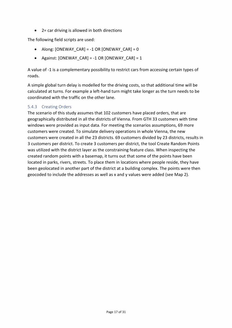
5.4.3 Creating Orders
The scenario of this study assumes that 102 customers have placed orders, that are
geographically distributed in all the districts of Vienna. From GTH 33 customers with time
windows were provided as input data. For meeting the scenarios assumptions, 69 more
customers were created. To simulate delivery operations in whole Vienna, the new
customers were created in all the 23 districts. 69 customers divided by 23 districts, results in
3 customers per district. To create 3 customers per district, the tool Create Random Points
was utilized with the district layer as the constraining feature class. When inspecting the
created random points with a basemap, it turns out that some of the points have been
located in parks, rivers, streets. To place them in locations where people reside, they have
been geolocated in another part of the district at a building complex. The points were then
geocoded to include the addresses as well as x and y values were added (see Map 2).

Page 18 of 31
Map 2: Creating orders
5.4.4 Creating Time Windows
Another preparation for the VRP concerns the modelling of time windows of customers.
Time windows are a way to indicate when the route/driver should arrive at that order
location. For the scenario hard time-windows were modelled, meaning that the route/driver
must show up during these designated time frames. A time window is considered violated if
the arrival time occurs after the time window has ended (ArcGIS Pro: VRP, n.d.).
Several types of time windows were modelled depending on the district (see Table 1 & Map
3). For the districts 1-9; 12; 15; 16, six distinct time windows with a 2-hour duration have
been modelled. Customers in these districts can choose any one of those time windows for
the delivery of the parcel. The different time windows were equally divided between the
customers and each district should not have more than one customer per time window. This
makes the scenario quite complex for the route planning.
Districts Time window Customers per time window (n)
1-9; 12; 15; 16 8:00 – 10:00 10
10:00 – 12:00 11
12:00 – 14:00 10
14:00 – 16:00 13

Page 19 of 31
Table 1: Time windows
For some districts time windows are merged (see Map 3). The decision on which districts to
merge was done on consultation with GTH. This is useful since these districts are larger in
area and customers can be much more spatially dispersed. Having time windows spread
over the whole day, would mean long travel distances for only a couple of customers. By
assigning a common time window for these districts, the routes should be accomplished
more efficiently and with shorter overall distance travelled.
The modelled time window per customer can be seen in the Table 9: Orders in the Appendix.
Map 3: Time windows per district
5.5 Modelling the Vehicle Routing Problem The factors, parameters and values that are modelled in the vehicle routing problem analysis
layer are presented in the following part. The modelling catalogue presents in more detail
how the assumed scenario for this study has been modelled (see Table 8: Modelling
catalogue in the Appendix). For each factor that should be considered in the route planning
the modelling catalogue presents on (1) what level this factor has been modelled in GIS, (2)
the operationalization, and (3) what value has been chosen. The following part is elaborating
on some of the modelled factors and parameters that need further explanation. The factors
are grouped in the categories: vehicles, drivers, breaks, parcels, customers, and depots.
Vehicles: The type of vehicle that is modelled in this study is an electric van used by GTH.
The van has a battery range of 180km and a cargo capacity of 3m3. To include these two
16:00 – 18:00 10
18:00 – 20:00 10
13; 14; 23 08:00-11:00 8
10; 11 11:00-14:00 9
17; 18; 19 14:00-17:00 11
20; 21; 22 17:00-20:00 10
102 = n-total

Page 20 of 31
factors in the route planning ensures that neither the vehicles capacity nor the battery range
is exceeded. Also modelling a certain vehicle type comes with vehicle-specific impedances
and restrictions for traversing the transport network.
Drivers: For the assumed scenario 5 drivers are modelled with 2 drivers working from 08:00 – 14:00 (6h), 2 drivers working from 14:00 – 20:00 (6h), and 1 driver working from 12:00-20:00 (8h) For limiting the working time to the working hours, the parameter values of MaxOrderCount in the route network analysis class were modelled with the working time in minutes. For the routes 1 to 4, the 6-hour work shifts, this is set to 360 minutes. Route five is the 8-hour afternoon shift with 480 minutes. The working shifts have fixed start and end times with no allowance for overtime. To consider the availability of drivers and the working schedules in the planning of routes is important for accurately allocating the orders to the drivers.
Breaks: In the vehicle routing problem analysis it is possible to store the rest periods of drivers that should be taken into account in the planning of routes. A break is associated with exactly one rote and can be taken after completing an order, while en route to an order, or prior to servicing an order. In this study, a time-window break was modelled, meaning that the break should begin within a delimited time range (ArcGIS Pro: VRP, n.d.). For the six-hour shifts, a 15-minute break was calculated to be taken within a time window of two hours. The window starts one and a half hours after the route has been started, meaning that the break can not be taken directly after departing from the depot, and similarly can not be taken just before ending the tour. For the eight-hour shift, a 30-minute shall be taken within a two-hour time window that starts two and a half hours after the start of the route. The starting time of the breaks can be violated by 30 minutes, modelled in the parameter MaxViolationTime. The break is paid, which is modelled by the parameter IsPaid. To include planned breaks in the route planning ensures that the driver can have a rest that is already accounted for in the planning. This ensures that factors such as working conditions can be considered in the route planning.
Parcels: In the assumed scenario every customer receives two parcels. For simplicity reasons
a uniform package size of 40x30x20cm is assumed. That translates to 0,024 m³ per package
in terms of volume. There is no definable number of how many customers can be serviced
by a route. This factor is rather limited by the quantity of orders and capacities of the
vehicle. Some shipments in last-mile delivery require a special infrastructure or special
qualification of the delivery staff. Two kinds of specialties have been modelled: refrigerated
parcels that need to be delivered by refrigerated vehicles; and drivers that have been trained
to meet the needs of certain customers. These specialties are modelled in the tables Order
Specialties and Route Specialties which link requirements of orders to routes that can meet
these requirements. The order “Location 75” is modelled as a refrigerated shipment and
should be only delivered by the refrigerated vehicle “Route 3”. Routes 1 & 2 are modelled as
trained for delivering the order to customer “Location 67”.
Customers: The service time at each customer is assumed to be 5 minutes. That includes the
walking time between vehicle and customer and the actual parcel handover time.
Depots: The routes are starting and ending at the GTH-hub depot in the outskirts of Vienna.
Before and after each route a service time at the depot is assumed with 10 minutes, which

Page 21 of 31
includes the time to load and unload parcels. That factor is important for the route planning
to define a start and end location for the routes as well as for planning time for preparation
before and after a route.
Route evaluation: To evaluate the costs of routes and drivers, several parameters have been
modelled. The fixed costs of 20€ for the vans per day were modelled in the field FixedCosts
of the Route class in the VRP. CostPerUnitTime refers to monetary cost incurred—per unit of
work time—for the total route duration, including travel times as well as service times and
wait times at orders, depots, and breaks (ArcGIS Pro: VRP, n.d.). This parameter reflects the
hourly salary of 15 Euros. Converted to the unit of the VRP minutes, this has been modelled
with 0.25€ per minute. For calculating the costs for tanking the vehicle, the parameter
CostPerUnitDistance has been modelled with 0,000067. This parameter represents the
monetary cost incurred—per unit of distance traveled (ArcGIS Pro: VRP, n.d.). The electric
cargo vans of GTH consume 20.93 kWh electricity on 100km. The price for a kWh for GTH
lays at 0.32€. That means that the costs of electricity for the cargo vans are 6,7€ per 100km.
This converts to 0,000067€ / m, which is modelled as the value for CostPerUnitDistance.
Evaluating the planned routes can account for strengths and weaknesses of the assumed
parameters.
After modelling all the relevant parameters described above, the VRP is ready to be solved
(see Map 4). Solving the modelled VRP layer will find the best solution to allocate the orders
to the modelled routes and produce output values.

Page 22 of 31
Map 4 VRP before calculating the routes
5.6 Limitations Increasingly important parameters in this study refer to criteria defined by the last-mile
delivery company GTH operating in Vienna. These parameters reflect the constraints and
requirements of this certain last-mile delivery operator and might not reflect criteria
identified by other operators.
The planning of routes with the vehicle routing problem is the method applied in this study.
This is accomplished by using GIS with the software ArcGIS Pro. ArcGIS Pro is just one out of
many software that allow the planning of routes for a fleet of vehicles (Rincon-Garcia et al.,
2018). The answering of the research question, which parameters can be reflected in the
planning of routes, is therefore limited to the capabilities of ArcGIS Pro. Conducting the
same study with another software might reveal that other parameters can be reflected in
the route planning. While this methodological choice is on the one hand a limitation, it can
also be seen as a contribution to the literature on the network analysis ArcGIS Pro. For

Page 23 of 31
example, creating network datasets was only possible after the release of ArcGIS Pro 2.5 in
June 2020 (ArcGIS Pro 2.5, n.d.).
A limitation of this study refers to the modelling of turns in the network dataset. A turn
models a movement from one edge element to another. Often turns are created to increase
the cost of making the movement or prohibit the turn entirely (ArcGIS Pro: Turns, n.d.). To
have accurate turn modeling contributes to more realistically simulate the road network and
ensure accurate analysis. This study does not include a turn feature source, as no
appropriate data has been found. To compensate that, a global turn delay has been
modelled that adds a fixed cost for turns in a certain direction.
Another limitation concerns the modelling of traffic. This study does consider traffic in the
planning of routes but not to the full potential. In this study rush-hour traffic and congestion
is accounted for by basing the impedance cost for traversing a road segment on the average
speed measured on these segments. To account for even more realistic travel times ArcGIS
Pro has the capability to model both historic and live traffic data. This study does not model
this kind of traffic data as no appropriate data source has been found. For some countries it
is possible to include traffic data by referencing the ArcGIS Online network dataset (ArcGIS
Pro: Network Coverage, n.d.). While this is approach is more favorable in terms of finding
appropriate traffic data, referencing the ArcGIS Online network dataset comes with other
modelling limitations. For example, the road network is provided by ArcGIS online, and can
not be manipulated. Furthermore, performing network analysis with the ArcGIS Online
network dataset uses credits (ArcGIS Pro: Online network dataset, n.d.). To consider time
dependent travel times in the form of traffic has been mentioned in the literature to be a
crucial parameter to include in the LMD route planning (Boysen et al., 2021). This is also one
of the relevant parameters mentioned by GTH. According to Rincon-Garcia et al. (Rincon-
Garcia et al., 2018, p. 130), not considering traffic in the route planning, might
underestimate the travel time with up to 10%.
6 Reuslts This chapter will present the results of modelling and running vehicle routing problem tool.
The result includes both the planned routes of the scenario, which is the main output of the
VRP, as well as possibilities and constraints faced in the modelling of the factors relevant to
last-mile delivery operations. That will answer the research question, to what extent the
increasingly important factors in the context of innovative last-mile delivery solutions can be
considered in the planning of routes.
6.1 Results related to orders The solution of the vehicle routing problem is the allocation of 100 orders to 5 different
routes (see Map 5).

Page 24 of 31
Map 5: Output of the VRP - The planned routes
Out of the 102 orders, 100 orders were successfully reached within their defined time-
windows. The two orders not reached are Location 53 and Location 59 with the time
windows 10:00 to 12:00 and 08:00 to 11:00 respectively. The reason for not reaching
location 53 is the hard time-window and that the total time for the other routes have been
exceeded, meaning having no time resources to visit it. Even though Route 3 and 5 have
been delivering to other orders in proximate distance, the working time of these routes and
the hard time window of location 53 resulted in the unsuccessful delivery (see Map 6).
Location 59 also could not be assigned due to a time window violation and the exceeded
total maximum travel time of other routes.
GTH defined the factor of setting priorities for certain customers as important in the
modelling of routes. For example, servicing premium customers should have a higher
importance than non-premium customers. In the VRP this factor can be modelled by
defining the relative importance of servicing orders. For this study all the orders have been
modelled with the same priority. For seeing the sequence in which the orders have been
serviced by each route, see the Table 9 in the Appendix.

Page 25 of 31
Map 6: Evaluation of unassigned order
The median distance to travel between two consecutive orders is 2.2 kilometers. The median
travel time between two consecutive orders is 9.7 minutes. These values differ slightly in the
inner-city districts (districts 3-9) where the travelled median distance to the consecutive
orders is 1,7km and 8.3 minutes. At 4 orders there is a waiting time, meaning that a route
must wait at the order for a time window to open. The combined wait time for all orders
sums up to 4 minutes and 32 seconds.
Decelerating and accelerating the vehicle before and after approaching the order as well as
time spent for parking is a time-consuming activity. With an average of 20 packages per
route, this activity takes 1 hour per route. One possibility to reduce this time is to service
proximate orders together, without returning to the vehicle. In the planned routes this was
once the case where Location 7 and 13 share the same time window and are located at the
same address.
One of the factors mentioned GTH by that would optimize the planning of routes is to have
information about the location of parking spots and the distance to customer. This can be
modelled in the VRP, however the results are not quite realistic. The output of the VRP
analysis indicates the location at the network graph where the vehicle has been parked. This
does not reflect actual possibilities to park in the real world. The VRP also indicates the
distance between the parking location and the actual location of the order defined by the
address. With further modelling this offers the possibility to account for the time needed to
walk between vehicle and customer.
The analyzed scenario simulated the delivery of refrigerated parcels of order Location 75
that were successfully delivered with the required refrigerated vehicle of Route 3. Another
factor to consider in the planning of routes are special requirements from the customers.
The scenario assumed that the customer (Location 67) requires to be serviced by specially
trained drivers (Route 1 or 2). This was successfully incorporated in the planning with Route
2 servicing the order Location 67.
The orders with both the input and output values created by the VRP analysis can be found
in Table 9 in the Appendix. This table also includes the modelled time windows for the
customers. Having templates for customers is one of the requirements mentioned by GREEN

Page 26 of 31
TO HOME that a routing software should offer. The order feature layer can be exported as
an Excel table and used as a template for customers. When planning new routes, the values
of the parameters can be adjusted in Excel, and the table can be imported to GIS. The table
needs to be geocoded to place the customers on the map. With the tool rematch addresses
it can be controlled if the addresses have been located correctly. After this process has been
completed the table can be imported to the VRP as an order feature layer with the modelled
values.
It is not possible to the authors knowledge to create a common database for customers,
drivers, cars and depots. All these factors are imported to the VRP from point- or line feature
layers or stand-alone tables.
6.2 Result Related to Routes The main output of the VRP are the routes planned for servicing the orders. The routes
calculated can be seen in Map 5. The scenario simulated an operational day with 5 available
drivers. It was possible to model the working shifts, per driver and to limit the working time
to these hours as presented in Table 2. Also, the specialties of the vehicles and drivers could
be modeled and successfully matched with the orders. All of the routes were assigned to at
least 17 orders, with all the 5 routes covering in total 100 stops. The amounts of orders
visited and the total traveled distance per route can be seen in Table 2. The Routes 1-4 with
6 hours working time travelled in average 74 km and are thereby far from the e-vehicles’
range of 180km. Given that, it was not necessary to include charging stations as a factor in
this scenario of the route planning. In any case, it was not possible to model charging
stations as an additional factor in the VRP. Another relevant factor for route planning
mentioned of GTH was the possibility to consider variations of the e-vehicle range according
to the seasons. Colder weather could affect the battery capacity and thereby reduce the
range of vehicles which in turn affects the number of orders that can be served. The range in
the VRP is modelled by a fixed value that is not season dependent.
Table 2: Overview of routes
Name Working schedule
Specialties Order Count Total distance travelled (in km)
Route 1 08-14 Trained driver 18 72.2 Route 2 08-14 Trained driver 21 68
Route 3 14-20 Refrigerated
vehicle 21 64
Route 4 14-20 - 17 93.7 Route 5 12-20 - 23 110.7

Page 27 of 31
The output of the VRP allows to evaluate the routes in terms of time. This evaluation of costs
per route is an important factor for last-mile delivery route planning, in order to optimize
future operations. The routes have been efficiently delivering packages with only 5 minutes
waiting time at customers due to not opened time windows. Also, the maximum possible
working time per route was almost used in every case (see Table 3). The output of the VRP
also reveals that approximately 60-65% of the total time is spent driving between orders.
The time spent servicing customers sums up to 25-30% of the total time (see Table 3)
Table 3: Evaluation of time
With the output values of the time spent driving and the driven distance per route, it is
possible to calculate the average driving speed of the vehicles (Table 4). The average speed
of the routes is 20,7 km/h. This cost for traversing the network results from the modelling of
the network dataset. In the network dataset the speed was referenced from a field in the
road data that indicates the average speed measured on the segments of the roads. The
result of the calculated average speed of the routes confirms that variations in the traffic
flows such as congestion could be taken into account in the planning of the routes.
Name km/h Average Travel Speed
Route 1 18,9347873
20,73763097
Route 2 19,7516304
Route 3 17,9224632
Route 4 24,7031221
Route 5 22,3761519 Table 4: Average travel speed
The live tracking of service time is not possible with the VRP in ArcGIS Pro. The VRP is a
deterministic tool to determine the route assignment and sequencing of orders (ArcGIS Pro:
VRP, n.d.). The tool is not used for the actual routing nor the collection of data. However, the
results of the VRP can be shared as a route layer in ArcGIS Pro that allows routing.
In terms of loaded quantity of parcels, it turns out that all of the vehicles are used far under
their cargo capacity. Not even 20% of the vehicles’ capacity was used (see Table 5). This
highlights that the challenge of last-mile delivery of e-commerce is not the quantity to be
delivered in terms of volume, but rather the large number of packages to individual
customers (Wang, 2021).
Service time (in min)
Time spent driving (in min)
Total time of route (in min)
% of total time used for servicing customers
% of total time used for driving
Route 1 90 229 354 25% 64%
Route 2 105 207 347 30 % 59%
Route 3 105 215 356 30 % 60%
Route 4 85 228 352 24 % 65%
Route 5 115 298 462 25 % 64%

Page 28 of 31
Name Loaded parcels
Parcel volume (in m3)
Capacity (in m3)
Capacity utilisation
Route 1 36 0,432 5 14,4 %
Route 2 42 0,504 5 16,8 %
Route 3 42 0,504 5 16,8 %
Route 4 34 0,408 5 13,6 %
Route 5 46 0,552 5 18,4 % Table 5: Loaded quantity of parcels and vehicle capacity
It was possible to calculate the breaks for each route (see Map 5). Table 6: Breaks shows that
it differs quite substantially at what time the breaks are planned. This is explained by the
flexible time window of two hours within the breaks should be taken. Furthermore, the VRP
places the breaks with consideration to the orders time window and the objective to fulfill as
many orders as possible.
RouteName Sequence of break Time until break is taken (in min)
Route 1 12 193
Route 2 9 129
Route 3 15 214
Route 4 7 113
Route 5 11 180 Table 6: Breaks
Restrictions
Realistic route planning needs to consider the various restrictions faced on the street
network. Oneway streets, pedestrian zones and regulations of the government can restrict
the access of vehicles to parts of the road network and can complicate the way to the
customers. Figure 4 shows that oneway roads could be successfully modelled. The value of
the field Oneway_car restricted the vehicle to access the last meters to the customers on the
road. The package could still be delivered, however by walking the last 123 meters.
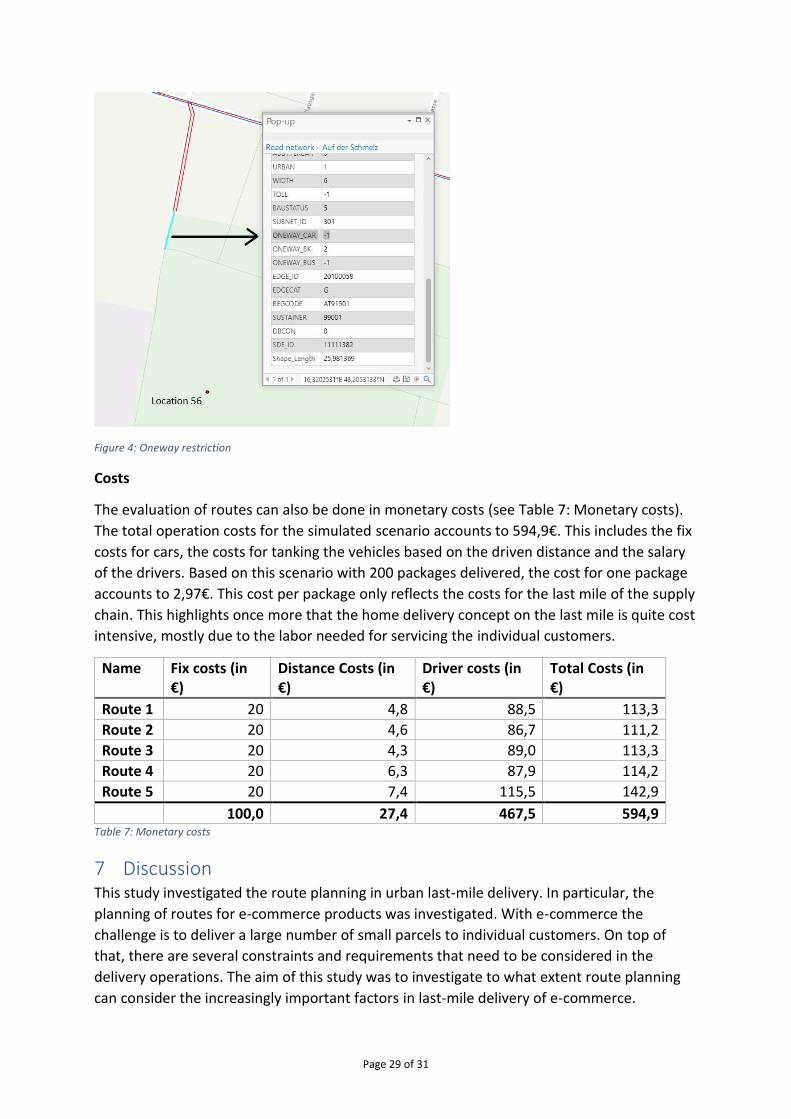
Page 29 of 31
Figure 4: Oneway restriction
Costs
The evaluation of routes can also be done in monetary costs (see Table 7: Monetary costs).
The total operation costs for the simulated scenario accounts to 594,9€. This includes the fix
costs for cars, the costs for tanking the vehicles based on the driven distance and the salary
of the drivers. Based on this scenario with 200 packages delivered, the cost for one package
accounts to 2,97€. This cost per package only reflects the costs for the last mile of the supply
chain. This highlights once more that the home delivery concept on the last mile is quite cost
intensive, mostly due to the labor needed for servicing the individual customers.
Name Fix costs (in €)
Distance Costs (in €)
Driver costs (in €)
Total Costs (in €)
Route 1 20 4,8 88,5 113,3
Route 2 20 4,6 86,7 111,2
Route 3 20 4,3 89,0 113,3
Route 4 20 6,3 87,9 114,2
Route 5 20 7,4 115,5 142,9 100,0 27,4 467,5 594,9
Table 7: Monetary costs
7 Discussion This study investigated the route planning in urban last-mile delivery. In particular, the
planning of routes for e-commerce products was investigated. With e-commerce the
challenge is to deliver a large number of small parcels to individual customers. On top of
that, there are several constraints and requirements that need to be considered in the
delivery operations. The aim of this study was to investigate to what extent route planning
can consider the increasingly important factors in last-mile delivery of e-commerce.

Page 30 of 31
7.1 Time Windows
One of the factors that are important to account for in last-mile delivery are time-windows.
The results of this study indicate that agreed time-windows with customers for the delivery
of parcels can be successfully considered in the planning of routes. The concept of time
windows reduces the risk of failed deliveries by ensuring that customers are home for
attended home-delivery, or to account for opening hours of commercial customers (Boysen
et al., 2021). In terms of route planning, hard time-windows add the complexity of delivering
an order within a certain time frame. The results of this study showed that the VRP could
account in 100 out of 102 cases for the time windows. A factor that contributed to meeting
all these time windows was to merge some of the districts in one shared time-window as
presented in Map 3. This was especially useful for the outer districts of Vienna that are larger
in area. The scenario analyzed in this study assumed only few and geographically dispersed
orders in those districts. The planned routes show that the orders in those districts could be
serviced consecutively by the same route. If hard time windows were assumed that spread
across the whole day, zigzag tours or even unsuccessful delivery would threaten (Boysen et
al., 2021). While these time windows increase the chance of successful delivery, their
practicality can be discussed out of the customers perspective. To combine time window-
based home delivery with the concept of parcel lockers could be interesting to look at
(Ranieri et al., 2018).
7.2 The potential of using cargo bikes
The results of this study shows that it is possible to account for parking in the planning of
routes and that this activity can take up considerable time of the delivery operations. Even
though it was possible to consider parking, it could not be modelled in a particularly realistic
way. This is due to the fact that the VRP in ArcGIS Pro parked the car at the closest point on
the street network to the order. It is unlikely that these positions reflect actual parking
possibilities. The result also shows that parking took on average one hour per route. Finding
parking spots is amongst the main on tour problems for home-delivery (Rincon-Garcia et al.,
2018). The utilisation of other types of vehicles, such as cargo bikes, could counteract this
problem. Cargo bikes have the advantage of being more flexible with parking, which is
especially relevant in congested city centres (Irnich et al., 2014). Another fact that could
favour the employment of cargo bikes in inner-city districts is the shorter travel distance
between consecutive stops. The results showed that in inner districts the median travel
distance is 33% lower than in the outer districts. This would definitely suggest to investigate
if bikes are more efficient in those areas due to a higher density of customers, as outlined by
Sheth et al. (2019).
7.3 Unused Vehicle Capacity & Return Packages
E-commerce articles, such as books, electronics or clothes, are usually small in size and
rather lightweight. The challenge faced in the delivery of e-commerce articles is that many
individual customers need to be serviced. The result of the analyzed scenario indicates that
not even 20% of the vehicles’ cargo capacity was used. While this is a problem due to unused
potential, there is an increasing need for first-mile delivery that could be addressed with this
capacity. The package return rate lays at about 40% in Austria. This is mostly due to the
product segment of clothes, in which almost every second package is returned
(Handelsverband Österreich, 2021). Innovative last-mile delivery solutions have already been

Page 31 of 31
reflecting on this fact and adapted the business concept to include pick-up of packages.
GREEN TO HOME is actually offering a pick-up service of return packages (GREEN TO HOME,
n.d.) This study has not been looking at this part of the supply chain, but given the unused
cargo capacity and the high return rate, this is definitely a factor to be looked at more
properly. However, this development highlights the need to critically think about the
consumption patterns.
8 Further Studies & Conclusion A factor that has not been properly touched upon in this study and that has gotten little
attention in research is the role of drivers. Factors such as working conditions, health and
safety issues as well as job satisfaction of drivers should be getting more attention in the
planning of routes (Dündar et al., 2021). Route planning is often reduced to the optimization
in terms of time and monetary costs. This instrumental view of workers in delivery is not
socially sustainable. The routes are still primarily planned for human drivers and should
therefore account for that.
Another factor to be investigated more thoroughly is the role of authorities and urban
planning in relation to last-mile delivery. The growth of the e-commerce sector is expected
to continue, which will require more transportation for e-commerce goods in cities. Policy
makers and urban players attempt to reduce the impact of transportation on cities by
imposing regulations and restrictions. These measures have an impact on the routing of last-
mile delivery. Measures that support sustainable last-miler delivery could be the planning of
infrastructure, such as separate lanes, e-charging stations and parking possibilities for cargo
bikes.
In conclusion it can be said that the factors to be considered in last-mile delivery route
planning are constantly developing. This study addressed the increasingly important factors
in the second decade of the 21st century. The challenges resulting of population growth,
urbanization and climate change will definitely develop the factors that are relevant to be
addressed in ten years from now.

32
9 References Adamec, V., Jedlička, J., Ličbinský, R., 2011. The Possibilities for Mitigating Negative Effects of
Transport. Trans. Transp. Sci. 4, 135–150. https://doi.org/10.2478/v10158-011-0012-x
Amazon, n.d. Amazon.com: [WWW Document]. URL https://www.amazon.com/-/de/Amazon-Prime-Air/b?ie=UTF8&node=8037720011 (accessed 4.28.22).
ArcGIS Pro 2.5, n.d. What’s new in ArcGIS Pro 2.5—ArcGIS Pro | Documentation [WWW Document]. URL https://pro.arcgis.com/en/pro-app/2.6/get-started/what-s-new-in-arcgis-pro-2-5.htm (accessed 5.10.22).
ArcGIS Pro: Geocoding, n.d. Convert a table to locations on the map—ArcGIS Pro | Documentation [WWW Document]. URL https://pro.arcgis.com/en/pro-app/2.8/help/data/geocoding/convert-a-table-to-locations-on-the-map.htm (accessed 5.9.22).
ArcGIS Pro: Network Coverage, n.d. Network analysis data coverage—ArcGIS Online Help | Documentation [WWW Document]. URL https://doc.arcgis.com/en/arcgis-online/reference/network-coverage.htm (accessed 5.10.22).
ArcGIS Pro: Network Analyst, n.d. What is the ArcGIS Network Analyst extension?—ArcGIS Pro | Documentation [WWW Document]. URL https://pro.arcgis.com/en/pro-app/2.7/help/analysis/networks/what-is-network-analyst-.htm (accessed 5.9.22).
ArcGIS Pro: Network dataset, n.d. What is a network dataset?—ArcGIS Pro | Documentation [WWW Document]. URL https://pro.arcgis.com/en/pro-app/2.7/help/analysis/networks/what-is-network-dataset-.htm (accessed 5.9.22).
ArcGIS Pro: Network elements, n.d. Network elements—ArcGIS Pro | Documentation [WWW Document]. URL https://pro.arcgis.com/en/pro-app/2.7/help/analysis/networks/network-elements.htm (accessed 5.9.22).
ArcGIS Pro: Online network dataset, n.d. Work with network analysis layers—ArcGIS Pro | Documentation [WWW Document]. URL https://pro.arcgis.com/en/pro-app/2.7/help/analysis/networks/new-network-analysis-layer.htm (accessed 5.10.22).
ArcGIS Pro: Rematch adresses, n.d. Rematch locations converted from a table—ArcGIS Pro | Documentation [WWW Document]. URL https://pro.arcgis.com/en/pro-app/2.8/help/data/geocoding/rematch-locations-converted-from-a-table.htm (accessed 5.9.22).
ArcGIS Pro: Turns, n.d. Turns in the network dataset—ArcGIS Pro | Documentation [WWW Document]. URL https://pro.arcgis.com/en/pro-app/2.7/help/analysis/networks/turns-in-the-network-dataset.htm (accessed 5.10.22).

33
ArcGIS Pro: VRP, n.d. Vehicle routing problem analysis layer—ArcGIS Pro | Documentation [WWW Document]. URL https://pro.arcgis.com/en/pro-app/2.7/help/analysis/networks/vehicle-routing-problem-analysis-layer.htm (accessed 5.9.22).
Boysen, N., Fedtke, S., Schwerdfeger, S., 2021. Last-mile delivery concepts: a survey from an operational research perspective. Spectr. 43, 1–58. https://doi.org/10.1007/s00291-020-00607-8
BRANCHENRADAR.com Marktanalyse GmbH, 2022. KEP-Dienste in Österreich 2022 | Branchenradar [WWW Document]. URL https://www.branchenradar.com/de/studien/dienstleistungen-und-konsum/kep-dienste-in-oesterreich-2022/ (accessed 5.6.22).
Dantzig, G.B., Ramser, J.H., 1959. The Truck Dispatching Problem. Manag. Sci., Management Science 6, 80–91. https://doi.org/10.1287/mnsc.6.1.80
data.gv.at, 2022. Intermodales Verkehrsreferenzsystem Österreich (GIP.at) Österreich - data.gv.at [WWW Document]. URL https://www.data.gv.at/katalog/dataset/3fefc838-791d-4dde-975b-a4131a54e7c5 (accessed 5.9.22).
data.gv.at, 2020. Bezirksgrenzen Wien - data.gv.at [WWW Document]. URL https://www.data.gv.at/katalog/dataset/stadt-wien_bezirksgrenzenwien (accessed 5.9.22).
Deng, Q., Fang, X., Lim, Y.F., 2021. Urban Consolidation Center or Peer‐to‐Peer Platform? The Solution to Urban Last‐Mile Delivery. Prod. Oper. Manag. 30, 997–1013. https://doi.org/10.1111/poms.13289
Dündar, H., Ömürgönülşen, M., Soysal, M., 2021. A review on sustainable urban vehicle routing. J. Clean. Prod. 285, 125444. https://doi.org/10.1016/j.jclepro.2020.125444
ESRI, n.d. About ArcGIS | Mapping & Analytics Software and Services [WWW Document]. URL https://www.esri.com/en-us/arcgis/about-arcgis/overview (accessed 6.2.22).
Gevaers, R., Van de Voorde, E., Vanelslander, T., 2014. Cost Modelling and Simulation of Last-mile Characteristics in an Innovative B2C Supply Chain Environment with Implications on Urban Areas and Cities. Procedia - Soc. Behav. Sci. 125, 398–411. https://doi.org/10.1016/j.sbspro.2014.01.1483
Global retail e-commerce market size 2014-2023, 2022. Statista [WWW Document]. Statista. URL https://www.statista.com/statistics/379046/worldwide-retail-e-commerce-sales/ (accessed 4.20.22).
GREEN TO HOME, n.d. GREEN TO HOME - Lösungen von morgen. Für die Paketzustellung von heute. [WWW Document]. URL https://www.greentohome.at/ (accessed 5.6.22).
Handelsverband Österreich, 2021. eCommerce-Studie-Oesterreich-2021 [WWW Document]. Handelsverband. URL

34
https://www.handelsverband.at/publikationen/studien/ecommerce-studie-oesterreich/ecommerce-studie-oesterreich-2021/?limit=all (accessed 5.6.22).
IMF, I.M.F., n.d. World Economic Outlook (April 2022) - GDP, current prices [WWW Document]. URL https://www.imf.org/external/datamapper/NGDPD@WEO (accessed 5.4.22).
Irnich, S., Toth, P., Vigo, D., 2014. Chapter 1: The Family of Vehicle Routing Problems, in: Toth, P., Vigo, D. (Eds.), Vehicle Routing. Society for Industrial and Applied Mathematics, Philadelphia, PA, pp. 1–33. https://doi.org/10.1137/1.9781611973594.ch1
Kim, G., Ong, Y.-S., Heng, C.K., Tan, P.S., Zhang, N.A., 2015. City Vehicle Routing Problem (City VRP): A Review. IEEE Trans. Intell. Transp. Syst. 16, 1654–1666. https://doi.org/10.1109/TITS.2015.2395536
Mobilitätsagentur, W., 2019. Mobilitätsreport Wien: 2019 15.
Montecinos, J., Ouhimmou, M., Chauhan, S., Paquet, M., Gharbi, A., 2021. Transport carriers’ cooperation on the last-mile delivery in urban areas. Transportation 48, 2401–2431. https://doi.org/10.1007/s11116-020-10134-8
Mucowska, M., 2021. Trends of Environmentally Sustainable Solutions of Urban Last-Mile Deliveries on the E-Commerce Market—A Literature Review. Sustainability 13, 5894. https://doi.org/10.3390/su13115894
Perboli, G., Rosano, M., Saint‐Guillain, M., Rizzo, P., 2018. Simulation–optimisation framework for City Logistics: an application on multimodal last‐mile delivery. IET Intell. Transp. Syst. 12, 262–269. https://doi.org/10.1049/iet-its.2017.0357
Petrovic, O., Harnisch, M.J., Puchleitner, T., 2013. Opportunities of mobile communication systems for applications in last-mile logistics, in: ICAdLT. IEEE, pp. 354–359. https://doi.org/10.1109/ICAdLT.2013.6568484
PostAG, n.d. Mail collection box - PostAG [WWW Document]. URL https://www.post.at/en/p/c/mail-collection-box (accessed 4.29.22).
Psaraftis, H.N., Wen, M., Kontovas, C.A., 2016. Dynamic vehicle routing problems: Three decades and counting. Networks 67, 3–31. https://doi.org/10.1002/net.21628
Ranieri, L., Digiesi, S., Silvestri, B., Roccotelli, M., 2018. A Review of Last Mile Logistics Innovations in an Externalities Cost Reduction Vision. Sustainability 10, 782. https://doi.org/10.3390/su10030782
Renaud, J., Laporte, G., Boctor, F.F., 1996. A tabu search heuristic for the multi-depot vehicle routing problem. Comput. Oper. Res. 23, 229–235. https://doi.org/10.1016/0305-0548(95)O0026-P

35
Rincon-Garcia, N., Waterson, B.J., Cherrett, T.J., 2018. Requirements from vehicle routing software: perspectives from literature, developers and the freight industry. Transp. Rev. 38, 117–138. https://doi.org/10.1080/01441647.2017.1297869
Sainato, M., 2021. 14-hour days and no bathroom breaks: Amazon’s overworked delivery drivers. The Guardian.
Schaefer, J.S., Figliozzi, M.A., 2021. Spatial accessibility and equity analysis of Amazon parcel lockers facilities. J. Transp. Geogr. 97, 103212. https://doi.org/10.1016/j.jtrangeo.2021.103212
Schmutzler, A., 2011. Local Transportation Policy and the Environment. Environ. Resour. Econ., Environmental & Resource Economics 48, 511–535. https://doi.org/10.1007/s10640-010-9447-5
Sheth, M., Butrina, P., Goodchild, A., McCormack, E., 2019. Measuring delivery route cost trade-offs between electric-assist cargo bicycles and delivery trucks in dense urban areas. Eur. Transp. Res. Rev. 11, 1–12. https://doi.org/10.1186/s12544-019-0349-5
Smith, A., 2020. Spatial Division of Labor, in: International Encyclopedia of Human Geography. Elsevier, pp. 387–393. https://doi.org/10.1016/B978-0-08-102295-5.10135-0
Stadt Wien, 2022. Zahlen und Fakten zum Wiener Straßennetz [WWW Document]. URL https://www.wien.gv.at/verkehr/strassen/fakten.html (accessed 5.6.22).
Stadt Wien, 2022a. Bevölkerungsstand Statistiken - Offizielle Statistik der Stadt Wien [WWW Document]. URL https://www.wien.gv.at/statistik/bevoelkerung/bevoelkerungsstand/ (accessed 5.6.22).
Transportstyrelsen, 2021. Trängselskatt i Göteborg - Transportstyrelsen [WWW Document]. URL https://www.transportstyrelsen.se/sv/vagtrafik/Trangselskatt/Trangselskatt-i-goteborg/ (accessed 4.28.22).
van Heeswijk, W., Larsen, R., Larsen, A., 2019. An urban consolidation center in the city of Copenhagen: A simulation study. Int. J. Sustain. Transp. 13, 675–691. https://doi.org/10.1080/15568318.2018.1503380
Visser, J., Nemoto, T., Browne, M., 2014. Home Delivery and the Impacts on Urban Freight Transport: A Review. Procedia Soc. Behav. Sci. 125, 15–27. https://doi.org/10.1016/j.sbspro.2014.01.1452
Wang, S., 2021. Retail geography. Routledge, New York, NY.
WKO, 2022. Lkw-Fahrverbot wegen Feinstaub in Wien und dem östlichen Niederösterreich [WWW Document]. URL https://www.wko.at/service/verkehr-betriebsstandort/LKW_Fahrverbot_wegen_Feinstaub_in_Wien,_Niederoesterreich_.html (accessed 5.6.22).

36
Zeiler, Michael., 2010. Modeling our world : the ESRI guide to geodatabase concepts, 2nd ed. ed. ESRI Press, Redlands, Calif.
Zitycity, n.d. Last-mile delivery: process deconstructed [WWW Document]. URL https://ziticity.com/blog/last-mile-delivery-why-choose-innovation-vs-tradition (accessed 6.2.22).

Page i
10 Appendix
10.1 A1: Modelling catalogue Table 8: Modelling catalogue
Factors to consider in route planning
Level of modelling
Operationalization Modelled parameter values
Vehicles Transport network & Route in VRP
Type of vehicle Transport Network & VRP Routes
Mode of transport; Costs; Routes in VRP
See Modelling the Network Dataset
Vehicle capacity VRP Routes RouteCapacity 3 m³
Range
VRP Routes MaxTotalDistance 180km
Range dependent on season (in km)
- - -
Drivers [Route]
Routes in VRP
Number of available drivers
VRP Routes Create new routes; Assignmnent Rule
5 drivers
Availabilities, shift schedule
VRP Routes EarliestStartTime; LatestStartTime; MaxTotalTime
See Scenario
Driver qualifications/specialties:
Route specialties; Order specialties
Link between: RouteName + SpecialtyName AND OrderName + SpecialtyName
Specialty Name: Trained; see scenario
Breaks for drivers Breaks in VRP
Fit with time windows of customers
VRP Breaks TimeWindow; ServiceTime; MaxViolationTime
See Modelling the Vehicle Routing Problem
Parcels
Orders in VRP
Capacity of parcels VRP Orders DeliveryQuantity1; DeliveryQuantity2
0,024 (package size in m3) ; 2 (number of packages)
Parcel specialties
Order specialties; Route specialties
Link between: OrderName + SpecialtyName AND RouteName + SpecialtyName
Specialty Name: Refrigerated; see Scenario
Customers Order in VRP

Page ii
Time windows per customer / opening times of business customers
VRP Orders TimeWindowStart; TimeWindowEnd; MaxViolationTime
See Creating Time Windows; MaxViolationTime= 0
Service time of customers (how long a delivery takes)
VRP Orders ServiceTime 5 (minutes)
Prioritization of customers
VRP Orders Revenue -
Contact details of customer:
VRP Orders Description Addresses
Information about preferred handover of parcel
VRP Orders Description -
Depots Depots in VRP
Save depot location and information
VRP Depots Name; description; TimeWindow
GTH main Hub modelled
Start depot of vehicle and driver
VRP Routes StartDepotName; EndDepotName
GTH main Hub
Set up of route-planning
Check if uploaded address from Excel is correctly located
Geoprocessing tool
Rematch Addresses See Data
Common database for customers, drivers/routes, car, depots, etc.
- - -
Templates for customers
VRP Orders Export orders as Excel table and manage data there
See A2: Orders
Vehicle routing
Include traffic data
Transport Network
Referencing ArcGIS Online network dataset
-
Vehicle type dependent restrictions for access of roads
Transport Network
Restrictions; Costs Based on fields in source data: Oneway_car; Average measured speed (Speedcar_T/B)
Time-dependent restrictions for access of roads
Transport Network
Restrictions Not modelled: no data found

Page iii
Information about the location of e-charging stations
Context features
- -
Information about the location of parking spots and distance to customers
VRP Orders DistanceToNetworkInMeters
Output value
Route evaluation Output fields of different VRP classes
Evaluation of driven routes
VRP Routes (Output fields)
TotalCost, RegularTimeCost, OvertimeCost, DistanceCost
See Reuslts
Service times: how long did the deliveries take?
• Parking (Place, Time)
• Distance/length of time from parking spot to customer
• Service time of parcel handover, e.g: delays
VRP Orders (Output)
FromPrevTravelTime; FromPrevDistance; WaitTime; ViolationTime
See Reuslts
Live tracking of service times
- - -

Page iv
Name Description ServiceTim
e
TimeWindow Start TimeWindow End MaxViolatio
nTime
Delivery
Quantity_1
Delivery
Quantity_2
Revenue Assignment
Rule
Route
Name
Sequence ViolatedConstr
aint_1
ViolatedConstr
aint_2
FromPrev
TravelTime
FromPrev
Distance (m)
Cumul
TravelTime
Cumul Distance
(m)
Cumul
Time
Arrive Time Depart
Time
Wait
Time
Violation
Time
Cumul
WaitTime
CumulViolati
onTime
DistanceToNetwor
kInMeters
Orders assigned to Route 1
Location 101 Dernjacgasse 19 ,1230 , Liesing , Wien 5 08:00:00 11:00:00 0 0,024 2 10 3 Route 1 2 9,5 3480 9,5 3480 25 08:19:33 08:24:33 0 0 0 0 8
Location 25 Schlöglgasse 4 ,1120 , Meidling , Wien 5 08:00:00 10:00:00 0 0,024 2 10 3 Route 1 3 11,3 3788 20,9 7269 41 08:35:52 08:40:52 0 0 0 0 7
Location 56 Auf der Schmelz W ,1150 , Rudolfsheim-Fünfhaus , Wien 5 08:00:00 10:00:00 0 0,024 2 10 3 Route 1 4 16,1 5295 36,9 12564 62 08:56:57 09:01:57 0 0 0 0 123
Location 52 Kirchstetterngasse 61 ,1160 , Ottakring , Wien 5 08:00:00 10:00:00 0 0,024 2 10 3 Route 1 5 7,8 1757 44,8 14321 75 09:09:47 09:14:47 0 0 0 0 7
Location 58 Flötzersteig 203 ,1140 , Penzing , Wien 5 08:00:00 11:00:00 0 0,024 2 10 3 Route 1 6 14,6 5255 59,3 19576 94 09:29:21 09:34:21 0 0 0 0 8
Location 61 Geylinggasse 27 ,1130 , Hietzing , Wien 5 08:00:00 11:00:00 0 0,024 2 10 3 Route 1 7 10,5 2162 69,8 21738 110 09:44:51 09:49:51 0 0 0 0 13
Location 62 Faistauergasse 53 ,1130 , Hietzing , Wien 5 08:00:00 11:00:00 0 0,024 2 10 3 Route 1 8 11,1 2334 80,9 24071 126 10:00:54 10:05:54 0 0 0 0 15
Location 63 Granichstaedtengasse 22 ,1130 , Hietzing , Wien 5 08:00:00 11:00:00 0 0,024 2 10 3 Route 1 9 10,5 2041 91,4 26113 141 10:16:23 10:21:23 0 0 0 0 4
Location 103 Maurer Lange Gasse 123 ,1230 , 23. Bezirk-Liesing , Wien 5 08:00:00 11:00:00 0 0,024 2 10 3 Route 1 10 13,7 3004 105,1 29117 160 10:35:03 10:40:03 0 0 0 0 5
Location 102 Elisenstraße 18 ,1230 , 23. Bezirk-Liesing , Wien 5 08:00:00 11:00:00 0 0,024 2 10 3 Route 1 11 12,5 3025 117,6 32143 178 10:52:35 10:57:35 0 0 0 0 5
Location 27 Albrechtsbergergasse 2 ,1120 , Meidling , Wien 5 10:00:00 12:00:00 0 0,024 2 10 3 Route 1 13 20,3 8066 137,9 40209 218 11:32:56 11:37:56 0 0 0 0 5
Location 57 Kürnbergergasse 3 ,1150 , Rudolfsheim-Fünfhaus , Wien 5 10:00:00 12:00:00 0 0,024 2 10 3 Route 1 14 6,1 957 144,0 41165 229 11:44:02 11:49:02 0 0 0 0 7
Location 88 Obere Amtshausgasse 27 ,1050 , Margareten , Wien 5 12:00:00 14:00:00 0 0,024 2 10 3 Route 1 15 10,7 2804 154,8 43969 245 11:59:45 12:05:00 0,25 0 0,25 0 8
Location 64 Unter-Meidlinger Straße 101 ,1120 , Meidling , Wien 5 12:00:00 14:00:00 0 0,024 2 10 3 Route 1 16 10,6 3280 165,3 47249 261 12:15:35 12:20:35 0 0 0,25 0 12
Location 23 Computerstraße 6 ,1100 , Favoriten , Wien 5 11:00:00 14:00:00 0 0,024 2 10 3 Route 1 17 9,4 3063 174,7 50312 275 12:30:00 12:35:00 0 0 0,25 0 14
Location 71 Graffgasse 22 ,1100 , Favoriten , Wien 5 11:00:00 14:00:00 0 0,024 2 10 3 Route 1 18 9,2 2837 183,9 53149 289 12:44:11 12:49:11 0 0 0,25 0 8
Location 70 Saligergasse 12 ,1100 , Favoriten , Wien 5 11:00:00 14:00:00 0 0,024 2 10 3 Route 1 19 13,1 3827 197,0 56976 307 13:02:18 13:07:18 0 0 0,25 0 8
Location 72 Franz-Mika-Weg 5 ,1100 , Favoriten , Wien 5 11:00:00 14:00:00 0 0,024 2 10 3 Route 1 20 13,2 3470 210,3 60446 326 13:20:31 13:25:31 0 0 0,25 0 139
Orders assigned to Route 2
Location 86 Stolberggasse 7 ,1050 , Margareten , Wien 5 08:00:00 10:00:00 0 0,024 2 10 3 Route 2 2 19,6 12330 19,6 12330 35 08:29:39 08:34:39 0 0 0 0 7
Location 94 Rennweg 31 ,1030 , Landstraße , Wien 5 08:00:00 10:00:00 0 0,024 2 10 3 Route 2 3 11,1 3154 30,8 15484 51 08:45:47 08:50:47 0 0 0 0 12
Location 24 Riemergasse 7 ,1010 , Innere Stadt , Wien 5 08:00:00 10:00:00 0 0,024 2 10 3 Route 2 4 9,8 2213 40,5 17696 66 09:00:32 09:05:32 0 0 0 0 8
Location 21 Zieglergasse 9 ,1070 , Neubau , Wien 5 08:00:00 10:00:00 0 0,024 2 10 3 Route 2 5 15,1 4316 55,7 22012 86 09:20:40 09:25:40 0 0 0 0 47
Location 13 Lerchenfelder Straße 125-127 ,1070 , Neubau , Wien 5 08:00:00 10:00:00 0 0,024 2 10 3 Route 2 6 7,6 1863 63,3 23876 98 09:33:15 09:38:15 0 0 0 0 10
Location 7 Lerchenfelder Straße 125-127 ,1070 , Neubau , Wien 5 08:00:00 10:00:00 0 0,024 2 10 3 Route 2 7 0,0 0 63,3 23876 103 09:38:15 09:43:15 0 0 0 0 10
Location 78 Laudongasse 57 ,1080 , 8. Bezirk-Josefstadt , Wien 5 08:00:00 10:00:00 0 0,024 2 10 3 Route 2 8 5,4 911 68,7 24787 114 09:48:41 09:53:41 0 0 0 0 7
Location 79 Bennogasse 3 ,1080 , 8. Bezirk-Josefstadt , Wien 5 10:00:00 12:00:00 0 0,024 2 10 3 Route 2 10 5,1 581 73,8 25368 139 10:13:48 10:18:48 0 0 0 0 6
Location 80 Kandlgasse 38 ,1070 , Neubau , Wien 5 10:00:00 12:00:00 0 0,024 2 10 3 Route 2 11 7,3 1461 81,1 26829 151 10:26:06 10:31:06 0 0 0 0 9
Location 14 Bernardgasse 6 ,1070 , Neubau , Wien 5 10:00:00 12:00:00 0 0,024 2 10 3 Route 2 12 6,0 851 87,1 27680 162 10:37:03 10:42:03 0 0 0 0 6
Location 8 Schottenfeldgasse 87 ,1070 , Neubau , Wien 5 10:00:00 12:00:00 0 0,024 2 10 3 Route 2 13 3,4 133 90,5 27813 170 10:45:30 10:50:30 0 0 0 0 9
Location 98 Schenkenstraße 8 ,1010 , Innere Stadt , Wien 5 10:00:00 12:00:00 0 0,024 2 10 3 Route 2 14 10,0 2195 100,5 30007 185 11:00:30 11:05:30 0 0 0 0 6
Location 41 Vereinsgasse 11A ,1020 , Leopoldstadt , Wien 5 10:00:00 12:00:00 0 0,024 2 10 3 Route 2 15 12,4 3389 112,9 33396 203 11:17:53 11:22:53 0 0 0 0 8
Location 87 Grüngasse 29 ,1050 , Margareten , Wien 5 10:00:00 12:00:00 0 0,024 2 10 3 Route 2 16 15,6 5095 128,5 38491 224 11:38:32 11:43:32 0 0 0 0 8
Location 19 Goldeggasse 8 ,1040 , Wieden , Wien 5 10:00:00 12:00:00 0 0,024 2 10 3 Route 2 17 11,0 3231 139,6 41721 240 11:54:33 11:59:33 0 0 0 0 7
Location 26 Schelleingasse 3 ,1040 , Wieden , Wien 5 12:00:00 14:00:00 0 0,024 2 10 3 Route 2 18 6,3 948 145,9 42669 251 12:05:54 12:10:54 0 0 0 0 10
Location 67 Lagerstraße ,1110 , 11. Bezirk-Simmering , Wien 5 11:00:00 14:00:00 0 0,024 2 10 3 Route 2 19 11,9 5996 157,8 48665 268 12:22:47 12:27:47 0 0 0 0 0
Location 68 Koblicekgasse 6 ,1110 , Simmering , Wien 5 11:00:00 14:00:00 0 0,024 2 10 3 Route 2 20 10,8 2742 168,6 51407 284 12:38:36 12:43:36 0 0 0 0 10
Location 1 Ewaldgasse 9 ,1110 , 11. Bezirk-Simmering , Wien 5 11:00:00 14:00:00 0 0,024 2 10 3 Route 2 21 10,3 2037 178,9 53444 299 12:53:56 12:58:56 0 0 0 0 10
Location 5 Ewaldgasse 7 ,1110 , Simmering , Wien 5 11:00:00 14:00:00 0 0,024 2 10 3 Route 2 22 3,0 4 181,9 53448 307 13:01:56 13:06:56 0 0 0 0 7
Location 2 Ewaldgasse 3 ,1110 , 11. Bezirk-Simmering , Wien 5 11:00:00 14:00:00 0 0,024 2 10 3 Route 2 23 3,4 123 185,4 53571 315 13:10:23 13:15:23 0 0 0 0 1
Orders assigned to Route 3
Location 10 Zieglergasse 7 ,1070 , Neubau , Wien 5 14:00:00 16:00:00 0 0,024 2 10 3 Route 3 2 24,2 14891 24,2 14891 39 14:34:10 14:39:10 0 0 0 0 52
Location 17 Zieglergasse 4 ,1070 , Neubau , Wien 5 14:00:00 16:00:00 0 0,024 2 10 3 Route 3 3 4,6 443 28,8 15334 49 14:43:46 14:48:46 0 0 0 0 69
Location 83 Windmühlgasse 6 ,1060 , Mariahilf , Wien 5 14:00:00 16:00:00 0 0,024 2 10 3 Route 3 4 7,0 1070 35,7 16404 61 14:55:43 15:00:43 0 0 0 0 8
Location 82 Karl-Schweighofer-Gasse 8 ,1070 , Neubau , Wien 5 14:00:00 16:00:00 0 0,024 2 10 3 Route 3 5 6,9 1086 42,6 17489 73 15:07:34 15:12:34 0 0 0 0 6
Location 100 Tiefer Graben 22 ,1010 , 1. Bezirk-Innere Stadt , Wien 5 14:00:00 16:00:00 0 0,024 2 10 3 Route 3 6 9,4 2178 52,0 19668 87 15:21:59 15:26:59 0 0 0 0 6
Location 73 Sensengasse 3A ,1090 , Alsergrund , Wien 5 14:00:00 16:00:00 0 0,024 2 10 3 Route 3 7 9,6 1846 61,5 21514 102 15:36:33 15:41:33 0 0 0 0 8
Location 32 Döblinger Hauptstraße 6 ,1190 , Döbling , Wien 5 14:00:00 17:00:00 0 0,024 2 10 3 Route 3 8 7,7 1840 69,2 23353 114 15:49:15 15:54:15 0 0 0 0 14
Location 51 Haslingergasse 20 ,1170 , Hernals , Wien 5 14:00:00 17:00:00 0 0,024 2 10 3 Route 3 9 10,7 3355 80,0 26708 130 16:04:57 16:09:57 0 0 0 0 5
Location 76 Fuhrmannsgasse 7 ,1080 , Josefstadt , Wien 5 16:00:00 18:00:00 0 0,024 2 10 3 Route 3 10 10,4 2064 90,3 28772 145 16:20:19 16:25:19 0 0 0 0 7
Location 18 Kandlgasse 5 ,1070 , Neubau , Wien 5 16:00:00 18:00:00 0 0,024 2 10 3 Route 3 11 8,1 1452 98,4 30225 158 16:33:25 16:38:25 0 0 0 0 7
Location 11 Neubaugasse 7 ,1070 , Neubau , Wien 5 16:00:00 18:00:00 0 0,024 2 10 3 Route 3 12 6,7 1026 105,1 31251 170 16:45:08 16:50:08 0 0 0 0 9
Location 84 Mittelgasse 5 ,1060 , Mariahilf , Wien 5 16:00:00 18:00:00 0 0,024 2 10 3 Route 3 13 8,7 1596 113,9 32847 184 16:58:52 17:03:52 0 0 0 0 6
Location 66 Steinbauergasse 31 ,1120 , Meidling , Wien 5 16:00:00 18:00:00 0 0,024 2 10 3 Route 3 14 9,7 2203 123,5 35049 199 17:13:33 17:18:33 0 0 0 0 13
Location 6 Musilplatz 5 ,1160 , Ottakring , Wien 5 16:00:00 18:00:00 0 0,024 2 10 3 Route 3 16 17,6 6324 141,1 41373 236 17:51:07 17:56:07 0 0 0 0 8
Location 53 Erdbrustgasse 56 ,1160 , Ottakring , Wien 5 10:00:00 12:00:00 0 0,024 2 10 3 2 5 5
Location 16 Musilplatz 4 ,1160 , Ottakring , Wien 5 18:00:00 20:00:00 0 0,024 2 10 3 Route 3 17 3,1 18 144,2 41391 245 17:59:11 18:05:00 0,82 0 0,817420129 0 8
Location 55 Stutterheimstraße 20 ,1150 , Rudolfsheim-Fünfhaus , Wien 5 18:00:00 20:00:00 0 0,024 2 10 3 Route 3 18 9,4 2556 153,6 43947 259 18:14:26 18:19:26 0 0 0,817420129 0 9
Location 75 Mariannengasse 27 ,1090 , Alsergrund , Wien 5 18:00:00 20:00:00 0 0,024 2 10 3 Route 3 19 10,1 3040 163,7 46988 275 18:29:32 18:34:32 0 0 0,817420129 0 6
Location 77 Wickenburggasse 3 ,1080 , 8. Bezirk-Josefstadt , Wien 5 18:00:00 20:00:00 0 0,024 2 10 3 Route 3 20 6,6 1042 170,3 48030 286 18:41:06 18:46:06 0 0 0,817420129 0 6
Location 20 Bernardgasse 5 ,1070 , Neubau , Wien 5 18:00:00 20:00:00 0 0,024 2 10 3 Route 3 21 8,6 1605 178,9 49635 300 18:54:42 18:59:42 0 0 0,82 0 5
Location 59 Satzberggasse 25 ,1140 , Penzing , Wien 5 08:00:00 11:00:00 0 0,024 2 10 3 2 5 10
Location 12 Kandlgasse 3 ,1070 , Neubau , Wien 5 18:00:00 20:00:00 0 0,024 2 10 3 Route 3 22 5,4 722 184,3 50358 310 19:05:08 19:10:08 0 0 0,82 0 7
Location 85 Brückengasse 8 ,1060 , Mariahilf , Wien 5 18:00:00 20:00:00 0 0,024 2 10 3 Route 3 23 9,6 2166 193,9 52523 325 19:19:42 19:24:42 0 0 0,82 0 7
Orders assigned to Route 4
Location 22 Franz Schubert-Gasse 3 ,2340 , Mödling , Niederösterreich 5 14:00:00 16:00:00 0 0,024 2 10 3 Route 4 2 13,6 5644 13,6 5644 29 14:23:39 14:28:39 0 0 0 0 11
Location 29 Franz Schubert-Gasse 4 ,2340 , Mödling , Niederösterreich 5 14:00:00 16:00:00 0 0,024 2 10 3 Route 4 3 3,0 5 16,7 5649 37 14:31:40 14:36:40 0 0 0 0 13
Location 65 Pottendorferstraße ,1120 , 12. Bezirk-Meidling , Wien 5 14:00:00 16:00:00 0 0,024 2 10 3 Route 4 4 23,2 15312 39,9 20961 65 14:59:55 15:04:55 0 0 0 0 76
Location 33 Keilgasse 8 ,1030 , Landstraße , Wien 5 14:00:00 16:00:00 0 0,024 2 10 3 Route 4 5 15,2 5704 55,2 26665 85 15:20:09 15:25:09 0 0 0 0 8
Location 89 Schelleingasse 26 ,1040 , 4. Bezirk-Wieden , Wien 5 14:00:00 16:00:00 0 0,024 2 10 3 Route 4 6 8,0 1809 63,2 28474 98 15:33:11 15:38:11 0 0 0 0 7
Location 90 Seisgasse 7 ,1040 , Wieden , Wien 5 16:00:00 18:00:00 0 0,024 2 10 3 Route 4 8 4,8 494 68,0 28968 125 15:58:01 16:05:00 1,98 0 1,98 0 9
Location 92 Dannebergplatz 15 ,1030 , Landstraße , Wien 5 16:00:00 18:00:00 0 0,024 2 10 3 Route 4 9 12,1 3172 80,1 32140 142 16:17:05 16:22:05 0 0 1,98 0 7
Location 43 Barawitzkagasse 27 ,1190 , Döbling , Wien 5 14:00:00 17:00:00 0 0,024 2 10 3 Route 4 10 20,9 8006 101,0 40146 168 16:42:58 16:47:58 0 0 1,98 0 14
Location 96 Robert-Blum-Gasse 1 ,1200 , Brigittenau , Wien 5 17:00:00 20:00:00 0 0,024 2 10 3 Route 4 11 10,2 2017 111,2 42163 185 16:58:12 17:05:00 1,80 0 3,77 0 8
Location 95 Helgolandgasse 12 ,1200 , Brigittenau , Wien 5 17:00:00 20:00:00 0 0,024 2 10 3 Route 4 12 7,1 1244 118,3 43407 197 17:12:05 17:17:05 0 0 3,77 0 9
Location 97 Vorgartenstraße 42 ,1200 , Brigittenau , Wien 5 17:00:00 20:00:00 0 0,024 2 10 3 Route 4 13 6,4 1115 124,7 44522 208 17:23:26 17:28:26 0 0 3,77 0 13
Location 30 Donaueschingenstraße 5 ,1200 , Brigittenau , Wien 5 17:00:00 20:00:00 0 0,024 2 10 3 Route 4 14 6,2 856 130,8 45379 220 17:34:36 17:39:36 0 0 3,77 0 12
Location 31 Am Tabor 7 ,1020 , Leopoldstadt , Wien 5 16:00:00 18:00:00 0 0,024 2 10 3 Route 4 15 7,8 1456 138,7 46834 232 17:47:26 17:52:26 0 0 3,77 0 12
Location 40 Hafnergasse 2 ,1020 , Leopoldstadt , Wien 5 18:00:00 20:00:00 0 0,024 2 10 3 Route 4 16 7,9 1414 146,6 48248 245 18:00:20 18:05:20 0 0 3,77 0 6
Location 91 Hoyosgasse 5 ,1040 , Wieden , Wien 5 18:00:00 20:00:00 0 0,024 2 10 3 Route 4 17 10,4 2882 157,0 51130 261 18:15:46 18:20:46 0 0 3,77 0 8
Location 93 Hörnesgasse 23 ,1030 , Landstraße , Wien 5 18:00:00 20:00:00 0 0,024 2 10 3 Route 4 18 11,2 3969 168,2 55098 277 18:31:56 18:36:56 0 0 3,77 0 7
Location 35 Bernhardinerallee ,1220 , 22. Bezirk-Donaustadt , Wien 5 17:00:00 20:00:00 0 0,024 2 10 3 Route 4 19 25,3 12931 193,5 68030 307 19:02:17 19:07:17 0 0 3,77 0 30
Orders assigned to Route 5
Location 42 Ausstellungsstraße 29 ,1020 , Leopoldstadt , Wien 5 12:00:00 14:00:00 0 0,024 2 10 3 Route 5 2 25,7 21333 25,7 21333 41 12:35:42 12:40:42 0 0 0 0 15
Location 99 Lothringerstraße 5 ,1010 , Innere Stadt , Wien 5 12:00:00 14:00:00 0 0,024 2 10 3 Route 5 3 11,5 3619 37,2 24952 57 12:52:10 12:57:10 0 0 0 0 33
Location 15 Bernardgasse 1 ,1070 , Neubau , Wien 5 12:00:00 14:00:00 0 0,024 2 10 3 Route 5 4 9,3 2554 46,5 27507 72 13:06:31 13:11:31 0 0 0 0 5
Location 81 Wimbergergasse 40 ,1070 , Neubau , Wien 5 12:00:00 14:00:00 0 0,024 2 10 3 Route 5 5 5,0 610 51,5 28117 82 13:16:31 13:21:31 0 0 0 0 8
Location 9 Lerchenfelder Straße 125-127 ,1070 , Neubau , Wien 5 12:00:00 14:00:00 0 0,024 2 10 3 Route 5 6 4,3 435 55,8 28552 91 13:25:48 13:30:48 0 0 0 0 10
Location 54 Roseggergasse 19 ,1160 , Ottakring , Wien 5 12:00:00 14:00:00 0 0,024 2 10 3 Route 5 7 9,6 3029 65,4 31580 105 13:40:27 13:45:27 0 0 0 0 10
Location 3 Musilplatz 5 ,1160 , Ottakring , Wien 5 12:00:00 14:00:00 0 0,024 2 10 3 Route 5 8 6,9 1121 72,4 32701 117 13:52:22 13:57:22 0 0 0 0 8
Location 4 Musilplatz 6 ,1160 , Ottakring , Wien 5 14:00:00 16:00:00 0 0,024 2 10 3 Route 5 9 3,1 20 75,4 32722 125 14:00:27 14:05:27 0 0 0 0 8
Location 104 Staargasse 53 ,1140 ,Penzing ,Wien 5 14:00:00 16:00:00 0 0,024 2 10 3 Route 5 10 10,9 2774 86,4 35496 141 14:16:24 14:21:24 0 0 0 0 7
Location 49 Promenadegasse 22 ,1170 , Hernals , Wien 5 14:00:00 17:00:00 0 0,024 2 10 3 Route 5 12 12,6 3557 107,6 41477 198 15:12:37 15:17:37 0 0 0 0 6
Location 50 Dornbacher Straße 61 ,1170 , Hernals , Wien 5 14:00:00 17:00:00 0 0,024 2 10 3 Route 5 13 7,4 1276 115,0 42752 210 15:25:02 15:30:02 0 0 0 0 9
Location 46 Wallrißstraße 71 ,1180 , Währing , Wien 5 14:00:00 17:00:00 0 0,024 2 10 3 Route 5 14 15,0 3266 130,0 46018 230 15:45:00 15:50:00 0 0 0 0 7
Location 48 Leschetitzkygasse 58 ,1180 , Währing , Wien 5 14:00:00 17:00:00 0 0,024 2 10 3 Route 5 15 7,2 1193 137,2 47211 242 15:57:13 16:02:13 0 0 0 0 3
Location 47 Pötzleinsdorfer Straße 91 ,1180 , Währing , Wien 5 14:00:00 17:00:00 0 0,024 2 10 3 Route 5 16 7,7 1348 144,9 48560 255 16:09:54 16:14:54 0 0 0 0 11
Location 44 Hutweidengasse 12 ,1190 , Döbling , Wien 5 14:00:00 17:00:00 0 0,024 2 10 3 Route 5 17 13,9 3220 158,9 51780 274 16:28:51 16:33:51 0 0 0 0 8
Location 45 Paul-Ehrlich-Gasse 13 ,1190 , Döbling , Wien 5 14:00:00 17:00:00 0 0,024 2 10 3 Route 5 18 8,9 1671 167,8 53452 288 16:42:47 16:47:47 0 0 0 0 5
Location 28 Gallmeyergasse 4 ,1190 , Döbling , Wien 5 14:00:00 17:00:00 0 0,024 2 10 3 Route 5 19 11,2 2329 179,0 55781 304 16:59:00 17:04:00 0 0 0 0 8
Location 74 Latschkagasse 10 ,1090 , Alsergrund , Wien 5 16:00:00 18:00:00 0 0,024 2 10 3 Route 5 20 9,6 1863 188,6 57644 319 17:13:37 17:18:37 0 0 0 0 9
Location 39 Anton-Störck-Gasse 78 ,1210 , Floridsdorf , Wien 5 17:00:00 20:00:00 0 0,024 2 10 3 Route 5 21 12,0 5824 200,6 63468 336 17:30:34 17:35:34 0 0 0 0 11
Location 38 Schippergasse 42 ,1210 , Floridsdorf , Wien 5 17:00:00 20:00:00 0 0,024 2 10 3 Route 5 22 13,6 4592 214,2 68059 354 17:49:12 17:54:12 0 0 0 0 11
Location 37 Morettigasse 3 ,1210 , Floridsdorf , Wien 5 17:00:00 20:00:00 0 0,024 2 10 3 Route 5 23 12,8 3761 227,0 71821 372 18:06:58 18:11:58 0 0 0 0 35
Location 36 Obachgasse 13 ,1220 , Donaustadt , Wien 5 17:00:00 20:00:00 0 0,024 2 10 3 Route 5 24 24,2 10081 251,2 81902 401 18:36:11 18:41:11 0 0 0 0 14
Location 34 Farngasse 26 ,1220 , Donaustadt , Wien 5 17:00:00 20:00:00 0 0,024 2 10 3 Route 5 25 17,3 5199 268,5 87101 423 18:58:29 19:03:29 0 0 0 0 7
10.2 A2: Orders Table 9: Orders