natural intelligence in artificial creatures - dca
TRANSCRIPT
Natural Intelligencein Artificial Creatures
––––––––––Christian Balkenius
Lund University Cognitive Studies 371995

First edition© 1995 by Christian Balkenius
All rights reserved. No part of this publication may be reproduced, stored in a retrieval sys-tem, or transmitted, in any form or by any means, electronic, mechanical, photocopying, re-cording or otherwise without the prior permission of the copyright owner, except by a re-viewer who may quote brief passages in a review.
Printed in Sweden by Lunds OffsetISBN 91-628-1599-7ISSN 1101-8453ISRN LUHFDA/HFKO--1004--SELund University Cognitive Studies 37

To my friends and enemies

Table of Contents
1. Introduction 92. Biological Learning 153. Design Principles 474. Reactive Behavior 795. Modeling Learning 1276. Motivation and Emotion 1617. Perception 1858. Spatial Orientation 2079. Cognition 227
10. Conclusion 245Appendices 261

Christian Balkenius, 1995, Natural Intelligence in Artificial Creatures, Lund University Cognitive Studies 37, 1995.
Chapter 1
Introduction
It is the goal of several sciences to construct models of behavior and cognition.Two fundamental questions for all such endeavors are: What mechanisms are re-quired to support cognitive processes in an animal or a robot. How do such mech-anisms interact with each other? This book is an attempt to study these questionswithin the field of behavior-based systems and artificial neural networks.
The overall task will be to construct complete, artificial nervous systems forsimulated artificial creatures. This enterprise will take as its starting point studiesmade of biological systems within ethology and animal learning theory. We willalso consider many ideas from neurobiology and psychology, as well as from be-havior-based robotics and control theory. All these areas have valuable insights tocontribute to the understanding of cognition.
Ethology has stressed the importance of innate fixed-action patterns, or in-stincts, in the explanation of behavior. Another significant contribution is the de-mand that behavior should be studied in the natural habitat of an animal. This leadsto a view of behavior and cognition which is very different from the one suggestedby animal learning theory. This latter theory attempts to understand the basis oflearning by observing the behavior of animals in laboratory experiments. It sug-gests a view of cognition that is complementary to that offered by ethology, sinceit stresses the role of learning rather than innate mechanisms. However, as moreempirical data become available, the models in both ethology and animal learningtheory gradually converge on what may become a substantially more unified theo-ry of animal learning and behavior.
10 – Introduction
Other important insights about the mechanisms of cognition are offered byneurobiology and psychology. The goal of neurobiology is to uncover the neuro-physiological mechanisms of the nervous system from the neural level and up.Much research within this tradition investigates the properties of individual neu-rons, however, but here we will mainly consider models at a system level. Suchmodels are closer to psychology where a number of relevant models can be found.In this book, we will consider results from both the behavioral and cognitive tradi-tions in psychology. Although we do not adhere to the views of the behavioral po-sition, much of the terminology we will use originates from that tradition. Howev-er, we will mainly look at phenomena typically studied in the more cognitiveapproach, such as expectancy, categorization, planning and problem solving.
From the engineering sciences we will borrow ideas from both behavior-basedrobotics and control theory. In many respects, behavior-based robotics is the coun-terpart of ethology within robotics. Many of the models within this area are verysimilar to those proposed in ethology. The important difference is, of course, thatbehavior-based robotics attempts to build working robots, and is not an attempt tostudy biological systems. A number of concepts from control theory will also beused in this book. The most important one is the view of an animal as engaged inclosed-loop interaction with the environment.
Somewhere in the middle of these fields is cognitive science with the ambitionto cut across the boundaries of these more traditional approaches (Norman 1990).The present book is such an attempt to combine ideas from all these different are-as.
This book has three goals. The first is to identify the systems required in a com-plete, artificial creature. We will argue that such a creature requires a large set ofinteracting systems. Some of these are fixed, while others must include differenttypes of learning mechanisms. Our main task will be to identify these systems,rather than give any final solutions to their operation. We will, however, take careto construct fully working miniature models of all the proposed systems.
The second goal is to investigate how the different systems should interact witheach other to make the overall behavior of the creature consistent. Many differentmodels have been proposed in the various areas we will consider, and our attemptwill be to make an inventory of these different mechanisms. Again, we will pro-pose a number of fully worked out mechanisms.
Finally, we want to map out the way for more cognitive abilities, such as plan-ning and problem solving. We believe that an overall emphasis on the concept ofexpectations will promote a transition to such abilities.
In taking a design perspective to animal behavior and learning, we will considerhow to construct systems that produce sensible coherent behavior rather than try toexplain behavioral data. If successful, this approach should give us insights aboutwhy real animals are constructed as they are. This requires that the components ofthe model are developed to a level where they can successfully operate together.
Introduction – 11
The model proposed here will be based on a large set of findings within animallearning theory, but our goal is not to settle any disputes about animal learning orbehavior. Instead, the aim of this book is to construct a set of mechanisms thatreflect those found in biological systems. The goal is, thus, to find a consistentmodel of a complete creature. Since the model we will propose is computational,consistency will always be the prime condition, and agreement with empirical dataonly a secondary requirement. Of course, this does not mean that we will ignoreempirical data, but it will not be ultimately constraining. The creatures developedwill, in fact, be mostly based on empirical findings, although it is necessary to sim-plify many details in order to get the overall system to function.
Even though it would obviously be interesting to try to emulate neurophysiolog-ical and behavioral data more closely, the current knowledge of the brain makessuch an endeavor very difficult, even for a very restricted sub-system. To constructan entirely realistic model of a complete nervous system based on our currentknowledge is clearly impossible. The proposed model can, thus, be compared toreal nervous systems on a functional level only. We believe, however, that thefunctional sub-systems we propose must have parallels in real nervous systems. Acomplete model of a creature can, therefore, be of great use in two areas.
The first is in the study of biological systems where it can be used both to sug-gest mechanisms to look for, and to give an understanding of the number of sys-tems interacting with each other. We hope the model proposed in this book willgive the overall picture that is often missing when specific abilities or systems arediscussed. It should be kept in mind, however, that this book deals primarily withartificial creatures, and as such, it cannot give us any direct model of any particularreal animal. Such questions are better handled by empirical studies.
The second area where the model can be used is within autonomous systems.Since the model is detailed enough to be implemented in a computer, it can alsopotentially be adapted for robotic control. This would very likely require manychanges within low level aspects of the model, but the overall structure would bethe same. The presented model can, thus, be seen as a framework for an autono-mous agent.
Since it is the overall picture that is our interest, we will try to use as few math-ematical concepts as possible, in order to make the text more comprehensible. For-mal specifications of all systems are given in the appendices, although there islittle formal treatment of the model. Such an analysis would, of course, be interest-ing, but is not the primary goal of this book. The reported simulations will, thus,have to serve both as examples, and as proof of the performance of the system.
Chapter 2 presents an overview of the different problems that have to be solvedin order to construct a model of a complete creature. The emphasis will be on var-ious results from animal learning theory. The goal of this chapter is to show that ageneral learning system is not realistic from a biological perspective. We will ar-gue that biological systems use many interacting systems for different abilities,
12 – Introduction
and the conclusion will be that it is necessary to take this into account if we wantto produce an artificial system with similar abilities. This chapter is, thus, intendedboth as a presentation of the biological background and as an attempt to set thegoal for the model we will be developing in the remaining chapters.
Chapter 3 gives a background to the design principles that will be used in theconstruction of the model. We will briefly review a number of ideas from behav-ior–based robotics and discuss how they can be used to constrain the design of ar-tificial creatures. It is argued that the basic building block for artificial creaturesshould be the behavior module , which represents a particular mapping from sen-sors to effectors, that is, a particular control strategy. It is suggested that behaviormodules can be combined into hierarchies called engagement modules , each ofwhich controls one particular task of the creature. We also introduce the type of ar-tificial neural network that is used for the artificial nervous systems of our crea-tures. The chapter concludes with a concrete example of an artificial creaturewhich illustrates how neural networks can be used to control a simple body in asimulated environment.
Chapter 4 initiates the development of the model. We present a taxonomy ofdifferent reactive behaviors and a number of elementary components that can beused to construct them. We first discuss the directedness of behavior and identifyfour general categories of behavior. Appetitive behavior is directed toward an at-tractive object or situation. Aversive behavior is directed away from negative situ-ations. Exploratory behavior is directed toward stimuli that are novel in the envi-ronment. Finally, we describe a class of neutral behaviors relating to objects thatare neither appetitive nor aversive. This classification is a step away from a singlehedonic dimension and it gives a richer framework for understanding reactive be-havior. It becomes possible to distinguish between active avoidance used for es-cape, passive avoidance used to inhibit inappropriate behavior, and neutral avoid-ance used to negotiate obstacles. The new classification also captures thedifference between exploratory and appetitive behavior in a natural way. Wefinally present a number of ways in which behavior modules can be coordinatedboth sequentially and in parallel. The chapter concludes with an example of anelementary reactive repertoire for our model creature.
Chapter 5 discusses how adaptation can be included within and betweenengagement modules to coordinate which behavior modules should be activated orinhibited. Starting from the two classical types of learning: instrumental andclassical conditioning, we present a new real-time model of conditioning that canbe used for both types of learning. The model combines many properties of earliertwo-process models of conditioning (Mowrer 1960, Gray 1975, Klopf 1988), buthas the additional ability to distinguish between appetitive, aversive, neutral andunknown situations. It can, thus, select between the different types of behaviorsdescribed in chapter 4. The model also shares many properties with other rein-
Introduction – 13
forcement learning techniques, such as Q-learning (Watkins 1990) and temporal–difference learning (Sutton and Barto 1990). We will describe how the proposedlearning system can model a number of experimental situations, including delayand trace conditioning, backward conditioning, extinction, blocking, overshadow-ing, and higher-order conditioning. We also give a number of examples of how itcan be used within an engagement system for appetitive and aversive learning, forsequential behavior chaining, and for the learning of expectations. The general ob-servation will be that learning should be triggered by a mismatch between the ex-pected and actual sensory state of the system.
Apart from learning, behavior is also influenced by motivation. This concept isdiscussed in chapter 6, where it is identified with a central system for behavior se-lection. This system is based on the classical notions of drives (as internal needs)and incentives (as external possibilities) (Hull 1952). We identify the classes ofexternal incentives which are based on directly perceivable goals and internal in-centives derived from stimuli that only predict the goal. These incentives can beeither primary, that is, innate, or secondary, that is, acquired using the learningmechanisms described in chapter 5. The motivational system combines informa-tion about these factors to form a decision about what the creature should do.
We develop a new model of action selection based on the view of the motiva-tional state as a transient representation of the currently most favored behaviorrather than as a fixed goal representation. In this model, motivational competitionallows the creature to rapidly switch between different engagements while thepositive feedback-loop set up by the incentive mechanism avoids behavioral oscil-lation. Within this framework, it is possible to interpret emotions as states pro-duced by reinforcing stimuli (Rolls 1990). We will argue that motivational stateshave the function of telling the creature what it should do, while emotions tell thecreature what it should have done. The conclusion will be that the concepts of mo-tivation and emotion must play a central role in a cognitive theory.
In chapter 7, we investigate categorical learning and its relation to perception.We will argue that the role of categories is to reduce the complexity of the per-ceived world by generating orthogonal representations for similar sensory patternswhen needed. This allows expectations to be added together in a straight-forwardway. As in chapter 5, learning will be driven by different mismatch conditions. Wewill identify three situations in which it is necessary to construct new categories.In the first situation, none of the existing categories match the external stimulussituation sufficiently well. In the second case, the creature does not receive the ex-pected reward and, thus, needs a better representation of the situation. Finally,there is the more general case when expectations of the environment are not suffi-ciently fulfilled. It is shown that when this categorization mechanism is added, thecreature can learn the higher-order expectations which are required in negativepatterning experiments. We also present a simple model for place-approach which
14 – Introduction
can learn a generalization surface around a goal. This surface can in turn be usedto guide the locomotion of the creature when the goal is not directly perceivable.This chapter finally describes how exploration can be driven by unfulfilled expec-tations. Novel and omitted stimuli in the environment trigger exploratory behaviorwhich helps the creature learn about the new state of the world. By using behaviormodules for place-approach, the creature can investigate the location where a stim-ulus used to be before it was removed.
In chapter 8, we will investigate learning and relearning of behavioral sequenc-es using different types of elementary behaviors and learning mechanisms. Weshow how the systems proposed earlier in the book can be used to solve problemsin the spatial domain. Perceptual categorization is combined with behavior chain-ing to enable the creature to learn a simple maze. A neural network architecture isproposed which uses recurrent expectations to make local choices about what be-havior to perform. This system is able to solve shortcut and detour problems andcan be said to organize a cognitive map. We finally propose that procedural andexpectancy learning is related to the distinction between implicit and explicitmemory.
Chapter 9 discusses how the mechanism presented earlier could possibly be ex-tended to handle more advanced cognitive abilities such as multi-modal categori-zation, association and generalization. We will sketch how these abilities can beused as a basis for an internal environment, which in turn makes planning andproblem solving possible. With the proposed extensions of the model, planningand problem solving become truly emergent properties since there is no distinctplanning module within the system. The chapter concludes with a brief discussionof the relation between motivation, emotion and planning.
Finally, chapter 10 presents an overview of the proposed model and shows howthe various components can interact with each other in different ways. We alsodiscuss the model from an evolutionary perspective and compare the various sys-tems with functions suggested as residing in different areas of the brain. The con-cluding section discusses some theoretical and practical limitations of the modeland presents directions for further research.
Christian Balkenius, 1995, Natural Intelligence in Artificial Creatures, Lund University Cognitive Studies 37, 1995.
Chapter 2
Biological Learning
2.1 IntroductionIt was once taken for granted that learning in animals and man could be explainedwith a simple set of general learning rules, but over the last hundred years, a sub-stantial amount of evidence has been accumulated that points in a quite differentdirection. In animal learning theory, the laws of learning are no longer consideredgeneral. Instead, it has been necessary to explain behavior in terms of a large set ofinteracting learning mechanisms and innate behaviors. Artificial intelligence isnow on the edge of making the transition from general theories to a view of intel-ligence that is based on an amalgamate of interacting systems. In this section wewill argue that in the light of the evidence from animal learning theory, such atransition is to be highly desired.
For many years, researchers within both animal learning theory and artificial in-telligence have been searching for the general laws of learning. We want to pro-pose that such laws cannot be found for the simple reason that they do not exist.Below, we will give a number of different examples of classical experiments thathave shown that a number of mechanisms are involved in learning, none of whichis general enough to suffice in all situations. Any attempt to construct artificial in-telligence based on one or a few simple principles is thus bound to fail.
The classical strategy in artificial intelligence has been to depend either on anaxiomatic system as in the logical tradition (Charniak and McDermott 1985) or tobase all intelligence on a simple principle such as chunking (Newell 1990). In both
16 – Biological Learning
cases, the problem of intelligence is reduced to that of searching (cf. Brooks1991). The problem of search control is, however, still mainly unsolved and, as wewill argue below, will remain so unless artificial intelligence makes the transitioninto a more diversified view of intelligence.
Before starting, we would like to make a few remarks on our use of the notionsof learning and intelligence. Both terms are, of course, exceedingly vague and wewill make no attempt to change that situation. We have, nevertheless, some intui-tive appreciation of the meaning of the two concepts and no harm can come fromsubjecting them to closer examination1.
Konrad Lorenz defined learning as adaptive changes of behavior and that is in-deed the reason for its existence in animals and man (Lorenz 1977). However, itmay be too restrictive to exclude behavioral changes which are not adaptive. Thereare in practice, many behavioral changes that we would like to call learning al-though they are not at all adaptive. We should not forget, however, that these in-stances of learning are more or less parasitic on an ability that was originally con-structed to control adaptive changes. Hence, it seems reasonable to considerlearning as a change in behavior that is more likely than not to be adaptive.
Next, we turn to the concept of intelligence. Behavior is usually considered in-telligent when it can be seen as adaptive. An animal is considered intelligent whenwe can see how its behavior fulfils its present or future needs. A squirrel that hidesnuts in apparent anticipation of the winter is thought of as more intelligent than alemming that throws itself over a cliff. But when we learn that the squirrel willcontinue to collect nuts even when it has hidden infinitely more than it can possi-bly eat over winter, we begin to question its intelligence. Eventually, we find outthat it does not even remember where it has hidden its winter supply, and the casefor squirrel intelligence is settled.
This example shows that we call behavior intelligent only when we see how thatbehavior is adaptive for the animal. This is precisely the idea that “intelligence isin the eyes of the beholder” (Brooks 1991a). We should not, however, be temptedto believe that intelligence is only in our eyes. If we change the environment of theanimal in such a way that its initial behavior is no longer adaptive, we can make aninteresting observation. If the animal persists in its original behavior, we no longerconsider it intelligent. If it, on the other hand, changes its behavior to adapt it tothe new circumstances, we will still think of it as intelligent in some sense. In ouropinion, this perspective makes intelligence equivalent to the capacity of learning.
1. It is with some hesitation we introduce a concept such as intelligence. While it was oncea required ingredient of any text on learning, its use today is more often than not considereda mortal sin.

2.2 The Legacy of Behaviorism – 17
2.2 The Legacy of BehaviorismDuring the reign of behaviorism it was habitually taken for granted that all behav-ior could be explained in terms of stimulus–response (S–R) associations. Based onthis assumption, innumerable experiments were conducted with one single goal inmind: to establish the general rule for S–R formation. Once this rule was discov-ered, we would know everything there was to know about learning.
Following this line of thought, it seemed reasonable to simplify the learning sit-uation as much as possible until only the essential core of the task was left. In theearly experiments, researchers were using a small copy of the garden maze atHampton Court for their animals (Small 1901). This maze turned out to be muchtoo complex2 and as time went on the mazes became more and more simple untilthe development culminated in the ingenious Skinner box. This device was entire-ly devoid of any behavioral possibilities except for bar pressing. While the animalin the Hampton Court Maze could perform a large number of actions, the rat in theSkinner box could do only one of two things; either it could press a lever and re-ceive food or it could refrain from doing so.
One may object that there are many ways to press the lever and even more waysto refrain, but all these cases were conveniently lumped together using operationaldefinitions of the two cases. It was the movement of the lever that counted as a re-sponse not the movement of the animal. Hence the name operant learning proce-dure.
Based on the fundamental belief that all behavior in all species could be ex-plained in terms S-R associations, it was entirely immaterial for the behavioristswhether they would study rats in the Skinner box or humans learning universitymathematics. The process involved would be the same. Of course, it was muchmore practical to study rats in the laboratory and that is how the research proceed-ed.
One may ask whether the animals had any choice other than to learn an S–R as-sociation? What else was there to learn? The experimentalists had removed all oth-er possibilities of learning based on the presupposition that they did not exist. Con-sequently, they had eliminated all possibilities of disproving their underlyingassumption. Years of effort were devoted to the simplest form of learning conceiv-able. It is the irony of the whole approach that we still, almost 100 years afterPavlov’s and Thorndike’s initial experiments, do not know exactly what rules gov-ern the formation of the supposed S–R association.
2. Too complex for the researchers, that is, the animals did not have any trouble. In fact,when rats are given a choice, they prefer to explore complex mazes instead of simple ones.
18 – Biological Learning
2.3 There is Nothing General about LearningWhat would happen if we arranged for other types of learning than pure stimulus–response formation? What if we construct tasks where learning of simple associa-tions does not suffice? Let us look at some experiments.
One of the very first experiments to question the view that responses werelearned was conducted by MacFarlane in 1930. He trained rats to swim in a mazein order to obtain food placed on a goal platform. When the rats had learned theirway in the maze, it was drained of water and the rats were again placed in the startbox. It turned out that they could still approach the goal with almost no errors eventhough they were now running instead of swimming.
Whatever they had learned, it could not have been the response of performingsome specific swimming motion associated with the stimuli at each place in themaze. According to Tolman, the rats had not learned a series of responses but in-stead the spatial layout of the maze. This ‘cognitive map’ could then be used to getfrom the start to the goal in any of a number of ways. While this experiment cer-tainly shows that something more abstract than a S–R association was learned, wecannot resolve the question as to whether it is anything like a cognitive map or not.For this, we need more evidence.
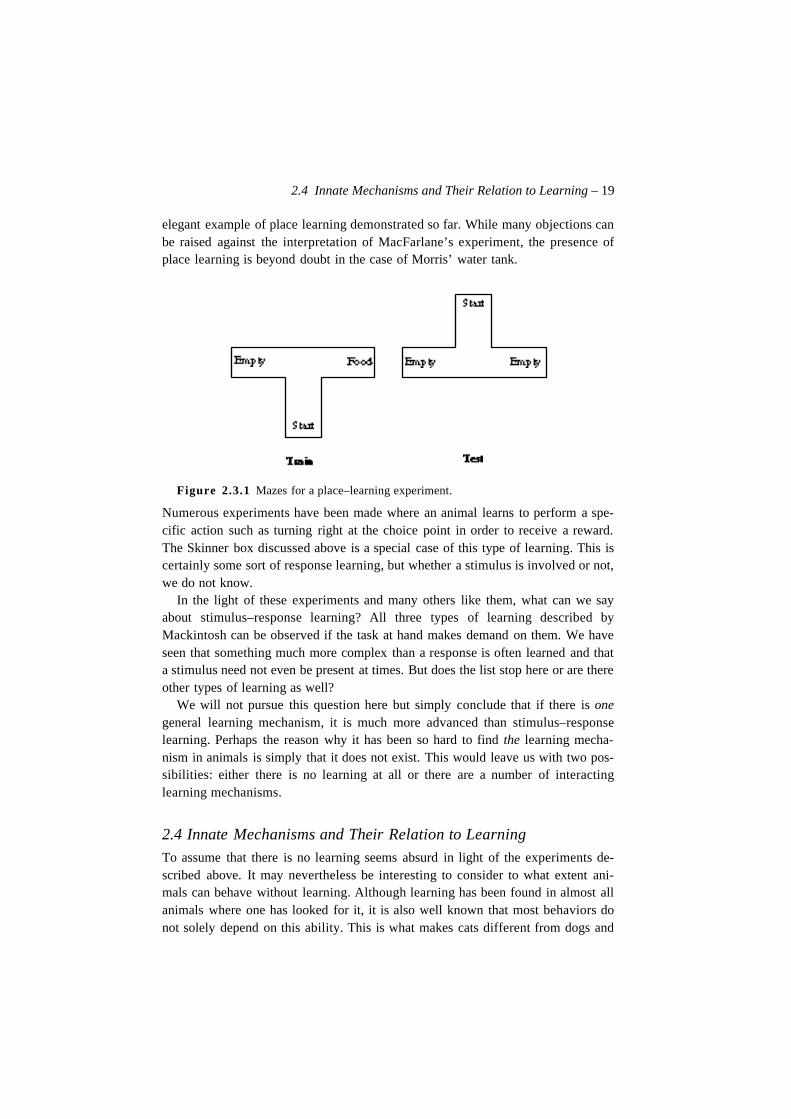
Another of MacFarlane’s experiments was again supposed to show that animalslearn a map of the maze and not a response chain. In this experiment, animals weretrained to find a goal box in a simple T–maze. Once the rats had learned the placeof the food, the maze was turned 180° and the food removed as shown in figure2.3.1. As a result, the arms of the maze were interchanged. If the rats had learnedto make the response of turning right at the choice point, they would continue to doso even after the maze was turned. If they, on the other hand, had learned the spa-tial location of the food they would now turn to the left. And so they did. Again itcould not have been the response that had been learned.
It has later been shown that under some circumstances the rats will continue toturn right. The important observation made is that in some cases, a place strategyis clearly within the ability of rats.
Mackintosh (1983) distinguishes between three types of possible learningmechanisms in simple T–mazes. If the two arms of the maze are physically differ-ent, the animal can use this difference to associate the correct arm with the food. Ifthe two arms are identical, a place learning strategy could be used instead, as in theMacFarlane experiment. Finally, if no cues at all are available, say if the maze isplaced in a dark room, the animal could learn simply to turn in the correct directionat the choice point.
Morris (1981) has shown that rats can learn to swim toward a platform hidden inopaque water although there is no visual stimulus to approach. In this case, the an-imals obviously use a place strategy. Somehow various stimuli in the room areused to identify the position of the hidden platform. This is perhaps the most
2.4 Innate Mechanisms and Their Relation to Learning – 19
elegant example of place learning demonstrated so far. While many objections canbe raised against the interpretation of MacFarlane’s experiment, the presence ofplace learning is beyond doubt in the case of Morris’ water tank.
Figure 2.3.1 Mazes for a place–learning experiment.
Numerous experiments have been made where an animal learns to perform a spe-cific action such as turning right at the choice point in order to receive a reward.The Skinner box discussed above is a special case of this type of learning. This iscertainly some sort of response learning, but whether a stimulus is involved or not,we do not know.
In the light of these experiments and many others like them, what can we sayabout stimulus–response learning? All three types of learning described byMackintosh can be observed if the task at hand makes demand on them. We haveseen that something much more complex than a response is often learned and thata stimulus need not even be present at times. But does the list stop here or are thereother types of learning as well?
We will not pursue this question here but simply conclude that if there is onegeneral learning mechanism, it is much more advanced than stimulus–responselearning. Perhaps the reason why it has been so hard to find the learning mecha-nism in animals is simply that it does not exist. This would leave us with two pos-sibilities: either there is no learning at all or there are a number of interactinglearning mechanisms.
2.4 Innate Mechanisms and Their Relation to Learning
To assume that there is no learning seems absurd in light of the experiments de-scribed above. It may nevertheless be interesting to consider to what extent ani-mals can behave without learning. Although learning has been found in almost allanimals where one has looked for it, it is also well known that most behaviors donot solely depend on this ability. This is what makes cats different from dogs and
20 – Biological Learning
mice different from men. At this point, we must enter the area of species–specificbehavior.
Such behaviors are perhaps most well known through the use and abuse of theword instinct. Everything specific to a species was once called an instinct. Eventu-ally the concept was extended to explain all animal behavior and was at the sametime rendered meaningless. A more useful concept is that of innate releasingmechanisms as introduced by Tinbergen and Lorenz.
A classic example of such a mechanism, originally from von Uexküll, is the bitereaction of the common tick (Ixodes rhicinus). As described in Lorenz, (1977),“the tick will bite everything that has a temperature of +37 °C and smells of butyr-ic acid”. There is no learning involved in this behavior. Instead, an innate releasingmechanism is used that reacts on a specific sign stimulus that starts a fixed motorpattern . Perhaps this type of innate releasing mechanisms can be used to explainalmost all animal behavior. Perhaps what we believe to be intelligence is only anamalgamation of such fixed behaviors. Can it be that learning only plays the roleof adjusting these fixed behaviors to minor changes in the environment or body ofthe animal? Is learning simply a process of parameter setting in an essentiallyfixed cognitive system?
There is a strong tradition within linguistics which considers the acquisition ofgrammar as an instance of parameter setting of the above type. Though we do notpersonally subscribe to this view in the context of language acquisition, this couldcertainly be the case in many other situations. Most fixed motor patterns would ob-viously profit from some degree of adaptation. This, of course, would no longermake them fixed.
A system of this kind that has been much studied in recent years is the vestibu-lo–ocular reflex (VOR) found in many animals (Ito 1982). The role of this reflexis to keep the image on the retina steady when the animal moves. The reflex sys-tem is controlled by an essentially fixed system that monitors the position and ac-celeration of the head and flow of the retinal image and tries to compensate for itby moving the eyes. While the behavior is entirely fixed, its high demands on thecontrol circuits involved makes learning necessary. This is an example of an es-sentially fixed motor pattern that is constantly fine tuned. We may call a system ofthis kind a parametrized motor pattern .
Another example can be found in the ‘imitation’ behavior of newborn children(Stein and Meredith 1993). Almost immediately after birth, a child will imitate anumber of facial gestures such as sticking the tongue out or opening the mouth.While this phenomenon is often referred to as a very early ability to transform avisual cue to motor control, it may as well be governed by something very similarto a sign stimulus. In either case, this ability develops over the years into some-thing much more complex and is thus another example of an innate ability thatshows some degree of adaptation.
2.4 Innate Mechanisms and Their Relation to Learning – 21
A related mechanism is the smiling ‘reflex’ that also can be shown in neonates(Melzoff and Moore 1977). A newborn child smiles towards any visual patternthat shows some critical similarities with a human face. As the child grows older,the patterns that elicit this reaction will gradually change and will need to be moreand more similar to real faces. Again, we have a behavior that is innate but chang-es as a result of experience.
This phenomenon is similar in many respects to imprinting in animals. The ani-mal has some innate conception of what will constitute an appropriate stimulus forthe reaction, but this innate template is enhanced by learning. In the case of im-printing and the well known following behavior, for example, of geese, the learn-ing process is very fast. The first moving object that the goose sees will be im-printed and thereafter constantly followed.
In other cases, for instance in song learning, the process is much slower and re-quires considerable practice (Marler 1970). The bird has an innate template thatdescribes the approximate song of its species but the precise song must be learnedfrom listening to other birds. If a bird is reared in an environment where it cannothear the song of its own species, it will instead imitate the song most similar to itstemplate. If it does not hear any song sufficiently similar to this template, singingwill not develop much.
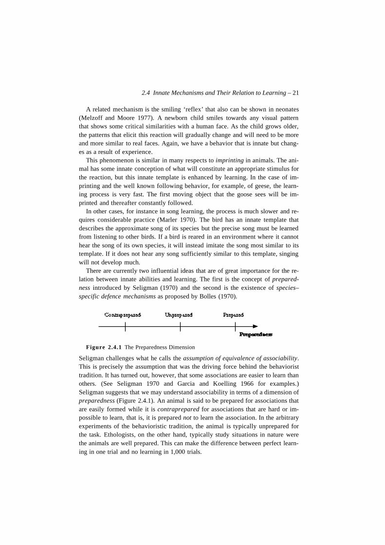
There are currently two influential ideas that are of great importance for the re-lation between innate abilities and learning. The first is the concept of prepared-ness introduced by Seligman (1970) and the second is the existence of species–specific defence mechanisms as proposed by Bolles (1970).
Figure 2.4.1 The Preparedness Dimension
Seligman challenges what he calls the assumption of equivalence of associability.This is precisely the assumption that was the driving force behind the behavioristtradition. It has turned out, however, that some associations are easier to learn thanothers. (See Seligman 1970 and Garcia and Koelling 1966 for examples.)Seligman suggests that we may understand associability in terms of a dimension ofpreparedness (Figure 2.4.1). An animal is said to be prepared for associations thatare easily formed while it is contraprepared for associations that are hard or im-possible to learn, that is, it is prepared not to learn the association. In the arbitraryexperiments of the behavioristic tradition, the animal is typically unprepared forthe task. Ethologists, on the other hand, typically study situations in nature werethe animals are well prepared. This can make the difference between perfect learn-ing in one trial and no learning in 1,000 trials.
22 – Biological Learning
A classical example of preparedness was demonstrated in an experiment byGarcia and Koelling (1966). Rats were allowed to drink ‘bright, noisy water’ andlater confronted with its dreadful consequences. The water was made bright andnoisy by a device that would flash a light and make a noise as soon as the animalcame into contact with the water. After drinking this water, one group of rats wasgiven electric shock. Another group was instead made sick by being injected witha toxic substance. Two other groups of rats were allowed to drink water tastingsaccharine. One of these groups was also given electric shock while the other wasmade sick.
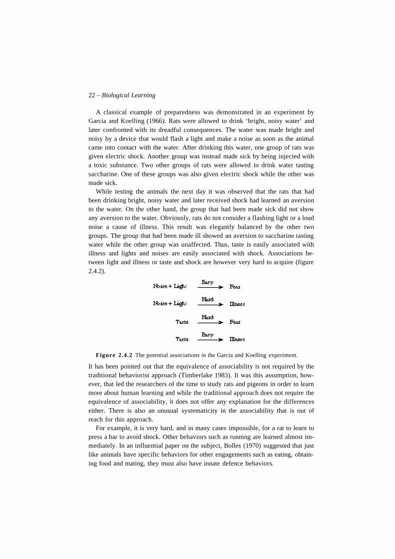
While testing the animals the next day it was observed that the rats that hadbeen drinking bright, noisy water and later received shock had learned an aversionto the water. On the other hand, the group that had been made sick did not showany aversion to the water. Obviously, rats do not consider a flashing light or a loudnoise a cause of illness. This result was elegantly balanced by the other twogroups. The group that had been made ill showed an aversion to saccharine tastingwater while the other group was unaffected. Thus, taste is easily associated withillness and lights and noises are easily associated with shock. Associations be-tween light and illness or taste and shock are however very hard to acquire (figure2.4.2).
Figure 2.4.2 The potential associations in the Garcia and Koelling experiment.
It has been pointed out that the equivalence of associability is not required by thetraditional behaviorist approach (Timberlake 1983). It was this assumption, how-ever, that led the researchers of the time to study rats and pigeons in order to learnmore about human learning and while the traditional approach does not require theequivalence of associability, it does not offer any explanation for the differenceseither. There is also an unusual systematicity in the associability that is out ofreach for this approach.
For example, it is very hard, and in many cases impossible, for a rat to learn topress a bar to avoid shock. Other behaviors such as running are learned almost im-mediately. In an influential paper on the subject, Bolles (1970) suggested that justlike animals have specific behaviors for other engagements such as eating, obtain-ing food and mating, they must also have innate defence behaviors.
2.4 Innate Mechanisms and Their Relation to Learning – 23
Such behaviors must be innately organized because nature provides little op-portunity for animals to learn to avoid predators and other natural hazards. Asmall defenceless animal like the rat cannot afford to learn to avoid thesehazards; it must have innate defence behaviors that keep it out of trouble.(Bolles, 1978, p. 184)
The hypothesis is that associations that are in agreement with the species–specificdefence mechanisms (SSDMs) are easily learned while others are much harder oreven impossible to acquire. To receive food, a pigeon will easily learn to peck at abar since pecking is in agreement with its innate eating behavior and consequentlyin agreement with food. But this behavior is highly incompatible with its innateavoidance mechanism and will thus only with great difficulty be associated withshock evasion. We see that here we have a possible explanation of the variabilityof preparedness as suggested by Seligman.
There are even cases where the SSDMs may hinder the animal from performingthe response to be learned. This is the case, for instance, when the frightened ratfreezes instead of pressing the lever in the Skinner box. Another striking exampleof the role of SSDMs have been shown in a modified version of the experimentwhere a rat has to avoid shock by pressing a bar. In this experiment, pressing thebar would remove the rat from the box and would consequently let it avoid theshock. In this variant of the experiment, the rat could easily learn to press the bar(Masterson 1970). Getting away from the box could apparently reinforce barpressing while simply avoiding the shock could not. Considering these examples itis hard to understand how the behaviorists were ever able to teach their animalsany of their arbitrary behaviors.
The truth of the matter is that our finest learning researchers have been keenobservers of the organization underlying an animal’s behavior; they simplyincorporated their observations and knowledge into the design of their appa-ratus and procedures rather than into their theories. It is this talent in observa-tion, as much as the power of the accompanying theoretical analyses, that hasmade the arbitrary approach so viable. A truly arbitrary approach to animallearning would have failed long ago, as it has for countless pet owners, par-ents, and students in the introductory psychology laboratory. (Timberlake1983, p. 183)
We may conclude that there exist a large number of innate behaviors which inter-act with learning in a highly complex way. These innate behaviors may makelearning either easier or harder. There also exist innate preferences for formingcertain associations and not others. Again we see that there is nothing generalabout learning. The supposedly general law the behaviorists tried to discover wasthe result of the arbitrariness of their experiments. In an arbitrary experiment, theanimal is generally unprepared and can be supposed to learn slowly and regularly.
24 – Biological Learning
In nature, however, the animal is well prepared for the types of learning that it willbe confronted with. The mechanisms involved in these situations may be entirelydifferent.
2.5 Interacting Learning Systems
In a recent learning experiment, Eichenbaum et al. (1991) have shown that ratswill learn to categorize odors without being reinforced for doing so. Rats that weretrained to discriminate between odors on a first trial were no more successful at asecond trail than rats that had initially been exposed to the same odors without re-inforcement. On the other hand, both these groups performed better at the secondtrial than the rats which had not been previously exposed to the odors at all.
A conclusion that can be drawn from this experiment is that there exist two dis-tinct learning mechanisms which are used in the discrimination task. The firstmechanism is concerned with the categorization of odors while the second mecha-nism is used to associate odor categories with the appropriate responses. Learningby the second system is typically performed on a single trial once the odors areknown, while the first system is somewhat slower. This would explain why priorexposure to the odors speeds up learning regardless of whether or not discrimina-tion is reinforced. What we have here is an example of perceptual categorization asa process independent of response learning.
It should be noted that there exists some evidence that at first may seem to be inconflict with this discovery. Skarda and Freeman (1987) report changes in theEEG of the olfactory bulb as a result of reinforcement. Since the bulb is generallyassumed to be responsible for olfactory categorization, this finding seems to indi-cate that the categorization process is influenced by reinforcement. Such a conclu-sion rests, however, on the assumption that physical areas of the brain can be iden-tified with specific learning systems and this needs not necessarily be correct.
The idea that there exists more than one learning system is not new. Evenamong the behaviorists, we find researchers holding this position. Clark Hull, forexample, postulated (at times) that two interacting learning systems were neededto explain the experimental data. In the primary system, learning was induced byreduction of drive, while the secondary system was controlled by conditioned re-inforcers, that is, events that had acquired reinforcing properties through condi-tioning (Hull 1952).
While Hull’s two systems are no longer considered an accurate model of learn-ing, they do show that not all behaviorists believed in one general learning system.It should be noted that Hull was one of the few early psychologists that were moreinterested in fitting the theory to data than selecting data supporting the theory.“Hull’s willingness to be wrong was a remarkable, perhaps unique, virtue. It is avirtue that is, unfortunately, not shared by many theorists” (Bolles, 1978, p. 104).
2.6 The Role of Reinforcement – 25
2.6 The Role of ReinforcementWe have seen above that learning of odors can occur entirely without reinforce-ment although this learning may not be expressed in behavior until reinforcementis introduced. During the 1950s, the role of reinforcement was one of the most in-tense research areas within learning theory. Hull had made the entirely sensible,but as we now know, insufficient assumption that an animal will learn to performan action if its internal drive or need is reduced. For example, a hungry rat that isallowed to eat after having pressed a bar will reduce its hunger drive. Drive–reduc-tion would then reinforce bar pressing. This drive–reduction hypothesis becameone of the most influential ideas in psychology ever.
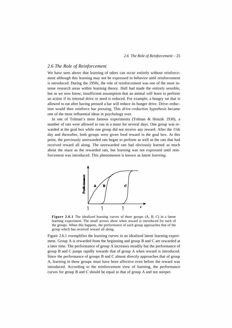
In one of Tolman’s most famous experiments (Tolman & Honzik 1930), anumber of rats were allowed to run in a maze for several days. One group was re-warded at the goal box while one group did not receive any reward. After the 11thday and thereafter, both groups were given food reward in the goal box. At thispoint, the previously unrewarded rats began to perform as well as the rats that hadreceived reward all along. The unrewarded rats had obviously learned as muchabout the maze as the rewarded rats, but learning was not expressed until rein-forcement was introduced. This phenomenon is known as latent learning.
Figure 2.6.1 The idealized learning curves of three groups (A, B, C) in a latentlearning experiment. The small arrows show when reward is introduced for each ofthe groups. When this happens, the performance of each group approaches that of thegroup which has received reward all along.
Figure 2.6.1 exemplifies the learning curves in an idealized latent learning experi-ment. Group A is rewarded from the beginning and group B and C are rewarded ata later time. The performance of group A increases steadily but the performance ofgroup B and C jumps rapidly towards that of group A when reward is introduced.Since the performance of groups B and C almost directly approaches that of groupA, learning in these groups must have been affective even before the reward wasintroduced. According to the reinforcement view of learning, the performancecurves for group B and C should be equal to that of group A and not steeper.
26 – Biological Learning
There are also many situations where it is hard to define exactly what the rein-forcer should be. Avoidance learning is one such case.
By definition, the avoidance response prevents shock from occurring, so wecannot point to the shock as a potential source of reinforcement. On the otherhand, it is not satisfactory to cite the nonoccurrence of shock as a reinforcerbecause, logically, there is a host of things that do not occur, and one is hardput to say why not being shocked should be relevant, whereas, say, not beingstepped on is irrelevant. (Bolles, 1978, p. 184)
The explanation of learning in these cases may again be caused by interaction withspecies–specific defence mechanisms.
An alternative to the drive–reduction hypothesis is that it is the occurrence ofcertain stimuli that are reinforcing. This was the mechanism behind reinforcementin Hull’s secondary learning system (Hull 1952). Could all learning be explainedby this mechanism? If an animal can respond to a number of innately reinforcingstimuli, then perhaps all learning could be derived from the effect of these rein-forcing stimuli.
Contrary to the idea that only stimuli have reinforcing properties, Premack(1971) has proposed that all experiences have different values that can be used asreinforcement. The value of an activity is proportional to the probability that ananimal will engage in that activity. The Premack principle states that access to anymore probable activity will reinforce any less probable activity.
This principle was tested in an experiment where children were allowed eitherto eat candy or play with a pinball machine (Premack 1965). In the first phase ofthe experiment, it was recorded how long the children engaged in each of these ac-tivities. In the second phase, access to one activity was used as reward for per-forming the other. It turned out, as the Premack principle would imply, that thechildren that were initially more likely to eat candy than to play pinball would playbinball in order to be allowed to eat candy. The other children were, however, un-affected by the candy. Thus, candy had only a reinforcing effect when it was usedto reward a less probable activity. The exact nature of reinforcement is howeverstill debated and will probably continue to be so for a long time.
This view of reinforcement is very different from the traditional view ofThorndike and Hull. While possibly more general, it is very hard to see how thisprinciple can be explained in mechanistic terms. There also exists a number of cas-es where the principle does not hold (see Dunham 1977). It appears that reinforce-ment does play a role in some but not all learning.
A different view of these matters is given by Gallistel (1990), who argues thatthere need not be any direct relation between the learning situation and the behav-ioral context in which the animal makes use of the acquired knowledge or habit.For example, certain migratory birds learn the constellations of the stars at a timewhen they cannot yet fly. Since the stars do not play any role in the nestbound
2.7 What Does the Animal Learn? – 27
stage of their life, it cannot be the utility of the acquired knowledge that reiniforceslearning. This process thus appears to be similar to imprinting. It relies on an in-nate mechanism which triggers learning under some specific condition. There canobviously be no general principle for this type of learning.
2.7 What Does the Animal Learn?What is learned when an animal in a maze succeeds in running the shortest pathfrom the start to the goal box? Has it learned to perform a fixed sequence of motorpatterns or has it constructed a cognitive map of the maze? Perhaps it has learnedto expect food at a certain place or to expect reward for running a certain route.The theories are almost as many as the researchers in the field. However, there aresome main directions that we will try to summarize in this section. Here we willonly consider what is learned and not how that learning has come about.
Stimulus–Response Associations
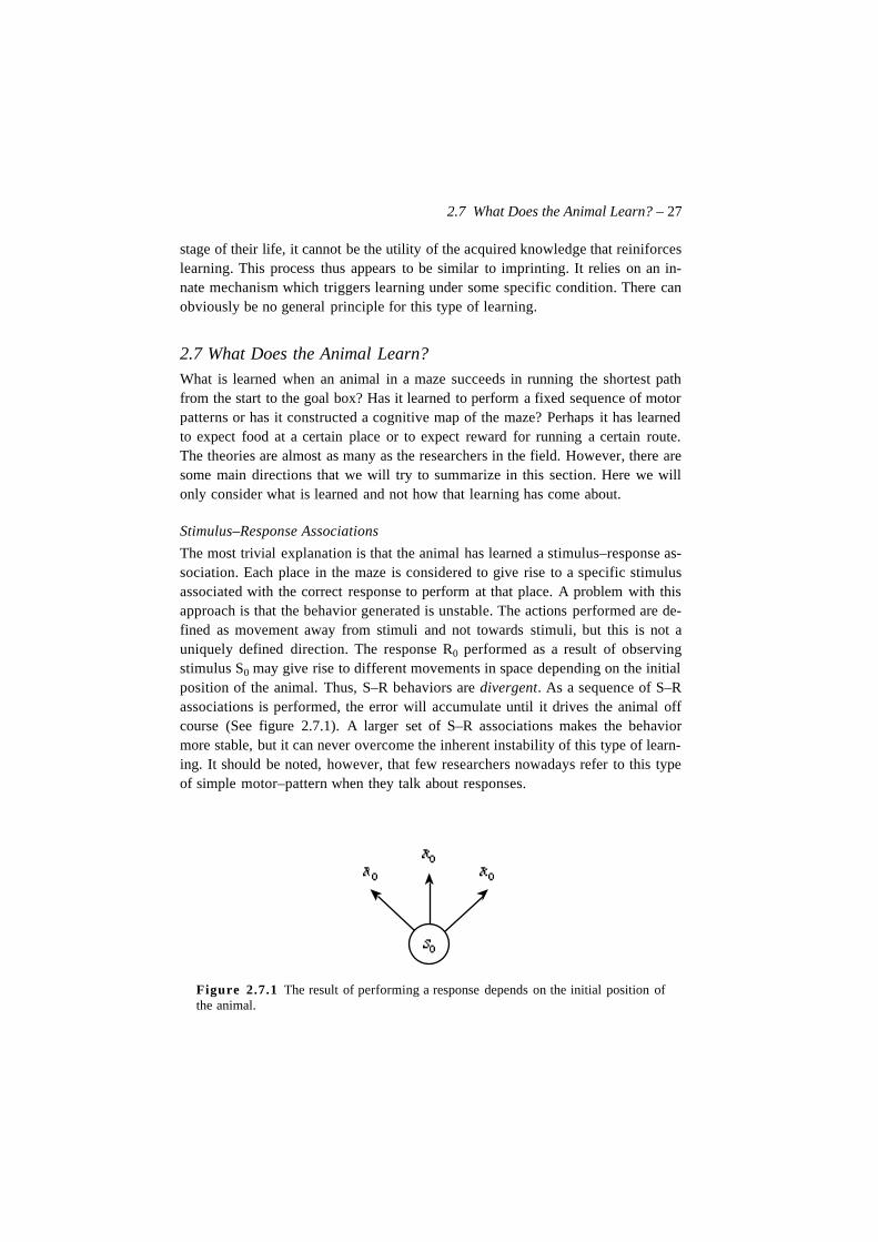
The most trivial explanation is that the animal has learned a stimulus–response as-sociation. Each place in the maze is considered to give rise to a specific stimulusassociated with the correct response to perform at that place. A problem with thisapproach is that the behavior generated is unstable. The actions performed are de-fined as movement away from stimuli and not towards stimuli, but this is not auniquely defined direction. The response R0 performed as a result of observingstimulus S0 may give rise to different movements in space depending on the initialposition of the animal. Thus, S–R behaviors are divergent. As a sequence of S–Rassociations is performed, the error will accumulate until it drives the animal offcourse (See figure 2.7.1). A larger set of S–R associations makes the behaviormore stable, but it can never overcome the inherent instability of this type of learn-ing. It should be noted, however, that few researchers nowadays refer to this typeof simple motor–pattern when they talk about responses.
Figure 2.7.1 The result of performing a response depends on the initial position ofthe animal.
28 – Biological Learning
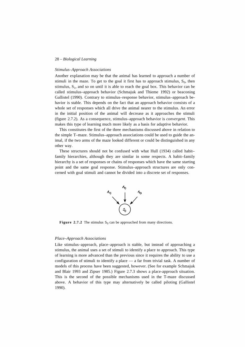
Stimulus–Approach Associations
Another explanation may be that the animal has learned to approach a number ofstimuli in the maze. To get to the goal it first has to approach stimulus, S0, thenstimulus, S1, and so on until it is able to reach the goal box. This behavior can becalled stimulus–approach behavior (Schmajuk and Thieme 1992) or beaconingGallistel (1990). Contrary to stimulus–response behavior, stimulus–approach be-havior is stable. This depends on the fact that an approach behavior consists of awhole set of responses which all drive the animal nearer to the stimulus. An errorin the initial position of the animal will decrease as it approaches the stimuli(figure 2.7.2). As a consequence, stimulus–approach behavior is convergent. Thismakes this type of learning much more likely as a basis for adaptive behavior.
This constitutes the first of the three mechanisms discussed above in relation tothe simple T–maze. Stimulus–approach associations could be used to guide the an-imal, if the two arms of the maze looked different or could be distinguished in anyother way.
These structures should not be confused with what Hull (1934) called habit–family hierarchies, although they are similar in some respects. A habit–familyhierarchy is a set of responses or chains of responses which have the same startingpoint and the same goal response. Stimulus–approach structures are only con-cerned with goal stimuli and cannot be divided into a discrete set of responses.
Figure 2.7.2 The stimulus S0 can be approached from many directions.
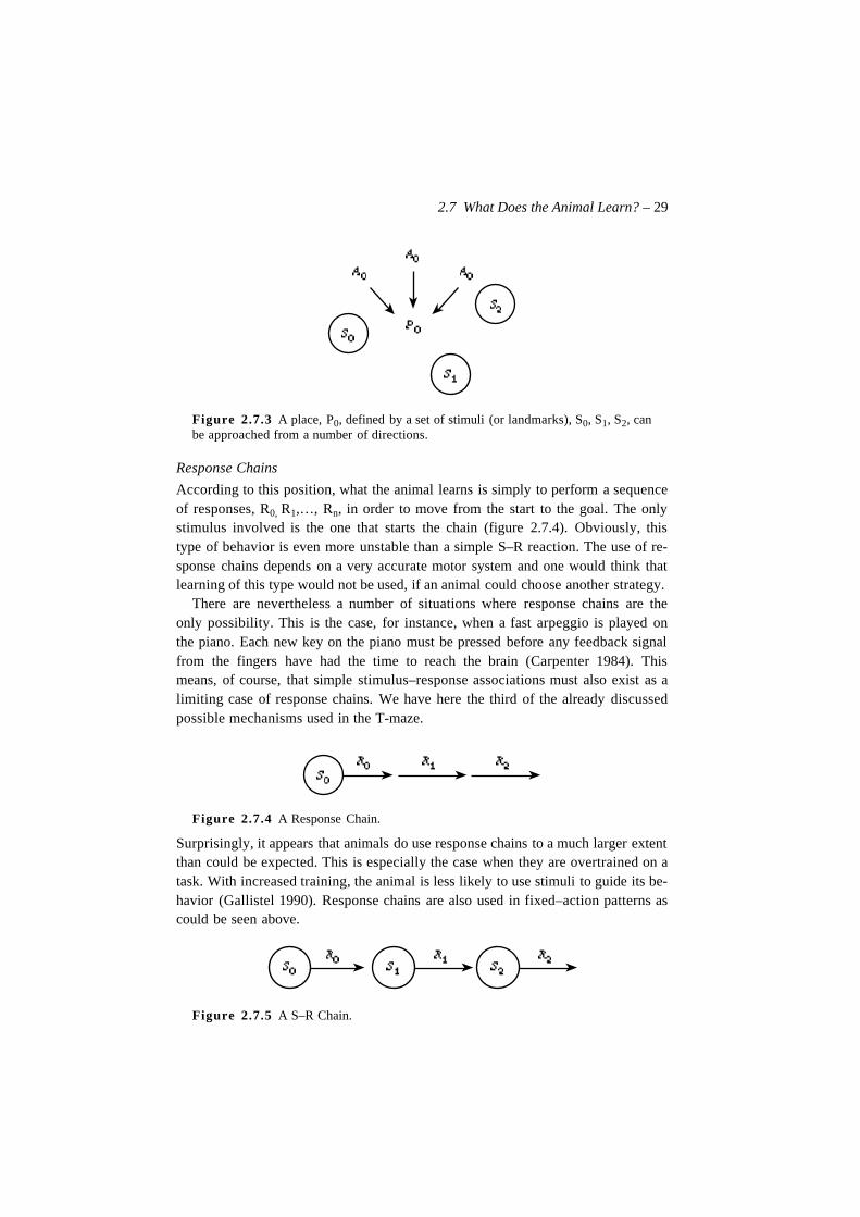
Place–Approach Associations
Like stimulus–approach, place–approach is stable, but instead of approaching astimulus, the animal uses a set of stimuli to identify a place to approach. This typeof learning is more advanced than the previous since it requires the ability to use aconfiguration of stimuli to identify a place — a far from trivial task. A number ofmodels of this process have been suggested, however. (See for example Schmajukand Blair 1993 and Zipser 1985.) Figure 2.7.3 shows a place-approach situation.This is the second of the possible mechanisms used in the T-maze discussedabove. A behavior of this type may alternatively be called piloting (Gallistel1990).
2.7 What Does the Animal Learn? – 29
Figure 2.7.3 A place, P0, defined by a set of stimuli (or landmarks), S0, S1, S2, canbe approached from a number of directions.
Response Chains
According to this position, what the animal learns is simply to perform a sequenceof responses, R0, R1,…, Rn, in order to move from the start to the goal. The onlystimulus involved is the one that starts the chain (figure 2.7.4). Obviously, thistype of behavior is even more unstable than a simple S–R reaction. The use of re-sponse chains depends on a very accurate motor system and one would think thatlearning of this type would not be used, if an animal could choose another strategy.
There are nevertheless a number of situations where response chains are theonly possibility. This is the case, for instance, when a fast arpeggio is played onthe piano. Each new key on the piano must be pressed before any feedback signalfrom the fingers have had the time to reach the brain (Carpenter 1984). Thismeans, of course, that simple stimulus–response associations must also exist as alimiting case of response chains. We have here the third of the already discussedpossible mechanisms used in the T-maze.
Figure 2.7.4 A Response Chain.
Surprisingly, it appears that animals do use response chains to a much larger extentthan could be expected. This is especially the case when they are overtrained on atask. With increased training, the animal is less likely to use stimuli to guide its be-havior (Gallistel 1990). Response chains are also used in fixed–action patterns ascould be seen above.
Figure 2.7.5 A S–R Chain.
30 – Biological Learning
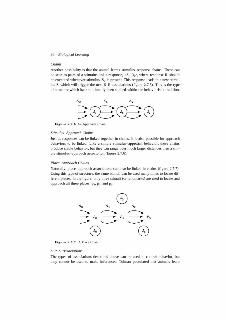
Chains
Another possibility is that the animal learns stimulus–response chains. These canbe seen as pairs of a stimulus and a response, <Si, Ri>, where response Ri shouldbe executed whenever stimulus, Si, is present. This response leads to a new stimu-lus Sj which will trigger the next S–R associations (figure 2.7.5). This is the typeof structure which has traditionally been studied within the behavioristic tradition.
Figure 2.7.6 An Approach Chain.
Stimulus–Approach Chains
Just as responses can be linked together in chains, it is also possible for approachbehaviors to be linked. Like a simple stimulus–approach behavior, these chainsproduce stable behavior, but they can range over much larger distances than a sim-ple stimulus–approach association (figure 2.7.6).
Place–Approach Chains
Naturally, place–approach associations can also be linked in chains (figure 2.7.7).Using this type of structure, the same stimuli can be used many times to locate dif-ferent places. In the figure, only three stimuli (or landmarks) are used to locate andapproach all three places, p1, p2, and p3.
Figure 2.7.7 A Place Chain.
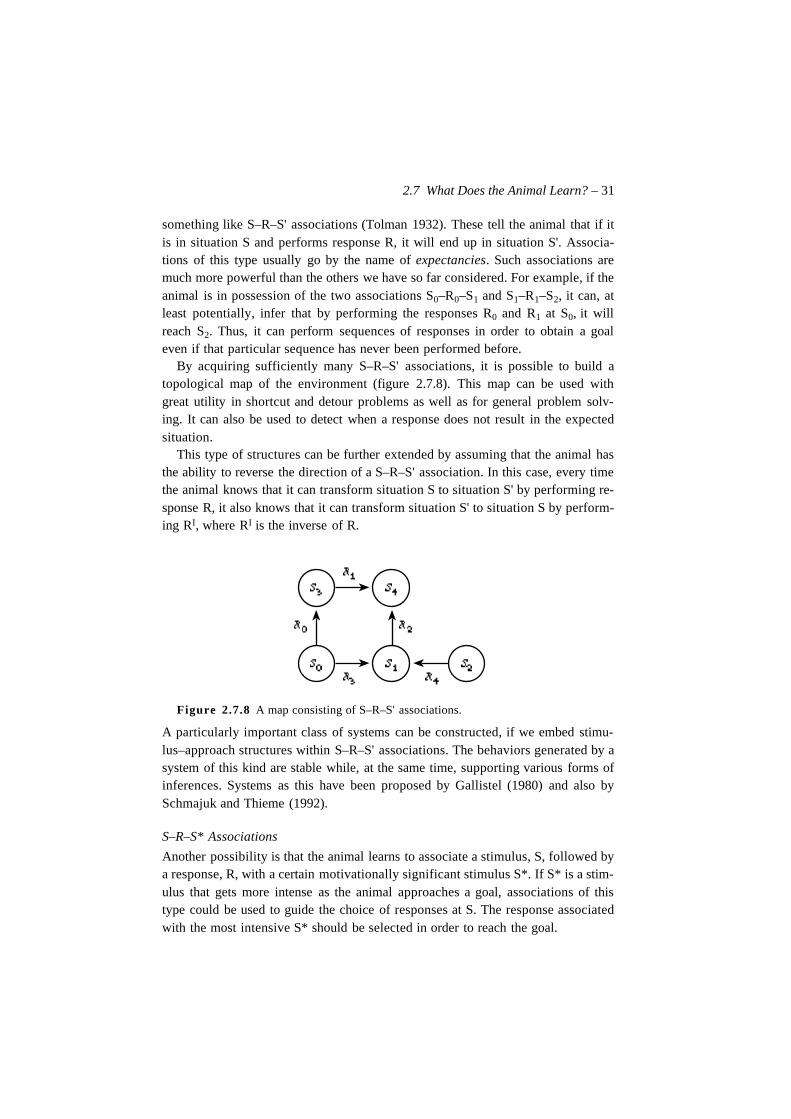
S–R–S' Associations
The types of associations described above can be used to control behavior, butthey cannot be used to make inferences. Tolman postulated that animals learn
2.7 What Does the Animal Learn? – 31
something like S–R–S' associations (Tolman 1932). These tell the animal that if itis in situation S and performs response R, it will end up in situation S'. Associa-tions of this type usually go by the name of expectancies. Such associations aremuch more powerful than the others we have so far considered. For example, if theanimal is in possession of the two associations S0–R0–S1 and S1–R1–S2, it can, atleast potentially, infer that by performing the responses R0 and R1 at S0, it willreach S2. Thus, it can perform sequences of responses in order to obtain a goaleven if that particular sequence has never been performed before.
By acquiring sufficiently many S–R–S' associations, it is possible to build atopological map of the environment (figure 2.7.8). This map can be used withgreat utility in shortcut and detour problems as well as for general problem solv-ing. It can also be used to detect when a response does not result in the expectedsituation.
This type of structures can be further extended by assuming that the animal hasthe ability to reverse the direction of a S–R–S' association. In this case, every timethe animal knows that it can transform situation S to situation S' by performing re-sponse R, it also knows that it can transform situation S' to situation S by perform-ing RI, where RI is the inverse of R.
Figure 2.7.8 A map consisting of S–R–S' associations.
A particularly important class of systems can be constructed, if we embed stimu-lus–approach structures within S–R–S' associations. The behaviors generated by asystem of this kind are stable while, at the same time, supporting various forms ofinferences. Systems as this have been proposed by Gallistel (1980) and also bySchmajuk and Thieme (1992).
S–R–S* Associations
Another possibility is that the animal learns to associate a stimulus, S, followed bya response, R, with a certain motivationally significant stimulus S*. If S* is a stim-ulus that gets more intense as the animal approaches a goal, associations of thistype could be used to guide the choice of responses at S. The response associatedwith the most intensive S* should be selected in order to reach the goal.
32 – Biological Learning
Like S–R–S' learning, this is a type of expectation learning, but here it is an ex-pectation of reward and not an expectation of a subsequent stimulus that is learned.As we will see below in chapter 8, a combination of these two types of expectationlearning can be very powerful.
S–S' Learning
We will finally consider associations between stimuli. In classical conditioning, ithas sometimes been assumed that it is not an association between stimulus and re-sponse that is formed but rather an association between the two stimuli involved.In this view, Pavlov’s dog does not salivate because the bell has been associatedwith salivation, but rather because the bell has been associated with food which inturn activates salivation. This is called the stimulus-substitution theory of condi-tioning (Mackintosh 1974).
There are a number of processes that have S–S' associations as their basis. Incategorization, a stimulus representing an instance of a category is associated witha stimulus representing its category. When the stimulus is perceived its corre-sponding category is activated. Of course, stimuli are here considered as some-thing internal to the organism and not as external cues. We are, in fact, talkingabout representations of stimuli. This view of learning is similar to the earlyassociationistic school that considered associations as links among ideas. Hebb’scell assembly theory is a more sophisticated variation on this theme (Hebb 1949).
The above list is by no means exhaustive. We have only touched on some of themost important ideas about what is learned by an animal. Numerous attempts havebeen made to explain each of the above learning types by means of the other, butso far there is no consensus in the area. The view we are advocating is that all theselearning types, and perhaps many more, co-exist and interact with each other dur-ing learning and behavior.
2.8 Internal Influences on Behavior
So far, we have described behavior as if it were guided primarily by external stim-uli. This is of course not the case. Internal determinants of behavior are very prom-inent in most situations.
One obvious internal determinant is the current need of an animal. In identicalexternal situations, a hungry animal will eat if possible while a satiated animal willnot. Internal stimuli are related to the concept of motivation, but since this deter-minant of behavior is not directly relevant to the present argument, we will notdwell on this matter here. We have so far assumed that there is only one goal topursue and that the animal is motivated to do so.
A determinant that is more relevant to the present argument is what we will callthe internal context of a situation. In many learning paradigms, the appropriate
2.8 Internal Influences on Behavior – 33
action for a given situation depends on some previous action performed at thesame place or in the same situation. To make the correct choice of an action at thesecond trial, the animal must remember what it did the last time. The internal con-text of a situation is the internal state that somehow reflects this previous choice.
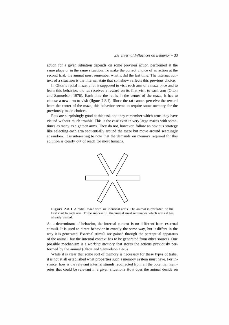
In Olton’s radial maze, a rat is supposed to visit each arm of a maze once and tolearn this behavior, the rat receives a reward on its first visit to each arm (Oltonand Samuelson 1976). Each time the rat is in the center of the maze, it has tochoose a new arm to visit (figure 2.8.1). Since the rat cannot perceive the rewardfrom the center of the maze, this behavior seems to require some memory for thepreviously made choices.
Rats are surprisingly good at this task and they remember which arms they havevisited without much trouble. This is the case even in very large mazes with some-times as many as eighteen arms. They do not, however, follow an obvious strategylike selecting each arm sequentially around the maze but move around seeminglyat random. It is interesting to note that the demands on memory required for thissolution is clearly out of reach for most humans.
Figure 2.8.1 A radial maze with six identical arms. The animal is rewarded on thefirst visit to each arm. To be successful, the animal must remember which arms it hasalready visited.
As a determinant of behavior, the internal context is no different from externalstimuli. It is used to direct behavior in exactly the same way, but it differs in theway it is generated. External stimuli are gained through the perceptual apparatusof the animal, but the internal context has to be generated from other sources. Onepossible mechanism is a working memory that stores the actions previously per-formed by the animal (Olton and Samuelson 1976).
While it is clear that some sort of memory is necessary for these types of tasks,it is not at all established what properties such a memory system must have. For in-stance, how is the relevant internal stimuli recollected from all the potential mem-ories that could be relevant in a given situation? How does the animal decide on
34 – Biological Learning
what to store in memory? Whatever properties a learning system involved in thistype of memory may have, it must interact with the different learning strategies wehave presented above.
2.9 Are the Internal Structures an Image of Reality?
Assuming that an animal behaves in an appropriate way, does this mean that itknows something about its world? It is tempting to assume that a rat which haslearned to run through a maze to receive food does so because it is hungry butwould prefer not to be. It knows where the food is located and how to get there andexpects to be less hungry if it eats the food. Based on this information, the rat caninfer that the best way to satisfy its goal is to run through the maze and eat thefood, and, as a consequence of this inference, it will decide to run through themaze and eat the food.
According to Tolman (1932), this is an adequate description of what goes on inthe mind of the rat and it is not hard to understand Guthrie’s objection that accord-ing to this view the rat would be “buried in thought”. However, the main criticismof this view has not come from within animal learning theory but instead fromethology and ecological psychology.
When the smell of butyric acid with a certain temperature causes the tick to bite,there is no reason to believe that it has some objective knowledge of mammals thatis used to decide on whether to bite or not (Sjölander 1993). In fact, it seems inap-propriate to talk about knowledge at all in this context. In nature, everything thatsmells of butyric acid and has a temperature of +37 °C is a mammal and in theworld of the common tick, this is all that a mammal is.
The part of reality that is within reach of the perceptual apparatus of an animalcan be referred to by the concept of Umwelt3 as proposed by von Uexküll. There isno reason to assume that an animal has a better conception of reality than is neces-sary. The Umwelt of the common tick is not very sophisticated, but it is sufficientfor it to survive. If the tick believes that everything that smells of butyric acid issomething it should bite, it will survive, if it does not, it will probably die. Thisdoes not mean that its conception of reality is true in any objective sense, but thisis not terribly important as long as it significantly increases the chance of survivalfor the animal. It is sufficient for the concepts of an animal to make it behave in theappropriate way. They do not necessarily need to represent the world in any greatdetail (Sjölander 1993).
In ecological optics (Gibson 1979), the idea of an ambient optic array is used ina way that is very similar to the Umwelt , but while this concept refers to all aspectsof the environment, the ambient optic array refers only to the visual surrounding ofan animal.
3. Umwelt means approximately surrounding environment.

2.10 When Does the Animal Learn? – 35
Ecological psychology emphasizes the role of invariants in the environmentthat can be directly picked up by an organism. The sign stimulus that causes thebite reaction in the tick is an example of such an invariant. As pointed out byRunesson (1989), it is sufficient that invariants are incomplete, that is, they shouldhold sufficiently often for the mechanisms that rely on them to be adaptive. This iscertainly the case with the sign stimulus of the bite reaction.
In the behaviorist accounts for learning it was often implicitly assumed that an-imals perceive the same (objective) world as humans. No-one was ever surprisedto find that animals attended to exactly those stimuli which were relevant to thelearning task. For some reason, the world of the animals coincided with that of theexperimental situation. As a consequence, only those stimuli specially preparedfor the learning task needed to be considered when attempting to explain learning.
In the light of the example above, this should be very surprising. Why should arat care about exactly those stimuli which were needed to solve the problem andnot on something entirely irrelevant like the smell of the experimenter? Of theclassical learning theorists, only Pavlov considered this problem in any detail(Pavlov 1927).
None of the different learning strategies presented above gives rise to objectiveknowledge of the world. Some of the learned structures even depend on the learn-ing animal in some unusual ways. For example S–R–S' association are based onthe behavioral repertoire of the animal. It will not learn that A is north of B butrather that some specific action is appropriate for moving from A to B. A structureof this kind is much more useful than an objective representation, if the animalwants to move from one place to another.
2.10 When Does the Animal Learn?
In this section we will consider how different proposed learning mechanisms re-late to the execution of a consummatory or terminal behavior. Learning has beendescribed as occurring either before, after, or at the same time as the terminal be-havior. We will call these different learning types early, synchronous and latelearning (See figure 2.10.1).
Figure 2.10.1 Different times when learning can occur in relation to a terminalbehavior.
36 – Biological Learning
Early Learning
Early learning is learning that occurs prior to the consummatory behavior. If a ratlearns the location of food without being allowed to eat it, we have an instance ofearly learning. Thus, early learning is involved in latent learning experiments. Wemay hypothesize one of two distinct processes responsible for early learning.
The first process, usually associated with Tolman, explains learning simply asthe gathering of information about the environment. The construction of a cogni-tive map is an example of such a process. Both S–R–S' and S–S' associations canbe constructed using this type of early learning. It is important to note that the de-mands on the cognitive apparatus which an animal needs for this mechanism arerather high. Consequently, we would only expect to find this type of learning inhigher animals.
The second process is driven by the distance to a goal object. An anticipatoryreinforcement signal is generated which is inversely proportional to the perceiveddistance to the goal object. The closer to the object, the larger the reinforcementwill be. In this case, an animal will learn to approach food even if it is not allowedto eat it. A learning mechanism of this type implies that maximal reinforcementwill be received when the goal object is actually reached.
While this type of learning has many important merits it critically depends on acompetent evaluation of the distance to the goal. Perhaps it is the failure to per-ceive this distance that makes the dedicated gambler risk even more money after‘almost winning the bet’. As far as we know, this type of learning has not beenstudied in the animal learning literature.
Since early learning does not depend on any reward, phenomena like latentlearning are easily explained with either of these learning mechanism. In the caseof shortcut and detour behaviors, it seems that the first learning mechanism isnecessary.
Synchronous Learning
Synchronous learning is perhaps the most obvious alternative to the drive-reduction hypothesis. Here it is the consummatory response that is the origin oflearning. When an animal eats the food, its previous responses are reinforced.Among the classical learning theorists, Guthrie is the main proponent of this view(see Bolles 1978).
It does not appear that synchronous learning can explain the more complex be-haviors of an animal but there are some situations where a mechanism of this typeseems most appropriate. For instance, learning the correlation between smell andtaste is obviously best done when both types of information are present, and this isonly the case while eating.
2.11 Summary of Animal Learning – 37
Late Learning
Hull’s drive-reduction hypothesis is a classical example of late learning. Here it isnot the reward itself, such as the food that causes learning, but rather its conse-quences on the organism. According to this hypothesis, the reduction of hungerwould reinforce learning while eating should not.
* * *
How are we to choose between these learning types? Again, we want to proposethat they are all effective but in different circumstances. In many cases, earlylearning is certainly the case, but can that type of learning explain all cases wherebehavior is changed? Because of the complexity involved in early learning it is notentirely unrealistic to assume that there also exist less complex learning mecha-nisms such as synchronous and late learning. At least in simpler organisms, theseare the mechanisms to look for.
We may also make the conjecture that if these less sophisticated learning typesare present in simpler organisms, they are also very likely to play a role in moreadvanced organisms. After all, they are still entirely sensible.
2.11 Summary of Animal LearningI hope to have shown that learning in animals is a highly complex and complicatedbusiness. It is quite unlikely that all the examples described above can be ex-plained by one mechanism and if it can, it is certainly very different from any ofthe currently proposed learning theories.
In summary, there are a number of important facts about animal learning thatwe must consider, if we want to construct or model an intelligent system.
• It is unlikely that there exists one general learning mechanism that can handleall situations. Animals are prepared to learn some associations and not oth-ers.
• Many alternative strategies are available to use for the same problem, likeplace learning, approach learning or response learning. The strategies are se-lected and combined according to the demands of the task.
• Animals have a number of species-specific mechanisms that interfere withlearning. Such innate behaviors are necessary to keep the animal alive whileit learns about the world. In some animals, almost all behaviors are of thiskind.
• What the animal learns can be represented in a number of ways. We haveseen at least nine ways to represent habit and knowledge. These structuresneed not be good descriptions of the external world. It is sufficient that theyhelp the animal stay alive.
38 – Biological Learning
• Memories of past actions or experiences are sometimes necessary to choosethe correct behavior.
• Learning can occur at different times with respect to a reward. Learning thatoccurs prior to any reward is in effect independent of the reward but can usu-ally only be demonstrated once a reward is introduced.
2.12 Parallels Between Artificial Intelligence and Animal LearningTheory
It is interesting to see that many artificial intelligence models show striking simi-larities to the animal theories. The reinforcement theories proposed by Thorndikeand Hull find their counterpart in the early learning algorithms such as the oneused in Samuel’s checkers program (Samuel 1959) and more contemporary rein-forcement learning models (Sutton and Barto 1990). The parallel of Tolman’stheory can be found in mainstream artificial intelligence in the use of internalworld models and planning. We also find the equivalent of the ethological ap-proach to animal behavior in the work of Brooks and others who emphasize therole of essentially fixed behavioral repertoires which are well adapted to the envi-ronment (Brooks 1986).
These similarities have made me curious to see whether it would be possible tomatch the different fields and perhaps transfer ideas between them. Can insightsfrom animal research be used to construct intelligent machines? Is it possible thatresearch on artificial intelligence has anything to say about how animals and hu-mans work? We think the answers to both these questions are affirmative and thepresent work is partly an attempt to carry out such a matching.
In the following sections, we will take a closer look at the different learningmethods used by various artificial intelligence researchers and try to match themwith the relevant animal learning theories. The result of this exercise will be an at-tempt to formulate some general design principles for an intelligent system.
2.13 S–R Associations in AI and Control
The rules used in rule based systems are very often similar to S–R associations.When one rule is used to generate the precondition for another rule, the process isnot entirely unlike the chaining of S–R associations. In the animal learning theo-ries, the environment holds the result of a response and may in turn trigger the nextS–R association. In rule based systems, the environment is replaced by an internalrepresentation of ‘facts’ generated by the triggered rules (Newell 1990). Computa-tionally, the two approaches are almost identical although the languages used todescribe them are entirely different.
Perhaps a clearer example of S–R associations can be found in the use of look-up tables (LUT) in both AI and control (Albus 1975). Look-up tables are used to
2.14 Reinforcement Learning – 39
store the output for a set of inputs. This has the advantage that no calculations haveto be made. For a given input, the result is simply looked up in the table. A controlstrategy can be coded once and for all in a look-up table to make the control fasterthan if the controlling signal had to be calculated for each input.
Look-up tables have two disadvantages however. The first is that there mayexist inputs which are not stored in the table. These inputs have no defined output.The second problem has already been mentioned in relation to S–R learning: be-havior generated by S–R associations is divergent. Both these problems have beenaddressed by generalizing look-up tables. These data structures will interpolatebetween the entries in the table to find an output for an unknown input.
Albus’ CMAC was one of the first mechanisms to use this idea (Albus 1975).The model was supposed to describe learning in the cerebellum and since its intro-duction it has been developed in two quite distinct directions. The first is in thefield of control where it is the basis for many control strategies based on general-izing look-up tables (e. g. Atkeson and Reinkensmeyer 1990, Kraft and Campagna1990). The other development of the model has been towards a more realistic mod-el of cerebellar learning. Most contemporary neurophysiological models of classi-cal conditioning have the CMAC model as their starting point (for example, Ito1989, Moore and Blazis 1989). Another connection between animal learning theo-ry and control theory is the Recorla–Wagner model of classical conditioning (Res-corla and Wagner 1972). This model is mathematically identical to the Widrow–Hoff learning rule for adaptive filtering (Widrow and Hoff 1960/1980).
2.14 Reinforcement LearningThorndike’s law of effect states that the learning of a response is governed by theeffects of that response. The cat will learn to press a lever to escape from its boxsince the effect of lever pressing, that is, the escape, is pleasant. The pleasant as-pect of escape reinforces the behavior that precedes it. As a consequence, this be-havior is more likely to be elicited again. If, on the other hand, a behavior is fol-lowed by some unpleasant event, the likelihood of the behavior is reduced instead.The closer in time a response is to the reward, the more the response will be rein-forced. While this description comes from animal learning theory, it is essentiallythe idea behind reinforcement learning as it is used in artificial intelligence.
Something similar to reinforcement learning was first used in Samuel’s check-ers program that was developed in the late fifties (Samuel 1959). When the com-puter wins a game, it receives a reward in the form of a positive evaluation of itslast few moves. During later games, this evaluation is propagated toward earlierpositions of the game. Moves which lead to favorable positions receive a higherreward (that is a better evaluation) than moves which are less successful. Eventu-ally all moves will have been evaluated and the computer will be able to play thegame fairly well.
40 – Biological Learning
While this learning scheme is feasible in principle, it will take an almost infiniteamount of time before all moves have been tested. This problem was overcome intwo ways. The first was to let the program use a static evaluation function onmoves that were far from any known position. The second solution was to let theprogram use a high-level description of the positions. Using this complex descrip-tion, evaluations of one position could be generalized to a position that had neverbeen encountered before. The high-level descriptions were also further enhancedby the introduction of learning.
This idea has later been included as a component in many learning systems. Thebucket brigade algorithm used in Holland’s classifier systems is another instanceof this general learning scheme (Holland et al. 1986). The learning system re-ceives a reward from the environment and its task is to adapt its internal rule basein such a way that it receives an optimal reward from the environment.
Q-learning as proposed by Watkins (1992) is perhaps the reinforcement learn-ing algorithm that is easiest to understand. The main element of this algorithm isthe Q-function that assigns an expected reward to each combination of a situation(or stimulus) and an action (or response). When the system finds itself in a certainsituation, it simply chooses the action for which its expected reward is largest. Ineffect, the Q-function describes a set of S–R–S* associations. The role of thelearning algorithm is to construct an estimation of the Q-function by trying out thedifferent actions in the environment.
Common to all of the above examples of reinforcement learning is that actionswhich are not immediately rewarded are reinforced by the actions that followthem. The propagation of reward from the terminal action towards the precedingones is not entirely unlike the anticipatory goal reaction, rG, proposed by Hull(1943, 1952). This reaction, whose only effect would be to generate an anticipato-ry goal stimulus, sG, would initially be associated with the rewarding response andwould later propagate through the chain of S–R associations and serve as the gluein a response sequence.
The connection between animal learning theory and reinforcement learning hasrecently been emphasized in a number of articles by Barto and Sutton (Barto,Sutton and Watkins 1990, Sutton and Barto 1990). Their temporal differencemethod has been used both as a biological model and as an adaptive control strat-egy and it is one of the most recent attempts to propose an explicit connection be-tween animal learning and control theory. Baird and Klopf (1993) describe a mod-ified version of the Q-learning paradigm which also clarifies this connection. Theyshow how Q-learning can be adapted to conform with the precise details of severalanimal learning experiments.
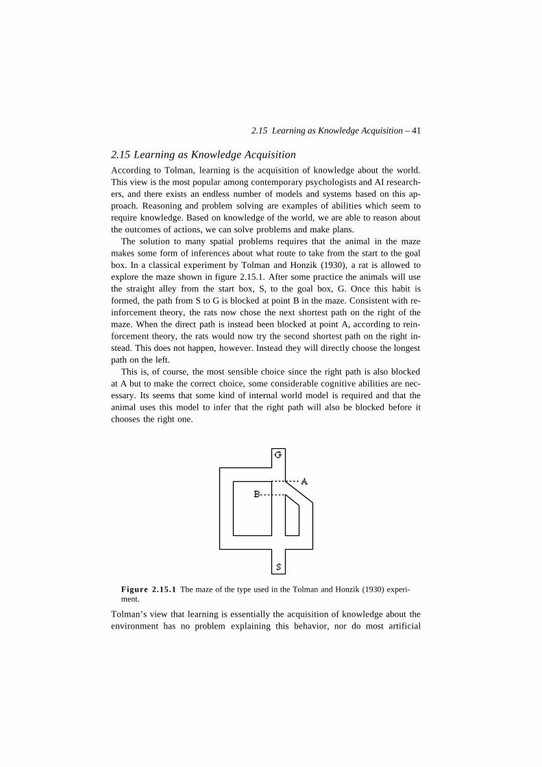
2.15 Learning as Knowledge Acquisition – 41
2.15 Learning as Knowledge AcquisitionAccording to Tolman, learning is the acquisition of knowledge about the world.This view is the most popular among contemporary psychologists and AI research-ers, and there exists an endless number of models and systems based on this ap-proach. Reasoning and problem solving are examples of abilities which seem torequire knowledge. Based on knowledge of the world, we are able to reason aboutthe outcomes of actions, we can solve problems and make plans.
The solution to many spatial problems requires that the animal in the mazemakes some form of inferences about what route to take from the start to the goalbox. In a classical experiment by Tolman and Honzik (1930), a rat is allowed toexplore the maze shown in figure 2.15.1. After some practice the animals will usethe straight alley from the start box, S, to the goal box, G. Once this habit isformed, the path from S to G is blocked at point B in the maze. Consistent with re-inforcement theory, the rats now chose the next shortest path on the right of themaze. When the direct path is instead been blocked at point A, according to rein-forcement theory, the rats would now try the second shortest path on the right in-stead. This does not happen, however. Instead they will directly choose the longestpath on the left.
This is, of course, the most sensible choice since the right path is also blockedat A but to make the correct choice, some considerable cognitive abilities are nec-essary. Its seems that some kind of internal world model is required and that theanimal uses this model to infer that the right path will also be blocked before itchooses the right one.
Figure 2.15.1 The maze of the type used in the Tolman and Honzik (1930) experi-ment.
Tolman’s view that learning is essentially the acquisition of knowledge about theenvironment has no problem explaining this behavior, nor do most artificial
42 – Biological Learning
intelligence systems for planning and problem solving. If the world is representedas a set of S–R–S' associations, the choice of the correct path is given by invalidat-ing the S–R–S' association that leads past the point A where the path is nowblocked and replan the route from S to G.
Most AI planning systems make use of representations that are very similar toS–R–S' associations. They are usually of the form:
precondition × action → outcome .
A plan is simply a sequence of these representations where the outcome of one ruleis the precondition for the next (Fikes and Nilsson 1971). Planning and problemsolving is thus reduced to a search for a sequence of rules which leads from thestart to the goal. If such a sequence is found, it is subsequently executed in the realworld (Newel and Simon 1963).
The planning process can be made more efficient by building new rules that de-scribe the combined result of executing several actions in succession. If the plan-ning system finds two rules, x:a → y and y:b → z, it can combine these into a newrule, x:b°a → z. The next time the planner wants to go from x to z no planning isnecessary. This process is called chunking and has been much studied in the cog-nitive literature. (See for example Newell 1990) As a result of chunking, the plan-ner will become better with additional experience.
The view that all behavior can be described in this way have received much crit-icism in recent years and many of the deficiencies of these types of mechanismshave been acknowledged (for example, Maes 1990). For example, it is often thecase that once the planning process has finished, the rules used to construct theplan may no longer be valid. There are nevertheless many situations where a prob-lem solving ability seems to be necessary. This has lead some researchers to try tocombine the reactive approach with planning in different ways. One of the greatestinsights gained from this work is that plans should be considered more as resourc-es than as programs to execute (Payton 1990). The immediate sensory readingsfrom the environment should always take precedence of an internal plan.
There have also been some attempts to combine an internal world model withreinforcement learning. The DYNA architecture proposed by Sutton (1992) is onenoticeable example of this. Using an internal world model, the agent can try outactions internally instead of confronting them with the cruel and unforgiving re-sults of reality. While these internal tests are performed, the reinforcement learn-ing system will adapt and the appropriate actions can then be executed externally.It has been shown that this approach speeds up Q-learning considerably (Peng andWilliams 1993). This is an example of a model where S–R–S' learning, (the inter-nal model) is combined with S–R–S* learning (the Q-function).
Another important role of planning is to anticipate future states of the world(Rosen 1985). This ability makes it possible to let anticipated future states of the
2.16 The Reactive Approach – 43
world influence the present behavior of the agent. For example, an animal that an-ticipates its own future needs may gather food even before it becomes hungry(compare Gulz 1991).
In summary, most behavior of an animal may be governed by rather simplemechanisms but they also have the ability to solve rather complex problems insome cases. This ability seems to require knowledge of some kind and this knowl-edge must be acquired by learning. There are plenty of models within AI that maybe used as a starting point for models of these phenomena.
2.16 The Reactive Approach
The view that animal behavior is best described by a number of interacting innatemotor patterns has been the inspiration for the currently most fashionableapproaches to robot control. “[T]he emphasis in these architectures is on moredirect coupling of perception to action, distributedness and decentralisation,dynamic interaction with the environment and intrinsic mechanisms to cope withresource limitations and incomplete knowledge” (Maes 1990). The most importantaspect of such architectures is their emphasis on complete creatures or systemsthat let us make observations which cannot be made from studies of isolatedmodules (Brooks 1986, 1991a, 1991b).
The subsumption architecture introduced by Brooks (1986) is a computationalmodel which is based on a network of asynchronously computing elements in afixed topology. The active elements communicate with each other and withsensors and effectors by sending and receiving messages. The meanings of themessages are given by the operations of both the sender and the receiver (Brooks1986). Typically, the messages are constrained to be very small values representedin a low number of bits. The communication rate is usually very low, on the orderof a few messages every second.
The robots built according to these principles differ from more traditionaldesigns in that they are behavior based (Connel 1990, Horswill and Brooks 1988).In this context, a behavior is a subsystem that is responsible for some specific ac-tion pattern of the robot. There are many connections between this approach andmodels in ethology. For instance, the behaviors of the robots are similar to fixedaction patterns.
There are also a number of similarities between the perceptual systems of theserobots and the idea of direct pick up in ecological optics. For instance, Horswill(1992) presents an interesting analysis of the visual invariants in an office environ-ment that is directly inspired by the ecological approach.
The most radical defenders of this view deny the need for any type of internalrepresentations or reasoning mechanisms (Brooks 1991a). Even memory is con-sidered harmful since it gives the robot an internal state. Since internal states may
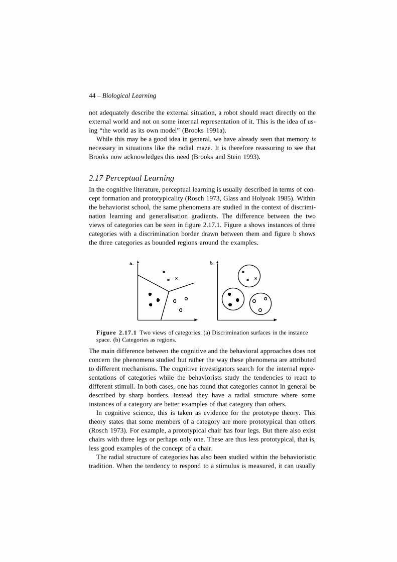
44 – Biological Learning
not adequately describe the external situation, a robot should react directly on theexternal world and not on some internal representation of it. This is the idea of us-ing “the world as its own model” (Brooks 1991a).
While this may be a good idea in general, we have already seen that memory isnecessary in situations like the radial maze. It is therefore reassuring to see thatBrooks now acknowledges this need (Brooks and Stein 1993).
2.17 Perceptual LearningIn the cognitive literature, perceptual learning is usually described in terms of con-cept formation and prototypicality (Rosch 1973, Glass and Holyoak 1985). Withinthe behaviorist school, the same phenomena are studied in the context of discrimi-nation learning and generalisation gradients. The difference between the twoviews of categories can be seen in figure 2.17.1. Figure a shows instances of threecategories with a discrimination border drawn between them and figure b showsthe three categories as bounded regions around the examples.
Figure 2.17.1 Two views of categories. (a) Discrimination surfaces in the instancespace. (b) Categories as regions.
The main difference between the cognitive and the behavioral approaches does notconcern the phenomena studied but rather the way these phenomena are attributedto different mechanisms. The cognitive investigators search for the internal repre-sentations of categories while the behaviorists study the tendencies to react todifferent stimuli. In both cases, one has found that categories cannot in general bedescribed by sharp borders. Instead they have a radial structure where someinstances of a category are better examples of that category than others.
In cognitive science, this is taken as evidence for the prototype theory. Thistheory states that some members of a category are more prototypical than others(Rosch 1973). For example, a prototypical chair has four legs. But there also existchairs with three legs or perhaps only one. These are thus less prototypical, that is,less good examples of the concept of a chair.
The radial structure of categories has also been studied within the behavioristictradition. When the tendency to respond to a stimulus is measured, it can usually
2.18 Conclusion – 45
be shown that there exists one specific stimulus for which the response is thestrongest or the most likely (Mackintosh 1983). As the stimulus is altered the re-sponse decreases with increased dissimilarity between the optimal and the alteredstimulus. There is said to be generalization gradient around the optimal stimulus.Is this not prototype theory in disguise?
Another way to study perceptual learning is to see whether an animal will reactin one way or another to a stimulus. In this way we will study discrimination sur-faces between different categories instead of their radial structure.
All these approaches to perceptual learning and many others can be found bothwithin the area of machine learning (see Davidsson 1994) as well as in neural net-works and statistical inference (Lippman 1987).
2.18 ConclusionAll the studies presented above, both within animal learning theory and artificialintelligence, have been concerned with some particular aspect of learning or be-havior. To date, very few models have attempted to deal with the full complexityof learning, although there certainly exist biological models which could explainmost aspects of learning, if they could only be combined in some sensible manner.
Too much effort has been spent on trying to figure out who is right and who iswrong instead of searching for the similarities between the different theories. Anattempt to merge the different theories into a coherent system would be very wel-come. However, such an enterprise would have to avoid two critical traps whichhave caught most previous attempts.
The first trap is to believe that all learning and behavior can be explained with asmall set of principles. The result of this approach has been the construction ofgrand theories which set out to explain all instances of learning but later arerevealed as too limited. It is not unusual for models of this kind to be both clearand elegant, but this is true only because their explanatory power has been sacri-ficed.
The second pitfall is to think that everyone is right and to simply combine allmodels one can find into one big theory of everything. This has often been the casewhen AI researchers have felt the need to build complete systems. The models forperceptual learning are usually highly incompatible with those for reasoning andproblem solving, but this has not stopped some people from combining them intoso called hybrid systems. While these systems have the advantage that they com-bine many mechanisms, all signs of elegance are usually far gone. Since mosthybrid systems have been directed towards specific technical applications, theirvalue as theories is also very limited.4
4. They may, of course, still be useful in technical applications.
46 – Biological Learning
In summary, what is needed is an approach where all the different aspects oflearning can be combined in an elegant manner. We want to propose that such anendeavour must satisfy the following three criteria.
First, it must be computational. Whatever the properties are of the system weare looking for, they will be highly complex. Thus, a model that is not computa-tional will inevitably contain many inconsistencies. Only within a computationalapproach are we required to specify a model in every detail, and that is absolutelynecessary in this case. This implies that we must model one particular individual.There exists no general animal and a fully specified system can never be generaleither.
Second, it must describe a complete system. A complete system includes sen-sors and effectors as well as everything in between. This assures that the systemwill be grounded (Harnad 1990), that is, all internal processes can be traced backto the peripheral systems. Like the computational approach, the complete systemsapproach also requires that we model one particular individual of one particularspecies.
Third, the system must be based on one descriptive vehicle. This may not be re-quired to build a working system, but it is a necessary feature of any attractivemodel. This will make it possible to describe a system in a coherent way as well asmaking the computational approach easier.
To conclude, we suggest that artificial intelligence learns the lessons from ani-mal learning theory and starts to consider complete systems where a large set ofinteracting mechanisms are combined in a coherent manner. The study of such sys-tems will be of great importance both for the success of artificial intelligence andfor our understanding of learning and intelligence in animals and man. The nextchapter is a brief introduction to this area.
Christian Balkenius, 1995, Natural Intelligence in Artificial Creatures, Lund University Cognitive Studies 37, 1995.
Chapter 3
Design Principles
3.1 IntroductionAs described in the preceding chapter, there are many ideas from animal learningtheory and artificial intelligence that can be used as a starting point for the con-struction of artificial creatures. In this chapter, we will introduce two areas of re-search that will play an important role in the rest of the book.
First we will take a look at a number of design principles that have recentlybeen proposed in the field of behavior-based robotics. Systems designed accordingto these ideas go by the names of situated agents (Agre and Chapman 1987), em-bedded systems (Kaebling 1993), autonomous agents (Maes 1990), and reactivecontrol (Arkin 1990). The principles introduced here will guide the construction ofour artificial creatures. We will also introduce some terminology that will be usedin later chapters.
Next, the basic principles behind neural networks will be described with the em-phasis on the types of systems that will be used in our artificial creatures. We willsee how model neurons can be connected in different ways to perform variousfunctions which will be used later on in the book.
The chapter concludes with a simple example of an artificial creature. In thisexample, we show how the proposed design principles constrain the constructionof an artificial nervous systems. The artificial world that will be used throughoutthe book is also introduced together with the sensors and effectors of the creature.
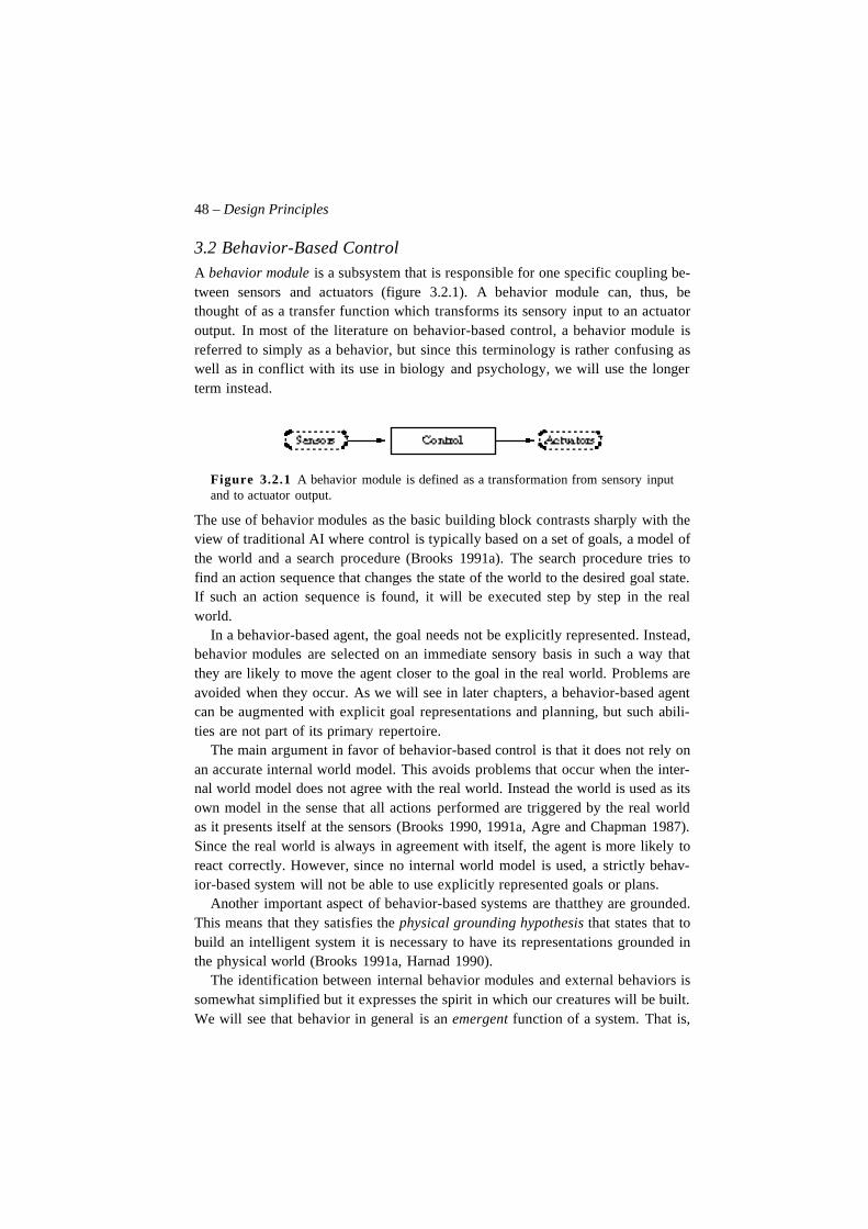
48 – Design Principles
3.2 Behavior-Based ControlA behavior module is a subsystem that is responsible for one specific coupling be-tween sensors and actuators (figure 3.2.1). A behavior module can, thus, bethought of as a transfer function which transforms its sensory input to an actuatoroutput. In most of the literature on behavior-based control, a behavior module isreferred to simply as a behavior, but since this terminology is rather confusing aswell as in conflict with its use in biology and psychology, we will use the longerterm instead.
Figure 3.2.1 A behavior module is defined as a transformation from sensory inputand to actuator output.
The use of behavior modules as the basic building block contrasts sharply with theview of traditional AI where control is typically based on a set of goals, a model ofthe world and a search procedure (Brooks 1991a). The search procedure tries tofind an action sequence that changes the state of the world to the desired goal state.If such an action sequence is found, it will be executed step by step in the realworld.
In a behavior-based agent, the goal needs not be explicitly represented. Instead,behavior modules are selected on an immediate sensory basis in such a way thatthey are likely to move the agent closer to the goal in the real world. Problems areavoided when they occur. As we will see in later chapters, a behavior-based agentcan be augmented with explicit goal representations and planning, but such abili-ties are not part of its primary repertoire.
The main argument in favor of behavior-based control is that it does not rely onan accurate internal world model. This avoids problems that occur when the inter-nal world model does not agree with the real world. Instead the world is used as itsown model in the sense that all actions performed are triggered by the real worldas it presents itself at the sensors (Brooks 1990, 1991a, Agre and Chapman 1987).Since the real world is always in agreement with itself, the agent is more likely toreact correctly. However, since no internal world model is used, a strictly behav-ior-based system will not be able to use explicitly represented goals or plans.
Another important aspect of behavior-based systems are thatthey are grounded.This means that they satisfies the physical grounding hypothesis that states that tobuild an intelligent system it is necessary to have its representations grounded inthe physical world (Brooks 1991a, Harnad 1990).
The identification between internal behavior modules and external behaviors issomewhat simplified but it expresses the spirit in which our creatures will be built.We will see that behavior in general is an emergent function of a system. That is,
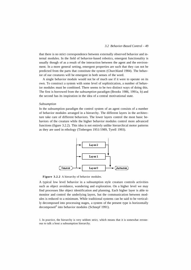
3.2 Behavior-Based Control – 49
that there is no strict correspondence between externally observed behavior and in-ternal modules. In the field of behavior-based robotics, emergent functionality isusually though of as a result of the interaction between the agent and the environ-ment. In a more general setting, emergent properties are such that they can not bepredicted from the parts that constitute the system (Churchland 1984). The behav-ior of our creatures will be emergent in both senses of the word.
A single behavior module would not be of much use if it were to operate on itsown. To construct a system with some level of sophistication, a number of behav-ior modules must be combined. There seems to be two distinct ways of doing this.The first is borrowed from the subsumption paradigm (Brooks 1986, 1991a, b) andthe second has its inspiration in the idea of a central motivational state.
Subsumption
In the subsumption paradigm the control system of an agent consists of a numberof behavior modules arranged in a hierarchy. The different layers in the architec-ture take care of different behaviors. The lower layers control the most basic be-haviors of the creature while the higher behavior modules control more advancedfunctions (figure 3.2.2). This idea is not entirely unlike hierarchical motor patternsas they are used in ethology (Tinbergen 1951/1989, Tyrell 1993).
Figure 3.2.2 A hierarchy of behavior modules.
A typical low level behavior in a subsumption style creature controls activitiessuch as object avoidance, wandering and exploration. On a higher level we mayfind processes like object identification and planning. Each higher layer is able tomonitor and control the underlying layers, but the communication between mod-ules is reduced to a minimum. While traditional systems can be said to be vertical-ly decomposed into processing stages, a system of the present type is horizontallydecomposed1 into behavior modules (Schnepf 1991).
1. In practice, the hierarchy is very seldom strict, which means that it is somewhat errone-ous to talk a bout a subsumption hierarchy.
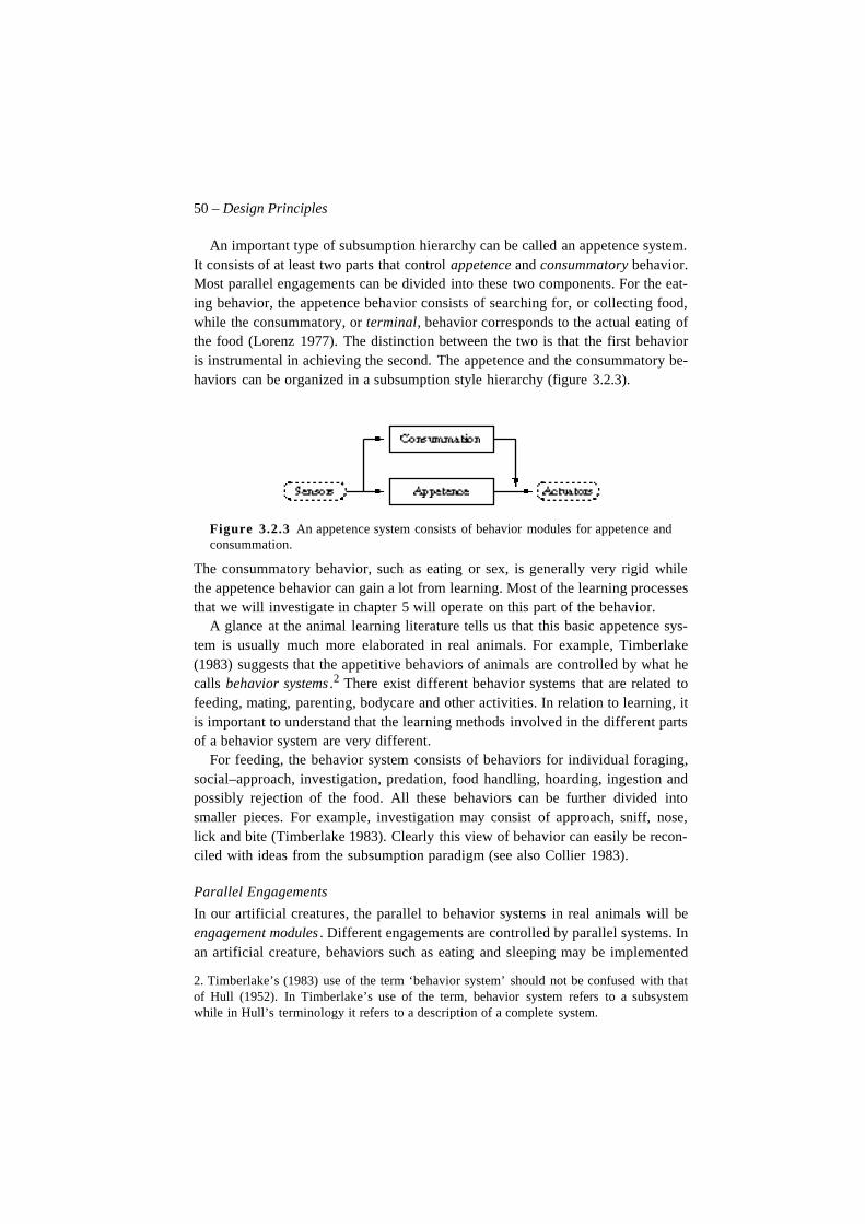
50 – Design Principles
An important type of subsumption hierarchy can be called an appetence system.It consists of at least two parts that control appetence and consummatory behavior.Most parallel engagements can be divided into these two components. For the eat-ing behavior, the appetence behavior consists of searching for, or collecting food,while the consummatory, or terminal, behavior corresponds to the actual eating ofthe food (Lorenz 1977). The distinction between the two is that the first behavioris instrumental in achieving the second. The appetence and the consummatory be-haviors can be organized in a subsumption style hierarchy (figure 3.2.3).
Figure 3.2.3 An appetence system consists of behavior modules for appetence andconsummation.
The consummatory behavior, such as eating or sex, is generally very rigid whilethe appetence behavior can gain a lot from learning. Most of the learning processesthat we will investigate in chapter 5 will operate on this part of the behavior.
A glance at the animal learning literature tells us that this basic appetence sys-tem is usually much more elaborated in real animals. For example, Timberlake(1983) suggests that the appetitive behaviors of animals are controlled by what hecalls behavior systems .2 There exist different behavior systems that are related tofeeding, mating, parenting, bodycare and other activities. In relation to learning, itis important to understand that the learning methods involved in the different partsof a behavior system are very different.
For feeding, the behavior system consists of behaviors for individual foraging,social–approach, investigation, predation, food handling, hoarding, ingestion andpossibly rejection of the food. All these behaviors can be further divided intosmaller pieces. For example, investigation may consist of approach, sniff, nose,lick and bite (Timberlake 1983). Clearly this view of behavior can easily be recon-ciled with ideas from the subsumption paradigm (see also Collier 1983).
Parallel Engagements
In our artificial creatures, the parallel to behavior systems in real animals will beengagement modules . Different engagements are controlled by parallel systems. Inan artificial creature, behaviors such as eating and sleeping may be implemented
2. Timberlake’s (1983) use of the term ‘behavior system’ should not be confused with thatof Hull (1952). In Timberlake’s use of the term, behavior system refers to a subsystemwhile in Hull’s terminology it refers to a description of a complete system.
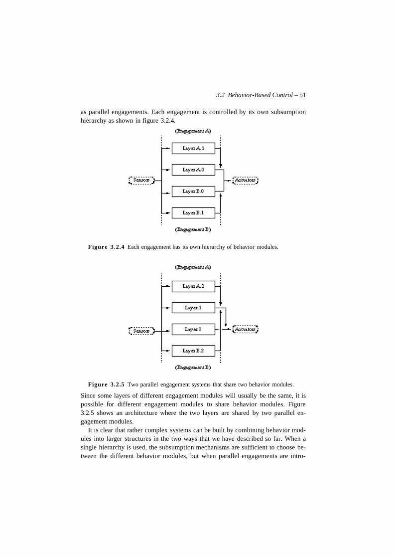
3.2 Behavior-Based Control – 51
as parallel engagements. Each engagement is controlled by its own subsumptionhierarchy as shown in figure 3.2.4.
Figure 3.2.4 Each engagement has its own hierarchy of behavior modules.
Figure 3.2.5 Two parallel engagement systems that share two behavior modules.
Since some layers of different engagement modules will usually be the same, it ispossible for different engagement modules to share behavior modules. Figure3.2.5 shows an architecture where the two layers are shared by two parallel en-gagement modules.
It is clear that rather complex systems can be built by combining behavior mod-ules into larger structures in the two ways that we have described so far. When asingle hierarchy is used, the subsumption mechanisms are sufficient to choose be-tween the different behavior modules, but when parallel engagements are intro-
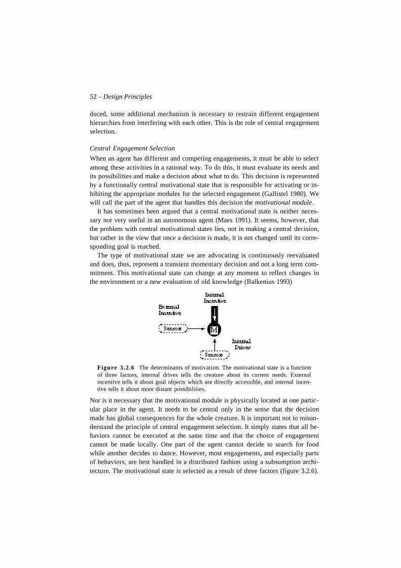
52 – Design Principles
duced, some additional mechanism is necessary to restrain different engagementhierarchies from interfering with each other. This is the role of central engagementselection.
Central Engagement Selection
When an agent has different and competing engagements, it must be able to selectamong these activities in a rational way. To do this, it must evaluate its needs andits possibilities and make a decision about what to do. This decision is representedby a functionally central motivational state that is responsible for activating or in-hibiting the appropriate modules for the selected engagement (Gallistel 1980). Wewill call the part of the agent that handles this decision the motivational module .
It has sometimes been argued that a central motivational state is neither neces-sary nor very useful in an autonomous agent (Maes 1991). It seems, however, thatthe problem with central motivational states lies, not in making a central decision,but rather in the view that once a decision is made, it is not changed until its corre-sponding goal is reached.
The type of motivational state we are advocating is continuously reevaluatedand does, thus, represent a transient momentary decision and not a long term com-mitment. This motivational state can change at any moment to reflect changes inthe environment or a new evaluation of old knowledge (Balkenius 1993)
Figure 3.2.6 The determinants of motivation. The motivational state is a functionof three factors, internal drives tells the creature about its current needs. Externalincentive tells it about goal objects which are directly accessible, and internal incen-tive tells it about more distant possibilities.
Nor is it necessary that the motivational module is physically located at one partic-ular place in the agent. It needs to be central only in the sense that the decisionmade has global consequences for the whole creature. It is important not to misun-derstand the principle of central engagement selection. It simply states that all be-haviors cannot be executed at the same time and that the choice of engagementcannot be made locally. One part of the agent cannot decide to search for foodwhile another decides to dance. However, most engagements, and especially partsof behaviors, are best handled in a distributed fashion using a subsumption archi-tecture. The motivational state is selected as a result of three factors (figure 3.2.6).
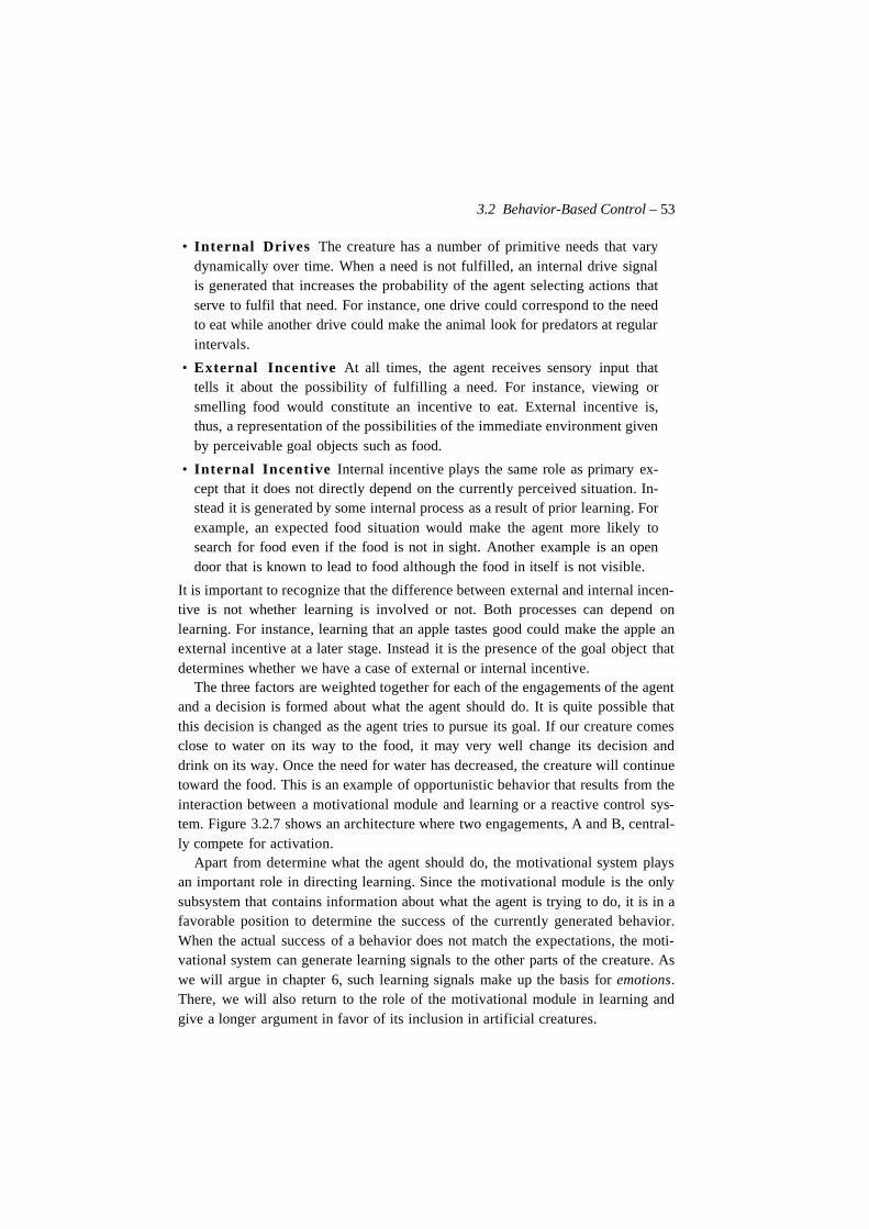
3.2 Behavior-Based Control – 53
• Internal Drives The creature has a number of primitive needs that varydynamically over time. When a need is not fulfilled, an internal drive signalis generated that increases the probability of the agent selecting actions thatserve to fulfil that need. For instance, one drive could correspond to the needto eat while another drive could make the animal look for predators at regularintervals.
• External Incentive At all times, the agent receives sensory input thattells it about the possibility of fulfilling a need. For instance, viewing orsmelling food would constitute an incentive to eat. External incentive is,thus, a representation of the possibilities of the immediate environment givenby perceivable goal objects such as food.
• Internal Incentive Internal incentive plays the same role as primary ex-cept that it does not directly depend on the currently perceived situation. In-stead it is generated by some internal process as a result of prior learning. Forexample, an expected food situation would make the agent more likely tosearch for food even if the food is not in sight. Another example is an opendoor that is known to lead to food although the food in itself is not visible.
It is important to recognize that the difference between external and internal incen-tive is not whether learning is involved or not. Both processes can depend onlearning. For instance, learning that an apple tastes good could make the apple anexternal incentive at a later stage. Instead it is the presence of the goal object thatdetermines whether we have a case of external or internal incentive.
The three factors are weighted together for each of the engagements of the agentand a decision is formed about what the agent should do. It is quite possible thatthis decision is changed as the agent tries to pursue its goal. If our creature comesclose to water on its way to the food, it may very well change its decision anddrink on its way. Once the need for water has decreased, the creature will continuetoward the food. This is an example of opportunistic behavior that results from theinteraction between a motivational module and learning or a reactive control sys-tem. Figure 3.2.7 shows an architecture where two engagements, A and B, central-ly compete for activation.
Apart from determine what the agent should do, the motivational system playsan important role in directing learning. Since the motivational module is the onlysubsystem that contains information about what the agent is trying to do, it is in afavorable position to determine the success of the currently generated behavior.When the actual success of a behavior does not match the expectations, the moti-vational system can generate learning signals to the other parts of the creature. Aswe will argue in chapter 6, such learning signals make up the basis for emotions.There, we will also return to the role of the motivational module in learning andgive a longer argument in favor of its inclusion in artificial creatures.
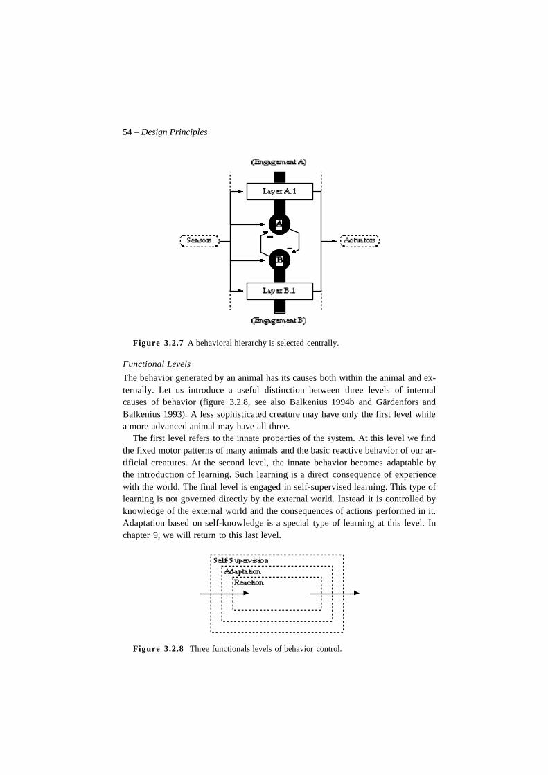
54 – Design Principles
Figure 3.2.7 A behavioral hierarchy is selected centrally.
Functional Levels
The behavior generated by an animal has its causes both within the animal and ex-ternally. Let us introduce a useful distinction between three levels of internalcauses of behavior (figure 3.2.8, see also Balkenius 1994b and Gärdenfors andBalkenius 1993). A less sophisticated creature may have only the first level whilea more advanced animal may have all three.
The first level refers to the innate properties of the system. At this level we findthe fixed motor patterns of many animals and the basic reactive behavior of our ar-tificial creatures. At the second level, the innate behavior becomes adaptable bythe introduction of learning. Such learning is a direct consequence of experiencewith the world. The final level is engaged in self-supervised learning. This type oflearning is not governed directly by the external world. Instead it is controlled byknowledge of the external world and the consequences of actions performed in it.Adaptation based on self-knowledge is a special type of learning at this level. Inchapter 9, we will return to this last level.
Figure 3.2.8 Three functionals levels of behavior control.
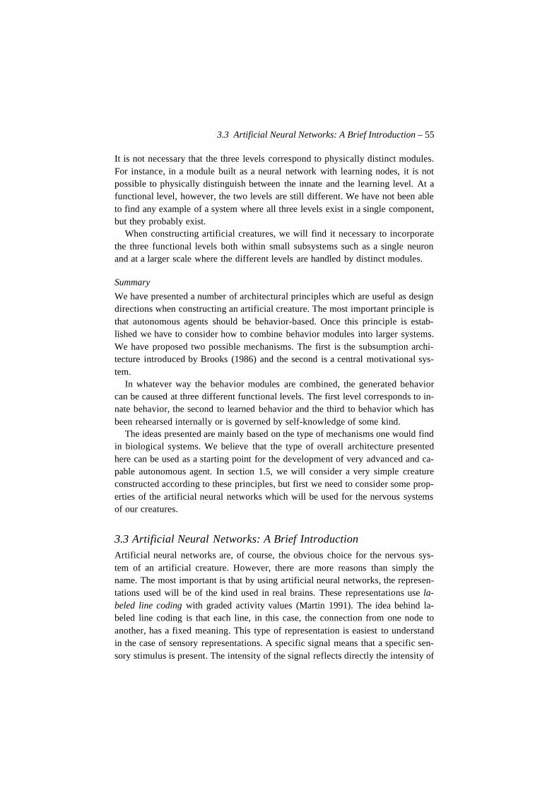
3.3 Artificial Neural Networks: A Brief Introduction – 55
It is not necessary that the three levels correspond to physically distinct modules.For instance, in a module built as a neural network with learning nodes, it is notpossible to physically distinguish between the innate and the learning level. At afunctional level, however, the two levels are still different. We have not been ableto find any example of a system where all three levels exist in a single component,but they probably exist.
When constructing artificial creatures, we will find it necessary to incorporatethe three functional levels both within small subsystems such as a single neuronand at a larger scale where the different levels are handled by distinct modules.
Summary
We have presented a number of architectural principles which are useful as designdirections when constructing an artificial creature. The most important principle isthat autonomous agents should be behavior-based. Once this principle is estab-lished we have to consider how to combine behavior modules into larger systems.We have proposed two possible mechanisms. The first is the subsumption archi-tecture introduced by Brooks (1986) and the second is a central motivational sys-tem.
In whatever way the behavior modules are combined, the generated behaviorcan be caused at three different functional levels. The first level corresponds to in-nate behavior, the second to learned behavior and the third to behavior which hasbeen rehearsed internally or is governed by self-knowledge of some kind.
The ideas presented are mainly based on the type of mechanisms one would findin biological systems. We believe that the type of overall architecture presentedhere can be used as a starting point for the development of very advanced and ca-pable autonomous agent. In section 1.5, we will consider a very simple creatureconstructed according to these principles, but first we need to consider some prop-erties of the artificial neural networks which will be used for the nervous systemsof our creatures.
3.3 Artificial Neural Networks: A Brief IntroductionArtificial neural networks are, of course, the obvious choice for the nervous sys-tem of an artificial creature. However, there are more reasons than simply thename. The most important is that by using artificial neural networks, the represen-tations used will be of the kind used in real brains. These representations use la-beled line coding with graded activity values (Martin 1991). The idea behind la-beled line coding is that each line, in this case, the connection from one node toanother, has a fixed meaning. This type of representation is easiest to understandin the case of sensory representations. A specific signal means that a specific sen-sory stimulus is present. The intensity of the signal reflects directly the intensity of
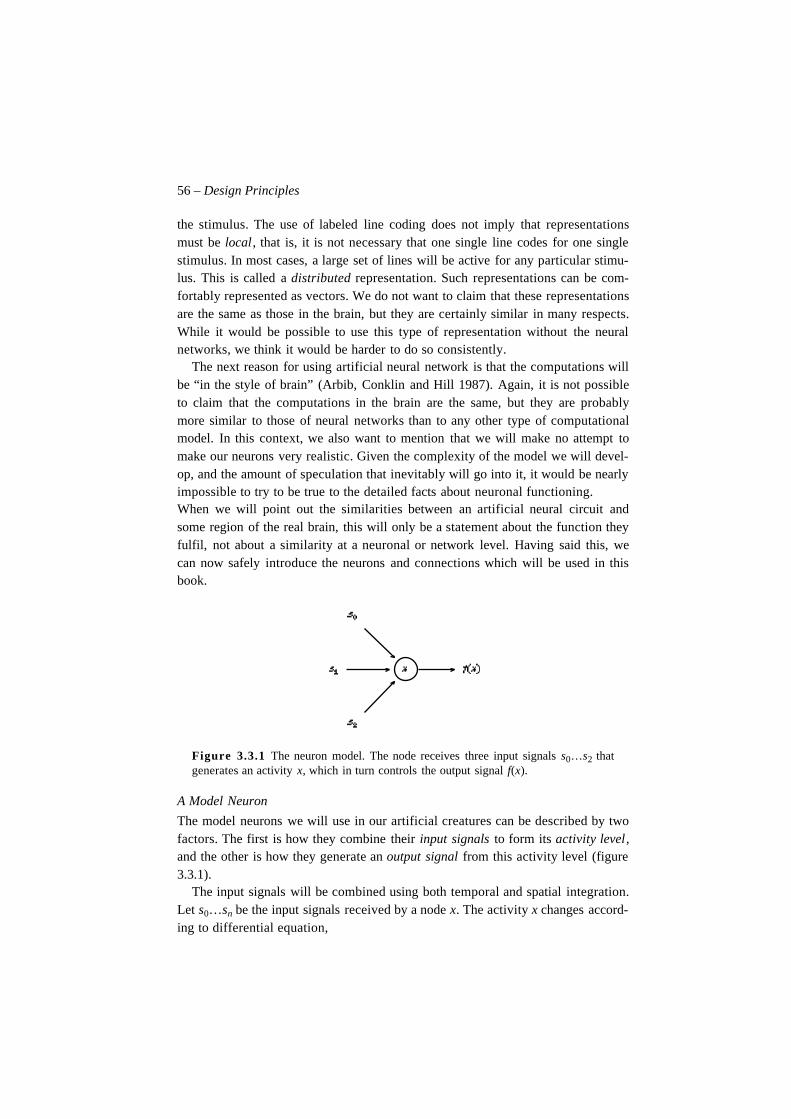
56 – Design Principles
the stimulus. The use of labeled line coding does not imply that representationsmust be local, that is, it is not necessary that one single line codes for one singlestimulus. In most cases, a large set of lines will be active for any particular stimu-lus. This is called a distributed representation. Such representations can be com-fortably represented as vectors. We do not want to claim that these representationsare the same as those in the brain, but they are certainly similar in many respects.While it would be possible to use this type of representation without the neuralnetworks, we think it would be harder to do so consistently.
The next reason for using artificial neural network is that the computations willbe “in the style of brain” (Arbib, Conklin and Hill 1987). Again, it is not possibleto claim that the computations in the brain are the same, but they are probablymore similar to those of neural networks than to any other type of computationalmodel. In this context, we also want to mention that we will make no attempt tomake our neurons very realistic. Given the complexity of the model we will devel-op, and the amount of speculation that inevitably will go into it, it would be nearlyimpossible to try to be true to the detailed facts about neuronal functioning.When we will point out the similarities between an artificial neural circuit andsome region of the real brain, this will only be a statement about the function theyfulfil, not about a similarity at a neuronal or network level. Having said this, wecan now safely introduce the neurons and connections which will be used in thisbook.
Figure 3.3.1 The neuron model. The node receives three input signals s0…s2 thatgenerates an activity x, which in turn controls the output signal f(x).
A Model Neuron
The model neurons we will use in our artificial creatures can be described by twofactors. The first is how they combine their input signals to form its activity level,and the other is how they generate an output signal from this activity level (figure3.3.1).
The input signals will be combined using both temporal and spatial integration.Let s0…sn be the input signals received by a node x. The activity x changes accord-ing to differential equation,
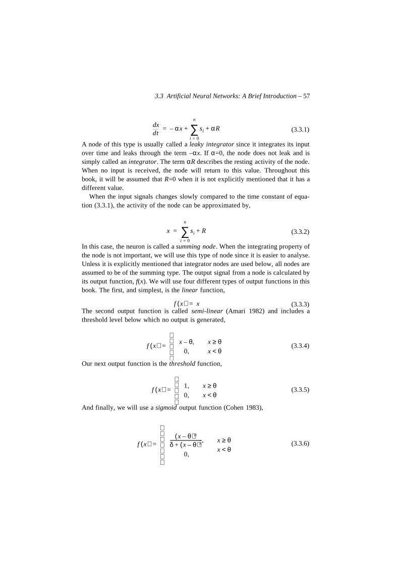
3.3 Artificial Neural Networks: A Brief Introduction – 57
(3.3.1)
A node of this type is usually called a leaky integrator since it integrates its inputover time and leaks through the term –αx. If α=0, the node does not leak and issimply called an integrator. The term αR describes the resting activity of the node.When no input is received, the node will return to this value. Throughout thisbook, it will be assumed that R=0 when it is not explicitly mentioned that it has adifferent value.
When the input signals changes slowly compared to the time constant of equa-tion (3.3.1), the activity of the node can be approximated by,
(3.3.2)
In this case, the neuron is called a summing node. When the integrating property ofthe node is not important, we will use this type of node since it is easier to analyse.Unless it is explicitly mentioned that integrator nodes are used below, all nodes areassumed to be of the summing type. The output signal from a node is calculated byits output function, f(x). We will use four different types of output functions in thisbook. The first, and simplest, is the linear function,
(3.3.3)The second output function is called semi-linear (Amari 1982) and includes athreshold level below which no output is generated,
(3.3.4)
Our next output function is the threshold function,
(3.3.5)
And finally, we will use a sigmoid output function (Cohen 1983),
(3.3.6)
tddx αx– si αR+
i 0=
n
∑+=
x si R+i 0=
n
∑=
f x( ) x=
f x( ) x θ– ,0,
x θ≥x θ<
=
f x( ) 1,0,
x θ≥x θ<
=
f x( )x θ–( )n
δ x θ–( )n+----------------------------,
0,
x θ≥x θ<
=
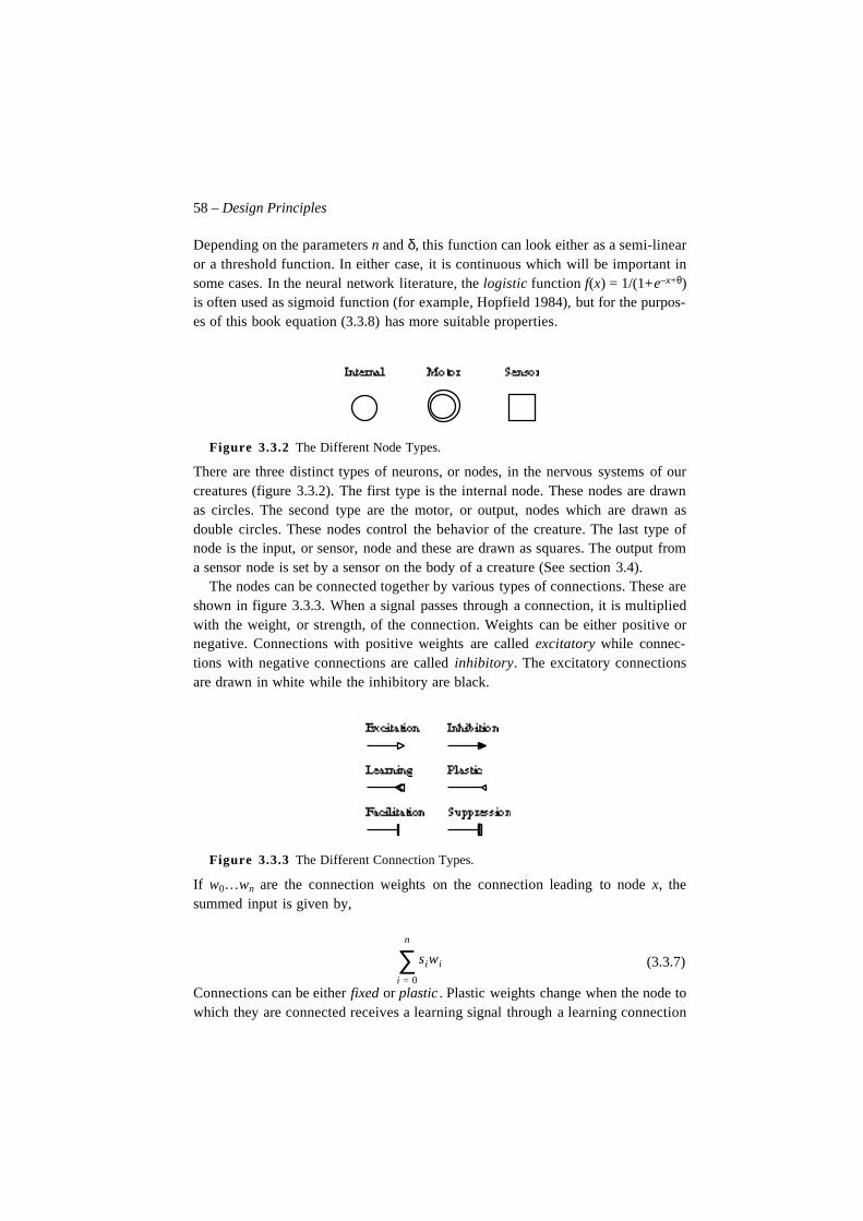
58 – Design Principles
Depending on the parameters n and δ, this function can look either as a semi-linearor a threshold function. In either case, it is continuous which will be important insome cases. In the neural network literature, the logistic function f(x) = 1/(1+e–x+θ)is often used as sigmoid function (for example, Hopfield 1984), but for the purpos-es of this book equation (3.3.8) has more suitable properties.
Figure 3.3.2 The Different Node Types.
There are three distinct types of neurons, or nodes, in the nervous systems of ourcreatures (figure 3.3.2). The first type is the internal node. These nodes are drawnas circles. The second type are the motor, or output, nodes which are drawn asdouble circles. These nodes control the behavior of the creature. The last type ofnode is the input, or sensor, node and these are drawn as squares. The output froma sensor node is set by a sensor on the body of a creature (See section 3.4).
The nodes can be connected together by various types of connections. These areshown in figure 3.3.3. When a signal passes through a connection, it is multipliedwith the weight, or strength, of the connection. Weights can be either positive ornegative. Connections with positive weights are called excitatory while connec-tions with negative connections are called inhibitory. The excitatory connectionsare drawn in white while the inhibitory are black.
Figure 3.3.3 The Different Connection Types.
If w0…wn are the connection weights on the connection leading to node x, thesummed input is given by,
(3.3.7)
Connections can be either fixed or plastic . Plastic weights change when the node towhich they are connected receives a learning signal through a learning connection
siwi
i 0=
n
∑
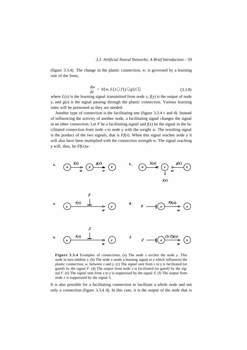
3.3 Artificial Neural Networks: A Brief Introduction – 59
(figure 3.3.4). The change in the plastic connection, w, is governed by a learningrule of the form,
(3.3.8)
where L(x) is the learning signal transmitted from node x, f(y) is the output of nodey, and g(z) is the signal passing through the plastic connection. Various learningrules will be presented as they are needed.
Another type of connection is the facilitating one (figure 3.3.4 c and d). Insteadof influencing the activity of another node, a facilitating signal changes the signalin an other connection. Let F be a facilitating signal and f(x) be the signal in the fa-cilitated connection from node x to node y with the weight w. The resulting signalis the product of the two signals, that is Ff(x). When this signal reaches node y itwill also have been multiplied with the connection strength w. The signal reachingy will, thus, be Ff(x)w.
Figure 3.3.4 Examples of connections. (a) The node x excites the node y. Thisnode in turn inhibits z. (b) The node x sends a learning signal to y which influences theplastic connection, w, between z and y. (c) The signal sent from x to y is facilitated (orgated) by the signal F. (d) The output from node x is facilitated (or gated) by the sig-nal F. (e) The signal sent from x to y is suppressed by the signal S. (f) The output fromnode x is suppressed by the signal S.
It is also possible for a facilitating connection to facilitate a whole node and notonly a connection (figure 3.3.4 d). In this case, it is the output of the node that is
tddw h w L x( ) f y( ) g z( ), , ,( ),=
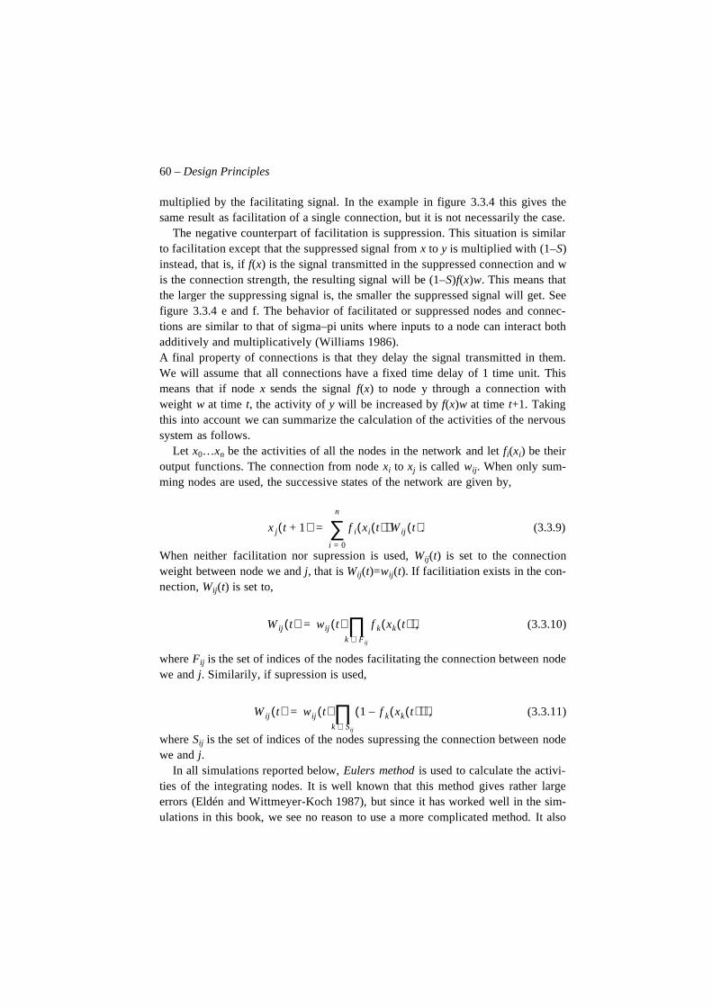
60 – Design Principles
multiplied by the facilitating signal. In the example in figure 3.3.4 this gives thesame result as facilitation of a single connection, but it is not necessarily the case.
The negative counterpart of facilitation is suppression. This situation is similarto facilitation except that the suppressed signal from x to y is multiplied with (1–S)instead, that is, if f(x) is the signal transmitted in the suppressed connection and wis the connection strength, the resulting signal will be (1–S)f(x)w. This means thatthe larger the suppressing signal is, the smaller the suppressed signal will get. Seefigure 3.3.4 e and f. The behavior of facilitated or suppressed nodes and connec-tions are similar to that of sigma–pi units where inputs to a node can interact bothadditively and multiplicatively (Williams 1986).A final property of connections is that they delay the signal transmitted in them.We will assume that all connections have a fixed time delay of 1 time unit. Thismeans that if node x sends the signal f(x) to node y through a connection withweight w at time t, the activity of y will be increased by f(x)w at time t+1. Takingthis into account we can summarize the calculation of the activities of the nervoussystem as follows.
Let x0…xn be the activities of all the nodes in the network and let fi(xi) be theiroutput functions. The connection from node xi to xj is called wij. When only sum-ming nodes are used, the successive states of the network are given by,
(3.3.9)
When neither facilitation nor supression is used, Wij(t) is set to the connectionweight between node we and j, that is Wij(t)=wij(t). If facilitiation exists in the con-nection, Wij(t) is set to,
(3.3.10)
where Fij is the set of indices of the nodes facilitating the connection between nodewe and j. Similarily, if supression is used,
(3.3.11)
where Sij is the set of indices of the nodes supressing the connection between nodewe and j.
In all simulations reported below, Eulers method is used to calculate the activi-ties of the integrating nodes. It is well known that this method gives rather largeerrors (Eldén and Wittmeyer-Koch 1987), but since it has worked well in the sim-ulations in this book, we see no reason to use a more complicated method. It also
x j t 1+( ) f i xi t( )( )W ij t( ).i 0=
n
∑=
W ij t( ) wij t( ) f k xk t( )( ),k F ij∈∏=
W ij t( ) wij t( ) 1 f– k xk t( )( )( ),k Sij∈∏=
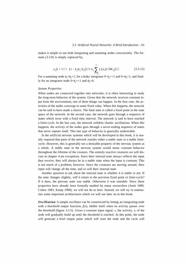
3.3 Artificial Neural Networks: A Brief Introduction – 61
makes it simple to use both integrating and summing nodes concurrently. The for-mula (3.3.9) is simply replaced by,
(3.3.12)
For a summing node εj=αj=1, for a leaky integrator 0<εj<<1 and 0<αj<1, and final-ly for an integrator node 0<εj<<1 and αj=0.
System Properties
When nodes are connected together into networks, it is often interesting to studythe long-term behavior of the system. Given that the network receives constant in-put from the environment, one of three things can happen. In the first case, the ac-tivities of the nodes converge to some fixed value. When this happens, the networkcan be said to have made a choice. The final state is called a fixed point in the statespace of the network. In the second case, the network goes through a sequence ofstates which recur with a fixed time interval. The network is said to have reacheda limit-cycle. In the last case, the network exhibits chaotic oscillations. When thishappens, the activity of the nodes goes through a never-ending sequence of statesthat never repeats itself. This last type of behavior is generally undesirable.
In the artificial nervous systems which will be developed in this book, it is usu-ally required that parts of the network reaches either a stable state or a stable limit-cycle. However, this is generally not a desirable property of the nervous system asa whole. A stable state in the nervous system would mean constant behaviorthroughout the lifetime of the creature. The entirely reactive creatures we will dis-cuss in chapter 4 are exceptions. Since their internal state always reflects the inputthey receive, they will always be in a stable state when the input is constant. Thisis not much of a problem, however. Since the creatures are moving around, theirinput will change all the time, and so will their internal state.
Another question to ask about the internal state is whether it is stable or not. Ifthe state changes slightly, will it return to the previous fixed point or limit-cycle?If it does, the prevous state was stable. Otherwise it was unstable. Since theseproperties have already been formally studied by many researchers (Amit 1989,Cohen 1983, Kamp 1990), we will not do so here. Instead, we will try to summa-rize some important architectures which we will use later on in this book.
Oscillation A simple oscillator can be constructed by letting an integrating nodewith a threshold output function, f(x), inhibit itself when its activity passes overthe threshold (figure 3.3.5). Given a constant input signal, s, the activity, x, of thenode will gradually build up until the threshold is reached. At this point, the nodewill generate a brief output pulse which will reset the node and the cycle will
x j t 1+( ) 1 ε jα j–( )x j t( ) ε j f i xi t( )( )W ij t( ).i 0=
n
∑+=
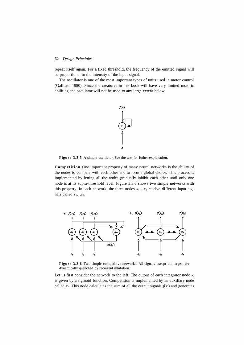
62 – Design Principles
repeat itself again. For a fixed threshold, the frequency of the emitted signal willbe proportional to the intensity of the input signal.
The oscillator is one of the most important types of units used in motor control(Gallistel 1980). Since the creatures in this book will have very limited motoricabilities, the oscillator will not be used to any large extent below.
Figure 3.3.5 A simple oscillator. See the text for futher explanation.
Competition One important property of many neural networks is the ability ofthe nodes to compete with each other and to form a global choice. This process isimplemented by letting all the nodes gradually inhibit each other until only onenode is at its supra-threshold level. Figure 3.3.6 shows two simple networks withthis property. In each network, the three nodes x1…x3 receive different input sig-nals called s1…s3.
Figure 3.3.6 Two simple competitive networks. All signals except the largest aredynamically quenched by recurrent inhibition.
Let us first consider the network to the left. The output of each integrator node xi
is given by a sigmoid function. Competition is implemented by an auxiliary nodecalled x0. This node calculates the sum of all the output signals f(xi) and generates
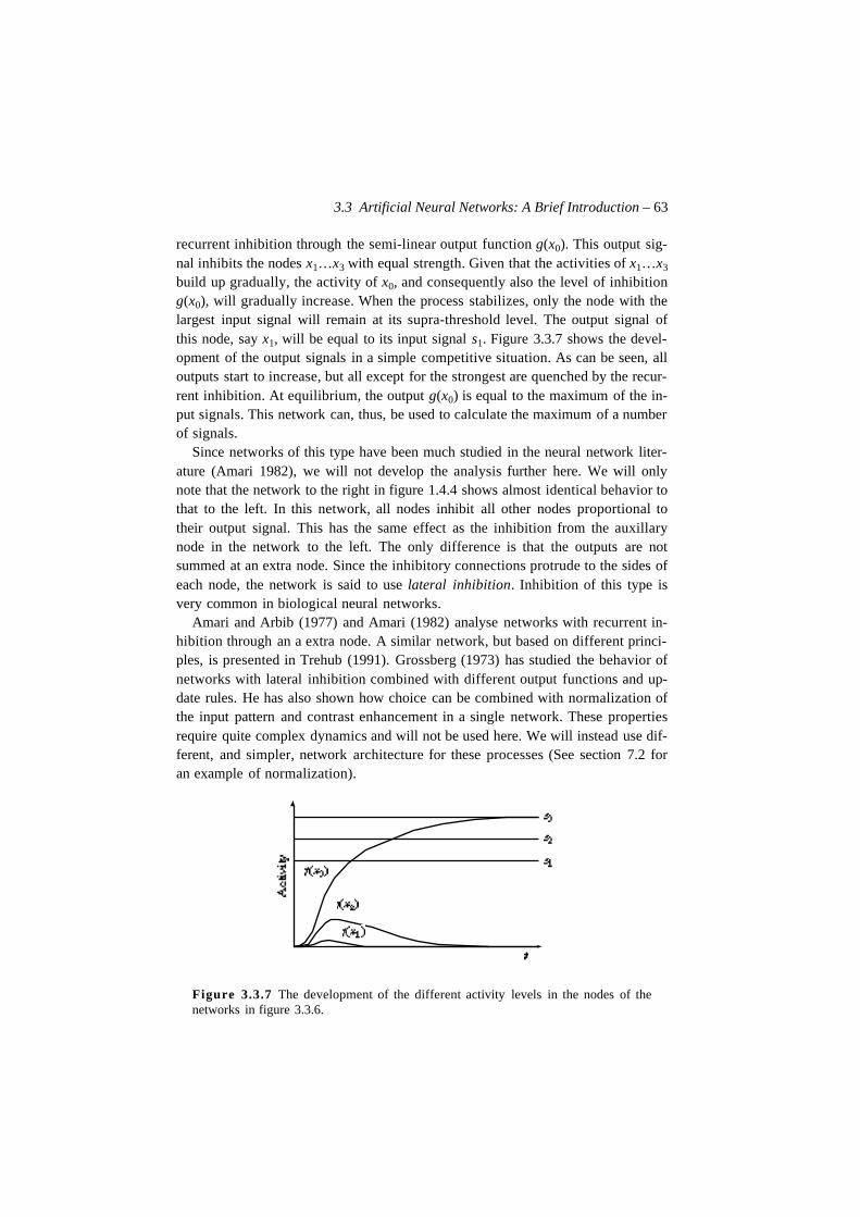
3.3 Artificial Neural Networks: A Brief Introduction – 63
recurrent inhibition through the semi-linear output function g(x0). This output sig-nal inhibits the nodes x1…x3 with equal strength. Given that the activities of x1…x3
build up gradually, the activity of x0, and consequently also the level of inhibitiong(x0), will gradually increase. When the process stabilizes, only the node with thelargest input signal will remain at its supra-threshold level. The output signal ofthis node, say x1, will be equal to its input signal s1. Figure 3.3.7 shows the devel-opment of the output signals in a simple competitive situation. As can be seen, alloutputs start to increase, but all except for the strongest are quenched by the recur-rent inhibition. At equilibrium, the output g(x0) is equal to the maximum of the in-put signals. This network can, thus, be used to calculate the maximum of a numberof signals.
Since networks of this type have been much studied in the neural network liter-ature (Amari 1982), we will not develop the analysis further here. We will onlynote that the network to the right in figure 1.4.4 shows almost identical behavior tothat to the left. In this network, all nodes inhibit all other nodes proportional totheir output signal. This has the same effect as the inhibition from the auxillarynode in the network to the left. The only difference is that the outputs are notsummed at an extra node. Since the inhibitory connections protrude to the sides ofeach node, the network is said to use lateral inhibition. Inhibition of this type isvery common in biological neural networks.
Amari and Arbib (1977) and Amari (1982) analyse networks with recurrent in-hibition through an a extra node. A similar network, but based on different princi-ples, is presented in Trehub (1991). Grossberg (1973) has studied the behavior ofnetworks with lateral inhibition combined with different output functions and up-date rules. He has also shown how choice can be combined with normalization ofthe input pattern and contrast enhancement in a single network. These propertiesrequire quite complex dynamics and will not be used here. We will instead use dif-ferent, and simpler, network architecture for these processes (See section 7.2 foran example of normalization).
Figure 3.3.7 The development of the different activity levels in the nodes of thenetworks in figure 3.3.6.
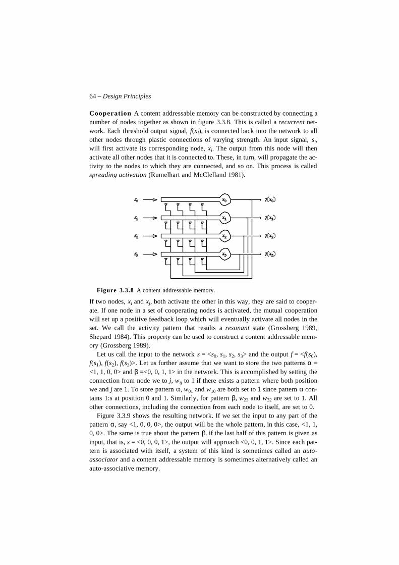
64 – Design Principles
Cooperation A content addressable memory can be constructed by connecting anumber of nodes together as shown in figure 3.3.8. This is called a recurrent net-work. Each threshold output signal, f(xi), is connected back into the network to allother nodes through plastic connections of varying strength. An input signal, si,will first activate its corresponding node, xi. The output from this node will thenactivate all other nodes that it is connected to. These, in turn, will propagate the ac-tivity to the nodes to which they are connected, and so on. This process is calledspreading activation (Rumelhart and McClelland 1981).
Figure 3.3.8 A content addressable memory.
If two nodes, xi and xj, both activate the other in this way, they are said to cooper-ate. If one node in a set of cooperating nodes is activated, the mutual cooperationwill set up a positive feedback loop which will eventually activate all nodes in theset. We call the activity pattern that results a resonant state (Grossberg 1989,Shepard 1984). This property can be used to construct a content addressable mem-ory (Grossberg 1989).
Let us call the input to the network s = <s0, s1, s2, s3> and the output f = <f(s0),f(s1), f(s2), f(s3)>. Let us further assume that we want to store the two patterns α =<1, 1, 0, 0> and β =<0, 0, 1, 1> in the network. This is accomplished by setting theconnection from node we to j, wij to 1 if there exists a pattern where both positionwe and j are 1. To store pattern α, w01 and w10 are both set to 1 since pattern α con-tains 1:s at position 0 and 1. Similarly, for pattern β, w23 and w32 are set to 1. Allother connections, including the connection from each node to itself, are set to 0.
Figure 3.3.9 shows the resulting network. If we set the input to any part of thepattern α, say <1, 0, 0, 0>, the output will be the whole pattern, in this case, <1, 1,0, 0>. The same is true about the pattern β. if the last half of this pattern is given asinput, that is, s = <0, 0, 0, 1>, the output will approach <0, 0, 1, 1>. Since each pat-tern is associated with itself, a system of this kind is sometimes called an auto-associator and a content addressable memory is sometimes alternatively called anauto-associative memory.
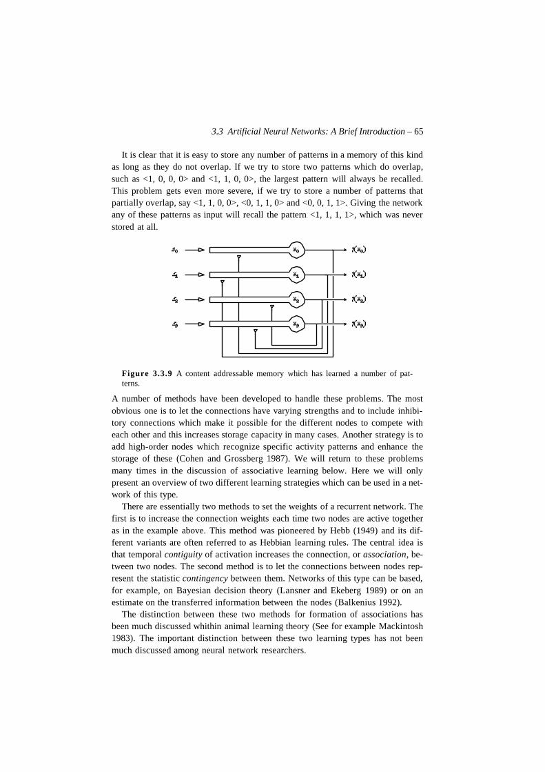
3.3 Artificial Neural Networks: A Brief Introduction – 65
It is clear that it is easy to store any number of patterns in a memory of this kindas long as they do not overlap. If we try to store two patterns which do overlap,such as <1, 0, 0, 0> and <1, 1, 0, 0>, the largest pattern will always be recalled.This problem gets even more severe, if we try to store a number of patterns thatpartially overlap, say <1, 1, 0, 0>, <0, 1, 1, 0> and <0, 0, 1, 1>. Giving the networkany of these patterns as input will recall the pattern <1, 1, 1, 1>, which was neverstored at all.
Figure 3.3.9 A content addressable memory which has learned a number of pat-terns.
A number of methods have been developed to handle these problems. The mostobvious one is to let the connections have varying strengths and to include inhibi-tory connections which make it possible for the different nodes to compete witheach other and this increases storage capacity in many cases. Another strategy is toadd high-order nodes which recognize specific activity patterns and enhance thestorage of these (Cohen and Grossberg 1987). We will return to these problemsmany times in the discussion of associative learning below. Here we will onlypresent an overview of two different learning strategies which can be used in a net-work of this type.
There are essentially two methods to set the weights of a recurrent network. Thefirst is to increase the connection weights each time two nodes are active togetheras in the example above. This method was pioneered by Hebb (1949) and its dif-ferent variants are often referred to as Hebbian learning rules. The central idea isthat temporal contiguity of activation increases the connection, or association, be-tween two nodes. The second method is to let the connections between nodes rep-resent the statistic contingency between them. Networks of this type can be based,for example, on Bayesian decision theory (Lansner and Ekeberg 1989) or on anestimate on the transferred information between the nodes (Balkenius 1992).
The distinction between these two methods for formation of associations hasbeen much discussed whithin animal learning theory (See for example Mackintosh1983). The important distinction between these two learning types has not beenmuch discussed among neural network researchers.
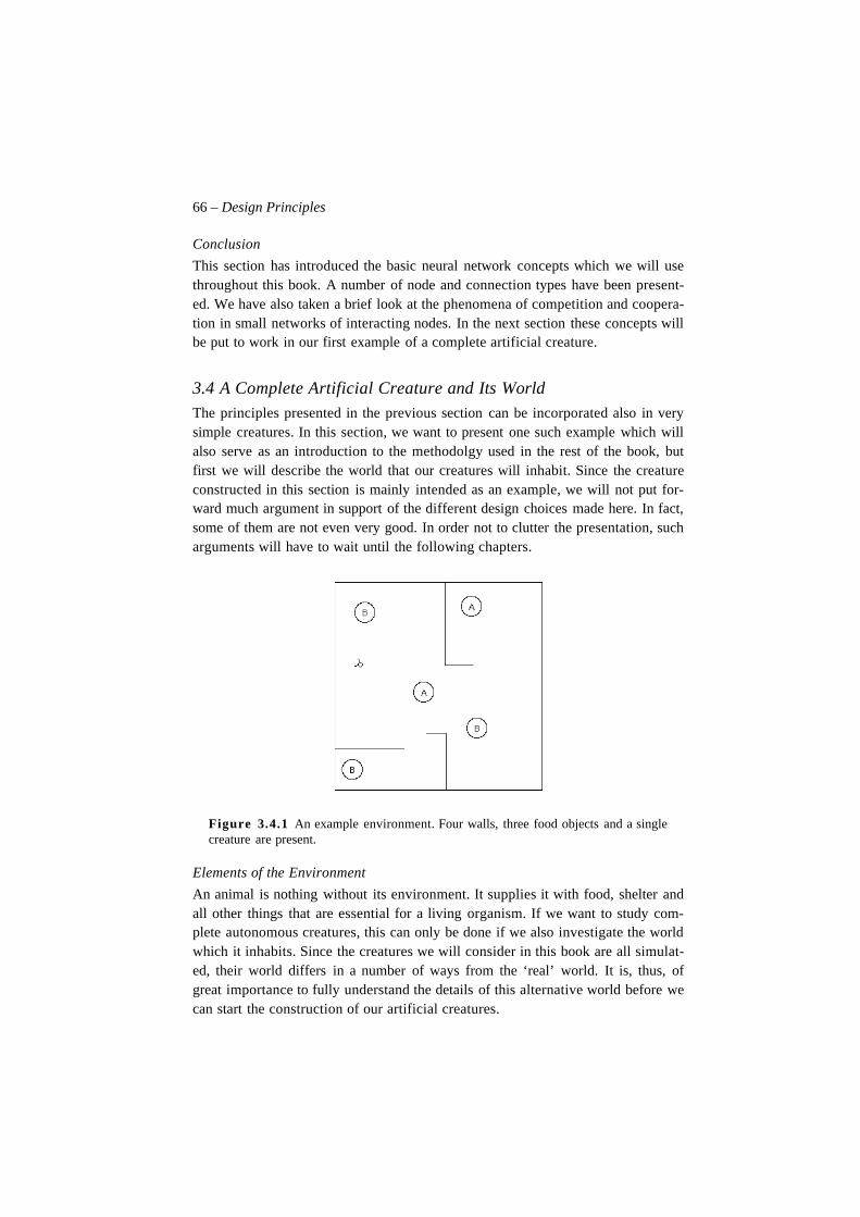
66 – Design Principles
Conclusion
This section has introduced the basic neural network concepts which we will usethroughout this book. A number of node and connection types have been present-ed. We have also taken a brief look at the phenomena of competition and coopera-tion in small networks of interacting nodes. In the next section these concepts willbe put to work in our first example of a complete artificial creature.
3.4 A Complete Artificial Creature and Its WorldThe principles presented in the previous section can be incorporated also in verysimple creatures. In this section, we want to present one such example which willalso serve as an introduction to the methodolgy used in the rest of the book, butfirst we will describe the world that our creatures will inhabit. Since the creatureconstructed in this section is mainly intended as an example, we will not put for-ward much argument in support of the different design choices made here. In fact,some of them are not even very good. In order not to clutter the presentation, sucharguments will have to wait until the following chapters.
Figure 3.4.1 An example environment. Four walls, three food objects and a singlecreature are present.
Elements of the Environment
An animal is nothing without its environment. It supplies it with food, shelter andall other things that are essential for a living organism. If we want to study com-plete autonomous creatures, this can only be done if we also investigate the worldwhich it inhabits. Since the creatures we will consider in this book are all simulat-ed, their world differs in a number of ways from the ‘real’ world. It is, thus, ofgreat importance to fully understand the details of this alternative world before wecan start the construction of our artificial creatures.
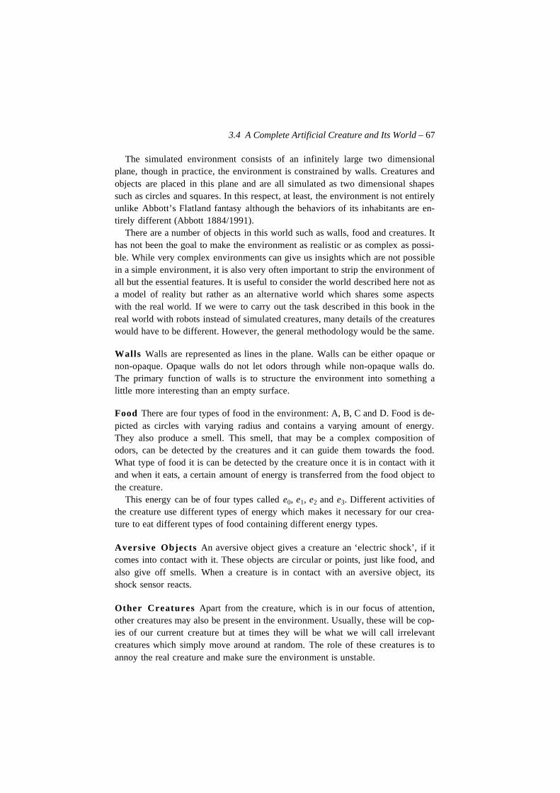
3.4 A Complete Artificial Creature and Its World – 67
The simulated environment consists of an infinitely large two dimensionalplane, though in practice, the environment is constrained by walls. Creatures andobjects are placed in this plane and are all simulated as two dimensional shapessuch as circles and squares. In this respect, at least, the environment is not entirelyunlike Abbott’s Flatland fantasy although the behaviors of its inhabitants are en-tirely different (Abbott 1884/1991).
There are a number of objects in this world such as walls, food and creatures. Ithas not been the goal to make the environment as realistic or as complex as possi-ble. While very complex environments can give us insights which are not possiblein a simple environment, it is also very often important to strip the environment ofall but the essential features. It is useful to consider the world described here not asa model of reality but rather as an alternative world which shares some aspectswith the real world. If we were to carry out the task described in this book in thereal world with robots instead of simulated creatures, many details of the creatureswould have to be different. However, the general methodology would be the same.
Walls Walls are represented as lines in the plane. Walls can be either opaque ornon-opaque. Opaque walls do not let odors through while non-opaque walls do.The primary function of walls is to structure the environment into something alittle more interesting than an empty surface.
Food There are four types of food in the environment: A, B, C and D. Food is de-picted as circles with varying radius and contains a varying amount of energy.They also produce a smell. This smell, that may be a complex composition ofodors, can be detected by the creatures and it can guide them towards the food.What type of food it is can be detected by the creature once it is in contact with itand when it eats, a certain amount of energy is transferred from the food object tothe creature.
This energy can be of four types called e0, e1, e2 and e3. Different activities ofthe creature use different types of energy which makes it necessary for our crea-ture to eat different types of food containing different energy types.
Aversive Objects An aversive object gives a creature an ‘electric shock’, if itcomes into contact with it. These objects are circular or points, just like food, andalso give off smells. When a creature is in contact with an aversive object, itsshock sensor reacts.
Other Creatures Apart from the creature, which is in our focus of attention,other creatures may also be present in the environment. Usually, these will be cop-ies of our current creature but at times they will be what we will call irrelevantcreatures which simply move around at random. The role of these creatures is toannoy the real creature and make sure the environment is unstable.
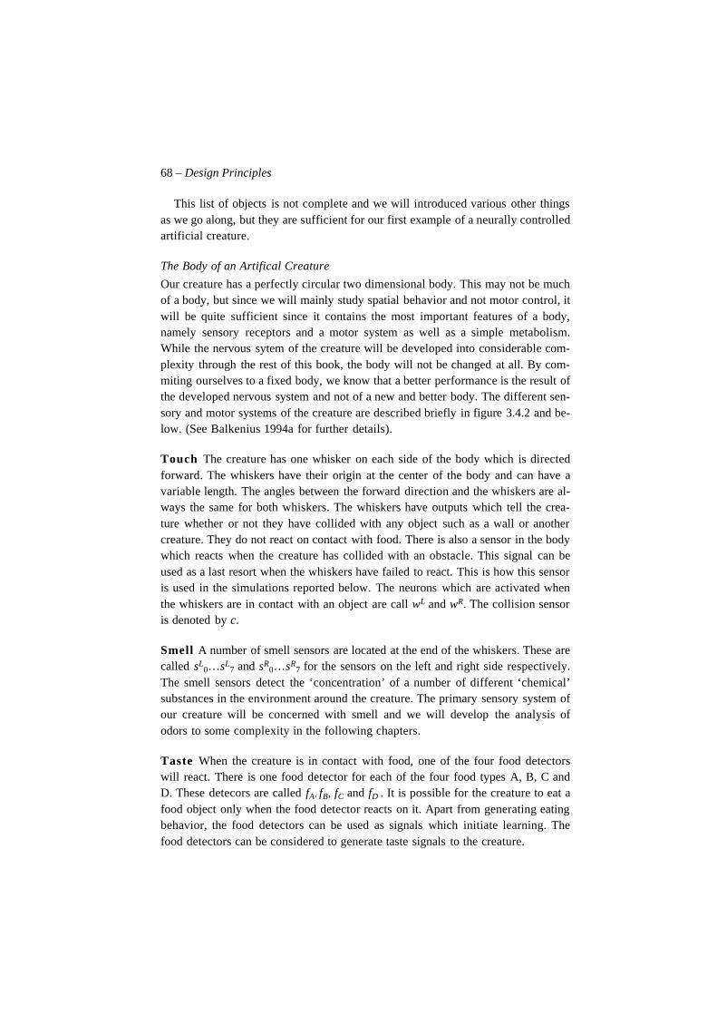
68 – Design Principles
This list of objects is not complete and we will introduced various other thingsas we go along, but they are sufficient for our first example of a neurally controlledartificial creature.
The Body of an Artifical Creature
Our creature has a perfectly circular two dimensional body. This may not be muchof a body, but since we will mainly study spatial behavior and not motor control, itwill be quite sufficient since it contains the most important features of a body,namely sensory receptors and a motor system as well as a simple metabolism.While the nervous sytem of the creature will be developed into considerable com-plexity through the rest of this book, the body will not be changed at all. By com-miting ourselves to a fixed body, we know that a better performance is the result ofthe developed nervous system and not of a new and better body. The different sen-sory and motor systems of the creature are described briefly in figure 3.4.2 and be-low. (See Balkenius 1994a for further details).
Touch The creature has one whisker on each side of the body which is directedforward. The whiskers have their origin at the center of the body and can have avariable length. The angles between the forward direction and the whiskers are al-ways the same for both whiskers. The whiskers have outputs which tell the crea-ture whether or not they have collided with any object such as a wall or anothercreature. They do not react on contact with food. There is also a sensor in the bodywhich reacts when the creature has collided with an obstacle. This signal can beused as a last resort when the whiskers have failed to react. This is how this sensoris used in the simulations reported below. The neurons which are activated whenthe whiskers are in contact with an object are call wL and wR. The collision sensoris denoted by c.
Smell A number of smell sensors are located at the end of the whiskers. These arecalled sL
0…sL7 and sR
0…sR7 for the sensors on the left and right side respectively.
The smell sensors detect the ‘concentration’ of a number of different ‘chemical’substances in the environment around the creature. The primary sensory system ofour creature will be concerned with smell and we will develop the analysis ofodors to some complexity in the following chapters.
Taste When the creature is in contact with food, one of the four food detectorswill react. There is one food detector for each of the four food types A, B, C andD. These detecors are called fA, fB, fC and fD . It is possible for the creature to eat afood object only when the food detector reacts on it. Apart from generating eatingbehavior, the food detectors can be used as signals which initiate learning. Thefood detectors can be considered to generate taste signals to the creature.
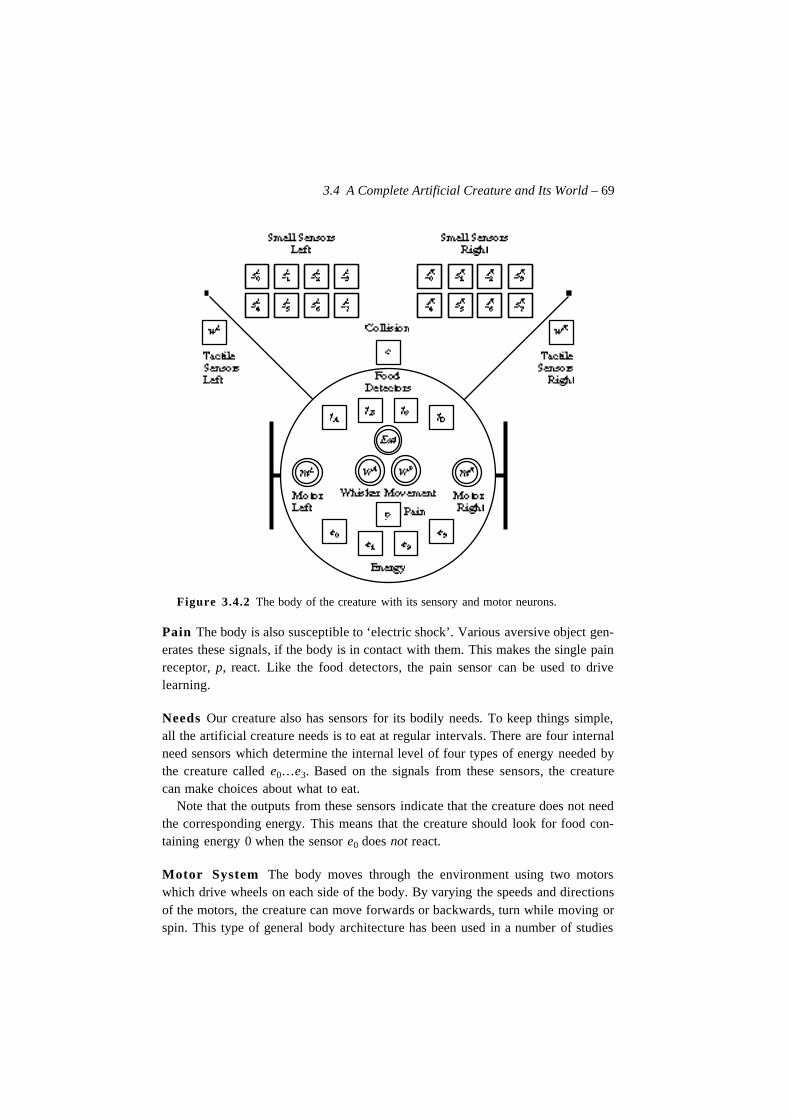
3.4 A Complete Artificial Creature and Its World – 69
Figure 3.4.2 The body of the creature with its sensory and motor neurons.
Pain The body is also susceptible to ‘electric shock’. Various aversive object gen-erates these signals, if the body is in contact with them. This makes the single painreceptor, p, react. Like the food detectors, the pain sensor can be used to drivelearning.
Needs Our creature also has sensors for its bodily needs. To keep things simple,all the artificial creature needs is to eat at regular intervals. There are four internalneed sensors which determine the internal level of four types of energy needed bythe creature called e0…e3. Based on the signals from these sensors, the creaturecan make choices about what to eat.
Note that the outputs from these sensors indicate that the creature does not needthe corresponding energy. This means that the creature should look for food con-taining energy 0 when the sensor e0 does not react.
Motor System The body moves through the environment using two motorswhich drive wheels on each side of the body. By varying the speeds and directionsof the motors, the creature can move forwards or backwards, turn while moving orspin. This type of general body architecture has been used in a number of studies
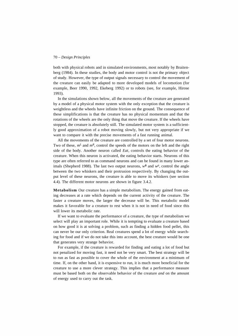
70 – Design Principles
both with physical robots and in simulated environments, most notably by Braiten-berg (1984). In these studies, the body and motor control is not the primary objectof study. However, the type of output signals necessary to control the movement ofthe creature can easily be adapted to more developed models of locomotion (forexample, Beer 1990, 1992, Ekeberg 1992) or to robots (see, for example, Hirose1993).
In the simulations shown below, all the movements of the creature are generatedby a model of a physical motor system with the only exception that the creature isweightless and the wheels have infinite friction on the ground. The consequence ofthese simplifications is that the creature has no physical momentum and that therotations of the wheels are the only thing that move the creature. If the wheels havestopped, the creature is absolutely still. The simulated motor system is a sufficient-ly good approximation of a robot moving slowly, but not very appropriate if wewant to compare it with the precise movements of a fast running animal.
All the movements of the creature are controlled by a set of four motor neurons.Two of these, mL and mR, control the speeds of the motors on the left and the rightside of the body. Another neuron called Eat, controls the eating behavior of thecreature. When this neuron is activated, the eating behavior starts. Neurons of thistype are often referred to as command neurons and can be found in many lower an-imals (Shepherd 1988). The last two output neurons, wϕ and wp, control the anglebetween the two whiskers and their protrusion respectively. By changing the out-put level of these neurons, the creature is able to move its whiskers (see section4.4). The different motor neurons are shown in figure 3.4.2.
Metabolism Our creature has a simple metabolism. The energy gained from eat-ing decreases at a rate which depends on the current activity of the creature. Thefaster a creature moves, the larger the decrease will be. This metabolic modelmakes it favorable for a creature to rest when it is not in need of food since thiswill lower its metabolic rate.
If we want to evaluate the performance of a creature, the type of metabolism weselect will play an important role. While it is tempting to evaluate a creature basedon how good it is at solving a problem, such as finding a hidden food pellet, thiscan never be our only criterion. Real creatures spend a lot of energy while search-ing for food and if we do not take this into account, the best creature would be onethat generates very strange behavior.
For example, if the creature is rewarded for finding and eating a lot of food butnot penalized for moving fast, it need not be very smart. The best strategy will beto run as fast as possible to cover the whole of the environment at a minimum oftime. If, on the other hand, it is expensive to run, it is much more beneficial for thecreature to use a more clever strategy. This implies that a performance measuremust be based both on the observable behavior of the creature and on the amountof energy used to carry out the task.
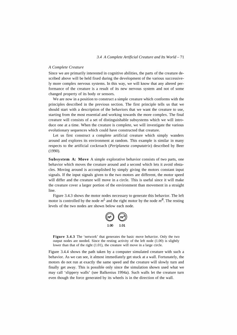
3.4 A Complete Artificial Creature and Its World – 71
A Complete Creature
Since we are primarily interested in cognitive abilities, the parts of the creature de-scribed above will be held fixed during the development of the various successive-ly more complex nervous systems. In this way, we will know that any altered per-formance of the creature is a result of its new nervous system and not of somechanged property of its body or sensors.
We are now in a position to construct a simple creature which conforms with theprinciples described in the previous section. The first principle tells us that weshould start with a description of the behaviors that we want the creature to use,starting from the most essential and working towards the more complex. The finalcreature will consists of a set of distinguishable subsystems which we will intro-duce one at a time. When the creature is complete, we will investigate the variousevolutionary sequences which could have constructed that creature.
Let us first construct a complete artificial creature which simply wandersaround and explores its environment at random. This example is similar in manyrespects to the artificial cockroach (Periplaneta computatrix) described by Beer(1990).
Subsystem A: Move A simple explorative behavior consists of two parts, onebehavior which moves the creature around and a second which lets it avoid obsta-cles. Moving around is accomplished by simply giving the motors constant inputsignals. If the input signals given to the two motors are different, the motor speedwill differ and the creature will move in a circle. This is useful since it will makethe creature cover a larger portion of the environment than movement in a straightline.
Figure 3.4.3 shows the motor nodes necessary to generate this behavior. The leftmotor is controlled by the node mL and the right motor by the node mR. The restinglevels of the two nodes are shown below each node.
Figure 3.4.3 The ‘network’ that generates the basic move behavior. Only the twooutput nodes are needed. Since the resting activity of the left node (1.00) is slightlylower than that of the right (1.01), the creature will move in a large circle.
Figure 3.4.4 shows the path taken by a computer simulated creature with such abehavior. As we can see, it almost immediately get stuck at a wall. Fortunately, themotors do not run at exactly the same speed and the creature will slowly turn andfinally get away. This is possible only since the simulation shown used what wemay call ‘slippery walls’ (see Balkenius 1994a). Such walls let the creature turneven though the force generated by its wheels is in the direction of the wall.
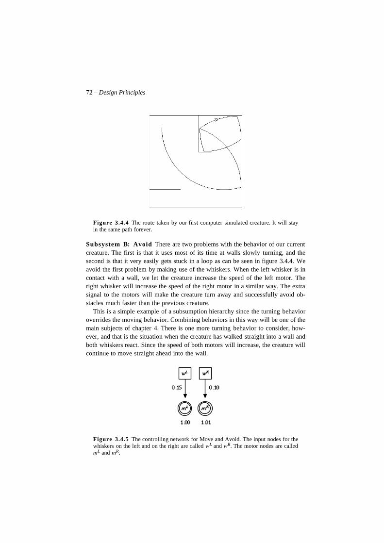
72 – Design Principles
Figure 3.4.4 The route taken by our first computer simulated creature. It will stayin the same path forever.
Subsystem B: Avoid There are two problems with the behavior of our currentcreature. The first is that it uses most of its time at walls slowly turning, and thesecond is that it very easily gets stuck in a loop as can be seen in figure 3.4.4. Weavoid the first problem by making use of the whiskers. When the left whisker is incontact with a wall, we let the creature increase the speed of the left motor. Theright whisker will increase the speed of the right motor in a similar way. The extrasignal to the motors will make the creature turn away and successfully avoid ob-stacles much faster than the previous creature.
This is a simple example of a subsumption hierarchy since the turning behavioroverrides the moving behavior. Combining behaviors in this way will be one of themain subjects of chapter 4. There is one more turning behavior to consider, how-ever, and that is the situation when the creature has walked straight into a wall andboth whiskers react. Since the speed of both motors will increase, the creature willcontinue to move straight ahead into the wall.
Figure 3.4.5 The controlling network for Move and Avoid. The input nodes for thewhiskers on the left and on the right are called wL and wR. The motor nodes are calledmL and mR.
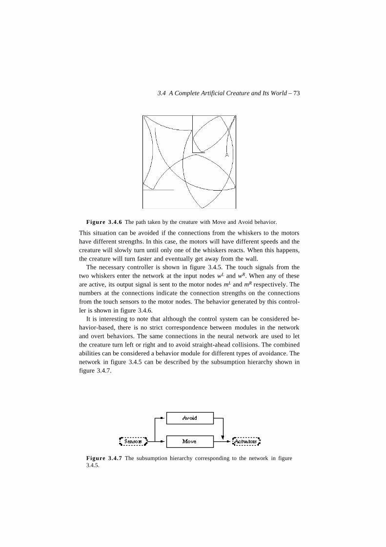
3.4 A Complete Artificial Creature and Its World – 73
Figure 3.4.6 The path taken by the creature with Move and Avoid behavior.
This situation can be avoided if the connections from the whiskers to the motorshave different strengths. In this case, the motors will have different speeds and thecreature will slowly turn until only one of the whiskers reacts. When this happens,the creature will turn faster and eventually get away from the wall.
The necessary controller is shown in figure 3.4.5. The touch signals from thetwo whiskers enter the network at the input nodes wL and wR. When any of theseare active, its output signal is sent to the motor nodes mL and mR respectively. Thenumbers at the connections indicate the connection strengths on the connectionsfrom the touch sensors to the motor nodes. The behavior generated by this control-ler is shown in figure 3.4.6.
It is interesting to note that although the control system can be considered be-havior-based, there is no strict correspondence between modules in the networkand overt behaviors. The same connections in the neural network are used to letthe creature turn left or right and to avoid straight-ahead collisions. The combinedabilities can be considered a behavior module for different types of avoidance. Thenetwork in figure 3.4.5 can be described by the subsumption hierarchy shown infigure 3.4.7.
Figure 3.4.7 The subsumption hierarchy corresponding to the network in figure3.4.5.
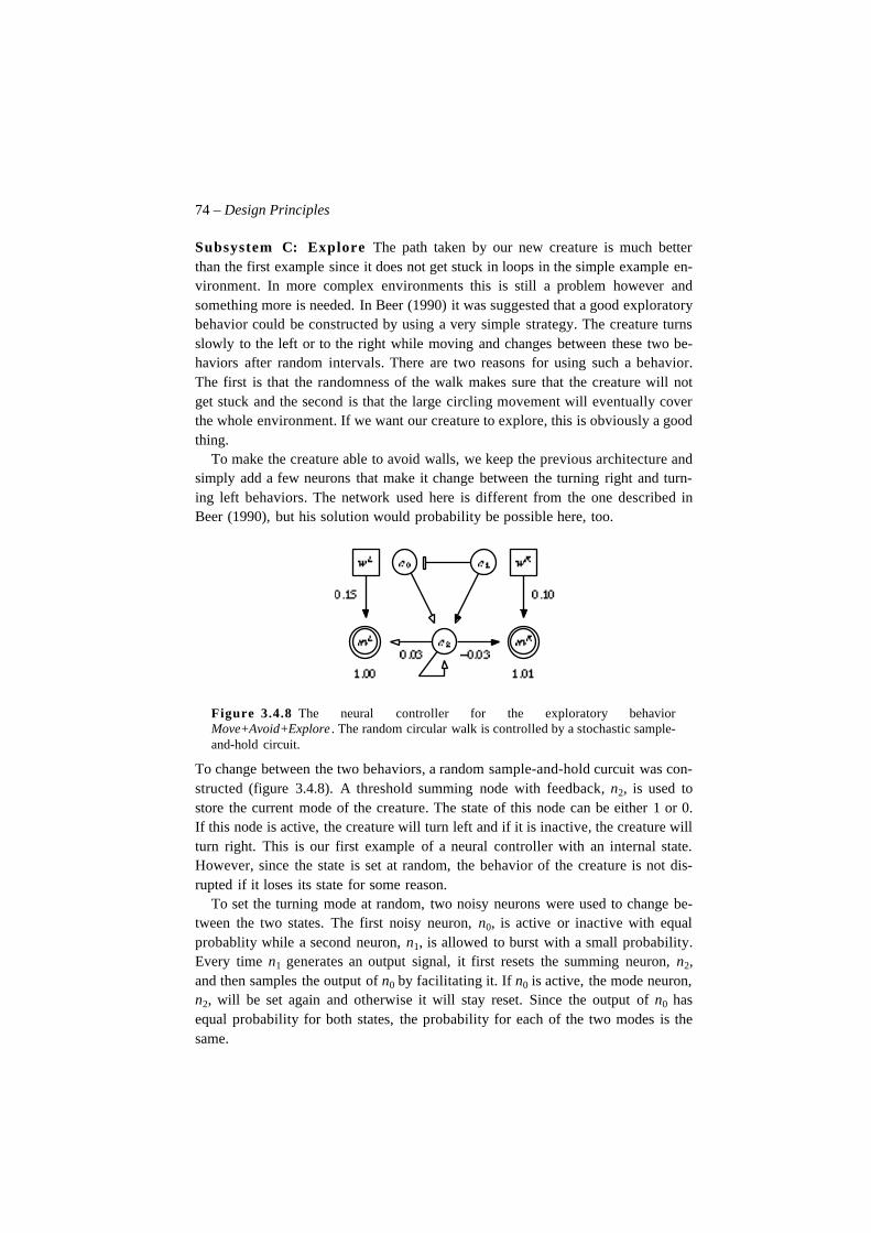
74 – Design Principles
Subsystem C: Explore The path taken by our new creature is much betterthan the first example since it does not get stuck in loops in the simple example en-vironment. In more complex environments this is still a problem however andsomething more is needed. In Beer (1990) it was suggested that a good exploratorybehavior could be constructed by using a very simple strategy. The creature turnsslowly to the left or to the right while moving and changes between these two be-haviors after random intervals. There are two reasons for using such a behavior.The first is that the randomness of the walk makes sure that the creature will notget stuck and the second is that the large circling movement will eventually coverthe whole environment. If we want our creature to explore, this is obviously a goodthing.
To make the creature able to avoid walls, we keep the previous architecture andsimply add a few neurons that make it change between the turning right and turn-ing left behaviors. The network used here is different from the one described inBeer (1990), but his solution would probability be possible here, too.
Figure 3.4.8 The neural controller for the exploratory behaviorMove+Avoid+Explore . The random circular walk is controlled by a stochastic sample-and-hold circuit.
To change between the two behaviors, a random sample-and-hold curcuit was con-structed (figure 3.4.8). A threshold summing node with feedback, n2, is used tostore the current mode of the creature. The state of this node can be either 1 or 0.If this node is active, the creature will turn left and if it is inactive, the creature willturn right. This is our first example of a neural controller with an internal state.However, since the state is set at random, the behavior of the creature is not dis-rupted if it loses its state for some reason.
To set the turning mode at random, two noisy neurons were used to change be-tween the two states. The first noisy neuron, n0, is active or inactive with equalprobablity while a second neuron, n1, is allowed to burst with a small probability.Every time n1 generates an output signal, it first resets the summing neuron, n2,and then samples the output of n0 by facilitating it. If n0 is active, the mode neuron,n2, will be set again and otherwise it will stay reset. Since the output of n0 hasequal probability for both states, the probability for each of the two modes is thesame.
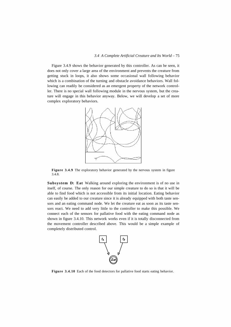
3.4 A Complete Artificial Creature and Its World – 75
Figure 3.4.9 shows the behavior generated by this controller. As can be seen, itdoes not only cover a large area of the environment and prevents the creature fromgetting stuck in loops, it also shows some occasional wall following behaviorwhich is a combination of the turning and obstacle avoidance behaviors. Wall fol-lowing can readily be considered as an emergent property of the network control-ler. There is no special wall following module in the nervous system, but the crea-ture will engage in this behavior anyway. Below, we will develop a set of morecomplex exploratory behaviors.
Figure 3.4.9 The exploratory behavior generated by the nervous system in figure3.4.8.
Subsystem D: Eat Walking around exploring the environment is of no use initself, of course. The only reason for our simple creature to do so is that it will beable to find food which is not accessible from its initial location. Eating behaviorcan easily be added to our creature since it is already equipped with both taste sen-sors and an eating command node. We let the creature eat as soon as its taste sen-sors react. We need to add very little to the controller to make this possible. Weconnect each of the sensors for pallative food with the eating command node asshown in figure 3.4.10. This network works even if it is totally disconnected fromthe movement controller described above. This would be a simple example ofcompletely distributed control.
Figure 3.4.10 Each of the food detectors for pallative food starts eating behavior.
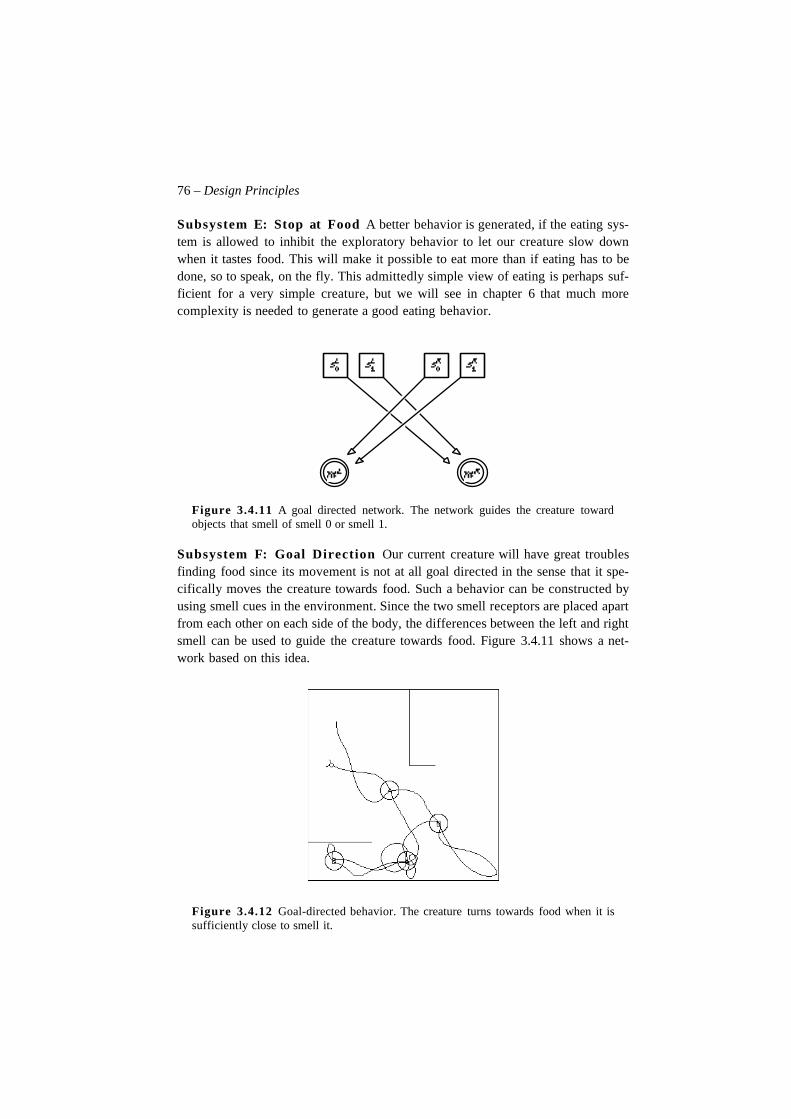
76 – Design Principles
Subsystem E: Stop at Food A better behavior is generated, if the eating sys-tem is allowed to inhibit the exploratory behavior to let our creature slow downwhen it tastes food. This will make it possible to eat more than if eating has to bedone, so to speak, on the fly. This admittedly simple view of eating is perhaps suf-ficient for a very simple creature, but we will see in chapter 6 that much morecomplexity is needed to generate a good eating behavior.
Figure 3.4.11 A goal directed network. The network guides the creature towardobjects that smell of smell 0 or smell 1.
Subsystem F: Goal Direction Our current creature will have great troublesfinding food since its movement is not at all goal directed in the sense that it spe-cifically moves the creature towards food. Such a behavior can be constructed byusing smell cues in the environment. Since the two smell receptors are placed apartfrom each other on each side of the body, the differences between the left and rightsmell can be used to guide the creature towards food. Figure 3.4.11 shows a net-work based on this idea.
Figure 3.4.12 Goal-directed behavior. The creature turns towards food when it issufficiently close to smell it.
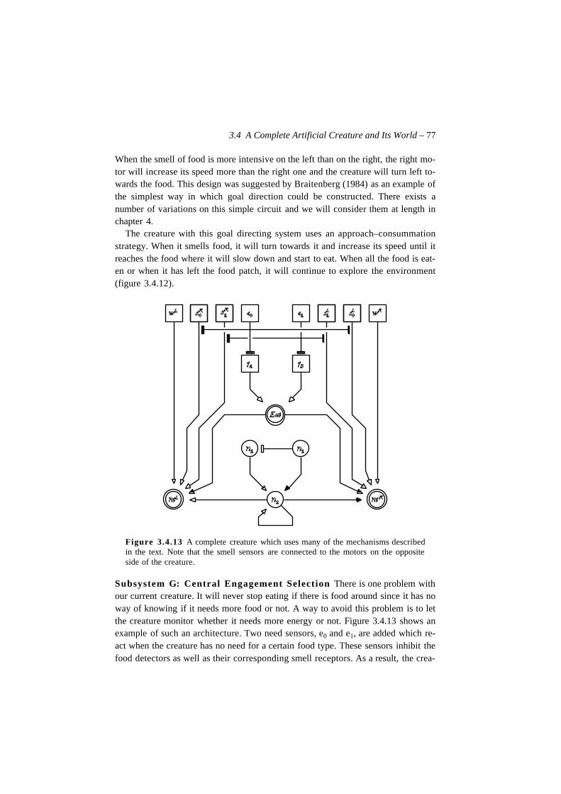
3.4 A Complete Artificial Creature and Its World – 77
When the smell of food is more intensive on the left than on the right, the right mo-tor will increase its speed more than the right one and the creature will turn left to-wards the food. This design was suggested by Braitenberg (1984) as an example ofthe simplest way in which goal direction could be constructed. There exists anumber of variations on this simple circuit and we will consider them at length inchapter 4.
The creature with this goal directing system uses an approach–consummationstrategy. When it smells food, it will turn towards it and increase its speed until itreaches the food where it will slow down and start to eat. When all the food is eat-en or when it has left the food patch, it will continue to explore the environment(figure 3.4.12).
Figure 3.4.13 A complete creature which uses many of the mechanisms describedin the text. Note that the smell sensors are connected to the motors on the oppositeside of the creature.
Subsystem G: Central Engagement Selection There is one problem withour current creature. It will never stop eating if there is food around since it has noway of knowing if it needs more food or not. A way to avoid this problem is to letthe creature monitor whether it needs more energy or not. Figure 3.4.13 shows anexample of such an architecture. Two need sensors, e0 and e1, are added which re-act when the creature has no need for a certain food type. These sensors inhibit thefood detectors as well as their corresponding smell receptors. As a result, the crea-
78 – Design Principles
ture is insensitive to the types of food it does not currently need and will conse-quently ignore them. This is a simple form of motivationally biased perception. Inchapter 7, this type of mechanism will be the basis for a discussion of attention.
The system consisting of the two need detectors and their inhibitory influenceson the rest of the controller is a simple system for central behavior selection. Wesee that this system only shows one of the three aspects of such a system, namelyinternal drive. The introduction of internal and external incentives will be post-poned until chapter 6, where their relation to motivation will be investigated.
Conclusion
This section described a complete creature showing how the design principles in-troduced in section 3.2 could be incorporated in a very simple creature. Our exam-ple creature implemented the principles of behavior-based control, subsumption,parallel engagements, and central engagement selection. Most of all, it is entirelyreactive. In the next chapter, we will take a closer look at different types of reac-tive behavior. In the later chapters of the book, we will take a closer look at learn-ing, motivation and perception in general, and in our artificial creature in particu-lar.
Christian Balkenius, 1995, Natural Intelligence in Artificial Creatures, Lund University Cognitive Studies 37, 1995.
Chapter 4
Reactive Behavior
4.1 IntroductionBehavior in its most elementary form is purely reactive. The motor patterns pro-duced are caused only by the immediate perceptual state of the animal. In thischapter, we will introduce some basic classes of reactive behaviors and considerwhat different properties they possess. There are two distinct historical lines thatwe will follow.
The first historical line has its start in Lewin’s topological psychology (Lewin1936) and his view of behavior as controlled by a force field generated by objectsor situations with positive or negative values or valences. The idea was later devel-oped by Hull (1932, 1943, 1952), who used it as the basis for his goal-gradientconstruction. After having fallen in disregard for many years, the idea has been re-cently resurrected through Arbib’s (1987, 1991) work on motor schemata andArkin’s (1987, 1990) use of potential field methods for robot navigation. The com-mon denominator of all these approaches is their account for the directedness ofbehavior. They all subscribe to the position of hedonism1, that is, the organism isconsidered to approach pleasure and avoid pain. This leads naturally to a distinc-
1. In ethics, the doctrine of hedonism argues that humans should strive for pleasure and tryto avoid pain. The corresponding position in psychology argues that this is already the case.Note also that the term is inherently circular. It appears to be impossible to define pleasureand pain without making any reference to the fact that people will strive for the first and tryto avoid the second.
80 – Reactive Behavior
tion between four types of behaviors: (1) appetitive behavior that is directed to-ward an object or a situation, (2) aversive behavior that is directed away from anobject or a situation, (3) exploratory behavior that relates to objects or situationsthat are unknown, and finally, (4) neutral behavior that is guided by objects thatare known to be neutral, that is, neither appetitive nor aversive.
The other historical line is that of reflexes and fixed motor patterns. The idea ofreflexes has a long history, but the word was not used until 1784 when it was intro-duced by Prochaska (See Shepherd 1988). The concept of fixed motor patterns wassuggested by Lorenz (1950). By introducing hierarchies of motor patterns,Tinbergen (1951/1989) made one of the most important contributions to this area.Recently, the development of behavior-based robots moves the idea in a new di-rection, from a descriptive framework to a foundation for design (See, for exam-ple, Brooks 1991a, and Maes 1990). While the first historical line is mainly con-cerned with directedness, this other line emphasizes coordination and sequencesof motions.
The two directions are not at all incompatible, of course. In fact, one of the con-clusions of the present chapter will be that a better understanding of reactive be-havior must be based on directedness as well as coordination and sequences of be-havior. The chapter concludes with an inventory of basic reactive behaviors.
4.2 The Directedness of BehaviorOne of the most fundamental aspects of most behaviors is that they are directed.Animals do not just move around at random but are guided by their perception ofthe world in such a way that their behavior is likely to accomplish something ofimportance, such as finding food or a mate. It will thus be necessary to considergoal-direction at some length before we can start the construction of an artificialcreature. To make the notion of direction precise, we will need to define a lan-guage suitable for the task. This language will take its starting point in Lewin’stopological psychology. We will tailor it to fit our needs, and as the language be-comes more precise, it will gradually begin to look like a theory of behavior.
To make the presentation clearer, we will start with behaviors that are purely re-active and relate to objects in space. This also makes it natural to use spatial con-cepts to describe behavior. As the theory moves away from reactive behavior, thespatial concepts will gradually be transferred from the external space to the inter-nal space of the animal. In the later chapters, we will try to make a case for the ideathat all cognition is based on spatial concepts and that goal-directed thought maymerely be goal-directed behavior made internal. Before we can make such broadclaims, however, we must first move back in time to the early days of topologicalpsychology.
4.2 The Directedness of Behavior – 81
Topology and Vectors: Lewin’s Field Theory
The psychology of 1930 left much to hope for in terms of descriptive precision. Itis not hard to understand why the psychologists of the time envied the exactnessand conceptual rigor of physics and mathematics. Inspired by the latest develop-ments in pure mathematics, Kurt Lewin tried to developed a formal mathematicallanguage for psychology. The foundations for this language were presented in hisbook Principles of Topological Psychology (Lewin 1936), which was the first in aseries of works that developed his ideas from a topological psychology into a vec-tor psychology where the behavior of a person was explained in terms of forcesacting on the individual.
The problem that hampered the development of a formal vector psychology wasthat it seemed difficult or impossible to define a metric on the psychological space.Without a metric, the concept of psychological vector or force is meaningless. Inthis respect, vector psychology could never offer more than a metaphorical de-scription of a person. However, as we will see below, for artificial creatures, atleast, a precise vector psychology is in fact possible. To make such a vector theorypossible, we must first consider Lewin’s theory in more detail.
The psychological theory developed in the language offered by topology andvectors is generally referred to as the field theory . The central concept of the fieldtheory is that of a life space that determines the behavior of an individual. The be-havior at any moment in time can be described as a function of the life space of theindividual. The life space includes the whole situation determining the behavior ofan individual, that is, both the person, P, and the environment, E. If we denote thebehavior of the individual by B, the field theory can be summarized in Lewin’s fa-mous formula,
(4.2.1)One of Lewin most important insights is that we should consider the momentarysituation of an individual in order to understand its behavior. This contrasted withmany of the popular theories at the time, where the causes of behavior were soughtnot in the present but in the past2. This does not mean that the past does not have arole in determining the present situation of an individual. On the contrary, both theexperienced past and the expected future, that is, the total life situation, may playa part in determining the immediate situation. But, it is this situation that deter-mines behavior and not the past or the future.
The goal as a psychological fact undoubtedly lies in the present. It really ex-ists at the moment and makes up an essential part of the momentary lifespace. On the other hand, the content of the goal … lies as a physical or
2. Strangely enough, this is also true of modern behaviorism that allows any time intervalbetween stimulus and response.
B f P E,( ).=
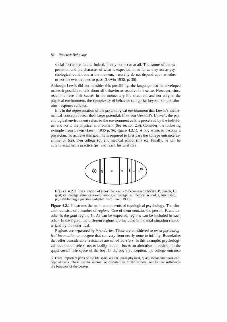
82 – Reactive Behavior
social fact in the future. Indeed, it may not occur at all. The nature of the ex-pectation and the character of what is expected, in so far as they act as psy-chological conditions at the moment, naturally do not depend upon whetheror not the event comes to pass. (Lewin 1936, p. 36)
Although Lewin did not consider this possibility, the language that he developedmakes it possible to talk about all behavior as reactive in a sense. However, sincereactions have their causes in the momentary life situation, and not only in thephysical environment, the complexity of behavior can go far beyond simple stim-ulus–response reflexes.
It is in the representation of the psychological environment that Lewin’s mathe-matical concepts reveal their large potential. Like von Uexküll’s Umwelt , the psy-chological environment refers to the environment as it is perceived by the individ-ual and not to the physical environment (See section 2.9). Consider, the followingexample from Lewin (Lewin 1936 p. 96; figure 4.2.1). A boy wants to become aphysician. To achieve this goal, he is required to first pass the college entrance ex-amination (ce), then college (c), and medical school (m), etc. Finally, he will beable to establish a practice (pr) and reach his goal (G).
Figure 4.2.1 The situation of a boy that wants to become a physician. P, person; G,goal; ce: college entrance examinations; c, college; m, medical school; i, internship;pr, establishing a practice (adapted from Lewi, 1936).
Figure 4.2.1 illustrates the main components of topological psychology. The situ-ation consists of a number of regions . One of them contains the person, P, and an-other is the goal region, G. As can be expected, regions can be included in eachother. In the figure, the different regions are included in the total situation charac-terized by the outer oval.
Regions are separated by boundaries. These are considered to resist psycholog-ical locomotion to a degree that can vary from nearly none to infinity. Boundariesthat offer considerable resistance are called barriers. In this example, psychologi-cal locomotion refers, not to bodily motion, but to an alteration in position in thequasi-social3 life space of the boy. In the boy’s conception, the college entrance
3. Three important parts of the life space are the quasi-physical, quasi-social and quasi-con-ceptual facts. These are the internal representations of the external reality that influencesthe behavior of the person.
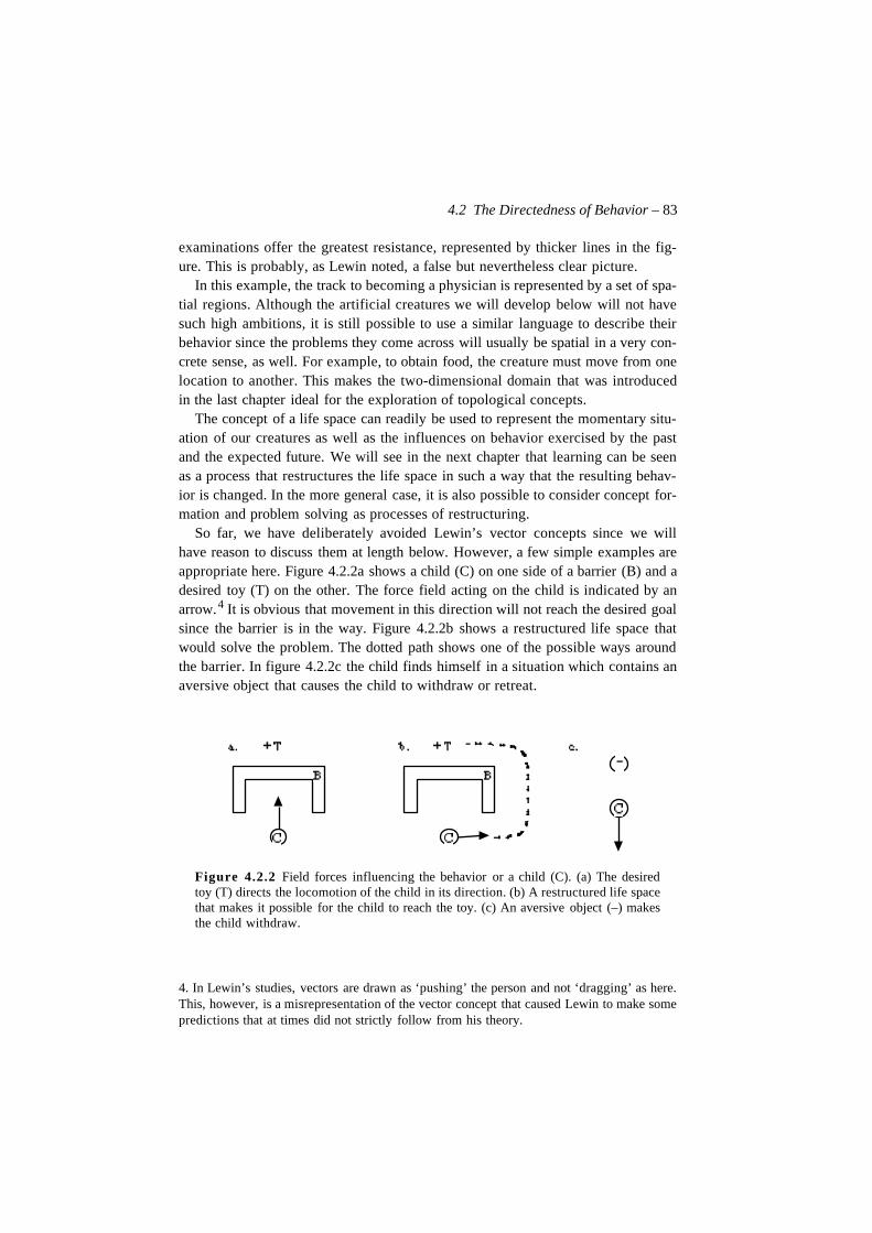
4.2 The Directedness of Behavior – 83
examinations offer the greatest resistance, represented by thicker lines in the fig-ure. This is probably, as Lewin noted, a false but nevertheless clear picture.
In this example, the track to becoming a physician is represented by a set of spa-tial regions. Although the artificial creatures we will develop below will not havesuch high ambitions, it is still possible to use a similar language to describe theirbehavior since the problems they come across will usually be spatial in a very con-crete sense, as well. For example, to obtain food, the creature must move from onelocation to another. This makes the two-dimensional domain that was introducedin the last chapter ideal for the exploration of topological concepts.
The concept of a life space can readily be used to represent the momentary situ-ation of our creatures as well as the influences on behavior exercised by the pastand the expected future. We will see in the next chapter that learning can be seenas a process that restructures the life space in such a way that the resulting behav-ior is changed. In the more general case, it is also possible to consider concept for-mation and problem solving as processes of restructuring.
So far, we have deliberately avoided Lewin’s vector concepts since we willhave reason to discuss them at length below. However, a few simple examples areappropriate here. Figure 4.2.2a shows a child (C) on one side of a barrier (B) and adesired toy (T) on the other. The force field acting on the child is indicated by anarrow.4 It is obvious that movement in this direction will not reach the desired goalsince the barrier is in the way. Figure 4.2.2b shows a restructured life space thatwould solve the problem. The dotted path shows one of the possible ways aroundthe barrier. In figure 4.2.2c the child finds himself in a situation which contains anaversive object that causes the child to withdraw or retreat.
Figure 4.2.2 Field forces influencing the behavior or a child (C). (a) The desiredtoy (T) directs the locomotion of the child in its direction. (b) A restructured life spacethat makes it possible for the child to reach the toy. (c) An aversive object (–) makesthe child withdraw.
4. In Lewin’s studies, vectors are drawn as ‘pushing’ the person and not ‘dragging’ as here.This, however, is a misrepresentation of the vector concept that caused Lewin to make somepredictions that at times did not strictly follow from his theory.
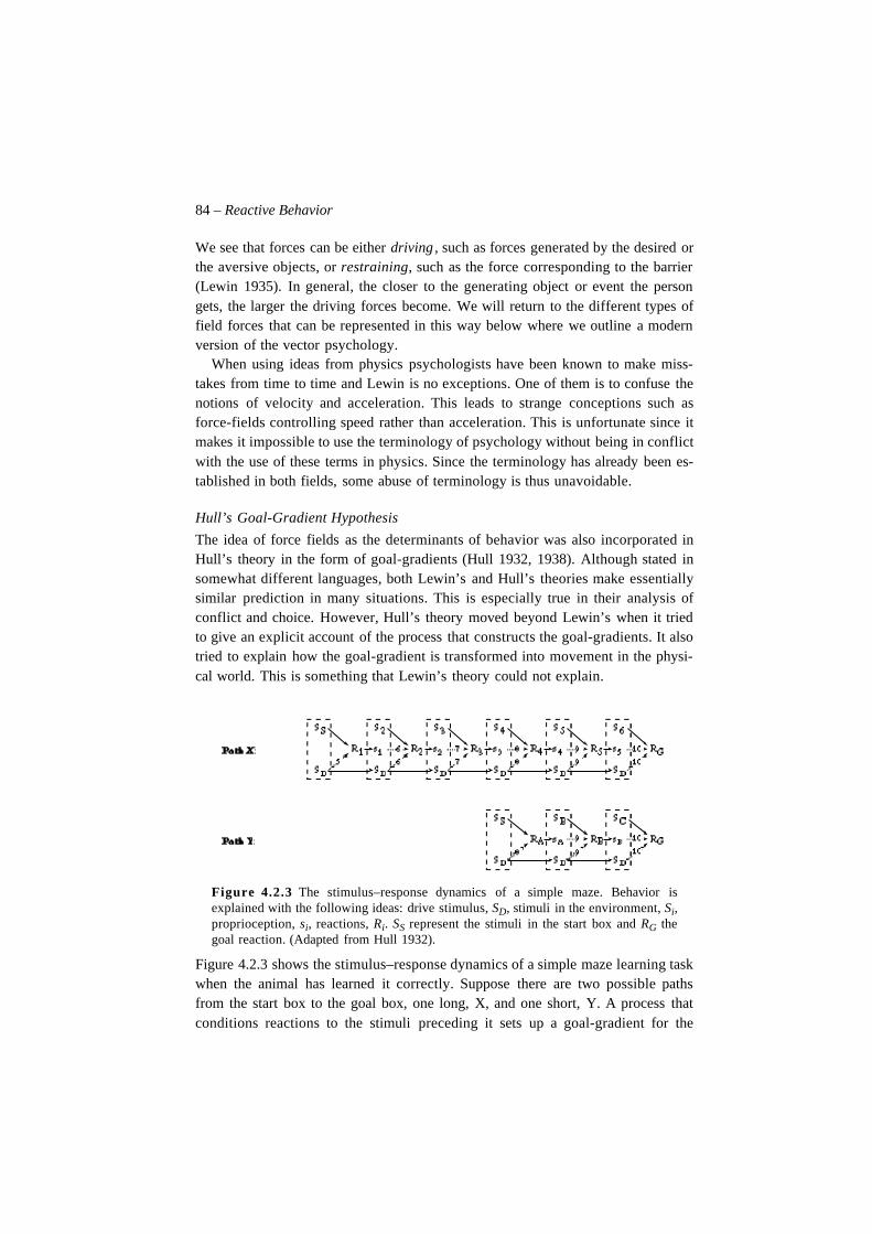
84 – Reactive Behavior
We see that forces can be either driving , such as forces generated by the desired orthe aversive objects, or restraining, such as the force corresponding to the barrier(Lewin 1935). In general, the closer to the generating object or event the persongets, the larger the driving forces become. We will return to the different types offield forces that can be represented in this way below where we outline a modernversion of the vector psychology.
When using ideas from physics psychologists have been known to make miss-takes from time to time and Lewin is no exceptions. One of them is to confuse thenotions of velocity and acceleration. This leads to strange conceptions such asforce-fields controlling speed rather than acceleration. This is unfortunate since itmakes it impossible to use the terminology of psychology without being in conflictwith the use of these terms in physics. Since the terminology has already been es-tablished in both fields, some abuse of terminology is thus unavoidable.
Hull’s Goal-Gradient Hypothesis
The idea of force fields as the determinants of behavior was also incorporated inHull’s theory in the form of goal-gradients (Hull 1932, 1938). Although stated insomewhat different languages, both Lewin’s and Hull’s theories make essentiallysimilar prediction in many situations. This is especially true in their analysis ofconflict and choice. However, Hull’s theory moved beyond Lewin’s when it triedto give an explicit account of the process that constructs the goal-gradients. It alsotried to explain how the goal-gradient is transformed into movement in the physi-cal world. This is something that Lewin’s theory could not explain.
Figure 4.2.3 The stimulus–response dynamics of a simple maze. Behavior isexplained with the following ideas: drive stimulus, SD, stimuli in the environment, Si,proprioception, si, reactions, Ri. SS represent the stimuli in the start box and RG thegoal reaction. (Adapted from Hull 1932).
Figure 4.2.3 shows the stimulus–response dynamics of a simple maze learning taskwhen the animal has learned it correctly. Suppose there are two possible pathsfrom the start box to the goal box, one long, X, and one short, Y. A process thatconditions reactions to the stimuli preceding it sets up a goal-gradient for the
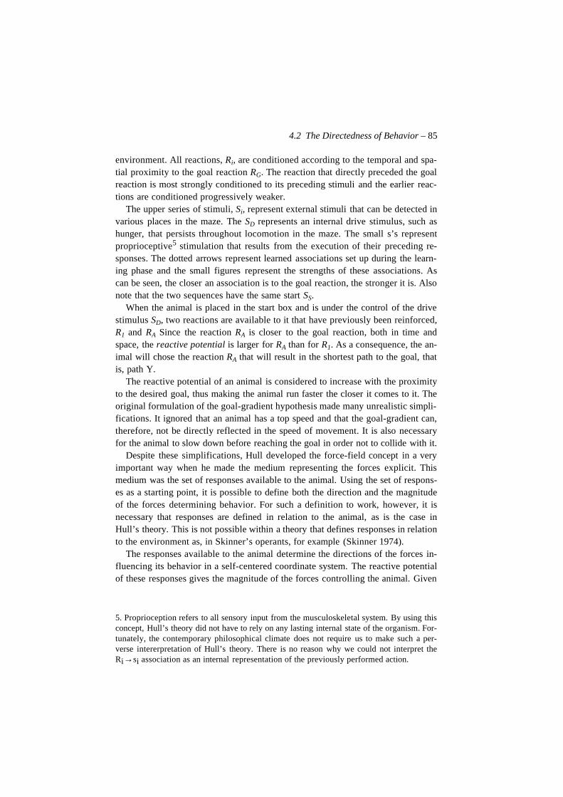
4.2 The Directedness of Behavior – 85
environment. All reactions, Ri, are conditioned according to the temporal and spa-tial proximity to the goal reaction RG. The reaction that directly preceded the goalreaction is most strongly conditioned to its preceding stimuli and the earlier reac-tions are conditioned progressively weaker.
The upper series of stimuli, Si, represent external stimuli that can be detected invarious places in the maze. The SD represents an internal drive stimulus, such ashunger, that persists throughout locomotion in the maze. The small s’s representproprioceptive5 stimulation that results from the execution of their preceding re-sponses. The dotted arrows represent learned associations set up during the learn-ing phase and the small figures represent the strengths of these associations. Ascan be seen, the closer an association is to the goal reaction, the stronger it is. Alsonote that the two sequences have the same start SS.
When the animal is placed in the start box and is under the control of the drivestimulus SD, two reactions are available to it that have previously been reinforced,R1 and RA Since the reaction RA is closer to the goal reaction, both in time andspace, the reactive potential is larger for RA than for R1. As a consequence, the an-imal will chose the reaction RA that will result in the shortest path to the goal, thatis, path Y.
The reactive potential of an animal is considered to increase with the proximityto the desired goal, thus making the animal run faster the closer it comes to it. Theoriginal formulation of the goal-gradient hypothesis made many unrealistic simpli-fications. It ignored that an animal has a top speed and that the goal-gradient can,therefore, not be directly reflected in the speed of movement. It is also necessaryfor the animal to slow down before reaching the goal in order not to collide with it.
Despite these simplifications, Hull developed the force-field concept in a veryimportant way when he made the medium representing the forces explicit. Thismedium was the set of responses available to the animal. Using the set of respons-es as a starting point, it is possible to define both the direction and the magnitudeof the forces determining behavior. For such a definition to work, however, it isnecessary that responses are defined in relation to the animal, as is the case inHull’s theory. This is not possible within a theory that defines responses in relationto the environment as, in Skinner’s operants, for example (Skinner 1974).
The responses available to the animal determine the directions of the forces in-fluencing its behavior in a self-centered coordinate system. The reactive potentialof these responses gives the magnitude of the forces controlling the animal. Given
5. Proprioception refers to all sensory input from the musculoskeletal system. By using thisconcept, Hull’s theory did not have to rely on any lasting internal state of the organism. For-tunately, the contemporary philosophical climate does not require us to make such a per-verse intererpretation of Hull’s theory. There is no reason why we could not interpret theRi→si association as an internal representation of the previously performed action.
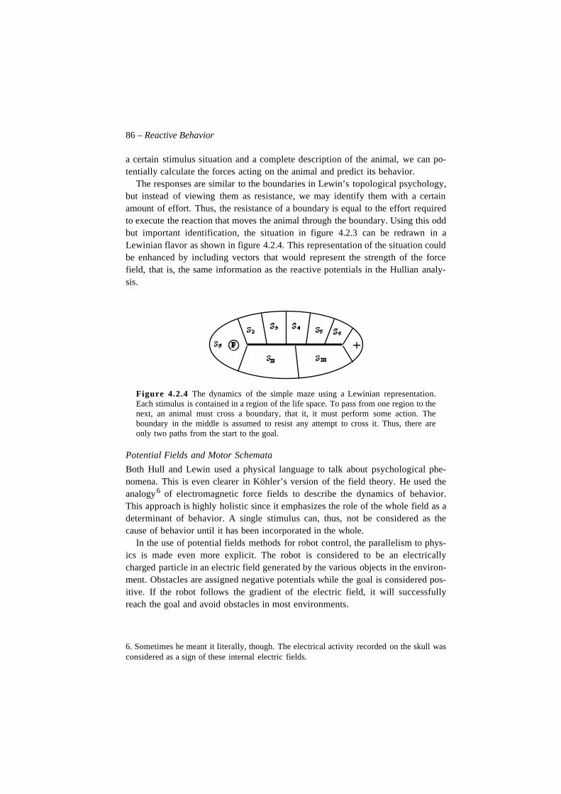
86 – Reactive Behavior
a certain stimulus situation and a complete description of the animal, we can po-tentially calculate the forces acting on the animal and predict its behavior.
The responses are similar to the boundaries in Lewin’s topological psychology,but instead of viewing them as resistance, we may identify them with a certainamount of effort. Thus, the resistance of a boundary is equal to the effort requiredto execute the reaction that moves the animal through the boundary. Using this oddbut important identification, the situation in figure 4.2.3 can be redrawn in aLewinian flavor as shown in figure 4.2.4. This representation of the situation couldbe enhanced by including vectors that would represent the strength of the forcefield, that is, the same information as the reactive potentials in the Hullian analy-sis.
Figure 4.2.4 The dynamics of the simple maze using a Lewinian representation.Each stimulus is contained in a region of the life space. To pass from one region to thenext, an animal must cross a boundary, that it, it must perform some action. Theboundary in the middle is assumed to resist any attempt to cross it. Thus, there areonly two paths from the start to the goal.
Potential Fields and Motor Schemata
Both Hull and Lewin used a physical language to talk about psychological phe-nomena. This is even clearer in Köhler’s version of the field theory. He used theanalogy6 of electromagnetic force fields to describe the dynamics of behavior.This approach is highly holistic since it emphasizes the role of the whole field as adeterminant of behavior. A single stimulus can, thus, not be considered as thecause of behavior until it has been incorporated in the whole.
In the use of potential fields methods for robot control, the parallelism to phys-ics is made even more explicit. The robot is considered to be an electricallycharged particle in an electric field generated by the various objects in the environ-ment. Obstacles are assigned negative potentials while the goal is considered pos-itive. If the robot follows the gradient of the electric field, it will successfullyreach the goal and avoid obstacles in most environments.
6. Sometimes he meant it literally, though. The electrical activity recorded on the skull wasconsidered as a sign of these internal electric fields.
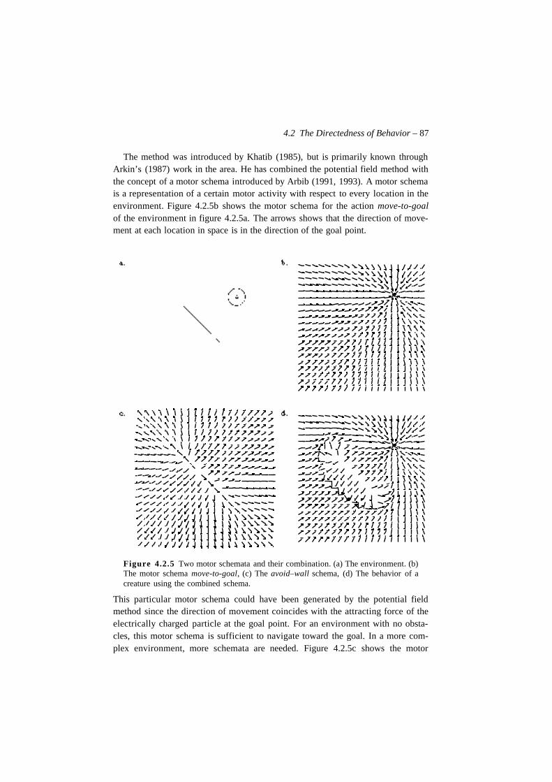
4.2 The Directedness of Behavior – 87
The method was introduced by Khatib (1985), but is primarily known throughArkin’s (1987) work in the area. He has combined the potential field method withthe concept of a motor schema introduced by Arbib (1991, 1993). A motor schemais a representation of a certain motor activity with respect to every location in theenvironment. Figure 4.2.5b shows the motor schema for the action move-to-goalof the environment in figure 4.2.5a. The arrows shows that the direction of move-ment at each location in space is in the direction of the goal point.
Figure 4.2.5 Two motor schemata and their combination. (a) The environment. (b)The motor schema move-to-goal, (c) The avoid–wall schema, (d) The behavior of acreature using the combined schema.
This particular motor schema could have been generated by the potential fieldmethod since the direction of movement coincides with the attracting force of theelectrically charged particle at the goal point. For an environment with no obsta-cles, this motor schema is sufficient to navigate toward the goal. In a more com-plex environment, more schemata are needed. Figure 4.2.5c shows the motor
88 – Reactive Behavior
schema avoid-wall considered as a field generated by the wall. The robot is sup-posed to move away from the wall.
If the wall and the goal are located in the same environment, the action of therobot can be calculated by adding the two force fields together as shown in figure4.2.5d. Note that the picture shows the path preferd by the robot rather than thesum of the two vector fields. By following this combined motor schema, the robotcan reach the goal without colliding with the obstacle. The most important aspectof this control method is that it generates stable control strategies. It does not mat-ter if the robot is accidentally moved off course since the gradient field will auto-matically compensate for this and get it on the right track again. Another niceproperty of the method is that the different motor schemata controlling the robotcan be calculated independently and then simply combined, either by adding themor by taking the maximium of them. For instance, the processes that calculate themove-to-goal schema do not communicate with the avoid–obstacle process at all.The potential field method is, thus, very well suited for parallelization (See alsosection 4.3).
Although this method has many merits, there are a number of important prob-lems; the most noticeable being that it very easily generates local maxima in thegradient landscape at other places than at the goal. One possible solution to thisproblem is to add noise to the motor schemata, but this is not entirely satisfactory(Arkin 1990). Another problem is that it is location based. This means that, in gen-eral, the location of the robot must be known before the force vectors can be calcu-lated. Potential fields may also give rise to strange behaviors, such as avoidance ofobjects behind the robot (Connel 1990).
Despite these problems, the idea of motor schemata is very attractive as a wayto represent the latent behavior of an agent. In many respects, it is similar toLewin’s vector fields, but instead of showing the direction of movement in an in-ternal psychological space, it shows the direction of movement in the physicalspace. If we keep the state of the agent constant, we can, potentially, move theagent to all possible locations in space and record its movement. This record is es-sentially an image of the psychological environment of the agent and we have,thus, found a way to make the notion of a psychological space precise. This is oneof the central ideas that we will use in the next section as we try to outline a mod-ern field theory.
Toward a Modern Field Theory
Though in theory, one should be able to measure all the parameters controlling ananimal in a given situation, this is not possible in practice. With artificial crea-tures, however, the situation is different. The problem here is not to keep track ofall the parameters, but rather to make sense of them. The modern version of thefield theory that we will outline in this section is intended to describe very
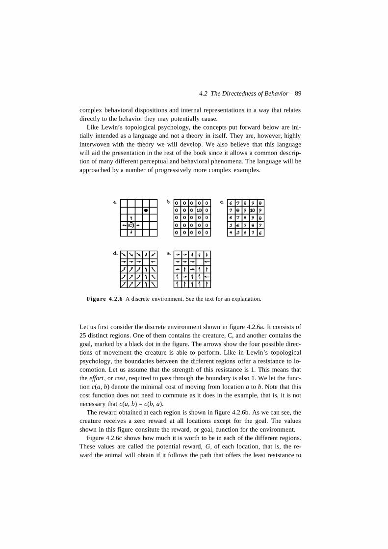
4.2 The Directedness of Behavior – 89
complex behavioral dispositions and internal representations in a way that relatesdirectly to the behavior they may potentially cause.
Like Lewin’s topological psychology, the concepts put forward below are ini-tially intended as a language and not a theory in itself. They are, however, highlyinterwoven with the theory we will develop. We also believe that this languagewill aid the presentation in the rest of the book since it allows a common descrip-tion of many different perceptual and behavioral phenomena. The language will beapproached by a number of progressively more complex examples.
Figure 4.2.6 A discrete environment. See the text for an explanation.
Let us first consider the discrete environment shown in figure 4.2.6a. It consists of25 distinct regions. One of them contains the creature, C, and another contains thegoal, marked by a black dot in the figure. The arrows show the four possible direc-tions of movement the creature is able to perform. Like in Lewin’s topologicalpsychology, the boundaries between the different regions offer a resistance to lo-comotion. Let us assume that the strength of this resistance is 1. This means thatthe effort , or cost, required to pass through the boundary is also 1. We let the func-tion c(a, b) denote the minimal cost of moving from location a to b. Note that thiscost function does not need to commute as it does in the example, that is, it is notnecessary that c(a, b) = c(b, a).
The reward obtained at each region is shown in figure 4.2.6b. As we can see, thecreature receives a zero reward at all locations except for the goal. The valuesshown in this figure consitute the reward, or goal, function for the environment.
Figure 4.2.6c shows how much it is worth to be in each of the different regions.These values are called the potential reward, G, of each location, that is, the re-ward the animal will obtain if it follows the path that offers the least resistance to
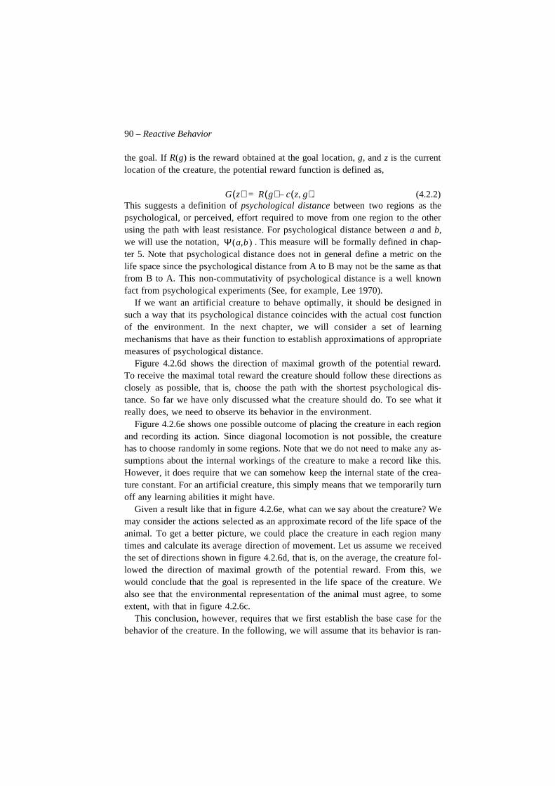
90 – Reactive Behavior
the goal. If R(g) is the reward obtained at the goal location, g, and z is the currentlocation of the creature, the potential reward function is defined as,
(4.2.2)This suggests a definition of psychological distance between two regions as thepsychological, or perceived, effort required to move from one region to the otherusing the path with least resistance. For psychological distance between a and b,we will use the notation, . This measure will be formally defined in chap-ter 5. Note that psychological distance does not in general define a metric on thelife space since the psychological distance from A to B may not be the same as thatfrom B to A. This non-commutativity of psychological distance is a well knownfact from psychological experiments (See, for example, Lee 1970).
If we want an artificial creature to behave optimally, it should be designed insuch a way that its psychological distance coincides with the actual cost functionof the environment. In the next chapter, we will consider a set of learningmechanisms that have as their function to establish approximations of appropriatemeasures of psychological distance.
Figure 4.2.6d shows the direction of maximal growth of the potential reward.To receive the maximal total reward the creature should follow these directions asclosely as possible, that is, choose the path with the shortest psychological dis-tance. So far we have only discussed what the creature should do. To see what itreally does, we need to observe its behavior in the environment.
Figure 4.2.6e shows one possible outcome of placing the creature in each regionand recording its action. Since diagonal locomotion is not possible, the creaturehas to choose randomly in some regions. Note that we do not need to make any as-sumptions about the internal workings of the creature to make a record like this.However, it does require that we can somehow keep the internal state of the crea-ture constant. For an artificial creature, this simply means that we temporarily turnoff any learning abilities it might have.
Given a result like that in figure 4.2.6e, what can we say about the creature? Wemay consider the actions selected as an approximate record of the life space of theanimal. To get a better picture, we could place the creature in each region manytimes and calculate its average direction of movement. Let us assume we receivedthe set of directions shown in figure 4.2.6d, that is, on the average, the creature fol-lowed the direction of maximal growth of the potential reward. From this, wewould conclude that the goal is represented in the life space of the creature. Wealso see that the environmental representation of the animal must agree, to someextent, with that in figure 4.2.6c.
This conclusion, however, requires that we first establish the base case for thebehavior of the creature. In the following, we will assume that its behavior is ran-
G z( ) R g( ) c z g,( ).–=
Ψ (a,b )
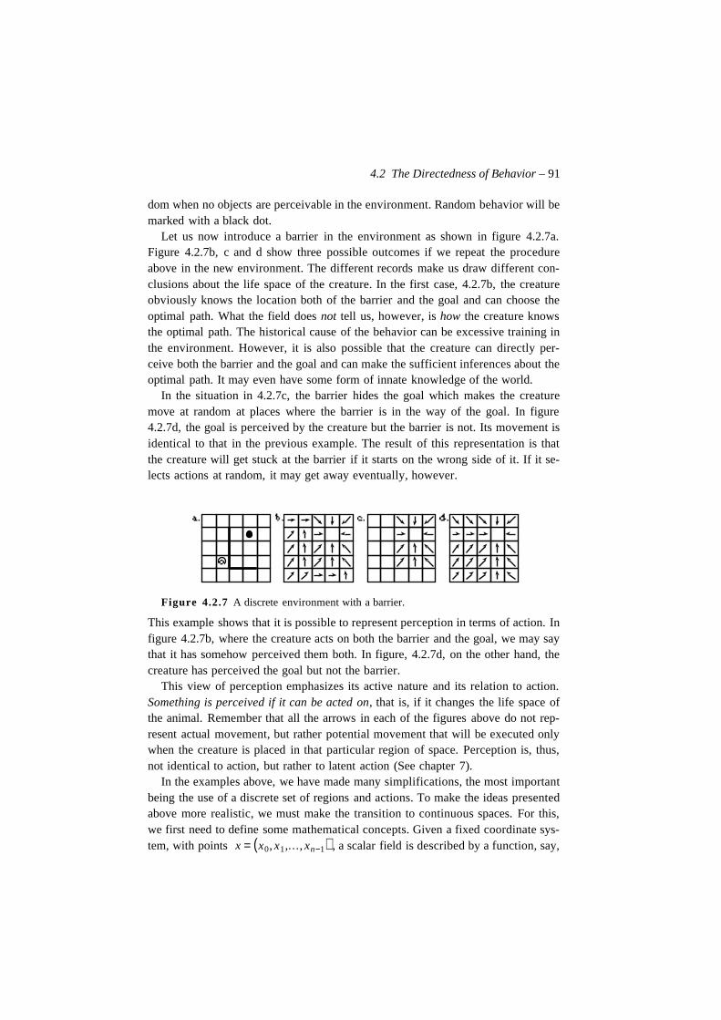
4.2 The Directedness of Behavior – 91
dom when no objects are perceivable in the environment. Random behavior will bemarked with a black dot.
Let us now introduce a barrier in the environment as shown in figure 4.2.7a.Figure 4.2.7b, c and d show three possible outcomes if we repeat the procedureabove in the new environment. The different records make us draw different con-clusions about the life space of the creature. In the first case, 4.2.7b, the creatureobviously knows the location both of the barrier and the goal and can choose theoptimal path. What the field does not tell us, however, is how the creature knowsthe optimal path. The historical cause of the behavior can be excessive training inthe environment. However, it is also possible that the creature can directly per-ceive both the barrier and the goal and can make the sufficient inferences about theoptimal path. It may even have some form of innate knowledge of the world.
In the situation in 4.2.7c, the barrier hides the goal which makes the creaturemove at random at places where the barrier is in the way of the goal. In figure4.2.7d, the goal is perceived by the creature but the barrier is not. Its movement isidentical to that in the previous example. The result of this representation is thatthe creature will get stuck at the barrier if it starts on the wrong side of it. If it se-lects actions at random, it may get away eventually, however.
Figure 4.2.7 A discrete environment with a barrier.
This example shows that it is possible to represent perception in terms of action. Infigure 4.2.7b, where the creature acts on both the barrier and the goal, we may saythat it has somehow perceived them both. In figure, 4.2.7d, on the other hand, thecreature has perceived the goal but not the barrier.
This view of perception emphasizes its active nature and its relation to action.Something is perceived if it can be acted on, that is, if it changes the life space ofthe animal. Remember that all the arrows in each of the figures above do not rep-resent actual movement, but rather potential movement that will be executed onlywhen the creature is placed in that particular region of space. Perception is, thus,not identical to action, but rather to latent action (See chapter 7).
In the examples above, we have made many simplifications, the most importantbeing the use of a discrete set of regions and actions. To make the ideas presentedabove more realistic, we must make the transition to continuous spaces. For this,we first need to define some mathematical concepts. Given a fixed coordinate sys-tem, with points , a scalar field is described by a function, say,x = x0, x1,…, xn−1( )
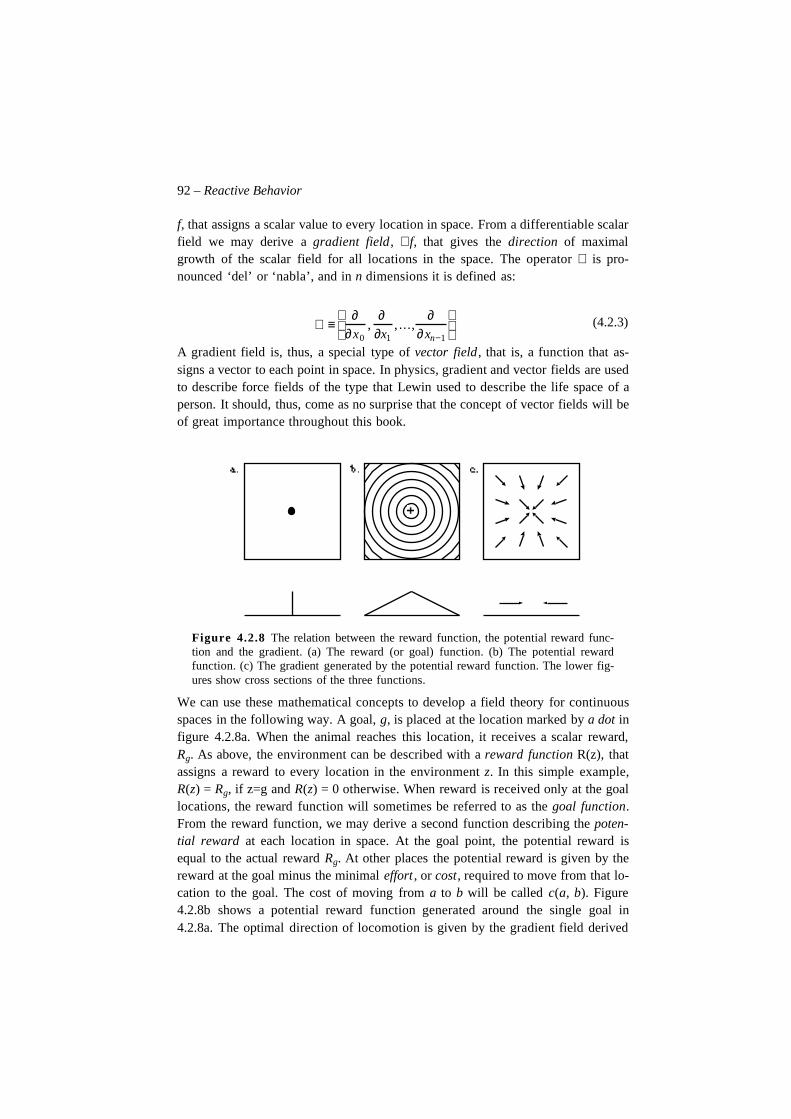
92 – Reactive Behavior
f, that assigns a scalar value to every location in space. From a differentiable scalarfield we may derive a gradient field, ∇f, that gives the direction of maximalgrowth of the scalar field for all locations in the space. The operator ∇ is pro-nounced ‘del’ or ‘nabla’, and in n dimensions it is defined as:
(4.2.3)
A gradient field is, thus, a special type of vector field, that is, a function that as-signs a vector to each point in space. In physics, gradient and vector fields are usedto describe force fields of the type that Lewin used to describe the life space of aperson. It should, thus, come as no surprise that the concept of vector fields will beof great importance throughout this book.
Figure 4.2.8 The relation between the reward function, the potential reward func-tion and the gradient. (a) The reward (or goal) function. (b) The potential rewardfunction. (c) The gradient generated by the potential reward function. The lower fig-ures show cross sections of the three functions.
We can use these mathematical concepts to develop a field theory for continuousspaces in the following way. A goal, g, is placed at the location marked by a dot infigure 4.2.8a. When the animal reaches this location, it receives a scalar reward,Rg. As above, the environment can be described with a reward function R(z), thatassigns a reward to every location in the environment z. In this simple example,R(z) = Rg, if z=g and R(z) = 0 otherwise. When reward is received only at the goallocations, the reward function will sometimes be referred to as the goal function.From the reward function, we may derive a second function describing the poten-tial reward at each location in space. At the goal point, the potential reward isequal to the actual reward Rg. At other places the potential reward is given by thereward at the goal minus the minimal effort , or cost, required to move from that lo-cation to the goal. The cost of moving from a to b will be called c(a, b). Figure4.2.8b shows a potential reward function generated around the single goal in4.2.8a. The optimal direction of locomotion is given by the gradient field derived
∇ ≡∂
∂x0,
∂∂x1
,…,∂
∂xn−1
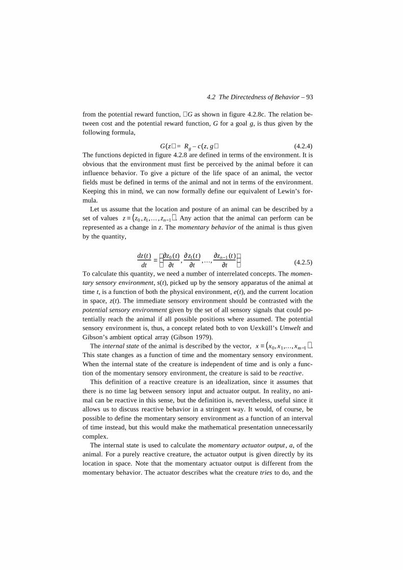
4.2 The Directedness of Behavior – 93
from the potential reward function, ∇G as shown in figure 4.2.8c. The relation be-tween cost and the potential reward function, G for a goal g, is thus given by thefollowing formula,
(4.2.4)The functions depicted in figure 4.2.8 are defined in terms of the environment. It isobvious that the environment must first be perceived by the animal before it caninfluence behavior. To give a picture of the life space of an animal, the vectorfields must be defined in terms of the animal and not in terms of the environment.Keeping this in mind, we can now formally define our equivalent of Lewin’s for-mula.
Let us assume that the location and posture of an animal can be described by aset of values . Any action that the animal can perform can berepresented as a change in z. The momentary behavior of the animal is thus givenby the quantity,
(4.2.5)
To calculate this quantity, we need a number of interrelated concepts. The momen-tary sensory environment, s(t), picked up by the sensory apparatus of the animal attime t, is a function of both the physical environment, e(t), and the current locationin space, z(t). The immediate sensory environment should be contrasted with thepotential sensory environment given by the set of all sensory signals that could po-tentially reach the animal if all possible positions where assumed. The potentialsensory environment is, thus, a concept related both to von Uexküll’s Umwelt andGibson’s ambient optical array (Gibson 1979).
The internal state of the animal is described by the vector, .This state changes as a function of time and the momentary sensory environment.When the internal state of the creature is independent of time and is only a func-tion of the momentary sensory environment, the creature is said to be reactive.
This definition of a reactive creature is an idealization, since it assumes thatthere is no time lag between sensory input and actuator output. In reality, no ani-mal can be reactive in this sense, but the definition is, nevertheless, useful since itallows us to discuss reactive behavior in a stringent way. It would, of course, bepossible to define the momentary sensory environment as a function of an intervalof time instead, but this would make the mathematical presentation unnecessarilycomplex.
The internal state is used to calculate the momentary actuator output , a, of theanimal. For a purely reactive creature, the actuator output is given directly by itslocation in space. Note that the momentary actuator output is different from themomentary behavior. The actuator describes what the creature tries to do, and the
G z( ) Rg c z g,( )–=
z = z0 , z1,… , zn−1( )
dz (t )
dt=
∂z0 (t)
∂t,∂z1(t )
∂t,…,
∂zn−1 (t )
∂t
x = x0, x1,…, xm −1( )
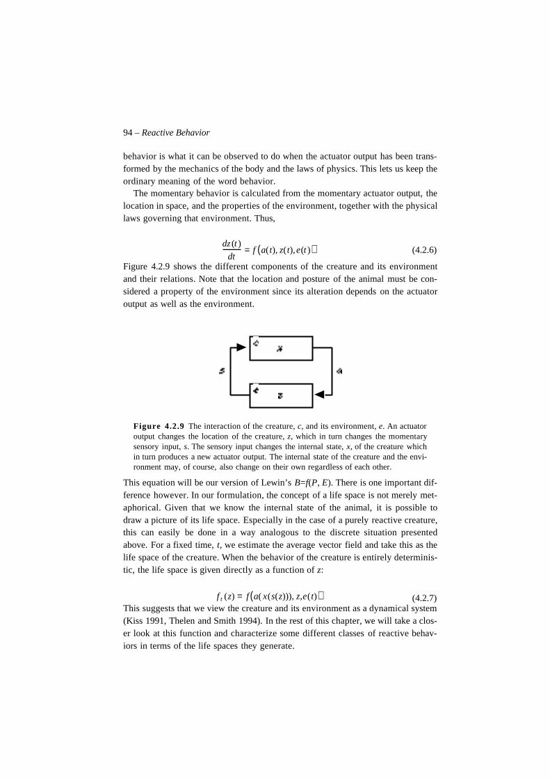
94 – Reactive Behavior
behavior is what it can be observed to do when the actuator output has been trans-formed by the mechanics of the body and the laws of physics. This lets us keep theordinary meaning of the word behavior.
The momentary behavior is calculated from the momentary actuator output, thelocation in space, and the properties of the environment, together with the physicallaws governing that environment. Thus,
(4.2.6)
Figure 4.2.9 shows the different components of the creature and its environmentand their relations. Note that the location and posture of the animal must be con-sidered a property of the environment since its alteration depends on the actuatoroutput as well as the environment.
Figure 4.2.9 The interaction of the creature, c, and its environment, e. An actuatoroutput changes the location of the creature, z, which in turn changes the momentarysensory input, s. The sensory input changes the internal state, x, of the creature whichin turn produces a new actuator output. The internal state of the creature and the envi-ronment may, of course, also change on their own regardless of each other.
This equation will be our version of Lewin’s B=f(P, E). There is one important dif-ference however. In our formulation, the concept of a life space is not merely met-aphorical. Given that we know the internal state of the animal, it is possible todraw a picture of its life space. Especially in the case of a purely reactive creature,this can easily be done in a way analogous to the discrete situation presentedabove. For a fixed time, t, we estimate the average vector field and take this as thelife space of the creature. When the behavior of the creature is entirely determinis-tic, the life space is given directly as a function of z:
(4.2.7)This suggests that we view the creature and its environment as a dynamical system(Kiss 1991, Thelen and Smith 1994). In the rest of this chapter, we will take a clos-er look at this function and characterize some different classes of reactive behav-iors in terms of the life spaces they generate.
dz (t )
dt= f a(t), z(t),e(t )( )
f t (z) = f a( x(s(z))), z,e(t)( )
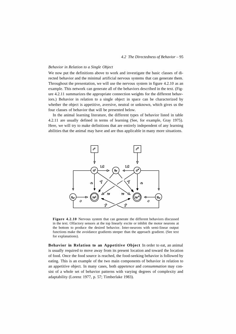
4.2 The Directedness of Behavior – 95
Behavior in Relation to a Single Object
We now put the definitions above to work and investigate the basic classes of di-rected behavior and the minimal artificial nervous systems that can generate them.Throughout the presentation, we will use the nervous system in figure 4.2.10 as anexample. This network can generate all of the behaviors described in the text. (Fig-ure 4.2.11 summarizes the appropriate connection weights for the different behav-iors.) Behavior in relation to a single object in space can be characterized bywhether the object is appetitive, aversive, neutral or unknown, which gives us thefour classes of behavior that will be presented below.
In the animal learning literature, the different types of behavior listed in table4.2.11 are usually defined in terms of learning (See, for example, Gray 1975).Here, we will try to make definitions that are entirely independent of any learningabilities that the animal may have and are thus applicable in many more situations.
Figure 4.2.10 Nervous system that can generate the different behaviors discussedin the text. Olfactory sensors at the top linearly excite or inhibit the motor neurons atthe bottom to produce the desired behavior. Inter-neurons with semi-linear outputfunctions make the avoidance gradients steeper than the approach gradient. (See textfor explanations).
Behavior in Relation to an Appetitive Object In order to eat, an animalis usually required to move away from its present location and toward the locationof food. Once the food source is reached, the food-seeking behavior is followed byeating. This is an example of the two main components of behavior in relation toan appetitive object. In many cases, both appetence and consummation may con-sist of a whole set of behavior patterns with varying degrees of complexity andadaptability (Lorenz 1977, p. 57; Timberlake 1983).
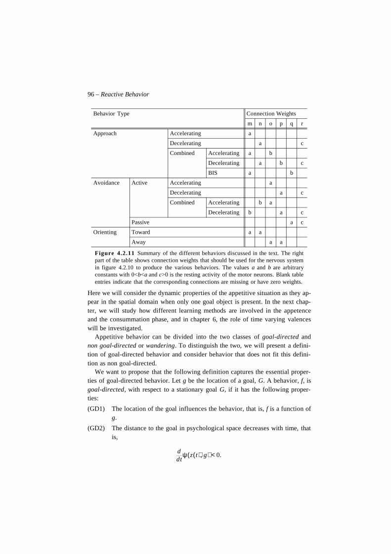
96 – Reactive Behavior
Figure 4.2.11 Summary of the different behaviors discussed in the text. The rightpart of the table shows connection weights that should be used for the nervous systemin figure 4.2.10 to produce the various behaviors. The values a and b are arbitraryconstants with 0<b<a and c>0 is the resting activity of the motor neurons. Blank tableentries indicate that the corresponding connections are missing or have zero weights.
Here we will consider the dynamic properties of the appetitive situation as they ap-pear in the spatial domain when only one goal object is present. In the next chap-ter, we will study how different learning methods are involved in the appetenceand the consummation phase, and in chapter 6, the role of time varying valenceswill be investigated.
Appetitive behavior can be divided into the two classes of goal-directed andnon goal-directed or wandering. To distinguish the two, we will present a defini-tion of goal-directed behavior and consider behavior that does not fit this defini-tion as non goal-directed.
We want to propose that the following definition captures the essential proper-ties of goal-directed behavior. Let g be the location of a goal, G. A behavior, f, isgoal-directed, with respect to a stationary goal G, if it has the following proper-ties:
(GD1) The location of the goal influences the behavior, that is, f is a function ofg.
(GD2) The distance to the goal in psychological space decreases with time, thatis,
Behavior Type Connection Weights
m n o p q r
Approach Accelerating a
Decelerating a c
Combined Accelerating a b
Decelerating a b c
BIS a b
Avoidance Active Accelerating a
Decelerating a c
Combined Accelerating b a
Decelerating b a c
Passive a c
Orienting Toward a a
Away a a
tdd ψ z t( ) g,( ) 0.<
4.2 The Directedness of Behavior – 97
Given this definition, it is neither necessary nor sufficient that the animal reach thegoal. This definition of goal–directedness is, thus, primarily concerned with thestriving of the behavior and not with its result. Also note that goal–directedness inthis sense is a momentary property of a behavior. Since goal–directed behavior canalternatively be characterized as approaching the goal, this type of behavior canalso be referred to as approach behavior. This does not mean that all behaviorswhich approach a goal necessarily are goal–directed. It is quite possible for an an-imal to approach a goal without utilizing an approach behavior.
The definition should be compared with the one presented by McFarland andBösser (1993) which requires that the goal is explicitly represented and is used toguide behavior over time. The differences between their notion of goal-directed-ness and the one we present here are very subtle, but it appears that their definitionis slightly more restrictive. Condition (GD1) appears to be weaker than the re-quirement for explicit representations and condition (GD2) does not require thatthe difference between the desired state of affairs and the current state is explicitlyused as feedback to control behavior, as they suggest. In the ethological literature,approach behaviors, as defined above, are usually referred to as topic responses ortaxes.
Common to all these taxes, the simplest and the most complex alike, is thefact that the creature turns directly, without any process of trial and error, inthe direction most favorable for its survival. In other words, the size and theangle through which it turns is directly dependent on that formed by the crea-ture’s longitudinal axis and the direction of the impinging stimulus. This ‘an-gle-controlled’ turning is characteristic of all taxes. (Lorenz 1977 p. 52)
The mechanisms that control taxes are called servo-mechanisms (Gallistel 1980).They are, thus, canonical examples of teleological behavior (Rosenbleut, Wienerand Bigelow 1943). To model goal-directed behaviors we will elaborate on theidea of potential reward functions. We have already seen how a potential rewardfunction can be defined around a goal. To describe the dynamics of the appetitivesituation, some further functions of a similar kind are needed. We will call thesegoal-gradients7 in agreement with Hull’s use of the term (Hull 1932). The goal-gradient around an appetitive object describes the strength of the approach tenden-cy at every distance from it. The size of the goal-gradient is considered to be re-flected in the speed of movement at different distances. The concept of a goal-gradient is, thus, related to the potential reward function described above.
In our artificial creatures, the smell gradients picked up by the olfactory sensorsgenerate signals that have the desired properties of a goal-gradient. Taking this
7. Here, the word gradient refers to a value that is graded by the distance to the goal. Themeaning is thus different from that used above in relation to gradient fields. This use of theword is unfortunate but the two different meanings of the word are already established with-in psychology and mathematics respectively.
98 – Reactive Behavior
into consideration we see that there are four possible types of goal-directed ap-proach behaviors (See figures 4.2.10 and 4.2.11). The first will be called acceler-ating. A behavior of this type becomes more vigorous as the psychological dis-tance to the goal decreases. The opposite behavior is also possible and will becalled decelerating. A behavior of this kind will typically cause the animal to stopat the goal. The behaviors of real animals usually show a combination of these twotypes. Up to a certain distance from the goal, the speed of movement increases un-til it reaches its top speed. After this point, the speed decreases instead and nearszero at the goal. This will be called a combined approach behavior. Note that acombined approach behavior can be generated by combining either an acceleratingapproach and an accelerating avoidance behavior or by combining two decelerat-ing behaviors.
Miller (1944) suggested that the combined approach behavior is the result of de-sired objects being both appetitive and aversive, thus generating both an approachgradient and an avoidance gradient. This corresponds to the idea that a goal objectmay be dangerous if the animal collides with it at high speed. Since the slope ofthe avoidance gradient is considered to be steeper than that of the approach gradi-ent, the sum of the two gradients will yield an approach behavior that increases inspeed as the animal gets closer to be goal but then drops off to zero when the goalis reached. Schmajuk and Blair (1993) have shown that if these ideas are combinedwith an appropriate physical model, the speed of movement generated closely fol-lows that of a real animal in a runway.
Finally, a creature can show orienting behavior. Such a behavior moves the an-imal closer to the goal in the sense that it directs its sensory apparatus toward thegoal. Table 4.2.11 shows the different types of goal-directed behavior, and in fig-ure 4.2.10 a nervous system that can generate the different behaviors is shown.
Figure 4.2.12 shows computer simulations of the three types of approach behav-iors using the type of smell cues described in the previous chapter. Acceleratingapproach causes the creature to move toward the goal. When the goal is reached,the locomotion of the creature starts to oscillate around the goal point (4.2.12a).Decelerating approach makes the creature move more slowly the closer it gets tothe goal. In the simulation in figure 4.2.12b, the creature stops before it reaches thegoal. Finally, in figure 4.2.12c, a combined approach behavior is simulated. Theresulting path shows an abrupt change at the distance from the goal where the ap-proach and the avoidance gradient are equally strong. At this point, the creaturestarts a circular locomotion around the goal point. The distance from the goal tothis circle depends on the relative strengts of the approach and the avoidance gra-dients. While the nervous systems simulated here were explicitly constructed, be-havior similar to that shown in the figure has also been automatically evolvedusing simulated evolution (Beer 1992). Very similar architectures have also beendiscussed by Braitenberg (1984).
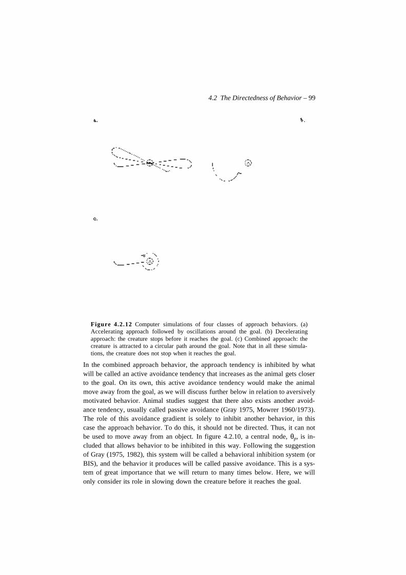
4.2 The Directedness of Behavior – 99
Figure 4.2.12 Computer simulations of four classes of approach behaviors. (a)Accelerating approach followed by oscillations around the goal. (b) Deceleratingapproach: the creature stops before it reaches the goal. (c) Combined approach: thecreature is attracted to a circular path around the goal. Note that in all these simula-tions, the creature does not stop when it reaches the goal.
In the combined approach behavior, the approach tendency is inhibited by whatwill be called an active avoidance tendency that increases as the animal gets closerto the goal. On its own, this active avoidance tendency would make the animalmove away from the goal, as we will discuss further below in relation to aversivelymotivated behavior. Animal studies suggest that there also exists another avoid-ance tendency, usually called passive avoidance (Gray 1975, Mowrer 1960/1973).The role of this avoidance gradient is solely to inhibit another behavior, in thiscase the approach behavior. To do this, it should not be directed. Thus, it can notbe used to move away from an object. In figure 4.2.10, a central node, θp, is in-cluded that allows behavior to be inhibited in this way. Following the suggestionof Gray (1975, 1982), this system will be called a behavioral inhibition system (orBIS), and the behavior it produces will be called passive avoidance. This is a sys-tem of great importance that we will return to many times below. Here, we willonly consider its role in slowing down the creature before it reaches the goal.
100 – Reactive Behavior
A creature using a passive avoidance gradient in a combined approach strategymust have a correct estimation of the distance to the goal if it wants to approach itsuccessfully. If the estimated distance to the goal is too short, it will stop beforethe goal is reached, and if it is to far, the creature will either run passed the goal orget hurt while colliding with it. To behave optimally, the creature should stop ex-actly at the goal; that is, the approach and avoidance gradients should be equal atthe goal location.
In figures 4.2.10 and 4.2.13, the connection weight m represents the slope of theapproach gradient, and n is the slope of the passive avoidance gradient. The inter-section of the avoidance gradient with the abscissa is given by the threshold, θp, ofthe interneuron whose transfer function is assumed to be semi-linear. The creaturewill stop when the positive and negative goal-gradients are equal. At this location,g, the smell intensity, s, is given by,
(4.2.8)
For optimal speed, n, m and θ should be chosen to satisfy this condition. Even so,we still need to make one change in the approach behavior to make the speed opti-mal.
Figure 4.2.13 The approach and avoidance gradients around a goal.
If G(z) is the potential reward function around G, and G is stationary, we see that abehavior is optimal , with respect to G, when . None of the approachbehaviors described so far are optimal with respect to the potential reward functionof the situation. As we have discussed above, the creature should try to follow thegradient of this function if it wants to reach the goal with the least possible effort.This corresponds to movement along a straight line from the start to the goal, butthe creature can only move in this way when it is already heading in the correct di-rection. An optimal behavior could thus be constructed if the creature could bemade to first orient itself toward the goal and then start its approach behavior.
s (g ) =nθ
n − m
f (z) = ∇G(z)
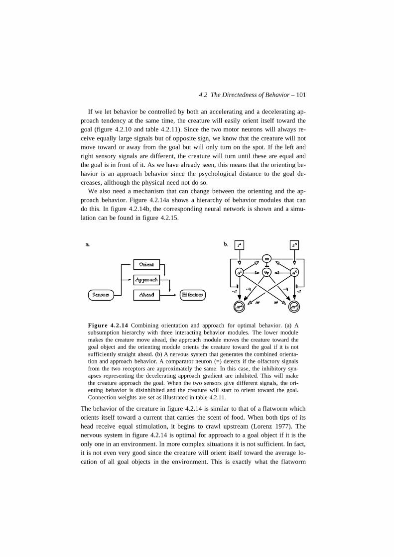
4.2 The Directedness of Behavior – 101
If we let behavior be controlled by both an accelerating and a decelerating ap-proach tendency at the same time, the creature will easily orient itself toward thegoal (figure 4.2.10 and table 4.2.11). Since the two motor neurons will always re-ceive equally large signals but of opposite sign, we know that the creature will notmove toward or away from the goal but will only turn on the spot. If the left andright sensory signals are different, the creature will turn until these are equal andthe goal is in front of it. As we have already seen, this means that the orienting be-havior is an approach behavior since the psychological distance to the goal de-creases, allthough the physical need not do so.
We also need a mechanism that can change between the orienting and the ap-proach behavior. Figure 4.2.14a shows a hierarchy of behavior modules that cando this. In figure 4.2.14b, the corresponding neural network is shown and a simu-lation can be found in figure 4.2.15.
Figure 4.2.14 Combining orientation and approach for optimal behavior. (a) Asubsumption hierarchy with three interacting behavior modules. The lower modulemakes the creature move ahead, the approach module moves the creature toward thegoal object and the orienting module orients the creature toward the goal if it is notsufficiently straight ahead. (b) A nervous system that generates the combined orienta-tion and approach behavior. A comparator neuron (=) detects if the olfactory signalsfrom the two receptors are approximately the same. In this case, the inhibitory syn-apses representing the decelerating approach gradient are inhibited. This will makethe creature approach the goal. When the two sensors give different signals, the ori-enting behavior is disinhibited and the creature will start to orient toward the goal.Connection weights are set as illustrated in table 4.2.11.
The behavior of the creature in figure 4.2.14 is similar to that of a flatworm whichorients itself toward a current that carries the scent of food. When both tips of itshead receive equal stimulation, it begins to crawl upstream (Lorenz 1977). Thenervous system in figure 4.2.14 is optimal for approach to a goal object if it is theonly one in an environment. In more complex situations it is not sufficient. In fact,it is not even very good since the creature will orient itself toward the average lo-cation of all goal objects in the environment. This is exactly what the flatworm
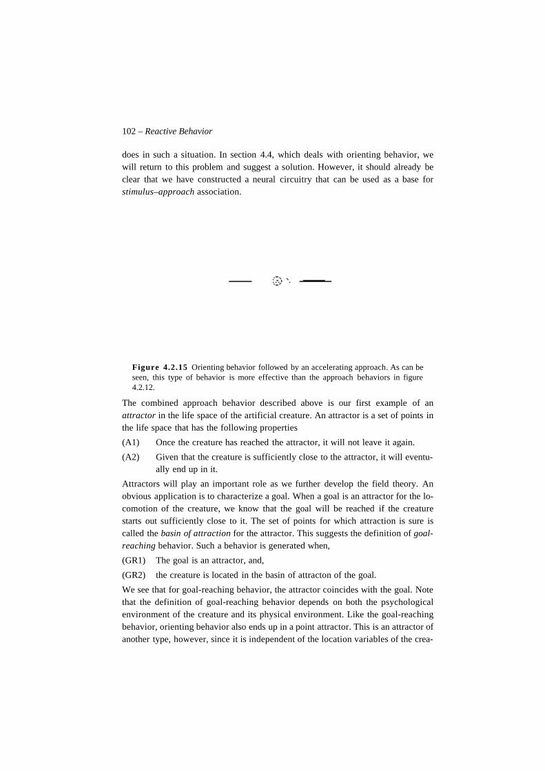
102 – Reactive Behavior
does in such a situation. In section 4.4, which deals with orienting behavior, wewill return to this problem and suggest a solution. However, it should already beclear that we have constructed a neural circuitry that can be used as a base forstimulus–approach association.
Figure 4.2.15 Orienting behavior followed by an accelerating approach. As can beseen, this type of behavior is more effective than the approach behaviors in figure4.2.12.
The combined approach behavior described above is our first example of anattractor in the life space of the artificial creature. An attractor is a set of points inthe life space that has the following properties
(A1) Once the creature has reached the attractor, it will not leave it again.
(A2) Given that the creature is sufficiently close to the attractor, it will eventu-ally end up in it.
Attractors will play an important role as we further develop the field theory. Anobvious application is to characterize a goal. When a goal is an attractor for the lo-comotion of the creature, we know that the goal will be reached if the creaturestarts out sufficiently close to it. The set of points for which attraction is sure iscalled the basin of attraction for the attractor. This suggests the definition of goal-reaching behavior. Such a behavior is generated when,
(GR1) The goal is an attractor, and,
(GR2) the creature is located in the basin of attracton of the goal.
We see that for goal-reaching behavior, the attractor coincides with the goal. Notethat the definition of goal-reaching behavior depends on both the psychologicalenvironment of the creature and its physical environment. Like the goal-reachingbehavior, orienting behavior also ends up in a point attractor. This is an attractor ofanother type, however, since it is independent of the location variables of the crea-
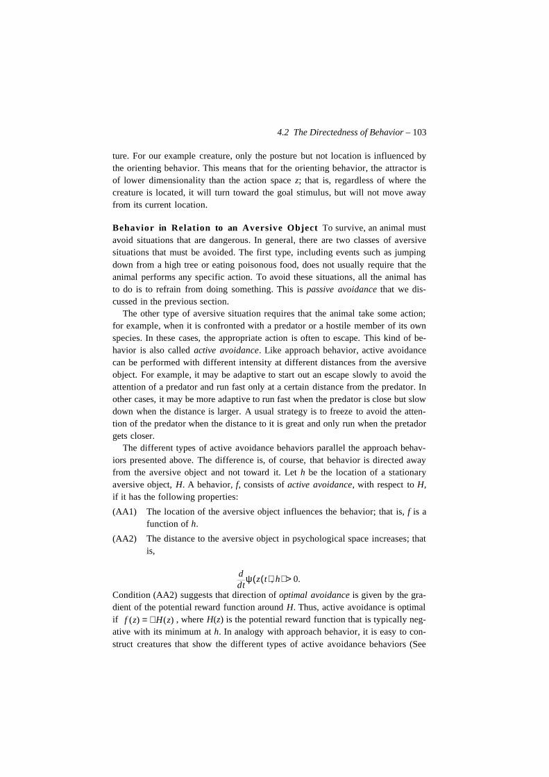
4.2 The Directedness of Behavior – 103
ture. For our example creature, only the posture but not location is influenced bythe orienting behavior. This means that for the orienting behavior, the attractor isof lower dimensionality than the action space z; that is, regardless of where thecreature is located, it will turn toward the goal stimulus, but will not move awayfrom its current location.
Behavior in Relation to an Aversive Object To survive, an animal mustavoid situations that are dangerous. In general, there are two classes of aversivesituations that must be avoided. The first type, including events such as jumpingdown from a high tree or eating poisonous food, does not usually require that theanimal performs any specific action. To avoid these situations, all the animal hasto do is to refrain from doing something. This is passive avoidance that we dis-cussed in the previous section.
The other type of aversive situation requires that the animal take some action;for example, when it is confronted with a predator or a hostile member of its ownspecies. In these cases, the appropriate action is often to escape. This kind of be-havior is also called active avoidance. Like approach behavior, active avoidancecan be performed with different intensity at different distances from the aversiveobject. For example, it may be adaptive to start out an escape slowly to avoid theattention of a predator and run fast only at a certain distance from the predator. Inother cases, it may be more adaptive to run fast when the predator is close but slowdown when the distance is larger. A usual strategy is to freeze to avoid the atten-tion of the predator when the distance to it is great and only run when the pretadorgets closer.
The different types of active avoidance behaviors parallel the approach behav-iors presented above. The difference is, of course, that behavior is directed awayfrom the aversive object and not toward it. Let h be the location of a stationaryaversive object, H. A behavior, f, consists of active avoidance, with respect to H,if it has the following properties:
(AA1) The location of the aversive object influences the behavior; that is, f is afunction of h.
(AA2) The distance to the aversive object in psychological space increases; thatis,
Condition (AA2) suggests that direction of optimal avoidance is given by the gra-dient of the potential reward function around H. Thus, active avoidance is optimalif , where H(z) is the potential reward function that is typically neg-ative with its minimum at h. In analogy with approach behavior, it is easy to con-struct creatures that show the different types of active avoidance behaviors (See
tdd ψ z t( ) h,( ) 0.>
f (z) = ∇H(z)
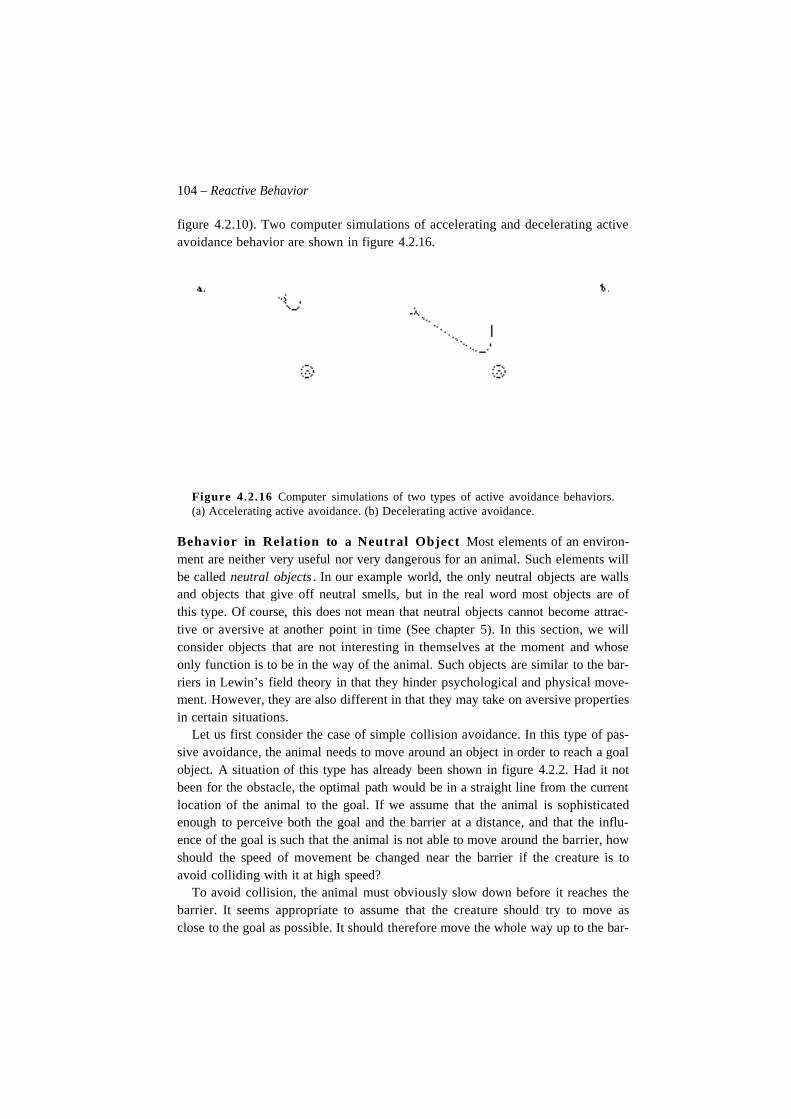
104 – Reactive Behavior
figure 4.2.10). Two computer simulations of accelerating and decelerating activeavoidance behavior are shown in figure 4.2.16.
Figure 4.2.16 Computer simulations of two types of active avoidance behaviors.(a) Accelerating active avoidance. (b) Decelerating active avoidance.
Behavior in Relation to a Neutral Object Most elements of an environ-ment are neither very useful nor very dangerous for an animal. Such elements willbe called neutral objects . In our example world, the only neutral objects are wallsand objects that give off neutral smells, but in the real word most objects are ofthis type. Of course, this does not mean that neutral objects cannot become attrac-tive or aversive at another point in time (See chapter 5). In this section, we willconsider objects that are not interesting in themselves at the moment and whoseonly function is to be in the way of the animal. Such objects are similar to the bar-riers in Lewin’s field theory in that they hinder psychological and physical move-ment. However, they are also different in that they may take on aversive propertiesin certain situations.
Let us first consider the case of simple collision avoidance. In this type of pas-sive avoidance, the animal needs to move around an object in order to reach a goalobject. A situation of this type has already been shown in figure 4.2.2. Had it notbeen for the obstacle, the optimal path would be in a straight line from the currentlocation of the animal to the goal. If we assume that the animal is sophisticatedenough to perceive both the goal and the barrier at a distance, and that the influ-ence of the goal is such that the animal is not able to move around the barrier, howshould the speed of movement be changed near the barrier if the creature is toavoid colliding with it at high speed?
To avoid collision, the animal must obviously slow down before it reaches thebarrier. It seems appropriate to assume that the creature should try to move asclose to the goal as possible. It should therefore move the whole way up to the bar-
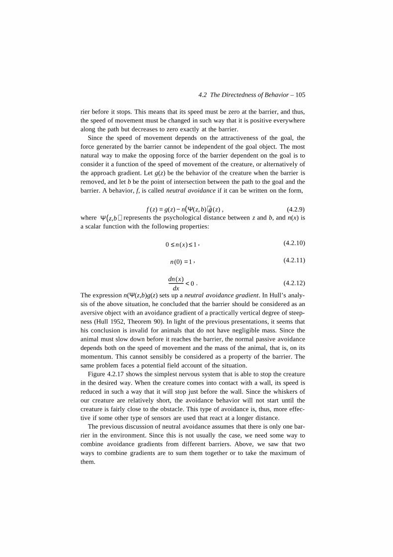
4.2 The Directedness of Behavior – 105
rier before it stops. This means that its speed must be zero at the barrier, and thus,the speed of movement must be changed in such way that it is positive everywherealong the path but decreases to zero exactly at the barrier.
Since the speed of movement depends on the attractiveness of the goal, theforce generated by the barrier cannot be independent of the goal object. The mostnatural way to make the opposing force of the barrier dependent on the goal is toconsider it a function of the speed of movement of the creature, or alternatively ofthe approach gradient. Let g(z) be the behavior of the creature when the barrier isremoved, and let b be the point of intersection between the path to the goal and thebarrier. A behavior, f, is called neutral avoidance if it can be written on the form,
, (4.2.9)where represents the psychological distance between z and b, and n(x) isa scalar function with the following properties:
, (4.2.10)
, (4.2.11)
. (4.2.12)
The expression n(Ψ(z,b)g(z) sets up a neutral avoidance gradient. In Hull’s analy-sis of the above situation, he concluded that the barrier should be considered as anaversive object with an avoidance gradient of a practically vertical degree of steep-ness (Hull 1952, Theorem 90). In light of the previous presentations, it seems thathis conclusion is invalid for animals that do not have negligible mass. Since theanimal must slow down before it reaches the barrier, the normal passive avoidancedepends both on the speed of movement and the mass of the animal, that is, on itsmomentum. This cannot sensibly be considered as a property of the barrier. Thesame problem faces a potential field account of the situation.
Figure 4.2.17 shows the simplest nervous system that is able to stop the creaturein the desired way. When the creature comes into contact with a wall, its speed isreduced in such a way that it will stop just before the wall. Since the whiskers ofour creature are relatively short, the avoidance behavior will not start until thecreature is fairly close to the obstacle. This type of avoidance is, thus, more effec-tive if some other type of sensors are used that react at a longer distance.
The previous discussion of neutral avoidance assumes that there is only one bar-rier in the environment. Since this is not usually the case, we need some way tocombine avoidance gradients from different barriers. Above, we saw that twoways to combine gradients are to sum them together or to take the maximum ofthem.
f (z) = g(z) − n Ψ(z, b)( )g (z)Ψ z,b( )
0 ≤ n (x) ≤ 1
n (0) = 1
dn (x)
dx< 0
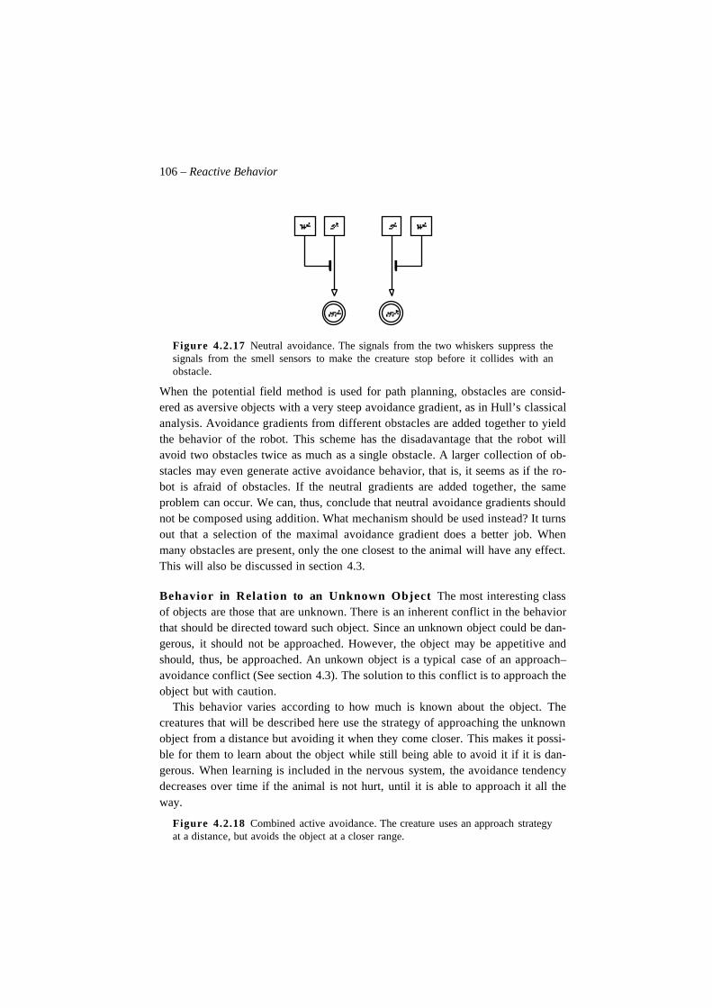
106 – Reactive Behavior
Figure 4.2.17 Neutral avoidance. The signals from the two whiskers suppress thesignals from the smell sensors to make the creature stop before it collides with anobstacle.
When the potential field method is used for path planning, obstacles are consid-ered as aversive objects with a very steep avoidance gradient, as in Hull’s classicalanalysis. Avoidance gradients from different obstacles are added together to yieldthe behavior of the robot. This scheme has the disadavantage that the robot willavoid two obstacles twice as much as a single obstacle. A larger collection of ob-stacles may even generate active avoidance behavior, that is, it seems as if the ro-bot is afraid of obstacles. If the neutral gradients are added together, the sameproblem can occur. We can, thus, conclude that neutral avoidance gradients shouldnot be composed using addition. What mechanism should be used instead? It turnsout that a selection of the maximal avoidance gradient does a better job. Whenmany obstacles are present, only the one closest to the animal will have any effect.This will also be discussed in section 4.3.
Behavior in Relation to an Unknown Object The most interesting classof objects are those that are unknown. There is an inherent conflict in the behaviorthat should be directed toward such object. Since an unknown object could be dan-gerous, it should not be approached. However, the object may be appetitive andshould, thus, be approached. An unkown object is a typical case of an approach–avoidance conflict (See section 4.3). The solution to this conflict is to approach theobject but with caution.
This behavior varies according to how much is known about the object. Thecreatures that will be described here use the strategy of approaching the unknownobject from a distance but avoiding it when they come closer. This makes it possi-ble for them to learn about the object while still being able to avoid it if it is dan-gerous. When learning is included in the nervous system, the avoidance tendencydecreases over time if the animal is not hurt, until it is able to approach it all theway.
Figure 4.2.18 Combined active avoidance. The creature uses an approach strategyat a distance, but avoids the object at a closer range.
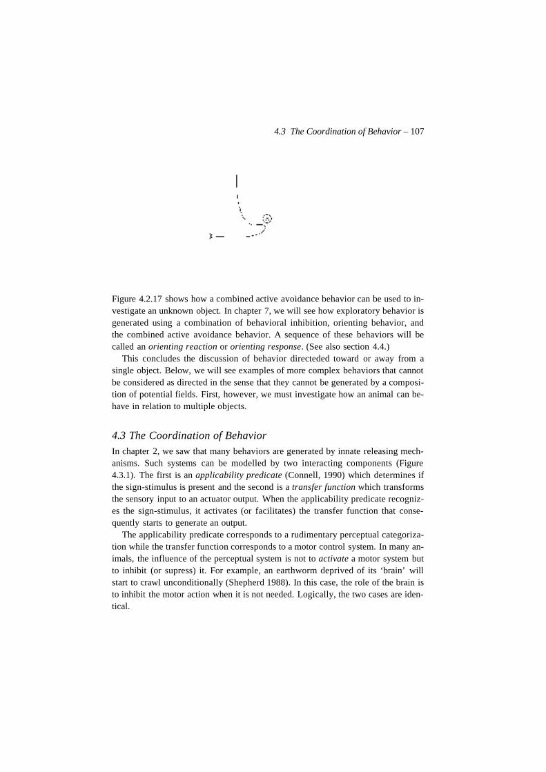
4.3 The Coordination of Behavior – 107
Figure 4.2.17 shows how a combined active avoidance behavior can be used to in-vestigate an unknown object. In chapter 7, we will see how exploratory behavior isgenerated using a combination of behavioral inhibition, orienting behavior, andthe combined active avoidance behavior. A sequence of these behaviors will becalled an orienting reaction or orienting response. (See also section 4.4.)
This concludes the discussion of behavior directeded toward or away from asingle object. Below, we will see examples of more complex behaviors that cannotbe considered as directed in the sense that they cannot be generated by a composi-tion of potential fields. First, however, we must investigate how an animal can be-have in relation to multiple objects.
4.3 The Coordination of BehaviorIn chapter 2, we saw that many behaviors are generated by innate releasing mech-anisms. Such systems can be modelled by two interacting components (Figure4.3.1). The first is an applicability predicate (Connell, 1990) which determines ifthe sign-stimulus is present and the second is a transfer function which transformsthe sensory input to an actuator output. When the applicability predicate recogniz-es the sign-stimulus, it activates (or facilitates) the transfer function that conse-quently starts to generate an output.
The applicability predicate corresponds to a rudimentary perceptual categoriza-tion while the transfer function corresponds to a motor control system. In many an-imals, the influence of the perceptual system is not to activate a motor system butto inhibit (or supress) it. For example, an earthworm deprived of its ‘brain’ willstart to crawl unconditionally (Shepherd 1988). In this case, the role of the brain isto inhibit the motor action when it is not needed. Logically, the two cases are iden-tical.
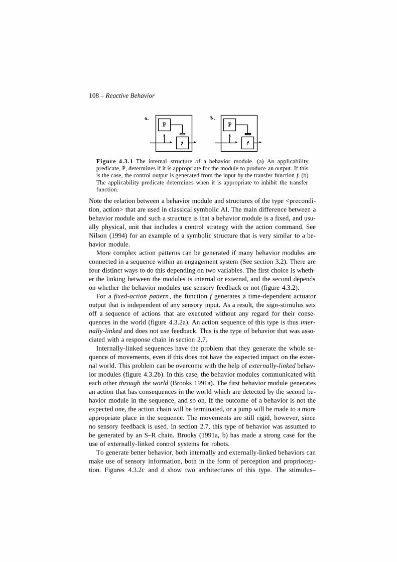
108 – Reactive Behavior
Figure 4.3.1 The internal structure of a behavior module. (a) An applicabilitypredicate, P, determines if it is appropriate for the module to produce an output. If thisis the case, the control output is generated from the input by the transfer function f. (b)The applicability predicate determines when it is appropriate to inhibit the transferfunction.
Note the relation between a behavior module and structures of the type <precondi-tion, action> that are used in classical symbolic AI. The main difference between abehavior module and such a structure is that a behavior module is a fixed, and usu-ally physical, unit that includes a control strategy with the action command. SeeNilson (1994) for an example of a symbolic structure that is very similar to a be-havior module.
More complex action patterns can be generated if many behavior modules areconnected in a sequence within an engagement system (See section 3.2). There arefour distinct ways to do this depending on two variables. The first choice is wheth-er the linking between the modules is internal or external, and the second dependson whether the behavior modules use sensory feedback or not (figure 4.3.2).
For a fixed-action pattern , the function f generates a time-dependent actuatoroutput that is independent of any sensory input. As a result, the sign-stimulus setsoff a sequence of actions that are executed without any regard for their conse-quences in the world (figure 4.3.2a). An action sequence of this type is thus inter-nally-linked and does not use feedback. This is the type of behavior that was asso-ciated with a response chain in section 2.7.
Internally-linked sequences have the problem that they generate the whole se-quence of movements, even if this does not have the expected impact on the exter-nal world. This problem can be overcome with the help of externally-linked behav-ior modules (figure 4.3.2b). In this case, the behavior modules communicated witheach other through the world (Brooks 1991a). The first behavior module generatesan action that has consequences in the world which are detected by the second be-havior module in the sequence, and so on. If the outcome of a behavior is not theexpected one, the action chain will be terminated, or a jump will be made to a moreappropriate place in the sequence. The movements are still rigid, however, sinceno sensory feedback is used. In section 2.7, this type of behavior was assumed tobe generated by an S–R chain. Brooks (1991a, b) has made a strong case for theuse of externally-linked control systems for robots.
To generate better behavior, both internally and externally-linked behaviors canmake use of sensory information, both in the form of perception and propriocep-tion. Figures 4.3.2c and d show two architectures of this type. The stimulus–
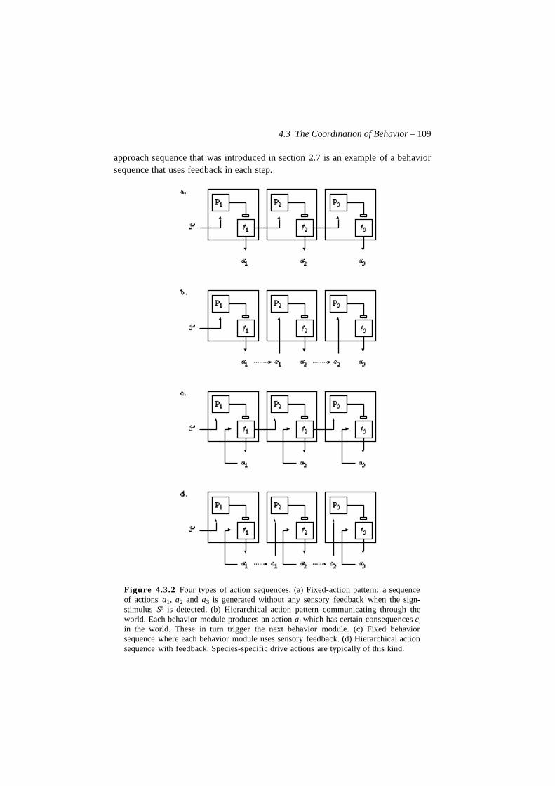
4.3 The Coordination of Behavior – 109
approach sequence that was introduced in section 2.7 is an example of a behaviorsequence that uses feedback in each step.
Figure 4.3.2 Four types of action sequences. (a) Fixed-action pattern: a sequenceof actions a1, a2 and a3 is generated without any sensory feedback when the sign-stimulus Ss is detected. (b) Hierarchical action pattern communicating through theworld. Each behavior module produces an action ai which has certain consequences ciin the world. These in turn trigger the next behavior module. (c) Fixed behaviorsequence where each behavior module uses sensory feedback. (d) Hierarchical actionsequence with feedback. Species-specific drive actions are typically of this kind.
110 – Reactive Behavior
In real animals, externally-linked behaviors are best known through the work ofTinbergen (Tinbergen 1951/1989), who called them hierarchically arrangedinstincts or hierarchical motor patterns. A related concept is that of a species-specific drive action (Lorenz 1977, p. 57). An important aspect of such sequencesis that each behavior leads to a new and more specific situation where a new sign-stimulus can be found. For example, a bat’s search for insects can be divided intoa distinct set of phases in this way (Simmons 1989). The first phase consists ofsearch for a prey. When a prey is detected, a second phase starts. At this point, anapproach behavior commences and continues until the bat is within approximatelyone meter of the target. Here the third phase begins, and the bat begins to track theinsect. Finally, a terminal behavior is executed which leads to the capture of theprey. In the bat, the various phases of the appetitive behavior can be distinguishedboth by the behavior of the animal and by the sound signals it emits to locate itsprey (Compare section 2.2).
Action Selection
In this section, we will consider a number of different ways in which behaviors canbe composed. In behavioral robotics, this selection process is often refered to asarbitration or action selection, and the nodes in the network of behavior modulesthat are responsible for the combination are called arbitration nodes. The role ofthese systems is to control the coordination of different actions.
The concept of action selection will be the basis for the theory of motivationthat will be developed in chapter 6. Here, we will only consider the most basicforms of action selection and behavior composition which are needed by a reactiveagent. The different types of arbitration methods are summarized in figure 4.3.3below.
Let us start with the additive composition. Two behavior modules generate con-trol signals that are simply added together. As we have already seen, this is themechanism that is mostly used to combine potential fields (Arkin 1990). A niceproperty of this method is that it does not matter whether we sum the potentials orthe gradients to get the composed behavior. This follows from the fact that ∇ is alinear operator. Thus, if Gi(z) is a set of potential reward functions,
(4.3.1)
The left hand expression corresponds to the situation where the individual poten-tial reward functions are first added together before the direction of movement iscalculated. The right hand expression corresponds to the case where each behaviormodule generates its own actuator output which is subsequently added togetherwith the other. Since the individual behavior modules may include an applicabilitypredicate that controls whether the module generates an output or not, no addition-al arbitration is necessary in many cases.
∇ Gi (z ) =i
∑ ∇Gi (z)i
∑

4.3 The Coordination of Behavior – 111
Figure 4.3.3 Summary of the different arbitration methods. The vector-valuedactuator commands from behavior modules A and B are called a and b, respectively.The output from the arbitration node is called c. Strength outputs are called sa and sband gating signals are called ga and gb. In central selection, the gating signals arefunctions of a central motivational state M. This state, in turn, depends on the strengthoutput from A and B.
Type Diagram Arbitration
Additive
Maximum
Suppression
Inhibition
MutualInhibition
CentralSelection
M = m(sa, sb)
c = a + b
c =a if a > b
b otherwise
c =b if a = 0
a otherwise
c a 1 sa–( )b+=
c 1 sb–( )a +=
1 sa–( )+ b
c = ga( M)a + gb ( M)b
112 – Reactive Behavior
One drawback with additive composition is that it generates unsuitable behavior insome cases. If there are a number of goals close to the creature in the environment,it will appoach the average position of the goals instead of one distinct goal. Thisis obviously not a very good strategy although it does manifest in real animals.
An animal can overcome the problem of multiple goals by using maximum com-position. In this arbitration scheme, only the control signal with the largest magni-tude is allowed to control the creature. This is similar to response competitionwhich has been an important part of many theories of behavior (Hull 1934, Grelle1981). Note that, in general, the control signals are vectors and not scalars. As aconsequence, it is necessary to look at the magnitude of the whole vector and notonly at the individual components when a control signal is selected.
The subsumption architecture invented by Brooks (1986) is yet another varia-tion on this theme. In this architecture, arbitration depends on a fixed hierarchy ofthe control signals. The arbitration nodes are called suppressor nodes. When thebehavior module at the top generates an output, it supresses the control signalsfrom the lower behavior module. This situation is shown in figure 4.3.3. The be-havior-based robots built by Brooks (1990) and coworkers) show that it is possibleto construct quite complex systems using an arbitration scheme of this type.
Supression can alternatively be seen as a form of inhibition. Inhibitory signalscan either decrease the intensity of the output of the other module or can be used toinhibit it completely. This second situation can be interpreted as if the applicabilitypredicate of the behavior module at the bottom depends on the output of the topmodule.
It is also possible for the behavior modules to mutually inhibit each other. Whenmutual inhibition is used, it is possible for the behavior modules to compete insuch a way that only one of them will be able to generate an output signal. In theneural network literature, this is usually refered to as a “winner take all” architec-ture (Compare section 2.3). In many respects, this arbitration scheme is similar tomaximum composition, but with one important difference. When maximum com-position is used, it is the magnitute of the output signals that determine which be-havior will win. With mutual inhibition, this need not be the case. It is quite possi-ble for the inhibitory output to be very strong and the control signal to be veryweak at the same time. This makes it possible to have a very strong tendency to dovery little. The signal that represents the strength of the behavior module will becalled the strength output in order to distinguish it from the control output (Seefigure 4.3.3).
An even more complex behavior selection scheme can be called central selec-tion. It is similar to mutual inhibition in that the different behavior modules com-pete for activation. Another similarity is that the signal that determines thestrength of each behavior tendency is independent of the control signal. A centralmotivational module is used to collect the strength outputs from each behavior
4.3 The Coordination of Behavior – 113
module and select which control signals should be let through the arbitration node.In chapter 6, we will study how the strength outputs can be used to represent theestimated potential reward that will be received if the behavior module from whichthey emanate are activated. We will argue that the motivational system is based onthis type of arbitration. In this case, the strength output from the behavior modulesare used as incentive signals (See chapter 6).
Finally, it is possible to select action according to a stochastic function. In ran-dom selection, the probability for a certain action is proportional to its strength. Ifa0…an are a set of behaviors generated by the behavior modules A0…An , the prob-ability that Ai will be performed is calculated from, for example, a Bolzmann-distribution as,
. (4.3.2)
The parameter T is called temperature and controls the randomness of selection(Ackley, Hinton and Sejnowski 1985). The probability of selecting the largest sig-nal increases with decreased temperature. When T approaches infinity, the arbitra-tion becomes entirely random. When it is close to 0, the behavior with the largeststrength is always selected. As in the case of central selection, it is possible to letstrength outputs control the choice instead of the actual behavior signals. Randomselection is, thus, a form of central selection since the choice of behavior must bebased on strength inputs from all behavior modules.
Behavior in Relation to Multiple Objects
In any realistic situation, the environment consists of a large number of objects,some of which are appetitive and some which are aversive. Those objects whichare appetitive and those which are aversive may change over time as the needs ofthe animal change. At a single moment, however, the potential rewards corre-sponding to each object in the environment can be considered constant. In Lewin’stheory, this is called the valence of an object (Lewin 1935). The valence is respon-sible for the strength and direction of the forces around an object. An object with apositive valence will attract the individual, while an object with negative valencewill push the individual away from it. The forces from all the objects in the envi-ronment are combined to describe the behavior of the animal. This clearly corre-sponds to the addition of potential fields which was discussed above. In this sec-tion, we will consider the dynamics of situations with more than one object. Thepresentation will start with some classical examples of conflicts.
The Approach–Approach Conflict Consider a runway with food placed ateach end (figure 4.3.4). A hungry rat that is placed in the middle of this runway has
p c ai=( ) eai T⁄
ea j T⁄
j 0=
n
∑-----------------------=
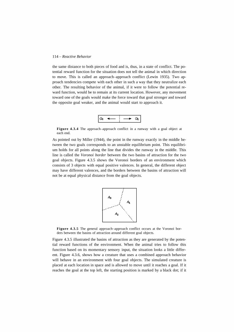
114 – Reactive Behavior
the same distance to both pieces of food and is, thus, in a state of conflict. The po-tential reward function for the situation does not tell the animal in which directionto move. This is called an approach–approach conflict (Lewin 1935). Two ap-proach tendencies compete with each other in such a way that they neutralize eachother. The resulting behavior of the animal, if it were to follow the potential re-ward function, would be to remain at its current location. However, any movementtoward one of the goals would make the force toward that goal stronger and towardthe opposite goal weaker, and the animal would start to approach it.
Figure 4.3.4 The approach–approach conflict in a runway with a goal object ateach end.
As pointed out by Miller (1944), the point in the runway exactly in the middle be-tween the two goals corresponds to an unstable equilibrium point. This equilibri-um holds for all points along the line that divides the runway in the middle. Thisline is called the Voronoi border between the two basins of attraction for the twogoal objects. Figure 4.3.5 shows the Voronoi borders of an environment whichconsists of 3 objects with equal positive valences. In general, the different objectmay have different valences, and the borders between the basins of attraction willnot be at equal physical distance from the goal objects.
Figure 4.3.5 The general approach–approach conflict occurs at the Voronoi bor-ders between the basins of attraction around different goal objects.
Figure 4.3.5 illustrated the basins of attraction as they are generated by the poten-tial reward functions of the environment. When the animal tries to follow thisfunction based on its momentary sensory input, the situation looks a little differ-ent. Figure 4.3.6, shows how a creature that uses a combined approach behaviorwill behave in an environment with four goal objects. The simulated creature isplaced at each location in space and is allowed to move until it reaches a goal. If itreaches the goal at the top left, the starting position is marked by a black dot; if it
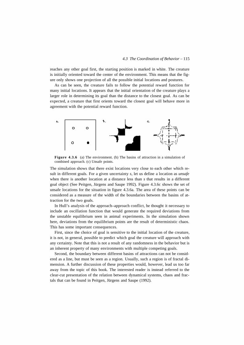
4.3 The Coordination of Behavior – 115
reaches any other goal first, the starting position is marked in white. The creatureis initially oriented toward the center of the environment. This means that the fig-ure only shows one projection of all the possible initial locations and postures.
As can be seen, the creature fails to follow the potential reward function formany initial locations. It appears that the initial orientation of the creature plays alarger role in determining its goal than the distance to the closest goal. As can beexpected, a creature that first orients toward the closest goal will behave more inagreement with the potential reward function.
Figure 4.3.6 (a) The environment. (b) The basins of attraction in a simulation ofcombined approach. (c) Unsafe points.
The simulation shows that there exist locations very close to each other which re-sult in different goals. For a given uncertainty s, let us define a location as unsafewhen there is another location at a distance less than s that results in a differentgoal object (See Peitgen, Jürgens and Saupe 1992). Figure 4.3.6c shows the set ofunsafe locations for the situation in figure 4.3.6a. The area of these points can beconsidered as a measure of the width of the boundaries between the basins of at-traction for the two goals.
In Hull’s analysis of the approach–approach conflict, he thought it necessary toinclude an oscillation function that would generate the required deviations fromthe unstable equilibrium seen in animal experiments. In the simulation shownhere, deviations from the equilibrium points are the result of deterministic chaos.This has some important consequences.
First, since the choice of goal is sensitive to the initial location of the creature,it is not, in general, possible to predict which goal the creature will approach withany certainty. Note that this is not a result of any randomness in the behavior but isan inherent property of many environments with multiple competing goals.
Second, the boundary between different basins of attractions can not be consid-ered as a line, but must be seen as a region. Usually, such a region is of fractal di-mension. A further discussion of these properties would, however, lead us too faraway from the topic of this book. The interested reader is instead referred to theclear-cut presentation of the relation between dynamical systems, chaos and frac-tals that can be found in Peitgen, Jürgens and Saupe (1992).
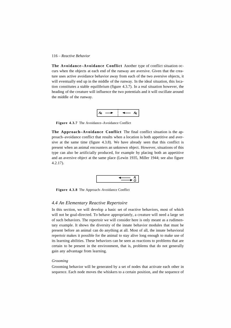
116 – Reactive Behavior
The Avoidance–Avoidance Conflict Another type of conflict situation oc-curs when the objects at each end of the runway are aversive. Given that the crea-ture uses active avoidance behavior away from each of the two aversive objects, itwill eventually end up in the middle of the runway. In the ideal situation, this loca-tion constitutes a stable equilibrium (figure 4.3.7). In a real situation however, theheading of the creature will influence the two potentials and it will oscillate aroundthe middle of the runway.
Figure 4.3.7 The Avoidance–Avoidance Conflict
The Approach–Avoidance Conflict The final conflict situation is the ap-proach–avoidance conflict that results when a location is both appetitive and aver-sive at the same time (figure 4.3.8). We have already seen that this conflict ispresent when an animal encounters an unknown object. However, situations of thistype can also be artificially produced, for example by placing both an appetitiveand an aversive object at the same place (Lewin 1935, Miller 1944; see also figure4.2.17).
Figure 4.3.8 The Approach–Avoidance Conflict
4.4 An Elementary Reactive RepertoireIn this section, we will develop a basic set of reactive behaviors, most of whichwill not be goal-directed. To behave appropriately, a creature will need a large setof such behaviors. The repertoir we will consider here is only meant as a rudimen-tary example. It shows the diversity of the innate behavior modules that must bepresent before an animal can do anything at all. Most of all, the innate behavioralrepertoir makes it possible for the animal to stay alive long enough to make use ofits learning abilities. These behaviors can be seen as reactions to problems that arecertain to be present in the environment, that is, problems that do not generallygain any advantage from learning.
Grooming
Grooming behavior will be generated by a set of nodes that activate each other insequence. Each node moves the whiskers to a certain position, and the sequence of
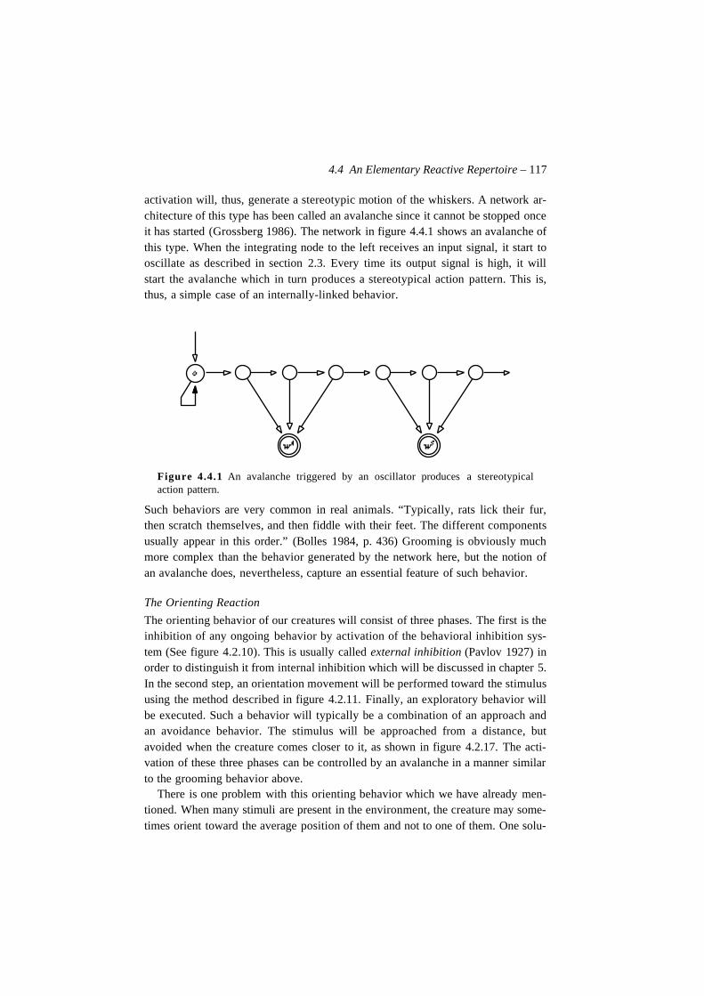
4.4 An Elementary Reactive Repertoire – 117
activation will, thus, generate a stereotypic motion of the whiskers. A network ar-chitecture of this type has been called an avalanche since it cannot be stopped onceit has started (Grossberg 1986). The network in figure 4.4.1 shows an avalanche ofthis type. When the integrating node to the left receives an input signal, it start tooscillate as described in section 2.3. Every time its output signal is high, it willstart the avalanche which in turn produces a stereotypical action pattern. This is,thus, a simple case of an internally-linked behavior.
Figure 4.4.1 An avalanche triggered by an oscillator produces a stereotypicalaction pattern.
Such behaviors are very common in real animals. “Typically, rats lick their fur,then scratch themselves, and then fiddle with their feet. The different componentsusually appear in this order.” (Bolles 1984, p. 436) Grooming is obviously muchmore complex than the behavior generated by the network here, but the notion ofan avalanche does, nevertheless, capture an essential feature of such behavior.
The Orienting Reaction
The orienting behavior of our creatures will consist of three phases. The first is theinhibition of any ongoing behavior by activation of the behavioral inhibition sys-tem (See figure 4.2.10). This is usually called external inhibition (Pavlov 1927) inorder to distinguish it from internal inhibition which will be discussed in chapter 5.In the second step, an orientation movement will be performed toward the stimulususing the method described in figure 4.2.11. Finally, an exploratory behavior willbe executed. Such a behavior will typically be a combination of an approach andan avoidance behavior. The stimulus will be approached from a distance, butavoided when the creature comes closer to it, as shown in figure 4.2.17. The acti-vation of these three phases can be controlled by an avalanche in a manner similarto the grooming behavior above.
There is one problem with this orienting behavior which we have already men-tioned. When many stimuli are present in the environment, the creature may some-times orient toward the average position of them and not to one of them. One solu-
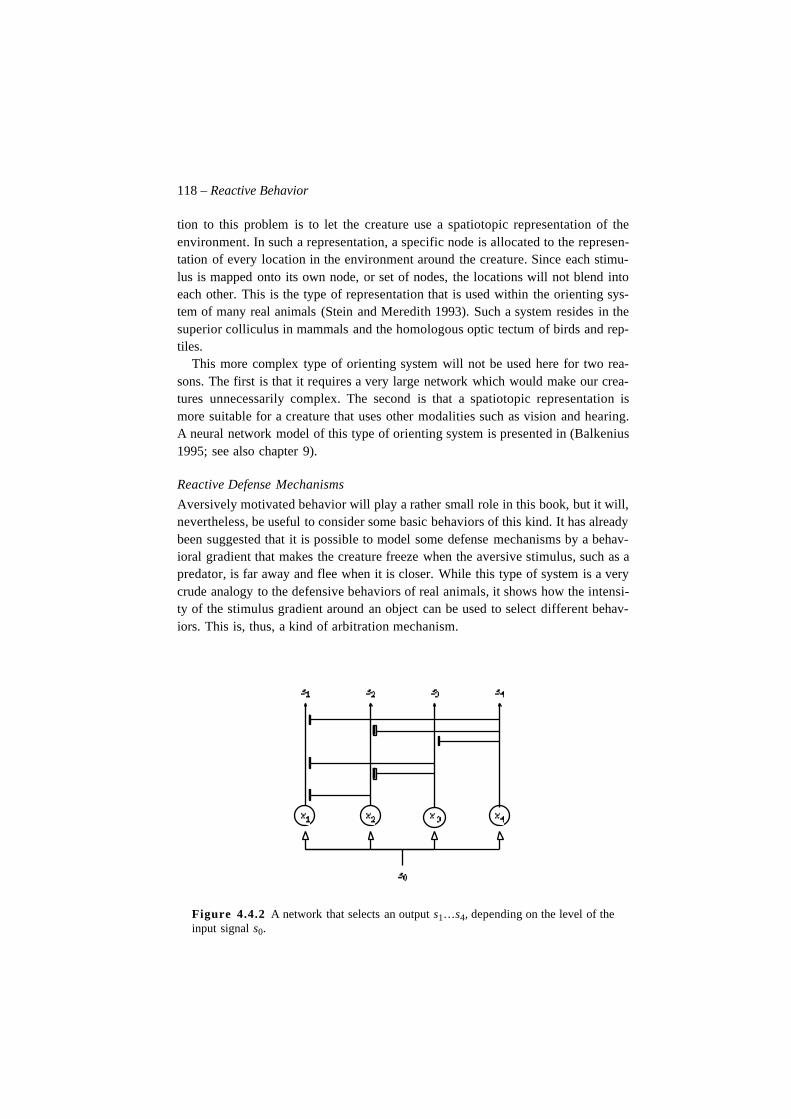
118 – Reactive Behavior
tion to this problem is to let the creature use a spatiotopic representation of theenvironment. In such a representation, a specific node is allocated to the represen-tation of every location in the environment around the creature. Since each stimu-lus is mapped onto its own node, or set of nodes, the locations will not blend intoeach other. This is the type of representation that is used within the orienting sys-tem of many real animals (Stein and Meredith 1993). Such a system resides in thesuperior colliculus in mammals and the homologous optic tectum of birds and rep-tiles.
This more complex type of orienting system will not be used here for two rea-sons. The first is that it requires a very large network which would make our crea-tures unnecessarily complex. The second is that a spatiotopic representation ismore suitable for a creature that uses other modalities such as vision and hearing.A neural network model of this type of orienting system is presented in (Balkenius1995; see also chapter 9).
Reactive Defense Mechanisms
Aversively motivated behavior will play a rather small role in this book, but it will,nevertheless, be useful to consider some basic behaviors of this kind. It has alreadybeen suggested that it is possible to model some defense mechanisms by a behav-ioral gradient that makes the creature freeze when the aversive stimulus, such as apredator, is far away and flee when it is closer. While this type of system is a verycrude analogy to the defensive behaviors of real animals, it shows how the intensi-ty of the stimulus gradient around an object can be used to select different behav-iors. This is, thus, a kind of arbitration mechanism.
Figure 4.4.2 A network that selects an output s1…s4, depending on the level of theinput signal s0.
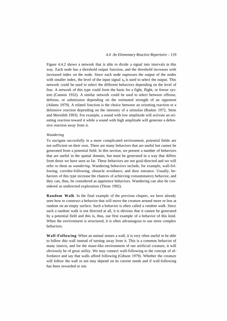
4.4 An Elementary Reactive Repertoire – 119
Figure 4.4.2 shows a network that is able to divide a signal into intervals in thisway. Each node has a threshold output function, and the threshold increases withincreased index on the node. Since each node supresses the output of the nodeswith smaller index, the level of the input signal s0 is used to select the output. Thisnetwork could be used to select the different behaviors depending on the level offear. A network of this type could form the basis for a fight, flight, or freeze sys-tem (Cannon 1932). A similar network could be used to select between offense,defense, or submission depending on the estimated strength of an opponent(Adams 1979). A related function is the choice between an orienting reaction or adefensive reaction depending on the intensity of a stimulus (Raskin 1972, Steinand Meredith 1993). For example, a sound with low amplitude will activate an ori-enting reaction toward it while a sound with high amplitude will generate a defen-sive reaction away from it.
Wandering
To navigate succesfully in a more complicated environment, potential fields arenot sufficient on their own. There are many behaviors that are useful but cannot begenerated from a potential field. In this section, we present a number of behaviorsthat are useful in the spatial domain, but must be generated in a way that differsfrom those we have seen so far. These behaviors are not goal-directed and we willrefer to them as wandering. Wandering behaviors include, for example, wall-fol-lowing, corridor-following, obstacle avoidance, and door entrance. Usually, be-haviors of this type increase the chances of achieving consummatory behavior, andthey can, thus, be considered as appetence behaviors. Wandering can also be con-sidered as undirected exploration (Thrun 1992).
Random Walk In the final example of the previous chapter, we have alreadyseen how to construct a behavior that will move the creature around more or less atrandom on an empty surface. Such a behavior is often called a random walk. Sincesuch a random walk is not directed at all, it is obvious that it cannot be generatedby a potential field and this is, thus, our first example of a behavior of this kind.When the environment is structured, it is often advantagous to use more complexbehaviors.
Wall-Following When an animal senses a wall, it is very often useful to be ableto follow this wall instead of turning away from it. This is a common behavior ofmany insects, and for the maze-like environment of our artificial creature, it willobviously be of great utility. We may connect wall-following to the concept of af-fordance and say that walls afford following (Gibson 1979). Whether the creaturewill follow the wall or not may depend on its current needs and if wall-followinghas been rewarded or not.
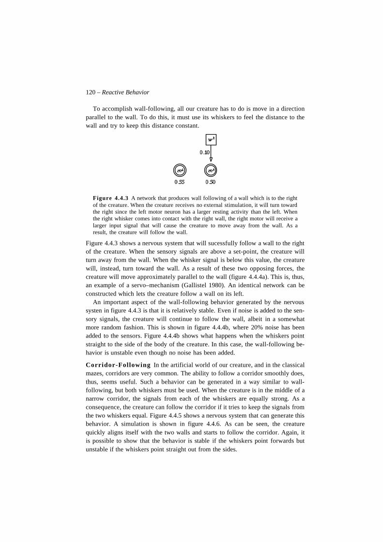
120 – Reactive Behavior
To accomplish wall-following, all our creature has to do is move in a directionparallel to the wall. To do this, it must use its whiskers to feel the distance to thewall and try to keep this distance constant.
Figure 4.4.3 A network that produces wall following of a wall which is to the rightof the creature. When the creature receives no external stimulation, it will turn towardthe right since the left motor neuron has a larger resting activity than the left. Whenthe right whisker comes into contact with the right wall, the right motor will receive alarger input signal that will cause the creature to move away from the wall. As aresult, the creature will follow the wall.
Figure 4.4.3 shows a nervous system that will sucessfully follow a wall to the rightof the creature. When the sensory signals are above a set-point, the creature willturn away from the wall. When the whisker signal is below this value, the creaturewill, instead, turn toward the wall. As a result of these two opposing forces, thecreature will move approximately parallel to the wall (figure 4.4.4a). This is, thus,an example of a servo–mechanism (Gallistel 1980). An identical network can beconstructed which lets the creature follow a wall on its left.
An important aspect of the wall-following behavior generated by the nervoussysten in figure 4.4.3 is that it is relatively stable. Even if noise is added to the sen-sory signals, the creature will continue to follow the wall, albeit in a somewhatmore random fashion. This is shown in figure 4.4.4b, where 20% noise has beenadded to the sensors. Figure 4.4.4b shows what happens when the whiskers pointstraight to the side of the body of the creature. In this case, the wall-following be-havior is unstable even though no noise has been added.
Corridor-Following In the artificial world of our creature, and in the classicalmazes, corridors are very common. The ability to follow a corridor smoothly does,thus, seems useful. Such a behavior can be generated in a way similar to wall-following, but both whiskers must be used. When the creature is in the middle of anarrow corridor, the signals from each of the whiskers are equally strong. As aconsequence, the creature can follow the corridor if it tries to keep the signals fromthe two whiskers equal. Figure 4.4.5 shows a nervous system that can generate thisbehavior. A simulation is shown in figure 4.4.6. As can be seen, the creaturequickly aligns itself with the two walls and starts to follow the corridor. Again, itis possible to show that the behavior is stable if the whiskers point forwards butunstable if the whiskers point straight out from the sides.
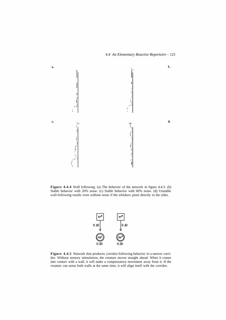
4.4 An Elementary Reactive Repertoire – 121
Figure 4.4.4 Wall following. (a) The behavior of the network in figure 4.4.3. (b)Stable behavior with 20% noise. (c) Stable behavior with 60% noise. (d) Unstablewall-following results even without noise if the whiskers point directly to the sides.
Figure 4.4.5 Network that produces corridor-following behavior in a narrow corri-dor. Without sensory stimulation, the creature moves straight ahead. When it comesinto contact with a wall, it will make a compensatory movement away from it. If thecreature can sense both walls at the same time, it will align itself with the corridor.
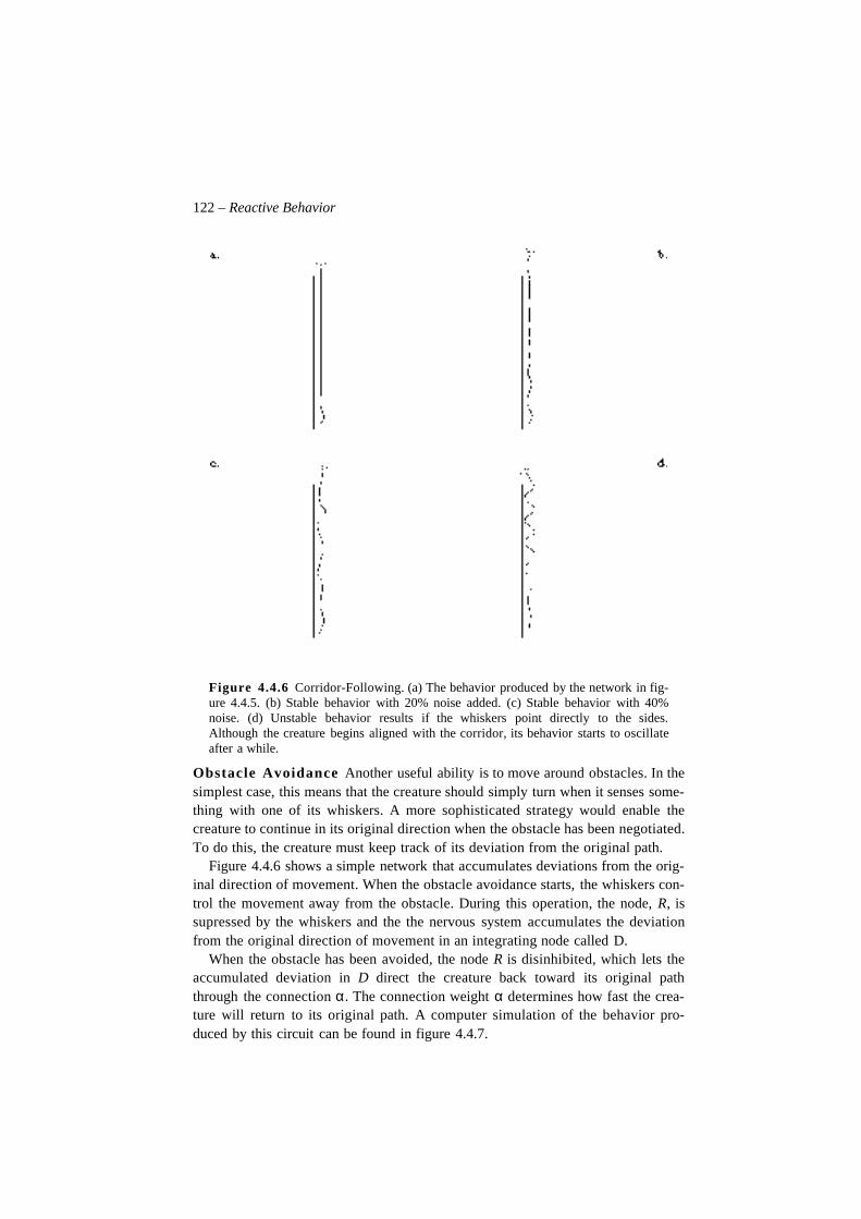
122 – Reactive Behavior
Figure 4.4.6 Corridor-Following. (a) The behavior produced by the network in fig-ure 4.4.5. (b) Stable behavior with 20% noise added. (c) Stable behavior with 40%noise. (d) Unstable behavior results if the whiskers point directly to the sides.Although the creature begins aligned with the corridor, its behavior starts to oscillateafter a while.
Obstacle Avoidance Another useful ability is to move around obstacles. In thesimplest case, this means that the creature should simply turn when it senses some-thing with one of its whiskers. A more sophisticated strategy would enable thecreature to continue in its original direction when the obstacle has been negotiated.To do this, the creature must keep track of its deviation from the original path.
Figure 4.4.6 shows a simple network that accumulates deviations from the orig-inal direction of movement. When the obstacle avoidance starts, the whiskers con-trol the movement away from the obstacle. During this operation, the node, R, issupressed by the whiskers and the the nervous system accumulates the deviationfrom the original direction of movement in an integrating node called D.
When the obstacle has been avoided, the node R is disinhibited, which lets theaccumulated deviation in D direct the creature back toward its original paththrough the connection α. The connection weight α determines how fast the crea-ture will return to its original path. A computer simulation of the behavior pro-duced by this circuit can be found in figure 4.4.7.
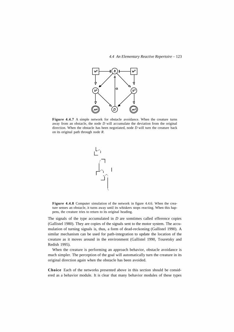
4.4 An Elementary Reactive Repertoire – 123
Figure 4.4.7 A simple network for obstacle avoidance. When the creature turnsaway from an obstacle, the node D will accumulate the deviation from the originaldirection. When the obstacle has been negotiated, node D will turn the creature backon its original path through node R.
Figure 4.4.8 Computer simulation of the network in figure 4.4.6. When the crea-ture senses an obstacle, it turns away until its whiskers stops reacting. When this hap-pens, the creature tries to return to its original heading.
The signals of the type accumulated in D are somtimes called efference copies(Gallistel 1980). They are copies of the signals sent to the motor system. The accu-mulation of turning signals is, thus, a form of dead-reckoning (Gallistel 1990). Asimilar mechanism can be used for path-integration to update the location of thecreature as it moves around in the environment (Gallistel 1990, Touretsky andRedish 1995).
When the creature is performing an approach behavior, obstacle avoidance ismuch simpler. The perception of the goal will automatically turn the creature in itsoriginal direction again when the obstacle has been avoided.
Choice Each of the networks presented above in this section should be consid-ered as a behavior module. It is clear that many behavior modules of these types
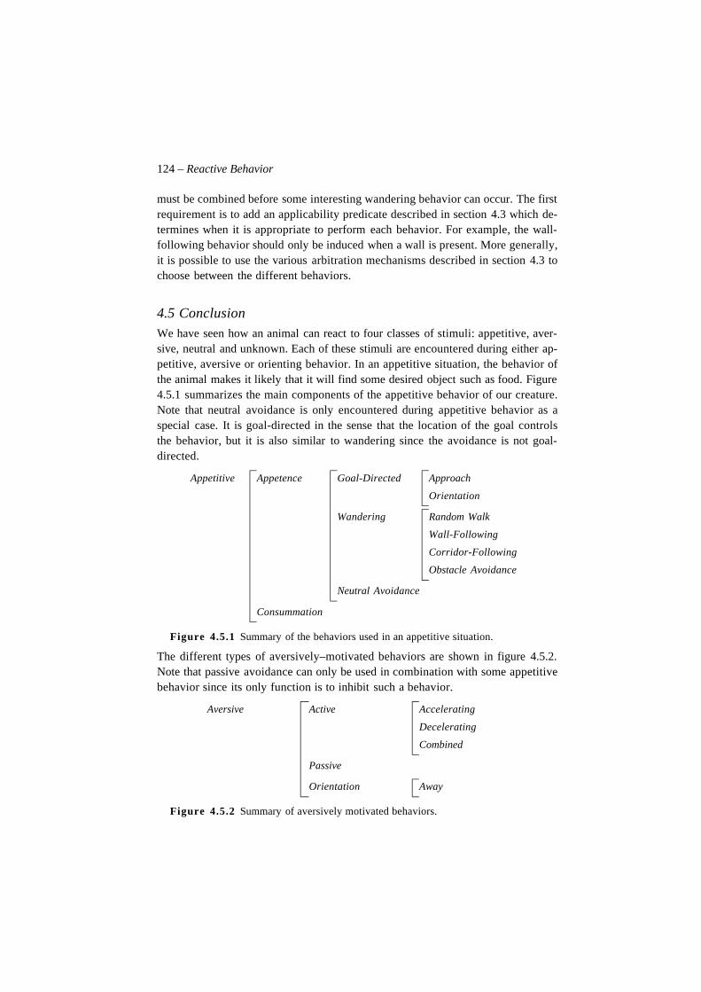
124 – Reactive Behavior
must be combined before some interesting wandering behavior can occur. The firstrequirement is to add an applicability predicate described in section 4.3 which de-termines when it is appropriate to perform each behavior. For example, the wall-following behavior should only be induced when a wall is present. More generally,it is possible to use the various arbitration mechanisms described in section 4.3 tochoose between the different behaviors.
4.5 ConclusionWe have seen how an animal can react to four classes of stimuli: appetitive, aver-sive, neutral and unknown. Each of these stimuli are encountered during either ap-petitive, aversive or orienting behavior. In an appetitive situation, the behavior ofthe animal makes it likely that it will find some desired object such as food. Figure4.5.1 summarizes the main components of the appetitive behavior of our creature.Note that neutral avoidance is only encountered during appetitive behavior as aspecial case. It is goal-directed in the sense that the location of the goal controlsthe behavior, but it is also similar to wandering since the avoidance is not goal-directed.
Figure 4.5.1 Summary of the behaviors used in an appetitive situation.
The different types of aversively–motivated behaviors are shown in figure 4.5.2.Note that passive avoidance can only be used in combination with some appetitivebehavior since its only function is to inhibit such a behavior.
Figure 4.5.2 Summary of aversively motivated behaviors.
Appetitive Appetence Goal-Directed Approach
Orientation
Wandering Random Walk
Wall-Following
Corridor-Following
Obstacle Avoidance
Neutral Avoidance
Consummation
Aversive Active Accelerating
Decelerating
Combined
Passive
Orientation Away
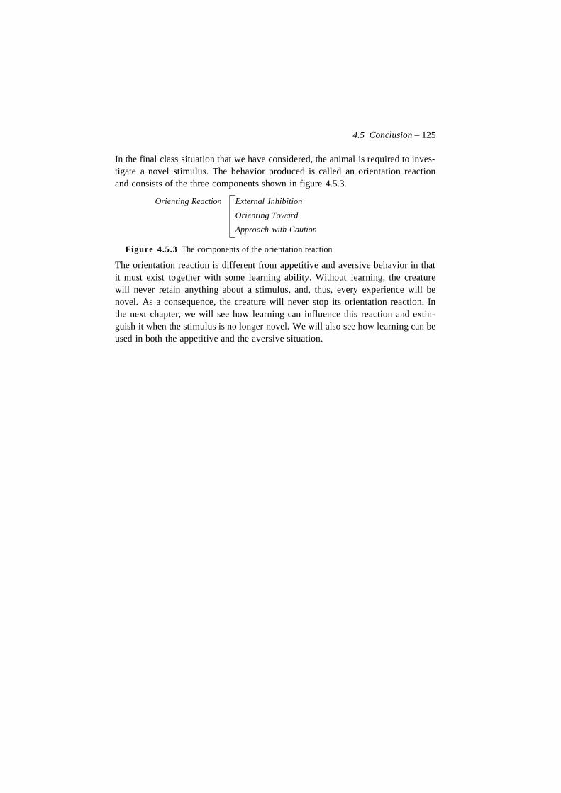
4.5 Conclusion – 125
In the final class situation that we have considered, the animal is required to inves-tigate a novel stimulus. The behavior produced is called an orientation reactionand consists of the three components shown in figure 4.5.3.
Figure 4.5.3 The components of the orientation reaction
The orientation reaction is different from appetitive and aversive behavior in thatit must exist together with some learning ability. Without learning, the creaturewill never retain anything about a stimulus, and, thus, every experience will benovel. As a consequence, the creature will never stop its orientation reaction. Inthe next chapter, we will see how learning can influence this reaction and extin-guish it when the stimulus is no longer novel. We will also see how learning can beused in both the appetitive and the aversive situation.
Orienting Reaction External Inhibition
Orienting Toward
Approach with Caution

126 – Reactive Behavior
Christian Balkenius, 1995, Natural Intelligence in Artificial Creatures, Lund University Cognitive Studies 37, 1995.
Chapter 5
Modeling Learning
5.1 IntroductionIn this chapter, we will take a look at the most fundamental types of learning andanalyse how they interact with each other to produce adaptive behavior. The pres-entation will start with the two major types of learning experiments that tradition-ally have received the most attention: classical and instrumental conditioning. Wewill then investigate, how these two experiment types relate first to learning mech-anisms, and then to each other. We will see that both types of learning can bebased on the same mechanism. This learning mechanism, which we will call a re-inforcement module , is an important component in the different engagement mod-ules using learning. The model we will develop is similar to earlier two-processmodels of conditioning (Mowrer 1960, Gray 1975, Klopf 1988) and also sharemany properties with other reinforcement learning schemes such as Q-learning(Watkins 1992) and temporal–difference learning (Sutton and Barto 1990).
The next step is to consider some basic engagement modules and how they ex-ploit learning. We will investigate learning in the appetitive food-related situation,learning of escape, learning of action sequences, and the learning of expectations.Perceptual learning will be discussed in chapter 7; and in chapter 8, the mecha-nisms described below will be used for learning in the spatial domain.
Our argument is, thus, that many types of learning can be based on similarmechanisms, and not that one learning mechanism solves all problems. Sincelearning is only useful when it is embedded in a specific engagement module, thereinforcement module in itself should be considered as an abstraction.
128 – Modeling Learning
5.2 Instrumental ConditioningThe study of instrumental learning is usually associated with Thorndike. In one ofhis well–known experiments, he placed a cat into a box where it was required topress a bar or drag a string in order to open the door and get out. When the cateventually succeeded in escaping, it was rewarded with food or water. Thorndikenoted that for each time the cat was put in the box, the faster it managed to escape.To explain why the cat performed better for each trial, Thorndike suggested thatthe reward given after the cat had escaped the box would gradually strengthenthose behaviors performed immediately before the reward was presented. As aconsequence, behaviors that let the cat escape would increase in probability whilebehaviors that had no effect would become less likely the more practice the cat re-ceived. This property was formulated as the ‘Law of Effect’, which states that theeffect or a behavior determines whether this behavior will be performed again ornot in the same situation.
The important property of instrumental learning is that learning depends on theconsequences of a behavior performed by the animal. A learning trial can be de-scribed by three components: (1) the situation perceived by the animal, (2) the be-havior performed by it, and finally, (3) the consequence of performing the behav-ior. The consequence is said to reinforce an assumed connection, or association,between the situation and the behavior. When the consequence is positive, the con-nection is strengthened, that is, positively reinforced. When the consequence isnegative, the connection is weakened, that is, negatively reinforced.1
A classification of different types of behavioral learning experiments was pre-sented in Gray (1975) and are reproduced in figure 5.2.1. This classification has itsorigin within the behavioristic tradition and should, thus, be seen as descriptionsof experimental procedures rather than learning mechanisms. Since mechanismsare the primary interest here, this piece of historical luggage will not bother ushere. We will see that there are reasons to believe that the different types of exper-imental procedures do, in fact, make use of different, but interacting learningmechanisms within an animal.
The different instrumental learning types can be distinguished by two factors.The first is the procedure used, and the second is the outcome it produces. The re-sult of the event can be either that the probability of a behavior preceding the pres-entation increases or decreases. When the probability of a behavior increases, the
1. In some theories of conditioning, the terms “positive” and “negative reinforcement” areused in a different way than here. As we use the term “negative reinforcement”, it refers tothe strengthening of an inhibitory connection. In Skinner’s theory it refers to the strengthen-ing of an excitatory relation between stimulus and response caused by the termination of anaversive state. In the model presented here, the term reinforcement can be equated withlearning signals within the artificial nervous systems, whether or not its effect is excitatoryor inhibitory.
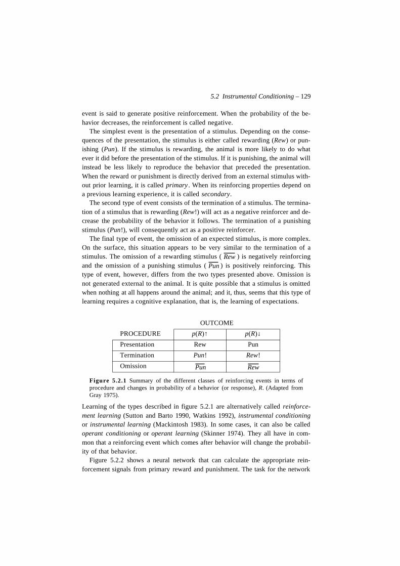
5.2 Instrumental Conditioning – 129
event is said to generate positive reinforcement. When the probability of the be-havior decreases, the reinforcement is called negative.
The simplest event is the presentation of a stimulus. Depending on the conse-quences of the presentation, the stimulus is either called rewarding (Rew) or pun-ishing (Pun). If the stimulus is rewarding, the animal is more likely to do whatever it did before the presentation of the stimulus. If it is punishing, the animal willinstead be less likely to reproduce the behavior that preceded the presentation.When the reward or punishment is directly derived from an external stimulus with-out prior learning, it is called primary . When its reinforcing properties depend ona previous learning experience, it is called secondary.
The second type of event consists of the termination of a stimulus. The termina-tion of a stimulus that is rewarding (Rew!) will act as a negative reinforcer and de-crease the probability of the behavior it follows. The termination of a punishingstimulus (Pun!), will consequently act as a positive reinforcer.
The final type of event, the omission of an expected stimulus, is more complex.On the surface, this situation appears to be very similar to the termination of astimulus. The omission of a rewarding stimulus ( ) is negatively reinforcingand the omission of a punishing stimulus ( ) is positively reinforcing. Thistype of event, however, differs from the two types presented above. Omission isnot generated external to the animal. It is quite possible that a stimulus is omittedwhen nothing at all happens around the animal; and it, thus, seems that this type oflearning requires a cognitive explanation, that is, the learning of expectations.
Figure 5.2.1 Summary of the different classes of reinforcing events in terms ofprocedure and changes in probability of a behavior (or response), R. (Adapted fromGray 1975).
Learning of the types described in figure 5.2.1 are alternatively called reinforce-ment learning (Sutton and Barto 1990, Watkins 1992), instrumental conditioningor instrumental learning (Mackintosh 1983). In some cases, it can also be calledoperant conditioning or operant learning (Skinner 1974). They all have in com-mon that a reinforcing event which comes after behavior will change the probabil-ity of that behavior.
Figure 5.2.2 shows a neural network that can calculate the appropriate rein-forcement signals from primary reward and punishment. The task for the network
OUTCOME
PROCEDURE p(R)↑ p(R)↓Presentation Rew Pun
Termination Pun! Rew!
Omission
RewPun
Pun Rew
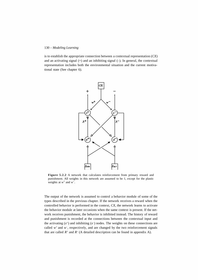
130 – Modeling Learning
is to establish the appropriate connection between a contextual representation (CX)and an activating signal (+) and an inhibiting signal (–). In general, the contextualrepresentation includes both the environmental situation and the current motiva-tional state (See chapter 6).
Figure 5.2.2 A network that calculates reinforcement from primary reward andpunishment. All weights in this network are assumed to be 1, except for the plasticweights at w+ and w–.
The output of the network is assumed to control a behavior module of some of thetypes described in the previous chapter. If the network receives a reward when thecontrolled behavior is performed in the context, CX, the network learns to activatethe behavior module at later occasions when the same context is present. If the net-work receives punishment, the behavior is inhibited instead. The history of rewardand punishment is recorded at the connections between the contextual input andthe activating (x+) and inhibiting (x–) nodes. The weights on these connections arecalled w+ and w–, respectively, and are changed by the two reinforcement signalsthat are called R+ and R– (A detailed description can be found in appendix A).
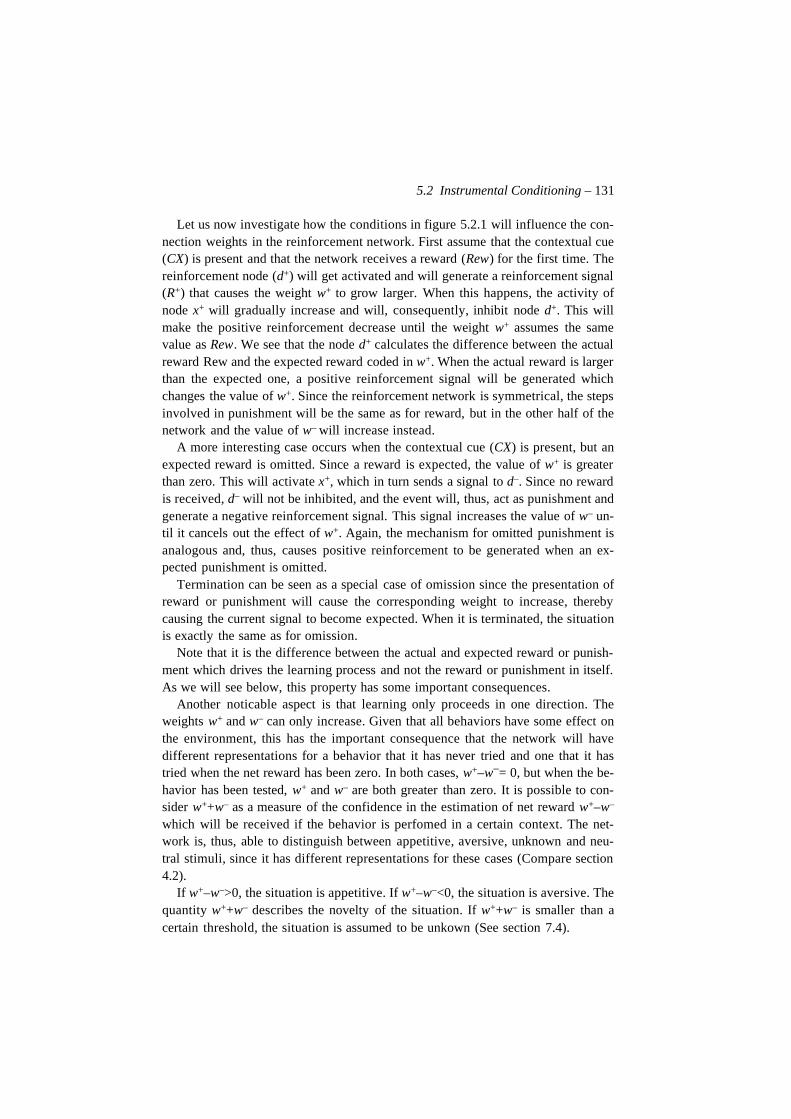
5.2 Instrumental Conditioning – 131
Let us now investigate how the conditions in figure 5.2.1 will influence the con-nection weights in the reinforcement network. First assume that the contextual cue(CX) is present and that the network receives a reward (Rew) for the first time. Thereinforcement node (d+) will get activated and will generate a reinforcement signal(R+) that causes the weight w+ to grow larger. When this happens, the activity ofnode x+ will gradually increase and will, consequently, inhibit node d+. This willmake the positive reinforcement decrease until the weight w+ assumes the samevalue as Rew. We see that the node d+ calculates the difference between the actualreward Rew and the expected reward coded in w+. When the actual reward is largerthan the expected one, a positive reinforcement signal will be generated whichchanges the value of w+. Since the reinforcement network is symmetrical, the stepsinvolved in punishment will be the same as for reward, but in the other half of thenetwork and the value of w– will increase instead.
A more interesting case occurs when the contextual cue (CX) is present, but anexpected reward is omitted. Since a reward is expected, the value of w+ is greaterthan zero. This will activate x+, which in turn sends a signal to d–. Since no rewardis received, d– will not be inhibited, and the event will, thus, act as punishment andgenerate a negative reinforcement signal. This signal increases the value of w– un-til it cancels out the effect of w+. Again, the mechanism for omitted punishment isanalogous and, thus, causes positive reinforcement to be generated when an ex-pected punishment is omitted.
Termination can be seen as a special case of omission since the presentation ofreward or punishment will cause the corresponding weight to increase, therebycausing the current signal to become expected. When it is terminated, the situationis exactly the same as for omission.
Note that it is the difference between the actual and expected reward or punish-ment which drives the learning process and not the reward or punishment in itself.As we will see below, this property has some important consequences.
Another noticable aspect is that learning only proceeds in one direction. Theweights w+ and w– can only increase. Given that all behaviors have some effect onthe environment, this has the important consequence that the network will havedifferent representations for a behavior that it has never tried and one that it hastried when the net reward has been zero. In both cases, w+–w–= 0, but when the be-havior has been tested, w+ and w– are both greater than zero. It is possible to con-sider w++w– as a measure of the confidence in the estimation of net reward w+–w–
which will be received if the behavior is perfomed in a certain context. The net-work is, thus, able to distinguish between appetitive, aversive, unknown and neu-tral stimuli, since it has different representations for these cases (Compare section4.2).
If w+–w–>0, the situation is appetitive. If w+–w–<0, the situation is aversive. Thequantity w++w– describes the novelty of the situation. If w++w– is smaller than acertain threshold, the situation is assumed to be unkown (See section 7.4).
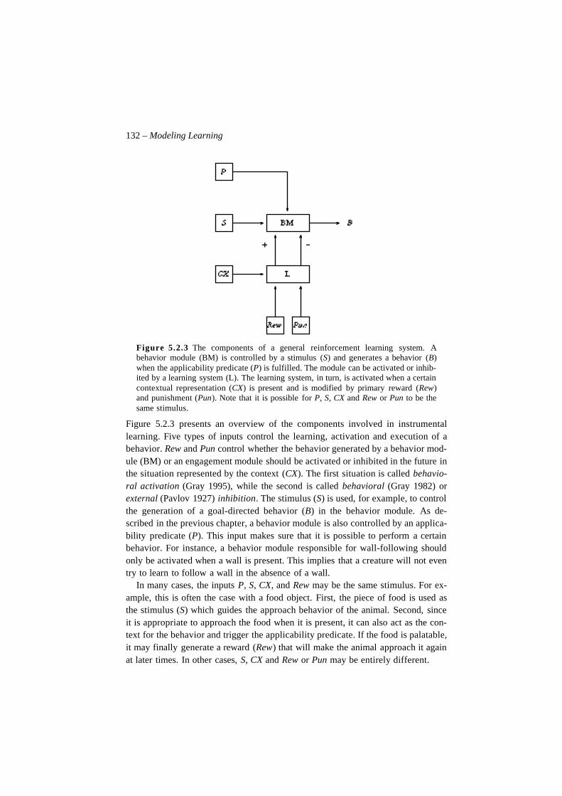
132 – Modeling Learning
Figure 5.2.3 The components of a general reinforcement learning system. Abehavior module (BM) is controlled by a stimulus (S) and generates a behavior (B)when the applicability predicate (P) is fulfilled. The module can be activated or inhib-ited by a learning system (L). The learning system, in turn, is activated when a certaincontextual representation (CX) is present and is modified by primary reward (Rew)and punishment (Pun). Note that it is possible for P, S, CX and Rew or Pun to be thesame stimulus.
Figure 5.2.3 presents an overview of the components involved in instrumentallearning. Five types of inputs control the learning, activation and execution of abehavior. Rew and Pun control whether the behavior generated by a behavior mod-ule (BM) or an engagement module should be activated or inhibited in the future inthe situation represented by the context (CX). The first situation is called behavio-ral activation (Gray 1995), while the second is called behavioral (Gray 1982) orexternal (Pavlov 1927) inhibition. The stimulus (S) is used, for example, to controlthe generation of a goal-directed behavior (B) in the behavior module. As de-scribed in the previous chapter, a behavior module is also controlled by an applica-bility predicate (P). This input makes sure that it is possible to perform a certainbehavior. For instance, a behavior module responsible for wall-following shouldonly be activated when a wall is present. This implies that a creature will not eventry to learn to follow a wall in the absence of a wall.
In many cases, the inputs P, S, CX, and Rew may be the same stimulus. For ex-ample, this is often the case with a food object. First, the piece of food is used asthe stimulus (S) which guides the approach behavior of the animal. Second, sinceit is appropriate to approach the food when it is present, it can also act as the con-text for the behavior and trigger the applicability predicate. If the food is palatable,it may finally generate a reward (Rew) that will make the animal approach it againat later times. In other cases, S, CX and Rew or Pun may be entirely different.
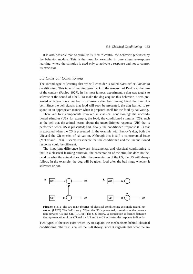
5.3 Classical Conditioning – 133
It is also possible that no stimulus is used to control the behavior generated bythe behavior module. This is the case, for example, in pure stimulus–responselearning, where the stimulus is used only to activate a response and not to controlits execution.
5.3 Classical ConditioningThe second type of learning that we will consider is called classical or Pavlovianconditioning. This type of learning goes back to the research of Pavlov at the turnof the century (Pavlov 1927). In his most famous experiment, a dog was taught tosalivate at the sound of a bell. To make the dog acquire this behavior, it was pre-sented with food on a number of occasions after first having heard the tone of abell. Since the bell signals that food will soon be presented, the dog learned to re-spond in an appropriate manner when it prepared itself for the food by salivating.
There are four components involved in classical conditioning: the uncondi-tioned stimulus (US), for example, the food; the conditioned stimulus (CS), suchas the bell that the animal learns about; the unconditioned response (UR) that isperformed when US is presented; and, finally the conditioned response (CR) thatis executed when the CS is presented. In the example with Pavlov’s dog, both theUR and the CR consist of salivation. Although this is still a controversial issue(McFarland 1993), it seems reasonable that the conditioned and the unconditionedresponse could be different.
The important difference between instrumental and classical conditioning isthat in a classical learning situation, the presentation of the stimulus does not de-pend on what the animal does. After the presentation of the CS, the US will alwaysfollow. In the example, the dog will be given food after the bell rings whether itsalivates or not.
Figure 5.3.1 The two main theories of classical conditioning as simple neural net-works. (LEFT) The S–R theory. When the US is presented, it reinforces the connec-tion between CS and CR. (RIGHT) The S–S theory. A connection is formed betweenthe representation of the CS and the US and the CS activates the response indirectly.
Two types of theories exist which try to explain the mechanisms behind classicalconditioning. The first is called the S–R theory, since it suggests that what the an-
134 – Modeling Learning
imal learns is an association between the CS and the CR and this learning is rein-forced by the US (Hull 1934). The second variation, which is called the S–S, orstimulus substitution, theory, proposes that what the animal learns is not an associ-ation between a stimulus and a response, but a relation between two stimuli(Pavlov 1927, Bolles 1978, Mackintosh 1983). On several occasions, the CS haspreceded the US, and this is what the animal has learned. Depending on how cog-nitive the theory tries to be, this knowledge is either assumed to be represented bya simple connection between the CS and the US or by some more complex cogni-tive structure (See, for example, Pavlov 1927 and Tolman 1932).Many versions exist of both the S–R and the S–S theory, and it is not possible todiscuss all here. We will merely note that both theories have different strengthsand weaknesses and it is possible that both are correct. One other thing to note isthat the S–S theory in its most elementary form has problems in cases where theUR and the CR are different. A simple example where this is the case is when thedog is allowed to eat the presented food. In this case, the UR is eating, but the CRis still salivation. Very often, the CR appears to be preparatory in, which, ofcourse, is entirely sensible. The extent to which the CR can be preparatory or nothas been, and still is, in much dispute however.
If we assume that the UR and the CR (for example, eating and salivation) areproduced by the same engagement module, it is possible to explain the differencein UR and CR as the consequence of different stimuli being present in the two cas-es. When food can be eaten, the UR (eating) will be produced; and when it can not,the CR (salivation) will be performed instead. The choice between these two be-haviors can be made by the use of applicability predicates as described above.Such a mechanism enables us to adhere to a S–S theory of classical conditioningwhile still allowing the CS and US to be different.
An interesting approach to understanding classical conditioning was pioneeredby Rescorla and Wagner (1972). They suggested that the association formed dur-ing classical conditioning should be considered as a record of how well the CS pre-dicts the US. The main idea behind their model was to consider the association be-tween CS and US, or possibly between CS and CR, as an expectation or aprediction that US will follow CS.
Figure 5.3.2 shows a variation of the S–R network in figure 5.3.1 which is basedon the idea that the CS predicts the US. The network is similar to the instrumentallearning network shown in figure 5.2.2, except that the context is replaced by theconditioned stimulus (CS) and the reward is replaced by the unconditioned stimu-lus (US). Like the S–R network in figure 5.3.1, it is assumed that the uncondi-tioned response is independent of the conditioned response.
We may interpret the weight w+ as the strength of the expectation that US willfollow CS and w– as the expectation that it will not. When US follows CS, w+ in-creases, and when CS is presented alone, w– may increase instead. To determine
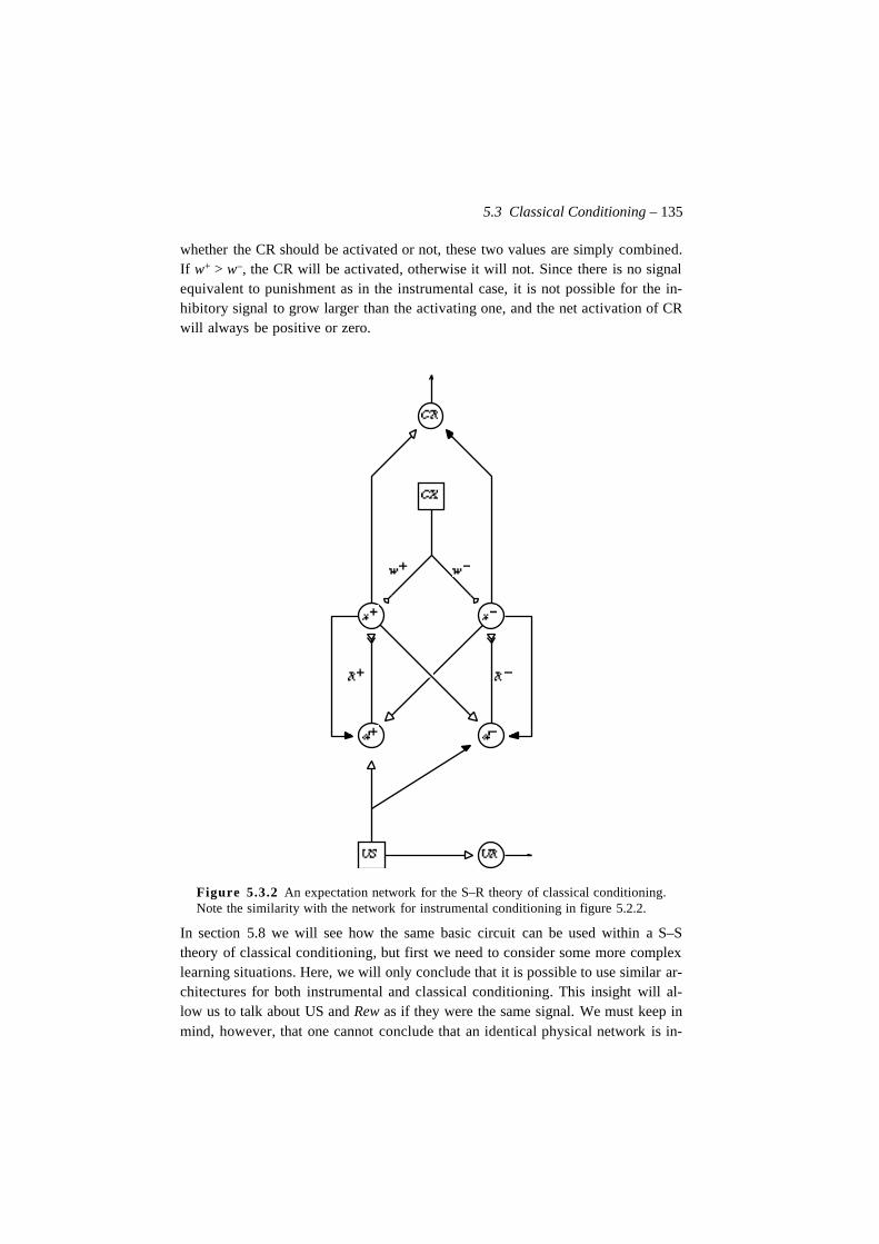
5.3 Classical Conditioning – 135
whether the CR should be activated or not, these two values are simply combined.If w+ > w–, the CR will be activated, otherwise it will not. Since there is no signalequivalent to punishment as in the instrumental case, it is not possible for the in-hibitory signal to grow larger than the activating one, and the net activation of CRwill always be positive or zero.
Figure 5.3.2 An expectation network for the S–R theory of classical conditioning.Note the similarity with the network for instrumental conditioning in figure 5.2.2.
In section 5.8 we will see how the same basic circuit can be used within a S–Stheory of classical conditioning, but first we need to consider some more complexlearning situations. Here, we will only conclude that it is possible to use similar ar-chitectures for both instrumental and classical conditioning. This insight will al-low us to talk about US and Rew as if they were the same signal. We must keep inmind, however, that one cannot conclude that an identical physical network is in-
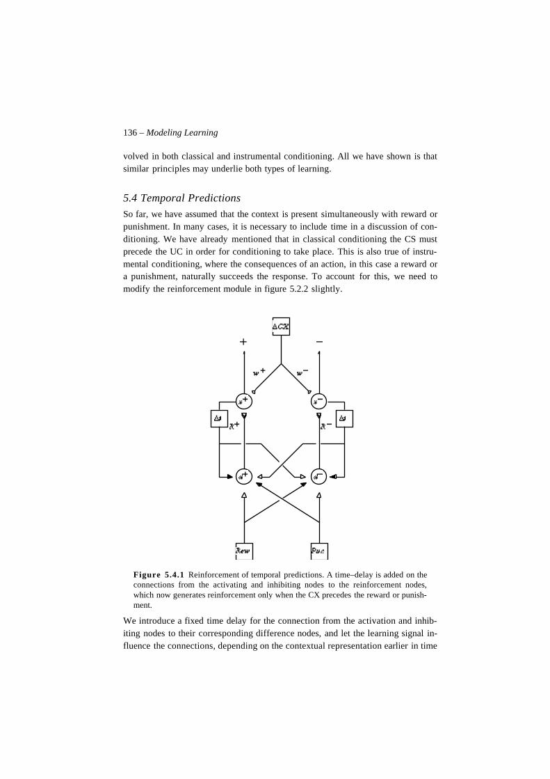
136 – Modeling Learning
volved in both classical and instrumental conditioning. All we have shown is thatsimilar principles may underlie both types of learning.
5.4 Temporal Predictions
So far, we have assumed that the context is present simultaneously with reward orpunishment. In many cases, it is necessary to include time in a discussion of con-ditioning. We have already mentioned that in classical conditioning the CS mustprecede the UC in order for conditioning to take place. This is also true of instru-mental conditioning, where the consequences of an action, in this case a reward ora punishment, naturally succeeds the response. To account for this, we need tomodify the reinforcement module in figure 5.2.2 slightly.
Figure 5.4.1 Reinforcement of temporal predictions. A time–delay is added on theconnections from the activating and inhibiting nodes to the reinforcement nodes,which now generates reinforcement only when the CX precedes the reward or punish-ment.
We introduce a fixed time delay for the connection from the activation and inhib-iting nodes to their corresponding difference nodes, and let the learning signal in-fluence the connections, depending on the contextual representation earlier in time
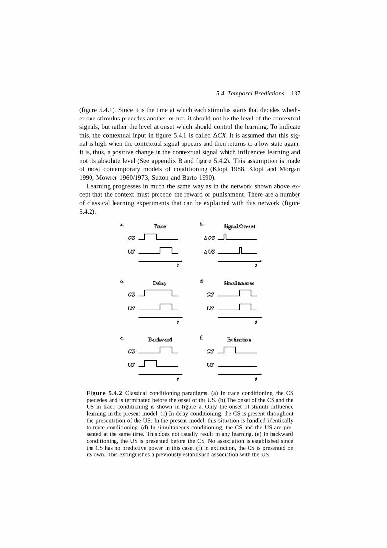
5.4 Temporal Predictions – 137
(figure 5.4.1). Since it is the time at which each stimulus starts that decides wheth-er one stimulus precedes another or not, it should not be the level of the contextualsignals, but rather the level at onset which should control the learning. To indicatethis, the contextual input in figure 5.4.1 is called ∆CX. It is assumed that this sig-nal is high when the contextual signal appears and then returns to a low state again.It is, thus, a positive change in the contextual signal which influences learning andnot its absolute level (See appendix B and figure 5.4.2). This assumption is madeof most contemporary models of conditioning (Klopf 1988, Klopf and Morgan1990, Mowrer 1960/1973, Sutton and Barto 1990).
Learning progresses in much the same way as in the network shown above ex-cept that the context must precede the reward or punishment. There are a numberof classical learning experiments that can be explained with this network (figure5.4.2).
Figure 5.4.2 Classical conditioning paradigms. (a) In trace conditioning, the CSprecedes and is terminated before the onset of the US. (b) The onset of the CS and theUS in trace conditioning is shown in figure a. Only the onset of stimuli influencelearning in the present model. (c) In delay conditioning, the CS is present throughoutthe presentation of the US. In the present model, this situation is handled identicallyto trace conditioning. (d) In simultaneous conditioning, the CS and the US are pre-sented at the same time. This does not usually result in any learning. (e) In backwardconditioning, the US is presented before the CS. No association is established sincethe CS has no predictive power in this case. (f) In extinction, the CS is presented onits own. This extinguishes a previously established association with the US.
138 – Modeling Learning
In simultaneous conditioning, the CS and US are presented at the same time. Thisconditioning paradigm usually results in no conditioning at all (Mackintosh 1983,Pavlov 1927, Smith, Coleman and Gormezano 1969). That is, the US is not able to re-inforce any association. This appears to be a rather general property of condition-ing, although some counter–examples exist (See Mackintosh 1983)). It is clear thatthe network presented here will not reinforce a connection if the CS and US arepresented simultaneously. This should be contrasted with theories that assumesthat connections are established when two signals coincide within the nervous sys-tem, such as Hebb’s cell–assembly theory (Hebb 1949). The relation betweenthese two views of learning will be discussed in section 7.7.
The learning paradigm that results in the strongest association is delay condi-tioning (Lieberman 1990). In this learning situation, the CS precedes the US and isallowed to be present until the offset of the US. We see that it is necessary to cor-relate the onset of the signals as described above since the two stimuli are, in fact,present simultaneously. This is the motivation for the use of the change in the con-textual signal instead of its absolute level.
Trace conditioning is very similar to delay conditioning except that the CS ter-minates before the presentation of the US. Since the CS is not perceptible when theUS is presented, the conditioning, which usually is quite good, must be the resultof a ‘memory trace’ of the CS, hence the name. Given that the delay between theonset of the CS and the presentation of the US is appropriate, trace conditioningwill give the same result as delay conditioning in the present model. According tomany animal experiments, trace conditioning usually gives a slightly weaker asso-ciation than delay conditioning (Lieberman 1990), which is not predicted by thepresent model.
In backward conditioning, the sequence of pairing is reversed. The US is nowpresented before the CS. As can be expected, no excitatory association is formedin this case, either in the animal experiments, or in the model (Mackintosh 1983).However, some studies have shown that an inhibitory connection is formed, whichis not predicted by the present model (See Klopf 1988).
Finally we need to consider extinction or internal inhibition, which is the proc-ess by which an association, or rather, the behavior it produces, is extinguished(Pavlov 1927). An extinction experiment is divided into two phases. In the first, anassociation is established, and in the second, it is extinguished by presenting theCS alone without the US. In this case, the omission of the US will generate a neg-ative reinforcement signal which increases the weight in the negative side of thesystem until the inhibiting signal becomes as strong as the activating one.
Figure 5.4.3 shows a computer simulation of the network in figure 5.4.1. In thefirst phase of the simulation, CS is paired with the US. This will establish an asso-ciation, w+ from the CS to the activating node x+. In the second phase, the CS ispresented on its own, and the association will be extinguished again. The extinc-
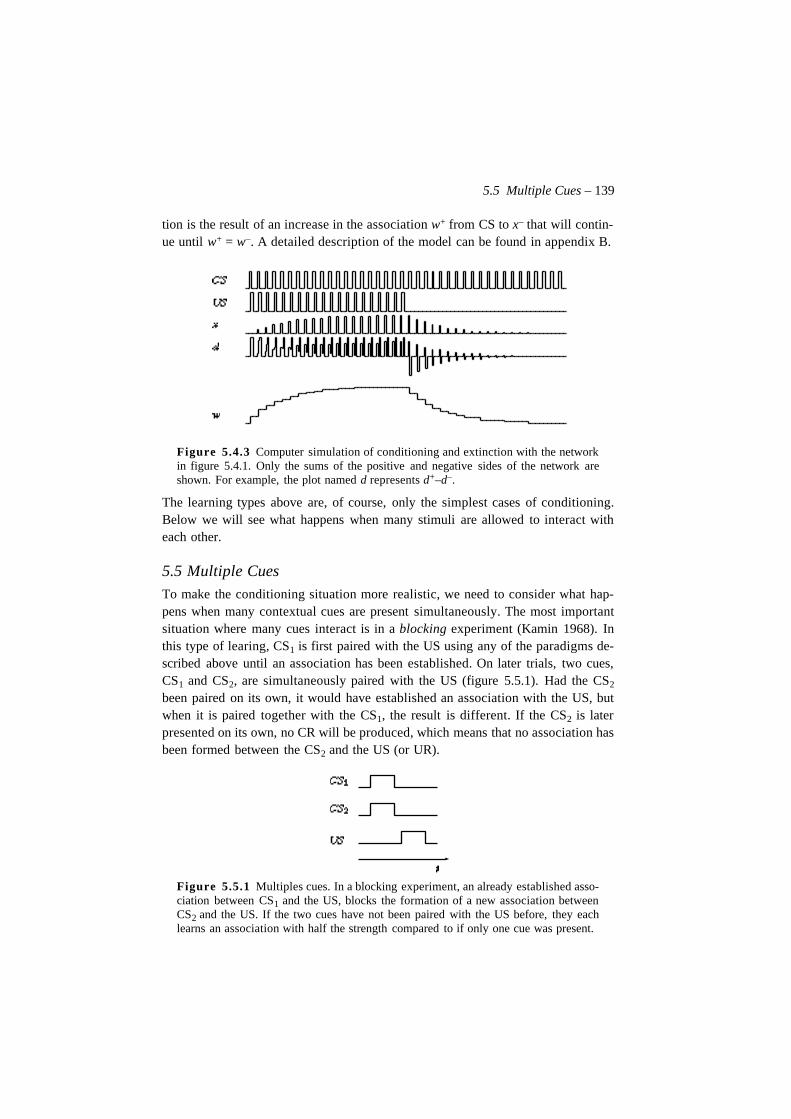
5.5 Multiple Cues – 139
tion is the result of an increase in the association w+ from CS to x– that will contin-ue until w+ = w–. A detailed description of the model can be found in appendix B.
Figure 5.4.3 Computer simulation of conditioning and extinction with the networkin figure 5.4.1. Only the sums of the positive and negative sides of the network areshown. For example, the plot named d represents d+–d–.
The learning types above are, of course, only the simplest cases of conditioning.Below we will see what happens when many stimuli are allowed to interact witheach other.
5.5 Multiple Cues
To make the conditioning situation more realistic, we need to consider what hap-pens when many contextual cues are present simultaneously. The most importantsituation where many cues interact is in a blocking experiment (Kamin 1968). Inthis type of learing, CS1 is first paired with the US using any of the paradigms de-scribed above until an association has been established. On later trials, two cues,CS1 and CS2, are simultaneously paired with the US (figure 5.5.1). Had the CS2
been paired on its own, it would have established an association with the US, butwhen it is paired together with the CS1, the result is different. If the CS2 is laterpresented on its own, no CR will be produced, which means that no association hasbeen formed between the CS2 and the US (or UR).
Figure 5.5.1 Multiples cues. In a blocking experiment, an already established asso-ciation between CS1 and the US, blocks the formation of a new association betweenCS2 and the US. If the two cues have not been paired with the US before, they eachlearns an association with half the strength compared to if only one cue was present.
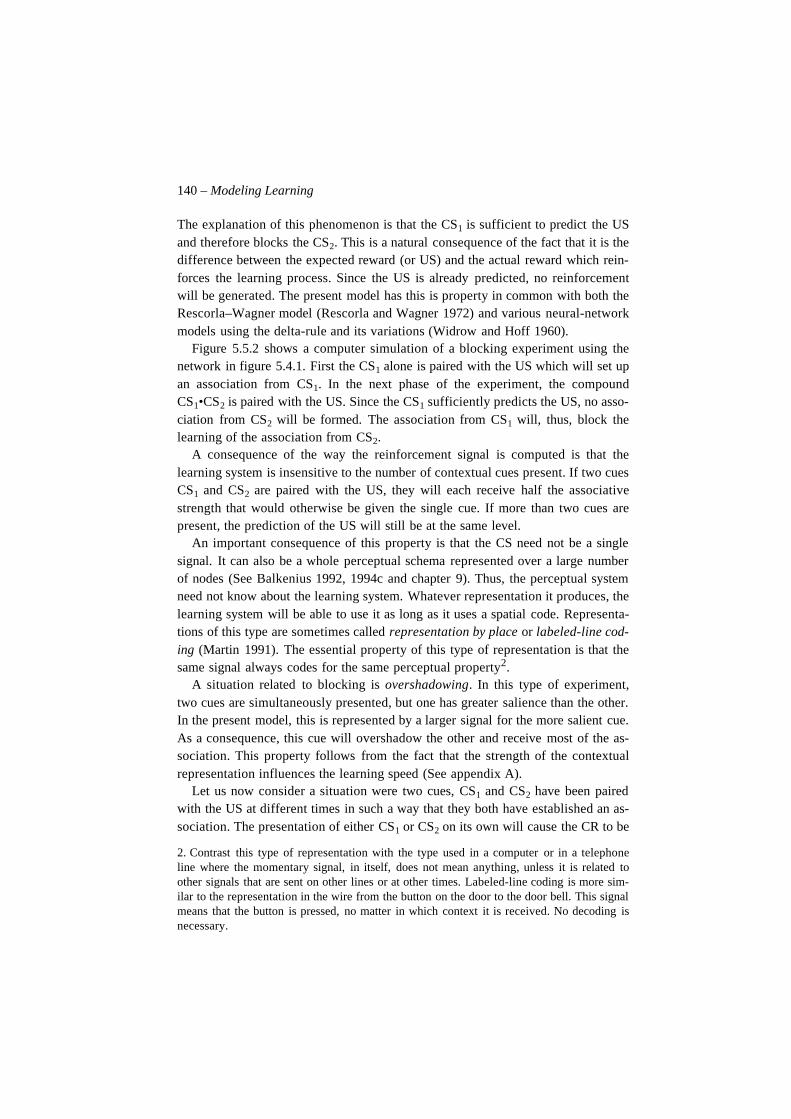
140 – Modeling Learning
The explanation of this phenomenon is that the CS1 is sufficient to predict the USand therefore blocks the CS2. This is a natural consequence of the fact that it is thedifference between the expected reward (or US) and the actual reward which rein-forces the learning process. Since the US is already predicted, no reinforcementwill be generated. The present model has this is property in common with both theRescorla–Wagner model (Rescorla and Wagner 1972) and various neural-networkmodels using the delta-rule and its variations (Widrow and Hoff 1960).
Figure 5.5.2 shows a computer simulation of a blocking experiment using thenetwork in figure 5.4.1. First the CS1 alone is paired with the US which will set upan association from CS1. In the next phase of the experiment, the compoundCS1•CS2 is paired with the US. Since the CS1 sufficiently predicts the US, no asso-ciation from CS2 will be formed. The association from CS1 will, thus, block thelearning of the association from CS2.
A consequence of the way the reinforcement signal is computed is that thelearning system is insensitive to the number of contextual cues present. If two cuesCS1 and CS2 are paired with the US, they will each receive half the associativestrength that would otherwise be given the single cue. If more than two cues arepresent, the prediction of the US will still be at the same level.
An important consequence of this property is that the CS need not be a singlesignal. It can also be a whole perceptual schema represented over a large numberof nodes (See Balkenius 1992, 1994c and chapter 9). Thus, the perceptual systemneed not know about the learning system. Whatever representation it produces, thelearning system will be able to use it as long as it uses a spatial code. Representa-tions of this type are sometimes called representation by place or labeled-line cod-ing (Martin 1991). The essential property of this type of representation is that thesame signal always codes for the same perceptual property2.
A situation related to blocking is overshadowing. In this type of experiment,two cues are simultaneously presented, but one has greater salience than the other.In the present model, this is represented by a larger signal for the more salient cue.As a consequence, this cue will overshadow the other and receive most of the as-sociation. This property follows from the fact that the strength of the contextualrepresentation influences the learning speed (See appendix A).
Let us now consider a situation were two cues, CS1 and CS2 have been pairedwith the US at different times in such a way that they both have established an as-sociation. The presentation of either CS1 or CS2 on its own will cause the CR to be
2. Contrast this type of representation with the type used in a computer or in a telephoneline where the momentary signal, in itself, does not mean anything, unless it is related toother signals that are sent on other lines or at other times. Labeled-line coding is more sim-ilar to the representation in the wire from the button on the door to the door bell. This signalmeans that the button is pressed, no matter in which context it is received. No decoding isnecessary.
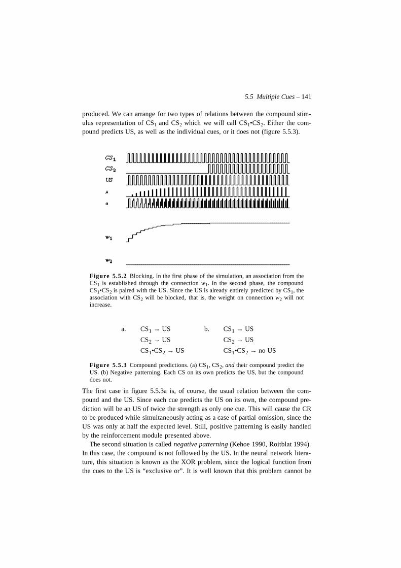
5.5 Multiple Cues – 141
produced. We can arrange for two types of relations between the compound stim-ulus representation of CS1 and CS2 which we will call CS1•CS2. Either the com-pound predicts US, as well as the individual cues, or it does not (figure 5.5.3).
Figure 5.5.2 Blocking. In the first phase of the simulation, an association from theCS1 is established through the connection w1. In the second phase, the compoundCS1•CS2 is paired with the US. Since the US is already entirely predicted by CS1, theassociation with CS2 will be blocked, that is, the weight on connection w2 will notincrease.
Figure 5.5.3 Compound predictions. (a) CS1, CS2, and their compound predict theUS. (b) Negative patterning. Each CS on its own predicts the US, but the compounddoes not.
The first case in figure 5.5.3a is, of course, the usual relation between the com-pound and the US. Since each cue predicts the US on its own, the compound pre-diction will be an US of twice the strength as only one cue. This will cause the CRto be produced while simultaneously acting as a case of partial omission, since theUS was only at half the expected level. Still, positive patterning is easily handledby the reinforcement module presented above.
The second situation is called negative patterning (Kehoe 1990, Roitblat 1994).In this case, the compound is not followed by the US. In the neural network litera-ture, this situation is known as the XOR problem, since the logical function fromthe cues to the US is “exclusive or”. It is well known that this problem cannot be
a. CS1 → US b. CS1 → US
CS2 → US CS2 → US
CS1•CS2 → US CS1•CS2 → no US
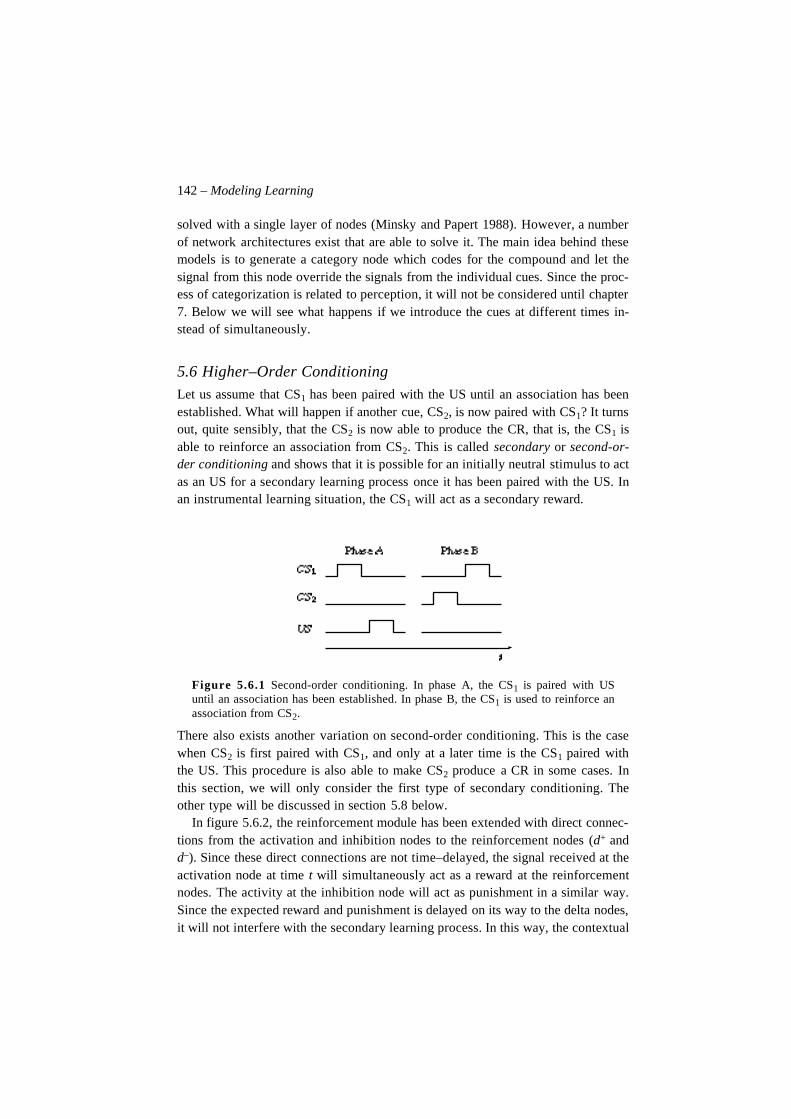
142 – Modeling Learning
solved with a single layer of nodes (Minsky and Papert 1988). However, a numberof network architectures exist that are able to solve it. The main idea behind thesemodels is to generate a category node which codes for the compound and let thesignal from this node override the signals from the individual cues. Since the proc-ess of categorization is related to perception, it will not be considered until chapter7. Below we will see what happens if we introduce the cues at different times in-stead of simultaneously.
5.6 Higher–Order ConditioningLet us assume that CS1 has been paired with the US until an association has beenestablished. What will happen if another cue, CS2, is now paired with CS1? It turnsout, quite sensibly, that the CS2 is now able to produce the CR, that is, the CS1 isable to reinforce an association from CS2. This is called secondary or second-or-der conditioning and shows that it is possible for an initially neutral stimulus to actas an US for a secondary learning process once it has been paired with the US. Inan instrumental learning situation, the CS1 will act as a secondary reward.
Figure 5.6.1 Second-order conditioning. In phase A, the CS1 is paired with USuntil an association has been established. In phase B, the CS1 is used to reinforce anassociation from CS2.
There also exists another variation on second-order conditioning. This is the casewhen CS2 is first paired with CS1, and only at a later time is the CS1 paired withthe US. This procedure is also able to make CS2 produce a CR in some cases. Inthis section, we will only consider the first type of secondary conditioning. Theother type will be discussed in section 5.8 below.
In figure 5.6.2, the reinforcement module has been extended with direct connec-tions from the activation and inhibition nodes to the reinforcement nodes (d+ andd–). Since these direct connections are not time–delayed, the signal received at theactivation node at time t will simultaneously act as a reward at the reinforcementnodes. The activity at the inhibition node will act as punishment in a similar way.Since the expected reward and punishment is delayed on its way to the delta nodes,it will not interfere with the secondary learning process. In this way, the contextual
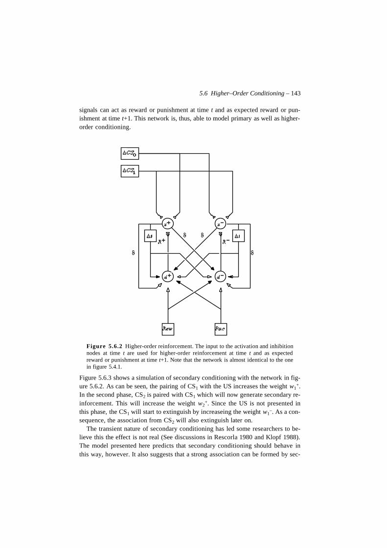
5.6 Higher–Order Conditioning – 143
signals can act as reward or punishment at time t and as expected reward or pun-ishment at time t+1. This network is, thus, able to model primary as well as higher-order conditioning.
Figure 5.6.2 Higher-order reinforcement. The input to the activation and inhibitionnodes at time t are used for higher-order reinforcement at time t and as expectedreward or punishment at time t+1. Note that the network is almost identical to the onein figure 5.4.1.
Figure 5.6.3 shows a simulation of secondary conditioning with the network in fig-ure 5.6.2. As can be seen, the pairing of CS1 with the US increases the weight w1
+.In the second phase, CS2 is paired with CS1 which will now generate secondary re-inforcement. This will increase the weight w2
+. Since the US is not presented inthis phase, the CS1 will start to extinguish by increaseing the weight w1
–. As a con-sequence, the association from CS2 will also extinguish later on.
The transient nature of secondary conditioning has led some researchers to be-lieve this the effect is not real (See discussions in Rescorla 1980 and Klopf 1988).The model presented here predicts that secondary conditioning should behave inthis way, however. It also suggests that a strong association can be formed by sec-
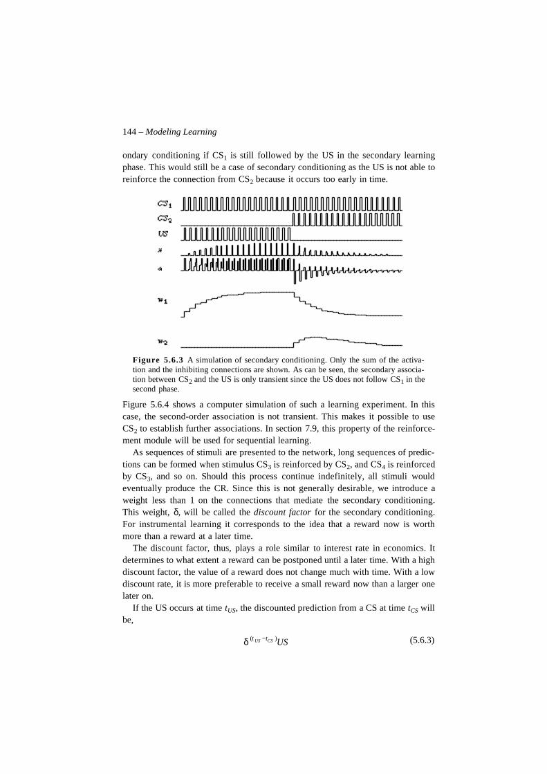
144 – Modeling Learning
ondary conditioning if CS1 is still followed by the US in the secondary learningphase. This would still be a case of secondary conditioning as the US is not able toreinforce the connection from CS2 because it occurs too early in time.
Figure 5.6.3 A simulation of secondary conditioning. Only the sum of the activa-tion and the inhibiting connections are shown. As can be seen, the secondary associa-tion between CS2 and the US is only transient since the US does not follow CS1 in thesecond phase.
Figure 5.6.4 shows a computer simulation of such a learning experiment. In thiscase, the second-order association is not transient. This makes it possible to useCS2 to establish further associations. In section 7.9, this property of the reinforce-ment module will be used for sequential learning.
As sequences of stimuli are presented to the network, long sequences of predic-tions can be formed when stimulus CS3 is reinforced by CS2, and CS4 is reinforcedby CS3, and so on. Should this process continue indefinitely, all stimuli wouldeventually produce the CR. Since this is not generally desirable, we introduce aweight less than 1 on the connections that mediate the secondary conditioning.This weight, δ, will be called the discount factor for the secondary conditioning.For instrumental learning it corresponds to the idea that a reward now is worthmore than a reward at a later time.
The discount factor, thus, plays a role similar to interest rate in economics. Itdetermines to what extent a reward can be postponed until a later time. With a highdiscount factor, the value of a reward does not change much with time. With a lowdiscount rate, it is more preferable to receive a small reward now than a larger onelater on.
If the US occurs at time tUS, the discounted prediction from a CS at time tCS willbe,
(5.6.3)δ (t US −tCS )US
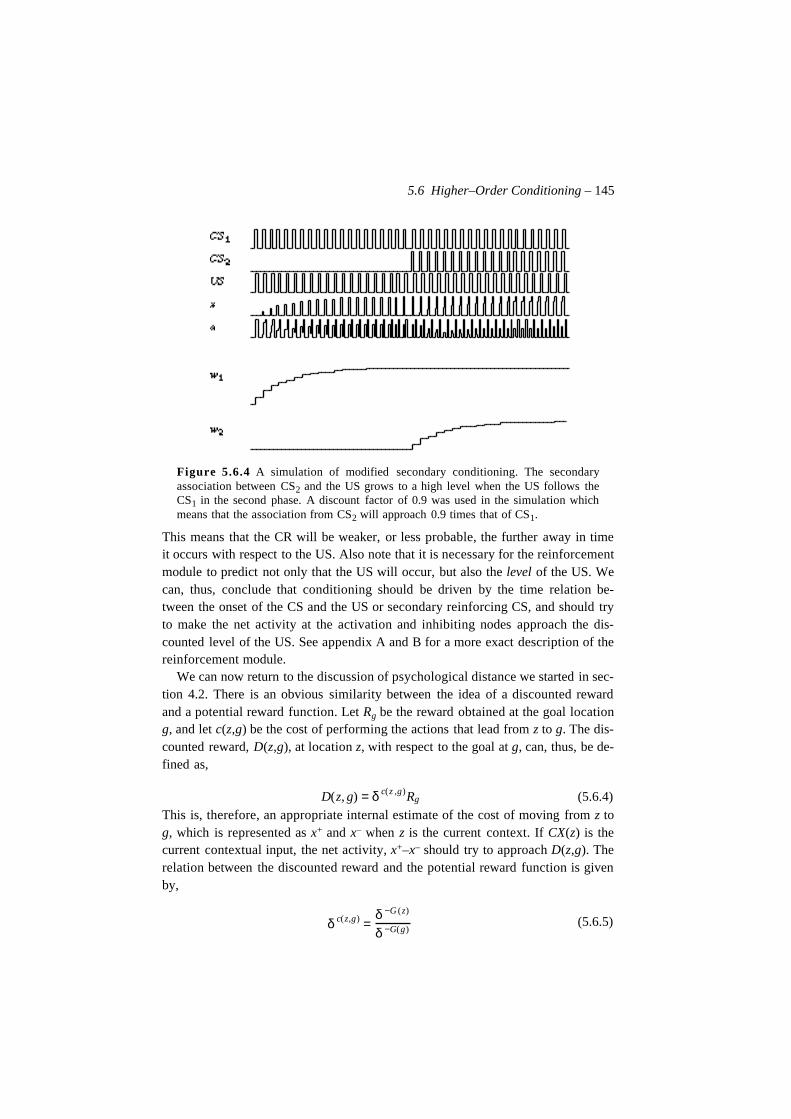
5.6 Higher–Order Conditioning – 145
Figure 5.6.4 A simulation of modified secondary conditioning. The secondaryassociation between CS2 and the US grows to a high level when the US follows theCS1 in the second phase. A discount factor of 0.9 was used in the simulation whichmeans that the association from CS2 will approach 0.9 times that of CS1.
This means that the CR will be weaker, or less probable, the further away in timeit occurs with respect to the US. Also note that it is necessary for the reinforcementmodule to predict not only that the US will occur, but also the level of the US. Wecan, thus, conclude that conditioning should be driven by the time relation be-tween the onset of the CS and the US or secondary reinforcing CS, and should tryto make the net activity at the activation and inhibiting nodes approach the dis-counted level of the US. See appendix A and B for a more exact description of thereinforcement module.
We can now return to the discussion of psychological distance we started in sec-tion 4.2. There is an obvious similarity between the idea of a discounted rewardand a potential reward function. Let Rg be the reward obtained at the goal locationg, and let c(z,g) be the cost of performing the actions that lead from z to g. The dis-counted reward, D(z,g), at location z, with respect to the goal at g, can, thus, be de-fined as,
(5.6.4)This is, therefore, an appropriate internal estimate of the cost of moving from z tog, which is represented as x+ and x– when z is the current context. If CX(z) is thecurrent contextual input, the net activity, x+–x– should try to approach D(z,g). Therelation between the discounted reward and the potential reward function is givenby,
(5.6.5)
D(z, g) = δ c(z ,g)Rg
δ c(z,g) =δ −G (z)
δ −G(g)
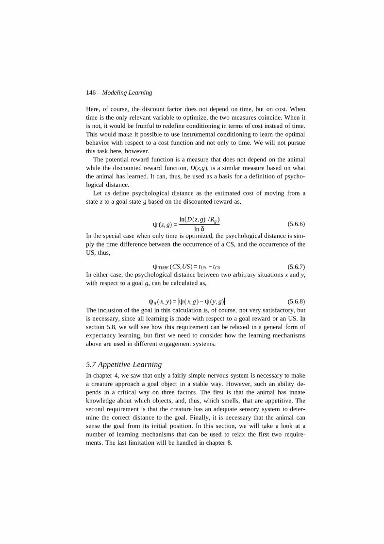
146 – Modeling Learning
Here, of course, the discount factor does not depend on time, but on cost. Whentime is the only relevant variable to optimize, the two measures coincide. When itis not, it would be fruitful to redefine conditioning in terms of cost instead of time.This would make it possible to use instrumental conditioning to learn the optimalbehavior with respect to a cost function and not only to time. We will not pursuethis task here, however.
The potential reward function is a measure that does not depend on the animalwhile the discounted reward function, D(z,g), is a similar measure based on whatthe animal has learned. It can, thus, be used as a basis for a definition of psycho-logical distance.
Let us define psychological distance as the estimated cost of moving from astate z to a goal state g based on the discounted reward as,
(5.6.6)
In the special case when only time is optimized, the psychological distance is sim-ply the time difference between the occurrence of a CS, and the occurrence of theUS, thus,
(5.6.7)In either case, the psychological distance between two arbitrary situations x and y,with respect to a goal g, can be calculated as,
(5.6.8)The inclusion of the goal in this calculation is, of course, not very satisfactory, butis necessary, since all learning is made with respect to a goal reward or an US. Insection 5.8, we will see how this requirement can be relaxed in a general form ofexpectancy learning, but first we need to consider how the learning mechanismsabove are used in different engagement systems.
5.7 Appetitive LearningIn chapter 4, we saw that only a fairly simple nervous system is necessary to makea creature approach a goal object in a stable way. However, such an ability de-pends in a critical way on three factors. The first is that the animal has innateknowledge about which objects, and, thus, which smells, that are appetitive. Thesecond requirement is that the creature has an adequate sensory system to deter-mine the correct distance to the goal. Finally, it is necessary that the animal cansense the goal from its initial position. In this section, we will take a look at anumber of learning mechanisms that can be used to relax the first two require-ments. The last limitation will be handled in chapter 8.
ψ (z, g) =ln(D(z, g) /Rg )
ln δ
ψ TIME (CS,US) = tUS − tCS
ψ g ( x, y) = ψ ( x, g ) − ψ (y, g)
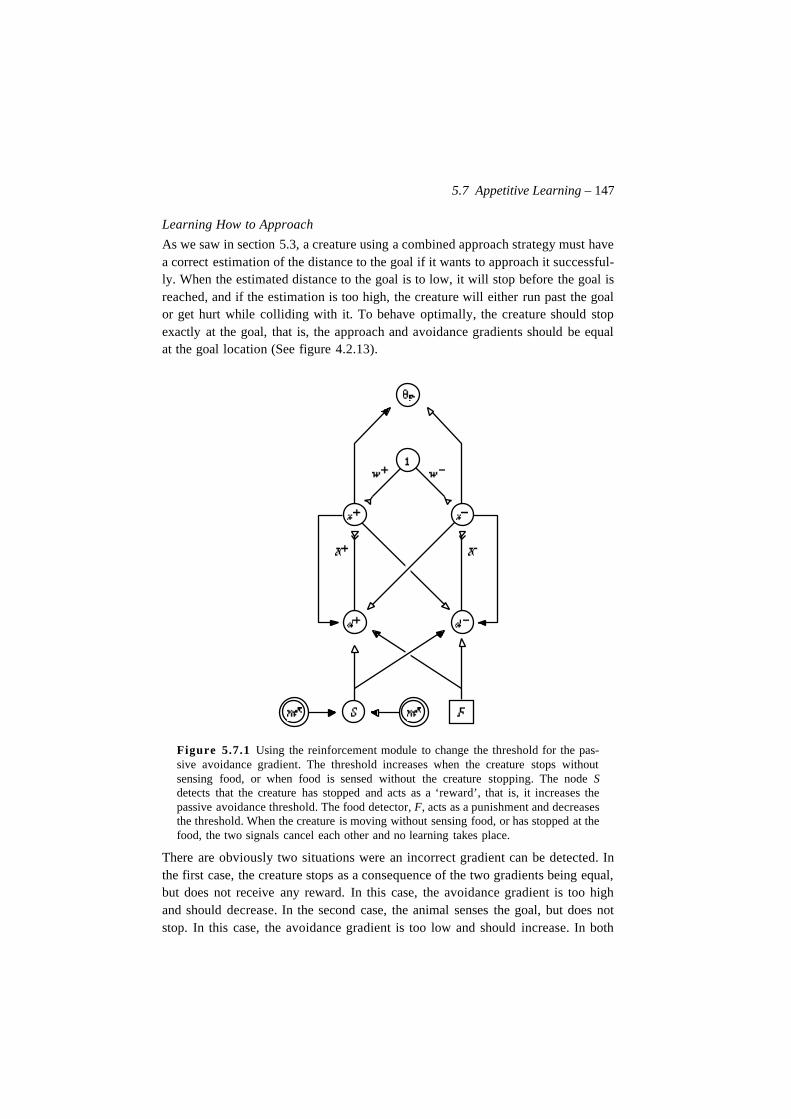
5.7 Appetitive Learning – 147
Learning How to Approach
As we saw in section 5.3, a creature using a combined approach strategy must havea correct estimation of the distance to the goal if it wants to approach it successful-ly. When the estimated distance to the goal is to low, it will stop before the goal isreached, and if the estimation is too high, the creature will either run past the goalor get hurt while colliding with it. To behave optimally, the creature should stopexactly at the goal, that is, the approach and avoidance gradients should be equalat the goal location (See figure 4.2.13).
Figure 5.7.1 Using the reinforcement module to change the threshold for the pas-sive avoidance gradient. The threshold increases when the creature stops withoutsensing food, or when food is sensed without the creature stopping. The node Sdetects that the creature has stopped and acts as a ‘reward’, that is, it increases thepassive avoidance threshold. The food detector, F, acts as a punishment and decreasesthe threshold. When the creature is moving without sensing food, or has stopped at thefood, the two signals cancel each other and no learning takes place.
There are obviously two situations were an incorrect gradient can be detected. Inthe first case, the creature stops as a consequence of the two gradients being equal,but does not receive any reward. In this case, the avoidance gradient is too highand should decrease. In the second case, the animal senses the goal, but does notstop. In this case, the avoidance gradient is too low and should increase. In both
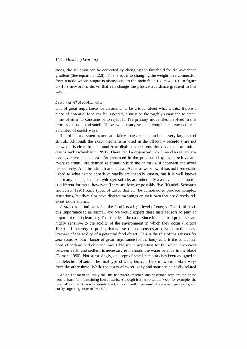
148 – Modeling Learning
cases, the situation can be corrected by changing the threshold for the avoidancegradient (See equation 4.2.8). This is equal to changing the weight on a connectionfrom a node whose output is always one to the node θp in figure 4.2.10. In figure5.7.1, a network is shown that can change the passive avoidance gradient in thisway.
Learning What to Approach
It is of great importance for an animal to be critical about what it eats. Before apiece of potential food can be ingested, it must be thoroughly examined to deter-mine whether to consume or to reject it. The primary modalities involved in thisprocess are taste and smell. These two sensory systems complement each other ina number of useful ways.
The olfactory system reacts at a fairly long distance and on a very large set ofstimuli. Although the exact mechanisms used in the olfactory receptors are notknown, it is clear that the number of distinct smell sensations is almost unlimited(Davis and Eichenbaum 1991). These can be organized into three classes: appeti-tive, aversive and neutral. As presented in the previous chapter, appetitive andaversive stimuli are defined as stimuli which the animal will approach and avoidrespectively. All other stimuli are neutral. As far as we know, it has not been estab-lished to what extent appetitive smells are innately known, but it is well knownthat many smells, such as hydrogen sulfide, are inherently aversive. The situationis different for taste, however. There are four, or possibly five (Kandel, Schwartzand Jessel 1991) basic types of tastes that can be combined to produce complexsensations, but they also have distinct meanings on their own that are directly rel-evant to the animal.
A sweet taste indicates that the food has a high level of energy. This is of obvi-ous importance to an animal, and we would expect these taste sensors to play animportant role in learning. This is indeed the case. Since biochemical processes arehighly sensitive to the acidity of the environment in which they occur (Tortora1990), it is not very surprising that one set of taste sensors are devoted to the meas-urement of the acidity of a potential food object. This is the role of the sensors forsour taste. Another factor of great importance for the body cells is the concentra-tions of sodium and chlorine ions. Chlorine is important for the water movementbetween cells, and sodium is necessary to maintain the water balance in the blood(Tortora 1990). Not surprisingly, one type of smell receptors has been assigned tothe detection of salt.3 The final type of taste, bitter , differs in two important waysfrom the other three. While the tastes of sweet, salty and sour can be easily related
3. We do not mean to imply that the behavioral mechanisms described here are the primemechanisms for maintaining homeostasis. Although it is important to keep, for example, thelevel of sodium at an appropriate level, this is handled primarily by internal processes, andnot by ingesting more or less salt.
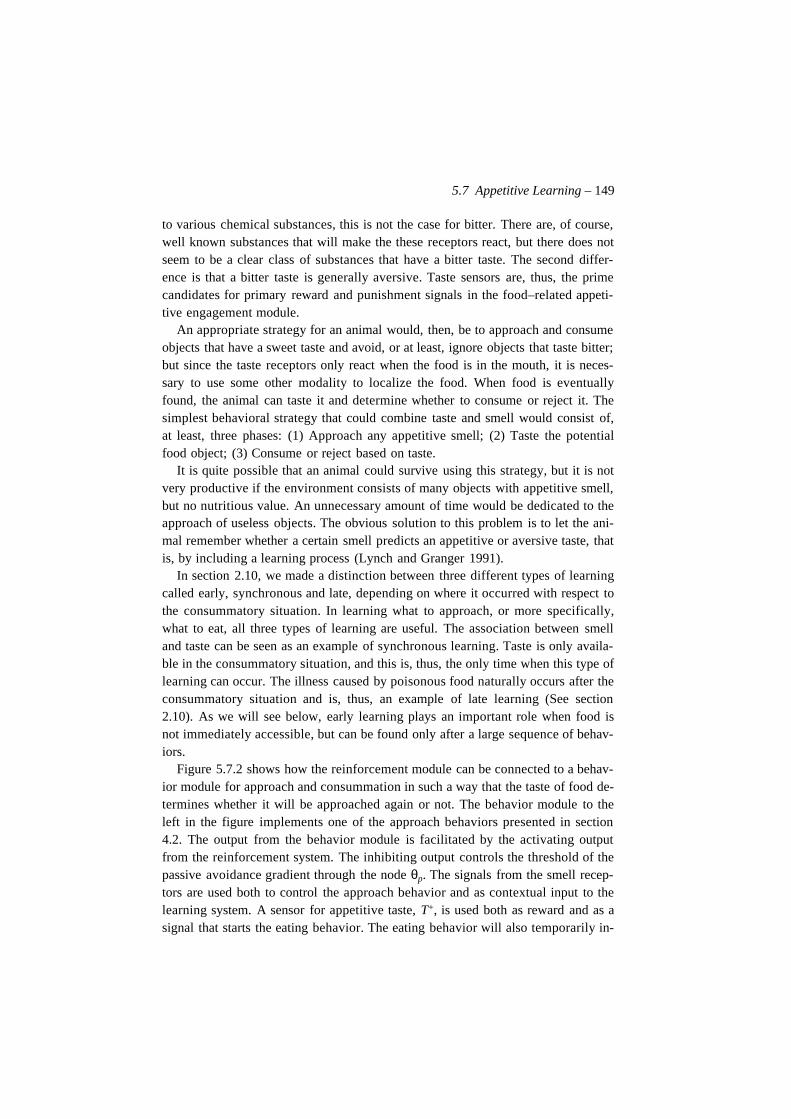
5.7 Appetitive Learning – 149
to various chemical substances, this is not the case for bitter. There are, of course,well known substances that will make the these receptors react, but there does notseem to be a clear class of substances that have a bitter taste. The second differ-ence is that a bitter taste is generally aversive. Taste sensors are, thus, the primecandidates for primary reward and punishment signals in the food–related appeti-tive engagement module.
An appropriate strategy for an animal would, then, be to approach and consumeobjects that have a sweet taste and avoid, or at least, ignore objects that taste bitter;but since the taste receptors only react when the food is in the mouth, it is neces-sary to use some other modality to localize the food. When food is eventuallyfound, the animal can taste it and determine whether to consume or reject it. Thesimplest behavioral strategy that could combine taste and smell would consist of,at least, three phases: (1) Approach any appetitive smell; (2) Taste the potentialfood object; (3) Consume or reject based on taste.
It is quite possible that an animal could survive using this strategy, but it is notvery productive if the environment consists of many objects with appetitive smell,but no nutritious value. An unnecessary amount of time would be dedicated to theapproach of useless objects. The obvious solution to this problem is to let the ani-mal remember whether a certain smell predicts an appetitive or aversive taste, thatis, by including a learning process (Lynch and Granger 1991).
In section 2.10, we made a distinction between three different types of learningcalled early, synchronous and late, depending on where it occurred with respect tothe consummatory situation. In learning what to approach, or more specifically,what to eat, all three types of learning are useful. The association between smelland taste can be seen as an example of synchronous learning. Taste is only availa-ble in the consummatory situation, and this is, thus, the only time when this type oflearning can occur. The illness caused by poisonous food naturally occurs after theconsummatory situation and is, thus, an example of late learning (See section2.10). As we will see below, early learning plays an important role when food isnot immediately accessible, but can be found only after a large sequence of behav-iors.
Figure 5.7.2 shows how the reinforcement module can be connected to a behav-ior module for approach and consummation in such a way that the taste of food de-termines whether it will be approached again or not. The behavior module to theleft in the figure implements one of the approach behaviors presented in section4.2. The output from the behavior module is facilitated by the activating outputfrom the reinforcement system. The inhibiting output controls the threshold of thepassive avoidance gradient through the node θp. The signals from the smell recep-tors are used both to control the approach behavior and as contextual input to thelearning system. A sensor for appetitive taste, T+, is used both as reward and as asignal that starts the eating behavior. The eating behavior will also temporarily in-
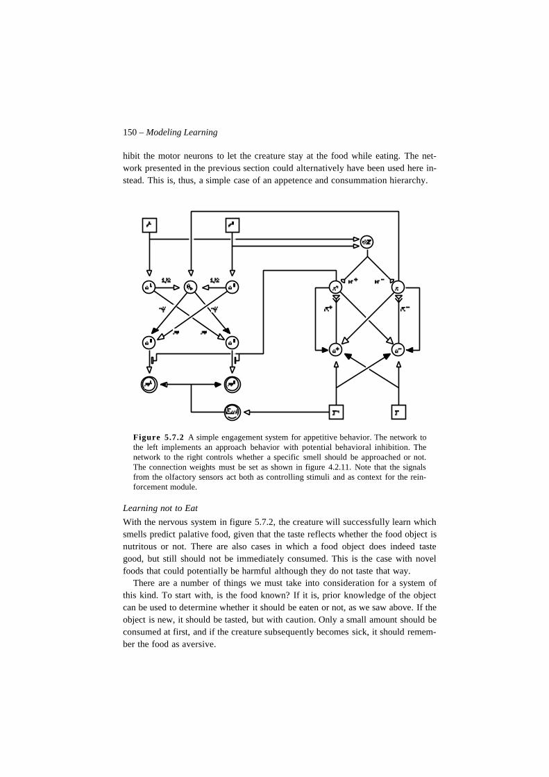
150 – Modeling Learning
hibit the motor neurons to let the creature stay at the food while eating. The net-work presented in the previous section could alternatively have been used here in-stead. This is, thus, a simple case of an appetence and consummation hierarchy.
Figure 5.7.2 A simple engagement system for appetitive behavior. The network tothe left implements an approach behavior with potential behavioral inhibition. Thenetwork to the right controls whether a specific smell should be approached or not.The connection weights must be set as shown in figure 4.2.11. Note that the signalsfrom the olfactory sensors act both as controlling stimuli and as context for the rein-forcement module.
Learning not to Eat
With the nervous system in figure 5.7.2, the creature will successfully learn whichsmells predict palative food, given that the taste reflects whether the food object isnutritous or not. There are also cases in which a food object does indeed tastegood, but still should not be immediately consumed. This is the case with novelfoods that could potentially be harmful although they do not taste that way.
There are a number of things we must take into consideration for a system ofthis kind. To start with, is the food known? If it is, prior knowledge of the objectcan be used to determine whether it should be eaten or not, as we saw above. If theobject is new, it should be tasted, but with caution. Only a small amount should beconsumed at first, and if the creature subsequently becomes sick, it should remem-ber the food as aversive.
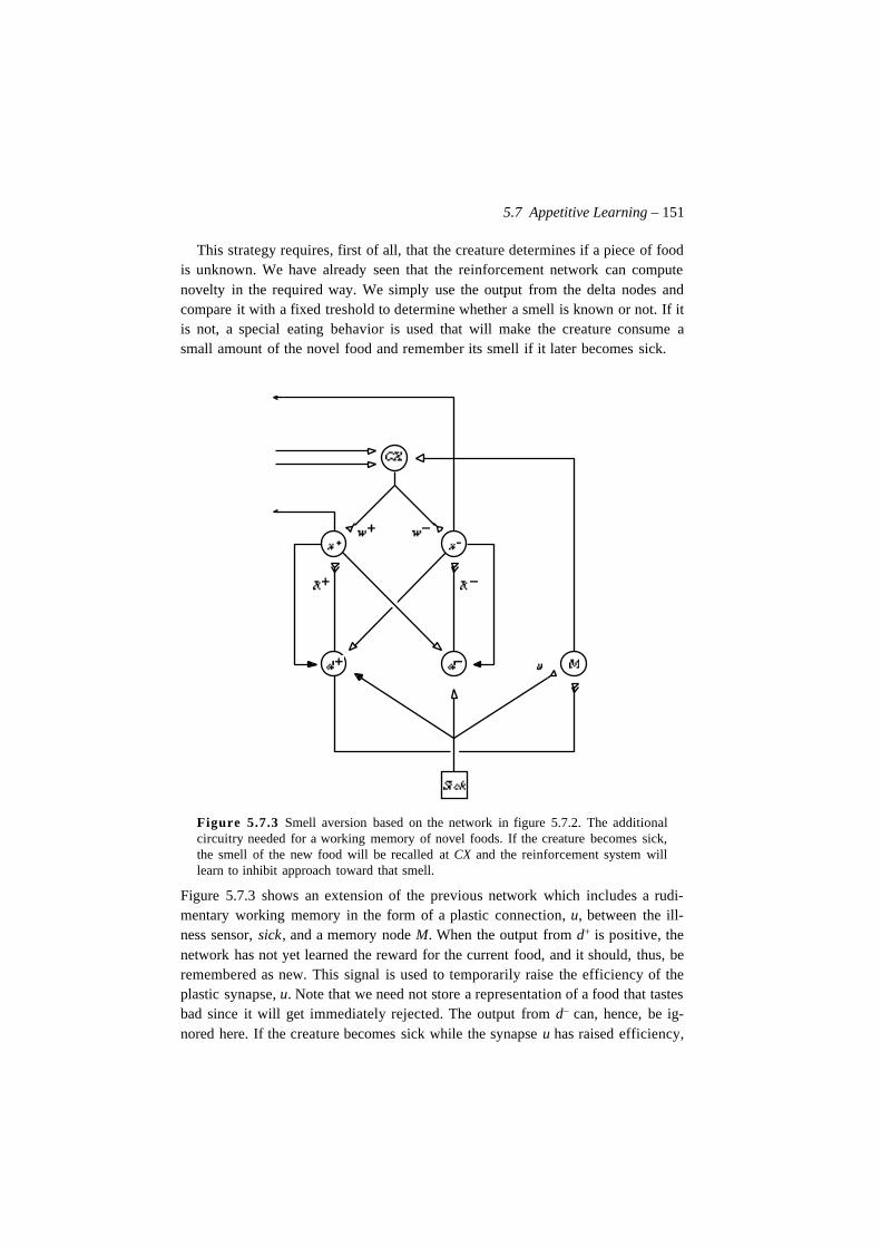
5.7 Appetitive Learning – 151
This strategy requires, first of all, that the creature determines if a piece of foodis unknown. We have already seen that the reinforcement network can computenovelty in the required way. We simply use the output from the delta nodes andcompare it with a fixed treshold to determine whether a smell is known or not. If itis not, a special eating behavior is used that will make the creature consume asmall amount of the novel food and remember its smell if it later becomes sick.
Figure 5.7.3 Smell aversion based on the network in figure 5.7.2. The additionalcircuitry needed for a working memory of novel foods. If the creature becomes sick,the smell of the new food will be recalled at CX and the reinforcement system willlearn to inhibit approach toward that smell.
Figure 5.7.3 shows an extension of the previous network which includes a rudi-mentary working memory in the form of a plastic connection, u, between the ill-ness sensor, sick, and a memory node M. When the output from d+ is positive, thenetwork has not yet learned the reward for the current food, and it should, thus, beremembered as new. This signal is used to temporarily raise the efficiency of theplastic synapse, u. Note that we need not store a representation of a food that tastesbad since it will get immediately rejected. The output from d– can, hence, be ig-nored here. If the creature becomes sick while the synapse u has raised efficiency,
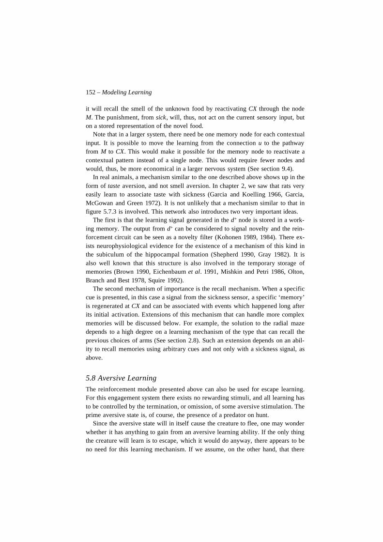
152 – Modeling Learning
it will recall the smell of the unknown food by reactivating CX through the nodeM. The punishment, from sick, will, thus, not act on the current sensory input, buton a stored representation of the novel food.
Note that in a larger system, there need be one memory node for each contextualinput. It is possible to move the learning from the connection u to the pathwayfrom M to CX. This would make it possible for the memory node to reactivate acontextual pattern instead of a single node. This would require fewer nodes andwould, thus, be more economical in a larger nervous system (See section 9.4).
In real animals, a mechanism similar to the one described above shows up in theform of taste aversion, and not smell aversion. In chapter 2, we saw that rats veryeasily learn to associate taste with sickness (Garcia and Koelling 1966, Garcia,McGowan and Green 1972). It is not unlikely that a mechanism similar to that infigure 5.7.3 is involved. This network also introduces two very important ideas.
The first is that the learning signal generated in the d+ node is stored in a work-ing memory. The output from d+ can be considered to signal novelty and the rein-forcement circuit can be seen as a novelty filter (Kohonen 1989, 1984). There ex-ists neurophysiological evidence for the existence of a mechanism of this kind inthe subiculum of the hippocampal formation (Shepherd 1990, Gray 1982). It isalso well known that this structure is also involved in the temporary storage ofmemories (Brown 1990, Eichenbaum et al. 1991, Mishkin and Petri 1986, Olton,Branch and Best 1978, Squire 1992).
The second mechanism of importance is the recall mechanism. When a specificcue is presented, in this case a signal from the sickness sensor, a specific ‘memory’is regenerated at CX and can be associated with events which happened long afterits initial activation. Extensions of this mechanism that can handle more complexmemories will be discussed below. For example, the solution to the radial mazedepends to a high degree on a learning mechanism of the type that can recall theprevious choices of arms (See section 2.8). Such an extension depends on an abil-ity to recall memories using arbitrary cues and not only with a sickness signal, asabove.
5.8 Aversive Learning
The reinforcement module presented above can also be used for escape learning.For this engagement system there exists no rewarding stimuli, and all learning hasto be controlled by the termination, or omission, of some aversive stimulation. Theprime aversive state is, of course, the presence of a predator on hunt.
Since the aversive state will in itself cause the creature to flee, one may wonderwhether it has anything to gain from an aversive learning ability. If the only thingthe creature will learn is to escape, which it would do anyway, there appears to beno need for this learning mechanism. If we assume, on the other hand, that there
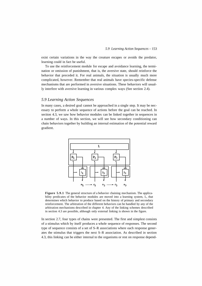
5.9 Learning Action Sequences – 153
exist certain variations in the way the creature escapes or avoids the predator,learning could in fact be useful.
To use the reinforcement module for escape and avoidance learning, the termi-nation or omission of punishment, that is, the aversive state, should reinforce thebehavior that preceded it. For real animals, the situation is usually much morecomplicated, however. Remember that real animals have species-specific defensemechanisms that are performed in aversive situations. These behaviors will usual-ly interfere with aversive learning in various complex ways (See section 2.4).
5.9 Learning Action Sequences
In many cases, a desired goal cannot be approached in a single step. It may be nec-essary to perform a whole sequence of actions before the goal can be reached. Insection 4.3, we saw how behavior modules can be linked together in sequences ina number of ways. In this section, we will see how secondary conditioning canchain behaviors together by building an internal estimation of the potential rewardgradient.
Figure 5.9.1 The general structure of a behavior chaining mechanism. The applica-bility predicates of the behavior modules are moved into a learning system, L, thatdetermines which behavior to produce based on the history of primary and secondaryreinforcement. The arbitration of the different behaviors can be handled by any of thearbitration mechanisms described in chapter 4. Any of the linking schemes describedin section 4.3 are possible, although only external linking is shown in the figure.
In section 2.7, four types of chains were presented. The first and simplest consistsof a stimulus which by itself produces a whole sequence of responses. The secondtype of sequence consists of a set of S–R associations where each response gener-ates the stimulus that triggers the next S–R association. As described in section4.3, this linking can be either internal to the organisms or rest on response depend-
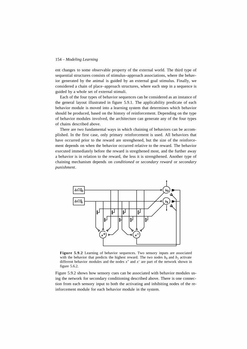
154 – Modeling Learning
ent changes to some observable property of the external world. The third type ofsequential structures consists of stimulus–approach associations, where the behav-ior generated by the animal is guided by an external goal stimulus. Finally, weconsidered a chain of place–approach structures, where each step in a sequence isguided by a whole set of external stimuli.
Each of the four types of behavior sequences can be considered as an instance ofthe general layout illustrated in figure 5.9.1. The applicability predicate of eachbehavior module is moved into a learning system that determines which behaviorshould be produced, based on the history of reinforcement. Depending on the typeof behavior modules involved, the architecture can generate any of the four typesof chains described above.
There are two fundamental ways in which chaining of behaviors can be accom-plished. In the first case, only primary reinforcement is used. All behaviors thathave occurred prior to the reward are strenghened, but the size of the reinforce-ment depends on when the behavior occurred relative to the reward. The behaviorexecuted immediately before the reward is stregthened most, and the further awaya behavior is in relation to the reward, the less it is strengthened. Another type ofchaining mechanism depends on conditioned or secondary reward or secondarypunishment.
Figure 5.9.2 Learning of behavior sequences. Two sensory inputs are associatedwith the behavior that predicts the highest reward. The two nodes b0 and b1 activatedifferent behavior modules and the nodes x+ and x– are part of the network shown infigure 5.6.2.
Figure 5.9.2 shows how sensory cues can be associated with behavior modules us-ing the network for secondary conditioning described above. There is one connec-tion from each sensory input to both the activating and inhibiting nodes of the re-inforcement module for each behavior module in the system.
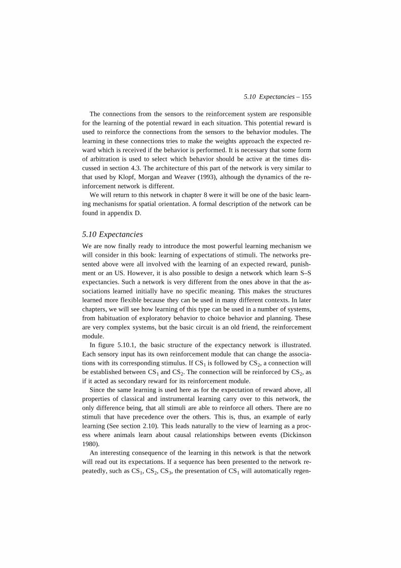
5.10 Expectancies – 155
The connections from the sensors to the reinforcement system are responsiblefor the learning of the potential reward in each situation. This potential reward isused to reinforce the connections from the sensors to the behavior modules. Thelearning in these connections tries to make the weights approach the expected re-ward which is received if the behavior is performed. It is necessary that some formof arbitration is used to select which behavior should be active at the times dis-cussed in section 4.3. The architecture of this part of the network is very similar tothat used by Klopf, Morgan and Weaver (1993), although the dynamics of the re-inforcement network is different.
We will return to this network in chapter 8 were it will be one of the basic learn-ing mechanisms for spatial orientation. A formal description of the network can befound in appendix D.
5.10 Expectancies
We are now finally ready to introduce the most powerful learning mechanism wewill consider in this book: learning of expectations of stimuli. The networks pre-sented above were all involved with the learning of an expected reward, punish-ment or an US. However, it is also possible to design a network which learn S–Sexpectancies. Such a network is very different from the ones above in that the as-sociations learned initially have no specific meaning. This makes the structureslearned more flexible because they can be used in many different contexts. In laterchapters, we will see how learning of this type can be used in a number of systems,from habituation of exploratory behavior to choice behavior and planning. Theseare very complex systems, but the basic circuit is an old friend, the reinforcementmodule.
In figure 5.10.1, the basic structure of the expectancy network is illustrated.Each sensory input has its own reinforcement module that can change the associa-tions with its corresponding stimulus. If CS1 is followed by CS2, a connection willbe established between CS1 and CS2. The connection will be reinforced by CS2, asif it acted as secondary reward for its reinforcement module.
Since the same learning is used here as for the expectation of reward above, allproperties of classical and instrumental learning carry over to this network, theonly difference being, that all stimuli are able to reinforce all others. There are nostimuli that have precedence over the others. This is, thus, an example of earlylearning (See section 2.10). This leads naturally to the view of learning as a proc-ess where animals learn about causal relationships between events (Dickinson1980).
An interesting consequence of the learning in this network is that the networkwill read out its expectations. If a sequence has been presented to the network re-peatedly, such as CS1, CS2, CS3, the presentation of CS1 will automatically regen-
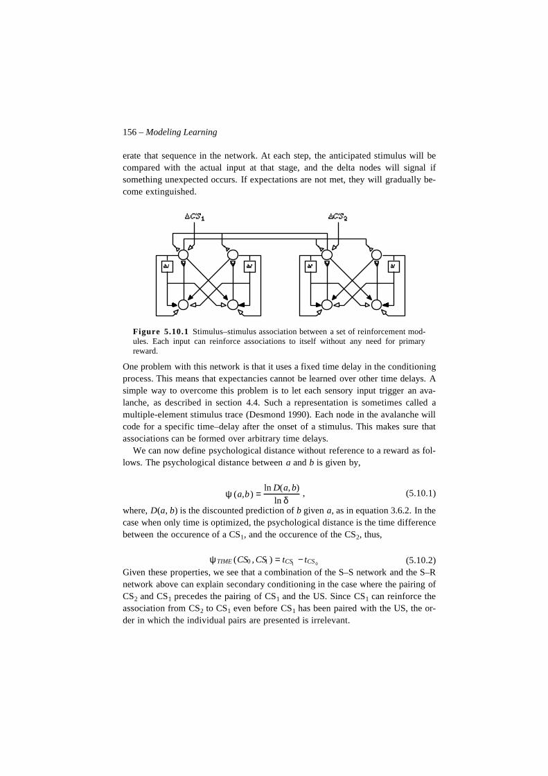
156 – Modeling Learning
erate that sequence in the network. At each step, the anticipated stimulus will becompared with the actual input at that stage, and the delta nodes will signal ifsomething unexpected occurs. If expectations are not met, they will gradually be-come extinguished.
Figure 5.10.1 Stimulus–stimulus association between a set of reinforcement mod-ules. Each input can reinforce associations to itself without any need for primaryreward.
One problem with this network is that it uses a fixed time delay in the conditioningprocess. This means that expectancies cannot be learned over other time delays. Asimple way to overcome this problem is to let each sensory input trigger an ava-lanche, as described in section 4.4. Such a representation is sometimes called amultiple-element stimulus trace (Desmond 1990). Each node in the avalanche willcode for a specific time–delay after the onset of a stimulus. This makes sure thatassociations can be formed over arbitrary time delays.
We can now define psychological distance without reference to a reward as fol-lows. The psychological distance between a and b is given by,
, (5.10.1)
where, D(a, b) is the discounted prediction of b given a, as in equation 3.6.2. In thecase when only time is optimized, the psychological distance is the time differencebetween the occurence of a CS1, and the occurence of the CS2, thus,
(5.10.2)Given these properties, we see that a combination of the S–S network and the S–Rnetwork above can explain secondary conditioning in the case where the pairing ofCS2 and CS1 precedes the pairing of CS1 and the US. Since CS1 can reinforce theassociation from CS2 to CS1 even before CS1 has been paired with the US, the or-der in which the individual pairs are presented is irrelevant.
ψ (a,b ) =ln D(a, b)
ln δ
ψ TIME (CS0 , CS1 ) = tCS1− tCS 0
5.11 Limitations of the Reinforcement Module – 157
We will return to this network in chapter 8 and 9, where we will discuss its rolein complex cognitive processes where it is used to anticipate future percepts toguide behavior by prediction of the future rather than the immediate perceptual en-vironment. A formal description is given in appendix E.
5.11 Limitations of the Reinforcement Module
There are a number of important limitations of the reinforcement module de-scribed in this chapter. The first is that it almost totally ignores interstimulus inter-val (ISI) effects. In the model, conditioning is only possible for a fixed time inter-val, and during this interval, the effect is the same regardless of the precise timingof the stimuli. Figure 5.11.1 shows the approximate relation between learning andinterstimulus interval found in empirical studies (Mackintosh 1983). The shape ofthis curve is approximately the same for all species, although the time scale canvary substantially. For example, for rabbit eyelid conditioning, the curve describesapproximately a second (Smith, Coleman and Gormezano 1969), but for pigeonkey-pecking, the same curve covers around half a minute (Gibbon et al. 1977). Forfood aversion, the ISI may be as much as 24 hours (Mackintosh 1983).
Figure 5.11.1 The effect of interstimulus interval on conditioning. The solid lineshows the approximate relation between interstimulus interval and strength of condi-tioning found in empirical studies. The dotted line shows the behavior of the presentmodel.
The model can easily be extended to handle ISI effects. Such an extension is de-scribed in appendix C, but will not be discussed here since it would make the pres-entation unnecessarily complicated.
A second limitation is that reinforcement is only generated at CS onset. It hasbeen found in empirical studies that CS offset also triggers learning, but of oppo-site sign (See Sutton and Barto 1990). To model this phenomenon within thepresent model, it would be required that the ∆CS be negative as well as positive.The only reason why this mechanism was not included above is that it requires the
158 – Modeling Learning
connections to the activation and inhibiting nodes to be negative as well as posi-tive, which is unrealistic from a neural point of view.
Another notable omission is that we have not considered learned irrelevance orlatent inhibition (Lubow and Moore 1959). This is the situation when an animallearn that a stimulus does not have any consequences at all and is, thereafter, reluc-tant to use it as a cue. Like many related models, (for example Klopf 1988), thepresent model fails to handle this situation unless a background stimulus and an in-ternal trial clock is postulated. In chapter 9, we will return to this type of learningand suggest that it may depend on cognitive processes of a very high level. A relat-ed phenomenon is overshadowing where a stimulus compound is paired with anUS, but some parts of the compound do not establish any association. The part ofthe compound that does establish a connection is said to overshadow the otherparts. Although the present model does model overshadowing, the way it does it isnot entirely satisfactory. An alternative explanation that sometimes seems morefruitful is that an attentional process selects a single stimulus when many arepresent, which would also result in overshadowing (Mackintosh 1974). We will re-turn to this alternative in chapter 9.
A final simplification is that we have assumed that the reinforcement module iscomposed of two identical halves. The system for reward is identical to the systemfor punishment. There is, however, a large difference in the way reward and pun-ishment affect behavior. When an animal is rewarded, it is likely to perform the re-warded behavior again. This will let the animal collect ever increasing pieces ofinformation about the rewarded behavior. After some trials, the animal will bevery well informed about which behavior is appropriate. In the case of punish-ment, the outcome is the reverse. Since the animal will become less likely to per-form the behavior that preceded the punishment, it will not be able to correct itspossibly faulty view of the punishment. This implies, of course, that punishment isnot a very good way to control the behavior of others.
5.12 ConclusionThis chapter presented a general reinforcement module that can be used as part ofa number of learning systems. It is important to realize that although this learningmodule can be used generally, it is not a general learning mechanism in the sensethat it solves all learning problems. It is only when this module is incorporated inother systems and connected to various behavior modules that it has any real pow-er. This power comes from its ability to coordinate behaviors, and not create be-haviors (Bolles 1984).
Although it can, in principle, learn arbitrary connections between stimuli andreponses, this is not the way the reinforcement module should be used. In chapter8, we will see that learning of this type is highly inefficient and is only useful with-
5.12 Conclusion – 159
in the context of a larger system. It is also necessary to modify the reinforcementmodule, depending on where it is used in a system.
We have seen how similar principles can be used to explain a large number oflearning paradigms. Many properties of classical and instrumental conditioningare very similar, which makes it possible to use similar models for both cases. Thequestion remains as to whether the same mechanism is responsible for these twotypes of learning in real animals.
Learning is only one of the determinants of behavior, however. Another impor-tant determinant is the current need of the animal. In the next chapter, we will con-sider how these needs change over time and how they influence learning and be-havior. We, thus, explore the area of motivation and emotion.

160 – Modeling Learning
Christian Balkenius, 1995, Natural Intelligence in Artificial Creatures, Lund University Cognitive Studies 37, 1995.
Chapter 6
Motivation and Emotion
6.1 IntroductionSome concepts are quite useless in their broadest meaning. Motivation is such aconcept. There is, however, a more restricted sense of the word which is useful oreven essential in any theory of cognition. This is the idea of motivation as a centralstate reflecting the combination of internal needs and external possibilities. In themotivational system, these two sources of information come together and they areused to form a decision on what to do. The representation of this decision consti-tutes the motivational state of the animal (See section 3.2), which tells the animalwhat it should do.
In this chapter, we will try to investigate the role of motivation as a determinantof behavior and learning. We will try to show that motivation and emotion playsan important role in cognitive processes which has often been overlooked in thepast. The traditional dichotomy between cognition and emotion is probably re-sponsible for the lack of interest in motivational theories within cognitive science(LeDoux 1995). This is unfortunate for a number of reasons.
First, there seems to be no clear distinction between cognition, motivation andemotion in our daily activities. For example, the planning of a vacation is usuallyconsidered to be a cognitive activity. Every step of the planning process is guidedby one’s ideas of a good holiday, one’s hopes, fears, etc. Without this side of theplanning process, the vacation would hardly be worth planning, since it could onlyresult in any of an infinite number of equally valued plans, none of which would fit
162 – Motivation and Emotion
one’s requirements for a good holiday. It appears that all thinking is biased byemotive values in this way.
Next, cognition cannot be understood without reference to motivation. Highercognitive processes like categorization and problem solving only play any rolewhen they are used to fulfil some goal of the individual, that is, only when they aremotivated. This is unfortunately an aspect of cognition that is often ingnored.
Last, it is important to realize that motivation precedes cognition. Cognition de-pends on the motivational system, whereas the motivational system can operatewithout cognition. This point will be developed further in section 6.8. We will alsoargue that the role of emotions is to tell the animal what it should have done, whenits expectations are inaccurate or its behavior is unsuccesful.
We will see that the motivational state has two important properties: First, themotivational state is central to the whole organism. This means that at all times,the organism is influenced by one single motivational state which selects a singleengagement. Second, the motivational state is dynamic . As the internal needs andexternal possibilities change or are reevaluated, the motivational state may changeat any time.
6.2 The Determinants of MotivationLearning is just one determinant of behavior. The other important determinant ismotivation. Some early theories did not consider motivation as a source of behav-ioral direction. Instead, they focused on learning alone. For example, the experi-ments of Pavlov (1927) did essentially ignore the role of motivation. This is curi-ous, since the classical association of a bell1 with salivation could only be learnedwhen the dog was hungry. A satiated dog simply does not show the salivation re-flex.
In Thorndike’s experiments, the role of motivation was even less clear. The catin its box was given food when it had managed to escape, but this was more or lessan afterthought. It was never clearly established whether the cat tried to escape be-cause it wanted food or because confinement is aversive to the animal.
The role of motivation compared to learning was clearly shown in an experi-ment by Clark (1958). A number of rats were trained to press a bar in order to ob-tain food. The rats were then placed in different groups and deprived of food forbetween 1 and 23 hours. The longer the rats had been deprived of food, the fasterthey pressed the bar to obtain it. Since all the rats had received equal training, thedifferences could not be due to differences in learning. Consequently, the experi-ment shows that motivation, or in this case, the deprivation of food, plays a signif-icant role in determining behavior.
1. In many of Pavlov’s original experiments, the sound of a metronome was used ratherthan a bell.
6.3 Drives – 163
Hull (1943) proposed that deprivation induces an aversive state in the organism.This state was called a drive. In his conception, drive increases the overall level ofarousal in an animal. Drive was thus considered as a property of need states whichmotivates behavior. Hull considered drive to have an overall effect on behavior inthat it energizes it, but does not determine what behavior is performed. This is usu-ally called a generalized drive and has now been replaced by the concept of arous-al (Gray 1975). The theory can be summarized in Hull’s law,
(6.2.1)
where D is the drive level, V the stimulus intensity, K the incentive motivation —a concept we will return to below — and SHR is the habit strength that results fromlearning. They all multiply to produce the reaction potential, SER, which is ameasure of the likelihood that an animal will produce a particular response, R, giv-en a stimulus, S.
Later studies have shown that the role of drive is to selectively increase the fre-quency of behaviors likely to reduce the drive2 (See Bolles 1967). In Hull’s formu-lation an increased drive caused by deprivation of food would increase the likeli-hood of any behavior, not only of eating. Taking this into account, we must relateboth the drive and the incentive to a particular type of motivation and Hull’s lawchanges to,
(6.2.2)Here, Dm is a specific drive, such as hunger, which relates to a particular motiva-tion, m, for example motivation to engage in food seeking behavior or eating. Theincentive motivation must also be related to the particular motivation that is indi-cated by the subscript m. Later studies have also shown that the interaction be-tween deprivation and learning may be more complicated than multiplication(Bolles 1969), but the basic idea is very sensible and as we will see below, the con-cept of motivation can be used to great utility as the basis for a theory of choice.
Another possible extension, which we will not investigate further here is to usevectors for the representations of drives. This makes it possible to have a whole setof motivational states which represent, for example, hunger (McFarland and Sibly,1972). This corresponds to the idea that one can have hunger for different types offoods.
6.3 Drives
Drive is probably one of the vaguest terms in psychology. It has been used in manydifferent meanings, some of which have gained a very bad reputation. The use ofdrive that is intended here is as a state or value representing the urgency of a be-
2. Note that this does not imply that it necessarily is the reduction of drive which controlsthe learning process.
ES R HS R D V K×××=
ES R HS R Dm V Km××× .=
164 – Motivation and Emotion
havior. In some cases, a drive relates to a physiological state produced by a depri-vation or increased levels of food, a hormone etc. In other cases they relate to thepresence of a noxious stimuli such as a loud noise, pain, heat, etc. In these cases,drives are equivalent to need states, but we will also allow constant drives whichcompete with these more usual drives. Constant drives represent the relative im-portance of different engagements which do not change over time.
Drives, thus, have the role of representing the relative importance of an engage-ment at a certain time. This implies that a creature must have one, or possiblymany, drives for each of its innate engagements. We can identify at least six differ-ent types of drives.
Homeostatic Drives The first type of drive that we will consider is generatedby violation of homeostasis. This includes, for example, hunger and thirst, but alsothe responses to heat and cold. Violation of homeostasis induces a drive signal intothe motivational system. The probability of an engagement increases with largerdeviation from the optimal level but the drive signal does not directly activate abehavior.
It is instructive to compare this notion of drives with the behavioral model pro-posed by Powers (1973). Powers’ model is built on the assumption that the presentaction of an organism is a function of its present perceptions and an internal refer-ence perception. These are compared to generate an error signal which facilitatesbehavior. This is exactly the idea that the discrepancy between the present state ofthe organism (the present perception) and its desired state (the reference percep-tion) drives behavior. The idea of an error signal is very similar to the idea of adrive. (Compare this idea with the discussion of approach behavior in chapter 4).
In Powers’ models, this idea is generalized to hierarchically connected compa-rators. The comparator on each level generates the reference perception to the sys-tem below it. What starts out as a mechanism for maintaining homeostasis hasturned into a behavioral control system. In the process, the motivational systemhas disappeared and so has the ability of the system to select among different en-gagements. Though elegant, Powers’ model cannot explain the selection of one en-gagement among many when several discrepancies are present. However, it de-serves recognition as an early and thorough system model of horizontaldecomposition of competence (Compare Brooks 1986, and Schnepf 1991).
Powers’ model treats behavior as a function of two variables: the present per-ception and the reference perception. We want to argue that three variables areneeded: the present perception, the present motivational state and the ‘referenceperception’. However, the ‘reference perception’ needs not be explicitly represent-ed since it is essentially fixed by evolution.
Discrepancies can thus be detected directly without reference to the optimalstate of the organism. Thus, the comparators do not exist in a physical sense and
6.3 Drives – 165
the reference perceptions are not really perceptions at all. Yet, the organism be-haves as if they were present.
Also, as we have already discussed, the role of the present perceptions is not todetermine the violation of homeostasis, but to modulate the motivational state.This is especially important in, for example, sexual and maternal behavior. Moti-vation for these are not brought about by lack of homeostasis.
In the following, we will stick to the simplistic model of homeostatic drives de-scribed here, but there are admittedly a number of extensions which could bemade. The most important extension is that most animals do not eat because theyare hungry, but rather to avoid becoming hungry (Collier 1983). This means thatan animal must be able to anticipate its future needs or alternatively defend theirfood intake rather than homeostasis. We can still use the notion of drive in thesecases by allowing it to have a less direct relation to immediate physiological need.
Noxious Drives We may also consider the signals from noxious stimuli asdrives. This includes, for example, the sensation of pain. Since noxious signalswill also constitute external incentives, it is possible to consider the drive foravoidance of noxious stimuli as constant. As we will see below in the discussion ofchoice mechanisms, there is reason to include constant drives of this types, since itmakes it easy to model individual dispositions of an animal as the levels of theseconstant drives. For example, an animal with a lower level on its ‘pain avoidance’drive, will appear to be more resistant to pain than one with a higher level on thisdrive since it will engage in avoidance more seldom and with less vigor.
Cyclical Drives There are a number of cyclical drives which vary with the timeof day or the year. These are not directly controlled by an internal or external stim-uli. Instead they are generated by an oscillator. This oscillator in turn is influencedby external stimuli such as the length of the day, odors, or the amount of light inthe environment. In this group of drives we find, for example, tiredness and wake-fulness, the sexual drives of most animals, and migratory drives.
It is interesting to consider to what extent hunger drives are also of this type.Perhaps hunger is also controlled by an internal oscillator which locks to the cyclewhich decides the time when an animal usually gets hungry and eats. A mecha-nism of this type would greatly simplify the anticipation of future hunger (Collier1983), but we will not consider it further here. It could also potentially account forfluctuation in eating behavior depending on the time of day or the season.
Default Drives The fourth type of drives can be called default drives since theyonly influence the animal when no external cue is present which commands the an-imal to do something else. The most important drive of this type is concerned withgrooming (Bolles 1984). Such behavior is performed when the animal has nothingelse to do. Typically, grooming behaviors consist of a fixed-action pattern (See
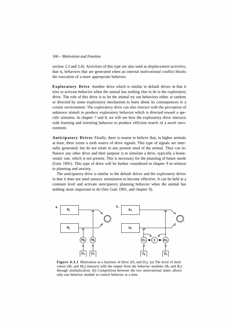
166 – Motivation and Emotion
section 2.3 and 2.4). Activities of this type are also used as displacement activities,that is, behaviors that are generated when an internal motivational conflict blocksthe execution of a more appropriate behavior.
Exploratory Drive Another drive which is similar to default drives in that ittries to activate behavior when the animal has nothing else to do is the exploratorydrive. The role of this drive is to let the animal try out behaviors either at randomor directed by some exploratory mechanism to learn about its consequences in acertain environment. The exploratory drive can also interact with the perception ofunknown stimuli to produce exploratory behavior which is directed toward a spe-cific stimulus. In chapter 7 and 8, we will see how the exploratory drive interactswith learning and orienting behavior to produce efficient search of a novel envi-ronment.
Anticipatory Drives Finally, there is reason to believe that, in higher animalsat least, there exists a sixth source of drive signals. This type of signals are inter-nally generated, but do not relate to any present need of the animal. They can in-fluence any other drive and their purpose is to simulate a drive, typically a home-ostatic one, which is not present. This is necessary for the planning of future needs(Gulz 1991). This type of drive will be further considered in chapter 9 in relationto planning and anxiety.
The anticipatory drive is similar to the default drives and the exploratory drivesin that it does not need sensory stimulation to become effective. It can be held at aconstant level and activate anticipatory planning behavior when the animal hasnothing more important to do (See Gulz 1991, and chapter 9).
Figure 6.3.1 Motivation as a function of drive (D1 and D2). (a) The level of moti-vation (M1 and M2) interacts with the output from the behavior modules (B1 and B2)through multiplication. (b) Competition between the two motivational states allowsonly one behavior module to control behavior at a time.
6.4 Incentive – 167
Motivation as Competing Drives
We see that drives can be classified as constant or varying . In many cases, it maynot be sensible to consider constant drives as drives at all, but in everyday lan-guage we talk about a curiosity drive much in the same way as a hunger drive. Al-though the mechanisms controlled by these two drives are very different, there isan underlying similarity in how the drives are involved and this makes it reasona-ble to use a similar formalization of both cases.
Let us now look at how the motivational state of an animal is changed by itsdrives. To a first approximation, the strength of a motivation, m, called Mm, de-pends only on a corresponding drive, Dm, which gives the following formula forthe calculation of motivation:
(6.3.1)In figure 6.3.1a, a simple network is drawn which can calculate motivation in thisway. The motivational state influenced behavior by facilitating the behavior com-mand sent from the two behavior modules (Werner 1994). In the right figure, com-petition between the two motivational states is introduced as described in section1.4. As a consequence, only one motivation can be active at a time. This propertyof the motivational system is useful when the additive composition of the behav-iors generated by the different behavior modules is not meaningful. When compe-tition is included in the motivational system (figure 6.6.1b), the creature uses arbi-tration by central selection, which allows it to perform one behavior at a time (Seesection 2.3).
Figure 6.3.2 shows how the life space of an animal changes as a result of changein drive level for the network with and without competition. In the simulations, theapproach tendency toward a goal of type m was multiplied with the correspondingmotivation, Mm. As can be seen, the borders between the basins of attraction aremoved away from the goal with the highest corresponding drive level as could beexpected. The animal will consequently be more likely to choose that goal insteadof the other. When competition between the two motivational states is added, onlygoals relating to the dominant motivation are perceived at all.
While this mechanism makes the creature attend to its most important need first,it does not generate optimal behavior. In chapter 7, we will investigate how an at-tentional mechanism can be added which lets the creature weigh together its needswith the psychological distance to the various goals. With an attentional mecha-nism, the creature can select the best overall goal without sacrificing its ability toperform one behavior at a time.
6.4 IncentiveAnother of Hull’s contributions to this area includes the idea that motivation is de-termined by two factors. As described above, the first is the need state or drive.
Mm Dm=
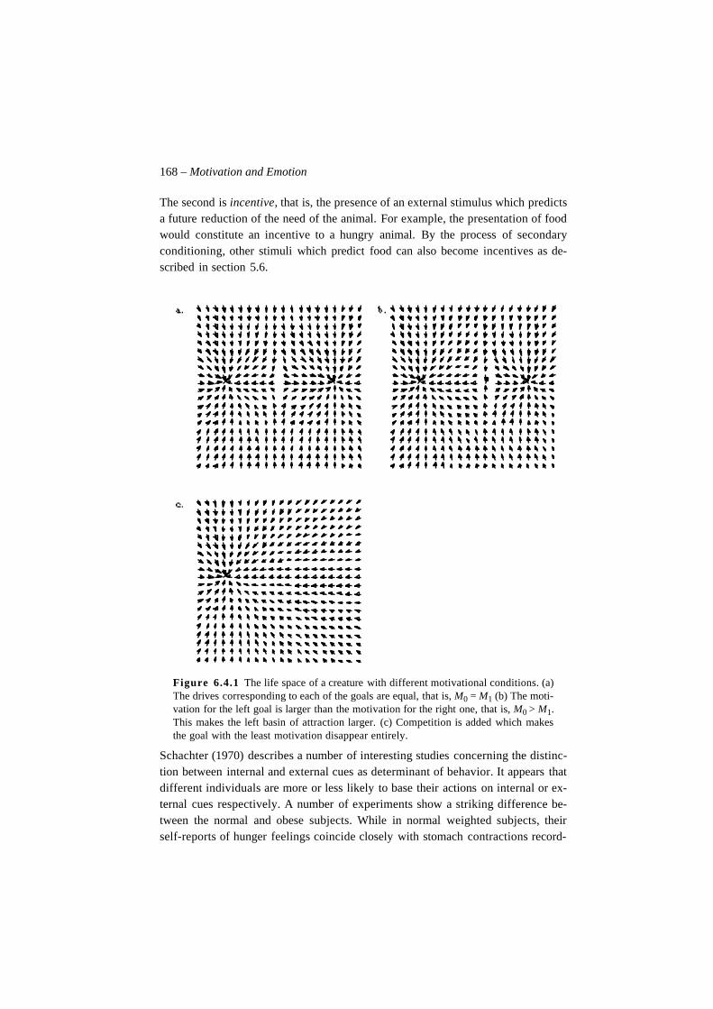
168 – Motivation and Emotion
The second is incentive, that is, the presence of an external stimulus which predictsa future reduction of the need of the animal. For example, the presentation of foodwould constitute an incentive to a hungry animal. By the process of secondaryconditioning, other stimuli which predict food can also become incentives as de-scribed in section 5.6.
Figure 6.4.1 The life space of a creature with different motivational conditions. (a)The drives corresponding to each of the goals are equal, that is, M0 = M1 (b) The moti-vation for the left goal is larger than the motivation for the right one, that is, M0 > M1.This makes the left basin of attraction larger. (c) Competition is added which makesthe goal with the least motivation disappear entirely.
Schachter (1970) describes a number of interesting studies concerning the distinc-tion between internal and external cues as determinant of behavior. It appears thatdifferent individuals are more or less likely to base their actions on internal or ex-ternal cues respectively. A number of experiments show a striking difference be-tween the normal and obese subjects. While in normal weighted subjects, theirself-reports of hunger feelings coincide closely with stomach contractions record-
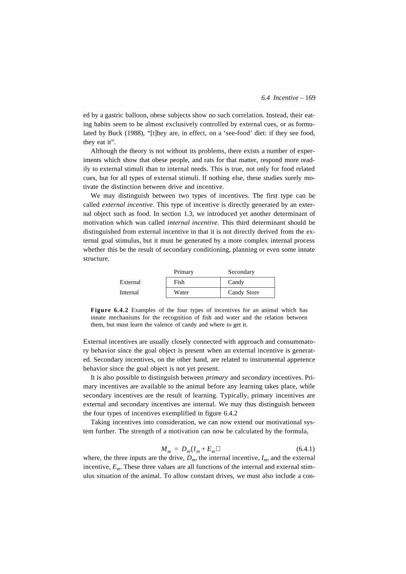
6.4 Incentive – 169
ed by a gastric balloon, obese subjects show no such correlation. Instead, their eat-ing habits seem to be almost exclusively controlled by external cues, or as formu-lated by Buck (1988), “[t]hey are, in effect, on a ‘see-food’ diet: if they see food,they eat it”.
Although the theory is not without its problems, there exists a number of exper-iments which show that obese people, and rats for that matter, respond more read-ily to external stimuli than to internal needs. This is true, not only for food relatedcues, but for all types of external stimuli. If nothing else, these studies surely mo-tivate the distinction between drive and incentive.
We may distinguish between two types of incentives. The first type can becalled external incentive. This type of incentive is directly generated by an exter-nal object such as food. In section 1.3, we introduced yet another determinant ofmotivation which was called internal incentive. This third determinant should bedistinguished from external incentive in that it is not directly derived from the ex-ternal goal stimulus, but it must be generated by a more complex internal processwhether this be the result of secondary conditioning, planning or even some innatestructure.
Figure 6.4.2 Examples of the four types of incentives for an animal which hasinnate mechanisms for the recognition of fish and water and the relation betweenthem, but must learn the valence of candy and where to get it.
External incentives are usually closely connected with approach and consummato-ry behavior since the goal object is present when an external incentive is generat-ed. Secondary incentives, on the other hand, are related to instrumental appetencebehavior since the goal object is not yet present.
It is also possible to distinguish between primary and secondary incentives. Pri-mary incentives are available to the animal before any learning takes place, whilesecondary incentives are the result of learning. Typically, primary incentives areexternal and secondary incentives are internal. We may thus distinguish betweenthe four types of incentives exemplified in figure 6.4.2
Taking incentives into consideration, we can now extend our motivational sys-tem further. The strength of a motivation can now be calculated by the formula,
(6.4.1)where, the three inputs are the drive, Dm, the internal incentive, Im, and the externalincentive, Em. These three values are all functions of the internal and external stim-ulus situation of the animal. To allow constant drives, we must also include a con-
Primary Secondary
External Fish Candy
Internal Water Candy Store
Mm Dm Im Em+( )=
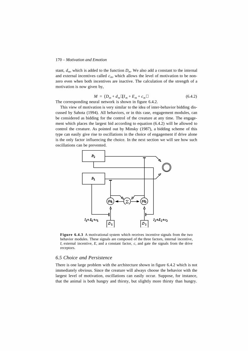
170 – Motivation and Emotion
stant, dm, which is added to the function Dm. We also add a constant to the internaland external incentives called cm, which allows the level of motivation to be non-zero even when both incentives are inactive. The calculation of the strength of amotivation is now given by,
(6.4.2)The corresponding neural network is shown in figure 6.4.2.
This view of motivation is very similar to the idea of inter-behavior bidding dis-cussed by Sahota (1994). All behaviors, or in this case, engagement modules, canbe considered as bidding for the control of the creature at any time. The engage-ment which places the largest bid according to equation (6.4.2) will be allowed tocontrol the creature. As pointed out by Minsky (1987), a bidding scheme of thistype can easily give rise to oscillations in the choice of engagement if drive aloneis the only factor influencing the choice. In the next section we will see how suchoscillations can be prevented.
Figure 6.4.3 A motivational system which receives incentive signals from the twobehavior modules. These signals are composed of the three factors, internal incentive,I, external incentive, E, and a constant factor, c, and gate the signals from the drivereceptors.
6.5 Choice and Persistence
There is one large problem with the architecture shown in figure 6.4.2 which is notimmediately obvious. Since the creature will always choose the behavior with thelargest level of motivation, oscillations can easily occur. Suppose, for instance,that the animal is both hungry and thirsty, but slightly more thirsty than hungry.
M Dm dm+( ) Im Em cm+ +( )=
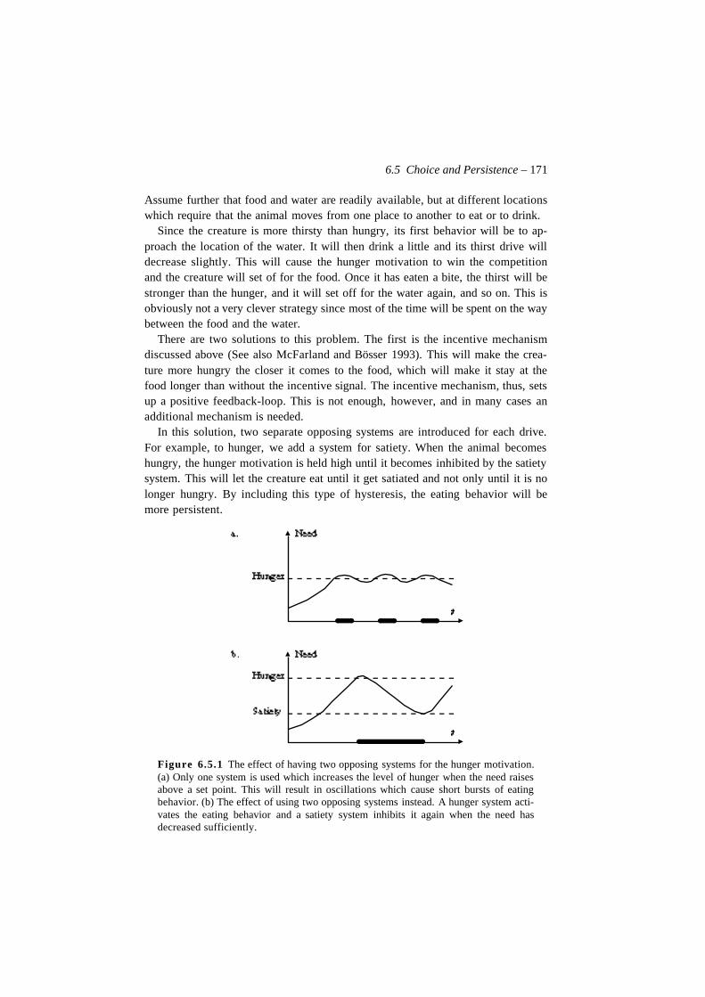
6.5 Choice and Persistence – 171
Assume further that food and water are readily available, but at different locationswhich require that the animal moves from one place to another to eat or to drink.
Since the creature is more thirsty than hungry, its first behavior will be to ap-proach the location of the water. It will then drink a little and its thirst drive willdecrease slightly. This will cause the hunger motivation to win the competitionand the creature will set of for the food. Once it has eaten a bite, the thirst will bestronger than the hunger, and it will set off for the water again, and so on. This isobviously not a very clever strategy since most of the time will be spent on the waybetween the food and the water.
There are two solutions to this problem. The first is the incentive mechanismdiscussed above (See also McFarland and Bösser 1993). This will make the crea-ture more hungry the closer it comes to the food, which will make it stay at thefood longer than without the incentive signal. The incentive mechanism, thus, setsup a positive feedback-loop. This is not enough, however, and in many cases anadditional mechanism is needed.
In this solution, two separate opposing systems are introduced for each drive.For example, to hunger, we add a system for satiety. When the animal becomeshungry, the hunger motivation is held high until it becomes inhibited by the satietysystem. This will let the creature eat until it get satiated and not only until it is nolonger hungry. By including this type of hysteresis, the eating behavior will bemore persistent.
Figure 6.5.1 The effect of having two opposing systems for the hunger motivation.(a) Only one system is used which increases the level of hunger when the need raisesabove a set point. This will result in oscillations which cause short bursts of eatingbehavior. (b) The effect of using two opposing systems instead. A hunger system acti-vates the eating behavior and a satiety system inhibits it again when the need hasdecreased sufficiently.
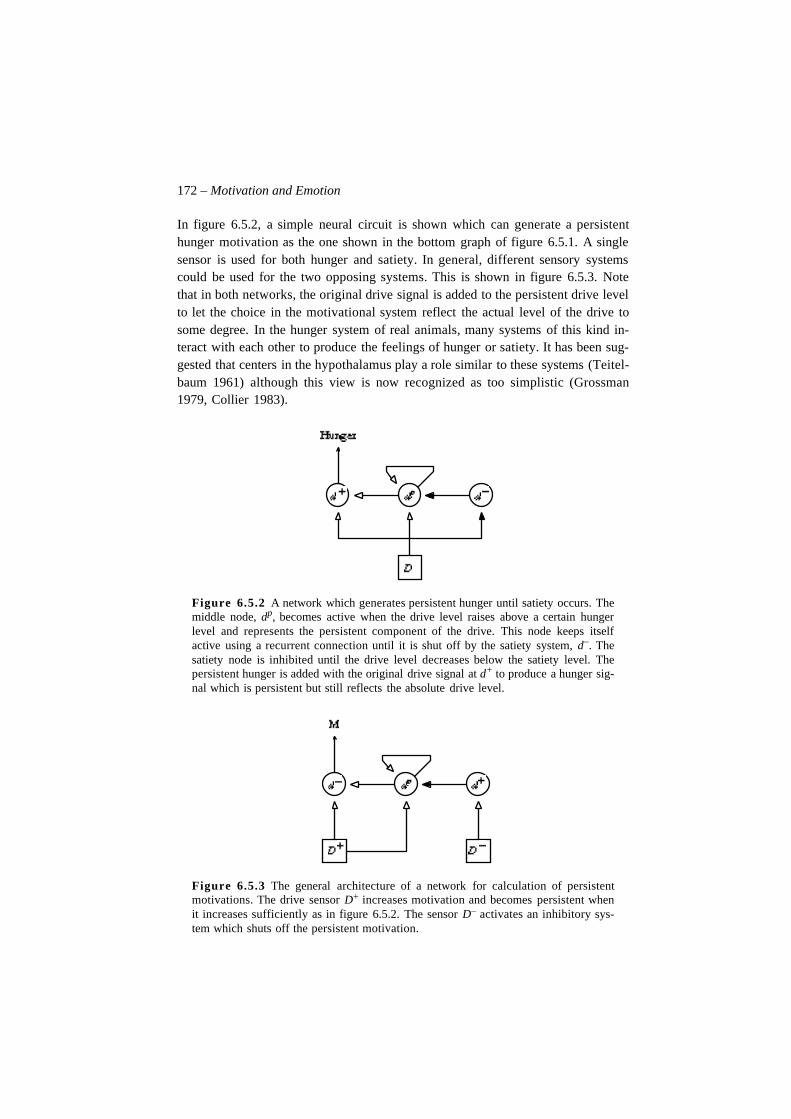
172 – Motivation and Emotion
In figure 6.5.2, a simple neural circuit is shown which can generate a persistenthunger motivation as the one shown in the bottom graph of figure 6.5.1. A singlesensor is used for both hunger and satiety. In general, different sensory systemscould be used for the two opposing systems. This is shown in figure 6.5.3. Notethat in both networks, the original drive signal is added to the persistent drive levelto let the choice in the motivational system reflect the actual level of the drive tosome degree. In the hunger system of real animals, many systems of this kind in-teract with each other to produce the feelings of hunger or satiety. It has been sug-gested that centers in the hypothalamus play a role similar to these systems (Teitel-baum 1961) although this view is now recognized as too simplistic (Grossman1979, Collier 1983).
Figure 6.5.2 A network which generates persistent hunger until satiety occurs. Themiddle node, dp, becomes active when the drive level raises above a certain hungerlevel and represents the persistent component of the drive. This node keeps itselfactive using a recurrent connection until it is shut off by the satiety system, d–. Thesatiety node is inhibited until the drive level decreases below the satiety level. Thepersistent hunger is added with the original drive signal at d+ to produce a hunger sig-nal which is persistent but still reflects the absolute drive level.
Figure 6.5.3 The general architecture of a network for calculation of persistentmotivations. The drive sensor D+ increases motivation and becomes persistent whenit increases sufficiently as in figure 6.5.2. The sensor D– activates an inhibitory sys-tem which shuts off the persistent motivation.
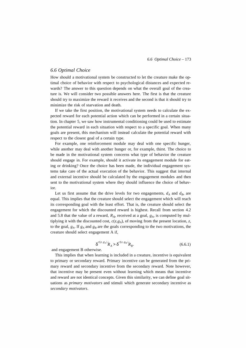
6.6 Optimal Choice – 173
6.6 Optimal ChoiceHow should a motivational system be constructed to let the creature make the op-timal choice of behavior with respect to psychological distances and expected re-wards? The answer to this question depends on what the overall goal of the crea-ture is. We will consider two possible answers here. The first is that the creatureshould try to maximize the reward it receives and the second is that it should try tominimize the risk of starvation and death.
If we take the first position, the motivational system needs to calculate the ex-pected reward for each potential action which can be performed in a certain situa-tion. In chapter 5, we saw how instrumental conditioning could be used to estimatethe potential reward in each situation with respect to a specific goal. When manygoals are present, this mechanism will instead calculate the potential reward withrespect to the closest goal of a certain type.
For example, one reinforcement module may deal with one specific hunger,while another may deal with another hunger or, for example, thirst. The choice tobe made in the motivational system concerns what type of behavior the creatureshould engage in. For example, should it activate its engagement module for eat-ing or drinking? Once the choice has been made, the individual engagement sys-tems take care of the actual execution of the behavior. This suggest that internaland external incentive should be calculated by the engagement modules and thensent to the motivational system where they should influence the choice of behav-ior.
Let us first assume that the drive levels for two engagements, dA and dB, areequal. This implies that the creature should select the engagement which will reachits corresponding goal with the least effort. That is, the creature should select theengagement for which the discounted reward is highest. Recall from section 4.2and 5.8 that the value of a reward, RA, received at a goal, gA, is computed by mul-tiplying it with the discounted cost, c(z,gA), of moving from the present location, z,to the goal, gA. If gA and gB are the goals corresponding to the two motivations, thecreature should select engagement A if,
(6.6.1)and engagement B otherwise.
This implies that when learning is included in a creature, incentive is equivalentto primary or secondary reward. Primary incentive can be generated from the pri-mary reward and secondary incentive from the secondary reward. Note however,that incentive may be present even without learning which means that incentiveand reward are not identical concepts. Given this similarity, we can define goal sit-uations as primary motivators and stimuli which generate secondary incentive assecondary motivators.
δc z gA,( )
RA δc z gB,( )
RB> .
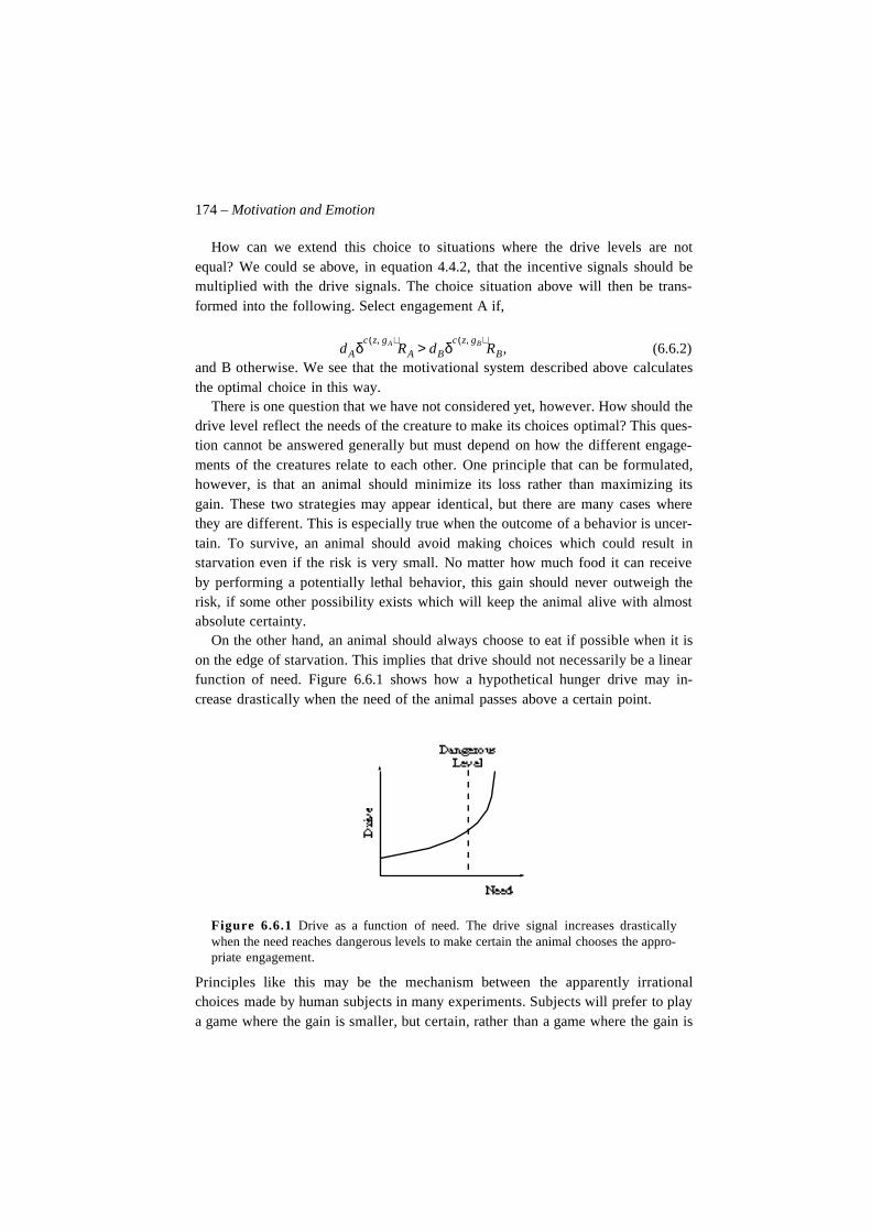
174 – Motivation and Emotion
How can we extend this choice to situations where the drive levels are notequal? We could se above, in equation 4.4.2, that the incentive signals should bemultiplied with the drive signals. The choice situation above will then be trans-formed into the following. Select engagement A if,
(6.6.2)and B otherwise. We see that the motivational system described above calculatesthe optimal choice in this way.
There is one question that we have not considered yet, however. How should thedrive level reflect the needs of the creature to make its choices optimal? This ques-tion cannot be answered generally but must depend on how the different engage-ments of the creatures relate to each other. One principle that can be formulated,however, is that an animal should minimize its loss rather than maximizing itsgain. These two strategies may appear identical, but there are many cases wherethey are different. This is especially true when the outcome of a behavior is uncer-tain. To survive, an animal should avoid making choices which could result instarvation even if the risk is very small. No matter how much food it can receiveby performing a potentially lethal behavior, this gain should never outweigh therisk, if some other possibility exists which will keep the animal alive with almostabsolute certainty.
On the other hand, an animal should always choose to eat if possible when it ison the edge of starvation. This implies that drive should not necessarily be a linearfunction of need. Figure 6.6.1 shows how a hypothetical hunger drive may in-crease drastically when the need of the animal passes above a certain point.
Figure 6.6.1 Drive as a function of need. The drive signal increases drasticallywhen the need reaches dangerous levels to make certain the animal chooses the appro-priate engagement.
Principles like this may be the mechanism between the apparently irrationalchoices made by human subjects in many experiments. Subjects will prefer to playa game where the gain is smaller, but certain, rather than a game where the gain is
dAδc z gA,( )
RA dBδc z gB,( )
RB> ,
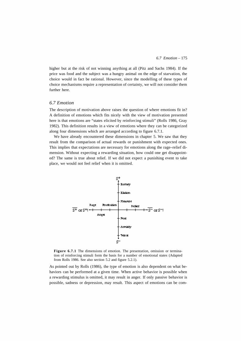
6.7 Emotion – 175
higher but at the risk of not winning anything at all (Pitz and Sachs 1984). If theprice was food and the subject was a hungry animal on the edge of starvation, thechoice would in fact be rational. However, since the modelling of these types ofchoice mechanisms require a representation of certainty, we will not consider themfurther here.
6.7 EmotionThe description of motivation above raises the question of where emotions fit in?A definition of emotions which fits nicely with the view of motivation presentedhere is that emotions are “states elicited by reinforcing stimuli” (Rolls 1986, Gray1982). This definition results in a view of emotions where they can be categorizedalong four dimensions which are arranged according to figure 6.7.1.
We have already encountered these dimensions in chapter 5. We saw that theyresult from the comparison of actual rewards or punishment with expected ones.This implies that expectations are necessary for emotions along the rage–relief di-mension. Without expecting a rewarding situation, how could one get disappoint-ed? The same is true about relief. If we did not expect a punishing event to takeplace, we would not feel relief when it is omitted.
Figure 6.7.1 The dimensions of emotion. The presentation, omission or termina-tion of reinforcing stimuli form the basis for a number of emotional states (Adaptedfrom Rolls 1986. See also section 5.2 and figure 5.2.1).
As pointed out by Rolls (1986), the type of emotion is also dependent on what be-haviors can be performed at a given time. When active behavior is possible whena rewarding stimulus is omitted, it may result in anger. If only passive behavior ispossible, sadness or depression, may result. This aspect of emotions can be com-
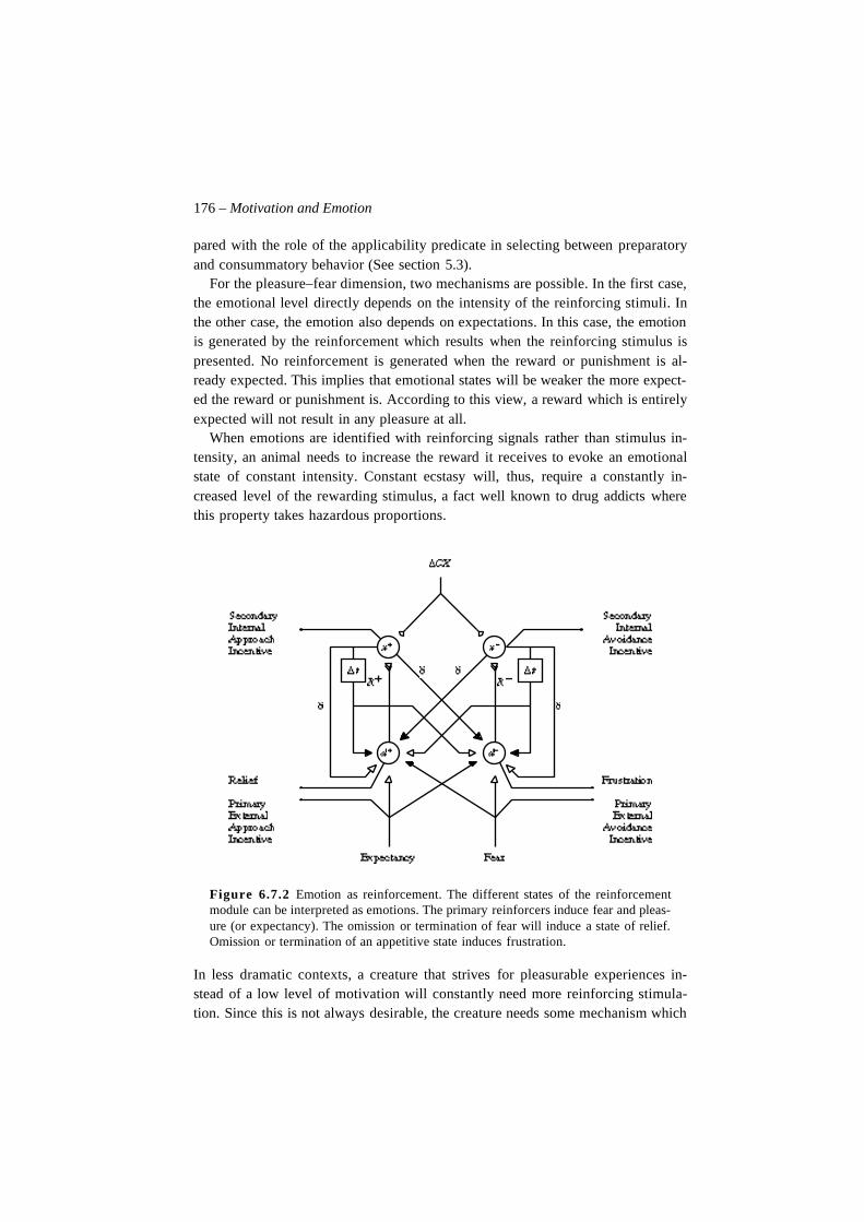
176 – Motivation and Emotion
pared with the role of the applicability predicate in selecting between preparatoryand consummatory behavior (See section 5.3).
For the pleasure–fear dimension, two mechanisms are possible. In the first case,the emotional level directly depends on the intensity of the reinforcing stimuli. Inthe other case, the emotion also depends on expectations. In this case, the emotionis generated by the reinforcement which results when the reinforcing stimulus ispresented. No reinforcement is generated when the reward or punishment is al-ready expected. This implies that emotional states will be weaker the more expect-ed the reward or punishment is. According to this view, a reward which is entirelyexpected will not result in any pleasure at all.
When emotions are identified with reinforcing signals rather than stimulus in-tensity, an animal needs to increase the reward it receives to evoke an emotionalstate of constant intensity. Constant ecstasy will, thus, require a constantly in-creased level of the rewarding stimulus, a fact well known to drug addicts wherethis property takes hazardous proportions.
Figure 6.7.2 Emotion as reinforcement. The different states of the reinforcementmodule can be interpreted as emotions. The primary reinforcers induce fear and pleas-ure (or expectancy). The omission or termination of fear will induce a state of relief.Omission or termination of an appetitive state induces frustration.
In less dramatic contexts, a creature that strives for pleasurable experiences in-stead of a low level of motivation will constantly need more reinforcing stimula-tion. Since this is not always desirable, the creature needs some mechanism which
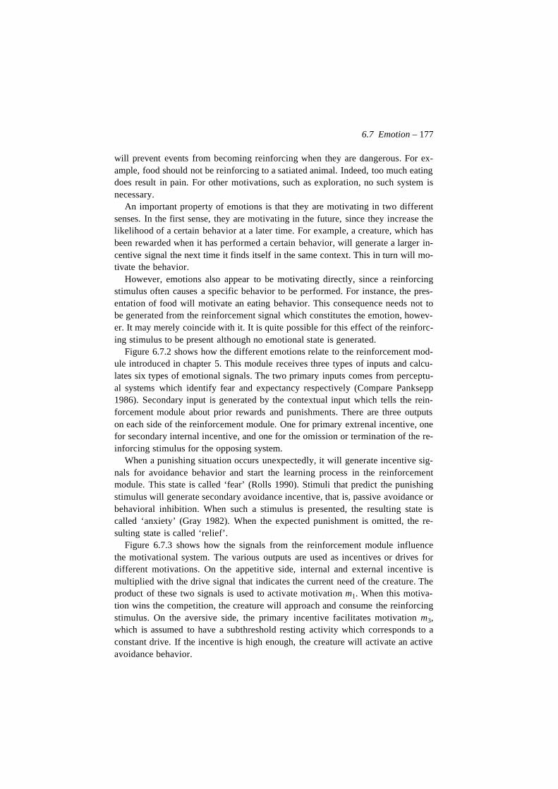
6.7 Emotion – 177
will prevent events from becoming reinforcing when they are dangerous. For ex-ample, food should not be reinforcing to a satiated animal. Indeed, too much eatingdoes result in pain. For other motivations, such as exploration, no such system isnecessary.
An important property of emotions is that they are motivating in two differentsenses. In the first sense, they are motivating in the future, since they increase thelikelihood of a certain behavior at a later time. For example, a creature, which hasbeen rewarded when it has performed a certain behavior, will generate a larger in-centive signal the next time it finds itself in the same context. This in turn will mo-tivate the behavior.
However, emotions also appear to be motivating directly, since a reinforcingstimulus often causes a specific behavior to be performed. For instance, the pres-entation of food will motivate an eating behavior. This consequence needs not tobe generated from the reinforcement signal which constitutes the emotion, howev-er. It may merely coincide with it. It is quite possible for this effect of the reinforc-ing stimulus to be present although no emotional state is generated.
Figure 6.7.2 shows how the different emotions relate to the reinforcement mod-ule introduced in chapter 5. This module receives three types of inputs and calcu-lates six types of emotional signals. The two primary inputs comes from perceptu-al systems which identify fear and expectancy respectively (Compare Panksepp1986). Secondary input is generated by the contextual input which tells the rein-forcement module about prior rewards and punishments. There are three outputson each side of the reinforcement module. One for primary extrenal incentive, onefor secondary internal incentive, and one for the omission or termination of the re-inforcing stimulus for the opposing system.
When a punishing situation occurs unexpectedly, it will generate incentive sig-nals for avoidance behavior and start the learning process in the reinforcementmodule. This state is called ‘fear’ (Rolls 1990). Stimuli that predict the punishingstimulus will generate secondary avoidance incentive, that is, passive avoidance orbehavioral inhibition. When such a stimulus is presented, the resulting state iscalled ‘anxiety’ (Gray 1982). When the expected punishment is omitted, the re-sulting state is called ‘relief’.
Figure 6.7.3 shows how the signals from the reinforcement module influencethe motivational system. The various outputs are used as incentives or drives fordifferent motivations. On the appetitive side, internal and external incentive ismultiplied with the drive signal that indicates the current need of the creature. Theproduct of these two signals is used to activate motivation m1. When this motiva-tion wins the competition, the creature will approach and consume the reinforcingstimulus. On the aversive side, the primary incentive facilitates motivation m3,which is assumed to have a subthreshold resting activity which corresponds to aconstant drive. If the incentive is high enough, the creature will activate an activeavoidance behavior.
178 – Motivation and Emotion
There are also two motivational states corresponding to the two emotional statesof relief and frustration. Both these emotions act as drives for particular motiva-tions. Motivation m1 which is associated with relief makes the creature act inwhatever way is appropriate when it feels relieved (perhaps it smiles). When astimulus appears that predicts punishment, motivation m4 is activated which gen-erates passive avoidance and when the creature becomes frustrated, motivation m5
is activated which may cause the creature to attack the cause of the frustration, orin other cases, an innocent bystander. Since there is no equivalent of behavioral in-hibition on the expectancy side of the reinforcement module, the effects of fearand expectancy are not symmetrical.
It is very common for the immediate motivation that accompanies emotions togenerate some form of communicative signals, but since we will not deal with so-cial interaction in this book, we will not consider them further here.
Figure 6.7.3 Motivational states influenced by the reinforcement module in figure6.7.2. Presentation, termination and omission of stimuli activate motivational statesfor agression and expressions of emotion. These motivations compete with the morebasic ones for appetitive and aversive behaviors.
The property of motivational states to cause frustration or relief when it is changedhas been called the motivational rebound effect . This effect rests on the fact thatmany motivational states seem to come in pairs: tiredness and wakefulness, hungerand satiety etc. When the need corresponding to the motivational state is satisfied,
6.8 The Roots of Motivation – 179
the opposite motivational state is activated. The phenomena have been much stud-ied, for example, in relation to drug abuse (Solomon 1980). The introduction of thedrug is followed by a state of happiness, but when the drug is removed the oppo-site feeling arises. The same is true of fear and relief. After being exposed to a sit-uation of extreme fear, the termination of fear does not result in a neutral state butrather in euphoria.
There is, however, more to motivation than can be included in the frameworkpresented above. In agreement with self-attribution theory (Schachter 1964), whata creature may experience as emotions is the result of its internal categorization ofthe motivational system and its effect on behavior. The motivational system, assuch, does not produce emotional experiences. The only function of the motiva-tional system is to direct behavior now and in the future. It may very well producethe external attributes of emotions such as a smile or tears, but the experience ofemotion is the result of an introspective process. This places the experience ofemotion clearly within the area of cognition.
This view also implies that emotions must be learned from experience. Howhunger effects behavior in the direction of food is not initially known to the ani-mal. It is learned from its own behavior and perhaps later learned to be ignored orsuppressed. If emotions are viewed in this way, it is not too remote to place loveand hate side by side to hunger and tiredness. They must all be experienced andlearned before they can become emotions. They differ in complexity only but notin nature.
To conclude it is possible to consider motivations as states which tell the organ-ism what it should do at a certain time based on its internal needs and external pos-sibilities. Emotion, on the other hand, is concerned with what the animal shouldhave done. When the reward or stimulus situation of the animal is unexpected, anemotional state is activated. This state has two functions. The first is to controllearning which lets the animal cope with the preceding situation in a better way thenext time it occurs. The second function is to motivate specific emotional behav-iors.
6.8 The Roots of Motivation
In this section, we will present a number of evolutionary steps that may have leadto the type of motivational system described above (See also Balkenius 1993). Todo this, we have to start with some design principles that seem reasonable from anevolutionary point of view. The first pair of principles is reduplication and varia-tion. Reduplication is a process which makes copies of an already existing struc-ture and variation is the process whereby existing structures can be changed. Wewant to propose that it is possible to find three architectural principles which su-perimpose on each other during evolution. Based on their underlying architectural
180 – Motivation and Emotion
principle, we can define three classes of systems: (1) the subsumption architecture,(2) the centralized control architecture, and (3) the layered architecture.
These architectural principles do not directly describe the motivational system,but the organism as a whole. Each class is necessary for the next to evolve andeach subsequent class of systems have a competetive advantage compared to sys-tems in the previous class. This ensures the adaptive value of architectural changeswhich moves a species towards a higher class. The rest of this section describes thedifferent classes in detail and identifies the necessary steps from one class to thenext.
The Subsumption Architecture
The simplest system will possess a subsumption architecture (Brooks 1986). Suchan architecture consists of a number of distributed systems which control differentbehaviors. They can, but need not interact, with each other. A subsumption archi-tecture typically consists of a number of layers which can subsume each other. Forexample, a lower layer can produce walking behavior while a layer on top tells itto walk forward, turn to the left or to the right. Within AI, this approach to the con-struction of intelligent robots have gained an increasing popularity during the lastfew years (Beer 1990).
An architecture of this kind has three main features. First, it is non-representa-tional. There do not exist any representations of the external world. Instead, theworld is used as its own best model (Brooks 1991a). Second, the creature is reac-tive. It reacts directly to stimuli in the world. For example, a creature can avoid anobstacle simply by changing the motor patterns of its legs when its whisker con-tacts with the obstacle. Third, behavior is distributed. Different behavioral mod-ules operate independently of each other to a large extent.
It is now possible to give examples of some simple creatures which use a sub-sumption architecture. We will try to keep the presentation as simple as possible toemphasize on the essential features of each architecture. Of course, real creaturesare much more complex.
Our simplest system will simply consist of sensors and effectors. The sensorsare connected directly to the effectors and either activate or inhibit them. Typicalexamples of such creatures are the vehicles invented by Braitenberg (1984). Thesimple control system of the vehicle is sufficient to produce taxic behavior. In pro-tozoa, the entire control system can reside in a single cell. In larger animals, how-ever, a simple nervous system is required to send the signal from the sensors to theeffectors.
In a larger creature, the need arises for a connecting inter-neuron between thesensor and effector. This step does not change the behavioral abilities of our crea-ture but is a requirement for its greater physical size. It is also essential to the fu-ture development of the species, as it is the origin of the nervous system. The next
6.8 The Roots of Motivation – 181
two classes can emerge in any order during evolution, but the two steps are bothnecessary for the evolution of the motivational system.
The introduction of an inter-neuron makes it possible for the sensory signals tointeract before they reach the effectors. For example, two sensory signals can con-verge on a single inter-neuron which will then detect the conjunction of two senso-ry events. It is also possible for one inter-neuron to inhibit or activate another in-ter-neuron to produce complex behavior. In these systems, the inter-neuronintegrates information from several sources and transforms it in some way insteadof just propagating it from one sensor to one effector. Many of the systems de-scribed in section 3.4 are of this kind.
A parallel development is the introduction of sensors which can be of twokinds: external and internal. This is the result of a bodily change that places somesensors inside the organism. An external sensor reacts on some external event orstate while an internal sensor reacts on the internal state of the organism. For ex-ample, the internal sensor of the feeding system could react on hunger and the ex-ternal system could react on food being present. If both sensors where signalling,an eating behavior would be triggered. Computer simulations have shown thatsuch nodes can spontaneously emerge during evolution (Cecconi and Parisi 1993).This is the origin of drives and incentives as defined above.
As in the simpler systems, a number of controlling systems can, in principle, ex-ist in parallel. Each system is governed by its own sensory signals which controlits behavior regardless of the other systems. The robots presented by Brooks(1991) are essentially of this complexity. They can produce very complex behav-ior without any central control mechanism. The central argument of this section isthat such an architecture cannot, however, be extended to include cognitive proc-esses without including a central control mechanism.
The Centralized Control Architecture
The creatures described above were characterized by the lack of central control.This is changed in the next class of creatures which exhibit the simplest possiblearchitecture capable of centralized decisions. This is a necessary step toward ahigher cognitive system and the origin of the motivational system. A similar posi-tion is held by Sjölander (1992) who discusses the need for centralized representa-tions of objects.
When the organism develop more complex behaviors, they will inevitably dis-turb each other. When this happens, it is essential that the different systems can in-hibit each other in order to produce one behavior at a time. In a neural context, thiscan be achieved by lateral inhibition (See section 3.3). There exist three differentforms of lateral inhibition which could produce the desired result: feed-forward in-hibition, feedback inhibition and recurrent inhibition (Grossberg 1973). Feed-for-ward inhibition is primarily used in other contexts to compensate for different
182 – Motivation and Emotion
overall activity levels (for example in the visual system in the LGN). Feedback in-hibition have been used in at least one model of animal behavior which was basedon the theories of Lorenz and Tinbergen (See Schnepf 1991).
In the following, we will assume that our creature is using recurrent inhibitionto select one behavior instead of the other as described above. The properties of re-current inhibition are essentially the same as for feedback inhibition, but they aresimpler to analyze. In a recurrent network where the lateral inhibitory connectionsare of the same strength, the behavior that receives the most activation will be se-lected. One layer collects the activation of each behavioral system and the nextlayer is responsible for the selection of the behavior with the strongest activation.
The Layered Architecture
The next evolutionary step is to include several levels of control. This is not to saythat a layered architecture is not possible on the lower levels. Indeed, the subsump-tion architecture is typically constructed in a number of layers. However, the na-ture of those layers are very different from the layers discussed here.
At this final stage, the system can develop in a new way. While the basic sub-sumption architecture, together with the lateral inhibition, keeps the creature alive,evolution can experiment on the next layer of our architecture. One of the mostpowerful mechanisms invented by evolution is that of learning. A learning abilitycan evolve on top of the previous system once motivation has been included, sincelearning has an obvious relation to motivation as we have seen above. Learningneeds the motivational state to detemine when a certain behavior is good. Withoutit, the creature could only learn that a behavior is good or bad, but could not relateit any of its needs.
The learning architecture makes it useful for the animal to develop a more ad-vanced perceptual system. It can supply the learning system with more advancedperceptual cues. Mechanisms for categorization and classification will now givethe animal an adaptive advantage. From these capabilities evolves the mecha-nisms, which are usually considered to constitute cognition.
6.9 Conclusion
Words such as drive, incentive, motivation and emotion have had many differentmeanings within different theories. Even today there is no consensus as to what,for example, an emotion is (LeDoux 1995). What is called drive in one theory maybe called emotion or motivation in another. We have tried to use these word in away that is, at least, consistent with each other while retaining as much as possibleof their ordinary meaning. Since our main concern is artificial creatures rather thanreal animals, one cannot help feeling that these concepts are more complicated inreal animals. Clearly, we are nowhere close to the complexity of human emotions.
6.9 Conclusion – 183
We believe, however, that in taking a design perspective on motivation and emo-tion, we have shown that these concepts can be used to great utility in the design ofartificial creatures.
We have seen that a creature needs a central motivational state which is respon-sible for the selection of one motivation at a time. This requirement is closely con-nected to the idea of separate modules for different engagements which is essen-tially a strategy for task decomposition (Tenenberg, Karlsson and Whitehead1993).
The choice of motivational state is influenced by three factors called internaland external incentive and drive. The incentives tell the creature about the currentpossibilities of fulfilling a need, while the drive signal informs it about the urgencyof that need. Incentives can also be classified as primary , that is, innate, or as sec-ondary , that is, acquired. Primary incentives were mapped onto the concept of pri-mary motivators, and secondary incentives were considered as secondary motiva-tors. This implies a close coupling between perception and motivation as will befurther developed in the next chapter.
The view of drives, which we have presented, assumes that there is one or sev-eral drives for each engagement of an animal. This is thus an attempt to resurrectone of the original meanings of the word drive where it was more or less analogousto the concept of an instinct. While it has been argued that the explanatory value ofthis drive concept is nil (See Bolles 1967), we hope to have shown that it is quiteuseful from a design perspective. This usefulness comes from the separation of thedrive concept from the engagement it controls.
The idea of pure emotions relating to a small set of biological processes is verysimilar to the idea of engagement systems described above (See Plutchik 1991).The problem for any such theory of emotion (or motivation) is, of course, to iden-tify exactly which these basic processes are (Ortony, Clore and Collins 1988). Wehave made no attempt to produce a comprehensive list of engagements, since wedo not believe that any such general list exists. The set of engagement systems re-quired by an artificial creature depends critically on what it is supposed to do, andso will its emotions.
It was shown how emotions can be seen as states caused by reinforcing stimuli.Depending on the nature of the stimulus, emotions could be categorized into fourbasic dimensions: pleasure, fear, frustration and relief. It was also shown how in-centives could be generated by the reinforcement module.
As mentioned at the end of chapter 5, the perfect symmetry between the differ-ent emotions is a simplification. Since many different engagement systems are in-volved, it would be more accurate to depict emotions in a three dimensional spacewhere the third dimension would represent the engagement. Some engagementsmay not include both the positive and negative side of the diagram shown in sec-tion 6.7. For example, an engagement system for aggression may not include the
184 – Motivation and Emotion
pleasurable side. Such an engagement system may, however, interact with othersystems (Compare Konorski 1967).
It has been suggested that the amygdala controls the emotional processes whichform associations with primary reward and punishment, while the orbitofrontalcortex may be involved in the detection of mismatch between actual and expectedreward or punishment which results in frustration or relief (Rolls 1986, 1995). Theamygdala receives inputs from a large variety of sources in the overlying temporallobe cortex and other areas. Some outputs from the amygdala, as well as from or-bitofrontal cortex, are directed towards the hypohalamus which is known to medi-ate motivational and emotional responses (Rolls 1986).
To summarize, the basic function of motivations is to tell the creature what itshould do, while the role of emotions is to tell the creature what it should havedone.
Christian Balkenius, 1995, Natural Intelligence in Artificial Creatures, Lund University Cognitive Studies 37, 1995.
Chapter 7
Perception
7.1 IntroductionAlthough this chapter is called perception, we will make no attempt to cover thiscomplex but interesting area to any great extent. Even for the simple modalities ofour artificial creatures, this would probably require more space than this entirebook offers. What we will do, instead, is to discuss what role perception plays inan organism and how it relates to the other areas we have already discussed. Whatis the role of perception in learning and behavior? How does it influence motiva-tion and emotion? How is perception controlled by the motivational state?
Depending on our perspective, the mechanisms we will present can be consid-ered to control either perception, associative learning or motor control. We willsee that it is not possible to make any clear distinction between these processes.We will identify at least three different roles that perception plays in an organism1.
The first is to characterize the situation in which the organism finds itself. Is itnew or familiar? Does the animal know what to do in this situation? The character-ization of the situation is used as the context in which behavior is performed. Thisis the origin of the contextual representation used in chapter 5. We will present amechanism that creates new situation categories when they are needed. Such a
1. Compare these functions of perception to the different types of stimuli that were used toinfluence associative learning in section 5.2 (See also figure 5.2.3)
186 – Perception
mechanism is also necessary for stimulus–response learning when the stimuli in-volved are not innately recognized.
The second function of perception is to guide the animal toward or away from aplace, situation or object. Which way should the animal move to reach an objectnot visible from its current location? We have already discussed this mechanism instimulus–approach behavior. In this chapter, we will extend it to place–approachor piloting behavior as defined in chapter 2. The important mechanism here will bethe ability to learn and perceive configurations of stimuli.
The third function of perception is to tell the motivational system about the ex-ternal possibilities present at a certain time. This mechanism was introduced inchapter 6 in relation to motivation. The signals sent to the motivational systemfrom the perceptual apparatus were called external incentives. They make it possi-ble for the motivational system to select the engagement which has the greatestchance of success at a given moment.
A related phenomenon is the motivational influence on perception. A hungryanimal will be more likely to perceive food related stimuli than a satiated one. Thismeans that the motivational state must somehow be able to bias the perceptualprocess. We, thus, need to transfer information in both directions between the per-ceptual and the motivational system. We will argue that the interaction betweenmotivation and perception is the basis for one form of attention.
7.2 Situational CategoriesIn chapter 4, we assumed that there were sensors for every stimulus relevant to theanimal. This was, of course, a simplification. In an environment with some com-plexity, it would constitute a large burden for a creature to have innate recognitionmechanisms for all potential stimuli, most of which it would never encounter. Amuch more economical solution would be to create new categories when unknownstimuli are enountered. This leaves us with a new problem. How do we know whena stimulus is unknown?
There are two distinct ways in which such a situation can be recognized. Thefirst mechanism is based on the similarity between the present stimulus and the al-ready recognized stimulus categories. If a stimulus does not match any of theknown categories sufficiently well, a new category must be created.
The other possible basis for category formation is to look at the predictionsmade from a recognized stimulus. If these predictions match expectations, every-thing is fine. If not, a new category may have to be created. We will see that thissecond mechanism depends on an ability to form expectations by classical condi-tioning.
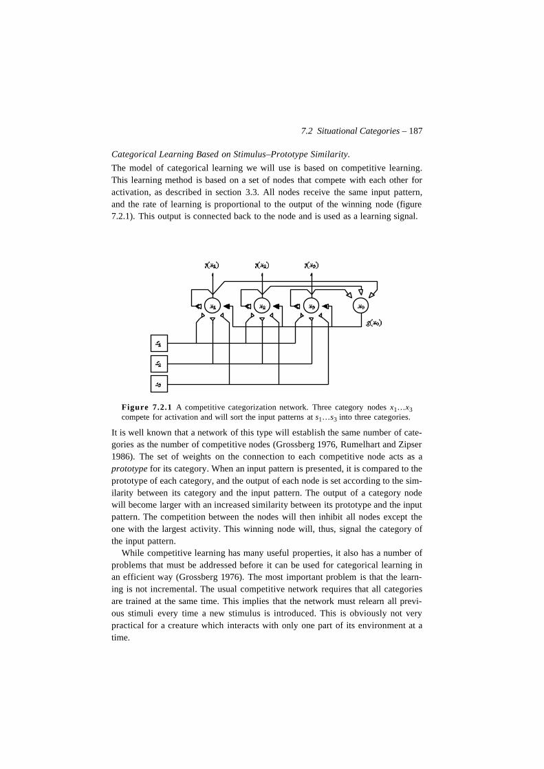
7.2 Situational Categories – 187
Categorical Learning Based on Stimulus–Prototype Similarity.
The model of categorical learning we will use is based on competitive learning.This learning method is based on a set of nodes that compete with each other foractivation, as described in section 3.3. All nodes receive the same input pattern,and the rate of learning is proportional to the output of the winning node (figure7.2.1). This output is connected back to the node and is used as a learning signal.
Figure 7.2.1 A competitive categorization network. Three category nodes x1…x3compete for activation and will sort the input patterns at s1…s3 into three categories.
It is well known that a network of this type will establish the same number of cate-gories as the number of competitive nodes (Grossberg 1976, Rumelhart and Zipser1986). The set of weights on the connection to each competitive node acts as aprototype for its category. When an input pattern is presented, it is compared to theprototype of each category, and the output of each node is set according to the sim-ilarity between its category and the input pattern. The output of a category nodewill become larger with an increased similarity between its prototype and the inputpattern. The competition between the nodes will then inhibit all nodes except theone with the largest activity. This winning node will, thus, signal the category ofthe input pattern.
While competitive learning has many useful properties, it also has a number ofproblems that must be addressed before it can be used for categorical learning inan efficient way (Grossberg 1976). The most important problem is that the learn-ing is not incremental. The usual competitive network requires that all categoriesare trained at the same time. This implies that the network must relearn all previ-ous stimuli every time a new stimulus is introduced. This is obviously not verypractical for a creature which interacts with only one part of its environment at atime.
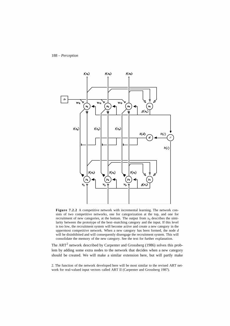
188 – Perception
Figure 7.2.2 A competitive network with incremental learning. The network con-sists of two competitive networks, one for categorization at the top, and one forrecruitment of new categories, at the bottom. The output from x0 describes the simi-larity between the prototype of the best–matching category and the input. If this levelis too low, the recruitment system will become active and create a new category in theuppermost competitive network. When a new category has been formed, the node dwill be disinhibited and will consequently disengage the recruitment system. This willconsolidate the memory of the new category. See the text for further explanation.
The ART2 network described by Carpenter and Grossberg (1986) solves this prob-lem by adding some extra nodes to the network that decides when a new categoryshould be created. We will make a similar extension here, but will partly make
2. The function of the network developed here will be most similar to the revised ART net-work for real-valued input vectors called ART II (Carpenter and Grossberg 1987).
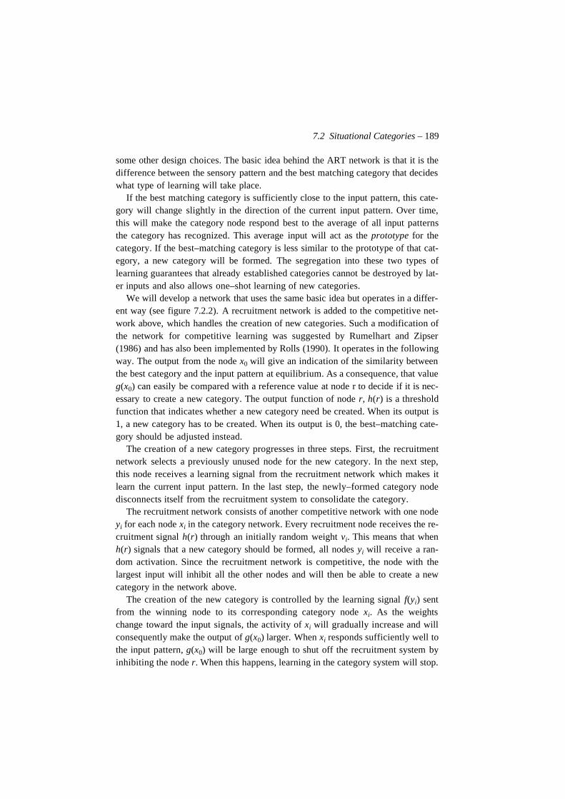
7.2 Situational Categories – 189
some other design choices. The basic idea behind the ART network is that it is thedifference between the sensory pattern and the best matching category that decideswhat type of learning will take place.
If the best matching category is sufficiently close to the input pattern, this cate-gory will change slightly in the direction of the current input pattern. Over time,this will make the category node respond best to the average of all input patternsthe category has recognized. This average input will act as the prototype for thecategory. If the best–matching category is less similar to the prototype of that cat-egory, a new category will be formed. The segregation into these two types oflearning guarantees that already established categories cannot be destroyed by lat-er inputs and also allows one–shot learning of new categories.
We will develop a network that uses the same basic idea but operates in a differ-ent way (see figure 7.2.2). A recruitment network is added to the competitive net-work above, which handles the creation of new categories. Such a modification ofthe network for competitive learning was suggested by Rumelhart and Zipser(1986) and has also been implemented by Rolls (1990). It operates in the followingway. The output from the node x0 will give an indication of the similarity betweenthe best category and the input pattern at equilibrium. As a consequence, that valueg(x0) can easily be compared with a reference value at node r to decide if it is nec-essary to create a new category. The output function of node r, h(r) is a thresholdfunction that indicates whether a new category need be created. When its output is1, a new category has to be created. When its output is 0, the best–matching cate-gory should be adjusted instead.
The creation of a new category progresses in three steps. First, the recruitmentnetwork selects a previously unused node for the new category. In the next step,this node receives a learning signal from the recruitment network which makes itlearn the current input pattern. In the last step, the newly–formed category nodedisconnects itself from the recruitment system to consolidate the category.
The recruitment network consists of another competitive network with one nodeyi for each node xi in the category network. Every recruitment node receives the re-cruitment signal h(r) through an initially random weight vi. This means that whenh(r) signals that a new category should be formed, all nodes yi will receive a ran-dom activation. Since the recruitment network is competitive, the node with thelargest input will inhibit all the other nodes and will then be able to create a newcategory in the network above.
The creation of the new category is controlled by the learning signal f(yi) sentfrom the winning node to its corresponding category node xi. As the weightschange toward the input signals, the activity of xi will gradually increase and willconsequently make the output of g(x0) larger. When xi responds sufficiently well tothe input pattern, g(x0) will be large enough to shut off the recruitment system byinhibiting the node r. When this happens, learning in the category system will stop.
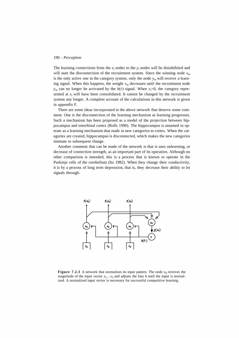
190 – Perception
The learning connections from the xi nodes to the yi nodes will be disinhibited andwill start the disconnection of the recruitment system. Since the winning node xm
is the only active one in the category system, only the node ym will receive a learn-ing signal. When this happens, the weight vm decreases until the recruitment nodeym can no longer be activated by the h(r) signal. When vi=0, the category repre-sented at xi will have been consolidated. It cannot be changed by the recruitmentsystem any longer. A complete account of the calculations in this network is givenin appendix F.
There are some ideas incorporated in the above network that deserve some com-ment. One is the disconnection of the learning mechanism as learning progresses.Such a mechanism has been proposed as a model of the projection between hip-pocampus and entorhinal cortex (Rolls 1990). The hippocampus is assumed to op-erate as a learning mechanism that reads in new categories to cortex. When the cat-egories are created, hippocampus is disconnected, which makes the new categoriesimmune to subsequent change.
Another comment that can be made of the network is that is uses unlearning, ordecrease of connection strength, as an important part of its operation. Although noother comparison is intended, this is a process that is known to operate in thePurkinje cells of the cerebellum (Ito 1982). When they change their conductivity,it is by a process of long term depression, that is, they decrease their ability to letsignals through.
Figure 7.2.3 A network that normalizes its input pattern. The node x0 receives themagnitude of the input vector s1…s3 and adjusts the bias b until the input is normal-ized. A normalized input vector is necessary for successful competitive learning.
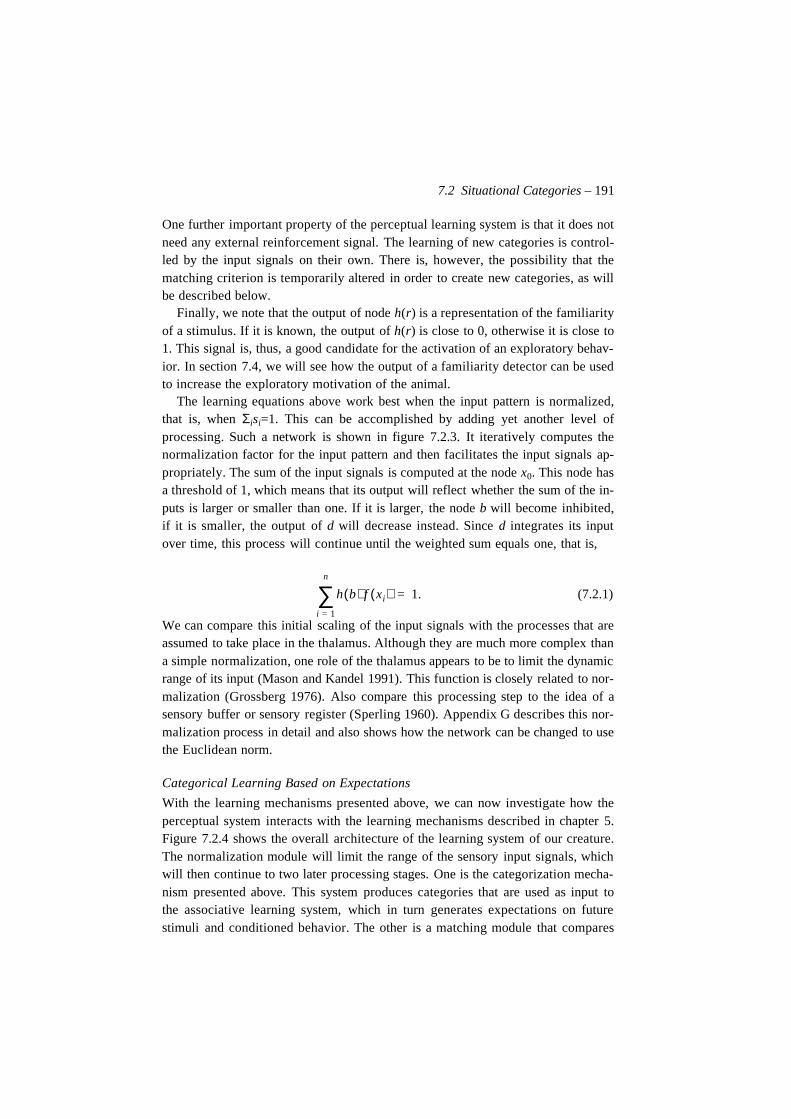
7.2 Situational Categories – 191
One further important property of the perceptual learning system is that it does notneed any external reinforcement signal. The learning of new categories is control-led by the input signals on their own. There is, however, the possibility that thematching criterion is temporarily altered in order to create new categories, as willbe described below.
Finally, we note that the output of node h(r) is a representation of the familiarityof a stimulus. If it is known, the output of h(r) is close to 0, otherwise it is close to1. This signal is, thus, a good candidate for the activation of an exploratory behav-ior. In section 7.4, we will see how the output of a familiarity detector can be usedto increase the exploratory motivation of the animal.
The learning equations above work best when the input pattern is normalized,that is, when Σisi=1. This can be accomplished by adding yet another level ofprocessing. Such a network is shown in figure 7.2.3. It iteratively computes thenormalization factor for the input pattern and then facilitates the input signals ap-propriately. The sum of the input signals is computed at the node x0. This node hasa threshold of 1, which means that its output will reflect whether the sum of the in-puts is larger or smaller than one. If it is larger, the node b will become inhibited,if it is smaller, the output of d will decrease instead. Since d integrates its inputover time, this process will continue until the weighted sum equals one, that is,
(7.2.1)
We can compare this initial scaling of the input signals with the processes that areassumed to take place in the thalamus. Although they are much more complex thana simple normalization, one role of the thalamus appears to be to limit the dynamicrange of its input (Mason and Kandel 1991). This function is closely related to nor-malization (Grossberg 1976). Also compare this processing step to the idea of asensory buffer or sensory register (Sperling 1960). Appendix G describes this nor-malization process in detail and also shows how the network can be changed to usethe Euclidean norm.
Categorical Learning Based on Expectations
With the learning mechanisms presented above, we can now investigate how theperceptual system interacts with the learning mechanisms described in chapter 5.Figure 7.2.4 shows the overall architecture of the learning system of our creature.The normalization module will limit the range of the sensory input signals, whichwill then continue to two later processing stages. One is the categorization mecha-nism presented above. This system produces categories that are used as input tothe associative learning system, which in turn generates expectations on futurestimuli and conditioned behavior. The other is a matching module that compares
h b( ) f xi( )i 1=
n
∑ 1.=
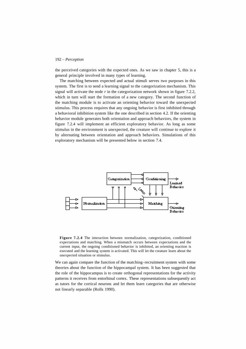
192 – Perception
the perceived categories with the expected ones. As we saw in chapter 5, this is ageneral principle involved in many types of learning.
The matching between expected and actual stimuli serves two purposes in thissystem. The first is to send a learning signal to the categorization mechanism. Thissignal will activate the node r in the categorization network shown in figure 7.2.2,which in turn will start the formation of a new category. The second function ofthe matching module is to activate an orienting behavior toward the unexpectedstimulus. This process requires that any ongoing behavior is first inhibited througha behavioral inhibition system like the one described in section 4.2. If the orientingbehavior module generates both orientation and approach behaviors, the system infigure 7.2.4 will implement an efficient exploratory behavior. As long as somestimulus in the environment is unexpected, the creature will continue to explore itby alternating between orientation and approach behaviors. Simulations of thisexploratory mechanism will be presented below in section 7.4.
Figure 7.2.4 The interaction between normalization, categorization, conditionedexpectations and matching. When a mismatch occurs between expectations and thecurrent input, the ongoing conditioned behavior is inhibited, an orienting reaction isexecuted and the learning system is activated. This will let the creature learn about theunexpected situation or stimulus.
We can again compare the function of the matching–recruitment system with sometheories about the function of the hippocampal system. It has been suggested thatthe role of the hippocampus is to create orthogonal representations for the activitypatterns it receives from entorhinal cortex. These representations subsequently actas tutors for the cortical neurons and let them learn categories that are otherwisenot linearly separable (Rolls 1990).

7.2 Situational Categories – 193
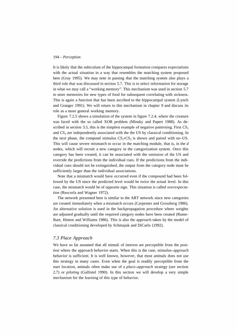
194 – Perception
It is likely that the subiculum of the hippocampal formation compares expectationswith the actual situation in a way that resembles the matching system proposedhere (Gray 1995). We may note in passing that the matching system also plays athird role that was discussed in section 5.7. This is to select information for storagein what we may call a “working memory”. This mechanism was used in section 5.7to store memories for new types of food for subsequent correlating with sickness.This is again a function that has been ascribed to the hippocampal system (Lynchand Granger 1991). We will return to this mechanism in chapter 9 and discuss itsrole as a more general working memory.
Figure 7.2.5 shows a simulation of the system in figure 7.2.4, where the creaturewas faced with the so called XOR problem (Minsky and Papert 1988). As de-scribed in section 3.5, this is the simplest example of negative patterning. First CS1
and CS2 are independently associated with the the US by classical conditioning. Inthe next phase, the compund stimulus CS1•CS2 is shown and paired with no–US.This will cause severe mismatch to occur in the matching module, that is, in the dnodes, which will recruit a new category in the categorization system. Once thiscategory has been created, it can be associated with the omission of the US andoverride the predictions from the individual cues. If the predictions from the indi-vidual cues should not be extinguished, the output from the category node must besufficiently larger than the individual associations.
Note that a mismatch would have occurred even if the compound had been fol-lowed by the US since the predicted level would be twice the actual level. In thiscase, the mismatch would be of opposite sign. This situation is called overexpecta-tion (Rescorla and Wagner 1972).
The network presented here is similar to the ART network since new categoriesare created immediately when a mismatch occurs (Carpenter and Grossberg 1986).An alternative solution is used in the backpropagation procedure where weightsare adjusted gradually until the required category nodes have been created (Rume-lhart, Hinton and Williams 1986). This is also the approach taken by the model ofclassical conditioning developed by Schmajuk and DiCarlo (1992).
7.3 Place Approach
We have so far assumed that all stimuli of interest are perceptible from the posi-tion where the approach behavior starts. When this is the case, stimulus–approachbehavior is sufficient. It is well known, however, that most animals does not usethis strategy in many cases. Even when the goal is readily perceptible from thestart location, animals often make use of a place–approach strategy (see section2.7) or piloting (Gallistel 1990). In this section we will develop a very simplemechanism for the learning of this type of behavior.
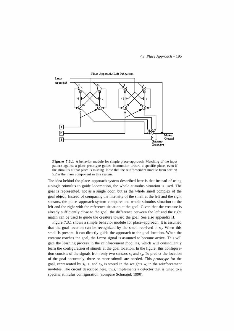
7.3 Place Approach – 195
Figure 7.3.1 A behavior module for simple place–approach. Matching of the inputpattern against a place prototype guides locomotion toward a specific place, even ifthe stimulus at that place is missing. Note that the reinforcement module from section5.2 is the main component in this system.
The idea behind the place–approach system described here is that instead of usinga single stimulus to guide locomotion, the whole stimulus situation is used. Thegoal is represented, not as a single odor, but as the whole smell complex of thegoal object. Instead of comparing the intensity of the smell at the left and the rightsensors, the place–approach system compares the whole stimulus situation to theleft and the right with the reference situation at the goal. Given that the creature isalready sufficiently close to the goal, the difference between the left and the rightmatch can be used to guide the creature toward the goal. See also appendix H.
Figure 7.3.1 shows a simple behavior module for place–approach. It is assumedthat the goal location can be recognized by the smell received at s0. When thissmell is present, it can directly guide the approach to the goal location. When thecreature reaches the goal, the Learn signal is assumed to become active. This willgate the learning process in the reinforcement modules, which will consequentlylearn the configuration of stimuli at the goal location. In the figure, this configura-tion consists of the signals from only two sensors s1 and s2. To predict the locationof the goal accurately, three or more stimuli are needed. This prototype for thegoal, represented by s0, s1 and s2, is stored in the weights wi in the reinforcementmodules. The circuit described here, thus, implements a detector that is tuned to aspecific stimulus configuration (compare Schmajuk 1990).
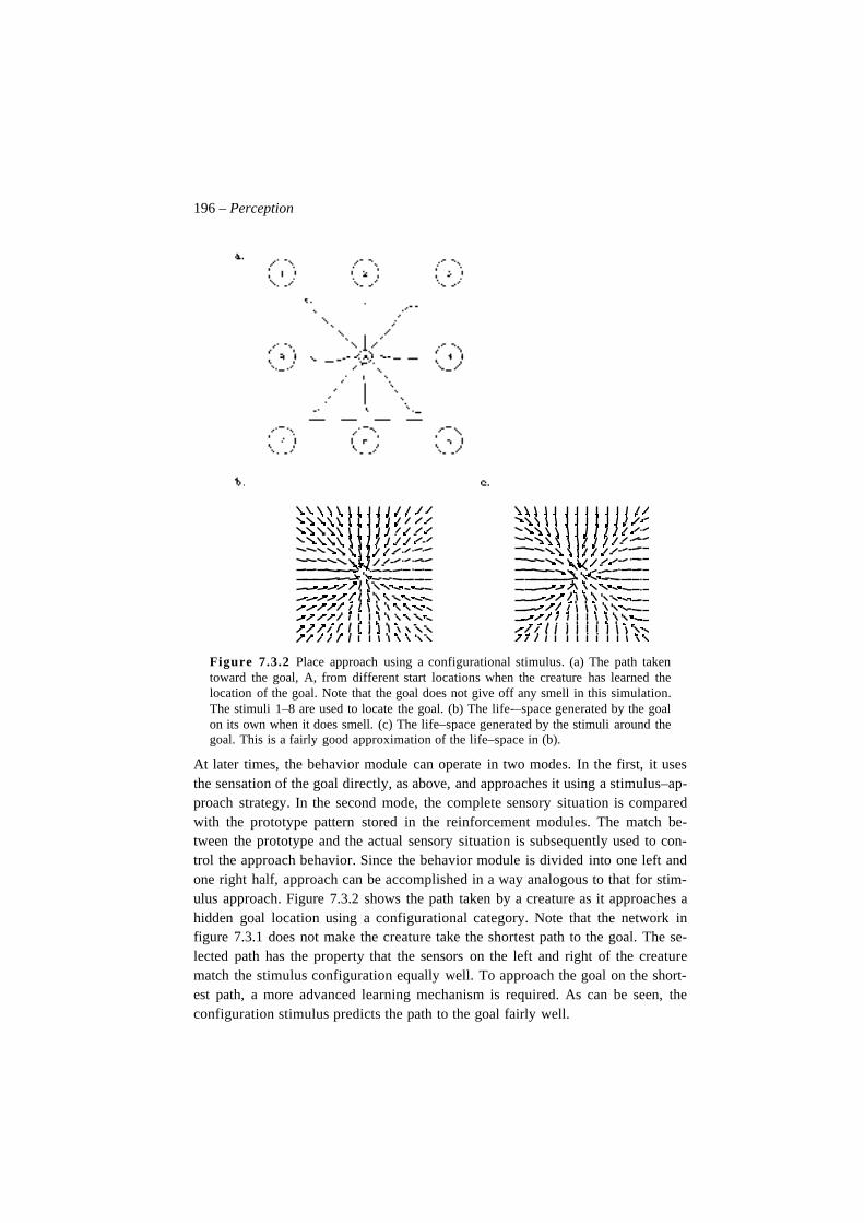
196 – Perception
Figure 7.3.2 Place approach using a configurational stimulus. (a) The path takentoward the goal, A, from different start locations when the creature has learned thelocation of the goal. Note that the goal does not give off any smell in this simulation.The stimuli 1–8 are used to locate the goal. (b) The life-–space generated by the goalon its own when it does smell. (c) The life–space generated by the stimuli around thegoal. This is a fairly good approximation of the life–space in (b).
At later times, the behavior module can operate in two modes. In the first, it usesthe sensation of the goal directly, as above, and approaches it using a stimulus–ap-proach strategy. In the second mode, the complete sensory situation is comparedwith the prototype pattern stored in the reinforcement modules. The match be-tween the prototype and the actual sensory situation is subsequently used to con-trol the approach behavior. Since the behavior module is divided into one left andone right half, approach can be accomplished in a way analogous to that for stim-ulus approach. Figure 7.3.2 shows the path taken by a creature as it approaches ahidden goal location using a configurational category. Note that the network infigure 7.3.1 does not make the creature take the shortest path to the goal. The se-lected path has the property that the sensors on the left and right of the creaturematch the stimulus configuration equally well. To approach the goal on the short-est path, a more advanced learning mechanism is required. As can be seen, theconfiguration stimulus predicts the path to the goal fairly well.
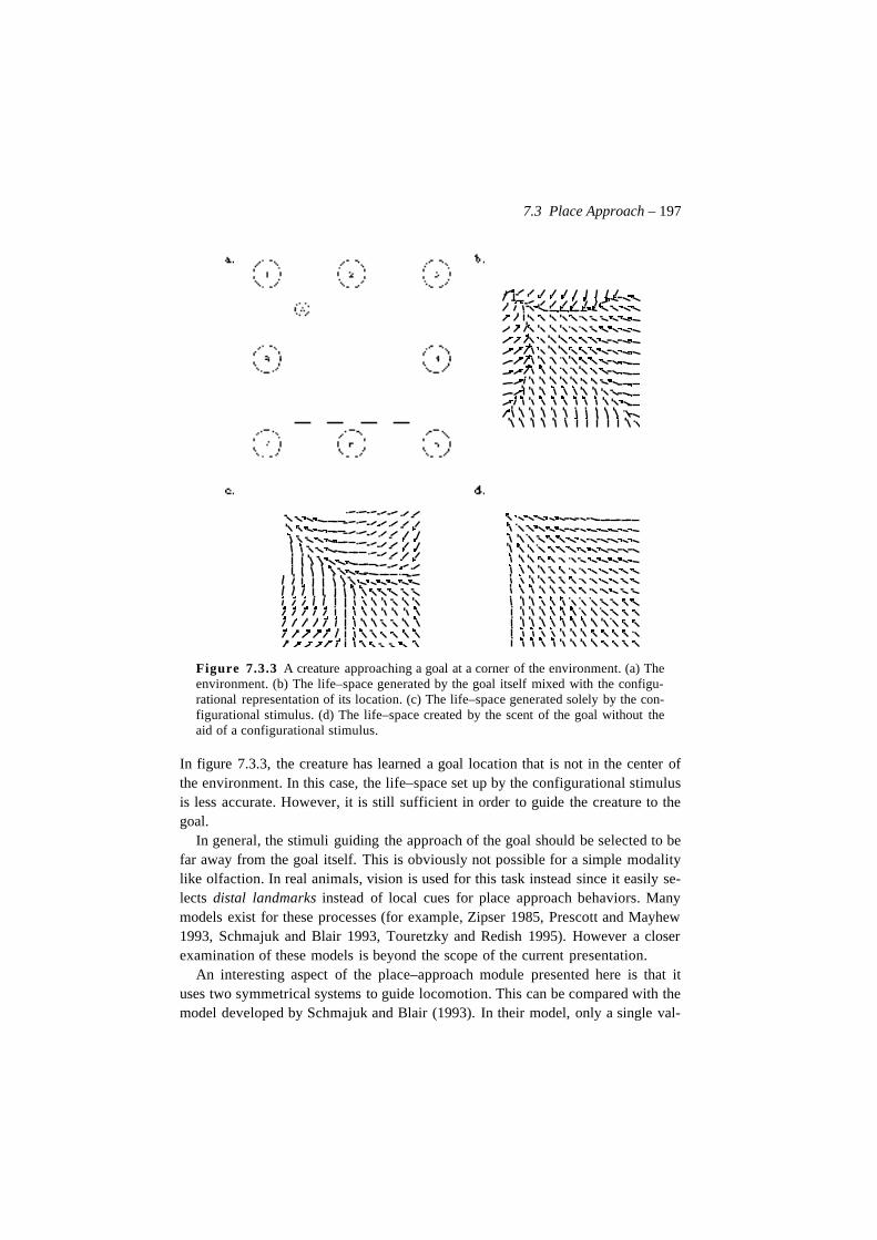
7.3 Place Approach – 197
Figure 7.3.3 A creature approaching a goal at a corner of the environment. (a) Theenvironment. (b) The life–space generated by the goal itself mixed with the configu-rational representation of its location. (c) The life–space generated solely by the con-figurational stimulus. (d) The life–space created by the scent of the goal without theaid of a configurational stimulus.
In figure 7.3.3, the creature has learned a goal location that is not in the center ofthe environment. In this case, the life–space set up by the configurational stimulusis less accurate. However, it is still sufficient in order to guide the creature to thegoal.
In general, the stimuli guiding the approach of the goal should be selected to befar away from the goal itself. This is obviously not possible for a simple modalitylike olfaction. In real animals, vision is used for this task instead since it easily se-lects distal landmarks instead of local cues for place approach behaviors. Manymodels exist for these processes (for example, Zipser 1985, Prescott and Mayhew1993, Schmajuk and Blair 1993, Touretzky and Redish 1995). However a closerexamination of these models is beyond the scope of the current presentation.
An interesting aspect of the place–approach module presented here is that ituses two symmetrical systems to guide locomotion. This can be compared with themodel developed by Schmajuk and Blair (1993). In their model, only a single val-
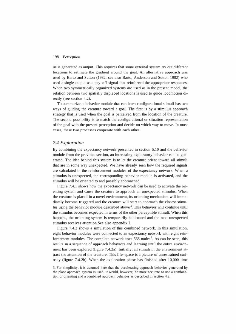
198 – Perception
ue is generated as output. This requires that some external system try out differentlocations to estimate the gradient around the goal. An alternative approach wasused by Barto and Sutton (1982, see also Barto, Anderson and Sutton 1982) whoused a single output as a pay–off signal that reinforced the appropriate responses.When two symmetrically organized systems are used as in the present model, therelation between two spatially displaced locations is used to guide locomotion di-rectly (see section 4.2).
To summarize, a behavior module that can learn configurational stimuli has twoways of guiding the creature toward a goal. The first is by a stimulus approachstrategy that is used when the goal is perceived from the location of the creature.The second possibility is to match the configurational or situation representationof the goal with the present perception and decide on which way to move. In mostcases, these two processes cooperate with each other.
7.4 ExplorationBy combining the expectancy network presented in section 5.10 and the behaviormodule from the previous section, an interesting exploratory behavior can be gen-erated. The idea behind this system is to let the creature orient toward all stimulithat are in some way unexpected. We have already seen how the required signalsare calculated in the reinforcement modules of the expectancy network. When astimulus is unexpected, the corresponding behavior module is activated, and thestimulus will be oriented to and possibly approached.
Figure 7.4.1 shows how the expectancy network can be used to activate the ori-enting system and cause the creature to approach an unexpected stimulus. Whenthe creature is placed in a novel environment, its orienting mechanism will imme-diately become triggered and the creature will start to approach the closest stimu-lus using the behavior module described above3. This behavior will continue untilthe stimulus becomes expected in terms of the other perceptible stimuli. When thishappens, the orienting system is temporarily habituated and the next unexpectedstimulus receives attention.See also appendix I.
Figure 7.4.2 shows a simulation of this combined network. In this simulation,eight behavior modules were connected to an expectancy network with eight rein-forcement modules. The complete network uses 568 nodes4. As can be seen, thisresults in a sequence of approach behaviors and learning until the entire environ-ment has been explored (figure 7.4.2a). Initially, all stimuli in the environment at-tract the attention of the creature. This life–space is a picture of unrestrained curi-osity (figure 7.4.2b). When the exploration phase has finished after 10,000 time
3. For simplicity, it is assumed here that the accelerating approach behavior generated bythe place approach system is used. It would, however, be more accurate to use a combina-tion of orienting and a combined approach behavior as described in section 4.2.
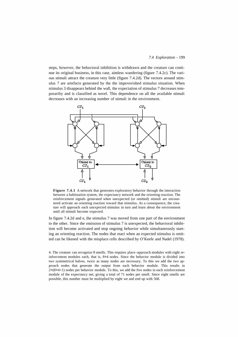
7.4 Exploration – 199
steps, however, the behavioral inhibition is withdrawn and the creature can conti-nue its original business, in this case, aimless wandering (figure 7.4.2c). The vari-ous stimuli attract the creature very little (figure 7.4.2d). The vectors around stim-ulus 7 are artefacts generated by the the impoverished stimulus situation. Whenstimulus 3 disappears behind the wall, the expectation of stimulus 7 decreases tem-porariliy and is classified as novel. This dependence on all the available stimulidecreases with an increasing number of stimuli in the environment.
Figure 7.4.1 A network that generates exploratory behavior through the interactionbetween a habituation system, the expectancy network and the orienting reaction. Thereinforcement signals generated when unexpected (or omitted) stimuli are encoun-tered activate an orienting reaction toward that stimulus. As a consequence, the crea-ture will approach each unexpected stimulus in turn and learn about the environmentuntil all stimuli become expected.
In figure 7.4.2d and e, the stimulus 7 was moved from one part of the environmentto the other. Since the omission of stimulus 7 is unexpected, the behavioral inhibi-tion will become activated and stop ongoing behavior while simultaneously start-ing an orienting reaction. The nodes that react when an expected stimulus is omit-ted can be likened with the misplace cells described by O’Keefe and Nadel (1978).
4. The creature can recognize 8 smells. This requires place–approach modules with eight re-inforcement modules each, that is, 8×4 nodes. Since the behavior module is divided intotwo symmetrical halves, twice as many nodes are necessary. To this we add the two ap-proach nodes that generate the output from each behavior module. This results in2×(8×4+1) nodes per behavior module. To this, we add the five nodes in each reinforcementmodule of the expectancy net, giving a total of 71 nodes per smell. Since eight smells arepossible, this number must be multiplied by eight we and end up with 568.
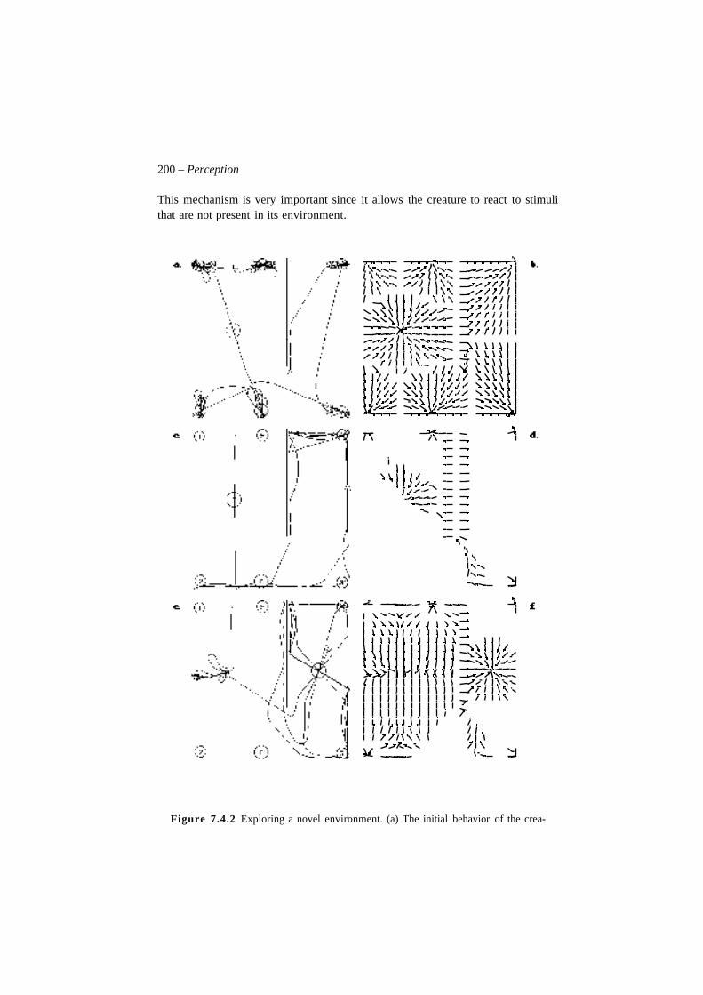
200 – Perception
This mechanism is very important since it allows the creature to react to stimulithat are not present in its environment.
Figure 7.4.2 Exploring a novel environment. (a) The initial behavior of the crea-
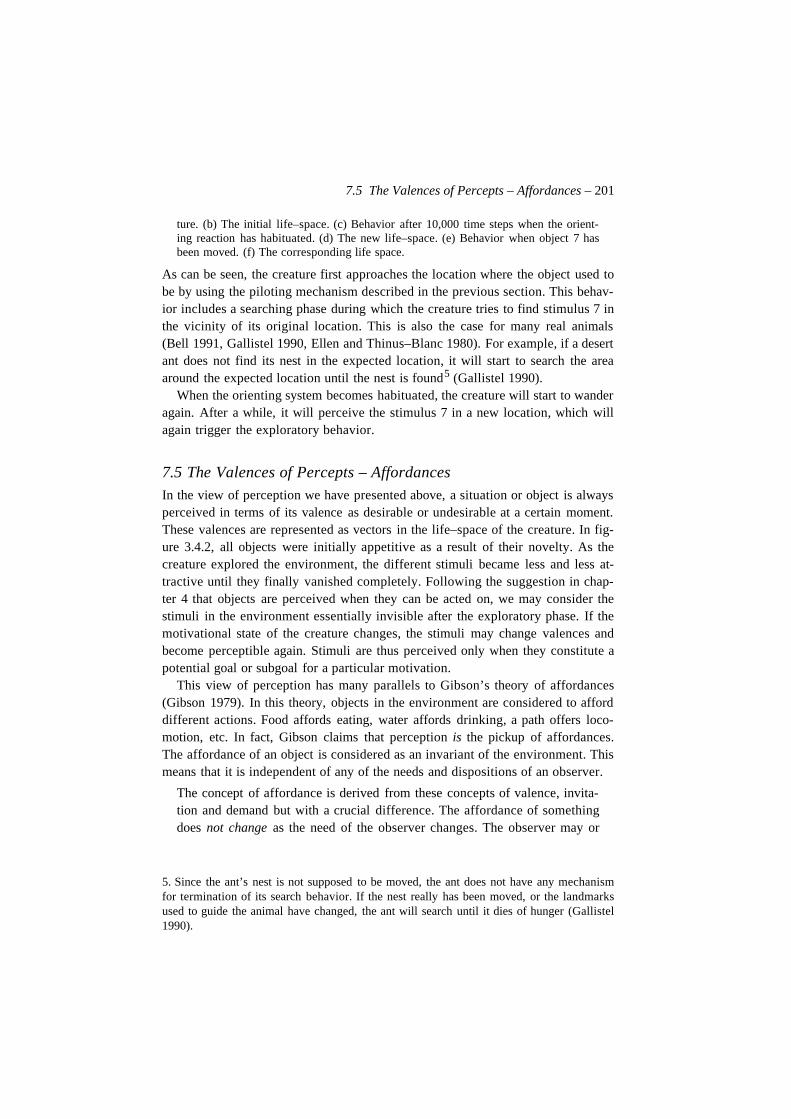
7.5 The Valences of Percepts – Affordances – 201
ture. (b) The initial life–space. (c) Behavior after 10,000 time steps when the orient-ing reaction has habituated. (d) The new life–space. (e) Behavior when object 7 hasbeen moved. (f) The corresponding life space.
As can be seen, the creature first approaches the location where the object used tobe by using the piloting mechanism described in the previous section. This behav-ior includes a searching phase during which the creature tries to find stimulus 7 inthe vicinity of its original location. This is also the case for many real animals(Bell 1991, Gallistel 1990, Ellen and Thinus–Blanc 1980). For example, if a desertant does not find its nest in the expected location, it will start to search the areaaround the expected location until the nest is found5 (Gallistel 1990).
When the orienting system becomes habituated, the creature will start to wanderagain. After a while, it will perceive the stimulus 7 in a new location, which willagain trigger the exploratory behavior.
7.5 The Valences of Percepts – AffordancesIn the view of perception we have presented above, a situation or object is alwaysperceived in terms of its valence as desirable or undesirable at a certain moment.These valences are represented as vectors in the life–space of the creature. In fig-ure 3.4.2, all objects were initially appetitive as a result of their novelty. As thecreature explored the environment, the different stimuli became less and less at-tractive until they finally vanished completely. Following the suggestion in chap-ter 4 that objects are perceived when they can be acted on, we may consider thestimuli in the environment essentially invisible after the exploratory phase. If themotivational state of the creature changes, the stimuli may change valences andbecome perceptible again. Stimuli are thus perceived only when they constitute apotential goal or subgoal for a particular motivation.
This view of perception has many parallels to Gibson’s theory of affordances(Gibson 1979). In this theory, objects in the environment are considered to afforddifferent actions. Food affords eating, water affords drinking, a path offers loco-motion, etc. In fact, Gibson claims that perception is the pickup of affordances.The affordance of an object is considered as an invariant of the environment. Thismeans that it is independent of any of the needs and dispositions of an observer.
The concept of affordance is derived from these concepts of valence, invita-tion and demand but with a crucial difference. The affordance of somethingdoes not change as the need of the observer changes. The observer may or
5. Since the ant’s nest is not supposed to be moved, the ant does not have any mechanismfor termination of its search behavior. If the nest really has been moved, or the landmarksused to guide the animal have changed, the ant will search until it dies of hunger (Gallistel1990).
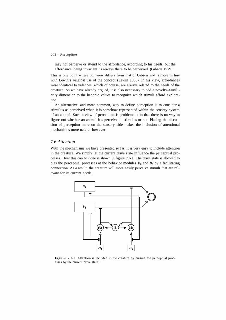
202 – Perception
may not perceive or attend to the affordance, according to his needs, but theaffordance, being invariant, is always there to be perceived. (Gibson 1979)
This is one point where our view differs from that of Gibson and is more in linewith Lewin’s original use of the concept (Lewin 1935). In his view, affordanceswere identical to valences, which of course, are always related to the needs of thecreature. As we have already argued, it is also necessary to add a novelty–famili-arity dimension to the hedonic values to recognize which stimuli afford explora-tion.
An alternative, and more common, way to define perception is to consider astimulus as perceived when it is somehow represented within the sensory systemof an animal. Such a view of perception is problematic in that there is no way tofigure out whether an animal has perceived a stimulus or not. Placing the discus-sion of perception more on the sensory side makes the inclusion of attentionalmechanisms more natural however.
7.6 AttentionWith the mechanisms we have presented so far, it is very easy to include attentionin the creature. We simply let the current drive state influence the perceptual pro-cesses. How this can be done is shown in figure 7.6.1. The drive state is allowed tobias the perceptual processes at the behavior modules B0 and B1 by a facilitatingconnection. As a result, the creature will more easily perceive stimuli that are rel-evant for its current needs.
Figure 7.6.1 Attention is included in the creature by biasing the perceptual proc-esses by the current drive state.
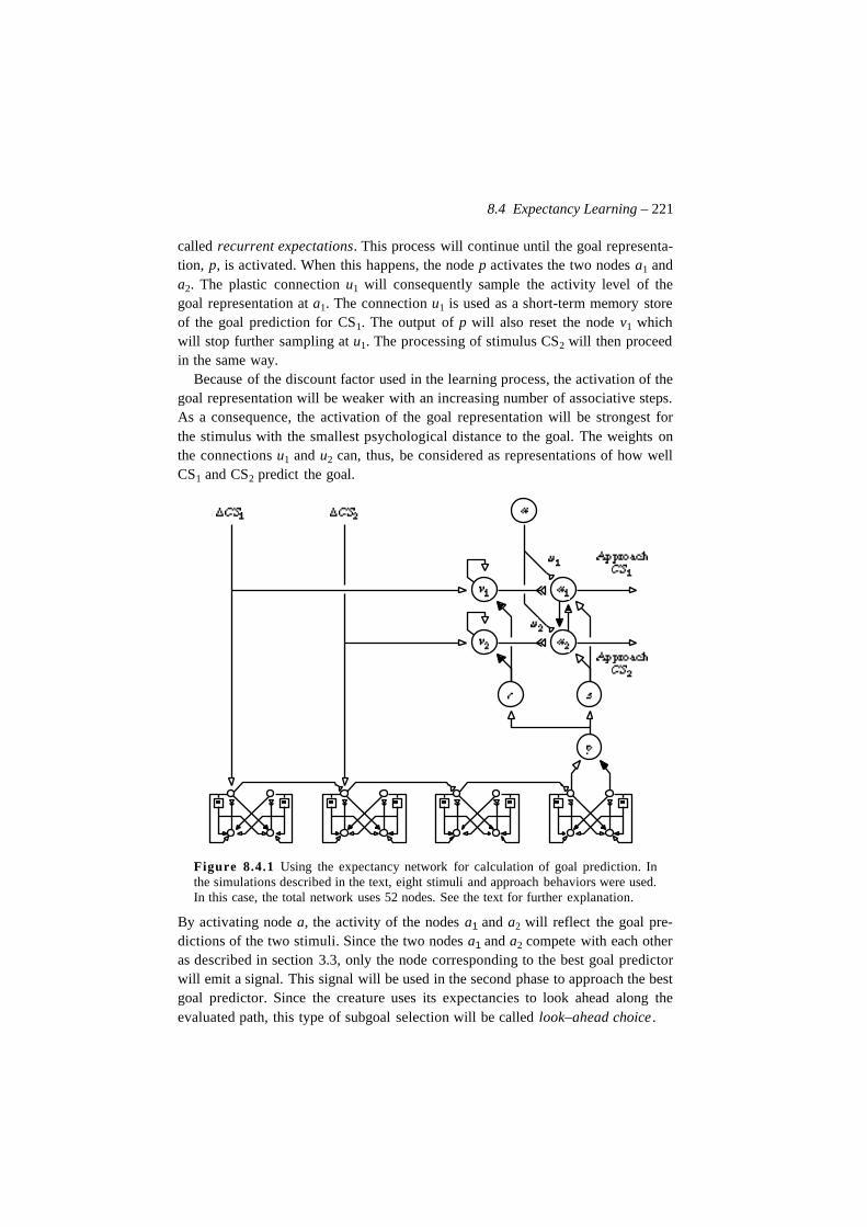
8.4 Expectancy Learning – 221
called recurrent expectations. This process will continue until the goal representa-tion, p, is activated. When this happens, the node p activates the two nodes a1 anda2. The plastic connection u1 will consequently sample the activity level of thegoal representation at a1. The connection u1 is used as a short-term memory storeof the goal prediction for CS1. The output of p will also reset the node v1 whichwill stop further sampling at u1. The processing of stimulus CS2 will then proceedin the same way.
Because of the discount factor used in the learning process, the activation of thegoal representation will be weaker with an increasing number of associative steps.As a consequence, the activation of the goal representation will be strongest forthe stimulus with the smallest psychological distance to the goal. The weights onthe connections u1 and u2 can, thus, be considered as representations of how wellCS1 and CS2 predict the goal.
Figure 8.4.1 Using the expectancy network for calculation of goal prediction. Inthe simulations described in the text, eight stimuli and approach behaviors were used.In this case, the total network uses 52 nodes. See the text for further explanation.
By activating node a, the activity of the nodes a1 and a2 will reflect the goal pre-dictions of the two stimuli. Since the two nodes a1 and a2 compete with each otheras described in section 3.3, only the node corresponding to the best goal predictorwill emit a signal. This signal will be used in the second phase to approach the bestgoal predictor. Since the creature uses its expectancies to look ahead along theevaluated path, this type of subgoal selection will be called look–ahead choice .
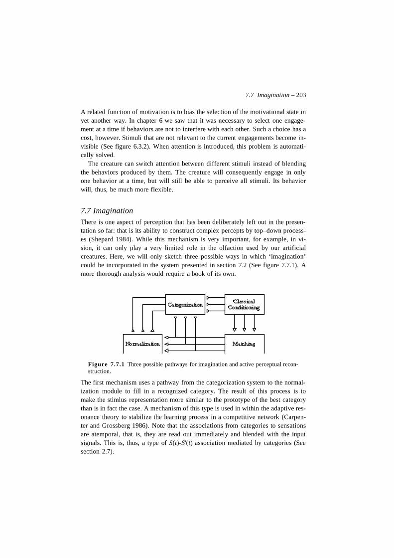
7.7 Imagination – 203
A related function of motivation is to bias the selection of the motivational state inyet another way. In chapter 6 we saw that it was necessary to select one engage-ment at a time if behaviors are not to interfere with each other. Such a choice has acost, however. Stimuli that are not relevant to the current engagements become in-visible (See figure 6.3.2). When attention is introduced, this problem is automati-cally solved.
The creature can switch attention between different stimuli instead of blendingthe behaviors produced by them. The creature will consequently engage in onlyone behavior at a time, but will still be able to perceive all stimuli. Its behaviorwill, thus, be much more flexible.
7.7 ImaginationThere is one aspect of perception that has been deliberately left out in the presen-tation so far: that is its ability to construct complex percepts by top–down process-es (Shepard 1984). While this mechanism is very important, for example, in vi-sion, it can only play a very limited role in the olfaction used by our artificialcreatures. Here, we will only sketch three possible ways in which ‘imagination’could be incorporated in the system presented in section 7.2 (See figure 7.7.1). Amore thorough analysis would require a book of its own.
Figure 7.7.1 Three possible pathways for imagination and active perceptual recon-struction.
The first mechanism uses a pathway from the categorization system to the normal-ization module to fill in a recognized category. The result of this process is tomake the stimlus representation more similar to the prototype of the best categorythan is in fact the case. A mechanism of this type is used in within the adaptive res-onance theory to stabilize the learning process in a competitive network (Carpen-ter and Grossberg 1986). Note that the associations from categories to sensationsare atemporal, that is, they are read out immediately and blended with the inputsignals. This is, thus, a type of S(t)-S'(t) association mediated by categories (Seesection 2.7).
204 – Perception
A connection from the learned expectations in the conditioning module to thecategorization system would make it possible for the creature to perceive its ex-pected categories as if they were externally generated. This type of imaginationdiffers from the one above in that it is categories which are imagined, not sensorydata. In both cases, perception can be seen as “externally guided hallucinations”(Shepard 1984). A neural network model which is in agreement with this idea waspresented by Trehub (1991).
If there is a time delay between the readouts of each expectation, it will be pos-sible to generate sequences of expectations. Each category generates expectationsof other categories, that in turn generate even more expectations. A temporal read–out is natural since classical conditioning is based on expectations of the future. Inother words, we have a case of S(t)-S'(t+1) associations. In chapter 7, we will ar-gue that this mechanism is the basis for planning and higher cognition.
Is it possible to use the same mechanism for both S(t)-S'(t) and S(t)-S'(t+1) asso-ciations? A natural extension of the system above would be to let the expectationsystem learn S(t)-S'(t+∆t) associations where the time delay between the ‘premise’S and the expectation S’ could vary. Associations of this type would generate ex-pectations of the type, ‘when S occurs, S' will occur after a time delay of ∆t’. Somemodels have tried to develop mechanisms of this type. See, for example, Gallistel(1990) and Schmajuk (1990).
A final imagination mechanism could be constructed by letting expectationswhich match sensations sufficiently well strengthen those sensations. A pathwayfrom the matching module to the sensory register could mediate such a mecha-nism. This mechanism could possibly be used to incorporate expected categoriesin new categories. Can this be used as a basis for a chunking mechanism? This is aquestion we will address in section 9.4.
All three mechanisms have in common that they let the animal perceive its en-vironment in terms of its own categories and expectations. When mechanisms ofthis type are included in a creature, we have something that can be called both bot-tom up and top down processes (Glass and Holyoak 1986).
7.8 ConclusionPerception rests on two interacting processes: categorization and association. Inour artificial creature, categorization is handled by a competitive network with re-cruitment learning. This system creates new categories when the already estab-lished do not represent the input pattern sufficiently well. Associations are handledby a conditioning system that learns associations between categories. These asso-ciations are treated as expectations that are matched against the input pattern.When expectations are not met, learning in the categorization system will be trig-gered.
7.8 Conclusion – 205
An important property of perceptual learning is that external reinforcement isnot necessary. Learning is governed by how well the internal categories and ex-pectations match the external input. No reward or punishment is necessary. How-ever, to produce behavior that uses the perceptual categories, reinforcement maybe needed (compare section 2.5 and 8.3).
We have seen how top–down and bottom–up processes can be combined at anumber of places in the system. Exploratory behavior was seen as a consequenceof orienting behavior toward unexpected stimuli. Such a mechanism will automat-ically make the creature explore the environment as long as some perceptible stim-ulus is unexpected. Another important aspect of perception is that it interacts con-tinuously with both motivational and behavioral processes.
Finally, we repeat the observation that it is not possible to separate perceptionfrom other processes on physical grounds. There is no specific part of the nervoussystem responsible for perception and some other that is not. The different systemsinvolved in perception are also used for behavioral learning and motivation.

206 – Perception
Christian Balkenius, 1995, Natural Intelligence in Artificial Creatures, Lund University Cognitive Studies 37, 1995.
Chapter 8
Spatial Orientation
8.1 IntroductionIn the previous chapters, the various learning mechanisms have only been used forvery simple problems. In this chapter we will see how an artificial creature can usethe mechanisms we have presented above to solve a number of problems in thespatial domain. We will investigate two different types of learning mechanisms.The first is procedural learning which uses the reinforcement module presented inchapter 5 to learn sequences of behaviors. The second mechanism uses the expect-ancy network as its main component to represent knowledge about the environ-ment, and uses it for look–ahead choice.
It is important to distinguish between the orienting reaction described in sec-tions 4.4 and 9.2 and the concept of spatial orientation. The orienting reaction di-rects the sensory apparatus of an animal toward a stimulus in the immediate envi-ronment, while spatial orientation refers to an ability to orient from one place toanother. A possible way to avoid confusion would be to call the present chapterspatial navigation. Since spatial navigation usually refers to more advanced mech-anisms than the ones which will be described here, we have chosen the first term,however.
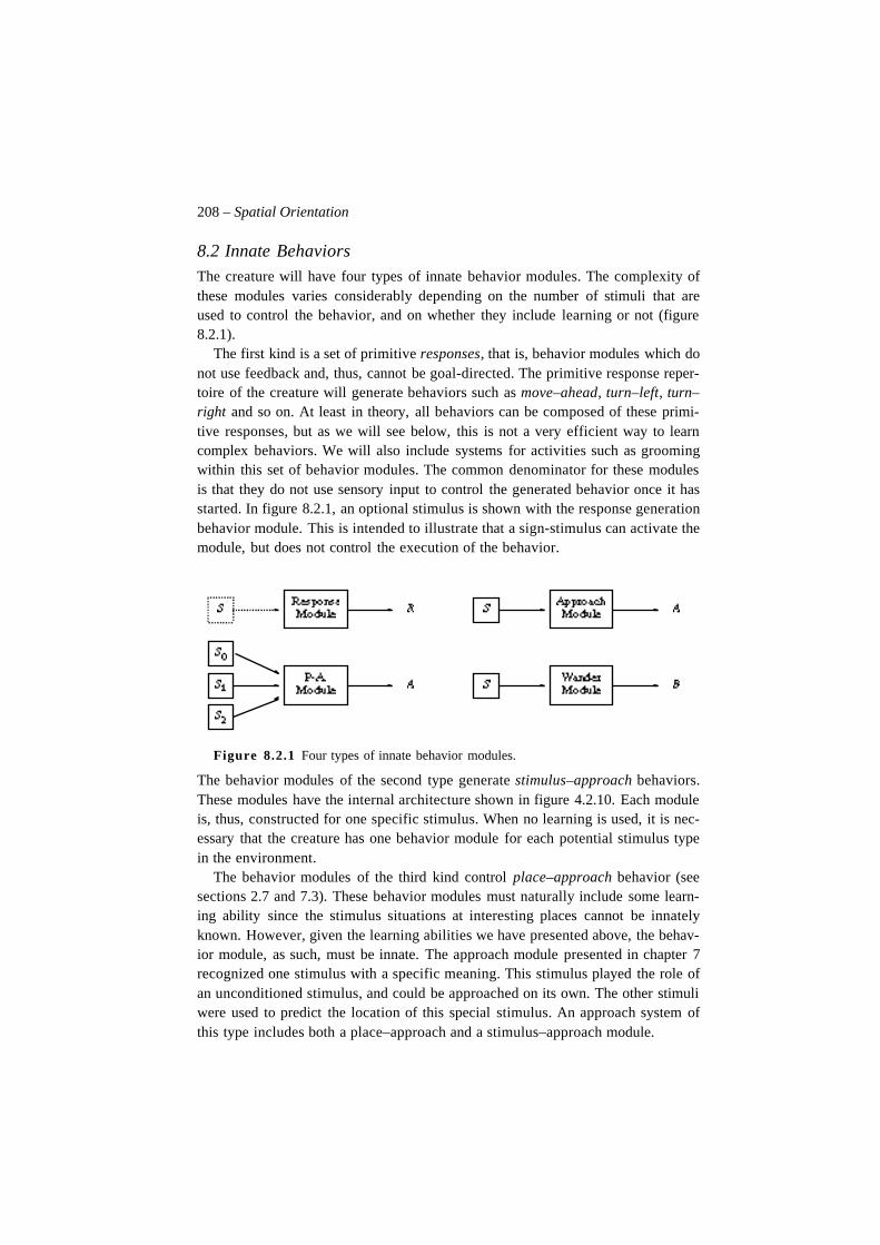
208 – Spatial Orientation
8.2 Innate BehaviorsThe creature will have four types of innate behavior modules. The complexity ofthese modules varies considerably depending on the number of stimuli that areused to control the behavior, and on whether they include learning or not (figure8.2.1).
The first kind is a set of primitive responses, that is, behavior modules which donot use feedback and, thus, cannot be goal-directed. The primitive response reper-toire of the creature will generate behaviors such as move–ahead, turn–left, turn–right and so on. At least in theory, all behaviors can be composed of these primi-tive responses, but as we will see below, this is not a very efficient way to learncomplex behaviors. We will also include systems for activities such as groomingwithin this set of behavior modules. The common denominator for these modulesis that they do not use sensory input to control the generated behavior once it hasstarted. In figure 8.2.1, an optional stimulus is shown with the response generationbehavior module. This is intended to illustrate that a sign-stimulus can activate themodule, but does not control the execution of the behavior.
Figure 8.2.1 Four types of innate behavior modules.
The behavior modules of the second type generate stimulus–approach behaviors.These modules have the internal architecture shown in figure 4.2.10. Each moduleis, thus, constructed for one specific stimulus. When no learning is used, it is nec-essary that the creature has one behavior module for each potential stimulus typein the environment.
The behavior modules of the third kind control place–approach behavior (seesections 2.7 and 7.3). These behavior modules must naturally include some learn-ing ability since the stimulus situations at interesting places cannot be innatelyknown. However, given the learning abilities we have presented above, the behav-ior module, as such, must be innate. The approach module presented in chapter 7recognized one stimulus with a specific meaning. This stimulus played the role ofan unconditioned stimulus, and could be approached on its own. The other stimuliwere used to predict the location of this special stimulus. An approach system ofthis type includes both a place–approach and a stimulus–approach module.
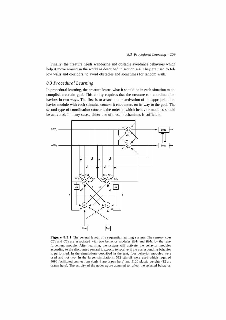
8.3 Procedural Learning – 209
Finally, the creature needs wandering and obstacle avoidance behaviors whichhelp it move around in the world as described in section 4.4. They are used to fol-low walls and corridors, to avoid obstacles and sometimes for random walk.
8.3 Procedural Learning
In procedural learning, the creature learns what it should do in each situation to ac-complish a certain goal. This ability requires that the creature can coordinate be-haviors in two ways. The first is to associate the activation of the appropriate be-havior module with each stimulus context it encounters on its way to the goal. Thesecond type of coordination concerns the order in which behavior modules shouldbe activated. In many cases, either one of these mechanisms is sufficient.
Figure 8.3.1 The general layout of a sequential learning system. The sensory cuesCS1 and CS2 are associated with two behavior modules BM1 and BM2, by the rein-forcement module. After learning, the system will activate the behavior modulesaccording to the discounted reward it expects to receive if the corresponding behavioris performed. In the simulations described in the text, four behavior modules wereused and not two. In the larger simulations, 512 stimuli were used which required4096 facilitated connections (only 8 are drawn here) and 5120 plastic weights (12 aredrawn here). The activity of the nodes bi are assumed to reflect the selected behavior.
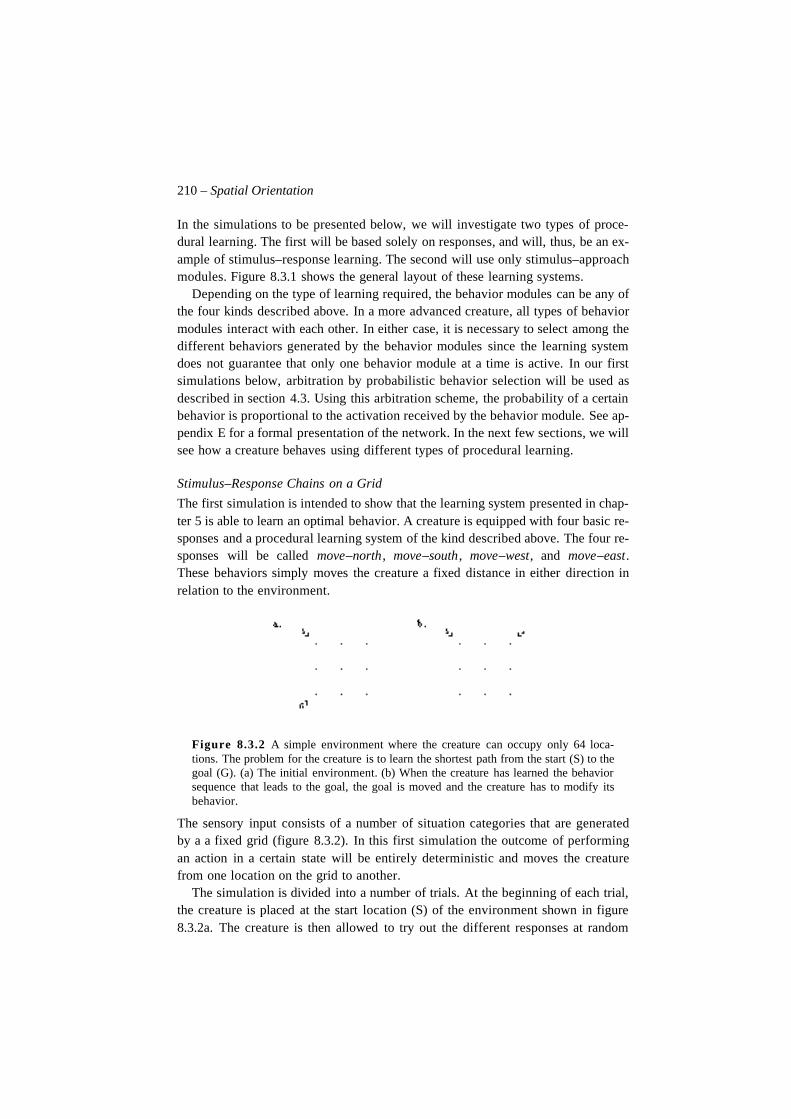
210 – Spatial Orientation
In the simulations to be presented below, we will investigate two types of proce-dural learning. The first will be based solely on responses, and will, thus, be an ex-ample of stimulus–response learning. The second will use only stimulus–approachmodules. Figure 8.3.1 shows the general layout of these learning systems.
Depending on the type of learning required, the behavior modules can be any ofthe four kinds described above. In a more advanced creature, all types of behaviormodules interact with each other. In either case, it is necessary to select among thedifferent behaviors generated by the behavior modules since the learning systemdoes not guarantee that only one behavior module at a time is active. In our firstsimulations below, arbitration by probabilistic behavior selection will be used asdescribed in section 4.3. Using this arbitration scheme, the probability of a certainbehavior is proportional to the activation received by the behavior module. See ap-pendix E for a formal presentation of the network. In the next few sections, we willsee how a creature behaves using different types of procedural learning.
Stimulus–Response Chains on a Grid
The first simulation is intended to show that the learning system presented in chap-ter 5 is able to learn an optimal behavior. A creature is equipped with four basic re-sponses and a procedural learning system of the kind described above. The four re-sponses will be called move–north, move–south, move–west, and move–east.These behaviors simply moves the creature a fixed distance in either direction inrelation to the environment.
Figure 8.3.2 A simple environment where the creature can occupy only 64 loca-tions. The problem for the creature is to learn the shortest path from the start (S) to thegoal (G). (a) The initial environment. (b) When the creature has learned the behaviorsequence that leads to the goal, the goal is moved and the creature has to modify itsbehavior.
The sensory input consists of a number of situation categories that are generatedby a a fixed grid (figure 8.3.2). In this first simulation the outcome of performingan action in a certain state will be entirely deterministic and moves the creaturefrom one location on the grid to another.
The simulation is divided into a number of trials. At the beginning of each trial,the creature is placed at the start location (S) of the environment shown in figure8.3.2a. The creature is then allowed to try out the different responses at random
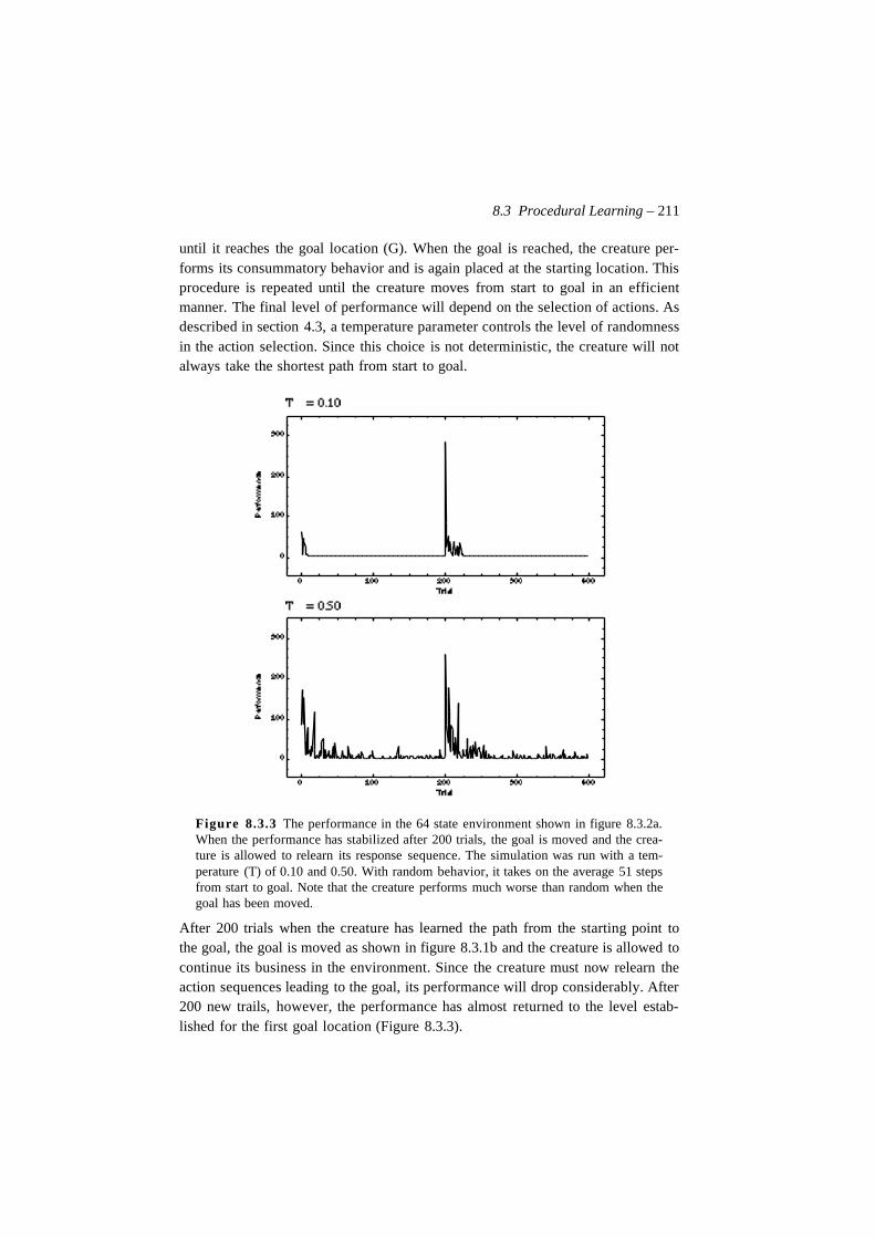
8.3 Procedural Learning – 211
until it reaches the goal location (G). When the goal is reached, the creature per-forms its consummatory behavior and is again placed at the starting location. Thisprocedure is repeated until the creature moves from start to goal in an efficientmanner. The final level of performance will depend on the selection of actions. Asdescribed in section 4.3, a temperature parameter controls the level of randomnessin the action selection. Since this choice is not deterministic, the creature will notalways take the shortest path from start to goal.
Figure 8.3.3 The performance in the 64 state environment shown in figure 8.3.2a.When the performance has stabilized after 200 trials, the goal is moved and the crea-ture is allowed to relearn its response sequence. The simulation was run with a tem-perature (T) of 0.10 and 0.50. With random behavior, it takes on the average 51 stepsfrom start to goal. Note that the creature performs much worse than random when thegoal has been moved.
After 200 trials when the creature has learned the path from the starting point tothe goal, the goal is moved as shown in figure 8.3.1b and the creature is allowed tocontinue its business in the environment. Since the creature must now relearn theaction sequences leading to the goal, its performance will drop considerably. After200 new trails, however, the performance has almost returned to the level estab-lished for the first goal location (Figure 8.3.3).
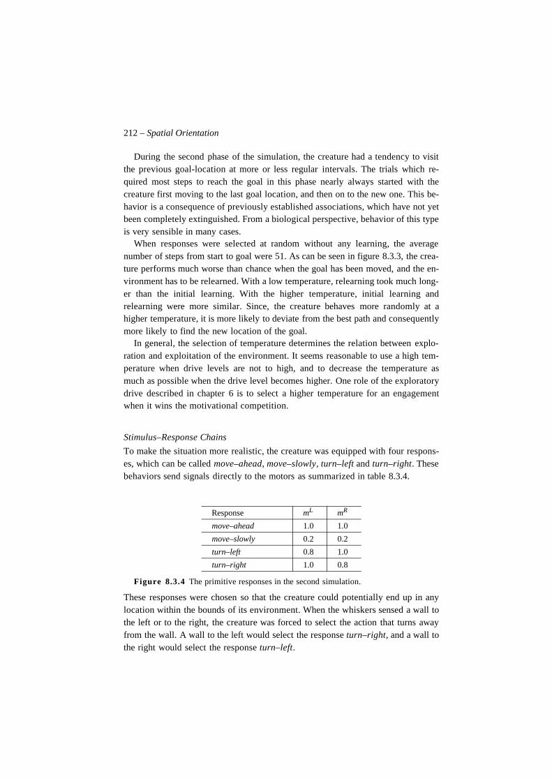
212 – Spatial Orientation
During the second phase of the simulation, the creature had a tendency to visitthe previous goal-location at more or less regular intervals. The trials which re-quired most steps to reach the goal in this phase nearly always started with thecreature first moving to the last goal location, and then on to the new one. This be-havior is a consequence of previously established associations, which have not yetbeen completely extinguished. From a biological perspective, behavior of this typeis very sensible in many cases.
When responses were selected at random without any learning, the averagenumber of steps from start to goal were 51. As can be seen in figure 8.3.3, the crea-ture performs much worse than chance when the goal has been moved, and the en-vironment has to be relearned. With a low temperature, relearning took much long-er than the initial learning. With the higher temperature, initial learning andrelearning were more similar. Since, the creature behaves more randomly at ahigher temperature, it is more likely to deviate from the best path and consequentlymore likely to find the new location of the goal.
In general, the selection of temperature determines the relation between explo-ration and exploitation of the environment. It seems reasonable to use a high tem-perature when drive levels are not to high, and to decrease the temperature asmuch as possible when the drive level becomes higher. One role of the exploratorydrive described in chapter 6 is to select a higher temperature for an engagementwhen it wins the motivational competition.
Stimulus–Response Chains
To make the situation more realistic, the creature was equipped with four respons-es, which can be called move–ahead, move–slowly, turn–left and turn–right. Thesebehaviors send signals directly to the motors as summarized in table 8.3.4.
Figure 8.3.4 The primitive responses in the second simulation.
These responses were chosen so that the creature could potentially end up in anylocation within the bounds of its environment. When the whiskers sensed a wall tothe left or to the right, the creature was forced to select the action that turns awayfrom the wall. A wall to the left would select the response turn–right, and a wall tothe right would select the response turn–left.
Response mL mR
move–ahead 1.0 1.0
move–slowly 0.2 0.2
turn–left 0.8 1.0
turn–right 1.0 0.8
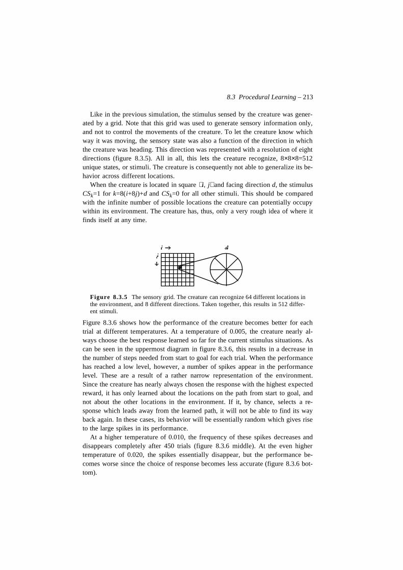
8.3 Procedural Learning – 213
Like in the previous simulation, the stimulus sensed by the creature was gener-ated by a grid. Note that this grid was used to generate sensory information only,and not to control the movements of the creature. To let the creature know whichway it was moving, the sensory state was also a function of the direction in whichthe creature was heading. This direction was represented with a resolution of eightdirections (figure 8.3.5). All in all, this lets the creature recognize, 8×8×8=512unique states, or stimuli. The creature is consequently not able to generalize its be-havior across different locations.
When the creature is located in square and facing direction d, the stimulusCSk=1 for k=8(i+8j)+d and CSk=0 for all other stimuli. This should be comparedwith the infinite number of possible locations the creature can potentially occupywithin its environment. The creature has, thus, only a very rough idea of where itfinds itself at any time.
Figure 8.3.5 The sensory grid. The creature can recognize 64 different locations inthe environment, and 8 different directions. Taken together, this results in 512 differ-ent stimuli.
Figure 8.3.6 shows how the performance of the creature becomes better for eachtrial at different temperatures. At a temperature of 0.005, the creature nearly al-ways choose the best response learned so far for the current stimulus situations. Ascan be seen in the uppermost diagram in figure 8.3.6, this results in a decrease inthe number of steps needed from start to goal for each trial. When the performancehas reached a low level, however, a number of spikes appear in the performancelevel. These are a result of a rather narrow representation of the environment.Since the creature has nearly always chosen the response with the highest expectedreward, it has only learned about the locations on the path from start to goal, andnot about the other locations in the environment. If it, by chance, selects a re-sponse which leads away from the learned path, it will not be able to find its wayback again. In these cases, its behavior will be essentially random which gives riseto the large spikes in its performance.
At a higher temperature of 0.010, the frequency of these spikes decreases anddisappears completely after 450 trials (figure 8.3.6 middle). At the even highertemperature of 0.020, the spikes essentially disappear, but the performance be-comes worse since the choice of response becomes less accurate (figure 8.3.6 bot-tom).
i j,⟨ ⟩
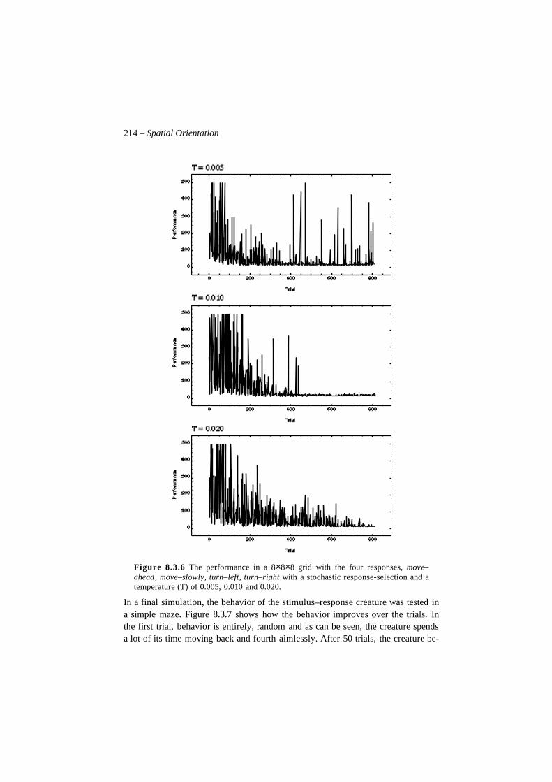
214 – Spatial Orientation
Figure 8.3.6 The performance in a 8×8×8 grid with the four responses, move–ahead, move–slowly, turn–left, turn–right with a stochastic response-selection and atemperature (T) of 0.005, 0.010 and 0.020.
In a final simulation, the behavior of the stimulus–response creature was tested ina simple maze. Figure 8.3.7 shows how the behavior improves over the trials. Inthe first trial, behavior is entirely, random and as can be seen, the creature spendsa lot of its time moving back and fourth aimlessly. After 50 trials, the creature be-
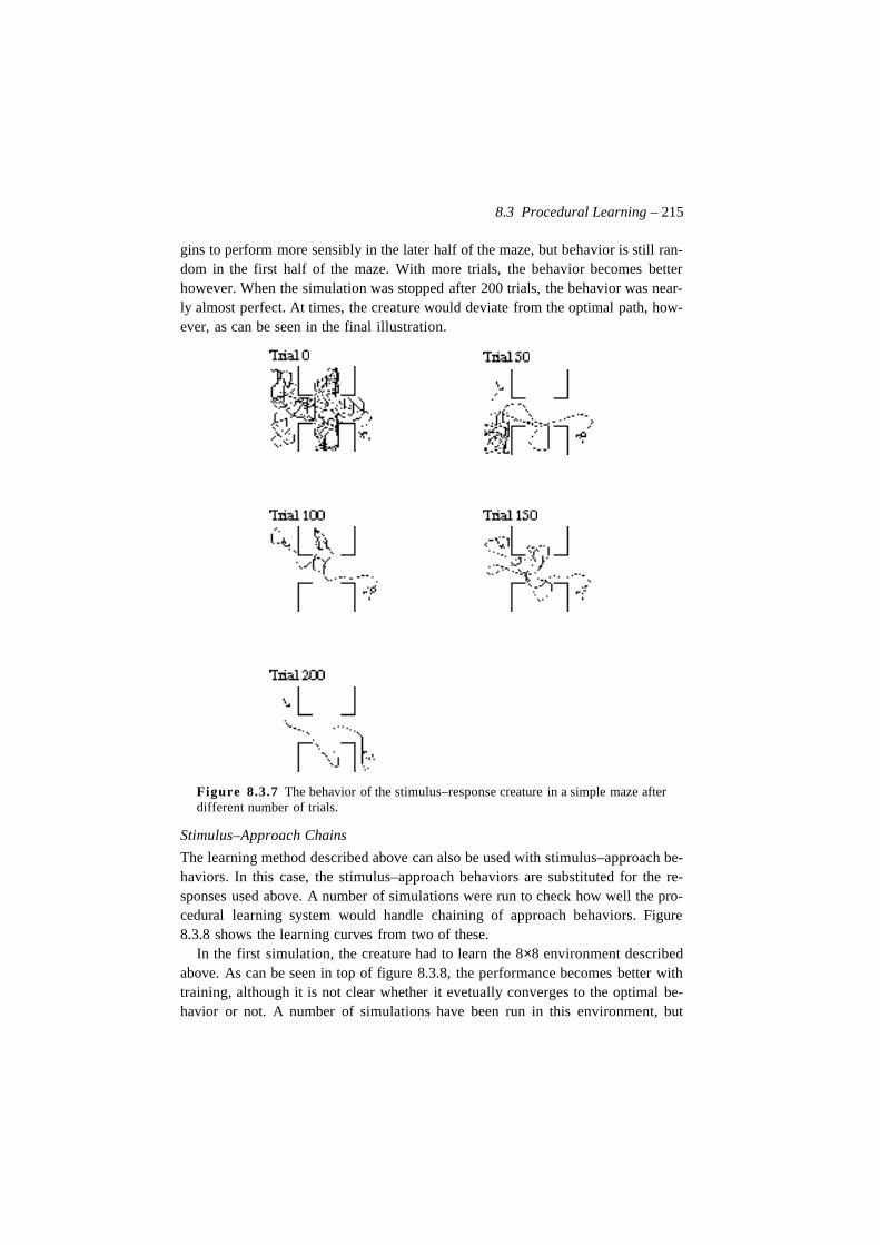
8.3 Procedural Learning – 215
gins to perform more sensibly in the later half of the maze, but behavior is still ran-dom in the first half of the maze. With more trials, the behavior becomes betterhowever. When the simulation was stopped after 200 trials, the behavior was near-ly almost perfect. At times, the creature would deviate from the optimal path, how-ever, as can be seen in the final illustration.
Figure 8.3.7 The behavior of the stimulus–response creature in a simple maze afterdifferent number of trials.
Stimulus–Approach Chains
The learning method described above can also be used with stimulus–approach be-haviors. In this case, the stimulus–approach behaviors are substituted for the re-sponses used above. A number of simulations were run to check how well the pro-cedural learning system would handle chaining of approach behaviors. Figure8.3.8 shows the learning curves from two of these.
In the first simulation, the creature had to learn the 8×8 environment describedabove. As can be seen in top of figure 8.3.8, the performance becomes better withtraining, although it is not clear whether it evetually converges to the optimal be-havior or not. A number of simulations have been run in this environment, but
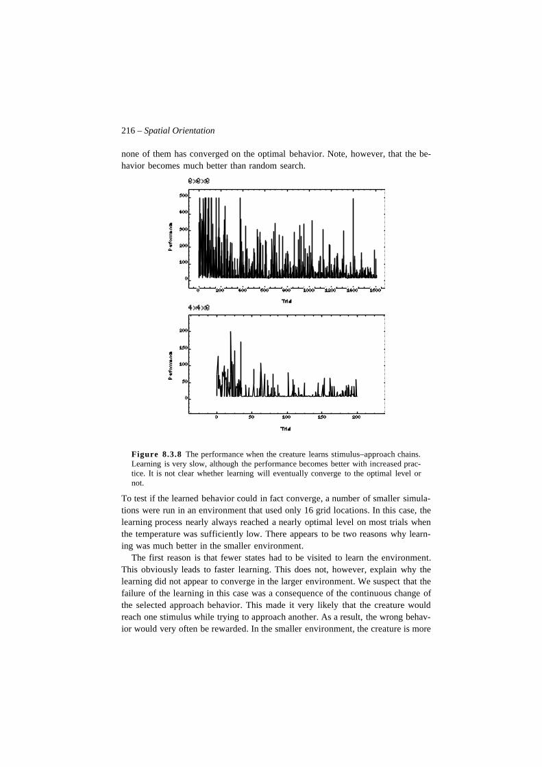
216 – Spatial Orientation
none of them has converged on the optimal behavior. Note, however, that the be-havior becomes much better than random search.
Figure 8.3.8 The performance when the creature learns stimulus–approach chains.Learning is very slow, although the performance becomes better with increased prac-tice. It is not clear whether learning will eventually converge to the optimal level ornot.
To test if the learned behavior could in fact converge, a number of smaller simula-tions were run in an environment that used only 16 grid locations. In this case, thelearning process nearly always reached a nearly optimal level on most trials whenthe temperature was sufficiently low. There appears to be two reasons why learn-ing was much better in the smaller environment.
The first reason is that fewer states had to be visited to learn the environment.This obviously leads to faster learning. This does not, however, explain why thelearning did not appear to converge in the larger environment. We suspect that thefailure of the learning in this case was a consequence of the continuous change ofthe selected approach behavior. This made it very likely that the creature wouldreach one stimulus while trying to approach another. As a result, the wrong behav-ior would very often be rewarded. In the smaller environment, the creature is more
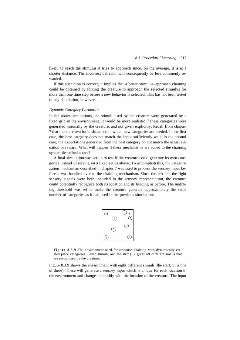
8.3 Procedural Learning – 217
likely to reach the stimulus it tries to approach since, on the average, it is at ashorter distance. The incorrect behavior will consequently be less commonly re-warded.
If this suspicion is correct, it implies that a better stimulus–approach chainingcould be obtained by forcing the creature to approach the selected stimulus formore than one time step before a new behavior is selected. This has not been testedin any simulation, however.
Dynamic Category Formation
In the above simulations, the stimuli used by the creature were generated by afixed grid in the environment. It would be more realistic if these categories weregenerated internally by the creature, and not given explicitly. Recall from chapter7 that there are two basic situations in which new categories are needed. In the firstcase, the best category does not match the input sufficiently well. In the secondcase, the expectations generated from the best category do not match the actual sit-uation or reward. What will happen if these mechanisms are added to the chainingsystem described above?
A final simulation was set up to test if the creature could generate its own cate-gories instead of relying on a fixed set as above. To accomplish this, the categori-zation mechanism described in chapter 7 was used to process the sensory input be-fore it was handled over to the chaining mechanism. Since the left and the rightsensory signals were both included in the sensory representation, the creaturecould potentially recognize both its location and its heading as before. The match-ing threshold was set to make the creature generate approximately the samenumber of categories as it had used in the previous simulations.
Figure 8.3.9 The environment used for response chaining with dynamically cre-ated place categories. Seven stimuli, and the start (S), gives off different smells thatare recognized by the creature.
Figure 8.3.9 shows the environment with eight different stimuli (the start, S, is oneof these). These will generate a sensory input which is unique for each location inthe environment and changes smoothly with the location of the creature. The input
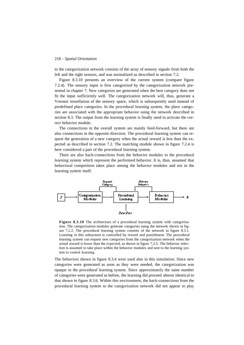
218 – Spatial Orientation
to the categorization network consists of the array of sensory signals from both theleft and the right sensors, and was normalized as described in section 7.2.
Figure 8.3.10 presents an overview of the current system (compare figure7.2.4). The sensory input is first categorized by the categorization network pre-sented in chapter 7. New categories are generated when the best category does notfit the input sufficiently well. The categorization network will, thus, generate aVoronoi tessellation of the sensory space, which is subsequently used instead ofpredefined place categories. In the procedural learning system, the place catego-ries are associated with the appropriate behavior using the network described insection 8.3. The output from the learning system is finally used to activate the cor-rect behavior module.
The connections in the overall system are mainly feed-forward, but there arealso connections in the opposite direction. The procedural learning system can re-quest the generation of a new category when the actual reward is less than the ex-pected as described in section 7.2. The matching module shown in figure 7.2.4 ishere considered a part of the procedural learning system.
There are also back-connections from the behavior modules to the procedurallearning system which represent the performed behavior. It is, thus, assumed thatbehavioral competition takes place among the behavior modules and not in thelearning system itself.
Figure 8.3.10 The architecture of a procedural learning system with categoriza-tion. The categorization modules generate catagories using the network shown in fig-ure 7.2.2. The procedural learning system consists of the network in figure 8.3.1.Learning in this subsystem is controlled by reward and punishment. The procedurallearning system can request new categories from the categorization network when theactual reward is lower than the expected, as shown in figure 7.2.5. The behavior selec-tion is assumed to take place within the behavior modules and sent to the learning sys-tem to control learning.
The behaviors shown in figure 8.3.4 were used also in this simulation. Since newcategories were generated as soon as they were needed, the categorization wasopaque to the procedural learning system. Since approximately the same numberof categories were generated as before, the learning did proceed almost identical tothat shown in figure 8.3.6. Within this environment, the back-connections from theprocedural learning system to the categorization network did not appear to play
8.3 Procedural Learning – 219
any role. Although some categories would be created using these back connec-tions, the speed of learning was not affected if these were removed. We suspectthat they will be needed in a more complex environment, however (compare sec-tion 7.2). Especially if we allow the creature to generalize (see chapter 9).
To summarize, we have shown how a categorization network in combinationwith a chaining mechanism can form its own categories which it subsequently usesto learn behavior sequences. This view of learning is consistent with the divisioninto separate systems for categorization and behavioral learning described in sec-tion 2.5. Also note that reward is used only within the procedural learning systemand not in the categorization network. If we assume that learning within the cate-gorization network is slower than within the procedural system, we would obtain afaster learning process if the creature is first exposed to the environment withoutbeing rewarded. This would, thus, be an example of latent learning.
Problems and Limitations
There are a number of problems in the procedural learning presented above. Thefirst can be found in the categorization module. It is necessary that the creaturegenerates sufficiently many categories to give a good representation of where it is,and in what direction it is heading. With only the eight stimuli available in the sim-ulator, it proved to be hard to place the stimuli in such a way that the generated cat-egories would be a good representation of the environment. In many cases, thegenerated categories would only recognize which stimulus was the closest ratherthan the whole stimulus configuration. The reason for this is that the intensity ofthe smells decays very rapidly as the creature moves away from a stimulus. Thestimulus closest to the creature has, thus, usually a much larger intensity than theothers. As a consequence, this stimulus will dominate the created categories com-pletely.
This problem was solved by placing the stimuli sufficiently close to each other.The drawback of this solution, apart from being a specially prepared environmentis that only a fairly small environment could be used. To solve the problem moregenerally, a better type of place–categories are needed. However, the model couldeasily be extended with real place–categories. Any of a number of models could beused here. For example the models proposed by Zipser (1985), Prescott andMayhew (1993), Schmajuk and Blair (1993), and Touretzky and Redish (1995).This problem is, thus, sensory rather than architectural.
The second problem has already been discussed in the end of chapter 5. Thechaining mechanism models interstimulus interval effects rather crudely. This de-mands that the stimulus category changes between each time step, which in turnrequires much more categories than would otherwise be necessary. We believethat by including a mechanism for ISI-effects, learning will be much faster (seeappendix C). In the simulations described above, the learning rate at the negative
220 – Spatial Orientation
side of the reinforcement module was half that of the one at the positive side tocompensate for the times when the category would not change as the creaturemoved. While this solution appears to work fairly well, it is still not very satisfac-tory.
The final limitation of the procedural learning system is that it cannot general-ize at all since it uses a localist representation of location and direction. Thismeans that one node in the network codes for each specific location. It is likelythat a better performance could be generated by letting the creature use distributedrepresentation instead. This is an idea we will again return to in chapter 9.
8.4 Expectancy Learning
Procedural learning is very general since it allows almost any behavior to beacquired given sufficient time to try out different behaviors. The drawback is, ofcourse, that it is very slow. In this section, we will investigate how the expectancynetwork presented in chapter 5 can be used to learn an environment much fasterthan by procedural learning.
The model of spatial orientation based on expectations we will present is similarin spirit to that of Schmajuk and Thieme (1992). The network used here is differ-ent in some respects, however. One important difference is that the present modelis based on an expectancy network instead of an ordinary recurrent network. Theexpectations used are, thus, considered to be established through classical condi-tioning during exploration of the environment as described in section 7.4.
We will assume that the appetence behavior of the creature is divided into twoalternating phases. In the first phase, the creature samples the various stimuli inthe environment and calculates how well each of them predicts the desired goal. Inthe second phase, the creature approaches the stimulus which is the best goal pre-dictor. (Compare the combined orientation and approach system described in sec-tion 4.2.)
Figure 8.4.1 presents a small network which uses an expectancy network to cal-culate how well each stimulus in the environment predicts the desired goal. Thepurpose of this network is to select the best goal-predictor and make the creatureapproach it (see also appendix E).
Let us assume the creature finds itself in a situation where two stimuli, CS1 andCS2, are present. The creature is assumed to evaluate each stimulus in turn in thefollowing way. First, a brief pulse, ∆CS1, is sent to the network. This signal willactivate the node v1 which will stay active as long as CS1 is evaluated. The pulsewill also enter the expectancy network where it will be propagated through the net-work and generate expectations from CS1. These new expectations will then enterthe expectancy network again and generate further expectations from the newnodes, and so on. The expectations which return to the network again will be
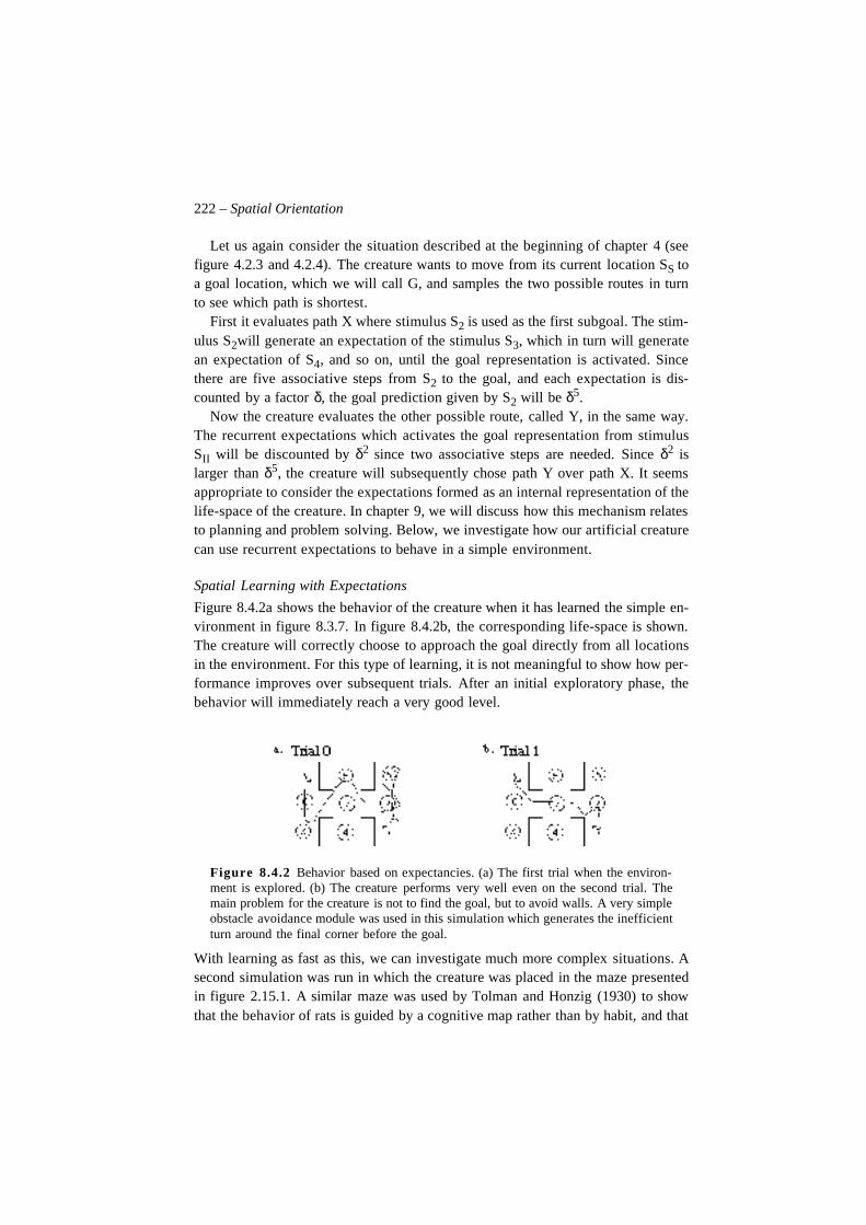
222 – Spatial Orientation
Let us again consider the situation described at the beginning of chapter 4 (seefigure 4.2.3 and 4.2.4). The creature wants to move from its current location SS toa goal location, which we will call G, and samples the two possible routes in turnto see which path is shortest.
First it evaluates path X where stimulus S2 is used as the first subgoal. The stim-ulus S2will generate an expectation of the stimulus S3, which in turn will generatean expectation of S4, and so on, until the goal representation is activated. Sincethere are five associative steps from S2 to the goal, and each expectation is dis-counted by a factor δ, the goal prediction given by S2 will be δ5.
Now the creature evaluates the other possible route, called Y, in the same way.The recurrent expectations which activates the goal representation from stimulusSII will be discounted by δ2 since two associative steps are needed. Since δ2 islarger than δ5, the creature will subsequently chose path Y over path X. It seemsappropriate to consider the expectations formed as an internal representation of thelife-space of the creature. In chapter 9, we will discuss how this mechanism relatesto planning and problem solving. Below, we investigate how our artificial creaturecan use recurrent expectations to behave in a simple environment.
Spatial Learning with Expectations
Figure 8.4.2a shows the behavior of the creature when it has learned the simple en-vironment in figure 8.3.7. In figure 8.4.2b, the corresponding life-space is shown.The creature will correctly choose to approach the goal directly from all locationsin the environment. For this type of learning, it is not meaningful to show how per-formance improves over subsequent trials. After an initial exploratory phase, thebehavior will immediately reach a very good level.
Figure 8.4.2 Behavior based on expectancies. (a) The first trial when the environ-ment is explored. (b) The creature performs very well even on the second trial. Themain problem for the creature is not to find the goal, but to avoid walls. A very simpleobstacle avoidance module was used in this simulation which generates the inefficientturn around the final corner before the goal.
With learning as fast as this, we can investigate much more complex situations. Asecond simulation was run in which the creature was placed in the maze presentedin figure 2.15.1. A similar maze was used by Tolman and Honzig (1930) to showthat the behavior of rats is guided by a cognitive map rather than by habit, and that
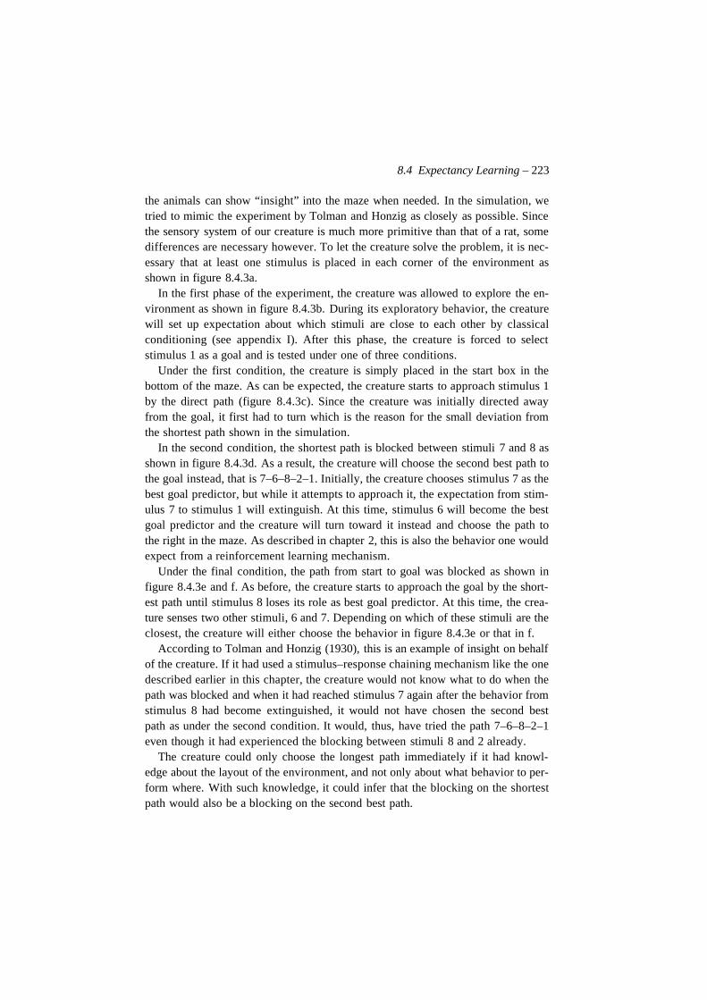
8.4 Expectancy Learning – 223
the animals can show “insight” into the maze when needed. In the simulation, wetried to mimic the experiment by Tolman and Honzig as closely as possible. Sincethe sensory system of our creature is much more primitive than that of a rat, somedifferences are necessary however. To let the creature solve the problem, it is nec-essary that at least one stimulus is placed in each corner of the environment asshown in figure 8.4.3a.
In the first phase of the experiment, the creature was allowed to explore the en-vironment as shown in figure 8.4.3b. During its exploratory behavior, the creaturewill set up expectation about which stimuli are close to each other by classicalconditioning (see appendix I). After this phase, the creature is forced to selectstimulus 1 as a goal and is tested under one of three conditions.
Under the first condition, the creature is simply placed in the start box in thebottom of the maze. As can be expected, the creature starts to approach stimulus 1by the direct path (figure 8.4.3c). Since the creature was initially directed awayfrom the goal, it first had to turn which is the reason for the small deviation fromthe shortest path shown in the simulation.
In the second condition, the shortest path is blocked between stimuli 7 and 8 asshown in figure 8.4.3d. As a result, the creature will choose the second best path tothe goal instead, that is 7–6–8–2–1. Initially, the creature chooses stimulus 7 as thebest goal predictor, but while it attempts to approach it, the expectation from stim-ulus 7 to stimulus 1 will extinguish. At this time, stimulus 6 will become the bestgoal predictor and the creature will turn toward it instead and choose the path tothe right in the maze. As described in chapter 2, this is also the behavior one wouldexpect from a reinforcement learning mechanism.
Under the final condition, the path from start to goal was blocked as shown infigure 8.4.3e and f. As before, the creature starts to approach the goal by the short-est path until stimulus 8 loses its role as best goal predictor. At this time, the crea-ture senses two other stimuli, 6 and 7. Depending on which of these stimuli are theclosest, the creature will either choose the behavior in figure 8.4.3e or that in f.
According to Tolman and Honzig (1930), this is an example of insight on behalfof the creature. If it had used a stimulus–response chaining mechanism like the onedescribed earlier in this chapter, the creature would not know what to do when thepath was blocked and when it had reached stimulus 7 again after the behavior fromstimulus 8 had become extinguished, it would not have chosen the second bestpath as under the second condition. It would, thus, have tried the path 7–6–8–2–1even though it had experienced the blocking between stimuli 8 and 2 already.
The creature could only choose the longest path immediately if it had knowl-edge about the layout of the environment, and not only about what behavior to per-form where. With such knowledge, it could infer that the blocking on the shortestpath would also be a blocking on the second best path.
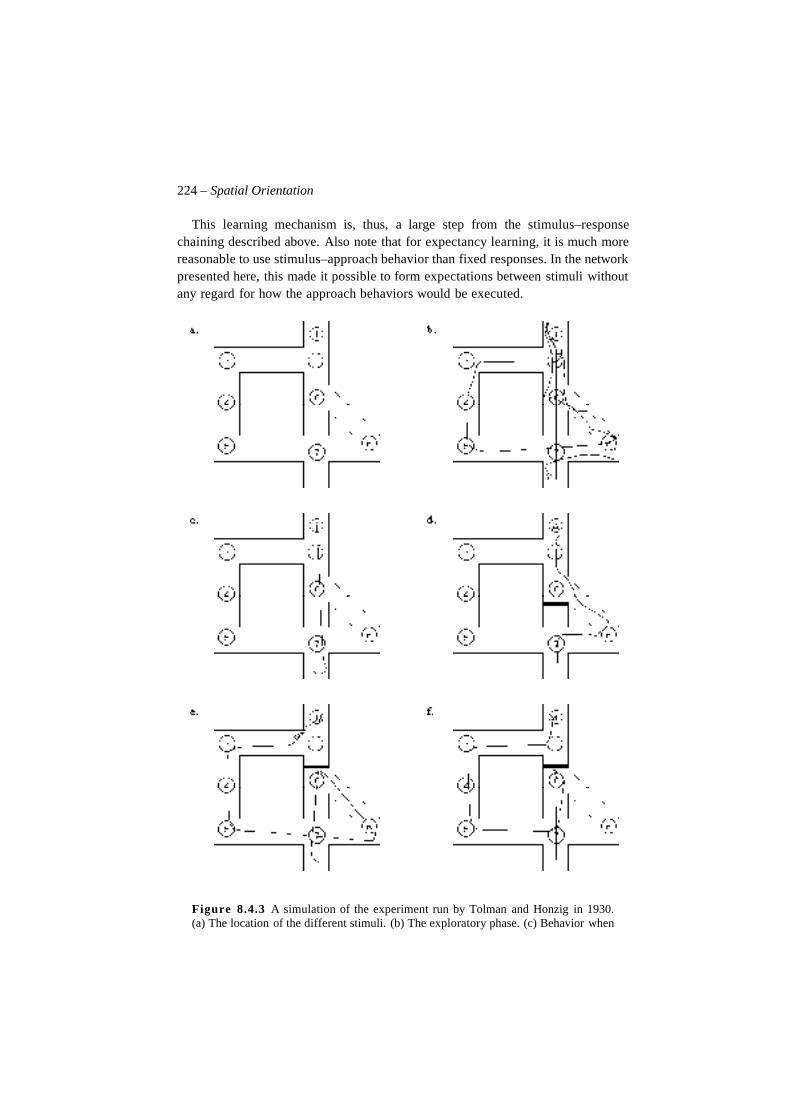
224 – Spatial Orientation
This learning mechanism is, thus, a large step from the stimulus–responsechaining described above. Also note that for expectancy learning, it is much morereasonable to use stimulus–approach behavior than fixed responses. In the networkpresented here, this made it possible to form expectations between stimuli withoutany regard for how the approach behaviors would be executed.
Figure 8.4.3 A simulation of the experiment run by Tolman and Honzig in 1930.(a) The location of the different stimuli. (b) The exploratory phase. (c) Behavior when
8.5 Conclusion – 225
all paths are free. The creature chooses the shortest path from start to goal (1). (d) Thecreature selects the second best path when the shortest is blocked. (e) One of twobehaviors generated when the shortest and the second shortest path are blocked at thesame place. When the creature finds the shortest path is blocked, it will select the sec-ond best goal predictor instead. In this simulation, stimuli 6 and 7 are equally goodgoal predictors. As a consequence, the creature will sometimes choose the behavior infigure (e) and sometimes the one in figure (f).
In the spatial domain, expectancy learning is obviously more efficient thanstimulus–response learning, but this type of learning also has its share of prob-lems. These are mainly a consequence of limitations of the expectancy network. Inthe simulation described above, the creature would alternate between two pathsfrom start to goal when the direct route had been blocked (figure 8.4.3e and f). Inthis simulation, the path 8–7–5… is always shorter than the path 8–6–7–5…, butthe creature would very often choose the longer path instead. The reason for this isthat the expectancy network does not convert physical distance into psychologicaldistance in the optimal way. Since stimuli 6 and 7 have both been conditioned tostimulus 5, they are both equally good goal predictors allthough the distance from6 to 5 is longer than the distance from 7 to 5 (see appendix E). To handle this prob-lem, physical distance must somehow be included in the expectations.
Including such information is not very hard if the absolute smell intensity ofeach stimulus is known, but it is hard to see how such information could be gener-ated by other modalities. What is needed here is a representation of the distancesbetween the different stimuli which is independent of the sensory modality used.Such distance information could possibly be generated by dead reckoning as thecreature moves from one location to the next during the exploration phase or by in-cluding systems for distance calculation within each modality. In either case, theassociation formed in the expectancy learning should be a function of the per-ceived distance from one stimulus to the next (compare section 5.10).
8.5 Conclusion
In this chapter, we have considered two radically different ways to learn a behav-ior sequence in the spatial domain: procedural and expectancy learning. It wasshown that expectancy learning is much faster and can also be used to solve simpleproblems. Procedural learning, on the other and, is slow and generates rigid behav-ior that cannot be easily changed.
In view of these properties of the two systems, one may ask whether we havebothered to present the procedural learning system at all. There are a number ofreasons for this. The first is that it is clear that a system of this kind exists in realanimals (Shimamura 1990). When a task has been tried on a large number of occa-sions, animals will typically start to behave as if a stimulus–response mechanismis involved. This is usually called overtraining (Gallistel 1990). One possible role
226 – Spatial Orientation
of the procedural learning system in this case may be to relieve the expectancy net-work of controlling repetitious behaviors, and to free it for more important tasks(see chapter 9). We may also view the expectancy system as a tutor for the proce-dural learning system. When the internal incentives generated by the procedurallearning system becomes higher than those of the expectancy system, the controlof behavior will automatically shift to the procedural system. The relation betweenthese two systems will be further discussed in chapter 10.
Another possible use of the procedural learning system is to modulate the be-havior generated by the more cognitive system. The expectancy network generatesa fairly good behavior very quickly, but it is not optimal. By combining both typesof systems, learning becomes fast while still being able to reach an optimal leveleventually. In this case, the expectancy network can be seen as a search-heuristicfor the procedural learning system. Since the expectancy system only executes ap-proximately correct behaviors, the procedural learning system will not have totrain on a large set of useless behavior sequences as when it is used on its own.
It is interesting to note that the network for expectancy learning is not muchmore complex than the one for procedural learning. The chaining of stimulus–response associations is in no way simpler than the learning of expectations. In themodels presented here, the same type of reinforcement module was used as themain building block for both systems.
The present chapter can, thus, bee seen as a contribution to the classical contro-versy between the two views of learning. In the tradition started by Thorndike,learning is seen as the acquisition of habits much like the behavior chainingdescribed above. In the other tradition, which is usually associated with Tolman(1932), animals are assumed to acquire knowledge about their environment ratherthan habits. If learning was, in fact, the acquisition of knowledge, the behaviors ofanimals in various experiment appeared much easier to explain than with a habittheory. There was one large problem with the cognitive theory, however. Itseemed impossible to give a mechanistic account for how the knowledge was con-verted into behavior.
It took many years before a mechanistic model was presented which could ex-plain the purposive behavior of animals (see Gallistel 1980). The first model wasprobably presented by Deutsch (1960), and used a mechanism which is in many re-spects similar to the one described above. This model was also different from theone presented here since associations would not flow from potential subgoals tothe goal, but instead from the goal to the current location of the creature. Asalready mentioned, the model presented by Schmajuk and Thieme (1992) is moresimilar to the expectancy net used here since it too selects a number of potentialgoal predictors and evaluates them sequentially.
We can compare the two systems presented here with the distinction betweenprocedural and declarative memory (Shimamura 1990, Squire 1992), although
8.5 Conclusion – 227
these systems are naturally much more complex in real animals. The view promot-ed by the present chapter is, thus, that both these theories are valid, but for differ-ent types of learning. We also believe that the use of expectations rather than sim-ple associations will make it easier to understand how planning and problemsolving abilities can be seen as a more advanced form of recurrent expectations.This is something we will return to in the next chapter.

228 – Spatial Orientation
Christian Balkenius, 1995, Natural Intelligence in Artificial Creatures, Lund University Cognitive Studies 37, 1995.
Chapter 9
Cognition
9.1 IntroductionThe mechanisms we have constructed in the previous chapters have all been di-rected toward fairly simple problems in the spatial domain, and it is now time toask what relevance these systems have for higher cognitive abilities. It is our beliefthat many cognitive abilities share the structure of the tasks we have so far dis-cussed, and in this chapter, we will outline a number of extensions that can bemade to the architecture.
We will argue that the systems developed so far constitutes a solid foundationfor a full-fledged cognitive system. We will point out a number of problems withthe architecture and sketch how the perceptual system can be extended to handlemore modalities and representations at various levels of generalization.
The expectancy network introduced in chapter 5 can be used as the startingpoint for the internal environment which is the corner-stone of planning and prob-lem solving. When internal categories are formed for recurrent expectations,chunkin becomes possible, which in turn allows planning at different levels of spe-cificity. All these extensions require that the creature uses multi-modal representa-tions however, and this will be the first topic of this chapter.
228 – Cognition
9.2 Multi-Modal RepresentationsThe creature introduced in chapter 3 has very limited sensory abilities. Everythingit knows about the world comes from 28 simple sensors. While this is a fairamount compared to the number of sensors in many robots, it is very low com-pared to almost any real animal. The amount of information extracted from thesensors is also very limited. There are, thus, a number of possible extensions thatcan be made to the model. Below, we will consider some of these to make the dis-cussion of cognition more general.
Olfaction
The modality we have called sense of smell is a very pale copy of the olfactory re-ceptors used by real animals. An extension of the model would use many more re-ceptors. In a more realistic model of smell diffusion, it would no longer be possi-ble to use the difference between the signals from the left and right sensors toguide locomotion directly. There are usually no static smell gradients in the envi-ronment to be picked up directly as we have so far assumed. Much more process-ing is necessary before the direction to the source of the smell can be established.This may be the reason why most animals do not have their olfactory sensors veryfar apart. There exists plenty of counterexamples of course. One is the ants whouse pheromone trails for homing. Since pheromone trails are much more stablethan substances diffusing through air, it is more favorable to use two sets of recep-tors in this case.
This view of olfaction is easily reconciled with the model of optimal approachbehavior presented in chapter 4. Such a behavior consists of the two phases orien-tation and approach. To use realistic smell signals, an animal would have to divideits behavior into successive phases of the olfactory based orientation toward thegoal, and the approach behavior. The approach behavior could possibly be blind inthis case, that is, it could consist of locomotion straight ahead. Alternatively, itcould be controlled by dead–reckoning (see Gallistel 1990).
Another point to mention about real olfactory sensors is that they have varyingdegree of specificity (Shepherd 1991). Some sensors react to very few chemicalsubstances while others fire for a much broader range of inputs. As we have al-ready seen in relation to perceptual categorization in chapter 7, nodes with largerspecificity should have a larger influence on later processing stages than nodeswith lesser specificity. In section 9.3 below, this will be formulated as a generalprinciple.
The Somatic Senses
Our creature has four sensors that can be called somatic. The first two are thewhiskers at the left and the right of the body. The third is the collision detector andthe fourth is the single pain receptor. The two whiskers show an important princi-
9.2 Multi-Modal Representations – 229
ple of the somatic sensors of real animals: They are spatially distributed on thebody. Using only two whiskers, the resolution is fairly limited, but it has alreadybeen seen how the whiskers can be used for obstacle avoidance in a fairly efficientmanner, since the sensors produce spatial information.
The collision sensor was included to handle cases where the whiskers do not re-act, but this is not a particularly good solution. Since the collision sensor does notgive any directional information, the best the creature can do when it reacts is toturn at random. A much better system would use many more whiskers or other tac-tile sensors everywhere on the body. Since the spatial pattern of activation wouldinform the creature of where an obstacle is and how large it is, a much more effi-cient avoidance behavior could be constructed. In some animals, such as the snake,it is even possible to let the avoidance behavior be calculated locally in the spinalcord using lateral inhibition (Hirose 1993).
The representation used in the tactile sensors can be considered as a representa-tion by place (Martin 1991). This means that a node has the same meaning eachtime it fires. The signal from the whisker on the left means that there is somethingtouching on the left. The intensity of the signal directly codes for the intensity ofthe touch and the signal always has the same meaning. There is no message codedin the signal other than intensity, which means that no decoding is necessary.
A second property of the somatic representation is that it is spatiotopic, that is,arranged according to the spatial location of the sensors. Sensors that are close toeach other on the body are represented by nodes that are physically close in thebrain (Kandel and Jessel 1991). We used this property in the construction of manyof the reactive behaviors described in chapter 4. Again, the resolution is very lowsince the creature can only distinguish between left and right. A better spatial res-olution would make many tasks much simpler. This property will be consideredagain below in relation to orienting behavior and multisensory mappings.
In most animals, the spatiotopic representation does not directly tell the animalwhere in space an object is located since this also depends on how the differentparts of its body are positioned at a certain time. The representation is in localbody coordinates and it appears sensible that this representation should somehowbe converted into a global egocentric coordinate system in many cases.
Vision
To make the model simple, we have deliberately avoided vision which is other-wise the most powerful sensory system used by real animals. Visual input has anumber of interesting properties that would be useful within the model presentedabove, however.
The first is that it works at almost any range. It can be used to recognize an ob-stacle long before the creature comes into contact with it. The same is true aboutthe identification of goals, landmarks and other cues. The inclusion of vision
230 – Cognition
makes all these processes simpler and more effective once the visual image hasbeen analysed. The analysis of the visual image itself is however a far from trivialproblem, and this is why this modality has not been considered above.
The second property of vision which is of importance in this context is that it isspatiotopic in a way similar to the somatic representations. For vision, however,the representation is arranged according to the location on the retina and not thebody. This type of representation is usually called retinotopic (Martin 1991). Likethe somatic senses, the coordinate system used in the visual representation is afunction of the orientation of various parts of the body, most notably the positionof the head and the eyes. To calculate the location of a visual cue in egocentric, oreven allocentric, coordinates, some form of coordinate transformation is neces-sary. Andersen and Zipser (1990) have proposed a computational model of howthis process may be implemented in the posterior parietal cortex.
It appears that the mammalian brain solves this problem by dissociating the cal-culation of spatial location from the identification of a visual cue (Mishkin, Unger-leider and Macko 1983). By centering the cue on the fovea, the brain does not gen-erally require that the representation is translation invariant. As a consequence, thecalculation of spatial location can be made without reference to the actual cue.Only the vergence angles between the eyes and the position of the head need to en-ter the calculation. This makes it much simpler to use a spatiotopic representationfor the location of a cue.
Orientation movements can, thus, be made with respect to the representation ofthe location of a cue without involving the representation of the cue in itself. Thatis, orientation movements will automatically be generalized to all visual cues. Itseems that some similar mechanism must operate for the somato-sensory modali-ties, but we are not aware of any empirical evidence that either supports or contra-dicts this idea.
The third property of the visual system which fits nicely with the model present-ed above is its organization as parallel visual control systems (Goldberg, Eggersand Gouras 1991). The visual system is equipped with behavior modules, possiblyinvolving the whole body, which perform some specific visual behavior such as asaccade movement, smooth pursuit or a visual orienting reaction. In smooth pur-suit, the eyes track a moving object to keep it fixed on the fovea. This is, thus, aform of approach movement as it was defined in chapter 4. The visual orienting re-action is, of course, just another kind of orienting reaction that also fits well withinthe framework presented in chapter 4. Like the behavior modules presented above,the visual behaviors can be used by different engagement modules for varying pur-poses.
9.2 Multi-Modal Representations – 231
Multi-Modal Interaction
The reason for introducing many modalities is that cognition is often concernedwith many types of sensory information at the same time. Such representations areusually called multi-modal to indicate that they are made up of many modalities(Stein and Meredith 1993). In other cases they are called supra-modal to show thatthey are, in a sense, above a single modality (Murray 1990). According to Sjö-lander (1993), the emergence of intermodal representation is one of the greatestbreak-throughs in the evolution of cognition and consciousness.
The important property of multi-modal representations is that information fromone modality can be transformed into another. By touching an object, we can im-agine how it looks, and by looking at it, we can imagine how it would feel totouch, and even what sound it would make when we touch it or if we would drop iton the floor. How this sort of transformation is performed is not very well knownexcept in the case of orienting movements, so we will concentrate on this type ofmulti-modal interaction.
In the case of the orienting reaction, the different modalities interact through theuse of a common spatiotopic code (Stein and Meredith 1993). Since it is only thelocation of an object that is important for an orienting movement, all modalitiescan easily be mapped onto this common spatial code (see Balkenius 1995). It doesnot matter whether an input comes from the visual, auditory or somato-sensorysystem since each of these modalities contains information about the location of astimulus, and it is only the location that needs to be represented in the orientingsystem.
The main problem solved by the orienting system1 is to choose which stimulusto attend to when many are simultaneously present (Johnston and Dark 1986). Thiscould be done by competition using the choice mechanisms presented in chapter 3.In this choice, the intensity of a stimulus together with a count of the number ofmodalities involved determine which stimulus will be chosen. The choice can po-tentially be biased by expectations about the current situations generated by an ex-pectancy network as described in chapters 5 and 8. One role of the expectancy net-work is, thus, to habituate the orienting reaction to stimuli that have already beenattended to (see also section 7.4).
Submodalities and Perceptual Dimensions
While multi-modal interaction is important, one should not forget the interactionwhich takes place within a single modality. This interaction occurs between differ-ent submodalities. Here, we will use vision as an exanple. It is well known that theanalysis of the visual input is segregated into a number of submodalities, the most
1. We are referring here to the system governing the orienting reaction and not a system forspatial orientation.
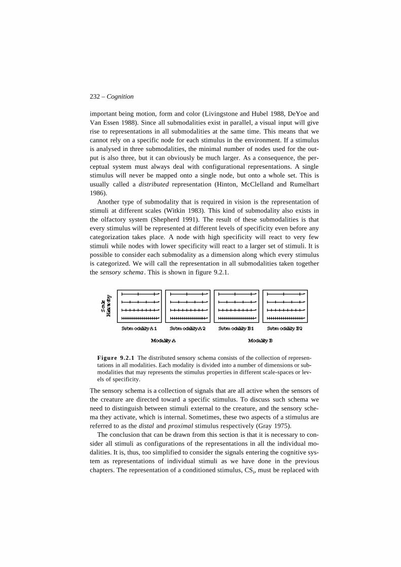
232 – Cognition
important being motion, form and color (Livingstone and Hubel 1988, DeYoe andVan Essen 1988). Since all submodalities exist in parallel, a visual input will giverise to representations in all submodalities at the same time. This means that wecannot rely on a specific node for each stimulus in the environment. If a stimulusis analysed in three submodalities, the minimal number of nodes used for the out-put is also three, but it can obviously be much larger. As a consequence, the per-ceptual system must always deal with configurational representations. A singlestimulus will never be mapped onto a single node, but onto a whole set. This isusually called a distributed representation (Hinton, McClelland and Rumelhart1986).
Another type of submodality that is required in vision is the representation ofstimuli at different scales (Witkin 1983). This kind of submodality also exists inthe olfactory system (Shepherd 1991). The result of these submodalities is thatevery stimulus will be represented at different levels of specificity even before anycategorization takes place. A node with high specificity will react to very fewstimuli while nodes with lower specificity will react to a larger set of stimuli. It ispossible to consider each submodality as a dimension along which every stimulusis categorized. We will call the representation in all submodalities taken togetherthe sensory schema . This is shown in figure 9.2.1.
Figure 9.2.1 The distributed sensory schema consists of the collection of represen-tations in all modalities. Each modality is divided into a number of dimensions or sub-modalities that may represents the stimulus properties in different scale-spaces or lev-els of specificity.
The sensory schema is a collection of signals that are all active when the sensors ofthe creature are directed toward a specific stimulus. To discuss such schema weneed to distinguish between stimuli external to the creature, and the sensory sche-ma they activate, which is internal. Sometimes, these two aspects of a stimulus arereferred to as the distal and proximal stimulus respectively (Gray 1975).
The conclusion that can be drawn from this section is that it is necessary to con-sider all stimuli as configurations of the representations in all the individual mo-dalities. It is, thus, too simplified to consider the signals entering the cognitive sys-tem as representations of individual stimuli as we have done in the previouschapters. The representation of a conditioned stimulus, CSi, must be replaced with
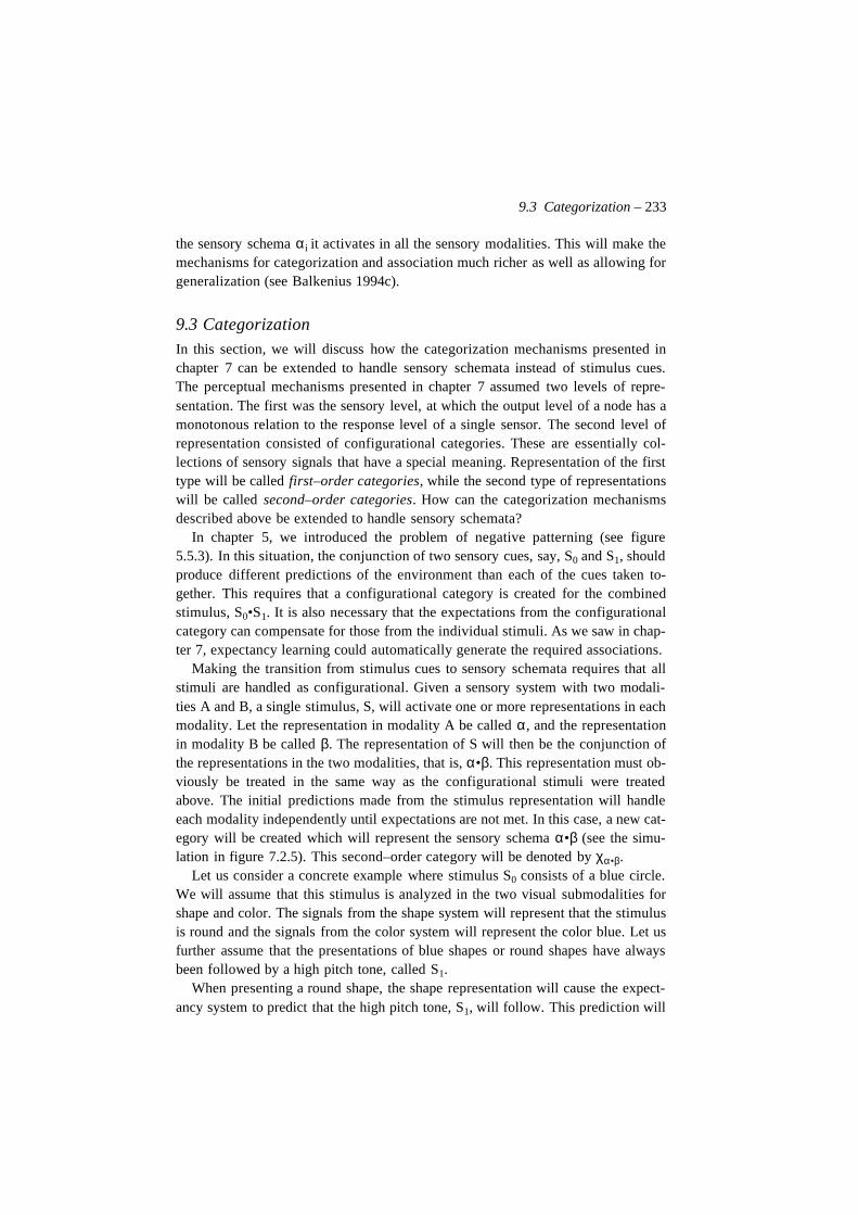
9.3 Categorization – 233
the sensory schema αi it activates in all the sensory modalities. This will make themechanisms for categorization and association much richer as well as allowing forgeneralization (see Balkenius 1994c).
9.3 CategorizationIn this section, we will discuss how the categorization mechanisms presented inchapter 7 can be extended to handle sensory schemata instead of stimulus cues.The perceptual mechanisms presented in chapter 7 assumed two levels of repre-sentation. The first was the sensory level, at which the output level of a node has amonotonous relation to the response level of a single sensor. The second level ofrepresentation consisted of configurational categories. These are essentially col-lections of sensory signals that have a special meaning. Representation of the firsttype will be called first–order categories, while the second type of representationswill be called second–order categories. How can the categorization mechanismsdescribed above be extended to handle sensory schemata?
In chapter 5, we introduced the problem of negative patterning (see figure5.5.3). In this situation, the conjunction of two sensory cues, say, S0 and S1, shouldproduce different predictions of the environment than each of the cues taken to-gether. This requires that a configurational category is created for the combinedstimulus, S0•S1. It is also necessary that the expectations from the configurationalcategory can compensate for those from the individual stimuli. As we saw in chap-ter 7, expectancy learning could automatically generate the required associations.
Making the transition from stimulus cues to sensory schemata requires that allstimuli are handled as configurational. Given a sensory system with two modali-ties A and B, a single stimulus, S, will activate one or more representations in eachmodality. Let the representation in modality A be called α, and the representationin modality B be called β. The representation of S will then be the conjunction ofthe representations in the two modalities, that is, α•β. This representation must ob-viously be treated in the same way as the configurational stimuli were treatedabove. The initial predictions made from the stimulus representation will handleeach modality independently until expectations are not met. In this case, a new cat-egory will be created which will represent the sensory schema α•β (see the simu-lation in figure 7.2.5). This second–order category will be denoted by χα•β.
Let us consider a concrete example where stimulus S0 consists of a blue circle.We will assume that this stimulus is analyzed in the two visual submodalities forshape and color. The signals from the shape system will represent that the stimulusis round and the signals from the color system will represent the color blue. Let usfurther assume that the presentations of blue shapes or round shapes have alwaysbeen followed by a high pitch tone, called S1.
When presenting a round shape, the shape representation will cause the expect-ancy system to predict that the high pitch tone, S1, will follow. This prediction will
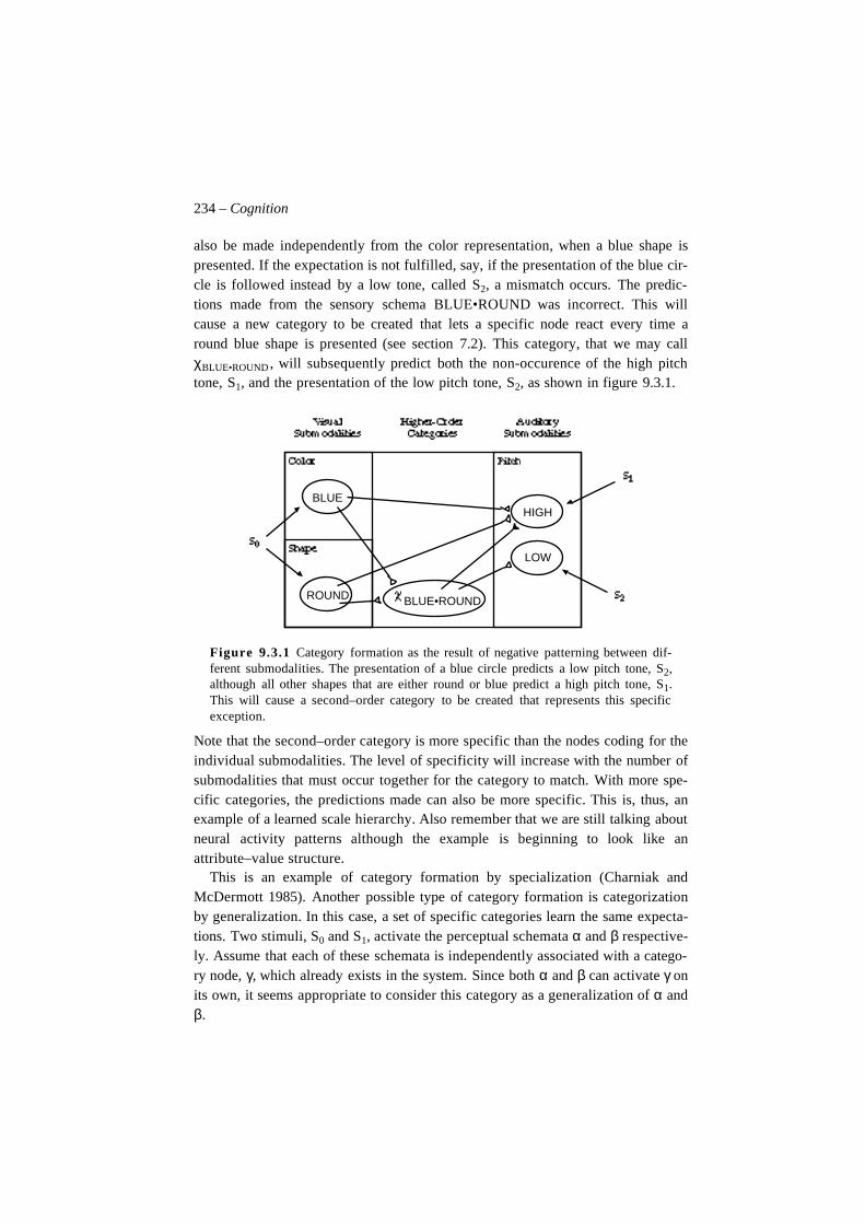
234 – Cognition
also be made independently from the color representation, when a blue shape ispresented. If the expectation is not fulfilled, say, if the presentation of the blue cir-cle is followed instead by a low tone, called S2, a mismatch occurs. The predic-tions made from the sensory schema BLUE•ROUND was incorrect. This willcause a new category to be created that lets a specific node react every time around blue shape is presented (see section 7.2). This category, that we may callχBLUE•ROUND , will subsequently predict both the non-occurence of the high pitchtone, S1, and the presentation of the low pitch tone, S2, as shown in figure 9.3.1.
Figure 9.3.1 Category formation as the result of negative patterning between dif-ferent submodalities. The presentation of a blue circle predicts a low pitch tone, S2,although all other shapes that are either round or blue predict a high pitch tone, S1.This will cause a second–order category to be created that represents this specificexception.
Note that the second–order category is more specific than the nodes coding for theindividual submodalities. The level of specificity will increase with the number ofsubmodalities that must occur together for the category to match. With more spe-cific categories, the predictions made can also be more specific. This is, thus, anexample of a learned scale hierarchy. Also remember that we are still talking aboutneural activity patterns although the example is beginning to look like anattribute–value structure.
This is an example of category formation by specialization (Charniak andMcDermott 1985). Another possible type of category formation is categorizationby generalization. In this case, a set of specific categories learn the same expecta-tions. Two stimuli, S0 and S1, activate the perceptual schemata α and β respective-ly. Assume that each of these schemata is independently associated with a catego-ry node, γ, which already exists in the system. Since both α and β can activate γ onits own, it seems appropriate to consider this category as a generalization of α andβ.
BLUE
ROUND
HIGH
LOW
BLUE•ROUND
9.4 The Internal Environment – 235
Figure 9.3.2 Categorization by generalization is handled by an associative process.No new category need to be created in this case.
A fairly simple extension of the mechanisms we have described earlier in this bookwould, thus, handle categorization based on both specialization and generaliza-tion. New categories are only created during specialization which is natural sincegeneralization assimilates the new instance to a category that already exists.
9.4 The Internal EnvironmentThe expectancy network introduced in chapter 5 can be used as a starting point forwhat might be called an internal environment. This environment is used to try outactions internally before they are confronted with external reality (Gulz 1991). Aswe will argue below in section 9.5, it can be used both for planning and problemsolving. In this section, we discuss how the expectancy network would have to bemodified to serve as an internal environment.
Temporal Expectations
The temporal expectations considered above all require a fixed time delay betweenthe cue and the predicted event. A prediction of this type will be written as,
(9.4.4)Using this type of representation, predictions over longer periods of time couldonly be made using avalanches started by a sensory cue or by secondary condition-ing (see chapter 5). In a more general system, predictions must be made over arbi-trary periods of time. It is not sufficient to represent that the presentation of Si attime t will predict the presentation of Sj at time t+1. A more useful expectationwould represent, not only that Sj will follow Si, but also when. Representations ofthis type would look the following way,
(9.4.5)Here, ∆ij is a parameter that is specific for each pair of stimuli. A further extensionwould replace the single parameter ∆ij with a function of time that assigns a prob-ability to the statement Si(t)→Sj(t+δ) for each value on δ. This function can be rep-resented either directly, or as a set of parameters.
Si t( ) S j t 1+( ).→
Si t( ) S j t ∆ij+( ).→
236 – Cognition
One way to parametrize the representation is to represent the prediction as aninterval [∆ij–ξij, ∆ij+ξij] around a mean value represented by ∆ij. This requires, ofcourse, that S0 has preceded S1 at least once. If it has not, the values of ∆ij and ξij
have no meaning, and this suggests that we should also represent the certainty ofboth ∆ij and ξij. This certainty, cij, should be zero initially, and increase as the esti-mates of ∆ij and ξij improve. This is not sufficient, however.
To know whether Si really predicts Sj, we need to weigh it against the probabil-ity that Sj is present without being preceded by Si. If, for instance, Sj is alwayspresent, Si has obviously no predictive power and there should be no associationbetween Si and Sj. A similar effect occurs in latent inhibition experiments wherethe presentation of a CS on its own retards the subsequent development of an asso-ciation with an US (Mackintosh 1983). In this case, the pre-exposure to the CSmakes the probability that the US will follow smaller than if the CS had never beenpresented before. This suggests that latent inhibition can be explained with amechanism that estimates the probability of occurance of each stimulus and com-pares it with the probability of each CS–US pair (Gallistel 1990).
Balkenius (1992) has presented a neural network architecture that is able to ex-tract the amount of information one node transmits about the state of another. Al-though it was not recognized in that paper, the proposed network model solves theproblem of latent inhibition in the case of simultaneous conditioning. However,the model is not easily extended to temporal predictions, and this is what is re-quired for a useful internal environment.
An extended creature will, thus, need to form predictions that are based ontransferred information and not on temporal contiguity. These predictions mustcode both when a stimulus is likely to follow another and with what certainty thisprediction is made. As in the case of categorization, these predictions must also bemade for distributed schemata and not for local stimulus representations, since it isnecessary to represent predictions from one submodality to another.
Working Memory
The segregation of the sensory analysis into ‘what’ and ‘where’ systems (Mishkin,Ungerleider and Macko 1983) has some interesting consequences. Let us assumethat the creature is equipped with a content addressable memory that works in thefollowing way (see section 3.3). When an orienting reaction is made toward an un-expected stimulus, the sensory schemata represented in the ‘what’ and the ‘where’systems are associated together in the content addressable memory.
This memory can be seen as a generalization of the working memory for novelfoods introduced in chapter 5. In that simple working memory, only the sicknesssensor could recall the stored memory. For a more general working memory, anysufficiently specific subschema from any modality should recall the entire sensoryschema with which it was stored. For example, the activation of a place represen-
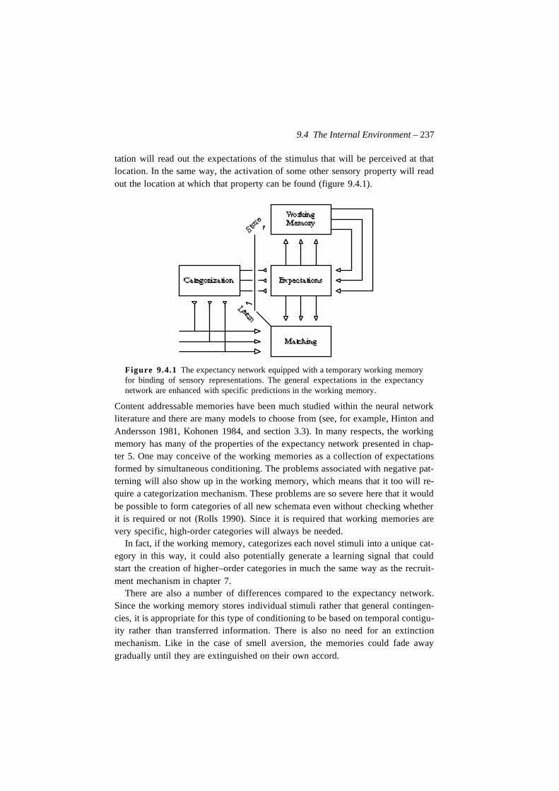
9.4 The Internal Environment – 237
tation will read out the expectations of the stimulus that will be perceived at thatlocation. In the same way, the activation of some other sensory property will readout the location at which that property can be found (figure 9.4.1).
Figure 9.4.1 The expectancy network equipped with a temporary working memoryfor binding of sensory representations. The general expectations in the expectancynetwork are enhanced with specific predictions in the working memory.
Content addressable memories have been much studied within the neural networkliterature and there are many models to choose from (see, for example, Hinton andAndersson 1981, Kohonen 1984, and section 3.3). In many respects, the workingmemory has many of the properties of the expectancy network presented in chap-ter 5. One may conceive of the working memories as a collection of expectationsformed by simultaneous conditioning. The problems associated with negative pat-terning will also show up in the working memory, which means that it too will re-quire a categorization mechanism. These problems are so severe here that it wouldbe possible to form categories of all new schemata even without checking whetherit is required or not (Rolls 1990). Since it is required that working memories arevery specific, high-order categories will always be needed.
In fact, if the working memory, categorizes each novel stimuli into a unique cat-egory in this way, it could also potentially generate a learning signal that couldstart the creation of higher–order categories in much the same way as the recruit-ment mechanism in chapter 7.
There are also a number of differences compared to the expectancy network.Since the working memory stores individual stimuli rather that general contingen-cies, it is appropriate for this type of conditioning to be based on temporal contigu-ity rather than transferred information. There is also no need for an extinctionmechanism. Like in the case of smell aversion, the memories could fade awaygradually until they are extinguished on their own accord.
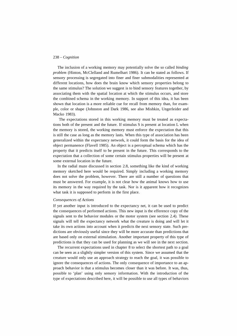
238 – Cognition
The inclusion of a working memory may potentially solve the so called bindingproblem (Hinton, McClelland and Rumelhart 1986). It can be stated as follows. Ifsensory processing is segregated into finer and finer submodalities represented atdifferent locations, how does the brain know which sensory properties belong tothe same stimulus? The solution we suggest is to bind sensory features together, byassociating them with the spatial location at which the stimulus occurs, and storethe combined schema in the working memory. In support of this idea, it has beenshown that location is a more reliable cue for recall from memory than, for exam-ple, color or shape (Johnston and Dark 1986, see also Mishkin, Ungerleider andMacko 1983).
The expectations stored in this working memory must be treated as expecta-tions both of the present and the future. If stimulus S is present at location L whenthe memory is stored, the working memory must enforce the expectation that thisis still the case as long as the memory lasts. When this type of association has beengeneralized within the expectancy network, it could form the basis for the idea ofobject permanence (Flavell 1985). An object is a perceptual schema which has theproperty that it predicts itself to be present in the future. This corresponds to theexpectation that a collection of some certain stimulus properties will be present atsome external location in the future.
In the radial maze discussed in section 2.8, something like the kind of workingmemory sketched here would be required. Simply including a working memorydoes not solve the problem, however. There are still a number of questions thatmust be answered. For example, it is not clear how the animal knows how to useits memory in the way required by the task. Nor is it apparent how it recognizeswhat task it is supposed to perform in the first place.
Consequences of Actions
If yet another input is introduced to the expectancy net, it can be used to predictthe consequences of performed actions. This new input is the efference copy of thesignals sent to the behavior modules or the motor system (see section 2.4). Thesesignals will tell the expectancy network what the creature is doing and will let ittake its own actions into account when it predicts the next sensory state. Such pre-dictions are obviously useful since they will be more accurate than predictions thatare based only on external stimulation. Another important property of this type ofpredictions is that they can be used for planning as we will see in the next section.
The recurrent expectations used in chapter 8 to select the shortest path to a goalcan be seen as a slightly simpler version of this system. Since we assumed that thecreature would only use an approach strategy to reach the goal, it was possible toignore the consequences of actions. The only consequence of importance to an ap-proach behavior is that a stimulus becomes closer than it was before. It was, thus,possible to ‘plan’ using only sensory information. With the introduction of thetype of expectations described here, it will be possible to use all types of behaviors
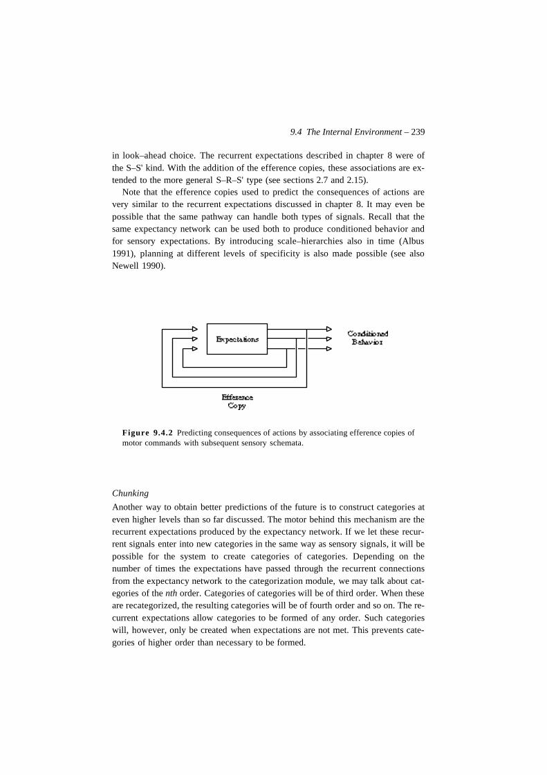
9.4 The Internal Environment – 239
in look–ahead choice. The recurrent expectations described in chapter 8 were ofthe S–S' kind. With the addition of the efference copies, these associations are ex-tended to the more general S–R–S' type (see sections 2.7 and 2.15).
Note that the efference copies used to predict the consequences of actions arevery similar to the recurrent expectations discussed in chapter 8. It may even bepossible that the same pathway can handle both types of signals. Recall that thesame expectancy network can be used both to produce conditioned behavior andfor sensory expectations. By introducing scale–hierarchies also in time (Albus1991), planning at different levels of specificity is also made possible (see alsoNewell 1990).
Figure 9.4.2 Predicting consequences of actions by associating efference copies ofmotor commands with subsequent sensory schemata.
Chunking
Another way to obtain better predictions of the future is to construct categories ateven higher levels than so far discussed. The motor behind this mechanism are therecurrent expectations produced by the expectancy network. If we let these recur-rent signals enter into new categories in the same way as sensory signals, it will bepossible for the system to create categories of categories. Depending on thenumber of times the expectations have passed through the recurrent connectionsfrom the expectancy network to the categorization module, we may talk about cat-egories of the nth order. Categories of categories will be of third order. When theseare recategorized, the resulting categories will be of fourth order and so on. The re-current expectations allow categories to be formed of any order. Such categorieswill, however, only be created when expectations are not met. This prevents cate-gories of higher order than necessary to be formed.
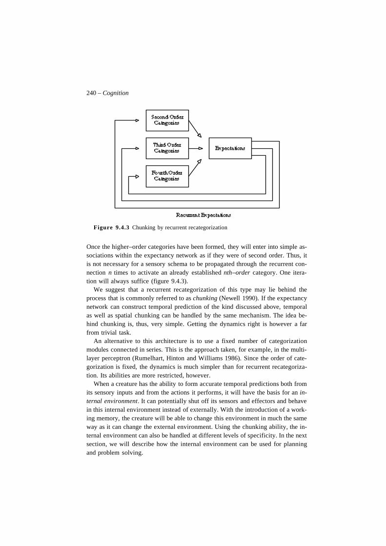
240 – Cognition
Figure 9.4.3 Chunking by recurrent recategorization
Once the higher–order categories have been formed, they will enter into simple as-sociations within the expectancy network as if they were of second order. Thus, itis not necessary for a sensory schema to be propagated through the recurrent con-nection n times to activate an already established nth–order category. One itera-tion will always suffice (figure 9.4.3).
We suggest that a recurrent recategorization of this type may lie behind theprocess that is commonly referred to as chunking (Newell 1990). If the expectancynetwork can construct temporal prediction of the kind discussed above, temporalas well as spatial chunking can be handled by the same mechanism. The idea be-hind chunking is, thus, very simple. Getting the dynamics right is however a farfrom trivial task.
An alternative to this architecture is to use a fixed number of categorizationmodules connected in series. This is the approach taken, for example, in the multi-layer perceptron (Rumelhart, Hinton and Williams 1986). Since the order of cate-gorization is fixed, the dynamics is much simpler than for recurrent recategoriza-tion. Its abilities are more restricted, however.
When a creature has the ability to form accurate temporal predictions both fromits sensory inputs and from the actions it performs, it will have the basis for an in-ternal environment. It can potentially shut off its sensors and effectors and behavein this internal environment instead of externally. With the introduction of a work-ing memory, the creature will be able to change this environment in much the sameway as it can change the external environment. Using the chunking ability, the in-ternal environment can also be handled at different levels of specificity. In the nextsection, we will describe how the internal environment can be used for planningand problem solving.
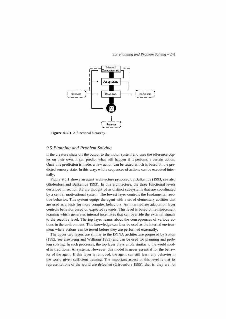
9.5 Planning and Problem Solving – 241
Figure 9.5.1 A functional hierarchy.
9.5 Planning and Problem SolvingIf the creature shuts off the output to the motor system and uses the efference cop-ies on their own, it can predict what will happen if it perfoms a certain action.Once this prediction is made, a new action can be tested which is based on the pre-dicted sensory state. In this way, whole sequences of actions can be executed inter-nally.
Figure 9.5.1 shows an agent architecture proposed by Balkenius (1993, see alsoGärdenfors and Balkenius 1993). In this architecture, the three functional levelsdescribed in section 3.2 are thought of as distinct subsystems that are coordinatedby a central motivational system. The lowest layer controls the fundamental reac-tive behavior. This system equips the agent with a set of elementary abilities thatare used as a basis for more complex behaviors. An intermediate adaptation layercontrols behavior based on expected rewards. This level is based on reinforcementlearning which generates internal incentives that can override the external signalsto the reactive level. The top layer learns about the consequences of various ac-tions in the environment. This knowledge can later be used as the internal environ-ment where actions can be tested before they are performed externally.
The upper two layers are similar to the DYNA architecture proposed by Sutton(1992, see also Peng and Williams 1993) and can be used for planning and prob-lem solving. In such processes, the top layer plays a role similar to the world mod-el in traditional AI systems. However, this model is never essential for the behav-ior of the agent. If this layer is removed, the agent can still learn any behavior inthe world given sufficient training. The important aspect of this level is that itsrepresentations of the world are detached (Gärdenfors 1995), that is, they are not
242 – Cognition
confined to here and now, but can be used independently of the current perceptualsituation.
By depending on the already existing systems, a planning ability is the result ofadding a single functional layer (see figure 3.2.8). We have an example of a truesystem property that cannot be localized in one specific module of the agent. Withthe model system, the agent can be engaged in planning, but this module does notplan in itself. The result of the planning process is to adapt the reactive system tothe internal environment, rather than to produce a fixed program to execute (com-pare Lyons, Hendriks and Mehta 1991).
The architecture presented here is in many respects similar to the one presentedby Gulz (1991). Planning is considered as internal simulation of external behavior.Instead of using the external world to generate new sensory information, actionsare performed in an internal model. The different actions are simulated in thismodel, and a new sensory input is generated internally. In this view, the internalmodel is not independent of the agent itself. It is a module which can generate thesensory information which would be the result if the agent had performed the cor-responding action externally.
The internal model is used very differently compared to the models used withinthe symbol processing paradigm. The model is not a description of the world. Asfar as our agent is concerned, the internal model is a world. However, to be suc-cessful, this internal world must be parallel to the external world. Planning can beseen as behavior in this internal world instead of the external world (Balkenius1993, see also Gärdenfors 1992, and Gärdenfors and Balkenius 1993). The onlydifference between a search in the internal world and actions performed external-lyd is that all actions can be undone as well as taking much less time to perform.The plan constructed from behavior in the internal world is in no way differentfrom the paths learned from externally tested action sequences. The same mecha-nisms are used, and the plan is represented and executed in the same way as a be-havior that has been practiced in the external world.
The plans constructed using the internal environment are also very differentfrom classical plans. A useful view of the type of plans constructed by this archi-tecture are as resources and not as programs (Payton 1990). Horswill and Stein(1995) have suggested that robot control systems can be classified according totheir commitment to generated plans. In this scheme, classical AI systems have ahigh degree of commitment. When the plan has been constructed, it is executedfrom the first step to the last. On the other hand, the plans constructed by the archi-tecture described here have a minimal degree of commitment, since plans are usedreactively. It may even be questionable to call the changes to the reinforcementsystem plans since they are not explicitly represented as a such.
When the abilities suggested in this chapter have been included in the architec-ture, the dynamics generated internally will parallel that between the creature and
9.6 Modes of Planning – 243
its environment (compare section 4.2). It is interesting to note that the dynamicalconcepts introduced in chapter 4 can be used to describe both the dynamics be-tween the organism and the environment, and the internal operation of a neuralsystem. For example, the planning of an approach behavior would correspond tothe convergence to an attractor within the artificial neural network controlling thecreature. If such a mapping can be done in general, it would allow a dynamicalview of cognition on all process levels. Goal-directed thought could, thus, be seenas internally performed goal-directed behavior.
9.6 Modes of Planning
Given that a creature is equipped with a planning ability of the kind describedabove, how and when should it be used? First we need to distinguish between twotypes of planning.
In the first case, planning is used to speed up learning of S–R associations by si-lently rehearsing stored copies of previous experiences. In this type of planning,no generalization is required in the internal environment. This is essentially thetype of learning used within the DYNA framework (Sutton 1992). Stored experi-ences are selected at random and used to train a reinforcement leaning module.Since planning of this type is not at all goal-directed, there is no guarantee that thetrained experiences will be relevant to the creature.
In the second type of planning, some form of goal-direction is involved. Suchplanning requires that the internal environment can be used for generalization. Ifthe behavior that leads to the goal is already known planning is unnecessary. If itis unknown, planning is impossible. Planning, thus, requires a situation that issomewhere in between. That is, a new situation to which old knowledge can beapplied.
Gulz (1991) distinguishes between two other types of planning. The first type iscalled immediate planning and is produced when the approach of a specific goal isobstructed. The planning that it generates is directed toward this specific goal. Forinstance, an unexpected encounter with an obstacle that is hard to overcome couldgenerate immediate planning behavior.
The second type of planning is called anticipatory. Such planning does not re-late to the current engagement of the creature. Instead, it is caused by simulatedneeds. The creature anticipates that it will become hungry tomorrow and plans itsday accordingly.
There is an obvious similarity between the situation in which the orienting reac-tion is executed and the situations in which immediate planning could be activated.In both cases, something unexpected happens in the environment and in both casesongoing behavior must be inhibited. This suggests that this type of planning isclosely connected to emotional states. The prototypical emotion activating imme-
244 – Cognition
diate planning is, thus, frustration caused by omission of an expected reward or byan unexpected obstacle.
Anticipatory planning, on the other hand, is not caused by any external event. Itmust, thus, compete with other engagements through the motivational system.This is the role of the anticipatory drive introduced in chapter 6.
There is, thus, a clear connection between emotion and immediate planning andmotivation and anticipatory planning. Depending on the type of emotion or on thetype of simulated motivation, we can identify different modes of planning. Differ-ent types of planning are caused by immediate punishment or frustration and bytheir anticipated counterparts. On the positive side, these modes are less clear, all-though one may possibly identify daydreaming with planning motivated by antici-pated reward.
9.7 ConclusionWe have discussed a number of limitations of the creature that was developed inthe previous chapters. It was suggested that before higher cognitive abilities can beincluded in the architecture, a number of problems must be solved.
First, it is necessary that the creature uses distributed representations at multiplescales and of many modalities to be able to generalize from one situation to anoth-er. This problem is addressed by adding more sensors and more sensory process-ing to the creature.
Second, the categorization mechanism described in chapter 5 must be extendedto handle these distributed representations. The main problem here is to devise amatching criterion that generates new categories at the right times. With an incor-rect matching rule, too many categories will be formed. While the mechanism de-scribed in chapter 7 can learn any expectancy, this is often done at the cost of alarge number of unnecessary category nodes. For a more economical system, amore advanced mechanism for category creation is needed.
Third, the internal environment puts some non-trivial requirements on to the ex-pectancy network. It must somehow represent both which stimulus will follow an-other, as well as when, and with what certainty. The need for a representation ofthe consequences of actions and for hierarchical chunking makes this problemeven more complex. This is an area for future research.
None of the above problems appear impossible to solve, however, and in re-stricted cases, they all have simple solutions. Given that these problems are solvedmore generally, we have shown that some complex cognitive abilities will becomepossible. It should be clear that these systems are natural extensions of the mecha-nisms we have already developed.
Christian Balkenius, 1995, Natural Intelligence in Artificial Creatures, Lund University Cognitive Studies 37, 1995.
Chapter 10
Conclusion
10.1 IntroductionThis final chapter presents an overview of how the various systems described inthe previous chapters can be put together into a coherent model.1 This completemodel will be viewed from three perspectives.
The next section of this chapter describes the individual components of themodel and their functional relations. We will, then, go on to describe the modelfrom an evolutionary perspective as a set of superimposed mechanisms, each ofwhich makes the performance of the system more adaptive. Finally, we will dis-cuss the relation between the models presented here and functional systems likelyto exist in the brain.
The last sections of this chapter discuss a number of theoretical and practicallimitations of the model and suggest some topics for further research.
10.2 The Components of the ModelWe have tried to promote a view of cognition as a process governed by a collectionof interacting systems. The main goal has been to present an overall model of howthe various systems should be put together.
1. To make this chapter more readable, references to chapters and sections in the rest of thebook will be given without the initial words ‘see section’ etc.
246 – Conclusion
Behavior is seen, not as the execution of actions or responses, but as the coordi-nated activation and inhibition of a large number of behavior modules (3.2, 4.3,5.2, 5.12, 6.3). Unlike responses, the behaviors controlled by behavior modulescan be of arbitrary complexity (4.3, 4.4). They can range from simple responses(8.2) to complex fixed–action patterns (4.3) and goal-directed behaviors (4.2) thatuse both adaptation (5.7) and external stimuli for control (8.2). In some cases, theadaptation is very simple, as in the tuning of an approach behavior (5.7). In othercases, it is very complex, as, for example, when long chains of behaviors arelearned (8.3). The adaptation within a behavior module can also consist of thelearning of the location of a stimulus based on multiple cues (7.3).
We have divided behaviors into four classes, depending on the status of the ob-ject or situation to which it relates (4.1, 4.2, 5.2). Appetitive behavior is directedtoward an object or a situation in the sense that it increases the probability that thegoal will be found. An appetitive behavior may or may not be goal-directed. Aver-sive behavior is directed away from an object or a situation. Neutral behavior re-lates to objects that are known to be neither appetitive nor aversive. Obstacles aretypically of this kind. Finally, we identified the class of exploratory behaviorswhich relate to objects or situations with unknown or uncertain valences. The va-lence of a stimulus always relates to a specific engagement. A stimulus that maybe appetitive for one engagement may be aversive or neutral for another.
In later chapters, exploratory behavior was seen to be highly dependent on theorienting reaction (4.4). Efficient exploration is generated by an orienting reactionthat habituates as unkown objects become aversive, appetitive or neutral (7.4).
Equipped with an appropriate behavior repertoire, the problem is to know wheneach behavior module should be activated or inhibited. We have described twomain mechanisms for this: learning (5) and motivation (6).
Learning is the process by which an animal aquires knowledge about itself andits environment, either by trying out different behaviors in different situations(5.2, 5.9, 8.3) or by learning about contingencies in the world (5.10, 8.4).
The first type of learning was termed procedural learning since it establishedsequences of activations of behavior modules (8.3). Learning of this type is con-trolled by primary and secondary reward or punishment (5.2–5.6). We presentedthree primary events that would generate reinforcement: presentation, terminationor omission of reward or punishment (5.2). The reinforcement generated in allthese cases was seen as the result of a matching between actual and expected con-sequences (5.2). The difference between expected reward and the actual reward isused to generate reinforcement signals that control learning. Reinforcement is,thus, different from reward and punishment.
In expectancy learning predictions are made, not only of future rewards or pun-ishments, but also of future sensory and perceptual states (5.10, 8.4). The basiclearning mechanism is the same, however. The animal learns when something is
10.2 The Components of the Model – 247
unexpected. Expectancy learning is viewed as the basic mechanism behind classi-cal conditioning, which is seen primarily as a process whereby an animal learns topredict future sensory states. Such predictions were used for different purposes inthree different systems. The first was to produce responses in the traditional way(5.3). The second was to habituate the orienting reaction and the exploratory be-havior (7.4). The third role was in the process we called look-ahead choice to gen-erate recurrent predictions many states ahead (8.4).
Motivation is the second mechanism controlling the activation or inhibition ofbehavior modules (6). While learning adjusts the behavior of an animal to the fu-ture, motivation adjusts behavior according to its present needs. In most cases, themotivational system activates not only a single behavior module but an entire en-gagement system , consisting of a large number of interacting behavior modulesand learning systems (3.2, 6.9).
The motivational system is, thus, seen as a choice mechanism that decideswhichbehavior or engagement should be active at a certain time (6.1, 6.5, 6.6).This choice depends on three factors (6.2). The first is the need of the animal rep-resented by its drive signals (6.3). The second is external incentive, generated bythe representation of an external goal (6.4) and the third is internal incentives,which are generated by the representation of external cues that in some way pre-dict the goal (6.4, 7.5). In this context emotions are seen as the internal states gen-erated by reinforcing stimuli (6.7).
Perception is considered to be a process serving at least three related functions(7.1). The first is to recognize the current situation and aid in the selection of theappropriate behavior (7.1, 7.2). The second is to guide the execution of this select-ed behavior (7.3). The final role of perception is to generate incentives to the mo-tivational system which helps in the selection of an engagement (6.4, 7.5). Catego-rization plays an important role in all these functions (7.2).
We have suggested that the categorization process is driven by three differenttypes of mismatch conditions. In the first, the best available category does not fitthe input pattern sufficiently well and a new category is created (7.2, 8.3). In thesecond condition, the expected reward or punishment does not match the actual re-ward or punishment (7.1, 8.3). This implies that a finer representation of the cur-rent situation is required, which causes a new category to be formed. In the finalmismatch condition, the expectations about the present situation are not matchedby external stimuli (7.2). Again, a new category is required. In all three cases, anew category is only created when the mismatch is sufficiently pronounced. Whenit is less severe, the already existing categories or expectancies are adjusted in-stead.
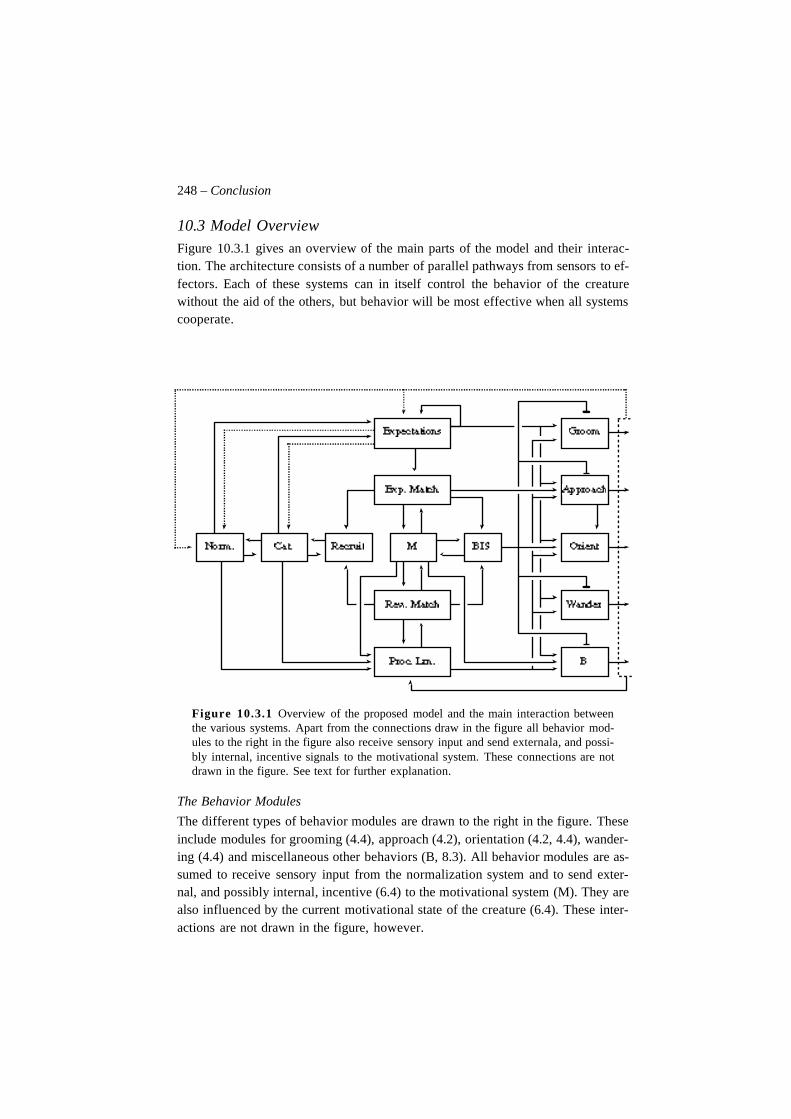
248 – Conclusion
10.3 Model OverviewFigure 10.3.1 gives an overview of the main parts of the model and their interac-tion. The architecture consists of a number of parallel pathways from sensors to ef-fectors. Each of these systems can in itself control the behavior of the creaturewithout the aid of the others, but behavior will be most effective when all systemscooperate.
Figure 10.3.1 Overview of the proposed model and the main interaction betweenthe various systems. Apart from the connections draw in the figure all behavior mod-ules to the right in the figure also receive sensory input and send externala, and possi-bly internal, incentive signals to the motivational system. These connections are notdrawn in the figure. See text for further explanation.
The Behavior Modules
The different types of behavior modules are drawn to the right in the figure. Theseinclude modules for grooming (4.4), approach (4.2), orientation (4.2, 4.4), wander-ing (4.4) and miscellaneous other behaviors (B, 8.3). All behavior modules are as-sumed to receive sensory input from the normalization system and to send exter-nal, and possibly internal, incentive (6.4) to the motivational system (M). They arealso influenced by the current motivational state of the creature (6.4). These inter-actions are not drawn in the figure, however.
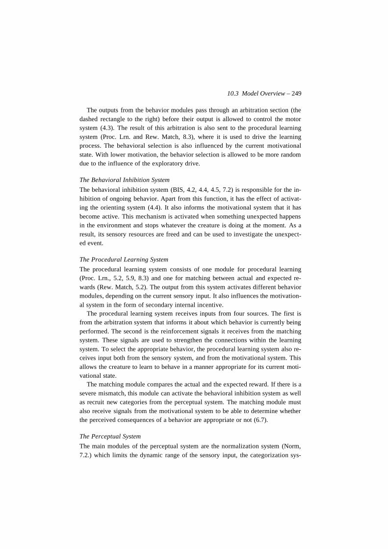
10.3 Model Overview – 249
The outputs from the behavior modules pass through an arbitration section (thedashed rectangle to the right) before their output is allowed to control the motorsystem (4.3). The result of this arbitration is also sent to the procedural learningsystem (Proc. Lrn. and Rew. Match, 8.3), where it is used to drive the learningprocess. The behavioral selection is also influenced by the current motivationalstate. With lower motivation, the behavior selection is allowed to be more randomdue to the influence of the exploratory drive.
The Behavioral Inhibition System
The behavioral inhibition system (BIS, 4.2, 4.4, 4.5, 7.2) is responsible for the in-hibition of ongoing behavior. Apart from this function, it has the effect of activat-ing the orienting system (4.4). It also informs the motivational system that it hasbecome active. This mechanism is activated when something unexpected happensin the environment and stops whatever the creature is doing at the moment. As aresult, its sensory resources are freed and can be used to investigate the unexpect-ed event.
The Procedural Learning System
The procedural learning system consists of one module for procedural learning(Proc. Lrn., 5.2, 5.9, 8.3) and one for matching between actual and expected re-wards (Rew. Match, 5.2). The output from this system activates different behaviormodules, depending on the current sensory input. It also influences the motivation-al system in the form of secondary internal incentive.
The procedural learning system receives inputs from four sources. The first isfrom the arbitration system that informs it about which behavior is currently beingperformed. The second is the reinforcement signals it receives from the matchingsystem. These signals are used to strengthen the connections within the learningsystem. To select the appropriate behavior, the procedural learning system also re-ceives input both from the sensory system, and from the motivational system. Thisallows the creature to learn to behave in a manner appropriate for its current moti-vational state.
The matching module compares the actual and the expected reward. If there is asevere mismatch, this module can activate the behavioral inhibition system as wellas recruit new categories from the perceptual system. The matching module mustalso receive signals from the motivational system to be able to determine whetherthe perceived consequences of a behavior are appropriate or not (6.7).
The Perceptual System
The main modules of the perceptual system are the normalization system (Norm,7.2.) which limits the dynamic range of the sensory input, the categorization sys-
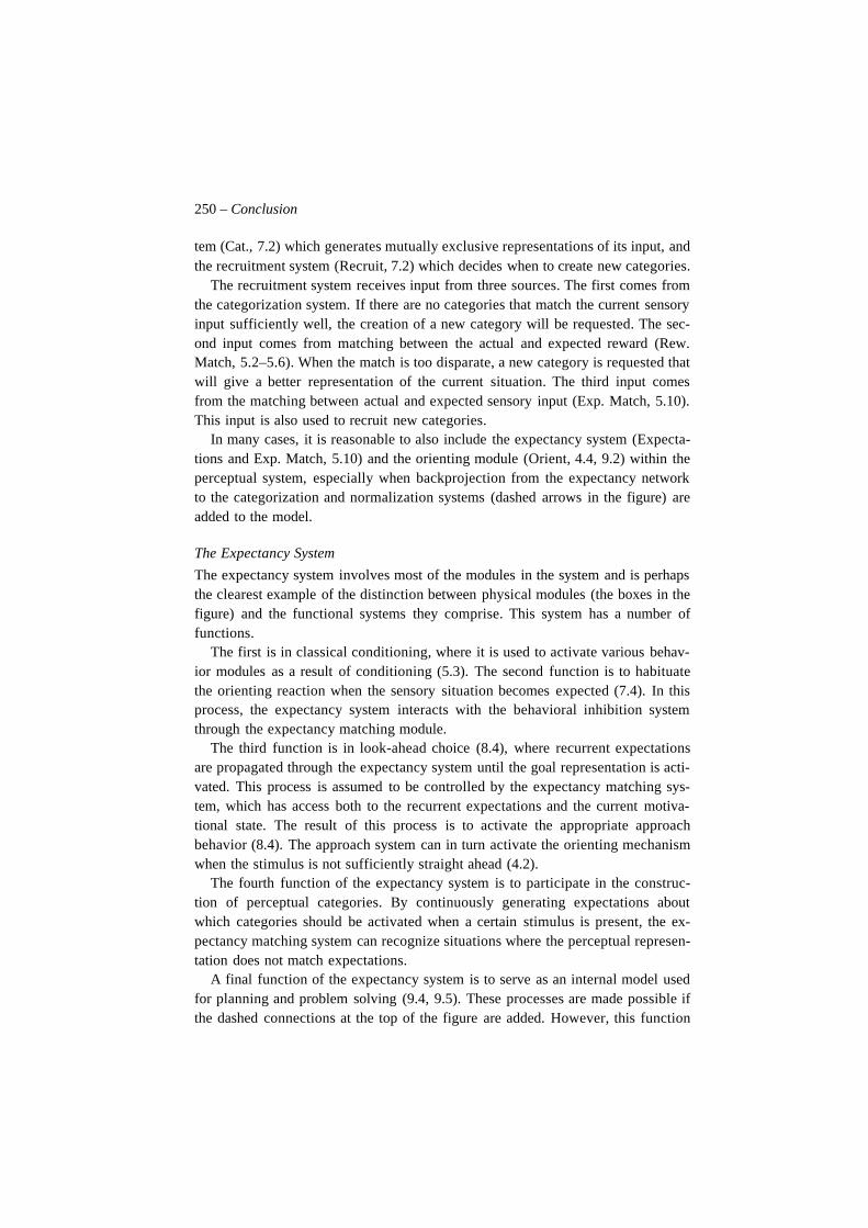
250 – Conclusion
tem (Cat., 7.2) which generates mutually exclusive representations of its input, andthe recruitment system (Recruit, 7.2) which decides when to create new categories.
The recruitment system receives input from three sources. The first comes fromthe categorization system. If there are no categories that match the current sensoryinput sufficiently well, the creation of a new category will be requested. The sec-ond input comes from matching between the actual and expected reward (Rew.Match, 5.2–5.6). When the match is too disparate, a new category is requested thatwill give a better representation of the current situation. The third input comesfrom the matching between actual and expected sensory input (Exp. Match, 5.10).This input is also used to recruit new categories.
In many cases, it is reasonable to also include the expectancy system (Expecta-tions and Exp. Match, 5.10) and the orienting module (Orient, 4.4, 9.2) within theperceptual system, especially when backprojection from the expectancy networkto the categorization and normalization systems (dashed arrows in the figure) areadded to the model.
The Expectancy System
The expectancy system involves most of the modules in the system and is perhapsthe clearest example of the distinction between physical modules (the boxes in thefigure) and the functional systems they comprise. This system has a number offunctions.
The first is in classical conditioning, where it is used to activate various behav-ior modules as a result of conditioning (5.3). The second function is to habituatethe orienting reaction when the sensory situation becomes expected (7.4). In thisprocess, the expectancy system interacts with the behavioral inhibition systemthrough the expectancy matching module.
The third function is in look-ahead choice (8.4), where recurrent expectationsare propagated through the expectancy system until the goal representation is acti-vated. This process is assumed to be controlled by the expectancy matching sys-tem, which has access both to the recurrent expectations and the current motiva-tional state. The result of this process is to activate the appropriate approachbehavior (8.4). The approach system can in turn activate the orienting mechanismwhen the stimulus is not sufficiently straight ahead (4.2).
The fourth function of the expectancy system is to participate in the construc-tion of perceptual categories. By continuously generating expectations aboutwhich categories should be activated when a certain stimulus is present, the ex-pectancy matching system can recognize situations where the perceptual represen-tation does not match expectations.
A final function of the expectancy system is to serve as an internal model usedfor planning and problem solving (9.4, 9.5). These processes are made possible ifthe dashed connections at the top of the figure are added. However, this function
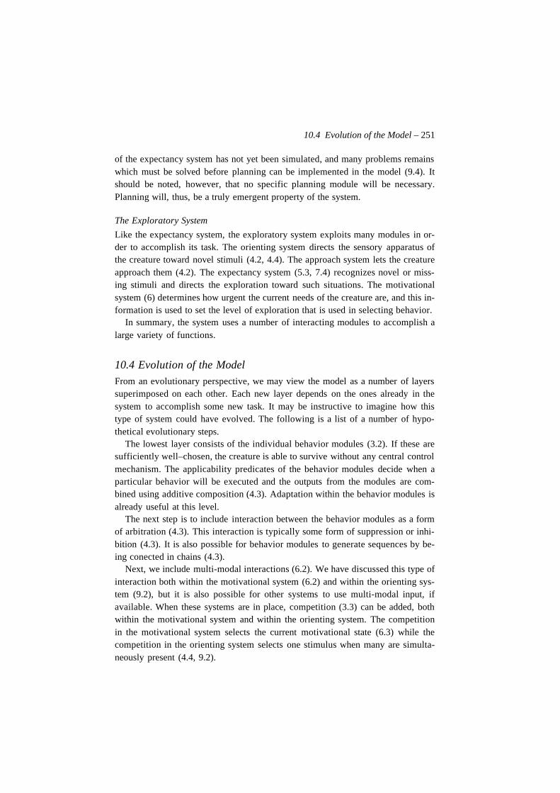
10.4 Evolution of the Model – 251
of the expectancy system has not yet been simulated, and many problems remainswhich must be solved before planning can be implemented in the model (9.4). Itshould be noted, however, that no specific planning module will be necessary.Planning will, thus, be a truly emergent property of the system.
The Exploratory System
Like the expectancy system, the exploratory system exploits many modules in or-der to accomplish its task. The orienting system directs the sensory apparatus ofthe creature toward novel stimuli (4.2, 4.4). The approach system lets the creatureapproach them (4.2). The expectancy system (5.3, 7.4) recognizes novel or miss-ing stimuli and directs the exploration toward such situations. The motivationalsystem (6) determines how urgent the current needs of the creature are, and this in-formation is used to set the level of exploration that is used in selecting behavior.
In summary, the system uses a number of interacting modules to accomplish alarge variety of functions.
10.4 Evolution of the Model
From an evolutionary perspective, we may view the model as a number of layerssuperimposed on each other. Each new layer depends on the ones already in thesystem to accomplish some new task. It may be instructive to imagine how thistype of system could have evolved. The following is a list of a number of hypo-thetical evolutionary steps.
The lowest layer consists of the individual behavior modules (3.2). If these aresufficiently well–chosen, the creature is able to survive without any central controlmechanism. The applicability predicates of the behavior modules decide when aparticular behavior will be executed and the outputs from the modules are com-bined using additive composition (4.3). Adaptation within the behavior modules isalready useful at this level.
The next step is to include interaction between the behavior modules as a formof arbitration (4.3). This interaction is typically some form of suppression or inhi-bition (4.3). It is also possible for behavior modules to generate sequences by be-ing conected in chains (4.3).
Next, we include multi-modal interactions (6.2). We have discussed this type ofinteraction both within the motivational system (6.2) and within the orienting sys-tem (9.2), but it is also possible for other systems to use multi-modal input, ifavailable. When these systems are in place, competition (3.3) can be added, bothwithin the motivational system and within the orienting system. The competitionin the motivational system selects the current motivational state (6.3) while thecompetition in the orienting system selects one stimulus when many are simulta-neously present (4.4, 9.2).
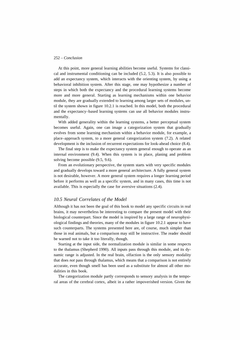
252 – Conclusion
At this point, more general learning abilities become useful. Systems for classi-cal and instrumental conditioning can be included (5.2, 5.3). It is also possible toadd an expectancy system, which interacts with the orienting system, by using abehavioral inhibition system. After this stage, one may hypothesize a number ofsteps in which both the expectancy and the procedural learning systems becomemore and more general. Starting as learning mechanisms within one behaviormodule, they are gradually extended to learning among larger sets of modules, un-til the system shown in figure 10.2.1 is reached. In this model, both the proceduraland the expectancy–based learning systems can use all behavior modules instru-mentally.
With added generality within the learning systems, a better perceptual systembecomes useful. Again, one can image a categorization system that graduallyevolves from some learning mechanism within a behavior module, for example, aplace–approach system, to a more general categorization system (7.2). A relateddevelopment is the inclusion of recurrent expectations for look-ahead choice (8.4).
The final step is to make the expectancy system general enough to operate as aninternal environment (9.4). When this system is in place, planing and problemsolving become possible (9.5, 9.6).
From an evolutionary perspective, the system starts with very specific modulesand gradually develops toward a more general architecture. A fully general systemis not desirable, however. A more general system requires a longer learning periodbefore it performs as well as a specific system, and in many cases, this time is notavailable. This is especially the case for aversive situations (2.4).
10.5 Neural Correlates of the Model
Although it has not been the goal of this book to model any specific circuits in realbrains, it may nevertheless be interesting to compare the present model with theirbiological counterpart. Since the model is inspired by a large range of neurophysi-ological findings and theories, many of the modules in figure 10.2.1 appear to havesuch counterparts. The systems presented here are, of course, much simpler thanthose in real animals, but a comparison may still be instructive. The reader shouldbe warned not to take it too literally, though.
Starting at the input side, the normalization module is similar in some respectsto the thalamus (Shepherd 1990). All inputs pass through this module, and its dy-namic range is adjusted. In the real brain, olfaction is the only sensory modalitythat does not pass through thalamus, which means that a comparison is not entirelyaccurate, even though smell has been used as a substitute for almost all other mo-dalities in this book.
The categorization module partly corresponds to sensory analysis in the tempo-ral areas of the cerebral cortex, albeit in a rather impoverished version. Given the
10.5 Neural Correlates of the Model – 253
simple sensory input used in our creature, the required sensory analysis is very el-ementary. Most of the sensory analysis thought to take place in cortex occurs be-fore any of the systems we have discussed in this book. We did recognize the needfor the dynamic creation of categories, however. This is a function that has beenascribed to the hippocampal system (Rolls 1990). If we accept this view, the hip-pocampus would correspond to the recruitment module and the entorhinal cortexto the categorization module (Rolls 1990). The expectancy matching module will,then, correspond to the subiculum of the hippocampal formation (Gray 1995). Thisbrain region has been suggested to compare the actual sensory input with the ex-pected situation. An alternative hypothesis is that matching is performed in theCA3 area of the hippocampus (Shepherd 1990). Within Gray’s theory, a mismatchwithin this system also activates the behavioral inhibition system (Gray 1982,1995). A further function of the hippocampus is to handle working memory (Shep-herd 1990, Squire 1992).
Procedural learning and some instances of classical conditioning are probablyhandled by the cerebellum (Ito 1982, Moore and Blazis 1989, Schmajuk and Di-Carlo 1992). The processing of primary reward and punishment is handled by theamygdala (LeDoux 1995, Rolls 1990). The matching of actual and expected re-ward has been suggested to take place in the orbitofrontal cortex (Rolls 1990,1995), which implies that this region is involved in the recognition of omitted (andpossibly terminated) reward and punishment.
Some parts of the motivational system, together with behavior modules for mo-tivational behavior, can be compared with various nuclei in the hypothalamus thathave been implicated in these functions (Panksepp 1986, Schachter 1970 ).
The equivalent of behavior modules can be found in a number of regions in thebrain. The basal ganglia may be involved in the production of approach behavior(Gray 1995). The orienting reaction is known to be controlled by the superior col-liculus (Stein and Meredith 1993), although higher regions also participate (Posnerand Rothbart 1992). This is also true of the behavior modules for wandering andwhat we called “miscellaneous behaviours” above. Large parts of these systemsprobably reside in the brain stem and the spinal cord (Kandel, Schwartz and Jessel1991).
For the higher levels, comparisons with the real brain are much more difficult tomake. Although various areas in the frontal cortex have been implicated in plan-ning and problem solving, it is not at all clear what types of functions these areascontribute to the overall process (Kandel, Schwartz and Jessel 1991). Gray (1995)has suggested that the system responsible for the required predictions is the Papezloop (subicular area–mammilary bodies–anteroventral thalamus–cingulate cortex–subicular area), which in turn is auumed to receive each step in a motor programfrom frontal cortex via its projections to the cingulate cortex.
254 – Conclusion
10.6 Theoretical LimitationsThroughout this book, the presentation has been at two different levels. On onehand, we have tried to describe a concrete artificial nervous system. This guaran-tees that there exists at least one functioning instance of the model we have pro-posed. On the other hand, we wanted the model to have more general implicationsfor a theory of cognition. With such an approach follows the inherent danger of notmaking clear which claims are made about the specific artificial creature andwhich have larger generality.
The discussion in this section will hopefully elucidate some of these issues aswe try to outline some of the theoretical limitations of the present model and givea list of problems that could, or, perhaps, should, have been addressed in thepresent model.
Stimulus Representation One of the largest limitations of the model is thatwe have assumed that there exists a small set of innately recognized stimuli. Eachof these stimuli is assumed to have its own approach and orientation modules with-in the system. While this may be the case for a few biologically important stimuli,it cannot be true in general. The introduction of place-approach modules is a stepaway from this limitation, but we nevertheless assumed that each place had its ownbehavior module.
A more natural way to handle place-approach would be to have one singleplace-approach module that could approach any place. In this case, place-learningwould be considered more as a perceptual process than as motor-learning. It ispossible that this alternative is only a change of view, however. As we saw inchapter 7, it is not possible to draw a clear line between perception and motor con-trol. Viewing place-learning as a perceptual process may only be a shift of thisline. This view does suggest a similarity between place-learning and category-learning, however.
The matching between categories and the current sensory situation is certainlysimilar to the matching between a place–category and the current input. Is it per-haps possible to use the same process in both cases? If such a process can befound, it would constitute an important breakthrough, since it would essentiallyequate the two different types of categories.
There are also a number of limitations of the place-recognition as it was de-scribed in chapter 7. These are mainly related to the simulated olfactory modalityused in our example creature. Future simulations will investigate how the modelhandles more realistic place categories.
Association and Generalization One important limitation of the model isthat it is not able to generalize from one situation to another. This limits the power
10.6 Theoretical Limitations – 255
of the model considerably. It seems reasonable that generalization can be includedwithin the model if distributed representations are used, and this is one of the mostimportant areas for future research.
It will also be necessary to combine mechanisms for simultaneous expectationsand for temporal predictions. Amit (1989) has proposed that in order to generatesequences, a neural network should include both fast symmetrical connections,corresponding to an auto-associative memory, and slow asymmetric connectionsthat govern the transition from one state to the next. In the present model, the auto-assocaitive part would correspond to expectations established through simultane-ous conditioning and by the working memory, and the slow connections wouldcorrespond to the temporal predictions made by the expectancy network.
As discussed in chapter 9, this solution is closely connected to the inclusion ofmore modalities and sub-modalities in the model. Many standard connectionistmodels handle generalization very well (Rumelhart and McClelland 1986), whichimplies that such abilities could easily be included in the present model. This stillhas to be tested, however.
Contingency vs. Contiguity One problem that the present model has in com-mon with most accounts for conditioning is that it cannot accurately handle thedifference between contingency and contiguity. Gallistel (1992) has argued thatclassical conditioning should be considered as an adaptive specialization for thesolution of multivariate, non-stationary time-series analysis. In many cases, vari-ous statistical methods appear to model the behavior of animals better than any ofthe associative accounts.
It would be interesting to attempt to combine the features of these very differentmodels. At present, the associative theories appear more realistic from a neuralperspective, but some unified model will be necessary if associative theories arenot to lose their credibility in the future.
This limitation relates to the somewhat limited predictions made by the presentmodel. While simulations have been run in which an extension similar to theDYNA architecture has been used for planning, a large set of alterations are re-quired to let the expectancy module operate as a richer internal environment (Seechapter 9).
Psychological Distance The notion of psychological distance we have used isrestricted to time as the only resource. This view is very simplified since it as-sumes that all behaviors are equally costly, and this limits the model as it standstoday, in many respects. A reasonable extension would be to include a bettermechanism for the calculation of psychological distance based on the actual effortneeded to perform a behavior. In chapter 5, such modifications were discussed, but
256 – Conclusion
it is not clear how the reinforcement module can be extended to this more generalcase.
A related area is the discount factor that we have assumed to be constant. In amore advanced model, this factor should also represent the confidence in the pre-diction of future. A high discount rate would represent a high confidence in theprediction and a lower discount rate a less probable prediction. As discussed inchapter 5, the reinforcement module does represent the certainty of a prediction tosome extent, but it does not influence the discount rate in the required way. De-spite these limitations, the notion of psychological distance as a basis for arbitra-tion seems very fruitful, however, and further research will show whether this isgenerally the case or not.
Hierarchical Learning It is well known that humans use hierarchical repre-sentations both in time and space. In the present model, this aspect of learning hasbeen ignored. The categorization mechanism presented in chapter 7 performs asimple form of spatial chunking, but only at a single level.
To model higher cognitive processes, some form of chunking is, thus, neces-sary. At present, this is an area where symbolic systems perform much better thantheir neural network counterparts. Many questions remains to be answered beforehierarchical processing becomes possible within the model.
Concurrency In the end of chapter 8, it was suggested that the expectancy sys-tem could be used as a search-heuristic for the procedural learning system. Whenthe procedural learning system has learned a behavioral sequence sufficientlywell, this model could generate routine behavior automatically without the aid ofthe expectancy system. It was proposed that this would allow the expectancy sys-tem to be freed for other tasks.
Although the expectancy system can certainly be disconnected when the proce-dural learning system has learned the task, it is not at all clear how the expectancysystem could be used without the involvement of the motivational system. Thereappear to be two solutions. The first is to include an additional motivational sys-tem within the expectancy system, which would be used for action selection whenit runs in “imagination mode”. During this period, the ordinary motivational sys-tem is used for action selection within the procedural system. The second solutionis to include a local system for arbitration within the procedural learning system,which would operate without the central motivational system.
Both these solutions have a number of problems, however. How do the differentarbitration mechanisms interact? How can expectancies be monitored if the ex-pectancy network is disconnected from the sensory apparatus? Perhaps, it is notpossible to address these questions within the framework for motivation presentedhere. However, we believe that this is possible, and will try to extend the architec-ture in this direction in the future.
10.7 Future Work – 257
A related problem is how the architecture can support concurrent behaviors. Anobvious extension is to let the various learning systems activate a set of behaviormodules rather than a single one, but this inevitably leads to a combinatorical ex-plosion of behavioral alternatives during training. Perhaps it is possible to equipthe creature initially with a set of useful motor–hierarchies (Gallistel 1980, Shep-herd 1988) that support some level of concurrency, but it is not clear what theseshould look like.
Arousal The concept of arousal has always been a problem for the theories oflearning (Gray 1975). In this book, we have chosen to ignore this important factoraltogether for various reasons. The first is that arousal is intimately connected withvarious autonomic responses that would greatly complicate the model if they wereincluded. The second is that arousal did not appear to be of any importance to ourexample creature.
To make the current model a realistic model of cognition, however, arousal can-not be ignored. The theory developed by Gray (1975, 1982) suggests a straightfor-ward way in which to extend the model in this direction, and this will be done inthe future.
Aversive Behavior A final limitation is that we have not considered aversivelymotivated behavior to any large extent. A more complete model must necessarilydeal with fight, flight, and freeze behavior, and other emergency reactions in moredetail.
10.7 Future Work
Apart from the theoretical problems described in the previous section, there arealso a number of more practical limitations that will be addressed in future work.This section gives a brief overview of these future areas of research.
The analysis of the model presented in this book is far from rigorous. It wouldbe interesting to do a mathematical analysis of the various learning systems. Underwhich conditions do they learn optimal behavior? When does the learning con-verge? How does learning-time depend on the number of behaviors and the type ofstimulus-representation used?
Earlier, we developed a mathematical framework for the analysis of neural rep-resentations (Balkenius and Gärdenfors 1991, Balkenius 1992, 1994c). A long-term future goal is to extend this framework to the sequential learning mechanismsdescribed in this book. This will hopefully make it possible to develop a model ofserial compound conditioning. This is the most general case of conditioning,which involves a stimulus distributed in both time and space. Many of the possibleextensions discussed in chapter 9 relate to this issue. The success of any complete
258 – Conclusion
theory of cognition will ultimately depend on a satisfactory account of this situa-tion.
A more nearby goal is to adapt the proposed architecture for the control of mo-bile robots. This will require a number of modifications on the sensory side of themodel. The most important extension is that vision will be used as the primary sen-sory system. This will allow us to use much more accurate place-representationsthan have been possible with the simple creature described in this book. A relateddevelopment is to convert the neural networks proposed here into efficient algo-rithms. To make the presentation above as clear as possible, we have tried to usesimilar reinforcement modules for all tasks. In many cases, however, more effi-cient implementations of the individual systems are possible.
An ambitious goal would be to have a central motivational and learning systemthat could make use of any perceptual or behavioral system to which it is connect-ed. The construction of a robot could then progress from a simple but operatingsystem, to a highly complex one, simply by adding an increasing number of behav-ior-modules and perceptual systems. As these systems became more advanced, themore able the robot would become; and the already working system would neverhave to be modified. This is, of course, also the goal of the subsumption paradigm;but in such systems, the arbitration between the behavior modules is a problem forthe designer of the system, not the robot itself. If this could be done automatically,the design of robots would be much easier. We think the ideas we have presentedabove are a step in this direction.
10.8 Final ConsiderationsThroughout this book, we have attempted to present many of the components thattogether constitute a cognitive system. Of course, we do not claim to have com-pletely describedof any of these components. Each one is certainly much morecomplicated than any of the miniature models presented here.
We believe, however, that the model presented in this book can give a deeperunderstanding of how a large number of interacting systems can be combined. Ifnothing else, we hope to have contributed to the view of cognition as a process re-sulting from the interaction between a large number of functional systems. Unfor-tunately, if this view is correct, it implies that the quest for intelligence will besolved, not by the construction of one general learning algorithm, but by a lot ofhard work.
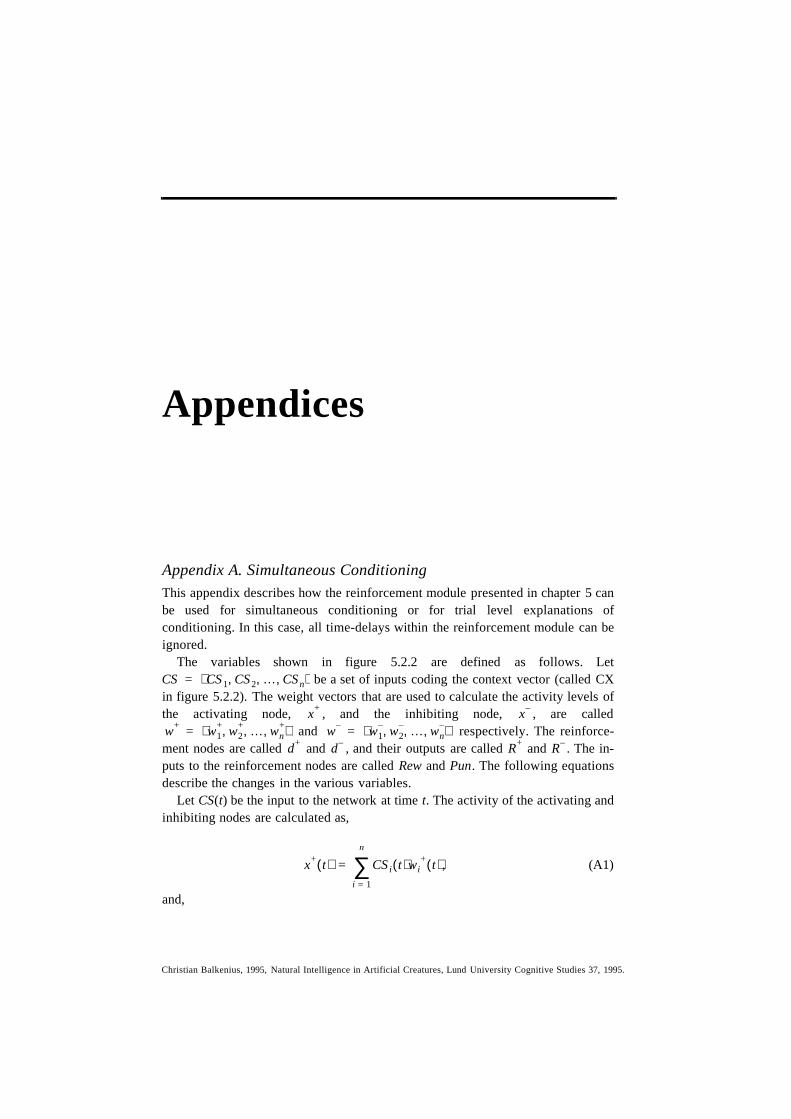
Christian Balkenius, 1995, Natural Intelligence in Artificial Creatures, Lund University Cognitive Studies 37, 1995.
Appendices
Appendix A. Simultaneous ConditioningThis appendix describes how the reinforcement module presented in chapter 5 canbe used for simultaneous conditioning or for trial level explanations ofconditioning. In this case, all time-delays within the reinforcement module can beignored.
The variables shown in figure 5.2.2 are defined as follows. Letbe a set of inputs coding the context vector (called CX
in figure 5.2.2). The weight vectors that are used to calculate the activity levels ofthe activating node, , and the inhibiting node, , are called
and respectively. The reinforce-ment nodes are called and , and their outputs are called and . The in-puts to the reinforcement nodes are called Rew and Pun. The following equationsdescribe the changes in the various variables.
Let CS(t) be the input to the network at time t. The activity of the activating andinhibiting nodes are calculated as,
(A1)
and,
CS CS1 CS2 … CSn, , ,⟨ ⟩=
x+ x–
w+ w1+ w2
+ … wn+, , ,⟨ ⟩= w– w1
– w2– … wn
–, , ,⟨ ⟩=d+ d– R+ R–
x+ t( ) CS i t( )wi+ t( ),
i 1=
n
∑=
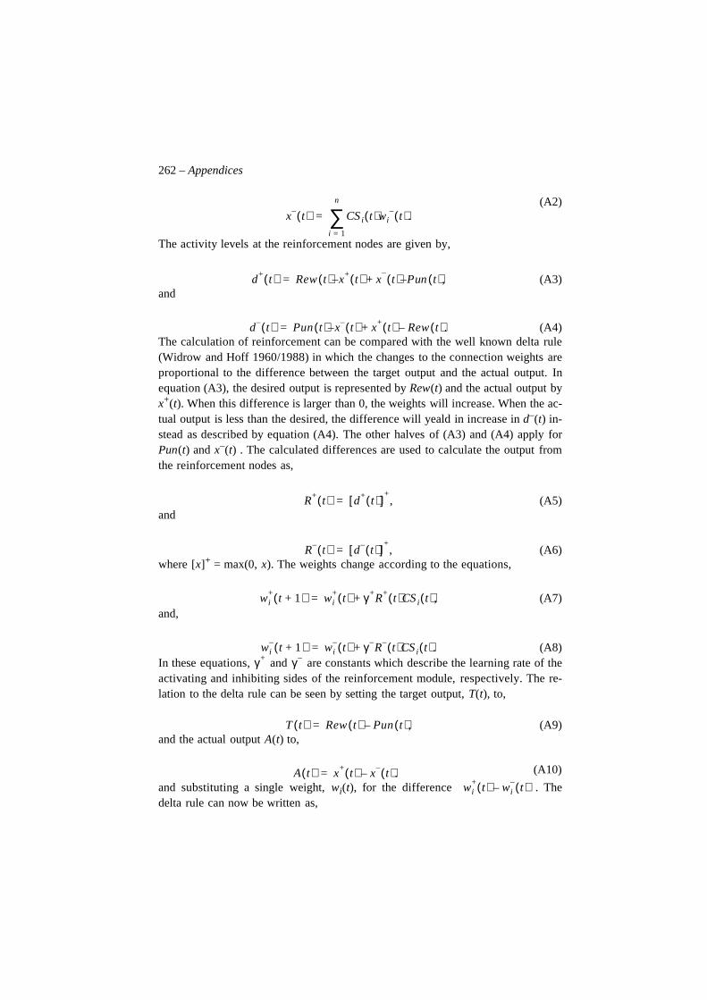
262 – Appendices
(A2)
The activity levels at the reinforcement nodes are given by,
(A3)and
(A4)The calculation of reinforcement can be compared with the well known delta rule(Widrow and Hoff 1960/1988) in which the changes to the connection weights areproportional to the difference between the target output and the actual output. Inequation (A3), the desired output is represented by Rew(t) and the actual output byx+(t). When this difference is larger than 0, the weights will increase. When the ac-tual output is less than the desired, the difference will yeald in increase in d–(t) in-stead as described by equation (A4). The other halves of (A3) and (A4) apply forPun(t) and x–(t) . The calculated differences are used to calculate the output fromthe reinforcement nodes as,
(A5)and
(A6)where [x]+ = max(0, x). The weights change according to the equations,
(A7)and,
(A8)In these equations, and are constants which describe the learning rate of theactivating and inhibiting sides of the reinforcement module, respectively. The re-lation to the delta rule can be seen by setting the target output, T(t), to,
(A9)and the actual output A(t) to,
(A10)
and substituting a single weight, wi(t), for the difference . Thedelta rule can now be written as,
x– t( ) CS i t( )wi– t( ).
i 1=
n
∑=
d+ t( ) Rew t( ) x+ t( ) x+–
t( ) P– un t( )– ,=
d– t( ) Pun t( ) x– t( ) x+ t( ) Rew t( )–+– .=
R+ t( ) d+ t( )[ ]+,=
R– t( ) d– t( )[ ]+,=
wi+ t 1+( ) wi
+ t( ) γ +R+ t( )CS i t( ),+=
wi– t 1+( ) wi
– t( ) γ –R– t( )CS i t( ).+=γ + γ –
T t( ) Rew t( ) Pun t( ),–=
A t( ) x+ t( ) x– t( ).–=wi
+ t( ) wi– t( )–
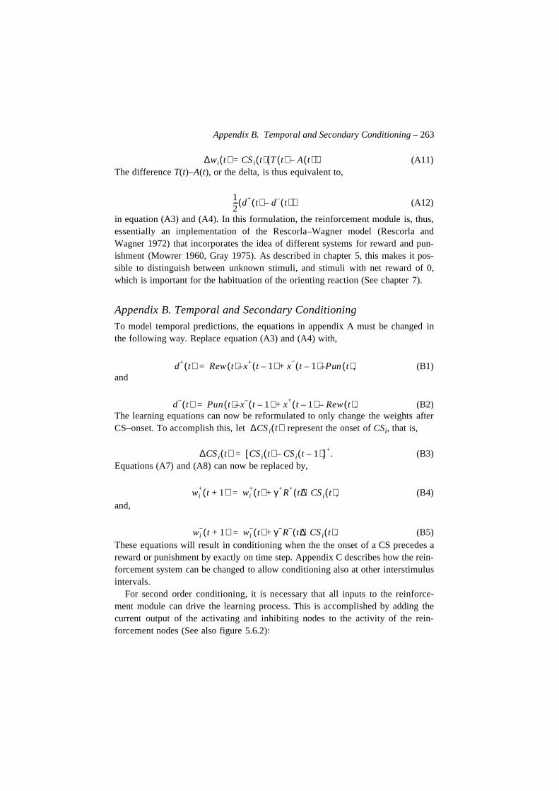
Appendix B. Temporal and Secondary Conditioning – 263
(A11)The difference T(t)–A(t), or the delta, is thus equivalent to,
(A12)
in equation (A3) and (A4). In this formulation, the reinforcement module is, thus,essentially an implementation of the Rescorla–Wagner model (Rescorla andWagner 1972) that incorporates the idea of different systems for reward and pun-ishment (Mowrer 1960, Gray 1975). As described in chapter 5, this makes it pos-sible to distinguish between unknown stimuli, and stimuli with net reward of 0,which is important for the habituation of the orienting reaction (See chapter 7).
Appendix B. Temporal and Secondary Conditioning
To model temporal predictions, the equations in appendix A must be changed inthe following way. Replace equation (A3) and (A4) with,
(B1)and
(B2)The learning equations can now be reformulated to only change the weights afterCS–onset. To accomplish this, let represent the onset of CSi, that is,
(B3)Equations (A7) and (A8) can now be replaced by,
(B4)and,
(B5)These equations will result in conditioning when the the onset of a CS precedes areward or punishment by exactly on time step. Appendix C describes how the rein-forcement system can be changed to allow conditioning also at other interstimulusintervals.
For second order conditioning, it is necessary that all inputs to the reinforce-ment module can drive the learning process. This is accomplished by adding thecurrent output of the activating and inhibiting nodes to the activity of the rein-forcement nodes (See also figure 5.6.2):
∆wi t( ) CS i t( ) T t( ) A t( )–( )= .
12--- d+ t( ) d– t( )–( )
d+ t( ) Rew t( ) x+ t 1–( ) x+–
t 1–( ) P– un t( )– ,=
d– t( ) Pun t( ) x– t 1–( ) x+ t 1–( ) Rew t( )–+– .=
∆CS i t( )
∆CS i t( ) CS i t( ) CS i t 1–( )–[ ]+.=
wi+ t 1+( ) wi
+ t( ) γ +R+ t( )∆CS i t( ),+=
wi– t 1+( ) wi
– t( ) γ –R– t( )∆CS i t( ).+=
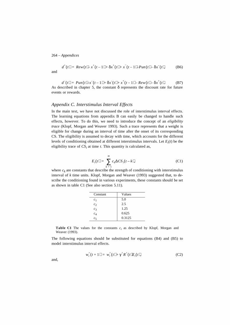
264 – Appendices
(B6)and
(B7)As described in chapter 5, the constant δ represents the discount rate for futureevents or rewards.
Appendix C. Interstimulus Interval Effects
In the main text, we have not discussed the role of interstimulus interval effects.The learning equations from appendix B can easily be changed to handle sucheffects, however. To do this, we need to introduce the concept of an eligibilitytrace (Klopf, Morgan and Weaver 1993). Such a trace represents that a weight iseligible for change during an interval of time after the onset of its correspondingCS. The eligibility is assumed to decay with time, which accounts for the differentlevels of conditioning obtained at different interstimulus intervals. Let Ei(t) be theeligibility trace of CSi at time t. This quantity is calculated as,
(C1)
where ck are constants that describe the strength of conditioning with interstimulusinterval of k time units. Klopf, Morgan and Weaver (1993) suggested that, to de-scribe the conditioning found in various experiments, these constants should be setas shown in table C1 (See also section 5.11).
Table C1 The values for the constants ci as described by Klopf, Morgan andWeaver (1993).
The following equations should be substituted for equations (B4) and (B5) tomodel interstimulus interval effects.
(C2)and,
Constant Values
c1c2c3c4c5
5.02.51.250.6250.3125
d+ t( ) Rew t( ) x+ t 1–( ) δx+ t( ) x+ +–
t 1–( ) P– un t( )– δx–– t( ),=
d– t( ) Pun t( ) x– t 1–( ) δx- t( ) x+ t 1–( ) Rew t( )– δx+ t( )–+ +– .=
E i t( ) ck∆CS i t k–( ),k 1=
m
∑=
wi+ t 1+( ) wi
+ t( ) γ +R+ t( )E i t( ),+=
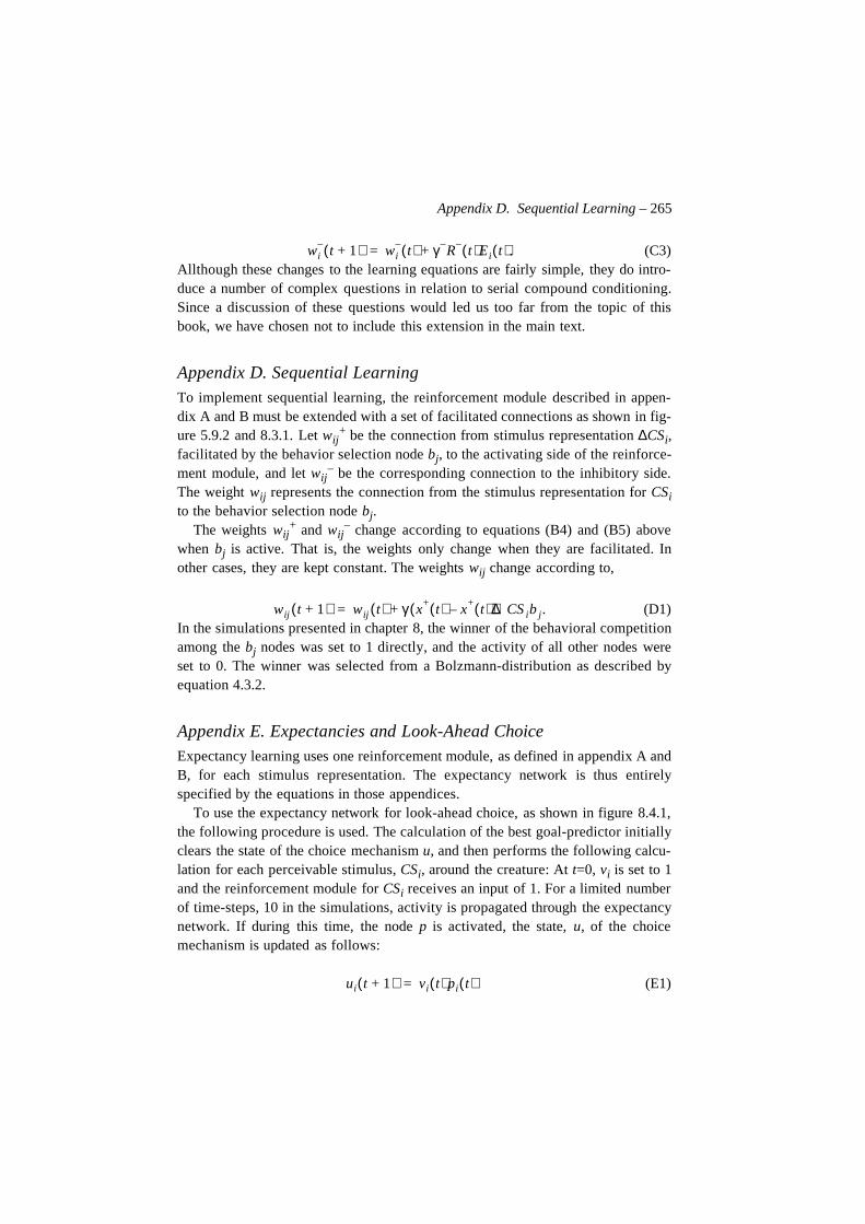
Appendix D. Sequential Learning – 265
(C3)Allthough these changes to the learning equations are fairly simple, they do intro-duce a number of complex questions in relation to serial compound conditioning.Since a discussion of these questions would led us too far from the topic of thisbook, we have chosen not to include this extension in the main text.
Appendix D. Sequential LearningTo implement sequential learning, the reinforcement module described in appen-dix A and B must be extended with a set of facilitated connections as shown in fig-ure 5.9.2 and 8.3.1. Let wij
+ be the connection from stimulus representation ∆CSi,facilitated by the behavior selection node bj, to the activating side of the reinforce-ment module, and let wij
– be the corresponding connection to the inhibitory side.The weight wij represents the connection from the stimulus representation for CSito the behavior selection node bj.
The weights wij+ and wij
– change according to equations (B4) and (B5) abovewhen bj is active. That is, the weights only change when they are facilitated. Inother cases, they are kept constant. The weights wij change according to,
(D1)In the simulations presented in chapter 8, the winner of the behavioral competitionamong the bj nodes was set to 1 directly, and the activity of all other nodes wereset to 0. The winner was selected from a Bolzmann-distribution as described byequation 4.3.2.
Appendix E. Expectancies and Look-Ahead ChoiceExpectancy learning uses one reinforcement module, as defined in appendix A andB, for each stimulus representation. The expectancy network is thus entirelyspecified by the equations in those appendices.
To use the expectancy network for look-ahead choice, as shown in figure 8.4.1,the following procedure is used. The calculation of the best goal-predictor initiallyclears the state of the choice mechanism u, and then performs the following calcu-lation for each perceivable stimulus, CSi, around the creature: At t=0, vi is set to 1and the reinforcement module for CSi receives an input of 1. For a limited numberof time-steps, 10 in the simulations, activity is propagated through the expectancynetwork. If during this time, the node p is activated, the state, u, of the choicemechanism is updated as follows:
(E1)
wi– t 1+( ) wi
– t( ) γ –R– t( )E i t( ).+=
wij t 1+( ) wij t( ) γ x+ t( ) x+ t( )–( )∆CS ib j.+=
ui t 1+( ) vi t( ) pi t( )=
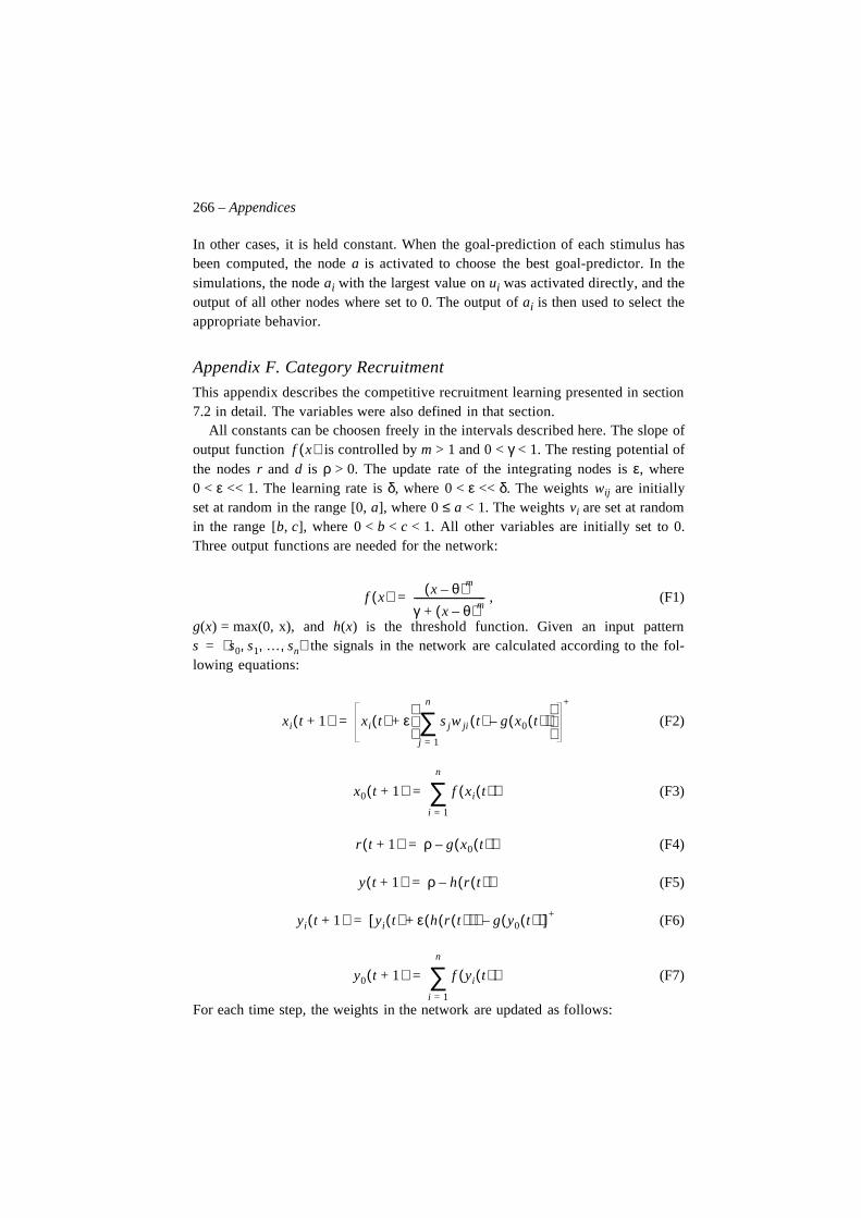
266 – Appendices
In other cases, it is held constant. When the goal-prediction of each stimulus hasbeen computed, the node a is activated to choose the best goal-predictor. In thesimulations, the node ai with the largest value on ui was activated directly, and theoutput of all other nodes where set to 0. The output of ai is then used to select theappropriate behavior.
Appendix F. Category Recruitment
This appendix describes the competitive recruitment learning presented in section7.2 in detail. The variables were also defined in that section.
All constants can be choosen freely in the intervals described here. The slope ofoutput function is controlled by m > 1 and 0 < γ < 1. The resting potential ofthe nodes r and d is ρ > 0. The update rate of the integrating nodes is ε, where0 < ε << 1. The learning rate is δ, where 0 < ε << δ. The weights wij are initiallyset at random in the range [0, a], where 0 ≤ a < 1. The weights vi are set at randomin the range [b, c], where 0 < b < c < 1. All other variables are initially set to 0.Three output functions are needed for the network:
, (F1)
g(x) = max(0, x), and h(x) is the threshold function. Given an input patternthe signals in the network are calculated according to the fol-
lowing equations:
(F2)
(F3)
(F4)
(F5)
(F6)
(F7)
For each time step, the weights in the network are updated as follows:
f x( )
f x( ) x θ–( )m
γ x θ–( )m+-----------------------------=
s s0 s1 … sn, , ,⟨ ⟩=
xi t 1+( ) xi t( ) ε s jw ji t( ) g x0 t( )( )–j 1=
n
∑
+
+
=
x0 t 1+( ) f xi t( )( )i 1=
n
∑=
r t 1+( ) ρ g x0 t( )( )–=
y t 1+( ) ρ h r t( )( )–=
yi t 1+( ) yi t( ) ε h r t( )( )( ) g y0 t( )( )–+[ ]+=
y0 t 1+( ) f yi t( )( )i 1=
n
∑=
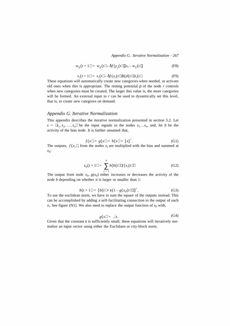
Appendix G. Iterative Normalization – 267
(F8)
(F9)These equations will automatically create new categories when needed, or activateold ones when this is appropriate. The resting potential ρ of the node r controlswhen new categories must be created. The larger this value is, the more categorieswill be formed. An external input to r can be used to dynamically set this level,that is, to create new categores on demand.
Appendix G. Iterative Normalization
This appendix describes the iterative normalization presented in section 5.2. Letbe the input signals to the nodes x1…xn, and, let b be the
activity of the bias node. It is further assumed that,
(G1)The outputs, , from the nodes xi are multiplied with the bias and summed atx0:
(G2)
The output from node x0, g(x0) either increases or decreases the activity of thenode b depending on whether it is larger or smaller than 1:
(G3)To use the euclidean norm, we have to sum the square of the outputs instead. Thiscan be accomplished by adding a self-facilitating connection to the output of eachxi. See figure (N1). We also need to replace the output function of x0 with,
(G4)
Given that the constant ε is sufficiently small, these equations will iteratively nor-malize an input vector using either the Euclidaen or city-block norm.
wij t 1+( ) wij t( ) δf y j t( )( ) si wij t( )–[ ]–=
vi t 1+( ) vi t( ) δf xi t( )( )h d t( )( )vi t( )–=
s s1 s2 … sn, , ,⟨ ⟩=
f x( ) g x( ) h x( ) x[ ]+.= = =f xi( )
x0 t 1+( ) h b t( )( ) f xi t( )( )i 1=
n
∑=
b t 1+( ) b t( ) ε 1 g x0 t( )( )–( )+[ ]+.=
g x( ) x.=
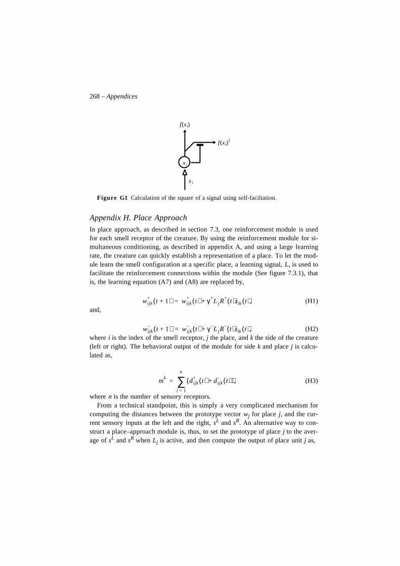
268 – Appendices
Figure G1 Calculation of the square of a signal using self-faciliation.
Appendix H. Place Approach
In place approach, as described in section 7.3, one reinforcement module is usedfor each smell receptor of the creature. By using the reinforcement module for si-multaneous conditioning, as described in appendix A, and using a large learningrate, the creature can quickly establish a representation of a place. To let the mod-ule learn the smell configuration at a specific place, a learning signal, L, is used tofacilitate the reinforcement connections within the module (See figure 7.3.1), thatis, the learning equation (A7) and (A8) are replaced by,
(H1)and,
(H2)where i is the index of the smell receptor, j the place, and k the side of the creature(left or right). The behavioral output of the module for side k and place j is calcu-lated as,
(H3)
where n is the number of sensory receptors.From a technical standpoint, this is simply a very complicated mechanism for
computing the distances between the prototype vector wj for place j, and the cur-rent sensory inputs at the left and the right, sL and sR. An alternative way to con-struct a place–approach module is, thus, to set the prototype of place j to the aver-age of sL and sR when Lj is active, and then compute the output of place unit j as,
xi
s i
f(xi)
f(xi)2
wijk+ t 1+( ) wijk
+ t( ) γ +L jR+ t( )sik t( ),+=
wijk– t 1+( ) wijk
– t( ) γ –L jR– t( )sik t( ),+=
mk d ijk+ t( ) d ijk
– t( )+( ),i 1=
n
∑=
Appendix I. Exploration – 269
(H4)
Alternatively, the Euclidean distance could have been used instead. In a creaturewith visual abilities, it would be more advantageous to use visual input rather thansmell. In this case, the smells would be replaced by the visual angles of a numberof distal landmarks (Compare Zipser 1985, Schmajuk and Blair 1983).
Appendix I. Exploration
This appendix describes the details of the exploration network shown in figure7.4.1. The expectancy part of the network uses the reinforcement module de-scribed in appendix A. Instead of using the actual intensity of each smell input, CSiis set to 1, if smell i is present, and to 0 otherwise. To choose which stimulus to ap-proach, each orientation and approach module weigh together three factors. Thefirst is the the ‘unexpectancy’ factor which is , where T is thethreshold function. The second is the ‘misplace’ factor, . Here, α andβ control when a stimulus is sufficiently unexpected or misplaced to activate theorienting system. The constant γ determines the salience of a missing stimulus.The last factor is the ‘novelty’ of a stimulus that models habituation within the ori-entation module. The habituation of module i is represented by the value hi, whichchanges according to the following equation when module i is active:
(I1)The ‘novelty’ factor is computed as . Here, the constantδ describes how fast the approach behavior habituates, and ε controls the salienceof a novel stimulus. Note that equation (I1) describes habituation that is not revers-ible. To be more realistic, the habituation should slowly decrease to zero again.
The three factors described here are added together in each orienting module,and is used as a strength output in the behavioral competition between these mod-ules. In the simulations described in chapter 7, the orienting modules also competewith a wandering module that wins the competition when the strength outputs ofthe orienting modules are to low.
Appendix J. The Simulator
All the models presented in this book have been implemented as computer simula-tions. Since many of the models involves dynamic situations, viewing the behaviorof the creatures ’live’, rather than as static images, makes it much easier to under-stand how they behave. The dynamics of the interaction between a creature and itsenvironment simply cannot be given justice in the format offered by a book. Toremedy this situation, the simulator, “BERRY”, which runs on Macintosh™ com-
mk wijk sik– .
i 1=
n
∑=
CS iT d i+ α–( )
γT d i– β–( )
hi t 1+( ) hi t( ) δCS i t( ) 1 hi t( )–( )+=1 hi–( ) εT CS i( ) CS i+( )
270 – Appendices
puters, is available to anyone interested. It can be downloaded from the world-wide web or obtained directly from the author. To obtain the simulator thoughworld-wide web, open,
http://lucs.fil.lu.se/Simulators/BERRY-III/
and follow the instructions on–line. The simulator can also be obtained directlyfrom the author, who can be contacted either by e-mail to,
(place the word ‘BERRY’ in the subject line) or by ordinary mail to,
Christian BalkeniusLund University Cognitive ScienceKungshuset/LundagårdS–222 22 LUND, Sweden
Christian Balkenius, 1995, Natural Intelligence in Artificial Creatures, Lund University Cognitive Studies 37, 1995.
References
Abbott, E. A., (1884/1991), Flatland, Princeton, NJ: Princeton Univerity Press.Ackley, D. H., Hinton, G. E. & Sejnowski, T. J., (1985), “A learning algorithm for
Bolzmann machines”, Cognitive Science , 9 , 147–169.Adams, D. B., (1979), “Brain mechanisms for offense, defense, and submission”,
The Behavioral and Brain Sciences, 2 , 201–243.Agre, P. E. & Chapman, D., (1987), “Pengi: an implementation of a theory of
activity”. Proceedings of the Sixth National Conference on ArtificialIntelligence, 1 , 268–272, Morgan Kaufman.
Albus, J. S., (1975), “A new approach to manipulator control: the cerebellar modelarticulation controller (CMAC)”, Transactions of ASME Journal of DynamicalSystems, Measurement, and Control , 97 , 25–61.
Albus, J. S., (1991), “Outline for a theory of intelligence”, IEEE Transactions onSystems, Man and Cybernetics, 21 , 473–509.
Amari, S.–I., (1982), “Competitive and cooperative aspects in dynamics of neuralexcitation and self-organization”. In S.–I. Amari and M. A. Arbib (eds.),Competition and Cooperation in Neural Nets, 1–28, Berlin: Springer–Verlag.
Amari, S.–I. & Arbib, M. A., (1977), “Competition and cooperation in neuralnets”. In J. Metzler (ed.), Systems Neuroscience, 119–165, Academic Press.
Amit, D. J., (1989), Modelling Brain Function, Cambridge: Cambridge UniversityPress.
272 – References
Andersen, R. A. & Zipser, D., (1990), “A network model for learned spatialrepresentation in the posterior parietal cortex”. In J. L. McGaugh, N. M.Weinberger and G. Lynch (eds.), Brain Organization and Memory: Cells,Systems, and Circuits, 271–284, Oxford: Oxford University Press.
Arbib, M. A. & Cobas, A., (1991), “Schemas for prey-catching in frog and toad”.In J.–A. Meyer and S. W. Wilson (eds.), From Animals to Animats , 540–549,Cambridge, MA: MIT Press.
Arbib, M. A., Conklin, E. J. & Hill, J., (1987), From Schema Theory to Language,Oxford University Press.
Arbib, M. A. & House, D. H., (1987), “Depth and detours: an essay on visuallyguided behavior”. In M. A. Arbib and A. R. Hanson (eds.), Vision, Brain andCooperative Computation, 129–163, Cambridge, MA: MIT Press.
Arbib, M. A. & Lee, H. B., (1993), “Anural visuomotor coordination for detourbehaviour: from retina to motor schemas”. In J.–A. Mayer, H. L. Roitblat andS. W. Wilson (ed.), From Animals to Animats II, Cambridge, MA: MIT Press.
Arkin, R. A., (1990), “Integrating behavioral, perceptual and world knowledge inreactive navigation”. In P. Maes (ed.), Designing Autonomous Agents , 105–122, Cambridge, MA: MIT Press.
Arkin, R. C., (1987), “Motor schema based navigation for a mobile robot: anapproach to programming by behavior”. (ed.), Proceedings of the 1987 IEEEInternational Conference on Robotics and Automation, 264–271.
Atkeson, C. G. & Rinkensmeyer, D. J., (1990), “Using associative content-addressable memories to control robots”. In P. H. Winston and S. A. Shellard(eds.), Artificial Intelligence at MIT: Expanding Frontiers, Cambridge, MA:MIT Press.
Baird, L. C. & Klopf, H. A., (1993), “A hierarchical network of provably optimallearning control systems: extensions of the associative control process (ACP)network”, Adaptive Behavior, 1 , 321–352.
Balkenius, C. & Gärdenfors, P., (1991), “Non-monotonic inferences in neuralnetworks”. In J. A. Allen, R. Fikes and E. Sandewall (eds.), Principles ofKnowledge Representation and Reasoning: Proceedings of the SecondInternational Conference, 32-39, San Mateo, CA: Morgan Kaufman.
Balkenius, C., (1992), “Neural mechanisms for self-organization of emergentschemata, dynamical schema processing, and semantic constraint satisfaction”,Lund University Cognitive Studies , 14 .
Balkenius, C., (1993), “The roots of motivation”. In J.–A. Mayer, H. L. Roitblatand S. W. Wilson (eds.), From Animals to Animats II, Cambridge, MA: MITPress.
Balkenius, C., (1994a), “All you never wanted to know about the BERRY IIIenvironment”, LUCS Minor, 2 .
References – 273
Balkenius, C., (1994b), “Natural intelligence for autonomous agents – extendedversion”, Lund University Cognitive Studies , 29 . (Also printed in B. Svensson(ed.), Proceedings of the International Workshop on Mechatronical ComputerSystems for Perception and Action , 1993, 181–196.)
Balkenius, C., (1994c), “Some properties of neural representations”. In L. F.Niklasson and M. B. Bodén (eds.), Connectionism in a Broad Perspective, 79–88, New York: Ellis Horwood.
Balkenius, C., (1995), “Multi-modal sensing for robot control”. In L. F. Niklassonand M. B. Bodén (eds.), Current Trends in Connectionism, 203–216, Hillsdale,NJ: Lawrence Erlbaum.
Barto, A. G., Anderson, C. W. & Sutton, R. S., (1982), “Synthesis of nonlinearcontrol surfaces by a layered associative search network”, BiologicalCybernetics, 43 , 175–185.
Barto, A. G. & Sutton, R. S., (1981), “Landmark learning: an illustration ofassociative search”, Biological Cybernetics, 42 , 1–8.
Barto, A. G., Sutton, R. S. & Watkins, C. J. C. H., (1990), “Learning andsequential decision making”. In M. Gabriel and J. Moore (eds.), Learning andComputational Neuroscience: Foundations of Adaptive Networks, 539–602,Cambridge, MA: MIT Press.
Beer, D. B., (1990), Intelligence as Adaptive Behavior, San Diego: AcademicPress.
Beer, R. A., Chiel, H. J., Quinn, R. D. & Larsson, P., (1992), “A distributed neuralnetwork architecture for hexapod robot locomotion”, Neural Computation, 4 ,356–365.
Beer, R. D. & Gallagher, J. C., (1992), “Evolving dynamical neural netwoks foradaptive behavior”, Adaptive Behavior, 1 , 92–122.
Bell, W. J., (1991), Searching Behaviour, London: Chapman and Hall.Bolles, R. C., (1967), Theory of Motivation, New York: Harper and Row.Bolles, R. C., (1970), “Species-specific defence reactions and avoidance
learning”, Psychological Review , 77 , 32–48.Bolles, R. C., (1978), Learning Theory , Fort Worth: Holt, Rinehart and Winston,
Inc.Bolles, R. C., (1978), “The role of stimulus learning in defensive behaviour”. In S.
H. Hulse, H. Fowler and W. K. Honig (eds.), Cognitive Processes in AnimalBehavior, 89–108, Hillsadale, NJ: Lawrence Erlbaum Associates.
Bolles, R. C., (1984), “Species-typical response predispositions”. In P. Marler andH. S. Terrace (eds.), The Biology of Learning, 435–446, Berlin: Springer–Verlag.
Braitenberg, V., (1984), Vehicles: Experiments in Synthetic Psychology,Cambridge, MA: MIT Press.
274 – References
Brooks, R. A., (1986), “Achieving artificial intelligence through building robots”,899, MIT A. I. Memo.
Brooks, R. A., (1990), “Elephants don't play chess”. In P. Maes (ed.), DesigningAutonomous Agents , 3–15, Cambridge, MA: MIT Press.
Brooks, R. A., (1991a), “Intelligence without reason”. Proceedings of IJCAI–91,569–595.
Brooks, R. A., (1991b), “New approaches to robotics”, Science , 253 , 1227–1232.Brooks, R. A. & Stein, L. A., (1993), “Building brains for bodies”, MIT A. I.
Memo, No. 1439, MIT.Brown, M. W., (1990), “Why does the brain have a hippocampus?”. In M. Gabriel
and J. Moore (eds.), Learning and Computational Neuroscience: Foundationsof Adaptive Networks, 233–282, Cambridge, MA: MIT Press.
Buck, R., (1988), Human Motivation and Emotion , New York: John Wiley &Sons.
Cannon, W. B., (1932), The Wisdom of the Body, New York: Norton.Carpenter, G. A. & Grossberg, S., (1986), “Neural dynamics of category learning
and recognition: attention, memory consolidation and amnesia”. In S.Grossberg (ed.), The Adaptive Brain, 238–308, Amsterdam: North–Holland.
Carpenter, G. & Grossberg, S., (1987), “ART2: Self-organization of stablecategory recognition codes for analog input patterns”, Applied Optics , 26,4919-4930.
Carpenter, R. H. S., (1984), Neurophysiology, London: Edward Arnold Ltd.Cecconi, F. & Parisi, D., (1993), “Neuronal networks with motivational units”. In
J.–A. Mayer, H. L. Roitblat and S. W. Wilson (eds.), From Animals to AnimatsII, 346–355, Cambridge, MA: MIT Press.
Charniak, E. & McDermott, D., (1985), Introduction to Artificial Intelligence,Reading, MA: Addison–Wesley.
Churchland, P. M., (1984), Matter and Consciouness: A ContemporaryIntroduction to the Philosophy of Mind, Cambridge, MA: MIT Press.
Clark, F. C., (1958), “The effect of deprivation and frequency of reinforcement onvariable–interval responding”, Journal of the Experimental Analysis ofBehavior, 1 , 211–227.
Cohen, M. A. & Grossberg, S., (1983), “Absolute stability of global patternformation and parallel memory storage by competitive neural networks”, IEEETransactions on Systems, Man, and Cybernetics, SMC–13 , 815–826.
Cohen, M. A. & Grossberg, S., (1987), “Masking fields: a massively parallelneural architecture for learning, recognition, and predicting multiple groupingsof patterned data”, Applied Optics , 26, 1866-1891.
Collier, G. H., (1983), “Life in a closed economy: the ecology of learning andmotivation”. In M. D. Zeiler and P. Harzem (ed.), Advances in Analysis ofBehavior, 223–274, New York: John Wiley.
References – 275
Connell, J. H., (1990), Minimalist Mobile Robots , Boston: Academic Press.Davidsson, P., (1994), “Concepts and autonomous agents”, LU–CS–TR, 94–124,
Department of Computer Science, Lund University.Davis, J. L. & Eichenbaum, H., (1991), Olfaction, Cambridge, MA: MIT Press.Desmond, J. E., (1990), “Temporally adaptive responses in neural models: the
stimulus trace”. In M. Gabriel and J. Moore (eds.), Learning andComputational Neuroscience: Foundations of Adaptive Networks, 421–456,Cambridge, MA: MIT Press.
Deutsch, J. A., (1960), The Structural Basis of Behavior, Chicago: University ofChicago Press.
DeYoe, E. A. & Van Essen, D. C., (1988), “Concurrent processing streams inmonkey visual cortex”, Trends in Neurosciences, 11 , 219–226.
Dickinson, A., (1980), Contemporary Animal Learning Theory , Cambridge:Cambridge University Press.
Dunham, P. J., (1977), “The nature of reinforcing stimuli”. In W. K. Honig and J.E. R. Staddon (ed.), Handbook of Operant Behavior, Englewood Cliffs, NJ:Prentice–Hall.
Eichenbaum, H., Otto, T. A., Wible, C. G. & Piper, J. M., (1991), “Building amodel of the hippocampus in olfaction and memory”. In J. L. Davis and H.Eichenbaum (eds.), Olfaction, 167–210, Cambridge, MA: MIT Press.
Ekeberg, Ö., (1992), Computer Simulation Techniques in the Study of NeuralSystems , Stockholm: Royal Institute of Technology, Dept. of NumericalAnalysis and Computing Science.
Eldén, L. & Wittmeyer-Koch, L., (1987), Numerisk Analys – En Introduktion,Lund: Studentlitteratur.
Ellen, P. & Thinus-Blanc, C., (1987), Cognitive Processes and Spatial Orientationin Animal and Man, Dordrecht: Nijhoff.
Fikes, R. E. & Nilsson, N. J., (1971), “STRIPS: A new approach to the applicationof theorem proving to problem solving”, Artificial Intelligence, 2, 189–208.
Flavell, J. H., (1985), Cognitive Development, New Jersey: Prentice-Hall.Gallistel, C. R., (1980), The Organization of Action: A New Synthesis, Hilldsdale,
NJ: Erlbaum.Gallistel, C. R., (1990), The Organization of Learning, Cambridge, MA: MIT
Press.Gallistel, C. R., (1992), “Classical conditioning as an adaptive specialization: a
computational model”, In The Psychology of Learning and Motivation:Advances in Research and Theory , Medin, D. L., (ed.),, 35–67, New York:Academic Press.
Garcia, J. & Koelling, R. A., (1966), “Relation of cue to consequences inavoidance learning”, Psychonomic Science , 4 , 123–124.
276 – References
Garcia, J., McGowan, B. K. & Green, K. F., (1972), “Biological constraints onconditioning”. In A. H. Black and W. F. Prokasy (eds.), Classical ConditioningII: Current Research and Theory , 3–27, New York: Appleton–Century–Crofts.
Gärdenfors, P., (1992), “Medvetandets evolution”. Blotta Tanken, ch 5, Nya Doxa.Gärdenfors, P., (1995), “Cued and detached representations in animal cognition”,
to appear in Behavioural Processes.Gärdenfors, P. & Balkenius, C., (1993), “Varför finns det inga riktiga robotar?”,
Framtider, 12 , 11–14.Gibbon, J., Baldock, M. D., Locurto, C., Gold, L. & Terrace, H. S., (1977), “Trial
and intertrial durations in autoshaping”, Journal of Experimental PsychologyAnimal Behavioral Processes, 3 , 264–284.
Gibson, J. J., (1979), The Ecological Approach to Visual Perception, Hillsdale,NJ: Lawrence Erlbaum Associates.
Glass, A. L. & Holyoak, K. J., (1985), Cognition, New York: Random House.Goldberg, M. E., Eggers, H. M. & Fouras, P., (1991), “The ocular motor system”,
In E. R. Kandel, J. H. Schwartz and T. M. Jessel (eds.), Principles of NeuralScience , 660–678, New York: Elsevier.
Gray, J. A., (1975), Elements of a Two-Process Theory of Learning, London:Academic Press.
Gray, J. A., (1982), The Neuropsychology of Anxiety: An Enquiry into theFunctions of the Septo-Hippocampal System , Oxford: Oxford University Press.
Gray, J. A., (1995), “A model of the limbic system and the basal ganglia:applications to anxiety and schizophrenia”, In Gazzaniga, M. S. (ed.),, TheCognitive Neurosciences, 1165–1176, Cambridge, MA: MIT Press.
Grelle, M. J. & James, J. H., (1981), “Conditioned inhibition of fear: evidence fora competing response mechanism”, Learning and Motivation, 12 , 300–320.
Grossberg, S., (1973), “Contour enhancement, short term memory, andconstancies in reverbating neural networks”, Studies in Applied Mathematics,LII , 213–257.
Grossberg, S., (1976), “Adaptive pattern classification and universal recoding: I.Parallel development and coding of neural feature detectors”, BiologicalCybernetics, 23 , 121–134.
Grossberg, S., (1986), “The adaptive self-organization of serial order in behavior:speech, language, and motor control”. In E. C. Schwab and H. C. Nusbaum(eds.), Pattern Recognition by Humans and Machines, Academic Press.
Grossberg, S., (1989), “Nonlinear neural networks: principles, mechanisms, andarchitectures”, Neural Networks, 1 , 17–66.
Grossman, S. P., (1979), “The biology of motivation”, Annual Review ofPsychology, 30 , 209–242.
Gulz, A., (1991), “The planning of action as a cognitive and biologicalphenomenon”, Lund University Cognitive Studies , 2 .
References – 277
Hebb, D. O., (1949), The Organization of Behavior, New York: John Wiley andSons.
Harnad, S., (1987), “The symbol grounding problem”, Physica D, 42 , 335-346.Hinton, G. E. & Andersson, J. A., (1981), Parallel Models of Associative Memory ,
Hillsdale, N.J.: Erlbaum.Hinton, G. E., McClelland, J. L. & Rumelhart, D. E., (1986), “Distributed
representations”. In D. E. Rumelhart and J. L. McClelland (eds.), Paralleldistributed processing, Cambridge, MA: MIT Press.
Hirose, S., (1993), Biolgically Inspired Robots , Oxford: Oxford University Press.Holland, J. H., Holyoak, K. J., Nisbett, R. E. & Thagard, P. R., (1986), Induction:
Processes of Inference, Learning and Discovery, Cambridge, MA: MIT Press.Hopfield, J. J., (1984), “Neurons with graded response have collective
computational properties like those of two-state neurons”, Proceedings of theNational Academy of Sciences, 81 ,
Horswill, I. D., (1992), “Characterizing adaptation by constraints”. In F. J. Varelaand P. Bourgine (eds.), Towards a Practice of Autonomous Systems , 58–63,Cambridge, MA: MIT Press.
Horswill, I. D. & Brooks, R. A., (1988), “Situated vision in a dynamic world:chasing objects”. Proceedings of AAAI–88 , 796–800, St Paul, MN.
Horswill, I. D. & Stein, L. A., (1995), “Life after planning and reaction”,manuscript, MIT A. I. Lab.
Hull, C. L., (1932), “The goal-gradient hypothesis and maze learning”,Psychological Review , 39 , 25–43.
Hull, C. L., (1934), “The concept of the habit-family hierarchy and mazelearning”, Psychological Review , 41 , 33–52, 134–152.
Hull, C. L., (1938), “The goal-gradient hypothesis applied to some “field-force”problems in the behaviors of young children”, Psychological Review , 45 , 271–299.
Hull, C. L., (1943), Principles of Behavior, New York: Appleton–Century–Crofts.Hull, C. L., (1952), A Behavior System , New Haven: Yale University Press.Ito, M., (1982), “Mechanisms of motor learning”. In S. Amari and M. A. Arbib
(eds.), Competition and Cooperation in Neural Nets, 418–429, Berlin:Springer–Verlag.
Johnston, A. J. & Dark, V. J., (1986), “Selective attention”, Annual Review ofPsychology, 37 , 43–75.
Kaelbling, L. P., (1993), Learning in Embedded Systems , Cambridge, MA: MITPress.
Kamin, L. J., (1968), “Attention-like processes in classical conditioning”. In M. R.Jones (ed.), Miami Symposium on the Prediction of Behavior: AversiveStimulation, 9–31, Miami: University of Miami Press.
278 – References
Kamp, Y. & Hasler, M., (1990), Recursive Neural Networks for AssociativeMemory , Chichester: John Wiley & Sons.
Kandel, E. R., (1991), “Perception of motion, depth, and form”. In E. R. Kandel, J.H. Schwartz and T. M. Jessel (eds.), Principles of Neural Science , 440–466,New York: Elsevier.
Kandel, E. R. & Jessel, T. M., (1991), “Touch”. In E. R. Kandel, J. H. Schwartzand T. M. Jessel (eds.), Principles of Neural Science , 367–384, New York:Elsevier.
Kandel, E. R., Schwartz, J. H. & Jessel, T. M., (1991), Principles of NeuralScience , New York: Elsevier.
Kehoe, E. J., (1990), “Classical conditioning: fundamental issues for adaptivenetwork models”. In M. Gabriel and J. Moore (eds.), Learning andComputational Neuroscience: Foundations of Adaptive Networks, 390–420,Cambridge, MA: MIT Press.
Khatib, O., (1985), “Real-time obstacle avoidance for manipulators and mobilerobots”. Proceedings of the 1985 IEEE International Conference on Roboticsand Automation, 500–505.
Kiss, G., (1991), “Autonomous agents, AI and chaos theory”. In J.–A. Meyer andS. W. Wilson (ed.), From Animals to Animats , 518–524, Cambridge, MA: MITPress.
Klopf, A. H., (1988), “A neuronal model of classical conditioning”,Psychobiology, 16 , 85–125.
Klopf, A. H. & Morgan, J. S., (1990), “The role of time in natural intelligence:implications of classical and instrumental conditioning for neuronal andneural-network modeling”. In M. Gabriel and J. Moore (eds.), Learning andComputational Neuroscience: Foundations of Adaptive Networks, 463–495,Cambridge, MA: MIT Press.
Klopf, A. H., Morgan, J. S. & Weaver, S. E., (1993), “A hierarchical network ofcontrol systems that learn: modelling nervous system function during classicaland instrumental conditioning”, Adaptive Behavior, 1 , 263–319.
Kohonen, T., (1984), Self-Organization and Associative Memory. , Berlin:Springer Verlag.
Kohonen, T., Oja, E. & Lehtiö, P., (1989), “Storage and processing of informationin distributed associative memory systems”. In G. E. Hinton and J. A.Anderson (eds.), Parallel Models of Associative Memory , 125–167, Hillsdale,NJ: Lawrence Erlbaum.
Konorski, J., (1967), Integrative Activity of the Brain, Chicago: University ofChicago Press.
Kraft, L. G. & Campagna, D. P., (1990), “A summary comparison of CMACneural network and traditional adaptive control systems”. In W. T. Miller, R. S.
References – 279
Sutton and P. J. Werbos (eds.), Neural Networks for Control , 143–169,Cambridge, MA: MIT Press.
Lansner, A. & Ekeberg, Ö., (1989), “A one-layer artificial neural network with aBayesian learning rule”, International Journal of Neural Systems , 1 , 77–87.
LeDoux, J. E., (1995), “In search of an emotional system in the brain: leaping fromfear to emotion and consciousness”. In M. S. Gazzaniga (ed.), The CognitiveNeurosciences, 1049–1061, Cambridge, MA: MIT Press.
Lee, T., (1970), “Perceived distance as a function of direction in the city”,Envrionmental Behavour, 2 , 40–51.
Lewin, K., (1935), A Dynamic Theory of Personality: Selected Papers , New York:McGraw–Hill.
Lewin, K., (1936), Principles of Topological Psychology, New York: McGraw–Hill.
Lieberman, D. A., (1990), Learning: Behavior and Cognition, Belmont, CA:Wadsworth Publishing Company.
Lippman, R. P., (1987), “An introduction to computing with neural nets”, IEEEASSP Magazine, 4–22.
Livingstone, M. & Hubel, D., (1988), “Segregation of form, color, movement, anddepth: Anatomy, physiology, and perception”, Science , 740–749.
Lorenz, K., (1950), “The comparative method in studying innate behaviorpatterns”, Society for Experimental Biology, Symposium no. 4, PhysiologicalMechanisms of Animal Behavior, 221–268, New York: Academic Press.
Lorenz, K., (1977), Behind the Mirror , London: Methuen & co Ltd.Lubow, R. E. & Moore, A. U., (1959), “Latent inhibition: the effect of
nonreinforced preexposure to the conditioned stimulus”, Journal ofComparative Physiological Psychology, 52 , 415–419.
Lynch, G. & Granger, R., (1991), “Serial steps in memory processing: possibleclues from studies of plasticity in the olfactory–hippocampal circuit”. In J. L.Davis and H. Eichenbaum (eds.), Olfaction, 141–165, Cambridge, MA: MITPress.
Lyons, D. M., Hendriks, A. J. & Mehta, S., (1991), “Achieving robustness bycasting planning as adaptation of a reactive system”. Proceedings of the 1991IEEE International Conference on Robotics and Automation,
MacFarlane, D. A., (1930), “The role of kinesthesis in maze learning”, Universityof California Publications in Psychology, 4 , 277–305.
Mackintosh, N. J., (1974), The Psychology of Animal Learning, New York:Academic Press.
Mackintosh, N. J., (1983), Conditioning and Associative Learning, Oxford:Oxford University Press.
Maes, P., (1990), “Designing autonomous agents”. In P. Maes (ed.), DesigningAutonomous Agents , 1–2, Cambridge, MA: MIT Press.
280 – References
Maes, P., (1990), Designing Autonomous Agents , Cambridge, MA: MIT Press.Maes, P., (1991), “A bottom-up mechanism for behavior selection in an artificial
creature”. In J.–A. Meyer and S. W. Wilson (eds.), From Animals to Animats ,238–246, Cambridge, MA: MIT Press.
Marler, P., (1970), “A comparative approach to vocal learning: song–developmentin white-crowned sparrows”, Journal of Comparative and PhysiologicalPsychology Monograph, 71 , pt. 2, 1–25.
Martin, J. H., (1991), “Coding and processing of sensory information”. In E. R.Kandel, J. H. Schwartz and T. M. Jessel (eds.), Principles of Neural Science ,329–340, New York: Elsevier.
Mason, C. & Kandel, E. R., (1991), “Central Visual Pathways”. In E. R. Kandel, J.H. Schwartz and T. M. Jessel (eds.), Principles of Neural Science , New York:Elsevier.
Masterson, F. A., (1970), “Is termination of a warning signal an effective rewardfor the rat?”, Journal of Comparative and Physiological Psychology, 72 , 471–475.
McFarland, D., (1993), Animal Behaviour, Harlow: Longman.McFarland, D. & Bösser, T., (1993), Intelligent Behavior in Animals and Robots ,
Cambridge, MA: MIT Press.McFarland, D. & Sibly, R., (1972), “ ‘Unitary drives’ revisited”, Animal Behavior,
20 , 548–563.Melzoff, A. N. & Moore, M. K., (1977), “Imitation of facial and manual gestures
by human neonates”, Science , 198 , 75–78.Miller, N. E., (1944), “Experimental studies of conflict”. In J. M. Hunt (ed.),
Personality and the Behavior Disorders, New York: The Ronald Press Co.Minsky, M., (1987), The Society of Mind, London: Heineman.Minsky, M. & Papert, S., (1988), Perceptrons – expanded edition , Cambridge,
MA: MIT Press.Mishkin, M. & Petri, H. L., (1986), “Memories and habit: some implications for
the analysis of learning and retention”. In L. R. Squire and N. Butters (eds.),Neuropsychology of Memory , 287–296, New York: Guildford Press.
Mishkin, M., Ungerleider, L. G. & Macko, K. A., (1983), “Object vision andspatial vision: two cortical pathways”, Trends in Neuroscience, 6 , 414–417.
Moore, J. W. & Blazis, D. E. J., (1989), “Cerebellar implementation of acomputational model of classical conditioning”. In P. Strata (ed.), TheOlivocerebellar System in Motor Control , Berlin: Springer–Verlag.
Morris, R. G. M., (1981), “Spatial location does not require the presence of localcues”, Learning and Motivation, 12 , 239–260.
Mowrer, O. H., (1960/1973), Learning Theory and Behavior, New York: Wiley.
References – 281
Murray, E. A., (1990), “Representational memory in nonhuman primates”. In R. P.Kesner and D. S. Olton (eds.), Neurobiology of Comparative Cognition,Hillsdale, NJ: Lawrence Erlbaum.
Newell, A., (1990), Unified Theories of Cognition, Cambridge, MA: HarvardUniversity Press.
Newell, A. & Simon, H. A., (1963), “GPS, a program that simulates humanthought”. In E. A. Feigenbaum and J. Feldman (eds.), Computers and Thought ,New York: McGraw–Hill.
Nilsson, N. J., (1994), “Teleo-reactive programs for agent control”, Journal ofArtificial Intelligence Research, 1 , 139–158.
Norman, D. A., (1990), “Four (more) issues for Cognitive Science”, Report 9001,Department of Cognitive Science, San Diego, La Jolla, CA.
O’Keefe, J. & Nadel, L., (1978), The Hippocampus as a Cognitive Map, Oxford:Clarendon Press.
Olton, D. S., Branch, M. & Best, P., (1978), “Spatial correlates of hippocampalunit activity”, Experimental Neurobiology, 387–409.
Olton, D. S. & Samuelson, R. J., (1976), “Remembrance of places past: spatialmemory in rats”, Journal of Experimental Psychology: Animal BehaviorProcesses, 2 , 97–116.
Ortony, A., Clore, G. L. & Collins, A., (1988), The Cognitive Structure ofEmotions, Cambridge: Cambridge University Press.
Panksepp, J., (1986), “The neurochemistry of behavior”, Annual Review ofPsychology, 37 , 77–107.
Pavlov, I. P., (1927), Conditioned Reflexes, Oxford: Oxford University Press.Payton, D. W., (1990), “Internalized plans: a representation for action resources”.
In P. Maes (ed.), Designing Autonomous Agents , 89–103, Cambridge, MA:MIT Press.
Peitgen, H. O., Jürgens, H. & Saupe, D., (1992), Chaos and Fractals: NewFrontiers of Science , Berlin: Springer-Verlag.
Peng, J. & Williams, R. J., (1993), “Efficient learning and planning within theDyna framework”, Adaptive Behavior, 1 , 437–454.
Pitz, G. F., & Sachs, N. J., (1984), “Judgement and decisions: Theory andapplication”, Annual Review of Psychology, 35, 139-163.
Plutchik, R., (1991), The Emotions, Lanham: University Press of America.Powers, W. T., (1973), Behavior: The Control of Perception, Chicago: Aldine
Publishing Company.Posner, M. I. & Rothbart, M. K. (1992), “Attention regulation: from mechanism to
culture”, In P. Bertelson, P. Elen and G. d’Ydewalle, G., (eds.), CurrentAdvances in Psychological Science: Ongoing Research, Hove: LawrenceErlbaum.
282 – References
Premack, D., (1965), “Reinforcement theory”. In D. Levine (ed.), NebraskaSymposium on Motivation, Lincoln: University of Nebraska Press.
Premack, D., (1971), “Catching up on common sense, or two sides ofgeneralization: reinforcement and punishment”. In R. Glazer (ed.), On theNature of Reinforcement, New York: Academic Press.
Prescott, T. J. & Mayhew, E. W., (1993), “Building long-range cognitive mapsusing local landmarks”. In J.–A. Mayer, H. L. Roitblat and S. W. Wilson (ed.),From Animals to Animats II, 233–242, Cambridge, MA: MIT Press.
Raskin, D. C., (1972), “Orienting and defensive reflexes and conditioning”. In A.H. Black and W. F. Prokasy (eds.), Classical Conditioning II: CurrentResearch and Theory , 269–289, New York: Appleton–Century–Crofts.
Rescorla, R. A., (1980), Pavlovian Second–Order Conditioning: Studies inAssociative Learning, New York: Erlbaum/Wiley.
Rescorla, R. A. & Wagner, A. R., (1972), “A theory of Pavlovian conditioning:variations in the effectiveness of reinforcement and nonreinforcement”. In A.H. Black and W. F. Prokasy (eds.), Classical Conditioning II: CurrentResearch and Theory , 64–99, New York: Appleton–Century–Crofts.
Roitblat, H. L., (1994), “Mechanism and process in animal behavior: models ofanimals, animals as models”. In D. Cliff, P. Husband, J.–A. Meyer and S. W.Wilson (eds.), From Animals to Animats III, Cambridge, MA: MIT Press.
Rolls, E. T., (1986), “A theory of emotion, and its application to understanding theneural basis of emotion”. In Y. Oomura (ed.), Emotions: Neural and ChemicalControl , 325–344, Tokyo: Japan Scientific Societies Press.
Rolls, E. T., (1990), “Functions of neuronal networks in the hippocampus and ofbackprojections in the cerebral cortex in memory”. In J. L. McGaugh, N. M.Weinberger and G. Lynch (eds.), Brain Organization and Memory: Cells,Systems, and Circuits, 184–210, Oxford: Oxford University Press.
Rolls, E. T., (1995), “A theory of emotion and consciousness, and its applicationto understanding the neural basis of emotion”. In M. S. Gazzaniga (ed.), TheCognitive Neurosciences, 1091–1106, Cambridge, MA: MIT Press.
Rosch, E. H., (1973), “Developmental changes in memory and the acquisition oflanguage”. In T. Moore (ed.), Cognitive Development and the Acquisition ofLanguage, 111–144, New York: Academic Press.
Rosen, R., (1985), Anticipatory Systems – Philosophical, Mathematical andMethodological Foundations, Elmsford, N.Y.: Pergamon Press.
Rosenbleuth, A., Wiener, N. & Bigelow, J., (1943), “Behavior, purpose, andteleology”, Philosophy of Science , 10 , 18–24.
Rumelhart, D. E., Hinton, G. E. & Williams, R. J., (1986), “Learning internalrepresentations by error propagation”. In D. E. Rumelhart and J. L. McClelland(eds.), Parallel Distributed Processing, 318–362, Cambridge MA: MIT Press.
References – 283
Rumelhart, D. E. & McClelland, J. L., (1981), “Interactive processing throughspreading activation”. In A. M. Lesgold and C. A. Perfetti (eds.), InteractiveProcesses in Reading , Hillsdale, NJ: Erlbaum.
Rumelhart D. E., and McClelland, J. L., (1986), Parallel Distributed Processing,Cambridge MA: MIT Press.
Rumelhart, D. E. & Zipser, D., (1986), “Feature discovery by competativelearning”. In D. E. Rumelhart and J. L. McClelland (eds.), Parallel DistributedProcessing, 151–193, Cambridge MA: MIT Press.
Runeson, S., (1989), “A note on the utility of ecological incomplete invariants”,Newsletter of the International Society for Ecological Psychology, 4 , 6–9.
Sahota, M. K., (1994), “Action selection for robots in dynamic environmentsthrough inter-behaviour bidding”. In D. Cliff, P. Husbands, J.–A. Meyer and S.W. Wilson (eds.), From Animals to Animats III, 138–142, Cambridge, MA:MIT Press.
Samuel, A. L., (1959), “Some studies in machine learning using the game ofcheckers”, IBM Journal of Research Development, 3 , 210–229.
Schachter, S., (1964), “The interaction of cognitive and physiologicaldeterminants of emotional state”. In L. Berkowitz (ed.), Advances inExperimental Social Psychology, New York: Academic Press.
Schachter, S., (1970), “Some extraordinary facts about obese humans and rats”,American Psychologist, 26 , 129–144.
Schmajuk, N. A., (1990), “Role of the hippocampus in temporal and spatialnavigation: an adaptive neural network”, Behavioral Brain Research, 39 , 205–229.
Schmajuk, N. A. & Blair, H. T., (1993), “Place learning and the dynamics ofspatial navigation: a neural network approach”, Adaptive Behavior, 1 , 353–385.
Schmajuk, N. A. & DiCarlo, J. J., (1992), “Stimulis configuration, classicalconditioning, and hippocampal function”, Psychological Review , 99 , 268–305.
Schmajuk, N. A. & Thieme, A. D., (1992), “Purposive behavior and cognitivemapping: a neural network model”, Biological Cybernetics, 67 , 165–174.
Schnepf, U., (1991), “Robot ethology: a proposal for the research into intelligentautonomous systems.”. In J.–A. Meyer and S. W. Wilson (eds.), From Animalsto Animats , 465–474, Cambridge, MA: MIT Press.
Seligman, M. E. P., (1970), “On the generality of the laws of learning”,Psychological Review , 77 , 406–418.
Shepard, (1984), “Ecological constraints on internal representation: resonantkinematics of perceiving, imagining, thinking, and dreaming”, PsychologicalReview , 91 , 417–447.
Shepherd, G. M., (1988), Neurobiology, Oxford: Oxford University Press.
284 – References
Shepherd, G. M., (1990), The Synaptic Organization of the Brain, New York:Oxford Univeristy Press.
Shepherd, G. M., (1991), “Computational structure of the olfactory system”. In J.L. Davis and H. Eichenbaum (eds.), Olfaction, 3–41, Cambridge, MA: MITPress.
Shimamura, A. P., (1990), “Forms of memory: issues and directions”. In J. L.McGaugh, N. M. Weinberger and G. Lynch (eds.), Brain Organization andMemory: Cells, Systems, and Circuits, 159–173, Oxford: Oxford UniversityPress.
Simmons, J. A., (1989), “A view of the world through the bat’s ear: the formationof acoustic images in echolocation”, Cognition, 33 , 155–199.
Sjölander, S., (1993), “Fulguration, Dezentrierung und inneres Probehandeln.Evolutionäre Durchbrüche in der Evolution der Sprache und Kommunikation,im Sinne von Lorenz, Piaget und Freud.”, Wiener Beiträge zurWissenschafftstheorie, 5 .
Skarda, C. A. & Freeman, W. J., (1987), “How brains make chaos in order to makesense of the world”, Behavioral and Brain Sciences, 10 , 161–195.
Skinner, B. F., (1974), About Behaviorism, New York: Vintage Book.Small, W. S., (1901), “Experimental study of the mental processes of the rat II”,
American Journal of Psychology, 12 , 206–239.Smith, M. C., Coleman, S. R. & Gormezano, I., (1969), “Classical conditioning of
the rabbit’s nictitating membrane response at backward, simultaneous, andforward CS–US interval”, Journal of Comparative and PhysiologicalPsychology, 69 , 226–31.
Solomon, R. L., (1980), “The opponent process theory of acquired motivation”,American Psychologist, 35 , 691–712.
Sperling, G., (1960), “The information available in brief visual presentations”,Psychological Monographs, 74 ,
Squire, L. R., (1992), “Memory and the hippocampus: a synthesis from findingswith rats, monkeys, and humans”, Psychological Review , 99 , 195–231.
Stein, B. E. & Meredith, M. A., (1993), The Merging of the Senses , Cambridge,MA: MIT Press.
Sutton, R. S., (1992), “Reinforcement learning architectures for animats”. In J.–A.Meyer and S. W. Wilson (eds.), From Animals to Animats , 288–296,Cambridge, MA: MIT Press.
Sutton, R. S. & Barto, A. G., (1990), “Time-derivative models of Pavlovianreinforcement”. In M. Gabriel and J. Moore (eds.), Learning andComputational Neuroscience: Foundations of Adaptive Networks, 497–538,Cambridge, MA: MIT Press.
References – 285
Teitelbaum, P., (1961), “Disturbances of feeding and drinking behavior afterhypothalamic lesions”. In M. R. Jones (ed.), Nebraska Symposium onMotivation, Lincoln: University of Nebraska Press.
Tenenberg, J., Karlsson, J. & Whitehead, S., (1993), “Learning via taskdecomposition”. In J.–A. Mayer, H. L. Roitblat and S. W. Wilson (eds.), FromAnimals to Animats II, Cambridge, MA: MIT Press.
Thelen, E. & Smith, L. B., (1994), A Dynamical Systems Approach to theDevelopment of Cognition and Action , Cambridge, MA: MIT Press.
Thrun, S. B., (1992), “Efficient exploration in reinforcement learning”, CMU–CS–92–102, Carnegie Mellon University.
Timberlake, W., (1983), “The functional organization of appetitive behavior:behavior systems and learning”. In M. D. Zeiler and P. Harzem (eds.),Advances in the Analysis of Behavior, New York: Wiley.
Tinbergen, N., (1951/1989), The Study of Instinct, Oxford: Oxford UniversityPress.
Tolman, E. C., (1932), Purposive Behavior in Animals and Men, New York:Appleton–Century–Crofts.
Tolman, E. C. & Honzik, C. H., (1930), “ ‘Insight’ in rats”, University ofCalifornia Publications in Psychology, 4 , 215–232.
Tortora, G. J. & Anagnostakos, N. P., (1990), Principles of Anatomy andPhysiology, New York: Harper Collins.
Touretzky, D. S. & Redish, A. D., (1995), “Landmark arrays and the hippocampalcognitive map”. In L. F. Niklasson and M. B. Bodén (eds.), Current Trends inConnectionism, 1–13, Hillsdale, NJ: Lawrence Erlbaum.
Trehub, A., (1991), The Cognitive Brain, Cambridge, MA: MIT Press.Tyrell, T., (1993), Computational Mechanisms for Action Selection, Unpublished
doctoral thesis, Centre for Cognitive Science, University of Edinburgh,Scotland.
Watkins, C. J. C. H., (1992), “Q–learning”, Machine Learning, 8 , 279–292.Werner, G. M., (1994), “Using second order neural connections for motivation of
behavioral choices”. In D. Cliff, P. Husbands, J.–A. Meyer and S. W. Wilson(eds.), From Animals to Animats III, 154–161, Cambridge, MA: MIT Press.
Widrow, B. & Hoff, M. E., (1960/1988), “Adaptive switching circuits”. In J. A.Anderson and E. Rosenfeld (eds.), Neurocomputing: Foundations of Research,123–134, Cambridge, MA: MIT Press.
Williams, R. J., (1986), “The logic of activation functions”. In D. E. Rumelhartand J. L. McClelland (eds.), Parallel Distributed Processing, 423–443,Cambridge, MA: MIT Press.
Witkin, A., (1983), “Scale-space filtering”, 8th International Joint Conference onArtificial Intelligence, 1019-1022.
286 – References
Zipser, D., (1985), “A computational model of hippocampal place fields”,Behavioral Neuroscience, 99 , 1006–1018.