How Multi-Objectivity Can CharacterizeThe Complexities of Artificial Creatures

Technical Report: CS08/03

Jason Teo and Hussein A. Abbass

1

How Multi-Objectivity Can Characterize The Complexities of ArtificialCreatures

Jason Teo and Hussein A. Abbassj.teo,h.abbass@adfa.edu.auArtificial Life and Adaptive Robotics (A.L.A.R.) Lab, School of Computer Science,University of New South Wales, Australian Defence Force Academy, Canberra, ACT2600, Australia.

Abstract

This paper proposes a novel perspective to the use of evolutionary multi-objective optimization (EMO) as a paradigm for the characterization of com-plexity. Our objective is not to introduce a new measure of complexity butrather providing a framework for comparing the complexity of an object acrossdifferent complexity scales. EMO provides a practical (from artificial life prac-titioners’ perspective) yet mathematically-sound methodology that, by com-bining existing measures of complexity, enables complexity comparisons to beconducted. We show empirically that the partial order feature inherited inthe Pareto concept exhibits characteristics which are suitable for comparingbetween the complexities of artificially evolved embodied organisms. More-over, we present a first attempt at quantifying the morphological complexity oforganisms as well as their behaviors.

1 Introduction

Complexity has been and will remain a debatable concept. We all know it when wesee it, yet when we need to provide a functional definition of complexity, it becomes amythical entity. Although the study of complex systems has attracted much interestover the last decade and a half, the definition of what makes a system complex is stillthe subject of much debate among researchers [2, 24, 47]. What is complexity? Isthere a universal measure of complexity? Does complexity arise when a system reachesa critical point or is there a phase transition between simple and complex systems?Are adaptability, adaptation, emergence, hierarchy, bifurcation, and self-organizationevidence for complexity? These are all common issues raised by researchers whenspeaking of complex systems and complexity itself.

Although there are numerous methods available in the literature for measuringcomplexity [7, 20], it has been argued however that such complexity measures aretypically too difficult to compute to be of use for any practical purpose or intent[44]. This paper attempts to unfold some mysteries about complexity and to poseevolutionary multi-objective optimization (EMO) as a simple and highly accessiblemethodology for characterizing the complexity of artificially evolved creatures us-ing a multi-objective methodology. One of the main objectives of evolving artificialcreatures is to synthesize increasingly complex behaviors and/or morphologies eitherthrough evolutionary or lifetime learning [9, 34, 31, 42, 43]. Needless to say, the term

2

“complex” is generally used very loosely since there is currently no general methodfor comparing between the complexities of these evolved artificial creatures’ behaviorsand morphologies. As such, without a quantitative measure for behavioral or mor-phological complexity, an objective evaluation between these artificial evolutionarysystems becomes very hard and typically ends up being some sort of a subjectiveargument.

We first present attempts at defining complexity followed by a comprehensive re-view of the different views of complexity from the social sciences to more concretemeasures in the biological and physical sciences. Then, we propose a characterizationof the notion of complexity in using multi-objectivity as a natural and theoretically-sound paradigm in mathematics. With the proposed methodology in hand, we thenproceed to re-visit the characterization of complexity in the social, biological andphysical sciences using multi-objectivity. Specifically, we will attempt to empiricallycharacterize the behavioral and morphological complexities of different evolved ar-tificially embodied creatures using the Pareto multi-objective approach. In the lastsection, we conclude with the major findings of this paper.

2 Complexity Defined?

The following list provides some suggested definitions of complexity and complexsystems:

• “The complexity of a system S is a contingent property, depending upon thenature of the observables describing S, and their mutual interactions.” — Casti[13, p.155]

• “Complexity is the study of the behavior of macroscopic collections of suchunits that are endowed with the potential to evolve over time.” — Coveney &Highfield [17, p.7]

• “. . . a “theory of complexity” could be viewed as a theory of modelling, en-compassing various reduction schemes (elimination or aggregation of variables,separation of weak from strong couplings, averaging over subsystems, evaluat-ing their efficiency and, possibly, suggesting novel representations of naturalphenomena.” — Badii & Politi [7, p.6]

• “I use complex and complexity intuitively to describe self-organized systemsthat have many components and many characteristic aspects, exhibit manystructures in various scales, undergo many processes in various rates, and havethe capabilities to change abruptly and adapt to external environments.” —Auyang [6, p.13]

• “Complexity is that property of a model which makes it difficult to formulate itsoverall behavior in a given language, even when given reasonably complete in-formation about its atomic components and their inter-relations.” — Edmonds[20, p.72]

3

• “. . . in defining complexity we need to consider both functions of perception andanalysis. For what we want to know is not whether a simple or short descriptioncan be found of every detail of something, but merely whether such a descriptioncan be found of those features in which we happen to be interested.” — Wolfram[58, p.557].

It is surprising to note that although there is a large body of literature that dis-cusses issues relating to complexity, few actually provide a definition to complexityas used in their respective contexts [24]. As pointed out in the introduction to thispaper, the task of defining complexity is difficult in itself, which may explain why theterm “complexity” is so commonly used without qualification. A number of books au-thored about complexity theory confirms this observation, where an enormous rangeof views were drawn about what complexity means to different researchers and todifferent disciplines [35, 37, 56].

In the social sciences, complex systems typically refer to social phenomena thatexhibit some form of dynamic nonlinear behavior that are difficult to explain usingbasic linear models. Examples of complex systems described in the social sciences in-clude fluctuations of stock markets and exchange rates, impacts of economic policies,human population growth and migration, societal organization, political revolutions,organizational cooperation and conflict, human interactions and their communica-tion structures [17]. With reference to complex systems and the evolution of humansociety, Mainzer [37] states that

“The crucial point of the complex system approach is that from a macro-scopic point of view the development of political, social, or cultural order isnot only the sum of single intentions, but the collective result of nonlinearinteractions.” (p.253)

Biological organisms and processes associated with living things and life in generaltypically correspond to what we intuitively know as objects and systems that exhibitthe highest degree of complexity [7]. Examples of complex systems in the biologicalsciences include genomic evolution, genetic regulatory networks, population ecology,morphogenesis and biological neural networks to name but a few [37]. More specificstudies of biological complex systems have been conducted on the self-replicationof bio-molecules, in-vitro RNA evolution, self-regulation of the glycolytic process,self-organization of slime moulds, pattern formation of the hydra, oscillations of theheart, spatio-temporal organization of hymenoptera colonies, punctuated equilibriumas catastrophe theory, planetary self-regulation and Gaia theory [17].

In chemical and physical systems, complexity is often attributed to processes thatexhibit some form of aperiodicity or possess high degrees of freedom [7]. Termscommonly associated with complex physical and chemical systems include chaos,phase transitions, bifurcation, self-organized criticality and percolation. Examplesof such complex phenomena include cement formation caused by the percolation ofwater through irregularly shaped particles in cement powder, criticality of sand-pilesthat produce avalanches beyond a certain geometric configuration, fluid instabilitiesthat produce turbulence, optical instabilities in lasers that produce quasi-periodic

4

light patterns and fluctuations of spin-glasses caused by the disorderly arrangementsof spinning electrons [2, 7, 17].

As can be seen from the diverse interpretations and applications to social, biolog-ical and physical systems, complexity provides very different meanings depending onthe context it is being referred to. Perhaps Mainzer [37] provides the best summaryof what complex systems encompasses:

“. . . the theory of nonlinear complex systems cannot be reduced to specialnatural laws of physics . . . it is an interdisciplinary methodology to ex-plain the emergence of certain macroscopic phenomena via the nonlinearinteractions of microscopic elements . . . ” (p.1)

In the next section, we will provide more concrete examples of complex systems andspecifically what types of measures have been formulated to capture complexity acrossthe different disciplines.

3 Measures of Complexity

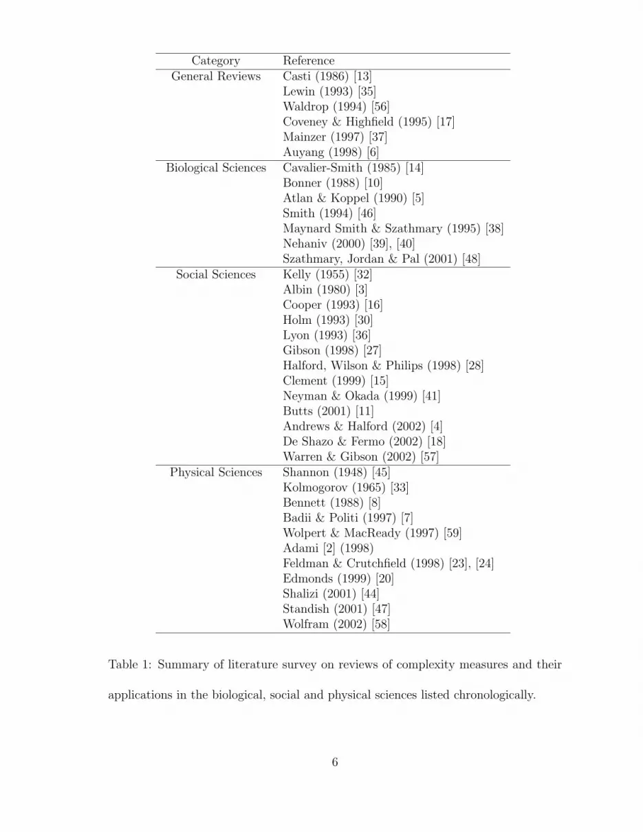
In this section, we present a review of existing measures for defining or simplycharacterizing complexity as viewed from the social, physical and biological sciences’perspectives. A summary of the literature surveyed on general reviews and specificapplications of complexity measures is given in Table 1. Here we give a high-levelsurvey of the more significant measures from these diverse fields. Our intention issimply to provide an indication of the wide spectrum of efforts in trying to capturecomplexity into something mathematical or formal so as to assist with the characteri-zation or comparison of different systems. A more comprehensive and detailed surveyof existing complexity measures is available elsewhere [20]. Nonetheless, our shortersurvey will show that such measures are often highly specific, being specially designedor formulated for application in a particular domain or area of research not readilytransferable to another application domain. A discussion of the advantages and dis-advantages associated with these different methodologies for measuring complexitywill be also highlighted. We will also cover the more recent complexity measuressuggested since the review conducted by Edmonds [20] especially for biological or-ganisms as they may provide critical insights to the measurement of complexity intheir artificial counterparts.

3.1 Social Sciences

An early attempt to capture complexity in a numerical form exists in the psychol-ogy literature. It is called cognitive complexity and is used to describe the complexityof mental constructions of the world possessed by an individual [32]. Cognitive com-plexity here is estimated numerically by counting the number of different relationshipsconstructed by the subject from given object attributes. In this sense, a person whosees the world in more dimensions would be considered to have a higher cognitive

5

Category ReferenceGeneral Reviews Casti (1986) [13]

Lewin (1993) [35]Waldrop (1994) [56]Coveney & Highfield (1995) [17]Mainzer (1997) [37]Auyang (1998) [6]

Biological Sciences Cavalier-Smith (1985) [14]Bonner (1988) [10]Atlan & Koppel (1990) [5]Smith (1994) [46]Maynard Smith & Szathmary (1995) [38]Nehaniv (2000) [39], [40]Szathmary, Jordan & Pal (2001) [48]

Social Sciences Kelly (1955) [32]Albin (1980) [3]Cooper (1993) [16]Holm (1993) [30]Lyon (1993) [36]Gibson (1998) [27]Halford, Wilson & Philips (1998) [28]Clement (1999) [15]Neyman & Okada (1999) [41]Butts (2001) [11]Andrews & Halford (2002) [4]De Shazo & Fermo (2002) [18]Warren & Gibson (2002) [57]

Physical Sciences Shannon (1948) [45]Kolmogorov (1965) [33]Bennett (1988) [8]Badii & Politi (1997) [7]Wolpert & MacReady (1997) [59]Adami [2] (1998)Feldman & Crutchfield (1998) [23], [24]Edmonds (1999) [20]Shalizi (2001) [44]Standish (2001) [47]Wolfram (2002) [58]

Table 1: Summary of literature survey on reviews of complexity measures and their

applications in the biological, social and physical sciences listed chronologically.

6

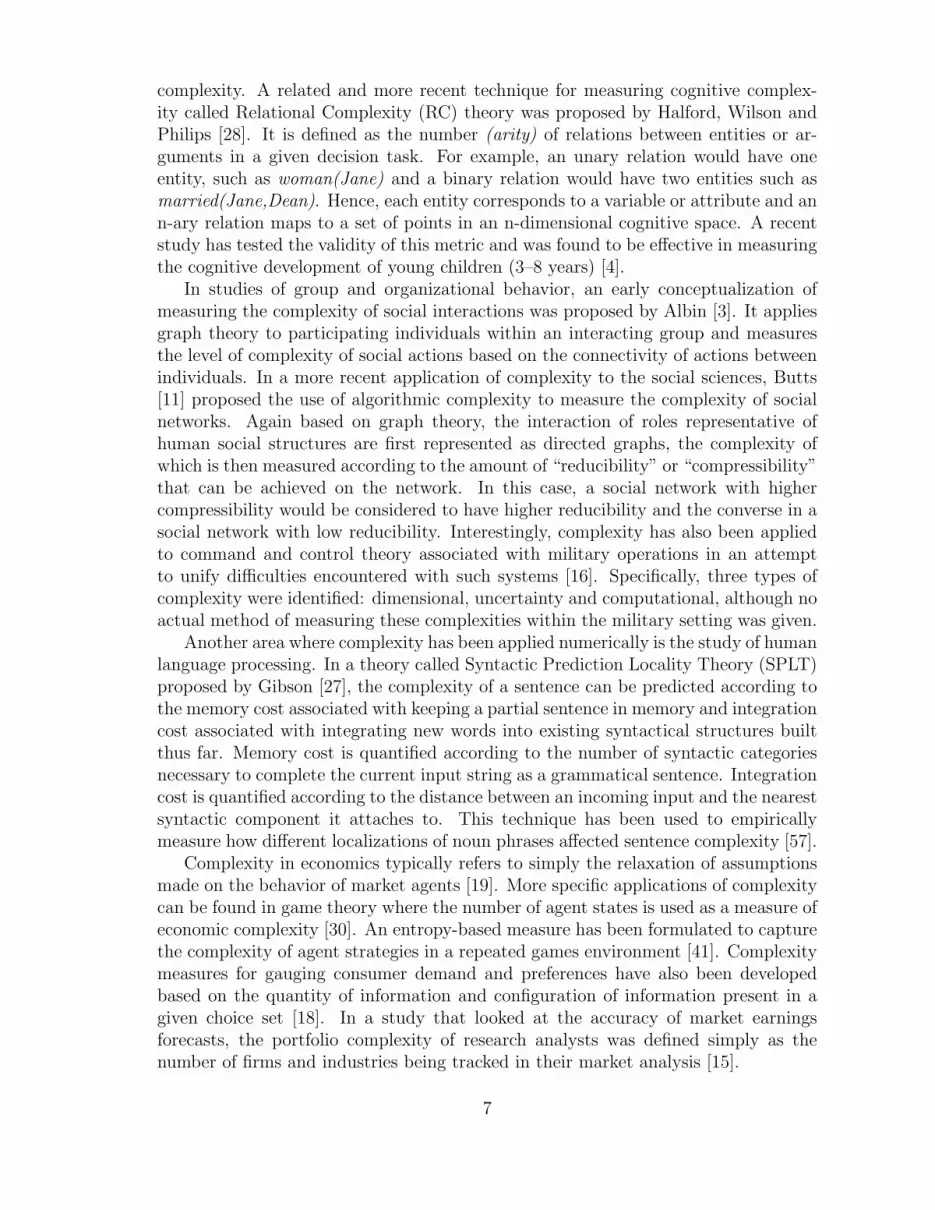
complexity. A related and more recent technique for measuring cognitive complex-ity called Relational Complexity (RC) theory was proposed by Halford, Wilson andPhilips [28]. It is defined as the number (arity) of relations between entities or ar-guments in a given decision task. For example, an unary relation would have oneentity, such as woman(Jane) and a binary relation would have two entities such asmarried(Jane,Dean). Hence, each entity corresponds to a variable or attribute and ann-ary relation maps to a set of points in an n-dimensional cognitive space. A recentstudy has tested the validity of this metric and was found to be effective in measuringthe cognitive development of young children (3–8 years) [4].

In studies of group and organizational behavior, an early conceptualization ofmeasuring the complexity of social interactions was proposed by Albin [3]. It appliesgraph theory to participating individuals within an interacting group and measuresthe level of complexity of social actions based on the connectivity of actions betweenindividuals. In a more recent application of complexity to the social sciences, Butts[11] proposed the use of algorithmic complexity to measure the complexity of socialnetworks. Again based on graph theory, the interaction of roles representative ofhuman social structures are first represented as directed graphs, the complexity ofwhich is then measured according to the amount of “reducibility” or “compressibility”that can be achieved on the network. In this case, a social network with highercompressibility would be considered to have higher reducibility and the converse in asocial network with low reducibility. Interestingly, complexity has also been appliedto command and control theory associated with military operations in an attemptto unify difficulties encountered with such systems [16]. Specifically, three types ofcomplexity were identified: dimensional, uncertainty and computational, although noactual method of measuring these complexities within the military setting was given.

Another area where complexity has been applied numerically is the study of humanlanguage processing. In a theory called Syntactic Prediction Locality Theory (SPLT)proposed by Gibson [27], the complexity of a sentence can be predicted according tothe memory cost associated with keeping a partial sentence in memory and integrationcost associated with integrating new words into existing syntactical structures builtthus far. Memory cost is quantified according to the number of syntactic categoriesnecessary to complete the current input string as a grammatical sentence. Integrationcost is quantified according to the distance between an incoming input and the nearestsyntactic component it attaches to. This technique has been used to empiricallymeasure how different localizations of noun phrases affected sentence complexity [57].

Complexity in economics typically refers to simply the relaxation of assumptionsmade on the behavior of market agents [19]. More specific applications of complexitycan be found in game theory where the number of agent states is used as a measure ofeconomic complexity [30]. An entropy-based measure has been formulated to capturethe complexity of agent strategies in a repeated games environment [41]. Complexitymeasures for gauging consumer demand and preferences have also been developedbased on the quantity of information and configuration of information present in agiven choice set [18]. In a study that looked at the accuracy of market earningsforecasts, the portfolio complexity of research analysts was defined simply as thenumber of firms and industries being tracked in their market analysis [15].

7

Measures of complexity have largely been applied at only a very superficial level inthe social sciences, typically taking size as a simplistic basis for describing or captur-ing complexity. There are obvious deficiencies associated with size-based complexitymeasures, the most evident being that not all large systems are complex [20]. It hasbeen argued that the application of complex systems theory to the social sciences re-sults in reductionist view of complexity when applied to the social domain [36]. Theimportant point raised is that contextual relationships such as political and moralissues are lost during the transformation into a mathematical or metaphoric modelfor complexity analysis.

3.2 Biological Sciences

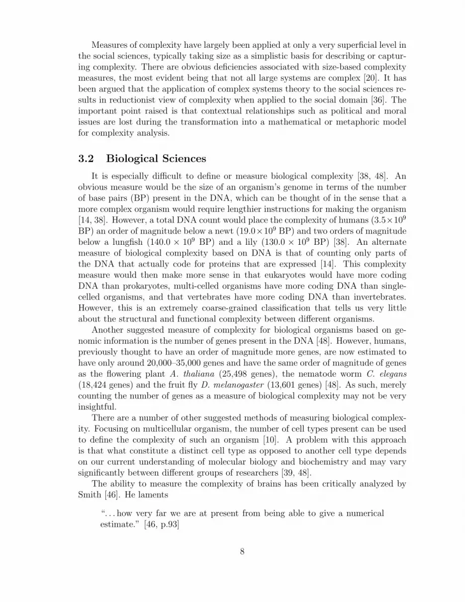
It is especially difficult to define or measure biological complexity [38, 48]. Anobvious measure would be the size of an organism’s genome in terms of the numberof base pairs (BP) present in the DNA, which can be thought of in the sense that amore complex organism would require lengthier instructions for making the organism[14, 38]. However, a total DNA count would place the complexity of humans (3.5×109

BP) an order of magnitude below a newt (19.0×109 BP) and two orders of magnitudebelow a lungfish (140.0 × 109 BP) and a lily (130.0 × 109 BP) [38]. An alternatemeasure of biological complexity based on DNA is that of counting only parts ofthe DNA that actually code for proteins that are expressed [14]. This complexitymeasure would then make more sense in that eukaryotes would have more codingDNA than prokaryotes, multi-celled organisms have more coding DNA than single-celled organisms, and that vertebrates have more coding DNA than invertebrates.However, this is an extremely coarse-grained classification that tells us very littleabout the structural and functional complexity between different organisms.

Another suggested measure of complexity for biological organisms based on ge-nomic information is the number of genes present in the DNA [48]. However, humans,previously thought to have an order of magnitude more genes, are now estimated tohave only around 20,000–35,000 genes and have the same order of magnitude of genesas the flowering plant A. thaliana (25,498 genes), the nematode worm C. elegans(18,424 genes) and the fruit fly D. melanogaster (13,601 genes) [48]. As such, merelycounting the number of genes as a measure of biological complexity may not be veryinsightful.

There are a number of other suggested methods of measuring biological complex-ity. Focusing on multicellular organism, the number of cell types present can be usedto define the complexity of such an organism [10]. A problem with this approachis that what constitute a distinct cell type as opposed to another cell type dependson our current understanding of molecular biology and biochemistry and may varysignificantly between different groups of researchers [39, 48].

The ability to measure the complexity of brains has been critically analyzed bySmith [46]. He laments

“. . . how very far we are at present from being able to give a numericalestimate.” [46, p.93]

8

Showing the inadequacies of “borrowed” complexity measures from the physical sci-ences, he argues that organization as well as levels of organization need to be con-sidered when attempting to capture the complexity of brains. A numerical measurebased on the columnar organization of the neocortex was suggested citing a quanti-tative example that estimates the complexity of human brains, with roughly 300,000such columns, to be 375 times greater than that of mouse brains, with only 800columns.

A more formal approach based on algorithmic complexity to measuring biologicalcomplexity has been suggested by considering the number of developmental stepsrequired to produce the organism from its DNA [5]. However, as critically pointedout by Szathmary, Jordan & Pal [48],

“The snag here is that evolution is not an engineer but a tinkerer, so thatthere is no reason to expect that, for example, elephants have developedaccording to a minimalist program.” (p.1315)

Another formal measure for biological complexity was suggested by Nehaniv [39]based on the notion of hierarchical complexity. In this measure, biological systemsare assigned an integer value which gives the least number of hierarchical organizedcomputing levels needed to construct an automata model of the biological system.Although powerful in terms of generalization since it does not require the actualknowledge of how a biological system is built nor its components, it does howeverhave the requirement that the system can first be adequately modelled using finiteautomata [39]. The process of transforming biological systems into such automatais highly subjective and can be executed in a myriad of ways depending on how thesystem is viewed by the transformer. This measure of complexity was later appliedto the measurement of evolvability in a later study and argued that open-endedevolutionary systems should show unbounded complexity increase over time [40].

Szathmary, Jordan & Pal [48] more recently proposed the measurement of biolog-ical complexity by considering the connectivity of networks of transcription factorsand the genes that regulate rather than direct counting of genes or the interactionsamong genes. They argue that biological complexity normally thought of in termsof morphological and behavioral complexity correlates better with the connectivityof gene-networks than direct measurements such as gene numbers since the formerwill correctly account for the presence of so-called delegated information processingsystems in the form of vertebrate nervous and immune systems. However, currentartificial evolutionary systems lack the level of sophistication in terms of such gene-regulatory networks and as such, do not readily lend themselves to such an analysis.Nonetheless, work has begun to imbue artificial evolutionary systems with some formof genetic regulation [9] in the hope of evolving more sophisticated artificial organismsand will conceivably in the future allow for such a measure to be applied.

3.3 Physical Sciences

In the physical sciences literature, there are generally two widely-accepted viewsof measuring complexity. The first is an information-theoretic approach based on

9

Shannon’s entropy [45] and is commonly referred to as statistical complexity due toits formulation based on probability. Shannon’s entropy measure H(X) of a randomvariable X, where the outcomes xi occur with probability pi, is given by

H(X) = − C

N∑i

pi log pi (1)

where C is the constant related to the base chosen to express the logarithm. It is aprobabilistic measure of disorder present in a system and thus gives an indication ofhow much we do not know about a particular system’s structure. Shannon’s entropyis used to measure the amount of information content present within a given messageor more generally any system of interest. Thus a more complex system would beexpected to give a much higher information content than a less complex system. Inother words, a more complex system would require more bits to describe compared to aless complex system. However, a sequence of random numbers will lead to the highestentropy and hence give a false indication of the system being complex when it is reallyjust random. In this sense, complexity is somehow a measure of order or disorder thatdoes not give a true indication of the information value present in the system, which inturn leads to an inaccurate characterization of complexity. Furthermore, an entropicmeasure does not take into account the semantic nature of the system. Consider forexample a simple behavior such as walking. Let us assume that we are interested inmeasuring the complexity of walking in different environments and the walking itself isundertaken by an ANN. From Shannon’s perspective, the complexity can be measuredusing the entropy of the data structure holding the neural network. Obviously adrawback for this view is its ignorance of the context and the concepts of embodimentand situatedness. The complexity of walking on a flat landscape is entirely differentfrom walking on a rough landscape. Two neural networks may be represented usingthe same number of bits but exhibit entirely different behaviors. Using the outputsfrom the neural networks as a measure of entropy is similarly problematic. Considerthe case where a particular neural network optimized to perform robotic control hastwo of its output nodes swapped. The entropy as measured from the outputs ofboth the original and modified networks will remain the same but the behavior of therobot will change dramatically since the signals being sent to the individual actuatorsconnected to these swapped output nodes have been disrupted. Hence, the change inthe robot’s behavior cannot be captured using this form of entropic measure.

The other approach to measuring complexity is a computation-theoretic approachbased on Kolmogorov’s application of universal Turing machines [33] and is commonlyknown as Kolmogorov complexity or algorithmic complexity. It is a deterministic mea-sure concerned with finding the shortest possible computer program or any abstractautomaton that is capable of reproducing a given string. The Kolmogorov complexityK(s) of a string s is given by

K(s) = min|p| | s = CT (p) (2)

where |p| represents the length of program p and CT (p) represents the result of run-ning program p on Turing machine T . A more complex string would thus require

10

a longer program while a simpler string would require a much shorter program. Inessence, the complexity of a particular system is measured by the minimum amountof computation required to recreate the system in question. A well-known theoreticalshortcoming of Kolmogorov complexity is that it is effectively incomputable since byvirtue of the halting problem [54], it cannot be determined with certainty that theabsolute shortest program or description has been found [7, 20, 44]. On an empiri-cal level, the following example will show the limitations of Kolmogorov complexity.Assume we have a sequence of random numbers. Obviously the shortest programwhich is able to reproduce this sequence is the sequence itself. Consequently, it issomehow also a measure of order or disorder, thereby endowing it with highly similarproperties to that of Shannon’s entropy [7, 20]. In addition, let us re-visit the neuralnetwork example. Assume that the robot is not using a fixed neural network but someform of evolvable hardware (which may be an evolutionary neural network). If thefitness landscape for the problem at hand is monotonically increasing, a hill climberwill simply be the shortest program which guarantees to re-produce the behavior.However, if the landscape is rugged, reproducing the behavior is only achievable if weknow the seed. Otherwise, the problem will require complete enumeration to recreatethe behavior. Unlike Shannon’s entropy measure, Kolmogorov complexity is both asyntactic and semantic measure of complexity but ignores the pragmatic nature of thesystem. Furthermore, Kolmogorov complexity has been shown to be a poor measurefor biological complexity [46, 48].

A measure of complexity commonly discussed in computer science and softwareengineering literature is computational complexity, which is the time and storagespace required by actual algorithms to solve a given problem [7]. Normally, it isreferred to by the big-O notation which is a worst-case complexity measure thatis defined as the order of the rate of growth of the resources required to computethe output to a problem as compared to the size of its input [20]. For example,an algorithm with computational complexity O(n2) would be expected to have aquadratic increase in computational resources with each linear increase in its inputwhile an algorithm with computational complexity of O(n3) would be expected to havea cubic increase with each linear increase in its input. The analysis of computationalcomplexity has important implications in the study of NP-completeness [25]. Theproblem is to ascertain whether or not a particular problem is tractable or intractable,or more accurately to determine whether or not a polynomial time algorithm existsthat can solve the problem on a von Neumann architecture. However, computationalcomplexity provides only a rough approximation as it is measured only according tothe order of the polynomial associated with the increase required in computationalresources when there is an increase in input. Furthermore, this measure of complexityspecifically looks at the construction of program code and how the computational costis affected by this code. Again, it measures complexity at the syntactic level and thusis unable to accommodate notions of environments or interactions which would beparamount in a study of embodied organisms.

Bennett [8] proposed a measure of complexity called logical depth by combiningthe notions of Kolmogorov complexity and computational complexity. The logical

11

depth Ds(x) of a string s at level x is defined as

Dx(s) = minT (p) | |p| − |p∗| < x ∧ U(p) = x (3)

where p is the range of programs, T (p) is the run-time required by program p, p∗

is the smallest such program and U is a Turing machine. It essentially states thatthe logical depth of a string is based on the running time of the shortest algorithmthat will reproduce a given string. It is poised between Kolmogorov complexity andcomputational complexity in that it considers the size of the shortest program aswell as the run-time of the program respectively [7]. Logical depth was proposedas a measure of the value of information as reflected by the degree to which thatinformation has been organized in a particular object. However, as logical depth isdefined based on Kolmogorov complexity, it too is essentially incomputable [7].

A starkly contrasting measure of complexity based on self-dissimilarity proper-ties was recently proposed by Wolpert [59]. Incorporating statistical inference andinformation theory, this complexity measure based on self-dissimilarity argues thatthe spatio-temporal signatures of complex systems vary markedly at different scaleswhereas the spatio-temporal signatures of simple systems do not differ significantlybetween different scales. Furthermore, the variation in a complex system’s patternsover different space and time scales are considered to be the very essence of com-plexity rather than just an aberration of the modelling or measurement process. Thespatio-temporal patterns in terms of the internal structure of a complex biologicalsystem for example, differs greatly when the observation scale is changed from themolecular level, to the cellular level, to the level of organs and to the level of theorganisms itself. On the other hand, this self-dissimilarity measure argues that thespatio-temporal patterns of simple systems such as crystals, gases and even fractalsdo not change very much as one changes the scale of observation. However, as statedby the authors themselves, this notion of complexity has only been formulated at thetheoretical level and its real worth will only be proven when it is finally applied toreal-world data [59].

In another research field known as computational mechanics, which is concernedwith the dynamics of automata behavior, a mathematically-based entity that capturesstatistical complexity called the ε-machine was proposed by Feldman & Crutchfield[23]. The ε-machine acts as a model for capturing the ensembles allowable configura-tions of a state machine. In other words, it is an object which allows for the inferenceof causal architecture from observed behavior [44]. As such, it allows for the defini-tion and calculation of the global and macroscopic properties that reflect the averageinformation processing capabilities of the system. The ε-machine has been appliedempirically to measure the amount of self-organization achieved by four increasinglysophisticated types of process: memoryless transducers, time series, transducers withmemory, and cellular automata [44]. Although the ε-machine has been shown to beeffective and useful in capturing the increase in statistical complexity of such self-organized systems, this complexity measure is again based on automata theory andas such requires that the system being studied readily transforms into some formof state machine. As with other automata-based methods [39], the question of howthese transformations should be undertaken and what effects these transformations

12

ultimately have when applied to less readily transformable systems such as creaturebehaviors and morphologies remains unanswered. More importantly, it provides aone dimensional view of complexity through the reduction of complex processes intoa finite state machine and as such, does not leave any room for the interpretationof interactions between the system and its environment, for example. Hence, suchautomata-based complexity measures may not be a suitable methodology to apply toareas such as embodied cognition in terms of usefulness and pragmatic value wherethe essence of complexity lies in the system operating as a fully-interacting, adaptableand reactive whole.

4 Proposed EMO-Based Complexity Measure

We will now introduce the use of EMO as a convenient platform which researcherscan utilize practically in attempting to define, measure, or simply characterize thecomplexity of everyday problems in a useful and purposeful manner. We first ex-plain the EMO concepts of Pareto optimality and dominance. Then we explain whya Pareto view to complexity is advantageous and proceed to present our proposedmethod of measuring complexity using EMO.

4.1 Dominance and Pareto Optimality

The optimization problem (hereafter referred to as P1) can be stated as

(P1): Minimise f(x)subject to: θ(x) = x ∈ Rn | G(x) ≤ 0

where x is the set of decision variables, f(x) is the objective function, G(x) is a setof constraints, and θ(x) is the set of feasible solutions. If the optimization problemis maximization, it is equivalent to a minimization problem by multiplying the ob-jective by (−1). Also, if a constraint is an equation, it can be represented by twoinequalities — one is “less than or equal” and the other is “greater than or equal”.A “greater than or equal” inequality can be transformed to a “less than or equal”inequality by multiplying both sides by (−1). In short, any optimization problem canbe represented in the previous general form.

Two important types of optimal solutions will be used in this paper, local andglobal optimal solutions. Let us define the open ball, that is a neighborhood centeredon x and defined by the Euclidean distance δ, as follows

Bδ(x) = x ∈ Rn | ||x− x|| < δ

Definition 1: Local optimality A point x ∈ θ(x) is said to be a local minimum ofthe optimisation problem iff ∃ δ > 0 such that f(x) ≤ f(x), ∀x ∈ (Bδ(x)∩θ(x)).

Definition 2: Global optimality A point x ∈ θ(x) is said to be a global minimumof the optimization problem iff f(x) ≤ f(x), ∀x ∈ θ(x).

13

Usually, there is more than a single objective to be optimized in real life appli-cations. In this case, the problem is called a multi-objective optimization problem(MOP). The problem P1 can be re-defined as a general multi-objective optimizationproblem, MOP1, by replacing the objective function f(x) with a vector of objectivesF (x) as follows

(MOP1): Minimize F (x)subject to: θ(x) = x ∈ Rn | G(x) ≤ 0

When the objectives are in conflict, the existence of a unique optimal solution is nolonger a valid concept. The solution which satisfies the optimality conditions of oneobjective may be a bad solution for another. Consequently, we need to redefine theconcepts of local and global optimality in multi-objective problems. To do this, wedefine two operators, and ≺ and then assume two vectors, X and Y . X Y iff∃ xi ∈ X and yi ∈ Y such that xi 6= yi. X ≺ Y iff ∀ xi ∈ X and yi ∈ Y, xi ≤ yi,and X Y . and ≺ can be seen as the “not equal to” and “less than” operators overtwo vectors. We can now define the equivalent concepts of local and global optimalityin a MOP.

Definition 3: Local efficient (non-inferior) solution: A vector of objective va-lues F (x), x ∈ θ(x) is said to be a local efficient solution of MOP iff @ x ∈(Bδ(x) ∩ θ(x)) such that F (x) ≺ F (x) for some positive δ.

Definition 4: Global efficient (non-inferior) solution: A vector of objective val-ues F (x), x ∈ θ(x) is said to be a local efficient solution of MOP iff @ x ∈ θ(x))such that F (x) ≺ F (x).

Definition 5: Pareto solutions: A point x ∈ θ(x) is said to be a Pareto solutionof MOP iff F (x) is a global efficient solution of MOP.

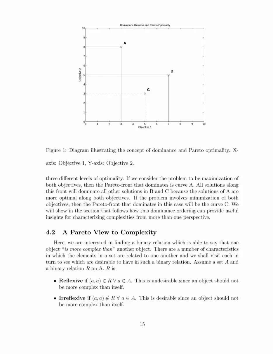
The concept of dominance and Pareto optimality is depicted in Figure 1. Let usconsider the case where there are three solutions A, B, and C and assume that thetwo objectives 1 and 2 are to be maximized. A is not dominated by any other solutionsince it has the highest value for objective 2. Similarly, B is not dominated by anyother solution since it has the highest value for objective 1. C is not dominated by Asince it has a higher value for objective 1. However, C is dominated by B since it haslower values for both objectives 1 and 2 compared to B. Hence we have the followingsituation

dominate(A) = φdominate(B) = φ

dominate(C) = Bwhere dominate(C) denotes the set of solutions that dominate C. Therefore, the setof non-dominated or Pareto optimal solutions is given by A,B

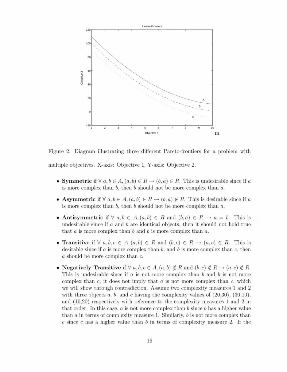
Figure 2 provides an illustration of three layers of a potential Pareto-front of a par-ticular multi-objective optimization problem. These layers can be viewed as providing

14

0 1 2 3 4 5 6 7 8 9 100

1

2

3

4

5

6

7

8

9

10Dominance Relation and Pareto Optimality

Objective 1

Obj

ectiv

e 2

A

B

C

Figure 1: Diagram illustrating the concept of dominance and Pareto optimality. X-

axis: Objective 1, Y-axis: Objective 2.

three different levels of optimality. If we consider the problem to be maximization ofboth objectives, then the Pareto-front that dominates is curve A. All solutions alongthis front will dominate all other solutions in B and C because the solutions of A aremore optimal along both objectives. If the problem involves minimization of bothobjectives, then the Pareto-front that dominates in this case will be the curve C. Wewill show in the section that follows how this dominance ordering can provide usefulinsights for characterizing complexities from more than one perspective.

4.2 A Pareto View to Complexity

Here, we are interested in finding a binary relation which is able to say that oneobject “is more complex than” another object. There are a number of characteristicsin which the elements in a set are related to one another and we shall visit each inturn to see which are desirable to have in such a binary relation. Assume a set A anda binary relation R on A. R is

• Reflexive if (a, a) ∈ R ∀ a ∈ A. This is undesirable since an object should notbe more complex than itself.

• Irreflexive if (a, a) /∈ R ∀ a ∈ A. This is desirable since an object should notbe more complex than itself.

15

1 2 3 4 5 6 7 8 9 10−20

0

20

40

60

80

100

120

Objective 1

Obj

ectiv

e 2

Pareto−Frontiers

A

B

C

m

Figure 2: Diagram illustrating three different Pareto-frontiers for a problem with

multiple objectives. X-axis: Objective 1, Y-axis: Objective 2.

• Symmetric if ∀ a, b ∈ A, (a, b) ∈ R → (b, a) ∈ R. This is undesirable since if ais more complex than b, then b should not be more complex than a.

• Asymmetric if ∀ a, b ∈ A, (a, b) ∈ R → (b, a) /∈ R. This is desirable since if ais more complex than b, then b should not be more complex than a.

• Antisymmetric if ∀ a, b ∈ A, (a, b) ∈ R and (b, a) ∈ R → a = b. This isundesirable since if a and b are identical objects, then it should not hold truethat a is more complex than b and b is more complex than a.

• Transitive if ∀ a, b, c ∈ A, (a, b) ∈ R and (b, c) ∈ R → (a, c) ∈ R. This isdesirable since if a is more complex than b, and b is more complex than c, thena should be more complex than c.

• Negatively Transitive if ∀ a, b, c ∈ A, (a, b) /∈ R and (b, c) /∈ R → (a, c) /∈ R.This is undesirable since if a is not more complex than b and b is not morecomplex than c, it does not imply that a is not more complex than c, whichwe will show through contradiction. Assume two complexity measures 1 and 2with three objects a, b, and c having the complexity values of (20,30), (30,10),and (10,20) respectively with reference to the complexity measures 1 and 2 inthat order. In this case, a is not more complex than b since b has a higher valuethan a in terms of complexity measure 1. Similarly, b is not more complex thanc since c has a higher value than b in terms of complexity measure 2. If the

16

complexity relation R is negatively transitive, then this implies that a is notmore complex than c. However, this is a contradiction as a is actually morecomplex than c since a has higher values in terms of both complexity measures.Therefore, this axiom is undesirable for the complexity binary relation R.

• Connected if ∀ a, b ∈ A, a 6= b → (a, b) ∈ R or (b, a) ∈ R. This is undesirablesince some pairs of objects may share the same complexity class and hencenot all pairs of objects are necessarily connected through the relation that oneobject is more complex than the other. We will show that connectedness isan undesirable axiom using the example described above. Neither is a morecomplex than b nor b is more complex than a. Thus, this axiom is undesirablefor the complexity binary relation R since some objects may share the samecomplexity class.

• Strongly Connected if ∀ a, b ∈ A, (a, b) ∈ R or (b, a) ∈ R. This is undesirablesince if the connectedness axiom does not hold true, then this axiom cannothold true.

Therefore, the binary relation “is more complex than”, R, should satisfy the irreflex-ivity, asymmetry and transitivity axioms.

It is important to point out that our purpose here is not to introduce anothermeasure of complexity that can supposedly overcome all previous limitations associ-ated with existing measures neither claiming that it is an all-encompassing techniquewhich will be able to calculate a definitive complexity value for complex systems. Ourobjective here is simply to propose and demonstrate that the Pareto set of solutionsarising from an EMO process can be highly beneficial for characterizing and compar-ing between the complexities of different systems and at the same time satisfy theaxioms desirable in a complexity binary relation. Furthermore, we will show throughour experiments that the Pareto approach is a useful complexity measure. A com-plexity measure is said to be useful when it is able to capture what we intuitivelyregard as complex [20].

There are two major advantages associated with using an EMO-based approach forcapturing complexity. Firstly, it measures complexity of a particular system as seenfrom an observer’s point of view. This has been argued by Casti [13] to be paramountsince the complexity of a system only has meaning through the interaction with itsobserver, particularly in more subjective areas such as behavioral complexity. As heputs it,

“. . . system complexity is a contingent property arising out of the interac-tion I between a system S and an observer/decision-maker O. Thus, anyperception and measure of complexity is necessarily a function of S, O,and I.” [13, p.149]

More importantly, he highlights the fact that

“Conditioned by the physical sciences, we typically regard S as the activesystem, with O being a passive observer or disengaged controller. Such

17

a picture misses the crucial point that generally the system S can alsobe regarded as an observer of O and that the interaction I is a two-waypath.” [13, p.149]

Since a Pareto set is the result of optimization across two (or more) objectives, thesolutions can be viewed as the result of a two-way interaction that occurs betweenthe different objectives during the optimization process. Hence, a Pareto approachprovides a distinct advantage when used to capture complexity by generating a setof solutions that inherently exhibits properties of a two-way interaction and whichcan be reversibly used simply by looking at the results from the other optimizationobjective’s view.

Secondly, we contend that the Pareto approach achieves a certain level of pragma-tism when used as a complexity measure as opposed to simply providing a syntacticor semantic measure of complexity. In other words, it does not simply measure thecomplexity at the level of the language or symbols used to construct the system asin a typical syntactic measure nor does it measure the system’s complexity withinsome predefined context or environment as would a semantic measure. Cariani [12]explains that the syntactic axis represents operations conducted at the symbolic level,the semantic axis represents operations where symbolic information is extracted fromthe environment through measurement and control while the pragmatic axis repre-sents the selection of appropriate measurements and controls that are advantageous tothe operation of the system. In this sense, the proposed EMO methodology towardscapturing complexity goes one step further in that it captures complexity throughan evolutionary optimization process that continually generates new solutions frommodification of previous solutions arising from testing and measurement of the sys-tem’s performance within a given context or environment, which in turn is guided bythe Pareto approach that imposes evolutionary pressures from multiple dimensions.In other words, it provides a view of complexity from a practical standpoint sincea Pareto set comprises of solutions from a selection and adaptation process therebyconstituting a pragmatic approach when such a Pareto set is used as a measure ofcomplexity.

4.3 The Complexity Measure

We now present the formulation of our proposed complexity measure and demon-strate how it can be applied to characterize as well as compare the behavioral andmorphological complexities of embodied artificial creatures. First, we define an em-bodied organism as the interaction between five components: morphology, behavior,controller, environment, and the learning algorithm. We will then show how complex-ity can be defined as a partial order relation over this five-dimensional hyperspace.Accordingly, the complexity of two embodied organisms can be compared using thispartial order relation. Finally, we support our argument with some experimentalresults which is presented in Section 5.4.

What follows is our proposal of a generic definition for complexity using the multi-objective paradigm. However, before we proceed with our definition, we need first to

18

explain the concept of partial order.

Definition 1: Partial and Lexicographic Order. Assume the two sets A andB. Assume the l-subsets over A and B such that A = a1 < . . . < al andB = b1 < . . . < bl.A partial order is defined as A ≤j B if aj ≤ bj, ∀j ∈ 1, . . . , lA Lexicographic order is defined as A <j B if ∃ak < bk and aj = bj, j <k, ∀j, k ∈ 1, . . . , l

In other words, a lexicographic order is a total order. In multi-objective optimiza-tion, the concept of Pareto optimality is normally used. A solution x belongs to thePareto set if there is not a solution y in the feasible solution set such that y dominatesx (that is x has to be at least as good as y when measured on all objectives and betterthan y on at least one objective). The Pareto concept thus forms partial orders inthe objective space.

The objective of the embodied cognition problem is to study the relationship be-tween the behavior, controller, environment, learning algorithm and morphology. Atypical question that one may ask is “What is the optimal behavior for a given mor-phology, controller, learning algorithm and environment?”. We can formally representthe problem of embodied cognition as the five sets B, C, E, L, and M for the five-dimensional hyperspace of behavior, controller, environment, learning algorithm, andmorphology respectively. We also need to differentiate between the robot behavior Band the desired behavior B. The former can be seen as the actual value of the fitnessfunction and the latter can be seen as the real maximum of the fitness function. Forexample, if the desired behavior (task) is to maximize the locomotion distance, thenthe global maximum of this function is the desired behavior, whereas the distanceachieved by the robot (what the robot is actually doing) is the actual behavior. Intraditional robotics, the problem can be seen as Given the desired behavior B, find Lwhich optimizes C subject to E

⋃M . In psychology, the problem can be formulated

as Given C, E, L and M , study the characteristics of the set B. In co-evolving mor-phology and mind, the problem is Given the desired behavior B and L, optimize Cand M subject to E. A general observation is that the learning algorithm is usuallyfixed during the experiments.

In asking a question such as “Is a human more complex than a Monkey?”, anatural question that follows would be “In what sense?”. Complexity is not a uniqueconcept. It is usually defined or measured within some context. For example, a humancan be seen as more complex than a Monkey if we are looking at the complexity ofintelligence, whereas a Monkey can be seen as more complex than the human if we arelooking at the number of different gaits the monkey has for locomotion. Therefore,what is important from an artificial life perspective is to establish the complexityhierarchy on different scales. Consequently, we introduce the following definition forcomplexity.

Definition 2: Complexity is a strict partial order relation.

19

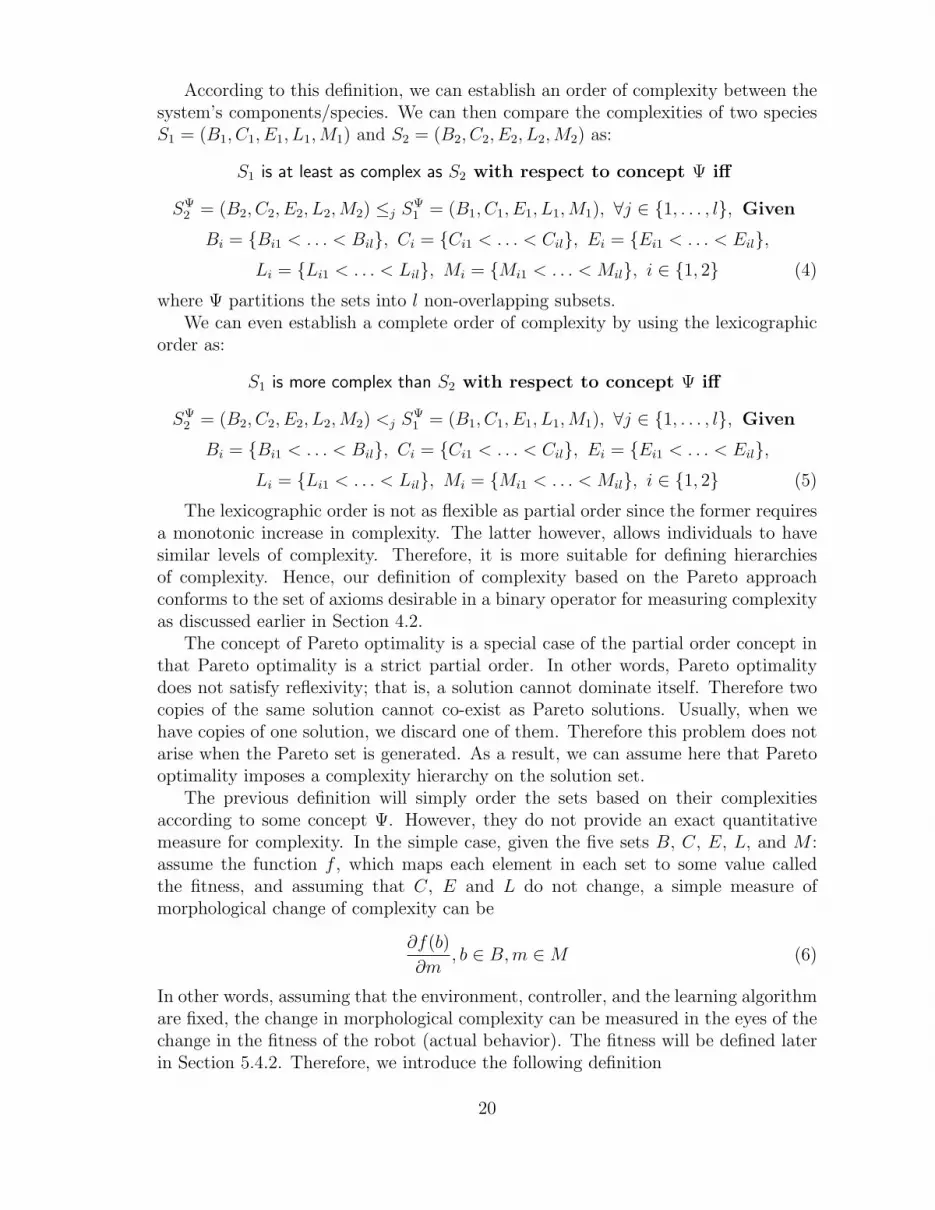
According to this definition, we can establish an order of complexity between thesystem’s components/species. We can then compare the complexities of two speciesS1 = (B1, C1, E1, L1,M1) and S2 = (B2, C2, E2, L2,M2) as:

S1 is at least as complex as S2 with respect to concept Ψ iff

SΨ2 = (B2, C2, E2, L2,M2) ≤j SΨ

1 = (B1, C1, E1, L1,M1), ∀j ∈ 1, . . . , l, Given

Bi = Bi1 < . . . < Bil, Ci = Ci1 < . . . < Cil, Ei = Ei1 < . . . < Eil,Li = Li1 < . . . < Lil, Mi = Mi1 < . . . < Mil, i ∈ 1, 2 (4)

where Ψ partitions the sets into l non-overlapping subsets.We can even establish a complete order of complexity by using the lexicographic

order as:

S1 is more complex than S2 with respect to concept Ψ iff

SΨ2 = (B2, C2, E2, L2,M2) <j SΨ

1 = (B1, C1, E1, L1,M1), ∀j ∈ 1, . . . , l, Given

Bi = Bi1 < . . . < Bil, Ci = Ci1 < . . . < Cil, Ei = Ei1 < . . . < Eil,Li = Li1 < . . . < Lil, Mi = Mi1 < . . . < Mil, i ∈ 1, 2 (5)

The lexicographic order is not as flexible as partial order since the former requiresa monotonic increase in complexity. The latter however, allows individuals to havesimilar levels of complexity. Therefore, it is more suitable for defining hierarchiesof complexity. Hence, our definition of complexity based on the Pareto approachconforms to the set of axioms desirable in a binary operator for measuring complexityas discussed earlier in Section 4.2.

The concept of Pareto optimality is a special case of the partial order concept inthat Pareto optimality is a strict partial order. In other words, Pareto optimalitydoes not satisfy reflexivity; that is, a solution cannot dominate itself. Therefore twocopies of the same solution cannot co-exist as Pareto solutions. Usually, when wehave copies of one solution, we discard one of them. Therefore this problem does notarise when the Pareto set is generated. As a result, we can assume here that Paretooptimality imposes a complexity hierarchy on the solution set.

The previous definition will simply order the sets based on their complexitiesaccording to some concept Ψ. However, they do not provide an exact quantitativemeasure for complexity. In the simple case, given the five sets B, C, E, L, and M :assume the function f , which maps each element in each set to some value calledthe fitness, and assuming that C, E and L do not change, a simple measure ofmorphological change of complexity can be

∂f(b)

∂m, b ∈ B, m ∈ M (6)

In other words, assuming that the environment, controller, and the learning algorithmare fixed, the change in morphological complexity can be measured in the eyes of thechange in the fitness of the robot (actual behavior). The fitness will be defined laterin Section 5.4.2. Therefore, we introduce the following definition

20

Definition 3: Change of Complexity Value for the morphology is the rate ofchange in behavioral fitness when the morphology changes, given that both theenvironment, learning algorithm and controller are fixed.

The previous definition can be generalized to cover the controller and environmentquite easily by simply replacing “morphology” by either “environment”, “learningalgorithm”, or “controller”. Based on this definition, if we can come up with a goodmeasure for behavioral complexity, we can use this measure to quantify the changein complexity for morphology, controller, learning algorithm, or environment. In thesame manner, if we have a complexity measure for the controller, we can use it toquantify the change of complexity in the other four parameters. Therefore, we proposethe notion of defining the complexity of one object as viewed from the perspectiveof another object. This is not unlike Emmeche’s idea of complexity as put in theeyes of the beholder [21]. However, we formalize and solidify this idea by putting itinto practical and quantitative usage through the multi-objective approach. We willdemonstrate that results from an EMO run of two conflicting objectives results in aPareto-front that allows a comparison of the different aspects of an artificial creature’scomplexity.

In the literature, there are a number of related topics which can help here. Forexample, the Vapnik-Chervonenkis (VC) dimension [55] can be used as a complexitymeasure for the controller. A feed-forward neural network using a threshold activationfunction has a VC dimension of O(WlogW ) while a similar network with a sigmoidactivation has a VC dimension of O(W 2), where W is the number of free parametersin the network [29]. It is apparent from here that one can control the complexityof a network by minimizing the number of free parameters which can be done in anumber of ways, the most obvious being the minimization of the number of synapsesand/or the number of hidden units. It is important to separate between the learningalgorithm and the model itself. For example, two identical neural networks with fixedarchitectures may perform differently if one of them is trained using back-propagationwhile the other is trained using an evolutionary algorithm. In this case, the separationbetween the model and the algorithm helps us to isolate their individual effects andgain an understanding of their individual roles.

In this set of experiments, we are essentially posing two questions, what is thechange of (1) behavioral complexity, and (2) morphological complexity of the artificialcreature in the eyes of its controller. In other words, how complex is the behaviorand morphology in terms of evolving a successful controller?

5 Complexity Measures Revisited

Before we proceed with an empirical experiment of how this complexity measurebased on the Pareto concept can be applied to capturing the morphological and be-havioral complexities of artificially evolved creatures, we first provide some examplesof how this methodology can be applied in a more general manner to the biological,social and physical sciences.

21

5.1 Biological Sciences

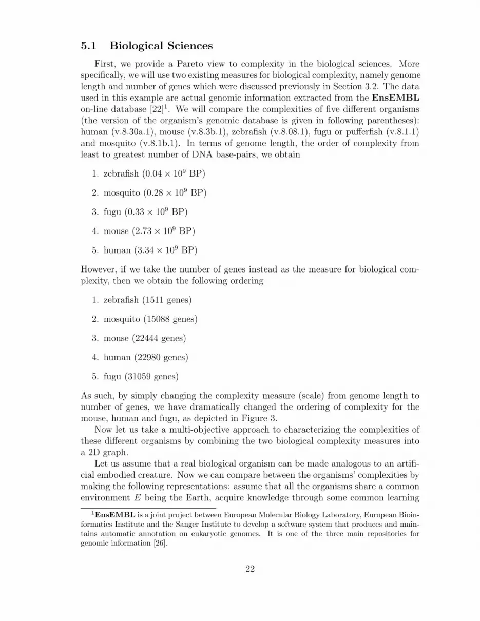
First, we provide a Pareto view to complexity in the biological sciences. Morespecifically, we will use two existing measures for biological complexity, namely genomelength and number of genes which were discussed previously in Section 3.2. The dataused in this example are actual genomic information extracted from the EnsEMBLon-line database [22]1. We will compare the complexities of five different organisms(the version of the organism’s genomic database is given in following parentheses):human (v.8.30a.1), mouse (v.8.3b.1), zebrafish (v.8.08.1), fugu or pufferfish (v.8.1.1)and mosquito (v.8.1b.1). In terms of genome length, the order of complexity fromleast to greatest number of DNA base-pairs, we obtain

1. zebrafish (0.04× 109 BP)

2. mosquito (0.28× 109 BP)

3. fugu (0.33× 109 BP)

4. mouse (2.73× 109 BP)

5. human (3.34× 109 BP)

However, if we take the number of genes instead as the measure for biological com-plexity, then we obtain the following ordering

1. zebrafish (1511 genes)

2. mosquito (15088 genes)

3. mouse (22444 genes)

4. human (22980 genes)

5. fugu (31059 genes)

As such, by simply changing the complexity measure (scale) from genome length tonumber of genes, we have dramatically changed the ordering of complexity for themouse, human and fugu, as depicted in Figure 3.

Now let us take a multi-objective approach to characterizing the complexities ofthese different organisms by combining the two biological complexity measures intoa 2D graph.

Let us assume that a real biological organism can be made analogous to an artifi-cial embodied creature. Now we can compare between the organisms’ complexities bymaking the following representations: assume that all the organisms share a commonenvironment E being the Earth, acquire knowledge through some common learning

1EnsEMBL is a joint project between European Molecular Biology Laboratory, European Bioin-formatics Institute and the Sanger Institute to develop a software system that produces and main-tains automatic annotation on eukaryotic genomes. It is one of the three main repositories forgenomic information [26].

22

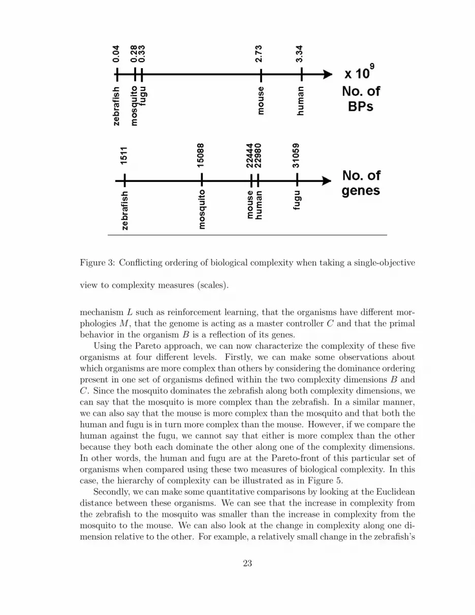
Figure 3: Conflicting ordering of biological complexity when taking a single-objective

view to complexity measures (scales).

mechanism L such as reinforcement learning, that the organisms have different mor-phologies M , that the genome is acting as a master controller C and that the primalbehavior in the organism B is a reflection of its genes.

Using the Pareto approach, we can now characterize the complexity of these fiveorganisms at four different levels. Firstly, we can make some observations aboutwhich organisms are more complex than others by considering the dominance orderingpresent in one set of organisms defined within the two complexity dimensions B andC. Since the mosquito dominates the zebrafish along both complexity dimensions, wecan say that the mosquito is more complex than the zebrafish. In a similar manner,we can also say that the mouse is more complex than the mosquito and that both thehuman and fugu is in turn more complex than the mouse. However, if we compare thehuman against the fugu, we cannot say that either is more complex than the otherbecause they both each dominate the other along one of the complexity dimensions.In other words, the human and fugu are at the Pareto-front of this particular set oforganisms when compared using these two measures of biological complexity. In thiscase, the hierarchy of complexity can be illustrated as in Figure 5.

Secondly, we can make some quantitative comparisons by looking at the Euclideandistance between these organisms. We can see that the increase in complexity fromthe zebrafish to the mosquito was smaller than the increase in complexity from themosquito to the mouse. We can also look at the change in complexity along one di-mension relative to the other. For example, a relatively small change in the zebrafish’s

23

0 0.5 1 1.5 2 2.5 3 3.5 4

x 104

0

0.5

1

1.5

2

2.5

3

3.5

4x 10

9

human

mouse

zebrafishfugu mosquito

No. of genes

No.

of B

Ps

Biological Complexity of 5 Organisms

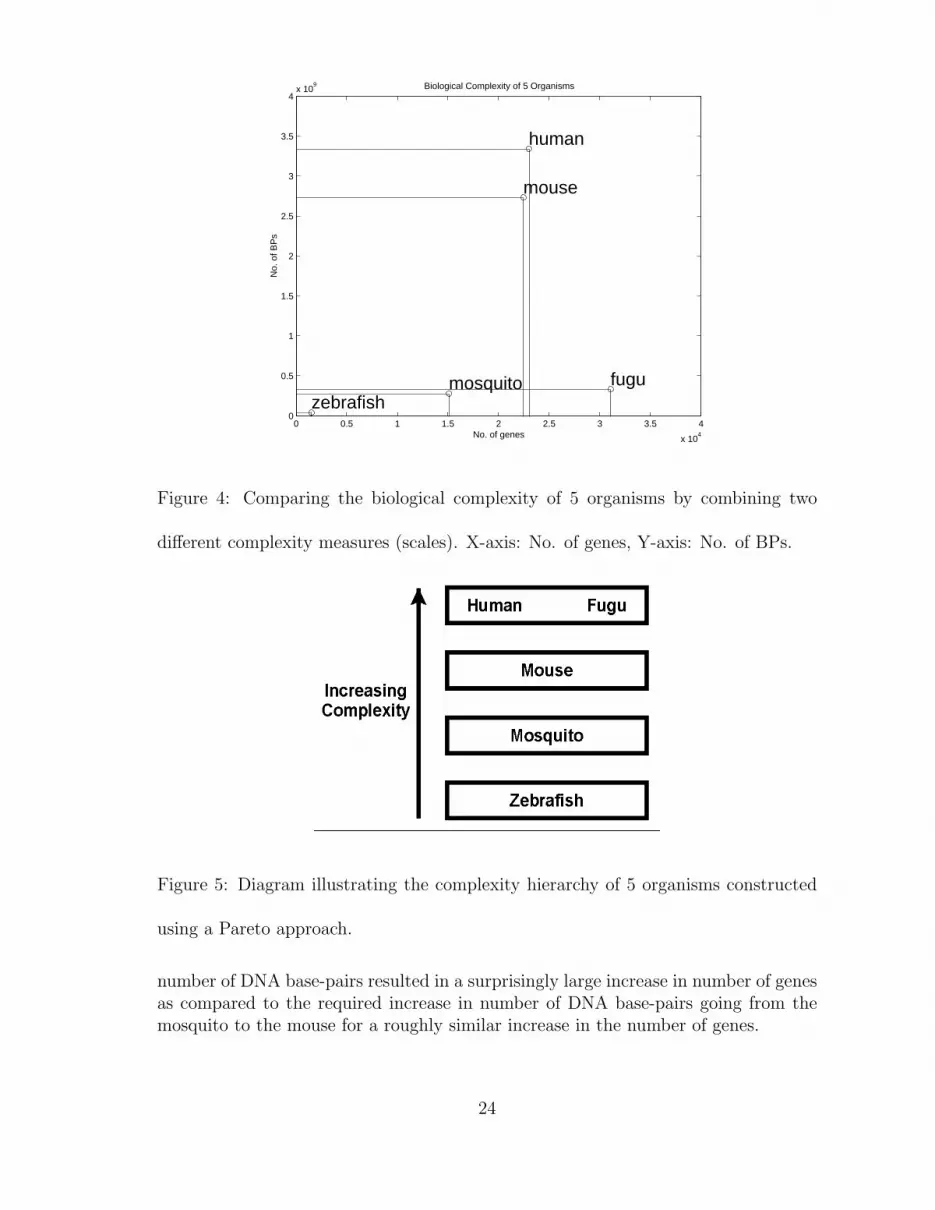
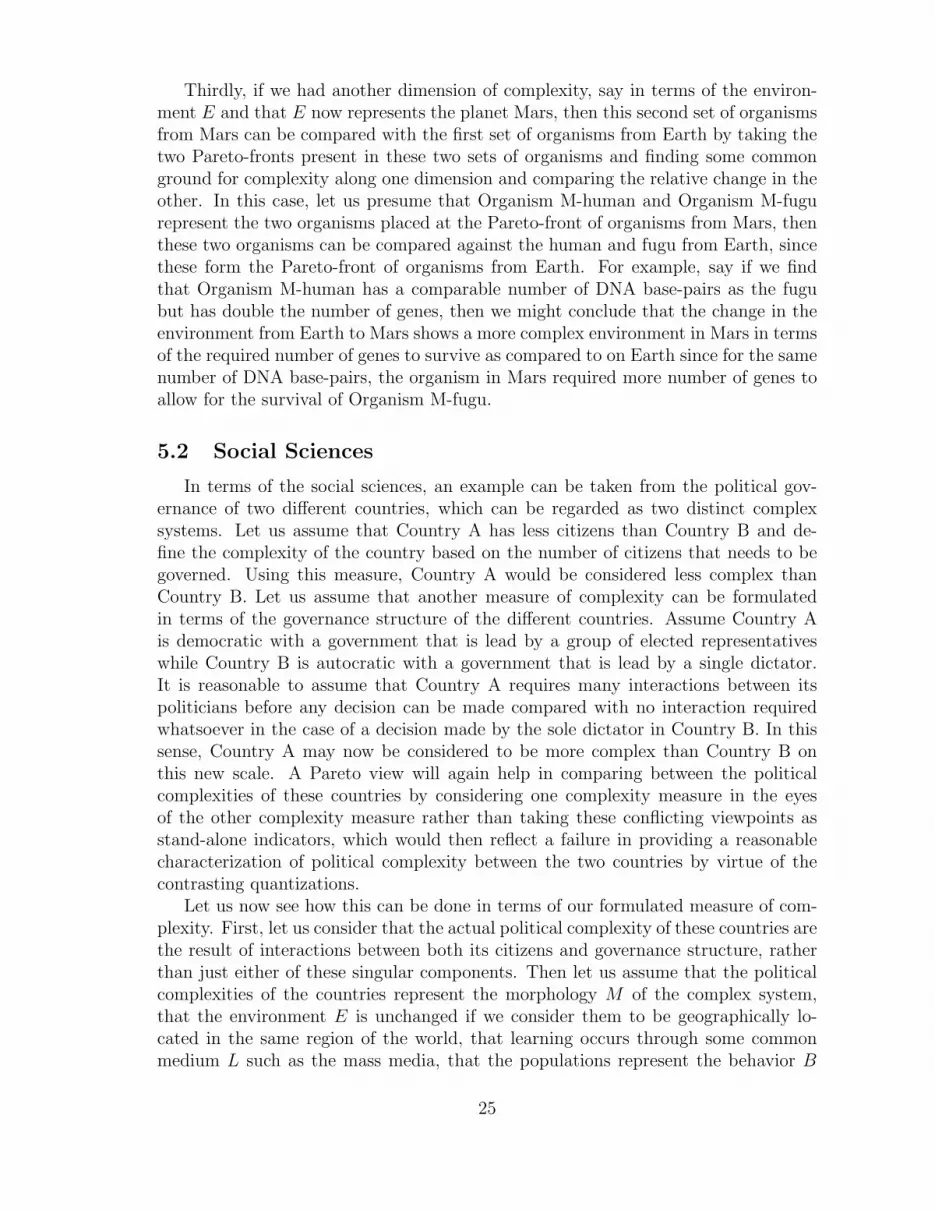
Figure 4: Comparing the biological complexity of 5 organisms by combining two

different complexity measures (scales). X-axis: No. of genes, Y-axis: No. of BPs.

Figure 5: Diagram illustrating the complexity hierarchy of 5 organisms constructed

using a Pareto approach.

number of DNA base-pairs resulted in a surprisingly large increase in number of genesas compared to the required increase in number of DNA base-pairs going from themosquito to the mouse for a roughly similar increase in the number of genes.

24

Thirdly, if we had another dimension of complexity, say in terms of the environ-ment E and that E now represents the planet Mars, then this second set of organismsfrom Mars can be compared with the first set of organisms from Earth by taking thetwo Pareto-fronts present in these two sets of organisms and finding some commonground for complexity along one dimension and comparing the relative change in theother. In this case, let us presume that Organism M-human and Organism M-fugurepresent the two organisms placed at the Pareto-front of organisms from Mars, thenthese two organisms can be compared against the human and fugu from Earth, sincethese form the Pareto-front of organisms from Earth. For example, say if we findthat Organism M-human has a comparable number of DNA base-pairs as the fugubut has double the number of genes, then we might conclude that the change in theenvironment from Earth to Mars shows a more complex environment in Mars in termsof the required number of genes to survive as compared to on Earth since for the samenumber of DNA base-pairs, the organism in Mars required more number of genes toallow for the survival of Organism M-fugu.

5.2 Social Sciences

In terms of the social sciences, an example can be taken from the political gov-ernance of two different countries, which can be regarded as two distinct complexsystems. Let us assume that Country A has less citizens than Country B and de-fine the complexity of the country based on the number of citizens that needs to begoverned. Using this measure, Country A would be considered less complex thanCountry B. Let us assume that another measure of complexity can be formulatedin terms of the governance structure of the different countries. Assume Country Ais democratic with a government that is lead by a group of elected representativeswhile Country B is autocratic with a government that is lead by a single dictator.It is reasonable to assume that Country A requires many interactions between itspoliticians before any decision can be made compared with no interaction requiredwhatsoever in the case of a decision made by the sole dictator in Country B. In thissense, Country A may now be considered to be more complex than Country B onthis new scale. A Pareto view will again help in comparing between the politicalcomplexities of these countries by considering one complexity measure in the eyesof the other complexity measure rather than taking these conflicting viewpoints asstand-alone indicators, which would then reflect a failure in providing a reasonablecharacterization of political complexity between the two countries by virtue of thecontrasting quantizations.

Let us now see how this can be done in terms of our formulated measure of com-plexity. First, let us consider that the actual political complexity of these countries arethe result of interactions between both its citizens and governance structure, ratherthan just either of these singular components. Then let us assume that the politicalcomplexities of the countries represent the morphology M of the complex system,that the environment E is unchanged if we consider them to be geographically lo-cated in the same region of the world, that learning occurs through some commonmedium L such as the mass media, that the populations represent the behavior B

25

and that the governance structures represent the controller C. Now we can com-pare the change in political complexity between these two different countries ∂M bymeasuring some quantitative change in the behavior of the population ∂B throughsome commonality that can be found in the hyperspace of the controlling governancestructure C. Conversely, we can compare the governance complexity between thetwo countries ∂M from the reverse viewpoint by measuring some quantitative changein terms of the controlling governance structure ∂C through establishing some com-monality in the hyperspace of the population’s behavior B. Casti [13] provides anelegant example of how such a complex system emerges from the interactions betweenits governance structure and its citizens. Here, he states that the citizens views thegovernance structure as complex if the actions taken by its political leaders seem tobe incomprehensible:

“. . . they [the citizens ] see a byzantine and unwieldy government bureau-cracy and a large number of independent decision-makers (governmentagencies) affecting their day-to-day life.” (p.150)

Similarly, the government typically also views its citizens as being very complex:

“They [the political leaders ] would see a seemingly fickle, capricious public,composed of a large number of independent self-interest groups clamoringfor more and more public goods and services.” (p.150)

Hence, we can see that a multi-objective view to the study of social sciences such aspolitical complexity can again be very insightful and valuable.

5.3 Physical Sciences

In revisiting complexity measures for the physical sciences, let us turn to an ex-ample from computer science itself. Wuensche [60] has recently devised a method forautomatic classification of 1D cellular automata (CA) rules into one of three dynam-ical groups, that is ordered, complex and chaotic systems based on the frequency ofparticular updating rules being looked-up over time called the input-entropy. Basedon Shannon’s entropy measure, Wuensche [60] formulated input-entropy S at time-step t as

St = −2k∑i=1

(Qt

i

n× log(

Qti

n)) (7)

where k and n are the neighborhood and system size of the CA, and Qti is the lookup

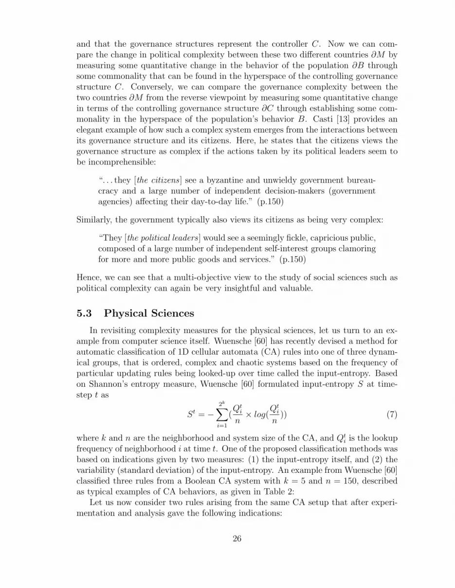
frequency of neighborhood i at time t. One of the proposed classification methods wasbased on indications given by two measures: (1) the input-entropy itself, and (2) thevariability (standard deviation) of the input-entropy. An example from Wuensche [60]classified three rules from a Boolean CA system with k = 5 and n = 150, describedas typical examples of CA behaviors, as given in Table 2:

Let us now consider two rules arising from the same CA setup that after experi-mentation and analysis gave the following indications:

26

Rule No. Classification Input-Entropy Variability of Input-Entropy01 dc 96 10 Ordered low low6c 1e 53 a8 Complex medium high99 4a 6a 65 Chaotic high low

Table 2: Classification of 3 cellular automata rules according to Wuensche [60].

• Rule X: moderately high entropy, moderately high variability

• Rule Y: very high entropy, very high variability

It would be difficult to classify these two rules since they are placed mid-way betweenthe existing classes. However, if we take a multi-objective view to this problem, wewould be able to provide the following perspective:

0 10

1

Ordered

Chaotic

Rule X

Complex

Rule Y

Variability of input−entropy

Inpu

t−en

trop

y

Multi−Objective View of 5 CA Rules

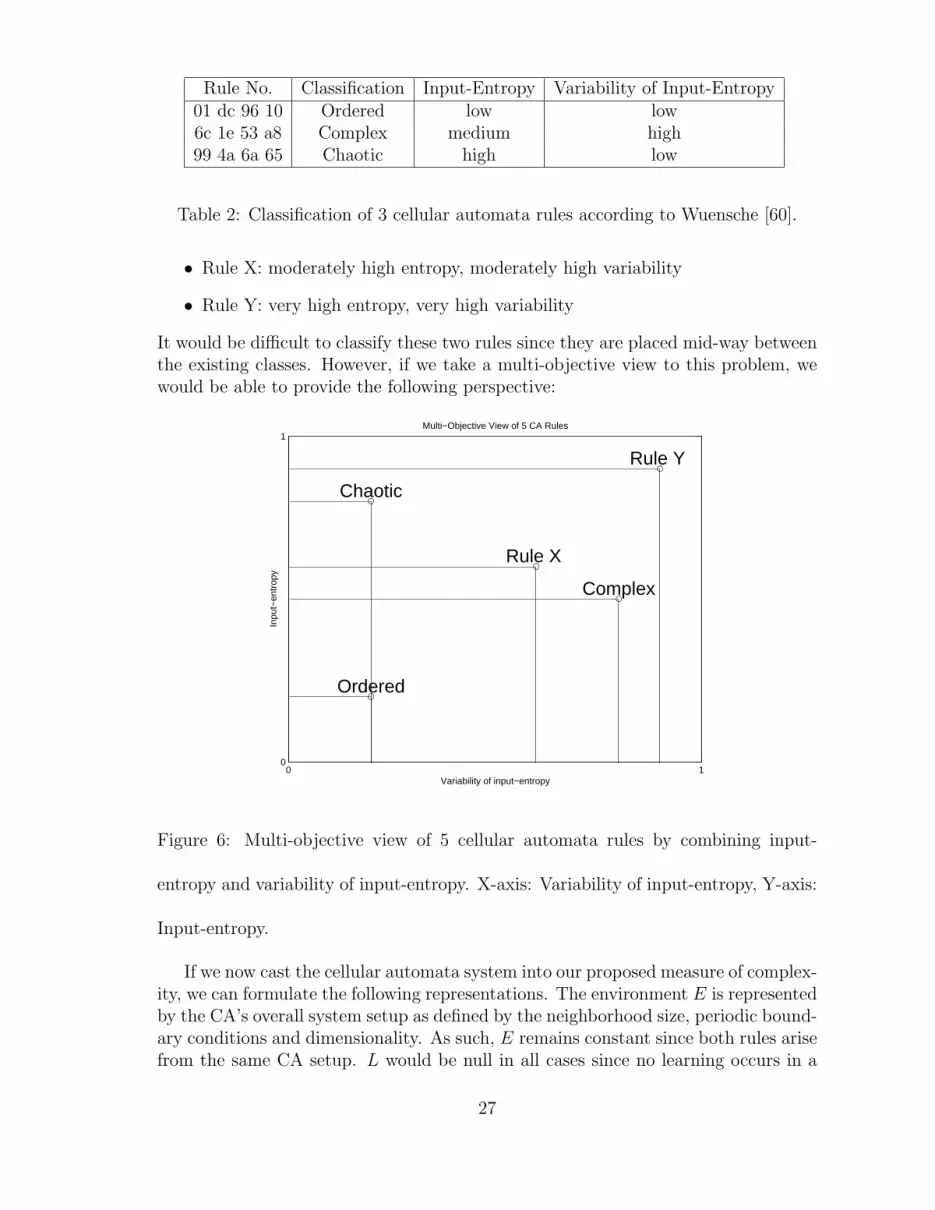
Figure 6: Multi-objective view of 5 cellular automata rules by combining input-

entropy and variability of input-entropy. X-axis: Variability of input-entropy, Y-axis:

Input-entropy.

If we now cast the cellular automata system into our proposed measure of complex-ity, we can formulate the following representations. The environment E is representedby the CA’s overall system setup as defined by the neighborhood size, periodic bound-ary conditions and dimensionality. As such, E remains constant since both rules arisefrom the same CA setup. L would be null in all cases since no learning occurs in a

27

CA system. Let us now consider that the difference between Rule X and Rule Yrepresents a change in the controller C of the CA system since the dynamics of aCA is dependent on the rule being used in the CA. Next, we shall consider that themorphology M of the CA is represented by the input-entropy and that the behaviorB of the CA is represented by the variability in the input-entropy.

Firstly, we can see that Rule Y dominates all other rules in this particular systemsince it has higher values for both complexity dimensions of B and M . As such, wecan say that Rule Y is the most complex rule from a multi-objective perspective.Also, we can see that a Pareto-front is formed by the Chaotic and Complex rules,and that both rules are as complex as each other since they both dominate each otherin one dimension. Furthermore, since Rule X is not dominated by either the Chaoticnor the Complex rule in both dimensions, it too belongs to the Pareto set for thisparticular CA system and that its complexity can be characterized as being similar tothat of the Chaotic and Complex rules in terms of B and M . As for the Ordered rule,it has the same value for B (variability of input-entropy) as the Chaotic rule and hasa lower value for M (input-entropy) than the Chaotic rule. As such, the Ordered ruleis dominated by the Pareto-front of which the Chaotic rule is a member. Hence, it canbe characterized as being the least complex among all the rules in this particular CAsystem since it is dominated by all other rules. As with the biological example visitedearlier, a change in the environment E, for example increasing the neighborhoodsize, will produce a second set of observations which can then be compared with thisfirst set of observations by comparing the two Pareto-fronts obtained from these twodifferent CA systems.

In the next section, we will describe the setup of the experiments which demon-strate empirically how our proposed measure for capturing complexity can be appliedto the comparison of the morphological and behavioral complexities of artificiallyevolved creatures.

5.4 An Experiment in Comparing the Complexities of Arti-ficially Evolved Embodied Creatures

5.4.1 Two Artificial Creatures

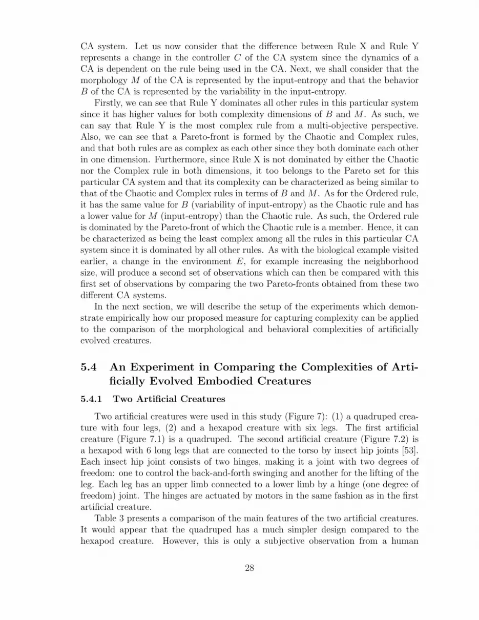
Two artificial creatures were used in this study (Figure 7): (1) a quadruped crea-ture with four legs, (2) and a hexapod creature with six legs. The first artificialcreature (Figure 7.1) is a quadruped. The second artificial creature (Figure 7.2) isa hexapod with 6 long legs that are connected to the torso by insect hip joints [53].Each insect hip joint consists of two hinges, making it a joint with two degrees offreedom: one to control the back-and-forth swinging and another for the lifting of theleg. Each leg has an upper limb connected to a lower limb by a hinge (one degree offreedom) joint. The hinges are actuated by motors in the same fashion as in the firstartificial creature.

Table 3 presents a comparison of the main features of the two artificial creatures.It would appear that the quadruped has a much simpler design compared to thehexapod creature. However, this is only a subjective observation from a human

28

Figure 7: Screen dump of the 1. quadruped (left), 2. hexapod (right) artificial

creatures.

Morphological Characteristic Simulated Quadruped Simulated HexapodNo. of legs 4 6

Degrees of freedom 8 24No. of sensors 12 24No. of motors 8 18

Table 3: A comparison of the simulated quadruped and hexapod creatures’ morpho-

logical characteristics.

designer’s perspective. It remains to be seen whether this view will hold when wecompare the complexities of these two artificial creatures from the controller’s andbehavior’s perspectives.

5.4.2 Controller Architecture

The Pareto-frontier of our evolutionary runs are obtained from optimizing twoconflicting objectives: (1) minimizing the number of hidden units used in the ANNthat act as the creature’s controller, and (2) maximizing horizontal locomotion dis-tance of the artificial creature. What we obtain at the end of the runs are againPareto sets of ANNs that trade-off between number of hidden units and locomotiondistance. The locomotion distances achieved by the different Pareto solutions willprovide a common ground where locomotion competency can be used to comparedifferent behaviors and morphologies. It will provide a set of ANNs with the smallesthidden layer capable of achieving a variety of locomotion competencies. The struc-tural definition of the evolved ANNs can now be used as a measure of complexity forthe different creature behaviors and morphologies.

The type of ANN architecture used for the experiments in this experiment isNNType3 as presented in Figure 8, which has fully-connected feed-forward network

29

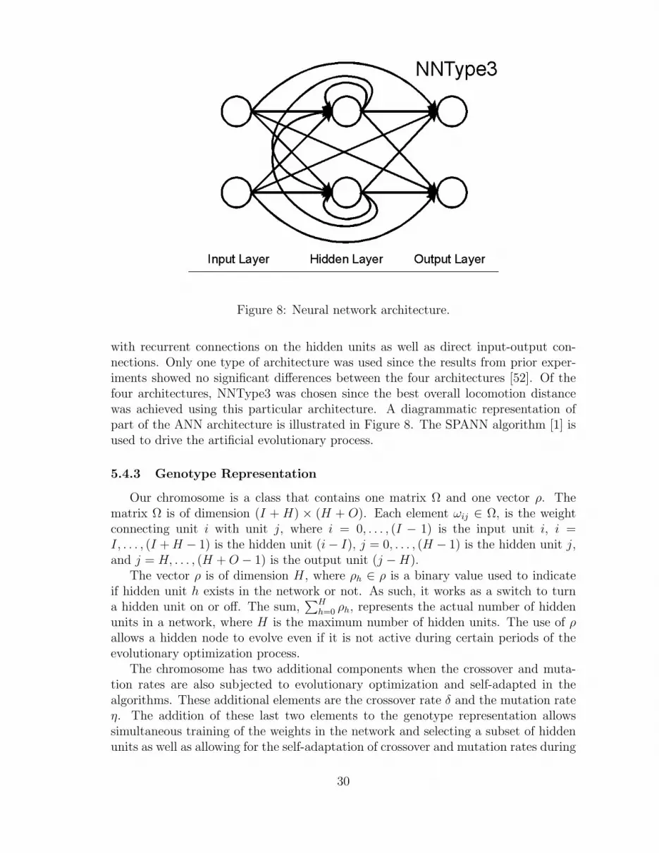
Figure 8: Neural network architecture.

with recurrent connections on the hidden units as well as direct input-output con-nections. Only one type of architecture was used since the results from prior exper-iments showed no significant differences between the four architectures [52]. Of thefour architectures, NNType3 was chosen since the best overall locomotion distancewas achieved using this particular architecture. A diagrammatic representation ofpart of the ANN architecture is illustrated in Figure 8. The SPANN algorithm [1] isused to drive the artificial evolutionary process.

5.4.3 Genotype Representation

Our chromosome is a class that contains one matrix Ω and one vector ρ. Thematrix Ω is of dimension (I + H) × (H + O). Each element ωij ∈ Ω, is the weightconnecting unit i with unit j, where i = 0, . . . , (I − 1) is the input unit i, i =I, . . . , (I + H − 1) is the hidden unit (i− I), j = 0, . . . , (H − 1) is the hidden unit j,and j = H, . . . , (H + O − 1) is the output unit (j −H).

The vector ρ is of dimension H, where ρh ∈ ρ is a binary value used to indicateif hidden unit h exists in the network or not. As such, it works as a switch to turna hidden unit on or off. The sum,

∑Hh=0 ρh, represents the actual number of hidden

units in a network, where H is the maximum number of hidden units. The use of ρallows a hidden node to evolve even if it is not active during certain periods of theevolutionary optimization process.

The chromosome has two additional components when the crossover and muta-tion rates are also subjected to evolutionary optimization and self-adapted in thealgorithms. These additional elements are the crossover rate δ and the mutation rateη. The addition of these last two elements to the genotype representation allowssimultaneous training of the weights in the network and selecting a subset of hiddenunits as well as allowing for the self-adaptation of crossover and mutation rates during

30

optimization.A direct encoding method was chosen to represent these variables in the genotype

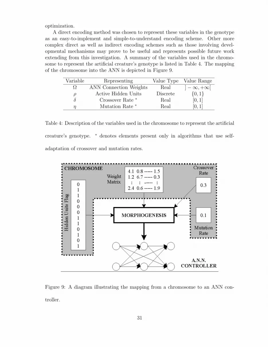
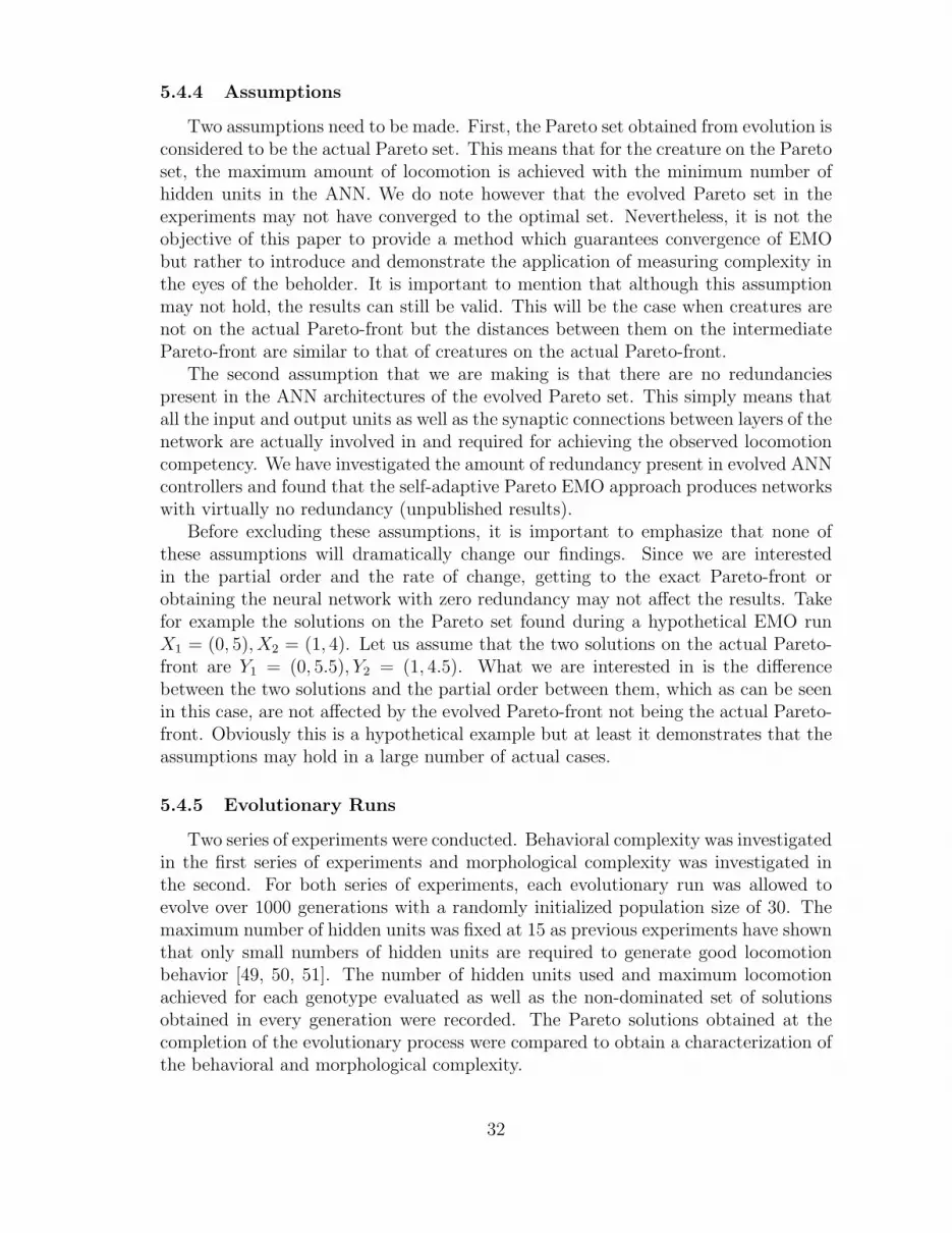
as an easy-to-implement and simple-to-understand encoding scheme. Other morecomplex direct as well as indirect encoding schemes such as those involving devel-opmental mechanisms may prove to be useful and represents possible future workextending from this investigation. A summary of the variables used in the chromo-some to represent the artificial creature’s genotype is listed in Table 4. The mappingof the chromosome into the ANN is depicted in Figure 9.

Variable Representing Value Type Value RangeΩ ANN Connection Weights Real ]−∞, +∞[ρ Active Hidden Units Discrete 0, 1δ Crossover Rate ∗ Real [0, 1]η Mutation Rate ∗ Real [0, 1]

Table 4: Description of the variables used in the chromosome to represent the artificial

creature’s genotype. ∗ denotes elements present only in algorithms that use self-

adaptation of crossover and mutation rates.

Figure 9: A diagram illustrating the mapping from a chromosome to an ANN con-

troller.

31

5.4.4 Assumptions

Two assumptions need to be made. First, the Pareto set obtained from evolution isconsidered to be the actual Pareto set. This means that for the creature on the Paretoset, the maximum amount of locomotion is achieved with the minimum number ofhidden units in the ANN. We do note however that the evolved Pareto set in theexperiments may not have converged to the optimal set. Nevertheless, it is not theobjective of this paper to provide a method which guarantees convergence of EMObut rather to introduce and demonstrate the application of measuring complexity inthe eyes of the beholder. It is important to mention that although this assumptionmay not hold, the results can still be valid. This will be the case when creatures arenot on the actual Pareto-front but the distances between them on the intermediatePareto-front are similar to that of creatures on the actual Pareto-front.

The second assumption that we are making is that there are no redundanciespresent in the ANN architectures of the evolved Pareto set. This simply means thatall the input and output units as well as the synaptic connections between layers of thenetwork are actually involved in and required for achieving the observed locomotioncompetency. We have investigated the amount of redundancy present in evolved ANNcontrollers and found that the self-adaptive Pareto EMO approach produces networkswith virtually no redundancy (unpublished results).

Before excluding these assumptions, it is important to emphasize that none ofthese assumptions will dramatically change our findings. Since we are interestedin the partial order and the rate of change, getting to the exact Pareto-front orobtaining the neural network with zero redundancy may not affect the results. Takefor example the solutions on the Pareto set found during a hypothetical EMO runX1 = (0, 5), X2 = (1, 4). Let us assume that the two solutions on the actual Pareto-front are Y1 = (0, 5.5), Y2 = (1, 4.5). What we are interested in is the differencebetween the two solutions and the partial order between them, which as can be seenin this case, are not affected by the evolved Pareto-front not being the actual Pareto-front. Obviously this is a hypothetical example but at least it demonstrates that theassumptions may hold in a large number of actual cases.

5.4.5 Evolutionary Runs

Two series of experiments were conducted. Behavioral complexity was investigatedin the first series of experiments and morphological complexity was investigated inthe second. For both series of experiments, each evolutionary run was allowed toevolve over 1000 generations with a randomly initialized population size of 30. Themaximum number of hidden units was fixed at 15 as previous experiments have shownthat only small numbers of hidden units are required to generate good locomotionbehavior [49, 50, 51]. The number of hidden units used and maximum locomotionachieved for each genotype evaluated as well as the non-dominated set of solutionsobtained in every generation were recorded. The Pareto solutions obtained at thecompletion of the evolutionary process were compared to obtain a characterization ofthe behavioral and morphological complexity.

32

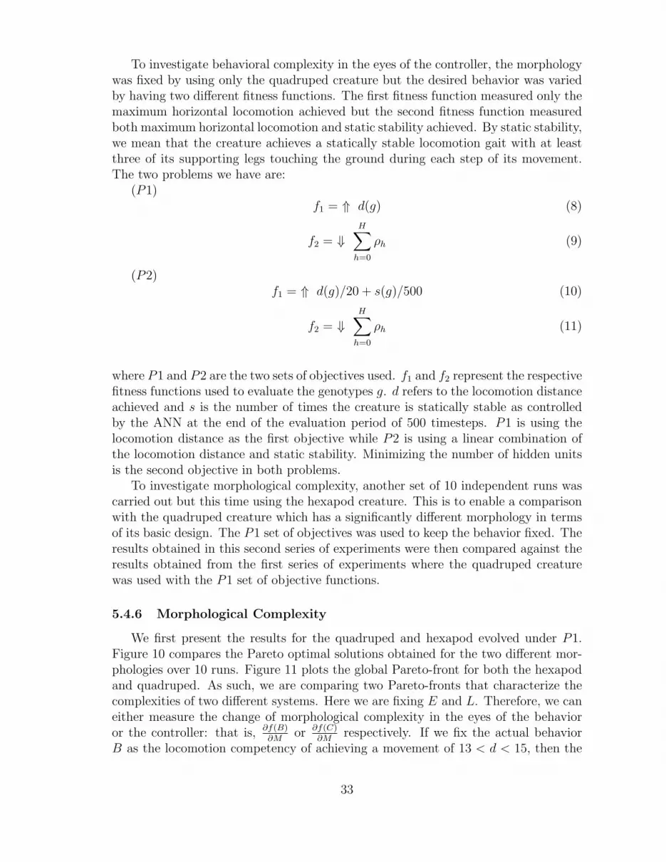
To investigate behavioral complexity in the eyes of the controller, the morphologywas fixed by using only the quadruped creature but the desired behavior was variedby having two different fitness functions. The first fitness function measured only themaximum horizontal locomotion achieved but the second fitness function measuredboth maximum horizontal locomotion and static stability achieved. By static stability,we mean that the creature achieves a statically stable locomotion gait with at leastthree of its supporting legs touching the ground during each step of its movement.The two problems we have are:

(P1)f1 = ⇑ d(g) (8)

f2 = ⇓H∑

h=0

ρh (9)

(P2)f1 = ⇑ d(g)/20 + s(g)/500 (10)

f2 = ⇓H∑

h=0

ρh (11)

where P1 and P2 are the two sets of objectives used. f1 and f2 represent the respectivefitness functions used to evaluate the genotypes g. d refers to the locomotion distanceachieved and s is the number of times the creature is statically stable as controlledby the ANN at the end of the evaluation period of 500 timesteps. P1 is using thelocomotion distance as the first objective while P2 is using a linear combination ofthe locomotion distance and static stability. Minimizing the number of hidden unitsis the second objective in both problems.

To investigate morphological complexity, another set of 10 independent runs wascarried out but this time using the hexapod creature. This is to enable a comparisonwith the quadruped creature which has a significantly different morphology in termsof its basic design. The P1 set of objectives was used to keep the behavior fixed. Theresults obtained in this second series of experiments were then compared against theresults obtained from the first series of experiments where the quadruped creaturewas used with the P1 set of objective functions.

5.4.6 Morphological Complexity

We first present the results for the quadruped and hexapod evolved under P1.Figure 10 compares the Pareto optimal solutions obtained for the two different mor-phologies over 10 runs. Figure 11 plots the global Pareto-front for both the hexapodand quadruped. As such, we are comparing two Pareto-fronts that characterize thecomplexities of two different systems. Here we are fixing E and L. Therefore, we caneither measure the change of morphological complexity in the eyes of the behavioror the controller: that is, ∂f(B)

∂Mor ∂f(C)

∂Mrespectively. If we fix the actual behavior

B as the locomotion competency of achieving a movement of 13 < d < 15, then the

33

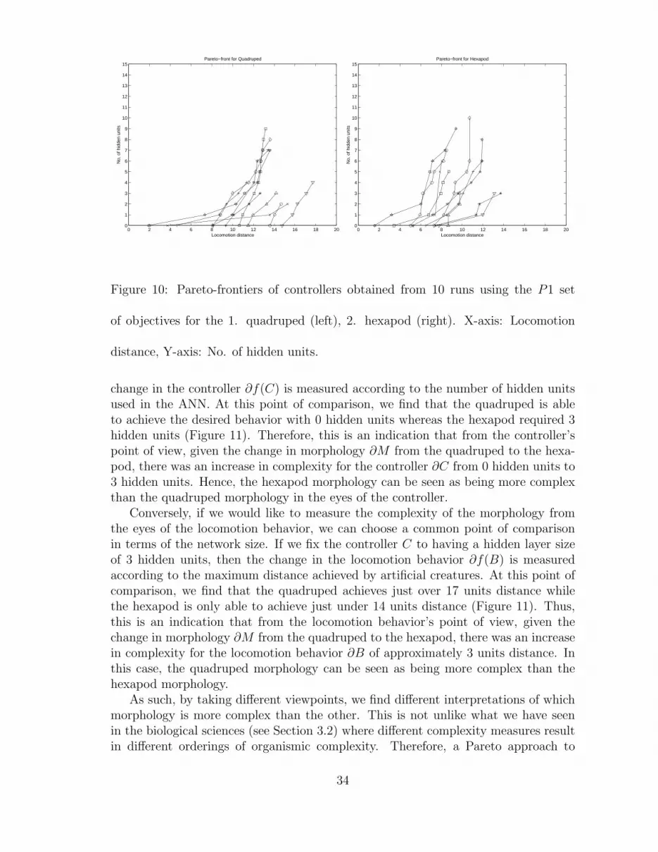
0 2 4 6 8 10 12 14 16 18 200

1

2

3

4

5

6

7

8

9

10

11

12

13

14

15

Locomotion distance

No.

of h

idde

n un

its

Pareto−front for Quadruped

0 2 4 6 8 10 12 14 16 18 200

1

2

3

4

5

6

7

8

9

10

11

12

13

14

15

Locomotion distance

No.

of h

idde

n un

its

Pareto−front for Hexapod

Figure 10: Pareto-frontiers of controllers obtained from 10 runs using the P1 set

of objectives for the 1. quadruped (left), 2. hexapod (right). X-axis: Locomotion

distance, Y-axis: No. of hidden units.

change in the controller ∂f(C) is measured according to the number of hidden unitsused in the ANN. At this point of comparison, we find that the quadruped is ableto achieve the desired behavior with 0 hidden units whereas the hexapod required 3hidden units (Figure 11). Therefore, this is an indication that from the controller’spoint of view, given the change in morphology ∂M from the quadruped to the hexa-pod, there was an increase in complexity for the controller ∂C from 0 hidden units to3 hidden units. Hence, the hexapod morphology can be seen as being more complexthan the quadruped morphology in the eyes of the controller.

Conversely, if we would like to measure the complexity of the morphology fromthe eyes of the locomotion behavior, we can choose a common point of comparisonin terms of the network size. If we fix the controller C to having a hidden layer sizeof 3 hidden units, then the change in the locomotion behavior ∂f(B) is measuredaccording to the maximum distance achieved by artificial creatures. At this point ofcomparison, we find that the quadruped achieves just over 17 units distance whilethe hexapod is only able to achieve just under 14 units distance (Figure 11). Thus,this is an indication that from the locomotion behavior’s point of view, given thechange in morphology ∂M from the quadruped to the hexapod, there was an increasein complexity for the locomotion behavior ∂B of approximately 3 units distance. Inthis case, the quadruped morphology can be seen as being more complex than thehexapod morphology.

As such, by taking different viewpoints, we find different interpretations of whichmorphology is more complex than the other. This is not unlike what we have seenin the biological sciences (see Section 3.2) where different complexity measures resultin different orderings of organismic complexity. Therefore, a Pareto approach to

34

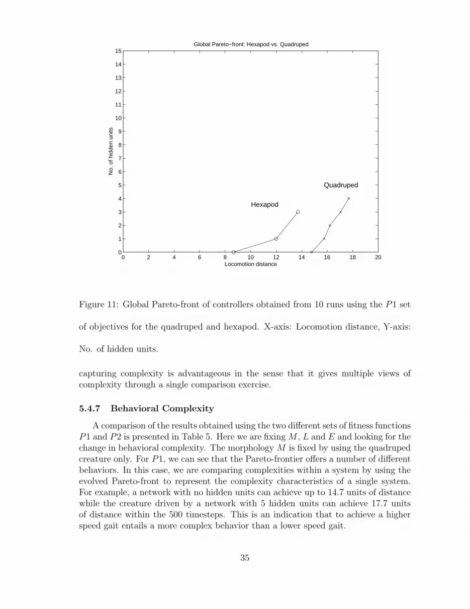
0 2 4 6 8 10 12 14 16 18 200

1

2

3

4

5

6

7

8

9

10

11

12

13

14

15

Locomotion distance

No.

of h

idde

n un

its

Global Pareto−front: Hexapod vs. Quadruped

Hexapod

Quadruped

Figure 11: Global Pareto-front of controllers obtained from 10 runs using the P1 set

of objectives for the quadruped and hexapod. X-axis: Locomotion distance, Y-axis:

No. of hidden units.

capturing complexity is advantageous in the sense that it gives multiple views ofcomplexity through a single comparison exercise.

5.4.7 Behavioral Complexity

A comparison of the results obtained using the two different sets of fitness functionsP1 and P2 is presented in Table 5. Here we are fixing M , L and E and looking for thechange in behavioral complexity. The morphology M is fixed by using the quadrupedcreature only. For P1, we can see that the Pareto-frontier offers a number of differentbehaviors. In this case, we are comparing complexities within a system by using theevolved Pareto-front to represent the complexity characteristics of a single system.For example, a network with no hidden units can achieve up to 14.7 units of distancewhile the creature driven by a network with 5 hidden units can achieve 17.7 unitsof distance within the 500 timesteps. This is an indication that to achieve a higherspeed gait entails a more complex behavior than a lower speed gait.

35

Type of Pareto No. of Locomotion StaticBehavior Controller Hidden Units Distance Stability

P1 1 0 14.7730 192 1 15.7506 243 2 16.2295 304 3 17.0663 265 4 17.6994 14

P2 1 0 5.2065 3042 1 3.3355 4083 2 3.5935 4204 3 3.6829 419

Table 5: Comparison of number of hidden units, locomotion distance and static

stability for global Pareto optimal controllers obtained using the quadruped for the

P1 and P2 sets of objective functions.

We can also see the effect of static stability, which requires a walking behavior,by comparing the two Pareto-fronts that characterize the P1 and P2 systems respec-tively. By comparing a running behavior using a dynamic gait in P1 with no hiddenunits against a walking behavior using a static gait in P2 with no hidden units, wecan see that using the same number of hidden units, the creature achieves both adynamic as well as a quasi-static gait. If more static stability is required, this willnecessitate an increase in controller complexity.

At this point of comparison, we find that the behavior achieved with the P1fitness functions consistently produced a higher locomotion distance than the behaviorachieved with the P2 fitness functions. This meant that it was much harder for theP2 behavior to achieve the same level of locomotion competency in terms of distancemoved as the P1 behavior due to the added sub-objective of having to achieve staticstability during locomotion. Thus, the complexity of achieving the P2 behavior canbe seen as being at a higher level of the complexity hierarchy than the P1 fitnessfunction in the eyes of the controller.

Figure 12 depicts the locomotion distance achieved using the quadruped with theP2 set of objectives, which measure for both locomotion distance and static stability,along with the Pareto-fronts obtained from using the P1 set of objectives. Note thatthe graph for P2 does not depict Pareto-fronts since we are only interested in thelocomotion distance, which is only part of the objective function. Here we see thatthe locomotion distance achieved was much lower due to the added sub-objective ofattempting to maximize static stability. This is expected since the creature will bediscouraged from jumping behaviors, which may allow for greater locomotion capa-bilities. No controllers could be found that achieved a locomotion distance of d > 7.As such, it was not possible to compare the behavioral complexities of standard lo-comotion versus locomotion with stability since the quadruped evolved for standard

36

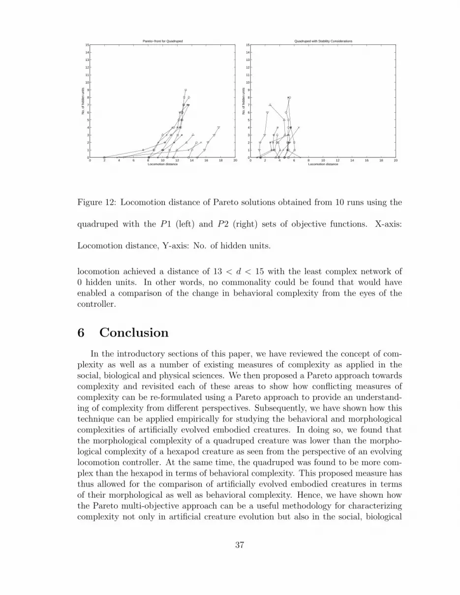
0 2 4 6 8 10 12 14 16 18 200

1

2

3

4

5

6

7

8

9

10

11

12

13

14

15

Locomotion distance

No.

of h

idde

n un

its

Pareto−front for Quadruped

0 2 4 6 8 10 12 14 16 18 200

1

2

3

4

5

6

7

8

9

10

11

12

13

14

15

Locomotion distance

No.

of h

idde

n un

its

Quadruped with Stability Considerations

Figure 12: Locomotion distance of Pareto solutions obtained from 10 runs using the

quadruped with the P1 (left) and P2 (right) sets of objective functions. X-axis:

Locomotion distance, Y-axis: No. of hidden units.

locomotion achieved a distance of 13 < d < 15 with the least complex network of0 hidden units. In other words, no commonality could be found that would haveenabled a comparison of the change in behavioral complexity from the eyes of thecontroller.

6 Conclusion

In the introductory sections of this paper, we have reviewed the concept of com-plexity as well as a number of existing measures of complexity as applied in thesocial, biological and physical sciences. We then proposed a Pareto approach towardscomplexity and revisited each of these areas to show how conflicting measures ofcomplexity can be re-formulated using a Pareto approach to provide an understand-ing of complexity from different perspectives. Subsequently, we have shown how thistechnique can be applied empirically for studying the behavioral and morphologicalcomplexities of artificially evolved embodied creatures. In doing so, we found thatthe morphological complexity of a quadruped creature was lower than the morpho-logical complexity of a hexapod creature as seen from the perspective of an evolvinglocomotion controller. At the same time, the quadruped was found to be more com-plex than the hexapod in terms of behavioral complexity. This proposed measure hasthus allowed for the comparison of artificially evolved embodied creatures in termsof their morphological as well as behavioral complexity. Hence, we have shown howthe Pareto multi-objective approach can be a useful methodology for characterizingcomplexity not only in artificial creature evolution but also in the social, biological

37

and physical sciences in general.

References

[1] Hussein A. Abbass. Speeding up back-propagation using multiobjective evolu-tionary algorithms. Neural Computation (Accepted to appear), 2003.

[2] Christoph Adami. Introduction to Artificial Life. Telos Publishing, Santa Clara,CA, 1998.

[3] Peter S. Albin. The complexity of social groups and social systems described bygraph structures. Mathematical Social Sciences, 1(1):101–129, 1980.

[4] Glenda Andrews and Graeme S. Halford. A cognitive complexity metric appliedto cognitive development. Cognitive Psychology, 45(2):153–219, 2002.

[5] Henri Atlan and Moshe Koppel. The cellular computer DNA: Program or data.Bulletin of Mathematical Biology, 52(3):335–348, 1990.

[6] Sunny Y. Auyang. Foundations of Complex-System Theories: In Economics,Evolutionary Biology and Statistical Physics. Cambridge University Press, Cam-bridge, UK, 1998.

[7] Remo Badii and Antonio Politi. Complexity: Hierarchical Structures and Scalingin Physics. Cambridge University Press, Cambridge, UK, 1997.

[8] Charles H. Bennett. Logical depth and physical complexity. In R. Herken, edi-tor, Universal Turing Machine, A Half-Century Survey, pages 227–257. OxfordUniversity Press, Oxford, 1988.

[9] Josh C. Bongard. Evolving modular genetic regulatory networks. In Proceedingsof the 2002 Congress on Evolutionary Computation (CEC2002), pages 1872–1877. IEEE Press, Piscataway, NJ, 2002.

[10] John T. Bonner. The Evolution of Complexity by Means of Natural Selection.Princeton University Press, Princeton, NJ, 1988.

[11] Carter T. Butts. The complexity of social networks: Theoretical and empiricalfindings. Social Networks, 23(1):31–71, 2001.

[12] Peter Cariani. Emergence and artificial life. In C.G. Langton, C. Taylor, J.D.Farmer, and S. Rasmussen, editors, Artificial Life II: Proceedings of the Sec-ond International Workshop on the Synthesis and Simulation of Living Systems,pages 775–797. Addison-Wesley, Redwood City, CA, 1992.

[13] John L. Casti. On system complexity: Identification, measurement and manage-ment. In J.L. Casti and A. Karlqvist, editors, Complexity, Language and Life:Mathematical Approaches, chapter 6, pages 146–173. Springer-Verlag, Berlin,1986.

38

[14] Thomas Cavalier-Smith. The Evolution of Genome Size. Wiley, New York, 1985.

[15] Michael B. Clement. Analyst forecast accuracy: Do ability, resources, and port-folio complexity matter? Journal of Accounting and Economics, 27(3):285–303,1999.

[16] Clive Cooper. Complexity in C3I systems. In D.G. Green and T. Bossomaier,editors, Complex Systems: From Biology to Computation, pages 223–231. IOSPress, Amsterdam, 1993.

[17] Peter Coveney and Roger Highfield. Frontiers of Complexity: The Search forOrder in a Chaotic World. Fawcett Columbine, New York, 1995.

[18] J.R. DeShazo and German Fermo. Designing choice sets for stated preferencemethods: The effects of complexity on choice consistency. Journal of Environ-mental Economics and Management, 44(1):123–143, 2002.

[19] Bruce Edmonds. From complexity to agent modelling and back again - someimplications for economics [online]. In Workshop on Economics and the Sciencesof Complexity, Brussels, Belgium, 1997. http://cfpm.org/cpmrep24.html [cited -17 October 2002].

[20] Bruce Edmonds. Syntactic Measures of Complexity. Unpublished PhD thesis,University of Manchester, England, 1999.

[21] Claus Emmeche. Garden in the Machine. Princeton University Press, Princeton,NJ, 1994.

[22] EnsEMBL.Org. Ensembl genome browser [online]. http://www.ensembl. org[cited - 6 November 2002], 2002.

[23] David P. Feldman and James P. Crutchfield. Discovering noncritical organiza-tion: Statistical mechanical, information theoretic, and computational views ofpatterns in one-dimensional spin systems. Working Paper 98-04-026, Sante FeInstitute, 1998.

[24] David P. Feldman and James P. Crutchfield. Measures of statistical complexity:Why? Physics Letters A, 238:244–252, 1998.

[25] Michael R. Garey and David S. Johnson. Computers and Intractability : A Guideto the Theory of NP-Completeness. W.H. Freeman, San Francisco, 1979.

[26] Cynthia Gibas and Per Jambeck. Developing Bioinformatics Skills. O’Reilly,Sebastopol, CA, 2001.

[27] Edward Gibson. Linguistic complexity: Locality of syntactic dependencies. Cog-nition, 68(1):1–76, 1998.

39

[28] Graeme S. Halford, William H. Wilson, and Steven Phillips. Processing capacitydefined by relational complexity: Implications for comparative, developmental,and cognitive psychology. Behaviorial and Brain Sciences, 21(6):803–831, 1998.

[29] Simon Haykin. Neural Networks: A Comprehensive Foundation. Prentice-Hall,Upper Saddle River, NJ, 2nd edition, 1999.

[30] Hakan J. Holm. Complexity in Economic Theory: Automata Theoretical Ap-proach. Unpublished PhD thesis, Lund University, Lund, Sweden, 1993.

[31] Gregory S. Hornby and Jordan B. Pollack. Body-brain coevolution using L-systems as a generative encoding. In L. Spector, E. Goodman, A. Wu, W.B.Langdon, H.M Voight, M. Gen, S. Sen, M. Dorigo, S. Pezeshk, M. Garzon, andE. Burke, editors, Proceedings of the Genetic and Evolutionary ComputationConference (GECCO-2001), pages 868–875. Morgan Kaufmann, San Francisco,2001.

[32] George A. Kelly. The Psychology of Personal Constructs. Norton, New York,1955.

[33] Andrei N. Kolmogorov. Three approaches to the quantitative definition of infor-mation. Problems of Information Transmission, 1:1–7, 1965.

[34] Maciej Komosinski and Adam Rotaru-Varga. Comparison of different genotypeencodings for simulated three-dimensional agents. Artificial Life, 7(4):395–418,2001.

[35] Roger Lewin. Complexity: Life at the Edge of Chaos. Phoenix, London, 1993.

[36] Margot L. Lyon. Complexity and emergence: The seduction and reduction ofnon-linear models in the social sciences. In D.G. Green and T. Bossomaier,editors, Complex Systems: From Biology to Computation, pages 173–180. IOSPress, Amsterdam, 1993.

[37] Klaus Mainzer. Thinking in Complexity: The Complex Dynamics of Matter,Mind and Mankind. Springer-Verlag, Berlin, 3rd edition, 1997.

[38] John Maynard Smith and Eors Szathmary. The Major Transitions in Evolution.W.H. Freeman and Company, New York, 1995.

[39] Chrystopher L. Nehaniv. Measuring evolvability as the rate of complexity in-crease. Artificial Life, 6(1):45–67, 2000.

[40] Chrystopher L. Nehaniv. Measuring evolvability as the rate of com-plexity increase [online]. In C.C. Maley and E. Boudreau, editors, Ar-tificial Life 7 Workshop Proceedings, pages 55–57, Portland, US, 2000.http://homepage.feis.herts.ac.uk/ ∼nehaniv/ [cited - 30 August 2002].

40

[41] Abraham Neyman and Daijiro Okada. Strategic entropy and complexity in re-peated games. Games and Economic Behavior, 29(1–2):191–223, 1999.

[42] Stefano Nolfi and Dario Floreano. Evolutionary Robotics: The Biology, Intelli-gence, and Technology of Self-Organizing Machines. MIT Press/Bradford Books,Cambridge, MA, 2000.

[43] Rolf Pfeifer and Christian Scheier. Understanding Intelligence. MIT Press, Cam-bridge, MA, 1999.

[44] Cosma R. Shalizi. Causal Architecture, Complexity and Self-Organization inTime Series and Cellular Automata. Unpublished PhD thesis, University ofWisconsin at Madison, Wisconsin, 2001.

[45] Claude E. Shannon. A mathematical theory of communication. The Bell SystemTechnical Journal, 27(3):379–423, 1948.

[46] Chris U.M. Smith. The complexity of brains: A biologist’s view. In R.J. Stonierand X.H. Yu, editors, Complex Systems: Mechanisms of Adaptation, pages 93–100. IOS Press, Amsterdam, 1994.

[47] Russell K. Standish. On complexity and emergence [online]. Complexity Inter-national 9. http://life.csu.edu.au/ci/vol09/standi09/ [cited - 30 August 2002],2001.

[48] Eors Szathmary, Ference Jordan, and Csaba Pal. Can genes explain biologicalcomplexity? Science, 292:1315–1316, 2001.

[49] Jason Teo and Hussein A. Abbass. Coordination and synchronization of loco-motion in a virtual robot. In L. Wang, J.C. Rajapakse, K. Fukushima, S.Y. Lee,and X. Yao, editors, Proceedings of the 9th International Conference on NeuralInformation Processing (ICONIP’02), volume 4, pages 1931–1935, Singapore,2002. Nanyang Technological University, ISBN 981-04-7525-X.

[50] Jason Teo and Hussein A. Abbass. Multi-objectivity for brain-behavior evolutionof a physically-embodied organism. In R. Standish, M.A. Bedau, and H.A. Ab-bass, editors, Artificial Life VIII: The 8th International Conference on ArtificialLife, pages 312–318. MIT Press, Cambridge, MA, 2002.

[51] Jason Teo and Hussein A. Abbass. Trading-off mind complexity and locomotionin a physically simulated quadruped. In L. Wang, K.C. Tan, T. Furuhashi, J.H.Kim, and X. Yao, editors, Proceedings of the 4th Asia-Pacific Conference on Sim-ulated Evolution And Learning (SEAL’02), volume 2, pages 776–780, Singapore,2002. Nanyang Technological University, ISBN 981-04-7523-3.

[52] Jason Teo and Hussein A. Abbass. Search space difficulty of evolutionary neuro-controlled legged robots. International Journal of Knowledge-Based IntelligentEngineering Systems (Accepted to appear), 2003.

41

[53] Jason Teo, Minh Ha Nguyen, and Hussein A. Abbass. Multi-objectivity as a toolfor constructing hierarchical complexity. In Proceedings of the Genetic and Evolu-tionary Computation Conference (GECCO-2003) (Accepted to appear), LectureNotes in Computer Science (LNCS), Chicago, IL, 2003. Springer-Verlag.

[54] Alan M. Turing. On computable numbers, with an application to the entschei-dungsproblem. Proceedings of the London Mathematical Society (Series 2),42:230–265, 1936.

[55] Vladimir N. Vapnik and A. Ya Chervonenkis. On the uniform convergence ofrelative frequencies of events to their probabilities. Theoretical Probability andIts Applications, 16(2):264–280, 1971.

[56] M. Mitchell Waldrop. Complexity: The Emerging Science at the Edge of Orderand Chaos. Penguin Books, London, 1994.

[57] Tessa Warren and Edward Gibson. The influence of referential processing onsentence complexity. Cognition, 85(1):79–112, 2002.

[58] Stephen Wolfram. A New Kind of Science. Wolfram Media Inc., Champaign,IL, 2002.

[59] David H. Wolpert and William G. MacReady. Self-dissimilarity: An empiricalmeasure of complexity. Working Paper 97-12-087, Sante Fe Institute, 1997.

[60] Andy Wuensche. Classifying cellular automata automatically: Finding gliders,filtering, and relating space-time patterns, attractor basins, and the Z parameter.Complexity, 4(3):47–66, 1999.

42