national expenditures on local amenities
TRANSCRIPT
National Expenditures on Local Amenities
By DAVID S. BIERI, NICOLAI V. KUMINOFF, AND JAREN C. POPE*
A significant fraction of GDP is generated by implicit expenditures on nonmarket ameni-
ties such as climate, public goods, urban infrastructure, and pollution. Households pay for
the localized component of these amenities indirectly, through spatial variation in housing
prices, wages, and property taxes. In this paper, we develop a methodology for estimating
indirect amenity expenditures that is consistent with principles of national accounting and
fundamentals of spatial sorting behaviour. We construct a county-level database of 75
amenities, match it to the location choices made by 5 million households, and develop the
first estimates for implicit amenity expenditures in the United States. We find that expendi-
tures exceeded 8% of personal consumption expenditures in the U.S. during 2000 ($562
billion). Our estimates also reveal significant regional variation in the expenditure share
for nonmarket amenities, with households in the Pacific giving up the largest fraction of
their potential income to consume localized amenities (17%) and households in the West
South Central region giving up the smallest fraction (6%).
First draft: December 2010
Last revision: July 2013
* Kuminoff: Arizona State University, Dept. of Economics, Tempe, AZ 85287 (e-mail: [email protected]).
Bieri: University of Michigan, Dept. of Urban and Regional Planning, Ann Arbor, MI 48109 (e-mail:
[email protected]). Pope: Brigham Young University, Dept. of Economics, Provo, UT 84602 (e-mail:
[email protected]). Several colleagues provided helpful comments and suggestions on this research,
including Ken Baerenklau, Spencer Banzhaf, Richard Carson, Maureen Cropper, Susana Ferreira, Mark
Jacobsen, Kyle Mangum, Ed Prescott, Chris Redfearn, Todd Schollman, V. Kerry Smith, Chris Timmins,
Gustavo Ventura, and Randy Walsh. We also thank participants at seminar and conference presentations at
Camp resources (2009), AEA meetings (2011), AERE meetings (2011), Arizona State University, Brigham
Young University, Georgia State University, Lincoln Institute of Land Policy, Portland State University,
Resources for the Future, UC San Diego, University of Maryland, University of Michigan, and Virginia
Tech.
1
National income and product accounts are the primary source of information on the per-
formance of modern economies. Since their inception, economists have suggested expand-
ing the accounts to provide a richer description of nonmarket goods and services that affect
the quality of life (Kuznets 1934, Nordhaus and Tobin 1972, Eisner 1988). Growing sup-
port for this idea led the National Research Council (1999) to recommend that the U.S.
construct satellite accounts for nonmarket goods and services, culminating in the develop-
ment of a new architecture for integrating nonmarket activity (Jorgenson, Landefeld and
Nordhaus 2006). Despite these conceptual advances, there has been little progress on
systematically measuring economic activity occurring outside of direct market transac-
tions.1
The National Research Council (2005) identifies “environmental services”, “local pub-
lic goods”, and “urban infrastructure” as top priorities for integrating nonmarket activity
into the national accounts. While we rarely observe consumers purchasing non-market
amenities directly, there is no doubt that they affect the economy. Local amenities con-
tribute to GDP indirectly when spatial variation in their supply affects consumer expendi-
tures on complementary private goods, such as housing. Numerous studies have used
housing prices to estimate homebuyers’ willingness to pay for local amenities. However,
these studies are typically limited to analyzing either the variation in a single amenity or
the variation of a few amenities over a small geographic area.2 Inconsistency in study
areas, time periods, and econometric assumptions makes it impossible to add up prior
1 Two notable exceptions are Landefeld, Fraumeni, and Vojtech (2009) who develop a prototype satellite
2 For example, see the literature on air quality valuation (Smith and Huang 1995, Banzhaf and Walsh 2008).
2
estimates for different amenities to get consistent national figures. Furthermore, the lack
of comprehensive databases on amenities has precluded prior studies from attempting to
estimate national amenity expenditures directly.
In this paper we develop a methodology for estimating indirect expenditures on local
nonmarket amenities, using data on housing and labor market outcomes. In doing so, our
work sits at the intersection of three research frontiers: (i) improving our national account-
ing system by developing satellite accounts for nonmarket goods and services; (ii) under-
standing the origins of spatial and temporal fluctuations in land values, wages, and migra-
tion; and (iii) developing a set of stylized facts about the tradeoffs U.S. households make
between their consumption of public and private goods.
Our approach begins from the fundamentals of spatial equilibrium in the presence of
Tiebout sorting and Roy sorting.3 When heterogeneous households sort themselves across
the housing and labor markets based, in part, on their idiosyncratic job skills and prefer-
ences for amenities, the spatial variation in amenities gets capitalized into land values and
wages.4 As a result, people must pay to live in high amenity areas through some combina-
tion of higher housing prices, higher property taxes, and/or lower real wages. We refer to
the real income that households forego in order to consume the amenities conveyed by the
locations they choose as their “implicit amenity expenditures”.
Developing a consistent macroeconomic measure of amenity expenditures requires ad-
3 For surveys of the literature on Tiebout sorting and the role of amenities in spatial equilibrium see
Blomquist (2006), Kahn (2006), Epple, Gordon, and Sieg (2010), and Kuminoff, Smith, and Timmins
(2013). Key papers on spatial Roy sorting include Dahl (2002) and Bayer, Kahn, and Timmins (2011). 4 Local amenities are a key determinant of where people choose to live. For example, the Census Bureau’s
2001 American Housing Survey reports that 25% of recent movers listed the main reason for their move as:
“looks/design of neighborhood”, “good schools”, “convenient to leisure activities”, “convenient to public
transportation”, or “other public services.”
3
dressing three key challenges: data, identification, and normalization. The data challenge
is to measure the quantities of local amenities throughout the United States. The identifi-
cation challenge is to develop a strategy for using spatial variation in property values,
property taxes, wages, and amenities to identify the relative expenditures associated with
moving between any two locations; i.e. the nominal change in consumption of private
goods a household would experience by moving from its present location to a location with
a different amenity bundle. The normalization challenge is to pin down real expenditures.
This requires defining how far households would consider moving and accounting for
moving costs and spatial variation in purchasing power, income taxes, and tax subsidies to
homeowners. We address these challenges by building a comprehensive and detailed
database on amenities, migration flows, moving costs, the tax code, and participation in the
housing and labor markets.
As part of this analysis, we have constructed the first national database on nonmarket
amenities in U.S. counties. For every county in the lower 48 states, we collected data
describing features of its climate and geography, environmental externalities, local public
goods, transportation infrastructure, and access to cultural and urban amenities. Examples
of the 75 specific amenities in our database include rainfall, humidity, temperature, fre-
quency of extreme weather, wilderness areas, state and national parks, air quality, hazard-
ous waste sites, municipal parks, crime rates, teacher-pupil ratios, child mortality, inter-
state highway mileage, airports, train stations, restaurants and bars, golf courses, and
research universities.5 We matched these amenities to the most comprehensive micro data
5 In comparison, the most detailed data in the existing literature were developed by Blomquist, Berger, and
4
on households and their location choices—the 5% public use sample from the 2000 Cen-
sus. Thus, our analysis uses data on the housing prices, wages, and amenities experienced
as a result of location choices made by over 5 million households.
In the first stage of our analysis, we calculate real wages and real housing expenditures
for each household. Specifically, we adjust their gross wages for spatial variation in pur-
chasing power and income tax burdens, and then we calculate their real housing expendi-
tures, controlling for property taxes and tax subsidies to homeowners (Poterba 1992,
Himmelberg, Mayer, and Sinai 2005). Our user-cost approach to calculating expenditures
on owner occupied housing differs from the “rental equivalency” imputations in the Na-
tional Income and Product Accounts. Similar to Prescott (1997), we argue that the user
cost approach provides a more consistent measure of the economic cost of homeownership.
The second stage of our analysis uses a two-step, fixed effects estimator to extract the
spatial variation in real wages and rents due to spatial variation in amenities. Our identifi-
cation strategy relies on brute force. We demonstrate that total amenity expenditures are
identified as long as any omitted amenity can be expressed as a linear function of the
observed amenities.6 This strategy is supported by two points. First, amenities tend to
exhibit a high degree of spatial correlation. Second, the size and diversity of our amenity
database allows us to make a case that any omitted amenity will be highly correlated with
several of the ones we observe. We control for sorting on unobserved job skill (i.e. spatial
Hoehn (1988), who collected information on 15 amenities provided by 253 urban counties. Their amenity
data covers 8% of all U.S. counties, primarily describing climate, geography, and environmental externalities
circa 1980. 6 It would be nice to separately identify virtual prices for each of the 75 amenities as an intermediate step
toward calculating total expenditures. In an ideal world, this could be accomplished by running a field
experiment that randomly assigns amenity levels to counties. This of course is a highly improbable set-up
for even one amenity, not to mention seventy five.
5
Roy sorting) by adapting Dahl’s (2002) semiparametric sample selection correction for the
wage equation. Our results are robust to using an alternative control function based on
Bayer, Kahn, and Timmins (2011).
Finally, we use data on physical moving costs, financial moving costs, and historical
migration flows to define a subset of locations in the contiguous U.S. where households in
each location would be likely to consider moving. These “consideration sets” provide the
final normalization needed to calculate real amenity expenditures. Under a variety of
alternative definitions for the consideration sets, our estimates range from $385 billion to
$632 billion for the year 2000. Our preferred point estimate of $562 billion is equivalent
to 8.2% of personal consumption expenditures on private goods. These figures imply the
average household sacrifices over five thousand dollars per year to consume the nonmarket
amenities at their home location. Expenditures are generally higher in the west, mountains
and northeast, and lower in the mid-west and south. Among major metropolitan areas,
expenditures per household are highest in San Francisco, New York, and Los Angeles and
lowest in Detroit, Baltimore, and Houston. These findings are consistent with evidence of
regional differences in land leverage where the value of housing is largely accounted for by
the value of land in high-amenity metro areas compared to low-amenity metros where
land’s share of house value is relatively small (Davis and Heathcote 2007).
Our research makes several contributions to the literature. Most importantly: (i) we in-
troduce the first national database of nonmarket amenities; (ii) we develop a methodology
for estimating aggregate amenity expenditures that is consistent with spatial sorting based
on heterogeneous preferences and skills, and adjusts for spatial variation in moving costs,
6
tax subsidies to homeownership, income taxes, and property taxes; and (iii) we present the
first national estimate of amenity expenditures, along with regional and county-level esti-
mates. In addition to augmenting the national accounting system, estimates for amenity
expenditures could help to calibrate the new generation of general equilibrium models for
evaluating federal polices for mitigating climate change and regulating environmental
pollutants (e.g. Rogerson 2013, Shimer 2013).
The rest of the paper proceeds as follows. Section I uses a model of sorting in the hous-
ing and labor markets to define “implicit amenity expenditures.” Section II summarizes
the data. Section III explains our methodology, section IV presents the main results, and
section V concludes. Additional modeling details and robustness checks are provided in a
supplemental appendix.
I. Conceptual Framework
A. Dual-Market Sorting Equilibrium
We begin from the standard static framework for modeling spatial sorting behavior, in
which heterogeneous firms and households are assumed to choose spatial locations to
maximize profits and utility (Roback 1982, Blomquist, Berger, and Hoehn 1988, Bayer,
Keohane, and Timmins 2009, Kuminoff 2013).7 To formalize ideas, we first divide the
nation into locations. Locations differ in the wages paid to workers, , in
the annualized after-tax price of land, which we call rent, , and in a vector of K nonmar-
7 It is difficult to develop dynamic models of spatial sorting behavior that retain the heterogeneity in prefer-
ences and skills thought to underlie sorting equilibria. Kennan and Walker (2011), Bayer et al. (2011) and
Mangum (2012) take first steps in this direction.
7
ket amenities, [ ]. We define “amenities” broadly to include all attributes
of a location that matter to households but are not formally traded. Examples include
climate, geography, pollution, public goods, opportunities for dining and entertainment,
and transportation infrastructure. Some of these amenities are exogenous (e.g. climate,
geography). Others may be influenced by Tiebout sorting through voting on property tax
rates, social interactions, and feedback effects (e.g. school quality, pollution).
Heterogeneous households choose locations that maximize utility. They differ in their
job skills, preferences for amenities, and in the set of locations they consider. Let
denote the subset of locations considered by a household of type . If we define locations
to be counties, for example, then the typical household may only consider a small subset of
the 3000+ counties in the U.S.
Households enjoy the quality of life provided by the amenities in their chosen location.
Each household supplies one unit of labor, for which it is paid according to its skills. A
portion of this income is used to rent land, , and the remainder is spent on a nationally
traded private good, .8 Thus, households maximize utility by selecting a location and
using their wages to purchase x and h,
( )
( ) ( )
Households also face differentiated costs of moving to a given location. This is represent-
ed by . Notice that we use to index all forms of household heterogeneity. Each -
type has a unique combination of preferences, skills, and moving costs, and considers a
8 The composite good includes the physical characteristics of housing.
8
specific subset of the locations.
The firm side of the model is analogous. -type firms with heterogeneous production
technologies and management styles choose locations that minimize their cost of produc-
ing the numéraire good, ( ).9
A dual-market sorting equilibrium occurs when rents, wages, amenities, and location
choices are defined such that markets for land, labor, and the numéraire good clear and no
agent would be better off by moving. This implies that utility and costs are equalized
across all of the locations occupied by households of each -type and firms of each -type.
Denoting these subsets of occupied locations as
and rewriting utility in indirect
terms, we have:
(2.a) ( ) .
(2.b) ( ) .
Under the assumption that each location provides a unique bundle of amenities, we can use
hedonic price and wage functions to describe the spatial relationships between rents, wag-
es, and amenities that must be realized in equilibrium:
(3) [ ( ) ( ) ( )] and [ ( ) ( ) ( )],
where F, G, and H denote the distributions of amenities, households, and firms.10
Follow-
9 Amenities may affect the cost of doing business. An example would be a firm with a dirty production
technology facing stricter environmental regulations if it locates in a county that violates federal standards for
air quality. Firms may also face heterogeneous costs of moving physical capital to a given location. 10
If each location has a distinct bundle of amenities, as in our application, it is trivial to prove that the equi-
9
ing standard practice in the empirical sorting literature, we assume that markets are ob-
served in equilibrium and then focus on using the properties of equilibrium to infer the
price of consuming amenities (Epple, Gordon, and Sieg 2010, Kuminoff, Smith, and Tim-
mins 2013)
Spatial variation in rents and wages determines the implicit price of consuming ameni-
ties. Consider air quality. There are two ways to induce a household to move to a smoggi-
er location: higher wages or lower rents. The extent to which movers are compensated
through wages, relative to rents, will depend on the spatial distribution of air quality as
well as the extent to which air quality affects the cost of production and the quality of life.
B. Implicit Expenditures on Amenities
We define a household’s implicit amenity expenditures to be the amount of income it
chooses to sacrifice in order to consume the amenities conveyed by its preferred location.
To define this concept formally let represent the household’s consumption at its
utility-maximizing location, and let represent amenity expenditures for an -type
household. Then we have,
( )
( )
Thus, is the additional income a household would collect if it were to move from its
present location to the least expensive location in its consideration set and rent a house
librium relationship between rents and amenities (or wages and amenities) can be described by a hedonic
price function, as opposed to a correspondence. Roback (1988), Bayer, Keohane, and Timmins (2009), and
Kuminoff (2013) analyze the properties of dual-market sorting equilibria under specific assumptions about
household heterogeneity.
10
identical to the one it occupies currently.11
The least expensive location in defines the
household’s reference point, , used to normalize the expenditure calculation. Different
households may have different reference points due to heterogeneity in job skills, consid-
eration sets, and moving costs.
In addition to providing the logic for our expenditure calculations, equation (4) illus-
trates how our model relates to the literature on measuring “quality-of-life” and to research
on developing satellite accounts for nonmarket goods. The connection to the quality-of-
life literature begins with the observation that is simply the revealed prefer-
ence notion of an income equivalent (Fleurbaey 2009). Income equivalents generally lack
a precise welfare interpretation. In our case, a welfare interpretation for would require
strong assumptions. In particular, (2)-(3) simplify to Roback’s (1982) model of compen-
sating differentials if households and firms are assumed: (i) to consider locating in every
jurisdiction: ; (ii) to be freely mobile: ; and (iii) to be
homogenous.12
Under these restrictions, defines the representative agent’s Hicksian
willingness to pay for the associated amenity bundle. This interpretation underlies the
literature on ranking cities by a universal measure for the quality-of-life (e.g. Blomquist,
Berger, and Hoehn 1988, Gyourko and Tracy 1991, Kahn 2006, Blomquist 2006). Relax-
ing the full information, free mobility, and homogeneity assumptions does not compromise
11
Amenity expenditures must be nonnegative because equals zero for the household’s current location. 12
To obtain the result from Roback (1982) differentiate indirect utility,
, and apply Roy’s identity to obtain (
)
(
)
⁄ . The implicit price of
an amenity, , is defined by the rent differential times land rented, minus the wage differential. The second
equality indicates that the equilibrium value for reveals the representative agent’s willingness to pay for
one unit of the amenity.
11
our ability to calculate amenity expenditures—which is our main objective. However, it
does prevent us from interpreting expenditures as welfare measures or as an index of the
quality of life that would be agreed upon by all households.
The connection to satellite accounting is based on the fact that the national income and
product accounts (NIPA) track wage income and housing expenditures. These measures
will conflate the market values of land and labor with the implicit prices of amenities. This
is an important point and deserves repeating. To the extent that spatially delineated ameni-
ties are capitalized into rents and/or wages, our current national accounting system will
capture implicit expenditures on localized amenities. The challenge is to extract this in-
formation from observable features of the spatial distribution of rents, wages, and ameni-
ties. Disentangling the amenity components of wages and rents would be a significant step
toward establishing satellite accounts for nonmarket goods and services (Kuznets 1934,
1946, Nordhaus and Tobin 1972, Nordhaus 2000, National Research Council 1999, 2005,
Jorgenson, Landefeld, and Nordhaus 2006, Stiglitz, Sen, Fituossi et al. 2009).
II. Data
We have collected data on 75 amenities conveyed by each of the 3,108 counties com-
prising the contiguous United States.13
Using information on house location, we matched
these amenities to public use microdata records from the 2000 Census of Population and
Housing, describing 5.2 million households and their participation in the housing and labor
13
Unfortunately, we were unable to obtain data on several amenities in Alaska and Hawaii. We chose to
omit these states, rather than the amenities. Omitting Alaska and Hawaii is unlikely to have a significant
impact on our approximations to national amenity expenditures because, in 2000, the two states jointly
accounted for less than 0.75% of GDP.
12
markets. Our national database on households and amenities is the first of its kind. The
closest comparison is to Blomquist, Berger, and Hoehn (1988) who assembled data on 15
amenities for 253 urban counties circa 1980, in order to develop “quality-of-life” rankings.
A. Amenities
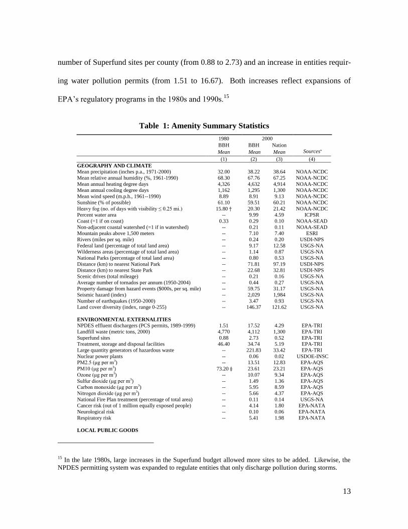
Table 1 reports summary statistics for the amenities we collected. As a baseline for
comparison, we also report means for the subset collected by Blomquist, Berger, and
Hoehn (1998) [henceforth BBH]. Column (1) reports 1980 means for the BBH amenities.
Column (2) reports year 2000 means for our full set of amenities in the 253 urban counties
studied by BBH. Finally, column (3) reports year 2000 means for our full set of amenities
in all 3,108 counties.14
Most of the BBH amenities were fairly constant between 1980 and 2000. In cases
where we do see large changes, they appear to be due to changes in the way a variable is
measured and reported, or refinements on our part. For example, we refine the definition
of a “coastal” county to distinguish between counties that are physically adjacent to the
coast and counties that are part of a coastal watershed, but not physically adjacent. Simi-
larly, in the case of particulate matter (PM), we replaced total suspended particulates with
measures of PM2.5 and PM10 to reflect changes in the way the Environmental Protection
Agency (EPA) monitors air pollution. The two largest changes are an increase in the
14
Variables that were measured at a finer level of spatial resolution than a county were aggregated to the
county level. For some of the geographic and environmental variables, we use irregularly-spaced NOAA and
EPA source data from which we then produce county-level data. In these cases, we spatially interpolated the
amenity data to the population-weighted county centroids via universal kriging. Universal kriging produces
superior results to simpler techniques such as inverse distance weighting because it permits the spatial
variogram to assume functional forms that include directional dependence.
13
number of Superfund sites per county (from 0.88 to 2.73) and an increase in entities requir-
ing water pollution permits (from 1.51 to 16.67). Both increases reflect expansions of
EPA’s regulatory programs in the 1980s and 1990s.15
Table 1: Amenity Summary Statistics
1980 2000
BBH BBH Nation
Mean Mean Mean Sources*
(1) (2) (3) (4)
GEOGRAPHY AND CLIMATE Mean precipitation (inches p.a., 1971-2000) 32.00 38.22 38.64 NOAA-NCDC
Mean relative annual humidity (%, 1961-1990) 68.30 67.76 67.25 NOAA-NCDC
Mean annual heating degree days 4,326 4,632 4,914 NOAA-NCDC Mean annual cooling degree days 1,162 1,295 1,300 NOAA-NCDC
Mean wind speed (m.p.h., 1961--1990) 8.89 8.91 9.13 NOAA-NCDC
Sunshine (% of possible) 61.10 59.51 60.21 NOAA-NCDC
Heavy fog (no. of days with visibility ≤ 0.25 mi.) 15.80 20.30 21.42 NOAA-NCDC
Percent water area -- 9.99 4.59 ICPSR
Coast (=1 if on coast) 0.33 0.29 0.10 NOAA-SEAD
Non-adjacent coastal watershed (=1 if in watershed) -- 0.21 0.11 NOAA-SEAD Mountain peaks above 1,500 meters -- 7.10 7.40 ESRI
Rivers (miles per sq. mile) -- 0.24 0.20 USDI-NPS
Federal land (percentage of total land area) -- 9.17 12.58 USGS-NA Wilderness areas (percentage of total land area) -- 1.14 0.87 USGS-NA
National Parks (percentage of total land area) -- 0.80 0.53 USGS-NA
Distance (km) to nearest National Park -- 71.81 97.19 USDI-NPS Distance (km) to nearest State Park -- 22.68 32.81 USDI-NPS
Scenic drives (total mileage) -- 0.21 0.16 USGS-NA
Average number of tornados per annum (1950-2004) -- 0.44 0.27 USGS-NA Property damage from hazard events ($000s, per sq. mile) -- 59.75 31.17 USGS-NA
Seismic hazard (index) -- 2,029 1,984 USGS-NA
Number of earthquakes (1950-2000) -- 3.47 0.93 USGS-NA Land cover diversity (index, range 0-255) -- 146.37 121.62 USGS-NA
ENVIRONMENTAL EXTERNALITIES NPDES effluent dischargers (PCS permits, 1989-1999) 1.51 17.52 4.29 EPA-TRI
Landfill waste (metric tons, 2000) 4,770 4,112 1,300 EPA-TRI
Superfund sites 0.88 2.73 0.52 EPA-TRI
Treatment, storage and disposal facilities 46.40 34.74 5.19 EPA-TRI
Large quantity generators of hazardous waste -- 221.83 33.42 EPA-TRI
Nuclear power plants -- 0.06 0.02 USDOE-INSC PM2.5 (μg per m3) -- 13.51 12.83 EPA-AQS
PM10 (μg per m3) 73.20 23.61 23.21 EPA-AQS
Ozone (μg per m3) -- 10.07 9.34 EPA-AQS
Sulfur dioxide (μg per m3) -- 1.49 1.36 EPA-AQS Carbon monoxide (μg per m3) -- 5.95 8.59 EPA-AQS
Nitrogen dioxide (μg per m3) -- 5.66 4.37 EPA-AQS
National Fire Plan treatment (percentage of total area) -- 0.11 0.14 USGS-NA Cancer risk (out of 1 million equally exposed people) -- 4.14 1.80 EPA-NATA
Neurological risk -- 0.10 0.06 EPA-NATA
Respiratory risk -- 5.41 1.98 EPA-NATA
LOCAL PUBLIC GOODS
15
In the late 1980s, large increases in the Superfund budget allowed more sites to be added. Likewise, the
NPDES permitting system was expanded to regulate entities that only discharge pollution during storms.
14
Local direct general expenditures ($ per capita) -- 3.44 2.93 COG97
Local exp. for hospitals and health ($ per capita) -- 47.05 564.60 COG97 Local exp. on parks, rec. and nat. resources ($ pc) -- 15.83 126.71 COG97
Museums and historical sites (per 1,000 people) -- 8.53 1.73 CBP
Municipal parks (percentage of total land area) -- 1.54 0.25 ESRI Campgrounds and camps -- 6.42 2.30 CBP
Zoos, botanical gardens and nature parks -- 1.82 0.36 CBP
Crime rate (per 100,000 persons) 647 4,784 2,653 ICPSR Teacher-pupil ratio 0.080 0.092 0.107 COG97
Local expenditure per student ($, 1996-97 fiscal year) -- 37.05 19.51 COG97
Private school to public school enrollment (%) -- 23.54 13.13 2000 Census Child mortality (per 1000 births, 1990--2000) -- 7.31 7.52 CDC-NCHS
INFRASTRUCTURE
Federal expenditure ($ pc, non-wage, non-defence) -- 5,169 4,997 COG97
Number of airports -- 2.13 1.23 USGS-NA
Number of ports -- 0.27 0.05 USGS-NA Interstate highways (total mileage per sq. mile) -- 0.09 0.03 USGS-NA
Urban arterial (total mileage per sq. mile) -- 0.26 0.05 USGS-NA
Number of Amtrak stations -- 1.19 0.25 USGS-NA Number of urban rail stops -- 7.50 0.81 USGS-NA
Railways (total mileage per sq. mile) -- 0.48 0.27 USGS-NA
CULTURAL AND URBAN AMENITIES
Number of restaurants and bars (per 1,000 people) -- 0.92 1.01 CBP
Theatres and musicals (per 1,000 people) -- 0.02 0.01 CBP Artists (per 1,000 people) -- 0.18 0.11 CBP
Movie theatres (per 1,000 people) -- 0.02 0.02 CBP Bowling alleys (per 1,000 people) -- 0.02 0.03 CBP
Amusement, recreation establishments (per 1,000 people) -- 0.42 0.32 CBP
Research I universities (Carnegie classification) -- 0.24 0.03 CCIHE Golf courses and country clubs -- 16.15 3.79 CBP
Military areas (percentage of total land area) -- 1.18 0.83 USGS-NA
Housing stress (=1 if > 30% of households distressed) -- 0.37 0.16 USDA-ERS Persistent poverty (=1 if > 20% of pop. in poverty) -- 0.03 0.12 USDA-ERS
Retirement destination (=1 if growth retirees > 15%) -- 0.07 0.14 USDA-ERS
Distance (km) to the nearest urban center -- 10.98 33.59 PRAO-JIE09 Incr. distance to a metropolitan area of any size -- 0.20 35.80 PRAO-JIE09
Incr. distance to a metro area > 250,000 -- 23.11 54.90 PRAO-JIE09
Incr. distance to a metro area > 500,000 -- 32.09 39.36 PRAO-JIE09 Incr. distance to a metro area > 1.5 million -- 76.45 86.79 PRAO-JIE09
Notes: The amenity data were constructed from the following sources: CCIHE: Carnegie Classification of Institutions of Higher
Education; CBP: 2000 County Business Patterns published by the Census Bureau; CDC-NCHS: Centers for Disease Control and
Prevention, National Center for Health Statistics; COG97: 1997 Census of Governments; EPA-AQS: 2000 data for criteria air pollutants from the Air Quality System produced by the Environmental Protection Agency (EPA); EPA-NATA: 1999 National-Scale Air Toxics
Assessment conducted by the EPA; EPA-TRI: 2000 Toxic Release Inventory published by the EPA; ESRI: Environmental Systems
Research Institute ArcGIS maps; ICPSR: U.S. County characteristics complied by the Inter-university Consortium for Political and Social Research ICPSR2008; NOAA-SEAD: Strategic Environmental Assessments Division of the National Oceanic and Atmospheric
Administration; NOAA-NCDC: National Climatic Data Center of the National Oceanic and Atmospheric Administration; PRAO-JIE09:
Partridege et al. (2009); USDA-ERS: Economic Research Service of the US Department of Agriculture; USDI-NPS: National Park Service of the US Department of the Interior; USDOE-EERE: Energy Efficiency and Renewable Energy, US Department of Energy;
USDOE-INSC: International Nuclear Safety Center at the US Department of Energy; USGS-NA: National Atlas of the US Geological
Survey. The unit in the BBH visibility variable is miles, rather than total days with a minimum visibility of less than 0.25 miles. BBH use data on total suspended particulates (TSP), a precursor measure to PM10.
15
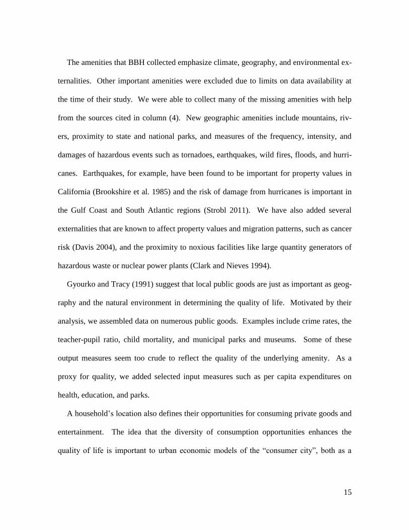
The amenities that BBH collected emphasize climate, geography, and environmental ex-
ternalities. Other important amenities were excluded due to limits on data availability at
the time of their study. We were able to collect many of the missing amenities with help
from the sources cited in column (4). New geographic amenities include mountains, riv-
ers, proximity to state and national parks, and measures of the frequency, intensity, and
damages of hazardous events such as tornadoes, earthquakes, wild fires, floods, and hurri-
canes. Earthquakes, for example, have been found to be important for property values in
California (Brookshire et al. 1985) and the risk of damage from hurricanes is important in
the Gulf Coast and South Atlantic regions (Strobl 2011). We have also added several
externalities that are known to affect property values and migration patterns, such as cancer
risk (Davis 2004), and the proximity to noxious facilities like large quantity generators of
hazardous waste or nuclear power plants (Clark and Nieves 1994).
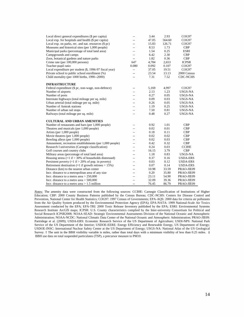
Gyourko and Tracy (1991) suggest that local public goods are just as important as geog-
raphy and the natural environment in determining the quality of life. Motivated by their
analysis, we assembled data on numerous public goods. Examples include crime rates, the
teacher-pupil ratio, child mortality, and municipal parks and museums. Some of these
output measures seem too crude to reflect the quality of the underlying amenity. As a
proxy for quality, we added selected input measures such as per capita expenditures on
health, education, and parks.
A household’s location also defines their opportunities for consuming private goods and
entertainment. The idea that the diversity of consumption opportunities enhances the
quality of life is important to urban economic models of the “consumer city”, both as a
16
driver of growth and in determining the wage structure (Glaeser et al. 2001, Lee 2010).
Therefore, we developed several measures of the concentration of cultural and urban
amenities (major research universities, theatres, restaurants and bars, golf courses, etc.).
As an additional proxy, we measure the distance from each county to the nearest small
(less than 0.25 million), medium (0.25m to 0.5m), large (0.5m to 1.5m), and really large
(greater than 1.5m) metropolitan area. These measures will help to distinguish non-metro
counties that are just outside a major metro area, but close enough to enjoy its shopping
and entertainment, from counties that are located far from metro areas.
Finally, transportation infrastructure may influence the quality of life. The importance
of congestion is well documented. Other influences may be more subtle. For example,
Burchfield et al. (2006) find that metro areas with less public transportation tend to have
more sprawl and Baum-Snow (2007) demonstrates that interstate highways led to a signifi-
cant increase in sprawl. To help control for these effects, we measured the mileage of
interstate highways and urban arterials per square mile. We also collected data on the
concentration of railways, train stations, shipping ports, and airports as proxies for the ease
of travel.
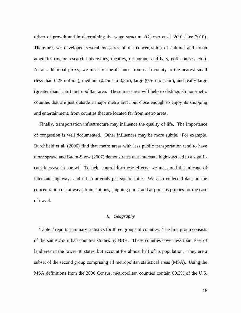
B. Geography
Table 2 reports summary statistics for three groups of counties. The first group consists
of the same 253 urban counties studies by BBH. These counties cover less than 10% of
land area in the lower 48 states, but account for almost half of its population. They are a
subset of the second group comprising all metropolitan statistical areas (MSA). Using the
MSA definitions from the 2000 Census, metropolitan counties contain 80.3% of the U.S.
17
population and 29.7% of its land area. The final group of counties covers the contiguous
U.S. This is our study area.
Table 2: Geographic Coverage and Population Coverage
Geography
BBH counties Metropolitan
counties * All counties
No. of counties 253 1,085 3,108
No. of PUMAs 1,061 1,835 2,057
PUMAs per county 4.19 1.69 0.67
Population 1980 110,617,710 170,867,817 226,545,805
2000 138,618,694 224,482,276 279,583,437
Pop. Coverage 1980 48.8% 75.4% 100.0%
2000 49.6% 80.3% 100.0%
Pop. density (per mi2)
1980 419 197 77
2000 525 259 94
Land area (mi
2) 263,840 865,437 2,959,064
Water area (mi2) 25,273 61,081 160,820
Total area (mi2) 289,113 926,518 3,119,885
Areal coverage 9.3% 29.7% 100.0%
No. obs from PUMS workers 4,833,916 8,875,172 10,198,936
households 2,587,457 4,795,515 5,484,870
Notes: PUMAs must have a minimum census population of 100,000. * Using 1980 or 2000 OMB definitions of metropolitan statistical
areas. Contiguous United States only. Alaska and Hawaii are excluded.
We obtained data on 5.2 million households containing 10.2 million workers from the
5% public-use microdata sample (PUMS) of the 2000 Census. Their residential locations
are identified at the level of a “public use microdata area” or PUMA. Because each PU-
MA must have a population of at least 100,000, PUMA size varies inversely with density.
Most metropolitan counties are subdivided into several PUMAs. In contrast, a single
PUMA can span several rural counties.16
16
The most densely populated county (New York County, NY) has 66,951 people per square mile and is
18
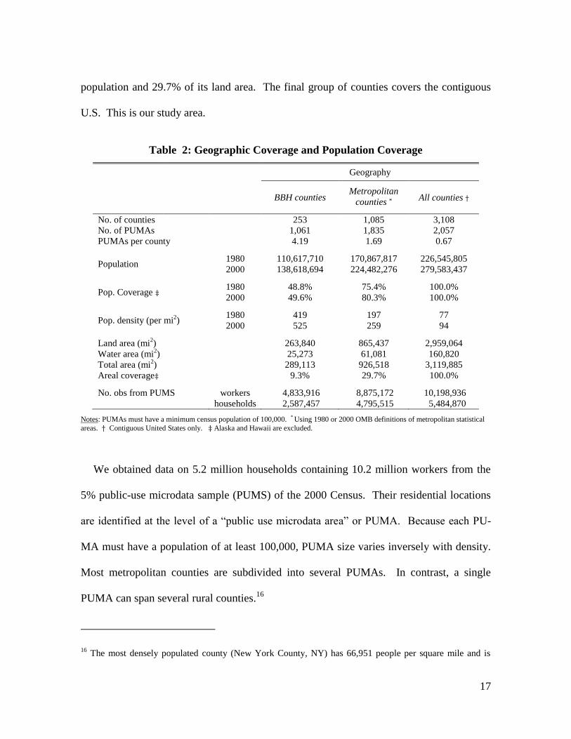
Figure 1: Geography Used to Match Rents, Wages, and Amenities
Note: The figure depicts the 950 locations that we use to calculate amenity expenditures. Every location is a direct aggregation of U.S.
counties. There are 379 individual counties containing multiple PUMAs; 495 individual PUMAs containing multiple counties; and 76 county clusters containing PUMAs that overlap county borders.
We merged PUMS data with the amenities in table 1 at the highest possible spatial reso-
lution. This resulted in aggregating the 3,108 counties into 950 locations shown in figure
1. Of these 950 locations, 379 are metropolitan counties. They cover 60% of the U.S.
population. In rural areas where one PUMA covers multiple counties we aggregate ameni-
ties to the PUMA level using county population weights.17
The resulting 495 PUMAs
contain 25% of the population. We believe this aggregation is a reasonable approximation.
Because the affected counties are rural, residents are more likely to have to cross county
lines within the PUMA to access public goods, urban infrastructure, and cultural amenities.
covered by ten PUMAs. At the opposite extreme, Loving County, TX—which is the least populous and the
least densely populated county in the US—has only 0.09 people per square mile; its corresponding PUMA
covers fourteen counties. 17
Population-weighted amenities can be thought of as the average amenities experienced by residents in a
given PUMA (as opposed to applying area-weights which would yield average amenities associated with
parcels of land inside a PUMA).
19
Finally, PUMAs occasionally overlap county borders without encompassing both counties.
In these cases, we merged the adjacent counties. There are 76 such PUMA-county unions,
representing 15% of the population. Thus, each of the 950 locations is a county or the
union of adjacent counties. Our estimation procedures treat each location as offering a
distinct bundle of amenities.
C. Calculating Real Wages and Real Housing Expenditures
We use the PUMS data as a starting point for deriving real wages and real housing ex-
penditures. Our derivations adjust the raw Census data on nominal wages and self-
reported housing values to control for spatial variation in the tax code and purchasing
power. Specifically, we follow Gyourko and Tracy (1991) in adjusting gross wages for
state and federal income tax rates and for the cost of living (excluding housing).18
To calculate real housing expenditures we adapt the user cost methodology (Poterba
1984, 1992, Himmelberg, Mayer, and Sinai 2005). Our approach differs from the way
housing is treated in NIPA. Unlike their “rental equivalency” imputation for expenditures
on owner-occupied housing, the user cost methodology attempts to measure the real eco-
nomic cost of homeownership.19
Importantly, this includes direct payments for local
public goods via property taxes.
Given that the homeownership rate was 67.5% in 2000, translating homeowners’ self-
assessed housing values into a measure of annualized expenditures is an important step in
our analysis. It requires controlling for the tax benefits of homeownership. In 2003, some
18
Our calculations are documented in the supplemental appendix. 19
The rental equivalency approach attempts to measure the foregone rent that homeowners could collect if
they were to rent their house. For details and discussion see Prescott (1997) and Poole et al. (2005)
20
40 million households claimed an average of $9,500 in mortgage interest deductions and
almost $3,000 in property tax deductions. This renders the homeownership subsidy as one
of the most prominent features of the American tax code. Moreover, the spatial incidence
of benefits is uneven. Gyourko and Sinai (2003) place the average annual benefits for
owner-occupied households at $917 in South Dakota compared to $8,092 in California.
Spatial variation in the homeownership subsidy and property tax rates affects the appro-
priate discount rate by which housing values are converted into rents. This important point
has been overlooked by previous studies. For example, BBH used a constant rate of 7.86%
based on simulations by Peiser and Smith (1985) for an ownership interval from 1987-90
under a scenario of anticipated rising inflation. Subsequent studies adopted the same
constant rate of 7.86% (Gyourko and Tracy, 1991, Gabriel and Rosenthal 2004, Chen and
Rosenthal 2008). If regional variation in the homeownership subsidy and property taxes is
not trivial, then incorrectly assuming a uniform discount rate will tend to overstate (under-
state) expenditures in areas with below (above) average housing costs.
To translate housing values into a spatially explicit measure of rents, we define an indi-
vidual’s annual cost of home ownership in location j as
(5) [ ( ) ],
where is the self-reported property value; is the risk free rate (10-year average of 3-
month T-bill rates); is the mortgage rate (10-year average of 30-year fixed rate mort-
gage); is the property tax rate (including state and local taxes); is the marginal in-
come tax rate; is the depreciation rate; is the expected capital gain; and is the
owner’s risk premium. Thus, imputed rents can be derived as , where
21
represents the user cost of housing.
The third term in brackets, ( ), represents the subsidy to homeowners due to
the deductibility of mortgage interest payments and property taxes.20
We impute from
reported property tax payments and house values. It has a mean of 1.54% in our national
sample.21
For , we use average effective marginal income tax rates for 1999 which we
collect from the NBER TAXSIM model. Finally, using the estimates from Harding,
Rosenthal, and Sirmans (2007), we set , , ,
(long-run inflation of 2% plus real appreciation of 1.8%), and .
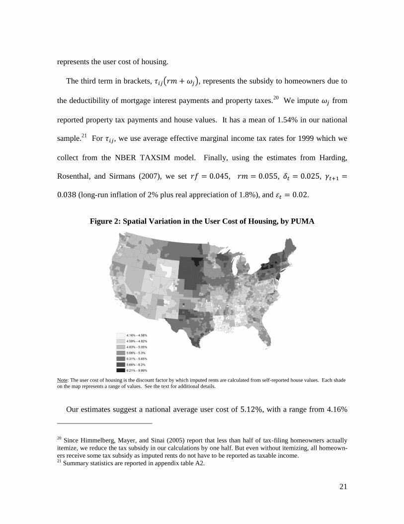
Figure 2: Spatial Variation in the User Cost of Housing, by PUMA
Note: The user cost of housing is the discount factor by which imputed rents are calculated from self-reported house values. Each shade
on the map represents a range of values. See the text for additional details.
Our estimates suggest a national average user cost of , with a range from 4.16%
20
Since Himmelberg, Mayer, and Sinai (2005) report that less than half of tax-filing homeowners actually
itemize, we reduce the tax subsidy in our calculations by one half. But even without itemizing, all homeown-
ers receive some tax subsidy as imputed rents do not have to be reported as taxable income. 21
Summary statistics are reported in appendix table A2.
22
to 9.89%. This implies a range of values for the price-to-rent ratio of 24.0 to 10.1, with an
average of 19.5.22
Figure 2 illustrates the spatial variation in our estimates. The user cost
of housing varies greatly across metro areas, and there are also significant within-metro
differences.
III. Approximating Amenity Expenditures
We use our measures for real wages, real housing expenditures, and amenities in each of
the locations to approximate implicit amenity expenditures. First we esti-
mate relative expenditures for each location. Then we normalize our estimates to approx-
imate real expenditures by adding information on moving costs and the set of alternative
locations considered by each household. The remainder of this section describes our ap-
proach to calculating relative expenditures. Normalizations are explained in section IV.
A. Relative Expenditures
Multiplying the amenities in each location by their implicit prices provides a linear ap-
proximation to relative expenditures. Equation (6) illustrates how we make the calculation
using the results from hedonic rent and wage regressions.
(6) ∑ [
(
)
(
)] .
In the equation, and are parameter vectors describing the shapes of the empirical ana-
logs to the price and wage functions from (3), and {
} are Census PUMS variables
22
In comparison, the 7.86% figure used in BBH and subsequent studies would imply a price-to-rent ratio of
12.7. Focusing our user cost estimates more narrowly on the 253 urban counties studied by BBH has very
little impact on the results. The average user cost increases marginally to 5.16%.
23
describing the physical characteristics of houses and the demographic charac-
teristics of workers who live in location j.23
We estimate and in two stages. First we regress rents and wages on the Census
PUMS variables, adding fixed effects for locations to each regression. Then we regress the
estimated fixed effects on amenities. Our main specification of the first-stage model is
based on a semi-log parameterization,
(7.a) rent function:
(7.b) wage function:
,
where denotes household i’s annual expenditures on housing, denotes worker m’s
annual wages,
are the location fixed effects, and are error terms that include
unobserved attributes of houses and workers.24
After removing the variation in and that can be explained by the
observable attributes of houses and workers, any remaining variation across counties will
be absorbed by the location fixed effects:
. However, the fixed effects will
conflate the implicit prices for amenities with the implicit prices for latent attributes of
23
Control variables in the rent regression include: rooms, bedrooms, size of building, age of building, acre-
age, type of unit, condominium status, and quality of kitchen and plumbing facilities. The model also in-
cludes interactions between all variables and an indicator for renter status. In the wage regression the control
variables include: experience measured as age-schooling-6, experience^2, gender*experience, gen-
der*experience^2, marital status, race, gender*marital status, age, children under 18, educational attainment,
educational enrollment, citizen status, employment disability, NAICS-based industry class, NAICS-based
occupation class, and military status. In both the rent and wage regressions, all variables are also interacted
with indicators for Census divisions. 24
Equation (7.b) recognizes that a worker may or may not work in their home county. The maintained
assumption is that two workers with identical skills, experiences, and demographics who live in the same
county will also earn the same wage. In principle, one could extend our analysis to model spatial heterogene-
ity in the return to attributes using a semiparametric model similar to Black, Kolesnikova and Taylor (2009).
24
houses and workers. We extract the variation in the fixed effects explained by localized
amenities by estimating:
(8)
and
.
The resulting estimates for and are then used to calculate relative expenditures in
each location.
It is important to reiterate that our second stage mitigates confounding by omitted at-
tributes of workers and houses. To assess the practical implications of this point we com-
pared our ranking of locations by expenditures to an alternate one where expenditures are
calculated from the first-stage fixed effects (subsuming omitted attributes of workers and
houses). The Spearman correlation was 0.83—far enough from 1 for our approach to
provide a large improvement in accuracy.
A remaining concern with our model is that latent attributes of workers and houses
(
) could be spatially correlated with amenities, biasing our estimates for and .
This is less of a concern in the housing regression because Census micro data provide a
fairly complete accounting of physical housing attributes. Indeed, the hedonic property
value literature assumes that correlation between amenities and latent physical housing
attributes is small enough to ignore. In contrast, there is widespread concern that Roy
sorting biases wage regressions (e.g. Hwang, Reed, and Hubbard 1992; Dahl 2002; Bayer,
Kahn, and Timmins 2011). This could pose a serious problem. In particular, if higher
skilled workers tend to live in higher amenity areas, then may conflate the negative
effects of amenities on wages with the positive effects of latent human capital, biasing
expenditures toward zero.
25
We address sorting on unobserved job skill by following Dahl’s (2002) approach to
using migration data to develop control functions for the first stage wage regression (7.b).
Dahl’s key insight is that a semiparametric sample selection correction for a spatial wage
equation can be developed from migration probabilities. Therefore we extend the set of
control variables, , to include second order polynomial functions of worker-specific
migration probabilities. As in Dahl (2002), we calculate probabilites by assigning workers
to thirty bins, based on their demographics: five levels of education {less than high school,
high school, some college, college graduate, advanced degree} by marriage {0,1} by the
age range of their children {all under 6 years, at least one between 6 and 18, none under
18}. Then we use information on each migrant’s birth state and current location to
determine the probability of that migration choice. For workers who stay in their birth
state, we use both the retention probability and the probability for their first-best
alternative location. This control function approach allows spatial sorting by unobserved
skill to vary systematically across workers.
B. Identification
It would be nice to separately identify the virtual prices of every amenity as an interme-
diate step toward calculating total amenity expenditures. However, it is not realistic to do
so.25
Nor is it necessary. A credible approximation to total expenditures can be recovered
as long as our amenity data are sufficiently comprehensive that any important amenity we
25
There is a vast literature on estimating virtual prices for amenities. Recent studies have made progress in
developing research designs that mitigate omitted variable bias and other sources of confounding (for a
review, see Kuminoff, Smith, and Timmins 2013). However, no study has developed a research design for
the contiguous United States. This makes it highly improbable that one could develop a national research
design for 75 separate amenities at the same time.
26
have omitted is highly correlated with a linear function of the amenities we have collected.
To formalize this reasoning, consider one additional amenity, . The ideal
approximation to expenditures is
(9) ( ) ( ) ,
where and are consistent estimates for the rent and wage differentials arising from
spatial variation in .26
If is omitted from the econometric model, then the second-stage
equation for rents takes the following form:
(10)
,
where
and [ | ] .
The probability limit of our estimator for is now
(11) , where and [ | ] .
Since is defined analagously, our estimator for total expenditures can be written as
(12) ( ) ( )( )
after some substitution.
Equations (11)-(12) formalize the intuition for our brute force approach to identifica-
tion. There are two key points. First, notice that (11) provides a consistent estimator for
the implicit prices of each observed amenity as . Yet, the estimator for total
expenditures in (12) is inconsistent. If , then , and ( ).
26
Since the dependent variables in the first stage of our model are measured in natural logs we must use the
Halvorsen-Palmquist adjustment to correct the dependent variables prior to second stage estimation and
convert the “percentage” coefficients into dollar values. This procedure is reflected in the hats on model
coefficients.
27
In other words, if we want to identify the implicit prices of individual amenities and
calculate total expenditures, then we must rule out the possiblity of omitting any amenities.
This is highly implausible, which brings us to our second key point. If most of the spatial
variation in omitted amenities can be explained by variation in observed amenities, then we
can obtain a credible approximation to expenditures even if and
are inconsistent
estimators for and . Specifically, as the from regressing z on A approaches 1,
and . This illustrates why collecting data on a comprehensive set of
amenities is essential to developing a credible approximation to national amenity
expenditures.
IV. Results
A. United States Amenity Expenditures
Our estimates for U.S. amenity expenditures are based on the 950 locations in figure 1.
Using all of the data from these locations, we estimate the model in (6)-(8) and calculate
relative expenditures. To convert relative expenditures into real expenditures we must first
take a stance on moving costs and define the subset of locations where each household
would consider relocating.27
Table 3 reports the sensitivity of our results to a variety of
approaches.
First, if we naively assume that people are freely mobile and fully informed about the
spatial distribution of rents, wages, and amenities, then households face an unconstrained
27
A significant literature on migration highlights the role of amenities in the interregional re-distribution of
population (Greenwood et al. 1991). See Molloy et al. (2011) for an overview of the literature and recent
trends in the U.S.
28
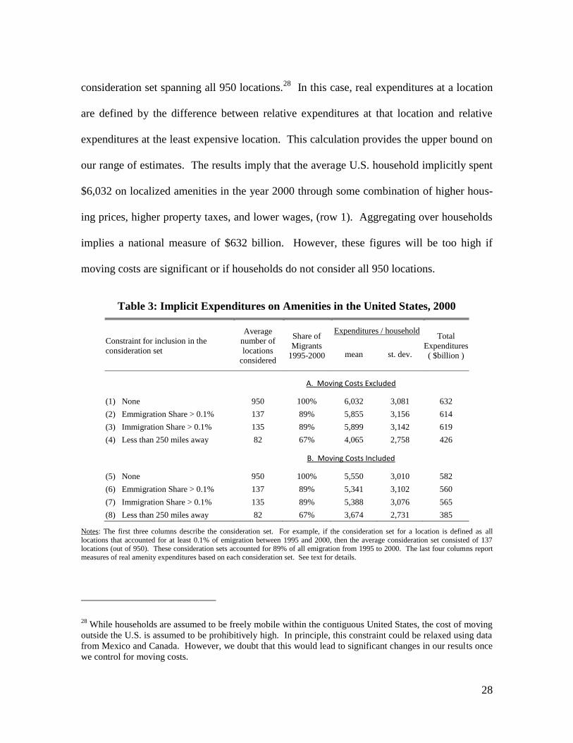
consideration set spanning all 950 locations.28
In this case, real expenditures at a location
are defined by the difference between relative expenditures at that location and relative
expenditures at the least expensive location. This calculation provides the upper bound on
our range of estimates. The results imply that the average U.S. household implicitly spent
$6,032 on localized amenities in the year 2000 through some combination of higher hous-
ing prices, higher property taxes, and lower wages, (row 1). Aggregating over households
implies a national measure of $632 billion. However, these figures will be too high if
moving costs are significant or if households do not consider all 950 locations.
Table 3: Implicit Expenditures on Amenities in the United States, 2000
Constraint for inclusion in the
consideration set
Average
number of
locations
considered
Share of
Migrants
1995-2000
Expenditures / household Total
Expenditures
( $billion ) mean st. dev.
A. Moving Costs Excluded
(1) None 950 100% 6,032 3,081 632
(2) Emmigration Share > 0.1% 137 89% 5,855 3,156 614
(3) Immigration Share > 0.1% 135 89% 5,899 3,142 619
(4) Less than 250 miles away 82 67% 4,065 2,758 426
B. Moving Costs Included
(5) None 950 100% 5,550 3,010 582
(6) Emmigration Share > 0.1% 137 89% 5,341 3,102 560
(7) Immigration Share > 0.1% 135 89% 5,388 3,076 565
(8) Less than 250 miles away 82 67% 3,674 2,731 385
Notes: The first three columns describe the consideration set. For example, if the consideration set for a location is defined as all
locations that accounted for at least 0.1% of emigration between 1995 and 2000, then the average consideration set consisted of 137 locations (out of 950). These consideration sets accounted for 89% of all emigration from 1995 to 2000. The last four columns report
measures of real amenity expenditures based on each consideration set. See text for details.
28
While households are assumed to be freely mobile within the contiguous United States, the cost of moving
outside the U.S. is assumed to be prohibitively high. In principle, this constraint could be relaxed using data
from Mexico and Canada. However, we doubt that this would lead to significant changes in our results once
we control for moving costs.
29
To address the concern that households are unlikely to consider every location in the
United States, we first restrict their consideration sets to include only those locations that
accounted for greater than 0.1% of emigration (row 2) or immigration (row 3) from their
present location between 1995 and 2000.29
For example, the households living in Marin
County, CA are assumed to be familiar with only the locations that accounted for at least
0.1% of migration to (or from) Marin. Imposing this constraint limits the typical consider-
ation set to nearby locations (both urban and rural) and urban counties in the biggest metro
areas, such as New York, Chicago, Phoenix, and Los Angeles.30
This pattern seems con-
sistent with evidence on migrant information networks (Pissarides and Wadsworth 1989).
The 0.1% threshold reduces the number of locations the average household is assumed
to consider from 950 to 137 (emigration) or 135 (immigration). These locations account
for 89% of all migration. It is somewhat surprising that reducing the size of the considera-
tion set by 85% only reduces our expenditure measure by 2% to 3% (comparing row 1
with rows 2 and 3).31
The reason for this can be seen from figure 3. Expensive locations
are predominantly located along the coasts and in resort areas in the Rocky Mountains.
Inexpensive locations are predominantly located in the mid-west, south, and Appalachian
regions. However, expensive and inexpensive locations are not completely stratified.
There are inexpensive areas in California’s central valley and expensive areas in the mid-
west, for example. When expensive and inexpensive areas are close together, the migra-
29
Migration flows were calculated for all pairwise combinations of locations using the Census Bureau’s
county-to-county migration flow files. Our results are robust to using much larger thresholds on migration
shares. This is discussed in section D. 30
An exception is that immigration-based consideration sets for rural locations are less likely to include
distant metropolitan counties. 31
Recall that real expenditures are defined by the difference between relative expenditures at a given location
and relative expenditures at the least expensive alternative in the corresponding constrained consideration set.
30
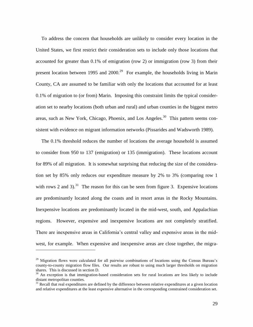
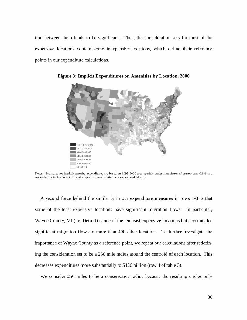
tion between them tends to be significant. Thus, the consideration sets for most of the
expensive locations contain some inexpensive locations, which define their reference
points in our expenditure calculations.
Figure 3: Implicit Expenditures on Amenities by Location, 2000
Notes: Estimates for implicit amenity expenditures are based on 1995-2000 area-specific emigration shares of greater than 0.1% as a
constraint for inclusion in the location specific consideration set (see text and table 3).
A second force behind the similarity in our expenditure measures in rows 1-3 is that
some of the least expensive locations have significant migration flows. In particular,
Wayne County, MI (i.e. Detroit) is one of the ten least expensive locations but accounts for
significant migration flows to more than 400 other locations. To further investigate the
importance of Wayne County as a reference point, we repeat our calculations after redefin-
ing the consideration set to be a 250 mile radius around the centroid of each location. This
decreases expenditures more substantially to $426 billion (row 4 of table 3).
We consider 250 miles to be a conservative radius because the resulting circles only
31
contain 67% of migration flows. Furthermore, 250 miles is roughly a 5-hour drive, close
enough to take day trips to one’s prior location. Physical proximity should mitigate the
psychological cost of moving away from family and friends.32
To formally address mov-
ing costs, we revise our calculations to account for the average physical and financial cost
of moving between each pair of locations.33
To calculate financial costs, we collected data
on location-specific realtor fees, location-specific closing costs on housing sales, and
search costs for home finding trips. To calculate the physical cost of a move, we used the
calculator provided by movesource.com, along with information on the distance travelled,
the weight of household goods transported based on the number of rooms in the origin
location, and the cost of transporting cars (full calculations are documented in section A3
of the supplemental appendix.)
Our estimate for the physical cost of moving differs for every pair of locations.34
The
average is $12,123 and the standard deviation is $2,729. We convert these one-time costs
into annualized measures using a 37-year interval (reflecting the expected life years re-
maining for the average household head) and a real interest rate of 2.5%.35
This implies
the annual cost of a $10,000 move is $419.
32
This is among the reasons why empirical studies of Tiebout sorting and labour migration often treat work-
ing households as being fully informed and freely mobile within a single state or within a metropolitan region
(Bayer, Keohane, and Timmins 2009, Kennan and Walker 2011). 33
While we do not formally model migration, our empirical measures of distance- and migration-based
moving cost are consistent with a migration model that endogenizes moving cost (Carrington et al, 1996) or
worker flows (Coen-Pirani 2010). 34
The average cost of moving between a pair of counties is not symmetric. Direction matters because the
physical cost of a move depends on the weight of goods transported which, in turn, depends on the number of
rooms in the origin location. 35
There are two reasons why actual moving costs may be lower for job-related moves. First, some employ-
ers pay for part or all of the cost. Second, some costs for job-related moves can be deducted from federal
income taxes. By ignoring these forms of compensation, we will tend to overstate moving cost, and under-
state amenity expenditures slightly.
32
When we account for the cost of moving, our estimates range from $385 to $582 billion
(rows 5-8 of table 3). We consider $385 billion to be a conservative lower bound. The
fact that one third of migrants moved further than 250 miles suggests that the expenditure
reference points of the circular consideration sets will tend to be biased upward, causing
us to understate expenditures. At the opposite extreme, if we assume that every household
perceives Detroit to be its reference point, then $582 billion is a better measure. While
this assumption is not implausible given the media coverage of Detroit’s decline, it will
lead us to overstate expenditures for households who are unfamiliar with the area. With
this in mind we interpret $582 billion as a conservative upper bound.
Our preferred estimates are the ones derived from the migration-based consideration
sets with moving costs. They imply a range of $560 to $565 billion. Taking the midpoint,
$562, would suggest that implicit amenity expenditures were equivalent to 8.2% of per-
sonal consumption expenditures in 2000.
Finally, as a robustness check on the Dahl (2002) correction for Roy sorting, we repeat
the estimation using an alternative procedure based on Bayer, Kahn, and Timmins (2011).
Specifically, we multiply our raw wage data by the proportional correction factors they
report by Census region and education level. This approach aims to remove the effect of
latent human capital on wages prior to estimation. It increases our preferred expenditure
measure from $562 to $591 billion. Thus, two different approaches to correcting for Roy
sorting produce very similar results. This is not because the correction factors are small. If
we do nothing to address the bias from Roy sorting, expenditures drop to $422 billion.
The large positive increase that occurs when we implement either correction is consistent
33
with the intuition that higher-skilled workers are more likely to live in higher-amenity
areas, biasing our expenditures measures toward zero.
B. Regional Amenity Expenditures
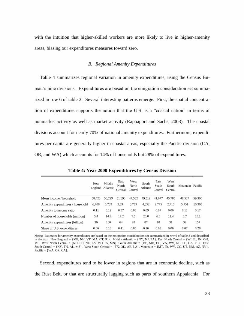
Table 4 summarizes regional variation in amenity expenditures, using the Census Bu-
reau’s nine divisions. Expenditures are based on the emigration consideration set summa-
rized in row 6 of table 3. Several interesting patterns emerge. First, the spatial concentra-
tion of expenditures supports the notion that the U.S. is a “coastal nation” in terms of
nonmarket activity as well as market activity (Rappaport and Sachs, 2003). The coastal
divisions account for nearly 70% of national amenity expenditures. Furthermore, expendi-
tures per capita are generally higher in coastal areas, especially the Pacific division (CA,
OR, and WA) which accounts for 14% of households but 28% of expenditures.
Table 4: Year 2000 Expenditures by Census Division
New
England
Middle
Atlantic
East
North
Central
West
North
Central
South
Atlantic
East
South
Central
West
South
Central
Mountain Pacific
Mean income / household 58,428 56,229 51,690 47,532 49,512 41,677 45,785 48,527 59,300
Amenity expenditures / household 6,708 6,733 3,694 3,789 4,352 2,775 2,710 5,751 10,368
Amenity to income ratio 0.11 0.12 0.07 0.08 0.09 0.07 0.06 0.12 0.17
Number of households (million) 5.4 14.9 17.2 7.5 20.0 6.6 11.4 6.7 15.1
Amenity expenditures (billion) 36 100 64 28 87 18 31 39 157
Share of U.S. expenditures 0.06 0.18 0.11 0.05 0.16 0.03 0.06 0.07 0.28
Notes: Estimates for amenity expenditures are based on the emigration consideration set summarized in row 6 of table 3 and described in the text. New England = {ME, NH, VT, MA, CT, RI}. Middle Atlantic = {NY, NJ, PA}. East North Central = {WI, IL, IN, OH,
MI}. West North Central = {ND, SD, NE, KS, MO, IA, MN}. South Atlantic = {DE, MD, DC, VA, WV, NC, SC, GA, FL}. East
South Central = {KY, TN, AL, MS}. West South Central = {TX, OK, AR, LA}. Mountain = {MT, ID, WY, CO, UT, NM, AZ, NV}. Pacific = {WA, OR, CA}.
Second, expenditures tend to be lower in regions that are in economic decline, such as
the Rust Belt, or that are structurally lagging such as parts of southern Appalachia. For
34
example, expenditures per household in the East North Central division, which roughly
coincides with the Great Lakes region, are less than half the size of expenditures in the
Pacific division.36
Finally, if we look within the Census divisions the ranking of locations by expenditures
makes intuitive sense. The least expensive locations include Baltimore, Detroit, Houston,
and county aggregates comprised of small cities and towns in the south and mid-west. The
most expensive locations include San Francisco, New York, Los Angeles, and county
aggregates containing small cities and towns that are known for their amenities, such as
Aspen, Bozeman, Martha’s Vineyard, and Santa Fe. More broadly, a weighted least
squares regression of expenditures on income implies an elasticity of 0.95.37
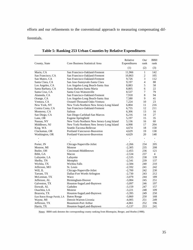
C. A Comparison to “Quality of Life” Rankings of Counties
To further examine the micro foundations for our national estimates in tables 3 and 4,
we use our results to revisit Blomquist, Berger, and Hoehn’s (1988) classic “quality of
life” ranking of 253 urban counties by relative amenity expenditures.38
Table 5 reports our
top 20 and bottom 20 counties within this subset, along with the original BBH rankings.39
This comparison provides an intuitive way to evaluate the impact of our data collection
36
Similarly, households in the Pacific, who also have the highest regional incomes, give up the largest
fraction of their potential incomes to consume localized amenities (17%). Households in the West South
Central region give up the smallest fraction (6%). 37
The unit of observation is a location (N=950) and the weights are the number of households. The p-value
on the coefficient for average household income is zero out to four decimal places and R2=0.80. If we
replace average household income in the regression with median household income or income per capita the
elasticities equal 0.95 and 0.94.
38 As explained earlier, our objective is to measure amenity expenditures, not the quality of life. We put
“quality of life” in quotes to reiterate that one must be willing to make strong assumptions about consumer
heterogeneity to interpret any ranking of counties by amenity expenditures as a measure of the quality of life
that all households would agree with. 39
Complete econometric results and rankings for all counties can be produced from our data and code.
35
efforts and our refinements to the conventional approach to measuring compensating dif-
ferentials.
Table 5: Ranking 253 Urban Counties by Relative Expenditures
County, State Core Business Statistical Area
Relative
Expenditures
Our
rank
BBH
rank
(1) (2) (3)
Marin, CA San Francisco-Oakland-Fremont 11,966 1 142
San Francisco, CA San Francisco-Oakland-Fremont 10,863 2 105
San Mateo, CA San Francisco-Oakland-Fremont 9,726 3 112
Santa Clara, CA San Jose-Sunnyvale-Santa Clara 9,197 4 88
Los Angeles, CA Los Angeles-Long Beach-Santa Ana 8,883 5 58
Santa Barbara, CA Santa Barbara-Santa Maria 8,805 6 22
Santa Cruz, CA Santa Cruz-Watsonville 8,537 7 79
Alameda, CA San Francisco-Oakland-Fremont 7,918 8 94
Orange, CA Los Angeles-Long Beach-Santa Ana 7,580 9 41
Ventura, CA Oxnard-Thousand Oaks-Ventura 7,224 10 23
New York, NY New York-Northern New Jersey-Long Island 6,804 11 216
Contra Costa, CA San Francisco-Oakland-Fremont 6,755 12 211
Monterey, CA Salinas 6,306 13 16
San Diego, CA San Diego-Carlsbad-San Marcos 6,216 14 27
Lane, OR Eugene-Springfield 5,197 15 35
Nassau, NY New York-Northern New Jersey-Long Island 5,136 16 60
Middlesex, NJ New York-Northern New Jersey-Long Island 4,998 17 204
King. WA Seattle-Tacoma-Bellevue 4,674 18 158
Clackamas, OR Portland-Vancouver-Beaverton 4,629 19 138
Washington, OR Portland-Vancouver-Beaverton 4,629 20 148
. . . . .
. . . . .
Porter, IN Chicago-Naperville-Joliet -2,266 234 205
Monroe, MI Monroe -2,305 235 208
Butler, OH Cincinnati-Middletown -2,455 236 121
Bibb, GA Macon -2,534 237 4
Lafayette, LA Lafayette -2,535 238 139
Shelby, TN Memphis -2,541 239 137
Wichita, TX Wichita Falls -2,584 240 210
Jefferson, MO St. Louis -2,592 241 242
Will, IL Chicago-Naperville-Joliet -2,700 242 230
Tarrant, TX Dallas-Fort Worth-Arlington -2,730 243 212
McLennan, TX Waco -3,079 244 189
Jefferson, AL Birmingham-Hoover -3,084 245 251
Galveston, TX Houston-SugarLand-Baytown -3,097 246 197
Etowah, AL Gadsden -3,159 247 157
Ouachita, LA Monroe -3,221 248 109
Brazoria, TX Houston-SugarLand-Baytown -3,395 249 250
East Baton Rouge Parish, LA Baton Rouge -3,860 250 168
Wayne, MI Detroit-Warren-Livonia -4,005 251 249
Jefferson, TX Beaumont-Port Arthur -4,861 252 196
Harris, TX Houston-SugarLand-Baytown -5,137 253 241
Notes: BBH rank denotes the corresponding county ranking from Blomquist, Berger, and Hoehn (1988).
36
The top ranked county in our model is Marin County, CA and the bottom ranked county
is Harris County, TX. A freely mobile household who chooses to live in Marin instead of
Harris would pay an extra $17,103 per year (11,966 + 5,137). To put this statistic in per-
spective, it is equivalent to 20% of the average household’s income. The underlying
thought experiment is the following: if the average Marin County household were to move
to Harris, be paid according to its education and experience, and rent a house that is identi-
cal to the one it currently occupies, then the Marin County household would gain an extra
$17,103 of real income each year. What do Marinites “buy” when they sacrifice this in-
come? Located directly north of San Francisco, Marin is a coastal county with a mild
climate, clean air, some of the best public schools in California, a large share of land in
parks, and the lowest rate of child mortality. Its residents also have easy access to the
cultural and urban amenities of San Francisco.
More generally, the top counties tend to be located on the West Coast and/or in large
metro areas. Furthermore, 13 of the top 20 are in the San Francisco Bay area, the Los
Angeles metro area, and the New York metro area. A quick comparison between columns
(2) and (3) is sufficient to see that our measures of relative expenditures are positively
correlated with those of BBH ( ). Therefore, the implied measures of real expend-
itures will also be similar. For example, if we treat the 253 counties studied by BBH as the
consideration set and ignore moving costs, then our average measure of expenditures per
household in the 253 urban counties is $6,670. If we use the CPI to convert BBH’s 1980
results to year 2000 dollars, then their implied expenditure measure is $4,269.
However, there are three generic differences between our results and BBH. First, our
37
rankings display higher spatial correlation, as can be seen from the clusters of adjacent San
Francisco and New York counties in column (2). This is because our analysis quintuples
the number of amenities and most amenities are spatially correlated. Second, most coun-
ties move dramatically in the rankings. Thirteen of our top 20 counties advance more than
50 places relative to BBH and nine advance more than 100 places. The largest increase is
Rockland County, New York (#236 in BBH; #28 in our study). Rockland is approximately
10 miles north of Manhattan and is among the top 10 counties in the nation, ranked by
median household income. Bibb County, Georgia has the largest decrease (#4 in BBH;
#237 in our study). Its low ranking is not surprising. Bibb has the second highest rate of
child mortality and 19% of its population falls below the poverty line. Finally, our
measures for relative expenditures are also positively correlated with year 2000 income per
capita ( ), consistent with empirical evidence on Tiebout sorting.40
Overall, ap-
plying our new data and methods to the same 253 counties studied by BBH produces
patterns that seem intuitively plausible.
D. Caveats and Future Research
There are several caveats to our results that provide opportunities for future research.
First, the specific thresholds that we used to define consideration sets in our national analy-
sis are admittedly arbitrary. One could make a case for larger or smaller thresholds for
migration shares or distance cutoffs. Likewise, one could make a case for different ap-
40
In comparison, the expenditure measures that BBH produced for 1980 are essentially uncorrelated with
year 2000 income per capita ( ). We suspect this reflects the limited amenity data that were
available at the time of the BBH study and changes in the spatial distribution of income and amenities
between 1980 and 2000. See Kuminoff, Smith, and Timmins (2013) for a review of the evidence on income
stratification from the literature on Tiebout sorting.
38
proaches to annualizing the one-time cost of a move. We have experimented with con-
servative alternatives in each dimension and found that the order of magnitude of our main
result is robust.41
For example, increasing the threshold immigration share from 0.1% to
1.0% would reduce expenditures from $560 billion to $253 billion. However, moving to a
1.0% threshold would also reduce the share of migrants covered from 89% to 57% and it
would reduce the average number of locations in the consideration set from 135 to 14. In
our opinion, this represents an excessively narrow definition for the consideration set that
fails to adequately capture empirical migration patterns.
Second, our expenditure measures are unlikely to capture the full impact of nonmarket
amenities on the U.S. economy. We have limited our analysis to the effects of amenities
on housing prices, wages, and property taxes. While we expect this to reflect the majority
of implicit expenditures, the resulting measures are surely incomplete. For example, ac-
cess to trails may increase the local demand for running shoes and mountain bikes; like-
wise, air pollution may reduce agricultural yields and expenditures on recreation. By
omitting these effects, our current expenditure measures will tend to provide lower bounds.
Third, as we noted earlier, amenity expenditures do not generally provide an exact
measure of willingness to pay. Developing measures of social welfare that adjust for
health, longevity, leisure, and environmental quality is an important and challenging area
for research (e.g. see Becker, Philipson, and Soares 2005, Fleurbaey 2009, Stiglitz et al.
2009, Jones and Klenow 2011). We conjecture that it should be possible to define plausi-
ble conditions for interpreting our estimates as lower bounds on Hicksian compensating
41
The data and code in our supplemental appendix can be modified to consider any alternative consideration
set.
39
differentials for amenity bundles.
Finally, it is important to reiterate that our expenditure measures only cover one of sev-
eral important areas for satellite accounting. We have not attempted to measure the value
of natural resource stocks (e.g. forests, fish) or ecosystem services (e.g. watershed purifica-
tion and wetland buffers against hurricanes). Nor have we attempted to impute the value
of home production and leisure. Thus, our account of implicit amenity expenditures only
represents one dimension of the complete set of satellite accounts recommended by the
National Research Council (1999, 2005) and envisioned by Jorgenson, Landefeld and
Nordhaus (2006).
V. Conclusion
We set out to develop a methodology for estimating national amenity expenditures. Our
estimate for the United States in the year 2000 ($562 billion) suggests that households
reduced their potential expenditures on private goods by more than 8% in order to con-
sume nonmarket amenities at their home locations. Strikingly, this figure is several times
larger than measures of direct expenditures on local public goods. For example, house-
holds’ reported property tax payments ($137 billion) are less than a quarter of their ameni-
ty expenditures. Thus, our results suggest that most spending on nonmarket amenities
occurs indirectly through sales of complementary private goods, especially housing and
labor.
In order to estimate national amenity expenditures, we assembled a new database of 75
nonmarket amenities for United States counties. Our database provides the first compre-
hensive and spatially refined source of nationally consistent information on local ameni-
40
ties. These data allowed us to mitigate two threats to identification—omitted variables and
Roy sorting. The form of the omitted variable problem is somewhat novel due to our focus
on estimating total expenditures (rather than prices of individual amenities). We demon-
strated that the bias in our expenditure measure increases as the correlation between in-
cluded and omitted amenities decreases. This problem cannot be solved with fixed effects
or quasi-experimental research designs. We therefore relied on a brute force approach to
identification that exploited the breadth and depth of our amenity database. Our estimator
identifies total expenditures as long as any omitted amenity can be expressed as a linear
function of the 75 amenities we collected. The fact that this strategy produces an intuitive
pattern of results increases our confidence in its validity. We find that the locations with
the highest per/household amenity expenditures include San Francisco, Los Angeles, New
York, Aspen, and Martha’s Vineyard, while the lowest expenditure locations include
Detroit, Baltimore, Houston, and the rural south.
From a methodological perspective, the results from our analysis have three broader im-
plications. First, we find that spatial Roy sorting places a large downward bias on our
expenditure measures. The problem is intuitive. Higher skill workers are more likely to
locate in higher amenity areas, causing the opposing effects of amenities and latent human
capital to be conflated in the wage regression. This mechanism provides a spatial analogue
to Hwang, Reed, and Hubbard’s (1992) model of occupational Roy sorting in which higher
skill workers choose both pecuniary and non-pecuniary compensation. When we adapt
features of the estimators from Dahl (2002) or Bayer, Kahn, and Timmins (2011) to miti-
gate the resulting bias, expenditures increase by 33% to 40%. This is striking because
41
spatial Roy sorting has generally been ignored by prior research on pricing amenities.42
Second, researchers using data on housing prices from multiple metropolitan areas should
be aware of the considerable spatial variation in the real economic cost of homeownership.
Our estimates for the annual user cost of housing vary across residential locations from as
low as 4% to as high as 10%. Finally, we have demonstrated a new way to use infor-
mation on migration and the financial cost of moving to relax the somewhat dubious as-
sumptions of free mobility and full information that often underlie national models of
spatial equilibrium in the housing and labor markets (Kuminoff, Smith, and Timmins
2013).
By building a national amenity database and developing a methodology to estimate na-
tional amenity expenditures we have addressed one of the top priorities set by the U.S.
National Panel to Study the Design of Nonmarket Accounts (2005).43
These data may be
useful for calibrating general equilibrium models for evaluating national policies targeting
environmental quality and other nonmarket goods (Rogerson 2013, Shimer 2013, Smith
2012). Next steps in this line of research include extending our methodology to other
countries to allow international comparisons, tracking how amenity expenditures change
over time, and decomposing our aggregate expenditure measure into more refined catego-
ries such as urban infrastructure, climate, and environmental quality.
42
Bayer, Kahn, and Timmins (2011) make a similar observation, and Bayer, Keohane, and Timmins (2009)
and Hamilton and Phaneuf (2012) provide notable counterexamples. 43
Specifically, we have addressed the priority of tracking implicit expenditures on environmental services,
local public goods, and urban infrastructure. Our estimates are also consistent with the double-entry nature
of NIPA since our approach can be related to equilibrium compensating differentials that give rise to non-
market expenditures.
42
REFERENCES
Banzhaf, H.S. and Walsh, R.P. 2008 “Do People Vote with Their Feet? An Empirical Test
of Tiebout's Mechanism”, American Economic Review. 98(3): 843–863.
Baum-Snow, N. 2007. “Did Highways Cause Suburbanization?” Quarterly Journal of
Economics. 122 (2): 775–805.
Bayer, P., N. Keohane, and C. Timmins. 2009. “Migration and Hedonic Valuation: The
Case of Air Quality,” Journal of Environmental Economics and Management.
58(1): 1–25.
Bayer P., S. Khan, and C. Timmins. 2011. “Nonparametric Identification and Estimation in
a Roy Model with Common Nonpecuniary Returns.” Journal of Business and Eco-
nomic Statistics. 29(2): 201–215.
Bayer, P. R. McMillan, A. Murphy, and C. Timmins. 2011. “A Dynamic Model of De-
mand for Houses and Neighborhoods.” NBER Working Paper 17250.
Black, D.A., N.A. Kolesnikova and L.J. Taylor. 2009. “Earnings Functions When Wages
and Prices Vary by Location.” Journal of Labor Economics. 27(1): 21–47.
Blomquist, G.C. 2006. “Measuring Quality of Life.” A Companion to Urban Economics,
Blackwell Publishing, New York, NY.
Blomquist, G.C., M.C. Berger, and J.P. Hoehn. 1988. “New Estimates of Quality of Life
in Urban Areas.” American Economic Review. 78(1): 89–107.
Brookshire, D.S., M.A. Thayer, J. Tschirhart, and W.D. Schulze. 1985. “A Test of the
Expected Utility Model: Evidence from Earthquake Risks.” Journal of Political
Economy. 93(2): 369–389.
Burchfield, M., H.G. Overman, D. Puga, and M.A. Turner. 2006. “Causes of Sprawl: A
Portrait from Space.” Quarterly Journal of Economics. 121(3): 587–632.
Carrington, W.J., E. Detragiache, and T. Vishwanath. 1996. “Migration with Endogenous
Moving Cost.” American Economic Review. 86(4): 909–930.
Chen, Y. and S. S. Rosenthal. 2008. “Local Amenities and Life-cycle Migration: Do Peo-
ple Move for Jobs or Fun?” Journal of Urban Economics. 64(4): 519–537.
Clark, D. E. and L. A. Nieves. 1994. “An Interregional Hedonic Analysis of Noxious
Facility Impacts on Local Wages and Property Values.” Journal of Environmental
Economics and Management. 27(3): 235-253.
Coen-Pirani, D. 2010. “Understanding Gross Worker Flows across U.S. States.” Journal of
Monetary Economics. 57(7): 769–784
Dahl, G. B. 2002. “Mobility and the Return to Education: Testing a Roy Model with Mul-
tiple Markets.” Econometrica 70(6): 2367–2420.
Davis, L.W. 2004. “The Effect of Health Risk on Housing Values: Evidence from a Cancer
Cluster.” American Economic Review. 94(5): 1693–1704.
Davis, M.A. and J. Heathcote. 2007. “The Price and Quantity of Residential Land in the
United States.” Journal of Monetary Economics. 54(8): 2595–2620.
Eisner, R. 1988. “Extended Accounts for National Income and Product.” Journal of Eco-
nomic Literature. 26(4): 1611–1684.
Epple, D., B. Gordon, and H. Sieg. 2010. "Drs. Muth and Mills Meet Dr. Tiebout: Integrat-
ing Location-Specific Amenities into Multi-Community Equilibrium Models."
Journal of Regional Science, 50(1): 381–400.
43
Feenberg, D. and E. Coutts. 1993. “An Introduction to the TAXSIM Model.” Journal of
Policy Analysis and Management. 12(1): 189–194.
Fleurbaey, M. 2009. “Beyond GDP: The Quest for a Measure of Social Welfare.” Journal
of Economic Literature. 47(4): 1029–75.
Gabriel, S.A. and S. S. Rosenthal. 2004. “Quality of the Business Environment versus
Quality of Life: Do Firms and Households Like the Same Cities?” Review of Eco-
nomics and Statistics. 86(1): 438–444.
Glaeser, E.L., J. Kolko and A, Saiz. 2001. “Consumer City.” Journal of Economic Geog-
raphy. 1(1): 27–50.
Greenwood, M.J., G.L Hunt, D.S. Rickman and G.I. Treyz. 1991. “Migration, Regional
Equilibrium, and the Estimation of Compensating Differentials.” American Eco-
nomic Review. 81(5): 1382–1390.
Gyourko, J.E. and J. Tracy. 1991. “The Structure of Local Public Finance and the Quality
of Life.” Journal of Political Economy. 99(1): 774–806.
Gyourko, J.E. and T. Sinai. 2003. “The Spatial Distribution of Housing-Related Ordinary
Income Tax Benefits.” Real Estate Economics. 31(4): 527–575.
Hamilton, T.L. and D.J. Phaneuf. 2012. “An Integrated Model of Regional and Local
Residential Sorting with An Application to Air Quality.” Working paper..
Harding, J.P., S.S. Rosenthal, and C.F. Sirmans. 2007 “Depreciation of Housing Capital,
Maintenance, and House Price Inflation: Estimates from a Repeat Sales Model.”
Journal of Urban Economics. 61(2): 193–217.
Himmelberg, C., C. Mayer, and T. Sinai. 2005. “Assessing High House Prices: Bubbles,
Fundamentals, and Misperceptions.” Journal of Economic Perspectives. 19(4): 67–
92.
Hwang, H. W.R. Reed, and C. Hubbard. 1992. “Compensating Wage Differentials and
Unobserved Productivity.” Journal of Political Economy. 100(4): 835–858.
Jones, C.I., and P.J. Klenow 2011. “Beyond GDP? Welfare across Countries and Time,”
Working Paper.
Jorgenson, D.W., J.S. Landefeld, and W.D. Nordhaus (eds.) 2006. A New Architecture for
the U.S. National Accounts, NBER Studies in Income and Wealth. University of
Chicago Press, Chicago, IL.
Kahn, M.E. 1995. “A Revealed Preference Approach to Ranking City Quality of Life.”
Journal of Urban Economics, 38(2): 221–235.
Kahn, M.E. 2006. “Environmental Valuation Using Cross-City Hedonic Methods.” Envi-
ronmental Valuation: Interregional and Intraregional Perspectives, edited by John
I. Carruthers and Bill Mundy, Ashgate Publishing Limited, Hampshire, England.
Kennan, J. and J. R. Walker. 2011. “The Effect of Expected Income on Individual Migra-
tion Decisions.” Econometrica, 79(1): 211–251.
Kuminoff, N.V. 2013. “Partial Identification of Preferences from a Dual-Market Sorting
Equilibrium”. Working paper.
Kuminoff, N.V., V.K. Smith, and C. Timmins. 2013. “The New Economics of Equilibrium
Sorting and Policy Evaluation Using Housing Markets.” Journal of Economic Lit-
erature, forthcoming.
Kuznets, S. 1934. National Income 1929-1932. Senate Document No. 124, 73rd
Congress,
44
Washington, DC.
Kuznets, S. 1946. National Income: A Summary of Findings. NBER, New York.
Landefeld, J.S., B.M Fraumeni, and C.M. Vojtech. 2009. “Accounting for Household
Production: A Prototype Satellite Account using the American Time Use Survey.”
Review of Income and Wealth. 55(2): 205–225.
Lee, S.C. 2010. “Ability Sorting and Consumer City.” Journal of Urban Economics. 68(1):
20–33.
Mangum, K. 2012. “A Dynamic Model of Cities and Labor Markets.” Working Paper.
Molloy, R. C.L. Smith, and A. Wozniak. 2011. “Internal Migration in the U.S.” Journal of
Economic Perspectives. 25(3): 173–196.
Moretti. E. 2013. “Real Wage Inequality.” American Economic Journal: Applied Econom-
ics. 5(1): 65–103.
Muller, N., R. Mendelsohn, and W.D. Nordhaus. 2011. “Environmental Accounting for
Pollution in the United States Economy.” American Economic Review. 101(5):
1649–1675.
National Research Council. 1999. Nature's Numbers: Expanding the National Economic
Accounts to Include the Environment, Panel on Integrated Environmental and Eco-
nomic Accounting. National Academies Press, Washington, DC.
National Research Council. 2005. Beyond the Market: Designing Nonmarket Accounts for
the United States, Panel to Study the Design of Nonmarket Accounts. National
Academies Press, Washington, DC.
Nordhaus, W.D. 2000. “New Directions in National Economic Accounting.” American
Economic Review. 90(2): 259–263.
Nordhaus, W.D. and J. Tobin. 1972. “Is Growth Obsolete?” The Measurement of Econom-
ic and Social Performance, Studies in Income and Wealth, NBER, Cambridge,
MA.
Pissarides, C.A. and J. Wadsworth. 1989. “Unemployment and the Inter-Regional Mobility
of Labor.” Economic Journal. 99(397): 739–755.
Poole, R. F. Ptacek, and R. Verbrugge. 2005. “Treatment of Owner-Occupied Housing in
the CPI.” Bureau of Labor Statistics Working Paper.
Poterba, J.M. 1984. “Tax Subsidies to Owner-Occupied Housing: An Asset Market Ap-
proach.” Quarterly Journal of Economics. 99(4): 729–752.
Poterba, J. M. 1992. “Taxation and Housing: Old Questions, New Answers.” American
Economic Review. 82(2): 237–242.
Prescott, E.C. 1997. “On Defining Real Consumption.” Review of the Federal Reserve
Bank of St. Louis, May/June: 47–53.
Rappaport, J. and J.D. Sachs. 2003. “The United States as a Coastal Nation.” Journal of
Economic Growth. 8(1): 5–46.
Roback, J. 1982. “Wages, Rents, and the Quality of Life.” Journal of Political Economy.
90(6): 1257–1278.
Roback, J. 1988. “Wages, Rents, and Amenities: Differences Among Workers and Re-
gions.” Economic Inquiry. 26(1): 23-41.
Rogerson, R. 2013. “Assessing the Economic Effects of Environmental Regulations: A
General Equilibrium Approach.” Working Paper.
45
Rosen, S. 1979. “Wage Based Indices of Quality of Life.” Current Issues in Urban Eco-
nomics, John Hopkins Press, Baltimore, MD.
Shimer, R. 2013. “A Framework for Valuing the Employment Consequences of Environ-
mental Regulation.” Working Paper.
Smith, V.K. 2012. “Reflections—In Search of Crosswalks between Macroeconomics and
Environmental Economics.” Review of Environmental Economics and Policy. 6(2):
298–317.
Stiglitz, J.E., A. Sen and J.-P. Fitoussi. 2009. Commission on the Measurement of Eco-
nomic Performance and Social Progress. Report by the Commission on the Meas-
urement of Economic Performance and Social Progress, Paris, France.
Strobl, E. 2011. “The Economic Growth Impact of Hurricanes: Evidence from U.S.
Coastal Counties.” Review of Economics and Statistics. 93(2): 575–589.
1
SUPPLEMENTAL APPENDIX: FOR ONLINE PUBLICATION ONLY
A1. Data
All of our data used in the hedonic wage and housing regressions is taken from the 5%
sample of the public use microdata (PUMS) in the 2000 Census. We restrict our sample to
non-farm households and person records above the age of 18 for which we construct a
measure of hourly wages and monthly housing expenditure.
i. Hourly wages
We compute implied hourly wages for full-time workers from self-reported annual
income, weeks worked and hours worked per week. Full-time workers are defined using
the standard BLS definition as persons who work at least 35 hours or more per week.
In order to assess the impact of regional variations in the burden of federal and state
income taxes on quality-of-life estimates, we derive a measure of hourly after-tax wages.
For this purpose, we use estimates of average marginal tax rates for federal and state
income taxes for 1999 from the NBER's TAXSIM database (Feenberg and Coutts 1993).
We also account for differences in the level of state excise tax rates which are obtained
from from the Book of States (Council of State Governments, 2000) minus food tax
exemptions (share weighted).44
The summary statistics of hourly after-tax wages across
our three samples are also shown in table A1.
44 See: Council of State Governments. 2000. The Book of the States, Vol 33. The Council of State Governments, Lexington, KY.
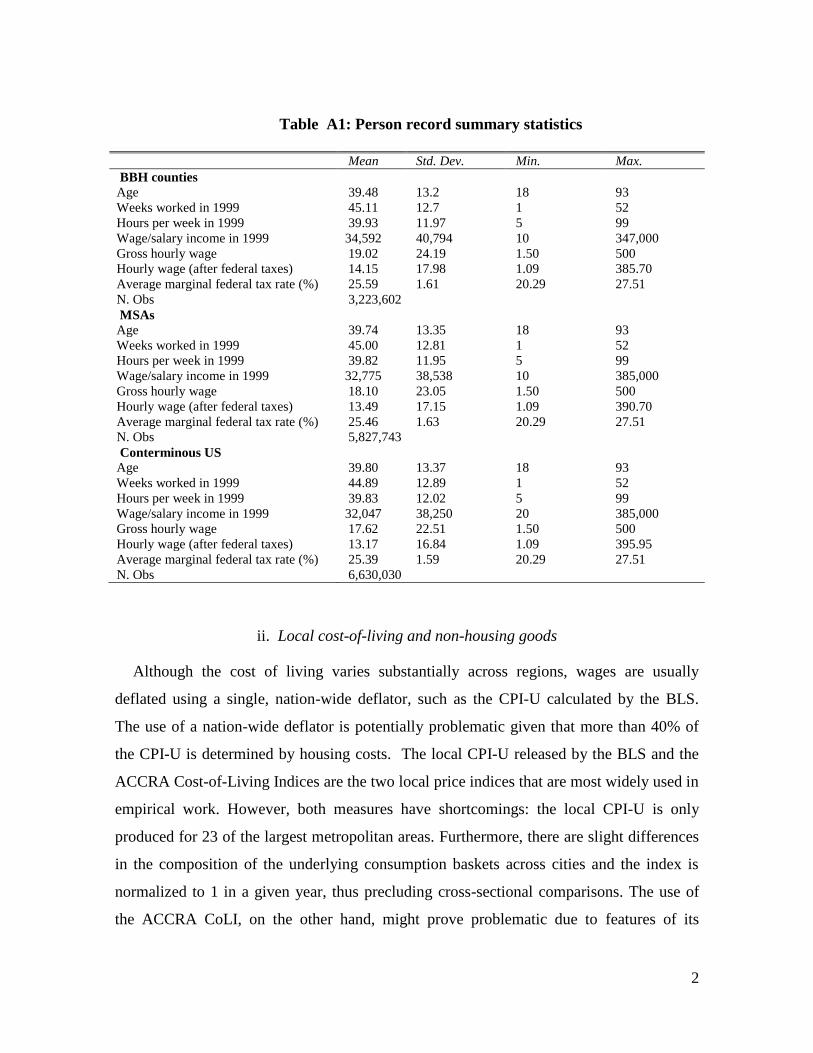
2
Table A1: Person record summary statistics
Mean Std. Dev. Min. Max.
BBH counties
Age 39.48 13.2 18 93
Weeks worked in 1999 45.11 12.7 1 52
Hours per week in 1999 39.93 11.97 5 99
Wage/salary income in 1999 34,592 40,794 10 347,000
Gross hourly wage 19.02 24.19 1.50 500
Hourly wage (after federal taxes) 14.15 17.98 1.09 385.70
Average marginal federal tax rate (%) 25.59 1.61 20.29 27.51
N. Obs 3,223,602
MSAs
Age 39.74 13.35 18 93
Weeks worked in 1999 45.00 12.81 1 52
Hours per week in 1999 39.82 11.95 5 99
Wage/salary income in 1999 32,775 38,538 10 385,000
Gross hourly wage 18.10 23.05 1.50 500
Hourly wage (after federal taxes) 13.49 17.15 1.09 390.70
Average marginal federal tax rate (%) 25.46 1.63 20.29 27.51
N. Obs 5,827,743
Conterminous US
Age 39.80 13.37 18 93
Weeks worked in 1999 44.89 12.89 1 52
Hours per week in 1999 39.83 12.02 5 99
Wage/salary income in 1999 32,047 38,250 20 385,000
Gross hourly wage 17.62 22.51 1.50 500
Hourly wage (after federal taxes) 13.17 16.84 1.09 395.95
Average marginal federal tax rate (%) 25.39 1.59 20.29 27.51
N. Obs 6,630,030
ii. Local cost-of-living and non-housing goods
Although the cost of living varies substantially across regions, wages are usually
deflated using a single, nation-wide deflator, such as the CPI-U calculated by the BLS.
The use of a nation-wide deflator is potentially problematic given that more than 40% of
the CPI-U is determined by housing costs. The local CPI-U released by the BLS and the
ACCRA Cost-of-Living Indices are the two local price indices that are most widely used in
empirical work. However, both measures have shortcomings: the local CPI-U is only
produced for 23 of the largest metropolitan areas. Furthermore, there are slight differences
in the composition of the underlying consumption baskets across cities and the index is
normalized to 1 in a given year, thus precluding cross-sectional comparisons. The use of
the ACCRA CoLI, on the other hand, might prove problematic due to features of its
3
theoretical design, data collection, and sampling design, as discussed by Koo, Phillips, and
Sigalla (2000).45
The lack of reliable regional cost-of-living indices thus means that most empirical
studies do not deflate nominal wages beyond the adjustment in the cost of housing
services, as measured by local rents. However, recent work on urban compensating
differentials suggests that non-housing goods might also play an important role in
determining the local cost-of-living. In order to account for the local variation in the price
of non-housing goods, we follow Moretti (forthcoming) who proposes an index that allows
the cost of housing and non-housing consumption to each vary across metropolitan areas.
While the city-level CPI-U published by the BLS is limited in its geographical coverage, it
can still be used to estimate what share of non-housing costs varies with the local cost of
housing. The local CPI-U for city j in year t is a weighted average of housing costs,
t
jHC , and non-housing costs (t
jNHC ) such that
(A1) ,NHC)(1HC=BLS t
j
t
j
t
j
where is the CPI weight used by the BLS for housing expenditure. Non-housing costs
can now be expressed as consisting of an element that varies systematically with housing
costs and an element that evolves independently form housing cost, i.e.
t
j
t
j
t
j HC=NHC . Using first-differenced prices to avoid non-stationarity then gives the
regression t
j
t
j
t
j HC=BLS , which in turn can be used to back-out an estimate of
by estimating , since
1
ˆ=ˆ . We use panel data on the small sample of 23 MSAs for
which a local BLS CPI is available from 1976-2000 to obtain the fixed-effects estimate for
which yields:
45 Koo, J., K.R. Phillips, and F.D. Sigalla. 2000. “Measuring Regional Cost of Living.” Journal of Business and Economic Statistics.
18(1): 127-136.
4
(A2) 0.74.=HC0.6191.792=BLS 2Rjjj
(0.01)(0.07)
With = 0.427 according to the BLS CPI-U weights in 2000, we can then impute the
systematic component of non-housing costs for all MSAs based on their housing cost, i.e.
2000HCˆj with = 0.332. Lastly, we compute a local price index as the weighted sum of
the cost of housing, the component of non-housing costs that varies with housing, and the
component of non-housing costs that does not vary with housing. Our parameter estimates
are close to Moretti’s estimates of = 0.35 which corresponds to = 0.63 in 2000.46
iii. Self-reported housing values
In the long form of the 2000 Census (question 51), housing values are self-reported in
24 intervals from ``less than $10,000'' to a top-coded category of ``$1,000,000 or more''.
This implies that the data on housing values, our dependent variable for the housing
hedonic regressions, is both interval censored and left- and right-censored. Using an ad-
hoc OLS regression on the midpoints of the intervals of such grouped data could lead to
inconsistent estimates, because it might not adequately reflect the true uncertainty
concerning the nature of the exact values within each interval and because it might also
inadequately deal with the left- and right-censoring issues in the tails. We address this
issue by comparing the parameters from estimating the housing regression via OLS using
the interval mid-points to those from using the more appropriate maximum-likelihood
interval estimator.
As a result of our large sample sizes combined with a large number of intervals, we do
not find a significant differences between the two sets of estimates. This suggests that the
consequences of grouping are unlikely to be important for our application. Furthermore,
the root mean-square errors for the two estimators are very similar which suggests that the
46 Albouy (2008) uses ACCRA data to run a regression similar to equation (2) and obtains a slightly smaller value of = 0.26. See
Albouy, D.Y. 2008. “Are Big Cities Bad Places to Live? Estimating Quality-of-Life across Metropolitan Areas.” NBER Working Paper No. 14472.
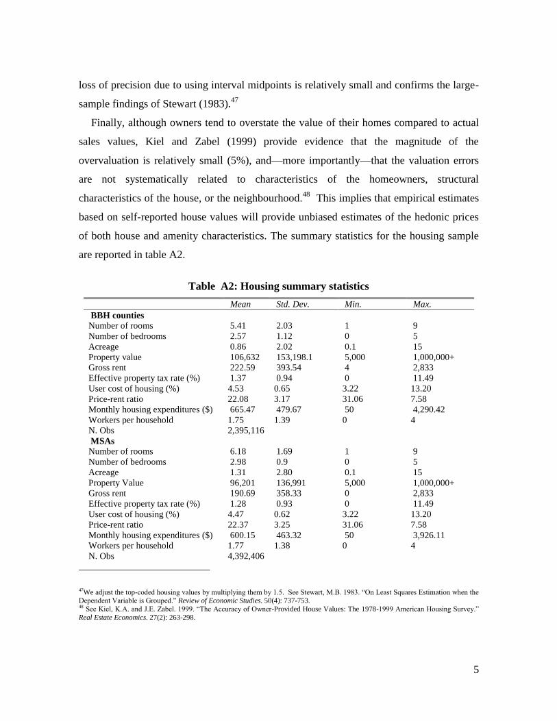
5
loss of precision due to using interval midpoints is relatively small and confirms the large-
sample findings of Stewart (1983).47
Finally, although owners tend to overstate the value of their homes compared to actual
sales values, Kiel and Zabel (1999) provide evidence that the magnitude of the
overvaluation is relatively small (5%), and—more importantly—that the valuation errors
are not systematically related to characteristics of the homeowners, structural
characteristics of the house, or the neighbourhood.48
This implies that empirical estimates
based on self-reported house values will provide unbiased estimates of the hedonic prices
of both house and amenity characteristics. The summary statistics for the housing sample
are reported in table A2.
Table A2: Housing summary statistics
Mean Std. Dev. Min. Max.
BBH counties
Number of rooms 5.41 2.03 1 9
Number of bedrooms 2.57 1.12 0 5
Acreage 0.86 2.02 0.1 15
Property value 106,632 153,198.1 5,000 1,000,000+
Gross rent 222.59 393.54 4 2,833
Effective property tax rate (%) 1.37 0.94 0 11.49
User cost of housing (%) 4.53 0.65 3.22 13.20
Price-rent ratio 22.08 3.17 31.06 7.58
Monthly housing expenditures ($) 665.47 479.67 50 4,290.42
Workers per household 1.75 1.39 0 4
N. Obs 2,395,116
MSAs
Number of rooms 6.18 1.69 1 9
Number of bedrooms 2.98 0.9 0 5
Acreage 1.31 2.80 0.1 15
Property Value 96,201 136,991 5,000 1,000,000+
Gross rent 190.69 358.33 0 2,833
Effective property tax rate (%) 1.28 0.93 0 11.49
User cost of housing (%) 4.47 0.62 3.22 13.20
Price-rent ratio 22.37 3.25 31.06 7.58
Monthly housing expenditures ($) 600.15 463.32 50 3,926.11
Workers per household 1.77 1.38 0 4
N. Obs 4,392,406
47We adjust the top-coded housing values by multiplying them by 1.5. See Stewart, M.B. 1983. “On Least Squares Estimation when the Dependent Variable is Grouped.” Review of Economic Studies. 50(4): 737-753. 48 See Kiel, K.A. and J.E. Zabel. 1999. “The Accuracy of Owner-Provided House Values: The 1978-1999 American Housing Survey.”
Real Estate Economics. 27(2): 263-298.
6
Conterminous US
Number of rooms 6.15 1.68 1 9
Number of bedrooms 2.97 0.89 0 5
Acreage 1.52 3.08 0.1 15
Property value 92,535.94 132,544 5,000 1,000,000+
Gross Rent 175.19 340.25 0 2,917
Effective property tax rate (%) 1.28 0.95 0 12.49
User cost of housing (%) 4.48 0.68 3.22 13.20
Price-rent ratio 22.32 3.24 31.06 7.58
Monthly housing expenditures ($) 571.19 450.82 50 3,926.11
Workers per household 1.76 1.38 0 4
N. Obs 5,163,123
A2. Moving Costs
We calculated average moving costs between counties by combining information on
both the average physical and financial costs of moving. The physical cost of the move
includes cost of transporting household goods, vehicles and the people in the household.
The financial costs included information on realtor fees, location-specific closing costs and
search costs from trips to search for a new residence.
i. Physical Costs
The first step in calculating physical costs was to calculate the linear distance in miles
between the population weighted centroids from each county in the United States to every
other county. The next step was to use the PUMS data to calculate the average number of
bedrooms and the fraction of renters in each of the counties. Based on the average number
of bedrooms in a county, we used the “weight estimator guide” at www.movesource.com
to calculate the weight (in pounds) that the average sized household would be transporting
from their “origin” county to their “destination” county. The average number of bed-
rooms in the counties ranged from a minimum of 1.36 to a maximum of 3.46. Based on
the weight estimator guide, counties with an average number of bedrooms between 1 and 2
were assigned a transportation weight that varied linearly between 3,500 (for a 1 bedroom)
and 5,000 (for a 2 bedroom) pounds. For counties with an average number of bedrooms
between 2 and 3, transportation weight ranged between 5,000 and 7,500 pounds and for
counties with an average number of bedrooms between 3 and 4 the transportation weight
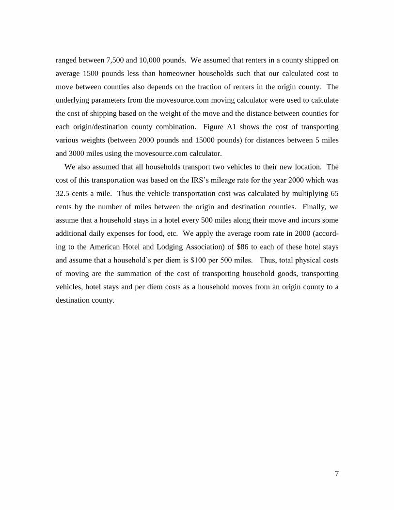
7
ranged between 7,500 and 10,000 pounds. We assumed that renters in a county shipped on
average 1500 pounds less than homeowner households such that our calculated cost to
move between counties also depends on the fraction of renters in the origin county. The
underlying parameters from the movesource.com moving calculator were used to calculate
the cost of shipping based on the weight of the move and the distance between counties for
each origin/destination county combination. Figure A1 shows the cost of transporting
various weights (between 2000 pounds and 15000 pounds) for distances between 5 miles
and 3000 miles using the movesource.com calculator.
We also assumed that all households transport two vehicles to their new location. The
cost of this transportation was based on the IRS’s mileage rate for the year 2000 which was
32.5 cents a mile. Thus the vehicle transportation cost was calculated by multiplying 65
cents by the number of miles between the origin and destination counties. Finally, we
assume that a household stays in a hotel every 500 miles along their move and incurs some
additional daily expenses for food, etc. We apply the average room rate in 2000 (accord-
ing to the American Hotel and Lodging Association) of $86 to each of these hotel stays
and assume that a household’s per diem is $100 per 500 miles. Thus, total physical costs
of moving are the summation of the cost of transporting household goods, transporting
vehicles, hotel stays and per diem costs as a household moves from an origin county to a
destination county.
8
Figure A1: Physical Cost Matrix
ii. Financial Costs
Financial costs also vary by renter and homeowner. We assume that homeowners (not
renters) must pay closing costs to sell their house in their origin county. Our calculations
are based on Bankrate.com’s 2005 survey which provides average closing costs by state.
We also assume that homeowners (not renters) pay a real estate agent 3% to facilitate
selling their house and a real estate agent 3% to buy a house. Thus, we calculate these
costs as 3% of the average housing value in the origin county and 3% of the average hous-
ing value in the destination county. We assume that both homeowners and renters pay to
search for a new residence. These “finding costs” for moves within 60 miles, between 60
and 180, between 180 and 500, between 500 and 1000, and greater than 1,000 miles are
assumed to be 0, 250, 500, 1,000 and 2,000 dollars. These finding costs reflect our best
guess for the search costs when travel is local, requires at least a day, requires an overnight
stay, or likely requires plane tickets in order to look for a new residence in the destination
county.
0
2000
4000
6000
8000
10000
12000
14000
16000
5
12
5
24
5
36
5
48
5
60
5
72
5
84
5
96
5
10
85
12
05
13
25
14
45
15
65
16
85
18
05
19
25
20
45
21
65
22
85
24
05
25
25
26
45
27
65
28
85
Co
st o
f Tr
ansp
ort
ing
We
igh
t
Distance Between Counties in Miles
2000 3500 5000 7500 10000 12500 15000
9
Total financial costs are calculated by summing up the financial costs of searching for a
new residence (for renters and homeowners) and the costs of buying and selling a home
(for homeowners only). The weight assigned to the homeowner and the renter calculations
is again based on the fraction of renters in a county. The total moving cost used in the
final robustness check of the paper is calculated by summing the physical and financial
costs we have described above.
A3. Amenity Database and Stata Code
The Stata file amenity.dta contains our county level database on amenities. The zip file
results.zip contains data and code to replicate all of the tables in the paper. It also includes
instructions to produce expenditure measures for specific counties, PUMAs, or puma-
county unions. See the readme.pdf file for details.