nano-engineered surfaces developed for mercury sensing
TRANSCRIPT
Nano-Engineered Surfaces Developed For Mercury Sensing
Ylias Mohammad Sabri B.Eng. (Hons)
A thesis submitted in fulfillment of the requirements for the degree of Doctor of Philosophy
School of Applied Sciences RMIT University
March 2010

i
Declaration
I certify that except where due acknowledgement has been made, the work is that of
the author alone; the work has not been submitted previously, in whole or in part, to
qualify for any other academic award; the content of the thesis is the result of work
which has been carried out since the official commencement date of the approved
research program; and, any editorial work, paid or unpaid, carried out by a third party
is acknowledged.
Ylias M Sabri

ii
Acknowledgments
I gratefully acknowledge the constant encouragement, support and guidance of my
supervisors Prof. Suresh Bhargava, Adj. Prof. Dinesh Sood and Dr Samuel Ippolito
throughout this project. Prof. Suresh Bhargava has been a wonderful example to learn from
in all facets of life and without his continuous support this work would have been far from
over. The knowledge, skill and dedication of Prof. Dinesh Sood as a research scientist is an
inspiration and I could not have hoped for a better mentor. I cannot thank Dr. Samuel Ippolito
enough for his input, encouragement, consideration and invaluable assistance that enabled
me to experience a great deal of success throughout my PhD research program.
I thank the Commonwealth Government Postgraduate Award (APA) scholarship program as
well as Australian Research Council – Linkage (ARC-L), BHP Billiton and ALCOA, Australia
for providing me with financial support from the beginning of my PhD program. The Authors
is grateful to AINSE for funding the use of SIMS instrument at ANSTO, Sydney as well as
awarding travel grant to visit IMCS conference in USA.
My deepest sense of gratitude to Dr. Vipul Bansal, Dr. James Tardio and Dr. Mohammad
Al kobaisi for their incredible support throughout the course of my PhD studies, their
invaluable scientific discussions, criticism and positive approach to problems will be my guide
for life.
Special thanks to Dr. Ian Harrison, Mr. Mark Mullet, Dr. Steven Grocott, Dr. Steven
Rosenberg and Mr. Eric Boom for their invaluable help, direction and input. I can never forget
the input, help and support from the industrial aspect of the project that I got from Mr. Mark
Mullet.
I thank Dr. Kathryne Prince and Mr. Armand Anatacio for their scientific discussions during
my visit to ANSTO and also Dr. Dennis Mather and Ms. Rhiannon Still for their hospitality.
I thank Dr. Anthony O’Mullane, Dr. Kourosh Kalantar Zadeh, Ms. Heather Wymer, Mr. Firew
Beshah, Dr. Abdul-Cadir Hussein, Ms. Hailey Reynolds, Prof. Ashish Garg, Mr. Mohammad
Omar, Dr. Pandiyan Murugaraj, Dr. Margaret Tate, Mr. Abdurahman Anod, Dr. Prashant
Sawant, Dr. Deepak Dhawan, Dr. Dinesh Vinkatachalam, Mrs. Gopa Karr, Dr. Glen
Matthews, Mr. Blake Plowman and Dr. Lisa Hodgson for providing a friendly and energetic
atmosphere and being there when ever I needed their help.
My heartful thanks go to all my colleagues, technical, administrative and laboratory staff at
RMIT University. Thanks specially to Mrs. Nadia Zakhartchouk, Mrs. Zahra Homan, Mr.
Yuxun Cao, Mr Karl lang, Mr. Paul Jones, Mr. Howard Anderson, Mr. Peter Laming, Mrs.
Chi-Ping Wu, Mrs. Diane Mileo, Mrs Ruth Cepriano-hall, Mr. Paul Morrison, Mr. Frank
Antolasic, Mr. David Welsh, Mr. Bob Kealy and last but not least Mr. Phillip Francis, whom
have all taken extra stressful steps at times to help me throughout my research project.

iii
I would also like to take this opportunity to express my sincerest love to my parents, brothers,
sisters, and extended family, their love, support and understanding and whom without their
sacrifices and help I wouldn’t be who I am, and I am thankful for who I am.
Ylias M. Sabri

iv
This thesis is dedicated to my family,
my parents, Zargoona and Mohammad Asif
and brothers and sisters, Khalid, Farshta, Idress, Harees, Arif, and
Mezhgon
v
Abstract
Mercury is highly toxic but often neglected element that is readily emitted into the
environment via a number of industrial processes. In Australia, coal-fired power plants and
the alumina industry are the two largest emitters of mercury. In order to maintain the alumina
industry’s commitment to reduce the environmental impact of its processes and remain
economically sustainable, innovative technologies are required that can monitor mercury
concentrations within its processes. The aim of this research project was to develop robust
quartz crystal microbalance (QCM) based sensors for measuring Hg vapour levels in
challenging industrial environments, such as those found in the alumina industry (i.e. Hg
concentrations of 1-40 mg/m3 at 20-90°C).
In order to gain a deeper understanding of Hg vapour interactions with the surface of the
QCM electrodes, parameters such as Hg sorption and desorption rates, sticking probability
and Hg diffusion were studied in detail. When Hg diffusion in ultra-thin films of Au was
studied, it was observed that Hg accumulation occurred at the interface between the Au
sensitive and SiO2 layers. These observations lead to the exploration of two different
electrochemical methods for the direct formation of Hg selective and sensitive
nanostructured Au films directly on QCM crystals. In the first case, galvanic replacement
(GR) reactions were employed to form Ni-Au hybrid nanoclusters. This method resulted in Hg
sensors with 93-100% recovery, excellent selectivity towards Hg in the presence of ammonia
and humidity and ~27% higher sensitivity than the Au control QCM. The second case
involved forming highly oriented and ornate Au nanostructures (nanospikes) with controlled
crystallographic facets onto the QCM electrode by a single step electrodeposition method.
These sensors were tested towards Hg vapour in the presence of ammonia and humidity at
~90°C for a 50 day period in a specially designed and developed 8-channel computer
controlled gas calibration system. The testing sequences were made to simulate some of the
conditions found in Hg-emitting industries. The nanospike QCM showed high selectivity,
recovery and around 4.7 times higher sensitivity than the Au control QCM, with low
degradation in response magnitude over the long testing period.
The high sensitivity of the nanospikes was found to be not only due to high surface area but
also due to the increased number of surface defect sites created during the electrodeposition
step. Due to its excellent performance, a nanospike QCM was then tested towards Hg in the
presence of several volatile organic compounds (VOCs) that either had high affinity towards
Au or was present in alumina effluent streams. The nanospikes based QCM was tested
against VOCs such as acetone, dimethyl disulphide, methylethyl ketone, ethyl mercaptan,
acetaldehyde as well as ammonia and humidity. The nanospike QCM was observed to
maintain high selectivity and sensitivity towards Hg vapour when compared to Au control

vi
QCM. The success of the data presented in this thesis has resulted in a PCT patent of the
developed nanospikes and is due to undergo preliminary testing at industry partners’ sites. If
successful, the developed sensor will assist industries in complying with mercury emission
targets and would be a significant technological breakthrough with potential for many other
applications in pollution control.
vii
Table of contents
Chapter 1 Introduction and Literature Review....................................................1
1.1 Introduction ............................................................................................................ 2
1.1.1 Motivation ........................................................................................................... 2
1.1.2 Objectives........................................................................................................... 3
1.1.3 Outcomes and Author’s Achievements ............................................................... 4
1.1.4 Thesis Organisation............................................................................................ 6
1.2 Literature Review ................................................................................................... 8
1.2.1 Hg and the Environment ..................................................................................... 8
1.2.1.1 Impacts of Hg.............................................................................................. 8
1.2.1.2 Anthropogenic Hg Emissions ...................................................................... 8
1.2.2 Metal Surfaces as Collection Media for Mercury............................................... 10
1.2.3 Hg interaction with Gold and Silver Surfaces .................................................... 10
1.2.4 Non-Metal to Metal Transition of Hg ................................................................. 13
1.2.5 Current Methods to Measure Hg....................................................................... 14
1.2.5.1 Spectroscopic based Hg Sensors ............................................................. 14
1.2.5.2 Mercury Capture ....................................................................................... 17
1.2.5.3 Commercial Mercury Sensor Systems ...................................................... 18
1.2.6 Acoustic Based Sensors................................................................................... 21
1.2.6.1 Types of Acoustic Wave Gas Sensors ...................................................... 21
1.2.6.2 Quartz Crystal Microbalance (QCM) ......................................................... 23
1.2.6.3 Advantages of QCM over Other Transducers ........................................... 26
1.2.6.4 State of the Art Acoustic Based Hg Sensors ............................................. 27
1.3 Conclusions.......................................................................................................... 31
1.4 References........................................................................................................... 32
Chapter 2 Experimental Setup ...........................................................................39
2.1 Overview .............................................................................................................. 40
2.1.1 Mercury Delivery and Sampling System ........................................................... 40
2.1.2 Hg Vapour Generator and Calibration............................................................... 44
2.1.3 Calibration data of the Humidity Generator ....................................................... 46
2.1.4 Testing Chamber Operating Temperatures....................................................... 47
2.2 QCM Fabrication .................................................................................................. 47
2.2.1 Metal Deposition............................................................................................... 47
2.2.2 Surface Modification ......................................................................................... 48
2.2.2.1 Galvanic Replacement.............................................................................. 48
2.2.2.2 Electrodeposition ...................................................................................... 48
2.3 QCM Characterization .......................................................................................... 48
viii
2.4 Surface Characterization ......................................................................................51
2.4.1 Scanning Electron Microscope (SEM)...............................................................51
2.4.2 X-Ray Diffraction (XRD)....................................................................................51
2.4.3 X-ray Photoelectron Spectroscopy (XPS) .........................................................51
2.4.4 Atomic Force Microscopy (AFM).......................................................................51
2.4.5 Secondary Ion Mass Spectrometry (SIMS) .......................................................51
2.4.6 Inductively Coupled Plasma Mass Spectrometry (ICPMS)................................52
2.4.7 Electrochemical Surface Area Analysis.............................................................52
2.5 Hg Testing Patterns..............................................................................................53
2.5.1 Pre-treatment....................................................................................................53
2.5.2 Temperature Profile ..........................................................................................53
2.5.3 Hg Sensing in the Presence of Interferent Gases .............................................55
2.5.4 Memory Effect – Hg Concentration Fluctuations ...............................................56
2.5.5 Hg Sensing – Interferent Gases Concentration Fluctuations.............................56
2.5.6 Mercury Saturation of Au Thin and Ultra-thin Films...........................................57
2.6 References...........................................................................................................59
Chapter 3 Investigation of Hg Interaction with Various Thin Metal Films and
Surface Morphologies ............................................................................................ 61
3.1 Introduction...........................................................................................................62
3.2 Hg Sorption/Desorption of Surfaces Investigated..................................................63
3.2.1 Metals Types Investigated ................................................................................63
3.2.2 Surface Types Investigated ..............................................................................63
3.2.3 Surface Morphology – SEM..............................................................................63
3.2.4 Determination of Equilibrium Time ....................................................................64
3.2.5 Morphology Influence on Hg Sorption and Desorption Characteristics..............66
3.2.6 Morphology Influence on Sensor Response Time.............................................69
3.2.7 Morphology Influence on Hg Diffusion Behaviour .............................................69
3.2.8 Surface Provoked Hg Affinity (Sticking Probability) ...........................................73
3.2.9 Outperformance of Au-Rough over Other Surfaces ..........................................76
3.3 Feasibility of Au-rough as a Hg Vapour Sensor ....................................................77
3.3.1 Temperature Profile and Adsorption Isotherms.................................................77
3.3.2 Sorption, Desorption and Their Rates...............................................................80
3.4 Repeatability of Au-Rough QCM...........................................................................84
3.4.1 Repeatability and Stability.................................................................................84
3.4.2 Long Term Stability and the Influence of Interferent Gases...............................86
3.4.3 Au-rough Surface Morphology Change Following Hg Exposure........................88
3.5 Summary..............................................................................................................90
3.6 References...........................................................................................................91
ix
Chapter 4 Study of Hg Interaction kinetics on Au Thin Films .........................93
4.1 Introduction .......................................................................................................... 94
4.2 Experimental Setup .............................................................................................. 94
4.3 Parameters Influencing Hg Sorption and Desorption Characteristics.................... 95
4.3.1 Influence of Hg Exposure Period and Surface Coverage .................................. 96
4.3.2 Influence of Operating Temperature ................................................................. 98
4.3.3 Influence of Hg Vapour Concentration ............................................................ 100
4.4 Temperature Profile of Au Thin Film Based QCM Sensors................................. 102
4.4.1 Test Pattern.................................................................................................... 102
4.4.2 Temperature Profile Studies ........................................................................... 103
4.4.3 Analysis of Temperature Profile Shape........................................................... 104
4.4.4 Influence of Operating Temperature and Surface Morphology........................ 106
4.4.4.1 Hg Sorption Isotherm.............................................................................. 106
4.4.4.2 Effect of Morphology on Detection Limit and Sensitivity .......................... 107
4.4.4.3 Effects of Surface Area on Hg Sorption Capacity.................................... 108
4.4.4.4 Effects of Surface Morphology on Hg Sorption/Desorption Kinetics ........ 109
4.4.4.5 Effects of Surface Morphology on Hg Desorption/Sorption Ratio ............ 110
4.5 Summary............................................................................................................ 111
4.6 References......................................................................................................... 113
Chapter 5 Investigation of Hg Sorption and Diffusion Behaviour on
Ultra-thin Films of Gold.........................................................................................115
5.1 Introduction ........................................................................................................ 116
5.2 Experimental Setup ............................................................................................ 117
5.3 Differentiation of Hg Vapour Sorption Processes on Gold .................................. 117
5.3.1 Influence of Hg Concentration on Hg Sorption Processes on Gold ................. 118
5.3.1.1 Hg Concentration of 10.55 mg/m3 ........................................................... 118
5.3.1.2 Hg Concentration of 3.65 mg/m3 ............................................................. 123
5.3.1.3 Hg Concentration of 1.02 mg/m3 ............................................................. 126
5.3.2 Influence of Operating Temperature on Hg sorption Processes on Gold ........ 128
5.3.2.1 Operating Temperature of 89°C.............................................................. 128
5.3.2.2 Operating Temperature of 55°C.............................................................. 130
5.3.2.3 Operating Temperature of 28°C.............................................................. 131
5.4 Hg Diffusion Behaviour in Ultra-thin Films of Gold .............................................. 133
5.4.1 Influence of Hg Concentration on Hg Diffusion Behaviour .............................. 133
5.4.1.1 Hg Concentration of 10.55 mg/m3 ........................................................... 133
5.4.1.2 Hg Concentration of 3.65 mg/m3 ............................................................. 135
5.4.2 Influence of Operating Temperature on Hg Diffusion Behaviour ..................... 136
5.5 Summary............................................................................................................ 138
x
5.6 References......................................................................................................... 140
Chapter 6 QCM Based Hg Vapour Sensor Enhancement by Surface
Modification using Galvanic Replacement Reaction......................................... 143
6.1 Introduction......................................................................................................... 144
6.2 Experimental Setup ............................................................................................ 145
6.3 Ni-Au hybrid Sensitive Layer Characterisations .................................................. 145
6.3.1 Surface Morphology – SEM............................................................................ 146
6.3.2 Surface Roughness - AFM.............................................................................. 147
6.3.3 Crystallography - XRD .................................................................................... 149
6.3.4 Surface Chemical Analysis - XPS................................................................... 150
6.4 Hg Sensing Performance of Galvanically Replaced QCMs................................. 152
6.4.1 Influence of Operating Temperature on Hg Sorption and Desorption
Characteristics............................................................................................................. 153
6.4.1.1 Operating Temperature of 28°C.............................................................. 153
6.4.1.2 Operating Temperature of 89°C.............................................................. 154
6.4.2 Influence of Operating Temperature on Hg Sensing ....................................... 156
6.4.3 Influence of Operating Temperature on Response Time and Response
Magnitude ................................................................................................................... 157
6.4.4 Influence of GR reaction time on QCM Response Magnitude and Recovery .. 159
6.4.5 Influence of GR reaction time and Operating Temperature on QCM Sensitivity
and Limit of Detection.................................................................................................. 160
6.4.6 Influence of Hg in the Presence of Interferent Gases on the Galvanically
Replaced QCMs .......................................................................................................... 161
6.5 Hg Diffusion Bahaviour in GR Surfaces .............................................................. 165
6.6 Summary............................................................................................................ 167
6.7 References......................................................................................................... 168
Chapter 7 QCM Based Hg Vapour Sensor Enhancement by Surface
Modification using Gold Electrodeposition........................................................ 169
7.1 Introduction......................................................................................................... 170
7.2 Experimental Setup ............................................................................................ 171
7.2.1.1 Mass of Gold Nanospikes ....................................................................... 172
7.2.1.2 Electrochemical Surface Area of Gold Nanospikes ................................. 174
7.3 Gold Nanospikes Sensitive Layer Characterisation ............................................ 175
7.3.1 Surface Morphology – SEM............................................................................ 175
7.3.1.1 Thermal Stability of the Nanospikes ........................................................ 177
7.3.1.2 Adherence – Scratch Test....................................................................... 179
7.3.2 Surface Chemical Composition – EDX............................................................ 179
7.3.3 Crystallography – XRD ................................................................................... 180
xi
7.4 Hg Sensing Performance of Nanospike Based QCM.......................................... 182
7.4.1 Influence of Operating Temperature on Response Magnitude........................ 182
7.4.1.1 Temperature Profile ................................................................................ 184
7.4.1.2 Sensitivity and Limit of Detection ............................................................ 185
7.4.2 Sensor Repeatability ...................................................................................... 186
7.4.3 Influence of Humidity Interference .................................................................. 187
7.4.4 Influence of Ammonia Interference ................................................................. 188
7.4.5 Influence of Humidity and Ammonia Interference............................................ 189
7.5 Long Term Sensor Performance ........................................................................ 190
7.5.1 Surface Morphology Change Following Long Term Testing............................ 193
7.5.2 Hg Accumulation and Sensor Lifetime ............................................................ 194
7.6 Preliminary Industrial Trial Testing...................................................................... 195
7.7 Summary............................................................................................................ 198
7.8 References......................................................................................................... 200
Chapter 8 Conclusions and Future Work ........................................................213
8.1 Summary of Work............................................................................................... 214
8.1.1 Gravimetric Based Hg Vapour Sensor ............................................................ 214
8.1.2 Importance of Experimental Set-up................................................................. 214
8.1.3 Hg Interaction with Metal Films....................................................................... 215
8.1.3.1 Influence of Au Film Thickness ............................................................... 215
8.1.3.2 Hg Sorption and Diffusion Behaviour in Ultra-thin Films.......................... 216
8.1.4 Use of Galvanic Replacement Reaction to Enhance Sensor Recovery........... 216
8.1.5 Use of Electrodeposition to Enhance Sensor Response Magnitude................ 217
8.1.6 Performance Comparison of the Developed Nano-engineered Sensors ......... 217
8.2 Conclusions........................................................................................................ 220
8.3 Ongoing Future Work ......................................................................................... 221
Appendices..................................................................................................................... 223
Appendix A.................................................................................................................. 224
Appendix B:................................................................................................................. 229
Appendix C.................................................................................................................. 232
Appendix D:................................................................................................................. 233
Appendix E.................................................................................................................. 237
Appendix F .................................................................................................................. 243
Appendix G ................................................................................................................. 249
xii
List of figures
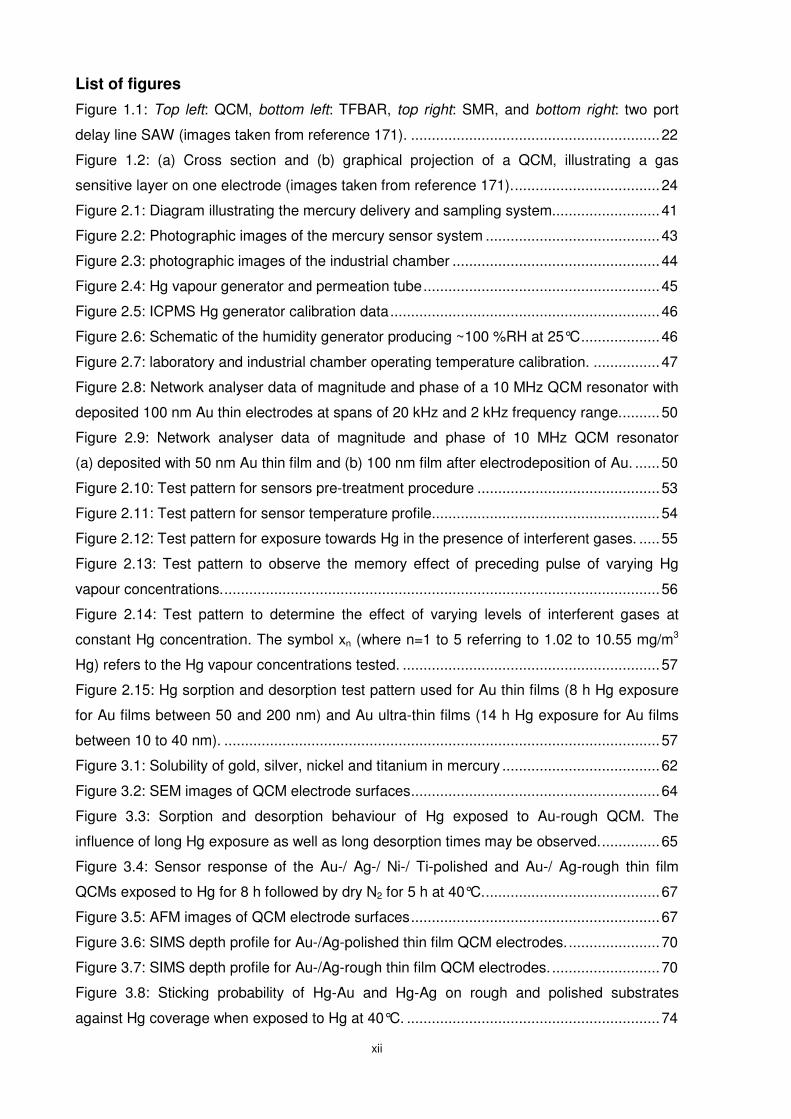
Figure 1.1: Top left: QCM, bottom left: TFBAR, top right: SMR, and bottom right: two port
delay line SAW (images taken from reference 171). ............................................................22
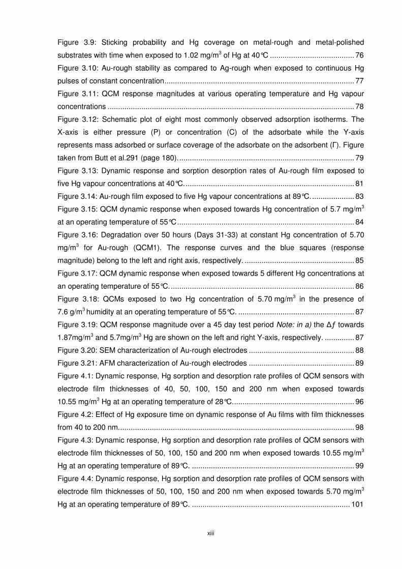
Figure 1.2: (a) Cross section and (b) graphical projection of a QCM, illustrating a gas
sensitive layer on one electrode (images taken from reference 171)....................................24
Figure 2.1: Diagram illustrating the mercury delivery and sampling system..........................41
Figure 2.2: Photographic images of the mercury sensor system ..........................................43
Figure 2.3: photographic images of the industrial chamber ..................................................44
Figure 2.4: Hg vapour generator and permeation tube.........................................................45
Figure 2.5: ICPMS Hg generator calibration data.................................................................46
Figure 2.6: Schematic of the humidity generator producing ~100 %RH at 25°C...................46
Figure 2.7: laboratory and industrial chamber operating temperature calibration. ................47
Figure 2.8: Network analyser data of magnitude and phase of a 10 MHz QCM resonator with
deposited 100 nm Au thin electrodes at spans of 20 kHz and 2 kHz frequency range..........50
Figure 2.9: Network analyser data of magnitude and phase of 10 MHz QCM resonator
(a) deposited with 50 nm Au thin film and (b) 100 nm film after electrodeposition of Au. ......50
Figure 2.10: Test pattern for sensors pre-treatment procedure ............................................53
Figure 2.11: Test pattern for sensor temperature profile.......................................................54
Figure 2.12: Test pattern for exposure towards Hg in the presence of interferent gases. .....55
Figure 2.13: Test pattern to observe the memory effect of preceding pulse of varying Hg
vapour concentrations..........................................................................................................56
Figure 2.14: Test pattern to determine the effect of varying levels of interferent gases at
constant Hg concentration. The symbol xn (where n=1 to 5 referring to 1.02 to 10.55 mg/m3
Hg) refers to the Hg vapour concentrations tested. ..............................................................57
Figure 2.15: Hg sorption and desorption test pattern used for Au thin films (8 h Hg exposure
for Au films between 50 and 200 nm) and Au ultra-thin films (14 h Hg exposure for Au films
between 10 to 40 nm). .........................................................................................................57
Figure 3.1: Solubility of gold, silver, nickel and titanium in mercury ......................................62
Figure 3.2: SEM images of QCM electrode surfaces............................................................64
Figure 3.3: Sorption and desorption behaviour of Hg exposed to Au-rough QCM. The
influence of long Hg exposure as well as long desorption times may be observed...............65
Figure 3.4: Sensor response of the Au-/ Ag-/ Ni-/ Ti-polished and Au-/ Ag-rough thin film
QCMs exposed to Hg for 8 h followed by dry N2 for 5 h at 40°C...........................................67
Figure 3.5: AFM images of QCM electrode surfaces............................................................67
Figure 3.6: SIMS depth profile for Au-/Ag-polished thin film QCM electrodes.......................70
Figure 3.7: SIMS depth profile for Au-/Ag-rough thin film QCM electrodes. ..........................70
Figure 3.8: Sticking probability of Hg-Au and Hg-Ag on rough and polished substrates
against Hg coverage when exposed to Hg at 40°C. .............................................................74
xiii
Figure 3.9: Sticking probability and Hg coverage on metal-rough and metal-polished
substrates with time when exposed to 1.02 mg/m3 of Hg at 40°C ........................................ 76
Figure 3.10: Au-rough stability as compared to Ag-rough when exposed to continuous Hg
pulses of constant concentration.......................................................................................... 77
Figure 3.11: QCM response magnitudes at various operating temperature and Hg vapour
concentrations ..................................................................................................................... 78
Figure 3.12: Schematic plot of eight most commonly observed adsorption isotherms. The
X-axis is either pressure (P) or concentration (C) of the adsorbate while the Y-axis
represents mass adsorbed or surface coverage of the adsorbate on the adsorbent (Г). Figure
taken from Butt et al.291 (page 180).................................................................................... 79
Figure 3.13: Dynamic response and sorption desorption rates of Au-rough film exposed to
five Hg vapour concentrations at 40°C................................................................................. 81
Figure 3.14: Au-rough film exposed to five Hg vapour concentrations at 89°C..................... 83
Figure 3.15: QCM dynamic response when exposed towards Hg concentration of 5.7 mg/m3
at an operating temperature of 55°C.................................................................................... 84
Figure 3.16: Degradation over 50 hours (Days 31-33) at constant Hg concentration of 5.70
mg/m3 for Au-rough (QCM1). The response curves and the blue squares (response
magnitude) belong to the left and right axis, respectively. .................................................... 85
Figure 3.17: QCM dynamic response when exposed towards 5 different Hg concentrations at
an operating temperature of 55°C........................................................................................ 86
Figure 3.18: QCMs exposed to two Hg concentration of 5.70 mg/m3 in the presence of
7.6 g/m3 humidity at an operating temperature of 55°C. ....................................................... 87
Figure 3.19: QCM response magnitude over a 45 day test period Note: in a) the ∆ƒ towards
1.87mg/m3 and 5.7mg/m3 Hg are shown on the left and right Y-axis, respectively. .............. 87
Figure 3.20: SEM characterization of Au-rough electrodes .................................................. 88
Figure 3.21: AFM characterization of Au-rough electrodes .................................................. 89
Figure 4.1: Dynamic response, Hg sorption and desorption rate profiles of QCM sensors with
electrode film thicknesses of 40, 50, 100, 150 and 200 nm when exposed towards
10.55 mg/m3 Hg at an operating temperature of 28°C.......................................................... 96
Figure 4.2: Effect of Hg exposure time on dynamic response of Au films with film thicknesses
from 40 to 200 nm................................................................................................................ 98
Figure 4.3: Dynamic response, Hg sorption and desorption rate profiles of QCM sensors with
electrode film thicknesses of 50, 100, 150 and 200 nm when exposed towards 10.55 mg/m3
Hg at an operating temperature of 89°C. ............................................................................. 99
Figure 4.4: Dynamic response, Hg sorption and desorption rate profiles of QCM sensors with
electrode film thicknesses of 50, 100, 150 and 200 nm when exposed towards 5.70 mg/m3
Hg at an operating temperature of 89°C. ........................................................................... 101
xiv
Figure 4.5: Four QCMs exposed to Hg concentrations of 1.02, 1.87, 3.65, 5.70 and 10.55
mg/m3 at an operating temperature of 55°C....................................................................... 102
Figure 4.6: Temperature profile of QCMs with thin Au film electrodes................................ 104
Figure 4.7: Influence of Operating temperature on the change in solubility of Au in Hg and
vapour pressure of Hg in air............................................................................................... 105
Figure 4.8: Hg sorption Isotherm for the 100 nm Au QCM at various operating temperatures.
.......................................................................................................................................... 106
Figure 4.9: Linear plots of Hg sorption isotherms at 28 and 89°C. The linear plots are used to
calculate sensitivity and detection limit of QCM based Hg vapour sensors......................... 107
Figure 4.10: Hg sorption capacity ratio of rough/polished Au QCMs at various operating
temperatures and Hg vapour concentrations...................................................................... 109
Figure 4.11: Hg sorption in the first two minutes for both optically polished and mechanically
roughened Au QCMs ......................................................................................................... 109
Figure 4.12: Desorption/sorption ratios for optically polished and mechanically roughened Au
QCMs at Hg vapour concentration of 10.55 mg/m3 and various operating temperatures.... 110
Figure 5.1: Expected ∆f of four QCMs with film thicknesses of 10, 20, 30 and 40 nm Au
electrode exposed to constant Hg vapour and operating temperature – data extrapolation to
zero thickness (ETZT) method. .......................................................................................... 118
Figure 5.2: Dynamic response and ETZT graphic representation of QCM sensors with
electrode film thicknesses of 10, 20, 30, and 40 nm when exposed towards 10.55 mg/m3 Hg
at 28°C............................................................................................................................... 119
Figure 5.3: Hg sorption and desorption rates of QCM sensors with electrode film thicknesses
of 10, 20, 30, and 40 nm when exposed to 10.55 mg/m3 Hg at 28°C. ................................ 121
Figure 5.4: SEM images of ultra thin Au films before (a and b) and after (c and d) Hg
exposure at a concentration of 10.55 mg/m3 and 28°C. ..................................................... 122
Figure 5.5: Au ultra-thin film based QCM response magnitude towards Hg vapour
concentration of 10.55 mg/m3 at 28°C at various Hg exposure times. Inset shows the QCMs’
response curve in the first 60 minutes of Hg exposure period. ........................................... 123
Figure 5.6: Dynamic response and ETZT graphic representation of QCM sensors with
electrode film thicknesses of 10, 20, 30, and 40 nm when exposed towards 3.65 mg/m3 Hg at
28°C................................................................................................................................... 123
Figure 5.7: Zero-shifted QCM response during desorption period of QCM sensors with
electrode film thicknesses of 10, 20, 30, and 40 nm when exposed towards dry nitrogen for 5
hours following a 14 hour Hg exposure period at 28°C. ..................................................... 125
Figure 5.8: Hg sorption and desorption rate profiles of QCM sensors with Au electrode
ultra-thin film thicknesses of 10, 20, 30, and 40 nm when exposed towards 3.65 mg/m3 Hg at
28°C................................................................................................................................... 125
xv
Figure 5.9: Hg sorption and desorption rate profiles of QCM sensors with Au electrode
ultra-thin film thicknesses of 10, 20, 30, and 40 nm when exposed towards 1.02 mg/m3 Hg at
28°C. ................................................................................................................................. 126
Figure 5.10: Dynamic response, ETZT graphic representation, Hg sorption and desorption
rate profiles of QCM sensors with electrode film thicknesses of 10, 20, 30, and 40 nm when
exposed towards 10.55 mg/m3 Hg at 89°C. Inset of (d) shows the zero-shifted desorption
dynamic response data of the QCMs. ................................................................................ 128
Figure 5.11: Dynamic response and ETZT graphic representation of QCM sensors with
electrode film thicknesses of 10, 20, 30, and 40 nm when exposed towards 10.55 mg/m3 Hg
at 55°C. ............................................................................................................................. 130
Figure 5.12: SIMS depth profile of the Au ultra-thin films exposed to10.55 mg/m3 Hg at an
operating temperature of 28°C........................................................................................... 133
Figure 5.13: SIMS depth profiles of the Au ultra-thin films exposed to 10.55 mg/m3 Hg at an
operating temperature of 28°C........................................................................................... 134
Figure 5.14: SIMS depth profile of the Au ultra-thin films exposed to a Hg concentration of
10.55 mg/m3 at an operating temperature of 28°C. ............................................................ 135
Figure 5.15: SIMS depth profile of the Au ultra-thin films exposed to a Hg concentration
3.65 mg/m3 at an operating temperature of 28°C. .............................................................. 136
Figure 5.16: SIMS depth profile of the Au ultra-thin films exposed to 10.55 mg/m3 Hg at an
operating temperature of 55 and 89°C. .............................................................................. 136
Figure 5.17: The area under the SIMS depth profiles (in counts.s) showing the influence of
operating temperature and Hg vapour concentration on the amount of diffused and
accumulated Hg in the Au ultra-thin films. .......................................................................... 137
Figure 6.1: SEM images showing the Ni-Au surfaces at various GR reaction times. Inset in
(B) shows some of the Au islands grown following 2 hours of reaction time....................... 146
Figure 6.2: AFM images showing the Ni-Au surfaces at various GR reaction times. Scale for
x, y and z axis are 500, 500 and 100 nm, respectively. ...................................................... 148
Figure 6.3: Surface roughness and surface area change with respect of GR reaction time as
obtained from AFM resolution for the Ni-Au system. .......................................................... 149
Figure 6.4: XRD spectra of Ni and Au control as well as all the GR reaction time samples.
The uppermost spectrum is for Au substrate. Inset: Au [200]/Ni [111] region. .................... 150
Figure 6.5: XPS spectra of Ni-Au system. .......................................................................... 151
Figure 6.6: Peak area ratios showing the ratio of Au to Ni as well as NiO to Ni as a function of
GR reaction time. Peak areas for the NiO composition were obtained from deconvoluted XPS
spectra shown in appendix F, Figure F1. ........................................................................... 152
Figure 6.7: QCM response curves of all GR QCMs as well as the Ni and Au controls exposed
to Hg concentration of 5.7 mg/m3 for eight hours before a five hour recovery period using dry
nitrogen. The desorption curves (b) have been zero-shifted for comparison purposes....... 153
xvi
Figure 6.8: QCM response curves of all GR QCMs as well as the Ni and Au controls exposed
to Hg concentration of 5.7 mg/m3 for eight hours before a five hour recovery period using dry
nitrogen. The desorption curves (b) have been zero-shifted for comparison purposes....... 155
Figure 6.9: QCM response curves for the controls as well as the Ni-Au systems modified by
GR reaction and exposed to Hg at various concentrations and operating temperatures. ... 157
Figure 6.10: QCM data showing the influence of operating temperature on the t90 and
response magnitude of the sensors when exposed to 1.02 mg/m3 Hg pulses. ................... 158
Figure 6.11: GR and Au control sensors response dynamics towards Hg in the presence of
interferent gases (mix 3) at 89°C........................................................................................ 161
Figure 6.12: QCM data – 1 h GR QCM exposed to Hg vapour concentrations ranging from
1.02 to 10.55 mg/m3 at an operating temperature of 89°C with and without the presence of
interferent gases. ............................................................................................................... 162
Figure 6.13: QCM data – 4 h GR QCM exposed to Hg vapour concentrations ranging from
1.02 to 10.55 mg/m3 at an operating temperature of 89°C with and without the presence of
interferent gases. ............................................................................................................... 163
Figure 6.14: QCM data – 8 h GR QCM exposed to Hg vapour concentrations ranging from
1.02 to 10.55 mg/m3 at an operating temperature of 89°C with and without the presence of
interferent gases. ............................................................................................................... 164
Figure 6.15: SIMS data showing lack of Hg accumulation between the Au nanostructures and
Ni film. A sputter time of 100s refers to 11 nm in the X-axis. .............................................. 166
Figure 7.1: Electro-deposition set-up showing all the ions present in the electrolyte and the
electrolyte cyclic voltammeter measurement (CV). The Pb UPD and the Au oxidation and
reduction regions are indicated by arrows. ......................................................................... 172
Figure 7.2: Sauerbrey’s (curve 1) and Faraday’s (curve 2) equation comparison of the mass
deposited on the QCM gold electrodes at various electrodeposition time points. The inset
shows the current curves for the different surfaces obtained during electrodeposition at -2V
potential. ............................................................................................................................ 173
Figure 7.3: Images a) to h) represent SEM micrographs of electrodeposited gold thin films
with deposition times of 0 to 150 seconds (as labelled). Scale bars represent 500nm. ...... 176
Figure 7.4: a) and b) SEM showing the dimensions of Au nanospikes in a 40° angular side-
view image of a QCM edge; c) low magnification SEM image showing the extremely uniform
coverage of Au nanospikes obtained after 150 sec of electrodeposition time..................... 177
Figure 7.5: SEM of Au nanospikes following heat treatment at (a) 150°C for 10 hours then (b)
220°C for 48 hours, compared with Au dendritic structures (c) before and (d) after heat
treatment at 150°C for 10 hours. ........................................................................................ 178
Figure 7.6: SEM image showing rigid adherence of nanospikes on the Au electrode......... 179
Figure 7.7: EDX spectra of the Au nanospikes, showing no observed Pb peaks................ 180
xvii
Figure 7.8: XRD patterns of 100 nm Au film e-beam deposited on to a QCM, followed by Au
electrodeposition in the presence of Pb2+ ions for 15, 30, 45, 60, 90, 120 and 150 sec. The
inset graph shows the peak intensity ratios of (111) to (200) crystal planes against deposition
time, the XRD patterns for which are shown in the main figure. ......................................... 181
Figure 7.9: Sensor response of 100 nm e-beam deposited Au film (curve 1) and
electrodeposited nanospikes (curve 2) towards Hg pulse sequence, with Hg concentrations
ranging from 1.02 to 10.55 mg/m3 at operating temperatures of 28 and 89°C. ................... 183
Figure 7.10: Temperature profile of the nanospike QCM and the increase in response
magnitude of the nanospike QCM over the Au control QCM with operating temperature. .. 184
Figure 7.11: Sensor response magnitudes showing the linearity of the response magnitudes
of the respective surfaces towards different concentrations of Hg vapour at operating
temperatures of 28 and 89°C. Data extracted from Figure 7.9. .......................................... 185
Figure 7.12: Degradation of nanospike and Au control QCMs over a 3 day testing period. The
COV (in percentage, %) is shown for each Hg vapour concentration at 89°C. ................... 186
Figure 7.13: Effect of humidity and temperature on Au control and the nanospike QCMs. . 187
Figure 7.14: Response magnitude of the Au control and nanospike QCMs towards Hg in the
presence of ammonia at different operating temperatures. ................................................ 189
Figure 7.15: Effect of ammonia and humidity (mix levels 1 to 3) on modified and non-
modified QCMs. ................................................................................................................. 190
Figure 7.16: Response of the nanospike QCM during a memory effect testing sequence. The
top curve (left axis) is the QCM response and the bottom curve (right axis) is the QCM
response rate data............................................................................................................. 191
Figure 7.17: Response of nanospike QCM for x3 Set W (x3 = 3.65 mg/m3 Hg). .................. 191
Figure 7.18: Statistically calculated change in oscillation frequency and rate of change in
oscillation frequency for both the Au control and nanospike QCMs.................................... 192
Figure 7.19: SEM images of Au control and nanospike QCM electrodes following 50 day
testing period towards Hg vapour with and without the presence of interferent gases........ 193
Figure 7.20: Response dynamics of Au control and Nanospike QCMs towards Hg
concentration of 1.87 mg/m3 at 89°C in the presence of contaminant gases. ..................... 196
Figure 7.21: Statistically calculated change in oscillation frequency for both the Au control
and nanospike QCMs. Note the significant overlap in error bars for the response magnitude
values of the Au control QCM when compared to the nanospike QCM. ............................. 197
xviii
List of tables
Table 1.1: Current commercially available Hg vapour sensors. ............................................19
Table 1.2: Typical properties of commonly utilized acoustic wave based sensors. ...............22
Table 1.3: Physical, electrical and thermal parameters to which acoustic waves are sensitive
towards. ...............................................................................................................................23
Table 3.1: QCM adsorption/desorption data of Hg on Au-/ Ag-rough and Au-/ Ag-polished
thin films. .............................................................................................................................68
Table 3.2: Parameters a, b and c (to three decimal places) for Equation 3.1........................72
Table 4.1: Drift and noise of the five QCM optically polished Au electrodes thicknesses at
operating temperatures of 28 and 89°C. ..............................................................................95
Table 5.1: Effect of Hg concentration on the amount of Hg sorption, adsorption and diffusion
in the various Au ultra-thin films at an operating temperature of 28°C................................ 127
Table 5.2: Effect of Hg concentration on the amount of Hg sorption, adsorption and diffusion
in the various Au ultra-thin films at an operating temperatures of 55 and 89°C. ................. 132
Table 6.1: Sensor data for all GR , Au thin films and Au-rough based QCMs demonstrating
Hg sorption, desorption and Hg desorption to sorption ratio observed at Hg vapour
concentration of 10.55 mg/m3 and an operating temperature of 89°C. ............................... 159
Table 6.2: Calculated sensitivity and limit of detection for all GR and Au control QCMs for
operating temperature of 28 and 89°C ............................................................................... 160
Table 7.1: QCM data showing response magnitude and degradation for both the Au control
and nanospike QCMs tested over a 50 day period............................................................. 193
Table 7.2: Interferent gases levels in the mixture (Pi) to which the QCMs were exposed. .. 195
Table 7.3: Sensitivity and detection limit of the Au control and nanospike QCMs at an
operating temperature of 89°C in laboratory and industrial testing chambers..................... 197
Table 8.1: QCM data for all sensors tested demonstrating Hg sorption, desorption and the
observed Hg desorption to sorption ratio. The data presented are for Hg concentration of
10.55 mg/m3 at an operating temperature of 89°C (unless otherwise specified)................. 219
1
Chapter I
Chapter 1 Introduction and Literature
Review
The motivation behind this research project, the objectives of the project and a
critical review of the relevant literature are given in this chapter. Topics discussed
and reviewed include the effects of mercury (Hg) on human health and the
environment, major industrial sources of Hg emissions, and the currently available
technologies for measuring these emissions. The rationale for the approach
undertaken for developing a new device for measuring Hg from industrial sources -
the development of a nano-engineered mass sensing device - is also discussed.
2
1.1 Introduction
This section addresses the research motivation, objectives, the author’s achievements and
thesis organisation.
1.1.1 Motivation
Mercury (Hg) is a toxic element that is emitted into the environment via natural processes
such as volcanic eruptions, and a number of processes developed by man such as coal fired
electricity generators. The adverse effects of mercury on human health and the environment
have been well documented over the last four decades and have led many governments to
introduce policies that limit industrial mercury emissions. Of the numerous industries that
emit mercury the coal fired electricity generation industry is the largest source of man-made
mercury emissions worldwide. Other significant contributors include the waste treatment
industry (mostly via incineration based processes) and the alumina industry.1,2 In Australia
the alumina industry is the second largest emitter of mercury. The mercury emitted from the
alumina industry is of particular concern as it is almost exclusively gaseous elemental
mercury - a form of mercury that can travel long distances and is therefore difficult to control
once it is deposited on the surface.3
Hg reduction targets set by industry and regulators have spurred attempts to develop real
time monitoring technologies for evaluating the efficiency of mercury removal processes.4 Hg
vapour sensors can form part of an early warning system, notifying the appropriate
authorities or provide the feedback signals to a process control system making them an
integral part of monitoring and controlling Hg emissions.5,6
New technologies to reduce mercury are being trialed at various alumina refineries; for
example, either upgrading existing or installing additional condensers. Furthermore, the trial
of sulphide dosing of carbon to perform possible emission controls for oxalate kilns and
calciners in the Bayer process is also being conducted.7 In order to better understand
mercury emission sources, migration, and environmental and societal impacts of Hg vapour,
continuous emissions monitors (CEMs) located at strategic points within the Bayer process in
alumina refineries are imperative. The sensor could be located at the digestion or
evaporation stacks, or at the output of a Regenerable Thermal Oxidizer (RTO) to allow
operators to determine where mercury is most likely to escape in the gas phase.8,9
Commercially available sensors are mostly based on cold vapour atomic absorption
spectrometry (CV-AAS) technology. These systems are sensitive and are suited to detecting
low Hg concentrations. However industries such as the alumina and many coal fired power
plants are reported to emit high concentrations of Hg vapour in the milligrams rather than
3
micrograms per cubic meter range.10-13 More so, in practice, spectrometry based sensors
face many obstacles including undesired photochemical reactions from interferent gases and
are not viable to be used as CEMs.14-17 Additionally, the spectrometry techniques posses
several challenges to long-term, low maintenance operation, the most significant of which
include sample collection and flue gas conditioning. Thus the use of these types of
instrumentation by the myriad of small- and medium-sized emitters is not believed to ever be
economically feasible.17,18
The most common approach for measuring Hg emissions from anthropogenic point sources
consist of sampling train methods.19 These impinger-based wet chemistry methods rely on
isokinetically sampling, filtering and diluting the flue gas sample followed by transportation
through various liquid and/or solid sorbents and finally analysis of the collected gas using the
common CV-AAS technique. To date, Hg monitoring approaches are costly, time consuming,
labor intensive and are limited to time-average data collection.20
In light of the presented issues, the Australian research council (ARC) together with two large
alumina industries, namely, BHP Billiton and Alcoa World Alumina has granted the current
research project to RMIT University through an ARC-Linkage grant. It was postulated that
through this project a cheap, robust, selective and sensitive Hg vapour sensor may be
developed which is applicable to the alumina refineries and possibly other Hg emitting
industries with highly concentrated effluent gases. The industry’s imposed conditions were
operating temperature range of 20 – 90°C, Hg vapour concentrations of 1 – 40 mg/m3 and
Hg in the presence of various levels of ammonia and humidity interferent gases. The current
commercially available sensors utilized by such industries have been found to be susceptible
to significant cross sensitivity issues in the presence of these interferent gases when they are
used as CEMs thus producing the need to research and develop an online Hg vapour CEM.
1.1.2 Objectives
The aim of this research program is to investigate the interaction between mercury vapour in
simulated alumina refinery effluent stream and gold surfaces, with a view to develop a
sensor, based on enhanced Hg-Au interaction, for on-line monitoring of mercury vapour in
these effluents. The prototype sensor developed from this research must be nano-
engineered to achieve high selectivity and sensitivity towards Hg vapour in the presence of
ammonia and humidity interferent gases. In order to develop such a sensor, this research
program embraced the following main objectives,
• To design and construct a sensor test chamber and supporting calibration and mixing
assembly of mercury, humidity and ammonia gases,
4
• Develop a firm understanding of the interaction between Au surfaces and Hg vapour
by investigating the influence of the following parameters
o Au film thickness
o Au Surface morphologies
o Hg diffusion in Au films
o Differentiation of Hg adsorption from that of amalgamation/diffusion
o Operating temperatures on sorption/desorption of Hg
• Investigate enhancements of this interaction via nano-scale surface modification
(electrochemical techniques) of gold thin films to produce Hg selective surface layers
on sensitive quartz crystal microbalance (QCM) electrodes.
• To investigate
o Desorption behaviour of the adsorbed Hg and
o The effect of the presence of ammonia and/or humidity interferent gases
on the modified sensors under conditions similar to those encountered in alumina
refineries.
Furthermore, the developed sensitive layers are characterized by Scanning Electron
Microscopy (SEM), Energy Dispersive X-ray Spectroscopy (EDX), Atomic Force Microscopy
(AFM), X-ray Photoelectron Spectroscopy (XPS), X-ray Diffraction Spectroscopy (XRD) and
Secondary Ion Mass Spectrometry (SIMS) where relevant.
1.1.3 Outcomes and Author’s Achievements
Based on a critical review of literature and initial experimental results, the author made an
informed decision to investigate novel Au nanostructured QCMs employing intermediate Ti
adhesion layers as sensitive and selective Hg vapour sensor. As a result, this PhD program
has lead to many novel outcomes and contributions to the body of knowledge in the field of
surface science and QCM based Hg vapour sensors. To the best of the author’s knowledge,
there have been no reports published in the public domain on nanostructured Au electrode
QCMs for Hg sensing and the author was the first to propose them. Furthermore, there has
been no reports of the sensor operating conditions (i.e. optimum operating temperature of
~90°C based on the temperature profile experiments) which may be used for enhanced Hg
sorption and desorption.
Additionally, to the best of the author’s knowledge, this is the first time QCM sensors were
used to differentiate between sorption and adsorption of Hg vapour on Au films. Significant
contributions have also been made by the author investigating the sorption/desorption rate,
Hg sticking probability and the Hg interaction with various metals and surface morphologies.
Surface response curves were analysed to better understand Hg sorption on Au substrates
5
deposited on QCMs to function as the transducer electrodes and Hg selective layers. The Hg
vapour sensors developed were found to be operating temperature and interferent gases
resistant while being selective towards elemental Hg vapour over long-term testing periods.
The developed nanostructures grown directly on the QCM Au electrodes were nano-islands,
nanospikes or nanoprisms. These nanostructures showed QCM response magnitude
enhancements of more than 800% compared to the non-modified QCMs while coping with
temperature fluctuations, interferent gas species and still maintaining high selectivity and
sensitivity over long testing periods. To test the long-term performance of the sensors,
unmodified and nanospikes modified QCMs were simultaneously exposed to different Hg
concentrations at 89°C for 70 days. Remarkably, the modified QCM sensor with nanospikes
showed only 6.0 % degradation in their response magnitude in comparison to the unmodified
sensor, which degraded by 20.8 % over the long testing period. The modified sensor was
also found to be little effected by ammonia and humidity interferent gases being highly
selective and capable of sensing Hg vapour in such harsh environments.
The Author successfully fulfilled the objective of developing highly sensitive and selective
QCM based Hg vapour sensor which can potentially be used as an online Hg sensor in the
harsh industrial gaseous effluent environments. The developed sensors offer great
commercialization opportunities due to their highly selective surfaces, long term stability and
suitability to sensing Hg in the concentration range applicable to many industrial situations.
The results presented in this thesis have lead to the project having at least one year
extension with the full financial support by the industrial partners to undergo industrial trial
testing of the developed sensors. The project now involves sensor exposure to Hg with the
presence of other interfering gases present in the Alumina refinery gaseous effluents.
The author’s achievements include
• Co-author of one provisional patent regarding the nanospikes structures for Hg
vapour sensing applications
• 7 journal article publications
• 3 refereed conference proceedings,
• 2 conference proceedings,
• 2 national and 2 international – Conference abstracts, posters or oral presentations.
• 2 AINSE grants totalling over A$30,000 awards for the author to use SIMS at
ANSTO, Sydney, Australia,
• 1 AINSE student travel grant for the author to present SIMS data in international
conference in Ohio, USA,
6
• Over 15 media citations of the research work in major scientific websites and news
papers and radio interviews and
• The author received the Particle and Surface Science award in two consecutive years
during his PhD in 2007 and 2008 at RMIT University,
A full list of publications by the author can be found in Appendix A.
1.1.4 Thesis Organisation
This thesis is structured to provide a logical progression of the research conducted by the
author. It shows the advancement from investigating Hg-Au interactions to applying the new
knowledge gained in the development of an elegant, robust and inexpensive on-line mercury
vapour sensor. These QCM based Hg sensors are then shown to withstand the harsh
industrial effluents environment duplicated in the laboratory over long testing periods. To
communicate this investigation, this thesis contains eight chapters and seven appendices.
It commences with this chapter, in which the author’s motivation for undertaking research in
the field of Hg vapour sensing is addressed. It outlines the objectives and provides a
summary of the contributions pertained as a direct result of this PhD research program.
Furthermore, literature related to this work is discussed in an ordered manner that justifies
the author’s proposed systematic experiments throughout this dissertation.
Chapter 2 describes the sensor calibration system which was specially designed and built to
operate at conditions imposed by the industry partners. These conditions included various
operating temperatures and Hg vapour concentration in the presence of various levels of
ammonia and humidity interferent gases. The operating conditions, surface characterization
techniques and the Hg exposure test patterns conducted are also discussed.
In chapter 3, the influence of Hg sorption and desorption on several metal layers is
presented. Optically polished and mechanically roughened quartz substrates with Ti, Ni, Ag
or Au thin films were investigated. Mechanically rough quartz was used due to their
increased surface area compared to the polished quartz substrates. Due to the roughened
Au QCM’s excellent performance towards Hg vapour, Au-rough sensor was further tested
towards Hg with and without the presence of interferent gases (ammonia and humidity at
various levels). This sensor was found to degrade significantly with time and the presence of
interferent gases was found to have detrimental effects on the sensor response.
Chapter 4 investigates the influence of Hg sorption and desorption on Au thin films of various
thickness 40 – 200 nm range. Au QCM electrode film thicknesses that produced most
7
enhanced sensor signal to noise ratio were selected for further studies. The optimum
operating temperature for Hg vapour sensing was also determined to be approximately 90°C
based on the high desorption/sorption ratio and the QCM response dynamic range between
the Hg vapour concentrations. This temperature was found to be similar to that used by
industries when capturing Hg vapour as reported in literature.
In chapter 5, the QCM with Au electrode thickness of 150 nm was further modified for the
investigation of diffusion of Hg in Au substrates. The novel idea of using QCM with layered
Ti/Au/SiO2/Au electrodes to differentiate Hg sorption/amalgamation from that of adsorption is
reported for the first time. Characterisation of the surfaces using SIMS depth profiling in order
to observe the diffusion behaviour of Hg in the upper most ultra-thin (10 – 40 nm) Au layer is
also presented. These studies provided an insight into how Hg vapour interacts with Au films.
The potential of using either thin galvanically replaced Ni-Au hybrid or thick electrodeposited
Au films as Hg selective surfaces directly on QCM electrodes was realised.
In chapter 6, the surfaces modified using a novel avenue of galvanic replacement reactions
directly on the QCM electrodes is presented. This procedure produced highly active and
rigidly adhered nanostructured Au-Ni hybrid surfaces (nano-islands) for the detection of high
concentrations of Hg vapour with and without the presence of interferent gases (NH3 and
H2O). As postulated, these sensors were found to have excellent regeneration properties.
The author provides experimental data from SIMS depth profiling to show the reasons for the
high Hg regeneration properties of these sensors.
Chapter 7 presents the surfaces modified using the simple, rapid, template-less and
surfactant-free electrodeposition method. The Au nanospikes produced for the first time were
tightly packed and highly [111] oriented while rigidly adhered directly to the 100 nm QCM Au
electrodes. These sensors were exposed to Hg vapour with and without the presence of
additional interferent gases under long term testing periods duplicating Alumina industrial
effluent stream conditions. The data presented showed outstanding performance illustrating
sensitive, selective, robust, long life and stable Hg vapour sensor under the tested
conditions.
Finally chapter 8 summarizes the thesis, providing conclusions, and presents some possible
future research directions.
8
1.2 Literature Review
Section 1.2 covers the literature related to this research program.
1.2.1 Hg and the Environment
This subsection reviews the ill effects mercury has on the environment and human health. It
also covers some of the Hg sources and the emissions data worldwide.
1.2.1.1 Impacts of Hg
According to USEPA, more than 60,000 babies are born in the US alone each year with
mercury related diseases because pregnant mothers either inhale volatile mercury
compounds or eat mercury contaminated fish.21,22 Mercury is poisonous and can damage the
brain, kidneys and the central nervous system with fetuses being particularly vulnerable.23,24
Mercury occurs in three forms, namely, metallic or elemental, organic, and inorganic.25
Organic mercury compounds include ethylmercury, methylmercury phenylmercury,
thimerosal (Merthiolate), and merbromin (mercurochrome) and are the most dangerous
forms of mercury. Some of the inorganic compounds include ammoniated mercury, mercuric
chloride, mercuric oxide, mercuric sulphide, mercurous chloride, mercuric iodide and
phenylmercuric salts.26 The degree of health consequence caused by mercury depends on
the form of exposure, time and its concentration. The primary route of elemental mercury
exposure is through inhalation. Chronic exposure to elemental mercury vapour can cause
lung damage, nausea, vomiting, diarrhea, increased blood pressure or heart rate, skin
rashes, eye irritation, emotional instability, tremors, inflammation of the gums, gingivitis and
anorexia among other effects.27
A Blood mercury level of 5.8 µg/L or more is know to result in loss of intelligence quotient
(IQ) as well as other ill effects in humans. The diminished economic productivity that results
from the loss of IQ in children alone due to Hg exposure is estimated to be over 15.8 and
43.8 billion dollars in the United States and world wide, respectively (Costs are in year 2000
US$).28
1.2.1.2 Anthropogenic Hg Emissions
Environmental contamination of Hg vapour resulted from human activities such as mining,
smelting, burning fossil fuels, waste incineration, nuclear fuel and weapons production and
disposal just to name a few.29 Due to the ill effects of mercury on the environment and human
health, the US EPA added metallic mercury among the toxic trace metal emissions in its
1990 Clean Air Act Amendments.30,31 Although Hg emissions have decreased since 1990
levels,32-36 in 1995 an estimated 5500 metric tons of mercury was added into the earth’s
9
atmosphere37 of which 70% was anthropogenic mercury resulting from industrial activities.28
The 1995 estimates show Asia, America and Australia (Australia and Oceania) emitted
1074.3, 272.7 and 105.5 tonnes of mercury from major anthropogenic sources that year
respectively.38 Over 300 tons of anthropogenic mercury is added to the atmosphere each
year in Europe alone as a consequence of industrial activity.39 More recent reports show an
estimated ~2400 tons of mercury per year is currently released to the atmosphere worldwide
as a result of human activity.40 Although more stringent rules are encouraging reductions in
mercury emissions in some countries like the United States,24 greater emission rates are
observed in other countries like China.37 For example the human activity based mercury
emission in China is estimated to be 536 ± 236, 625 ± 284 and 765 ± 337 tonnes per year for
1999, 2002 and 2004 base years respectiviely.37
Australia, for example, is a leading producer of mining commodities which form a large share
of its exports. The National Pollutant Inventory report indicated the Australian Alumina
industry alone was responsible for about 6.6% (1.6 tonnes) of Australia’s total mercury
vapour emissions in the year span 2007-2008.9 Although the Hg emission rate was much
lower than the 2006-2007 estimates of approximately 2.9 tonnes of mercury vapour emission
by the same industry.41 The trace quantities of Hg that have been found in emissions from
various sources in the Alumina refineries include, in particular: oxalate kiln, digestion,
calciners, and other minor sources such as liquor burner and boilers.8
Depending on the origin of the bauxite ore as a raw material for alumina production, mercury
contents of 50 mg,42 431 mg43 and up to 20 – 1500 mg13 per tonne of bauxite have been
reported. Mercury emitted from the Alumina refineries (based on the Bayer process)
originates mainly from the sulphide minerals such as pyrite within the bauxite.44 Almost
all the mercury emitted from the Bayer refineries is elemental mercury13 due to the
digestion process being chemically reducing.44 During the refinery process much effort is
made to capture the mercury before it is emitted into the environment, however measurable
quantities of Hg are still emitted for every metric tonne of alumina produced.
The large mercury emissions around the world are due to Hg emitting industries lacking
appropriate retention devices.45 The significant reduction of released mercury with time is
partly due to the use of alternative materials being used in commercial products where
traditionally they contained mercury.46 A well known example is the environmental
regulations banning mercury in primary batteries as corrosion inhibitor for zinc. These type of
restrictions have also made the recycling of the batteries with replaced plastic insulation
easier while giving them more than twice the capacity of the same size mercury Batteries.47
10
In spite of all these efforts, the continued emission of anthropogenic mercury threatens
millions of people all over the world.
Mercury has an estimated 1 – 2 years48 and up to 5.7 years49 of residence time in the
atmosphere, which is the main pathway for its global distribution. Mercury released from
anthropogenic sources enters waterways where microbes convert them into its most toxic
form, methylmercury which accumulates in fish.21,22,50,51 Once formed, methylmercury
bioaccumulates up the food chain from small fish being eaten by bigger fish which are then
eaten by animals and humans.52,53 The list of adverse effects of Hg on the environment and
human health is ongoing yet beyond the scope of this work. A more in depth coverage of the
topic is available elsewhere.54-58
1.2.2 Metal Surfaces as Collection Media for Mercury
The adsorption and desorption of Hg on noble metal thin films is the basis of many current
commercially available Hg vapour sensors.59 High capacity Hg vapour sorbents such as Ag,
Au, Pd, Pt, Al, Zn, Se, MnO2, PdCl2, hopcalite, and even fine dust collected by a hot gas filter
have been used to collect and/or detect Hg vapour.60-67 Among the range of these Hg sorbent
materials, metallic Ag and Au are attractive collectors of Hg from ambient air. They readily
adsorb and retain Hg at low temperatures but can be made to release it quantitatively upon
heating.68
1.2.3 Hg interaction with Gold and Silver Surfaces
Because of the ready wetting of gold by mercury,69 there has been a mistaken belief by
many scientists that gold has relatively high solubility in mercury at room temperature.70 In
fact, Henry reported, in as early as 1855, that the solubility of gold in mercury at room
temperature is ~0.14 at%. Others have also reported similar values.71-77 However, the
solubility of gold in mercury does increase significantly with temperature having a value of
0.25, 0.68 and 3 at% at 50, 100 and 200°C respectively.72-74
The ability for gold, as one of the most frequently used noble metals, to absorb and
amalgamate mercury is well documented.61,78-80 Gold is commonly used to adsorb Hg before
it is released by heating and measured by spectroscopic techniques.81
Numerous surface science techniques including microscopy and spectroscopy have been
used in the past to study the adsorption of Hg on Au and Ag surfaces.78,82-86 Despite the
numerous studies, the process of Hg-Au and Hg-Ag is still far from fully being understood
leading to limitations of using the noble metals as Hg collectors to determine Hg
concentrations in gaseous effluents.87 The fundamental studies to understand Hg/Au
11
amalgamation process are ongoing, in order to improve the vast number of commercially
available Hg vapour sensors based on such process.88,89
To date, there are only limited studies available concerning the diffusion of Hg into Au
substrates. A comprehensive list of Hg diffusion coefficients in bulk (single crystal), grain
boundary (dependent on structure) and polycrystalline gold surfaces from the available
literature has been compiled by George90. However the diffusion coefficient for Hg in Au
system has also been reported elsewhere91 to be 8-10 orders of magnitude higher than those
listed by George. Such contradictions highlight a lack of understanding of Hg diffusion in Au
thus resulting in numerous bodies of work to be undertaken in understanding Hg diffusion in
Au films.69,81,89,92
It has been shown by Battistoni et al.81 that low Hg vapour concentration is adsorbed by the
first 5 – 6nm sub-layer of a thin gold film after only 30 minutes exposure to Hg at µg/m3 range
concentrations. This makes gold difficult to regenerate in a reproducible manner due to the
swift diffusion of Hg into gold thin films.67,89 Furthermore it has also been shown that the film
morphology is critical for an optimum thin film sensor response to Hg, and that the rougher,
more porous films promote diffusion of the mercury into the films’ grain boundaries and into
the gold bulk.93 Although Au and silver are some of the costly metals with low regeneration
ability following Hg exposure, they have been widely used in Hg vapour sensor designs due
to the ability of the metals to withstand heat cycling at high temperatures, which is used to
desorb the amalgamated Hg.18,84 A full review of the use of gold and silver as collection
media for elemental Hg may be found elsewhere.68
Hg adsorption to gold and silver surfaces occurs preferentially at grain boundaries forming
small islands on the surface.82 Prior to island formation, the Hg is believed to adsorb on the
surfaces and be mobile until the atom either desorbs or is adsorbed at an edge site/defect on
the surface, as a single Hg atom does not have the energy required to create an adsorption
site.93 Levlin et al.78 proposed a place exchange process to help explain the formation of the
islands on the Au and Ag films. In this model, some of the adsorbed Hg atoms replace the Au
or Ag atoms on outermost surface layer. The replaced Au or Ag atoms are believed to shift
and nucleate at the top of the surface creating islands.
Mercury is similar to gold in size and charge density, yet is different in valency and band
structure. When Hg adsorbs on Au surface, the Au film resistance increases due to the
electrical characteristics of thin Au films involve electronic scattering at grain boundaries and
other surface defects as well as diffuse scattering of the conduction electrons at the surface-
12
bulk interface.94 Such change in electrical characteristics is used to develop the
conductimeteric Hg vapour sensors61 mentioned in section 1.2.6.4.
Exposure of Au78,85,86 and Ag78,95 films to Hg vapour in µg/m3 concentration range at only a
few minutes under vacuum has been shown to result in adsorption of the latter.87 Between 1
to 10 minutes adsorption is reported to be rapid but slowing between 15 and 20 minutes at
15 ppm Hg vapour exposure.84 Longer exposure times are found to induce diffusion of Hg
into the Au film resulting in the available adsorption site on the surface for additional Hg
sorption.83,84 Longer exposure periods or higher Hg vapour concentrations have also been
observed to result in the surfaces undergoing irreversible changes due to the formation of
Au-Hg or Ag-Hg alloy/amalgams.96 Usually the film disrupts and amalgam island of various
shapes and sizes are formed.78,81,86,87 The amalgam size and shape are reported to be
unstable and changes with time due to their mobility, usually on the gold surface deposited
on SiO2 substrates.86,87 This may be due to desorption processes where morphological
changes on Au surfaces have been observed upon desorption of Hg84 using the necessary
high temperatures ranging from 150 to 800°C.18,67,97
It has been well established85 that molecular hydrogen, air and argon does not influence
surface processes in the reaction of amalgam formation, but they solely influence the Hg
diffusion in the gas phase. The rate of amalgamation was found to be the lowest in the air
atmosphere. Hence the presence of various gases with Hg vapour is expected to effect the
amalgam formation kinetics on the film surfaces.85,98 This finding is a great step forward from
a sensing point of view where interferent gases are also generally present in the analyte gas
when sensing Hg vapour in the alumina industries.
The morphology of the Au has been repeatedly reported to greatly affect the degree of Hg
sorption/amalgamation.83,93 Similar findings were found, as part of the work in this thesis, on
the effect of Ag morphology upon the degree of Hg sorption/amalgamation.89 The rougher,
more porous films have been shown to promote diffusion of the mercury into the films’ grain
boundaries with higher Hg sorption capacity, which is also thought to be thickness
dependent.93,99,100 The theoretical value of the mass of Hg required to make a monolayer on
1 cm2 Au film is estimated to be 0.36 µg however the study of Levlin et. al.78 did not find any
evidence of complete monolayer formation of Hg even after extensive Hg exposures
probably due to rapid diffusion of Hg into Au films.93
Another parameter that defines the affinity of an absorbent with that of an analyte is the
sticking probability, S, which is defined as the ratio of the rate of adsorption to the rate at
which atoms from the vapour phase strike a surface.89 The S for Hg vapour on gold and
13
silver films is well known to be close to unity and decrease rapidly when the coverage
exceeds ∼0.5 to 1 monolayer at room temperature.89,101,102 The S value is highly dependent
on the gas partial pressure and operating temperature as well as the substrate on which
adsorption occurs.89 Therefore, the affinity of the Au-Hg system may be optimised by
operating in the conditions with high S values.
Some operating conditions to achieve optimum Au affinity for Hg have been investigated in
the past.103 Often, In typical field sampling of trace amounts of Hg, an operating temperature
of around 90°C is used. Surprisingly, at this operating temperature no detectable gold
surface change was observed upon exposure to low Hg vapour concentrations (30 µg/m3)
otherwise observed at higher Hg concentrations (130 µg/m3) and/or lower operating
temperatures.78 Furthermore, a collection efficiency of 99% has been observed at an
operating temperature of 89°C.103,104 It was suggested that at higher temperatures Hg
adsorbed only partly at step edges. Short collection time, higher operating temperatures and
lower air flow rates (<350sccm) are suggested to be the better conditions for collecting or
detecting mercury. These conditions are thought to optimise the Hg collection capacity of Au.
1.2.4 Non-Metal to Metal Transition of Hg
The number of atoms in close contact with another atom has a profound effect on the nature
of the chemical bond between the atoms.105 Mercury having a completely filled s-and d-shell
in its atomic state would have no preference for one type of bond or another and so there will
be a competition between a van der Waals (non-metallic) modification and a metallic
modification.106 Van der Waals modification is the weak attraction force that occurs between
metal atoms in small clusters resulting in non-metallic properties.107 Semi-empirical models
have shown that van der Waals-modification becomes more and more favourable when
going to a smaller number of atoms especially for mercury where a linear chain or even a
monolayer is said to be predominantly non-metallic.105,108 Furthermore, it has been predicted
that by having a low surface energy substrate or elevated pressure or both, monolayers of
mercury being non-metallic is highly possible.108 Mercury being divalent may also behave as
a semimetallic as in the solid the Fermi surface intersects the boundary of the first Brillouin
zone. The Brillouin zone is the volume of the surface taken at the same distance from one
element of the lattice and its neighbours. The metal – non-metal transition in mercury have
been observed experimentally at elevated temperatures and pressures109-112 and in
conductivity experiments.113 The mechanism of van der Waals modification to metallic
modification is well known. Briefly, by reducing the interatomic distance of the separated
divalent atoms in space, the atomic levels broaden in to band. The gaining of the energy is
accomplished by lowering the average energy of the highest occupied band. This lowering of
energy is caused by these highest occupied bands interacting with the lowest unoccupied
14
bands and so van der Waals-type bonding is achieved. By the atoms approaching in close
proximity to each other, the valence s-band starts to overlap with the unoccupied p-band
making the system metallic.105 On this respect mercury bonding varies from primary van der
Waals in the dimer to covalent in small clusters to metallic in the larger clusters of
mercury.114-116 Miedema and Dorleijn,108 in 1981, proposed the number 22 being the critical
number of atoms per cluster before mercury can show any signs of metallic properties. They
have also suggested that a particle containing 36 atoms of Hg may be metallic with chemical
properties comparable to that of the bulk with the top layer having a van der Waals
modification. Bloch and Rice showed from their reflectivity and ellipsometric data that the
surface layer of liquid mercury had conduction properties that deviated very strongly from
those of the bulk metal yet again indicating a metal to non-metal transition behaviour.117
In regards to mercury binding with another metal, Hg binding is found to be stronger on the
(001) surface as compared to the (111) surface. In addition, the order of the metal surface
according to increasing reactivity towards Hg is suggested to be Ag<Au<Cu<Ni<Pt<Pd.116
Furthermore, the process of amalgamation is said to follow the wetting process.71,77 For
surface wetting to occur, the mercury atom concentration needs to be high enough for it to
have bulk (i.e. liquid metal) properties.118 Decreasing Hg collection capacity with increasing
operating temperature is therefore expected as calculations performed in past studies have
shown that the general trend for surface tension is that it decreases with the increase of
temperature, reaching zero at the critical temperature.119-123 As discussed, Increased
operating temperatures are also known to increase solubility of Hg in Au (increase Au-Hg
affinity), Hg vapour pressure (tendency of Hg to stay in gas phase rather than adsorb on a
surface) and preference of non-metallic modification.
1.2.5 Current Methods to Measure Hg
Two approaches to measuring mercury are currently considered acceptable. One is direct
instrument method. The other is with sorbent traps.19 These traps capture the mercury for a
period of up to two weeks and is then analysed in a laboratory (ideally using spectroscopic
techniques) to determine the mass of mercury captured during the period.
1.2.5.1 Spectroscopic based Hg Sensors
There exist different methods to measure Hg levels, typically employing different types of
spectroscopy. Spectroscopy is the process by which an electrical current of light is
introduced to a gaseous mixture containing mercury. The light structure that is re-emitted
from the particles is then analysed to determine what chemical compounds are present. The
mercury signature can then be calculated, and the strength of the signature indicates the
concentration of Hg in the sample.
15
Various spectroscopic methods for the analysis of mercury exists and these include:
photometry, fluorescence, and mass-spectroscopy.124,125 These include atomic absorption
spectroscopy (AAS), atomic fluorescence spectrometry (AFS), UV differential optical
absorption spectroscopy (DOAS), inductively coupled plasma atomic emission spectrometry
(ICP-AES) and inductively coupled plasma mass spectrometry (ICP-MS). A review of these
methods have been published elsewhere.126 The most commonly used methods for Hg
vapour sensing are the AAS and AFS. The most convenient and widely used method of
sample introduction of mercury is the cold vapour (CV) technique. Due to high vapour
pressure of Hg (~14 mg/m3 at 20°C) the cold vapour technique allows direct determination
without an atomizer unit.126 CV-AFS has superior sensitivity and detection limits than CV-
AAS. However, due to the requirements of most industrial applications and due to the
quenching of the fluorescence signal by nitrogen and oxygen being more frequent in the CV-
AFS systems, the most widely used method for Hg vapour sensing applications is often the
CV-AAS systems.127
The underlying mechanism of spectroscopic methods (i.e. CV-AAS) for measuring mercury is
based on the absorption and emission of 253.7nm wavelength band by Hg atoms.128-131
Although a number of commercially available mercury sensors (table 1.1) are based on this
technique due to its superiority over other spectroscopy methods, there are several
limitations associated with them some of which are discussed below.
Limitations
The limitation of using the CV-AAS based Hg vapour sensors as CEMs leaves little choice
for (i.e. Alumina) industries but to contract specialists to capture and monitor Hg vapour. This
is done at extremely high costs per sample basis in order to comply with the enforced
environmental regulations.
Some of the major obstacles with CV-AAS measurements include: the occurrence of
undesired photochemical reactions, collisional quenching and spurious scattered incident
light, loss or oxidation of Hg via adsorption or catalysis on solid surfaces, and small
temperature fluctuations (which cause small changes in the output intensity of the UV
source, thus leading to errors).132,133 These limitations are preventing the use of the CV-AAS
based instruments currently available commercially, for continuously monitoring Hg in the
alumina industries in addition to their lack of reliability, complexity, cost and precision issues
that have not yet been established.6,20 When used as CEMs, loss of mercury from dilute
solutions can be a significant problem16 specially in the alumina industries where the 1000
times higher Hg concentrations than most other industries are being emitted. These Hg
16
levels would require higher dilution factors in order to use the available systems for
monitoring and process control applications.
Other gases present in industrial steams, such as SO2, NO2 and many carbonyl containing
volatile organic compounds (VOCs) like benzene, toluene and acetone also absorb light at
the same UV wavelength (253.7 nm) as mercury and thus act as interferents.15,131,134,135 To
overcome the effect of interferent gases, the utilization of a noble metal (i.e. gold or silver)
trap to enrich the Hg sample is used in CV-AAS and many other spectrometry based
systems.68,126 Mercury vapour is amalgamated with the gold trap and later released via
heating for detection. This allows ventilation of interfering substances from the gas stream
before measurement. However, gold is not solely selective towards mercury; other
contaminants present in industrial streams (such as thiols, sulphides, alcohols, ammonia and
humidity) have also been known to readily adsorb on to gold surfaces.136-144 Therefore the
presence of such contaminants and lack of the right conditions to stop sorption of such
chemicals would result in cross sensitivity issues.
During the high temperature heating/release cycle, there is also the possibility of distillation
of the gold trap. This is a major limitation of the CV-AAS systems since it would lead to
condensation of small amounts of Au on the cooler parts of the system, introducing
unmonitored collection sites for Hg and a consequent negative systematic error.68
Conventionally, gold traps used for Hg collection consist of granulated sand or quartz coated
with gold. The drawback of these systems are the difficulty to prepare them in a reproducible
way.104 Moreover, thermodynamic and hydrodynamic problems may occur while releasing Hg
from the gold trap for analysis.145 The use of Au or Ag traps in the alumina industry is an
example where the Hg collector would saturate abruptly due to the gas streams containing
high Hg vapour concentrations. This is due to such metals ability to capture only a limited
amount of Hg vapour as they are constricted by their Hg collection capacity, which is defined
as the amount of mercury collected before breakthrough (before any mercury passes the
collector) occurs.146 The occurrence of a breakthrough during sensing would result in severe
underestimation of the Hg vapour concentrations in the gaseous effluents. The collection
capacity is dependent on sampling flow rate, duration, aging time of the collector, gaseous
effluent nature (i.e. other interferent gases being present), operating pressure and
temperature. Experimental values for Hg collection capacity of Au vary significantly from
0.0117 to 0.7 µg/cm2 while for silver it is reported to be ~360 µg/cm2 decreasing significantly
with aging.89 These values equate to 1 – 1.5 monolayers of mercury.89 Therefore, in order to
overcome the memory effects (due to diffusion of Hg into the collector material) and
17
saturation issues (due to high concentrations of Hg), a high surface area to volume ratio
collector is required.67
Another disadvantage of gold traps is the high pressure drop caused by the dense packing of
these adsorbents making it impossible to use high flow rates during sampling procedure. To
overcome this limitation, denuder techniques have been used where reactive wall coatings
are used to trap mercury. However, this procedure requires laminar flow for optimum
adsorption and it is also well known that the extent of Hg adsorbed on the surface is greatly
dependent on the gas flow rate.104,147
1.2.5.2 Mercury Capture
Currently, the most common approach to measure Hg vapour from anthropogenic point
sources are the wet-chemistry procedures involving EPA sampling train methods followed by
analysis of the sample using one of the spectroscopic methods.19 Some of the accepted and
commonly used methods include EPA method 29, EPA method 101A, the tris buffer method,
the Research Triangle Institute method and the Ontario Hydro method.19,20,31 All these
methods are impinger-based and rely on the collection of the flue gas through a variety of
liquid and solid sorbents before quantification analysis.
Limitations
Although these methods have produced good results in the past with high level sensitivities
(~0.5 µg/m3), the sampling methods generally require extensive and complex analyte
recovery and preparation steps due to the strongly oxidizing and acidic reagents that may
introduce contamination or result in loss of mercury. EPA method 29 is commonly used by
industries for the determination of Hg concentrations. This method involves having 2
impingers in series (out of the total 7) both containing 10% (v/v) H2SO4 with 4% (w/v) KMnO4
to capture elemental mercury vapour before analyzing the solution.20 Some of the practical
limitations originate from the problems and difficulties of using complex sample trains that are
composed of relatively large amounts of glassware and tubing in the field. These methods
also require high level of quality assurance and quality control with well trained personnel.
The methods do not provide real-time data and often in practice has a 2-week or more
turnaround time for results,19 making mercury emission variations difficult to predict.6
Moreover, for effective measurements, the sample gas either needs to be transported to a
conditioning system or conditioned at the sampling point and transported to the instrument.20
Other methods such as the flue gas mercury sorbent speciation (FMSS) or the Quick SEMTM
(QSEM) methods use dry sorbent-based techniques like adsorption, amalgamation, diffusion
and ion exchange processes to capture mercury. However, these methods only provide a
time-average mercury concentration and fail to provide the real-time data often required by
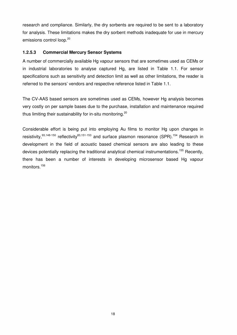
18
research and compliance. Similarly, the dry sorbents are required to be sent to a laboratory
for analysis. These limitations makes the dry sorbent methods inadequate for use in mercury
emissions control loop.20
1.2.5.3 Commercial Mercury Sensor Systems
A number of commercially available Hg vapour sensors that are sometimes used as CEMs or
in industrial laboratories to analyse captured Hg, are listed in Table 1.1. For sensor
specifications such as sensitivity and detection limit as well as other limitations, the reader is
referred to the sensors’ vendors and respective reference listed in Table 1.1.
The CV-AAS based sensors are sometimes used as CEMs, however Hg analysis becomes
very costly on per sample bases due to the purchase, installation and maintenance required
thus limiting their sustainability for in-situ monitoring.20
Considerable effort is being put into employing Au films to monitor Hg upon changes in
resistivity,93,148-150 reflectivity83,151-153 and surface plasmon resonance (SPR).154 Research in
development in the field of acoustic based chemical sensors are also leading to these
devices potentially replacing the traditional analytical chemical instrumentations.155 Recently,
there has been a number of interests in developing microsensor based Hg vapour
monitors.156
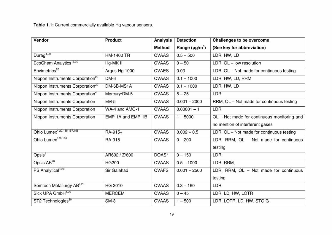
19
Table 1.1: Current commercially available Hg vapour sensors.
Vendor Product Analysis
Method
Detection
Range (µg/m3)
Challenges to be overcome
(See key for abbreviation)
Durag4,20 HM-1400 TR CVAAS 0.5 – 500 LDR, HW, LD
EcoChem Analytics16,20 Hg-MK II CVAAS 0 – 50 LDR, OL – low resolution
Envimetrics20 Argus-Hg 1000 CVAES 0.03 LDR, OL – Not made for continuous testing
Nippon Instruments Corporation20 DM-6 CVAAS 0.1 – 1000 LDR, HW, LD, RRM
Nippon Instruments Corporation20 DM-6B-MS1A CVAAS 0.1 – 1000 LDR, HW, LD
Nippon Instruments Corporation4 Mercury/DM-5 CVAAS 5 – 25 LDR
Nippon Instruments Corporation EM-5 CVAAS 0.001 – 2000 RRM, OL – Not made for continuous testing
Nippon Instruments Corporation WA-4 and AMG-1 CVAAS 0.00001 – 1 LDR
Nippon Instruments Corporation EMP-1A and EMP-1B CVAAS 1 – 5000 OL – Not made for continuous monitoring and
no mention of interferent gases
Ohio Lumex4,20,135,157,158 RA-915+ CVAAS 0.002 – 0.5 LDR, OL – Not made for continuous testing
Ohio Lumex159,160 RA-915 CVAAS 0 – 200 LDR, RRM, OL – Not made for continuous
testing
Opsis4 AR602 / Z/600 DOAS* 0 – 150 LDR
Opsis AB20 HG200 CVAAS 0.5 – 1000 LDR, RRM,
PS Analytical4,20 Sir Galahad CVAFS 0.001 – 2500 LDR, RRM, OL – Not made for continuous
testing
Semtech Metallurgy AB4,20 HG 2010 CVAAS 0.3 – 160 LDR,
Sick UPA GmbH4,20 MERCEM CVAAS 0 – 45 LDR, LD, HW, LOTR
ST2 Technologies20 SM-3 CVAAS 1 – 500 LDR, LOTR, LD, HW, STOIG
20
Tekran, Inc.20 3300 CVAFS 1 – 10 LDR, STOIG, LD, HW
Tekran, Inc.4 2537A CVAFS 0.0001 – 10 LDR, HW, LD, OL – Large sample volumes
Seefelder Messtechnik4 Hg-Mat 2 CVAAS 0 – 75 LDR, LOTR, OL – requires nitrogen at high
flow rates of 6 L/min
Arizona Instrument161-164 Jerome 431-X and
Jerome 431-XE
RGFS** 1 – 990 LDR, LOTR, ABH
Arizona Instrument163 Jerome J405 RGFS** 0.5 – 999 LDR, LOTR, ABH
Arizona Instrument163 Jerome 471 CVAAS 0.03 – 250 LDR
Mercury Instruments Corporation
USA165-168
Mercury Tracker 3000
IP and VM 3000
CVAAS 0.1 – 2000 RRM, OL – works at room temperature and
based gold traps
Institute of Physics -
Lithuania169,170
GARDIS 1A CVAAS 0 – 0.0001 LDR, RRM, ABH
*DOAS = UV Differential Optical Absorption Spectroscopy **RGFS = Resistive Gold Film Sensor
LOTR = Low operating temperature range LD = large Dimension LDR = Low Detection Range
OL = Other Limitations RRM = Requires regular maintenance HW = Heavy Weight
ABH = Affected by humidity STOIG = Sensitive to other interferent gases
21
1.2.6 Acoustic Based Sensors
This section introduces acoustic based sensors and provides justification of using QCM over
the other available acoustic based sensors. Furthermore, a review of the literature is
undertaken where acoustic based Hg vapour sensor developments have been reported.
1.2.6.1 Types of Acoustic Wave Gas Sensors
Acoustic wave gas sensors are based on high frequency mechanical vibrations. This makes
them highly sensitive towards surface perturbations and exhibit good linearity with low
hysteresis and so are ideal for chemical and physical sensing.171,172 They are typically small,
relatively inexpensive, and offer a simple means of analyte monitoring, with several
advantages over other solid-state sensors. These include: well established fabrication
processes, chemical inertness of the substrate materials and high structural rigidity.
The microelectronics industry has developed numerous piezoelectric transducer platforms,
which in turn has widely encouraged the development and improvement of various acoustic
based chemical sensors.171,173 These devices have also been used for the monitoring of
mass uptake,174,175 density,176 viscosity,66 elasticity,177 roughness,178 conductivity and
temperature changes179,180 or a combination of these parameters.181
Acoustic wave devices come in a number of configurations, each with their own distinct
acoustic and electrical characteristics. Two different groups of acoustic wave devices that are
most commonly employed for gas sensing are Bulk Acoustic Wave (BAW) devices, which
concern acoustic wave propagation through the bulk of the structure and as Surface Acoustic
Wave (SAW) devices, utilizing acoustic waves confined to the surface of the piezoelectric
material. These acoustic wave devices operate in a narrow frequency range between 106 –
109 Hz.182 The BAW category of devices includes the QCM and Thin Film Resonators
(TFRs), the latter encapsulating Thin Film Bulk Acoustic Resonator (TFBAR) and Solidly
Mounted Resonator (SMR) structures. Schematic diagrams of all above mentioned devices
these can be observed in Figure 1.1.
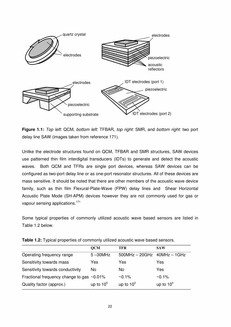
22
Figure 1.1: Top left: QCM, bottom left: TFBAR, top right: SMR, and bottom right: two port
delay line SAW (images taken from reference 171).
Unlike the electrode structures found on QCM, TFBAR and SMR structures, SAW devices
use patterned thin film interdigital transducers (IDTs) to generate and detect the acoustic
waves. Both QCM and TFRs are single port devices, whereas SAW devices can be
configured as two-port delay line or as one-port resonator structures. All of these devices are
mass sensitive. It should be noted that there are other members of the acoustic wave device
family, such as thin film Flexural-Plate-Wave (FPW) delay lines and Shear Horizontal
Acoustic Plate Mode (SH-APM) devices however they are not commonly used for gas or
vapour sensing applications.171
Some typical properties of commonly utilized acoustic wave based sensors are listed in
Table 1.2 below.
Table 1.2: Typical properties of commonly utilized acoustic wave based sensors.
QCM TFR SAW
Operating frequency range 5 –30MHz 500MHz – 20GHz 40MHz – 1GHz
Sensitivity towards mass Yes Yes Yes
Sensitivity towards conductivity No No Yes
Fractional frequency change to gas ~0.01% ~0.1% ~0.1%
Quality factor (approx.) up to 105 up to 103 up to 104
electrodes
quartz crystal
piezoelectric
electrodes
supporting substrate
electrodes
piezoelectric
acoustic reflectors
piezoelectric
IDT electrodes (port 2)
IDT electrodes (port 1)
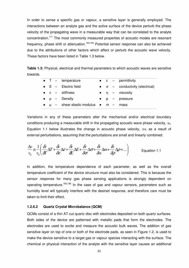
23
In order to sense a specific gas or vapour, a sensitive layer is generally employed. The
interactions between an analyte gas and the active surface of the device perturb the phase
velocity of the propagating wave in a measurable way that can be correlated to the analyte
concentration.171 The most commonly measured properties of acoustic modes are resonant
frequency, phase shift or attenuation.183,184 Potential sensor response can also be achieved
due to the attributions of other factors which affect or perturb the acoustic wave velocity.
These factors have been listed in Table 1.3 below.
Table 1.3: Physical, electrical and thermal parameters to which acoustic waves are sensitive
towards.
T – temperature ε – permittivity
E – Electric field σ – conductivity (electrical)
c – stiffness η – viscosity
ρ – Density p – pressure
µ – shear elastic modulus m – mass
Variations in any of these parameters alter the mechanical and/or electrical boundary
conditions producing a measurable shift in the propagating acoustic wave phase velocity, v0.
Equation 1.1 below illustrates the change in acoustic phase velocity, ∆v, as a result of
external perturbations, assuming that the perturbations are small and linearly combined:
+∆+∆+∆+∆+∆+∆≅
∆...
1
00
ρδρ
δ
δ
δσ
δσ
δ
δ
δε
δε
δ
δ
δ vm
m
vvE
E
vvT
T
v
vv
v Equation 1.1
In addition, the temperature dependence of each parameter, as well as the overall
temperature coefficient of the device structure must also be considered. This is because the
sensor response for many gas phase sensing applications is strongly dependent on
operating temperature.185,186 In the case of gas and vapour sensors, parameters such as
humidity level will typically interfere with the desired response, and therefore care must be
taken to limit their effect.
1.2.6.2 Quartz Crystal Microbalance (QCM)
QCMs consist of a thin AT-cut quartz disc with electrodes deposited on both quartz surfaces.
Both sides of the device are patterned with metallic pads that form the electrodes. The
electrodes are used to excite and measure the acoustic bulk waves. The addition of gas
sensitive layer on top of one or both of the electrode pads, as seen in Figure 1.2, is used to
make the device sensitive to a target gas or vapour species interacting with the surface. The
chemical or physical interaction of the analyte with the sensitive layer causes an additional
24
mass deposition on the quartz surface and as a result a dramatic change in resonant
conditions occurs. The resulting frequency shift can be detected easily and precisely, e.g. in
an oscillator circuit with the resonator as frequency determining part173 or by using a phase
lock loop system.187,188 Additionally the frequency characteristics can be observed by using a
network analyser.189
Figure 1.2: (a) Cross section and (b) graphical projection of a QCM, illustrating a gas
sensitive layer on one electrode (images taken from reference 171).
The application of QCM devices in gas sensing is now well established and
documented.181,190-194 However, it was not until 1959 when Sauerbrey174 determined the
linear relationship between the resonance frequency (∆ƒ) and the mass of a substance
rigidly adsorbed onto the surface (∆m) of the piezoelectric QCM according to the following
equation:
mSmA
ff f
∆−=∆−=∆ρµ
2
02 Equation 1.2
where, 0f is the resonant frequency of the fundamental mode of the crystal, A is the active
area of the electrodes in cm-2, ρq is the quartz crystal density (2.648 g-1.cm-3), µq is the shear
modulus of quartz (2.947×10¹¹ g.cm-1.s-2) and Sƒ is the integral mass sensitivity or Sauerbrey
constant.180,191,195-197 The sensitivity of a QCM device is the ratio of the fractional change in
output signal per fractional change in analyte concentration.
Vapour or gas
Gas sensitive layer
Metal electrodes AT-cut quartz
Gas sensitive layer (active sensing area)
Metal contact
Metal electrode
(a) Cross-section
(b) Graphical projection
25
The main advantage of an increase of 0f is that the mass sensitivity Sƒ=∆ƒ/∆m increases
with 2
0f .198 However, due to the relationship of 0f with that of the bare resonator’s
thickness, sh (equation below) an increased 0f results in a thinner more fragile quartz
substrate.
s
q
q
hf
20
ρµ
= Equation 1.3
A higher mass sensitivity may also be achieved by operating the QCM at higher resonant
frequencies corresponding to odd harmonics in the device, however at the cost of lower
signal to noise ratio.173 According to equation 1.3, the bare quartz resonator thickness for a 5,
10 and 30 MHz QCMs would have thicknesses of 330, 165 and 55 µm respectively.198 Most
applications utilize 5 – 10 MHz resonators. Such plate thicknesses provide a sufficient
mechanical stability as well as high mass sensitivity.199-201
A measure for the quality of the quartz resonator is the Q-factor, which is defined as ratio of
stored energy to that of the dissipated energy. The maximum value for Q is given by material
constants. For the relation to the frequency the following equation applies198:
113
0
1106.1 −×−= s
ff Equation 1.4
The Q-factor of quartz resonators is influenced by factors like impurities, mobility of
impurities, dislocations, hydrogen content of the quartz material, the diameter/thickness ratio
and parallelity of the quartz surfaces.202 Due to additional losses, the value calculated from
equation above is, therefore, not reached in practice. The Q-factor can be calculated on the
base of a modified Butterworth-van-Dyke (BVD) circuit203-205 simplified to the following
equation
lossP
storedEnergyfQ
ower
2 0π= or
dBf
fQ
3
0
∆= Equation 1.5
Where ƒ3dB is the 3 dB bandwidth that can be determined from the resonance behaviour of
the resonators using network analyser.206
Some methods to increase the Q-factor include reducing the diameters of the deposited
electrodes and/or bevelling of the quartz edges (energy trapping method).207 A detailed
description of these concepts is beyond the scope of this thesis and may be found
26
elsewhere.198,208 The fluid mediums as well as the sensitive layer both act as acoustic load on
the quartz resonator when using it as chemical sensor. This results in increased damping
and as a consequence the excitation with an oscillator will be more difficult. The quality of
QCM resonator used as gas sensor strongly depends on the characteristic properties of the
layer (density, viscoelaticity, thickness, etc.).198,209
It is well known that the Sauerbrey’s equation is linear and accurate only up to total electrode
mass loads of ~2% of the mass of quartz substrate204,210 or a frequency change of 2-5% of
the fundamental frequency207,211. The quartz shear modulus and density are 2.947 x 10¹¹
g.cm-1.s and 2.648 g/cm-3 respectively. The quartz wafers considered in this study are 7.5
mm in diameter with a calculated ~167 µm thickness for a 10MHz crystal.198 Considering the
mass loading limitation imposed by Sauerbrey, the maximum total allowable deposited mass
is between 391 to 977 µg given the crystal weighs 19.3 mg.
1.2.6.3 Advantages of QCM over Other Transducers
By far, the most commonly used microsensor is the QCM having an extensive history of use
for quantification of physical and chemical adsorption in both commercial and fundamental
research applications.171 Extensive research has been undertaken examining the prospect of
the QCM as a chemical and gravimetric sensor in different areas, and several commercial
chemical sensing applications of QCMs have been developed, especially for gaseous
species.171,181,212 The QCM is an ideal choice as a transducer in the application of high
concentration Hg vapour sensing since
• They possess relatively high mass sensitivities195
• It has a linear response over a wide range of mass load213
• Stable having zero temperature coefficient around room temperature 214
• Unlike SAW and FPW devices, QCMs are less sensitive to a high mass load, density
and viscosity of the medium making it more robust and suitable for harsh
environments181 and less prone to damping 198
• Unlike TFRs, higher quality factors can be achieved with QCMs increasing the signal
to noise ratio of the device171
Details regarding the comparison of acoustic devices as chemical sensors are given
elsewhere.215-218
In summary, QCMs and their respective electronics are much cheaper than the other
acoustic based sensors mentioned. They attain excellent signal to noise ratio, have excellent
temperature stability specially around room temperature, can be made less fragile while
maintaining high enough sensitivity and are relatively easy to fabricate.198 QCMs are widely
used as on-line thickness monitors in metallic films’ deposition processes.205 Therefore, Hg
27
being a metal itself, it is most practical to use QCMs as the sensor transducer for Hg vapour
sensing.
1.2.6.4 State of the Art Acoustic Based Hg Sensors
CEMs are one of the proposed tools that the EPA sanctions for the analysis of Hg
concentrations in flue gases219 as they offer benefits like20
• Real- or near real-time measure of pollutants’ emission data
• Evaluation and feedback for mercury control strategies
• Greater understanding of process variability and operation
• Potential to be less costly than the current chemical methods, as they require minimal
operator input
• Availability of complete history of data collection
• Greater public assurance
Currently, there are at least nine different CEM models that have been verified by the EPA to
be utilized for monitoring emission of Hg into the air. Many of these are spectroscopy based
and these measurement and monitoring technologies are not entirely accurate or
complete.219 Studies132,220-223 are being undertaken worldwide to overcome the limitations of
CV-AAS and other spectroscopic based Hg sensors and so the quest to develop a robust,
cheap and accurate Hg vapour sensor based on techniques other than CV-AAS is ongoing.
The Jerome analyser, for example, determines the concentration of mercury based on the
resistivity change of the Au electrode upon Hg adsorption/amalgamation.93,94,104,224 This
change in resistance is said to be due to an increase in scattering of conduction electrons at
the Au film when mercury is adsorbed on the surface.61,93,94,225 The Au resistive based
(conductometric) Jerome analyzer is small, easily transported and is useful for indoor
spills.159 It is widely used in some industrial applications.226 However, it is reported to be
incompatible with ammonia and acetylene along with many other interferent chemicals thus
limiting its use in the alumina industries.
Ryan et al.156,227-229 showed an array of conductometric sensors could detect Hg vapour in
humid air. However the sensor was made for the detection of low levels of Hg vapour (ppb
range) and was therefore not suitable for alumina refinery gaseous effluents streams.
Furthermore, the gold film could not be regenerated on the transducer and so PdCl2 was
used as the Hg selective layer. PdCl2 is well known to be incompatible with some VOCs,
acids, nitrates, moisture and ammonia and so this sensor would not be compatible with the
harsh alumina gaseous streams.230,231
28
The Differential Absorption Lidar (DIAL) technique using dye laser systems232 has been used
by various chlor-alkali plants in the past to measure elemental Hg vapour, especially in
Europe.233 They have the disadvantage of needing frequent service due to its fast degrading
gain medium.39 Past attempts overcome the technique’s numerous challenges have
continuously failed. These attempts and the resulting disadvantages is thoroughly covered by
Svanberg et al.39
Toth et al.234 in 2007 reported their ability to identify and measure mercury by prompt gamma
emission, generated by bombardment with neutrons. The method is typically used to sense
in part per billion concentration range of mercury in the gaseous phase. Other methods with
low detection limits also include systems based on laser Induced Fluorescence (LIF)
detection, acoustic and magnetoelastic based sensor that utilise gold thin films. In the case
of the LIF detection, a quantitative determination of gaseous elemental mercury in several
gas matrixes was invented by D’Ottone et al. in 2006.235 In this case Hg is monitored by
exciting either via 1-photon LIF or 2-photon LIF and subsequently detecting the fluorescent
light with an appropriate photomultiplier tube. However, the presence of nitrogen and some
other gases can decrease the signal to noise ratio.
Shao et al.14 used a mercury vapour dosimeter based on a gold-coated magnetoelastic
sensor. Detection of mercury vapour is achieved by monitoring the shift in the sensor’s
acoustic resonant frequency, which changes due to the absorption of mercury on the gold
coating. However, the study of such sensors did not include the effect of interferent gases
while sensing Hg.
In 2005 Thundat et al.236 used the adsorption induced bending method of a piezoelectric
microcantilever to detect 50 ppb mercury concentration in N2 gas. This was a follow up and
improved work done by the same group in 1995.237 Upon Hg vapour exposure, Au coated
microcantilevers, such as those used in atomic force microscopy (AFM), undergo bending
due to the differential stress produced during adsorption, between the microcantilever and its
sensitive layer. This bending reduces the resonating frequency of the resonating
microcantilever. Both the variation of the resonant frequency resulting from the mass
modification of the system or the bending variation may be correlated with the Hg vapour
concentration.238 In Thundat’s case the rate of change of the oscillation frequency was
correlated with the mercury vapour concentration.237,239 These systems however, have also
been shown to detect other chemicals using the same Au sensitive layer240,241, making it
prone to cross sensitivity issues.
29
Butler et al.153 reported a novel device to detect Hg vapour based on the principle that Hg
adsorption to thin Au films causes increase in reflectivity. The reflectivity of the film as a
function of Hg vapour adsorption was followed by measuring the amount of light reflected
back through the Au evaporated fibre. The small size of the device and the small detection
limit in the ppb range were quite exceptional. However, the group later demonstrated in a
separate paper that the same instrument was also sensitive to the adsorption of small
molecules such as SO2, H2S and other species, requiring further development or a separate
filtering step for accurate mercury quantifications.242 past studies have shown however that
by having a filtering stage in the sensing process, reduced Hg readings are observed due to
loss in the filtering stage.88
Acoustic based gravimetric sensors based on Hg sorption to Au sensitive substrate have
been widely studied.80,243-247 Bristow248 first demonstrated the use of Au electrode QCM for
Hg vapour sensing in 1972. Other investigators followed demonstrating the use of these
devices for Hg vapour sensing in the proceeding years due to the QCM device being so ideal
for such application.97,213,249-254 However, none of the studies have shown Hg sensing in the
presence of moisture, ammonia or any other interferent gases. A highly selective layer is
required on the QCM electrode surface for Hg vapour sensing in alumina refinery gaseous
applications.
Vetelino’s group have used ST-cut quartz to fabricate SAW based sensor for low
temperature mercury vapour sensing. It was demonstrated, by studying Au film thickness on
the response of the SAW mercury sensor, that the response magnitude was highest for a
75Å thick gold film. Due to its high sensitivity however, these SAW sensors were only tested
against 20 – 100 ppb Hg vapour without the presence of any interferent gases.99,255,256
Overall, it is generally recognised that acoustic based sensors are less sensitive143 than that
of spectroscopic techniques.67,126 This is highly due to the fact that spectroscopic techniques
use gold traps between sampling and sensing steps while acoustic based sensors may be
used to continuously detect mercury levels in real time. The use of acoustic based sensors in
conjunction with gold trap may also lower their detection limits. Fortunately, for the
development of an acoustic wave based high concentration Hg vapour sensor, such high
sensitivities are not required.
Levlin et al.146 showed that the rate of mercury adsorption on gold is large and significantly
drops after the adsorption of approximately 0.4µg/cm2. This value is just above the estimated
value of 0.36µg/cm2 referring to a monolayer of mercury on a gold surface.67,257 For high
concentrations of Hg vapour, this limit can be reached quite quickly, making the sensor
30
device incapable of differentiating between Hg concentrations. At this stage an acoustic
based sensors’ Au surface needs to be annealed and regenerated. The annealing
temperatures required are reported to range from 150 – 700°C.18,97 Problems are known to
occur at such high annealing temperatures.61,258
The most critical disadvantage of acoustic based sensors arises from the selectivity of the
gold film to collect mercury in the presence of other interferents including hydrogen sulphide
(H2S). Commercially available H2S sensors are available from Jerome based on the same
principle of resistance change of the gold film upon H2S exposure indistinguishable from that
of mercury adsorption.61,259,260 Fortunately, due to the differences in their chemical structures
the response due to H2S is optimum for flatter films having uniform crystallites and compact
grain boundaries. On the other hand, mercury responds optimally on porous polycrystalline
films that contain wide grain boundaries90. This indicates that differentiation may be possible
by using the right selective surface morphology and sensor platform.
Finklea et al.261 investigated the blocking effect of alkanethiol-formed self assembled
monolayers (SAM) on the electrochemical oxidation of gold. Mirsky et al.143 further developed
this concept for Hg vapour sensing in the presence of volatile organic compounds (VOCs).
The conductometric sensor was based on the decreasing lateral electrical conductivity of thin
Au films upon sorption of Hg vapour. Hexadecanethiol SAM was deposited on the gold film
before exposure to Hg in the presence of interferents. It was found that the SAM layers
blocked the effects of humidity as well as some volatile sulphuric compounds but not of Hg.
However, other studies have shown that Hg adsorption on Au substrates with alkanethiol
SAMs induces reorientation and reorganisation of the alkanethiols both on complete and
incomplete monolayers262,263 creating Hg nanoparticles.264 These SAMs layer containing Hg
sensors are therefore non-stable when exposed to Hg containing environments and needs
further development.
There exists a need for development of acoustic based sensors to overcome the limitations
of, for example spectroscopic techniques for Hg vapour sensing in industrial environment
applications. However, acoustic based sensors themselves are associated with their own
limitations. These limitations are encouraged to be overcome with research and development
since advantages such as their overall small size, ease of use, ability to be used as
continuous online sensors, low cost and low power consumption far outweigh their
limitations. The low cost is the result of their easy fabrication in batch quantities making them
thousands of dollars less than their competing spectroscopic techniques.155,265
31
1.3 Conclusions
Over 90% of Hg emissions occur from anthropogenic sources. The ill effects of Hg on health
and environment are well documented yet there is lack of any reliable, robust and accurate
online Hg vapour sensor for monitoring and control of anthropogenic Hg vapour emissions.
The current commercially available Hg vapour sensors all have drawbacks such as
sensitivity (i.e. high Hg concentrations saturating the sorbent material resulting in
breakthrough of the metal and underestimation of the concentrations) and cross
contamination due to other interferent gases present in the effluent streams. This is the
reason for various groups investigating new collectors and methods for Hg vapour sensing.
These collection and analysis methods themselves are found to have limitations.
Literature on the interaction of Hg with that of Au suggests lack of full understanding of the
process. Therefore further investigation is required before the development of highly stable,
sensitive and selective Hg vapour sensors. For such sensors, high surface area of the
sensitive layer as well as low Hg exposure times is prescribed. QCM sensors are thought to
be the optimal choice of transducers. Among all else, their electrode surfaces may be
modified to produce a sensitive and selective Hg sensor. A good balance between sensitivity,
signal to noise ratio and fragility is postulated to be the choice of a 10 MHz crystal. Being
less fragile, their electrode surfaces may be modified for selectivity and sensitivity more
efficiently.
To the best of the Author’s knowledge, no work exists regarding the surface modification of
Au for Hg vapour sensing in industrial effluents. Further investigation is required to study to
interaction of Hg with that of Au in order to decide on the optimum surface modification
technique(s) for Hg vapour sensor development. The development of a mercury sensor
suited to alumina refineries will be a significant breakthrough in controlling anthropogenic
mercury emissions from many industries.
32
1.4 References
(1) Goldman, R. L.; Shannon, M. W. Pediatrics 2001, 108, 197-205. (2) Rong, Y.; David Tee, L.; Joo Hwa, T. Environmental Science and Pollution Research
International 2003, 10, 399-407. (3) Palomares, E.; Vilar, R.; Durrant, J. R. Chem. Commun. 2004, 362-363. (4) Laudal, D. L.; French, N. B. In Conference On Air Quality II: Mercury 2000; Vol. 2, p 1-16. (5) Lockley, I. Emission Reduction program, 2007. (6) Sabri, Y. M.; Ippolito, S. J.; Bhargava, S. K. Light Metals 2009 2009, 37-42. (7) Government, A.; Department of the Environment, W., Heritage and the Arts, Ed.; National
Pullutant Inventory: 2009; Vol. 2007-2008. (8) Morency, J. Filtration & Separation 2002, 39, 24-26. (9) Germani, M. S.; Zollert, W. H. Environmental Science & Technology 1988, 22, 1079-1085. (10) Fthenakis, V. M.; Lipfert, F. W.; Moskowitz, P. D.; Saroff, L. Journal of Hazardous Materials
1995, 44, 267-283. (11) Dobbs, C.; Armanios, C.; McGuiness, L.; Bauer, G.; Ticehurst, P.; Lochore, J.; Irons, R.; Ryan,
R.; Adamek, G. In 7th International Alumina Quality Workshop Perth, Western Australia, 2005, p 199-204.
(12) Shao, R.; Tan, E. L.; Grimes, C. A.; Ong, K. G. Sensors Letters 2007, 5, 6. (13) Windham, R. L. Analytical Chemistry 1972, 44, 1334-1336. (14) Sabri, Y. M.; Ippolito, S. J.; Tardio, J.; Sood, D. K.; Bhargava, S. K.; Mullett, M.; Harrison, I.;
Rosenberg, S. In 8th International Alumina Quality Workshop Darwin, Australia, 2008, p 260-266.
(15) Caron, J. J. Surface Acoustic Wave Continuous Emissions Monitor for Total Mercury, Sensor Research and Development Corporation, 2001.
(16) Schweyer, M. G.; Andle, J. C.; McAllister, D. J.; Vetelino, J. F. Sensors and Actuators B: Chemical 1996, 35, 170-175.
(17) Laudal, D. L.; Thompson, J. S.; Pavlish, J. H.; Brickett, L. A.; Chu, P. Fuel Processing Technology 2004, 85, 501-511.
(18) Holmes, M.; Pavlish, J.; EERC, Ed. North Dakota, 2004; Vol. 2009. (19) Canstein, H. V.; Kelly, S.; Li, Y.; Wagner-Dobler, I. Applied and Environmental Microbiology
2002, 68, 2829-2837. (20) Schrope, M. Nature news 2001, 409, 124-124. (21) Smith, R. P. Nature 2005, 436, 779-779. (22) Stokstad, E. Science 2004, 303, 34-. (23) Boyd, A. S.; Seger, D.; Vannucci, S.; Langley, M.; Abraham, J. L.; King, L. E. J. Journal of the
American Academy of Dermatology 2000, 43, 81-90. (24) Graeme, K. A.; Pollack, C. V. The Journal of emergency medicine 1998, 16, 45-56. (25) Baughman, T. A. Environmental Health Perspectives 2006, 114, 147-152. (26) Trasande, L.; Landrigan, P. J.; Schechter, C. Environmental Health Perspectives 2005, 113,
590-596. (27) LaMontagne, A. D.; Steenland, N. K.; Kelsey, K. Ethylene oxide; fourth ed.; Lippincott &
Wilkins: Philadelphia, 2007. (28) Morris, T. A. PhD by Research, The University of Alabama, 2004. (29) Laudal, D. L.; Brown, T. D.; Nott, B. R. Fuel Processing Technology 2000, 65-66, 157-165. (30) Bergan, T.; Gallardo, L.; Rodhe, H. Atmospheric Environment 1999, 33, 1575-1585. (31) Pacyna, E. G.; Pacyna, J. M.; Pirrone, N. Atmospheric Environment 2001, 35, 2987-2996. (32) Kalac, P.; Niznanská, M.; Bevilaqua, D.; Stasková, I. Science of The Total Environment 1996,
177, 251-258. (33) Mukherjee, A. B.; Melanen, M.; Ekqvist, M.; Verta, M. The Science of The Total Environment
2000, 259, 73-83. (34) Slemr, F.; Scheel, H. E. Atmospheric Environment 1998, 32, 845-853. (35) Shetty, S. K.; Lin, C.-J.; Streets, D. G.; Jang, C. Atmospheric Environment 2008, 42, 8674-
8685. (36) Pacyna, E. G.; Pacyna, J. M. Water, Air, & Soil Pollution 2002, 137, 149-165. (37) Sjöholm, M.; Weibring, P.; Edner, H.; Svanberg, S. Opt. Express 2004, 12, 551-556. (38) Swain, E. B.; Jakus, P. M.; Rice, G.; Lupi, F.; Maxson, P. A.; Pacyna, J. M.; Penn, A.; Spiegel,
S. J.; Veiga, M. M. AMBIO: A Journal of the Human Environment 2007, 36, 45-61. (39) Government, A. Mercury & compounds Emissions - All sources: Australia, National Pollutant
Inventory, 2006-2007. (40) Alcoa Environmental Review and Management Program, Alcoa, 2005.
33
(41) Kockman, D.; Horvat, M.; Jacimovic, R.; Gibicar, D. RMZ - Materials and Geoenvironment 2005, 52, 71-74.
(42) Mullett, M.; Tardio, J.; Bhargava, S.; Dobbs, C. Journal of Hazardous Materials 2007, 144, 274-282.
(43) Lacerda, L. D. Water, Air, & Soil Pollution 1997, 97, 247-255. (44) Johnson, J. Chemical and Engineering News 2001, 79, 18-19. (45) Powers, R. A. Proceedings of the IEEE 1995, 83, 687-693. (46) Pavlish, J. H.; Sondreal, E. A.; Mann, M. D.; Olson, E. S.; Galbreath, K. C.; Laudal, D. L.;
Benson, S. A. Fuel Processing Technology 2003, 82, 89-165. (47) Camargo, J. A. Nature 1993, 365, 302-302. (48) Hirokatsu Akagi, Y. F., Eigo Takabatake, Photochemistry and Photobiology 1977, 26, 363-
370. (49) Pak, K.-R.; Bartha, R. Appl. Environ. Microbiol. 1998, 64, 1987-1990. (50) Bidone, E. D.; Castilhos, Z. C.; Cid de Souza, T. M.; Lacerda, L. D. Bulletin of Environmental
Contamination and Toxicology 1997, 59, 194-201. (51) Carpi, A. Water, Air, & Soil Pollution 1997, 98, 241-254. (52) Vallee, B. L.; Ulmer, D. D. Annual Review of Biochemistry 1972, 41, 91-128. (53) Gillis, A. A.; Miller, D. R. The Science of The Total Environment 2000, 260, 191-200. (54) Schroeder, W. H.; Munthe, J. Atmospheric Environment 1998, 32, 809-822. (55) Hacon, S.; Rochedo, E. R.; Campos, R.; Rosales, G.; Lacerda, L. D. Water, Air, & Soil
Pollution 1997, 97, 91-105. (56) Scallan, K. F., University of California, 2007. (57) Levlin, M.; Ikävalko, E.; Laitinen, T. Fresenius' Journal of Analytical Chemistry 1999, 365, 577-
586. (58) Guminski, C. Journal of the Less Common Metals 1991, 168, 329-334. (59) McNerney, J. J.; Buseck, P. R.; Hanson, R. C. Science 1972, 178, 611-612. (60) Granite, E. J.; Pennline, H. W.; Hargis, R. A. Industrial & Engineering Chemistry Research
2000, 39, 1020-1029. (61) Braman, R. S.; Johnson, D. L. Environmental Science & Technology 1974, 8, 996-1003. (62) Yan, T. Y. Industrial & Engineering Chemistry Research 1994, 33, 3010-3014. (63) Diggs, T. H.; Ledbetter, J. O. American Industrial Hygiene Association Journal 1983, 44, 606 -
608. (64) Reed, C. E.; Kanazawa, K. K.; Kaufman, J. H. Journal of Applied Physics 1990, 68, 1993-
2001. (65) Dumarey, R.; Dams, R.; Hoste, J. Analytical Chemistry 1985, 57, 2638-2643. (66) Schroeder, W. H.; Hamilton, M. C.; Stobart, S. R. REV. ANALYT. CHEM. 1985, 8, 179-209. (67) Be'er, A.; Lereah, Y.; Frydman, A.; Taitelbaum, H. Physica A: Statistical Mechanics and its
Applications 2002, 314, 325-330. (68) Guminski, C.; Galus, A.; Hirayama, C. In Solubility Data Series: Metals in Mercury; Warsaw,
U. O., Ed.; Pergamon Press: Warsaw, Poland, 1986; Vol. 25, p 258-384. (69) Strachan, J. F.; Harris, N. L. Journal of the Institute of Metals 1956, 85, 17-24. (70) Sunier, A. A.; Gramkee, B. E. Journal of the American Chemical Society 1929, 51, 1703-1708. (71) Sunier, A. A.; Weiner, L. G. Journal of the American Chemical Society 1931, 53, 1714-1721. (72) Sunier, A. A.; White, C. M. Journal of American Chemical Society 1930, 52, 1842-1850. (73) Mees, G. Journal of the American Chemical Society 1938, 60, 870-871. (74) Anderson, J. T. The Journal of Physical Chemistry 1932, 36, 2145-2165. (75) Brown, J. B. Journal of Chemical Education 1960, 37, 415. (76) Levlin, M.; Ikavalko, E.; Laitinen, T. Fresenius Journal of Analytical Chemistry 1999, 365, 577-
586. (77) Rex, M.; Hernandez, F. E.; Campiglia, A. D. Analytical Chemistry 2006, 78, 445-451. (78) Ruys, D. P.; Andrade, J. F.; Guimaraes, O. M. Analytica Chimica Acta 2000, 404, 95-100. (79) Battistoni, C.; Bemporad, E.; Galdikas, A.; Kaciulis, S.; Mattogno, G.; Mickevicius, S.;
Olevano, V. Applied Surface Science 1996, 103, 107-111. (80) Morris, T.; Szulczewski, G. Langmuir 2002, 18, 5823-5829. (81) Morris, T.; Szulczewski, G. Langmuir 2002, 18, 2260-2264. (82) Morris, T.; Sun, J.; Szulczewski, G. Analytica Chimica Acta 2003, 496, 279-287. (83) Kobiela, T.; Nowakowski, B.; Dus, R. Applied Surface Science 2003, 206, 78-89. (84) Nowakowski, R.; Kobiela, T.; Wolfram, Z.; Dus, R. Applied Surface Science 1997, 115, 217-
231. (85) Fialkowski, M.; Grzeszczak, P.; Nowakowski, R.; Holyst, R. The Journal of Physical Chemistry
B 2004, 108, 5026-5030. (86) Brosset, C.; Iverfeldt, Å. Water, Air, & Soil Pollution 1989, 43, 147-168.
34
(87) Sabri, Y. M.; Ippolito, S. J.; Tardio, J.; Atanacio, A. J.; Sood, D. K.; Bhargava, S. K. Sensors and Actuators B: Chemical 2009, 137, 246-252.
(88) George, M. A. PhD by research, Arizona State University, 1991. (89) Aiyer, H. N.; Kawazoe, T.; Lim, J.; Echigo, Y.; Ohtsu, M. Nanotechnology 2001, 12, 368-371. (90) Be'er, A.; Hecht, I.; Taitelbaum, H. Physical Review E 2005, 72, 031606. (91) George, M. A.; Glaunsinger, W. S. Thin Solid Films 1994, 245, 215-224. (92) George, M. A.; Glaunsinger, W. S.; Thundat, T.; Lindsay, S. M. Thin Solid Films 1990, 189,
59-72. (93) Nowakowski, R.; Pielaszek, J.; Dus, R. Applied Surface Science 2002, 199, 40-51. (94) Yang, X. M.; Tonami, K.; Nagahara, L. A.; Hashimoto, K.; Wei, Y.; Fujishima, A. Surface
Science 1994, 319, L17-L22. (95) Scheide, E. P.; Taylor, J. K. American Industrial Hygiene Association Journal 1975, 36, 897 -
901. (96) Stobinski, L.; Dus, R. Surface Science 1993, 298, 101-106. (97) Haskell, R. L. B.; Caron, J. J.; Duptisea, M. A.; Ouellette, J. J.; Vetelino, J. F. In Ultrasonics
Symposium, 1999. Proceedings; IEEE: Orono, ME, 1999; Vol. 1, p 429-434 vol.1. (98) Chaurasia, H. K.; Huizinga, A.; Voss, W. A. G. Journal of Physics D: Applied Physics 1975, 8,
214-218. (99) Drelich, J.; White, C. L.; Xu, Z. Environ. Sci. Technol. 2008, 42, 2072-2078. (100) Kalb, G. W. Atomic Absorption Newsletter 1970, 9, 4. (101) Larjava, K.; Laitinen, T.; Vahlman, T.; Artmann, S.; Siemens, V.; Broekaert, J. A. C.; Klockow,
D. International journal of environmental analytical chemistry 1992, 49, 73 - 85. (102) Larjava, K.; Laitinen, T.; Kiviranta, T.; Siemens, V.; Klockow, D. International journal of
environmental analytical chemistry 1993, 52, 65-73. (103) Jansen, H. J. F.; Freeman, A. J.; Weinert, M.; Wimmer, E. Physical Review B 1983, 28, 593. (104) Mott, N. F. Philosophical Magazine 1961, 6, 287 - 309. (105) Dowben, P. A. Surface Science Reports 2000, 40, 151-247. (106) Miedema, A. R.; Dorleijn, J. W. F. Philosophical Magazine Part B: Physics of Condensed
matter: Statistical Mechanics, Electronics, Optical and Magnetic Properties 1981, 43, 251-272. (107) Schmutzler, R. W.; Hensel, F. Journal of Non-Crystalline Solids 1972, 8-10, 718-721. (108) El-Hanany, U.; Warren, W. W. Physical Review Letters 1975, 34, 1276. (109) Even, U.; Jortner, J. Physical Review Letters 1972, 28, 31. (110) Hensel, F. Berichte der Bunsengesellschaft fur Physikalische Chemie 1976, 80, 786-789. (111) Cheshnovski, O.; Even, U.; Jortner, J. Solid State Communications 1977, 22, 745-748. (112) Gaston, N.; Schwerdtfeger, P. Physical Review B (Condensed Matter and Materials Physics)
2006, 74, 024105-12. (113) Ballone, P.; Galli, G. Physical Review B 1989, 40, 8563. (114) Steckel, J. A. Physical Review B (Condensed Matter and Materials Physics) 2008, 77,
115412. (115) Bloch, A. N.; Rice, S. A. Physical Review 1969, 185, 933. (116) Kutana, A.; Giapis, K. P. Nano Lett. 2006, 6, 656-661. (117) Chandra, S.; Di Marzo, M.; Qiao, Y. M.; Tartarini, P. Fire Safety Journal 1996, 27, 141-158. (118) Henn, A. R. Biophysical Chemistry 2003, 105, 533-543. (119) Lennard-Jones, J. E.; Corner, J. Transactions of the Faraday Society 1940, 36, 1156-1162. (120) Joseph McGuire, E. L., Robert D. Sproull, Surface and Interface Analysis 1990, 15, 603-608. (121) Rhee, S. K. Journal of the American Ceramic Society 1970, 53, 386-389. (122) Granite, E. J. In Annual International Pittsburgh Coal Conference Pittsburgh, 2003; Vol. 20, p
983-1010. (123) Abollino, O.; Giacomino, A.; Malandrino, M.; Piscionieri, G.; Mentasti, E. Electroanalysis 2008,
20, 75-83. (124) Clevenger, W. L.; Smith, B. W.; Winefordner, J. D. Critical Reviews in Analytical Chemistry
1997, 27, 1-26. (125) Temmerman, E.; Vandecasteele, C.; Vermeir, G.; Leyman, R.; Dams, R. Analytica Chimica
Acta 1990, 236, 371-376. (126) Sánchez Uría, J. E.; Sanz-Medel, A. Talanta 1998, 47, 509-524. (127) Blanco, R. M.; Villanueva, M. T.; Uría, J. E. S.; Sanz-Medel, A. Analytica Chimica Acta 2000,
419, 137-144. (128) Das, A. K.; de la Guardia, M.; Cervera, M. L. Talanta 2001, 55, 1-28. (129) Logar, M.; Horvat, M.; Akagi, H.; Pihlar, B. Analytical and Bioanalytical Chemistry 2002, 374,
1015-1021. (130) Tong, X.; Barat, R. B.; Poulos, A. T. Review of Scientific Instruments 2002, 73, 2392-2397. (131) Granite, E. J.; Pennline, H. W. Industrial & Engineering Chemistry Research 2002, 41, 5470-
5476.
35
(132) Weissberg, B. G. Economic Geology 1971, 66, 1042-1047. (133) Sholupov, S.; Pogarev, S.; Ryzhov, V.; Mashyanov, N.; Stroganov, A. Fuel Processing
Technology 2004, 85, 473-485. (134) Rocha, T. A. P.; Gomes, M. T. S. R.; Duarte, A. C.; Oliveira, J. A. B. P. Analytical
Communication 1998, 35, 415-416. (135) Richton, R. E.; Farrow, L. A. The Journal of Physical Chemistry 2002, 85, 3577-3581. (136) Bilic, A.; Reimers, J. R.; Hush, N. S.; Hafner, J. The Journal of Chemical Physics 2002, 116,
8981-8987. (137) Kay, B. D.; Lykke, K. R.; Creighton, J. R.; Ward, S. J. The Journal of Chemical Physics 1989,
91, 5120-5121. (138) Surplice, N. A.; Brearley, W. Surface Science 1975, 52, 62-74. (139) Nuss, H.; Jansen, M. ChemInform 2006, 37. (140) de Vooys, A. C. A.; Mrozek, M. F.; Koper, M. T. M.; van Santen, R. A.; van Veen, J. A. R.;
Weaver, M. J. Electrochemistry Communications 2001, 3, 293-298. (141) Mirsky, V. M.; Vasjari, M.; Novotny, I.; Rehacek, V.; Tvarozek, V.; Wolfbeis, O. S.
Nanotechnology 2002, 13, 175-178. (142) Meyer, R.; Lemire, C.; Shaikhutdinov, S. K.; Freund, H. Gold Bulletin 2004, 37, 72-124. (143) Caron, J. J. O., ME), Haskell, Reichl B. (Veazie, ME), Freeman, Carl J. (Rockville, MD),
Vetelino, John F. (Orono, ME); Sensor Research and Development Corp. (Orono, ME): United States, 1999.
(144) Levlin, M.; Niemi, H. E. M.; Hautojärvi, P.; Ikävalko, E.; Laitinen, T. Fresenius' Journal of Analytical Chemistry 1996, 355, 2-9.
(145) Kvietkus, K.; Xiao, Z.; Lindqvist, O. Water, Air, & Soil Pollution 1995, 80, 1209-1216. (146) RA-915+, l. (147) Lumex 2008. (148) Gochfeld, M. Ecotoxicology and Environmental Safety 2003, 56, 174-179. (149) Holland, K. New York, 2005; Vol. 2009. (150) Ritchie, K. A.; Burke, F. J. T.; Gilmour, W. H.; Macdonald, E. B.; Dale, I. M.; Hamilton, R. M.;
McGowan, D. A.; Binnie, V.; Collington, D.; Hammersley, R. British Dental Journal 2004, 197, 625-632.
(151) Kramer, C. 2001; Vol. 2008. (152) Arizona Instruments LLC Arizona, 2007; Vol. 2009, p mercury sensors. (153) Wu, J. M.; Huang, H. S.; Livengood, C. D. Development of a sorbent-based technology for
control of mercury in flue gas, 1996. (154) Loredo, J.; Soto, J.; Álvarez, R.; Ordóñez, A. Environmental Monitoring and Assessment
2007, 130, 201-214. (155) Monitor, T. V. M. V. 2006, p Mercury sensor. (156) Choi, H. K.; Lee, S. H.; Kim, S. S. Fuel Processing Technology 2009, 90, 107-112. (157) Mercury Instruments USA 2009; Vol. 2009. (158) Wängberg, I.; Edner, H.; Ferrara, R.; Lanzillotta, E.; Munthe, J.; Sommar, J.; Sjöholm, M.;
Svanberg, S.; Weibring, P. The Science of The Total Environment 2003, 304, 29-41. (159) Ferrara, R.; Mazzolai, B. The Science of The Total Environment 1998, 215, 51-57. (160) Skreblin, M.; Byrne, A. R. Vestnik Slovenskega Kemijskega Drustva 1991, 38, 16. (161) Mazzolai, B.; Mattoli, V.; Raffa, V.; Tripoli, G.; Accoto, D.; Menciassi, A.; Dario, P. Sensors
and Actuators A: Physical 2004, 113, 282-287. (162) Mazzolai, B.; Mattoli, V.; Raffa, V.; Tripoli, G.; Accoto, D.; Menciassi, A.; Dario, P. In Sensors
and Microsystems, Proceedings of the Italian Conference; 8 ed. Trento, Italy,, 2003; Vol. 8, p 369-375.
(163) Morris, T.; Kloepper, K.; Wilson, S.; Szulczewski, G. Journal of Colloid and Interface Science 2002, 254, 49-55.
(164) Dimasi, E.; Tostmann, H.; Ocko, B. M.; Huber, P.; Shpyrko, O. G.; Pershan, P. S.; Deutsch, M.; Berman, L. E. In Materials Research Society Symposium Proceedings 2000; Vol. 590, p 183-188.
(165) Butler, M. A.; Ricco, A. J.; Baughman, R. J. Journal of Applied Physics 1990, 67, 4320-4326. (166) Chah, S.; Yi, J.; Zare, R. N. Sensors and Actuators B: Chemical 2004, 99, 216-222. (167) Hughes, R. C.; Ricco, A. J.; Butler, M. A.; Martin, S. J. Science 1991, 254, 74-80. (168) Ryan, M. A.; Homer, M. L.; Shevade, A. V.; Lara, L. M.; Yen, S.-P. S.; Kisor, A. K.; Manatt, K.
S. ECS Meeting Abstracts 2008, 16, 431-439. (169) Ippolito, S. J.; Trinchi, A.; Powell, D. A.; Wlodarski, W. Solid State Gas Sensing; Springer
Science+Business Media, LLC: Brescia, Italy, 2009; Vol. 1. (170) Ballantine, D. S.; Wohltjen, H. Analytical Chemistry 1989, 61, 704A-715A. (171) Ward, M. D.; Buttry, D. A. Science 1990, 249, 1000-1007. (172) Sauerbrey, G. Zeitschrift für Physik A Hadrons and Nuclei 1959, 155, 206-222.
36
(173) Martin, S. J.; Granstaff, V. E.; Frye, G. C. Analytical Chemistry 1991, 63, 2272-2281. (174) Kanazawa, K. K.; Gordon, J. G. Analytical Chemistry 1985, 57, 1770-1771. (175) Martin, S. J.; Frye, G. C.; Ricco, A. J.; Senturia, S. D. Analytical Chemistry 1993, 65, 2910-
2922. (176) Dong, Y. Sensors and Actuators B: Chemical 2005, 108, 622-626. (177) Smith, A. L.; Shirazi, H. M. Thermochimica Acta 2005, 432, 202-211. (178) Smith, A. L.; Shirazi, H. M.; Mulligan, S. R. Biochimica et Biophysica Acta (BBA) - Protein
Structure and Molecular Enzymology 2002, 1594, 150-159. (179) Al Kobaisi, M. Doctor of Philosophy, Royal Melbourne Institue of Technology University, 2008. (180) Janshoff, A.; Galla, H.-J.; Steinem, C. Angewandte Chemie 2000, 39, 4004-4032. (181) Beil, F. W.; Blick, R. H.; Wixforth, A. Physica E: Low-dimensional Systems and Nanostructures
2004, 21, 1106-1110. (182) Schweyer, M. G.; Weaver, J. T.; Andle, J. C.; McAllister, D. J.; French, L.; Vetelino, J.; Height,
J. J. In Frequency Control Symposium, 1997., Proceedings of the 1997 IEEE International 1997, p 147-155.
(183) Venema, A.; Nieuwkoop, E.; Vellekoop, M. J.; Ghijsen, W. J.; Barendsz, A. W.; Nieuwenhuizen, M. S. IEEE Transactions on Ultrasonics, Ferroelectrics and Frequency Control 1987, 34, 148-155.
(184) Thiele, J. A.; da Cunha, M. P. Sensors and Actuators B: Chemical 2006, 113, 816-822. (185) Arnau, A.; Ferrari, V.; Soares, D.; Perrot, H. In Piezoelectric Transducers and Applications;
Springer Berlin Heidelberg: 2008, p 117-186. (186) Arnau, A. Sensors 2008, 8, 370-411. (187) O'Sullivan, C. K.; Guilbault, G. G. Biosensors and Bioelectronics 1999, 14, 663-670. (188) James, D.; Scott, S. M.; Ali, Z.; O’Hare, W. T. Microchimica Acta 2005, 149, 1-17. (189) Cheeke, J. D. N.; Wang, Z. Sensors and Actuators B: Chemical 1999, 59, 146-153. (190) Khlebarov, Z. P.; Stoyanova, A. I.; Topalova, D. I. Sensors and Actuators B: Chemical 1992,
8, 33-40. (191) Fox, C. G.; Alderm, J. F. Analyst 1989, 114, 997-1004. (192) Ali, Z. Journal of thermal analysis and calorimetry 1999, 55, 397-412. (193) Tsionsky, V.; Gileadi, E. Langmuir 1994, 10, 2830-2835. (194) Flitti, F.; Far, A.; Guo, B.; Bermak, A. Journal of Sensors 2008, 2008, 1-6. (195) Buck, R. P.; Lindner, E.; Kutner, W.; Inzelt, G. Pure & Applied Chemistry 2004, 76, 1139-1160. (196) Zimmermann, B.; Lucklum, R.; Hauptmann, P.; Rabe, J.; Büttgenbach, S. Sensors and
Actuators B: Chemical 2001, 76, 47-57. (197) Sagmeister, B. P.; Graz, I. M.; Schwödiauer, R.; Gruber, H.; Bauer, S. Biosensors and
Bioelectronics 2009, 24, 2643-2648. (198) Bender, J. W.; Krim, J. In Microscale Diagnostic Techniques 2005, p 227-259. (199) Herrmann, F.; Jakoby, B.; Rabe, J.; Büttgenbach, S. Sensors Update 2001, 9, 105-160. (200) Ballato, A.; Gualtieri, J. G. Ultrasonics, Ferroelectrics and Frequency Control, IEEE
Transactions on 1994, 41, 834-844. (201) Lakin, K. M.; Wang, J. S. Applied Physics Letters 1981, 38, 125-127. (202) Granstaff, V. E.; Martin, S. J. Journal of Applied Physics 1994, 75, 1319-1329. (203) Behling, C.; Lucklum, R.; Hauptmann, P. Sensors and Actuators A: Physical 1997, 61, 260-
266. (204) Thanner, H.; Krempl, P.; Selic, R.; Wallnöfer, W.; Worsch, P. Journal of Thermal Analysis and
Calorimetry 2003, 71, 53-59. (205) Bechmann, R. Journal of Scientific Instruments 1952, 29, 73-76. (206) Shockley, W.; Curran, D. R.; Koneval, D. J. The Journal of the Acoustical Society of America
1967, 41, 981-993. (207) Behling, C.; Lucklum, R.; Hauptmann, P. Sensors and Actuators A: Physical 1998, 68, 388-
398. (208) Mecea, V. M. Sensors and Actuators A: Physical 1994, 40, 1-27. (209) Lu, C.-S.; Lewis, O. Journal of Applied Physics 1972, 43, 4385-4390. (210) Ippolito, S. J. PhD by research, RMIT university, 2006. (211) Ho, M. H.; Guilbault, G. G.; Scheide, E. P. Analytica Chimica Acta 1981, 130, 141-147. (212) Konash, P. L.; Bastiaans, G. J. Analytical Chemistry 1980, 52, 1929-1931. (213) Grate, J. W.; Martin, S. J.; White, R. M. Analytical Chemistry 1993, 65, 987A-996A. (214) Benes, E.; Gröschl, M.; Burger, W.; Schmid, M. Sensors and Actuators A: Physical 1995, 48,
1-21. (215) Auge, J., University of Magdeburg, 1995. (216) Janata, J.; Josowicz, M.; DeVaney, D. M. Analytical Chemistry 1994, 66, 207-228. (217) Bethea, T.; Cady-Sawyer, K.; Ettenson, L.; Harris, K.; Mandl, D.; Martynowicz, K.;
Raeisghasem, A.; Westman, D. Columbia, USA, 2005.
37
(218) Fox, B. S.; Mason, K. J.; McElroy, F. C. Journal of ASTM International (JAI) 2005, 2, 11. (219) Meischen, S. J.; VanPelt, V. J.; Zarate, E. A. In 95
th Proceedings of the Air & Waste
Management Association’s Annual Conference & Exhibition 2002, p 1364-1378. (220) Magnuson, J. K.; Anderson, T. N.; Lucht, R. P.; Vijayasarathy, U. A.; Kalyan, A. In 23
rd
Proceedings - Annual International Pittsburgh Coal Conference (2006) Pittsburgh, 2006; Vol. 14, p 1-14.
(221) Appel, D.; Grassi, J. H.; Kita, D.; Socha, J. United States, 2008. (222) Raffa, V.; Mazzolai, B.; Mattoli, V.; Mondini, A.; Dario, P. Sensors and Actuators B: Chemical
2006, 114, 513-521. (223) McNerney, J. J.; Buseck, P. R. Gold Bulletin 1973, 6, 106-107. (224) Jerome411X. (225) Shevade, A.; Blanco, M.; Goddard, W.; Ryan, M.; Homer, M.; Taylor, C.; Jewell, A.; Kisor, A.;
Yen, S.-P.; Manatt, K.; Zhou, H.; Pelletier, C.; Lewis, C. ECS Meeting Abstracts 2006, 601, 1243-1243.
(226) Ryan, M. A.; Homer, M. L.; Zhou, H.; Mannat, K.; Manfreda, A.; Kisor, A. K.; Shevade, A. V.; Yen, S.-P. S. In International Conference on Environmental Systems; Jet Propulsion Laboratory, National Aeronautics and Space Administration: Rome, Italy, 2005, p 1-8.
(227) Ryan, M. A.; Shevade, A. V.; Zhou, H.; Homer, M. L. MRS Bulletin 2004, 29, 714. (228) Huang, S. W.; Neoh, K. G.; Shih, C. W.; Lim, D. S.; Kang, E. T.; Han, H. S.; Tan, K. L.
Synthetic Metals 1998, 96, 117-122. (229) Choudary, B. M.; Madhi, S.; Chowdari, N. S.; Kantam, M. L.; Sreedhar, B. Journal of the
American Chemical Society 2002, 124, 14127-14136. (230) Weibring, P.; Andersson, M.; Edner, H.; Svanberg, S. Applied Physics B: Lasers and Optics
1998, 66, 383-388. (231) Edner, H.; Ragnarson, P.; Wallinder, E. Environmental Science & Technology 2002, 29, 330-
337. (232) Toth, J. J.; Wittman, R.; Schenter, R. E.; Cooper, J. A. Nuclear Instruments and Methods in
Physics Research Section A: Accelerators, Spectrometers, Detectors and Associated Equipment 2007, 572, 1102-1105.
(233) D'ottone, L. K. B., FL, US) United States, 2006. (234) Adams, J. D.; Rogers, B.; Manning, L.; Hu, Z.; Thundat, T.; Cavazos, H.; Minne, S. C. Sensors
and Actuators A: Physical 2005, 121, 457-461. (235) Thundat, T.; Wachter, E. A.; Sharp, S. L.; Warmack, R. J. Applied Physics Letters 1995, 66,
1695-1697. (236) Fadel, L.; Dufour, I.; Lochon, F.; Francais, O. Sensors and Actuators B: Chemical 2004, 102,
73-77. (237) Hu, Z.; Thundat, T.; Warmack, R. J. Journal of Applied Physics 2001, 90, 427-431. (238) Berger, R.; Delamarche, E.; Lang, H. P.; Gerber, C.; Gimzewski, J. K.; Meyer, E.; Güntherodt,
H. J. Applied Physics A: Materials Science & Processing 1998, 66, S55-S59. (239) Marie, R.; Jensenius, H.; Thaysen, J.; Christensen, C. B.; Boisen, A. Ultramicroscopy 2002,
91, 29-36. (240) Butler, M. A.; Ricco, A. J. Applied Physics Letters 1988, 53, 1471-1473. (241) Manganiello, L.; Rios, A.; Valcarcel, M. Analytical Chemistry 2002, 74, 921-925. (242) Yao, S.; Tan, S.; Nie, L. Fenxi Huaxue 1986, 14, 6. (243) Casilli, S.; Malitesta, C.; Conoci, S.; Petralia, S.; Sortino, S.; Valli, L. Biosensors and
Bioelectronics 2004, 20, 1190-1195. (244) Rogers, B.; Bauer, C. A.; Adams, J. D. Micro-Electro-Mechanical Systems 2003, 5, 663-666. (245) Gomes, M. T. S. R.; Oliveira, M. O.; Oliveira, J. A. B. P. Langmuir 1999, 15, 8780-8782. (246) Bristow, Q. Journal of Geochemical Exploration 1972, 1, 55-76. (247) Scheide, E. P.; Taylor, J. K. Environ. Sci. Technol. 1974, 8, 1097-1099. (248) Scheide, E. P. Physics Teacher 1977, 15, 47-51. (249) McCammon, C. S. J.; Woodfin, J. W. American Industrial Hygiene Association Journal 1977,
38, 378-386. (250) Scheide, E. P.; Warnar, R. B. American Industrial Hygiene Association Journal 1978, 39, 745-
749. (251) Mogilevski, A. N.; Mayorov, A. D.; Stroganova, N. S.; Stavrovski, D. B.; Galkina, I. P.;
Spassov, L.; Mihailov, D.; Zaharieva, R. Sensors and Actuators A: Physical 1991, 28, 35-39. (252) Spassov, L.; Yankov, D. Y.; Mogilevski, A. N.; Mayorov, A. D. Review of Scientific Instruments
1993, 64, 225-227. (253) Caron, J. J.; Haskell, R. B.; Benoit, P.; Vetelino, J. F. IEEE transactions on ultrasonics,
ferroelectrics, and frequency control 1998, 45, 1393-1398. (254) Haskell, R. B. Masters, University of Maine, 2003. (255) Mercer, T. T. Analytical Chemistry 1979, 51, 5.
38
(256) Hirvonen, J. K.; Weisenberger, W. H.; Westmoreland, J. E.; Meussner, R. A. Applied Physics Letters 1972, 21, 37-39.
(257) Cox, H. H. J.; Deshusses, M. A. Chemical Engineering Journal 2002, 87, 101-110. (258) McNamara, J. D.; Wagner, N. J. Gas Separation & Purification 1996, 10, 137-140. (259) Finklea, H. O.; Avery, S.; Lynch, M.; Furtsch, T. Langmuir 2002, 3, 409-413. (260) Himmelhaus, M.; Buck, M.; Grunze, M. Applied Physics B: Lasers and Optics 1999, 68, 595-
598. (261) Thome, J.; Himmelhaus, M.; Zharnikov, M.; Grunze, M. Langmuir 1998, 14, 7435-7449. (262) Aliganga, A. K. A.; Wang, Z.; Mittler, S. The Journal of Physical Chemistry B 2004, 108,
10949-10954. (263) Li, D.; Ma, M. Sensors and Actuators B: Chemical 2000, 69, 75-84.
39
Chapter II
Chapter 2 Experimental Setup
Experimental setup, sensor fabrication, instrumentation and literature
considerations during the course of the present work are discussed in this chapter.
40
2.1 Overview
The development and testing of QCM sensors for mercury vapour requires many
considerations. There are numerous physical and electrical components that make up the
mercury vapour calibration system and the instrumentation used to characterize the sensors’
material properties and performance. In this chapter, the chemicals, list of characterization
techniques, sensor fabrication methods and Hg sensing system as well as their theoretical
considerations will be listed and discussed.
2.1.1 Mercury Delivery and Sampling System
A mercury vapour delivery and data acquisition system was designed and constructed, the
schematic of which is shown in Figure 2.1. One mass flow power supply (A, 647C Four-
channel Mass Flow and Pressure Programmer/Display) controlling four mass flow meters
(A1-A4, Mass-Flo® M100B), were purchased from MKS, USA. A1 was connected to
3388 ppm ammonia cylinder balanced by nitrogen gas (CORGAS, Australia). A2-A4 were all
connected to dry nitrogen gas supplies. A2 was used as the nitrogen dilution gas in the
system while A3 and A4 were connected to the humidity (B) and Hg vapour (C) generators
respectively. The lines consisted of 1/8” SS tubing (SS25-T2-S-035-BA), electronic-no-space
3-way gas ball valve switches (D, 51SC – electrical part and SS-41GXS2 – ball valve switch),
10 psi check valves for one way gas flow only (E, SS-2C-10), Pressure gauges (F, PGI-63B-
PG20_CAQ1), Vernier meter for pressure control (G, SS-SS2-VH), and back pressure
regulators (H, KBP1D0D4A5A20000) all purchased from Swagelok, Australia. The sulfur
impregnated carbon traps (I) SS parts were built from Swagelok products. The sensors’
housing/testing chamber (J) was made from Teflon and SS parts that were custom machined
(also referred to as laboratory chamber. The baratron (K, 628D Baratron® Heated Absolute
Capacitance Manometer (0-2,000 Torr) Temperature Controlled to 100°C) at the chamber
exit was also purchased from MKS, USA and used to measure and log the online pressure in
the chamber. The flow meters at the end of the lines (L) were used to confirm gas flow out of
the system. The temperature of the chamber was controlled with a high current power supply
(M, 6033A – Agilent Technologies, Australia) while the heating tapes (HT, EW-36050-55,
Cole Parmer, Australia) were controlled with the temperature controller (N, TCCOBOXU –
Temperature Controls) and was able to be monitored through the system temperature logger
(O, USB TC-08, Pico Technology, USA) and control and acquisition computers (P). The
issues of contamination, Hg or humidity condensation in the system, temperature fluctuations
or pressure fluctuations were all dealt with by controlling the temperature of each section of
the system and installation of various parts listed above. The Hg trap bottles (Q) containing
potassium permanganate and sulfuric acid solutions (Sigma Aldrich, Australia) were placed
just before the gas stream entered the sensors’ chamber. The water trap (Q2) was place to
ensure flow of the NH3 gas while bleeding the cylinder before directing the flow to the testing
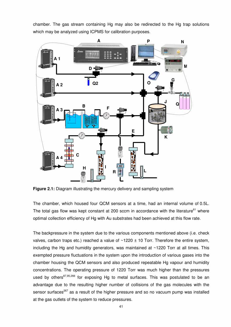
41
chamber. The gas stream containing Hg may also be redirected to the Hg trap solutions
which may be analyzed using ICPMS for calibration purposes.
Figure 2.1: Diagram illustrating the mercury delivery and sampling system
The chamber, which housed four QCM sensors at a time, had an internal volume of 0.5L.
The total gas flow was kept constant at 200 sccm in accordance with the literature61 where
optimal collection efficiency of Hg with Au substrates had been achieved at this flow rate.
The backpressure in the system due to the various components mentioned above (i.e. check
valves, carbon traps etc.) reached a value of ~1220 ± 10 Torr. Therefore the entire system,
including the Hg and humidity generators, was maintained at ~1220 Torr at all times. This
exempted pressure fluctuations in the system upon the introduction of various gases into the
chamber housing the QCM sensors and also produced repeatable Hg vapour and humidity
concentrations. The operating pressure of 1220 Torr was much higher than the pressures
used by others87,95,266 for exposing Hg to metal surfaces. This was postulated to be an
advantage due to the resulting higher number of collisions of the gas molecules with the
sensor surfaces267 as a result of the higher pressure and so no vacuum pump was installed
at the gas outlets of the system to reduce pressures.
A 1
A 2
A 3
A 4 C
B
A
A
D
F
K
E
I
J
G
L
M
NP
Q
O
RH
Q2
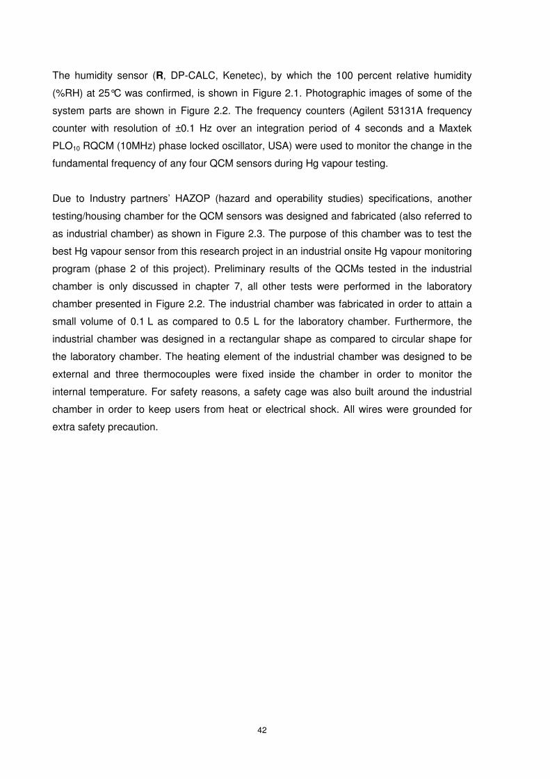
42
The humidity sensor (R, DP-CALC, Kenetec), by which the 100 percent relative humidity
(%RH) at 25°C was confirmed, is shown in Figure 2.1. Photographic images of some of the
system parts are shown in Figure 2.2. The frequency counters (Agilent 53131A frequency
counter with resolution of ±0.1 Hz over an integration period of 4 seconds and a Maxtek
PLO10 RQCM (10MHz) phase locked oscillator, USA) were used to monitor the change in the
fundamental frequency of any four QCM sensors during Hg vapour testing.
Due to Industry partners’ HAZOP (hazard and operability studies) specifications, another
testing/housing chamber for the QCM sensors was designed and fabricated (also referred to
as industrial chamber) as shown in Figure 2.3. The purpose of this chamber was to test the
best Hg vapour sensor from this research project in an industrial onsite Hg vapour monitoring
program (phase 2 of this project). Preliminary results of the QCMs tested in the industrial
chamber is only discussed in chapter 7, all other tests were performed in the laboratory
chamber presented in Figure 2.2. The industrial chamber was fabricated in order to attain a
small volume of 0.1 L as compared to 0.5 L for the laboratory chamber. Furthermore, the
industrial chamber was designed in a rectangular shape as compared to circular shape for
the laboratory chamber. The heating element of the industrial chamber was designed to be
external and three thermocouples were fixed inside the chamber in order to monitor the
internal temperature. For safety reasons, a safety cage was also built around the industrial
chamber in order to keep users from heat or electrical shock. All wires were grounded for
extra safety precaution.
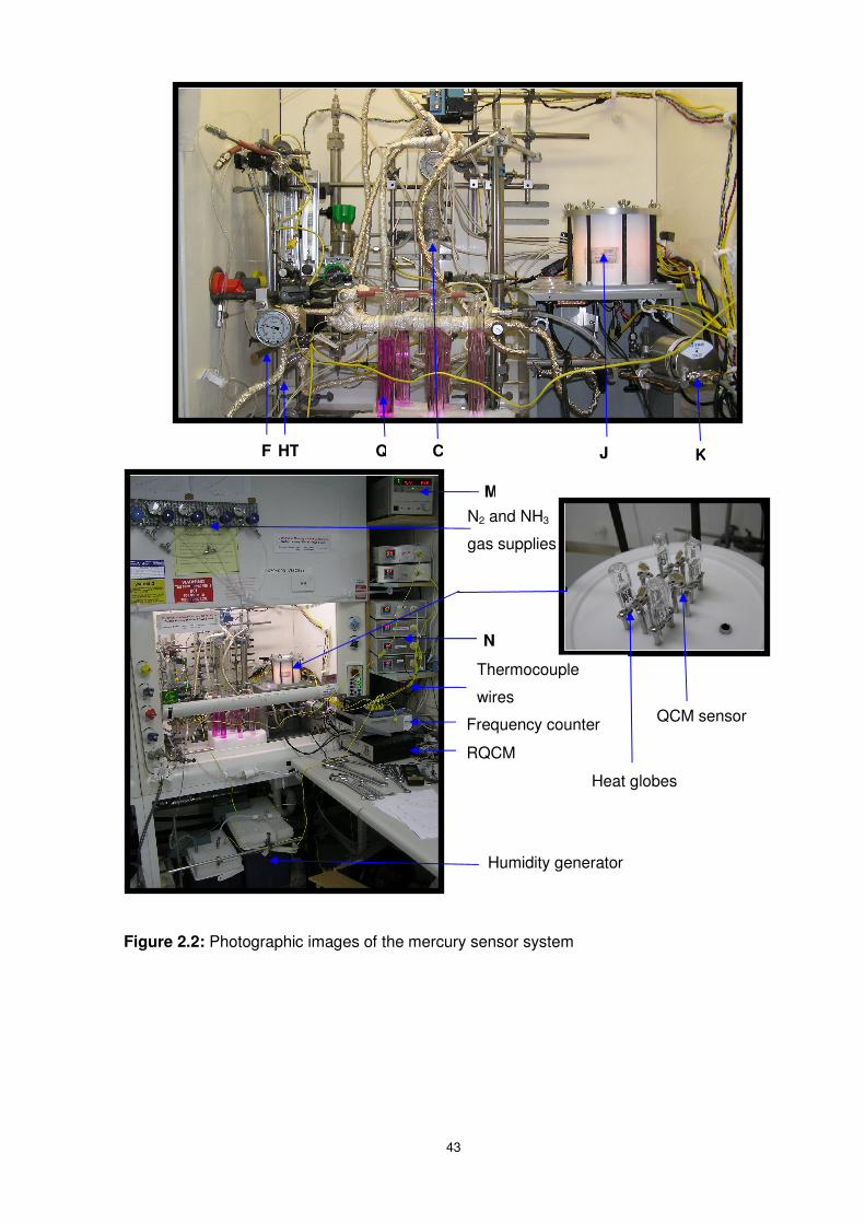
43
Figure 2.2: Photographic images of the mercury sensor system
Humidity generator
F HT Q C J K
Thermocouple
wires
Frequency counter
RQCM
N2 and NH3
gas supplies
M
N
QCM sensor
Heat globes
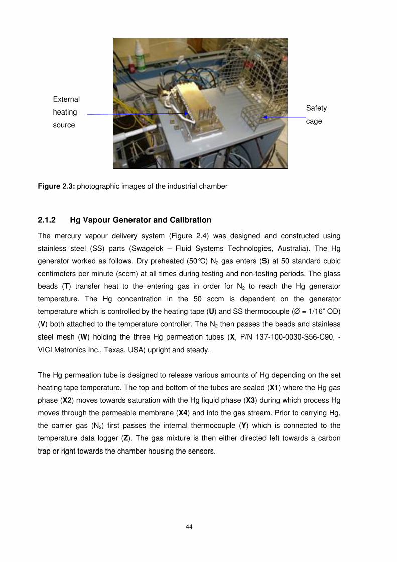
44
Figure 2.3: photographic images of the industrial chamber
2.1.2 Hg Vapour Generator and Calibration
The mercury vapour delivery system (Figure 2.4) was designed and constructed using
stainless steel (SS) parts (Swagelok – Fluid Systems Technologies, Australia). The Hg
generator worked as follows. Dry preheated (50°C) N2 gas enters (S) at 50 standard cubic
centimeters per minute (sccm) at all times during testing and non-testing periods. The glass
beads (T) transfer heat to the entering gas in order for N2 to reach the Hg generator
temperature. The Hg concentration in the 50 sccm is dependent on the generator
temperature which is controlled by the heating tape (U) and SS thermocouple (Ø = 1/16” OD)
(V) both attached to the temperature controller. The N2 then passes the beads and stainless
steel mesh (W) holding the three Hg permeation tubes (X, P/N 137-100-0030-S56-C90, -
VICI Metronics Inc., Texas, USA) upright and steady.
The Hg permeation tube is designed to release various amounts of Hg depending on the set
heating tape temperature. The top and bottom of the tubes are sealed (X1) where the Hg gas
phase (X2) moves towards saturation with the Hg liquid phase (X3) during which process Hg
moves through the permeable membrane (X4) and into the gas stream. Prior to carrying Hg,
the carrier gas (N2) first passes the internal thermocouple (Y) which is connected to the
temperature data logger (Z). The gas mixture is then either directed left towards a carbon
trap or right towards the chamber housing the sensors.
External
heating
source
Safety
cage
45
Figure 2.4: Hg vapour generator and permeation tube
Calibration
The Hg permeation tubes were verified by calibrating them in line with the system using a
method similar to that of EPA method 101A.268 This involved preparing the trap solution
which was made of 10% (v/v) sulfuric acid and 4% (m/v) potassium permanganate balanced
by milli-Q water (resistivity of 18.2 MΩ.cm, purified by use of a milli-Q reagent deionizer,
Millipore). A train of 3 dreschel bottles was then connected in series, each bottle containing
the trap solution and was connected to the system close to the point where Hg vapour enters
the chamber. The gas stream was redirected isokinetically (200 sccm with 50sccm from Hg
generator and 150 sccm N2 gas through 1/8” SS tubes from the chamber towards the Hg trap
train for 100 minutes, repeated three times at each of the five Hg vapour concentrations
tested. The solution from each bottle was then diluted and analysed by ICPMS (as described
in section 2.5.6), the overall results over the course of the work are shown in Figure 2.5. The
mercury vapour generated was found to be repeatable within ±0.05 mg/m3 over the 100
minute calibration period. The temperature inside the Hg generator was data logged to
monitor the Hg generation stability at all times. The pressure of the generator was constant
whether the gas was directed towards the carbon trap, the chamber or the Hg traps for
calibration. The calibration graph shows the Hg concentration in the final 200 sccm gas
entering the chamber. This means the 50 sccm flow through the Hg generator consists of 4
times the Hg concentration. The 50°C temperature of the tubes (controlled by heating tapes
X
X 1
Z
X 4
X 3
W
SS tube Ø = 1” OD
SS nut Ø = 1” OD
SS nut Ø = 1/16” OD
Y
T
X
Two way switch directing Hg stream
X 2
S
U
V
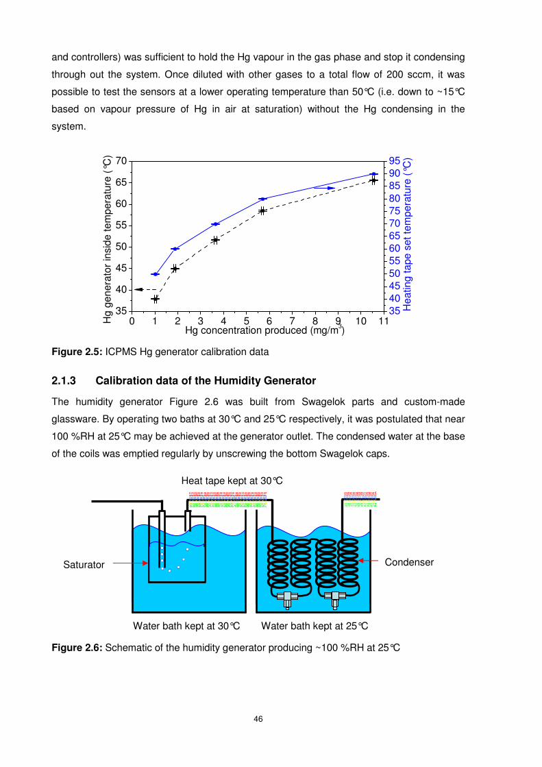
46
and controllers) was sufficient to hold the Hg vapour in the gas phase and stop it condensing
through out the system. Once diluted with other gases to a total flow of 200 sccm, it was
possible to test the sensors at a lower operating temperature than 50°C (i.e. down to ~15°C
based on vapour pressure of Hg in air at saturation) without the Hg condensing in the
system.
Figure 2.5: ICPMS Hg generator calibration data
2.1.3 Calibration data of the Humidity Generator
The humidity generator Figure 2.6 was built from Swagelok parts and custom-made
glassware. By operating two baths at 30°C and 25°C respectively, it was postulated that near
100 %RH at 25°C may be achieved at the generator outlet. The condensed water at the base
of the coils was emptied regularly by unscrewing the bottom Swagelok caps.
Figure 2.6: Schematic of the humidity generator producing ~100 %RH at 25°C
Water bath kept at 30°C Water bath kept at 25°C
Heat tape kept at 30°C
Saturator Condenser
0 1 2 3 4 5 6 7 8 9 10 1135
40
45
50
55
60
65
70
Hea
ting
tape
set
tem
pera
ture
(°C
)
Hg
gene
rato
r in
side
tem
pera
ture
(°C
)
Hg concentration produced (mg/m3)
35404550556065707580859095
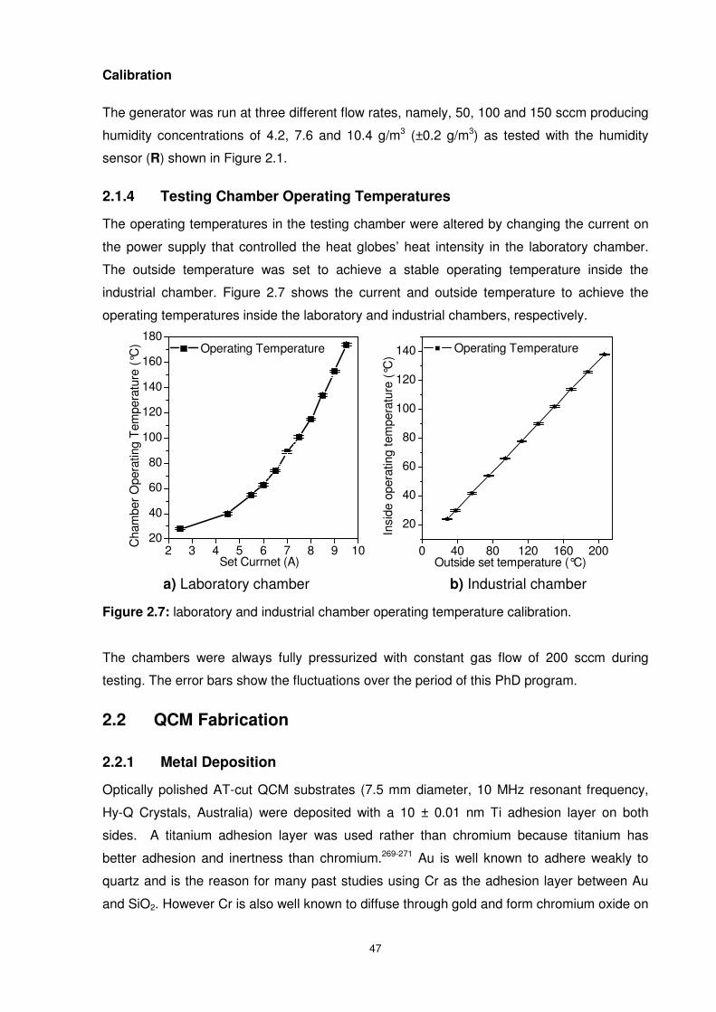
47
Calibration
The generator was run at three different flow rates, namely, 50, 100 and 150 sccm producing
humidity concentrations of 4.2, 7.6 and 10.4 g/m3 (±0.2 g/m3) as tested with the humidity
sensor (R) shown in Figure 2.1.
2.1.4 Testing Chamber Operating Temperatures
The operating temperatures in the testing chamber were altered by changing the current on
the power supply that controlled the heat globes’ heat intensity in the laboratory chamber.
The outside temperature was set to achieve a stable operating temperature inside the
industrial chamber. Figure 2.7 shows the current and outside temperature to achieve the
operating temperatures inside the laboratory and industrial chambers, respectively.
Figure 2.7: laboratory and industrial chamber operating temperature calibration.
The chambers were always fully pressurized with constant gas flow of 200 sccm during
testing. The error bars show the fluctuations over the period of this PhD program.
2.2 QCM Fabrication
2.2.1 Metal Deposition
Optically polished AT-cut QCM substrates (7.5 mm diameter, 10 MHz resonant frequency,
Hy-Q Crystals, Australia) were deposited with a 10 ± 0.01 nm Ti adhesion layer on both
sides. A titanium adhesion layer was used rather than chromium because titanium has
better adhesion and inertness than chromium.269-271 Au is well known to adhere weakly to
quartz and is the reason for many past studies using Cr as the adhesion layer between Au
and SiO2. However Cr is also well known to diffuse through gold and form chromium oxide on
2 3 4 5 6 7 8 9 1020
40
60
80
100
120
140
160
180
Operating Temperature
Set Currnet (A)
Cha
mbe
r O
pera
ting
Tem
pera
ture
(°C
)
b) Industrial chamber a) Laboratory chamber
0 40 80 120 160 200
20
40
60
80
100
120
140
Outside set temperature (°C)
Operating Temperature
Insi
de o
pera
ting
tem
pera
ture
(°C
)
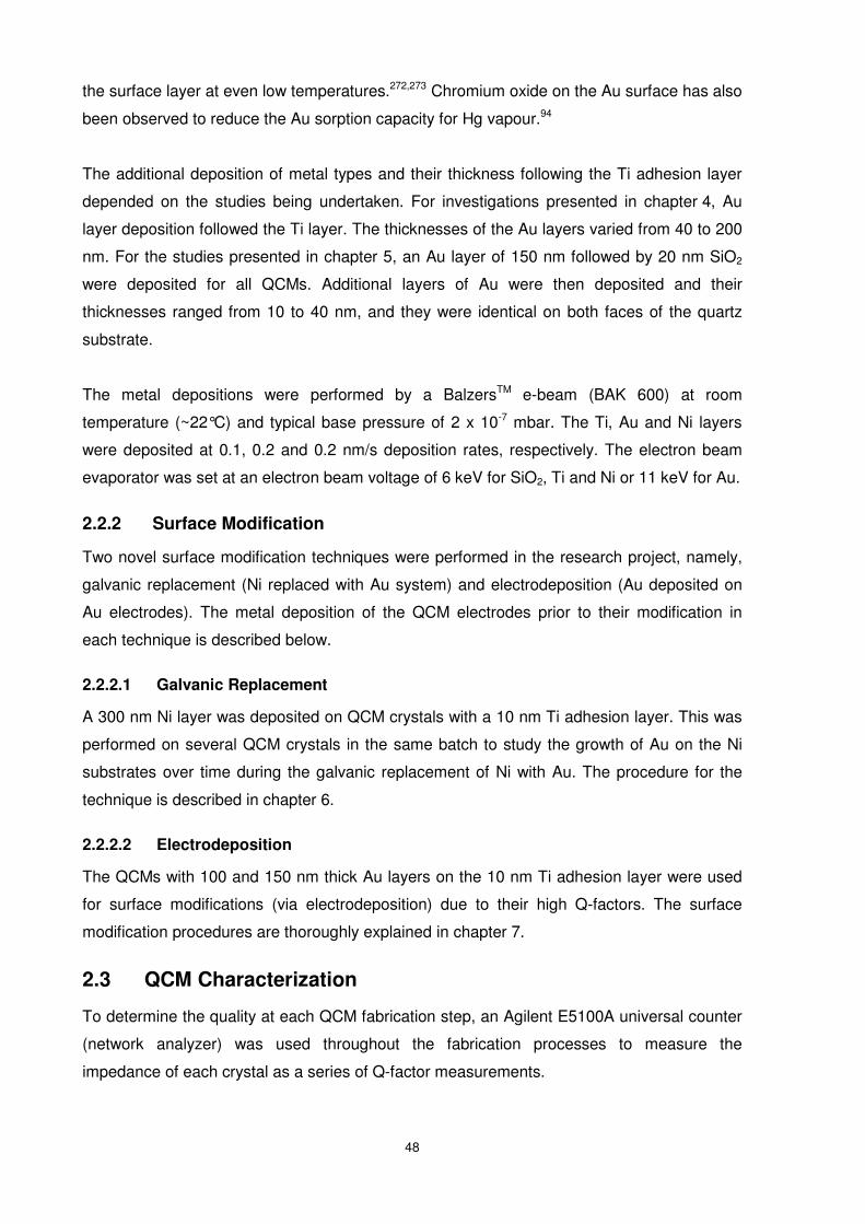
48
the surface layer at even low temperatures.272,273 Chromium oxide on the Au surface has also
been observed to reduce the Au sorption capacity for Hg vapour.94
The additional deposition of metal types and their thickness following the Ti adhesion layer
depended on the studies being undertaken. For investigations presented in chapter 4, Au
layer deposition followed the Ti layer. The thicknesses of the Au layers varied from 40 to 200
nm. For the studies presented in chapter 5, an Au layer of 150 nm followed by 20 nm SiO2
were deposited for all QCMs. Additional layers of Au were then deposited and their
thicknesses ranged from 10 to 40 nm, and they were identical on both faces of the quartz
substrate.
The metal depositions were performed by a BalzersTM e-beam (BAK 600) at room
temperature (~22°C) and typical base pressure of 2 x 10⁻⁷ mbar. The Ti, Au and Ni layers
were deposited at 0.1, 0.2 and 0.2 nm/s deposition rates, respectively. The electron beam
evaporator was set at an electron beam voltage of 6 keV for SiO2, Ti and Ni or 11 keV for Au.
2.2.2 Surface Modification
Two novel surface modification techniques were performed in the research project, namely,
galvanic replacement (Ni replaced with Au system) and electrodeposition (Au deposited on
Au electrodes). The metal deposition of the QCM electrodes prior to their modification in
each technique is described below.
2.2.2.1 Galvanic Replacement
A 300 nm Ni layer was deposited on QCM crystals with a 10 nm Ti adhesion layer. This was
performed on several QCM crystals in the same batch to study the growth of Au on the Ni
substrates over time during the galvanic replacement of Ni with Au. The procedure for the
technique is described in chapter 6.
2.2.2.2 Electrodeposition
The QCMs with 100 and 150 nm thick Au layers on the 10 nm Ti adhesion layer were used
for surface modifications (via electrodeposition) due to their high Q-factors. The surface
modification procedures are thoroughly explained in chapter 7.
2.3 QCM Characterization
To determine the quality at each QCM fabrication step, an Agilent E5100A universal counter
(network analyzer) was used throughout the fabrication processes to measure the
impedance of each crystal as a series of Q-factor measurements.
49
For electrical characterisation, the resonators were mounted on a circuit board. The
electrodes were wire bonded. All impedance data were calibrated and test fixture
compensated. All the impedance measurements, to U/45 crystal bases, were carried out at
room temperature (22°C). A PI network test fixture containing a coupler and power splitter
was used to study the QCM resonator coating properties in the sensor development
process.181 All the circuit connections were BNC and all the leads RG 58 coaxial cables.
One of the characteristic features of quartz resonators are the frequencies of the harmonic
vibration modes where the surface movement is in phase and the same direction. Beside
these harmonic modes, inharmonic vibration modes are generated, which are often called
spurious modes. These are characterised by the movement of particles in several regions of
the quartz surface in antiphase. One of the most important requirements for operating a
quartz resonator as a chemical sensor is the frequency stability. If the frequency separation
between the harmonic and inharmonic modes is not sufficient, neighbouring frequencies may
cross each other. This could cause effects such as mode coupling and frequency jumps. All
these effects would impede a reliable frequency measurement, which commonly serves as
output signal. One of the main goals in the design of the resonators is a sufficient separation
of the harmonic from the inharmonic vibration modes.198
For this reason a relatively wide frequency band width had to be scanned in order to examine
the separation of the inharmonic and the harmonic fundamental modes. For the
measurement of the broad band characteristics, the bandwidths ranged from 9 to 11 MHz
depending on the frequency position of the inharmonics relative to the fundamental mode.
For a detailed characterisation and the determination of the equivalent circuit values at the
fundamental resonant frequency, the bandwidth was reduced to 1-2 kHz. The data for the 10
MHz optically polished Au (Ti/Au = 10/100 nm) at spans of 20 kHz and 2 kHz is shown in
Figures 2.8a and 2.8b, respectively.
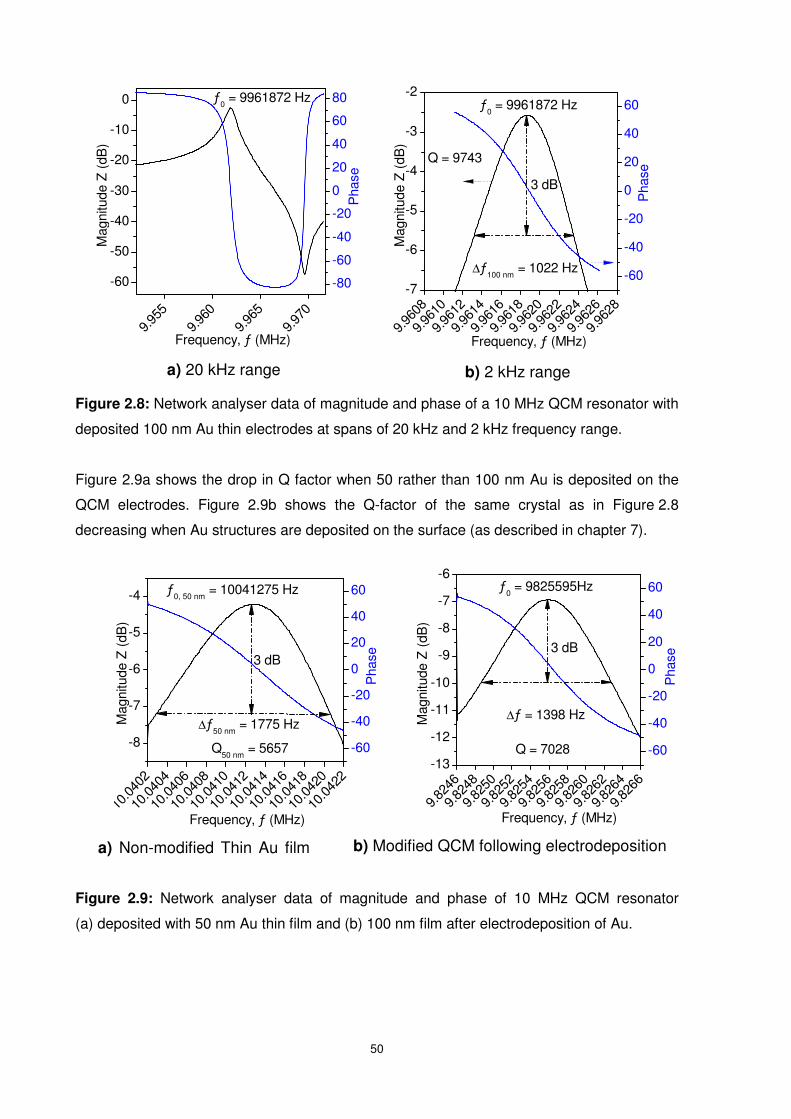
50
Figure 2.8: Network analyser data of magnitude and phase of a 10 MHz QCM resonator with
deposited 100 nm Au thin electrodes at spans of 20 kHz and 2 kHz frequency range.
Figure 2.9a shows the drop in Q factor when 50 rather than 100 nm Au is deposited on the
QCM electrodes. Figure 2.9b shows the Q-factor of the same crystal as in Figure 2.8
decreasing when Au structures are deposited on the surface (as described in chapter 7).
Figure 2.9: Network analyser data of magnitude and phase of 10 MHz QCM resonator
(a) deposited with 50 nm Au thin film and (b) 100 nm film after electrodeposition of Au.
b) Modified QCM following electrodeposition a) Non-modified Thin Au film
10.04
02
10.04
04
10.04
06
10.04
08
10.04
10
10.04
12
10.04
14
10.04
16
10.04
18
10.04
20
10.04
22
-8
-7
-6
-5
-4
-60
-40
-20
0
20
40
60
ƒ0, 50 nm
= 10041275 Hz
3 dB
Frequency, ƒ (MHz)
Pha
se
Mag
nitu
de Z
(dB
)
Q50 nm
= 5657
∆ƒ50 nm
= 1775 Hz
9.824
6
9.824
8
9.825
0
9.825
2
9.825
4
9.825
6
9.825
8
9.826
0
9.826
2
9.826
4
9.826
6-13
-12
-11
-10
-9
-8
-7
-6
-60
-40
-20
0
20
40
60
ƒ0 = 9825595Hz
3 dB
Frequency, ƒ (MHz)
Pha
se
Mag
nitu
de Z
(dB
)
Q = 7028
∆ƒ = 1398 Hz
b) 2 kHz range a) 20 kHz range
9.955
9.960
9.965
9.970
-60
-50
-40
-30
-20
-10
0
-80
-60
-40
-20
0
20
40
60
80
ƒ
0 = 9961872 Hz
Frequency, ƒ (MHz)P
hase
Mag
nitu
de Z
(dB
)
9.960
8
9.961
0
9.961
2
9.961
4
9.961
6
9.961
8
9.962
0
9.962
2
9.962
4
9.962
6
9.962
8-7
-6
-5
-4
-3
-2
-60
-40
-20
0
20
40
60
ƒ0 = 9961872 Hz
3 dB
Frequency, ƒ (MHz)
Pha
se
Mag
nitu
de Z
(dB
)
Q = 9743
∆ƒ100 nm
= 1022 Hz
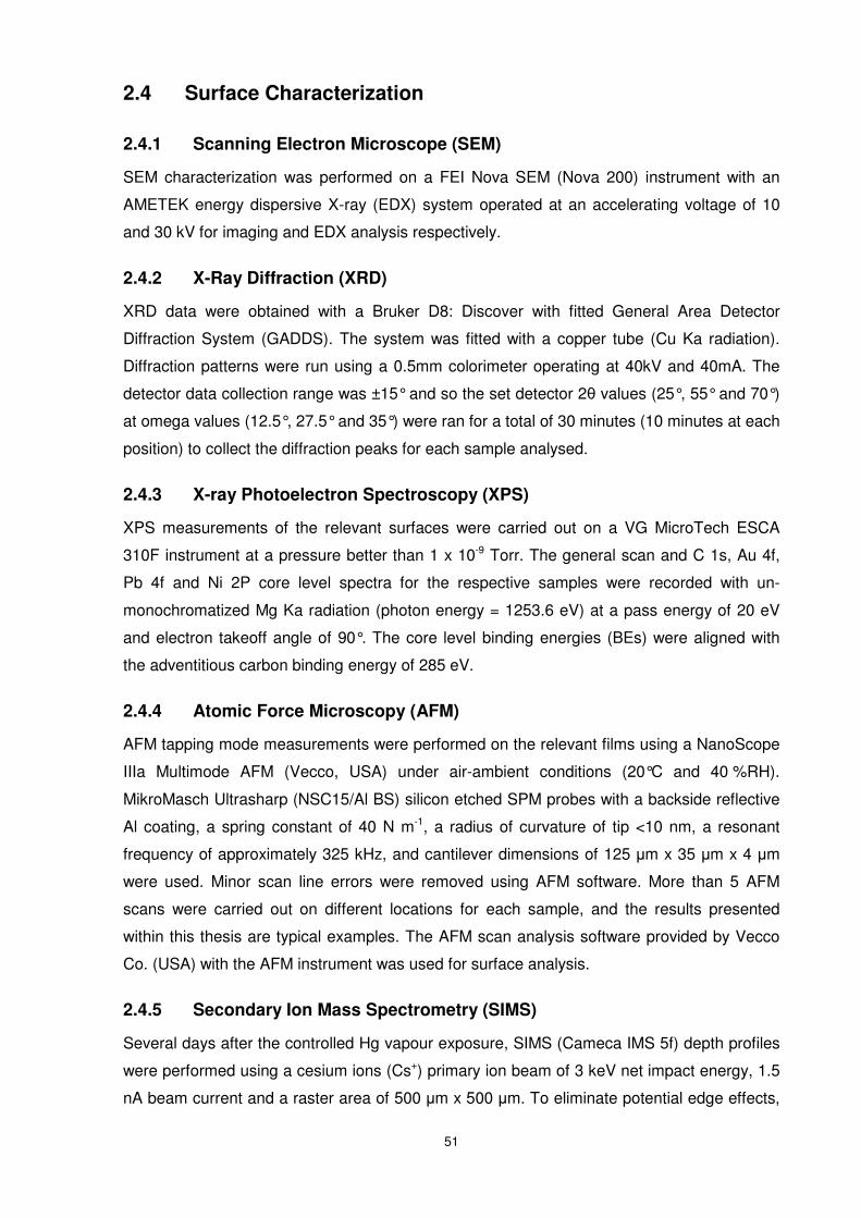
51
2.4 Surface Characterization
2.4.1 Scanning Electron Microscope (SEM)
SEM characterization was performed on a FEI Nova SEM (Nova 200) instrument with an
AMETEK energy dispersive X-ray (EDX) system operated at an accelerating voltage of 10
and 30 kV for imaging and EDX analysis respectively.
2.4.2 X-Ray Diffraction (XRD)
XRD data were obtained with a Bruker D8: Discover with fitted General Area Detector
Diffraction System (GADDS). The system was fitted with a copper tube (Cu Ka radiation).
Diffraction patterns were run using a 0.5mm colorimeter operating at 40kV and 40mA. The
detector data collection range was ±15° and so the set detector 2θ values (25°, 55° and 70°)
at omega values (12.5°, 27.5° and 35°) were ran for a total of 30 minutes (10 minutes at each
position) to collect the diffraction peaks for each sample analysed.
2.4.3 X-ray Photoelectron Spectroscopy (XPS)
XPS measurements of the relevant surfaces were carried out on a VG MicroTech ESCA
310F instrument at a pressure better than 1 x 10⁻⁹ Torr. The general scan and C 1s, Au 4f,
Pb 4f and Ni 2P core level spectra for the respective samples were recorded with un-
monochromatized Mg Ka radiation (photon energy = 1253.6 eV) at a pass energy of 20 eV
and electron takeoff angle of 90°. The core level binding energies (BEs) were aligned with
the adventitious carbon binding energy of 285 eV.
2.4.4 Atomic Force Microscopy (AFM)
AFM tapping mode measurements were performed on the relevant films using a NanoScope
IIIa Multimode AFM (Vecco, USA) under air-ambient conditions (20°C and 40 %RH).
MikroMasch Ultrasharp (NSC15/Al BS) silicon etched SPM probes with a backside reflective
Al coating, a spring constant of 40 N m-1, a radius of curvature of tip <10 nm, a resonant
frequency of approximately 325 kHz, and cantilever dimensions of 125 µm x 35 µm x 4 µm
were used. Minor scan line errors were removed using AFM software. More than 5 AFM
scans were carried out on different locations for each sample, and the results presented
within this thesis are typical examples. The AFM scan analysis software provided by Vecco
Co. (USA) with the AFM instrument was used for surface analysis.
2.4.5 Secondary Ion Mass Spectrometry (SIMS)
Several days after the controlled Hg vapour exposure, SIMS (Cameca IMS 5f) depth profiles
were performed using a cesium ions (Cs+) primary ion beam of 3 keV net impact energy, 1.5
nA beam current and a raster area of 500 µm x 500 µm. To eliminate potential edge effects,
52
a combination of lens setting was used to restrict the secondary ion yield to a 100 µm
diameter region within the centre of the rastered area. The SIMS measurements were
conducted at the Australian Nuclear Science and Technology Organisation (ANSTO) facility
in NSW, Australia through several Australian Institute of Nuclear Science and Engineering
(AINSE) grants.
2.4.6 Inductively Coupled Plasma Mass Spectrometry (ICPMS)
ICPMS measurements were performed using a HP4500 series 300, ShieldTorch System
ICPMS instrument. The samples analysed by ICPMS include the Hg calibration trapping
solutions (discussed in section 2.2.1.1) as well as the solution containing the digested Au or
silver electrodes exposed to Hg (discussed in chapter 3). The solutions were then diluted
such that the final solution for analysis contained no more than 5 ppb Hg and had a clear
colour (no potassium permanganate’s purple colour could be visible); in order to avoid
detector memory effects and blockage of sampling tubes on the HP4500. All solutions were
spiked with 100 ppb terbium (Tb) as the internal standard and 100 ppb Au to keep Hg
solution stable and draw all the Hg out of the sampling tubes on the HP4500. All solutions
contained 5% HNO3 with less than 0.02% of HCl for more accurate results. The sampling
tubes of the ICPMS were washed with 5% HNO3 solution as well as milli-Q water before
each sample solution was analysed for better accuracy. The control software was set to
analysed each sample three times before an average Hg concentration was displayed and
recorded.
2.4.7 Electrochemical Surface Area Analysis
Electrochemical surface areas of the selected layers were determined in order to distinguish
whether the improved sensing capability of the modified sensors was solely due to their
higher surface area or whether their surface morphology, crystallographic orientation and
other surface factors also played some role in improving their performance. The surface area
of the samples was electrochemically determined by calculating the charge required for
reducing the monolayer oxide as described by Rand and Woods.274 The geometrical surface
area of all the surfaces was 0.32 cm2 as determined from the mask dimensions used to e-
beam deposit the metal electrodes on the quartz substrates. The linear sweep voltammetry
curves are shown where required throughout this thesis.
Voltametric experiments were conducted at 20 ± 2°C with a CH Instruments (CHI 760C)
electrochemical analyser in an electrochemical cell that allowed reproducible positioning of
the working, reference and auxiliary electrodes and a nitrogen inlet tube. An e-beam
evaporated Au film was used as the working electrode (i.e. the QCM electrode), which was
washed in acetone and methanol followed by drying in a stream of dry nitrogen gas prior to
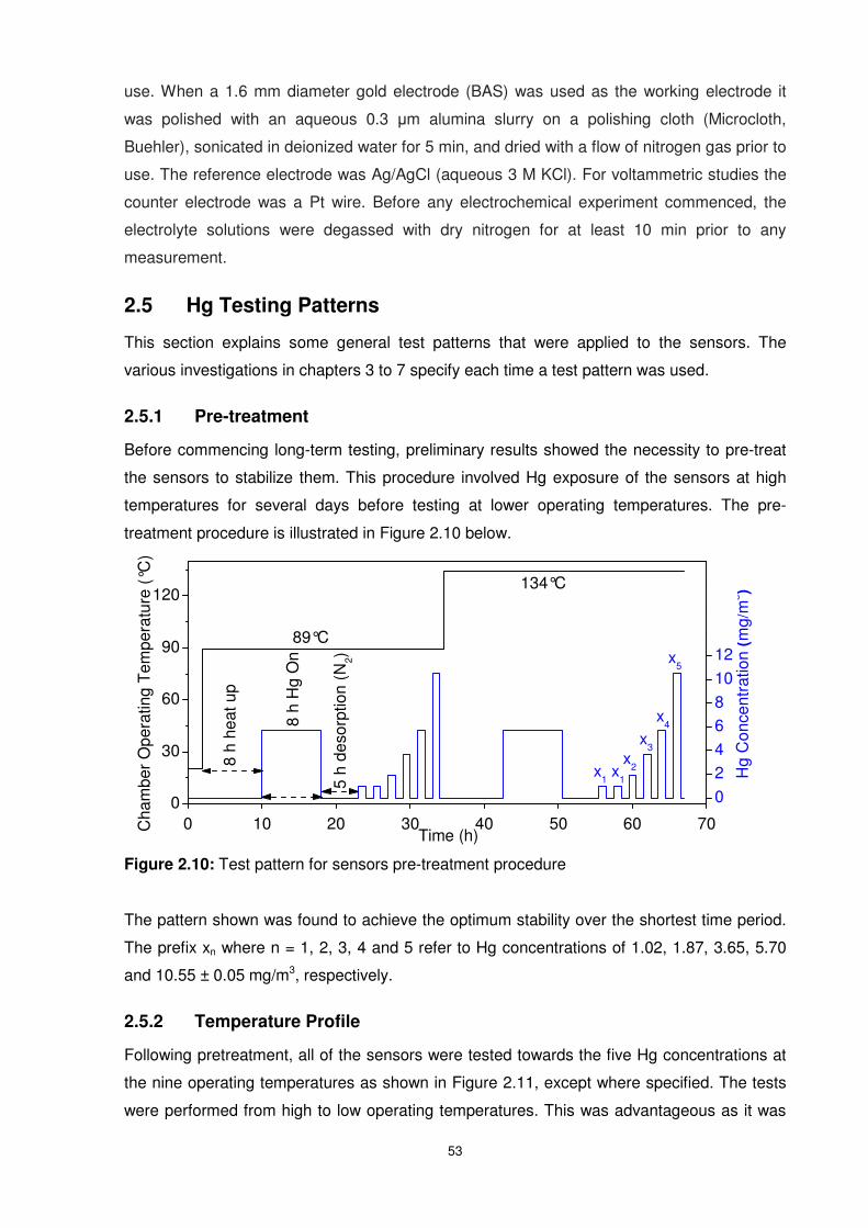
53
use. When a 1.6 mm diameter gold electrode (BAS) was used as the working electrode it
was polished with an aqueous 0.3 µm alumina slurry on a polishing cloth (Microcloth,
Buehler), sonicated in deionized water for 5 min, and dried with a flow of nitrogen gas prior to
use. The reference electrode was Ag/AgCl (aqueous 3 M KCl). For voltammetric studies the
counter electrode was a Pt wire. Before any electrochemical experiment commenced, the
electrolyte solutions were degassed with dry nitrogen for at least 10 min prior to any
measurement.
2.5 Hg Testing Patterns
This section explains some general test patterns that were applied to the sensors. The
various investigations in chapters 3 to 7 specify each time a test pattern was used.
2.5.1 Pre-treatment
Before commencing long-term testing, preliminary results showed the necessity to pre-treat
the sensors to stabilize them. This procedure involved Hg exposure of the sensors at high
temperatures for several days before testing at lower operating temperatures. The pre-
treatment procedure is illustrated in Figure 2.10 below.
Figure 2.10: Test pattern for sensors pre-treatment procedure
The pattern shown was found to achieve the optimum stability over the shortest time period.
The prefix xn where n = 1, 2, 3, 4 and 5 refer to Hg concentrations of 1.02, 1.87, 3.65, 5.70
and 10.55 ± 0.05 mg/m3, respectively.
2.5.2 Temperature Profile
Following pretreatment, all of the sensors were tested towards the five Hg concentrations at
the nine operating temperatures as shown in Figure 2.11, except where specified. The tests
were performed from high to low operating temperatures. This was advantageous as it was
0 10 20 30 40 50 60 700
30
60
90
120
Hg
Con
cent
ratio
n (m
g/m
3 )
Time (h)Cha
mbe
r O
pera
ting
Tem
pera
ture
(°C
)
02468101214161820
x1
x5
x4
x3
x2x
1
134°C
8 h
heat
up
5 h
deso
rptio
n (N
2)
8 h
Hg
On
89°C
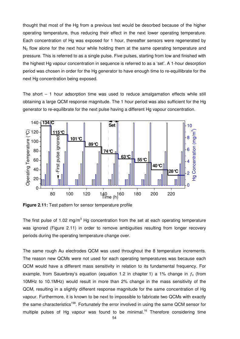
54
thought that most of the Hg from a previous test would be desorbed because of the higher
operating temperature, thus reducing their effect in the next lower operating temperature.
Each concentration of Hg was exposed for 1 hour, thereafter sensors were regenerated by
N2 flow alone for the next hour while holding them at the same operating temperature and
pressure. This is referred to as a single pulse. Five pulses, starting from low and finished with
the highest Hg vapour concentration in sequence is referred to as a ‘set’. A 1-hour desorption
period was chosen in order for the Hg generator to have enough time to re-equillibrate for the
next Hg concentration being exposed.
The short – 1 hour adsorption time was used to reduce amalgamation effects while still
obtaining a large QCM response magnitude. The 1 hour period was also sufficient for the Hg
generator to re-equilibrate for the next pulse having a different Hg vapour concentration.
Figure 2.11: Test pattern for sensor temperature profile
The first pulse of 1.02 mg/m3 Hg concentration from the set at each operating temperature
was ignored (Figure 2.11) in order to remove ambiguities resulting from longer recovery
periods during the operating temperature change over.
The same rough Au electrodes QCM was used throughout the 8 temperature increments.
The reason new QCMs were not used for each operating temperatures was because each
QCM would have a different mass sensitivity in relation to its fundamental frequency. For
example, from Sauerbrey’s equation (equation 1.2 in chapter 1) a 1% change in ƒ0 (from
10MHz to 10.1MHz) would result in more than 2% change in the mass sensitivity of the
QCM, resulting in a slightly different response magnitude for the same concentration of Hg
vapour. Furthermore, it is known to be next to impossible to fabricate two QCMs with exactly
the same characteristics198. Fortunately the error involved in using the same QCM sensor for
multiple pulses of Hg vapour was found to be minimal.16 Therefore considering time
80 100 120 140 160 180 200 2200
20
40
60
80
100
120
140
H
g C
once
ntra
tion
(mg/
m3 )
Time (h)
Ope
ratin
g T
empe
ratu
re (
°C)
0
2
4
6
8
10Set134°C
28°C
40°C
55°C63°C
74°C
89°C101°C
115°C
Firs
t pul
se ig
nore
d
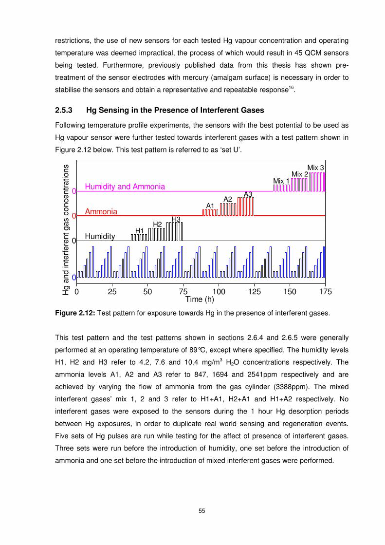
55
restrictions, the use of new sensors for each tested Hg vapour concentration and operating
temperature was deemed impractical, the process of which would result in 45 QCM sensors
being tested. Furthermore, previously published data from this thesis has shown pre-
treatment of the sensor electrodes with mercury (amalgam surface) is necessary in order to
stabilise the sensors and obtain a representative and repeatable response16.
2.5.3 Hg Sensing in the Presence of Interferent Gases
Following temperature profile experiments, the sensors with the best potential to be used as
Hg vapour sensor were further tested towards interferent gases with a test pattern shown in
Figure 2.12 below. This test pattern is referred to as ‘set U’.
Figure 2.12: Test pattern for exposure towards Hg in the presence of interferent gases.
This test pattern and the test patterns shown in sections 2.6.4 and 2.6.5 were generally
performed at an operating temperature of 89°C, except where specified. The humidity levels
H1, H2 and H3 refer to 4.2, 7.6 and 10.4 mg/m3 H2O concentrations respectively. The
ammonia levels A1, A2 and A3 refer to 847, 1694 and 2541ppm respectively and are
achieved by varying the flow of ammonia from the gas cylinder (3388ppm). The mixed
interferent gases’ mix 1, 2 and 3 refer to H1+A1, H2+A1 and H1+A2 respectively. No
interferent gases were exposed to the sensors during the 1 hour Hg desorption periods
between Hg exposures, in order to duplicate real world sensing and regeneration events.
Five sets of Hg pulses are run while testing for the affect of presence of interferent gases.
Three sets were run before the introduction of humidity, one set before the introduction of
ammonia and one set before the introduction of mixed interferent gases were performed.
0 25 50 75 100 125 150 175
Time (h)
Hg
and
inte
rfer
ent g
as c
once
ntra
tions
Humidity and Ammonia
Ammonia
Humidity
0
0
0
0
Mix 3Mix 2
Mix 1
A3A2
A1
H3H2
H1
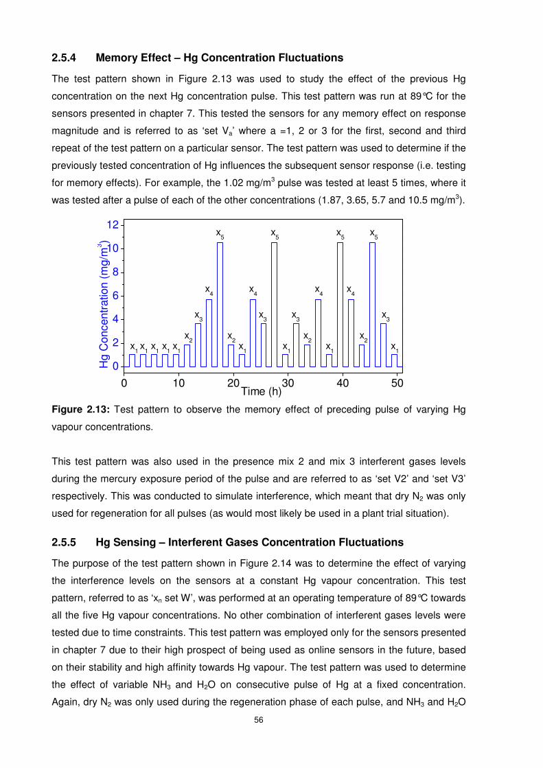
56
2.5.4 Memory Effect – Hg Concentration Fluctuations
The test pattern shown in Figure 2.13 was used to study the effect of the previous Hg
concentration on the next Hg concentration pulse. This test pattern was run at 89°C for the
sensors presented in chapter 7. This tested the sensors for any memory effect on response
magnitude and is referred to as ‘set Va’ where a =1, 2 or 3 for the first, second and third
repeat of the test pattern on a particular sensor. The test pattern was used to determine if the
previously tested concentration of Hg influences the subsequent sensor response (i.e. testing
for memory effects). For example, the 1.02 mg/m3 pulse was tested at least 5 times, where it
was tested after a pulse of each of the other concentrations (1.87, 3.65, 5.7 and 10.5 mg/m3).
Figure 2.13: Test pattern to observe the memory effect of preceding pulse of varying Hg
vapour concentrations.
This test pattern was also used in the presence mix 2 and mix 3 interferent gases levels
during the mercury exposure period of the pulse and are referred to as ‘set V2’ and ‘set V3’
respectively. This was conducted to simulate interference, which meant that dry N2 was only
used for regeneration for all pulses (as would most likely be used in a plant trial situation).
2.5.5 Hg Sensing – Interferent Gases Concentration Fluctuations
The purpose of the test pattern shown in Figure 2.14 was to determine the effect of varying
the interference levels on the sensors at a constant Hg vapour concentration. This test
pattern, referred to as ‘xn set W’, was performed at an operating temperature of 89°C towards
all the five Hg vapour concentrations. No other combination of interferent gases levels were
tested due to time constraints. This test pattern was employed only for the sensors presented
in chapter 7 due to their high prospect of being used as online sensors in the future, based
on their stability and high affinity towards Hg vapour. The test pattern was used to determine
the effect of variable NH3 and H2O on consecutive pulse of Hg at a fixed concentration.
Again, dry N2 was only used during the regeneration phase of each pulse, and NH3 and H2O
0 10 20 30 40 50
0
2
4
6
8
10
12
x3
x4
x5
x5
x4
x2
x3
x1
x2
x1
x1
x5
x3
x4
x1
x2
x5
x4
x3
x2
x1
x1
x1
x1
Time (h)
Hg
Con
cent
ratio
n (m
g/m
3 )
x1
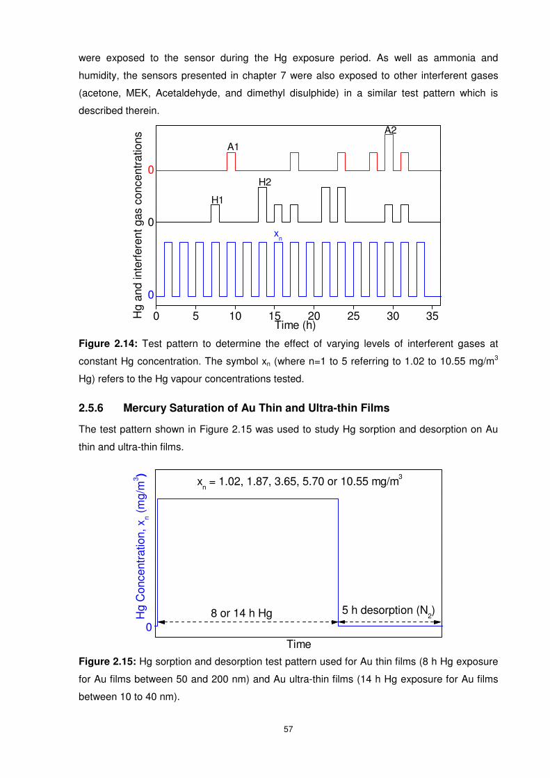
57
were exposed to the sensor during the Hg exposure period. As well as ammonia and
humidity, the sensors presented in chapter 7 were also exposed to other interferent gases
(acetone, MEK, Acetaldehyde, and dimethyl disulphide) in a similar test pattern which is
described therein.
Figure 2.14: Test pattern to determine the effect of varying levels of interferent gases at
constant Hg concentration. The symbol xn (where n=1 to 5 referring to 1.02 to 10.55 mg/m3
Hg) refers to the Hg vapour concentrations tested.
2.5.6 Mercury Saturation of Au Thin and Ultra-thin Films
The test pattern shown in Figure 2.15 was used to study Hg sorption and desorption on Au
thin and ultra-thin films.
Figure 2.15: Hg sorption and desorption test pattern used for Au thin films (8 h Hg exposure
for Au films between 50 and 200 nm) and Au ultra-thin films (14 h Hg exposure for Au films
between 10 to 40 nm).
Time
xn = 1.02, 1.87, 3.65, 5.70 or 10.55 mg/m3
0
Hg
Con
cent
ratio
n, x
n (m
g/m
3 )
5 h desorption (N2)8 or 14 h Hg
0 5 10 15 20 25 30 35
Hg
and
inte
rfer
ent g
as c
once
ntra
tions
xn
0
0
Time (h)
H1
H2
A1
A2
0
58
A Hg exposure period of either 8 hours (Au thin films) or 14 hours (Au ultra-thin films) was
used at various Hg vapour concentrations and operating temperatures. Thereafter, a
recovery period (using dry nitrogen) of 5 hours was used. The increased exposure time of 14
hours for the Au ultra-thin films (chapter 5) rather than 8 hour periods used for Au thin films
(chapter 4) was due to the high dependency of the experimental outcomes on the saturation
(or near saturation in the case of Hg-Au system) of Au with Hg vapour.
In summary, the experimental setup, sensor fabrication, instrumentation and literature
considerations during the course of the present work are presented. The test patterns
described in this chapter will be refered to in the proceeding results chapters
throughout this thesis.
59
2.6 References
(1) McNerney, J. J.; Buseck, P. R.; Hanson, R. C. Science 1972, 178, 611-612. (2) Joyner, R. W.; Roberts, M. W. Journal of the Chemical Society Faraday Transactions 1 1973,
69, 1242-1250. (3) Nowakowski, R.; Pielaszek, J.; Dus, R. Applied Surface Science 2002, 199, 40-51. (4) Fialkowski, M.; Grzeszczak, P.; Nowakowski, R.; Holyst, R. The Journal of Physical Chemistry
B 2004, 108, 5026-5030. (5) Atkins, P. W. Physical Chemistry; 2nd ed.; Oxford University Press: Oxford, Great Britain,
1982. (6) Nott, B. R. Water, Air, & Soil Pollution 1995, 80, 1311-1314. (7) Nilsson, S.; Klett, O.; Svedberg, M.; Amirkhani, A.; Nyholm, L. Rapid Communications in Mass
Spectrometry 2003, 17, 1535-1540. (8) Hoogvliet, J. C.; van Bennekom, W. P. Electrochimica Acta 2001, 47, 599-611. (9) Sexton, B. A.; Feltis, B. N.; Davis, T. J. Sensors and Actuators A: Physical 2008, 141, 471-
475. (10) Ali, M. B.; Bessueille, F.; Chovelon, J. M.; Abdelghani, A.; Jaffrezic-Renault, N.; Maaref, M. A.;
Martelet, C. Materials Science and Engineering: C 2008, 28, 628-632. (11) Moody, N. R.; Adams, D. P.; Medlin, D.; Headley, T.; Yang, N.; Volinsky, A. International
Journal of Fracture 2003, 120, 407-419. (12) George, M. A.; Glaunsinger, W. S.; Thundat, T.; Lindsay, S. M. Thin Solid Films 1990, 189,
59-72. (13) Al Kobaisi, M. Doctor of Philosophy, Royal Melbourne Institue of Technology University, 2008. (14) Zimmermann, B.; Lucklum, R.; Hauptmann, P.; Rabe, J.; Büttgenbach, S. Sensors and
Actuators B: Chemical 2001, 76, 47-57. (15) Rand, D. A. J.; Woods, R. Journal of Electroanalytical Chemistry 1971, 31, 29-38. (16) Sabri, Y. M.; Ippolito, S. J.; Tardio, J.; Sood, D. K.; Bhargava, S. K.; Mullett, M.; Harrison, I.;
Rosenberg, S. In 8th International Alumina Quality Workshop Darwin, Australia, 2008, p 260-266.

60
61
Chapter III
Chapter 3 Investigation of Hg Interaction
with Various Thin Metal Films
and Surface Morphologies
The influence of Hg sorption and desorption characteristics on Au and Ag thin films which
have been e-beam deposited on optically polished or mechanically roughened quartz
substrates are presented in this chapter. Additionally, QCMs with Ni and Ti thin film
electrodes are shown to undergo minimal Hg vapour sorption thus confirming the
correlation between metal solubility in Hg and metal affinity for Hg vapour during sensing.
The Au and Ag QCMs were exposed to Hg vapour and the sensors’ dynamic response is
used to calculate t90 and sticking probability of Hg to the thin metal films. The thin films
were then characterized using AFM, SEM and SIMS depth profiling. Thereafter they were
acid digested and analysed using ICP-MS. Hg distribution was found to follow an
asymptotic function through the depth of each thin metal film investigated. Furthermore,
the optimal thin film (in terms of Hg sorption and desorption kinetics as well as high Hg
affinity) is tested towards Hg vapour in the presence of interferent gases (ammonia and
humidity).
Part of the work presented in this chapter has been published:
Sabri, Y.M; Ippolito, S.J; Tardio, J; Atanacio, A. J; Sood, D. K and Bhargava, S. K; “Mercury
diffusion in gold and silver thin film electrodes on quartz crystal microbalance sensors”
Sensors and Actuators B: Chemical, 2009, 137(1), pp. 246 – 252.
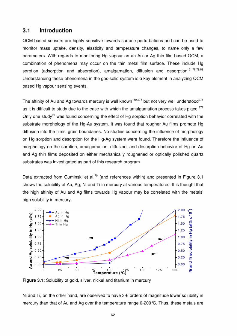
62
3.1 Introduction
QCM based sensors are highly sensitive towards surface perturbations and can be used to
monitor mass uptake, density, elasticity and temperature changes, to name only a few
parameters. With regards to monitoring Hg vapour on an Au or Ag thin film based QCM, a
combination of phenomena may occur on the thin metal film surface. These include Hg
sorption (adsorption and absorption), amalgamation, diffusion and desorption.61,78,79,89
Understanding these phenomena in the gas-solid system is a key element in analyzing QCM
based Hg vapour sensing events.
The affinity of Au and Ag towards mercury is well known159,275 but not very well understood276
as it is difficult to study due to the ease with which the amalgamation process takes place.277
Only one study93 was found concerning the effect of Hg sorption behavior correlated with the
substrate morphology of the Hg-Au system. It was found that rougher Au films promote Hg
diffusion into the films’ grain boundaries. No studies concerning the influence of morphology
on Hg sorption and desorption for the Hg-Ag system were found. Therefore the influence of
morphology on the sorption, amalgamation, diffusion, and desorption behavior of Hg on Au
and Ag thin films deposited on either mechanically roughened or optically polished quartz
substrates was investigated as part of this research program.
Data extracted from Guminski et al.70 (and references within) and presented in Figure 3.1
shows the solubility of Au, Ag, Ni and Ti in mercury at various temperatures. It is thought that
the high affinity of Au and Ag films towards Hg vapour may be correlated with the metals’
high solubility in mercury.
Figure 3.1: Solubility of gold, silver, nickel and titanium in mercury
Ni and Ti, on the other hand, are observed to have 3-6 orders of magnitude lower solubility in
mercury than that of Au and Ag over the temperature range 0-200°C. Thus, these metals are
0 25 50 75 100 125 150 175 200
0.00
0.25
0.50
0.75
1.00
1.25
1.50
1.75
2.00 Au in Hg Ag in Hg
Ni
an
d T
i so
lub
ilit
y i
n H
g (
at%
x 1
0-3)
Au
an
d A
g s
olu
bil
ity
in
Hg
(at%
)
Temperature (°C)
0.00
0.25
0.50
0.75
1.00
1.25
1.50
1.75
2.00
Ni in Hg Ti in Hg
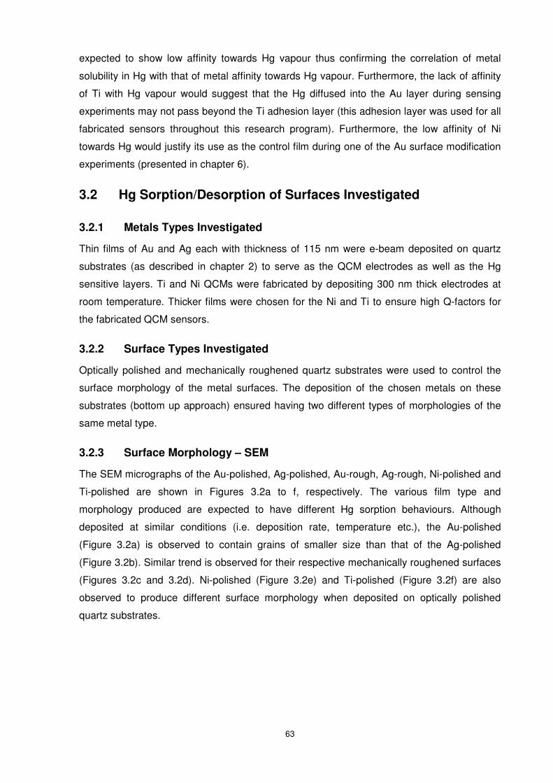
63
expected to show low affinity towards Hg vapour thus confirming the correlation of metal
solubility in Hg with that of metal affinity towards Hg vapour. Furthermore, the lack of affinity
of Ti with Hg vapour would suggest that the Hg diffused into the Au layer during sensing
experiments may not pass beyond the Ti adhesion layer (this adhesion layer was used for all
fabricated sensors throughout this research program). Furthermore, the low affinity of Ni
towards Hg would justify its use as the control film during one of the Au surface modification
experiments (presented in chapter 6).
3.2 Hg Sorption/Desorption of Surfaces Investigated
3.2.1 Metals Types Investigated
Thin films of Au and Ag each with thickness of 115 nm were e-beam deposited on quartz
substrates (as described in chapter 2) to serve as the QCM electrodes as well as the Hg
sensitive layers. Ti and Ni QCMs were fabricated by depositing 300 nm thick electrodes at
room temperature. Thicker films were chosen for the Ni and Ti to ensure high Q-factors for
the fabricated QCM sensors.
3.2.2 Surface Types Investigated
Optically polished and mechanically roughened quartz substrates were used to control the
surface morphology of the metal surfaces. The deposition of the chosen metals on these
substrates (bottom up approach) ensured having two different types of morphologies of the
same metal type.
3.2.3 Surface Morphology – SEM
The SEM micrographs of the Au-polished, Ag-polished, Au-rough, Ag-rough, Ni-polished and
Ti-polished are shown in Figures 3.2a to f, respectively. The various film type and
morphology produced are expected to have different Hg sorption behaviours. Although
deposited at similar conditions (i.e. deposition rate, temperature etc.), the Au-polished
(Figure 3.2a) is observed to contain grains of smaller size than that of the Ag-polished
(Figure 3.2b). Similar trend is observed for their respective mechanically roughened surfaces
(Figures 3.2c and 3.2d). Ni-polished (Figure 3.2e) and Ti-polished (Figure 3.2f) are also
observed to produce different surface morphology when deposited on optically polished
quartz substrates.
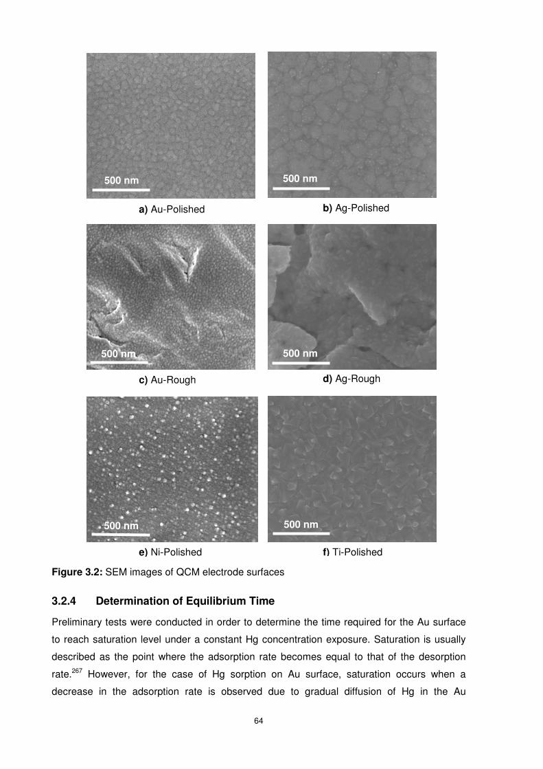
64
Figure 3.2: SEM images of QCM electrode surfaces
3.2.4 Determination of Equilibrium Time
Preliminary tests were conducted in order to determine the time required for the Au surface
to reach saturation level under a constant Hg concentration exposure. Saturation is usually
described as the point where the adsorption rate becomes equal to that of the desorption
rate.267 However, for the case of Hg sorption on Au surface, saturation occurs when a
decrease in the adsorption rate is observed due to gradual diffusion of Hg in the Au
500 nm 500 nm
500 nm 500 nm
500 nm 500 nm
a) Au-Polished b) Ag-Polished
c) Au-Rough d) Ag-Rough
e) Ni-Polished f) Ti-Polished
65
films.78,278 Following saturation, the thin film surfaces were exposed to dry nitrogen in order to
observe the fraction of Hg that may be desorbed off the surface.
As an initial step, the Au-rough QCM was exposed to Hg followed by dry nitrogen for
extended periods of time in order to estimate the time required to saturate and regenerate
the gold surface, respectively. The QCM response from the Hg and dry nitrogen exposure at
Hg vapour concentration of 3.65 mg/m3 and an operating temperature of 55°C is shown in
Figure 3.3. It can be seen that due to the Hg present on the gold surface from the first 8-hour
Hg vapour exposure, a second pulse of 8-hour Hg exposure results in the sensor saturating
around the same ∆ƒ value (~530 Hz) as the first exposure. Although the signal from the
second 8-hour Hg exposure is observed to drop by ~150 Hz than the first 8-hour Hg
exposure pulse, the total Hg (or total ∆f from when t=0) adsorbed on the surface following
saturation is found to be similar.
Figure 3.3: Sorption and desorption behaviour of Hg exposed to Au-rough QCM. The
influence of long Hg exposure as well as long desorption times may be observed.
A similar observation was made for the 40-hour Hg exposure period where the total Hg on
the Au surface is observed to be similar to that of the first 8-hour Hg exposure period before
saturation level has been reached. The slow increase in response magnitude during the 40
hour Hg exposure indicates a small accumulation of Hg on the sensor electrode surface. In
addition, following the first 8-hour Hg sorption and 5-hour desorption period, the pre-exposed
surface is observed to undergo a similar amount of Hg sorption thereon to reach saturation. It
then follows that an 8-hour Hg exposure pulse is sufficient to reach saturation point.
Coincidentally, a maximum 8 hour mercury exposure period is also the time-weighted
average (TWA) recommended by the National Institute for Occupational Safety and Health
(NIOSH) at Hg concentration of 0.05 mg/m3.14
0 20 40 60 80 100 120-550
-500
-450
-400
-350
-300
-250
-200
-150
-100
-50
0
50Hg concentration of 3.65 mg/m3 at operating temperature of 55°C
Sen
so
r R
es
po
nse,
∆∆ ∆∆f
(Hz)
Time (h)
8 ho
urs
of H
g
8 ho
urs
of H
g
40 hours of Hg
5 hours of dry N2
58 hours of dry N2
66
The 150 Hz drop in response observed in the second 8-hour compared to the first 8-hour Hg
exposure pulse is equivalent to 658.7 ng/cm2, which is the amount of Hg that has
amalgamated with Au and is not desorbed even after extended periods of exposure to dry
nitrogen. It then follows that Hg amalgamation is relatively higher on a fresh unexposed Au
surface than that of the Hg exposed Au surface. In addition, it is observed that better
repeatability in response magnitude may also be obtained with the pre-exposed Au surface.
Approximately 100% recovery (compared to the initial contaminated state) is reached when
the Au surface is exposed to dry nitrogen following the 8-hour Hg exposure period. The
desorption of Hg beyond the initial 5 hour period was found to be minimal as shown in Figure
3.3, thus justifying the chosen 5 hour desorption time used in the experiments following the
saturation of the films with Hg. That is, the amount of Hg desorbing off the Au film is
observed to be similar whether a 5-hour or 58-hour recovery time is used.
Based on these findings, the QCM sensors were exposed to Hg vapour for 8 hours followed
by exposure to dry N2 for a further 5 hours. No prior pre-treatment of the surfaces was
performed. In order to estimate the remaining amalgamated/adsorbed Hg content on the Au
and Ag electrode surfaces, the QCM devices were made and tested in duplicates before
being digested in aqua regia (1:3 concentrated HNO3:HCl) directly following their removal
from the chamber. The solution was then analysed by ICP-MS with the procedure detailed in
Chapter 2. The duplicate samples were characterized by AFM, FE-SEM and SIMS. QCM
results revealed good repeatability of around ±0.6% of the mean response magnitude
between duplicate tests and of similar substrates.
3.2.5 Morphology Influence on Hg Sorption and Desorption Characteristics
The dynamic response of the six QCM devices, namely, Ti-polished, Ni-polished, Ag-
polished, Au-polished, Ag-rough and Au-rough electrode QCMs towards 3.65 and 1.02
mg/m3 of Hg vapour are shown in Figures 3.4a and b, respectively. No detectable Hg vapour
sorption occurred on the Ni or Ti QCM electrodes and so no further characterization was
deemed necessary for these two samples.
The AFM images of the Au-polished, Ag-polished, Au-rough and Ag-rough AFM images prior
to Hg exposure are shown in Figure 3.5. The average roughness (Ra) and root-mean-square
roughness (Rq) over a 500 x 500 nm scan size are also shown for the respective thin films.
The AFM measurements revealed the Au-Polished QCM electrodes have a 4.75% larger
surface area than its projected surface area. Similarly Au-rough, Ag-polished and Ag-rough
were found to have 18.9, 7.7 and 41.8% higher surface areas than their projected surface
areas.
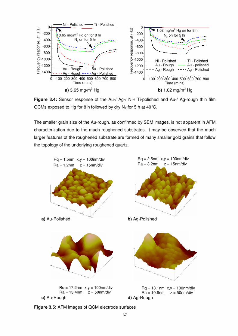
67
Figure 3.4: Sensor response of the Au-/ Ag-/ Ni-/ Ti-polished and Au-/ Ag-rough thin film
QCMs exposed to Hg for 8 h followed by dry N2 for 5 h at 40°C.
The smaller grain size of the Au-rough, as confirmed by SEM images, is not apparent in AFM
characterization due to the much roughened substrates. It may be observed that the much
larger features of the roughened substrate are formed of many smaller gold grains that follow
the topology of the underlying roughened quartz.
Figure 3.5: AFM images of QCM electrode surfaces
Ra = 1.2nm z = 15nm/div
Rq = 17.2nm x,y = 100nm/div Ra = 13.4nm z = 50nm/div Ra = 10.6nm z = 50nm/div
Ra = 3.2nm z = 15nm/div Rq = 1.5nm x,y = 100nm/div
b) Ag-Polished a) Au-Polished
d) Ag-Rough c) Au-Rough
Rq = 2.5nm x,y = 100nm/div
Rq = 13.1nm x,y = 100nm/div
0 100 200 300 400 500 600 700 800
-1400
-1200
-1000
-800
-600
-400
-200
0 Ni - Polished Ti - Polished
N2 on for 5 hr
Au - Rough Au - Polished Ag - Rough Ag - PolishedF
requ
ency
res
pons
e, ∆
f (H
z)
Time (mins)
3.65 mg/m3 Hg on for 8 hr
b) 1.02 mg/m3 Hg a) 3.65 mg/m3 Hg
0 100 200 300 400 500 600 700 800
-1400
-1200
-1000
-800
-600
-400
-200
0
Ni - Polished Ti - Polished Au - Rough Au - polished Ag - Rough Ag - Polished
Fre
quen
cy r
espo
nse,
∆f (
Hz)
Time (mins)
1.02 mg/m3 Hg on for 8 hrN
2 on for 5 hr
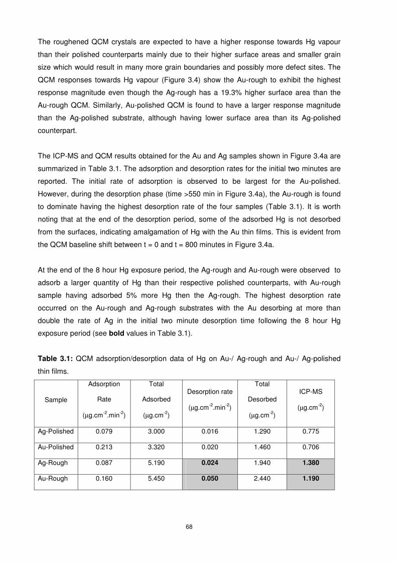
68
The roughened QCM crystals are expected to have a higher response towards Hg vapour
than their polished counterparts mainly due to their higher surface areas and smaller grain
size which would result in many more grain boundaries and possibly more defect sites. The
QCM responses towards Hg vapour (Figure 3.4) show the Au-rough to exhibit the highest
response magnitude even though the Ag-rough has a 19.3% higher surface area than the
Au-rough QCM. Similarly, Au-polished QCM is found to have a larger response magnitude
than the Ag-polished substrate, although having lower surface area than its Ag-polished
counterpart.
The ICP-MS and QCM results obtained for the Au and Ag samples shown in Figure 3.4a are
summarized in Table 3.1. The adsorption and desorption rates for the initial two minutes are
reported. The initial rate of adsorption is observed to be largest for the Au-polished.
However, during the desorption phase (time >550 min in Figure 3.4a), the Au-rough is found
to dominate having the highest desorption rate of the four samples (Table 3.1). It is worth
noting that at the end of the desorption period, some of the adsorbed Hg is not desorbed
from the surfaces, indicating amalgamation of Hg with the Au thin films. This is evident from
the QCM baseline shift between t = 0 and t = 800 minutes in Figure 3.4a.
At the end of the 8 hour Hg exposure period, the Ag-rough and Au-rough were observed to
adsorb a larger quantity of Hg than their respective polished counterparts, with Au-rough
sample having adsorbed 5% more Hg then the Ag-rough. The highest desorption rate
occurred on the Au-rough and Ag-rough substrates with the Au desorbing at more than
double the rate of Ag in the initial two minute desorption time following the 8 hour Hg
exposure period (see bold values in Table 3.1).
Table 3.1: QCM adsorption/desorption data of Hg on Au-/ Ag-rough and Au-/ Ag-polished
thin films.
Sample
Adsorption
Rate
(µg.cm-2.min-2)
Total
Adsorbed
(µg.cm-2)
Desorption rate
(µg.cm-2.min-2)
Total
Desorbed
(µg.cm-2)
ICP-MS
(µg.cm-2)
Ag-Polished 0.079 3.000 0.016 1.290 0.775
Au-Polished 0.213 3.320 0.020 1.460 0.706
Ag-Rough 0.087 5.190 0.024 1.940 1.380
Au-Rough 0.160 5.450 0.050 2.440 1.190
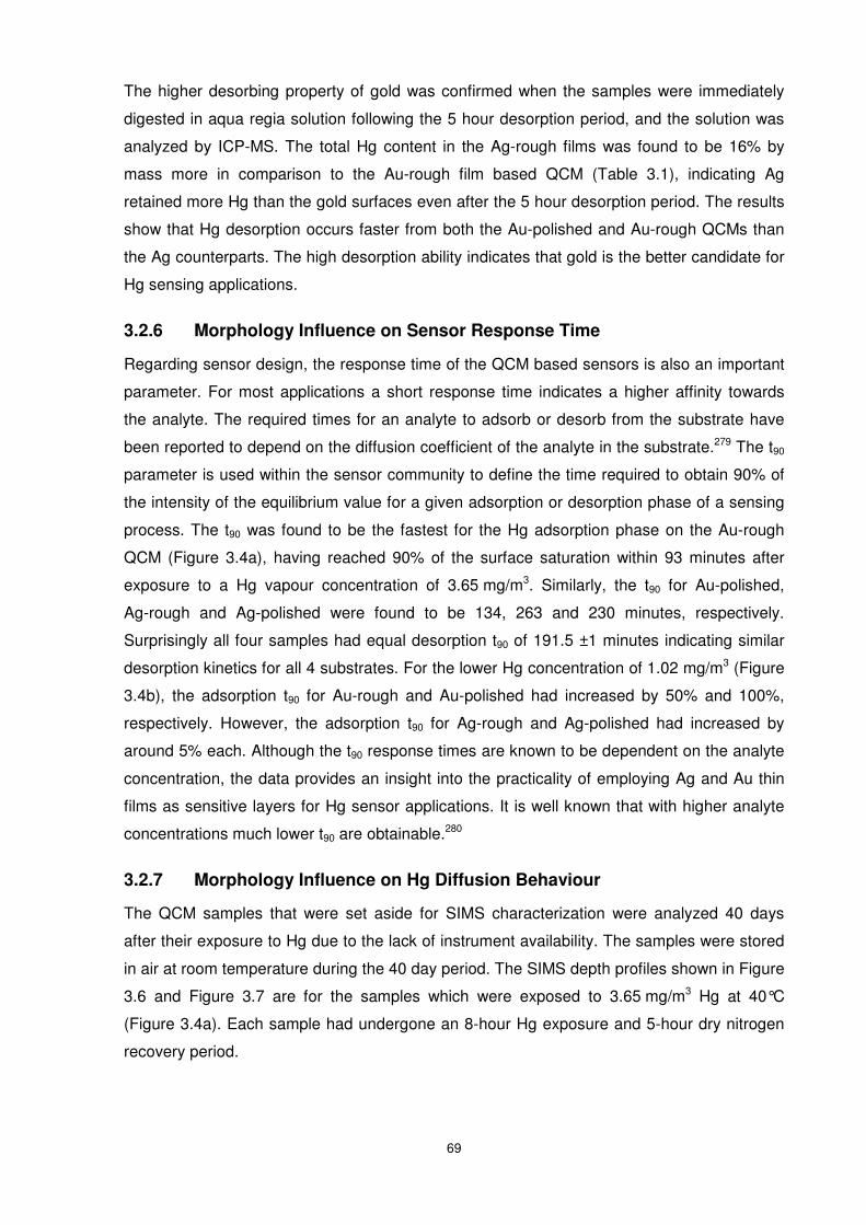
69
The higher desorbing property of gold was confirmed when the samples were immediately
digested in aqua regia solution following the 5 hour desorption period, and the solution was
analyzed by ICP-MS. The total Hg content in the Ag-rough films was found to be 16% by
mass more in comparison to the Au-rough film based QCM (Table 3.1), indicating Ag
retained more Hg than the gold surfaces even after the 5 hour desorption period. The results
show that Hg desorption occurs faster from both the Au-polished and Au-rough QCMs than
the Ag counterparts. The high desorption ability indicates that gold is the better candidate for
Hg sensing applications.
3.2.6 Morphology Influence on Sensor Response Time
Regarding sensor design, the response time of the QCM based sensors is also an important
parameter. For most applications a short response time indicates a higher affinity towards
the analyte. The required times for an analyte to adsorb or desorb from the substrate have
been reported to depend on the diffusion coefficient of the analyte in the substrate.279 The t90
parameter is used within the sensor community to define the time required to obtain 90% of
the intensity of the equilibrium value for a given adsorption or desorption phase of a sensing
process. The t90 was found to be the fastest for the Hg adsorption phase on the Au-rough
QCM (Figure 3.4a), having reached 90% of the surface saturation within 93 minutes after
exposure to a Hg vapour concentration of 3.65 mg/m3. Similarly, the t90 for Au-polished,
Ag-rough and Ag-polished were found to be 134, 263 and 230 minutes, respectively.
Surprisingly all four samples had equal desorption t90 of 191.5 ±1 minutes indicating similar
desorption kinetics for all 4 substrates. For the lower Hg concentration of 1.02 mg/m3 (Figure
3.4b), the adsorption t90 for Au-rough and Au-polished had increased by 50% and 100%,
respectively. However, the adsorption t90 for Ag-rough and Ag-polished had increased by
around 5% each. Although the t90 response times are known to be dependent on the analyte
concentration, the data provides an insight into the practicality of employing Ag and Au thin
films as sensitive layers for Hg sensor applications. It is well known that with higher analyte
concentrations much lower t90 are obtainable.280
3.2.7 Morphology Influence on Hg Diffusion Behaviour
The QCM samples that were set aside for SIMS characterization were analyzed 40 days
after their exposure to Hg due to the lack of instrument availability. The samples were stored
in air at room temperature during the 40 day period. The SIMS depth profiles shown in Figure
3.6 and Figure 3.7 are for the samples which were exposed to 3.65 mg/m3 Hg at 40°C
(Figure 3.4a). Each sample had undergone an 8-hour Hg exposure and 5-hour dry nitrogen
recovery period.
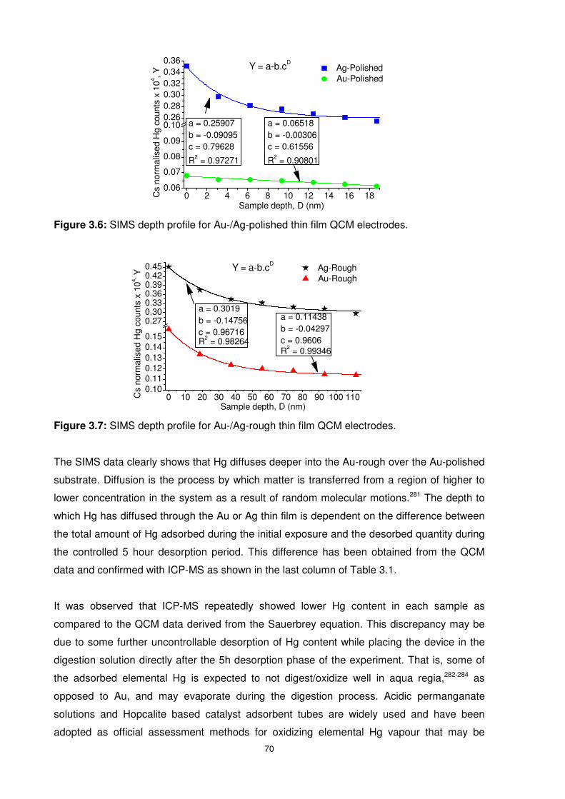
70
Figure 3.6: SIMS depth profile for Au-/Ag-polished thin film QCM electrodes.
Figure 3.7: SIMS depth profile for Au-/Ag-rough thin film QCM electrodes.
The SIMS data clearly shows that Hg diffuses deeper into the Au-rough over the Au-polished
substrate. Diffusion is the process by which matter is transferred from a region of higher to
lower concentration in the system as a result of random molecular motions.281 The depth to
which Hg has diffused through the Au or Ag thin film is dependent on the difference between
the total amount of Hg adsorbed during the initial exposure and the desorbed quantity during
the controlled 5 hour desorption period. This difference has been obtained from the QCM
data and confirmed with ICP-MS as shown in the last column of Table 3.1.
It was observed that ICP-MS repeatedly showed lower Hg content in each sample as
compared to the QCM data derived from the Sauerbrey equation. This discrepancy may be
due to some further uncontrollable desorption of Hg content while placing the device in the
digestion solution directly after the 5h desorption phase of the experiment. That is, some of
the adsorbed elemental Hg is expected to not digest/oxidize well in aqua regia,282-284 as
opposed to Au, and may evaporate during the digestion process. Acidic permanganate
solutions and Hopcalite based catalyst adsorbent tubes are widely used and have been
adopted as official assessment methods for oxidizing elemental Hg vapour that may be
0 10 20 30 40 50 60 70 80 90 100 1100.100.110.120.130.140.15
0.270.300.330.360.390.420.45 Y = a-b.cD
Ag-Rough Au-Rough
Cs
norm
alis
ed H
g co
unts
x 1
04, Y
Sample depth, D (nm)
R2 = 0.99346c = 0.9606b = -0.04297a = 0.11438
a = 0.3019b = -0.14756c = 0.96716R2 = 0.98264
0 2 4 6 8 10 12 14 16 180.06
0.07
0.08
0.09
0.100.260.280.300.320.340.36
R2 = 0.97271
c = 0.79628b = -0.09095
Ag-Polished Au-Polished
Cs
norm
alis
ed H
g co
unts
x 1
04 , Y
Sample depth, D (nm)
Y = a-b.cD
a = 0.25907 a = 0.06518b = -0.00306c = 0.61556
R2 = 0.90801
71
desorbed off the sample surface.285-287 These methods have not been used in this case due
to the additional need to dissolve the Au film for the analysis of amalgamated Hg. It has been
reported earlier that all the Hg may not be dissolved off the Au surface by acid dissolution
alone84 and so digestion of the sorbent metal film was also necessary in order to detect the
amalgamated as well as the adsorbed Hg. In any case, with the current digestion method
used, the ICP-MS results conclusively confirm the lower mercury content in Au samples as
compared to Ag substrates with similar surface morphology.
The Hg depth profile in Au film presented in Figures 3.6 and 3.7 correspond to the
conclusions made by George et al.93 indicating that Hg vapour nucleates and diffuses better
at surfaces with more surface defects and grain boundaries, thus showing that the rough
surfaces do indeed provide a higher concentration of adsorption sites. Therefore the extent
of roughness of the material used as the sensing layer for Hg sorption is suggested as the
dominant factor in the extent of diffusion/amalgamation that occurs as the rougher surfaces
are expected to have higher density of surface defects and grain boundaries.
The depth profiles show that from the 4 different surface configurations, the least amount of
Hg diffusion occurred through the Au-polished sample. This further supports the mass
change calculated from the Sauerbrey equation and the ICP-MS results (Table 3.1), showing
that the Ag samples retain the larger proportion of the adsorbed Hg content when compared
to the Au QCMs.
The trend lines (Figures 3.6 and 3.7) were fitted to the data points using best line of fit
method. These fitted lines are found to best follow the asymptotic equation (equation 3.1):
DcbaY .−= , Equation 3.1
where Y is the normalized Hg count, parameters a , b and c are constants, and D is the
surface depth to which Hg has diffused.89 Due to a lack of SIMS Au-Hg reference materials,
the normalized Hg counts were not quantified. The parameters a , b and c for the three
different Hg concentrations on the 4 different substrate configurations are shown in Table
3.2. The product of ( Dcb. ) in Equation 3.1 is indicative of the extent of diffusion occurring in a
substrate while the parameter a indicates the flux/counts of Hg in the substrate where no
further diffusion occurs. A high a value indicates the lower ability of Hg diffusion in the
substrate.
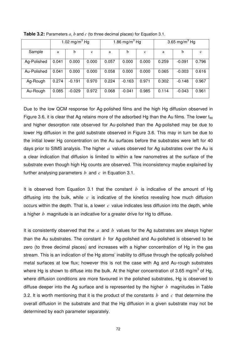
72
Table 3.2: Parameters a, b and c (to three decimal places) for Equation 3.1.
1.02 mg/m3 Hg 1.86 mg/m3 Hg 3.65 mg/m3 Hg
Sample a b c a b c a b c
Ag-Polished 0.041 0.000 0.000 0.057 0.000 0.000 0.259 -0.091 0.796
Au-Polished 0.041 0.000 0.000 0.058 0.000 0.000 0.065 -0.003 0.616
Ag-Rough 0.274 -0.191 0.970 0.224 -0.163 0.971 0.302 -0.148 0.967
Au-Rough 0.085 -0.029 0.972 0.068 -0.041 0.985 0.114 -0.043 0.961
Due to the low QCM response for Ag-polished films and the high Hg diffusion observed in
Figure 3.6, it is clear that Ag retains more of the adsorbed Hg than the Au films. The lower t90
and higher desorption rate observed for Au-polished than the Ag-polished may be due to
lower Hg diffusion in the gold substrate observed in Figure 3.6. This may in turn be due to
the initial lower Hg concentration on the Au surfaces before the substrates were left for 40
days prior to SIMS analysis. The higher a values observed for Ag substrates over the Au is
a clear indication that diffusion is limited to within a few nanometres at the surface of the
substrate even though high Hg counts are observed. This inconsistency maybe explained by
further analysing parameters b and c in Equation 3.1.
It is observed from Equation 3.1 that the constant b is indicative of the amount of Hg
diffusing into the bulk, while c is indicative of the kinetics revealing how much diffusion
occurs within the depth. That is, a lower c value indicates less diffusion into the depth, while
a higher b magnitude is an indicative for a greater drive for Hg to diffuse.
It is consistently observed that the a and b values for the Ag substrates are always higher
than the Au substrates. The constant b for Ag-polished and Au-polished is observed to be
zero (to three decimal places) and increases with a higher concentration of Hg in the gas
stream. This is an indication of the Hg atoms’ inability to diffuse through the optically polished
metal surfaces at low flux; however this is not the case with Ag and Au-rough substrates
where Hg is shown to diffuse into the bulk. At the higher concentration of 3.65 mg/m3 of Hg,
where diffusion conditions are more favoured in the polished substrates, Hg is observed to
diffuse deeper into the Ag surface and is represented by the higher b magnitudes in Table
3.2. It is worth mentioning that it is the product of the constants b and c that determine the
overall diffusion in the substrate and that the Hg diffusion in a given substrate may not be
determined by each parameter separately.
73
The constant c for the rough surfaces is observed to be similar in magnitude for all
concentrations of Hg vapour; however, the increase in constant c for the Ag film is more
defined when comparing the polished substrates at the higher Hg concentration of
3.65mg/m3. These higher c values are further evidence that Hg diffusion is more favoured in
the silver substrates compared to their Au counterparts.
3.2.8 Surface Provoked Hg Affinity (Sticking Probability)
It is often argued when comparing substrates that high surface area to volume ratios are the
reasons for high sorption capacity. In order to illustrate the domination of active adsorption
sites on the roughened Au substrates, the sticking probability, S , was calculated. Sticking
probability is defined as the ratio of the rate of adsorption ( adsK ) to the rate at which atoms
from the vapour phase strike a surface ( WZ ). The S for Hg vapour on gold film is well known
to be close to unity and decrease rapidly when the coverage exceeds ~0.5 to 1 monolayer at
room temperature.61,78,101,102,257 Sticking probability is also well known to depend on the Hg
partial pressure (P, mmHg), the temperature (T, K) and the atomic mass of Hg (m, u)101,267 as
well as the adsorbate (which is Hg in this case) and the substrate (Au or Ag), as shown in
Equations 3.2 and 3.3 where k is the Boltzmann constant:
W
ads
ZK
S = Equation 3.2
( ) 21
2−
×= mkTPZW π Equation 3.3
By calculating adsK from the rate of the QCM response, and defining a monolayer, the affect
of surface area may be diminished. However, some discrepancies appear in the literature
defining one monolayer of Hg. The number of sites on a gold surface is reported to be ~1.4 x
1015 sites.cm-2.195 Assuming each site could support one Hg atom, one monolayer of Hg
would consist of ~470 ng.cm-2. By assuming that the mercury atoms are stacked side by side
on the surface of a flat gold film with no surface morphology, Haskell et. al.256 calculated a
monolayer of Hg to be 285 ng.cm-2. Other reports have indicated that one monolayer of
mercury on a gold surface contains 360 ng.cm-2.146 Mercer257 estimated the absorptive
capacity of gold films to be 700 ng.cm-2, while for Ag it was reported to vary significantly with
aging (time) ranging from 2/3 to one and a half monolayers of Hg or approximately
360 ng/cm2. Morris et al.84 used X-ray photoelectron spectroscopy to estimate 1/70th of a
monolayer of Hg on polycrystalline gold having ~2x10¹³ atoms/cm2, which converts to a
monolayer having 469 ng.cm-2. For the purpose of this work, it is thought that the
experimental value of 469 ng.cm-2 is a good representation for the mass of Hg monolayer. By
differentiating the sensor response in Figure 3.4a with respect to time, to calculate adsK and
then using adsK in conjunction with Equations 3.2 and 3.3 a plot of S versus the number of
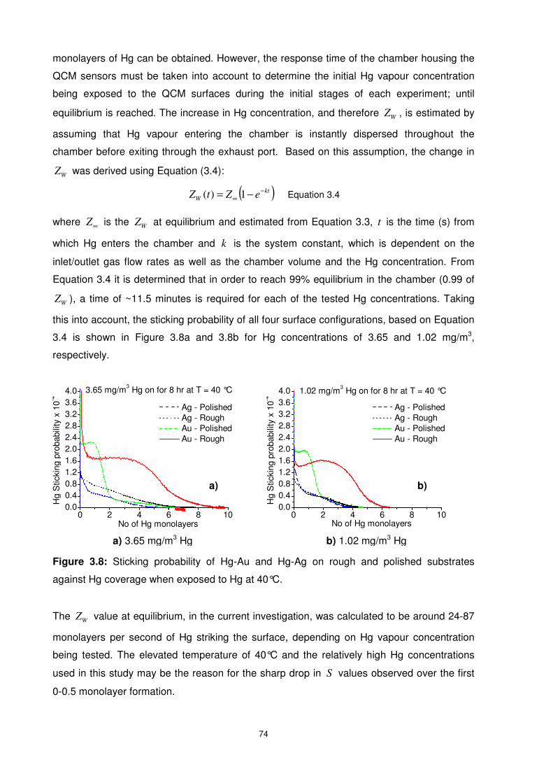
74
monolayers of Hg can be obtained. However, the response time of the chamber housing the
QCM sensors must be taken into account to determine the initial Hg vapour concentration
being exposed to the QCM surfaces during the initial stages of each experiment; until
equilibrium is reached. The increase in Hg concentration, and therefore WZ , is estimated by
assuming that Hg vapour entering the chamber is instantly dispersed throughout the
chamber before exiting through the exhaust port. Based on this assumption, the change in
WZ was derived using Equation (3.4):
( )kt
W eZtZ−
∞ −= 1)( Equation 3.4
where ∞Z is the WZ at equilibrium and estimated from Equation 3.3, t is the time (s) from
which Hg enters the chamber and k is the system constant, which is dependent on the
inlet/outlet gas flow rates as well as the chamber volume and the Hg concentration. From
Equation 3.4 it is determined that in order to reach 99% equilibrium in the chamber (0.99 of
WZ ), a time of ~11.5 minutes is required for each of the tested Hg concentrations. Taking
this into account, the sticking probability of all four surface configurations, based on Equation
3.4 is shown in Figure 3.8a and 3.8b for Hg concentrations of 3.65 and 1.02 mg/m3,
respectively.
Figure 3.8: Sticking probability of Hg-Au and Hg-Ag on rough and polished substrates
against Hg coverage when exposed to Hg at 40°C.
The WZ value at equilibrium, in the current investigation, was calculated to be around 24-87
monolayers per second of Hg striking the surface, depending on Hg vapour concentration
being tested. The elevated temperature of 40°C and the relatively high Hg concentrations
used in this study may be the reason for the sharp drop in S values observed over the first
0-0.5 monolayer formation.
a)
0 2 4 6 8 100.00.40.81.21.62.02.42.83.23.64.0 1.02 mg/m3 Hg on for 8 hr at T = 40 °C
Hg
Stic
king
pro
babi
lity
x 10
-4
No of Hg monolayers
Ag - Polished Ag - Rough Au - Polished Au - Rough
0 2 4 6 8 100.00.40.81.21.62.02.42.83.23.64.0
Ag - Polished Ag - Rough Au - Polished Au - Rough
Hg
Stic
king
pro
babi
lity
x 10
-4
No of Hg monolayers
3.65 mg/m3 Hg on for 8 hr at T = 40 °C
b)
a) 3.65 mg/m3 Hg b) 1.02 mg/m3 Hg
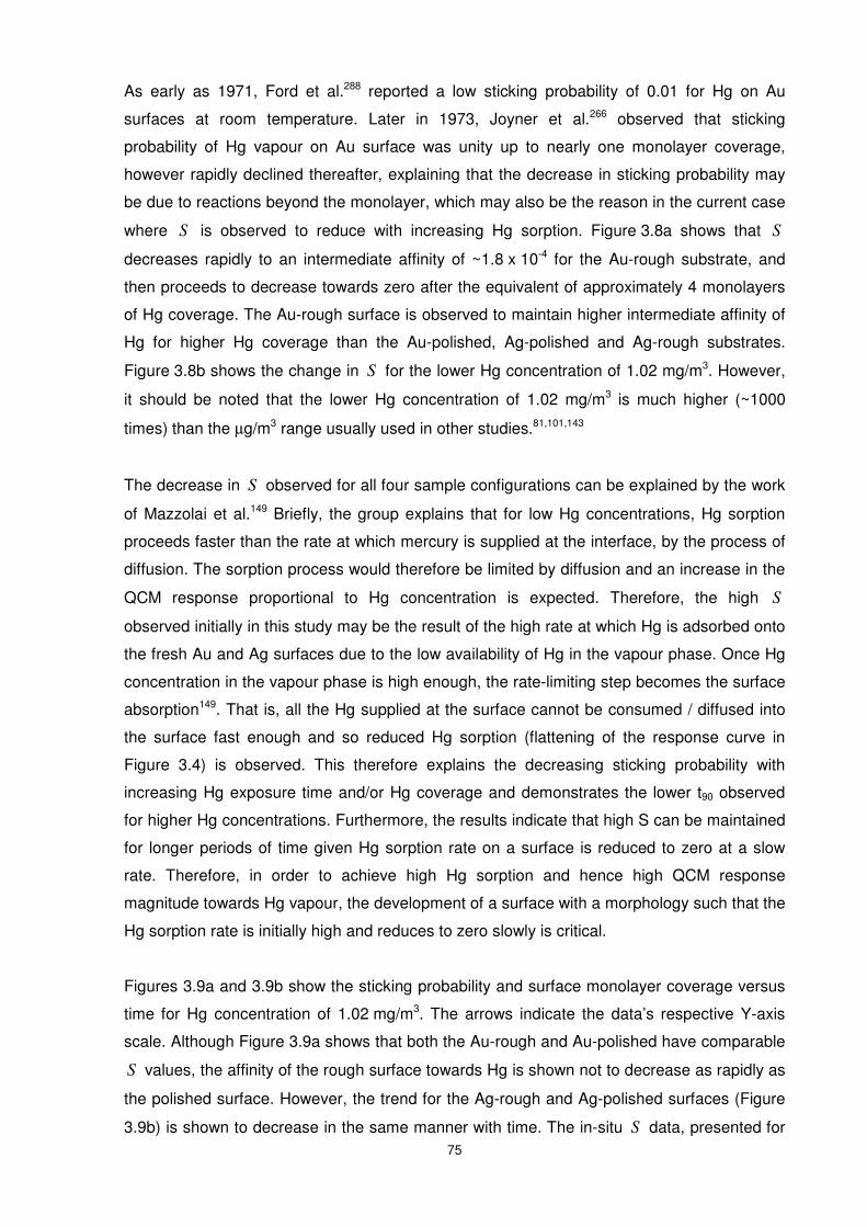
75
As early as 1971, Ford et al.288 reported a low sticking probability of 0.01 for Hg on Au
surfaces at room temperature. Later in 1973, Joyner et al.266 observed that sticking
probability of Hg vapour on Au surface was unity up to nearly one monolayer coverage,
however rapidly declined thereafter, explaining that the decrease in sticking probability may
be due to reactions beyond the monolayer, which may also be the reason in the current case
where S is observed to reduce with increasing Hg sorption. Figure 3.8a shows that S
decreases rapidly to an intermediate affinity of ~1.8 x 10⁻⁴ for the Au-rough substrate, and
then proceeds to decrease towards zero after the equivalent of approximately 4 monolayers
of Hg coverage. The Au-rough surface is observed to maintain higher intermediate affinity of
Hg for higher Hg coverage than the Au-polished, Ag-polished and Ag-rough substrates.
Figure 3.8b shows the change in S for the lower Hg concentration of 1.02 mg/m3. However,
it should be noted that the lower Hg concentration of 1.02 mg/m3 is much higher (~1000
times) than the µg/m3 range usually used in other studies.81,101,143
The decrease in S observed for all four sample configurations can be explained by the work
of Mazzolai et al.149 Briefly, the group explains that for low Hg concentrations, Hg sorption
proceeds faster than the rate at which mercury is supplied at the interface, by the process of
diffusion. The sorption process would therefore be limited by diffusion and an increase in the
QCM response proportional to Hg concentration is expected. Therefore, the high S
observed initially in this study may be the result of the high rate at which Hg is adsorbed onto
the fresh Au and Ag surfaces due to the low availability of Hg in the vapour phase. Once Hg
concentration in the vapour phase is high enough, the rate-limiting step becomes the surface
absorption149. That is, all the Hg supplied at the surface cannot be consumed / diffused into
the surface fast enough and so reduced Hg sorption (flattening of the response curve in
Figure 3.4) is observed. This therefore explains the decreasing sticking probability with
increasing Hg exposure time and/or Hg coverage and demonstrates the lower t90 observed
for higher Hg concentrations. Furthermore, the results indicate that high S can be maintained
for longer periods of time given Hg sorption rate on a surface is reduced to zero at a slow
rate. Therefore, in order to achieve high Hg sorption and hence high QCM response
magnitude towards Hg vapour, the development of a surface with a morphology such that the
Hg sorption rate is initially high and reduces to zero slowly is critical.
Figures 3.9a and 3.9b show the sticking probability and surface monolayer coverage versus
time for Hg concentration of 1.02 mg/m3. The arrows indicate the data’s respective Y-axis
scale. Although Figure 3.9a shows that both the Au-rough and Au-polished have comparable
S values, the affinity of the rough surface towards Hg is shown not to decrease as rapidly as
the polished surface. However, the trend for the Ag-rough and Ag-polished surfaces (Figure
3.9b) is shown to decrease in the same manner with time. The in-situ S data, presented for
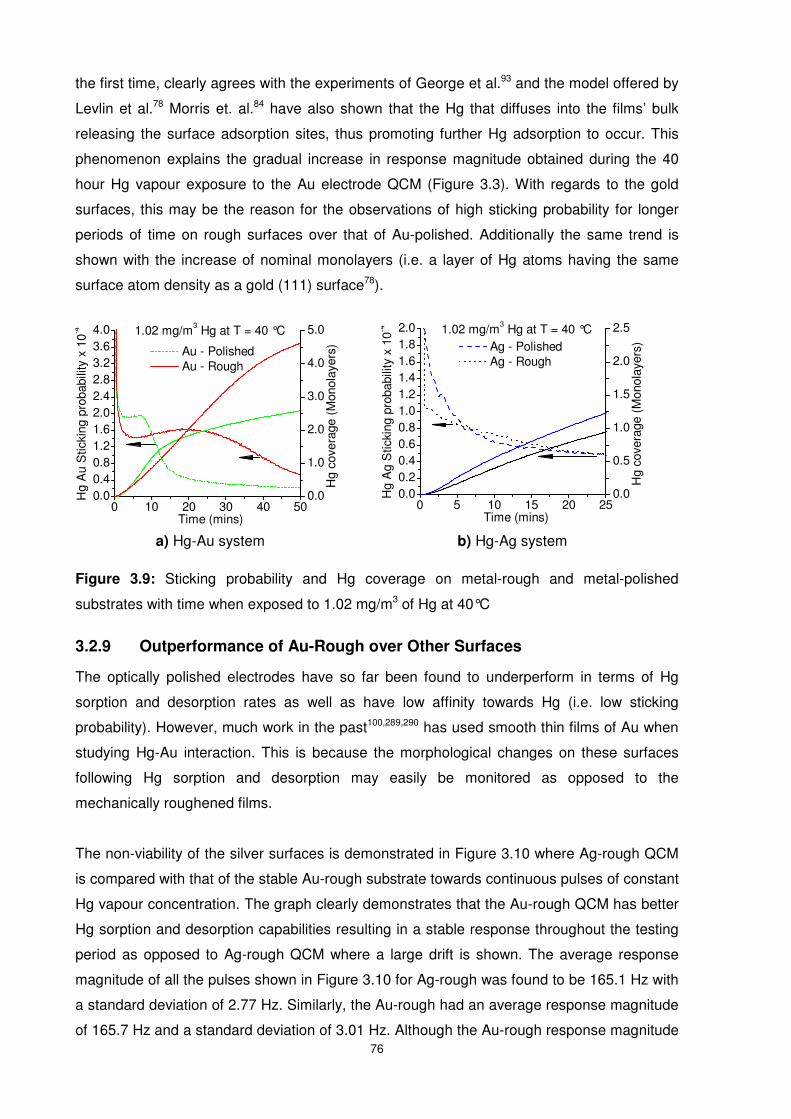
76
the first time, clearly agrees with the experiments of George et al.93 and the model offered by
Levlin et al.78 Morris et. al.84 have also shown that the Hg that diffuses into the films’ bulk
releasing the surface adsorption sites, thus promoting further Hg adsorption to occur. This
phenomenon explains the gradual increase in response magnitude obtained during the 40
hour Hg vapour exposure to the Au electrode QCM (Figure 3.3). With regards to the gold
surfaces, this may be the reason for the observations of high sticking probability for longer
periods of time on rough surfaces over that of Au-polished. Additionally the same trend is
shown with the increase of nominal monolayers (i.e. a layer of Hg atoms having the same
surface atom density as a gold (111) surface78).
Figure 3.9: Sticking probability and Hg coverage on metal-rough and metal-polished
substrates with time when exposed to 1.02 mg/m3 of Hg at 40°C
3.2.9 Outperformance of Au-Rough over Other Surfaces
The optically polished electrodes have so far been found to underperform in terms of Hg
sorption and desorption rates as well as have low affinity towards Hg (i.e. low sticking
probability). However, much work in the past100,289,290 has used smooth thin films of Au when
studying Hg-Au interaction. This is because the morphological changes on these surfaces
following Hg sorption and desorption may easily be monitored as opposed to the
mechanically roughened films.
The non-viability of the silver surfaces is demonstrated in Figure 3.10 where Ag-rough QCM
is compared with that of the stable Au-rough substrate towards continuous pulses of constant
Hg vapour concentration. The graph clearly demonstrates that the Au-rough QCM has better
Hg sorption and desorption capabilities resulting in a stable response throughout the testing
period as opposed to Ag-rough QCM where a large drift is shown. The average response
magnitude of all the pulses shown in Figure 3.10 for Ag-rough was found to be 165.1 Hz with
a standard deviation of 2.77 Hz. Similarly, the Au-rough had an average response magnitude
of 165.7 Hz and a standard deviation of 3.01 Hz. Although the Au-rough response magnitude
0 10 20 30 40 500.00.40.81.21.62.02.42.83.23.64.0
Hg
cove
rage
(M
onol
ayer
s)
Hg
Au
Stic
king
pro
babi
lity
x 10
-4
Time (mins)
Au - Polished Au - Rough
0.0
1.0
2.0
3.0
4.0
5.01.02 mg/m3 Hg at T = 40 °C
0 5 10 15 20 250.00.20.40.60.81.01.21.41.61.82.0
Hg
cove
rage
(M
onol
ayer
s)
Hg
Ag
Stic
king
pro
babi
lity
x 10
-4
Time (mins)
Ag - Polished Ag - Rough
0.0
0.5
1.0
1.5
2.0
2.51.02 mg/m3 Hg at T = 40 °C
a) Hg-Au system b) Hg-Ag system
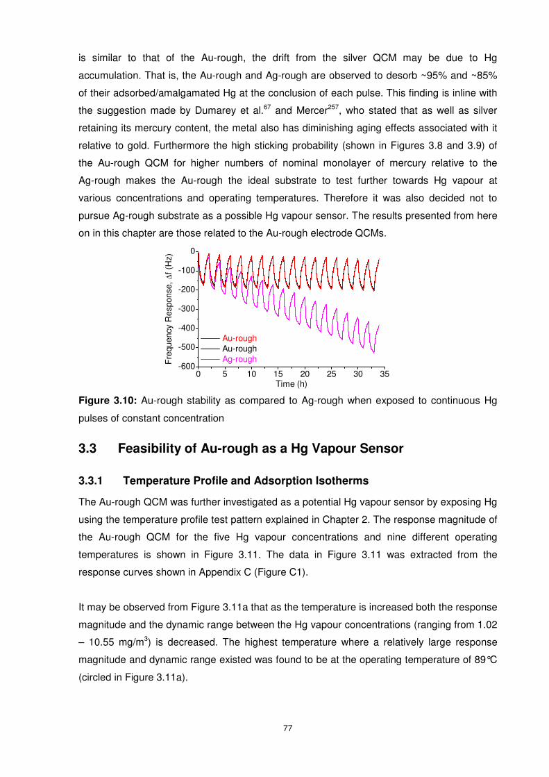
77
is similar to that of the Au-rough, the drift from the silver QCM may be due to Hg
accumulation. That is, the Au-rough and Ag-rough are observed to desorb ~95% and ~85%
of their adsorbed/amalgamated Hg at the conclusion of each pulse. This finding is inline with
the suggestion made by Dumarey et al.67 and Mercer257, who stated that as well as silver
retaining its mercury content, the metal also has diminishing aging effects associated with it
relative to gold. Furthermore the high sticking probability (shown in Figures 3.8 and 3.9) of
the Au-rough QCM for higher numbers of nominal monolayer of mercury relative to the
Ag-rough makes the Au-rough the ideal substrate to test further towards Hg vapour at
various concentrations and operating temperatures. Therefore it was also decided not to
pursue Ag-rough substrate as a possible Hg vapour sensor. The results presented from here
on in this chapter are those related to the Au-rough electrode QCMs.
Figure 3.10: Au-rough stability as compared to Ag-rough when exposed to continuous Hg
pulses of constant concentration
3.3 Feasibility of Au-rough as a Hg Vapour Sensor
3.3.1 Temperature Profile and Adsorption Isotherms
The Au-rough QCM was further investigated as a potential Hg vapour sensor by exposing Hg
using the temperature profile test pattern explained in Chapter 2. The response magnitude of
the Au-rough QCM for the five Hg vapour concentrations and nine different operating
temperatures is shown in Figure 3.11. The data in Figure 3.11 was extracted from the
response curves shown in Appendix C (Figure C1).
It may be observed from Figure 3.11a that as the temperature is increased both the response
magnitude and the dynamic range between the Hg vapour concentrations (ranging from 1.02
– 10.55 mg/m3) is decreased. The highest temperature where a relatively large response
magnitude and dynamic range existed was found to be at the operating temperature of 89°C
(circled in Figure 3.11a).
0 5 10 15 20 25 30 35-600
-500
-400
-300
-200
-100
0
Fre
quen
cy R
espo
nse,
∆f (
Hz)
Time (h)
Au-rough Au-rough Ag-rough
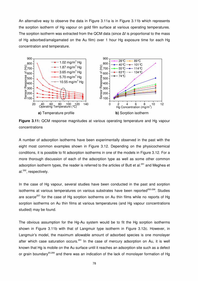
78
An alternative way to observe the data in Figure 3.11a is in Figure 3.11b which represents
the sorption isotherm of Hg vapour on gold film surface at various operating temperatures.
The sorption isotherm was extracted from the QCM data (since ∆f is proportional to the mass
of Hg adsorbed/amalgamated on the Au film) over 1 hour Hg exposure time for each Hg
concentration and temperature.
Figure 3.11: QCM response magnitudes at various operating temperature and Hg vapour
concentrations
A number of adsorption isotherms have been experimentally observed in the past with the
eight most common examples shown in Figure 3.12. Depending on the physicochemical
conditions, it is possible to fit adsorption isotherms in one of the models in Figure 3.12. For a
more thorough discussion of each of the adsorption type as well as some other common
adsorption isotherm types, the reader is referred to the articles of Butt et al.291 and Meghea et
al.292, respectively.
In the case of Hg vapour, several studies have been conducted in the past and sorption
isotherms at various temperatures on various substrates have been reported293-298. Studies
are scarce257 for the case of Hg sorption isotherms on Au thin films while no reports of Hg
sorption isotherms on Au thin films at various temperatures (and Hg vapour concentrations
studied) may be found.
The obvious assumption for the Hg-Au system would be to fit the Hg sorption isotherms
shown in Figure 3.11b with that of Langmuir type isotherm in Figure 3.12c. However, in
Langmuir’s model, the maximum allowable amount of adsorbed species is one monolayer
after which case saturation occurs.291 In the case of mercury adsorption on Au, it is well
known that Hg is mobile on the Au surface until it reaches an adsorption site such as a defect
or grain boundary93,289 and there was an indication of the lack of monolayer formation of Hg
20 40 60 80 100 120 140
100
200
300
400
500
600
700
800
900 1.02 mg/m3 Hg 1.87 mg/m3 Hg 3.65 mg/m3 Hg 5.70 mg/m3 Hg 10.55 mg/m3 Hg
Sen
sor
Res
pons
e ∆
f (H
z)
Operating Temperature (°C)0 2 4 6 8 10 12
100
200
300
400
500
600
700
800
900 28°C 89°C 40°C 101°C 55°C 114°C 63°C 134°C 74°C
Sen
sor
Res
pons
e ∆
f (H
z)
Hg Concentration (mg/m3)
b) Sorption isotherm a) Temperature profile
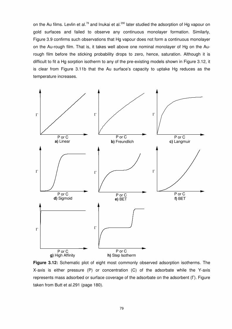
79
on the Au films. Levlin et al.78 and Inukai et al.290 later studied the adsorption of Hg vapour on
gold surfaces and failed to observe any continuous monolayer formation. Similarly,
Figure 3.9 confirms such observations that Hg vapour does not form a continuous monolayer
on the Au-rough film. That is, it takes well above one nominal monolayer of Hg on the Au-
rough film before the sticking probability drops to zero, hence, saturation. Although it is
difficult to fit a Hg sorption isotherm to any of the pre-existing models shown in Figure 3.12, it
is clear from Figure 3.11b that the Au surface’s capacity to uptake Hg reduces as the
temperature increases.
Figure 3.12: Schematic plot of eight most commonly observed adsorption isotherms. The
X-axis is either pressure (P) or concentration (C) of the adsorbate while the Y-axis
represents mass adsorbed or surface coverage of the adsorbate on the adsorbent (Г). Figure
taken from Butt et al.291 (page 180).
Γ
P or Ca) Linear
Γ
P or Cb) Freundlich
Γ
P or Cc) Langmuir
Γ
P or Cd) Sigmoid
Γ
P or Ce) BET
Γ
P or Cf) BET
Γ
P or Cg) High Affinity
Γ
P or Ch) Step Isotherm
80
Even though only five concentrations of Hg vapour have been studied in this research
program, it is quite clear from Figure 3.11b that the Hg-Au adsorption may fit a linear type
adsorption isotherm at room temperature, transforms to a Freundlich type as the temperature
increases towards 100°C and progresses to a Langmuir type above 100°C. The equations
describing the linear, Freundlich and Langmuir isotherms are shown in Equations 3.4, 3.5
and 3.6, respectively291, Where Γ and monΓ are the amount of adsorbed gas and amount of
one monolayer of adsorbed gas respectively. HK , FK and )1( <qq are constants and θ is
the relative coverage.
PK H=Γ ……………………………………………Equation 3.4
q
F PK ⋅=Γ …………………………………….…..Equation 3.5
PK
PK
L
L
+=
1θ with
monΓ
Γ=θ ……………………..Equation 3.6
The constant for the QCMs used in this study is calculated to be 227.71 Hz.cm2.µg-1. The
electrochemical surface area of the Au-rough was found (using the procedure outlined in
Chapter 2) to be ~1.22 cm2. The QCM response magnitude is therefore ~88 Hz for every
nominal monolayer of Hg vapour deposited (Hg sorption) on the surface. The Au-rough QCM
response magnitude for Hg concentrations of 1.02 and 10.55 mg/m3 was observed to be 93
and 202 Hz respectively at an operating temperature of 134°C. These values are observed to
be higher at the lower operating temperatures (Figure 3.11), indicating that at least one
nominal monolayer of Hg sorption occurs upon each Hg pulse at any concentration or
operating temperature. This suggests that saturation does not occur due to the formation of
Hg monolayer on the surface, as no saturation is observed at 28°C sorption isotherm.
Furthermore the Hg vapour pressure at 28 and 134°C may be converted to the values of
25.6 and 41524mg/m3 respectively.299 It is clear that the tendency of Hg to stay in the vapour
phase rather than adsorb on the Au surface increases three orders of magnitude with little
increase in temperature. These results are a clear indication that the change in the sorption
isotherms is operating temperature dependent and the tendency of Hg atoms to stay in the
gas phase due to high vapour pressure of Hg at the higher temperatures enhances
saturation due to reduction in the Hg sorption capacity of the Au-rough surface and not due
to monolayer formation.
3.3.2 Sorption, Desorption and Their Rates
The Hg sorption, desorption and their rate curves (in Appendix C) are overlayed following
their baseline to zero and shown in Figures 3.13 and 3.14 for the operating temperatures of
40°C and 89°C, respectively. The increase in the amount of Hg sorption as well as an
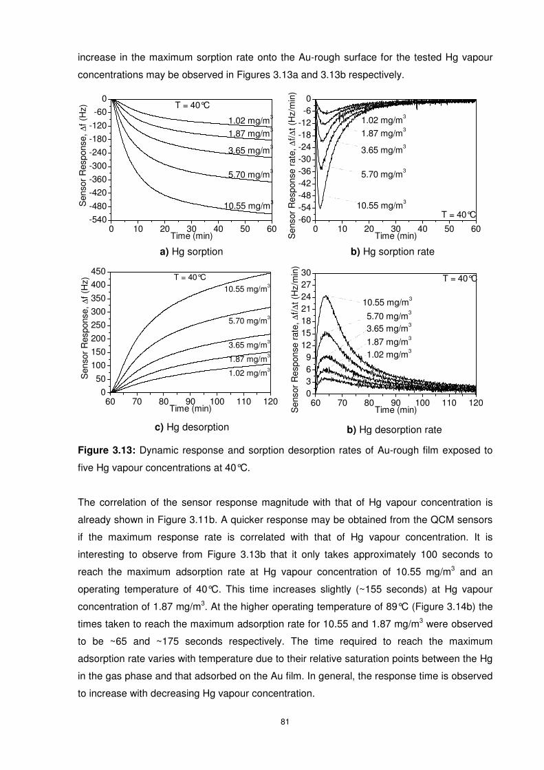
81
increase in the maximum sorption rate onto the Au-rough surface for the tested Hg vapour
concentrations may be observed in Figures 3.13a and 3.13b respectively.
Figure 3.13: Dynamic response and sorption desorption rates of Au-rough film exposed to
five Hg vapour concentrations at 40°C.
The correlation of the sensor response magnitude with that of Hg vapour concentration is
already shown in Figure 3.11b. A quicker response may be obtained from the QCM sensors
if the maximum response rate is correlated with that of Hg vapour concentration. It is
interesting to observe from Figure 3.13b that it only takes approximately 100 seconds to
reach the maximum adsorption rate at Hg vapour concentration of 10.55 mg/m3 and an
operating temperature of 40°C. This time increases slightly (~155 seconds) at Hg vapour
concentration of 1.87 mg/m3. At the higher operating temperature of 89°C (Figure 3.14b) the
times taken to reach the maximum adsorption rate for 10.55 and 1.87 mg/m3 were observed
to be ~65 and ~175 seconds respectively. The time required to reach the maximum
adsorption rate varies with temperature due to their relative saturation points between the Hg
in the gas phase and that adsorbed on the Au film. In general, the response time is observed
to increase with decreasing Hg vapour concentration.
0 10 20 30 40 50 60-540
-480
-420
-360
-300
-240
-180
-120
-60
0
10.55 mg/m3
5.70 mg/m3
3.65 mg/m3
1.87 mg/m3
1.02 mg/m3
Sen
sor
Res
pons
e, ∆
f (H
z)
Time (min)
T = 40°C
0 10 20 30 40 50 60-60-54-48-42-36-30-24-18-12-60
10.55 mg/m3
5.70 mg/m3
3.65 mg/m3
1.87 mg/m3
1.02 mg/m3
Sen
sor
Res
pons
e ra
te, ∆
f/∆t (
Hz/
min
)
Time (min)
T = 40°C
60 70 80 90 100 110 1200369
12151821242730
10.55 mg/m3
5.70 mg/m3
3.65 mg/m3
1.87 mg/m3
1.02 mg/m3
Sen
sor
Res
pons
e ra
te, ∆
f/∆t (
Hz/
min
)
Time (min)
T = 40°C
60 70 80 90 100 110 1200
50
100
150
200
250
300
350
400
450
10.55 mg/m3
5.70 mg/m3
3.65 mg/m3
1.87 mg/m3
1.02 mg/m3
Sen
sor
Res
pons
e, ∆
f (H
z)
Time (min)
T = 40°C
a) Hg sorption b) Hg sorption rate
c) Hg desorption b) Hg desorption rate
82
As expected, the maximum sorption rate is observed to increase with increasing Hg vapour
concentration. Furthermore, the higher the Hg vapour concentration, the slower the rate of
sorption drops back towards zero after reaching the maximum sorption rate (Figure 3.13b).
This slow return back to zero sorption rate is also the reason for the higher response
magnitude, hence there are larger number of Hg atoms adsorbed/amalgamated rigidly on the
gold surface. But the slower return back towards zero sorption rate also implies more
diffusion of mercury into the gold bulk. That is, diffusion is promoted by the higher
concentrations of Hg on the surface and it is well known that diffusion of mercury releases
the sorption site for more Hg to adsorb/amalgamate89,93. Since this phenomenon is promoted
better with the higher Hg vapour concentrations, a slower decrease in the Hg sorption rate
(Figure 3.13b) as well as a slow decrease in the sticking probability (comparison of
Figures 3.8a and b) is observed.
Operating temperature is also observed to affect the Hg sorption rate. The sorption rate,
having reached maximum, decreases faster back towards zero at 89°C as compared to
40°C, possibly due to the higher vapour pressure of Hg at the higher temperature of 89°C
(Figure 3.13b as compared to Figure 3.14b). It is for this quick approach towards the zero
sorption rate that caused the decreased response magnitude as well as lower Hg uptake
capacity to be observed at the higher operating temperatures (Figures 3.13a and 3.14a).
Similarly a higher magnitude of maximum Hg sorption rate is observed at the higher
operating temperature of 89°C than that of 40°C for every Hg vapour concentration. This may
be due to the increasing solubility (or affinity) of Au in Hg at the higher operating
temperatures (Figure 3.1). That is, the increased surface affinity towards Hg may be a result
of the tendency of the small size Au clusters on the Au-rough film to melt at lower
temperatures than that of bulk Au.300
The comparison of desorption with the sorption response curves (Figures 3.13a with 3.13c
and Figures 3.14a with 3.14c) clearly indicates that not all mercury adsorbed on the surface
is fully desorbed within the 1 hour desorption period. This is a clear indication that Hg has
amalgamated strongly and diffused through gold making it difficult for full desorption to occur.
An increase in temperature following the Hg exposure period is required before full
desorption may be observed.67,84,97 An increase in operating temperature is impractical when
using QCMs as online Hg vapour sensors due to their high sensitivity to temperature
fluctuations at higher than 25°C.301 Therefore the approach that will be discussed in Chapter
4 is to find an operating temperature where high sorption and desorption is observed.
For a given surface Jones and Perry295 have suggested that desorption of Hg vapour maybe
coverage dependent. This is evident from desorption rate curves in Figures 3.13d and 3.14d
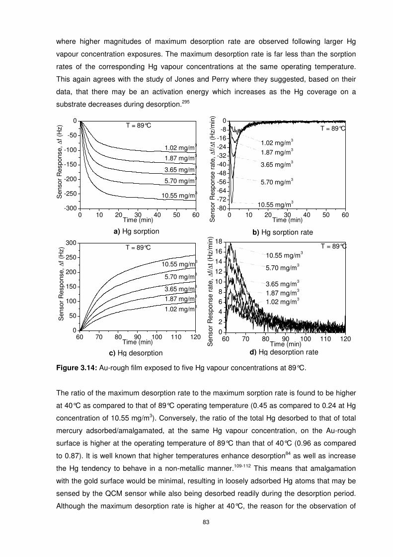
83
where higher magnitudes of maximum desorption rate are observed following larger Hg
vapour concentration exposures. The maximum desorption rate is far less than the sorption
rates of the corresponding Hg vapour concentrations at the same operating temperature.
This again agrees with the study of Jones and Perry where they suggested, based on their
data, that there may be an activation energy which increases as the Hg coverage on a
substrate decreases during desorption.295
Figure 3.14: Au-rough film exposed to five Hg vapour concentrations at 89°C.
The ratio of the maximum desorption rate to the maximum sorption rate is found to be higher
at 40°C as compared to that of 89°C operating temperature (0.45 as compared to 0.24 at Hg
concentration of 10.55 mg/m3). Conversely, the ratio of the total Hg desorbed to that of total
mercury adsorbed/amalgamated, at the same Hg vapour concentration, on the Au-rough
surface is higher at the operating temperature of 89°C than that of 40°C (0.96 as compared
to 0.87). It is well known that higher temperatures enhance desorption84 as well as increase
the Hg tendency to behave in a non-metallic manner.109-112 This means that amalgamation
with the gold surface would be minimal, resulting in loosely adsorbed Hg atoms that may be
sensed by the QCM sensor while also being desorbed readily during the desorption period.
Although the maximum desorption rate is higher at 40°C, the reason for the observation of
0 10 20 30 40 50 60-300
-250
-200
-150
-100
-50
0
10.55 mg/m3
5.70 mg/m3
3.65 mg/m3
1.87 mg/m3
1.02 mg/m3
Sen
sor
Res
pons
e, ∆
f (H
z)
Time (min)
T = 89°C
60 70 80 90 100 110 1200
50
100
150
200
250
300
10.55 mg/m3
5.70 mg/m3
3.65 mg/m3
1.87 mg/m3
1.02 mg/m3
Sen
sor
Res
pons
e, ∆
f (H
z)
Time (min)
T = 89°C
0 10 20 30 40 50 60-80-72-64-56-48-40-32-24-16-80
10.55 mg/m3
5.70 mg/m3
3.65 mg/m3
1.87 mg/m3
1.02 mg/m3
Sen
sor
Res
pons
e ra
te, ∆
f/∆t (
Hz/
min
)Time (min)
T = 89°C
a) Hg sorption b) Hg sorption rate
d) Hg desorption rate c) Hg desorption
60 70 80 90 100 110 1200
2
4
6
8
10
12
14
16
18
1.02 mg/m31.87 mg/m33.65 mg/m3
5.70 mg/m3
10.55 mg/m3
Sen
sor
Res
pons
e ra
te, ∆
f/∆t (
Hz/
min
)
Time (min)
T = 89°C
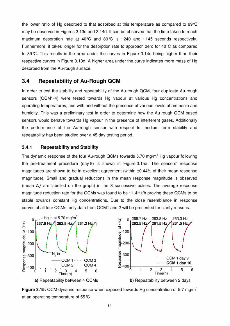
84
the lower ratio of Hg desorbed to that adsorbed at this temperature as compared to 89°C
may be observed in Figures 3.13d and 3.14d. It can be observed that the time taken to reach
maximum desorption rate at 40°C and 89°C is ~240 and ~145 seconds respectively.
Furthermore, it takes longer for the desorption rate to approach zero for 40°C as compared
to 89°C. This results in the area under the curves in Figure 3.14d being higher than their
respective curves in Figure 3.13d. A higher area under the curve indicates more mass of Hg
desorbed from the Au-rough surface.
3.4 Repeatability of Au-Rough QCM
In order to test the stability and repeatability of the Au-rough QCM, four duplicate Au-rough
sensors (QCM1-4) were tested towards Hg vapour at various Hg concentrations and
operating temperatures, and with and without the presence of various levels of ammonia and
humidity. This was a preliminary test in order to determine how the Au-rough QCM based
sensors would behave towards Hg vapour in the presence of interferent gases. Additionally
the performance of the Au-rough sensor with respect to medium term stability and
repeatability has been studied over a 45 day testing period.
3.4.1 Repeatability and Stability
The dynamic response of the four Au-rough QCMs towards 5.70 mg/m3 Hg vapour following
the pre-treatment procedure (day 9) is shown in Figure 3.15a. The sensors’ response
magnitudes are shown to be in excellent agreement (within ±0.44% of their mean response
magnitude). Small and gradual reductions in the mean response magnitude is observed
(mean ∆ƒ are labelled on the graph) in the 3 successive pulses. The average response
magnitude reduction rate for the QCMs was found to be ~1.4Hz/h proving these QCMs to be
stable towards constant Hg concentrations. Due to the close resemblance in response
curves of all four QCMs, only data from QCM1 and 2 will be presented for clarity reasons.
Figure 3.15: QCM dynamic response when exposed towards Hg concentration of 5.7 mg/m3
at an operating temperature of 55°C
0 1 2 3 4 5 6-400
-300
-200
-100
0
Res
pons
e m
agni
tude
, ∆f (
Hz) 263.3 Hz
261.5 Hz
263.8 Hz261.5 Hz
QCM 1 day 9 QCM 1 day 10
Time(h)
268.7 Hz262.5 Hz
0 1 2 3 4 5 6-400
-300
-200
-100
0261.2 Hz262.8 Hz
Hg in at 5.70 mg/m3
QCM 1 QCM 3 QCM 2 QCM 4
Time(h)
Res
pons
e m
agni
tude
, ∆f (
Hz)
N2 in
267.6 Hz
a) Repeatability between 4 QCMs b) Repeatability between 2 days
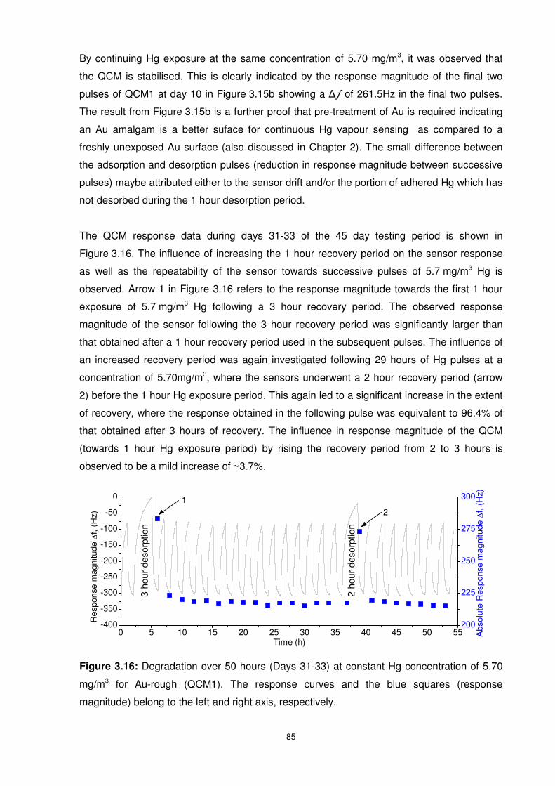
85
By continuing Hg exposure at the same concentration of 5.70 mg/m3, it was observed that
the QCM is stabilised. This is clearly indicated by the response magnitude of the final two
pulses of QCM1 at day 10 in Figure 3.15b showing a ∆ƒ of 261.5Hz in the final two pulses.
The result from Figure 3.15b is a further proof that pre-treatment of Au is required indicating
an Au amalgam is a better suface for continuous Hg vapour sensing as compared to a
freshly unexposed Au surface (also discussed in Chapter 2). The small difference between
the adsorption and desorption pulses (reduction in response magnitude between successive
pulses) maybe attributed either to the sensor drift and/or the portion of adhered Hg which has
not desorbed during the 1 hour desorption period.
The QCM response data during days 31-33 of the 45 day testing period is shown in
Figure 3.16. The influence of increasing the 1 hour recovery period on the sensor response
as well as the repeatability of the sensor towards successive pulses of 5.7 mg/m3 Hg is
observed. Arrow 1 in Figure 3.16 refers to the response magnitude towards the first 1 hour
exposure of 5.7 mg/m3 Hg following a 3 hour recovery period. The observed response
magnitude of the sensor following the 3 hour recovery period was significantly larger than
that obtained after a 1 hour recovery period used in the subsequent pulses. The influence of
an increased recovery period was again investigated following 29 hours of Hg pulses at a
concentration of 5.70mg/m3, where the sensors underwent a 2 hour recovery period (arrow
2) before the 1 hour Hg exposure period. This again led to a significant increase in the extent
of recovery, where the response obtained in the following pulse was equivalent to 96.4% of
that obtained after 3 hours of recovery. The influence in response magnitude of the QCM
(towards 1 hour Hg exposure period) by rising the recovery period from 2 to 3 hours is
observed to be a mild increase of ~3.7%.
Figure 3.16: Degradation over 50 hours (Days 31-33) at constant Hg concentration of 5.70
mg/m3 for Au-rough (QCM1). The response curves and the blue squares (response
magnitude) belong to the left and right axis, respectively.
0 5 10 15 20 25 30 35 40 45 50 55-400
-350
-300
-250
-200
-150
-100
-50
0
3 ho
ur d
esor
ptio
n
Abs
olut
e R
espo
nse
mag
nitu
de ∆
f, (H
z)
Res
pons
e m
agni
tude
∆f,
(Hz)
Time (h)
12
2 ho
ur d
esor
ptio
n
200
225
250
275
300
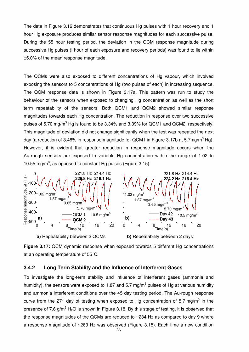
86
The data in Figure 3.16 demonstrates that continuous Hg pulses with 1 hour recovery and 1
hour Hg exposure produces similar sensor response magnitudes for each successive pulse.
During the 55 hour testing period, the deviation in the QCM response magnitude during
successive Hg pulses (I hour of each exposure and recovery periods) was found to lie within
±5.0% of the mean response magnitude.
The QCMs were also exposed to different concentrations of Hg vapour, which involved
exposing the sensors to 5 concentrations of Hg (two pulses of each) in increasing sequence.
The QCM response data is shown in Figure 3.17a. This pattern was run to study the
behaviour of the sensors when exposed to changing Hg concentration as well as the short
term repeatability of the sensors. Both QCM1 and QCM2 showed similar response
magnitudes towards each Hg concentration. The reduction in response over two successive
pulses of 5.70 mg/m3 Hg is found to be 3.34% and 3.39% for QCM1 and QCM2, respectively.
This magnitude of deviation did not change significantly when the test was repeated the next
day (a reduction of 3.48% in response magnitude for QCM1 in Figure 3.17b at 5.7mg/m3 Hg).
However, it is evident that greater reduction in response magnitude occurs when the
Au-rough sensors are exposed to variable Hg concentration within the range of 1.02 to
10.55 mg/m3, as opposed to constant Hg pulses (Figure 3.15).
Figure 3.17: QCM dynamic response when exposed towards 5 different Hg concentrations
at an operating temperature of 55°C.
3.4.2 Long Term Stability and the Influence of Interferent Gases
To investigate the long-term stability and influence of interferent gases (ammonia and
humidity), the sensors were exposed to 1.87 and 5.7 mg/m3 pulses of Hg at various humidity
and ammonia interferent conditions over the 45 day testing period. The Au-rough response
curve from the 27th day of testing when exposed to Hg concentration of 5.7 mg/m3 in the
presence of 7.6 g/m3 H2O is shown in Figure 3.18. By this stage of testing, it is observed that
the response magnitudes of the QCMs are reduced to ~234 Hz as compared to day 9 where
a response magnitude of ~263 Hz was observed (Figure 3.15). Each time a new condition
0 4 8 12 16 20-500
-400
-300
-200
-100
0
0 4 8 12 16 20
214.4 Hz219.1 Hz
QCM 1 QCM 2
10.5 mg/m3
5.70 mg/m33.65 mg/m3
1.87 mg/m3
Res
pons
e m
agni
tude
, ∆f (
Hz)
Time(h)
1.02 mg/m3
221.8 Hz226.8 Hz
214.4 Hz216.4 Hz
221.8 Hz224.2 Hz
Day 42 Day 43
10.5 mg/m3
5.70 mg/m33.65 mg/m3
1.87 mg/m3
Time(h)
1.02 mg/m3
a) b)
a) Repeatability between 2 QCMs b) Repeatability between 2 days
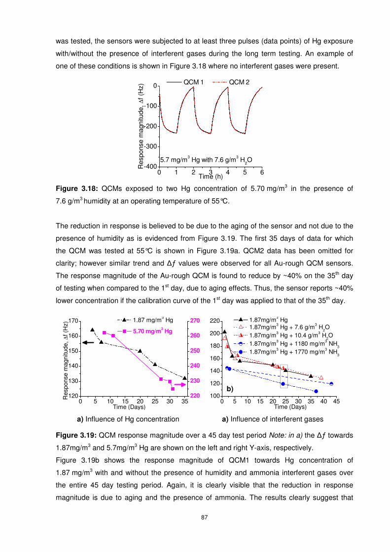
87
was tested, the sensors were subjected to at least three pulses (data points) of Hg exposure
with/without the presence of interferent gases during the long term testing. An example of
one of these conditions is shown in Figure 3.18 where no interferent gases were present.
Figure 3.18: QCMs exposed to two Hg concentration of 5.70 mg/m3 in the presence of
7.6 g/m3 humidity at an operating temperature of 55°C.
The reduction in response is believed to be due to the aging of the sensor and not due to the
presence of humidity as is evidenced from Figure 3.19. The first 35 days of data for which
the QCM was tested at 55°C is shown in Figure 3.19a. QCM2 data has been omitted for
clarity; however similar trend and ∆ƒ values were observed for all Au-rough QCM sensors.
The response magnitude of the Au-rough QCM is found to reduce by ~40% on the 35th day
of testing when compared to the 1st day, due to aging effects. Thus, the sensor reports ~40%
lower concentration if the calibration curve of the 1st day was applied to that of the 35th day.
Figure 3.19: QCM response magnitude over a 45 day test period Note: in a) the ∆ƒ towards
1.87mg/m3 and 5.7mg/m3 Hg are shown on the left and right Y-axis, respectively.
Figure 3.19b shows the response magnitude of QCM1 towards Hg concentration of
1.87 mg/m3 with and without the presence of humidity and ammonia interferent gases over
the entire 45 day testing period. Again, it is clearly visible that the reduction in response
magnitude is due to aging and the presence of ammonia. The results clearly suggest that
0 1 2 3 4 5 6-400
-300
-200
-100
0
5.7 mg/m3 Hg with 7.6 g/m3 H2O
QCM 1 QCM 2
Time (h)
Res
pons
e m
agni
tude
, ∆f (
Hz)
a) Influence of Hg concentration
b)
0 5 10 15 20 25 30 35120
130
140
150
160
170
0 5 10 15 20 25 30 35 40 45100
120
140
160
180
200
220
Time (Days)
1.87 mg/m3 Hg
Res
pons
e m
agni
tude
, ∆f (
Hz)
Time (Days)
220
230
240
250
260
270
5.70 mg/m3 Hg
1.87mg/m3 Hg + 10.4 g/m3 H2O
1.87mg/m3 Hg + 1180 mg/m3 NH3
1.87mg/m3 Hg + 1770 mg/m3 NH3
1.87mg/m3 Hg + 7.6 g/m3 H2O
1.87mg/m3 Hg
a) Influence of interferent gases
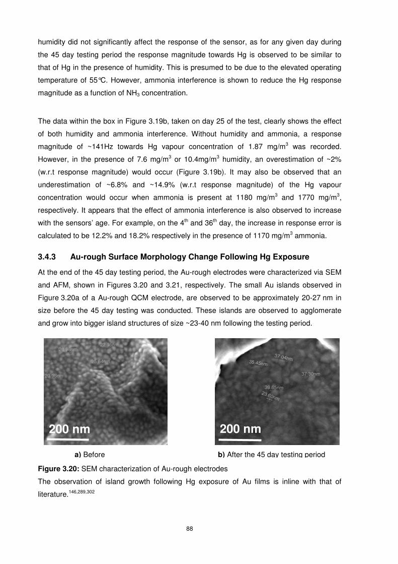
88
humidity did not significantly affect the response of the sensor, as for any given day during
the 45 day testing period the response magnitude towards Hg is observed to be similar to
that of Hg in the presence of humidity. This is presumed to be due to the elevated operating
temperature of 55°C. However, ammonia interference is shown to reduce the Hg response
magnitude as a function of NH3 concentration.
The data within the box in Figure 3.19b, taken on day 25 of the test, clearly shows the effect
of both humidity and ammonia interference. Without humidity and ammonia, a response
magnitude of ~141Hz towards Hg vapour concentration of 1.87 mg/m3 was recorded.
However, in the presence of 7.6 mg/m3 or 10.4mg/m3 humidity, an overestimation of ~2%
(w.r.t response magnitude) would occur (Figure 3.19b). It may also be observed that an
underestimation of ~6.8% and ~14.9% (w.r.t response magnitude) of the Hg vapour
concentration would occur when ammonia is present at 1180 mg/m3 and 1770 mg/m3,
respectively. It appears that the effect of ammonia interference is also observed to increase
with the sensors’ age. For example, on the 4th and 36th day, the increase in response error is
calculated to be 12.2% and 18.2% respectively in the presence of 1170 mg/m3 ammonia.
3.4.3 Au-rough Surface Morphology Change Following Hg Exposure
At the end of the 45 day testing period, the Au-rough electrodes were characterized via SEM
and AFM, shown in Figures 3.20 and 3.21, respectively. The small Au islands observed in
Figure 3.20a of a Au-rough QCM electrode, are observed to be approximately 20-27 nm in
size before the 45 day testing was conducted. These islands are observed to agglomerate
and grow into bigger island structures of size ~23-40 nm following the testing period.
Figure 3.20: SEM characterization of Au-rough electrodes
The observation of island growth following Hg exposure of Au films is inline with that of
literature.146,289,302
200 nm 200 nm
a) Before b) After the 45 day testing period
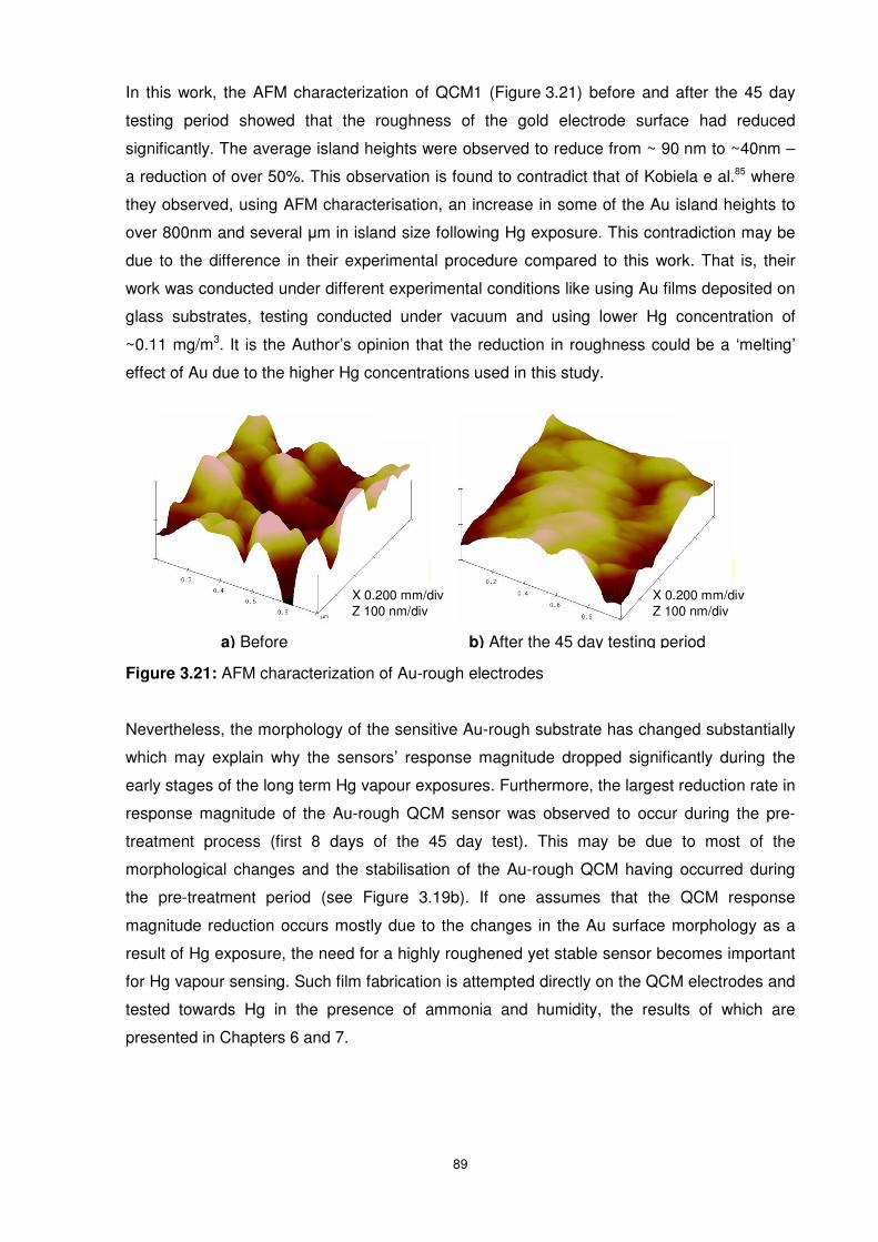
89
In this work, the AFM characterization of QCM1 (Figure 3.21) before and after the 45 day
testing period showed that the roughness of the gold electrode surface had reduced
significantly. The average island heights were observed to reduce from ~ 90 nm to ~40nm –
a reduction of over 50%. This observation is found to contradict that of Kobiela e al.85 where
they observed, using AFM characterisation, an increase in some of the Au island heights to
over 800nm and several µm in island size following Hg exposure. This contradiction may be
due to the difference in their experimental procedure compared to this work. That is, their
work was conducted under different experimental conditions like using Au films deposited on
glass substrates, testing conducted under vacuum and using lower Hg concentration of
~0.11 mg/m3. It is the Author’s opinion that the reduction in roughness could be a ‘melting’
effect of Au due to the higher Hg concentrations used in this study.
Figure 3.21: AFM characterization of Au-rough electrodes
Nevertheless, the morphology of the sensitive Au-rough substrate has changed substantially
which may explain why the sensors’ response magnitude dropped significantly during the
early stages of the long term Hg vapour exposures. Furthermore, the largest reduction rate in
response magnitude of the Au-rough QCM sensor was observed to occur during the pre-
treatment process (first 8 days of the 45 day test). This may be due to most of the
morphological changes and the stabilisation of the Au-rough QCM having occurred during
the pre-treatment period (see Figure 3.19b). If one assumes that the QCM response
magnitude reduction occurs mostly due to the changes in the Au surface morphology as a
result of Hg exposure, the need for a highly roughened yet stable sensor becomes important
for Hg vapour sensing. Such film fabrication is attempted directly on the QCM electrodes and
tested towards Hg in the presence of ammonia and humidity, the results of which are
presented in Chapters 6 and 7.
X 0.200 mm/divZ 100 nm/div
X 0.200 mm/divZ 100 nm/div
a) Before b) After the 45 day testing period
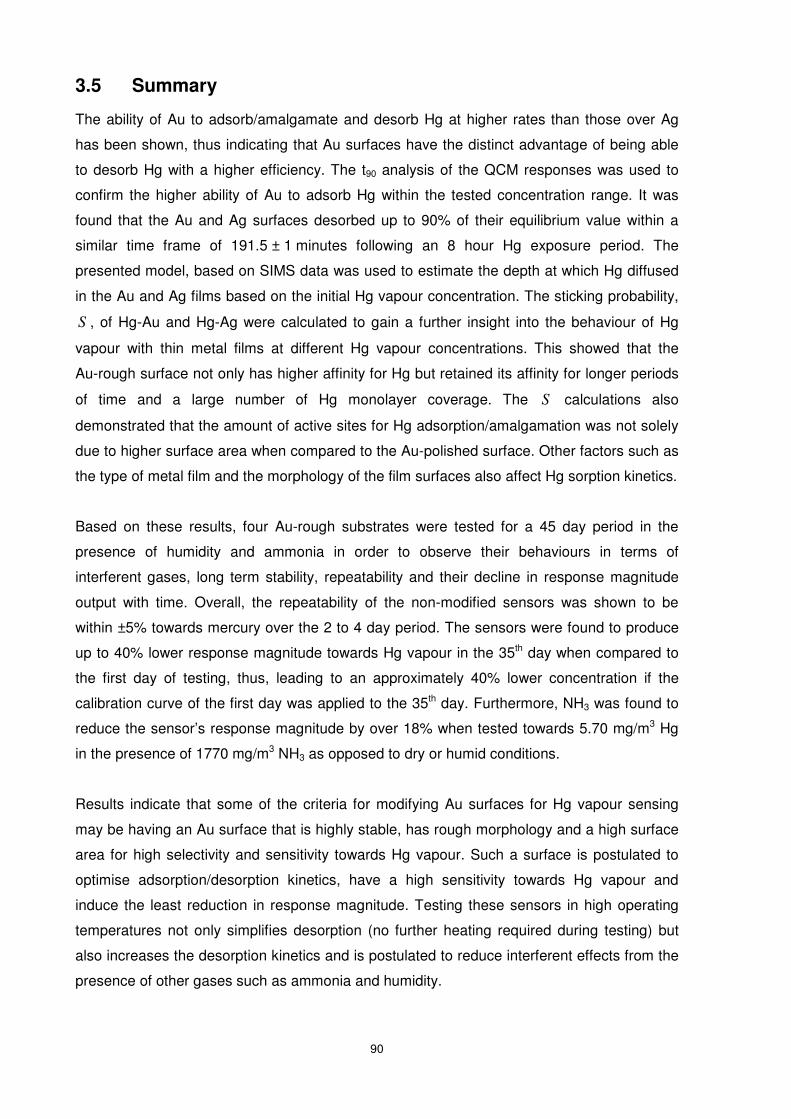
90
3.5 Summary
The ability of Au to adsorb/amalgamate and desorb Hg at higher rates than those over Ag
has been shown, thus indicating that Au surfaces have the distinct advantage of being able
to desorb Hg with a higher efficiency. The t90 analysis of the QCM responses was used to
confirm the higher ability of Au to adsorb Hg within the tested concentration range. It was
found that the Au and Ag surfaces desorbed up to 90% of their equilibrium value within a
similar time frame of 191.5 ± 1 minutes following an 8 hour Hg exposure period. The
presented model, based on SIMS data was used to estimate the depth at which Hg diffused
in the Au and Ag films based on the initial Hg vapour concentration. The sticking probability,
S , of Hg-Au and Hg-Ag were calculated to gain a further insight into the behaviour of Hg
vapour with thin metal films at different Hg vapour concentrations. This showed that the
Au-rough surface not only has higher affinity for Hg but retained its affinity for longer periods
of time and a large number of Hg monolayer coverage. The S calculations also
demonstrated that the amount of active sites for Hg adsorption/amalgamation was not solely
due to higher surface area when compared to the Au-polished surface. Other factors such as
the type of metal film and the morphology of the film surfaces also affect Hg sorption kinetics.
Based on these results, four Au-rough substrates were tested for a 45 day period in the
presence of humidity and ammonia in order to observe their behaviours in terms of
interferent gases, long term stability, repeatability and their decline in response magnitude
output with time. Overall, the repeatability of the non-modified sensors was shown to be
within ±5% towards mercury over the 2 to 4 day period. The sensors were found to produce
up to 40% lower response magnitude towards Hg vapour in the 35th day when compared to
the first day of testing, thus, leading to an approximately 40% lower concentration if the
calibration curve of the first day was applied to the 35th day. Furthermore, NH3 was found to
reduce the sensor’s response magnitude by over 18% when tested towards 5.70 mg/m3 Hg
in the presence of 1770 mg/m3 NH3 as opposed to dry or humid conditions.
Results indicate that some of the criteria for modifying Au surfaces for Hg vapour sensing
may be having an Au surface that is highly stable, has rough morphology and a high surface
area for high selectivity and sensitivity towards Hg vapour. Such a surface is postulated to
optimise adsorption/desorption kinetics, have a high sensitivity towards Hg vapour and
induce the least reduction in response magnitude. Testing these sensors in high operating
temperatures not only simplifies desorption (no further heating required during testing) but
also increases the desorption kinetics and is postulated to reduce interferent effects from the
presence of other gases such as ammonia and humidity.
91
3.6 References
(1) McNerney, J. J.; Buseck, P. R.; Hanson, R. C. Science 1972, 178, 611-612. (2) Levlin, M.; Ikavalko, E.; Laitinen, T. Fresenius Journal of Analytical Chemistry 1999, 365, 577-
586. (3) Rex, M.; Hernandez, F. E.; Campiglia, A. D. Analytical Chemistry 2006, 78, 445-451. (4) Sabri, Y. M.; Ippolito, S. J.; Tardio, J.; Atanacio, A. J.; Sood, D. K.; Bhargava, S. K. Sensors
and Actuators B: Chemical 2009, 137, 246-252. (5) García-Sánchez, A.; Contreras, F.; Adams, M.; Santos, F. Environmental Geochemistry and
Health 2006, 28, 529-540. (6) Gochfeld, M. Ecotoxicology and Environmental Safety 2003, 56, 174-179. (7) Li, J.; Herrero, E.; Abruña, H. D. Colloids and Surfaces A: Physicochemical and Engineering
Aspects 1998, 134, 113-131. (8) George, M. A.; Glaunsinger, W. S. Thin Solid Films 1994, 245, 215-224. (9) Guminski, C.; Galus, A.; Hirayama, C. In Solubility Data Series: Metals in Mercury; Warsaw,
U. O., Ed.; Pergamon Press: Warsaw, Poland, 1986; Vol. 25, p 258-384. (10) Atkins, P. W. Physical Chemistry; 2nd ed.; Oxford University Press: Oxford, Great Britain,
1982. (11) Scott, J. E.; Ottaway, J. M. Analyst 1981, 106, 1076-1081. (12) Shao, R.; Tan, E. L.; Grimes, C. A.; Ong, K. G. Sensors Letters 2007, 5, 6. (13) McDonagh, C.; Bowe, P.; Mongey, K.; MacCraith, B. D. Journal of Non-Crystalline Solids
2002, 306, 138-148. (14) Bohets, H.; Vanhoutte, K.; De Maesschalck, R.; Cockaerts, P.; Vissers, B.; Nagels, L. J.
Analytica Chimica Acta 2007, 581, 181-191. (15) Crank, J. The Mathematics of Diffusion; Oxford University Press, London, England, 1975; Vol.
2nd edition. (16) Richaud, R.; Lachas, H.; Healey, A. E.; Reed, G. P.; Haines, J.; Jarvis, K. E.; Herod, A. A.;
Dugwell, D. R.; Kandiyoti, R. Fuel 2000, 79, 1077-1087. (17) Krata, A.; Bulska, E. Spectrochimica Acta Part B: Atomic Spectroscopy 2005, 60, 345-350. (18) Ping, L.; Dasgupta, P. K. Analytical Chemistry 1989, 61, 1230-1235. (19) Takaya, M.; Joeng, J. Y.; Ishihara, N.; Serita, F.; Kohyama, N. Industrial Health 2006, 44, 287-
290. (20) Marins, R. V.; de Andrade, J. B.; Pereira, P. A. d. P.; Paiva, E. C.; Paraquetti, H. H. M. Journal
of Environmental Monitoring 2000, 2, 325-328. (21) Moreno, F. N.; Anderson, C. W. N.; Stewart, R. B.; Robinson, B. H. Environmental and
Experimental Botany 2008, 62, 78-85. (22) Morris, T.; Sun, J.; Szulczewski, G. Analytica Chimica Acta 2003, 496, 279-287. (23) Kalb, G. W. Atomic Absorption Newsletter 1970, 9, 4. (24) Drelich, J.; White, C. L.; Xu, Z. Environ. Sci. Technol. 2008, 42, 2072-2078. (25) Mercer, T. T. Analytical Chemistry 1979, 51, 5. (26) Tsionsky, V.; Gileadi, E. Langmuir 1994, 10, 2830-2835. (27) Haskell, R. B. Masters, University of Maine, 2003. (28) Levlin, M.; Niemi, H. E. M.; Hautojärvi, P.; Ikävalko, E.; Laitinen, T. Fresenius' Journal of
Analytical Chemistry 1996, 355, 2-9. (29) Ford, R. R.; Pritchard, J. Transactions of the Faraday Society 1971, 67, 216-221. (30) Joyner, R. W.; Roberts, M. W. Journal of the Chemical Society Faraday Transactions 1 1973,
69, 1242-1250. (31) Battistoni, C.; Bemporad, E.; Galdikas, A.; Kaciulis, S.; Mattogno, G.; Mickevicius, S.;
Olevano, V. Applied Surface Science 1996, 103, 107-111. (32) Mirsky, V. M.; Vasjari, M.; Novotny, I.; Rehacek, V.; Tvarozek, V.; Wolfbeis, O. S.
Nanotechnology 2002, 13, 175-178. (33) Mazzolai, B.; Mattoli, V.; Raffa, V.; Tripoli, G.; Accoto, D.; Menciassi, A.; Dario, P. Sensors
and Actuators A: Physical 2004, 113, 282-287. (34) George, M. A.; Glaunsinger, W. S.; Thundat, T.; Lindsay, S. M. Journal of Microscopy 1988,
152, 703-713. (35) Chaurasia, H. K.; Huizinga, A.; Voss, W. A. G. Journal of Physics D: Applied Physics 1975, 8,
214-218. (36) Inukai, J.; Sugita, S.; Itaya, K. Journal of Electroanalytical Chemistry 1996, 403, 159-168. (37) Dumarey, R.; Dams, R.; Hoste, J. Analytical Chemistry 1985, 57, 2638-2643. (38) Butt, H.-J.; Graf, K.; Kappl, M. In Physics and Chemistry of Interfaces 2004, p 177-205.
92
(39) Meghea, A.; Rehner, H.; Peleanu, I.; Mihalache, R. Journal of Radioanalytical and Nuclear Chemistry 1998, 229, 105-110.
(40) Jones, R. G.; Perry, D. L. Surface Science 1978, 71, 59-74. (41) Jones, R. G.; Perry, D. L. Surface Science 1979, 82, 540-548. (42) Jones, R. G.; Perry, D. L. Vacuum 1981, 31, 493-498. (43) Singh, N. K.; Jones, R. G. Surface Science 1990, 232, 229-242. (44) Levine, H. S.; MacCallum, C. J. Journal of Applied Physics 1960, 31, 595-599. (45) Yoshida, Z. Bulletin of the Chemical Society of Japan 1981, 54, 562-567. (46) Aylward, G. H.; Findlay, T. J. V. SI Chemical Data; John Wiley & Sons, 2002; Vol. 5. (47) Buffat, P.; Borel, J. P. Physical Review A 1976, 13, 2287. (48) Scheide, E. P.; Taylor, J. K. American Industrial Hygiene Association Journal 1975, 36, 897 -
901. (49) Lucklum, R.; Eichelbaum, F. In Piezoelectric Sensors 2007, p 3-47. (50) Schmutzler, R. W.; Hensel, F. Journal of Non-Crystalline Solids 1972, 8-10, 718-721. (51) El-Hanany, U.; Warren, W. W. Physical Review Letters 1975, 34, 1276. (52) Even, U.; Jortner, J. Physical Review Letters 1972, 28, 31. (53) Hensel, F. Berichte der Bunsengesellschaft fur Physikalische Chemie 1976, 80, 786-789. (54) Yang, X.; Tonami, K.; Nagahara, L. A.; Hashimoto, K.; Wei, Y.; Fujishima, A. Chemistry
Letters 1994, 11, 2059-2062. (55) Kobiela, T.; Nowakowski, B.; Dus, R. Applied Surface Science 2003, 206, 78-89.
93
Chapter IV
Chapter 4 Study of Hg Interaction kinetics
on Au Thin Films
The effect of Hg sorption and desorption on thin Au-polished films of different thickness
deposited on QCM crystals is investigated and the results are presented in this chapter.
An investigation to determine the optimum Au film thickness and operating temperature
for Hg vapour sensing is also carried out. The trend of increasing sorption capacity with
decreasing Au film thicknesses is shown not to follow for all Au thicknesses and is found
to depend on parameters such as Hg vapour concentration and operating temperature. In
choosing the optimum operating temperature, a trade off between maintaining a large
dynamic range of the sensor response and the ratio of desorbed to adsorbed and/or
amalgamated Hg is considered. A comparison of Hg sorption and desorption kinetics is
also made between the Au-rough and Au-polished films.
Part of the work presented in this chapter has been published:
1) Sawant, P.D; Sabri, Y.M; Ippolito, S.J; Bansal, V and Bhargava, S.K. “In-depth nano-scale
analysis of complex interactions of Hg with gold nanostructures using AFM based power
spectrum density method” Physical Chemistry Chemical Physics, 2009, 11(14), pp. 2374 –
2378.
94
4.1 Introduction
The development of selective and sensitive chemical sensors cannot simply rely on empirical
observations, but requires a more fundamental understanding of the involved interaction
phenomena of the target chemical (adsorbate) on the sensitive layer’s (adsorbent) surface.
The key parameters usually investigated to understand analyte sorption capacity of a
sensitive layer are the variations in film thickness,303-305 operating temperature306-308 and
analyte concentration.309-311
Film thickness studies have been performed for Au based Hg sensors in order to study
Hg-Au interaction phenomenon61. The thickness of Hg layer on Au films is assumed to be
fixed at saturation under a constant Hg vapour concentration and operating temperature
conditions.99 Therefore, from Sauerbrey’s equation (Equation 1.2), a larger surface area
should result in proportionally larger Hg sorption and hence greater frequency change.
Studies have shown that the optimum Au film thickness for Hg sorption is between 7.5 – 10
nm, above which, is postulated to reduce sensitivity.99 This is because at thicknesses above
7.5 nm the Au film is believed to undergo transition from small Au islands into a continuous
film due to coalescence of the islands and therefore reduction in the available surface area
resulting in reduced Hg sorption.61,99,100,256
The influence of parameters such as Hg partial pressure (concentration), Hg exposure time,
operating temperature and Au film thickness on Hg sorption capacity, to the best of the
Author’s knowledge, has so far not been described in literature. It was therefore deemed
necessary to investigate the influence of the above mentioned parameters for Au film
thickness between 40 and 200 nm deposited on QCM crystals.
4.2 Experimental Setup
Studies198,301 have shown that a 10 MHz QCM crystal with 4mm diameter Au electrodes (As
used in this study) must consist of Au film thickness of approximately 100 nm in order to
obtain high Q factors. It has also been established that at least 80 nm thick Au film is
required to be deposited on the 10 MHz quartz crystal of even the largest electrode diameter
in order for the sensor to oscillate and maintain good electrical properties of the QCM
electrodes. However, as discussed above, thinner Au films are said to increase sensitivity
when monitoring Hg vapour100. Furthermore, previous studies have shown that thin film
properties become highly dependent on film thickness for thickness below 150 nm.312
To study the influence of Au film thickness on Hg sorption and desorption kinetics, Au films of
40, 50, 100, 150 and 200 nm were deposited on both AT-cut quartz crystals’ faces following
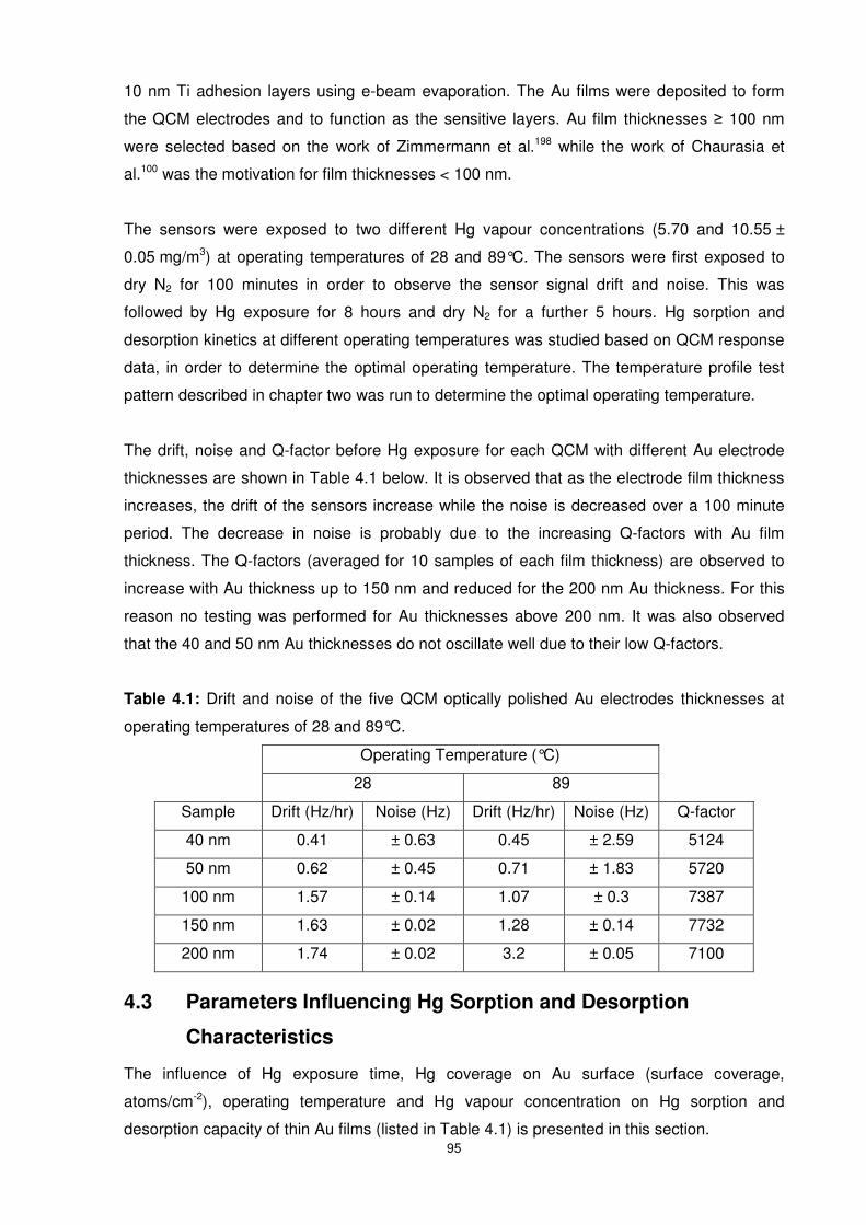
95
10 nm Ti adhesion layers using e-beam evaporation. The Au films were deposited to form
the QCM electrodes and to function as the sensitive layers. Au film thicknesses ≥ 100 nm
were selected based on the work of Zimmermann et al.198 while the work of Chaurasia et
al.100 was the motivation for film thicknesses < 100 nm.
The sensors were exposed to two different Hg vapour concentrations (5.70 and 10.55 ±
0.05 mg/m3) at operating temperatures of 28 and 89°C. The sensors were first exposed to
dry N2 for 100 minutes in order to observe the sensor signal drift and noise. This was
followed by Hg exposure for 8 hours and dry N2 for a further 5 hours. Hg sorption and
desorption kinetics at different operating temperatures was studied based on QCM response
data, in order to determine the optimal operating temperature. The temperature profile test
pattern described in chapter two was run to determine the optimal operating temperature.
The drift, noise and Q-factor before Hg exposure for each QCM with different Au electrode
thicknesses are shown in Table 4.1 below. It is observed that as the electrode film thickness
increases, the drift of the sensors increase while the noise is decreased over a 100 minute
period. The decrease in noise is probably due to the increasing Q-factors with Au film
thickness. The Q-factors (averaged for 10 samples of each film thickness) are observed to
increase with Au thickness up to 150 nm and reduced for the 200 nm Au thickness. For this
reason no testing was performed for Au thicknesses above 200 nm. It was also observed
that the 40 and 50 nm Au thicknesses do not oscillate well due to their low Q-factors.
Table 4.1: Drift and noise of the five QCM optically polished Au electrodes thicknesses at
operating temperatures of 28 and 89°C.
Operating Temperature (°C)
28 89
Sample Drift (Hz/hr) Noise (Hz) Drift (Hz/hr) Noise (Hz) Q-factor
40 nm 0.41 ± 0.63 0.45 ± 2.59 5124
50 nm 0.62 ± 0.45 0.71 ± 1.83 5720
100 nm 1.57 ± 0.14 1.07 ± 0.3 7387
150 nm 1.63 ± 0.02 1.28 ± 0.14 7732
200 nm 1.74 ± 0.02 3.2 ± 0.05 7100
4.3 Parameters Influencing Hg Sorption and Desorption
Characteristics
The influence of Hg exposure time, Hg coverage on Au surface (surface coverage,
atoms/cm-2), operating temperature and Hg vapour concentration on Hg sorption and
desorption capacity of thin Au films (listed in Table 4.1) is presented in this section.
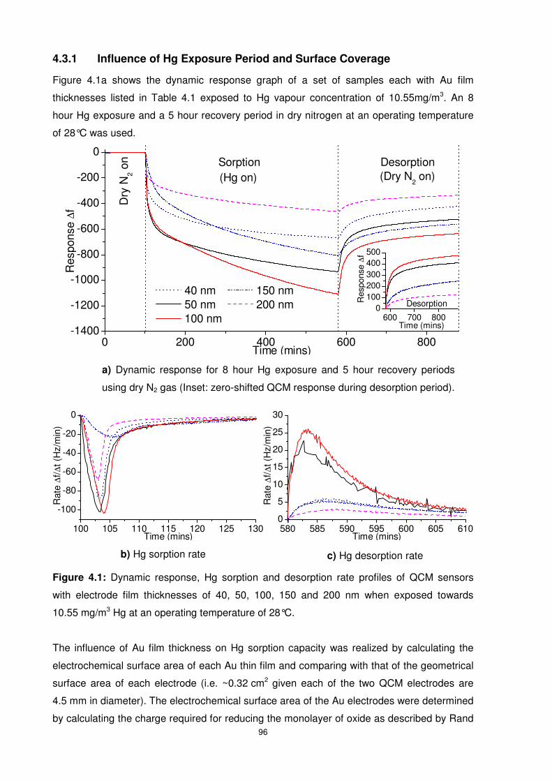
96
4.3.1 Influence of Hg Exposure Period and Surface Coverage
Figure 4.1a shows the dynamic response graph of a set of samples each with Au film
thicknesses listed in Table 4.1 exposed to Hg vapour concentration of 10.55mg/m3. An 8
hour Hg exposure and a 5 hour recovery period in dry nitrogen at an operating temperature
of 28°C was used.
Figure 4.1: Dynamic response, Hg sorption and desorption rate profiles of QCM sensors
with electrode film thicknesses of 40, 50, 100, 150 and 200 nm when exposed towards
10.55 mg/m3 Hg at an operating temperature of 28°C.
The influence of Au film thickness on Hg sorption capacity was realized by calculating the
electrochemical surface area of each Au thin film and comparing with that of the geometrical
surface area of each electrode (i.e. ~0.32 cm2 given each of the two QCM electrodes are
4.5 mm in diameter). The electrochemical surface area of the Au electrodes were determined
by calculating the charge required for reducing the monolayer of oxide as described by Rand
0 200 400 600 800-1400
-1200
-1000
-800
-600
-400
-200
0
Dry
N2 o
n
(Dry N2 on)
Desorption
Res
pons
e ∆f
Time (mins)
40 nm 150 nm 50 nm 200 nm 100 nm
Sorption(Hg on)
a) Dynamic response for 8 hour Hg exposure and 5 hour recovery periods
using dry N2 gas (Inset: zero-shifted QCM response during desorption period).
b) Hg sorption rate c) Hg desorption rate
600 700 8000
100200300400500
DesorptionRes
pons
e ∆
f
Time (mins)
100 105 110 115 120 125 130
-100
-80
-60
-40
-20
0
Rat
e ∆
f/∆t (
Hz/
min
)
Time (mins)580 585 590 595 600 605 6100
5
10
15
20
25
30
Rat
e ∆
f/∆t (
Hz/
min
)
Time (mins)
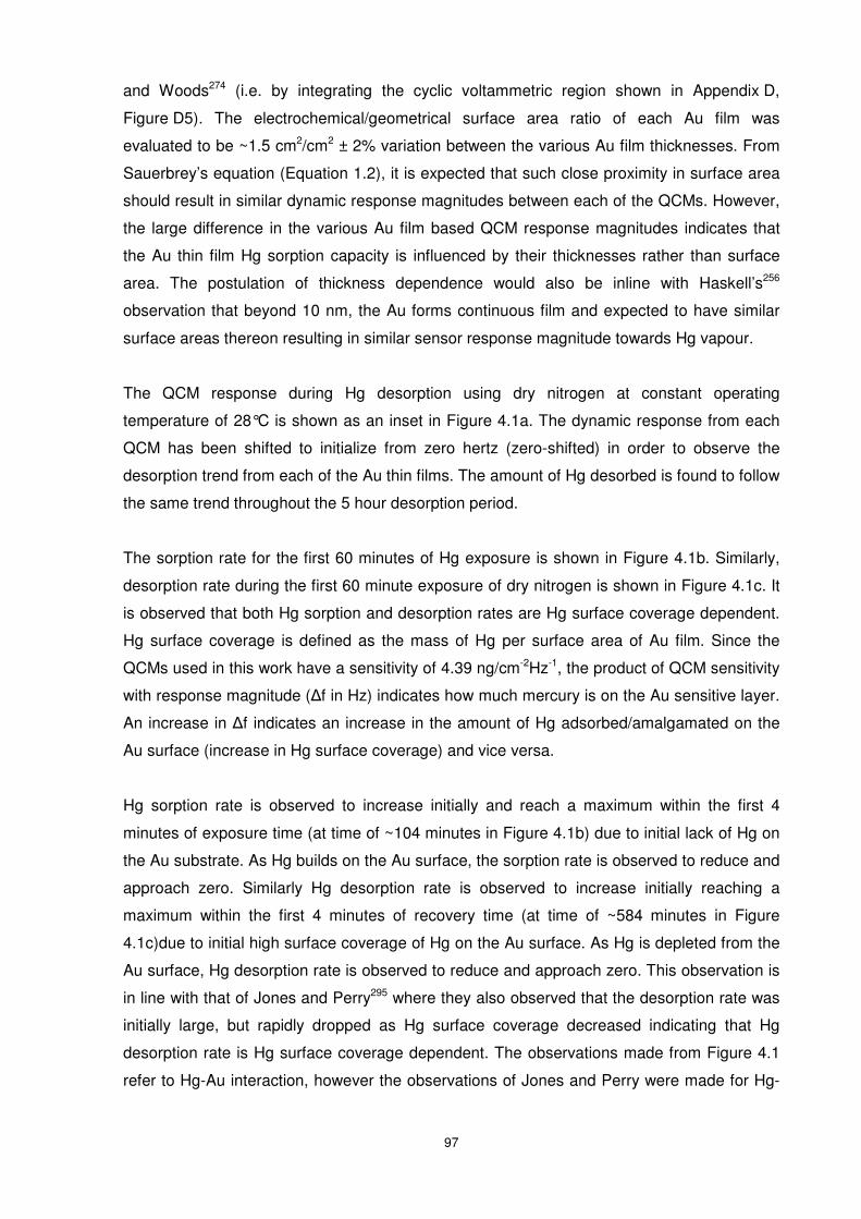
97
and Woods274 (i.e. by integrating the cyclic voltammetric region shown in Appendix D,
Figure D5). The electrochemical/geometrical surface area ratio of each Au film was
evaluated to be ~1.5 cm2/cm2 ± 2% variation between the various Au film thicknesses. From
Sauerbrey’s equation (Equation 1.2), it is expected that such close proximity in surface area
should result in similar dynamic response magnitudes between each of the QCMs. However,
the large difference in the various Au film based QCM response magnitudes indicates that
the Au thin film Hg sorption capacity is influenced by their thicknesses rather than surface
area. The postulation of thickness dependence would also be inline with Haskell’s256
observation that beyond 10 nm, the Au forms continuous film and expected to have similar
surface areas thereon resulting in similar sensor response magnitude towards Hg vapour.
The QCM response during Hg desorption using dry nitrogen at constant operating
temperature of 28°C is shown as an inset in Figure 4.1a. The dynamic response from each
QCM has been shifted to initialize from zero hertz (zero-shifted) in order to observe the
desorption trend from each of the Au thin films. The amount of Hg desorbed is found to follow
the same trend throughout the 5 hour desorption period.
The sorption rate for the first 60 minutes of Hg exposure is shown in Figure 4.1b. Similarly,
desorption rate during the first 60 minute exposure of dry nitrogen is shown in Figure 4.1c. It
is observed that both Hg sorption and desorption rates are Hg surface coverage dependent.
Hg surface coverage is defined as the mass of Hg per surface area of Au film. Since the
QCMs used in this work have a sensitivity of 4.39 ng/cm-2Hz-1, the product of QCM sensitivity
with response magnitude (∆f in Hz) indicates how much mercury is on the Au sensitive layer.
An increase in ∆f indicates an increase in the amount of Hg adsorbed/amalgamated on the
Au surface (increase in Hg surface coverage) and vice versa.
Hg sorption rate is observed to increase initially and reach a maximum within the first 4
minutes of exposure time (at time of ~104 minutes in Figure 4.1b) due to initial lack of Hg on
the Au substrate. As Hg builds on the Au surface, the sorption rate is observed to reduce and
approach zero. Similarly Hg desorption rate is observed to increase initially reaching a
maximum within the first 4 minutes of recovery time (at time of ~584 minutes in Figure
4.1c)due to initial high surface coverage of Hg on the Au surface. As Hg is depleted from the
Au surface, Hg desorption rate is observed to reduce and approach zero. This observation is
in line with that of Jones and Perry295 where they also observed that the desorption rate was
initially large, but rapidly dropped as Hg surface coverage decreased indicating that Hg
desorption rate is Hg surface coverage dependent. The observations made from Figure 4.1
refer to Hg-Au interaction, however the observations of Jones and Perry were made for Hg-
98
Fe and assumed for all metal surfaces interacting with Hg. The results presented in Figure
4.1 confirm such assumption for Hg-Au system.
The Hg sorption capacity is also found to be affected by Hg exposure time on the different Au
film thicknesses. The trend in Hg sorption capacity for each Au film thickness is observed to
change at exposure times of ~20 and ~200 minutes as observed from Figure 4.1a. The
response magnitude of the various Au film thicknesses at times of 10, 100 and end of the
exposure period (480 minutes) is shown in Figure 4.2. It is apparent that the Hg exposure
time influences the trend of Hg sorption capacity of the various Au films and is a critical
parameter to be considered when using Au films for Hg vapour sensing.
Figure 4.2: Effect of Hg exposure time on dynamic response of Au films with film
thicknesses from 40 to 200 nm.
4.3.2 Influence of Operating Temperature
In order to determine the influence of operating temperature on Au film Hg sorption capacity,
a set of new QCMs with various Au film thicknesses were tested towards Hg vapour
concentration of 10.55 mg/m3 at an operating temperature of 89°C. The 40 nm thick Au film
was excluded from any further testing as it was found to be noisy and not able to oscillate at
the higher operating temperature of 89°C. The response curves for the QCMs are shown in
Figure 4.3.
Comparing Figure 4.1a with that of 4.3a, it can be clearly observed that the Hg sorption
capacity of the different Au film thicknesses is greatly affected by the operating temperature.
Hg sorption capacity is observed to increase with increasing Au thickness following 8 hours
of Hg exposure at 89°C (Figure 4.3a) as opposed to 28°C (Figure 4.1a). Exposure time is
again observed to affect the sorption trend of the different Au thicknesses. For example, at
exposure times less than 7 hours, the 150 nm Au QCM is observed to undergo the largest
0
300
600
900
1200
10 100
Res
pons
e ∆
f (H
z)
Hg exposure time (min)
40 nm 50 nm 100 nm 150 nm 200 nm
480
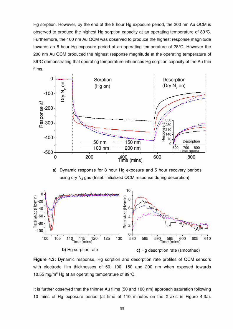
99
Hg sorption. However, by the end of the 8 hour Hg exposure period, the 200 nm Au QCM is
observed to produce the highest Hg sorption capacity at an operating temperature of 89°C.
Furthermore, the 100 nm Au QCM was observed to produce the highest response magnitude
towards an 8 hour Hg exposure period at an operating temperature of 28°C. However the
200 nm Au QCM produced the highest response magnitude at the operating temperature of
89°C demonstrating that operating temperature influences Hg sorption capacity of the Au thin
films.
Figure 4.3: Dynamic response, Hg sorption and desorption rate profiles of QCM sensors
with electrode film thicknesses of 50, 100, 150 and 200 nm when exposed towards
10.55 mg/m3 Hg at an operating temperature of 89°C.
It is further observed that the thinner Au films (50 and 100 nm) approach saturation following
10 mins of Hg exposure period (at time of 110 minutes on the X-axis in Figure 4.3a).
a) Dynamic response for 8 hour Hg exposure and 5 hour recovery periods
using dry N2 gas (Inset: initialized QCM response during desorption)
b) Hg sorption rate c) Hg desorption rate (smoothed)
580 585 590 595 600 605 6100
2
4
6
8
10
Rat
e ∆
f/∆t (
Hz/
min
)
Time (mins)100 105 110 115 120 125 130
-100
-80
-60
-40
-20
0
Rat
e ∆
f/∆t (
Hz/
min
)
Time (mins)
0 200 400 600 800-500
-400
-300
-200
-100
0
Res
pons
e ∆f
Time (mins)
50 nm 150 nm 100 nm 200 nm
Dry
N2 o
n
(Dry N2 on)
Desorption(Hg on)Sorption
600 700 8000
70140210280350
DesorptionRes
pons
e ∆
f
Time (mins)
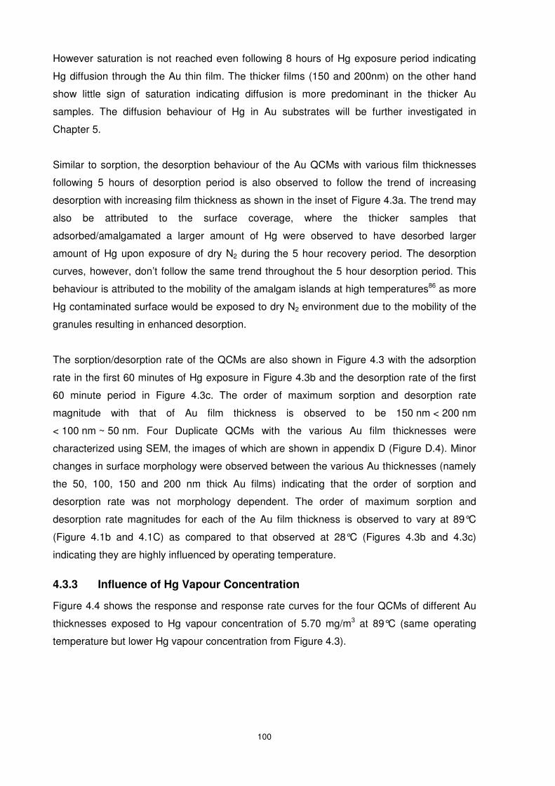
100
However saturation is not reached even following 8 hours of Hg exposure period indicating
Hg diffusion through the Au thin film. The thicker films (150 and 200nm) on the other hand
show little sign of saturation indicating diffusion is more predominant in the thicker Au
samples. The diffusion behaviour of Hg in Au substrates will be further investigated in
Chapter 5.
Similar to sorption, the desorption behaviour of the Au QCMs with various film thicknesses
following 5 hours of desorption period is also observed to follow the trend of increasing
desorption with increasing film thickness as shown in the inset of Figure 4.3a. The trend may
also be attributed to the surface coverage, where the thicker samples that
adsorbed/amalgamated a larger amount of Hg were observed to have desorbed larger
amount of Hg upon exposure of dry N2 during the 5 hour recovery period. The desorption
curves, however, don’t follow the same trend throughout the 5 hour desorption period. This
behaviour is attributed to the mobility of the amalgam islands at high temperatures86 as more
Hg contaminated surface would be exposed to dry N2 environment due to the mobility of the
granules resulting in enhanced desorption.
The sorption/desorption rate of the QCMs are also shown in Figure 4.3 with the adsorption
rate in the first 60 minutes of Hg exposure in Figure 4.3b and the desorption rate of the first
60 minute period in Figure 4.3c. The order of maximum sorption and desorption rate
magnitude with that of Au film thickness is observed to be 150 nm < 200 nm
< 100 nm ~ 50 nm. Four Duplicate QCMs with the various Au film thicknesses were
characterized using SEM, the images of which are shown in appendix D (Figure D.4). Minor
changes in surface morphology were observed between the various Au thicknesses (namely
the 50, 100, 150 and 200 nm thick Au films) indicating that the order of sorption and
desorption rate was not morphology dependent. The order of maximum sorption and
desorption rate magnitudes for each of the Au film thickness is observed to vary at 89°C
(Figure 4.1b and 4.1C) as compared to that observed at 28°C (Figures 4.3b and 4.3c)
indicating they are highly influenced by operating temperature.
4.3.3 Influence of Hg Vapour Concentration
Figure 4.4 shows the response and response rate curves for the four QCMs of different Au
thicknesses exposed to Hg vapour concentration of 5.70 mg/m3 at 89°C (same operating
temperature but lower Hg vapour concentration from Figure 4.3).
101
Figure 4.4: Dynamic response, Hg sorption and desorption rate profiles of QCM sensors
with electrode film thicknesses of 50, 100, 150 and 200 nm when exposed towards
5.70 mg/m3 Hg at an operating temperature of 89°C.
Comparing Figure 4.4a with that of 4.3a, the Hg sorption and desorption trends for the
various Au film thicknesses are quite similar. This indicates that the trend of Hg sorption
capacity with respect to thickness is similar at the operating temperature of 89°C and that the
trend is not affected by a decrease in Hg vapour concentration. The sorption and desorption
rates are also found to follow similar trends as indicated by Figures 4.4b and c respectively.
The 100 nm sample is found to show some instability in the response curve in Figure 4.4a.
This may be due to surface changes resulting from amalgamation or simply the instability of
the QCM at the higher operating temperature during the 8 hour Hg exposure period.
b) Dynamic response for 8 hour Hg exposure and 5 hour recovery periods
using dry N2 gas (Inset: initialized QCM response during desorption)
b) Hg sorption rate c) Hg desorption rate
580 585 590 595 600 605 6100
2
4
6
8
10
Rat
e ∆
f/∆t (
Hz/
min
)
Time (mins)100 105 110 115 120 125 130
-100
-80
-60
-40
-20
0
Rat
e ∆
f/∆t (
Hz/
min
)
Time (mins)
0 200 400 600 800-500
-400
-300
-200
-100
0
Res
pons
e ∆f
Time (mins)
50 nm 150 nm 100 nm 200 nm
Dry
N2 o
n
(Dry N2 on)
Desorption(Hg on)Sorption
600 700 8000
70140210280350
DesorptionRes
pons
e ∆
f
Time (mins)
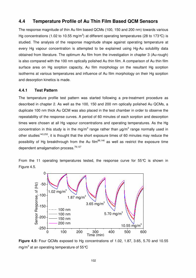
102
4.4 Temperature Profile of Au Thin Film Based QCM Sensors
The response magnitude of thin Au film based QCMs (100, 150 and 200 nm) towards various
Hg concentrations (1.02 to 10.55 mg/m3) at different operating temperatures (28 to 173°C) is
studied. The analysis of the response magnitude shape against operating temperature at
every Hg vapour concentration is attempted to be explained using Hg-Au solubility data
obtained from literature. The optimum Au film from the investigation in chapter 3 (Au-rough)
is also compared with the 100 nm optically polished Au thin film. A comparison of Au thin film
surface area on Hg sorption capacity, Au film morphology on the resultant Hg sorption
isotherms at various temperatures and influence of Au film morphology on their Hg sorption
and desorption kinetics is made.
4.4.1 Test Pattern
The temperature profile test pattern was started following a pre-treatment procedure as
described in chapter 2. As well as the 100, 150 and 200 nm optically polished Au QCMs, a
duplicate 100 nm thick Au QCM was also placed in the test chamber in order to observe the
repeatability of the response curves. A period of 60 minutes of each sorption and desorption
times were chosen at all Hg vapour concentrations and operating temperatures. As the Hg
concentration in this study is in the mg/m3 range rather than µg/m3 range normally used in
other studies143,252, it is thought that the short exposure times of 60 minutes may reduce the
possibility of Hg breakthrough from the Au film88,146 as well as restrict the exposure time
dependent amalgamation process.78,127
From the 11 operating temperatures tested, the response curve for 55°C is shown in
Figure 4.5.
Figure 4.5: Four QCMs exposed to Hg concentrations of 1.02, 1.87, 3.65, 5.70 and 10.55
mg/m3 at an operating temperature of 55°C
0 100 200 300 400 500 600-250
-200
-150
-100
-50
0
10.55 mg/m3
5.70 mg/m3
3.65 mg/m3
1.87 mg/m3
1.02 mg/m3
Sen
sor
Res
pons
e, ∆
f (H
z)
Time (min)
100 nm 100 nm 150 nm 200 nm
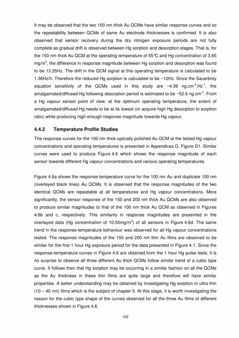
103
It may be observed that the two 100 nm thick Au QCMs have similar response curves and so
the repeatability between QCMs of same Au electrode thicknesses is confirmed. It is also
observed that sensor recovery during the dry nitrogen exposure periods are not fully
complete as gradual drift is observed between Hg sorption and desorption stages. That is, for
the 150 nm thick Au QCM at the operating temperature of 55°C and Hg concentration of 3.65
mg/m3, the difference in response magnitude between Hg sorption and desorption was found
to be 13.35Hz. The drift in the QCM signal at this operating temperature is calculated to be
1.36Hz/h. Therefore the reduced Hg sorption is calculated to be ~12Hz. Since the Sauerbrey
equation sensitivity of the QCMs used in this study are ~4.39 ng.cm-2.Hz-1, the
amalgamated/diffused Hg following desorption period is estimated to be ~52.6 ng.cm-2. From
a Hg vapour sensor point of view, at the optimum operating temperature, the extent of
amalgamated/diffused Hg needs to be at its lowest (or acquire high Hg desorption to sorption
ratio) while producing high enough response magnitude towards Hg vapour.
4.4.2 Temperature Profile Studies
The response curves for the 100 nm thick optically polished Au QCM at the tested Hg vapour
concentrations and operating temperatures is presented in Appendices D, Figure D1. Similar
curves were used to produce Figure 4.6 which shows the response magnitude of each
sensor towards different Hg vapour concentrations and various operating temperatures.
Figure 4.6a shows the response-temperature curve for the 100 nm Au and duplicate 100 nm
(overlayed black lines) Au QCMs. It is observed that the response magnitudes of the two
identical QCMs are repeatable at all temperatures and Hg vapour concentrations. More
significantly, the sensor response of the 150 and 200 nm thick Au QCMs are also observed
to produce similar magnitudes to that of the 100 nm thick Au QCM as observed in Figures
4.6b and c, respectively. This similarity in response magnitudes are presented in the
overlayed data (Hg concentration of 10.55mg/m3) of all sensors in Figure 4.6d. The same
trend in the response-temperature behaviour was observed for all Hg vapour concentrations
tested. The response magnitudes of the 150 and 200 nm thin Au films are observed to be
similar for the first 1 hour Hg exposure period for the data presented in Figure 4.1. Since the
response-temperature curves in Figure 4.6 are obtained from the 1 hour Hg pulse tests, it is
no surprise to observe all three different Au thick QCMs follow similar trend of a cubic type
curve. It follows then that Hg sorption may be occurring in a similar fashion on all the QCMs
as the Au thickness in these thin films are quite large and therefore will have similar
properties. A better understanding may be obtained by investigating Hg sorption in ultra thin
(10 – 40 nm) films which is the subject of chapter 5. At this stage, it is worth investigating the
reason for the cubic type shape of the curves observed for all the three Au films of different
thicknesses shown in Figure 4.6.
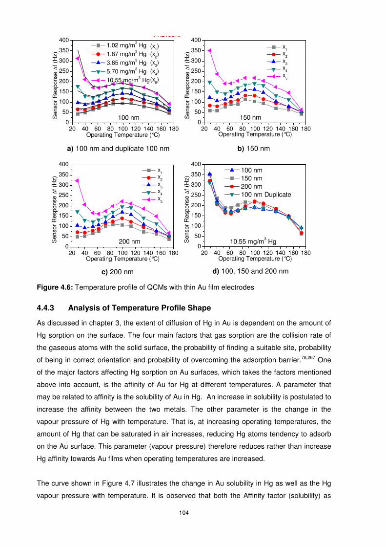
104
Figure 4.6: Temperature profile of QCMs with thin Au film electrodes
4.4.3 Analysis of Temperature Profile Shape
As discussed in chapter 3, the extent of diffusion of Hg in Au is dependent on the amount of
Hg sorption on the surface. The four main factors that gas sorption are the collision rate of
the gaseous atoms with the solid surface, the probability of finding a suitable site, probability
of being in correct orientation and probability of overcoming the adsorption barrier.78,267 One
of the major factors affecting Hg sorption on Au surfaces, which takes the factors mentioned
above into account, is the affinity of Au for Hg at different temperatures. A parameter that
may be related to affinity is the solubility of Au in Hg. An increase in solubility is postulated to
increase the affinity between the two metals. The other parameter is the change in the
vapour pressure of Hg with temperature. That is, at increasing operating temperatures, the
amount of Hg that can be saturated in air increases, reducing Hg atoms tendency to adsorb
on the Au surface. This parameter (vapour pressure) therefore reduces rather than increase
Hg affinity towards Au films when operating temperatures are increased.
The curve shown in Figure 4.7 illustrates the change in Au solubility in Hg as well as the Hg
vapour pressure with temperature. It is observed that both the Affinity factor (solubility) as
a) 100 nm and duplicate 100 nm
20 40 60 80 100 120 140 160 1800
50
100
150
200
250
300
350
400 100 nm 150 nm 200 nm 100 nm Duplicate
10.55 mg/m3 HgSen
sor
Res
pons
e ∆
f (H
z)
Operating Temperature (°C)
b) 150 nm
c) 200 nm d) 100, 150 and 200 nm
20 40 60 80 100 120 140 160 1800
50
100
150
200
250
300
350
400
(x5)
(x4)
(x3)
(x2)
(x1)
100 nm
PAu100A12
Sen
sor
Res
pons
e ∆
f (H
z)
Operating Temperature (°C)
1.02 mg/m3 Hg 1.87 mg/m3 Hg 3.65 mg/m3 Hg 5.70 mg/m3 Hg 10.55 mg/m3 Hg
1
PAu100A8
20 40 60 80 100 120 140 160 1800
50
100
150
200
250
300
350
400
150 nmSen
sor
Res
pons
e ∆
f (H
z)
Operating Temperature (°C)
x5
x4
x3
x2
x1
20 40 60 80 100 120 140 160 1800
50
100
150
200
250
300
350
400
Sen
sor
Res
pons
e ∆
f (H
z)
Operating Temperature (°C)
200 nm
x5
x4
x3
x2
x1
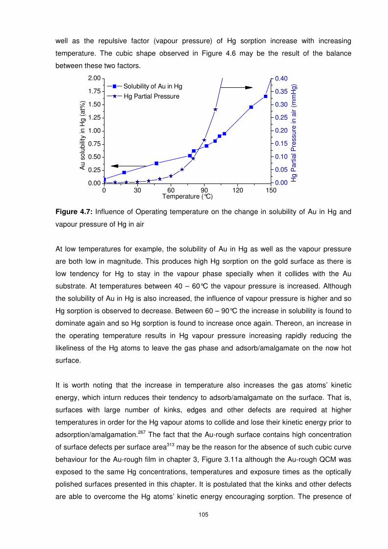
105
well as the repulsive factor (vapour pressure) of Hg sorption increase with increasing
temperature. The cubic shape observed in Figure 4.6 may be the result of the balance
between these two factors.
Figure 4.7: Influence of Operating temperature on the change in solubility of Au in Hg and
vapour pressure of Hg in air
At low temperatures for example, the solubility of Au in Hg as well as the vapour pressure
are both low in magnitude. This produces high Hg sorption on the gold surface as there is
low tendency for Hg to stay in the vapour phase specially when it collides with the Au
substrate. At temperatures between 40 – 60°C the vapour pressure is increased. Although
the solubility of Au in Hg is also increased, the influence of vapour pressure is higher and so
Hg sorption is observed to decrease. Between 60 – 90°C the increase in solubility is found to
dominate again and so Hg sorption is found to increase once again. Thereon, an increase in
the operating temperature results in Hg vapour pressure increasing rapidly reducing the
likeliness of the Hg atoms to leave the gas phase and adsorb/amalgamate on the now hot
surface.
It is worth noting that the increase in temperature also increases the gas atoms’ kinetic
energy, which inturn reduces their tendency to adsorb/amalgamate on the surface. That is,
surfaces with large number of kinks, edges and other defects are required at higher
temperatures in order for the Hg vapour atoms to collide and lose their kinetic energy prior to
adsorption/amalgamation.267 The fact that the Au-rough surface contains high concentration
of surface defects per surface area313 may be the reason for the absence of such cubic curve
behaviour for the Au-rough film in chapter 3, Figure 3.11a although the Au-rough QCM was
exposed to the same Hg concentrations, temperatures and exposure times as the optically
polished surfaces presented in this chapter. It is postulated that the kinks and other defects
are able to overcome the Hg atoms’ kinetic energy encouraging sorption. The presence of
0 30 60 90 120 1500.00
0.25
0.50
0.75
1.00
1.25
1.50
1.75
2.00 Solubility of Au in Hg
Hg
Par
tial P
ress
ure
in a
ir (m
mH
g)
Au
solu
bilit
y in
Hg
(at%
)
Temperature (°C)
0.00
0.05
0.10
0.15
0.20
0.25
0.30
0.35
0.40
Hg Partial Pressure
106
such surface defects may alter the kinetics of Hg sorption on the Au-rough surface and
therefore the cubic curve type shape is not observed in the response-temperature curve.
4.4.4 Influence of Operating Temperature and Surface Morphology
The temperature profile of Au-rough film was presented in chapter 3 (Figure 3.11a) while that
of the Au-polished film (100 nm Au thin film) is shown in Figure 4.6a. In this section, Hg
sorption isotherm at various operating temperatures, Hg sorption capacity, Hg
sorption/desorption kinetics and Hg desorption/sorption ratio a comparison is made (using
the temperature profile response curves of both Au-rough and Au-polished films) between
the two surfaces in terms of Hg sorption isotherm and capacity.
4.4.4.1 Hg Sorption Isotherm
A comparison of the Hg sorption isotherms at various operating temperatures for the 100 nm
thick Au QCM is presented in Figure 4.8. The Hg sorption isotherms for the duplicate 100nm
as well as the 150 and 200 nm Au QCMs were observed to be similar and shown in
Appendix D (Figure D2). Needless to say, these curves are plotted from the data observed in
Figure 4.6a above.
Figure 4.8: Hg sorption Isotherm for the 100 nm Au QCM at various operating temperatures.
The adsorption isotherms in Figure 4.8 for the optically polished Au film may be compared
with that of the mechanically roughened Au film presented in chapter 3 Figure 3.11b. It may
be observed that the Hg sorption capacity follows a more ordered trend on the mechanically
roughened Au than the optically polished thin Au films. The general trend for Hg sorption on
the Au-rough film is that it increases with increasing Hg concentration or decreasing
operating temperature. However for an optically polished film, no such trend is observed. The
postulation made in chapter 3 that roughened surface morphology may be the optimum
sensitive films to be used as a potential online Hg vapour sensor, is now becoming more
evident. The lack of order in the trend for the optically polished Au film indicates that if used
0 2 4 6 8 10 120
50
100
150
200
250
300
350
400
100 nm Au QCM
173°C 73°C 153°C 62°C 133°C 53°C 113°C 40°C 99°C 28°C 89°C
Sen
sor
Res
pons
e ∆
f (H
z)
Hg Concentration (mg/m3)
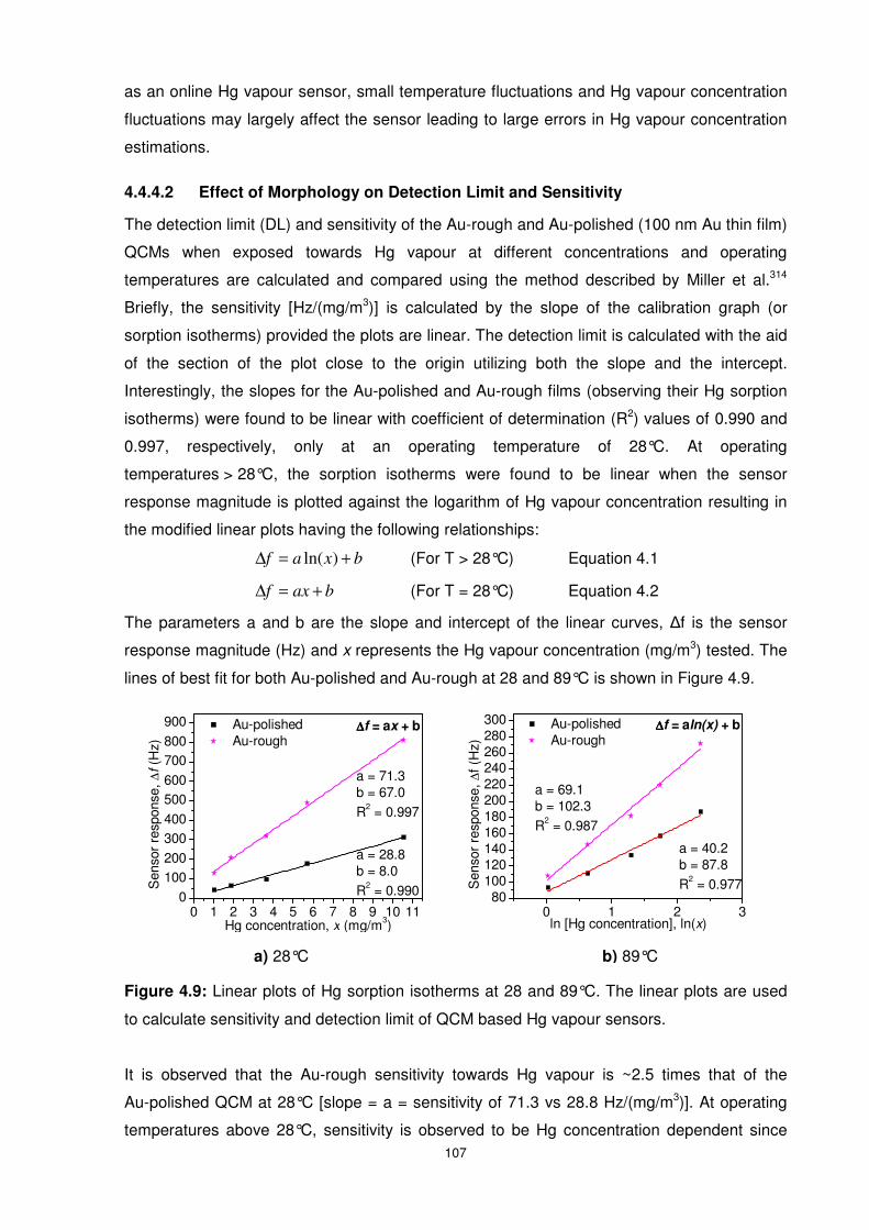
107
as an online Hg vapour sensor, small temperature fluctuations and Hg vapour concentration
fluctuations may largely affect the sensor leading to large errors in Hg vapour concentration
estimations.
4.4.4.2 Effect of Morphology on Detection Limit and Sensitivity
The detection limit (DL) and sensitivity of the Au-rough and Au-polished (100 nm Au thin film)
QCMs when exposed towards Hg vapour at different concentrations and operating
temperatures are calculated and compared using the method described by Miller et al.314
Briefly, the sensitivity [Hz/(mg/m3)] is calculated by the slope of the calibration graph (or
sorption isotherms) provided the plots are linear. The detection limit is calculated with the aid
of the section of the plot close to the origin utilizing both the slope and the intercept.
Interestingly, the slopes for the Au-polished and Au-rough films (observing their Hg sorption
isotherms) were found to be linear with coefficient of determination (R2) values of 0.990 and
0.997, respectively, only at an operating temperature of 28°C. At operating
temperatures > 28°C, the sorption isotherms were found to be linear when the sensor
response magnitude is plotted against the logarithm of Hg vapour concentration resulting in
the modified linear plots having the following relationships:
bxaf +=∆ )ln( (For T > 28°C) Equation 4.1
baxf +=∆ (For T = 28°C) Equation 4.2
The parameters a and b are the slope and intercept of the linear curves, ∆f is the sensor
response magnitude (Hz) and x represents the Hg vapour concentration (mg/m3) tested. The
lines of best fit for both Au-polished and Au-rough at 28 and 89°C is shown in Figure 4.9.
Figure 4.9: Linear plots of Hg sorption isotherms at 28 and 89°C. The linear plots are used
to calculate sensitivity and detection limit of QCM based Hg vapour sensors.
It is observed that the Au-rough sensitivity towards Hg vapour is ~2.5 times that of the
Au-polished QCM at 28°C [slope = a = sensitivity of 71.3 vs 28.8 Hz/(mg/m3)]. At operating
temperatures above 28°C, sensitivity is observed to be Hg concentration dependent since
0 1 2 380
100120140160180200220240260280300 Au-polished
Au-rough∆∆∆∆f = aln(x) + b
a = 40.2b = 87.8R2 = 0.977
a = 69.1b = 102.3R2 = 0.987
Sen
sor
resp
onse
, ∆f (
Hz)
ln [Hg concentration], ln(x)0 1 2 3 4 5 6 7 8 9 10 11
0100200300400500600700800900
a = 28.8b = 8.0R2 = 0.990
Au-polished Au-rough
Sen
sor
resp
onse
, ∆f (
Hz)
Hg concentration, x (mg/m3)
∆∆∆∆f = ax + b
a = 71.3b = 67.0R2 = 0.997
a) 28°C b) 89°C
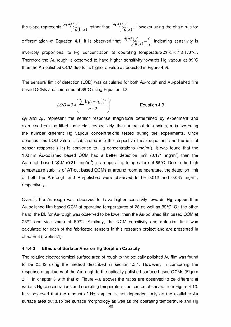
108
the slope represents )(ln
)(x
f∂
∆∂ rather than )(
)(x
f∂
∆∂ . However using the chain rule for
differentiation of Equation 4.1, it is observed that x
a
xf =
∂∆∂
)()( indicating sensitivity is
inversely proportional to Hg concentration at operating temperature CTC °≤<° 17328 .
Therefore the Au-rough is observed to have higher sensitivity towards Hg vapour at 89°C
than the Au-polished QCM due to its higher a value as depicted in Figure 4.9b.
The sensors’ limit of detection (LOD) was calculated for both Au-rough and Au-polished film
based QCMs and compared at 89°C using Equation 4.3.
( ) 2
12
23
−
∆−∆×=∑
n
ffLOD
ei Equation 4.3
∆fi and ∆fe represent the sensor response magnitude determined by experiment and
extracted from the fitted linear plot, respectively. the number of data points, n, is five being
the number different Hg vapour concentrations tested during the experiments. Once
obtained, the LOD value is substituted into the respective linear equations and the unit of
sensor response (Hz) is converted to Hg concentrations (mg/m3). It was found that the
100 nm Au-polished based QCM had a better detection limit (0.171 mg/m3) than the
Au-rough based QCM (0.311 mg/m3) at an operating temperature of 89°C. Due to the high
temperature stability of AT-cut based QCMs at around room temperature, the detection limit
of both the Au-rough and Au-polished were observed to be 0.012 and 0.035 mg/m3,
respectively.
Overall, the Au-rough was observed to have higher sensitivity towards Hg vapour than
Au-polished film based QCM at operating temperatures of 28 as well as 89°C. On the other
hand, the DL for Au-rough was observed to be lower then the Au-polished film based QCM at
28°C and vice versa at 89°C. Similarly, the QCM sensitivity and detection limit was
calculated for each of the fabricated sensors in this research project and are presented in
chapter 8 (Table 8.1).
4.4.4.3 Effects of Surface Area on Hg Sorption Capacity
The relative electrochemical surface area of rough to the optically polished Au film was found
to be 2.542 using the method described in section 4.3.1. However, in comparing the
response magnitudes of the Au-rough to the optically polished surface based QCMs (Figure
3.11 in chapter 3 with that of Figure 4.6 above) the ratios are observed to be different at
various Hg concentrations and operating temperatures as can be observed from Figure 4.10.
It is observed that the amount of Hg sorption is not dependent only on the available Au
surface area but also the surface morphology as well as the operating temperature and Hg
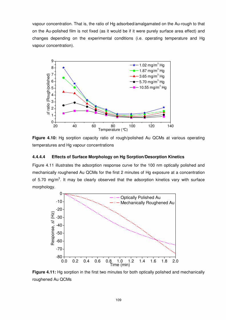
109
vapour concentration. That is, the ratio of Hg adsorbed/amalgamated on the Au-rough to that
on the Au-polished film is not fixed (as it would be if it were purely surface area effect) and
changes depending on the experimental conditions (i.e. operating temperature and Hg
vapour concentration).
Figure 4.10: Hg sorption capacity ratio of rough/polished Au QCMs at various operating
temperatures and Hg vapour concentrations
4.4.4.4 Effects of Surface Morphology on Hg Sorption/Desorption Kinetics
Figure 4.11 illustrates the adsorption response curve for the 100 nm optically polished and
mechanically roughened Au QCMs for the first 2 minutes of Hg exposure at a concentration
of 5.70 mg/m3. It may be clearly observed that the adsorption kinetics vary with surface
morphology.
Figure 4.11: Hg sorption in the first two minutes for both optically polished and mechanically
roughened Au QCMs
0.0 0.2 0.4 0.6 0.8 1.0 1.2 1.4 1.6 1.8 2.0-80
-70
-60
-50
-40
-30
-20
-10
0
Res
pons
e, ∆
f (H
z)
Time (min)
Optically Polished Au Mechanically Roughened Au
20 40 60 80 100 120 1400
1
2
3
4
5
6
7
8
9
1.02 mg/m3 Hg 1.87 mg/m3 Hg 3.65 mg/m3 Hg 5.70 mg/m3 Hg 10.55 mg/m3 Hg
∆f r
atio
(R
ough
/pol
ishe
d)
Temperature (°C)
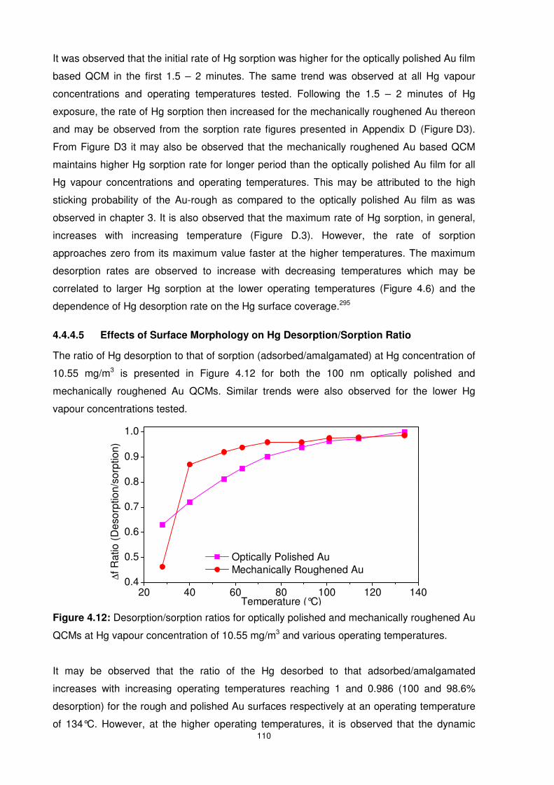
110
It was observed that the initial rate of Hg sorption was higher for the optically polished Au film
based QCM in the first 1.5 – 2 minutes. The same trend was observed at all Hg vapour
concentrations and operating temperatures tested. Following the 1.5 – 2 minutes of Hg
exposure, the rate of Hg sorption then increased for the mechanically roughened Au thereon
and may be observed from the sorption rate figures presented in Appendix D (Figure D3).
From Figure D3 it may also be observed that the mechanically roughened Au based QCM
maintains higher Hg sorption rate for longer period than the optically polished Au film for all
Hg vapour concentrations and operating temperatures. This may be attributed to the high
sticking probability of the Au-rough as compared to the optically polished Au film as was
observed in chapter 3. It is also observed that the maximum rate of Hg sorption, in general,
increases with increasing temperature (Figure D.3). However, the rate of sorption
approaches zero from its maximum value faster at the higher temperatures. The maximum
desorption rates are observed to increase with decreasing temperatures which may be
correlated to larger Hg sorption at the lower operating temperatures (Figure 4.6) and the
dependence of Hg desorption rate on the Hg surface coverage.295
4.4.4.5 Effects of Surface Morphology on Hg Desorption/Sorption Ratio
The ratio of Hg desorption to that of sorption (adsorbed/amalgamated) at Hg concentration of
10.55 mg/m3 is presented in Figure 4.12 for both the 100 nm optically polished and
mechanically roughened Au QCMs. Similar trends were also observed for the lower Hg
vapour concentrations tested.
Figure 4.12: Desorption/sorption ratios for optically polished and mechanically roughened Au
QCMs at Hg vapour concentration of 10.55 mg/m3 and various operating temperatures.
It may be observed that the ratio of the Hg desorbed to that adsorbed/amalgamated
increases with increasing operating temperatures reaching 1 and 0.986 (100 and 98.6%
desorption) for the rough and polished Au surfaces respectively at an operating temperature
of 134°C. However, at the higher operating temperatures, it is observed that the dynamic
20 40 60 80 100 120 1400.4
0.5
0.6
0.7
0.8
0.9
1.0
∆f R
atio
(D
esor
ptio
n/so
rptio
n)
Temperature (°C)
Optically Polished Au Mechanically Roughened Au
111
range between the Hg concentrations is reduced (Figure 4.8). The optimum temperature at
which a high Hg desorption/sorption ratio, high sensor response magnitude as will as large
dynamic range was reached was found to be ~90°C. This result was in line with those of
Larjava et al103,104 whom performed experiments in order to determine the collection
efficiency of gold diffusion screens (Hg traps, similar to those used in CVAAS techniques for
Hg sensing). They have also found that Hg collection efficiencies above 99% may be
achieved at operating temperatures of ~90°C.
The combination of high Hg collection efficiency of Au found in past studies and the high
desorption/sorption ratio found in this work at ~90°C is encouraging. It is envisaged to use an
operating temperature of ~90°C for Hg sensing tests with/without the presence of ammonia
and humidity interferents when undergoing medium and long term testing of the modified
sensors (presented in chapters 6 and 7). The relatively high operating temperature of ~90°C
is expected to produce high sensitivity towards Hg vapour as well as low cross sensitivity
issues from the interferent gases.
4.5 Summary
In this chapter, it was shown that the optimum Au film thickness for QCM based Hg vapour
sensors were the 100 and 150 nm thick Au films. To the best of the author’s knowledge, this
is the first time it is observed that the dependence of increasing sorption capacity of Au films
did not follow a simple trend with film thickness. It was found that Hg sorption capacity also
depended on other parameters such as Hg vapour concentrations, Hg exposure time and
operating temperatures. A change in one of these parameters results in either film having the
largest sorption capacity depending on which parameter is altered.
Interestingly, the 100, 150 and 200 nm thin Au film based QCMs were observed to produce
similar response magnitudes at all Hg vapour concentrations and operating temperatures
provided 1 hour pulses were used. The temperature profiles for the various thin Au films
were observed to be cubic type and was proposed to be due the competition between
increasing Au solubility in mercury (affinity factor of Au for Hg) and increasing Hg vapour
pressure (repulsive factor).
Hg sorption and desorption kinetics data obtained using QCM sensors showed maximum Hg
sorption rate increased with increasing operating temperature. However, the rate of Hg
sorption approaches zero from its maximum value faster at the higher temperatures resulting
in relatively low response magnitudes. Desorption rate is found to follow an opposite trend
where increased maximum desorption rate was observed with decreasing temperature. This
is inline with literature where it was reported that desorption rate is Hg surface coverage
112
dependent. That is, it was observed from the data presented in this chapter that decreased
temperatures results in increased Hg sorption and therefore Hg surface coverage.
The optimum operating temperature was found to be ~90°C based on desorption/sorption
ratios and the dynamic range of the sensors’ response towards various Hg vapour
concentrations. A comparison of Hg sorption and desorption kinetics is also made between
the mechanically roughened and optically polished Au films. The findings lead the author to
believe that modification for Hg vapour sensing requires being of roughened morphology for
optimum sorption and desorption properties. These morphologies will be incorporated during
the surface modification procedures and will be presented chapters 6 and 7. Prior to surface
modification of the 100 and 150 nm thick Au films for optimum Hg vapour sorption and
desorption, it is necessary to understand the diffusion of Hg through ultra thin Au films. The
diffusion of Hg through ultra thin Au films is presented in the next chapter.
113
4.6 References
(1) Sakai, G.; Baik, N. S.; Miura, N.; Yamazoe, N. Sensors and Actuators B: Chemical 2001, 77, 116-121.
(2) Hsieh, J. C.; Liu, C. J.; Ju, Y. H. Thin Solid Films 1998, 322, 98-103. (3) Lucklum, R.; Behling, C.; Hauptmann, P. Analytical Chemistry 1999, 71, 2488-2496. (4) Schramm, U.; Roesky, C. E. O.; Winter, S.; Rechenbach, T.; Boeker, P.; Schulze Lammers,
P.; Weber, E.; Bargon, J. Sensors and Actuators B: Chemical 1999, 57, 233-237. (5) Cavicchi, R. E.; Suehle, J. S.; Kreider, K. G.; Gaitan, M.; Chaparala, P. Sensors and Actuators
B: Chemical 1996, 33, 142-146. (6) Sakai, G.; Matsunaga, N.; Shimanoe, K.; Yamazoe, N. Sensors and Actuators B: Chemical
2001, 80, 125-131. (7) Bakker, E.; Pretsch, E.; Buhlmann, P. Analytical Chemistry 2000, 72, 1127-1133. (8) Hahm, J.-i.; Lieber, C. M. Nano Lett. 2003, 4, 51-54. (9) Zheng, G.; Patolsky, F.; Cui, Y.; Wang, W. U.; Lieber, C. M. Nat Biotech 2005, 23, 1294-1301. (10) McNerney, J. J.; Buseck, P. R.; Hanson, R. C. Science 1972, 178, 611-612. (11) Haskell, R. L. B.; Caron, J. J.; Duptisea, M. A.; Ouellette, J. J.; Vetelino, J. F. In Ultrasonics
Symposium, 1999. Proceedings; IEEE: Orono, ME, 1999; Vol. 1, p 429-434 vol.1. (12) Haskell, R. B. Masters, University of Maine, 2003. (13) Chaurasia, H. K.; Huizinga, A.; Voss, W. A. G. Journal of Physics D: Applied Physics 1975, 8,
214-218. (14) Zimmermann, B.; Lucklum, R.; Hauptmann, P.; Rabe, J.; Büttgenbach, S. Sensors and
Actuators B: Chemical 2001, 76, 47-57. (15) Lucklum, R.; Eichelbaum, F. In Piezoelectric Sensors 2007, p 3-47. (16) Dryzek, J.; Czapla, A. Journal of Materials Science Letters 1986, 5, 1269-1270. (17) Rand, D. A. J.; Woods, R. Journal of Electroanalytical Chemistry 1971, 31, 29-38. (18) Jones, R. G.; Perry, D. L. Vacuum 1981, 31, 493-498. (19) Nowakowski, R.; Kobiela, T.; Wolfram, Z.; Dus, R. Applied Surface Science 1997, 115, 217-
231. (20) Mirsky, V. M.; Vasjari, M.; Novotny, I.; Rehacek, V.; Tvarozek, V.; Wolfbeis, O. S.
Nanotechnology 2002, 13, 175-178. (21) Scheide, E. P.; Warnar, R. B. American Industrial Hygiene Association Journal 1978, 39, 745-
749. (22) Levlin, M.; Niemi, H. E. M.; Hautojärvi, P.; Ikävalko, E.; Laitinen, T. Fresenius' Journal of
Analytical Chemistry 1996, 355, 2-9. (23) Brosset, C.; Iverfeldt, Å. Water, Air, & Soil Pollution 1989, 43, 147-168. (24) Temmerman, E.; Vandecasteele, C.; Vermeir, G.; Leyman, R.; Dams, R. Analytica Chimica
Acta 1990, 236, 371-376. (25) Levlin, M.; Ikavalko, E.; Laitinen, T. Fresenius Journal of Analytical Chemistry 1999, 365, 577-
586. (26) Atkins, P. W. Physical Chemistry; 2nd ed.; Oxford University Press: Oxford, Great Britain,
1982. (27) Green, T. A. Gold Bulletin 2007, 40, 105-114. (28) Miller, J. C.; Miller, J. N. Statistics for Analytical Chemistry; 3rd ed.; Ellis Horwood Limited:
West Sussex, 1993. (29) Larjava, K.; Laitinen, T.; Vahlman, T.; Artmann, S.; Siemens, V.; Broekaert, J. A. C.; Klockow,
D. International journal of environmental analytical chemistry 1992, 49, 73 - 85. (30) Larjava, K.; Laitinen, T.; Kiviranta, T.; Siemens, V.; Klockow, D. International journal of
environmental analytical chemistry 1993, 52, 65-73.

114
115
Chapter V
Chapter 5 Investigation of Hg Sorption and
Diffusion Behaviour on
Ultra-thin Films of Gold
The contribution of Hg adsorption and absorption on response magnitude by studying the
dynamic response curve and diffusion profile of Hg in QCM sensors that employ ultra-thin
films (10 – 40 nm) of Au electrodes is presented in this chapter. In order to differentiate
the two sorption processes for Hg-Au system the response magnitudes of the QCMs were
studied under different operating conditions. The response magnitudes of the Au ultra-thin
film based QCMs were then extrapolated to zero thickness (ETZT) in an attempt to
determine the contribution of adsorbed Hg in the sensor response. The effect of Hg
concentration and operating temperature on the adsorbed-to-absorbed ratio is also
presented. Finally, the QCMs were characterised using SIMS depth profiling in order to
study the diffusion behaviour of Hg in the Au films and correlate with the diffusion rates
calculated using the QCM data.
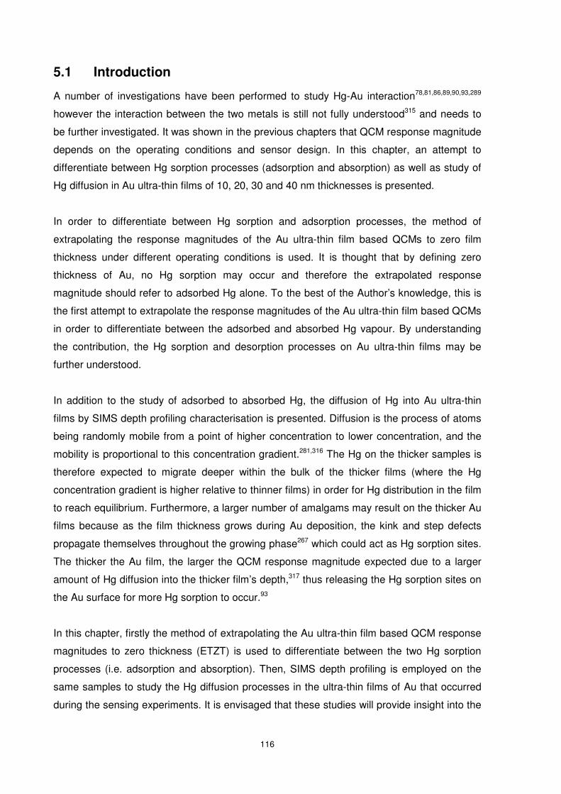
116
5.1 Introduction
A number of investigations have been performed to study Hg-Au interaction78,81,86,89,90,93,289
however the interaction between the two metals is still not fully understood315 and needs to
be further investigated. It was shown in the previous chapters that QCM response magnitude
depends on the operating conditions and sensor design. In this chapter, an attempt to
differentiate between Hg sorption processes (adsorption and absorption) as well as study of
Hg diffusion in Au ultra-thin films of 10, 20, 30 and 40 nm thicknesses is presented.
In order to differentiate between Hg sorption and adsorption processes, the method of
extrapolating the response magnitudes of the Au ultra-thin film based QCMs to zero film
thickness under different operating conditions is used. It is thought that by defining zero
thickness of Au, no Hg sorption may occur and therefore the extrapolated response
magnitude should refer to adsorbed Hg alone. To the best of the Author’s knowledge, this is
the first attempt to extrapolate the response magnitudes of the Au ultra-thin film based QCMs
in order to differentiate between the adsorbed and absorbed Hg vapour. By understanding
the contribution, the Hg sorption and desorption processes on Au ultra-thin films may be
further understood.
In addition to the study of adsorbed to absorbed Hg, the diffusion of Hg into Au ultra-thin
films by SIMS depth profiling characterisation is presented. Diffusion is the process of atoms
being randomly mobile from a point of higher concentration to lower concentration, and the
mobility is proportional to this concentration gradient.281,316 The Hg on the thicker samples is
therefore expected to migrate deeper within the bulk of the thicker films (where the Hg
concentration gradient is higher relative to thinner films) in order for Hg distribution in the film
to reach equilibrium. Furthermore, a larger number of amalgams may result on the thicker Au
films because as the film thickness grows during Au deposition, the kink and step defects
propagate themselves throughout the growing phase267 which could act as Hg sorption sites.
The thicker the Au film, the larger the QCM response magnitude expected due to a larger
amount of Hg diffusion into the thicker film’s depth,317 thus releasing the Hg sorption sites on
the Au surface for more Hg sorption to occur.93
In this chapter, firstly the method of extrapolating the Au ultra-thin film based QCM response
magnitudes to zero thickness (ETZT) is used to differentiate between the two Hg sorption
processes (i.e. adsorption and absorption). Then, SIMS depth profiling is employed on the
same samples to study the Hg diffusion processes in the ultra-thin films of Au that occurred
during the sensing experiments. It is envisaged that these studies will provide insight into the
117
type of Au surface modification techniques required to develop selective QCM based Hg
vapour sensors.
5.2 Experimental Setup
In order to study the Hg interaction with ultra-thin films of Au using SIMS depth profiling and
ETZT method, Au ultra-thin films of thicknesses between 10-40 nm were evaporated on to
specially prepared QCM sensors. It has been previously reported99 that at Au film
thicknesses above 7.5 nm, a transition from non-continuous to a continuous form occurs.
Therefore a minimum Au film thickness of 10 nm is chosen in order to ensure the thinnest
continuous film possible for extrapolation to zero Au film thickness. Thereon Au film
thicknesses of increments of 10 nm up to 40 nm are chosen to achieve different response
magnitude data points for extrapolation purposes.
Prior to depositing the Au ultra-thin films, QCMs with high Q-factors were prepared. In
accordance with the results presented in Chapter 4, 150 nm optically polished Au films were
used as these were found to have highest Q-factors. Therefore QCMs with 150 nm Au film
on 10 nm Ti adhesion layer were deposited on each side of the quartz substrate. This was
followed by a 20 nm SiO2 layer (barrier layer) to stop any mercury from diffusing into the 150
nm Au film below it. After this critical layer, an ultra-thin film of Au with thicknesses of 10, 20,
30 or 40nm was deposited over both electrode faces. A set of 10 QCMs was prepared for
each thickness of the Au ultra-thin films. Of the total of 40 QCMs, 36 QCMs were exposed to
Hg vapour and 4 were kept aside as experimental controls. Each thickness was exposed to
Hg vapour concentrations of 1.02, 3.65 or 10.55 mg/m3 at operating temperatures of 28, 55
or 89°C. The time of Hg exposure was 14 hours followed by 5 hours of recovery period under
dry nitrogen atmosphere (as explained in Chapter 2 Section 2.6.6). The 40 Au ultra-thin films
were then characterised using SIMS depth profiling. Due to the lack of availability of SIMS,
the Au films of all 40 QCMs were characterised within a 3 day period, 8 weeks after being
exposed to Hg vapour.
5.3 Differentiation of Hg Vapour Sorption Processes on Gold
It was realised in Chapter 4, Section 4.3 that Hg sorption capacity of Au is dependent on the
Au film thicknesses, Hg concentration, operating temperature and Hg exposure period.
Therefore, QCMs with different Au film thicknesses are postulated to produce different signal
outputs (∆f values) for each film thickness when exposed to identical Hg vapour
concentration, operating temperature and Hg exposure period (see Figure 5.1). The
extrapolation of ∆ƒ values to zero Au film thickness corresponds to Hg adsorption alone thus
enabling the response magnitude contribution due to adsorption to be determined at zero
thickness from the combined response of adsorption and absorption. It is well known84 that
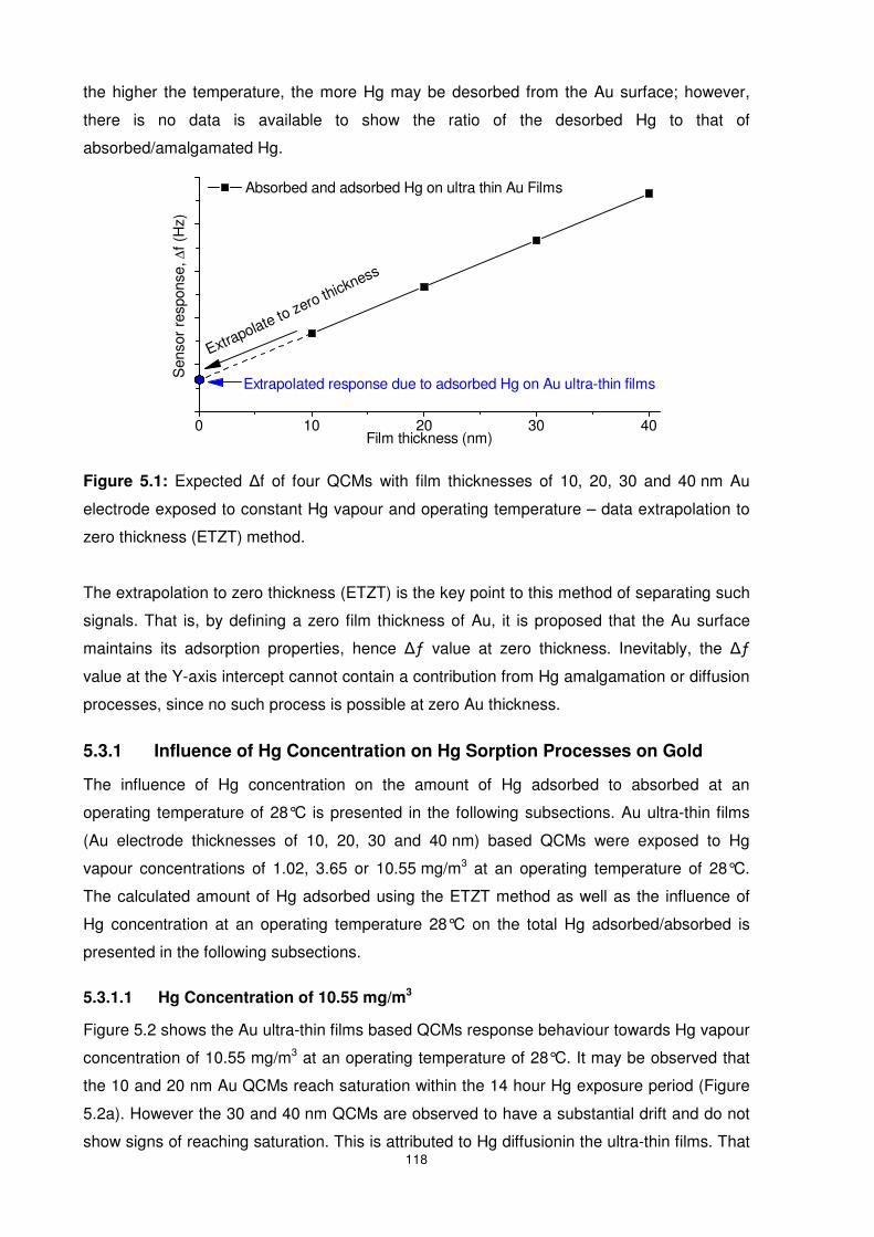
118
the higher the temperature, the more Hg may be desorbed from the Au surface; however,
there is no data is available to show the ratio of the desorbed Hg to that of
absorbed/amalgamated Hg.
Figure 5.1: Expected ∆f of four QCMs with film thicknesses of 10, 20, 30 and 40 nm Au
electrode exposed to constant Hg vapour and operating temperature – data extrapolation to
zero thickness (ETZT) method.
The extrapolation to zero thickness (ETZT) is the key point to this method of separating such
signals. That is, by defining a zero film thickness of Au, it is proposed that the Au surface
maintains its adsorption properties, hence ∆ƒ value at zero thickness. Inevitably, the ∆ƒ
value at the Y-axis intercept cannot contain a contribution from Hg amalgamation or diffusion
processes, since no such process is possible at zero Au thickness.
5.3.1 Influence of Hg Concentration on Hg Sorption Processes on Gold
The influence of Hg concentration on the amount of Hg adsorbed to absorbed at an
operating temperature of 28°C is presented in the following subsections. Au ultra-thin films
(Au electrode thicknesses of 10, 20, 30 and 40 nm) based QCMs were exposed to Hg
vapour concentrations of 1.02, 3.65 or 10.55 mg/m3 at an operating temperature of 28°C.
The calculated amount of Hg adsorbed using the ETZT method as well as the influence of
Hg concentration at an operating temperature 28°C on the total Hg adsorbed/absorbed is
presented in the following subsections.
5.3.1.1 Hg Concentration of 10.55 mg/m3
Figure 5.2 shows the Au ultra-thin films based QCMs response behaviour towards Hg vapour
concentration of 10.55 mg/m3 at an operating temperature of 28°C. It may be observed that
the 10 and 20 nm Au QCMs reach saturation within the 14 hour Hg exposure period (Figure
5.2a). However the 30 and 40 nm QCMs are observed to have a substantial drift and do not
show signs of reaching saturation. This is attributed to Hg diffusionin the ultra-thin films. That
0 10 20 30 40
Absorbed and adsorbed Hg on ultra thin Au Films
Extrapolated response due to adsorbed Hg on Au ultra-thin films
Sen
sor
resp
onse
, ∆f (
Hz)
Film thickness (nm)
Extrapolate to zero thickness
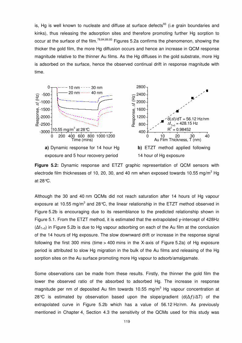
119
is, Hg is well known to nucleate and diffuse at surface defects93 (i.e grain boundaries and
kinks), thus releasing the adsorption sites and therefore promoting further Hg sorption to
occur at the surface of the film.78,84,89,93 Figures 5.2a confirms the phenomenon, showing the
thicker the gold film, the more Hg diffusion occurs and hence an increase in QCM response
magnitude relative to the thinner Au films. As the Hg diffuses in the gold substrate, more Hg
is adsorbed on the surface, hence the observed continual drift in response magnitude with
time.
Figure 5.2: Dynamic response and ETZT graphic representation of QCM sensors with
electrode film thicknesses of 10, 20, 30, and 40 nm when exposed towards 10.55 mg/m3 Hg
at 28°C.
Although the 30 and 40 nm QCMs did not reach saturation after 14 hours of Hg vapour
exposure at 10.55 mg/m3 and 28°C, the linear relationship in the ETZT method observed in
Figure 5.2b is encouraging due to its resemblance to the predicted relationship shown in
Figure 5.1. From the ETZT method, it is estimated that the extrapolated y-intercept of 428Hz
(∆fT=0) in Figure 5.2b is due to Hg vapour adsorbing on each of the Au film at the conclusion
of the 14 hours of Hg exposure. The slow downward drift or increase in the response signal
following the first 300 mins (time > 400 mins in the X-axis of Figure 5.2a) of Hg exposure
period is attributed to slow Hg migration in the bulk of the Au films and releasing of the Hg
sorption sites on the Au surface promoting more Hg vapour to adsorb/amalgamate.
Some observations can be made from these results. Firstly, the thinner the gold film the
lower the observed ratio of the absorbed to adsorbed Hg. The increase in response
magnitude per nm of deposited Au film towards 10.55 mg/m3 Hg vapour concentration at
28°C is estimated by observation based upon the slope/gradient (d(∆ƒ)/∆T) of the
extrapolated curve in Figure 5.2b which has a value of 56.12 Hz/nm. As previously
mentioned in Chapter 4, Section 4.3 the sensitivity of the QCMs used for this study was
a) Dynamic response for 14 hour Hg
exposure and 5 hour recovery period
0 200 400 600 800 1000 1200-3000
-2500
-2000
-1500
-1000
-500
0
Res
pons
e, ∆
f (H
z)
Time (mins)
10 nm 30 nm 20 nm 40 nm
10.55 mg/m3 at 28°C
b) ETZT method applied following
14 hour of Hg exposure
0 10 20 30 40400
800
1200
1600
2000
2400
2800
R2 = 0.98452
∆fT=0
= 428.15 Hz
Res
pons
e, ∆
f (H
z)
Au Film Thickness, T (nm)
d(∆f)/dT = 56.12 Hz/nm
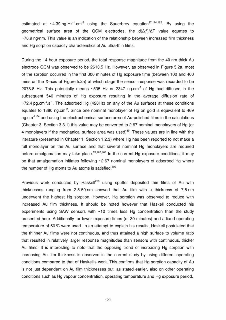
120
estimated at ~4.39 ng.Hz-1.cm-2 using the Sauerbrey equation97,174,182. By using the
geometrical surface area of the QCM electrodes, the d(∆ƒ)/∆T value equates to
~78.9 ng/nm. This value is an indication of the relationship between increased film thickness
and Hg sorption capacity characteristics of Au ultra-thin films.
During the 14 hour exposure period, the total response magnitude from the 40 nm thick Au
electrode QCM was observed to be 2613.5 Hz. However, as observed in Figure 5.2a, most
of the sorption occurred in the first 300 minutes of Hg exposure time (between 100 and 400
mins on the X-axis of Figure 5.2a) at which stage the sensor response was recorded to be
2078.8 Hz. This potentially means ~535 Hz or 2347 ng.cm-2 of Hg had diffused in the
subsequent 540 minutes of Hg exposure resulting in the average diffusion rate of
~72.4 pg.cm-2.s-1. The adsorbed Hg (428Hz) on any of the Au surfaces at these conditions
equates to 1880 ng.cm-2. Since one nominal monolayer of Hg on gold is equivalent to 469
ng.cm-2 84 and using the electrochemical surface area of Au-polished films in the calculations
(Chapter 3, Section 3.3.1) this value may be converted to 2.67 nominal monolayers of Hg (or
4 monolayers if the mechanical surface area was used)89. These values are in line with the
literature (presented in Chapter 1, Section 1.2.3) where Hg has been reported to not make a
full monolayer on the Au surface and that several nominal Hg monolayers are required
before amalgamation may take place.78,105,108 In the current Hg exposure conditions, it may
be that amalgamation initiates following ~2.67 nominal monolayers of adsorbed Hg where
the number of Hg atoms to Au atoms is satisfied.302
Previous work conducted by Haskell256 using sputter deposited thin films of Au with
thicknesses ranging from 2.5-50 nm showed that Au film with a thickness of 7.5 nm
underwent the highest Hg sorption. However, Hg sorption was observed to reduce with
increased Au film thickness. It should be noted however that Haskell conducted his
experiments using SAW sensors with ~10 times less Hg concentration than the study
presented here. Additionally far lower exposure times (of 30 minutes) and a fixed operating
temperature of 50°C were used. In an attempt to explain his results, Haskell postulated that
the thinner Au films were not continuous, and thus attained a high surface to volume ratio
that resulted in relatively larger response magnitudes than sensors with continuous, thicker
Au films. It is interesting to note that the opposing trend of increasing Hg sorption with
increasing Au film thickness is observed in the current study by using different operating
conditions compared to that of Haskell’s work. This confirms that Hg sorption capacity of Au
is not just dependent on Au film thicknesses but, as stated earlier, also on other operating
conditions such as Hg vapour concentration, operating temperature and Hg exposure period.
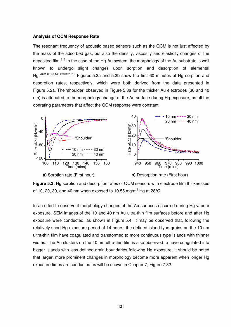
121
Analysis of QCM Response Rate
The resonant frequency of acoustic based sensors such as the QCM is not just affected by
the mass of the adsorbed gas, but also the density, viscosity and elasticity changes of the
deposited film.318 In the case of the Hg-Au system, the morphology of the Au substrate is well
known to undergo slight changes upon sorption and desorption of elemental
Hg.78,81,86,96,146,289,302,319 Figures 5.3a and 5.3b show the first 60 minutes of Hg sorption and
desorption rates, respectively, which were both derived from the data presented in
Figure 5.2a. The ‘shoulder’ observed in Figure 5.3a for the thicker Au electrodes (30 and 40
nm) is attributed to the morphology change of the Au surface during Hg exposure, as all the
operating parameters that affect the QCM response were constant.
Figure 5.3: Hg sorption and desorption rates of QCM sensors with electrode film thicknesses
of 10, 20, 30, and 40 nm when exposed to 10.55 mg/m3 Hg at 28°C.
In an effort to observe if morphology changes of the Au surfaces occurred during Hg vapour
exposure, SEM images of the 10 and 40 nm Au ultra-thin film surfaces before and after Hg
exposure were conducted, as shown in Figure 5.4. It may be observed that, following the
relatively short Hg exposure period of 14 hours, the defined island type grains on the 10 nm
ultra-thin film have coagulated and transformed to more continuous type islands with thinner
widths. The Au clusters on the 40 nm ultra-thin film is also observed to have coagulated into
bigger islands with less defined grain boundaries following Hg exposure. It should be noted
that larger, more prominent changes in morphology become more apparent when longer Hg
exposure times are conducted as will be shown in Chapter 7, Figure 7.32.
a) Sorption rate (First hour) b) Desorption rate (First hour)
940 950 960 970 980 990 1000
0
10
20
30
40 10 nm 30 nm 20 nm 40 nm
Rat
e ∆
f/∆t (
Hz/
min
)
Time (mins)
'Shoulder'
100 110 120 130 140 150 160-120
-80
-40
0
10 nm 30 nm 20 nm 40 nmR
ate
∆f/∆
t (H
z/m
in)
Time (mins)
'Shoulder'
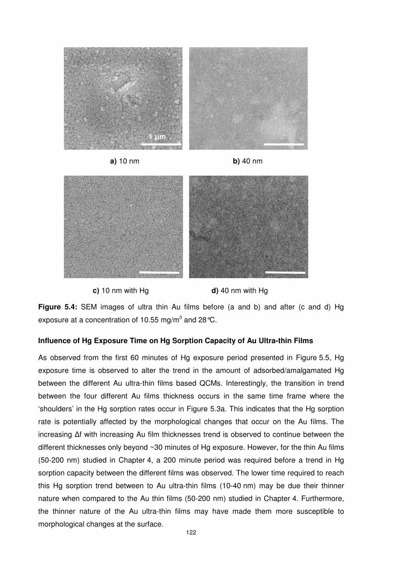
122
Figure 5.4: SEM images of ultra thin Au films before (a and b) and after (c and d) Hg
exposure at a concentration of 10.55 mg/m3 and 28°C.
Influence of Hg Exposure Time on Hg Sorption Capacity of Au Ultra-thin Films
As observed from the first 60 minutes of Hg exposure period presented in Figure 5.5, Hg
exposure time is observed to alter the trend in the amount of adsorbed/amalgamated Hg
between the different Au ultra-thin films based QCMs. Interestingly, the transition in trend
between the four different Au films thickness occurs in the same time frame where the
‘shoulders’ in the Hg sorption rates occur in Figure 5.3a. This indicates that the Hg sorption
rate is potentially affected by the morphological changes that occur on the Au films. The
increasing ∆f with increasing Au film thicknesses trend is observed to continue between the
different thicknesses only beyond ~30 minutes of Hg exposure. However, for the thin Au films
(50-200 nm) studied in Chapter 4, a 200 minute period was required before a trend in Hg
sorption capacity between the different films was observed. The lower time required to reach
this Hg sorption trend between to Au ultra-thin films (10-40 nm) may be due their thinner
nature when compared to the Au thin films (50-200 nm) studied in Chapter 4. Furthermore,
the thinner nature of the Au ultra-thin films may have made them more susceptible to
morphological changes at the surface.
1 µm
a) 10 nm b) 40 nm
d) 40 nm with Hg c) 10 nm with Hg
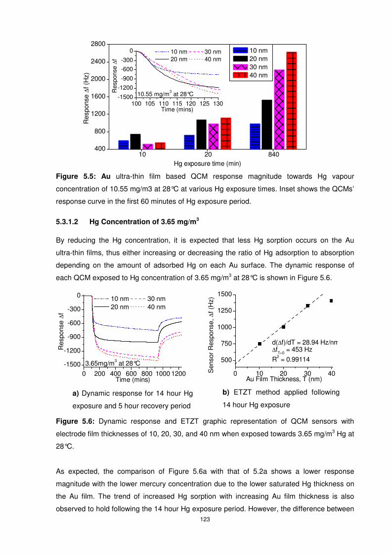
123
Figure 5.5: Au ultra-thin film based QCM response magnitude towards Hg vapour
concentration of 10.55 mg/m3 at 28°C at various Hg exposure times. Inset shows the QCMs’
response curve in the first 60 minutes of Hg exposure period.
5.3.1.2 Hg Concentration of 3.65 mg/m3
By reducing the Hg concentration, it is expected that less Hg sorption occurs on the Au
ultra-thin films, thus either increasing or decreasing the ratio of Hg adsorption to absorption
depending on the amount of adsorbed Hg on each Au surface. The dynamic response of
each QCM exposed to Hg concentration of 3.65 mg/m3 at 28°C is shown in Figure 5.6.
Figure 5.6: Dynamic response and ETZT graphic representation of QCM sensors with
electrode film thicknesses of 10, 20, 30, and 40 nm when exposed towards 3.65 mg/m3 Hg at
28°C.
As expected, the comparison of Figure 5.6a with that of 5.2a shows a lower response
magnitude with the lower mercury concentration due to the lower saturated Hg thickness on
the Au film. The trend of increased Hg sorption with increasing Au film thickness is also
observed to hold following the 14 hour Hg exposure period. However, the difference between
a) Dynamic response for 14 hour Hg
exposure and 5 hour recovery period
b) ETZT method applied following
14 hour Hg exposure
0 200 400 600 800 1000 1200-1500
-1200
-900
-600
-300
0
Res
pons
e ∆
f
Time (mins)
10 nm 30 nm 20 nm 40 nm
3.65mg/m3 at 28°C
0 10 20 30 40
500
750
1000
1250
1500
Sen
sor
Res
pons
e, ∆
f (H
z)
Au Film Thickness, T (nm)
R2 = 0.99114
∆fT=0
= 453 Hzd(∆f)/dT = 28.94 Hz/nm
400
800
1200
1600
2000
2400
2800
Res
pons
e ∆
f (H
z)
Hg exposure time (min)
10 nm 20 nm 30 nm 40 nm
10 20 840
100 105 110 115 120 125 130-1500
-1200
-900
-600
-300
0
10.55 mg/m3 at 28°CRes
pons
e ∆
fTime (mins)
10 nm 30 nm 20 nm 40 nm
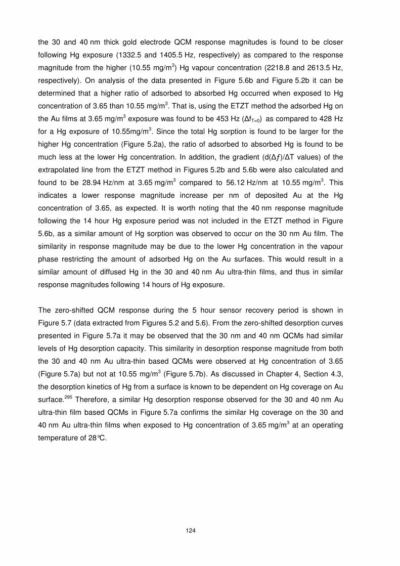
124
the 30 and 40 nm thick gold electrode QCM response magnitudes is found to be closer
following Hg exposure (1332.5 and 1405.5 Hz, respectively) as compared to the response
magnitude from the higher (10.55 mg/m3) Hg vapour concentration (2218.8 and 2613.5 Hz,
respectively). On analysis of the data presented in Figure 5.6b and Figure 5.2b it can be
determined that a higher ratio of adsorbed to absorbed Hg occurred when exposed to Hg
concentration of 3.65 than 10.55 mg/m3. That is, using the ETZT method the adsorbed Hg on
the Au films at 3.65 mg/m3 exposure was found to be 453 Hz (∆fT=0) as compared to 428 Hz
for a Hg exposure of 10.55mg/m3. Since the total Hg sorption is found to be larger for the
higher Hg concentration (Figure 5.2a), the ratio of adsorbed to absorbed Hg is found to be
much less at the lower Hg concentration. In addition, the gradient (d(∆ƒ)/∆T values) of the
extrapolated line from the ETZT method in Figures 5.2b and 5.6b were also calculated and
found to be 28.94 Hz/nm at 3.65 mg/m3 compared to 56.12 Hz/nm at 10.55 mg/m3. This
indicates a lower response magnitude increase per nm of deposited Au at the Hg
concentration of 3.65, as expected. It is worth noting that the 40 nm response magnitude
following the 14 hour Hg exposure period was not included in the ETZT method in Figure
5.6b, as a similar amount of Hg sorption was observed to occur on the 30 nm Au film. The
similarity in response magnitude may be due to the lower Hg concentration in the vapour
phase restricting the amount of adsorbed Hg on the Au surfaces. This would result in a
similar amount of diffused Hg in the 30 and 40 nm Au ultra-thin films, and thus in similar
response magnitudes following 14 hours of Hg exposure.
The zero-shifted QCM response during the 5 hour sensor recovery period is shown in
Figure 5.7 (data extracted from Figures 5.2 and 5.6). From the zero-shifted desorption curves
presented in Figure 5.7a it may be observed that the 30 nm and 40 nm QCMs had similar
levels of Hg desorption capacity. This similarity in desorption response magnitude from both
the 30 and 40 nm Au ultra-thin based QCMs were observed at Hg concentration of 3.65
(Figure 5.7a) but not at 10.55 mg/m3 (Figure 5.7b). As discussed in Chapter 4, Section 4.3,
the desorption kinetics of Hg from a surface is known to be dependent on Hg coverage on Au
surface.295 Therefore, a similar Hg desorption response observed for the 30 and 40 nm Au
ultra-thin film based QCMs in Figure 5.7a confirms the similar Hg coverage on the 30 and
40 nm Au ultra-thin films when exposed to Hg concentration of 3.65 mg/m3 at an operating
temperature of 28°C.
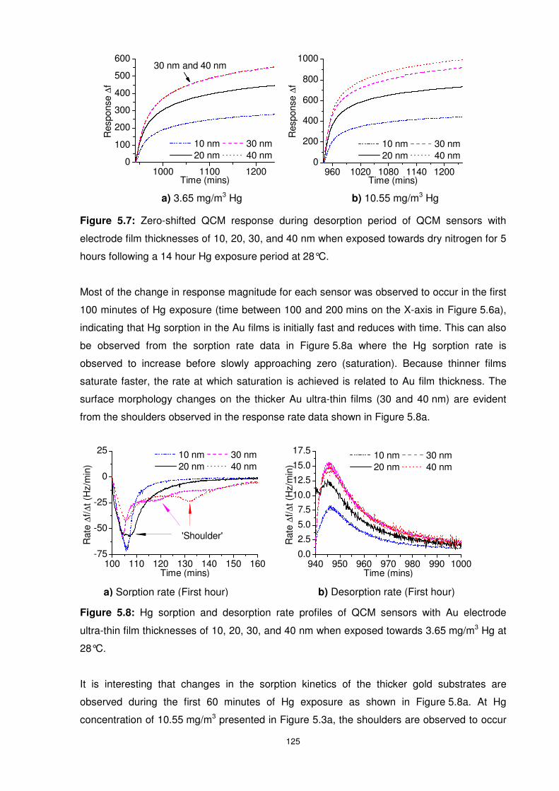
125
Figure 5.7: Zero-shifted QCM response during desorption period of QCM sensors with
electrode film thicknesses of 10, 20, 30, and 40 nm when exposed towards dry nitrogen for 5
hours following a 14 hour Hg exposure period at 28°C.
Most of the change in response magnitude for each sensor was observed to occur in the first
100 minutes of Hg exposure (time between 100 and 200 mins on the X-axis in Figure 5.6a),
indicating that Hg sorption in the Au films is initially fast and reduces with time. This can also
be observed from the sorption rate data in Figure 5.8a where the Hg sorption rate is
observed to increase before slowly approaching zero (saturation). Because thinner films
saturate faster, the rate at which saturation is achieved is related to Au film thickness. The
surface morphology changes on the thicker Au ultra-thin films (30 and 40 nm) are evident
from the shoulders observed in the response rate data shown in Figure 5.8a.
Figure 5.8: Hg sorption and desorption rate profiles of QCM sensors with Au electrode
ultra-thin film thicknesses of 10, 20, 30, and 40 nm when exposed towards 3.65 mg/m3 Hg at
28°C.
It is interesting that changes in the sorption kinetics of the thicker gold substrates are
observed during the first 60 minutes of Hg exposure as shown in Figure 5.8a. At Hg
concentration of 10.55 mg/m3 presented in Figure 5.3a, the shoulders are observed to occur
a) 3.65 mg/m3 Hg b) 10.55 mg/m3 Hg
960 1020 1080 1140 12000
200
400
600
800
1000
Res
pons
e ∆
f
Time (mins)
10 nm 30 nm 20 nm 40 nm
1000 1100 12000
100
200
300
400
500
60030 nm and 40 nm
Res
pons
e ∆
f
Time (mins)
10 nm 30 nm 20 nm 40 nm
a) Sorption rate (First hour) b) Desorption rate (First hour)
100 110 120 130 140 150 160-75
-50
-25
0
25
Rat
e ∆
f/∆t (
Hz/
min
)
Time (mins)
10 nm 30 nm 20 nm 40 nm
'Shoulder'
940 950 960 970 980 990 10000.0
2.5
5.0
7.5
10.0
12.5
15.0
17.5
Rat
e ∆
f/∆t (
Hz/
min
)
Time (mins)
10 nm 30 nm 20 nm 40 nm
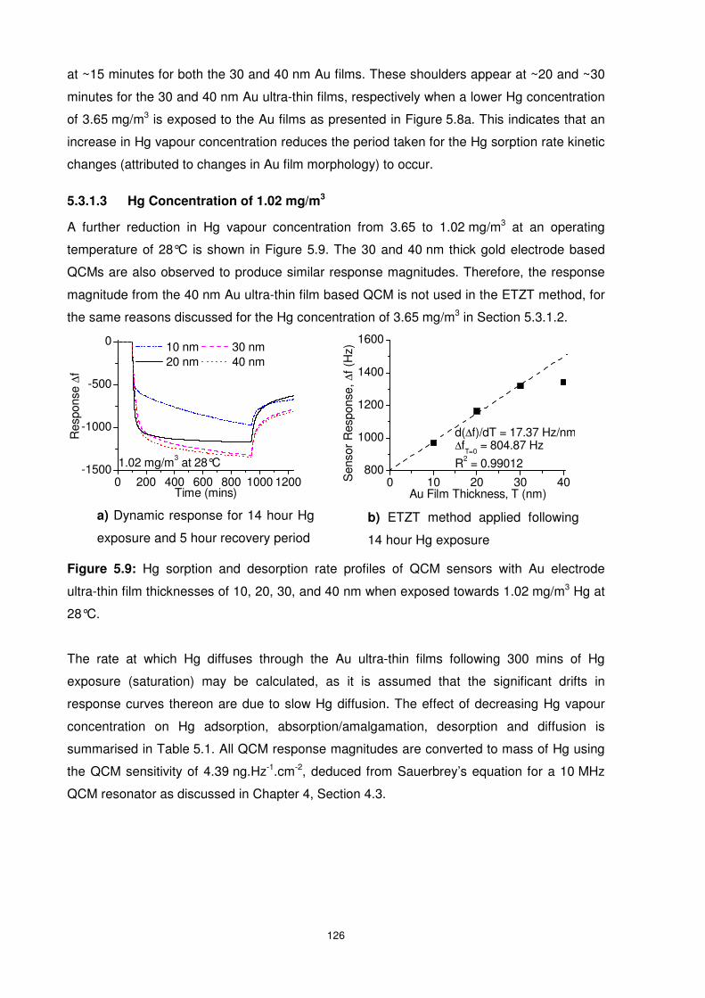
126
at ~15 minutes for both the 30 and 40 nm Au films. These shoulders appear at ~20 and ~30
minutes for the 30 and 40 nm Au ultra-thin films, respectively when a lower Hg concentration
of 3.65 mg/m3 is exposed to the Au films as presented in Figure 5.8a. This indicates that an
increase in Hg vapour concentration reduces the period taken for the Hg sorption rate kinetic
changes (attributed to changes in Au film morphology) to occur.
5.3.1.3 Hg Concentration of 1.02 mg/m3
A further reduction in Hg vapour concentration from 3.65 to 1.02 mg/m3 at an operating
temperature of 28°C is shown in Figure 5.9. The 30 and 40 nm thick gold electrode based
QCMs are also observed to produce similar response magnitudes. Therefore, the response
magnitude from the 40 nm Au ultra-thin film based QCM is not used in the ETZT method, for
the same reasons discussed for the Hg concentration of 3.65 mg/m3 in Section 5.3.1.2.
Figure 5.9: Hg sorption and desorption rate profiles of QCM sensors with Au electrode
ultra-thin film thicknesses of 10, 20, 30, and 40 nm when exposed towards 1.02 mg/m3 Hg at
28°C.
The rate at which Hg diffuses through the Au ultra-thin films following 300 mins of Hg
exposure (saturation) may be calculated, as it is assumed that the significant drifts in
response curves thereon are due to slow Hg diffusion. The effect of decreasing Hg vapour
concentration on Hg adsorption, absorption/amalgamation, desorption and diffusion is
summarised in Table 5.1. All QCM response magnitudes are converted to mass of Hg using
the QCM sensitivity of 4.39 ng.Hz-1.cm-2, deduced from Sauerbrey’s equation for a 10 MHz
QCM resonator as discussed in Chapter 4, Section 4.3.
a) Dynamic response for 14 hour Hg
exposure and 5 hour recovery period
b) ETZT method applied following
14 hour Hg exposure
0 200 400 600 800 1000 1200-1500
-1000
-500
0
Res
pons
e ∆
f
Time (mins)
10 nm 30 nm 20 nm 40 nm
1.02 mg/m3 at 28°C
0 10 20 30 40800
1000
1200
1400
1600S
enso
r R
espo
nse,
∆f (
Hz)
Au Film Thickness, T (nm)
R2 = 0.99012
∆fT=0
= 804.87 Hzd(∆f)/dT = 17.37 Hz/nm
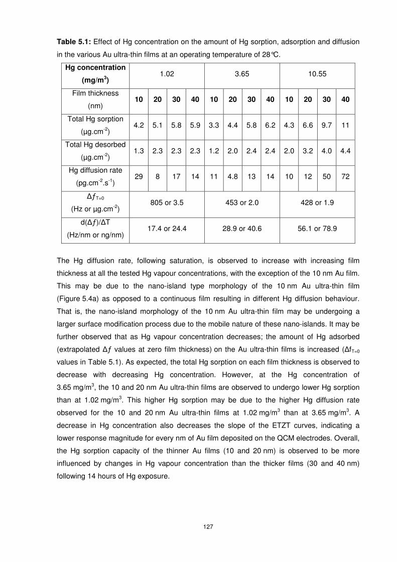
127
Table 5.1: Effect of Hg concentration on the amount of Hg sorption, adsorption and diffusion
in the various Au ultra-thin films at an operating temperature of 28°C.
Hg concentration
(mg/m3) 1.02 3.65 10.55
Film thickness
(nm) 10 20 30 40 10 20 30 40 10 20 30 40
Total Hg sorption
(µg.cm-2) 4.2 5.1 5.8 5.9 3.3 4.4 5.8 6.2 4.3 6.6 9.7 11
Total Hg desorbed
(µg.cm-2) 1.3 2.3 2.3 2.3 1.2 2.0 2.4 2.4 2.0 3.2 4.0 4.4
Hg diffusion rate
(pg.cm-2.s-1) 29 8 17 14 11 4.8 13 14 10 12 50 72
∆ƒT=0
(Hz or µg.cm-2) 805 or 3.5 453 or 2.0 428 or 1.9
d(∆ƒ)/∆T
(Hz/nm or ng/nm) 17.4 or 24.4 28.9 or 40.6 56.1 or 78.9
The Hg diffusion rate, following saturation, is observed to increase with increasing film
thickness at all the tested Hg vapour concentrations, with the exception of the 10 nm Au film.
This may be due to the nano-island type morphology of the 10 nm Au ultra-thin film
(Figure 5.4a) as opposed to a continuous film resulting in different Hg diffusion behaviour.
That is, the nano-island morphology of the 10 nm Au ultra-thin film may be undergoing a
larger surface modification process due to the mobile nature of these nano-islands. It may be
further observed that as Hg vapour concentration decreases; the amount of Hg adsorbed
(extrapolated ∆ƒ values at zero film thickness) on the Au ultra-thin films is increased (∆fT=0
values in Table 5.1). As expected, the total Hg sorption on each film thickness is observed to
decrease with decreasing Hg concentration. However, at the Hg concentration of
3.65 mg/m3, the 10 and 20 nm Au ultra-thin films are observed to undergo lower Hg sorption
than at 1.02 mg/m3. This higher Hg sorption may be due to the higher Hg diffusion rate
observed for the 10 and 20 nm Au ultra-thin films at 1.02 mg/m3 than at 3.65 mg/m3. A
decrease in Hg concentration also decreases the slope of the ETZT curves, indicating a
lower response magnitude for every nm of Au film deposited on the QCM electrodes. Overall,
the Hg sorption capacity of the thinner Au films (10 and 20 nm) is observed to be more
influenced by changes in Hg vapour concentration than the thicker films (30 and 40 nm)
following 14 hours of Hg exposure.
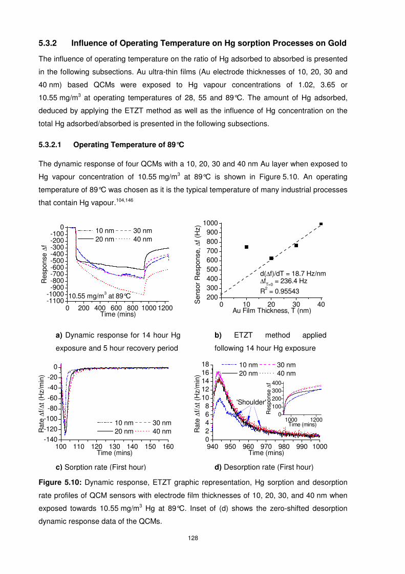
128
5.3.2 Influence of Operating Temperature on Hg sorption Processes on Gold
The influence of operating temperature on the ratio of Hg adsorbed to absorbed is presented
in the following subsections. Au ultra-thin films (Au electrode thicknesses of 10, 20, 30 and
40 nm) based QCMs were exposed to Hg vapour concentrations of 1.02, 3.65 or
10.55 mg/m3 at operating temperatures of 28, 55 and 89°C. The amount of Hg adsorbed,
deduced by applying the ETZT method as well as the influence of Hg concentration on the
total Hg adsorbed/absorbed is presented in the following subsections.
5.3.2.1 Operating Temperature of 89°C
The dynamic response of four QCMs with a 10, 20, 30 and 40 nm Au layer when exposed to
Hg vapour concentration of 10.55 mg/m3 at 89°C is shown in Figure 5.10. An operating
temperature of 89°C was chosen as it is the typical temperature of many industrial processes
that contain Hg vapour.104,146
Figure 5.10: Dynamic response, ETZT graphic representation, Hg sorption and desorption
rate profiles of QCM sensors with electrode film thicknesses of 10, 20, 30, and 40 nm when
exposed towards 10.55 mg/m3 Hg at 89°C. Inset of (d) shows the zero-shifted desorption
dynamic response data of the QCMs.
a) Dynamic response for 14 hour Hg
exposure and 5 hour recovery period
b) ETZT method applied
following 14 hour Hg exposure
c) Sorption rate (First hour) d) Desorption rate (First hour)
0 200 400 600 800 1000 1200-1100-1000-900-800-700-600-500-400-300-200-100
0
10.55 mg/m3 at 89°C
Res
pons
e ∆
f
Time (mins)
10 nm 30 nm 20 nm 40 nm
100 110 120 130 140 150 160-140
-120
-100
-80
-60
-40
-20
0
10 nm 30 nm 20 nm 40 nmR
ate
∆f/∆
t (H
z/m
in)
Time (mins)940 950 960 970 980 990 100002468
1012141618
1000 12000
100200300400
Res
pons
e ∆
f
Time (mins)
'Shoulder'
10 nm 30 nm 20 nm 40 nm
Rat
e ∆
f/∆t (
Hz/
min
)
Time (mins)
0 10 20 30 40200300400500600700800900
1000
Sen
sor
Res
pons
e, ∆
f (H
z)
Au Film Thickness, T (nm)
R2 = 0.95543
∆fT=0
= 236.4 Hzd(∆f)/dT = 18.7 Hz/nm
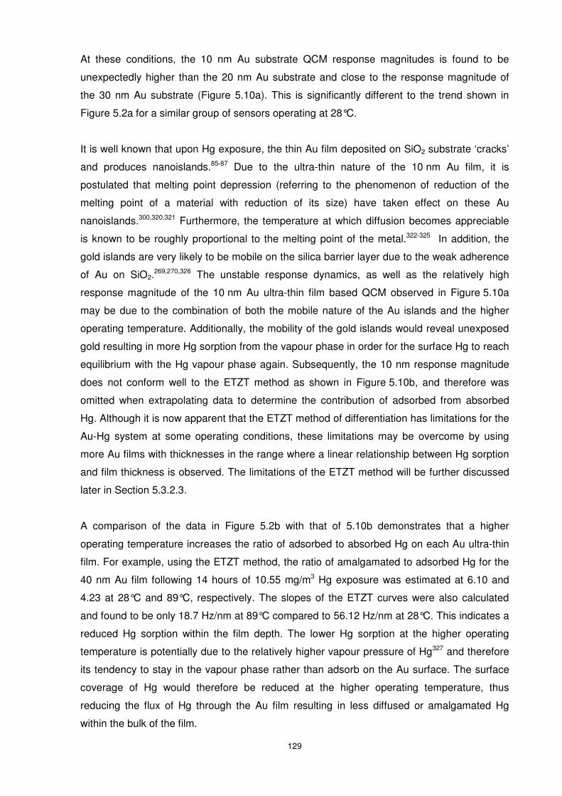
129
At these conditions, the 10 nm Au substrate QCM response magnitudes is found to be
unexpectedly higher than the 20 nm Au substrate and close to the response magnitude of
the 30 nm Au substrate (Figure 5.10a). This is significantly different to the trend shown in
Figure 5.2a for a similar group of sensors operating at 28°C.
It is well known that upon Hg exposure, the thin Au film deposited on SiO2 substrate ‘cracks’
and produces nanoislands.85-87 Due to the ultra-thin nature of the 10 nm Au film, it is
postulated that melting point depression (referring to the phenomenon of reduction of the
melting point of a material with reduction of its size) have taken effect on these Au
nanoislands.300,320,321 Furthermore, the temperature at which diffusion becomes appreciable
is known to be roughly proportional to the melting point of the metal.322-325 In addition, the
gold islands are very likely to be mobile on the silica barrier layer due to the weak adherence
of Au on SiO2.269,270,326 The unstable response dynamics, as well as the relatively high
response magnitude of the 10 nm Au ultra-thin film based QCM observed in Figure 5.10a
may be due to the combination of both the mobile nature of the Au islands and the higher
operating temperature. Additionally, the mobility of the gold islands would reveal unexposed
gold resulting in more Hg sorption from the vapour phase in order for the surface Hg to reach
equilibrium with the Hg vapour phase again. Subsequently, the 10 nm response magnitude
does not conform well to the ETZT method as shown in Figure 5.10b, and therefore was
omitted when extrapolating data to determine the contribution of adsorbed from absorbed
Hg. Although it is now apparent that the ETZT method of differentiation has limitations for the
Au-Hg system at some operating conditions, these limitations may be overcome by using
more Au films with thicknesses in the range where a linear relationship between Hg sorption
and film thickness is observed. The limitations of the ETZT method will be further discussed
later in Section 5.3.2.3.
A comparison of the data in Figure 5.2b with that of 5.10b demonstrates that a higher
operating temperature increases the ratio of adsorbed to absorbed Hg on each Au ultra-thin
film. For example, using the ETZT method, the ratio of amalgamated to adsorbed Hg for the
40 nm Au film following 14 hours of 10.55 mg/m3 Hg exposure was estimated at 6.10 and
4.23 at 28°C and 89°C, respectively. The slopes of the ETZT curves were also calculated
and found to be only 18.7 Hz/nm at 89°C compared to 56.12 Hz/nm at 28°C. This indicates a
reduced Hg sorption within the film depth. The lower Hg sorption at the higher operating
temperature is potentially due to the relatively higher vapour pressure of Hg327 and therefore
its tendency to stay in the vapour phase rather than adsorb on the Au surface. The surface
coverage of Hg would therefore be reduced at the higher operating temperature, thus
reducing the flux of Hg through the Au film resulting in less diffused or amalgamated Hg
within the bulk of the film.
130
Hg sorption and desorption rates for the first 60 minutes are shown in Figures 5.10c and
5.10d, respectively. It may be observed that both maximum sorption and desorption rates are
reached in less time at the higher operating temperature of 89°C than at 28°C (Figures 5.3a
and 5.3b). In Addition, a number of shoulders may be observed in the desorption rate curve
of the 10 nm Au film during the first 60 minutes of the desorption period at 89°C. These
shoulders are again attributed to the mobility of the amalgam islands86 on the 10 nm Au film
during the recovery period.
5.3.2.2 Operating Temperature of 55°C
In order to study the influence of reducing the operating temperature from 89 to 55°C, a new
set of Au ultra-thin film based QCMs were exposed to Hg vapour concentration of
10.55 mg/m3 at 55°C, the response dynamics of which are shown in Figure 5.11a. It is
observed that at the operating temperature of 55°C, the 10 and 20 nm Au ultra-thin films had
similar response magnitudes at the conclusion of the 14 hour Hg exposure period. The
thicker Au films (30 and 40 nm) also had similar response magnitudes. These similarities are
attributed to the influence of operating temperature and exposure time on Hg sorption
capacity of Au films, as discussed in Chapter 4, Section 4.3. Therefore only the 20 and the
30 nm Au ultra-thin films were used in the ETZT method to differentiate Hg adsorption from
absorption for comparison, as shown in Figure 5.11b. This is another operating condition
where a limitation of the ETZT method is observed. The limitation may be overcome in future
studies by using more Au film thicknesses in the range 20≤T≤30 at the operating temperature
of 55°C and Hg vapour concentration of 10.55 mg/m3 before applying the ETZT method.
Figure 5.11: Dynamic response and ETZT graphic representation of QCM sensors with
electrode film thicknesses of 10, 20, 30, and 40 nm when exposed towards 10.55 mg/m3 Hg
at 55°C.
a) Dynamic response for 14 hour Hg
exposure and 5 hour recovery period
b) ETZT method applied following
14 hour Hg exposure
0 200 400 600 800 1000 1200
-1200
-900
-600
-300
0
Res
pons
e ∆
f
Time (mins)
10 nm 30 nm 20 nm 40 nm
10.55 mg/m3 at 55°C
0 10 20 30 40250
500
750
1000
1250
1500
Sen
sor
Res
pons
e, ∆
f (H
z)
Au Film Thickness, T (nm)
Response magnitude (14 hour Hg exposure
Line of best fit
R2 = 1
∆fT=0
= 313.2 Hzd(∆f)/dT = 28.21 Hz/nm
131
An increased amount of adsorbed Hg is observed at the lower temperature of 55°C
(extrapolated ∆ƒ value of 313.2 Hz) relative to 89°C (extrapolated response magnitude of
236.4 Hz). However, the relatively higher ∆ƒ values of the QCMs at 55°C has resulted in a
reduced ratio of adsorbed to absorbed Hg, due to the decreased operating temperature.
5.3.2.3 Operating Temperature of 28°C
In order to study the influence of reducing the operating temperature from 89 and 55°C to
28°C, the response curves presented in Figures 5.10 and 5.11 is compared with Figure 5.2.
Similar operating conditions were used in all the experiments presented in Figures 5.10, 5.11
and 5.2, with the only changed parameter being a reduction in the operating temperature
from 89 or 55 to 28°C, respectively. The influence of reducing the operating temperature
from 55 to 28°C is observed to be similar to that observed when reducing the operating
temperature from 89 to 55°C, as presented in Section 5.3.2.2. It is shown that there is a
larger extrapolated response magnitude at 28°C relative to the higher temperatures of 55
and 89°C, which indicates that the amount of adsorbed Hg increases with decreasing
operating temperature.
The ETZT calculations (for operating conditions of 1.02 mg/m3 Hg at 55°C, 3.65 mg/m3 Hg at
55°C, 1.02 mg/m3 Hg at 89°C, 3.65 mg/m3 Hg at 89°C) as well as the zero-shifted desorption
curves are presented in Appendix E (Figures E1-E5). The results of all nine operating
conditions are summarised in Table 5.2 for operating temperatures of 55 and 89°C. The data
for 28°C was presented in Table 5.1. It is clear from the results presented in Tables 5.1 and
5.2 that the ETZT method of differentiation has limitations and can only be used in certain
conditions for the film thicknesses used (for example, Hg concentration of 10.55 mg/m3 at an
operating temperature of 28°C). However, the method gives an insight into the influence of
film thickness on Hg sorption capacity and how the ratio of adsorbed to absorbed Hg
influences Hg diffusion rate on the different ultra-thin films of Au, following saturation or 300
minutes of Hg exposure. In the case of other conditions (for example, a Hg concentration of
10.55 mg/m3 at and operating temperature of 89°C), these influences may be studied in
greater detail by using more Au ultra-thin films with thicknesses of 20<T<40 nm, as observed
in Figure 5.10b. In general, it is observed from Table 5.2 that the amount of Hg adsorbed
(∆ƒT=0) and Hg sorption per nm of deposited Au films (d(∆ƒ)/∆T values) reduces with
increasing operating temperature. It is also observed that the Hg diffusion rate in the Au
ultra-thin films is slow (in pg.cm-2.s-1) following Hg exposure beyond 300 minutes (after
saturation is reached) at all operating temperatures. The ambiguities with the diffusion rate
and Hg sorption capacity between the different Au ultra-thin films at the different operating
conditions may be further understood by studying the Hg diffusion behaviour in these films.
This is the subject of Section 5.4.
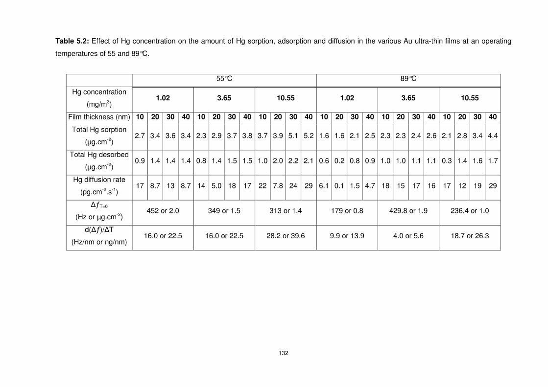
132
Table 5.2: Effect of Hg concentration on the amount of Hg sorption, adsorption and diffusion in the various Au ultra-thin films at an operating
temperatures of 55 and 89°C.
55°C 89°C
Hg concentration
(mg/m3) 1.02 3.65 10.55 1.02 3.65 10.55
Film thickness (nm) 10 20 30 40 10 20 30 40 10 20 30 40 10 20 30 40 10 20 30 40 10 20 30 40
Total Hg sorption
(µg.cm-2) 2.7 3.4 3.6 3.4 2.3 2.9 3.7 3.8 3.7 3.9 5.1 5.2 1.6 1.6 2.1 2.5 2.3 2.3 2.4 2.6 2.1 2.8 3.4 4.4
Total Hg desorbed
(µg.cm-2) 0.9 1.4 1.4 1.4 0.8 1.4 1.5 1.5 1.0 2.0 2.2 2.1 0.6 0.2 0.8 0.9 1.0 1.0 1.1 1.1 0.3 1.4 1.6 1.7
Hg diffusion rate
(pg.cm-2.s-1) 17 8.7 13 8.7 14 5.0 18 17 22 7.8 24 29 6.1 0.1 1.5 4.7 18 15 17 16 17 12 19 29
∆ƒT=0
(Hz or µg.cm-2) 452 or 2.0 349 or 1.5 313 or 1.4 179 or 0.8 429.8 or 1.9 236.4 or 1.0
d(∆ƒ)/∆T
(Hz/nm or ng/nm) 16.0 or 22.5 16.0 or 22.5 28.2 or 39.6 9.9 or 13.9 4.0 or 5.6 18.7 or 26.3
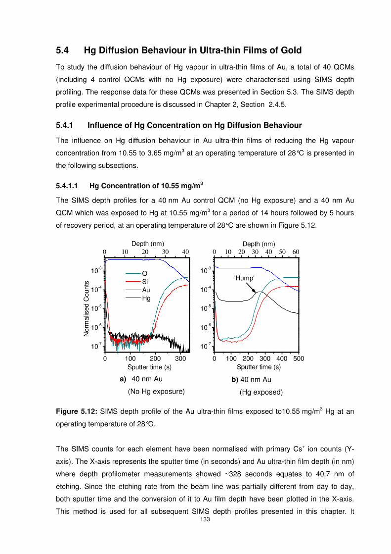
133
5.4 Hg Diffusion Behaviour in Ultra-thin Films of Gold
To study the diffusion behaviour of Hg vapour in ultra-thin films of Au, a total of 40 QCMs
(including 4 control QCMs with no Hg exposure) were characterised using SIMS depth
profiling. The response data for these QCMs was presented in Section 5.3. The SIMS depth
profile experimental procedure is discussed in Chapter 2, Section 2.4.5.
5.4.1 Influence of Hg Concentration on Hg Diffusion Behaviour
The influence on Hg diffusion behaviour in Au ultra-thin films of reducing the Hg vapour
concentration from 10.55 to 3.65 mg/m3 at an operating temperature of 28°C is presented in
the following subsections.
5.4.1.1 Hg Concentration of 10.55 mg/m3
The SIMS depth profiles for a 40 nm Au control QCM (no Hg exposure) and a 40 nm Au
QCM which was exposed to Hg at 10.55 mg/m3 for a period of 14 hours followed by 5 hours
of recovery period, at an operating temperature of 28°C are shown in Figure 5.12.
Figure 5.12: SIMS depth profile of the Au ultra-thin films exposed to10.55 mg/m3 Hg at an
operating temperature of 28°C.
The SIMS counts for each element have been normalised with primary Cs+ ion counts (Y-
axis). The X-axis represents the sputter time (in seconds) and Au ultra-thin film depth (in nm)
where depth profilometer measurements showed ~328 seconds equates to 40.7 nm of
etching. Since the etching rate from the beam line was partially different from day to day,
both sputter time and the conversion of it to Au film depth have been plotted in the X-axis.
This method is used for all subsequent SIMS depth profiles presented in this chapter. It
a) 40 nm Au
(No Hg exposure)
b) 40 nm Au
(Hg exposed)
0 100 200 300
10-7
10-6
10-5
10-4
10-3
Nor
mal
ised
Cou
nts
Sputter time (s)
O Si Au Hg
0 10 20 30 40
Depth (nm)
0 100 200 300 400 500
10-7
10-6
10-5
10-4
10-3
Depth (nm)
Sputter time (s)
'Hump'
0 10 20 30 40 50 60
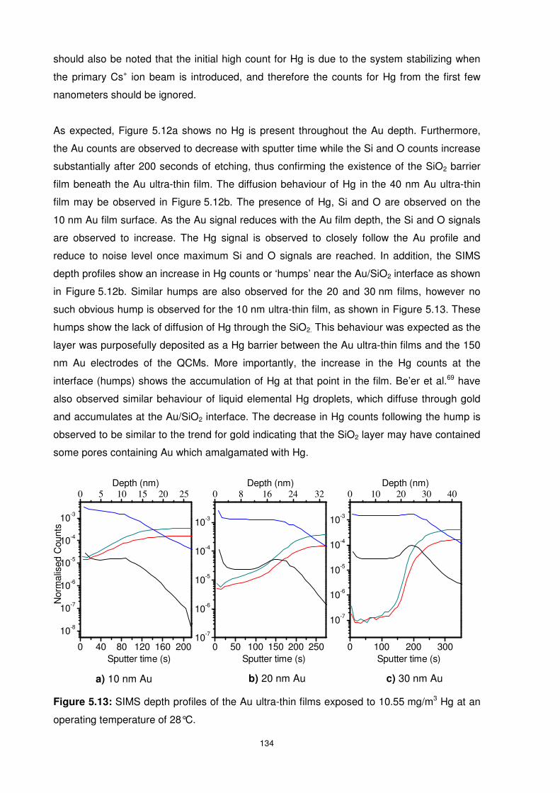
134
should also be noted that the initial high count for Hg is due to the system stabilizing when
the primary Cs+ ion beam is introduced, and therefore the counts for Hg from the first few
nanometers should be ignored.
As expected, Figure 5.12a shows no Hg is present throughout the Au depth. Furthermore,
the Au counts are observed to decrease with sputter time while the Si and O counts increase
substantially after 200 seconds of etching, thus confirming the existence of the SiO2 barrier
film beneath the Au ultra-thin film. The diffusion behaviour of Hg in the 40 nm Au ultra-thin
film may be observed in Figure 5.12b. The presence of Hg, Si and O are observed on the
10 nm Au film surface. As the Au signal reduces with the Au film depth, the Si and O signals
are observed to increase. The Hg signal is observed to closely follow the Au profile and
reduce to noise level once maximum Si and O signals are reached. In addition, the SIMS
depth profiles show an increase in Hg counts or ‘humps’ near the Au/SiO2 interface as shown
in Figure 5.12b. Similar humps are also observed for the 20 and 30 nm films, however no
such obvious hump is observed for the 10 nm ultra-thin film, as shown in Figure 5.13. These
humps show the lack of diffusion of Hg through the SiO2. This behaviour was expected as the
layer was purposefully deposited as a Hg barrier between the Au ultra-thin films and the 150
nm Au electrodes of the QCMs. More importantly, the increase in the Hg counts at the
interface (humps) shows the accumulation of Hg at that point in the film. Be’er et al.69 have
also observed similar behaviour of liquid elemental Hg droplets, which diffuse through gold
and accumulates at the Au/SiO2 interface. The decrease in Hg counts following the hump is
observed to be similar to the trend for gold indicating that the SiO2 layer may have contained
some pores containing Au which amalgamated with Hg.
Figure 5.13: SIMS depth profiles of the Au ultra-thin films exposed to 10.55 mg/m3 Hg at an
operating temperature of 28°C.
a) 10 nm Au b) 20 nm Au c) 30 nm Au
0 40 80 120 160 200
10-8
10-7
10-6
10-5
10-4
10-3
Nor
mal
ised
Cou
nts
Depth (nm)
Sputter time (s)
0 5 10 15 20 25
0 50 100 150 200 25010-7
10-6
10-5
10-4
10-3
Depth (nm)
Sputter time (s)
0 8 16 24 32
0 100 200 300
10-7
10-6
10-5
10-4
10-3
Depth (nm)
Sputter time (s)
0 10 20 30 40
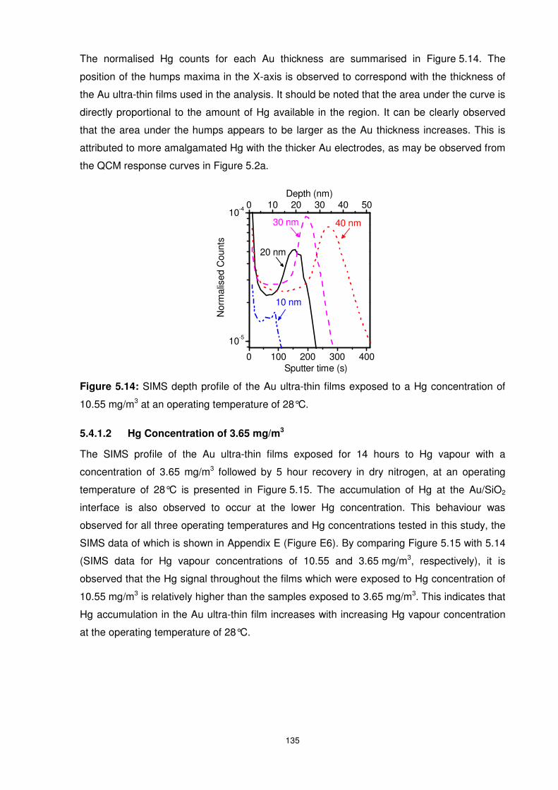
135
The normalised Hg counts for each Au thickness are summarised in Figure 5.14. The
position of the humps maxima in the X-axis is observed to correspond with the thickness of
the Au ultra-thin films used in the analysis. It should be noted that the area under the curve is
directly proportional to the amount of Hg available in the region. It can be clearly observed
that the area under the humps appears to be larger as the Au thickness increases. This is
attributed to more amalgamated Hg with the thicker Au electrodes, as may be observed from
the QCM response curves in Figure 5.2a.
Figure 5.14: SIMS depth profile of the Au ultra-thin films exposed to a Hg concentration of
10.55 mg/m3 at an operating temperature of 28°C.
5.4.1.2 Hg Concentration of 3.65 mg/m3
The SIMS profile of the Au ultra-thin films exposed for 14 hours to Hg vapour with a
concentration of 3.65 mg/m3 followed by 5 hour recovery in dry nitrogen, at an operating
temperature of 28°C is presented in Figure 5.15. The accumulation of Hg at the Au/SiO2
interface is also observed to occur at the lower Hg concentration. This behaviour was
observed for all three operating temperatures and Hg concentrations tested in this study, the
SIMS data of which is shown in Appendix E (Figure E6). By comparing Figure 5.15 with 5.14
(SIMS data for Hg vapour concentrations of 10.55 and 3.65 mg/m3, respectively), it is
observed that the Hg signal throughout the films which were exposed to Hg concentration of
10.55 mg/m3 is relatively higher than the samples exposed to 3.65 mg/m3. This indicates that
Hg accumulation in the Au ultra-thin film increases with increasing Hg vapour concentration
at the operating temperature of 28°C.
0 100 200 300 400
10-5
10-4
Nor
mal
ised
Cou
nts
40 nm30 nm
20 nm
Sputter time (s)
10 nm
0 10 20 30 40 50Depth (nm)
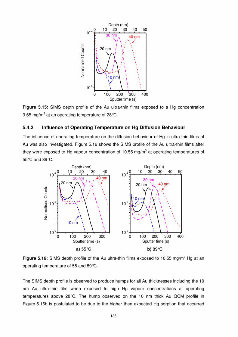
136
Figure 5.15: SIMS depth profile of the Au ultra-thin films exposed to a Hg concentration
3.65 mg/m3 at an operating temperature of 28°C.
5.4.2 Influence of Operating Temperature on Hg Diffusion Behaviour
The influence of operating temperature on the diffusion behaviour of Hg in ultra-thin films of
Au was also investigated. Figure 5.16 shows the SIMS profile of the Au ultra-thin films after
they were exposed to Hg vapour concentration of 10.55 mg/m3 at operating temperatures of
55°C and 89°C.
Figure 5.16: SIMS depth profile of the Au ultra-thin films exposed to 10.55 mg/m3 Hg at an
operating temperature of 55 and 89°C.
The SIMS depth profile is observed to produce humps for all Au thicknesses including the 10
nm Au ultra-thin film when exposed to high Hg vapour concentrations at operating
temperatures above 28°C. The hump observed on the 10 nm thick Au QCM profile in
Figure 5.16b is postulated to be due to the higher then expected Hg sorption that occurred
a) 55°C b) 89°C
0 100 200 300 40010-6
10-5
10-4
Sputter time (s)
0 10 20 30 40 50Depth (nm)
40 nm30 nm
20 nm
10 nm
0 100 200 30010-6
10-5
10-4
Nor
mal
ised
Cou
nts
Sputter time (s)
0 10 20 30 40
40 nm30 nm20 nm
10 nm
Depth (nm)
0 100 200 300 400
10-5
10-4
Nor
mal
ised
Cou
nts
Sputter time (s)
10 nm
20 nm
30 nm 40 nm
0 10 20 30 40 50Depth (nm)
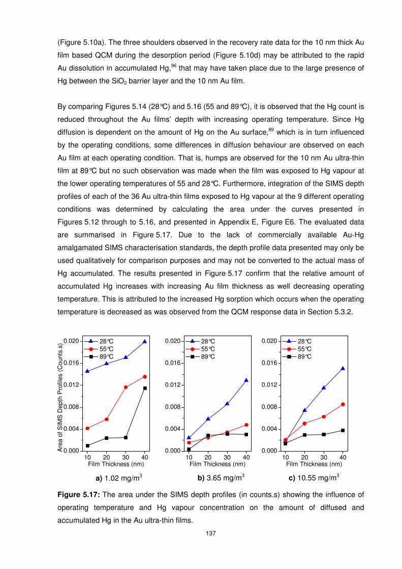
137
(Figure 5.10a). The three shoulders observed in the recovery rate data for the 10 nm thick Au
film based QCM during the desorption period (Figure 5.10d) may be attributed to the rapid
Au dissolution in accumulated Hg,96 that may have taken place due to the large presence of
Hg between the SiO2 barrier layer and the 10 nm Au film.
By comparing Figures 5.14 (28°C) and 5.16 (55 and 89°C), it is observed that the Hg count is
reduced throughout the Au films’ depth with increasing operating temperature. Since Hg
diffusion is dependent on the amount of Hg on the Au surface,89 which is in turn influenced
by the operating conditions, some differences in diffusion behaviour are observed on each
Au film at each operating condition. That is, humps are observed for the 10 nm Au ultra-thin
film at 89°C but no such observation was made when the film was exposed to Hg vapour at
the lower operating temperatures of 55 and 28°C. Furthermore, integration of the SIMS depth
profiles of each of the 36 Au ultra-thin films exposed to Hg vapour at the 9 different operating
conditions was determined by calculating the area under the curves presented in
Figures 5.12 through to 5.16, and presented in Appendix E, Figure E6. The evaluated data
are summarised in Figure 5.17. Due to the lack of commercially available Au-Hg
amalgamated SIMS characterisation standards, the depth profile data presented may only be
used qualitatively for comparison purposes and may not be converted to the actual mass of
Hg accumulated. The results presented in Figure 5.17 confirm that the relative amount of
accumulated Hg increases with increasing Au film thickness as well decreasing operating
temperature. This is attributed to the increased Hg sorption which occurs when the operating
temperature is decreased as was observed from the QCM response data in Section 5.3.2.
Figure 5.17: The area under the SIMS depth profiles (in counts.s) showing the influence of
operating temperature and Hg vapour concentration on the amount of diffused and
accumulated Hg in the Au ultra-thin films.
a) 1.02 mg/m3 b) 3.65 mg/m3 c) 10.55 mg/m3
10 20 30 400.000
0.004
0.008
0.012
0.016
0.020 28°C 55°C 89°C
Are
a of
SIM
S D
epth
Pro
files
(C
ount
s.s)
Film Thickness (nm)10 20 30 40
0.000
0.004
0.008
0.012
0.016
0.020 28°C 55°C 89°C
Film Thickness (nm)10 20 30 40
0.000
0.004
0.008
0.012
0.016
0.020 28°C 55°C 89°C
Film Thickness (nm)
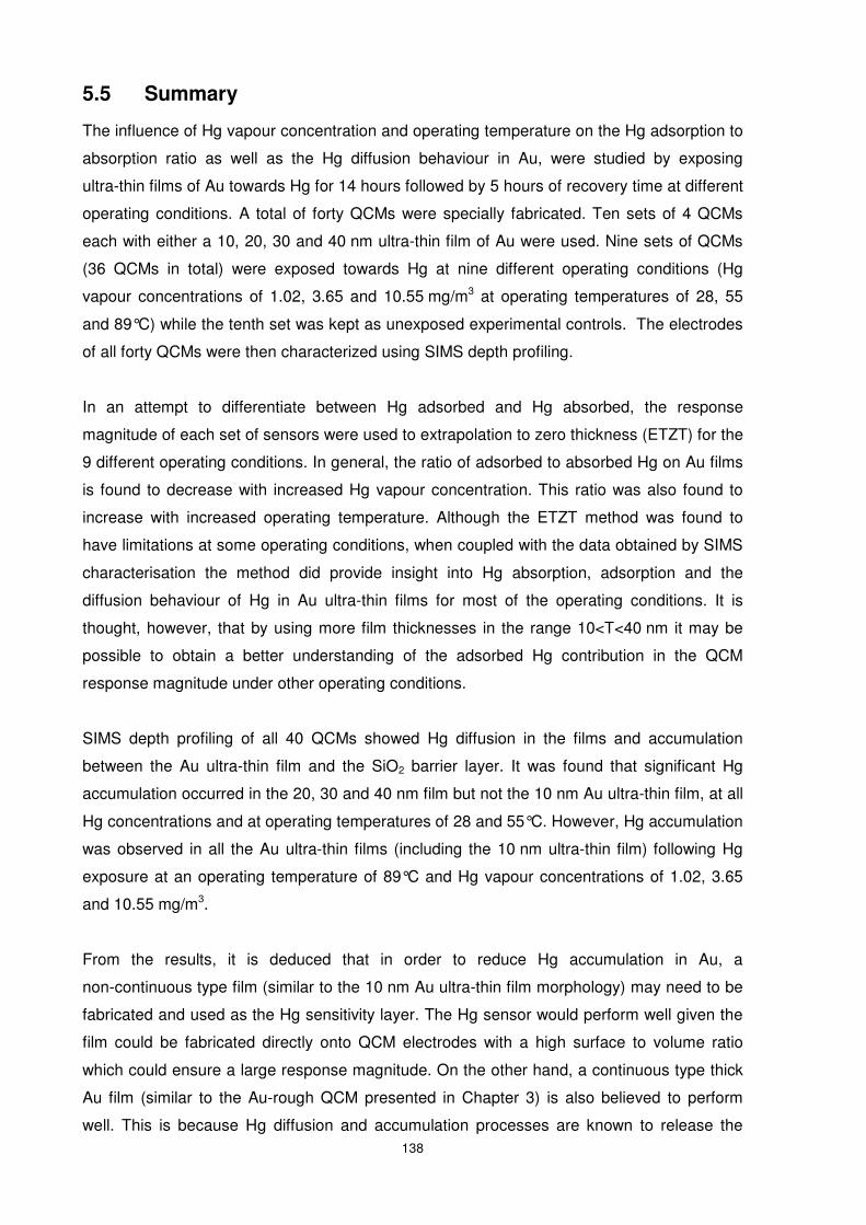
138
5.5 Summary
The influence of Hg vapour concentration and operating temperature on the Hg adsorption to
absorption ratio as well as the Hg diffusion behaviour in Au, were studied by exposing
ultra-thin films of Au towards Hg for 14 hours followed by 5 hours of recovery time at different
operating conditions. A total of forty QCMs were specially fabricated. Ten sets of 4 QCMs
each with either a 10, 20, 30 and 40 nm ultra-thin film of Au were used. Nine sets of QCMs
(36 QCMs in total) were exposed towards Hg at nine different operating conditions (Hg
vapour concentrations of 1.02, 3.65 and 10.55 mg/m3 at operating temperatures of 28, 55
and 89°C) while the tenth set was kept as unexposed experimental controls. The electrodes
of all forty QCMs were then characterized using SIMS depth profiling.
In an attempt to differentiate between Hg adsorbed and Hg absorbed, the response
magnitude of each set of sensors were used to extrapolation to zero thickness (ETZT) for the
9 different operating conditions. In general, the ratio of adsorbed to absorbed Hg on Au films
is found to decrease with increased Hg vapour concentration. This ratio was also found to
increase with increased operating temperature. Although the ETZT method was found to
have limitations at some operating conditions, when coupled with the data obtained by SIMS
characterisation the method did provide insight into Hg absorption, adsorption and the
diffusion behaviour of Hg in Au ultra-thin films for most of the operating conditions. It is
thought, however, that by using more film thicknesses in the range 10<T<40 nm it may be
possible to obtain a better understanding of the adsorbed Hg contribution in the QCM
response magnitude under other operating conditions.
SIMS depth profiling of all 40 QCMs showed Hg diffusion in the films and accumulation
between the Au ultra-thin film and the SiO2 barrier layer. It was found that significant Hg
accumulation occurred in the 20, 30 and 40 nm film but not the 10 nm Au ultra-thin film, at all
Hg concentrations and at operating temperatures of 28 and 55°C. However, Hg accumulation
was observed in all the Au ultra-thin films (including the 10 nm ultra-thin film) following Hg
exposure at an operating temperature of 89°C and Hg vapour concentrations of 1.02, 3.65
and 10.55 mg/m3.
From the results, it is deduced that in order to reduce Hg accumulation in Au, a
non-continuous type film (similar to the 10 nm Au ultra-thin film morphology) may need to be
fabricated and used as the Hg sensitivity layer. The Hg sensor would perform well given the
film could be fabricated directly onto QCM electrodes with a high surface to volume ratio
which could ensure a large response magnitude. On the other hand, a continuous type thick
Au film (similar to the Au-rough QCM presented in Chapter 3) is also believed to perform
well. This is because Hg diffusion and accumulation processes are known to release the

139
surface Hg sorption sites, therefore having little affect on the performance of QCM based Hg
vapour sensors, as was observed in Chapter 3, Section 3.4.1. The fabrication of QCM based
Hg vapour sensors with non-continuous thin film and continuous thick film electrodes are the
subjects of Chapter 6 and Chapter 7, respectively.
140
5.6 References
(1) Sabri, Y. M.; Ippolito, S. J.; Tardio, J.; Atanacio, A. J.; Sood, D. K.; Bhargava, S. K. Sensors and Actuators B: Chemical 2009, 137, 246-252.
(2) George, M. A.; Glaunsinger, W. S.; Thundat, T.; Lindsay, S. M. Journal of Microscopy 1988, 152, 703-713.
(3) George, M. A. PhD by research, Arizona State University, 1991. (4) Nowakowski, R.; Kobiela, T.; Wolfram, Z.; Dus, R. Applied Surface Science 1997, 115, 217-
231. (5) Battistoni, C.; Bemporad, E.; Galdikas, A.; Kaciulis, S.; Mattogno, G.; Mickevicius, S.;
Olevano, V. Applied Surface Science 1996, 103, 107-111. (6) Levlin, M.; Ikavalko, E.; Laitinen, T. Fresenius Journal of Analytical Chemistry 1999, 365, 577-
586. (7) George, M. A.; Glaunsinger, W. S. Thin Solid Films 1994, 245, 215-224. (8) Li, J.; Abruna, H. D. The Journal of Physical Chemistry B 1997, 101, 2907-2916. (9) Crank, J. The Mathematics of Diffusion; Oxford University Press, London, England, 1975; Vol.
2nd edition. (10) Jain, R. K. Cancer and Metastasis Reviews 1990, 9, 253-266. (11) Atkins, P. W. Physical Chemistry; 2nd ed.; Oxford University Press: Oxford, Great Britain,
1982. (12) Wei, G. C. T.; Wuensch, B. J. Journal of the American Ceramic Society 1976, 59, 295-299. (13) Haskell, R. L. B.; Caron, J. J.; Duptisea, M. A.; Ouellette, J. J.; Vetelino, J. F. In Ultrasonics
Symposium, 1999. Proceedings; IEEE: Orono, ME, 1999; Vol. 1, p 429-434 vol.1. (14) Morris, T.; Sun, J.; Szulczewski, G. Analytica Chimica Acta 2003, 496, 279-287. (15) Sauerbrey, G. Zeitschrift für Physik A Hadrons and Nuclei 1959, 155, 206-222. (16) Janshoff, A.; Galla, H.-J.; Steinem, C. Angewandte Chemie 2000, 39, 4004-4032. (17) Scheide, E. P.; Taylor, J. K. American Industrial Hygiene Association Journal 1975, 36, 897 -
901. (18) Jansen, H. J. F.; Freeman, A. J.; Weinert, M.; Wimmer, E. Physical Review B 1983, 28, 593. (19) Miedema, A. R.; Dorleijn, J. W. F. Philosophical Magazine Part B: Physics of Condensed
matter: Statistical Mechanics, Electronics, Optical and Magnetic Properties 1981, 43, 251-272. (20) Yang, X.; Tonami, K.; Nagahara, L. A.; Hashimoto, K.; Wei, Y.; Fujishima, A. Chemistry
Letters 1994, 11, 2059-2062. (21) Haskell, R. B. Masters, University of Maine, 2003. (22) Buttry, D. A.; Ward, M. D. Chem. Rev. 1992, 92, 1355-1379. (23) Zierhut, A.; Leopold, K.; Harwardt, L.; Worsfold, P.; Schuster, M. Journal of Analytical Atomic
Spectrometry 2009, 24, 767-774. (24) Levlin, M.; Niemi, H. E. M.; Hautojärvi, P.; Ikävalko, E.; Laitinen, T. Fresenius' Journal of
Analytical Chemistry 1996, 355, 2-9. (25) Yang, X. M.; Tonami, K.; Nagahara, L. A.; Hashimoto, K.; Wei, Y.; Fujishima, A. Surface
Science 1994, 319, L17-L22. (26) Jones, R. G.; Perry, D. L. Vacuum 1981, 31, 493-498. (27) Larjava, K.; Laitinen, T.; Kiviranta, T.; Siemens, V.; Klockow, D. International journal of
environmental analytical chemistry 1993, 52, 65-73. (28) Fialkowski, M.; Grzeszczak, P.; Nowakowski, R.; Holyst, R. The Journal of Physical Chemistry
B 2004, 108, 5026-5030. (29) Kobiela, T.; Nowakowski, B.; Dus, R. Applied Surface Science 2003, 206, 78-89. (30) Buffat, P.; Borel, J. P. Physical Review A 1976, 13, 2287. (31) Huang, D.; Liao, F.; Molesa, S.; Redinger, D.; Subramanian, V. Journal of the Electrochemical
Society 2003, 150, G412-G417. (32) Akita, T.; Okumura, M.; Tanaka, K.; Kohyama, M.; Haruta, M. Journal of Materials Science
2005, 40, 3101-3106. (33) Akhter, J. I.; Ahmed, E.; Ahmad, M. Materials Chemistry and Physics 2005, 93, 504-507. (34) Porter, D. A.; Easterling, K. E. Phase Transformations in Metals and Alloys; 2nd Edition ed.;
CRC Press, 1992. (35) Mehrer, H. Diffusion in Solids; 1 ed.; Springer, 2007. (36) Avallone, E. A.; Baumeister, T.; Sadegh, A.; Marks, L. S. Marks' Standard Handbook for
Mechanical Engineers; 11 ed.; McGraw-Hill Professional, 2006. (37) Hoogvliet, J. C.; van Bennekom, W. P. Electrochimica Acta 2001, 47, 599-611. (38) Caron, J.; Freeman, C. J. Surface Acoustic Wave Mercury Vapor Sensor, Sensor Research
and Development Corporation, 1998.
141
(39) Nilsson, S.; Klett, O.; Svedberg, M.; Amirkhani, A.; Nyholm, L. Rapid Communications in Mass Spectrometry 2003, 17, 1535-1540.
(40) Sanemasa, I. Bulletin of the Chemical Society of Japan 1975, 48, 1795-1798. (41) Be'er, A.; Lereah, Y.; Frydman, A.; Taitelbaum, H. Physica A: Statistical Mechanics and its
Applications 2002, 314, 325-330.

142
143
Chapter VI
Chapter 6 QCM Based Hg Vapour Sensor
Enhancement by Surface
Modification using Galvanic
Replacement Reaction
This chapter presents the result of surface modification of Ni-Au hybrid based QCMs used
to sense Hg vapour selectively in the presence of interferent gas species. The
modification step was performed using the novel idea of growing well adhered Au
nanostructures directly on the Ni electrodes by galvanic replacement reaction. More
specifically, 300 nm thin nickel films were thermally evaporated onto QCM substrates, and
subsequently reacted with AuCl4- ions in a time-dependent controlled manner.
Investigations towards the Hg-sensing capabilities of the resultant Ni-Au hybrid sensors
showed Hg desorption or sensor recovery of approximately 100% following Hg exposure.
Furthermore, the modified sensors are found to be highly selective towards Hg vapour in
the presence of NH3 and H2O interferent gases.
144
6.1 Introduction
In this chapter, the prospect of galvanic replacement (GR) reaction is investigated as a
modification technique to produce Ni-Au hybrid surfaces to enhance QCM based Hg vapour
sensor response characteristics. GR reactions are single-step reactions that utilize the
difference in the standard electrode potentials of the two metals leading to deposition of the
more noble metal (Au) and dissolution of the less noble metal (Ni).328 In chapter 3 it was
demonstrated that Au-rough morphology with high number of surface defects was an ideal
surface for optimum Hg sorption and desorption properties. In chapter 5 it was realised that
reduced Hg accumulation occurs on thin non-continuous Au films when exposed to Hg
vapour. It is postulated that such Au films having large number of surface defects and
non-continuous nature can be fabricated using GR the technique.
GR reactions operate on the basis of differences in the standard reduction potential of the
systems under investigation. Since the standard reduction potential of the Au3+/Au pair (+1.4
V vs. standard hydrogen electrode329 (SHE)) is much higher than that of the Ni2+/Ni pair (–
0.25 V vs. SHE)328, the reaction between the replacement of Ni0 with that of Au3+ ions
(Equation 6.1) is kinetically favourable.
++ +→+ 2
)(
0
)(
3
)(
0
)( 3223 aqsaqs NiAuAuNi Equation 6.1
The oxidation of solid Ni results in its dissolution in the surrounding aqueous environment as
Ni2+ ions while elemental gold (Au0) is simultaneously produced (via reduction from the
aqueous solution of AuCl4-) and deposited onto both QCM Ni electrodes. Therefore three
atoms of Ni are expected to be replaced by two atoms of Au creating surface defects which
would result in increased Hg sorption and desorption properties of the gold island
nanostructures on the Ni substrate.
In the past, GR reactions have been employed for the synthesis of highly active
hollow/porous metal alloy nanoparticles in aqueous and organic environments.330-335
However recently, GR reactions have been performed on thin films in order to create
surfaces with significantly larger surface area, surface defect sites and activity (i.e. SPR,
catalysis etc.) relative to their unreacted counterparts328,336-340. The electroless nature of
galvanic replacement reactions provides unique and significant advantage of simplicity.
For the Ni-Au system presented in this work, nickel was chosen as an ideal support metal
because of its negligible solubility in mercury (as shown in Chapter 3, Figure 3.1). In fact, the
interaction between Hg and Ni is so low that past studies have shown that Ni vessels are
good for encapsulating mercury341. The galvanic replacement of the Ni film with gold was
145
chosen to form highly active sensing material because of gold metal’s well-known highest
affinity towards Hg. By forming well adhered nano-sized Au structures on QCM electrode
surfaces using GR reaction, it is envisaged the sensor will have excellent Hg sorption and
desorption properties due to the thin, well dispersed Au nanostructures. That is, the Au ultra-
thin films presented in Chapter 5 (Section 5.4) were observed to accumulate Hg between the
Au and SiO2 barrier layer. In the case of the Au nanostructures formed on Ni electrode
surfaces, a large number of defects and therefore Hg sorption sites will be created while at
the same time hindering any unwanted Hg accumulation at the surface. It is postulated that
the nano-sized Au nanostructures would promote Hg desorption from their side edges rather
than Hg accumulation (due to their non-continuous film nature) resulting in optimised Hg
desorption properties.
6.2 Experimental Setup
The specially prepared QCM for this work were fabricated by evaporating thin titanium and
nickel layers of 10 and 300 nm thick by e-beam evaporation onto AT-cut quartz substrates.
The purpose of the Ti layer was to assist with the adhesion of the Ni layer to the substrate
surface. The 2 sided Quartz crystal microbalance with 10nm Ti adhesion layer and 300nm Ni
film on each side (0.32 cm2 total surface area) was placed in a dialysis bag (12 kDa cut-off)
containing 10 mL of deionized water (Milli-Q, Elix 3) and dialysed against 100 mL of HAuCl4
(2 x 10⁻⁴ M) under constant stirring at room temperature for various time intervals (0.5 h, 1 h,
2 h, 4 h, and 8 h). The nickel films obtained after galvanic replacement reactions were
thoroughly washed with Milli-Q water and dried under nitrogen. The confinement of nickel
thin film in the dialysis bag assisted in the controlled inward movement of Au3+ ions to react
slowly with nickel film, as well as simultaneous outward movement of leached Ni2+ ions. The
resultant Ni-Au hybrid nanostructures were characterized by using scanning electron
microscopy (SEM), X-ray diffraction (XRD), X-ray photoemission spectroscopy (XPS) and
secondary ion mass spectroscopy (SIMS) techniques. The QCMs from each time point were
then exposed to Hg vapour using the temperature profile test sequence outlined in Chapter 2
(Section 2.5.2). Selected QCMs were then exposed to Hg vapour of various concentrations
in the presence of H2O, NH3 and mixture of both H2O and NH3 at various levels.
6.3 Ni-Au hybrid Sensitive Layer Characterisations
Important information about the GR reaction can be obtained by recording the changes in the
surface features of Ni-Au system during a time-dependent GR experiment. In this section the
various surface characterization techniques used to analyze the modified surfaces using GR
reactions is presented.
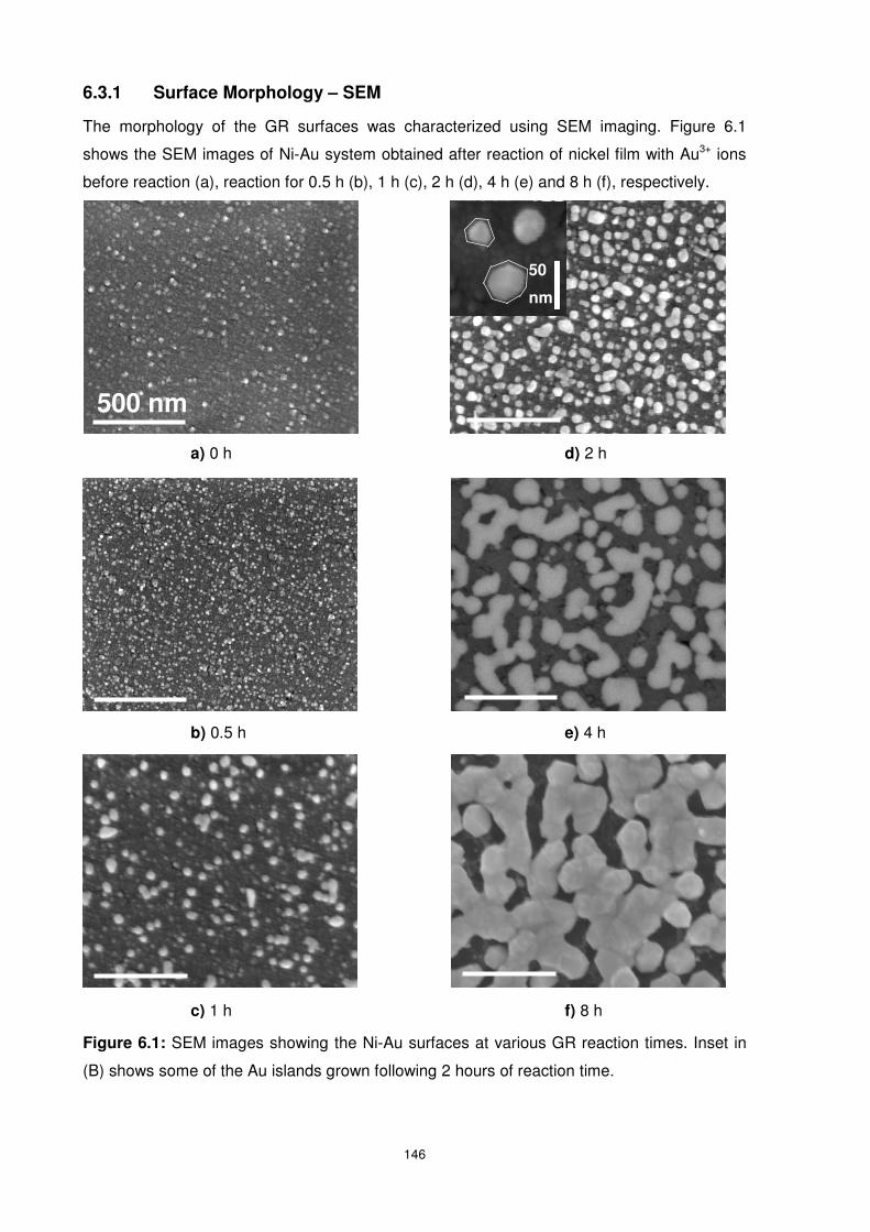
146
6.3.1 Surface Morphology – SEM
The morphology of the GR surfaces was characterized using SEM imaging. Figure 6.1
shows the SEM images of Ni-Au system obtained after reaction of nickel film with Au3+ ions
before reaction (a), reaction for 0.5 h (b), 1 h (c), 2 h (d), 4 h (e) and 8 h (f), respectively.
Figure 6.1: SEM images showing the Ni-Au surfaces at various GR reaction times. Inset in
(B) shows some of the Au islands grown following 2 hours of reaction time.
500 nm
a) 0 h
b) 0.5 h
c) 1 h
50
nm
d) 2 h
e) 4 h
f) 8 h
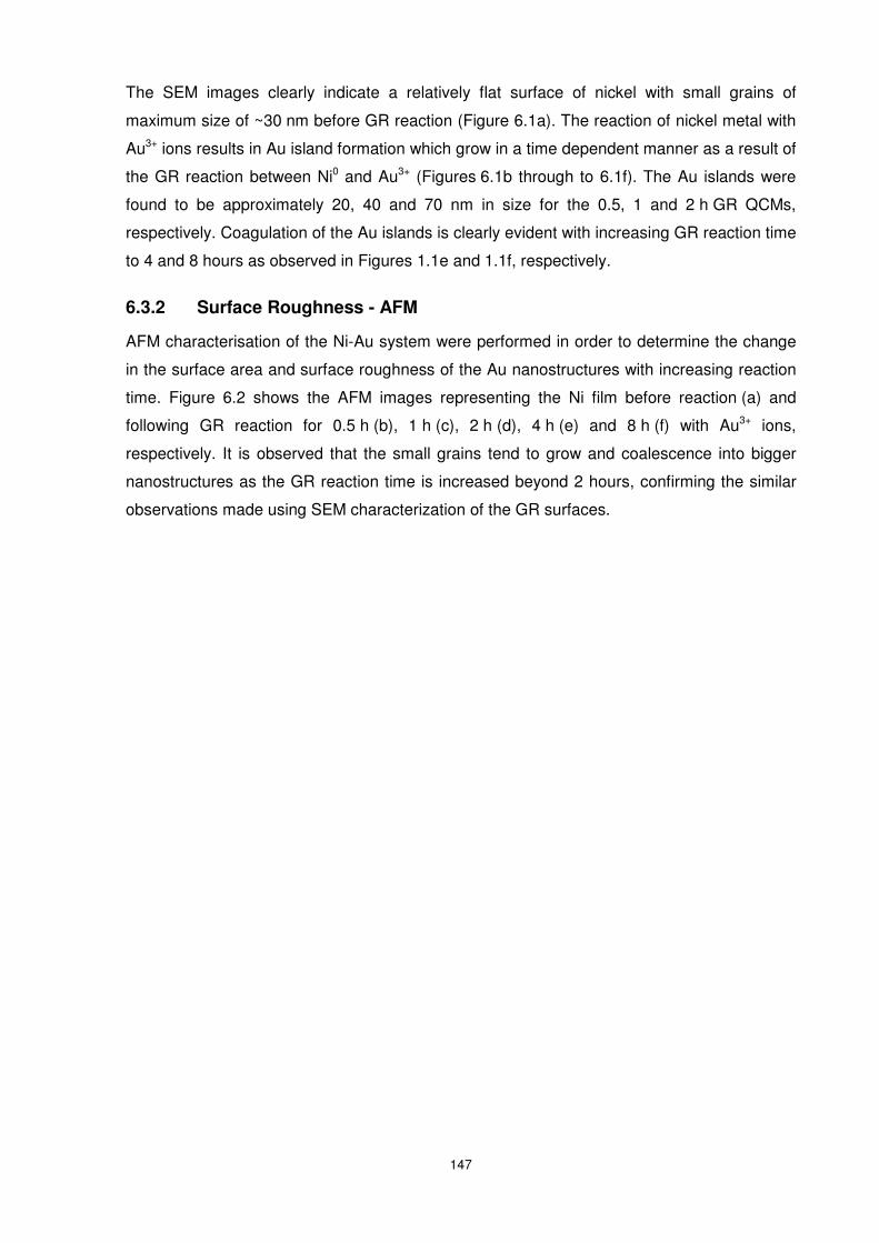
147
The SEM images clearly indicate a relatively flat surface of nickel with small grains of
maximum size of ~30 nm before GR reaction (Figure 6.1a). The reaction of nickel metal with
Au3+ ions results in Au island formation which grow in a time dependent manner as a result of
the GR reaction between Ni0 and Au3+ (Figures 6.1b through to 6.1f). The Au islands were
found to be approximately 20, 40 and 70 nm in size for the 0.5, 1 and 2 h GR QCMs,
respectively. Coagulation of the Au islands is clearly evident with increasing GR reaction time
to 4 and 8 hours as observed in Figures 1.1e and 1.1f, respectively.
6.3.2 Surface Roughness - AFM
AFM characterisation of the Ni-Au system were performed in order to determine the change
in the surface area and surface roughness of the Au nanostructures with increasing reaction
time. Figure 6.2 shows the AFM images representing the Ni film before reaction (a) and
following GR reaction for 0.5 h (b), 1 h (c), 2 h (d), 4 h (e) and 8 h (f) with Au3+ ions,
respectively. It is observed that the small grains tend to grow and coalescence into bigger
nanostructures as the GR reaction time is increased beyond 2 hours, confirming the similar
observations made using SEM characterization of the GR surfaces.
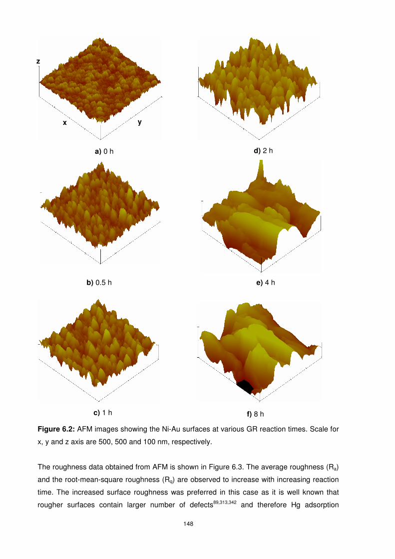
148
Figure 6.2: AFM images showing the Ni-Au surfaces at various GR reaction times. Scale for
x, y and z axis are 500, 500 and 100 nm, respectively.
The roughness data obtained from AFM is shown in Figure 6.3. The average roughness (Ra)
and the root-mean-square roughness (Rq) are observed to increase with increasing reaction
time. The increased surface roughness was preferred in this case as it is well known that
rougher surfaces contain larger number of defects89,313,342 and therefore Hg adsorption
a) 0 h
b) 0.5 h
d) 2 h
e) 4 h
c) 1 h f) 8 h
x y
z
149
sites.93,290 The actual surface area increase as compared to the scanned projected surface
area of 4 µm2 was observed to fluctuate between the reaction time points. Furthermore, the
largest increase in surface area was observed to be at the GR reaction time of 2 hours with
an increase in the projected surface area of 40.4% (within the AFM resolution limitations).
The modified films’ surface area was observed to resemble closely the projected surface
area for the higher GR reaction times (4 and 8 hour) QCMs which indicates the approach of
continuous Au film formation. The combination of large surface area and roughness is
expected to increase Hg sorption during Hg vapour sensing. Therefore the 2 hour GR QCM
is expected to have a larger response magnitude towards Hg vapour than the QCMs with
lower GR reaction times. The 4 and 8 hour GR QCMs are also expected to undergo high Hg
sorption due to their high roughness, however the total Hg sorption could be lower than the
2 h GR QCM due to their lower surface area. It is expected however that the 8 h GR QCM
undergo higher Hg sorption than the 4 h GR QCM due to its relatively higher surface area
and roughness.
Figure 6.3: Surface roughness and surface area change with respect of GR reaction time as
obtained from AFM resolution for the Ni-Au system.
6.3.3 Crystallography - XRD
XRD analysis was performed in order to determine the crystallographic orientation of the
deposited Au as well as to confirm the existence of Au-Ni alloy at the Au and Ni interface.
The Au nanostructures may be rigidly adhered on the Ni surface when alloying between the
two metals occur resulting in strong metalic bonds between the Ni atoms on the thin film and
the gold atoms in the Au nanostrucutres. Figure 6.4 below shows the XRD (with a GAADS
detector) spectra of the GR reaction samples reacted for various time points with the upper
most peak refering to pure Au substrate. Spectra from all Ni-Au system samples have been
normalised to the Ni [200] peak. It is observed that as reaction time progresses, the Au [111]
as well as the overlapped Au[200]/Ni[111] peaks increases. The inset in Figure 6.4 shows
0 1 2 3 4 5 6 7 80
10
20
30
40
50
60
Sur
face
Are
a In
crea
se (
%)
Sur
face
Rou
ghne
ss (
nm)
Reaction Time (hour)
Ra
Rq
Area
10
20
30
40
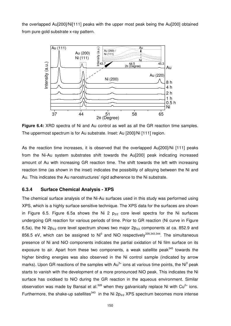
150
the overlapped Au[200]/Ni[111] peaks with the upper most peak being the Au[200] obtained
from pure gold substrate x-ray pattern.
Figure 6.4: XRD spectra of Ni and Au control as well as all the GR reaction time samples.
The uppermost spectrum is for Au substrate. Inset: Au [200]/Ni [111] region.
As the reaction time increases, it is observed that the overlapped Au[200]/Ni [111] peaks
from the Ni-Au system substrates shift towards the Au[200] peak indicating increased
amount of Au with increasing GR reaction time. The shift towards the left with increasing
reaction time (as shown in the inset) indicates the possibility of alloying between the Ni and
Au. This indicates the Au nanostructures’ rigid adherence to the Ni substrate.
6.3.4 Surface Chemical Analysis - XPS
The chemical surface analysis of the Ni-Au surfaces used in this study was performed using
XPS, which is a highly surface sensitive technique. The XPS data for the surfaces are shown
in Figure 6.5. Figure 6.5a shows the Ni 2 p3/2 core level spectra for the Ni surfaces
undergoing GR reaction for various periods of time. Prior to GR reaction (Ni curve in Figure
6.5a), the Ni 2p3/2 core level spectrum shows two major 2p3/2 components at ca. 852.9 and
856.5 eV, which can be assigned to Ni0 and NiO respectively328,343,344. The simultaneous
presence of Ni and NiO components indicates the partial oxidation of Ni film surface on its
exposure to air. Apart from these two components, a weak satellite peak345 towards the
higher binding energies was also observed in the Ni control sample (indicated by arrow
marks). Upon GR reactions of the samples with Au3+ ions at various time points, the Ni0 peak
starts to vanish with the development of a more pronounced NiO peak. This indicates the Ni
surface has oxidised to NiO during the GR reaction in the aqueous environment. Similar
observation was made by Bansal et al.328 when they galvanically replace Ni with Cu2+ ions.
Furthermore, the shake-up satellites343 in the Ni 2p3/2 XPS spectrum becomes more intense
37 44 51 58 65
Au (200) /Ni (111)
Au
Ni
2θ (Degree)Inte
nsity
(a.
u.)
Ni0.5 h1 h
Au
Au (220)Ni (200)
Au (200)Ni (111)
Inte
nsity
(a.
u.)
2θ (Degree)
Au (111)
8 h4 h2 h
43.7 44.5 45.3
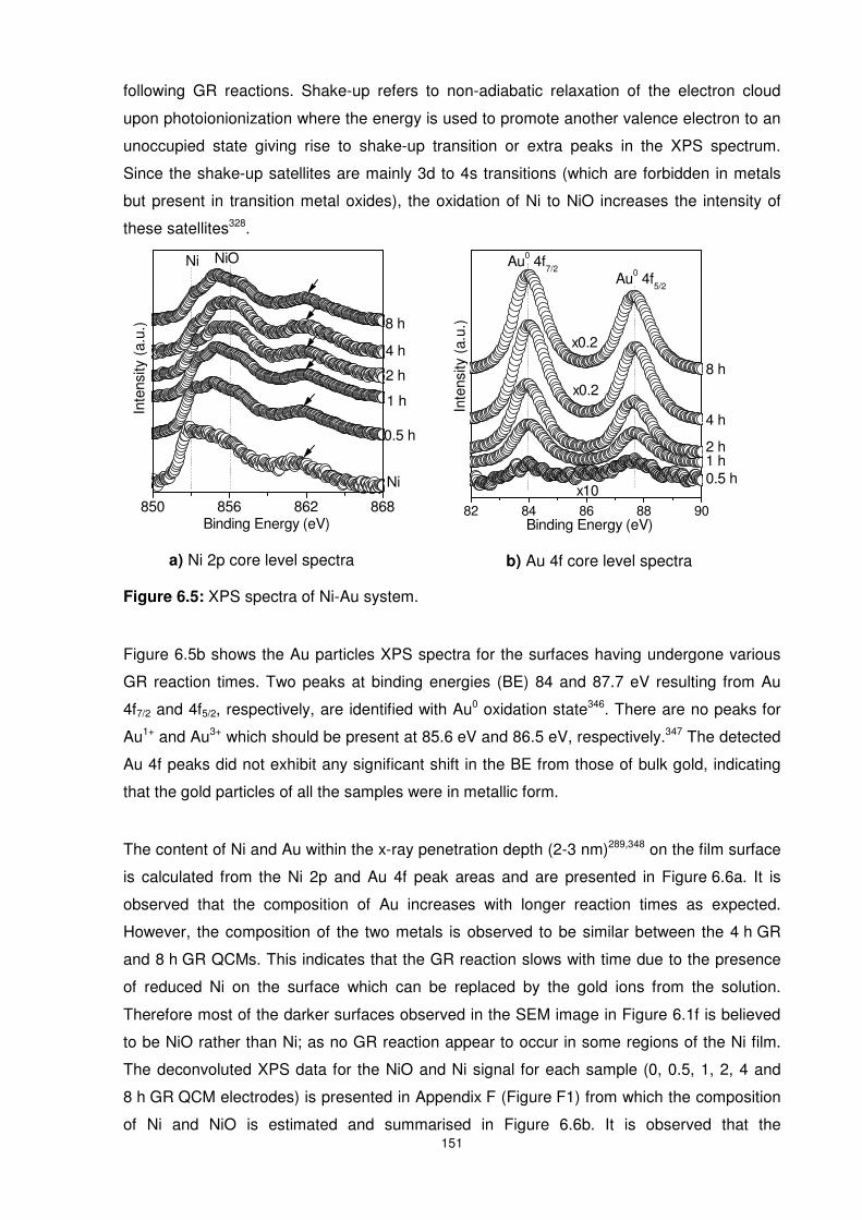
151
following GR reactions. Shake-up refers to non-adiabatic relaxation of the electron cloud
upon photoionionization where the energy is used to promote another valence electron to an
unoccupied state giving rise to shake-up transition or extra peaks in the XPS spectrum.
Since the shake-up satellites are mainly 3d to 4s transitions (which are forbidden in metals
but present in transition metal oxides), the oxidation of Ni to NiO increases the intensity of
these satellites328.
Figure 6.5: XPS spectra of Ni-Au system.
Figure 6.5b shows the Au particles XPS spectra for the surfaces having undergone various
GR reaction times. Two peaks at binding energies (BE) 84 and 87.7 eV resulting from Au
4f7/2 and 4f5/2, respectively, are identified with Au0 oxidation state346. There are no peaks for
Au1+ and Au3+ which should be present at 85.6 eV and 86.5 eV, respectively.347 The detected
Au 4f peaks did not exhibit any significant shift in the BE from those of bulk gold, indicating
that the gold particles of all the samples were in metallic form.
The content of Ni and Au within the x-ray penetration depth (2-3 nm)289,348 on the film surface
is calculated from the Ni 2p and Au 4f peak areas and are presented in Figure 6.6a. It is
observed that the composition of Au increases with longer reaction times as expected.
However, the composition of the two metals is observed to be similar between the 4 h GR
and 8 h GR QCMs. This indicates that the GR reaction slows with time due to the presence
of reduced Ni on the surface which can be replaced by the gold ions from the solution.
Therefore most of the darker surfaces observed in the SEM image in Figure 6.1f is believed
to be NiO rather than Ni; as no GR reaction appear to occur in some regions of the Ni film.
The deconvoluted XPS data for the NiO and Ni signal for each sample (0, 0.5, 1, 2, 4 and
8 h GR QCM electrodes) is presented in Appendix F (Figure F1) from which the composition
of Ni and NiO is estimated and summarised in Figure 6.6b. It is observed that the
850 856 862 868
In
tens
ity (
a.u.
)
Binding Energy (eV)
Ni NiO
8 h
4 h
2 h
1 h
0.5 h
Ni
82 84 86 88 90
x10
x0.2
x0.2
In
tens
ity (
a.u.
)
Binding Energy (eV)
Au0 4f5/2
Au0 4f7/2
8 h
4 h
2 h1 h0.5 h
a) Ni 2p core level spectra b) Au 4f core level spectra
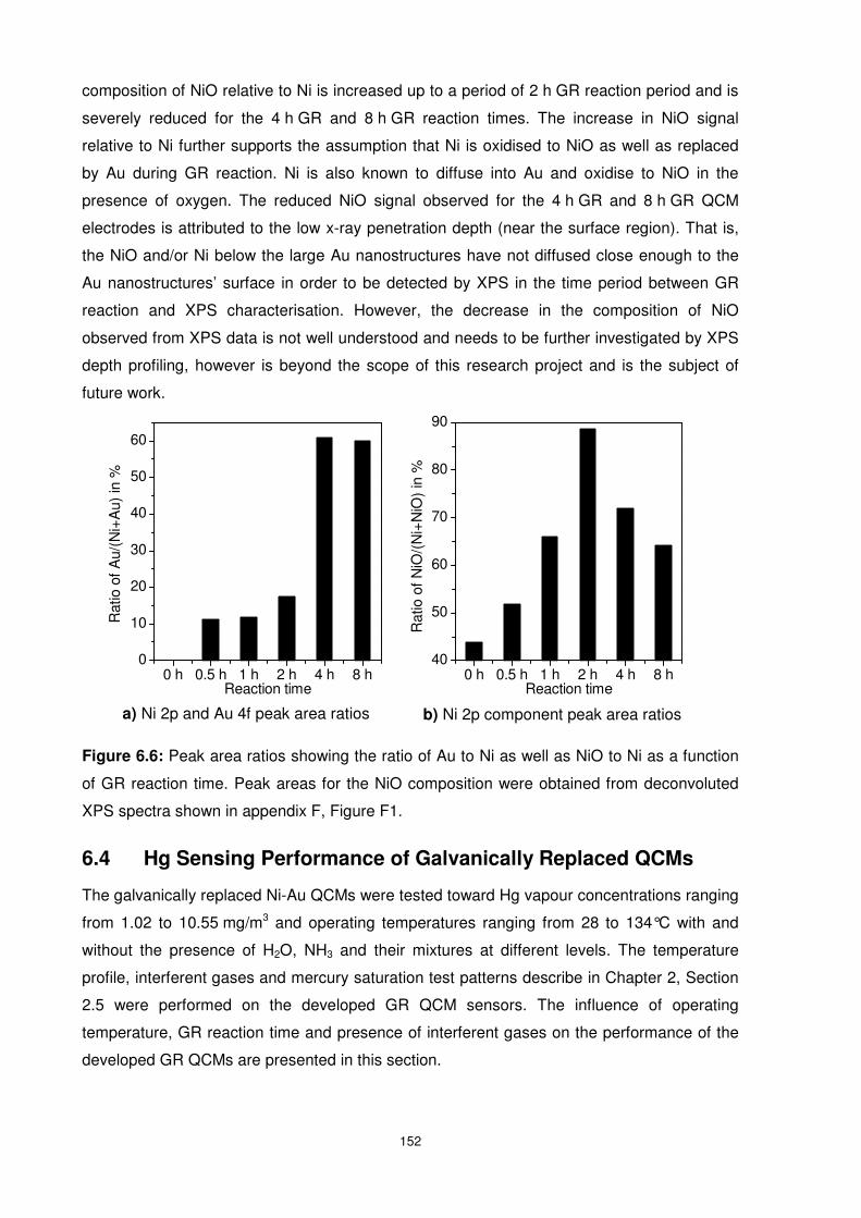
152
composition of NiO relative to Ni is increased up to a period of 2 h GR reaction period and is
severely reduced for the 4 h GR and 8 h GR reaction times. The increase in NiO signal
relative to Ni further supports the assumption that Ni is oxidised to NiO as well as replaced
by Au during GR reaction. Ni is also known to diffuse into Au and oxidise to NiO in the
presence of oxygen. The reduced NiO signal observed for the 4 h GR and 8 h GR QCM
electrodes is attributed to the low x-ray penetration depth (near the surface region). That is,
the NiO and/or Ni below the large Au nanostructures have not diffused close enough to the
Au nanostructures’ surface in order to be detected by XPS in the time period between GR
reaction and XPS characterisation. However, the decrease in the composition of NiO
observed from XPS data is not well understood and needs to be further investigated by XPS
depth profiling, however is beyond the scope of this research project and is the subject of
future work.
Figure 6.6: Peak area ratios showing the ratio of Au to Ni as well as NiO to Ni as a function
of GR reaction time. Peak areas for the NiO composition were obtained from deconvoluted
XPS spectra shown in appendix F, Figure F1.
6.4 Hg Sensing Performance of Galvanically Replaced QCMs
The galvanically replaced Ni-Au QCMs were tested toward Hg vapour concentrations ranging
from 1.02 to 10.55 mg/m3 and operating temperatures ranging from 28 to 134°C with and
without the presence of H2O, NH3 and their mixtures at different levels. The temperature
profile, interferent gases and mercury saturation test patterns describe in Chapter 2, Section
2.5 were performed on the developed GR QCM sensors. The influence of operating
temperature, GR reaction time and presence of interferent gases on the performance of the
developed GR QCMs are presented in this section.
b) Ni 2p component peak area ratios a) Ni 2p and Au 4f peak area ratios
0 h 0.5 h 1 h 2 h 4 h 8 h0
10
20
30
40
50
60
Rat
io o
f Au/
(Ni+
Au)
in %
Reaction time0 h 0.5 h 1 h 2 h 4 h 8 h
40
50
60
70
80
90R
atio
of N
iO/(
Ni+
NiO
) in
%
Reaction time
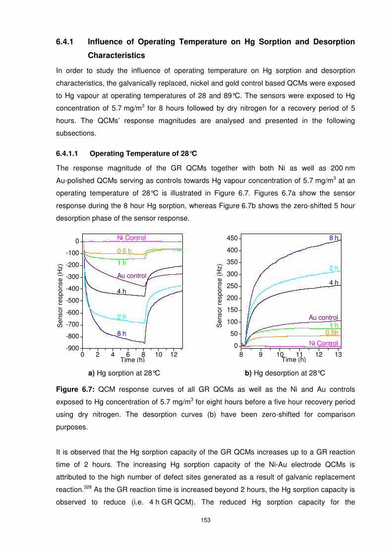
153
6.4.1 Influence of Operating Temperature on Hg Sorption and Desorption
Characteristics
In order to study the influence of operating temperature on Hg sorption and desorption
characteristics, the galvanically replaced, nickel and gold control based QCMs were exposed
to Hg vapour at operating temperatures of 28 and 89°C. The sensors were exposed to Hg
concentration of 5.7 mg/m3 for 8 hours followed by dry nitrogen for a recovery period of 5
hours. The QCMs’ response magnitudes are analysed and presented in the following
subsections.
6.4.1.1 Operating Temperature of 28°C
The response magnitude of the GR QCMs together with both Ni as well as 200 nm
Au-polished QCMs serving as controls towards Hg vapour concentration of 5.7 mg/m3 at an
operating temperature of 28°C is illustrated in Figure 6.7. Figures 6.7a show the sensor
response during the 8 hour Hg sorption, whereas Figure 6.7b shows the zero-shifted 5 hour
desorption phase of the sensor response.
Figure 6.7: QCM response curves of all GR QCMs as well as the Ni and Au controls
exposed to Hg concentration of 5.7 mg/m3 for eight hours before a five hour recovery period
using dry nitrogen. The desorption curves (b) have been zero-shifted for comparison
purposes.
It is observed that the Hg sorption capacity of the GR QCMs increases up to a GR reaction
time of 2 hours. The increasing Hg sorption capacity of the Ni-Au electrode QCMs is
attributed to the high number of defect sites generated as a result of galvanic replacement
reaction.328 As the GR reaction time is increased beyond 2 hours, the Hg sorption capacity is
observed to reduce (i.e. 4 h GR QCM). The reduced Hg sorption capacity for the
0 2 4 6 8 10 12-900
-800
-700
-600
-500
-400
-300
-200
-100
0
Ni Control
8 h
Au control
2 h
4 h
1 h
0.5 h
Sen
sor
resp
onse
(H
z)
Time (h)8 9 10 11 12 13
0
50
100
150
200
250
300
350
400
450
Sen
sor
resp
onse
(H
z)
Time (h)
Ni Control
8 h
Au control
2 h
4 h
1 h0.5h
a) Hg sorption at 28°C b) Hg desorption at 28°C
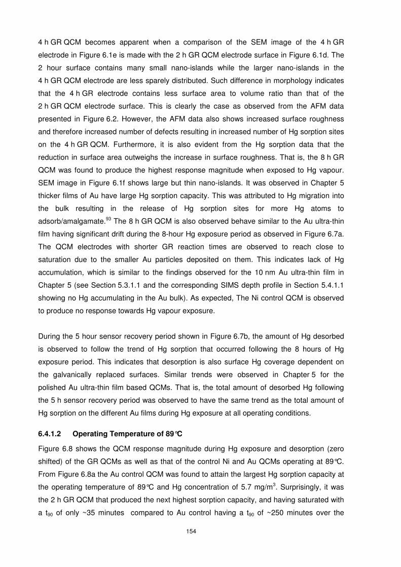
154
4 h GR QCM becomes apparent when a comparison of the SEM image of the 4 h GR
electrode in Figure 6.1e is made with the 2 h GR QCM electrode surface in Figure 6.1d. The
2 hour surface contains many small nano-islands while the larger nano-islands in the
4 h GR QCM electrode are less sparely distributed. Such difference in morphology indicates
that the 4 h GR electrode contains less surface area to volume ratio than that of the
2 h GR QCM electrode surface. This is clearly the case as observed from the AFM data
presented in Figure 6.2. However, the AFM data also shows increased surface roughness
and therefore increased number of defects resulting in increased number of Hg sorption sites
on the 4 h GR QCM. Furthermore, it is also evident from the Hg sorption data that the
reduction in surface area outweighs the increase in surface roughness. That is, the 8 h GR
QCM was found to produce the highest response magnitude when exposed to Hg vapour.
SEM image in Figure 6.1f shows large but thin nano-islands. It was observed in Chapter 5
thicker films of Au have large Hg sorption capacity. This was attributed to Hg migration into
the bulk resulting in the release of Hg sorption sites for more Hg atoms to
adsorb/amalgamate.93 The 8 h GR QCM is also observed behave similar to the Au ultra-thin
film having significant drift during the 8-hour Hg exposure period as observed in Figure 6.7a.
The QCM electrodes with shorter GR reaction times are observed to reach close to
saturation due to the smaller Au particles deposited on them. This indicates lack of Hg
accumulation, which is similar to the findings observed for the 10 nm Au ultra-thin film in
Chapter 5 (see Section 5.3.1.1 and the corresponding SIMS depth profile in Section 5.4.1.1
showing no Hg accumulating in the Au bulk). As expected, The Ni control QCM is observed
to produce no response towards Hg vapour exposure.
During the 5 hour sensor recovery period shown in Figure 6.7b, the amount of Hg desorbed
is observed to follow the trend of Hg sorption that occurred following the 8 hours of Hg
exposure period. This indicates that desorption is also surface Hg coverage dependent on
the galvanically replaced surfaces. Similar trends were observed in Chapter 5 for the
polished Au ultra-thin film based QCMs. That is, the total amount of desorbed Hg following
the 5 h sensor recovery period was observed to have the same trend as the total amount of
Hg sorption on the different Au films during Hg exposure at all operating conditions.
6.4.1.2 Operating Temperature of 89°C
Figure 6.8 shows the QCM response magnitude during Hg exposure and desorption (zero
shifted) of the GR QCMs as well as that of the control Ni and Au QCMs operating at 89°C.
From Figure 6.8a the Au control QCM was found to attain the largest Hg sorption capacity at
the operating temperature of 89°C and Hg concentration of 5.7 mg/m3. Surprisingly, it was
the 2 h GR QCM that produced the next highest sorption capacity, and having saturated with
a t90 of only ~35 minutes compared to Au control having a t90 of ~250 minutes over the
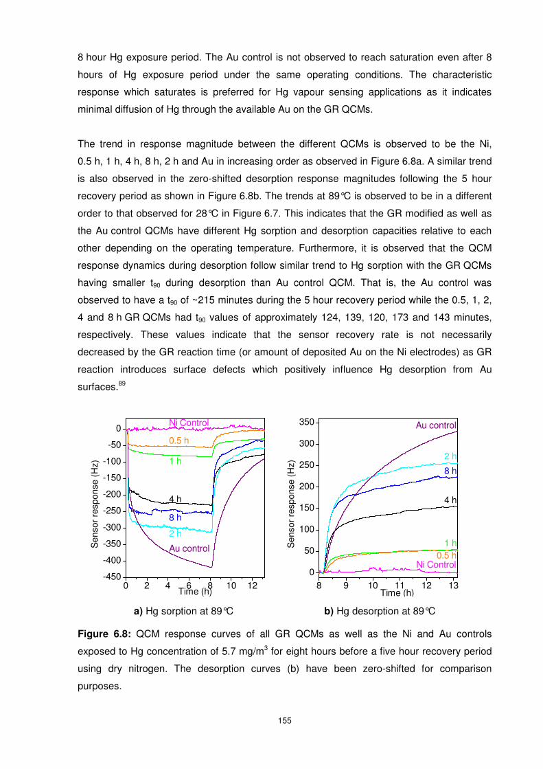
155
8 hour Hg exposure period. The Au control is not observed to reach saturation even after 8
hours of Hg exposure period under the same operating conditions. The characteristic
response which saturates is preferred for Hg vapour sensing applications as it indicates
minimal diffusion of Hg through the available Au on the GR QCMs.
The trend in response magnitude between the different QCMs is observed to be the Ni,
0.5 h, 1 h, 4 h, 8 h, 2 h and Au in increasing order as observed in Figure 6.8a. A similar trend
is also observed in the zero-shifted desorption response magnitudes following the 5 hour
recovery period as shown in Figure 6.8b. The trends at 89°C is observed to be in a different
order to that observed for 28°C in Figure 6.7. This indicates that the GR modified as well as
the Au control QCMs have different Hg sorption and desorption capacities relative to each
other depending on the operating temperature. Furthermore, it is observed that the QCM
response dynamics during desorption follow similar trend to Hg sorption with the GR QCMs
having smaller t90 during desorption than Au control QCM. That is, the Au control was
observed to have a t90 of ~215 minutes during the 5 hour recovery period while the 0.5, 1, 2,
4 and 8 h GR QCMs had t90 values of approximately 124, 139, 120, 173 and 143 minutes,
respectively. These values indicate that the sensor recovery rate is not necessarily
decreased by the GR reaction time (or amount of deposited Au on the Ni electrodes) as GR
reaction introduces surface defects which positively influence Hg desorption from Au
surfaces.89
Figure 6.8: QCM response curves of all GR QCMs as well as the Ni and Au controls
exposed to Hg concentration of 5.7 mg/m3 for eight hours before a five hour recovery period
using dry nitrogen. The desorption curves (b) have been zero-shifted for comparison
purposes.
8 9 10 11 12 130
50
100
150
200
250
300
350
Ni Control
8 h
Au control
2 h
4 h
1 h0.5 h
Sen
sor
resp
onse
(H
z)
Time (h)0 2 4 6 8 10 12
-450
-400
-350
-300
-250
-200
-150
-100
-50
0
Ni Control
8 h
Au control
2 h
4 h
1 h
0.5 h
Sen
sor
resp
onse
(H
z)
Time (h)
a) Hg sorption at 89°C b) Hg desorption at 89°C
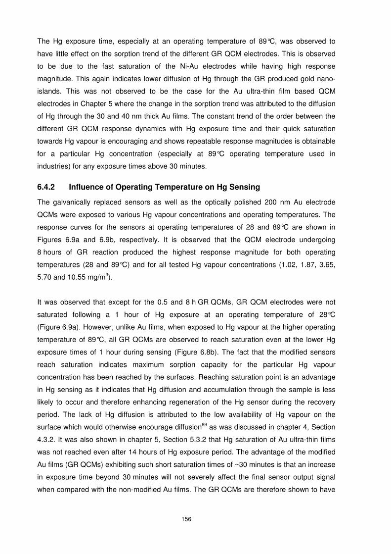
156
The Hg exposure time, especially at an operating temperature of 89°C, was observed to
have little effect on the sorption trend of the different GR QCM electrodes. This is observed
to be due to the fast saturation of the Ni-Au electrodes while having high response
magnitude. This again indicates lower diffusion of Hg through the GR produced gold nano-
islands. This was not observed to be the case for the Au ultra-thin film based QCM
electrodes in Chapter 5 where the change in the sorption trend was attributed to the diffusion
of Hg through the 30 and 40 nm thick Au films. The constant trend of the order between the
different GR QCM response dynamics with Hg exposure time and their quick saturation
towards Hg vapour is encouraging and shows repeatable response magnitudes is obtainable
for a particular Hg concentration (especially at 89°C operating temperature used in
industries) for any exposure times above 30 minutes.
6.4.2 Influence of Operating Temperature on Hg Sensing
The galvanically replaced sensors as well as the optically polished 200 nm Au electrode
QCMs were exposed to various Hg vapour concentrations and operating temperatures. The
response curves for the sensors at operating temperatures of 28 and 89°C are shown in
Figures 6.9a and 6.9b, respectively. It is observed that the QCM electrode undergoing
8 hours of GR reaction produced the highest response magnitude for both operating
temperatures (28 and 89°C) and for all tested Hg vapour concentrations (1.02, 1.87, 3.65,
5.70 and 10.55 mg/m3).
It was observed that except for the 0.5 and 8 h GR QCMs, GR QCM electrodes were not
saturated following a 1 hour of Hg exposure at an operating temperature of 28°C
(Figure 6.9a). However, unlike Au films, when exposed to Hg vapour at the higher operating
temperature of 89°C, all GR QCMs are observed to reach saturation even at the lower Hg
exposure times of 1 hour during sensing (Figure 6.8b). The fact that the modified sensors
reach saturation indicates maximum sorption capacity for the particular Hg vapour
concentration has been reached by the surfaces. Reaching saturation point is an advantage
in Hg sensing as it indicates that Hg diffusion and accumulation through the sample is less
likely to occur and therefore enhancing regeneration of the Hg sensor during the recovery
period. The lack of Hg diffusion is attributed to the low availability of Hg vapour on the
surface which would otherwise encourage diffusion89 as was discussed in chapter 4, Section
4.3.2. It was also shown in chapter 5, Section 5.3.2 that Hg saturation of Au ultra-thin films
was not reached even after 14 hours of Hg exposure period. The advantage of the modified
Au films (GR QCMs) exhibiting such short saturation times of ~30 minutes is that an increase
in exposure time beyond 30 minutes will not severely affect the final sensor output signal
when compared with the non-modified Au films. The GR QCMs are therefore shown to have
157
quick response times with high response magnitudes towards Hg vapour which makes them
ideal candidates for Hg vapour sensing applications at 89°C.
Figure 6.9: QCM response curves for the controls as well as the Ni-Au systems modified by
GR reaction and exposed to Hg at various concentrations and operating temperatures.
6.4.3 Influence of Operating Temperature on Response Time and Response
Magnitude
The response time of the Au control as well as the modified sensors was assessed by their
t90 parameters. Figure 6.10 illustrates the influence of temperature on t90 (Figure 6.10a) as
well as the response magnitude (Figure 6.10b) for Au control and the GR modified QCMs at
various operating temperatures and Hg concentration of 1.02 mg/m3.
0 120 240 360 480 600
-300
-250
-200
-150
-100
-50
03.65 mg/m31.87 mg/m3 5.70 mg/m3 10.55 mg/m31.02 mg/m3
Sen
sor
resp
onse
(H
z)
Time (min)
Ni control Au control Ni-Au 0.5 h Ni-Au 1 h Ni-Au 2 h Ni-Au 4 h Ni-Au 8 h
a) Operating temperature of 28°C
b) Operating temperature of 89°C
0 120 240 360 480 600
-600
-500
-400
-300
-200
-100
0 3.65 mg/m31.87 mg/m3 5.70 mg/m3 10.55 mg/m31.02 mg/m3
Sen
sor
resp
onse
(H
z)
Time (min)
Ni control Au control Ni-Au 0.5 h Ni-Au 1 h Ni-Au 2 h Ni-Au 4 h Ni-Au 8 h
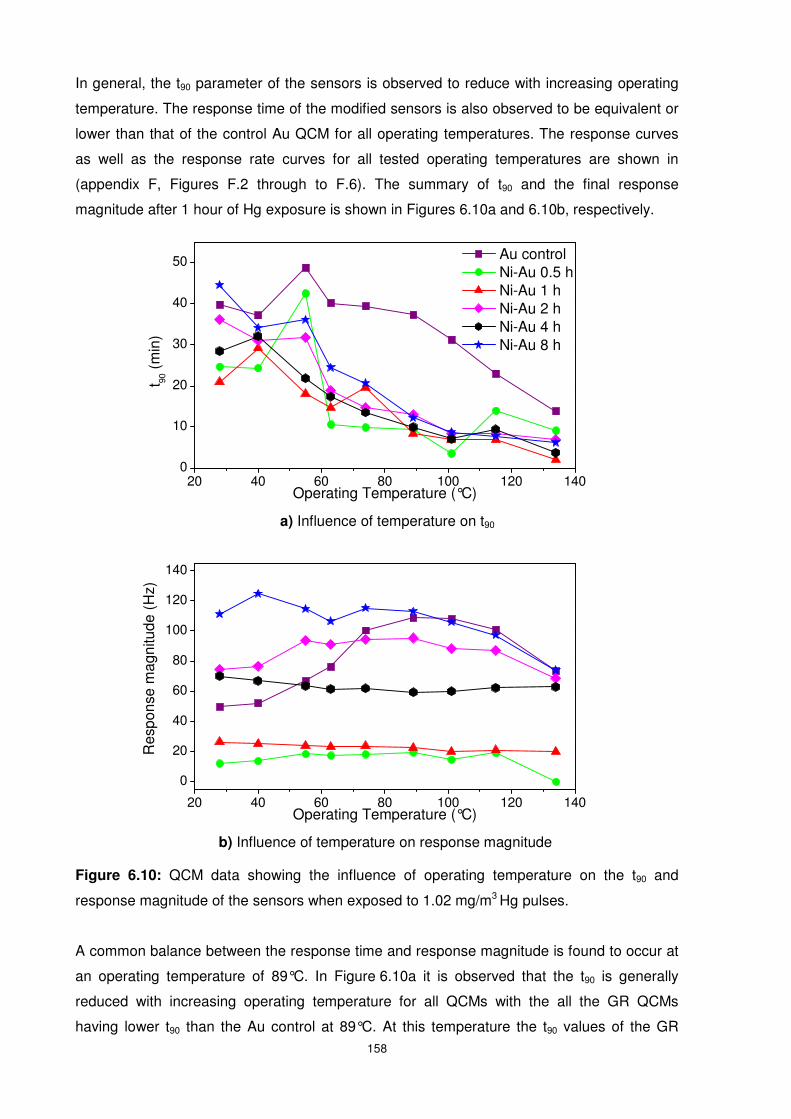
158
In general, the t90 parameter of the sensors is observed to reduce with increasing operating
temperature. The response time of the modified sensors is also observed to be equivalent or
lower than that of the control Au QCM for all operating temperatures. The response curves
as well as the response rate curves for all tested operating temperatures are shown in
(appendix F, Figures F.2 through to F.6). The summary of t90 and the final response
magnitude after 1 hour of Hg exposure is shown in Figures 6.10a and 6.10b, respectively.
Figure 6.10: QCM data showing the influence of operating temperature on the t90 and
response magnitude of the sensors when exposed to 1.02 mg/m3 Hg pulses.
A common balance between the response time and response magnitude is found to occur at
an operating temperature of 89°C. In Figure 6.10a it is observed that the t90 is generally
reduced with increasing operating temperature for all QCMs with the all the GR QCMs
having lower t90 than the Au control at 89°C. At this temperature the t90 values of the GR
20 40 60 80 100 120 140
0
20
40
60
80
100
120
140
Res
pons
e m
agni
tude
(H
z)
Operating Temperature (°C)
a) Influence of temperature on t90
b) Influence of temperature on response magnitude
20 40 60 80 100 120 1400
10
20
30
40
50 Au control Ni-Au 0.5 h Ni-Au 1 h Ni-Au 2 h Ni-Au 4 h Ni-Au 8 h
t 90 (
min
)
Operating Temperature (°C)
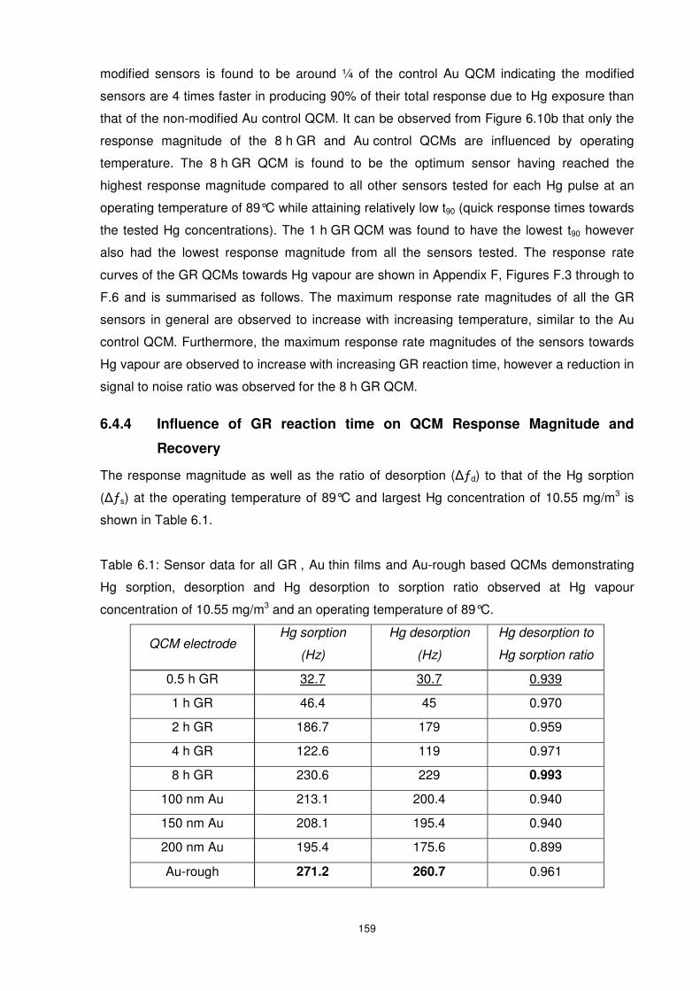
159
modified sensors is found to be around ¼ of the control Au QCM indicating the modified
sensors are 4 times faster in producing 90% of their total response due to Hg exposure than
that of the non-modified Au control QCM. It can be observed from Figure 6.10b that only the
response magnitude of the 8 h GR and Au control QCMs are influenced by operating
temperature. The 8 h GR QCM is found to be the optimum sensor having reached the
highest response magnitude compared to all other sensors tested for each Hg pulse at an
operating temperature of 89°C while attaining relatively low t90 (quick response times towards
the tested Hg concentrations). The 1 h GR QCM was found to have the lowest t90 however
also had the lowest response magnitude from all the sensors tested. The response rate
curves of the GR QCMs towards Hg vapour are shown in Appendix F, Figures F.3 through to
F.6 and is summarised as follows. The maximum response rate magnitudes of all the GR
sensors in general are observed to increase with increasing temperature, similar to the Au
control QCM. Furthermore, the maximum response rate magnitudes of the sensors towards
Hg vapour are observed to increase with increasing GR reaction time, however a reduction in
signal to noise ratio was observed for the 8 h GR QCM.
6.4.4 Influence of GR reaction time on QCM Response Magnitude and
Recovery
The response magnitude as well as the ratio of desorption (∆ƒd) to that of the Hg sorption
(∆ƒs) at the operating temperature of 89°C and largest Hg concentration of 10.55 mg/m3 is
shown in Table 6.1.
Table 6.1: Sensor data for all GR , Au thin films and Au-rough based QCMs demonstrating
Hg sorption, desorption and Hg desorption to sorption ratio observed at Hg vapour
concentration of 10.55 mg/m3 and an operating temperature of 89°C.
QCM electrode Hg sorption
(Hz)
Hg desorption
(Hz)
Hg desorption to
Hg sorption ratio
0.5 h GR 32.7 30.7 0.939
1 h GR 46.4 45 0.970
2 h GR 186.7 179 0.959
4 h GR 122.6 119 0.971
8 h GR 230.6 229 0.993
100 nm Au 213.1 200.4 0.940
150 nm Au 208.1 195.4 0.940
200 nm Au 195.4 175.6 0.899
Au-rough 271.2 260.7 0.961
160
All the tested QCMs presented in chapter 3 through to chapter 6 are shown for comparative
reasons. The maximum and minimum values for each column are indicated by a bold and
underlined font, respectively. It is observed that the 8 h GR QCM had the second highest
sorption capacity towards Hg (after the Au-rough QCM) while having the highest Hg
desorption to sorption ratio than any other QCM tested so far. The highest desorption
response magnitude observed for the Au-rough QCM is due to the high Hg sorption (or Hg
surface coverage) which occurred before the one hour recovery period. The 0.5 h GR QCM
is observed to have the lowest response magnitude and the minimum Hg desorption/Hg
sorption ratio making it inadequate as a potential Hg vapour sensor.
6.4.5 Influence of GR reaction time and Operating Temperature on QCM
Sensitivity and Limit of Detection
The sensitivity and limit of detection (LOD) of each QCM was calculated for 28 and 89°C
following the procedure described in Chapter 4, Section 4.4.4.2 in order to determine the
influence of operating temperature on these parameters of the GR sensors. A summary of
the calculated parameters is presented in Table 6.2.
Table 6.2: Calculated sensitivity and limit of detection for all GR and Au control QCMs for
operating temperature of 28 and 89°C
Detection limit
(mg/m3)
Sensitivity
[Hz/(mg/m3)] QCM electrode
28°C 89°C 28°C 89°C
200 nm Au control 0.031 0.108 28.7 38.8
0.5 h GR 0.126 0.103 2.66 5.91
1 h GR 0.058 0.138 8.69 10.2
2 h GR 0.020 0.147 25.1 39.6
4 h GR 0.022 0135 25.1 27.0
8 h GR 0.014 0.128 43.3 49.4
It is observed that the 2, 4 and 8 h GR QCMs outperform the LOD of the Au control QCM at
28°C. However, only the 0.5 h GR QCM has better LOD than the Au control QCM at 89°C
but with reduced response magnitude as was observed in Table 6.1. The sensitivity of the
GR QCM towards Hg vapour are observed to increase with increasing reaction time at 28°C,
with only the 8 h GR QCM outperforming the Au control sensor. However, when exposing Hg
at 89°C, similar trend is observed for all the GR QCMs except for the 2 h GR QCM. The 2
and 4 h GR QCMs were both observed to outperform the Au control sensor at 89°C. In
general it is observed that an increase in operating temperature increases the LOD of the
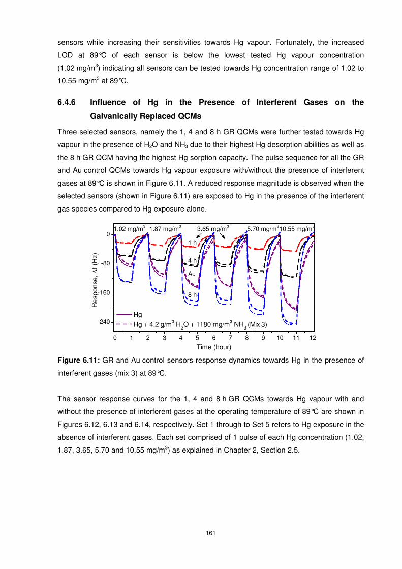
161
sensors while increasing their sensitivities towards Hg vapour. Fortunately, the increased
LOD at 89°C of each sensor is below the lowest tested Hg vapour concentration
(1.02 mg/m3) indicating all sensors can be tested towards Hg concentration range of 1.02 to
10.55 mg/m3 at 89°C.
6.4.6 Influence of Hg in the Presence of Interferent Gases on the
Galvanically Replaced QCMs
Three selected sensors, namely the 1, 4 and 8 h GR QCMs were further tested towards Hg
vapour in the presence of H2O and NH3 due to their highest Hg desorption abilities as well as
the 8 h GR QCM having the highest Hg sorption capacity. The pulse sequence for all the GR
and Au control QCMs towards Hg vapour exposure with/without the presence of interferent
gases at 89°C is shown in Figure 6.11. A reduced response magnitude is observed when the
selected sensors (shown in Figure 6.11) are exposed to Hg in the presence of the interferent
gas species compared to Hg exposure alone.
Figure 6.11: GR and Au control sensors response dynamics towards Hg in the presence of
interferent gases (mix 3) at 89°C.
The sensor response curves for the 1, 4 and 8 h GR QCMs towards Hg vapour with and
without the presence of interferent gases at the operating temperature of 89°C are shown in
Figures 6.12, 6.13 and 6.14, respectively. Set 1 through to Set 5 refers to Hg exposure in the
absence of interferent gases. Each set comprised of 1 pulse of each Hg concentration (1.02,
1.87, 3.65, 5.70 and 10.55 mg/m3) as explained in Chapter 2, Section 2.5.
0 1 2 3 4 5 6 7 8 9 10 11 12
-240
-160
-80
01 h
4 h
8 h
Hg Hg + 4.2 g/m3 H2O + 1180 mg/m3 NH3 (Mix 3)
Res
pons
e, ∆
f (H
z)
Time (hour)
Au
1.02 mg/m3 1.87 mg/m3 3.65 mg/m3 5.70 mg/m310.55 mg/m3
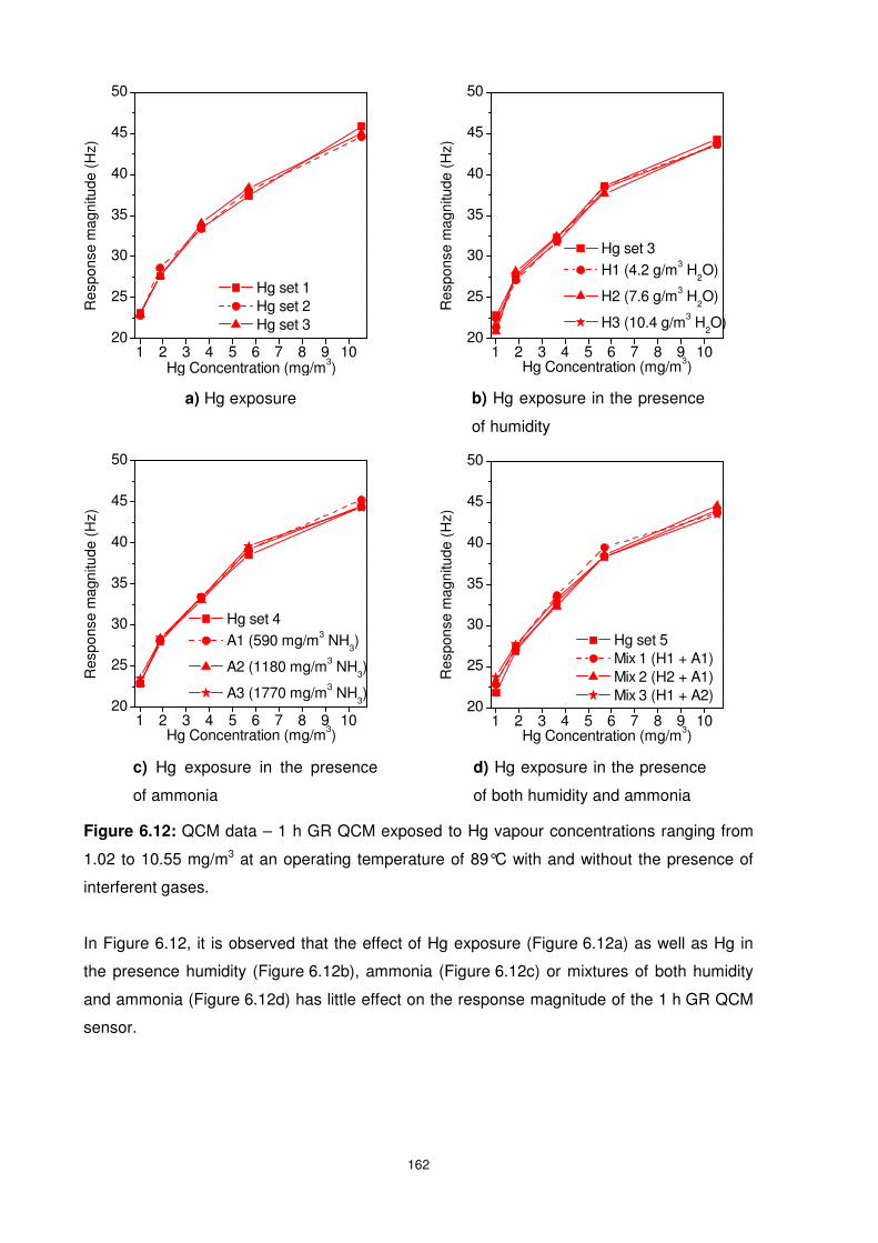
162
Figure 6.12: QCM data – 1 h GR QCM exposed to Hg vapour concentrations ranging from
1.02 to 10.55 mg/m3 at an operating temperature of 89°C with and without the presence of
interferent gases.
In Figure 6.12, it is observed that the effect of Hg exposure (Figure 6.12a) as well as Hg in
the presence humidity (Figure 6.12b), ammonia (Figure 6.12c) or mixtures of both humidity
and ammonia (Figure 6.12d) has little effect on the response magnitude of the 1 h GR QCM
sensor.
d) Hg exposure in the presence
of both humidity and ammonia
1 2 3 4 5 6 7 8 9 1020
25
30
35
40
45
50R
espo
nse
mag
nitu
de (
Hz)
Hg Concentration (mg/m3)
Hg set 1 Hg set 2 Hg set 3
a) Hg exposure
1 2 3 4 5 6 7 8 9 1020
25
30
35
40
45
50
Hg set 3 H1 (4.2 g/m3 H
2O)
H2 (7.6 g/m3 H2O)
H3 (10.4 g/m3 H2O)
Res
pons
e m
agni
tude
(H
z)
Hg Concentration (mg/m3)
1 2 3 4 5 6 7 8 9 1020
25
30
35
40
45
50
Hg set 5 Mix 1 (H1 + A1) Mix 2 (H2 + A1) Mix 3 (H1 + A2)
Res
pons
e m
agni
tude
(H
z)
Hg Concentration (mg/m3)1 2 3 4 5 6 7 8 9 10
20
25
30
35
40
45
50
Res
pons
e m
agni
tude
(H
z)
Hg Concentration (mg/m3)
Hg set 4 A1 (590 mg/m3 NH
3)
A2 (1180 mg/m3 NH3)
A3 (1770 mg/m3 NH3)
b) Hg exposure in the presence
of humidity
c) Hg exposure in the presence
of ammonia
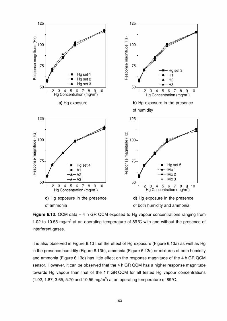
163
Figure 6.13: QCM data – 4 h GR QCM exposed to Hg vapour concentrations ranging from
1.02 to 10.55 mg/m3 at an operating temperature of 89°C with and without the presence of
interferent gases.
It is also observed in Figure 6.13 that the effect of Hg exposure (Figure 6.13a) as well as Hg
in the presence humidity (Figure 6.13b), ammonia (Figure 6.13c) or mixtures of both humidity
and ammonia (Figure 6.13d) has little effect on the response magnitude of the 4 h GR QCM
sensor. However, it can be observed that the 4 h GR QCM has a higher response magnitude
towards Hg vapour than that of the 1 h GR QCM for all tested Hg vapour concentrations
(1.02, 1.87, 3.65, 5.70 and 10.55 mg/m3) at an operating temperature of 89°C.
1 2 3 4 5 6 7 8 9 1050
75
100
125
Hg set 5 Mix 1 Mix 2 Mix 3
Res
pons
e m
agni
tude
(H
z)
Hg Concentration (mg/m3)1 2 3 4 5 6 7 8 9 10
50
75
100
125
Res
pons
e m
agni
tude
(H
z)
Hg Concentration (mg/m3)
Hg set 4 A1 A2 A3
d) Hg exposure in the presence
of both humidity and ammonia
a) Hg exposure b) Hg exposure in the presence
of humidity
c) Hg exposure in the presence
of ammonia
1 2 3 4 5 6 7 8 9 1050
75
100
125
Res
pons
e m
agni
tude
(H
z)
Hg Concentration (mg/m3)
Hg set 1 Hg set 2 Hg set 3
1 2 3 4 5 6 7 8 9 1050
75
100
125
Hg set 3 H1 H2 H3
Res
pons
e m
agni
tude
(H
z)
Hg Concentration (mg/m3)
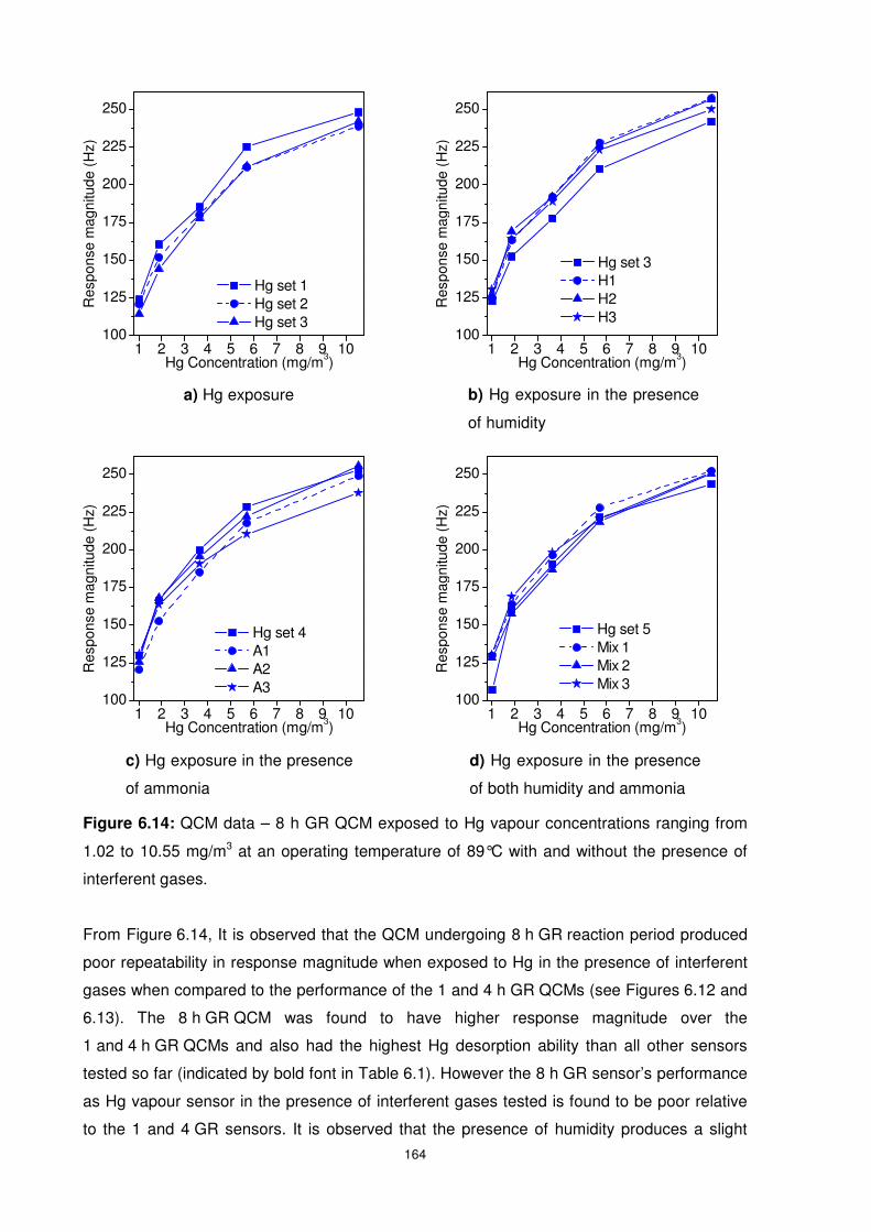
164
Figure 6.14: QCM data – 8 h GR QCM exposed to Hg vapour concentrations ranging from
1.02 to 10.55 mg/m3 at an operating temperature of 89°C with and without the presence of
interferent gases.
From Figure 6.14, It is observed that the QCM undergoing 8 h GR reaction period produced
poor repeatability in response magnitude when exposed to Hg in the presence of interferent
gases when compared to the performance of the 1 and 4 h GR QCMs (see Figures 6.12 and
6.13). The 8 h GR QCM was found to have higher response magnitude over the
1 and 4 h GR QCMs and also had the highest Hg desorption ability than all other sensors
tested so far (indicated by bold font in Table 6.1). However the 8 h GR sensor’s performance
as Hg vapour sensor in the presence of interferent gases tested is found to be poor relative
to the 1 and 4 GR sensors. It is observed that the presence of humidity produces a slight
1 2 3 4 5 6 7 8 9 10100
125
150
175
200
225
250
Res
pons
e m
agni
tude
(H
z)
Hg Concentration (mg/m3)
Hg set 5 Mix 1 Mix 2 Mix 3
1 2 3 4 5 6 7 8 9 10100
125
150
175
200
225
250
Res
pons
e m
agni
tude
(H
z)
Hg Concentration (mg/m3)
Hg set 4 A1 A2 A3
d) Hg exposure in the presence
of both humidity and ammonia
a) Hg exposure b) Hg exposure in the presence
of humidity
c) Hg exposure in the presence
of ammonia
1 2 3 4 5 6 7 8 9 10100
125
150
175
200
225
250R
espo
nse
mag
nitu
de (
Hz)
Hg Concentration (mg/m3)
Hg set 1 Hg set 2 Hg set 3
1 2 3 4 5 6 7 8 9 10100
125
150
175
200
225
250
Res
pons
e m
agni
tude
(H
z)
Hg Concentration (mg/m3)
Hg set 3 H1 H2 H3
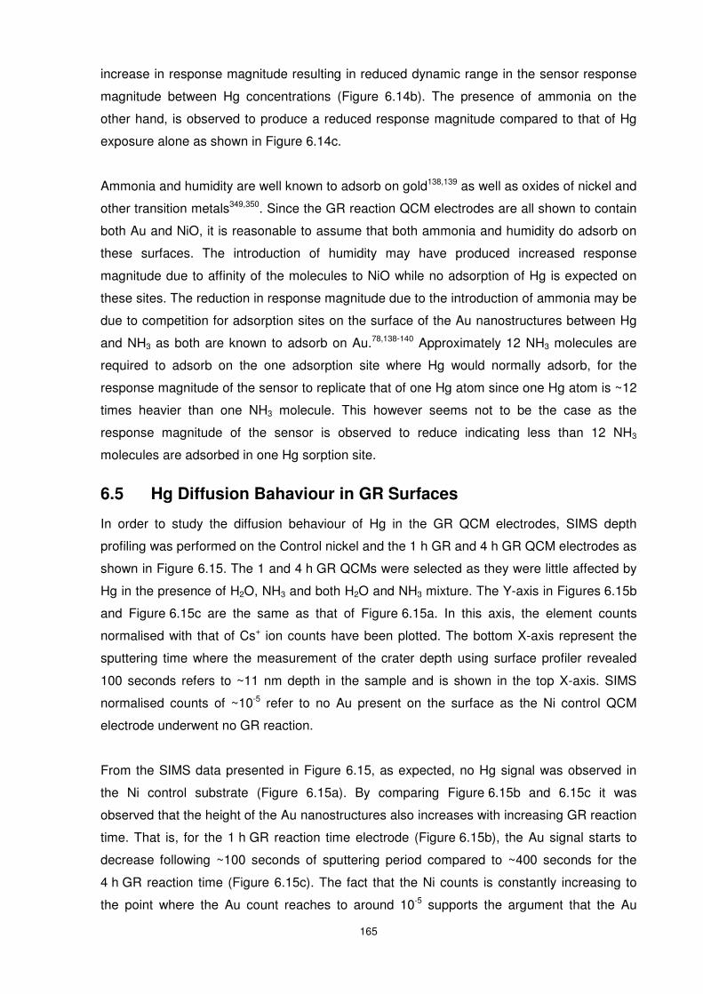
165
increase in response magnitude resulting in reduced dynamic range in the sensor response
magnitude between Hg concentrations (Figure 6.14b). The presence of ammonia on the
other hand, is observed to produce a reduced response magnitude compared to that of Hg
exposure alone as shown in Figure 6.14c.
Ammonia and humidity are well known to adsorb on gold138,139 as well as oxides of nickel and
other transition metals349,350. Since the GR reaction QCM electrodes are all shown to contain
both Au and NiO, it is reasonable to assume that both ammonia and humidity do adsorb on
these surfaces. The introduction of humidity may have produced increased response
magnitude due to affinity of the molecules to NiO while no adsorption of Hg is expected on
these sites. The reduction in response magnitude due to the introduction of ammonia may be
due to competition for adsorption sites on the surface of the Au nanostructures between Hg
and NH3 as both are known to adsorb on Au.78,138-140 Approximately 12 NH3 molecules are
required to adsorb on the one adsorption site where Hg would normally adsorb, for the
response magnitude of the sensor to replicate that of one Hg atom since one Hg atom is ~12
times heavier than one NH3 molecule. This however seems not to be the case as the
response magnitude of the sensor is observed to reduce indicating less than 12 NH3
molecules are adsorbed in one Hg sorption site.
6.5 Hg Diffusion Bahaviour in GR Surfaces
In order to study the diffusion behaviour of Hg in the GR QCM electrodes, SIMS depth
profiling was performed on the Control nickel and the 1 h GR and 4 h GR QCM electrodes as
shown in Figure 6.15. The 1 and 4 h GR QCMs were selected as they were little affected by
Hg in the presence of H2O, NH3 and both H2O and NH3 mixture. The Y-axis in Figures 6.15b
and Figure 6.15c are the same as that of Figure 6.15a. In this axis, the element counts
normalised with that of Cs+ ion counts have been plotted. The bottom X-axis represent the
sputtering time where the measurement of the crater depth using surface profiler revealed
100 seconds refers to ~11 nm depth in the sample and is shown in the top X-axis. SIMS
normalised counts of ~10-5 refer to no Au present on the surface as the Ni control QCM
electrode underwent no GR reaction.
From the SIMS data presented in Figure 6.15, as expected, no Hg signal was observed in
the Ni control substrate (Figure 6.15a). By comparing Figure 6.15b and 6.15c it was
observed that the height of the Au nanostructures also increases with increasing GR reaction
time. That is, for the 1 h GR reaction time electrode (Figure 6.15b), the Au signal starts to
decrease following ~100 seconds of sputtering period compared to ~400 seconds for the
4 h GR reaction time (Figure 6.15c). The fact that the Ni counts is constantly increasing to
the point where the Au count reaches to around 10-5 supports the argument that the Au
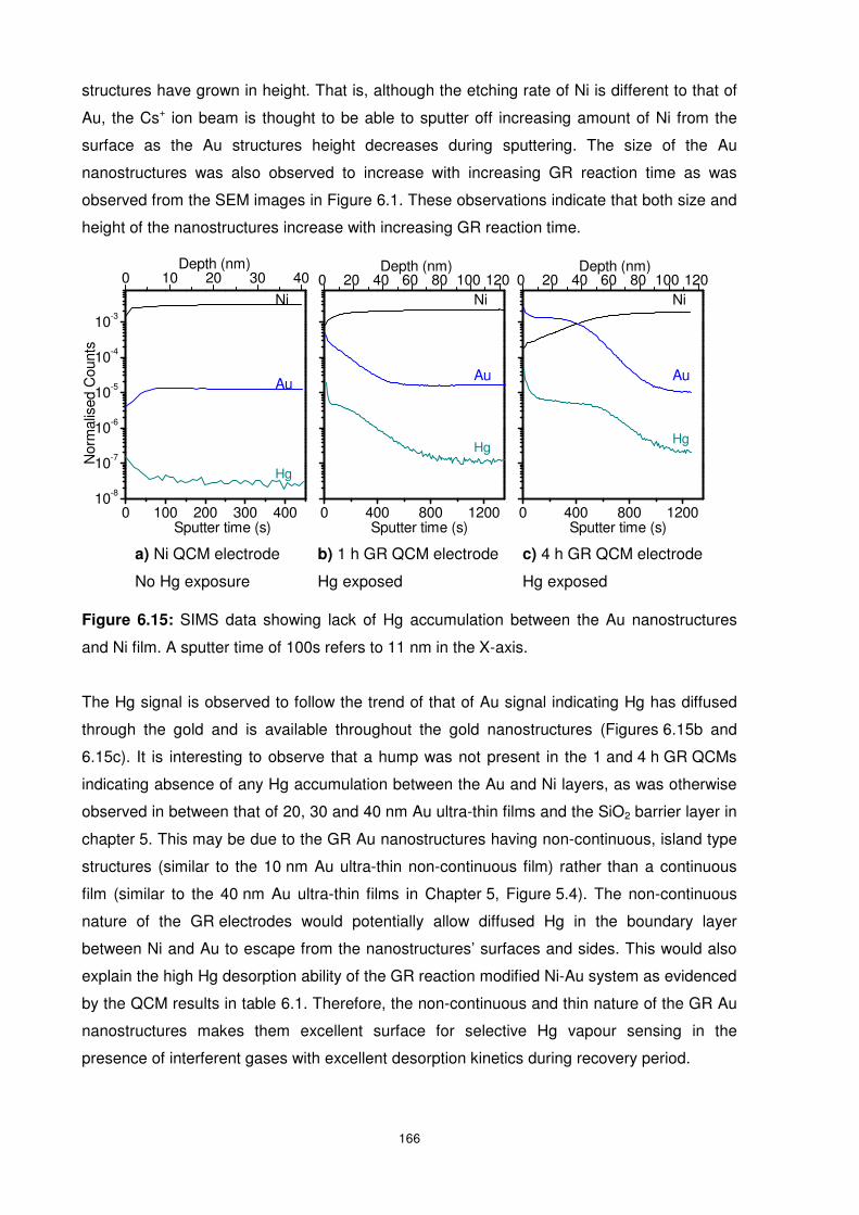
166
structures have grown in height. That is, although the etching rate of Ni is different to that of
Au, the Cs+ ion beam is thought to be able to sputter off increasing amount of Ni from the
surface as the Au structures height decreases during sputtering. The size of the Au
nanostructures was also observed to increase with increasing GR reaction time as was
observed from the SEM images in Figure 6.1. These observations indicate that both size and
height of the nanostructures increase with increasing GR reaction time.
Figure 6.15: SIMS data showing lack of Hg accumulation between the Au nanostructures
and Ni film. A sputter time of 100s refers to 11 nm in the X-axis.
The Hg signal is observed to follow the trend of that of Au signal indicating Hg has diffused
through the gold and is available throughout the gold nanostructures (Figures 6.15b and
6.15c). It is interesting to observe that a hump was not present in the 1 and 4 h GR QCMs
indicating absence of any Hg accumulation between the Au and Ni layers, as was otherwise
observed in between that of 20, 30 and 40 nm Au ultra-thin films and the SiO2 barrier layer in
chapter 5. This may be due to the GR Au nanostructures having non-continuous, island type
structures (similar to the 10 nm Au ultra-thin non-continuous film) rather than a continuous
film (similar to the 40 nm Au ultra-thin films in Chapter 5, Figure 5.4). The non-continuous
nature of the GR electrodes would potentially allow diffused Hg in the boundary layer
between Ni and Au to escape from the nanostructures’ surfaces and sides. This would also
explain the high Hg desorption ability of the GR reaction modified Ni-Au system as evidenced
by the QCM results in table 6.1. Therefore, the non-continuous and thin nature of the GR Au
nanostructures makes them excellent surface for selective Hg vapour sensing in the
presence of interferent gases with excellent desorption kinetics during recovery period.
a) Ni QCM electrode
No Hg exposure
b) 1 h GR QCM electrode
Hg exposed
c) 4 h GR QCM electrode
Hg exposed
0 100 200 300 40010-8
10-7
10-6
10-5
10-4
10-3
Hg
Au
Nor
mal
ised
Cou
nts
Sputter time (s)
Ni
0 10 20 30 40Depth (nm)
0 400 800 1200
Depth (nm)
Sputter time (s)
Hg
Au
Ni0 20 40 60 80 100 120
0 400 800 1200
Depth (nm)
Sputter time (s)
Hg
Au
Ni0 20 40 60 80 100 120
167
6.6 Summary
It is shown for the first time that the novel choice of Ni-Au hybrid nano-structures can be
grown directly on QCM substrates for Hg vapour sensing applications using galvanic
replacement reactions. The Ni-Au system was chosen based on the fact Ni has a low affinity
towards Hg vapour as opposed to Au which is known to readily undergo Hg sorption. This
approach was used to create nanostructures containing large number of surface defects (i.e.
Hg sorption sites). The thin and non-continuous nature of developed Au nanostructures was
thought to lead to quicker response, large response magnitude and recovery as well as
reduced Hg diffusion than thicker continuous films of Au alone. This approach was found to
fulfil its purpose where higher Hg sorption and therefore sensor response magnitudes were
observed when compared to the Au control QCM. Furthermore, upon the recovery phase,
the GR QCMs were observed to exhibit between 93 to 100% desorption of the adsorbed
amalgamated Hg compared to the Au control QCM where less than 90% regeneration was
observed. The QCM sensor electrodes modified using GR reaction times of 1 h and 4 h
showed small response magnitudes or sorption capacity towards Hg vapour but interestingly
showed to be little affected by interferent gases (H2O and NH3). The QCM electrode
undergoing 8 h GR reaction showed high response magnitude, sorption and desorption
capacity, however was found to be affected by the presence of the interferent gases much
the same as a continuous film of Au (which will be presented in Chapter 7). This indicated
that the GR reaction period, otherwise the amount of Au deposited on Ni surface, influences
the QCM based Hg vapour sensor’s performance towards the interferent gases. SIMS data
showed no accumulation of Hg at the Ni-Au boundary of these modified sensors as was
otherwise the case for the evaporated thin Au films presented in chapter 5. This is thought to
be the reason for the sensors high Hg desorption and lower drift during Hg sensing. The 1
and 4 h GR sensors developed in this work have great potential to be used as online Hg
vapour sensors in the presence of interferent gases such as H2O and NH3, thus making them
highly relevant to some industrial applications.
168
6.7 References
(1) Bansal, V.; Jani, H.; Plessis, J. D.; Coloe, P. J.; Bhargava, S. K. Adv. Mater. 2008, 20, 717-723.
(2) Bond, G. C. Catalysis Today 2002, 72, 5-9. (3) Sun, Y.; Mayers, B. T.; Xia, Y. Nano Lett. 2002, 2, 481-485. (4) Sun, Y.; Xia, Y. Journal of the American Chemical Society 2004, 126, 3892-3901. (5) Liang, H. P.; Guo, Y. G.; Zhang, H. M.; Hu, J. S.; Wan, L. J.; Bai, C. L. Chem. Commun. 2004,
1496-1497. (6) Liang, H.-P.; Wan, L.-J.; Bai, C.-L.; Jiang, L. The Journal of Physical Chemistry B 2005, 109,
7795-7800. (7) Shukla, S.; Priscilla, A.; Banerjee, M.; Bhonde, R. R.; Ghatak, J.; Satyam, P. V.; Sastry, M.
Chem. Mat. 2005, 17, 5000-5005. (8) Selvakannan, P. R.; Sastry, M. Chem. Commun. 2005, 1684-1686. (9) Viyannalage, L. T.; Vasilic, R.; Dimitrov, N. J. Phys. Chem. C 2007, 111, 4036-4041. (10) Vasilic, R.; Dimitrov, N. Electrochemical and Solid-State Letters 2005, 8, C173-C176. (11) Vasilic, R.; Viyannalage, L. T.; Dimitrov, N. Journal of the Electrochemical Society 2006, 153,
C648-C655. (12) Brankovic, S. R.; Wang, J. X.; Adzic, R. R. Surface Science 2001, 474, L173-L179. (13) Mrozek, M. F.; Xie, Y.; Weaver, M. J. Analytical Chemistry 2001, 73, 5953-5960. (14) Lipi´nski, L.; Szmyrka-Grzebyk, A.; Manuszkiewicz, H. Measurement Science and Technology
2000, 11, 738-742. (15) Sabri, Y. M.; Ippolito, S. J.; Tardio, J.; Atanacio, A. J.; Sood, D. K.; Bhargava, S. K. Sensors
and Actuators B: Chemical 2009, 137, 246-252. (16) Cherstiouk, O.; Gavrilov, A.; Plyasova, L.; Molina, I.; Tsirlina, G.; Savinova, E. Journal of Solid
State Electrochemistry 2008, 12, 497-509. (17) Green, T. A. Gold Bulletin 2007, 40, 105-114. (18) Inukai, J.; Sugita, S.; Itaya, K. Journal of Electroanalytical Chemistry 1996, 403, 159-168. (19) George, M. A.; Glaunsinger, W. S. Thin Solid Films 1994, 245, 215-224. (20) Fiermans, L.; Hoogewijs, R.; Vennik, J. Surface Science 1975, 47, 1-40. (21) Haseeb, A. S. M. A.; Chakraborty, P.; Ahmed, I.; Caccavale, F.; Bertoncello, R. Thin Solid
Films 1996, 283, 140-144. (22) Aravinda, C. L.; Mayanna, S. M.; Bera, P.; Jayaram, V.; Sharma, A. K. Journal of Materials
Science Letters 2002, 21, 205-208. (23) Jiang, P.; Zhou, J.-J.; Li, R.; Gao, Y.; Sun, T.-L.; Zhao, X.-W.; Xiang, Y.-J. Journal of
Nanoparticle Research 2006, 8, 927-934. (24) Qian, L.; Ming, M.; Yuqing, Z. H. A. Chinese Journal of Catalysis 2006, 27, 1111-1116. (25) George, M. A.; Glaunsinger, W. S.; Thundat, T.; Lindsay, S. M. Journal of Microscopy 1988,
152, 703-713. (26) Jin, Y.; Dong, S. The Journal of Physical Chemistry B 2003, 107, 12902-12905. (27) Bilic, A.; Reimers, J. R.; Hush, N. S.; Hafner, J. The Journal of Chemical Physics 2002, 116,
8981-8987. (28) Kay, B. D.; Lykke, K. R.; Creighton, J. R.; Ward, S. J. The Journal of Chemical Physics 1989,
91, 5120-5121. (29) Cain, S. R.; Matienzo, L. J.; Emmi, F. The Journal of Physical Chemistry 2002, 94, 4985-4990. (30) Fox, C. G.; Alder, J. F. Analyst 1989, 114, 997-1004. (31) Surplice, N. A.; Brearley, W. Surface Science 1975, 52, 62-74. (32) Levlin, M.; Ikavalko, E.; Laitinen, T. Fresenius Journal of Analytical Chemistry 1999, 365, 577-
586.
169
Chapter VII
Chapter 7 QCM Based Hg Vapour Sensor
Enhancement by Surface
Modification using Gold
Electrodeposition
In this chapter the novel idea of growing well adhered Au nanospikes on QCM electrodes
by electrodeposition is presented. Two nanospike QCMs were tested towards Hg vapour
in the presence of various interferent gases. The high response magnitude of the
nanospike QCM sensor towards Hg vapour was found to be not just to the increased
surface area alone but is also due to their rich (111) crystallographic orientation and the
presence of nodules and other surface defects that act as Hg sorption sites. The
nanospike QCM was also found to be selective towards Hg vapour in the presence of
interferent gases (humidity and ammonia) and had much higher sensitivity and lower
detection limits compared to that of an Au control QCM. The nanospike QCM was further
tested for its long term, 50 day stability towards Hg in the presence humidity and
ammonia. The long term testing was designed to simulate some of the industrial
conditions. The developed nanospike based Hg vapour sensor was found to have
enhanced sensitivity and selectivity towards Hg vapour in the presence of the interferent
gases tested over the 50 day testing period. Moreover, a separate nanospike sensor was
tested in a specially designed industrial chamber towards Hg vapour in the presence of
additional interferent gases including VOCs that are known to have high affinity with Au. It
was found that the nanospike QCMs maintained their selectivity towards Hg vapour. As a
result, the technique to fabricate nanospike based QCMs was patented and the nanospike
QCM was set aside for future onsite testing at the industry partners refineries.
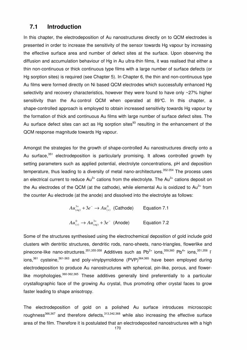
170
7.1 Introduction
In this chapter, the electrodeposition of Au nanostructures directly on to QCM electrodes is
presented in order to increase the sensitivity of the sensor towards Hg vapour by increasing
the effective surface area and number of defect sites at the surface. Upon observing the
diffusion and accumulation behaviour of Hg in Au ultra-thin films, it was realised that either a
thin non-continuous or thick continuous type films with a large number of surface defects (or
Hg sorption sites) is required (see Chapter 5). In Chapter 6, the thin and non-continuous type
Au films were formed directly on Ni based QCM electrodes which successfully enhanced Hg
selectivity and recovery characteristics, however they were found to have only ~27% higher
sensitivity than the Au control QCM when operated at 89°C. In this chapter, a
shape-controlled approach is employed to obtain increased sensitivity towards Hg vapour by
the formation of thick and continuous Au films with large number of surface defect sites. The
Au surface defect sites can act as Hg sorption sites93 resulting in the enhancement of the
QCM response magnitude towards Hg vapour.
Amongst the strategies for the growth of shape-controlled Au nanostructures directly onto a
Au surface,351 electrodeposition is particularly promising. It allows controlled growth by
setting parameters such as applied potential, electrolyte concentrations, pH and deposition
temperature, thus leading to a diversity of metal nano-architectures.352-354 The process uses
an electrical current to reduce Au3+ cations from the electrolyte. The Au3+ cations deposit on
the Au electrodes of the QCM (at the cathode), while elemental Au is oxidized to Au3+ from
the counter Au electrode (at the anode) and dissolved into the electrolyte as follows:
0
)(
3
)( 3 saq AueAu →+ −+ (Cathode) Equation 7.1
−+ +→ eAuAu aqs 33
)(
0
)( (Anode) Equation 7.2
Some of the structures synthesised using the electrochemical deposition of gold include gold
clusters with dentritic structures, dendritic rods, nano-sheets, nano-triangles, flowerlike and
pinecone-like nano-structures.351,355-358 Additives such as Pb2+ ions,359,360 Pb4+ ions,351,358 I-
ions,361 cysteine,361-363 and poly-vinylpyrrolidone (PVP)364,365 have been employed during
electrodeposition to produce Au nanostructures with spherical, pin-like, porous, and flower-
like morphologies.360-362,365 These additives generally bind preferentially to a particular
crystallographic face of the growing Au crystal, thus promoting other crystal faces to grow
faster leading to shape anisotropy.
The electrodeposition of gold on a polished Au surface introduces microscopic
roughness366,367 and therefore defects,313,342,368 while also increasing the effective surface
area of the film. Therefore it is postulated that an electrodeposited nanostructures with a high
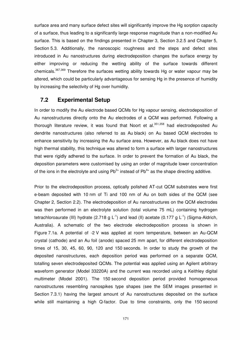
171
surface area and many surface defect sites will significantly improve the Hg sorption capacity
of a surface, thus leading to a significantly large response magnitude than a non-modified Au
surface. This is based on the findings presented in Chapter 3, Section 3.2.5 and Chapter 5,
Section 5.3. Additionally, the nanoscopic roughness and the steps and defect sites
introduced in Au nanostructures during electrodeposition changes the surface energy by
either improving or reducing the wetting ability of the surface towards different
chemicals.367,369 Therefore the surfaces wetting ability towards Hg or water vapour may be
altered, which could be particularly advantageous for sensing Hg in the presence of humidity
by increasing the selectivity of Hg over humidity.
7.2 Experimental Setup
In order to modify the Au electrode based QCMs for Hg vapour sensing, electrodeposition of
Au nanostructures directly onto the Au electrodes of a QCM was performed. Following a
thorough literature review, it was found that Noort et al.351,358 had electrodeposited Au
dendrite nanostructures (also referred to as Au black) on Au based QCM electrodes to
enhance sensitivity by increasing the Au surface area. However, as Au black does not have
high thermal stability, this technique was altered to form a surface with larger nanostructures
that were rigidly adhered to the surface. In order to prevent the formation of Au black, the
deposition parameters were customised by using an order of magnitude lower concentration
of the ions in the electrolyte and using Pb2+ instead of Pb4+ as the shape directing additive.
Prior to the electrodeposition process, optically polished AT-cut QCM substrates were first
e-beam deposited with 10 nm of Ti and 100 nm of Au on both sides of the QCM (see
Chapter 2, Section 2.2). The electrodeposition of Au nanostructures on the QCM electrodes
was then performed in an electrolyte solution (total volume 75 mL) containing hydrogen
tetrachloroaurate (III) hydrate (2.718 g L-1) and lead (II) acetate (0.177 g L-1) (Sigma-Aldrich,
Australia). A schematic of the two electrode electrodeposition process is shown in
Figure 7.1a. A potential of -2 V was applied at room temperature, between an Au-QCM
crystal (cathode) and an Au foil (anode) spaced 25 mm apart, for different electrodeposition
times of 15, 30, 45, 60, 90, 120 and 150 seconds. In order to study the growth of the
deposited nanostructures, each deposition period was performed on a separate QCM,
totalling seven electrodeposited QCMs. The potential was applied using an Agilent arbitrary
waveform generator (Model 33220A) and the current was recorded using a Keithley digital
multimeter (Model 2001). The 150 second deposition period provided homogeneous
nanostructures resembling nanospikes type shapes (see the SEM images presented in
Section 7.3.1) having the largest amount of Au nanostructures deposited on the surface
while still maintaining a high Q-factor. Due to time constraints, only the 150 second
172
nanospike based QCM was selected to be tested towards Hg vapour. This QCM is referred
to as the nanospike QCM from this point on.
The cyclic voltammetry (CV) trace for the electrolyte was later performed using a three
electrode system (CH Instruments, CHI 760C) in order to study the electrochemical
properties of the ions in the electrolyte and is shown in Figure 7.1b. The CV trace shows the
Au oxidation and reduction regions as well as the Pb under potential deposition (UPD)
regions. UPD is a phenomenon in electrodeposition that usually refers to the reduction of a
metal cation at a potential less negative than the equilibrium potential for the reduction of that
particular metal.370 The CV trace provided insight into the range of currents and voltages that
may be used to form the nanospike structures and confirmed that the voltage applied during
the 2 electrode depositions would not have reduced Pb ions in the electrolyte solution on the
QCM surface.
The customised deposition technique of the nanostructures was patented as they were found
to have a unique morphology and crystallographic orientation with high selectivity towards Hg
vapour in the presence of interferent gases (as will be discussed in this chapter).
Furthermore, the electro-catalytic and surface enhanced Raman scattering activities of the
developed nanostructures was also studied. However, this is beyond the scope of this work
and these results are published elsewhere.370,371
Figure 7.1: Electro-deposition set-up showing all the ions present in the electrolyte and the
electrolyte cyclic voltammeter measurement (CV). The Pb UPD and the Au oxidation and
reduction regions are indicated by arrows.
7.2.1.1 Mass of Gold Nanospikes
The mass of Au electrodeposited on the 100 nm Au film based QCM electrodes under a
constant potential of -2V between the anode and the cathode for specific time points of 15 to
A
Au
Au Au3+
Au3+
QCM
Pb2+ Cl
-H
+ CH3COO-
A
Au
Au Au3+
Au3+
QCM
Pb2+ Cl
-H
+ CH3COO-
a) Electrodeposition setup b) Cyclic voltammeter
-0.5 0.0 0.5 1.0 1.5
-60
-40
-20
0
20
40
60
Au Oxidation
Au Reduction
Cur
rent
(µA
)
Potential (V vs Ag/AgCl))
Electrolyte CV
Pb UPD
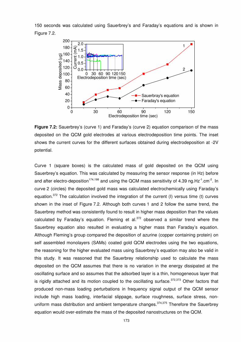
173
150 seconds was calculated using Sauerbrey’s and Faraday’s equations and is shown in
Figure 7.2.
Figure 7.2: Sauerbrey’s (curve 1) and Faraday’s (curve 2) equation comparison of the mass
deposited on the QCM gold electrodes at various electrodeposition time points. The inset
shows the current curves for the different surfaces obtained during electrodeposition at -2V
potential.
Curve 1 (square boxes) is the calculated mass of gold deposited on the QCM using
Sauerbrey’s equation. This was calculated by measuring the sensor response (in Hz) before
and after electro-deposition174,198 and using the QCM mass sensitivity of 4.39 ng.Hz-1.cm-2. In
curve 2 (circles) the deposited gold mass was calculated electrochemically using Faraday’s
equation.372 The calculation involved the integration of the current (I) versus time (t) curves
shown in the inset of Figure 7.2. Although both curves 1 and 2 follow the same trend, the
Sauerbrey method was consistently found to result in higher mass deposition than the values
calculated by Faraday’s equation. Fleming et al.372 observed a similar trend where the
Sauerbrey equation also resulted in evaluating a higher mass than Faraday’s equation.
Although Fleming’s group compared the deposition of azurine (copper containing protein) on
self assembled monolayers (SAMs) coated gold QCM electrodes using the two equations,
the reasoning for the higher evaluated mass using Sauerbrey’s equation may also be valid in
this study. It was reasoned that the Sauerbrey relationship used to calculate the mass
deposited on the QCM assumes that there is no variation in the energy dissipated at the
oscillating surface and so assumes that the adsorbed layer is a thin, homogeneous layer that
is rigidly attached and its motion coupled to the oscillating surface.372,373 Other factors that
produced non-mass loading perturbations in frequency signal output of the QCM sensor
include high mass loading, interfacial slippage, surface roughness, surface stress, non-
uniform mass distribution and ambient temperature changes.374,375 Therefore the Sauerbrey
equation would over-estimate the mass of the deposited nanostructures on the QCM.
0 30 60 90 120 1500
20
40
60
80
100
120
140
160
180
200
0 30 60 90 1201500.0
0.5
1.0
1.5
2.0
Cur
rent
(m
A)
Electrodeposition time (sec)
2
Sauerbray's equation Faraday's equation
Mas
s de
posi
ted
(µg)
Electrodeposition time (sec)
1
174
For the purpose of this study however, it must be determined whether the total deposited
mass on QCM substrate would produce a non-linear relationship between the QCM
response and Hg sorption during Hg vapour sensing. That is, it is well known that
Sauerbrey’s equation is linear and accurate only up to total electrode mass loads of ~2% of
the mass of quartz substrate.204,210 The deposited mass of Au nanospikes on the QCM Au
electrode (following 150 seconds of electrodeposition period) is estimated to be 191.1 µg (the
higher mass obtained from Sauerbrey’s equation) as shown in Figure 7.2. Combining this
value with the mass of the 10 nm Ti adhesion layer (2.27 µg) and 100 nm Au films (97.1 µg)
on both sides of the crystal, a total calculated mass of 290.47 µg (2.27 + 97.1 + 191.1 µg) is
obtained. Fortunately, the total estimated mass deposited on the quartz wafers is found to be
less than 386 µg (2% of mass of quartz substrate, i.e. 19.3 mg) including the original e-
beamed seed layer formed (191.1 µg + 99.38 µg), which is well within the 2% margin for
Sauerbrey’s equation to be valid during Hg sensing (as discussed in Chapter 1, Section
1.2.6.2). Furthermore, the Q-factor of the nanospike QCM was recorded to be 7028 and was
well above the acceptable value of 3000 required for oscillation to occur in the experimental
setup.
7.2.1.2 Electrochemical Surface Area of Gold Nanospikes
The influence of Au film surface area on Hg sorption capacity can be realized by calculating
the electrochemical surface area. The total geometric surface area of the two Au electrodes
of the QCM was calculated to be ~0.32cm2 (given that each of the two electrodes had a
diameter of 4.5 mm). The electrochemical surface area was determined by calculating the
charge required for reducing the monolayer of oxide as described by Rand and Woods274.
The electrochemical/geometrical surface area ratio of the Au control film (100 nm
Au-polished) was found to be ~1.5 cm2/cm2 as presented in Chapter 4, Section 4.3.1.
Similarly, from the integration of the cyclic voltammetric response region shown in Appendix
G.1, the electrochemical/geometrical surface area ratio of nanospikes was determined to be
~4.73 cm2/cm2 or ~3 times the Au control QCM electrode. Therefore the nanospike QCM is
expected to produce at least 3 times the response magnitude than the Au control QCM when
exposed towards the same Hg vapour concentration. In addition, the response magnitude is
expected to be even higher because the process of electrodeposition forms rough
surfaces356,376 with a high number of nodules and other surface defects313,342,368 which act as
Hg sorption sites.90
175
7.3 Gold Nanospikes Sensitive Layer Characterisation
In this section, the secondary electron microscopy (SEM), energy-dispersive X-ray (EDX)
spectroscopy and X-ray diffraction (XRD) characterisations of the electrodeposited
nanostructures are presented.
7.3.1 Surface Morphology – SEM
SEM characterisation of the electrodeposited nanostructures on QCM electrodes was
performed in order to determine the size and shape of the resulting nanostructures.
Figure 7.3a shows the SEM image of a 100 nm Au film e-beam deposited onto a QCM
substrate. The SEM image clearly indicates a relatively flat surface with well-dispersed Au
clusters. Figures 7.3b through to 7.3h show the representative SEM images of Au-coated
QCM crystals after subsequent electrodeposition of Au from a solution containing AuCl4- ions
in the presence of Pb2+ ions for (b) 15 sec, (c) 30 sec, (d) 45 sec, (e) 60 sec, (f) 90 sec, (g)
120 sec and (h) 150 sec, respectively. From the SEM images, it appears that during the
initial phase of Au electrodeposition, pre-existing Au nanoclusters of the e-beam-deposited
gold film (a) act as nucleation centres for the growth of Au nanoparticles (b and c), which
further start growing outwardly in a network-like structure of Au nanospikes as the reaction
continues for up to 60 sec (d and e). When the electrodeposition of Au is continued for
90 sec and 120 sec, the whole surface of the QCM crystal is found to be uniformly covered
with well-defined Au nanospikes with prismatic tapering ends (f and g). A further increase in
deposition time to 150 sec results in larger nanospikes with the appearance of sharp nodular
structures (h).
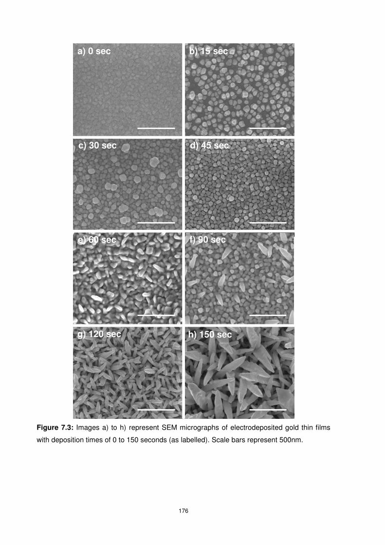
176
Figure 7.3: Images a) to h) represent SEM micrographs of electrodeposited gold thin films
with deposition times of 0 to 150 seconds (as labelled). Scale bars represent 500nm.
a) 0 sec b) 15 sec
c) 30 sec d) 45 sec
f) 90 sec
g) 120 sec h) 150 sec
e) 60 sec
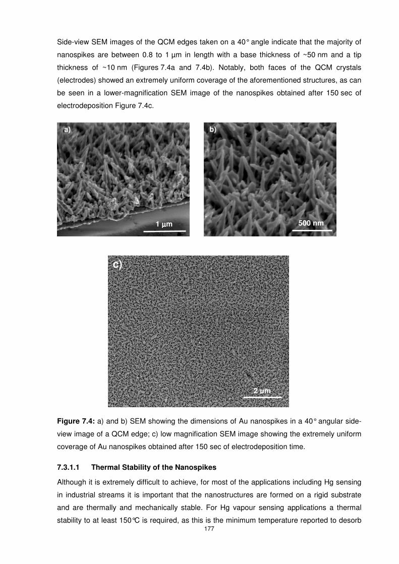
177
Side-view SEM images of the QCM edges taken on a 40° angle indicate that the majority of
nanospikes are between 0.8 to 1 µm in length with a base thickness of ~50 nm and a tip
thickness of ~10 nm (Figures 7.4a and 7.4b). Notably, both faces of the QCM crystals
(electrodes) showed an extremely uniform coverage of the aforementioned structures, as can
be seen in a lower-magnification SEM image of the nanospikes obtained after 150 sec of
electrodeposition Figure 7.4c.
Figure 7.4: a) and b) SEM showing the dimensions of Au nanospikes in a 40° angular side-
view image of a QCM edge; c) low magnification SEM image showing the extremely uniform
coverage of Au nanospikes obtained after 150 sec of electrodeposition time.
7.3.1.1 Thermal Stability of the Nanospikes
Although it is extremely difficult to achieve, for most of the applications including Hg sensing
in industrial streams it is important that the nanostructures are formed on a rigid substrate
and are thermally and mechanically stable. For Hg vapour sensing applications a thermal
stability to at least 150°C is required, as this is the minimum temperature reported to desorb
1 µµµµm
a) b)
2 µm
c)
500 nm
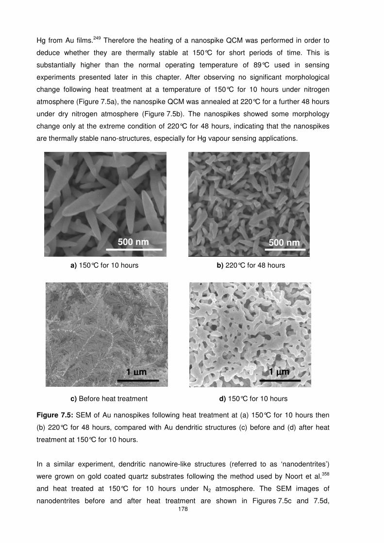
178
Hg from Au films.249 Therefore the heating of a nanospike QCM was performed in order to
deduce whether they are thermally stable at 150°C for short periods of time. This is
substantially higher than the normal operating temperature of 89°C used in sensing
experiments presented later in this chapter. After observing no significant morphological
change following heat treatment at a temperature of 150°C for 10 hours under nitrogen
atmosphere (Figure 7.5a), the nanospike QCM was annealed at 220°C for a further 48 hours
under dry nitrogen atmosphere (Figure 7.5b). The nanospikes showed some morphology
change only at the extreme condition of 220°C for 48 hours, indicating that the nanospikes
are thermally stable nano-structures, especially for Hg vapour sensing applications.
Figure 7.5: SEM of Au nanospikes following heat treatment at (a) 150°C for 10 hours then
(b) 220°C for 48 hours, compared with Au dendritic structures (c) before and (d) after heat
treatment at 150°C for 10 hours.
In a similar experiment, dendritic nanowire-like structures (referred to as ‘nanodentrites’)
were grown on gold coated quartz substrates following the method used by Noort et al.358
and heat treated at 150°C for 10 hours under N2 atmosphere. The SEM images of
nanodentrites before and after heat treatment are shown in Figures 7.5c and 7.5d,
a) 150°C for 10 hours b) 220°C for 48 hours
1 µµµµm 1 µµµµm
500 nm 500 nm
c) Before heat treatment d) 150°C for 10 hours
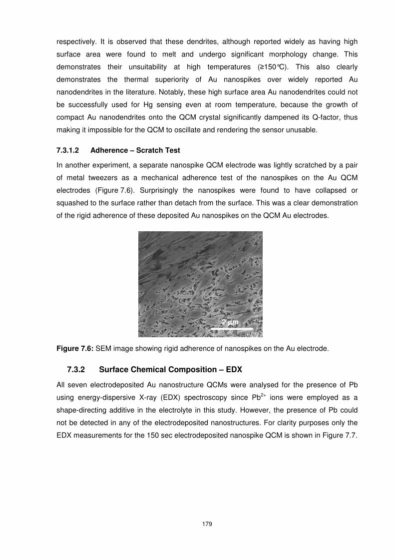
179
respectively. It is observed that these dendrites, although reported widely as having high
surface area were found to melt and undergo significant morphology change. This
demonstrates their unsuitability at high temperatures (≥150°C). This also clearly
demonstrates the thermal superiority of Au nanospikes over widely reported Au
nanodendrites in the literature. Notably, these high surface area Au nanodendrites could not
be successfully used for Hg sensing even at room temperature, because the growth of
compact Au nanodendrites onto the QCM crystal significantly dampened its Q-factor, thus
making it impossible for the QCM to oscillate and rendering the sensor unusable.
7.3.1.2 Adherence – Scratch Test
In another experiment, a separate nanospike QCM electrode was lightly scratched by a pair
of metal tweezers as a mechanical adherence test of the nanospikes on the Au QCM
electrodes (Figure 7.6). Surprisingly the nanospikes were found to have collapsed or
squashed to the surface rather than detach from the surface. This was a clear demonstration
of the rigid adherence of these deposited Au nanospikes on the QCM Au electrodes.
Figure 7.6: SEM image showing rigid adherence of nanospikes on the Au electrode.
7.3.2 Surface Chemical Composition – EDX
All seven electrodeposited Au nanostructure QCMs were analysed for the presence of Pb
using energy-dispersive X-ray (EDX) spectroscopy since Pb2+ ions were employed as a
shape-directing additive in the electrolyte in this study. However, the presence of Pb could
not be detected in any of the electrodeposited nanostructures. For clarity purposes only the
EDX measurements for the 150 sec electrodeposited nanospike QCM is shown in Figure 7.7.
C
2 µµµµm
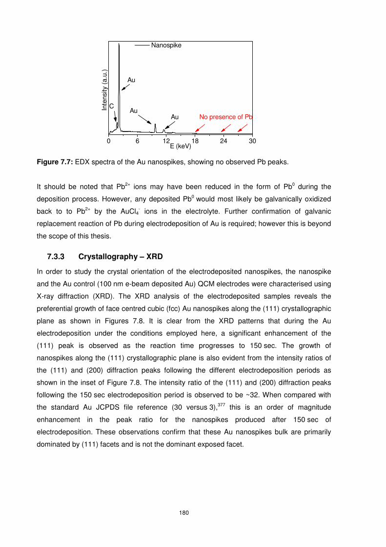
180
Figure 7.7: EDX spectra of the Au nanospikes, showing no observed Pb peaks.
It should be noted that Pb2+ ions may have been reduced in the form of Pb0 during the
deposition process. However, any deposited Pb0 would most likely be galvanically oxidized
back to to Pb2+ by the AuCl4- ions in the electrolyte. Further confirmation of galvanic
replacement reaction of Pb during electrodeposition of Au is required; however this is beyond
the scope of this thesis.
7.3.3 Crystallography – XRD
In order to study the crystal orientation of the electrodeposited nanospikes, the nanospike
and the Au control (100 nm e-beam deposited Au) QCM electrodes were characterised using
X-ray diffraction (XRD). The XRD analysis of the electrodeposited samples reveals the
preferential growth of face centred cubic (fcc) Au nanospikes along the (111) crystallographic
plane as shown in Figures 7.8. It is clear from the XRD patterns that during the Au
electrodeposition under the conditions employed here, a significant enhancement of the
(111) peak is observed as the reaction time progresses to 150 sec. The growth of
nanospikes along the (111) crystallographic plane is also evident from the intensity ratios of
the (111) and (200) diffraction peaks following the different electrodeposition periods as
shown in the inset of Figure 7.8. The intensity ratio of the (111) and (200) diffraction peaks
following the 150 sec electrodeposition period is observed to be ~32. When compared with
the standard Au JCPDS file reference (30 versus 3),377 this is an order of magnitude
enhancement in the peak ratio for the nanospikes produced after 150 sec of
electrodeposition. These observations confirm that these Au nanospikes bulk are primarily
dominated by (111) facets and is not the dominant exposed facet.
0 6 12 18 24 30
No presence of PbAuAu
Au
Inte
nsity
(a.
u.)
E (keV)
Nanospike
C
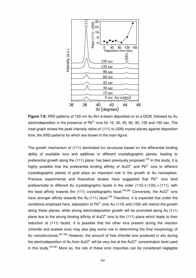
181
Figure 7.8: XRD patterns of 100 nm Au film e-beam deposited on to a QCM, followed by Au
electrodeposition in the presence of Pb2+ ions for 15, 30, 45, 60, 90, 120 and 150 sec. The
inset graph shows the peak intensity ratios of (111) to (200) crystal planes against deposition
time, the XRD patterns for which are shown in the main figure.
The growth mechanism of (111) dominated fcc structures based on the differential binding
ability of available ions and additives to different crystallographic planes, leading to
preferential growth along the (111) plane, has been previously proposed.378 In this study, it is
highly possible that the preferential binding affinity of AuCl4- and Pb2+ ions to different
crystallographic planes of gold plays an important role in the growth of Au nanospikes.
Previous experimental and theoretical studies have suggested that Pb2+ ions bind
preferentially to different Au crystallographic facets in the order (110) ≥ (100) > (111), with
the least affinity towards the (111) crystallographic facet.379,380 Conversely, the AuCl4- ions
have stronger affinity towards the Au (111) facet.378 Therefore, it is expected that under the
conditions employed here, adsorption of Pb2+ onto Au (110) and (100) will restrict the growth
along these planes, while strong electrodeposition growth will be promoted along Au (111)
plane due to the strong binding affinity of AuCl4- ions to the (111) plane which leads to their
reduction at (111) facets. It is possible that the other ions present during the reaction
(chloride and acetate ions) may also play some role in determining the final morphology of
Au nanostructures.381-386 However, the amount of free chloride ions produced in situ during
the electrodeposition of Au from AuCl4- will be very low at the AuCl4- concentration level used
in this study.370,387 More so, the role of these ionic impurities can be considered negligible
36 38 40 42 44 46
0 40 80 120 1600
8
16
24
32
Rat
io (
111)
/ (2
00)
Deposition time (sec)
150 sec
120 sec
90 sec
60 sec
45 sec
30 sec
15 sec0 sec Au control
(20
0)
Inte
nsity
(a.
u.)
2θ (degrees)
(11
1)
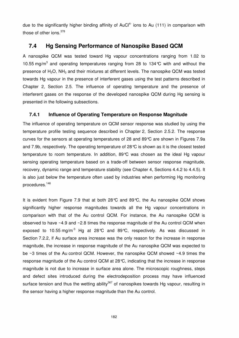
182
due to the significantly higher binding affinity of AuCl4- ions to Au (111) in comparison with
those of other ions.378
7.4 Hg Sensing Performance of Nanospike Based QCM
A nanospike QCM was tested toward Hg vapour concentrations ranging from 1.02 to
10.55 mg/m3 and operating temperatures ranging from 28 to 134°C with and without the
presence of H2O, NH3 and their mixtures at different levels. The nanospike QCM was tested
towards Hg vapour in the presence of interferent gases using the test patterns described in
Chapter 2, Section 2.5. The influence of operating temperature and the presence of
interferent gases on the response of the developed nanospike QCM during Hg sensing is
presented in the following subsections.
7.4.1 Influence of Operating Temperature on Response Magnitude
The influence of operating temperature on QCM sensor response was studied by using the
temperature profile testing sequence described in Chapter 2, Section 2.5.2. The response
curves for the sensors at operating temperatures of 28 and 89°C are shown in Figures 7.9a
and 7.9b, respectively. The operating temperature of 28°C is shown as it is the closest tested
temperature to room temperature. In addition, 89°C was chosen as the ideal Hg vapour
sensing operating temperature based on a trade-off between sensor response magnitude,
recovery, dynamic range and temperature stability (see Chapter 4, Sections 4.4.2 to 4.4.5). It
is also just below the temperature often used by industries when performing Hg monitoring
procedures.146
It is evident from Figure 7.9 that at both 28°C and 89°C, the Au nanospike QCM shows
significantly higher response magnitudes towards all the Hg vapour concentrations in
comparison with that of the Au control QCM. For instance, the Au nanospike QCM is
observed to have ~4.9 and ~2.8 times the response magnitude of the Au control QCM when
exposed to 10.55 mg/m-3 Hg at 28°C and 89°C, respectively. As was discussed in
Section 7.2.2, if Au surface area increase was the only reason for the increase in response
magnitude, the increase in response magnitude of the Au nanospike QCM was expected to
be ~3 times of the Au control QCM. However, the nanospike QCM showed ~4.9 times the
response magnitude of the Au control QCM at 28°C, indicating that the increase in response
magnitude is not due to increase in surface area alone. The microscopic roughness, steps
and defect sites introduced during the electrodeposition process may have influenced
surface tension and thus the wetting ability367 of nanospikes towards Hg vapour, resulting in
the sensor having a higher response magnitude than the Au control.

183
Figure 7.9: Sensor response of 100 nm e-beam deposited Au film (curve 1) and
electrodeposited nanospikes (curve 2) towards Hg pulse sequence, with Hg concentrations
ranging from 1.02 to 10.55 mg/m3 at operating temperatures of 28 and 89°C.
The drift, noise and response time of the nanospike QCM and Au control QCMs were also
calculated at 28 and 89°C. At 28°C both sensors had negligible noise and drift before Hg
exposure, which is most likely due to the well known zero temperature coefficient and
temperature stability of AT-cut quartz QCMs at around room temperature.301 However, before
Hg exposure at 89°C, the drift and noise of the Au control QCM was found to be 0.28 Hz/h
and ±0.59 Hz respectively. The spikes on the other hand had similar drift but with only
±0.08 Hz noise. When operated at 89°C and Hg concentration of 10.55mg/m3, the nanospike
QCM is observed to achieve a 90% response (t90) in ~18.5 minutes; more than 10 minutes
quicker then the Au control QCM. However, at 28°C the t90 for the nanospike and Au control
b) 89°C
a) 28°C
0 1 2 3 4 5 6 7 8 9 10-2.4
-2.0
-1.6
-1.2
-0.8
-0.4
0.0
10.55 mg m-3
5.70 mg m-3
3.65 mg m-3
1.87 mg m-3 1.02 mg m-3
QC
M R
espo
nse
(kH
z)
Time (h)
Au control Nanospike
0 1 2 3 4 5 6 7 8 9 10-0.8
-0.6
-0.4
-0.2
0.0
QC
M R
espo
nse
(kH
z)
Time (h)
Au control Nanospike
10.55 mg m-3
5.70 mg m-3
3.65 mg m-3
1.87 mg m-3
1.02 mg m-3
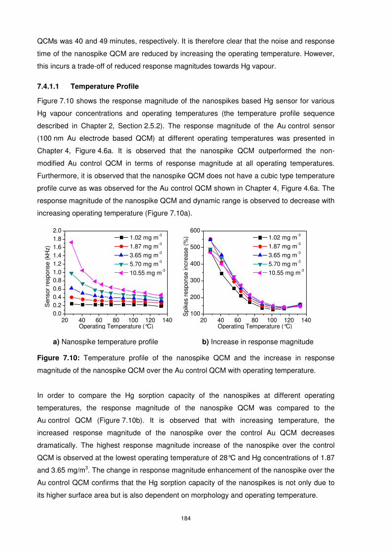
184
QCMs was 40 and 49 minutes, respectively. It is therefore clear that the noise and response
time of the nanospike QCM are reduced by increasing the operating temperature. However,
this incurs a trade-off of reduced response magnitudes towards Hg vapour.
7.4.1.1 Temperature Profile
Figure 7.10 shows the response magnitude of the nanospikes based Hg sensor for various
Hg vapour concentrations and operating temperatures (the temperature profile sequence
described in Chapter 2, Section 2.5.2). The response magnitude of the Au control sensor
(100 nm Au electrode based QCM) at different operating temperatures was presented in
Chapter 4, Figure 4.6a. It is observed that the nanospike QCM outperformed the non-
modified Au control QCM in terms of response magnitude at all operating temperatures.
Furthermore, it is observed that the nanospike QCM does not have a cubic type temperature
profile curve as was observed for the Au control QCM shown in Chapter 4, Figure 4.6a. The
response magnitude of the nanospike QCM and dynamic range is observed to decrease with
increasing operating temperature (Figure 7.10a).
Figure 7.10: Temperature profile of the nanospike QCM and the increase in response
magnitude of the nanospike QCM over the Au control QCM with operating temperature.
In order to compare the Hg sorption capacity of the nanospikes at different operating
temperatures, the response magnitude of the nanospike QCM was compared to the
Au control QCM (Figure 7.10b). It is observed that with increasing temperature, the
increased response magnitude of the nanospike over the control Au QCM decreases
dramatically. The highest response magnitude increase of the nanospike over the control
QCM is observed at the lowest operating temperature of 28°C and Hg concentrations of 1.87
and 3.65 mg/m3. The change in response magnitude enhancement of the nanospike over the
Au control QCM confirms that the Hg sorption capacity of the nanospikes is not only due to
its higher surface area but is also dependent on morphology and operating temperature.
a) Nanospike temperature profile b) Increase in response magnitude
20 40 60 80 100 120 1400.00.20.40.60.81.01.21.41.61.82.0
1.02 mg m-3
1.87 mg m-3
3.65 mg m-3
5.70 mg m-3
10.55 mg m-3
Sen
sor
resp
onse
(kH
z)
Operating Temperature (°C)20 40 60 80 100 120 140
100
200
300
400
500
600
Spi
kes
resp
onse
incr
ease
(%
)
Operating Temperature (°C)
1.02 mg m-3
1.87 mg m-3
3.65 mg m-3
5.70 mg m-3
10.55 mg m-3
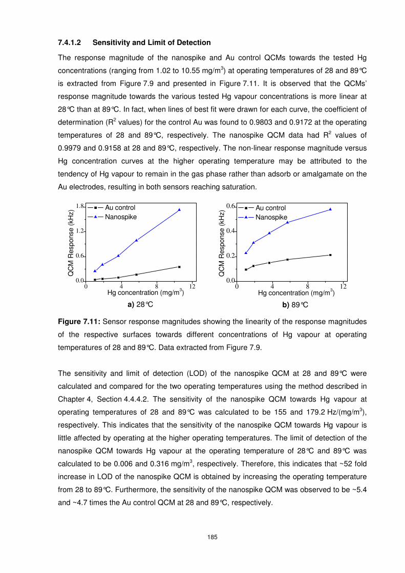
185
7.4.1.2 Sensitivity and Limit of Detection
The response magnitude of the nanospike and Au control QCMs towards the tested Hg
concentrations (ranging from 1.02 to 10.55 mg/m3) at operating temperatures of 28 and 89°C
is extracted from Figure 7.9 and presented in Figure 7.11. It is observed that the QCMs’
response magnitude towards the various tested Hg vapour concentrations is more linear at
28°C than at 89°C. In fact, when lines of best fit were drawn for each curve, the coefficient of
determination (R2 values) for the control Au was found to 0.9803 and 0.9172 at the operating
temperatures of 28 and 89°C, respectively. The nanospike QCM data had R2 values of
0.9979 and 0.9158 at 28 and 89°C, respectively. The non-linear response magnitude versus
Hg concentration curves at the higher operating temperature may be attributed to the
tendency of Hg vapour to remain in the gas phase rather than adsorb or amalgamate on the
Au electrodes, resulting in both sensors reaching saturation.
Figure 7.11: Sensor response magnitudes showing the linearity of the response magnitudes
of the respective surfaces towards different concentrations of Hg vapour at operating
temperatures of 28 and 89°C. Data extracted from Figure 7.9.
The sensitivity and limit of detection (LOD) of the nanospike QCM at 28 and 89°C were
calculated and compared for the two operating temperatures using the method described in
Chapter 4, Section 4.4.4.2. The sensitivity of the nanospike QCM towards Hg vapour at
operating temperatures of 28 and 89°C was calculated to be 155 and 179.2 Hz/(mg/m3),
respectively. This indicates that the sensitivity of the nanospike QCM towards Hg vapour is
little affected by operating at the higher operating temperatures. The limit of detection of the
nanospike QCM towards Hg vapour at the operating temperature of 28°C and 89°C was
calculated to be 0.006 and 0.316 mg/m3, respectively. Therefore, this indicates that ~52 fold
increase in LOD of the nanospike QCM is obtained by increasing the operating temperature
from 28 to 89°C. Furthermore, the sensitivity of the nanospike QCM was observed to be ~5.4
and ~4.7 times the Au control QCM at 28 and 89°C, respectively.
b) 89°C a) 28°C
0 4 8 120.0
0.2
0.4
0.6 Au control Nanospike
Hg concentration (mg/m3)
QC
M R
espo
nse
(kH
z)
0 4 8 120.0
0.6
1.2
1.8 Au control Nanospike
QC
M R
espo
nse
(kH
z)
Hg concentration (mg/m3)
186
7.4.2 Sensor Repeatability
In addition to the response magnitude, another important parameter that determines a
sensor’s performance is its reproducibility (precision) over a period of time. The precision of
the sensors may be estimated by calculating the coefficient of variation (COV) , which
describes the spread of the response magnitude data for a given Hg vapour concentration as
shown in Equation 7.3,
%100×=x
COVσ
Equation 7.3
where σ is the standard deviation and _
x is the mean of the sensor response magnitudes.
Figure 7.12 shows the response magnitude of the nanospike and Au control QCMs over a 72 hour
testing period (four repeated cycles of the sequence shown in Figure 7.9) and illustrates the
stability of the nanospike over the Au control QCM during a 3 day continuous testing period
at an operating temperature of 89°C. The maximum COV of the nanospike and Au control
QCMs towards Hg vapour over the 3 day testing period was observed to be ~1.6 and 3.6%,
respectively. This shows a good repeatability of the nanospike QCM and indicates that the
precision of both sensors can be enhanced or maintained by calibrating the sensors every 3
days.
Figure 7.12: Degradation of nanospike and Au control QCMs over a 3 day testing period.
The COV (in percentage, %) is shown for each Hg vapour concentration at 89°C.
It is noteworthy that the currently commercially available, highly accurate and precise, Hg
vapour sensor based on gold film resistivity (Jerome 431-X) can measure Hg concentrations
of up to only 0.99 mg/m3 with a precision of ± 5 % at 0.10 mg/m-3 and at an operating
temperature up to only 40°C.388 This clearly shows the superiority of these nanospike based
Hg vapour sensors over existing sensor technologies in high Hg vapour concentrations and
temperature ranges.
0 2 4 6 8 10
100
200
300
400
500
600
S
enso
r re
spon
se (
Hz)
Hg concentration mg/m3
1.0%
0.2%
1.6%
0.8%
1.6%0.7%
1.3%2.6%
1.6%3.6%
Nanospike
Au control
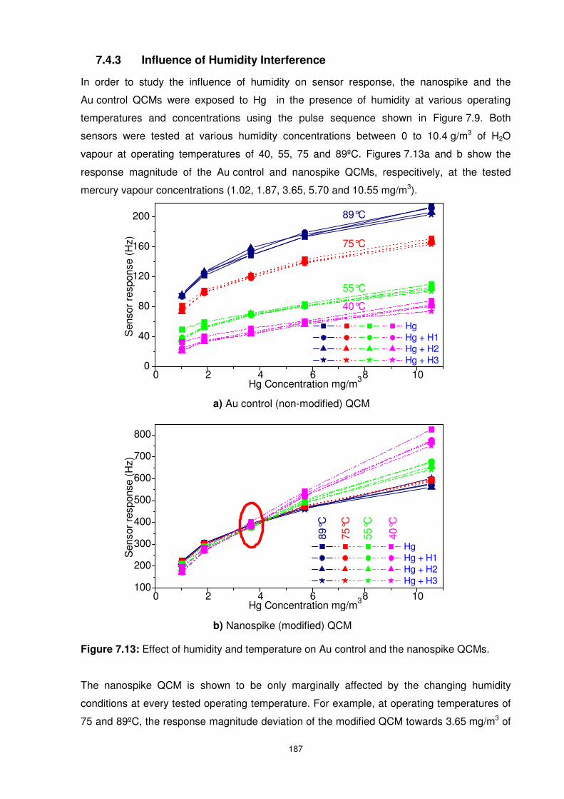
187
7.4.3 Influence of Humidity Interference
In order to study the influence of humidity on sensor response, the nanospike and the
Au control QCMs were exposed to Hg in the presence of humidity at various operating
temperatures and concentrations using the pulse sequence shown in Figure 7.9. Both
sensors were tested at various humidity concentrations between 0 to 10.4 g/m3 of H2O
vapour at operating temperatures of 40, 55, 75 and 89ºC. Figures 7.13a and b show the
response magnitude of the Au control and nanospike QCMs, respecitively, at the tested
mercury vapour concentrations (1.02, 1.87, 3.65, 5.70 and 10.55 mg/m3).
Figure 7.13: Effect of humidity and temperature on Au control and the nanospike QCMs.
The nanospike QCM is shown to be only marginally affected by the changing humidity
conditions at every tested operating temperature. For example, at operating temperatures of
75 and 89ºC, the response magnitude deviation of the modified QCM towards 3.65 mg/m3 of
0 2 4 6 8 100
40
80
120
160
200
Hg Hg + H1 Hg + H2 Hg + H3
89°C
40°C
55°C
75°C
Sen
sor
resp
onse
(H
z)
Hg Concentration mg/m3
0 2 4 6 8 10100
200
300
400
500
600
700
800
Hg Hg + H1 Hg + H2 Hg + H3
89°C
40°C
55°C
Sen
sor
resp
onse
(H
z)
Hg Concentration mg/m3
75°C
a) Au control (non-modified) QCM
b) Nanospike (modified) QCM
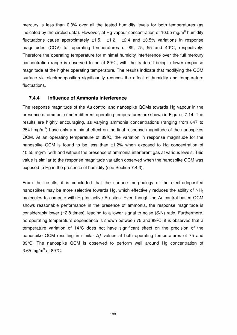
188
mercury is less than 0.3% over all the tested humidity levels for both temperatures (as
indicated by the circled data). However, at Hg vapour concentration of 10.55 mg/m3 humidity
fluctuations cause approximately ±1.5, ±1.2, ±2.4 and ±3.5% variations in response
magnitudes (COV) for operating temperatures of 89, 75, 55 and 40ºC, respectively.
Therefore the operating temperature for minimal humidity interference over the full mercury
concentration range is observed to be at 89ºC, with the trade-off being a lower response
magnitude at the higher operating temperature. The results indicate that modifying the QCM
surface via electrodeposition significantly reduces the effect of humidity and temperature
fluctuations.
7.4.4 Influence of Ammonia Interference
The response magnitude of the Au control and nanospike QCMs towards Hg vapour in the
presence of ammonia under different operating temperatures are shown in Figures 7.14. The
results are highly encouraging, as varying ammonia concentrations (ranging from 847 to
2541 mg/m3) have only a minimal effect on the final response magnitude of the nanospikes
QCM. At an operating temperature of 89ºC, the variation in response magnitude for the
nanospike QCM is found to be less than ±1.2% when exposed to Hg concentration of
10.55 mg/m3 with and without the presence of ammonia interferent gas at various levels. This
value is similar to the response magnitude variation observed when the nanospike QCM was
exposed to Hg in the presence of humidity (see Section 7.4.3).
From the results, it is concluded that the surface morphology of the electrodeposited
nanospikes may be more selective towards Hg, which effectively reduces the ability of NH3
molecules to compete with Hg for active Au sites. Even though the Au control based QCM
shows reasonable performance in the presence of ammonia, the response magnitude is
considerably lower (~2.8 times), leading to a lower signal to noise (S/N) ratio. Furthermore,
no operating temperature dependence is shown between 75 and 89ºC; it is observed that a
temperature variation of 14°C does not have significant effect on the precision of the
nanospike QCM resulting in similar ∆ƒ values at both operating temperatures of 75 and
89°C. The nanospike QCM is observed to perform well around Hg concentration of
3.65 mg/m3 at 89°C.
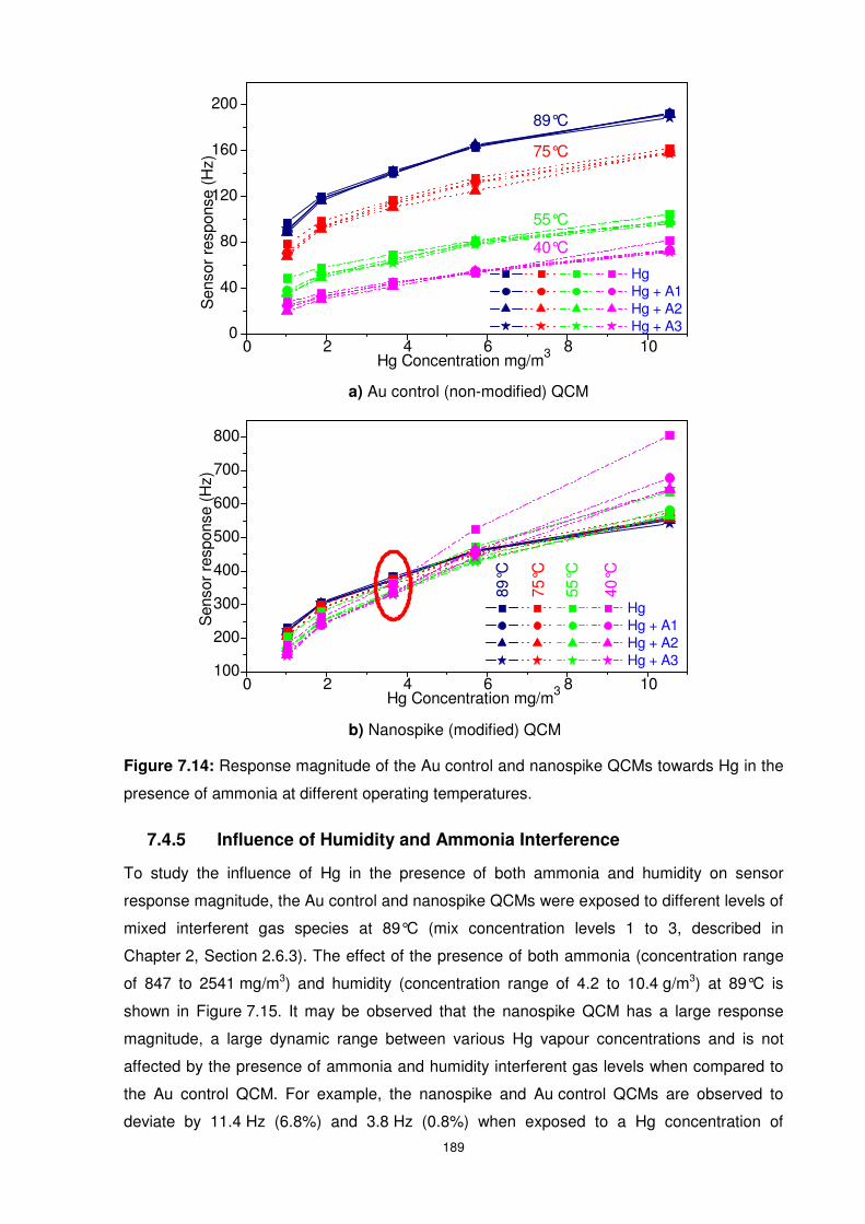
189
Figure 7.14: Response magnitude of the Au control and nanospike QCMs towards Hg in the
presence of ammonia at different operating temperatures.
7.4.5 Influence of Humidity and Ammonia Interference
To study the influence of Hg in the presence of both ammonia and humidity on sensor
response magnitude, the Au control and nanospike QCMs were exposed to different levels of
mixed interferent gas species at 89°C (mix concentration levels 1 to 3, described in
Chapter 2, Section 2.6.3). The effect of the presence of both ammonia (concentration range
of 847 to 2541 mg/m3) and humidity (concentration range of 4.2 to 10.4 g/m3) at 89°C is
shown in Figure 7.15. It may be observed that the nanospike QCM has a large response
magnitude, a large dynamic range between various Hg vapour concentrations and is not
affected by the presence of ammonia and humidity interferent gas levels when compared to
the Au control QCM. For example, the nanospike and Au control QCMs are observed to
deviate by 11.4 Hz (6.8%) and 3.8 Hz (0.8%) when exposed to a Hg concentration of
0 2 4 6 8 100
40
80
120
160
200
Hg Hg + A1 Hg + A2 Hg + A3
89°C
40°C
55°C
75°C
Sen
sor
resp
onse
(H
z)
Hg Concentration mg/m3
0 2 4 6 8 10100
200
300
400
500
600
700
800
Hg Hg + A1 Hg + A2 Hg + A3
89°C
40°C
55°C
Sen
sor
resp
onse
(H
z)
Hg Concentration mg/m3
75°C
a) Au control (non-modified) QCM
b) Nanospike (modified) QCM
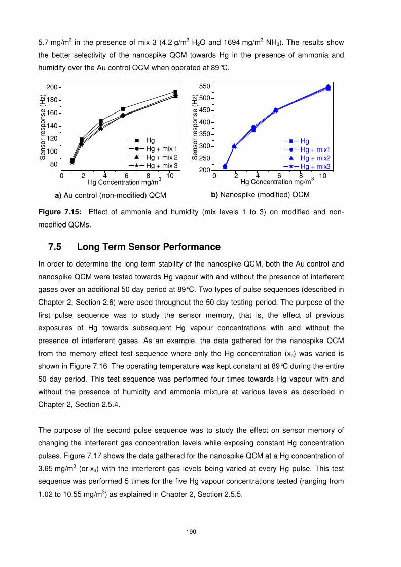
190
5.7 mg/m3 in the presence of mix 3 (4.2 g/m3 H2O and 1694 mg/m3 NH3). The results show
the better selectivity of the nanospike QCM towards Hg in the presence of ammonia and
humidity over the Au control QCM when operated at 89°C.
Figure 7.15: Effect of ammonia and humidity (mix levels 1 to 3) on modified and non-
modified QCMs.
7.5 Long Term Sensor Performance
In order to determine the long term stability of the nanospike QCM, both the Au control and
nanospike QCM were tested towards Hg vapour with and without the presence of interferent
gases over an additional 50 day period at 89°C. Two types of pulse sequences (described in
Chapter 2, Section 2.6) were used throughout the 50 day testing period. The purpose of the
first pulse sequence was to study the sensor memory, that is, the effect of previous
exposures of Hg towards subsequent Hg vapour concentrations with and without the
presence of interferent gases. As an example, the data gathered for the nanospike QCM
from the memory effect test sequence where only the Hg concentration (xn) was varied is
shown in Figure 7.16. The operating temperature was kept constant at 89°C during the entire
50 day period. This test sequence was performed four times towards Hg vapour with and
without the presence of humidity and ammonia mixture at various levels as described in
Chapter 2, Section 2.5.4.
The purpose of the second pulse sequence was to study the effect on sensor memory of
changing the interferent gas concentration levels while exposing constant Hg concentration
pulses. Figure 7.17 shows the data gathered for the nanospike QCM at a Hg concentration of
3.65 mg/m3 (or x3) with the interferent gas levels being varied at every Hg pulse. This test
sequence was performed 5 times for the five Hg vapour concentrations tested (ranging from
1.02 to 10.55 mg/m3) as explained in Chapter 2, Section 2.5.5.
0 2 4 6 8 10
80
100
120
140
160
180
200
Hg Hg + mix 1 Hg + mix 2 Hg + mix 3
Sen
sor
resp
onse
(H
z)
Hg Concentration mg/m3 0 2 4 6 8 10200
250
300
350
400
450
500
550
Hg Hg + mix1 Hg + mix2 Hg + mix3
Sen
sor
resp
onse
(H
z)
Hg Concentration mg/m3
b) Nanospike (modified) QCM a) Au control (non-modified) QCM
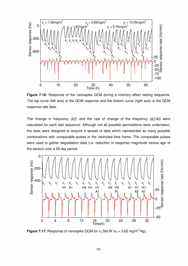
191
Figure 7.16: Response of the nanospike QCM during a memory effect testing sequence.
The top curve (left axis) is the QCM response and the bottom curve (right axis) is the QCM
response rate data.
The change in frequency (∆ƒ) and the rate of change of the frequency (∆ƒ/∆t) were
calculated for each test sequence. Although not all possible permeations were undertaken,
the tests were designed to acquire a spread of data which represented as many possible
combinations with comparable pulses in the restricted time frame. The comparable pulses
were used to gather degradation data (i.e. reduction in response magnitude versus age of
the sensor) over a 50 day period.
Figure 7.17: Response of nanospike QCM for x3 Set W (x3 = 3.65 mg/m3 Hg).
0 4 8 12 16 20 24 28 32-1000
-800
-600
-400
-200
0
x3
x3
H1A1
x3
H1 A2
x3
A1
x3
x3
H2 A1
x3
H2
x3
x3
H1 A1
x3
H1
x3
H2
x3
x3
A1
x3
H1
x3
x3
Sen
sor
resp
onse
(H
z)
Time(h)
x3
-50
-25
0
25
50
75
100
Sen
sor
resp
onse
rat
e (H
z/m
in)
0 10 20 30 40 50 60
-1200
-900
-600
-300
0
Sen
sor
resp
onse
(H
z)
Time (h)
-100-75-50-250255075100125150175200225
x3
x2
x4
x5
x5
x4
x2
x3
x1
x1
x1
x1
x1 x
1x
1x
1x
1
x5 = 10.55mg/m3
x4 = 5.70mg/m3
x3 = 3.65mg/m3
x2 = 1.87mg/m3
x1 = 1.02mg/m3
x5
x4
x3
x2
x1x
2x
3x
4x
5
x4
x3
x5
x3
x2
Sen
sor
resp
onse
rat
e (H
z/m
in)
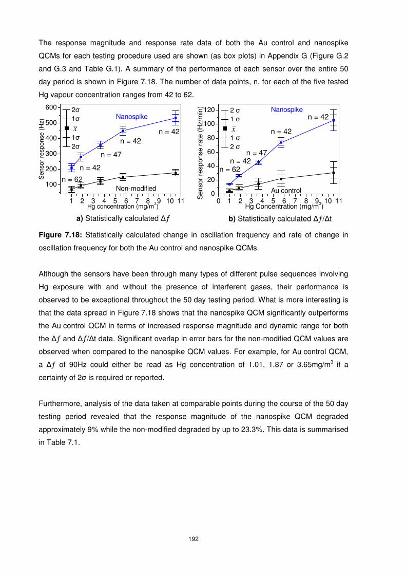
192
The response magnitude and response rate data of both the Au control and nanospike
QCMs for each testing procedure used are shown (as box plots) in Appendix G (Figure G.2
and G.3 and Table G.1). A summary of the performance of each sensor over the entire 50
day period is shown in Figure 7.18. The number of data points, n, for each of the five tested
Hg vapour concentration ranges from 42 to 62.
Figure 7.18: Statistically calculated change in oscillation frequency and rate of change in
oscillation frequency for both the Au control and nanospike QCMs.
Although the sensors have been through many types of different pulse sequences involving
Hg exposure with and without the presence of interferent gases, their performance is
observed to be exceptional throughout the 50 day testing period. What is more interesting is
that the data spread in Figure 7.18 shows that the nanospike QCM significantly outperforms
the Au control QCM in terms of increased response magnitude and dynamic range for both
the ∆ƒ and ∆ƒ/∆t data. Significant overlap in error bars for the non-modified QCM values are
observed when compared to the nanospike QCM values. For example, for Au control QCM,
a ∆ƒ of 90Hz could either be read as Hg concentration of 1.01, 1.87 or 3.65mg/m3 if a
certainty of 2σ is required or reported.
Furthermore, analysis of the data taken at comparable points during the course of the 50 day
testing period revealed that the response magnitude of the nanospike QCM degraded
approximately 9% while the non-modified degraded by up to 23.3%. This data is summarised
in Table 7.1.
a) Statistically calculated ∆ƒ b) Statistically calculated ∆ƒ/∆t
x
1σ 2σ
1σ 2σ
x
1 σ 2 σ
1 σ 2 σ
1 2 3 4 5 6 7 8 9 10 11
100
200
300
400
500
600
Hg concentration (mg/m3)
Non-modified
Nanospike
Sen
sor
resp
onse
(H
z)
n = 62
n = 42
n = 47
n = 42n = 42
0 1 2 3 4 5 6 7 8 9 10 110
20
40
60
80
100
120
Nanospike
Hg Concentration (mg/m3) S
enso
r re
spon
se r
ate
(Hz/
min
)Au control
n = 62n = 42
n = 47
n = 42
n = 42
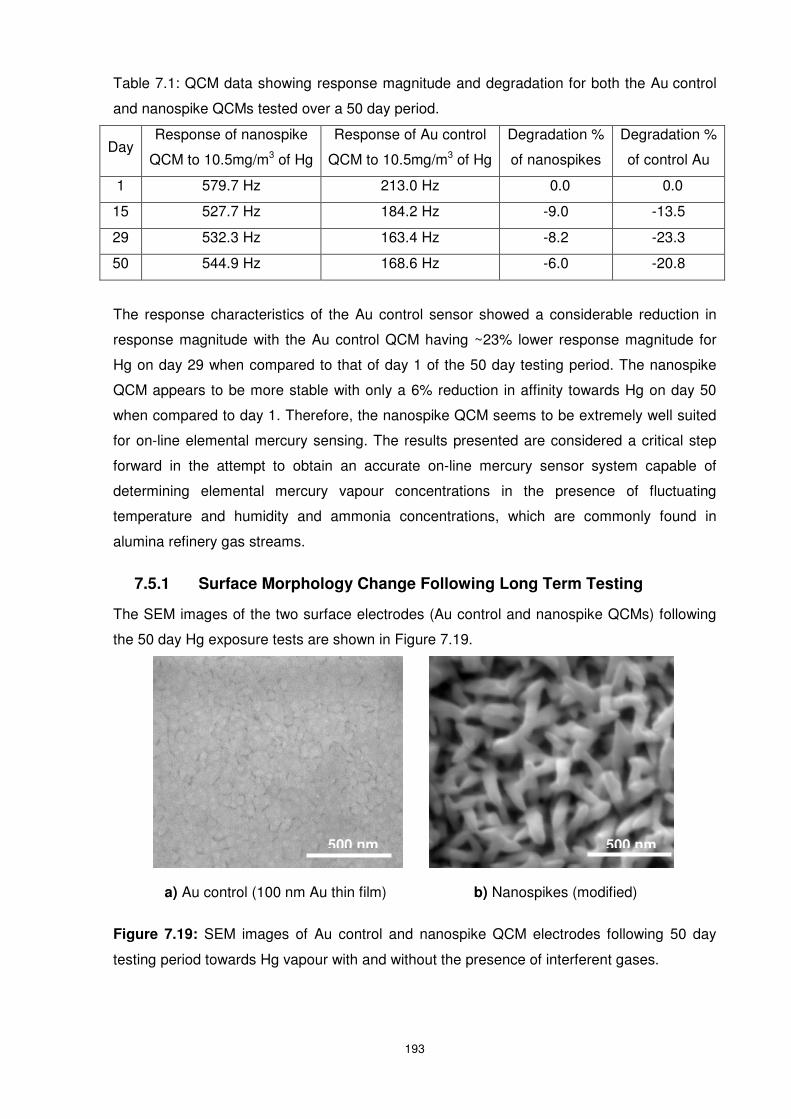
193
Table 7.1: QCM data showing response magnitude and degradation for both the Au control
and nanospike QCMs tested over a 50 day period.
Day Response of nanospike
QCM to 10.5mg/m3 of Hg
Response of Au control
QCM to 10.5mg/m3 of Hg
Degradation %
of nanospikes
Degradation %
of control Au
1 579.7 Hz 213.0 Hz 0.0 0.0
15 527.7 Hz 184.2 Hz -9.0 -13.5
29 532.3 Hz 163.4 Hz -8.2 -23.3
50 544.9 Hz 168.6 Hz -6.0 -20.8
The response characteristics of the Au control sensor showed a considerable reduction in
response magnitude with the Au control QCM having ~23% lower response magnitude for
Hg on day 29 when compared to that of day 1 of the 50 day testing period. The nanospike
QCM appears to be more stable with only a 6% reduction in affinity towards Hg on day 50
when compared to day 1. Therefore, the nanospike QCM seems to be extremely well suited
for on-line elemental mercury sensing. The results presented are considered a critical step
forward in the attempt to obtain an accurate on-line mercury sensor system capable of
determining elemental mercury vapour concentrations in the presence of fluctuating
temperature and humidity and ammonia concentrations, which are commonly found in
alumina refinery gas streams.
7.5.1 Surface Morphology Change Following Long Term Testing
The SEM images of the two surface electrodes (Au control and nanospike QCMs) following
the 50 day Hg exposure tests are shown in Figure 7.19.
Figure 7.19: SEM images of Au control and nanospike QCM electrodes following 50 day
testing period towards Hg vapour with and without the presence of interferent gases.
C
500 nm 500 nm
a) Au control (100 nm Au thin film) b) Nanospikes (modified)
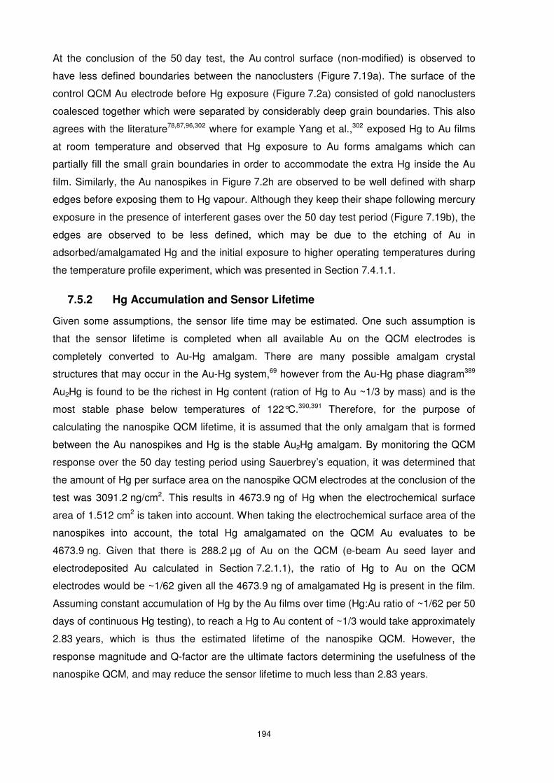
194
At the conclusion of the 50 day test, the Au control surface (non-modified) is observed to
have less defined boundaries between the nanoclusters (Figure 7.19a). The surface of the
control QCM Au electrode before Hg exposure (Figure 7.2a) consisted of gold nanoclusters
coalesced together which were separated by considerably deep grain boundaries. This also
agrees with the literature78,87,96,302 where for example Yang et al.,302 exposed Hg to Au films
at room temperature and observed that Hg exposure to Au forms amalgams which can
partially fill the small grain boundaries in order to accommodate the extra Hg inside the Au
film. Similarly, the Au nanospikes in Figure 7.2h are observed to be well defined with sharp
edges before exposing them to Hg vapour. Although they keep their shape following mercury
exposure in the presence of interferent gases over the 50 day test period (Figure 7.19b), the
edges are observed to be less defined, which may be due to the etching of Au in
adsorbed/amalgamated Hg and the initial exposure to higher operating temperatures during
the temperature profile experiment, which was presented in Section 7.4.1.1.
7.5.2 Hg Accumulation and Sensor Lifetime
Given some assumptions, the sensor life time may be estimated. One such assumption is
that the sensor lifetime is completed when all available Au on the QCM electrodes is
completely converted to Au-Hg amalgam. There are many possible amalgam crystal
structures that may occur in the Au-Hg system,69 however from the Au-Hg phase diagram389
Au2Hg is found to be the richest in Hg content (ration of Hg to Au ~1/3 by mass) and is the
most stable phase below temperatures of 122°C.390,391 Therefore, for the purpose of
calculating the nanospike QCM lifetime, it is assumed that the only amalgam that is formed
between the Au nanospikes and Hg is the stable Au2Hg amalgam. By monitoring the QCM
response over the 50 day testing period using Sauerbrey’s equation, it was determined that
the amount of Hg per surface area on the nanospike QCM electrodes at the conclusion of the
test was 3091.2 ng/cm2. This results in 4673.9 ng of Hg when the electrochemical surface
area of 1.512 cm2 is taken into account. When taking the electrochemical surface area of the
nanospikes into account, the total Hg amalgamated on the QCM Au evaluates to be
4673.9 ng. Given that there is 288.2 µg of Au on the QCM (e-beam Au seed layer and
electrodeposited Au calculated in Section 7.2.1.1), the ratio of Hg to Au on the QCM
electrodes would be ~1/62 given all the 4673.9 ng of amalgamated Hg is present in the film.
Assuming constant accumulation of Hg by the Au films over time (Hg:Au ratio of ~1/62 per 50
days of continuous Hg testing), to reach a Hg to Au content of ~1/3 would take approximately
2.83 years, which is thus the estimated lifetime of the nanospike QCM. However, the
response magnitude and Q-factor are the ultimate factors determining the usefulness of the
nanospike QCM, and may reduce the sensor lifetime to much less than 2.83 years.
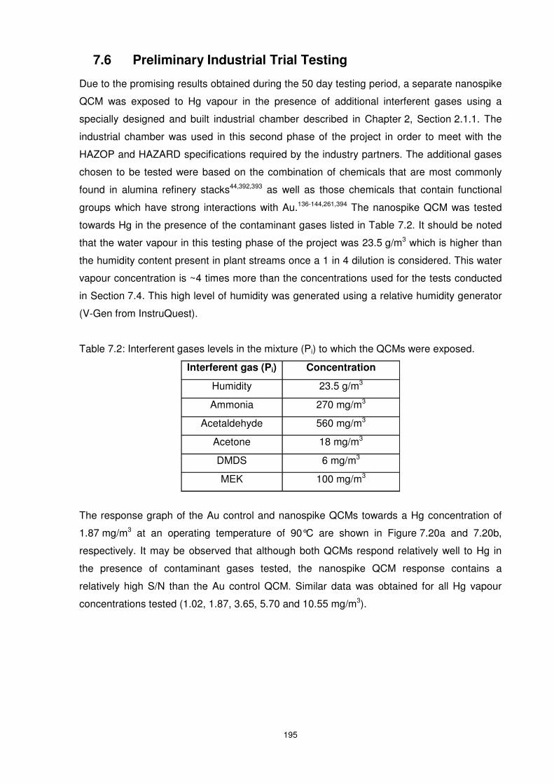
195
7.6 Preliminary Industrial Trial Testing
Due to the promising results obtained during the 50 day testing period, a separate nanospike
QCM was exposed to Hg vapour in the presence of additional interferent gases using a
specially designed and built industrial chamber described in Chapter 2, Section 2.1.1. The
industrial chamber was used in this second phase of the project in order to meet with the
HAZOP and HAZARD specifications required by the industry partners. The additional gases
chosen to be tested were based on the combination of chemicals that are most commonly
found in alumina refinery stacks44,392,393 as well as those chemicals that contain functional
groups which have strong interactions with Au.136-144,261,394 The nanospike QCM was tested
towards Hg in the presence of the contaminant gases listed in Table 7.2. It should be noted
that the water vapour in this testing phase of the project was 23.5 g/m3 which is higher than
the humidity content present in plant streams once a 1 in 4 dilution is considered. This water
vapour concentration is ~4 times more than the concentrations used for the tests conducted
in Section 7.4. This high level of humidity was generated using a relative humidity generator
(V-Gen from InstruQuest).
Table 7.2: Interferent gases levels in the mixture (Pi) to which the QCMs were exposed.
Interferent gas (Pi) Concentration
Humidity 23.5 g/m3
Ammonia 270 mg/m3
Acetaldehyde 560 mg/m3
Acetone 18 mg/m3
DMDS 6 mg/m3
MEK 100 mg/m3
The response graph of the Au control and nanospike QCMs towards a Hg concentration of
1.87 mg/m3 at an operating temperature of 90°C are shown in Figure 7.20a and 7.20b,
respectively. It may be observed that although both QCMs respond relatively well to Hg in
the presence of contaminant gases tested, the nanospike QCM response contains a
relatively high S/N than the Au control QCM. Similar data was obtained for all Hg vapour
concentrations tested (1.02, 1.87, 3.65, 5.70 and 10.55 mg/m3).
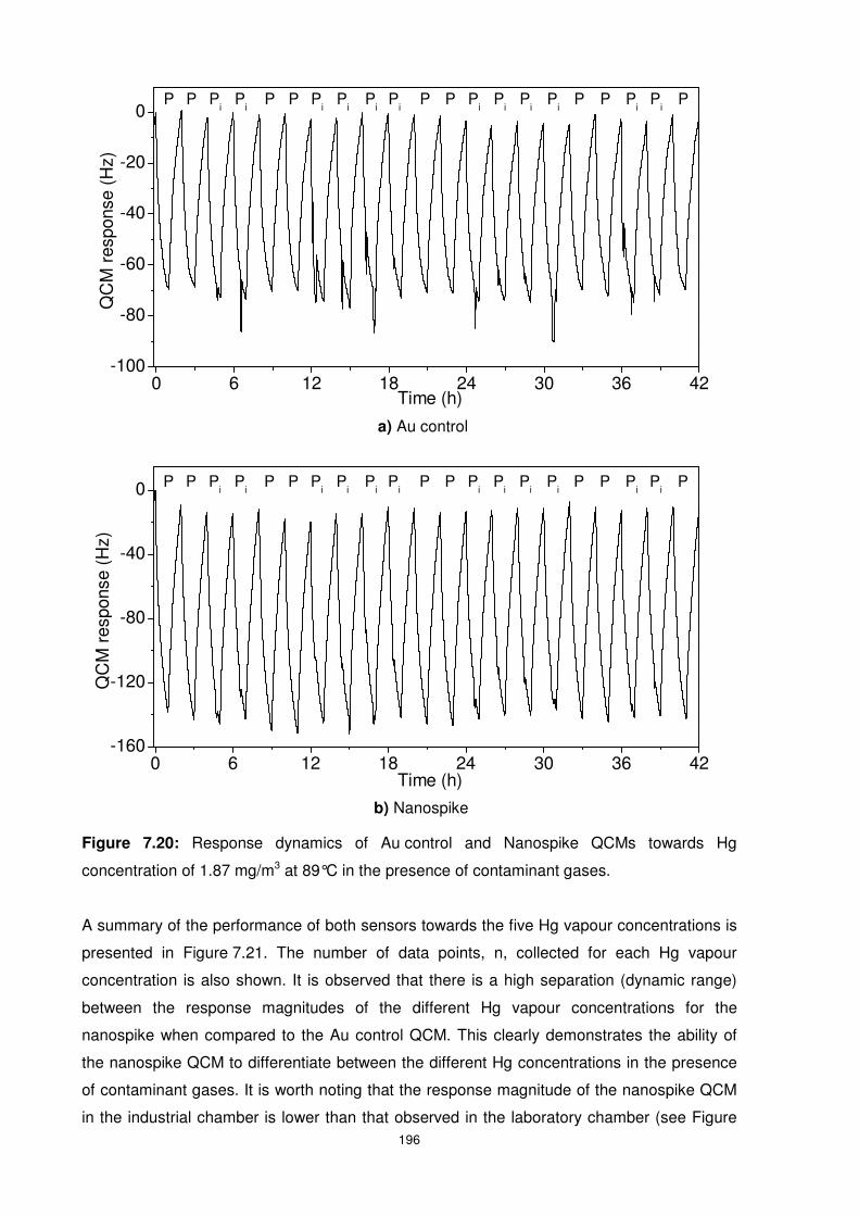
196
Figure 7.20: Response dynamics of Au control and Nanospike QCMs towards Hg
concentration of 1.87 mg/m3 at 89°C in the presence of contaminant gases.
A summary of the performance of both sensors towards the five Hg vapour concentrations is
presented in Figure 7.21. The number of data points, n, collected for each Hg vapour
concentration is also shown. It is observed that there is a high separation (dynamic range)
between the response magnitudes of the different Hg vapour concentrations for the
nanospike when compared to the Au control QCM. This clearly demonstrates the ability of
the nanospike QCM to differentiate between the different Hg concentrations in the presence
of contaminant gases. It is worth noting that the response magnitude of the nanospike QCM
in the industrial chamber is lower than that observed in the laboratory chamber (see Figure
a) Au control
b) Nanospike
0 6 12 18 24 30 36 42-160
-120
-80
-40
0
Time (h)
QC
M r
espo
nse
(Hz)
PPi
Pi
Pi
Pi
Pi
Pi
PPPPPPP P Pi
Pi
Pi
Pi
Pi
Pi
0 6 12 18 24 30 36 42-100
-80
-60
-40
-20
0
Q
CM
res
pons
e (H
z)
Time (h)
PPi
Pi
Pi
Pi
Pi
Pi
PPPPPPP P Pi
Pi
Pi
Pi
Pi
Pi
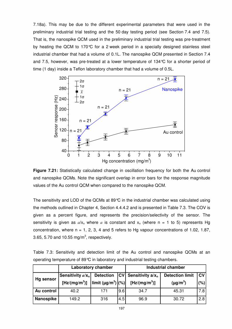
197
7.18a). This may be due to the different experimental parameters that were used in the
preliminary industrial trial testing and the 50 day testing period (see Section 7.4 and 7.5).
That is, the nanospike QCM used in the preliminary industrial trial testing was pre-treatment
by heating the QCM to 170°C for a 2 week period in a specially designed stainless steel
industrial chamber that had a volume of 0.1L. The nanospike QCM presented in Section 7.4
and 7.5, however, was pre-treated at a lower temperature of 134°C for a shorter period of
time (1 day) inside a Teflon laboratory chamber that had a volume of 0.5L.
Figure 7.21: Statistically calculated change in oscillation frequency for both the Au control
and nanospike QCMs. Note the significant overlap in error bars for the response magnitude
values of the Au control QCM when compared to the nanospike QCM.
The sensitivity and LOD of the QCMs at 89°C in the industrial chamber was calculated using
the methods outlined in Chapter 4, Section 4.4.4.2 and is presented in Table 7.3. The COV is
given as a percent figure, and represents the precision/selectivity of the sensor. The
sensitivity is given as a/xn where a is constant and xn (where n = 1 to 5) represents Hg
concentration, where n = 1, 2, 3, 4 and 5 refers to Hg vapour concentrations of 1.02, 1.87,
3.65, 5.70 and 10.55 mg/m3, respectively.
Table 7.3: Sensitivity and detection limit of the Au control and nanospike QCMs at an
operating temperature of 89°C in laboratory and industrial testing chambers.
Laboratory chamber Industrial chamber
Hg sensor Sensitivity a/xn
[Hz/(mg/m3)]
Detection
limit (µg/m3)
CV
(%)
Sensitivity a/xn
[Hz/(mg/m3)]
Detection limit
(µg/m3)
CV
(%)
Au control 40.2 171 9.6 34.7 45.31 7.8
Nanospike 149.2 316 4.5 96.9 30.72 2.8
x
1σ 2σ
1σ 2σ
0 1 2 3 4 5 6 7 8 9 10 1140
80
120
160
200
240
280
320 n = 21
n = 21
n = 21
n = 21
n = 21 Au control
Sen
osr
resp
onse
(H
z)
Hg concentration (mg/m3)
Nanospike
198
In the laboratory chamber, it was found that the Hg vapour sensitivity of the nanospike and
the Au control QCMs was Hg concentration dependent; the nanospike is observed to have
~4 times the sensitivity of Au control QCM towards Hg vapour. In the industrial chamber, the
nanospike QCM was observed to have better selectivity towards Hg vapour (low COV) and
~3 times the sensitivity of the Au control QCM. Although the response magnitude and
sensitivity of the nanospike has reduced in the industrial chamber due to the chamber’s
differing size, shape and construction (shown in Chapter 2), both the Au control and
nanospike QCMs are observed to attain the advantage of lower COV and LOD. This
indicates that using the nanospike QCM in the industrial chamber results in better selectivity
and the detection of lower Hg concentrations (down to 30.72 µg/m3) with a 95% confidence
level, as shown in Table 7.3. Overall, the nanospike Hg sensing data presented here
indicates that the nanospike QCMs could be used in a plant trial as a potential online Hg
vapour sensor for industrial effluent streams.
7.7 Summary
It is clearly evident from the mercury sensing studies that Au nanospikes directly
electrodeposited onto a QCM sensor can act as an excellent selective Hg vapour sensor in
the presence of various interferent gases. The Hg vapour sensing capability of this system at
an operating temperature of 89°C towards Hg vapour in the presence of interferent gases is
extremely relevant to industrial effluent streams. To the best of the Author’s knowledge, no
commercial sensor currently available in the market is capable of dealing with the interferent
gases tested during the preliminary industrial trial testing phase of this PhD program.
The developed Au nanospikes based QCM was clearly shown to have a quick response time
and large response magnitude due to the large surface area and presence of nodules and
other surface defects, which act as Hg sorption sites on the QCM. The deposited Au
nanospikes were observed to be highly (111) orientated, uniform and rigidly adhered to the
QCM Au electrode with the deposited mass not exceeding the linear region of the Sauerbrey
equation. The nanospike QCM tested in the Teflon laboratory chamber was found to
outperform the Au control QCM and had ~4 times the sensitivity and ~10 minutes faster
response time (t90) at an operating temperature of 89°C. Although the nanospike QCM had
~5.4 times the sensitivity of the Au control QCM at 28°C, data showed that selectivity
towards Hg vapour may be enhanced by operating at 89°C.
The nanospike sensor was tested towards a range of Hg vapour concentrations (1.02 to
10.55 mg/m3) in the presence of H2O and NH3 interferent gases at various levels over a 50
day period at an operating temperature of 89°C. The Hg pulse sequence during the long term
199
testing was developed to partially simulate industrial stream conditions. Due to the trade off
between response magnitude and dynamic range decreasing when operating temperature
increases, the operating temperature of 89°C was selected and kept constant during the
50 day testing period. The nanospike QCM was found to have high selectivity towards Hg
vapour in the presence of humidity and ammonia with a reduction of only 6 % in response
magnitude compared to the 20.8% reduction of the Au control based QCM following the
50 day testing period. Furthermore, the high dynamic range and low COV observed from the
data collected over the 50 day testing period indicated that the nanospikes are highly
sensitive and selective towards Hg vapour and may produce a more accurate result with high
precision when calibrated prior to use. That is, although a single calibration on the first day of
the 50 day testing produced excellent results with a Hg concentration reporting within ±7%
with a 95% confidence interval, if a calibration was conducted every 3 days, a reading within
±1.6% would be possible.
Due to the promising results, a separate nanospike QCM sensor was fabricated and an
industrial trial test was performed in the specially designed and built stainless steel chamber.
The sensor was tested towards Hg vapour in the presence of ammonia, humidity and
additional interferent gases that are commonly found in alumina refinery stacks as well as
those which contain functional groups which have strong affinity for Au (acetaldehyde,
acetone, dimethyl disulphide and methyl ethyl ketone). The nanospike QCM was observed to
maintain its high response magnitude, sensitivity and dynamic range relative to the
Au control based QCM. The high selectivity and sensitivity of the nanospike QCM towards
Hg vapour has resulted in financial support from industrial partners to undergo a plant trail
with the nanospike QCM in the near future. Furthermore, the electrodeposition conditions at
which the nanospikes are formed have been patented; due to the high potential for the
nanospike QCM to be used as online Hg vapour sensor (see Appendix A for patent details).
Future efforts are also directed towards the growth of Au nanospikes directly onto other
sensing platforms including the surface acoustic wave (SAW) platform99, so that sensors that
detect ultra-low concentrations of chemical and biological species can be developed. These
surfaces are also being investigated for (electro)-catalysis applications and as potential
surface enhanced Raman scattering (SERS) substrates. The vast potential commercial
implications of Au nanospikes for real-world sensing and catalysis applications cannot be
overemphasized.
200
7.8 References
(1) Veiga, M. M.; Maxson, P. A.; Hylander, L. D. Journal of Cleaner Production 2006, 14, 436-447.
(2) Reisch, M. In Business 2008; Vol. 86, p 22-23. (3) Goldman, R. L.; Shannon, M. W. Pediatrics 2001, 108, 197-205. (4) Rong, Y.; David Tee, L.; Joo Hwa, T. Environmental Science and Pollution Research
International 2003, 10, 399-407. (5) Palomares, E.; Vilar, R.; Durrant, J. R. Chem. Commun. 2004, 362-363. (6) Laudal, D. L.; French, N. B. In Conference On Air Quality II: Mercury 2000; Vol. 2, p
1-16. (7) Lockley, I. Emission Reduction program, 2007. (8) Sabri, Y. M.; Ippolito, S. J.; Bhargava, S. K. Light Metals 2009 2009, 37-42. (9) Government, A.; Department of the Environment, W., Heritage and the Arts, Ed.;
National Pullutant Inventory: 2009; Vol. 2007-2008. (10) Morency, J. Filtration & Separation 2002, 39, 24-26. (11) Germani, M. S.; Zollert, W. H. Environmental Science & Technology 1988, 22, 1079-
1085. (12) Fthenakis, V. M.; Lipfert, F. W.; Moskowitz, P. D.; Saroff, L. Journal of Hazardous
Materials 1995, 44, 267-283. (13) Dobbs, C.; Armanios, C.; McGuiness, L.; Bauer, G.; Ticehurst, P.; Lochore, J.; Irons,
R.; Ryan, R.; Adamek, G. In 7th International Alumina Quality Workshop Perth, Western Australia, 2005, p 199-204.
(14) Shao, R.; Tan, E. L.; Grimes, C. A.; Ong, K. G. Sensors Letters 2007, 5, 6. (15) Windham, R. L. Analytical Chemistry 1972, 44, 1334-1336. (16) Sabri, Y. M.; Ippolito, S. J.; Tardio, J.; Sood, D. K.; Bhargava, S. K.; Mullett, M.;
Harrison, I.; Rosenberg, S. In 8th International Alumina Quality Workshop Darwin, Australia, 2008, p 260-266.
(17) Caron, J. J. Surface Acoustic Wave Continuous Emissions Monitor for Total Mercury, Sensor Research and Development Corporation, 2001.
(18) Schweyer, M. G.; Andle, J. C.; McAllister, D. J.; Vetelino, J. F. Sensors and Actuators B: Chemical 1996, 35, 170-175.
(19) Laudal, D. L.; Thompson, J. S.; Pavlish, J. H.; Brickett, L. A.; Chu, P. Fuel Processing Technology 2004, 85, 501-511.
(20) Holmes, M.; Pavlish, J.; EERC, Ed. North Dakota, 2004; Vol. 2009. (21) Canstein, H. V.; Kelly, S.; Li, Y.; Wagner-Dobler, I. Applied and Environmental
Microbiology 2002, 68, 2829-2837. (22) Schrope, M. Nature news 2001, 409, 124-124. (23) Smith, R. P. Nature 2005, 436, 779-779. (24) Stokstad, E. Science 2004, 303, 34-. (25) Boyd, A. S.; Seger, D.; Vannucci, S.; Langley, M.; Abraham, J. L.; King, L. E. J.
Journal of the American Academy of Dermatology 2000, 43, 81-90. (26) Graeme, K. A.; Pollack, C. V. The Journal of emergency medicine 1998, 16, 45-56. (27) Baughman, T. A. Environmental Health Perspectives 2006, 114, 147-152. (28) Trasande, L.; Landrigan, P. J.; Schechter, C. Environmental Health Perspectives
2005, 113, 590-596. (29) LaMontagne, A. D.; Steenland, N. K.; Kelsey, K. Ethylene oxide; fourth ed.; Lippincott
& Wilkins: Philadelphia, 2007. (30) Morris, T. A. PhD by Research, The University of Alabama, 2004. (31) Laudal, D. L.; Brown, T. D.; Nott, B. R. Fuel Processing Technology 2000, 65-66,
157-165. (32) Bergan, T.; Gallardo, L.; Rodhe, H. Atmospheric Environment 1999, 33, 1575-1585. (33) Pacyna, E. G.; Pacyna, J. M.; Pirrone, N. Atmospheric Environment 2001, 35, 2987-
2996. (34) Kalac, P.; Niznanská, M.; Bevilaqua, D.; Stasková, I. Science of The Total
Environment 1996, 177, 251-258.
201
(35) Mukherjee, A. B.; Melanen, M.; Ekqvist, M.; Verta, M. The Science of The Total Environment 2000, 259, 73-83.
(36) Slemr, F.; Scheel, H. E. Atmospheric Environment 1998, 32, 845-853. (37) Shetty, S. K.; Lin, C.-J.; Streets, D. G.; Jang, C. Atmospheric Environment 2008, 42,
8674-8685. (38) Pacyna, E. G.; Pacyna, J. M. Water, Air, & Soil Pollution 2002, 137, 149-165. (39) Sjöholm, M.; Weibring, P.; Edner, H.; Svanberg, S. Opt. Express 2004, 12, 551-556. (40) Swain, E. B.; Jakus, P. M.; Rice, G.; Lupi, F.; Maxson, P. A.; Pacyna, J. M.; Penn, A.;
Spiegel, S. J.; Veiga, M. M. AMBIO: A Journal of the Human Environment 2007, 36, 45-61.
(41) Government, A. Mercury & compounds Emissions - All sources: Australia, National Pollutant Inventory, 2006-2007.
(42) Alcoa Environmental Review and Management Program, Alcoa, 2005. (43) Kockman, D.; Horvat, M.; Jacimovic, R.; Gibicar, D. RMZ - Materials and
Geoenvironment 2005, 52, 71-74. (44) Mullett, M.; Tardio, J.; Bhargava, S.; Dobbs, C. Journal of Hazardous Materials 2007,
144, 274-282. (45) Lacerda, L. D. Water, Air, & Soil Pollution 1997, 97, 247-255. (46) Johnson, J. Chemical and Engineering News 2001, 79, 18-19. (47) Powers, R. A. Proceedings of the IEEE 1995, 83, 687-693. (48) Pavlish, J. H.; Sondreal, E. A.; Mann, M. D.; Olson, E. S.; Galbreath, K. C.; Laudal, D.
L.; Benson, S. A. Fuel Processing Technology 2003, 82, 89-165. (49) Camargo, J. A. Nature 1993, 365, 302-302. (50) Hirokatsu Akagi, Y. F., Eigo Takabatake, Photochemistry and Photobiology 1977, 26,
363-370. (51) Pak, K.-R.; Bartha, R. Appl. Environ. Microbiol. 1998, 64, 1987-1990. (52) Bidone, E. D.; Castilhos, Z. C.; Cid de Souza, T. M.; Lacerda, L. D. Bulletin of
Environmental Contamination and Toxicology 1997, 59, 194-201. (53) Carpi, A. Water, Air, & Soil Pollution 1997, 98, 241-254. (54) Vallee, B. L.; Ulmer, D. D. Annual Review of Biochemistry 1972, 41, 91-128. (55) Gillis, A. A.; Miller, D. R. The Science of The Total Environment 2000, 260, 191-200. (56) Schroeder, W. H.; Munthe, J. Atmospheric Environment 1998, 32, 809-822. (57) Hacon, S.; Rochedo, E. R.; Campos, R.; Rosales, G.; Lacerda, L. D. Water, Air, &
Soil Pollution 1997, 97, 91-105. (58) Scallan, K. F., University of California, 2007. (59) Levlin, M.; Ikävalko, E.; Laitinen, T. Fresenius' Journal of Analytical Chemistry 1999,
365, 577-586. (60) Guminski, C. Journal of the Less Common Metals 1991, 168, 329-334. (61) McNerney, J. J.; Buseck, P. R.; Hanson, R. C. Science 1972, 178, 611-612. (62) Granite, E. J.; Pennline, H. W.; Hargis, R. A. Industrial & Engineering Chemistry
Research 2000, 39, 1020-1029. (63) Braman, R. S.; Johnson, D. L. Environmental Science & Technology 1974, 8, 996-
1003. (64) Yan, T. Y. Industrial & Engineering Chemistry Research 1994, 33, 3010-3014. (65) Diggs, T. H.; Ledbetter, J. O. American Industrial Hygiene Association Journal 1983,
44, 606 - 608. (66) Reed, C. E.; Kanazawa, K. K.; Kaufman, J. H. Journal of Applied Physics 1990, 68,
1993-2001. (67) Dumarey, R.; Dams, R.; Hoste, J. Analytical Chemistry 1985, 57, 2638-2643. (68) Schroeder, W. H.; Hamilton, M. C.; Stobart, S. R. REV. ANALYT. CHEM. 1985, 8,
179-209. (69) Be'er, A.; Lereah, Y.; Frydman, A.; Taitelbaum, H. Physica A: Statistical Mechanics
and its Applications 2002, 314, 325-330. (70) Guminski, C.; Galus, A.; Hirayama, C. In Solubility Data Series: Metals in Mercury;
Warsaw, U. O., Ed.; Pergamon Press: Warsaw, Poland, 1986; Vol. 25, p 258-384. (71) Strachan, J. F.; Harris, N. L. Journal of the Institute of Metals 1956, 85, 17-24.
202
(72) Sunier, A. A.; Gramkee, B. E. Journal of the American Chemical Society 1929, 51, 1703-1708.
(73) Sunier, A. A.; Weiner, L. G. Journal of the American Chemical Society 1931, 53, 1714-1721.
(74) Sunier, A. A.; White, C. M. Journal of American Chemical Society 1930, 52, 1842-1850.
(75) Mees, G. Journal of the American Chemical Society 1938, 60, 870-871. (76) Anderson, J. T. The Journal of Physical Chemistry 1932, 36, 2145-2165. (77) Brown, J. B. Journal of Chemical Education 1960, 37, 415. (78) Levlin, M.; Ikavalko, E.; Laitinen, T. Fresenius Journal of Analytical Chemistry 1999,
365, 577-586. (79) Rex, M.; Hernandez, F. E.; Campiglia, A. D. Analytical Chemistry 2006, 78, 445-451. (80) Ruys, D. P.; Andrade, J. F.; Guimaraes, O. M. Analytica Chimica Acta 2000, 404, 95-
100. (81) Battistoni, C.; Bemporad, E.; Galdikas, A.; Kaciulis, S.; Mattogno, G.; Mickevicius, S.;
Olevano, V. Applied Surface Science 1996, 103, 107-111. (82) Morris, T.; Szulczewski, G. Langmuir 2002, 18, 5823-5829. (83) Morris, T.; Szulczewski, G. Langmuir 2002, 18, 2260-2264. (84) Morris, T.; Sun, J.; Szulczewski, G. Analytica Chimica Acta 2003, 496, 279-287. (85) Kobiela, T.; Nowakowski, B.; Dus, R. Applied Surface Science 2003, 206, 78-89. (86) Nowakowski, R.; Kobiela, T.; Wolfram, Z.; Dus, R. Applied Surface Science 1997,
115, 217-231. (87) Fialkowski, M.; Grzeszczak, P.; Nowakowski, R.; Holyst, R. The Journal of Physical
Chemistry B 2004, 108, 5026-5030. (88) Brosset, C.; Iverfeldt, Å. Water, Air, & Soil Pollution 1989, 43, 147-168. (89) Sabri, Y. M.; Ippolito, S. J.; Tardio, J.; Atanacio, A. J.; Sood, D. K.; Bhargava, S. K.
Sensors and Actuators B: Chemical 2009, 137, 246-252. (90) George, M. A. PhD by research, Arizona State University, 1991. (91) Aiyer, H. N.; Kawazoe, T.; Lim, J.; Echigo, Y.; Ohtsu, M. Nanotechnology 2001, 12,
368-371. (92) Be'er, A.; Hecht, I.; Taitelbaum, H. Physical Review E 2005, 72, 031606. (93) George, M. A.; Glaunsinger, W. S. Thin Solid Films 1994, 245, 215-224. (94) George, M. A.; Glaunsinger, W. S.; Thundat, T.; Lindsay, S. M. Thin Solid Films 1990,
189, 59-72. (95) Nowakowski, R.; Pielaszek, J.; Dus, R. Applied Surface Science 2002, 199, 40-51. (96) Yang, X. M.; Tonami, K.; Nagahara, L. A.; Hashimoto, K.; Wei, Y.; Fujishima, A.
Surface Science 1994, 319, L17-L22. (97) Scheide, E. P.; Taylor, J. K. American Industrial Hygiene Association Journal 1975,
36, 897 - 901. (98) Stobinski, L.; Dus, R. Surface Science 1993, 298, 101-106. (99) Haskell, R. L. B.; Caron, J. J.; Duptisea, M. A.; Ouellette, J. J.; Vetelino, J. F. In
Ultrasonics Symposium, 1999. Proceedings; IEEE: Orono, ME, 1999; Vol. 1, p 429-434 vol.1.
(100) Chaurasia, H. K.; Huizinga, A.; Voss, W. A. G. Journal of Physics D: Applied Physics 1975, 8, 214-218.
(101) Drelich, J.; White, C. L.; Xu, Z. Environ. Sci. Technol. 2008, 42, 2072-2078. (102) Kalb, G. W. Atomic Absorption Newsletter 1970, 9, 4. (103) Larjava, K.; Laitinen, T.; Vahlman, T.; Artmann, S.; Siemens, V.; Broekaert, J. A. C.;
Klockow, D. International journal of environmental analytical chemistry 1992, 49, 73 - 85.
(104) Larjava, K.; Laitinen, T.; Kiviranta, T.; Siemens, V.; Klockow, D. International journal of environmental analytical chemistry 1993, 52, 65-73.
(105) Jansen, H. J. F.; Freeman, A. J.; Weinert, M.; Wimmer, E. Physical Review B 1983, 28, 593.
(106) Mott, N. F. Philosophical Magazine 1961, 6, 287 - 309. (107) Dowben, P. A. Surface Science Reports 2000, 40, 151-247.
203
(108) Miedema, A. R.; Dorleijn, J. W. F. Philosophical Magazine Part B: Physics of Condensed matter: Statistical Mechanics, Electronics, Optical and Magnetic Properties 1981, 43, 251-272.
(109) Schmutzler, R. W.; Hensel, F. Journal of Non-Crystalline Solids 1972, 8-10, 718-721. (110) El-Hanany, U.; Warren, W. W. Physical Review Letters 1975, 34, 1276. (111) Even, U.; Jortner, J. Physical Review Letters 1972, 28, 31. (112) Hensel, F. Berichte der Bunsengesellschaft fur Physikalische Chemie 1976, 80, 786-
789. (113) Cheshnovski, O.; Even, U.; Jortner, J. Solid State Communications 1977, 22, 745-
748. (114) Gaston, N.; Schwerdtfeger, P. Physical Review B (Condensed Matter and Materials
Physics) 2006, 74, 024105-12. (115) Ballone, P.; Galli, G. Physical Review B 1989, 40, 8563. (116) Steckel, J. A. Physical Review B (Condensed Matter and Materials Physics) 2008,
77, 115412. (117) Bloch, A. N.; Rice, S. A. Physical Review 1969, 185, 933. (118) Kutana, A.; Giapis, K. P. Nano Lett. 2006, 6, 656-661. (119) Chandra, S.; Di Marzo, M.; Qiao, Y. M.; Tartarini, P. Fire Safety Journal 1996, 27,
141-158. (120) Henn, A. R. Biophysical Chemistry 2003, 105, 533-543. (121) Lennard-Jones, J. E.; Corner, J. Transactions of the Faraday Society 1940, 36, 1156-
1162. (122) Joseph McGuire, E. L., Robert D. Sproull, Surface and Interface Analysis 1990, 15,
603-608. (123) Rhee, S. K. Journal of the American Ceramic Society 1970, 53, 386-389. (124) Granite, E. J. In Annual International Pittsburgh Coal Conference Pittsburgh, 2003;
Vol. 20, p 983-1010. (125) Abollino, O.; Giacomino, A.; Malandrino, M.; Piscionieri, G.; Mentasti, E.
Electroanalysis 2008, 20, 75-83. (126) Clevenger, W. L.; Smith, B. W.; Winefordner, J. D. Critical Reviews in Analytical
Chemistry 1997, 27, 1-26. (127) Temmerman, E.; Vandecasteele, C.; Vermeir, G.; Leyman, R.; Dams, R. Analytica
Chimica Acta 1990, 236, 371-376. (128) Sánchez Uría, J. E.; Sanz-Medel, A. Talanta 1998, 47, 509-524. (129) Blanco, R. M.; Villanueva, M. T.; Uría, J. E. S.; Sanz-Medel, A. Analytica Chimica
Acta 2000, 419, 137-144. (130) Das, A. K.; de la Guardia, M.; Cervera, M. L. Talanta 2001, 55, 1-28. (131) Logar, M.; Horvat, M.; Akagi, H.; Pihlar, B. Analytical and Bioanalytical Chemistry
2002, 374, 1015-1021. (132) Tong, X.; Barat, R. B.; Poulos, A. T. Review of Scientific Instruments 2002, 73, 2392-
2397. (133) Granite, E. J.; Pennline, H. W. Industrial & Engineering Chemistry Research 2002,
41, 5470-5476. (134) Weissberg, B. G. Economic Geology 1971, 66, 1042-1047. (135) Sholupov, S.; Pogarev, S.; Ryzhov, V.; Mashyanov, N.; Stroganov, A. Fuel
Processing Technology 2004, 85, 473-485. (136) Rocha, T. A. P.; Gomes, M. T. S. R.; Duarte, A. C.; Oliveira, J. A. B. P. Analytical
Communication 1998, 35, 415-416. (137) Richton, R. E.; Farrow, L. A. The Journal of Physical Chemistry 2002, 85, 3577-3581. (138) Bilic, A.; Reimers, J. R.; Hush, N. S.; Hafner, J. The Journal of Chemical Physics
2002, 116, 8981-8987. (139) Kay, B. D.; Lykke, K. R.; Creighton, J. R.; Ward, S. J. The Journal of Chemical
Physics 1989, 91, 5120-5121. (140) Surplice, N. A.; Brearley, W. Surface Science 1975, 52, 62-74. (141) Nuss, H.; Jansen, M. Angewandte Chemie 2006, 45, 4369-4371. (142) de Vooys, A. C. A.; Mrozek, M. F.; Koper, M. T. M.; van Santen, R. A.; van Veen, J.
A. R.; Weaver, M. J. Electrochemistry Communications 2001, 3, 293-298.
204
(143) Mirsky, V. M.; Vasjari, M.; Novotny, I.; Rehacek, V.; Tvarozek, V.; Wolfbeis, O. S. Nanotechnology 2002, 13, 175-178.
(144) Meyer, R.; Lemire, C.; Shaikhutdinov, S. K.; Freund, H. Gold Bulletin 2004, 37, 72-124.
(145) Caron, J. J. O., ME), Haskell, Reichl B. (Veazie, ME), Freeman, Carl J. (Rockville, MD), Vetelino, John F. (Orono, ME); Sensor Research and Development Corp. (Orono, ME): United States, 1999.
(146) Levlin, M.; Niemi, H. E. M.; Hautojärvi, P.; Ikävalko, E.; Laitinen, T. Fresenius' Journal of Analytical Chemistry 1996, 355, 2-9.
(147) Kvietkus, K.; Xiao, Z.; Lindqvist, O. Water, Air, & Soil Pollution 1995, 80, 1209-1216. (148) Skreblin, M.; Byrne, A. R. Vestnik Slovenskega Kemijskega Drustva 1991, 38, 16. (149) Mazzolai, B.; Mattoli, V.; Raffa, V.; Tripoli, G.; Accoto, D.; Menciassi, A.; Dario, P.
Sensors and Actuators A: Physical 2004, 113, 282-287. (150) Mazzolai, B.; Mattoli, V.; Raffa, V.; Tripoli, G.; Accoto, D.; Menciassi, A.; Dario, P. In Sensors
and Microsystems, Proceedings of the Italian Conference; 8 ed. Trento, Italy,, 2003; Vol. 8, p 369-375.
(151) Morris, T.; Kloepper, K.; Wilson, S.; Szulczewski, G. Journal of Colloid and Interface Science 2002, 254, 49-55.
(152) Dimasi, E.; Tostmann, H.; Ocko, B. M.; Huber, P.; Shpyrko, O. G.; Pershan, P. S.; Deutsch, M.; Berman, L. E. In Materials Research Society Symposium Proceedings 2000; Vol. 590, p 183-188.
(153) Butler, M. A.; Ricco, A. J.; Baughman, R. J. Journal of Applied Physics 1990, 67, 4320-4326.
(154) Chah, S.; Yi, J.; Zare, R. N. Sensors and Actuators B: Chemical 2004, 99, 216-222. (155) Hughes, R. C.; Ricco, A. J.; Butler, M. A.; Martin, S. J. Science 1991, 254, 74-80. (156) Ryan, M. A.; Homer, M. L.; Shevade, A. V.; Lara, L. M.; Yen, S.-P. S.; Kisor, A. K.;
Manatt, K. S. ECS Meeting Abstracts 2008, 16, 431-439. (157) RA-915+, l. (158) Lumex 2008. (159) Gochfeld, M. Ecotoxicology and Environmental Safety 2003, 56, 174-179. (160) Holland, K. New York, 2005; Vol. 2009. (161) Ritchie, K. A.; Burke, F. J. T.; Gilmour, W. H.; Macdonald, E. B.; Dale, I. M.; Hamilton,
R. M.; McGowan, D. A.; Binnie, V.; Collington, D.; Hammersley, R. British Dental Journal 2004, 197, 625-632.
(162) Kramer, C. 2001; Vol. 2008. (163) Arizona Instruments LLC Arizona, 2007; Vol. 2009, p mercury sensors. (164) Wu, J. M.; Huang, H. S.; Livengood, C. D. Development of a sorbent-based
technology for control of mercury in flue gas, 1996. (165) Loredo, J.; Soto, J.; Álvarez, R.; Ordóñez, A. Environmental Monitoring and
Assessment 2007, 130, 201-214. (166) Monitor, T. V. M. V. 2006, p Mercury sensor. (167) Choi, H. K.; Lee, S. H.; Kim, S. S. Fuel Processing Technology 2009, 90, 107-112. (168) Mercury Instruments USA 2009; Vol. 2009. (169) Wängberg, I.; Edner, H.; Ferrara, R.; Lanzillotta, E.; Munthe, J.; Sommar, J.; Sjöholm,
M.; Svanberg, S.; Weibring, P. The Science of The Total Environment 2003, 304, 29-41.
(170) Ferrara, R.; Mazzolai, B. The Science of The Total Environment 1998, 215, 51-57. (171) Ippolito, S. J.; Trinchi, A.; Powell, D. A.; Wlodarski, W. In Solid State Gas Sensing;
Comini, E., Faglia, G., Sberveglieri, G., Eds.; Springer Science+Business Media, LLC: Brescia, Italy, 2009; Vol. 1, p 329.
(172) Ballantine, D. S.; Wohltjen, H. Analytical Chemistry 1989, 61, 704A-715A. (173) Ward, M. D.; Buttry, D. A. Science 1990, 249, 1000-1007. (174) Sauerbrey, G. Zeitschrift für Physik A Hadrons and Nuclei 1959, 155, 206-222. (175) Martin, S. J.; Granstaff, V. E.; Frye, G. C. Analytical Chemistry 1991, 63, 2272-2281. (176) Kanazawa, K. K.; Gordon, J. G. Analytical Chemistry 1985, 57, 1770-1771. (177) Martin, S. J.; Frye, G. C.; Ricco, A. J.; Senturia, S. D. Analytical Chemistry 1993, 65,
2910-2922.
205
(178) Dong, Y. Sensors and Actuators B: Chemical 2005, 108, 622-626. (179) Smith, A. L.; Shirazi, H. M. Thermochimica Acta 2005, 432, 202-211. (180) Smith, A. L.; Shirazi, H. M.; Mulligan, S. R. Biochimica et Biophysica Acta (BBA) -
Protein Structure and Molecular Enzymology 2002, 1594, 150-159. (181) Al Kobaisi, M. Doctor of Philosophy, Royal Melbourne Institue of Technology
University, 2008. (182) Janshoff, A.; Galla, H.-J.; Steinem, C. Angewandte Chemie 2000, 39, 4004-4032. (183) Beil, F. W.; Blick, R. H.; Wixforth, A. Physica E: Low-dimensional Systems and
Nanostructures 2004, 21, 1106-1110. (184) Schweyer, M. G.; Weaver, J. T.; Andle, J. C.; McAllister, D. J.; French, L.; Vetelino, J.;
Height, J. J. In Frequency Control Symposium, 1997., Proceedings of the 1997 IEEE International 1997, p 147-155.
(185) Venema, A.; Nieuwkoop, E.; Vellekoop, M. J.; Ghijsen, W. J.; Barendsz, A. W.; Nieuwenhuizen, M. S. IEEE Transactions on Ultrasonics, Ferroelectrics and Frequency Control 1987, 34, 148-155.
(186) Thiele, J. A.; da Cunha, M. P. Sensors and Actuators B: Chemical 2006, 113, 816-822.
(187) Arnau, A.; Ferrari, V.; Soares, D.; Perrot, H. In Piezoelectric Transducers and Applications; Springer Berlin Heidelberg: 2008, p 117-186.
(188) Arnau, A. Sensors 2008, 8, 370-411. (189) O'Sullivan, C. K.; Guilbault, G. G. Biosensors and Bioelectronics 1999, 14, 663-670. (190) James, D.; Scott, S. M.; Ali, Z.; O’Hare, W. T. Microchimica Acta 2005, 149, 1-17. (191) Cheeke, J. D. N.; Wang, Z. Sensors and Actuators B: Chemical 1999, 59, 146-153. (192) Khlebarov, Z. P.; Stoyanova, A. I.; Topalova, D. I. Sensors and Actuators B: Chemical
1992, 8, 33-40. (193) Fox, C. G.; Alderm, J. F. Analyst 1989, 114, 997-1004. (194) Ali, Z. Journal of thermal analysis and calorimetry 1999, 55, 397-412. (195) Tsionsky, V.; Gileadi, E. Langmuir 1994, 10, 2830-2835. (196) Flitti, F.; Far, A.; Guo, B.; Bermak, A. Journal of Sensors 2008, 2008, 1-6. (197) Buck, R. P.; Lindner, E.; Kutner, W.; Inzelt, G. Pure & Applied Chemistry 2004, 76,
1139-1160. (198) Zimmermann, B.; Lucklum, R.; Hauptmann, P.; Rabe, J.; Büttgenbach, S. Sensors
and Actuators B: Chemical 2001, 76, 47-57. (199) Sagmeister, B. P.; Graz, I. M.; Schwödiauer, R.; Gruber, H.; Bauer, S. Biosensors
and Bioelectronics 2009, 24, 2643-2648. (200) Bender, J. W.; Krim, J. In Microscale Diagnostic Techniques 2005, p 227-259. (201) Herrmann, F.; Jakoby, B.; Rabe, J.; Büttgenbach, S. Sensors Update 2001, 9, 105-
160. (202) Ballato, A.; Gualtieri, J. G. Ultrasonics, Ferroelectrics and Frequency Control, IEEE
Transactions on 1994, 41, 834-844. (203) Lakin, K. M.; Wang, J. S. Applied Physics Letters 1981, 38, 125-127. (204) Granstaff, V. E.; Martin, S. J. Journal of Applied Physics 1994, 75, 1319-1329. (205) Behling, C.; Lucklum, R.; Hauptmann, P. Sensors and Actuators A: Physical 1997,
61, 260-266. (206) Thanner, H.; Krempl, P.; Selic, R.; Wallnöfer, W.; Worsch, P. Journal of Thermal
Analysis and Calorimetry 2003, 71, 53-59. (207) Bechmann, R. Journal of Scientific Instruments 1952, 29, 73-76. (208) Shockley, W.; Curran, D. R.; Koneval, D. J. The Journal of the Acoustical Society of
America 1967, 41, 981-993. (209) Behling, C.; Lucklum, R.; Hauptmann, P. Sensors and Actuators A: Physical 1998,
68, 388-398. (210) Mecea, V. M. Sensors and Actuators A: Physical 1994, 40, 1-27. (211) Lu, C.-S.; Lewis, O. Journal of Applied Physics 1972, 43, 4385-4390. (212) Ippolito, S. J. PhD by research, RMIT university, 2006. (213) Ho, M. H.; Guilbault, G. G.; Scheide, E. P. Analytica Chimica Acta 1981, 130, 141-
147. (214) Konash, P. L.; Bastiaans, G. J. Analytical Chemistry 1980, 52, 1929-1931.
206
(215) Grate, J. W.; Martin, S. J.; White, R. M. Analytical Chemistry 1993, 65, 987A-996A. (216) Benes, E.; Gröschl, M.; Burger, W.; Schmid, M. Sensors and Actuators A: Physical
1995, 48, 1-21. (217) Auge, J., University of Magdeburg, 1995. (218) Janata, J.; Josowicz, M.; DeVaney, D. M. Analytical Chemistry 1994, 66, 207-228. (219) Bethea, T.; Cady-Sawyer, K.; Ettenson, L.; Harris, K.; Mandl, D.; Martynowicz, K.;
Raeisghasem, A.; Westman, D. Columbia, USA, 2005. (220) Fox, B. S.; Mason, K. J.; McElroy, F. C. Journal of ASTM International (JAI) 2005, 2,
11. (221) Meischen, S. J.; VanPelt, V. J.; Zarate, E. A. In 95th Proceedings of the Air & Waste
Management Association’s Annual Conference & Exhibition 2002, p 1364-1378. (222) Magnuson, J. K.; Anderson, T. N.; Lucht, R. P.; Vijayasarathy, U. A.; Kalyan, A. In
23rd Proceedings - Annual International Pittsburgh Coal Conference (2006) Pittsburgh, 2006; Vol. 14, p 1-14.
(223) Appel, D.; Grassi, J. H.; Kita, D.; Socha, J. United States, 2008. (224) Raffa, V.; Mazzolai, B.; Mattoli, V.; Mondini, A.; Dario, P. Sensors and Actuators B:
Chemical 2006, 114, 513-521. (225) McNerney, J. J.; Buseck, P. R. Gold Bulletin 1973, 6, 106-107. (226) Jerome411X. (227) Shevade, A.; Blanco, M.; Goddard, W.; Ryan, M.; Homer, M.; Taylor, C.; Jewell, A.;
Kisor, A.; Yen, S.-P.; Manatt, K.; Zhou, H.; Pelletier, C.; Lewis, C. ECS Meeting Abstracts 2006, 601, 1243-1243.
(228) Ryan, M. A.; Homer, M. L.; Zhou, H.; Mannat, K.; Manfreda, A.; Kisor, A. K.; Shevade, A. V.; Yen, S.-P. S. In International Conference on Environmental Systems; Jet Propulsion Laboratory, National Aeronautics and Space Administration: Rome, Italy, 2005, p 1-8.
(229) Ryan, M. A.; Shevade, A. V.; Zhou, H.; Homer, M. L. MRS Bulletin 2004, 29, 714. (230) Huang, S. W.; Neoh, K. G.; Shih, C. W.; Lim, D. S.; Kang, E. T.; Han, H. S.; Tan, K. L.
Synthetic Metals 1998, 96, 117-122. (231) Choudary, B. M.; Madhi, S.; Chowdari, N. S.; Kantam, M. L.; Sreedhar, B. Journal of
the American Chemical Society 2002, 124, 14127-14136. (232) Weibring, P.; Andersson, M.; Edner, H.; Svanberg, S. Applied Physics B: Lasers and
Optics 1998, 66, 383-388. (233) Edner, H.; Ragnarson, P.; Wallinder, E. Environmental Science & Technology 2002,
29, 330-337. (234) Toth, J. J.; Wittman, R.; Schenter, R. E.; Cooper, J. A. Nuclear Instruments and
Methods in Physics Research Section A: Accelerators, Spectrometers, Detectors and Associated Equipment 2007, 572, 1102-1105.
(235) D'ottone, L. K. B., FL, US) United States, 2006. (236) Adams, J. D.; Rogers, B.; Manning, L.; Hu, Z.; Thundat, T.; Cavazos, H.; Minne, S. C.
Sensors and Actuators A: Physical 2005, 121, 457-461. (237) Thundat, T.; Wachter, E. A.; Sharp, S. L.; Warmack, R. J. Applied Physics Letters
1995, 66, 1695-1697. (238) Fadel, L.; Dufour, I.; Lochon, F.; Francais, O. Sensors and Actuators B: Chemical
2004, 102, 73-77. (239) Hu, Z.; Thundat, T.; Warmack, R. J. Journal of Applied Physics 2001, 90, 427-431. (240) Berger, R.; Delamarche, E.; Lang, H. P.; Gerber, C.; Gimzewski, J. K.; Meyer, E.;
Güntherodt, H. J. Applied Physics A: Materials Science & Processing 1998, 66, S55-S59.
(241) Marie, R.; Jensenius, H.; Thaysen, J.; Christensen, C. B.; Boisen, A. Ultramicroscopy 2002, 91, 29-36.
(242) Butler, M. A.; Ricco, A. J. Applied Physics Letters 1988, 53, 1471-1473. (243) Manganiello, L.; Rios, A.; Valcarcel, M. Analytical Chemistry 2002, 74, 921-925. (244) Yao, S.; Tan, S.; Nie, L. Fenxi Huaxue 1986, 14, 6. (245) Casilli, S.; Malitesta, C.; Conoci, S.; Petralia, S.; Sortino, S.; Valli, L. Biosensors and
Bioelectronics 2004, 20, 1190-1195.
207
(246) Rogers, B.; Bauer, C. A.; Adams, J. D. Micro-Electro-Mechanical Systems 2003, 5, 663-666.
(247) Gomes, M. T. S. R.; Oliveira, M. O.; Oliveira, J. A. B. P. Langmuir 1999, 15, 8780-8782.
(248) Bristow, Q. Journal of Geochemical Exploration 1972, 1, 55-76. (249) Scheide, E. P.; Taylor, J. K. Environ. Sci. Technol. 1974, 8, 1097-1099. (250) Scheide, E. P. Physics Teacher 1977, 15, 47-51. (251) McCammon, C. S. J.; Woodfin, J. W. American Industrial Hygiene Association
Journal 1977, 38, 378-386. (252) Scheide, E. P.; Warnar, R. B. American Industrial Hygiene Association Journal 1978,
39, 745-749. (253) Mogilevski, A. N.; Mayorov, A. D.; Stroganova, N. S.; Stavrovski, D. B.; Galkina, I. P.;
Spassov, L.; Mihailov, D.; Zaharieva, R. Sensors and Actuators A: Physical 1991, 28, 35-39.
(254) Spassov, L.; Yankov, D. Y.; Mogilevski, A. N.; Mayorov, A. D. Review of Scientific Instruments 1993, 64, 225-227.
(255) Caron, J. J.; Haskell, R. B.; Benoit, P.; Vetelino, J. F. IEEE transactions on ultrasonics, ferroelectrics, and frequency control 1998, 45, 1393-1398.
(256) Haskell, R. B. Masters, University of Maine, 2003. (257) Mercer, T. T. Analytical Chemistry 1979, 51, 5. (258) Hirvonen, J. K.; Weisenberger, W. H.; Westmoreland, J. E.; Meussner, R. A. Applied
Physics Letters 1972, 21, 37-39. (259) Cox, H. H. J.; Deshusses, M. A. Chemical Engineering Journal 2002, 87, 101-110. (260) McNamara, J. D.; Wagner, N. J. Gas Separation & Purification 1996, 10, 137-140. (261) Finklea, H. O.; Avery, S.; Lynch, M.; Furtsch, T. Langmuir 2002, 3, 409-413. (262) Himmelhaus, M.; Buck, M.; Grunze, M. Applied Physics B: Lasers and Optics 1999,
68, 595-598. (263) Thome, J.; Himmelhaus, M.; Zharnikov, M.; Grunze, M. Langmuir 1998, 14, 7435-
7449. (264) Aliganga, A. K. A.; Wang, Z.; Mittler, S. The Journal of Physical Chemistry B 2004,
108, 10949-10954. (265) Li, D.; Ma, M. Sensors and Actuators B: Chemical 2000, 69, 75-84. (266) Joyner, R. W.; Roberts, M. W. Journal of the Chemical Society Faraday Transactions
1 1973, 69, 1242-1250. (267) Atkins, P. W. Physical Chemistry; 2nd ed.; Oxford University Press: Oxford, Great
Britain, 1982. (268) Nott, B. R. Water, Air, & Soil Pollution 1995, 80, 1311-1314. (269) Nilsson, S.; Klett, O.; Svedberg, M.; Amirkhani, A.; Nyholm, L. Rapid Communications
in Mass Spectrometry 2003, 17, 1535-1540. (270) Hoogvliet, J. C.; van Bennekom, W. P. Electrochimica Acta 2001, 47, 599-611. (271) Sexton, B. A.; Feltis, B. N.; Davis, T. J. Sensors and Actuators A: Physical 2008, 141,
471-475. (272) Ali, M. B.; Bessueille, F.; Chovelon, J. M.; Abdelghani, A.; Jaffrezic-Renault, N.;
Maaref, M. A.; Martelet, C. Materials Science and Engineering: C 2008, 28, 628-632. (273) Moody, N. R.; Adams, D. P.; Medlin, D.; Headley, T.; Yang, N.; Volinsky, A.
International Journal of Fracture 2003, 120, 407-419. (274) Rand, D. A. J.; Woods, R. Journal of Electroanalytical Chemistry 1971, 31, 29-38. (275) García-Sánchez, A.; Contreras, F.; Adams, M.; Santos, F. Environmental
Geochemistry and Health 2006, 28, 529-540. (276) Li, J.; Herrero, E.; Abruña, H. D. Colloids and Surfaces A: Physicochemical and
Engineering Aspects 1998, 134, 113-131. (277) Schoettel, G.; Vittal, J. J.; Puddephatt, R. J. Journal of the American Chemical
Society 1990, 112, 6400-6402. (278) Scott, J. E.; Ottaway, J. M. Analyst 1981, 106, 1076-1081. (279) McDonagh, C.; Bowe, P.; Mongey, K.; MacCraith, B. D. Journal of Non-Crystalline
Solids 2002, 306, 138-148.
208
(280) Bohets, H.; Vanhoutte, K.; De Maesschalck, R.; Cockaerts, P.; Vissers, B.; Nagels, L. J. Analytica Chimica Acta 2007, 581, 181-191.
(281) Crank, J. The Mathematics of Diffusion; Oxford University Press, London, England, 1975; Vol. 2nd edition.
(282) Richaud, R.; Lachas, H.; Healey, A. E.; Reed, G. P.; Haines, J.; Jarvis, K. E.; Herod, A. A.; Dugwell, D. R.; Kandiyoti, R. Fuel 2000, 79, 1077-1087.
(283) Krata, A.; Bulska, E. Spectrochimica Acta Part B: Atomic Spectroscopy 2005, 60, 345-350.
(284) Ping, L.; Dasgupta, P. K. Analytical Chemistry 1989, 61, 1230-1235. (285) Takaya, M.; Joeng, J. Y.; Ishihara, N.; Serita, F.; Kohyama, N. Industrial Health 2006,
44, 287-290. (286) Marins, R. V.; de Andrade, J. B.; Pereira, P. A. d. P.; Paiva, E. C.; Paraquetti, H. H.
M. Journal of Environmental Monitoring 2000, 2, 325-328. (287) Moreno, F. N.; Anderson, C. W. N.; Stewart, R. B.; Robinson, B. H. Environmental
and Experimental Botany 2008, 62, 78-85. (288) Ford, R. R.; Pritchard, J. Transactions of the Faraday Society 1971, 67, 216-221. (289) George, M. A.; Glaunsinger, W. S.; Thundat, T.; Lindsay, S. M. Journal of Microscopy
1988, 152, 703-713. (290) Inukai, J.; Sugita, S.; Itaya, K. Journal of Electroanalytical Chemistry 1996, 403, 159-
168. (291) Butt, H.-J.; Graf, K.; Kappl, M. In Physics and Chemistry of Interfaces 2004, p 177-
205. (292) Meghea, A.; Rehner, H.; Peleanu, I.; Mihalache, R. Journal of Radioanalytical and
Nuclear Chemistry 1998, 229, 105-110. (293) Jones, R. G.; Perry, D. L. Surface Science 1978, 71, 59-74. (294) Jones, R. G.; Perry, D. L. Surface Science 1979, 82, 540-548. (295) Jones, R. G.; Perry, D. L. Vacuum 1981, 31, 493-498. (296) Singh, N. K.; Jones, R. G. Surface Science 1990, 232, 229-242. (297) Levine, H. S.; MacCallum, C. J. Journal of Applied Physics 1960, 31, 595-599. (298) Yoshida, Z. Bulletin of the Chemical Society of Japan 1981, 54, 562-567. (299) Aylward, G. H.; Findlay, T. J. V. SI Chemical Data; John Wiley & Sons, 2002; Vol. 5. (300) Buffat, P.; Borel, J. P. Physical Review A 1976, 13, 2287. (301) Lucklum, R.; Eichelbaum, F. In Piezoelectric Sensors 2007, p 3-47. (302) Yang, X.; Tonami, K.; Nagahara, L. A.; Hashimoto, K.; Wei, Y.; Fujishima, A.
Chemistry Letters 1994, 11, 2059-2062. (303) Sakai, G.; Baik, N. S.; Miura, N.; Yamazoe, N. Sensors and Actuators B: Chemical
2001, 77, 116-121. (304) Hsieh, J. C.; Liu, C. J.; Ju, Y. H. Thin Solid Films 1998, 322, 98-103. (305) Lucklum, R.; Behling, C.; Hauptmann, P. Analytical Chemistry 1999, 71, 2488-2496. (306) Schramm, U.; Roesky, C. E. O.; Winter, S.; Rechenbach, T.; Boeker, P.; Schulze
Lammers, P.; Weber, E.; Bargon, J. Sensors and Actuators B: Chemical 1999, 57, 233-237.
(307) Cavicchi, R. E.; Suehle, J. S.; Kreider, K. G.; Gaitan, M.; Chaparala, P. Sensors and Actuators B: Chemical 1996, 33, 142-146.
(308) Sakai, G.; Matsunaga, N.; Shimanoe, K.; Yamazoe, N. Sensors and Actuators B: Chemical 2001, 80, 125-131.
(309) Bakker, E.; Pretsch, E.; Buhlmann, P. Analytical Chemistry 2000, 72, 1127-1133. (310) Hahm, J.-i.; Lieber, C. M. Nano Lett. 2003, 4, 51-54. (311) Zheng, G.; Patolsky, F.; Cui, Y.; Wang, W. U.; Lieber, C. M. Nat Biotech 2005, 23,
1294-1301. (312) Dryzek, J.; Czapla, A. Journal of Materials Science Letters 1986, 5, 1269-1270. (313) Green, T. A. Gold Bulletin 2007, 40, 105-114. (314) Miller, J. C.; Miller, J. N. Statistics for Analytical Chemistry; 3rd ed.; Ellis Horwood
Limited: West Sussex, 1993. (315) Li, J.; Abruna, H. D. The Journal of Physical Chemistry B 1997, 101, 2907-2916. (316) Jain, R. K. Cancer and Metastasis Reviews 1990, 9, 253-266.
209
(317) Wei, G. C. T.; Wuensch, B. J. Journal of the American Ceramic Society 1976, 59, 295-299.
(318) Buttry, D. A.; Ward, M. D. Chem. Rev. 1992, 92, 1355-1379. (319) Zierhut, A.; Leopold, K.; Harwardt, L.; Worsfold, P.; Schuster, M. Journal of Analytical
Atomic Spectrometry 2009, 24, 767-774. (320) Huang, D.; Liao, F.; Molesa, S.; Redinger, D.; Subramanian, V. Journal of the
Electrochemical Society 2003, 150, G412-G417. (321) Akita, T.; Okumura, M.; Tanaka, K.; Kohyama, M.; Haruta, M. Journal of Materials
Science 2005, 40, 3101-3106. (322) Akhter, J. I.; Ahmed, E.; Ahmad, M. Materials Chemistry and Physics 2005, 93, 504-
507. (323) Porter, D. A.; Easterling, K. E. Phase Transformations in Metals and Alloys; 2nd
Edition ed.; CRC Press, 1992. (324) Mehrer, H. Diffusion in Solids; 1 ed.; Springer, 2007. (325) Avallone, E. A.; Baumeister, T.; Sadegh, A.; Marks, L. S. Marks' Standard Handbook
for Mechanical Engineers; 11 ed.; McGraw-Hill Professional, 2006. (326) Caron, J.; Freeman, C. J. Surface Acoustic Wave Mercury Vapor Sensor, Sensor
Research and Development Corporation, 1998. (327) Sanemasa, I. Bulletin of the Chemical Society of Japan 1975, 48, 1795-1798. (328) Bansal, V.; Jani, H.; Plessis, J. D.; Coloe, P. J.; Bhargava, S. K. Adv. Mater. 2008,
20, 717-723. (329) Bond, G. C. Catalysis Today 2002, 72, 5-9. (330) Sun, Y.; Mayers, B. T.; Xia, Y. Nano Lett. 2002, 2, 481-485. (331) Sun, Y.; Xia, Y. Journal of the American Chemical Society 2004, 126, 3892-3901. (332) Liang, H. P.; Guo, Y. G.; Zhang, H. M.; Hu, J. S.; Wan, L. J.; Bai, C. L. Chem.
Commun. 2004, 1496-1497. (333) Liang, H.-P.; Wan, L.-J.; Bai, C.-L.; Jiang, L. The Journal of Physical Chemistry B
2005, 109, 7795-7800. (334) Shukla, S.; Priscilla, A.; Banerjee, M.; Bhonde, R. R.; Ghatak, J.; Satyam, P. V.;
Sastry, M. Chem. Mat. 2005, 17, 5000-5005. (335) Selvakannan, P. R.; Sastry, M. Chem. Commun. 2005, 1684-1686. (336) Viyannalage, L. T.; Vasilic, R.; Dimitrov, N. J. Phys. Chem. C 2007, 111, 4036-4041. (337) Vasilic, R.; Dimitrov, N. Electrochemical and Solid-State Letters 2005, 8, C173-C176. (338) Vasilic, R.; Viyannalage, L. T.; Dimitrov, N. Journal of the Electrochemical Society
2006, 153, C648-C655. (339) Brankovic, S. R.; Wang, J. X.; Adzic, R. R. Surface Science 2001, 474, L173-L179. (340) Mrozek, M. F.; Xie, Y.; Weaver, M. J. Analytical Chemistry 2001, 73, 5953-5960. (341) Lipi´nski, L.; Szmyrka-Grzebyk, A.; Manuszkiewicz, H. Measurement Science and
Technology 2000, 11, 738-742. (342) Cherstiouk, O.; Gavrilov, A.; Plyasova, L.; Molina, I.; Tsirlina, G.; Savinova, E. Journal
of Solid State Electrochemistry 2008, 12, 497-509. (343) Fiermans, L.; Hoogewijs, R.; Vennik, J. Surface Science 1975, 47, 1-40. (344) Haseeb, A. S. M. A.; Chakraborty, P.; Ahmed, I.; Caccavale, F.; Bertoncello, R. Thin
Solid Films 1996, 283, 140-144. (345) Aravinda, C. L.; Mayanna, S. M.; Bera, P.; Jayaram, V.; Sharma, A. K. Journal of
Materials Science Letters 2002, 21, 205-208. (346) Jiang, P.; Zhou, J.-J.; Li, R.; Gao, Y.; Sun, T.-L.; Zhao, X.-W.; Xiang, Y.-J. Journal of
Nanoparticle Research 2006, 8, 927-934. (347) Qian, L.; Ming, M.; Yuqing, Z. H. A. Chinese Journal of Catalysis 2006, 27, 1111-
1116. (348) Jin, Y.; Dong, S. The Journal of Physical Chemistry B 2003, 107, 12902-12905. (349) Cain, S. R.; Matienzo, L. J.; Emmi, F. The Journal of Physical Chemistry 2002, 94,
4985-4990. (350) Fox, C. G.; Alder, J. F. Analyst 1989, 114, 997-1004. (351) van Noort, D.; Mandenius, C. F. Biosensors & Bioelectronics 2000, 15, 203-209. (352) Tian, Y.; Liu, H. Q.; Deng, Z. F. Chem. Mat. 2006, 18, 5820-5822. (353) Natter, H.; Hempelmann, R. Z. Phys. Chem. 2008, 222, 319-354.
210
(354) O'Mullane, A. P.; Ippolito, S. J.; Sabri, Y. M.; Bansal, V.; Bhargava, S. K. Langmuir 2009, In press, Accepted, doi: la-2008-039016.R1.
(355) Sabri, Y. M.; Bansal, V.; Ippolito, S. J.; Bhargava, S. K. Adv. Mater. 2009, Under Review.
(356) Zhang, H.; Xu, J.-J.; Chen, H.-Y. The Journal of Physical Chemistry C 2008, 112, 13886-13892.
(357) Li, Y.; Shi, G. The Journal of Physical Chemistry B 2005, 109, 23787-23793. (358) van Noort, D.; Rani, R.; Mandenius, C.-F. Microchimica Acta 2001, 136, 49-53. (359) Toyama, S.; Takei, O.; Tsuge, M.; Usami, R.; Horikoshi, K.; Kato, S. Electrochemistry
Communications 2002, 4, 540-544. (360) Bonroy, K.; Friedt, J.-M.; Frederix, F.; Laureyn, W.; Langerock, S.; Campitelli, A.;
Sara, M.; Borghs, G.; Goddeeris, B.; Declerck, P. Analytical Chemistry 2004, 76, 4299-4306.
(361) El-Deab, M. S.; Sotomura, T.; Ohsaka, T. Electrochimica Acta 2006, 52, 1792-1798. (362) Gao, F.; El-Deab, M. S.; Okajima, T.; Ohsaka, T. Journal of the Electrochemical
Society 2005, 152, A1226-A1232. (363) El-Deab, M. S.; Sotomura, T.; Ohsaka, T. Journal of the Electrochemical Society
2005, 152, C730-C737. (364) Huang, S.; Ma, H.; Zhang, X.; Yong, F.; Feng, X.; Pan, W.; Wang, X.; Wang, Y.;
Chen, S. The Journal of Physical Chemistry B 2005, 109, 19823-19830. (365) Duan, G.; Cai, W.; Luo, Y.; Li, Z.; Li, Y. Applied Physics Letters 2006, 89, 211905. (366) Toyama, S.; Someya, M.; Takei, O.; Ohtake, T.; Usami, R.; Horikoshi, K.; Ikariyama,
Y. Chemistry Letters 2001, 30, 160-161. (367) Notsu, H.; Kubo, W.; Shitanda, I.; Tatsuma, T. Journal of Materials Chemistry 2005,
15, 1523-1527. (368) Peppler, K.; Polleth, M.; Meiss, S.; Rohnke, M.; Janek, J. Zeitschrift für Physikalische
Chemie 2006, 220. (369) Wenzel, R. N. The Journal of Physical and Colloid Chemistry 1949, 53, 1466-1467. (370) O'Mullane, A. P.; Ippolito, S. J.; Sabri, Y. M.; Bansal, V.; Bhargava, S. K. Langmuir
2009, 25, 3845-3852. (371) Plowman, B.; Ippolito, S. J.; Bansal, V.; Sabri, Y. M.; O'Mullane, A. P.; Bhargava, S.
K. Chem. Commun. 2009, 7, 5039-5041. (372) Fleming, B. D.; Praporski, S.; Bond, A. M.; Martin, L. L. Langmuir 2008, 24, 323-327. (373) Rodahl, M.; Hook, F.; Krozer, A.; Brzezinski, P.; Kasemo, B. Review of Scientific
Instruments 1995, 66, 3924-3930. (374) A. Sannino, S. P., L. Giotta, L. Valli, A. Maffezzoli, Journal of Applied Polymer
Science 2007, 106, 3040-3050. (375) Marx, K. A. In Piezoelectric Sensors 2007, p 371-424. (376) Zhang, X.; Shi, F.; Niu, J.; Jiang, Y.; Wang, Z. Journal of Materials Chemistry 2008,
18, 621-633. (377) Sun, X.; Dong, S.; Wang, E. Langmuir 2005, 21, 4710-4712. (378) Cao, L.; Zhu, T.; Liu, Z. Journal of Colloid and Interface Science 2006, 293, 69-76. (379) Schultze, J. W.; Dickertmann, D. Surface Science 1976, 54, 489-505. (380) Rojas, M. I.; Dassie, S. A.; Leiva, E. P. M. Zeitschrift fuer Physikalische Chemie 1994,
185, 33-50. (381) Wu, Q.; Barkey, D. Journal of the Electrochemical Society 2000, 147, 1038-1045. (382) Lamb, V. A.; Johnson, C. E.; Valentine, D. R. Journal of the Electrochemical Society
1970, 117, 291C-318C. (383) Kondo, K.; Murakami, H. Journal of the Electrochemical Society 2004, 151, C514-
C518. (384) Carneval, G.; Cusminsky, J. B. d. Journal of the Electrochemical Society 1981, 128,
1215-1221. (385) McIntyre, J. D. E.; Peck, W. F. Journal of the Electrochemical Society 1976, 123,
1800-1813. (386) Chang, B.-Y.; Ahn, E.; Park, S.-M. The Journal of Physical Chemistry C 2008, 112,
16902-16909. (387) Guo, S.; Wang, L.; Wang, E. Chem. Commun. 2007, 3163-3165.
211
(388) (ESCO), E. S. C. I. (389) Okamoto, H.; Massalski, T. Journal of Phase Equilibria 1989, 10, 50-58. (390) Rolfe, C.; Hume-Rothery, W. Journal of the Less Common Metals 1967, 13, 1-10. (391) Berndt, A. F.; Cummins, J. D. Acta Crystallographica, Section B: Structural
Crystallography and Crystal Chemistry 1970, 26, 864-7. (392) Forster, P. G.; Grocott, S. C. In Proceedings of the 4th International Alumina Quality
Workshop Darwin, N.T., 1996, p 478-487. (393) Mullett, M. E. Master of Applied Science, RMIT University, 2005. (394) Tanida, K.; Hoshino, M. The Rigaku Journal 1990, 7, 35-40. (395) Worden, S. Journal of Design History 2009, doi:10.1093/jdh/epn039. (396) Tan, R. B. H.; Khoo, H. H. Journal of Cleaner Production 2005, 13, 607-618. (397) Hetherington, D. The Full-Cost Economics of Climate Change - Aluminium: A Case
Study, Per Capita Australia Limited, 2008. (398) Frost, M.; Parton, K. In Australian Agriculture and Resource Economics Society
Cairns, Australia, 2009, p 1-17. (399) Mollard, W.; Richmond, S.; Haine, I.; Penney, K. Australian Commodities 2005, 12,
126-142. (400) Hind, A. R.; Bhargava, S. K.; Grocott, S. C. Colloids and Surfaces A:
Physicochemical and Engineering Aspects 1999, 146, 359-374. (401) Fthenakis, V. M.; Kim, H. C.; Wang, W. Life Cycle Inventory Analysis in the
Production of Metals Used in Photovoltaics, Brookhaven National Laboratory, 2007. (402) Waite, D. T.; Snihura, A. D.; Liu, Y.; Huang, G. H. Chemosphere 2002, 49, 341-351.

212

213
Chapter VIII
Chapter 8 Conclusions and Future Work
In this chapter, the summary of the work presented in this thesis and the potential
avenues for future work are discussed
214
8.1 Summary of Work
The sustainability of many industries around the world is reliant on attempts to detect and
reduce anthropogenic Hg vapour emissions due to their environmental and health impacts
that have resulted in stringent government regulations for pollution control. Currently
available commercial technologies to measure elemental Hg vapour are mostly based on
CVAAS instruments which are costly, time consuming, labor intensive, limited to
time-average applications and suffer from undesired photochemical reactions from interferent
gases, thus making them impractical for many industrial applications.
The novel idea of employing nano-engineered gold sensitive layers on quartz crystal
microbalance electrodes to selectively sense Hg vapour is presented in this PhD thesis. To
the best of Author’s knowledge, no work had been published using nanostructured Au based
QCMs for the detection of mercury in harsh industrial environments at the time the thesis
was started. Systematic experiments were used to achieve the final objective of producing a
nanomaterial based selective Hg vapour sensor in the presence of NH3 and H2O interferent
gas species. The industrial conditions imposed by the industrial partners, namely BHP
Billiton and ALCOA Australia, on the experiments included Hg vapour concentrations ranging
from 1 to 10 mg/m3 at temperatures of 20 to 80°C with various levels of interferent gases
(NH3 and H2O). According to the industry partners, these were the most problematic gases
when current commercially available Hg vapour sensors are used to perform spot sampling
measurements in alumina refineries.
The findings towards the development of QCMs with modified Au electrode based Hg vapour
sensors are discussed in the following subsections.
8.1.1 Gravimetric Based Hg Vapour Sensor
In the critical literature review undertaken in Chapter 1, it was shown that the qualities of the
QCM made it the ideal choice of transducer over other gravimetric based sensors for high
concentration Hg vapour sensing applications. Furthermore, topics such as Hg and Au
interaction, the effects of mercury on human health and the environment, major industrial
sources of Hg emissions and the currently available technologies for measuring Hg vapour in
laboratory and industrial applications were discussed.
8.1.2 Importance of Experimental Set-up
The designed, built and controlled mercury vapour gas calibration system was presented in
Chapter 2. The certified permeation tubes generating Hg vapour were recalibrated in the built
system using a method similar to EPA method 101A for verification. The system was
215
purposely designed to operate continuously and at a high pressure of 1220 mbar to
overcome a series of shortfalls (with other system designs). The increased pressure also
facilitated more gas-solid collisions, helping to increase the relatively low QCM transducer
sensitivity. The importance of maintaining different sub-system temperatures and pressures
in order to achieve repeatable Hg concentrations at many different operating chamber
conditions (temperature and interferent gas concentrations) was also discussed.
8.1.3 Hg Interaction with Metal Films
In Chapter 3, QCMs employing optically polished and mechanically roughened substrate
morphologies with either Au, Ag, Ni and Ti thin film sensitive layers were tested towards Hg
vapour in order to study the interaction of Hg on the different film types and morphologies. It
was found that the Au-rough based QCM had the highest Hg sorption capacity and
desorption rate, the fastest response time and maintained a higher sticking probability than
Au-polished, Ag-rough and Ag-polished QCMs. As expected, the Ti and Ni electrode based
QCMs did not show a response towards Hg vapour. By digesting and analysing the sensors
using ICPMS, it was found that the Au-rough contained 16% less by mass Hg amalgam than
the Ag-rough film, indicating that better regeneration occurs when the film has a higher
number of surface defects and grain boundaries. SIMS depth profiling performed on a
duplicate set of QCMs exposed to Hg vapour confirmed that Ag films retained a higher
portion of the adsorbed/amalgamated Hg than the Au films following a recovery period of 5
hours. Overall, the Au-rough based QCM was found to be the better sensor for Hg vapour
sensing compared to Au-polished, Ag-polished and Ag-rough QCMs. However, the
introduction of interferent gases was found to have detrimental effects on the Au-rough
electrode QCM, so it was necessary to better understand Hg interaction with Au films prior to
Au surface modification to develop a more Hg selective material.
8.1.3.1 Influence of Au Film Thickness
In Chapter 4, optically polished Au QCMs of film thicknesses between 40 and 200 nm were
exposed to various Hg vapour concentrations (1.02, 1.87, 3.65, 5.70 and 10.55 mg/m3) at
different operating temperatures (28, 40, 55, 63, 74, 89, 101, 114 and 134°C) in order to
better understand Hg interaction with Au-polished thin films. It was found that not only Au film
thickness but parameters such as Hg vapour concentration, Hg exposure period, operating
temperature and Hg surface coverage all influenced the Hg sorption and desorption
characteristics of thin Au films. The temperature profiles of the QCM response magnitudes
were observed to be a cubic type curve for all the Au-polished based QCMs. This indicated
that using an operating temperature of 89°C instead of near-room temperature resulted in
increased response time and better recovery, but in reduced QCM response magnitude and
dynamic range during Hg vapour sensing.
216
8.1.3.2 Hg Sorption and Diffusion Behaviour in Ultra-thin Films
In order to study Hg sorption and diffusion behaviour in ultra-thin films of Au sensitive layers
with thicknesses 10, 20, 30 and 40 nm, forty specially fabricated QCMs were exposed to Hg
vapour at various operating conditions before performing SIMS depth profiling. The Au
ultra-thin sensitive layers were separated from the Au electrodes by a 20 nm SiO2 boundary
layer to stop further diffusion of Hg vapour beyond the ultra-thin Au films and into the QCM
Au electrode. By extrapolating the QCM response magnitudes towards Hg vapour to zero Au
film thickness it was possible to differentiate between the adsorbed and absorbed Hg on the
ultra-thin Au sensitive layers. The ratio of adsorbed to absorbed Hg on Au films was found to
decrease with increased Hg vapour concentration and to increase with increased operating
temperature. The higher Hg sorption capacity of the 10 nm Au surface was attributed to the
mobility of Au nanoclusters on SiO2 films resulting in the exposure of non-amalgamated Au to
Hg vapour.
SIMS depth profiles of the ultra-thin Au films showed that Hg vapour behaved similarly to the
behaviour of liquid Hg on Au substrates that has been reported in literature. SIMS depth
profiling of all 40 QCMs showed Hg diffusion in the films and Hg accumulation between the
Au ultra-thin film and the SiO2 barrier layer in all tested films, except for the 10 nm film when
operated at 28°C. The findings suggested that in order to reduce Hg accumulation in Au and
increase sensor recovery, a non-continuous Au film needed to be fabricated and used as the
Hg sensitivity layer. On the other hand, the thicker and continuous Au films were observed to
undergo larger response magnitudes. This was possibly due to the reduced concentration
gradient of Hg through the Au film depth resulting in a higher diffusion factor, leading to
repeatable amount of Hg sorption capacity and good sensor repeatability. Based on these
results, two different surface modification techniques were employed to develop sensors with
high recovery and response magnitudes.
8.1.4 Use of Galvanic Replacement Reaction to Enhance Sensor Recovery
In Chapter 6, Au-Ni hybrid nanostructures were fabricated directly on to specially fabricated
QCM Ni electrodes by employing galvanic replacement (GR) reactions to improve sensor
recovery. The surfaces produced by the GR reaction method resulted in Au nano-islands on
the QCM Ni electrodes. Hg exposure tests showed 93 to 100% desorption or regeneration of
the GR sensors compared to < 90% for an Au control when operated at 89°C. SIMS depth
profiling analysis showed no evidence of accumulation of Hg at the Au/Ni boundary layer,
which is thought to be the reason for the near-full regeneration of these modified sensors. In
addition, the 1 h and 4 h GR QCMs showed good selectivity towards Hg vapour when tested
in the presence of humidity, ammonia or a mixture of both at different concentration levels.
However, low response magnitudes (leading to lower dynamic range between Hg vapour
217
concentrations) were observed for all the developed Ni-Au hybrid nanostructures when
compared to a 150 nm Au control QCM. Furthermore, XPS analysis showed NiO on the
surface, which may capture some VOCs during Hg sensing in industrial effluents thus
potentially reducing the selectivity of the Ni-Au hybrid nanostructures QCMs. In order to
increase QCM response magnitude and overcome the NiO issues, the thick continuous Au
nanostructured films on QCMs were pursued.
8.1.5 Use of Electrodeposition to Enhance Sensor Response Magnitude
In order to develop a sensor with a high response magnitude towards Hg vapour, a protocol
was established to synthesize Au nanospikes directly onto QCM Au electrodes as presented
in Chapter 7. This protocol has since been patented. The nanospike QCM had a 4.90 times
greater response magnitude than the Au control QCM when exposed to a Hg concentration
of 10.55 mg/m3 at an operating temperature of 28°C. The high response towards Hg vapour
of the nanospike QCM was confirmed not to be due to surface area increase alone but also
due to their rich (111) plane orientation and increased surface defect sites over evaporated
thin films. Furthermore, the nanospike QCM showed good selectivity towards Hg in the
presence of humidity and ammonia interferent gases. The nanospike QCMs also maintained
very good selectivity and higher response magnitude when tested towards Hg vapour with
and without the presence of interferent gases for a continuous 50 day period at 89°C. This
long term test was conducted in order to duplicate scenarios which may occur if the sensors
are used in online industrial streams.
Additionally, a separate Au nanospike QCM was then tested towards Hg vapour in the
presence of additional interferent gases that may be present in some alumina refinery
effluent gases that have high affinity towards Au. These preliminary industrial trial tests were
conducted in a testing chamber with a significantly smaller volume that was specially
designed and built by the author in accordance with the industrial partners’ HAZARD and
HAZOP specifications. The interferent gases tested were acetaldehyde, acetone, dimethyl
disulphide, methyl ethyl ketone, ammonia and humidity. The nanospike based sensor
maintained its higher response, selectivity and dynamic range compared to the Au control
QCM when exposed to Hg vapour in the presence of the interferent gases at 89°C and was
therefore selected to be tested onsite in an industrial trial in the near future.
8.1.6 Performance Comparison of the Developed Nano-engineered Sensors
The performance of Au based QCMs tested as potential Hg vapour sensors in this
dissertation are presented in Table 8.1. The bold and underlined data represents the
maximum and minimum values in each column, respectively. It may be observed that the
nanospikes QCMs produced the highest sensitivity of 149.2 Hz/(mg/m3), the maximum Hg
218
sorption rate of 123.8 Hz/min and the quickest response time of 1.9 minutes (using the rate
data) than all the other sensors tested in this work. The ratio of Hg desorption to that of
sorption is observed to be only slightly lower than the 8 h GR QCM. However it was
observed that the nanospike based QCMs were more selective towards Hg vapour in the
presence of the six tested interferent gases whereas the 8 h GR QCM was badly influenced
by the presence of ammonia and humidity. Although the response magnitude of the
nanospikes in the preliminary plant trial was observed to reduce, it was also observed to
maintain very high selectivity and a higher response magnitude than the Au control QCM,
making it an ideal candidate as an online Hg vapour sensor for industrial effluent streams.
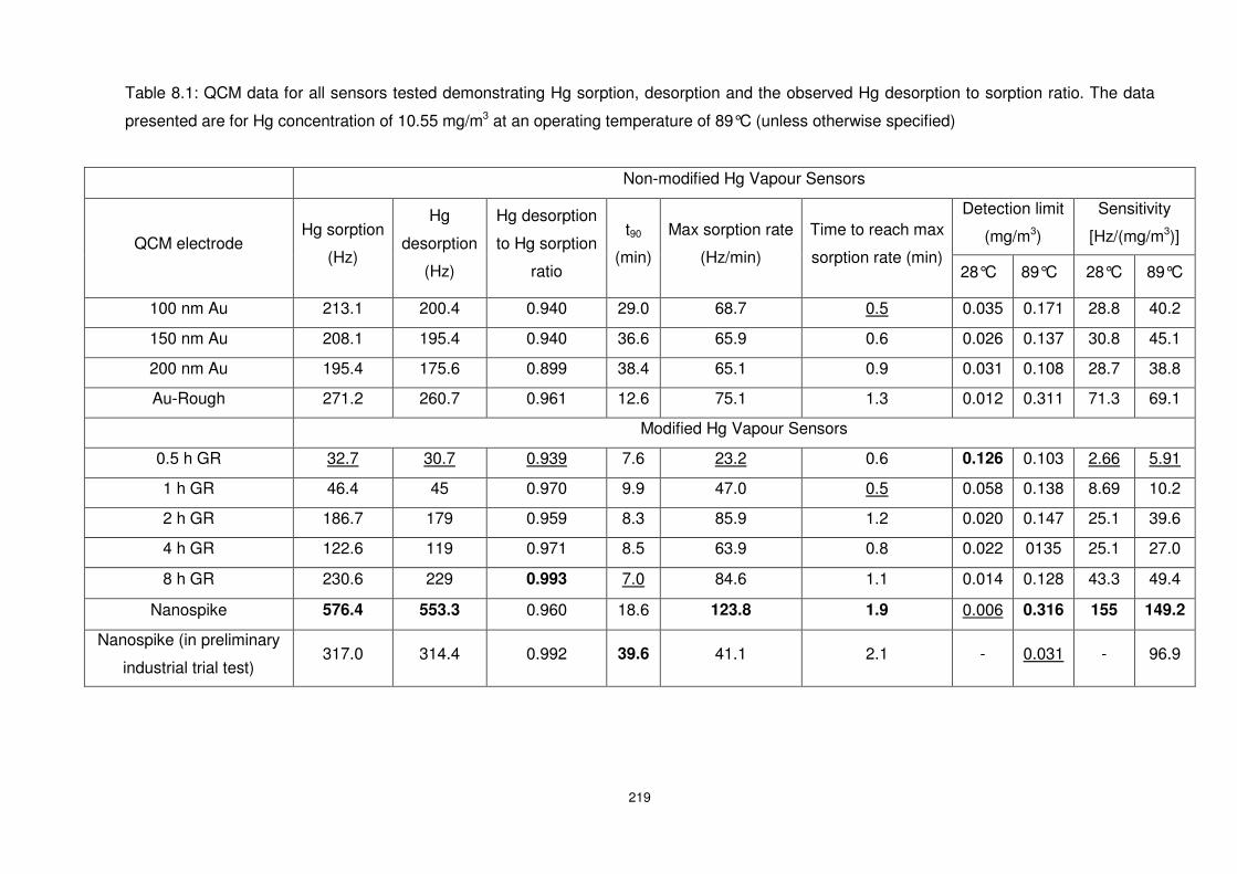
219
Table 8.1: QCM data for all sensors tested demonstrating Hg sorption, desorption and the observed Hg desorption to sorption ratio. The data
presented are for Hg concentration of 10.55 mg/m3 at an operating temperature of 89°C (unless otherwise specified)
Non-modified Hg Vapour Sensors
Detection limit
(mg/m3)
Sensitivity
[Hz/(mg/m3)] QCM electrode Hg sorption
(Hz)
Hg
desorption
(Hz)
Hg desorption
to Hg sorption
ratio
t90
(min)
Max sorption rate
(Hz/min)
Time to reach max
sorption rate (min) 28°C 89°C 28°C 89°C
100 nm Au 213.1 200.4 0.940 29.0 68.7 0.5 0.035 0.171 28.8 40.2
150 nm Au 208.1 195.4 0.940 36.6 65.9 0.6 0.026 0.137 30.8 45.1
200 nm Au 195.4 175.6 0.899 38.4 65.1 0.9 0.031 0.108 28.7 38.8
Au-Rough 271.2 260.7 0.961 12.6 75.1 1.3 0.012 0.311 71.3 69.1
Modified Hg Vapour Sensors
0.5 h GR 32.7 30.7 0.939 7.6 23.2 0.6 0.126 0.103 2.66 5.91
1 h GR 46.4 45 0.970 9.9 47.0 0.5 0.058 0.138 8.69 10.2
2 h GR 186.7 179 0.959 8.3 85.9 1.2 0.020 0.147 25.1 39.6
4 h GR 122.6 119 0.971 8.5 63.9 0.8 0.022 0135 25.1 27.0
8 h GR 230.6 229 0.993 7.0 84.6 1.1 0.014 0.128 43.3 49.4
Nanospike 576.4 553.3 0.960 18.6 123.8 1.9 0.006 0.316 155 149.2
Nanospike (in preliminary
industrial trial test) 317.0 314.4 0.992 39.6 41.1 2.1 - 0.031 - 96.9
220
8.2 Conclusions
Due to their high sensitivity and long term stability in the presence of interferent gases when
operated at 89°C, the nanospikes, 1, 2 and 4 h GR QCMs developed in this work offer
extensive commercialization opportunities. This dissertation shows the development of
low-cost, selective and sensitive elemental mercury vapour detectors by the integration of Au
nanostructures as the sensitive layer on QCM electrodes. The proposed detection
methodology and design, using the nanospikes QCM for example, offers many advantages
over the current commercially available Hg vapour sensors, such as:
• The need to pre-concentrate Hg is omitted, thus sensing is faster, requires less
material and avoids potential errors associated with memory effects.
• The sensor recovery methodology does not require any heating or acid dissolution
while the sensor is still able to reproduce similar response magnitudes for identical
Hg vapour concentration with and without the presence of interferent gases.
• The system is cost effective. The cost of AAS, AFS, AES or ICPMS systems, for
example, range from tens to hundreds of thousands of dollars. Currently, industries
pay ~$AU 10,000 per sample to detect the Hg concentration in each stream with the
results being revealed a little over 2 weeks later. The cost of 1 modified QCM as
described may be within tens of dollars, with the additional advantage of having
online measurements within 3 to 10 minutes of the 1 hour Hg exposure period (using
sorption rate data). The associated plumbing (i.e. mass flow controllers and sensor
testing chamber) and electronics (i.e. frequency counters and computers) may be
further engineered to make them significantly smaller and cheaper than the current
commercially available sensors used by industries. For example, a testing chamber
housing one QCM may be designed with the sensor signal being relayed to a single
remote computer operating from industry laboratories that communicates to a
multiplexed frequency counter.
• The modified QCM showed only 6% degradation in response magnitude following 50
days of Hg exposure in the presence of interferent gases at an operating temperature
of 89°C. No calibration was performed after the first day of testing. Calibration of the
sensors requires nothing more than exposure to five Hg concentrations lasting a total
of 14 hours and are required about 4 times a year to get Hg readings at least within
±7% with 95% confidence. Additionally this procedure has the potential to be
computer automated, requiring minimal user intervention.
• Because the sensors are gravimetric based rather than resistive, and because most
VOCs present in Hg emitting industries generally have lower molecular weights and
lower affinity for Au than Hg vapour, they are significantly less prone to interfere or
cause memory effects on the modified QCMs.
221
In summary, this PhD research program has produced significant contributions to the fields
of surface modification of gold and Hg vapour sensing. The author’s achievements
throughout this work include one provisional patent, six published refereed journal articles,
various news articles, and ABC (Australian Broadcasting Corporation) radio interview,
conference proceedings, presentations and posters. A full list of the author’s achievements
throughout this work may be found in Appendix A.
8.3 Ongoing Future Work
Throughout the course of this PhD program several areas of interest that have tremendous
research potential have been identified. Further research should embrace the following
investigations:
• Formation of the nanostructures described on SAW sensors, which may also be
made into hand held instruments for lower Hg vapour concentration monitoring.
• Under potential deposition of Pb during Au electrodeposition should be further
investigated to better understand the growth mechanism of the nanospikes.
• HR-TEM studies should be performed to demonstrate the nature of the exposed Au
facets along the nanospike walls and whether these exposed facets play any role in
terms of sensor performance (e.g. Hg sorption and/or desorption)
• The QCMs should undergo synthetic testing against other interferent gases including
VOCs which are present in other industries, such as those in coal-fired power
generation.
• The deposition of various types of self-assembled monolayers to reduce the sorption
of any potential interferent gases on the sensitive layer.
• The decrease in the composition of NiO on the galvanically replaced electrodes
observed from XPS data is not well understood and needs to be further investigated
by XPS depth profiling.
Finally, the direct growth of (111)-oriented nanostructures on an appropriate sensing platform
may also provide immense future opportunities towards detection of ultra-low concentrations
of other chemical and biological species. The author’s developed nanostructures may also
be investigated for their performance of (111)-oriented Au nanospikes as well as the
galvanically replaced nanostructures for electrocatalysis, biosensing, surface enhanced
Raman scattering (SERS) and various other applications. The vast potential implications of
Au nanospikes and galvanically replaced nanostructured materials for sensing and various
other applications cannot be overemphasized.

222

223
Appendices
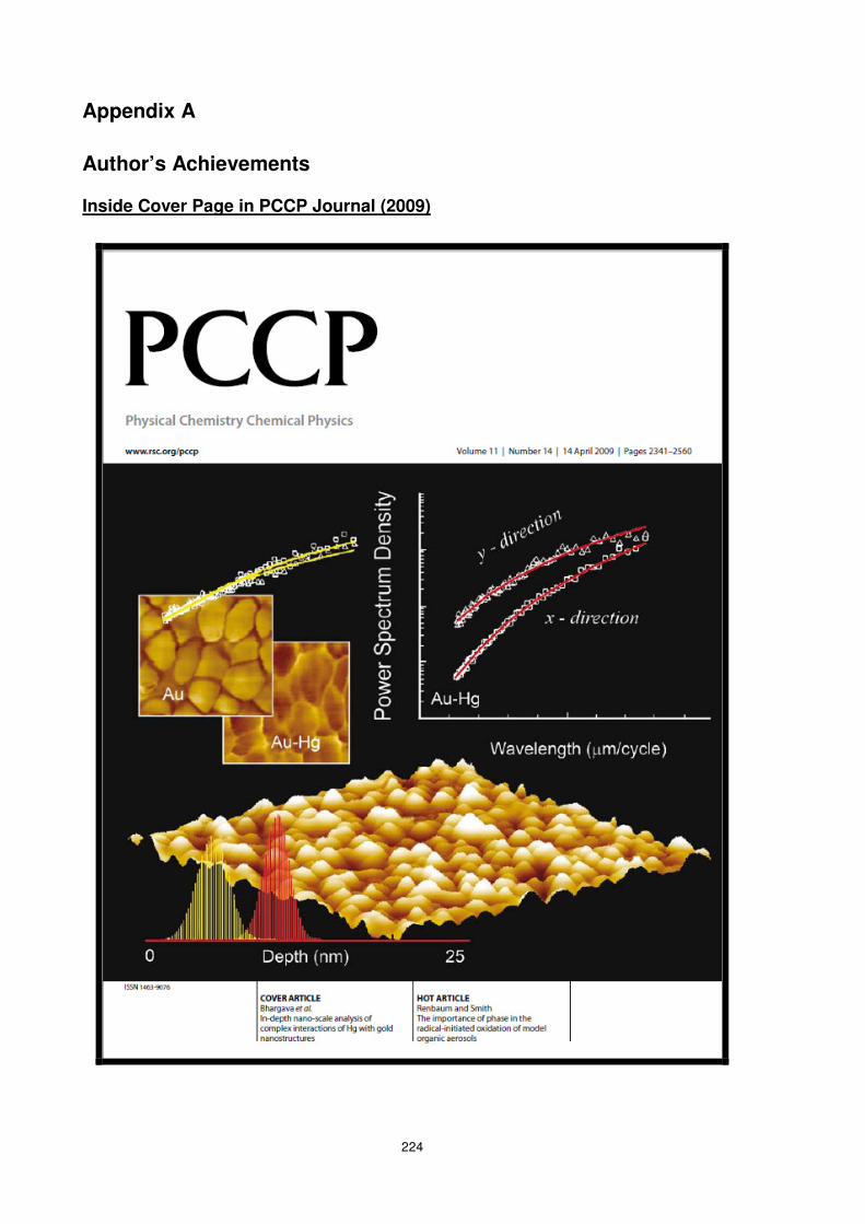
224
Appendix A
Author’s Achievements
Inside Cover Page in PCCP Journal (2009)
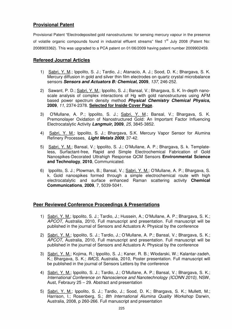
225
Provisional Patent
Provisional Patent “Electrodeposited gold nanostructures: for sensing mercury vapour in the presence
of volatile organic compounds found in industrial effluent streams” filed 1st July 2008 (Patent No:
2008903362). This was upgraded to a PCA patent on 01/06/2009 having patent number 2009902459.
Refereed Journal Articles
1) Sabri, Y. M.; Ippolito, S. J.; Tardio, J.; Atanacio, A. J.; Sood, D. K.; Bhargava, S. K. Mercury diffusion in gold and silver thin film electrodes on quartz crystal microbalance sensors Sensors and Actuators B: Chemical, 2009, 137, 246-252.
2) Sawant, P. D.; Sabri, Y. M.; Ippolito, S. J.; Bansal, V.; Bhargava, S. K. In-depth nano-scale analysis of complex interactions of Hg with gold nanostructures using AFM based power spectrum density method Physical Chemistry Chemical Physics, 2009, 11, 2374-2378. Selected for Inside Cover Page.
3) O'Mullane, A. P.; Ippolito, S. J.; Sabri, Y. M.; Bansal, V.; Bhargava, S. K. Premonolayer Oxidation of Nanostructured Gold: An Important Factor Influencing Electrocatalytic Activity Langmuir, 2009, 25, 3845-3852.
4) Sabri, Y. M.; Ippolito, S. J.; Bhargava, S.K. Mercury Vapor Sensor for Alumina Refinery Processes, Light Metals 2009, 37-42.
5) Sabri, Y. M.; Bansal, V.; Ippolito, S. J.; O’Mullane, A. P.; Bhargava, S. k. Template-less, Surfactant-free, Rapid and Simple Electrochemical Fabrication of Gold Nanospikes-Decorated Ultrahigh Response QCM Sensors Environmental Science and Technology, 2010, Communicated.
6) Ippolito, S. J.; Plowman, B.; Bansal, V.; Sabri, Y. M.; O’Mullane, A. P.; Bhargava, S. k. Gold nanospikes formed through a simple electrochemical route with high electrocatalytic and surface enhanced Raman scattering activity Chemical Communications, 2009, 7, 5039-5041.
Peer Reviewed Conference Proceedings & Presentations
1) Sabri, Y. M.; Ippolito, S. J.; Tardio, J.; Hussein, A.; O’Mullane, A. P.; Bhargava, S. K.; APCOT, Australia, 2010, Full manuscript and presentation. Full manuscript will be published in the journal of Sensors and Actuators A: Physical by the conference
2) Sabri, Y. M.; Ippolito, S. J.; Tardio, J.; O’Mullane, A. P.; Bansal, V.; Bhargava, S. K.; APCOT, Australia, 2010, Full manuscript and presentation. Full manuscript will be published in the journal of Sensors and Actuators A: Physical by the conference
3) Sabri, Y. M.; Kojima, R.; Ippolito, S. J.; Kaner, R. B.; Wlodarski, W.; Kalantar-zadeh, K.; Bhargava, S. K.; IMCS, Australia, 2010, Poster presentation. Full manuscript will be published in the journal of Sensors Letters by the conference
4) Sabri, Y. M.; Ippolito, S. J.; Tardio, J.; O’Mullane, A. P.; Bansal, V.; Bhargava, S. K.; International Conference on Nanoscience and Nanotechnology (ICONN 2010), NSW, Aust, Febraury 25 – 29. Abstract and presentation
5) Sabri, Y. M.; Ippolito, S. J.; Tardio, J.; Sood, D. K.; Bhargava, S. K.; Mullett, M.; Harrison, I.; Rosenberg, S.; 8th International Alumina Quality Workshop Darwin, Australia, 2008, p 260-266. Full manuscript and presentation
226
6) Sabri, Y. M.; Ippolito, S. J.; Bhargava, S. K.; Sood, D. K.; Bansal, V.; 12th international meeting on chemical sensors, columbus, Ohio, USA July 13 – 16 2008. Full manuscript and presentation
7) Sabri, Y. M.; Ippolito, S. J.; Bhargava, S. k.; Sood, D. K.; Tardio, J.; 12th international meeting on chemical sensors, columbus, Ohio, USA July 13 – 16 2008. Full manuscript and presentation
8) Bhargava, S. K.; Bansal, V.; Jani, H.; Sabri, Y.; Ippolito, S. J. 2008 International Conference on Nanoscience and Nanotechnology (ICONN 2008), Melb, VIC, Aust, Febraury 25 – 29. Abstract and presentation
9) Sabri, Y. M.; Ippolito, S. J.; Tardio, J.; Sood, D. K.; Bhargava, S. K. In Nanoscience and Nanotechnology, 2008. ICONN 2008. International Conference on 2008, p 71-74. Full manuscript and presentation. The manuscript is available from http://ieeexplore.ieee.org/stamp/stamp.jsp?tp=&arnumber=4639248&isnumber=4639211
10) Sabri, Y. M.; Sood, D. K.; Bhargava, S. K.; Ippolito, S. J.; 15th AINSE Conference on Nuclear and Complementary Techniques of Analysis (NCTA), Melbourne University, Melb, VIC, Aust, November 21 – 23 2007. pp.287-291. Full manuscript and poster
11) Dhawan, D.; Sabri, Y.; Bhargava, S.; Sood, D.; Kalantar-Zadeh, K. In Micro- and Nanotechnology: Materials, Processes, Packaging, and Systems III; 1 ed.; SPIE: Adelaide, Australia, 2006; Vol. 6415, p 641514-8. Full manuscript only
12) Sood, D. K.; Sabri, Y. M.; Bhargava, S. K.; Andrienko, I.; Wlodarski, W.; Evans, P. J.; 14th AINSE Conference on Nuclear and Complementary Techniques of Analysis & 19th Vacuum Society of Australia Congress (NCTA/VSA), Wellington, NZ, November 19 – 22; 2005. Full manuscript and presentation
Media Citations
1. Research on “Measuring Mercury with Nanotechnology” has been covered by reputed international scientific websites and magazines From May 2009.
ABC National – Science Show 2 May 2009-05-05 - Mercury released as coal is burnt in
power stations
http://www.abc.net.au/rn/scienceshow/stories/2009/2558479.htm
Stories of Australian Science 2010 - “Measuring mercury with a Midas touch”
http://www.scienceinpublic.com/stories/2009/measuring-mercury
AtoZofNano – “Using Nanotechnology to Measure Mercury”
http://www.azonano.com/details.asp?ArticleId=2395
AtoZofNano – Nanotechnology Thought Leader Series – Suresh Bhargava
http://www.azonano.com/experts.asp?iExpertID=70

227
The Age – “Mercury Falling” (19-11-2009)
http://www.theage.com.au/national/education/mercury-falling-20091119-iocb.html
RMIT Front page - “Measuring Mercury with Nanotechnology”
http://www.rmit.edu.au/browse;ID=xwzx3dxlgxzi
Australian Financial Review (RMIT insert) - “Midas Touch”
Nanotechnology Now - “Measuring Mercury with Nanotechnology”
http://www.nanotech-now.com/news.cgi?story_id=33383
Nanowerk – “Pioneering nanotechnology sensor can precisely measure mercury”
http://www.nanowerk.com/news/newsid=10860.php
Nano techwire.com - “Measuring Mercury with Nanotechnology”
http://nanotechwire.com/news.asp?nid=7979&ntid=&pg=1
Science Alert – “Gold nano-hairs find mercury”
http://www.sciencealert.com.au/news/20092805-19203.html
Nanotechnology & development news - “Measuring Mercury with Nanotechnology”
http://www.merid.org/NDN/more.php?id=1930
R&Dmag – “Gold spikes take accurate measure of industrial mercury”
http://www.rdmag.com/News/2009/05/Gold-spikes-take-accurate-measure-of-
industrial-mercury/
ICHemE – “21st century chimney sweeping: RMIT forest of nano-gold captures mercury”
http://www.tce-today.co.uk/tcetoday/NewsDetail.aspx?nid=11791
Also Mentioned in:
Gold – “Gold used in US Army DNA research”
http://www.utilisegold.com/news/2009/06/02/story/12162/gold_used_in_us_army_dna_resear
ch
2. Research on Mercury vapor sensing using modified Au surfaces incorporated on QCM transducers was covered by reputed newspaper (Financial Review) in 3rd of June 2009 edition.
3. “Measuring mercury with a Midas touch” was published in the 2010 edition of Stories of Australian Science magazine.
228
4. Two radio interviews were conducted, namely Australian Broadcasting Corporation (ABC) radio and Triple R Broadcasters Melbourne (3RRR) radio in the years 2009 and 2010, respectively.
Research Fellowships
Australian Institute of Nuclear Science and Engineering (AINSE) Award (Award No:
AINGRA06164P) Totalling $13406.00 – Granted in 2006
Australian Institute of Nuclear Science and Engineering (AINSE) Award (Award No: AINGRA08104P) Totalling $18,130.00 – Granted in 2007
Australian Institute of Nuclear Science and Engineering (AINSE) Travel Grant Totalling $500.00 – Granted in 2008
Student Awards
Particle & Surface Science Award (Includes $500 Award) for producing the best results using
the micromeritics system. The award was received twice in consecutive years of 2007 and
2008.
Student supervision
During the research candidature, the author was also involved in the supervision of three
students from final year undergraduates and the supervision of one honours student.
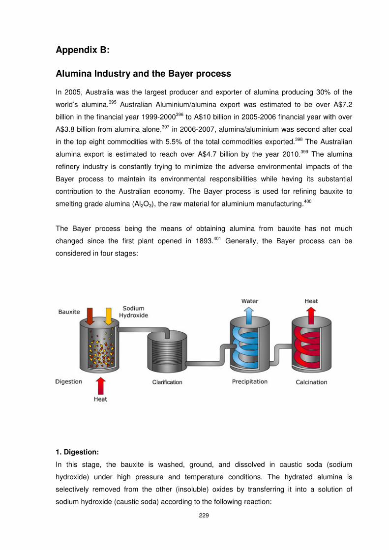
229
Appendix B:
Alumina Industry and the Bayer process
In 2005, Australia was the largest producer and exporter of alumina producing 30% of the
world’s alumina.395 Australian Aluminium/alumina export was estimated to be over A$7.2
billion in the financial year 1999-2000396 to A$10 billion in 2005-2006 financial year with over
A$3.8 billion from alumina alone.397 in 2006-2007, alumina/aluminium was second after coal
in the top eight commodities with 5.5% of the total commodities exported.398 The Australian
alumina export is estimated to reach over A$4.7 billion by the year 2010.399 The alumina
refinery industry is constantly trying to minimize the adverse environmental impacts of the
Bayer process to maintain its environmental responsibilities while having its substantial
contribution to the Australian economy. The Bayer process is used for refining bauxite to
smelting grade alumina (Al2O3), the raw material for aluminium manufacturing.400
The Bayer process being the means of obtaining alumina from bauxite has not much
changed since the first plant opened in 1893.401 Generally, the Bayer process can be
considered in four stages:
1. Digestion:
In this stage, the bauxite is washed, ground, and dissolved in caustic soda (sodium
hydroxide) under high pressure and temperature conditions. The hydrated alumina is
selectively removed from the other (insoluble) oxides by transferring it into a solution of
sodium hydroxide (caustic soda) according to the following reaction:
230
Al2O3.xH2O + 2NaOH = 2NaAlO2 + (x+1)H2O
The digestion is completed within a digester, typically operated at between 200 and 240°C
and can involve pressures of around 30 atm. The concentration of caustic soda can be as
high as 10%.
2. Clarification:
The removal of residues from the liquor stream after the digestion stage is complete.
After the digestion, the liquor (containing the dissolved Al2O
3) must be separated from the
insoluble bauxite residues (containing iron, silicon, and titanium), purified as much as
possible and filtered before it is delivered to a decomposer. These residues sink gradually to
the bottom of the tank and are removed. They are known colloquially as "red mud". Bauxite
residues (also known as red mud) are by-products of the Bayer Process. The amount of
residues generated, per tonne of alumina produced, varies depending on the type of bauxite
used, from 0.3 tonnes for high-grade bauxite to 2.5 tonnes for very low grade. The red mud is
thickened and washed so that the caustic soda can be removed and recycled.
3. Precipitation: The removal of crystals of alumina hydrate from the caustic solution of the
liquor stream.
After clarification, the clear sodium aluminate solution is pumped into a huge tank called a
precipitator. In this stage, crystalline alumina trihydrate is extracted from the digestion liquor
by the following hydrolysis reaction:
2NaAlO2 + 4H2O = Al2O3.3H2O + 2NaOH
This is basically the reverse of the digestion process. Fine particles of alumina are added
to seed the precipitation of pure alumina particles as the liquor cools. The particles sink
to the bottom of the tank and are removed. The liquor is recycled back to digestion.
4. Calcination: The removal of water crystallization from the alumina hydrate after
precipitation.
In this stage, the alumina trihydrate crystals are passed through a rotary calcination kiln
or a fluidized calciner at 1100°C to drive off the chemically combined water. The final
product is a fine white anhydrous aluminum oxide powder called alumina. This is the
basic material from which aluminum is made.
B.1 Hg in the Bayer Process
Bauxite contains trace amounts of mercury which may accumulate in the Bayer liquor,
alumina hydrate and oxalate in the processing of bauxite.13 The digestion and
231
evaporation steps of the Bayer process involve flash evaporation/cooling. This produces
as stream that is cooled in heat exchangers. This leaves a vapour that is in equilibrium
with the condensate. Significant concentrations of VOCs and Hg are present in this
vapour phase. The digestion and evaporation processes are reducing due to the
dissolved organic species, which can act as reducing agents within the liquor stream.
Gases exiting these streams include ammonia, water and various VOCs (i.e. acetone, 2-
butanone etc.) with the balance being nitrogen.392 The Hg emissions to air from Bayer
refineries are almost 100% elemental mercury from studies of emissions for Alcoa Bayer
refineries.13 Elemental Hg in the gaseous phase is in steady state with the concentration
in the condensate according to Henry’s law.327,402 The mercury concentration will
therefore depend on the temperature but typical mercury concentrations range from 3 –
30 mg/m3 at temperatures of 20 – 80°C. Hg emissions from Bayer refineries differ
significantly from refinery to refinery. Some refineries have significant mercury emissions
from digestion and calciners due to mercury in the alumina hydrate while other refineries
have a significantly higher portion of the Hg emissions from the digestion vent gases or
oxalate kiln.13 Hg emissions are also found, in small quantities, from the liquor burner
and boilers.8
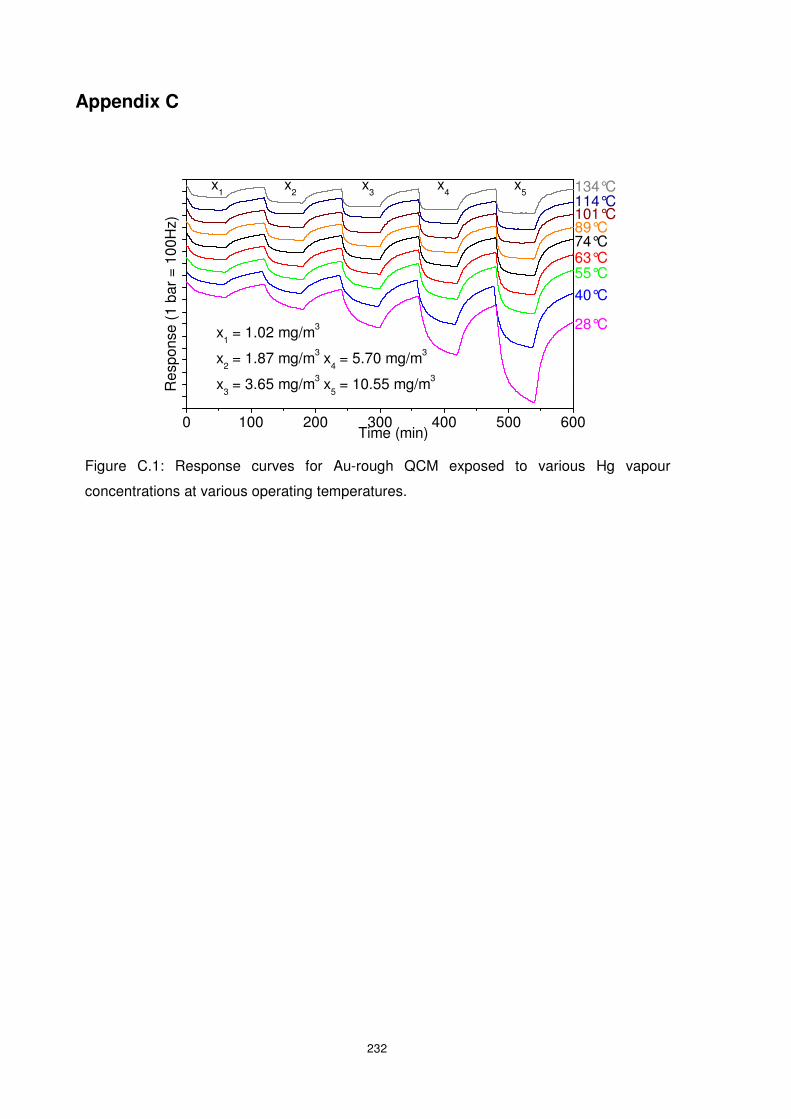
232
Appendix C
Figure C.1: Response curves for Au-rough QCM exposed to various Hg vapour
concentrations at various operating temperatures.
0 100 200 300 400 500 600
x5
x4
x3
x2
x1 = 1.02 mg/m3
x2 = 1.87 mg/m3 x
4 = 5.70 mg/m3
x3 = 3.65 mg/m3 x
5 = 10.55 mg/m3
134°CR
espo
nse
(1 b
ar =
100
Hz)
Time (min)
28°C
40°C
55°C63°C74°C89°C101°C114°C
x1
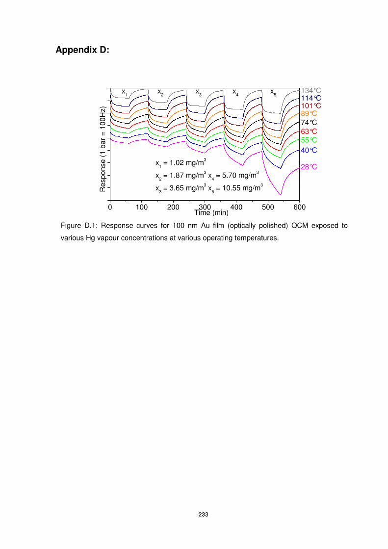
233
Appendix D:
Figure D.1: Response curves for 100 nm Au film (optically polished) QCM exposed to
various Hg vapour concentrations at various operating temperatures.
0 100 200 300 400 500 600
134°C
x1 = 1.02 mg/m3
x2 = 1.87 mg/m3 x
4 = 5.70 mg/m3
x3 = 3.65 mg/m3 x
5 = 10.55 mg/m3
28°C
40°C55°C63°C74°C89°C101°C
Res
pons
e (1
bar
= 1
00H
z)
Time (min)
114°Cx
5x
4x
3x
2x
1
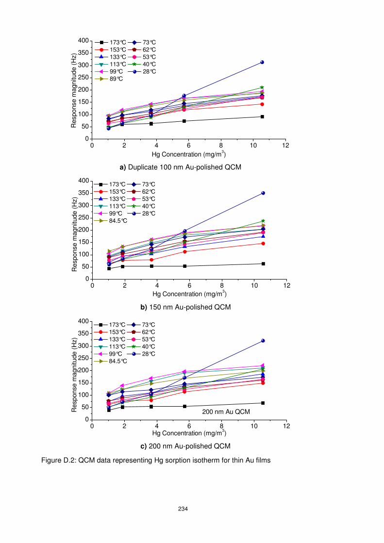
234
Figure D.2: QCM data representing Hg sorption isotherm for thin Au films
a) Duplicate 100 nm Au-polished QCM
b) 150 nm Au-polished QCM
c) 200 nm Au-polished QCM
0 2 4 6 8 10 120
50
100
150
200
250
300
350
400 173°C 73°C 153°C 62°C 133°C 53°C 113°C 40°C 99°C 28°C 84.5°C
Res
pons
e m
agni
tude
(H
z)
Hg Concentration (mg/m3)
0 2 4 6 8 10 120
50
100
150
200
250
300
350
400 173°C 73°C 153°C 62°C 133°C 53°C 113°C 40°C 99°C 28°C 89°C
Res
pons
e m
agni
tude
(H
z)
Hg Concentration (mg/m3)
0 2 4 6 8 10 120
50
100
150
200
250
300
350
400
200 nm Au QCM
173°C 73°C 153°C 62°C 133°C 53°C 113°C 40°C 99°C 28°C 84.5°C
Res
pons
e m
agni
tude
(H
z)
Hg Concentration (mg/m3)
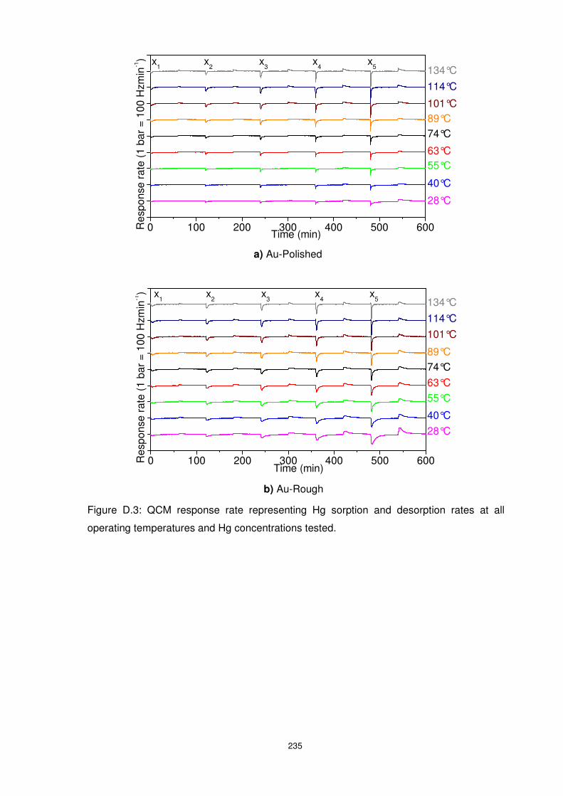
235
a) Au-Polished
b) Au-Rough
0 100 200 300 400 500 600
134°C
Res
pons
e ra
te (
1 ba
r =
100
Hzm
in-1)
Time (min)
28°C
40°C
55°C63°C
74°C89°C
101°C
114°C
x5
x4
x3
x2
x1
0 100 200 300 400 500 600
134°C
Res
pons
e ra
te (
1 ba
r =
100
Hzm
in-1)
Time (min)
28°C
40°C
55°C63°C
74°C89°C101°C
114°C
x5
x4
x3
x2
x1
Figure D.3: QCM response rate representing Hg sorption and desorption rates at all
operating temperatures and Hg concentrations tested.
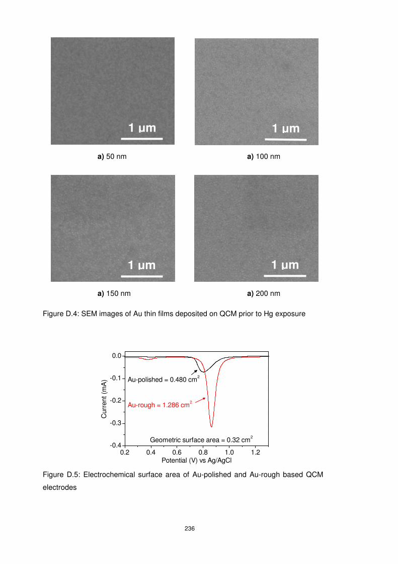
236
Figure D.5: Electrochemical surface area of Au-polished and Au-rough based QCM
electrodes
0.2 0.4 0.6 0.8 1.0 1.2-0.4
-0.3
-0.2
-0.1
0.0
Au-rough = 1.286 cm2
Au-polished = 0.480 cm2
Cur
rent
(m
A)
Potential (V) vs Ag/AgCl
Geometric surface area = 0.32 cm2
1 µm
Figure D.4: SEM images of Au thin films deposited on QCM prior to Hg exposure
1 µm
1 µm 1 µm
1 µm
a) 50 nm a) 100 nm
a) 150 nm a) 200 nm
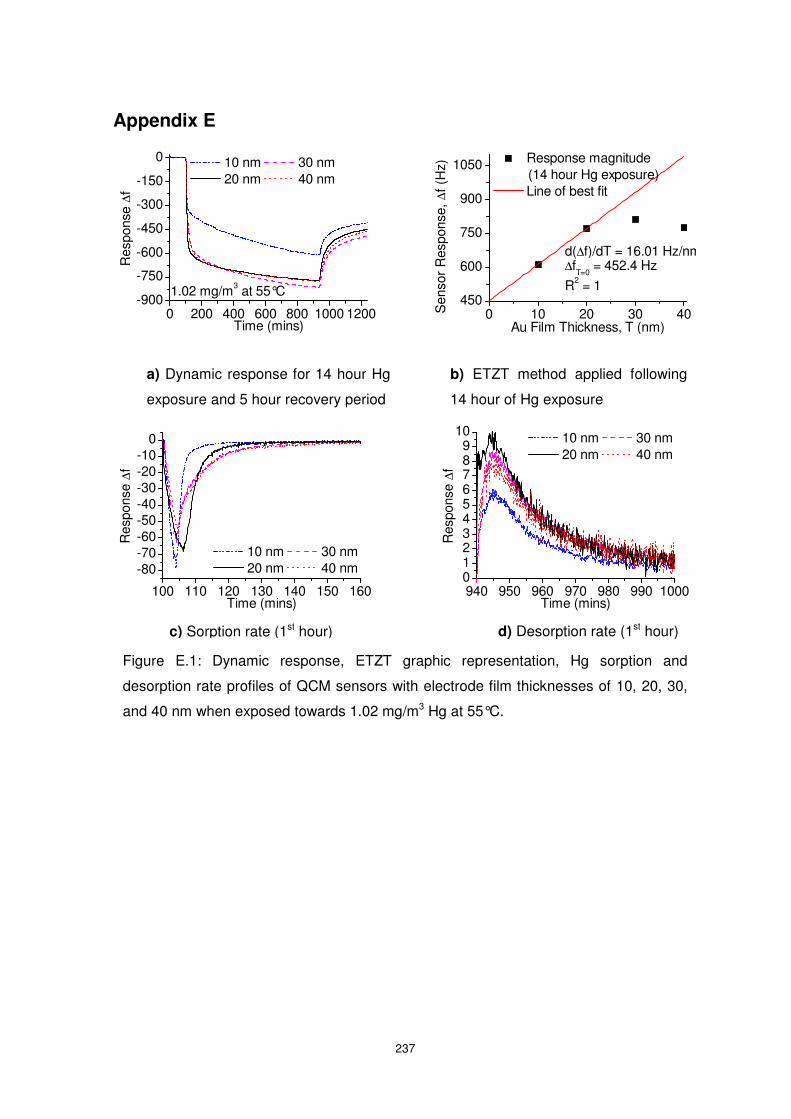
237
Appendix E
Figure E.1: Dynamic response, ETZT graphic representation, Hg sorption and
desorption rate profiles of QCM sensors with electrode film thicknesses of 10, 20, 30,
and 40 nm when exposed towards 1.02 mg/m3 Hg at 55°C.
a) Dynamic response for 14 hour Hg
exposure and 5 hour recovery period
b) ETZT method applied following
14 hour of Hg exposure
c) Sorption rate (1st hour) d) Desorption rate (1st hour)
0 200 400 600 800 1000 1200-900
-750
-600
-450
-300
-150
0
Res
pons
e ∆
f
Time (mins)
10 nm 30 nm 20 nm 40 nm
1.02 mg/m3 at 55°C
0 10 20 30 40450
600
750
900
1050 Response magnitude (14 hour Hg exposure)
Line of best fit
Sen
sor
Res
pons
e, ∆
f (H
z)
Au Film Thickness, T (nm)
R2 = 1
∆fT=0
= 452.4 Hzd(∆f)/dT = 16.01 Hz/nm
100 110 120 130 140 150 160
-80-70-60-50-40-30-20-10
0
Res
pons
e ∆
f
Time (mins)
10 nm 30 nm 20 nm 40 nm
940 950 960 970 980 990 10000123456789
10R
espo
nse
∆f
Time (mins)
10 nm 30 nm 20 nm 40 nm
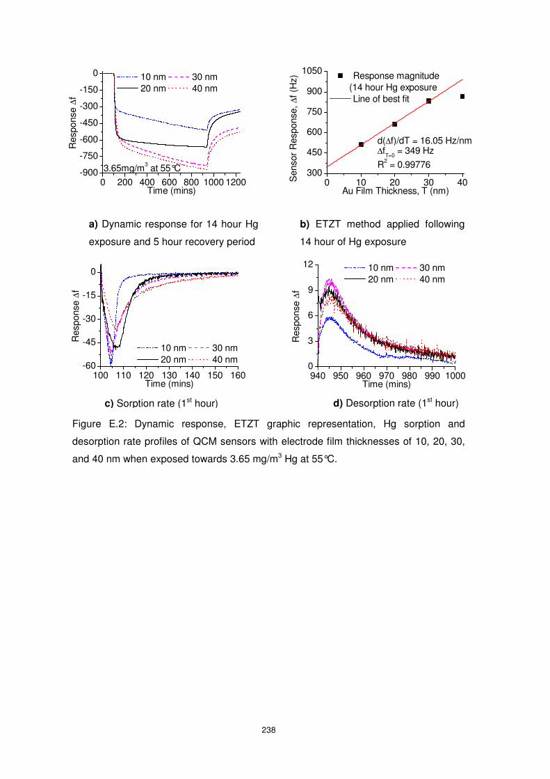
238
Figure E.2: Dynamic response, ETZT graphic representation, Hg sorption and
desorption rate profiles of QCM sensors with electrode film thicknesses of 10, 20, 30,
and 40 nm when exposed towards 3.65 mg/m3 Hg at 55°C.
a) Dynamic response for 14 hour Hg
exposure and 5 hour recovery period
b) ETZT method applied following
14 hour of Hg exposure
c) Sorption rate (1st hour) d) Desorption rate (1st hour)
0 200 400 600 800 1000 1200-900
-750
-600
-450
-300
-150
0R
espo
nse
∆f
Time (mins)
10 nm 30 nm 20 nm 40 nm
3.65mg/m3 at 55°C
0 10 20 30 40300
450
600
750
900
1050 Response magnitude (14 hour Hg exposure
Line of best fit
Sen
sor
Res
pons
e, ∆
f (H
z)
Au Film Thickness, T (nm)
R2 = 0.99776
∆fT=0
= 349 Hzd(∆f)/dT = 16.05 Hz/nm
100 110 120 130 140 150 160-60
-45
-30
-15
0
Res
pons
e ∆
f
Time (mins)
10 nm 30 nm 20 nm 40 nm
940 950 960 970 980 990 10000
3
6
9
12
Res
pons
e ∆
f
Time (mins)
10 nm 30 nm 20 nm 40 nm
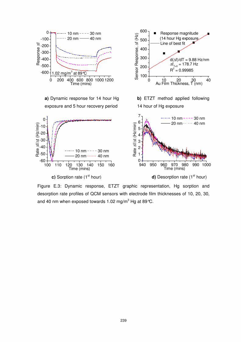
239
Figure E.3: Dynamic response, ETZT graphic representation, Hg sorption and
desorption rate profiles of QCM sensors with electrode film thicknesses of 10, 20, 30,
and 40 nm when exposed towards 1.02 mg/m3 Hg at 89°C.
a) Dynamic response for 14 hour Hg
exposure and 5 hour recovery period
b) ETZT method applied following
14 hour of Hg exposure
c) Sorption rate (1st hour) d) Desorption rate (1st hour)
0 200 400 600 800 1000 1200
-600
-500
-400
-300
-200
-100
0R
espo
nse
∆f
Time (mins)
10 nm 30 nm 20 nm 40 nm
1.02 mg/m3 at 89°C
0 10 20 30 40100
200
300
400
500
600 Response magnitude (14 hour Hg exposure
Line of best fit
Sen
sor
Res
pons
e, ∆
f (H
z)
Au Film Thickness, T (nm)
d(∆f)/dT = 9.88 Hz/nm∆f
T=0 = 178.7 Hz
R2 = 0.99985
100 110 120 130 140 150 160-60
-50
-40
-30
-20
-10
0
Rat
e ∆
f/∆t (
Hz/
min
)
Time (mins)
10 nm 30 nm 20 nm 40 nm
940 950 960 970 980 990 10000
1
2
3
4
5
6
7
Rat
e ∆
f/∆t (
Hz/
min
)
Time (mins)
10 nm 30 nm 20 nm 40 nm
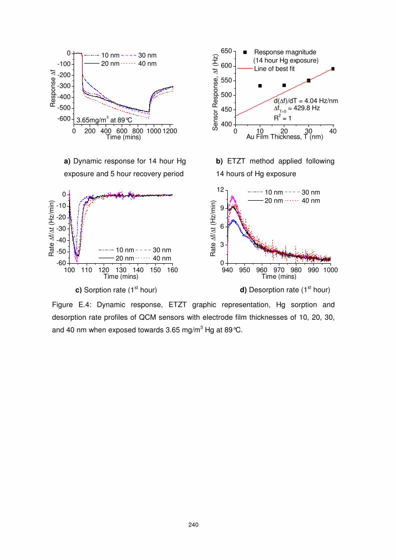
240
Figure E.4: Dynamic response, ETZT graphic representation, Hg sorption and
desorption rate profiles of QCM sensors with electrode film thicknesses of 10, 20, 30,
and 40 nm when exposed towards 3.65 mg/m3 Hg at 89°C.
a) Dynamic response for 14 hour Hg
exposure and 5 hour recovery period
b) ETZT method applied following
14 hours of Hg exposure
c) Sorption rate (1st hour) d) Desorption rate (1st hour)
0 200 400 600 800 1000 1200
-600
-500
-400
-300
-200
-100
0R
espo
nse
∆f
Time (mins)
10 nm 30 nm 20 nm 40 nm
3.65mg/m3 at 89°C
0 10 20 30 40400
450
500
550
600
650 Response magnitude (14 hour Hg exposure)
Line of best fit
Sen
sor
Res
pons
e, ∆
f (H
z)
Au Film Thickness, T (nm)
R2 = 1
∆fT=0
= 429.8 Hzd(∆f)/dT = 4.04 Hz/nm
100 110 120 130 140 150 160-60
-50
-40
-30
-20
-10
0
Rat
e ∆
f/∆t (
Hz/
min
)
Time (mins)
10 nm 30 nm 20 nm 40 nm
940 950 960 970 980 990 10000
3
6
9
12
Rat
e ∆
f/∆t (
Hz/
min
)
Time (mins)
10 nm 30 nm 20 nm 40 nm
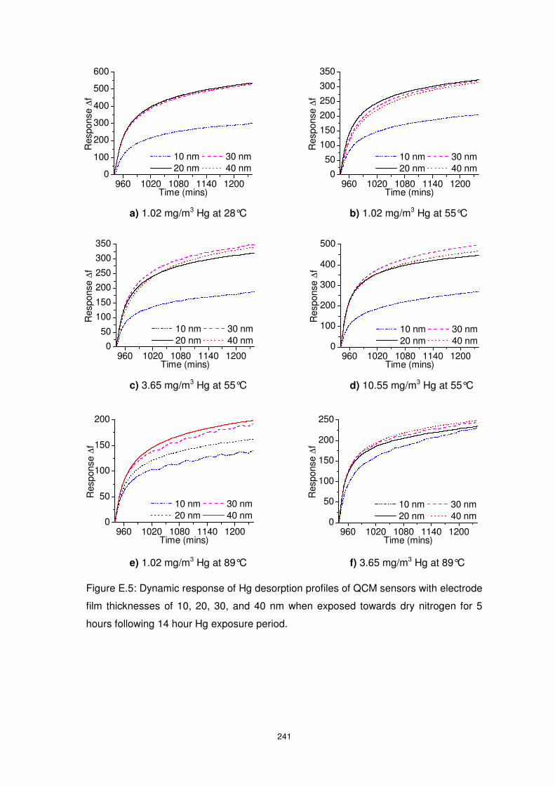
241
Figure E.5: Dynamic response of Hg desorption profiles of QCM sensors with electrode
film thicknesses of 10, 20, 30, and 40 nm when exposed towards dry nitrogen for 5
hours following 14 hour Hg exposure period.
a) 1.02 mg/m3 Hg at 28°C b) 1.02 mg/m3 Hg at 55°C
c) 3.65 mg/m3 Hg at 55°C
960 1020 1080 1140 12000
100
200
300
400
500
600
Res
pons
e ∆
f
Time (mins)
10 nm 30 nm 20 nm 40 nm
960 1020 1080 1140 12000
50
100
150
200
250
300
350
Res
pons
e ∆
f
Time (mins)
10 nm 30 nm 20 nm 40 nm
960 1020 1080 1140 12000
50
100
150
200
250
300
350
Res
pons
e ∆
f
Time (mins)
10 nm 30 nm 20 nm 40 nm
d) 10.55 mg/m3 Hg at 55°C
960 1020 1080 1140 12000
100
200
300
400
500
Res
pons
e ∆
f
Time (mins)
10 nm 30 nm 20 nm 40 nm
e) 1.02 mg/m3 Hg at 89°C f) 3.65 mg/m3 Hg at 89°C
960 1020 1080 1140 12000
50
100
150
200
Res
pons
e ∆
f
Time (mins)
10 nm 30 nm 20 nm 40 nm
960 1020 1080 1140 12000
50
100
150
200
250
Res
pons
e ∆
f
Time (mins)
10 nm 30 nm 20 nm 40 nm
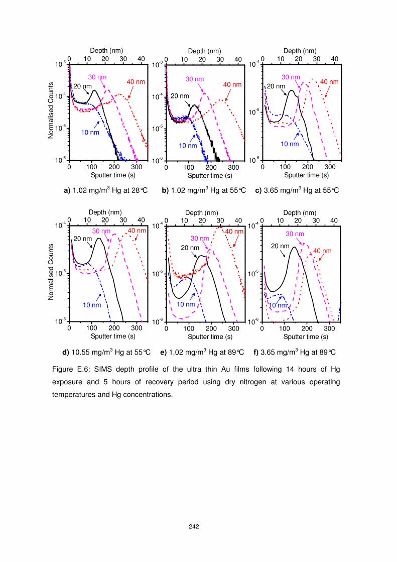
242
Figure E.6: SIMS depth profile of the ultra thin Au films following 14 hours of Hg
exposure and 5 hours of recovery period using dry nitrogen at various operating
temperatures and Hg concentrations.
c) 3.65 mg/m3 Hg at 55°C
0 100 200 30010-6
10-5
10-4
10-3
Nor
mal
ised
Cou
nts
Sputter time (s)
40 nm30 nm
20 nm
0 10 20 30 40Depth (nm)
10 nm
0 100 200 30010-6
10-5
10-4
10-3
Sputter time (s)
40 nm30 nm
20 nm
0 10 20 30 40Depth (nm)
10 nm
0 100 200 30010-6
10-5
10-4
Sputter time (s)
40 nm30 nm
20 nm
0 10 20 30 40Depth (nm)
10 nm
b) 1.02 mg/m3 Hg at 55°C a) 1.02 mg/m3 Hg at 28°C
0 100 200 30010-6
10-5
10-4
Nor
mal
ised
Cou
nts
Sputter time (s)
0 10 20 30 40
40 nm30 nm20 nm
10 nm
Depth (nm)
0 100 200 30010-6
10-5
10-4
Sputter time (s)
0 10 20 30 40
40 nm30 nm
20 nm
10 nm
Depth (nm)
0 100 200 30010-6
10-5
10-4
Sputter time (s)
0 10 20 30 40
40 nm
30 nm
20 nm
10 nm
Depth (nm)
f) 3.65 mg/m3 Hg at 89°C e) 1.02 mg/m3 Hg at 89°C d) 10.55 mg/m3 Hg at 55°C
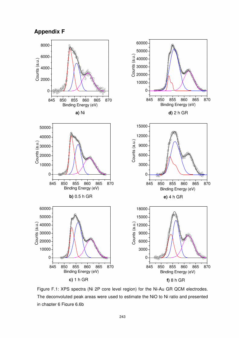
243
Appendix F
Figure F.1: XPS spectra (Ni 2P core level region) for the Ni-Au GR QCM electrodes.
The deconvoluted peak areas were used to estimate the NiO to Ni ratio and presented
in chapter 6 Figure 6.6b
a) Ni
b) 0.5 h GR
c) 1 h GR
d) 2 h GR
e) 4 h GR
f) 8 h GR
845 850 855 860 865 870
0
2000
4000
6000
8000
Cou
nts
(a.u
.)
Binding Energy (eV)
845 850 855 860 865 870
0
10000
20000
30000
40000
50000
Binding Energy (eV)
Cou
nts
(a.u
.)
845 850 855 860 865 870
0
10000
20000
30000
40000
50000
60000
Binding Energy (eV)
Cou
nts
(a.u
.)
845 850 855 860 865 870
0
10000
20000
30000
40000
50000
60000
Binding Energy (eV)
Cou
nts
(a.u
.)
845 850 855 860 865 870
0
3000
6000
9000
12000
15000
Binding Energy (eV)
Cou
nts
(a.u
.)
845 850 855 860 865 870
0
3000
6000
9000
12000
15000
18000
Binding Energy (eV)
Cou
nts
(a.u
.)
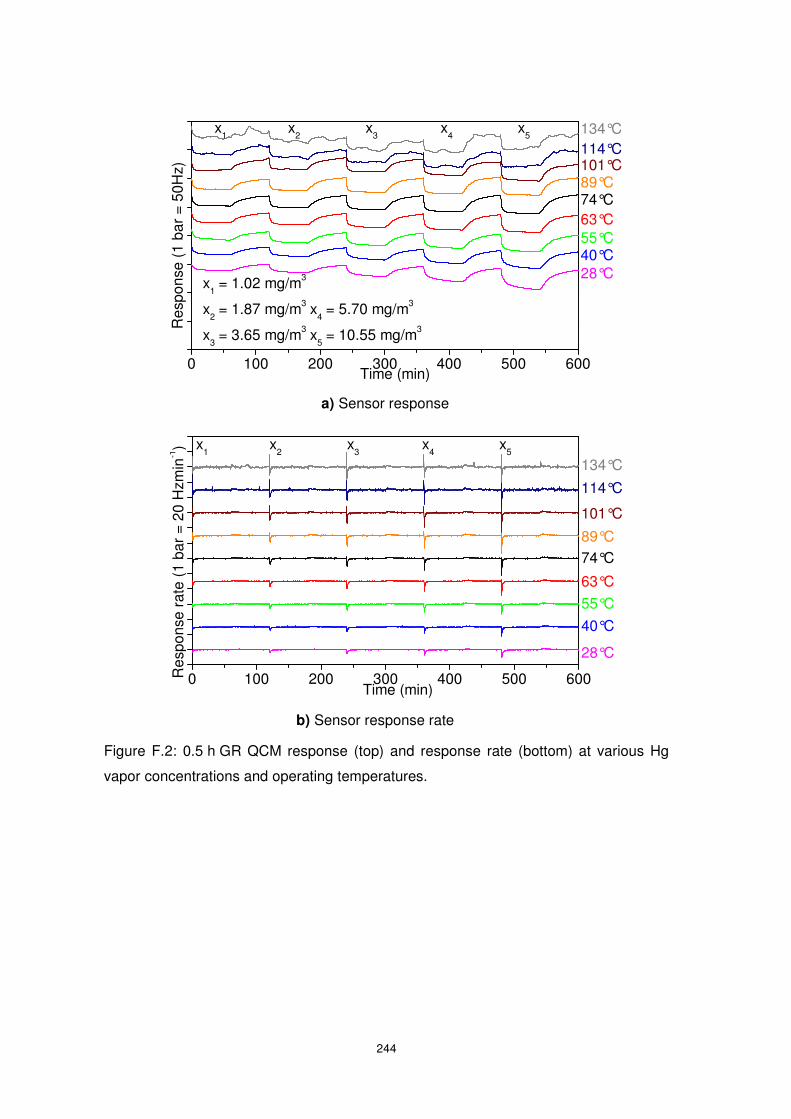
244
Figure F.2: 0.5 h GR QCM response (top) and response rate (bottom) at various Hg
vapor concentrations and operating temperatures.
a) Sensor response
b) Sensor response rate
0 100 200 300 400 500 600Res
pons
e ra
te (
1 ba
r =
20 H
zmin
-1)
Time (min)
134°C
28°C
40°C
55°C
63°C
74°C89°C
101°C
114°C
x5
x4
x3
x2
x1
0 100 200 300 400 500 600
x1 = 1.02 mg/m3
x2 = 1.87 mg/m3 x
4 = 5.70 mg/m3
x3 = 3.65 mg/m3 x
5 = 10.55 mg/m3R
espo
nse
(1 b
ar =
50H
z)
Time (min)
134°C
28°C40°C55°C63°C74°C89°C101°C114°C
x5
x4
x3
x2
x1
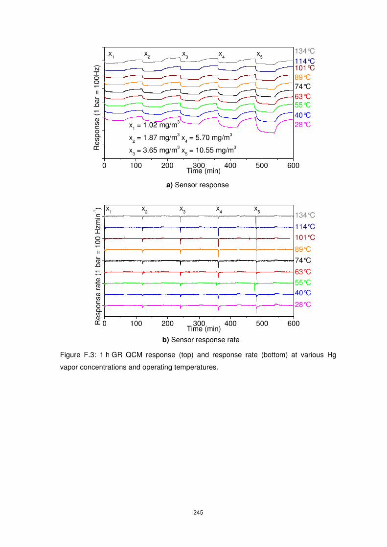
245
a) Sensor response
b) Sensor response rate
Figure F.3: 1 h GR QCM response (top) and response rate (bottom) at various Hg
vapor concentrations and operating temperatures.
0 100 200 300 400 500 600Res
pons
e ra
te (
1 ba
r =
100
Hzm
in-1)
Time (min)
134°C
28°C
40°C55°C
63°C
74°C
89°C
101°C
114°C
x5
x4
x3
x2
x1
0 100 200 300 400 500 600
x1 = 1.02 mg/m3
x2 = 1.87 mg/m3 x
4 = 5.70 mg/m3
x3 = 3.65 mg/m3 x
5 = 10.55 mg/m3R
espo
nse
(1 b
ar =
100
Hz)
Time (min)
134°C
28°C40°C55°C63°C74°C89°C101°C114°C
x5
x4
x3
x2
x1
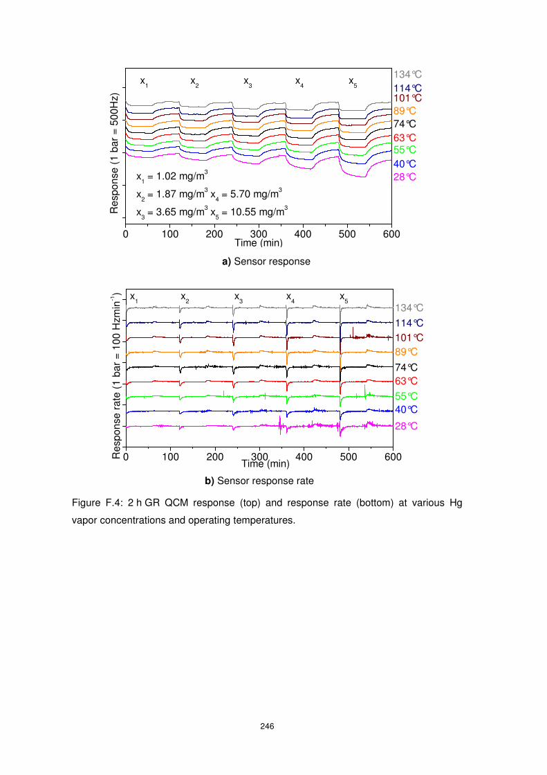
246
a) Sensor response
b) Sensor response rate
Figure F.4: 2 h GR QCM response (top) and response rate (bottom) at various Hg
vapor concentrations and operating temperatures.
0 100 200 300 400 500 600Res
pons
e ra
te (
1 ba
r =
100
Hzm
in-1)
Time (min)
134°C
28°C
40°C55°C
63°C74°C
89°C101°C114°C
x5
x4
x3
x2
x1
0 100 200 300 400 500 600
x1 = 1.02 mg/m3
x2 = 1.87 mg/m3 x
4 = 5.70 mg/m3
x3 = 3.65 mg/m3 x
5 = 10.55 mg/m3R
espo
nse
(1 b
ar =
500
Hz)
Time (min)
134°C
28°C40°C55°C63°C74°C89°C101°C114°C
x5
x4
x3
x2
x1
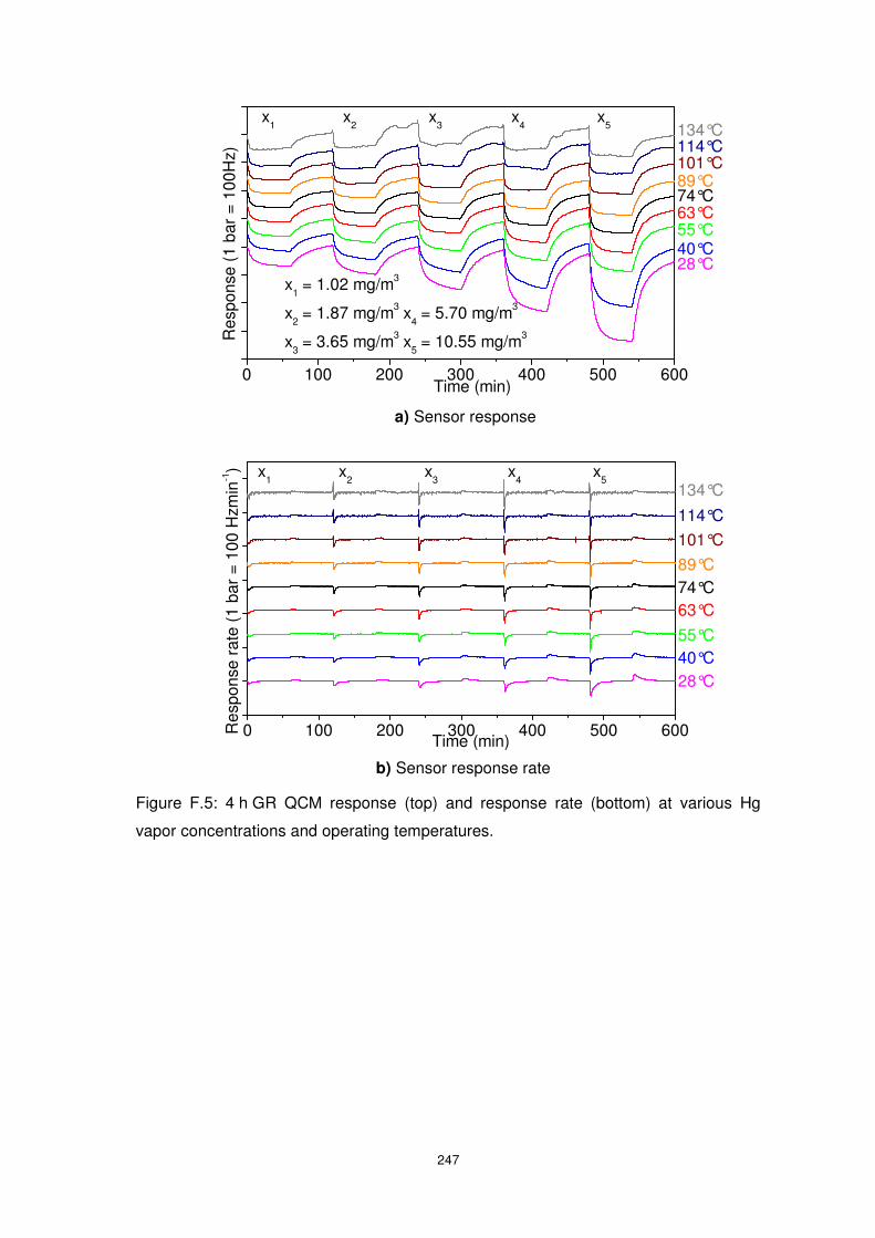
247
Figure F.5: 4 h GR QCM response (top) and response rate (bottom) at various Hg
vapor concentrations and operating temperatures.
a) Sensor response
b) Sensor response rate
0 100 200 300 400 500 600Res
pons
e ra
te (
1 ba
r =
100
Hzm
in-1)
Time (min)
134°C
28°C40°C55°C
63°C74°C89°C
101°C
114°C
x5
x4
x3
x2
x1
0 100 200 300 400 500 600
x1 = 1.02 mg/m3
x2 = 1.87 mg/m3 x
4 = 5.70 mg/m3
x3 = 3.65 mg/m3 x
5 = 10.55 mg/m3R
espo
nse
(1 b
ar =
100
Hz)
Time (min)
134°C
28°C40°C55°C63°C74°C89°C101°C114°C
x5
x4
x3
x2
x1
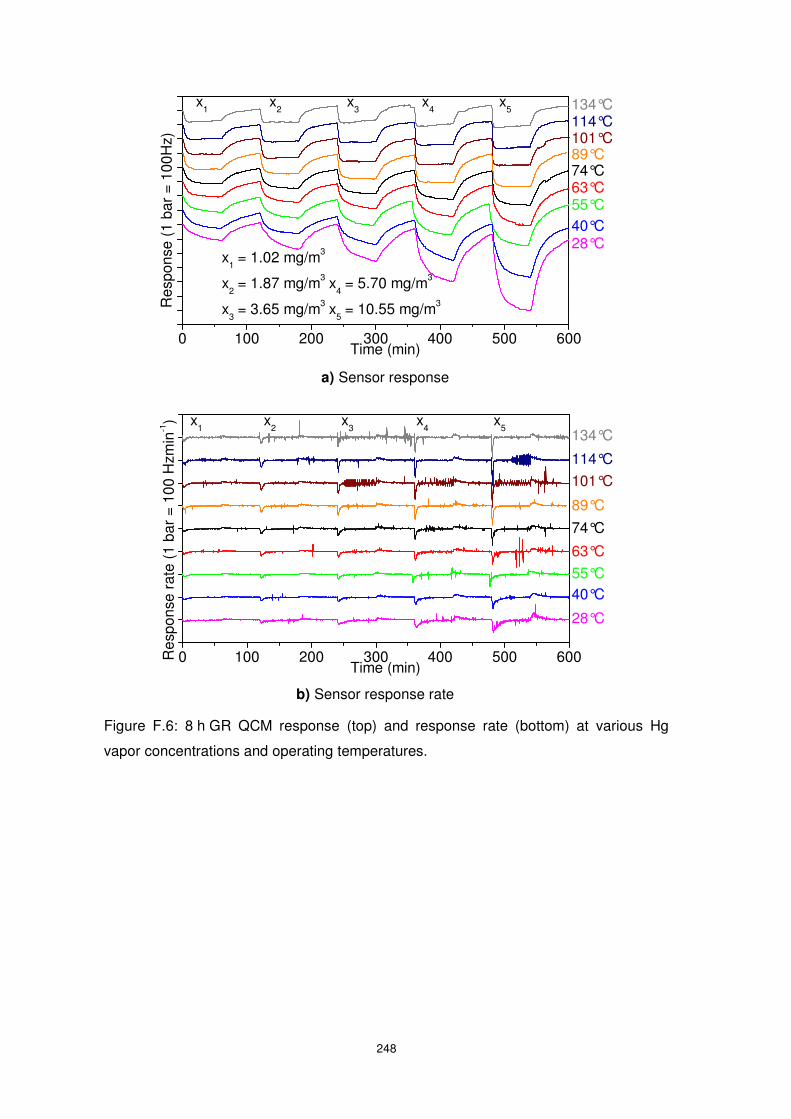
248
Figure F.6: 8 h GR QCM response (top) and response rate (bottom) at various Hg
vapor concentrations and operating temperatures.
a) Sensor response
b) Sensor response rate
0 100 200 300 400 500 600Res
pons
e ra
te (
1 ba
r =
100
Hzm
in-1)
Time (min)
134°C
28°C
40°C55°C
63°C
74°C
89°C
101°C
114°C
x5
x4
x3
x2
x1
0 100 200 300 400 500 600
x1 = 1.02 mg/m3
x2 = 1.87 mg/m3 x
4 = 5.70 mg/m3
x3 = 3.65 mg/m3 x
5 = 10.55 mg/m3R
espo
nse
(1 b
ar =
100
Hz)
Time (min)
134°C
28°C40°C55°C63°C74°C89°C101°C114°C
x5
x4
x3
x2
x1
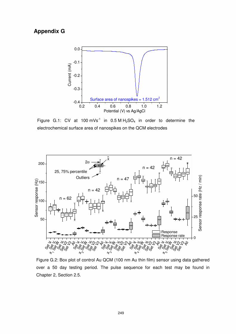
249
Appendix G
C
Figure G.1: CV at 100 mVs-1 in 0.5 M H2SO4 in order to determine the
electrochemical surface area of nanospikes on the QCM electrodes
0.2 0.4 0.6 0.8 1.0 1.2-0.4
-0.3
-0.2
-0.1
0.0
Cur
rent
(m
A)
Potential (V) vs Ag/AgCl
Surface area of nanospikes = 1.512 cm2
Figure G.2: Box plot of control Au QCM (100 nm Au thin film) sensor using data gathered
over a 50 day testing period. The pulse sequence for each test may be found in
Chapter 2, Section 2.5.
Set V
Set V
Set W
Set V
Set V
2Se
t V3 All
Set V
Set V
Set W
Set V
Set V
2Se
t V3 All
Set V
Set V
Set W
Set V
Set V
2Se
t V3 All
Set V
Set V
Set W
Set V
Set V
2Se
t V3 All
Set V
Set V
Set W
Set V
Set V
2Se
t V3 All
0
50
100
150
200
Sen
sor
resp
onse
(H
z)
x 1 x 2 x 3 x 4 x 5
Response
0
25
50
75
Sen
sor
resp
onse
rat
e (H
z / m
in)
321 1 2 3 1 2 3 1 2 3 1 2 3Outliers
25, 75% percentile
2σx
Response rate
n = 62
n = 42
n = 47
n = 42
n = 42
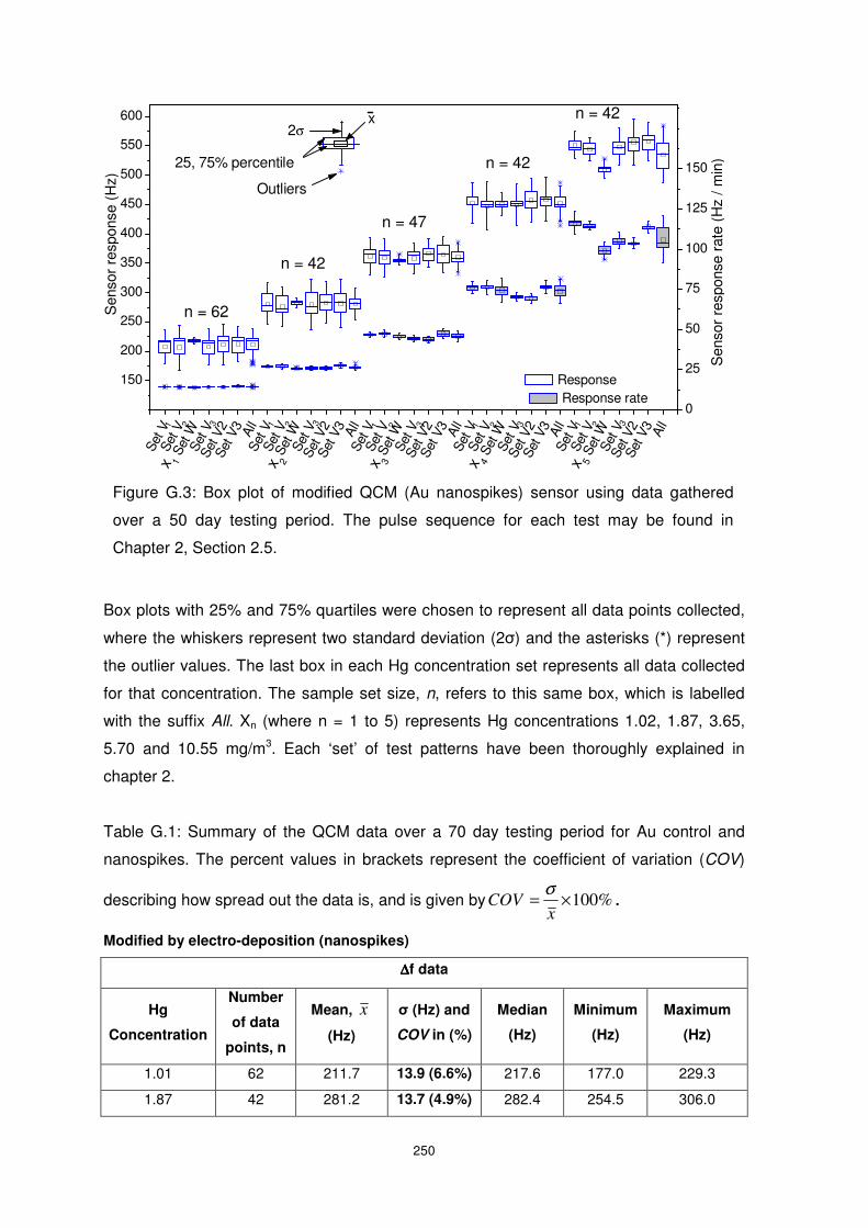
250
Box plots with 25% and 75% quartiles were chosen to represent all data points collected,
where the whiskers represent two standard deviation (2σ) and the asterisks (*) represent
the outlier values. The last box in each Hg concentration set represents all data collected
for that concentration. The sample set size, n, refers to this same box, which is labelled
with the suffix All. Xn (where n = 1 to 5) represents Hg concentrations 1.02, 1.87, 3.65,
5.70 and 10.55 mg/m3. Each ‘set’ of test patterns have been thoroughly explained in
chapter 2.
Table G.1: Summary of the QCM data over a 70 day testing period for Au control and
nanospikes. The percent values in brackets represent the coefficient of variation (COV)
describing how spread out the data is, and is given by %100×=x
COVσ
.
Modified by electro-deposition (nanospikes)
∆∆∆∆f data
Hg
Concentration
Number
of data
points, n
Mean, x
(Hz)
σ (Hz) and
COV in (%)
Median
(Hz)
Minimum
(Hz)
Maximum
(Hz)
1.01 62 211.7 13.9 (6.6%) 217.6 177.0 229.3
1.87 42 281.2 13.7 (4.9%) 282.4 254.5 306.0
Figure G.3: Box plot of modified QCM (Au nanospikes) sensor using data gathered
over a 50 day testing period. The pulse sequence for each test may be found in
Chapter 2, Section 2.5.
Set V
Set V
Set W
Set V
Set V
2Se
t V3 All
Set V
Set V
Set W
Set V
Set V
2Se
t V3 All
Set V
Set V
Set W
Set V
Set V
2Se
t V3 All
Set V
Set V
Set W
Set V
Set V
2Se
t V3 All
Set V
Set V
Set W
Set V
Set V
2Se
t V3 All
100
150
200
250
300
350
400
450
500
550
600
Sen
sor
resp
onse
(H
z)
Sen
sor
resp
onse
rat
e (H
z / m
in)
Response
0
25
50
75
100
125
150
175
Outliers
25, 75% percentile
2σx
321
x 5x 4x 3x 2x 1
n = 42
n = 42
n = 47
n = 42
n = 62
1 2 3 1 2 3 1 2 3 1 2 3
Response rate
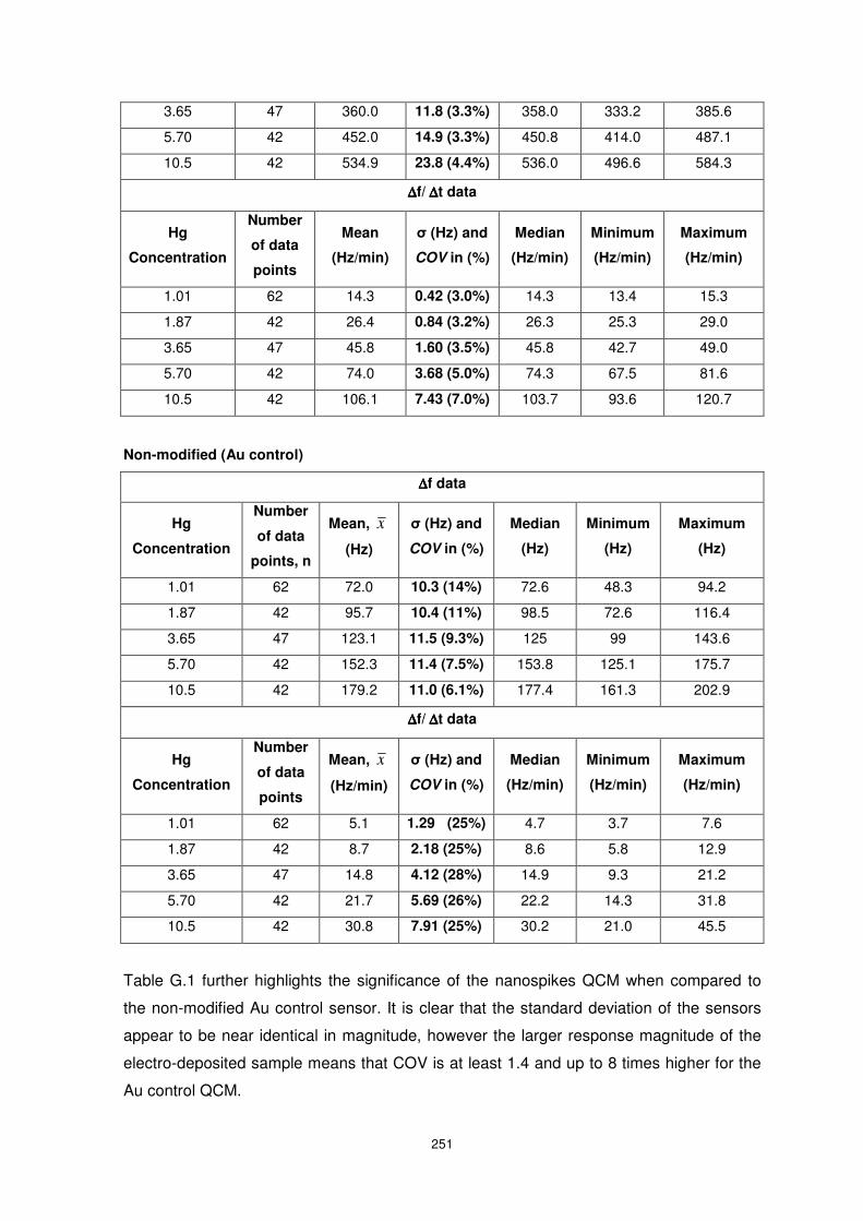
251
3.65 47 360.0 11.8 (3.3%) 358.0 333.2 385.6
5.70 42 452.0 14.9 (3.3%) 450.8 414.0 487.1
10.5 42 534.9 23.8 (4.4%) 536.0 496.6 584.3
∆∆∆∆f/ ∆ ∆ ∆ ∆t data
Hg
Concentration
Number
of data
points
Mean
(Hz/min)
σ (Hz) and
COV in (%)
Median
(Hz/min)
Minimum
(Hz/min)
Maximum
(Hz/min)
1.01 62 14.3 0.42 (3.0%) 14.3 13.4 15.3
1.87 42 26.4 0.84 (3.2%) 26.3 25.3 29.0
3.65 47 45.8 1.60 (3.5%) 45.8 42.7 49.0
5.70 42 74.0 3.68 (5.0%) 74.3 67.5 81.6
10.5 42 106.1 7.43 (7.0%) 103.7 93.6 120.7
Non-modified (Au control)
∆∆∆∆f data
Hg
Concentration
Number
of data
points, n
Mean, x
(Hz)
σ (Hz) and
COV in (%)
Median
(Hz)
Minimum
(Hz)
Maximum
(Hz)
1.01 62 72.0 10.3 (14%) 72.6 48.3 94.2
1.87 42 95.7 10.4 (11%) 98.5 72.6 116.4
3.65 47 123.1 11.5 (9.3%) 125 99 143.6
5.70 42 152.3 11.4 (7.5%) 153.8 125.1 175.7
10.5 42 179.2 11.0 (6.1%) 177.4 161.3 202.9
∆∆∆∆f/ ∆ ∆ ∆ ∆t data
Hg
Concentration
Number
of data
points
Mean, x
(Hz/min)
σ (Hz) and
COV in (%)
Median
(Hz/min)
Minimum
(Hz/min)
Maximum
(Hz/min)
1.01 62 5.1 1.29 (25%) 4.7 3.7 7.6
1.87 42 8.7 2.18 (25%) 8.6 5.8 12.9
3.65 47 14.8 4.12 (28%) 14.9 9.3 21.2
5.70 42 21.7 5.69 (26%) 22.2 14.3 31.8
10.5 42 30.8 7.91 (25%) 30.2 21.0 45.5
Table G.1 further highlights the significance of the nanospikes QCM when compared to
the non-modified Au control sensor. It is clear that the standard deviation of the sensors
appear to be near identical in magnitude, however the larger response magnitude of the
electro-deposited sample means that COV is at least 1.4 and up to 8 times higher for the
Au control QCM.