Comenius University, BratislavaFaculty of Mathematics, Physics and Informatics

Music Harmony Analysis:

Towards a Harmonic Complexity of Musical Pieces

Master’s Thesis

Bc. Ladislav Maršík, 2013

Comenius University, BratislavaFaculty of Mathematics, Physics and Informatics

Music Harmony Analysis:

Towards a Harmonic Complexity of Musical Pieces

Master’s Thesis

Course of study: InformaticsBranch of study: 2508 InformaticsDepartment: Department of Computer Science

Faculty of Mathematics, Physics and InformaticsComenius University, Bratislava

Supervisor: Mgr. Martin IlcíkICGA TU Wien

Date and place of publication: May 2013, Bratislava

Bc. Ladislav Maršík

Declaration

I hereby declare, that I wrote this thesis by myself, under the guidance of mysupervisor and with the help of the referenced literature.

............................................

Acknowledgments

I would like to thank my supervisor, Martin Ilcík for the most valuable timespent with this work. His experienced ideas gave the work a real value. I thankprofessor Stanislav Hochel from The Bratislava Conservatory because he gave thiswork the foundation, building my musical knowledge. I also thank the professorsfrom University Bordeaux 1, Pierre Hanna and Matthias Robine, for giving thiswork the right direction, when it needed most.

My dearest thank goes to my family. My parents and siblings are the greatestsupport and my grandma the greatest motivation that I could have, for my studies.I would also like to thank Pavla Liptáková, for giving me the belief and the vision,while working on this thesis.

Abstract

Author: Bc. Ladislav MaršíkTitle: Music Harmony AnalysisSubtitle: Towards a Harmonic Complexity of Musical PiecesUniversity: Comenius University, BratislavaFaculty: Faculty of mathematics, physics and informaticsDepartment: Department of computer scienceSupervisor: Mgr. Martin Ilcík

ICGA TU WienDate and place of publication: May 2013, Bratislava

In this work we present a new theoretical model for finding out the complexityof harmonic movements in a musical piece. We first define, what the yet unde-fined, term harmonic complexity means for us, finding different perspectives. Ourbasic model is based on tonal harmony. Utilizing the fundamental rules used inwestern music we define a grammar based model in which transition complexitiesbetween the harmonies can be evaluated as the computational time complexity ofderiving the harmony in the grammar. In graph representation the transition com-plexities can be found as the shortest path between the two harmonies. For thesepurposes we have created an object oriented model that implements the theoreticalmodel. In the end we deploy the system, Harmanal, capable of analyzing harmonytransitions from MIDI and WAVE input. We have used Harmanal for comparingmusic from different music genres. Moreover, we find Harmanal as a new pos-sibility for enhancing music information retrieval tasks such as implementing arecommender system for music.

Keywords: harmonic complexity, harmony analysis, chord transcription, chordprogression, music information retrieval

Abstrakt

Autor: Bc. Ladislav MaršíkNázov práce: Harmonická analýzaPodnázov: Smerujúc k harmonickej zložitosti hudobných dielŠkola: Univerzita Komenského v BratislaveFakulta Fakulta matematiky, fyziky a informatikyKatedra Katedra informatikyŠkolitel’: Mgr. Martin Ilcík

ICGA TU WienDátum a miesto vydania: Máj 2013, Bratislava

V práci uvádzame nový teoretický model pre nájdenie zložitosti harmonickýchprechodov v hudobnom diele. Najskôr popíšeme, co doposial’ nedefinovaný po-jem harmonická zložitost’ pre nás znamená. Nájdeme viaceré možné perspektívy,ktoré neskôr popíšeme. Náš základný model stavia na tonálnej harmónii. Extraho-vaním fundamentálnych zákonov používaných v teórii západnej hudby skonštru-ujeme model založený na formálnych gramatikách, v ktorom možno harmon-ický prechod medzi dvoma harmóniami zhodnotit’ ako casovú zložitost’ odvo-denia v gramatike. V reprezentácii na grafe môže byt’ zložitost’ prechodov náj-dená ako najkratšia cesta medzi harmóniami. Pre tieto úcely sme vytvorili objek-tovo orientovaný model ktorý implementuje popísaný teoretický model. Nakonieczavedieme systém Harmanal, schopný analyzovat’ harmonické prechody získanézo vstupov MIDI alebo WAV. Systém Harmanal sme použili na porovnanie hudbyz rôznych hudobných žánrov Navyše, systém Harmanal považujeme za novú al-ternatívu pre zefektívnenie úloh týkajúcich sa práce s hudbou na pocítacoch, akonapríklad vyhl’adávanie doporucenej hudby pre používatel’a.

Kl’úcové slová: harmonická zložitost’, harmonická analýza, prepis akordov,akordický rad, vyhl’adávanie hudby

Foreword

Back in the days when I was studying music composition, the biggest questionsI’ve had on my mind were – how to make the music more interesting? How tocreate more memorable tunes? Will the listener find the same aspects of musicbeautiful that I do? If you were ever creating some sort of art, you might haveended up with questions like these. . . Similarly, if we have our favorite musicpieces, what does really make them our favorite?

I have found, that it is not just the personal preference of everyone of us, butalso the function of our musical experience and knowledge. If we have devotedourselves into studying music harmony or music itself, our preference changes.We would eventually recognize the patterns of compositions and find the differ-ences between simple and more complex music. Interestingly enough, sometimesthe more we know about the possibilities in music, the more we can incline to-wards simpler music. More often, however, we may get tired of established prac-tices and seek different, more complex progress. In the result, the skilled com-poser of the 21st century can create music that may sound too complex or perhapstoo minimalistic and thus not beautiful for an inexperienced listener.

Generally speaking, it is difficult to decide whether simpler music can be morepopular, or vice versa. It is subjective matter. But what we can conclude is, thatintroducing a term music complexity can be helpful. Intuitively, our personal pref-erence of music may correlate with our preferred complexity of music. And forthe music, such a complexity can be measured.

Well, can it be measured? That is more of a musicologist’s question. I wouldalways prefer thorough analysis of a knowledgeable music analyst over an anal-ysis made by a machine, in the same way that I would prefer human-made artover a machine-made product. But given, that even the musicology does not haveany general rules for finding out the complexity, and not many works were yet

done in the mathematic or informatic field on this too, I decided to make the newpathways. The result will prove itself good if it is used by both, musicologists andprogram developers.

As strong as I believe that computers can not supersede the position of hu-man in producing and analyzing music, I also believe that music and mathematicsvastly overlap, if not, are the same. In that fashion I started to use different applica-tions easing the work of a musician, like notation softwares or music sequencers.Later I started creating my own. First of them, Ear training application[13] withchord naming model I will reference in this work, too. The next one you are read-ing right now. And, more are yet to come.

If you find this work useful for any kind of expansion or you are interested infurther discussion, please contact me at: laci@marsik.sk.

Table of Contents

1 Introduction 11.1 Music harmony . . . . . . . . . . . . . . . . . . . . . . . . . . . 1

1.1.1 Definition . . . . . . . . . . . . . . . . . . . . . . . . . . 11.1.2 History and tonal harmony . . . . . . . . . . . . . . . . . 2

1.2 Harmonic complexity . . . . . . . . . . . . . . . . . . . . . . . . 31.2.1 Beauty and complexity . . . . . . . . . . . . . . . . . . . 41.2.2 How can the complexity find its way to beauty . . . . . . 41.2.3 How can the beauty help define the complexity . . . . . . 6

1.3 Motivations . . . . . . . . . . . . . . . . . . . . . . . . . . . . . 81.4 Outline . . . . . . . . . . . . . . . . . . . . . . . . . . . . . . . 9

2 Understanding tonal harmony 112.1 Musicology disciplines . . . . . . . . . . . . . . . . . . . . . . . 112.2 Basics of music theory . . . . . . . . . . . . . . . . . . . . . . . 14

2.2.1 Finding the basic tones . . . . . . . . . . . . . . . . . . . 142.2.2 Intervals . . . . . . . . . . . . . . . . . . . . . . . . . . . 162.2.3 Scales . . . . . . . . . . . . . . . . . . . . . . . . . . . . 182.2.4 Chords . . . . . . . . . . . . . . . . . . . . . . . . . . . 202.2.5 Basics of music notation . . . . . . . . . . . . . . . . . . 22

2.3 Basics of tonal harmony . . . . . . . . . . . . . . . . . . . . . . 232.3.1 Basic harmonic functions . . . . . . . . . . . . . . . . . . 242.3.2 Diatonic functions . . . . . . . . . . . . . . . . . . . . . 24

2.4 Additional definitions . . . . . . . . . . . . . . . . . . . . . . . . 26

3 Related works and choosing the techniques 313.1 Extracting audio features . . . . . . . . . . . . . . . . . . . . . . 32

3.1.1 Vamp plugins . . . . . . . . . . . . . . . . . . . . . . . . 323.2 Chords transcription . . . . . . . . . . . . . . . . . . . . . . . . . 33

3.2.1 Fujishima and pattern matching . . . . . . . . . . . . . . 33

3.2.2 Chordal analysis . . . . . . . . . . . . . . . . . . . . . . 343.2.3 Music harmony analysis improving chord transcription . . 353.2.4 Working with added dissonances and tone clusters . . . . 36

3.3 Towards models for harmonic complexity . . . . . . . . . . . . . 383.3.1 Chord distance in tonal pitch space . . . . . . . . . . . . 393.3.2 Tonnetz and Neo-Riemannian theory . . . . . . . . . . . 39

3.4 Conclusion and defining the Harmanal system . . . . . . . . . . . 40

4 TSD distance model 464.1 Basic idea . . . . . . . . . . . . . . . . . . . . . . . . . . . . . . 464.2 Formal definition . . . . . . . . . . . . . . . . . . . . . . . . . . 48

4.2.1 Finding root harmonies . . . . . . . . . . . . . . . . . . . 514.2.2 Harmony complexity . . . . . . . . . . . . . . . . . . . . 554.2.3 Derivation explained . . . . . . . . . . . . . . . . . . . . 564.2.4 Transition complexity . . . . . . . . . . . . . . . . . . . 624.2.5 Comparison to Chomsky hierarchy . . . . . . . . . . . . 68

4.3 Graph representation – Christmas tree model . . . . . . . . . . . 694.3.1 Christmas forest . . . . . . . . . . . . . . . . . . . . . . 71

4.4 On computational complexity of the model . . . . . . . . . . . . 724.4.1 Time complexity of the main functions . . . . . . . . . . 73

4.5 Evaluating the complexity of the musical piece . . . . . . . . . . 744.5.1 Time complexity of the music analysis . . . . . . . . . . . 76

5 Other complexity models 785.1 Five harmonic complexities . . . . . . . . . . . . . . . . . . . . . 78

5.1.1 Voice leading complexity . . . . . . . . . . . . . . . . . . 795.1.2 Complexity of modulations . . . . . . . . . . . . . . . . . 805.1.3 Space complexity . . . . . . . . . . . . . . . . . . . . . . 805.1.4 Transition speed . . . . . . . . . . . . . . . . . . . . . . 81

6 Harmanal application 826.1 Technical information . . . . . . . . . . . . . . . . . . . . . . . . 826.2 Overview . . . . . . . . . . . . . . . . . . . . . . . . . . . . . . 836.3 Implementation details . . . . . . . . . . . . . . . . . . . . . . . 84

6.3.1 Harmanal static class . . . . . . . . . . . . . . . . . . . . 846.3.2 Chordanal static class . . . . . . . . . . . . . . . . . . . . 856.3.3 Application GUI . . . . . . . . . . . . . . . . . . . . . . 856.3.4 Other components . . . . . . . . . . . . . . . . . . . . . 85

6.4 Screenshots of usage . . . . . . . . . . . . . . . . . . . . . . . . 86

7 Results of analysis 887.1 Genre: Rock . . . . . . . . . . . . . . . . . . . . . . . . . . . . . 907.2 Genre: Popular . . . . . . . . . . . . . . . . . . . . . . . . . . . 907.3 Genre: Classical . . . . . . . . . . . . . . . . . . . . . . . . . . . 917.4 Other genres . . . . . . . . . . . . . . . . . . . . . . . . . . . . . 91

8 Conclusion and discussion 92

1 Introduction

1.1 Music harmony

„The most important in music is its harmony.“

Ilja Zeljenka, Slovak music composer

A great music has several qualities. It takes melody to make us memorize andhum the music on the street. It takes good rhythm to make us dance on the musicat the discotheque. For popular songs, lyrics and a good chorus can relate us evenmore to the song. And then there is music harmony, tones sounding together, thatcreates the atmosphere and the depth of music. What should we use to analyzethe true complexity of music?

Studying the music more and more, it is the harmony and its changing thatgives us the best platform for analysis. Even the melody by itself can have animplied harmony, harmony that could accompany it based on its tone material.Moreover, it has been ever since late baroque until now that majority of musicobeys certain harmony rules. That broadens our musical pieces space and givesus a way to compare pieces even from different genres and periods, using musicharmony1. Taking harmony as the subject of our research is therefore understand-able. And throughout the work we will trust our motto by Ilja Zeljenka, becauseit gives us confidence that we have chosen the right aspect.

1.1.1 Definition

According to Laborecký[8], music harmony is defined as follow:

1Supplementary to harmony, there is a comprehensive theory of counterpoint describing howwe can combine multiple voices together. There is much more to take into account before we castall music in the same mold and we should keep that in mind.

1

Music harmony is the study about the character of simultaneously soundingpitches, their meaning, transitions, functional relationships and usage in the musi-cal piece. It studies horizontal (subsequent) relationships in the time and vertical(concurrent) relationships among the tone space.

In other words, music harmony works with entities that represent simultane-ously sounding pitches. It has them, with the help of music theory, preciselylabeled and each entity has some meaning. Even more importantly, it specifiesthe rules that can connect these entities to the sequences. We thus obtain music,or more precisely, a musical accompaniment. There’s a counterpart to harmony,which is melody, that floats on the top of musical accompaniment and comprisessolely of sequence of tones and rests. For our analysis, we may choose to extractmelody from musical accompaniment or let the melody and the accompanimentsound together.

Note that, music harmony, as we defined it, is a scientific discipline, whereaswe will be interested in the harmony of a musical piece. Geared towards a singlepiece of music, we define:

Harmony of a musical piece is the use of simultaneously sounding pitchesand chords, their character, meaning, transitions and functional relations in a mu-sical piece2.

1.1.2 History and tonal harmony

The music harmony has grown over the ages. If we focus on western music,starting in late baroque in 18th century, a harmonic thinking has originated, thatwe now know as functional tonality, or tonal harmony. Its core is that every part

2Moreover, to increase the ambiguity even more, in this work we might also use the term„harmony“ to refer to the entities (simultaneously sounding pitches) that the music harmony workswith, i.e. interchangeably with the terms: chord, interval, cluster or chord with added dissonance,see chapter 2 for definitions. We hope that the positive reader will distinguish all the different usesand misuses of the term.

2

of a musical piece belongs to some major or minor key. It came to its very peak inmusic romanticism in 19th century. After that, many composers have founded newapproaches to music, moving outside the keys and breaching the tonal harmonyrules. Special rules also apply to modal folk songs, jazz or polyphonic pieces.Nevertheless, rules of tonal harmony still apply to vast majority of music todayand it is commonly being used as a way of teaching the basics of harmony. Wewill describe the aspects of tonal harmony important for this work, in the nextchapter.

1.2 Harmonic complexity

„Two impulses struggle with each other within man: the demand for

repetition of pleasant stimuli, and the opposing desire for variety, for

change, for a new stimulus“

Arnold Schönberg, Austrian composer and music theorist

The purpose of this section is to make the first steps to define the harmoniccomplexity and also to describe how it relates to the beauty in music, which willhelp us realize the major motivations for this work. Now, we may all relate to,that if the music is „all the same“ it may soon loose our interest. While listen-ing, we need variety, change and the new stimulus in the coming seconds. But ifwe get only different harmonies, we will certainly neglect something that we canrelate to, therefore we need repetition of our favorite passage, a pleasant stimuli.According to Zanette[24], these are the two fundamental principles that cast themusical form and that we expect in music. (And isn’t it the same in any other areaof life?)

Intuitively, we may define the music complexity as the variety, the change

and the occurrence of the new stimulus in music – the more unexpected changesoccur, the more is the musical piece complex. If that is the case, Arnold Schönberghas already helped us finding out, how much it relates to what we like or dislike in

3

music – should be the exact half of what we need. We also should take into consid-eration, that random and disordered changing of music harmonies should hardlyqualify as complex (Zanette[24]). However, it might be difficult to find out whatwas the composer’s intention to make particular harmonic movement, sometimesin the modern compositions the composers intentionally leave sections, where theperformer should choose random tones – should it be considered complex or not?We will therefore follow-up with our intuitive definition of complexity as the va-riety and change, that we believe can also get us closer to music beauty. How is itreally between music beauty and music complexity?

1.2.1 Beauty and complexity

Just like „The Beauty and The Beast“, it is clear that the beauty and the complexityof music are two different terms. But following the Disney’s storyline, we mayget to the point where they find the way towards each other.

1.2.2 How can the complexity find its way to beauty

The main difference between them is, that the beauty is subjective for every lis-tener, whereas the complexity can be measured generally for any musical piece.So, complexity and beauty may seem too distant at first. But like we said in theforeword, we may still use something that has to do with the listener’s preferredcomplexity of music. That is, the complexity of music that he or she is used to,that he or she likes. If something like this exists, we can measure it. Then wecan even use such measurings to find other music that he or she will like, too!This idea is well known as recommender systems, that well known internet radiosor portals such as Pandora, or Last.fm3, are using. Such systems have variousimplementations, filtering music based on its content, or based on other users’preferences (collaborative approach). But if they are based on music content, it isusually on the genre of the piece or the artist, but not on the complexity.

3http://www.last.fm; http://www.pandora.com

4

Therefore, another thing we may want to measure is the complexity of thespecified genre of music, or the concrete artists. If we, again, have good results,we may use harmonic complexity to specify the genre more accurately, but mainlyto find slight differences amongst the genre. It is quite obvious that two rockbands, let’s say Queen and Led Zeppelin, would have different music styles. Wemay end up finding that they have different complexities, too. That can be anotherevidence that using harmonic complexity for music retrieval is a good practice.

Similar researches were already done, finding out that usually the band or thecomposer uses certain „harmonic language“ (e.g. The Harmonic Language ofThe Beatles by KG Johansson[6]). But not much work was yet done on compar-ing these languages. According to these works, chances are, that if we define ourcomplexity well, we can gather such comparisons.

To summarize, we have found ourselves two tasks. We would wish to create aharmonic complexity model capable of:

• Finding out the complexity of music from different music periods, genresand artists.

• Finding out the complexity of music library of an user and implementing arecommender system searching for the music with the same complexity –the music he or she would like.

and therefore the complexity can find its way to the subjective beauty. Notethat, the first task is interesting by itself too, from the musicology perspective.That’s why, we will focus on this first experiment more in our work, gathering thereal results from the different periods and genres, and we will leave the secondtask open for future implementation. But it still remains one of the „ultimatemotivations“ for this work.

5

1.2.3 How can the beauty help define the complexity

Similarly to the fairytale, the beauty can help the complexity (the beast), to findits real self. Looking for the ways to define the complexity, there is an analogywith looking for the ways to define the beauty. Imagine that we look for the mostbeautiful human in the world. Rather like the prince traveling the world, lookingfor the most beautiful princess, he may take one of these, three approaches:

1. Take all of his human anatomy books with him, along with a measuringtape, and then measuring all potential princesses and comparing his resultswith the books.

2. Take several friends with him, meeting the young women in the kingdomand then at the evening campfire everyone would share their feelings aboutthe girls they’ve met. He would, then, choose the girl with the best rating.

3. Have the king call out, that every young woman should get to the courtyard,forming a line. He would, then, find about the beauty of the girls by goingfrom the first and comparing each one with the ones that he had alreadyseen. By the end of the line he would have a good eye on how the princessshould look like.

These three simple approaches represent: evaluation based on theory, evalua-tion based on perception and evaluation based on machine learning. All three arepossible and indeed great ways, to evaluate the complexity too.

1. Music theory and the part of it, tonal harmony, describes the set of rulesthat, if used well, can help us to evaluate the complexity.

2. Music perception is an important and vital part of the cognitive sciences. Wemay get the complexity by studying the opinions or the mental processes ofmusic listeners.

6

Figure 1: Approaches to music complexity

3. Machine learning is a common technique for music analysis. Teachingthe program on a sample of musical pieces, using hidden Markov models(HMMs) to learn what are the expected harmony transitions, can get us torelevant results too.

Comparing all of these approaches would be a nice study, however, out ofthe scope of this work. We should choose one. Machine learning is a commonapproach, even giving the best known results for naming the harmonies, although,we might be concerned that it always have better results if taught on music froma specific genre, and used on that same genre. There is also a belief presentedby De Haas et al.[3], that „certain musical segments can only be annotated when

musical knowledge not exhibited in the data is taken into account as well“. Musicperception is a discipline on its own and lot of statistical data need to be examinedto gather the results.

But having the good theoretical model first seems to be a good headstart forany future research. Thus, we have chosen the music theory, and its subset, tonalharmony as the basis of our work. We firmly believe, that, even if some other partsof music theory may enhance our results (such as theory of counterpoint or modalharmony), the way we use the key and scale based principles of tonal harmony isflexible for future modularity and apply to the majority of music we hear today,and is at the same time consistent with the related works on music theory too.

7

Going back to Arnold Schönberg’s statement, we may conclude that it is in-deed correct and we need both complexity and simplicity to find a musical piecebeautiful. How simple or how complex, that again depends on the personal prefer-ence of the listener (we need our prince for that). Nevertheless, beauty and com-plexity have many things in common, and in this work we do one step towardsbringing them together.

1.3 Motivations

To summarize it all up, the main motivations for this work are:

1. Create a good mathematical model for music complexity based on musictheory

2. Compare music from different periods, genres and artists

3. Introduce new option to retrieve music based on listener’s preferences

4. Create an application capable of complexity analysis

The mathematical model can be a good innovation in the field of musicologyand music information retrieval. Interestingly enough, there have not been manyattempts to evaluate the music complexity. There are analysis for tonal tension,voice leading, chord recognition, dissonances, and more, outputting different vi-sualizations, but, generally, music complexity has always had the label of „subjec-tive“ and „undefined“. The most common practice to call some music „simpler“ or„more complex“ than other was through some written or spoken analysis. Even ifit was taken into consideration in some works, it was suppressed because the finalproduct was to obtain different output such as chord sequence or visualization.Perhaps the reason why is the lack of clues in the harmony literature, where allthe rules are found, but seldom they are somehow ranked or evaluated. We hopeto use the same rules, but extracting the evaluation from them, too.

8

An important part of this thesis is creating an application for the end user,capable of music analysis. There is not clearly defined, who may the user ofsuch an application be. Either a musicologist retrieving information from musicalpieces, or a musician interested in chordal analysis, extracting the chords frommusic in order to reproduce them, or a composer playing with new harmonies, ora programmer implementing a plugin using the complexity model. Therefore, wetweak our application to provide all of these services:

• Processing WAV input for recorded musical pieces

• Parsing MIDI input for pluggable MIDI instruments

• Parsing text input for convenience

• Displaying analysis results for the whole musical piece, as well as for eachharmony transitions in the piece

• On-demand analysis for input harmonies

• As a by-product to obtain complexity, we will get to analyze every singleharmony from the input. Displaying the name for these harmonies can bea great help for musicians as well as theorists trying to understand how thecomplexity was generated

1.4 Outline

In the 2nd chapter, we introduce you to the basic concepts of tonal harmony,understandable also for a non-musician reader. The reader can find there the maindefinitions in order to understand, how our model works.

In the 3rd chapter, we switch our focus for a moment and we summarize theworks most related to ours. The reader can use that chapter in order to find outwhere trends are about now, in harmony analysis. In this chapter, we also choose

9

the fundamental techniques for our analysis.

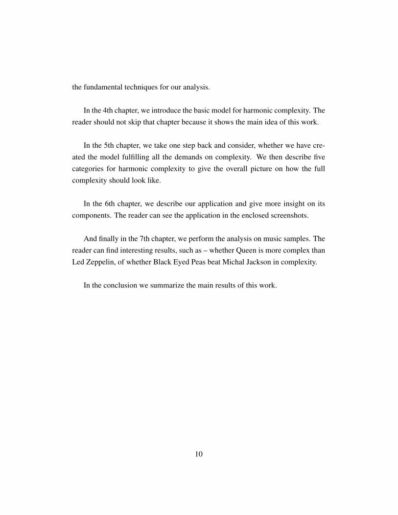
In the 4th chapter, we introduce the basic model for harmonic complexity. Thereader should not skip that chapter because it shows the main idea of this work.

In the 5th chapter, we take one step back and consider, whether we have cre-ated the model fulfilling all the demands on complexity. We then describe fivecategories for harmonic complexity to give the overall picture on how the fullcomplexity should look like.

In the 6th chapter, we describe our application and give more insight on itscomponents. The reader can see the application in the enclosed screenshots.

And finally in the 7th chapter, we perform the analysis on music samples. Thereader can find interesting results, such as – whether Queen is more complex thanLed Zeppelin, of whether Black Eyed Peas beat Michal Jackson in complexity.

In the conclusion we summarize the main results of this work.

10

2 Understanding tonal harmony

In this walkthrough on music tonal harmony, we will narrow our focus on defi-nitions for those terms, that will be repeatedly used in this work. The aim is toprovide clear meanings for the terms that will be used frequently, especially be-cause around the world the terms and sometimes also the meanings differ. Anotheraim is to invite a non-musician reader into discussion. The musicians may, on theother side, find some interesting insights into the broad topic of tonal harmony.

The definitions were compiled from Arnold Schönberg’s Theory of Harmony[21],the works of Zika and Korínek[25] or Pospíšil[17] designed for Slovak music con-servatories and a terminological dictionary by Riemann[18] and Laborecký[8]. Inthese works you can also find much more detailed elaboration.

Tonal harmony is a musical system, in which:

1. Every part of a musical piece belongs to a major or minor key.

2. Every harmony has some, close or distant relationship to the center of thekey, the first degree.

We have used some terms, that, to a non-musician, might need more clarifica-tion. We will define them in the subsequent sessions.

Firstly, we quickly clarify the umbrella terms, not to confuse the readers any-more, when using terms like music theory, musicology, music harmony, etc. Sec-ondly, we will hierarchically build the entities that we will work with. And lastly,we will get deeper into tonal harmony, describing the basic rules that are neededfor our analysis.

2.1 Musicology disciplines

Musicology is the scholarly study of music. It is the top umbrella term that in-cludes all musically relevant disciplines. It is just as science, as for example math-

11

ematics or informatics, but is considered social science because it studies the artcreations of mankind[15]. However, moving on, we find that splitting up musicol-ogy we get on one side historic musicology and ethnomusicology and on the othersystematic musicology, where the second mentioned contains plenty of subdisci-plines that usually interdisciplinary character.

The most important, for us, is the small, but fast growing discipline, musicinformation retrieval (MIR). Its common theme is retrieving information frommusic, and it has many real-world applications, such as recommender systems,track separation, music retrieval by queries, or automated music transcription.Our work falls under MIR.

We were already talking about music cognition, which is another musicologydiscipline, partially falling under systematic musicology.

Other discipline right in between musicology and physics, is called musicacoustics. It goes deep to describe how the physics in music works. But, im-portantly for us, there is another part of systematic musicology, that builds on theresults of music acoustics, called music theory.

Music theory is an applied discipline, which is, as proposed by many re-

searchers, an applied mathematics. Although music acoustics gave the theory its

building blocks, tones on the scale, and more and more evidences are there when

mathematic theories have helped develop the new harmonies, such as theory of

mathematic inversion, there is still some uncertainty in how much mathematics

can describe music. Perhaps the reason why is that historically, music and math-

ematics have developed separately, one originated as an art with no axiomatic

foundations, other as science. However, recent researchers are now filling the

gaps building new mathematical models and works4, in the same fashion as ours,

4Amongst many works we may highlight the works of David Lewin[11][12] and Neo-

12

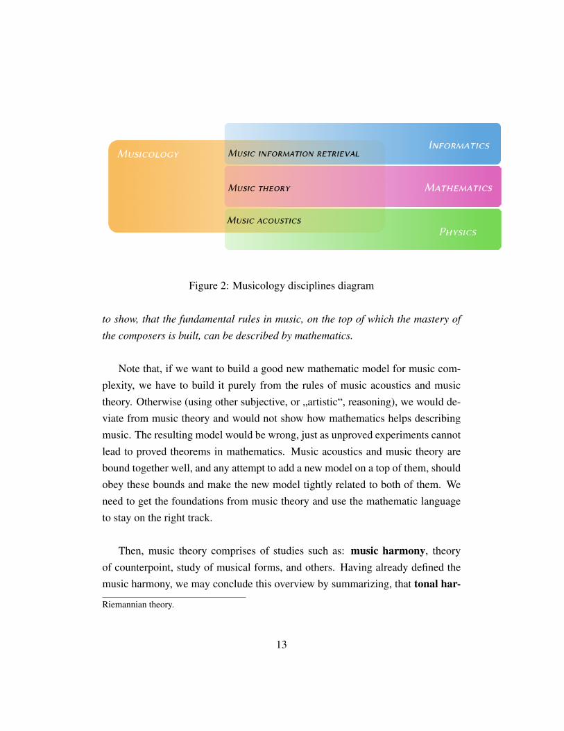
Figure 2: Musicology disciplines diagram

to show, that the fundamental rules in music, on the top of which the mastery of

the composers is built, can be described by mathematics.

Note that, if we want to build a good new mathematic model for music com-plexity, we have to build it purely from the rules of music acoustics and musictheory. Otherwise (using other subjective, or „artistic“, reasoning), we would de-viate from music theory and would not show how mathematics helps describingmusic. The resulting model would be wrong, just as unproved experiments cannotlead to proved theorems in mathematics. Music acoustics and music theory arebound together well, and any attempt to add a new model on a top of them, shouldobey these bounds and make the new model tightly related to both of them. Weneed to get the foundations from music theory and use the mathematic languageto stay on the right track.

Then, music theory comprises of studies such as: music harmony, theoryof counterpoint, study of musical forms, and others. Having already defined themusic harmony, we may conclude this overview by summarizing, that tonal har-

Riemannian theory.

13

mony is only one concrete system in music harmony. There are others, such asmodal system, using the scales commonly appearing in folk music. In the 20thcentury, multiple new systems arose, such as bitonality, polytonality, extendedtonality or also dodecaphony introduced by Arnold Schönberg.

2.2 Basics of music theory

Music acoustics has helped the music theory define these basic terms:

Tone is an acoustic sound, that is created by regular vibration of a source.

Music theory also defines the tone as the smallest element of a musical piece,characterized by its pitch, intensity, timbre and duration. Pitch can be quantifiedas frequency, but it takes comparison of a complex music sound to a pure tonewith sinusoidal waveform to determine the actual pitch, therefore the pitch shouldbe considered as a subjective attribute of sound.

2.2.1 Finding the basic tones

From the spectrum of all audible pitches, the western music only uses a narrowset with frequencies in such distribution, that their differences may be clearlyrecognized by an ear (88 tones of today’s piano keyboard). In this set, the twopitches, one with a double of frequency of the other, blend in the sound whileplayed simultaneously so they resemble one sound, although they have differentpitches. To these pitches, a distance of one octave is assigned. Within an octave,we differentiate a scale of 7 tones that is periodically repeated. These tones wereassigned the alphabet letters, forming the basis of musical alphabet:

a,b,c,d,e, f ,g

However, with stabilizing the tone c as the beginning of what became a major

scale, we more often refer to the tone order: c,d,e, f ,g,a,b.

14

Figure 3: Tones arranged in the octaves

To distinguish the different octaves, the labeling was established. In Helmholtz

notation commonly used by musicians, we label the octaves from the middle andup: „one-line“ (c′) , „two-line“ (c′′), „three-line“ (c′′′) and from the middle down:„small“ (c), „great“ (C) and „contra“ (C,). Some authors prefer the scientific no-

tation, simply labeling the octaves chronologically: 1,2,3,4,5,65.

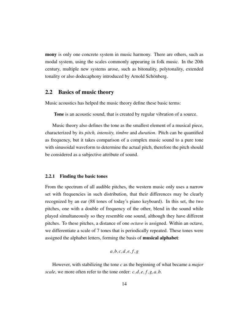
According to Schönberg, we can explain the basic pitches of a major scale ashaving been found through imitation of nature. A musical sound is a compositemade up of series of tones sounding together, the overtones, forming the har-monic series. It is due to the existence of additional oscillation nodes and partialwaves along with the original oscillation. The frequency of the original wave iscalled the fundamental frequency or first harmonics and represents the funda-mental tone in the composite, whereas the higher frequencies are referred to asthe overtones or higher harmonics (2nd, 3rd, . . . ). From a fundamental C, thehigher harmonics are:

c,g,c′,e′,g′,b[′,c′′,d′′,e′′, f ′′,g′′,etc.

The tones that occur first in the series, have also stronger presence in the com-

5On the standard piano, tones are ranging from sub contra a (A0) to five-line c (C8), MIDItones range even from double sub contra c (C-1) to six-line g (G9).

15

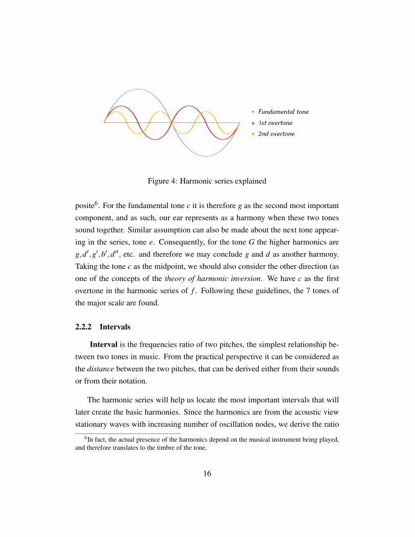
Figure 4: Harmonic series explained

posite6. For the fundamental tone c it is therefore g as the second most importantcomponent, and as such, our ear represents as a harmony when these two tonessound together. Similar assumption can also be made about the next tone appear-ing in the series, tone e. Consequently, for the tone G the higher harmonics areg,d′,g′,b′,d′′, etc. and therefore we may conclude g and d as another harmony.Taking the tone c as the midpoint, we should also consider the other direction (asone of the concepts of the theory of harmonic inversion. We have c as the firstovertone in the harmonic series of f . Following these guidelines, the 7 tones ofthe major scale are found.

2.2.2 Intervals

Interval is the frequencies ratio of two pitches, the simplest relationship be-tween two tones in music. From the practical perspective it can be considered asthe distance between the two pitches, that can be derived either from their soundsor from their notation.

The harmonic series will help us locate the most important intervals that willlater create the basic harmonies. Since the harmonics are from the acoustic viewstationary waves with increasing number of oscillation nodes, we derive the ratio

6In fact, the actual presence of the harmonics depend on the musical instrument being played,and therefore translates to the timbre of the tone.

16

between the second and first frequency as exactly 2 : 1, the ratio between the thirdand second is 3 : 2, the ratio between fourth and third is 4 : 3, etc.

The frequencies ratio 2 : 1 is denoted as the perfect octave. It can be foundfor example as the distance between c′ and c′′.

The frequencies ratio 3 : 2 is denoted as the perfect fifth. It can be found forexample as the distance between c′ and g′.

The frequencies ratio 4 : 3 is denoted as the perfect fourth. It can be foundfor example as the distance between c′ and f ′.

The frequencies ratio 5 : 4 is denoted as the major third. It can be found forexample as the distance between c′ and e′.

The frequencies ratio 6 : 5 is denoted as the minor third. It can be found forexample as the distance between c′ and e[′.

Following the ratios between the overtones, we have stepped out of the set oftones of a basic scale, discovering the tone e[′ in between d and e. The differencebetween the major third and the minor third is the frequencies ratio 25 : 24 (wecan get it by dividing the intervals). Similarly, we discover that the differencebetween the perfect fourth and major third is 16 : 15. These ratios, almost indis-tinguishable by an ear, along with couple of others occurring between the basictones, have been denoted as the semitone or the minor second. The semitonesets the smallest commonly used distance between the tones in western music andcan be used to measure the distance of larger intervals. Similarly, the distance thatapproximates as the double-semitone distance is denoted as the whole tone or themajor second, most commonly appearing as the frequencies ratio 9 : 8.

17

Thus, multiple tones out of the basic major scale were added (black tones onthe piano keyboard), and we differentiate two ways how to describe their presence– by two types of accidentals:

• If the tone can be described as created by augmenting the original tone by asemitone, we mark it with the accidental ] next to the original tone, and callit „sharp“ (c sharp: c], d sharp: d], f sharp: f ], g sharp: g], and a sharp:a]).

• If the tone can be described as created by diminishing the original tone by asemitone, we mark it with the accidental [ next to the original tone, and callit „flat“ (d flat: d[, e flat: e[, g flat: g[, a flat: a[ an b flat: b[).

In today’s music theory, the ambiguity between the different semitones in thetone scale have become impractical for some instruments. Therefore, a commoninterval ratio for the semitone was established, with the value of 12

√2 : 1. This tun-

ing is known as tempered tuning, as opposed to just tuning based on the exactratios from the harmonic series.

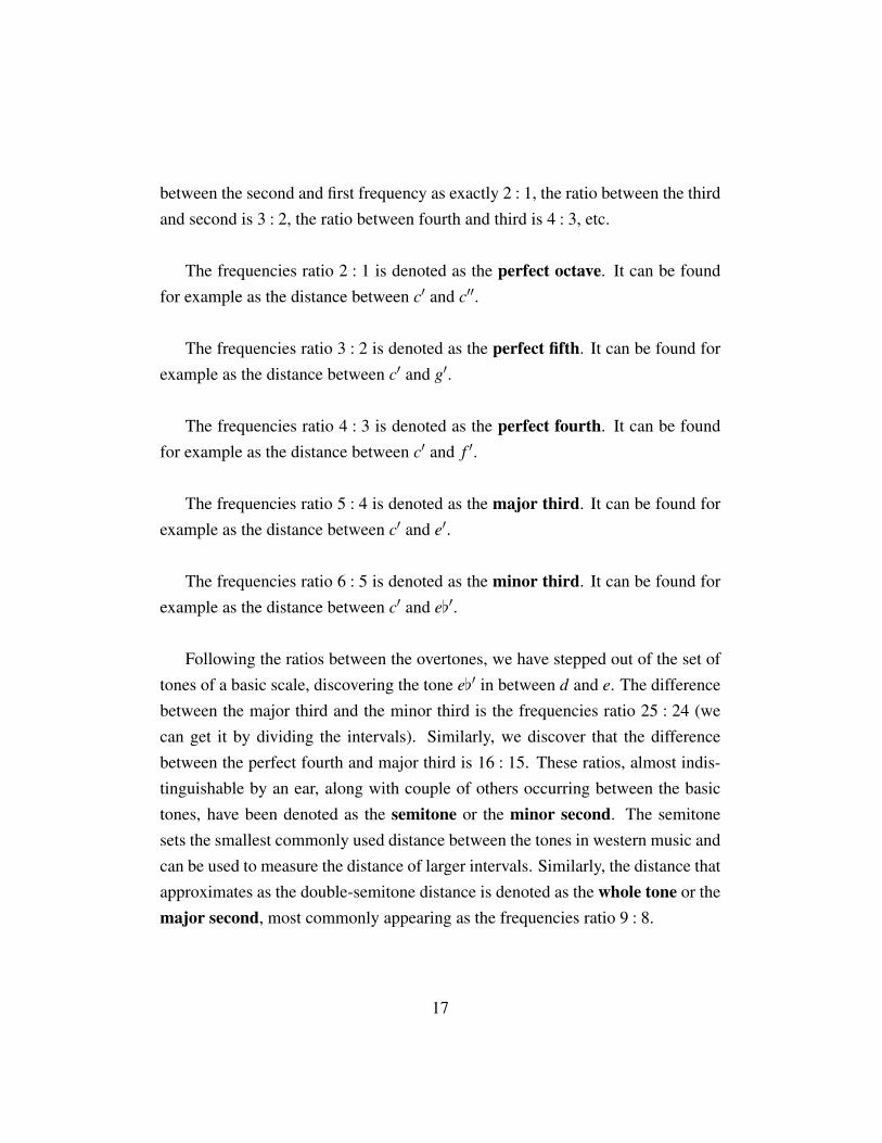
For summary, all the commonly used intervals can be found in the table 1.

Note that, augmenting or diminishing these basic intervals using accidentalswe get theoretical augmented or diminished intervals that share the same nameas the original interval, but sound like a different interval, e.g. augmented third =perfect fourth.

2.2.3 Scales

Scale is a series of increasing or decreasing pitches bounded by an octave.

Diatonic scales are the scales created by semitone and whole tone intervals.They contain 8 tones.

We divide 2 types of diatonic scales:

18

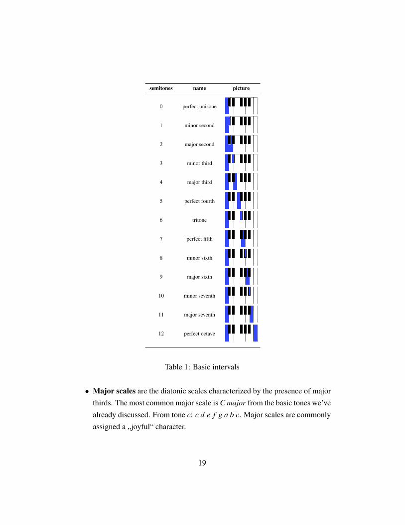
semitones name picture

0 perfect unisone

1 minor second

2 major second

3 minor third

4 major third

5 perfect fourth

6 tritone

7 perfect fifth

8 minor sixth

9 major sixth

10 minor seventh

11 major seventh

12 perfect octave

Table 1: Basic intervals

• Major scales are the diatonic scales characterized by the presence of majorthirds. The most common major scale is C major from the basic tones we’vealready discussed. From tone c: c d e f g a b c. Major scales are commonlyassigned a „joyful“ character.

19

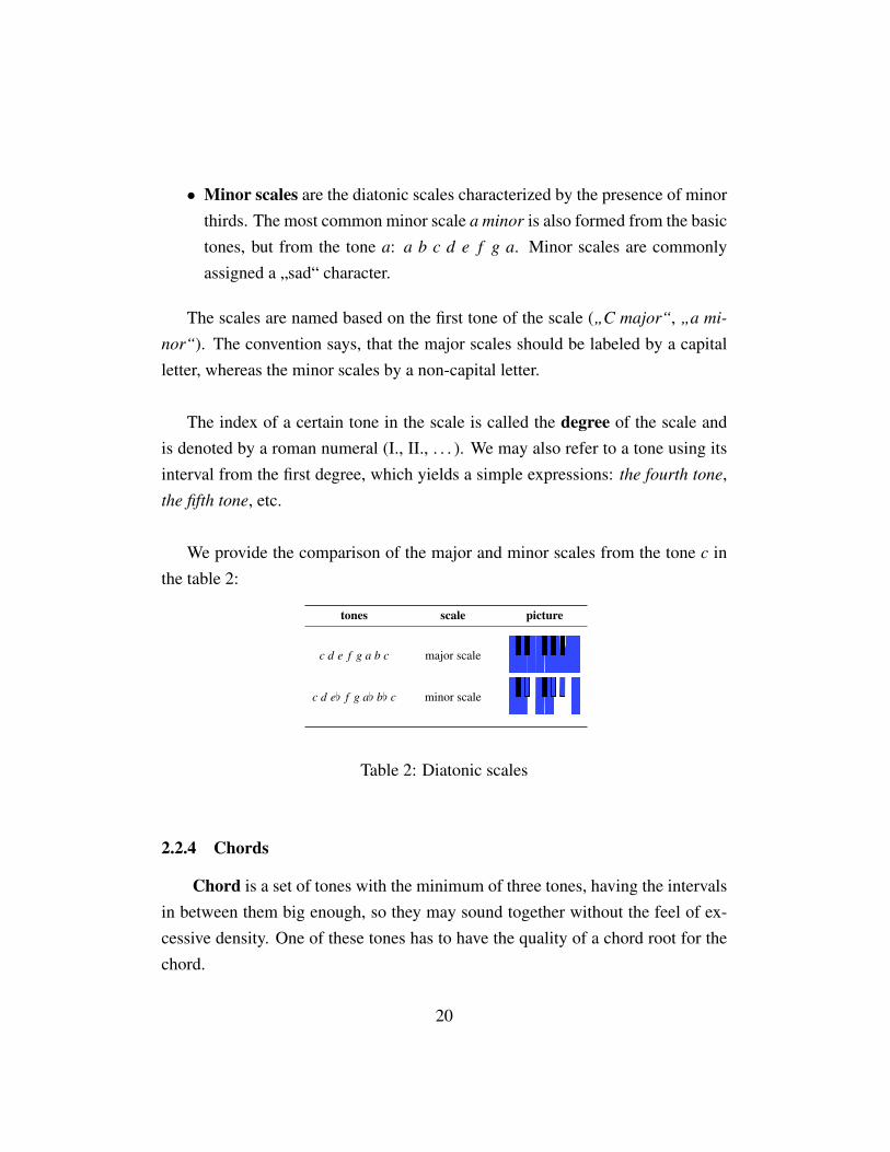
• Minor scales are the diatonic scales characterized by the presence of minorthirds. The most common minor scale a minor is also formed from the basictones, but from the tone a: a b c d e f g a. Minor scales are commonlyassigned a „sad“ character.

The scales are named based on the first tone of the scale („C major“, „a mi-

nor“). The convention says, that the major scales should be labeled by a capitalletter, whereas the minor scales by a non-capital letter.

The index of a certain tone in the scale is called the degree of the scale andis denoted by a roman numeral (I., II., . . . ). We may also refer to a tone using itsinterval from the first degree, which yields a simple expressions: the fourth tone,the fifth tone, etc.

We provide the comparison of the major and minor scales from the tone c inthe table 2:

tones scale picture

c d e f g a b c major scale

c d e[ f g a[ b[ c minor scale

Table 2: Diatonic scales

2.2.4 Chords

Chord is a set of tones with the minimum of three tones, having the intervalsin between them big enough, so they may sound together without the feel of ex-cessive density. One of these tones has to have the quality of a chord root for thechord.

20

Chord root is the tone upon which the chord can be built by stacking thirdsintervals. If the root of the chord is indeed the bottom tone of the chord, we saythat chord is in a root position. We can also obtain the chord inversions, byreorganizing the tones in such manner, that the root of the chord is put to the topof the chord – first inversion – or as the second from the top – second inversion– etc.

We will use the term chord tone for each of the tones within the tone materialof the chord in the context. The term non-chord tone will denote a tone out of thetone material of the chord. Note that, the tone material implies considering thetones mapped to one scale, i.e. taking the tone c as a tone chord if the c from anyoctave is present in the chord. We will always distinguish whether we considerthe real pitches where order of the tones matters, or mapped tones, the so called,pitch classes. In general, it is desirable to consider the real pitches for harmonystudy and therefore distinguish different inversions of the chord.

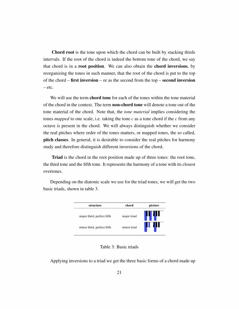
Triad is the chord in the root position made up of three tones: the root tone,the third tone and the fifth tone. It represents the harmony of a tone with its closestovertones.

Depending on the diatonic scale we use for the triad tones, we will get the twobasic triads, shown in table 3.

structure chord picture

major third, perfect fifth major triad

minor third, perfect fifth minor triad

Table 3: Basic triads

Applying inversions to a triad we get the three basic forms of a chord made up

21

of three tones, shown in table 4 (on a major triad).

type name picture

root position triad

1st inversion sixth chord

2nd inversion four-six chord

Table 4: Triad inversions

Besides major and minor triads we also distinguish diminished triad (minorthird, diminished fifth) and augmented triad (major third, augmented fifth).

2.2.5 Basics of music notation

It is out of the scope of this work to go through all the rules of music notation. Wewill only briefly show how the basics work, so non-musician readers may navigatethrough the music samples we will use later in the work. For our purposes it willbe sufficient only to localize what tones are present in the notation.

The staff consists of five lines. We mark the tones on the staff using the spe-cial markings, notes. Higher pitches are marked higher in the staff, either on theline or in between the lines. To determine the actual pitch, we need to identify atleast one position on the staff, which is done by the clef. For the instruments withhigh range, the G clef is used, determining the g′ (and also derived from the letter„g“, although it resembles the letter just remotely). For specifying the pitch, anaccidental (], [) may be used before the note. All the other attributes of the tone(length, intensity, the instrument playing the tone) can be derived using the specialmarkings and guidelines – for more information we refer to Pospíšil[17].

22

b �

���g

�� �c

�f

��e �

�c�

a �d

�

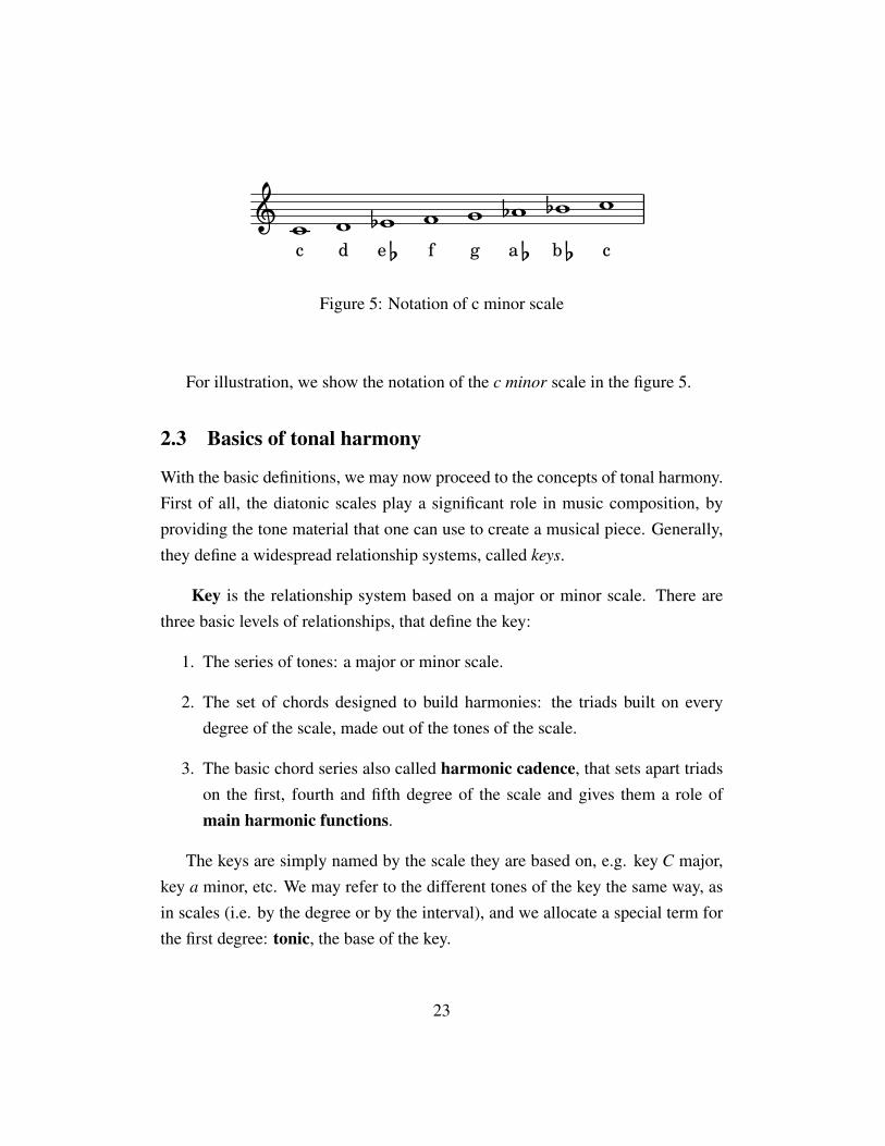
Figure 5: Notation of c minor scale

For illustration, we show the notation of the c minor scale in the figure 5.

2.3 Basics of tonal harmony

With the basic definitions, we may now proceed to the concepts of tonal harmony.First of all, the diatonic scales play a significant role in music composition, byproviding the tone material that one can use to create a musical piece. Generally,they define a widespread relationship systems, called keys.

Key is the relationship system based on a major or minor scale. There arethree basic levels of relationships, that define the key:

1. The series of tones: a major or minor scale.

2. The set of chords designed to build harmonies: the triads built on everydegree of the scale, made out of the tones of the scale.

3. The basic chord series also called harmonic cadence, that sets apart triadson the first, fourth and fifth degree of the scale and gives them a role ofmain harmonic functions.

The keys are simply named by the scale they are based on, e.g. key C major,key a minor, etc. We may refer to the different tones of the key the same way, asin scales (i.e. by the degree or by the interval), and we allocate a special term forthe first degree: tonic, the base of the key.

23

The complicated definition of the key simply means, that in tonal harmony, werecognize different keys, of which each defines a set of chords and their possiblesequences – we may say, a set of rules. That of course makes creating the musicor musical accompaniment much easier.

2.3.1 Basic harmonic functions

According to the definition of the key, some of the chords have more importantroles in the key than others. They set the three basic levels of tension towards thetonic, and are the basis of tonal harmony. We recognize them as the three mainharmonic functions:

• Tonic is the triad on the first degree of the key. It is the function of a har-monic steadiness and release. All the harmonic impulses origin in tonic andreturn back to tonic. We label it with T .

• Subdominant is the triad on the fourth degree of the key. It brings thedeviation from the tonic, and is the intermediary function in between tonicand dominant. We label it with S.

• Dominant is the triad on the fifth degree of the key. It represents the maxi-mal tension, that requires an ease, transition to tonic. We label it with D.

The harmonies in music start usually in tonic. Optionally, the harmony de-viates from tonic by transition to subdominant. Finally, the harmonic movementculminates in dominant and goes back to tonic again. We call this the basic har-monic progression T – S – D – T. According to Zika an Korínek, it is the skeletonof every music motion in musical pieces in the tonal harmony system.

2.3.2 Diatonic functions

It is possible to build a triad on every degree of a diatonic scale, using the tones ofthat scale. Every such triad we can then assign a function.

24

VII

���

leadingsubmediant

D 7Tp,Sl

VI

���

D

�

dominant

�

Sp

supertonicII

���IV

�

T

tonicI

��� �V

���

S

subdominant

Dp,Tl

mediantIII

���

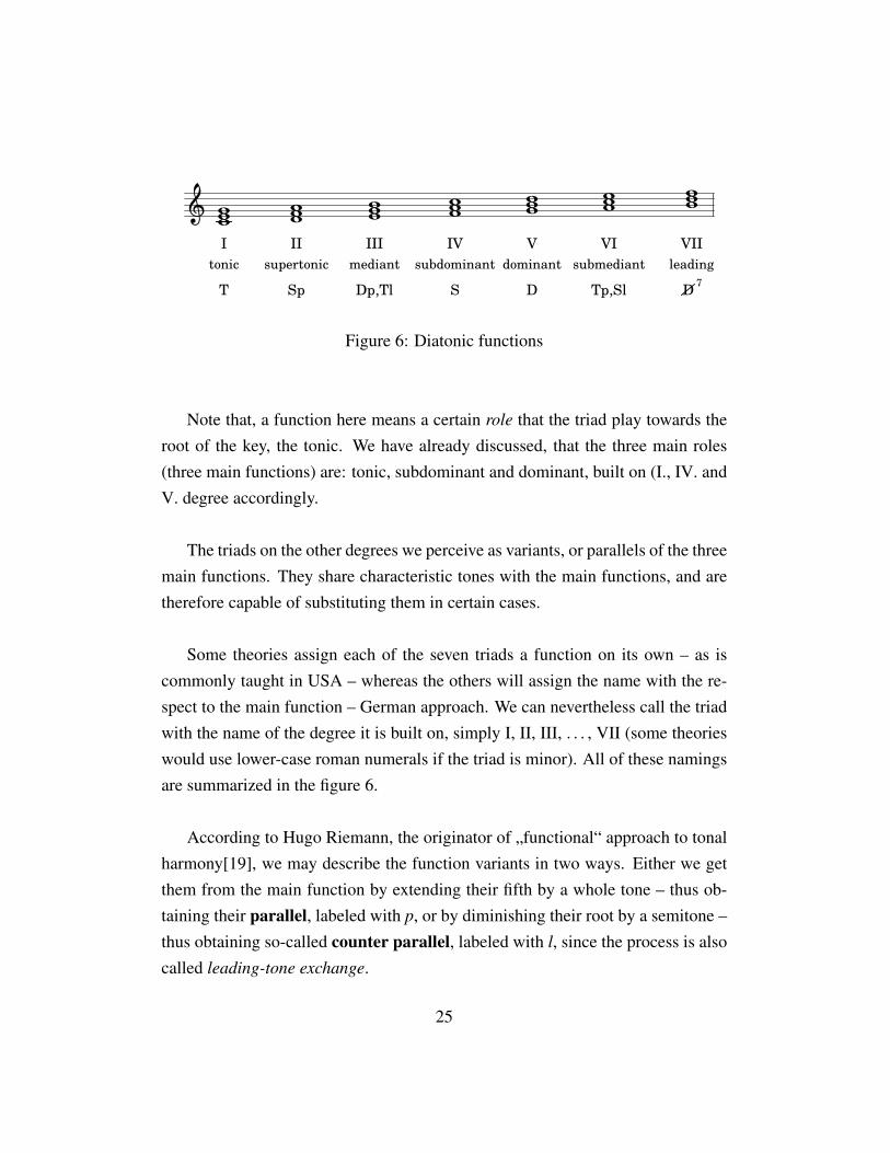
Figure 6: Diatonic functions

Note that, a function here means a certain role that the triad play towards theroot of the key, the tonic. We have already discussed, that the three main roles(three main functions) are: tonic, subdominant and dominant, built on (I., IV. andV. degree accordingly.

The triads on the other degrees we perceive as variants, or parallels of the threemain functions. They share characteristic tones with the main functions, and aretherefore capable of substituting them in certain cases.

Some theories assign each of the seven triads a function on its own – as iscommonly taught in USA – whereas the others will assign the name with the re-spect to the main function – German approach. We can nevertheless call the triadwith the name of the degree it is built on, simply I, II, III, . . . , VII (some theorieswould use lower-case roman numerals if the triad is minor). All of these namingsare summarized in the figure 6.

According to Hugo Riemann, the originator of „functional“ approach to tonalharmony[19], we may describe the function variants in two ways. Either we getthem from the main function by extending their fifth by a whole tone – thus ob-taining their parallel, labeled with p, or by diminishing their root by a semitone –thus obtaining so-called counter parallel, labeled with l, since the process is alsocalled leading-tone exchange.

25

• The triad II represents the variant of subdominant, subdominant parallel.We label it with Sp.

• The triad III represents both the dominant parallel and tonic counter par-allel. We label it with Dp or Tl.

• The triad VI represents both the tonic parallel and subdominant counterparallel. We label it with Tp or Sl.

• The triad VII is an exception, although it resembles dominant counter par-allel, the root is diminished one more semitone down, thus obtaining not amajor nor minor chord, but a „diminished “chord. However, because of itscharacteristic structure – upper 3 tones of dominant seventh chord, that wewill discuss later – it is simply called incomplete dominant seventh andlabeled D/ 7.

The study of tonal harmony also describes additional chord structures that maybe considered as one of these functions – some of them will be mentioned in thenext section – but mostly describes different ways of connecting these functions inmusic. The common transitions are: T – S, T – D, S – T, D – T, only the transitionD – S is not used. According to Zika, however, we know some exceptions, e.g.when subdominant substitutes dominant only temporarily. But the main messageremains, that with simple T – S – D – T transitions, the music would be too narrowand limited and – considered easy. But instead of main functions we may alwaysuse the variant, parallel, of the main function. This makes the music much moreinteresting, changing, and complex.

2.4 Additional definitions

In this section we will define all the rest of the musical terms, that will be used inthis work. If You have enough of definitions for now, feel free to continue readingthe chapter 3 and use the rest of this chapter as a dictionary that You can referback to.

26

(a)

C C] D D] E F F] G G] A A] B

0.74 0.00 0.10 0.00 0.53 0.04 0.00 0.66 0.00 0.15 0.00 0.10

(b)

C C] D D] E F F] G G] A A] B

1 0 0 0 1 0 0 1 0 0 0 0

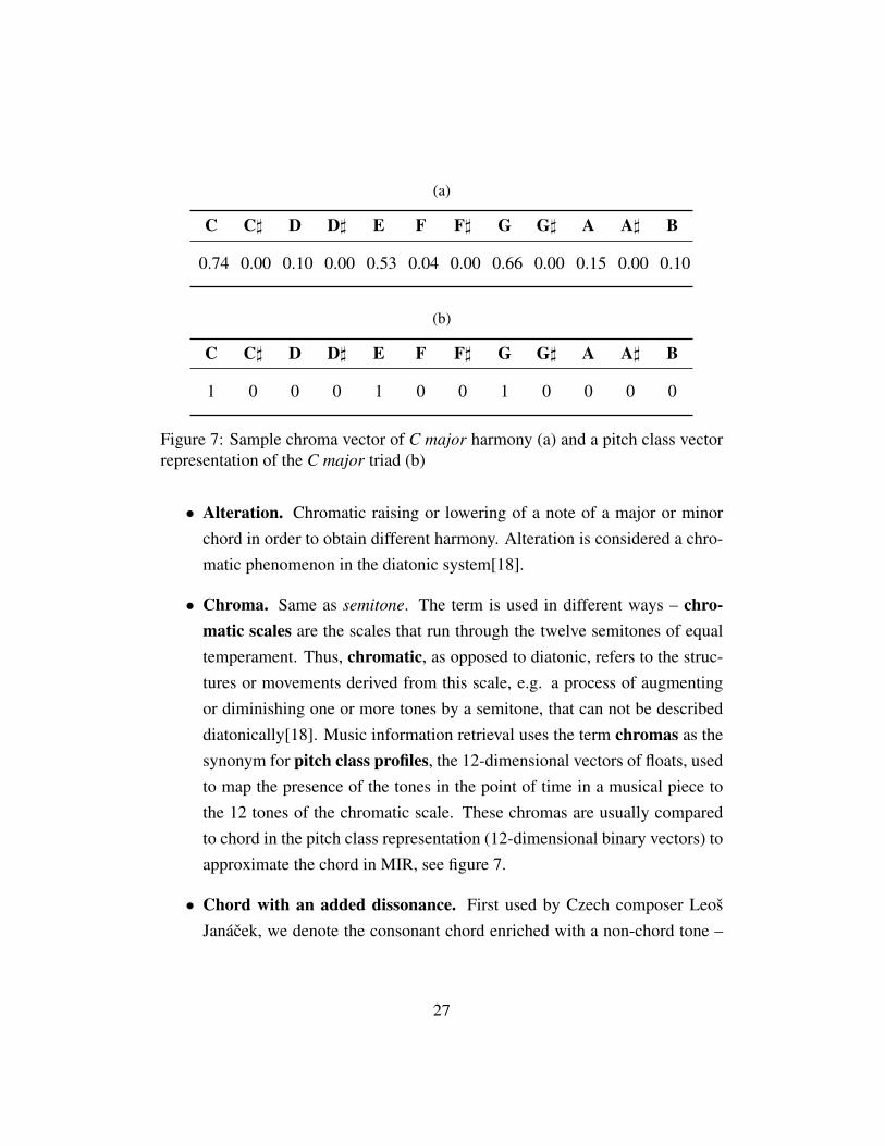
Figure 7: Sample chroma vector of C major harmony (a) and a pitch class vectorrepresentation of the C major triad (b)

• Alteration. Chromatic raising or lowering of a note of a major or minorchord in order to obtain different harmony. Alteration is considered a chro-matic phenomenon in the diatonic system[18].

• Chroma. Same as semitone. The term is used in different ways – chro-matic scales are the scales that run through the twelve semitones of equaltemperament. Thus, chromatic, as opposed to diatonic, refers to the struc-tures or movements derived from this scale, e.g. a process of augmentingor diminishing one or more tones by a semitone, that can not be describeddiatonically[18]. Music information retrieval uses the term chromas as thesynonym for pitch class profiles, the 12-dimensional vectors of floats, usedto map the presence of the tones in the point of time in a musical piece tothe 12 tones of the chromatic scale. These chromas are usually comparedto chord in the pitch class representation (12-dimensional binary vectors) toapproximate the chord in MIR, see figure 7.

• Chord with an added dissonance. First used by Czech composer LeošJanácek, we denote the consonant chord enriched with a non-chord tone –

27

Figure 8: Circle of fifths

thus creating dissonances – as a chord with an added dissonance7. Theyrepresent the intermediate stage in between the chords and clusters. We donot use this term if the chord can be described otherwise, e.g. as a seventhchord[23].

• Circle of fifths. The rotation through the twelve tones of the chromatic

scale, by fifth intervals, represented graphically in a circle. It is commonlyused to represent the keys, because, starting from C major and a minor, thekeys following by fifth intervals in one direction, have increasing numberof tones with sharp accidentals, and starting from the same (C major, a mi-

nor) going the other direction, have increasing number of tones with flat

accidentals (see figure 8). This is also a common way to determine howmany augmented or diminished tones are there in the particular key – find-ing out the number of steps in the circle of fifths. The set of accidentals fora particular key is referred to as the key signature.

• Cluster. Cluster or tone cluster refers to a set of tones sounding together,with at least three adjacent tones (with smaller than a whole tone interval),where the functional substance of the chord can not be identified anymore[8].

7In Czech language the term is more simple and has the meaning similar to densed chord. Weprefer using the formal translation not to confuse with new terms.

28

• Consonance. The harmonious sound or coalescence of two or more tones,giving the impression of harmonic stability to the listener. On the basicinterval scale, all of the perfect intervals, major and minor thirds and majorand minor sixths are consonant[8].

• Dissonance. The inharmonious sound, opposite to consonance, that re-quires harmonic transition. On the basic interval scale, major second andminor seventh are considered „mild“ dissonances, whereas minor secondand major seventh are considered „sharp“ dissonances. A special disso-nance is also assign to specific inharmonious sound of the tritone interval[8].

• Leading tone. A tone leading to another causing the another tone to beexpected in harmony after the presence of the leading tone. This is usuallydue to a dissonance in the preceding harmony, that needs to be relaxed –turned into consonance. A leading tone is always a semitone down or upfrom the expected tone. We find leading tones especially in the diatonicscale, a semitone below the tonic (b leading to c in C major). But there isanother type of leading tones – every sharp or flat accidental which raises orlowers the tone of the diatonic triad in the process of alteration introducesthe tone which produces the effect of leading tone[18].

• Modulation. Passing from one key to another in a musical piece, a changeof tonality[18]. It is used to add interest to the musical piece or to high-light or create the structure of the piece. From simplified perspective, it canbe either diatonic, if all of the transitions can be described functionally, orchromatic, if the chromatic transition was used. In case of diatonic modu-

lation we look for a common chord , called pivot chord, that has functionalmeaning in both of the keys[25].

• Seventh chord. The chord in the root position made of the root, the third,the fifth and the seventh (stacking three thirds on the top of each other). Theseventh chords and their inversions (five-six chord, three-four chord, sec-ond chord), although containing a dissonance, are very important structures

29

in tonal harmony. We name the seventh chord (and its inversion) based onthe name of the lower triad and the name of the seventh, e.g. major/minor

seventh chord. The importance of seventh chords lies in the fact, that foreach key, characteristic dissonances can be found, that may, too, substi-tute the main harmony functions. These are: dominant seventh chord as amajor/minor seventh chord on the V. degree, having a strong dominant char-acter, half-diminished seventh chord as a diminished/minor seventh chordon the II. degree, having a subdominant character, and diminished sev-enth chord as a diminished/diminished seventh chord on the VII. degree,having a dominant character and because of its specific structure commonfor multiple keys, used for modulations. It is mainly the presence of addi-tional leading tones that yields the usage of these dissonances in functionalharmony[25].

30

3 Related works and choosing the techniques

In this chapter we provide the summary of the works most related to our. Mu-sic Information Retrieval is a modern discipline. Before 2000 the works werescattered, focusing on different aspects of computer music. But the revolution ofmusic distribution and storage has ignited the interest of musicians and scientiststo MIR and brought to the beginning of the conferences ISMIR8 (2000) and theyearly evaluation for systems and algorithms MIREX9 (2005), where many moreworks can be found.

It is clear that our task consists of more smaller steps. Since tonal harmonyprovides us with rules to build chord transitions, we ultimately want to extractchords from the audio. Our final list of tasks then looks like this:

1. Extracting the features from the audio

2. Chords recognition

3. Creating a model for harmonic complexity

4. Comparing music from different music periods and genres

For each step, multiple works have been already done. In following sectionswe provide the quick summary of the state-of-the-art approaches and, if applica-ble, choose the best practices for our analysis. In the last section we summarizethe chosen components for our application, so the groundwork is ready and wemay then simply plug in the model that is discussed in chapter 4. We also discuss,what we neglect in the previously proposed models and set the expectations forthe rest of the work.

8http://www.ismir.net9http://www.music-ir.org/mirex/wiki/MIREX_HOME

31

3.1 Extracting audio features

We are interested in obtaining the chroma features from the audio. The extrac-tion is based on discrete-time Fourier transform (DFT) that takes time-domaininput and provides us with frequency-domain output. To obtain semitone-spacedchromas one must first apply transcription that takes the harmonic series of eachtone into consideration and derives the approximation on what tones are sound-ing together. Finally, the obtained tones are mapped into 12-dimensional arrays –chromas. This algorithm has some known implementations already.

3.1.1 Vamp plugins

The popular implementation is the use of Vamp plugins10. The NNLS ChromaVamp plugin11 developed by Matthias Mauch from Queen Mary University ofLondon outputs the chromas for given WAVE audio. In his work[14], Mauch de-scribes how the algorithm for solving non-negative least squares (NNLS) can beused to obtain the tones from the frequency-based data. NNLS Chroma plugin isfree to obtain and re-use under GPL licence.

Another feature we might want to obtain from the audio, if possible, is theexact start and end time of the chords in the musical piece. However, the chordboundaries are loose, moving them in one direction or another will result in dif-ferent, but possibly valid chord recognition. Some researches use various seg-mentation techniques, where the final boundaries of the chords are found as thebest scoring option after matching the segments to chord templates. This approachwas used by Pardo and Birmingham[16] and we explain it a little more in the nextsection.

Other researchers use an approach, where the segmentation is derived from adifferent aspect: rhythm. Chord boundaries are approximated at the time of the

10http://www.vamp-plugins.org11http://isophonics.net/nnls-chroma

32

beats. The core idea of this method is, that the harmonic changes often appear atthe beats – not only in popular music, but also in classical pieces. Convenientlyenough, there is another Vamp plugin called Bar and Beat Tracker by Davies andStark[22], that estimates the position of metrical beats within the music.

For the simplicity, we have decided to utilize both Vamp plugins (NNLSChroma and Bar and Beat Tracker) for our first practical complexity analysis re-sults. Whereas NNLS Chroma seems to be the best option, finding chord bound-aries by beat tracking may introduce some inaccuracies, so it can be later changedin favor of the further musical analysis.

3.2 Chords transcription

The process of obtaining chords from the audio input is called chord transcrip-tion. Fujishima was the first to use the pattern matching method to choose fromchord candidates, in 1999[4]. From 2008, chord transcription became the com-mon benchmarking topic at the MIREX challenge – between 7 to 19 algorithmsare presented annualy, with various approaches and results. Again, by summa-rizing the related works we look for the best yet simple option to get the chordsequence for our complexity analysis.

3.2.1 Fujishima and pattern matching

Takuya Fujishima[4] was the first one to design chord transcription algorithm,and has also introduced the common technique of using DFT to obtain pitch classprofiles (chromas). He has used simple summing of the related frequencies toobtain the chromas. Then Fujishima chooses 27 commonly used musical chordsfor each root pitch – we refer to this set as the chord dictionary – and matcheseach chroma sample to a chord in the dictionary. The scoring algorithm thatFujishima proposes uses Euclidean distance between the dictionary chord and thechroma – he calls it the nearest neighbor method – the nearest chord (with the

33

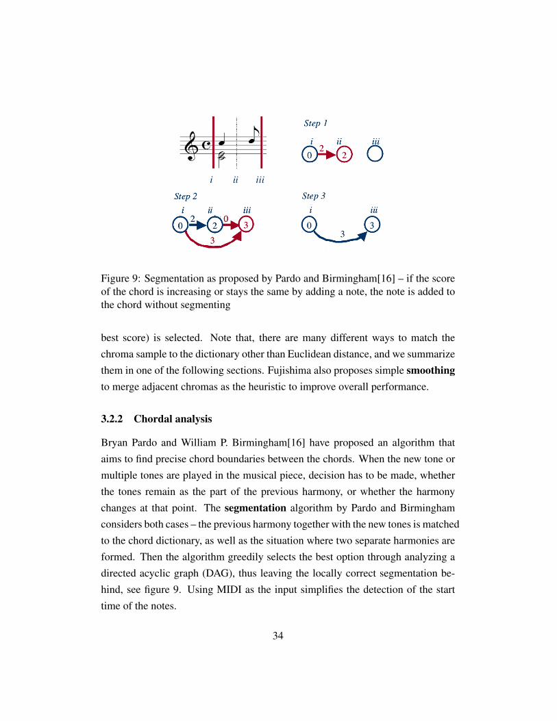
Figure 9: Segmentation as proposed by Pardo and Birmingham[16] – if the scoreof the chord is increasing or stays the same by adding a note, the note is added tothe chord without segmenting

best score) is selected. Note that, there are many different ways to match thechroma sample to the dictionary other than Euclidean distance, and we summarizethem in one of the following sections. Fujishima also proposes simple smoothingto merge adjacent chromas as the heuristic to improve overall performance.

3.2.2 Chordal analysis

Bryan Pardo and William P. Birmingham[16] have proposed an algorithm thataims to find precise chord boundaries between the chords. When the new tone ormultiple tones are played in the musical piece, decision has to be made, whetherthe tones remain as the part of the previous harmony, or whether the harmonychanges at that point. The segmentation algorithm by Pardo and Birminghamconsiders both cases – the previous harmony together with the new tones is matchedto the chord dictionary, as well as the situation where two separate harmonies areformed. Then the algorithm greedily selects the best option through analyzing adirected acyclic graph (DAG), thus leaving the locally correct segmentation be-hind, see figure 9. Using MIDI as the input simplifies the detection of the starttime of the notes.

34

3.2.3 Music harmony analysis improving chord transcription

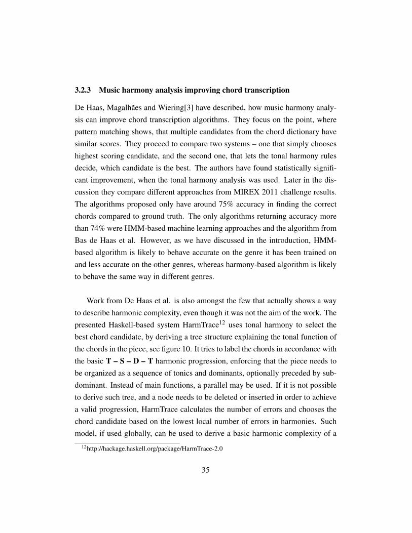
De Haas, Magalhães and Wiering[3] have described, how music harmony analy-sis can improve chord transcription algorithms. They focus on the point, wherepattern matching shows, that multiple candidates from the chord dictionary havesimilar scores. They proceed to compare two systems – one that simply chooseshighest scoring candidate, and the second one, that lets the tonal harmony rulesdecide, which candidate is the best. The authors have found statistically signifi-cant improvement, when the tonal harmony analysis was used. Later in the dis-cussion they compare different approaches from MIREX 2011 challenge results.The algorithms proposed only have around 75% accuracy in finding the correctchords compared to ground truth. The only algorithms returning accuracy morethan 74% were HMM-based machine learning approaches and the algorithm fromBas de Haas et al. However, as we have discussed in the introduction, HMM-based algorithm is likely to behave accurate on the genre it has been trained onand less accurate on the other genres, whereas harmony-based algorithm is likelyto behave the same way in different genres.

Work from De Haas et al. is also amongst the few that actually shows a wayto describe harmonic complexity, even though it was not the aim of the work. Thepresented Haskell-based system HarmTrace12 uses tonal harmony to select thebest chord candidate, by deriving a tree structure explaining the tonal function ofthe chords in the piece, see figure 10. It tries to label the chords in accordance withthe basic T – S – D – T harmonic progression, enforcing that the piece needs tobe organized as a sequence of tonics and dominants, optionally preceded by sub-dominant. Instead of main functions, a parallel may be used. If it is not possibleto derive such tree, and a node needs to be deleted or inserted in order to achievea valid progression, HarmTrace calculates the number of errors and chooses thechord candidate based on the lowest local number of errors in harmonies. Suchmodel, if used globally, can be used to derive a basic harmonic complexity of a

12http://hackage.haskell.org/package/HarmTrace-2.0

35

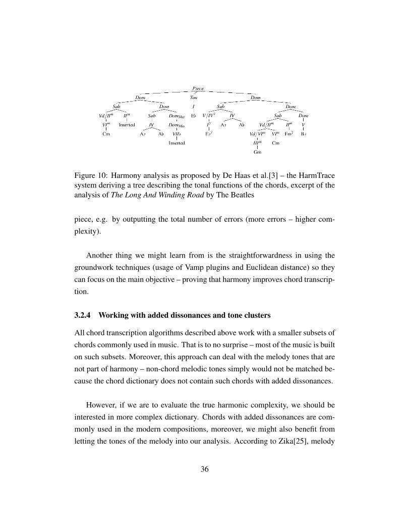
Figure 10: Harmony analysis as proposed by De Haas et al.[3] – the HarmTracesystem deriving a tree describing the tonal functions of the chords, excerpt of theanalysis of The Long And Winding Road by The Beatles

piece, e.g. by outputting the total number of errors (more errors – higher com-plexity).

Another thing we might learn from is the straightforwardness in using thegroundwork techniques (usage of Vamp plugins and Euclidean distance) so theycan focus on the main objective – proving that harmony improves chord transcrip-tion.

3.2.4 Working with added dissonances and tone clusters

All chord transcription algorithms described above work with a smaller subsets ofchords commonly used in music. That is to no surprise – most of the music is builton such subsets. Moreover, this approach can deal with the melody tones that arenot part of harmony – non-chord melodic tones simply would not be matched be-cause the chord dictionary does not contain such chords with added dissonances.

However, if we are to evaluate the true harmonic complexity, we should beinterested in more complex dictionary. Chords with added dissonances are com-monly used in the modern compositions, moreover, we might also benefit fromletting the tones of the melody into our analysis. According to Zika[25], melody

36

may be in harmony with its accompaniment, or it may create dissonances andadditional tension towards the next movements. It would be interesting if ourcomplexity analysis would differentiate two songs with the same music accompa-niment, but one having more dissonant melody. Having broad dictionary with alot of dissonant chords is therefore desirable.

In our previous work, Ear training application[13], we have created a systemChordanal, that was able to name all harmonies from chords to clusters. Theaim was to create an interactive application for music conservatories for the Eartraining course. First, the student selects the lesson. Then he gets the chord as-signment – the program plays the chord. Student’s task is to write in the text fieldexactly what he or she hears. The student may use standard name for the chord,if possible. But usually, if the assignment becomes harder, the training worksstep-by-step and the student only writes what he is sure to hear, e.g. the boundaryinterval of the chords. This way, he learns fast to recognize the musical sounds.This way, also, the more complex harmonies may be named – chords with addeddissonances may be denoted as the original chord plus the interval that createsthe dissonance. Chordanal standardizes such naming and given the chord withan added dissonance it can distinguish the chord and the dissonance, in multipleways if possible.

First of all, parts of Chordanal system (since it is a Java object-oriented frame-work) help us work with the chords encapsulating them in the class, and then an-alyze what are the possible diatonic function of the chords. Secondly, Chordanalsystem also help us name all harmonies during the analysis, to provide more ver-bose output for the user. Re-using and broadening the system seems as a goodoption for our work.

To conclude this section, the best approach seems to be using pattern matchingto a chord dictionary, like in the works presented. If possible, the results of har-

37

mony analysis should be used to determine the final chord sequence. And sincewe actually are interested in finding more dissonant chords, rather than choosinga common subset of chords, we broaden the dictionary as much as possible withthe help of Chordanal.

3.3 Towards models for harmonic complexity

In this section we discuss, what are the options to evaluate harmonic complexityonce we have the chord sequence. The HarmTrace system developed by De Haaset al.[3] shows a simple way how to evaluate complexity of the musical piece.There are other models, that relate to harmonic complexity, since creating variousmodels is the core study of not only MIR, but modern music theory itself. Lots ofworks have been done on tonal tension (see Lerdahl and Krumhansl[10]). How-ever, tonal tension falls more under music perception – and we want to obtaintheoretical model. Another reason why we might not be able to reuse works oftonal tension is, that it focuses on the distance from tonic, whereas we might con-sider the tonic, subdominant and dominant as equivalent, meaning that they areall three the fundamentals of any simple musical piece. Nevertheless, the workson tonal tension can point us in the right direction.

Other types of models that closely relate to music complexity, are models forchord distance. Many musical models have already been proposed to describethe relationships between tones, chords or keys. We have already talked about us-ing Euclidean distance to find the best match amongst the chord candidates. Muchmore approaches can be used.

The work by Rocher, Hanna, Robine and Desainte-Catherine from Univer-sity of Bordeaux[20] summarizes 8 different chord distances and examines theirperformance when used for chord transcription in pattern matching. The workconcludes, that particular type of distance may be good for particular applica-tions, therefore we need to choose the chord distance type based on what we want

38

Figure 11: Basic tonal pitch space as proposed by Lerdahl[9], set to C major

to achieve. From their summary, we choose those chord distances, that seem themost useful for harmonic complexity.

3.3.1 Chord distance in tonal pitch space

Lerdahl[9] introduces the term tonal pitch space, a model describing distancesbetween pitches, chords and keys. The model starts with the basic space. Thedifferent levels of the basic space are shown in figure 11. Then transformationsof the basic space measure the distance between chords. Lerdahl proposes thechord distance of two chords Cx, Cy from the possibly different keys Kx, Ky to becalculated as:

δ (x,y) = i+ j+ k

where i is the distance between the keys Kx, Ky in the circle of fifths, i.e. thenumber of moves in the circle of fifths at level (d), j is the distance between thechords Cx and Cy in the circle of fifths, i.e. the number of moves in the circle offifths at levels (a-c), and k is the number of non-common pitch classes in the spacex compared to the space y.

3.3.2 Tonnetz and Neo-Riemannian theory

Another important model is that of geometric harmonic grid called Tonnetz (tone

network in German), proposed by Hugo Riemann[18]. The idea, first describedby Leonhard Euler, is to represent tonal space as a two-dimensional pitch spacegrid, see figure 12a. The relationships represented by the edges originate in the

39

just tuning and have been adapted to mirror the fundamental rules of tonal har-mony. These ideas are extended in the Neo-Riemannian theory. First proposedby David Lewin[11][12], the triads may be modified using three basic transforma-tions, see figure 12b. The R transformation exchanges a triad for its Relative, e.g.C major to a minor, the L transformation exchanges a triad for its Leading-toneexchange, e.g. C major to e minor, and the P transformation exchanges a triadfor its Parallel, e.g. C major to c minor. Note the ambiguity in the parallel term– here, the parallel comes from the notation commonly used in USA, and meansmodifying C major to c minor, whereas the parallels how we defined them, basedon original Riemann’s German notation, yields modifying C major to a minor,which would be called relative in USA (the same ambiguity is in describing thekeys). The triads are shown on Tonnetz as triangles (more complex chords andharmonic progression may be then visualized e.g. as proposed by Bergstrom etal.[1], see figure 12c) and Neo-Riemannian transformations are shown as inver-sions of the triangles around one of its edges. For more information, the readermay refer to Cohn[2].

We may conclude this section by stating, that there are plenty of models relatedto harmonic complexity, but the way how they can help evaluate the complexityof a musical piece was not yet described13.

3.4 Conclusion and defining the Harmanal system

We summarize what groundwork techniques we use to evaluate the harmonic com-plexity of the piece and also what we expect from our complexity model. For

13There actually is an article defining music space complexity the same way as the computa-tional complexity theory: The Complexity of Songs by Donald E. Knuth[7]. Knuth describes thespace complexity of songs as linear, but finds interesting results for Old McDonald had a farmsong, and even logarithmic and constant complexity for some modern popular songs. Althoughpublished as an inside joke on computational complexity theory, we can take the advice of us-ing computational complexity as a measure for harmonic complexity. Even more importantly, wecan quote him on that repetitions and refrains – or simply the space complexity – should not beforgotten when defining the harmonic complexity as well.

40

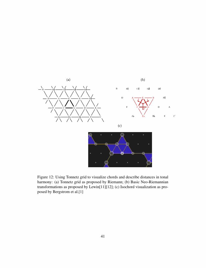
Figure 12: Using Tonnetz grid to visualize chords and describe distances in tonalharmony: (a) Tonnetz grid as proposed by Riemann; (b) Basic Neo-Riemanniantransformations as proposed by Lewin[11][12]; (c) Isochord visualization as pro-posed by Bergstrom et al.[1]

41

groundwork, we prefer simple techniques rather than complex (with the excep-tion of chord dictionary), because our main focus is to put new complexity modelinto practice rather than optimizing the little pieces for best precision or perfor-mance.

The outline for our Harmanal system to evaluate harmonic complexity is asfollows:

1. We take WAV sound files as the input.

2. Feature extraction: We use Vamp plugins to extract the audio features –chromas and beats (NNLS Chroma Plugin, Bar and Beat Tracker Plugin).

3. Smoothing 1: We merge the chromas according to the beats, thus obtainingbeat-synchronized chromas. The merging is done by averaging the chromavectors between the two beats.

4. Chord approximation: We do pattern matching using the Euclidean distanceto estimate the chord using the nearest neighbor technique – the best can-didate is chosen. We choose the chord dictionary to contain all possiblechords, chords with added dissonances and clusters made op of k tones14.We rely on Chordanal system to identify the chords with the increasing k.Having the maximum of tones k, the pattern matching simply means choos-ing the k strongest chroma features. Since the features are floats mapped to< 0,1 >, we take the k highest floats and set them to 1, and set the otherpitch classes to 0 to obtain the chord (as in figure 7). However, a thresh-old of T is introduced to distinguish the important sounding tones from theones that do not play significant role and are almost not noticeable in theharmony. So even though we are interested in additional dissonances, weset 0 for all features lower than T .

14We specify k in the concrete implementation, but we may assume k <= 12, since workingwith pitch classes. Note that, for the simplicity, we do not yet work with the chord inversions,therefore we neglect the bass tone. But since NNLS Chroma Plugin can extract also bass vectors,using of chord inversions is later possible in order to bring our complexity model to the next level.

42

5. Smoothing 2: If adjacent chords are the same, we merge them into one. Inthe result, we obtain the chord sequence {Ci}i≤l = c1,c2, . . . ,cl .

6. Complexity evaluation: Chordanal help us analyze the chord or cluster, ex-tracting as many tonal-related informations as possible (root, possible keys,dissonances, etc.). We then use a complexity model on {Cl} to determinethe complexity of the piece.

7. The other output of the Harmanal system is, with the help of Chordanal,labeling the chords to provide verbose output for the user. As we describein [13], there are multiple way to perceive and label a single chord. How-ever, during the analysis, based on the complexity model it uses, Harmanalchooses one possibility for the chord label that fits the best for the analy-sis, or two possibilities, if the chord is having a role of pivot chord in thediatonic modulation. Therefore, outputting the sequence of chord names{NAMESi} is a by-product of the analysis.

The schema of the Harmanal system is depicted in figure 13. Thanks to theflexibility of the object oriented framework we work with, and due to the desiredflexibility of our application, there is also another variant of Harmanal system thatparses a real-time MIDI input from MIDI instruments (figure 14):

1. We take MIDI signal as the input to obtain two separate harmonies, c1 andc2.

2. Complexity evaluation: Chordanal helps us analyze the two harmonies.Here, we do not define the maximum of tones, because, fundamentally,Chordanal and the complexity model works for as many as 12 pitch classessounding together (in the first variant the maximum of tones was used foroptimizing the performance). We do not use the threshold as well becausewe suppose that if the musician played the tone, he or she wants to have itinvolved in the analysis. Our complexity model analyzes the complexity ofthe transition from c1 to c2.

43

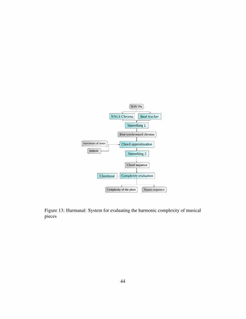
Figure 13: Harmanal: System for evaluating the harmonic complexity of musicalpieces

44

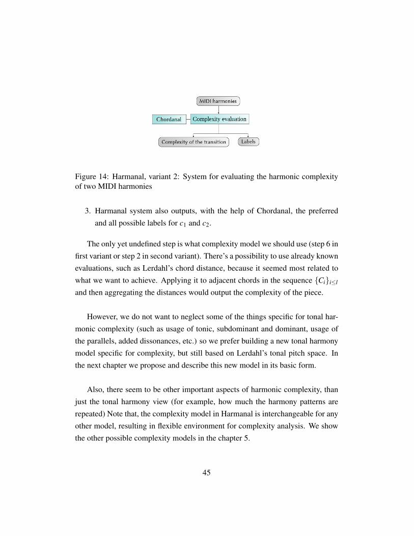
Figure 14: Harmanal, variant 2: System for evaluating the harmonic complexityof two MIDI harmonies

3. Harmanal system also outputs, with the help of Chordanal, the preferredand all possible labels for c1 and c2.

The only yet undefined step is what complexity model we should use (step 6 infirst variant or step 2 in second variant). There’s a possibility to use already knownevaluations, such as Lerdahl’s chord distance, because it seemed most related towhat we want to achieve. Applying it to adjacent chords in the sequence {Ci}i≤l

and then aggregating the distances would output the complexity of the piece.

However, we do not want to neglect some of the things specific for tonal har-monic complexity (such as usage of tonic, subdominant and dominant, usage ofthe parallels, added dissonances, etc.) so we prefer building a new tonal harmonymodel specific for complexity, but still based on Lerdahl’s tonal pitch space. Inthe next chapter we propose and describe this new model in its basic form.

Also, there seem to be other important aspects of harmonic complexity, thanjust the tonal harmony view (for example, how much the harmony patterns arerepeated) Note that, the complexity model in Harmanal is interchangeable for anyother model, resulting in flexible environment for complexity analysis. We showthe other possible complexity models in the chapter 5.

45

4 TSD distance model

In this section we focus on one concrete aspect of harmonic complexity – the com-plexity of the harmony transitions based on the tonal harmony functions. Havingtwo harmonies, our aim here is to find out what function the harmonies represent,and how complex is the transition between them. Therefore, we name the newmodel the TSD distance model, as an acronym for tonic, subdominant, domi-nant distance model. Note that, it is not an exhaustive tonal harmony model –it does not include modulations, nor voice leading, which are both fundamentalparts of the tonal harmony. Modulations and voice leading should be treated inseparate models, because they work on different levels of the tonal pitch space.TSD distance model can nevertheless be used to analyze the complexity of thepieces modulating to different keys. For more information on this separation ofcomplexities and the summary of all other harmonic complexities, see chapter 5.

4.1 Basic idea

The basic idea is to measure, how far the harmony transitions of the piece de-viates from the basic T – S – D – T progression. Slightly differently from thetonal tension – we are not interested in how much the music deviates from thetonic, rather we study how much the music deviates from the transitions betweenall three functions. To describe it even more, the main difference is not focusingon where we are in the progression, but how this is different from a simple pro-gression. For example, if we are in basic tonic and move to basic subdominant,the tonal tension rises. If we then move to basic dominant, the tonal tension risesagain. But our complexity should remain the same.

We build this model on the overtone series rules and the consequent harmonyrules by Riemann[19]. The transitions from the basic harmonic progression T –S, T – D, S – T, D – T are indeed according to Riemann the simplest harmony

transitions, due to the simplicity of the fifth interval. If dominant is built on the

46

fifth degree above tonic, then subdominant is built on the fifth degree below tonic,and from that we derive not only the name for subdominant, but also some „equal-ity of rights“ between subdominant and dominant, when it comes to the usage inmusic, as opposed to the tension. In conclusion, if only these transitions are used,we should consider the harmony very simple. The special case when the musicstays at one function all the time is, again, out of the scope of this model and isbriefly referenced in chapter 5.

We should take a closer look to the transitions S – D and D – S.

• The former, S – D is described by music theory as more difficult than thefifth interval transition, because it the interval between the root tones is awhole tone. However, since we have already described that subdominanthas the same „right“to be in the piece as dominant, we can denote this tran-sition as being very common in music as well, and it indeed is, as the partof the basic harmonic progression.

• The latter, D – S, should not be used based on the rules of original tonalharmony. However, as we have stated in the 2nd chapter, theorists allowdifferent exceptions to this rule, and nowadays we might listen to this tran-sition quite a lot.

The point is, that we might want to differentiate these transitions from the fifthinterval transitions, however, we rather do not want to, because they can still beconsidered as the part of the basic T – S – D – T progression, and we want tomeasure the distance from that progression.

What we therefore focus on are the parallels, or modifications of these mainfunctions, or the harmonies that can be created by adding dissonances to them.Graphically, we may imagine the basic idea like in the figure 15. If the musicstays in the T – S – D triangle, we consider it simple. However, if it deviates from

47

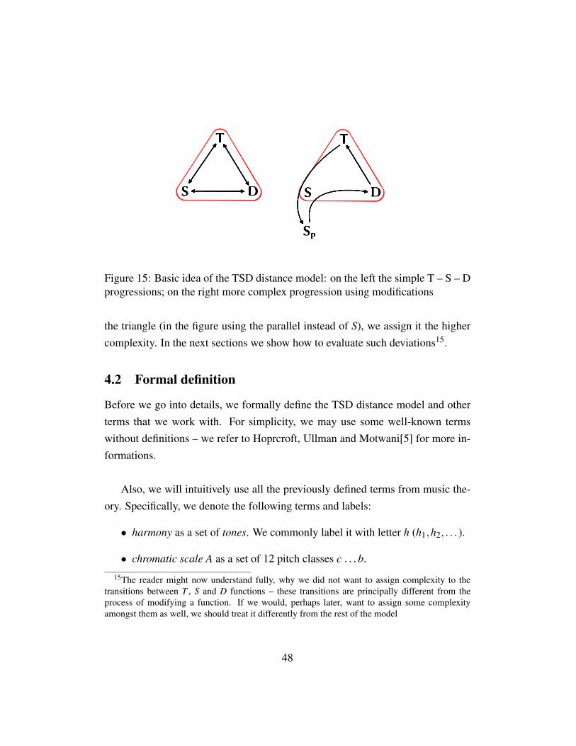
Figure 15: Basic idea of the TSD distance model: on the left the simple T – S – Dprogressions; on the right more complex progression using modifications

the triangle (in the figure using the parallel instead of S), we assign it the highercomplexity. In the next sections we show how to evaluate such deviations15.

4.2 Formal definition

Before we go into details, we formally define the TSD distance model and otherterms that we work with. For simplicity, we may use some well-known termswithout definitions – we refer to Hoprcroft, Ullman and Motwani[5] for more in-formations.

Also, we will intuitively use all the previously defined terms from music the-ory. Specifically, we denote the following terms and labels:

• harmony as a set of tones. We commonly label it with letter h (h1,h2, . . . ).

• chromatic scale A as a set of 12 pitch classes c . . . b.

15The reader might now understand fully, why we did not want to assign complexity to thetransitions between T , S and D functions – these transitions are principally different from theprocess of modifying a function. If we would, perhaps later, want to assign some complexityamongst them as well, we should treat it differently from the rest of the model

48

• tone will obtain pitch class (relative) values: t ∈ A (so we may consider A

as the tone universe). We commonly label the tones with letter t (t1, t2, . . . ).

• harmony universe U as the set of all possible harmonies: U = 2T .

• key and scale we might use interchangeably, both referring to a subset of T

containing 7 elements. We might also notation such as t ∈ C ma jor. Wecommonly label the keys using k letter and scales using s letter.

• key universe K as a set of all possible diatonic keys, 12 major and 12 minor.

• harmonic function universe F as a set of all possible harmonic function:F = {T,S,D} for tonic, subdominant and dominant accordingly.

• harmonic function as the element of F , either tonic, or subdominant or dom-inant ( f ∈ F).

Although harmony does not need to be ordered set, given that we work withpitch classes, we here benefit from a simple notation for a harmony – orderedpitch classes: h = ce[g for c minor triad. We may also use a pitch class profile

format, 12-dimensional binary vector: < 1,0,0,1,0,0,0,1,0,0,0,0 >.

Definition 1. TSD distance model is a tuple (T,P,roots,c, tc), where T is a finite

terminal alphabet, P is a finite set of operations, roots is a finite function: U →2K×F×U , d is a finite function: U → N and td is a finite function: U×U → N.

The reader might have noticed the some similarity between the TSD distancemodel and grammars. We indeed designed it to behave similarly to context-sensitive grammars, with the difference that there is no nonterminal set and nostart symbol, and instead of rules we have operations. The high-level idea is, thatstarting from a basic harmony function (T , S, or D) and with a given key, we wantto make a derivation of the given harmony. Hence we describe the first function,roots as a function that for a given harmony return the basic harmony function h

belongs to – but not only that, it returns also the tonic, subdominant or dominant

49

harmony, that the harmony h can be derived from – let us call it r, or the root har-

mony. The last output of the roots function is the key k in which the root harmonywas found. So we can consider r as the start sentential form for the derivation,as opposed to start symbol in grammars. Another difference is, that the derivationalso depends on the key k, concretely the behaviour of the operations. We there-fore refer to the derivation of the harmony h always with parameters k and r.

For now we may understand the TSD distance model as a set of context-sensitive grammars for each key and not starting with the start symbol, but ratherwith already more complex sentential form. Later we provide more satisfiabledefinition, also for the remaining terms – perhaps for now we may also disclosethat the function c is harmony complexity, and describes the complexity of givenharmony, whereas td is transition complexity and describes the complexity of tran-sition for given, two harmonies.

In following, we work with a concrete model: T SDBASIC. We use the basic

label, because we are aware that more functionality can be added later. In certainmoments, we make some proposals for the model T SDCOMPLET E

16 and for thefuture works.

Definition 2. T SDBASIC is a TSD distance model:

(ABASIC,PBASIC,rootsBASIC,cBASIC,ctBASIC)

Now we will, as collecting puzzle pieces, step by step describe all the 5 ele-ments of T SDBASIC.

16One of the proposal we can make from the beginning is, knowing that T SDBASIC does nottake the bass tone into the account and therefore it can not work with chord inversions. A morecomplete model T SDCOMPLET E can take all the rules from T SDBASIC and add the functionality forinversions.

50

4.2.1 Finding root harmonies

First we treat the problem of how to determine, what is the root harmony of theharmony h (that goes in hand with determining the function f for h). Analyzingthe tone material of h, and comparing it to T , S, D harmonies of different keys, ifh contains all three tones of the function, we may conclude that the function is itsroot harmony.

From Zika[25] and other harmony textbooks we can see evidences, that some-times, even two chord tones are sufficient to represent the functions. Zika specifiesthat in some cases, the tonic triad in the end of the musical phrase contains onlyroot tone and the third. Note that, it can still retain the major or minor character.We also find evidences, that in particular cases, also root tone and the fifth maybe considered an incomplete triad, although in this case we can not state the char-acter. Moreover, the stand-alone I., IV. or V. degree can intuitively represent thefunction too, if no other tones are present. So if the function triad is not presentin the harmony h, we may lower our boundary and look for only portions of thefunction triad. On the other hand, if we have found the match for multiple tonesfrom the function, there is no reason to look for smaller matches. Since 1 tone istoo small of an evidence for the presence of a function, we consider one-tone rootharmony match only if there are no 2 or more tones matches, in all the other keys.

We find the confidence in such approach in Leoš Janácek’s conception ofchords with added dissonances, theoretically described by Volek[23]. Janácekpromotes, that by adding certain amount of dissonances, the chord still retains thesame function, provided that these dissonances can not be described otherwise,diatonically. The good measure is, that the number of added dissonances shouldnot outrank the number of tones in the root harmony. However, there are cases(large clusters) where no such configuration can be found – in that case we choosethe largest possible root harmony again. So we use the measure from the previousparagraph – 2 tones (interval) root harmony is sufficient, if no 3-tones root har-

51

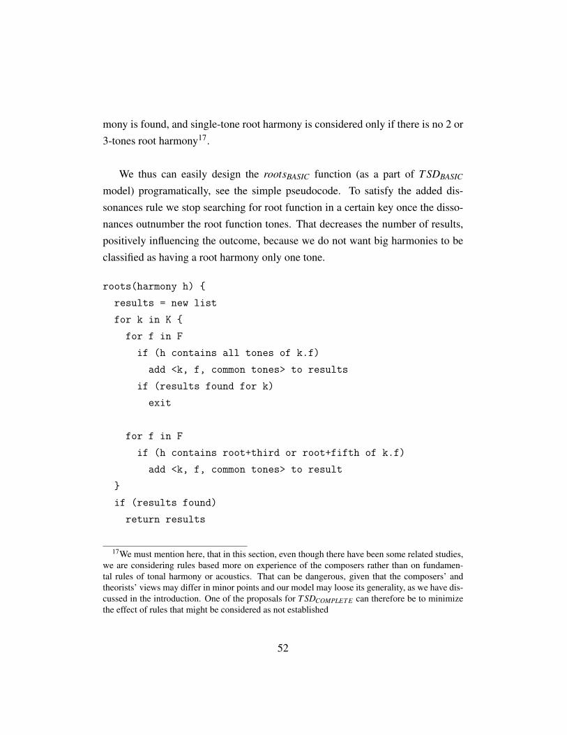
mony is found, and single-tone root harmony is considered only if there is no 2 or3-tones root harmony17.

We thus can easily design the rootsBASIC function (as a part of T SDBASIC

model) programatically, see the simple pseudocode. To satisfy the added dis-sonances rule we stop searching for root function in a certain key once the disso-nances outnumber the root function tones. That decreases the number of results,positively influencing the outcome, because we do not want big harmonies to beclassified as having a root harmony only one tone.

roots(harmony h) {

results = new list

for k in K {

for f in F

if (h contains all tones of k.f)

add <k, f, common tones> to results

if (results found for k)

exit

for f in F

if (h contains root+third or root+fifth of k.f)

add <k, f, common tones> to result

}

if (results found)

return results

17We must mention here, that in this section, even though there have been some related studies,we are considering rules based more on experience of the composers rather than on fundamen-tal rules of tonal harmony or acoustics. That can be dangerous, given that the composers’ andtheorists’ views may differ in minor points and our model may loose its generality, as we have dis-cussed in the introduction. One of the proposals for T SDCOMPLET E can therefore be to minimizethe effect of rules that might be considered as not established

52

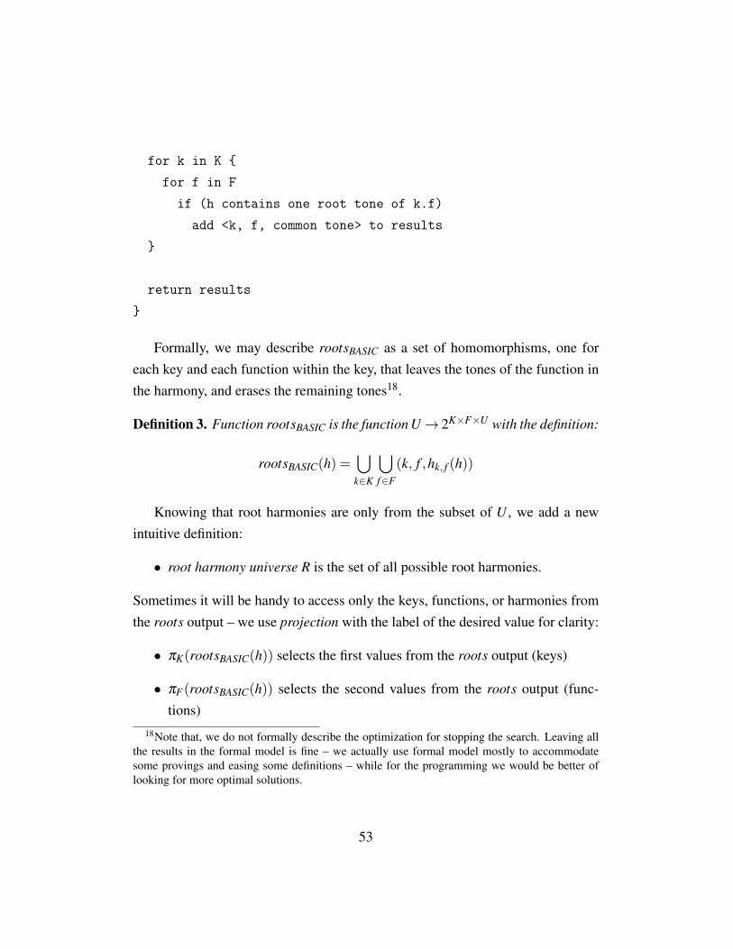
for k in K {

for f in F

if (h contains one root tone of k.f)

add <k, f, common tone> to results

}

return results

}

Formally, we may describe rootsBASIC as a set of homomorphisms, one foreach key and each function within the key, that leaves the tones of the function inthe harmony, and erases the remaining tones18.

Definition 3. Function rootsBASIC is the function U→ 2K×F×U with the definition:

rootsBASIC(h) =⋃

k∈K

⋃f∈F

(k, f ,hk, f (h))

Knowing that root harmonies are only from the subset of U , we add a newintuitive definition:

• root harmony universe R is the set of all possible root harmonies.

Sometimes it will be handy to access only the keys, functions, or harmonies fromthe roots output – we use projection with the label of the desired value for clarity:

• πK(rootsBASIC(h)) selects the first values from the roots output (keys)

• πF(rootsBASIC(h)) selects the second values from the roots output (func-tions)

18Note that, we do not formally describe the optimization for stopping the search. Leaving allthe results in the formal model is fine – we actually use formal model mostly to accommodatesome provings and easing some definitions – while for the programming we would be better oflooking for more optimal solutions.

53

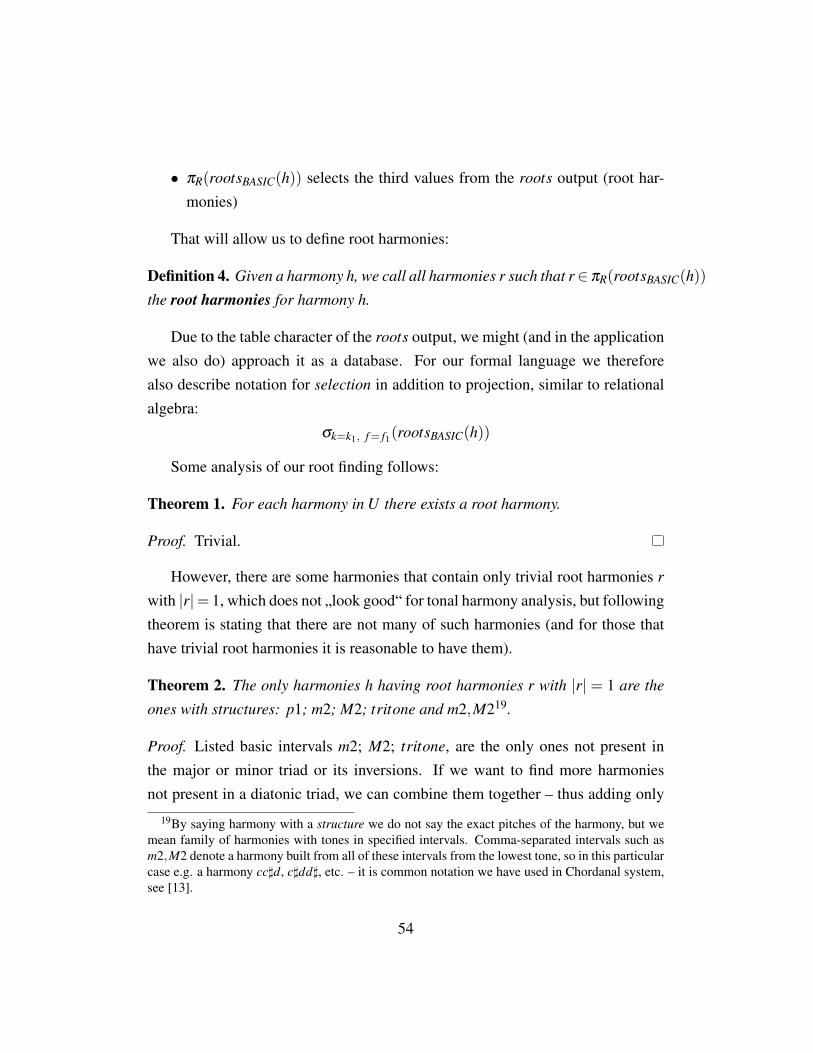
• πR(rootsBASIC(h)) selects the third values from the roots output (root har-monies)

That will allow us to define root harmonies:

Definition 4. Given a harmony h, we call all harmonies r such that r∈ πR(rootsBASIC(h))

the root harmonies for harmony h.

Due to the table character of the roots output, we might (and in the applicationwe also do) approach it as a database. For our formal language we thereforealso describe notation for selection in addition to projection, similar to relationalalgebra:

σk=k1, f= f1(rootsBASIC(h))

Some analysis of our root finding follows:

Theorem 1. For each harmony in U there exists a root harmony.

Proof. Trivial.

However, there are some harmonies that contain only trivial root harmonies r

with |r|= 1, which does not „look good“ for tonal harmony analysis, but followingtheorem is stating that there are not many of such harmonies (and for those thathave trivial root harmonies it is reasonable to have them).

Theorem 2. The only harmonies h having root harmonies r with |r| = 1 are the

ones with structures: p1; m2; M2; tritone and m2,M219.

Proof. Listed basic intervals m2; M2; tritone, are the only ones not present inthe major or minor triad or its inversions. If we want to find more harmoniesnot present in a diatonic triad, we can combine them together – thus adding only

19By saying harmony with a structure we do not say the exact pitches of the harmony, but wemean family of harmonies with tones in specified intervals. Comma-separated intervals such asm2,M2 denote a harmony built from all of these intervals from the lowest tone, so in this particularcase e.g. a harmony cc]d, c]dd], etc. – it is common notation we have used in Chordanal system,see [13].

54

m2,M2 harmony, because other combinations lead to an interval present in dia-tonic triad. Adding anything else to this set (not counting unisone) would lead tointroduce an interval present in diatonic triad, therefore matching some interval intonic, subdominant or dominant function.

Consequence 1. Nice consequence is, that all the remaining harmonies (= vast

majority) have at least 3 non-trivial root harmonies (because for any third, fourth,

fifth or sixth interval there is a key in which tonic matches, another key in which

subdominant matches and the third key where dominant matches). The same – that

always some tonic, subdominant and dominant matches – works also for trivial

root harmonies, so we may modify the Theorem 1 in way, that each harmony has

at least 3 root harmonies.

We should be careful though, because if there are too many matches, we mightencounter some time complexity issues. Note also how we were working with in-tervals in the proof – we work in Z12 group, so when considering an interval, weas well consider its inversion (e.g. major second, minor seventh).

4.2.2 Harmony complexity

First important complexity that we are able to evaluate is the complexity of a har-mony. For TSD distance model it is be nothing else than the distance from basicfunctions, i.e. the length of derivation from a root harmony to the harmony. Har-mony complexity is however a global term, that may be re-defined in other modelslater (and quite similar approaches already in the literature, e.g. the surface ten-

sion from Lerdahl[?]) so we prefer more global definition with the possibility ofswitching the model, to perform some comparisons later:

Definition 5. Harmony complexity cmodel(h) evaluates the static complexity of the

harmony h using the specified model.

For T SDBASIC we define:

55

Definition 6. Harmony complexity in T SDBASIC model: cBASIC(h) is the length of

minimal derivation of h.

Note that the harmony complexity defined this way is actually the computa-

tional time complexity of the harmony in our model.

Sometimes we might want to look for the complexity of the harmony within

the specific key – the syntax then is cmodel(k,h). If we want to be even more spe-cific, we may specify the key and the function, thus obtaining the complexity ofthe harmony from the the specific function in the key: cmodel(k, f ,h).

As we mentioned earlier, by derivation we mean the same as derivation ingrammars, with the difference that T SDBASIC implicitly takes the start sententialform from πU(roots(h)). The important note is, that to obtain the harmony com-plexity, we really need to compare derivations starting from all root harmoniesin πU(roots(h). During the derivation we also need to remember the key k. Theharmony complexity is then found as the minimal length of derivation amongst allof these derivations. We define and describe derivation in the following section.

4.2.3 Derivation explained

Let’s consider the following example:

k =C ma jor

r = ce

h = ce f ]g]

According to Janácek’s added dissonances, adding a tone can be consideredas a fundamental operation that we can do multiple times, provided that the chord

56

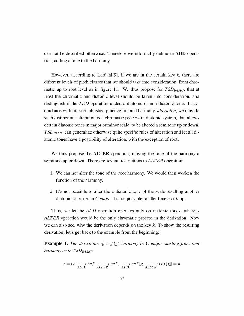
can not be described otherwise. Therefore we informally define an ADD opera-tion, adding a tone to the harmony.

However, according to Lerdahl[9], if we are in the certain key k, there aredifferent levels of pitch classes that we should take into consideration, from chro-matic up to root level as in figure 11. We thus propose for T SDBASIC, that atleast the chromatic and diatonic level should be taken into consideration, anddistinguish if the ADD operation added a diatonic or non-diatonic tone. In ac-cordance with other established practice in tonal harmony, alteration, we may dosuch distinction: alteration is a chromatic process in diatonic system, that allowscertain diatonic tones in major or minor scale, to be altered a semitone up or down.T SDBASIC can generalize otherwise quite specific rules of alteration and let all di-atonic tones have a possibility of alteration, with the exception of root.

We thus propose the ALTER operation, moving the tone of the harmony asemitone up or down. There are several restrictions to ALT ER operation:

1. We can not alter the tone of the root harmony. We would then weaken thefunction of the harmony.

2. It’s not possible to alter the a diatonic tone of the scale resulting anotherdiatonic tone, i.e. in C major it’s not possible to alter tone e or b up.

Thus, we let the ADD operation operates only on diatonic tones, whereasALT ER operation would be the only chromatic process in the derivation. Nowwe can also see, why the derivation depends on the key k. To show the resultingderivation, let’s get back to the example from the beginning:

Example 1. The derivation of ce f ]g] harmony in C major starting from root

harmony ce in T SDBASIC:

r = ce−−−→ADD

ce f −−−−→ALT ER

ce f ]−−−→ADD

ce f ]g−−−−→ALT ER

ce f ]g]= h

57

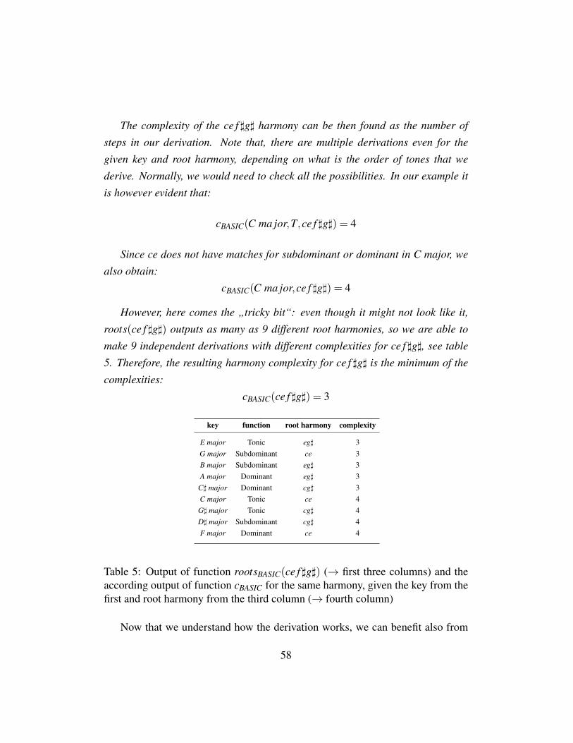
The complexity of the ce f ]g] harmony can be then found as the number of

steps in our derivation. Note that, there are multiple derivations even for the

given key and root harmony, depending on what is the order of tones that we

derive. Normally, we would need to check all the possibilities. In our example it

is however evident that:

cBASIC(C ma jor,T,ce f ]g]) = 4

Since ce does not have matches for subdominant or dominant in C major, we

also obtain:

cBASIC(C ma jor,ce f ]g]) = 4

However, here comes the „tricky bit“: even though it might not look like it,

roots(ce f ]g]) outputs as many as 9 different root harmonies, so we are able to

make 9 independent derivations with different complexities for ce f ]g], see table

5. Therefore, the resulting harmony complexity for ce f ]g] is the minimum of the

complexities:

cBASIC(ce f ]g]) = 3

key function root harmony complexity

E major Tonic eg] 3G major Subdominant ce 3B major Subdominant eg] 3A major Dominant eg] 3

C] major Dominant cg] 3C major Tonic ce 4G] major Tonic cg] 4D] major Subdominant cg] 4F major Dominant ce 4

Table 5: Output of function rootsBASIC(ce f ]g]) (→ first three columns) and theaccording output of function cBASIC for the same harmony, given the key from thefirst and root harmony from the third column (→ fourth column)

Now that we understand how the derivation works, we can benefit also from

58

Figure 16: Graphical representation of harmony complexity

graphical representation of the harmony complexity, see figure 16 (complexity ofmodified subdominant, denoted Sm. The reader might remember the picture fromthe first section of this chapter (figure 15), where we have used a subdominantparallel. The model was designed in the way, that every commonly used modifi-cations20 such as parallels or counter parallels, or minor chord instead of majorchord, etc., output the harmony complexity c(h) = 1 (the reader can easily verify).However, a little drawback of our T SDBASIC model might be, that they are not dis-tinguished, and other chords with added dissonances also qualify for c(h) = 1. Wethus leave a proposal for more advanced model T SDCOMPLET E to implement thecomplexity with smaller granularity.

For clarity, we provide more formal definition of the whole derivation process.

Definition 7. Let ABASIC = A be the set of terminal symbols we work with.

20The term modification of the function is used in some music theory literature as a commonterm for parallels and counter parallels of the function[25].

59

Then sentential form in T SDBASIC is an ordered word A+. In other words, sen-

tential form is a harmony. We may use the terms harmony and sentential form

interchangeably.

Definition 8. Operation in T SDBASIC is a binary relation −−−−−−→NAME(k,r)

on A+ de-

noted by its NAME and parametrized by the and key k and root harmony r.

In the following, we simplify the writing of the operation – we write it withoutthe brackets containing root harmony and key, but we’ll assume that every opera-tion still knows what is the key and what was the root harmony that the derivationstarted with.

Definition 9. ADD is an operation defined as follows:

h−−−→ADD

g⇔ h = t1, t2, . . . ...tn∧g = t1, . . . ti, t, ti+1, . . . tn; where t ∈ k∧ t /∈ r.

Definition 10. ALTER is an operation defined as follows:

h −−−−→ALT ER

g ⇔ h = t1, . . . ...ti, t, ti+1, . . . tn ∧ g = t1, . . . ti, talt , ti+1, . . . tn; where t ∈k∧ talt /∈ k ∧talt is a semitone up or down from t ∧ t /∈ r.

We may now denote PBASIC = ADD,ALT ER. Note that, we really need to havevariants of these operations for all possibilities of key and root harmonies.

Definition 11. In a TSD distance model (T,P,roots,c, tc), we call derivation of

a harmony h with the parameters k and r, where k is the key and r is some root

harmony of h, and denote ∆(k,r,h) such finite sequence of operations from P with

parameters r and k, that starts with r and finishes with h. Harmony r is called

start sentential form of the derivation. Length of the derivation is the number of

operations used to derive h.

So in conclusion a short quiz:

Example 2. • Question: What our model really does, when somebody asks it

cBASIC(h) =??

60

• Correct answer: It first calls the roots(h) function that enumerates the tu-

ples in the form: (K,F,R). It then performs all the derivations ∆(k,r,h);k ∈πK(rootsBASIC(h)),r ∈ πR(rootsBASIC(h)) and outputs the smallest length of

derivation it encountered.

As we did also for the function roots, we provide a short pseudocode forcBASIC too, that also helps us analyze the computational time. The actual deriva-tion (shown in the code as r = r.add and r = r.alter) is pretty straightforward,because we know what the derivation should end up, so the only question is whatorder of adding tones we choose. However, we can also notice (without proof) thatwith a given key and root harmony, the operations ADD and ALT ER are designedthat way, that each different derivation ∆(k,r,h) of h yields the same complexity.For uniformity, we may choose to add tones in the order of the chromatic scale.

c(harmony h) {

int count = 0

int min = |A|

table = roots(h)

for k in table[keys] {

for r in table[root_harmonies] {

for (1 to n - |r|) {

r = r.add

count++

if (the added tone needs to be altered)

r = r.alter

count++

}

if (count < min)

min = count

}

61

}

return min

}

4.2.4 Transition complexity

Having described the complexity of a harmony we can move on to describe thecomplexity of a transition. What we are trying to achieve is, find out how „far“isthe musical piece from the basic T – S – D – T progression. What we could simplydo is sum all the harmony complexities in the piece – we would obtain a measure,how far are the functions from basic harmony functions. That is ok, but we wouldneglect seeing what happens in between the harmonies. It often happens, for ex-ample, that two harmonies share the tone material, so the transition is smooth forthe listener, however both of the harmony complexities might be high because ofthe shared tones.

For that purpose, in our complexity model we have transition complexity func-tion (TC). TC is closely related to chord distance (CD), however, in general, CD isnot focusing on harmony functions. It would be nevertheless interesting to com-pare our TC with some CD algorithms from [20].

Definition 12. Transition complexity tcmodel(h1,h2) evaluates the dynamic com-

plexity between harmonies h1, h2 using the specified model.

We first define a sample transition complexity, that we later modify to fit all ofour needs.

Definition 13. tcCOMMON(h1,h2) is the sum of the lengths of minimal derivations

of h1 and h2 from its nearest common ancestor in derivation. If nearest common

ancestor can not be found for h1, h2, but there exists a common key k in their roots

tables, tcCOMMON(h1,h2) = cBASIC(k,h1)+ cBASIC(k,h2).

62

Definition 14. For two harmonies, h1 and h2, the common ancestor in derivation(CA(h1,h2)) is such sentential form, that appears in at least one derivation of both

harmonies h1, h2.

Definition 15. For two harmonies, h1 and h2, the nearest common ancestor inderivation (NCA(h1,h2)) is such CA, for which the sum of the lengths of minimal

derivations from CA to h1 and from CA to h2 is minimal.

More easily stated, if we somehow (hypothetically) invert the operations ADD

and ALTER, and we want to get from h1 to h2 as fast as possible, sometimes thepath is not going from h1 all the way to the root harmony, then potentially changethe root harmony (which is for free) and then derive h2. If they have a non-trivialCA (non-trivial = non root harmony), we can just invert the operations up til theCA and then derive h2. If CA can not be found, but the harmonies h1, h2 sharecommon key k, we encounter a transition between functions, so we go all the wayto the root of h1 Even though we really do not want to invert the operation to keepthe model simple, and the work is therefore hypothetical, we may, again, see thatthis definition is pretty much the computational time complexity in our model.For a graphical representation of transition complexity, see figure 17.

Example 3. Derivation of ce f in C major: ce−−−→ADD

ce f

Derivation of ce f ] in C major: ce−−−→ADD

ce f −−−−→ALT ER

ce f ]

NCA(ce f ,ce f ]) in C major is ce f itself.

Length of minimal derivation of ce f starting from ce f : 0

Length of minimal derivation of ce f ] starting from ce f : 1

Therefore: tcCOMMON(ce f ,ce f ]) = 0+1 = 1

Theorem 3. If r is a root harmony for h, then cBASIC(h) = tcCOMMON(r,h)

Proof. Trivially, the NCA of h and its root harmony r is r.

63

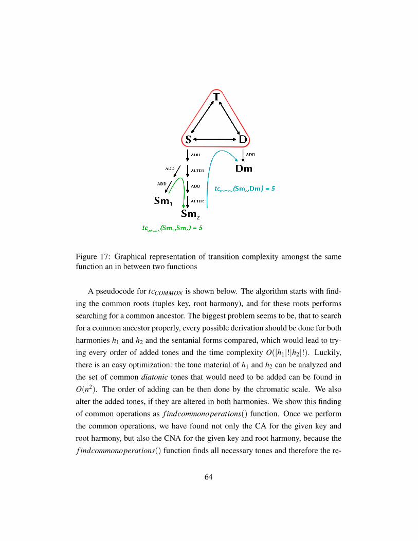
Figure 17: Graphical representation of transition complexity amongst the samefunction an in between two functions

A pseudocode for tcCOMMON is shown below. The algorithm starts with find-ing the common roots (tuples key, root harmony), and for these roots performssearching for a common ancestor. The biggest problem seems to be, that to searchfor a common ancestor properly, every possible derivation should be done for bothharmonies h1 and h2 and the sentanial forms compared, which would lead to try-ing every order of added tones and the time complexity O(|h1|!|h2|!). Luckily,there is an easy optimization: the tone material of h1 and h2 can be analyzed andthe set of common diatonic tones that would need to be added can be found inO(n2). The order of adding can be then done by the chromatic scale. We alsoalter the added tones, if they are altered in both harmonies. We show this findingof common operations as f indcommonoperations() function. Once we performthe common operations, we have found not only the CA for the given key androot harmony, but also the CNA for the given key and root harmony, because thef indcommonoperations() function finds all necessary tones and therefore the re-

64

sulting sentential form is the largest possible. Then we only need to check all thedifferent NCAs for the different tuples (key, root harmony) and choose the onewith the highest complexity.

tc(harmony h1,harmony h2) {

// common roots searching

table1 = roots(h1)

table2 = roots(h2)

table commonroots = table1 intersection table2

// nearest common ancestor searching

int mincomplexity = 2|A|

harmony nca

complexity = 0

for k in commonroots[keys] {

for r in commonroots[rootharmonies] {

operations = findcommonoperations()

for (1 to |operations|) {

r = r.add

complexity++

if (the added tone needs to be altered)

r = r.alter

complexity++

}

if (complexity < mincomplexity)

nca = r

65

if (nca != null)

int complexity1 = c(h1) - c(nca)

int complexity2 = c(h2) - c(nca)

return complexity1 + complexity2

else if (commonroots[keys] != null)

// no common ancestor but common key found

int complexity1 = c(h1)

int complexity2 = c(h2)

return complexity1 + complexity2

}

If for harmony complexity the Theorems 1 and 2 with Consequence 1 werethe most important, because they show that we can work with any harmony fromU – proof of completeness – and that we also have relevant results for every har-mony, in transition complexity the situation is different.

Theorem 4. Function tcCOMMON(h1,h2) does not return result for every tuple of

harmonies h1, h2, even when it comes to harmonies with |h|= 4.

Proof. These two harmonies do not have common keys: cc]dd] (possible keys:C minor, F minor, G minor), c]dd]e (possible keys: C] minor or D[ minor, F]

minor or G[ minor, G] minor or A[ minor)

This is a simple consequence of the fact, that it is not possible to perform di-atonic modulation from every harmony to every other harmony. We are here ina deadlock situation, because we propose, that TSD distance model should notevaluate modulations (it indeed does not – T SDBASIC treats every transition as adiatonic movement and if the modulation occurs, it wouldn’t notify it) and we pro-pose different ways of evaluating modulation complexity in the following chapter.

66

However, T SDBASIC still should output how far is the transition from being „dif-ficult“ (similarly to chord distances concept), so leaving the transition complexityunevaluated would not be a good idea. However, remembering our constructing

approach in evaluating the complexity, we may still come up with some ideas,where even for those tuples of harmonies we can find the way how to disassembleone and construct the other one.

We propose 3 ways of „completing “ the tcCOMMON definition for those tuplesof harmonies that do not have common keys, in order to achieve completeness aswell:

1. tcLAZY behaves like if the harmonies had common keys and simply returncBASIC(h1) + cBASIC(h2).

2. tcCOMPLEX performs the roots function for both harmonies once again, butuses a modified version of roots without the optimization to omit trivial rootharmonies. Then there is only O(|A|) tuples for which we still would not beable to find common keys (usually single tones and clusters, proof can befound simply through trying all types of harmonies starting from |h|= 1, for|h|= 3 we would find out that they all have common keys). For these specialharmonies we have different options, but the best would be following thesame constructing algorithm as in the rest of the model – we allow an emptyroot harmony. That would let us find a common root harmony even for thesetuples and the resulting model would have the attribute of completeness.The transition then literally is disassembling one harmony and building theother from „scratch“.

3. tcCHROMAT IC is based on the idea of chromatic modulation – even thoughthe common key can not be found (= diatonic modulation), by alteringseveral tones of h1, obtaining h′1, we may find the common keys for h′1and h2. The constructing approach then advices: tcCHROMAT IC(h1,h2) =

tcCOMMON(h1,h′1)+ tcCOMMON(h′1,h2). The completeness of this approach

67

has to be treated individually, because even chromatic modulation is notpossible from every key, harmony tuple to every other key, harmony tuple.

Because we want to preserve the uniformity of the T SDBASIC model, we choosethe tcCOMPLEX as the supplementary function to tcCOMMON . From the computa-tional perspective, finding more roots only more cycles in our loops, so the com-plexity does not rise asymptotically.

Definition 16. tcBASIC(h1,h2) behaves as tcCOMMON in case that πR(rootsBASIC(h1))∩πR(rootsBASIC(h2) 6= 0, and as tcCOMPLEX otherwise.

4.2.5 Comparison to Chomsky hierarchy

We quickly and informally compare the T SDBASIC model to the grammars ofChomsky’s hierarchy, so we don’t leave any confusion in between them.

T SDBASIC model indeed works as a finite set of context-sensitive grammars,however, with a coordinator (that should be touring-complete). If the coordinator,has CSG for each key k and each root r, then by performing the function root(h),it chooses those grammars that have their representation in root(h). Each suchgrammar has the step from its start symbol to r, in its terminal alphabet it has thetones of r and all the tones from A−k, the rest of the tones would be non-terminalsymbols. Then the non-terminal symbols have rules for changing into respectiveaugmented or diminished terminals (ALT ER operation), and the sentential form isprepared with the „ADD“non-terminals that can change into respective tone non-terminals, depending on the contextual information. The coordinator lets eachgrammar make a derivation of the harmony and then collect the resulting lengths,and output the best one.

However, even though the coordinating „machinery“ makes T SDBASIC seemlike even much more complex system, we need to conclude with, that it of coursecan not derive any non-regular harmony, because of the finite array we work with

68

(Z12, maximum of 212 harmonies). The grammars are therefore here only for the„feel“ of working with a known model – we may state that our model is „gram-mar based“.

Other question comes on mind – what is the language generated by T SDBASIC?The answer is simple, since it works in Z12 array, it is regular. The harmonyuniverse is limited with 212 possible harmonies. Even the set of all audible pitchesis finite, so unlimited harmony space is only hypothetical and really out of thequestion – once again, context-sensitive grammars are here only for the feel ofworking with „known model“21.

4.3 Graph representation – Christmas tree model

A beautiful aspect of our model is, that it is finite – since the harmony universecontains precisely 212 harmonies. So another beautiful aspect is, that the resultsfor tcBASIC can be pre-calculated, simply by running the function 212.(212−1)

2 times,since tcBASIC(h1,h2) = tcBASIC(h2,h1). This yields to the creation of graph thatrepresents our model.

However, the resulting graph with weighted edges would be complete, there-fore huge and very impractical to store and create, even if we bound the numberof tones by a constant smaller than 12. Therefore we conclude our description ofT SDBASIC model with another graph representation, much more attainable. Snip-pets of it we have already used in the previous section. Due to its meaningfulappearance we call it Christmas tree model.

Christmas tree model is a graph visualization of T SDBASIC model for a spe-cific key, CT M(k) = (V,E), where the root node represents family of harmonies– all possible root harmonies for a given key, and all the other nodes represent

21Note that, even the space of all musical pieces we analyze is regular, since we „accept“ it byour model that can be approximated as DFA, because its transition function is finite – see nextsection

69

(a) (b)

Figure 18: Christmas tree model in its basic form (a); and including zero edges(b)

a single harmony. The edges represent either an operation ADD or ALTER andeach edge has a weight 1.

The basic form of Christmas tree model can be seen on figure 18a. The mainharmony functions listed on the top represent all the roots (T = possible tonicroots, S = possible subdominant roots, D = possible dominant roots) and the„bells“represent the graphs that are created by modifying the root, as already seene.g. on figure 17. As we have denoted earlier, the arrows in between T , S, D are„zero“edges, because they do not hold any transition complexity. By definition,therefore, we should merge them into one node. However, the same applies alsofor some nodes in the bells – many harmonies can be derived from multiple func-tions. Hence we modify („decorate“) a tree with markings, that make clear wherethe nodes are merged into one, see figure 18b.

It is important to notice, that merging the nodes destroys the tree structure. Inthis merging, of course, lies the functionality of our model (it is the sound of theharmony that matters + we are interested in the distance from the whole T – S

70

– D progression and let the functions rename dynamically). But because it alsodestroys the Christmas tree visualization, we prefer using the above figures as thevisual representation.

The next theorem summarizes what the merging of the nodes really does inour model.

Theorem 5. By merging two nodes (combining them into one and deleting the

created loop from the node to itself) in the graph containing only edges with weight

1, we again obtain the graph containing only the edges with weight 1.

Proof. Since both of the nodes did have only the neighbours in a distance 1, andnow they are forming one node, they neighbours combine together and are againin a distance 1 from the new node.

Although we loose the possibility to use some tree searching algorithms, weare given a solid graph with equal edges where each harmony is represented byone node with the exception of root nodes. The next section explains a little bitmore the significance of the rood nodes.

4.3.1 Christmas forest

Spreading the idea towards all of the keys, we get the graph that we may callChristmas forest, see figure 19. Starting from root nodes of 24 major and minorkeys, The edges intertwine together heavily towards the more complex harmonies,having many common nodes (on figure coloured) – in fact, the pivot chords ofpossible modulations. Note that, we did not mark the possibility of traversingdirectly between the basic harmony functions which is possible – between thekeys that are in the relationship of perfect fifth (from tonic C major directly totonic of G major since it is the zero edge in C major from T to D). We did iton purpose – imagining that there are zero edges as well between the colorfultriangles from the figure and that we can therefore „travel “on the whole circle offifths for free leads to a misunderstanding of the concept. The root nodes form

71

one node, but still contain multiple harmonies in which we can not be at one time.We can explain it the best by the following game example, along with figure 19:

Example 4. Super Mario is running through the Christmas forest, searching for

his blond princess. While he searches, it is difficult (complex) to move and he

gets the point for every edge he travels over (optionally the computer-fashioned

music also plays the harmonies along). Sometimes he gets tired and looks for

the triangular colorful house to recover. Often he finds himself quite near one of

them. When in the house, it is not difficult (complex) to move, but it still takes some

time; the triangular house has 3 main compartments and each of them a room for

a giant (three tones), 2 human sized (two tones) and one lilliputian person (one

tone, naturally, Super Mario fits to all of them). The only thing he notices is the

light flashing in the room when he’s in, while in the other rooms there’s dark.

Super Mario is interested by that flashing, and he finds a hidden teleport in the

room, and if he chooses, suddenly he can reappear in a house with different color!

Not to mention, that the teleporting does not take the time at all. Later he realizes,

that every time he enters the house and the room in the house, particular other

rooms in other houses (in the distance of the fifth) flash the light too – a teleport

being activated.

This illustrates the point, that we indeed do not track modulations and it shouldbe done separately.

4.4 On computational complexity of the model

The importance of the Christmas tree model lies in the theoretical possibility ofimplementing the T SDBASIC model by pre-calculating the graph prior to analysis.Such pre-calculation would still contain all harmonies from U , therefore boundingit might be a good idea, but the creation is quite fast – we can inductively generateall the harmonies starting from all the roots and using the operations ADD andALT ER and remember only the trivial edges, as opposed from the complete graphat the beginning. Then, having the two harmonies h1, h2, the speed of algorithm

72

Figure 19: Christmas forest

would only depend on the graph algorithms. However, we can also use the algo-rithms built around the pseudocodes provided in this chapter and not on the graphcreation and search. In this section, we consider both ways of implementation andevaluate their computational complexity.

4.4.1 Time complexity of the main functions

Let n be the maximal length of the harmonies used (n = 12 if not set differently),k the number of keys used (k = 24), f the number of functions within k ( f = 3).From the analysis of the pseudocode we get:

• rootsBASIC(h) ∈ O(k f n)

• cBASIC(h) ∈ O(k2 f n); if we work with the search of the root database, weuse the upper bound for the keys k and the upper bound for the roots k f

• tcBASIC(h1,h2) ∈ O(k2 f n2)

73

More optimizations are possible, mostly by caching the expensive look-ups inthe database for keys and functions, but since these are constant, then quadraticcomplexity from the length of harmony is not bad for the analysis. If the perfor-mance of the algorithm would be slow, we may lower the maximal length thuslowering the quadratic element.

If we choose the graph traversal algorithms, the best option is to use breadth-first search (BFS), since the edges are all equal to 1, resulting in complexity O(2n).Even though exponential, comparing the pseudocode approach (242 ∗ 3 ∗ 122 =

248832) and graph search (212 = 4096) yields to the usage of the graph algorithms.

4.5 Evaluating the complexity of the musical piece

Finally, by using the T SDBASIC model on the chord sequence {Ci}i≤l (which isthe sequence of harmonies), we get the final harmonic complexity of the piece.There are many options on how to do it, moreover we have transition complexity

(as a sequence {ti}i<l; ti = tcBASIC(Ci,Ci+1)), but also harmony complexity (as asequence {hi}i≤l;hi = cBASIC(Ci)) that we can both use.

Also, we have mentioned earlier the analogy with computational time com-plexity – and in fact, our model implements this idea literally, tc outputs exactlythe assembling or disassembling time, the work needed to do to change one har-mony to another. We remain true to this analogy too.

Some data might help first: The output of one call of tc is in < 0,44 > intheoretical perspective, because starting from 0 tones, we can add 12 tones, alter5 of them and add 5 new tones harmony complexity, times 2 for upper bound oftransition complexity. Normally, the values are somewhere between 0 and 10, 0- 5 we might encounter commonly in classical and popular music, 10 is alreadyfor chords with 3 or more added dissonances and clusters (note that, this is takenfrom notation, these values may change based on the threshold we use and for theaudio are usually higher).

74

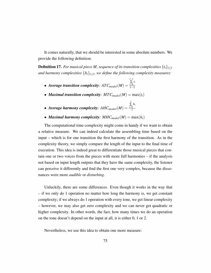
It comes naturally, that we should be interested in some absolute numbers. Weprovide the following definition.

Definition 17. For musical piece M, sequence of its transition complexities {ti}i≤l

and harmony complexities {hi}i≤l , we define the following complexity measures:

• Average transition complexity: ATCmodel(M) =

l−1∑

i=0ti

l−1

• Maximal transition complexity: MTCmodel(M) = max(ti)

• Average harmony complexity: AHCmodel(M) =

l∑

i=0hi

l

• Maximal harmony complexity: MHCmodel(M) = max(hi)

The computational time complexity might come in handy if we want to obtaina relative measure. We can indeed calculate the assembling time based on theinput – which is for one transition the first harmony of the transition. As in thecomplexity theory, we simply compare the length of the input to the final time ofexecution. This idea is indeed great to differentiate those musical pieces that con-tain one or two voices from the pieces with more full harmonies – if the analysisnot based on input length outputs that they have the same complexity, the listenercan perceive it differently and find the first one very complex, because the disso-nances were more audible or disturbing.

Unluckily, there are some differences. Even though it works in the way that– if we only do 1 operation no matter how long the harmony is, we get constantcomplexity; if we always do 1 operation with every tone, we get linear complexity– however, we may also get zero complexity and we can never get quadratic orhigher complexity. In other words, the fact, how many times we do an operationon the tone doesn’t depend on the input at all, it is either 0, 1 or 2.

Nevertheless, we use this idea to obtain one more measure:

75

Definition 18. For musical piece M, sequence of its transition complexities {ti}and sequence of its harmonies {Ci}, we define relative transition complexity:

RTCmodel(M) =

l−1∑

i=0ti

l−1∑

i=0|Ci|

We also take advice from the computational complexity notation, and definethe following notations:

Definition 19. Let k ∈ N

M ∈ ATCT SDBASIC(k)⇔ k−1 < ATCT SDBASIC(M)≤ k

M ∈ AHCT SDBASIC(k)⇔ k−1 < MTCT SDBASIC(M)≤ k

M ∈MTCT SDBASIC(k)⇔MTCT SDBASIC(M) = k

M ∈MHCT SDBASIC(k)⇔MHCT SDBASIC(M) = k

4.5.1 Time complexity of the music analysis

Secondly we would be interested in the time complexity of analysis of the mu-sical piece. Although the concrete implementations might differ, we base ourestimations on the figures of Harmanal system from chapter 3. We do not takethe feature extractions algorithms into our analysis, nor the smoothing 1 sincesmoothing 1 depends on the outputs of the Vamp plugins. We start from obtainingbeat-synchronized chromas. Let l be the number of beats from the audio.

• We do O(ln) operations to get the chord candidates, since we only comparethe chroma features to the threshold

• We do O(l) algorithms for smoothing 2, thus obtaining the chord sequence{Ci}, with the length bounded by l

76

• We then do l times calculation of transition complexity, resulting in com-plexity O(k2 f n2l) or O(2nl) depending on which implementation we choosefor the model

• Finally we calculate the harmonic complexity of the piece in O(l). We alsoin O(l) revise the list of potential labels for the harmonies using convolutionmethod

Since n, k, f can be considered constants, our complexity analysis is thereforeO(l).

77

5 Other complexity models

In this section we provide an overview on what other harmonic complexities arethere other than TSD distance complexity, to give as complete picture as possible.

5.1 Five harmonic complexities

There are different views on complexity when it comes to harmony, even fromtheoretical perspective (not talking about music perception or machine learning).It can be either how simple or complex transitions are being used (chord distanceconcept, as we have described in previous chapter, it is close to computationalcomplexity from complexity theory). It can be how much the repetitions are used– refrain, verses (space complexity). Then there also is how fast the transitionsappear (speed of transitions, this resembles computational time complexity too).

Then in transitions, we might differentiate, if modulations were used in thepiece, how often and between what keys, because majority of chord distanceswould not take it into consideration. And there are also another 2 ways how tolook at the transitions between the harmonies — instead of evaluating the simplic-ity or complexity of the transition, we can also find how far they are from tonic(tonal tension) or, how smooth are the transition (voice leading concept).

To summarize – five complexities in music harmony:

1. chord distances and tonal tension

2. voice leading

3. modulations

4. repetitions

5. transition speed

78

In this thesis, we have provided the proposal for the first one, that takes bothchord distance and T – S – D rules into account, We shortly summarize someproposals for the other ones as well.

These complexities may be better perceived as categories – we put chord dis-tances and tonal tension together, because they all take care of the transitionsbetween the chords, only evaluate them from the different perspective, tonal ten-sion is rather cumulative approach for the musical piece, whereas chord distancesuffices with 2 chords, and our approach combined these two together. Hencethe complexity algorithms can either focus on the full category, or some concretesubcategories.

Some of the algorithms may combine multiple categories into one, for exam-ple Lerdahl’s chord distance is taking also the key relationships into account[9].However, to provide more verbose and accurate output, we propose to leave thecategories separate. All five categories work on different levels. For example,1 and 2 and 3 would be from different levels of tonal pitch space: 1 is how tri-ads change within the key, 2 studies relationships between the keys, 3 studies thetones within the triad. So we propose that the resulting harmonic complexity fora musical piece would then use five different scores, which is not a bad practice,in comparison to obtaining one number but nobody would understand why thenumber is so. Of course, some heuristics can be used to calculate the total score,too.

5.1.1 Voice leading complexity

This is a proposal for calculating the harmonic complexity from a different per-spective – voice leading. Both tonal harmony and theory of counterpoint rulescan, and should, be used. The idea is, that some transitions may sound harmon-ically The idea that may be thought of for future works is, whether a LEADING

operation can be safely introduced, in the same fashion that ADD and ALTER op-

79

erators. Such LEADING operation should however, more like generative systemrather than grammar, be used on every tone of the chord and it would no longer bethe length of derivation that matters, but rather what sort of LEADING operationwere used.

Different possibilities occur: Moving semitone up or down (leading tone) maybe considered as „not complex“, whole tone can be considered more complex.Perhaps it should be distinguished whether the movement was within the key, oroutside the key, or the complex rules of tonal harmony can aid us in deciding whatshould happen.

5.1.2 Complexity of modulations

There have been several attempts in describing the modulations and we believethat soon enough also some methods arise to compare all of types of modula-tions and evaluate their complexity. The best practice seems to be modulationsevaluation based on number of steps on the circle of fifths.

5.1.3 Space complexity

As an important note on our TSD distance complexity, we provide an example: Asong or classical piece that would use 3, very harmonically interesting transitions,may appear very interesting at the beginning. But as soon as it would rotate these3 chords all the way to the end, we would loose interest quickly. Space complex-ity needs to be therefore considered in the final evaluation of complexities. Wepropose using pattern matching methods, to find all similar regions e.g. throughself-similarity matrices, or more easily, using the extracted chord sequence. Thenthe resulting complexity is the total length of transitions that are not repeated any-where in the piece. This approach is similar to Knuth[7].

80

5.1.4 Transition speed

Transition speed simply denotes how many transitions per unit of time are used.Simply stated, however this needs more sophisticated algorithm to find the chordboundaries, because approximating transitions on beats would lead to impreciseresults. We refer to [16] for more information on chord segmentation.

81

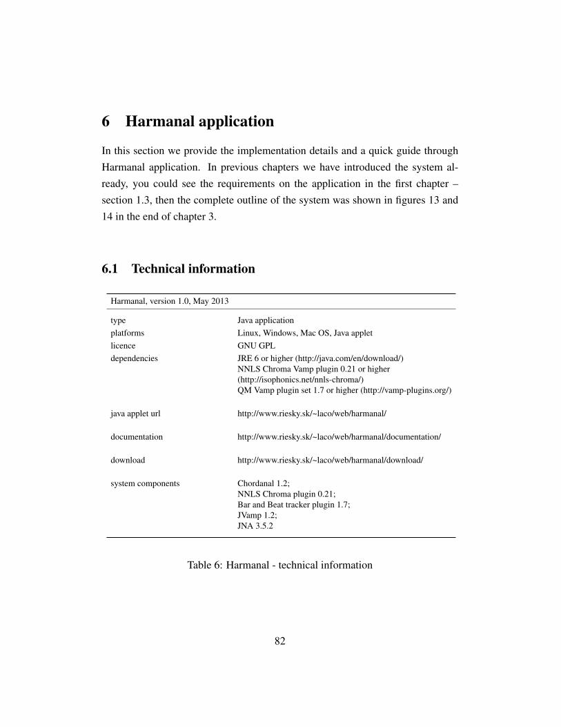
6 Harmanal application

In this section we provide the implementation details and a quick guide throughHarmanal application. In previous chapters we have introduced the system al-ready, you could see the requirements on the application in the first chapter –section 1.3, then the complete outline of the system was shown in figures 13 and14 in the end of chapter 3.

6.1 Technical information

Harmanal, version 1.0, May 2013

type Java applicationplatforms Linux, Windows, Mac OS, Java appletlicence GNU GPLdependencies JRE 6 or higher (http://java.com/en/download/)

NNLS Chroma Vamp plugin 0.21 or higher(http://isophonics.net/nnls-chroma/)QM Vamp plugin set 1.7 or higher (http://vamp-plugins.org/)

java applet url http://www.riesky.sk/~laco/web/harmanal/

documentation http://www.riesky.sk/~laco/web/harmanal/documentation/

download http://www.riesky.sk/~laco/web/harmanal/download/

system components Chordanal 1.2;NNLS Chroma plugin 0.21;Bar and Beat tracker plugin 1.7;JVamp 1.2;JNA 3.5.2

Table 6: Harmanal - technical information

82

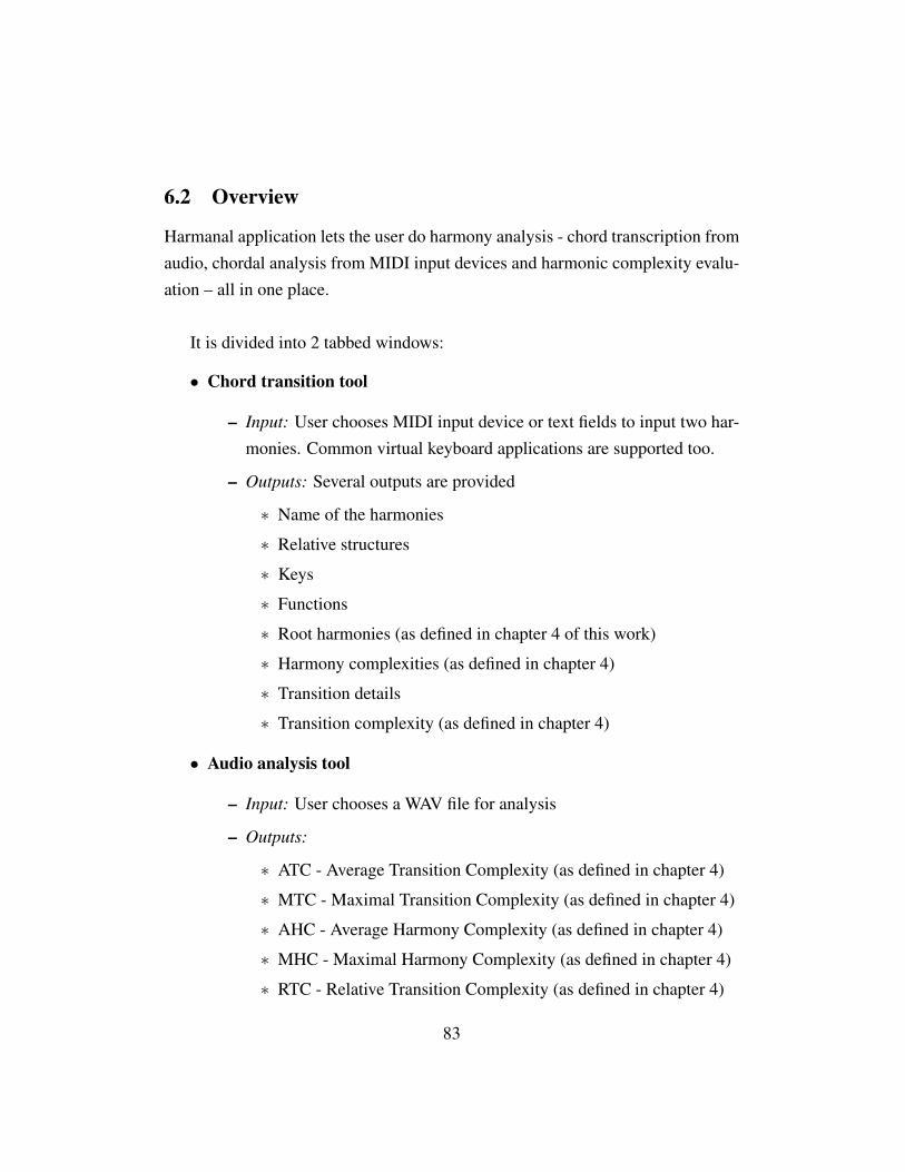
6.2 Overview

Harmanal application lets the user do harmony analysis - chord transcription fromaudio, chordal analysis from MIDI input devices and harmonic complexity evalu-ation – all in one place.

It is divided into 2 tabbed windows:

• Chord transition tool

– Input: User chooses MIDI input device or text fields to input two har-monies. Common virtual keyboard applications are supported too.

– Outputs: Several outputs are provided

∗ Name of the harmonies

∗ Relative structures

∗ Keys

∗ Functions

∗ Root harmonies (as defined in chapter 4 of this work)

∗ Harmony complexities (as defined in chapter 4)

∗ Transition details

∗ Transition complexity (as defined in chapter 4)

• Audio analysis tool

– Input: User chooses a WAV file for analysis

– Outputs:

∗ ATC - Average Transition Complexity (as defined in chapter 4)

∗ MTC - Maximal Transition Complexity (as defined in chapter 4)

∗ AHC - Average Harmony Complexity (as defined in chapter 4)

∗ MHC - Maximal Harmony Complexity (as defined in chapter 4)

∗ RTC - Relative Transition Complexity (as defined in chapter 4)

83

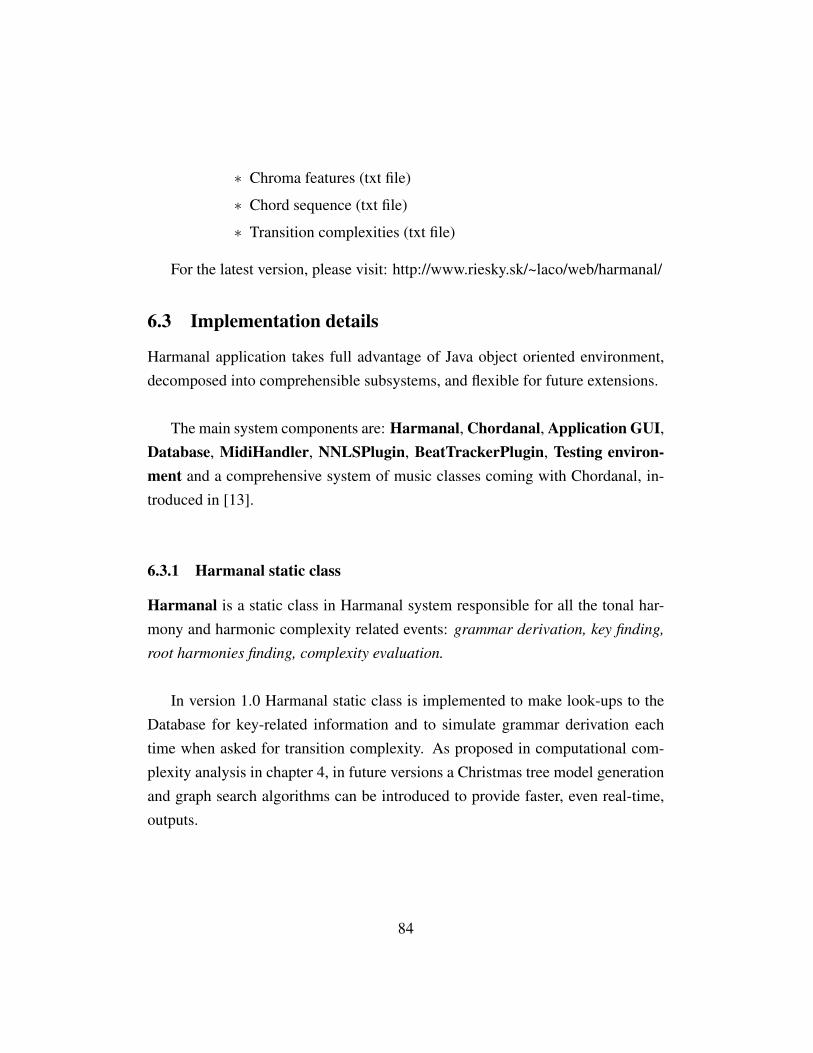
∗ Chroma features (txt file)

∗ Chord sequence (txt file)

∗ Transition complexities (txt file)

For the latest version, please visit: http://www.riesky.sk/~laco/web/harmanal/

6.3 Implementation details

Harmanal application takes full advantage of Java object oriented environment,decomposed into comprehensible subsystems, and flexible for future extensions.

The main system components are: Harmanal, Chordanal, Application GUI,Database, MidiHandler, NNLSPlugin, BeatTrackerPlugin, Testing environ-ment and a comprehensive system of music classes coming with Chordanal, in-troduced in [13].

6.3.1 Harmanal static class

Harmanal is a static class in Harmanal system responsible for all the tonal har-mony and harmonic complexity related events: grammar derivation, key finding,

root harmonies finding, complexity evaluation.

In version 1.0 Harmanal static class is implemented to make look-ups to theDatabase for key-related information and to simulate grammar derivation eachtime when asked for transition complexity. As proposed in computational com-plexity analysis in chapter 4, in future versions a Christmas tree model generationand graph search algorithms can be introduced to provide faster, even real-time,outputs.

84

6.3.2 Chordanal static class

Chordanal is a static class in Harmanal system responsible for all the naming andstructure analysis related events: factory methods to create music entities, naming

methods, abbreviating methods, parsing methods, music entities analysis

Chordanal was first introduced in 2010 in [13]. Its powerful naming and pars-ing capabilities for chords used for Ear training were re-used in this work. Someadvanced terms might be still missing in 1.2 due to the translation from Slovaklanguage. Chordanal’s strength lies in the look-ups to the Database full of datafrom music theory, that it is able to recreate on every run of the program.

Along with Chordanal static class, an object oriented framework for musicentities have been introduced. Following classes are contained in version 1.2:Tone, Harmony, Key

6.3.3 Application GUI

For GUI documentation, visit:http://www.riesky.sk/~laco/web/harmanal/documentation

6.3.4 Other components

MidiHandler is a class responsible for any MIDI related events: thanks to JavaSound API it is able to catch MIDI events as well as send MIDI signals to playtones.NNLSPlugin developed by Mauch[14] and BeatTrackerPlugin developed byStark and Davies[22] are Vamp plugins developed under GNU GPL licence thatwere integrated into Harmanal using JVamp wrappers for native C++ Vamp plu-gins and JNA library. Provided that the user installs the plugins on his machine,JRE is able to load the respective libraries and Harmanal can run cross-platform.

85

Note: In versions before 1.0 the Bar and Beat tracker plugin is not yet intro-

duced, and the transitions are instead calculated for each chroma feature transi-

tion and therefore takes longer. Also, less outputs are shown in GUI, but the user

can find them in the output file.

6.4 Screenshots of usage

When user runs the Harmanal application, a tabbed window with Chord transition

tool is opened so he can start his queries right away. The usage is intuitive – fromup to down, first the user selects from the available MIDI devices. If everythingworks fine, next the user sees that it is possible either to press the „Capture“buttonor to use text field. When the capture button is on, all played MIDI signals arebeing processed and as soon as the button is off, the user sees the analyzed inputin most of the text fields. As soon as he inputs the second harmony, the rest of thetext fields containing the transition information are filled out. Nice feature is, thatif the user is not happy with the input, he or she may modify or reassign the inputusing textfield – the easiest way is using the relative text field, where he or shesimply writes e.g. C E G to get the C major chord. The screenshot of the usage ofChord transition tool is on figure 20.

When the user wants to analyze audio files, he or she selects the other tab withAudio analysis tool label. Again, the usage is very straightforward: from up todown. Importantly, the user must first hit the button „Load plugins“– it usuallytakes around 1-2 seconds to load the plugins. The user is notified if there was aproblem in loading the plugins. Then the user inputs the URL of the WAV he orshe wants to analyze, optionally changes the output txt files and hits the button„Analyze“. Normally, it takes around 10-15 seconds for an analysis of 3 minuteWAV file, 44100 Hz, 32bit samples. When done, the user reviews the filled textfields and may open the files for further analysis information. The screenshot ofAudio analysis tool is on figure 21.

86

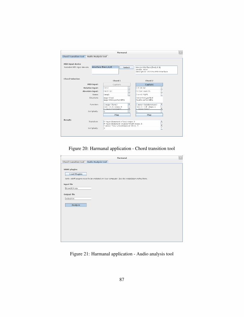
Figure 20: Harmanal application - Chord transition tool

Figure 21: Harmanal application - Audio analysis tool

87

7 Results of analysis

Harmanal system was tested on:

• 20 Rock songs (Beatles, Queen, Led Zeppelin, Pink Floyd, AC/DC)

• 20 Pop songs (Madonna, Black Eyed Peas, Bruno Mars, Katy Perry)

• 20 Classical pieces from different periods (Baroque, Classicism, Roman-tism, 20th century)

• 20 Folk and country songs (Europe, Asia, USA)

• 20 Jazz musical pieces (Marcus Miller, Hiromi, Groovin’ Heads, RudyLinka)

• 20 pieces from different genres (metal, punk, electronic music, ska, hip hop)

The aim was:

1. to obtain all the complexity-related measures

2. to compare the music amongst the genres

3. to compare the genres against each other

The results are also used:

• to find out the usefulness of harmonic complexity for musicology analysisor for recommender systems

• to get a feedback on our complexity model and use it for further improve-ment

As a Bonus, several challenges are proposed (Madonna vs Mozart, Queen vsBeatles, etc.) and the secret of what harmonic complexity lies beneath the chartwinners of the past year is revealed.

88

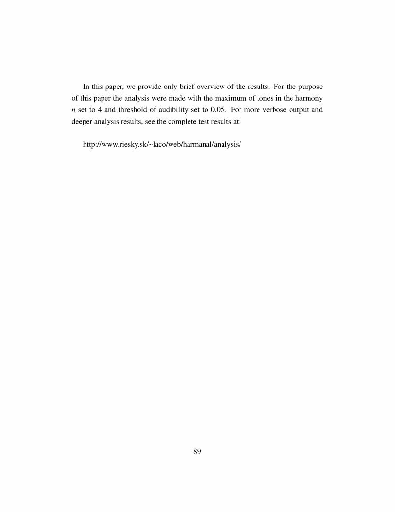
In this paper, we provide only brief overview of the results. For the purposeof this paper the analysis were made with the maximum of tones in the harmonyn set to 4 and threshold of audibility set to 0.05. For more verbose output anddeeper analysis results, see the complete test results at:

http://www.riesky.sk/~laco/web/harmanal/analysis/

89

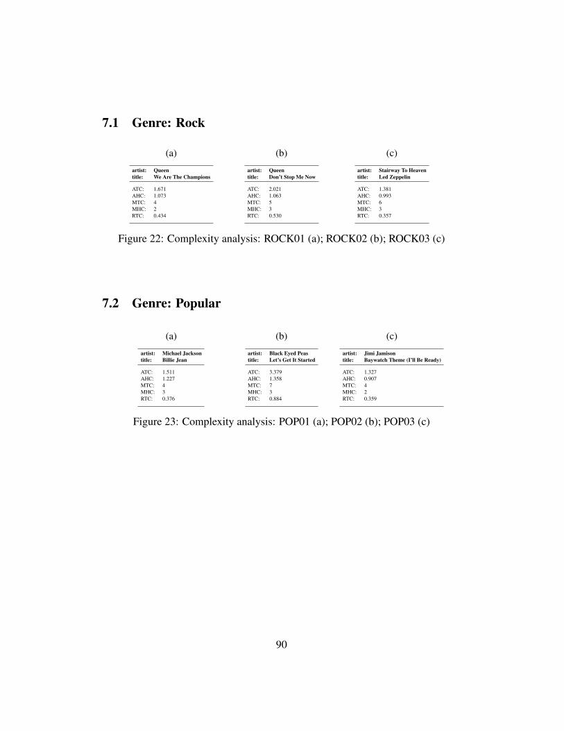
7.1 Genre: Rock

(a)

artist: Queentitle: We Are The Champions

ATC: 1.671AHC: 1.073MTC: 4MHC: 2RTC: 0.434

(b)

artist: Queentitle: Don’t Stop Me Now

ATC: 2.021AHC: 1.063MTC: 5MHC: 3RTC: 0.530

(c)

artist: Stairway To Heaventitle: Led Zeppelin

ATC: 1.381AHC: 0.993MTC: 6MHC: 3RTC: 0.357

Figure 22: Complexity analysis: ROCK01 (a); ROCK02 (b); ROCK03 (c)

7.2 Genre: Popular

(a)

artist: Michael Jacksontitle: Billie Jean

ATC: 1.511AHC: 1.227MTC: 4MHC: 3RTC: 0.376

(b)

artist: Black Eyed Peastitle: Let’s Get It Started

ATC: 3.379AHC: 1.358MTC: 7MHC: 3RTC: 0.884

(c)

artist: Jimi Jamisontitle: Baywatch Theme (I’ll Be Ready)

ATC: 1.327AHC: 0.907MTC: 4MHC: 2RTC: 0.359

Figure 23: Complexity analysis: POP01 (a); POP02 (b); POP03 (c)

90

7.3 Genre: Classical

(a)

artist: J.S.Bachtitle: Jesu Joy Of Man’s Desiring

ATC: 1.442AHC: 1.0MTC: 3MHC: 2RTC: 0.368

(b)

artist: George Gershwintitle: Rhapsody in Blue

ATC: 2.578AHC: 1.383MTC: 7MHC: 3RTC: 0.651

(c)

artist: Pyotr Ilyich Tchaikovskytitle: Swan Lake: Scene, Moderato

ATC: 1.740AHC: 0.919MTC: 7MHC: 3RTC: 0.470

Figure 24: Complexity analysis: BAROQUE01 (a); MODERN01 (b); ROMAN-TICISM01 (c)

7.4 Other genres

(a)

artist: Miki Ryvolatitle: Bedna od whisky

ATC: 1.646AHC: 1.146MTC: 5MHC: 3RTC: 0.415

(b)

artist: Eminemtitle: Lose Yourself

ATC: 2.508AHC: 1.559MTC: 7MHC: 3RTC: 0.649

(c)

artist: Hiromititle: 010101 (Binary System)

ATC: 4.554AHC: 2.597MTC: 7MHC: 4RTC: 1.556

Figure 25: Complexity analysis: FOLK01 (a); RAP01 (b); JAZZ01 (c)

91

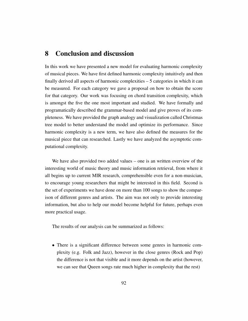
8 Conclusion and discussion

In this work we have presented a new model for evaluating harmonic complexityof musical pieces. We have first defined harmonic complexity intuitively and thenfinally derived all aspects of harmonic complexities – 5 categories in which it canbe measured. For each category we gave a proposal on how to obtain the scorefor that category. Our work was focusing on chord transition complexity, whichis amongst the five the one most important and studied. We have formally andprogramatically described the grammar-based model and give proves of its com-pleteness. We have provided the graph analogy and visualization called Christmastree model to better understand the model and optimize its performance. Sinceharmonic complexity is a new term, we have also defined the measures for themusical piece that can researched. Lastly we have analyzed the asymptotic com-putational complexity.

We have also provided two added values – one is an written overview of theinteresting world of music theory and music information retrieval, from where itall begins up to current MIR research, comprehensible even for a non-musician,to encourage young researchers that might be interested in this field. Second isthe set of experiments we have done on more than 100 songs to show the compar-ison of different genres and artists. The aim was not only to provide interestinginformation, but also to help our model become helpful for future, perhaps evenmore practical usage.

The results of our analysis can be summarized as follows:

• There is a significant difference between some genres in harmonic com-plexity (e.g. Folk and Jazz), however in the close genres (Rock and Pop)the difference is not that visible and it more depends on the artist (however,we can see that Queen songs rate much higher in complexity that the rest)

92

• The colorful instrumentation, chorals and variable structure adds to com-plexity, in opposition to single voice and simple musical accompaniment(high ranking of Queen and Let’s Get It Started from Black Eyed Peas)

• For 20th century classical music, and generally for modern pieces (the pi-anist Hiromi is famous for her fast and complicated pieces, plus, the pieceBinary System was the closest to computer music from what we had in ouranalysis) we have found out that they are apart of the rest and we can seehow the harmonic thinking have changed over the ages

These results show that harmonic complexity is useful tool for future works inMIR.

We have left the last conclusions for this discussion. From the harmonic com-plexities, we would choose AMT and RMT for the later usage – it seems that theyprovide the most statistically interesting output. Moreover, the notation specifiedwith them proved itself meaningful and usable (AMT ranging from zero to almost5).

For future works, much can be done in specifying the other complexities, evenimproving the model for our complexity – if the basic model already gives goodresults, then the more advanced might give even better results. Moreover, thereis the important step we have described in the introduction – analyzing the musiclibrary of the user and implementing a recommender system based on music com-plexity.

Lot of other models around harmonic complexity have been proposed andstudied, such as chord distance or tonal tension, but the term music complexitywas mostly omitted in formal conversations, perhaps because of the subjectivityit sometimes may associate. But from theoretical perspective – checking if somemusic obeys the rules of theory or not is quite simple and very objective task,provided that we build it on established rules. We hope that by showing another

93

point of view we have moved the thinking a little step further and, perhaps, inducesome new ideas in someone else’s mind.

Bibliography

[1] BERGSTROM, T., KARAHALIOS, K., AND HART, J. C. Isochords: Visual-izing Structure in Music. Graphics Interface 2007 (2007).

[2] COHN, R. Introduction to Neo-Riemannian Theory: A Survey and a Histor-ical Perspective. Journal of Music Theory 42/2 (1998).

[3] DE HAAS, W. B., MAGALHÃES, J. P., AND WIERING, F. Improving AudioChord Transcription by Exploiting Harmonic and Metric Knowledge. ISMIR

2012 (2012).

[4] FUJISHIMA, T. Realtime Chord Recognition of Musical Sound: A Sys-tem Using Common Lisp Music. International Computer Music Conference

1999 (1999).

[5] HOPCROFT, J. E., MOTWANI, R., AND ULLMAN, J. D. Introduction to Au-

tomata Theory, Languages, and Computation, second ed. Addison-Wesley,Boston, 2001.

[6] JOHANSSON, K. The Harmonic Language of The Beatles. STM-Online 2

(1999).

[7] KNUTH, D. E. The Complexity of Songs. Communications of the ACM

28/3 (1984).

[8] LABORECKÝ, J. Music Terminological Dictionary. SPN, Bratislava, 2000.

[9] LERDAHL, F. Tonal Pitch Space. Oxford University Press, Oxford, 2001.

[10] LERDAHL, F., AND KRUMHANSL, C. L. Modeling Tonal Tension. Music

Perception: An Interdisciplinary Journal 24/4 (2007).

94

[11] LEWIN, D. A Formal Theory of Generalized Tonal Functions. Journal of

Music Theory 26/1 (1982).

[12] LEWIN, D. Generalized Musical Intervals and Transformations. Yale Uni-versity Press, New Haven, 1987.

[13] MARŠÍK, L. Ear training application. Bachelor’s thesis, Faculty of Mathe-matics, Physics and Informatics, Comenius University in Bratislava, 2010.

[14] MAUCH, M., AND DIXON, S. Approximate Note Transcription for theImproved Identification of Difficult Chords. ISMIR 2010 (2010).

[15] MÓŽI, A. Study Materials on Music History. Academy of Performing Arts,Bratislava, 1994.

[16] PARDO, B., AND BIRMINGHAM, W. P. The Chordal Analysis of TonalMusic. Computer Music Journal 26/2 (2002).

[17] POSPÍŠIL, J. Music Theory for Music Conservatories, vol. 1. SPN,Bratislava, 1985.

[18] RIEMANN, H. Dictionary of Music. Augener Ltd., London, 1896.

[19] RIEMANN, H. Harmony Simplified. Augener Ltd., London, 1896.

[20] ROCHER, T., ROBINE, M., HANNA, P., AND DESAINTE-CATHERINE, M.A Survey of Chord Distances With Comparison For Chord Analysis. ICMC

2010 (2010).

[21] SCHÖNBERG, A. Theory of Harmony. University of California Press, LosAngeles, 1922.

[22] STARK, A. M., DAVIS, M. E. P., AND PLUMBLEY, M. D. Real-TimeBeat-Synchronous Analysis of Musical Audio. DAFx 2009 (2009).

[23] VOLEK, J. The Structure and Figures of Music. Panton, Prague, 1988.

95

[24] ZANETTE, D. H. Music, Complexity, Information. The Computing Re-

search Repository abs/0807.0565 (2008).

[25] ZIKA, P., AND KORÍNEK, M. Tonal Harmony for 1st-3rd Class of Music

Conservatory. SPN, Bratislava, 1990.

96