multiple stellar populations in 47 tucanae

arX

iv:1

109.

0900

v1 [

astr

o-ph

.SR

] 5

Sep

201

1

–

Multiple Stellar Populations in 47 Tucanae. 1

A. P. Milone2,3, G. Piotto4, L. R. Bedin5, I. R. King6, J. Anderson5, A. F. Marino7, A.

Bellini4, R. Gratton8, A. Renzini8, P. B. Stetson9, S. Cassisi10, A. Aparicio2,3, A.

Bragaglia11, E. Carretta11, F. D’Antona12, M. Di Criscienzo12, S. Lucatello8, M. Monelli2,3,

and A. Pietrinferni10

ABSTRACT

We use Hubble Space Telescope (HST) and ground-based imaging to study

the multiple populations of 47 Tuc, combining high-precision photometry with

2Instituto de Astrofısica de Canarias, E-38200 La Laguna, Tenerife, Canary Islands, Spain; [milone,

aparicio, monelli]@iac.es

3Department of Astrophysics, University of La Laguna, E-38200 La Laguna, Tenerife, Canary Islands,

Spain

4Dipartimento di Astronomia, Universita di Padova, Vicolo dell’Osservatorio 3, Padova I-35122, Italy;

[giampaolo.piotto, andrea.bellini]@unipd.it

5Space Telescope Science Institute, 3800 San Martin Drive, Baltimore, MD 21218; [jayan-

der,bedin]@stsci.edu

6Department of Astronomy, University of Washington, Box 351580, Seattle, WA 98195-1580;

[email protected]

7Max Plank Institute for Astrophysics, Postfach 1317, D-85741 Garching, Germany; amarino@MPA-

Garching.MPG.DE

8INAF-Osservatorio Astronomico di Padova, Vicolo dell’Osservatorio 5, I-35122 Padua, Italy; [raf-

faele.gratton, alvio.renzini, sara.lucatello]@oapd.inaf.it

9Dominion Astrophysical Observatory, Herzberg Institute of Astrophysics, National Research Council,

5071 West Saanich Road, Victoria, British Columbia V9E 2E7, Canada; [email protected]

10INAF-Osservatorio Astronomico di Collurania, via Mentore Maggini, I-64100 Teramo, Italy [cassisi,

pietrinferni]@oa-teramo.inaf.it

11INAF, Osservatorio Astronomico di Bologna, via Ranzani 1, I-40127 Bologna, Italy; [angela.bragaglia,

eugenio.carretta]@oabo.inaf.it

12INAF-Osservatorio Astronomico di Roma, Via Frascati 33, I-00040 Monte Porzio Catone, Rome, Italy;

[email protected], [email protected]

http://arxiv.org/abs/1109.0900v1

– 2 –

calculations of synthetic spectra. Using filters covering a wide range of wave-

lengths, our HST photometry splits the main sequence into two branches, and

we find that this duality is repeated in the subgiant and red-giant regions, and

on the horizontal branch. We calculate theoretical stellar atmospheres for main

sequence stars, assuming different chemical composition mixtures, and we com-

pare their predicted colors through the HST filters with our observed colors. We

find that we can match the complex of observed colors with a pair of populations,

one with primeval abundance and another with enhanced nitrogen and a small

helium enhancement, but with depleted C and O. We confirm that models of red

giant and red horizontal branch stars with that pair of compositions also give

colors that fit our observations. We suggest that the different strengths of molec-

ular bands of OH, CN, CH and NH, falling in different photometric bands, are

responsible for the color splits of the two populations. Near the cluster center, in

each portion of the color-magnitude diagram the population with primeval abun-

dances makes up only ∼ 20% of the stars, a fraction that increases outwards,

approachng equality in the outskirts of the cluster, with a fraction ∼ 30% aver-

aged over the whole cluster. Thus the second, He/N-enriched population is more

concentrated and contributes the majority of the present-day stellar content of

the cluster. We present evidence that the color-magnitude diagram of 47 Tuc

consists of intertwined sequences of the two populations, whose separate iden-

tities can be followed continuously from the main sequence up to the red giant

branch, and thence to the horizontal branch. A third population is visible only

in the subgiant branch, where it includes ∼ 8% of the stars.

Subject headings: globular clusters: individual (NGC 104)—Hertzsprung-Russell

diagram

1. Introduction

The presence of multiple stellar populations in globular clusters (GCs) has been widely

established both by photometric and by spectroscopic studies. More than 40 years ago the

red giant branch (RGB) of ω Centauri (NGC 5139) was found to have a photometric spread in

color (Woolley 1966), associated with a metallicity spread (Freeman & Rodgers 1975, Norris

1Based on observations with the NASA/ESA Hubble Space Telescope, obtained at the Space Telescope

Science Institute, which is operated by AURA, Inc., under NASA contract NAS 5-26555.

– 3 –

& Bessel 1975), but the first real challenge to the traditional picture of GCs as simple stellar

populations came from the discovery of abundance anomalies among stars within the same

GCs (e.g., Kraft 1979). All Galactic GCs studied so far show Na-O anti-correlations (e.g.,

Carretta et al. 2009a), indicative of contamination from products of proton-capture reactions

at high temperature (Denisenkov & Denisenkova 1989, Langer et al. 1993). Moreover, the

presence of such anti-correlations in unevolved main sequence (MS) stars (e.g., Gratton et al.

2001; Ramirez & Cohen 2002), which have not yet reached sufficiently high temperatures in

their interiors, suggests that more than one generation of stars has formed within Galactic

GCs (see Gratton et al. 2004 for a review), possibly in combination with accretion onto

low-mass stars of ejecta from either intermediate-mass stars (D’Antona et al. 1983; Renzini

1983), fast-rotating massive stars (e. g. , Decressin et al. 2007), or massive binaries (De Mink

et al. 2009).

Clear evidence of a complex star-formation history in GCs has come from high-precision

Hubble Space Telescope (HST) photometry, which showed unequivocally that the phe-

nomenon of multiple sequences in the color-magnitude diagrams (CMDs) of GCs is not

confined to the special case of ω Centauri (for which see, e.g., Anderson 1997, Bedin et al.

2004). Split or spread MSs have been observed in NGC 2808, 47 Tucanae (NGC 104), and

NGC 6752 (Piotto et al. 2007, Anderson et al. 2009, Milone et al. 2010), while splits in the

subgiant branches (SGBs) have been detected in NGC 1851, NGC 6656 (M22), 47 Tuc, and

at least five other GCs (Milone et al. 2008, Marino et al. 2009, Anderson et al. 2009, Piotto

2009). The splitting of the red-giant branch (RGB) has been observed in all the GCs studied

to date with appropriate photometric bands (e.g., Marino et al. 2008; Yong et al. 2008, Lee

at al. 2009, Lardo et al. 2011). The photometric investigations definitively confirm that it is

common for GCs to contain multiple stellar populations.

More recently it has been possible to connect the photometrically observed multiple

sequences with differences of chemical composition among the stars in the same cluster.

The aim of such studies has been to understand how successive generations of stars could

have formed in a GC, and what could be inferred about the nature of the polluters from

their chemical imprint on the second-generation stars. The first notable results were by

Piotto et al. (2005), who showed that the bluer MS in ω Centauri is more metal-rich than

the redder one. The only way to reconcile the photometric and spectroscopic results is to

assume that the bluer MS is strongly He-enhanced. Other examples are given by Marino et

al. (2008), who showed that the presence of two groups of stars with different C, N, Na, and

O content is at the root of the difference in the (U − B) color of the RGB stars in NGC

6121 (M4). Na-poor (CN-weak) giants define a sequence bluer than the one occupied by

the Na-rich (CN-strong) ones. Yong et al. (2008) found that RGB spreads are present in a

large number of GCs, when using the Stromgren c1 index, which is a powerful tracer of the

https://www.researchgate.net/publication/258976578_Possible_Explanation_of_the_Correlation_Between_Nitrogen_and_Sodium_Over_Abundances_for_Red_Giants_in_Globular_Clusters?el=1_x_8&enrichId=rgreq-d8ae7d0753d6b47b18f58e9c9f6029d7-XXX&enrichSource=Y292ZXJQYWdlOzUxOTM1Mjk2O0FTOjk5NTk2NzA1NDY4NDE2QDE0MDA3NTcxMTM0Mzg=

– 4 –

N abundance. In general, stellar evolutionary models suggest that observed multiple MSs

should correspond to stellar populations with different He abundance, the bluer sequences

having a higher helium abundance than primordial (e.g., Norris 2004; D’Antona et al. 2005;

Piotto et al. 2005, 2007; Di Criscienzo et al. 2010, 2011). According to this picture, the triple

MS in NGC 2808 can also correspond to the three groups of stars with different oxygen and

sodium abundances observed among the RGB stars (Carretta et al. 2006), likely to come from

three successive episodes of star formation. In fact, hydrogen burning at high temperatures

through the CNO cycle and subsequent proton captures result in a He enrichment, and at

the same time in an enhancement of N, Na, and Al, and a depletion of C, O, and Mg. This

scenario has been nicely confirmed for NGC 2808 by Bragaglia et al. (2010), who measured

chemical abundances of one star on the red MS and one on the blue MS, and found that the

latter shows an enhancement of N, Na, and Al, and a depletion in C and Mg. To date there

are no spectroscopic studies of stars on the middle branch of the MS, however.

Finally, theoretical models have proposed that the SGB split observed in some GCs

could be due to two stellar groups with either an age difference of 1–2 Gyr or a different

C+N+O content (Cassisi et al. 2008, Ventura et al. 2009). In support of the chemical-content

scenario, a bimodality in the s-process elements and in the CNO has been detected in NGC

1851 and M22 (Yong et al. 2009, Marino et al. 2011a).

Summarizing the observational and theoretical scenarios:

• split MSs suggest helium enrichment, and also correspond to different groups of stars

in the Na-O anticorrelation;

• multiple SGBs might be ascribed to different total abundance of C+N+O or to different

age;

• photometrically multiple RGBs might be due to differences in C, N, O content, via the

different strengths of the corresponding molecular features;

• there appears to be no strong indication of any significant spread in [Fe/H] (except for

a few clusters: ω Centauri, M22, Terzan 5, and NGC 2419).

Multiple stellar populations with different helium abundance also offer an explanation

for the complex, extended, and clumpy HB morphology exhibited by some clusters (e.g.,

D’Antona et al. 2005, D’Antona & Caloi 2008, Catelan, Valcarce, & Sweigart 2009, Gratton

et al. 2010). A direct confirmation of a connection of the HB shape with the chemical content

of the HB comes from recent work by Marino et al. (2011b), who have found that stars on

the blue side of the instability strip of the cluster M4 are Na-rich and O-poor, whereas stars

on the red HB are all Na-poor.

– 5 –

While the presence of multiple stellar populations in GCs as revealed by multiplicities

of the MS, SGB, RGB, or HB has been clearly established in many clusters, efforts to

unequivocally connect the various evolutionary stages of each individual stellar generation

have met with only modest success so far, because individual sequences appear to merge

and even cross each other in some parts of the CMD, strongly depending on the photometric

bands used to build the CMD. Connecting the various branches from the MS to the HB would

greatly help to fully characterize each individual stellar generation, in terms of composition

and age.

In the present paper we attack this problem by applying high-precision HST photometry

to the globular cluster 47 Tucanae (GO-12311, PI Piotto). This is one of the GCs in the

Milky Way where multiple stellar populations have recently been detected and studied both

photometrically and spectroscopically. From the analysis of a large number of archival HST

images of the inner ∼ 3× 3 arcmin, Anderson et al. (2009) found that the SGB is spread in

magnitude, with at least two distinct branches: a brighter one with an intrinsic broadening

in luminosity, and a second one about 0.05 mag fainter that includes a small fraction of the

stars. Anderson et al. were also able to study the MS in a less crowded field 6 arcmin from the

center and found an intrinsic broadening that increases towards fainter magnitudes. They

interpreted the MS spread in terms of a variation of helium abundance of ∼ 0.02–0.03. Di

Criscienzo et al. (2010) suggested that a spread in helium of ∼ 0.02 might be responsible for

both the luminosity spread of the bright SGB and the HB morphology, whereas an increase

in the overall C+N+O abundance could be responsible for the faint SGB. In substantial

agreement with the above estimates of the differences in helium content in 47 Tuc, Nataf et

al. (2011) have estimated a helium difference of ∆Y ≃ 0.03 between two sub-populations of

this cluster, based on the strength and luminosity of the RGB bump and on the luminosity

of the HB. They also noted that the helium-rich population is more centrally concentrated.

Since the early seventies, spectroscopic investigations have shown that RGB stars in

47 Tuc exhibit large star-to-star variations in CN band strength (e.g., McClure & Osborn

1974, Bell, Dickens, & Gustafsson 1975), with two distinct groups of stars showing different

CN content (Norris & Freeman 1979, Briley 1997); this dichotomy is also present among MS

stars (Cannon 1998, Harbeck et al. 2003). A Na–O anticorrelation has recently been studied

by Carretta et al. (2009a,b), with ∼ 30% of the stars being Na-poor and O-rich, while the

remaining ∼ 70% are depleted in oxygen and enhanced in sodium.

This paper is organized as follows: In Section 2 we describe the data and the reduc-

tion. Section 3 reveals a split in the MS, and in Section 4 we explore possible theoretical

interpretations. Sections 5, 6, and 7 return to the pursuit of multiple sequences along the

SGB, the RGB, and the HB respectively, and also explore their interpretation. The spatial

https://www.researchgate.net/publication/24268964_Mixed_Populations_in_Globular_Clusters_Et_Tu_47_Tuc?el=1_x_8&enrichId=rgreq-d8ae7d0753d6b47b18f58e9c9f6029d7-XXX&enrichSource=Y292ZXJQYWdlOzUxOTM1Mjk2O0FTOjk5NTk2NzA1NDY4NDE2QDE0MDA3NTcxMTM0Mzg=

– 6 –

distribution of multiple stellar populations is investigated in Section 8, while in Section 9 we

attempt to connect the multiple sequences that we have found along the MS, the SGB, the

RGB, and the HB, and to trace the CMD of each of the two stellar generations. A summary

and some final discussion follow in Section 10.

2. Observations and data reduction

For our study of the stellar populations in 47 Tuc, we used data sets from two different

telescopes. For the crowded central regions of the cluster we used HST images taken with

the Wide Field Channel of the Advanced Camera for Surveys (ACS/WFC) and the UVIS

channel of Wide Field Camera 3 (WFC3/UVIS), while to study the spatial distribution of

the populations we made use of U, B, V, and I ground-based photometry from the data base

of 856 original and archival CCD images from Stetson (2000). Among them, 480 images

were obtained with the Wide-Field Imager of the ESO/MPI 2.2 m telescope, and 200 with

the 1.5 m telescope at Cerro Tololo Inter-American Observatory, while the remaining 176

images come from various other telescopes. These observations are described in detail in

Bergbusch & Stetson (2009). They were reduced following the protocol outlined in some

detail by Stetson (2005) and are calibrated on the Landolt (1992) photometric system.

Table 1 summarizes the characteristics of the HST images that we used, while Fig. 1

shows their footprints. The ACS images, and a number of the WFC3 images, were archival,

except that the images of GO-12311 (PI Piotto) were taken expressly for this project, and

were crucial to its success.

The ACS/WFC images were reduced by using the software described in Anderson et al.

(2008). It consists of a package that analyzes all the exposures simultaneously to generate a

catalog of stars over the whole field of view. Stars are measured in each image independently

by using for each filter a spatially variable point-spread-function model from Anderson &

King (2006) plus a “perturbation PSF” that allows for the effects of focus variations. The

photometry was put into the Vega-mag system following the recipes of Bedin et al. (2005)

and using the encircled energy and zero points of Sirianni et al. (2005).

Star positions and fluxes in the WFC3 images were measured with software that is

mostly based on img2xym WFI (Anderson et al. 2006); this will be presented in a separate

paper. Star positions and fluxes were corrected for pixel area and geometric distortion by

using the solution given by Bellini & Bedin (2009) and Bellini, Anderson & Bedin (2011),

and were calibrated as in Bedin et al. (2005).

The work that we present here is based mainly on high-precision photometry, for which

– 7 –

Fig. 1.— Footprints of our HST fields. The small circles are the corners of ACS/WFC chip

1. The footprints of WFC3/UVIS exposures are distinguished by having no such marking.

our next step was to select a high-quality sample of stars that are relatively isolated and have

small photometric and astrometric errors, and are also well fit by the PSF. For this we used

the quality indices that our photometry software produces, in a procedure that is described

in detail by Milone et al. (2009, Sect. 2.1). Finally we corrected our photometry for some

remaining position-dependent errors, due to small inadequacies in our PSFs that were quite

small but were different for each filter. Since all the uses of our photometry would depend

on colors, we generated the 36 colors that can be derived from our 9 filters. For each of

these colors we drew the main-sequence ridgeline in the corresponding CMD; then for each

star we identified its 50 closest well-measured neighbors, and found their median color offset

from the main-sequence ridgeline. Since this constituted a good estimate of the systematic

color error at the position of the target star, for that pair of filters we corrected the observed

color of the star by that amount.

– 8 –

Table 1: HST data sets used in this paper.INSTR DATE N×EXPTIME FILT PROGRAM PI

UVIS/WFC3 Nov 21-22 2011 2×323s+12×348s F275W 12311 Piotto

UVIS/WFC3 Sep 28 2010 30s+1160s F336W 11729 Holtzman

UVIS/WFC3 Sep 28 2010 2×10s+2×348s+2×940s F390W 11664 Brown

ACS/WFC Sep 30-Oct 11 2002 9×105s F435W 9281 Grindlay

ACS/WFC Apr 05 2002 20×60s F475W 9028 Meurer

ACS/WFC Jul 07 2002 5×60s F475W 9443 King

ACS/WFC Jul 07 2002 1×150s F555W 9443 King

ACS/WFC Mar 13 2006 3s+4×50s F606W 10775 Sarajedini

ACS/WFC Sep 30-Oct 11 2002 20×65s F625W 9281 Grindlay

ACS/WFC Mar 13 2006 3s+4×50s F814W 10775 Sarajedini

3. The double Main Sequence

As already mentioned in Section 1, the initial evidence that the MS of 47 Tuc is not

consistent with a single stellar population comes from the recent work by Anderson et al.

(2009), who detected an intrinsic spread in the mF606W −mF814W color ranging from ∼ 0.01

mag near mF606W ∼ 19.0 to ∼ 0.02 mag around mF606W = 22.0. Our present data set,

however, allowed us to study the main sequence with higher precision than was possible for

Anderson et al. with the data available at that time.

An inspection of the large number of CMDs that we obtain from the data set listed in

Table 1 showed that the multiple populations along the MS are best recognized and separated

from photometry that combines mF275W with mF336W. The left-hand panel of Fig. 2 shows

the Hess diagram ofmF275W vs. mF275W−mF336W, after the quality selection and photometric

corrections described in the previous Section. We immediately note a widely spread RGB,

a bimodal SGB, and a double MS. To examine these more closely, in the right-hand half of

the figure we show a CMD that is zoomed around the upper MS, the SGB, and the start of

the RGB. We defer discussion of the SGB and RGB to later Sections, and concentrate here

on the main-sequence morphology.

The CMD in the right-hand panel suggests that the MS of 47 Tuc is bimodal, in analogy

with the multiple MSs observed in ω Centauri, NGC 2808, and NGC 6752. In 47 Tuc,

however, the majority of MS stars populate the blue component (hereafter MSb), while a

small but significant fraction of the stars lie on a redder MS branch (MSa). The two sequences

merge close to the turn-off, but on the MS the separation of the two components increases

towards fainter magnitudes, from 0.08 mag at mF275W = 19.5 to 0.15 mag at mF275W = 23

— as illustrated in more detail in Figure 3. Such large, clear separations allow us to exclude

any possibility that the MS split might be due to measuring errors.

We note here that the “verticalizing” of the MS in Fig. 3 is a process that we will carry



– 9 –

Fig. 2.— mF275W vs. mF275W −mF336W Hess diagram (left), and CMD zoomed around the

MS region (right). The continuous and the dashed red lines in the right panel mark the MS

ridge line of MSb and the equal-mass binary sequence, respectively.

out several times in the course of this paper, and we now explain it once and for all: We first

designated MSb as our target sequence, by means of a hand-drawn first approximation to

its ridge line, and we also chose a limited color range around this line. We then put a spline

through the median colors in successive short intervals of magnitude, and did an iterated

sigma-clipping of outliers; the result was a fiducial sequence for MSb. The verticalization

then consisted of subtracting from the color of each star the color of the fiducial sequence at

the magnitude of that star.

Fig. 3 allows us to estimate the fractions of MSa and MSb stars by assigning to each

star a verticalized color (left panel of the figure), as explained above. The right-hand panels

of the figure show the color histograms for five magnitude bins; in each bin we fitted the

histogram with a pair of Gaussians, shown in magenta and green. These colors will be used

consistently hereafter, to distinguish these two sequences and their post-MS progeny. From

the areas under the Gaussians we estimate that 82% of the stars belong to MSb and 18%

to MSa; within the statistical uncertainties of these numbers they have the same values in

each of the magnitude intervals.

We also note that MSa cannot be ascribed to a sequence of binaries. The dashed line in

Fig. 2 is the equal-mass-binary sequence that corresponds to the fiducial sequence of MSb.

Interpreting the stars of MSa as binaries would require making the outlandish hypothesis

that about a fourth of the MS stars in 47 Tuc are in binary systems with mass ratio in the

narrow interval 0.7–0.8. In addition, assuming that all MSa stars are binaries would imply

a binary fraction (≥15%), in sharp contrast with recent estimates of a 2% binary fraction

– 10 –

Fig. 3.— Left: The same CMD as in Fig. 2, but after subtracting from the color of the MS

the color of the ridge line of MSb. Right: Color distributions of the points in the left panel,

showing two clear peaks. The magenta and green solid lines are the least-squares fits of two

Gaussians to the histograms, while the gray line is their sum. We have also indicated the

reduced-χ2 value corresponding to each bi-Gaussian fit.

by Milone et al. (2008, 2011)2. In view of this, we expect that binaries do not affect the

following discussion in any significant way.

The double MS is also evident in CMDs that use a different combination of magnitude

and color, as shown in the mF336W vs. mF336W −mF435W Hess diagram and CMD of Fig. 4.

2We note that the larger binary fraction for 47 Tuc proposed by Albrow et al. (2001) comes from extrap-

olation from the fraction of W UMa stars that they found in the same cluster, based on assumptions about

the distribution of binary periods, and W UMa binary evolution

– 11 –

Fig. 4.— mF336W vs. mF336W −mF435W Hess diagram (left panel) and CMD zoomed around

the region where the split is most evident (right panel). Note that, contrary to its behavior

in the CMD of Fig. 2, the less populous MS is bluer here than the bulk of MS stars.

It is important to note that in this color system the less populous MS component is bluer

than the other MS stars.

Since these two CMDs from the filter set F275W, F336W, F435W behave so differently,

we construct the two-color diagram that is shown on the left side of Figure 5. There is a

clear separation between the two populations, and in the right panel the stars on opposite

sides of the dividing line have been colored green and magenta to identify stars of MSa and

MSb, respectively.

With high-accuracy photometric measurements in nine bands, 36 different CMDs could

be generated, if we were to use all possible combinations of magnitude and color. In the upper

panels of Figure 6 we show three of the most representative of these CMDs, zoomed around

the MS region, with each star colored green or magenta, according to its membership in MSa

or MSb as shown in Fig. 5. In the bottom panels of Fig. 6 the same CMDs are replicated, and

superimposed on the observed CMDs are the fiducial ridge lines of MSa and MSb, derived

for each CMD using the method described above.

The fiducials for the two MSs are then shown again in Fig. 7 (mF275W vs. mF275W−mX),

Fig. 8 (mF336W vs. mF336W −mX or mX −mF336W), and Fig. 9 (mF814W vs. mX −mF814W),

where mX is indicated on the ordinate of each of row of figures. We note that MSa is redder

than MSb in most of these CMDs, but the color ordering of the two fiducial lines is otherwise

in some of them: MSa stars become bluer than MSb stars in the mF336W−mX colors (Fig. 6,

lower right panel, and Fig. 8).

– 12 –

Fig. 5.— The mF275W −mF336W vs. mF336W −mF435W two-color diagram for MS stars with

19.56 < mF275W < 23.11. The dot-dash line in the right-hand panel separates the MSa and

MSb stars, shown in green and magenta colors, respectively.

4. Interpreting the Two Branches of the Main Sequence

Surely the bizarre behavior of the two branches of the MS in our various CMDs is telling

us something about the physical origin of the split. In hopes of clarifying the complicated

observational picture, we will focus on a critical subset of the data, then we will compare

the observations against synthetic spectra that have been calculated for atmospheres with

various chemical compositions.

The challenge of choosing a critical subset from our mass of observational results is

similar to the one faced by Bellini et al. (2010) in their multicolor study of ω Centauri; we

follow their lead, and look at the separation of the sequences as a function of the color index

in which they are observed. Figure 10 shows the separation of MSa and MSb in each of

eight colors; the figure also compares these observational separations of the sequences with

calculated separations, from three theoretical scenarios that we will describe below.

On the theoretical side, multiplicity of MSs has been attributed to differences in helium

content (e.g., Norris 2004, D’Antona et al. 2005, Piotto et al. 2005, 2007) or in light-element

abundances (e.g., Sbordone et al. 2011), so we will explore both of these possibilities, by

making three different choices for the abundances of He, C, N, and O. We will calculate

synthetic colors for MSa and MSb stars for each of these options, seeking the composition

that best reproduces all the observed color differences between the two MSs. All three of the

options use the same abundance mixture for MSa. For He in MSa we choose the primordial

– 13 –

Fig. 6.— Example of the definition of MS fiducials. Upper panels show three different

CMDs zoomed around the MS, with the MSa and MSb stars defined in Fig. 5 plotted in

green and magenta colors, respectively. In the lower panels we have superposed on these

CMDs the MSa fiducial line (green continuous line) and the MSb fiducial (magenta dashed

line), calculated in each case by the median-color, spline, sigma-clip procedure that was

described earlier in the text.

He abundance, Y = 0.256, and, following Cannon et al. (1998), we choose [C/Fe] = 0.06 and

[N/Fe] = 0.20, which are typical for CN-weak stars. As for [O/Fe], we take 0.40, typical for

first-generation stars (Carretta et al. 2009a,b). For MSb stars we try three different options.

In Option I we assume that helium is the only cause of the MS split, and adopt Y = 0.28.

In Option II we keep helium the same in the two populations but instead change the light-

element abundances, adopting the values listed in Table 2. Finally, in Option III we adjust

both helium and the light elements, again as given in Table 2.

We chose to characterize the fiducial sequences by measuring the color difference between

MSa and MSb at the reference magnitude of mF814W = 18.2, that is, the magnitude level

indicated by the horizontal lines in Fig. 9. For an assumed distance modulus (m−M)F814W =

13.41 and a reddening E(B − V ) = 0.04, this corresponds to an absolute magnitude of

– 14 –

Fig. 7.— MS fiducial lines for MSa (green continuous line) and MSb (magenta dashed line)

in the mF275W vs. mF275W − mX plane. In all these combinations of magnitude and colors

the MSa stars are systematically redder than the MSb stars.

MF814W = 4.85. The adopted distance modulus and reddening are those that provide the

best fitting of the isochrones to the data in themF606W vs. mF606W−mF814W plane, and are in

agreement with those provided by Gratton et al. (2003) and Harris (1996, Dec. 2010 update

). To determine the absorption in the F814W band we used the relations given by Bedin

et al. (2005). We assumed [Fe/H] = −0.75 and [α/Fe] = 0.4, in agreement with the values

found by Carretta et al. (2009). To compare the observations against synthetic photometry,

we adopted the isochrones from the Teramo group (Pietrinferni et al. 2004, 2006) specifically

calculated for the populations listed in Table 2, then determined Teff and log g for MS stars

at MF814W = 4.85. These temperatures and gravities were then used to calculate model

atmospheres with the ATLAS12 code (Kurucz 2005, Castelli 2005, Sbordone 2005, Sbordone

et al. 2007), which allows us to use arbitrary chemical compositions. Spectral synthesis from

2000 A to 10000 A was then performed using the SYNTHE code (Kurucz 2005, Sbordone et

al. 2007), and the resulting synthetic spectra were integrated over the transmission of each

– 15 –

Fig. 8.— MS fiducial lines for MSa (green continuous line) and MSb (magenta dashed line)

in the mF336W vs. mF336W-mX (mF275W − mF336W in the upper left panel) plane. As in all

the CMDs of Fig. 7, MSb is bluer than MSa in all the mF336W vs. mF275W-mF336W CMDs.

But notably, MSa becomes bluer than MSb in the mF275W −mF336W color.

of our nine filters to produce the synthetic magnitudes and colors.

We did this separately for an MSa star and for an MSb star, using for the latter each of

the three composition options that Table 2 lists for MSb. We concentrate here on the eight

mX−mF814W colors, comparing the synthetic MSa − MSb color differences with the observed

ones shown in Figure 10. The results of our synthetic-spectrum calculations for Option I

are shown in the figure as blue squares. At wavelengths longer than ∼ 4300 A there is good

agreement with the observed color differences between the two MSs, but sizable discrepancies

appear at shorter wavelengths, in particular in the F336W band, and we conclude that helium

alone cannot account for the observed MS split. The colors that result from Option II (same

helium but different CNO proportions) are plotted as gray triangles in Figure 10. Again

there is a strong discrepancy between the simulated and the observed color differences in

– 16 –

Fig. 9.— MS fiducial lines for MSa (green continuous line) and MSb (magenta dashed

line) in the mF814W vs. mX-mF814W plane. In these combinations of magnitude and color

the MSa stars are systematically redder than the MSb stars, apart from the mF814W vs.

mF336W −mF814W CMD, where MSb is marginally redder than MSa. Horizontal grey lines

mark the magnitude at which we have calculated the color difference between the two MSs

(mF814W=18.2, see text for more details).

the two near-UV bands (F336W and F390W), but now in the opposite direction. Turning

instead to Option III, with differences in both helium and the CNO elements, we see that the

red asterisks in Figure 10 are in fair agreement with all of the observed color differences. The

agreement is somewhat poorer for the F275W filter, but note that we have not fine-tuned

the composition differences between the two MSs, and that UV colors can be very sensitive

to the adopted mix of He and the CNO elements.

The effect of chemical composition differences on MS colors can be summarized as

follows. The main effect of increased helium is to increase the temperatures, making all

– 17 –

Fig. 10.— Color separations of the ridge lines of MSa and MSb for different color baselines.

The colors used are mX − mF814W, where X is one of the other eight filters. Each color

separation is shown at the central wavelength of its filter X. (For example, the leftmost

point is the separation of the two sequences in mF275W −mF814W.) All color separations are

measured at mF814W = 18.2. A positive value of ∆(color) means that MSa is bluer; negative

would mean that MSa is redder. Observations are plotted as open circles, while the color

differences expected from theoretical Options I, II, and III are shown as blue squares, gray

triangles, and red asterisks, respectively.

colors bluer. The effects of CNO are more subtle, since a specific molecule affects some

bands but not others. Thus nitrogen affects the near-UV F336W and F390W bands via the

NH band and CN bands, respectively, whereas oxygen affects the F275W band, via the OH

band. This is illustrated in the top panel of Figure 11, showing the synthetic spectra of an

MSa and an MSb star as calculated for Option III (in green and magenta respectively). The

difference between the two is shown in the middle panel, while the band-passes of our filters

– 18 –

Table 2: Parameters used to simulate synthetic spectra of an MSa and an MSb star with

mF814W=18.2, for the three assumed options. For all the populations we assumed [Fe/H] =

−0.75 and [α/Fe] = 0.4.MS (Option) Teff log g Y [C/Fe] [N/Fe] [O/Fe]

MSa (all) 5563 5.42 0.256 0.06 0.20 0.40

MSb (I) 5648 5.41 0.288 0.06 0.20 0.40

MSb (II) 5563 5.42 0.256 −0.15 1.05 −0.10

MSb (III) 5592 5.41 0.272 −0.15 1.05 −0.10

are plotted in the bottom panel.

These results indicate that the observed color differences between MSa and MSb can be

understood by assuming that MSa corresponds to a first stellar generation, with primordial

He, and O-rich/N-poor stars, whereas MSb corresponds to a population that is enriched in

He and N but depleted in O. This need for differences in both helium and CNO to account for

all the color differences fits quite well with nucleosynthesis expectations, as helium-enriched

stellar regions are also inevitably oxygen-depleted and nitrogen-enriched, and vice versa —

for example, in the layers subject to the second dredge-up, at the beginning of the AGB

phase, or those subject to the so-called envelope-burning process, later during this phase

(Renzini & Voli 1981, Ventura & D’Antona 2009).

5. Multiple stellar populations along the Subgiant Branch

The first photometric evidence for multiple populations in 47 Tuc came from the dis-

covery of its bimodal SGB (Anderson et al. 2009). These authors analyzed the large number

of ACS/WFC archival HST images of the core of 47 Tuc, and found that the SGB is split

into two distinct components: a brighter SGB showing an intrinsic broadening in the F475W

magnitude, and a second one about 0.05 mag fainter, containing a minor fraction (a few per

cent) of the stars. Anderson et al. also examined the SGB in an outer field, ∼ 6 arcmin west

of the cluster center, finding a similar vertical spread of the SGB. These SGBs have been

further investigated by Piotto et al. (2011), with a multi-band photometric analysis, showing

that the magnitude difference between the faint and bright SGBs is almost constant in each

of the nine HST filters they used, and finding a similar behavior in five other Galactic GCs

that have multiple SGBs. Piotto et al. also found that the faint SGB makes up 8 ± 3 per

cent of the stars in the central field of 47 Tuc. Di Criscienzo et al. (2010) suggest that the

spread in luminosity of the bright SGB can be accounted for by a small spread in helium

(∆Y ∼ 0.02), whereas they suggest that the minor population that makes up the faint SGB


– 19 –

Fig. 11.— Upper panel: comparison of the synthetic spectra of an MSa star (green) and

an MSb star (magenta). See text for more details. Middle panel: Difference between the

spectra of the MSa star and the MSb star. Lower panel: Normalized responses of the HST

filters used in this paper.

(fSGB) would be characterized by a small increase in C+N+O.

In our multicolor set of CMDs, the SGB region turns out to be unexpectedly complex.

Figure 12 shows in the left panel the visible-light CMD of mF435W vs. mF606W −mF814W, in

which the fSGB component of Anderson et al., marked in red, is clearly visible as a separate

sequence. In the right panels are the ultraviolet CMDs, withmF275W vs.mF275W−mF336W and

mF275W vs. mF336W −mF435W; in them the same stars instead fall on top of the numerically

dominant sequence, which in turn splits into two separate sequences, bringing the total to

– 20 –

Fig. 12.— CMDs zoomed around the SGB: mF435W vs. mF606W-mF814W (left panel), mF275W

vs. mF275W −mF336W (middle panel) and mF275W vs. mF336W − mF435W (right panel). The

leftmost CMD has been used to select a sample of faint SGB stars, represented by red X’s

in all three CMDs.

three recognizable SGBs. How can this be?

By analogy with what we did for the MS stars, in Figure 13 we plot the UV two-color

diagram of the SGB stars. Here again we see a bimodal distribution, and we therefore repeat

the points on the right, and draw a separator line. Again by analogy, we color the stars on

either side of the line green and magenta, respectively, and attach to the two regions the

names SGBa and SGBb. In this case, however, we also distinguish with red X’s the stars

that belonged to the fSGB in the left panel of Fig. 12.

The next step is to bring to bear on the SGB puzzle our full multicolor resources. In

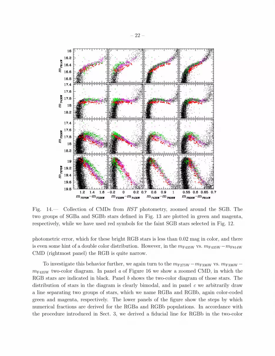
Figure 14 we show a 4 × 4 array of CMDs, with a different magnitude in each row, plotted

against a different color in each column. Although these CMDs are worth looking at one

by one, taken together they add up to an embarras de richesse. We therefore note for the

reader the characteristics that strike us as systematic and significant:

(1) SGBa stars share some similarities with MSa: in the CMDs that use the mF275W-

mF336W color they are on average redder than the other SGB stars, but when the mF336W −

mF435W color is used instead, the SGBa stars are on average bluer than the bulk of SGB

stars. No significant color difference between the two SGB groups is evident in the other

color combinations.

(2) SGBa stars are typically brighter than SGBb stars in mF336W (note in particular

the third row of panels). Their being brighter than others in this band explains why they

are redder than SGBb and fSGB in the mF275W −mF336W color, and bluer than them in the

mF336W −mF435W color. No major systematic magnitude difference between SGBa and the

two other SGB groups is apparent in any of the other panels.

– 21 –

Fig. 13.— mF275W − mF336W vs. mF336W − mF435W two-color diagram for SGB stars. The

dot-dash line in the right panel arbitrarily separates the SGBa and SGBb stars, which are

plotted green and magenta, respectively.

(3) In all of the CMDs the fSGB stars follow the same trend as the bulk of the SGBb

stars, with the fSGB running parallel to SGBb.

The nature of two of the three SGBs is now clear. In the first and second CMDs in the

bottom row of Fig. 14 (mF275W vs. mF275W −mF336W and mF275W vs. mF336W −mF435W) the

green and magenta sequences interchange their order, exactly as we saw for MSa and MSb

in these same colors (upper left and upper right CMDs in Fig. 6). This justifies the name

that we gave this pair of sequences, SGBa and SGBb, since they appear to be the direct

descendants of MSa and MSb.

The sequence that we have marked in red establishes the existence of a third population

in 47 Tuc, but we see it only here on the SGB; in other parts of the CMD we find no evidence

of this third sequence. It is ironic that the very stars whose existence led us to study multiple

populations in 47 Tuc should be left as an anomaly that does not fit into the picture that

will emerge at the end of the present paper.

6. Multiple stellar populations on the red giant branch

Figure 15 shows the red-giant region of 47 Tuc in three different CMDs. Both the

mF275W vs. mF275W-mF336W and the mF336W vs. mF336W −mF435W diagrams suggest that the

RGB is intrinsically broad; the observed color spread of 0.1–0.2 mag is much larger than the

– 22 –

Fig. 14.— Collection of CMDs from HST photometry, zoomed around the SGB. The

two groups of SGBa and SGBb stars defined in Fig. 13 are plotted in green and magenta,

respectively, while we have used red symbols for the faint SGB stars selected in Fig. 12.

photometric error, which for these bright RGB stars is less than 0.02 mag in color, and there

is even some hint of a double color distribution. However, in the mF435W vs. mF435W−mF814W

CMD (rightmost panel) the RGB is quite narrow.

To investigate this behavior further, we again turn to the mF275W−mF336W vs. mF336W−

mF435W two-color diagram. In panel a of Figure 16 we show a zoomed CMD, in which the

RGB stars are indicated in black. Panel b shows the two-color diagram of those stars. The

distribution of stars in the diagram is clearly bimodal, and in panel c we arbitrarily draw

a line separating two groups of stars, which we name RGBa and RGBb, again color-coded

green and magenta, respectively. The lower panels of the figure show the steps by which

numerical fractions are derived for the RGBa and RGBb populations. In accordance with

the procedure introduced in Sect. 3, we derived a fiducial line for RGBb in the two-color

– 23 –

Fig. 15.— This figure illustrates the three CMDs from HST photometry that best summarize

the behavior of RGB stars. Note the wide color spread of ∼ 0.1–0.2 mag in the left and the

middle CMDs, which also show some hints of color bimodality. The RGB becomes narrower

and well defined in the right-hand CMD.

diagram; the line is shown in panel d. In panel e we have subtracted from the color of

each star the color of the fiducial line at the magnitude of the star, so as to verticalize the

sequences. In panel f we plot a histogram of the verticalized colors, and fit it with Gaussians

to represent the RGBa and RGBb populations. The result is that RGBa represents 19± 3%

of the total.

6.1. The double RGB in the outer parts of the cluster

Ground-based photometry available for a field of view that goes out to 25 arcmin allows

us to investigate the radial behavior of the populations. However, the lack of an equivalent

to the F275W passband deprives us of our sharpest tool, and we must look for the best

population discriminant among the ground-based passbands that are available. Fortunately,

ground-based U , B, V , and I are quite similar to our HST F336W, F435W, F555W and

F814W bands. Our procedure, then, was as follows: Since our use of the F275W and F336W

bands had separated the RGBa and RGBb stars, we took those two samples of stars and

examined their behavior in the many different diagrams that can be plotted using only the

four bands that have ground-based equivalents, in order to see if we could find a surrogate

for the two missing bands. As a result, we found that RGB stars separate into two groups

when we plot mF435W against the combination mF336W+mF814W − mF435W, as is shown in

Figure 17.

– 24 –

Fig. 16.— Panel a: mF435W vs. mF435W −mF814W CMD from ACS/WFC photometry. The

black points are the RGB stars that we show in the other panels. b: mF275W −mF336W vs.

mF336W − mF435W two-color diagram for these stars. c: We arbitrarily drew by hand the

dash-dot line that separates RGBa (green) and RGBb (magenta). d : The dashed line is the

fiducial sequence of the RGBb stars, drawn by the fitting method that we described in Sect.

3. e: The verticalized colors of the stars. f : Histogram of the colors in panel e, with a fit

by two Gaussians, whose sum is shown by the solid gray line.

Just to demonstrate the effectiveness of this separation, we use it to separate the stars

of RGBa and RGBb, instead of using the easier route offered by Figure 16. As in similar

situations encountered earlier, we draw a fiducial line for RGBb, by putting a spline through

the median colors in successive short intervals of magnitude, and doing an iterated sigma-

clipping of outliers. We again subtract the color of the fiducial line from the color of each star,

to produce the verticalized colors shown in the left panel of Figure 18. The corresponding

two-Gaussian fit to the color distributions of the resulting RGBa and RGBb stars is shown

in the right panel of the figure.

Finally, in Figure 19, which is analogous to Figure 16, we use U , B, and I magnitudes

to separate RGBa and RGBb stars in our entire ground-based field, in exactly the same way

– 25 –

Fig. 17.— The mF435W vs. mF336W+mF814W−mF435W diagram for RGB stars. The dash-dot

black line is the fiducial line of the RGBb sequence.

as we demonstrated with our HST photometry using the corresponding F336W, F435W,

and F814W passbands. Then we calculate the difference between the U + I − B value of

each star and the value of the fiducial line at the magnitude of the star, ∆(U + I − B).

This process makes the RGB vertical, and we show that in the left panel of Figure 20. The

corresponding histograms are plotted in the right panel of the figure, again fitted by two

overlapping Gaussians.

Having developed a method of using ground-based filters for separating populations, we

now study the spatial distribution of the two RGB components, by dividing our ground-

based field of view into three annuli, each containing about the same number of RGB stars,

and applying the procedure described above to each group separately. The histograms of the

∆(U + I − B) distributions are shown in Figure 21. It is clear from this figure that RGBb

– 26 –

Fig. 18.— Left : The same points as in Fig. 17, but after subtracting from the mF336W +

mF814W −mF435W value of each star the value of the fiducial at the same magnitude. Right :

Histogram of the colors in the left panel. The gray line is the best fit of two Gaussians, which

are plotted as dotted and dashed black lines, and are shaded green and magenta respectively.

Fig. 19.— Similar to what was shown in Fig. 17, but now using the ground-based photometry

for the RGB stars. The left panel is a (B,B − I) CMD in which the black points are the

RGB stars that will be used for the separation of RGBa and RGBb. On the right is the

CMD in B vs. U + I −B, with a red fiducial line drawn through the RGBb stars.

– 27 –

Fig. 20.— Left : same diagram as in Fig. 19 but after subtracting the RGB fiducial. Right :

histograms of ∆(U + I − B) for RGB stars in our ground-based photometry.

is more centrally concentrated than RGBa, with the fraction of RGBa stars ranging from

0.22±0.04 in the 1.7–3.5 arcmin bin, to 0.32±0.04 at radial distances from 3.5 to 7.8 arcmin,

up to 0.43± 0.04 for stars in the 7.8–25 arcmin bin. This result will be discussed in detail in

Section 8, where we also compare the radial distributions of the two RGB components with

those of MS and HB components.

Fig. 21.— Histogram of the ∆(U+I−B) distributions of RGB stars at three different radial

distances.

We note finally that we carefully analyzed the SGB and the MS in the B vs. U + I −B

diagram, the same as we have just done for the RGB, but for those other regions we found no

– 28 –

evidence for multiple sequences, presumably because of the larger errors in the ground-based

photometry of those fainter stars.

6.2. The chemical content of stars in the two RGB sequences

Since the red giants are the brightest stars in 47 Tuc, their spectroscopy has a long

history. In the early seventies, large star-to-star cyanogen variations showed that the cluster

is not chemically homogeneous (e.g., McClure & Osborn 1974; Bell, Dickens, & Gustafsson

1975; Hesser, Hartwick, & McClure 1977; Norris 1978; Hesser 1978), and in a paper that

set a standard of spectroscopic accuracy at that time, Norris & Freeman (1979) measured

CN in 142 RGB stars of 47 Tuc and found a bimodal distribution, with CN-strong stars

more centrally concentrated. Our Figure 22 is adapted from their Figure 1, and here we plot

their values of the DDO C(4142) index (which is sensitive to the blue CN bands) against

our V magnitude. The dashed line separates the CN-strong and CN-weak stars, which for

added emphasis we have indicated by magenta circles and green triangles, respectively. We

have 80 RGB stars in common with Norris & Freeman, and in Figure 23 we have marked

their CN-strong and CN-weak stars with distinctive symbols as defined above, in a repeat

of our Figure 19. Note that most of the CN-strong stars belong to RGBb, and nearly all the

CN-weak stars lie on RGBa. It is obviously very tempting to associate the two groups of

CN-weak and CN-strong stars with the two RGBs. More accurate measurements would be

needed, however, to establish whether the few exceptions to this rule are real, or are due to

errors in either the photometric or the spectroscopic measures.

It is now well established that a chemical signature of multiple stellar populations in

GCs is offered by the Na-O anticorrelation that has been noticed in virtually every cluster

observed so far. The Na-O anticorrelation in RGB stars of 47 Tuc has recently been studied

by Carretta et al. (2009a), and their data are shown in Figure 24, where we have made

an arbitrary division into Na-poor/O-rich stars (green triangles) and Na-rich/O-poor stars

(magenta circles). The U vs. U −B CMD shown in Figure 25 gives photometric evidence for

a spread in color that extends from the base of the RGB to its tip. We then identify stars

from Carretta et al. (2009a) in our ground-based CMDs of 47 Tuc, and the two groups of

stars defined in Figure 24 are found to segregate on the RGB as illustrated in Figure 25, with

Na-rich/O-poor stars being systematically bluer in U −B compared to the Na-poor/O-rich

stars, while mixing with them in the B vs. B−I CMD, in analogy with the results of Marino

et al. (2008) for M4.

Finally, in Figure 26 we plot the Na-poor/O-rich and Na-rich/O-poor stars in the B vs.

U + I −B diagram and in the B vs. ∆(U + I − B) diagram, to investigate the abundances

– 29 –

Fig. 22.— Adaptation of Fig. 1 of Norris & Freeman (1979), showing C(4142) index vs. V

magnitude for their sample of RGB stars. Their full line follows the lower bound of the data,

while our dashed line separates the CN-weak stars (green triangles) from the CN-strong ones

(magenta circles).

of Na and O in the two RGBs. We find that RGBa is populated mainly by Na-poor/O-rich

stars, while all the Na-rich/O-poor stars belong to RGBb.

7. Multiple stellar populations on the Horizontal Branch

We now turn to the horizontal branch of 47 Tuc. Figure 27 shows the HST data in the

same plots as were used for the other sequences. In order to point out the stars that we

are studying here, we show in panel a a long-wavelength CMD, with the HB emphasized

in black. In panel b we show the ultraviolet two-color diagram of these stars, with the two

HB sequences HBa and HBb identified as usual in panel c. In panel d we show the same

– 30 –

Fig. 23.— The CN-strong and CN-weak stars defined in Fig. 22, marked in our B vs.

U + I −B plane (left panel) and B vs. ∆(U + I −B) plane (right panel).

plot again, but with a fiducial line through the HBb locus. We verticalize the sequences in

the usual way in panel e. Panel f shows the corresponding histogram, with the fit by two

Gaussians that are colored appropriately. Perhaps quite unsurprisingly at this stage, the

result that HBa makes up 19± 3% of the HB stars is very similar to what we found for the

RGB.

To study the radial distribution of the two HB populations, we again use ground-based

photometry. In panel a of Figure 28 we show the B vs. B − I CMD of all the stars that

passed the selection criteria described in Section 2, and the selected HB stars are marked in

black. Panel b shows a zoom of the HB, in the same color system, and in panel c we plot the

same stars in the B vs. U + I − B diagram, where the distribution shows some bimodality.

The red dashed line is the fiducial line of the more populous HB component, and by analogy

with the previous figure we refer to the lower-left stars as HBa and the upper-right stars

as HBb. The rectified B vs. U + I − B plot is shown in panel d, and the corresponding

histogram is shown in panel e.

It has been suspected for a long time that the HB of 47 Tuc might contain multiple

populations. Norris & Freeman (1982) measured the strengths of CN and CH bands in the

spectra of 14 HB stars and concluded that their results were “consistent with a dichotomy

as found for the giants”, which agrees with the result that we have just presented. They also

noted that CN-weak stars are on average ∼ 0.04 mag brighter in V than CN-strong stars —

– 31 –

Fig. 24.— Sodium-oxygen anticorrelation for RGB stars, from Carretta et al. (2009a). The

dashed line arbitrarily separates Na-rich/O-poor stars (magenta circles) from Na-poor/O-

rich stars (green triangles).

which is similar to what we see in panel e of Figure 27 and panel d of Figure 28.

Fig. 1a from Norris & Freeman (1982) is reproduced here as Fig. 30. We plotted their

S(3839) index measurements for 14 HB stars as a function of the (B-V) color and drew the

line that shows the dependence of S(3839) on effective temperature, as discussed by Norris

& Freeman (1982). The two groups of CN-weak and CN-strong stars defined by Norris &

Freeman are plotted as green triangles and magenta circles, respectively. Our ground-based

catalog has in common nine out these fourteen stars. These stars are marked with black

circles. Among them three are CN-strong and six CN-weak stars.

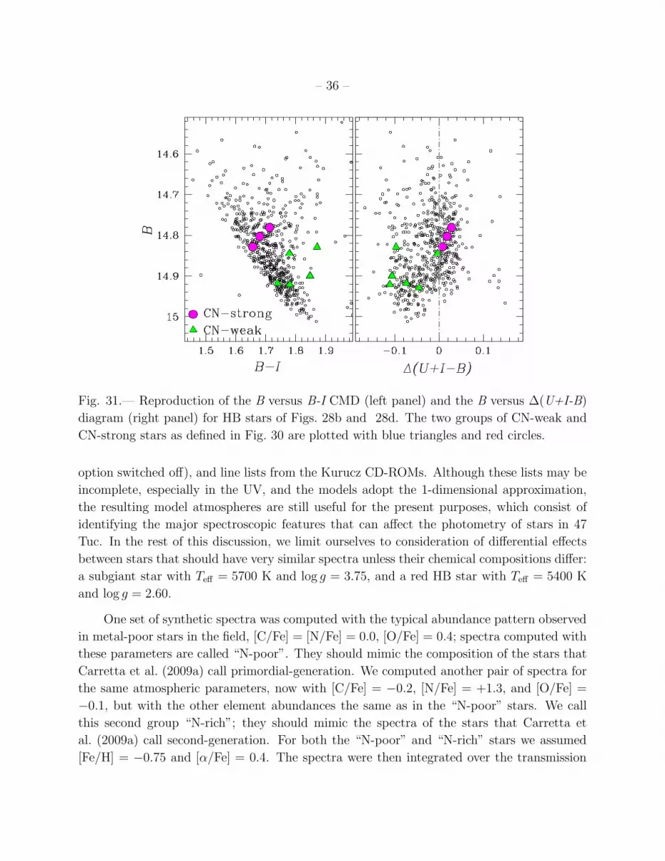
In Fig. 31 we show the position in the B vs. B-I CMD (right panel) and in the B

vs. ∆(U + I − B) diagram the nine stars in common (left panel). CN-strong stars are on

– 32 –

Fig. 25.— U vs. U − B (left panel) and B vs. B − I (right panel) CMD from ground-based

photometry. The stars belonging to the two groups of Na-rich (O-poor) and Na-poor (O-rich)

stars are represented with magenta circles and green triangles, respectively.

Fig. 26.— The Na-poor/O-rich and Na-rich/O-poor RGB stars defined in Fig. 24 are plotted

here in B vs. U + I − B (left panel); the right-hand panel shows a verticalized version, in

our usual way.

average brighter than CN-weak ones in the B band. The right panel shows that CN-strong

and CN-weak stars have ∆(U + I −B) values consistent to that of the bulk of the HBb and

– 33 –

Fig. 27.— The HB stars highlighted in black in panel a can be seen to have a bimodal

distribution in the two-color diagram of panel b, and in the next panel they are separated

into two components. In the bottom row of panels their distribution in color is fitted with

two Gaussians; see text for details.

HBa groups, respectively. An exception to this rule is given by a CN-weak star which has

a B magnitude and ∆(U + I − B) value close to that of HBb stars. It is not clear if this

anomalous position in the latter diagram is an intrinsic property of this star or is due to

either photometric or spectroscopic errors.

The connection between the HB morphology in GCs and the groups of stars with dif-

ferent abundances of light elements (Na, O, C, N) is not a peculiarity of 47 Tuc but has

been also observed in the GC NGC 6121 (M4). As already mentioned in Sect. 1, this cluster

hosts two groups of stars with different Na and O content (Marino et al. 2008), as well as

a bimodal HB. Marino et al. (2010) have recently measured oxygen and sodium for stars

in the blue and the red HB segments of M4, and found that the red HB is made by stars

with low Na and high O content, while blue HB stars are all Na-enhanced and O-depleted

(possibly He-rich).

– 34 –

Fig. 28.— Panel a: B vs. B− I CMD from ground-based photometry. HB stars are marked

in black. A zoom of this CMD around the HB region is plotted in panel b. Panel c: HB stars

in the (B, U + I −B) plane; the red dashed line is the HBb fiducial drawn by hand. Panels

d and e show the rectified B vs. ∆(U + I − B) diagram and the histogram of the rectified

colors.

Fig. 29.— Histogram of the ∆(U + I − B) distribution of HB stars from ground-based

photometry at two radial distances from the cluster center.

These results on 47 Tuc and NGC 6121 provide direct evidence that the HB morphology

of these GCs is strictly related to the multiple stellar generations they host, and suggest that

– 35 –

Fig. 30.— S(3839) index for 14 HB stars as a function of B-V from Norris & Freeman (1982).

The line shows the dependence of S(3839) on the effective temperature as proposed by these

authors. The CN-weak and CN-strong stars are plotted with green triangles and magenta

circles, respectively, while we have marked with black black contours the nine stars for which

we have U, B and V photometry.

the multiple sequences discovered in the CMDs of many GCs may be connected with the

HB morphology.

7.1. The role of C, N, and O on the SGB and the HB

In order to better understand the origin of the multicolor distribution of SGB and HB

stars, we present here an analysis similar to that described in Section 4 for MS stars, using a

number of synthetic spectra over the wavelength range of interest (i. e., 2000 < λ < 5000 A).

They were computed using the Kurucz (1993) model atmospheres (with the overshooting

– 36 –

Fig. 31.— Reproduction of the B versus B-I CMD (left panel) and the B versus ∆(U+I-B)

diagram (right panel) for HB stars of Figs. 28b and 28d. The two groups of CN-weak and

CN-strong stars as defined in Fig. 30 are plotted with blue triangles and red circles.

option switched off), and line lists from the Kurucz CD-ROMs. Although these lists may be

incomplete, especially in the UV, and the models adopt the 1-dimensional approximation,

the resulting model atmospheres are still useful for the present purposes, which consist of

identifying the major spectroscopic features that can affect the photometry of stars in 47

Tuc. In the rest of this discussion, we limit ourselves to consideration of differential effects

between stars that should have very similar spectra unless their chemical compositions differ:

a subgiant star with Teff = 5700 K and log g = 3.75, and a red HB star with Teff = 5400 K

and log g = 2.60.

One set of synthetic spectra was computed with the typical abundance pattern observed

in metal-poor stars in the field, [C/Fe] = [N/Fe] = 0.0, [O/Fe] = 0.4; spectra computed with

these parameters are called “N-poor”. They should mimic the composition of the stars that

Carretta et al. (2009a) call primordial-generation. We computed another pair of spectra for

the same atmospheric parameters, now with [C/Fe] = −0.2, [N/Fe] = +1.3, and [O/Fe] =

−0.1, but with the other element abundances the same as in the “N-poor” stars. We call

this second group “N-rich”; they should mimic the spectra of the stars that Carretta et

al. (2009a) call second-generation. For both the “N-poor” and “N-rich” stars we assumed

[Fe/H] = −0.75 and [α/Fe] = 0.4. The spectra were then integrated over the transmission

– 37 –

NH CN CN CHOH

Fig. 32.— Top Panel : Comparison between two synthetic spectra: one for a N-rich star

(magenta) and one for a N-poor star (black). The spectra are given as flux (in arbitrary

units) and are smoothed at 1A resolution for clarity; they have been computed for param-

eters typical of a subgiant star in 47 Tuc, with chemical compositions given in the text.

For reference, the normalized throughputs of the bluest broad-band filters of WFC3/UVIS

F(275/336/390/435/475)W are also shown. Labels on the bottom indicate the wavelength

range where important spectroscopic features involving CNO elements cause significant ab-

sorption. The most important contributions come from OH at ∼2600-3100A and NH at

∼3300-3600A. Bottom Panel : a zoom-in of the spectral region that is of particular interest

for the present paper.

of HST filters F275W, F336W, F390W, and F435W, to derive the fluxes expected in those

bands.

Figure 32 compares a pair of synthetic spectra (those corresponding to subgiant stars),

– 38 –

and shows the transmissions of the filters. This figure shows that the differences between

the “N-poor” and “N-rich” spectra are essentially due to different strengths of the molecular

bands: The OH band (in the wavelength range 2600–3200 A), is stronger in “N-poor” stars

and falls within the F275W band; the NH band at ∼ 3400 A is stronger in the “N-rich”

spectra and falls within the F336W band. The CN violet bands (stronger in N-rich spectra) at

3883 A and 4216 A, and the CH G-band (stronger in N-poor spectra) falls in the F390W band.

The last two molecular bands are also within the F435W pass-band. As a consequence, the

flux predicted for both the F336W and the F390W bands is smaller for the “N-rich” spectra

than for the “N-poor” ones. The difference is greater for the F336W band, where it can be

as much as 0.1 mag. The opposite holds for the F275W band. Abundance variations of C,

N, O elements do not appreciably affect the stellar flux for passbands at longer wavelengths.

We can now compare our theoretical values of three UV colors with the observed ones:

• mF275W −mF336W: This color index is predicted to be larger (redder) for N-poor and

smaller (bluer) for N-rich stars; this is the combined effect of less OH absorption in

the F275W band and more NH absorption in the F336W band in N-rich compared to

N-poor stars. If N varies while He and Mg do not, the predicted color difference for

the abundances given above is 0.17 mag for the subgiant, and 0.19 mag for the red HB

star.

• mF336W −mF435W: This index is larger (redder) for the N-rich and smaller (bluer) for

the N-poor stars, again a result of stronger NH absorption in the F336W band. If there

is again no difference in He and Mg, the predicted color difference is 0.09 mag for the

subgiant and 0.10 mag for the red HB star.

• mF390W −mF435W: This index is larger (redder) for the N-rich and smaller (bluer) for

the N-poor star, again due to stronger NH and especially CN absorption in the F390W

band, and less CH absorption in the F435W band. If there is no difference in He and

Mg, the predicted color difference is 0.05 mag for the subgiant and 0.07 mag for the

red HB star.

These predicted differences are indeed similar to those observed in the two-color diagram in

panels b and c of Fig. 27.

It is of course a complication that additional differences are expected if the abundances

of He and/or Mg are also different. The F275W band includes the very strong resonance

doublet of Mg II, so that the impact of Mg is appreciable (up to ∼ 0.05 mag). The main

effect of a helium difference is a change in the effective temperatures of the stars: N-rich

stars that are also He-rich are expected to be warmer and bluer. Even a small temperature

– 39 –

difference has a quite dramatic effect on the UV bands: a difference of 100 K (corresponding

to a change of ∼ 0.07 in Y ) makes mF275W−mF336W bluer by a further ∼ 0.2 mag, and more

than offsets the difference in mF336W −mF435W color between N-rich and N-poor stars. Such

a large difference is clearly excluded by the photometry of 47 Tuc, which on the whole agrees

quite well with only a minimal variation in helium (∆Y ∼ 0.015), as suggested in Sect. 4 in

our attempt to explain the multicolor observations of the double MS.

8. The radial distribution of stellar populations

In the previous sections, we examined the radial gradients of the populations one se-

quence at a time. Here, we put all the information together to develop a comprehensive

picture of the cluster. Since from an abundance perspective, most studies have focused on

CN, we will frame the discussion in terms of that molecule.

The spatial distribution of stellar populations with different CN in 47 Tuc has been

widely studied and debated in the literature, and little doubt remains concerning the presence

of a significant radial gradient. On the basis of CN measurements of 142 RGB stars Norris

& Freeman (1979) found that the CN-strong population is more centrally concentrated. But

the same data were further analyzed by Hartwick & McClure (1980), who found no evidence

of differences in radial distribution of stars with different CN strength. Norris & Smith (1981)

found CN-strong stars in the majority in the inner ∼ 3 arcmin, a nearly equal fraction of CN-

strong and CN-weak stars between ∼ 3 and ∼ 15 arcmin, and a predominance of CN-weak

stars at larger radial distances. Langer et al. (1989) concluded that because of the small

sample size the results of Norris & Freeman (1979) should be considered inconclusive. Finally,

Briley (1997) studied the radial distribution of the CN-strong and CN-weak populations on

the basis of ∼ 300 RGB stars with radial distances larger than 4 arcmin. He found that the

relative numbers of CN-rich and CN-poor stars are roughly constant within ∼ 13 arcmin

of the cluster center, while the distribution exterior to 13 arcmin is clearly biased toward

CN-poor stars, thus confirming the radial gradient first detected by Norris & Freeman (1979).

An obvious advantage of photometric measurements is that we can study more stars

and therefore get better statistics. In the following we take advantage of the large size of

our photometric catalogs to analyze the radial distributions of the multiple stellar sequences

along the RGB and the HB. In Section 6 we used both HST and ground-based photometry to

estimate the RGB population ratio in four radial intervals, while in Section 7 we determined

the fraction of stars in the two HB segments at three radial distances.

The results for the radial distributions of HB and RGB stars are summarized in Fig-

– 40 –

Fig. 33.— Radial distribution of the fraction of HBb (green triangles), RGBb (red circles),

and MSb stars (blue square) with respect to the total number (component a + component

b) of HB, RGB, and MS stars, respectively. The horizontal lines indicate the radial extent

of the region corresponding to each measure. Vertical dotted and dashed lines mark the core

and the half-mass radius, respectively.

ure 33, where we have plotted the fraction of HBb with respect to the total HB stars (green

triangles) and the fraction of RGBb stars with respect to the total number of RGB stars

(red dots). For completeness we also show, (as a blue square) the fraction of MSb stars with

respect to the total number of MS stars. (The MS split could be measured only at the center,

where we have deep HST images; the ground-based images are too shallow and crowded to

allow the MS populations to be discerned). We find that in the central field the fraction of

MSb, RGBb, and HBb stars with respect to the total number of MS, RGB, or HB stars,

respectively, is about 80–82% for each. For the RGB and HB this fraction falls to about

60% in the outer parts of the cluster. Thus the RGBb and HBb populations, which likely

represent a second generation, appear to be more centrally concentrated. An integration of

the a/b population ratio, adopting a King model appropriate for 47 Tuc, reveals that globally

the first generation (MSa, SGBa, RGBa, HBa) accounts for ∼ 30% of the present-day stellar

content of the cluster, while the second generation (MSb, SGBb, RGBb, HBb) accounts for

– 41 –

the ∼ 70% majority share of the cluster, in agreement with the fraction of first and second

generation stars measured by Carretta et al. (2009a) on the basis of the Na and O content.

One final note: it should be remembered that the proportions that we have quoted refer only

to the sum of the components that we have called a and b, which together make up only 92%

of the total, the other 8% being the third population, which we glimpse only as the faint

component of the SGB. In the other regions of the CMD the third population presumably

makes up some small fraction of the parts that we call a and b.

Such a global predominance of the second generation sets strong constraints on scenarios

for the formation of multiple populations in GCs, and actually for the formation of GCs tout

court. The fact that the second generation is much more centrally concentrated has also

been observed in other GCs (such as ω Centauri, Sollima et al. 2007, Bellini et al. 2009)

and suggests that much of the first generation (whatever it was) might have been tidally

stripped from the progenitor of 47 Tuc. This is consistent with a similar suggestion for ω

Cen by Bekki & Norris (2006). We note that hydrodynamic plus N -body simulations of the

formation of multiple stellar populations in GCs predict a larger concentration of second

generation stars in the cluster central regions (D’Ercole et al. 2008, Decressin et al. 2008).

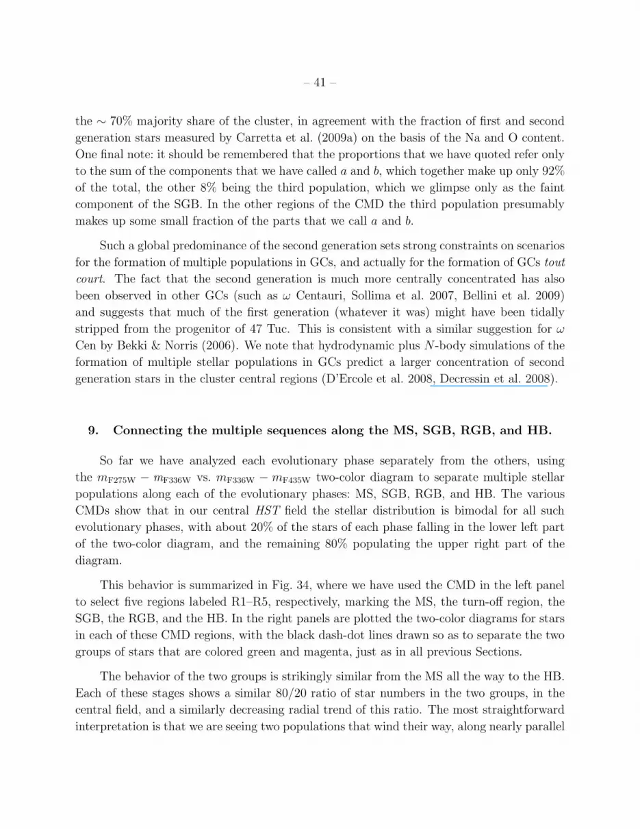
9. Connecting the multiple sequences along the MS, SGB, RGB, and HB.

So far we have analyzed each evolutionary phase separately from the others, using

the mF275W − mF336W vs. mF336W − mF435W two-color diagram to separate multiple stellar

populations along each of the evolutionary phases: MS, SGB, RGB, and HB. The various

CMDs show that in our central HST field the stellar distribution is bimodal for all such

evolutionary phases, with about 20% of the stars of each phase falling in the lower left part

of the two-color diagram, and the remaining 80% populating the upper right part of the

diagram.

This behavior is summarized in Fig. 34, where we have used the CMD in the left panel

to select five regions labeled R1–R5, respectively, marking the MS, the turn-off region, the

SGB, the RGB, and the HB. In the right panels are plotted the two-color diagrams for stars

in each of these CMD regions, with the black dash-dot lines drawn so as to separate the two

groups of stars that are colored green and magenta, just as in all previous Sections.

The behavior of the two groups is strikingly similar from the MS all the way to the HB.

Each of these stages shows a similar 80/20 ratio of star numbers in the two groups, in the

central field, and a similarly decreasing radial trend of this ratio. The most straightforward

interpretation is that we are seeing two populations that wind their way, along nearly parallel

https://www.researchgate.net/publication/45848661_The_evolution_of_two_stellar_populations_in_globular_clusters_I_The_dynamical_mixing_timescale?el=1_x_8&enrichId=rgreq-d8ae7d0753d6b47b18f58e9c9f6029d7-XXX&enrichSource=Y292ZXJQYWdlOzUxOTM1Mjk2O0FTOjk5NTk2NzA1NDY4NDE2QDE0MDA3NTcxMTM0Mzg=

– 42 –

Fig. 34.— Left : mF814W vs. mF435W−mF814W CMD from HST photometry, used to define the

five regions labeled R1,R2,...,R5. Right : mF275W −mF336W vs. mF336W −mF435W two-color

diagrams for stars in the five CMD regions. Dash-dot lines are used to arbitrarily separate

the two sequences that are present in each part of the CMD.

paths, through the various successive stages of stellar evolution. This continuity is pictured

in Figure 35, whose two CMDs emphasize the crucial role that the F275W and F336W filters

play in seeing such simplicity in what would otherwise have been a perplexing melange of

details.

Finally, the main properties of the two populations are summarized in Table 3.

Table 3: Chemical composition and fraction of stars relative to the total number, for the two

main population groups.

Group color code sequences chemical composition fraction fraction

R<∼2 arcmin R>∼15arcmin

a green MSa+SGBa+RGBa+HBa CN-weak, O-rich, Na-poor, Y∼0.25 ∼20% ∼40%

b magenta MSb+SGBb+RGBb+HBb CN-strong, O-poor, Na-rich, Y∼0.265 ∼80% ∼60%

– 43 –

Fig. 35.— CMDs with mF275W vs. mF275W−mF336W (left) and mF336W vs. mF336W−mF435W

(right). We have colored in green and magenta the two groups of stars selected in Fig. 34.

This is the first time anyone has been able to follow two stellar populations in a globular

cluster from the main sequence to the horizontal branch.

10. Summary and Discussion

We have analyzed a large set of HST and ground-based images of the Galactic globular

cluster NGC 104 (47 Tuc) in nine photometric bands, finding multiple sequences throughout

the various CMDs, from the main sequence all the way to the horizontal branch. Exploiting

this wealth of HST data to investigate the behavior of the multiple populations as seen in

several different combinations of magnitudes and colors, we found that among the rainbow

of possible CMDs, those involving the F275W and F336W filters are particularly effective in

separating components of otherwise entangled cluster populations. Taking a cue from HST,

we were able to construct a color system based on the U band that exhibited a similarly

effective separation of the populations in ground-based data.

We found that the distribution of stars along the MS, SGB, RGB, and HB was in every

case bimodal in the mF275W−mF336W vs. mF336W−mF435W two-color diagram, and we finally

put together the groups of stars that we had separated in this way, so as to draw a continuous

connection between their successive evolutionary phases.

Near the cluster center all evolutionary phases split into two near-parallel sequences,

with the richer one making up about 80% of the cluster stars, and the poorer one the re-

maining 20%. Wide-field ground-based photometry allowed us to identify and separate the

– 44 –

two sub-populations at larger radial distances from the cluster center, with the result that

the majority population is more centrally concentrated, but its relative fraction decreases

outward and approaches 50/50 in the outskirts of the cluster. Globally, the majority popula-

tion accounts for ∼ 70% of the whole population of 47 Tuc, most of the remainder consisting

of the minority population. Radial gradients in the stellar populations of this cluster have

been known for a long time, with a CN-strong population more centrally concentrated than

the CN-weak one. This suggests that the numerically dominant population is CN-strong.

Along these same lines, we used CN band strengths and Na and O abundances that are

available from the literature for some RGB and HB stars of both populations, to investigate

their chemical content. It appears that the more populous RGBb and HBb sequences consist

of CN-strong/Na-rich/O-poor stars, while the bulk of the CN-weak/Na-poor/O-rich stars

belong to the numerically poorer RGBa and HBa.

On the theoretical side, we calculated synthetic spectra of main-sequence stars with

different chemical compositions, derived the corresponding colors for our filter set, and com-

pared them with the observed colors in the two distinct populations. The colors of the

minority population are well reproduced by stars with primordial helium abundance and an

oxygen-rich/nitrogen-poor composition that is typical of halo stars of metallicity similar to

that of 47 Tuc. On the other hand, the colors of the majority population stars are well

reproduced by a composition in which nitrogen is greatly enhanced, along with a slightly

increased helium, while carbon and oxygen are depleted. Synthetic spectra for RGB and HB

stars confirm this result.

The most straightforward interpretation of these differences is that the minority popula-

tion is the remnant of the first stellar generation, which formed out of the interstellar medium

of its time, and shared its chemical composition. The chemical composition of the majority

population, by contrast, carries the signatures of CNO and proton-capture processing at high

temperatures, such as depletion of oxygen in favor of nitrogen and sodium, accompanied by

helium enhancement. Therefore the majority population should be regarded as the second

stellar generation of 47 Tuc, which formed out of material that had been partly processed

through stars of the first generation.

Since both populations share the same iron abundance, one can exclude from the en-

richment history of the second-generation material any significant contribution by massive

stars, exploding as core-collapse supernovae. This leaves intermediate-mass stars of the first

generation as the obvious candidates for having processed the material that is now incorpo-

rated into the second generation, a view that is indeed widely entertained in the literature.

Furthermore, it is certainly striking that the second generation is today more populous than

the first. This sets strong constraints on the nature of the progenitor of the present cluster

– 45 –

47 Tuc, and on the initial mass of the first generation, which must have been one to two

orders of magnitude more massive than the portion that is still bound to the cluster.

Finally, we must again remind the reader that besides the two populations that we have

called first and second, we have found unmistakable evidence for the presence of a third

population, including some ∼ 8% of the stars, which we can distinguish it only on the SGB,

but it appears to have the abundance distribution of the “b” population. This remains

as a strident reminder that the stellar populations in 47 Tuc are more complex than the

two-generation picture that we have just sketched.

A.P.M., G.P., A.B., R.G., S.C., A.R., A.B., E.C., F.D., M.D.C., S.L., and A.P. acknowl-

edge partial support by PRIN MIUR 20075TP5K9 and PRIN INAF ”Formation and Early

Evolution of Massive Star Clusters. G.P., S.C., and A.R. acknowledge partial support by

ASI under the program ASI-INAF I/016/07/0. J. A. and I. R. K. acknowledge support from

STScI grant GO-12311.

REFERENCES

Albrow, M. D., Gilliland, R. L., Brown, T. M., Edmonds, P. D., Guhathakurta, P., &

Sarajedini, A. 2001, ApJ, 559, 1060

Anderson, A. J. 1997, Ph.D. Thesis, Univ. of California, Berkeley

Anderson, J., & King, I. R. 2006, Instrument Science Report ACS 2006-01, 34 pages, 1

Anderson, J., et al. 2008, AJ, 135, 2055

Anderson, J., Piotto, G., King, I. R., Bedin, L. R., & Guhathakurta, P. 2009, ApJ, 697, L58

Bedin, L. R., Piotto, G., Anderson, J., Cassisi, S., King, I. R., Momany, Y., & Carraro, G.

2004, ApJ, 605, L125

Bedin, L. R., Cassisi, S., Castelli, F., Piotto, G., Anderson, J., Salaris, M., Momany, Y., &

Pietrinferni, A. 2005, MNRAS, 357, 1038

Bekki, K. & Norris, J.E. 2006, ApJ, 637, L109

Bell, R. A., Dickens, R. J., & Gustafsson, B. 1975, BAAS, 7, 535

Bellini, A., Piotto, G., Bedin, L. R., King, I. R., Anderson, J., Milone, A. P., & Momany,

Y. 2009, A&A, 507, 1393


– 46 –

Bellini, A., & Bedin, L. R. 2010, A&A, 517, A34

Bellini, A., Bedin, L. R., Piotto, G., Milone, A. P., Marino, A. F., & Villanova, S. 2010, AJ,

140, 631

Bellini, A., Anderson, J., & Bedin, L. R. 2011, arXiv:1102.5218

Bergbusch, P. A., & Stetson, P. B. 2009, AJ, 138, 1455

Bragaglia, A., et al. 2010, ApJ, 720, L41

Briley, M. M. 1997, AJ, 114, 1051

Cannon, R. D., Croke, B. F. W., Bell, R. A., Hesser, J. E., & Stathakis, R. A. 1998, MNRAS,

298, 601

Carretta, E., Bragaglia, A., Gratton, R. G., Leone, F., Recio-Blanco, A., & Lucatello, S.

2006, A&A, 450, 523

Carretta, E., et al. 2009a, A&A, 505, 117

Carretta, E., Bragaglia, A., Gratton, R., & Lucatello, S. 2009b, A&A, 505, 139

Cassisi, S. et al. 2004, ApJ, 616, 498

Cassisi, S., Salaris, M., Pietrinferni, A., Piotto, G., Milone, A. P., Bedin, L. R., & Anderson,

J. 2008, ApJ, 672, L115

Catelan, M., Valcarce, A. A. R., & Sweigart, A. V. 2010, IAU Symposium, 266, 281

D’Antona F., Gratton R., Chieffi A., 1983, Mem. Soc. Astron. Ital., 54, 173

D’Antona, F., & Caloi, V. 2004, ApJ, 611, 871

D’Antona, F., Bellazzini, M., Caloi, V., Pecci, F. F., Galleti, S., & Rood, R. T. 2005, ApJ,

631, 868

D’Ercole, A., Vesperini, E., D’Antona, F., McMillan, S. L. W., & Recchi, S. 2008, MNRAS,

391, 825

Decressin, T., Meynet, G., Charbonnel, C., Prantzos, N., & Ekstrom, S. 2007, A&A, 464,

1029

Decressin, T., Baumgardt, H., & Kroupa, P. 2008, A&A, 492, 101

http://arxiv.org/abs/1102.5218

– 47 –

de Mink, S. E., Pols, O. R., Langer, N., & Izzard, R. G. 2009, A&A, 507, L1

Denisenkov, P. A., & Denisenkova, S. N. 1989, Astronomicheskij Tsirkulyar, 1538, 11

di Criscienzo, M., Ventura, P., D’Antona, F., Milone, A., & Piotto, G. 2010, MNRAS, 408,

999

Di Criscienzo, M., et al. 2011, arXiv:1103.0867

Freeman, K. C., & Rodgers, A. W. 1975, ApJ, 201, L71

Gratton, R. G., et al. 2001, A&A, 369, 87

Gratton, R. G., Bragaglia, A., Carretta, E., Clementini, G., Desidera, S., Grundahl, F., &

Lucatello, S. 2003, A&A, 408, 529

Gratton, R., Sneden, C., & Carretta, E. 2004, ARA&A, 42, 385

Gratton, R. G., Carretta, E., Bragaglia, A., Lucatello, S., & D’Orazi, V. 2010, A&A, 517,

A81

Harris, W. E. 1996, AJ, 112, 1487, Dec. 2010 update

Harbeck, D., Smith, G. H., & Grebel, E. K. 2003, AJ, 125, 197

Hartwick, F. D. A., & McClure, R. D. 1980, ApJ, 235, 470

Kraft, R. P. 1979, ARA&A, 17, 309

Kurucz, R. 1993, ATLAS9 Stellar Atmosphere Programs and 2 km/s grid. Kurucz CD-ROM

No. 13. Cambridge, Mass.: Smithsonian Astrophysical Observatory, 1993., 13,

Kurucz, R. L. 2005, Memorie della Societa Astronomica Italiana Supplementi, 8, 14

Landolt, A. U. 1992, AJ, 104, 340

Langer, G. E., Shipman, R. F., & Weida, M. J. 1989, PASP, 101, 811

Langer, G. E., Hoffman, R., & Sneden, C. 1993, PASP, 105, 301

Lardo, C., Bellazzini, M., Pancino, E., Carretta, E., Bragaglia, A., & Dalessandro, E. 2011,

A&A, 525, A114

Lee, J.-W., Kang, Y.-W., Lee, J., & Lee, Y.-W. 2009, Nature, 462, 480


https://www.researchgate.net/publication/258976578_Possible_Explanation_of_the_Correlation_Between_Nitrogen_and_Sodium_Over_Abundances_for_Red_Giants_in_Globular_Clusters?el=1_x_8&enrichId=rgreq-d8ae7d0753d6b47b18f58e9c9f6029d7-XXX&enrichSource=Y292ZXJQYWdlOzUxOTM1Mjk2O0FTOjk5NTk2NzA1NDY4NDE2QDE0MDA3NTcxMTM0Mzg=

https://www.researchgate.net/publication/200455822_CD-ROM_13_atlas9_Stellar_Atmosphere_Programs_and_2_km_s-1_grid?el=1_x_8&enrichId=rgreq-d8ae7d0753d6b47b18f58e9c9f6029d7-XXX&enrichSource=Y292ZXJQYWdlOzUxOTM1Mjk2O0FTOjk5NTk2NzA1NDY4NDE2QDE0MDA3NTcxMTM0Mzg=

https://www.researchgate.net/publication/200455822_CD-ROM_13_atlas9_Stellar_Atmosphere_Programs_and_2_km_s-1_grid?el=1_x_8&enrichId=rgreq-d8ae7d0753d6b47b18f58e9c9f6029d7-XXX&enrichSource=Y292ZXJQYWdlOzUxOTM1Mjk2O0FTOjk5NTk2NzA1NDY4NDE2QDE0MDA3NTcxMTM0Mzg=

– 48 –

Marino, A. F., Villanova, S., Piotto, G., Milone, A. P., Momany, Y., Bedin, L. R., & Medling,

A. M. 2008, A&A, 490, 625

Marino, A. F., Milone, A. P., Piotto, G., Villanova, S., Bedin, L. R., Bellini, A., & Renzini,

A. 2009, A&A, 505, 1099

Marino, A. F. et al. 2011a, A&A, 532, A8

Marino, A. F., Villanova, S., Milone, A. P., Piotto, G., Lind, K., Geisler, D., & Stetson,

P. B. 2011b, ApJ, 730, L16

McClure, R. D., & Osborn, W. 1974, ApJ, 189, 405

Milone, A. P., et al. 2008, ApJ, 673, 241

Milone, A. P., Bedin, L. R., Piotto, G., & Anderson, J. 2009, A&A, 497, 755

Milone, A. P., et al. 2010, ApJ, 709, 1183

Milone, A. P., et al. 2011 submitted to A&A

Nataf, D. M., Gould, A., Pinsonneault, M. H., & Stetson, P. B. 2011, arXiv:1102.3916

Norris, J., & Bessell, M. S. 1975, ApJ, 201, L75

Norris, J., & Freeman, K. C. 1979, ApJ, 230, L179

Norris, J., & Smith, G. H. 1981, IAU Colloq. 68: Astrophysical Parameters for Globular

Clusters, 109

Norris, J., & Freeman, K. C. 1982, ApJ, 254, 143

Norris, J. E. 2004, ApJ, 612, L25

Pietrinferni, A., Cassisi, S., Salaris, M., & Castelli, F. 2004, ApJ, 612, 168

Pietrinferni, A., Cassisi, S., Salaris, M., Percival, S., & Ferguson, J. W. 2009, ApJ, 697, 275

Piotto, G., et al. 2005, ApJ, 621, 777

Piotto, G., et al. 2007, ApJ, 661, L53

Piotto, G. 2009, IAU Symposium, 258, 233

Piotto, G., et al. 2011 in preparation


– 49 –

Ramırez, S. V., & Cohen, J. G. 2002, AJ, 123, 3277

Renzini, A., & Voli, M. 1981, A&A, 94, 175

Renzini, A., 1983, Mem. Soc. Astron. Ital., 54, 335

Sbordone, L. 2005, Memorie della Societa Astronomica Italiana Supplementi, 8, 61

Sbordone, L., Salaris, M., Weiss, A., & Cassisi, S. 2011, arXiv:1103.5863

Sirianni, M., et al. 2005, PASP, 117, 1049

Sollima, A., Ferraro, F. R., Bellazzini, M., Origlia, L., Straniero, O., & Pancino, E. 2007,

ApJ, 654, 915

Stetson, P. B. 2000, PASP, 112, 925

Stetson, P. B. 2005, PASP, 117, 563

Ventura, P., & D’Antona, F. 2009, A&A, 499, 835

Ventura, P., Caloi, V., D’Antona, F., Ferguson, J., Milone, A., & Piotto, G. P. 2009, MNRAS,

399, 934

Woolley, R. V. D. R. 1966, Royal Observatory Annals, 2, 1

Yong, D., & Grundahl, F. 2008, ApJ, 672, L29

Yong, D., Grundahl, F., Johnson, J. A., & Asplund, M. 2008, ApJ, 684, 1159

Yong, D., Grundahl, F., D’Antona, F., Karakas, A. I., Lattanzio, J. C., & Norris, J. E. 2009,

ApJ, 695, L62

This preprint was prepared with the AAS LATEX macros v5.2.


multiple stellar populations in 47 tucanae

Documents