multilevel monte carlo approximation of distribution functions and densities

DFG-Schwerpunktprogramm 1324

”Extraktion quantifizierbarer Information aus komplexen Systemen”

Multi-Level Monte Carlo Approximation ofDistribution Functions and Densities

M. Giles, T. Nagapetyan, K. Ritter

Preprint 157

Edited by

AG Numerik/OptimierungFachbereich 12 - Mathematik und InformatikPhilipps-Universitat MarburgHans-Meerwein-Str.35032 Marburg

DFG-Schwerpunktprogramm 1324

”Extraktion quantifizierbarer Information aus komplexen Systemen”

Multi-Level Monte Carlo Approximation ofDistribution Functions and Densities

M. Giles, T. Nagapetyan, K. Ritter

Preprint 157

The consecutive numbering of the publications is determined by theirchronological order.

The aim of this preprint series is to make new research rapidly availablefor scientific discussion. Therefore, the responsibility for the contents issolely due to the authors. The publications will be distributed by theauthors.

MULTI-LEVEL MONTE CARLO APPROXIMATION OFDISTRIBUTION FUNCTIONS AND DENSITIES

MIKE GILES, TIGRAN NAGAPETYAN, AND KLAUS RITTER

Abstract. We construct and analyze multi-level Monte Carlo methods for the approxi-

mation of distribution functions and densities of univariate random variables. Since, by

assumption, the target distribution is not known explicitly, approximations have to be

used. We provide a general analysis under suitable assumptions on the weak and strong

convergence. We apply the results to smooth path-independent and path-dependent func-

tionals and to stopped exit times of SDEs.

1. Introduction

Let Y denote a real-valued random variable with distribution function F and density ρ.We study the approximation of F and ρ with respect to the supremum norm on a compactinterval [S0, S1], without assuming that the distribution of Y is explicitly known or thatthe simulation of Y is feasible. Instead, we suppose that a sequence of random variablesY (�) is at hand that converge to Y in a suitable way and that are suited to simulation.

We present a general approach, which is later on applied in the context of stochasticdifferential equations (SDEs). In this specific setting we aim at the distribution of Lipschitzcontinuous, path-independent or path-dependent functionals of the solution process, orthe distribution of stopped exit times from bounded domains.

In the general setting a naive Monte Carlo algorithm for the approximation of ρ worksas follows: Choose a level � ∈ N and a replication number n ∈ N, generate n independentsamples according to Y (�), and apply a kernel density estimator, say, to these samples.For the approximation of F one proceeds analogously, and here the empirical distributionfunction of the samples is the most elementary choice.

In this paper we develop the multi-level Monte Carlo approach, which relies on thecoupled simulation of Y (�) and Y (�−1) on a finite range of levels �. For the multi-levelapproach to work well for the approximation of distribution functions or densities, asmoothing step is necessary on every level. The smoothing is based on rescaled translatesof a suitable function g, which is meant to approximate either the indicator function of]−∞, 0] or the Dirac functional at zero. In a first stage the multi-level algorithm providesan approximation to F or ρ at discrete points, which is then extended to a function on[S0, S1] in a standard and purely deterministic way.

For the approximation of F and ρ on [S0, S1] our assumptions are as follows:

(i) The density ρ of Y is r-times continuously differentiable,(ii) The simulation of the joint distribution of Y (�) and Y (�−1) is possible at cost

O(M �) for every � ∈ N, where M > 1.(iii) A weak error estimate

sups∈[S0,S1]

��E�g((Y − s)/δ) − g((Y (�) − s)/δ)

�� ≤ O�min

�δ−α1 ·M−�·α2 ,M−�·α3

��

Date: February 2, 2014.1

2 GILES, NAGAPETYAN, AND RITTER

holds for all positive, sufficiently small δ and all � ∈ N0, where α1 ≥ 0, α2 > 0,and α2 ≥ α3 ≥ 0.

(iv) A strong error estimate

Emin((Y − Y (�))2/δ2, 1) ≤ O�δ−β4 ·M−�·β5

�

holds for all positive, sufficiently small δ and all � ∈ N0, where β4 ≥ 0 and β5 > 0.

We also study the approximation of the distribution function F at a single point s ∈[S0, S1], and here (iv) is replaced by the following assumption:

(v) A strong error estimate

sups∈[S0,S1]

E�g((Y − s)/δ) − g((Y (�) − s)/δ)

�2 ≤ O�min

�δ−β1 ·M−�·β2 ,M−�·β3

��

holds for all positive, sufficiently small δ and all � ∈ N0, where β1 ≥ 0, β2 > 0,and β2 ≥ β3 ≥ 0.

The parameters of a multi-level algorithm A are the minimal and maximal level, thereplication numbers per level, the smoothing parameter δ, and the number of discretepoints to be used in the first stage. We derive upper bounds for error(A), the root meansquare error, and cost(A), the computational cost, in terms of these parameters and thevalues of r, αi, and βi, and we present the asymptotically optimal choice of the parameterswith respect to our upper bounds. This leads to a final estimate of the form

cost(A) ≤ O�error(A)−θ+ε

�

for every ε > 0, where θ > 0. Roughly speaking, θ is the order of convergence of themulti-level algorithm. See Theorems 1–3 for the precise statements involving also powersof log error(A).

Here we only present a particular application of these theorems for functionals

ϕ : C([0, T ],Rd) → R

of the solution process X of a d-dimensional system of SDEs, i.e., Y = ϕ(X). For simplicitywe take the Euler scheme with equidistant time-steps for the approximation of X in theconstruction of the multi-level algorithm, and we assume that r ≥ 1 for the rest of theintroduction. Table 1 contains the values of θ for the approximation of F and ρ on [S0, S1]as well as for the approximation of F at a single point s ∈ [S0, S1]. In the first row ϕis assumed to be Lipschitz continuous, and based on a well known upper bound for thestrong error of the Euler scheme we show that (iii)–(v) are satisfied with

α1 = 0, α2 = 1/2 − ε, α3 = 1/2 − ε

and

β1 = 1 + ε, β2 = 1 − ε, β3 = 1/2 − ε, β4 = 2, β5 = 1 − ε

for every ε > 0. In the second row

ϕ(x) = inf{t ≥ 0 : x(t) ∈ ∂D} ∧ T

is a stopped exit time from a bounded domain D ⊂ Rd, and based on a recent result byBouchard, Geiss, Gobet (2013) we obtain

α1 = 1, α2 = 1/2, α3 = 1/4

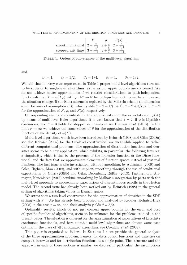
MULTI-LEVEL APPROXIMATION OF DISTRIBUTION FUNCTIONS AND DENSITIES 3

F ρ F (s)

smooth functional 2 + 2r+1

2 + 4r

2 + 1r+1

stopped exit time 3 + 2r+1

3 + 5r

3 + 2r+1

Table 1. Orders of convergence of the multi-level algorithm

and

β1 = 1, β2 = 1/2, β3 = 1/4, β4 = 1, β5 = 1/2.

We add that in every case represented in Table 1 proper multi-level algorithms turn outto be superior to single-level algorithms, as far as our upper bounds are concerned. Wedo not achieve better upper bounds if we restrict considerations to path-independentfunctionals, i.e., Y = ϕ(XT ) with ϕ : Rd → R being Lipschitz continuous; here, however,the situation changes if the Euler scheme is replaced by the Milstein scheme (in dimensiond = 1 because of assumption (ii)), which yields θ = 2 + 1/(r + 1), θ = 2 + 3/r, and θ = 2for the approximation of F , ρ, and F (s), respectively.

Corresponding results are available for the approximation of the expectation of ϕ(X)by means of multi-level Euler algorithms. It is well known that θ = 2, if ϕ is Lipschitzcontinuous, and θ = 3 holds for stopped exit times ϕ, see Higham et al. (2013). In thelimit r → ∞ we achieve the same values of θ for the approximation of the distributionfunction or the density of ϕ(X).

Multi-level algorithms, which have been introduced by Heinrich (1998) and Giles (2008a),see also Kebaier (2005) for the two-level construction, are meanwhile applied to ratherdifferent computational problems. The approximation of distribution functions and den-sities seems to be a new application, which exhibits, in particular, the following features:a singularity, which is due to the presence of the indicator function or the Dirac func-tional, and the fact that we approximate elements of function spaces instead of just realnumbers. The first issue is also investigated, without smoothing, by Avikainen (2009) andGiles, Higham, Mao (2009), and with implicit smoothing through the use of conditionalexpectations by Giles (2008b) and Giles, Debrabant, Roßler (2013). Furthermore, Alt-mayer, Neuenkirch (2013) combine smoothing by Malliavin integration by parts with themulti-level approach to approximate expectations of discontinuous payoffs in the Hestonmodel. The second issue has already been worked out by Heinrich (1998) in the generalsetting of algorithms taking values in Banach spaces.

We stress that a two-level construction for the approximation of densities in the SDEsetting with Y = XT has already been proposed and analyzed by Kebaier, Kohatsu-Higa(2008) in the case r = ∞, and their analysis yields θ = 5/2.

Optimality results, which do not just concern upper bounds for the error and costof specific families of algorithms, seem to be unknown for the problems studied in thepresent paper. The situation is different for the approximation of expectations of Lipschitzcontinuous functionals, and here suitable multi-level algorithms are almost worst caseoptimal in the class of all randomized algorithms, see Creutzig et al. (2008).

This paper is organized as follows. In Sections 2–4 we provide the general analysisof the three approximation problem, namely, for distribution functions and densities oncompact intervals and for distribution functions at a single point. The structure and theapproach in each of these sections is similar: we discuss, in particular, the assumptions


on the weak and the strong convergence, and we construct and analyze the respectivemulti-level algorithms. Section 5 contains, in particular, the application of the resultsfrom Sections 2–4 to functionals of the solutions of SDEs, which is complemented bynumerical experiments for simple test cases in Section 6.

2. Approximation of Distribution Functions on Compact Intervals

We consider a random variable Y , and we study the approximation of its distributionfunction F on a compact interval [S0, S1], with S0 < S1 being fixed throughout thissection. We do not assume that the distribution of Y can be simulated exactly. Instead,we assume that the simulation is feasible for random variables Y (�) that converge to Y ina suitable way.

2.1. Smoothing. For the approximation of F a straight-forward application of the multi-level Monte Carlo approach based on

F (s) = E(1]−∞,s](Y ))

could suffer from the discontinuity of 1]−∞,s], see Remark 8 below. This can be avoided bya smoothing step, provided that a density exists and is sufficiently smooth. Specifically,we assume that

(A1) the random variable Y has a density ρ on R that is r-times continuously differ-entiable on [S0 − δ0, S1 + δ0] for some r ∈ N0 and δ0 > 0.

The smoothing is based on rescaled translates of a function g : R → R with the followingproperties:

(S1) The cost of computing g(s) is bounded by a constant, uniformly in s ∈ R.(S2) g is Lipschitz continuous.(S3) g(s) = 1 for s < −1 and g(s) = 0 for s > 1.

(S4)� 1

−1sj · (1]−∞,0](s) − g(s)) ds = 0 for j = 0, . . . , r − 1.

Obviously, g is bounded due to (S2) and (S3).

Remark 1. Such a function g is easily constructed as follows. There exists a uniquelydetermined polynomial p of degree at most r + 1 such that

� 1

−1

sj · p(s) ds = (−1)j/(j + 1), j = 0, . . . , r − 1,

as well as p(1) = 0 and p(−1) = 1. The extension g of p with g(s) = 1 for s < −1 andg(s) = 0 for s > 1 has the properties as claimed. Since g − 1/2 is an odd function, thesame function g arises in this way for r and r + 1, if r is even.

We have the following estimate for the bias that is induced by smoothing with parameterδ, i.e., by approximation of 1]−∞,s] by g((· − s)/δ).

Lemma 1. There exists a constant c > 0 such that

sups∈[S0,S1]

|F (s) − E(g((Y − s)/δ))| ≤ c · δr+1

holds for all δ ∈ ]0, δ0].


Proof. Clearly

F (s) − E(g((Y − s)/δ)) =

� ∞

−∞ρ(u) · (1]−∞,s](u) − g((u− s)/δ)) du

= δ ·� 1

−1

ρ(δu + s) · (1]−∞,0](u) − g(u)) du,

so that the statement follows in the case r = 0. For r ≥ 1 the Taylor expansion

ρ(δu + s) =r−1�

j=0

ρ(j)(s) · (δu)j/j! + R(δu, s)

yields

|F (s) − E(g((Y − s)/δ))| ≤ δ ·� 1

−1

|R(δu, s)| · |1]−∞,0](u) − g(u)| du ≤ c · δr+1.

�2.2. Assumptions on Weak and Strong Convergence. Our multi-level Monte Carloconstruction is based on a sequence (Y (�))�∈N0 of random variables, defined on a commonprobability space together with Y , with the following properties for some constant c > 0:

(A2) There exists a constant M > 1 such that the simulation of the joint distributionof Y (�) and Y (�−1) is possible at cost at most c ·M � for every � ∈ N.

(A3) There exist constants α1 ≥ 0, α2 > 0, and α2 ≥ α3 ≥ 0 such that the weak errorestimate

sups∈[S0,S1]

��E�g((Y − s)/δ) − g((Y (�) − s)/δ)

�� ≤ c · min�δ−α1 ·M−�·α2 ,M−�·α3

�

holds for all δ ∈ ]0, δ0] and � ∈ N0.(A4) There exist constants β4 ≥ 0 and β5 > 0 such that the strong error estimate

Emin((Y − Y (�))2/δ2, 1) ≤ c · δ−β4 ·M−�·β5

holds for all δ ∈ ]0, δ0] and � ∈ N0.

For specific applications we present suitable approximations Y (�) and correspondingvalues of the parameters M , αi and βi in Section 5. Here we proceed with a generaldiscussion of (A3) and (A4).

Note that (A4) implies (A3) with α1 = β4/2, α2 = β5/2, and α3 = 0, but often betterestimates for the weak error are known, see Sections 4.2 and 5. The presence of α1 and β4

in these assumptions is motivated by weak and strong error estimates for SDEs or SPDEs,which often scale with some power of δ. See, however, Sections 5.1 and 5.2

Let �Z�p = (E |Z|p)1/p for any random variable Z and 1 ≤ p < ∞. Typically, strongerror estimates for Y − Y (�) instead of min(|Y − Y (�)|, δ) are available in the literature.Straightforward relations to (A3) and (A4) are provided by

(1) sups∈[S0,S1]

��E�g((Y − s)/δ) − g((Y (�) − s)/δ)

�� ≤ cL · δ−1 · �Y − Y (�)�1,

where cL denotes a Lipschitz constant for g, as well as

(2) Emin((Y − Y (�))2, δ2) ≤ min(�Y − Y (�)�22, δ2)and

(3) Emin((Y − Y (�))2, δ2) ≤ E(δ · min(|Y − Y (�)|, δ)) ≤ min(δ · �Y − Y (�)�1, δ2).


In the following case of equivalence of norms the upper bound in (2) is sharp, and thenwe have β4 = 2 in (A4), while the optimal value of β5 is determined by the asymptoticbehavior of �Y − Y (�)�22. See Sections 5.1 and 5.2 for examples.

Lemma 2. Suppose that there exist c1 > 0 and p > 2 such that

0 < �Y − Y (�)�p ≤ c1 · �Y − Y (�)�2for all � ∈ N0. Then there exists c2 > 0 such that

Emin((Y − Y (�))2, δ2) ≥ c2 · min(�Y − Y (�)�22, δ2)for all δ ∈ ]0, δ0] and � ∈ N0.

Proof. Put

Z� =(Y − Y (�))2

�Y − Y (�)�22.

We show that there exists a constant c2 > 0 such that

Emin(Z�, δ) ≥ c2 · min(1, δ)

for all � ∈ N0 and δ > 0.Clearly E(Z�) = 1 and E(Z

p/2� ) ≤ cp1. It follows that

P ({Z� > u}) ≤ cp1up/2

.

Put

d� = P ({Z� > 1/2}).We claim that

d = inf�∈N0

d� > 0.

Assume that d = 0. Use

1 = E(Z�) =

� ∞

0

P ({Z� > u}) du ≤ 1/2 +

� ∞

1/2

min(d�, cp1/u

p/2) du

and dominated convergence to conclude that, for a minimizing subsequence,

limk→∞

� ∞

1/2

min(d�k , cp1/u

p/2) du = 0,

which leads to a contradiction. Therefore

Emin(Z�, δ) =

� δ

0

P ({Z� > u}) du ≥ min(δ, 1/2) · d ≥ d/2 · min(1, δ).

�On the other hand, if �Y − Y (�)�22 and �Y − Y (�)�1 are asymptotically equivalent, then

(3) is preferable to (2). See Section 5.3 for examples.Assumption (A4) and the Lipschitz continuity and boundedness of g immediately yield

the following fact.


E sups∈[S0,S1]

�g((Y − s)/δ) − g((Y (�) − s)/δ)

�2 ≤ c · min(δ−β4 ·M−�·β5 , 1)



2.3. The Multi-level Algorithm. The approximation of F on the interval [S0, S1] isbased on its approximation at finitely many points

(4) S0 ≤ s1 < · · · < sk ≤ S1,

followed by a suitable extension to [S0, S1].For notational convenience we put

gk,δ(t) = (g((t− s1)/δ), . . . , g((t− sk)/δ)) ∈ Rk, t ∈ R,

as well as Z(0)i = Y (−1) = 0.

We choose L0, L1 ∈ N0 with L0 ≤ L1 as the minimal and the maximal level, respectively,and we choose replication numbers N� ∈ N for all levels � = L0, . . . , L1, as well as k ∈ Nand δ ∈ ]0, δ0]. The corresponding multi-level algorithm for the approximation at thepoints si is defined by

(5) Mk,δ,L0,L1

NL0,...,NL1

=1

NL0

·NL0�

i=1

gk,δ(Y(L0)i ) +

L1�

�=L0+1

1

N�

·N��

i=1

�gk,δ(Y

(�)i ) − gk,δ(Z

(�)i )

�

with an independent family of R2-valued random variables (Y(�)i , Z

(�)i ) for � = L0, . . . , L1

and i = 1, . . . , N� such that equality in distribution holds for (Y(�)i , Z

(�)i ) and (Y (�), Y (�−1)).

Remark 2. In the particular case L = L0 = L1, i.e., in the single-level case, we actuallyhave a classical Monte Carlo algorithm, based on independent copies of Y (L) only. Inaddition to

Mk,δ,L,LN =

1

N·

N�

i=1

gk,δ(Y(L)i )

with δ > 0, we also consider the single-level algorithm without smoothing. Hence we put

gk,0(t) =�1]−,∞,s1](t), . . . , 1]−,∞,sk](t)

�∈ Rk, t ∈ R,

to obtain

Mk,0,L,LN =

1

N·

N�

i=1

gk,0(Y(L)i ).

Observe that Mk,0,L,LN yields the values of the empirical distribution function, based on

N independent copies of Y (L), at the points si.For the analysis of the single-level algorithm it suffices to assume that the simulation

of the distribution of Y (�) is possible at cost at most c · M � for every � ∈ N, cf. (A2).Furthermore, there is no need for a strong error estimate like (A4), and if we do notemploy smoothing, then (A3) may be replaced by the following assumption. There exista constant α > 0 such that the weak error estimate

(6) sups∈[S0,S1]

��E�1]−∞,s](Y ) − 1]−∞,s](Y

(�))�� ≤ c ·M−�·α

holds for all � ∈ N0. It turns out that the analysis of single-level algorithms withoutsmoothing is formally reduced to the case δ > 0 if we take

(7) α1 = 0, α2 = α, α3 = α.


In the sequel � · �∞ denotes the supremum norm on C([S0, S1]) and | · |∞ denotes the�∞-norm on Rk.

For the extension we take a sequence of linear mappings Qrk : Rk → C([S0, S1]) with

the following properties for some constant c > 0:

(E1) For all k ∈ N and x ∈ Rk the cost for computing Qrk(x) is bounded by c · k.

(E2) For all k ∈ N and x ∈ Rk

�Qrk(x)�∞ ≤ c · |x|∞.

(E3) For all k ∈ N

�F −Qrk(F (s1), . . . , F (sk))�∞ ≤ c · k−(r+1).

These properties are achieved, e.g., by piecewise polynomial interpolation with degreemax(r, 1) at equidistant points si = S0 + (i− 1) · (S1 − S0)/(k − 1) with k ≥ 2.

We employ Qrk(M) with M = Mk,δ,L0,L1

NL0,...,NL1

as a randomized algorithm for the approxi-

mation of F on [S0, S1]. Observe that M is square-integrable, since g is bounded, so that(E2) yields E �Qr

k(M)�2∞ < ∞. The error of Qrk(M) is defined by

error(Qrk(M)) =

�E �F −Qr

k(M)�2∞�1/2

.

Since the error is based on the supremum norm, error(Qrk(M)) does not increase if we

replace Qrk(x) by s �→ supu∈[S0,s](Q

rk(x))(u) to get a non-decreasing approximation on

[S0, S1].The variance of any square-integrable Rk-valued random variable M is defined by

Var(M) = E |M− E(M)|2∞,

and

E |x−M|2∞ ≤ 2 · (|x− E(M)|2∞ + Var(M))

holds for x ∈ Rk. Furthermore,

Var(M) ≤ 4 · E(|M|2∞).

The Bienayme formula for real-valued random variables turns into the inequality

(8) Var(M) ≤ c · log k ·n�

i=1

Var(Mi),

if M =�n

i=1 Mi with independent square-integrable random variables Mi taking valuesin Rk. Here c is a universal constant. In the context of multi-level algorithms this isexploited in Heinrich (1998).

We say that a sequence of randomized algorithms An converges with order (γ, η) ∈]0,∞[ × R if limn→∞ error(An) = 0 and if there exists a constant c > 0 such that

cost(An) ≤ c · (error(An))−γ · (− log error(An))

η.

Moreover, we put

(9) q = min

�r + 1 + α1

α2

,r + 1

α3

�.


Theorem 1. The following order, with η = 1, is achieved by algorithms Qrk(Mk,δ,L0,L1

NL0,...,NL1

)

with suitably chosen parameters:

q ≤ max(1, β4/β5) ⇒ γ = 2 +max(1, q)

r + 1,(10)

q > max(1, β4/β5) ∧ β5 > 1 ⇒ γ = 2 +max(1, β4/β5)

r + 1,(11)

q > 1 > β4 ∧ β5 = 1 ⇒ γ = 2 +1

r + 1,(12)

q > max(1, β4/β5) ∧ β5 < 1 ⇒ γ = 2 +max(1, β4 + (1 − β5) · q)

r + 1.(13)

Moreover, with η = 3,

q > β4 ≥ 1 ∧ β5 = 1 ⇒ γ = 2 +β4

r + 1.(14)

Proof. Let M denote any square-integrable random variable with values in Rk. For theerror of Qr

k(M) we have

error(Qrk(M)) ≤ �F −Qr

k(F (s1), . . . , F (sk))�∞ +�E �Qr

k((F (s1), . . . F (sk)) −M)�2∞�1/2

≤ c ·�k−(r+1) +

�E |(F (s1), . . . F (sk)) −M|2∞

�1/2�

≤ 2c ·�k−2(r+1) + |(F (s1), . . . F (sk)) − E(M)|2∞ + Var(M)

�1/2

with a constant c > 0 according to (E2) and (E3).

Now we consider the algorithm M = Mk,δ,L0,L1

NL0,...,NL1

with δ > 0. We write a � b if there

exists a constant c > 0 that does not depend on the parameters k, δ, L0, L1, NL0 , . . . , NL1

such that a ≤ c · b. Moreover, a � b means b � a, and a � b stands for a � b and a � b.Note that E(M) = E(gk,δ(Y (L1))). Hence the bias term is estimated by

|(F (s1), . . . , F (sk)) − E(M)|∞ = supi=1,...,k

|F (si) − E(g((Y (L1) − si)/δ))|

� δr+1 + min�δ−α1 ·M−L1·α2 ,M−L1·α3

�,

see Lemma 1 and (A3).The variance of M is estimated as follows. From (8) we obtain

Var(M) � log k ·�

1

NL0

· Var(gk,δ(Y (L0))) +

L1�

�=L0+1

1

N�

· Var�gk,δ(Y (�)) − gk,δ(Y (�−1))

��.

Moreover,

Var�gk,δ(Y (�)) − gk,δ(Y (�−1))

�≤ 4 · E sup

i=1,...,k

�g((Y (�) − si)/δ) − g((Y (�−1) − si)/δ)

�2

� min(δ−β4 ·M−�·β5 , 1)

for � = L0 + 1, . . . , L1, see Lemma 3, and

Var(gk,δ(Y (L0))) � 1,


since g is bounded. Therefore

Var(M) � log k ·�

1

NL0

+

L1�

�=L0+1

min(δ−β4 ·M−�·β5 , 1)

N�

�.

Combining these estimates we finally get

error2(Qrk(M)) � k−2(r+1) + δ2(r+1) + min

�δ−2α1 ·M−L1·2α2 ,M−L1·2α3

�(15)

+ log k ·�

1

NL0

+

L1�

�=L0+1

min(δ−β4 ·M−�·β5 , 1)

N�

�.

Now we analyze the computational cost of the algorithm M. For � = L0, . . . , L1 and

i = 1, . . . , N� the cost of computing gk,δ(Y(�)i ) or gk,δ(Y

(�)i ) − gk,δ(Z

(�)i ) is bounded by

M � + k, up to a constant, see (S1) and (A2). Use (E1) to obtain

(16) cost(Qrk(M)) � c(k, L0, L1, NL0 , . . . , NL1)

with

(17) c(k, L0, L1, NL0 , . . . , NL1) =

L1�

�=L0

N� · (M � + k).

Note that for every k the cost per replication is essentially constant on all levels � ≤ L∗,where

(18) L∗ = logM k.

Observe that the estimates (15) and (16) are valid, too, for single-level algorithmswithout smoothing, i.e., for L0 = L1 and δ = 0, if we formally define the parameters αi

by (7), which leads to q = (r + 1)/α.We determine parameters of the algorithm Qr

k(M) such that an error of about � ∈�0,min(1, δr+1

0 )�is achieved at a small cost. More precisely, we minimize the upper bound

(16) for the cost, subject to the constraint that the upper bound (15) for the squarederror is at most �2, up to multiplicative constants for both quantities.

First of all we consider the case δ > 0, and we choose

(19) δ = �1/(r+1)

and, up to integer rounding,

(20) k = �−1/(r+1)

and

(21) NL0 = �−2 · logM �−1.

This yields

error2(Qrk(M)) � �2 + a2(L1) + log �−1 ·

L1�

�=L0+1

min(δ−β4 ·M−�·β5 , 1)

N�

with

(22) a(L1) = min�δ−α1 ·M−L1·α2 ,M−L1·α3

�.


Furthermore,

(23) L∗ =1

r + 1· logM �−1.

Due to the dependence of (16) on k and the decay of a(L1) and min(δ−β4 ·M−�·β5 , 1)as functions of L1 and �, respectively, it suffices to study

(24) L0 ≥ L∗.

Moreover, a(L1) ≤ � requires L1 ≥ q · L∗. Consequently, we choose

(25) L1 = max(1, q) · L∗,

up to integer rounding.For a single-level algorithm with smoothing, i.e., for L0 = L1 and δ > 0, all parameters

have thus been determined, and we obtain error(Qrk(M)) � � as well as

(26) c(k, L1, L1, NL1) � �−2 · log �−1 ·ML∗= �−2−1/(r+1) · log �−1

if q ≤ 1, and

(27) c(k, L1, L1, NL1) � �−2 · log �−1 ·M q·L∗= �−2−q/(r+1) · log �−1,

if q > 1. For a single-level algorithm without smoothing we obtain the same result.For a proper multi-level algorithm with

L∗ ≤ L0 < L1

we obtain

error2(Qrk(M)) � �2 + log �−1 ·

L1�

�=L0+1

v�N�

withv� = min(ML∗·β4 ·M−�·β5 , 1)

as well as

c(k, L0, L1, NL0 , . . . , NL1) � �−2 · log �−1 ·ML0 +

L1�

�=L0+1

N� ·M �.

Observingc(k, L0, L1, NL0 , . . . , NL1) � �−2 · log �−1 ·ML∗

and (26), we get (10) in the case q ≤ 1 already by single-level algorithms.To establish the theorem in the case

q > 1

we fix L0 for the moment, and we minimize

h(L0, NL0+1, . . . , NL1) = �−2 · log �−1 ·ML0 +

L1�

�=L0+1

N� ·M �

subject toL1�

�=L0+1

v�N�

≤ �2/ log �−1.

A Lagrange multiplier leads to

(28) N� = �−2 · log �−1 ·G(L0) ·�v� ·M−�

�1/2,


up to integer rounding, which satisfies the constraint with

G(L0) =

L1�

�=L0+1

�v� ·M �

�1/2=

L1�

�=L0+1

�min(ML∗·β4 ·M−�·β5 , 1) ·M �

�1/2.

Moreover, this choice of NL0+1, . . . , NL1 yields

(29) h(L0, NL0+1, . . . , NL1) = �−2 · log �−1 ·�ML0 + G2(L0)

�.

Put

L† =β4

β5

· L∗.

Consider the case

1 < q ≤ β4/β5.

Then we have L1 ≤ L†, and therefore

ML0 + G2(L0) = ML0 +

�L1�

�=L0+1

M �/2

�2

� ML0 + ML1 � ML∗·q.

Observing (27) we get (10) in the present case already by single-level algorithms.From now on we consider the case

q > max(1, β4/β5).

Suppose that L0 < L†, which requires β4/β5 > 1 to hold. Then we get

ML0 + G2(L0) � ML0 +

L†�

�=L0+1

M �/2

2

+ ML∗·β4 ·

L1�

�=L†+1

M �·(1−β5)/2

2

� ML†+ ML∗·β4 ·

L1�

�=L†+1

M �·(1−β5)/2

2

� ML†+ G2(L†).

It therefore suffices to study the case

L0 ≥ L†,

where we have

ML0 + G2(L0) = ML0 + ML∗·β4 ·�

L1�

�=L0+1

M �·(1−β5)/2

�2

.

If β5 = 1 then

ML0 + G2(L0) � ML0 + ML∗·β4 · (L1 − L0)2.

If β5 > 1 then

ML0 + G2(L0) � ML0 + ML∗·β4 ·ML0·(1−β5) � ML0 .

If β5 < 1 then

ML0 + G2(L0) � ML0 + ML∗·β4 ·ML1·(1−β5).

Hence we choose

(30) L0 = max(1, β4/β5) · L∗


in all these cases. Hereby we obtain

ML0 + G2(L0) � ML∗·max(1,β4/β5) ·�

(L∗)2 , if β5 = 1 and β4 ≥ 1,

1, if β5 > 1 or β5 = 1 and β4 < 1,

as well as

ML0 + G2(L0) � Mmax(1,β4/β5,β4+(1−β5)·q)·L∗

if β5 < 1. In any case these estimates are superior to ML∗·q, cf. (27). Use (29) andML∗

= �−1/(r+1) to derive (11)–(14). �

Remark 3. Theorem 1 is based on the upper bounds (15) and (16) for the error and

the cost, respectively, of the algorithms Qrk(Mk,δ,L0,L1

NL0,...,NL1

). The parameters that we have

determined in the proof of Theorem 1 are optimal in the following sense: they minimizethe upper bound for the cost, subject to the constraint that the upper bound for the erroris at most �, up to multiplicative constants for both quantities.

Obviously, this optimality holds true for the choice of δ, k, NL0 , and L1 according to(19), (20), (21), and (25). Moreover, the constraint (24) is without loss of generality, sothat the minimal level L0 slowly increases with decreasing �.

This completes, in particular, the optimization of the parameters of single-level algo-rithms, where L0 = L1. For proper multi-level algorithms the optimal values of N� for� = L0 + 1, . . . , L1 are presented in (28) and the optimal value of L0 is presented in (30),if q > max(1, β4/β5). It is straightforward to verify

(31) N� = �−2−β4/(r+1) · log �−1 ·M−�·(1+β5)/2 ·

L∗, if β5 = 1,

ML∗·max(1,β4/β5)·(1−β5)/2 if β5 > 1,

ML∗·q·(1−β5)/2, if β5 < 1.

Furthermore, we have carried out the comparison of multi-level and single-level algo-rithms in the proof of Theorem 1. This comparison, too, is merely based on the upperbounds for the error and the cost, and on the assumption that α = α3 in (6). In this sensewe have a superiority of proper multi-level algorithms over single-level algorithms if andonly if

(32) q > max(1, β4/β5),

which corresponds to (11)–(14) in Theorem 1. The lack of superiority, which is presentin (10) in Theorem 1, is explained as follows. For q ≤ 1 the maximal level can be chosenso small that the computational cost on all levels is dominated by the number k ofdiscretization points that is needed to achieve a good approximation of F even fromexact data F (s1), . . . , F (sk). For 1 < q ≤ β4/β5 the negative impact of smoothing on thevariances leads to variances min(δ−β4 ·M−�·β5 , 1) of order one on all levels � = L0+1, . . . , L1.

Single-level algorithms with smoothing are never inferior to single-level algorithms with-out smoothing, and they are superior if and only if

(33)r + 1

α3

> max(1, q).

For large values of r the latter holds true if and only if α2 > α3; see Section 5.3 for anexample.


Remark 4. In the limit r → ∞ we get

γ = 2 +max(1 − β5, 0)

α2

in Theorem 1, which coincides with the order for the approximation of expectations bymeans of multi-level algorithms, see Giles (2008a, Thm. 3.1).

Consider the empirical distribution function Fn based on n independent copies of Y .The Dvoretzky-Kiefer-Wolfowitz inequality, with the optimal constant due to Massart(1990), yields �

E sups∈R

|F (s) − Fn(s)|2�1/2

≤ n−1/2,

which corresponds to an order two of approximation in terms of the number of samplesfrom the target distribution. In our analysis we do not assume that sampling from thetarget distribution is feasible, and we fully take into account the computational cost togenerate samples from approximate distributions. Still, if β5 is almost one and if r is large,a suitable multi-level algorithm almost achieves the order two. See Sections 5.1 and 5.2for examples.

3. Approximation of Densities on Compact Intervals

In this section we study the approximation of the density ρ of Y on an interval [S0, S1]for some fixed S0 < S1. The construction and analysis closely follows the approach fromSection 2.

3.1. Smoothing. We employ assumption (A1) with r ≥ 1, and g : R → R is assumed tosatisfy the properties (S1) and (S2), while (S3) and (S4) are replaced by:

(S5) g(s) = 0 if |s| > 1.

(S6)� 1

−1g(s) ds = 1 and

� 1

−1sj · g(s) ds = 0 for j = 1, . . . , r − 1.

Obviously, g is bounded due to (S2) and (S5). Moreover, if g ∈ C1(R) satisfies (S3) and(S4) and g� is Lipschitz continuous, then −g�, instead of g, satisfies (S5) and (S6). Inkernel density estimation, a function g with integral one and vanishing moments up toorder r − 1 is called a kernel of order (at least) r.

Remark 5. We modify the construction from Remark 1 as follows. There exists a uniquelydetermined polynomial p of degree at most r + 1 such that

� 1

−1

p(s) ds = 1

and � 1

−1

sj · p(s) ds = 0, j = 0, . . . , r − 1,

as well as p(1) = p(−1) = 0. Extend p by zero to obtain g with the properties as claimed.Since g is an even function, the same function g arises in this way for r and r + 1, if r isodd.

We have the following estimate for the bias that is induced by smoothing with parameterδ, i.e., by approximation of the Dirac functional at s by 1/δ·g((·−s)/δ). See, e.g., Tsybakov(2009, Prop. 1.2).



sups∈[S0,S1]

|ρ(s) − 1/δ · E(g((Y − s)/δ))| ≤ c · δr

holds for all δ ∈ ]0, δ0].

Proof. Clearly

ρ(s) − 1/δ · E(g((Y − s)/δ)) =

� 1

−1

g(u) · (ρ(s) − ρ(δu + s)) du.

Use a Taylor expansion to derive

|ρ(s) − 1/δ · E(g((Y − s)/δ))| ≤ c · δr.

�

3.2. Assumptions on Weak and Strong Convergence. We employ the assumptions(A2)–(A4) from Section 2.2 with possibly different values of αi in the weak error estimate(A3). We make use of Lemma 3, and we refer to Section 5 for specific examples withcorresponding values of αi.

3.3. The Multi-level Algorithm. The definition (5) of the algorithms Mk,δ,L0,L1

NL0,...,NL1

also

applies for the approximation of densities, except for gk,δ, which is now defined by

gk,δ(t) =1

δ· (g((t− s1)/δ), . . . , g((t− sk)/δ)) ∈ Rk, t ∈ R.

In the present setting we have δ > 0 also for single-level algorithms.Hereby we obtain approximations to ρ at the points (4), which are extended to functions

on [S0, S1] by means of linear mappings Qrk : Rk → C([S0, S1]). We assume that (E1) and

(E2) are satisfied, but instead of (E3) the following property is assumed to hold with someconstant c > 0:

(E4) For all k ∈ N

�ρ−Qrk(ρ(s1), . . . , ρ(sk))�∞ ≤ c · k−r.

As before, piecewise polynomial interpolation at equidistant points, now of degree max(r−1, 1), might be used for this purpose.

We employ Qrk(M) with M = Mk,δ,L0,L1

NL0,...,NL1

as a randomized algorithm for the approxi-

mation of ρ on [S0, S1], and the error of Qrk(M) is defined by

error(Qrk(M)) =

�E �ρ−Qr

k(M)�2∞�1/2

.

Clearly the error does not increase if we replace Qrk(x) by max(Qr

k(x), 0).Recall the definition of q from (9).


Theorem 2. The following order, with η = 1, is achieved by algorithms Qrk(Mk,δ,L0,L1

NL0,...,NL1

)

with suitably chosen parameters:

q ≤ max(1, β4/β5) ⇒ γ = 2 +max(1, q) + 2

r,(34)

q > max(1, β4/β5) ∧ β5 > 1 ⇒ γ = 2 +max(1, β4/β5) + 2

r,(35)

q > 1 > β4 ∧ β5 = 1 ⇒ γ = 2 +3

r,(36)

q > max(1, β4/β5) ∧ β5 < 1 ⇒ γ = 2 +max(1, β4 + (1 − β5) · q) + 2

r.(37)


q > β4 ≥ 1 ∧ β5 = 1 ⇒ γ = 2 +β4 + 2

r.(38)

Proof. We mimic the proof of Theorem 1. We use (A3), (E2) and (E4), Lemma 3 andLemma 4, and the boundedness of g to obtain

error2(Qrk(M)) � k−2r + δ2r + 1/δ2 · min

�δ−2α1 ·M−L1·2α2 ,M−L1·2α3

�(39)

+ log k/δ2 ·�

1

NL0

+

L1�

�=L0+1

min(δ−β4 ·M−�·β5 , 1)

N�

�,

where M = Mk,δ,L0,L1

NL0,...,NL1

. The upper bound (16) for the computational cost is also valid in

the present case. We minimize (16), subject to the constraint that the upper bound (39)for the squared error is at most �2, up to multiplicative constants for both quantities.

Put

� = �1+1/r.

First of all we choose

(40) δ = �1/r = �1/(r+1)

and, up to integer rounding,

(41) k = �−1/r = �−1/(r+1)

and

(42) NL0 = �−2−2/r · logM �−1 � �−2 · logM �−1.

This yields

error2(Qrk(M)) � �2 + 1/δ2 ·

�a2(L1) + log �−1 ·

L1�

�=L0+1

min(δ−β4 ·M−�·β5 , 1)

N�

�,

where a(L1) is given by (22). Furthermore,

(43) L∗ =1

r· logM �−1 =

1

r + 1· logM �−1,

see (18), and it suffices to study L0 ≥ L∗.Since δ · � = �, the proof of Theorem 1 is applicable with � being replaced by �. We

obtain the same values for η, but γ must be replaced by γ · (1 + 1/r). �


Remark 6. The following comments on optimality etc. are meant in the sense of Re-mark 3. We have a superiority of proper multi-level algorithms over single-level algorithmsif and only if (32) holds true. Moreover, the optimal values of δ, k, and NL0 , and L1 aregiven by (40), (41), (42), and

L1 =max(1, q)

r· logM �−1,

see (25). In particular, this completes the optimization of the parameters of single-levelalgorithms, where L0 = L1.

Suppose that q > max(1, β4/β5), so that we consider proper multi-level algorithms. Theoptimal value of L0 is given by

L0 =max(1, β4/β5)

r· logM �−1,

see (30), The optimality of

N� = �−2−(β4+2)/r · log �−1 ·M−�·(1+β5)/2 ·

L∗, if β5 = 1,

ML∗·max(1,β4/β5)·(1−β5)/2 if β5 > 1,

ML∗·q·(1−β5)/2, if β5 < 1.

for � = L0 + 1, . . . , L1, with L∗ given by (43), is derived from (28) in a straightforwardway.

4. Approximation of Distribution Functions at a Single Point

Now we study the approximation of the distribution function F of Y at a single fixedpoint s ∈ [S0, S1].

4.1. Smoothing. We employ assumption (A1) and the smoothing approach from Sec-tion 2.1, which involves the assumptions (S1)–(S4). In particular, we make use of Lemma 1.

4.2. Assumptions on Weak and Strong Convergence. We consider the setting fromSection 2.2, and we assume (A2) and (A3) while, instead of (A4), the following propertyis assumed to hold with a constant c > 0:

(A5) There exist constants β1 ≥ 0 and β2 > β3 ≥ 0 such that the strong error estimate

sups∈[S0,S1]

E�g((Y − s)/δ) − g((Y (�) − s)/δ)

�2 ≤ c · min�δ−β1 ·M−�·β2 ,M−�·β3

�


See Section 5 for specific applications and approximations Y (�) with correspondingvalues of the parameters βi.

We use different assumptions on the strong error for approximation of F on compactintervals and at a single point, namely (A4) with Lemma 3 as an immediate consequencein the first case and (A5) in the second case. Clearly, (A4) implies (A5) for every boundedand Lipschitz continuous function g with

(44) β1 = β4, β2 = β5, β3 = 0,

which is used in Section 5.3, but better values of β1, β2, and β3 may be available. SeeSection 5 for examples where β1 < β4 and β3 > 0. Note that (A5) corresponds directly to


the weak error estimate (A3), and it yields the latter for every bounded and measurablefunction g with

(45) αi = βi/2

for i = 1, 2, 3. See Section 5 for applications.Strong error estimates for Y −Y (�) or 1]−∞,s](Y )−1]−∞,s](Y

(�)) may be used to establish(A5) and (A3). From the Lipschitz continuity of g we immediately get (A5) with β1 = 2and β3 = 0, while the value of β2 is determined by the asymptotic behavior of �Y −Y (�)�22.A refined analysis, which merely requires Y to have a bounded density, yields the followingresults, which are applicable under the assumptions (S2) and (S3) or (S2) and (S5) on g.

Lemma 5 (Avikainen (2009)). There exists a constant c > 0 such that

sups∈[S0,S1]

�g((Y − s)/δ) − g((Y (�) − s)/δ)�qq ≤ cq · sups∈[S0−δ0,S1+δ0]

�1]−∞,s](Y ) − 1]−∞,s](Y(�))�1

andsup

s∈[S0−δ,S1+δ]

�1]−∞,s](Y ) − 1]−∞,s](Y(�))�1 ≤ c · �Y − Y (�)�p/(p+1)

p

holds for all p, q ≥ 1, δ ∈ ]0, δ0], and � ∈ N0.

Proof. See Avikainen (2009, p. 387) for the proof of the first estimate and Avikainen(2009, Lemma 3.4) for the second estimate. �

Lemma 6. For every 1 ≤ q ≤ p < ∞ there exists a constant c > 0 such that

sups∈[S0,S1]

�g((Y − s)/δ) − g((Y (�) − s)/δ)�qq ≤ c · δ1−q−q/p · �Y − Y (�)�qp

holds for all δ ∈ ]0, δ0/2] and � ∈ N0.

Proof. PutΔ = g((Y − s)/δ) − g((Y (�) − s)/δ).

In the sequel, we adopt the notation � from the proof of Theorem 1, where now thehidden constant must not depend on δ, � or s.

Because of assumption (A1), the density ρ of Y is bounded on [S0 − δ0, S1 + δ0]. ByLemma 5,

EΔq � �Y − Y (�)�p/(p+1)p ,

so all that remains is to establish

EΔq � δ1−q−q/p · �Y − Y (�)�qpin the case δ1−q−q/p · �Y − Y (�)�qp ≤ �Y − Y (�)�p/(p+1)

p , i.e., for

(46) �Y − Y (�)�p ≤ δ1+1/p.

If |Y − s| > 2δ and |Y − Y (�)| < δ, then |Y (�) − s| > δ and hence Δ = 0 follows, since gis constant on ]−∞,−1[ as well as on ]1,∞[. Accordingly, we consider

A1 = {|Y − s| ≤ 2δ} ,A2 = {|Y − s| > 2δ} ∩

�|Y − Y (�)| ≥ δ

�,

A3 = {|Y − s| > 2δ} ∩�|Y − Y (�)| < δ

�,

and we then haveEΔq = E(Δq · 1A1) + E(Δq · 1A2).


Provided that p1 = P (A1) > 0, Jensen’s inequality and the Lipschitz continuity of ggive

E(Δq |A1) ≤ (E(Δp |A1))q/p � δ−q p

−q/p1 · �Y − Y (�)�qp.

Hence, using the boundedness of the density of Y ,

E(Δq · 1A1) � δ−q p1−q/p1 · �Y − Y (�)�qp � δ1−q−q/p · �Y − Y (�)�qp.

Turning now to A2, Markov’s inequality gives

P ({|Y − Y (�)| ≥ δ}) ≤ δ−p · �Y − Y (�)�pp,and hence, using the boundedness of g,

E(Δq · 1A2) � δ−p · �Y − Y (�)�pp ≤ δ1−q−q/p · �Y − Y (�)�qp,with the last step coming from (46). �

If �Y −Y (�)�p and �Y −Y (�)�1 are asymptotically equivalent for every 1 ≤ p < ∞, thenLemma 5 and Lemma 6 should be applied with large values of p, and this yields (A5)with β1 arbitrarily close to 1 and (A3) with α1 arbitrarily close to 0. See Sections 5.1 and5.2 for examples.

4.3. The Multi-level Algorithm. We study multi-level algorithms

Mδ,L0,L1

NL0,...,NL1

=1

NL0

·NL0�

i=1

gδ(Y(L0)i ) +

L1�

�=L0+1

1

N�

·N��

i=1

�gδ(Y

(�)i ) − gδ(Z

(�)i )

�

with

gδ(t) = g((t− s)/δ), t ∈ R,which form a particular instance of (5). The error of M = Mδ,L0,L1

NL0,...,NL1

is defined by

error(M) =�E |F (s) −M|2

�1/2,

and Remark 2 applies to single-level algorithms.Put

β† =β1

β2 − β3

,

and recall the definition of q from (9).

Theorem 3. The following order, with η = 0, is achieved by algorithms Mδ,L0,L1

NL0,...,NL1

with

suitably chosen parameters:

q ≤ β† ∧ β3 �= 1 ⇒ γ = 2 +(1 − β3)+ · q

r + 1,(47)

q > β† ∧ β3 �= 1 ∧ β2 > 1 ⇒ γ = 2 +(1 − β3)+ · β†

r + 1,(48)

q > β† ∧ β2 < 1 ⇒ γ = 2 +β1 + (1 − β2) · q

r + 1.(49)


β3 = 1 ⇒ γ = 2,(50)

q > β† ∧ β2 = 1 ⇒ γ = 2 +β1

r + 1.(51)


Proof. We proceed analogously to the proof of Theorem 1. Use Lemma 1, the assumptions(A3) and (A5), and the boundedness of g to obtain

error2(M) � δ2(r+1) + min�δ−2α1 ·M−L1·2α2 ,M−L1·2α3

�(52)

+1

NL0

+

L1�

�=L0+1

min�δ−β1 ·M−�·β2 ,M−�·β3

�

N� · δ2

for M = Mδ,L0,L1

NL0,...,NL1

. Furthermore, by (S1) and (A2),

(53) cost(M) � c(L0, L1, NL0 , . . . , NL1)

with

c(L0, L1, NL0 , . . . , NL1) =

L1�

�=L0

N� ·M �.

We minimize the upper bound (53) for the cost, subject to the constraint that the upperbound (52) for the squared error is at most �2, up to multiplicative constants for bothquantities.

To this end we choose δ according to (19), and, up to integer rounding,

(54) NL0 = �−2

as well as

(55) L1 = q · L∗

with L∗ given by (23).For a single-level algorithm, i.e., L0 = L1, this yields error(M) � � and

(56) c(L1, L1, NL1) � �−2−q/(r+1).

For a proper multi-level algorithm, i.e., L0 < L1, we obtain

error2(M) � �2 +

L1�

�=L0+1

v�N�

with

v� = min�ML∗·β1 ·M−�·β2 ,M−�·β3

�

as well as

c(L0, L1, NL0 , . . . , NL1) � �−2 ·ML0 +

L1�

�=L0+1

N� ·M �.

Fix L0 for the moment. We minimize

h(L0, NL0+1, . . . , NL1) = �−2 ·ML0 +

L1�

�=L0+1

N� ·M �

subject toL1�

�=L0+1

v�N�

≤ �2.

A Lagrange multiplier leads to

(57) N� = �−2 ·G(L0) ·�v� ·M−�

�1/2,


up to integer rounding, which satisfies the constraint with

G(L0) =

L1�

�=L0+1

�v� ·M �

�1/2=

L1�

�=L0+1

�min(ML∗·β1 ·M−�·β2 ,M−�·β3) ·M �

�1/2.

Moreover, this choice of NL0+1, . . . , NL1 yields

h(L0, NL0+1, . . . , NL1) = �−2 ·�ML0 + G2(L0)

�.

Put

L† = β† · L∗.

In the case q ≤ β† we have L1 ≤ L†, and therefore

ML0 + G2(L0) = ML0 +

�L1�

�=L0+1

M �·(1−β3)/2

�2

.

In the case q > β† we have L† < L1, and therefore

ML0 + G2(L0) = ML0 +

L†�

�=L0+1

M �·(1−β3)/2 + ML∗·β1/2 ·L1�

�=L†+1

M �·(1−β2)/2

2

.

Since

ML0 +

�L�

�=L0+1

M �·(1−β3)/2

�2

�

ML0 , if β3 > 1,

ML0 + (L− L0)2, if β3 = 1,

ML0 + ML·(1−β3), if β3 < 1,

for L = L1 and L = L†, we take

L0 = 0

in both cases.This leads to

ML0 + G2(L0) �

1, if β3 > 1,

L21, if β3 = 1,

ML1·(1−β3), if β3 < 1,

if q ≤ β†. Moreover, it is straightforward to verify

ML0 + G2(L0) �

1, if β3 > 1,

(L†)2, if β3 = 1,

ML†·(1−β3), if β3 < 1 and β2 > 1,

ML∗·β1 · (L1 − L†)2, if β2 = 1,

ML∗·(β1+q(1−β2)), if β2 < 1,

if q > β†. Except for the case β3 = 0 and q ≤ β† these estimates are superior to ML1 ,which corresponds to (56). �

Remark 7. The following comments on optimality etc. are meant in the sense of Re-mark 3. The optimal values of δ, NL0 , and L1 are given by (19), (54), and (55), whichcompletes the optimization of the parameters of single-level algorithms. For proper multi-level algorithms, L0 = 0 is optimal, and the optimal replication numbers NL0+1, . . . , NL1

and L0 can be easily derived from (57).


Proper multi-level algorithms are superior to single-level algorithms if and only if

β3 �= 0 ∨ q > β1/β2.

In the case β3 = 0 and q ≤ β1/β2 the lack of superiority is caused by the negative impactof smoothing, which leads to variances of order one on all levels level � = 0, . . . , L1.

Single-level algorithms with smoothing are superior to single-level algorithms withoutsmoothing if and only if

(58)r + 1

α3

>r + 1 + α1

α2

.

5. Applications

At first we consider a general situation, where all we have at hand is (A1), (A2), andan upper bound on the order of the strong error of Y − Y (�), which does not depend onp. Specifically, we assume that there exists a constant

0 < β ≤ 2

with the following property. For every 1 ≤ p < ∞ there exists a constant cp > 0 such that

(59) �Y − Y (�)�p ≤ cp ·M−�·β/2

for every � ∈ N. In the sequel ε > 0 may be chosen arbitrarily small.From (59) we obtain (A4) with

(60) β4 = 2, β5 = β,

see (2), and Lemma 5 and Lemma 6 yield (A5) with

(61) β1 = 1 + ε, β2 = β, β3 = β/2 − ε

under the assumptions (S2) and (S3) or (S2) and (S5). Using Lemma 5 and Lemma 6again we get (A3) under both sets of assumptions on g with

(62) α1 = ε, α2 = β/2, α3 = β/2 − ε,

and (6) holds with

(63) α = β/2 − ε.

It follows that

q =2 · (r + 1)

β+ ε

and

max(1, β4/β5) = 2/β,

so that (11), (13), and (14) in Theorem 1 yield

1 ≤ β ≤ 2 ⇒ γ = 2 +2

β · (r + 1),(64)

0 < β < 1 ⇒ γ =2

β+

2

r + 1+ ε(65)


for the approximation of F on [S0, S1]. Likewise, (35), (37), and (38) in Theorem 2 yield

1 ≤ β ≤ 2 ⇒ γ = 2 +2 · (1 + β)

β · r ,(66)

0 < β < 1 ⇒ γ =2

β+

2 · (1 + β)

β · r + ε,(67)

for the approximation of ρ on [S0, S1]. Moreover,

β† = 2/β + ε,

so that (48), (49), and (51) in Theorem 3 yield

1 ≤ β ≤ 2 ⇒ γ = 2 +2 − β

β · (r + 1)+ ε,(68)

0 < β < 1 ⇒ γ =2

β+

1

r + 1+ ε(69)

for the approximation of F at a single point s ∈ [S0, S1]. For all three problems weget γ = max(2, 2/β) in the limit r → ∞, and proper multi-level algorithms are alwayssuperior to single-level algorithms, see Remarks 3, 6, and 7.

Remark 8. We compare the smoothing approach for the approximation of F at a singlepoint with a direct approach, which is due to Avikainen (2009) and which only requiresthat Y has a bounded density ρ, see Lemma 5.

We study multi-level algorithms

ML0,L1

NL0,...,NL1

=1

NL0

·NL0�

i=1

1]−∞,s](Y(L0)i ) +

L1�

�=L0+1

1

N�

·N��

i=1

�1]−∞,s](Y

(�)i ) − 1]−∞,s](Z

(�)i )

�

for the approximation of F (s). As previously, we assume that (59) with 0 < β ≤ 2 is allwe have at hand. The analysis from Theorem 3 directly applies, if we take

β1 = 0, β2 = β/2 − ε, β3 = β/2 − ε,

and

α1 = 0, α2 = β/2 − ε, α3 = β/2 − ε.

We achieve the order (γ�, η�) with

γ� =2 + β

β+ ε,

so that the smoothing approach is superior to the direct approach iff β < 2 and r ≥ 1.

In the sequel we consider three specific settings in the context of stochastic differentialequations (SDEs). We let X denote the solution process of the SDE, which is supposedto take values in Rd. For simplicity, we alway take the Euler scheme with equidistanttime-steps for approximation of X, and we do not discuss results on the existence andsmoothness of densities. As previously, ε > 0 may be chosen arbitrarily small.


5.1. Smooth Path-independent Functionals for SDEs. Let

Y = ϕ(XT ),

where ϕ : Rd → R is Lipschitz continuous. We assume that the cost of computing ϕ(x) is

uniformly bounded for x ∈ Rd, and for approximation of Y we use Y (�) = ϕ(X(�)T ), where

X(�) denotes the Euler scheme with 2� equidistant time-steps. Obviously, (A2) holds withM = 2. For weak error estimates we refer to Bally, Talay (1996a). Hereby we obtain (A3)with

(70) α1 = 0, α2 = 1, α3 = 1

under the assumptions (S2) and (S3) or (S2) and (S5) on g and the smoothness and non-degeneracy assumptions (C) and (UH) on the coefficients of the SDE. Furthermore, (6)holds with

α = 1.

It is well-known that (59) holds with

β = 1

already under standard assumptions on the coefficients of the SDE. Hence we get (A4)with

(71) β4 = 2, β5 = 1,

see (60), and (A5) with

β1 = 1 + ε, β2 = 1, β3 = 1/2 − ε,

see (61).We therefore have q = r + 1 and max(1, β4/β5) = 2, and (10) and (14) in Theorem 1

yield

(γ, η) =

�(3, 1), if r ≤ 1,

(2 + 2/(r + 1), 3), if r ≥ 2,

for the approximation of F on [S0, S1]. Likewise, (34) and (38) in Theorem 2 yield

(γ, η) =

�(6, 1), if r = 1,

(2 + 4/r, 3), if r ≥ 2,

for the approximation of ρ on [S0, S1]. For both problems, proper multi-level algorithmsare superior to single-level algorithms if and only if r ≥ 2, see Remarks 3 and 6. Moreover,β† = 2 + ε, so that (47) and (51) in Theorem 3 yield

γ =

�5/2 + ε, if r = 0,

2 + 1/(r + 1) + ε, if r ≥ 1,

for the approximation of F at a single point s ∈ [S0, S1]. For this problem, proper multi-level algorithms are superior to single-level algorithms for every r ∈ N0, see Remark 7.For all three problems we get γ = 2 in the limit r → ∞.

If the coefficients of the SDE merely satisfy the standard assumptions, instead of (C)and (UH) from Bally, Talay (1996a), we may apply (62) to obtain α1 = ε, α2 = 1/2,and α3 = 1/2 − ε, see also Kebaier (2005, Sec. 2.2). While the latter is inferior to (70),it leads to essentially the same orders of convergence for approximation of densities ordistribution functions if r ≥ 1, see (64), (66), and (68).


Remark 9. A two-level construction of the form

Mδ,L0,L1

NL0,NL1

=1

NL0

·NL0�

i=1

gδ(Y(L0)i ) +

1

NL1

·NL1�

i=1

�gδ(Y

(L1)i ) − gδ(Z

(L1)i )

�,

which is the counterpart of the two-level construction from Kebaier (2005) for the ap-proximation of E(ϕ(XT )), is employed in Kebaier, Kohatsu-Higa (2008) for the approx-imation of the density ρ of Y = XT at a single point s. Here the sequence (Y (�))�∈Nconsists of suitably regularized Euler schemes with � equidistant time-steps. By assump-tion, ρ ∈ C∞

b (Rd,R), i.e., the multi-dimensional counterpart to (A1) is satisfied for everyr ∈ N0. Using Malliavin calculus techniques, the authors derive a central limit theoremfor L1 · (Mδ,L0,L1

NL0,NL1

− ρ(x)) with properly chosen parameters L0, NL0 , NL1 , and δ as L1

tends to infinity. For every dimension d the order γ = 5/2 + ε is achieved in this way,while the multi-level approach achieves the order γ = 2 + ε (at least for d = 1).

Remark 10. Consider the problem of approximating a quantile of Y , which is studiedin Talay, Zheng (2004) in the particular case of a projection ϕ(x) = xi. By assumption,ρ ∈ C∞

b (R,R). The authors employ a single-level algorithm that is based on a suitablyregularized Euler scheme, cf. Remark 9. The approximation to the quantile is given as thecorresponding empirical quantile, and an error of order γ = 3 is achieved, if ρ is boundedaway from zero in a neighborhood of the quantile.

Under the latter assumption, the order of approximation to F in the supremum normand to the quantile coincide, and given (A1) for every r ∈ N0 we expect our multi-levelalgorithm to achieve the order γ = 2 + ε also for quantile approximation and everyLipschitz continuous function ϕ. Furthermore, the multi-level algorithm may be used toapproximate the distribution function F and the density ρ in parallel, which allows tocontrol the impact of inverting the approximation to F .

Remark 11. We comment on the optimality of the parameters αi and βi according to(70) and (71) in (A3) and (A4). Due to Bally, Talay (1996a), the estimate (A3) with (70)is sharp under the assumptions (C) and (UH). Under standard assumptions, 2�/2 · (X −X(�)) converges in distribution to a stochastic process U with UT being non-degenerate ingeneral, see Jacod, Protter (1998). In the latter case we have a projection ϕ(x) = xi suchthat (59) with M = 2 and p = 1 does not hold for any β > 1. A slight generalization ofLemma 2 shows that (A4) does not hold for any β4 < 2 or β5 > 1. Hence the estimate(A4) with (71) cannot be improved in general for the Euler scheme.

The approximation of marginal densities of SDE in studied in a number of papersunder different aspects. The convergence rate of the density of the Euler approximation

X(�)T towards ρ is studied in, e.g., Bally, Talay (1996b) and Gobet, Labart (2008). Milstein,

Schoenmakers, Spokoiny (2004) construct a forward-reverse kernel estimator and providean upper bound for its variance.

5.2. Smooth Path-dependent Functionals for SDEs. Let

Y = ϕ(X)

with ϕ : C([0, T ],Rd) → R being Lipschitz continuous. We assume that the cost of com-puting ϕ(x) for a piecewise linear path x ∈ C([0, T ],Rd) with m breakpoints is boundedby a constant times m, and for approximation of Y we use Y (�) = ϕ(X(�)), where X(�)


denotes the Euler scheme with 2� equidistant time-steps and piecewise linear interpola-tion. Then (A2) holds with M = 2, and the following fact is well-known under standardassumptions on the coefficients of the SDE. For every 1 ≤ p < ∞ there exists a constantcp > 0 such that

�Y − Y (�)�p ≤ cp ·�� ·M−�

�1/2

for every � ∈ N. Consequently, (59) holds with

β = 1 − ε,

and we get (A4) with

(72) β4 = 2, β5 = 1 − ε

see (60), (A5) with

β1 = 1 + ε, β2 = 1 − ε, β3 = 1/2 − ε

under the assumptions (S2) and (S3) or (S2) and (S5), see (61), as well as (A3) with

(73) α1 = 0, α2 = 1/2 − ε, α3 = 1/2 − ε,

see (62). Furthermore, (6) holds with

α = 1/2 − ε,

see (63).We therefore have q = 2 · (r + 1) + ε and max(1, β4/β5) = 2 + ε, and (13) in Theorem

1 yields

γ = 2 + 2/(r + 1) + ε

for the approximation of F on [S0, S1]. Likewise, (37) in Theorem 2 yields

γ = 2 + 4/r + ε

for the approximation of ρ on [S0, S1]. Moreover, β† = 2 + ε, so that (49) in Theorem 3yields

γ = 2 + 1/(r + 1) + ε

for the approximation of F at a single point s ∈ [S0, S1]. For all three problems propermulti-level algorithms are always superior to single-level algorithms, see Remarks 3, 6,and 7.

Note that Section 5.1 is dealing with a particular instance of the functionals studiedhere. We achieve essentially the same order of convergence for the problems studied inSections 5.1 and 5.2, if r ≥ 1, and we always get γ = 2 in the limit r → ∞.

Remark 12. We comment on the optimality of the parameters αi and βi according to(73) and (72) in (A3) and (A4). Due to Remark 11 the estimate (A4) with (72) cannotbe improved in general for the Euler scheme. Concerning (A3) we are not aware of anoptimality result. We refer, however, to Alfonsi, Jourdain, Kohatsu-Higa (2013), whostudy processes Y (�) that coincide with the Euler scheme X(�) at the discretization points,but instead of 2� Brownian increments the whole trajectory of the Brownian motion isemployed. They provide an upper bound of the order 2/3− ε for Wasserstein distance ofX and Y (�) in the case d = 1.


5.3. Stopped Exit Times for SDEs. Consider a bounded domain D ⊂ Rd such thatX0 ∈ D, and let

Y = ϕ(X)

be the corresponding exit time, stopped at T > 0, i.e.,

ϕ(x) = inf{t ≥ 0 : x(t) ∈ ∂D} ∧ T

for x ∈ C([0, T ],Rd). We assume that the cost of computing ϕ(x) for a piecewise linearpath x ∈ C([0, T ],Rd) with m breakpoints is bounded by a constant times m, and as inthe previous section Y (�) is the Euler scheme X(�) composed with ϕ. Then (A2) holdswith M = 2. For every 1 ≤ p < ∞ there exists a constant cp > 0 such that

(74) �Y − Y (�)�p ≤ cp ·M−�/(2p)

for every � ∈ N, see Bouchard, Geiss, Gobet (2013). From (3) we get (A4) with

β4 = 1, β5 = 1/2,

and (44) and Lemma 5 yield (A5) with

β1 = 1, β2 = 1/2, β3 = 1/4.

Furthermore, (1) and Lemma 5 yield (A3) with

α1 = 1, α2 = 1/2, α3 = 1/4

under the assumptions (S2) and (S3) or (S2) and (S5), while (6) holds with

α = 1/4.

We therefore have q = 2r + 4 and max(1, β4/β5) = 2, and (13) in Theorem 1 yields

(γ, η) = (3 + 2/(r + 1), 1)

for the approximation of F on [S0, S1]. Likewise, (37) in Theorem 2 yields

(γ, η) = (3 + 5/r, 1)

for the approximation of ρ on [S0, S1]. Moreover, β† = 3, so that (49) in Theorem 3 yields

(75) (γ, η) = (3 + 2/(r + 1), 0)

for the approximation of F at a single point s ∈ [S0, S1]. For all three problems, propermulti-level algorithms are superior to single-level algorithms for every r ∈ N0, see Remarks3, 6, and 7, but we only get γ = 3 in the limit r → ∞. The latter is in contrast to theresults from Sections 5.1 and 5.2, and it is basically due to the fact that the upper bound(74) for strong approximation of Y by Y (�) depends on p in the most unfavorable way. Weadd that numerical experiments suggest that the upper bound (74) cannot be improved,in general. Furthermore, observe that for stopped exit times the same order γ is achievedfor the approximation of F on a compact interval and at a single point.

We add that (33) and (58) are satisfied for every r ≥ 1, and therefore smoothing alreadyhelp for the single-level algorithm to approximate the distribution function of the stoppedexit time.

Remark 13. For the approximation of the mean E(Y ) of the stopped exit time a multi-level Euler algorithm has been constructed and analyzed in Higham et al. (2013). It isshown that the order γ = 3 + ε is achieved under standard smoothness assumptions onthe coefficients of the SDE and on the domain D.


−1 −0.5 0 0.5 1−0.2

0

0.2

0.4

0.6

0.8

1

1.2

r = 3

r = 5

r = 7

r = 9

r = 11

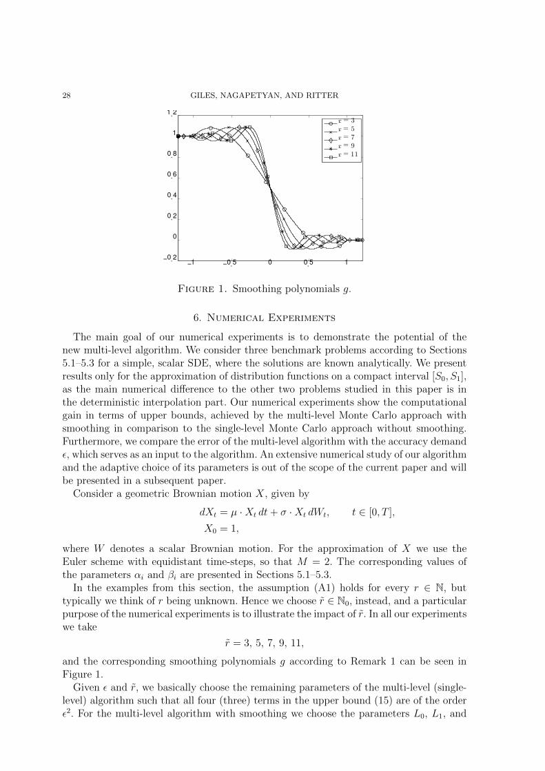
Figure 1. Smoothing polynomials g.

6. Numerical Experiments

The main goal of our numerical experiments is to demonstrate the potential of thenew multi-level algorithm. We consider three benchmark problems according to Sections5.1–5.3 for a simple, scalar SDE, where the solutions are known analytically. We presentresults only for the approximation of distribution functions on a compact interval [S0, S1],as the main numerical difference to the other two problems studied in this paper is inthe deterministic interpolation part. Our numerical experiments show the computationalgain in terms of upper bounds, achieved by the multi-level Monte Carlo approach withsmoothing in comparison to the single-level Monte Carlo approach without smoothing.Furthermore, we compare the error of the multi-level algorithm with the accuracy demand�, which serves as an input to the algorithm. An extensive numerical study of our algorithmand the adaptive choice of its parameters is out of the scope of the current paper and willbe presented in a subsequent paper.

Consider a geometric Brownian motion X, given by

dXt = µ ·Xt dt + σ ·Xt dWt, t ∈ [0, T ],

X0 = 1,

where W denotes a scalar Brownian motion. For the approximation of X we use theEuler scheme with equidistant time-steps, so that M = 2. The corresponding values ofthe parameters αi and βi are presented in Sections 5.1–5.3.

In the examples from this section, the assumption (A1) holds for every r ∈ N, buttypically we think of r being unknown. Hence we choose r ∈ N0, instead, and a particularpurpose of the numerical experiments is to illustrate the impact of r. In all our experimentswe take

r = 3, 5, 7, 9, 11,

and the corresponding smoothing polynomials g according to Remark 1 can be seen inFigure 1.

Given � and r, we basically choose the remaining parameters of the multi-level (single-level) algorithm such that all four (three) terms in the upper bound (15) are of the order�2. For the multi-level algorithm with smoothing we choose the parameters L0, L1, and


N� according to (30), (25), (21), and (31), with r replaced by r, while

δ = 2−1/(r+1) · �1/(r+1),

cf. (19). For the single-level algorithm without smoothing, see Remark 2, we choose L =L0 = L1 and NL according to (25) and (21), too, however observing (7), which leads toq = (r + 1)/α.

In the second stage of the algorithm we employ piecewise polynomial interpolation Q3k

of degree 3 with equidistant knots for any r. Due to the Lebesgue constants involved,this is preferable to Qr

k with a large value of r if the overall number k of interpolationpoints is comparatively small. Furthermore, it is convenient if k − 1 is a multiple of 3and proportional to the length of the interval [S0, S1]. In both cases, single-level andmulti-level, we therefore take

(76) k = 3 ·�5 · �−1/(r+1) · (S1 − S0)/3

�+ 1,

cf. (20).To specify the computational gain we compare the upper bound (17) for the cost of the

multi-level Monte Carlo algorithm with smoothing and the corresponding upper bound

c(k, L,N) = N · (2L + k),

for the cost of the single-level algorithm. The ratio c(k, L0, L1, NL0 , . . . , NL1)/c(k, L,N),which is a function of the desired accuracy �, is used to describe the computational gain.

To assess the accuracy of the multi-level algorithm, error(Q3k(M)), which depends on �

and r, should be compared with the desired accuracy �. Since error(Q3k(M)) is not known

exactly, we employ a simple Monte Carlo experiment with 25 independent replications foreach of the values of r and each of the values � = 2−i for i = 3, . . . , 11. The estimate isdenoted by RMSE(�, r). In the present approach we do not have an exact control of theerror of the multi-level (single-level) algorithm for a given �, since the parameters of thealgorithm are chosen on the basis of the asymptotic analysis from Section 2. Thereforewe only aim at RMSE(�, r) being reasonably close to �.

6.1. Smooth Path-independent Functionals for SDEs. In this section we set

µ = 0.05, σ = 0.2, T = 1,

and we approximate the distribution function F (s) = E(1]∞,s](Y )) of

Y = XT

on the interval

[S0, S1] = [0, 2].

Note that Y is lognormally distributed with parameters µ− σ2/2 and σ2.The computational gain as well as the replication numbers N� for the multi-level algo-

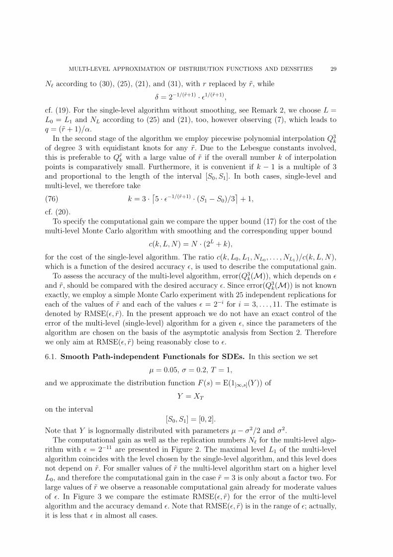
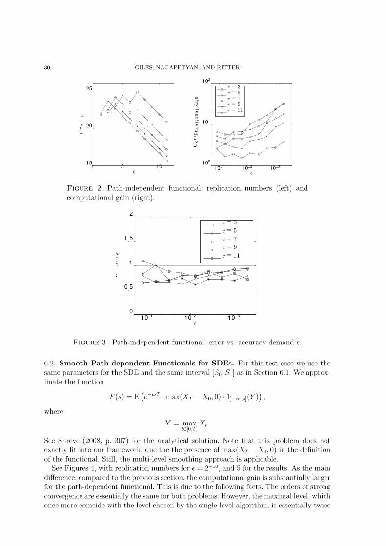
rithm with � = 2−11 are presented in Figure 2. The maximal level L1 of the multi-levelalgorithm coincides with the level chosen by the single-level algorithm, and this level doesnot depend on r. For smaller values of r the multi-level algorithm start on a higher levelL0, and therefore the computational gain in the case r = 3 is only about a factor two. Forlarge values of r we observe a reasonable computational gain already for moderate valuesof �. In Figure 3 we compare the estimate RMSE(�, r) for the error of the multi-levelalgorithm and the accuracy demand �. Note that RMSE(�, r) is in the range of �; actually,it is less that � in almost all cases.


10−3

10−2

10−1

100

101

102

ǫ

Computationalgain

r = 3r = 5

r = 7r = 9r = 11

1 5 1015

20

25

ℓ

log2N

ℓ

Figure 2. Path-independent functional: replication numbers (left) andcomputational gain (right).

10−3

10−2

10−1

0

0.5

1

1.5

2

ǫ

RMSE/ǫ

r = 3

r = 5

r = 7

r = 9

r = 11

Figure 3. Path-independent functional: error vs. accuracy demand �.

6.2. Smooth Path-dependent Functionals for SDEs. For this test case we use thesame parameters for the SDE and the same interval [S0, S1] as in Section 6.1. We approx-imate the function

F (s) = E�e−µ·T · max(XT −X0, 0) · 1]−∞,s](Y )

�,

where

Y = maxt∈[0,T ]

Xt.

See Shreve (2008, p. 307) for the analytical solution. Note that this problem does notexactly fit into our framework, due the the presence of max(XT −X0, 0) in the definitionof the functional. Still, the multi-level smoothing approach is applicable.

See Figures 4, with replication numbers for � = 2−10, and 5 for the results. As the maindifference, compared to the previous section, the computational gain is substantially largerfor the path-dependent functional. This is due to the following facts. The orders of strongconvergence are essentially the same for both problems. However, the maximal level, whichonce more coincide with the level chosen by the single-level algorithm, is essentially twice


10−3

10−2

10−1

100

102

104

ǫ

Computationalgain

r = 3r = 5

r = 7r = 9r = 11

1 5 10 15 200

5

10

15

20

25

ℓ

log2N

ℓ

Figure 4. Path-dependent functional: replication numbers (left) and com-putational gain (right).

10−3

10−2

10−1

0

0.5

1

1.5

2

ǫ

RMSE/ǫ

r = 3

r = 5

r = 7

r = 9

r = 11

Figure 5. Path-dependent functional: error vs. accuracy demand �.

as large as in the previous case, due to the slower decay of the bias. This results in alarger value of L1 − L0, which provides an advantage to the multi-level approach.

6.3. Stopped Exit Times for SDEs. In this section we set

µ = 0.01, σ = 0.2, T = 2,

and we approximate the distribution function F (s) = E(1]∞,s](Y )) of

Y = inf{t ≥ 0 : Xt = b} ∧ T

with b = 0.8 on the interval

[S0, S1] = [0, 1].

The distribution of inf{t ≥ 0 : Xt = b} is an inverse Gaussian distribution with parametersln b/(µ− σ2/2) and (ln b)2/σ2, and this yields an explicit formula for F since T > S1.

See Figures 6, with replication numbers for � = 2−9, and 7 for the results. Observe thatthe computational gain is even larger than in the previous section. This difference is dueto the fact that smoothing already yields an improved weak error estimate for the present


10−3

10−2

10−1

102

104

106

ǫ

Computationalgain

r = 3r = 5

r = 7r = 9r = 11

1 5 10 15 20 2510

15

20

25

ℓ

log2N

ℓ

Figure 6. Stopped exit time: replication numbers per level (left) and com-putational gain (right).

10−3

10−2

10−1

0

0.5

1

1.5

2

ǫ

RMSE/ǫ

r = 3

r = 5

r = 7

r = 9

r = 11

Figure 7. Stopped exit time: error vs. accuracy demand �.

problem. Consequently,

L1 =

�2 +

2

r + 1

�· log2 �−1

is the maximal level for the multi-level algorithm, up to integer rounding, but for thesingle-level algorithm without smoothing we have to take

L = 4 · log2 �−1.

Acknowledgments. This work is inspired by a joint project with Oleg Iliev. The authorsthank Oleg Iliev and Winfried Sickel for helpful discussions.

Tigran Nagapetyan was supported by the BMBF within the project 03MS612D FROPT,and Klaus Ritter was partially supported by the DFG within the Priority Program 1324.

References

Alfonsi, A., Jourdain, B., Kohatsu-Higa, A. (2013), Pathwise optimal transport bounds betweena one-dimensional diffusion and its Euler scheme, Preprint, arXiv:1209.0576.


Altmayer, M., Neuenkirch, A. (2013), Multilevel Monte Carlo quadrature of discontinuous pay-offs in the generalized Heston model using Malliavin integration by parts, Preprint 144, DFGSPP 1324.

Avikainen, R. (2009), On irregular functionals of SDEs and the Euler scheme, Finance Stoch.13, 381–401.

Bally, V., Talay, D. (1996a), The law of the Euler scheme for stochastic differential equations,I. Convergence rate of the distribution function, Probab. Theory Relat. Fields 104, 43–60.

Bally, V., Talay, D. (1996b), The law of the Euler scheme for stochastic differential equations,II. Convergence rate of the density, Monte Carlo Meth. Appl. 2, 93–128

Bouchard, B., Geiss, S., Gobet, E. (2013), First time to exit of a continuous Ito process: gen-eral moment estimates and L1-convergence rate for discrete time approximations, Preprint,arXiv:1307.4247.

Creutzig, J., Dereich, S., Muller-Gronbach, T., Ritter, K. (2009), Infinite-dimensional quadratureand approximation of distributions, Found. Comput. Math. 9, 391–429.

Giles, M. B. (2008a), Multilevel Monte Carlo path simulation, Oper. Res. 56, 607–617.

Giles, M. B. (2008b), Improved multilevel Monte Carlo convergence using the Milstein scheme,in Monte Carlo and Quasi-Monte Carlo Methods 2006, Keller, A., Heinrich, S., Niederreiter, H.,eds., Springer, Heidelberg, pp. 343–358,

Giles, M. B., Debrabant, K., Roßler, A. (2013), Numerical analysis of multilevel Monte Carlopath simulation using the Milstein discretisation, Preprint, arXiv:1302.4676.

Giles, M. B., Higham, D. J., Mao, X. (2009), Analyzing multi-level Monte Carlo for options withnon-globally Lipschitz payoff, Finance Stoch. 13, 403–413.

Gobet, E., Labart, C. (2008), Sharp estimates for the convergence of the density of the Eulerscheme in small time, Elect. Comm. in Probab. 13, 352–363.

Heinrich, S. (1998), Monte Carlo complexity of global solution of integral equations, J. Com-plexity 14, 151–175.

Higham, D. J., Mao. X., Roj, M., Song, Q., Yin, G. (2013), Mean exit times and the multilevelMonte Carlo method, SIAM/ASA J. Uncert. Quant. 1, 2–18.

Jacod, J., Protter, P. (1998), Asymptotic error distributions for the Euler method for stochasticdifferential equations, Ann. Probab. 26, 267–307.

Kebaier, A., (2005), Statistical Romberg extrapolation: a new variance reduction method andapplications to option pricing, Ann. Appl. Prob. 15, 2681–2705.

Kebaier, A., Kohatsu-Higa, A. (2008), An optimal control variance reduction method for densityestimation, Stochastic Processes Appl. 118, 2143–2180.

Massart, P. (1990), The tight constant in the Dvoretzky-Kiefer-Wolfowitz inequality, Ann.Probab. 18, 1269–1283.

Milstein, G. N., Schoenmakers, J. G. M., Spokoiny, V. (2004), Transition density estimation forstochastic differential equations via forward-reverse representations, Bernoulli 10, 281–312.

Shreve, E. S. (2008), Stochastic Calculus for Finance II. Continuous-Time Models. Springer,New York.

Talay, D., Zheng Z. (2004), Approximation of quantiles of components of diffusion processes,Stochastic Processes Appl. 109, 23–46.


Tsybakov, A. B. (2009), Introduction to Nonparametric Estimation, Springer, New York.

Mathematical Institute, 24–29 St Giles’, Oxford OX1 3LB, England

E-mail address: [email protected]

Department of Flow and Material Simulation, Fraunhofer ITWM, Fraunhofer-Platz 1,

67663 Kaiserslautern, Germany


Fachbereich Mathematik, Technische Universitat Kaiserslautern, Postfach 3049, 67653

Kaiserslautern, Germany


Preprint Series DFG-SPP 1324

http://www.dfg-spp1324.de

Reports

[1] R. Ramlau, G. Teschke, and M. Zhariy. A Compressive Landweber Iteration forSolving Ill-Posed Inverse Problems. Preprint 1, DFG-SPP 1324, September 2008.

[2] G. Plonka. The Easy Path Wavelet Transform: A New Adaptive Wavelet Trans-form for Sparse Representation of Two-dimensional Data. Preprint 2, DFG-SPP1324, September 2008.

[3] E. Novak and H. Wozniakowski. Optimal Order of Convergence and (In-)Tractability of Multivariate Approximation of Smooth Functions. Preprint 3,DFG-SPP 1324, October 2008.

[4] M. Espig, L. Grasedyck, and W. Hackbusch. Black Box Low Tensor Rank Ap-proximation Using Fibre-Crosses. Preprint 4, DFG-SPP 1324, October 2008.

[5] T. Bonesky, S. Dahlke, P. Maass, and T. Raasch. Adaptive Wavelet Methodsand Sparsity Reconstruction for Inverse Heat Conduction Problems. Preprint 5,DFG-SPP 1324, January 2009.

[6] E. Novak and H. Wozniakowski. Approximation of Infinitely Differentiable Mul-tivariate Functions Is Intractable. Preprint 6, DFG-SPP 1324, January 2009.

[7] J. Ma and G. Plonka. A Review of Curvelets and Recent Applications. Preprint 7,DFG-SPP 1324, February 2009.

[8] L. Denis, D. A. Lorenz, and D. Trede. Greedy Solution of Ill-Posed Problems:Error Bounds and Exact Inversion. Preprint 8, DFG-SPP 1324, April 2009.

[9] U. Friedrich. A Two Parameter Generalization of Lions’ Nonoverlapping DomainDecomposition Method for Linear Elliptic PDEs. Preprint 9, DFG-SPP 1324,April 2009.

[10] K. Bredies and D. A. Lorenz. Minimization of Non-smooth, Non-convex Func-tionals by Iterative Thresholding. Preprint 10, DFG-SPP 1324, April 2009.

[11] K. Bredies and D. A. Lorenz. Regularization with Non-convex Separable Con-straints. Preprint 11, DFG-SPP 1324, April 2009.

[12] M. Dohler, S. Kunis, and D. Potts. Nonequispaced Hyperbolic Cross Fast FourierTransform. Preprint 12, DFG-SPP 1324, April 2009.

[13] C. Bender. Dual Pricing of Multi-Exercise Options under Volume Constraints.Preprint 13, DFG-SPP 1324, April 2009.

[14] T. Muller-Gronbach and K. Ritter. Variable Subspace Sampling and Multi-levelAlgorithms. Preprint 14, DFG-SPP 1324, May 2009.

[15] G. Plonka, S. Tenorth, and A. Iske. Optimally Sparse Image Representation bythe Easy Path Wavelet Transform. Preprint 15, DFG-SPP 1324, May 2009.

[16] S. Dahlke, E. Novak, and W. Sickel. Optimal Approximation of Elliptic Problemsby Linear and Nonlinear Mappings IV: Errors in L2 and Other Norms. Preprint 16,DFG-SPP 1324, June 2009.

[17] B. Jin, T. Khan, P. Maass, and M. Pidcock. Function Spaces and Optimal Currentsin Impedance Tomography. Preprint 17, DFG-SPP 1324, June 2009.

[18] G. Plonka and J. Ma. Curvelet-Wavelet Regularized Split Bregman Iteration forCompressed Sensing. Preprint 18, DFG-SPP 1324, June 2009.

[19] G. Teschke and C. Borries. Accelerated Projected Steepest Descent Method forNonlinear Inverse Problems with Sparsity Constraints. Preprint 19, DFG-SPP1324, July 2009.

[20] L. Grasedyck. Hierarchical Singular Value Decomposition of Tensors. Preprint 20,DFG-SPP 1324, July 2009.

[21] D. Rudolf. Error Bounds for Computing the Expectation by Markov Chain MonteCarlo. Preprint 21, DFG-SPP 1324, July 2009.

[22] M. Hansen and W. Sickel. Best m-term Approximation and Lizorkin-TriebelSpaces. Preprint 22, DFG-SPP 1324, August 2009.

[23] F.J. Hickernell, T. Muller-Gronbach, B. Niu, and K. Ritter. Multi-level MonteCarlo Algorithms for Infinite-dimensional Integration on RN. Preprint 23, DFG-SPP 1324, August 2009.

[24] S. Dereich and F. Heidenreich. A Multilevel Monte Carlo Algorithm for LevyDriven Stochastic Differential Equations. Preprint 24, DFG-SPP 1324, August2009.

[25] S. Dahlke, M. Fornasier, and T. Raasch. Multilevel Preconditioning for AdaptiveSparse Optimization. Preprint 25, DFG-SPP 1324, August 2009.

[26] S. Dereich. Multilevel Monte Carlo Algorithms for Levy-driven SDEs with Gaus-sian Correction. Preprint 26, DFG-SPP 1324, August 2009.

[27] G. Plonka, S. Tenorth, and D. Rosca. A New Hybrid Method for Image Approx-imation using the Easy Path Wavelet Transform. Preprint 27, DFG-SPP 1324,October 2009.

[28] O. Koch and C. Lubich. Dynamical Low-rank Approximation of Tensors.Preprint 28, DFG-SPP 1324, November 2009.

[29] E. Faou, V. Gradinaru, and C. Lubich. Computing Semi-classical Quantum Dy-namics with Hagedorn Wavepackets. Preprint 29, DFG-SPP 1324, November2009.

[30] D. Conte and C. Lubich. An Error Analysis of the Multi-configuration Time-dependent Hartree Method of Quantum Dynamics. Preprint 30, DFG-SPP 1324,November 2009.

[31] C. E. Powell and E. Ullmann. Preconditioning Stochastic Galerkin Saddle PointProblems. Preprint 31, DFG-SPP 1324, November 2009.

[32] O. G. Ernst and E. Ullmann. Stochastic Galerkin Matrices. Preprint 32, DFG-SPP1324, November 2009.

[33] F. Lindner and R. L. Schilling. Weak Order for the Discretization of the StochasticHeat Equation Driven by Impulsive Noise. Preprint 33, DFG-SPP 1324, November2009.

[34] L. Kammerer and S. Kunis. On the Stability of the Hyperbolic Cross DiscreteFourier Transform. Preprint 34, DFG-SPP 1324, December 2009.

[35] P. Cerejeiras, M. Ferreira, U. Kahler, and G. Teschke. Inversion of the noisy Radontransform on SO(3) by Gabor frames and sparse recovery principles. Preprint 35,DFG-SPP 1324, January 2010.

[36] T. Jahnke and T. Udrescu. Solving Chemical Master Equations by AdaptiveWavelet Compression. Preprint 36, DFG-SPP 1324, January 2010.

[37] P. Kittipoom, G. Kutyniok, and W.-Q Lim. Irregular Shearlet Frames: Geometryand Approximation Properties. Preprint 37, DFG-SPP 1324, February 2010.

[38] G. Kutyniok and W.-Q Lim. Compactly Supported Shearlets are OptimallySparse. Preprint 38, DFG-SPP 1324, February 2010.

[39] M. Hansen and W. Sickel. Best m-Term Approximation and Tensor Products ofSobolev and Besov Spaces – the Case of Non-compact Embeddings. Preprint 39,DFG-SPP 1324, March 2010.

[40] B. Niu, F.J. Hickernell, T. Muller-Gronbach, and K. Ritter. Deterministic Multi-level Algorithms for Infinite-dimensional Integration on RN. Preprint 40, DFG-SPP 1324, March 2010.

[41] P. Kittipoom, G. Kutyniok, and W.-Q Lim. Construction of Compactly SupportedShearlet Frames. Preprint 41, DFG-SPP 1324, March 2010.

[42] C. Bender and J. Steiner. Error Criteria for Numerical Solutions ofBackward SDEs. Preprint 42, DFG-SPP 1324, April 2010.

[43] L. Grasedyck. Polynomial Approximation in Hierarchical Tucker Format byVector-Tensorization. Preprint 43, DFG-SPP 1324, April 2010.

[44] M. Hansen und W. Sickel. Best m-Term Approximation and Sobolev-Besov Spacesof Dominating Mixed Smoothness - the Case of Compact Embeddings. Preprint 44,DFG-SPP 1324, April 2010.

[45] P. Binev, W. Dahmen, and P. Lamby. Fast High-Dimensional Approximation withSparse Occupancy Trees. Preprint 45, DFG-SPP 1324, May 2010.

[46] J. Ballani and L. Grasedyck. A Projection Method to Solve Linear Systems inTensor Format. Preprint 46, DFG-SPP 1324, May 2010.

[47] P. Binev, A. Cohen, W. Dahmen, R. DeVore, G. Petrova, and P. Wojtaszczyk.Convergence Rates for Greedy Algorithms in Reduced Basis Methods. Preprint 47,DFG-SPP 1324, May 2010.

[48] S. Kestler and K. Urban. Adaptive Wavelet Methods on Unbounded Domains.Preprint 48, DFG-SPP 1324, June 2010.

[49] H. Yserentant. The Mixed Regularity of Electronic Wave Functions Multiplied byExplicit Correlation Factors. Preprint 49, DFG-SPP 1324, June 2010.

[50] H. Yserentant. On the Complexity of the Electronic Schrodinger Equation.Preprint 50, DFG-SPP 1324, June 2010.

[51] M. Guillemard and A. Iske. Curvature Analysis of Frequency Modulated Manifoldsin Dimensionality Reduction. Preprint 51, DFG-SPP 1324, June 2010.

[52] E. Herrholz and G. Teschke. Compressive Sensing Principles and Iterative SparseRecovery for Inverse and Ill-Posed Problems. Preprint 52, DFG-SPP 1324, July2010.

[53] L. Kammerer, S. Kunis, and D. Potts. Interpolation Lattices for Hyperbolic CrossTrigonometric Polynomials. Preprint 53, DFG-SPP 1324, July 2010.

[54] G. Kutyniok and W.-Q Lim. Shearlets on Bounded Domains. Preprint 54, DFG-SPP 1324, July 2010.

[55] A. Zeiser. Wavelet Approximation in Weighted Sobolev Spaces of Mixed Orderwith Applications to the Electronic Schrodinger Equation. Preprint 55, DFG-SPP1324, July 2010.

[56] G. Kutyniok, J. Lemvig, and W.-Q Lim. Compactly Supported Shearlets.Preprint 56, DFG-SPP 1324, July 2010.

[57] A. Zeiser. On the Optimality of the Inexact Inverse Iteration Coupled with Adap-tive Finite Element Methods. Preprint 57, DFG-SPP 1324, July 2010.

[58] S. Jokar. Sparse Recovery and Kronecker Products. Preprint 58, DFG-SPP 1324,August 2010.

[59] T. Aboiyar, E. H. Georgoulis, and A. Iske. Adaptive ADER Methods Using Kernel-Based Polyharmonic Spline WENO Reconstruction. Preprint 59, DFG-SPP 1324,August 2010.

[60] O. G. Ernst, A. Mugler, H.-J. Starkloff, and E. Ullmann. On the Convergence ofGeneralized Polynomial Chaos Expansions. Preprint 60, DFG-SPP 1324, August2010.

[61] S. Holtz, T. Rohwedder, and R. Schneider. On Manifolds of Tensors of FixedTT-Rank. Preprint 61, DFG-SPP 1324, September 2010.

[62] J. Ballani, L. Grasedyck, and M. Kluge. Black Box Approximation of Tensors inHierarchical Tucker Format. Preprint 62, DFG-SPP 1324, October 2010.

[63] M. Hansen. On Tensor Products of Quasi-Banach Spaces. Preprint 63, DFG-SPP1324, October 2010.

[64] S. Dahlke, G. Steidl, and G. Teschke. Shearlet Coorbit Spaces: Compactly Sup-ported Analyzing Shearlets, Traces and Embeddings. Preprint 64, DFG-SPP 1324,October 2010.

[65] W. Hackbusch. Tensorisation of Vectors and their Efficient Convolution.Preprint 65, DFG-SPP 1324, November 2010.

[66] P. A. Cioica, S. Dahlke, S. Kinzel, F. Lindner, T. Raasch, K. Ritter, and R. L.Schilling. Spatial Besov Regularity for Stochastic Partial Differential Equationson Lipschitz Domains. Preprint 66, DFG-SPP 1324, November 2010.

[67] E. Novak and H. Wozniakowski. On the Power of Function Values for the Ap-proximation Problem in Various Settings. Preprint 67, DFG-SPP 1324, November2010.

[68] A. Hinrichs, E. Novak, and H. Wozniakowski. The Curse of Dimensionality forMonotone and Convex Functions of Many Variables. Preprint 68, DFG-SPP 1324,November 2010.

[69] G. Kutyniok and W.-Q Lim. Image Separation Using Shearlets. Preprint 69,DFG-SPP 1324, November 2010.

[70] B. Jin and P. Maass. An Analysis of Electrical Impedance Tomography withApplications to Tikhonov Regularization. Preprint 70, DFG-SPP 1324, December2010.

[71] S. Holtz, T. Rohwedder, and R. Schneider. The Alternating Linear Scheme forTensor Optimisation in the TT Format. Preprint 71, DFG-SPP 1324, December2010.

[72] T. Muller-Gronbach and K. Ritter. A Local Refinement Strategy for ConstructiveQuantization of Scalar SDEs. Preprint 72, DFG-SPP 1324, December 2010.

[73] T. Rohwedder and R. Schneider. An Analysis for the DIIS Acceleration Methodused in Quantum Chemistry Calculations. Preprint 73, DFG-SPP 1324, December2010.

[74] C. Bender and J. Steiner. Least-Squares Monte Carlo for Backward SDEs.Preprint 74, DFG-SPP 1324, December 2010.

[75] C. Bender. Primal and Dual Pricing of Multiple Exercise Options in ContinuousTime. Preprint 75, DFG-SPP 1324, December 2010.

[76] H. Harbrecht, M. Peters, and R. Schneider. On the Low-rank Approximation bythe Pivoted Cholesky Decomposition. Preprint 76, DFG-SPP 1324, December2010.

[77] P. A. Cioica, S. Dahlke, N. Dohring, S. Kinzel, F. Lindner, T. Raasch, K. Ritter,and R. L. Schilling. Adaptive Wavelet Methods for Elliptic Stochastic PartialDifferential Equations. Preprint 77, DFG-SPP 1324, January 2011.

[78] G. Plonka, S. Tenorth, and A. Iske. Optimal Representation of Piecewise HolderSmooth Bivariate Functions by the Easy Path Wavelet Transform. Preprint 78,DFG-SPP 1324, January 2011.

[79] A. Mugler and H.-J. Starkloff. On Elliptic Partial Differential Equations withRandom Coefficients. Preprint 79, DFG-SPP 1324, January 2011.

[80] T. Muller-Gronbach, K. Ritter, and L. Yaroslavtseva. A Derandomization of theEuler Scheme for Scalar Stochastic Differential Equations. Preprint 80, DFG-SPP1324, January 2011.

[81] W. Dahmen, C. Huang, C. Schwab, and G. Welper. Adaptive Petrov-Galerkinmethods for first order transport equations. Preprint 81, DFG-SPP 1324, January2011.

[82] K. Grella and C. Schwab. Sparse Tensor Spherical Harmonics Approximation inRadiative Transfer. Preprint 82, DFG-SPP 1324, January 2011.

[83] D.A. Lorenz, S. Schiffler, and D. Trede. Beyond Convergence Rates: Exact In-version With Tikhonov Regularization With Sparsity Constraints. Preprint 83,DFG-SPP 1324, January 2011.

[84] S. Dereich, M. Scheutzow, and R. Schottstedt. Constructive quantization: Ap-proximation by empirical measures. Preprint 84, DFG-SPP 1324, January 2011.

[85] S. Dahlke and W. Sickel. On Besov Regularity of Solutions to Nonlinear EllipticPartial Differential Equations. Preprint 85, DFG-SPP 1324, January 2011.

[86] S. Dahlke, U. Friedrich, P. Maass, T. Raasch, and R.A. Ressel. An adaptivewavelet method for parameter identification problems in parabolic partial differ-ential equations. Preprint 86, DFG-SPP 1324, January 2011.

[87] A. Cohen, W. Dahmen, and G. Welper. Adaptivity and Variational Stabilizationfor Convection-Diffusion Equations. Preprint 87, DFG-SPP 1324, January 2011.

[88] T. Jahnke. On Reduced Models for the Chemical Master Equation. Preprint 88,DFG-SPP 1324, January 2011.

[89] P. Binev, W. Dahmen, R. DeVore, P. Lamby, D. Savu, and R. Sharpley. Com-pressed Sensing and Electron Microscopy. Preprint 89, DFG-SPP 1324, March2011.

[90] P. Binev, F. Blanco-Silva, D. Blom, W. Dahmen, P. Lamby, R. Sharpley, andT. Vogt. High Quality Image Formation by Nonlocal Means Applied to High-Angle Annular Dark Field Scanning Transmission Electron Microscopy (HAADF-STEM). Preprint 90, DFG-SPP 1324, March 2011.

[91] R. A. Ressel. A Parameter Identification Problem for a Nonlinear Parabolic Dif-ferential Equation. Preprint 91, DFG-SPP 1324, May 2011.

[92] G. Kutyniok. Data Separation by Sparse Representations. Preprint 92, DFG-SPP1324, May 2011.

[93] M. A. Davenport, M. F. Duarte, Y. C. Eldar, and G. Kutyniok. Introduction toCompressed Sensing. Preprint 93, DFG-SPP 1324, May 2011.

[94] H.-C. Kreusler and H. Yserentant. The Mixed Regularity of Electronic WaveFunctions in Fractional Order and Weighted Sobolev Spaces. Preprint 94, DFG-SPP 1324, June 2011.

[95] E. Ullmann, H. C. Elman, and O. G. Ernst. Efficient Iterative Solvers forStochastic Galerkin Discretizations of Log-Transformed Random Diffusion Prob-lems. Preprint 95, DFG-SPP 1324, June 2011.

[96] S. Kunis and I. Melzer. On the Butterfly Sparse Fourier Transform. Preprint 96,DFG-SPP 1324, June 2011.

[97] T. Rohwedder. The Continuous Coupled Cluster Formulation for the ElectronicSchrodinger Equation. Preprint 97, DFG-SPP 1324, June 2011.

[98] T. Rohwedder and R. Schneider. Error Estimates for the Coupled Cluster Method.Preprint 98, DFG-SPP 1324, June 2011.

[99] P. A. Cioica and S. Dahlke. Spatial Besov Regularity for Semilinear StochasticPartial Differential Equations on Bounded Lipschitz Domains. Preprint 99, DFG-SPP 1324, July 2011.

[100] L. Grasedyck and W. Hackbusch. An Introduction to Hierarchical (H-) Rank andTT-Rank of Tensors with Examples. Preprint 100, DFG-SPP 1324, August 2011.

[101] N. Chegini, S. Dahlke, U. Friedrich, and R. Stevenson. Piecewise Tensor ProductWavelet Bases by Extensions and Approximation Rates. Preprint 101, DFG-SPP1324, September 2011.

[102] S. Dahlke, P. Oswald, and T. Raasch. A Note on Quarkonial Systems and Multi-level Partition of Unity Methods. Preprint 102, DFG-SPP 1324, September 2011.

[103] A. Uschmajew. Local Convergence of the Alternating Least Squares AlgorithmFor Canonical Tensor Approximation. Preprint 103, DFG-SPP 1324, September2011.

[104] S. Kvaal. Multiconfigurational time-dependent Hartree method for describing par-ticle loss due to absorbing boundary conditions. Preprint 104, DFG-SPP 1324,September 2011.

[105] M. Guillemard and A. Iske. On Groupoid C*-Algebras, Persistent Homology andTime-Frequency Analysis. Preprint 105, DFG-SPP 1324, September 2011.

[106] A. Hinrichs, E. Novak, and H. Wozniakowski. Discontinuous information in theworst case and randomized settings. Preprint 106, DFG-SPP 1324, September2011.

[107] M. Espig, W. Hackbusch, A. Litvinenko, H. Matthies, and E. Zander. EfficientAnalysis of High Dimensional Data in Tensor Formats. Preprint 107, DFG-SPP1324, September 2011.

[108] M. Espig, W. Hackbusch, S. Handschuh, and R. Schneider. Optimization Problemsin Contracted Tensor Networks. Preprint 108, DFG-SPP 1324, October 2011.

[109] S. Dereich, T. Muller-Gronbach, and K. Ritter. On the Complexity of ComputingQuadrature Formulas for SDEs. Preprint 109, DFG-SPP 1324, October 2011.

[110] D. Belomestny. Solving optimal stopping problems by empirical dual optimizationand penalization. Preprint 110, DFG-SPP 1324, November 2011.

[111] D. Belomestny and J. Schoenmakers. Multilevel dual approach for pricing Amer-ican style derivatives. Preprint 111, DFG-SPP 1324, November 2011.

[112] T. Rohwedder and A. Uschmajew. Local convergence of alternating schemes foroptimization of convex problems in the TT format. Preprint 112, DFG-SPP 1324,December 2011.

[113] T. Gorner, R. Hielscher, and S. Kunis. Efficient and accurate computation ofspherical mean values at scattered center points. Preprint 113, DFG-SPP 1324,December 2011.

[114] Y. Dong, T. Gorner, and S. Kunis. An iterative reconstruction scheme for pho-toacoustic imaging. Preprint 114, DFG-SPP 1324, December 2011.

[115] L. Kammerer. Reconstructing hyperbolic cross trigonometric polynomials by sam-pling along generated sets. Preprint 115, DFG-SPP 1324, February 2012.

[116] H. Chen and R. Schneider. Numerical analysis of augmented plane waves methodsfor full-potential electronic structure calculations. Preprint 116, DFG-SPP 1324,February 2012.

[117] J. Ma, G. Plonka, and M.Y. Hussaini. Compressive Video Sampling with Ap-proximate Message Passing Decoding. Preprint 117, DFG-SPP 1324, February2012.

[118] D. Heinen and G. Plonka. Wavelet shrinkage on paths for scattered data denoising.Preprint 118, DFG-SPP 1324, February 2012.

[119] T. Jahnke and M. Kreim. Error bound for piecewise deterministic processes mod-eling stochastic reaction systems. Preprint 119, DFG-SPP 1324, March 2012.

[120] C. Bender and J. Steiner. A-posteriori estimates for backward SDEs. Preprint120, DFG-SPP 1324, April 2012.

[121] M. Espig, W. Hackbusch, A. Litvinenkoy, H.G. Matthiesy, and P. Wahnert. Eff-cient low-rank approximation of the stochastic Galerkin matrix in tensor formats.Preprint 121, DFG-SPP 1324, May 2012.

[122] O. Bokanowski, J. Garcke, M. Griebel, and I. Klompmaker. An adaptive sparsegrid semi-Lagrangian scheme for first order Hamilton-Jacobi Bellman equations.Preprint 122, DFG-SPP 1324, June 2012.

[123] A. Mugler and H.-J. Starkloff. On the convergence of the stochastic Galerkinmethod for random elliptic partial differential equations. Preprint 123, DFG-SPP1324, June 2012.

[124] P.A. Cioica, S. Dahlke, N. Dohring, U. Friedrich, S. Kinzel, F. Lindner, T. Raasch,K. Ritter, and R.L. Schilling. On the convergence analysis of Rothe’s method.Preprint 124, DFG-SPP 1324, July 2012.

[125] P. Binev, A. Cohen, W. Dahmen, and R. DeVore. Classification Algorithms usingAdaptive Partitioning. Preprint 125, DFG-SPP 1324, July 2012.

[126] C. Lubich, T. Rohwedder, R. Schneider, and B. Vandereycken. Dynamical approx-imation of hierarchical Tucker and Tensor-Train tensors. Preprint 126, DFG-SPP1324, July 2012.

[127] M. Kovacs, S. Larsson, and K. Urban. On Wavelet-Galerkin methods for semilinearparabolic equations with additive noise. Preprint 127, DFG-SPP 1324, August2012.

[128] M. Bachmayr, H. Chen, and R. Schneider. Numerical analysis of Gaussian ap-proximations in quantum chemistry. Preprint 128, DFG-SPP 1324, August 2012.

[129] D. Rudolf. Explicit error bounds for Markov chain Monte Carlo. Preprint 129,DFG-SPP 1324, August 2012.

[130] P.A. Cioica, K.-H. Kim, K. Lee, and F. Lindner. On the Lq(Lp)-regularity andBesov smoothness of stochastic parabolic equations on bounded Lipschitz domains.Preprint 130, DFG-SPP 1324, December 2012.

[131] M. Hansen. n−term Approximation Rates and Besov Regularity for Elliptic PDEson Polyhedral Domains. Preprint 131, DFG-SPP 1324, December 2012.

[132] R. E. Bank and H. Yserentant. On the H1 -stability of the L2 -projection ontofinite element spaces. Preprint 132, DFG-SPP 1324, December 2012.

[133] M. Gnewuch, S. Mayer, and K. Ritter. On Weighted Hilbert Spaces and Inte-gration of Functions of Infinitely Many Variables. Preprint 133, DFG-SPP 1324,December 2012.

[134] D. Crisan, J. Diehl, P.K. Friz, and H. Oberhauser. Robust Filtering: CorrelatedNoise and Multidimensional Observation. Preprint 134, DFG-SPP 1324, January2013.

[135] Wolfgang Dahmen, Christian Plesken, and Gerrit Welper. Double Greedy Algo-rithms: Reduced Basis Methods for Transport Dominated Problems. Preprint135, DFG-SPP 1324, February 2013.

[136] Aicke Hinrichs, Erich Novak, Mario Ullrich, and Henryk Wozniakowski. The Curseof Dimensionality for Numerical Integration of Smooth Functions. Preprint 136,DFG-SPP 1324, February 2013.

[137] Markus Bachmayr, Wolfgang Dahmen, Ronald DeVore, and Lars Grasedyck. Ap-proximation of High-Dimensional Rank One Tensors. Preprint 137, DFG-SPP1324, March 2013.

[138] Markus Bachmayr and Wolfgang Dahmen. Adaptive Near-Optimal Rank TensorApproximation for High-Dimensional Operator Equations. Preprint 138, DFG-SPP 1324, April 2013.

[139] Felix Lindner. Singular Behavior of the Solution to the Stochastic Heat Equationon a Polygonal Domain. Preprint 139, DFG-SPP 1324, May 2013.

[140] Stephan Dahlke, Dominik Lellek, Shiu Hong Lui, and Rob Stevenson. AdaptiveWavelet Schwarz Methods for the Navier-Stokes Equation. Preprint 140, DFG-SPP 1324, May 2013.

[141] Jonas Ballani and Lars Grasedyck. Tree Adaptive Approximation in the Hierar-chical Tensor Format. Preprint 141, DFG-SPP 1324, June 2013.

[142] Harry Yserentant. A short theory of the Rayleigh-Ritz method. Preprint 142,DFG-SPP 1324, July 2013.

[143] M. Hefter and K. Ritter. On Embeddings of Weighted Tensor Product HilbertSpaces. Preprint 143, DFG-SPP 1324, August 2013.

[144] M. Altmayer and A. Neuenkirch. Multilevel Monte Carlo Quadrature of Discon-tinuous Payoffs in the Generalized Heston Model using Malliavin Integration byParts. Preprint 144, DFG-SPP 1324, August 2013.

[145] L. Kammerer, D. Potts, and T. Volkmer. Approximation of multivariate functionsby trigonometric polynomials based on rank-1 lattice sampling. Preprint 145,DFG-SPP 1324, September 2013.

[146] C. Bender, N. Schweizer, and J. Zhuo. A primal-dual algorithm for BSDEs.Preprint 146, DFG-SPP 1324, October 2013.

[147] D. Rudolf. Hit-and-run for numerical integration. Preprint 147, DFG-SPP 1324,October 2013.

[148] D. Rudolf and M. Ullrich. Positivity of hit-and-run and related algorithms.Preprint 148, DFG-SPP 1324, October 2013.

[149] L. Grasedyck, M. Kluge, and S. Kramer. Alternating Directions Fitting (ADF) ofHierarchical Low Rank Tensors. Preprint 149, DFG-SPP 1324, October 2013.

[150] F. Filbir, S. Kunis, and R. Seyfried. Effective discretization of direct reconstructionschemes for photoacoustic imaging in spherical geometries. Preprint 150, DFG-SPP 1324, November 2013.

[151] E. Novak, M. Ullrich, and H. Wozniakowski. Complexity of Oscillatory Integrationfor Univariate Sobolev Spaces. Preprint 151, DFG-SPP 1324, November 2013.

[152] A. Hinrichs, E. Novak, and M. Ullrich. A Tractability Result for the ClenshawCurtis Smolyak Algorithm. Preprint 152, DFG-SPP 1324, November 2013.

[153] M. Hein, S. Setzer, L. Jost, and S. Rangapuram. The Total Variation on Hy-pergraphs - Learning on Hypergraphs Revisited. Preprint 153, DFG-SPP 1324,November 2013.

[154] M. Kovacs, S. Larsson, and F. Lindgren. On the Backward Euler Approximationof the Stochastic Allen-Chan Equation. Preprint 154, DFG-SPP 1324, November2013.

[155] S. Dahlke, M. Fornasier, U. Friedrich, and T. Raasch. Multilevel preconditioningfor sparse optimization of functionals with nonconvex fidelity terms. Preprint 155,DFG-SPP 1324, December 2013.

[156] T. Muller-Gronbach, K. Ritter, and L. Yaroslavtseva. On the complexity of com-puting quadrature formulas for marginal distributions of SDEs. Preprint 156,DFG-SPP 1324, January 2014.

[157] M. Giles, T. Nagapetyan, and K. Ritter. Multi-Level Monte Carlo Approximationof Distribution Functions and Densities. Preprint 157, DFG-SPP 1324, February2014.

multilevel monte carlo approximation of distribution functions and densities

Documents