1  

MULTILEVEL (ML-ICLV) & SINGLE LEVEL INTEGRATED DISCRETE CHOICE AND LATENT VARIABLE (ICLV) MODELS

USING ALTERNATIVE LATENT STRUCTURES’ CONCEPTUALIZATIONS

George Chryssochoidis and Charlie Wilson

University of East Anglia

Introduction The aim of the present endeavor is to experiment regarding the further advancement of integrated discrete choice and latent variable (ICVL) models using alternative factorial structures’ conceptualizations and do so at both Single Level (Level 0) but also Multilevel (ML-ICVL). In doing, specific independent variables were selected that were amenable to alternative latent variables’ conceptualization, including: a) 1st-order latent variables (1st-order factors) (FM; FW), b) 1st-order latent variables (1st-order factors) (FM; FW) forming a 2nd-order factor (F), c) Multi-level (two-level) factorial structures (FML0; FML1 and FWL0; FWL1), as well as d) Bi-Factor factorial structures (FM; FW; FG). The results may be of use to researchers interested in using valid, reliable, and accurate structures of latent variables in ICLV models. The results confirm that alternative latent structures of divergent factorial nature exist for the same observed variables, and may have different impact upon the dependent observed choice variable in the ICLV models. Second, DCE utility is conceptualized and estimated at both Level 0 and Level 1 and the differences are demonstrated. Further evidence is provided regarding the treatment of causal links as moderated versus sequential/mediated. The theoretical background, the conceptualization of the different latent variables’ structures and alternative models, the content of the study, the model estimations, the results and discussions follow in turn. ICLV Models Walker (2001) had already mentioned (p. 24) that at the core of the DCE model which is based around a standard multinomial logit model, extensions are added to relax simplifying assumptions and enrich the capabilities of the basic model, and that among these extensions are: First, a factor analytic (probit-like) disturbances in order to provide a flexible covariance

structure, thereby relaxing the IIA condition and enabling estimation of unobserved heterogeneity through, for example, random parameters.

Second, the incorporation of latent variables in order to provide a richer explanation of behavior by explicitly representing the formation and effects of latent constructs such as attitudes and perceptions.

She further wrote (p. 81) that DCE models have traditionally presented an individual’s choice process as a black box, in which the inputs are the attributes of available alternatives and individual characteristics, and the output is the observed choice. The resulting models directly link the observed inputs to the observed output, thereby assuming that the inner workings of the black box are implicitly captured by the model and further that behavioral researchers have stressed the importance of the cognitive workings inside the black box on choice behavior. McFadden (1986) argues that the empirical study of economic behavior would benefit from closer attention to how perceptions are formed and how they influence decision-making.

2  

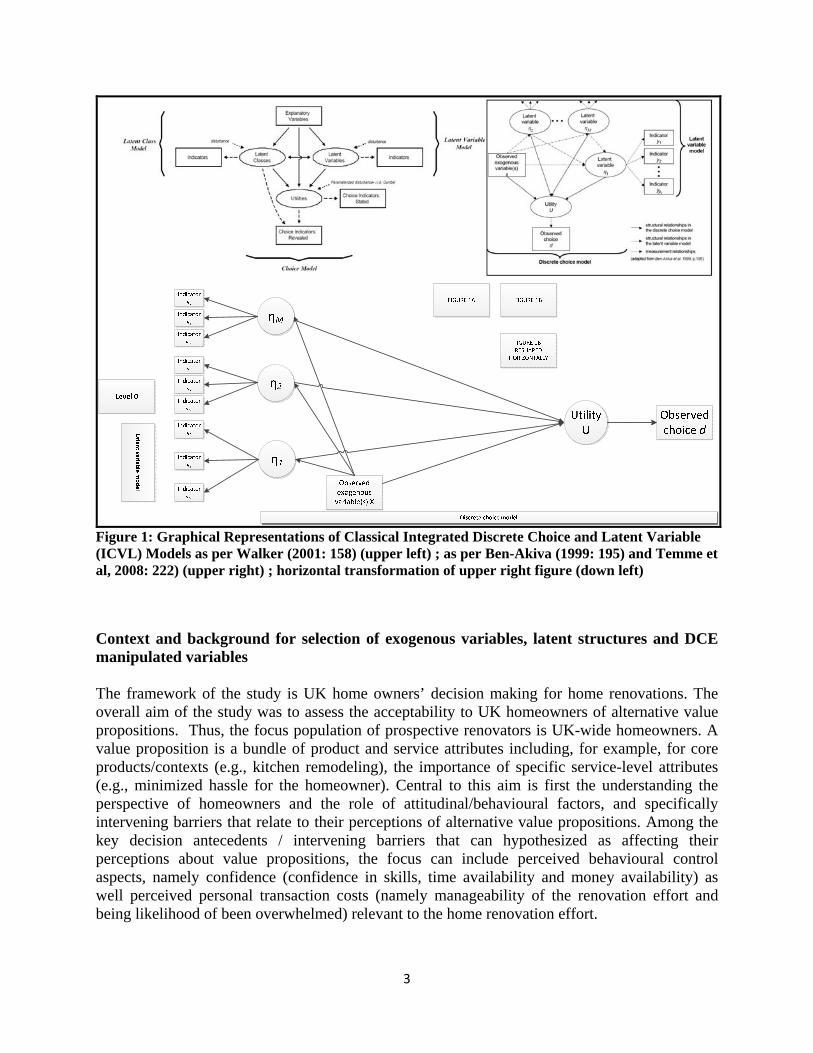
Work subsequently picked up by several researchers and references in the area include –among others, Morikawa and Sasaki (1998), Walker (2001), Ashok et al (2002), Ben-Akiva et al. (1999; 2002; 2002), Bierlaire (2003) and the latest version of Biogeme, Walker and Li (2007), and Bolduc et al. (2005), but also Zeid (2009), Temme et al (2008), Hess and Stathopoulos (2010) and Danthurebandara et al. (2013). Ashok et al. (2002) showed how to do so in a simultaneous manner although their approach was constrained by the number of latent factors to include in the ICLV model. Temme et al. (2008) extended the classical travel mode choice model to incorporate individuals' attitudes and values and showed how to include a larger number of latent variables in ICLV models. La Paix et al. (2011) applied these in the travel field, where they study the impact of the propensity to travel on the choice of tour structures. Danthurebandara et al (2013) tested if improvements occur through a simultaneous versus sequential (two-step) procedure. Rungie et al. (2011) proposed and described a comprehensive theoretical framework that integrates choice models and structural equation models, referred to as “structural choice modelling, Across almost all efforts, the ICLV model was based on the conditional logit model and the market heterogeneity was modelled by incorporating individuals’ specific latent factors while at the same time a parallel effort has often been used to model the market heterogeneity (for example, Bliemer and Rose, 2010). Figure 1 provides a birds’ eye of the overall ICLV models’ framework and also does so in both vertical format – traditional to the DCE world, but also horizontal format- the working method in the SEM world. Nonetheless, there is an important area that still requires further investigation. There is limited evidence of the influence of alternative structures of the latent variables in the framework of ICLV models. The traditional way to see these in the DCE world is mostly 1st-order factors either correlated with each other or influencing each other in a sequential causal link (e.g. Temme et al, 2008). This is far from what such factorial structures can eventual turn out to be. As such, an effort is needed to demonstrate what such factorial structures can be, what underlying theories may be at work, and what impact they will have for the conceptualization and estimation of ICLV models. Furthermore, no effort has been identified regarding the conceptualization and estimation of ICLV models in a multilevel framework. The present study attempts to fill this void. It is clearly more of a conceptual effort demonstrated through a number of graphical representations accompanied by evidence of the differences that derive from the alternative factorial conceptualizations and competing model estimations.

3  

Figure 1: Graphical Representations of Classical Integrated Discrete Choice and Latent Variable (ICVL) Models as per Walker (2001: 158) (upper left) ; as per Ben-Akiva (1999: 195) and Temme et al, 2008: 222) (upper right) ; horizontal transformation of upper right figure (down left)

Context and background for selection of exogenous variables, latent structures and DCE manipulated variables The framework of the study is UK home owners’ decision making for home renovations. The overall aim of the study was to assess the acceptability to UK homeowners of alternative value propositions. Thus, the focus population of prospective renovators is UK-wide homeowners. A value proposition is a bundle of product and service attributes including, for example, for core products/contexts (e.g., kitchen remodeling), the importance of specific service-level attributes (e.g., minimized hassle for the homeowner). Central to this aim is first the understanding the perspective of homeowners and the role of attitudinal/behavioural factors, and specifically intervening barriers that relate to their perceptions of alternative value propositions. Among the key decision antecedents / intervening barriers that can hypothesized as affecting their perceptions about value propositions, the focus can include perceived behavioural control aspects, namely confidence (confidence in skills, time availability and money availability) as well perceived personal transaction costs (namely manageability of the renovation effort and being likelihood of been overwhelmed) relevant to the home renovation effort.

4  

Within the above context, value propositions manipulated within the context of a stated preference DCE can be characterized as decision alternatives and can be conceptually located at a lower level (Level 0) (the decision level per se). These decision alternatives can be defined as sets of product/service attributes of varying attractiveness to home-owners (e.g. effort and transactional simplicity involved in the renovation process, degree of hassle and disruption during renovation work, warranty levels, cost). In such a context, a value proposition that homeowners can in reality be proposed by service providers may contain, besides the actual cost as well a level of warranty (in years): Effort of deciding, namely how much effort it is to decide what and how to renovate as this

effort can vary a lot. This can be thought as the amount of anxiety and stress caused by trying to decide about renovations. The degree of such effort can range from no effort deciding (namely, useful information may be easy to find and understand, different options can be easily compared, and organising the renovations is straightforward) to a lot of effort deciding (namely, useful information may be very hard to find and understand, different options are not at all comparable, and it is really tiring trying to organise renovations).

The hassle factor, namely the amount of hassle associated with the actual renovation work being done in a home. The degree of such effort can vary from been hassle free (namely, having contractors in the home been a minimal disruption to domestic life, and there’s no need to redecorate or patch things up once they’ve left) to major hassle (namely, having contractors in the home is a major disruption to domestic life, and there is a need to do a lot of redecorating or patching things on once they have left).

In contrast to decision alternatives which are more decision-focus and decision-content specific, antecedents can include a wider range set of elements, which can best be considered as ultimate or proximate antecedents. Ultimate antecedents can be the broader set of personal and household characteristics (the context for decision processes) including social, economic, demographic, and geographic factors, homeowners’ values, goals and motivations. These, in their most broad sense, can encompass symbolic, functional, and social meanings of homes, how these relate to the personal and social identities of household members, and internal household dynamics (see e.g., Ehn and Löfgren, 2009; Hand et al., 2007; Leonard et al. 2004; Munro and Leather, 2000). Proximate antecedents can in turn, include factors that can be related to the home renovation process per se, namely transaction costs and personal confidence to engage and perform the action, or person-level perceptions and assessment of their circumstances with reference to such renovation process(es) or content. These are of immense value to the present focus. These are factors directly influencing how homeowners will decide between alternatives (e.g., perceived behavioural control over renovation process and perceived transaction costs) (Ajzen, 1991). Nonetheless, the important issue is that they can be modeled / tested as at the same level of the decision alternatives (= Level 0), or as at a higher level, namely decision-context or person level (Level 1). They also refer to psychological elements of different forms to decision- focus or decision–content and they can be conceptually in multiple forms. Due to limited available space, no comprehensive treatment and the theoretical underpinnings of the nature and links between them will be presented. Yet, to clarify the theory-based hypothesized, but also emergent stance

5  

from the study qualitative stage findings, the conceptual links between confidence and transactions costs as independent but also latent variables are described as below. Confidence includes, and refers to, at least 3 different types of confidence, which in our case and our focus decision alternatives can be: Confidence if the person/household possesses the skills and knowledge needed for

renovating (confidence-skills) Confidence regarding time, i.e., if the person/household can find the time necessary for

renovating (confidence-time) Confidence regarding money, i.e., if the person/ household can find the money necessary for

renovating (confidence-money) Given their nature, alternative gains/losses, alternative mental pathways at operation for each aspect, and neuroscience-based brain divergent activation regions, these confidence aspects may not be treated as a single latent variable (thus best be treated as separate and observed exogenous variables). Transaction costs include at least 6 independent observable elements which can be potentially treated as two distinct latent variables, namely manageability and being overwhelmed. These latent variables do not form two directly opposite poles, neither they reflect the same psychological processes nor they can be treated as accounting for a single 1st-order latent variable. The 6 observable elements included are: Time available, i.e., if in general, the time the person/household can spend on renovating is

as they would expect (manage-time) Physical effort involved, i.e., if in general, the time the physical effort the person/household

can put into renovating is manageable (manage physical effort) Time and effort availability to treat information, i.e., if the person/ household time spending

for finding and making sense of information about renovating is manageable (manage time for information)

Psychological feeling of been overwhelmed, i.e. if in general, renovating is too overwhelming for the person/household (overwhelmed – psychological aspects)

Disruption impact is overwhelming, i.e. if in general, renovating has a disruptive impact on the person/household’s domestic life (overwhelmed – disruption aspects)

Money spending impact is overwhelming, i.e., if in general, renovating places undue financial strain on our household (overwhelmed – financial aspects)

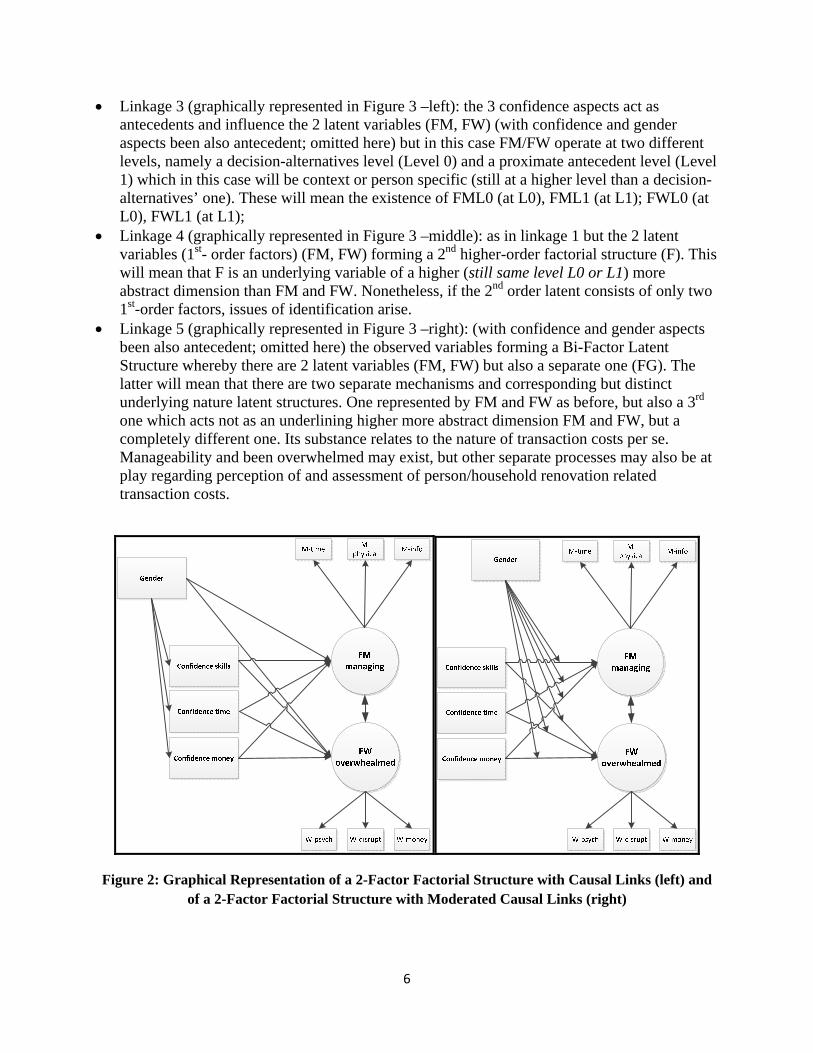
The first 3 items relate to a potential latent structure, namely manageability (FM); the latter to another latent structure, namely been overwhelmed (FW). The conceptual linkages at operation between them are multiple, and they can all be accepted on, namely: Linkage 1 (graphically represented in Figure 2 –left): the 3 confidence aspects act as

antecedents and influence the 2 latent variables (FM, FW) with gender aspects been also antecedent. In this case, gender is hypothesized to affect perceptions of and assessment about personal confidence.

Linkage 2 (graphically represented in Figure 2 –right): the 3 confidence aspects act as antecedents and influence the 2 latent variables (FM, FW) but gender aspects be a moderator in the relationship between confidence and FM/FW.

6  

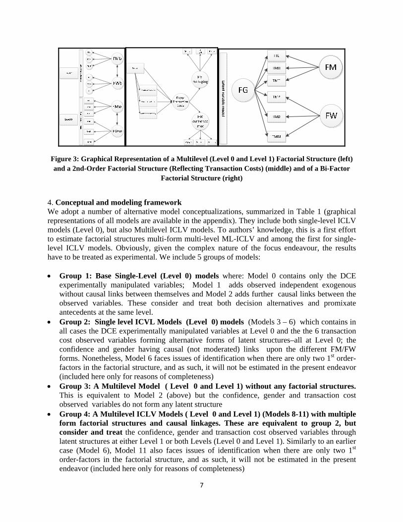
Linkage 3 (graphically represented in Figure 3 –left): the 3 confidence aspects act as antecedents and influence the 2 latent variables (FM, FW) (with confidence and gender aspects been also antecedent; omitted here) but in this case FM/FW operate at two different levels, namely a decision-alternatives level (Level 0) and a proximate antecedent level (Level 1) which in this case will be context or person specific (still at a higher level than a decision-alternatives’ one). These will mean the existence of FML0 (at L0), FML1 (at L1); FWL0 (at L0), FWL1 (at L1);

Linkage 4 (graphically represented in Figure 3 –middle): as in linkage 1 but the 2 latent variables (1st- order factors) (FM, FW) forming a 2nd higher-order factorial structure (F). This will mean that F is an underlying variable of a higher (still same level L0 or L1) more abstract dimension than FM and FW. Nonetheless, if the 2nd order latent consists of only two 1st-order factors, issues of identification arise.

Linkage 5 (graphically represented in Figure 3 –right): (with confidence and gender aspects been also antecedent; omitted here) the observed variables forming a Bi-Factor Latent Structure whereby there are 2 latent variables (FM, FW) but also a separate one (FG). The latter will mean that there are two separate mechanisms and corresponding but distinct underlying nature latent structures. One represented by FM and FW as before, but also a 3rd one which acts not as an underlining higher more abstract dimension FM and FW, but a completely different one. Its substance relates to the nature of transaction costs per se. Manageability and been overwhelmed may exist, but other separate processes may also be at play regarding perception of and assessment of person/household renovation related transaction costs.

Figure 2: Graphical Representation of a 2-Factor Factorial Structure with Causal Links (left) and of a 2-Factor Factorial Structure with Moderated Causal Links (right)

7  

Figure 3: Graphical Representation of a Multilevel (Level 0 and Level 1) Factorial Structure (left) and a 2nd-Order Factorial Structure (Reflecting Transaction Costs) (middle) and of a Bi-Factor

Factorial Structure (right)

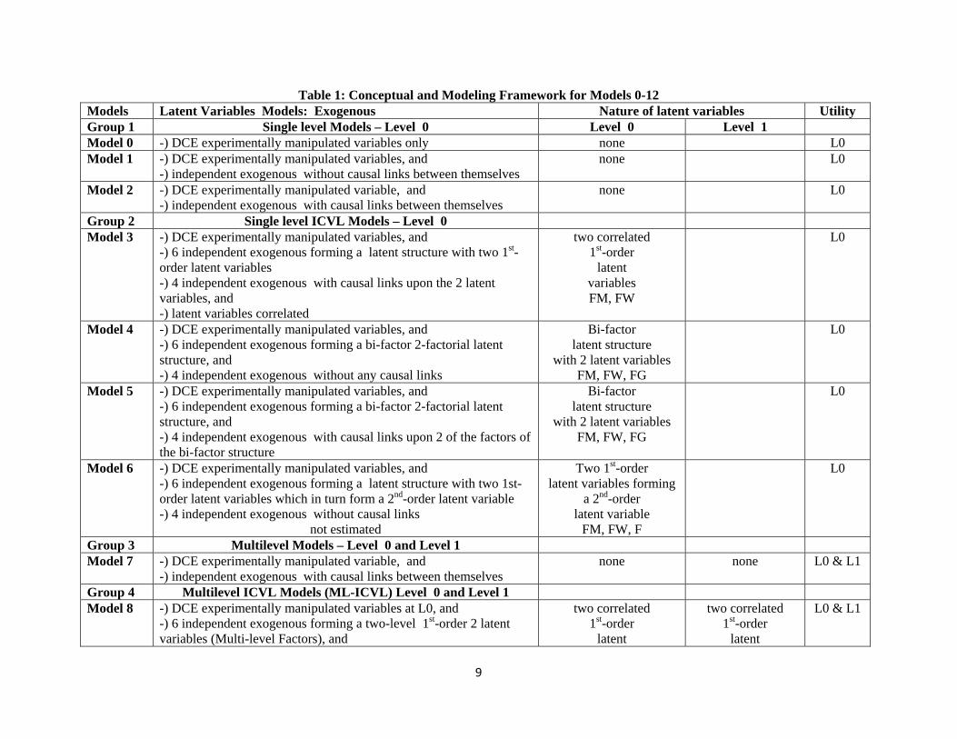
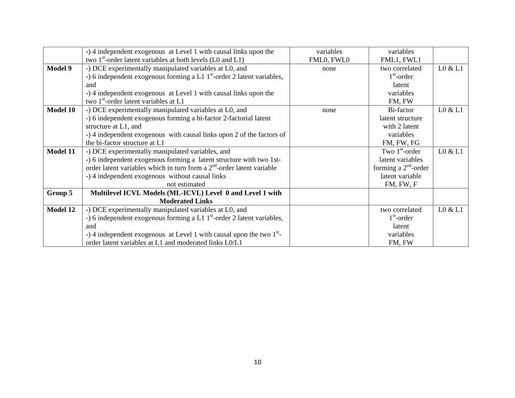
4. Conceptual and modeling framework We adopt a number of alternative model conceptualizations, summarized in Table 1 (graphical representations of all models are available in the appendix). They include both single-level ICLV models (Level 0), but also Multilevel ICLV models. To authors’ knowledge, this is a first effort to estimate factorial structures multi-form multi-level ML-ICLV and among the first for single-level ICLV models. Obviously, given the complex nature of the focus endeavour, the results have to be treated as experimental. We include 5 groups of models: Group 1: Base Single-Level (Level 0) models where: Model 0 contains only the DCE

experimentally manipulated variables; Model 1 adds observed independent exogenous without causal links between themselves and Model 2 adds further causal links between the observed variables. These consider and treat both decision alternatives and promixate antecedents at the same level.

Group 2: Single level ICVL Models (Level 0) models (Models 3 – 6) which contains in all cases the DCE experimentally manipulated variables at Level 0 and the the 6 transaction cost observed variables forming alternative forms of latent structures–all at Level 0; the confidence and gender having causal (not moderated) links upon the different FM/FW forms. Nonetheless, Model 6 faces issues of identification when there are only two 1st order-factors in the factorial structure, and as such, it will not be estimated in the present endeavor (included here only for reasons of completeness)

Group 3: A Multilevel Model ( Level 0 and Level 1) without any factorial structures. This is equivalent to Model 2 (above) but the confidence, gender and transaction cost observed variables do not form any latent structure

Group 4: A Multilevel ICLV Models ( Level 0 and Level 1) (Models 8-11) with multiple form factorial structures and causal linkages. These are equivalent to group 2, but consider and treat the confidence, gender and transaction cost observed variables through latent structures at either Level 1 or both Levels (Level 0 and Level 1). Similarly to an earlier case (Model 6), Model 11 also faces issues of identification when there are only two 1st order-factors in the factorial structure, and as such, it will not be estimated in the present endeavor (included here only for reasons of completeness)

8  

Group 5: Multilevel ICVL Models (ML-ICVL) Level 0 and Level 1 with Moderated Links (Model 12), the moderation originating from Gender and occurring at both levels (Level 0 and Level 1). The conceptual underpinning is that gender aspects will penetrate across both proximate antecedent as well as decision alternatives levels and they are not shaping up the initial formation of the perceptions regarding confidence and manageability/been overwhelmed.

9  

Table 1: Conceptual and Modeling Framework for Models 0-12 Models Latent Variables Models: Exogenous Nature of latent variables Utility Group 1 Single level Models – Level 0 Level 0 Level 1 Model 0 -) DCE experimentally manipulated variables only none L0 Model 1 -) DCE experimentally manipulated variables, and

-) independent exogenous without causal links between themselves none L0

Model 2 -) DCE experimentally manipulated variable, and -) independent exogenous with causal links between themselves

none L0

Group 2 Single level ICVL Models – Level 0 Model 3 -) DCE experimentally manipulated variables, and

-) 6 independent exogenous forming a latent structure with two 1st-order latent variables -) 4 independent exogenous with causal links upon the 2 latent variables, and -) latent variables correlated

two correlated 1st-order

latent variables FM, FW

L0

Model 4 -) DCE experimentally manipulated variables, and -) 6 independent exogenous forming a bi-factor 2-factorial latent structure, and -) 4 independent exogenous without any causal links

Bi-factor latent structure

with 2 latent variables FM, FW, FG

L0

Model 5 -) DCE experimentally manipulated variables, and -) 6 independent exogenous forming a bi-factor 2-factorial latent structure, and -) 4 independent exogenous with causal links upon 2 of the factors of the bi-factor structure

Bi-factor latent structure

with 2 latent variables FM, FW, FG

L0

Model 6 -) DCE experimentally manipulated variables, and -) 6 independent exogenous forming a latent structure with two 1st-order latent variables which in turn form a 2nd-order latent variable -) 4 independent exogenous without causal links

not estimated

Two 1st-order latent variables forming

a 2nd-order latent variable

FM, FW, F

L0

Group 3 Multilevel Models – Level 0 and Level 1 Model 7 -) DCE experimentally manipulated variable, and

-) independent exogenous with causal links between themselves none none L0 & L1

Group 4 Multilevel ICVL Models (ML-ICVL) Level 0 and Level 1 Model 8 -) DCE experimentally manipulated variables at L0, and

-) 6 independent exogenous forming a two-level 1st-order 2 latent variables (Multi-level Factors), and

two correlated 1st-order

latent

two correlated 1st-order

latent

L0 & L1

10  

-) 4 independent exogenous at Level 1 with causal links upon the two 1st-order latent variables at both levels (L0 and L1)

variables FML0, FWL0

variables FML1, FWL1

Model 9 -) DCE experimentally manipulated variables at L0, and -) 6 independent exogenous forming a L1 1st-order 2 latent variables, and -) 4 independent exogenous at Level 1 with causal links upon the two 1st-order latent variables at L1

none two correlated 1st-order

latent variables FM, FW

L0 & L1

Model 10 -) DCE experimentally manipulated variables at L0, and -) 6 independent exogenous forming a bi-factor 2-factorial latent structure at L1, and -) 4 independent exogenous with causal links upon 2 of the factors of the bi-factor structure at L1

none Bi-factor latent structure with 2 latent

variables FM, FW, FG

L0 & L1

Model 11 -) DCE experimentally manipulated variables, and -) 6 independent exogenous forming a latent structure with two 1st-order latent variables which in turn form a 2nd-order latent variable -) 4 independent exogenous without causal links

not estimated

Two 1st-order latent variables

forming a 2nd-order latent variable

FM, FW, F

L0 & L1

Group 5 Multilevel ICVL Models (ML-ICVL) Level 0 and Level 1 with Moderated Links

Model 12 -) DCE experimentally manipulated variables at L0, and -) 6 independent exogenous forming a L1 1st-order 2 latent variables, and -) 4 independent exogenous at Level 1 with causal upon the two 1st-order latent variables at L1 and moderated links L0/L1

two correlated 1st-order

latent variables FM, FW

L0 & L1

11  

Data Collection and Experiment Data are drawn from a simultaneous DCE and survey conducted within the framework of UK home owners’ decision making for home renovations. The overall aim of the study was to assess the acceptability to UK homeowners of alternative value propositions. As a pertinent value proposition is a bundle of product and service attributes including, core products (e.g., kitchen remodeling), and additional services (e.g., hassle, effort, cost and warranty). Thus, the focus population of prospective renovators is UK-wide homeowners costing between 3500-6500 UKP is the focus of the DCE. The selection of proximate antecedents, as well as value proposition decision alternatives’ attributes are informed by three strands of research and were further validated by industry. First, we conducted a systematic review of both academic and grey literature relevant to renovation decision making. This ranged from discrete choice models to social theories of practice and domestication. Second, we conducted a series of 35 interviews with owner-occupied households in the period January - May 2012 split between two study sites: Rackheath in Norfolk, and Sutton in South London. The interview sample was recruited using a 3*2 design to include: households who had recently renovated, households who were thinking about renovating at some point in the future, and households with no plans to renovate. The first two sub-samples were further split between energy efficient and amenity renovators. Common amenity renovations include kitchen remodelling, loft conversions, and new bathrooms. Throughout this paper, we use the term ‘renovations’ to meaning major, structural changes or additions to the home typically requiring outside contractors with specialist expertise (cf. Maller and Horne 2011). The literature review and interview data informed the design of the survey questions and instrument. This was refined iteratively in three rounds of pre-testing and testing during the summer of 2012. The selected aspects were discussed with the third largest European retailer. HQ’s staff have commented on and suggested attributes to include in the DCE and other aspects of the work. Certainly additional attributes are at work, so the selected and tested sub-set reflects only a handful of attributes relating to potential decision alternatives. Data collection took place through a nationally representative online survey of UK homeowners in September 2012. Sampling and survey administration was contracted to a market research company. Summary statistics of the survey sample are provided in Table 2

Table 2: Summary of socio-demographics for the entire study

Mean respondent age 49.8 yrs

Frequency of female respondents 52.4%

Median household income £30 - 35,000 / yr

Mean household size 2.4 people

Most common (mode) house type semi-detached house

Most common (mode) house vintage 1950-1989

Most common (mode) length of tenure 10-20 yrs

Irrespectively of what renovations respondents have conducted, considered renovating (75% of N=1028) or not (25% of the sample), all respondents were assigned to a number of experiments.

12  

We report on an experiment which was taken by respondents irrespective of what their actual renovation context they are at. The content and layout of the questionnaire was designed by the university staff, with consultation and feedback provided by researchers at Ipsos MORI. The questionnaire structure consisted of the main body of the questionnaire followed by a specific version of a choice experiment, and some final follow-up questions. The average time taken to complete the survey was 25.6 minutes. In order to boost the representativeness of the survey, the initial invites to take part in the research were balanced to reflect the UK population profile across key socio-demographic variables: gender, geographic region, age and employment status. Panellist information relating to these demographic variables was sourced from the information initially provided by panellists at the point of recruitment. Quotas were set using information from the Labour Force Survey statistics from 2006. Only owner-occupier households (i.e. those who own their home outright or are paying off a mortgage on it) were included in the survey; we excluded all people renting their homes and in other types of accommodation. Within these eligible households, only individuals who are at least partly responsible for financial decisions regarding their home were eligible for the survey; anyone who has no responsibility for these decisions was excluded. Exploratory online research prior to the main survey highlighted that the overall penetration of UK individuals aged 18+ that would be eligible for the survey on the basis of these two factors is around 60%. The total of respondents who undertook the work was N=1028 and each experiment was answered by N=250. Attributes used included and used in the DCE analysis are displayed in Table 3.

Table 3: DCE attribute and levels

Attributes Description Level

Cost Cost of renovation continuous from 3500 to 6500

Effort of deciding effort deciding (as text description)

0= a lot (base); 1= some effort; 2= no effort

Hassle factor Hassle (as text description) 0= major hassle (base; 1= manageable hassle; 2= hassle free

warranty warranty in years continuous from 1 to 7 years

Analysis Bayesian estimation was employed for reasons relating to the complexity of the models and the principal advantage that we do not have to specify the conditional distributions explicitly. For each model, we performed 50000 iterations in total, half of which were used for burn-in and the remaining half draws, which were thinned by selecting each 10th draw to reduce the autocorrelation. An unperturbed estimation was conducted (Chains =2). The choice dependent was treated as categorical rather than nominal for several reasons. They include, the treatment of the utility best as y* being continuous, estimation of a nominal dependent with complex latent, nominal exogenous and moderating variables in a multilevel setting risk errors in interpretability of the results and model comparability. Furthermore, the complexity of simultaneous estimation of an increasing number, complexity and multi-level

13  

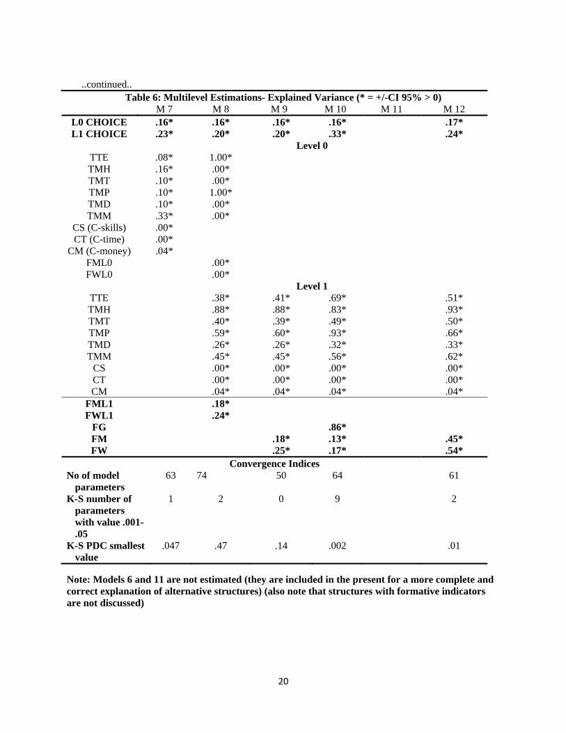
nature of latent variables increases dramatically due to integration aspects as well as the current state of understanding Multi-level ICLV models with nominal dependent variables. To authors’ knowledge, this is a first effort to estimate factorial multi-form multi-level ML-ICLV and single-level ICLV models. Bayes estimation was also employed because of the nature of present model conceptualization(s) where, for each model parametrization, the posterior distribution is proportional to the products of corresponding likelihoods of the involved observed variables and latent variables, the measurement and structural hypothesized linkages, and the prior distributions of the model parameters. The posteriors involved in the present treatments are much more complex than the posteriors involved in the estimation of classical DCEs or single-level ICLV. Non-standard distributions are likely to exist and they need to be estimated, thus only bayes estimations with non-informative priors appear to be best suited for the purpose. All raw scores (except gender) were standardized before entering in the estimation process and costs was also scaled down by 1000. Two of the experimentally manipulated variables in the DCE (effort and hassle, each with 3 original levels and a base of 0), were dummy coded and the two dummy codes (Effort 1 and Effort 2; Hassle 1 and Hassle 2) were used in the estimation. Reported results (see Table 4-6) are standardized StdY for binary covariates and StdYX for all independent as well as latent variables as well as the interaction terms for Gender (0= male; 1= female X independent exogenous) which masks an underlying Poisson distribution for the interaction term (0 for males; and continuous for females). StdYX is used since where y = y* the latent response variable underlying the observed categorical variable y (=choice). Bayesian thinking regarding acceptability of model estimates needs to be applied. Kolmogorov-Smirnov PDC smallest values were above acceptable thresholds indicating convergence of the chains and the number of parameters in the range of the marginal space of 0.001-0.5 were very few. The asterisk following the coefficients refers to whether +/-CI 95% been above 0. Explained variance of the dependent variables FM; FW; and CHOICE are also displayed for both Level 0 and Level 1 estimations.

14  

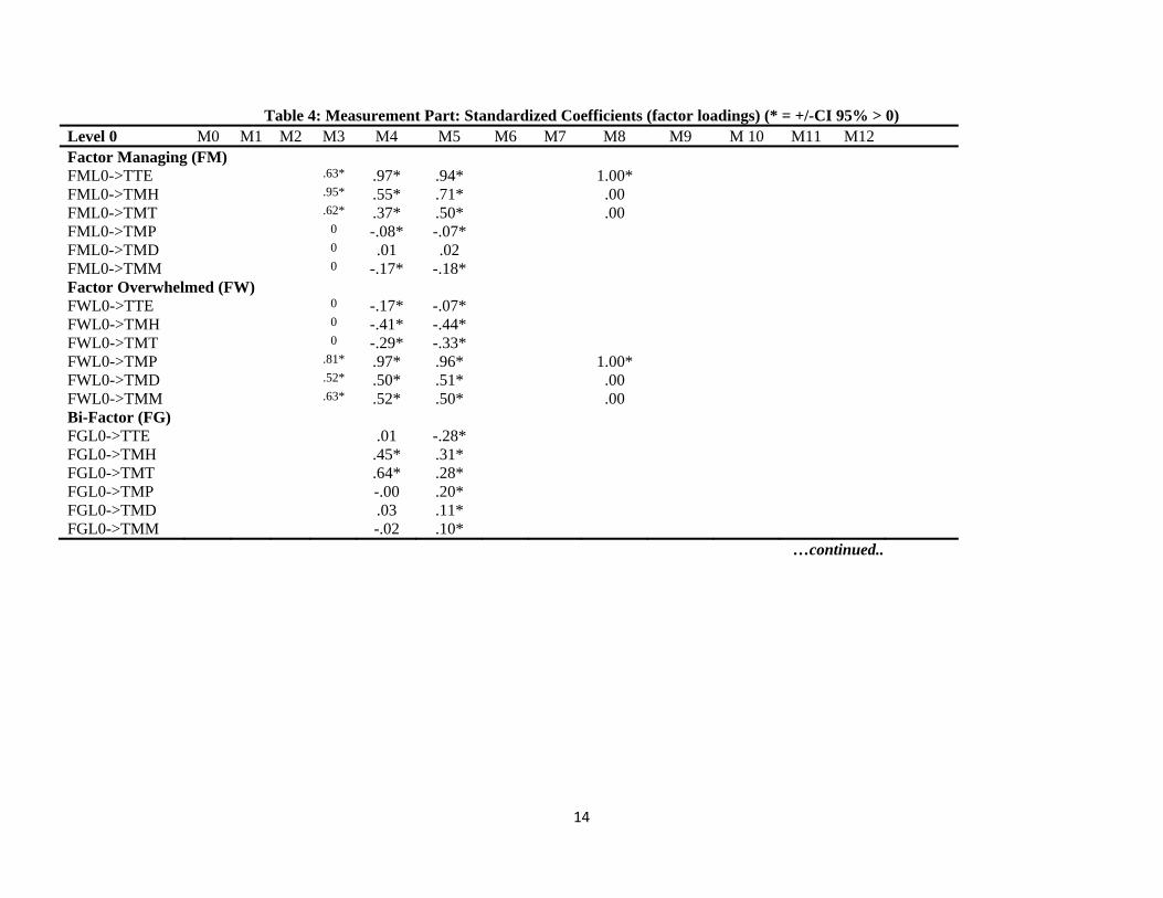
Table 4: Measurement Part: Standardized Coefficients (factor loadings) (* = +/-CI 95% > 0) Level 0 M0 M1 M2 M3 M4 M5 M6 M7 M8 M9 M 10 M11 M12 Factor Managing (FM) FML0->TTE .63* .97* .94* 1.00* FML0->TMH .95* .55* .71* .00 FML0->TMT .62* .37* .50* .00 FML0->TMP 0 -.08* -.07* FML0->TMD 0 .01 .02 FML0->TMM 0 -.17* -.18* Factor Overwhelmed (FW) FWL0->TTE 0 -.17* -.07* FWL0->TMH 0 -.41* -.44* FWL0->TMT 0 -.29* -.33* FWL0->TMP .81* .97* .96* 1.00* FWL0->TMD .52* .50* .51* .00 FWL0->TMM .63* .52* .50* .00 Bi-Factor (FG) FGL0->TTE .01 -.28* FGL0->TMH .45* .31* FGL0->TMT .64* .28* FGL0->TMP -.00 .20* FGL0->TMD .03 .11* FGL0->TMM -.02 .10*

…continued..

15  

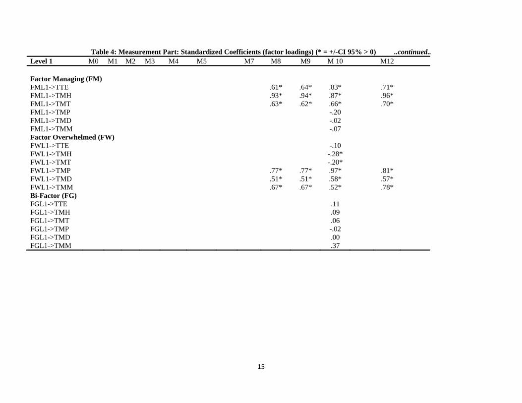
Table 4: Measurement Part: Standardized Coefficients (factor loadings) (* = +/-CI 95% > 0) ..continued.. Level 1 M0 M1 M2 M3 M4 M5 M7 M8 M9 M 10 M12 Factor Managing (FM) FML1->TTE .61* .64* .83* .71* FML1->TMH .93* .94* .87* .96* FML1->TMT .63* .62* .66* .70* FML1->TMP -.20 FML1->TMD -.02 FML1->TMM -.07 Factor Overwhelmed (FW) FWL1->TTE -.10 FWL1->TMH -.28* FWL1->TMT -.20* FWL1->TMP .77* .77* .97* .81* FWL1->TMD .51* .51* .58* .57* FWL1->TMM .67* .67* .52* .78* Bi-Factor (FG) FGL1->TTE .11 FGL1->TMH .09 FGL1->TMT .06 FGL1->TMP -.02 FGL1->TMD .00 FGL1->TMM .37

16  

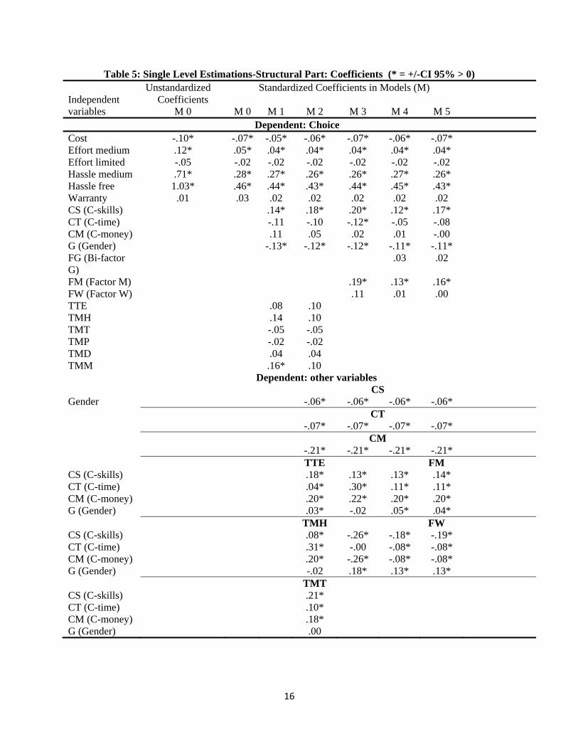
Table 5: Single Level Estimations-Structural Part: Coefficients (* = +/-CI 95% > 0) Independent variables

Unstandardized Coefficients

Standardized Coefficients in Models (M)

M 0 M 0 M 1 M 2 M 3 M 4 M 5 Dependent: Choice Cost -.10* -.07* -.05* -.06* -.07* -.06* -.07* Effort medium .12* .05* .04* .04* .04* .04* .04* Effort limited -.05 -.02 -.02 -.02 -.02 -.02 -.02 Hassle medium .71* .28* .27* .26* .26* .27* .26* Hassle free 1.03* .46* .44* .43* .44* .45* .43* Warranty .01 .03 .02 .02 .02 .02 .02 CS (C-skills) .14* .18* .20* .12* .17* CT (C-time) -.11 -.10 -.12* -.05 -.08 CM (C-money) .11 .05 .02 .01 -.00 G (Gender) -.13* -.12* -.12* -.11* -.11* FG (Bi-factor G)

.03 .02

FM (Factor M) .19* .13* .16* FW (Factor W) .11 .01 .00 TTE .08 .10 TMH .14 .10 TMT -.05 -.05 TMP -.02 -.02 TMD .04 .04 TMM .16* .10

Dependent: other variables CS

Gender -.06* -.06* -.06* -.06* CT -.07* -.07* -.07* -.07* CM -.21* -.21* -.21* -.21*

TTE FM CS (C-skills) .18* .13* .13* .14* CT (C-time) .04* .30* .11* .11* CM (C-money) .20* .22* .20* .20* G (Gender) .03* -.02 .05* .04*

TMH FW CS (C-skills) .08* -.26* -.18* -.19* CT (C-time) .31* -.00 -.08* -.08* CM (C-money) .20* -.26* -.08* -.08* G (Gender) -.02 .18* .13* .13*

TMT CS (C-skills) .21* CT (C-time) .10* CM (C-money) .18* G (Gender) .00

17  

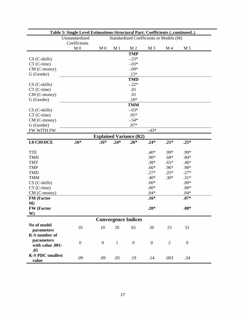
Table 5: Single Level Estimations-Structural Part: Coefficients (..continued..) Unstandardized

Coefficients Standardized Coefficients in Models (M)

M 0 M 0 M 1 M 2 M 3 M 4 M 5 TMP

CS (C-skills) -.23* CT (C-time) -.03* CM (C-money) -.09* G (Gender) .13*

TMD CS (C-skills) -.22* CT (C-time) .01 CM (C-money) .01 G (Gender) .18*

TMM CS (C-skills) -.03* CT (C-time) .05* CM (C-money) -.54* G (Gender) .07* FW WITH FW -.43*

Explained Variance (R2) L0 CHOICE .16* .16* .24* .26* .24* .21* .25* TTE .40* .99* .99* TMH .90* .68* .84* TMT .38* .65* .46* TMP .66* .96* .98* TMD .27* .25* .27* TMM .40* .30* .31* CS (C-skills) .00* .00* CT (C-time) .00* .00* CM (C-money) .04* .04* FM (Factor M)

.16* .07*

FW (Factor W)

.20* .08*

Convergence Indices No of model

parameters 10 10 20 65 20 23 51

K-S number of parameters with value .001-.05

0 0 1 0 0 2 0

K-S PDC smallest value

.09 .09 .05 .19 .14 .003 .34

   

18  

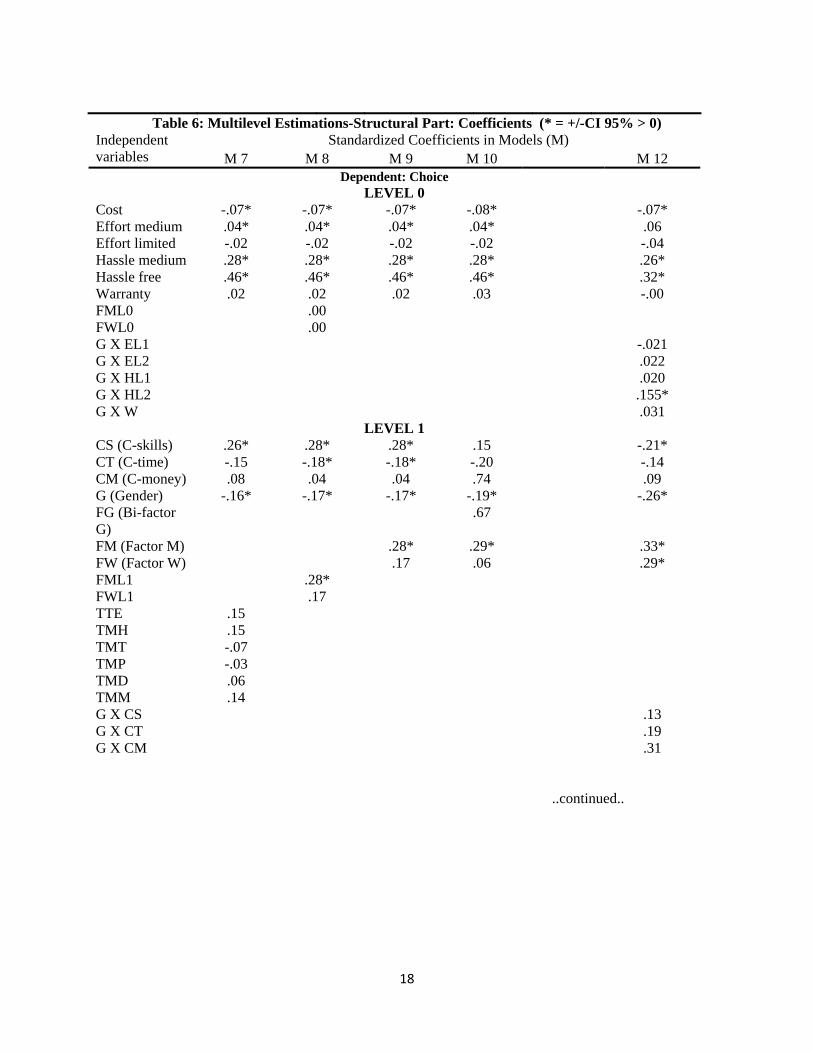
Table 6: Multilevel Estimations-Structural Part: Coefficients (* = +/-CI 95% > 0)

Independent variables

Standardized Coefficients in Models (M) M 7 M 8 M 9 M 10 M 12

Dependent: ChoiceLEVEL 0

Cost -.07* -.07* -.07* -.08* -.07* Effort medium .04* .04* .04* .04* .06 Effort limited -.02 -.02 -.02 -.02 -.04 Hassle medium .28* .28* .28* .28* .26* Hassle free .46* .46* .46* .46* .32* Warranty .02 .02 .02 .03 -.00 FML0 .00 FWL0 .00 G X EL1 -.021 G X EL2 .022 G X HL1 .020 G X HL2 .155* G X W .031

LEVEL 1 CS (C-skills) .26* .28* .28* .15 -.21* CT (C-time) -.15 -.18* -.18* -.20 -.14 CM (C-money) .08 .04 .04 .74 .09 G (Gender) -.16* -.17* -.17* -.19* -.26* FG (Bi-factor G)

.67

FM (Factor M) .28* .29* .33* FW (Factor W) .17 .06 .29* FML1 .28* FWL1 .17 TTE .15 TMH .15 TMT -.07 TMP -.03 TMD .06 TMM .14 G X CS .13 G X CT .19 G X CM .31

..continued..

19  

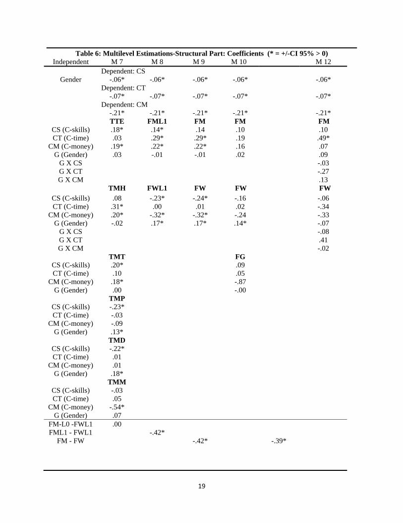
Table 6: Multilevel Estimations-Structural Part: Coefficients (* = +/-CI 95% > 0) Independent M 7 M 8 M 9 M 10 M 12

Dependent: CS Gender -.06* -.06* -.06* -.06* -.06*

Dependent: CT -.07* -.07* -.07* -.07* -.07*

Dependent: CM -.21* -.21* -.21* -.21* -.21*

TTE FML1 FM FM FM CS (C-skills) .18* .14* .14 .10 .10 CT (C-time) .03 .29* .29* .19 .49*

CM (C-money) .19* .22* .22* .16 .07 G (Gender) .03 -.01 -.01 .02 .09

G X CS -.03 G X CT -.27 G X CM .13

TMH FWL1 FW FW FW CS (C-skills) .08 -.23* -.24* -.16 -.06 CT (C-time) .31* .00 .01 .02 -.34

CM (C-money) .20* -.32* -.32* -.24 -.33 G (Gender) -.02 .17* .17* .14* -.07

G X CS -.08 G X CT .41 G X CM -.02

TMT FG CS (C-skills) .20* .09 CT (C-time) .10 .05

CM (C-money) .18* -.87 G (Gender) .00 -.00

TMP CS (C-skills) -.23* CT (C-time) -.03

CM (C-money) -.09 G (Gender) .13*

TMD CS (C-skills) -.22* CT (C-time) .01

CM (C-money) .01 G (Gender) .18*

TMM CS (C-skills) -.03 CT (C-time) .05

CM (C-money) -.54* G (Gender) .07

FM-L0 -FWL1 .00 FML1 - FWL1 -.42*

FM - FW -.42* -.39*

20  

..continued..

Table 6: Multilevel Estimations- Explained Variance (* = +/-CI 95% > 0) M 7 M 8 M 9 M 10 M 11 M 12

L0 CHOICE .16* .16* .16* .16* .17* L1 CHOICE .23* .20* .20* .33* .24*

Level 0 TTE .08* 1.00* TMH .16* .00* TMT .10* .00* TMP .10* 1.00* TMD .10* .00* TMM .33* .00*

CS (C-skills) .00* CT (C-time) .00*

CM (C-money) .04* FML0 .00* FWL0 .00*

Level 1 TTE .38* .41* .69* .51* TMH .88* .88* .83* .93* TMT .40* .39* .49* .50* TMP .59* .60* .93* .66* TMD .26* .26* .32* .33* TMM .45* .45* .56* .62*

CS .00* .00* .00* .00* CT .00* .00* .00* .00* CM .04* .04* .04* .04*

FML1 .18* FWL1 .24*

FG .86* FM .18* .13* .45* FW .25* .17* .54*

Convergence Indices No of model

parameters 63 74 50 64 61

K-S number of parameters with value .001-.05

1 2 0 9 2

K-S PDC smallest value

.047 .47 .14 .002 .01

Note: Models 6 and 11 are not estimated (they are included in the present for a more complete and correct explanation of alternative structures) (also note that structures with formative indicators are not discussed)

21  

Discussion and Conclusion The aim of the present endeavor was to experiment regarding the further advancement of integrated discrete choice and latent variable (ICVL) models using alternative factorial structures’ conceptualizations and do so at both multilevel (ML-ICVL) & single level and for both the independent but also dependent side of the ICVL. In doing, specific independent variables were selected that were amenable to alternative latent variables’ conceptualizations. These included for instance: 1st-order latent variables (1st-order factors) (FM; FW) 1st-order latent variables (1st-order factors) (FM; FW) forming a 2nd-order factor (F) Multi-level (two-level) factorial structures (FML0; FML1 and FWL0; FWL1) Bi-Factor factorial structures (FM; FW; FG) These were also considered within the framework of both Single-Level and Multi-Level (Two-Level) conceptualizations, and further extended from causal sequential linkages to moderated influences. Moreover, an effort was made to consider and treat the observed choice (dependent) variable as actually been a reflection of a separate underlying latent structure which is pertinent to the observed choice itself. The underlying logic in that case was that separately to the notion of utility per se (possibly linked also to?), a separate notion and an underlying latent structure may also be at work, this one linked to, and observed through, the choice variables per se. The hypothesis at work is that it is possible that underlying the choices selected by the individuals may exist not a single latent (y*), but probably either a partially captured single latent, or a different latent structure. The results displayed above show in summary, the following: 1. Structure of Latent Variables. The results (see Table 4) confirm that the chosen alternative forms of factorial structures can be each defended on the basis of significant loadings and fit indices as well as underlying theoretical support. Thus, their inclusion in alternative models (withstanding the linkage 4 where a 2nd-order same level factor structure was not possible to be tested because of the existence of only 2 factors resulting in model identification issues) latent divergent latent variable structures is acceptable, and warrant greater investigation regarding their exact impact upon the dependent choice variable. Furthermore, divergent results are evident and this means that selecting one factorial structure in the ICLV without further and deeper investigation of alternative conceptualizations and how these conceptualizations do influence results increases the risk of inaccurate scientific results. For example, it is evident that both a bi-factor factorial structure (see Measurement Part in Model 4 and Model 5) (FM; FW; FG) can also be at work, and a Two-Level Factorial Structure (FML0; FML1 and FWL0; FWL1) (the same for 2nd-order factors (F)) are real competing alternatives to traditional 1st-order latent variables (FM; FW). 2. Utility explained in Level 0 and Level 1. It is clearly demonstrated that the utility estimated in the framework of DCEs is explained better through multi-level modeling whereby decision alternatives are modeled at Level 0 and (proximate) antecedents can be conceptualized at both Level 0 and/ or Level 1. DCE-utility explained variance of the underlying continuous y* through Level 0 models ranged between .16 to .25. This has increased to .36-.39 through Level 1

22  

and most of the increase is due to the addition of the latent structures which primarily exercise, however, their influence at Level 1. 3. Moderation between (latent) variables is also an alternative which can also impact through a direct influence of exogenous variables upon both Level 0 and Level 1 variables (see Model 12). References

Ajzen, I. (1991). "The Theory of Planned Behavior." Organizational Behavior and Human Decision Processes 50(2): 179-211.

Ashok, K., W.R. Dillon, and S. Yuan, 2002. Extending Discrete Choice Models to Incorporate Attitudinal and Other Latent Variables. Journal of Marketing Research 39(1) 31-46. Ben-Akiva, M., J. Walker, A. Bernardino, D. Gopinath, T. Morikawa, and A. Polydoropoulou, 2002. Integration of Choice and Latent Variable Models, in (H. Mahmassani, Ed.) In Perpetual Motion: Travel Behaviour Research Opportunities and Application Challenges. Elsevier Science. 431-470. Ben-Akiva, Moshe, Daniel McFadden, Tommy Gärling, Dinesh Gopinath, Joan Walker, Denis Bolduc, Axel Börsch-Supan, Philippe Delquié, Oleg Larichev, Taka Morikawa, Amalia Polydoropoulou, and Vithala Rao (1999): Extended framework for modeling choice behavior, Marketing Letters, 10 (3): 187–203. Ben-Akiva, Moshe, Daniel McFadden, Kenneth Train, Joan Walker, Chandra Bhat, Michel Bierlaire, Denis Bolduc, Axel Börsch-Supan, David Brownstone, David S. Bunch, Andrew Daly, Andre De Palma, Dinesh Gopinath, Anders Karlstrom, and Marcela A. Munizaga (2002): Hybrid choice models: Progress and challenges, Marketing Letters, 13 (3): 163–175. Bierlaire, M. (2003) BIOGEME: a free package for the estimation of discrete choice models, paper presented at Swiss Transport Research Conference. Bliemer, M.C.J., J.M. Rose (2010). Construction of Experimental Designs for Mixed Logit Models Allowing for Correlation Across Choice Observations. Transportation Research Part B: Methodological. 44 720-734. Bolduc, Denis, Moshe Ben-Akiva, Joan Walker, and Alain Michaud (2005): Hybrid choice models with logit kernel: Applicability to large scale models, in: Martin Lee-Gosselin and Sean T. Doherty (eds.): Integrated land-use and transportation models, Elsevier, Amsterdam, 275–302. Danthurebandara, V. M., M. Vandebroek, and J. Yu (2013). Integrated Mixed Logit and Latent Variable Models, Marketing Letters (upcoming)

23  

Ehn, B. and O. Löfgren (2009). Routines - Made and Unmade. Time, Comsumption and Everyday Life: Practice, Materiality and Culture. E. Shove, F. Trentmann and R. Wilk. Oxford, Berg: 231.

Hand, M., E. Shove, et al. (2007). "Home extensions in the United Kingdom: space, time, and practice." Environment and Planning D-Society & Space 25(4): 668-681.

Hess, S., and A. Stathopoulos, 2010. Linking Response Quality to Survey Engagement: A Combined Random Scale and Latent Variable Approach. Proceedings of the European Transport Conference (ETC 2010), Glasgow, Scotland, UK. La Paix, L., M. Bierlaire, E. Cherchi, and A. Monzón, 2011. How Urban Environment A_ects Travel Behaviour? Integrated Choice and Latent Variable Model for Travel Schedules. Proceedings of the Second International Choice Modelling Conference (ICMC 2011), Leeds, North England, UK. Leonard, L. I., H. C. Perkins, et al. (2004). Presenting and Creating Home: The Influence of Popular and Building Trade Print Media in the Construction of Home. Housing, Theory and Society. 21: 97-110.

McFadden, Daniel L. (1986): The choice theory approach to marketing research, Marketing Science, 5 (4): 275–297. Morikawa, T. and Sasaki, K. (1998): Discrete Choice Models with Latent Variables Using Subjective Data. In Ortúzar, J de D., Hensher, D. A. and Jara-Diaz, S.: Travel Behaviour Research: Updating the State of Play, 435-455, Pergamon, Oxford Munro, M. and P. Leather (2000). "Nest-building or investing in the future? Owner-occupiers' home improvement behaviour." Policy and Politics 28(4): 511-526. Rungie, C. M., L. V. Coote, and J. Louviere (2011). Structural Choice Modeling: Theory and Applications to Combining Choice experiments. Journal of Choice Modelling, 4(3), 2011, 1-29 Temme, D., M. Paulssen, and T. Dannewald, 2008. Incorporating Latent Variables into Discrete Choice Models - A Simultaneous Estimation Approach Using SEM Software. Business Research. 1(2) 220-237. Walker, J. L. (2001) Extended discrete choice models: integrated framework, flexible error structures, and latent variables, Ph.D. Thesis, Massachusetts Institute of Technology. Walker, Joan L. and Jieping Li (2007): Latent lifestyle preferences and household location decisions, Journal of Geographical Systems, 9,(1): 77–101. Abou Zeid, M. (2009) Measuring and modeling travel and activity well-being, Ph.D. Thesis, Massachusetts Institute of Technology.

24  

Appendix: Graphical representations of Models 1-12

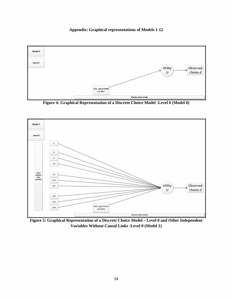
Figure 4: Graphical Representation of a Discrete Choice Model -Level 0 (Model 0)

Observed choice d

Observed exogenous variable(s) X

TMP

TMD

TMM

TTE

TMH

TMT UtilityU

CS

CT

CM

Discrete choice model

G

Level 0

DCE experiment variables

Model 1

Other indepen

dent variables

Figure 5: Graphical Representation of a Discrete Choice Model – Level 0 and Other Independent Variables Without Causal Links -Level 0 (Model 1)

25  

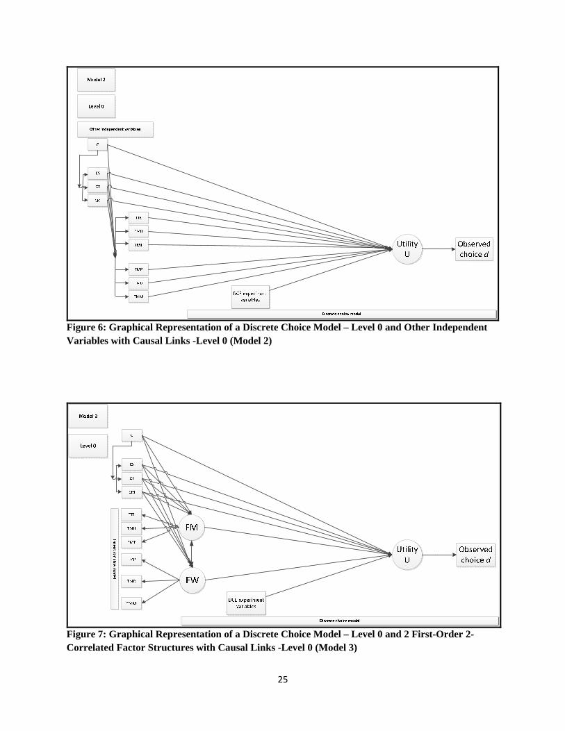
Figure 6: Graphical Representation of a Discrete Choice Model – Level 0 and Other Independent Variables with Causal Links -Level 0 (Model 2)

Figure 7: Graphical Representation of a Discrete Choice Model – Level 0 and 2 First-Order 2-Correlated Factor Structures with Causal Links -Level 0 (Model 3)

26  

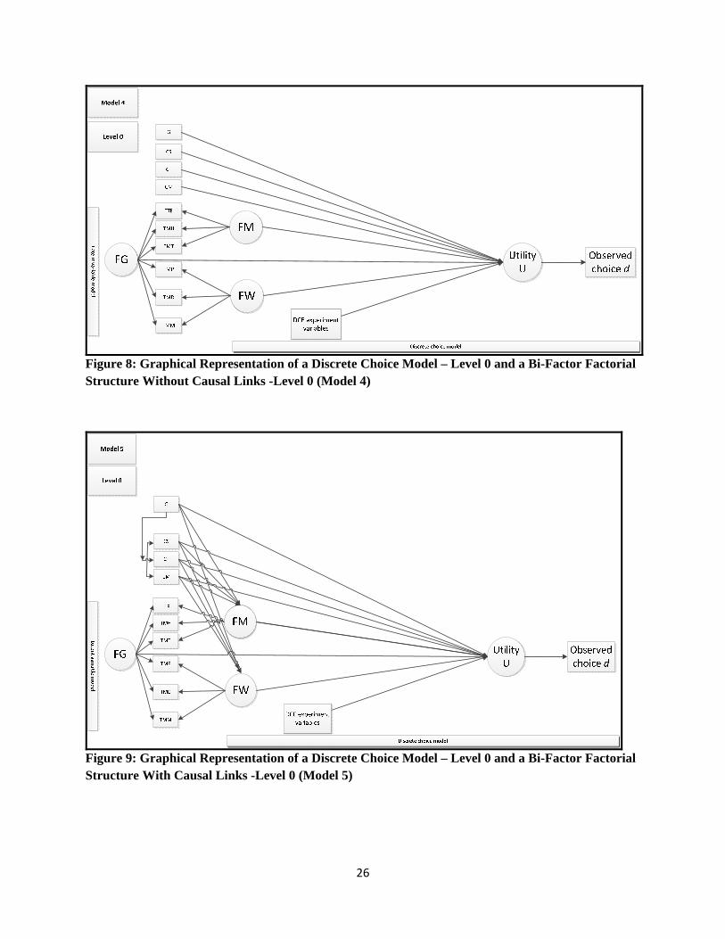
Figure 8: Graphical Representation of a Discrete Choice Model – Level 0 and a Bi-Factor Factorial Structure Without Causal Links -Level 0 (Model 4)

Figure 9: Graphical Representation of a Discrete Choice Model – Level 0 and a Bi-Factor Factorial Structure With Causal Links -Level 0 (Model 5)

27  

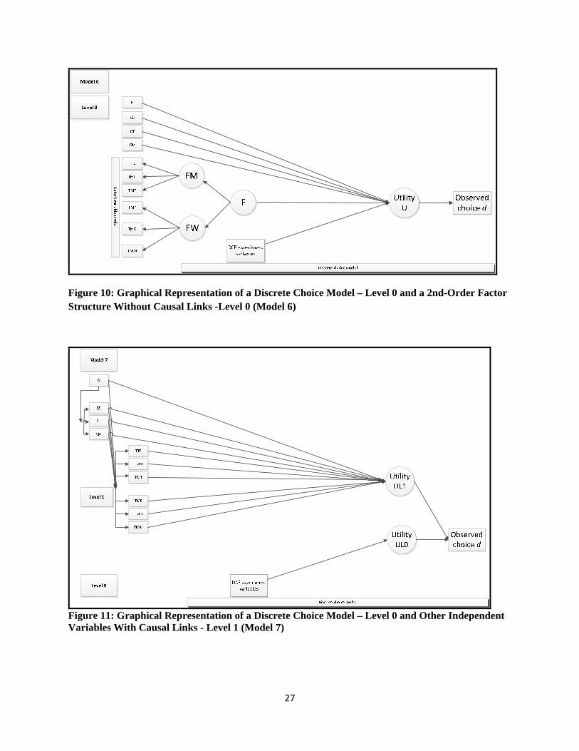
Figure 10: Graphical Representation of a Discrete Choice Model – Level 0 and a 2nd-Order Factor Structure Without Causal Links -Level 0 (Model 6)

Figure 11: Graphical Representation of a Discrete Choice Model – Level 0 and Other Independent Variables With Causal Links - Level 1 (Model 7)

28  

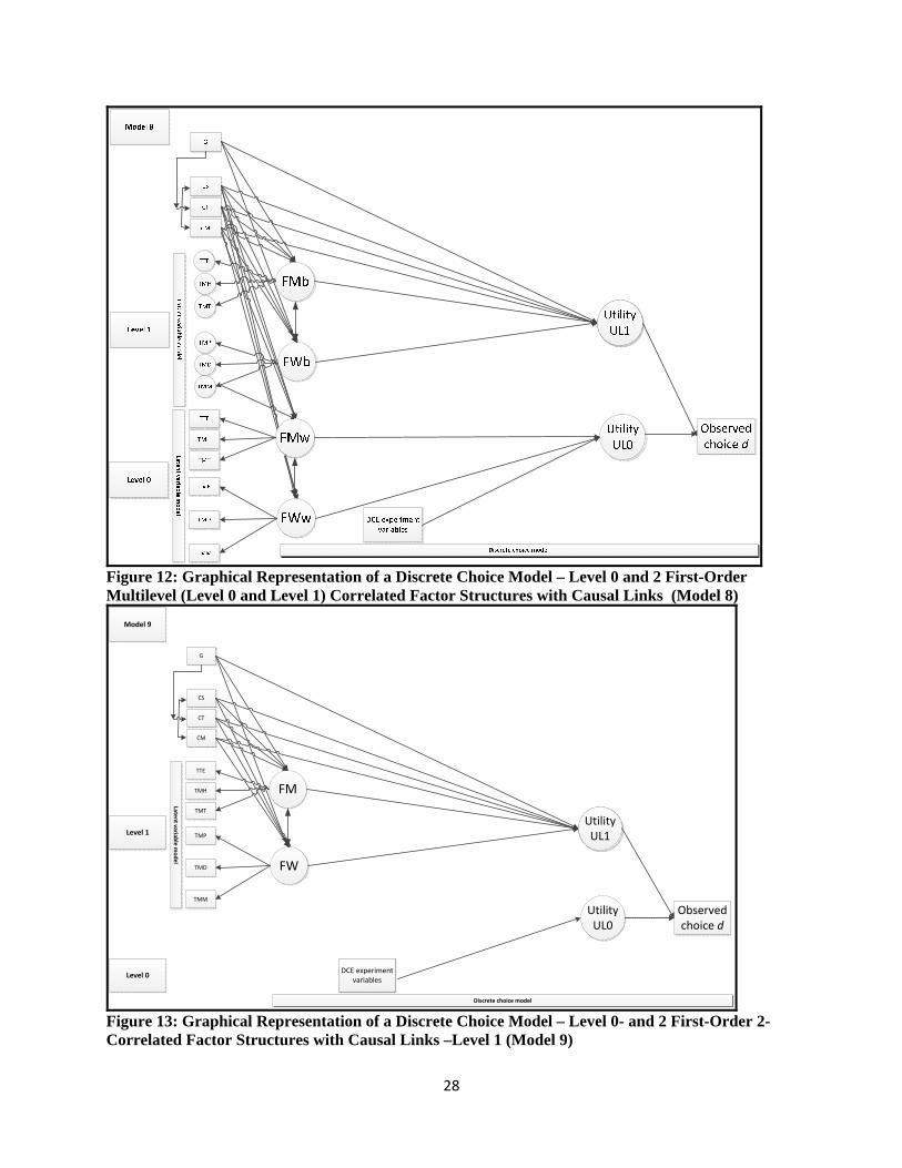
Figure 12: Graphical Representation of a Discrete Choice Model – Level 0 and 2 First-Order Multilevel (Level 0 and Level 1) Correlated Factor Structures with Causal Links (Model 8)

Observed exogenous variable(s) X

FW

TMP

TMD

TMM

FM

TTE

TMH

TMT

UtilityU

Level 0

Late

nt variab

le mo

del

Discrete choice model

Model 9

DCE experiment variables

CS

CT

CM

G

Level 1

Observed choice d

UtilityUL1

UtilityUL0

Figure 13: Graphical Representation of a Discrete Choice Model – Level 0- and 2 First-Order 2-Correlated Factor Structures with Causal Links –Level 1 (Model 9)

29  

FW

TMP

TMD

TMM

FM

TTE

TMH

TMT

UtilityU

Level 1

Latent varia

ble m

od

el

Discrete choice model

Model 10

FG

FM

CS

CT

CM

G

UtilityU

UtilityU

DCE experiment variables

Observed choice d

UtilityUL1

UtilityUL0

Level 0

Figure 14: Graphical Representation of a Discrete Choice Model – Level 0 and a Bi-Factor Factorial Structure With Causal Links -Level 1 (Model 10)

Laten

t variable

mo

del

Figure 15: Graphical Representation of a Discrete Choice Model – Level 0 and a 2nd-Order Factor Structure with Causal Links -Level 1 (Model 11)

30  

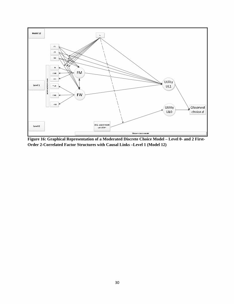
Figure 16: Graphical Representation of a Moderated Discrete Choice Model – Level 0- and 2 First-Order 2-Correlated Factor Structures with Causal Links –Level 1 (Model 12)