MULTIGRADED COMBINATORIAL HOPF ALGEBRAS ANDREFINEMENTS OF ODD AND EVEN SUBALGEBRAS

SAMUEL K. HSIAO AND GIZEM KARAALI

Abstract. We develop a theory of multigraded (i.e., Nl -graded) combinatorial Hopf alge-bras modeled on the theory of graded combinatorial Hopf algebras developed by Aguiar,Bergeron, and Sottile [Compos. Math. 142 (2006), 1–30]. In particular we introduce thenotion of canonical k-odd and k-even subalgebras associated with any multigraded combi-natorial Hopf algebra, extending simultaneously the work of Aguiar et al. and Ehrenborg.Among our results are specific categorical results for higher level quasisymmetric functions,several basis change formulas, and a generalization of the descents-to-peaks map.

Contents

1. Introduction 22. Background and examples of multigraded Hopf algebras 42.1. The Hopf algebra R(l) 52.2. The Hopf subalgebra R(l),k ⊆ R(l) 62.3. The Hopf algebra P(l) 62.4. Vector compositions 7

2.5. The Hopf algebra FQSym(l) 9

2.6. The Hopf algebra Sym(l) 10

2.7. The Hopf algebra Sym(l) 12

2.8. The Hopf algebra QSym(l) 13

2.9. Duality between QSym(l) and Sym(l) 143. The category of multigraded combinatorial Hopf algebras 153.1. Definitions 153.2. Universality of the Hopf algebra QSym(l) 163.3. The Bergeron-Hohlweg theory of colored combinatorial Hopf algebras 194. Definitions and basic properties of k-odd and k-even Hopf algebras 224.1. Basic constructions 224.2. k-analogs of odd and even subalgebras 244.3. Invertible linear functionals 254.4. k-odd linear functionals 264.5. k-even linear functionals 305. The k-odd and k-even Hopf subalgebras of QSym(l) 31

5.1. The k-odd Hopf subalgebra of QSym(l) 31

2000 Mathematics Subject Classification. 05E99, 16W30, 06A07, 06A11.Key words and phrases. Combinatorial Hopf algebra, multigraded Hopf algebra, quasisymmetric function,

symmetric function, noncommutative symmetric function, Eulerian poset.This work began while S.K. Hsiao was supported by an NSF Postdoctoral Research Fellowship.

1

5.2. The Euler character and generators for IOk 345.3. The η-basis for Ok 365.4. Hilbert series of Ok 385.5. The k-even subalgebra of QSym(l) 396. A k-analogue of the descents-to-peaks map 406.1. The k-odd functional νk

Q 406.2. The specialization k = ∞ 436.3. The specialization l = 1 47References 48

1. Introduction

Quasisymmetric functions appear throughout algebraic combinatorics, in contexts thatoften seem unrelated. Within the framework of combinatorial Hopf algebras developed in [2],this can be explained in category-theoretic terms: The combinatorial Hopf algebra QSym ofquasisymmetric functions is a terminal object of the category of combinatorial Hopf algebras.In this framework, a special role is claimed by the odd subalgebra of QSym, the algebra ofpeak functions, as the terminal object of the category of odd combinatorial Hopf algebras.

In this paper, we work with a natural generalization of QSym. Specifically we focus onQSym(l), the multigraded (i.e., Nl -graded) algebra of quasisymmetric functions of level l ,and show that in the corresponding category of multigraded combinatorial Hopf algebras, ananalogous universal property still holds (Theorem 3.1). Along the way we obtain several moregeneral results about the objects of this category, which are natural multigraded analoguesof results in [2].

Another goal of ours is to obtain a refinement of the notions of odd and even subalgebrasof [2] by developing “k-analogues” of the relevant constructions. We attain this goal inSections 4 and 5. There we show that given a multigraded Hopf algebra H =

⊕n∈Nl Hn

and a character on H, for every k ∈ (N ∪ {∞})l we have two canonically defined Hopfsubalgebras Ok(H) and Ek(H). As expected our k-analogues generalize the original notions:When l = 1 and k = ∞, Ok(H) and Ek(H) are precisely the odd and even subalgebrasof [2]. Moreover in the l = 1 case our construction refines what is known about QSym byproviding a sequence of Hopf subalgebras

QSym = O0(QSym) ) O2(QSym) ) O4(QSym) ) · · · ) O∞(QSym)

with certain universal properties. This sequence includes the algebra of Billey-Haiman shiftedquasisymmetric functions (our O2(QSym)) and Stembridge’s peak algebra (our O∞(QSym)).

When l > 1 and k = (∞, . . . ,∞), our Ok(QSym(l)) may be regarded as a higher levelanalogue of the peak algebra.

This work stems from several related but distinct threads of earlier research. In the fol-lowing we summarize a few key points related to quasisymmetric functions, Eulerian posets,and colored and multigraded Hopf algebras. For more details we refer the reader to ourbibliography.

2

Quasisymmetric functions were first defined explicitly by Gessel [20], who introduced themas generating functions for weights of P -partitions and gave applications to permutationenumeration. The Hopf algebra structure on QSym was studied in detail by Malvenutoand Reutenauer [27]. The Hopf algebraic approach allows us to interpret a multitude ofconstructions related to quasisymmetric functions in one uniform manner. A particularlyrelevant construction in this flavor is Ehrenborg’s F -homomorphism, which associates eachgraded poset P with a quasisymmetric function F (P ) that encodes the flag f -vector of P .When P is restricted to the class of Eulerian posets, the F (P ) span a Hopf subalgebra ofQSym. Viewed within the combinatorial Hopf algebra framework of [2], this Hopf subalgebrais precisely the odd subalgebra of QSym, which also happens to be Stembridge’s peak algebra[36]. We study multigraded analogues of these ideas in this paper. For example we definea Hopf algebra of multigraded posets, and then consider a generalization of Ehrenborg’s F -homomorphism from this Hopf algebra to QSym(l) (see Example 3.2). As one would expect,the image of an Eulerian multigraded poset under this homomorphism always lies in theodd subalgebra O(∞,...,∞)(QSym(l)) (cf. Example 3.3). This in turn implies that the naturallevel l versions of the generalized Dehn-Sommerville relations hold for multigraded Eulerianposets (see Example 4.17 and Remark 5.13).

We actually develop the multigraded version of the story relating graded posets and Hopfalgebras even further. In a somewhat different context, Ehrenborg [18] introduced a refine-ment of the notion of an Eulerian poset, called a k-Eulerian poset (k ∈ N ∪ {∞}), andproposed that one could define canonical algebras corresponding to k-Eulerian posets in away that would generalize the notion of an odd subalgebra. (Actually Ehrenborg’s worktakes place in the setting of Newtonian coalgebras, or infinitesimal Hopf algebras [1], whereinstead of “odd subalgebra” one has the analogous notion of “Eulerian subalgebra,” but itis easy to translate his idea into the language of combinatorial Hopf algebras.) We take thisidea one step further by providing multigraded versions of these constructions suggested byEhrenborg. In particular our algebras Ok(H) are in some sense multigraded generalizationsof the Ek(A) mentioned in [18, §5].

The level l quasisymmetric functions QSym(l) considered in this paper were introduced byPoirier [31] to handle enumeration problems involving colored permutations (i.e., elementsof wreath products Zn oSn). The term “level l” was coined by Novelli and Thibon [29] andrefers to the larger of the two algebras appearing in Poirier’s work1. The terminology andbasic Hopf algebraic properties of QSym(l) that we build on, as well as two other examplesof multigraded Hopf algebras that we discuss–the higher level noncommutative symmetricfunctions and free quasisymmetric functions–are due to Novelli and Thibon [29, 30]. Ourpaper adds the category-theoretic perspective and gives concrete results about new combi-natorially interesting bases, subalgebras, and maps within QSym(l), as well as maps fromother Hopf algebras to QSym(l).

We should mention that the smaller of Poirier’s algebras, usually referred to as the algebraof colored quasisymmetric functions, denoted here by QSym [l ], has been well studied by manyauthors. Baumann and Hohlweg [6] proved that QSym [l ] is a Hopf algebra and related it to

the larger Hopf algebra QSym(l). Their work places QSym [l ] within a general descent theory

1The reader may like to refer to [6, §6.2] for an analysis of the two different colored generalizations ofquasisymmetric functions in [31]

3

for wreath products and reveals the functorial nature of many related colored constructions,notably the colored descent algebras of Mantaci and Reutenauer [28]. In subsequent work,Bergeron and Hohlweg [12] continued to explain and unify various colored constructions, andalong the way they propose a theory of colored combinatorial Hopf algebras analogous to thetheory developed in [2]; this theory is developed further in [23]. Some connections betweenour work and the Bergeron-Hohlweg theory are discussed briefly in §§3.3. One key pointthat distinguishes our viewpoint from theirs is our emphasis on the Nl -graded structure. Itseems, however, that many of the k-refinements that we consider here should translate intoanalogous constructions within the framework suggested by Bergeron and Hohlweg.

One final topic that we consider in this paper is the notion of a k-analogue of the classicdescents-to-peaks map on quasisymmetric functions, which shows up naturally in severaldifferent settings. When viewing QSym and the peak algebra as arising from ordinary andenriched P -partitions, the descents-to-peaks map is Stembridge’s θ-map [36], which sendsthe P -partition weight enumerator of a labeled poset to the enriched P -partition weightenumerator of the same poset. In the setting of noncommutative symmetric functions, thedual of the descents-to-peaks map appears in the work of Krob, Leclerc and Thibon [24] asthe specialization at q = −1 of the A→ (1−q)A transform. Yet another interpretation of thismap involving flag enumeration in oriented matroids was given in [13]. We do not attemptto develop level l versions or k-analogues of these general frameworks which give rise to thedescents-to-peaks map (although see [23] for a related story on colored P -partitions). Insteadwe employ the character-theoretic approach of [2] to define the appropriate k-analogues

Θk : QSym(l) → QSym(l) and give explicit formulas to help compute these maps.

The rest of this paper is organized as follows. In Section 2 we provide the necessarybackground on l -partite numbers and vector compositions, and introduce several examplesof multigraded (Hopf) algebras. In Section 3 we study the category of multigraded combi-

natorial Hopf algebras and formulate the universal property of QSym(l). We also describehow to relate our constructions to earlier work. Section 4 contains our basic results on k-oddand k-even Hopf subalgebras. In particular we show that a substantial part of the standardtheory of combinatorial Hopf algebras developed in [2] goes through for these k-analogues.Section 5 contains more explicit descriptions of the k-odd and k-even Hopf subalgebras ofQSym(l). We focus mostly on the k-odd algebras, for which we describe various bases andcompute Hilbert series. In Section 6 we define the k-analogue of the descents-to-peaks mapand introduce k-analogues of the basis of peak functions.

We thank Marcelo Aguiar, Nantel Bergeron, Christophe Hohlweg and Jean-Yves Thibonfor helpful comments.

2. Background and examples of multigraded Hopf algebras

Throughout this paper, let N = { 0, 1, 2, . . . } denote the set of nonnegative integers andP = {1, 2, . . .} denote the set of positive integers. If m,n ∈ N then [n] = {1, 2, . . . , n}, and[n,m] = {n, n + 1, n + 2, . . . ,m}. In particular, [0] = ∅ and [n,m] = ∅ if n > m. In thispaper, we use the term multigraded to mean Nl -graded, where l is a fixed positive integer.We call the elements of Nl l -partite numbers and treat them as column vectors. Thus 0 ∈ Nl

denotes the zero vector, and for each i ∈ [0, l − 1], ei ∈ Nl denotes the coordinate vector4

with a 1 in position i and 0 everywhere else. When needed, we add vectors componentwise,and we sometimes use a partial order on Nl given by i ≤ j if each coordinate of i is less thanor equal to the corresponding coordinate of j. The l -partite number

n =

n0...

nl−1

∈ Nl

is said to have weight |n| = n1 + · · ·+ nl and support supp(n) = {i ∈ [0, l − 1] | ni 6= 0}.This section provides the necessary background on l -partite numbers and vector composi-

tions, and introduces several examples of multigraded (Hopf) algebras that appear through-out the paper. These algebras are

R(l) multigraded posetsR(l),k multigraded k-Eulerian posetsP(l) colored posets

FQSym(l) free quasisymmetric functions of level l

Sym(l) noncommutative symmetric functions of level l

QSym(l) quasisymmetric functions of level l

Sym(l) MacMahon’s multi-symmetric functions

Generally speaking, the Hopf algebras that we work with are Nl -graded bialgebras H =⊕n∈Nl Hn that are connected, meaning H0 is the one-dimensional vector space spanned by

the unit element; the counit is always defined to be the projection onto H0. Such a bialgebraalways has a recursively defined antipode (see, e.g., [17, Lemma 2.1]), so it automaticallybecomes a Hopf algebra.

Our discussion of vector compositions and the Hopf algebras QSym(l), Sym(l), and FQSym(l)

follows Novelli and Thibon [30], where most of the relevant definitions and results can befound.

2.1. The Hopf algebra R(l). A finite poset P is said to be graded if it has a uniqueminimum element 0 and a unique maximum element 1, and it is equipped with a rankfunction rk : P → N with the property that if y covers x in P then rk(y) = rk(x) + 1.

Definition 2.1. A multigraded poset is a (finite) graded poset P together with a functionrkP : P → Nl such that rkP (0) = 0 and if y covers x in P then rkP (y) = rkP (x) + ei forsome coordinate vector ei ∈ Nl . We call rkP the multirank function of P and say that themultirank of P is rkP (1).

Each interval [x, y] = {z ∈ P | x ≤ z ≤ y} in a multigraded poset P is again a multigradedposet with multirank function rk[x,y](z) = rkP (z)− rkP (x). Two multigraded posets P andQ are said to be isomorphic if there is an isomorphism of posets ϕ : P → Q such thatrkQ ◦ϕ = rkP .

Let R(l) be the vector space with basis the set of isomorphism classes of multigraded

posets. We get a multigrading R(l) =⊕

n∈Nl R(l)n by taking R(l)

n to be the linear span of all(isomorphism classes of) posets with multirank n.

5

Multiplication inR(l) is defined to be the usual Cartesian product P×Q with rkP×Q(x, y) =rkP (x) + rkQ(y) for (x, y) ∈ P ×Q. The coproduct is defined by

∆(P ) =∑

0≤x≤1

[0, x]⊗ [x, 1].

The unit is the one-element poset. When l = 1, the Hopf algebra R(l) specializes to Rota’sHopf algebra (see, e.g., [2, Example 2.2]).

2.2. The Hopf subalgebra R(l),k ⊆ R(l). Recall that a graded poset P is said to be Euler-ian if whenever x ≤P y, the Mobius function satisfies µ([x, y]) = (−1)rk(y)−rk(x). Generalizing[18, Definition 4.1], we make the following definition.

Definition 2.2. Let P be a multigraded poset and let k ∈ (N ∪ {∞})l . We say that P isk-Eulerian if every interval of rank n ≤ k is Eulerian.

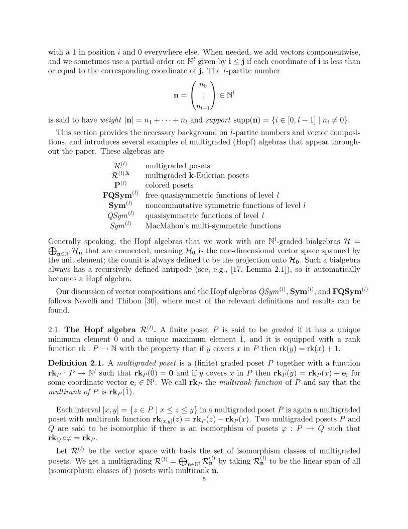
For example, the multigraded poset

s@@ ��

s�� s@@ ��

s�� s@@s

(0,0)

(1,0) (0,1)

(1,1) (0,2)

(1,2)

is (1, 1)-Eulerian but not (0, 2)-Eulerian.

Let R(l),k be the subspace of R(l) spanned by all k-Eulerian posets. Using the fact thatthe Mobius function is multiplicative, i.e., µ(P×Q) = µ(P ) ·µ(Q), it is easy to show that theCartesian product of two k-Eulerian posets is a k-Eulerian poset. It is also clear that everyinterval in a k-Eulerian poset is again k-Eulerian. Therefore R(l),k is a Hopf subalgebra ofR(l).

2.3. The Hopf algebra P(l). Let A = P× [0, l −1] be the set of l -colored positive integers.If x = (i, j) ∈ A then we call |x| = i the absolute value of x and γ(x) = j the color of x.

Definition 2.3. A finite subset P ⊆ A together with a partial order <P will be called acolored poset if {|x| | x ∈ P} = {1, 2, . . . , |P |}.

Let P(l) denote the vector space of formal Q-linear combinations of colored posets. Ifwe define the multidegree of a colored poset P to be (n0, . . . , nl−1)T ∈ Nl , where ni is the

number of occurrences of color i in the multiset {γ(x) | x ∈ P}, and denote by P(l)n the

subspace of colored posets of multidegree n, then P(l) becomes a multigraded vector space

P(l) =⊕

n∈Nl P(l)n .

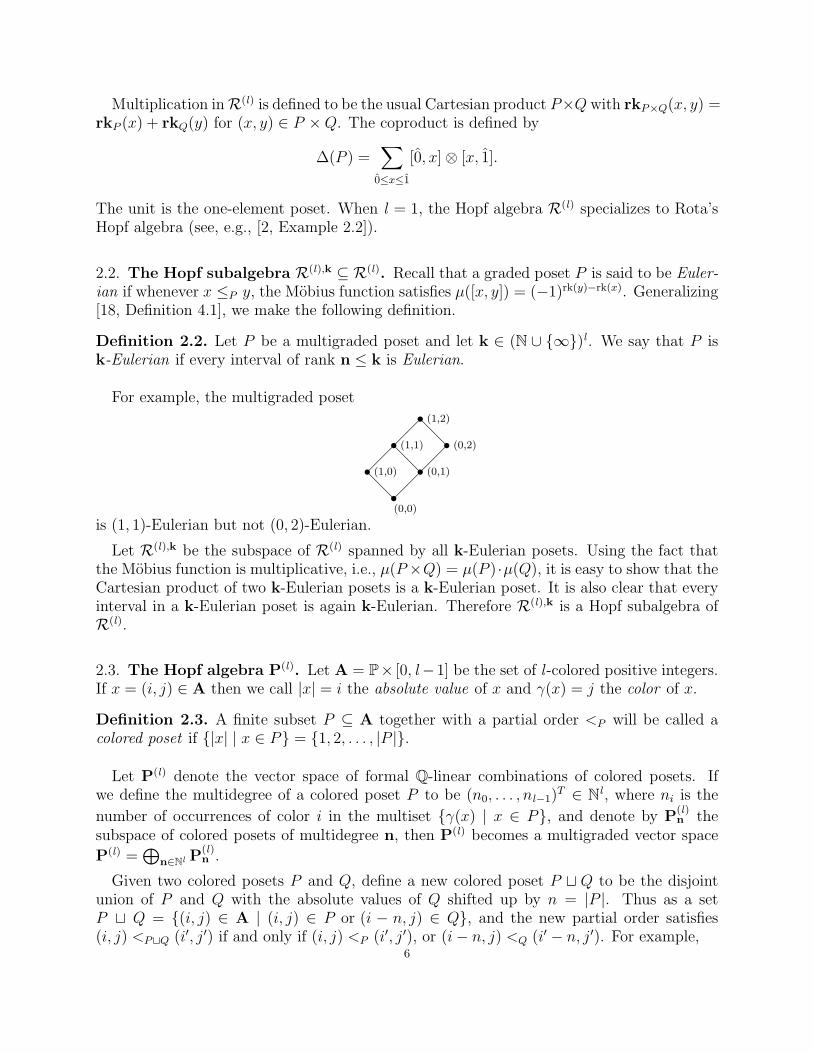
Given two colored posets P and Q, define a new colored poset P t Q to be the disjointunion of P and Q with the absolute values of Q shifted up by n = |P |. Thus as a setP t Q = {(i, j) ∈ A | (i, j) ∈ P or (i − n, j) ∈ Q}, and the new partial order satisfies(i, j) <PtQ (i′, j′) if and only if (i, j) <P (i′, j′), or (i− n, j) <Q (i′ − n, j′). For example,

6

ss(1,0)

(2,2)

t ��@@s s s

(1,2)

(2,0)

(3,0)

=ss(1,0)

(2,2)

��@

@s s s(3,2)

(4,0)

(5,0)

With this product P(l) becomes a noncommutative multigraded algebra whose unit elementis the empty colored poset. When l = 1 we recover the construction discussed in [16, §3.8].

To define the coproduct, first recall that a (lower) order ideal of a poset P is a subsetI ⊆ P such that if x ∈ I and y <P x then y ∈ I. Every order ideal I and its complementP − I can be thought of as a subposet of P . The set of order ideals of P is denoted by I(P ).Now suppose that P is a colored poset and Q = {(i1, j1) . . . (im, jm)} is any subposet (notnecessarily a colored poset). The standardization of Q is the colored poset st(Q) obtainedby relabeling (ir, jr) by (i′r, jr) for each (ir, jr) ∈ Q, where i′1i

′2 . . . i

′m is the standardization

of i1i2 . . . im. In other words i′1i′2 . . . i

′m is the unique permutation of [m] such that i′r < i′s if

and only if ir < is for every r, s ∈ [m]. Now we can define the coproduct of a colored posetP by

∆(P ) =∑I∈I(P )

st(I)⊗ st(P − I).

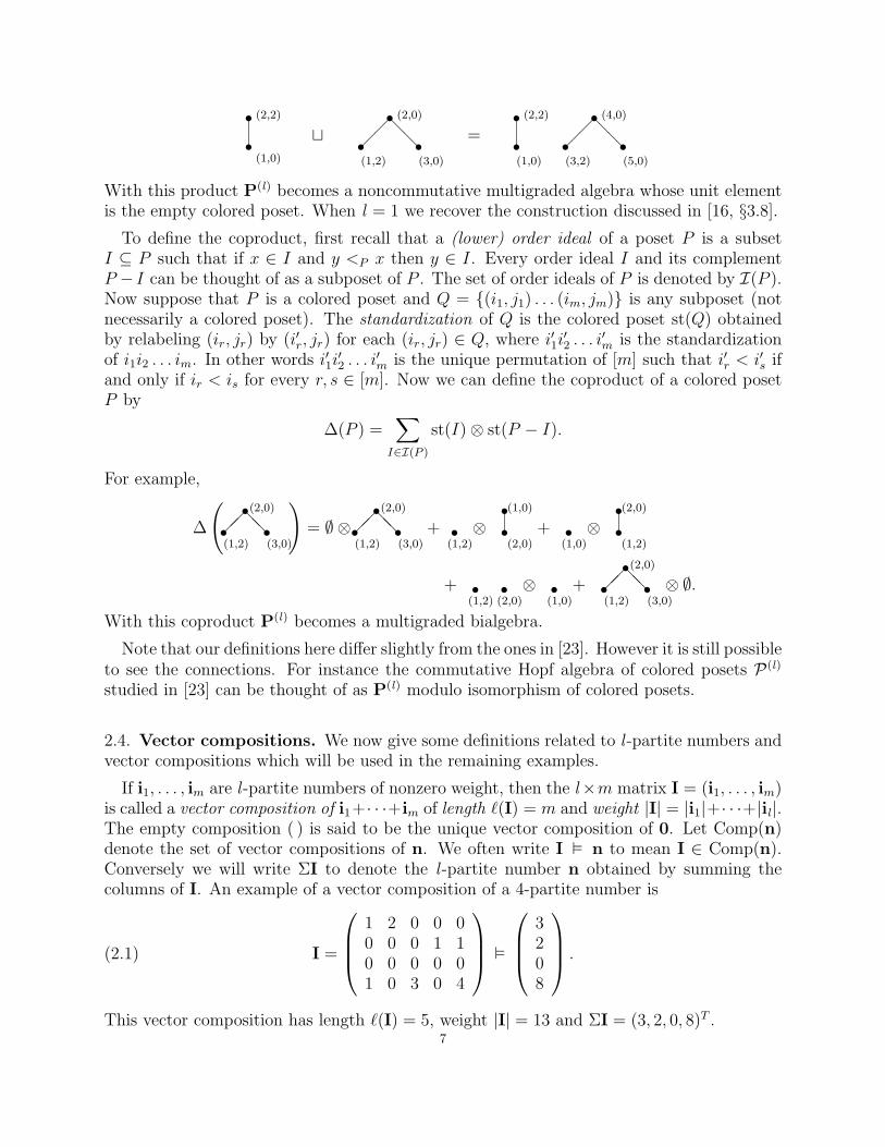
For example,

∆

(��@@s s s(1,2)

(2,0)

(3,0)

)= ∅ ⊗��@@s s s

(1,2)

(2,0)

(3,0)

+ s(1,2)

⊗ ss(2,0)

(1,0)

+ s(1,0)

⊗ ss(1,2)

(2,0)

+ s s(1,2) (2,0)

⊗ s(1,0)

+ ��@@s s s

(1,2)

(2,0)

(3,0)⊗ ∅.

With this coproduct P(l) becomes a multigraded bialgebra.

Note that our definitions here differ slightly from the ones in [23]. However it is still possibleto see the connections. For instance the commutative Hopf algebra of colored posets P(l)

studied in [23] can be thought of as P(l) modulo isomorphism of colored posets.

2.4. Vector compositions. We now give some definitions related to l -partite numbers andvector compositions which will be used in the remaining examples.

If i1, . . . , im are l -partite numbers of nonzero weight, then the l×m matrix I = (i1, . . . , im)is called a vector composition of i1+· · ·+im of length `(I) = m and weight |I| = |i1|+· · ·+|il |.The empty composition ( ) is said to be the unique vector composition of 0. Let Comp(n)denote the set of vector compositions of n. We often write I � n to mean I ∈ Comp(n).Conversely we will write ΣI to denote the l -partite number n obtained by summing thecolumns of I. An example of a vector composition of a 4-partite number is

(2.1) I =

1 2 0 0 00 0 0 1 10 0 0 0 01 0 3 0 4

�

3208

.

This vector composition has length `(I) = 5, weight |I| = 13 and ΣI = (3, 2, 0, 8)T .7

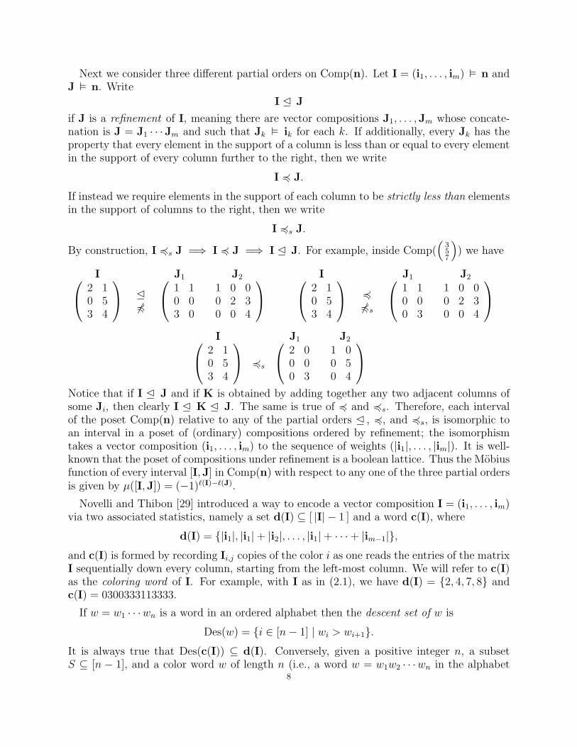
Next we consider three different partial orders on Comp(n). Let I = (i1, . . . , im) � n andJ � n. Write

I E J

if J is a refinement of I, meaning there are vector compositions J1, . . . ,Jm whose concate-nation is J = J1 · · ·Jm and such that Jk � ik for each k. If additionally, every Jk has theproperty that every element in the support of a column is less than or equal to every elementin the support of every column further to the right, then we write

I 4 J.

If instead we require elements in the support of each column to be strictly less than elementsin the support of columns to the right, then we write

I 4s J.

By construction, I 4s J =⇒ I 4 J =⇒ I E J. For example, inside Comp((

357

)) we have

I J1 J2 2 10 53 4

E64

1 10 03 0

1 0 00 2 30 0 4

I J1 J2 2 1

0 53 4

464s

1 10 00 3

1 0 00 2 30 0 4

I J1 J2 2 1

0 53 4

4s

2 00 00 3

1 00 50 4

Notice that if I E J and if K is obtained by adding together any two adjacent columns ofsome Ji, then clearly I E K E J. The same is true of 4 and 4s. Therefore, each intervalof the poset Comp(n) relative to any of the partial orders E , 4, and 4s, is isomorphic toan interval in a poset of (ordinary) compositions ordered by refinement; the isomorphismtakes a vector composition (i1, . . . , im) to the sequence of weights (|i1|, . . . , |im|). It is well-known that the poset of compositions under refinement is a boolean lattice. Thus the Mobiusfunction of every interval [I,J] in Comp(n) with respect to any one of the three partial ordersis given by µ([I,J]) = (−1)`(I)−`(J).

Novelli and Thibon [29] introduced a way to encode a vector composition I = (i1, . . . , im)via two associated statistics, namely a set d(I) ⊆ [ |I| − 1 ] and a word c(I), where

d(I) = {|i1|, |i1|+ |i2|, . . . , |i1|+ · · ·+ |im−1|},and c(I) is formed by recording Ii,j copies of the color i as one reads the entries of the matrixI sequentially down every column, starting from the left-most column. We will refer to c(I)as the coloring word of I. For example, with I as in (2.1), we have d(I) = {2, 4, 7, 8} andc(I) = 0300333113333.

If w = w1 · · ·wn is a word in an ordered alphabet then the descent set of w is

Des(w) = {i ∈ [n− 1] | wi > wi+1}.It is always true that Des(c(I)) ⊆ d(I). Conversely, given a positive integer n, a subsetS ⊆ [n − 1], and a color word w of length n (i.e., a word w = w1w2 · · ·wn in the alphabet

8

[0, l − 1]) such that Des(w) ⊆ S, there is a unique vector composition I such that d(I) = Sand c(I) = w. Note that

I 4 J if and only if c(I) = c(J) and d(I) ⊆ d(J).

In the following, most notably in §§2.7, besides the notion of vector compositions, we willneed the analogous notion of a vector partition. For us a vector partition will be a multisetλ of l -partite numbers λ = {λ1, . . . ,λm}. Note for example that the multiset cols(I) of thecolumns of a given vector composition I is in fact a vector partition.

We conclude this subsection with two more definitions. If u = u1u2 . . . un ∈ [0, l − 1]n isa color word and ni is the number of occurrences of color i for each i ∈ [0, l − 1], then wedefine the multidegree of u to be

(2.2) deg(u) =

n0...

nl−1

.

We also associate a vector composition Eu to each such color word u:

Eu = (eu1 , · · · , eun).

A vector composition that is either empty or whose columns consist of coordinate vectors(i.e., standard basis vectors) will be called a coordinate vector composition.

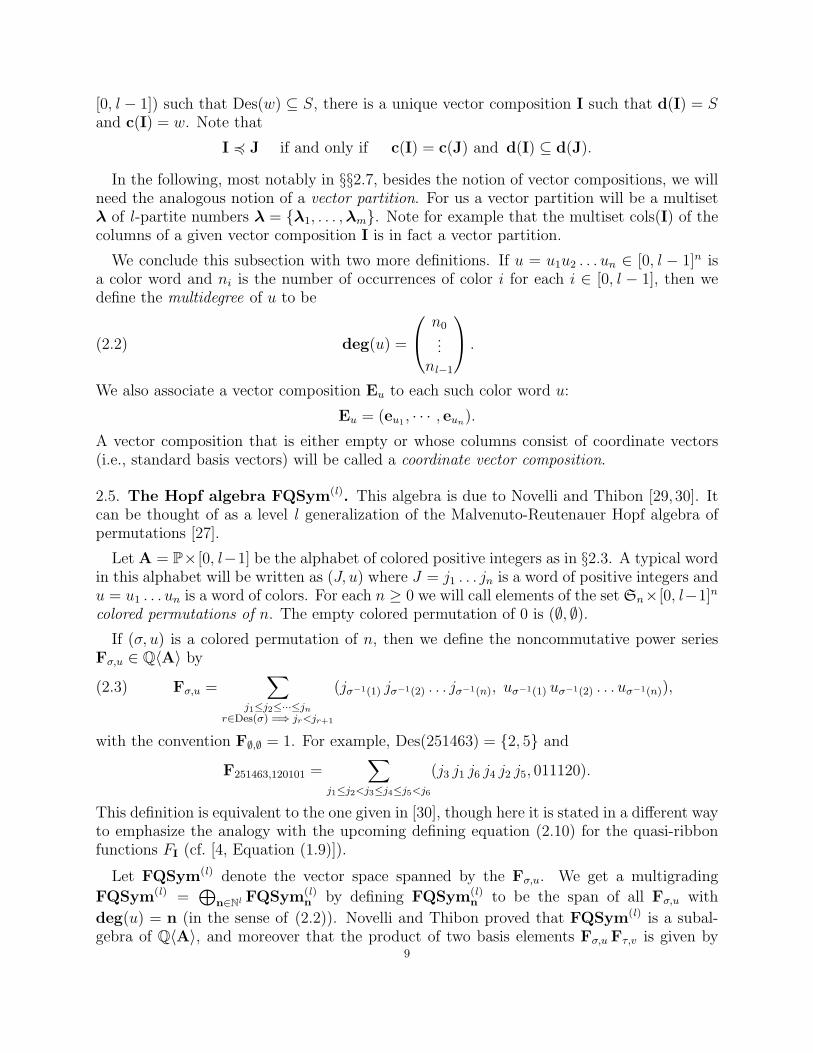
2.5. The Hopf algebra FQSym(l). This algebra is due to Novelli and Thibon [29, 30]. Itcan be thought of as a level l generalization of the Malvenuto-Reutenauer Hopf algebra ofpermutations [27].

Let A = P× [0, l−1] be the alphabet of colored positive integers as in §2.3. A typical wordin this alphabet will be written as (J, u) where J = j1 . . . jn is a word of positive integers andu = u1 . . . un is a word of colors. For each n ≥ 0 we will call elements of the set Sn×[0, l−1]n

colored permutations of n. The empty colored permutation of 0 is (∅, ∅).If (σ, u) is a colored permutation of n, then we define the noncommutative power series

Fσ,u ∈ Q〈A〉 by

(2.3) Fσ,u =∑

j1≤j2≤···≤jnr∈Des(σ) =⇒ jr<jr+1

(jσ−1(1) jσ−1(2) . . . jσ−1(n), uσ−1(1) uσ−1(2) . . . uσ−1(n)),

with the convention F∅,∅ = 1. For example, Des(251463) = {2, 5} and

F251463,120101 =∑

j1≤j2<j3≤j4≤j5<j6

(j3 j1 j6 j4 j2 j5, 011120).

This definition is equivalent to the one given in [30], though here it is stated in a different wayto emphasize the analogy with the upcoming defining equation (2.10) for the quasi-ribbonfunctions FI (cf. [4, Equation (1.9)]).

Let FQSym(l) denote the vector space spanned by the Fσ,u. We get a multigrading

FQSym(l) =⊕

n∈Nl FQSym(l)n by defining FQSym(l)

n to be the span of all Fσ,u with

deg(u) = n (in the sense of (2.2)). Novelli and Thibon proved that FQSym(l) is a subal-gebra of Q〈A〉, and moreover that the product of two basis elements Fσ,u Fτ,v is given by

9

shifted shuffling ; i.e., to get the result, we simply shift the letters of τ up by the length of σ,then shuffle σ and τ together, all the while keeping track of their corresponding colors. Forexample,

F21,02 F12,10 = F2134,0210 + F2314,0120 + F2341,0102 + F3241,1002 + F3214,1020 + F3421,1002.

The coproduct on FQSym(l) is defined by breaking up σ into a concatenation of two(possibly empty) subwords, σ = τ τ ′ and taking the standardization of each subword τ andτ ′. For example,

∆(F1423,0021) = 1⊗F1423,0021 +F1,0⊗F312,021 +F12,00⊗F12,21 +F132,002⊗F1,1 +F1423,0021⊗1.

We refer the reader to [30] for further details and precise definitions.

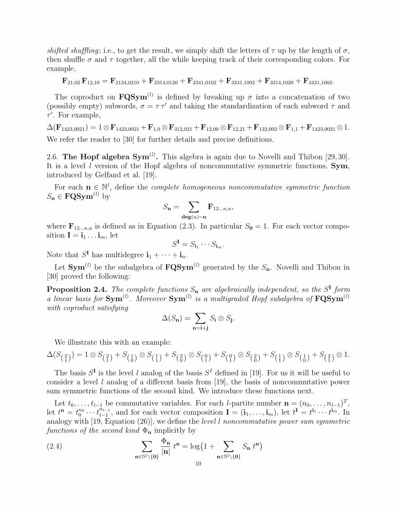
2.6. The Hopf algebra Sym(l). This algebra is again due to Novelli and Thibon [29, 30].It is a level l version of the Hopf algebra of noncommutative symmetric functions, Sym,introduced by Gelfand et al. [19].

For each n ∈ Nl , define the complete homogeneous noncommutative symmetric functionSn ∈ FQSym(l) by

Sn =∑

deg(u)=n

F12...n,u,

where F12...n,u is defined as in Equation (2.3). In particular S0 = 1. For each vector compo-sition I = i1 . . . im, let

SI = Si1 · · ·Sim .

Note that SI has multidegree i1 + · · ·+ in.

Let Sym(l) be the subalgebra of FQSym(l) generated by the Sn. Novelli and Thibon in[30] proved the following:

Proposition 2.4. The complete functions Sn are algebraically independent, so the SI forma linear basis for Sym(l). Moreover Sym(l) is a multigraded Hopf subalgebra of FQSym(l)

with coproduct satisfying

∆(Sn) =∑

n=i+j

Si ⊗ Sj.

We illustrate this with an example:

∆(S( 21 )) = 1⊗ S( 2

1 ) + S( 10 ) ⊗ S( 1

1 ) + S( 20 ) ⊗ S( 0

1 ) + S( 01 ) ⊗ S( 2

0 ) + S( 11 ) ⊗ S( 1

0 ) + S( 21 ) ⊗ 1.

The basis SI is the level l analog of the basis SI defined in [19]. For us it will be useful toconsider a level l analog of a different basis from [19], the basis of noncommutative powersum symmetric functions of the second kind. We introduce these functions next.

Let t0, . . . , tl−1 be commutative variables. For each l -partite number n = (n0, . . . , nl−1)T ,let tn = tn0

0 · · · tnl−1

l−1 , and for each vector composition I = (i1, . . . , im), let tI = ti1 · · · tim . Inanalogy with [19, Equation (26)], we define the level l noncommutative power sum symmetricfunctions of the second kind Φn implicitly by

(2.4)∑

n∈Nl\{0}

Φn

|n|tn = log

(1 +

∑n∈Nl\{0}

Sn tn)

10

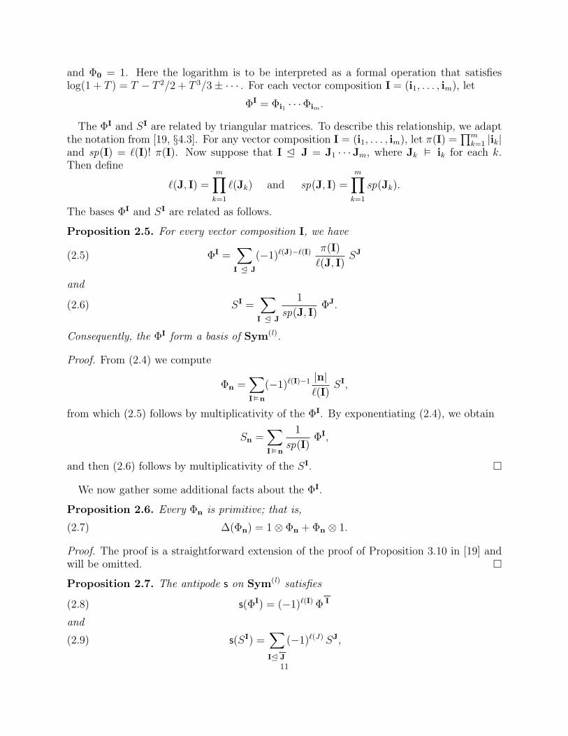
and Φ0 = 1. Here the logarithm is to be interpreted as a formal operation that satisfieslog(1 + T ) = T − T 2/2 + T 3/3± · · · . For each vector composition I = (i1, . . . , im), let

ΦI = Φi1 · · ·Φim .

The ΦI and SI are related by triangular matrices. To describe this relationship, we adaptthe notation from [19, §4.3]. For any vector composition I = (i1, . . . , im), let π(I) =

∏mk=1 |ik|

and sp(I) = `(I)! π(I). Now suppose that I E J = J1 · · ·Jm, where Jk � ik for each k.Then define

`(J, I) =m∏k=1

`(Jk) and sp(J, I) =m∏k=1

sp(Jk).

The bases ΦI and SI are related as follows.

Proposition 2.5. For every vector composition I, we have

(2.5) ΦI =∑I E J

(−1)`(J)−`(I) π(I)

`(J, I)SJ

and

(2.6) SI =∑I E J

1

sp(J, I)ΦJ.

Consequently, the ΦI form a basis of Sym(l).

Proof. From (2.4) we compute

Φn =∑I�n

(−1)`(I)−1 |n|`(I)

SI,

from which (2.5) follows by multiplicativity of the ΦI. By exponentiating (2.4), we obtain

Sn =∑I�n

1

sp(I)ΦI,

and then (2.6) follows by multiplicativity of the SI. �

We now gather some additional facts about the ΦI.

Proposition 2.6. Every Φn is primitive; that is,

(2.7) ∆(Φn) = 1⊗ Φn + Φn ⊗ 1.

Proof. The proof is a straightforward extension of the proof of Proposition 3.10 in [19] andwill be omitted. �

Proposition 2.7. The antipode s on Sym(l) satisfies

(2.8) s(ΦI) = (−1)`(I) Φ←−I

and

(2.9) s(SI) =∑IE←−J

(−1)`(J) SJ,

11

where←−I is the vector composition obtained by reading the columns of I in reverse order.

Proof. It follows from (2.7) that s(Φn) = −Φn. Since s is an anti-homomorphism of algebras,(2.8) follows. Next, following the same argument leading up to Equation (2.14) in [27], wehave ∑

n≥0

s(Sn) tn = s

(∑n≥0

Sn tn

)= s

(exp

(∑n6=0

Φn tn

))

= exp

(∑n6=0

s(Φn) tn

)= exp

(∑n6=0

−Φn tn

)=

(∑n≥0

Sn tn

)−1

which implies

s(Sn) =∑I�n

(−1)`(I)SI.

Again since s is an anti-homomorphism, (2.9) follows. �

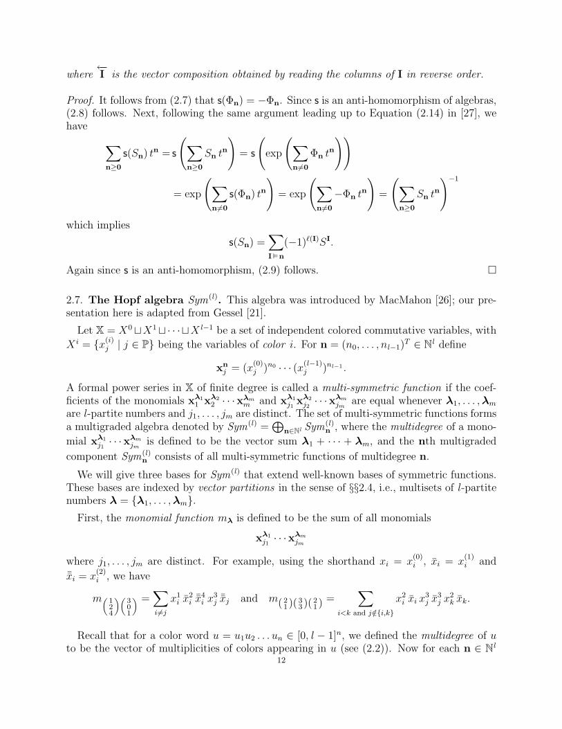
2.7. The Hopf algebra Sym(l). This algebra was introduced by MacMahon [26]; our pre-sentation here is adapted from Gessel [21].

Let X = X0tX1t· · ·tX l−1 be a set of independent colored commutative variables, with

X i = {x(i)j | j ∈ P} being the variables of color i. For n = (n0, . . . , nl−1)T ∈ Nl define

xnj = (x

(0)j )n0 · · · (x(l−1)

j )nl−1 .

A formal power series in X of finite degree is called a multi-symmetric function if the coef-ficients of the monomials xλ1

1 xλ22 · · ·xλm

m and xλ1j1

xλ2j2· · ·xλm

jmare equal whenever λ1, . . . ,λm

are l -partite numbers and j1, . . . , jm are distinct. The set of multi-symmetric functions formsa multigraded algebra denoted by Sym(l) =

⊕n∈Nl Sym(l)

n , where the multidegree of a mono-

mial xλ1j1· · ·xλm

jmis defined to be the vector sum λ1 + · · · + λm, and the nth multigraded

component Sym(l)n consists of all multi-symmetric functions of multidegree n.

We will give three bases for Sym(l) that extend well-known bases of symmetric functions.These bases are indexed by vector partitions in the sense of §§2.4, i.e., multisets of l -partitenumbers λ = {λ1, . . . ,λm}.

First, the monomial function mλ is defined to be the sum of all monomials

xλ1j1· · ·xλm

jm

where j1, . . . , jm are distinct. For example, using the shorthand xi = x(0)i , xi = x

(1)i and

¯xi = x(2)i , we have

m„ 124

«„301

« =∑i 6=j

x1i x

2i

¯x4i x

3j

¯xj and m( 21 )( 3

3 )( 21 ) =

∑i<k and j /∈{i,k}

x2i xi x

3j x

3j x

2k xk.

Recall that for a color word u = u1u2 . . . un ∈ [0, l − 1]n, we defined the multidegree of uto be the vector of multiplicities of colors appearing in u (see (2.2)). Now for each n ∈ Nl

12

with weight n = |n|, we can define the complete function hn by

hn =∑

u=u1u2...un∈[0,l−1]n

deg(u)=n

∑j1≤j2≤···≤jn

x(u1)j1

x(u2)j2· · ·x(un)

jn.

For example, there are two color words u = 01 and u = 10 of multidegree ( 11 ), so

h( 11 ) =

∑i≤j

xixj +∑i≤j

xixj = 2m( 11 ) +m( 1

0 )( 01 ).

The basis hλ is defined multiplicatively, by hλ = hλ1hλ1 · · · .Lastly, we define the power sum function pn by

pn =∞∑j=1

xnj = mn.

and set pλ = pλ1pλ2 · · · . Again the multi-symmetric functions pλ form a basis for Sym(l).

We can define a coproduct in Sym(l) by generalizing the coproduct of ordinary symmetricfunctions:

∆(pn) = 1⊗ pn + pn ⊗ 1.

Alternatively, the same coproduct can be defined by the usual method of introducing aduplicate set of variables Y and letting ∆(f(X)) = f(X+ Y).

2.8. The Hopf algebra QSym(l). This algebra is due to Poirier [31]; our presentation isadapted from Novelli and Thibon [29,30].

Let X = X0tX1t· · ·tX l−1 be commutative colored variables as before. A formal powerseries in X of finite degree is called a quasisymmetric function of level l if the coefficientsof the monomials xi1

1 · · ·ximm and xi1

j1· · ·xim

jmare equal whenever j1 < · · · < jm and I =

(i1, . . . , im) is a vector composition. The set of quasisymmetric functions of level l forms

a multigraded vector space QSym(l) =⊕

n∈Nl QSym(l)n with various natural bases indexed

by vector compositions. The nth multigraded component QSym(l)n is the vector space of

homogeneous quasisymmetric functions of multidegree n, where once again we define themultidegree of a monomial xi1

1 · · ·ximm as the vector sum i1 + · · ·+ im.

Here we will consider two bases. First is the quasisymmetric analog of the monomialmulti-symmetric functions mλ. For a nonempty vector composition I = (i1, . . . , im), definethe level l monomial quasisymmetric function MI by

MI =∑

j1<···<jm

xi1j1· · ·xim

jm

and let M( ) = 1. For example,

M„1 32 04 1

« =∑i<j

xi x2i

¯x4i x

3j

¯xj and M( 2 3 21 3 1 ) =

∑i<j<k

x2i xi x

3j x

3j x

2k xk.

As in the level 1 case (see, e.g., [17, Lemma 3.3]), and as observed by Aval et al. [5] in thelevel-2 case, multiplying two monomial functions MIMJ can be described in terms of quasi-shuffling. A quasi-shuffle of two vector compositions I and J is a shuffling of the columns of

13

I with the columns of J in which two columns may be added together as they are shuffledpast each other. An example should make this clear:

M( 1 30 2 )M( 2 1

5 0 ) =M( 1 3 2 10 2 5 0 ) +M( 1 5 1

0 7 0 ) +M( 1 2 3 10 5 2 0 ) +M( 1 2 4

0 5 2 ) +M( 1 2 1 30 5 0 2 ) +M( 3 3 1

5 2 0 )

+M( 3 45 2 ) +M( 3 1 3

5 0 2 ) +M( 2 1 3 15 0 2 0 ) +M( 2 1 4

5 0 2 ) +M( 2 2 35 0 2 ) + 2M( 2 1 1 0

5 0 0 2 ).

Thus QSym(l) is a quasi-shuffle algebra. General properties of such algebras are discussed in[22,25].

The coproduct is given on the monomial basis by

∆(MI) =∑I=JK

MJ ⊗MK,

the sum being over all ways of writing I as a concatenation of two (possibly empty) vectorcompositions J and K. For example,

∆(M( 1 0 2

4 3 0 ))

= 1⊗M( 1 0 24 3 0 ) +M( 1

4 ) ⊗M( 0 23 0 ) +M( 1 0

4 3 ) ⊗M( 20 ) +M( 1 0 2

4 3 0 ) ⊗ 1.

This coproduct can be equivalently defined by the usual method of introducing a duplicateset of variables Y and letting ∆(f(X)) = f(X+ Y).

It is clear from the definitions that Sym(l) is a Hopf subalgebra of QSym(l), and that themonomial bases of these two algebras are related by

mλ =∑

cols(I)=λ

MI

where cols(I) denotes the multiset of columns of I.

Next we consider the basis of level l quasi-ribbon functions FI, defined by

(2.10) FI =∑

j1≤j2≤···≤jnr∈d(I) =⇒ jr<jr+1

x(u1)j1· · ·x(un)

jn=∑I4J

MJ

where I is a nonempty vector composition of weight n, and u1 · · ·un = c(I). For example,

F„ 2 00 11 0

« =∑

i≤j≤k<`

xixj ¯xkx` = M„2 00 11 0

« +M„2 0 00 0 10 1 0

« +M„1 1 00 0 10 1 0

« +M„1 1 0 00 0 0 10 0 1 0

«.This basis specializes to Gessel’s fundamental basis [20] when l = 1. Unlike the level 1 case,however, the product FI FJ is not always F -positive. For example,

F„ 1 00 00 1

«F„ 010

« = F„ 0 1 01 0 00 0 1

« + F„ 1 01 00 1

« + F„ 1 00 10 1

« − F„ 1 0 00 1 00 0 1

« + F„ 1 0 00 0 10 1 0

«.

2.9. Duality between QSym(l) and Sym(l). As Novelli and Thibon observed [29,30], the

multigraded dual Hopf algebra of Sym(l) may be identified with QSym(l) by making SI

the dual basis of MJ. More precisely, for each n we have (QSym(l)n )∗ = Sym(l)

n , for any

two vector compositions I and J we have SI(MJ) = δI,J, and for any T, U ∈ Sym(l) and

G,H ∈ QSym(l), we have

TU(G) =∑

T (G1)U(G2) and T (GH) =∑

T1(G)T2(H),

where ∆(G) =∑G1 ⊗G2 and ∆(T ) =

∑T1 ⊗ T2 in Sweedler notation.

14

We can use this duality in several ways. As an example, if we let sQ denote the antipodeon QSym(l), then by taking the dual of (2.9), we get

(2.11) sQ(MI) = (−1)`(I)∑JE←−I

MJ.

As before,←−I is the vector composition obtained by reversing the order of the columns of I.

There is yet another interesting pair of dual bases for these two Hopf algebras. Let usdefine PI to be the basis of QSym(l) that is dual to the power sum basis ΦI of Sym(l). Thus,

ΦI(PJ) = δI,J.

Then by (2.6) we get

PI =∑JE I

1

sp(I,J)MJ.

Since the Φn are primitive, the PI make up a shuffle basis for QSym(l). It is well-known thata shuffle algebra is freely generated by its Lyndon words; see, for example, [32, Theorem 6.1].We will come back to these ideas in §§5.1.

3. The category of multigraded combinatorial Hopf algebras

In this section we define the category of multigraded combinatorial Hopf algebras andderive a universal property satisfied by QSym(l) similar to, and inspired by, [2, Theorem 4.1].

This leads to a systematic way to investigate morphisms H → QSym(l). The closely relatedcategory of colored combinatorial Hopf algebras was explained by Bergeron and Hohlweg[12] and studied further in [23]. We describe how to relate our work to these earlier versionsin the second half of this section.

We will work over the rationals Q, but results in this section are valid over any field.

3.1. Definitions. Let H =⊕

n∈Nl Hn be a multigraded connected Hopf algebra over Q. Letϕ : H → Q be a multiplicative invertible linear functional, or a character, on H (see §§4.3for more on (convolution) invertible linear functionals). Then we say that the ordered pair(H, ϕ) (or simply H if ϕ is unambiguous from the context) is a multigraded combinatorialHopf algebra. Morphisms in the category of multigraded combinatorial Hopf algebras arehomomorphisms Ψ : H → H′ of Nl -graded Hopf algebras for the multigraded combinatorialHopf algebras (H, ϕ) and (H′, ϕ′) such that ϕ = ϕ′ ◦Ψ.

When l = 1 we recover the original construction of a combinatorial Hopf algebra in [2].

Each of the algebras discussed in §2 can be naturally made into a multigraded combi-natorial Hopf algebra by pairing it with a character. In the context of this paper, themost important example is the Hopf algebra QSym(l) paired with the universal character

ζQ : QSym(l) → Q, defined by setting each of the variables x(0)1 , x

(1)1 , . . . , x

(l−1)1 to 1 and all

other variables x(i)j , j 6= 1, to 0. Alternatively, ζQ can be defined by

(3.1) ζQ(MI) = ζQ(FI) =

{1 if I = ( ) or `(I) = 1

0 otherwise.15

Clearly ζQ is a character since it is an evaluation map. The significance of this character willbe discussed next.

3.2. Universality of the Hopf algebra QSym(l). The pair (QSym(l), ζQ) is terminal inthe category of multigraded combinatorial Hopf algebras; this generalizes the l = 1 case[2, Theorem 4.1]. More specifically we have:

Theorem 3.1. For every multigraded combinatorial Hopf algebra (H, ζ), there exists a

unique morphism Ψ : (H, ζ)→ (QSym(l), ζQ). Explicitly, if n ∈ Nl and h ∈ Hn then

(3.2) Ψ(h) =∑I�n

ζI(h)MI

where if I = (i1, . . . , ip) then ζI is the composite map

H ∆(p−1)

−−−−→ H⊗p projection−−−−−→ Hi1 ⊗ · · · ⊗ Hip

ζ⊗p

−−→ Q⊗p multiplication−−−−−−−→ Q.

This theorem is actually just the k = 0 case of Theorem 4.13 (and also of Theorem 4.22),so we will defer the proof until §4 and focus on examples for now.

Example 3.2. Recall that we introduced the Hopf algebra R(l) of multigraded posets in§§2.1. Now we define ζ : R(l) → Q to be

ζ(P ) = 1 for every multigraded poset P .

Clearly ζ is a character, so (R(l), ζ) is a multigraded combinatorial Hopf algebra. Theorem

3.1 then implies that we have a morphism F : R(l) → QSym(l) such that ζQ ◦ F = ζ. Asobserved in [2, Example 4.4], the l = 1 version of this morphism is the F -homomorphismintroduced by Ehrenborg [17].

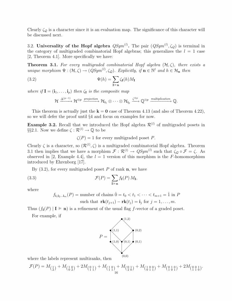
By (3.2), for every multigraded poset P of rank n, we have

(3.3) F(P ) =∑I�n

fI(P )MI,

wherefi1i2...im(P ) = number of chains 0 = t0 < t1 < · · · < tm+1 = 1 in P

such that rk(tj+1)− rk(tj) = ij for j = 1, . . . ,m.

Thus (fI(P ) | I � n) is a refinement of the usual flag f -vector of a graded poset.

For example, if

P =

s@@@ ���

s s@@@ ���s

s��� s@@@s

(0,0)

(1,0) (0,1) (0,1)

(1,1) (0,2)

(1,2)

where the labels represent multiranks, then

F(P ) = M( 12 ) +M( 1 0

0 2 ) + 2M( 0 11 1 ) +M( 1 0

1 1 ) +M( 0 12 0 ) +M( 1 0 0

0 1 1 ) +M( 0 1 01 0 1 ) + 2M( 0 0 1

1 1 0 ).

16

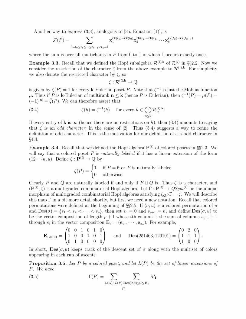
Another way to express (3.3), analogous to [35, Equation (1)], is

F(P ) =∑

0=t0≤t1≤···≤tk−1<tk=1

xrk(t1)−rk(t0)1 x

rk(t2)−rk(t1)2 · · ·xrk(tk)−rk(tk−1)

k

where the sum is over all multichains in P from 0 to 1 in which 1 occurs exactly once.

Example 3.3. Recall that we defined the Hopf subalgebra R(l),k of R(l) in §§2.2. Now weconsider the restriction of the character ζ from the above example to R(l),k. For simplicitywe also denote the restricted character by ζ, so

ζ : R(l),k → Qis given by ζ(P ) = 1 for every k-Eulerian poset P . Note that ζ−1 is just the Mobius functionµ. Thus if P is k-Eulerian of multirank n ≤ k (hence P is Eulerian), then ζ−1(P ) = µ(P ) =(−1)|n| = ζ(P ). We can therefore assert that

(3.4) ζ(h) = ζ−1(h) for every h ∈⊕n≤k

R(l),kn .

If every entry of k is ∞ (hence there are no restrictions on h), then (3.4) amounts to sayingthat ζ is an odd character, in the sense of [2]. Thus (3.4) suggests a way to refine thedefinition of odd character. This is the motivation for our definition of a k-odd character in§4.4.

Example 3.4. Recall that we defined the Hopf algebra P(l) of colored posets in §§2.3. Wewill say that a colored poset P is naturally labeled if it has a linear extension of the form(12 · · ·n, u). Define ζ : P(l) → Q by

ζ(P ) =

{1 if P = ∅ or P is naturally labeled

0 otherwise.

Clearly P and Q are naturally labeled if and only if P t Q is. Thus ζ is a character, and(P(l), ζ) is a multigraded combinatorial Hopf algebra. Let Γ : P(l) → QSym(l) be the uniquemorphism of multigraded combinatorial Hopf algebras satisfying ζQ◦Γ = ζ. We will describethis map Γ in a bit more detail shortly, but first we need a new notation. Recall that coloredpermutations were defined at the beginning of §§2.5. If (σ, u) is a colored permutation of nand Des(σ) = {s1 < s2 < · · · < sp}, then set s0 = 0 and sp+1 = n, and define Des(σ, u) tobe the vector composition of length p + 1 whose ith column is the sum of columns si−1 + 1through si in the vector composition Eu = (eu1 , · · · , eun). For example,

E120101 =

0 0 1 0 1 01 0 0 1 0 10 1 0 0 0 0

and Des(251463, 120101) =

0 2 01 1 11 0 0

.

In short, Des(σ, u) keeps track of the descent set of σ along with the multiset of colorsappearing in each run of ascents.

Proposition 3.5. Let P be a colored poset, and let L(P ) be the set of linear extensions ofP . We have

(3.5) Γ(P ) =∑

(σ,u)∈L(P )

∑Des(σ,u)E IEEu

MI.

17

Proof. For each subset I ⊆ P , let deg(I) = (n0, . . . , nl−1)T ∈ Nl where ni is the number ofelements in I with color i. By (3.2) we have

Γ(P ) =∑

∅=I0(I1(I2(···(Im=P

ζ(st(I1 \ I0))ζ(st(I2 \ I1)) · · · ζ(st(Im \ Im−1))

·M(deg(I1\I0),deg(I2\I1),...,deg(Im\Im−1))

where the sum is over all chains of order ideals in P . By the definition of ζ we only need tosum over chains ∅ = I0 ( · · · ( Im = P such that st(Ii \ Ii−1) is naturally labeled for each i.For every such chain C, let [Ii \ Ii−1] denote the word obtained by reading the elements ofIi \ Ii−1 in order of increasing absolute value, and let π(C) = [I1 \ I0] · · · [Im \ Im−1]. Thusπ(C) is a linear extension of P , written as a concatenation of subwords with no descents.This linear extension (and its decomposition into subwords) contributes a term of the formMI, Des(π(C)) E I E Eu to our expression for Γ(P ), where u = c(π(C)). Conversely, forany linear extension (σ, u) ∈ L(P ) and any I = (i1, . . . , im) such that Des(σ, u) E I E Eu,we can find a unique chain C = {∅ = I0 ( I1 ( · · · ( Im = P} with π(C) = (σ, u) anddeg(Ij \ Ij−1) = ij for every j by letting I1 be the first |i1| elements of (σ, u), I2 \ I1 be thenext |i2| elements of (σ, u), and so forth. �

Another way to get from P(l) to QSym(l) is through the Hopf algebra R(l) of multigradedposets. If P is a colored poset, let J(P ) as usual denote the poset (distributive lattice) oforder ideals of P ordered by inclusion. We make J(P ) into a multigraded poset by definingthe multirank of an order ideal I ∈ J(P ) to be the multidegree of I as a colored poset (i.e.,the vector of multiplicities of the colors appearing in I). This gives us a map

J : P(l) → R(l)

which is easily shown to be a morphism of Hopf algebras using elementary properties of orderideals. Notice that J(P ) depends only on the colors of the elements of P and not on theirabsolute values. When l = 1 this is essentially the map considered in [2, Example 2.4].

Example 3.6. Recall that we defined the Hopf algebra FQSym(l) in §§2.5. Now we defineζ : FQSym(l) → Q by

ζ(Fσ,u) =

{1 if σ is the identity permutation in Sn for some n

0 otherwise.

It is easy to see that ζ is a character, so by Theorem 3.1, there is a unique morphism ofmultigraded combinatorial Hopf algebras D : FQSym(l) → QSym(l) such that ζQ ◦ D = ζ.

Now using (3.2), we can see that

(3.6) D(Fσ,u) =∑

Des(σ,u) E I E (eu1 ,...,eun )

MI =∑

j1≤j2≤···≤jnr∈Des(σ) =⇒ jr<jr+1

x(u1)j1

x(u2)j2· · ·x(un)

jn.

As a special case of (3.6), if Des(u) ⊆ Des(σ) then

(3.7) D(Fσ,u) = FDes(σ,u).

It also follows from (3.6) that for every n ∈ Nl ,

D(Sn) = hn.18

Thus Sym(l) is the commutative image of Sym(l) under D.

Novelli and Thibon [30] noted that each FI arises as the commutative image of certain

Fσ,u under the abelianization map ab : Q〈A〉 � Q[X], (j, i) 7→ x(i)j . Comparing (2.3) with

(3.6), we see that the morphism D is in fact just the restriction of ab. To summarize, thediagram

Sym(l) � � //

D����

FQSym(l) � � //

D����

Q〈〈A〉〉

ab����

Sym(l) � � // QSym(l) � � // Q[[X]]

is commutative (cf. [4, §1.3]).

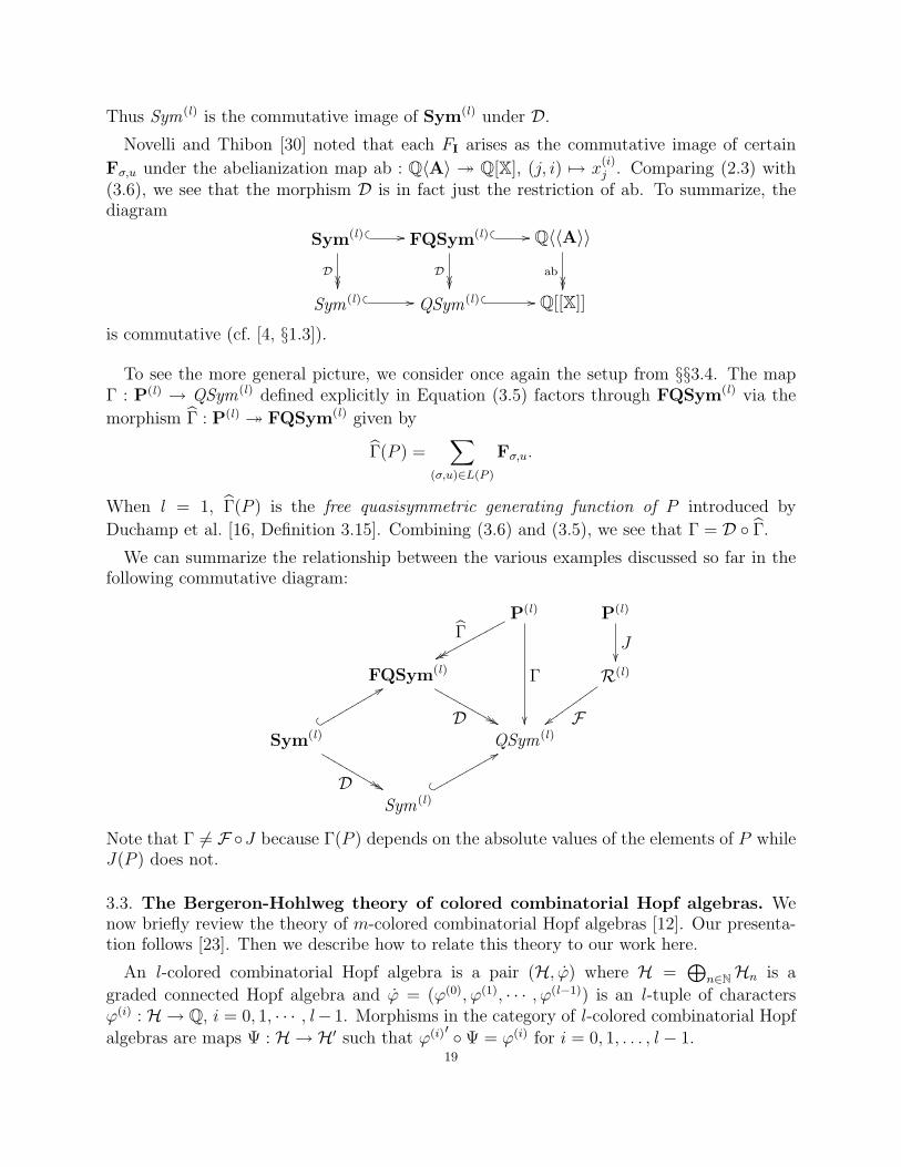
To see the more general picture, we consider once again the setup from §§3.4. The mapΓ : P(l) → QSym(l) defined explicitly in Equation (3.5) factors through FQSym(l) via the

morphism Γ : P(l) � FQSym(l) given by

Γ(P ) =∑

(σ,u)∈L(P )

Fσ,u.

When l = 1, Γ(P ) is the free quasisymmetric generating function of P introduced by

Duchamp et al. [16, Definition 3.15]. Combining (3.6) and (3.5), we see that Γ = D ◦ Γ.

We can summarize the relationship between the various examples discussed so far in thefollowing commutative diagram:

P(l)

Γxxxxppppppppppp

Γ

��

P(l)

J��

FQSym(l)

D && &&MMMMMMMMMM R(l)

Fzzvvvvvvvvv

Sym(l)

+ �

88rrrrrrrrrr

D && &&LLLLLLLLLLQSym(l)

Sym(l)

+ �

88qqqqqqqqqq

Note that Γ 6= F ◦J because Γ(P ) depends on the absolute values of the elements of P whileJ(P ) does not.

3.3. The Bergeron-Hohlweg theory of colored combinatorial Hopf algebras. Wenow briefly review the theory of m-colored combinatorial Hopf algebras [12]. Our presenta-tion follows [23]. Then we describe how to relate this theory to our work here.

An l -colored combinatorial Hopf algebra is a pair (H, ϕ) where H =⊕

n∈NHn is a

graded connected Hopf algebra and ϕ = (ϕ(0), ϕ(1), · · · , ϕ(l−1)) is an l -tuple of charactersϕ(i) : H → Q, i = 0, 1, · · · , l − 1. Morphisms in the category of l -colored combinatorial Hopfalgebras are maps Ψ : H → H′ such that ϕ(i)′ ◦Ψ = ϕ(i) for i = 0, 1, . . . , l − 1.

19

Remark 3.7. To see explicitly how the l -colored combinatorial Hopf algebras (H, ϕ) of [12]correspond to the l -colored combinatorial Hopf algebras (H, ϕ) of [23], recall first that for[12], an l -colored combinatorial Hopf algebra is a pair (H, ϕ) where H =

⊕n∈NHn and

ϕ : H → Q[Cl ]. Here Cl is the cyclic group generated by w, a primitive lth root of unity.Elements of Q[Cl ] are polynomial expressions of the form q0 + q1w + q2w

2 + · · · + ql−1wl−1

where qi ∈ Q for each i = 0, 1, · · · , l − 1. To make these two definitions of l -coloredcombinatorial Hopf algebras compatible, the multiplication in Q[Cl ] should be defined on thecolor components via:

wiwj =

{wi if i = j;

0 otherwise

and extended linearly [23]. Then we can identify any particular map ϕ : H → Q[Cl ] with anl -tuple ϕ = (ϕ(0), ϕ(1), · · · , ϕ(l−1)) by first defining the functions qi : H → Q such that forany h ∈ H we have:

ϕ(h) = q0(h) + q1(h)w + q2(h)w2 + · · ·+ ql−1(h)wl−1.

Then we simply set ϕ(i) = qi for i = 0, 1, · · · , l − 1. We will have:

ϕ(h) = ϕ(0)(h) + ϕ(1)(h)w + ϕ(2)(h)w2 + · · ·+ ϕ(l−1)(h)wl−1 for all h ∈ H.

The terminal object in this category is the Hopf algebra QSym [l ] of l -colored quasisym-metric functions, first studied by Poirier [31]. The bases of QSym [l ] are typically indexed byl -colored compositions α = ((α1, u1), . . . , (αm, um)), where (α1, . . . , αm) is an integer compo-sition (vector of positive integers) and u1 . . . um ∈ [0, l−1]m is a color vector. In the following

we will write α � l n when α is an l -colored composition of n. A natural basis for QSym [l ]

is the set of colored monomial quasisymmetric functions M(l)α , defined by

M (l)α =

∑(j1,u1)<lex···<lex(jm,um)

(x(u1)j1

)α1(x(u2)j2

)α2 · · · (x(um)jm

)αm

where <lex refers to the lexicographic order on P× [0, l − 1].

Baumann and Hohlweg [6] proved that QSym [l ] is a Hopf subalgebra of QSym(l). A

different but isomorphic realization of QSym [l ] was introduced by Novelli and Thibon [29].

To see that QSym [l ] ⊆ QSym(l), note that the monomial functions M(l)α can be written in

the monomial basis MI as follows (recall that ei denotes the ith coordinate vector in Nl andthat the partial order 4s is defined in §2.4):

(3.8) M (l)α =

∑I4s(α1·eu1 ,...,αm·eum )

MI

with α = ((α1, u1), . . . , (αm, um)). For example,

M(3)((2,1),(1,0),(1,2),(3,0)) =

∑i1<i2<i3<i4

(x(1)i1

)2(x(0)i2

)(x(2)i3

)(x(0)i4

)3 +∑

i1<i2<i3

(x(1)i1

)2(x(0)i2

)(x(2)i2

)(x(0)i3

)3

= M„0 1 0 32 0 0 00 0 1 0

« +M„0 1 32 0 00 1 0

«.Details of the Hopf algebra structure of QSym [l ] can be found in [12,23,29,30].

20

The universal character ψ = (ψ(0), . . . , ψ(l−1)) of QSym [l ] is defined as a tuple of evaluation

characters: each ψ(i) takes the variable x(i)1 to 1 and all other variables to 0. Equivalently,

ψ(i)(M (l)α ) =

{1 if α = ( ) or α = ((a, i))

0 otherwise.

In [23, Theorem 13] it is shown that for any colored combinatorial Hopf algebra (H, ϕ), there

is a unique morphism Ψc : (H, ϕ) → (QSym [l ], ψ) of colored combinatorial Hopf algebrasgiven explicitly by

(3.9) Ψc(h) =∑α� ln

ϕα(h)M (l)α ,

for any h ∈ Hn, where for α = (ωj1α1, . . . , ωjkαk), ϕα is the composite map:

H ∆(k−1)

−−−−→ H⊗k projection−−−−−→ Hα1 ⊗ · · · ⊗ Hαk

ϕ(j1)⊗···ϕ(jk)

−−−−−−−−→ Q⊗k m−→ Q.

We will now see how QSym(l) fits into this picture. Let ζ(i), i = 0, 1, . . . , l − 1 be the

character on QSym(l) that takes x(i)1 to 1 and all other variables to 0. Let ζ = (ζ(0), . . . , ζ(l−1)),

so (QSym(l), ζ) becomes an l -colored combinatorial Hopf algebra. Note that we are ignoring

the multigrading on QSym(l) and thinking of it as an ordinary graded Hopf algebra QSym(l) =⊕∞n=0 QSym(l)

n , where QSym(l)n =

⊕|n|=n QSym(l)

n .

Since ψ(i) defined above is just the restriction of ζ(i) to the subalgebra QSym [l ], it followsthat (QSym [l ], ψ) is a combinatorial Hopf subalgebra of (QSym(l), ζ).

Proposition 3.8. In the category of colored combinatorial Hopf algebras, the morphism

(QSym [l ], ψ) ↪→ (QSym(l), ζ)

is the inclusion map.

Conversely, the result quoted above [23, Theorem 13] implies that there is a morphism

going in the other direction, (QSym(l), ˙ζQ) → (QSym [l ], ψ). We now describe this mapmore explicitly. A vector composition I will be called monochromatic if it is of the formI = (α1 ·eu1 , α2 ·eu2 , . . . , αm ·eum) for some u1, . . . , um ∈ [0, l−1]. In this case we define w(I)to be the colored composition w(I) = ((α1, u1), . . . , (αm, um)). The following can be provedby a straightforward application of (3.9).

Proposition 3.9. Let Ψc : QSym(l) → QSym [l ] be the unique morphism of graded Hopf

algebras satisfying ψ(i) ◦Ψc = ζ(i)Q for all i. For every vector composition I, we have

Ψc(MI) =

{Mw(I) if I is monochromatic

0 otherwise.

A consequence of Proposition 3.9 is that QSym [l ] can be identified with QSym(l) modulo

the relations x(p)i x

(q)i for p 6= q and i = 1, 2, . . .. This realization of QSym [l ] was first given

by Novelli and Thibon [29].

Lastly, one can view QSym [l ] as a multigraded combinatorial Hopf algebra by pairing itwith the character ψ = ψ(0)ψ(1) · · ·ψ(l−1). Then Theorem 3.1 implies the existence of a

21

morphism Ψ : QSym [l ] → QSym(l) of multigraded combinatorial Hopf algebras satisfyingζQ ◦Ψ = ψ. It is clear from the definitions that

ζQ(M (l)α ) = ψ(M (l)

α ) =

{1 if α = ( ) or α = ((α1, u1), . . . , (αm, um)), u1 < u2 < · · · < um

0 otherwise.

Therefore Ψ is the inclusion map. In other words, the following holds:

Proposition 3.10. In the category of multigraded combinatorial Hopf algebras, the mor-phism

(QSym [l ], ψ) ↪→ (QSym(l), ζQ)

is the inclusion map.

4. Definitions and basic properties of k-odd and k-even Hopf algebras

In this section we develop the notions of k-odd and k-even subalgebras of multigradedcombinatorial Hopf algebras. Our constructions and results directly generalize the definitionsand basic properties of odd and even Hopf subalgebras developed by Aguiar et al. [2].

4.1. Basic constructions. Let H =⊕

n∈Nl Hn be a multigraded connected Hopf algebra.For a linear functional ϕ : H → Q, let ϕn denote the restriction of ϕ to Hn. This is anelement of degree n of the (multi)graded dual H∗. We also define ϕ to be the functionalgiven by ϕ(h) = (−1)|n|ϕ(h) for h ∈ Hn.

Let ϕ, ψ : H → Q be characters. The canonical Hopf subalgebra S(ϕ, ψ) and its orthogonalHopf ideal I(ϕ, ψ) are defined in [2, Section 5] for N-graded Hopf algebras. Generalizing tothe Nl -graded case, we define S(ϕ, ψ) to be the largest graded subcoalgebra of H such that

∀h ∈ S(ϕ, ψ), ϕ(h) = ψ(h),

and I(ϕ, ψ) to be the ideal of H∗ generated by ϕn − ψn for each n ∈ Nl .

We now define k-analogs of these.

Let l be a positive integer, to be fixed for the rest of this section. It will be convenient towork with the “extended” l -partite numbers (N∪{∞})l , where the symbol∞ is understoodto be larger than every natural number.

For k ∈ (N ∪ {∞})l , let Sk(ϕ, ψ) denote the largest graded subcoalgebra of H with theproperty that

(4.1) ϕ(h) = ψ(h) for all h ∈ Sk(ϕ, ψ) ∩⊕n≤k

Hn.

(When forming direct sums it should be understood that our indices lie in Nl .) Equation(4.1) defines Sk(ϕ, ψ) as the largest graded subcoalgebra of H whose graded pieces up todegree k are all contained in ker (ϕ− ψ). In other words, Sk(ϕ, ψ) is the largest gradedsubcoalgebra of H whose intersection with

⊕n≤kHn, the k-initial graded piece of H, lies in

the kernel of ϕ− ψ.22

Note that this last statement is equivalent to asserting that the graded pieces up to degreek of Sk(ϕ, ψ) lie in

⊕n≤k(kerϕn − ψn). Thus, we can alternatively define Sk(ϕ, ψ) as the

largest graded subcoalgebra of H with the property that

(4.2) ∀h ∈ Sk(ϕ, ψ), ϕn(h) = ψn(h) for all n ≤ k.

Next we let Ik(ϕ, ψ) denote the ideal of the graded dual H∗ generated by ϕn − ψn foreach n ≤ k. Each Ik(ϕ, ψ) is generated by homogeneous elements and so is a (multi)gradedideal of H∗.

Recall that 0 ∈ Nl denotes the zero vector. Let ∞ ∈ (N∪ {∞})l denote the vector whoseentries are all ∞. For any k ∈ (N ∪ {∞})l ,

S0(ϕ, ψ) ⊃ Sk(ϕ, ψ) ⊃ S∞(ϕ, ψ) = S(ϕ, ψ)

and

I0(ϕ, ψ) ⊂ Ik(ϕ, ψ) ⊂ I∞(ϕ, ψ) = I(ϕ, ψ).

The properties of S(ϕ, ψ) and I(ϕ, ψ) stated in [2, Theorem 5.3], along with their proofs,extend without difficulty to their k-analogs:

Theorem 4.1. LetH =⊕

n∈Nl Hn be a multigraded connected Hopf algebra and let ϕ, ψ : H → Qbe characters on H. Define Sk(ϕ, ψ) and Ik(ϕ, ψ) as above. For k ∈ (N∪{∞})l the followingproperties hold:

(a) Sk(ϕ, ψ) = (Ik(ϕ, ψ))⊥;(b) Ik(ϕ, ψ) is a graded Hopf ideal of H∗;(c) Sk(ϕ, ψ) is a graded Hopf subalgebra of H.

Here, Ik(ϕ, ψ)⊥ is the set {h ∈ H : f(h) = 0 for all f ∈ Ik(ϕ, ψ)}.

The proof of this result follows the main lines of the proof of [2, Theorem 5.3]. Weinclude it here in order to demonstrate the general feel of the proofs of some of the morestraightforward extensions of the results of [2] to their k-analogs:

Proof. We begin with part (a). Since Ik(ϕ, ψ) is a (multi)graded ideal of H∗, Ik(ϕ, ψ)⊥ is a(multi)graded subcoalgebra of H. Let h =

∑i∈Nl hi ∈ Ik(ϕ, ψ)⊥, where all but finitely many

of the hi are zero and hence the sum is finite. Because ϕi − ψi ∈ Ik(ϕ, ψ) for all i ≤ k, wehave ϕi(h) = ϕi(hi) = ψi(hi) = ψi(h) for all i ≤ k. Then it follows from the definition ofSk(ϕ, ψ) (as the greatest subcoalgebra of H satisfying Equation (4.2)) that h ∈ Sk(ϕ, ψ).

Next let C be a graded subcoalgebra of H such that for all i ≤ k, ϕi(h) = ψi(h) for allh =

∑i∈Nl hi ∈ C; here once again we assume that all but finitely many of the terms hi

are zero. Since C is a coalgebra and Ik(ϕ, ψ) is the ideal generated by ϕi − ψi for i ≤ k,it follows that f(C) = 0 for all f ∈ Ik(ϕ, ψ). This shows that Sk(ϕ, ψ) ⊂ Ik(ϕ, ψ)⊥ andconcludes the proof of part (a).

To prove parts (b) and (c), we begin by noting that the product C · D of two gradedsubcoalgebras of H is again a graded subcoalgebra. This makes Sk(ϕ, ψ) · Sk(ϕ, ψ) a gradedsubcoalgebra of H. By the multiplicativity of ϕ and ψ we have:

(4.3) (ϕ− ψ)(xy) = (ϕ− ψ)(x)ϕ(y) + ψ(x)(ϕ− ψ)(y)23

Now if x, y ∈ Sk(ϕ, ψ) such that xy ∈⊕

n≤kHn, we also have x, y ∈⊕

n≤kHn and soby Equation (4.1), we have (ϕ − ψ)(x) = (ϕ − ψ)(y) = 0. Equation (4.3) then gives us(ϕ− ψ)(xy) = 0. This proves that Sk(ϕ, ψ) · Sk(ϕ, ψ) ⊂ Sk(ϕ, ψ).

Finally we note that H0 = Q · 1 is a graded subcoalgebra of H and ϕ(1) = ψ(1) = 1 sowe can conclude that H0 is included in Sk(ϕ, ψ). This proves part (c), or in other words,that Sk(ϕ, ψ) is indeed a Hopf subalgebra of H. Together with part (a), this implies thatIk(ϕ, ψ) is a coideal of H∗, and thus we are also done with part (b). �

Remark 4.2. A natural k-analog of part (d) of [2, Thm.5.3] is also valid: More specificallyone can easily show that a homogeneous element h ∈ H belongs to Sk(ϕ, ψ) if and only if

(id⊗ (ϕn − ψn)⊗ id) ◦∆(2)(h) = 0

for all n ∈ Nl such that n ≤ k.

In the next proposition we list a few properties of Sk(ϕ, ψ) and the associated idealsIk(ϕ, ψ).

Proposition 4.3. Let H = ⊕n∈NlHn be a multigraded connected Hopf algebra and letϕ, ϕ′, ψ, ψ′ be characters on H. The following hold for all k ∈ (N ∪ {∞})l :

(a) There is an isomorphism of graded Hopf algebras

Sk(ϕ, ψ) ∼= H∗/Ik(ϕ, ψ).

(b) Suppose thatψ−1ϕ = (ψ′)−1ϕ′ or ϕψ−1 = ϕ′(ψ′)−1.

ThenSk(ϕ, ψ) = Sk(ϕ′, ψ′) and Ik(ϕ, ψ) = Ik(ϕ′, ψ′).

(c) Sk(ϕ, ψ) = Sk(ψ, ϕ) and Ik(ϕ, ψ) = Ik(ψ, ϕ).

Proof. Parts (a) and (b) are the k-analogs of Corollary 5.4 and Proposition 5.5 of [2], re-spectively, and their proofs follow the proofs of those results in a straightforward manner.Part (c) follows directly from the definitions. �

4.2. k-analogs of odd and even subalgebras. Theorem 4.1 justifies the following gen-eralization of the definition of the odd subalgebra S−(H, ϕ) = S(ϕ, ϕ−1) of a combinatorialHopf algebra (H, ϕ) [2, Def.5.7]:

Definition 4.4. Given a multigraded combinatorial Hopf algebra (H, ϕ) and k ∈ (N∪{∞})l ,we call Sk(ϕ, ϕ−1) the k-odd Hopf subalgebra of (H, ϕ) and denote it by Ok(H, ϕ), or simplyby Ok(H) when ϕ is obvious from context.

Similarly we can make the following definition (cf. [2, Def.5.7]):

Definition 4.5. Given a multigraded combinatorial Hopf algebra (H, ϕ) and k ∈ (N∪{∞})l ,we call Sk(ϕ, ϕ) the k-even Hopf subalgebra of (H, ϕ) and denote it by Ek(H, ϕ), or simplyby Ek(H) when ϕ is obvious from context.

We introduce a special notation for the associated ideals:24

Definition 4.6. Given a multigraded combinatorial Hopf algebra (H, ϕ) and k ∈ (N∪{∞})l ,we call Ik(ϕ, ϕ−1) the k-odd Hopf ideal of (H, ϕ) and denote it by IOk(H, ϕ), or simplyby IOk(H) when ϕ is obvious from context. Similarly, we call Ik(ϕ, ϕ) the k-even ideal of(H, ϕ) and denote it by IEk(H, ϕ), or simply by IEk(H) when ϕ is obvious from context.

For future reference, we collect together a few basic properties of k-odd and k-even sub-algebras in the next proposition:

Proposition 4.7. Let (H, ϕ) be a multigraded combinatorial Hopf algebra.

(a) Ok(H) and Ek(H) are multigraded Hopf subalgebras of H, for each k ∈ (N ∪ {∞})l .(b) IOk(H) and IEk(H) are multigraded Hopf ideals of H∗, for each k ∈ (N ∪ {∞})l .(c) There are isomorphisms of multigraded Hopf algebras

Ok(H) ∼= H∗/IOk(H) and Ek(H) ∼= H∗/IEk(H)

for each k ∈ N.(d) Let k ∈ (N ∪ {∞})l . Ok(H) is the largest subcoalgebra of H with the property that

ϕ−1(h) = (−1)|n|ϕ(h)

for every h ∈ Ok(H) of degree n ≤ k. Similarly Ek(H) is the largest subcoalgebra ofH with the property that

ϕ(h) = (−1)|n|ϕ(h)

for every h ∈ Ok(H) of degree n ≤ k.

Proof. Parts (a), (b) and (c) are simple specializations of earlier results. Part (d) followsfrom Equation (4.2), which allows us to describe Ok(H) as the largest subcoalgebra of Hwith the property that

(ϕ−1)n(h) = (−1)| i |ϕn(h) for all n ≤ k

for every h ∈ Ok(H) of degree i, and Ek(H) as the largest subcoalgebra of H with theproperty that

ϕn(h) = (−1)| i |ϕn(h) for all n ≤ k

for every h ∈ Ok(H) of degree i. �

4.3. Invertible linear functionals. Let H be a multigraded connected Hopf algebra overQ. Recall that the convolution product of two linear functionals ϕ, ψ : H → Q is given as:

H → H⊗H → Q⊗Q→ Q

where the arrows are, respectively, ∆H, ϕ⊗ψ and mQ. In the following, we choose simplicityand write convolution by concatenation; in other words, we denote the convolution of ϕ andψ simply by ϕψ. Moreover we simply say invertible when we mean convolution invertible.

We know that the set X(H) of characters of an arbitrary Hopf algebra H is a group underthe convolution product, where the unit element is given by the counit εH of H and theinverse of a given element ϕ of X(H) is ϕ−1 = ϕ ◦ sH. Here sH is the antipode of H. It iseasy to see that ϕ(ϕ ◦ sH) = (ϕ ◦ sH)ϕ = εH.

25

In this paper, invertible linear functionals play an important role. Therefore we nowfocus on the notion of invertibility and collect together some facts about invertible linearfunctionals on a combinatorial Hopf algebra. Here is a basic characterization of invertibility,which is noted in [3]:

Lemma 4.8. Let ϕ : H → Q be a linear functional. Then ϕ is invertible if and only ifϕ(1) 6= 0.

Because of this lemma, we will make the reasonable assumption that all of our linearfunctionals satisfy ϕ(1) 6= 0. In fact, all the linear functionals we will be considering willsatisfy ϕ(1) = 1.

Here are two more simple observations about invertible linear functionals.

Lemma 4.9. Let ϕ and ρ be invertible linear functionals on H. Assume that ϕ(1) = ρ(1) =1. Let k ≥ 0. If ϕn = ρn for all n ≤ k, then (ϕ−1)n = (ρ−1)n for all n ≤ k.

Proof. We prove this by induction on n. For the base case we have (ϕ−1)0 = (ρ−1)0 = ε. Letn be such that 0 < n ≤ k. Then by induction we have

(ϕ−1)n = −∑

0 6= i ≤ n

ϕi(ϕ−1)n−i = −

∑0 6= i ≤ n

ρi(ρ−1)n−i = (ρ−1)n. �

Lemma 4.10. Let ϕ be an invertible linear functional on H such that ϕ(1) = 1. Then

ϕ−1 = ϕ−1.

Proof. It is easy to verify that (ϕ−1)0 = (ϕ−1)0 = ε. For n > 0, by induction we have

(ϕ−1)n = −∑

0 6= i ≤ n

ϕi(ϕ−1)n−i = −

∑0 6= i ≤ n

ϕi(ϕ−1)n−i

= −∑

0 6= i ≤ n

ϕi(ϕ−1)n−i = (ϕ−1)n = (ϕ−1)n. �

4.4. k-odd linear functionals. We next recall the definition of an odd character from [2]:A character ϕ of an N-graded Hopf algebra H is odd if ϕ = ϕ−1. Here the bar denotes theinvolution ϕ 7→ ϕ on the characters of H defined by ϕ(h) = (−1)nϕ(h) for h ∈ Hn. Recallalso that at the beginning of this section, we introduced the analogous involution for themultigraded case: ϕ(h) = (−1)|n|ϕ(h) for h ∈ Hn.

In order to define the k-analogs of odd characters, we once again focus on invertibilityfirst. We begin with the following:

Definition 4.11. A (convolution) invertible linear functional ϕ is called k-odd if (ϕ)n =(ϕ−1)n for all n ≤ k.

Note that for l = 1, k is simply a natural number k, and an odd character in the sense of[2] is k-odd for all k ∈ N. Thus the following is a most natural notion to introduce:

Definition 4.12. A (convolution) invertible linear functional ϕ on H is called odd if it isk-odd for all k ∈ Nl (equivalently, for all k ∈ (N ∪ {∞})l).

26

In the rest of this section, we will use the notation Ok for Ok(QSym(l)), the k-odd subal-

gebra Sk(ζQ, (ζQ)−1) of QSym(l). Similarly we will use the notation Ek for Ek(QSym(l)), the

k-even subalgebra Sk(ζQ, ζQ) of QSym(l).

Here is the main result of this subsection:

Theorem 4.13. Let H be a multigraded Hopf algebra H and let k ∈ (N ∪ {∞})l .

(1) If ϕ : H → Q is a k-odd linear functional on H, then there exists a unique morphism

Ψ : H → QSym(l) of Nl -graded coalgebras such that ζQ ◦Ψ = ϕ. The image of Ψ liesin Ok.

(2) Explicitly, if n ∈ Nl and h ∈ Hn then

(4.4) Ψ(h) =∑I�n

ϕI(h)MI,

where if I = (i1, . . . , im) � n then ϕI is the composite map:

H ∆(m−1)

−−−−→ H⊗m projection−−−−−→ Hi1 ⊗Hi2 ⊗ · · · ⊗ Him

ϕ⊗m

−−→ Q⊗m multiplication−−−−−−−→ Q.

(3) If ϕ is a character then Ψ is a homomorphism of multigraded (combinatorial) Hopfalgebras. In other words, (Ok, ζQ) is the terminal object of the category of multigraded(combinatorial) Hopf algebras with k-odd characters.

Remark 4.14. For k = 0, Ok is equal to QSym(l), and the above theorem reduces toTheorem 3.1.

Proof. For a linear functional ϕ : H → Q, Theorem 4.1 of [2] provides us with a unique

graded coalgebra map Ψ between H and QSym(l) satisfying ζQ ◦Ψ = ϕ provided l = 1. Herewe are interested in general l . Moreover, the statement we are making applies to a certainclass of linear functionals on Nl -graded connected Hopf algebras, the k-odd ones. In thiscase, our theorem asserts that the image of the relevant morphism lies in Ok. Below wefollow the construction in the proof of Theorem 4.1 of [2] carefully and modify as necessaryto make sure that we get what we want.

We first construct a map Φ : Sym(l) → H∗. Recall from §§2.6 that Sym(l) is freelygenerated as an algebra by {Sn | n ∈ Nl}. We let Φ be the algebra homomorphism thatmaps Sn to ϕn, the restriction of ϕ to Hn. Clearly ϕn is in (Hn)∗ = (H∗)n, so Φ preservesthe Nl -grading.

We next set Ψ = Φ∗ be the dual map from H into Sym(l)∗ = QSym(l). In particular thesetwo maps ought to satisfy

Φ(Sn)(h) = (Sn ◦Ψ)(h) or equivalently, (ϕn(h) = Sn ◦Ψ)(h).

Then Ψ is a graded coalgebra map.

Now since as an element of QSym(l)∗ = Sym(l), the nth graded piece of ζQ is Sn, we have:

ζQ ◦Ψ|Hn= ζQ|QSym

(l)n◦ Ψ|Hn

= Sn ◦ Ψ|Hn= Φ(Sn) = ϕn,

and therefore ζQ ◦Ψ = ϕ. This shows that Ψ : H → QSym(l) is a morphism of combinatorialcoalgebras.

27

Next for any vector composition I = (i1, . . . , im) � n define ϕI to be the composition:

H → H⊗m → Hi1 ⊗Hi2 ⊗ · · · ⊗ Him → Q⊗m multiplication−−−−−−−→ Q

where the unlabeled arrows stand for ∆(m−1), the tensor product of the canonical projec-tions onto the appropriate homogeneous components, and ϕ⊗m, respectively. Since SI =Si1 · · ·Sim , we can see that Φ(SI) = ϕI, and so Ψ is given by:

Ψ(h) =∑I�n

ϕI(h)MI,

where h ∈ Hn. Uniqueness of Ψ follows from the uniqueness of Φ by duality.

Finally we need to show that the image of Ψ lies in Ok. Now, if ϕ is k-odd, then bydefinition, we have: (ϕ)n = (ϕ−1)n for all n ≤ k. But then, since Sk(ϕ, ϕ−1) is the largestsubcoalgebra of H satisfying

∀h ∈ Sk(ϕ, ϕ−1), ϕn(h) = (ϕ−1)n(h) for all n ≤ k,

(cf. Equation (4.2)), we can easily see that

Sk(ϕ, (ϕ)−1) = H.

But since we have Ok = Sk(ζQ, (ζQ)−1), our statement reduces to:

Ψ(Sk(ϕ, (ϕ)−1)) ⊂ Sk(ζQ, (ζQ)−1).

This will follow readily from a modification of Prop.5.6(a) of [2] (also see [2, Prop.5.8(e)]):

Lemma 4.15. Let ϕ and ψ be linear functionals on the multigraded coalgebra H, and let ϕ′

and ψ′ be linear functionals on the multigraded coalgebra H′. Let Ψ : H → H′ be a morphismof multigraded coalgebras with ϕ = ϕ′ ◦ Ψ and ψ = ψ′ ◦ Ψ. Then Ψ(Sk(ϕ, ψ)) ⊂ Sk(ϕ′, ψ′))for each k ∈ Nl .

Modulo the proof of this proposition (which can be obtained by a simple modification of therelevant arguments in [2]), we are done with the proof of part (a).

Part (b) follows from the observation that ζQ ◦ Ψ = ϕ now implies that Ψ is in fact amorphism of multigraded combinatorial Hopf algebras. The argument follows the same routeas that in the proof of Theorem 4.1 in [2]. In particular we consider the two commutativediagrams:

H⊗2 m //

ϕ⊗2 B

BBBB

BBBB

H //

ϕ

��

QSym(l)

ζQ{{wwwwwwwww

Q

and H⊗2 //

ϕ⊗2

&&LLLLLLLLLLLL (QSym(l))⊗2 m //

ζ⊗2Q��

QSym(l)

ζQwwppppppppppppp

Q

where the unlabeled arrows represent Ψ and Ψ⊗2 respectively, and m stands for the multi-plication in the appropriate space. The fact that all the arrows in both diagrams are gradedcoalgebra maps, together with the universal property of QSym(l) as a combinatorial coalge-bra which has already been established, implies that the two diagrams can be glued togetherto obtain Ψ ◦ m = m ◦ Ψ⊗2. From this we can conclude that Ψ indeed is a morphism of(combinatorial Hopf) algebras.

28

Note that the above implies that Ψ is multiplicative if ϕ is. This gives us the followingformula which is not obvious from basic definitions: Given h1 ∈ Hn1 , h2 ∈ Hn2 , (and soh1h2 ∈ Hn1+n2), we have:

Ψ(h1h2) =∑

I�n1+n2

ϕI(h1h2)MI =∑

I1 �n1

ϕI1(h1)MI1

∑I2 �n2

ϕI2(h2)MI2 = Ψ(h1)Ψ(h2). �

Remark 4.16. A k-analog of part (b) of Proposition 5.6 from [2] can also be proved, butwe will not need it in this paper.

Example 4.17. Recall that we defined the Hopf algebra R(l),k of k-Eulerian posets in §§2.2and described a suitable character ζ on it in Example 3.3; also see Equation (3.3). Now wecan see from Equation (3.4) that this ζ is indeed a k-odd character. Thus if P is k-Eulerian,then F(P ) ∈ Ok. This in turn implies that the flag numbers fI(P ) must satisfy certainlinear relations. To understand what these relations are, first notice that

SI(F(P )) = fI(P )

for every vector composition I and every multigraded poset P of multirank n = ΣI. There-fore, given scalars aI ∈ Q, I � n, we have∑

I�n

aI SI ∈ IOk(QSym(l)) =⇒

∑I�n

aI fI(P ) = 0 for all P such that F(P ) ∈ Ok.

The ideal IOk(QSym(l)) is described explicitly in §5; see in particular Theorems 5.1, 5.11 and5.19 and Corollary 5.12. We continue with this example in Remark 5.13 where we explicitlydescribe the linear equations the flag numbers fI(P ) must satisfy. More specifically we showthere that the natural k-analogues of the generalized Dehn-Sommerville equations hold forall k-Eulerian posets.

Here is a characterization of k-odd characters in terms of the k-odd subalgebra of amultigraded combinatorial Hopf algebra which follows easily from definitions:

Proposition 4.18. Let (H, ϕ) be a multigraded combinatorial Hopf algebra. Then ϕ is k-oddif and only if Ok(H) = H.

One can also relate k-odd characters on a combinatorial Hopf algebra to k-odd subalgebrasof the dual Hopf algebra:

Proposition 4.19. Let H be a multigraded connected Hopf algebra with a character ϕ : H →Q and let η : H∗ → Q be any character on the dual Hopf algebra H∗. If ϕ is k-odd, then forn ≤ k, the homogeneous component ϕn belongs to Ok(H∗, η).

Proof. This is a straightforward k-analog of Proposition 5.9 of [2], and the proof followssimilarly. Also see Remark 4.2. �

We will study a most fundamental example of k-odd functionals in Section 6.29

4.5. k-even linear functionals. We will now briefly ponder the question of what we cansay about the k-analogs of even characters. Recall from [2] that a character ϕ of a gradedHopf algebra H is even if ϕ = ϕ. Therefore, we will define k-even functionals as follows:

Definition 4.20. A (convolution) invertible linear functional ϕ is called k-even if (ϕ)n =(ϕ)n for all n ≤ k.

Note that when l = 1, k is simply a natural number k, and an even character in the senseof [2] is k-even for all k ∈ N. Thus the following is a most natural notion to introduce:

Definition 4.21. A (convolution) invertible linear functional ϕ on H is called even if it isk-even for all k ∈ Nl (equivalently for all k ∈ (N ∪ {∞})l).

Recall that we use the notation Ek for Ek(QSym), the k-even subalgebra Sk(ζQ, ζQ) ofQSym. With these definitions one can prove the following result analogous to Theorem 4.13:

Theorem 4.22. Let H be a multigraded Hopf algebra H and let k ∈ (N ∪ {∞})l .

(1) If ϕ : H → Q is a k-even linear functional on H, then there exists a unique morphism

Ψ : H → QSym(l) of Nl -graded coalgebras such that ζQ ◦Ψ = ϕ. The image of Ψ liesin Ek.

(2) Explicitly, if n ∈ Nl and h ∈ Hn then

(4.5) Ψ(h) =∑I�n

ϕI(h)MI,

where if I = (i1, . . . , im) � n then ϕI is the composite map:

H ∆(m−1)

−−−−→ H⊗m projection−−−−−→ Hi1 ⊗Hi2 ⊗ · · · ⊗ Him

ϕ⊗m

−−→ Q⊗m multiplication−−−−−−−→ Q.(3) If ϕ is a character then Ψ is a homomorphism of multigraded (combinatorial) Hopf

algebras. In other words, (Ek, ζQ) is the terminal object of the category of multigraded(combinatorial) Hopf algebras with k-even characters.

The proof is similar to that of Theorem 4.13 and will be skipped.

Remark 4.23. For k = 0, Ek is equal to QSym(l), and the above theorem reduces toTheorem 3.1.

Here is a characterization of k-even characters in terms of the k-even subalgebra of amultigraded combinatorial Hopf algebra which follows easily from definitions:

Proposition 4.24. Let (H, ϕ) be a multigraded combinatorial Hopf algebra. ϕ is k-even ifand only if Ek(H) = H.

One can also relate k-even characters on a combinatorial Hopf algebra to k-even subalge-bras of the dual Hopf algebra:

Proposition 4.25. Let H be a multigraded connected Hopf algebra with a character ϕ : H →Q and let η : H∗ → Q be any character on the dual Hopf algebra H∗. If ϕ is k-even, thenfor n ≤ k, the homogeneous component ϕn belongs to Ek(H∗, η).

Proof. This is a straightforward k-analog of Proposition 5.9 of [2], and the proof followssimilarly. Also see Remark 4.2. �

30

5. The k-odd and k-even Hopf subalgebras of QSym(l)

Throughout this section, fix l > 0 and k = (k0, . . . , kl−1)T ∈ (N∪{∞})l , and let ζQ denote

the universal character on QSym(l) as defined in §§3.1. In this section we give two bases forthe k-odd Hopf algebra

Ok = Ok(QSym(l), ζQ)

and compute its Hilbert series. We also describe explicitly the ideal

IOk = IOk(QSym(l), ζQ).

At the end of the section, we discuss very briefly the k-even Hopf algebra

Ek = Ek(QSym(l), ζQ).

5.1. The k-odd Hopf subalgebra of QSym(l). Recall that the level l noncommutativepower sum symmetric functions ΦI of Sym(l) were introduced in §§2.6, and in §§2.9 wedefined the functions PI which form the dual basis in QSym(l).

Theorem 5.1. The canonical k-odd Hopf ideal IOk ⊆ Sym(l) is given by

IOk = 〈Φn | 0 < n ≤ k and |n| even 〉 .On the dual side, the canonical k-odd Hopf algebra Ok ⊆ QSym(l) is given by

(5.1) Ok = span{P(i1,...,im) | ir ≤ k =⇒ |ir| odd }.

Proof. Recall that IOk = Ik(ζQ, ζ−1Q ) is the ideal generated by ¯(ζQ)n − (ζ−1

Q )n such that

n ≤ k. Let n ∈ Nl and assume n ≤ k. Since as an element of QSym(l)∗ = Sym(l), the nthgraded piece of ζQ is Sn, we get ¯(ζQ)n = (−1)|n|Sn and (ζ−1

Q )n = s(Sn), so by (2.6) and (2.9),

(5.2) ¯(ζQ)n − (ζ−1Q )n =

∑I�n

[(−1)|n|

sp(I)− (−1)`(I)

sp(I)

]ΦI =

∑I�n

`(I) 6≡ |n| (mod2)

2 (−1)|n|

sp(I)ΦI.

The condition `(I) 6≡ |n| (mod 2) holds if and only if I has an odd number of columns ofeven weight. If I = (i1, . . . , im) is such a vector composition, then some column ir has evenweight, and moreover ir ≤ k. Therefore ΦI = Φi1 · · ·Φim is in the ideal generated by thoseΦi such that i ≤ k and |i| is even. Consequently ¯(ζQ)n − (ζ−1

Q )n is also in this ideal, andtherefore IOk is a subset of this ideal.

To prove the reverse inclusion, first note that every l -partite number of weight 2 is of theform ei + ej for some i, j ∈ [0, l − 1]. By (5.2) we have

Φei+ej= ( ¯(ζQ))ei+ej

− (ζ−1Q )ei+ej

.

Now suppose that n ∈ Nl has even weight and |n| > 2. By (5.2),

(5.3)2

|n|Φn = ¯(ζQ)n − (ζ−1

Q )n −∑I�nI6=n

`(I) 6≡ |n| (mod2)

2

sp(I)ΦI.

As we already observed, if a vector composition I = (i1, . . . , im) appears in the previous sum,then one of its columns, say ir, has even weight, and moreover |ir| < |n|. By induction Φir is

31

in the ideal⟨(ζQ)i − (ζ−1

Q )i | i ≤ ir⟩, so ΦI is also in this ideal. In light of (5.3), we conclude

that Φn ∈⟨(ζQ)i − (ζ−1

Q )i | i ≤ n⟩⊆ IOk provided n ≤ k. �

Example 5.2. With l = 3 we have

IO„

403

«=⟨Φ„ 4

02

«,Φ„ 400

«,Φ„ 303

«,Φ„ 301

«,Φ„ 202

«,Φ„ 200

«,Φ„ 101

«⟩and

O„

403

«= span

{P(i1,...,im) | ir /∈

{(402

),(

400

),(

303

),(

301

),(

202

),(

200

),(

101

)}}.

Example 5.3. If l = 1 and k ∈ N then

IOk =⟨

Φ2,Φ4, . . . ,Φ2bk/2c⟩

andOk = span{P(i1,...,im) | ir /∈ {2, 4, . . . , 2bk/2c} for every r }.

In the limit case, IO∞ is generated by the set of all even-degree power sums Φ2,Φ4, . . ., andthe odd subalgebra of QSym is spanned by the quasisymmetric functions PI where I rangesover all (ordinary) compositions with only odd parts.

Remark 5.4. Aguiar et al. [2, Proposition 6.5] showed that the odd subalgebra of QSymis Stembridge’s peak Hopf algebra [36], which is the image of the descents-to-peaks homo-morphism Θ : QSym → QSym of Stembridge [36]. On the dual side, it is implicit in thework of Krob et al. [24] (as explained in [11]; see also and [34, Prop. 7.6]) that the non-commutative power sums Φ2,Φ4, . . . ∈ Sym of even degree generate the kernel of the dualmap Θ∗ : Sym → Sym. This kernel, being orthogonal to the peak Hopf algebra, coincideswith the canonical ideal IO∞. Thus the special case of Theorem 5.1 in which l = 1 andk = ∞ follows from these results. However, our proof of Theorem 5.1 is self-contained andin particular does not use any properties of the peak algebra or the descents-to-peaks map.

We now discuss some corollaries of Theorem 5.1. First is an immediate consequence.

Corollary 5.5. If all coordinates of k are even, then IOk = IOk+ei for each i ∈ [0, l − 1].

Example 5.6. Given any l we have

O0 = Oei = QSym(l)

for every coordinate vector ei ∈ Nl . If l = 1 then

O0 = O1 ) O2 = O3 ) O4 = O5 ) · · · ) O∞.

For the next result, first observe that since ΦI and PI are dual bases (§§2.9) and the Φn

are primitive (Proposition 2.6), multiplying two P -basis elements PI ·PJ is given by shufflingthe columns of I with the columns of J. For example,

P( a bc d ) · P“e fg h

” = P“ a b e fc d g h

” + P“ a e b fc g d h

” + P“ a e f bc g h d

” + P“ e a b gf c d h

” + P“ e a f bg c h d

” + P“ e f a bg h c d

”.Thus from (5.1) it is clear that Ok is a shuffle algebra in the sense of [32].

Now let us endow the set of nonzero l -partite numbers Nl \ {0} with an arbitrary lin-ear order. A vector composition (thought of as a word in the alphabet Nl \ {0}) that is

32

lexicographically smaller than all of its nontrivial cyclic permutations is called a Lyndonvector composition. For a subset A ⊆ Nl \ {0}, let L(A) denote the set of Lyndon vectorcompositions in A. For example, if we order the 2-partite numbers lexicographically by( 0

1 ) <lex ( 02 ) <lex · · · <lex ( 1

0 ) <lex ( 11 ) <lex · · · , then the Lyndon vector compositions of

weight 3 are ( 03 ), ( 1

2 ), ( 21 ), ( 3

0 ), ( 0 01 2 ), ( 0 1

1 1 ), ( 0 21 0 ), ( 0 1

2 0 ), ( 0 0 11 1 0 ), and ( 0 1 1

1 0 0 ). It is well-knownthat a shuffle algebra is freely generated by its Lyndon words. We refer to [32] for furtherdetails.

In this context the following is now obvious:

Corollary 5.7. As an algebra Ok is the polynomial algebra

Ok = Q[PI | I ∈ L({n ∈ Nl \ {0} | n ≤ k =⇒ |n| odd })].

In the case l = 1 and k =∞, this follows from results of Schocker [34, §7].

A further consequence of Theorem 5.1 is the following description of the multi-symmetricpart Ok ∩ Sym(l) of Ok, extending results of Malvenuto and Reutenauer [27, Corollary 2.2](the l = 1, k = 0 case) and Schocker [34, §7] (the l = 1, k = ∞ case). Recall that we

introduced the Hopf algebra Sym(l) of MacMahon’s multi-symmetric functions in §§2.7.

Corollary 5.8. The multi-symmetric part of Ok is freely generated as an algebra by a subsetof the l-partite power sum symmetric functions pn =

∑∞j=1 xn

j . More explicitly we have

Ok ∩ Sym(l) = Q[ pn | n ≤ k =⇒ |n| odd ].

Consequently, Ok is free as a module over Ok ∩ Sym(l).

Proof. Let λ be an l -partition in the sense of §§2.4. For each nonzero i ∈ Nl , let mi be themultiplicity of i in λ. Using the shuffling interpretation of multiplication of the PI that wementioned just before Corollary 5.7, we deduce that

(5.4) pλ =∏

i∈Nl−{0}

Pmii = z−1

λ

∑cols(I)=λ

PI,

where zλ =∏

i∈Nl−{0} mi! |i|mi and cols(I) denotes the multiset of columns of I. It followsfrom Theorem 5.1 that if every element of λ belongs to the set

A = {n ∈ Nl \ {0} | n ≤ k =⇒ |n| odd },then pλ ∈ Ok ∩ Sym(l). This shows that Ok ∩ Sym(l) ⊇ Q[ pn | n ∈ A ]. Conversely, given∑

λ aλ pλ ∈ Ok ∩ Sym(l) where each aλ is a scalar, Theorem 5.1 together with (5.4) ensurethat aλ vanishes if the elements of λ do not all belong to A.

Finally, since A ⊆ L(A) and pi = 1|i| Pi for every nonzero i ∈ Nl , we have a free generating

set {pi | i ∈ A} for Ok ∩ Sym(l) contained in a free generating set { 1|I|PI | I ∈ L(A)} for

QSym(l). It follows that Ok is a free module over Ok ∩QSym(l). �

Example 5.9. With l = 2 we have

O( 32 ) ∩ Sym(2) = Q[ pn | n ∈ Nl \ {( 0

0 ) , ( 11 ) , ( 2

0 ) , ( 02 ) , ( 2

2 ) , ( 31 )} ].

Example 5.10. If l = 1 and k ∈ N then

O2k+1 ∩ Sym = Q[ pi | i ∈ N \ {0, 2, 4, . . . , 2k} ].33

5.2. The Euler character and generators for IOk. In this subsection we give anotherdescription of IOk in terms of the Euler character χ on QSym(l), defined as in [2] by

χ = ζQζQ.

For any l -partite number n ∈ Nl , we have

(5.5) χn =∑j≤n

(−1)|j|S(j,n−j).

When l = 1 these are essentially the χn of [14] and [18]. Billera and Liu proved that onlythe even Euler forms χ2, χ4, . . . are needed to generate the ideal 〈χ1, χ2, χ3, . . .〉. This isgeneralized in the following result.

Theorem 5.11. We have

IOk = 〈χn | 0 < n ≤ k〉 = 〈χn | 0 < n ≤ k, |n| even〉 .

Proof. From the definition of χ, we get ζQ − ζ−1Q = (χ − ε)ζ−1

Q . Equating homogeneouscomponents gives:

(ζQ)n − (ζ−1Q )n = (ζQ − ζ−1

Q )n =∑i≤n

(χ− ε)i(ζ−1Q )n−i =

∑i≤n

(χ)i(ζ−1Q )n−i

for each n 6= 0. (Note that here we use the fact that the restriction of any character, and so inparticular χ, to the zeroth graded piece is equal to ε). Thus (ζQ)i−(ζ−1

Q )i ∈ 〈χn | 0 < n ≤ k〉for each i ≤ k, and hence IOk ⊆ 〈χn | 0 < n ≤ k〉. The opposite inclusion, hence equality,is a consequence of

χn = (χ− ε)n =∑i≤n

(ζQ − ζ−1Q )i(ζQ)n−i =

∑i≤n

((ζQ)i − (ζ−1Q )i)(ζQ)n−i

for n 6= 0, which is derived from the identity χ− ε = (ζQ − ζ−1Q )ζQ.

Now we give a dimension argument to see that only the χn where |n| is even are neededto generate the ideal IOk. Given vector compositions I1, . . . , Im and l -partite numbersn1, . . . ,nm−1 with ni ≤ k and |ni| even for all i, let J = (I1,n1, I2,n2, . . . ,nm−1, Im) anddefine T J = SI1χn1S

I2χn1 · · ·χnm−1SIm , which is an element of 〈χn | 0 < n ≤ k, |n| even〉.

By (5.5), T J has leading term 2SJ followed by a linear combination of SI where I is strictlylarger than J relative to E . This shows that the T J are upper triangular in the SI relative toE , and hence they are linearly independent. The possible indices J (after removing columnsthat are zero or empty) are exactly the vector compositions in which every column i such thati ≤ k has even weight. From Theorem 5.1 we know that the number of such compositions isequal to dimQ IOk. �

The next result simply describes the elements SIχnSJ ∈ IOk more explicitly.

Corollary 5.12. Let (i1, . . . , im) be a vector composition, and let r ∈ {1, . . . ,m} be suchthat ir ≤ k. We have

(5.6)∑j≤ir

(−1)|j|S(i1,...,ir−1, j, ir−j, ir+1,...,im) ∈ IOk,

where columns of zero weight are omitted.34

Remark 5.13. (Example 4.17 continued) Recall that we studied the Hopf algebraR(l),k of k-Eulerian posets in §§2.2 and in Example 3.3. Now we derive the linear equationsannounced in Example 4.17. We deduce, from Equation (5.6), that if (i1, . . . , im) � n andir is a column such that ir ≤ k, then for every k-Eulerian poset P of multirank n we have

(5.7)∑j≤ir

(−1)|j|f(i1,...,ir−1, j,ir−j,ir+1,...,im)(P ) = 0

where columns of zero weight are omitted. When l = 1 and k = ∞, the relations of theform (5.7) are precisely the generalized Dehn-Sommerville relations discovered by Bayer andBillera [7]; see also [2, Example 5.10]. Furthermore Ehrenborg proved that for all k ∈ N, thelinear combinations of these relations give all possible linear relations satisfied by k-Eulerianposets [18].

With the help of Theorem 5.11 we can provide the following interpretations of the algebrasOk when l = 1.

Proposition 5.14. When l = 1, we have

Ok = span{F(P ) | P is a k-Eulerian poset}

for every k ∈ N.

Proof. Ehrenborg proved that the ideal 〈χ1, . . . , χk〉 is orthogonal to the vector space spannedby the F(P ) where P is k-Eulerian poset [18, Theorem 4.2]. Since this ideal is orthogonalto Ok, the result follows. �

Remark 5.15. For arbitrary l and k ∈ (N ∪ {∞})l , we already observed in Example 4.17that F(P ) ∈ Ok for every k-Eulerian poset P . It should be possible to generalize Ehrenborg’sconstructions in the l = 1 case (i.e., [18, Lemma 4.3]) to prove that the span of the F(P ),where P is k-Eulerian, is all of Ok, but we will not pursue this point here.

Lastly, observe that when l = 1, we have

IO2 = 〈χ2〉 =⟨2S(2) − S(1,1)

⟩.

It is known from the work of Bergeron et al. [8, Theorem 5.7] that this ideal is orthogonalto the Hopf subalgebra of QSym spanned by Billey and Haiman’s shifted quasisymmetricfunctions [9, 15]. Thus we have the following:

Proposition 5.16. When l = 1, the 2-odd subalgebra O2 of QSym(l) = QSym is the Hopfalgebra spanned by the shifted quasisymmetric functions.

Remark 5.17. Noting that the peak Hopf algebra is dual to Sym/ 〈χ2, χ4, . . .〉 and thatthe Hopf algebra of shifted quasisymmetric functions is dual to Sym/ 〈χ2〉, Bergeron et al.long ago suggested [10] that the “intermediate” Hopf algebras Sym/ 〈χ2, χ4, . . . , χ2k〉, wherek = 1, 2, . . ., might be of interest. As we have now shown, these Hopf algebras are preciselythe graded duals of our canonically defined (2k)-odd subalgebras of QSym.

We will revisit shifted quasisymmetric functions briefly in §6.35

5.3. The η-basis for Ok. We now describe a basis for Ok which directly generalizes theη-basis studied by Aguiar et al. [2, §6] and is closely related to Ehrenborg’s encoding of theflag f -vector of a k-Eulerian poset via certain noncommutative polynomials.

Let I be a vector composition. Define

ηI =∑JE I

2`(J)MJ.

By Mobius inversion we get

MI =1

2`(I)

∑JE I

(−1)`(I)−`(J) ηJ.

Let (ΥI) denote the basis for Sym(l) that is dual to (ηI), so ΥI(ηJ) = δI,J. By duality, thetwo equations above become

(5.8) SI = 2`(I)∑IE J

ΥJ

and

(5.9) ΥI =∑IE J

(−1)`(J)−`(I) SJ

2`(J).

Formula (5.9) makes it clear that the basis (ΥI) is multiplicative, in the sense that

Υ(i1,...,im) = Υi1 · · ·Υim

where Υi = Υi.

Next we determine the relationship between the bases (ΥI) and (ΦI). Let En denote thenth Euler number, as defined by tan(t) + sec(t) =

∑n≥0

En

n!tn (see, e.g., [33, p. 149]).

Proposition 5.18. Let n ∈ Nl and I be a vector composition of n. Then

(5.10) ηI =∑

I=I1···Im∀r, `(Ir) is odd

2m|I1|`(I1)

· · · |Im|`(Im)

P(ΣI1,...,ΣIm)

and

(5.11) PI =∑

I=I1···Im∀i, `(Ii) is odd

(−1)(`(I)−m)/2

2mE`(I1)

`(I1)!· · ·

E`(Im)

`(Im)!η(ΣI1,...,ΣIm).

Proof. It follows from (5.8) that

1 +∑n>0

Sn tn = 1 + 2

∑m≥1

(∑n>0

Υn tn

)m

=1 +

∑n>0 Υn t

n

1−∑

n>0 Υn tn

where t is a new commutative variable. By (2.4),

(5.12)∑n>0

Φn

|n|tn = log

(1 +

∑n>0 Υn t

n

1−∑

n>0 Υn tn

)= 2 tanh−1

(∑n>0

Υn tn

)36

where tanh−1(T ) =∑

m≥01

2m+1T 2m+1. Thus, for any vector composition I = (i1, . . . , im),

ΦI

π(I)=

∑J=J1···Jm

∀r,Jr � ir and `(Jr) is odd

2m

`(J1) · · · `(Jm)·ΥJ

which is equivalent to (5.10) by duality.

The formal inverse of the series tanh−1(T ) is tanh(T ) =∑

m≥0(−1)m E2m+1

(2m+1)!T 2m+1. By

(5.12),

Υn =∑

I�n: `(J) is odd

(−1)(`(J)−1)/2

2`(J)

E`(J)

sp(J)ΦJ.

Thus, for I = (i1, . . . , im),

(5.13) ΥI =∑

J=J1···Jm∀r,Jr � ir and `(Jr) is odd

(−1)(`(J)−m)/2

2`(J)

E`(J1)

sp(J1)· · ·

E`(Jm)

sp(Jm)ΦJ.

which is equivalent to (5.11) by duality. �

The canonical k-odd ideal and k-odd Hopf algebra can be expressed in terms of the η-basisin a manner similar to Theorem 5.1.

Theorem 5.19. The canonical k-odd Hopf ideal IOk ⊆ Sym(l) is given by

IOk = 〈Υn | 0 < n ≤ k and |n| even 〉 .

On the dual side, the canonical k-odd Hopf algebra Ok ⊆ QSym(l) is given by

Ok = span{ η(i1,...,im) | ir ≤ k =⇒ |ir| odd }.

Proof. Suppose that n has even weight and n ≤ k. If I � n and `(I) is odd, then I musthave a column of even weight, hence ΦI ∈ IOk by Theorem 5.1. This implies Υn ∈ IOk inview of (5.13). Thus 〈Υn | 0 < n ≤ k and |n| even 〉 ⊆ 〈Φn | 0 < n ≤ k and |n| even 〉 . Butthese two ideals clearly have the same dimension as Nl -graded vector spaces, hence they areequal. The second equation follows immediately by duality. �

Note that specializing Theorem 5.19 to l = 1 and k = ∞ gives [2, Proposition 6.5].

Remark 5.20. We now explain the connection between the η-basis and one of Ehrenborg’sconstructions [18]. Recall that the ab-index of a graded poset P is a certain polynomialΨ(P ) in two noncommutative variables a and b that encodes the flag f -vector of P . Thereis a well-defined linear map τ : Q〈a,b〉 → QSym that takes the ab-index of a poset to theF -quasisymmetric function of that same poset; i.e., τ(Ψ(P )) = F (P ). Ehrenborg showed[18, Theorem 2.1] that the linear span of the polynomials Ψ(P ) as P ranges over the (2k+1)-Eulerian posets is the subring Q〈c, e2, e2k+1〉, where c = a + b and e = a− b. To describea linear basis for this subring, we introduce the notation (x,y)I , where x,y ∈ Q〈a,b〉 andI = (i1, . . . , im) is a composition, defined by

(x,y)I = xi1−1 · y · xi2−1 · y · · ·y · xim−1.37

For instance (x,y)(3,4,1,2) = x2 y x3 y2 x, and (x,y)(n) = xn−1. The set {(e, c)I} is a basisfor Q〈c, e2, e2k+1〉 if we let I range over all compositions whose parts are in the set N −{0, 2, 4, . . . , 2k}. One can show that τ((e,b)I) = MI , and hence

τ((e, c)I) =1

2ηI .

Using this equation and Theorem 5.19, we can recover our earlier observation, Proposi-tion 5.14, that O(k) is the linear span of F (P ) as P ranges over all k-Eulerian posets.

5.4. Hilbert series of Ok. We next determine the Hilbert series of the Nl -grading of Ok.

Proposition 5.21. Let k = (k0, . . . , kl−1)T ∈ (N ∪ {∞})l . We have

∑n∈Nl

dim((Ok)n) tn =

l−1∏i=0

(1− t2i )

l−1∏i=0

(1− t2i )−l−1∏i=0

(1 + ti) +∑

b∈{0,1}l|b| even

l−1∏i=0

tbii (1− t2bki−bi

2 c+2

i )

where if n = (n0, . . . , nl−1)T ∈ Nl then tn =∏l−1

i=0 tnii . Here the term t

2b ki−bi2 c+2

i is taken tobe 0 when ki =∞.

Proof. Let f be the multivariate generating function for l -partite numbers n of even weightsuch that n ≤ k; by (5.1) these are precisely the l -partite numbers that are forbidden fromappearing as columns in the vector compositions I used to index the basis elements PI ofOk. Thus, letting g =

∏l−1i=0

11−ti be the generating function for all l -partite numbers, we get∑n∈Nl

dim((Ok)n) tn =1

1− (g − f).

To determine f , for each subset S of [0, l − 1] of even size we enumerate l -partite numbersn = (n1, . . . , nl)

T ≤ k such that ni is odd if and only if i ∈ S. This leads to the formula

f =∑S⊆[l ]|S| even

∏i∈S

b(ki−1)/2c∑j=0

t2j+1i

∏i/∈S

bki/2c∑j=0

t2ji

=1∏l−1

i=0(1− t2i )

∑b∈{0,1}l|b| even

l−1∏i=0

tbii (1− t2bki−bi

2c+2

i ).

Substituting this into 1/(1− (g − f)) gives the desired result. �

Example 5.22. Let us consider a few specializations of Proposition 5.21:

(1) The Hilbert series of Ok when l = 1 and k ∈ N ∪ {∞} is

∞∑n=0

dim((Ok)n) tn =1− t2

1− t− t2 − t2bk/2c+2

which reduces to the generating function for the Fibonacci numbers when k =∞.38

(2) When l = 2 and k = ( pq ) ∈ N2, we have∑(mn )∈N2

dim((O( pq ))(mn ))xmyn

=(1− x2)(1− y2) (1− x2)(1− y2)− (1 + x)(1 + y) + (1−x2b p

2c+2)(1− y2b q2c+2)

− xy(1− x2b p−12 c+2)(1− y2b q−1

2 c+2)

(3) For any l ≥ 1 and S ⊆ [0, l − 1], let kS = (k1, . . . , kl)

T ∈ {0,∞}l be defined byki =∞ if i ∈ S and ki = 0 otherwise. Then

∑n∈Nl

dim((OkS )n) tn =

l−1∏i=0

(1− t2i )

l−1∏i=0

(1− t2i )−l−1∏i=0

(1 + ti) +1

2

[∏i/∈S

(1− ti) +∏i/∈S

(1 + ti)

] .Setting every ti equal to the same variable t yields the Hilbert series of OkS gradedby weight. This series, which depends only on l and r = |S|, is denoted by

fl ,r(t) =∑n∈Nl

dim((O(∞r,0l−r))n) t|n|.

Here are examples of fl ,r(t) for small values of l and r:

f1,1(t) = 1 + t+ t2 + 2t3 + 3t4 + 5t5 + 8t6 + 13t7 + 21t8 + 34t9 + · · ·f2,1(t) = 1 + 2t+ 6t2 + 20t3 + 64t4 + 206t5 + 662t6 + 2128t7 + · · ·f2,2(t) = 1 + 2t+ 4t2 + 12t3 + 32t4 + 86t5 + 232t6 + 624t7 + · · ·f3,3(t) = 1 + 3t+ 9t2 + 37t3 + 141t4 + 534t5 + 2035t6 + 7740t7 + · · ·

Note that fl ,l(t) is the weight enumerator of vector compositions whose columns haveodd weight.

5.5. The k-even subalgebra of QSym(l). We briefly investigate the k-even Hopf algebraEk and its orthogonal ideal IEk.

Theorem 5.23. The canonical k-even Hopf ideal IEk ⊆ Sym(l) is given by

IEk = 〈Sn | 0 < n ≤ k and |n| odd 〉 .

On the dual side, the canonical k-even Hopf algebra Ek ⊆ QSym(l) is given by

Ek = span{M(i1,...,im) | ir ≤ k =⇒ |ir| even }.

Proof. The ideal IEk = Ik(ζQ, ζQ) is generated by elements of the form

ζQn − (ζQ)n = (−1)|n|Sn − Sn =

{−2Sn |n| odd

0 otherwise39

where n ≤ k. Hence the first result follows. Equivalently we can write this as IEk =span{Si1,...,im | ir ≤ k =⇒ |ir| odd}. Since the MI are dual to the SI, the second result nowfollows. �

Note that specializing Theorem 5.23 to l = 1 and k = ∞ gives [2, Proposition 6.3].

6. A k-analogue of the descents-to-peaks map

The canonical odd character νQ = ζ−1Q ζQ was studied in [2], where it was shown that

the unique morphism of Hopf algebras Θ : QSym → QSym such that ζQ ◦ Θ = νQ is thedescents-to-peaks map investigated by Stembridge [36]. Our main goal in this section is torefine the notion of the canonical odd character to a k-odd linear functional and to giveexplicit formulas to compute this character. We also give formulas for the correspondinginduced map Θk : QSym(l) → QSym(l) in the case where l is arbitrary and k = ∞, and inthe case l = 1 and k is arbitrary. In the former case, the images of the FI under Θ∞ giverise to a basis of level l peak functions.

6.1. The k-odd functional νkQ. For k ∈ (N ∪ {∞})l , let ζk

Q be the linear functional on

QSym(l) defined by

(6.1) (ζkQ)n =

{(ζQ)n n ≤ k

(ζQ)n otherwise.

To obtain a k-analog of νQ, we replace ζ−1Q with ζk

Q ◦ sQ and define the linear functional νkQ

on QSym(l) by

νkQ = (ζk

Q ◦ sQ) ζQ.

According to Theorem 4.13, there exists a unique morphism of multigraded coalgebras

Θk : QSym(l) → QSym(l)

such that ζQ ◦Θk = νkQ. Moreover, Θk(QSym(l)) ⊆ Ok. This map is the natural k-analog of

the descents-to-peaks map.

Note that νkQ is not necessarily a character. For example when l = 1 we have

ν(4)(M(2)M(3)) = 2 6= 0 = ν(4)(M(2))ν(4)(M(3)).

Hence Θk is not necessarily an algebra homomorphism. However, if k ∈ {0,∞}l then clearlyζkQ is a character, and hence so is νk

Q. In particular ν∞Q is a character and so Θ∞ is a

morphism of Hopf algebras.

Proposition 6.1. The linear functional νkQ is k-odd for all k ∈ (N ∪ {∞})l .

Proof. It is clear that νkQ(1) = 1, so νk

Q is invertible. Therefore we only need to show that

(νkQ)n = ((νk

Q)−1)n whenever n ≤ k.

Since ζQ is a character, ζkQ is multiplicative “up to rank k,” meaning that ζk

Q(ab) =ζkQ(a)ζk

Q(b) for all a, b ∈ H such that ab ∈⊕

n≤kHn. Thus the usual formula for the inverse40

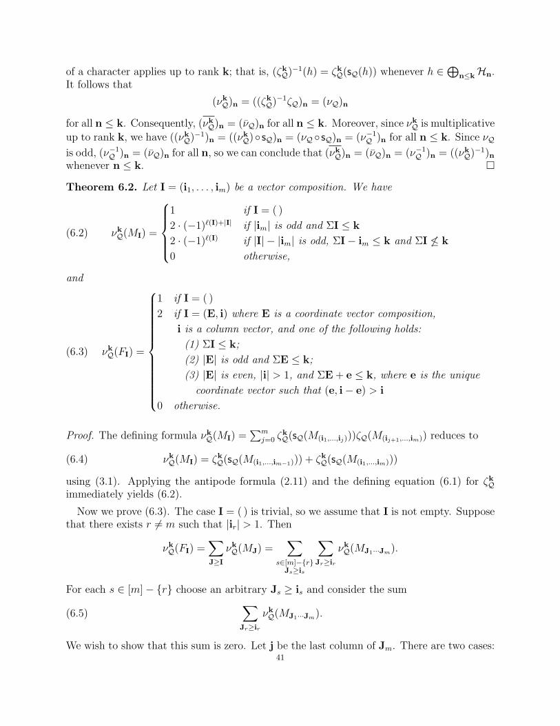
of a character applies up to rank k; that is, (ζkQ)−1(h) = ζk

Q(sQ(h)) whenever h ∈⊕

n≤kHn.It follows that

(νkQ)n = ((ζk

Q)−1ζQ)n = (νQ)n

for all n ≤ k. Consequently, (νkQ)n = (νQ)n for all n ≤ k. Moreover, since νk

Q is multiplicative

up to rank k, we have ((νkQ)−1)n = ((νk

Q)◦ sQ)n = (νQ ◦ sQ)n = (ν−1Q )n for all n ≤ k. Since νQ

is odd, (ν−1Q )n = (νQ)n for all n, so we can conclude that (νk

Q)n = (νQ)n = (ν−1Q )n = ((νk

Q)−1)nwhenever n ≤ k. �

Theorem 6.2. Let I = (i1, . . . , im) be a vector composition. We have

(6.2) νkQ(MI) =

1 if I = ( )

2 · (−1)`(I)+|I| if |im| is odd and ΣI ≤ k

2 · (−1)`(I) if |I| − |im| is odd, ΣI− im ≤ k and ΣI 6≤ k

0 otherwise,

and

(6.3) νkQ(FI) =

1 if I = ( )

2 if I = (E, i) where E is a coordinate vector composition,

i is a column vector, and one of the following holds:

(1) ΣI ≤ k;

(2) |E| is odd and ΣE ≤ k;

(3) |E| is even, |i| > 1, and ΣE + e ≤ k, where e is the unique

coordinate vector such that (e, i− e) > i

0 otherwise.

Proof. The defining formula νkQ(MI) =

∑mj=0 ζ

kQ(sQ(M(i1,...,ij)))ζQ(M(ij+1,...,im)) reduces to

(6.4) νkQ(MI) = ζk

Q(sQ(M(i1,...,im−1))) + ζkQ(sQ(M(i1,...,im)))

using (3.1). Applying the antipode formula (2.11) and the defining equation (6.1) for ζkQ

immediately yields (6.2).

Now we prove (6.3). The case I = ( ) is trivial, so we assume that I is not empty. Supposethat there exists r 6= m such that |ir| > 1. Then

νkQ(FI) =

∑J≥I

νkQ(MJ) =

∑s∈[m]−{r}

Js≥is

∑Jr≥ir

νkQ(MJ1···Jm).

For each s ∈ [m]− {r} choose an arbitrary Js ≥ is and consider the sum

(6.5)∑Jr≥ir

νkQ(MJ1···Jm).

We wish to show that this sum is zero. Let j be the last column of Jm. There are two cases:41

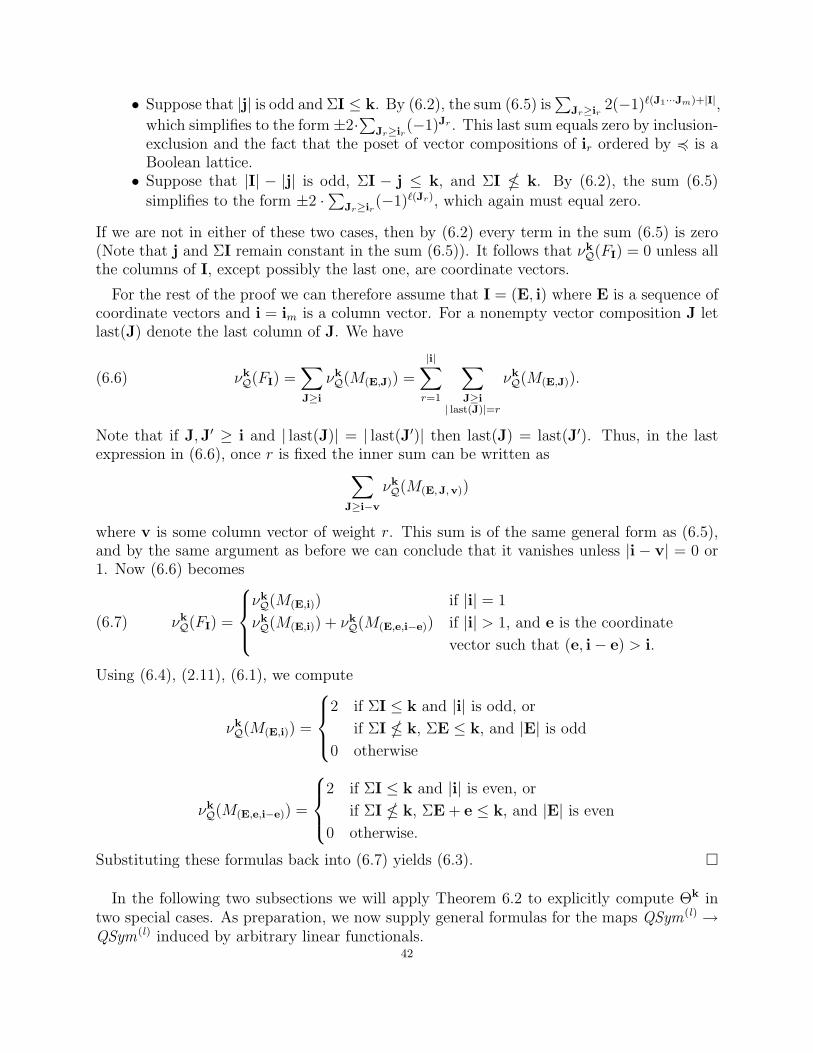
• Suppose that |j| is odd and ΣI ≤ k. By (6.2), the sum (6.5) is∑

Jr≥ir2(−1)`(J1···Jm)+|I|,

which simplifies to the form±2·∑

Jr≥ir(−1)Jr . This last sum equals zero by inclusion-

exclusion and the fact that the poset of vector compositions of ir ordered by 4 is aBoolean lattice.• Suppose that |I| − |j| is odd, ΣI − j ≤ k, and ΣI � k. By (6.2), the sum (6.5)

simplifies to the form ±2 ·∑

Jr≥ir(−1)`(Jr), which again must equal zero.

If we are not in either of these two cases, then by (6.2) every term in the sum (6.5) is zero(Note that j and ΣI remain constant in the sum (6.5)). It follows that νk

Q(FI) = 0 unless allthe columns of I, except possibly the last one, are coordinate vectors.

For the rest of the proof we can therefore assume that I = (E, i) where E is a sequence ofcoordinate vectors and i = im is a column vector. For a nonempty vector composition J letlast(J) denote the last column of J. We have

(6.6) νkQ(FI) =

∑J≥i

νkQ(M(E,J)) =

|i|∑r=1

∑J≥i

| last(J)|=r

νkQ(M(E,J)).

Note that if J,J′ ≥ i and | last(J)| = | last(J′)| then last(J) = last(J′). Thus, in the lastexpression in (6.6), once r is fixed the inner sum can be written as∑

J≥i−v

νkQ(M(E,J,v))

where v is some column vector of weight r. This sum is of the same general form as (6.5),and by the same argument as before we can conclude that it vanishes unless |i − v| = 0 or1. Now (6.6) becomes

(6.7) νkQ(FI) =

νkQ(M(E,i)) if |i| = 1

νkQ(M(E,i)) + νk

Q(M(E,e,i−e)) if |i| > 1, and e is the coordinate

vector such that (e, i− e) > i.

Using (6.4), (2.11), (6.1), we compute

νkQ(M(E,i)) =

2 if ΣI ≤ k and |i| is odd, or

if ΣI � k, ΣE ≤ k, and |E| is odd

0 otherwise

νkQ(M(E,e,i−e)) =

2 if ΣI ≤ k and |i| is even, or

if ΣI � k, ΣE + e ≤ k, and |E| is even

0 otherwise.

Substituting these formulas back into (6.7) yields (6.3). �

In the following two subsections we will apply Theorem 6.2 to explicitly compute Θk intwo special cases. As preparation, we now supply general formulas for the maps QSym(l) →QSym(l) induced by arbitrary linear functionals.

42

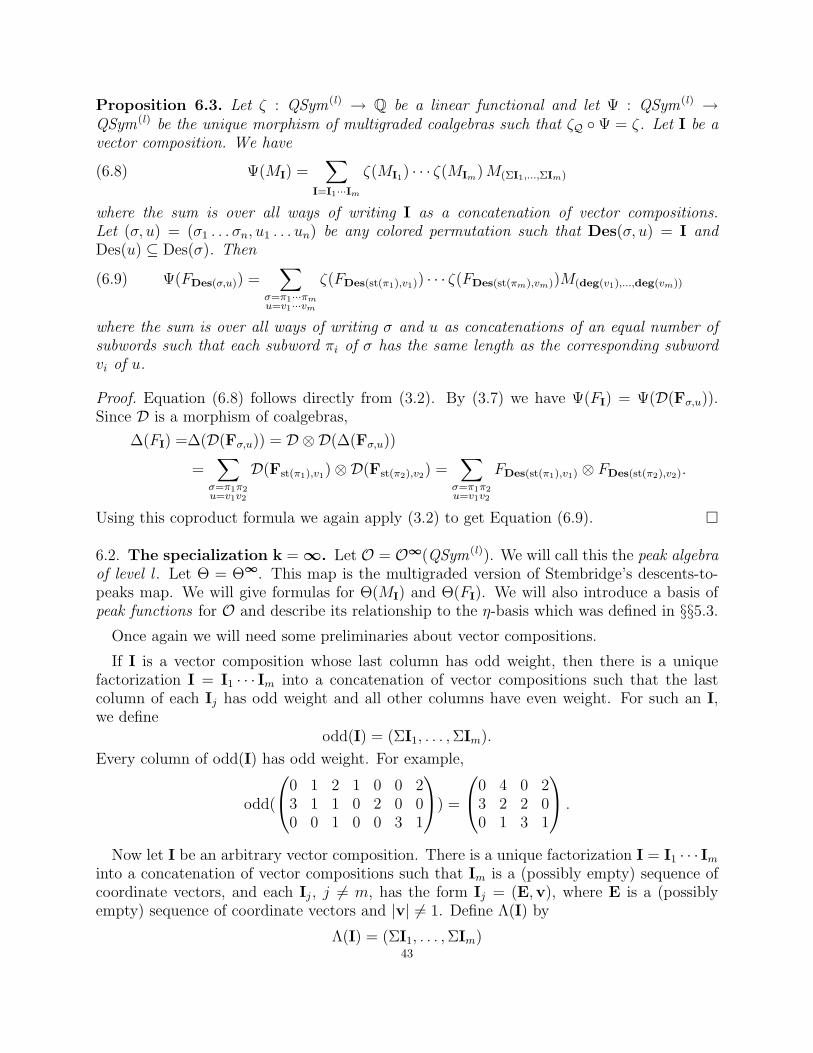
Proposition 6.3. Let ζ : QSym(l) → Q be a linear functional and let Ψ : QSym(l) →QSym(l) be the unique morphism of multigraded coalgebras such that ζQ ◦Ψ = ζ. Let I be avector composition. We have

(6.8) Ψ(MI) =∑

I=I1···Im

ζ(MI1) · · · ζ(MIm)M(ΣI1,...,ΣIm)

where the sum is over all ways of writing I as a concatenation of vector compositions.Let (σ, u) = (σ1 . . . σn, u1 . . . un) be any colored permutation such that Des(σ, u) = I andDes(u) ⊆ Des(σ). Then

(6.9) Ψ(FDes(σ,u)) =∑

σ=π1···πmu=v1···vm

ζ(FDes(st(π1),v1)) · · · ζ(FDes(st(πm),vm))M(deg(v1),...,deg(vm))

where the sum is over all ways of writing σ and u as concatenations of an equal number ofsubwords such that each subword πi of σ has the same length as the corresponding subwordvi of u.

Proof. Equation (6.8) follows directly from (3.2). By (3.7) we have Ψ(FI) = Ψ(D(Fσ,u)).Since D is a morphism of coalgebras,

∆(FI) =∆(D(Fσ,u)) = D ⊗D(∆(Fσ,u))

=∑

σ=π1π2u=v1v2

D(Fst(π1),v1)⊗D(Fst(π2),v2) =∑

σ=π1π2u=v1v2

FDes(st(π1),v1) ⊗ FDes(st(π2),v2).

Using this coproduct formula we again apply (3.2) to get Equation (6.9). �

6.2. The specialization k = ∞. Let O = O∞(QSym(l)). We will call this the peak algebraof level l . Let Θ = Θ∞. This map is the multigraded version of Stembridge’s descents-to-peaks map. We will give formulas for Θ(MI) and Θ(FI). We will also introduce a basis ofpeak functions for O and describe its relationship to the η-basis which was defined in §§5.3.

Once again we will need some preliminaries about vector compositions.

If I is a vector composition whose last column has odd weight, then there is a uniquefactorization I = I1 · · · Im into a concatenation of vector compositions such that the lastcolumn of each Ij has odd weight and all other columns have even weight. For such an I,we define

odd(I) = (ΣI1, . . . ,ΣIm).

Every column of odd(I) has odd weight. For example,

odd(

0 1 2 1 0 0 23 1 1 0 2 0 00 0 1 0 0 3 1

) =

0 4 0 23 2 2 00 1 3 1

.

Now let I be an arbitrary vector composition. There is a unique factorization I = I1 · · · Iminto a concatenation of vector compositions such that Im is a (possibly empty) sequence ofcoordinate vectors, and each Ij, j 6= m, has the form Ij = (E,v), where E is a (possiblyempty) sequence of coordinate vectors and |v| 6= 1. Define Λ(I) by

Λ(I) = (ΣI1, . . . ,ΣIm)43

For example,

Λ(

0 1 2 1 0 0 0 1 3 1 01 0 1 0 2 0 0 0 0 0 00 0 1 0 0 3 1 0 2 0 1

) =

3 1 0 4 12 2 0 0 01 0 3 3 1

.

We will call Λ(I) the peak vector composition of I for the following reason. Recall that thepeak set of a permutation σ = (σ1, . . . , σn) ∈ Sn is the set

Peak(σ) = {i ∈ [2, n− 1] | σi−1 < σi > σi+1}.If (σ, u) is a colored permutation then

d(Λ(Des(σ, u))) = Peak(σ).

Accordingly, we define the peak set of any vector composition I to be

p(I) = d(Λ(I)).

In essence, p(I) keeps track of where the columns of weight at least 2 occur in I.

Proposition 6.4. For any vector composition I we have

(6.10) Θ(MI) =

1 if I = ( )

(−1)`(I)+|I|ηodd(I) if the last column of I has odd weight

0 otherwise,

and if u = c(I) is the coloring word of I, then

(6.11) Θ(FI) =∑

JEEup(I)⊆d(J)∪(d(J)+1)

2`(J)MJ.

Proof. Letting νQ = ν∞Q , we obtain the following specializations to k = ∞ of the formulas

in Theorem 6.2

(6.12) νQ(MI) =

1 if I = ( )

2 · (−1)`(I)+|I| if the last column of I has odd weight

0 otherwise,

and

(6.13) νQ(FI) =

1 if I = ( )

2 if I = (E,v), where E is a (possibly empty) sequence

of coordinate vectors and v is any column vector

0 otherwise.

Let last(J) denote the last column of any vector composition J. By (6.8) and then (6.12),we have

Θ(MI) =∑

I=I1···Im

νQ(MI1) · · · νQ(MIm)M(ΣI1,...,ΣIm) =∑

I=I1···Im∀i | last(Ii)| is odd

(−1)`(I)+|I|2mM(ΣI1,...,ΣIm).

In the last sum, every Ii ends in a column of odd weight if and only if ΣIi is the sum ofcolumns in odd(I). Thus (6.10) follows.

44

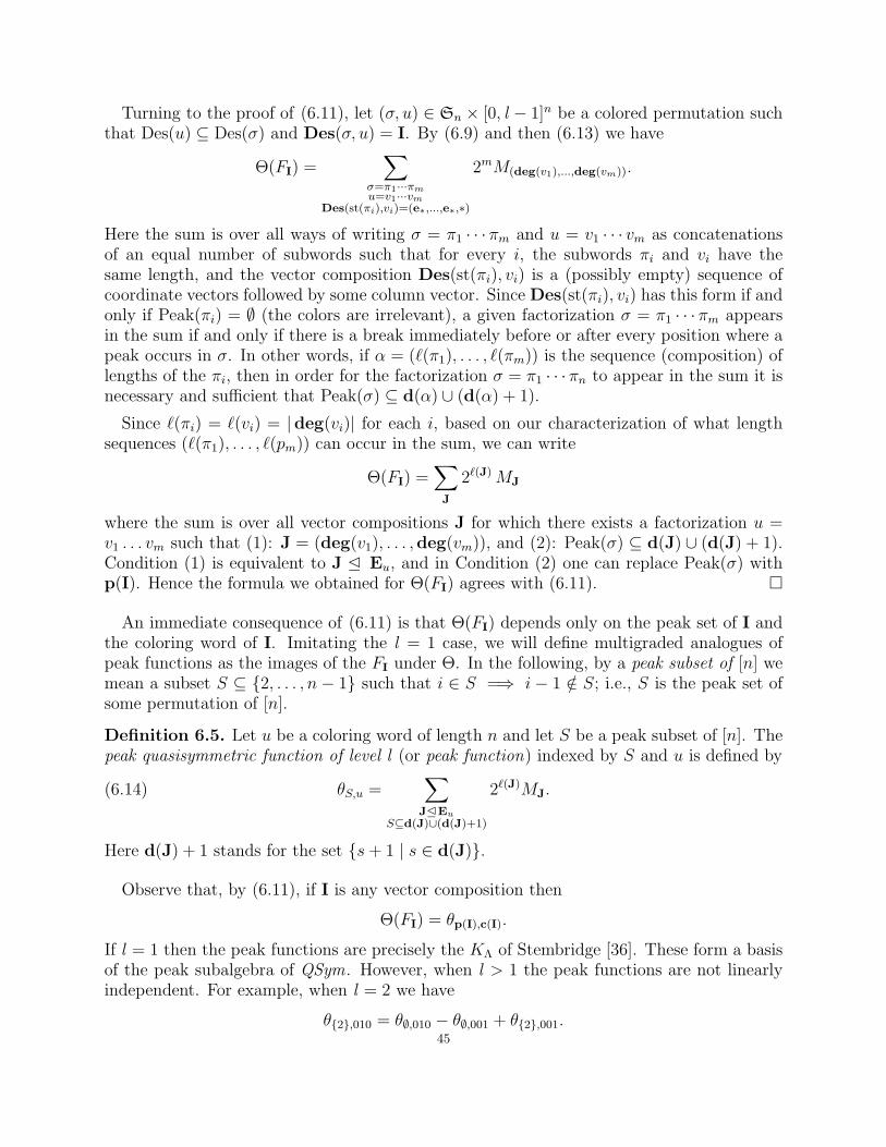
Turning to the proof of (6.11), let (σ, u) ∈ Sn × [0, l − 1]n be a colored permutation suchthat Des(u) ⊆ Des(σ) and Des(σ, u) = I. By (6.9) and then (6.13) we have

Θ(FI) =∑

σ=π1···πmu=v1···vm

Des(st(πi),vi)=(e∗,...,e∗,∗)

2mM(deg(v1),...,deg(vm)).

Here the sum is over all ways of writing σ = π1 · · · πm and u = v1 · · · vm as concatenationsof an equal number of subwords such that for every i, the subwords πi and vi have thesame length, and the vector composition Des(st(πi), vi) is a (possibly empty) sequence ofcoordinate vectors followed by some column vector. Since Des(st(πi), vi) has this form if andonly if Peak(πi) = ∅ (the colors are irrelevant), a given factorization σ = π1 · · · πm appearsin the sum if and only if there is a break immediately before or after every position where apeak occurs in σ. In other words, if α = (`(π1), . . . , `(πm)) is the sequence (composition) oflengths of the πi, then in order for the factorization σ = π1 · · · πn to appear in the sum it isnecessary and sufficient that Peak(σ) ⊆ d(α) ∪ (d(α) + 1).

Since `(πi) = `(vi) = |deg(vi)| for each i, based on our characterization of what lengthsequences (`(π1), . . . , `(pm)) can occur in the sum, we can write

Θ(FI) =∑J

2`(J) MJ

where the sum is over all vector compositions J for which there exists a factorization u =v1 . . . vm such that (1): J = (deg(v1), . . . ,deg(vm)), and (2): Peak(σ) ⊆ d(J) ∪ (d(J) + 1).Condition (1) is equivalent to J E Eu, and in Condition (2) one can replace Peak(σ) withp(I). Hence the formula we obtained for Θ(FI) agrees with (6.11). �

An immediate consequence of (6.11) is that Θ(FI) depends only on the peak set of I andthe coloring word of I. Imitating the l = 1 case, we will define multigraded analogues ofpeak functions as the images of the FI under Θ. In the following, by a peak subset of [n] wemean a subset S ⊆ {2, . . . , n− 1} such that i ∈ S =⇒ i− 1 /∈ S; i.e., S is the peak set ofsome permutation of [n].

Definition 6.5. Let u be a coloring word of length n and let S be a peak subset of [n]. Thepeak quasisymmetric function of level l (or peak function) indexed by S and u is defined by

(6.14) θS,u =∑

JEEuS⊆d(J)∪(d(J)+1)

2`(J)MJ.

Here d(J) + 1 stands for the set {s+ 1 | s ∈ d(J)}.

Observe that, by (6.11), if I is any vector composition then

Θ(FI) = θp(I),c(I).

If l = 1 then the peak functions are precisely the KΛ of Stembridge [36]. These form a basisof the peak subalgebra of QSym. However, when l > 1 the peak functions are not linearlyindependent. For example, when l = 2 we have

θ{2},010 = θ∅,010 − θ∅,001 + θ{2},001.45

Note also that, unlike the l = 1 case, the higher level peak functions are not always F -positive. For example, when l = 2 we have

θ∅,010 = 2F( 21 ) − 2F( 2 0

0 1 ) + 2F( 1 10 1 ) + 4F( 1 1

1 0 ) − 2F( 1 1 00 0 1 ).

Our next goal is to describe a subset of peak functions that form a basis for O. We willalso describe how this basis relates to the η-basis. Before we proceed we will need someadditional definitions and a lemma. Let u ∈ [0, l − 1]n be a color word. Given an odd vector

composition I (meaning every column of I has odd weight), we define I to be the vectorcomposition with the same coloring word as I, obtained by replacing each column of I bya new vector composition of equal weight whose last column has weight 1 and all othercolumns have weight 2. For example,

I =

2 0 30 0 21 1 0

=⇒ I =

2 0 0 2 1 00 0 0 0 1 10 1 1 0 0 0

.

Next, let u be a color word of length n and let S be a peak subset of [n]. We define IS,u tobe the unique vector composition satisfying the following three properties: (1) every columnof IS,u has weight 1 or 2; (2) the coloring word of IS,u is u; and (3) p(IS,u) = S. Note thatthe last column of IS,u must have weight 1, so it makes sense to talk about odd(IS,u). Forexample, when l = 3, if S = {2, 6, 8} and u = 002200011 then

IS,u =

2 0 0 2 1 00 0 0 0 1 10 1 1 0 0 0

and odd(IS,u) =

2 0 30 0 21 1 0

.

The pair (S, u) will be called admissible if c(odd(IS,u)) = u. The previous example is of

an admissible pair. When l = 1 the correspondence I ↔ p(I) is a bijection between oddcompositions and peak subsets of {1, . . . , |I|}, as observed by Schocker [34]. This observationgeneralizes to vector compositions; the proof of the following lemma is similar to that ofProposition 3.1 in [34] and will be omitted.

Lemma 6.6. Let u ∈ [0, l − 1]n be a color word. The map I 7→ (p(I), u) is a bijectionfrom the set OComp(u) to the set of admissible pairs with second coordinate equal to u. Theinverse of this map is given by (S, u) 7→ odd(IS,u).

Here is our main result on peak functions:

Theorem 6.7. The peak functions θS,u indexed by admissible pairs (S, u) form a basis forthe higher level peak algebra O. Moreover, we can explicitly describe the relationship betweenthe θS,u and the ηI as follows: If I is an odd vector composition and u = c(I), then

(6.15) ηI =∑S⊆p(eI)

(−1)|S| θS,u,

and if (S, u) is any admissible pair then

(6.16) θS,u =∑T⊆S

(−1)|T | ηodd(IT,u).

46

Proof. As shown in Theorem 5.19, the ηI such that I is an odd vector composition form abasis for O. It therefore suffices to prove (6.15), which is equivalent to (6.16) by Mobiusinversion.

To prove (6.15), we apply the definition of θS,u (see (6.14)) to get∑S⊆p(eI)

(−1)|S| θS,Eu =∑

JEEu

2`(J)MJ

∑S⊆p(I)∩(d(J)∪(d(J)+1))

(−1)|S|.

Now p(I) ∩ (d(J) ∪ (d(J) + 1)) = ∅ ⇐⇒ d(J) ∪ (d(J) + 1) ⊆ [n − 1] \ p(I) ⇐⇒ d(J) ⊆[n− 1] \ ((p(I)− 1)∪p(I)) = d(I). The last equality is essentially Equation (8) of [34]. Thusthe inner sum is 1 if d(J) ⊆ d(I) and 0 otherwise. Since both J E Eu and I E Eu, thecondition d(J) ⊆ d(I) is equivalent to J E I, as required. �

Remark 6.8. When l = 1, our η-basis for O is, up to sign, dual to the Γ-basis introducedby Schocker [34, Equation (9)].

6.3. The specialization l = 1. In this case, QSym(l) = QSym, and for each k ∈ N, we have

a k-odd linear functional ν(k)Q on the Hopf algebra of (ordinary) quasisymmetric functions

QSym. Therefore we get an induced morphism of coalgebras Θ(k) : QSym → QSym whoseimage is contained in the k-odd Hopf subalgebra Ok(QSym). We will apply Theorem 6.2 to

give a formula for Θ(k).

Proposition 6.9. Let k > 0 be an odd integer and I be a composition of n. We haveΘ(k) = Θ(k+1) and

Θ(k)(FI) =∑J �n

p(I)⊆d(J)∪(d(J)+1)d(I)⊆d(J)∪(d(J)+1)∪···∪(d(J)+k)

2`(J) MJ .

Proof. Equation (6.3) becomes

ν(k)Q (FI) = ν

(k+1)Q (FI) =

1 if I = ( )

2 if I = (j) or I = (1i, j) or some i ∈ {1, . . . , k} and j ≥ 1

0 otherwise.

Let σ = (σ1, . . . , σn) be a permutation with descent composition Des(σ) = Des(σ, 11 . . . 1) =I. Then by (6.9),

Θ(k)(FI) =∑

2mM(`(π1),...,`(πm))

where the sum is over all ways of writing σ = π1 · · · πm as a concatenation of subwords πisuch that for every i, Des(st(πi)) has for form (j) or (1i, j) for some i ∈ {1, . . . , k} andj ≥ 1. The composition Des(st(πi)) has this form if and only if πi begins with at mostk descents followed by only ascents; in particular πi has no peaks, so a break occurs inthe factorization σ = π1 · · · πm immediately before or after every peak. Thus in order fora factorization σ = π1 · · · πm to appear in the sum it is necessary and sufficient that thecomposition J = (`(π1), . . . , `(πm)) satisfy Des(σ) ⊆ d(J) ∪ (d(J) + 1) ∪ · · · ∪ (d(J) + k)and Peak(σ) ⊆ d(J) ∪ (d(J) + 1). �

47

We can also write the expression in Proposition 6.9 using operations on vector compositionsrather than sets, in the following way. For any composition I = (i1, . . . , im), let I?k be thecomposition obtained by replacing every component ir with (1ir) if ir ≤ k, and with (ikr , ir−k)if ir > k. Write I? for I?1. Then we can rewrite the expression in Proposition 6.9 as:

Θ(k)(FI) =∑J �n

Λ(I)E J?

IE J?k

2`(J)MJ .

Consider the case k = 2. It was already observed in Proposition 5.16 that O2 is the Hopfalgebra spanned by all shifted quasisymmetric functions (sqs-function). Going a bit further,

let us remark that the map Θ(2) takes each fundamental basis element FI to an sqs-functions.Let I = (i1, . . . , im) be a composition with i1 > 1, and let θI be the sqs-function as definedin [9, Definition 3.1]. It is shown in [9, Theorem 3.6] that the θI are precisely the functionsdefined by Billey and Haiman in [15, Equation (3.2)]. It follows from Proposition 6.9 that

Θ(2)(FI) = θI .

Furthermore, clearly Θ(2)(F(1,i1−1,i2,...,im)) = Θ(2)(FI), so Θ(2)(FJ) is an sqs-function for everycomposition J .

References

[1] Marcelo Aguiar, Infinitesimal Hopf algebras and the cd-index of polytopes, Discrete Comput. Geom. 27(2002), no. 1, 3–28. Geometric combinatorics (San Francisco, CA/Davis, CA, 2000).

[2] Marcelo Aguiar, Nantel Bergeron, and Frank Sottile, Combinatorial Hopf algebras and generalized Dehn-Sommerville relations, Compos. Math. 142 (2006), no. 1, 1–30.

[3] Marcelo Aguiar and Samuel K. Hsiao, Canonical characters on quasi-symmetric functions and bivariateCatalan numbers, Electron. J. Combin. 11 (2004/06), no. 2, Research Paper 15, 34 pp. (electronic).

[4] Marcelo Aguiar and Frank Sottile, Structure of the Malvenuto-Reutenauer Hopf algebra of permutations,Adv. Math. 191 (2005), no. 2, 225–275.

[5] J.-C. Aval, F. Bergeron, and N. Bergeron, Diagonal Temperley-Lieb invariants and harmonics, Sem.Lothar. Combin. 54A (2005/07), Art. B54Aq, 19 pp. (electronic).

[6] Pierre Baumann and Christophe Hohlweg, A Solomon descent theory for the wreath products G o Sn,Trans. Amer. Math. Soc. 360 (2008), no. 3, 1475–1538 (electronic).

[7] Margaret M. Bayer and Louis J. Billera, Generalized Dehn-Sommerville relations for polytopes, spheresand Eulerian partially ordered sets, Invent. Math. 79 (1985), no. 1, 143–157.

[8] Nantel Bergeron, Stefan Mykytiuk, Frank Sottile, and Stephanie van Willigenburg, NoncommutativePieri operators on posets, J. Combin. Theory Ser. A 91 (2000), no. 1-2, 84–110. In memory of Gian-Carlo Rota.

[9] , Shifted quasi-symmetric functions and the Hopf algebra of peak functions, Discrete Math. 246(2002), no. 1-3, 57–66 (English, with English and French summaries). Formal power series and algebraiccombinatorics (Barcelona, 1999).

[10] , Personal communication (2001).[11] Nantel Bergeron, Florent Hivert, and Jean-Yves Thibon, The peak algebra and the Hecke-Clifford alge-

bras at q = 0, J. Combin. Theory Ser. A 107 (2004), no. 1, 1–19.[12] Nantel Bergeron and Christophe Hohlweg, Coloured peak algebras and Hopf algebras, J. Algebraic Com-

bin. 24 (2006), no. 3, 299–330.[13] Louis J. Billera, Samuel K. Hsiao, and Stephanie van Willigenburg, Peak quasisymmetric functions and

Eulerian enumeration, Adv. Math. 176 (2003), no. 2, 248–276.[14] Louis J. Billera and Niandong Liu, Noncommutative enumeration in graded posets, J. Algebraic Combin.

12 (2000), no. 1, 7–24.48

[15] Sara Billey and Mark Haiman, Schubert polynomials for the classical groups, J. Amer. Math. Soc. 8(1995), no. 2, 443–482.

[16] Gerard Duchamp, Florent Hivert, and Jean-Yves Thibon, Noncommutative symmetric functions. VI.Free quasi-symmetric functions and related algebras, Internat. J. Algebra Comput. 12 (2002), no. 5,671–717.

[17] Richard Ehrenborg, On posets and Hopf algebras, Adv. Math. 119 (1996), no. 1, 1–25.[18] , k-Eulerian posets, Order 18 (2001), no. 3, 227–236.[19] Israel M. Gelfand, Daniel Krob, Alain Lascoux, Bernard Leclerc, Vladimir S. Retakh, and Jean-Yves

Thibon, Noncommutative symmetric functions, Adv. Math. 112 (1995), no. 2, 218–348.[20] Ira M. Gessel, Multipartite P -partitions and inner products of skew Schur functions, Combinatorics

and algebra (Boulder, Colo., 1983), Contemp. Math., vol. 34, Amer. Math. Soc., Providence, RI, 1984,pp. 289–317.

[21] , Enumerative applications of symmetric functions, Seminaire Lotharingien de CombinatoireB17a (1987), 17pp.

[22] Michael E. Hoffman, Quasi-shuffle products, J. Algebraic Combin. 11 (2000), no. 1, 49–68.[23] Samuel K. Hsiao and T. Kyle Petersen, Colored posets and colored quasisymmetric functions, Ann.

Combin., to appear.[24] D. Krob, B. Leclerc, and J.-Y. Thibon, Noncommutative symmetric functions. II. Transformations of

alphabets, Internat. J. Algebra Comput. 7 (1997), no. 2, 181–264.[25] Jean-Louis Loday, On the algebra of quasi-shuffles, Manuscripta Math. 123 (2007), no. 1, 79–93.[26] Percy A. MacMahon, Combinatory analysis. Vol. I, II (bound in one volume), Dover Phoenix Editions,

Dover Publications Inc., Mineola, NY, 2004. Reprint of An introduction to combinatory analysis (1920)and Combinatory analysis. Vol. I, II (1915, 1916).

[27] Clauda Malvenuto and Christophe Reutenauer, Duality between quasi-symmetric functions and theSolomon descent algebra, J. Algebra 177 (1995), no. 3, 967–982.

[28] R. Mantaci and C. Reutenauer, A generalization of Solomon’s algebra for hyperoctahedral groups andother wreath products, Comm. Algebra 23 (1995), no. 1, 27–56.

[29] Jean-Christophe Novelli and Jean-Yves Thibon, Free quasi-symmetric functions of arbitrary level (2004),available at http://arxiv.org/abs/math.CO/0405597.

[30] , Free quasi-symmetric functions and descent algebras for wreath products, and noncommutativemulti-symmetric functions (2008), available at http://arxiv.org/abs/0806.3682.

[31] Stephane Poirier, Cycle type and descent set in wreath products, Proceedings of the 7th Conference onFormal Power Series and Algebraic Combinatorics (Noisy-le-Grand, 1995), 1998, pp. 315–343.

[32] Christophe Reutenauer, Free Lie algebras, London Mathematical Society Monographs. New Series, vol. 7,The Clarendon Press Oxford University Press, New York, 1993. Oxford Science Publications.

[33] Richard P. Stanley, Enumerative combinatorics. Vol. 1, Cambridge Studies in Advanced Mathematics,vol. 49, Cambridge University Press, Cambridge, 1997. With a foreword by Gian-Carlo Rota; Correctedreprint of the 1986 original.

[34] Manfred Schocker, The peak algebra of the symmetric group revisited, Adv. Math. 192 (2005), no. 2,259–309.

[35] Richard P. Stanley, Flag-symmetric and locally rank-symmetric partially ordered sets, Electron. J. Com-bin. 3 (1996), no. 2, Research Paper 6, approx. 22 pp. (electronic). The Foata Festschrift.

[36] John R. Stembridge, Enriched P -partitions, Trans. Amer. Math. Soc. 349 (1997), no. 2, 763–788.

Mathematics Program, Bard College, Annandale-on-Hudson, NY 12504

E-mail address: hsiao@bard.edu

Department of Mathematics, Pomona College, Claremont, CA 91711

E-mail address: gizem.karaali@pomona.edu

49