bimonads and hopf monads on categories

arX

iv:0

710.

1163

v3 [

mat

h.Q

A]

11

Jun

2008

BIMONADS AND HOPF MONADS ON CATEGORIES

BACHUKI MESABLISHVILI, TBILISIAND

ROBERT WISBAUER, DUSSELDORF

Abstract. The purpose of this paper is to develop a theory of bimonads and Hopf monadson arbitrary categories thus providing the possibility to transfer the essentials of the theoryof Hopf algebras in vector spaces to more general settings. There are several extensionsof this theory to monoidal categories which in a certain sense follow the classical trace.Here we do not pose any conditions on our base category but we do refer to the monoidalstructure of the category of endofunctors on any category A and by this we retain someof the combinatorial complexity which makes the theory so interesting. As a basic toolwe use distributive laws between monads and comonads (entwinings) on A: we define abimonad on A as an endofunctor B which is a monad and a comonad with an entwiningλ : BB → BB satisfying certain conditions. This λ is also employed to define the categoryA

BB of (mixed) B-bimodules. In the classical situation, an entwining λ is derived from the

twist map for vector spaces. Here this need not be the case but there may exist specialdistributive laws τ : BB → BB satisfying the Yang-Baxter equation (local prebraidings)which induce an entwining λ and lead to an extension of the theory of braided Hopf algebras.

An antipode is defined as a natural transformation S : B → B with special propertiesand for categories A with limits or colimits and bimonads B preserving them, the existenceof an antipode is equivalent to B inducing an equivalence between A and the category A

BB

of B-bimodules. This is a general form of the Fundamental Theorem of Hopf algebras.Finally we observe a nice symmetry: If B is an endofunctor with a right adjoint R,

then B is a (Hopf) bimonad if and only if R is a (Hopf) bimonad. Thus a k-vector spaceH is a Hopf algebra if and only if Homk(H,−) is a Hopf bimonad. This provides a richsource for Hopf monads not defined by tensor products and generalises the well-knownfact that a finite dimensional k-vector space H is a Hopf algebra if and only if its dualH∗ = Homk(H,k) is a Hopf algebra. Moreover, we obtain that any set G is a group if andonly if the functor Map(G,−) is a Hopf monad on the category of sets.

Contents

1. Introduction 12. Distributive laws 33. Actions on functors and Galois functors 64. Bimonads 125. Antipode 156. Local prebraidings for Hopf monads 187. Adjoints of bimonads 28References 32

1. Introduction

The theory of algebras (monads) as well as of coalgebras (comonads) is well understoodin various fields of mathematis as algebra (e.g. [8]), universal algebra (e.g. [13]), logic oroperational semantics (e.g. [31]), theoretical computer science (e.g. [23]). The relationshipbetween monads and comonads is controlled by distributive laws introduced in the seventies

1

http://arXiv.org/abs/0710.1163v3

2 BACHUKI MESABLISHVILI, TBILISI AND ROBERT WISBAUER, DUSSELDORF

by Beck (see [2]). In algebra one of the fundamental notions emerging in this context arethe Hopf algebras. The definition is making heavy use of the tensor product and thusgeneralisations of this theory were mainly considered for monoidal categories. They allowreadily to transfer formalisms from the category of vector spaces to the more general settings(e.g. Bespalov and Brabant [3] and [21]).

A Hopf algebra is an algebra as well as a coalgebra. Thus one way of generalisation is toconsider distinct algebras and coalgebras and some relationship between them. This leadsto the theory of entwining structures and corings over associative rings (e.g. [8]) and onemay ask how to formulate this in more general categories. The definition of bimonads on amonoidal category as monads whose functor part is comonoidal by Bruguieres and Virelizierin [7, 2.3] may be seen as going in this direction. Such functors are called Hopf monadsin Moerdijk [22] and opmonoidal monads in McCrudden [18, Example 2.5]. In 2.2 we givemore details of this notion.

Another extension of the theory of corings are the generalised bialgebras in Loday in[17]. These are Schur functors (on vector spaces) with a monad structure (operads) and aspecified coalgebra structure satisfying certain compatibility conditions [17, 2.2.1]. While in[17] use is made of the canonical twist map, it is stressed in [7] that the theory is built upwithout reference to any braiding. More comments on these constructions are given in 2.3.

The purpose of the present paper is to formulate the essentials of the classical theory ofHopf algebras for any (not necessarily monoidal) category, thus making it accessible to awide field of applications. We also employ the fact that the category of endofunctors (withthe Godement product as composition) always has a tensor product given by compositionof natural transformations but no tensor product is required for the base category.

Compatibility between monads and comonads are formulated as distributive laws whoseproperties are recalled in Section 2. In Section 3, general categorical notions are presentedand Galois functors are defined and investigated, in particular equivalences induced forrelated categories (relative injectives).

As suggested in [33, 5.13], we define a bimonad H = (H,m, e, δ, ε) on any category A as anendofunctor H with a monad and a comonad structure satisfying compatibility conditions(entwining) (see 4.1). The latter do not refer to any braiding but in special cases they canbe derived from a local prebraiding τ : HH → HH (see 6.3). In this case the bimonad showsthe characteristics of braided bialgebras (Section 6).

Related to a bimonad H there is the (Eilenberg-Moore) category AHH of bimodules with

a comparison functor KH : A → AHH . An antipode is defined as a natural transformation

S : H → H satisfying m · SH · δ = e · ε = m · HS · δ. It exists if and only if the naturaltransformation γ := Hm · δH : HH → HH is an isomorphism. If the category A is Cauchycomplete and H preserves limits or colimits, the existence of an antipode is equivalent to thecomparison functor being an equivalence (see 5.6). This is a general form of the FundamentalTheorem for Hopf algebras. Any generalisation of Hopf algebras should offer an extensionof this important result.

Of course, bialgebras and Hopf algebras over commutative rings R provide the prototypesfor this theory: on R-Mod, the category of R-modules, one considers the endofunctor B ⊗R

− : R-Mod→ R-Mod where B is an R-module with algebra and coalgebra structures, andan entwining derived from the twist map (braiding) M ⊗R N → N ⊗R M (e.g. [5, Section8]).

More generally, for a comonad H, the entwining λ : HH → HH may be derived froma local prebraiding τ : HH → HH (see 6.7) and then results similar to those known forbraided Hopf algebras are obtained. In particular, the composition HH is again a bimonad(see 6.8) and, if τ2 = 1, an opposite bimonad can be defined (see 6.10).

BIMONADS AND HOPF MONADS ON CATEGORIES 3

In case a bimonad H on A has a right (or left) adjoint endofunctor R, then R is againa bimonad and has an antipode (or local prebraiding) if and only if so does H (see 7.5).In particular, for R-modules B, the functor HomR(B,−) is right adjoint to B ⊗R − andhence B is a Hopf algebra if and only if HomR(B,−) is a Hopf monad. This provides arich source for examples of Hopf monads not defined by a tensor product and extends asymmetry principle known for finite dimensional Hopf algebras (see 7.8). We close withthe observation that a set G is a group if and only if the endofunctor Map(G,−) is a Hopfmonad on the catgeory of sets (7.9).

Note that the pattern of our definition of bimonads resembles the definition of Frobeniusmonads on any category by Street in [27]. Those are monads T = (T, µ, η) with naturaltransformations ε : T → I and ρ : T → TT , subject to suitable conditions, which inducea comonad structure δ = Tµ · ρT : T → TT and product and coproduct on T satisfy thecompatibility condition Tµ · δT = δ · µ = µT · Tδ.

2. Distributive laws

Distributive laws between endofunctors were studied by Beck [2], Barr [1] and others inthe seventies of the last century. They are a fundamental tool for us and we recall somefacts needed in the sequel. For more details and references we refer to [33].

2.1. Entwining from monad to comonad. Let T = (T,m, e) be a monad and G =(G, δ, ε) a comonad on a category A. A natural transformation λ : TG → GT is called amixed distributive law or entwining from the monad T to the comonad G if the diagrams

GeG

~~||||

|||| Ge

!!CCC

CCCC

C

TGλ

// GT,

TG

Tε !!CCC

CCCC

C

λ // GT

εT}}{{{{

{{{{

T

TG

λ��

Tδ // TGGλG // GTG

Gλ��

and TTG

mG��

Tλ // TGTλT // GTT

Gm��

GTδT

// GGT TGλ

// GT

are commutative.It is shown in [34] that for an arbitrary mixed distributive law λ : TG → GT from a

monad T to a comonad G, the triple G = (G, δ, ε), is a comonad on the category AT ofT-modules (also called T-algebras), where for any object (a, ha) of AT,

• G(a, ha) = (G(a), G(ha) · λa);

• (δ)(a,ha) = δa, and• (ε)(a,ha) = εa.

G is called the lifting of G corresponding to the mixed distributive law λ.

Furthermore, the triple T = (T , m, e) is a monad on the category AG of G-comodules,

where for any object (a, θa) of the category AG,

• T (a, θa) = (T (a), λa · T (θa));

• (m)(a,θa) = ma, and

• (e)(a,θa) = ea.


This monad is called the lifting of T corresponding to the mixed distributive law λ. Onehas an isomorphism of categories

(AG)bT≃ (AT )

bG,

and we write AGT (λ) for this category. An object of A

GT (λ) is a triple (a, ha, θa), where

(a, ha) ∈ AT and (a, θa) ∈ AG with commuting diagram

(2.1) T (a)ha //

T (θa)��

aθa // G(a)

TG(a)λa

// GT (a).

G(ha)

OO

We consider two examples of entwinings which may (also) be considered as generalisationsof Hopf algebras. They are different from our approach and we will not refer to them lateron.

2.2. Opmonoidal functors. Let (V,⊗, I) be a strict monoidal category. Following Mc-Crudden [18, Example 2.5], one may call a monad (T, µ, η) on V opmonoidal if there existmorphisms

θ : T (I) → I and χX,Y : T (X ⊗ Y ) → T (X) ⊗ T (Y ),

the latter natural in X,Y ∈ V, which are compatible with the tensor structure of V and themonad structure of T .

Such functors can also be characterised by the condition that the tensor product of V canbe lifted to the category of T -modules (e.g. [33, 3.4]). They were introduced and namedHopf monads by Moerdijk in [22, Definition 1.1] and called bimonads by Bruguieres andVirelizier in [7, 2.3]. It is mentioned in [7, Example 2.8] that Szlachanyi’s bialgebroids in[29] may be interpreted in terms of such ”bimonads”. It is preferable to use the terminologyfrom [18] since these functors are neither bimonads nor Hopf monads in a strict sense butrather an entwining (as in 2.1) between the monad T and the comonad T (I) ⊗− on V:

Indeed, the compatibility conditions required in the definitions induce a coproduct χI,I :T (I) → T (I) ⊗ T (I) with counit θ : T (I) → I. Moreover, the relation between χ and µ (e.g.(15) in [7, 2.3]) lead to the commutative diagram (using X ⊗ I = X)

TT (X)µ //

T (χI,X)

��

T (X)χI,X // T (I) ⊗ T (X)

T (T (I) ⊗ T (X))χT (I),T (X) // TT (I) ⊗ TT (X)

µI⊗TT (X) // T (I) ⊗ TT (X)

T (I)⊗µX

OO

This shows that T (X) is a mixed (T, T (I) ⊗−)-bimodule for the entwining map

λ = (µI ⊗ T (−)) ◦ χT (I),− : T (T (I) ⊗−) → T (I) ⊗ T (−).

The antipode of a classical Hopf algebra H is defined as a special endomorphism of H. Sinceopmonoidal monads T relate two distinct functors it is not surprising that the notion of anantipode can not be transferred easily to this situation and the attempt to do so leads to an”apparently complicated definition” in [7, 3.3 and Remark 3.5]. Hereby the base categoryC is required to be autonomous.

2.3. Generalized bialgebras and Hopf operads. The generalised bialgebras over fieldsas defined in Loday [17, Section 2.1] are similar to the mixed bimodules (see 2.1): they arevector spaces which are modules over some operad A (Schur functors with multiplicationand unit) and comodules over some coalgebras Cc, which are linear duals of some operad C.


Similar to the opmonoidal monads the coalgebraic structure is based on the tensor product(of vector spaces). The Hypothesis (H0) in [7] resembles the role of the entwining λ in2.1. The Hypothesis (H1) requires that the free A-algebra is a (CC ,A)-bialgebra: this issimilar to the condition on an A-coring C, A an associative algebra, to have a C-comodulestructure (equivalently the existence of a group-like element, e.g. [8, 28.2]). The condition(H2iso) plays the role of the canonical isomorphism defining Galois corings and the GaloisCoring Structure Theorem [8, 28.19] may be compared with the Rigidity Theorem [17, 2.3.7].The latter can be considered as a generalisation of the Hopf-Borel Theorem (see [17, 4.1.8])and of the Cartier-Milnor-Moore Theorem (see [17, 4.1.3]). In [17, 3.2], Hopf operads aredefined in the sense of Moerdijk [22] and thus the coalgebraic part is dependent on thetensor product. This is only a sketch of the similarities between Loday’s setting and ourapproach here. It will be interesting to work out the relationship in more detail.

Similar to 2.1 we will also need the notion of mixed distributive laws from a comonad toa monad.

2.4. Entwining from comonad to monad. A natural transformation λ : GT → TG is amixed distributive law from a comonad G to a monad T, also called an entwining of G andT, if the diagrams

GGe

~~||||

|||| eG

!!DDD

DDDD

D GT

εT BBB

BBBB

B

λ // TG

Tε~~||||

||||

GTλ

// TG , T

GTT

Gm

��

λT // TGTTλ // TTG

mG��

GGTGλ // GTG

λG // TGG

GTλ

// TG, GT

δT

OO

λ// TG

Tδ

OO

are commutive.

For convenience we recall the distributive laws between two monads and between twocomonads (e.g. [2], [1], [33, 4.4 and 4.9]).

2.5. Monad distributive. Let F = (F,m, e) and T = (T,m′, e′) be monads on the categoryA. A natural transformation λ : FT → TF is said to be monad distributive if it induces thecommutative diagrams

TeT

~~||||

|||| Te

!!BBB

BBBB

B

FTλ // TF,

FFe′

}}{{{{

{{{{ e′

F

!!CCC

CCCC

C

FTλ // TF.

FFTmT //

Fλ

��

FT

λ��

FTFλF // TFF

Tm // TF,

FTTFm′

//

λT

��

FT

λ��

TFTTλ // TTF

m′

F // TF.

In this case λ : FT → TF induces a canonical monad structure on TF .

2.6. Comonad distributive. Let G = (G, δ, ε) and T = (T, δ′, ε′) be comonads on thecategory A. A natural transformation ϕ : TG → GT is said to be comonad distributive if itinduces the commutative diagrams


TG

Tε !!CCC

CCCC

C

ϕ // GT

εT}}{{{{

{{{{

T ,

TG

ε′G !!CCC

CCCC

C

ϕ // GT

Gε′}}{{{{

{{{{

G ,

TGTδ //

ϕ

��

TGGϕG // GTG

Gϕ

��GT

δT // GGT,

TGδ′G //

ϕ

��

TTGTϕ // TGT

ϕT

��GT

Gδ′ // GTT.

In this case ϕ :TG → GT induces a canonical comonad structure on TG.

3. Actions on functors and Galois functors

The language of modules over rings can also be used to describe actions of monads onfunctors. Doing this we define Galois functors and to characterise those we investigate therelationships between categories of relative injective objects.

3.1. T-actions on functors. Let A and B be categories. Given a monad T = (T,m, e) onA and any functor L : A → B, we say that L is a (right) T-module if there exists a naturaltransformation αL : LT → L such that the diagrams

(3.1) L

AAAA

AAAA

AAAA

AAAA

Le // LT

αL

��L,

LTTLm //

αLT

��

LT

αL

��LT αL

// L

commute. It is easy to see that (T,m) and (TT, Tm) both are T-modules.Similarly, given a comonad G = (G, δ, ε) on A, a functor K : B → A is a left G-comodule

if there exists a natural transformation βK : K → GK for which the diagrams

K

CCCC

CCCC

CCCC

CCCC

βK // GK

εK��

K,

KβK //

βK

��

GK

δK��

GKGβK

// GGK

commute.Given two T-modules (L,αL), (L′, αL′), a natural transformation g : L → L′ is called

T-linear if the diagram

(3.2) LTgT //

αL

��

L′T

αL′

��L g

// L′

commutes.

3.2. Lemma. Let (L,αL) be a T-module. If f, f ′ : TT → L are T-linear morphisms fromthe T-module (TT, Tm) to the T-module (L,αL) such that f · Te = f ′ · Te, then f = f ′.


Proof. Since f · Te = f ′ · Te, we have αL · fT · TeT = αL · f ′T · TeT. Moreover, since f

and f ′ are both T-linear, we have the commutative diagrams

TTT

Tm

��

fT // LT

αL

��TT

f // L,

TTT

Tm��

f ′T // LT

αL

��TT

f ′

// L.

Thus αL · fT = f · Tm and αL · f ′T = f ′ · Tm, and we have f · Tm · TeT = f ′ · Tm · TeT .It follows - since Tm · TeT = 1 - that f = f ′. ⊔⊓

3.3. Left G-comodule functors. Let G be a comonad on a category A, let UG : AG → A

be the forgetful functor and write φG : A → AG for the cofree G-comodule functor. Fix a

functor F : B → A, and consider a functor F : B → AG making the diagram

(3.3) BF //

F ��>>>

>>>>

AG

UG~~}}

}}}}

}}

A

commutative. Then F (b) = (F (b), αF (b)) for some αF (b) : F (b) → GF (b). Consider thenatural transformation

(3.4) αF : F → GF,

whose b-component is αF (b). It should be pointed out that αF makes F a left G-comodule,

and it is easy to see that there is a one to one correspondence between functors F : B → AG

making the diagram (3.3) commute and natural transformations αF : F → GF making F aleft G-comodule.

The following is an immediate consequence of (the dual of) [10, Propositions II,1.1 andII,1.4]:

3.4. Theorem. Suppose that F has a right adjoint R : A → B with unit η : 1 → RF andcounit ε : FR → 1. Then the composite

tF : FRαF R // GFR

Gε // G.

is a morphism from the comonad G′ = (FR,FηR, ε) generated by the adjunction η, ε : F ⊣

R : A → B to the comonad G. Moreover, the assignment

F −→ tF

yields a one to one correspondence between functors F : B → AG making the diagram (3.3)

commutative and morphisms of comonads tF : G′ → G.

3.5. Definition. We say that a left G-comodule F : B → A with a right adjoint R : B → A isG-Galois if the corresponding morphism tF : FR → G of comonads on A is an isomorphism.

As an example, consider an A-coring C, A an associative ring, and any right C-comoduleP with S = EndC(P ). Then there is a natural transformation

µ : HomA(P,−) ⊗S P → −⊗A C

and P is called a Galois comodule provided µX is an isomorphism for any right A-moduleX, that is, the functor −⊗S P : MS → M

C is a −⊗A C-Galois comodule (see [32, Definiton4.1]).


3.6. Right adjoint functor of F . When the category B has equalisers, the functor F hasa right adjoint, which can be described as follows: Writing βR for the composite

RηR // RFR

RtF // RG,

it is not hard to see that the equaliser (R, e) of the following diagram

RUGRUGηG //

βRUG

// RGUG = RUGφGUG,

where ηG : 1 → φGUG is the unit of the adjunction UG ⊣ φG, is right adjoint to F .

3.7. Adjoints and monads. For categories A, B, let L : A → B be a functor with rightadjoint R : B → A. Let T = (T,m, e) be a monad on A and suppose there exists a functorR : B → AT yielding the commutative diagram

BR //

R ��@@@

@@@@

@ AT

UT}}||||

||||

A.

Then R(b) = (R(b), βb) for some βb : TR(b) → R(b) and the collection {βb, b ∈ B} con-stitutes a natural transformation βR : TR → R. It is proved in [10] that the naturaltransformation

tR : TTη // TRL

βL // RL

is a morphism of monads. By the dual of [21, Theorem 4.4], we obtain:

The functor R is an equivalence of categories iff the functor R is monadic and tR is anisomorphism of monads.

In view of the characterisation of Galois functors we have a closer look at some relatedclasses of relative injective objects.

Let F : B → A be any functor. Recall (from [14]) that an object b ∈ B is said to beF -injective if for any diagram in B,

b1

g

��

f // b2

h��b

with F (f) a split monomorphism in A, there exists a morphism h : b2 → b such that hf = g.We write Inj(F, B) for the full subcategory of B with objects all F -injectives.

The following result from [26] will be needed.

3.8. Proposition. Let η, ε : F ⊣ R : A → B be an adjunction. For any object b ∈ B, thefollowing assertions are equivalent:

(a) b is F -injective;

(b) b is a coretract for some R(a), with a ∈ A;

(c) the b-component ηb : b → RF (b) of η is a split monomorphism.

3.9. Remark. For any a ∈ A, R(εa) · ηR(a) = 1 by one of the triangular identities for theadjunction F ⊣ R. Thus, R(a) ∈ Inj(F, B) for all a ∈ A. Moreover, since the composite ofcoretracts is again a coretract, it follows from (b) that Inj(F, B) is closed under coretracts.


3.10. Functor between injectives. Let KG′ : B → AG′

be the comparison functor (nota-tion as in 3.4). If b ∈ B is F -injective, then KG′(b) = (F (b), F (ηb)) is UG′-injective, since bythe fact that ηb is a split monomorphism in B, (ηG′)φG′ (b) = F (ηb) is a split monomorphism

in AG′

(G′ as in 3.4). Thus the functor KG′ : B → AG′ yields a functor

Inj(KG′) : Inj(F, B) → Inj(φG′

, AG′

).

When B has equalisers, this functor is an equivalence of categories (see [26]).

We shall henceforth assume that B has equalisers.

3.11. Proposition. The functor R : AG → B restricts to a functor

R′: Inj(UG, AG) → Inj(F, B).

Proof. Let (a, θa) be an arbitrary object of Inj(UG, AG). Then, by Proposition 3.8,there exists an object a0 ∈ A such that (a, θa) is a coretraction of φG(a0) = (G(a0), δa0) inA

G, i.e., there exist morphisms

f : (a, θa) → (G(a0), δa0) and g : (G(a0), δa0) → (a, θa)

in AG with gf = 1. Since f and g are morphisms in A

G, the diagram

G(a0)

g

��

(δG)a0// GG(a0)

G(g)��

a

f

OO

θa

// G(a)

G(f)

OO

commutes. By naturality of βR, the diagram

RG(a0)

R(g)��

(βR)G(a0) // RGG(a0)

RG(g)��

R(a)

R(f)

OO

(βR)a

// RG(a)

RG(f)

OO

also commutes. Consider now the following commutative diagram

(3.5) R(a0)

��

βa0 // RG(a0)

R(g)

��

(βR)G(a0) //

R((δG)a0 )// RGG(a0)

RG(g)

��R(a, θa)

OO

e(a,θa)

// R(a)

R(f)

OO

(βR)a //

R(θa)// RG(a).

RG(f)

OO

It is not hard to see that the top row of this diagram is a (split) equaliser (see, [12]),and since the bottom row is an equaliser by the very definition of e, it follows from thecommutativity of the diagram that R(a, θa) is a coretract of R(a0), and thus is an object ofInj(F, B) (see Remark 3.9). It means that the functor R : A

G → B can be restricted to a

functor R′: Inj(UG, AG) → Inj(F, B). ⊔⊓

3.12. Proposition. Suppose that for any b ∈ B, (tF )F (b) is an isomorphism. Then the

functor F : B → AG can be restricted to a functor

F′: Inj(F, B) → Inj(UG, AG).


Proof. Let δ′ denote the comultiplication in the comonad G′ (see 3.4), i.e., δ′ = FηR.

Then for any b ∈ B,

F (RF (b)) = AtF(φG′

(UF (b))) = AtF(FRF (b), FηRF (b))

= AtF(G′F (b), δ′

F (b)) = (G′F (b), (tF )G′F (b) · δ′F (b)).

Consider now the diagram

G′F (b)(t

F)F (b) //

δ′F (b)

��

GF (b)

δF (b)

��

G′G′F (b)

(1)

(tF

)F (b).(tF )F (b)

''NNNNNNNNNNNNNNNNNNNNNNNN

(tF

)G′F (b)

��GG′F (b)

G((tF

)F (b))// GGF (b) ,

in which the triangle commutes by the definition of the composite (tF )F (b).(tF )F (b), whilethe diagram (1) commutes since tF is a morphism of comonads. The commutativity of

the outer diagram shows that (tF )F (b) is a morphism from the G-coalgebra F (RF (b)) =(G′F (b), (tF )G′F (b) ·δ

′F (b)) to the G-coalgebra (GF (b), δF (b)). Moreover, (tF )F (b) is an isomor-

phism by our assumption. Thus, for any b ∈ B, F (RF (b)) is isomorphic to the G-coalgebra(GF (b), δF (b)), which is of course an object of the category Inj(UG, AG). Now, since anyb ∈ Inj(F, B) is a coretract of RF (b) (see Remark 3.9), and since any functor takes coretractsto coretracts, it follows that, for any b ∈ Inj(F, B), F (b) is a coretract of the G-coalgebra(GF (b), δF (b)) ∈ Inj(UG, AG), and thus is an object of the category Inj(UG, AG) again byRemark 3.9. This completes the proof. ⊔⊓

The following technical observation is needed for the next proposition.

3.13. Lemma. Let ι, κ : W ⊣ W ′ : Y → X be an adjunction of any categories. If i : x′ → x

and j : x → x′ are morphisms in X such that ji = 1 and if ιx is an isomorphism, then ιx′

is also an isomorphism.

Proof. Since ji = 1, the diagram

x′i // x

1 //

ij// x

is a split equaliser. Then the diagram

W ′W (x′)W ′W (i) // W ′W (x)

1 //

W ′W (ij)// W ′W (x)

is also a split equaliser. Now considering the following commutative diagram

x′

ιx′

��

i // x

κx

��

1 //

ij// x

κx

��W ′W (x′)

W ′W (i)// W ′W (x)

1 //

W ′W (ij)// W ′W (x)


and recalling that the vertical two morphisms are both isomorphisms by assumption, we getthat the morphism ιx′ is also an isomorphism. ⊔⊓

3.14. Proposition. In the situation of Proposition 3.12, Inj(F, B) is (isomorphic to) acoreflective subcategory of the category Inj(UG, AG).

Proof. By Proposition 3.11, the functor R restricts to a functor

R′: Inj(UG, AG) → Inj(F, B),

while according to Proposition 3.12, the functor F restricts to a functor

F′: Inj(F, B) → Inj(UG, AG).

Since

• F is a left adjoint to R,• Inj(F, B) is a full subcategory of B, and• Inj(UG, AG) is a full subcategory of A

G,

the functor F′is left adjoint to the functor R

′, and the unit η′ : 1 → R

′F

′of the adjunction

F′⊣ R

′is the restriction of η : F ⊣ R to the subcategory Inj(F, B), while the counit

ε′ : F′R

′→ 1 of this adjunction is the restriction of ε : FR → 1 to the subcategory

Inj(UG, AG).Next, since the top of the diagram 3.5 is a (split) equaliser, R(G(a0), δa0) ≃ R(a0). In

particular, taking (GF (b), δF (b)), we see that

RF (b) ≃ R(GF (b), δF (b)) = R F (UF (b)).

Thus, the RF (b)-component η′RF (b) of the unit η′ : 1 → R

′F

′of the adjunction F

′⊣ R

′is

an isomorphism. It now follows from Lemma 3.13 - since any b ∈ Inj(F, B) is a coretractionof RF (b) - that η′b is an isomorphism for all b ∈ Inj(F, B) proving that the unit η′ of the

adjunction F′⊣ R

′is an isomorphism. Thus Inj(F, B) is (isomorphic to) a coreflective

subcategory of the category Inj(UG, AG). ⊔⊓

3.15. Corollary. In the situation of Proposition 3.12, suppose that each component of theunit η : 1 → RF is a split monomorphism. Then the category B is (isomorphic to) acoreflective subcategory of Inj(UG, AG).

Proof. When each component of the unit η : 1 → RF is a split monomorphism, it followsfrom Proposition 3.8 that every b ∈ B is F -injective; i.e. B = Inj(F, B). The assertion nowfollows from Proposition 3.14. ⊔⊓

3.16. Characterisation of G-Galois comodules. Assume B to admit equalisers, let Gbe a comonad on A, and F : B → A a functor with right adjoint R : A → B. If there existsa functor F : A → A

G with UGF = F , then the following are equivalent:

(a) F is G-Galois, i.e. tF : G ′ → G is an isomorphism;

(b) the following composite is an isomorphism:

FRηGFR // φGUGFR = φGFR

φGε // φG ;

(c) the functor F : B → AG restricts to an equivalence of categories

Inj(F, B) → Inj(UG, AG);

(d) for any (a, θa) ∈ Inj(UG, AG), the (a, θa)-component ε(a,θa) of the counit ε of the

adjunction F ⊣ R, is an isomorphism;


(e) for any a ∈ A, εφG(a) = ε(G(a),δa) is an isomorphism.

Proof. That (a) and (b) are equivalent is proved in [9]. By the proof of [12, Theoremof 2.6], for any a ∈ A, εφG(a) = ε(G(a),δa) = (tF )a, thus (a) and (e) are equivalent.

By Remark 3.9, (d) implies (e).Since B admits equalisers by our assumption on B, it follows from Proposition 3.10 that

the functor Inj(KG′) is an equivalence of categories. Now, if tF : G′ → G is an isomorphism

of comonads, then the functor AtF

is an isomorphism of categories, and thus F is isomorphic

to the comparison functor KG′ . It now follows from Proposition 3.10 that F restricts to thefunctor Inj(F, B) → Inj(UG, AG) which is an equivalence of categories. Thus (a) ⇒ (c).

If the functor F : B → AG restricts to a functor

F′: Inj(F, B) → Inj(UG, AG),

then one can prove as in the proof of Proposition 3.9 that F′is left adjoint to R

′and that

the counit ε′ : F′R

′→ 1 of this adjunction is the restriction of the counit ε : F R → 1

of the adjunction F ⊣ R to the subcategory Inj(UG, AG). Now, if F′is an equivalence of

categories, then ε′ is an isomorphism. Thus, for any (a, θa) ∈ Inj(UG, AG), ε′(a,θa) is an

isomorphism proving that (c)⇒(d). ⊔⊓

4. Bimonads

The following definition was suggested in [33, 5.13]. For monoidal categories similarconditions were considered by Takeuchi [30, Definition 5.1] and in [21]. Notice that theterm bimonad is used with a different meaning in by Bruguieres and Virelizier (see 2.2).

4.1. Definition. A bimonad H on a category A is an endofunctor H : A → A which has amonad structure H = (H,m, e) and a comonad structure H = (H, δ, ε) such that

(i) ε : H → 1 is a morphism from the monad H to the identity monad;

(ii) e : 1 → H is a morphism from the identity comonad to the comonad H;

(iii) there is a mixed distributive law λ : HH → HH from the monad H to the comonadH yielding the commutative diagram

(4.1) HHm //

Hδ

��

Hδ // HH

HHHλH

// HHH,

Hm

OO

Note that the conditions (i), (ii) just mean commutativity of the diagrams

(4.2) HHHε //

m

��

H

ε

��H

ε // 1,

1e //

e

��

H

δ��

HeH

// HH

, 1e //

=��?

????

??? H

ε

��1.

4.2. Hopf modules. Given a bimonad H = (H,H, λ) on A, the objects of AHH(λ) are

called mixed H-bimodules or H-Hopf modules. By 2.1, they are triples (a, ha, θa), where

(a, ha) ∈ AH and (a, θa) ∈ AH with commuting diagram


(4.3) H(a)ha //

H(θa)

��

aθa // H(a)

HH(a)λa

// HH(a).

H(ha)

OO

The morphisms in AHH(λ) are morphisms in A which are H-monad as well as H-comonad

morphisms,

Recall that a morphism q : a → a in a category A is an idempotent when qq = q, and anidempotent q is said to split if q has a factorization q = i· q with q ·i = 1. This happens if andonly if the equaliser i = Eq(1a, q) exists or - equivalently - the coequaliser q = Coeq(1a, q)exists (e.g. [6, Proposition 1]). The catgeory A is called Cauchy complete provided everyidempotent in A splits.

4.3. Comparison functors. Given a bimonad H = (H = (H,m, e),H = (H, δ, ε), λ) on acategory A, the mixed distributive law λ induces functors

KH : A → (AH)bH , a 7→ ((H(a),ma), δa),

KH : A → (AH)bH, a 7→ ((H(a), δa),ma),

where H is the lifting of the comonad H and H is the lifting of the monad H by the mixed

distributive law λ. We know that (AH)bH ≃ (AH)bH

and denote this category by AHH(λ) (see

2.1). There are commutative diagrams

(4.4) AKH //

φH

AAA

AAAA

AAAA

AAAA

AAA (AH)

bH

UbH

��AH ,

AK

H //

φH

AAA

AAAA

AAAA

AAAA

AAA

(AH)bH

U bH

��

AH .

(i) The functor φH . The forgetful functor UH : AH → A is right adjoint to the freefunctor φH and the unit ηH : 1 → UHφH of this adjunction is the natural transformatione : 1 → H. Since ε : H → 1 is a morphism from the monad H to the identity monad,ε · e = 1, thus e is a split monomorphism.

The adjunction φH ⊣ UH generates the comonad φHUH on AH . Recall that for any

(a, ha) ∈ AH , φHUH(a, ha) = (H(a),ma) and H(a, ha) = (H(a),H(ha) · λa).As pointed out in [21], for any object b of A, KH(b) = (H(b), αH(b)) for some α : H(b) →

HH(b), thus inducing a natural transformation

αKH: φH → HφH ,

whose component at b ∈ A is αH(b), we may choose it to be just δb, and we have a morphismof comonads

tKH: φHUH

αKHUH

// HφHUH

bHεH // H,


where εH is the counit of the adjunction φH ⊣ UH , and since (εH)(a,ha) = ha, we see thatfor all (a, ha) ∈ AH , (tKH

)(a,ha) is the composite

(4.5) H(a)δa // HH(a)

H(ha)// H(a).

(ii) The functor φH . The cofree H-comodule functor φH has the forgetful functor

UH : AH → A as a left adjoint. The unit η : 1 → φHUH and counit σ : UHφH → 1 of the

adjunction UH ⊣ φH are given by the formulas:

η(a, θa) = θa : (a, θa) → φHUH(a, θa) = (H(a), δa)

and

σa = εa : H(a) = UHφH(a) → a.

Since ε is a split epimorphism, it follows from Corollary 3.17 of [20] that, when A is Cauchy

complete, the functor φH is monadic.Since KH(a) = ((H(a), δa),ma), it is easy to see that the a-component of

αKH

: HKH → KH

is just the morphism ma : HH(a) → H(a), and we have a monad morphism

tKH

: HbHη // HφHUH

αKH

UH

// φHUH .

It follows that for any (a, θa) ∈ AH , (tK

H)(a, θa) is the composite

(4.6) H(a)H(θa)

// HH(a)ma // H(a) .

4.4. The comparison functor as an equivalence. Let A be a Cauchy complete category.For a bimonad H = (H = (H,m, e),H = (H, δ, ε), λ), the following are equivalent:

(a) KH : A → AHH(λ), a → (H(a), δa,ma), is an equivalence of categories;

(b) tKH: φHUH → H is an isomorphism of comonads;

(c) for any (a, ha) ∈ AH , the composite H(ha) · δa is an isomorphism;

(d) tKH

: H → φHUH is an isomorphism of monads;

(e) for any (a, θa) ∈ AH , the composite ma · H(θa) is an isomorphism.

Proof. We may identify the functors KH , KH and KH .(a)⇔(b) Since A is Cauchy complete and since the unit ηH : 1 → UHφH of the adjunction

φH ⊣ UH is a split monomorphism, the functor φH is comonadic by the dual of [19, Theorem6]. Now, by [21, Theorem 4.4.], KH is an equivalence if and only if tKH

is an isomorphism.

(b)⇔(c) and (d)⇔(e). By 4.3, the morphisms in (b) come out as the morphisms in (c),and the morphisms in (d) are just those in (e).

(a)⇔(d) Since ε is a split epimorphism, it follows from [20, Corollary 3.17] that (since A

is Cauchy complete) the functor φH is monadic and hence K is an equivalence by 3.7. ⊔⊓


5. Antipode

We consider a bimonad H = (H,m, e, δ, ε, λ) on any catgeory A.

5.1. Canonical maps. Define the composites

(5.1)γ : HH

δH // HHHHm // HH,

γ′ : HHHδ // HHH

mH // HH.

In the diagram

HHHδHH //

Hm

��

HHHHHmH //

HHm

��

HHH

Hm

��HH

δH// HHH

Hm// HH,

the left square commutes by naturality of δ, while the right square commutes by associativityof m. From this we see that γ is left H-linear as a morphism from (HH,Hm) to itself. Asimilar diagram shows that γ′ is right H-linear as a morphism from (HH,mH) to itself.Moreover, in the diagram

HHe //

δ

��

HHδH // HHH

Hm

��HH

HHe

66llllllllllllllllllllllllllllllHH

the top triangle commutes by functoriality of composition, while the bottom triangle com-mutes because m · He = 1. Drawing a similar diagram for Hδ and mH, we obtain

(5.2) γ · He = δ, γ′ · eH = δ.

5.2. Definition. A natural transformation S : H → H is said to be

• a left antipode if m · (SH) · δ = e · ε;

• a right antipode if m · (HS) · δ = e · ε;

• an antipode if it is a left and a right antipode.

A bimonad H is said to be a Hopf monad provided it has an antipode.

Following the pattern of the proof of [8, 15.2] we obtain:

5.3. Proposition. We refer to the notation in 5.1.

(1) If γ has an H-linear left inverse, then H has a left antipode.

(2) If γ′ has an H-linear left inverse, then H has a right antipode.

Proof. (1) Suppose there exists an H-linear morphism β : HH → HH with β · γ = 1.Consider the composite

S : HHe // HH

β // HHεH // H.


We claim that S is a left antipode of H. Indeed, in the diagram

Hδ // HH

HeH //

PPPPPPPPPPPPPP

PPPPPPPPPPPPPP HHH(1)

βH //

Hm

��

HHH(2)

Hm

��

εHH // HH

m

��HH

β// HH

εH// H ,

the triangle commutes since e is the unit for the monad H, rectangle (1) commutes byH-linearity of β, and rectangle (2) commutes by naturality of ε. Thus

m · SH · δ = m · εHH · βH · HeH · δ = εH · β · δ,

and using (5.2), we have

εH · β · δ = εH · β · γ · He = εH · He = e · ε.

Therefore S is a left antipode of H.

(2) Denoting the left inverse of γ′ by β′, it is shown along the same lines that S′ =Hε · β′ · eH is a right antipode. ⊔⊓

5.4. Lemma. Suppose that γ is an epimorphism. If f, g : H → H are two natural transfor-mations such that

m · fH · δ = m · gH · δ or m · Hf · δ = m · Hg · δ,

then f = g.

Proof. Assume m · fH · δ = m · gH · δ. Since γ · He = δ by (5.2), we have

m · fH · γ · He = m · gH · γ · He,

and, since γ is also H-linear, it follows by Lemma 3.2 that

m · fH · γ = m · gH · γ.

But γ is an epimorphism by our assumption, thus

m · fH = m · gH.

By naturality of e : 1 → H, we have the commutative diagrams

H

He

��

f // H

He��

HHfH // HH,

H

He��

g // H

He��

HHgH // HH.

Thus, since m · He = 1,

f = m · He · f = m · fH · He = m · gH · He = m · He · g = g.

If m · Hf · δ = m · Hg · δ similar arguments apply. ⊔⊓

5.5. Characterising Hopf monads. Let H = (H,m, e, δ, ε, λ) be a bimonad.

(1) The following are equivalent:

(a) γ = Hm · δH : HH → HH is an isomorphism;

(b) γ′ = mH · Hδ : HH → HH is an isomorphism;

(c) H has an antipode.


(2) If H has an antipode and A admits equalisers, then the comparison functor (see 4.3)

KH : A → AHH(λ)

makes A (isomorphic to) a coreflective subcategory of the category AHH(λ).

Proof. (1) (c)⇒(a) The proof for [21, Proposition 6.10] applies almost literally.(a)⇒(c) Write β : HH → HH for the inverse of γ. Since γ is H-linear, it follows that

β also is H-linear. Then, by Proposition 5.3, S = εH · β · He is a left antipode of H. Weshow that S is also a right antipode of H. In the diagram

Hδ //

δ

!!BBB

BBBB

BBBB

BBBB

BBHH

(1)

δH // HHH

(2)

HSH // HHH

(3)

mH //

Hm

��

HH

m

��HH

Hδ

<<yyyyyyyyyyyyyyyyyyHε // H

He // HHm // H .

• (1) commutes by coassociativity of δ;

• (2) commutes because S is a left antipode of H;

• (3) commutes by associativity of m.

Since m · He = 1 = m · eH and Hε · δ = 1 = εH · δ, it follows that

m · (m · HS · δ)H · δ = m · mH · HSH · δH · δ = m · He · Hε · δ

= m · eH · εH · δ = m · ((e · ε)H) · δ.

γ being an epimorphism, Lemma 5.4 implies m ·HS · δ = e · ε, proving that S is also a rightantipode of H.

(b)⇔(c) can be shown in a similar way.

(2) Since

• to say that γ is an isomorphism is to say that (tKH)(H(a),ma) is an isomorphism for

all a ∈ A;• (H(a),ma) = φH(a);• the unit ηH : 1 → φHUH of the adjunction φH ⊣ UH is just e : 1 → H, which is a

split monomorphism,

we can apply Corollary 3.15 to get the desired result. ⊔⊓

Combining 5.5 and 4.4, we get:

5.6. Antipode and equivalence. Let H = (H,m, e, δ, ε, λ) be a bimonad on a category A

and assume that A admits colimits or limits and H preserves them. Then the following areequivalent:

(a) H has an antipode;

(b) γ = Hm · δH : HH → HH is an isomorphism;

(c) γ′ = mH · Hδ : HH → HH is an isomorphism;

(d) KH : A → AHH(λ), a → (H(a), δa,ma), is an equivalence.

Proof. (a)⇔(b)⇔(c) (in any category) is shown in 5.5.(b)⇔(d) Since H preserves colimits, the category AH admits colimits and the functor

UH : AH → A creates them (see, for example, [24]). Thus

• the functor φHUH preserves colimits;


• any functor L : B → AH preserves colimits if and only if the composite UHL does; so, in

particular, the functor H preserves colimits, since UHH = HUH and since the functor

HUH , being the composite of two colimit-preserving functors, is colimit-preserving.

The full subcategory of AH given by the free H-modules is dense and since the functors

φHUH and H both preserve colimits, it follows from [24, Theorem 17.2.7] that the naturaltransformation (see 4.4)

tKH: φHUH → H

is an isomorphism if and only if its restriction to the free H-modules is so; i.e. if (tKH)φH(a)

is an isomorphism for all a ∈ A. But since φH(a) = (H(a),ma), tKHis an isomorphism if

and only if the composite

HH(a)δH(a) // HHH(a)

H(ma)// HH(a)

is an isomorphism for all a ∈ A, that is, the isomorphism

γ : HHδH // HHH

Hm // HH .

(c)⇔(d) Since the functor H preserves limits, the category AH admits and the functor

UH creates limits. Since φH , being right adjoint, preserves limits, the functor φHUH also

preserves limits. Moreover, since the monad H is a lifting of the monad H along the functor

UH , UHH = HUH , implying that the functor H also preserves limits. Now, since the full

subcategory of AH spanned by cofree H-comodules is codense, it follows from the dual of [24,

Theorem 17.2.7] that the natural transformation tKH

(see 4.4) is an isomorphism if and only

if its restriction to free H-comodules is so. But for any a ∈ A, (tKH

)(H(a),δa) = mH(a) ·H(δa).

Thus tKH

is an isomorphism if and only if the composite γ′ is an isomorphism. ⊔⊓

6. Local prebraidings for Hopf monads

For any category A we now fix a system H = (H,m, e, δ, ε) consisting of an endofunctorH : A → A and natural transformations m : HH → H, e : 1 → H, δ : H → HH andε : H → 1 such that the triple H = (H,m, e) is a monad and the triple H = (H, δ, ε) is acomonad on A.

6.1. Double entwinings. A natural transformation τ : HH → HH is called a doubleentwining if

(i) τ is a mixed distributive law from the monad H to the comonad H;

(ii) τ is a mixed distributive law from the comonad H to the monad H.

These conditions are obviously equivalent to

(iii) τ is a monad distributive law for the monad H;

(iv) τ is a comonad distributive law for the comonad H.

Explicitely (i) encodes the identities

(6.1) He = τ · eH

(6.2) Hε = εH · τ

(6.3) δH · τ = Hτ · τH · Hδ

(6.4) τ · mH = Hm · τH · Hτ,


and (ii) is equivalent to the identities

(6.5) eH = τ · He

(6.6) εH = Hε · τ

(6.7) Hδ · τ = τH · Hτ · δH

(6.8) τ · Hm = mH · Hτ · τH

6.2. τ-bimonad. Let τ : HH → HH be a double entwining. Then H is called a τ -bimonadprovided the diagram

(6.9) HH

δδ��

m // Hδ // HH

HHHHHτH

// HHHH

mm

OO

is commutative, that is

δ · m = mm · HτH · δδ = Hm · mHH · HτH · HHδ · δH,

and also the following diagrams commute

(6.10) HHHε //

m

��

H

ε

��H

ε // 1,

1e //

e

��

H

δ��

HeH

// HH,

1e //

=��?

????

??? H

ε

��1.

6.3. Proposition. Let H be a τ -bimonad. Then the composite

τ : HHδH // HHH

Hτ // HHHmH // HH

is a mixed distributive law from the monad H to the comonad H. Thus H is a bimonad (asin 4.1) with mixed distributive law τ .

Proof. We have to show that τ satisfies

(6.11) He = τ · eH

(6.12) Hε = εH · τ

(6.13) δH · τ = Hτ · τH · Hδ

(6.14) τ · mH = Hm · τH · Hτ

Consider the diagram

H

(1)

eH //

eH

��

HH

(2)

τ //

eHH

��

HH

eH

�� FFFFFFFFFFFFFFFFFF

FFFFFFFFFFFFFFFFFF

HHδH

// HHHHτ // HHH

mH // HH ,

which is commutative since square (1) commutes by (6.10); square (2) commutes by functo-riality of composition; the triangle commutes since e is the identity of the monad H. Thusτ · eH = mH · Hτ · δH · eH = τ · eH, and (6.1) implies τ · eH = He, showing (6.11).



HHδH // HHH

Hτ //

HHε %%KKKKKK

KKKK

εHH

��

HHH(1)

mH //

HεH��

HH

εH��

HHεH // H

HH

(2)

Hε

44iiiiiiiiiiiiiiiiiiii

in which square (1) commutes because ε is a morphism of monads and thus ε · m = ε · Hε;the triangle commutes because of (6.2), diagram (2) commutes because of functoriality ofcomposition.

Thus εH · τ = εH · mH · Hτ · δH = Hε · εHH · δH = Hε, showing (6.12).Constructing suitable commutative diagram we can show

τ · mH = mH · Hτ · δH · mH

= mH · HHm · HmHH · HHτH · HτHH · HHHτ · δδH,

Hm · τH · Hτ = Hm · mHH · HτH · δHH · HmH · HHτ · HδH

= mH · HHm · HmHH · HHτH · HτHH · HHHτ · δδH.

Comparing this two identities we get the condition (6.14).To show that (6.13) also holds, consider the diagram

HHHδHH //

δHH

��33

33

33

33

33

33

33

33

33

33

33

(1)HHHH

HτH //

HδHH��

HHHHmHH //

HHδH��

(3)HHH

HδH��

HHHHH(2)

HHτH

��

HHHHH

HHHτ

��

mHHH//

(4)

HHHH

HHτ

��HH

δδ//

Hδ

OO

HHHH

δHHH

>>|||||||||||||||||HHHHH

HτHH

==zzzzzzzzzzzzzzzzz

HHHHH

mmH ))SSSSSSSSSSSSSSS

mHHH // HHHH

HmH��

HHH,

in which the triangles and diagrams (1) and (3) commute by functoriality of composition;diagram (2) commutes by (6.7); diagram (4) commutes by naturality of m.

Finally we construct the diagram

HH

δδ��

δH // HHH(1)

HHδttjjjjjjjjjjjjjjjj

Hτ // HHH

(2)

HδH��

mH // HH

δH��

HHHH

(3)

HτH//

δHHH

��

HHHH

(4)δHH

��

HHτ // HHHH

δHHH

��

HHH

HHHHHHHτH

// HHHHH

HτHH **TTTTTTTTTTTTTTT

HHHτ // HHHHHHτHH //

(5)

HHHHH

mmH

OO

HHHHH

HHHτ

44jjjjjjjjjjjjjjj


in which diagram (1) commutes by (6.3); diagram (2) commutes by (6.9) because δHHH ·HδH = δδH; the triangle and diagrams (3), (4) and (5) commute by functoriality of com-position.

It now follows from the commutativity of these diagrams that

δH · τ = δH · mH · Hτ · δH

= mmH · HHHτ · HτHH · HHτH · δHHH · δδ

= (HmH · HHτ · HδH) · (mHH · HτH · δHH) · Hδ

= Hτ · τH · Hδ.

Therefore τ satisfies the conditions (6.11)-(6.14) and hence is a mixed distributive law fromthe monad H to the comonad H. ⊔⊓

6.4. Corollary. In the situation of the previous proposition, if (a, θa) ∈ AH , then (H(a), θH(a)) ∈

AH , where θH(a) is the composite

H(a)H(θa)

// HH(a)δH(a) // HHH(a)

Hτa // HHH(a)mH(a) // HH(a) .

Proof. Write H for the monad on the category AH that is the lifting of H corresponding

to the mixed distributive law τ . Since θH(a) = τa · H(θa), it follows that (H(a), θH(a)) =

H(a, θa), and thus (H(a), θH(a)) is an object of the category AH . ⊔⊓

6.5. τ-Bimodules. Given the conditions of Proposition 6.3, we have the commutativediagram (see (4.1))

HHm //

Hδ

��

Hδ // HH

HHHτH

// HHH,

Hm

OO

and thus H is a bimonad by the entwining τ and the mixed bimodules are objects a in A

with a module structure ha : H(a) → a and a comodule structure θa : a → H(A) with acommutative diagram

H(a)

H(θa)��

ha // aθa // H(a)

HH(a)τa // HH(a).

H(ha)

OO

By definition of τ , commutativity of this diagram is equivalent to the commtativity of

(6.15) H(a)H(θa)

yyrrrrrrrrrr

ha // aθa // H(a)

HH(a)

δH(a) &&LLLLLLLLLLHH(a)

H(ha)ffLLLLLLLLLL

HHH(a)H(τa)

// HHH(a)

mH(a)

99rrrrrrrrrr.

A morphism f : (a, ha, θa) → (a′, ha′ , θa′) is a morphism f : a → a′ such that f ∈ AH and

f ∈ AH .

We denote the category AHH(τ) by A

HH .


6.6. Antipode of a τ-bimonad. Let H = (H,m, e, δ, ε) be a τ -bimonad with an antipodeS where τ : HH → HH is a double entwining. Then

(6.16) S · m = m · SS · τ and δ · S = τ · SS · δ.

If τ ·HS = SH ·τ and τ ·SH = HS ·τ , then S : H → H is a monad as well as a comonadmorphism.

Proof. Since (HH,HτH · δ, εε) is a comonad and (H,m, e) is a monad, the collectionNat(HH,H) of all natural transformations from HH to H forms a semigroup with unite · εε and with product

f ∗ g : HHδδ // HHHH

HτH // HHHHfg // HH

m // H .


HH

m

��

Hε

wwooooooooooooo

δδ // HHHH

(2)

HτH // HHHH

mHH��

H(1)

ε

��???

????

????

????

??? H

ε

��

δ ((RRRRRRRRRRRRRRRR HHH

SHH��

Hm

uukkkkkkkkkkkkkkk

HH

(3)

(4)

SH))SSSSSSSSSSSSSSSS HHH

Hm��

I e// H HHm

oo

in which the diagrams (1),(2) and (3) commute because H is a bimonad, while diagram (4)commutes by naturality. It follows that

m · Hm · SHH · mHH · HτH · δδ = e · ε · Hε = εε · e.

Thus S ·m = m−1 in Nat(HH,H). Furthermore, by (a somewhat tedious) computation wecan show

m · Hm · HHS · HSH · Hτ · mHH · HτH · δδ = e · ε · Hε = e · εε.

This shows that m · SS · τ = m−1 in Nat(HH,H). Thus m · SS · τ = S · m.

To prove the formula for the coproduct consider Nat(H,HH) as a monoid with unit ee · εand the convolution product for f, g ∈ Nat(H,HH) given by

f ∗ g : Hδ // HH

fH // HHHHHg// HHHH

mm // HH .

By computation we get

(δ · S) ∗ δ = eH · e · ε = ee · ε,δ ∗ (τ · SS · δ) = He · e · ε = ee · ε.

Thus (δ · S) ∗ δ = 1 and δ ∗ (τ · SS · δ) = 1, and hence δ · S = τ · SS · δ.

Now assume τ · HS = SH · τ and τ · SH = HS · τ. Then we have

SS · τ = SH · HS · τ = SH · τ · SH = τ · HS · SH = τ · SS, thus

S · m = m · SS · τ = m · τ · SS = m′ · SS.

Moreover, since m · He = 1, we have

S · e = m · He · S · enat= m · SH · He · e

(6.10)= m · SH · δ · e

antip.= e · ε · e

(6.10)= e .

Hence S is a monad morphism from (H,m, e) to (H,m · τ, e).


For the coproduct, SS · τ = τ · SS implies

δ · S = τ · SS · δ = SS · τ · δ = SS · δ′.

Furthermore,

ε · S = ε · S · Hε · δnat= ε · Hε · SH · δ

(6.10)= ε · m · SH · δ

antip.= ε · e · ε

(6.10)= ε.

This shows that S is a comonad morphism from (H, δ, ε) to (H, τ · δ, ε). ⊔⊓

It is readily checked that for a bimonad H, the composite HH is again a comonad as wellas a monad. However, the compatibility between these two structures needs an additionalproperty of the double entwining τ . This will also help to construct a bimonad ”opposite”to H.

6.7. Local prebraiding. Let τ : HH → HH be a natural transformation. τ is said tosatisfy the Yang-Baxter equation (YB) if it induces commutativity of the diagram

HHHτH //

Hτ��

HHHHτ // HHH

τH��

HHHτH

// HHHHτ

// HHH .

τ is called a local prebraiding provided it is a double entwining (see 6.1) and satisfies theYang-Baxter equation.

6.8. Doubling a bimonad. Let H = (H,m, e, δ, ε) be a τ -bimonad where τ : HH → HH

is a local prebraiding. Then HH = (HH, m, e, δ, ε) is a τ -bimonad with e = ee, ε = εε,

m : HHHHHτH // HHHH

mm // HH ,

δ : HHδδ // HHHH

HτH // HHHH

and double entwining

τ : HHHHHτH // HHHH

τHH // HHHHHHτ // HHHH

HτH // HHHH .

Proof. We already know that (HH, m, e) is a monad and that (HH, δ, ε) is a comonad.First we have to show that τ is a mixed distributive law from the monad (HH, m, e) to thecomonad(HH, δ, ε), that is

HHe = τ · eHH, HHε = εHH · τ ,

HHm · τHH · HHτ = τ · mHH,

HHτ · τHH · HHδ = δHH · τ .

The first two equalities can be verified by placing the composites in suitable commutativediagrams. The second two identities are obtained by lengthy standard computations (asknown for classical Hopf algebras).

It remains to show that (HH, m, e, δ, ε) satisfies the conditions of Definition 4.1 withrespect to τ . Again

ε · m = ε · Hε · HHεε = ε · HHε, and

δ · e = HHee · He · e = HHee

are shown by standard computations and

εe = ε · εH · eH · e(4.2)= ε · e = 1.


To show that (HH, m, e, δ, ε, τ) satisfies (4.1), consider the diagram

H4

(1)

H2δH

��

HτH // H4

HδH2

''NNNNNNNNNNNNNmH

2

// H3

δHH''NNNNNNNNNNNNN

Hm // H2

(3)

δH // H3

H2δ

��

H5

(4)

(2)

τH3

''NNNNNNNNNNNNN H4

H2m

77ooooooooooooo

H3δ

��H5

(5)

H4δ

��

HτH2

// H5

(6)

H2τH

77ppppppppppppp

H4δ

��

τH3

// H5

(7)H

4δ

��

H2τH

// H5(8)

HmH2

77ppppppppppppp

H4δ

��

H5(9)

(10)

H2τH

2

''OOOOOOOOOOOOO H4 HτH // H4

H5

(11)

(12)

HτH2

//

H3m

OO

H5

H3m

OO

H6

H3τH

��

HτH3

// H6

(14)H

3τH

��

(13)

τH4

// H6

(15)H

3τH

��

H2τH

2

// H6

HmH3

@@��

H3τH

// H6

HmH3

77ooooooooooooo

H2τH

2

// H6

(16)

HτH3

// H6

H2mH

2

OO

H6

HτH3

// H6

τH4

// H6

H2τH

2

// H6

H3τH

>>}}}}}}}}}}}}}}}}}

HτH3

// H6,

H3τH

>>}}}}}}}}}}}}}}}}}

in which diagram (1) commutes because τ is a mixed distributive law and thus

Hτ · τH · Hδ = δH · τ ;

the diagrams (2) and (9) commute by (4.1); the diagrams (3)-(8), (10), (11), (13), (14) and(16) commute by naturality; diagram (12) commutes because τ is a mixed distributive law(hence Hm · τH · Hτ = τ · mH); diagram (15) commutes by 6.7. By commutativity of thewhole diagram,

δ · m = HτH · H2δ · δH · Hm · mH2 · HτH

= H2m · H2mH2 · H3τH · HτH3 · H2τH2 · τH4 · HτH3 · H3τH · H4δ · H2δH

= HHδ · τHH · HHm,

and hence HH = (HH, m, e, δ, ε) is a τ -bimonad. ⊔⊓

6.9. Opposite monad and comonad. Let τ : HH → HH be a natural transformationsatisfying the Yang-Baxter equation.

(1) If (H,m, e) is a monad and τ is monad distributive, then (H,m · τ, e) is also a monadand τ is monad distributive for it.

(2) If (H, δ, ε) is a comonad and τ is comonad distributive, then (H, τ · δ, ε) is also acomonad and τ is comonad distributive for it.


Proof. (1) To show that m · τ is associative construct the diagram

HHHτH //

Hτ

��

(1)

HHHmH //

Hτ�� (2)

HH

τ

��

HHH

τH

��HHH

τH //

Hm

��

(3)

HHHHτ // HHH

Hm //

mH

��

(4)

HH

m

��HH

τ // HHm // H,

where the rectangle (1) is commutative by the YB-condition, (2) and (3) are commutativeby the monad distributivity of τ , and the square (4) is commutative by associativity of m.Now commutativity of the outer diagram shows associativity of m · τ .

From 2.5 we know that τ · eH = He and τ · He = eH and this implies that e is also theunit for (H,m · τ, e).

The two pentagons for monad distributivity of τ for (H,m · m, e) can be read from theabove diagram by combining the two top rectangles as well as the two left hand rectangles.

(2) The proof is dual to the proof of (1). ⊔⊓

6.10. Opposite bimonad. Let τ : HH → HH be a local prebraiding with τ2 = I and letH = (H,m, e, δ, ε) be a τ -bimonad on A. Then:

(1) H′ = (H,m · τ, e, τ · δ, ε) is also a τ -bimonad.

(2) If H has an antipode S with τ · HS = SH · τ and τ · SH = HS · τ , then S is aτ -bimonad morphism between the τ -bimonads H and H′.

In this case S is an antipode for H′.

Proof. (1) By (1), (2) in 6.9, τ is a (co)monad distributive law from the (co)monad H

to the (co)monad H ′, and ε′ · e′ = ε · e = 1 by (6.10). Moreover,

ε′ · m′ = ε · m · τ(6.10)

= ε · Hε · τ2.4= ε · εH = ε · Hε = ε′ · Hε′, and

δ′ · e′ = τ · δ · e(6.10)

= τ · eH · e2.1= He · e = eH · e = e′H · e′.

To prove compatibility for H′ we have to show the commutativity of the diagram

(6.17) HHm′

//

δ′δ′

��

Hδ′ // HH

HHHHHτH

// HHHH.

m′m′

OO

For this standard computations (from Hopf algebras) apply.(2) By 6.6, S is a τ -bimonad morphism from the τ -bimonad H to the τ -bimonad H′. To

show that S is an antipode for H′ we need the equalities

m′ · SH · δ′ = e′ · ε′ = e · ε and m′ · HS · δ′ = e′ · ε′ = e · ε.

Since τ · SH = HS · τ , we have

m′ · SH · δ′ = m · τ · SH · τ · δ = m · HS · τ · τ · δτ2=1= m · HS · δ = e · ε.

Since τ · HS = SH · τ , we have

m′ · HS · δ′ = m · τ · HS · τ · δ = m · SH · τ · τ · δτ2=1= m · SH · δ = e · ε.


⊔⊓

As we have seen in Theorem 5.6, the existence of an antipode for a bimonad H on acategory A is equivalent to the comparison functor being an equivalence provided A isCauchy complete and H preserves colimits. Given a local prebraiding the latter conditionon H can be replaced by conditions on the antipode (compare [3, Theorem 3.4], [4, Lemma4.2] for the situation in braided monoidal category).

6.11. Antipode and equivalence. Let τ : HH → HH be a local prebraiding and letH = (H,m, e, δ, ε) be a τ -bimonad on a category A in which idempotents split. Consider thecategory of bimodules

AHH = A

HH(τ),

where τ = mH · Hτ · δH (see 6.3, 6.5).If H has an antipode S such that τ ·SH = HS ·τ and τ ·HS = SH ·τ , then the comparison

functor KH : A → AHH is an equivalence of categories.

Proof. We know that the functor KH has a right adjoint if for each (a, ha, θa) ∈ AHH ,

the equaliser of the (a, ha, θa)−component of the pair of functors

(6.18) UHUbH

UHUbHe b

H //

βUHU

bH

// UHHU

bH = UHU

bHφ

bHU

bH

exists. Here ebH

: 1 → φbHU

bH is the unit of the adjunction U

bH ⊣ φ

bH and βUH

is the composite

UH

eHUH // UHφHUH

UH(tKH)

// UHH.

Using the fact that for any (a, ha) ∈ AH ,

(tKH)(a,ha) = H(ha) · δa and

H(ha) · δa · ea = H(ha) · H(ea) · ea = ea,

it is not hard to show that the (a, ha, θa)-component of Diagram 6.18 is the pair

aθa

//ea //

H(a).

Thus, KH has a right adjoint if for each (a,Ha, θa) ∈ AHH , the equaliser of the pair of

morphisms (ea, θa) exists.Suppose now that H has an antipode S : H → H. For each (a, ha, θa) ∈ A

HH , consider the

composite qa = ha · Sa · θa : a → a. By a (tedious) standard computation - applying 6.15,6.6, 2.4 - one can show

ea · qa = θa · qa and qa · qa = qa.

6.12. Remark. Dually, one can prove that for each (a, ha, θa) ∈ AHH , qa · εa = qa · ha, thus

ia · qa ·εa = ia · qa ·ha, and since ia is a (split) monomorphism, it follows that qa ·εa = qa ·ha.

Since idempotents split in A, there exist morphisms ia : a → a and qa : a → a such thatqa · ia = 1a and ia · qa = qa. Since qa is a (split) epimorphism and since ea · ia · qa = ea · qa =θa · qa = θ · ia · qa, it follows that

(6.19) ea · ia = θa · ia.


Using this equality it is straightforward to show that the diagram

(6.20) aia

// a

qa

ttea

//

θa

// H(a)

ha·Sa

ss

is a split equaliser. Hence for any (a, ha, θa) ∈ AHH , the equaliser of the pair of morphisms

(ea, θa) exists, which implies that the functor KH has a right adjoint RH : AHH → A which

is given byRH(a,Ha, θa) = a.

Since for any (a, ha, θa) ∈ AHH ,

• δa · ea = eH(a) · ea and εa · ea = 1 by 6.2;• εH(a) · δa = 1, since (H, ε, δ) is a comonad;• ea · εa = εH(a) · eH(a) by naturality,

we get a split equaliser diagram

aea

// H(a)εa

sseH(a)

//

δa

// H2(a)

H(εa)rr

.

This is preserved by any functor, and since RH(H(a),ma, δa) is the equaliser of the pair ofmorphisms (eH(a), δa), in particular a ≃ RH(H(a),ma, δa) = RH(KH(a)). Thus RHKH ≃ 1.

For any (a, ha, θa) ∈ AHH , write αa for the composite ha ·H(ia) : H(a) → a. We claim that

αa is a morphism in AHH from KH(a) = (H(a),ma, δa) to (a, ha, θa). Indeed, we have

αa · ma = ha · H(ia) · ma

naturality = ha · ma · H2(ia)

(a, ha) ∈ AH = ha · H(ha) · H2(ia) = ha · H(H(ha) · ia) = ha · H(αa),

and this just means that αa is a morphism in AH from (H(a),ma) to (a, ha).Next - using 6.15, 6.19 - we compute

θa · αa = H(αa) · δa.

Thus, αa is a morphism in AH from (H(a), δa) to (a, δa), and hence αa is a morphism in

AHH from KH(a) = (a,ma, δa) to (a, ha, θa).Similarly it is proved that the composite βa = H(qa) · θa : a → H(a) is a morphism in

AH from (a, ha, δa) to (H(a),ma, δa) and a further calculation yields

αa · βa = 1a and βa · αa = 1H(a).

Hence we have proved that for any (a, ha, θa) ∈ AHH , αa is an isomorphism in A

HH , and

using the fact that the same argument as in Remark 2.4 in [12] shows that αa is the counitof the adjunction KH ⊣ RH , one concludes that KHRH ≃ 1. Thus the functor KH is anequivalence of categories. This completes the proof. ⊔⊓

For an example, let V = (V,⊗, I, σ) be a braided monoidal category and H = (H,m, e, δ, ε)a bialgebra in V. Then

(H ⊗−,m ⊗−, e ⊗−, δ ⊗−, ε ⊗−, τ = σH,H ⊗−)

is a bimonad on V, and it is easy to see that the category VHH of Hopf modules is just the

category VH⊗−H⊗−

(τ ) = VH⊗−H⊗−

.

6.13. Theorem. Let V = (V,⊗, I, σ) be a braided monoidal category such that idempotentssplit in V. Then for any bialgebra H = (H,m, e, δ, ε) in V, the following are equivalent:


(a) H has an antipode;

(b) the comparison functor

KH : V → VHH , V 7→ (H ⊗ V,m ⊗ V, δ ⊗ V ), f 7→ H ⊗ f,

is an equivalence of categories.

7. Adjoints of bimonads

This section deals with the transfer of properties of monads and comonads to adjoint(endo-)functors. The relevance of this interplay was already observed by Eilenberg andMoore in [11]. An effective formalism to handle this was developed for adjunctions in 2-categories and is nicely presented in Kelly and Street [16]. For our purpose we only needthis for the 2-category of categories and for convenience we recall the basic facts of thissituation here.

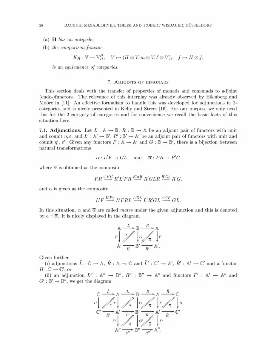
7.1. Adjunctions. Let L : A → B, R : B → A be an adjoint pair of functors with unitand counit η, ε, and L′ : A

′ → B′, R′ : B

′ → A′ be an adjoint pair of functors with unit and

counit η′, ε′. Given any functors F : A → A′ and G : B → B

′, there is a bijection betweennatural transformations

α : L′F → GL and α : FR → R′G

where α is obtained as the composite

FRη′FR−→ R′L′FR

R′αR−→ R′GLR

R′Gε−→ R′G,

and α is given as the composite

L′FL′Fη−→ L′FRL

L′αL−→ L′R′GL

ε′GF−→ GL.

In this situation, α and α are called mates under the given adjunction and this is denotedby a ⊣ α. It is nicely displayed in the diagram

AL //

F��

BR //

G��

A

F��αz� ||

||||

|

||||

|||

A′

α

:B}}}}}}}

}}}}}}}

L′

//B′

R′

//A′.

Given further(i) adjunctions L : C → A, R : A → C and L′ : C

′ → A′, R′ : A

′ → C′ and a functor

H : C → C′, or

(ii) an adjunction L′′ : A′′ → B

′′, R′′ : B′′ → A

′′ and functors F ′ : A′ → A

′′ andG′ : B

′ → B′′, we get the diagram

CL //

H��

AL //

F��

BR //

G��

A

F��αy� {{

{{{{

{{

{{{{

{{{{

R // C

γy� {{{{

{{{

{{{{

{{{

H��

C′

R′

//γ

:B|||||||

|||||||

A′

α

9A||||||||

||||||||

L′

//

F ′

��

B′

R′

//

G′

��

A′

F ′

��βy� ||||

||||

||||

|||| R′

//C′

A′′

L′′

//β

:B}}}}}}}

}}}}}}}

B′′

R′′

// A′′,


yielding the mates

(M1) L′′F ′FβF−→ G′L′F

G′α−→ G′GL ⊣ F ′FG

F ′α−→ F ′R′G

βG−→ R′′G′G,

(M2) L′L′HL′β−→ L′FL

αL−→ LGL ⊣ HRR

βG−→ R′R′G

R′β−→ R′R′G.

7.2. Properties of mates. Let L,L′ : A → B be functors with right adjoints R, R′,respectively, and α : L′ → L a natural transformation.

(i) If L′′ : A → B is a functor with right adjoint R′′ and β : L′′ → L′ a natural transfor-mation, then

α · β ⊣ β · α.

(ii) If L : C → A is a functor with right adjoint R, then

(αL′ : L′L → LL) ⊣ (Rα : RR → RR′).

(iii) If Lo : B → C is a functor with right adjoint Ro, then

(Loα : LoL′ → LoL) ⊣ (αRo : RRo → R′Ro).

Proof. (i) is a special case of 7.1(M1).(ii) follows from 7.1(M2) by putting A

′ = A, B′ = B, C′ = C and H ′ = H.

(iii) is derived by applying 7.1 to the diagram

AL // B

Lo// C

Ro// B

I{� ��

��

��

��

R // A

αz� ~~~~

~~~

~~~~

~~~

AL′

//α

;C��

��

B

I

;C��

��

Lo// C

Ro// B

R′

// A.

⊔⊓

As observed by Eilenberg and Moore in [11, Section 3], for a left adjoint endofunctor whichis a monad, the right adjoint (if it exists) is a comonad (and vice versa). The techniquesoutlined above provide a convenient and effective way to describe this transition and toprove related properties. Recall that for any endofunctor L : A → A with right adjoint R,for a positive integer n, the powers Ln have the right adjoints Rn.

7.3. Adjoints of monads and comonads. Let L : A → A be an endofunctor with rightadjoint R.

(1) If L = (L,mL, eL) is a monad, then R = (R, δR, εR) is a comonad, where δR, εR arethe mates of mL, eL in the diagrams

AL // A

R // A

εR{� ~~~~

~~~

~~~~

~~~

A

eL

;C��

��

I// A

I// A,

AL // A

R // A

δRz� ~~~~

~~~

~~~~

~~~

A

mL

;C��

��

HH// A

RR// A.

(2) If L = (L, δL, εL) is a comonad, then R = (R,mR, eR) is a monad where mR, eR arethe mates of δL, εL in the diagrams

AI // A

I // A

eR{� ~~~~

~~~

~~~~

~~~

A

εL

;C��

��

L// A

R// A,

ALL // A

RR // A

mRz� ~~~~

~~~

~~~~

~~~

A

δL

;C��

��

L// A

R// A.


Proof. (1) Since eL ⊣ εR and mL ⊣ δR, it follows from 7.2 (ii) and (iii) that

LeL ⊣ εRR, eLL ⊣ RεR, mLL ⊣ RδR, LmL ⊣ δRR.

Applying 7.2 (i) now yields

mL · LeL ⊣ εRR · δR, mL · eLL ⊣ RεR · δR,

mL · mLL ⊣ RδR · δR, mL · LmL ⊣ δRR · δR.

Since L is a monad we have mL · eLL = mL ·LeL = I and mL ·mLL = mL ·LmL, implying

εRR · δR = RεR · δR = I and RδR · δR = δRR · δR.

This shows that R = (R, δR, εR) is a comonad.

The proof of (2) is similar. ⊔⊓

The methods under consideration also apply to the natural transformations LL → LL

which were basic for the definition and investigation of bimonads in previous sections. Thefollowing results were obtained in cooperation with Gabriella Bohm and Tomasz Brzezinski.

7.4. Adjointness and distributive laws. Let L : A → A be an endofunctor with rightadjoint R and a natural transformation λL : LL → LL. This yields a mate λR : RR → RR

in the diagram

ALL // A

RR // A

λR{� ��

��

��

��

A

λL

;C��

��

LL// A

RR// A

with the following properties:

(1) LλL ⊣ λRR and λLL ⊣ RλR.

(2) λL satisfies the Yang-Baxter equation if and only if λR does.

(3) λ2L = I if and only if λ2

R = I.

(4) If L = (L,mL, eL) is a monad and λL is monad distributive, then λR is comonaddistributive for the comonad R = (R, δR, εR).

(5) If L = (L, δL, εL) is a comonad and λL is comonad distributive, then λR is monaddistributive for the comonad R = (R,mR, eR).

Proof. (1) follows from 7.2, (ii) and (iii). The remaining assertions follow by (1) andthe identities in the proof of 7.3. ⊔⊓

Recall from Definition 4.1 that a bimonad H is a monad and a comonad with compatibilityconditions involving an entwining λH : HH → HH.

7.5. Adjoints of bimonads. Let H be a monad H = (H,mH , eH) and a comonadH = (H, δH , εH) on the category A. Then a right adjoint R of H induces a monadR = (R,mR, eR) and a comonad R = (R, δR, εR) (see 7.3) and

(1) H = (H,H) is a bimonad with entwining λH : HH → HH if and only if R = (R,R)is a bimonad with entwining λR : RR → RR.

(2) H = (H,H) is a bimonad with entwining λ′H : HH → HH if and only if R = (R,R)

is a bimonad with entwining λ′R : RR → RR.

(3) If H = (H,H, λH) is a bimonad with antipode, then R = (R,R, λR) is a bimonadwith antipode (Hopf monad).


Proof. (1) With arguments similar to those in the proof of 7.4 we get that λR is anentwining from R to R. It remains to show the properties required in Definition 4.1. From7.2(i) we know that

εH · HεH ⊣ eRR · eR, εH · mH ⊣ δR · eR,

δH · eH ⊣ εR · mR, eHH · eH ⊣ εR · RεR, εH · eH ⊣ εR · eR.

Thus the equalities

εH · HεH = εH · mH , δH · eH = εHH · eH , εH · eH = I

hold if and only if

eRR · eR = δR · eR, εR · mR = εR · RεR, εR · eR = I.

The transfer of the compatibility between product and coproduct 4.1 is seen from thecorresponding diagrams

HHmH //

HδH

��

HδH // HH

HHHλHH

// HHH,

HmH

OO RR RδRoo RR

mRoo

δRR

��RRR

mRR

OO

RRR.RλR

oo

The proof of (2) is similar.(3) By 5.5, the existence of an antipode is equivalent to the bijectivity of the morphism

γH = HmH · δHH : HH → HH.

Since δHH ⊣ RmR and HmH ⊣ δRR, γH is an isomorphism if and only if γR = RmR · δRR

is an isomorphism. ⊔⊓

Functors with right (resp. left) adjoints preserve colimits (resp. limits) and thus 5.6 and7.5 imply:

7.6. Hopf monads with adjoints. Assume the category A to admit limits or colimits.Let H = (H,mH , eH , δH , εH , λH) be a bimonad on A with a right adjoint bimonad R =(R,mR, eR, δR, εR, λR). Then the following are equivalent:

(a) the comparison functor KH : A → AHH(λH) is an equivalence;

(b) the comparison functor KR : A → ARR(λR) is an equivalence;

(c) H has an antipode;

(d) R has an antipode.

Finally we observe that local prebraidings are also tranferred to the adjoint functor.

7.7. Adjointness of τ-bimonads. Let H be a monad H = (H,mH , eH) and a comonadH = (H, δH , εH) on the category A with a right adjoint R.

If H = (H,H) is a bimonad with double entwining τH : HH → HH, then R = (R,R) isa bimonad with double entwining τR : RR → RR.

Moreover, τH satisfies the Yang-Baxter equation if and only if so does τR.

Proof. Most of the assertions follow immediately from 7.4 and 7.5.It remains to verify the compatibility condition 6.9. For this observe that from 7.2(i) we

getδHδH ⊣ mHmH , HτHH ⊣ RτRR, mHmH ⊣ δRδR,

and hence

mHmH · τHH · δHδH ⊣ mRmR · RτRR · δRδR and δH · mM ⊣ δR · mR.


It follows that H satifies 6.9 if and only if so does R. ⊔⊓

7.8. Dual Hopf algebras. Let B be a module over a commutative ring R. B is a Hopfalgebra if and only if the endofunctor B ⊗R − on the catgeory of R-modules is a Hopfmonad. By 7.5, B ⊗R − is a bimonad (with antipode) if and only if its right adjoint functorHomR(B,−) is a bimonad (with antipode). This situation is considered in more detail in[5].

If B is finitely generated and projective as an R-module and B∗ = HomR(B,R), thenHomR(B,−) ≃ B∗ ⊗R − and we obtain the familiar result that B is a Hopf algebra if andonly if B∗ is.

7.9. Characterisations of groups. For any set G, the endofunctor G × − : Set → Setis a Hopf bimonad on the category of sets if and only if G has a group structure (e.g. [33,5.20]). Since the functor Map(G,−) is right adjoint to G×−, it follows from 7.6 that a setG is a group if and only if the functor Map(G,−) : Set → Set is a Hopf monad.

Acknowledgements. The authors want to express their thanks to Gabriella Bohmand Tomasz Brzezinski for inspiring discussions and helpful comments. The research wasstarted during a visit of the first author at the Department of Mathematics at the HeinrichHeine University of Dusseldorf supported by the German Research Foundation (DFG). Heis grateful to his hosts for the warm hospitality and to the DFG for the financial help.

References

[1] Barr, M., Composite cotriples and derived functors, in: Sem. Triples Categor. Homology Theory, SpringerLN Math. 80, 336-356 (1969)

[2] Beck, J., Distributive laws, in: Seminar on Triples and Categorical Homology Theory, B. Eckmann (ed.),Springer LNM 80, 119-140 (1969)

[3] Bespalov, Y. and Drabant, B., Hopf (bi-)modules and crossed modules in braided monoidal categories,J. Pure Appl. Algebra 123(1-3), 105-129 (1998)

[4] Bespalov, Y., Kerler, Th., Lyubashenko V. and Turaev, V., Integrals for braided Hopf algebras, J. PureAppl. Algebra 148(2), 113-164 (2000)

[5] Bohm, G., Brzezinski, T. and Wisbauer, R., Monads and comonads in module categories, preprint[6] Borceux, F. and Dejean, D., Cauchy completion in category theory, Cah. Topol. Geom. Differ.

Categoriques 27, 133-146 (1986)[7] Bruguieres, A. and Virelizier, A., Hopf monads, Adv. Math. 215(2), 679-733 (2007)[8] Brzezinski, T. and Wisbauer, R., Corings and Comodules, London Math. Soc. Lecture Note Series 309,

Cambridge University Press (2003)[9] Dubuc, E., Adjoint triangles, Rep. Midwest Category Semin. 2, Lect. Notes Math. 61, 69-91 (1968)

[10] Dubuc, E., Kan extensions in enriched category theory, Lecture Notes in Mathematics 145, Berlin-Heidelberg-New York: Springer-Verlag (1970)

[11] Eilenberg, S. and Moore, J.C., Adjoint functors and triples, Ill. J. Math. 9, 381-398 (1965)[12] Gomez-Torrecillas, J., Comonads and Galois corings, Appl. Categ. Struct. 14(5-6), 579-598 (2006)[13] Gumm, H.P., Universelle Coalgebra, in: Allgemeine Algebra, Ihringer, Th., Berliner Stud. zur Math.,

Band 10, 155-207, Heldermann Verlag (2003)[14] Hardie, K.A., Projectivity and injectivity relative to a functor, Math. Colloq., Univ. Cape Town 10,

68-80 (1957/76)[15] Janelidze, G. and W. Tholen, W., Facets of Descent, III : Monadic Descent for Rings and Algebras,

Appl. Categorical Structures 12, 461-476 (2004)[16] Kelly, G.M. and Street, R., Review of the elements of 2-categories, Category Sem., Proc., Sydney

1972/1973, Lect. Notes Math. 420, 75-103 (1974)[17] Loday, J.-L., Generalized bialgebras and triples of operads, arXiv:math/0611885[18] McCrudden, P., Opmonoidal monads, Theory Appl. Categ. 10, 469-485 (2002)[19] Mesablishvili, B., Descent in categories of (co)algebras, Homology, Homotopy and Applications 7, 1-8

(2005)[20] Mesablishvili, B., Monads of effective descent type and comonadicity, Theory Appl. Categ. 16, 1-45

(2006)

http://arXiv.org/abs/math/0611885


[21] Mesablishvili, B., Entwining Structures in Monoidal Categories, J. Algebra 319(6), 2496-2517 (2008)[22] Moerdijk, I., Monads on tensor categories, J. Pure Appl. Algebra 168(2-3), 189-208 (2002)[23] Power, J. and Watanabe, H., Combining a monad and a comonad, Theor. Comput. Sci. 280(1-2), 137-162

(2002)[24] Schubert, H., Categories, Berlin-Heidelberg-New York, Springer-Verlag (1972)[25] Skoda, Z., Distributive laws for actions of monoidal categories,

arXiv:math.CT/0406310 (2004)[26] Sobral, M., Restricting the comparison functor of an adjunction to projective objects, Quaest. Math. 6,

303-312 (1983)[27] Street, R., Frobenius monads and pseudomonoids, J. Math. Phys. 45(10), 3930-3948 (2004)[28] Szlachanyi, K., The monoidal Eilenberg-Moore construction and bialgebroids, J. Pure Appl. Algebra

182(2-3), 287-315 (2003)[29] Szlachanyi, K., Adjointable monoidal functors and quantum groupoids, Caenepeel, S. (ed.) et al., Hopf

algebras in noncommutative geometry and physics, Proc. conf. on Hopf algebras and quantum groups,Brussels 2002. Marcel Dekker. LN PAM 239, 291-307 (2005)

[30] Takeuchi, M., Survey of braided Hopf algebras, in: New trends in Hopf algebra theory, Proc. Coll. Quan-tum Groups and Hopf Algebras, La Falda, Argentina 1999, Andruskiewitsch, N. et al.(ed.), Providence,RI: American Math. Soc., Contemp. Math. 267, 301-323 (2000)

[31] Turi, D. and Plotkin, G., Towards a mathematical operational semantics, Proceedings 12th Ann. IEEESymp. on Logic in Computer Science, LICS’97, Warsaw, Poland (1997)

[32] Wisbauer, R., On Galois comodules, Commun. Algebra 34(7), 2683-2711 (2006)[33] Wisbauer, R., Algebras versus coalgebras, Appl. Categor. Struct. 16(1-2), 255-295 (2008)[34] Wolff, H., V-Localizations and V-monads. J. Algebra 24, 405-438 (1973)

Addresses:Razmadze Mathematical Institute, Tbilisi 0193, Republic of Georgia

[email protected]

Department of Mathematics of HHU, 40225 Dusseldorf, [email protected]

http://arXiv.org/abs/math/0406310

bimonads and hopf monads on categories

Documents