arX

iv:m

ath/

0702

337v

1 [

mat

h.R

T]

12

Feb

2007

BRAIDED HOPF ALGEBRAS OBTAINED FROM

COQUASITRIANGULAR HOPF ALGEBRAS

MARGARET BEATTIE AND DANIEL BULACU

Abstract. Let (H, σ) be a coquasitriangular Hopf algebra, not necessarilyfinite dimensional. Following methods of Doi and Takeuchi, which parallel

the constructions of Radford in the case of finite dimensional quasitriangularHopf algebras, we define Hσ , a sub-Hopf algebra of H0, the finite dual ofH. Using the generalized quantum double construction and the theory ofHopf algebras with a projection, we associate to H a braided Hopf algebrastructure in the category of Yetter-Drinfeld modules over H

copσ . Specializing to

H = SLq(N), we obtain explicit formulas which endow SLq(N) with a braidedHopf algebra structure within the category of left Yetter-Drinfeld modules overUext

q (slN )cop.

1. Introduction

The Drinfeld double construction plays an important role in the theory of mini-mal quasitriangular Hopf algebras since the Drinfeld double of a finite dimensionalHopf algebra is minimal quasitriangular. Conversely, any minimal quasitriangularHopf algebra is a quotient of a Drinfeld double [15]. This second statement is aconsequence of the following facts. If (H,R) is a quasitriangular Hopf algebra thenfrom an expression for R ∈ H ⊗ H of minimal length, one can define two finitedimensional sub-Hopf algebras of H , denoted by R(l) and R(r), respectively, andthere is a quasitriangular Hopf algebra morphism between the Drinfeld double ofR(l) and H whose image is HR = R(l)R(r), the minimal quasitriangular Hopf al-

gebra associated to (H,R). Note that there is an isomorphism R∗cop(l)

∼= R(r) and

this isomorphism, together with the evaluation map, gives a skew pairing fromR(r) ⊗R(l) to k.

Now suppose that (H,σ) is a coquasitriangular Hopf algebra, not necessarilyfinite dimensional. The analogues of the Hopf algebras R(l) and R(r), denoted by Hl

andHr, are, in general, infinite dimensional sub-Hopf algebras ofH0, the finite dualof H , and HrHl = HlHr is a sub-Hopf algebra of H0 denoted by Hσ. In general,there is no analogue to the isomorphism R∗cop

(l)∼= R(r), but the coquasitriangular

map σ induces a skew pairing on Hr⊗Hl. Although the classical Drinfeld double isnot available in this setting, there exists a generalized quantum double, in the senseof Majid [13] or Doi and Takeuchi [5], for Hopf algebras in duality, so that the skewpairing betweenHr andHl gives a generalized quantum double, denotedD(Hr, Hl).In general, D(Hr, Hl) has no (co)quasitriangular structure (see Proposition 2.8 and

Support for the first author’s research, and partial support for the second author, came froman NSERC Discovery Grant. The second author held a postdoctoral fellowship at Mount AllisonUniversity during this project. He would like to thank Mount Allison University for their warmhospitality.

1

2 MARGARET BEATTIE AND DANIEL BULACU

Remark 5.4); however, there is a surjective Hopf algebra morphism from D(Hr, Hl)to Hσ given by multiplication in H0. Note that, if (H,σ) is finite dimensionalthen Hσ = H∗

R, the minimal quasitriangular Hopf algebra associated to (H∗, R),where R is the matrix of H∗ obtained from σ. Thus, in the finite dimensional case,(Hσ, R) is quasitriangular. In the infinite dimensional case, neither Hσ nor H0 isguaranteed a quasitriangular structure.

Drinfeld [6] observed that for a finite dimensional quasitriangular Hopf alge-bra H , its double D(H) is a Hopf algebra with a projection. Majid [10] provedthat the converse of Drinfeld’s result also holds, and computed on H∗ the braidedHopf algebra structure associated to this projection [16]. Here, for (H,σ) coquasi-triangular but not necessarily finite dimensional, using the evaluation pairing, weconstruct the generalized quantum double D(Hcop

σ , H). In the finite dimensionalcase, Hcop

σ = (H∗R)cop has a quasitriangular structure and there is a Hopf algebra

morphism from D(Hcopσ , H) to Hcop

σ covering the natural inclusion, so D(Hcopσ , H)

is a Hopf algebra with a projection. We show that, for H not necessarily finitedimensional, D(Hcop

σ , H) is still a Hopf algebra with projection, and we describeexplicitly the induced structure on H of a braided Hopf algebra in the category ofleft Yetter-Drinfeld modules over Hcop

σ .

This paper is organized as follows. In Section 2, Preliminaries, we first definepairings and skew pairings on Hopf algebras and give the construction of the gener-alized quantum double. Coquasitriangular Hopf algebras give important examplesof Hopf algebras with a skew pairing. As well, we describe the structure of a Hopfalgebra A with projection (see [16]), so that A is isomorphic to a Radford biproductB × K, where B is a braided Hopf algebra in the category of left Yetter-Drinfeldmodules over K.

In Section 3, we first work in a rather general context. For U, V bialgebrassuch that there is an invertible pairing from U ⊗ V to k, we show that there is aprojection from D(U cop, V ) to U cop covering the natural inclusion if and only ifthere is a bialgebra morphism γ : V → U cop satisfying a relation analogous to thecoquasitriangularity condition for a skew pairing. (See also [5] and [17].) Now ifU, V are Hopf algebras with an invertible pairing and γ exists as above, then V has aHopf algebra structure in the category of left Yetter-Drinfeld modules over U cop. Wedescribe this structure explicitly. For example, if (U,R) is quasitriangular, then sucha map γ exists. Then, for H finite dimensional we prove that there is a projectionπ : D(H) = D(H∗cop, H) → H∗cop covering the inclusion H∗cop → D(H) if andonly if H is coquasitriangular (Proposition 3.9). A fortiori, H has a braided Hopfalgebra structure. Moreover, this structure allows us to obtain the left version ofthe transmutation theory for coquasitriangular Hopf algebras (Remark 4.3).

The transmutation theory for coquasitriangular Hopf algebras is due to Majid[11]. Using the dual reconstruction theorem, he associated to any coquasitriangularHopf algebra (H,σ), a braided commutative Hopf algebraH in the category of rightH-comodules, called the function algebra braided group associated to H . In Section4.1 we show that H can be obtained by writing a generalized quantum double as a

Radford biproduct using the projection π : D(H,H) → H given by multiplicationin H . To this projection corresponds a braided Hopf algebra H in the category

BRAIDED FROM CQT HOPF ALGEBRAS 3

of left H-comodules. By considering the co-opposite case, we obtain, after someidentification, that (Hcop)cop = H , as braided Hopf algebras (Proposition 4.2).

In Section 4.2, we describe the “dual case”, and show thatD(Hcopσ , H) is always a

Hopf algebra with a projection. This follows from a more general construction wherewe take A and X to be sub-Hopf algebras of H , HrA

and HlX the correspondingsub-Hopf algebras of Hr and Hl respectively, and HX,A the corresponding sub-Hopfalgebra of Hσ. Then there is a Hopf algebra projection from D(Hcop

X,A, X) to HcopX,A

which covers the inclusion. We stress the fact that this “dual case” give rise to a newbraided Hopf algebra structure on X (denoted by X) in the category of left Hcop

X,A

Yetter-Drinfeld modules. This new construction cannot be viewed as an exampleof the transmutation theory because the transmutation theory associates to anordinary coquasitriangular Hopf algebra a braided Hopf algebra in the category ofcorepresentations over itself. We show that, in fact, the two constructions aboveare related by a non-canonical braided functor. More exactly, we show that there

exists a braided functor F : MX →H

copX,A

HcopX,A

YD such that F(X) = X (Theorem 4.10).

Nevertheless, we think it worthwhile to have the construction of X. This is first ofall because X lies in a category of left Yetter-Drinfeld modules over Hcop

X,A which, in

general, may not have a quasitriangular structure. (See the example in Section 6).Secondly, this is because evaluation gives a duality between HX,A and X and theassociated quantum double, D(Hcop

X,A, X), is isomorphic to X ×HcopX,A.

In Section 5 we present the finite dimensional case in full detail, linking the resultsof this paper to those of Radford described above. Also, we note that starting witha finite dimensional quasitriangular Hopf algebra (H,R) and taking A = X = H∗

then the corresponding braided Hopf algebra H∗ is precisely the categorical dual ofHcop, the associated enveloping algebra braided group of (Hcop, R21) constructed

by Majid in [12] (Remarks 5.8).

Finally, in Section 6, we apply the constructions of Section 4.2 to the coquasitri-angular Hopf algebra H := SLq(N). By direct computations we show that Hl andHr are the Borel-like Hopf algebras Uq(b+) and Uq(b−), respectively, associatedto U ext

q (slN ), and obtain that Hσ = U extq (slN ). The general theory above leads

to more conceptual proofs for some well known results. Namely, there exist dualparings of the pairs of Hopf algebras Uq(b+)cop and Uq(b−), U ext

q (slN ) and SLq(N),and Uq(slN ) and SLq(N), respectively (Corollary 6.11 and Corollary 6.14), andU ext

q (slN ) and Uq(slN ) are factors of generalized quantum doubles (Corollary 6.12and Remark 6.13). Also, the Hopf algebra structure of Uq(slN ) is achieved in anatural way (Remark 6.9 and Remark 6.13). The rest of the Section 6 is dedicatedto a description of the braided Hopf algebra structure of SLq(N) in the categoryof left U ext

q (slN )cop Yetter-Drinfeld modules. The explicit formulas for this braidedHopf algebra structure can be found in Proposition 6.16 and Theorem 6.17.

Concluding, the general results in this paper have led not only to some propertiesof the couple (U ext

q (slN ), SLq(N)) well known in quantum group theory, but alsoto some new ones. Namely, SLq(N) has a braided Hopf algebra structure in thecategory of left Yetter-Drinfeld modules over U ext

q (slN )cop which coincides with thatof the image of the transmutation object of SLq(N) through a non-canonical braidedfunctor, and the corresponding Radford biproduct is isomorphic to the generalizedquantum double associated to this dual pair.

4 MARGARET BEATTIE AND DANIEL BULACU

2. Preliminaries

Throughout, we work over a field k and maps are assumed to be k-linear. Anyunexplained definitions or notation may be found in [3],[8], [13], [14] or [18].

For B a k-bialgebra, we write the comultiplication in B as ∆(b) = b1⊗b2 for b ∈ B.For M a left B-comodule, we write the coaction as ρ(m) = m−1⊗m0. For M a rightB-comodule, we will use the subscript bracket notation to differentiate subscriptsfrom those in comultiplication expressions, i.e. we will write ρ(m) = m(0) ⊗m(1) form ∈ M. For k-spaces M and N, tw will denote the usual twist map from M ⊗ N

to N ⊗ M.

2.1. Pairings on Hopf algebras and the generalized quantum double. Wefirst recall the definition for two bialgebras or Hopf algebras to be in duality (see[21, Section 1] or [13, Section 1.4]); this notion was first introduced by Takeuchiand called a Hopf pairing.

Throughout this section U and V will denote bialgebras over k.

Definition 2.1. A bilinear form 〈, 〉 : U ⊗ V → k is called a pairing of U and V if

〈mn, x〉 = 〈m,x1〉〈n, x2〉,(2.1)

〈m,xy〉 = 〈m1, x〉〈m2, y〉,(2.2)

〈1, x〉 = ε(x), 〈m, 1〉 = ε(m),(2.3)

for all m,n ∈ U and x, y ∈ V . Then U and V are said to be in duality.

Remarks 2.2. (i) A bilinear form from U ⊗ V to k is called a skew pairing if it is apairing from U cop ⊗ V to k or, equivalently, a pairing from U ⊗ V op to k.

(ii) The form 〈, 〉 is a pairing of U and V if and only if there is a bialgebramorphism φ : U → V 0, defined by φ(u)(v) = 〈u, v〉, if and only if there exists abialgebra morphism ψ : V → U0 defined by ψ(v)(u) = 〈u, v〉. If U and V are Hopfalgebras, these maps are Hopf algebra maps.

(iii) If U and V are Hopf algebras and 〈, 〉 is a pairing of U and V , then thisbilinear form is invertible in the convolution algebra Hom(U ⊗V, k) and its inverseis the bilinear form which maps u⊗ v to 〈SU (u), v〉 = 〈u, SV (v)〉 .

(iv) If 〈, 〉 is a (skew) pairing between U and V , then there is a (skew) pairingbetween the sub-bialgebras φ(U) ⊆ V 0 and ψ(V ) ⊆ U0 defined by the bilinear formB : φ(U) ⊗ ψ(V ) → k,

B(φ(u), ψ(v)) = 〈u, v〉.

The form B is well-defined since φ(u) = φ(u′) if and only if 〈u,−〉 = 〈u′,−〉 andψ(v) = ψ(v′) if and only if 〈−, v〉 = 〈−, v′〉. It is straightforward to check that B isa (skew) pairing.

(v) If 〈, 〉 is a pairing of the bialgebras U and V and U ⊆ U , V ⊆ V are sub-bialgebras then the restriction of 〈, 〉 to U ⊗ V is a pairing of U and V. As above,the bialgebras φ(U) and ψ(V) are also in duality.

Example 2.3. For H a bialgebra, then the evaluation map provides a dualitybetween H0, the finite dual of H , and H , that is, 〈f, h〉 = f(h) for all f ∈ H0 andh ∈ H .

Another class of examples for bialgebras in duality is provided by coquasitrian-gular bialgebras, also called braided bialgebras. This concept is dual to the idea ofquasitriangular bialgebras (see [8] or [13] for the defintion). We recall the notion ofcoquasitriangularity.

BRAIDED FROM CQT HOPF ALGEBRAS 5

Definition 2.4. A bialgebra H is called coquasitriangular (CQT for short) if thereexists a convolution invertible k-bilinear skew pairing σ : H ⊗H → k, i.e., for allh, h′, g ∈ H ,

σ(hh′, g) = σ(h, g1)σ(h′, g2)(2.4)

σ(g, hh′) = σ(g2, h)σ(g1, h′)(2.5)

σ(1, h) = σ(h, 1) = ε(h),(2.6)

which also satisfies the coquasitriangular condition,

(2.7) σ(h1, h′1)h2h

′2 = h′1h1σ(h2, h

′2).

Remarks 2.5. (i) Doi [4] showed that for (H,σ) a CQT Hopf algebra, one maydefine an invertible element v ∈ H∗ by

(2.8) v(h) = σ(h1, S(h2)) with inverse v−1(h) = σ(S2(h1), h2),

and

(2.9) S2(h) = v−1(h1)h2v(h3), ∀ h ∈ H.

Similarly, the element u ∈ H∗ defined by u(h) = σ(h2, S(h1)), is invertible withinverse u−1(h) = σ(S2(h2), h1) and also defines the square of the antipode S of Has a co-inner automorphism of H , i.e., S2(h) = u(h1)h2u

−1(h3), for all h ∈ H . Inparticular, the antipode S is bijective.

(ii) Let (H,σ) be a CQT bialgebra. Then σ is a convolution invertible pairingbetween H and Hop and also between Hcop and H .

(iii) Clearly any sub-bialgebra of a CQT bialgebra (H,σ) is CQT.(iv) If (H,σ) is CQT, then so are (Hop, σ−1) and (Hcop, σ−1) where, if H is a

Hopf algebra, σ−1 = σ ◦ (SH ⊗ IdH) = σ ◦ (IdH ⊗ S−1H ) is the convolution inverse

of σ [4, 1.2]. Moreover, (H,σ−121 = σ−1 ◦ tw) is another CQT structure for H , so

that (Hop, σ21 := σ ◦ tw) and (Hcop, σ21) are CQT also.

Let B, H be bialgebras and ℘ an invertible skew pairing ℘ : B ⊗ H → k. Wenow define the bialgebra (Hopf algebra) structure on B ⊗ H to be studied in thispaper. We follow the presentation in [5].

For A a bialgebra, an invertible bilinear form τ on A is called a unital 2-cocycleif for all a, b, c ∈ A,

τ(a1, b1)τ(a2b2, c) = τ(b1, c1)τ(a, b2c2) and τ(a, 1) = τ(1, a) = ε(a).

If τ is a 2-cocycle on A, then we may form Aτ , the bialgebra which has coalgebrastructure from A but with the new multiplication

a • b = τ(a1, b1)a2b2τ−1(a3, b3).

It is shown in [5] that since ℘ is an invertible skew pairing on B⊗H, then the bilinearform on B⊗ H defined by τ(b ⊗ h, b′ ⊗ h′) = ε(b)℘(b′, h)ε(h′) is a unital 2-cocycle.Then we may form the bialgebra (B ⊗ H)τ . As a coalgebra, (B ⊗ H)τ = B ⊗ H,the unit is 1 ⊗ 1, and the multiplication is defined by

(2.10) (b ⊗ h)(b′ ⊗ h′) = ℘(b′1, h1)℘−1(b′3, h3)bb′2 ⊗ h2h

′.

For B,H Hopf algebras with bijective antipodes, the inverse of ℘ as a skew-pairing on B ⊗ H is given by ℘−1(b, h) = ℘(SB(b), h) = ℘(b, S−1

H (h)). Then (B ⊗

6 MARGARET BEATTIE AND DANIEL BULACU

H)τ , also often denoted by B ⊲⊳τ H, has antipode given by

S(b ⊗ h) = (1 ⊗ SH(h)) • (SB(b) ⊗ 1)

= ℘(SB(b3), SH(h3))℘−1(SB(b1), SH(h1))SB(b2) ⊗ SH(h2).(2.11)

This construction is a special case of the generalized quantum double (see [13,Chapter 7]) for matched pairs of Hopf algebras.

Definition 2.6. We denote (B ⊗ H)τ by D(B,H) and will refer to this bialgebra(Hopf algebra) with multiplication as in (2.10), coalgebra structure from the tensorproduct B ⊗ H, and antipode as in (2.11) as a generalized quantum double.

In fact, in many of our constructions, we will begin with a pairing 〈, 〉 : U⊗V → kwhich is then a skew pairing ρ from U cop ⊗ V → k. Then, continuing to writesubscripts in U , and using the fact that 〈S−1

U (m), SV (x)〉 = 〈m,x〉, we have thatthe formulas for the multiplication, comultiplication and antipode in D(U cop, V )are given by

(m⊗ x)(n ⊗ y) = 〈n3, x1〉〈S−1U (n1), x3〉mn2 ⊗ x2y(2.12)

∆(m⊗ x) = (m2 ⊗ x1) ⊗ (m1 ⊗ y2)(2.13)

S(m⊗ x) = 〈m1, x3〉〈m3, S−1V (x1)〉S

−1U (m2) ⊗ SV (x2).(2.14)

Example 2.7. (cf. [13, 7.2.5]) If H is a finite dimensional Hopf algebra, then H∗

and H are in duality via the evaluation map as mentioned above and the doubleD(H∗cop, H) is the usual Drinfeld double, denoted in this case by D(H).

It is shown in [13] that if (H,σ) is CQT, so is the double (H ⊗H)τ = D(H,H),where τ is the unital 2-cocycle on H ⊗H defined by the skew-pairing σ.

The next proposition shows that this generalizes to D(B,H) where B,H areCQT Hopf algebras.

Proposition 2.8. Let B,H be Hopf algebras, ℘ : B ⊗ H → k a skew pairing, andD = D(B,H) = (B ⊗ H)τ the generalized quantum double of Definition 2.6. ThenD is CQT if and only if B and H are.

Proof. Since sub-Hopf algebras of a CQT Hopf algebra are CQT, then if D is CQT,so are B and H.

Now suppose that (B, σB) and (H, σH) are CQT. Then we form the CQT Hopfalgebra (A, σ) = (B ⊗ H, (σB ⊗ σH) ◦ (IdB ⊗ tw ⊗ IdH)). From the above discus-sion, τ : A⊗A→ k is a unital 2-cocycle, where τ(b⊗ h, b′ ⊗ h′) = ε(b)℘(b′, h)ε(h′).Then by [13, p.61 (2.24)], Aτ is CQT via the bilinear form ω defined by ω(a, a′) =τ(a′1, a1)σ(a2, a

′2)τ

−1(a3, a′3). Specifically, (D = Aτ , ω) is coquasitriangular where

ω(b ⊗ h, b′ ⊗ h′) = ℘(b1, h′1)σB(b2, b

′1)σH(h1, h

′2)℘(SB(b′2), h2).

(By using (2.7) for ℘ generously, one can even check the coquasitriangularity con-ditions (2.4) to (2.7) for ω directly.) �

Next we show how the doubles D(U cop, V ) and D(φ(U cop), ψ(V )) are related.

Lemma 2.9. Let U, V be Hopf algebras and 〈, 〉 a pairing of U and V . Thenφ(U) ⊆ V 0 and ψ(V ) ⊆ U0 are also Hopf algebras with a pairing B on φ(U)⊗ψ(V )defined by B(φ(u), ψ(v)) = 〈u, v〉. Then φ ⊗ ψ : D(U cop, V ) → D(φ(U cop), ψ(V ))is a surjection of Hopf algebras.

BRAIDED FROM CQT HOPF ALGEBRAS 7

Proof. From Remarks 2.2 and the fact that φ ⊗ ψ : U cop ⊗ V → φ(U cop) ⊗ ψ(V )is a Hopf algebra surjection, it remains only to show that φ ⊗ ψ respects themultiplication in the double. This can be checked by a straightforward compu-tation, or by noting that for D(U cop, V ) = (U cop ⊗ V )τ and D(φ(U cop), ψ(V )) =

(φ(U cop) ⊗ ψ(V ))τ ′

for cocycles τ, τ ′ as above, then τ(m ⊗ x, n ⊗ y) = τ ′(φ(m) ⊗ψ(x), φ(n) ⊗ ψ(y)). �

2.2. Hopf algebras with projection. Let K be a bialgebra. Recall that a leftYetter-Drinfeld module over K is a left K-module M which is also a left K-comodule,such that the following compatibility relation holds. For all κ ∈ K and m ∈M :

(2.15) κ1m−1 ⊗ κ2 · m0 = (κ1 · m)−1κ2 ⊗ (κ1 · m)0,

where K ⊗ M ∋ κ ⊗ m 7→ κ · m ∈ M is the left K-action. The category of leftYetter-Drinfeld modules over K and k-linear maps that preserve the K-action andK-coaction is denoted by K

KYD.The category K

KYD is pre-braided. If M,N ∈ KKYD then M⊗ N is a left Yetter-

Drinfeld module over K via the structures defined by

(2.16) κ · (m ⊗ n) = κ1 · m ⊗ κ2 · n and m ⊗ n 7→ m−1n−1 ⊗ m0 ⊗ n0,

for all κ ∈ K, m ∈ M and n ∈ N. The pre-braiding is given by

(2.17) cM,N(m ⊗ n) = m−1 · n ⊗ m0.

If K is a Hopf algebra then c is invertible, so KKYD is a braided monoidal category.

The structure of a Hopf algebra with projection was given in [16]. More precisely,

if K and A are Hopf algebras with Hopf algebra maps Ki-�π

A such that π ◦ i =

IdK, then there exists a braided Hopf algebra B in the category of left Yetter-Drinfeld modules K

KYD such that A ∼= B × K as Hopf algebras, where B × Kdenotes Radford’s biproduct between B and K (for more details see [16]).

As k-vector space B = {a ∈ A | a1 ⊗ π(a2) = a ⊗ 1}. Now, B is a K-modulesubalgebra of A where A is a left K-module algebra via the left adjoint actioninduced by i, that is κ ⊲i a = i(κ1)ai(S(κ2)), for all κ ∈ K and a ∈ A. Moreover,B is an algebra in the braided category K

KYD where the left coaction of K on B isgiven for all b ∈ B by

(2.18) λB(b) = π(b1) ⊗ b2.

Also, as k-vector space, B is the image of the k-linear map Π : A → A definedfor all a ∈ A by

(2.19) Π(a) = a1i(S(π(a2))).

For all a ∈ A, we define

(2.20) ∆(Π(a)) = Π(a1) ⊗ Π(a2).

This makes B into a coalgebra in KKYD and a bialgebra in K

KYD. The counit ofB is ε = ε |B. Moreover, we have that B is a braided Hopf algebra in K

KYD withantipode S given by

(2.21) S(b) = i(π(b1))SA(b2),

where SA is the antipode of A.The Hopf algebra isomorphism χ : B × K → A is given by

(2.22) χ(b× κ) = bi(κ),

8 MARGARET BEATTIE AND DANIEL BULACU

for all b ∈ B and κ ∈ K.Note that the description of a Hopf with a projection in terms of a braided Hopf

algebra is due to Majid [12].

3. Generalized quantum doubles which are Radford biproducts

It is well-known (Majid [10]) that if H is a finite dimensional Hopf algebra, thenthe Drinfeld double D(H) is a Radford biproduct. In this section, we give necessaryand sufficient conditions for a generalized quantum double D = D(U cop, V ) to bea Radford biproduct B×U cop, and determine the structure of B as a Hopf algebrain Ucop

UcopYD.Suppose first that U and V are bialgebras in duality with 〈, 〉 : U ⊗ V → k

an invertible pairing, so that ρ = 〈, 〉 is an invertible skew pairing on U cop ⊗ V .We form the generalized quantum double D = D(U cop, V ) as in Subsection 2.1.There are bialgebra morphisms i : U cop → D(U cop, V ) given by i(m) = m⊗ 1 andj : V → D(U cop, V ) given by j(x) = 1 ⊗ x.

Proposition 3.1. Let U, V be as above.(i) There exists a bialgebra projection π from D = D(U cop, V ) to U cop that splits

i if and only if there is a bialgebra map γ : V → U cop such that for all y ∈ V ,m ∈ U , we have

(3.1) γ(y)m = ρ−1(m1, y3)ρ(m3, y1)m2γ(y2).

(ii) Similarly, there exists a bialgebra projection from D to V that splits j if andonly if there is a bialgebra morphism µ : U cop → V such that for all y ∈ V,m ∈ U ,we have

(3.2) yµ(m) = ρ−1(m1, y3)ρ(m3, y1)µ(m2)y2.

If U, V are Hopf algebras, then these maps are Hopf algebra morphisms.

Proof. (i) Suppose that there is a bialgebra morphism γ : V → U cop satisfying(3.1). Define π to be π(m ⊗ x) = mγ(x), for all m ∈ U and x ∈ V . Then form ∈ U , we have that π ◦ i(m) = π(m ⊗ 1) = mγ(1) = m. Furthermore, by [5,2.4] with B = J = U cop, H = V , α = IdU , β = γ, we have that π is a bialgebramorphism.

Conversely, given π, define γ by γ = π ◦ j where j : V → D(U cop, V ) is definedby j(x) = 1 ⊗ x. Then, since π, j are bialgebra maps, so is γ. To verify that (3.1)holds, we compute

γ(y)m = (π ◦ j)(y)m

= π(1 ⊗ y)π(m⊗ 1) = π((1 ⊗ y)(m⊗ 1))

= ρ−1(m1, y3)ρ(m3, y1)m2γ(y2).

(ii) The proof of (ii) is analogous. �

Example 3.2. (cf. [5, 3.1]) Let σ be an invertible skew pairing on a bialgebra Hand form D(H,H). Then the identity map IdH satisfies (3.1) if and only if (H,σ)is CQT if and only if the multiplication map π : D(H,H) → H , π(h⊗ l) = hl is abialgebra map.

Example 3.3. In the setting of Proposition 3.1, if V is quasitriangular via R =R1 ⊗ R2 ∈ V ⊗ V , then the map π : D(U cop, V ) → V defined by π(m ⊗ x) =

BRAIDED FROM CQT HOPF ALGEBRAS 9

〈m,R1〉R2x is a bialgebra projection. Here the map µ : U cop → V is given byµ(m) = 〈m,R1〉R2. (The details can be found in [5, 2.5].)

Likewise, if U is quasitriangular with the R-matrix R = R1 ⊗R2 ∈ U ⊗U , thenπ : D(U cop, V ) → U cop defined by π(m ⊗ x) = 〈R2, x〉mS(R1) is a Hopf algebraprojection. In this case the map γ : V → U cop is given by γ(y) = 〈R2, y〉S(R1).

Remarks 3.4. (i) In later computations we will use that (3.1) is equivalent to

(3.3) ρ(m1, y2)γ(y1)m2 = ρ(m2, y1)m1γ(y2).

If m = γ(x), x ∈ V , then (3.1) becomes

(3.4) ρ(γ(x2), y2)γ(y1)γ(x1) = ρ(γ(x1), y1)γ(x2)γ(y2).

(ii) Note that if the above map γ : V → U cop is injective then the map σ :V ⊗ V → k defined by σ(x, y) = ρ(γ(x), y) = 〈γ(x), y〉 gives V a CQT structure.The relations (2.4), (2.5), (2.6) are easy to check and (2.7) is equivalent to

〈γ(x1), y1〉x2y2 = 〈γ(x2), y2〉y1x1.

This equation holds if and only if it holds when the injective map γ is applied toboth sides, i.e., when (3.4) holds.

If U, V are Hopf algebras with bijective antipodes, then for ρ a skew pairing fromU cop ⊗ V to k, we have ρ−1(m,x) = 〈S−1

U (m), x〉 = 〈m,S−1V (x)〉. In this case, we

have the identities below which are useful in the following computations and alsoprovide generalizations of the equations describing the square of the antipode inRemarks 2.5(i).

Proposition 3.5. Let U, V be Hopf algebras in duality and assume that there existsa map γ as in Proposition 3.1. Then:

(i) The map ϑ ∈ V ∗ defined by ϑ(x) = 〈γ(x1), SV (x2)〉, for all x ∈ V , isconvolution invertible with ϑ−1(x) = 〈γ(S2

V (x1)), x2〉. Moreover, for anyx ∈ V ,

(3.5) γ(S2V (x)) = ϑ−1(x1)γ(x2)ϑ(x3).

(ii) Similarly, the map υ ∈ V ∗ defined by υ(x) = 〈γ(x2), SV (x1)〉, for all x ∈ V ,is convolution invertible with υ−1(x) = 〈γ(S2

V (x2)), x1〉. In addition, for allx ∈ V ,

(3.6) γ(S2V (x)) = υ(x1)γ(x2)υ

−1(x3).

Proof. We only sketch the proof for (i); the rest of the details are left to the reader.For all x ∈ V we have

ϑ(x1)γ(S2V (x2)) = 〈γ(x3), SV (x4)〉γ(x1)γ(SV (x2))γ(S

2V (x5))

= 〈γ(x3), SV (x4)〉γ(x1)S−1U (γ(SV (x5))γ(x2))

(3.4)= 〈γ(x2), SV (x5)〉γ(x1)S

−1U (γ(x3)γ(SV (x4)))

= 〈γ(x2), SV (x3)〉γ(x1) = γ(x1)ϑ(x2),

and, in a similar manner, one can prove that

(3.7) γ(S2V (x1))ϑ

−1(x2) = ϑ−1(x1)γ(x2).

Now, for x ∈ V , using the fact that γ : V → U cop is a Hopf algebra map, we have

ϑ(x1)ϑ−1(x2) = ϑ(x1)〈γ(S

2V (x2)), x3〉 = ϑ(x2)〈γ(x1), x3〉

= 〈γ(x2), SV (x3)〉〈γ(x1), x4〉 = 〈γ(x1), SV (x2)x3〉 = ε(x).

10 MARGARET BEATTIE AND DANIEL BULACU

Similarly, using (3.7) we can show that ϑ−1(x1)ϑ(x2) = ε(x), so we are done. �

Now suppose that U, V are Hopf algebras with bijective antipodes and we havea Hopf algebra projection π from D(U cop, V ) to U cop that splits i. Then thereexists a Hopf algebra B in the category of Yetter-Drinfeld modules Ucop

UcopYD suchthat D = D(U cop, V ) ∼= B × U cop, a Radford biproduct. From Subsection 2.2, weknow that

B = {a ∈ D | a1 ⊗ π(a2) = a⊗ 1}.

Proposition 3.6. The map θ : V → B given by θ(y) = γ(S−1V (y2)) ⊗ y1 =

SU (γ(y2)) ⊗ y1 is a bijection.

Proof. Clearly the map θ is injective since ε ◦ γ = ε. It remains to show thatIm(θ) = B. For y ∈ V , we have θ(y) ∈ B since

θ(y)1 ⊗ π(θ(y)2) = (SU (γ(y4)) ⊗ y1) ⊗ π(SU (γ(y3)) ⊗ y2)

= (SU (γ(y4)) ⊗ y1) ⊗ γ(S−1V (y3)y2)

= (SU (γ(y2)) ⊗ y1) ⊗ 1 = θ(y) ⊗ 1.

Conversely, suppose that m ⊗ y ∈ B, i.e., (m2 ⊗ y1) ⊗m1γ(y2) = (m ⊗ y) ⊗ 1 ∈D ⊗ U cop. Then we have

m⊗ y = SU (1)m⊗ y

= SU (m1γ(y2))m2 ⊗ y1

= SU (γ(y2))SU (m1)m2 ⊗ y1

= εU (m)θ(y).

Similarly, if z =∑i

mi ⊗ yi ∈ B, then z = θ(∑i

ε(mi)yi). �

Now we denote by V the vector space V with the structure of a Yetter-Drinfeldmodule induced by that of B.

Proposition 3.7. The structure of the left U cop Yetter-Drinfeld module V is givenby the left action and left coaction

m⊲ y = 〈m1, S−1V (y1)〉y2〈m2, S

−2V (y3)〉 = 〈m,S−1

V (S−1V (y3)y1)〉y2;(3.8)

λV (y) = γ(S−1V (y3)y1) ⊗ y2.(3.9)

Proof. For m ∈ U and y ∈ V , we have that m⊲ y = θ−1(m⊲i θ(y)) by Section 2.2and using (2.12), (3.1) and the fact that 〈m, v〉 = 〈S−1

U (m), SV (v)〉, we compute

i(m2)θ(y)i(S−1U (m1))

= (m2 ⊗ 1)(γ(S−1V (y2)) ⊗ y1)(S

−1U (m1) ⊗ 1)

= m4γ(S−1V (y4))S

−1U (m2)〈S

−1U (m3), S

−1V (y3)〉 ⊗ y2〈S

−1U (m1), y1〉

(3.3)= m4S

−1U (m3)γ(S

−1V (y3))〈S

−1U (m2), S

−1V (y4)〉 ⊗ y2〈S

−1U (m1), y1〉

= 〈S−1U (m1), y1〉θ(y2)〈S

−1U (m2), S

−1V (y3)〉

= 〈m,S−1V (y1)S

−2V (y3)〉θ(y2),

BRAIDED FROM CQT HOPF ALGEBRAS 11

and this concludes the proof of the formula for the action. We now compute thecoaction.

(IdU ⊗ θ) ◦ λV (y) = (π ⊗ IdD)∆(θ(y))

= (π ⊗ IdD)∆(γ(S−1V (y2)) ⊗ y1)

= (π ⊗ IdD)((γ(S−1V (y4)) ⊗ y1) ⊗ (γ(S−1

V (y3)) ⊗ y2))

= γ(S−1V (y4)y1) ⊗ γ(S−1

V (y3)) ⊗ y2

= γ(S−1V (y3)y1) ⊗ θ(y2),

for all y ∈ V , and thus the formula for the coaction is also verified. �

We now describe the structure of V as a Hopf algebra in the category of leftYetter Drinfeld modules over U cop.

Proposition 3.8. The structure of V as a Hopf algebra in the category Ucop

UcopYD isgiven by the formulas:

x · y = 〈γ(y2), SV (x1)x3〉x2y1;(3.10)

∆(x) = 〈γ(SV (x4)x6), S−1V (x3)x1〉x2 ⊗ x5;(3.11)

S(x) = 〈γ(x4), x1SV (x3)〉SV (x2).(3.12)

The identity in V is θ−1(1 ⊗ 1) = 1 and the counit is ε = ε.

Proof. To see (3.10), we compute

θ(x)θ(y) = (SU (γ(x2)) ⊗ x1)(SU (γ(y2)) ⊗ y1)

(2.12)= 〈γ(y2), x3〉〈SU (γ(y4)), x1〉SU (γ(y3)γ(x4)) ⊗ x2y1

(3.4)= 〈γ(y3), x4〉〈SU (γ(y4)), x1〉SU (γ(x3)γ(y2)) ⊗ x2y1

= 〈γ(y2), x3〉〈γ(y3), SV (x1)〉θ(x2y1)

= 〈γ(y2), SV (x1)x3〉θ(x2y1).

Similarly, to verify (3.11), we compute

∆(θ(x)) = (Π ⊗ Π)(∆(θ(x))) = (Π ⊗ Π)(∆(SU (γ(x2)) ⊗ x1))

= Π(SU (γ(x4)) ⊗ x1) ⊗ Π(SU (γ(x3)) ⊗ x2))

= Π(SU (γ(x3)) ⊗ x1) ⊗ θ(x2)

(2.19)= (SU (γ(x5)) ⊗ x1)

(S−1

U (π(SU (γ(x4)) ⊗ x2)) ⊗ 1)⊗ θ(x3)

(2.12,2.1)= 〈γ(x12), S

−1V (x4)〉〈S

−1U (γ(x6)), S

−1V (x5)〉〈S

−1U (γ(x8)), x1〉

×〈γ(x10), x2〉γ(S−1V (x13)SV (x7)x11) ⊗ x3 ⊗ θ(x9)

Now we use the equivalent form of (3.5)

ϑ−1(S−1V (y2))γ(S

−1V (y1)) = γ(SV (y2))ϑ

−1(S−1V (y1)),

to replace 〈S−1U (γ(x6)), S

−1V (x5)〉γ(SV (x7)) by 〈S−1

U (γ(x7)), S−1V (x6)〉γ(S

−1V (x5)),

and obtain

∆(θ(x)) = 〈γ(x12), S−1V (x4)〉〈S

−1U (γ(x7)), S

−1V (x6)〉〈S

−1U (γ(x8)), x1〉

×〈γ(x10), x2〉γ(S−1V (x13)S

−1V (x5)x11) ⊗ x3 ⊗ θ(x9).

From (3.4), we have

〈γ(x12), S−1V (x4)〉γ(S

−1V (x5))γ(x11) = 〈γ(x11), S

−1V (x5)〉γ(x12)γ(S

−1V (x4)),

12 MARGARET BEATTIE AND DANIEL BULACU

so we can conclude that

∆(θ(x)) = 〈γ(x11), S−1V (x5)〉〈S

−1U (γ(x7)), S

−1V (x6)〉〈S

−1U (γ(x8)), x1〉〈γ(x10), x2〉

×γ(S−1V (x13)x12)γ(S

−1V (x4)) ⊗ x3 ⊗ θ(x9)

= 〈γ(x10), S−1V (x4)〉〈S

−1U (γ(x6)), S

−1V (x5)〉〈S

−1U (γ(x7)), x1〉

×〈γ(x9), x2〉θ(x3) ⊗ θ(x8)

= 〈γ(SV (x4)x8), S−1V (x3)〉〈γ(SV (x5)x7), x1〉θ(x2) ⊗ θ(x6)

= 〈γ(SV (x4)x6), S−1V (x3)x1〉θ(x2) ⊗ θ(x5).

Finally, we verify (3.12). From (2.21), we have that

S(θ(x)) = i(π(θ(x)1))S(θ(x)2)

= (SU (γ(x4))γ(x1) ⊗ 1)S(SU (γ(x3)) ⊗ x2)

= (SU (γ(x4))γ(x1) ⊗ 1)(1 ⊗ SV (x2))(γ(x3) ⊗ 1)

= 〈S−1U (γ(x7)), SV (x2)〉〈γ(x5), SV (x4)〉SU (γ(x8))γ(x1)γ(x6) ⊗ SV (x3)

= 〈γ(x7), x2〉〈γ(x5), SV (x4)〉SU (γ(x8))γ(x1)γ(x6) ⊗ SV (x3).

By (3.4) we can replace 〈γ(x7), x2〉γ(x1)γ(x6) by 〈γ(x6), x1〉γ(x7)γ(x2) and weobtain

S(θ(x)) = 〈γ(x6), x1〉〈γ(x5), SV (x4)〉SU (γ(x8))γ(x7)γ(x2) ⊗ SV (x3)

= 〈γ(x6), x1〉〈γ(x5), SV (x4)〉γ(x2) ⊗ SV (x3)

= 〈γ(x5), x1SV (x4)〉SU (γ(SV (x2))) ⊗ SV (x3)

= 〈γ(x4), x1SV (x3)〉θ(SV (x2)).

The final statement is clear. �

We noted in Example 3.3 that if V is quasitriangular then D(U cop, V ) is a Hopfalgebra with a projection. So for V = (H,R) a finite dimensional quasitriangularHopf algebra and U = H∗ we obtain Drinfeld’s projection [6], and by an analogueof Propositions 3.7 and 3.8, the structure of H∗ as a braided Hopf algebra in H

HYDcomputed by Majid in [10]. (In fact, it can be proved that this braided Hopf algebralies in the image of a canonical braided functor from HM to H

HYD.) On the otherhand, if U = H∗ is quasitriangular, and V = H , then we have the following.

Proposition 3.9. Let H be a finite dimensional Hopf algebra. Then there ex-ists a Hopf algebra projection π : D(H) → H∗cop covering the natural inclusionH∗cop → D(H) if and only if H is CQT. Moreover, if this is the case, then π is aquasitriangular morphism.

Proof. Suppose (H,σ) is CQT and let {ei, ei} be a dual basis for H . Then H∗ is

quasitriangular with R-matrix R =∑i,j

σ(ei, ej)ei ⊗ej . Since D(H) = D(H∗cop, H),

from Example 3.3 the map π : D(H) → H∗cop given by

π(h∗ ⊗ h) =∑

i,j

σ(ei, ej)ej(h)h∗(ei ◦ S) =

∑

i

σ(ei, h)h∗(ei ◦ S),

for all h∗ ∈ H∗ and h ∈ H , is a Hopf algebra morphism which covers the inclusionH∗cop → D(H).

BRAIDED FROM CQT HOPF ALGEBRAS 13

Conversely, if such a morphism exists, then by Proposition 3.1 there exists aHopf algebra morphism γ : H → H∗cop satisfying

〈h∗1, x2〉γ(x1)h∗2 = 〈h∗2, x1〉h

∗1γ(x2),

for all x ∈ H and h∗ ∈ H∗, where 〈, 〉 : H∗ ⊗ H → k is the evaluation map. It isclear that the above condition is equivalent to

〈γ(x1), y1〉x2y2 = 〈γ(x2), y2〉y1x1,

for all x, y ∈ H . Now, if we define σ(x, y) = 〈γ(x), y〉, for all x, y ∈ H , then one caneasily check that σ defines a CQT structure on H (see also [17, Theorem 3.3.14]).

Finally, the canonical R-matrix of D(H) is R =∑i

(ε⊗ei)⊗ (ei⊗1). So if (H,σ)

is CQT then the above morphism π is quasitriangular since

(π ⊗ π)(R) =∑

i,j

σ(ej , S−1(ei))e

j ⊗ ei =∑

i,j

σ−1(ej , ei)ej ⊗ ei,

and, from the dual version of Remarks 2.5 (iv), the last term defines a QT structurefor H∗cop. �

For H finite dimensional it is not hard to see that the categories H∗cop

H∗copYD and

HYDH are isomorphic as braided monoidal categories (the braided structures arethe ones obtained from the left or right center construction, see [2]). The iso-morphism is produced by the following functor F . If (M, ·, λ) ∈ H∗cop

H∗copYD then

F(M) = M becomes an object in HYDH via the structure

h • m = m−1(h)m0, m 7→ ei · m ⊗ ei.

F sends a morphism to itself.By the above identification, Proposition 3.9 and Propositions 3.7 and 3.8 we

obtain the following which may be viewed as a left version of the transmutationtheory for CQT Hopf algebras. Further details will follow in Section 4.1.

Corollary 3.10. If H is a CQT Hopf algebra then H has a braided Hopf algebrastructure, denoted by H, within HYDH . Namely, H is a left-right Yetter-Drinfeldmodule over H via

x 7→ x(0) ⊗ x(1) := x2 ⊗ S−1(x1)S−2(x3)

h • x = σ(h, S−1(x1)S−2(x3))x2 = σ−1

21 (S−1(x3)x1, h)x2,

for all h, x ∈ H. H is a Hopf algebra in HYDH with the same unit and counit asH and

x · y = σ(S(x1)x3, S−1(y2))x2y1 = σ−1

21 (y2, S(x1)x3)x2y1,

∆(x) = σ(S−1(x3)x1, S−1(x6)x4)x2 ⊗ x5 = σ−1

21 (S(x4)x6, S−1(x3)x1)x2 ⊗ x5,

S(x) = σ(x1S(x3), S−1(x4))S(x2) = σ−1

21 (x4, x1S(x3))S(x2).

Proof. We only note that from the proof of Proposition 3.9 the Hopf algebra mor-phism γ : H → H∗cop is given in this case by γ(h) = lS−1(h), for all h ∈ H . �

If B is a bialgebra and M is a left Yetter-Drinfeld module over B, then the mapRM : M ⊗ M → M ⊗ M, RM(m ⊗ m′) = m′

−1 · m ⊗ m′0 is a solution in End(M⊗3)

of the quantum Yang-Baxter equation

R12R13R23 = R23R13R12.

14 MARGARET BEATTIE AND DANIEL BULACU

Above, we have that V is a left Yetter-Drinfeld module over U cop. Then asolution RV ∈ End(V ⊗ V ) to the quantum Yang-Baxter equation is given by

RV (x⊗ y) = γ(SV (y3)y1) ⊲ x⊗ y2

= 〈γ(S−1V (y3)y1), S

−1V (S−1

V (x3)x1)〉x2 ⊗ y2.

4. Coquasitriangular bialgebras and generalized quantum doubles

4.1. Transmutation theory. As was mentioned in the introduction, the braidedreconstruction theorem associates to any CQT Hopf algebra H a braided commu-tative Hopf algebra H in the category of right H-comodules, MH . The goal of thissubsection is to show that H can be obtained from the structure of a generalizedquantum double with a projection.

Let X and A be sub-Hopf algebras of a CQT Hopf algebra (H,σ). Then σinduces a skew pairing on A⊗X , still denoted by σ and the generalized quantumdouble D(A,X) is defined. By (2.7) it follows that XA = AX , so XA is a sub-Hopfalgebra of H . From [5, 3.1] the map

π′ : D(A,X) → AX = XA, π′(a⊗ x) = ax

is a surjective Hopf algebra morphism. Although D(H,H) is a Hopf algebra withprojection, we cannot, in general, make the same claim for D(A,X). Nevertheless,XA and X are sub-Hopf algebras of (H,σ), so applying the same arguments wefind that

π : D(AX,X) → AX = XA, π(ax ⊗ y) = axy

is a surjective Hopf algebra morphism covering the inclusion map i : AX →D(AX,X) with the map γ from Proposition 3.1 being the inclusion ofX into AX =XA. From Propositions 3.7 and 3.8 for γ : X → AX and 〈, 〉 = σ : AX ⊗X → k,X has a braided Hopf algebra structure in the braided monoidal category XA

XAYD;this braided Hopf algebra is denoted, as usual, by X. The structures are given by

xa ⊲ y = σ(xa, S−1(S−1(y3)y1))y2,

λX(y) = S−1(y3)y1 ⊗ y2,

x · y = σ(y2, S(x1)x3)x2y1, 1 = 1,

∆(x) = σ(S(x4)x6, S−1(x3)x1)x2 ⊗ x5, ε = ε,

S(x) = σ(x4, x1S(x3))S(x2),

for all x, y ∈ X and a ∈ A. Next, we show that X lies in the image of a canonicalbraided functor from XM to XA

XAYD, so this general context reduces to the caseX = A = H . We recall some background on CQT Hopf algebras and braidedmonoidal categories.

For a CQT bialgebra (B, ς) it is well known that its category of left or rightB comodules has a braided monoidal structure. Namely, if M and N are two left(respectively right) B comodules then

M ⊗ N ∋ m ⊗ n 7→ m−1n−1 ⊗ m0 ⊗ n0 ∈ B ⊗ M ⊗ N

defines the monoidal structure of BM and

(4.1) cM,N : M ⊗ N → N ⊗ M, cM,N(m ⊗ n) = ς(n−1,m−1)n0 ⊗ m0

defines a braiding on BM, while

(4.2) M ⊗ N ∋ m ⊗ n 7→ ⊗m(0) ⊗ n(0) ⊗ m(1)n(1) ∈ M ⊗ N ⊗ B

BRAIDED FROM CQT HOPF ALGEBRAS 15

gives the monoidal structure of MB and

(4.3) cM,N : M ⊗ N → N ⊗ M, cM,N(m ⊗ n) = ς(m(1), n(1))n(0) ⊗ m(0)

provides a braided structure on MB (see [8, 13] for terminology).We denote by (B,ς)M the category of left B-comodules with the braiding in (4.1).

Similarly, M(B,ς) is the category of right B-comodules with the braiding defined by(4.3). One can easily see that (Bcop,ς21)M ≡ M(B,ς), as braided monoidal categories,where ς21 = ς ◦ tw is the CQT structure of Bcop defined in Remarks 2.5.

Secondly, if (B, ς) is a CQT bialgebra and M a left B-comodule then M is a leftYetter-Drinfeld module over B with the initial comodule structure and with theB-action defined by

(4.4) b · m := ς(m−1, b)m0.

Thus there is a well defined braided functor F(B,ς) : (B,ς)M → BBYD where F(B,ς)

sends a morphism to itself.

Lemma 4.1. In the setting above, the braided Hopf algebra X lies in the image

of the composite of the canonical functor (X,σ−121 )M → (XA,σ−1

21 )M and the functorF(XA,σ−1

21 ).

Proof. We haveλX(x) := x−1 ⊗ x0 = S−1(x3)x1 ⊗ x2.

Therefore the X-action on X can be rewritten as

x ⊲ y = σ(x, S−1(y−1))y0 = σ−1(x, y−1)x0 = σ−121 (y−1, x)y0,

and this finishes the proof. �

In general, if C is a braided monoidal category with braiding c then Cin is C as amonoidal category, but with the mirror-reversed braiding cM,N = c−1

N,M . Note that,if B ∈ C is a braided Hopf algebra with comultiplication ∆ and bijective antipodeS then Bcop, the same object B, but with the comultiplication and antipode

∆cop = c−1B,B ◦ ∆ and Scop = S−1

respectively, and with the other structure morphisms the same as for B, is a braidedHopf algebra in the category Cin. Now, since the transmutation object H is a

braided Hopf algebra in MH and not HM we must apply the above correspondenceX 7→ X to (Hcop, σ21) rather than (H,σ) and thus obtain a braided Hopf algebra

Hcop ∈ (Hcop,σ−1)M ≡ M(H,σ−121 ) ≡ M(H,σ)in.

We can now prove the connection between Hcop and H . The structures of H

can be found in [13, Example 9.4.10].

Proposition 4.2. Let (H,σ) be a CQT Hopf algebra. Then (Hcop)cop = H as

braided Hopf algebras in M(H,σ).

Proof. One can easily see that (Hcop)cop is an object of MH via the structure

h 7→ h(0) ⊗ h(1) = h2 ⊗ S(h1)h3,

and that its algebra structure within M(H,σ) is given by

h · g = σ(S−1(h3)h1, g1)h2g2 = σ(S(h1)h3, S(g1))h2g2,

for all h, g ∈ H . Clearly, the unit of (Hcop)cop is the unit of H .

16 MARGARET BEATTIE AND DANIEL BULACU

Now, by (4.3) we have that c−1, the inverse of the braiding c of M(H,σ−121 ), is

defined by c−1M,N(n ⊗ m) = σ(n(1),m(1))m(0) ⊗ n(0). Therefore, the comultiplication

of (Hcop)cop is given by

h 7→ σ(S(h4)h6, S−1(h3)h1)c

−1(h5, h2)

= σ((h2)(1), S−1((h1)(1)))c

−1((h2)(0) ⊗ (h1)(0))

= σ−1((h2)(2), (h1)(2))σ((h2)(1), (h1)(1))(h1)(0) ⊗ (h2)(0)

= h1 ⊗ h2 = ∆(h),

the comultiplication of H . The counit of (Hcop)cop is ε, the counit of H .Finally, the antipode of Hcop is defined by S(h) = σ(h4S

−1(h2), h1)S−1(h3), so

the antipode of (Hcop)cop is given, for all h ∈ H , by

S−1(h) = σ(S2(h3)S(h1), h4)S(h2).

Indeed, for all h ∈ H we have

(S ◦ S−1)(h) = σ(h1S(h6), S−1(h7))σ(S(h2)h4, S(h5))h3

(2.4)= σ(h1, S

−1(h9))σ(S(h7), S−1(h8))σ(h2, h6)σ(h4, S(h5))h3

= σ(h1, S−1(h7))v(h4)σ(h2, h5)v

−1(h6)h3

(2.9)= σ(h1, S

−1(h5))σ(h2, S−2(h4))h3

(2.5)= σ(h1, S

−2(h3)S−1(h4))h2 = h,

as needed. In a similar way we can prove that S−1 ◦ S = IdH , the details are leftto the reader. Comparing the above structures of (Hcop)cop with those of H from

[13] we conclude that(Hcop)cop = H , as braided Hopf algebras in M(H,σ). �

Remark 4.3. From Corollary 3.10 we can deduce the left version of the transmu-tation theory for a CQT Hopf algebra (H,σ) as follows. Observe that there is a

braided functor G : (H,σ)M → HYDH defined by G(M) = M but now viewed asleft-right H Yetter-Drinfeld module via

h · m = σ(h, S−1(m−1))m0, m 7→ ρ(m) := m0 ⊗ S−1(m−1).

G sends a morphism to itself.Now, one can easily see that H in Corollary 3.10 lies in the image of the functor

G. In other words we can associate to (H,σ) a Hopf algebra structure in (H,σ)M,still denoted by H . Note that H has the left H-comodule structure given by

x 7→ λH(x) = x−1 ⊗ x0 = S−1(x3)x1 ⊗ x2,

for all x ∈ H, and is a braided Hopf algebra in (H,σ)M via the structure in Corol-lary 3.10. (In fact, this H is the braided Hopf algebra in Lemma 4.1 correspondingto X = (H,σ−1

21 ).) We can conclude now that Hop,cop is the braided Hopf algebra

in (H,σ)M associated to (H,σ) through the left transmutation theory. By Hop,cop

we denote H viewed now as a Hopf algebra in (H,σ)M via

x ⋄ y =: mH ◦ cH,H(x, y) = σ(y−1, x−1)y0x0 = σ(y2, S(x1)x3)x2y1,

∆Hop,cop = c−1H,H ◦ ∆ = ∆,

and the other structure morphisms equal those of H .

BRAIDED FROM CQT HOPF ALGEBRAS 17

4.2. The “dual” case. Let (H,σ) be a CQT bialgebra, so that σ is a pairingfrom H ⊗Hop to k and Hcop ⊗H to k. Then by Remarks 2.2, we have bialgebramorphisms

φ : Hcop → H0 defined by φ(h)(l) = σ(h, l)

and

ψ : Hop → H0 defined by ψ(h)(l) = σ(l, h).

We denote rh := φ(h) = σ(h,−) and Hr = Im(φ). Similarly, lh := ψ(h) = σ(−, h)andHl = Im(ψ). More generally, if X and A are sub-bialgebras of a CQT bialgebraH then we define

HrA:= φ(Acop) = {ra = σ(a,−) | a ∈ A}

HlX := ψ(Xop) = {lx = σ(−, x) | x ∈ X}.

Proposition 4.4. Let (H,σ) be a CQT bialgebra (Hopf algebra) and X,A ⊆ Htwo sub-bialgebras (sub-Hopf algebras). Then

(i) HlX and HrAare sub-bialgebras (sub-Hopf algebras) of H0. The structure

maps for ψ(Xop) = HlX are given by

(4.5) lxy = lylx; l1 = ε; ∆(lx) = lx1 ⊗ lx2 ; ε(lx) = ε(x); S(lx) = lS−1(x),

and the structure maps for φ(Acop) = HrAare given by

(4.6) rab = rarb; r1 = ε; ∆(ra) = ra2 ⊗ ra1 ; ε(ra) = ε(a); S(ra) = rS−1(a).

(ii) The bilinear form from HrA⊗ HlX to k defined for all a ∈ A, x ∈ X, by

ra ⊗ lx → σ(a, x), is a skew pairing between HrAand HlX .

(iii) HrAHlX = HlXHrA

is a sub-bialgebra of H0 and is a sub-Hopf algebra ifA,X are sub-Hopf algebras of the Hopf algebra H.

Proof. (i) If X is a sub-bialgebra (sub-Hopf algebra) of H , then Xop is a sub-bialgebra (sub-Hopf algebra) of Hop. Since σ : H ⊗ Hop → k is a duality, byRemarks 2.2, ψ : Xop ⊆ Hop → H0 is a bialgebra morphism and thus HlX , the im-age of Xop under ψ, is a sub-bialgebra (sub-Hopf algebra) of H0 with the structuremaps given above. The proof for HrA

is similar, using the map φ.(ii) Follows directly from Remarks 2.2 since σ : Acop⊗Xop → k is a skew pairing.(iii) We refer to [5, 3.2 (b)]. Here it is shown that the map from D(Hcop, Hop)

to H0 defined by a⊗ h→ ralh is a bialgebra map, and our statement follows. Theproof is based on the observation that

lyra = σ(a1, S(y3))σ(a3, y1)ra2 ly2 or, equivalently,(4.7)

raly = σ(S−1(a3), y1)σ(a1, y3)ly2ra2 ,(4.8)

for any y ∈ X , a ∈ A. �

We now assume that H is a Hopf algebra. We denote by HX,A the Hopf subal-gebra of H0 equal to HlXHrA

= HrAHlX .

Proposition 4.5. Let (H,σ) be a CQT Hopf algebra, X, A and H sub-Hopf alge-bras of H, and HlX and HrA

the sub-Hopf algebras of H0 from Proposition 4.4. LetD(HrA

, HlX ) be the generalized quantum double from the skew pairing in Proposi-tion 4.4 (ii) induced by σ.

(i) The map f : D(HrA, HlX ) → HX,A, f(ra ⊗ lx) = ralx, a ∈ A, x ∈ X, is a

surjective Hopf algebra morphism.

18 MARGARET BEATTIE AND DANIEL BULACU

(ii) Then the evaluation map 〈, 〉 : HX,A ⊗H → k defined for all x ∈ X, a ∈ Aand h ∈ H by

(4.9) 〈lxra, h〉 = σ(h1, x)σ(a, h2) = lx(h1)ra(h2)

provides a duality between the Hopf algebras HX,A and H, and thereforebetween D(HrA

, HlX ) and H via the map f in (i). In particular, 〈, 〉 is askew pairing on Hcop

X,A ⊗H and D(HrA, HlX )cop ⊗H.

Proof. Statement (i) follows directly from [5, 2.4] with α = IdHrA, β = IdHlX

and

using (4.7). Statement (ii) is immediate. �

From now on, we assume that (H,σ) is a CQT Hopf algebra with X,A andthe evaluation pairing 〈, 〉 as above. Consider the generalized quantum doubleD(Hcop

X,A, X). From (2.12), the multiplication in D(HcopX,A, X) is given by

(4.10) (lxra ⊗ y)(lx′rb ⊗ y′) = 〈lx′

1rb3 , S

−1(y3)〉〈lx′

3rb1 , y1〉lxralx′

2rb2 ⊗ y2y

′,

for all x, x′, y, y′ ∈ X , a, b ∈ A, and since D(HcopX,A, X) = Hcop

X,A ⊗X as a coalgebra,the comultiplication is given by

(4.11) ∆(lxra ⊗ y) = (lx2ra1 ⊗ y1) ⊗ (lx1ra2 ⊗ y2).

The unit is ε⊗ 1 and the counit is defined by ε(lxra ⊗ y) = ε(x)ε(a)ε(y).We now prove that there is a Hopf algebra projection from D(Hcop

X,A, X) to HcopX,A

which covers the canonical inclusion i : HcopX,A → D(Hcop

X,A, X).

Proposition 4.6. The map π : D(HcopX,A, X) → Hcop

X,A defined by

(4.12) π(lxra ⊗ y) = lxralS−1(y),

for all x, y ∈ X, a ∈ A, is a Hopf algebra morphism such that π ◦ i = idHcopX,A

.

Proof. Define γ : X → HcoplX

⊆ HcopX,A by γ(x) = lS−1(x). We show that γ is a

bialgebra morphism and that (3.1) holds.For x, y ∈ X , we have

γ(xy) = lS−1(xy) = lS−1(y)S−1(x) = lS−1(x)lS−1(y) = γ(x)γ(y),

so that γ preserves multiplication. Similarly,

(γ ⊗ γ)(x1 ⊗ x2) = lS−1(x1) ⊗ lS−1(x2) = ∆HcopX,A

(γ(x)),

so that comultiplication is preserved. Clearly γ preserves the unit and counit. Toverify (3.1), we compute

γ(x)ly = lS−1(x)ly = lyS−1(x)

(2.4)= σ(S−1(x2), y2)σ(x1, y3)ly1S−1(x3)

(2.7)= σ(S−1(x3), y1)σ(x1, y3)lS−1(x2)y2

= 〈ly1 , S−1(x3)〉〈ly3 , x1〉ly2γ(x2).

As well we have that

γ(x2)ra = lS−1(x2)ra

(4.7)= σ(a1, S(S−1(x2)))σ(a3, S

−1(x4))ra2 lS−1(x3)

= 〈ra1 , x2〉〈ra3 , S−1(x4)〉ra2 lS−1(x3).

BRAIDED FROM CQT HOPF ALGEBRAS 19

Combining these equations, we obtain

γ(x)lyra = 〈ly3ra1 , x1〉〈ly1ra3 , S−1(x3)〉(ly2ra2)γ(x2)

= 〈(lyra)3, x1〉〈(lyra)1, S−1(x3)〉(lyra)2γ(x2).

Since π = mH0 ◦ (Id⊗ γ), the statement follows from Proposition 3.1. �

We now apply the results of Section 3 to this Radford biproduct.

Proposition 4.7. Let H,X,A, γ, π be as above. Then D(HcopX,A, X) ∼= B ×Hcop

X,A

where B is a Hopf algebra in the categoryH

copX,A

HcopX,A

YD. In addition,

(i) B = {lS−2(x2) ⊗ x1 | x ∈ X} and is isomorphic to X as a k-space;(ii) X is a left Hcop

X,A Yetter-Drinfeld module with the structure

lxra ⊲ y = 〈lxra, S−1(y1)S

−2(y3)〉y2,(4.13)

λX(y) = lS−1(y1)S−2(y3) ⊗ y2.(4.14)

Proof. Statement (i) follows directly from Proposition 3.6, while statement (ii)follows from Proposition 3.7. �

From now on, X will be the k-vector space X , with the structure of Hopf algebra

in the braided categoryH

copX,A

HcopX,A

YD induced from B via the above isomorphism. Next

we compute the structure maps of X in this category.

Theorem 4.8. The structure of X as a Hopf algebra inH

copX,A

HcopX,A

YD is given by the

formulas

x ◦ y = σ(S(x3)S2(x1), y2)x2y1,(4.15)

∆(x) = σ(S(x1)x3, S(x4)x6)x2 ⊗ x5,(4.16)

S(x) = σ(S2(x3)S(x1), x4)S(x2),(4.17)

for all x, y ∈ X. X has the same unit and counit as X ⊆ H.

Proof. Apply the formulas in Proposition 3.8 with U = HX,A and V = X . �

Remarks 4.9. (i) From Equations (2.8) and (2.9) in Remarks 2.5, we obtain anotherformula for the antipode S of X. For we note that

S(x) = σ(S2(x3), x4)σ(S(x1), x5)S(x2)

= σ(S(x1), x4)v−1(x3)S(x2)

= σ(S(x1), x4)v−1(x2)S

−1(x3)

= σ(S(x1), x5)σ(S2(x2), x3)S−1(x4)

= σ(S(x1), S−1(x2)x4)S

−1(x3).

(ii) The Hopf algebra isomorphism χ : X × HcopX,A → D(Hcop

X,A, X) is given by

χ(x× lyra) = (lS−2(x2) ⊗ x1)(lyra ⊗ 1), for all x, y ∈ X and a ∈ A.(iii) One can easily check that, in general,X is neither quantum commutative nor

quantum cocommutative as a bialgebra inH

copX,A

HcopX,A

YD. But, if σ restricted to X ⊗X

gives a triangular structure on X (that is, σ−1(x, y) = σ(y, x), for all x, y ∈ X)then X is quantum commutative, i.e.

x ◦ y = (x−1 ⊲ y) ◦ x0, ∀ x, y ∈ X.

20 MARGARET BEATTIE AND DANIEL BULACU

(iv) Any proper Hopf subalgebra X of a CQT Hopf algebra (H,σ) can be viewedas a braided Hopf algebra in (at least) three different left Yetter-Drinfeld modulecategories by applying Proposition 4.7 and Theorem 4.8 with different A. Specif-ically, over Hcop

lX(take A = k), over the co-opposite of HlXHrX

= HrXHlX (take

A = X), and over the co-opposite of HlXHr = HrHlX (take A = H). Note thatHlX ⊆ HlXHrX

⊆ HlXHr.

We note that the solution to the Yang-Baxter equation from the Yetter Drinfeldmodule X comes from the adjoint coaction.

For if (B, σ) is a CQT bialgebra and M a left B-comodule then we have seen thatM is a left Yetter-Drinfeld module over B with the initial comodule structure andwith the B-action defined by (4.4). In particular, we get that RM ∈ End(M ⊗ M)given for all m,m′ ∈ M by

RM(m ⊗ m′) = σ(m−1,m′−1)m0 ⊗ m′

0,

is a solution for the quantum Yang-Baxter equation.In the present setting, with (H,σ) CQT, then X is a left X-comodule via x 7→

S(x1)x3 ⊗ x2. Then RXad∈ End(X ⊗X) given for all x, y ∈ X by

RXad(x⊗ y) = σ(S(x1)x3, S(y1)y3)x2 ⊗ y2

is a solution for the quantum Yang-Baxter equation. From the discussion at theend of Section 3, writing S for SX , we note that

RX(x⊗ y) = 〈γ(S−1(y3)y1), S−1(S−1(x3)x1)〉x2 ⊗ y2

= 〈lS−1(S−1(y3)y1), S−1(S−1(x3)x1)〉x2 ⊗ y2

= σ(S−1(S−1(x3)x1), S−1(S−1(y3)y1))x2 ⊗ y2

= σ(S(x1)x3, S(y1)y3)x2 ⊗ y2

= RXad(x⊗ y).

Next, we show the connection between our X and the transmutation theory.

Theorem 4.10. Let (H,σ) be a CQT Hopf algebra and A,X sub-Hopf algebras of

H. Then there is a braided functor F : MX →H

copX,A

HcopX,A

YD such that F(X) = X.

Proof. We start by constructing the functor F explicitly. For M a rightX-comodule,let F(M) = M as a k-vector space, endowed with the following structures:

lxra ⊲m = lxra(S−2(m(1)))m(0) and λM(m) = lS−2(m(1)) ⊗ m(0),(4.18)

for any lxra ∈ HX,A and m ∈ M. From the definitions, F(M) is both a left HcopX,A-

module and comodule. Actually, F(M) is a Yetter-Drinfeld module over HcopX,A.

Here, using the co-opposite of the structure maps in Proposition 4.4, we see thatrelation (2.15) is

〈lx1ra2 , S−2(m(1))〉lx2ra1 lS−2(m(2)) ⊗ m(0)

= 〈lx2ra1 , S−2(m(2))〉lS−2(m(1))lx1ra2 ⊗ m(0)

BRAIDED FROM CQT HOPF ALGEBRAS 21

and this holds since

〈lx1ra2 , y1〉lx2ra1 ly2 = σ(y1, x1)σ(a2, y2)lx2ra1 ly3

(4.8)= σ(y1, x1)σ(a4, y2)σ(S−1(a3), y3)σ(a1, y5)lx2 ly4ra2

(2.5)= σ(y1, x1)σ(a1, y3)ly2x2ra2

(2.7)= σ(y2, x2)σ(a1, y3)lx1y1ra2

= 〈lx2ra1 , y2〉ly1 lx1ra2 ,

for all x, y ∈ X and a ∈ A. So F is a well defined functor from MX toH

copX,A

HcopX,A

YD.

(F sends a morphism to itself.)We claim that F has a monoidal structure defined by ϕ0 = Id : k → F(k) and

ϕ2(M,N) : F(M) ⊗ F(N) → F(M ⊗ N), the family of natural isomorphisms inH

copX,A

HcopX,A

YD given by

ϕ2(M,N)(m ⊗ n) = σ−1(m(1), n(1))m(0) ⊗ n(0),

for all m ∈ M ∈ MX and n ∈ N ∈ MX (for more details see for example [8, XI.4]).To this end, observe that ϕ2(M,N) is left Hcop

X,A-linear since

ϕ2(M,N)(lxra ⊲ (m ⊗ n))

(2.16)= ϕ2(M,N)(lx2ra1 ⊲m ⊗ lx1ra2 ⊲ n)

(4.18)= 〈lxra, S

−2(n(1)m(1))〉ϕ2(M,N)(m(0) ⊗ n(0))

= 〈lxra, S−2(n(2)m(2))〉σ

−1(m(1), n(1))m(0) ⊗ n(0)

(2.7)= 〈lxra, S

−2(m(1)n(1))〉σ−1(m(2), n(2))m(0) ⊗ n(0)

(4.2,4.18)= σ−1(m(1), n(1))lxra ⊲ (m(0) ⊗ n(0))

= lxra ⊲ ϕ2(M,N)(m ⊗ n),

for all x ∈ X , a ∈ A, m ∈ M and n ∈ N. The fact that ϕ2(M,N) is left HcopX,A-

colinear can be proved in a similar manner, the details are left to the reader.Clearly, ϕ2(M,N) is bijective and ϕ0 makes the left and right unit constraints

in MX andH

copX,A

HcopX,A

YD compatible. So it remains to prove that ϕ2 respects the

associativity constraints of the two categories above. It is not hard to see that thisfact is equivalent to

σ(h1, g1)σ(h2g2, h′) = σ(g1, h

′1)σ(h, h′2g2),

for all h, h′, g ∈ H , i.e., σ is a 2-cocycle, a well known fact which follows by applyingthe properties of coquasitriangularity or see [4].

Moreover, we have F a braided functor, this means

F(cM,N) ◦ ϕ2(M,N) = ϕ2(N,M) ◦ cF(M),F(N),

for all M,N ∈ MX . Indeed, on one hand, by (4.3) we have

F(cM,N) ◦ ϕ2(M,N)(m ⊗ n) = n ⊗ m.

22 MARGARET BEATTIE AND DANIEL BULACU

On the other hand, by (2.17) and (4.18) we compute:

ϕ2(N,M) ◦ cF(M),F(N)(m ⊗ n) = ϕ2(N,M)(lS−2(m(1)) ⊲ n⊗ m(0))

= σ(S−2(n(1)), S−2(m(1))ϕ2(N,M)(n(0) ⊗ m(0))

= n ⊗ m,

as needed.Finally, by Proposition 4.2 and Proposition 4.7 it follows that F(X) = X, as

objects inH

copX,A

HcopX,A

YD. Furthermore, since F is a braided functor and X is a braided

Hopf algebra in MX it follows that F(X) is a braided Hopf algebra inH

copX,A

HcopX,A

YD

with multiplication given by

mF(X) : F(X) ⊗ F(X)

ϕ2(X,X)- F(X ⊗X)F(mX)

- F(X),

the comultiplication defined by

∆F(X) : F(X)

F(∆X)- F(X ⊗X)

ϕ−12 (X,X)- F(X) ⊗ F(X),

and the same antipode as those of X . More precisely, according to the proof ofProposition 4.2 the multiplication • is given by

x • y = σ−1(x(1), y(1))x(0) · y(0)

= σ−1(x(1), S(y1)y3)x(0) · y2

= σ(x(2), S−1(y4)y1)σ(x(1), S(y2))x(0)y3

(2.5)= σ(x(1), S

−1(y2))x(0)y1 = σ(S(x3)S2(x1), y2)x2y1,

for all x, y ∈ X . Similarly, we have

∆F(X)(x) = σ((x1)(1), (x2)(1))(x1)(0) ⊗ (x2)(0)

= σ(S(x1)x3, S(x4)x6)x2 ⊗ x5,

for all x ∈ X . Comparing to the structures in Theorem 4.8 we conclude that

F(X) = X as braided Hopf algebras inH

copX,A

HcopX,A

YD, and this finishes the proof. �

We end this section with few comments.

Remarks 4.11. Let (H,σ), X and A be as above.(i) One can easily see that the map γ : A→ Hcop

rA⊆ Hcop

X,A given by γ(a) = ra is

a Hopf algebra morphism. Moreover, for this map γ, (3.1) reduces to

rarb = σ−1(b3, a3)σ(b1, a1)rb2ra2

which holds by (2.7). So on the k-vector space A we have a braided Hopf algebra

structure, denoted by A, inH

copX,A

HcopX,A

YD. Namely, A is a left Yetter-Drinfeld module

over HcopX,A via

lxra ⊲ b = 〈lxra, S−1(b1)S

−2(b3)〉b2, λA(a) = rS−1(a3)a1⊗ a2,

BRAIDED FROM CQT HOPF ALGEBRAS 23

and a Hopf algebra with the same unit and counit as A and

a · b = σ(b2, S(a1)a3)a2b1 = σ−121 (S(a3)S

2(a1), b2)a2b1,

∆(a) = σ(S(a4)a6, S−1(a3)a1)a2 ⊗ a5 = σ−1

21 (S(a1)a3, S(a4)a6)a2 ⊗ a5,

S(a) = σ(a4, a1S(a3))S(a2) = σ−121 (S2(a3)S(a1), a4)S(a2).

Comparing with the structure of X we conclude that A can be obtained from X byreplacing (H,σ) with (H,σ−1

21 ) and interchangingX and A. For this, observe that if

la and rx are the elements of H0 corresponding to H = (H,σ−121 ) then rx = lS−1(x)

and la = rS(a), so HA,X := HlAHrX

= HrAHlX = HX,A, as Hopf algebras. The

remaining details are now trivial.(ii) Although it might seem more natural to try to obtain a braided Hopf algebra

structure inH

copX,A

HcopX,A

YD on XA = AX , for this we would need a Hopf algebra map

π : AX → HcopX,A satisfying condition (3.1) in Proposition 3.1. A candidate is

π(ax) = ralS−1(x) but, in general, it is not well defined. (Take for example X =A = H = (SLq(N), σ), the CQT Hopf algebra defined in the last section of thispaper.)

5. The finite dimensional case

In this section we discuss how our results thus far relate to those of Radford [15]for finite dimensional Hopf algebras.

Throughout this section, (H,R) is a finite dimensional quasitriangular (QT forshort) Hopf algebra, so its dual linear space H∗ has a CQT structure given byσ : H∗ ⊗H∗ → k, σ(p, q) = p(R1)q(R2), for all p, q ∈ H∗, where R := R1 ⊗ R2 ∈H ⊗H . Thus, we can consider the sub-Hopf algebras H∗

l and H∗r of H∗∗ defined

in the previous section. Identifying H∗∗ and H via the canonical Hopf algebraisomorphism

Θ : H → H∗∗, Θ(h)(h∗) = h∗(h),

for all h ∈ H and h∗ ∈ H∗, we will prove that the sub-Hopf algebras H∗l and H∗

r ofH∗∗ can be identified with the sub-Hopf algebras R(l) and R(r) of H constructedin [15]. Recall that

R(l) := {q(R2)R1 | q ∈ H∗} and R(r) := {p(R1)R2 | p ∈ H∗}.

Also, note that, if we write R =m∑

i=1

ui⊗vi ∈ H⊗H , withm as small as possible, then

{u1, · · · , um} is a basis for R(l) and {v1, · · · , vm} is a basis for R(r), respectively. We

extend {u1, · · · , um} to a basis {u1, · · · , um, · · · , un} of H and denote by {ui}i=1,n

the dual basis of H∗ corresponding to {ui}i=1,n. Similarly, we extend {v1, · · · , vm}

to a basis {v1, · · · , vm, · · · , vn} of H and denote by {vi}i=1,n the dual basis of H∗

corresponding to {vi}i=1,n.

Lemma 5.1. For the above context the following statements hold:

i) The map µl : H∗l → R(l) defined by µl(lq) = q(R2)R1, for all q ∈ H∗,

is well defined and a Hopf algebra isomorphism. Its inverse is given byµ−1

l (ui) = lvi , for all i = 1,m. In particular, {lvi}i=1,m is a basis for H∗l .

ii) The map µr : H∗r → R(r) given by µr(rp) = p(R1)R2, for all p ∈ H∗,

is well defined and a Hopf algebra isomorphism. Its inverse is defined byµ−1

r (vi) = rui , for all i = 1,m. In particular, {rui}i=1,m is a basis for H∗r .

24 MARGARET BEATTIE AND DANIEL BULACU

Proof. We show only i), with the proof of ii) being similar. First observe that

lq(h∗) = σ(h∗, q) = h∗(R1)q(R2) = Θ(q(R2)R1)(h∗),

for all h∗ ∈ H∗. Thus H∗l = {Θ(q(R2)R1) | q ∈ H∗} = Θ(R(l)) ∼= R(l). Clearly µl is

precisely the restriction and corestriction of Θ−1 at Θ(R(l)) and R(l), respectively.Hence µl is well defined and a Hopf algebra isomorphism.

Finally, for all h∗ ∈ H∗ we have

lvi(h∗) = σ(h∗, vi) = h∗(R1)vi(R2) =

m∑

j=1

h∗(uj)vi(vj),

and therefore lvi = 0, for all i ∈ {m+ 1, · · · , n}, and lvi(h∗) = h∗(ui) = Θ(ui)(h∗),

i.e. lvi = Θ(ui), for all i = 1,m. This shows that µ−1l (ui) = lvi , for all i = 1,m, so

the proof is complete. �

From Proposition 4.4, σ gives a pairing on H∗copr ⊗ H∗

l , and we consider thegeneralized quantum double D(H∗

r , H∗l ). On the other hand, H∗

r and H∗l are finite

dimensional Hopf algebras, so we can construct the usual Drinfeld quantum doublesD(H∗

l ) and D(H∗r ). To demonstrate the connections between these Hopf algebras,

we first need the following lemma.

Lemma 5.2. Suppose that 〈, 〉 : U ⊗ V → k defines a duality between the finite di-mensional Hopf algebras U and V such that there exists a Hopf algebra isomorphismΨ : V ∗ → U with the property

(5.1) 〈Ψ(v∗), v〉 = v∗(v), ∀ v∗ ∈ V ∗, v ∈ V.

Then D(U cop, V ) ∼= D(V ) ∼= D(Uop,cop)op as Hopf algebras.

Proof. As coalgebras

D(U cop, V ) = U cop ⊗ V Ψ−1⊗Id∼=

V ∗cop ⊗ V = D(V ).

Thus will be enough to check that Ψ ⊗ Id : D(V ) → D(U cop, V ) is an algebramorphism. For all x∗, y∗ ∈ V ∗ and x, y ∈ V we compute

(Ψ ⊗ Id) ((x∗ ⊗ x)(y∗ ⊗ y))

= y∗1(S−1(x3))y∗3(x1)Ψ(x∗y∗2) ⊗ x2y

= 〈Ψ(y∗1), S−1(x3)〉〈Ψ(y∗3), x1〉Ψ(x∗)Ψ(y∗2) ⊗ x2y

= (Ψ(x∗) ⊗ x) (Ψ(y∗) ⊗ y) = (Ψ ⊗ Id) (x∗ ⊗ x) (Ψ ⊗ Id) (y∗ ⊗ y) ,

as needed. Clearly, Ψ ⊗ Id respects the units, so Ψ⊗ Id : D(U cop, V ) → D(V ) is aHopf algebra isomorphism.

From [15, Theorem 3] we know thatD(Uop,cop)op ∼= D(U∗) as Hopf algebras. ButU∗ ∼= V ∗∗ ∼= V as Hopf algebras, and therefore D(U∗) ∼= D(V ) as Hopf algebras.We conclude that D(Uop,cop)op ∼= D(V ) as Hopf algebras, and this finishes theproof. �

Proposition 5.3. Let (H,R) be a finite dimensional QT Hopf algebra with an R-

matrix R =m∑

i=1

ui ⊗ vi ∈ H ⊗H, with m as small as possible. If H∗l and H∗

r are

the Hopf subalgebras of H∗∗ ∼= H defined above then

D(H∗r , H

∗l ) ∼= D(H∗

l ) ∼= D((H∗r )op)op,

as Hopf algebras.

BRAIDED FROM CQT HOPF ALGEBRAS 25

Proof. We apply Lemma 5.2 for U = (H∗r )cop and V = H∗

l . So we shall prove thatthere exists a Hopf algebra morphism Ψ : (H∗

l )∗ → (H∗r )cop (or, equivalently, from

(H∗l )∗cop to H∗

r ) satisfying (5.1), this means 〈Ψ(η), lq〉 = η(q), for all η ∈ (H∗l )∗

and q ∈ H∗. We will use the Hopf algebra isomorphism ξ : R∗cop(l) → R(r) from

[15, Proposition 2(c)] defined by ξ(ζ) = ζ(R1)R2, for all ζ ∈ R∗(l). Note that

ξ−1(vi) = ui, for all i = 1,m, where ui is the restriction of ui at R(l).Now, define Ψ : (H∗

l )∗cop → H∗r as the composition of the following Hopf algebra

isomorphisms

Ψ : (H∗l )∗cop

(µ−1l

)∗- R∗cop(l)

ξ- R(r)µ−1

r- H∗r .

Explicitly, we have Ψ(η) =m∑

i=1

η(lvi)rui , for all η ∈ (H∗l )∗, and this allows us to

compute 〈Ψ(η), lvs〉 to be

m∑

i=1

η(lvi)〈rui , lvs〉 =

m∑

i

η(lvi)σ(ui, vs) =

m∑

i,j=1

η(lvi)ui(uj)vs(vj) = η(lvs),

for all s = 1,m. Since {lvs | s = 1,m} is a basis for H∗l it follows that 〈Ψ(η), lq〉 =

η(q), for all η ∈ (H∗l )∗ and q ∈ H∗, so the proof is finished. �

Remark 5.4. Let U and V be two Hopf algebras in duality via the bilinear form

〈, 〉. If there is an elementt∑

i=1

ui ⊗ vi ∈ U ⊗ V such that, for all u ∈ U and v ∈ V ,

(5.2)

t∑

i=1

〈ui, v〉vi = v and

t∑

i=1

〈u, vi〉ui = u,

then R =t∑

i=1

(1 ⊗ vi) ⊗ (ui ⊗ 1) is an R-matrix for D(U cop, V ).

Let now (H,R) be a finite dimensional QT Hopf algebra with R =m∑

i=1

ui ⊗ vi,

with m as small as possible. Thenm∑

i=1

rui ⊗ lvi ∈ H∗r ⊗H∗

l satisfies the conditions

in (5.2). Indeed, for all p ∈ H∗ we have

m∑

i=1

〈rp, lvi〉rui =

m∑

i,j=1

p(uj)vi(vj)rui =

m∑

i=1

p(ui)Θ(vi) = Θ(p(R1)R2) = rp,

and in a similar manner one can verify thatm∑

i=1

〈rui , lq〉lvi = lq, for all q ∈ H∗.

Therefore, R =m∑

i=1

(1 ⊗ lvi) ⊗ (rui ⊗ 1) is an R-matrix for D(H∗r , H

∗l ).

On the other hand, a basis on (H∗l )∗ can be obtained by using the inverse of

the Hopf algebra isomorphism Ψ constructed in Proposition 5.3. Since Ψ−1(rui) =ui ◦ µl it follows that {ui ◦ µl | i = 1,m} is a basis of (H∗

l )∗. Moreover, we caneasily see that it is the basis of (H∗

l )∗ dual to the basis {lvi | i = 1,m} of H∗l , so

R =m∑

i=1

(1 ⊗ lvi) ⊗ (ui ◦ µl ⊗ 1) is an R-matrix for D(H∗l ). Thus, we can conclude

that the Hopf algebra isomorphism Ψ ⊗ Id : D(H∗l ) → D(H∗

r , H∗l ) constructed in

26 MARGARET BEATTIE AND DANIEL BULACU

Proposition 5.3 is actually a QT Hopf algebra isomorphism, that is, in addition,((Ψ ⊗ Id) ⊗ (Ψ ⊗ Id)) (R) = R. The verification of the details is left to the reader.

We are now able to prove that, for our context, the Hopf algebra surjection fromProposition 4.5 is in fact a QT morphism, and that it can be deduced from thesurjective QT morphism F : D(R(l)) → HR := R(l)R(r) = R(r)R(l) considered in[15, Theorem 2]. Namely, F (ζ ⊗ ~) = ξ(ζ)~, for all ζ ∈ R∗

(l) and ~ ∈ R(l), where

ξ(ζ) = ζ(R1)R2 is the Hopf algebra isomorphism from R∗cop(l) to R(r) considered in

Proposition 5.3.

Proposition 5.5. Under the above circumstances and notations we have the fol-lowing diagram commutative.

D(H∗r , H

∗l )

f - H∗σ := H∗

rH∗l = H∗

l H∗r

D(H∗l )

Ψ−1 ⊗ Id ∼=

? (µ−1l )∗ ⊗ µl

∼=- D(R(l))

F- HR := R(r)R(l) = R(l)R(r)

∼= µ−1r µ−1

l

6

Here (µ−1l )∗ is the transpose of µ−1

l and µ−1r µ−1

l is defined by

µ−1r µ−1

l (p(r1)r2q(R2)R1) = rplq, ∀ p, q ∈ H∗,

where R = R1 ⊗R2 = r1 ⊗ r2 is the R matrix of H.

Proof. Straightforward. We only note that p(r1)r2q(R2)R1 = p′(r1)r2q′(R2)R1 iffΘ−1(rp)Θ

−1(lq) = Θ−1(rp′ )Θ−1(lq′), iff Θ−1(rplq) = Θ−1(rp′ lq′), iff rplq = rp′ lq′ ,

so µ−1r µ−1

l is well defined. �

Corollary 5.6. H∗σ is QT with ℜ =

m∑i=1

lvi ⊗ rui and in this way f becomes a

surjective QT Hopf algebra morphism.

Finally, we are able to show that in the finite dimensional case the morphism πin Proposition 4.6 arises from the particular situation described above.

Corollary 5.7. Let (H,R) be a finite dimensional QT Hopf algbera with an R

matrix R =m∑

i=1

ui ⊗ vi, m as small as possible. For any Hopf subalgebra X of H∗

there exists a surjective Hopf algebra morphism π : D(H∗copσ , X) → H∗cop

σ coveringthe canonical inclusion iH∗

σ: H∗cop

σ → D(H∗copσ , X).

Proof. From Corollary 5.6 and Example 3.3, such a morphism π exists. Moreover,using the definition of π in Example 3.3, for all p, q ∈ H∗ and h∗ ∈ X , we have

π(lprq ⊗ h∗) =

m∑

i=1

〈lui , h∗〉lprqlS∗−1(vi) =

m∑

i,j=1

ui(uj)h∗(vj)lprqlS∗−1(vi)

=m∑

i=1

h∗(vi)lprqlS∗−1(vi) =n∑

i=1

h∗(vi)lprqlS∗−1(vi)

= lprq lS∗−1(h∗),

BRAIDED FROM CQT HOPF ALGEBRAS 27

where S∗ is the antipode of H∗ as usual. �

Remarks 5.8. (i) Here, the sub-Hopf algebra H∗σ of H∗∗ ∼= H is the smallest sub-

Hopf algebra C of H∗∗ such that R := (Θ⊗Θ)(R) ∈ C⊗C and R played a crucialrole in the definition of π. Now, for H CQT not necessarily finite dimensional withsub-Hopf algebras X and A as in Proposition 4.6, we cannot ensure that HX,A hasa quasitriangular structure but we can define the projection π in the same way.

(ii) Applying Corollary 5.7 with X = H∗ we see that H∗ has a braided Hopfalgebra structure in the braided category of left Yetter-Drinfeld modules overH∗cop

σ .

IdentifyingH∗copσ withHcop

R we obtain thatH∗ is a braided Hopf algebra inH

copR

HcopR

YD,

denoted in what follows by H∗. From Proposition 4.7 the structure of H∗ as leftHcop

R Yetter-Drinfeld module is given by

~ · ϕ = (S∗−1(ϕ1)S∗−2(ϕ3))(~)ϕ2 = S−2(~2) ⇀ ϕ ↼ S−1(~1),

λH∗(ϕ) = (S∗−1(ϕ1)S∗−2(ϕ3))(R

2)R1 ⊗ ϕ2 = R1 ⊗ R2 · ϕ,

for all ~ ∈ HR and ϕ ∈ H∗, and from Theorem 4.8 the structure ofH∗ as a bialgebra

inH

copR

HcopR

YD is the following. The multiplication is defined by

ϕ◦ψ = ϕ3(S(R11))ϕ1(S

2(R12))ψ2(R

2)ϕ2ψ1

= S(R11) ⇀ ϕ ↼ S2(R1

2) ⊗R2 ⇀ ψ,

for all ϕ, ψ ∈ H∗, the unit is ε, the comultiplication is given by

∆H∗(ϕ) = ϕ1(S(R11))ϕ3(R

12)ϕ4(S(R2

1))ϕ6(R22)ϕ2 ⊗ ϕ5

= R12 ⇀ ϕ1 ↼ S(R1

1) ⊗R22 ⇀ ϕ2 ↼ S(R2

1),

for all ϕ ∈ H∗, and the counit is Θ(1). Finally, according to the part 1) of Re-marks 4.9, H∗ is a braided Hopf algbera with antipode

SH∗(ϕ) = ϕ1(S(R1))ϕ4(R21)ϕ2(S

−1(R22))ϕ3 ◦ S

−1

= (R21 ⇀ ϕ ↼ S(R1)S−1(R2

2)) ◦ S−1.

Using similar arguments to those in Subsection 4.1 one can easily see that H∗

coincides with (Hcop)⋆, the categorical right dual of Hcop in HcopM, viewed as

a braided Hopf algebra inH

copR

HcopR

YD through a composite of two canonical braided

functors. (The structures of Hcop, the associated enveloping algebra braided group

of (Hcop, R21 := R2 ⊗R1), can be obtained from [13, Example 9.4.9], and then thebraided structure of (Hcop)⋆ can be deduced from [1] or [2].)

More precisely, H∗ = F(Hcop,R21)G(Hcop,R21)((Hcop)⋆), as braided Hopf algebras

inH

copR

HcopR

YD, where, in general, if (H,R) is a QT Hopf algebra then

(i) F(H,R) : HM → HHM is the braided functor which acts as identity on

objects and morphisms and for M ∈ HM, FH(M) = M as H-module, andhas the left H-coaction given by λM (m) = R2 ⊗R1 · m, for all m ∈ M;

(ii) G(H,R) : (H,R)M → (HR,R)M is the functor of restriction of scalars whichis braided because the inclusion HR → H is a QT Hopf algebra morphism.

The verification of all these details is left to the reader.

28 MARGARET BEATTIE AND DANIEL BULACU

6. The Hopf algebras SLq(N) and U extq (slN )

In this section we apply the results in Section 4 to the CQT Hopf algebraH = SLq(N) introduced in [21]. We will show by explicit computation thatHσ

∼= U extq (slN ). The computation should be compared to results of [5, 3.2] and

the description of U extq (slN ) from [9, Ch. 8, Theorem 33].

Our approach is to study the image of the map ω in [5, 3.2(b)], that is, Hσ,a sub-Hopf algebra of H0. If, instead, we studied the image of the map θ in [5,3.2(a)], then we would be considering a sub-bialgebra of (H0)cop. Constructing theisomorphism between these two approaches seems to be no simpler computationallythan the direct calculations we supply below.

To make this section as self-contained as possible, we first recall the definitionof the CQT bialgebra Mq(N), and outline the construction of SLq(N).

For V a k-vector space with finite basis {e1, · · · , eN} and any 0 6= q ∈ k, weassociate a solution c of the Yang-Baxter equation, c : V ⊗ V → V ⊗ V , by

c(ei ⊗ ej) = qδi,jej ⊗ ei + [i > j](q − q−1)ei ⊗ ej ,

for all 1 ≤ i, j ≤ N , where δi,j is Kronecker’s symbol and [i > j] is the Heavisidesymbol, that is, [i > j] = 0 if i ≤ j and [i > j] = 1 if i > j (see for instance [8,Proposition VIII 1.4]). By the FRT construction, to any solution c of the quantumYang-Baxter equation we can associate a CQT bialgebra, denoted by A(c), (see[7, 8]), obtained by taking a quotient of the free algebra generated by the family ofindeterminates (xij)1≤i,j≤N . For the map c above, A(c) is denoted by Mq(N) andhas the following structure, cf. [8, Exercise 10, p. 197]. As an algebra Mq(N) isgenerated by 1 and by (xi,j)1≤i,j≤N . (Note that we write xi,j as xij if the meaningis clear.) Multiplication in Mq(N) is defined by the following relations:

ximxin = qxinxim, ∀ n < m,(6.1)

xjmxim = qximxjm, ∀ i < j,(6.2)

xjnxim = ximxjn, ∀ i < j and n < m,(6.3)

xjmxin − xinxjm = (q − q−1)ximxjn, ∀ i < j and n < m.(6.4)

The coalgebra structure on the xij is that of a comatrix coalgebra, that is

(6.5) ∆(xij) =

N∑

k=1

xik ⊗ xkj , ε(xij) = δi,j ,

for all 1 ≤ i, j ≤ N .A CQT structure on Mq(N) is given by the skew pairing σ′ : Mq(N)⊗Mq(N) →

k defined on generators xim, xjn by

(6.6) σ′(xim, xjn) = qδi,jδm,iδn,j + [j > i](q − q−1)δm,jδn,i,

and satisfying (2.4) to (2.7). Complete details of this construction can be found in[8, Theorem VIII 6.4] or see [5, (3.3)] and [4]. This skew pairing is invertible withinverse obtained in the formulas above by replacing q by q−1.

For z ∈ k such that zN = q−1, we define another skew pairing σ on Mq(N) ⊗Mq(N) by defining

(6.7) σ(1,−) = σ(−, 1) = ε and σ(xim, xjn) = zσ′(xim, xjn)

BRAIDED FROM CQT HOPF ALGEBRAS 29

and extending. For example, σ(ximxkl, xjn) = z2N∑

r=1σ′(xim, xjr)σ

′(xkl, xrn). Since

σ satisfies (2.7) when h, h′ are generators xij , then by [8, Lemma VIII 6.8], σ satisfies(2.7), and σ gives Mq(N) a CQT structure. Explicitly, we have that

σ(xii, xii) = zq;(6.8)

σ(xii, xjj) = z for i 6= j;(6.9)

σ(xij , xji) = z(q − q−1) if i < j;(6.10)

σ(xij , xst) = 0 otherwise.(6.11)

The inverse σ−1 is obtained by replacing q by q−1 and z by z−1.The bialgebra Mq(N) does not have a Hopf algebra structure, but it possesses a

remarkable grouplike central element

detq =∑

p∈SN

(−q)−l(p)x1p(1) · · ·xNp(N),

which allows us to construct SLq(N) := Mq(N)/(detq − 1). Here SN denotes thegroup of permutations of order N , and l(p) the number of the inversions of p ∈ SN .As an algebra, SLq(N) is generated by (xij)1≤i,j≤N with relations (6.1)-(6.4) and

(6.12)∑

p∈SN

(−q)−l(p)x1p(1) · · ·xNp(N) = 1.

The coalgebra structure is the comatrix coalgebra structure. To define the antipodeS of SLq(N), denote X = (xij)1≤i,j≤N and then define Yij as the generic (N −1)×(N − 1) matrix obtained by deleting the ith row and the jth column of X . Then

S(xij) = (−q)j−idetq(Yji)

= (−q)j−i∑

p∈Sj,i

(−q)−l(p)x1p(1) · · ·xj−1p(j−1)xj+1p(j+1) · · ·xNp(N),(6.13)

where Sj,i is the set of bijective maps from {1, . . . , j−1, j+1, . . . , N} to {1, . . . , i−1, i+ 1, . . . , N}. Moreover, for all 1 ≤ i, j ≤ N , we have

(6.14) S2(xij) = q2(j−i)xij .

We include the next lemma to provide complete details of the construction.

Lemma 6.1. For σ the skew pairing defined by (6.8) to (6.11), for all x ∈Mq(N),

(6.15) σ(detq, x) = σ(x, detq) = ε(x)

and thus σ is well defined on SLq(N) ⊗ SLq(N).

Proof. Since detq is a grouplike element, from (2.4) and (2.5), it suffices to checkthat (6.15) holds on generators. From (6.6) it follows that σ′(xim, xjn) = 0 unless

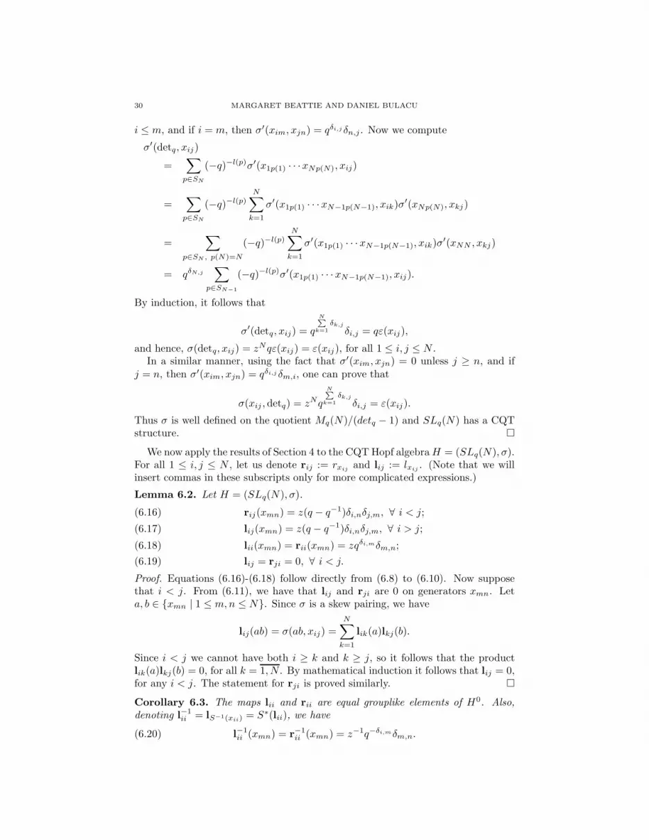
30 MARGARET BEATTIE AND DANIEL BULACU

i ≤ m, and if i = m, then σ′(xim, xjn) = qδi,j δn,j . Now we compute

σ′(detq, xij)

=∑

p∈SN

(−q)−l(p)σ′(x1p(1) · · ·xNp(N), xij)

=∑

p∈SN

(−q)−l(p)N∑

k=1

σ′(x1p(1) · · ·xN−1p(N−1), xik)σ′(xNp(N), xkj)

=∑

p∈SN , p(N)=N

(−q)−l(p)N∑

k=1

σ′(x1p(1) · · ·xN−1p(N−1), xik)σ′(xNN , xkj)

= qδN,j

∑

p∈SN−1

(−q)−l(p)σ′(x1p(1) · · ·xN−1p(N−1), xij).

By induction, it follows that

σ′(detq, xij) = q

NP

k=1

δk,j

δi,j = qε(xij),

and hence, σ(detq, xij) = zNqε(xij) = ε(xij), for all 1 ≤ i, j ≤ N .In a similar manner, using the fact that σ′(xim, xjn) = 0 unless j ≥ n, and if

j = n, then σ′(xim, xjn) = qδi,j δm,i, one can prove that

σ(xij , detq) = zNq

NP

k=1

δk,j

δi,j = ε(xij).

Thus σ is well defined on the quotient Mq(N)/(detq − 1) and SLq(N) has a CQTstructure. �

We now apply the results of Section 4 to the CQT Hopf algebraH = (SLq(N), σ).For all 1 ≤ i, j ≤ N , let us denote rij := rxij

and lij := lxij. (Note that we will

insert commas in these subscripts only for more complicated expressions.)

Lemma 6.2. Let H = (SLq(N), σ).

rij(xmn) = z(q − q−1)δi,nδj,m, ∀ i < j;(6.16)

lij(xmn) = z(q − q−1)δi,nδj,m, ∀ i > j;(6.17)

lii(xmn) = rii(xmn) = zqδi,mδm,n;(6.18)

lij = rji = 0, ∀ i < j.(6.19)

Proof. Equations (6.16)-(6.18) follow directly from (6.8) to (6.10). Now supposethat i < j. From (6.11), we have that lij and rji are 0 on generators xmn. Leta, b ∈ {xmn | 1 ≤ m,n ≤ N}. Since σ is a skew pairing, we have

lij(ab) = σ(ab, xij) =N∑

k=1

lik(a)lkj(b).

Since i < j we cannot have both i ≥ k and k ≥ j, so it follows that the productlik(a)lkj(b) = 0, for all k = 1, N . By mathematical induction it follows that lij = 0,for any i < j. The statement for rji is proved similarly. �

Corollary 6.3. The maps lii and rii are equal grouplike elements of H0. Also,denoting l−1

ii = lS−1(xii) = S∗(lii), we have

(6.20) l−1ii (xmn) = r−1

ii (xmn) = z−1q−δi,mδm,n.

BRAIDED FROM CQT HOPF ALGEBRAS 31

Proof. The fact that lii and rii are grouplike follows directly from (6.19). Then,since these are algebra maps equal on generators, they are equal. The rest isimmediate. �

The next lemma describes the commutation relations for the generators of Hr

and Hl.

Lemma 6.4. In Hr the commutation relations for the generators rij are given by:

rimrin = qrinrim, ∀ n < m; rjmrim = qrimrjm, ∀ i < j;(6.21)

rjnrim = rimrjn; rjmrin − rinrjm = (q − q−1)rimrjn, ∀ i < j, n < m.(6.22)

In Hl the commutation relations for the generators are given by:

linlim = qlimlin, ∀ n < m ; limljm = qljmlim, ∀ i < j;(6.23)

limljn = ljnlim; linljm − ljmlin = (q − q−1)ljnlim, ∀ i < j and n < m.(6.24)

As well, for all i, j, we have that

(6.25) l11l22 · · · lNN = r11r22 · · · rNN = ε and riirjj = liiljj = ljj lii = rjjrii.

Proof. Relations (6.21) to (6.24) follow from (6.1) to (6.4) together with (4.5), (4.6).The first relation in (6.25) follows from (6.12), (6.19) and Corollary 6.3. By thesecond relation in (6.24) we have that liiljj − ljj lii = (q − q−1)ljilij if i < j, andljj lii − liiljj = (q − q−1)lij lji if j < i. By (6.19), these are both 0. Therefore,liiljj = ljj lii, for all 1 ≤ i, j ≤ N . �

Note that (6.22) and (6.24) imply that

rjmrin = rinrjm if i < j, n < m and either i > m or j > n;

linljm = ljmlin if i < j, n < m and either i < m or j < n.(6.26)

We now describe another set of algebra generators for Hl and Hr.

Proposition 6.5. Let 1 ≤ i ≤ N and 1 ≤ s, t ≤ N − 1 and define:

Ki := lii, K−1

i := l−1ii ;

Es := l−1s+1,s+1ls+1,s = qls+1,sl

−1s+1,s+1;

Fs := (q − q−1)−2r−1ss rs,s+1 = (q − q−1)−2qrs,s+1r

−1ss .

As an algebra Hl is generated by Ki, K−1

i , and the Es, with the following relations.

KiKj = KjKi, KiK−1

i = K−1

i Ki = ε, K1K2 · · · KN = ε;(6.27)

KiEtK−1

i = qδi,t−δi,t+1Et;(6.28)

EtEs = EsEt, if | s− t |> 1;(6.29)

E2sEt − (q + q−1)EsEtEs + EtE

2s = 0, if | s− t |= 1.(6.30)

Similarly, Hr is generated as an algebra by the Ki, K−1

i , and the Fs, withrelations (6.27) and

KiFtK−1

i = qδi,t+1−δi,tFt;(6.31)

FtFs = FsFt, if | s− t |> 1;(6.32)

F 2s Ft − (q + q−1)FsFtFs + FtF

2s = 0, if | s− t |= 1.(6.33)

32 MARGARET BEATTIE AND DANIEL BULACU

Proof. We prove only the statements for Hl; the proofs for Hr are similar. Note

that the map Ki 7→ K−1

i , Es 7→ Fs, is a well defined algebra isomorphism from Hl

to Hr.Since {lij | i ≥ j} is a set of algebra generators for Hl, it suffices to prove that

for any 1 ≤ i ≤ N and 1 ≤ j ≤ N − i the element li+j,i can be written as a

linear combination of products of the elements K±1

1 , · · · , K±1

N , E1, · · · , EN−1 to see

that these elements generate. For 1 ≤ i ≤ N − 1, we have li+1,i = Ki+1Ei =

q−1EiKi+1. Suppose that li+j,i can be written as a linear combination of products

of the elements K±1

1 , · · · , K±1

N , E1, · · · , EN−1. By the second relation in (6.24),

li+j,ili+j+1,i+j − li+j+1,i+j li+j,i = (q − q−1)li+j+1,ili+j,i+j

for all 1 ≤ j ≤ N − i− 1. Now we compute

li+j+1,i

= (q − q−1)−1[li+j,ili+j+1,i+j l−1i+j,i+j − li+j+1,i+j li+j,il

−1i+j,i+j ]

(6.23,6.24)= (q − q−1)−1q−1[li+j,iEi+j li+j+1,i+j+1l

−1i+j,i+j − li+j+1,i+j l

−1i+j,i+jli+j,i]

(6.23)= (q2 − 1)−1[li+j,iEi+jKi+j+1K

−1

i+j − q−1Ei+jKi+j+1K−1

i+j li+j,i],

and the statement follows by mathematical induction.Now we show that (6.27) to (6.30) hold. Relations (6.27) are immediate from

(6.25). In order to prove (6.28) observe that

KiEtK−1

i = liil−1t+1,t+1lt+1,tl

−1ii = l−1

t+1,t+1liilt+1,tl−1ii .

We now verify (6.28) case by case.

Case I: If i < t or i > t+ 1, by (6.24) we have liilt+1,t = lt+1,tlii, and therefore

KiEtK−1

i = l−1t+1,t+1lt+1,t = Et = qδi,t−δi,t+1Et.

Case II: If i = t, by (6.23) we have lttlt+1,t = qlt+1,tltt, so that

KtEtK−1

t = ql−1t+1,t+1lt+1,t = qEt = qδt,t−δt,t+1Et.

Case III: If i = t+ 1, again using (6.23) we have lt+1,tlt+1,t+1 = qlt+1,t+1lt+1,t, and

Kt+1EtK−1

t+1 = lt+1,tl−1t+1,t+1 = q−1Et = qδt+1,t−δt+1,t+1Et.

Now to verify (6.29), we first note that if t < s − 1, (6.26) implies that the pairslt+1,t and ls+1,s+1, lt+1,t and ls+1,s, and ls+1,s and lt+1,t+1 commute and thus

EtEs = l−1t+1,t+1lt+1,tl

−1s+1,s+1ls+1,s = EsEt.

If t > s + 1 then s < t − 1, so interchanging s and t in the argument above weobtain EsEt = EtEs.

It remains to prove the relation in (6.30). We first compute

EsEs+1 = l−1s+1,s+1ls+1,sl

−1s+2,s+2ls+2,s+1

(6.26)= l−1

s+1,s+1l−1s+2,s+2ls+1,sls+2,s+1

(6.24)= l−1

s+2,s+2l−1s+1,s+1[ls+2,s+1ls+1,s + (q − q−1)ls+2,sls+1,s+1]

(6.23,6.24)= q−1l

−1s+2,s+2ls+2,s+1l

−1s+1,s+1ls+1,s + (q − q−1)l−1

s+2,s+2ls+2,s.

BRAIDED FROM CQT HOPF ALGEBRAS 33

In other words, we have proved that

(6.34) EsEs+1 = q−1Es+1Es + (q − q−1)l−1s+2,s+2ls+2,s,

for all 1 ≤ s ≤ N − 2. Clearly, this is equivalent to

(6.35) Es+1Es = qEsEs+1 − q(q − q−1)l−1s+2,s+2ls+2,s,

for all 1 ≤ s ≤ N − 2. Using the two relations above we obtain

E2sEs+1 = q−1EsEs+1Es + (q − q−1)Esl

−1s+2,s+2ls+2,s,

Es+1E2s = qEsEs+1Es − q(q − q−1)l−1

s+2,s+2ls+2,sEs,

from which we compute

E2sEs+1 − (q−1 + q)EsEs+1Es + Es+1E

2s

= (q − q−1)[Esl−1s+2,s+2ls+2,s − ql−1

s+2,s+2ls+2,sEs].

Now, since

Esl−1s+2,s+2ls+2,s = l−1

s+1,s+1ls+1,sl−1s+2,s+2ls+2,s

(6.26)= l−1

s+1,s+1l−1s+2,s+2ls+1,sls+2,s

(6.23)= ql−1

s+2,s+2l−1s+1,s+1ls+2,sls+1,s

(6.24)= ql−1

s+2,s+2ls+2,sl−1s+1,s+1ls+1,s = ql−1

s+2,s+2ls+2,sEs,

it follows that E2sEs+1 − (q−1 + q)EsEs+1Es +Es+1E

2s = 0, for all 1 ≤ s ≤ N − 2.

Similarly, again using (6.34) and (6.35) we have

E2s+1Es = qEs+1EsEs+1 − q(q − q−1)Es+1l

−1s+2,s+2ls+2,s,

EsE2s+1 = q−1Es+1EsEs+1 + (q − q−1)l−1

s+2,s+2ls+2,sEs+1,

and therefore

E2s+1Es − (q + q−1)Es+1EsEs+1 + EsE

2s+1

= (q − q−1)[l−1s+2,s+2ls+2,sEs+1 − qEs+1l

−1s+2,s+2ls+2,s].

Now, we have

qEs+1l−1s+2,s+2ls+2,s

(6.23)= q2l−1

s+2,s+2ls+2,s+1ls+2,sl−1s+2,s+2

(6.23)= ql−1

s+2,s+2ls+2,sls+2,s+1l−1s+2,s+2

(6.23)= l−1

s+2,s+2ls+2,sl−1s+2,s+2ls+2,s+1 = l−1

s+2,s+2ls+2,sEs+1,

and therefore E2s+1Es − (q+ q−1)Es+1EsEs+1 +EsE

2s+1 = 0, for all 1 ≤ s ≤ N −2,

and this finishes the proof. �

Next we fix some notation:

Definition 6.6. For any x and y, let [x, y]q := qxy − yx.

(i) For 1 ≤ i ≤ j ≤ N , define Fi,i := 1, Fi,i+1 := q(1 − q−2)2Fi, and

Fi,j := q(1 − q−2)j−i+1[Fj−1, [Fj−2, · · · [Fi+1, Fi]q · · · ]q]q, for j ≥ i+ 2,

i.e., the Fi,j are defined inductively by Fi,j+1 = (1 − q−2)[Fj ,Fi,j ]q.(ii) Similarly, define Ej,j := 1, Ej+1,j := q−1Ej and,

Ei,j := q−1(q2 − 1)j−i[· · · [[Ej , Ej+1]q, Ej+2]q, · · · , Ei−1]q, for i ≥ j + 2,

i.e., the Ei,j are defined inductively by Ei+1,j = (q2 − 1)−1[Ei,j , Ei]q.

34 MARGARET BEATTIE AND DANIEL BULACU

Now, using Proposition 6.5, lij and rij can be expressed in terms of the new

generators K±1

i , Es and Fs in the spirit of Serre relations.

Corollary 6.7. For 1 ≤ i ≤ j ≤ N , we have that lji = Ej,iKj, and rij = Fi,jKi.

Proof. We prove the statement for rij by mathematical induction on j; the similarproof for lji is left to the reader. If j = i, the statement is clear. If j = i + 1,then the statement follows from Lemma 6.4 and the definitions. Now assume thatrij = FijKi for rij with j ≥ i+ 1 and we show that it holds for ri,j+1. By (6.22),we have

rj,j+1ri,j − ri,jrj,j+1 = (q − q−1)ri,j+1rj,j ,

and thus

ri,j+1 = (q − q−1)−1[rj,j+1ri,jr−1j,j − ri,jrj,j+1r

−1j,j ]

(6.21)= (q − q−1)−1[qrj,j+1r

−1j,j ri,j − q−1ri,jr

−1j,j rj,j+1]

(6.21)= (q − q−1)[Fjri,j − q−1ri,jFj ]

= (1 − q−2)[Fj , ri,j ]q

= (1 − q−1)[Fj ,FijKi]qby the induction assumption

(6.31)= (1 − q−2)[Fj ,Fij ]qKi

= (1 − q−2)Fi,j+1Ki,

and the proof is complete. �

The next proposition describes the comultiplication, counit and antipode for Hl

and Hr.

Proposition 6.8. The coalgebra structure ∆, ε and the antipode S for Hl aredetermined by

∆(K±1

i ) = K±1

i ⊗ K±1

i , ε(K±1

i ) = 1,(6.36)

∆(Es) = ε⊗ Es + Es ⊗ K−1

s+1Ks, ε(Es) = 0,(6.37)

S(K±1

i ) = K∓1

i , S(Es) = −EsK−1

s Ks+1,(6.38)

for 1 ≤ i ≤ N and 1 ≤ s ≤ N − 1. Similarly, the coalgebra structure ∆, ε and theantipode S for Hr are determined by (6.36), the first equality in (6.38) and

∆(Fs) = Fs ⊗ ε+ Ks+1K−1

s ⊗ Fs, ε(Fs) = 0,(6.39)

S(Fs) = −KsK−1

s+1Fs.(6.40)

Proof. We give the details for Es and leave those for Fs to the reader. Also, we

note that the algebra isomorphism Ki 7→ K−1

i , Es 7→ Fs, defined in the proof ofProposition 6.5, is actually a Hopf algebra isomorphism between Hl and Hcop

r .Now, we compute:

∆(Es) = ∆(l−1s+1,s+1ls+1,s) = (l−1

s+1,s+1 ⊗ l−1s+1,s+1)

s+1∑

k=s

ls+1,k ⊗ lks

= (l−1s+1,s+1 ⊗ l−1

s+1,s+1)(ls+1,s ⊗ lss + ls+1,s+1 ⊗ ls+1,s)

= Es ⊗ K−1

s+1Ks + ε⊗ Es,

BRAIDED FROM CQT HOPF ALGEBRAS 35

as needed. Also, ε(Es) = ε(l−1s+1,s+1ls+1,s) = δs+1,s = 0, for all 1 ≤ s ≤ N − 1. The

formula for S(Es) is then immediate. �

Remark 6.9. For 1 ≤ i ≤ N − 1 we now define Ki := K−1

i+1Ki = KiK−1

i+1, and then

define H ′l to be the subalgebra of Hl generated by {K±1

i , Ei | 1 ≤ i ≤ N−1}. FromProposition 6.5 one can easily see that the relations between the algebra generatorsof H ′

l are (6.29), (6.30) and

(6.41) K±1i K∓1

i = ε, KiKj = KjKi, KiEjK−1i = qaijEj ,

for all 1 ≤ i, j ≤ N − 1, where aii = 2, aij = −1 if | i − j |= 1, and aij = 0 if| i − j |> 1. Actually, H ′

l is a Hopf subalgebra of Hl. The induced Hopf algebrastructure is given by

∆(K±1i ) = K±1

i ⊗K±1i , ε(K±1

i ) = 1,

∆(Ei) = ε⊗ Ei + Ei ⊗Ki, ε(Ei) = 0,

S(K±1i ) = K∓1

i , S(Ei) = −EiK−1i ,

for all 1 ≤ i ≤ N − 1. Similarly, define H ′r to be the subalgebra of Hr generated

by {K±i , Fi | 1 ≤ i ≤ N − 1}. Then its algebra generators satisfy the relations in

(6.32), (6.33), the first two relations in (6.41) and

(6.42) KiFjK−1i = q−aijFj , ∀ 1 ≤ i, j ≤ N − 1,

where aij are the scalars defined above. Moreover, H ′r is a Hopf subalgebra of Hr.

The elements K±i are grouplike elements and

(6.43) ∆(Fi) = K−1i ⊗ Fi + Fi ⊗ ε, ε(Fi) = 0, S(Fi) = −KiFi,

for all 1 ≤ i ≤ N − 1. Also, the map Ki 7→ K−1i , Ei 7→ Fi, is well defined and a

Hopf algebra isomorphism from H ′l to H ′cop

r .

We can now describe the Hopf algebra structure of Hσ := HlHr.

Proposition 6.10. The Hopf algebra Hσ := HlHr can be presented as follows. It

is the algebra generated by {K±1

i | 1 ≤ i ≤ N} ∪ {Es, Fs | 1 ≤ s ≤ N − 1} withrelations (6.27)-(6.33) and

(6.44) EsFt − FtEs = δs,t(q − q−1)−1[KsK−1

s+1 − K−1

s Ks+1],

for all 1 ≤ s, t ≤ N − 1. The Hopf algebra structure of Hσ is given by the relationsin Proposition 6.8. In other words, Hσ ≡ U ext

q (slN ), the extended Hopf algebra ofUq(slN ) defined in [9, Section 8.5.3].

Proof. It remains only to prove (6.44). It suffices to show first that (6.44) holdswhen applied to xmn for all 1 ≤ m,n ≤ N , and then to show that if the maps in(6.44) are equal on a and b then they are also equal on ab.

The relations from Lemma 6.2 will be key in the following computations. Also

we will sometimes use the notation Ks = KsK−1

s+1 from Remark 6.9.

Recall that Ki(xmn) = lii(xmn) = zqδi,mδm,n by (6.18) and K−1

i (xmn) =

l−1ii (xmn) = z−1q−δi,mδm,n by (6.20). Thus,

Es(xmn) = l−1s+1,s+1ls+1,s(xmn) =

N∑

k=1

l−1s+1,s+1(xmk)ls+1,s(xkn)

= q−δm,s+1(q − q−1)δs+1,nδs,m = (q − q−1)δs+1,nδs,m.

36 MARGARET BEATTIE AND DANIEL BULACU

Similarly, we compute Ft(xmn) = (q − q−1)−1δt,nδt+1,m, and therefore

EsFt(xmn) =

N∑

k=1

Es(xmk)Ft(xkn) = (q − q−1)δs,mFt(xs+1,n)

= δs,mδt,nδs,t = δs,mδs,tδm,n,

and

FtEs(xmn) =n∑

k=1

Ft(xmk)Es(xkn) = (q − q−1)−1δt+1,mEs(xtn)

= δt+1,mδs+1,nδs,t = δs+1,mδs,tδm,n.

We conclude that

(6.45) (EsFt − FtEs)(xmn) = δs,t[δs,m − δs+1,m]δm,n.

On the other hand, we have

KsK−1

s+1(xmn) =

N∑

k=1

Ks(xmk)K−1

s+1(xkn)

= zqδs,mδm,kz−1q−δs+1,mδk,n = qδs,m−δs+1,mδm,n.

Similarly, K−1

s Ks+1(xmn) = qδs+1,m−δs,mδm,n. Thus

[KsK−1

s+1 − K−1

s Ks+1](xmn) = [qδs,m−δs+1,m − qδs+1,m−δs,m ]δm,n.

Since

qδs,m−δs+1,m − qδs+1,m−δs,m =

0 , if m 6∈ {s, s+ 1}q − q−1 , if m = s−(q − q−1) , if m = s+ 1

,

it follows that δs,t(q− q−1)−1[Ks −K−1s ](xmn) = δs,t[δs,m − δs+1,m]δm,n. Together

with (6.45) this proves that (6.44) holds on generators.Since the Ks are grouplike, the right hand side of (6.44) is (Ks,K

−1s )-primitive.

Also the left hand side is (Ks,K−1t )-primitive. This follows from the fact that the

matrix (aij)1≤i,j≤N defined in Remark 6.9 is symmetric, and thus

K−1t Es ⊗ FtKs = q−atsEsK

−1t ⊗ qastKsFt = EsK

−1t ⊗KsFt.

If s 6= t, then both sides of (6.44) are 0 on generators a, b ∈ SLq(N), and thus,being skew-primitive, on ab. Otherwise, both sides are (Ks,K

−1s )-primitive and

thus equal on the product ab. The statement then follows by induction. �

From Proposition 6.8 and Proposition 6.10 we conclude that the Hopf algebrasHl and Hr are precisely Uq(b−) and Uq(b+), the Borel-like Hopf algebras associatedto U ext

q (slN ). The fact that Uq(b+)cop and Uq(b−) are Hopf algebras in duality iswell known but using the general theory above we are now able to present a moreconceptual proof.

Corollary 6.11. The pairing 〈, 〉 : Uq(b+) ⊗ Uq(b−) → k defined by

〈Ki, Kj〉 = 〈K−1

i , K−1

j 〉 = zqδi,j , 〈Ki, K−1

j 〉 = 〈K−1

i , Kj〉 = z−1q−δi,j ,

〈Ki, Es〉 = 〈K−1

i , Es〉 = 0, 〈Fs, Kj〉 = 〈Fs, K−1

j 〉 = 0,

〈Fs, Et〉 = (q − q−1)−1δs,t,

BRAIDED FROM CQT HOPF ALGEBRAS 37

for all 1 ≤ i, j ≤ N and 1 ≤ s, t ≤ N − 1, defines a duality between Uq(b+)cop andUq(b−) as in Proposition 4.4.

Also, Uq(b−) is self dual, in the sense that there is a duality between Uq(b−) anditself given for all 1 ≤ i, j ≤ N and 1 ≤ s, t ≤ N − 1 by

〈Ki, Kj〉 = 〈K−1

i , K−1

j 〉 = z−1q−δi,j , 〈Ki, K−1

j 〉 = 〈K−1

i , Kj〉 = zqδi,j ,

〈Ki, Es〉 = 〈K−1

i , Es〉 = 〈Es, Ki〉 = 〈Es, K−1

i 〉 = 0,

〈Es, Et〉 = (q − q−1)−1δs,t.

Proof. The first set of equations follows from Proposition 4.4 and from (6.8)- (6.11).We verify only the third equation of the first set. Note first that 〈rss, lij〉 = 0 unlessi = j by (6.8)- (6.11) so that 〈r−1

ss , Et〉 = 0. Now we compute

〈Fs, Et〉 = (q − q−1)−2〈r−1ss rs,s+1, Et〉

(6.37)= (q − q−1)−2[〈r−1

ss , ε〉〈rs,s+1, Et〉 + 〈r−1ss , Et〉〈rs,s+1, K

−1

t+1Kt〉]

= (q − q−1)−2〈rs,s+1, l−1t+1,t+1lt+1,t〉

= (q − q−1)−2[〈rss, l−1t+1,t+1〉〈rs,s+1, lt+1,t〉

+〈rs,s+1, l−1t+1,t+1〉〈rs+1,s+1, lt+1,t〉]

= (q − q−1)−2K−1

t+1(xss)lt+1,t(xs,s+1)

(6.17,6.18)= (q − q−1)−2z−1q−δs,t+1z(q − q−1)δs,t = (q − q−1)−1δs,t,

as we claimed. The second set of equations follows from the isomorphism betweenHcop

r and Hl described at the beginning of the proof of Proposition 6.8. �

Corollary 6.12. The Hopf algebra U extq (slN ) is isomorphic to a factor of the gen-

eralized quantum double D(Uq(b+), Uq(b−)) ≡ D(Uq(b−)cop, Uq(b−)).

Proof. It is an immediate consequence of Corollary 6.11 and Proposition 4.5. �

Remark 6.13. Further to Remark 6.9, define H ′σ = H ′

lH′r = H ′

σ = H ′rH

′l , a Hopf

subalgebra of Hσ ≡ U extq (slN ). As expected, H ′

σ ≡ Uq(slN ), the Hopf algebra with

algebra generators {K±1i , Ei, Fi | 1 ≤ i ≤ N − 1} and relations from Remark 6.9 as

well as

EiFj − FjEi = δijKi −K−1

i

q − q−1, ∀ 1 ≤ i, j ≤ N − 1,

from Proposition 6.10. The comultiplication, the counit and the antipode are de-fined in Remark 6.9. (For more details see [8, VI.7& VII.9].)

Note that H ′r and H ′

l are exactly the Borel-like Hopf algebras associated toUq(slN ) and the situation is similar to that of Corollary 6.11, i.e., there is a dualityon H ′cop

r ⊗H ′l given by

〈Ki,Kj〉 = 〈K−1i ,K−1

j 〉 = qaij , 〈K−1i ,Kj〉 = 〈Ki,K

−1j 〉 = q−aij ,

〈Ki, Es〉 = 〈K−1i , Es〉 = 〈Fs,Ki〉 = 〈Fs,K

−1i 〉 = 0,

〈Fs, Et〉 = (q − q−1)−1δs,t,

for all 1 ≤ i, j ≤ N and 1 ≤ s, t ≤ N − 1. Moreover, since H ′copr is isomorphic

to H ′l , then H ′

l is self dual and the generalized quantum double D(H ′r, H

′l) ≡

D((H ′l)

cop, H ′l). Furthermore, one can easily see that the associated generalized

quantum double D(H ′r, H

′l) can be identified as a sub-Hopf algebra of D(Hr, Hl);

38 MARGARET BEATTIE AND DANIEL BULACU

hence we have a Hopf algebra morphism from D(H ′r, H

′l) to Hσ. The image of this

morphism is H ′σ, so Uq(slN ) is also a factor of a generalized quantum double.

Corollary 6.14. The evaluation pairings on U extq (slN ) ⊗ SLq(N) and Uq(slN ) ⊗

SLq(N), are given by

〈Ki, xmn〉 = zqδi,mδm,n, 〈K−1

i , xmn〉 = z−1q−δi,mδm,n,

〈Es, xmn〉 = (q − q−1)δs+1,nδs,m, 〈Fs, xmn〉 = (q − q−1)−1δs,nδs+1,m;

and

〈Ki, xmn〉 = qδi,m−δi+1,mδm,n, 〈K−1i , xmn〉 = qδi+1,m−δi,mδm,n,

〈Ei, xmn〉 = (q − q−1)δi+1,nδi,m, 〈Fi, xmn〉 = (q − q−1)−1δi,nδi+1,m,

respectively.

Proof. Both U extq (slN ) and Uq(slN ) are Hopf subalgebras of SLq(N)0, so the eval-

uation map gives dual pairings. The formulas for the pairings come directly fromLemma 6.2 or from the proof of Proposition 6.10. �

From Theorem 4.8, SLq(N) is a braided Hopf algebra in the braided category ofleft Yetter-Drinfeld modules over U ext

q (slN )cop. We end this paper by computingthe structures of the braided Hopf algebra SLq(N). First we need the following.

Lemma 6.15. For any 1 ≤ s ≤ N − 1 and 1 ≤ m,n ≤ N we have

ls+1,s(S(xmn)) = −z−1(q − q−1)δs+1,nδs,m,(6.46)

rs,s+1(S(xmn)) = −z−1q−2(q − q−1)δs,nδs+1,m.(6.47)

Proof. As usual, we only prove (6.46); (6.47) can be proved similarly. Recall thatσ−1 is obtained by replacing q by q−1 and z by z−1 in (6.6) and (6.7). We compute

ls+1,s(S(xmn)) = σ(S(xmn), xs+1,s) = σ−1(xmn, xs+1,s)

= z−1[q−δm,s+1δm,nδs,s+1 + [s+ 1 > m](q−1 − q)δs+1,nδs,m]

= −z−1(q − q−1)δs+1,nδs,m,

since [s+ 1 > m]δs,m = δs,m, so the proof is complete. �

Now we can describe concretely the left Yetter-Drinfeld module structure ofSLq(N) over U ext

q (slN )cop.

Proposition 6.16. SLq(N) is a left Yetter-Drinfeld module over U extq (slN )cop via

the structure

Ki ⊲ xmn = qδi,n−δi,mxmn, K−1

i ⊲ xmn = qδi,m−δi,nxmn,

Es ⊲ xmn = (1 − q−2)[q−1δs+1,nxms − qδs,n−δs+1,nδs,mxs+1n],

Fs ⊲ xmn = q(1 − q−2)−1[qδs,m−δs+1,mδs,nxms+1 − q−1δs+1,mxsn],

xmn 7−→

N∑

j=n

q2(j−n)Ej,nKj

(K

−1

m ⊗ xmj

+∑

1≤i≤m−1

∑

p∈Bi,m

(−q)−l(p)+(m−i)Em,p(m) · · · Ei+1,p(i+1)K−1

i ⊗ xij

),

BRAIDED FROM CQT HOPF ALGEBRAS 39

where the Ei,j are from Definition 6.6. Also for i ≤ m − 1, Bi,m denotes the setof bijective maps p : {i + 1, · · · ,m} → {i, · · · ,m − 1} such that p(k) ≤ k, for alli+ 1 ≤ k ≤ m.

Proof. We apply Proposition 4.7 to this setting. By (4.13), and recalling again from

(6.18) and (6.20) that K±1

i (xmn) = (zqδi,m)±1δm,n for 1 ≤ i,m, n ≤ N , we have

K±1

i ⊲ xmn =

N∑

j,k=1

K±1

i (S−1(xmj)S−2(xkn))xjk =

N∑

j,k=1

K∓1

i (xmj)K±1

i (xkn)xjk

= q±(δi,n−δi,m)xmn.

Next, using (6.46), we compute

Es(S(xmn)) = 〈l−1s+1s+1ls+1s, S(xmn)〉 =

N∑

i=1

Ks+1(xin)ls+1s(S(xmi))

= zqδs+1,nls+1s(S(xmn)) = −qδs+1,n(q − q−1)δs,mδs+1,n

= −q(q − q−1)δs,mδs+1,n.

Now, we use the above computation together with the fact that Es(xmn) = (q −q−1)δs+1,nδs,m and Ks(xmn) = qδs+1,m−δs,mδs,m from the proof of Proposition 6.10,to compute the action of Es on xmn.

Es ⊲ xmn

(4.13)=

N∑

i,j=1

Es(S−1(xmi)S

−2(xjn))xij

(6.37,6.14)=

N∑

i,j=1

[q2(j−n)δm,iEs(xjn) + q2(m−i)+2(j−n)Es(S(xmi))K−1

s+1Ks(xjn)]xij

= q−1(q − q−1)[q−1δs+1,nxms − δs,m

N∑

j=1

q2(j−n)Ks(xjn)xs+1j ]

= (1 − q−2)[q−1δs+1,nxms − qδs,n−δs+1,nδs,mxs+1n],

as claimed. Similarly, one can compute Fs ⊲ xmn; the verification of the details isleft to the reader.

Finally, from (4.14) and (6.14), we see that the coaction of U extq (slN )cop on

SLq(N) is defined by

xmn 7→N∑

i,j=1

lS−1(xmi)S−2(xjn) ⊗ xij =∑

1≤i,j≤N

q2(j−n)+2(m−i)ljnlS(xmi) ⊗ xij .

From (6.13) we have

lS(xmi) = (−q)i−m∑

p∈Si,m

(−q)−l(p)lx1,p(1)···xi−1,p(i−1)xi+1,p(i+1)···xN,p(N)

= (−q)i−m∑

p∈Si,m

(−q)−l(p)lN,p(N) · · · li+1,p(i+1)li−1,p(i−1) · · · l1,p(1),

and this forces k ≥ p(k), for any k 6= i. Since p is bijective, non-zero summandsoccur only when

40 MARGARET BEATTIE AND DANIEL BULACU

(i) i = m and p(k) = k, for all k 6= i;(ii) i ≤ m − 1 and p(1) = 1, · · · , p(i − 1) = i − 1, {p(i + 1), · · · , p(m)} =

{i, · · · ,m − 1}, p(m + 1) = m + 1, · · · , p(N) = N , and p(k) ≤ k, for anyk ∈ {i+ 1, · · · ,m}.

In other words, we have proved that lS(xmm) = l−1mm, and that for 1 ≤ i ≤ m− 1,

lS(xmi)

= (−q)i−m∑

p∈Bi,m

(−q)−l(p)lNN · · · lm+1,m+1lm,p(m) · · · li+1,p(i+1)li−1,i−1 · · · l11.

From (6.26), for i+ 1 ≤ k ≤ m, m+ 1 ≤ t ≤ N and 1 ≤ s ≤ i− 1 we have

(6.48) lkp(k)ltt = lttlkp(k) and lsslkp(k) = lkp(k)lss,

so that, using (6.25), we have

lS(xmi) = (−q)i−m∑

p∈Bi,m

(−q)−l(p)lmp(m) · · · li+1p(i+1)l−1ii · · · l−1

mm,

for 1 ≤ i ≤ m − 1. Now, by Corollary 6.7 we have lkp(k) = Ek,p(k)Kk, for allk ∈ {i+ 1, · · · ,m}. In particular, if i = m− 1 we then have

lS(xmi) = −q−1lmp(m)K−1

m−1K−1

m = −q−1Em,p(m)K−1

i .

Now let 1 ≤ i ≤ m− 2. From (6.28) it follows that KsEt = EtKs, for all s > t+ 1,

so from the definition of Ei,j we conclude that Km−tEk,p(k) = Ek,p(k)Km−t, for all0 ≤ t ≤ m− i− 2 and i+ 1 ≤ k ≤ m− t− 1. Consequently,

lS(xmi) = (−q)i−m∑

p∈Bi,m

(−q)−l(p)Em,p(m) · · · Ei+1,p(i+1)K−1

i ,

for all 1 ≤ i ≤ m− 1. Again using Corollary 6.7 for ljn and the formulas above forlS(xmi) we obtain the coaction in the statement of the theorem. �

We now apply the results of Theorem 4.8 to obtain the multiplication, comulti-plication, unit, counit and antipode for SLq(N).

Theorem 6.17. The structure of SLq(N) as a braided Hopf algebra in the category

of left U extq (slN )cop Yetter-Drinfeld modules is the following. The unit and counit

are as in SLq(N). The multiplication is defined by

xim ◦ xjn = qδi,n−δm,nximxjn + (q − q−1)δi,n∑

s>n

q2(s−i)−δs,mxsmxjs

−[m > n]qδi,n(q − q−1)xinxjm − [m > n+ 1](q − q−1)2δi,n∑

n<s<m

q2(s−i)xssxjm.

BRAIDED FROM CQT HOPF ALGEBRAS 41

Comultiplication is given by

∆(xim) = q−2N−1{q−δi,m

∑

s

q2s+δs,i+δs,mxis ⊗ xsm + (q − q−1)[xim ⊗ x>m+

−δi,m∑

s;t>i

q2(s+δs,i)xts ⊗ xst + x>i+ ⊗ xim] + (q − q−1)2[

∑

s>i,m

q2s−1xsm ⊗ xis

−[i > m]q2i+1∑

s>i

xsm ⊗ xis − [m > i]q2m+1∑

s>m

xsm ⊗ xis]

−(q − q−1)3∑

t>s>i,m

q2sxtm ⊗ xit},

where we denoted x>k+ :=

∑s>k

q2sxss. The antipode is determined by

S(xim) = q2N+1[q−2m−δi,mS(xim) − (q − q−1)δi,mS(x>m− )],

where x>m− :=

∑s>m

q−2sxss and S is the antipode of SLq(N).

Proof. From Lemma 6.2 we have

lij(xmn) = zqδm,iδm,nδi,j + [i > j]z(q − q−1)δn,iδm,j,

l−ij(xmn) = z−1q−δm,iδm,nδi,j − [i > j]z−1(q − q−1)δn,iδm,j,

where l−ij denotes the map σ−1(−, xij) = lS−1(xij).Now, the multiplication of SLq(N) from Theorem 4.8 can be rewritten as

x ◦ y = σ−1(x3, y2)σ(S2(x1), y3)x2y1,

and together with (6.14) this allows us to compute

xim ◦ xjn =

N∑

s,t,u,v=1

q2(s−i)σ−1(xtm, xuv)σ(xis, xvn)xstxju

=

N∑

s,t,u,v=1

q2(s−i)l−uv(xtm)lvn(xis)xstxju

=

N∑

s,t,u,v=1

q2(s−i)(q−δt,uδt,mδu,v − [u > v](q − q−1)δm,uδv,t

)

×(qδi,vδi,sδv,n + [v > n](q − q−1)δs,vδi,n

)xstxju.

Splitting the sum above into four separate sums, we obtain the formula in thestatement of the theorem.

The computation of ∆(xim) is much more complicated. Firstly, observe that thecomultiplication in Theorem 4.8 can be rewritten as

(6.49) ∆(x) = σ(x1, x6)σ−1(x2, x8)σ(x4, x9)v(x5)x3 ⊗ x7,

42 MARGARET BEATTIE AND DANIEL BULACU

where v is the map v(y) = σ(y1, S(y2)) as in (2.8). Next, we compute

v(xim) =N∑

k=1

σ(xik , S(xkm)) =N∑

k=1

q2(m−k)l−km(xik)

=N∑

k=1

z−1q2(m−k)(q−δi,kδi,kδk,m − [k > m](q − q−1)δi,m)

= z−1[q−δi,m − q(1 − q−2)∑

k>m

(q−2)k−m]δi,m

= z−1[q−1 − q−1(1 − (q−2)N−m)]δi,m = z−1q−2(N−m)−1δi,m,

for all 1 ≤ i,m ≤ N . Therefore, by (6.49) we have

∆(xim) =

N∑

a,··· ,h=1

lef (xia)l−gh(xab)lhm(xcd)v(xde)xbc ⊗ xfg

=

N∑

a,b,c,d,f,g,h=1

q−2(N−d)−1(qδi,dδi,aδd,f + [d > f ](q − q−1)δd,aδi,f

)

×(q−δa,gδa,bδg,h − [g > h](q − q−1)δg,bδh,a

)

×(qδc,hδc,dδh,m + [h > m](q − q−1)δh,dδc,m

)xbc ⊗ xfg.

Again, splitting the above sum into eight separate sums, a tedious but straightfor-ward computation yields the formula for ∆(xim) in the statement of the theorem.

Finally, the equation for S(xij) follows easily by the general formula in Theo-rem 4.8 and by computations similar to the ones above. �

References

[1] N. Andruskiewitsch and M. Grana, Braided Hopf algebras over non-abelian finite groups,Bol. Acad. Ciencias (Cordoba) 63 (1999), 45–78.

[2] D. Bulacu, S. Caenepeel and F. Panaite, Yetter-Drinfeld categories for quasi-Hopf algebras,Comm. Algebra 34 (2006), no. 1, 1–35.

[3] S. Dascalescu, C. Nastasescu and S. Raianu, “Hopf Algebras: An Introduction”, in: Mono-graphs Textbooks in Pure Appl. Math., Vol. 235, Dekker, New York, 2001.

[4] Y. Doi, Braided bialgebras and quadratic bialgebras, Comm. Algebra 21(5) (1993), 1731-1749.

[5] Y. Doi and M. Takeuchi, Multiplication alteration by two - cocycles - the quantum version,Comm. Algebra 22 (1994), 5715-5732.

[6] V. G. Drinfeld, On almost cocommutative Hopf algebras, Leningrad Math. J., Vol. 1 (1990),No. 2, 321–342.

[7] L. Faddeev, N. Reshetikhin and L. Takhtajan, Quantum groups. Braid group, knot theoryand statistical mechanics, Adv. Ser. Math. Phys. 9 (1989), World Sci. Publishing, Teaneck,NJ, 97–110.

[8] C. Kassel, “Quantum Groups”, Graduate Texts in Mathematics 155, Springer Verlag, Berlin,1995.

[9] A. Klimyk and K. Schmudgen, “Quantum groups and their representations”, Texts and

Monographs in Physics, Springer-Verlag, Berlin, 1997.[10] S. Majid, Doubles of quasitriangular Hopf algebras, Comm. Algebra 19 (1991), 3061–3073.

[11] S. Majid, Braided groups, J. Pure and Appl. Algebra 86 (1993), 187–221.[12] S. Majid, Algebras and Hopf algebras in braided categories, Marcel Dekker, L. N. in Math.

158 (1994), 55–105.[13] S. Majid, “Foundations of quantum group theory”, Cambridge Univ. Press, 1995.

BRAIDED FROM CQT HOPF ALGEBRAS 43

[14] S. Montgomery, “Hopf algebras and their actions on rings”, American Mathematical Society,Providence, 1993.

[15] D. Radford, Minimal quasitriangular Hopf algebras, J. Algebra 157(1993), 285–315.[16] D. Radford, The structure of Hopf algebras with a projection, J. Algebra 92(1985), 322–347.[17] P. Schauenburg, On coquasitriangular Hopf algebras and the quantum Yang-Baxter equation,

Algebra Berichte [Algebra Reports] 67, Verlag Reinhard Fischer, Munich, 1992.[18] M. E. Sweedler, “Hopf algebras”, Benjamin, New York, 1969.[19] M. Takeuchi, Finite Hopf algebras in in braided tensor categories, J. Pure Appl. Algebra 138

(1999), 59–82.[20] M. Takeuchi, Hopf algebra techniques applied to the quantum group Uq(sl(2)), Contemp.

Math. 134 (1992), 309–323.[21] M. Takeuchi, Some topics on GLq(n), J. Algebra 147 (1992), 379–410.

Department of Mathematics and Computer Science, Mount Allison University, Sack-

ville, NB E4L 1E6, Canada

E-mail address: mbeattie@mta.ca

Faculty of Mathematics and Informatics, University of Bucharest, Str. Academiei

14, RO-010014 Bucharest 1, Romania

E-mail address: