1

MULTIDIMENSIONAL POVERTY MONITORING:A METHODOLOGY AND IMPLEMENTATION IN VIETNAM

LOUIS-MARIE ASSELIN & VU TUAN ANH *

1. INTRODUCTION

Moneymetric analysis of poverty can be proud of its achievements since twenty-five years. Methodologieshave been developed to better describe the difficult situation of families marginalized within theircommunities in regard of the general level of welfare and to better tackle the problems they are facing. Butchange has happened, thanks to this pioneering work on poverty. The concept of poverty has evolved to amultidimensional view. A eight-year old child not going to school is individually poor even if he is livingin a family not monetary poor: he is lacking an essential good, education. This a normative assertion, nodiscussion about that. And his family has a poverty problem, because some of his members are poor. Thesame if the mother, in this family, usually gives birth without any skilled assistance. This raises newtechnical challenges: how to measure poverty now? By multiple indicators? But then, how to define therelevant indicators? How to weight these multiple measurements to get a composite (integrated)mesurement of a family welfare, in view of identifying the poorest?

In addition to this conceptual extension, an operational issue has become more and more acute: thelimitations in the analytical power of standard household surveys designed to measure as accurately theirstandard of living, i.e. their monetary poverty. Can we capture the multidimensional face of povertythrough a small set of reliable indicators, light and easy to measure?

Policy makers ask for reliable poverty measurements with a very high level of disaggregation as wellgeographically as in socioeconomic groups, and regularly updated, annually or quarterly if possible.Developing countries cannot meet these policy requirements with the high costs of standard householdsurveys.

These are the issues addressed by several national groups of researchers (a Vietnamese group included)working within the Micro Impacts of Macroeconomic Adjustment Policies Network (MIMAP) 1 supportedsince fifteen years by the International Development Research Center of Canada (IDRC).

One of the key objectives of the research work conducted by the Vietnamese research group since 1998 isto describe multidimensional poverty in Vietnam2 and its change across time, with a specific tooldeveloped. This tool consists of two parts :

a) A small set of light household poverty indicators identified through community-based surveys;

b) A methodology to build a composite indicator.

The present paper aims to produce three outputs:

• A relevant and significant multidimensional poverty profile of Vietnam, static and dynamic (1993 and1998)3, including a composite poverty indicator;

* Louis-Marie Asselin, Ph. D., Institut de Mathématique C.F. Gauss, Quebec, Canada. Email :imgasselin@globetrotter.net.

Vu Tuan Anh, Ph.D, Socio-Economic Development Centre, Hanoi, Vietnam. Email : vtanh@vnea.org.

1 Micro Impacts of Macroeconomic Adjustment and Policy. A large part of the program is now implemented throughthe PEP (Poverty and Economic Policy) network, including a CBMS (Community Based Monitoring System) sub-network.2 From now on, the word "poverty", without any qualifier, will implicitly mean "multidimensional poverty", andthere will be eventually a qualification like "income (monetary) poverty", "health poverty", etc.

2

• An assessment of the analytical capacity of the MIMAP methodology developed in Vietnam, by acomparison with the standard income poverty analysis;

• Some recommendations to improve the methodology of identifying who are the poor in Vietnam, as atool for better designed and targeted poverty alleviation policies.

We won't go extensively into the policy area, and the paper will be essentially methodological.

2. METHODOLOGY

2.1. Steps of analysis

The analysis goes through the five steps.

Step 1: to identify among the community-based surveys in Vietnam a set of poverty indicators whoseequivalent can be extracted from large scale national surveys 4.

Step 2: to construct the MIMAP indicators from the large database provided by each of the two nationalsurveys.

Step 3: to estimate a national multidimensional poverty profile for 1993 and 1998. These profiles will beaccompanied by precision estimates and significance tests integrating the complex survey designsprobabilistic structures. Results will be compared with the analysis of income poverty as published inofficial reports on VLSS-1993 and VLSS-1998.

Step 4: To refine the analysis by building a composite poverty indicator integrating the set of MIMAPindicators, and, on the basis of this unique indicator, to develop a static and dynamic poverty analysiscompared to the moneymetric analysis.

Step 5: To apply the composite indicator to the MIMAP 1999 survey data, to get an aggregated povertyprofile from this survey.

Basing on analysis results, the final activitiy is to produce proposals for improving the povertymeasurement methodology in Vietnam.

2.2. Set of indicators

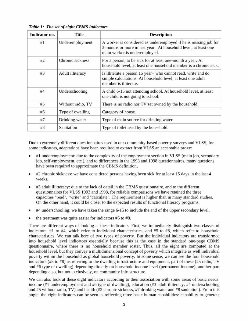
By a comparative analysis of our community-based poverty monitoring survey (CBMS) and VLSSquestionnaires, in view of identifying a small set of indicators for which equivalent indicators can beextracted from the large VLSS databases, it has been possible to identify eight such indicators. They aredescribed in Table 1.

3 These two years are determined by the availability of nationally representative data sets. The methodologydeveloped here will obviously be applied to susequent years (e.g. 2002) as soon as data sets are available.4 Essentially, we consider a MIMAP survey conducted in year 1999 in four provinces , twenty communes and22770 households. All households have been surveyed in each selected commune, which explains the large samplesize. Indicators are taken from the one-page questionnaire used in this survey. (This survey is described in Vu TuanAnh (2000), Poverty Monitoring in Vietnam, Annual MIMAP meeting held in Palawan, Philippines, Sept. 2000.IDRC, Ottawa, mimeo). One additional indicator, sanitation, is identified in an extended MIMAP questionnaire usedin the baseline survey of a poverty alleviation project implemented in the province of Thanh Hoa province.

Two large scale national household surveys are used to assess the relevance of these MIMAP indicators: the VietnamLiving Standard Survey conducted in 1993 (VLSS-1), with a nationally representative sample of 4800 households,and the similar VNLSS-2 survey conducted in 1998, with a sample of 6002 households.

3

Table 1: The set of eight CBMS indicators

Indicator no. Title Description

#1 Underemployment A worker is considered as underemployed if he is missing job for3 months or more in last year. At household level, at least onemain worker is underemployed.

#2 Chronic sickness For a person, to be sick for at least one-month a year. Athousehold level, at least one household member is a chronic sick.

#3 Adult illiteracy Is illiterate a person 15 year+ who cannot read, write and dosimple calculations. At household level, at least one adultmember is illiterate.

#4 Underschooling A child 6-15 not attending school. At household level, at leastone child is not going to school.

#5 Without radio, TV There is no radio nor TV set owned by the household.

#6 Type of dwelling Category of house.

#7 Drinking water Type of main source for drinking water.

#8 Sanitation Type of toilet used by the household.

Due to extremely different questionnaires used in our community-based poverty surveys and VLSS, forsome indicators, adaptations have been required to extract from VLSS an acceptable proxy:

• #1 underemployment: due to the complexity of the employment section in VLSS (main job, secondaryjob, self-employment, etc.), and to differences in the 1993 and 1998 questionnaires, many questionshave been required to approximate the CBMS definition,

• #2 chronic sickness: we have considered persons having been sick for at least 15 days in the last 4weeks,

• #3 adult illitteracy: due to the lack of detail in the CBMS questionnaire, and to the differentquestionnaires for VLSS 1993 and 1998, for reliable comparisons we have retained the threecapacities "read", "write" and "calculate". The requirement is higher than in many standard studies.On the other hand, it could be closer to the expected results of functional literacy programs.

• #4 underschooling: we have taken the range 6-15 to include the end of the upper secondary level.

• the treatment was quite easier for indicators #5 to #8.

There are different ways of looking at these indicators. First, we immediately distinguish two classes ofindicators, #1 to #4, which refer to individual characteristics, and #5 to #8, which refer to householdcharacteristics. We can talk here of two types of poverty. But the individual indicators are transformedinto household level indicators essentially because this is the case in the standard one-page CBMSquestionnaire, where there is no household member roster. Thus, all the eight are computed at thehousehold level, but they convey a multidimensional concept of poverty which integrate as well individualpoverty within the household as global household poverty. In some sense, we can see the four householdindicators (#5 to #8) as referring to the dwelling infrastructure and equipment, part of these (#5 radio, TVand #6 type of dwelling) depending directly on household income level (permanent income), another partdepending also, but not exclusively, on community infrastructure.

We can also look at these eight indicators according to their association with some areas of basic needs:income (#1 underemployment and #6 type of dwelling), education (#3 adult illiteracy, #4 underschoolingand #5 without radio, TV) and health (#2 chronic sickness, #7 drinking water and #8 sanitation). From thisangle, the eight indicators can be seen as reflecting three basic human capabilities: capability to generate

4

income, capability to access learning and to communicate, capability to live a healthy and long life. Wewill refer to them as expressing three forms of poverty. If we look more carefully at the income dimensionreflected in #6 type of dwelling, #5 radio/TV, #8 sanitation, we can see that it is more the investmentcomponent of income, rather than the consumption component, which is found in our set of indicators.

To summarize, we can say that our eight indicators present a concept of human (#1 to #4) and physical (#5to #8) assets household poverty.

From this way of reading the indicators, we should bear in mind the different facets of poverty thusintegrated in our multidimensional measurement when analysing the poverty profiles presented below.

3. MEASURMENT OF MULTIDIMENSIONAL POVERTY

3.1. A multidimensional poverty profile for the base-year 1993

We first produce a disaggregated profile based on the specific distribution of each indicator, and thencompute a composite indicator to understand more clearly and analyse more deeply the distribution ofmultidimensional poverty in Vietnam. Disaggregations are according to :

a) geographical location:

- rural/urban;

- seven regions: Northern Uplands (1), Red River Delta (2), North Central (3), Central Coast(4), Central Highlands (5), South East (6), Mekong River Delta (7);

- North (regions 1 and 2), Center (regions 3, 4 and 5), South (regions 6 and 7).

b) social characteristics:

- ethnicity (Kinh, minorities)

- household size

- gender of household head

- main activity (farm, non-farm)

c) moneymetric poverty:

- relative income poverty: relatively poor household are those below half the median incomeper capita,

- expenditure quintile.

On the basis of the sampling weights determined by the sample design, two estimators are provided ineach household category coming out of cross-classifying the eight indicators with the nine disaggregationfactors, which gives 72 two-way tables. The two indicators are the total number and the percentage ofhouseholds in each category. The total number of households is not usually presented in other povertyprofiles, but we believe it is important to view the population size of different type of poverty (targeting,program costs, etc.), as well as to integrate the population dynamics into the poverty dynamic analysis. Asignificance test has been runned for the distribution differences in each of the 72 two-way tables.This testis the Pearson chi-squared test adjusted to take into account the effects of the complex sample design onthis well-known test in the i.i.d. case 5.

5 The statistic then follows a F-distribution. See Rao J.N.K. and Scott A.J., On chi-squared tests for multiwaycontingency tables with cell proportions estimated from survey data, The Annals of Statistics, 1984, Vol. 12, No.1,46-60. We use the test as implemented in the Stata procedure svytab.

5

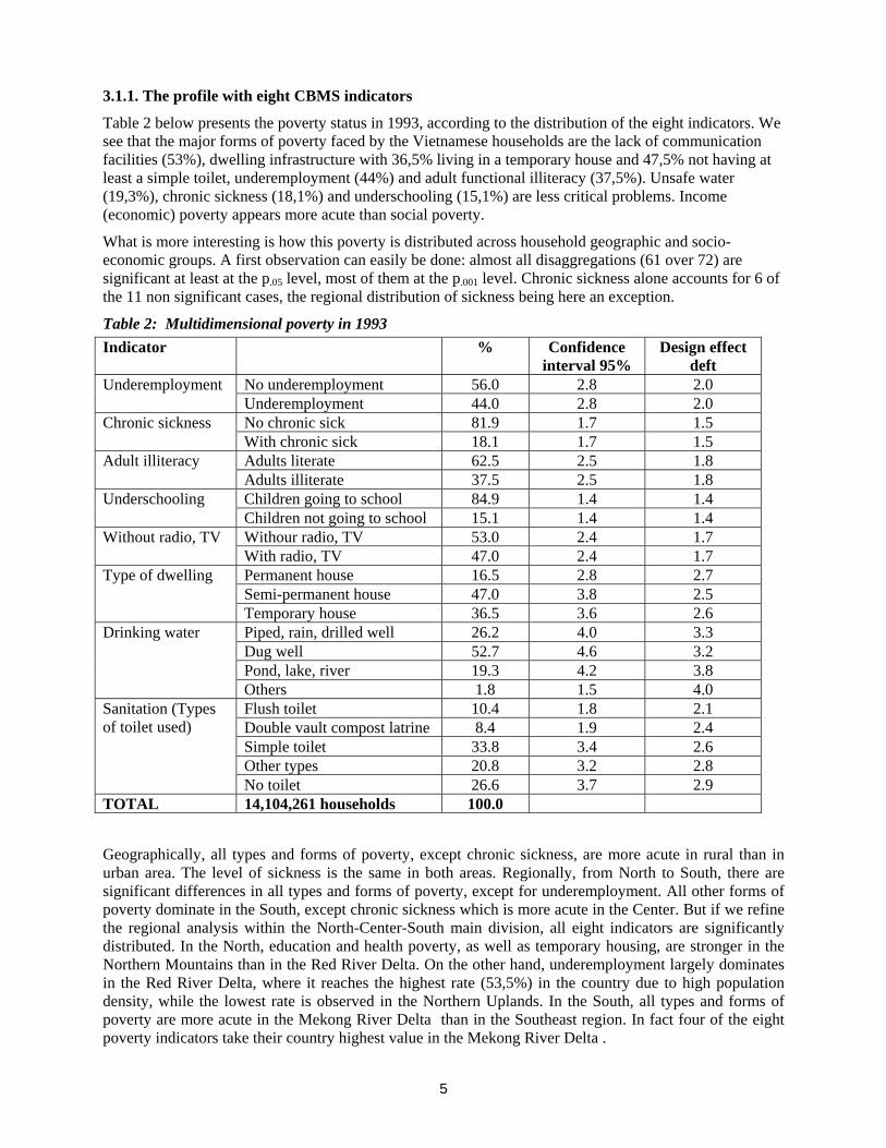
3.1.1. The profile with eight CBMS indicators

Table 2 below presents the poverty status in 1993, according to the distribution of the eight indicators. Wesee that the major forms of poverty faced by the Vietnamese households are the lack of communicationfacilities (53%), dwelling infrastructure with 36,5% living in a temporary house and 47,5% not having atleast a simple toilet, underemployment (44%) and adult functional illiteracy (37,5%). Unsafe water(19,3%), chronic sickness (18,1%) and underschooling (15,1%) are less critical problems. Income(economic) poverty appears more acute than social poverty.

What is more interesting is how this poverty is distributed across household geographic and socio-economic groups. A first observation can easily be done: almost all disaggregations (61 over 72) aresignificant at least at the p.05 level, most of them at the p.001 level. Chronic sickness alone accounts for 6 ofthe 11 non significant cases, the regional distribution of sickness being here an exception.

Table 2: Multidimensional poverty in 1993Indicator % Confidence

interval 95%Design effect

deftNo underemployment 56.0 2.8 2.0UnderemploymentUnderemployment 44.0 2.8 2.0No chronic sick 81.9 1.7 1.5Chronic sicknessWith chronic sick 18.1 1.7 1.5Adults literate 62.5 2.5 1.8Adult illiteracyAdults illiterate 37.5 2.5 1.8Children going to school 84.9 1.4 1.4UnderschoolingChildren not going to school 15.1 1.4 1.4Withour radio, TV 53.0 2.4 1.7Without radio, TVWith radio, TV 47.0 2.4 1.7Permanent house 16.5 2.8 2.7Semi-permanent house 47.0 3.8 2.5

Type of dwelling

Temporary house 36.5 3.6 2.6Piped, rain, drilled well 26.2 4.0 3.3Dug well 52.7 4.6 3.2Pond, lake, river 19.3 4.2 3.8

Drinking water

Others 1.8 1.5 4.0Flush toilet 10.4 1.8 2.1Double vault compost latrine 8.4 1.9 2.4Simple toilet 33.8 3.4 2.6Other types 20.8 3.2 2.8

Sanitation (Typesof toilet used)

No toilet 26.6 3.7 2.9TOTAL 14,104,261 households 100.0

Geographically, all types and forms of poverty, except chronic sickness, are more acute in rural than inurban area. The level of sickness is the same in both areas. Regionally, from North to South, there aresignificant differences in all types and forms of poverty, except for underemployment. All other forms ofpoverty dominate in the South, except chronic sickness which is more acute in the Center. But if we refinethe regional analysis within the North-Center-South main division, all eight indicators are significantlydistributed. In the North, education and health poverty, as well as temporary housing, are stronger in theNorthern Mountains than in the Red River Delta. On the other hand, underemployment largely dominatesin the Red River Delta, where it reaches the highest rate (53,5%) in the country due to high populationdensity, while the lowest rate is observed in the Northern Uplands. In the South, all types and forms ofpoverty are more acute in the Mekong River Delta than in the Southeast region. In fact four of the eightpoverty indicators take their country highest value in the Mekong River Delta .

6

Socially, we observe that the ethnic minority groups are less literate and have lower quality dwelling andsanitation facilities than the Kinh. On the other hand, the Kinh are much more underemployed. Femaleheaded households are better off relative to underemployment, schooling, safe water and sanitation, whilemale headed households are better off in terms of literacy and communication means. Except for chronicsickness where they do not differ, farming household are significantly poorer than non farming ones in allother forms of poverty. Large household size means more individual poverty, no surprise with that,according to the nature of the indicators. On the other hand, larger households are better equipped in termsof communication means, while their sanitation facilities seems to be less satisfactory.

Economically, income poverty is directly associated with illiteracy, no communication facilities,temporary housing, unsafe water and bad sanitation facilities. Relative income poverty does not affectchildren schooling significantly, but there is a significant drop in underscooling for the richest households.The same is observed regarding underemployment: it drops significantly only for the richest. Incomepoverty has no significant effect on chronic sickness.

From this analysis of multidimensional poverty as represented in the eight indicators, we see that it isdifficult to draw a clear view of the socioeconomic distribution of poverty without an aggregate measureof the human and physical asset poverty. To this end, we need a composite indicator.

3.1.2. The profile with a composite indicator and comparative analysis with the moneymetricapproach

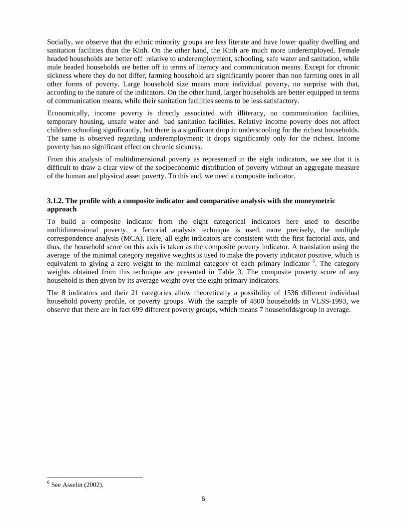
To build a composite indicator from the eight categorical indicators here used to describemultidimensional poverty, a factorial analysis technique is used, more precisely, the multiplecorrespondence analysis (MCA). Here, all eight indicators are consistent with the first factorial axis, andthus, the household score on this axis is taken as the composite poverty indicator. A translation using theaverage of the minimal category negative weights is used to make the poverty indicator positive, which isequivalent to giving a zero weight to the minimal category of each primary indicator 6. The categoryweights obtained from this technique are presented in Table 3. The composite poverty score of anyhousehold is then given by its average weight over the eight primary indicators.

The 8 indicators and their 21 categories allow theoretically a possibility of 1536 different individualhousehold poverty profile, or poverty groups. With the sample of 4800 households in VLSS-1993, weobserve that there are in fact 699 different poverty groups, which means 7 households/group in average.

6 See Asselin (2002).

7

Table 3: Category weights according to Multiple Correspondence AnalysisIndicator Category Weight Poverty

thresholdUnderemployment 0UnderemploymentNo underemployment 575With chronic sick 0Households with chronic

sick 15 days No chronic sick 626Adults illiterate 0Households with adult

illiteracy Adults literate 1544Children not going to school 0Households with children

of 6-15 not schooling Children going to school 1059Without radio, TV 0Households without

radio, TV With radio, TV 1988Temporary house 0Semi-permanent house 1845

Type of dwelling

Permanent house 4302Pond, lake, river 0Other water sources 348Dug well 1534

Drinking water

Piped, rain, drilled well 3667No toilet, other types 0Simple toilet 1315Double vault compost latrine 2559

Sanitation (Types oftoilet used)

Flush toilet 5098

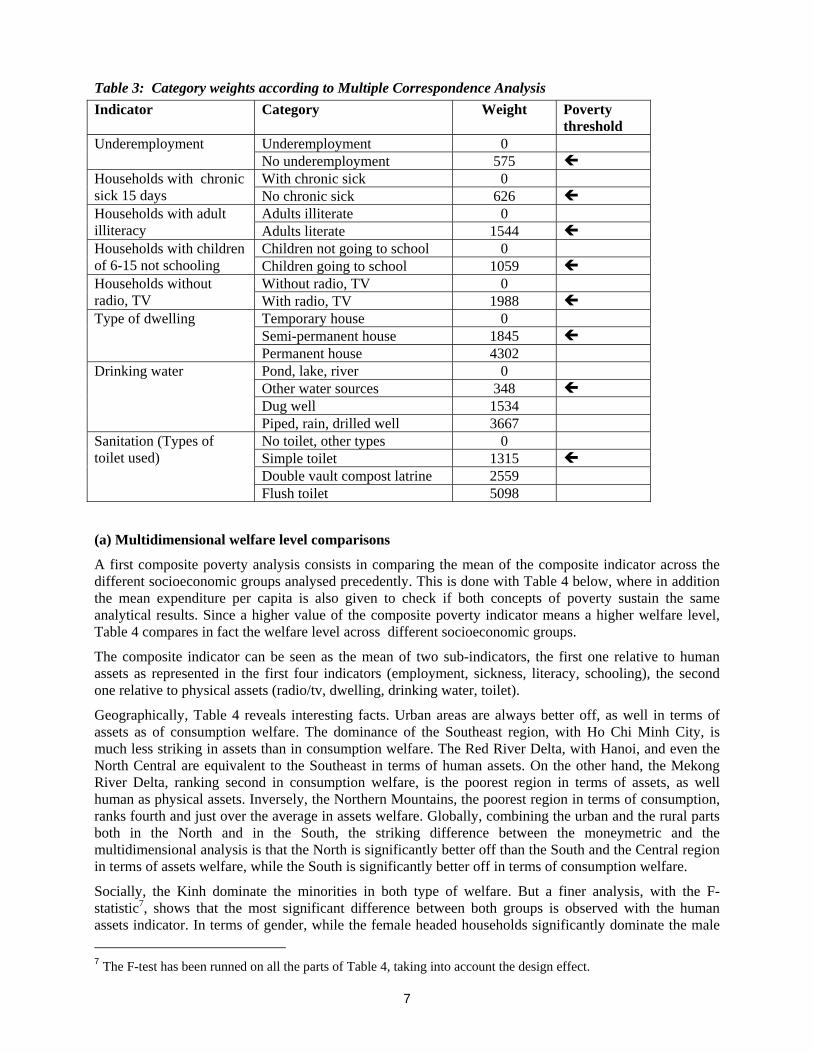
(a) Multidimensional welfare level comparisons

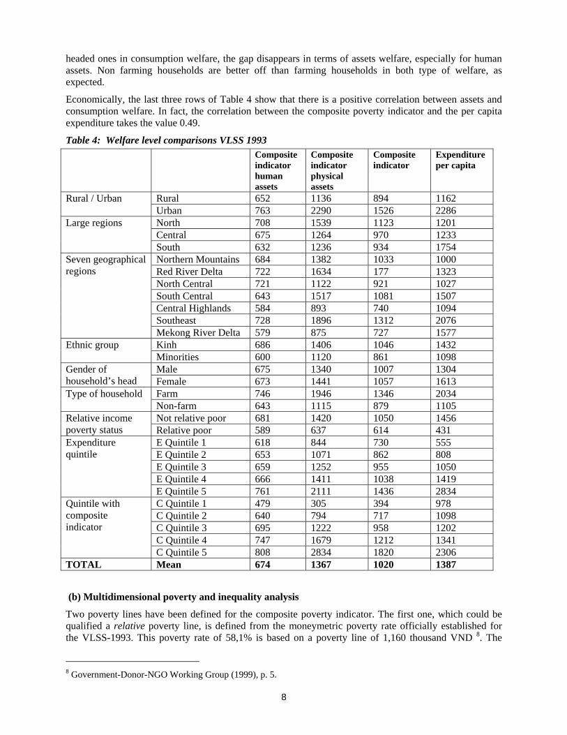
A first composite poverty analysis consists in comparing the mean of the composite indicator across thedifferent socioeconomic groups analysed precedently. This is done with Table 4 below, where in additionthe mean expenditure per capita is also given to check if both concepts of poverty sustain the sameanalytical results. Since a higher value of the composite poverty indicator means a higher welfare level,Table 4 compares in fact the welfare level across different socioeconomic groups.

The composite indicator can be seen as the mean of two sub-indicators, the first one relative to humanassets as represented in the first four indicators (employment, sickness, literacy, schooling), the secondone relative to physical assets (radio/tv, dwelling, drinking water, toilet).

Geographically, Table 4 reveals interesting facts. Urban areas are always better off, as well in terms ofassets as of consumption welfare. The dominance of the Southeast region, with Ho Chi Minh City, ismuch less striking in assets than in consumption welfare. The Red River Delta, with Hanoi, and even theNorth Central are equivalent to the Southeast in terms of human assets. On the other hand, the MekongRiver Delta, ranking second in consumption welfare, is the poorest region in terms of assets, as wellhuman as physical assets. Inversely, the Northern Mountains, the poorest region in terms of consumption,ranks fourth and just over the average in assets welfare. Globally, combining the urban and the rural partsboth in the North and in the South, the striking difference between the moneymetric and themultidimensional analysis is that the North is significantly better off than the South and the Central regionin terms of assets welfare, while the South is significantly better off in terms of consumption welfare.

Socially, the Kinh dominate the minorities in both type of welfare. But a finer analysis, with the F-statistic7, shows that the most significant difference between both groups is observed with the humanassets indicator. In terms of gender, while the female headed households significantly dominate the male 7 The F-test has been runned on all the parts of Table 4, taking into account the design effect.

8

headed ones in consumption welfare, the gap disappears in terms of assets welfare, especially for humanassets. Non farming households are better off than farming households in both type of welfare, asexpected.

Economically, the last three rows of Table 4 show that there is a positive correlation between assets andconsumption welfare. In fact, the correlation between the composite poverty indicator and the per capitaexpenditure takes the value 0.49.

Table 4: Welfare level comparisons VLSS 1993Compositeindicatorhumanassets

Compositeindicatorphysicalassets

Compositeindicator

Expenditureper capita

Rural 652 1136 894 1162Rural / UrbanUrban 763 2290 1526 2286North 708 1539 1123 1201Central 675 1264 970 1233

Large regions

South 632 1236 934 1754Northern Mountains 684 1382 1033 1000Red River Delta 722 1634 177 1323North Central 721 1122 921 1027South Central 643 1517 1081 1507Central Highlands 584 893 740 1094Southeast 728 1896 1312 2076

Seven geographicalregions

Mekong River Delta 579 875 727 1577Kinh 686 1406 1046 1432Ethnic groupMinorities 600 1120 861 1098Male 675 1340 1007 1304Gender of

household’s head Female 673 1441 1057 1613Farm 746 1946 1346 2034Type of householdNon-farm 643 1115 879 1105Not relative poor 681 1420 1050 1456Relative income

poverty status Relative poor 589 637 614 431E Quintile 1 618 844 730 555E Quintile 2 653 1071 862 808E Quintile 3 659 1252 955 1050E Quintile 4 666 1411 1038 1419

Expenditurequintile

E Quintile 5 761 2111 1436 2834C Quintile 1 479 305 394 978C Quintile 2 640 794 717 1098C Quintile 3 695 1222 958 1202C Quintile 4 747 1679 1212 1341

Quintile withcompositeindicator

C Quintile 5 808 2834 1820 2306TOTAL Mean 674 1367 1020 1387

(b) Multidimensional poverty and inequality analysis

Two poverty lines have been defined for the composite poverty indicator. The first one, which could bequalified a relative poverty line, is defined from the moneymetric poverty rate officially established forthe VLSS-1993. This poverty rate of 58,1% is based on a poverty line of 1,160 thousand VND 8. The

8 Government-Donor-NGO Working Group (1999), p. 5.

9

value of the composite indicator giving the same poverty rate 58,1% is 1062, and this is the relativepoverty line used for poverty comparisons between socioeconomic groups. The second poverty line, akind of absolute poverty line, is built by choosing a poverty threshold for each primary poverty indicator,as indicated in Table 3 above. The choice is not obvious only in the case of a multinomial indicator, andthen requires a social consensus. Let W* be the mean of the weights corresponding to these primarythresholds. Then W* is taken as the poverty line: an household is considered as poor if and only if thevalue of his composite indicator is strictly below W* 9. Here, this poverty line takes the value 1163.

Table 5: Poverty incidence comparisons VLSS 1993Poverty compositeindicator withabsolute line = 1163

Poverty compositeindicator based on58.1% line = 1062

Povertymoneymetricindicator accordingto line = 1160 thdsVND (58.1%)

% Rank % Rank % RankRural 77.1 2 66.5 2 66.4 2Rural / UrbanUrban 29.6 1 24.1 1 24.9 1North 57.7 1 45.5 1 69.4 3Central 73.5 2 62.5 2 63.4 2

Large regions

South 73.6 3 67.9 3 41.9 1Northern Mountains 63.8 4 51.3 3 78.6 7Red River Delta 53.3 2 41.3 1 62.8 4North Central 78.4 5 62.5 5 74.5 6South Central 63.4 3 57.1 4 49.6 3Central Highlands 91.3 7 82.1 6 70.0 5Southeast 49.5 1 41.4 2 32.7 1

Seven geographicalregions

Mekong River Delta 87.3 6 82.8 7 47.1 2Kinh 65.5 1 55.6 1 55.1 1Ethnic groupMinorities 79.6 2 71.1 2 74.7 2Male 69.4 2 59.4 2 61.0 2Gender of

household’s head Female 61.8 1 53.5 1 48.2 1Farm 42.6 1 34.6 2 30.8 1Type of householdNon-farm 78.2 2 67.9 1 69.6 2Not relative poor 65.4 1 55.3 1 54.6 1Relative income

poverty status Relative poor 95.4 2 90.9 2 100.0 2E Quintile 1 90.0 5 82.3 5 100.0 3E Quintile 2 79.7 4 69.0 4 100.0 3E Quintile 3 70.8 3 58.6 3 90.6 2E Quintile 4 62.2 2 52.1 2 0 1

Expenditurequintile

E Quintile 5 35.6 1 28.3 1 0 1C Quintile 1 100.0 3 100.0 3 76.4 5C Quintile 2 100.0 3 100.0 3 71.1 4C Quintile 3 100.0 3 88.4 2 63.7 3C Quintile 4 38.4 2 0 1 55.0 2

Quintile withcompositeindicator

C Quintile 5 0 1 0 1 23.8 1TOTAL 67.7 58.0 58.1

9 See Asselin (2002) for some properties of this type of poverty line.

10

From Table 5, with the relative poverty line 1062, we observe that:

a) in rural and urban areas, the poverty incidence is the same for asset poverty than for consumptionpoverty.

b) for the seven regions, the poverty rate is quite different for asset and consumption poverty. Interms of consumption, Northern Mountains is the poorest region (78,6%), while Mekong RiverDelta is the poorest in terms of assets (82,8%). While we observe a large difference inconsumption poverty between Red River Delta (62,8%) and Southeast (32,7%), both regions arethe less poor in assets with the same rate of 41%.

c) globally, the North is significantly less poor in assets than the South and the Central region, whilethe situation is reverse for the consumption poverty: the South is significantly less poor than therest of the country.

d) the gap between male and female headed households is lessened in assets poverty, in comparisonwith consumption poverty.

e) the substantial poverty rates in quintiles 4 and 5 show clearly that the two concepts of povertyrevealed respectively by the composite indicator (assets) and the moneymetric one (consumption)are not equivalent.

f) similar conclusions are obtained from the absolute poverty line of 1163, which gives a nationalpoverty rate of 67,7 %.

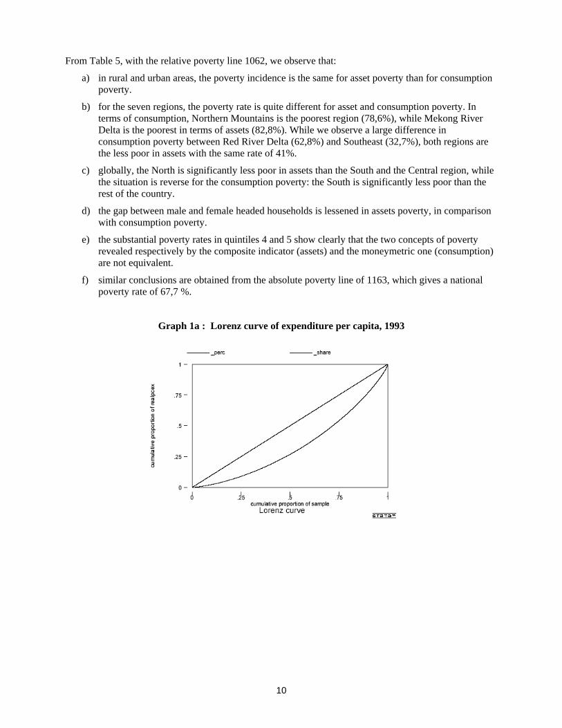
Graph 1a : Lorenz curve of expenditure per capita, 1993

11

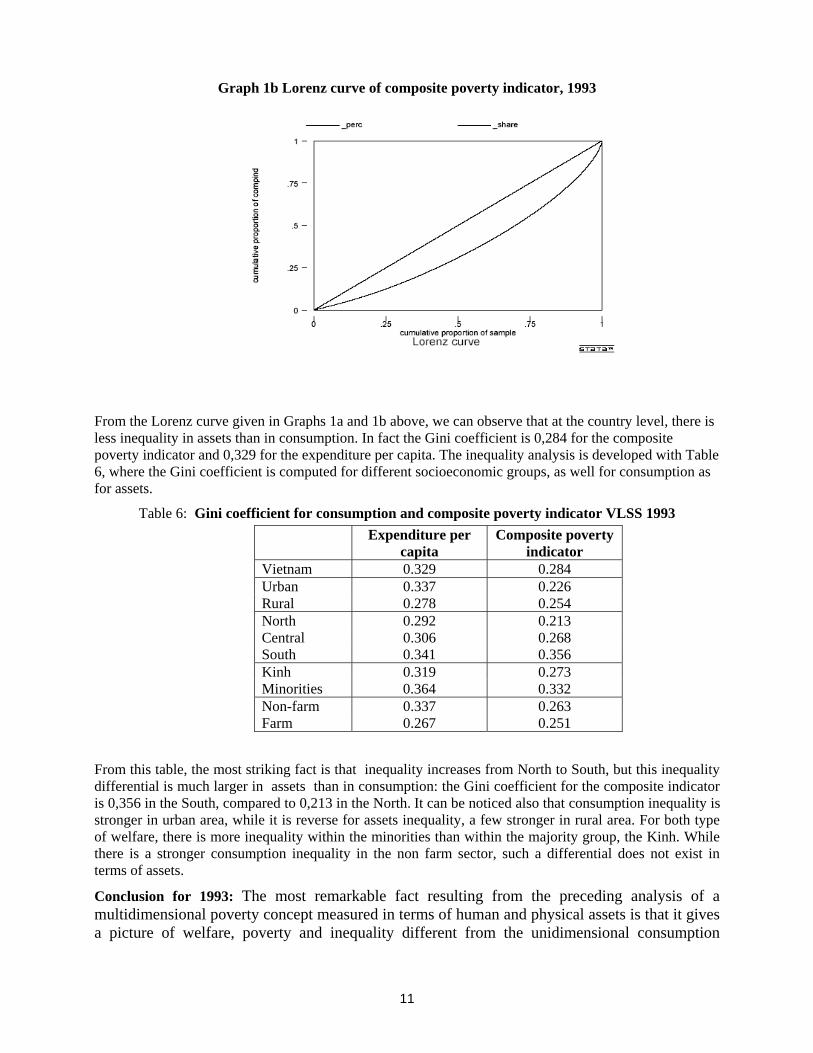
Graph 1b Lorenz curve of composite poverty indicator, 1993

From the Lorenz curve given in Graphs 1a and 1b above, we can observe that at the country level, there isless inequality in assets than in consumption. In fact the Gini coefficient is 0,284 for the compositepoverty indicator and 0,329 for the expenditure per capita. The inequality analysis is developed with Table6, where the Gini coefficient is computed for different socioeconomic groups, as well for consumption asfor assets.

Table 6: Gini coefficient for consumption and composite poverty indicator VLSS 1993Expenditure per

capitaComposite poverty

indicatorVietnam 0.329 0.284Urban 0.337 0.226Rural 0.278 0.254North 0.292 0.213Central 0.306 0.268South 0.341 0.356Kinh 0.319 0.273Minorities 0.364 0.332Non-farm 0.337 0.263Farm 0.267 0.251

From this table, the most striking fact is that inequality increases from North to South, but this inequalitydifferential is much larger in assets than in consumption: the Gini coefficient for the composite indicatoris 0,356 in the South, compared to 0,213 in the North. It can be noticed also that consumption inequality isstronger in urban area, while it is reverse for assets inequality, a few stronger in rural area. For both typeof welfare, there is more inequality within the minorities than within the majority group, the Kinh. Whilethere is a stronger consumption inequality in the non farm sector, such a differential does not exist interms of assets.

Conclusion for 1993: The most remarkable fact resulting from the preceding analysis of amultidimensional poverty concept measured in terms of human and physical assets is that it givesa picture of welfare, poverty and inequality different from the unidimensional consumption

12

approach. It means that both concepts are complementary, even if there is an expected correlationbetween them.

3.2. A multidimensional poverty profile for 1998 and dynamic analysis

As for the profile of 1993, for the same eight indicators, we first produce a disaggregated profile based onthe specific distribution of each indicator. The change from 1993 to 1998 is computed. A summary isgiven in Table 7 below. Then a composite indicator is computed at the household level, based on theweights computed for 1993 and given in Table 3.

3.2.1. The 1998 profile with eight CBMS indicator

Table 7: Multidimensional poverty in 1998 and variation 93-98 (%)Indicator 1998 Variation

1993 - 1998No underemployment 71.1 15.1UnderemploymentUnderemployment 28.9 -15.5No chronic sick 79.4 -2.5Chronic sicknessWith chronic sick 20.6 2.5Adults literate 60.8 2.3Adult illiteracyAdults illiterate 35.2 -2.3Children going to school 91.6 6.7UnderschoolingChildren not going to school 8.4 -6.7Withour radio, TV 28.8 -24.2Without radio, TVWith radio, TV 71.2 24.2Permanent house 15.7 -0.8Semi-permanent house 59.2 12.2

Type of dwelling

Temporary house 25.0 -11.5Piped, rain, drilled well 41.0 14.8Dug well 43.2 -9.5Pond, lake, river 11.4 -7.9

Drinking water

Others 4.4 2.6Flush toilet 17.0 6.6Double vault compost latrine 9.8 1.4Simple toilet 39.7 5.9Other types 13.6 -7.2

Sanitation (Typesof toilet used)

No toilet 19.8 -6.8TOTAL 16,128,313 households 100.0 0

We observe that over the period 1993-1998, six of the eight poverty indicators have improved inpercentage, the other two, chronic sickness and adult illiteracy, having not changed significantly. Themost important changes are with the lack of communication facilities (-24,2%), underemployment (-15,1%), no simple toilet (-14%) and temporary house (-11,5%). Due to the population growth (+14,4%households), there are more households suffering from functional illiteracy (+7,2%) and especially fromchronic sickness (+29,8%).

Analysing these changes more deeply, we observe that:

- the improvement in communication facilities has occurred more in Central Highlands (-35,8%) and less in Northern Mountains (-14,8%) as well as among the minorities (-12,6%);

13

- underemployment has decreased at a high rate in two of the three regions having the highestrates, North Central (-27,2%) and Red River Delta (-23,8%), the third one, Mekong RiverDelta, remaining high with a small decrease of only - 4,1%;

- sanitation has improved strongly in North Central, but less than the average in Mekong RiverDelta, where it was and remains the most deficient. Minorities have been particularlyperformant on this aspect;

- reduction of temporary housing has been particularly spectacular in Central Highland (-30,8%), but very low in Mekong River Delta (- 6,2%), which remains by far the mostdeficient region on this regard;

- adult illiteracy have decreased significantly in Central Highlands (- 17%), where it had thehighest rate in 1993, and which is at the same level in 1998 than Mekong River Delta, whoseimprovement has been only –3,7%;

- chronic sickness has decreased spectacularly in Southern Central region (- 15,2%), but morethan doubled in Southeast region (+ 9,9%) and almost doubled in Red River Delta (+9,6%).

From this analysis, we see again that the dynamics of multidimensional poverty would be easier toobserve with a composite poverty indicator.

3.2.2. The 1998 profile with a composite indicator and comparative analysis with the moneymetricapproach

As stated above, a multidimensional composite poverty indicator has been computed for 1998 on the basisof the category weights established for 1993. Contrarily to a moneymetric indicator, no price adjustment isrequired with such a categorical based indicator. The same remark applies for poverty lines built on thebasis of the composite indicator.

(a) Multidimensional welfare level comparisons and dynamics from 93 to 98

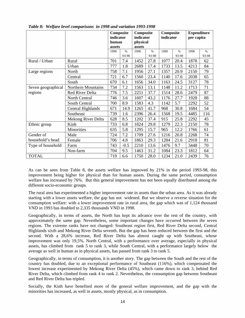
Table 8 below is similar to Table 4, with an additional component, the variation in percentage from 1993to 1998. This variation is given for the two components of the composite indicator, the human andphysical assets sub-indicators. Regarding the moneymetric analysis, 1998 real expenditure per capita hasbeen deflated taking 1993 as the basis. The deflator takes the value 1,225, as given in the official 1999report 10.

10 See Government-Donor-NGO Working Group (1999), annex 2, p. 163.

14

Table 8: Welfare level comparisons in 1998 and variation 1993-1998Compositeindicatorhumanassets

Compositeindicatorphysicalassets

Compositeindicator

Expenditureper capita

1998 %93-98

1998 %93-98

1998 %93-98

1998 %93-98

Rural 701 7.4 1452 27.8 1077 20.4 1878 62Rural / UrbanUrban 777 1.8 2689 17.4 1733 13.5 4213 84North 758 7.1 1956 27.1 1357 20.9 2150 79Central 721 6.7 1560 23.4 1140 17.6 2038 65

Large regions

South 670 6.1 1656 34.0 1163 24.5 3127 78Northern Mountains 734 7.2 1563 13.1 1148 11.2 1713 71Red River Delta 776 7.5 2251 37.7 1514 28.6 2479 87North Central 746 3.6 1607 43.2 1176 27.7 1928 88South Central 700 8.9 1583 4.3 1142 5.7 2292 52Central Highlands 671 14.9 1265 41.7 968 30.8 1684 54Southeast 739 1.6 2396 26.4 1568 19.5 4485 116

Seven geographicalregions

Mekong River Delta 628 8.5 1202 37.4 915 25.8 2292 45Kinh 733 6.8 1824 29.8 1279 22.3 2150 78Ethnic groupMinorities 635 5.8 1295 15.7 965 12.2 1766 61Male 724 7.2 1709 27.6 1216 20.8 2268 74Gender of

household’s head Female 706 4.8 1863 29.3 1284 21.6 2918 81Farm 743 -0.5 2210 13.6 1476 9.7 3448 70Type of householdNon-farm 704 9.5 1463 31.2 1084 23.3 1812 64

TOTAL 719 6.6 1750 28.0 1234 21.0 2439 76

As can be seen from Table 8, the assets welfare has improved by 21% in the period 1993-98, thisimprovement being higher for physical than for human assets. During the same period, consumptionwelfare has increased by 76%. But this general improvement has not been equally distributed among thedifferent socio-economic groups.

The rural area has experimented a higher improvement rate in assets than the urban area. As it was alreadystarting with a lower assets welfare, the gap has not widened. But we observe a reverse situation for theconsumption welfare: with a lower improvement rate in rural area, the gap which was of 1,124 thousandVND in 1993 has doubled to 2,335 thousands VND in 1998.

Geographically, in terms of assets, the North has kept its advance over the rest of the country, withapproximately the same gap. Nevertheless, some important changes have occurred between the sevenregions. The extreme ranks have not changed: Southeast region first, Red River Delta second, CentralHighlands sixth and Mekong River Delta seventh. But the gap has been reduced between the first and thesecond. With a 28,6% increase, Red River Delta has almost caught up with Southeast, whoseimprovement was only 19,5%. North Central, with a performance over average, especially in physicalassets, has climbed from rank 5 to rank 3, while South Central, with a performance largely below theaverage as well in human as in physical assets, has passed from rank 3 to rank 5.

Geographically, in terms of consumption, it is another story. The gap between the South and the rest of thecountry has doubled, due to an exceptional performance of Southeast (116%), which compensated thelowest increase experimented by Mekong River Delta (45%), which came down to rank 3, behind RedRiver Delta, which climbed from rank 4 to rank 2. Nevertheless, the consumption gap between Southeastand Red River Delta has tripled.

Socially, the Kinh have benefited more of the general welfare improvement, and the gap with theminorities has increased, as well in assets, mostly physical, as in consumption.

15

The gender gap has significantly increased only in terms of consumption in favor of female headedhouseholds, remaining very low and not really significant in terms of assets.

Farming households have performed much better than non-farming ones as well in human as in physicalassets, so that the assets gap has been reduced. On the other hand, the consumption gap has almostdoubled.

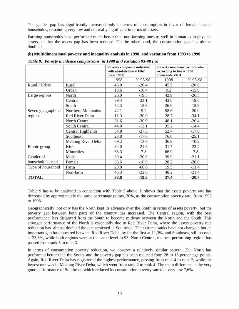
(b) Multidimensional poverty and inequality analysis in 1998, and variation from 1993 to 1998

Table 9: Poverty incidence comparisons in 1998 and variation 93-98 (%)Poverty composite indicatorwith absolute line = 1062(base 1993)

Poverty moneymetric indicatoraccording to line = 1790thousands VND

1998 % 93-98 1998 % 93-98Rural 46.0 -20.4 45.5 -20.8Rural / UrbanUrban 13.6 -10.4 9.2 -15.8North 26.0 -19.5 42.9 -26.5Central 39.4 -23.1 43.8 -19.6

Large regions

South 52.3 -15.6 26.0 -15.9Northern Mountains 42.1 -9.2 58.6 -20.0Red River Delta 11.3 -30.0 28.7 -34.1North Central 31.6 -30.9 48.1 -26.4South Central 44.0 -13.1 35.2 -14.4Central Highlands 54.8 -27.3 52.4 -17.6Southeast 23.8 -17.6 76.0 -25.1

Seven geographicalregions

Mekong River Delta 69.2 -13.6 36.9 -10.2Kinh 34.0 -21.6 31.7 -23.4Ethnic groupMinorities 63.3 -7.8 66.9 -7.8Male 39.4 -20.0 39.9 -21.1Gender of

household’s head Female 36.6 -16.9 28.2 -20.0Farm 28.0 -66.0 19.5 -11.4Type of householdNon-farm 45.3 -22.6 48.2 -21.4

TOTAL 38.8 -19.3 37.4 -20.7

Table 9 has to be analysed in connection with Table 5 above. It shows that the assets poverty rate hasdecreased by approximately the same percentage points, 20%, as the consumption poverty rate, from 1993to 1998.

Geographically, not only has the North kept its advance over the South in terms of assets poverty, but thepoverty gap between both parts of the country has increased. The Central region, with the bestperformance, has distanced from the South to become midway between the North and the South. Thisstronger performance of the North is essentially due to Red River Delta, where the assets poverty ratereduction has almost doubled the one achieved in Southeast. The extreme ranks have not changed, but animportant gap has appeared between Red River Delta, by far the first at 11,3%, and Southeast, still second,at 23,8%, while both regions were at the same level in 93. North Central, the best performing region, haspassed from rank 5 to rank 3.

In terms of consumption poverty reduction, we observe a relatively similar pattern. The North hasperformed better than the South, and the poverty gap has been reduced from 28 to 16 percentage points.Again, Red River Delta has registrered the highest performance, passing from rank 4 to rank 2, while thelowest one was in Mekong River Delta, which went from rank 2 to rank 4. The main difference is the verygood performance of Southeast, which reduced its consumption poverty rate to a very low 7,6%.

16

Socially, the Kinh have achieved a poverty reduction rate three times higher than the minorities, as well inassets as in consumption. As already noticed above for the welfare level, the poverty gap between bothgroups has widened, from twenty percentage points to thirty and more. Male and female headedhouseholds have performed almost equally in both types of poverty reduction. Farming households haveperformed much better than non farming ones in both types of poverty reduction, and the gaps betweenboth categories of household have been cut by 50%.

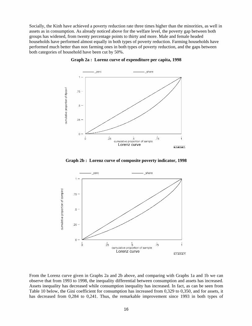
Graph 2a : Lorenz curve of expenditure per capita, 1998

Graph 2b : Lorenz curve of composite poverty indicator, 1998

From the Lorenz curve given in Graphs 2a and 2b above, and comparing with Graphs 1a and 1b we canobserve that from 1993 to 1998, the inequality differential between consumption and assets has increased.Assets inequality has decreased while consumption inequality has increased. In fact, as can be seen fromTable 10 below, the Gini coefficient for consumption has increased from 0,329 to 0,350, and for assets, ithas decreased from 0,284 to 0,241. Thus, the remarkable improvement since 1993 in both types of

17

welfare, consumption and assets, has been accompanied by an opposite effect in inequality: moreconsumption inequality, but less assets inequality.

Table 10: Gini coefficient for consumption and composite poverty indicator VLSS 1993 and 1998Expenditure per capita Composite poverty indicator

1993 1998 1993 1998Vietnam 0.329 0.350 0.284 0.241Urban 0.337 0.340 0.226 0.173Rural 0.278 0.270 0.254 0.215North 0.292 0.321 0.213 0.195Central 0.306 0.315 0.268 0.210South 0.341 0.367 0.356 0.299Kinh 0.319 0.339 0.273 0.229Minorities 0.364 0.359 0.332 0.268Non-farm 0.337 0.361 0.263 0.239Farm 0.267 0.259 0.251 0.207

The increase in consumption inequality did not occur in rural neither in urban area. It occurred as well inNorth, Center and South, but not within the minorities, neither for the farming households. The reductionof assets inequality has been general across the different socioeconomic groups. Assets inequality isparticularly low in the urban area (0,173) and in the North (0,195).

Conclusion for 1998 : The multidimensional poverty analysis, with a composite indicator based onhuman and physical assets, confirms the extensively analysed trend, from a moneymetric consumptionperspective, of a general remarkable improvement during the period 1993-1998. The global reduction ofpoverty is approximately of –20%, from both perspective. But the dynamics have been different,according to the two approaches to poverty. A striking fact is that inequality in consumption, alreadyhigher in 1993 than assets inequality, has still increased while inequality in assets has decreased. Theregional differential in assets poverty has increased in favor of the North, already ahead of the South in1993, but it has decreased in terms of consumption poverty again in favor of the North, which was farbehind the South in 1993. The South nevertheless still leads in terms of the general consumption level andof the rate of consumption poverty.

4. CONCLUSION

Eight simple non-monetary, categorical indicators of human and physical assets developed in CBMSresearch in Vietnam, have been identified in the VLSS-1993 and 2 survey data sets. They have beenanalysed and aggregated in a composite indicator using the factorial technique, more precisely theMultiple Correspondance Analysis. Categorical weights have thus been computed for the eight indicators,twenty one categories (Table 3), on which rely the composite indicator, with 1993 as the base-year, andkept the same for 1998.

The comparison of this multidimensional approach to poverty measurement with the moneymetric onebase on total household expenditures, we observe the following convergence:

a) in the base-year 1993, with the 58% global moneymetric poverty rate as a benchmark, povertyrates are comparable for both methodologies across the rural/urbain and ethnicityclassifications (Table 5);

b) the female-headed households are less poor than the male-headed ones (Table 5);

c) the inequality is higher from North to South, as well in 1993 as in 1998 (Tables 6 and 10);

18

d) in terms of poverty dynamics, the poverty rate has decreased by the same amount, minus 20%(Table 9), and this is the most striking convergence fact between both measurementmethodologies;

e) the remarkable success in poverty reduction has globally been greater in the North than in theSouth for both type of poverty (Table 9).

On the other hand, there are many divergence facts:

a) the regional incidence of poverty is reverse according to the two types of indicators: fromNorth to South, monetary (consumption) poverty decreases while multidimensional assetpoverty increases, as well in 1993 as in 1998 (Tables 5 and 9). We get a different ranking ofthe seven regions and significantly different poverty differentials;

b) as a general result of the performance of the North, the multidimensional asset povertydifferential between the North and the South has increased, while the consumption povertydifferential has decreased (Tables 5 and 9);

c) the differential between male and female headed households is larger for consumption povertyin 1993 (Table 5) and still much larger in 1998 (Table 9) than for multidimensional poverty;

d) while the consumption inequality has globally increased from 1993 to 1998, themultidimensional asset poverty has decreased, particularly in the Central and South regions,where it nevertheless remains higher than in the North part of the country (table 10).

When loooked at attentively, taking into account the different concepts of poverty measured by bothmethodologies, these convergence and divergence facts seem confirmed by the real situation as observedin the field. It must be kept in mind that the multidimensional composite indicator includes a strongcomponent of human assets (education and health), partly built through community facilities, and here thedivergence facts can find an explanation. On the other hand, the owning of many of the assets included inthis composite indicator is related to income, essentially to permanent income, what the expenditureapproach tries to catch, and this can help to explain the convergence facts. In fact, the correlation betweenboth indicators, while highly significant, is not so high at approximatively 0,49 in both years 1993 and1998. From all this it appears that the multidimensional poverty composite indicator reveals a face ofpoverty different than the one expressed through the expenditure indicator, not in an opposite but ratherin a complementary way.

This type of measurement of multidimensional poverty has a great advantage: being based on a set ofcategorical or qualitative simple indicators, it avoids the important difficulties of a price basedmoneymetric indicator, especially for poverty analysis across time and space. But it is not a panacea to thechallenge of measuring poverty. There are some major caveats and sensitive issues, among which:

a) The choice of the primary indicators is not obvious. We must be able to explicit which aspectof poverty each one is supposed to reveal. Also, they must be meaningful across the socio-economic groups we intend to analyse poverty, especially across the rural/urban areas and thedifferent ecological regions. Housing characteristics, safe water, etc., are difficult to measureso that they are comparable across the whole country. But this is true of any analysis variablein a national household survey;

b) Poverty line determination does not rely on any strong theoretical ground. It does not meanthat it is completely arbitrary, but we have to be clear on the rational supporting the choice.The relative approach of a quantile exogenously determined, as we have done here in the baseyear 1993, is interesting to make comparable different methodological and conceptualapproaches to poverty. The absolute approach of fixing a poverty line for each primaryindicator is not to be excluded. With binary indicators, there is no arbitrariness. With nonbinary ones, the selected threshold can represent a consensual social choice in terms of astandard to achieve in terms of poverty eradication, for example in terms of sanitory facilities,

19

safe water, housing characteristics, etc. Whatever be the approach, this base poverty line mustobviously be kept constant across time for the dynamic analysis of poverty changes;

c) The base categorical weights are also to be kept constant, as for the computation of a CPIrelative to a fixed basket of goods.

This short list is far from being exhaustive.

The research presented here could be pursued in trying to expand the list of basic indicators from thevariables available in the sequence of VLSS surveys, including the third one completed in 2002. Inparticular, some light, non-monetary indicators of poverty dimensions not explicitly represented here, asnutrition, could be looked for. Also, for an annual monitoring of poverty, some more short-term sensitiveindicators should be looked for.

To conclude, we think that the CBMS type indicators present a strong analytical potential formultidimensional poverty analysis, being complementary to the more standard moneymetric analysis. Inaddition, due to their easiness and their low cost, they should be looked at to meet the objective ofregularly producing largely disaggregated poverty profiles for a more efficient monitoring of povertyreduction policies and programs. They could also suggest some very simple questions to be integrated innational censuses in view of mapping poverty at the lowest level with a national coverage. This does notpreclude these indicators from being useful at the level where they have first been designed, thecommunity level, for poverty targeting through local development interventions. The weights developed ata national level, as done here from a representative survey, can be easily used within small communities torank the households according to their multidimensional poverty level, to enhance the efficient of CBMS.

References

Asselin Louis-Marie (2002), Multidimensional Poverty, Theory, IDRC, in MIMAP Training Session onMultidimensional Poverty, Quebec, June 2002.

Government-Donor-NGO Working Group (1999), Attacking Poverty, Vietnam Development Report 2000,Publishing Department of Ministry of Culture & Information, 179 pp.

General Statistical Office & State Committee for Planning (1993), Vietnam Living Standards Survey1992-1993. Hanoi.

General Statistical Office (1999), Vietnam Living Standards Survey 1997-1998. Hanoi.

Vu Tuan Anh (2000), Poverty Monitoring in Vietnam, Annual MIMAP meeting held in Palawan,Philippines, Sept. 2000. IDRC, Ottawa, mimeo.

Vu Tuan Anh & Vu Van Toan (2004), Implementaion of the community-based poverty monitoring inVietnam, Vietnam’s Socio-Economic Development Review, No. 39, Hanoi, Autumn 2004.