Paper 465e

Multi-Objective Control-Relevant Demand Modelingfor Supply Chain Management

Jay Schwartz and Daniel E. Rivera1

Control Systems Engineering LaboratoryDepartment of Chemical EngineeringIra A. Fulton School of Engineering

Arizona State University, Tempe, Arizona 85287-6006

Prepared for presentation at the Annual AIChE 2006 MeetingSan Francisco, CA, November 12- November 17, 2006

Session: [465] Supply Chain Optimization

Copyright © Control Systems Engineering Laboratory, ASU.

September, 2006UNPUBLISHED

AIChE shall not be responsible for statements or opinions contained in papers or printed in publications.

Abstract

The development of control-oriented decision policies for inventory management in supply chainshas received considerable interest in recent years, and demand modeling to supply forecasts for thesepolicies is an important component of an effective solution to this problem. Drawing from the prob-lem of control-relevant identification, we present an approach for demand modeling based on data thatrelies on a control-relevant prefilter to tailor the emphasis of the fit to the intended purpose of themodel, which is to provide forecast signals to a tactical inventory management policy based on ModelPredictive Control. Integrating the demand modeling and inventory control problems offers the oppor-tunity to obtain reduced-order models that exhibit superior performance, with potentially lower usereffort relative to traditional “open-loop” methods. A systematic approach to generating these prefiltersis presented and the benefits resulting from their use are demonstrated on a representative produc-tion/inventory system case study. A multi-objective formulation is developed that allows the user toemphasize minimizing inventory variance, minimizing starts variance, or their combination.

1To whom all correspondence should be addressed. phone: (480) 965-9476 fax: (480) 965-0037; e-mail:daniel.rivera@asu.edu

1 Introduction

Efficient supply chain management has become a significant imperative for many modern-day enterprises.Properly characterizing and predicting demand plays a significant role in achieving high performancefrom supply chain management systems. The presence of error in a demand forecast will adversely affectdecision-making in a supply chain. Inaccurate market research, customer order changes, out-of-date infor-mation, and misreading product/business cycles may have a negative effect on the profitability of a supplychain dependent corporation. While eliminating all sources of error from a demand forecast is impossible,it may be possible to mitigate its detrimental effects. Therefore, it is important to understand the effects offorecast error on a supply chain decision policy.

Control-oriented approaches have been recently proposed to deal with the inventory managementproblems inherent in supply chains (Tzafestas et al., 1997; Dejonckheere et al., 2002; Perea-Lopez etal., 2003; Braun et al., 2003; Seferlis and Giannelos, 2004; Wang et al., 2004; Schwartz et al., 2006). Inthese approaches, demand is treated as an exogenous “disturbance” signal that must be properly “rejected”by a sensibly-designed control system. However, an understanding of how a demand forecast should beproperly developed for the sake of this class of supply chain management policies has not been exam-ined. This paper attempts to gain a broader understanding of disturbance/demand modeling and the effectsof forecast error on a Model Predictive Control (MPC)-based tactical decision policy. The relationshipbetween demand forecast error and changes in inventory and starts are examined for a control-orientedtactical decision policy in a single node of the manufacturing process. Understanding this relationshiprepresents one step towards a fundamental understanding that will allow planning personnel to deal withinherently erroneous forecasts in an educated manner.

To accomplish this goal, we will draw from ideas in control-relevant identification (Rivera et al., 1992).The result is a systematic framework for conducting control-relevant demand modeling in the case ofa standard production/inventory system. However, these ideas can be generalized to larger topologies.Results from a case study will show that the use of the framework not only improves the performance ofthe supply chain, but also enables planners to reduce the complexity of customer demand models.

Section 2 begins with a discussion of the modeling of a production/inventory system using a fluidanalogy and the development of a model-based inventory controller relying on Model Predictive Control.In Section 3, the closed-loop transfer functions describing forecast error are developed and the effectof erroneous forecasts is studied in both the time and frequency domains. A procedure for performingcontrol-relevant demand modeling is presented. Section 4 is a case study involving the use of an MPCscheme to manage a production/inventory system. Section 5 highlights the important conclusions that canbe drawn from the analysis in this paper.

2 System and Controller

2.1 Inventory Control Fluid Analogy

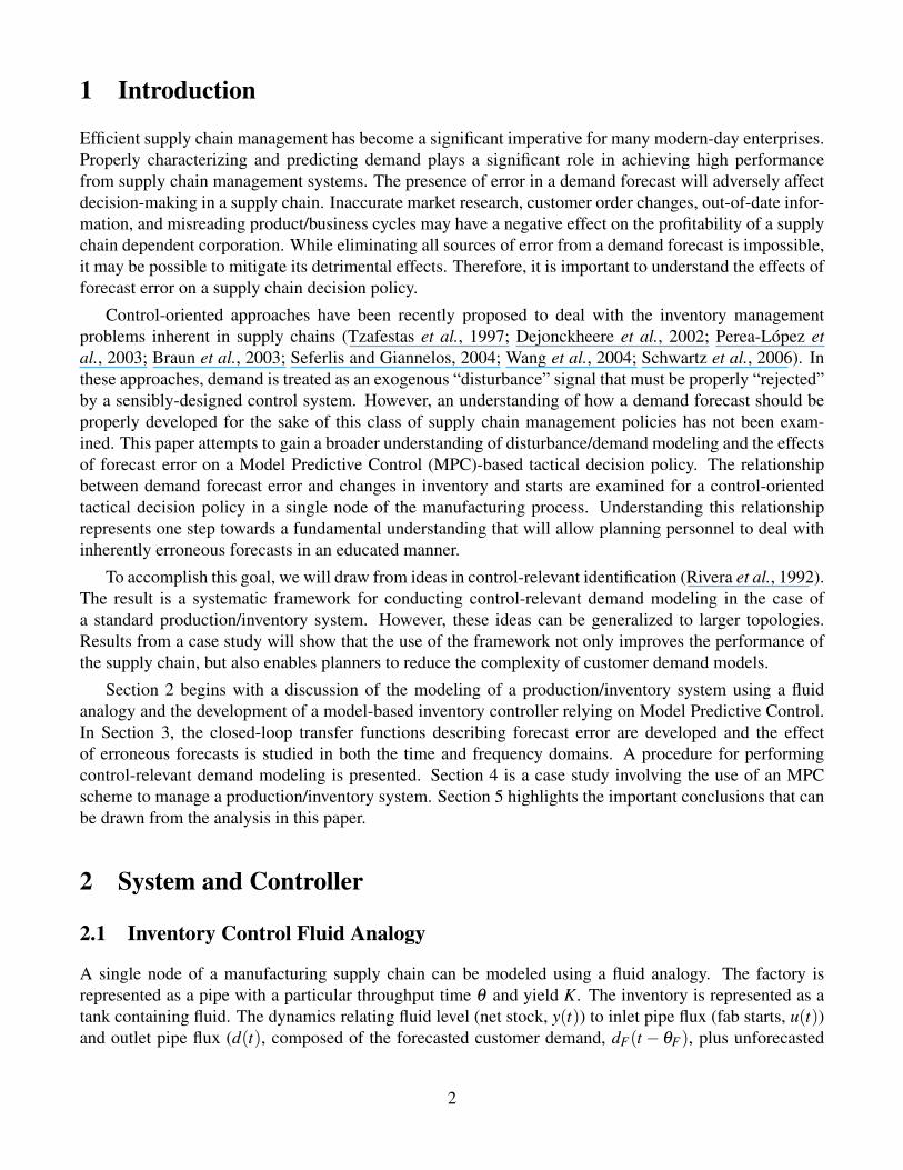
A single node of a manufacturing supply chain can be modeled using a fluid analogy. The factory isrepresented as a pipe with a particular throughput time θ and yield K. The inventory is represented as atank containing fluid. The dynamics relating fluid level (net stock, y(t)) to inlet pipe flux (fab starts, u(t))and outlet pipe flux (d(t), composed of the forecasted customer demand, dF(t − θF), plus unforecasted

2

Starts(Manipulated)

(Throughput Time)

LT

LIC

Net Stock(Controlled)

Demand

Forecast

Actual

y(t)

u(t)

(Disturbance)

dF (t)

d(t)

! K

!d

(Yield)

(Delivery Time)

Figure 1: Fluid analogy: a single manufacturing node represented as a system of pipes and a tank.

customer demand, dU(t)) is represented in (1). Note that θF is the forecast horizon. The underlyingdynamical system has delayed, integrating dynamics according to

y(t) =Kz−θ u(t)

1− z−1 − z−θF dF(t)1− z−1 − dU(t)

1− z−1 (1)

The operational goal of the system is to meet customer demand while maintaining the inventory levelat a specified target. This can be accomplished by adjusting the factory starts. An anticipated (forecasted)demand signal can be used for feedforward compensation in this regard.

2.2 Model Predictive Control

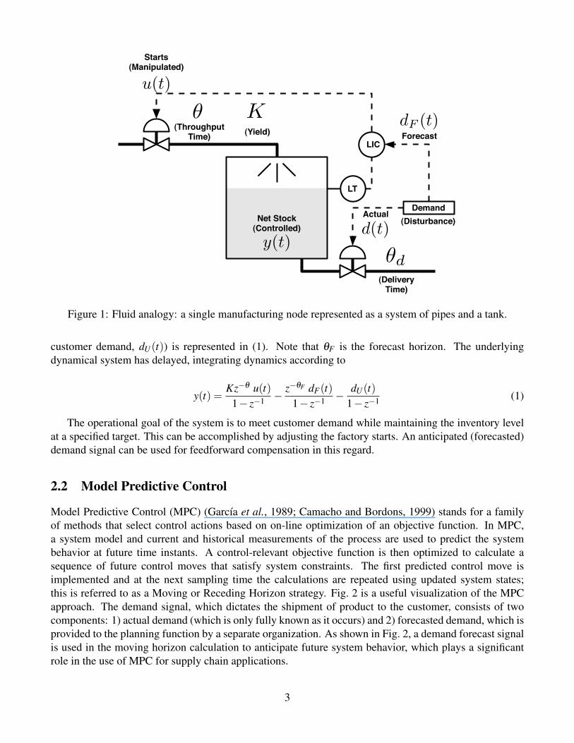
Model Predictive Control (MPC) (Garcıa et al., 1989; Camacho and Bordons, 1999) stands for a familyof methods that select control actions based on on-line optimization of an objective function. In MPC,a system model and current and historical measurements of the process are used to predict the systembehavior at future time instants. A control-relevant objective function is then optimized to calculate asequence of future control moves that satisfy system constraints. The first predicted control move isimplemented and at the next sampling time the calculations are repeated using updated system states;this is referred to as a Moving or Receding Horizon strategy. Fig. 2 is a useful visualization of the MPCapproach. The demand signal, which dictates the shipment of product to the customer, consists of twocomponents: 1) actual demand (which is only fully known as it occurs) and 2) forecasted demand, which isprovided to the planning function by a separate organization. As shown in Fig. 2, a demand forecast signalis used in the moving horizon calculation to anticipate future system behavior, which plays a significantrole in the use of MPC for supply chain applications.

3

PredictedInventory

y(t+k)

Future Starts u(t+k)

ActualDemand

PreviousStarts

t t+1 t+m t+p

Move Horizon

Prediction Horizon

Umax

Umin

Forecasted Demand dF(t+k)

Inventory Setpoint r(t+k)

Dist

urba

nce

Out

put

Inpu

t

Past Future

Figure 2: Receding horizon representation of Model Predictive Control.

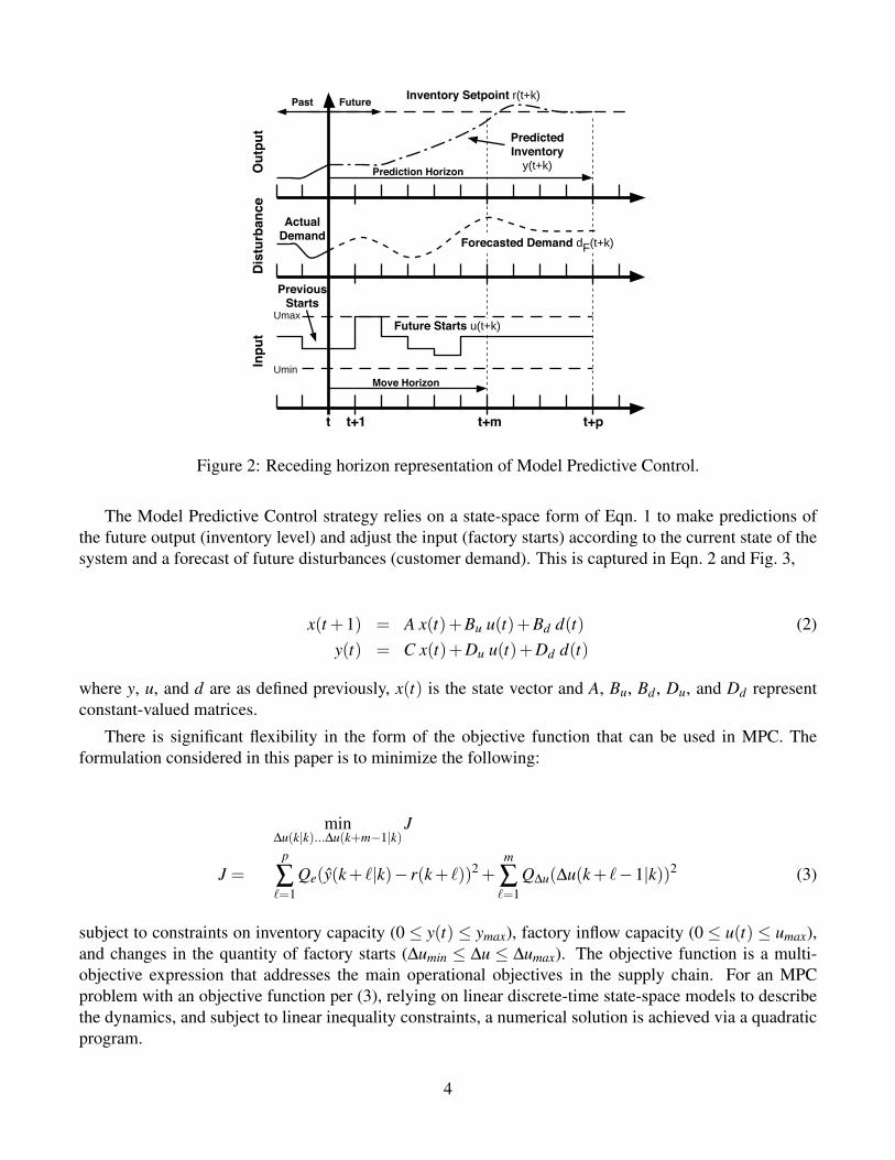
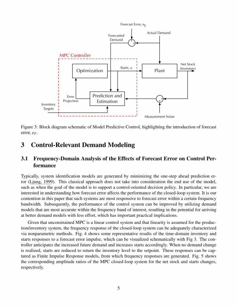
The Model Predictive Control strategy relies on a state-space form of Eqn. 1 to make predictions ofthe future output (inventory level) and adjust the input (factory starts) according to the current state of thesystem and a forecast of future disturbances (customer demand). This is captured in Eqn. 2 and Fig. 3,

x(t +1) = A x(t)+Bu u(t)+Bd d(t) (2)y(t) = C x(t)+Du u(t)+Dd d(t)

where y, u, and d are as defined previously, x(t) is the state vector and A, Bu, Bd , Du, and Dd representconstant-valued matrices.

There is significant flexibility in the form of the objective function that can be used in MPC. Theformulation considered in this paper is to minimize the following:

min∆u(k|k)...∆u(k+m−1|k)

J

J =p

∑`=1

Qe(y(k + `|k)− r(k + `))2 +m

∑`=1

Q∆u(∆u(k + `−1|k))2 (3)

subject to constraints on inventory capacity (0 ≤ y(t) ≤ ymax), factory inflow capacity (0 ≤ u(t) ≤ umax),and changes in the quantity of factory starts (∆umin ≤ ∆u ≤ ∆umax). The objective function is a multi-objective expression that addresses the main operational objectives in the supply chain. For an MPCproblem with an objective function per (3), relying on linear discrete-time state-space models to describethe dynamics, and subject to linear inequality constraints, a numerical solution is achieved via a quadraticprogram.

4

PlantOptimization

Prediction and Estimation

ErrorProjection

Forecast Error, eF

Actual DemandForecastedDemand

Net Stock(Inventory)Starts, u

Measurement Noise

InventoryTargets

MPC Controller

++

++

Figure 3: Block diagram schematic of Model Predictive Control, highlighting the introduction of forecasterror, eF .

3 Control-Relevant Demand Modeling

3.1 Frequency-Domain Analysis of the Effects of Forecast Error on Control Per-formance

Typically, system identification models are generated by minimizing the one-step ahead prediction er-ror (Ljung, 1999). This classical approach does not take into consideration the end use of the model,such as when the goal of the model is to support a control-oriented decision policy. In particular, we areinterested in understanding how forecast error affects the performance of the closed-loop system. It is ourcontention in this paper that such systems are most responsive to forecast error within a certain frequencybandwidth. Subsequently, the performance of the control system can be improved by utilizing demandmodels that are most accurate within the frequency band of interest, resulting in the potential for arrivingat better demand models with less effort, which has important practical implications.

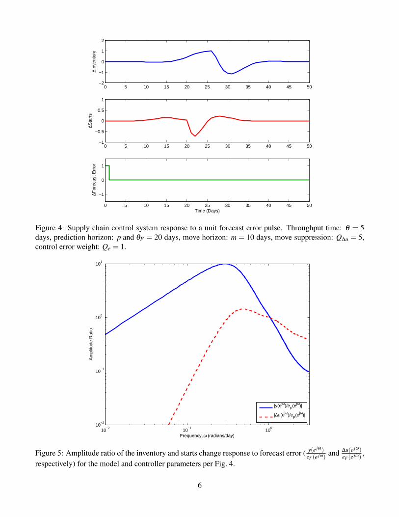
Given that unconstrained MPC is a linear control system and that linearity is assumed for the produc-tion/inventory system, the frequency response of the closed-loop system can be adequately characterizedvia nonparametric methods. Fig. 4 shows some representative results of the time-domain inventory andstarts responses to a forecast error impulse, which can be visualized schematically with Fig 3. The con-troller anticipates the increased future demand and increases starts accordingly. When no demand changeis realized, starts are reduced to return the inventory level to the setpoint. These responses can be cap-tured as Finite Impulse Response models, from which frequency responses are generated. Fig. 5 showsthe corresponding amplitude ratios of the MPC closed-loop system for the net stock and starts changes,respectively.

5

0 5 10 15 20 25 30 35 40 45 50−2

−1

0

1

2

∆Inv

ento

ry

0 5 10 15 20 25 30 35 40 45 50−1

−0.5

0

0.5

1

∆Sta

rts

0 5 10 15 20 25 30 35 40 45 50

−1

0

1

∆For

ecas

t Err

or

Time (Days)

Figure 4: Supply chain control system response to a unit forecast error pulse. Throughput time: θ = 5days, prediction horizon: p and θF = 20 days, move horizon: m = 10 days, move suppression: Q∆u = 5,control error weight: Qe = 1.

10−2

10−1

100

10−2

10−1

100

101

Frequency, ω (radians/day)

Am

plitu

de R

atio

|y(ejω)/eF(ejω)|

|∆u(ejω)/eF(ejω)|

Figure 5: Amplitude ratio of the inventory and starts change response to forecast error ( y(e jω )eF (e jω ) and ∆u(e jω )

eF (e jω ) ,respectively) for the model and controller parameters per Fig. 4.

6

0 200 400 600 800 1000−20

0

20

(a)

∆Inv

ento

ry

0 200 400 600 800 1000−20

0

20

(b)

∆Inv

ento

ry

0 200 400 600 800 1000−20

0

20

∆Inv

ento

ry

(c) Time (Days)

10−3

10−2

10−1

100

10−2

10−1

100

101

(a) (b) (c)

Frequency, ω (radians/day)

Am

plitu

de R

atio

Low Frequency Forecast ErrorIntermediate Frequency Forecast ErrorHigh Frequency Forecast Error|y(ejω)/e

F(ejω)|

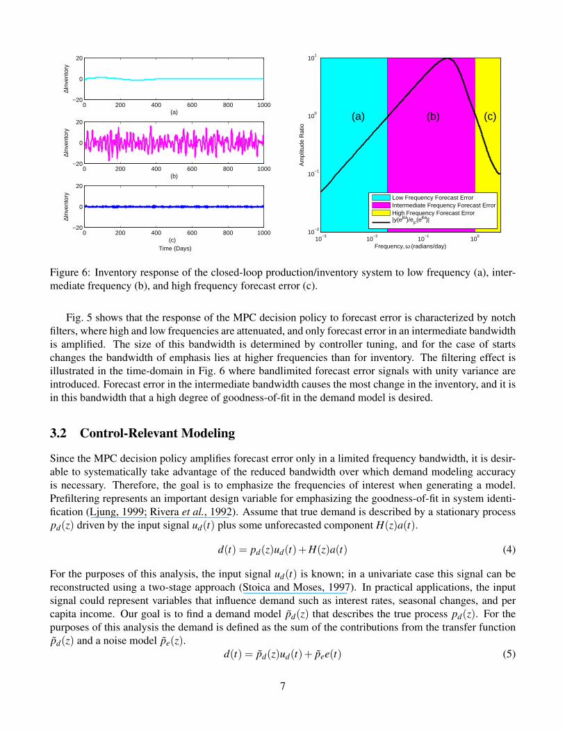
Figure 6: Inventory response of the closed-loop production/inventory system to low frequency (a), inter-mediate frequency (b), and high frequency forecast error (c).

Fig. 5 shows that the response of the MPC decision policy to forecast error is characterized by notchfilters, where high and low frequencies are attenuated, and only forecast error in an intermediate bandwidthis amplified. The size of this bandwidth is determined by controller tuning, and for the case of startschanges the bandwidth of emphasis lies at higher frequencies than for inventory. The filtering effect isillustrated in the time-domain in Fig. 6 where bandlimited forecast error signals with unity variance areintroduced. Forecast error in the intermediate bandwidth causes the most change in the inventory, and it isin this bandwidth that a high degree of goodness-of-fit in the demand model is desired.

3.2 Control-Relevant Modeling

Since the MPC decision policy amplifies forecast error only in a limited frequency bandwidth, it is desir-able to systematically take advantage of the reduced bandwidth over which demand modeling accuracyis necessary. Therefore, the goal is to emphasize the frequencies of interest when generating a model.Prefiltering represents an important design variable for emphasizing the goodness-of-fit in system identi-fication (Ljung, 1999; Rivera et al., 1992). Assume that true demand is described by a stationary processpd(z) driven by the input signal ud(t) plus some unforecasted component H(z)a(t).

d(t) = pd(z)ud(t)+H(z)a(t) (4)

For the purposes of this analysis, the input signal ud(t) is known; in a univariate case this signal can bereconstructed using a two-stage approach (Stoica and Moses, 1997). In practical applications, the inputsignal could represent variables that influence demand such as interest rates, seasonal changes, and percapita income. Our goal is to find a demand model pd(z) that describes the true process pd(z). For thepurposes of this analysis the demand is defined as the sum of the contributions from the transfer functionpd(z) and a noise model pe(z).

d(t) = pd(z)ud(t)+ pee(t) (5)

7

The forecast error, eF(t) is defined as the difference between the actual and forecasted customer demand,as shown in Eqn. 6.

eF(t) = d(t)− d(t) = d(t)− pd(z)ud(t) = pee(t) (6)

e(t) is the one-step ahead prediction error; if pe = 1 then e(t) = eF(t). The system identification problemthen involves minimizing the squared sum of the filtered one-step ahead prediction error, where L(z) is theprefilter,

minpd

V = minpd

N

∑t=1

[L(z)e(t)]2 = minpd

N

∑t=1

e2L(t) (7)

and the filtered prediction error is comprised of:

eL(t) =L(z)pe(z)

[(pd(z)− pd(z))ud(t)+H(z)a(t)] =L(z)pe(z)

eF(t) (8)

The application of Parseval’s theorem allows an analysis of the problem in the frequency domain.

limN→∞

1N

N

∑t=1

e2L(t) =

12π

∫π

−π

∣∣∣∣ L(e jω)pe(e jω)

∣∣∣∣2

ΦeF (ω)dω (9)

where

ΦeF (ω) =∣∣pd(e jω)− pd(e jω)

∣∣2Φud(ω)+

∣∣H(e jω)∣∣2

Φa(ω) (10)

From Eqn. 9 we know that we can use L(z) to provide user-defined emphasis, although it is important tonote that the noise model pe(z) will also act to emphasize certain frequency regimes. The user choice ofan Output Error structure results in pe(z) = 1, eliminating the bias introduced by the noise model.

Our goal is to obtain estimates pd(z) of the true demand process pd(z) with emphasis in the frequenciesof interest defined by the control-relevant prefilter L(z). Emphasis can be applied for the purpose of eitherdecreasing inventory deviations from a setpoint r(t), starts variance, or some weighted combination ofboth. First, the time-domain relationships and corresponding power spectra for the control error andfactory starts change signals are defined: as

ec(t) = y(t)− r(t) = Lec(z)eF(t) (11)∆u(t) = (1− z−1)u(t) = L∆u(z)eF(t) (12)

Φec(ω) = |Lec(ejω)|2ΦeF (ω) (13)

Φ∆u(ω) = |L∆u(e jω)|2ΦeF (ω) (14)

where Lec(z) and L∆u(z) are the transfer functions relating forecast error to inventory deviations and startschanges, obtained using the nonparametric approach described previously. Φec(ω) and Φ∆u(ω) are theircorresponding power spectra.

A supply chain planner may choose to reduce either depending on the cost of inventory deviation,stockout, or changing a factory setup. In essence, it is desirable to meet the following control objective

minpd ,pe

[∫∞

0(1− γ)e2

c(t)dt +λ

∫∞

0γ∆u2(t)dt

](15)

where γ is used as a weight to emphasize either inventory deviation from setpoint (γ = 0) or factorystarts variance (γ = 1). The user-adjustable parameter λ is used to keep the variances of the two signalsequivalent.

8

Rearranging Eqn. 15 and applying Parseval’s theorem results in Eqn. 16, which allows for the analysisto be conducted in the frequency domain. The amplitude ratios represented by Lec and L∆u correspond tothose shown in Figure 5.

minpd ,pe

[(1− γ)

12π

∫π

−π

Φec(ω)dω + γλ1

2π

∫π

−π

Φ∆u(ω)dω

](16)

Comparing Eqn. 16 with Eqn. 9 leads to the following relationship.

|L(e jω)|2

|pe(e jω)|2ΦeF (ω) = (1− γ)|Lec(e

jω)|2ΦeF (ω)+ γλ |L∆u(e jω)|2ΦeF (ω) (17)

By assuming an output error model structure ( pe = 1), the control-relevant prefilter L(z) can be reduced tothe following form.

|L(e jω)|2 = (1− γ)|Lec(ejω)|2 + γλ |L∆u(e jω)|2 (18)

A curve fitting procedure is then used to obtain an Infinite Impulse Response filter that matches the am-plitude ratio of the control-relevant prefilter. A standard curve fitting algorithm for rational discrete-timetransfer functions can be used for this purpose, such as the output-error minimizing algorithm as imple-mented in the MATLAB® function invfreqz.

9

4 Case Studies

4.1 Representative Case Study

A representative production/inventory system with an MPC-based tactical decision policy will be usedto quantify the benefits achieved through the use of control-relevant demand modeling. The case studyinvolves the single node shown in Fig. 1 where the throughput time of the factory (θ ) is 5 days, the yieldis unity, the forecast horizon (θF , which is also the MPC prediction horizon p) is 20 days, the MPCmove optimization horizon (m) is 10 days, and MPC weights for penalizing starts changes and inventorydeviation (Q∆u and Qe) are 5 and 1, respectively. A data set was generated from the true demand processpd(z) subject to a white noise input in ud(t).

d(t) =1+ z−1 + z−2

1−0.4z−1 +0.5z−2 ud(t) (19)

In all analyses shown in this paper, the value of the parameter λ will be defined as the ratio of the maximumsquared amplitude ratio values of the control error and starts change transfer functions

λ =supω |Lec|2

supω |L∆u|2(20)

For the MPC production/inventory problem described the value of λ is approximately 48.

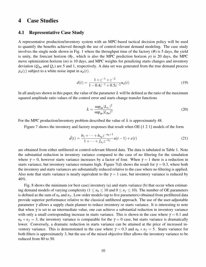
Figure 7 shows the inventory and factory responses that result when OE-[1 2 1] models of the form

d(t) =b1 + · · ·+bnbz−nb+1

1+ · · ·+ fn f z−n f

u(t−1)+ e(t) (21)

are obtained from either unfiltered or control-relevant filtered data. The data is tabulated in Table 1. Notethe substantial reduction in inventory variance compared to the case of no filtering for the simulationwhere γ = 0, however starts variance increases by a factor of four. When γ = 1 there is a reduction instarts variance, but inventory variance remains high. Figure 7(d) shows the result for γ = 0.3, where boththe inventory and starts variances are substantially reduced relative to the case where no filtering is applied.Also note that starts variance is nearly equivalent to the γ = 1 case, but inventory variance is reduced by40%.

Fig. 8 shows the minimum (or best case) inventory (a) and starts variance (b) that occur when estimat-ing demand models of varying complexity (1≤ nb ≤ 10 and 0≤ n f ≤ 10). The number of OE parametersis defined as the sum of nb and n f . Low order models (up to five parameters) obtained from prefiltered dataprovide superior performance relative to the classical unfiltered approach. The use of the user-adjustableparameter γ allows a supply chain planner to reduce inventory or starts variance. It is interesting to notethat when γ is set to an intermediate value, one can achieve a substantial reduction in inventory variancewith only a small corresponding increase in starts variance. This is shown in the case where γ = 0.1 andnb + n f = 3, the inventory variance is comparable for the γ = 0 case, but starts variance is dramaticallylower. Conversely, a dramatic reduction in starts variance can be attained at the price of increased in-ventory variance. This is demonstrated in the case where γ = 0.3 and nb + n f = 5. Starts variance forboth filters is approximately 3, but the use of the mixed objective filter allows the inventory variance to bereduced from 80 to 50.

10

500 550 600 650 700 750 800 850 900 950 1000

−2

0

2∆I

nven

tory

OE121 from raw data : Σ(y−r)2 = 136.13 Σ(∆u)2 = 3.55

500 550 600 650 700 750 800 850 900 950 1000−1

−0.5

0

0.5

1

∆Sta

rts

500 550 600 650 700 750 800 850 900 950 1000−1

−0.5

0

0.5

1

∆For

ecas

t

Time (Days)

500 550 600 650 700 750 800 850 900 950 1000

−2

0

2

∆Inv

ento

ry

OE121, γ = 0.0: Σ(y−r)2 = 32.83 Σ(∆u)2 = 8.04

500 550 600 650 700 750 800 850 900 950 1000−1

−0.5

0

0.5

1

∆Sta

rts

500 550 600 650 700 750 800 850 900 950 1000−1

−0.5

0

0.5

1

∆For

ecas

t

Time (Days)

(a) (b)

500 550 600 650 700 750 800 850 900 950 1000

−2

0

2

∆Inv

ento

ry

OE121, γ = 1: Σ(y−r)2 = 75.66 Σ(∆u)2 = 2.68

500 550 600 650 700 750 800 850 900 950 1000−1

−0.5

0

0.5

1

∆Sta

rts

500 550 600 650 700 750 800 850 900 950 1000−1

−0.5

0

0.5

1

∆For

ecas

t

Time (Days)

500 550 600 650 700 750 800 850 900 950 1000

−2

0

2

∆Inv

ento

ry

OE121, γ = 0.3: Σ(y−r)2 = 52.16 Σ(∆u)2 = 3.03

500 550 600 650 700 750 800 850 900 950 1000−1

−0.5

0

0.5

1

∆Sta

rts

500 550 600 650 700 750 800 850 900 950 1000−1

−0.5

0

0.5

1

∆For

ecas

t

Time (Days)

(c) (d)

Figure 7: Time series for closed-loop responses of the production/inventory system where the demandforecast is developed from (a) an OE-[1 2 1] fit to unfiltered data, (b) an OE-[1 2 1] fit to control-relevantfiltered data (γ = 0.0), (c) an OE-[1 2 1] fit to control-relevant filtered data (γ = 1.0), and (d) an OE-[1 21] fit to control-relevant filtered data (γ = 0.3).

Filter Type Σ(y− r)2 Σ(∆u)2 Time SeriesNo Filtering 136.1 3.6 Figure 8(a)

γ = 1.0 75.7 2.7 Figure 8(c)γ = 0.3 52.2 3.0 Figure 8(d)γ = 0.1 42.1 3.6 not shownγ = 0.0 32.8 8.0 Figure 8(b)

Table 1: Results summary of OE121 demand models fit to unfiltered and control-relevant filtered data.

11

0 1 2 3 4 5 6 7 8 9 1010

1

102

103

Number of OE Parameters, nb + n

f

min

Σ(y−

r)2

No Filteringγ = 1.0γ = 0.3γ = 0.1γ = 0.0

(a)

0 1 2 3 4 5 6 7 8 9 1010

0

101

102

Number of OE Parameters, nb + n

f

min

Σ(∆

u)2

No Filteringγ = 1.0γ = 0.3γ = 0.1γ = 0.0

(b)

Figure 8: Lowest inventory variance (a) and starts variance (b) for a variety of estimated OE demandmodels. The plot shows the best performance for the group of models defined as having nb+n f parameters.

12

10−2

10−1

100

10−2

10−1

100

101

Frequency, ω (radians/day)

Am

plitu

de R

atio

Actual Demand ModelControl Relevant FilterOE121 − No FilteringOE121 − γ = 0.3

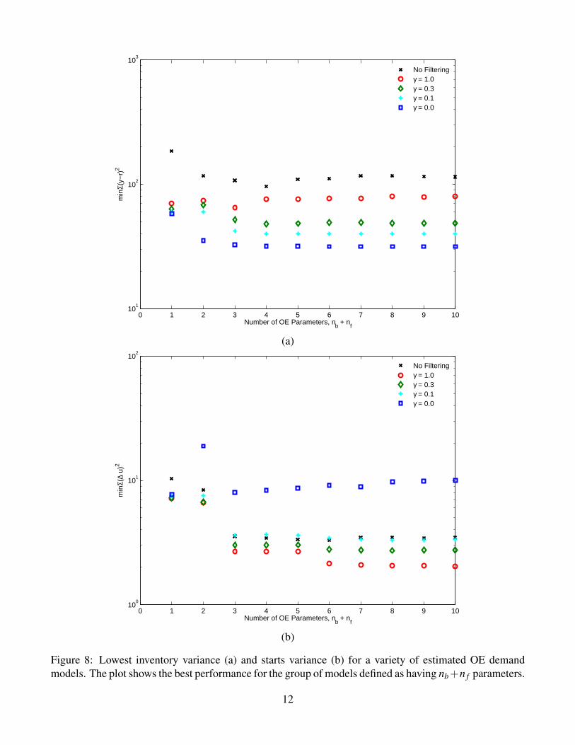
Figure 9: Corresponding frequency responses where the demand forecast is developed from an OE-[1 2 1]fit to unfiltered data and an OE-[1 2 1] fit to control-relevant filtered data obtained from the user definedweighting function (γ = 0.3).

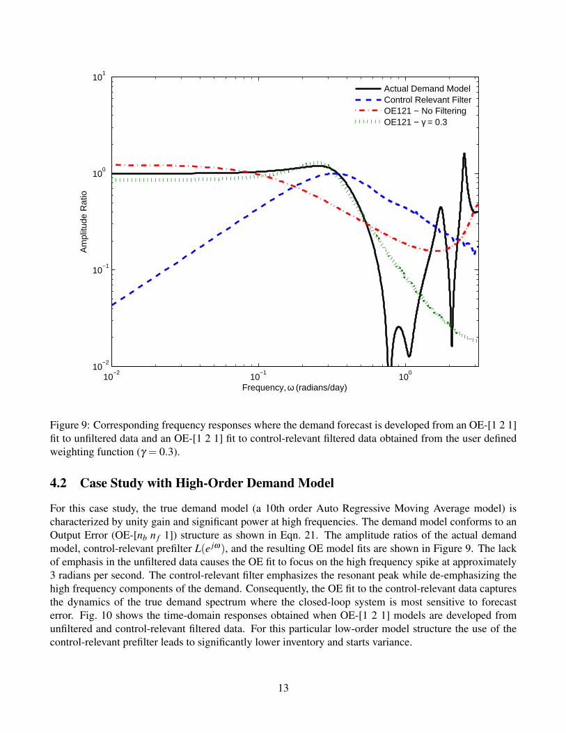
4.2 Case Study with High-Order Demand Model

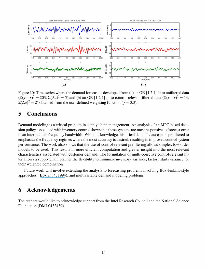
For this case study, the true demand model (a 10th order Auto Regressive Moving Average model) ischaracterized by unity gain and significant power at high frequencies. The demand model conforms to anOutput Error (OE-[nb n f 1]) structure as shown in Eqn. 21. The amplitude ratios of the actual demandmodel, control-relevant prefilter L(e jω), and the resulting OE model fits are shown in Figure 9. The lackof emphasis in the unfiltered data causes the OE fit to focus on the high frequency spike at approximately3 radians per second. The control-relevant filter emphasizes the resonant peak while de-emphasizing thehigh frequency components of the demand. Consequently, the OE fit to the control-relevant data capturesthe dynamics of the true demand spectrum where the closed-loop system is most sensitive to forecasterror. Fig. 10 shows the time-domain responses obtained when OE-[1 2 1] models are developed fromunfiltered and control-relevant filtered data. For this particular low-order model structure the use of thecontrol-relevant prefilter leads to significantly lower inventory and starts variance.

13

500 550 600 650 700 750 800 850 900 950 1000

−2

0

2

∆Inv

ento

ry

OE121 from raw data : Σ(y−r)2 = 203.26 Σ(∆u)2 = 4.59

500 550 600 650 700 750 800 850 900 950 1000−1

−0.5

0

0.5

1

∆Sta

rts

500 550 600 650 700 750 800 850 900 950 1000−1

−0.5

0

0.5

1

∆For

ecas

t

Time (Days)

500 550 600 650 700 750 800 850 900 950 1000

−2

0

2

∆Inv

ento

ry

OE121, γ = 0.3: Σ(y−r)2 = 13.76 Σ(∆u)2 = 1.78

500 550 600 650 700 750 800 850 900 950 1000−1

−0.5

0

0.5

1

∆Sta

rts

500 550 600 650 700 750 800 850 900 950 1000−1

−0.5

0

0.5

1

∆For

ecas

t

Time (Days)

(a) (b)

Figure 10: Time series where the demand forecast is developed from (a) an OE-[1 2 1] fit to unfiltered data(Σ(y− r)2 = 203, Σ(∆u)2 = 5) and (b) an OE-[1 2 1] fit to control-relevant filtered data (Σ(y− r)2 = 14,Σ(∆u)2 = 2) obtained from the user defined weighting function (γ = 0.3).

5 Conclusions

Demand modeling is a critical problem in supply chain management. An analysis of an MPC-based deci-sion policy associated with inventory control shows that these systems are most responsive to forecast errorin an intermediate frequency bandwidth. With this knowledge, historical demand data can be prefiltered toemphasize the frequency regimes where the most accuracy is desired, resulting in improved control systemperformance. The work also shows that the use of control-relevant prefiltering allows simpler, low-ordermodels to be used. This results in more efficient computation and greater insight into the most relevantcharacteristics associated with customer demand. The formulation of multi-objective control-relevant fil-ter allows a supply chain planner the flexibility to minimize inventory variance, factory starts variance, ortheir weighted combination.

Future work will involve extending the analysis to forecasting problems involving Box-Jenkins-styleapproaches (Box et al., 1994), and multivariable demand modeling problems.

6 Acknowledgements

The authors would like to acknowledge support from the Intel Research Council and the National ScienceFoundation (DMI-0432439).

14

References

Box, G. E., G. M. Jenkins and G. C. Reinsel (1994). Time Series Analysis Forecasting and Control.Prentice-Hall. Englewood Cliffs, NJ.

Braun, M. W., D. E. Rivera, M. E. Flores, W. M. Carlyle and K. G. Kempf (2003). AModel Predictive Control framework for robust management of multi-product, multi-echolon de-mand networks. Annual Reviews in Control 27, 229–245.

Camacho, E. F. and C. Bordons (1999). Model Predictive Control. Springer-Verlag. London.

Dejonckheere, J., S. M. Disney, M. R. Lambrecht and D. R. Towill (2002). Transfer function analysisof forecasting induced bullwhip in supply chains. International Journal of Production Economics78, 133–144.

Garcıa, C. E., D. M. Prett and M. Morari (1989). Model predictive control: theory and practice-a survey.Automatica 25(3), 335–348.

Ljung, L. (1999). System Identification: Theory for the User. Prentice-Hall. Upper Saddle River, NewJersey.

Perea-Lopez, E., B. E. Ydstie and I. E. Grossman (2003). A model predictive control strategy for supplychain optimization. Computers and Chemical Engineering 27, 1201–1218.

Rivera, D. E., J. F. Pollard and C. E. Garcıa (1992). Control-relevant prefiltering: A systematic designapproach and case study. IEEE Transactions on Automatic Control 37(7), 964–974.

Schwartz, J.D., W. Wang and D. E. Rivera (2006). Simulation-based optimization of model predictivecontrol policies for inventory management in supply chains. Automatica 42(8), 1311–1320.

Seferlis, P. and N. F. Giannelos (2004). A two-layered optimisation-based control strategy for multi-echelon supply chain networks. Computers and Chemical Engineering 28, 799–809.

Stoica, P. and R. Moses (1997). Introduction to Spectral Analysis. Prentice-Hall. Upper Saddle River, NewJersey.

Tzafestas, S., G. Kapsiotis and E. Kyriannakis (1997). Model-based predictive control for generalizedproduction planning problems. Computers in Industry 34, 201–210.

Wang, W., D. E. Rivera, K. G. Kempf and K. D. Smith (2004). A model predictive control strategy forsupply chain management in semiconductor manufacturing under uncertainty. In: Proceedings of theAmerican Control Conference. Boston, MA. pp. 4577–4582.

15