Convective Initiation – Relevant Processes andTheir Representation in Convection-Permitting

Models

Mirjam Johanna Hirt

München - 2020

Convective Initiation – Relevant Processes andTheir Representation in Convection-Permitting

Models

Mirjam Johanna Hirt

Dissertationan der Fakultät für Physik

der Ludwig–Maximilians–UniversitätMünchen

vorgelegt vonMirjam Johanna Hirt

aus Friedberg

München, 7. April 2020

Mirjam Hirt: Convective Initiation – Relevant Processes and Their Representation in Convection-Permitting Models, PhD thesis in Physics, April 2020

erstgutachter: Prof. Dr. George C. Craigzweitgutachter: Prof. Dr. Mark Wenigdatum der abgabe: 07.04.2020

datum der mündlichen prüfung: 24.06.2020

Parts of this thesis are contained in:

Hirt, M., Rasp, S., Blahak, U., & Craig, G. (2019). Stochastic parameterization of pro-cesses leading to convective initiation in kilometre-scale models. Monthly Weather Re-view, 147, 3917–3934, doi: 10.1175/MWR-D-19-0060.1. ©American Meteorological Soci-ety. Used with permission.

Hirt, M., Craig, G. C., Schäfer, S., Savre, J., & Heinze, R. (2020). Cold pool driven con-vective initiation: using causal graph analysis to determine what km-scale models aremissing. Quarterly Journal of the Royal Meteorological Society, doi: 10.1002/qj.3788.

Z U S A M M E N FA S S U N G

Die Vorhersage von konvektivem Niederschlag ist für heutige, numerische Wettervorhersagemo-delle eine besondere Herausforderung. Die Ursache dafür liegt insbesondere an unzureichendaufgelösten Grenzschichtprozessen, welche für die Entstehung von Konvektion besonders re-levant sind. Diese Arbeit befasst sich mit drei solchen Prozessen, die Grenzschichtturbulenz,mechanische Hebung durch Subgrid-skalige Orographie und Cold Pools. Ziel ist es, systemati-sche Fehler in den simulierten Prozessen zu identifizieren und die Darstellung der Prozesse inKonvektions-erlaubenden Modellen zu verbessern.

Grenzschichtturbulenz wird in den meisten Modellen durch Parameterisierungen näherungs-weise dargestellt, indem nur der mittlere Einfluss der Turublenz in einer Gitterbox berücksich-tigt wird. Für die Entstehung von Konvektion ist jedoch die subgrid-skalige Variabilität vonentscheidender Bedeutung. Um diese fehlende Variabilität dennoch zu berücksichtigen, habenKober und Craig (2016) ein physikalisch basiertes, stochastisches Störungschema (PSP) entwi-ckelt, wodurch zusätzlich Modellunsicherheiten direkt dort quantifiziert werden, wo sie entste-hen. Das ist besonders wichtig, um zuverlässige Vorhersagen zu erhalten. Das Verhalten desPSP-Schemas zeigt jedoch in manchen Fällen unerwünschte Effekte, welche wir in dieser Arbeitverringern. Dafür entwickeln wir einige Modifikationen des PSP Schemas. Zum Beispiel stö-ren wir die horizontalen Wind-Komponenten, sodass 3d Divergenzfreiheit gegeben ist und dieVertikalwindstörungen länger anhalten. Daraus entsteht eine entsprechend verbesserte Version,das PSP2, welches stärker unserem physikalischen Verständnis folgt und ähnliche Verbesse-rungen beim Einsetzen von konvektivem Niederschlag aufweist wie in dem ursprünglichemPSP-Schema und zusätzlich eine verbesserte Strukture der Niederschlagszellen zeigt.

Als nächst-wichtigsten Prozess für die Konvektionsauslösung berücksichtigen wir die He-bung durch subgrid-skalige Orographie. Dafür entwickeln wir eine weitere, stochastische Para-meterisierung, das SSOSP-Schema, welches den Effekt der mechanischen Hebung durch subgrid-skalige Orographie darstellt. Dazu wird die Amplitude von Schwerewellen durch Informatio-nen zur subgrid-skaligen Orographie dargestellt und verwendet. Zwar ist durch das SSOSP-Schema eine deutliche Erhöhung der Konvektionsauslösung in orografischen Regionen möglich,jedoch fällt dies mit einem unerwünschten Einfluss auch auf nicht-orografische Regionen zu-sammen. Im Gegensatz zu unseren ursprünglichen Erwartungen kommen wir zu dem Schluss,dass die subgrid-skalige Orographie keine entscheidende Rolle spielt, da sie meist von aufge-löster Orographie begleitet wird.

Der bedeutendste Teil der Arbeit befasst sich mit Cold Pools. Cold Pools sind vor Allem fürdie Organisation von Konvektion entscheidend, sowie für die Auslösung von Konvektion amNachmittag und Abend. Dass Konvektions-erlaubende Modelle Cold Pools nicht ausreichendgut darstellen können, liegt nahe. Um genauer zu verstehen, welche Aspekte der Cold Poolsmangelhaft dargestellt werden, verwenden wir hochauflösende Simulationen um Cold Pools,Cold Pool Ränder und ausgelöste Konvektion zu identifizieren. Dabei stellen wir fest, dassCold Pools in Simulationen mit niedrigerer Auflösung häufiger, kleiner und weniger intensivsind und schwächere Böenfronten aufweisen. Wir verwenden eine lineare Kausalitätsanalyse,um verschiedene indirekte Effekte zu quantifizieren. Dabei finden wir einen dominierendenEffekt: Durch die Reduzierung der Gittergrößen wird der aufwärts-gerichtete Massenfluss ander Böenfront reduziert, was zu geringeren Wahrscheinlichkeiten für die Konvektionsauslösungführt.

vii

Basierend auf diesem gewonnen Verständnis entwickeln wir anschließend eine determinis-tische Cold-Pool-Parametrisierung, CPP, die die Aufwärtsbewegung an den Böenfronten vonCold-Pools verstärkt, um die Konvektionsauslösung durch Cold Pools zu verbessern. Dabeiwird der Niederschlag besonders am Nachmittag und Abend verstärkt und die Organisationder Konvektion nimmt zu, woruch Niederschlagsvorhersagen verbessert werden.

viii

A B S T R A C T

Current deficits of numerical weather prediction models in predicting convective precipitationare presumably caused by insufficiently resolved boundary-layer processes and their role ininitiating convection. This thesis addresses three such boundary-layer processes, which are ex-pected to be the most relevant ones for convective initiation. We identify current deficits andimprove their representation in convection-permitting models to improve the representationof convection itself. The three considered processes are boundary-layer turbulence, mechanicallifting by subgrid-scale orography and cold pools.

Boundary layer turbulence is mostly parameterized in these models and only representedby the average effect on a grid box. As the subgrid-scale variability is crucial for convectiveinitiation, Kober and Craig (2016) have developed a unique, physically based stochastic pertur-bation scheme (PSP) to reintroduce the subgrid-scale variability of boundary-layer turbulence ina stochastic manner. This allows the quantification of model uncertainty at its source - a crucial,but rarely performed step for reliable forecasts. As the PSP scheme also introduced some un-desired behavior, we develop several modifications to pertain the positive effect of the originalPSP scheme while being physically more consistent. For example, we included perturbationsin horizontal wind components in a 3d non-divergent way to obtain persistent vertical velocityperturbations. A revised version, PSP2, is physically more consistent and shows improvementsin the onset of convective precipitation similar to the original scheme and an improved structureof precipitation cells.

The next important process is assumed to be convective initiation by subgrid-scale orography.We develop an additional stochastic parameterization, the SSOSP scheme, to include the effectof mechanical lifting by subgrid-scale orography using a gravity wave formalism and informa-tion on subgrid-scale orography. While a clear increase in convective initiation over orographicregions is possible by the SSOSP scheme, this usually coincides with an undesired impact alsoon non-orographic regions. We conclude - in contrast to our initial expectations - that, mostlikely, subgrid-scale orography does not play a crucial role because it is mostly accompanied byresolved orography.

The most notable parts of this thesis are concerned with cold pools. Cold pools are expectedto play a crucial role in the convective organization and for late afternoon and evening convec-tive initiation. However, km-scale models are not expected to simulate cold pools with sufficientaccuracy. To better understand, which aspects of cold pools are insufficiently represented, weidentify cold pools, cold pool boundaries and initiated convection in high-resolution simula-tions. We find that cold pools are more frequent, smaller, less intense and have weaker gustfronts in lower resolution simulations. We use a linear causal graph analysis to disentangle dif-ferent indirect effects. Doing so, we identify one single, dominant effect: reducing grid sizesreduces upward mass flux at the gust front directly, which causes weaker triggering probabili-ties.

Based on these results, we then develop a deterministic cold pool parameterization, CPP,which strengthens the upward motion at cold pool gust fronts to improve cold pool drivenconvective initiation. We find that precipitation is amplified and becomes more organized in theafternoon and evening. Better precipitation forecasts will then be possible.

ix

C O N T E N T S

1 introduction 1

1.1 Numerical weather prediction . . . . . . . . . . . . . . . . . . . . . . . . . 2

1.1.1 Errors and uncertainty . . . . . . . . . . . . . . . . . . . . . . . . . . 2

1.1.2 Challenges for convective scale NWP . . . . . . . . . . . . . . . . . 3

1.1.3 Atmospheric models of different scales . . . . . . . . . . . . . . . . 4

1.2 Parameterizations . . . . . . . . . . . . . . . . . . . . . . . . . . . . . . . . . 6

1.2.1 Scale separation and grey zones . . . . . . . . . . . . . . . . . . . . 7

1.2.2 Stochastic parameterizations . . . . . . . . . . . . . . . . . . . . . . 9

1.3 Relevant physical processes and their model representation . . . . . . . . 11

1.3.1 Convection and its initiation . . . . . . . . . . . . . . . . . . . . . . 11

1.3.2 Boundary layer turbulence . . . . . . . . . . . . . . . . . . . . . . . 14

1.3.3 Orographic convection and the role of subgrid-scale orography . . 17

1.3.4 Cold pools . . . . . . . . . . . . . . . . . . . . . . . . . . . . . . . . . 19

1.4 Summary and research goals . . . . . . . . . . . . . . . . . . . . . . . . . . 21

1.5 Outline . . . . . . . . . . . . . . . . . . . . . . . . . . . . . . . . . . . . . . . 24

1.6 Publications . . . . . . . . . . . . . . . . . . . . . . . . . . . . . . . . . . . . 24

2 cosmo : model setup, simulation period and verification 25

2.1 Model and simulation setup . . . . . . . . . . . . . . . . . . . . . . . . . . . 25

2.2 Simulation period with COSMO . . . . . . . . . . . . . . . . . . . . . . . . 26

2.3 Observations . . . . . . . . . . . . . . . . . . . . . . . . . . . . . . . . . . . . 27

2.4 Verification metrics . . . . . . . . . . . . . . . . . . . . . . . . . . . . . . . . 27

2.4.1 Fraction skill score . . . . . . . . . . . . . . . . . . . . . . . . . . . . 27

2.4.2 The structure component of the SAL-score . . . . . . . . . . . . . . 28

2.4.3 Size and frequency distributions . . . . . . . . . . . . . . . . . . . . 29

3 representing boundary-layer turbulence variability 31

3.1 Conception of the stochastic perturbations . . . . . . . . . . . . . . . . . . 33

3.1.1 Physically based stochastic perturbations for subgrid-scale turbu-lence (PSP) . . . . . . . . . . . . . . . . . . . . . . . . . . . . . . . . . 33

3.1.2 Modifications to the PSP scheme . . . . . . . . . . . . . . . . . . . . 34

3.2 Strategy for evaluating the impact of the PSP modifications . . . . . . . . 36

3.3 Results . . . . . . . . . . . . . . . . . . . . . . . . . . . . . . . . . . . . . . . 37

3.3.1 Autoregressive Process in PSP-AR . . . . . . . . . . . . . . . . . . . 37

3.3.2 Adaptive boundary-layer height restriction in PSP-HPBLcut . . . . 38

3.3.3 Masking of already precipitating areas in PSP-mask . . . . . . . . . 39

3.3.4 3D non-divergent perturbations in PSP-3D . . . . . . . . . . . . . . 40

3.3.5 Combining the modifications for PSP2 . . . . . . . . . . . . . . . . . 41

3.4 Summary and Discussion . . . . . . . . . . . . . . . . . . . . . . . . . . . . 43

4 representing lifting by subgrid-scale orography 45

xi

xii contents

4.1 Formulation of the parameterization . . . . . . . . . . . . . . . . . . . . . . 46

4.1.1 The SSOSP scheme . . . . . . . . . . . . . . . . . . . . . . . . . . . . 46

4.1.2 Physical scaling based on orographic gravity waves . . . . . . . . . 48

4.2 Model simulations, observations and simulation period . . . . . . . . . . . 49

4.3 Simulation results . . . . . . . . . . . . . . . . . . . . . . . . . . . . . . . . . 49

4.4 Summary and discussion . . . . . . . . . . . . . . . . . . . . . . . . . . . . . 52

5 cold pool driven convective initiation (i) 53

5.1 Data and methods . . . . . . . . . . . . . . . . . . . . . . . . . . . . . . . . . 55

5.1.1 ICON-LEM simulations . . . . . . . . . . . . . . . . . . . . . . . . . 55

5.1.2 Selected days and their synoptic situations . . . . . . . . . . . . . . 55

5.1.3 Detection of cold pools and their edges . . . . . . . . . . . . . . . . 56

5.1.4 Defining convective initiation . . . . . . . . . . . . . . . . . . . . . . 59

5.1.5 Diagnostic approaches . . . . . . . . . . . . . . . . . . . . . . . . . . 60

5.1.6 Estimating linear causal effects . . . . . . . . . . . . . . . . . . . . . 62

5.2 Results . . . . . . . . . . . . . . . . . . . . . . . . . . . . . . . . . . . . . . . 65

5.2.1 Linking precipitation and convective initiation with cold pools . . 65

5.2.2 Sensitivity of cold pool properties to resolution . . . . . . . . . . . 67

5.2.3 Identifying causes of the resolution dependence of convective ini-tiation . . . . . . . . . . . . . . . . . . . . . . . . . . . . . . . . . . . . 70

5.3 Summary and discussion . . . . . . . . . . . . . . . . . . . . . . . . . . . . . 74

6 cold pool driven convective initiation (ii) 79

6.1 Strategy for developing CPP and evaluating its impact . . . . . . . . . . . 80

6.2 Cold pool perturbations CPP . . . . . . . . . . . . . . . . . . . . . . . . . . 81

6.2.1 Scale of gust front vertical velocity . . . . . . . . . . . . . . . . . . . 81

6.2.2 Basic approach of CPP . . . . . . . . . . . . . . . . . . . . . . . . . . 82

6.2.3 Approximation of w0 and αcp . . . . . . . . . . . . . . . . . . . . . . 83

6.2.4 Vertical distribution of the perturbations . . . . . . . . . . . . . . . 84

6.2.5 Time scale τcp . . . . . . . . . . . . . . . . . . . . . . . . . . . . . . . 84

6.2.6 Limiting perturbations to cold pools . . . . . . . . . . . . . . . . . . 85

6.2.7 Overview of parameters . . . . . . . . . . . . . . . . . . . . . . . . . 87

6.3 Impact of CPP . . . . . . . . . . . . . . . . . . . . . . . . . . . . . . . . . . . 87

6.3.1 Cold pool gust fronts . . . . . . . . . . . . . . . . . . . . . . . . . . . 87

6.3.2 Impact on precipitation . . . . . . . . . . . . . . . . . . . . . . . . . 88

6.3.3 Other impacts of CPP . . . . . . . . . . . . . . . . . . . . . . . . . . 91

6.3.4 Parameter sensitivity of CPP . . . . . . . . . . . . . . . . . . . . . . 92

6.3.5 10 day period . . . . . . . . . . . . . . . . . . . . . . . . . . . . . . . 94

6.3.6 Combining CPP with PSP2 . . . . . . . . . . . . . . . . . . . . . . . 95

6.4 Discussion . . . . . . . . . . . . . . . . . . . . . . . . . . . . . . . . . . . . . 96

6.4.1 Benefits for precipitation . . . . . . . . . . . . . . . . . . . . . . . . . 96

6.4.2 Other impacts of CPP . . . . . . . . . . . . . . . . . . . . . . . . . . 96

6.4.3 Future steps . . . . . . . . . . . . . . . . . . . . . . . . . . . . . . . . 97

7 summary and conclusions 99

7.1 Summary . . . . . . . . . . . . . . . . . . . . . . . . . . . . . . . . . . . . . . 99

contents xiii

7.2 Future steps for PSP2 and CPP . . . . . . . . . . . . . . . . . . . . . . . . . 101

7.3 Conclusions . . . . . . . . . . . . . . . . . . . . . . . . . . . . . . . . . . . . 102

7.4 Causal methods and their potential for improving NWP . . . . . . . . . . 103

Appendix I

a details on the causal analysis IIIa.1 Single door criterion for the causal model . . . . . . . . . . . . . . . . . . . IIIa.2 Sensitivity and robustness of the causal analysis . . . . . . . . . . . . . . . III

b dimensional analysis for cold pool gust fronts VII

c list of abbreviations IX

1I N T R O D U C T I O N

Atmospheric deep convection, or simply convection, represents the formation of fast-developing cloud systems, that extend throughout the whole depth of the troposphere.The most prominent example of such clouds are thunderstorms. Such convective cloudscan result in high wind speeds, heavy precipitation, hail or flooding, thereby disturbingour everyday life, devastating areas and causing material losses and even casualties. InJune 2019, for instance, a specifically large and long-lived thunderstorm occured overBavaria which caused hail with up to 5 cm diameter, extreme precipitation (27 mm h−1),and wind speeds of up to 120 km h−1 (Deutscher Wetterdienst, 2019). According to Mu-nich Re (2020), damages of almost 1 billion dollars occured, which made this singlethunderstorm event the most expensive natural hazard in Germany in 2019. A differ-ent, highly convective weather situation caused severe flooding and damages in severaltowns in Germany in May and June 2016. These floodings lead to financial losses ofup to 2.2 billion dollars (Piper et al., 2016; Kron et al., 2019). To prevent, or at least mit-igate, such tremendous damages, people, companies or governments require reliablewarnings and, hence, predictions of such convective events sufficiently in advance.

However, predicting convective clouds has been a long-standing challenge. Until thelast century, the prediction of thunderstorms was based on eye-observations of clouds,the categorization of previous weather types and experience (Nebeker, 1997). Conse-quently, only very short-term or relatively crude predictions were possible. When thefirst numerical weather predictions became operational in the 1950s and 60s (Goldinget al., 2004; Harper et al., 2007; Randall et al., 2018), it was finally possible to predictthe larger-scale weather based on physical equations, which tremendously improvedweather forecasts. However, the lack of computational power, model complexity andobservations still prohibited the explicit simulation of deep convective clouds for sev-eral decades. In the late 1980s, with the availability of radar and satellite observations,nowcasting techniques were developed to project the behavior of existing clouds intothe future (Golding et al., 2004). These extrapolation techniques, however, could notpredict the initiation of new cells, nor were their forecasts skillful beyond a few hours.

A milestone was reached when increasing computational possibilities joined with in-tensive model development enabled the explicit simulation of deep convective circula-tions with numerical models in the 1990s. At first, such simulations were only feasiblefor research purposes and selected events (Clark et al., 2016). Lilly (1990) speculatedabout the operational, numerical prediction of thunderstorms in 1990, but it still tookmore than a decade for most weather services to develop and afford models suitedfor this challenge (e.g., Baldauf et al., 2011; Clark et al., 2016). Today, such convection-permitting models are the model type of choice for regional weather prediction andmany other applications.

1

2 introduction

While these models have undoubtedly led to a step-change in forecasting deep con-vection (Clark et al., 2016), several deficits remain. The primary deficits in simulatingdeep convective systems manifest in biases in the diurnal cycle and a lack of organi-zation of convection. Responsible are processes, that are tightly coupled to convection,but are so small, that even convection-permitting models cannot resolve them explicitly.This grey zone for convection modeling poses a severe challenge for current weatherprediction. The largest portion of these deficits is ascribed to insufficiently representedprocesses in the boundary layer (≈ the lowest kilometer of the atmosphere), which arecrucial for initiating the formation of deep convective clouds. The presumably threemost essential processes for improving convective initiation are boundary-layer turbu-lence, small-scale orography and cold pools. In this thesis, we will better understandwhich aspects of these processes are insufficiently represented in numerical models anddevelop new or recently proposed approaches to improve their representation. Doingso, we address the current challenge of the convective grey zone.

1.1 numerical weather prediction

Numerical weather prediction (NWP) uses computational models that describe atmo-spheric flow to a certain degree of complexity. They consist of physical, partial differ-ential equations, including the momentum equations for each velocity component, thethermodynamic equation, the continuity equation and prognostic equations for mois-ture quantities. As they cannot be solved analytically, these equations are approximatedfor a discrete three-dimensional grid representing the earth’s atmosphere. First, a cur-rent state of the atmosphere, i.e., the initial condition, has to be derived from obser-vations and previous forecasts, a process termed data assimilation. Then numericalintegration for future, discrete time steps enables a prediction of the future state of theatmosphere. Processes that occur on scales smaller than the model grid spacing, i.e.,subgrid-scale processes, are therefore not explicitly included. Instead, their impact isapproximated in terms of the resolved variables and parameters. Such approximationsare called parameterizations and will be introduced in more detail in Sec. 1.2 and 1.3.

1.1.1 Errors and uncertainty

The fundamental challenge of NWP originates due to the atmosphere’s chaotic nature- a characteristic made popular by the butterfly effect - which is intimately connectedwith a myriad of atmospheric scales interacting with each other. As a consequence,small errors, e.g., in the initial conditions, grow rapidly in space and time and arehence projected on all scales. This error growth radically limits our ability to predictthe weather to a few weeks, days and sometimes even hours1.

1 Often, a clear distinction between intrinsic and practical predictability is made. The former describes forhow long in advance useful, hypothetical predictions can be made given infinitesimal errors. Despitethe deterministic nature of the governing equations, this time scale does not grow indefinitely withdecreasing errors. The practical predictability, on the other hand, is a characteristic of current NWPsystems with finite errors. The specific limit of both types of predictability strongly depends on thespatial scales of interest and the flow situation.

1.1 numerical weather prediction 3

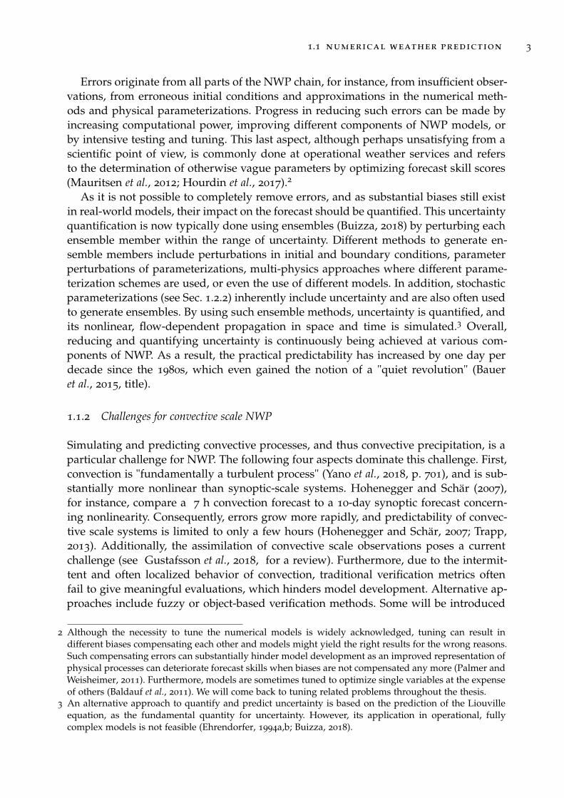
Errors originate from all parts of the NWP chain, for instance, from insufficient obser-vations, from erroneous initial conditions and approximations in the numerical meth-ods and physical parameterizations. Progress in reducing such errors can be made byincreasing computational power, improving different components of NWP models, orby intensive testing and tuning. This last aspect, although perhaps unsatisfying from ascientific point of view, is commonly done at operational weather services and refersto the determination of otherwise vague parameters by optimizing forecast skill scores(Mauritsen et al., 2012; Hourdin et al., 2017).2

As it is not possible to completely remove errors, and as substantial biases still existin real-world models, their impact on the forecast should be quantified. This uncertaintyquantification is now typically done using ensembles (Buizza, 2018) by perturbing eachensemble member within the range of uncertainty. Different methods to generate en-semble members include perturbations in initial and boundary conditions, parameterperturbations of parameterizations, multi-physics approaches where different parame-terization schemes are used, or even the use of different models. In addition, stochasticparameterizations (see Sec. 1.2.2) inherently include uncertainty and are also often usedto generate ensembles. By using such ensemble methods, uncertainty is quantified, andits nonlinear, flow-dependent propagation in space and time is simulated.3 Overall,reducing and quantifying uncertainty is continuously being achieved at various com-ponents of NWP. As a result, the practical predictability has increased by one day perdecade since the 1980s, which even gained the notion of a "quiet revolution" (Baueret al., 2015, title).

1.1.2 Challenges for convective scale NWP

Simulating and predicting convective processes, and thus convective precipitation, is aparticular challenge for NWP. The following four aspects dominate this challenge. First,convection is "fundamentally a turbulent process" (Yano et al., 2018, p. 701), and is sub-stantially more nonlinear than synoptic-scale systems. Hohenegger and Schär (2007),for instance, compare a 7 h convection forecast to a 10-day synoptic forecast concern-ing nonlinearity. Consequently, errors grow more rapidly, and predictability of convec-tive scale systems is limited to only a few hours (Hohenegger and Schär, 2007; Trapp,2013). Additionally, the assimilation of convective scale observations poses a currentchallenge (see Gustafsson et al., 2018, for a review). Furthermore, due to the intermit-tent and often localized behavior of convection, traditional verification metrics oftenfail to give meaningful evaluations, which hinders model development. Alternative ap-proaches include fuzzy or object-based verification methods. Some will be introduced

2 Although the necessity to tune the numerical models is widely acknowledged, tuning can result indifferent biases compensating each other and models might yield the right results for the wrong reasons.Such compensating errors can substantially hinder model development as an improved representation ofphysical processes can deteriorate forecast skills when biases are not compensated any more (Palmer andWeisheimer, 2011). Furthermore, models are sometimes tuned to optimize single variables at the expenseof others (Baldauf et al., 2011). We will come back to tuning related problems throughout the thesis.

3 An alternative approach to quantify and predict uncertainty is based on the prediction of the Liouvilleequation, as the fundamental quantity for uncertainty. However, its application in operational, fullycomplex models is not feasible (Ehrendorfer, 1994a,b; Buizza, 2018).

4 introduction

in Chapter 2. Another major complication arises as many scales relevant for convectionare so small that they are often only poorly represented by the model dynamics or theparameterizations. These include evaporation, droplet formation, entrainment, the ini-tiation of convection and sometimes even the deep convective circulations themselves.This aspect will become more evident in the following section.

1.1.3 Atmospheric models of different scales

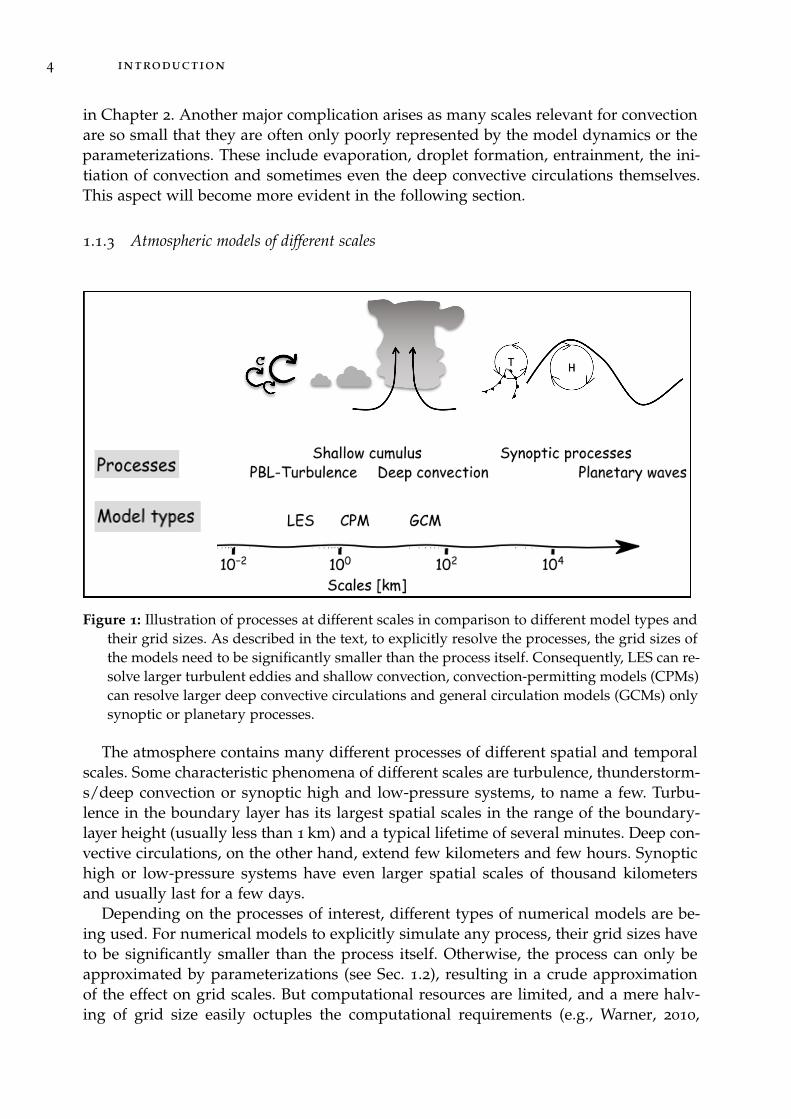
Figure 1: Illustration of processes at different scales in comparison to different model types andtheir grid sizes. As described in the text, to explicitly resolve the processes, the grid sizes ofthe models need to be significantly smaller than the process itself. Consequently, LES can re-solve larger turbulent eddies and shallow convection, convection-permitting models (CPMs)can resolve larger deep convective circulations and general circulation models (GCMs) onlysynoptic or planetary processes.

The atmosphere contains many different processes of different spatial and temporalscales. Some characteristic phenomena of different scales are turbulence, thunderstorm-s/deep convection or synoptic high and low-pressure systems, to name a few. Turbu-lence in the boundary layer has its largest spatial scales in the range of the boundary-layer height (usually less than 1 km) and a typical lifetime of several minutes. Deep con-vective circulations, on the other hand, extend few kilometers and few hours. Synoptichigh or low-pressure systems have even larger spatial scales of thousand kilometersand usually last for a few days.

Depending on the processes of interest, different types of numerical models are be-ing used. For numerical models to explicitly simulate any process, their grid sizes haveto be significantly smaller than the process itself. Otherwise, the process can only beapproximated by parameterizations (see Sec. 1.2), resulting in a crude approximationof the effect on grid scales. But computational resources are limited, and a mere halv-ing of grid size easily octuples the computational requirements (e.g., Warner, 2010,

1.1 numerical weather prediction 5

p. 362). Therefore, the computational requirements of smaller grid sizes are compen-sated by reducing computational requirements otherwise. Usually, this is obtained byreducing total domain size, but limiting total integration time or ensemble dimensionreduces computing requirements as well. This tradeoff gives rise to various types of at-mospheric, numerical models depending on their purpose and the respective processesthat they can simulate explicitly.

We illustrate this hierarchy of atmospheric models by considering three types ofmodels as selected examples, namely global NWP models or general circulation mod-els (GCMs), convection-permitting models (CPMs) and large eddy models for turbulentscales (LES). See also Fig. 1 for the grid sizes of these models and corresponding pro-cesses.

Global weather prediction models, which simulate the global atmosphere of theearth, usually can only afford grid sizes of ten kilometers. For instance, the opera-tional setup from the German weather service (DWD), has an effective grid spacing of13 km (Reinert et al., 2018) and the European center for medium-range weather fore-casting (ECMWF) uses a discretization of approximately 9 km and 18 km for their high-resolution run and their ensemble, respectively (ECMWF, 2019). Such resolutions aresufficient to simulate synoptic fronts, cyclones or other high- and low-pressure systemsor planetary waves explicitly.

To resolve thunderstorm circulations or larger convective clouds, grid sizes of lessthan a few kilometers are necessary, often 1-5 km grid sizes are used. We will refer tosuch models as km-scale or convection-permitting models (CPM). This regime of models isnow widely used for different applications: convection-permitting models are used forregional weather prediction by most weather services (Baldauf et al., 2011; Clark et al.,2016); they are being tested for applications in regional climate modeling (Leutwyleret al., 2017; Schär et al., 2019); and they are even used for exploratory, global convection-permitting simulations (Judt, 2018; Stevens et al., 2019b; Zhou et al., 2019). Convection-permitting models will doubtlessly be used for even more applications in the future.For instance, at ECMWF, global models are planned to have 5 km grid sizes by 2025

(ECMWF, 2016), and Palmer (2019a) is speculating that global ensemble simulationswill have 1 km grid sizes in 25 years.

On even smaller scales, large-eddy simulations (LES) can be used to simulate largerturbulent eddies in the planetary boundary layer explicitly. These models require gridsizes well below 1 km, and sometimes have grid sizes of only tens of meters. LES areoften used for idealized cases, but also more realistic situations have been computedfor research purposes (Heinze et al., 2017; Stevens et al., 2019a). As far as we are aware,no plans exist to make such models operational in the next decade.

Hence, models with grid sizes of few kilometers will likely dominate the atmosphericmodeling landscape for years to come. Maximizing the highly flow-, space- and time-dependent predictability of convection within such km-scale models is consequentlya dominant challenge for NWP today, and much research is devoted towards it. Thisincludes coupling subgrid-scale processes to the resolved convective scales and quanti-fying uncertainties accordingly. This will be a challenge throughout this thesis, wherewe specifically focus on the improved representation of convective initiation by subgrid-scale or insufficiently resolved processes. Such coupling of resolved and unresolved

6 introduction

processes can be achieved by parameterizations, which we will formally introduce inthe following.

1.2 parameterizations

Parameterizations approximate the effect of subgrid-scale, unresolved processes on theresolved scale. Let us consider the set of variables φ averaged over the model grid box,φ. The residual, i.e., the subgrid-scale fluctuations from the grid mean, is representedas φ′, so that φ = φ + φ′. This partitioning is often denoted as Reynolds averaging.4

Then numerical weather prediction can be conceptualized as the numerical integrationof the prognostic equation for φ:

∂φ

∂t= f (φ) + g(φ, φ′), (1)

where f (φ) corresponds to resolved scale dynamics and g(φ, φ′) represents interactionsbetween resolved and subgrid-scales and how they impact the resolved scale variables.However, the subgrid-scale fluctuations φ′ are not specified and g(φ, φ′) needs to beapproximated only in terms of φ, i.e., g(φ, φ′) ≈ h(φ). This approximation is calledparameterization.

A wide variety of processes is usually parameterized separately. The impact of unre-solved eddies is approximated in turbulence parameterizations. The influence of shal-low and deep convection on resolved scales is usually considered separately in param-eterizations. Cloud processes, like condensation or droplet formation, are representedby microphysics parameterizations. Radiative processes are approximated for compu-tational efficiency in radiation parameterization. Furthermore, many other processeslike gravity wave drag, land surface processes or atmosphere-ocean interactions areoften represented in some form of parameterization. In addition, interactions betweendifferent parameterizations also need to be included.

Various approaches are used to build parameterizations. Traditional parameteriza-tions are usually based on empirical methods and conceptual process understanding.Sometimes parameterizations can be derived with several approximations from firstprinciples, although empirical closure assumptions usually have to be made. Conse-quently, such parameterizations represent severe sources of errors and uncertainty inweather and climate models, and considerable effort is made to improve their accuracy.Progress with traditional parameterizations is ongoing, but also different perspectivesare being considered (Yano, 2016; Rio et al., 2019).

In the last years, the development of other approaches has grown. Exceptionally ac-curate are Super- or even Ultraparameterizations, which embed higher resolution modelswithin each grid box of the coarser model (Grabowski, 2004; Parishani et al., 2017; Ran-

4 Reynolds averaging represents the process of averaging equations after separating each variable x into aslowly varying mean x and a fluctuating perturbation term x′: x = x + x′. The average can be consideredeither over time, space or an ensemble (Wyngaard, 2010). See e.g., Markowski and Richardson (2011) forthe fundamental three averaging rules and application.

1.2 parameterizations 7

dall et al., 2018)5. Per large scale time step, the subgrid-scale tendencies can then explic-itly be computed, which enables a high precision of these tendencies. The major draw-back is the immense computational power required for the embedded high-resolutionsimulations. Hence, their application in operational modeling is not useful. Approachesbased on deep neural networks are now also being developed. The neural networks aretrained with traditional parameterizations, CRMs or Superparameterizations to emu-late their behavior while being computationally more efficient (Gentine et al., 2018; Raspet al., 2018a; Brenowitz and Bretherton, 2018). Several challenges, however, remain to besolved. Recently, so-called multi-fluid representations have been tested in meteorolog-ical applications, where the subgrid fluid is conditionally decomposed into multiplecomponents (e.g., updrafts or downdrafts) (Thuburn et al., 2018, 2019). More and morepopular are stochastic parameterizations, where stochastic components are included inparameterizations to quantify uncertainty. They will play a major role in this thesis, andfurther details will be given in Section 1.2.2.

1.2.1 Scale separation and grey zones

Figure 2: Illustration of the scale separation of convection parameterizations. The boxes repre-sent model grid boxes. (a) displays the situation where the cloud scales and grid scales arewell separated. In (b), the grey zone situation is displayed where some clouds are almost aslarge as the grid boxes themselves. From Palmer (2019a).

A fundamental problem for parameterizations is the artificial separation betweenthe resolved and parameterized scales. For instance, in Fig. 2b, we can assume thatthe large-scale, synoptic conditions are identical for all four grid boxes, but the cloudsare not. We see that there is a distribution of different cloud sizes where individualclouds can be as large as the grid size, while other clouds are too small to be explicitlyresolved. Furthermore, some clouds can be attributed to more than just one grid box.Also, the lifetimes of these clouds may or may not be longer than the model time step.Despite identical large scale conditions, the average effect of the clouds on each gridbox is not necessarily identical. Instead the impact on each grid box can be viewed asone realization of a distribution for g(φ, φ′) (see Equ. (1)), as conceptually illustrated in

5 Superparameterizations usually embed convection-permitting simulations with grid sizes of few kilome-ters within in the coarser model. Recently, LES-type models with grid sizes of only a few hundred metershave been embedded in a coarser model as Ultraparameterization (Parishani et al., 2017).

8 introduction

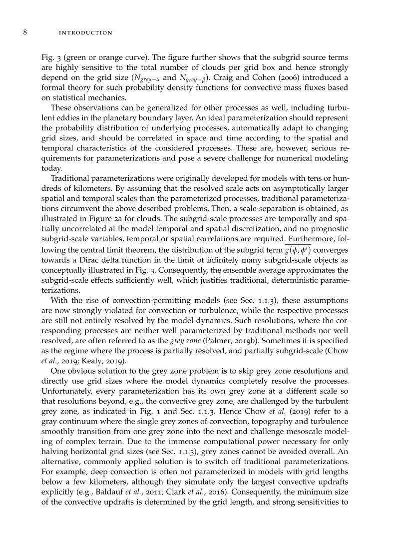
Fig. 3 (green or orange curve). The figure further shows that the subgrid source termsare highly sensitive to the total number of clouds per grid box and hence stronglydepend on the grid size (Ngrey−α and Ngrey−β). Craig and Cohen (2006) introduced aformal theory for such probability density functions for convective mass fluxes basedon statistical mechanics.

These observations can be generalized for other processes as well, including turbu-lent eddies in the planetary boundary layer. An ideal parameterization should representthe probability distribution of underlying processes, automatically adapt to changinggrid sizes, and should be correlated in space and time according to the spatial andtemporal characteristics of the considered processes. These are, however, serious re-quirements for parameterizations and pose a severe challenge for numerical modelingtoday.

Traditional parameterizations were originally developed for models with tens or hun-dreds of kilometers. By assuming that the resolved scale acts on asymptotically largerspatial and temporal scales than the parameterized processes, traditional parameteriza-tions circumvent the above described problems. Then, a scale-separation is obtained, asillustrated in Figure 2a for clouds. The subgrid-scale processes are temporally and spa-tially uncorrelated at the model temporal and spatial discretization, and no prognosticsubgrid-scale variables, temporal or spatial correlations are required. Furthermore, fol-lowing the central limit theorem, the distribution of the subgrid term g(φ, φ′) convergestowards a Dirac delta function in the limit of infinitely many subgrid-scale objects asconceptually illustrated in Fig. 3. Consequently, the ensemble average approximates thesubgrid-scale effects sufficiently well, which justifies traditional, deterministic parame-terizations.

With the rise of convection-permitting models (see Sec. 1.1.3), these assumptionsare now strongly violated for convection or turbulence, while the respective processesare still not entirely resolved by the model dynamics. Such resolutions, where the cor-responding processes are neither well parameterized by traditional methods nor wellresolved, are often referred to as the grey zone (Palmer, 2019b). Sometimes it is specifiedas the regime where the process is partially resolved, and partially subgrid-scale (Chowet al., 2019; Kealy, 2019).

One obvious solution to the grey zone problem is to skip grey zone resolutions anddirectly use grid sizes where the model dynamics completely resolve the processes.Unfortunately, every parameterization has its own grey zone at a different scale sothat resolutions beyond, e.g., the convective grey zone, are challenged by the turbulentgrey zone, as indicated in Fig. 1 and Sec. 1.1.3. Hence Chow et al. (2019) refer to agray continuum where the single grey zones of convection, topography and turbulencesmoothly transition from one grey zone into the next and challenge mesoscale model-ing of complex terrain. Due to the immense computational power necessary for onlyhalving horizontal grid sizes (see Sec. 1.1.3), grey zones cannot be avoided overall. Analternative, commonly applied solution is to switch off traditional parameterizations.For example, deep convection is often not parameterized in models with grid lengthsbelow a few kilometers, although they simulate only the largest convective updraftsexplicitly (e.g., Baldauf et al., 2011; Clark et al., 2016). Consequently, the minimum sizeof the convective updrafts is determined by the grid length, and strong sensitivities to

1.2 parameterizations 9

resolution occur (Hanley et al., 2015; Morrison, 2016b; Jeevanjee, 2017; Panosetti et al.,2019).

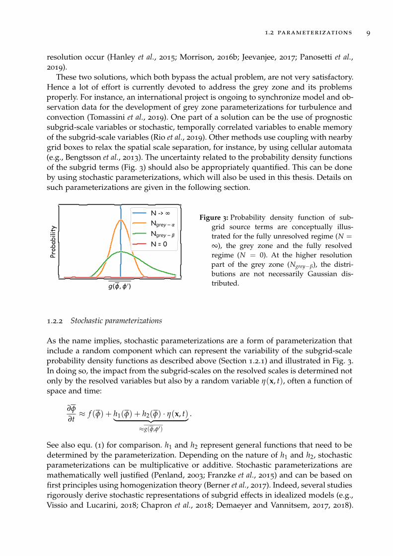
These two solutions, which both bypass the actual problem, are not very satisfactory.Hence a lot of effort is currently devoted to address the grey zone and its problemsproperly. For instance, an international project is ongoing to synchronize model and ob-servation data for the development of grey zone parameterizations for turbulence andconvection (Tomassini et al., 2019). One part of a solution can be the use of prognosticsubgrid-scale variables or stochastic, temporally correlated variables to enable memoryof the subgrid-scale variables (Rio et al., 2019). Other methods use coupling with nearbygrid boxes to relax the spatial scale separation, for instance, by using cellular automata(e.g., Bengtsson et al., 2013). The uncertainty related to the probability density functionsof the subgrid terms (Fig. 3) should also be appropriately quantified. This can be doneby using stochastic parameterizations, which will also be used in this thesis. Details onsuch parameterizations are given in the following section.

Figure 3: Probability density function of sub-grid source terms are conceptually illus-trated for the fully unresolved regime (N =

∞), the grey zone and the fully resolvedregime (N = 0). At the higher resolutionpart of the grey zone (Ngrey−β), the distri-butions are not necessarily Gaussian dis-tributed.

1.2.2 Stochastic parameterizations

As the name implies, stochastic parameterizations are a form of parameterization thatinclude a random component which can represent the variability of the subgrid-scaleprobability density functions as described above (Section 1.2.1) and illustrated in Fig. 3.In doing so, the impact from the subgrid-scales on the resolved scales is determined notonly by the resolved variables but also by a random variable η(x, t), often a function ofspace and time:

∂φ

∂t≈ f (φ) + h1(φ) + h2(φ) · η(x, t)︸ ︷︷ ︸

≈g(φ,φ′)

.

See also equ. (1) for comparison. h1 and h2 represent general functions that need to bedetermined by the parameterization. Depending on the nature of h1 and h2, stochasticparameterizations can be multiplicative or additive. Stochastic parameterizations aremathematically well justified (Penland, 2003; Franzke et al., 2015) and can be based onfirst principles using homogenization theory (Berner et al., 2017). Indeed, several studiesrigorously derive stochastic representations of subgrid effects in idealized models (e.g.,Vissio and Lucarini, 2018; Chapron et al., 2018; Demaeyer and Vannitsem, 2017, 2018).

10 introduction

For fully complex NWP or climate models, however, this is more challenging, if notimpossible.

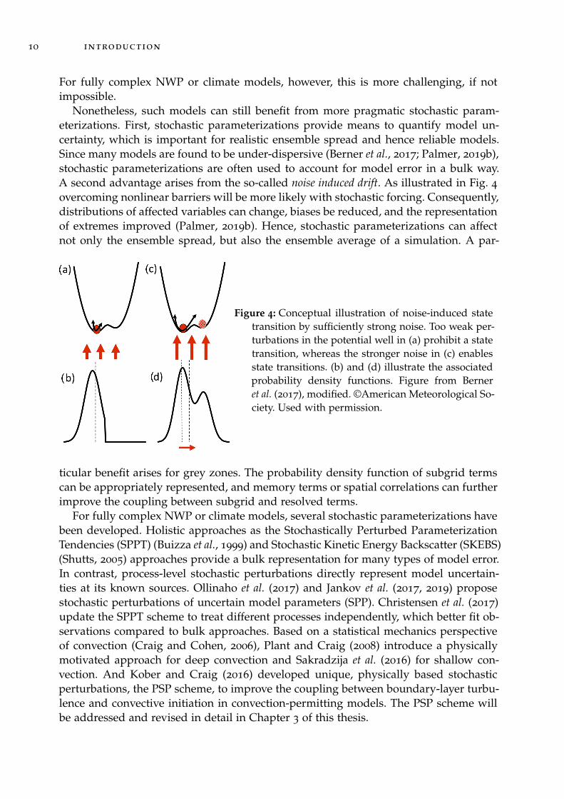
Nonetheless, such models can still benefit from more pragmatic stochastic param-eterizations. First, stochastic parameterizations provide means to quantify model un-certainty, which is important for realistic ensemble spread and hence reliable models.Since many models are found to be under-dispersive (Berner et al., 2017; Palmer, 2019b),stochastic parameterizations are often used to account for model error in a bulk way.A second advantage arises from the so-called noise induced drift. As illustrated in Fig. 4

overcoming nonlinear barriers will be more likely with stochastic forcing. Consequently,distributions of affected variables can change, biases be reduced, and the representationof extremes improved (Palmer, 2019b). Hence, stochastic parameterizations can affectnot only the ensemble spread, but also the ensemble average of a simulation. A par-

Figure 4: Conceptual illustration of noise-induced statetransition by sufficiently strong noise. Too weak per-turbations in the potential well in (a) prohibit a statetransition, whereas the stronger noise in (c) enablesstate transitions. (b) and (d) illustrate the associatedprobability density functions. Figure from Berneret al. (2017), modified. ©American Meteorological So-ciety. Used with permission.

ticular benefit arises for grey zones. The probability density function of subgrid termscan be appropriately represented, and memory terms or spatial correlations can furtherimprove the coupling between subgrid and resolved terms.

For fully complex NWP or climate models, several stochastic parameterizations havebeen developed. Holistic approaches as the Stochastically Perturbed ParameterizationTendencies (SPPT) (Buizza et al., 1999) and Stochastic Kinetic Energy Backscatter (SKEBS)(Shutts, 2005) approaches provide a bulk representation for many types of model error.In contrast, process-level stochastic perturbations directly represent model uncertain-ties at its known sources. Ollinaho et al. (2017) and Jankov et al. (2017, 2019) proposestochastic perturbations of uncertain model parameters (SPP). Christensen et al. (2017)update the SPPT scheme to treat different processes independently, which better fit ob-servations compared to bulk approaches. Based on a statistical mechanics perspectiveof convection (Craig and Cohen, 2006), Plant and Craig (2008) introduce a physicallymotivated approach for deep convection and Sakradzija et al. (2016) for shallow con-vection. And Kober and Craig (2016) developed unique, physically based stochasticperturbations, the PSP scheme, to improve the coupling between boundary-layer turbu-lence and convective initiation in convection-permitting models. The PSP scheme willbe addressed and revised in detail in Chapter 3 of this thesis.

1.3 relevant physical processes and their model representation 11

1.3 relevant physical processes and their model representation

As identified before (Section 1.1.3 and 1.1.2), a common model type for NWP today arekm-scale models. Maximizing their skill is a current challenge for the NWP researchcommunity. One of the most effective ways to address this challenge is presumablyto improve the initiation of convection by still subgrid-scale processes. As this will beaddressed in detail in this thesis, we will now properly introduce atmospheric deepconvection, its initiation, and how it is often represented in models. Then, we focus onthe three most relevant processes for convective initiation based on their frequency, theirdifferent effects on convection and their insufficient respresentation in current models.These processes are boundary-layer turbulence, orographic convection and cold poolsand are likely responsible for most deficiencies concerning convective initiation.

1.3.1 Convection and its initiation

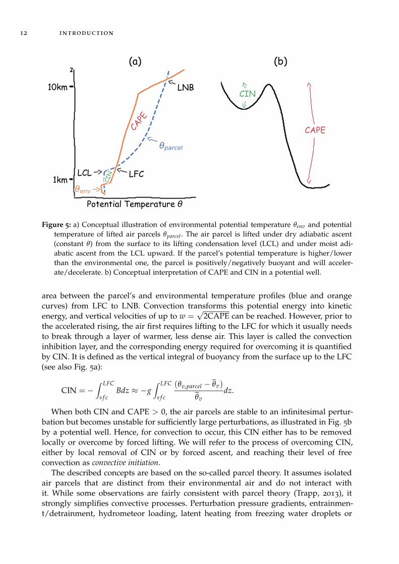
Atmospheric deep convection represents the rapid formation of clouds in a condition-ally unstable atmosphere. Such clouds extend throughout the depth of the troposphereand coincide with strong condensation and often heavy precipitation. In principle, theatmosphere is stably stratified, so that small displacements do not lead to an accelera-tion of rising air parcels. This is illustrated in Fig. 5a by the increase of environmentalpotential temperature with height throughout most of the troposphere. However, if airparcels are lifted beyond their lifting condensation level (LCL), clouds form due to con-densation, latent heat is released, and the rising parcels become even warmer and lessdense. At some point, called the level of free convection (LFC), the air will becomeless dense than its environment, and the lifted air will accelerate due to the continuedrelease of latent heat (see Fig. 5a). This rising usually continues throughout the depthof the troposphere. Only at the tropopause, where temperatures start increasing withheight, the acceleration ceases at the level of neutral buoyancy (LNB). This acceleratedrising air is termed atmospheric deep moist convection or simply convection6.

Typically, the possibility and strength of convection are characterized by the convec-tive available potential energy, CAPE, and the convective inhibition, CIN. CAPE definesthe energy that can be released due to evaporation and is given by the vertical integralof positive buoyancy B (Markowski and Richardson, 2011):

CAPE =∫ LNB

LFCBdz ≈ g

∫ LNB

LFC

(θv,parcel − θv)

θvdz.

The buoyancy is approximated in terms of the acceleration of gravity g and the virtualpotential temperatures of a horizontally uniform reference state θv and a hypothetical,rising parcel θv,parcel. In Fig. 5, we regard the reference temperature as characteristicfor the environmental temperature with typical vertical profiles similar to the orangecurve. The dry and moist adiabatic rising of a surface air parcel results in a typicalvertical profile of θv similar to the blue curve. CAPE can then be interpreted as the

6 In the field of meteorology dry convection, i.e., buoyantly driven unsaturated thermals, or shallow moistconvection are also often referred to by convection. In this thesis, however, we will use the term as anabbreviation for deep moist convection and specify other types of convection accordingly.

12 introduction

Figure 5: a) Conceptual illustration of environmental potential temperature θenv and potentialtemperature of lifted air parcels θparcel . The air parcel is lifted under dry adiabatic ascent(constant θ) from the surface to its lifting condensation level (LCL) and under moist adi-abatic ascent from the LCL upward. If the parcel’s potential temperature is higher/lowerthan the environmental one, the parcel is positively/negatively buoyant and will acceler-ate/decelerate. b) Conceptual interpretation of CAPE and CIN in a potential well.

area between the parcel’s and environmental temperature profiles (blue and orangecurves) from LFC to LNB. Convection transforms this potential energy into kineticenergy, and vertical velocities of up to w =

√2CAPE can be reached. However, prior to

the accelerated rising, the air first requires lifting to the LFC for which it usually needsto break through a layer of warmer, less dense air. This layer is called the convectioninhibition layer, and the corresponding energy required for overcoming it is quantifiedby CIN. It is defined as the vertical integral of buoyancy from the surface up to the LFC(see also Fig. 5a):

CIN =−∫ LFC

s f cBdz ≈ −g

∫ LFC

s f c

(θv,parcel − θv)

θvdz.

When both CIN and CAPE > 0, the air parcels are stable to an infinitesimal pertur-bation but becomes unstable for sufficiently large perturbations, as illustrated in Fig. 5bby a potential well. Hence, for convection to occur, this CIN either has to be removedlocally or overcome by forced lifting. We will refer to the process of overcoming CIN,either by local removal of CIN or by forced ascent, and reaching their level of freeconvection as convective initiation.

The described concepts are based on the so-called parcel theory. It assumes isolatedair parcels that are distinct from their environmental air and do not interact withit. While some observations are fairly consistent with parcel theory (Trapp, 2013), itstrongly simplifies convective processes. Perturbation pressure gradients, entrainmen-t/detrainment, hydrometeor loading, latent heating from freezing water droplets or

1.3 relevant physical processes and their model representation 13

compensating environmental subsidence are neglected (Markowski and Richardson,2011). A major implication is that buoyant acceleration is overestimated as persistentplumes are often necessary to sustain the buoyancy of detraining air (Trapp, 2013).

Convective initiation can occur due to numerous processes and their interactions.Surface heating can locally remove CIN or produce unstable, rising air parcels or turbu-lent eddies with sufficient buoyancy or kinetic energy to overcome CIN (see Sec. 1.3.2).Furthermore, several aspects of orographically induced flow can result in lifting to theLFC (see Sec. 1.3.3). A third mechanism that is actively investigated in many studies isthe secondary convective initiation by cold pools (Sec. 1.3.4). Further processes includesynoptically driven frontal systems, convergence lines, horizontal convective rolls ormesoscale circulations like land see breezes.

As already described in Section 1.1.3, the representation of convection in modelsstrongly depends on the used grid sizes. NWP models with grid sizes of O(10 km)−O(100 km) (e.g., global NWP models, see Sec. 1.1.3) are not able to resolve these deepconvective overturning circulations. Instead, parameterizations are used to representtheir effect on the resolved variables. Most schemes apply a mass flux approach intro-duced by Arakawa and Schubert (1974), where fast convective mass fluxes are assumedto balance large scale and radiative forcing (quasi-equilibrium assumption). A wide va-riety of different approaches and modifications exist and are still being developed (Rioet al., 2019). Current development focuses explicitly on improving the transition fromshallow to deep convection, unifying shallow and deep convection schemes, includingconvective memory and stochastic schemes to account for cloud size distributions (Rioet al., 2019).

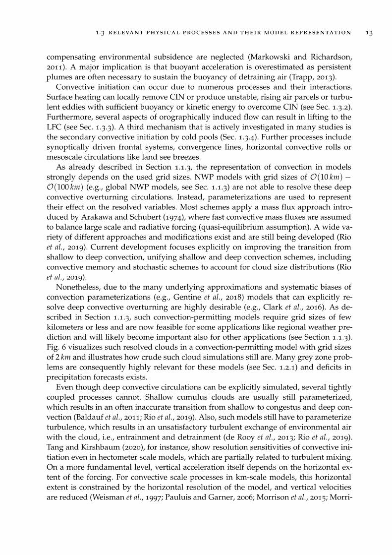
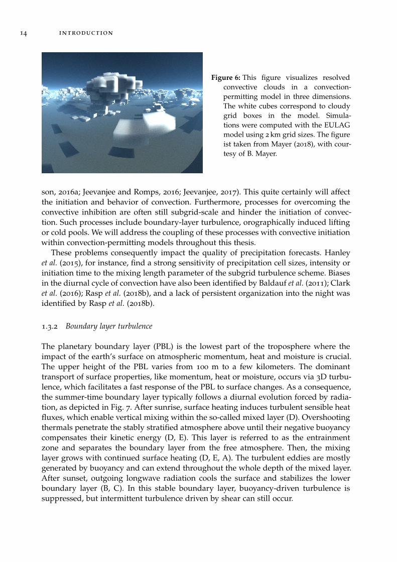
Nonetheless, due to the many underlying approximations and systematic biases ofconvection parameterizations (e.g., Gentine et al., 2018) models that can explicitly re-solve deep convective overturning are highly desirable (e.g., Clark et al., 2016). As de-scribed in Section 1.1.3, such convection-permitting models require grid sizes of fewkilometers or less and are now feasible for some applications like regional weather pre-diction and will likely become important also for other applications (see Section 1.1.3).Fig. 6 visualizes such resolved clouds in a convection-permitting model with grid sizesof 2 km and illustrates how crude such cloud simulations still are. Many grey zone prob-lems are consequently highly relevant for these models (see Sec. 1.2.1) and deficits inprecipitation forecasts exists.

Even though deep convective circulations can be explicitly simulated, several tightlycoupled processes cannot. Shallow cumulus clouds are usually still parameterized,which results in an often inaccurate transition from shallow to congestus and deep con-vection (Baldauf et al., 2011; Rio et al., 2019). Also, such models still have to parameterizeturbulence, which results in an unsatisfactory turbulent exchange of environmental airwith the cloud, i.e., entrainment and detrainment (de Rooy et al., 2013; Rio et al., 2019).Tang and Kirshbaum (2020), for instance, show resolution sensitivities of convective ini-tiation even in hectometer scale models, which are partially related to turbulent mixing.On a more fundamental level, vertical acceleration itself depends on the horizontal ex-tent of the forcing. For convective scale processes in km-scale models, this horizontalextent is constrained by the horizontal resolution of the model, and vertical velocitiesare reduced (Weisman et al., 1997; Pauluis and Garner, 2006; Morrison et al., 2015; Morri-

14 introduction

Figure 6: This figure visualizes resolvedconvective clouds in a convection-permitting model in three dimensions.The white cubes correspond to cloudygrid boxes in the model. Simula-tions were computed with the EULAGmodel using 2 km grid sizes. The figureist taken from Mayer (2018), with cour-tesy of B. Mayer.

son, 2016a; Jeevanjee and Romps, 2016; Jeevanjee, 2017). This quite certainly will affectthe initiation and behavior of convection. Furthermore, processes for overcoming theconvective inhibition are often still subgrid-scale and hinder the initiation of convec-tion. Such processes include boundary-layer turbulence, orographically induced liftingor cold pools. We will address the coupling of these processes with convective initiationwithin convection-permitting models throughout this thesis.

These problems consequently impact the quality of precipitation forecasts. Hanleyet al. (2015), for instance, find a strong sensitivity of precipitation cell sizes, intensity orinitiation time to the mixing length parameter of the subgrid turbulence scheme. Biasesin the diurnal cycle of convection have also been identified by Baldauf et al. (2011); Clarket al. (2016); Rasp et al. (2018b), and a lack of persistent organization into the night wasidentified by Rasp et al. (2018b).

1.3.2 Boundary layer turbulence

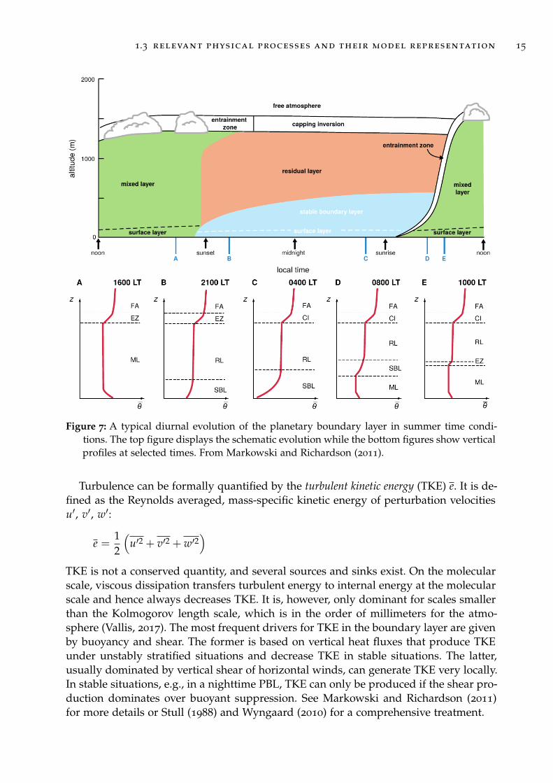
The planetary boundary layer (PBL) is the lowest part of the troposphere where theimpact of the earth’s surface on atmospheric momentum, heat and moisture is crucial.The upper height of the PBL varies from 100 m to a few kilometers. The dominanttransport of surface properties, like momentum, heat or moisture, occurs via 3D turbu-lence, which facilitates a fast response of the PBL to surface changes. As a consequence,the summer-time boundary layer typically follows a diurnal evolution forced by radia-tion, as depicted in Fig. 7. After sunrise, surface heating induces turbulent sensible heatfluxes, which enable vertical mixing within the so-called mixed layer (D). Overshootingthermals penetrate the stably stratified atmosphere above until their negative buoyancycompensates their kinetic energy (D, E). This layer is referred to as the entrainmentzone and separates the boundary layer from the free atmosphere. Then, the mixinglayer grows with continued surface heating (D, E, A). The turbulent eddies are mostlygenerated by buoyancy and can extend throughout the whole depth of the mixed layer.After sunset, outgoing longwave radiation cools the surface and stabilizes the lowerboundary layer (B, C). In this stable boundary layer, buoyancy-driven turbulence issuppressed, but intermittent turbulence driven by shear can still occur.

1.3 relevant physical processes and their model representation 15

Figure 7: A typical diurnal evolution of the planetary boundary layer in summer time condi-tions. The top figure displays the schematic evolution while the bottom figures show verticalprofiles at selected times. From Markowski and Richardson (2011).

Turbulence can be formally quantified by the turbulent kinetic energy (TKE) e. It is de-fined as the Reynolds averaged, mass-specific kinetic energy of perturbation velocitiesu′, v′, w′:

e =12

(u′2 + v′2 + w′2

)TKE is not a conserved quantity, and several sources and sinks exist. On the molecularscale, viscous dissipation transfers turbulent energy to internal energy at the molecularscale and hence always decreases TKE. It is, however, only dominant for scales smallerthan the Kolmogorov length scale, which is in the order of millimeters for the atmo-sphere (Vallis, 2017). The most frequent drivers for TKE in the boundary layer are givenby buoyancy and shear. The former is based on vertical heat fluxes that produce TKEunder unstably stratified situations and decrease TKE in stable situations. The latter,usually dominated by vertical shear of horizontal winds, can generate TKE very locally.In stable situations, e.g., in a nighttime PBL, TKE can only be produced if the shear pro-duction dominates over buoyant suppression. See Markowski and Richardson (2011)for more details or Stull (1988) and Wyngaard (2010) for a comprehensive treatment.

16 introduction

As described in the previous section, the boundary layer is closely linked to convec-tive initiation. The depth of the boundary layer, in combination with the temperaturedifference in the entrainment zone, determine the convective inhibition (see Fig. 5). Fur-thermore, if a parcel’s buoyancy is sufficiently large, it can reach the LFC and transforminto a deep convective updraft.

So how can chaotic turbulence be represented by NWP models with grid sizes largerthan the typical scale of the eddies? By Reynolds-averaging the primitive equations,resolved scale model equations can, in principle, be derived from first principles. Thearising equations constitute prognostic equations for Reynolds averaged quantities. Forthe x-component of the Navier-Stokes equation under the assumption of constant den-sity ρ, we obtain the following equation:

∂u∂t

+ (v · ∇)u =− 1ρ

∂p∂x−∇ · (v′u′), (2)

with ∇ · (v′u′) = ∂

∂xu′u′ +

∂

∂yv′u′ +

∂

∂zw′u′

(Vallis, 2017). The last term in (2), the Reynolds stress term, describes the influence of thesubgrid-scale eddies on the resolved term. The arising subgrid terms for all averagedequations can be categorized into turbulent kinematic momentum fluxes, consisting onlyof velocity components, turblent kinematic heat fluxes (e.g., w′θ′) and turbulent kinematicmoisture fluxes (e.g., w′r′v). As these terms cannot be solved explicitly by the model,they need to be specified using resolved, i.e., Reynolds averaged variables. A variety ofapproaches exist to determine these subgrid terms (Stensrud, 2007). Usually, such PBLschemes assume horizontally homogenous situations and, thus, only consider verticalflux terms. Hence, such schemes are one-dimensional turbulence parameterizations.Local schemes determine the turbulent fluxes only by using local flow characteristics.Non-local schemes, in contrast, often include characteristics of the whole boundarylayer.

A common local approach applies the so-called K-theory. Doing so, these terms areviewed in analogy to molecular viscosity, so they are approximated by the resolvedscale gradients, e.g., u′w′ ≈ −Km

∂u∂z . Km is denoted as the eddy viscosity and needs to

be specified. Often a characteristic mixing length l is used to determine Km. Higher-order schemes include prognostic equations also for eddy terms. Then, however, thirdor even higher-order eddy terms arise which need a parameterization. One exampleis a so-called 1.5 TKE closures, where a prognostic equation for the TKE is used tospecify the eddy correlation terms. Common schemes that combine local and non-localbehavior are eddy diffusivity/mass flux schemes (EDMF) (Siebesma et al., 2007) andare now also being developed as unified parameterization for turbulence and shallowor deep convection (Tan et al., 2018) or with stochastic components (Sakradzija et al.,2016).

As horizontal grid sizes reach the scale of the boundary-layer height, the assumptionsof the Reynolds averaged equations break down.7 If grid sizes become so small that

7 As argued in Wyngaard (2010), Reynolds averaging should at best refer to an ensemble average, i.e.,the average over many realizations under the same larger-scale conditions. Due to the often practicallimitations of an ensemble average, it can be approximated by temporal or spatial averages under certain

1.3 relevant physical processes and their model representation 17

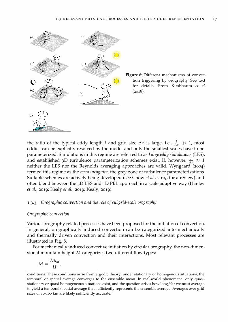
Figure 8: Different mechanisms of convec-tion triggering by orography. See textfor details. From Kirshbaum et al.(2018).

the ratio of the typical eddy length l and grid size ∆x is large, i.e., l∆x � 1, most

eddies can be explicitly resolved by the model and only the smallest scales have to beparameterized. Simulations in this regime are referred to as Large eddy simulations (LES),and established 3D turbulence parameterization schemes exist. If, however, l

∆x ≈ 1neither the LES nor the Reynolds averaging approaches are valid. Wyngaard (2004)termed this regime as the terra incognita, the grey zone of turbulence parameterizations.Suitable schemes are actively being developed (see Chow et al., 2019, for a review) andoften blend between the 3D LES and 1D PBL approach in a scale adaptive way (Hanleyet al., 2019; Kealy et al., 2019; Kealy, 2019).

1.3.3 Orographic convection and the role of subgrid-scale orography

Orographic convection

Various orography related processes have been proposed for the initiation of convection.In general, orographically induced convection can be categorized into mechanicallyand thermally driven convection and their interactions. Most relevant processes areillustrated in Fig. 8.

For mechanically induced convective initiation by circular orography, the non-dimen-sional mountain height M categorizes two different flow types:

M =Nhm

U,

conditions. These conditions arise from ergodic theory: under stationary or homogenous situations, thetemporal or spatial average converges to the ensemble mean. In real-world phenomena, only quasi-stationary or quasi-homogeneous situations exist, and the question arises how long/far we must averageto yield a temporal/spatial average that sufficiently represents the ensemble average. Averages over gridsizes of 10-100 km are likely sufficiently accurate.

18 introduction

with the Brunt-Väisälä freqeuncy N, the mountain height hm and a characteristic hori-zontal wind speed U. For M < 1, the horizontal flow contains sufficient kinetic energyto overcome the height barrier of the mountain, and if the lifted air reaches its LFC,convection occurs (Fig. 8a). We will refer to this mechanism as mechanical lifting andspecifically focus on it in this thesis. For M > 1, on the other hand, the kinetic energy isinsufficient, and the flow is blocked by the mountain. Several possibilities for initiatingconvection occur. Flow deceleration by upstream blocking may result in convection onthe mountain luv (Fig. 8b). Another possibility is the lee-side convergence with sub-sequent convection, as illustrated in Fig. 8c. Additionally, mountain generated gravitywaves and hydraulic jumps can result in further convective initiation.

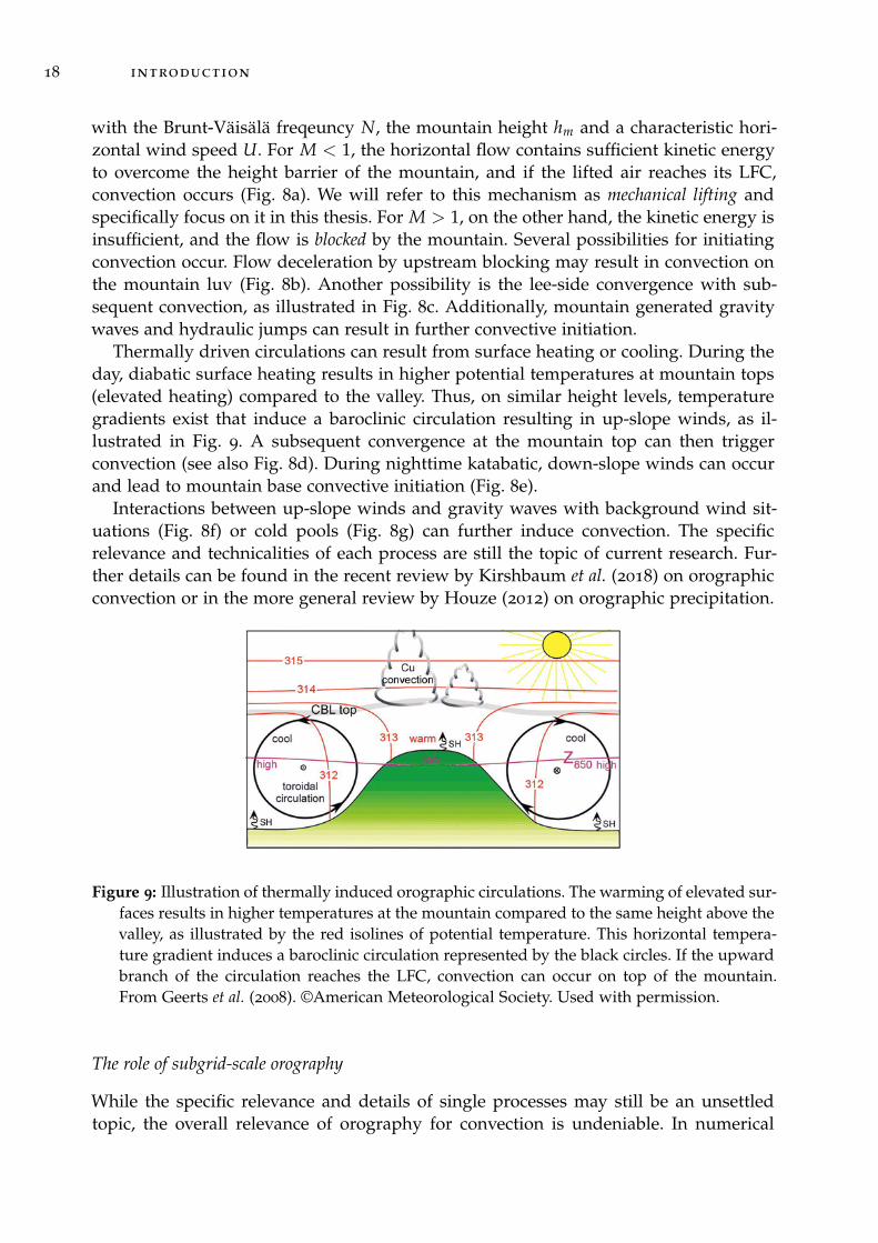
Thermally driven circulations can result from surface heating or cooling. During theday, diabatic surface heating results in higher potential temperatures at mountain tops(elevated heating) compared to the valley. Thus, on similar height levels, temperaturegradients exist that induce a baroclinic circulation resulting in up-slope winds, as il-lustrated in Fig. 9. A subsequent convergence at the mountain top can then triggerconvection (see also Fig. 8d). During nighttime katabatic, down-slope winds can occurand lead to mountain base convective initiation (Fig. 8e).

Interactions between up-slope winds and gravity waves with background wind sit-uations (Fig. 8f) or cold pools (Fig. 8g) can further induce convection. The specificrelevance and technicalities of each process are still the topic of current research. Fur-ther details can be found in the recent review by Kirshbaum et al. (2018) on orographicconvection or in the more general review by Houze (2012) on orographic precipitation.

Figure 9: Illustration of thermally induced orographic circulations. The warming of elevated sur-faces results in higher temperatures at the mountain compared to the same height above thevalley, as illustrated by the red isolines of potential temperature. This horizontal tempera-ture gradient induces a baroclinic circulation represented by the black circles. If the upwardbranch of the circulation reaches the LFC, convection can occur on top of the mountain.From Geerts et al. (2008). ©American Meteorological Society. Used with permission.

The role of subgrid-scale orography

While the specific relevance and details of single processes may still be an unsettledtopic, the overall relevance of orography for convection is undeniable. In numerical

1.3 relevant physical processes and their model representation 19

models, however, the effects of orography are, in general, only included if the modelgrid sufficiently resolves orography. With decreasing grid sizes of numerical models,more and more of the fractal orography is resolved by the model grid, enabling anexplicit representation of these processes. In fact, better resolving orography is oftenmentioned as a dominant benefit of increased resolutions (Wagner et al., 2014; Kealy,2019).

Nonetheless, it is also possible to include the effects of subgrid-scale orography (SSO)to some extent via SSO-parameterizations. The effect of non-local orographic drag isrepresented in parameterizations for orographic gravity waves (Lott and Miller, 1997).Furthermore, the more local effect is accounted for in the specification of the roughnesslength. The recent development of parameter perturbations even allows for uncertaintyin the roughness length (Ruckstuhl and Janjic, 2020). Current developments further aimto properly include SSO in boundary-layer turbulence parameterizations (Rotach et al.,2015). The influence of SSO on convection, however, is otherwise not parameterized inmodels.

This consequently raises the question of whether SSO, i.e., small orographic scales,is, in fact, necessary for convection. Several studies have addressed this question. WhileKirshbaum et al. (2007a) find that scales smaller than few kilometers are not dominantfor convective initiation when a range of orographic scales exist, various studies em-phasize the role of small scale orographic features using analytical models, idealizedsimulations or case studies. Panosetti et al. (2016) find differences in thermally inducedorographic convection between idealized LES and CRM simulations. Kirshbaum et al.(2007b,a) also show that small, single scale orographic features can dictate the spacingof convective bands, and Langhans et al. (2011) conclude that small scale orography con-tributes significantly to convective initiation. By evaluating the effect of smoothed ter-rain on convection in high-resolution simulations, Schneider et al. (2018) find complexinteractions between background flow and orographic scales. These diverse results il-lustrate the complexity of the problem and that the relevance of small orographic scalesfor convection is still uncertain.

Despite these ambiguous conclusions for small scale orography, and hence SSO, itcould be worth to consider its effect for convective initiation in a parameterization. Ingeneral, orography can act as an intrinsic source of predictability for otherwise oftenunpredictable summertime convection (Bachmann et al., 2019, 2020). Also, Kirshbaumet al. (2018) recognizes the lack of SSO in convection parameterizations as a "longstand-ing deficiency". The authors further emphasize that, within the "mountain ’grey zone’,where a smoothed profile of a mountain range is explicitly resolved, but importantsmaller-scale forcing is not", (Kirshbaum et al., 2018, p.19) the development of scaleaware parameterizations is required to include convective initiation by SSO.

1.3.4 Cold pools

Cold pools are volumes of negatively buoyant air that originate from precipitatingdowndrafts. Evaporation of precipitation in the sub-cloud layer, combined with theweight of the condensed water, creates negative buoyancy and thereby accelerates thedowndraft. When these cold, moist air masses hit the surface, they spread in circular-

20 introduction

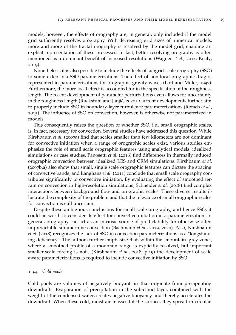
Figure 10: Schematic illustration of cold pool generatation by convective downdrafts (a) andmaintenance of convective cells by secondary convective initiation via mechanical forcing(b). Shear-driven horizontal vorticity is displayed in purple, buoyancy related horizontalvorticity in white. From Markowski and Richardson (2011).

like shapes, as illustrated in Fig. 10a. Cold pools can be regarded as density currents,which are well studied fluid dynamical objects. One well-established framework pro-vides the possibility to estimate the propagation speed of density currents as U =

√BH,

where B represents the buoyancy anomaly of the cold pool and H the height of theanomaly (see, e.g., von Kármán, 1940; Benjamin, 1968; Bryan and Rotunno, 2014b,a). Inthe atmosphere, cold pools actively interact with the surface (Peters and Hohenegger,2017; Grant and van den Heever, 2018; Gentine et al., 2018) and are lead by a gust front,where lifting occurs that fosters the initiation of new convection (Fig. 10b).

In recent decades, three major mechanisms have been proposed as explanations forthis secondary convective initiation. First, Rotunno et al. (1988) and Weisman and Ro-tunno (2004) proposed that horizontal vorticity linked to cold pool induced buoyancygradients at the gust front interacts with the vorticity generated by the backgroundwind shear to yield approximately vertical updrafts. This pattern of convergence andascent is optimal for initiating new convection and thereby enables the reinforcementand propagation of squall lines (Rotunno et al., 1988; Weisman and Rotunno, 2004;Markowski and Richardson, 2011). We will refer to this mechanism as mechanical lift-ing. Second, the collision of cold pools has been identified as a major contributor forinitiating new convection (Feng et al., 2015; Cafaro and Rooney, 2018; Haerter et al.,2018; Torri and Kuang, 2019). Collisions of two cold pools can cause a superposition oftheir updraft velocity resulting in stronger updrafts. Collisions of three cold pools can

1.4 summary and research goals 21

trap non-cold pool air in between the colliding fronts, which results in even strongervertical motion (Haerter et al., 2018). Third, Tompkins (2001) proposed a mechanismbased on buoyancy-driven initiation: decaying cold pools accumulate moisture fromthe perished precipitation downdrafts at their boundaries. This increased moisture cancompensate the effect of cold temperatures on buoyancy (especially for "old" cold pools,where entrainment has depleted the cold air) and thereby reduce the convective inhibi-tion, which supports the initiation of new convection. Torri et al. (2015) investigated therelevance of the mechanical and thermodynamic mechanisms in idealized studies andfound that, initially, mechanical lifting drives the vertical motion, whereas higher in theboundary layer, moisture seems to be relevant for vertical acceleration. Independent ofthe specific mechanism, the effect of cold pools is to trigger convection in the vicinityof already existing convection, leading to the organization of convective cells and amore clustered precipitation pattern. Cold pools may also influence the diurnal cycle ofconvection since they are relevant triggering mechanisms, only after initial precipitationevents have occurred. Especially in the late afternoon/evening, when other mechanismslike surface heating are no longer strong, cold pool triggering may dominate.

In coarser weather and climate models, cold pools are often not resolved. Yet onlyrecently are the effects of cold pools being considered in convection parameterizations(e.g., in Grandpeix and Lafore, 2010; Grandpeix et al., 2010), often to improve convec-tive memory and organization (Rio et al., 2019). With km-scale grid sizes, models cansimulate cold pools explicitly. Cold pool properties, however, are highly sensitive tochanges in model resolution, suggesting that these models are not able to simulate coldpools accurately. Grid sizes of below 100 m are expected to be necessary for accuratelyresolving the fine-scale structures of cold pool gust fronts (Grant and van den Heever,2016). How to best tackle this cold pool grey zone is still an open question. A coexis-tence of resolved and parameterized cold pools may be useful for the coarser grid sizes,whereas alternative approaches might directly improve the resolved cold pools.

1.4 summary and research goals

A large part of precipitation and associated hazards comes from deep convective cloudswhich develop due to accelerated rising air by condensation. To reduce associated dam-ages, early and reliable predictions are crucial. Predicting such deep convection, how-ever, has been a long-standing challenge. In the last decade, km-scale models, whichenable the explicit simulation of such deep convection (i.e., convection-permitting mod-els), have become more and more accessible for operational weather prediction (Bal-dauf et al., 2011; Clark et al., 2016) and even climate projections (Leutwyler et al., 2017;Stevens et al., 2019a), and they are expected to prevail for the next decades (Palmer,2019a). Consequently, convection parameterizations - containing many approximationsand systematic biases (Gentine et al., 2018) - are not required any more, and convectionforecasts were significantly improved (Baldauf et al., 2011; Clark et al., 2016). Nonethe-less, not all deficits concerning convective precipitation have been solved just by turningfrom parameterized convection to convection-permitting simulations. Most importantly,capturing the diurnal cycle of convection is still problematic (Baldauf et al., 2011; Clarket al., 2016; Hanley et al., 2019) and a lack of persistent organization into the night

22 introduction

was identified by Rasp et al. (2018b). These inconsistencies become particularly relevantwhen synoptic forcing is weak, and local mechanisms are the main driver for overcom-ing convective inhibition (Keil et al., 2014).

The underlying causes for these deficits can mostly be ascribed to the grey zoneproblem: grid sizes of convection-permitting models only allow the explicit simulationof large deep convective clouds; smaller convective systems and many processes, thatare tightly coupled to convection, can still not sufficiently be resolved. These processesinclude evaporation and condensation, droplet formation, entrainment or detrainment,but, most importantly, the initiation of convection (Baldauf et al., 2011; Yano et al., 2018;Kober and Craig, 2016): for the formation of deep convective clouds to be kicked off, airparcels need to overcome the convective inhibition, which often requires local triggeringprocesses related to boundary-layer processes. Currently, the most efficient way to im-prove convection is likely by improving the reprentation of processes that are relevantfor convective intiation.

Hence, in this this thesis, we aim to understand how such triggering processes areinsufficiently accounted for in convection-permitting models and to improve their rep-resentation accordingly. Based on their frequency, their distinct influence on convectionand their insufficient representation in current models, we choose the three processesthat are most promising to benefit convective initiation. These processes are boundary-layer turbulence, subgrid-scale orographic lifting and cold pools.

boundary layer turbulence Boundary layer turbulence is an omnipresent phe-nomenon in summer-time boundary layers, occurs in a variety of situations and conse-quently contributes substantially to total convective initiation. It is specifically impor-tant during summer-time situations when synoptic, resolved scale forcing mechanismsare weak. Boundary layer turbulence is a subgrid-scale process in km-scale models andonly represented approximately via parameterizations. Km-scale grid sizes specificallychallenge traditional turbulence parameterizations as they approach the grey zone ofturbulence. To improve its representation in km-scale models, we consider one of thefirst process-level stochastic parameterizations, the aforementioned PSP scheme (Koberand Craig, 2016), which introduces stochastic perturbations to account for the miss-ing subgrid-scale variability of turbulence. We substantially revise the PSP scheme toimprove its physical consistency and to eliminate some undesired effects. For example,previously ineffective vertical velocity perturbations are improved to be more persistentby also perturbing horizontal wind components in a 3d non-divergent way. The revisedPSP scheme, PSP2, is then applied on a 10 day period to confirm its impact.

subgrid-scale orographic lifting The next most relevant process is thoughtto be orographically driven convective initiation. It is limited to orographic regions,yet many parts of Germany, Europe or the whole earth are indeed subject to complexterrain. Small scale orography, i.e., subgrid-scale orography, is not explicitly resolved,and its effect can only be approximated in the form of parameterizations. As explainedin Section 1.3.3, however, it is not yet clear how relevant small scale orography, i.e.,subgrid-scale orography in km-scale models, is for convective initiation. To contribute

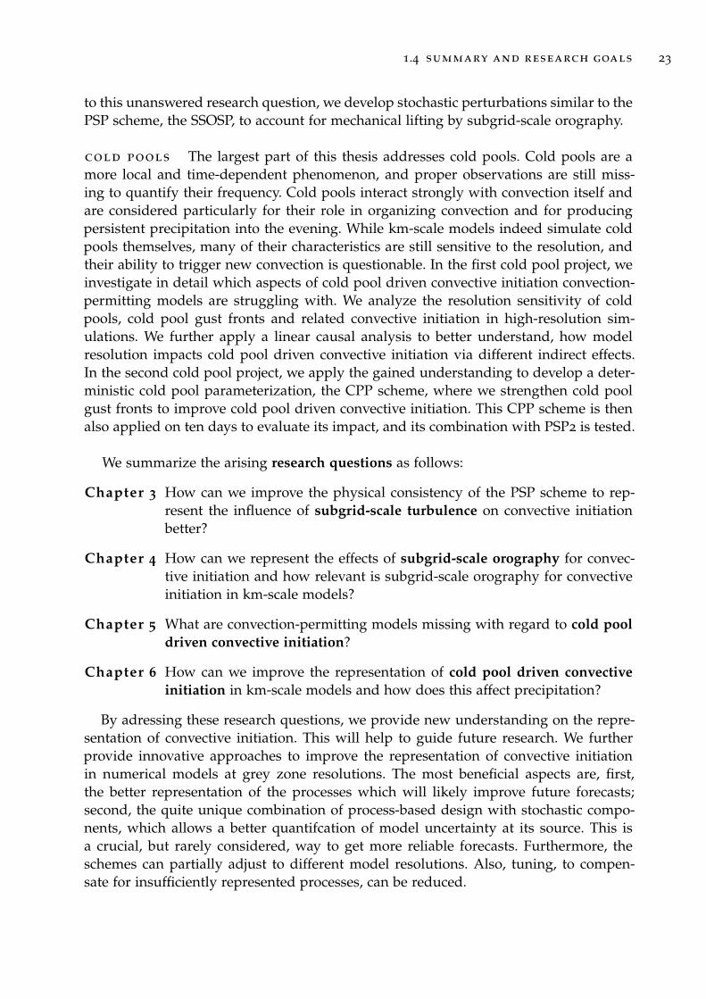
1.4 summary and research goals 23

to this unanswered research question, we develop stochastic perturbations similar to thePSP scheme, the SSOSP, to account for mechanical lifting by subgrid-scale orography.

cold pools The largest part of this thesis addresses cold pools. Cold pools are amore local and time-dependent phenomenon, and proper observations are still miss-ing to quantify their frequency. Cold pools interact strongly with convection itself andare considered particularly for their role in organizing convection and for producingpersistent precipitation into the evening. While km-scale models indeed simulate coldpools themselves, many of their characteristics are still sensitive to the resolution, andtheir ability to trigger new convection is questionable. In the first cold pool project, weinvestigate in detail which aspects of cold pool driven convective initiation convection-permitting models are struggling with. We analyze the resolution sensitivity of coldpools, cold pool gust fronts and related convective initiation in high-resolution sim-ulations. We further apply a linear causal analysis to better understand, how modelresolution impacts cold pool driven convective initiation via different indirect effects.In the second cold pool project, we apply the gained understanding to develop a deter-ministic cold pool parameterization, the CPP scheme, where we strengthen cold poolgust fronts to improve cold pool driven convective initiation. This CPP scheme is thenalso applied on ten days to evaluate its impact, and its combination with PSP2 is tested.

We summarize the arising research questions as follows:

Chapter 3 How can we improve the physical consistency of the PSP scheme to rep-resent the influence of subgrid-scale turbulence on convective initiationbetter?

Chapter 4 How can we represent the effects of subgrid-scale orography for convec-tive initiation and how relevant is subgrid-scale orography for convectiveinitiation in km-scale models?

Chapter 5 What are convection-permitting models missing with regard to cold pooldriven convective initiation?

Chapter 6 How can we improve the representation of cold pool driven convectiveinitiation in km-scale models and how does this affect precipitation?

By adressing these research questions, we provide new understanding on the repre-sentation of convective initiation. This will help to guide future research. We furtherprovide innovative approaches to improve the representation of convective initiationin numerical models at grey zone resolutions. The most beneficial aspects are, first,the better representation of the processes which will likely improve future forecasts;second, the quite unique combination of process-based design with stochastic compo-nents, which allows a better quantifcation of model uncertainty at its source. This isa crucial, but rarely considered, way to get more reliable forecasts. Furthermore, theschemes can partially adjust to different model resolutions. Also, tuning, to compen-sate for insufficiently represented processes, can be reduced.

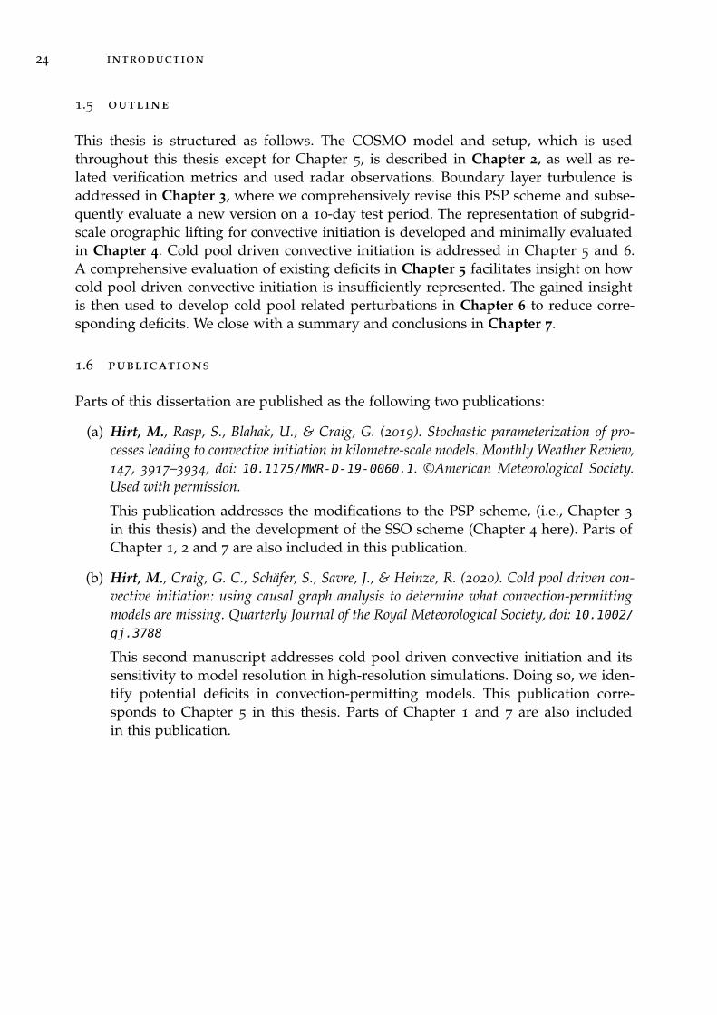
24 introduction

1.5 outline

This thesis is structured as follows. The COSMO model and setup, which is usedthroughout this thesis except for Chapter 5, is described in Chapter 2, as well as re-lated verification metrics and used radar observations. Boundary layer turbulence isaddressed in Chapter 3, where we comprehensively revise this PSP scheme and subse-quently evaluate a new version on a 10-day test period. The representation of subgrid-scale orographic lifting for convective initiation is developed and minimally evaluatedin Chapter 4. Cold pool driven convective initiation is addressed in Chapter 5 and 6.A comprehensive evaluation of existing deficits in Chapter 5 facilitates insight on howcold pool driven convective initiation is insufficiently represented. The gained insightis then used to develop cold pool related perturbations in Chapter 6 to reduce corre-sponding deficits. We close with a summary and conclusions in Chapter 7.

1.6 publications

Parts of this dissertation are published as the following two publications:

(a) Hirt, M., Rasp, S., Blahak, U., & Craig, G. (2019). Stochastic parameterization of pro-cesses leading to convective initiation in kilometre-scale models. Monthly Weather Review,147, 3917–3934, doi: 10.1175/MWR-D-19-0060.1. ©American Meteorological Society.Used with permission.

This publication addresses the modifications to the PSP scheme, (i.e., Chapter 3

in this thesis) and the development of the SSO scheme (Chapter 4 here). Parts ofChapter 1, 2 and 7 are also included in this publication.

(b) Hirt, M., Craig, G. C., Schäfer, S., Savre, J., & Heinze, R. (2020). Cold pool driven con-vective initiation: using causal graph analysis to determine what convection-permittingmodels are missing. Quarterly Journal of the Royal Meteorological Society, doi: 10.1002/qj.3788

This second manuscript addresses cold pool driven convective initiation and itssensitivity to model resolution in high-resolution simulations. Doing so, we iden-tify potential deficits in convection-permitting models. This publication corre-sponds to Chapter 5 in this thesis. Parts of Chapter 1 and 7 are also includedin this publication.

2C O S M O : M O D E L S E T U P, S I M U L AT I O N P E R I O D A N DV E R I F I C AT I O N

For chapters 3, 4 and 6, we aim to improve convective precipitation forecasts by develop-ing better representations of boundary-layer processes for state-of-the-art, convection-permitting models. With this objective, we choose the COSMO model in a convection-pertmitting setup as it is used for the operational weather prediction by the GermanWeather Service. To test the impact of the parameterization schemes and their adaptabil-ity to different flow situations, we select a ten day time period with active convectionand different synoptic situations. The used domain over Germany also contains oro-graphic regions in the Southern part of the domain (Alps) and flat terrain in NorthernGermany. This enables the better evaluation of the subgrid-scale orography scheme indifferent orographic situations. To evaluate the influence of the schemes on precipita-tion, we compare the simulation results to radar observations of precipitation, whichhave a high spatial coverage compared to other types of precipitation measurements.This comparison entails the computation of verification metrics, which allow meaning-ful insight in intermittent precipitation fields. Further details on these aspects are givenbelow. Simulations and methods used for Chapter 5 will be explained then.

2.1 model and simulation setup

Most simulations (except for those used in Chapter 5) are computed with the COSMO(COnsortium for Small-scale MOdeling) model (Baldauf et al., 2011), version 5.4g, in aconvection-permitting setup with ∆x = 0.025◦, roughly 2.8 km, and a time step of 25 s.The setup uses 50 vertically stretched model layers ranging from 10 m above groundto 22 km above mean sea level. A staggered grid (Arakawa-C/Lorenz) is used withterrain following coordinates (Schättler et al., 2016). As a consequence, a proper trans-formation between model level and height depends on the horizontal coordinates. Forcomparability, we will give approximate, domain averaged transformations when nec-essary. Shallow convection is parameterized using the Tiedtke scheme. Details on pa-rameterizations can be found in Doms et al. (2011). The setup follows the operationalCOSMO-DE setup with 461 by 421 grid points centered over Germany at 10

◦E and50◦N.The only major deviation from the current operational setup is a change of the tuning

parameter tur_len in the boundary-layer scheme to 500 m. For the operational COSMOversion, a decision was made to decrease tur_len to 150 m in order to reduce a lack ofsummer-time convection (Baldauf et al., 2011). This, however, comes at the expense oftemperature biases, which are widely observed in different studies (Baldauf et al., 2011;Schraff et al., 2016; Leutwyler et al., 2017; Necker et al., 2018). Baldauf et al. (2011) arguethat "the improved forecasts of deep convection outweigh those disadvantages" (p. 3902,

25

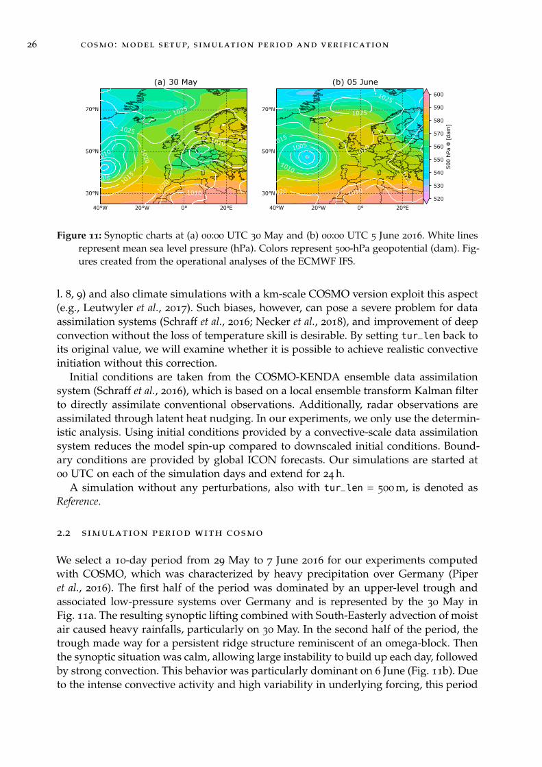
26 cosmo : model setup, simulation period and verification

30°N

50°N

70°N

40°W 20°W 0° 20°E

1005

1010

1010

1010

1015

1015

1020

1020

1025

1025

(a) 30 May

30°N

50°N

70°N

40°W 20°W 0° 20°E

1005

1010

1010 1015

1015

1020

1020

1025

1025

(b) 05 June

520

530

540

550

560

570

580

590

600

500 h

Pa

[dam

]

Figure 11: Synoptic charts at (a) 00:00 UTC 30 May and (b) 00:00 UTC 5 June 2016. White linesrepresent mean sea level pressure (hPa). Colors represent 500-hPa geopotential (dam). Fig-ures created from the operational analyses of the ECMWF IFS.

l. 8, 9) and also climate simulations with a km-scale COSMO version exploit this aspect(e.g., Leutwyler et al., 2017). Such biases, however, can pose a severe problem for dataassimilation systems (Schraff et al., 2016; Necker et al., 2018), and improvement of deepconvection without the loss of temperature skill is desirable. By setting tur_len back toits original value, we will examine whether it is possible to achieve realistic convectiveinitiation without this correction.

Initial conditions are taken from the COSMO-KENDA ensemble data assimilationsystem (Schraff et al., 2016), which is based on a local ensemble transform Kalman filterto directly assimilate conventional observations. Additionally, radar observations areassimilated through latent heat nudging. In our experiments, we only use the determin-istic analysis. Using initial conditions provided by a convective-scale data assimilationsystem reduces the model spin-up compared to downscaled initial conditions. Bound-ary conditions are provided by global ICON forecasts. Our simulations are started at00 UTC on each of the simulation days and extend for 24 h.

A simulation without any perturbations, also with tur_len = 500 m, is denoted asReference.

2.2 simulation period with cosmo

We select a 10-day period from 29 May to 7 June 2016 for our experiments computedwith COSMO, which was characterized by heavy precipitation over Germany (Piperet al., 2016). The first half of the period was dominated by an upper-level trough andassociated low-pressure systems over Germany and is represented by the 30 May inFig. 11a. The resulting synoptic lifting combined with South-Easterly advection of moistair caused heavy rainfalls, particularly on 30 May. In the second half of the period, thetrough made way for a persistent ridge structure reminiscent of an omega-block. Thenthe synoptic situation was calm, allowing large instability to build up each day, followedby strong convection. This behavior was particularly dominant on 6 June (Fig. 11b). Dueto the intense convective activity and high variability in underlying forcing, this period

2.3 observations 27

has been considered in a number of studies on convection (Rasp et al., 2018b; Baur et al.,2018; Bachmann et al., 2019; Keil et al., 2019) and provides a good testing ground for thedeveloped schemes. For specific purposes, single days from this period are investigatedin more detail.

2.3 observations

We compare our simulations to radar-derived precipitation fields. We use the Radar On-line Aneichung (RADOLAN) quality-controlled radar observations (EY product) pro-vided by the German Weather Service, which is based on European radar reflectivitiesand provides radar coverage for most of our domain (Deutscher Wetterdienst, 2018a,b).For all analyses of our simulations, we restrict the geographical region to grid pointswhere radar data is available.

We mostly focus on the systematic impact of the developed schemes on the behaviorof the model. The comparison to radar observation only serves as a guideline. Trying toimprove the forecast scores would require much longer simulation periods and tuningof several model parameters (e.g., tur_len). We anticipate, however, that the systematicimpacts of the here considered schemes are independent of the specific model configu-ration.

2.4 verification metrics

As we are mostly interested in convection, we focus on the verification of precipitation.Traditional measures like mean absolute error or the root mean squared error are oftennot very effective when intermittent, localized precipitation fields are considered. Forinstance, if precipitation objects are slightly shifted between observations and modelsimulations, such methods penalize twice: once for regions where precipitation occursin the observations but not in the simulations, and once where precipitation occursin the simulations but not in the observations. This problem is often referred to asthe double penalty problem. Furthermore, such skill scores easily improve with moreprecipitation. Alternative measures to quantify the quality of simulated precipitationin comparison to observations, however, exist. Fuzzy verification methods reduce thedouble penalty by filtering the precipitation fields and thereby allowing for some spatialshifts in the precipitation fields. A widely used fuzzy/neighborhood metric is the so-called fraction skill score, FSS (see Sec. 2.4.1). Other approaches are based on objects.Such methods identify single objects, i.e., clouds or precipitation cells, and comparetheir characteristics with each other. Such metrics include the Structure component ofthe Structure-Amplitude-Location (SAL, Sec. 2.4.2) score or simple size and frequencydistributions of the identified objects (Sec. 2.4.3). See, e.g., Gilleland et al. (2009) for anintercomparison of some methods.

2.4.1 Fraction skill score

The fraction skill score (FSS) evaluates how two precipitation fields, usually radar ob-servations O and model forecast F, agree with each other within a given neighborhood.

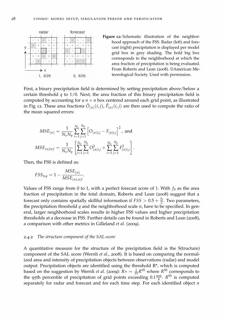
28 cosmo : model setup, simulation period and verification

Figure 12: Schematic illustration of the neighbor-hood approach of the FSS. Radar (left) and fore-cast (right) precipitation is displayed per modelgrid box in grey shading. The bold big boxcorresponds to the neighborhood at which thearea fraction of precipitation is being evaluated.From Roberts and Lean (2008). ©American Me-teorological Society. Used with permission.

First, a binary precipitation field is determined by setting precipitation above/below acertain threshold q to 1/0. Next, the area fraction of this binary precipitation field iscomputed by accounting for a n× n box centered around each grid point, as illustratedin Fig 12. These area fractions O(n)(i, j), F(n)(i, j) are then used to compute the ratio ofthe mean squared errors:

MSE(n) =1

NxNy

Nx

∑i=1

Ny

∑j=1

[O(n)i,j − F(n)i,j

]2, and

MSE(n)re f =1

NxNy

[Nx

∑i=1

Ny

∑j=1

O2(n)i,j +

Nx

∑i=1

Ny

∑j=1

F2(n)i,j

].

Then, the FSS is defined as:

FSSn,q = 1−MSE(n)

MSE(n),re f.

Values of FSS range from 0 to 1, with a perfect forecast score of 1. With f0 as the areafraction of precipitation in the total domain, Roberts and Lean (2008) suggest that aforecast only contains spatially skillful information if FSS > 0.5 + f0

2 . Two parameters,the precipitation threshold q and the neighborhood scale n, have to be specified. In gen-eral, larger neighborhood scales results in higher FSS values and higher precipitationthresholds at a decrease in FSS. Further details can be found in Roberts and Lean (2008),a comparison with other metrics in Gilleland et al. (2009).

2.4.2 The structure component of the SAL-score

A quantitative measure for the structure of the precipitation field is the S(tructure)component of the SAL score (Wernli et al., 2008). It is based on comparing the normal-ized area and intensity of precipitation objects between observations (radar) and modeloutput. Precipitation objects are identified using the threshold R*, which is computedbased on the suggestion by Wernli et al. (2009): R∗ = 1

15 R95 where R95 corresponds tothe 95th percentile of precipitation of grid points exceeding 0.1 mm

h . R95 is computedseparately for radar and forecast and for each time step. For each identified object n

2.4 verification metrics 29

a "scaled volume" Vn is computed as the total precipitation of the object Rn = ∑i,j Ri,jnormalized by its maximum precipitation rate Rmax

n :

Vn =Rn

Rmaxn

.

Having computed this scaled volume for all precipitation objects its weighted averagecan be computed:

V(R) =∑M

n1RnVn

∑Mn1

Vn

Finally the S-score is computed as the normalized difference in V between model (mod)and observations (obs):

S =V(Rmod)−V(Robs)

0.5 [V(Rmod)−V(Robs)]

Negative S values imply that the simulated precipitation cells are too small and peakedcompared to the radar observations while S = 0 suggests a perfect match in termsof structure. Different threshold choices, such as fixed precipitation amounts, did notchange the outcome qualitatively.

The amplitude (A) and location (L) score of the SAL score are also object-basedmethods. For our purposes, however, we do not find additional value in consideringthem.

2.4.3 Size and frequency distributions

It is also possible to simply analyze size or frequency distributions of identified precip-itation objects. Objects are then simply identified as a connected agglomeration of gridpoints with precipitation higher than a specific threshold.

3R E P R E S E N T I N G B O U N D A RY- L AY E R T U R B U L E N C E VA R I A B I L I T Y

As explained in Sec. 1.3.2, boundary-layer turbulence is strongly coupled to convectiveinitiation. Daytime surface heating stimulates boundary-layer turbulence and therebywarms up the boundary layer via mixing, reduces CIN and preconditions the boundarylayer for convective initiation. Stronger turbulent eddies can further push through theconvective inhibition, reach their LFC and develop to convective plumes.

The largest turbulent eddies in the boundary layer have characteristic scales corre-sponding to the boundary-layer height, i.e., around 1 km, and have to be parameterizedin NWP models (see Sec. 1.1.3 and 1.2). Originally such boundary-layer parameteri-zations were developed for grid sizes that are large relative to the turbulent eddiesand typically only represent the mean mixing caused by subgrid-scale eddies in a de-terministic way. The parameterization predicts the mean effect of a large ensemble ofeddies, and the variability associated with the individual eddies is averaged out. Forconvection-permitting models, however, a km-scale grid box will contain only a smallnumber of the largest eddies, and their variability will have a substantial effect on thegrid-box mean (see Sec. 1.2.1 on grey zones). As a result, the variability on the smallestresolved scales in convection-permitting model is under-represented, and difficulties inovercoming convective inhibition arise. This ultimately causes deficits in precipitationforecasts, particularly when synoptic forcing is weak (Keil et al., 2014). These deficits arespecifically a lack of convective initiation during the day, a late onset of convection, toofrequent grid cell storms, and a shortage of organization (Baldauf et al., 2011; Hanleyet al., 2015; Clark et al., 2016; Rasp et al., 2018b).

In this chapter, we aim to improve the representation of convective initiation byboundary-layer turbulence in km-scale models. We use process-level stochastic pertur-bations, which better represent the subgrid-scale variability and accordingly quantifyuncertainty, as explained in Sec. 1.2.2. A corresponding parameterization was originallydeveloped by Kober and Craig (2016), the physically-based stochastic perturbations, i.e.,PSP. We revise this scheme to improve its consistency using COSMO. Based on theseresults, an updated version of the PSP scheme will be defined that has the potential toimprove forecast skill for convective precipitation.

The PSP scheme (Kober and Craig, 2016) aims to better couple subgrid-scale tur-bulence to convective initiation by reintroducing missing subgrid-scale variance to theresolved scales. This is done by adding stochastic perturbations to the model tendenciesof temperature, humidity and vertical velocity. The perturbation structure is given by ahorizontally correlated random field that is regenerated every 10 minutes, a time spanthat represents the average lifetime of a boundary-layer eddy. Since such eddies spanthe entire depth of the convective boundary layer, the perturbations are kept verticallycoherent by applying the same random field at all model levels. Most importantly, theamplitudes of the perturbations are scaled by physical information on the subgrid-scale

31

32 representing boundary-layer turbulence variability

variance computed in the turbulence parameterization. This scaling links the perturba-tion strength to the physical processes that cause small-scale turbulence. Furthermore,this enables the scheme to adapt to different atmospheric situations.

The PSP scheme showed promising results in a range of case studies (Kober andCraig, 2016). Under weak synoptic forcing, the perturbations trigger more convectivecells and consequently produce more precipitation. This improved the diurnal cycleand amplitude of precipitation. Further, Rasp et al. (2018b) have successfully exploitedits capability to create different realizations of the convective cloud field for the samesynoptic situation by generating different random fields for each ensemble member. Themagnitude of the ensemble spread created by different PSP realizations was also foundto be comparable to operational ensembles (Keil et al., 2019). And in a convective-scaledata assimilation framework, the PSP scheme produced a beneficial impact in ensemblespread and precipitation forecasts (Zeng et al., 2020).

However, the original version of the PSP scheme also leads to undesirable side effects.We investigate these issues and propose modifications to alleviate them. In particular,four topics will be covered:

1. In its current formulation, the evolution of the random field is temporally dis-continuous, being regenerated every 10 minutes. To avoid these discontinuities,we introduce a continuously evolving random field using an autoregressive (AR)process.

2. Unrealistically high night-time precipitation has been observed using the PSPscheme (Rasp et al., 2018b). As we will show, this is related to perturbations inthe free-troposphere. These do not fit with the rationale of the PSP scheme, whichis designed to represent vertically coherent structures in convective boundary lay-ers. Hence to remove these artifacts, we restrict the perturbations to the boundarylayer.

3. Furthermore organized convective structures were found to be broken apart bythe perturbations. To prevent this, we investigate the use of a mask to switch offthe perturbations in regions where precipitation is already occurring.

4. Finally, the vertical velocity perturbations were found to have an insignificant ef-fect compared to the temperature and humidity perturbations (Kober and Craig,2016). As we will discuss in this paper, this is associated with the generation ofacoustic modes, which lead to the rapid dissipation of the imposed vertical ve-locity perturbations. By introducing balanced, 3D wind perturbations, we obtainlasting and effective wind perturbations.

After evaluating the modifications separately, we propose a revised version of thescheme, which we will call PSP2.

In Section 3.1, the formulation of the PSP scheme is explained in detail, as well asthe four modifications mentioned above. In Section 3.2, we describe our strategy for themodel. The results are presented in Section 3.3 followed by a summary and discussionin Section 3.4.

3.1 conception of the stochastic perturbations 33

3.1 conception of the stochastic perturbations

In this section, we summarize the original perturbation scheme for boundary-layer tur-bulence (PSP) by Kober and Craig (2016) and then describe our modifications to im-prove the physical consistency of the scheme.

3.1.1 Physically based stochastic perturbations for subgrid-scale turbulence (PSP)

The PSP scheme for boundary-layer turbulence was first described in Kober and Craig(2016). Here we present an updated formulation according to Rasp et al. (2018b).

The PSP scheme reintroduces the influence of the lost small-scale variability of bound-ary layer eddies by adding perturbations to the tendencies of the temperature, hu-midity and vertical velocity field (T, qv, w) on the smallest effectively resolved scale,∆xeff = 5∆x (see e.g., Bierdel et al., 2012). For this we assume a random, horizontaleddy field η(x, y, t) with temporal and spatial correlation scales τeddy and ∆xeff (seeFig. 13a). The temporal correlation is given by the typical life time of convective eddies,i.e., τeddy = 10 min, and is also theoretically justified by the missing scale separationbetween resolved and subgrid-scales which necessitates the representation of memoryeffects (see e.g., Berner et al., 2017, or Sec. 1.2). The perturbation amplitude is chosen

to be proportional to the subgrid standard deviation√

Φ′2 for Φ ∈ {T, qv, w}, whichis taken directly from the turbulence scheme. The COSMO model uses a 1.5 order clo-sure (Raschendorfer, 2001) based on level 2.5 of Mellor and Yamada (1982), in whichthe second moments are diagnostically computed based on the turbulence kinetic en-ergy and the vertical gradients of the variables in question. In addition, the schemeadapts to the grid spacing. For uncorrelated subgrid-scale eddies the variability scaleswith 1/

√Neddy, where Neddy = ∆x2

l2eddy

is the number of eddies of scale leddy = 1000 m

in a grid box (Craig and Cohen, 2006). Dividing by τeddy ensures that the accumulated

perturbations during this time period scale asleddy∆xeff

√Φ′2. The complete mathematical

formulation is:

∂tΦ|PSP = αtuningη1

τeddy

leddy

∆xeff

√Φ′2, (3)

where αtuning is a free parameter that should be of order one, if the length, time andvariance scales that appear in the equation have the correct orders of magnitude. Asingle choice of αtuning should apply for all weather regimes and model resolutions, ifthe physical assumptions of the scheme are satisfied. Example fields for the randomfield η, the subgrid standard deviation for temperature and the resulting temperatureperturbations are shown in Fig. 13.

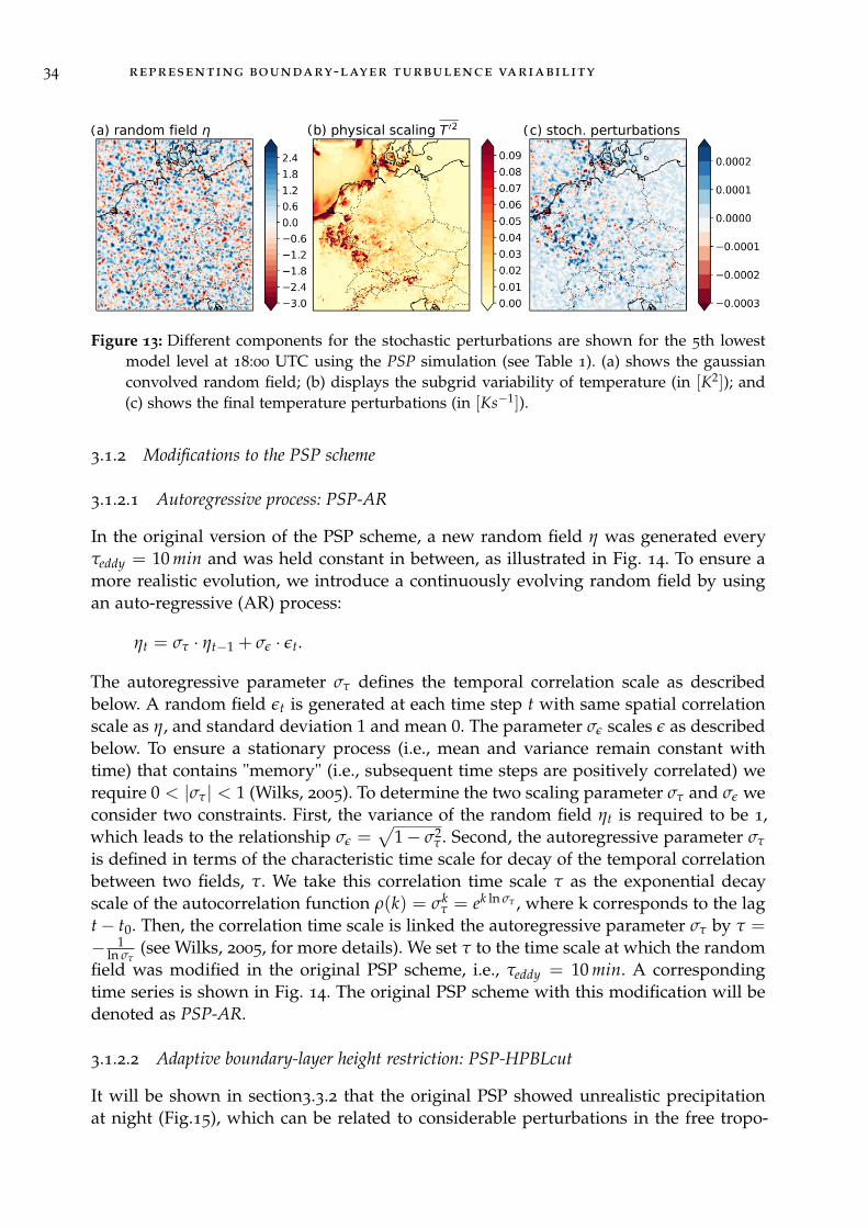
34 representing boundary-layer turbulence variability

Figure 13: Different components for the stochastic perturbations are shown for the 5th lowestmodel level at 18:00 UTC using the PSP simulation (see Table 1). (a) shows the gaussianconvolved random field; (b) displays the subgrid variability of temperature (in [K2]); and(c) shows the final temperature perturbations (in [Ks−1]).

3.1.2 Modifications to the PSP scheme

3.1.2.1 Autoregressive process: PSP-AR

In the original version of the PSP scheme, a new random field η was generated everyτeddy = 10 min and was held constant in between, as illustrated in Fig. 14. To ensure amore realistic evolution, we introduce a continuously evolving random field by usingan auto-regressive (AR) process:

ηt = στ · ηt−1 + σε · εt.

The autoregressive parameter στ defines the temporal correlation scale as describedbelow. A random field εt is generated at each time step t with same spatial correlationscale as η, and standard deviation 1 and mean 0. The parameter σε scales ε as describedbelow. To ensure a stationary process (i.e., mean and variance remain constant withtime) that contains "memory" (i.e., subsequent time steps are positively correlated) werequire 0 < |στ| < 1 (Wilks, 2005). To determine the two scaling parameter στ and σε weconsider two constraints. First, the variance of the random field ηt is required to be 1,which leads to the relationship σε =

√1− σ2

τ . Second, the autoregressive parameter στ

is defined in terms of the characteristic time scale for decay of the temporal correlationbetween two fields, τ. We take this correlation time scale τ as the exponential decayscale of the autocorrelation function ρ(k) = σk

τ = ek ln στ , where k corresponds to the lagt− t0. Then, the correlation time scale is linked the autoregressive parameter στ by τ =− 1

ln στ(see Wilks, 2005, for more details). We set τ to the time scale at which the random

field was modified in the original PSP scheme, i.e., τeddy = 10 min. A correspondingtime series is shown in Fig. 14. The original PSP scheme with this modification will bedenoted as PSP-AR.

3.1.2.2 Adaptive boundary-layer height restriction: PSP-HPBLcut

It will be shown in section3.3.2 that the original PSP showed unrealistic precipitationat night (Fig.15), which can be related to considerable perturbations in the free tropo-

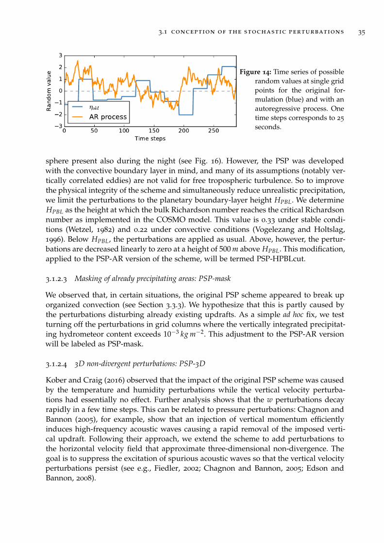
3.1 conception of the stochastic perturbations 35

Figure 14: Time series of possiblerandom values at single gridpoints for the original for-mulation (blue) and with anautoregressive process. Onetime steps corresponds to 25

seconds.

sphere present also during the night (see Fig. 16). However, the PSP was developedwith the convective boundary layer in mind, and many of its assumptions (notably ver-tically correlated eddies) are not valid for free tropospheric turbulence. So to improvethe physical integrity of the scheme and simultaneously reduce unrealistic precipitation,we limit the perturbations to the planetary boundary-layer height HPBL. We determineHPBL as the height at which the bulk Richardson number reaches the critical Richardsonnumber as implemented in the COSMO model. This value is 0.33 under stable condi-tions (Wetzel, 1982) and 0.22 under convective conditions (Vogelezang and Holtslag,1996). Below HPBL, the perturbations are applied as usual. Above, however, the pertur-bations are decreased linearly to zero at a height of 500 m above HPBL. This modification,applied to the PSP-AR version of the scheme, will be termed PSP-HPBLcut.

3.1.2.3 Masking of already precipitating areas: PSP-mask

We observed that, in certain situations, the original PSP scheme appeared to break uporganized convection (see Section 3.3.3). We hypothesize that this is partly caused bythe perturbations disturbing already existing updrafts. As a simple ad hoc fix, we testturning off the perturbations in grid columns where the vertically integrated precipitat-ing hydrometeor content exceeds 10−3 kg m−2. This adjustment to the PSP-AR versionwill be labeled as PSP-mask.

3.1.2.4 3D non-divergent perturbations: PSP-3D

Kober and Craig (2016) observed that the impact of the original PSP scheme was causedby the temperature and humidity perturbations while the vertical velocity perturba-tions had essentially no effect. Further analysis shows that the w perturbations decayrapidly in a few time steps. This can be related to pressure perturbations: Chagnon andBannon (2005), for example, show that an injection of vertical momentum efficientlyinduces high-frequency acoustic waves causing a rapid removal of the imposed verti-cal updraft. Following their approach, we extend the scheme to add perturbations tothe horizontal velocity field that approximate three-dimensional non-divergence. Thegoal is to suppress the excitation of spurious acoustic waves so that the vertical velocityperturbations persist (see e.g., Fiedler, 2002; Chagnon and Bannon, 2005; Edson andBannon, 2008).

36 representing boundary-layer turbulence variability

Non-divergence is given by:

∇ ·~v =∂u∂x

+∂v∂y

+∂w∂z

= 0.

We neglect modifications due to the terrain following vertical coordinate system of theCOSMO-model and the metrical terms due to the spherical earth as well as compress-ibility. Neglecting the distortion to the grid due to these effects greatly simplifies thecomputation, but implies that the resulting wind perturbations will not be exactly non-divergent, and some perturbation energy will be lost to acoustic waves. However, thislost perturbation energy will be small in comparison to the lost perturbation energyof the original PSP scheme, where the wind perturbation was entirely divergent, andalmost all the energy was rapidly dissipated. The COSMO-model employs a rotatedspherical coordinate system with earth radius R, rotated longitude λ and latitude φ,so that ∂x = R cos φ∂λ and ∂y = R∂φ. Due to the rotated coordinate system and thecomparably small domain, we neglect the trigonometric terms for simplicity.

This results in the following approximate non-divergence criterion for the PSP setup:

−R · ∂w∂z

=

[∂u∂λ

+∂v∂φ

](4)

We define the horizontal perturbations by the velocity potential χ: ~vh = ∇χ. Con-sequently, the horizontal perturbations are non-rotational, which is in accordance withthe incentive of the perturbations.

Computing the divergence of ~vh and substituting in equation 4 we obtain the follow-ing Poisson equation:

−R2 · ∂w∂z

=

[∂2χ

∂λ2 +∂2χ

∂φ2

](5)

For a vertical velocity perturbation (increment) given by eq. 3 we derive u and v per-turbations by solving (5) for the corresponding perturbation of χ. A finite-differenceapproximation is obtained by replacing the Laplace operator with a five-point-stencilLaplace matrix.

To avoid large vertical velocity gradients ∂w∂z near the lower boundary, we linearly

increase w perturbations from 0 at the surface to the original value at z0. We chosez0 = 500 m to include a sufficient number of vertical model levels while ensuring thatthe full perturbation amplitude is active at the height of the daytime inversion, wherewe expect the perturbations to be most effective.

Applying these balanced wind perturbations to PSP-AR will be denoted as PSP-3D.

3.2 strategy for evaluating the impact of the psp modifications

To evaluate the impact of the PSP variants, we compute several simulations with differ-ent setups of the COSMO model. We investigate each modification of PSP individuallyon one day with weak synoptic forcing of convection, 6 June 2016. For comparison, weuse 30 May, 2016 as an example of a strong forcing day with synoptically driven, co-herent precipitation. Based on these results, we decide on a suitable configuration for a

3.3 results 37

01 04 07 10 13 16 19 22 01Time [HH UTC]

0.0

0.1

0.2

Preci

pitation [

mm

/h]

RadarReferencePSP, 0

PSP-AR, 0

PSP-HPBLcut, 0

PSP-mask, 0

PSP, 0

PSP-AR, 0 PSP-HPBLcut, 0 PSP-mask, 0

(a) (b)

Figure 15: (a) Hourly accumulated domain-mean precipitation for 6 June 2016. The domain-mean is computed only for the region of available radar data. (b) Snapshots of hourlyprecipitation accumulation at 1500 UTC on 6 June 2016. Grey shading indicates missingradar data. The different experiments are listed in Table 1 (The perturbed simulationsshown were computed using α0 = 7.2).

revised PSP version, PSP2, and compute 10 subsequent days with total simulation timeof 24h to confirm our findings. See Table 1 for an overview of the experiments. Detailson COSMO, the selected days, the used radar observations and verification metrics canbe found in Chapter 2.

Table 1: Overview of the considered experiments and corresponding model settings.

Pert. variables

Exp. name T, qv w u-v rand. field αtuning Description

PSP yes yes no const. for τ α0 = 7.2 As in Kober and Craig (2016)

PSP-AR yes yes no AR α0 = 7.2, α1 = 2 Auto-regressive random field

PSP-HPBLcut yes yes no AR α0 = 7.2 Pert. go to zero above BL height

PSP-mask yes yes no AR α0 = 7.2 No pert. in precipitating columns

PSP-AR Tqv yes no no AR α1 = 2 Only pert. to thermodynamic variables

PSP-3D w no yes yes AR α1 = 2 Only 3D non-divergent wind pert.

PSP-3D all yes yes yes AR α1 = 2 Pert. to all fields

PSP2 yes yes yes AR α f inal = 1.5 Comb. modifications (3D all + HPBLcut)

3.3 results

3.3.1 Autoregressive Process in PSP-AR

To test the influence of the AR random field, we focus on 6 June, a weakly forced dayon which the perturbations are expected to have a large influence on the precipita-

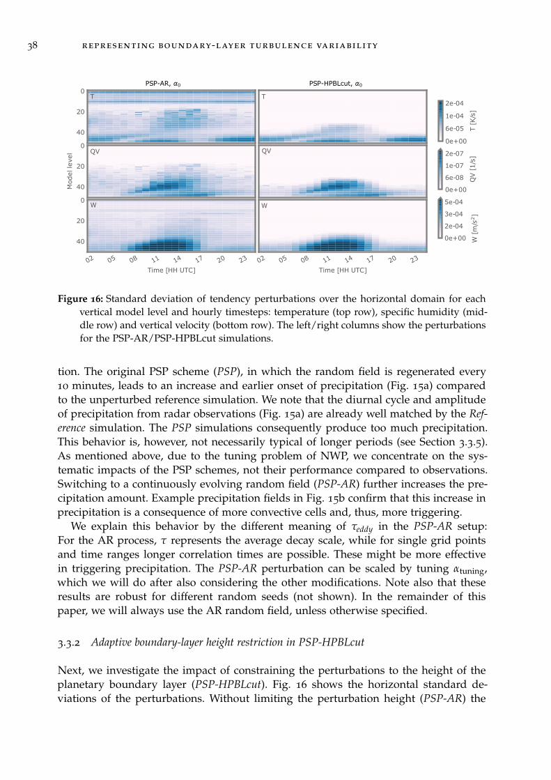
38 representing boundary-layer turbulence variability

0

20

40

PSP-AR, 0 PSP-HPBLcut, 0

time

0

20

40Model l

eve

l

time

02 05 08 11 14 17 20 23

Time [HH UTC]

0

20

40

02 05 08 11 14 17 20 23

Time [HH UTC]

0e+00

6e-05

1e-04

2e-04

T [

K/s

]

TT

0e+00

6e-08

1e-07

2e-07

QV [

1/s

]

QV QV

0e+00

2e-04

3e-04

5e-04

W [

m/s

2]

W W

Figure 16: Standard deviation of tendency perturbations over the horizontal domain for eachvertical model level and hourly timesteps: temperature (top row), specific humidity (mid-dle row) and vertical velocity (bottom row). The left/right columns show the perturbationsfor the PSP-AR/PSP-HPBLcut simulations.

tion. The original PSP scheme (PSP), in which the random field is regenerated every10 minutes, leads to an increase and earlier onset of precipitation (Fig. 15a) comparedto the unperturbed reference simulation. We note that the diurnal cycle and amplitudeof precipitation from radar observations (Fig. 15a) are already well matched by the Ref-erence simulation. The PSP simulations consequently produce too much precipitation.This behavior is, however, not necessarily typical of longer periods (see Section 3.3.5).As mentioned above, due to the tuning problem of NWP, we concentrate on the sys-tematic impacts of the PSP schemes, not their performance compared to observations.Switching to a continuously evolving random field (PSP-AR) further increases the pre-cipitation amount. Example precipitation fields in Fig. 15b confirm that this increase inprecipitation is a consequence of more convective cells and, thus, more triggering.

We explain this behavior by the different meaning of τeddy in the PSP-AR setup:For the AR process, τ represents the average decay scale, while for single grid pointsand time ranges longer correlation times are possible. These might be more effectivein triggering precipitation. The PSP-AR perturbation can be scaled by tuning αtuning,which we will do after also considering the other modifications. Note also that theseresults are robust for different random seeds (not shown). In the remainder of thispaper, we will always use the AR random field, unless otherwise specified.

3.3.2 Adaptive boundary-layer height restriction in PSP-HPBLcut

Next, we investigate the impact of constraining the perturbations to the height of theplanetary boundary layer (PSP-HPBLcut). Fig. 16 shows the horizontal standard de-viations of the perturbations. Without limiting the perturbation height (PSP-AR) the

3.3 results 39

01 04 07 10 13 16 19 22 01Time [HH UTC]

0.2

0.4

0.6

Preci

pitat

ion [m

m/h

]RadarReferencePSP-AR, 0

PSP-mask, 0

PSP2, 1

PSP2, 0.75 1PSP-AR, 0

PSP-mask, 0 PSP2, 1 PSP2, 0.75 1

(a) (c)

(b)

01 04 07 10 13 16 19 22 01Time [HH UTC]

1.0

0.5

0.0

0.5

S: Str

uct

ure

Figure 17: Illustrating the impact of precipitation mask: time evolution for the 30 May 2016

for (a) domain averaged precipitation and (b) structure component of SAL. (c) Exampleprecipitation fields for 30 May 2016, 08 UTC.

perturbations are largest in the boundary layer, but significant perturbations in themid-troposphere are present as well. As discussed above, this is conceptually inconsis-tent with the rationale of the PSP scheme. Limiting the height in HPBLcut removes thisinconsistency. This modification leads to a decrease in the total precipitation amountand, most importantly, removes the precipitation peak at night (Fig. 15a).

3.3.3 Masking of already precipitating areas in PSP-mask

In the original and the PSP-AR scheme, we observed a breaking up of larger-scale pre-cipitation structures. An example for this can be seen on 30 May (Fig. 17c), a stronglyforced convective day. A coherent, synoptically-driven precipitation structure is presentover Western Germany and Belgium, which is well reproduced by the reference sim-ulation. Adding the PSP-AR perturbations breaks up this structure into many smallerconvective cells. Turning off the perturbations in precipitating columns, PSP-mask cor-rects this problem but also reduces the impact on weak forcing days (see Fig. 15). Atoo-small threshold for precipitating hydrometeors can be responsible for switching offthe perturbations before deep convection has developed.

A quantitative measure for the structure of the precipitation field is the S(tructure)component of the SAL score (Wernli et al., 2008) displayed in Fig. 17 b. Negative S valuesimply that the simulated precipitation cells are too small and peaked compared to theradar observations, while S = 0 suggests a perfect match in terms of structure (see 2.4.2for details). During the morning hours on 30 June, when the synoptic structure is mostsalient, the PSP-AR simulations show a clear reduction of the S score, indicating smallercells. The precipitation mask reverts the structure back to its original value.

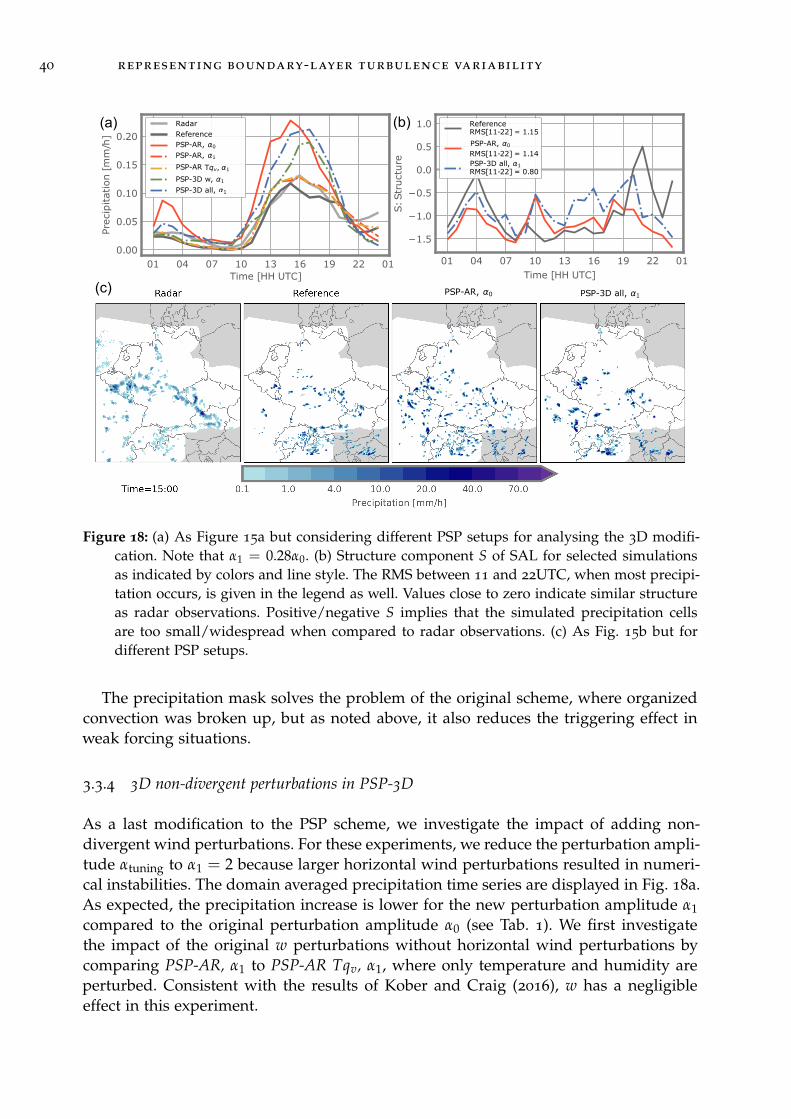
40 representing boundary-layer turbulence variability

01 04 07 10 13 16 19 22 01Time [HH UTC]

0.00

0.05

0.10

0.15

0.20

Preci

pitation [

mm

/h]

RadarReferencePSP-AR, 0

Tqv, 1

PSP-3D w, 1

PSP-3D all, 1

01 04 07 10 13 16 19 22 01Time [HH UTC]

1.5

1.0

0.5

0.0

0.5

1.0

S: Str

uct

ure

ReferenceRMS[11-22] = 1.15

RMS[11-22] = 1.14

RMS[11-22] = 0.80PSP-3D all, 1

PSP-3D all, 1

(a)PSP-AR, 0

PSP-AR, 0

PSP-AR, 1

PSP-AR

(b)

(c)

Figure 18: (a) As Figure 15a but considering different PSP setups for analysing the 3D modifi-cation. Note that α1 = 0.28α0. (b) Structure component S of SAL for selected simulationsas indicated by colors and line style. The RMS between 11 and 22UTC, when most precipi-tation occurs, is given in the legend as well. Values close to zero indicate similar structureas radar observations. Positive/negative S implies that the simulated precipitation cellsare too small/widespread when compared to radar observations. (c) As Fig. 15b but fordifferent PSP setups.

The precipitation mask solves the problem of the original scheme, where organizedconvection was broken up, but as noted above, it also reduces the triggering effect inweak forcing situations.

3.3.4 3D non-divergent perturbations in PSP-3D

As a last modification to the PSP scheme, we investigate the impact of adding non-divergent wind perturbations. For these experiments, we reduce the perturbation ampli-tude αtuning to α1 = 2 because larger horizontal wind perturbations resulted in numeri-cal instabilities. The domain averaged precipitation time series are displayed in Fig. 18a.As expected, the precipitation increase is lower for the new perturbation amplitude α1compared to the original perturbation amplitude α0 (see Tab. 1). We first investigatethe impact of the original w perturbations without horizontal wind perturbations bycomparing PSP-AR, α1 to PSP-AR Tqv, α1, where only temperature and humidity areperturbed. Consistent with the results of Kober and Craig (2016), w has a negligibleeffect in this experiment.

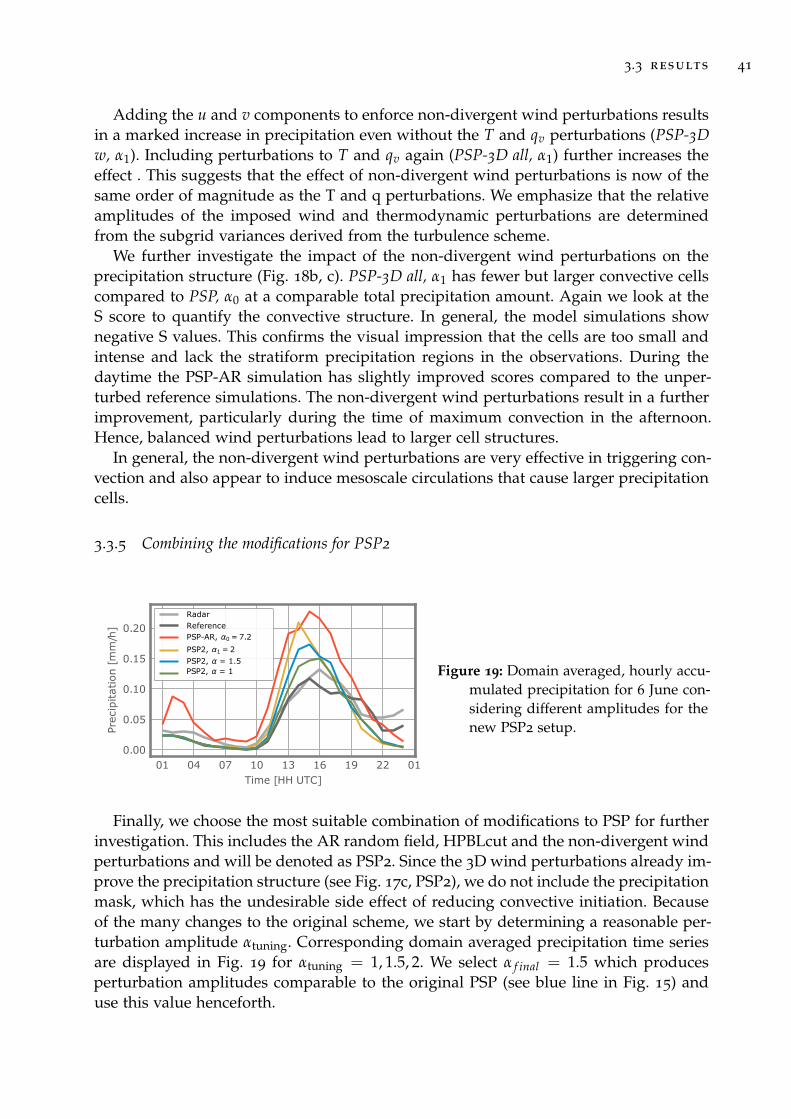
3.3 results 41

Adding the u and v components to enforce non-divergent wind perturbations resultsin a marked increase in precipitation even without the T and qv perturbations (PSP-3Dw, α1). Including perturbations to T and qv again (PSP-3D all, α1) further increases theeffect . This suggests that the effect of non-divergent wind perturbations is now of thesame order of magnitude as the T and q perturbations. We emphasize that the relativeamplitudes of the imposed wind and thermodynamic perturbations are determinedfrom the subgrid variances derived from the turbulence scheme.

We further investigate the impact of the non-divergent wind perturbations on theprecipitation structure (Fig. 18b, c). PSP-3D all, α1 has fewer but larger convective cellscompared to PSP, α0 at a comparable total precipitation amount. Again we look at theS score to quantify the convective structure. In general, the model simulations shownegative S values. This confirms the visual impression that the cells are too small andintense and lack the stratiform precipitation regions in the observations. During thedaytime the PSP-AR simulation has slightly improved scores compared to the unper-turbed reference simulations. The non-divergent wind perturbations result in a furtherimprovement, particularly during the time of maximum convection in the afternoon.Hence, balanced wind perturbations lead to larger cell structures.

In general, the non-divergent wind perturbations are very effective in triggering con-vection and also appear to induce mesoscale circulations that cause larger precipitationcells.

3.3.5 Combining the modifications for PSP2

01 04 07 10 13 16 19 22 01Time [HH UTC]

0.00

0.05

0.10

0.15

0.20

Preci

pitation [

mm

/h]

RadarReferencePSP-AR, 0 = 7.2

PSP2, 1 = 2PSP2, = 1.5PSP2, = 1 Figure 19: Domain averaged, hourly accu-

mulated precipitation for 6 June con-sidering different amplitudes for thenew PSP2 setup.

Finally, we choose the most suitable combination of modifications to PSP for furtherinvestigation. This includes the AR random field, HPBLcut and the non-divergent windperturbations and will be denoted as PSP2. Since the 3D wind perturbations already im-prove the precipitation structure (see Fig. 17c, PSP2), we do not include the precipitationmask, which has the undesirable side effect of reducing convective initiation. Becauseof the many changes to the original scheme, we start by determining a reasonable per-turbation amplitude αtuning. Corresponding domain averaged precipitation time seriesare displayed in Fig. 19 for αtuning = 1, 1.5, 2. We select α f inal = 1.5 which producesperturbation amplitudes comparable to the original PSP (see blue line in Fig. 15) anduse this value henceforth.

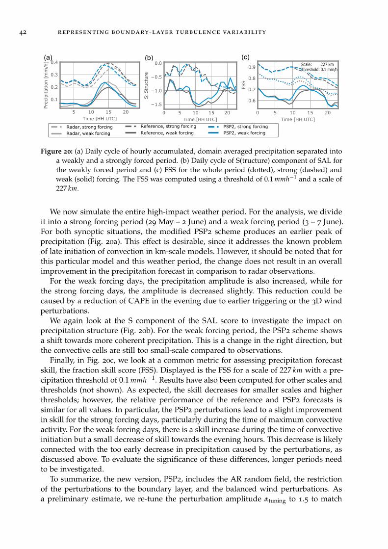
42 representing boundary-layer turbulence variability

(b) (c)

5 10 15 20Time [HH UTC]

0.1

0.2

0.3

0.4

Preci

pitat

ion [m

m/h

]

Radar, strong forcingRadar, weak forcing

Reference, strong forcingReference, weak forcing

PSP2, strong forcingPSP2, weak forcing

0 5 10 15 20Time [HH UTC]

0.6

0.7

0.8

0.9

FSS

Scale: 227 kmThreshold: 0.1 mm/h

(a)

0 5 10 15 20Time [HH UTC]

1.5

1.0

0.5

0.0

S: Str

uct

ure

Figure 20: (a) Daily cycle of hourly accumulated, domain averaged precipitation separated intoa weakly and a strongly forced period. (b) Daily cycle of S(tructure) component of SAL forthe weakly forced period and (c) FSS for the whole period (dotted), strong (dashed) andweak (solid) forcing. The FSS was computed using a threshold of 0.1 mmh−1 and a scale of227 km.

We now simulate the entire high-impact weather period. For the analysis, we divideit into a strong forcing period (29 May – 2 June) and a weak forcing period (3 – 7 June).For both synoptic situations, the modified PSP2 scheme produces an earlier peak ofprecipitation (Fig. 20a). This effect is desirable, since it addresses the known problemof late initiation of convection in km-scale models. However, it should be noted that forthis particular model and this weather period, the change does not result in an overallimprovement in the precipitation forecast in comparison to radar observations.

For the weak forcing days, the precipitation amplitude is also increased, while forthe strong forcing days, the amplitude is decreased slightly. This reduction could becaused by a reduction of CAPE in the evening due to earlier triggering or the 3D windperturbations.

We again look at the S component of the SAL score to investigate the impact onprecipitation structure (Fig. 20b). For the weak forcing period, the PSP2 scheme showsa shift towards more coherent precipitation. This is a change in the right direction, butthe convective cells are still too small-scale compared to observations.

Finally, in Fig. 20c, we look at a common metric for assessing precipitation forecastskill, the fraction skill score (FSS). Displayed is the FSS for a scale of 227 km with a pre-cipitation threshold of 0.1 mmh−1. Results have also been computed for other scales andthresholds (not shown). As expected, the skill decreases for smaller scales and higherthresholds; however, the relative performance of the reference and PSP2 forecasts issimilar for all values. In particular, the PSP2 perturbations lead to a slight improvementin skill for the strong forcing days, particularly during the time of maximum convectiveactivity. For the weak forcing days, there is a skill increase during the time of convectiveinitiation but a small decrease of skill towards the evening hours. This decrease is likelyconnected with the too early decrease in precipitation caused by the perturbations, asdiscussed above. To evaluate the significance of these differences, longer periods needto be investigated.

To summarize, the new version, PSP2, includes the AR random field, the restrictionof the perturbations to the boundary layer, and the balanced wind perturbations. Asa preliminary estimate, we re-tune the perturbation amplitude αtuning to 1.5 to match

3.4 summary and discussion 43

the precipitation amplitude of the original PSP scheme. For operational use, this choicewould have to be revisited to produce the best overall precipitation forecast over along test period. Although a clear overall improvement in forecast skill scores was notdemonstrated in the preliminary evaluation here, the specific impacts of the changesto the scheme were as expected. In particular, PSP2 maintains the desired effect of theoriginal PSP scheme, namely an earlier peak and increased amplitude of convectionprecipitation in weak forcing situations, while several drawbacks have been eliminated.In addition, it improves the cell structure and the spatial forecast skill compared to theunperturbed simulation.

3.4 summary and discussion

Four concerns of the original PSP scheme were addressed and corrected by modifyingdifferent aspects of the original PSP scheme:

1. The autoregressive process in PSP-AR generates a physically more realistic, con-tinuous evolution of the random field and hence refines the concept of the scheme.The performance is qualitatively comparable to the original PSP.

2. In PSP-HPBLcut, we constrain vertically correlated perturbations to the boundarylayer in accordance with the vertical extent of boundary-layer eddies. This re-moves perturbations in the free troposphere that resulted in spurious night timeprecipitation.

3. By excluding perturbations in precipitating regions in PSP-mask, we are able toreestablish organized convective structures. However, we decided not to includethe PSP-mask adjustments in the revised PSP2 version for two reasons: first, theother modifications improved the break-up of organized structures already; sec-ond, this ad hoc fix has the undesirable side effect of reducing convective initiationoverall.

4. In PSP-3D, we included 3D non-divergent wind perturbations to prevent the rapiddissipation of vertical velocity perturbations. Interestingly, these consistent windperturbations are at least as effective as the T and qv perturbations in triggeringconvection. The relative importance of buoyant and mechanical lifting in initiatingconvective updrafts in nature is still unknown. Both processes were found by Torriet al. (2015) to play a role in secondary initiation by cold pools. It also appearsthat the cell structures in the simulations with non-divergent wind perturbationswere more comparable to radar observations. The relationship between triggeringprocesses and the resulting convective structures is an important topic for futureresearch.

We combined the first, second and fourth modification to define the PSP2 schemeand selected a tuning parameter of αtuning = 1.5 to match the precipitation amplitudeof the original PSP. The optimal value of the tuning parameter is of order one, whichis an encouraging sign that our physical reasoning is appropriate. By evaluating PSP2

on a longer time period, we find its behavior well in accordance with the rationale of

44 representing boundary-layer turbulence variability

the original scheme: when synoptic forcing is weak, we observe a small shift in thediurnal cycle and an increase in total precipitation amplitude; this could counteractlong-standing biases in current NWP systems (Baldauf et al., 2011; Clark et al., 2016).During strongly forced episodes or at night, the scheme has only a small impact.

In addition to the systematic impact of the PSP scheme on convective initiation, stud-ies have also demonstrated its ability to increase ensemble spread (Rasp et al., 2018b;Keil et al., 2019). This has the potential to help reduce the under-dispersion in manycurrent convective-scale ensemble forecasting and data assimilation systems (see, e.g.,Berner et al., 2017; Ollinaho et al., 2017). Direct radar assimilation might benefit espe-cially from such a perturbation scheme where sufficient spread in the first guess ensem-ble is particularly necessary. One remaining, undesired effect of the PSP2 scheme is adecrease of precipitation towards the evening. We note that this has also been identifiedfor the original PSP by Rasp et al. (2018b), who related this to a lack of convective or-ganization. The organization of convection is caused by processes other than the onesaddressed with the PSP2 scheme, most notably cold pools. A better representation ofthese features and their ability to trigger new convection might be necessary to captureorganized evening convection. This will be addressed in in Chapter 5 and 6.

Overall, we conclude the PSP revisions by recommending PSP2 instead of the origi-nal PSP: PSP2 contains comparable advantages as the PSP while being physically moreconsistent.

4R E P R E S E N T I N G L I F T I N G B Y S U B G R I D - S C A L E O R O G R A P H Y

In this chapter, we address the influence of subgrid-scale orography (SSO) on triggeringconvection as a complementary process to turbulence. As described in the introduction(Sec. 1.3.3), the importance of orography on convective initiation is unquestioned. Manydifferent mechanisms contribute to orographic convection, including thermally drivenslope winds or mechanical lifting, but specific details are less understood. In addition,the relevance of small scale orography, as a proxy for subgrid-scale orography in km-scale models, has not been universally quantified (Tucker and Crook, 2005; Kirshbaumet al., 2007b,a; Langhans et al., 2011; Schneider et al., 2018). Nonetheless, Kirshbaum et al.(2018) emphasize the need to account for SSO in convection parameterizations and fordeveloping scale-aware parameterizations in the mountain grey zone. This is furthermotivated, as SSO can potentially act as a source of predictability (Bachmann et al.,2019, 2020). While most NWP models include some form of parameterization for SSO,vertical motion responsible for triggering convection by SSO, however, is not addressedin these parameterizations (see Sec. 1.3.3).

Consequently, we propose stochastic perturbations to account for convective initia-tion by subgrid-scale orography. We will name it the SSOSP scheme. We focus on theeffects of mechanical lifting and the resulting gravity waves. This process is chosen asthe most direct effect of orography among those mentioned in Sec. 1.3.3: the flow over amountain causes an upward displacement of the air parcels, i.e., a vertical velocity per-turbation, which may decay with height, or propagate as gravity wave away from thesource, depending on the stratification of the atmosphere. The upward displacementmay cause the parcels to reach their level of free convection (LFC) and thereby initiatedeep convective updrafts. See Fig. 21 for an illustration.

The new scheme closely follows the formulation of the PSP scheme: vertical velocitytendencies are randomly perturbed with an amplitude that scales with theoretical grav-ity waves excited by SSO, and horizontal wind fields are accordingly perturbed to yield3D non-divergence, as illustrated in Fig. 21. We present a considerably revised schemeof one already developed by Brundke (2015) as part of his Master thesis.

Investigating the impact of this scheme will further allow us to estimate the impor-tance of SSO for convective initiation, thereby contributing to the discussion mentionedin the introduction.

We will first introduce the concept of the SSOSP scheme in Sec. 4.1. Then, in Sec. 4.2,we will explain the model simulations to evaluate the scheme. The corresponding re-sults are presented in Sec. 4.3, followed by a summary and discussion in Sec. 4.4.

45

46 representing lifting by subgrid-scale orography

Figure 21: Schematic illustration of the SSOSP scheme. The left box illustrates the physical pro-cess of mechanical lifting by subgrid-scale orography. The right box shows, how this pro-cess is parameterized with SSOSP.

4.1 formulation of the parameterization

4.1.1 The SSOSP scheme

Inspired by the PSP scheme, we introduce stochastic vertical velocity perturbations thatscale with the amplitude of the SSO lifting and the induced gravity waves. The horizon-tal wind is perturbed to approximate non-divergence, as described in Section 3.1.2.4.Since the errors in the estimation of the non-divergent wind perturbations are likelyto be largest over strong orography where the grid is most distorted, there will be anadditional source of noise in these regions. However, we were unable to identify anyobvious effects in the simulation results.

The tendency of vertical velocity w is perturbed according to

∂w∂t

∣∣∣∣sso

=αtuning

τ· η · w′. (6)

η(τη, σ) denotes a horizontally correlated AR random field as described in Sec. 3.1.2.1.Instead of τ = τeddy we assume that slower processes such as the synoptic wind fieldand the diurnal cycle dominate the evolution of orographically induced flow structures.Craig and Selz (2018) for example show that the time scales of gravity waves (even onscales of 1 km) can range from minutes to days. Since no single time scale stands out,we test several values, τ = 30 min, 2 h, 5 h. As for the PSP scheme, αtuning is a tuningparameter; ideally, O(1) if the physical scaling is appropriate.

The variable w′ represents the physical scaling of the perturbations. It depends onthe amplitude w0 (at given height) and vertical wavenumber m of a gravity wave in-duced by the SSO. This includes both propagating and decaying gravity waves andalso represents the effect of mechanical lifting. Both w0 and m are considered in termsof forced gravity waves as in Gill (1982) and approximated with available SSO infor-mation. Following Baines and Palmer (1990), the subgrid-scale orography for one gridbox of the COSMO model is represented by four parameters, namely θsso, γsso, σsso and

4.1 formulation of the parameterization 47

Figure 22: Four fields describing the subgrid-scale orography information. These are the stan-dard deviation µsso [m], the shape γsso, the orientation θsso and the slope σsso, and µsso.The data is derived from 30 m ASTER elevation data (Schättler et al., 2016).

µsso. They describe the orientation, shape, slope and standard deviation of the heightof the orography, respectively, and are displayed in Fig. 22. The specific formulationfor w0 and m in terms of horizontal wind speed, Brunt-Väisälä frequency N and SSOinformation is presented in the next two sections.

To avoid numerical instabilities near the surface, we decrease the perturbations lin-early to zero between zmax = 500 m and the surface. We further constrain the pertur-bations to the planetary boundary layer, where we assume triggering processes to bemost relevant: we impose an exponential decay of the perturbations at zmax that scales

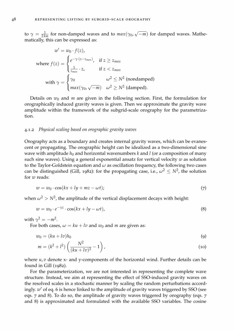
48 representing lifting by subgrid-scale orography

to γ = 12 km for non-damped waves and to max(γ0,

√−m) for damped waves. Mathe-

matically, this can be expressed as:

w′ = w0 · f (z),

where f (z) =

e−γ·(z−zmax), if z ≥ zmax

1zmax· z, if z < zmax

with γ =

γ0 ω2 ≤ N2 (nondamped)

max(γ0,√−m) ω2 ≥ N2 (damped).

Details on w0 and m are given in the following section. First, the formulation fororographically induced gravity waves is given. Then we approximate the gravity waveamplitude within the framework of the subgrid-scale orography for the parametriza-tion.

4.1.2 Physical scaling based on orographic gravity waves

Orography acts as a boundary and creates internal gravity waves, which can be evanes-cent or propagating. The orographic height can be idealized as a two-dimensional sinewave with amplitude h0 and horizontal wavenumbers k and l (or a composition of manysuch sine waves). Using a general exponential ansatz for vertical velocity w as solutionto the Taylor-Goldstein equation and ω as oscillation frequency, the following two casescan be distinguished (Gill, 1982): for the propagating case, i.e., ω2 ≤ N2, the solutionfor w reads:

w = w0 · cos(kx + ly + mz−ωt); (7)

when ω2 > N2, the amplitude of the vertical displacement decays with height:

w = w0 · e−γz · cos(kx + ly−ωt), (8)

with γ2 = −m2.For both cases, ω = ku + lv and w0 and m are given as:

w0 = (ku + lv)h0 (9)

m = (k2 + l2)

(N2

(ku + lv)2 − 1)

, (10)

where u, v denote x- and y-components of the horizontal wind. Further details can befound in Gill (1982).

For the parameterization, we are not interested in representing the complete wavestructure. Instead, we aim at representing the effect of SSO-induced gravity waves onthe resolved scales in a stochastic manner by scaling the random perturbations accord-ingly. w′ of eq. 6 is hence linked to the amplitude of gravity waves triggered by SSO (seeeqs. 7 and 8). To do so, the amplitude of gravity waves triggered by orography (eqs. 7

and 8) is approximated and formulated with the available SSO variables. The cosine

4.2 model simulations , observations and simulation period 49

terms in (7) and (8) are consequently neglected. w0 and m are formulated in terms ofSSO information. We specify the velocities u, v as u′, v′ in the rotated system of the SSO:

u′ = u · cos θsso + v · sin θsso

v′ = v · cos θsso − u · sin θsso.

The horizontal wave numbers k and l (in the rotated system of the SSO) are obtainedby using the semi-minor and semi-major axes a, b for the elliptical mountains that resultwhen the orography is represented by sine waves:

k =π

2a≈ π

2σsso

µsso

l =π

2b≈ π

2σssoγsso

µsso

(Lott and Miller, 1997). We set h0 to be µsso, implying that higher mountains will resultin larger vertical displacements.

Using these approximations, we can formulate the vertical wavenumber m and waveamplitude w0, given by (10) and (9), in the following way:

m2 = (1 + γ2sso) ·

(N2

(u′ + v′γsso)2 −π2σ2

sso4µ2

sso

),

w0 =π

2· σsso · (u′ + v′γsso).

w0 and m can now be used as physical scaling for the stochastic parameterization.

4.2 model simulations , observations and simulation period

As for the PSP scheme, we evaluate the impact of the SSOSP scheme by computing sev-eral simulations with different setups using the COSMO model as described in Chap-ter 2. We only consider 6 June 2016 as a day with weak synoptic forcing (see Chapter 2).First, we test several settings of the SSOSP scheme, namely the impact of the correlationtime scale τ and the perturbation amplitude αre f , where αre f =

αtuning·2hτ . This re-scales

the final perturbation amplitude for different values of τ with respect to a referencetimescale τre f = 2 h. We identify the most appropriate setting and compute an ensem-ble simulation with 10 members, where different random seeds of the random field η

are used.To see the effects of the orography more clearly, we analyze orographic and flat grid

points separately by defining orographic/flat grid points as gridpoints where the SSOstandard deviation µsso is larger/lower than 20 m. This threshold approximately coin-cides with the median of SSO-std height. Separating Southern and Northern Germanyor the Alpine region instead of single grid points showed similar results.

4.3 simulation results

First, we investigate the impact on the precipitation amount for different values ofthe correlation time scale τ and perturbation amplitude αre f . Corresponding domain

50 representing lifting by subgrid-scale orography

01 04 07 10 13 16 19 22 01Time [HH UTC]

0.0

0.1

0.2

0.3

0.4Pr

eci

pitation [

mm

/h]

RadarReference

= 30min, ref= 0.18

= 2h, ref= 0.18

= 5h, ref= 0.18

= 30min, ref= 0.42

= 2h, ref= 0.42

= 5h, ref= 0.42

= 30min, ref= 0.60

= 2h, ref= 0.60

= 5h, ref= 0.60

(a)

01 04 07 10 13 16 19 22 01Time [HH UTC]

0.00

0.02

0.04

0.06

0.08

0.10

Preci

pitation [

mm

/h]

(b)

Figure 23: Domain averaged, hourly accumulated precipitation for a several different SSOSPsettings. Left figure shows precipitation averaged over all grid points, that have a SSO-std≥ 20 m, the right figure summarizes grid points with SSO-std< 20 m.

averaged precipitation is displayed in Fig. 23. For orographic grid points increasing αre ffrom 0.18 to 0.42 leads to more precipitation but, counter-intuitively, a further increaseof αre f causes a reduction in the precipitation amount. Interestingly, flat grid points onlyexperience a reduction with increased αre f . One hypothesis for this decrease is that theperturbations enhance the mixing of boundary-layer and free tropospheric air, reducinginstability, and leading to a reduction in precipitation. Monotonically increasing τ leadsto more precipitation. More slowly evolving perturbations allow stronger updrafts todevelop. These stronger updrafts cause an increased probability of convective initiation.

For maximum impact we chose αre f = 0.42 and τ = 5 h for further ensemble ex-periments with 10 members. The domain averaged precipitation time series in Fig. 24

shows reasonable spread between ensemble members for both orographic and flat gridpoints. This spread is comparable to the spread generated by the original PSP scheme(see Kober and Craig (2016), Fig. 7d). While spread over orographic regions is desired,further insight is necessary to understand the behavior over flat grid points. Moreover,the behavior of individual ensemble members suggests a significant increase in precip-itation over orographic grid points and a decrease over flat grid points. This is furtherillustrated in Fig. 24 where ensemble precipitation fields are displayed for two timesteps: precipitation within the SSOSP scheme mainly occurs in the alpine region whilemost parts of Germany are precipitation free.

Overall, the SSOSP scheme shows a non-monotonic dependence on perturbationamplitude αre f , while increasing the correlation time scale τ appears to give increasingprecipitation over orographic regions. For flat regions, however, the scheme causes anundesired reduction of precipitation.

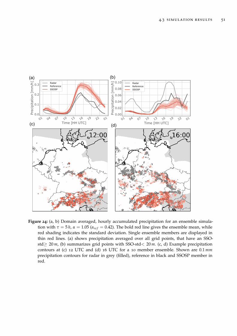
4.3 simulation results 51

01 04 07 10 13 16 19 22 01

Time [HH UTC]

0.0

0.1

0.2

0.3

Preci

pitation [

mm

/h]

RadarReferenceSSOSP

01 04 07 10 13 16 19 22 01

Time [HH UTC]

0.00

0.02

0.04

0.06

0.08

0.10

Preci

pitation [

mm

/h]

RadarReferenceSSOSP

(a) (b)

(c) (d)

Figure 24: (a, b) Domain averaged, hourly accumulated precipitation for an ensemble simula-tion with τ = 5 h, α = 1.05 (αre f = 0.42). The bold red line gives the ensemble mean, whilered shading indicates the standard deviation. Single ensemble members are displayed inthin red lines. (a) shows precipitation averaged over all grid points, that have an SSO-std≥ 20 m, (b) summarizes grid points with SSO-std< 20 m. (c, d) Example precipitationcontours at (c) 12 UTC and (d) 16 UTC for a 10 member ensemble. Shown are 0.1 mmprecipitation contours for radar in grey (filled), reference in black and SSOSP member inred.

52 representing lifting by subgrid-scale orography

4.4 summary and discussion

We have developed SSOSP, a scheme to account for subgrid-scale orography and itsimpact on convective initiation. Doing so, we consider mechanical lifting by SSO takinginto account the stratification of the atmosphere. Again, reasonable values of the tuningparameter αtuning are of order one, supporting our physical reasoning.

The impact of the SSOSP on precipitation is not clear-cut. While we observe a pre-cipitation increase over orographic regions, the scheme also leads to a reduction ofprecipitation over flat terrain. Furthermore, there is a non-monotonic relationship be-tween the perturbation amplitude and the precipitation amount, which may be relatedto a combination of mechanical triggering and a mixing-induced reduction of CAPE.An ensemble simulation with SSOSP showed that spread over orographic terrain isgenerated but also over flat regions, which is conceptually not desired.

This behavior of the SSOSP makes it hard to employ. Furthermore, the impacts arenot clearly complementary to those of PSP2: the precipitation impact of SSOSP is ei-ther too weak or coupled with an undesired impact on flat regions, and the generationof ensemble spread by SSOSP can also be achieved with PSP2. For these reasons, werefrained from combining the SSOSP perturbations and the PSP2 configuration. Concep-tually, however, schemes for different subgrid-scale processes could easily be combined.

In the introduction, we referred to the open question of whether small-scale orog-raphy matters for convective initiation. Here we tested this by modeling subgrid-scalemechanical lifting on the smallest resolved scale. Our results suggest that the subgrid-scale orographic triggering effect most likely is not that relevant. On the one hand,to see the desired effect in mountainous regions, we had to increase the perturbationstrength to a point where unwanted effects occurred over flat terrain. On the other hand,the perturbations introduced by our scheme are active on the smallest resolved scales ofthe km-scale model. Actual small-scale orography perturbations would be even smaller,and therefore likely even less influential. In general, our results confirm in a realisticsetup, what has been observed in other studies (Tucker and Crook, 2005; Kirshbaumet al., 2007b; Langhans et al., 2013; Schneider et al., 2018): conceptually, SSO may be rele-vant in regions of insignificant resolved orography; yet due to the fractal, scale-invariantstructure of orography (Turcotte, 1987) regions of high subgrid-scale orographic varia-tions are generally also regions of high grid-scale orography. This larger scale, resolvedorography may dominate the triggering of convection so that SSO is virtually irrelevantfor convective initiation.

5C O L D P O O L D R I V E N C O N V E C T I V E I N I T I AT I O N ( I ) : W H AT A R EC O N V E C T I O N - P E R M I T T I N G M O D E L S M I S S I N G ?

Now we focus on the role of cold pools in driving convective initiation and their rep-resentation in convection-permitting models. As introduced in Sec. 1.3.4, cold poolsarise from evaporation in precipitating downdrafts and spread as density currents atthe surface. Their gust fronts have the potential to trigger new convection mostly in thevicinity of already existing convection. Such secondary convective initiation can lead tothe organization of convection, but also may be a pronounced trigger mechanism in thelate afternoon and thereby contribute to the diurnal cycle of convection.

The difficulty of capturing the diurnal cycle of convection has been documented in avariety of km-scale models (Baldauf et al., 2011; Hanley et al., 2015; Clark et al., 2016). Incontrast to convection-parameterized models, where convection occurs too early duringthe day (Leutwyler et al., 2017), convection in convection-permitting models starts toolate during the day (Baldauf et al., 2011; Clark et al., 2016). This error can be improvedby tuning the model, e.g., with the turbulent mixing length, but at the expense ofother biases (Baldauf et al., 2011; Schraff et al., 2016; Leutwyler et al., 2017). By usinga more physically based approach, the PSP/PSP2 scheme (see Chapter 3), we wereable to improve the onset of convection using stochastic perturbations to account forboundary-layer turbulence (see Chapter 3). However, a lack of precipitation in the lateafternoon and evening remained. A similar behavior was documented by Rasp et al.(2018b) based on a 12-day summertime convective period over Germany. In addition,missing convective organization and structural deficits in cloud sizes were found (Raspet al., 2018b; Senf et al., 2018; Panosetti et al., 2019).

Given the deficits of convective forecasts from convection-permitting models, thequestion arises whether such models can simulate cold pool related triggering processeswith sufficient accuracy. Grant and van den Heever (2016) have revealed a resolutiondependence of cold pool gust fronts in idealized, two-dimensional LES simulations withgrid sizes of 50-400m, namely weaker maximum vertical velocities in coarser models.This is consistent with studies showing a general sensitivity of vertical velocity to modelresolution (e.g., Heinze et al., 2017; Jeevanjee, 2017). Squitieri and Gallus (2020) recentlyidentified a resolution sensitivity of cold pools in mesoscale convective systems witha higher frequency and larger areas in higher-resolution simulations. However, thesestudies have not investigated how well the triggering mechanisms are represented inconvection-permitting models.

Considering the characteristics of cold pools, as described in the first paragraph (orSection 1.3.4), we expect cold pools to be relevant for the lack of late afternoon/eveningprecipitation and organization. A quantitative understanding of how cold pools andthe associated circulations depend on the model resolution could potentially providethe basis for an improved treatment in km-scale models, similar to the improved repre-

53

54 cold pool driven convective initiation (i)

sentation of marginally-resolved boundary-layer turbulence given by the PSP2 schemefrom Chapter 3.

In this study, we address the following three research questions:

1. Are cold pools a significant factor for the diurnal cycle and the organization ofconvection for mid-latitude, continental weather?

2. Can convection-permitting models adequately represent cold pool driven convec-tive initiation processes?

3. If not, which misrepresented processes are responsible for the deficiencies in coldpool driven convective initiation?

Since observations of cold pools are sparse and often incomplete, we base our workon high-resolution simulations of realistic weather situations over Germany. Simula-tions with 156 m grid sizes are available from the HD(CP)2 project (Heinze et al., 2017).The simulations have been thoroughly compared to observations, confirming that theirturbulence profiles or cloud distributions are sufficiently comparable to observations(Heinze et al., 2017). We assume that cold pool dynamics will be sufficiently resolved aswell. The 156 m simulation can be compared with additional simulations at 312 m and625 m grid spacing. By comparing cold pool and convective initiation characteristicsbetween these resolutions, we draw conclusions regarding the ability of convection-permitting models to represent cold pool driven convective initiation. In doing this, weassume that higher resolution produces more realistic cold pools and cold pool drivenconvective initiation and that the simulations with 625 m grid spacing are sufficientlyrepresentative of convection-permitting simulations - or at least its higher resolutionend of the spectrum. Due to the immense computational cost of the high-resolutionsimulations, we are only able to analyze four summertime convective days. These dayshave been selected with a range of large-scale meteorological conditions that we believeare representative of the diversity typically found in nature. To address the questionof which processes are responsible for the differences between the simulations at dif-ferent resolutions, we apply linear causal effect estimation based on Pearl’s causality(Pearl, 2009) and the graphical representation of causal structures (Wright, 1921; Pearl,2013; Chen and Pearl, 2015). This enables a formalized estimation of different direct orindirect causal effects in the model data. While this framework is not yet commonly ap-plied in atmospheric sciences, some climate studies have applied and developed relatedcausality concepts (e.g., Ebert-Uphoff and Deng, 2012; Runge et al., 2015; Kretschmeret al., 2016; Samarasinghe et al., 2019). A recent review of causality inference in Earthsystem science can be found in Runge et al. (2019).

This chapter is structured as follows. In Section 5.1 we lay out relevant details ofthe numerical simulations and the days to be investigated, how we identify cold pools,cold pool boundaries and convective initiation, and the applied diagnostic and causalmethods. Section 5.2 presents the results of this study organized around the three re-search questions. In Section 5.3, we provide a summary of our results and discuss theirunderlying assumptions and implications.

5.1 data and methods 55

5.1 data and methods

5.1.1 ICON-LEM simulations

The basis of this study is a set of high-resolution summertime simulations over Ger-many performed with the large-eddy version of the ICOsahedral Non-hydrostatic at-mosphere model (Zängl et al., 2015; Dipankar et al., 2015) in limited area model con-figuration (Heinze et al., 2017) as part of the HD(CP)2 project. Simulations have beenperformed at horizontal resolutions of 156 m, 312 m and 625 m on a number of days witha range of meteorological conditions. Details of the model setup and a comprehensiveevaluation of the simulations can be found in Heinze et al. (2017). The meteorologi-cal situations, thermodynamic conditions and cloud and precipitation properties seenin observations are generally well captured in the ICON-LEM simulations and showimprovements when compared to km-scale simulations (Heinze et al., 2017). For com-parability, the model output is interpolated onto a common 1.2 km latitude-longitudegrid for all three resolutions. We select a region of 5.503-14.496

◦ E and 47.599-54.496◦ N

for our analysis, which is available for all dates and resolutions. The simulation outputis available from 6:00 UTC to 24:00 UTC with 5-minute output frequency (simulationsstart at 00:00 UTC).

5.1.2 Selected days and their synoptic situations

We have selected four days that represent diverse large scale conditions and exhibitsummertime convection and cold pools, namely 5 July 2015, 29 May, 6 June and 1 Au-gust 2016. Snapshots of buoyancy intensity (as defined in Sec. 5.1.3.1), precipitation andcold pool boundaries are shown for each day in Fig. 25. Time series of selected domainaggregated variables that capture the large scale convective situation are displayed inFig 26.

On 5 July 2015, Germany lay in the warm sector of a frontal system that had ap-proached from France. The approaching front was led by a convergence line, and rel-atively strong south-westerly winds were present. High CIN, CAPE, bulk Richardsonnumber (BRN) 8 and significant wind shear were present over the simulated domain(see Fig. 26a, b, e, f). Squall line-like structures developed in the simulations, travel-ing over Germany from West to East, accompanied by two enormous cold pools (seeFig. 25a, the second enormous cold pool is entering the domain from the West at thistime). On 29 May 2016, a low-pressure system connected to an omega block was cen-tered over Germany. Cyclonic rotation, large scale lifting (Fig. 26d) and intense anddamaging flooding, especially in Braunsbach, Baden-Württemberg, occurred. Severalcold pools are found in the simulations. The high-pressure system of the omega blockslowly shifted subsequently to fully enclose Germany on 6 June 2016, suppressing largescale lifting (Fig. 26d) and wind shear (Fig. 26f), but leaving high values of CAPE andBRN (Fig. 26b, e). During the day, widespread scattered convection is simulated, and

8 The bulk Richardson number is computed as specified by Markowski and Richardson (2011). For the 0-6km mean wind, the model levels 76 to 150 are used and for the 0-500 m mean wind model levels 139 to150 are used.

56 cold pool driven convective initiation (i)

(a) (b)

(c) (d)

~100 km

Figure 25: Example snap-shots of buoyancy in-tensity (see Sec. 5.1.3.1)[m s−1] in color, coldpool boundary regionsin grey shading andprecipitation intensityin white (1 mm h−1)to black (20 mm h−1)are displayed for eachday from the 156 mgrid size simulations.Dotted and solid blacklines show countryborders and coastlinesrespectively.

an organized band forms from merged cold pools and spreads over South-Eastern Ger-many during the afternoon. Due to the intense convective activity and high variabilityin underlying forcing, the period spanning 29 May and 6 June 2016 has been consideredin a number of studies on convection (Rasp et al., 2018b; Baur et al., 2018; Bachmannet al., 2019; Keil et al., 2019) and analyzed in detail by Piper et al. (2016). As explainedin Chapter 2, these days are also considered in chapters 3, 4 and 6. On 1 August 2016, alow-pressure system over Scandinavia and a small high-pressure system over Switzer-land dominated the synoptic situation over Germany. Relatively small CAPE values(Fig. 26b), a deep boundary layer, some large scale subsidence, and significant shear aresimulated (Fig. 26c, d, f). The simulations produce many small cold pools over northernGermany (see Fig 25d).

5.1.3 Detection of cold pools and their edges

5.1.3.1 Cold pool detection

We identify cold pools using the density potential temperature perturbation and precip-itation on the lowest layer above the surface. Density potential temperature is definedas θρ = θ(1 + 0.608rv − rw − ri − rr − rs − rg − rh) (Emanuel, 1994, eq. 4.3.2 and 4.3.6,using an approximation to first order in r analogous to eq. 4.3.1). Here θ denotes the

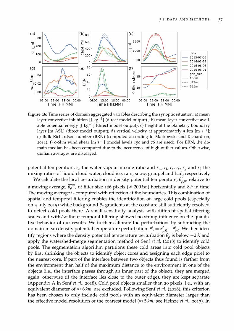
5.1 data and methods 57

Figure 26: Time series of domain aggregated variables describing the synoptic situation: a) meanlayer convective inhibition [J kg−1] (direct model output) ; b) mean layer convective avail-able potential energy [J kg−1] (direct model output); c) height of the planetary boundarylayer [m ASL] (direct model output); d) vertical velocity at approximately 5 km [m s−1];e) Bulk Richardson number (BRN) (computed according to Markowski and Richardson,2011); f) 0-6km wind shear [m s−1] (model levels 150 and 76 are used). For BRN, the do-main median has been computed due to the occurrence of high outlier values. Otherwise,domain averages are displayed.

potential temperature, rv the water vapour mixing ratio and rw, ri, rr, rs, rg and rh themixing ratios of liquid cloud water, cloud ice, rain, snow, graupel and hail, respectively.

We calculate the local perturbation in density potential temperature, θ′ρ,0, relative to

a moving average, θρm

, of filter size 166 pixels (≈ 200 km) horizontally and 8 h in time.The moving average is computed with reflection at the boundaries. This combination ofspatial and temporal filtering enables the identification of large cold pools (especiallyon 5 July 2015) while background θρ gradients at the coast are still sufficiently resolvedto detect cold pools there. A small sensitivity analysis with different spatial filteringscales and with/without temporal filtering showed no strong influence on the qualita-tive behavior of our results. We further calibrate the perturbations by subtracting thedomain-mean density potential temperature perturbation: θ′ρ = θ′ρ,0− θ′ρ,0. We then iden-tify regions where the density potential temperature perturbation θ′ρ is below −2 K andapply the watershed-merge segmentation method of Senf et al. (2018) to identify coldpools. The segmentation algorithm partitions these cold areas into cold pool objectsby first shrinking the objects to identify object cores and assigning each edge pixel tothe nearest core. If part of the interface between two objects thus found is farther fromthe environment than half of the maximum distance to the environment in one of theobjects (i.e., the interface passes through an inner part of the object), they are mergedagain, otherwise (if the interface lies close to the outer edge), they are kept separate(Appendix A in Senf et al., 2018). Cold pool objects smaller than 20 pixels, i.e., with anequivalent diameter of ≈ 6 km, are excluded. Following Senf et al. (2018), this criterionhas been chosen to only include cold pools with an equivalent diameter larger thanthe effective model resolution of the coarsest model (≈ 5 km; see Heinze et al., 2017). In

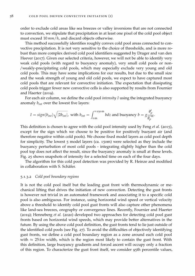
58 cold pool driven convective initiation (i)

order to exclude cold areas like sea breezes or valley inversions that are not connectedto convection, we stipulate that precipitation in at least one pixel of the cold pool objectmust exceed 10 mm/h, and discard objects otherwise.

This method successfully identifies roughly convex cold pool areas connected to con-vective precipitation. It is not very sensitive to the choice of thresholds, and is more ro-bust than more complex derived cold pool identifiers suggested by Drager and van denHeever (2017). Given our selected criteria, however, we will not be able to identify veryweak cold pools (with regard to buoyancy anomaly), very small cold pools or non-/weakly-precipitating cold pools, which may especially exclude very young and oldcold pools. This may have some implications for our results, but due to the small sizeand the weak strength of young and old cold pools, we expect to have captured mostcold pools that are relevant for convective initiation. The expectation that dissipatingcold pools trigger fewer new convective cells is also supported by results from Fournierand Haerter (2019).

For each air column, we define the cold pool intensity I using the integrated buoyancyanomaly bint over the lowest five layers:

I = sign(bint)√|2bint|, with bint =

∫ ≈150 m

0 mbdz and buoyancy b = g

θ′ρ

θρm .

This definition is chosen to agree with the cold pool intensity used by Feng et al. (2015),except for the sign which we choose to be positive for positively buoyant air (andtherefore negative within cold pools). We choose fixed model layers as cold pool depthfor simplicity. The lowest 5 model layers (ca. 150m) were selected as they include thebuoyancy perturbation of most cold pools - integrating slightly higher than the coldpool top does not affect the result, since the buoyancy anomaly is small at these levels.Fig. 25 shows snapshots of intensity for a selected time on each of the four days.

The algorithm for this cold pool detection was provided by R. Heinze and modifiedin collaboration with S. Schäfer.

5.1.3.2 Cold pool boundary regions

It is not the cold pool itself but the leading gust front with thermodynamic or me-chanical lifting that drives the initiation of new convection. Detecting the gust frontsis however not trivial in an automated framework and associating it to a specific coldpool is also ambiguous. For instance, using horizontal wind speed or vertical velocityabove a threshold to identify cold pool gust fronts will also capture other phenomenalike land-sea breezes, orography or convergence lines. Recently, Fournier and Haerter(2019); Henneberg et al. (2020) developed two approaches for detecting cold pool gustfronts based on horizontal wind speeds, which may provide better alternatives in thefuture. By using the above cold pool definition, the gust fronts tend to lie just outside ofthe identified cold pools (see Fig. 27). To avoid the difficulties of objectively identifyinggust fronts, we define a cold pool boundary region as a zone around each cold poolwith ≈ 25 km width, which is the region most likely to contain the gust front. Withthis definition, large buoyancy gradients and forced ascent will occupy only a fractionof this region. To characterize the gust front itself, we consider 95th percentile values,

5.1 data and methods 59

rather than averages over the entire gust front region. An advantage of considering thiscold pool boundary region is that the thermodynamic lifting will be included, whichmay not necessarily be located directly at the gust front. Grid points belonging to theoriginal cold pool or other cold pools are excluded from the boundary region. Overlapwith other cold pool boundary regions is, however, possible. We will consider overlap-ping boundary regions as a proxy for cold pool collisions.

Comparing cold pool boundaries with vertical velocity in Fig. 27, many line struc-tures of strong vertical velocity can be identified as cold pool gust fronts (e.g., A and Bin Fig. 27b) and generally they are positioned somewhere within the defined cold poolboundary region. This confirms that such cold pool boundaries are a useful proxy fortheir gust fronts.

5.1.4 Defining convective initiation

(a) (b)

(c) (d)

w [m s-1]

B

A Figure 27: Example snap-shots of verticalvelocity at ≈ 1 km incolor [m s−1], cold poolboundaries in greyshading and locationsof convective initiationin yellow for eachmodel resolution on6th June 2016 13:00

UTC. The black box in(a) marks the displayedregion for (b), (c) and(d).

There is no standard definition for identifying convective initiation. In this study,we aim to relate the initiation of a convective cloud to properties in the boundary layer,such as the gust front vertical velocity. Hence, to obtain an independent identification ofvertical velocity at the gust front and convective initiation, we refrain from using verticalvelocity as an indicator for convective initiation. We also avoid using quantities such asprecipitation particles, which occur later in the convective cloud life cycle and maybe difficult to associate with boundary-layer features due to advection of the cloud toneighboring grid points. With these conditions in mind, we choose the decisive variable

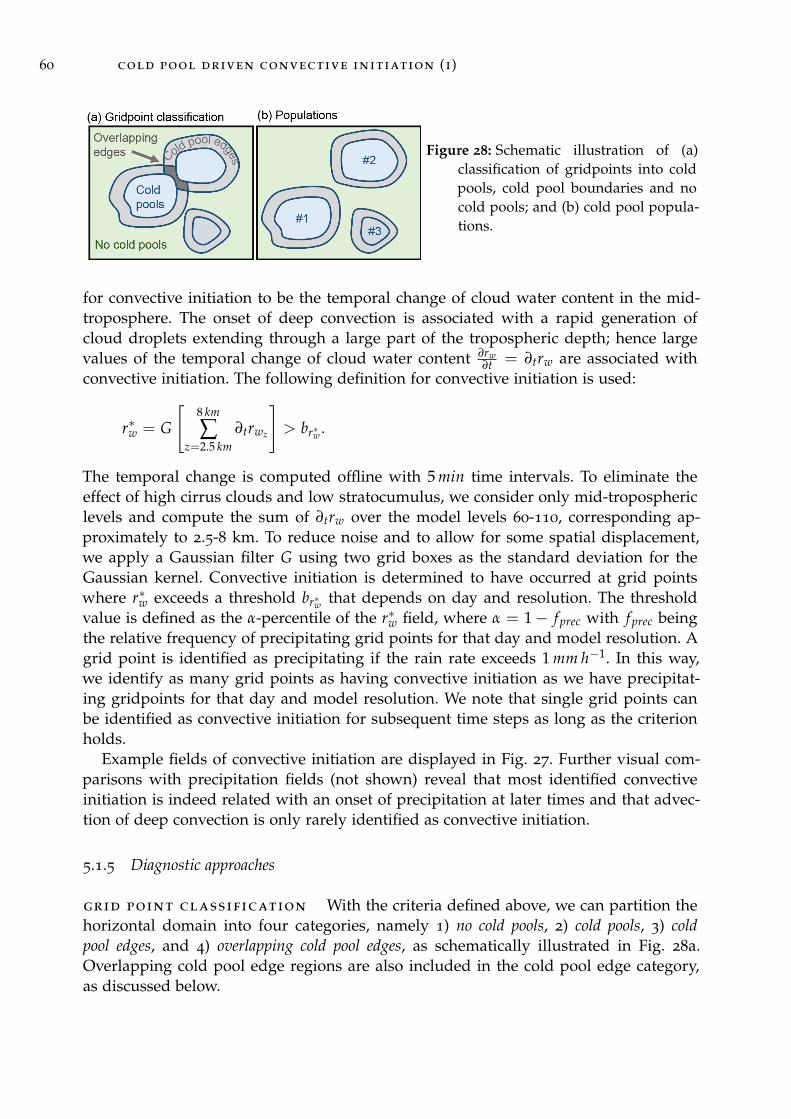
60 cold pool driven convective initiation (i)

((

Figure 28: Schematic illustration of (a)classification of gridpoints into coldpools, cold pool boundaries and nocold pools; and (b) cold pool popula-tions.

for convective initiation to be the temporal change of cloud water content in the mid-troposphere. The onset of deep convection is associated with a rapid generation ofcloud droplets extending through a large part of the tropospheric depth; hence largevalues of the temporal change of cloud water content ∂rw

∂t = ∂trw are associated withconvective initiation. The following definition for convective initiation is used:

r∗w = G

[8 km

∑z=2.5 km

∂trwz

]> br∗w .

The temporal change is computed offline with 5 min time intervals. To eliminate theeffect of high cirrus clouds and low stratocumulus, we consider only mid-troposphericlevels and compute the sum of ∂trw over the model levels 60-110, corresponding ap-proximately to 2.5-8 km. To reduce noise and to allow for some spatial displacement,we apply a Gaussian filter G using two grid boxes as the standard deviation for theGaussian kernel. Convective initiation is determined to have occurred at grid pointswhere r∗w exceeds a threshold br∗w that depends on day and resolution. The thresholdvalue is defined as the α-percentile of the r∗w field, where α = 1− fprec with fprec beingthe relative frequency of precipitating grid points for that day and model resolution. Agrid point is identified as precipitating if the rain rate exceeds 1 mm h−1. In this way,we identify as many grid points as having convective initiation as we have precipitat-ing gridpoints for that day and model resolution. We note that single grid points canbe identified as convective initiation for subsequent time steps as long as the criterionholds.

Example fields of convective initiation are displayed in Fig. 27. Further visual com-parisons with precipitation fields (not shown) reveal that most identified convectiveinitiation is indeed related with an onset of precipitation at later times and that advec-tion of deep convection is only rarely identified as convective initiation.

5.1.5 Diagnostic approaches

grid point classification With the criteria defined above, we can partition thehorizontal domain into four categories, namely 1) no cold pools, 2) cold pools, 3) coldpool edges, and 4) overlapping cold pool edges, as schematically illustrated in Fig. 28a.Overlapping cold pool edge regions are also included in the cold pool edge category,as discussed below.

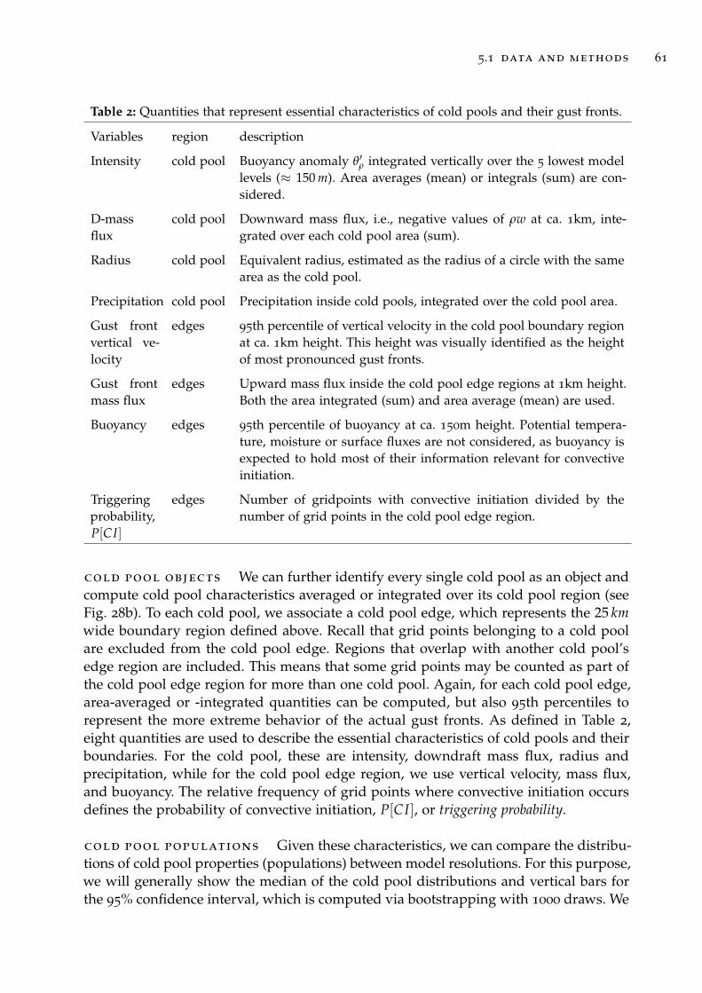
5.1 data and methods 61

Table 2: Quantities that represent essential characteristics of cold pools and their gust fronts.

Variables region description

Intensity cold pool Buoyancy anomaly θ′ρ integrated vertically over the 5 lowest modellevels (≈ 150 m). Area averages (mean) or integrals (sum) are con-sidered.

D-massflux

cold pool Downward mass flux, i.e., negative values of ρw at ca. 1km, inte-grated over each cold pool area (sum).

Radius cold pool Equivalent radius, estimated as the radius of a circle with the samearea as the cold pool.

Precipitation cold pool Precipitation inside cold pools, integrated over the cold pool area.

Gust frontvertical ve-locity

edges 95th percentile of vertical velocity in the cold pool boundary regionat ca. 1km height. This height was visually identified as the heightof most pronounced gust fronts.

Gust frontmass flux

edges Upward mass flux inside the cold pool edge regions at 1km height.Both the area integrated (sum) and area average (mean) are used.

Buoyancy edges 95th percentile of buoyancy at ca. 150m height. Potential tempera-ture, moisture or surface fluxes are not considered, as buoyancy isexpected to hold most of their information relevant for convectiveinitiation.

Triggeringprobability,P[CI]

edges Number of gridpoints with convective initiation divided by thenumber of grid points in the cold pool edge region.

cold pool objects We can further identify every single cold pool as an object andcompute cold pool characteristics averaged or integrated over its cold pool region (seeFig. 28b). To each cold pool, we associate a cold pool edge, which represents the 25 kmwide boundary region defined above. Recall that grid points belonging to a cold poolare excluded from the cold pool edge. Regions that overlap with another cold pool’sedge region are included. This means that some grid points may be counted as part ofthe cold pool edge region for more than one cold pool. Again, for each cold pool edge,area-averaged or -integrated quantities can be computed, but also 95th percentiles torepresent the more extreme behavior of the actual gust fronts. As defined in Table 2,eight quantities are used to describe the essential characteristics of cold pools and theirboundaries. For the cold pool, these are intensity, downdraft mass flux, radius andprecipitation, while for the cold pool edge region, we use vertical velocity, mass flux,and buoyancy. The relative frequency of grid points where convective initiation occursdefines the probability of convective initiation, P[CI], or triggering probability.

cold pool populations Given these characteristics, we can compare the distribu-tions of cold pool properties (populations) between model resolutions. For this purpose,we will generally show the median of the cold pool distributions and vertical bars forthe 95% confidence interval, which is computed via bootstrapping with 1000 draws. We

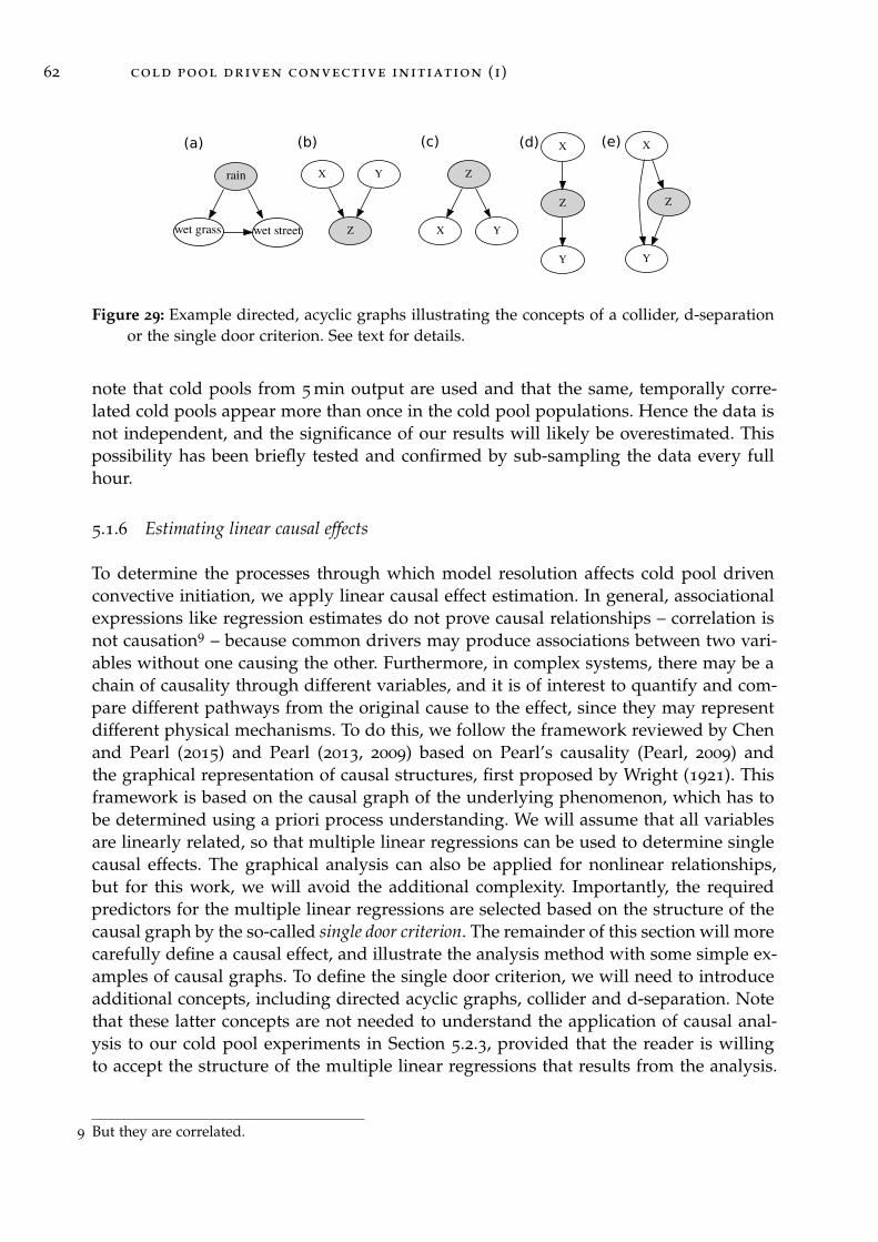
62 cold pool driven convective initiation (i)

X

Z

Y

X Y

ZX

Z

Y

(b) (c) (d) X

Y

Z

(e)

rain

wet streetwet grass

(a)

Figure 29: Example directed, acyclic graphs illustrating the concepts of a collider, d-separationor the single door criterion. See text for details.

note that cold pools from 5 min output are used and that the same, temporally corre-lated cold pools appear more than once in the cold pool populations. Hence the data isnot independent, and the significance of our results will likely be overestimated. Thispossibility has been briefly tested and confirmed by sub-sampling the data every fullhour.

5.1.6 Estimating linear causal effects

To determine the processes through which model resolution affects cold pool drivenconvective initiation, we apply linear causal effect estimation. In general, associationalexpressions like regression estimates do not prove causal relationships – correlation isnot causation9 – because common drivers may produce associations between two vari-ables without one causing the other. Furthermore, in complex systems, there may be achain of causality through different variables, and it is of interest to quantify and com-pare different pathways from the original cause to the effect, since they may representdifferent physical mechanisms. To do this, we follow the framework reviewed by Chenand Pearl (2015) and Pearl (2013, 2009) based on Pearl’s causality (Pearl, 2009) andthe graphical representation of causal structures, first proposed by Wright (1921). Thisframework is based on the causal graph of the underlying phenomenon, which has tobe determined using a priori process understanding. We will assume that all variablesare linearly related, so that multiple linear regressions can be used to determine singlecausal effects. The graphical analysis can also be applied for nonlinear relationships,but for this work, we will avoid the additional complexity. Importantly, the requiredpredictors for the multiple linear regressions are selected based on the structure of thecausal graph by the so-called single door criterion. The remainder of this section will morecarefully define a causal effect, and illustrate the analysis method with some simple ex-amples of causal graphs. To define the single door criterion, we will need to introduceadditional concepts, including directed acyclic graphs, collider and d-separation. Notethat these latter concepts are not needed to understand the application of causal anal-ysis to our cold pool experiments in Section 5.2.3, provided that the reader is willingto accept the structure of the multiple linear regressions that results from the analysis.

9 But they are correlated.

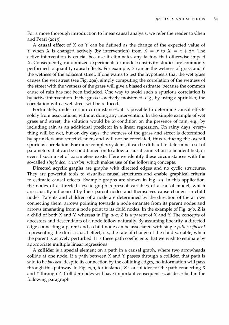
5.1 data and methods 63

For a more thorough introduction to linear causal analysis, we refer the reader to Chenand Pearl (2015).

A causal effect of X on Y can be defined as the change of the expected value ofY when X is changed actively (by intervention) from X = x to X = x + ∆x. Theactive intervention is crucial because it eliminates any factors that otherwise impactX. Consequently, randomized experiments or model sensitivity studies are commonlyperformed to quantify causal effects. For example, X can be the wetness of grass and Ythe wetness of the adjacent street. If one wants to test the hypothesis that the wet grasscauses the wet street (see Fig. 29a), simply computing the correlation of the wetness ofthe street with the wetness of the grass will give a biased estimate, because the commoncause of rain has not been included. One way to avoid such a spurious correlation isby active intervention. If the grass is actively moistened, e.g., by using a sprinkler, thecorrelation with a wet street will be reduced.

Fortunately, under certain circumstances, it is possible to determine causal effectssolely from associations, without doing any intervention. In the simple example of wetgrass and street, the solution would be to condition on the presence of rain, e.g., byincluding rain as an additional predictor in a linear regression. On rainy days, every-thing will be wet, but on dry days, the wetness of the grass and street is determinedby sprinklers and street cleaners and will not be correlated, thus reducing the overallspurious correlation. For more complex systems, it can be difficult to determine a set ofparameters that can be conditioned on to allow a causal connection to be identified, oreven if such a set of parameters exists. Here we identify these circumstances with theso-called single door criterion, which makes use of the following concepts.

Directed acyclic graphs are graphs with directed edges and no cyclic structures.They are powerful tools to visualize causal structures and enable graphical criteriato estimate causal effects. Example graphs are shown in Fig. 29. In this application,the nodes of a directed acyclic graph represent variables of a causal model, whichare causally influenced by their parent nodes and themselves cause changes in childnodes. Parents and children of a node are determined by the direction of the arrowsconnecting them: arrows pointing towards a node emanate from its parent nodes andarrows emanating from a node point to its child nodes. In the example of Fig. 29b, Z isa child of both X and Y, whereas in Fig. 29c, Z is a parent of X and Y. The concepts ofancestors and descendants of a node follow naturally. By assuming linearity, a directededge connecting a parent and a child node can be associated with single path coefficientrepresenting the direct causal effect, i.e., the rate of change of the child variable, whenthe parent is actively perturbed. It is these path coefficients that we wish to estimate byappropriate multiple linear regressions.

A collider is a special element on a path in a causal graph, where two arrowheadscollide at one node. If a path between X and Y passes through a collider, that path issaid to be blocked: despite its connection by the colliding edges, no information will passthrough this pathway. In Fig. 29b, for instance, Z is a collider for the path connecting Xand Y through Z. Collider nodes will have important consequences, as described in thefollowing paragraph.

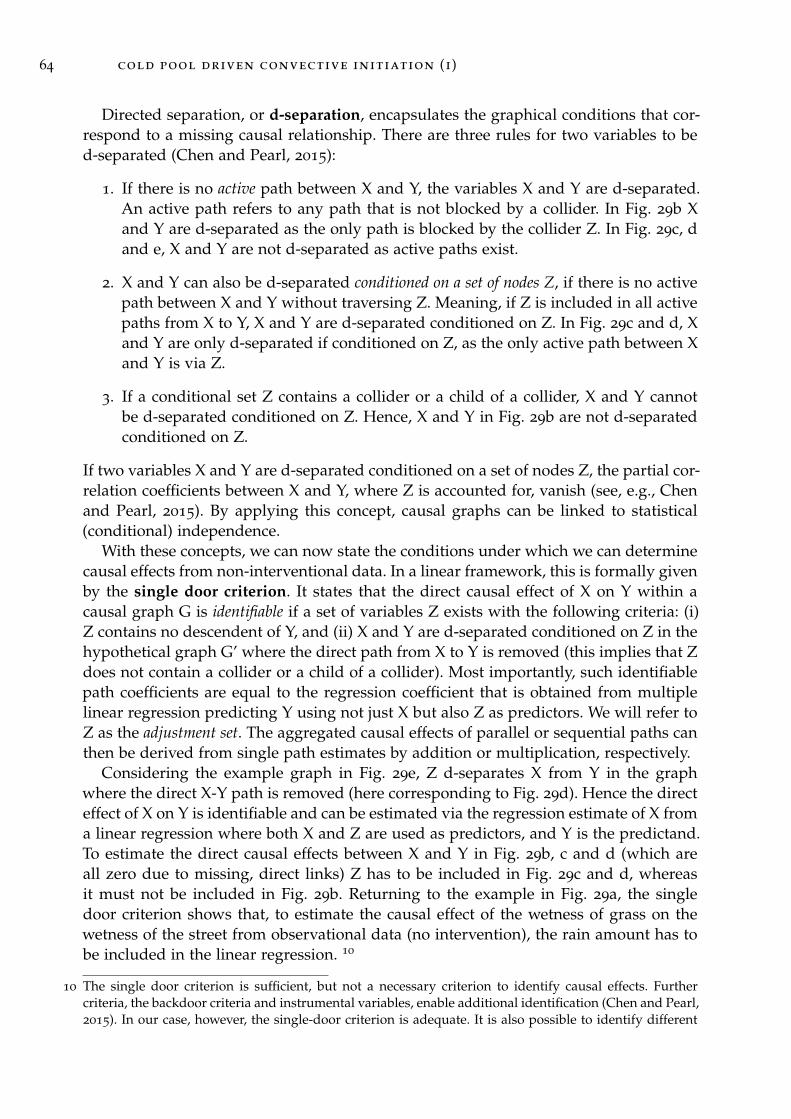
64 cold pool driven convective initiation (i)

Directed separation, or d-separation, encapsulates the graphical conditions that cor-respond to a missing causal relationship. There are three rules for two variables to bed-separated (Chen and Pearl, 2015):

1. If there is no active path between X and Y, the variables X and Y are d-separated.An active path refers to any path that is not blocked by a collider. In Fig. 29b Xand Y are d-separated as the only path is blocked by the collider Z. In Fig. 29c, dand e, X and Y are not d-separated as active paths exist.

2. X and Y can also be d-separated conditioned on a set of nodes Z, if there is no activepath between X and Y without traversing Z. Meaning, if Z is included in all activepaths from X to Y, X and Y are d-separated conditioned on Z. In Fig. 29c and d, Xand Y are only d-separated if conditioned on Z, as the only active path between Xand Y is via Z.

3. If a conditional set Z contains a collider or a child of a collider, X and Y cannotbe d-separated conditioned on Z. Hence, X and Y in Fig. 29b are not d-separatedconditioned on Z.

If two variables X and Y are d-separated conditioned on a set of nodes Z, the partial cor-relation coefficients between X and Y, where Z is accounted for, vanish (see, e.g., Chenand Pearl, 2015). By applying this concept, causal graphs can be linked to statistical(conditional) independence.

With these concepts, we can now state the conditions under which we can determinecausal effects from non-interventional data. In a linear framework, this is formally givenby the single door criterion. It states that the direct causal effect of X on Y within acausal graph G is identifiable if a set of variables Z exists with the following criteria: (i)Z contains no descendent of Y, and (ii) X and Y are d-separated conditioned on Z in thehypothetical graph G’ where the direct path from X to Y is removed (this implies that Zdoes not contain a collider or a child of a collider). Most importantly, such identifiablepath coefficients are equal to the regression coefficient that is obtained from multiplelinear regression predicting Y using not just X but also Z as predictors. We will refer toZ as the adjustment set. The aggregated causal effects of parallel or sequential paths canthen be derived from single path estimates by addition or multiplication, respectively.

Considering the example graph in Fig. 29e, Z d-separates X from Y in the graphwhere the direct X-Y path is removed (here corresponding to Fig. 29d). Hence the directeffect of X on Y is identifiable and can be estimated via the regression estimate of X froma linear regression where both X and Z are used as predictors, and Y is the predictand.To estimate the direct causal effects between X and Y in Fig. 29b, c and d (which areall zero due to missing, direct links) Z has to be included in Fig. 29c and d, whereasit must not be included in Fig. 29b. Returning to the example in Fig. 29a, the singledoor criterion shows that, to estimate the causal effect of the wetness of grass on thewetness of the street from observational data (no intervention), the rain amount has tobe included in the linear regression. 10

10 The single door criterion is sufficient, but not a necessary criterion to identify causal effects. Furthercriteria, the backdoor criteria and instrumental variables, enable additional identification (Chen and Pearl,2015). In our case, however, the single-door criterion is adequate. It is also possible to identify different

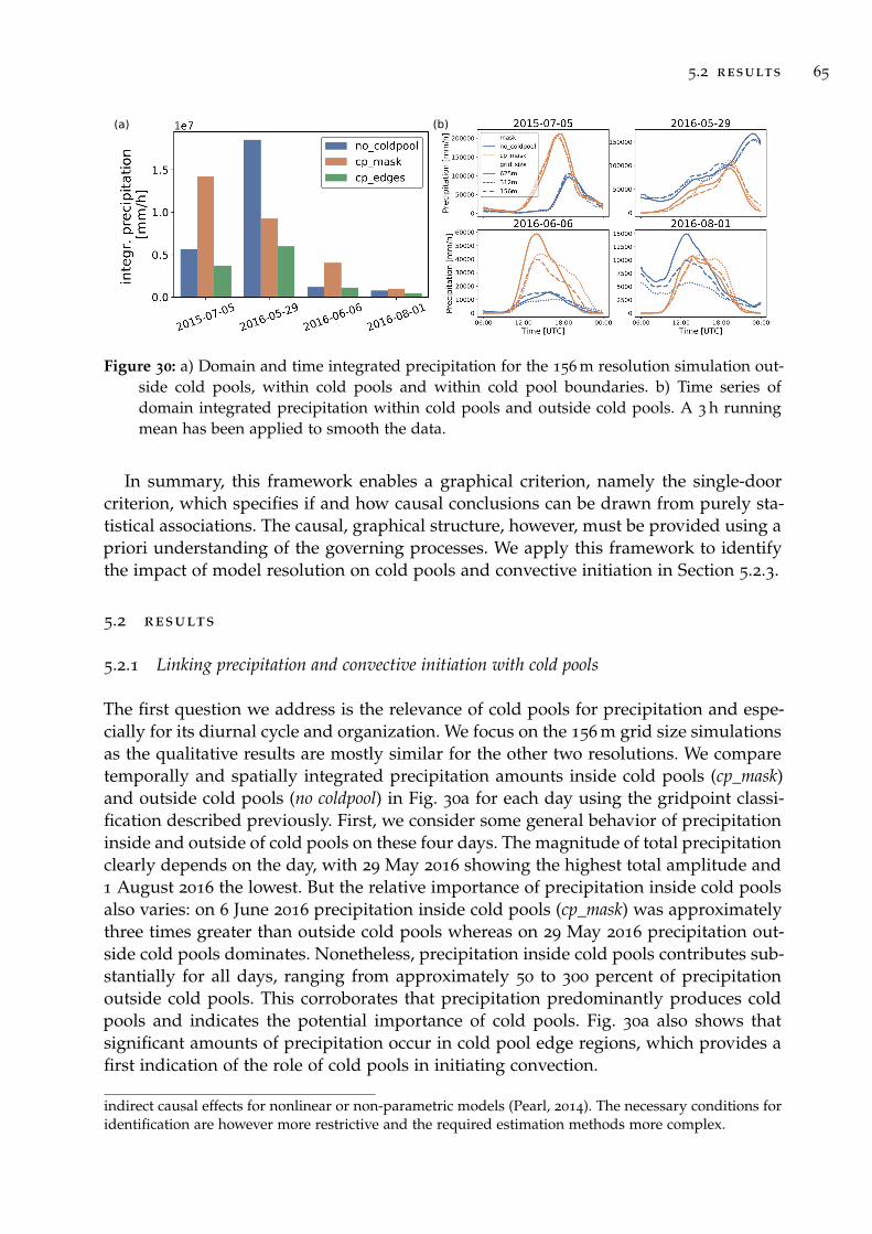
5.2 results 65

(a) (b)

Figure 30: a) Domain and time integrated precipitation for the 156 m resolution simulation out-side cold pools, within cold pools and within cold pool boundaries. b) Time series ofdomain integrated precipitation within cold pools and outside cold pools. A 3 h runningmean has been applied to smooth the data.

In summary, this framework enables a graphical criterion, namely the single-doorcriterion, which specifies if and how causal conclusions can be drawn from purely sta-tistical associations. The causal, graphical structure, however, must be provided using apriori understanding of the governing processes. We apply this framework to identifythe impact of model resolution on cold pools and convective initiation in Section 5.2.3.

5.2 results

5.2.1 Linking precipitation and convective initiation with cold pools

The first question we address is the relevance of cold pools for precipitation and espe-cially for its diurnal cycle and organization. We focus on the 156 m grid size simulationsas the qualitative results are mostly similar for the other two resolutions. We comparetemporally and spatially integrated precipitation amounts inside cold pools (cp_mask)and outside cold pools (no coldpool) in Fig. 30a for each day using the gridpoint classi-fication described previously. First, we consider some general behavior of precipitationinside and outside of cold pools on these four days. The magnitude of total precipitationclearly depends on the day, with 29 May 2016 showing the highest total amplitude and1 August 2016 the lowest. But the relative importance of precipitation inside cold poolsalso varies: on 6 June 2016 precipitation inside cold pools (cp_mask) was approximatelythree times greater than outside cold pools whereas on 29 May 2016 precipitation out-side cold pools dominates. Nonetheless, precipitation inside cold pools contributes sub-stantially for all days, ranging from approximately 50 to 300 percent of precipitationoutside cold pools. This corroborates that precipitation predominantly produces coldpools and indicates the potential importance of cold pools. Fig. 30a also shows thatsignificant amounts of precipitation occur in cold pool edge regions, which provides afirst indication of the role of cold pools in initiating convection.

indirect causal effects for nonlinear or non-parametric models (Pearl, 2014). The necessary conditions foridentification are however more restrictive and the required estimation methods more complex.

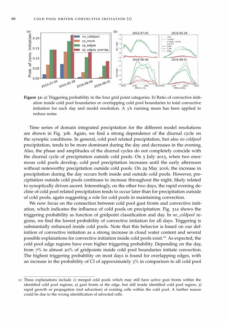
66 cold pool driven convective initiation (i)

(a) (b)

Figure 31: a) Triggering probability in the four grid point categories. b) Ratio of convective initi-ation inside cold pool boundaries or overlapping cold pool boundaries to total convectiveinitiation for each day and model resolution. A 3 h running mean has been applied toreduce noise.

Time series of domain integrated precipitation for the different model resolutionsare shown in Fig. 30b. Again, we find a strong dependence of the diurnal cycle onthe synoptic conditions. In general, cold pool related precipitation, but also no coldpoolprecipitation, tends to be more dominant during the day and decreases in the evening.Also, the phase and amplitudes of the diurnal cycles do not completely coincide withthe diurnal cycle of precipitation outside cold pools. On 5 July 2015, when two enor-mous cold pools develop, cold pool precipitation increases until the early afternoonwithout noteworthy precipitation outside cold pools. On 29 May 2016, the increase inprecipitation during the day occurs both inside and outside cold pools. However, pre-cipitation outside cold pools continues to increase throughout the night, likely relatedto synoptically driven ascent. Interestingly, on the other two days, the rapid evening de-cline of cold pool related precipitation tends to occur later than for precipitation outsideof cold pools, again suggesting a role for cold pools in maintaining convection.

We now focus on the connection between cold pool gust fronts and convective initi-ation, which indicates the influence of cold pools on precipitation. Fig. 31a shows thetriggering probability as function of gridpoint classification and day. In no_coldpool re-gions, we find the lowest probability of convective initiation for all days. Triggering issubstantially enhanced inside cold pools. Note that this behavior is based on our def-inition of convective initiation as a strong increase in cloud water content and severalpossible explanations for convective initiation inside cold pools exist.11 As expected, thecold pool edge regions have even higher triggering probability. Depending on the day,from 7% to almost 20% of gridpoints inside cold pool boundaries initiate convection.The highest triggering probability on most days is found for overlapping edges, withan increase in the probability of CI of approximately 3% in comparison to all cold pool

11 These explanations include 1) merged cold pools which may still have active gust fronts within theidentified cold pool regions; 2) gust fronts at the edge, but still inside identified cold pool region; 3)rapid growth or propagation (not advection) of existing cells within the cold pool. A further reasoncould be due to the wrong identification of advected cells.

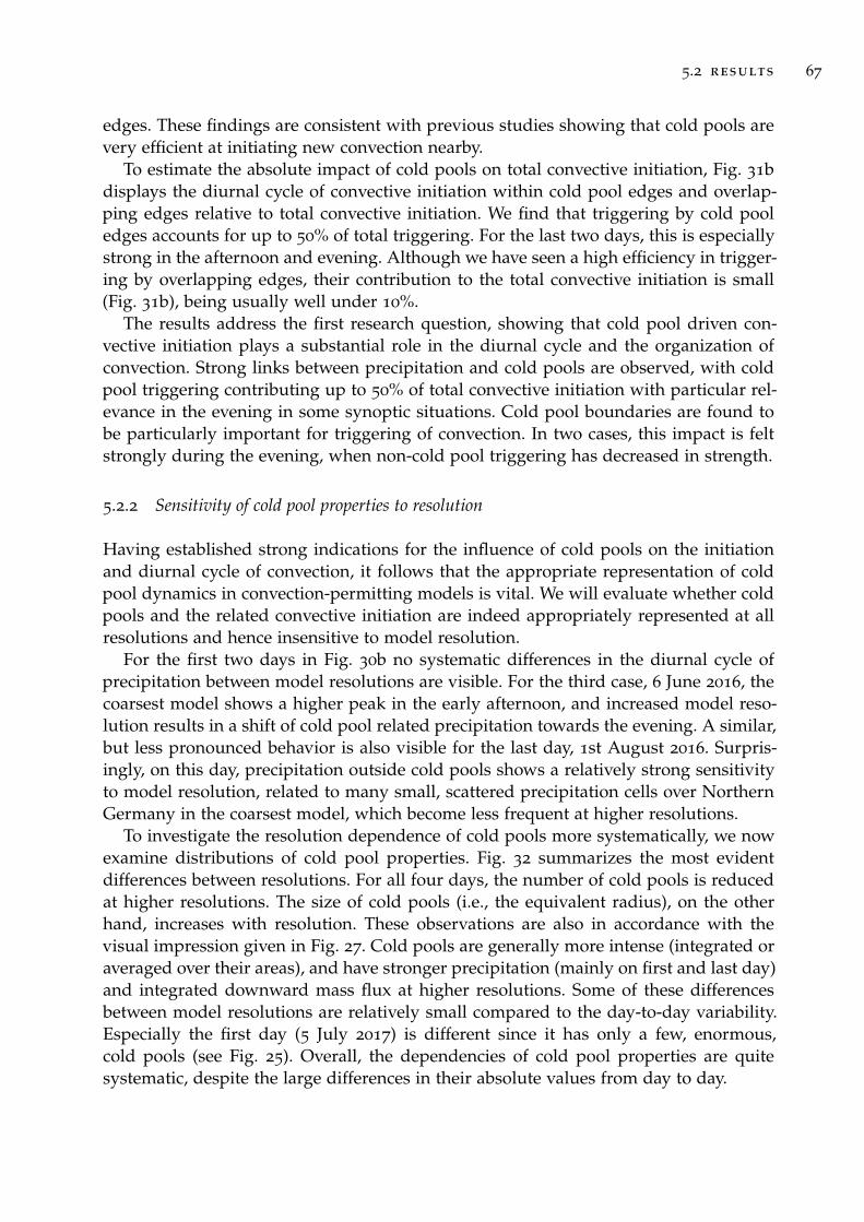
5.2 results 67

edges. These findings are consistent with previous studies showing that cold pools arevery efficient at initiating new convection nearby.

To estimate the absolute impact of cold pools on total convective initiation, Fig. 31bdisplays the diurnal cycle of convective initiation within cold pool edges and overlap-ping edges relative to total convective initiation. We find that triggering by cold pooledges accounts for up to 50% of total triggering. For the last two days, this is especiallystrong in the afternoon and evening. Although we have seen a high efficiency in trigger-ing by overlapping edges, their contribution to the total convective initiation is small(Fig. 31b), being usually well under 10%.

The results address the first research question, showing that cold pool driven con-vective initiation plays a substantial role in the diurnal cycle and the organization ofconvection. Strong links between precipitation and cold pools are observed, with coldpool triggering contributing up to 50% of total convective initiation with particular rel-evance in the evening in some synoptic situations. Cold pool boundaries are found tobe particularly important for triggering of convection. In two cases, this impact is feltstrongly during the evening, when non-cold pool triggering has decreased in strength.

5.2.2 Sensitivity of cold pool properties to resolution

Having established strong indications for the influence of cold pools on the initiationand diurnal cycle of convection, it follows that the appropriate representation of coldpool dynamics in convection-permitting models is vital. We will evaluate whether coldpools and the related convective initiation are indeed appropriately represented at allresolutions and hence insensitive to model resolution.

For the first two days in Fig. 30b no systematic differences in the diurnal cycle ofprecipitation between model resolutions are visible. For the third case, 6 June 2016, thecoarsest model shows a higher peak in the early afternoon, and increased model reso-lution results in a shift of cold pool related precipitation towards the evening. A similar,but less pronounced behavior is also visible for the last day, 1st August 2016. Surpris-ingly, on this day, precipitation outside cold pools shows a relatively strong sensitivityto model resolution, related to many small, scattered precipitation cells over NorthernGermany in the coarsest model, which become less frequent at higher resolutions.

To investigate the resolution dependence of cold pools more systematically, we nowexamine distributions of cold pool properties. Fig. 32 summarizes the most evidentdifferences between resolutions. For all four days, the number of cold pools is reducedat higher resolutions. The size of cold pools (i.e., the equivalent radius), on the otherhand, increases with resolution. These observations are also in accordance with thevisual impression given in Fig. 27. Cold pools are generally more intense (integrated oraveraged over their areas), and have stronger precipitation (mainly on first and last day)and integrated downward mass flux at higher resolutions. Some of these differencesbetween model resolutions are relatively small compared to the day-to-day variability.Especially the first day (5 July 2017) is different since it has only a few, enormous,cold pools (see Fig. 25). Overall, the dependencies of cold pool properties are quitesystematic, despite the large differences in their absolute values from day to day.

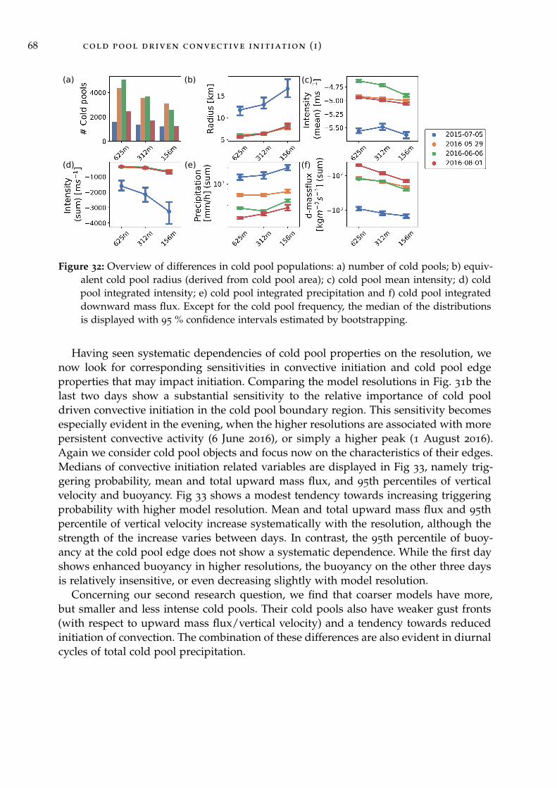
68 cold pool driven convective initiation (i)

(a) (b) (c)

(d) (e) (f)

Figure 32: Overview of differences in cold pool populations: a) number of cold pools; b) equiv-alent cold pool radius (derived from cold pool area); c) cold pool mean intensity; d) coldpool integrated intensity; e) cold pool integrated precipitation and f) cold pool integrateddownward mass flux. Except for the cold pool frequency, the median of the distributionsis displayed with 95 % confidence intervals estimated by bootstrapping.

Having seen systematic dependencies of cold pool properties on the resolution, wenow look for corresponding sensitivities in convective initiation and cold pool edgeproperties that may impact initiation. Comparing the model resolutions in Fig. 31b thelast two days show a substantial sensitivity to the relative importance of cold pooldriven convective initiation in the cold pool boundary region. This sensitivity becomesespecially evident in the evening, when the higher resolutions are associated with morepersistent convective activity (6 June 2016), or simply a higher peak (1 August 2016).Again we consider cold pool objects and focus now on the characteristics of their edges.Medians of convective initiation related variables are displayed in Fig 33, namely trig-gering probability, mean and total upward mass flux, and 95th percentiles of verticalvelocity and buoyancy. Fig 33 shows a modest tendency towards increasing triggeringprobability with higher model resolution. Mean and total upward mass flux and 95thpercentile of vertical velocity increase systematically with the resolution, although thestrength of the increase varies between days. In contrast, the 95th percentile of buoy-ancy at the cold pool edge does not show a systematic dependence. While the first dayshows enhanced buoyancy in higher resolutions, the buoyancy on the other three daysis relatively insensitive, or even decreasing slightly with model resolution.

Concerning our second research question, we find that coarser models have more,but smaller and less intense cold pools. Their cold pools also have weaker gust fronts(with respect to upward mass flux/vertical velocity) and a tendency towards reducedinitiation of convection. The combination of these differences are also evident in diurnalcycles of total cold pool precipitation.

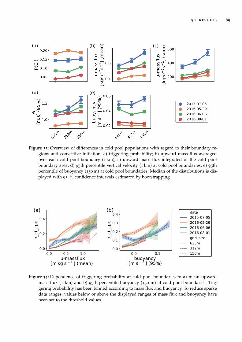
5.2 results 69

(a) (b) (c)

(d) (e)

Figure 33: Overview of differences in cold pool populations with regard to their boundary re-gions and convective initiation: a) triggering probability; b) upward mass flux averagedover each cold pool boundary (1 km); c) upward mass flux integrated of the cold poolboundary area; d) 95th percentile vertical velocity (1 km) at cold pool boundaries; e) 95thpercentile of buoyancy (150 m) at cold pool boundaries. Median of the distributions is dis-played with 95 % confidence intervals estimated by bootstrapping.

0.0 0.5 1.0

u-massfluxkg s 1 ] (mean)[m

0.0

0.2

0.4

p_c

i_cp

e

0.0 0.1

buoyancy [m s 2 ] (95%)

0.0

0.1

0.2

0.3

0.4

p_c

i_cp

e

date

2015-07-05

2016-05-29

2016-06-06

2016-08-01

grid_size

625m

312m

156m

(a) (b)

Figure 34: Dependence of triggering probability at cold pool boundaries to a) mean upwardmass flux (1 km) and b) 95th percentile buoyancy (150 m) at cold pool boundaries. Trig-gering probability has been binned according to mass flux and buoyancy. To reduce sparsedata ranges, values below or above the displayed ranges of mass flux and buoyancy havebeen set to the threshold values.

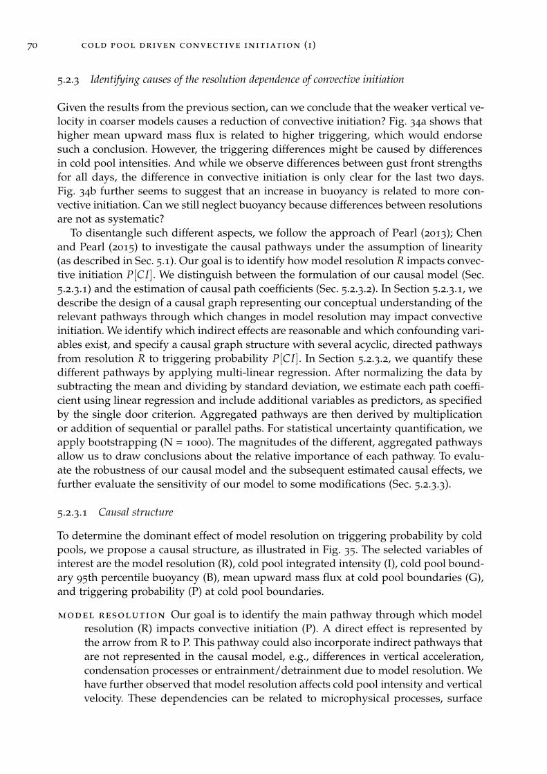
70 cold pool driven convective initiation (i)

5.2.3 Identifying causes of the resolution dependence of convective initiation

Given the results from the previous section, can we conclude that the weaker vertical ve-locity in coarser models causes a reduction of convective initiation? Fig. 34a shows thathigher mean upward mass flux is related to higher triggering, which would endorsesuch a conclusion. However, the triggering differences might be caused by differencesin cold pool intensities. And while we observe differences between gust front strengthsfor all days, the difference in convective initiation is only clear for the last two days.Fig. 34b further seems to suggest that an increase in buoyancy is related to more con-vective initiation. Can we still neglect buoyancy because differences between resolutionsare not as systematic?

To disentangle such different aspects, we follow the approach of Pearl (2013); Chenand Pearl (2015) to investigate the causal pathways under the assumption of linearity(as described in Sec. 5.1). Our goal is to identify how model resolution R impacts convec-tive initiation P[CI]. We distinguish between the formulation of our causal model (Sec.5.2.3.1) and the estimation of causal path coefficients (Sec. 5.2.3.2). In Section 5.2.3.1, wedescribe the design of a causal graph representing our conceptual understanding of therelevant pathways through which changes in model resolution may impact convectiveinitiation. We identify which indirect effects are reasonable and which confounding vari-ables exist, and specify a causal graph structure with several acyclic, directed pathwaysfrom resolution R to triggering probability P[CI]. In Section 5.2.3.2, we quantify thesedifferent pathways by applying multi-linear regression. After normalizing the data bysubtracting the mean and dividing by standard deviation, we estimate each path coeffi-cient using linear regression and include additional variables as predictors, as specifiedby the single door criterion. Aggregated pathways are then derived by multiplicationor addition of sequential or parallel paths. For statistical uncertainty quantification, weapply bootstrapping (N = 1000). The magnitudes of the different, aggregated pathwaysallow us to draw conclusions about the relative importance of each pathway. To evalu-ate the robustness of our causal model and the subsequent estimated causal effects, wefurther evaluate the sensitivity of our model to some modifications (Sec. 5.2.3.3).

5.2.3.1 Causal structure

To determine the dominant effect of model resolution on triggering probability by coldpools, we propose a causal structure, as illustrated in Fig. 35. The selected variables ofinterest are the model resolution (R), cold pool integrated intensity (I), cold pool bound-ary 95th percentile buoyancy (B), mean upward mass flux at cold pool boundaries (G),and triggering probability (P) at cold pool boundaries.

model resolution Our goal is to identify the main pathway through which modelresolution (R) impacts convective initiation (P). A direct effect is represented bythe arrow from R to P. This pathway could also incorporate indirect pathways thatare not represented in the causal model, e.g., differences in vertical acceleration,condensation processes or entrainment/detrainment due to model resolution. Wehave further observed that model resolution affects cold pool intensity and verticalvelocity. These dependencies can be related to microphysical processes, surface

5.2 results 71

Figure 35: Conceptual causal modelof how model resolution can im-pact convective initiation. Blackarrows are used to emphasizetheir role as common driver.Blue/red arrows are used forpaths that influence how modelresolution (R) impacts convec-tive initiation (P). The red pathsdisplay the below identifieddominant pathway. See text forexplanation.

fluxes or vertical acceleration. For buoyancy, the influence was not found to bevery systematic, but we evaluate its strength in this model anyway. These causalrelationships are represented by the arrows from R to I, G and B.

cold pool intensity It is reasonable to assume that stronger cold pools have dif-ferent buoyancy (B) or vertical velocity (G) at the cold pool boundary. Hence, wedraw two paths IB and IG. We have further included a direct arrow from coldpool intensity to convective initiation to evaluate whether we are missing someimportant processes that are not captured by buoyancy or vertical velocity (IP).

buoyancy Buoyancy certainly influences vertical velocity, but there might also be adirect effect on triggering. These effects are represented by the arrows BG and BP.

gustfront The impact of gust front upward mass flux (mean) on convective initiationis represented by the arrow GP.

triggering We don’t consider any impact of triggering on other variables. Hencethere is no feedback, and we consequently have a directed acyclic graph. This is anecessary feature to enable the following estimation of causal pathways.

Furthermore, we have included the synoptic situation and diurnal cycle (D), as repre-sented by the variables given in Fig. 26. This is necessary because we expect them to becommon drivers for cold pool intensity, buoyancy, gust front and convective initiation.Time of day, however, is not taken into account explicitly.

Several noteworthy assumptions have been made with regard to the causal struc-ture. First, no temporal evolution or time lag is considered. Hence we assume that the

72 cold pool driven convective initiation (i)

autocorrelation time scale of the variables of interest is longer than the time it takesfor stronger cold pool intensities to affect gust fronts, buoyancy or convective initia-tion. This also means, that the data are not independent, as subsequent time steps mayinclude the same, temporally correlated cold pool. The causal time series approach in-troduced by Runge et al. (2015) is likely better suited for time series, and we considerits application to tracked cold pools in the future. We also neglect any feedback cycles,e.g., that stronger convective initiation might lead to a strengthening of cold pools. Thisis justified if the autocorrelation time scale of the variables of interest is expected to besmaller than the 15–30 min timescale for precipitation development. Furthermore, noimpact of model resolution on synoptic conditions is assumed (no link between R andD). This is justified by the small resolution sensitivity of the domain aggregated, largescale variables in Figure 26. Finally, we assume that we have captured all major vari-ables that have a strong influence on at least two of the variables of interest (assumptionof no unobserved common drivers).

5.2.3.2 Estimating causal effects

To estimate the path coefficients of the causal graph, we apply multiple linear regres-sion based on the single door criterion using all identified cold pools at all time steps.Table 4 displays the predictor sets considered for each path. The resulting average pathestimates are illustrated in Fig. 36a. As expected, strong paths are observed betweenbuoyancy and gust front upward mass flux, and also between gust front mass fluxand triggering probability. The impact of buoyancy on triggering probability, however,seems to be completely mediated by the gust front. More intense cold pools lead to anincrease in buoyancy at the cold pool boundaries and a small decrease in upward massflux (the signs of these paths arise from the fact that intensity is negative). The graphfurther shows that, in comparison to synoptic conditions, the model resolution is of sec-ondary importance for the variables of interest. Hence, all models are able to capturethe dominant, physical processes. This is to be expected and does not undermine theimportance of comparably small, systematic biases due to model resolution.

To evaluate dominant direct and indirect pathways between resolution and trigger-ing probability, aggregated path estimates are displayed in Fig. 36b. The ∗ in R ∗ B ∗ Pdenotes that all possible direct or indirect paths between the two specified variablesare accounted for. This shows that the RP, RIP, RIGP and R ∗ B ∗ P paths are rela-tively small. Hence, the dependence of the cold pool intensity and the buoyancy onresolution do not play an important role in triggering probability. The RGP path clearlydominates: larger grid sizes decrease upward mass flux at the cold pool boundaries,which consequently reduces convective initiation. The displayed, de-normalized valueof −0.017 means that if model grid size is increased from 156 to 625 m, triggering prob-ability will be reduced by 0.017. This is somewhat less than some of the differencesobserved in Fig. 33 but still of comparable magnitude. Furthermore, this correspondsto a difference of 10-30% in median triggering probability.

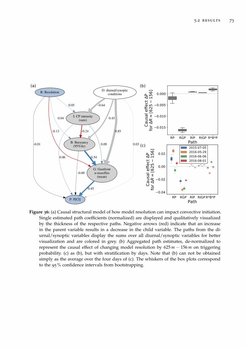
5.2 results 73

(a) (b)

(c)

RP RGP RIP RIGP R*B*P

Path

0.015

0.010

0.005

0.000

Causa

l eff

ect

P

for

R=

[62

51

56

]

G: Gustfrontu-massflux

(mean)

P: P[CI]

0.45

I: CP intensity(sum)

0.09

0.06

B: Buoyancy(95%ile)

-0.24

0.54

-0.00

R: Resolution

-0.13

0.05

-0.01

0.04

D: diurnal/synopticconditions

0.85

-0.64

0.03

0.45

Figure 36: (a) Causal structural model of how model resolution can impact convective initiation.Single estimated path coefficients (normalized) are displayed and qualitatively visualizedby the thickness of the respective paths. Negative arrows (red) indicate that an increasein the parent variable results in a decrease in the child variable. The paths from the di-urnal/synoptic variables display the sums over all diurnal/synoptic variables for bettervisualization and are colored in grey. (b) Aggregated path estimates, de-normalized torepresent the causal effect of changing model resolution by 625 m − 156 m on triggeringprobability. (c) as (b), but with stratification by days. Note that (b) can not be obtainedsimply as the average over the four days of (c). The whiskers of the box plots correspondto the 95 % confidence intervals from bootstrapping.

74 cold pool driven convective initiation (i)

5.2.3.3 Robustness

The statistical robustness of the results and their sensitivity to several of the assump-tions made in constructing the causal graph are examined in Appendix A.2. This in-cludes tests of the statistical significance of the linear regression results, the linearityof the response to changing model resolution, selecting different variables as proxiesfor gust front or cold pool intensity, sensitivity to stratification by days, and of the im-pact of model resolution on the synoptic conditions. One noteworthy concern arisesfrom sometimes relatively small R2 values, which can imply that several informativevariables may not be included in our causal graph. This can increase the likelihood ofmissing common driver, which causes biased causal effect estimates (see Appendix A.2for more details).

Nonetheless, the causal effect estimates vary moderately under most modificationswith no strong dependence on the specific resolution range or the selected variables.Only the stratification of the data into the four individual days substantially influencesthe causal effects. The path estimates computed for each of the four days are illustratedin Fig 36c. The estimates for the paths RIP and RIGP show some variability betweendays, but the values are all close to zero. The path estimates of the R*B*P path showstronger variability among the days, although centered around zero. The RGP path,which we have earlier identified as the dominant path, shows moderate variability be-tween the days, with values ranging from -0.02 to -0.04. Thus, this effect is relativelyrobust to the stratification by days and is consistently stronger than other indirect ef-fects. On the other hand, the direct effect of resolution on triggering (RP) shows a strongsensitivity to the day, ranging from 0.03 to -0.01. Since the direct RP path includes influ-ences of causal processes not represented explicitly in the graph, it is interesting to notethat it is strongest on 29 May 2016, when the diurnal cycle of precipitation is disturbedby strong synoptic forcing. In such situations, the initiation of convection may be lessinfluenced by cold pool effects.

Overall, we conclude that the relatively robust RGP path predominates in most situ-ations. Hence, to answer our third research question, the reduction in cold pool drivenconvective initiation in coarser models is a direct result of reduced upward mass flux atcold pool boundaries. The eventual impact on precipitation, however, is very dependenton the weather situation, since the dominant RGP path can be partially compensatedby other processes.

5.3 summary and discussion

This work aims to identify the relevance of cold pools for the diurnal cycle and theorganization of convection; whether convection-permitting models can adequately rep-resent cold pool driven convective initiation; and which misrepresented processes dom-inate the deficiencies in cold pool driven convective initiation. To do so, we comparedavailable high-resolution ICON simulations with grid sizes 156 m, 312 m and 625 m offour selected days over Germany and identified cold pools, cold pool boundaries andconvective initiation locations.

5.3 summary and discussion 75

The first research question was to determine whether cold pools are a significantfactor for the diurnal cycle and organization of convection. To address this, we haveevaluated identified cold pools and quantified the related precipitation and convectiveinitiation. We found strong links between precipitation and cold pools. Although day-to-day variability is high, cold pool driven convective initiation can be as much as 50%of the total convective initiation. For two of the four days, this is especially prominentin the late afternoon and evening. Cold pool boundary regions, where gust fronts occur,were identified as very efficient convection initiators, with triggering probabilities sev-eral times higher than outside cold pools. Consistent with previous studies (e.g., Böinget al., 2012; Schlemmer and Hohenegger, 2014; Feng et al., 2015), these results demon-strate the importance of cold pools for convective organization and the diurnal cycle ofconvection, but also the strong role of the synoptic environment.

The second research question asks whether convection-permitting models can accu-rately represent the convective initiation process. This was addressed by evaluating thesensitivity of cold pool related properties to model resolution, using simulations withgrid sizes from 156 m, where there is some hope of resolving the relevant processes, to625 m, where the characteristic errors of convection-permitting models should be appar-ent. For two of the four days we identified a significant sensitivity of the diurnal cycle ofprecipitation and convective initiation to model resolution. The cold pools themselveswere found to be smaller and less intense at coarser resolutions, which is in agreementwith the results from Squitieri and Gallus (2020). Regarding the influence of model res-olution on convective initiation, a reduced triggering probability with increasing gridsize was found for two of the four simulated days. Vertical velocity and upward massflux at the gust fronts were reduced with increasing grid sizes, while buoyancy in thisregion did not show a systematic sensitivity. These findings show that coarser mod-els have difficulties in representing cold pool driven convective initiation. The specificcharacter, however, seems to depend on the large scale situation.

The third research question is concerned with which errors in the coarse resolu-tion simulations lead to the observed differences in convective initiation with changingmodel resolution. To evaluate the relative importance of different causal mechanisms,we applied a linear causal effect estimation based on causal graphs. Again the day-to-day variability is large, but a systematic and dominant causal effect was identified:Coarser models yield weaker updrafts at the cold pool gust fronts, which then causereduced convective initiation. Since the intensity of the cold pools and the buoyancy ofthe lifted air do not appear to play a role in the sensitivity, it is likely that the reducedupward motion at the boundary is simply a result of insufficiently resolving sharpgradients at the gust front.

The causal analysis is based on several assumptions of the underlying model, thathave been mentioned and tested to some extent in Section 5.2.3.1, 5.2.3.3 and AppendixA.2. Open issues include the possibility of missing common drivers, e.g., due to ne-glecting the temporal evolution of cold pools or due to missing other variables. Thispossibility is strengthened by moderately high R2 values (see Appendix A.2). Further-more, by using identified cold pools from 5 min model output, subsequent time stepsinclude the same cold pools, and the data is not independent. This may cause an over-estimation of the significance. Extensive testing of the robustness of the causal analysis

76 cold pool driven convective initiation (i)

revealed one important sensitivity, namely the dependence on the different synopticconditions present on the four days. This resulted in a large variability of the direct ef-fect of model resolution on triggering probability (RP). On some days, this direct effectpartially compensates the effect of reduced convective initiation by weaker gust fronts(RGP), whereas on other days, the effect is negligible or complements the RGP path.Since the direct path includes the effects of mechanisms not represented in the causalgraph (which was focused on cold pool processes), it may become important whenstrong synoptic forcing leads to convective quasi-equilibrium, and local triggering pro-cesses are less relevant (Keil et al., 2014). To investigate such processes thoroughly willrequire a much larger number of simulation days than are currently available. It isworth recalling, however, that there was no day in the current analysis where the RPpath became as strong as the dominant RGP path.

While we investigated the causes of the reduced triggering probability for our thirdresearch question, we have not addressed the causes of the differences in cold poolsizes and intensities. We speculate that the following processes may be relevant. First,the representation of cloud microphysics can have a substantial influence on precip-itating downdrafts or on sub-cloud layer evaporation, which can, in turn, influencecold pool numbers, sizes and intensities. Entrainment or detrainment into or from thedowndraft or the cold pool can also be relevant. They are mostly determined by tur-bulence parameterizations, which show substantial deficiencies even in models withresolutions of hundreds of meters, often denoted as the terra incognita, or grey zone, ofturbulence parameterization (Wyngaard, 2004; Honnert, 2016). Surface fluxes have alsobeen found to have a significant impact on cold pools (Gentine et al., 2018; Grant andvan den Heever, 2018) and can be sensitive to the resolution of small scale surface fea-tures. Finally, stronger convective initiation at the gust front can result in reinforcementof the original cold pool and thereby increase cold pool size and intensity (Böing et al.,2012; Schlemmer and Hohenegger, 2014). Further analysis of the statistics of cold poolsand the mechanisms that influence them within the ICON simulations is planned for afuture publication.

The original motivation for this study came from systematic errors observed inkilometer-scale numerical weather prediction models. The extrapolation of the presentresults to such models is based on two critical assumptions. First, the highest resolu-tion simulation examined here must behave sufficiently similar to the real atmosphereto serve as a reference. A thorough evaluation of the ICON configuration used here(Heinze et al., 2017) confirms that the highest resolution configuration is able to re-produce observed turbulence profiles well and generates cloud size distributions thatare more realistic than for the coarser resolutions. Pscheidt et al. (2019) still find somedeficits in precipitation and cloud coverage, but convective organization seems to bewell captured. Second, the errors in the coarser-resolution runs must be representativeof errors found in the NWP models, if the results are to provide guidance for correctingthose errors. One concern regards the different approaches for turbulence parameteriza-tions. While a three-dimensional, LES-type turbulence closure (Heinze et al., 2017) wasemployed in the hectometer-scale simulations analysed, most km-scale models, includ-ing the COSMO model (Chapter 2), are equipped with a one-dimensional PBL-scheme(e.g., Kealy, 2019, or Chapter 1.3.2). However, both hectometer- and km-scale models

5.3 summary and discussion 77

suffer from similar deficiencies: the lag in timing of the diurnal cycle of convection anda relative lack of convective organization, especially late in the day (e.g., Baldauf et al.,2011; Clark et al., 2016; Rasp et al., 2018b). Hence we conclude, that the here obtainedbiases in cold pool driven convective initiation for hectometer-simulations are valid andlikely even more pronounced in km-scale models and that they are partially responsi-ble for biases in precipitation forecasts. However, given the large day to day variabilityseen here, future studies using much longer time periods are desirable.

In the next chapter, we will now use the gained understanding to improve the rep-resentation of cold pool driven convection in the km-scale model COSMO. We expectthat the observed systematic errors can thereby be reduced.

6C O L D P O O L D R I V E N C O N V E C T I V E I N I T I AT I O N ( I I ) : R E D U C I N GM O D E L D E F I C I T S

Now we turn again to km-scale models and address how we can improve the inade-quate cold pool driven convective initiation in such models.

As already described in Chapter 1.3.4 and confirmed in chapter 5, cold pool gustfronts provide efficient triggers for new convection in the vicinity of already existingconvection. As a consequence, cold pools contribute to the organization of convectionand provide enhanced trigger mechanisms in the late afternoon, which impacts thediurnal cycle of convection.

Both a lack of organization and difficulties in capturing the diurnal cycle have beenidentified in km-scale models by several studies. Missing convective organization, struc-tural deficits in cloud sizes or biases in the onset of convection and the afternoon andevening amplitude were found (Baldauf et al., 2011; Hanley et al., 2015; Clark et al., 2016;Senf et al., 2018; Rasp et al., 2018b; Panosetti et al., 2019).

That cold pools will be responsible for at least part of these deficits was further sup-ported by results from the previous chapter. In the previous chapter, we evaluated thesensitivity of cold pools and cold pool driven convective initiation to model resolution.We found that cold pools are more frequent, but smaller, less intense and trigger lessnew convection in coarser resolutions. Specifically, we found that the dominant deficitin triggering probabilities comes from too weak gust fronts. Total cold pool driven con-vective initiation is likely further affected by the size of the cold pools. Smaller coldpools mean less total convective initiation even if the gust fronts have the same trigger-ing probabilities.

Building on these previous results, we now aim to improve the representation ofcold pools in km-scale models. Few such cold pool parameterizations already existfor convection parameterized models, but their application in convection-permittingsimulations is generally not valid (Rozbicki et al., 1999; Grandpeix and Lafore, 2010;Grandpeix et al., 2010; Park, 2014). The ParaCon project (ParaCon, 2020) is currently de-veloping a new type of scale-adaptive convection parameterizations for the convectivegrey zone, which will include parameterized cold pools to enhance convective initiation(personal communication). Although they pursue a scale adaptive grey zone parameter-ization, their parameterized cold pools will likely coincide with crudely resolved coldpools. Here, we explicitly target km-scale models where cold pools are comparably wellresolved, and - instead of parameterizing whole cold pools - we aim to modify resolvedcold pools in a more subtle way to obtain more realistic triggering of convection at theirgust fronts.

Based on the results from the previous chapter (Chapter 5) that differences in coldpool intensity only marginally impact the triggering probability (RIGP path) whereasthe resolution directly affects gust front strength and thereby triggering (RGP path)

79

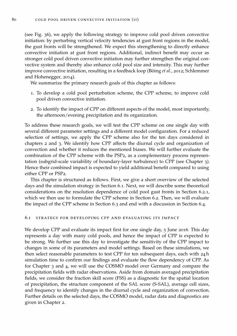
80 cold pool driven convective initiation (ii)

(see Fig. 36), we apply the following strategy to improve cold pool driven convectiveinitiation: by perturbing vertical velocity tendencies at gust front regions in the model,the gust fronts will be strengthened. We expect this strengthening to directly enhanceconvective initiation at gust front regions. Additional, indirect benefit may occur asstronger cold pool driven convective initiation may further strengthen the original con-vective system and thereby also enhance cold pool size and intensity. This may furtherimprove convective initiation, resulting in a feedback loop (Böing et al., 2012; Schlemmerand Hohenegger, 2014).

We summarize the primary research goals of this chapter as follows:

1. To develop a cold pool perturbation scheme, the CPP scheme, to improve coldpool driven convective initiation.

2. To identify the impact of CPP on different aspects of the model, most importantly,the afternoon/evening precipitation and its organization.

To address these research goals, we will test the CPP scheme on one single day withseveral different parameter settings and a different model configuration. For a reducedselection of settings, we apply the CPP scheme also for the ten days considered inchapters 2 and 3. We identify how CPP affects the diurnal cycle and organization ofconvection and whether it reduces the mentioned biases. We will further evaluate thecombination of the CPP scheme with the PSP2, as a complementary process represen-tation (subgrid-scale variability of boundary-layer turbulence) to CPP (see Chapter 3).Hence their combined impact is expected to yield additional benefit compared to usingeither CPP or PSP2.

This chapter is structured as follows. First, we give a short overview of the selecteddays and the simulation strategy in Section 6.1. Next, we will describe some theoreticalconsiderations on the resolution dependence of cold pool gust fronts in Section 6.2.1,which we then use to formulate the CPP scheme in Section 6.2. Then, we will evaluatethe impact of the CPP scheme in Section 6.3 and end with a discussion in Section 6.4.

6.1 strategy for developing cpp and evaluating its impact

We develop CPP and evaluate its impact first for one single day, 5 June 2016. This dayrepresents a day with many cold pools, and hence the impact of CPP is expected tobe strong. We further use this day to investigate the sensitivity of the CPP impact tochanges in some of its parameters and model settings. Based on these simulations, wethen select reasonable parameters to test CPP for ten subsequent days, each with 24 hsimulation time to confirm our findings and evaluate the flow dependency of CPP. Asfor Chapter 3 and 4, we will use the COSMO model over Germany and compare theprecipitation fields with radar observations. Aside from domain averaged precipitationfields, we consider the fraction skill score (FSS) as a diagnostic for the spatial locationof precipitation, the structure component of the SAL score (S-SAL), average cell sizes,and frequency to identify changes in the diurnal cycle and organization of convection.Further details on the selected days, the COSMO model, radar data and diagnostics aregiven in Chapter 2.

6.2 cold pool perturbations cpp 81

6.2 cold pool perturbations cpp

In the previous chapter we have seen that lower resolution simulations yield weakervertical velocities at cold pool gust fronts. Hence, their gust fronts are expected tobe underresolved. As correcting measure, the cold pool perturbations aim to imposevertical velocity perturbations to achieve the following: lower resolution simulations ofotherwise underresolved gust fronts will then produce vertical velocity scales of fullyresolved cold pool gust fronts. To get a better understanding of how grid size affectsthe vertical velocity scale of gust fronts we use dimensional analysis in Section 6.2.1.This also provides a target vertical velocity scale w0 of fully resolved cold pools. In thesubsequent subsections, we use this target vertical velocity scale w0 to build appropriatecold pool perturbations for the numerical model.

6.2.1 Scale of gust front vertical velocity

For the dimensional analysis, the inviscid, Boussinesque approximated set of equationsfor the stream function Φ, vorticity η and vertical velocity w in a two dimensional planein x and z are used, which are often considered for density currents (Rotunno et al., 1988;Weisman and Rotunno, 2004; Bryan and Rotunno, 2014b). Characteristic scales are usedto non-dimensionalize the equations. A detailed derivation is given in Appendix B. Thefollowing characteristic scale W for the vertical velocity is then given as a function ofthe characteristic buoyancy scale B, the horizontal length scale L and the vertical lengthscale H:

W =

√BH

1 + L2

H2

. (11)

This relationship describes the characteristic, vertical velocity scale within a circulationdriven by horizontal buoyancy gradients and how it depends on both the horizontaland vertical length scales in addition to the characteristic buoyancy scale.

Similar relationships have been formulated for rising warm bubbles by Weisman et al.(1997); Pauluis and Garner (2006); Morrison (2016a,b); Jeevanjee and Romps (2016); Jee-vanjee (2017). These studies investigate buoyant acceleration and associated pressureperturbations, which arise from displacing the air above the vertically accelerating par-cel to make way for it. These pressure perturbations can reduce the effective accelera-tion substantially. Importantly, these pressure perturbations depend on the horizontalextent L and the vertical extent H of the buoyancy acceleration: for thin and tall parcels( L

H ≈ 1), the pressure perturbation deceleration is moderate while for wide and flatparcels ( L

H � 1) the pressure perturbation deceleration is larger as substantially moreair has to be displaced. Dependent on the specific formulation of the problem, thearising dependency of W on L

H varies in the different studies. However, Jeevanjee (2017)showed that the different scalings from Weisman et al. (1997); Pauluis and Garner (2006);Morrison (2016a); Jeevanjee (2017) are comparable. We have further confirmed a closeresemblance of (11) with the formulations of the mentioned studies. As the underlyingphysical processes for the generation of vertical motion are comparable for cold poolgust fronts, this resemblance is not surprising.

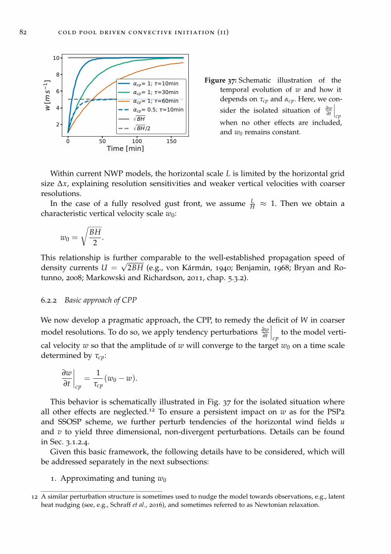
82 cold pool driven convective initiation (ii)

0 50 100 150Time [min]

2

4

6

8

10w

[ms

1 ] cp= 1; =10mincp= 1; =30mincp= 1; =60mincp= 0.5; =10minBH

BH /2

Figure 37: Schematic illustration of thetemporal evolution of w and how itdepends on τcp and αcp. Here, we con-

sider the isolated situation of ∂w∂t

∣∣∣cp

when no other effects are included,and w0 remains constant.

Within current NWP models, the horizontal scale L is limited by the horizontal gridsize ∆x, explaining resolution sensitivities and weaker vertical velocities with coarserresolutions.

In the case of a fully resolved gust front, we assume LH ≈ 1. Then we obtain a

characteristic vertical velocity scale w0:

w0 =

√BH2

.

This relationship is further comparable to the well-established propagation speed ofdensity currents U =

√2BH (e.g., von Kármán, 1940; Benjamin, 1968; Bryan and Ro-

tunno, 2008; Markowski and Richardson, 2011, chap. 5.3.2).

6.2.2 Basic approach of CPP

We now develop a pragmatic approach, the CPP, to remedy the deficit of W in coarsermodel resolutions. To do so, we apply tendency perturbations ∂w

∂t

∣∣∣cp

to the model verti-

cal velocity w so that the amplitude of w will converge to the target w0 on a time scaledetermined by τcp:

∂w∂t

∣∣∣∣cp

=1

τcp(w0 − w).

This behavior is schematically illustrated in Fig. 37 for the isolated situation whereall other effects are neglected.12 To ensure a persistent impact on w as for the PSP2

and SSOSP scheme, we further perturb tendencies of the horizontal wind fields uand v to yield three dimensional, non-divergent perturbations. Details can be foundin Sec. 3.1.2.4.

Given this basic framework, the following details have to be considered, which willbe addressed separately in the next subsections:

1. Approximating and tuning w0

12 A similar perturbation structure is sometimes used to nudge the model towards observations, e.g., latentheat nudging (see, e.g., Schraff et al., 2016), and sometimes referred to as Newtonian relaxation.

6.2 cold pool perturbations cpp 83

Figure 38: Comparison of maximum vertical velocity wmax in the lowest kilometer at the surface(a) and the target vertical velocity w0 (αcp = 1) as approximated from θv gradients (b). Notethe different scales of the colorbars.

2. Considering the vertical distribution of the perturbations

3. Finding a reasonable timescale τcp

4. Confining perturbations to cold pool gust fronts

6.2.3 Approximation of w0 and αcp

To compute the target vertical velocity for CPP, w0 =√

BH2 , we have to approximate the

cold pool buoyancy B and its height H. For simplicity, we fix H = 200 m. This heightcorresponds approximately to the buoyancy anomaly of cold pools within the COSMOsimulations (not shown) and has also been used in the ICON simulations in Chapter 5.As we do not intend to identify cold pools online in the model, we estimate the coldpool buoyancy as the local buoyancy gradient near the surface multiplied by the widthof the gradient. As the model cannot resolve sharp gradients, we assume that gradientswill be flattened on a scale of the effective model resolution of 5∆x. We define B as:

B = |∇θv| · 5∆xg1θv

,

where the bar denotes the mass-weighted average over the lowest 5 model levels, whichcorresponds approximately to the lowest 200 m.13

Doing so, we obtain√

BH with values of up to O(10 m s−1) at cold pool gust fronts,as displayed in Fig. 38b. While this is significantly stronger than what is currently sim-ulated for w with the model (Fig. 38a), and even with the 156 m ICON-LEM simulation

13 Instead of using the environmental θv as reference temperature (as is usually considered for buoyancy),we use the local values instead. With temperature differences of few Kelvin compared to reference tem-peratures of O(300K), this is a reasonable assumption and strongly simplifies the computation.

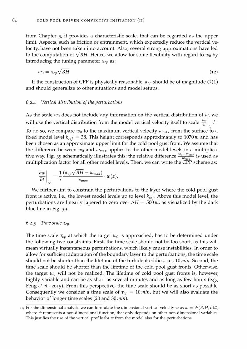
84 cold pool driven convective initiation (ii)

from Chapter 5, it provides a characteristic scale, that can be regarded as the upperlimit. Aspects, such as friction or entrainment, which expectedly reduce the vertical ve-locity, have not been taken into account. Also, several strong approximations have ledto the computation of

√BH. Hence, we allow for some flexibility with regard to w0 by

introducing the tuning parameter αcp as:

w0 = αcp√

BH (12)

If the construction of CPP is physically reasonable, αcp should be of magnitude O(1)and should generalize to other situations and model setups.

6.2.4 Vertical distribution of the perturbations

As the scale w0 does not include any information on the vertical distribution of w, wewill use the vertical distribution from the model vertical velocity itself to scale ∂w

∂t

∣∣∣cp

.14

To do so, we compare w0 to the maximum vertical velocity wmax from the surface to afixed model level kre f = 38. This height corresponds approximately to 1070 m and hasbeen chosen as an approximate upper limit for the cold pool gust front. We assume thatthe difference between w0 and wmax applies to the other model levels in a multiplica-tive way. Fig. 39 schematically illustrates this: the relative difference w0−wmax

wmaxis used as

multiplication factor for all other model levels. Then, we can write the CPP scheme as:

∂w∂t

∣∣∣∣cp

=1τ

(αcp√

BH − wmax)

wmax· w(z).

We further aim to constrain the perturbations to the layer where the cold pool gustfront is active, i.e., the lowest model levels up to level kre f . Above this model level, theperturbations are linearly tapered to zero over ∆H = 500 m, as visualized by the darkblue line in Fig. 39.

6.2.5 Time scale τcp

The time scale τcp at which the target w0 is approached, has to be determined underthe following two constraints. First, the time scale should not be too short, as this willmean virtually instantaneous perturbations, which likely cause instabilities. In order toallow for sufficient adaptation of the boundary layer to the perturbations, the time scaleshould not be shorter than the lifetime of the turbulent eddies, i.e., 10 min. Second, thetime scale should be shorter than the lifetime of the cold pool gust fronts. Otherwise,the target w0 will not be realized. The lifetime of cold pool gust fronts is, however,highly variable and can be as short as several minutes and as long as few hours (e.g.,Feng et al., 2015). From this perspective, the time scale should be as short as possible.Consequently we consider a time scale of τcp = 10 min, but we will also evaluate thebehavior of longer time scales (20 and 30 min).

14 For the dimensional analysis we can formulate the dimensional vertical velocity w as w = W(B, H, L)w,where w represents a non-dimensional function, that only depends on other non-dimensional variables.This justifies the use of the vertical profile for w from the model also for the perturbations.

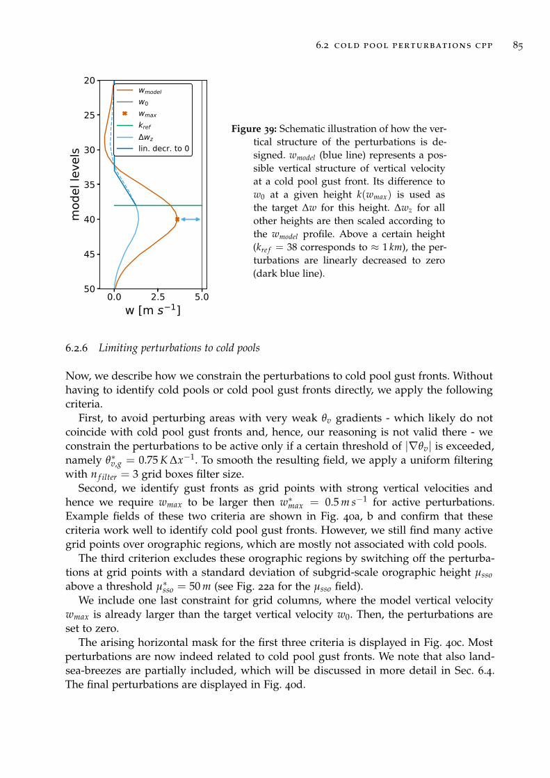
6.2 cold pool perturbations cpp 85

0.0 2.5 5.0w [m s 1]

20

25

30

35

40

45

50

mod

el le

vels

wmodel

w0wmax

kref wz

lin. decr. to 0

Figure 39: Schematic illustration of how the ver-tical structure of the perturbations is de-signed. wmodel (blue line) represents a pos-sible vertical structure of vertical velocityat a cold pool gust front. Its difference tow0 at a given height k(wmax) is used asthe target ∆w for this height. ∆wz for allother heights are then scaled according tothe wmodel profile. Above a certain height(kre f = 38 corresponds to ≈ 1 km), the per-turbations are linearly decreased to zero(dark blue line).

6.2.6 Limiting perturbations to cold pools

Now, we describe how we constrain the perturbations to cold pool gust fronts. Withouthaving to identify cold pools or cold pool gust fronts directly, we apply the followingcriteria.

First, to avoid perturbing areas with very weak θv gradients - which likely do notcoincide with cold pool gust fronts and, hence, our reasoning is not valid there - weconstrain the perturbations to be active only if a certain threshold of |∇θv| is exceeded,namely θ∗v,g = 0.75 K ∆x−1. To smooth the resulting field, we apply a uniform filteringwith n f ilter = 3 grid boxes filter size.

Second, we identify gust fronts as grid points with strong vertical velocities andhence we require wmax to be larger then w∗max = 0.5 m s−1 for active perturbations.Example fields of these two criteria are shown in Fig. 40a, b and confirm that thesecriteria work well to identify cold pool gust fronts. However, we still find many activegrid points over orographic regions, which are mostly not associated with cold pools.

The third criterion excludes these orographic regions by switching off the perturba-tions at grid points with a standard deviation of subgrid-scale orographic height µssoabove a threshold µ∗sso = 50 m (see Fig. 22a for the µsso field).

We include one last constraint for grid columns, where the model vertical velocitywmax is already larger than the target vertical velocity w0. Then, the perturbations areset to zero.

The arising horizontal mask for the first three criteria is displayed in Fig. 40c. Mostperturbations are now indeed related to cold pool gust fronts. We note that also land-sea-breezes are partially included, which will be discussed in more detail in Sec. 6.4.The final perturbations are displayed in Fig. 40d.

86 cold pool driven convective initiation (ii)

Figure 40: Illustration of how the perturbations are constrained to cold pool gust fronts. In (a),the buoyancy gradients are displayed with values smaller than 0.75 K ∆x−1 shaded grey. In(b), wmax is shown with values smaller 0.5 m s−1 shaded grey. In (c), wmax is shaded usingthe first two criteria combined with the orography criterion. In (d), the final perturbationsfor ∂w

∂t are shown.

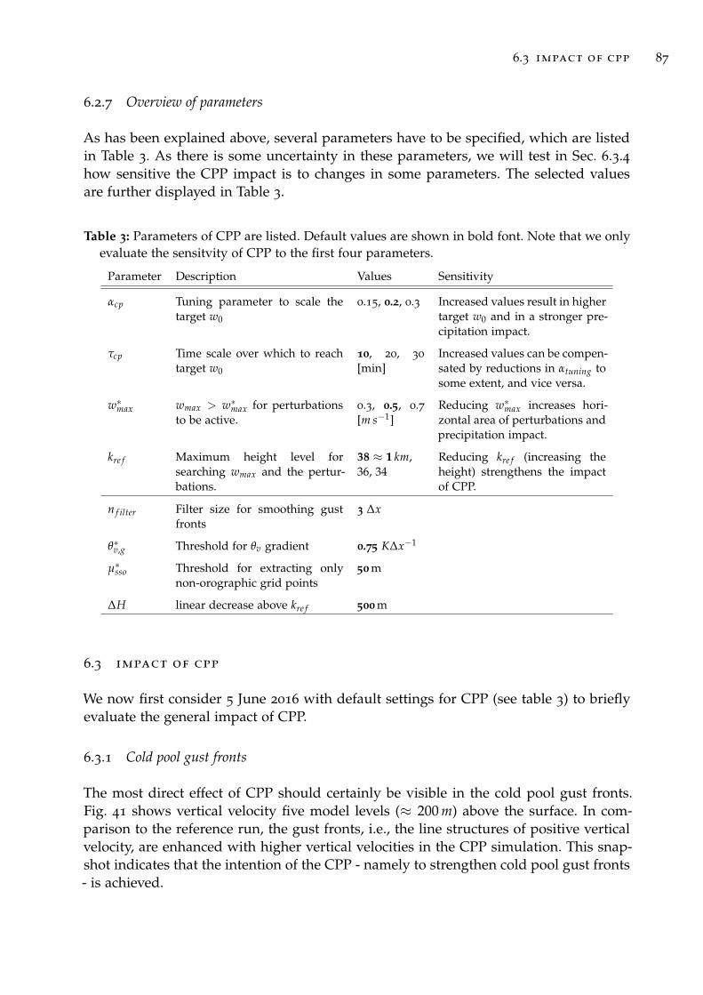
6.3 impact of cpp 87

6.2.7 Overview of parameters

As has been explained above, several parameters have to be specified, which are listedin Table 3. As there is some uncertainty in these parameters, we will test in Sec. 6.3.4how sensitive the CPP impact is to changes in some parameters. The selected valuesare further displayed in Table 3.

Table 3: Parameters of CPP are listed. Default values are shown in bold font. Note that we onlyevaluate the sensitvity of CPP to the first four parameters.

Parameter Description Values Sensitivity

αcp Tuning parameter to scale thetarget w0

0.15, 0.2, 0.3 Increased values result in highertarget w0 and in a stronger pre-cipitation impact.

τcp Time scale over which to reachtarget w0

10, 20, 30

[min]Increased values can be compen-sated by reductions in αtuning tosome extent, and vice versa.

w∗max wmax > w∗max for perturbationsto be active.

0.3, 0.5, 0.7[m s−1]

Reducing w∗max increases hori-zontal area of perturbations andprecipitation impact.

kre f Maximum height level forsearching wmax and the pertur-bations.

38 ≈ 1 km,36, 34

Reducing kre f (increasing theheight) strengthens the impactof CPP.

n f ilter Filter size for smoothing gustfronts

3 ∆x

θ∗v,g Threshold for θv gradient 0.75 K∆x−1

µ∗sso Threshold for extracting onlynon-orographic grid points

50m

∆H linear decrease above kre f 500m

6.3 impact of cpp

We now first consider 5 June 2016 with default settings for CPP (see table 3) to brieflyevaluate the general impact of CPP.

6.3.1 Cold pool gust fronts

The most direct effect of CPP should certainly be visible in the cold pool gust fronts.Fig. 41 shows vertical velocity five model levels (≈ 200 m) above the surface. In com-parison to the reference run, the gust fronts, i.e., the line structures of positive verticalvelocity, are enhanced with higher vertical velocities in the CPP simulation. This snap-shot indicates that the intention of the CPP - namely to strengthen cold pool gust fronts- is achieved.

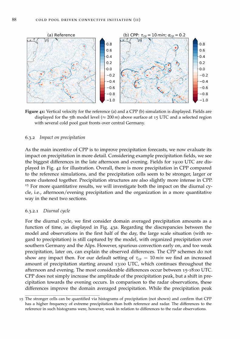
88 cold pool driven convective initiation (ii)

Figure 41: Vertical velocity for the reference (a) and a CPP (b) simulation is displayed. Fields aredisplayed for the 5th model level (≈ 200 m) above surface at 15 UTC and a selected regionwith several cold pool gust fronts over central Germany.

6.3.2 Impact on precipitation

As the main incentive of CPP is to improve precipitation forecasts, we now evaluate itsimpact on precipitation in more detail. Considering example precipitation fields, we seethe biggest differences in the late afternoon and evening. Fields for 19:00 UTC are dis-played in Fig. 42 for illustration. Overall, there is more precipitation in CPP comparedto the reference simulations, and the precipitation cells seem to be stronger, larger ormore clustered together. Precipitation structures are also slightly more intense in CPP.15 For more quantitative results, we will investigate both the impact on the diurnal cy-cle, i.e., afternoon/evening precipitation and the organization in a more quantitativeway in the next two sections.

6.3.2.1 Diurnal cycle

For the diurnal cycle, we first consider domain averaged precipitation amounts as afunction of time, as displayed in Fig. 43a. Regarding the discrepancies between themodel and observations in the first half of the day, the large scale situation (with re-gard to precipitation) is still captured by the model, with organized precipitation oversouthern Germany and the Alps. However, spurious convection early on, and too weakprecipitation, later on, can explain the observed differences. The CPP schemes do notshow any impact then. For our default setting of τcp = 10 min we find an increasedamount of precipitation starting around 13:00 UTC, which continues throughout theafternoon and evening. The most considerable differences occur between 15-18:00 UTC.CPP does not simply increase the amplitude of the precipitation peak, but a shift in pre-cipitation towards the evening occurs. In comparison to the radar observations, thesedifferences improve the domain averaged precipitation. While the precipitation peak

15 The stronger cells can be quantified via histograms of precipitation (not shown) and confirm that CPPhas a higher frequency of extreme precipitation than both reference and radar. The differences to thereference in such histograms were, however, weak in relation to differences to the radar observations.

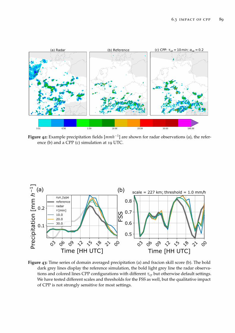
6.3 impact of cpp 89

Figure 42: Example precipitation fields [mmh−1] are shown for radar observations (a), the refer-ence (b) and a CPP (c) simulation at 19 UTC.

03 06 09 12 15 18 21 00

Time [HH UTC]

0.5

0.6

0.7

0.8

FSS

scale = 227 km; threshold = 1.0 mm/h

03 06 09 12 15 18 21 00

Time [HH UTC]

0.1

0.2

Preci

pitation [

mmh

1]

run_typereferenceradar

[min]10.020.030.0

(a) (b)

Figure 43: Time series of domain averaged precipitation (a) and fracion skill score (b). The bolddark grey lines display the reference simulation, the bold light grey line the radar observa-tions and colored lines CPP configurations with different τcp but otherwise default settings.We have tested different scales and thresholds for the FSS as well, but the qualitative impactof CPP is not strongly sensitive for most settings.

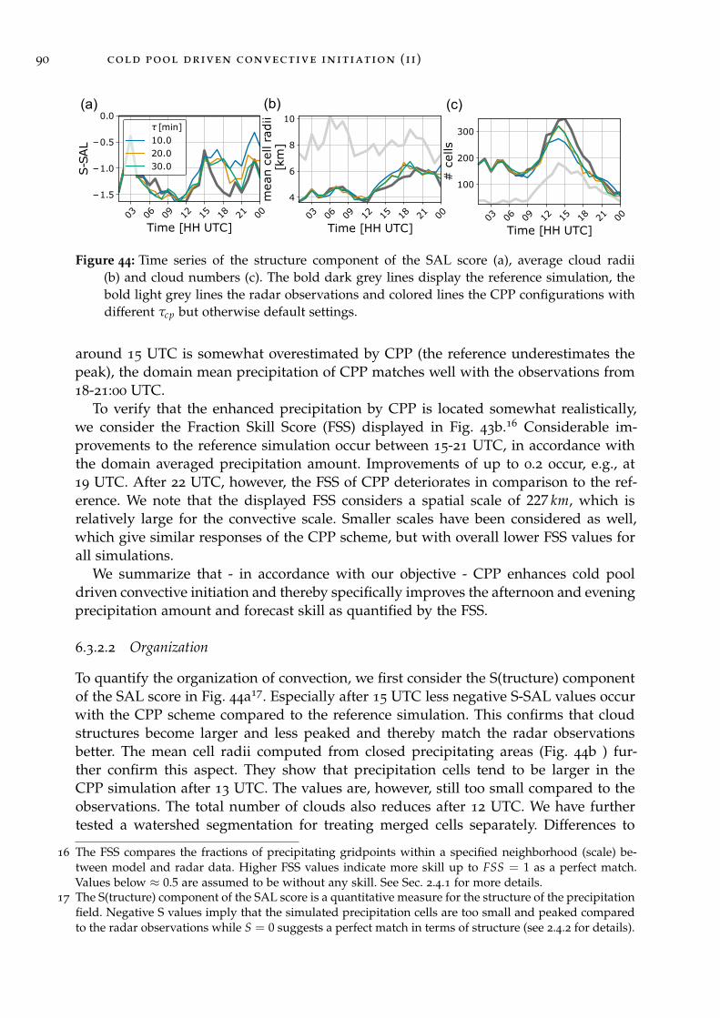
90 cold pool driven convective initiation (ii)

03 06 09 12 15 18 21 00

Time [HH UTC]

1.5

1.0

0.5

0.0

S-S

AL

[min]10.020.030.0

03 06 09 12 15 18 21 00

Time [HH UTC]

4

6

8

10

mean c

ell

radii

[km

]

03 06 09 12 15 18 21 00

Time [HH UTC]

100

200

300

# c

ells

(a) (b) (c)

Figure 44: Time series of the structure component of the SAL score (a), average cloud radii(b) and cloud numbers (c). The bold dark grey lines display the reference simulation, thebold light grey lines the radar observations and colored lines the CPP configurations withdifferent τcp but otherwise default settings.

around 15 UTC is somewhat overestimated by CPP (the reference underestimates thepeak), the domain mean precipitation of CPP matches well with the observations from18-21:00 UTC.

To verify that the enhanced precipitation by CPP is located somewhat realistically,we consider the Fraction Skill Score (FSS) displayed in Fig. 43b.16 Considerable im-provements to the reference simulation occur between 15-21 UTC, in accordance withthe domain averaged precipitation amount. Improvements of up to 0.2 occur, e.g., at19 UTC. After 22 UTC, however, the FSS of CPP deteriorates in comparison to the ref-erence. We note that the displayed FSS considers a spatial scale of 227 km, which isrelatively large for the convective scale. Smaller scales have been considered as well,which give similar responses of the CPP scheme, but with overall lower FSS values forall simulations.

We summarize that - in accordance with our objective - CPP enhances cold pooldriven convective initiation and thereby specifically improves the afternoon and eveningprecipitation amount and forecast skill as quantified by the FSS.

6.3.2.2 Organization

To quantify the organization of convection, we first consider the S(tructure) componentof the SAL score in Fig. 44a17. Especially after 15 UTC less negative S-SAL values occurwith the CPP scheme compared to the reference simulation. This confirms that cloudstructures become larger and less peaked and thereby match the radar observationsbetter. The mean cell radii computed from closed precipitating areas (Fig. 44b ) fur-ther confirm this aspect. They show that precipitation cells tend to be larger in theCPP simulation after 13 UTC. The values are, however, still too small compared to theobservations. The total number of clouds also reduces after 12 UTC. We have furthertested a watershed segmentation for treating merged cells separately. Differences to

16 The FSS compares the fractions of precipitating gridpoints within a specified neighborhood (scale) be-tween model and radar data. Higher FSS values indicate more skill up to FSS = 1 as a perfect match.Values below ≈ 0.5 are assumed to be without any skill. See Sec. 2.4.1 for more details.

17 The S(tructure) component of the SAL score is a quantitative measure for the structure of the precipitationfield. Negative S values imply that the simulated precipitation cells are too small and peaked comparedto the radar observations while S = 0 suggests a perfect match in terms of structure (see 2.4.2 for details).

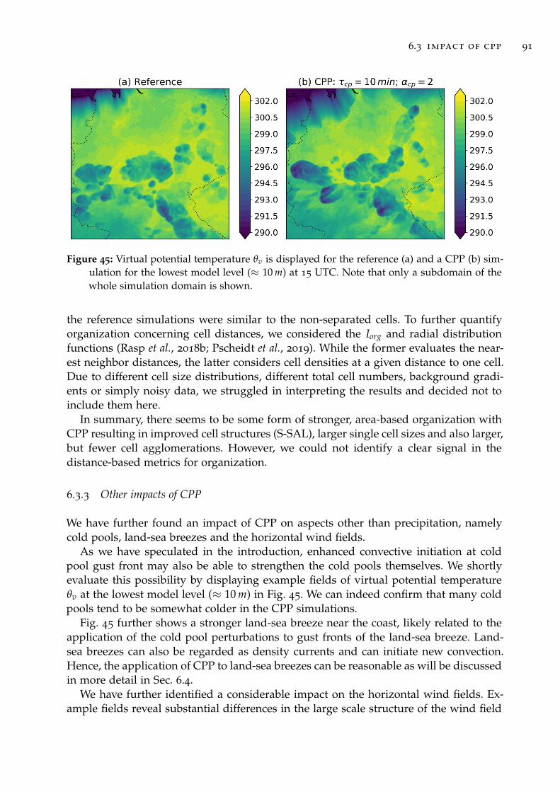
6.3 impact of cpp 91

Figure 45: Virtual potential temperature θv is displayed for the reference (a) and a CPP (b) sim-ulation for the lowest model level (≈ 10 m) at 15 UTC. Note that only a subdomain of thewhole simulation domain is shown.

the reference simulations were similar to the non-separated cells. To further quantifyorganization concerning cell distances, we considered the Iorg and radial distributionfunctions (Rasp et al., 2018b; Pscheidt et al., 2019). While the former evaluates the near-est neighbor distances, the latter considers cell densities at a given distance to one cell.Due to different cell size distributions, different total cell numbers, background gradi-ents or simply noisy data, we struggled in interpreting the results and decided not toinclude them here.

In summary, there seems to be some form of stronger, area-based organization withCPP resulting in improved cell structures (S-SAL), larger single cell sizes and also larger,but fewer cell agglomerations. However, we could not identify a clear signal in thedistance-based metrics for organization.

6.3.3 Other impacts of CPP

We have further found an impact of CPP on aspects other than precipitation, namelycold pools, land-sea breezes and the horizontal wind fields.

As we have speculated in the introduction, enhanced convective initiation at coldpool gust front may also be able to strengthen the cold pools themselves. We shortlyevaluate this possibility by displaying example fields of virtual potential temperatureθv at the lowest model level (≈ 10 m) in Fig. 45. We can indeed confirm that many coldpools tend to be somewhat colder in the CPP simulations.

Fig. 45 further shows a stronger land-sea breeze near the coast, likely related to theapplication of the cold pool perturbations to gust fronts of the land-sea breeze. Land-sea breezes can also be regarded as density currents and can initiate new convection.Hence, the application of CPP to land-sea breezes can be reasonable as will be discussedin more detail in Sec. 6.4.

We have further identified a considerable impact on the horizontal wind fields. Ex-ample fields reveal substantial differences in the large scale structure of the wind field

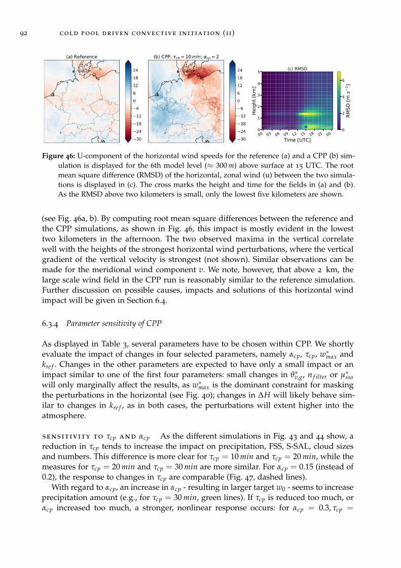
92 cold pool driven convective initiation (ii)

00 03 06 09 12 15 18 21 00Time [UTC]

0

1

2

3

4

5

Heig

ht [k

m]

(c) RMSD

0

2

4

6

RMSD

[m s

1 ]

Figure 46: U-component of the horizontal wind speeds for the reference (a) and a CPP (b) sim-ulation is displayed for the 6th model level (≈ 300 m) above surface at 15 UTC. The rootmean square difference (RMSD) of the horizontal, zonal wind (u) between the two simula-tions is displayed in (c). The cross marks the height and time for the fields in (a) and (b).As the RMSD above two kilometers is small, only the lowest five kilometers are shown.

(see Fig. 46a, b). By computing root mean square differences between the reference andthe CPP simulations, as shown in Fig. 46, this impact is mostly evident in the lowesttwo kilometers in the afternoon. The two observed maxima in the vertical correlatewell with the heights of the strongest horizontal wind perturbations, where the verticalgradient of the vertical velocity is strongest (not shown). Similar observations can bemade for the meridional wind component v. We note, however, that above 2 km, thelarge scale wind field in the CPP run is reasonably similar to the reference simulation.Further discussion on possible causes, impacts and solutions of this horizontal windimpact will be given in Section 6.4.

6.3.4 Parameter sensitivity of CPP

As displayed in Table 3, several parameters have to be chosen within CPP. We shortlyevaluate the impact of changes in four selected parameters, namely αcp, τcp, w∗max andkre f . Changes in the other parameters are expected to have only a small impact or animpact similar to one of the first four parameters: small changes in θ∗v,g, n f ilter or µ∗ssowill only marginally affect the results, as w∗max is the dominant constraint for maskingthe perturbations in the horizontal (see Fig. 40); changes in ∆H will likely behave sim-ilar to changes in kre f , as in both cases, the perturbations will extent higher into theatmosphere.

sensitivity to τcp and αcp As the different simulations in Fig. 43 and 44 show, areduction in τcp tends to increase the impact on precipitation, FSS, S-SAL, cloud sizesand numbers. This difference is more clear for τcp = 10 min and τcp = 20 min, while themeasures for τcp = 20 min and τcp = 30 min are more similar. For αcp = 0.15 (instead of0.2), the response to changes in τcp are comparable (Fig. 47, dashed lines).

With regard to αcp, an increase in αcp - resulting in larger target w0 - seems to increaseprecipitation amount (e.g., for τcp = 30 min, green lines). If τcp is reduced too much, orαcp increased too much, a stronger, nonlinear response occurs: for αcp = 0.3, τcp =

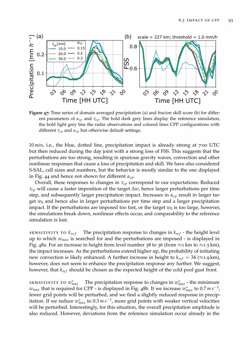
6.3 impact of cpp 93

03 06 09 12 15 18 21 00

Time [HH UTC]

0.1

0.2

Preci

pitation [

mm

h1]

[min]cp10.020.030.0

cp

0.150.20.3

03 06 09 12 15 18 21 00

Time [HH UTC]

0.6

0.8

FSS

scale = 227 km; threshold = 1.0 mm/h(a) (b)

Figure 47: Time series of domain averaged precipitation (a) and fracion skill score (b) for differ-ent parameters of αcp and τcp. The bold dark grey lines display the reference simulation,the bold light grey line the radar observations and colored lines CPP configurations withdifferent τcp and αcp but otherwise default settings.

10 min, i.e., the blue, dotted line, precipitation impact is already strong at 7:00 UTCbut then reduced during the day joint with a strong loss of FSS. This suggests that theperturbations are too strong, resulting in spurious gravity waves, convection and othernonlinear responses that cause a loss of precipitation and skill. We have also consideredS-SAL, cell sizes and numbers, but the behavior is mostly similar to the one displayedin Fig. 44 and hence not shown for different αcp.

Overall, these responses to changes in τcp correspond to our expectations: Reducedτcp will cause a faster imposition of the target ∆w, hence larger perturbations per timestep, and subsequently larger precipitation impact. Increases in αcp result in larger tar-get w0 and hence also in larger perturbations per time step and a larger precipitationimpact. If the perturbations are imposed too fast, or the target w0 is too large, however,the simulations break down, nonlinear effects occur, and comparability to the referencesimulation is lost.

sensitivity to k re f The precipitation response to changes in kre f - the height levelup to which wmax is searched for and the perturbations are imposed - is displayed inFig. 48a. For an increase in height from level number 38 to 36 (from ≈1 km to ≈1.5 km),the impact increases. As the perturbations extend higher up, the probability of initiatingnew convection is likely enhanced. A further increase in height to kre f = 34 (≈1.9 km),however, does not seem to enhance the precipitation response any further. We suggest,however, that kre f should be chosen as the expected height of the cold pool gust front.

sensitivity to w∗max The precipitation response to changes in w∗max - the minimumwmax that is required for CPP - is displayed in Fig. 48b. If we increase w∗max to 0.7 m s−1,fewer grid points will be perturbed, and we find a slightly reduced response in precip-itation. If we reduce w∗max to 0.3 m s−1, more grid points with weaker vertical velocitieswill be perturbed. Interestingly, for this situation, the overall precipitation amplitude isalso reduced. However, deviations from the reference simulation occur already in the

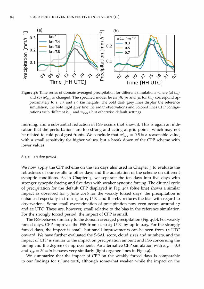
94 cold pool driven convective initiation (ii)

03 06 09 12 15 18 21 00

Time [HH UTC]

0.1

0.2

0.3

Preci

pitation [

mmh

1]

krefkref34kref36kref38

(a) (b)

03 06 09 12 15 18 21 00

Time [HH UTC]

0.1

0.2

Preci

pitation [

mmh

1]

w*max [ms 1]0.30.50.7

Figure 48: Time series of domain averaged precipitation for different simulations where (a) kre fand (b) w∗max is changed. The specified model levels 38, 36 and 34 for kre f correspond ap-proximately to 1, 1.5 and 1.9 km heights. The bold dark grey lines display the referencesimulation, the bold light grey line the radar observations and colored lines CPP configu-rations with different kre f and wmax∗ but otherwise default settings.

morning, and a substantial reduction in FSS occurs (not shown). This is again an indi-cation that the perturbations are too strong and acting at grid points, which may notbe related to cold pool gust fronts. We conclude that w∗max ≈ 0.5 is a reasonable value,with a small sensitivity for higher values, but a break down of the CPP scheme withlower values.

6.3.5 10 day period

We now apply the CPP scheme on the ten days also used in Chapter 3 to evaluate therobustness of our results to other days and the adaptation of the scheme on differentsynoptic conditions. As in Chapter 3, we separate the ten days into five days withstronger synoptic forcing and five days with weaker synoptic forcing. The diurnal cycleof precipitation for the default CPP displayed in Fig. 49a (blue line) shows a similarimpact as observed for 5 June 2016 for the weakly forced days: the precipitation isenhanced especially in from 15 to 19 UTC and thereby reduces the bias with regard toobservations. Some small overestimation of precipitation now even occurs around 17

and 22 UTC. These are, however, small relative to the bias in the reference simulation.For the strongly forced period, the impact of CPP is small.

The FSS behaves similarly to the domain averaged precipitation (Fig. 49b). For weaklyforced days, CPP improves the FSS from 14 to 23 UTC by up to 0.05. For the stronglyforced days, the impact is small, but small improvements can be seen from 15 UTConward. We have further evaluated the S-SAL score, cloud sizes and numbers, and theimpact of CPP is similar to the impact on precipitation amount and FSS concerning thetiming and the degree of improvements. An alternative CPP simulation with αcp = 0.3and τcp = 30 min behaves very similarly (light organge lines in Fig. 49).

We summarize that the impact of CPP on the weakly forced days is comparableto our findings for 5 June 2016, although somewhat weaker, while the impact on the

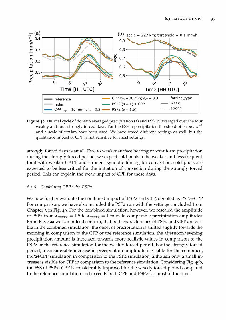
6.3 impact of cpp 95

5 10 15 20

Time [HH UTC]

0.1

0.2

0.3

0.4

Preci

pitation [

mmh

1]

referenceradarCPP cp= 10 min; cp= 0.2

CPP cp= 30 min; cp= 0.3

PSP2 ( = 1) + CPP

PSP2 ( = 1.5)

forcing_typeweakstrong

(a) (b)

5 10 15 20

Time [HH UTC]

0.5

0.6

0.7

0.8

0.9

FSS

scale = 227 km; threshold = 0.1 mm/h

Figure 49: Diurnal cycle of domain averaged precipitation (a) and FSS (b) averaged over the fourweakly and four strongly forced days. For the FSS, a precipitation threshold of 0.1 mm h−1

and a scale of 227 km have been used. We have tested different settings as well, but thequalitative impact of CPP is not sensitive for most settings.

strongly forced days is small. Due to weaker surface heating or stratiform precipitationduring the strongly forced period, we expect cold pools to be weaker and less frequent.Joint with weaker CAPE and stronger synoptic forcing for convection, cold pools areexpected to be less critical for the initiation of convection during the strongly forcedperiod. This can explain the weak impact of CPP for these days.

6.3.6 Combining CPP with PSP2

We now further evaluate the combined impact of PSP2 and CPP, denoted as PSP2+CPP.For comparison, we have also included the PSP2 run with the settings concluded fromChapter 3 in Fig. 49. For the combined simulation, however, we rescaled the amplitudeof PSP2 from αtuning = 1.5 to αtuning = 1 to yield comparable precipitation amplitudes.From Fig. 49a we can indeed confirm, that both characteristics of PSP2 and CPP are visi-ble in the combined simulation: the onset of precipitation is shifted slightly towards themorning in comparison to the CPP or the reference simulation; the afternoon/eveningprecipitation amount is increased towards more realistic values in comparison to thePSP2 or the reference simulation for the weakly forced period. For the strongly forcedperiod, a considerable increase in precipitation amplitude is visible for the combined,PSP2+CPP simulation in comparison to the PSP2 simulation, although only a small in-crease is visible for CPP in comparison to the reference simulation. Considering Fig. 49b,the FSS of PSP2+CPP is considerably improved for the weakly forced period comparedto the reference simulation and exceeds both CPP and PSP2 for most of the time.

96 cold pool driven convective initiation (ii)

6.4 discussion

In this chapter, we developed deterministic perturbations for the three wind compo-nents with the incentive to strengthen cold pool gust fronts and thereby enhance the af-ternoon/evening precipitation and organization of convection. The perturbations weredesigned so that the vertical velocity in the lowest kilometer at cold pool gust fronts con-verges towards a target vertical velocity, which was obtained from dimensional analysisand estimated by local buoyancy gradients.

6.4.1 Benefits for precipitation

Example fields of vertical velocity revealed stronger updrafts at cold pool gust frontswith CPP compared to the reference simulation. Afternoon/evening precipitation is en-hanced, and FSS improved by CPP. Both S-SAL and cloud size and numbers improvedto a small amount for the CPP simulations, which provide proxies for area-based or-ganization. These results confirmed that CPP indeed achieves the original goals of thescheme.

These generally positive results were further confirmed on five weakly forced days,although to a lesser extent. The impact of CPP on five strongly forced days is weak, asexpected, due to the assumed weaker role of cold pools for convective initiation. Hence,the design and settings of CPP, which we developed/chose based on 5 June 2016, arealso applicable to other situations, and CPP adapts well to different situations.

Furthermore, we tested how sensitive the impact of CPP is to changes in some ofthe CPP settings. As the most direct tuning parameters of CPP, reducing the time scaleτcp or enhancing αcp results in stronger perturbations and impacts of CPP. We foundfurther sensitivities to other parameters, but we recommend their default values basedon physical reasoning. If the chosen settings result in unusually high perturbation am-plitudes, i.e., by using too small τcp, w∗max or too large αcp, spurious gravity waves,convection and other artifacts arise, and the simulations lose their comparability to thereference simulation. Such settings should be avoided. We hope this sensitivity studywill give some guidance for future applications with CPP on which settings to choose.

The combined impact of CPP with the PSP2 scheme provides an additional high-light, as the combined simulation outperformed both singularly perturbed simulations.The results confirm the complementary behavior of the two process-based perturbationschemes PSP2 and CPP, and hence also the relevance of boundary-layer turbulence andcold pools for initiating convection. We can envision modeling frameworks where amultitude of complementary, process-level perturbation schemes can be combined toimprove weather forecasts. Such frameworks may also enable a better evaluation of therelevance of single processes or their interactions.

6.4.2 Other impacts of CPP

Aside from precipitation, we also identified impacts of CPP on other aspects, namelyon cold pools, land-sea breezes and horizontal wind fields.

6.4 discussion 97

Example θv fields near the surface suggest that cold pools are stronger with CPP. Aproper quantification of this effect is currently addressed in a Bachelor thesis, wherethe cold pool detection algorithm from the previous chapter (Chapter 5) is applied tothe here used COSMO simulations. Preliminary results indeed confirm this indication.Such strengthening of the cold pools by CPP hints at a feedback loop by which strongercold pool driven convective initiation by CPP strengthens the convection within theoriginal cold pools and thereby the cold pool itself. This feedback loop has further beenmentioned by Böing et al. (2012); Schlemmer and Hohenegger (2014).

These θv fields further displayed an impact on the land-sea breeze, where CPP wasalso active. As the land-sea breeze is also a form of a density current (e.g., Moncrieffand Liu, 1999), we expect a similar resolution sensitivity as for cold pools. In addition,land-sea breezes can also initiate new convection. These similarities between cold poolgust fronts and land-sea breezes suggest that it may be indeed appropriate to applyCPP to land-sea breezes. Further investigation will be necessary to identify whetherland-sea breezes are indeed insufficiently resolved at km-scales and whether the CPPscheme is an appropriate solution. This includes the applicability of the CPP settings,such as the height scale H = 200 m for land-sea breezes.

We further found an impact of CPP on the horizontal wind fields in the lowesttwo kilometers where the w-perturbations change strongest with height. The structureof this impact suggest that the positive, vertical velocity perturbations require a con-vergent flow near the surface, where the w-perturbations increase with height, and adivergent flow at ≈ 1.5 km, where the w-perturbations decrease with height to satisfy3d non-divergence. Due to the very localized w-perturbations, we expected the com-pensating horizontal flow to be small. Unfortunately, this seems not to be the case.Nonetheless, we do not expect that this behavior has a strong effect on precipitation:the strength of the vertical velocity should be the primary mechanism for convectiveinitiation, and, as the effect is localized to few height levels in the boundary layer, con-vective updrafts in the free troposphere should not be affected. Also, the positive impacton the spatial distribution of precipitation implies that the large scale situation is stillsufficiently represented. For the operational application of CPP, however, other aspects,e.g., transport of pollutants in the boundary layer, have to be considered as well, whichmay be negatively affected by the current impact of CPP on the horizontal wind fields.Hence, a reduction of this impact is desireable for the future. A possible solution couldbe to include compensating subsidence nearby cold pool gust fronts.

6.4.3 Future steps

Above, we already described possible actions to improve the current CPP scheme, mostimportantly, addressing the impact on the horizontal wind. Two other steps that shouldbe carefully considered are the modification of CPP for scale adaptivity and a compre-hensive tuning of the model joint with CPP.

As scale adaptivity is a crucial feature for grey zone parameterizations (see Sec. 1.2.1),it is worth considering the applicability of the current CPP for different model resolu-tions. Certainly, CPP should only be applied if the models can explicitly resolve coldpools and deep convection. This likely limits CPP to resolutions below ten or even

98 cold pool driven convective initiation (ii)

five kilometers. Nevertheless, the parameters chosen here will likely be required to beadapted. w∗max is expected to depend on model resolution as vertical velocity gener-ally depends on it (Weisman et al., 1997; Pauluis and Garner, 2006; Morrison, 2016a,b;Jeevanjee and Romps, 2016; Jeevanjee, 2017). Theoretically derived relationships for wand grid size, however, already exist (e.g., Jeevanjee, 2017) and could be used to formu-late a scale-dependent w∗max. Similarly, the threshold to exclude orographic grid pointsµ∗sso could be formulated using scaling laws of orography. As cold pool strengths alsoappear to be sensitive to resolution (see chap. 5), gradients of θv will change as well.Despite the expected, weak sensitivity of the CPP impact to θ∗v,g, the chosen thresholdfor θ∗v,g may have to be adapted for different model resolutions. If no theoretical for-mulation can be found, empirical relationships could be used to find a scale adaptiveformulation of θ∗v,g. Simulations with different model resolutions will then allow insighton the scale adaptivity of CPP.

We emphasize that current models have been tuned over years - and sometimeseven decades - to best fit observations. The arising presence of compensating errors iswidely acknowledged (e.g., Palmer and Weisheimer, 2011; Mauritsen et al., 2012; Hanleyet al., 2015; Berner et al., 2017; Hourdin et al., 2017), and challenges the development ofprocess-based schemes such as CPP. One aforementioned example includes the tuningof the turbulent lenght scale tur_len to improve precipitation forecasts at the expenseof temperature biases (Baldauf et al., 2011; Schraff et al., 2016). By providing process-based schemes instead, we hope that the physical processes will be represented morerealistically, and resulting model responses will occur for the right reasons. Anotherapproach that could prove beneficial with regard to cold pools is the use of a two-moment microphysics scheme, which allows for a more sophisticated representation ofcloud condensation and evaporation processes. But to obtain a useful model setup withCPP and a two-moment microphysics scheme, parameters of both schemes have to betuned simultaneously. Ideally, such process-based schemes, including also PSP2, shouldbe incorporated in the comprehensive tuning process of operational models before theycan be used operationally. This is a costly endeavor, beyond the scope of any researcher.We hope we have given enough reasons for national weather centers to take over.

In summary, to address our posed research goals, we successfully developed a coldpool parameterization which strengthens cold pool gust fronts and - to all appearances- thereby enhances cold pool driven convective initiation. As anticipated, the late after-noon/evening precipitation improves for weakly forced situations, and enhanced orga-nization is indicated. Further development and evaluation may be necessary to ensurescale adaptivity and to quantify unforeseen side effects.

7S U M M A RY A N D C O N C L U S I O N S

7.1 summary

Some of the largest problems of convective precipitation forecasts in state-of-the-art,convection-permitting models are biases in the diurnal cycle and the organization ofconvection. A large portion of theses deficits is currently ascribed to the insufficient rep-resentation of processes leading to convective initiation. These processes occur in theboundary layer and are mostly too small to be sufficiently resolved even by convection-permitting models. This thesis has contributed to this unsettled research topic - regard-ing the deficiency in convective initiation - by identifying model deficits and potentialsolutions. Specifically, three of the most important processes for convective initiationhave been considered in detail, namely boundary-layer turbulence, subgrid-scale orog-raphy and cold pools.

representing boundarylayer turbulence variability Turbulence is a ubiq-uitous process in convective boundary layers and tightly coupled to convective initia-tion. Km-scale models traditionally include turbulence in deterministic, parameterizedform, i.e., the mean impact on the resolved scales is considered. As the subgrid variabil-ity of turbulence can be crucial for convective initiation, the PSP scheme was introducedby Kober and Craig (2016) to account for this subgrid variability in a stochastic mannerand to enhance convective initiation. In the first part of this thesis, four modificationsof this scheme were considered to improve its physical consistency and reduce un-wanted side effects. These included an autoregressive, continuously evolving randomfield; a limitation of the perturbations to the boundary layer that removes artificial con-vection at night; a mask that turns off perturbations in precipitating columns to retaincoherent structures; and non-divergent wind perturbations that drastically increase theeffectiveness of the vertical velocity perturbations. In a revised version, PSP2, the com-bined modifications retain the physically-based coupling to the boundary-layer schemewhile being physically more consistent. In addition, the spatial structure of the simu-lated precipitation cells was improved and spurious night-time precipitation reduced.Overall, this scheme has the potential to improve predictions of convective initiation inkilometer-scale models while minimizing other biases.

representing lifting by subgrid-scale orography Orography is an unde-niable trigger for convective initiation by a range of different mechanisms. In km-scalemodels, a large part of the orography is explicitly included, and the relevance of smallscale, i.e., subgrid-scale orography, for convective initiation is ambiguous. Nonetheless,we developed a stochastic scheme to include the effect of mechanical lifting by subgrid-scale orography, the SSOSP scheme. The mechanical lifting effect was chosen as the

99

100 summary and conclusions

most direct effect and approximated by gravity wave formalism and information onsubgrid-scale orography. While a clear increase in convective initiation over orographicregions was possible by the SSOSP scheme, this usually coincided with an undesiredimpact also on non-orographic regions. We concluded, that too large perturbation am-plitudes were necessary to see a substantial impact and that most likely, subgrid-scaleorography is not of primary relevance in the presence of resolved orography. Hence,we will focus from now on more on PSP2 and cold pools.

In both the PSP2 and the SSOSP stochastic perturbations were chosen to better rep-resent subgrid-scale distributions in the grey zone. This combination of process-levelperturbations and stochastic components is rare and innovative. It enables the reduc-tion of model errors by noise-induced drift, for instance by improving precipitationamplitudes or the diurnal cycle of precipitation; but also it facilitates the quantificationof model uncertainty at its source, which is crucial - yet uncommon - for reliable ensem-bles. For example, the commonly used stochastic approaches SPPT (Buizza et al., 1999)and SKEBS (Shutts, 2005) only facilitate the increase in ensemble spread without anyattribution to specific, physical processes.

cold pool driven convective initiation The two most notable chapters ofthis thesis are concerned with cold pool driven convective initiation. Cold pools providetriggering mechanism nearby already existing convection and thereby contribute to theorganization of convection. This further can prolong the lifetime of convection and bean effective trigger mechanism in the late afternoon, which influences the diurnal cy-cle of convection. Whether cold pools and their contribution to convective initiationare properly represented in km-scale models was an open question. Hence, cold pooldriven convective initiation was investigated in the first of the two cold pool chapterswith a focus on the diurnal cycle and organization of convection and the sensitivity togrid size. Simulations of the ICON-LEM model with grid sizes from 156 m to 625 mover Germany were used. In these simulations, we identified cold pools, cold poolboundaries and initiated convection. Cold pool driven convective initiation can be asdominant as 50% of total convective initiation, in particular in the late afternoon. Inaddition, cold pool related triggering is many times more efficient than without coldpools. By comparing different model resolutions, we found that cold pools are morefrequent, smaller and less intense in lower resolution simulations. Furthermore, theirgust fronts are weaker and less likely to trigger new convection. To identify how modelresolution affects this triggering probability, we used a linear causal graph analysis. Indoing so, we postulated a graph structure with potential causal pathways and thenapplied multi-linear regression accordingly. Despite several possible indirect pathways,we found one dominant, systematic effect: reducing grid sizes directly reduces upwardmass flux at the gust front, which causes weaker triggering probabilities. These findingsare expected to be even more relevant for km-scale, numerical weather prediction mod-els. We expected that a better representation of cold pool driven convective initiationwill advance forecasts of convective precipitation.

Consequently, in the second cold pool chapter, we developed a deterministic coldpool scheme to strengthen cold pool gust fronts and thereby improve cold pool drivenconvective initiation in km-scale models. A target vertical velocity scale for cold pool

7.2 future steps for psp2 and cpp 101

gust fronts was derived using dimensional analysis and approximated based on lo-cal buoyancy gradients. Vertical velocity perturbations were then imposed so that themodel vertical velocity at cold pool gust fronts converges towards this target scale. Inaddition, horizontal wind components were perturbed in a 3d non-divergent manneras for PSP2 and SSOSP. Our results showed that cold pool gust fronts are strengthenedby CPP and - to all appearances - enhances cold pool driven convective initiation. Asanticipated, the late afternoon/evening precipitation is improved for weakly forced situ-ations and indications for enhanced organization were found. Further development andevaluation may be necessary to ensure scale adaptivity and to quantify and eliminateside effects.

In addition, we evaluated the combined use of both PSP2 and CPP, as they representtwo complementary processes. Such a combined simulation revealed the benefits ofboth schemes, with an earlier onset of convection and improved afternoon/eveningprecipitation. This confirms the possibility, that process-based schemes can be used inan additive way to yield quasi-additive improvements of the forecasts.

7.2 future steps for psp2 and cpp

For now, we have focused on understanding the systematic changes caused by theperturbation schemes rather than on absolute forecast scores. Thus, whether PSP2 orCPP18 will improve forecasts still needs to be fully determined before they can be usedin operational weather forecasts. To do so, the following steps to further evaluate anddevelop the schemes are advisable.

1. As the operational use and development of the here used COSMO-DE modelwill be migrated to the ICON model in the future (personal communication withDWD), so should PSP2 and CPP. First pursuits to transfer PSP2 to the ICON modelare currently underway, but new challenges due to an irregular grid structure inICON arise.

2. The computational efficiency of the schemes will likely have to be improved. Thiscan be achieved by improving the computational implementation of the schemes,or by allowing approximations of some of the more cost-intensive aspects of theschemes. This will be a priority for implementing PSP2 in ICON.

3. The schemes should be tested at different model resolutions to evaluate theirscale adaptivity, a greatly desirable characteristic (see Section 1.2.1). Additionaldevelopment will likely be required to satisfy it.

4. Simulations using a full ensemble prediction system over a sufficiently long timeperiod are necessary to thoroughly validate the impact of the schemes. This shouldinclude data assimilation, a comprehensive selection of different weather situa-tions, and comparison to observations.

5. A retuning of other model parameters will likely be necessary. Dealing with ahighly complex model with dozens of adjustable parameters inevitably conjures

18 As we have not found any potential benefit of the SSOSP scheme, I will concentrate on PSP2 and CPP.

102 summary and conclusions

up the curse of model tuning (Palmer and Weisheimer, 2011; Mauritsen et al., 2012;Hourdin et al., 2017). Over many years the parameters in an operational model aremodified to achieve the best forecast scores. This most likely invoked a multitudeof compensating errors. Introducing more physical parameterizations, therefore,demands a careful retuning of the parameters.

Most of these steps are of technical nature and should be addressed by the capacitiesand expertise of national weather services. We hope that, by now, national weatherservices have been convinced of the potential benefits of PSP2 and CPP to continuefurther development. In fact, the promises of the PSP scheme have motivated the Ger-man, Swiss and British weather services to adapt similar schemes for testing (personalcommunications with DWD, MeteoSwiss and MetOffice). Also, in a current project byDWD, the SINPHONY project (Deutscher Wetterdienst, 2020), plans exist to integratePSP2 in their new setup (personal communications).

7.3 conclusions

The research presented in this dissertation contributes to open research topics in dif-ferent ways. We provided answers to the open research questions concerning the sub-ordinate relevance of small scale orography for convective initiation or the resolutionsensitivity of cold pools and cold pool driven convective initiation. Such improved un-derstanding helped us, but will likely also help others in directing their research. Fur-thermore, we developed three different schemes, PSP2, SSOSP and CPP, which providenovel approaches to address boundary-layer turbulence, subgrid-scale orography, coldpools, convective initiation and model uncertainty. The specific advantage of PSP2 liesin the combination of a stochastic component and its process-level, physically-baseddesign, which not only reduces biases but also allows the quantification of uncertaintyat its source. The CPP scheme provides another, notable innovation on how cold poolscan be better represented at grey zone resolutions. By combining both PSP2 and CPPwe confirmed their quasi-additive benefits, which helps to improve convective initiationin a more realistic, flow-dependent way, without the requirement to compensate errorswith other processes and tuning. Importantly, PSP2 and CPP showed clear positiveimpacts on precipitation.

By developing these schemes, we substantially improved the representation of con-vective initiation in convection-permitting models. We comprehensively included pro-cesses relevant for convective initiation. At this point, we do not expect further, mea-surable benefits of including more processes or developing different schemes. Land-seabreezes, for instance, are already partially addressed by the CPP scheme, and otherprocesses will likely only marginally impact convective initiation. Nonetheless, not allbiases in convective precipitation forecasts were eliminated by the improved represen-tation of convective initiation in this thesis. For further improvements in convectiveprecipitation, aspects other than convective initiation should now be considered. Thecurrently most promising aspects are better representations of microphysical processes,advancing convective-scale data assimilation and making good use of ensemble simu-lations.

7.4 causal methods and their potential for improving nwp 103

Microphysical processes, such as evaporation, condensation and droplet formation,are often represented by single-moment microphysics schemes and are likely the mostcrudely approximated processes in current numerical models, despite their relevancefor almost any weather situation. Using and developing two-moment microphysicsschemes, instead, allows a more sophisticated representation of these processes, whichmay prove useful for the representation of clouds, convection and precipitation in thefuture (Seifert and Beheng, 2006; Baldauf et al., 2011; Igel et al., 2015).

Convective scale data assimilation uses a growing network of convective scale ob-servations in combination with previous forecasts to obtain better initial conditions forcurrent forecasts. Due to its youth (see, e.g., Schraff et al., 2016), its potential possibilitiesare not yet fully exploited (Gustafsson et al., 2018). In addition, data assimilation furtherrequires reliable ensemble spread of the previous forecast, which is often missing andhence artificially inflated. Zeng et al. (2020), for instance, showed that the use of the PSPscheme within data assimilation cycling improves forecasts due to enhanced spread.Further development of data assimilation techniques and their combination with newtechniques to quantify model uncertainty will likely benefit forecasting convection.

This already emphasizes the need for reliable ensembles. Most fundamentally, en-sembles will allow the simulation and quantification of uncertainty. Then, the limitsof predictability can be detected and the reliability of the forecast quantified. Unfortu-nately, finite computational capacities do not allow for sufficiently large ensembles foroperational weather forecasts. This leads to under-dispersive ensembles and spuriouscorrelations for data assimilation. Necker et al. (2020), however, has shown, that suchsampling errors can be reduced for small ensembles. Further research in improving con-vective scale model spread, in correcting sampling errors and in determining necessaryensemble sizes will benefit forecasts of convective precipitation.

In this dissertation, we have comprehensively improved the representation of convec-tive initiation in convection-permitting models. This contributed to improved represen-tation of convection itself and, thereby, will potentially benefit forecasts of precipitationin the future. Such improved forecasts will allow more reliable and early warnings andcan help our society to make better decisions to reduce casualties, financial losses andto improve our quality of life.

7.4 causal methods and their potential for improving nwp

This thesis contributed to the research community also on a methodological level. Weprovided an example, how causal methods can be used with atmospheric modelingdata to better understand the simulation of underlying processes (cold pool driven con-vective initiation). This gained understanding then helped to build a better parameteri-zation (the CPP scheme). We believe, such a procedure has great potential to improvethe development of parameterizations and NWP in the future.

The formal theory of causality is still fairly new to atmospheric sciences and only asmall - but growing - number of applications exist. Recently, Nowack et al. (2020) usedcausal networks to evaluate climate models and Krich et al. (2020) to better understandbiosphere-atmosphere interactions. The main advantage of the causal methods appliedin this thesis lies in the formal framework, which specifies how causal effects can be

104 summary and conclusions

estimated from non-interventional data without the need for complex methods. Otherapproaches even enable the detection of causal structures, i.e. causal discovery (Pearl,2009). Developments of new approaches and generalizations are growing. Runge et al.(2019), for instance, introduce an approach to detect nonlinear causal relationships intime series data.

These causal methods are useful for observations, but also simulation data sets wherefocused interventions are often not feasible. The increasing availability of computation-ally expensive model output will provide new opportunities to explore the physicalprocesses controlling cumulus convection and many other weather phenomena acrossa wide range of scales. Such data sets include the high-resolution simulations madeavailable by the HD(CP)2 project (Heinze et al., 2017; Stevens et al., 2019a) and the DYA-MOND model intercomparison project (Stevens et al., 2019b), or very large ensembles asin Necker et al. (2020). The gained process understanding can then be used, for instance,to build better parameterizations.

Nonetheless, for high-dimensional, causal structures or interacting, nonlinear causalrelationships, the application of such causal methods can be complex, if not impossible.Current developments of combining causal approaches with machine learning tech-niques seem promising and may overcome some fundamental problems of both causaland machine learning methods (see e.g. Athey, 2017; Schölkopf, 2019; Pearl, 2019). Thesuccessful outcome of such developments will have great implications not only for nu-merical weather prediction.

A P P E N D I X

I

AD E TA I L S O N T H E C A U S A L A N A LY S I S

a.1 single door criterion for the causal model

We provide the outcome of applying the single door criterion (see Sec. 5.1) to ourcausal structure (Fig. 35). Each set of adjustment variables that are necessary to estimatethe direct causal effects by means of linear regression is given in Table 4. The D inbrackets for the RI path marks a special situation: It is not necessary to include thediurnal/synoptic variables for the RI path, because we have postulated that modelresolution does not impact the large scale situation. However, including it should notaffect the regression estimate either, unless this hypothesis is violated. In the followingsection, we will also evaluate this hypothesis by comparing the regression estimates ofRI when the diurnal/synoptic conditions (D) are included or excluded.

a.2 sensitivity and robustness of the causal analysis

In this section we test the robustness of our causal analysis to some of the more impor-tant assumptions used in constructing the graph.

evaluation of linear regression By evaluating some standard properties ofthe applied linear regressions, some weak conclusions for our causal model can bedrawn. We focus here on the p-values, which contain similar information as the boot-strapping, and the coefficients of determination R2 (Wilks, 2005).

The p-values, displayed in Fig. 50a, b, are mostly small (below 0.05), which suggestthat the estimated correlation coefficients differ significantly from zero. This impliesthat the corresponding variables, that we have identified, are indeed correlated. It fol-lows that the variables are not d-separated under the adjustment sets given in Table 4.Consequently, there must be some causal connection between the selected variables.This causal connection, however, does not have to correspond to our causal structure(Pearl, 2009). Note that the RP and BP path (Fig. 50a) and a few path coefficients forsingle days (Fig. 50b), do not yield small p-values and no causal connection can beinferred.

The R2 values are given in Fig. 50c, d and characterize the relative amount of vari-ability that can be explained by the predictors. For gust front mass flux and triggeringprobability as predictands, the R2 values are approximately 0.4 (Fig. 50c), which im-plies that a substantial part of their variability is included in our model. If separatedays are considered, the highest R2 values are ca. 0.8 (Fig.50d). Such high values con-firm that a substantial part of the information necessary to determine the predictor hasbeen included. It is consequently less likely that we have missed influential commondrivers. Unfortunately, not all cases show such high R2 values. This can be problematic,

III

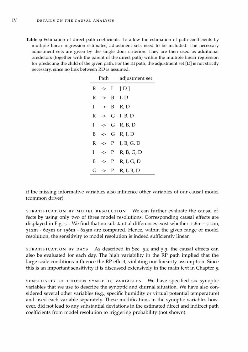
IV details on the causal analysis

Table 4: Estimation of direct path coefficients: To allow the estimation of path coefficients bymultiple linear regression estimates, adjustment sets need to be included. The necessaryadjustment sets are given by the single door criterion. They are then used as additionalpredictors (together with the parent of the direct path) within the multiple linear regressionfor predicting the child of the given path. For the RI path, the adjustment set [D] is not strictlynecessary, since no link between RD is assumed.

Path adjustment set

R -> I [ D ]

R -> B I, D

I -> B R, D

R -> G I, B, D

I -> G R, B, D

B -> G R, I, D

R -> P I, B, G, D

I -> P R, B, G, D

B -> P R, I, G, D

G -> P R, I, B, D

if the missing informative variables also influence other variables of our causal model(common driver).

stratification by model resolution We can further evaluate the causal ef-fects by using only two of three model resolutions. Corresponding causal effects aredisplayed in Fig. 51. We find that no substantial differences exist whether 156m - 312m,312m - 625m or 156m - 625m are compared. Hence, within the given range of modelresolution, the sensitivity to model resolution is indeed sufficiently linear.

stratification by days As described in Sec. 5.2 and 5.3, the causal effects canalso be evaluated for each day. The high variability in the RP path implied that thelarge scale conditions influence the RP effect, violating our linearity assumption. Sincethis is an important sensitivity it is discussed extensively in the main text in Chapter 5.

sensitivity of chosen synoptic variables We have specified six synopticvariables that we use to describe the synoptic and diurnal situation. We have also con-sidered several other variables (e.g., specific humidity or virtual potential temperature)and used each variable separately. These modifications in the synoptic variables how-ever, did not lead to any substantial deviations in the estimated direct and indirect pathcoefficients from model resolution to triggering probability (not shown).

A.2 sensitivity and robustness of the causal analysis V

(a) (b)

(c) (d)

Figure 50: The p (a, b) and R2 (c, d) values of the estimated path coefficients. (a, c) for all coldpools and (b, d) when stratified according to the four different days. The whiskers of thebox plots correspond to the 95% confidence intervals from bootstrapping.

Figure 51: Aggregated path coefficientscomputed using only two of the threemodel resolutions. The whiskers ofthe box plots correspond to the 95%confidence intervals from bootstrap-ping.

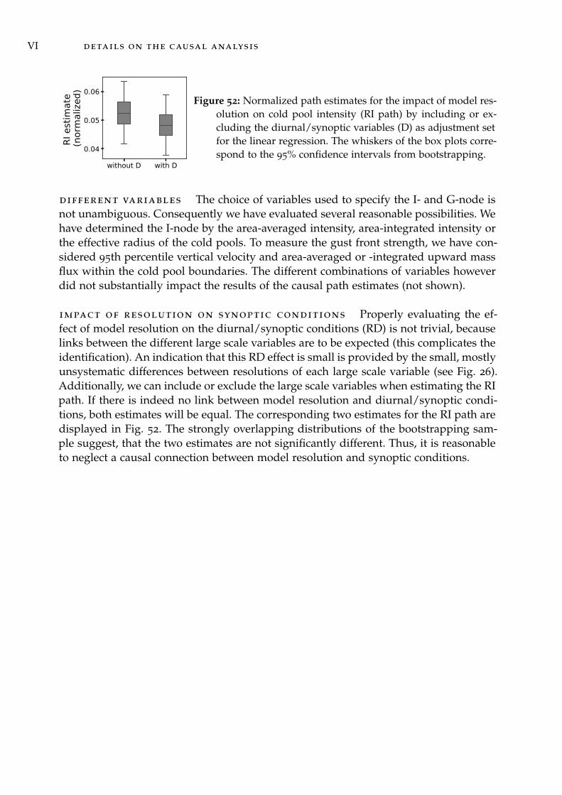
VI details on the causal analysis

without D with D

0.04

0.05

0.06

RI e

stim

ate

(nor

mal

ized) Figure 52: Normalized path estimates for the impact of model res-

olution on cold pool intensity (RI path) by including or ex-cluding the diurnal/synoptic variables (D) as adjustment setfor the linear regression. The whiskers of the box plots corre-spond to the 95% confidence intervals from bootstrapping.

different variables The choice of variables used to specify the I- and G-node isnot unambiguous. Consequently we have evaluated several reasonable possibilities. Wehave determined the I-node by the area-averaged intensity, area-integrated intensity orthe effective radius of the cold pools. To measure the gust front strength, we have con-sidered 95th percentile vertical velocity and area-averaged or -integrated upward massflux within the cold pool boundaries. The different combinations of variables howeverdid not substantially impact the results of the causal path estimates (not shown).

impact of resolution on synoptic conditions Properly evaluating the ef-fect of model resolution on the diurnal/synoptic conditions (RD) is not trivial, becauselinks between the different large scale variables are to be expected (this complicates theidentification). An indication that this RD effect is small is provided by the small, mostlyunsystematic differences between resolutions of each large scale variable (see Fig. 26).Additionally, we can include or exclude the large scale variables when estimating the RIpath. If there is indeed no link between model resolution and diurnal/synoptic condi-tions, both estimates will be equal. The corresponding two estimates for the RI path aredisplayed in Fig. 52. The strongly overlapping distributions of the bootstrapping sam-ple suggest, that the two estimates are not significantly different. Thus, it is reasonableto neglect a causal connection between model resolution and synoptic conditions.

BD I M E N S I O N A L A N A LY S I S F O R C O L D P O O L G U S T F R O N T S

Here, we give the full derivation for a characteristic vertical velocity scale W for coldpool gust fronts, which is used in Chapter 5. We consider the inviscid, Boussinesqueapproximated set of equations for the streamfunction Φ, vorticity η and vertical velocityw in a two dimensional plane in x and z, which is often considered for density currents(Rotunno et al., 1988; Weisman and Rotunno, 2004; Bryan and Rotunno, 2014b):

dη

dt= − ∂b

∂x,

∇2Φ = η,

w = −∂Φ∂x

and

w =dzdt

.

We consider a parcel situated at a horizontal, time-independent buoyancy gradient ∂b∂x

(i.e., a cold pool gust front). First, we non-dimensionalize the equations using character-istic scales B, H, L, W, η∗, Φ∗ and non-dimensional variables denoted wtih a tilde-sign,e.g. x:

b = Bb,x = Lx,z = Hx,t = Tt,

w = Ww,η = η∗η,

Φ = Φ∗Φ.

VII

VIII dimensional analysis for cold pool gust fronts

The non-dimensional variables here represent functions that depend only on other non-dimensional variables. This gives the following, transformed set of equations:

dη

dt= − BT

η∗L· ∂b

∂x,

∂Φ∂x2 =

η∗

Φ∗( 1L2 +

1H2 )· η,

w = − Φ∗

WL· ∂Φ

∂xand

w =H

WT· dz

dt.

The dimensionless factors consisting only of characteristic scales on the right-hand sidecan be set to equal 1, by determining values for η∗, φ∗, T and W accordingly:

η∗ =BTL

,

Φ∗ =η∗

( 1L2 +

1H2 )

,

W =Φ∗

L,

T =HW

.

Substituting the first, second and last equation into the third, we obtain the followingrelationship for W:

W =

√BH

1 + L2

H2

,

which describes the characteristic, vertical velocity scale within a circulation driven byhorizontal buoyancy gradients and how it depends on both the horizontal and verticallength scales L and H in addition to the characteristic buoyancy scale B. See Chapter 5

for further discussion, publications with similar W scalings and the approximationfor L

H ≈ 1. For a detailed introduction to dimensional analysis we refer the reader toBarenblatt (2003) or Witelski and Bowen (2015).

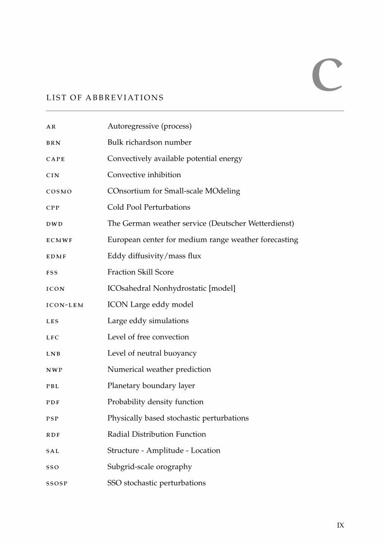
CL I S T O F A B B R E V I AT I O N S

ar Autoregressive (process)

brn Bulk richardson number

cape Convectively available potential energy

cin Convective inhibition

cosmo COnsortium for Small-scale MOdeling

cpp Cold Pool Perturbations

dwd The German weather service (Deutscher Wetterdienst)

ecmwf European center for medium range weather forecasting

edmf Eddy diffusivity/mass flux

fss Fraction Skill Score

icon ICOsahedral Nonhydrostatic [model]

icon-lem ICON Large eddy model

les Large eddy simulations

lfc Level of free convection

lnb Level of neutral buoyancy

nwp Numerical weather prediction

pbl Planetary boundary layer

pdf Probability density function

psp Physically based stochastic perturbations

rdf Radial Distribution Function

sal Structure - Amplitude - Location

sso Subgrid-scale orography

ssosp SSO stochastic perturbations

IX

B I B L I O G R A P H Y

Arakawa A, Schubert WH. 1974. Interaction of a Cumulus Cloud Ensemble with theLarge-Scale Environment, Part I. Journal of the Atmospheric Sciences 31(3): 674–701, doi:10.1175/1520-0469(1974)031<0674:IOACCE>2.0.CO;2.

Athey S. 2017. Beyond prediction: Using big data for policy problems. Science 355(6324):483–485, doi: 10.1126/science.aal4321.

Bachmann K, Keil C, Craig GC, Weissmann M, Welzbacher CA. 2020. Predictability ofdeep convection in idealized and operational forecasts: Effects of radar data assimila-tion, orography, and synoptic weather regime. Monthly Weather Review 148(1): 63–81,doi: 10.1175/MWR-D-19-0045.1.

Bachmann K, Keil C, Weissmann M, Branch A. 2019. Impact of Radar Data Assimilationand Orography on Predictability of Deep Convection. Quarterly Journal of the RoyalMeteorological Society 145(718): 117–130, doi: 10.1002/qj.3412.

Baines PG, Palmer TN. 1990. Rationale for a new physically-based parametrization ofsubgrid-scale orographic effects. Technical Report 169, European Centre for MediumRange Weather Forecasting, Shinfield Park, Reading, doi: 10.21957/h4h36b3u.

Baldauf M, Seifert A, Förstner J, Majewski D, Raschendorfer M, Reinhardt T. 2011. Op-erational convective-scale numerical weather prediction with the COSMO Model: De-scription and sensitivities. Monthly Weather Review 139(12): 3887–3905, doi: 10.1175/MWR-D-10-05013.1.

Barenblatt GI. 2003. Scaling, vol. 34. Cambridge University Press.

Bauer P, Thorpe A, Brunet G. 2015. The quiet revolution of numerical weather predic-tion. Nature 525(7567): 47, doi: 10.1038/nature14956.

Baur F, Keil C, Craig GC. 2018. Soil moisture–precipitation coupling over Central Eu-rope: Interactions between surface anomalies at different scales and the dynamicalimplication. Quarterly Journal of the Royal Meteorological Society 144(717): 2863–2875,doi: 10.1002/qj.3415.

Bengtsson L, Steinheimer M, Bechtold P, Geleyn JF. 2013. A stochastic parametrizationfor deep convection using cellular automata. Quarterly Journal of the Royal Meteorolog-ical Society 139(675): 1533–1543, doi: 10.1002/qj.2108.

Benjamin TB. 1968. Gravity currents and related phenomena. Journal of Fluid Mechanics31(2): 209–248, doi: 10.1017/S0022112068000133.

Berner J, Achatz U, Batté L, Bengtsson L, de la Cámara A, Christensen HM, Colan-geli M, Coleman DRB, Crommelin D, Dolaptchiev SI, Franzke CLE, Friederichs P,Imkeller P, Järvinen H, Juricke S, Kitsios V, Lott F, Lucarini V, Mahajan S, Palmer

XI

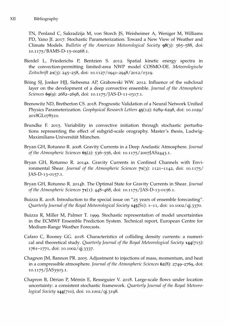
XII Bibliography

TN, Penland C, Sakradzija M, von Storch JS, Weisheimer A, Weniger M, WilliamsPD, Yano JI. 2017. Stochastic Parameterization: Toward a New View of Weather andClimate Models. Bulletin of the American Meteorological Society 98(3): 565–588, doi:10.1175/BAMS-D-15-00268.1.

Bierdel L, Friederichs P, Bentzien S. 2012. Spatial kinetic energy spectra inthe convection-permitting limited-area NWP model COSMO-DE. MeteorologischeZeitschrift 21(3): 245–258, doi: 10.1127/0941-2948/2012/0319.

Böing SJ, Jonker HJJ, Siebesma AP, Grabowski WW. 2012. Influence of the subcloudlayer on the development of a deep convective ensemble. Journal of the AtmosphericSciences 69(9): 2682–2698, doi: 10.1175/JAS-D-11-0317.1.

Brenowitz ND, Bretherton CS. 2018. Prognostic Validation of a Neural Network UnifiedPhysics Parameterization. Geophysical Research Letters 45(12): 6289–6298, doi: 10.1029/2018GL078510.

Brundke F. 2015. Variability in convective initiation through stochastic perturba-tions representing the effect of subgrid-scale orography. Master’s thesis, Ludwig-Maximilians-Universität München.

Bryan GH, Rotunno R. 2008. Gravity Currents in a Deep Anelastic Atmosphere. Journalof the Atmospheric Sciences 65(2): 536–556, doi: 10.1175/2007JAS2443.1.

Bryan GH, Rotunno R. 2014a. Gravity Currents in Confined Channels with Envi-ronmental Shear. Journal of the Atmospheric Sciences 71(3): 1121–1142, doi: 10.1175/JAS-D-13-0157.1.

Bryan GH, Rotunno R. 2014b. The Optimal State for Gravity Currents in Shear. Journalof the Atmospheric Sciences 71(1): 448–468, doi: 10.1175/JAS-D-13-0156.1.

Buizza R. 2018. Introduction to the special issue on “25 years of ensemble forecasting”.Quarterly Journal of the Royal Meteorological Society 145(S1): 1–11, doi: 10.1002/qj.3370.

Buizza R, Miller M, Palmer T. 1999. Stochastic representation of model uncertaintiesin the ECMWF Ensemble Prediction System. Technical report, European Centre forMedium-Range Weather Forecasts.

Cafaro C, Rooney GG. 2018. Characteristics of colliding density currents: a numeri-cal and theoretical study. Quarterly Journal of the Royal Meteorological Society 144(715):1761–1771, doi: 10.1002/qj.3337.

Chagnon JM, Bannon PR. 2005. Adjustment to injections of mass, momentum, and heatin a compressible atmosphere. Journal of the Atmospheric Sciences 62(8): 2749–2769, doi:10.1175/JAS3503.1.

Chapron B, Dérian P, Mémin E, Resseguier V. 2018. Large-scale flows under locationuncertainty: a consistent stochastic framework. Quarterly Journal of the Royal Meteoro-logical Society 144(710), doi: 10.1002/qj.3198.

Bibliography XIII

Chen B, Pearl J. 2015. Graphical tools for linear structural equation modeling. Techni-cal report, California Univ. Los Angeles Dept. of Computer Science, doi: 10.21236/ada609131.

Chow F, Schär C, Ban N, Lundquist K, Schlemmer L, Shi X. 2019. Crossing MultipleGray Zones in the Transition from Mesoscale to Microscale Simulation over ComplexTerrain. Atmosphere 10(5): 274, doi: 10.3390/atmos10050274.

Christensen HM, Lock SJ, Moroz IM, Palmer TN. 2017. Introducing independent pat-terns into the Stochastically Perturbed Parametrization Tendencies (SPPT) scheme.Quarterly Journal of the Royal Meteorological Society 143(706): 2168–2181, doi: 10.1002/qj.3075.

Clark P, Roberts N, Lean H, Ballard SP, Charlton-Perez C. 2016. Convection-permittingmodels: a step-change in rainfall forecasting. Meteorological Applications 23(2): 165–181,doi: 10.1002/met.1538.

Craig GC, Cohen BG. 2006. Fluctuations in an Equilibrium Convective Ensemble. PartI: Theoretical Formulation. Journal of the Atmospheric Sciences 63(8): 1996–2004, doi:10.1175/JAS3709.1.

Craig GC, Selz T. 2018. Mesoscale Dynamical Regimes in the Midlatitudes. GeophysicalResearch Letters doi: 10.1002/2017GL076174.

de Rooy WC, Bechtold P, Fröhlich K, Hohenegger C, Jonker H, Mironov D, PierSiebesma A, Teixeira J, Yano JI. 2013. Entrainment and detrainment in cumulus con-vection: an overview. Quarterly Journal of the Royal Meteorological Society 139(670): 1–19,doi: 10.1002/qj.1959.

Demaeyer J, Vannitsem S. 2017. Stochastic parametrization of subgrid-scale processesin coupled ocean–atmosphere systems: benefits and limitations of response theory.Quarterly Journal of the Royal Meteorological Society 143(703): 881–896, doi: 10.1002/qj.2973.

Demaeyer J, Vannitsem S. 2018. Stochastic parameterization of subgrid-scale processes: Areview of recent physically based approaches. Springer International Publishing: Cham,pp. 55–85, doi: 10.1007/978-3-319-58895-7_3.

Deutscher Wetterdienst. 2018a. Hoch aufgelöste Niederschlgsanalyse und -vorhersageauf der Basis quantitativer Radar- und Omrometerdaten für grenzüberschreit-ende Fluss-Einzugsgebiete von Deutschland im Echtzeitbetrieb - Beschreibungdes Kompositsformats Version 2.4.4. URL https://www.dwd.de/DE/leistungen/

radolan/radolan_info/radolan_radvor_op_komposit_format_pdf.pdf?__blob=

publicationFile&v=6, accessed 2019-13-05.

Deutscher Wetterdienst. 2018b. RADOLAN/RADVOR Produktübersicht. URLhttps://www.dwd.de/DE/leistungen/radolan/produktuebersicht/radolan_

produktuebersicht_pdf.pdf?__blob=publicationFile&v=6, accessed 2019-13-05.

XIV Bibliography

Deutscher Wetterdienst. 2019. Hagelunwetter in München und weitere schwere Gewit-ter an Pfingstmontag . URL https://www.dwd.de/DE/wetter/thema_des_tages/2019/

6/11.html, accessed 2020-03-30.

Deutscher Wetterdienst. 2020. Entwicklung des Integrierten Vorhersagesystems SIN-FONY (Seamless INtegrated FOrecastiNg sYstem) . URL https://www.dwd.de/DE/

forschung/forschungsprogramme/sinfony_iafe/sinfony_node.html, accessed 2020-03-25.

Dipankar A, Stevens B, Heinze R, Moseley C, Zängl G, Giorgetta M, Brdar S. 2015.Large eddy simulation using the general circulation model ICON. Journal of Advancesin Modeling Earth Systems 7(3): 963–986, doi: 10.1002/2015MS000431.

Doms G, Förstner J, Heise E, Herzog HJ, Mironov D, Raschendorfer M, Reinhardt T,Ritter B, Schrodin R, Schulz JP, Vogel G. 2011. A description of the nonhydrostaticregional COSMO model. Part II: physical parameterization. Deutscher Wetterdienst,Offenbach, Germany .

Drager AJ, van den Heever SC. 2017. Characterizing convective cold pools. Journal ofAdvances in Modeling Earth Systems 9(2): 1091–1115, doi: 10.1002/2016MS000788.

Ebert-Uphoff I, Deng Y. 2012. Causal discovery for climate research using graphicalmodels. Journal of Climate 25(17): 5648–5665, doi: 10.1175/JCLI-D-11-00387.10.

ECMWF. 2016. The strength of a common goal - A roadmap to 2025. Technicalreport, accessed 2019-11-07, URL https://www.ecmwf.int/sites/default/files/

ECMWF_Roadmap_to_2025.pdf.

ECMWF. 2019. Operational configurations of the ECMWF Integrated Forecasting Sys-tem (IFS). URL https://www.ecmwf.int/en/forecasts/documentation-and-support,accessed 2019-11-07.

Edson AR, Bannon PR. 2008. Nonlinear Atmospheric Adjustment to Thermal Forcing.Journal of the Atmospheric Sciences 62(12): 4253–4272, doi: 10.1175/JAS3517.1.

Ehrendorfer M. 1994a. The Liouville Equation and Its Potential Usefulness for the Pre-diction of Forecast Skill. Part I: Theory. Monthly Weather Review 122(4): 703–713, doi:10.1175/1520-0493(1994)122<0703:TLEAIP>2.0.CO;2.

Ehrendorfer M. 1994b. The Liouville Equation and Its Potential Usefulness for the Pre-diction of Forecast Skill. Part II: Applications. Monthly Weather Review 122(4): 714–728,doi: 10.1175/1520-0493(1994)122<0714:TLEAIP>2.0.CO;2.

Emanuel KA. 1994. Atmospheric convection. Oxford University Press.

Feng Z, Hagos S, Rowe AK, Burleyson CD, Martini MN, de Szoeke SP. 2015. Mech-anisms of convective cloud organization by cold pools over tropical warm oceanduring the AMIE/DYNAMO field campaign. Journal of Advances in Modeling EarthSystems 7(2): 357–381, doi: 10.1002/2014MS000384.

Bibliography XV

Fiedler BH. 2002. A wind transform for acoustic adjustment in compressible mod-els. Monthly Weather Review 130(3): 741–746, doi: 10.1175/1520-0493(2002)130<0741:AWTFAA>2.0.CO;2.

Fournier MB, Haerter JO. 2019. Tracking the gust fronts of convective cold pools. Journalof Geophysical Research: Atmospheres 124(21): 11 103–11 117, doi: 10.1029/2019JD030980.

Franzke CLE, O’Kane TJ, Berner J, Williams PD, Lucarini V. 2015. Stochastic climatetheory and modeling. Wiley Interdisciplinary Reviews: Climate Change 6(1): 63–78, doi:10.1002/wcc.318.

Geerts B, Miao Q, Demko JC. 2008. Pressure Perturbations and Upslope Flow over aHeated, Isolated Mountain. Monthly Weather Review 136(11): 4272–4288, doi: 10.1175/2008MWR2546.1.

Gentine P, Pritchard M, Rasp S, Reinaudi G, Yacalis G. 2018. Could Machine LearningBreak the Convection Parameterization Deadlock? Geophysical Research Letters 45(11):5742–5751, doi: 10.1029/2018GL078202.

Gill AE. 1982. Atmosphere-ocean dynamics. Academic Press, ISBN 9780080570525.

Gilleland E, Ahijevych D, Brown BG, Casati B, Ebert EE. 2009. Intercomparison ofSpatial Forecast Verification Methods. Weather and Forecasting 24(5): 1416–1430, doi:10.1175/2009WAF2222269.1.

Golding B, Mylne K, Clark P. 2004. The history and future of numerical weather predic-tion in the Met Office. Weather 59(11): 299–306, doi: 10.1256/wea.113.04.

Grabowski WW. 2004. An Improved Framework for Superparameterization. Journalof the Atmospheric Sciences 61(15): 1940–1952, doi: 10.1175/1520-0469(2004)061<1940:AIFFS>2.0.CO;2.

Grandpeix JY, Lafore JP. 2010. A density current parameterization coupled withEmanuel’s convection scheme. Part I: The models. Journal of the Atmospheric Sciences67(4): 881–897, doi: 10.1175/2009JAS3044.1.

Grandpeix JY, Lafore JP, Cheruy F. 2010. A density current parameterization coupledwith Emanuel’s convection scheme. Part II: 1D simulations. Journal of the AtmosphericSciences 67(4): 898–922, doi: 10.1175/2009JAS3045.1.

Grant LD, van den Heever SC. 2016. Cold pool dissipation. Journal of Geophysical Re-search: Atmospheres 121(3): 1138–1155.

Grant LD, van den Heever SC. 2018. Cold Pool-Land Surface Interactions in a DryContinental Environment. Journal of Advances in Modeling Earth Systems 10(7): 1513–1526, doi: 10.1029/2018MS001323.

Gustafsson N, Janjic T, Schraff C, Leuenberger D, Weissmann M, Reich H, Brousseau P,Montmerle T, Wattrelot E, Bucánek A, Mile M, Hamdi R, Lindskog M, Barkmeijer J,Dahlbom M, Macpherson B, Ballard S, Inverarity G, Carley J, Alexander C, Dowell D,

XVI Bibliography

Liu S, Ikuta Y, Fujita T. 2018. Survey of data assimilation methods for convective-scalenumerical weather prediction at operational centres. Quarterly Journal of the RoyalMeteorological Society 144(713): 1218–1256, doi: 10.1002/qj.3179.

Haerter JO, Boeing SJ, Henneberg O, Nissen SB. 2018. Reconciling cold pool dynamicswith convective self-organization. arXiv preprint; arXiv:1810.05518 .

Hanley K, Whitall M, Stirling A, Clark P. 2019. Modifications to the representation ofsubgrid mixing in kilometre-scale versions of the Unified Model. Quarterly Journal ofthe Royal Meteorological Society 145(725): 3361–3375, doi: 10.1002/qj.3624.

Hanley KE, Plant RS, Stein THM, Hogan RJ, Nicol JC, Lean HW, Halliwell C, ClarkPA. 2015. Mixing-length controls on high-resolution simulations of convective storms.Quarterly Journal of the Royal Meteorological Society 141(686): 272–284.

Harper K, Uccellini LW, Kalnay E, Carey K, Morone L. 2007. Symposium of the 50thanniversary of operational numerical weather prediction. Bulletin of the American Me-teorological Society 88(5): 639–650, doi: 10.1175/BAMS-88-5-639.

Heinze R, Dipankar A, Henken CC, Moseley C, Sourdeval O, Trömel S, Xie X, AdamidisP, Ament F, Baars H, Barthlott C, Behrendt A, Blahak U, Bley S, Brdar S, Brueck M,Crewell S, Deneke H, Di Girolamo P, Evaristo R, Fischer J, Frank C, Friederichs P,Göcke T, Gorges K, Hande L, Hanke M, Hansen A, Hege HC, Hoose C, Jahns T,Kalthoff N, Klocke D, Kneifel S, Knippertz P, Kuhn A, van Laar T, Macke A, MaurerV, Mayer B, Meyer CI, Muppa SK, Neggers RAJ, Orlandi E, Pantillon F, Pospichal B,Röber N, Scheck L, Seifert A, Seifert P, Senf F, Siligam P, Simmer C, Steinke S, StevensB, Wapler K, Weniger M, Wulfmeyer V, Zängl G, Zhang D, Quaas J. 2017. Large-eddy simulations over Germany using ICON: a comprehensive evaluation. QuarterlyJournal of the Royal Meteorological Society 143(702): 69–100, doi: 10.1002/qj.2947.

Henneberg O, Meyer B, Haerter JO. 2020. Particle-based tracking of cold pool gustfronts. Journal of Advances in Modeling Earth Systems : e2019MS001 910doi: 10.1029/2019MS001910.

Hohenegger C, Schär C. 2007. Atmospheric predictability at synoptic versus cloud-resolving scales. Bulletin of the American Meteorological Society 88(11): 1783–1793, doi:10.1175/BAMS-88-11-1783.

Honnert R. 2016. Representation of the grey zone of turbulence in the atmo-spheric boundary layer. Advances in Science and Research 13: 63–67, doi: 10.5194/asr-13-63-2016.

Hourdin F, Mauritsen T, Gettelman A, Golaz JC, Balaji V, Duan Q, Folini D, Ji D, KlockeD, Qian Y, Rauser F, Rio C, Tomassini L, Watanabe M, Williamson D. 2017. The artand science of climate model tuning. Bulletin of the American Meteorological Society98(3): 589–602, doi: 10.1175/BAMS-D-15-00135.1.

Houze RA. 2012. Orographic effects on precipitating clouds. Reviews of Geophysics 50(1):RG1001, doi: 10.1029/2011RG000365.

Bibliography XVII

Igel AL, Igel MR, van den Heever SC. 2015. Make It a Double? Sobering Results fromSimulations Using Single-Moment Microphysics Schemes. Journal of the AtmosphericSciences 72(2): 910–925, doi: 10.1175/JAS-D-14-0107.1.

Jankov I, Beck J, Wolff J, Harrold M, Olson JB, Smirnova T, Alexander C, Berner J. 2019.Stochastically Perturbed Parameterizations in an HRRR-Based Ensemble. MonthlyWeather Review 147(1): 153–173, doi: 10.1175/MWR-D-18-0092.1.

Jankov I, Berner J, Beck J, Jiang H, Olson JB, Grell G, Smirnova TG, Benjamin SG,Brown JM. 2017. A performance comparison between multiphysics and stochasticapproaches within a North American RAP ensemble. Monthly Weather Review 145(4):1161–1179.

Jeevanjee N. 2017. Vertical Velocity in the Gray Zone. Journal of Advances in ModelingEarth Systems 9(6): 2304–2316, doi: 10.1002/2017MS001059.

Jeevanjee N, Romps DM. 2016. Effective buoyancy at the surface and aloft. QuarterlyJournal of the Royal Meteorological Society 142(695): 811–820, doi: 10.1002/qj.2683.

Judt F. 2018. Insights into atmospheric predictability through global convection-permitting model simulations. Journal of the Atmospheric Sciences 75(5): 1477–1497, doi:10.1175/JAS-D-17-0343.1.

Kealy JC. 2019. Probing the ‘grey zone’ of NWP – is higher resolution always better?Weather 74(7): 246–249, doi: 10.1002/wea.3506.

Kealy JC, Efstathiou GA, Beare RJ. 2019. The onset of resolved boundary-layer turbu-lence at grey-zone resolutions. Boundary-Layer Meteorology 171(1): 31–52, doi: 10.1007/s10546-018-0420-0.

Keil C, Baur F, Bachmann K, Rasp S, Schneider L, Barthlott C. 2019. Relative contribu-tion of soil moisture, boundary-layer and microphysical perturbations on convectivepredictability in different weather regimes. Quarterly Journal of the Royal MeteorologicalSociety 145(724): 3102–3115, doi: 10.1002/qj.3607.

Keil C, Heinlein F, Craig GC. 2014. The convective adjustment time-scale as indicator ofpredictability of convective precipitation. Quarterly Journal of the Royal MeteorologicalSociety 140(679): 480–490, doi: 10.1002/qj.2143.

Kirshbaum D, Adler B, Kalthoff N, Barthlott C, Serafin S. 2018. Moist orographic con-vection: Physical mechanisms and links to surface-exchange processes. Atmosphere9(3): 80, doi: 10.3390/atmos9030080.

Kirshbaum DJ, Rotunno R, Bryan GH. 2007a. The spacing of orographic rainbandstriggered by small-scale topography. Journal of the Atmospheric Sciences 64(12): 4222–4245, doi: 10.1175/2007JAS2335.1.

Kirshbaum DJ, Rotunno R, Bryan GH, Durran DR. 2007b. The Triggering of OrographicRainbands by Small-Scale Topography. Journal of the Atmospheric Sciences 64(12): 4222–4245, doi: 10.1175/2007JAS2335.1.

XVIII Bibliography

Kober K, Craig GC. 2016. Physically Based Stochastic Perturbations (PSP) in the bound-ary layer to represent uncertainty in convective initiation. Journal of the AtmosphericSciences 73(7): 2893–2911, doi: 10.1175/JAS-D-15-0144.1.

Kretschmer M, Coumou D, Donges JF, Runge J. 2016. Using causal effect networks toanalyze different Arctic drivers of midlatitude winter circulation. Journal of Climate29(11): 4069–4081, doi: 10.1175/JCLI-D-15-0654.1.

Krich C, Runge J, Miralles DG, Migliavacca M, Perez-Priego O, El-Madany T, Car-rara A, Mahecha MD. 2020. Estimating causal networks in biosphere–atmosphereinteraction with the pcmci approach. Biogeosciences 17(4): 1033–1061, doi: 10.5194/bg-17-1033-2020.

Kron W, Eichner J, Kundzewicz ZW. 2019. Reduction of flood risk in Europe – Re-flections from a reinsurance perspective. Journal of Hydrology 576: 197–209, doi:10.1016/j.jhydrol.2019.06.050.

Langhans W, Gohm A, Zängl G. 2011. The orographic impact on patterns of embed-ded convection during the August 2005 Alpine flood. Quarterly Journal of the RoyalMeteorological Society 137(661): 2092–2105.

Langhans W, Schmidli J, Fuhrer O, Bieri S, Schar C. 2013. Long-term simulations ofthermally driven flows and orographic convection at convection-parameterizing andcloud-resolving resolutions. Journal of Applied Meteorology and Climatology 52(6): 1490–1510, doi: 10.1175/JAMC-D-12-0167.1.

Leutwyler D, Lüthi D, Ban N, Fuhrer O, Schär C. 2017. Evaluation of the convection-resolving climate modeling approach on continental scales. Journal of Geophysical Re-search: Atmospheres 122(10): 5237–5258, doi: 10.1002/2016JD026013.

Lilly DK. 1990. Numerical prediction of thunderstorms—has its time come? Quar-terly Journal of the Royal Meteorological Society 116(494): 779–798, doi: 10.1002/qj.49711649402.

Lott F, Miller MJ. 1997. A new subgrid-scale orographic drag parametrization: Its for-mulation and testing. Quarterly Journal of the Royal Meteorological Society 123: 101–127,doi: 10.1002/qj.49712353704.

Markowski P, Richardson Y. 2011. Mesoscale meteorology in midlatitudes, vol. 2. John Wiley& Sons.

Mauritsen T, Stevens B, Roeckner E, Crueger T, Esch M, Giorgetta M, Haak H, JungclausJ, Klocke D, Matei D, Mikolajewicz U, Notz D, Pincus R, Schmidt H, Tomassini L.2012. Tuning the climate of a global model. Journal of Advances in Modeling EarthSystems 4(3): 1–18, doi: 10.1029/2012MS000154.

Mayer B. 2018. Erwärmungs- und Abkühlungsraten - Wie wichtig ist der 3D-Strahlungsreport? promet 100: 98–110.

Bibliography XIX

Mellor GL, Yamada T. 1982. Development of a turbulence closure model for geophysicalfluid problems. Reviews of Geophysics 20(4): 851, doi: 10.1029/RG020i004p00851.

Moncrieff MW, Liu C. 1999. Convection Initiation by Density Currents: Role of Con-vergence, Shear, and Dynamical Organization. Monthly Weather Review 127(10): 2455–2464, doi: 10.1175/1520-0493(1999)127<2455:CIBDCR>2.0.CO;2.

Morrison H. 2016a. Impacts of updraft size and dimensionality on the perturba-tion pressure and vertical velocity in cumulus convection. Part I: Simple, gener-alized analytic solutions. Journal of the Atmospheric Sciences 73(4): 1441–1454, doi:10.1175/JAS-D-15-0040.1.

Morrison H. 2016b. Impacts of updraft size and dimensionality on the perturbation pres-sure and vertical velocity in cumulus convection. Part II: Comparison of theoreticaland numerical solutions and fully dynamical simulations. Journal of the AtmosphericSciences 73(4): 1455–1480, doi: 10.1175/JAS-D-15-0041.1.

Morrison H, Morales A, Villanueva-Birriel C. 2015. Concurrent sensitivities of an ide-alized deep convective storm to parameterization of microphysics, horizontal gridresolution, and environmental static stability. Monthly Weather Review 143(6): 2082–2104, doi: 10.1175/MWR-D-14-00271.1.

Munich Re. 2020. Wirbelstürme mit Milliardenschäden prägen Bilanz der Naturkatas-trophen 2019 . URL https://www.munichre.com/de/unternehmen/media-relations/

medieninformationen-und-unternehmensnachrichten/medieninformationen/2020/

milliardenschaeden-praegen-bilanz-naturkatastrophen-2019.html, accessed2020-03-30.

Nebeker F. 1997. Calculating the Weather: Meteorology in the 20th Century. Technologyand Culture 38(3): 786, doi: 10.2307/3106892.

Necker T, Geiss S, Weissmann M, Ruiz J, Miyoshi T, Lien GY. 2020. A convective-scale1,000-member ensemble simulation and potential applications. Quarterly Journal of theRoyal Meteorological Society doi: 10.1002/qj.3744.

Necker T, Weissmann M, Sommer M. 2018. The importance of appropriate verificationmetrics for the assessment of observation impact in a convection-permitting mod-elling system. Quarterly Journal of the Royal Meteorological Society 144(714): 1667–1680,doi: 10.1002/qj.3390.

Nowack P, Runge J, Eyring V, Haigh JD. 2020. Causal networks for climate model eval-uation and constrained projections. Nature Communications 11(1): 1–11, doi: 10.1038/s41467-020-15195-y.

Ollinaho P, Lock SJ, Leutbecher M, Bechtold P, Beljaars A, Bozzo A, Forbes RM, HaidenT, Hogan RJ, Sandu I. 2017. Towards process-level representation of model uncertain-ties: stochastically perturbed parametrizations in the ECMWF ensemble. QuarterlyJournal of the Royal Meteorological Society 143(702): 408–422, doi: 10.1002/qj.2931.

XX Bibliography

Palmer T. 2019a. The ECMWF ensemble prediction system: Looking back (more than)25 years and projecting forward 25 years. Quarterly Journal of the Royal MeteorologicalSociety 145(S1): 12–24, doi: 10.1002/qj.3383.

Palmer TN. 2019b. Stochastic weather and climate models. Nature Reviews Physics 1(7):463–471, doi: 10.1038/s42254-019-0062-2.

Palmer TN, Weisheimer A. 2011. Diagnosing the causes of bias in climate models–whyis it so hard? Geophysical & Astrophysical Fluid Dynamics 105(2-3): 351–365, doi: 10.1080/03091929.2010.547194.

Panosetti D, Böing S, Schlemmer L, Schmidli J. 2016. Idealized large-eddy andconvection-resolving simulations of moist convection over mountainous terrain. Jour-nal of the Atmospheric Sciences 73(10): 4021–4041, doi: 10.1175/JAS-D-15-0341.1.

Panosetti D, Schlemmer L, Schär C. 2019. Bulk and structural convergence at convection-resolving scales in real-case simulations of summertime moist convection over land.Quarterly Journal of the Royal Meteorological Society 145(721): 1427–1443, doi: 10.1002/qj.3502.

ParaCon. 2020. ParaCon - Representation of convection in models - Met Office.URL https://www.metoffice.gov.uk/research/approach/collaboration/paracon,accessed 2020-01-29.

Parishani H, Pritchard MS, Bretherton CS, Wyant MC, Khairoutdinov M. 2017. To-ward low-cloud-permitting cloud superparameterization with explicit boundarylayer turbulence. Journal of Advances in Modeling Earth Systems 9(3): 1542–1571, doi:10.1002/2017MS000968.

Park S. 2014. A Unified Convection Scheme (UNICON). Part I: Formulation. Journal ofthe Atmospheric Sciences 71(11): 3902–3930, doi: 10.1175/JAS-D-13-0233.1.

Pauluis O, Garner S. 2006. Sensitivity of Radiative–Convective Equilibrium Simulationsto Horizontal Resolution. Journal of the Atmospheric Sciences 63(7): 1910–1923, doi: 10.1175/JAS3705.1.

Pearl J. 2009. Causality. Cambridge university press.

Pearl J. 2013. Linear models: A useful “microscope” for causal analysis. Technical report,University of California, Los Angeles Computer Science Department.

Pearl J. 2014. Interpretation and identification of causal mediation. Psychological methods19(4): 459, doi: 10.1037/a0036434.

Pearl J. 2019. The seven tools of causal inference, with reflections on machine learning.Communications of the ACM 62(3): 54–60, doi: 10.1145/3241036.

Penland C. 2003. Noise out of chaos and why it won’t go away. Bulletin of the AmericanMeteorological Society 84(7): 921–926, doi: 10.1175/BAMS-84-7-921.

Bibliography XXI

Peters K, Hohenegger C. 2017. On the dependence of squall-line characteristics onsurface conditions. Journal of the Atmospheric Sciences 74(7): 2211–2228, doi: 10.1175/JAS-D-16-0290.1.

Piper D, Kunz M, Ehmele F, Mohr S, Mühr B, Kron A, Daniell J. 2016. Exceptionalsequence of severe thunderstorms and related flash floods in May and June 2016

in Germany – Part 1: Meteorological background. Natural Hazards and Earth SystemSciences 16(12): 2835–2850, doi: 10.5194/nhess-16-2835-2016.

Plant RS, Craig GC. 2008. A stochastic parameterization for deep convection based onequilibrium statistics. Journal of the Atmospheric Sciences 65(1): 87–105, doi: 10.1175/2007JAS2263.1.

Pscheidt I, Senf F, Heinze R, Deneke H, Trömel S, Hohenegger C. 2019. How organizedis deep convection over Germany? Quarterly Journal of the Royal Meteorological Society145(723): 2366–2384, doi: 10.1002/qj.3552.

Randall DA, Bitz CM, Danabasoglu G, Denning AS, Gent PR, Gettelman A, GriffiesSM, Lynch P, Morrison H, Pincus R, Thuburn J. 2018. 100 Years of Earth Sys-tem Model Development. Meteorological Monographs 59: 12.1–12.66, doi: 10.1175/AMSMONOGRAPHS-D-18-0018.1.

Raschendorfer M. 2001. The new turbulence parameterization of LM. COSMO newsletter1: 89–97.

Rasp S, Pritchard MS, Gentine P. 2018a. Deep learning to represent subgrid processesin climate models. Proceedings of the National Academy of Sciences 115(39): 9684–9689,doi: 10.1073/pnas.1810286115.

Rasp S, Selz T, Craig GC. 2018b. Variability and Clustering of Midlatitude SummertimeConvection: Testing the Craig and Cohen Theory in a Convection-Permitting Ensem-ble with Stochastic Boundary Layer Perturbations. Journal of the Atmospheric Sciences75(2): 691–706, doi: 10.1175/JAS-D-17-0258.1.

Reinert D, Prill F, Frank H, Denhard M, Zängl G. 2018. Database Reference Manualfor ICON and ICON-EPS. Technical Report Version 1.2.11, Deutscher Wetterdienst,Offenbach am Main, doi: 10.5676/DWD_pub/nwv/icon_1.2.11.

Rio C, Del Genio AD, Hourdin F. 2019. Ongoing Breakthroughs in Convec-tive Parameterization. Current Climate Change Reports 5(2): 95–111, doi: 10.1007/s40641-019-00127-w.

Roberts NM, Lean HW. 2008. Scale-Selective Verification of Rainfall Accumulationsfrom High-Resolution Forecasts of Convective Events. Monthly Weather Review 136(1):78–97, doi: 10.1175/2007MWR2123.1.

Rotach MW, Gohm A, Lang MN, Leukauf D, Stiperski I, Wagner JS. 2015. On the Ver-tical Exchange of Heat, Mass, and Momentum Over Complex, Mountainous Terrain.Frontiers in Earth Science 3(43): 514–515, doi: 10.3389/feart.2015.00076.

XXII Bibliography

Rotunno R, Klemp JB, Weisman ML. 1988. A theory for strong, long-lived squalllines. Journal of the Atmospheric Sciences 45(3): 463–485, doi: 10.1175/1520-0469(1988)045<0463:ATFSLL>2.0.CO;2.

Rozbicki JJ, Young GS, Qian L. 1999. Test of a Convective Wake Parameterization inthe Single-Column Version of CCM3. Monthly Weather Review 127(6): 1347–1361, doi:10.1175/1520-0493(1999)127<1347:TOACWP>2.0.CO;2.

Ruckstuhl Y, Janjic T. 2020. Combined state-parameter estimation with the letkf forconvective-scale weather forecasting. Monthly Weather Review 148(4): 1607–1628, doi:10.1175/MWR-D-19-0233.1.

Runge J, Bathiany S, Bollt E, Camps-Valls G, Coumou D, Deyle E, Glymour C,Kretschmer M, Mahecha MD, Muñoz-Marí J, van Nes EH, Peters J, Quax R, Reich-stein M, Scheffer M, Schölkopf B, Spirtes P, Sugihara G, Sun J, Zhang K, ZscheischlerJ. 2019. Inferring causation from time series in Earth system sciences. Nature Commu-nications 10(1): 2553, doi: 10.1038/s41467-019-10105-3.

Runge J, Petoukhov V, Donges JF, Hlinka J, Jajcay N, Vejmelka M, Hartman D, MarwanN, Paluš M, Kurths J. 2015. Identifying causal gateways and mediators in complexspatio-temporal systems. Nature communications 6: 8502, doi: 10.1038/ncomms9502.

Sakradzija M, Seifert A, Dipankar A. 2016. A stochastic scale-aware parameterizationof shallow cumulus convection across the convective gray zone. Journal of Advances inModeling Earth Systems 8(2): 786–812, doi: 10.1002/2016MS000634.

Samarasinghe SM, McGraw MC, Barnes EA, Ebert-Uphoff I. 2019. A study of linksbetween the Arctic and the midlatitude jet stream using Granger and Pearl causality.Environmetrics 30(4): e2540, doi: 10.1002/env.2540.

Schär C, Fuhrer O, Arteaga A, Ban N, Charpilloz C, Di Girolamo S, Hentgen L, HoeflerT, Lapillonne X, Leutwyler D, Osterried K, Panosetti D, Rüdisühli S, Schlemmer L,Schulthess T, Sprenger M, Ubbiali S, Wernli H. 2019. Kilometer-scale climate models:Prospects and challenges. Bulletin of the American Meteorological Society doi: 10.1175/BAMS-D-18-0167.1.

Schättler U, Doms G, Schraff C. 2016. A description of the nonhydrostatic regionalCOSMO model, Part VII: User’s guide, Consortium for Small-Scale Modelling(COSMO). Deutscher Wetterdienst, Offenbach, Germany .

Schlemmer L, Hohenegger C. 2014. The formation of wider and deeper clouds as aresult of cold-pool dynamics. Journal of the Atmospheric Sciences 71(8): 2842–2858, doi:10.1175/JAS-D-13-0170.1.

Schölkopf B. 2019. Causality for machine learning. arXiv preprint; arXiv:1911.10500v2 .

Schneider L, Barthlott C, Barrett AI, Hoose C. 2018. The precipitation response to vari-able terrain forcing over low mountain ranges in different weather regimes. QuarterlyJournal of the Royal Meteorological Society 144(713): 970–989, doi: 10.1002/qj.3250.

Bibliography XXIII

Schraff C, Reich H, Rhodin A, Schomburg A, Stephan K, Periáñez A, Potthast R. 2016.Kilometre-scale ensemble data assimilation for the COSMO model (KENDA). Quar-terly Journal of the Royal Meteorological Society 142(696): 1453–1472, doi: 10.1002/qj.2748.

Seifert A, Beheng KD. 2006. A two-moment cloud microphysics parameterization formixed-phase clouds. Part 1: Model description. Meteorology and Atmospheric Physics92(1-2): 45–66, doi: 10.1007/s00703-005-0112-4.

Senf F, Klocke D, Brueck M. 2018. Size-Resolved Evaluation of Simulated Deep TropicalConvection. Monthly Weather review 146(7): 2161–2182, doi: 10.1175/MWR-D-17-0378.1.

Shutts G. 2005. A kinetic energy backscatter algorithm for use in ensemble predictionsystems. Quarterly Journal of the Royal Meteorological Society 131(612): 3079–3102, doi:10.1256/qj.04.106.

Siebesma AP, Soares PMM, Teixeira J. 2007. A Combined Eddy-Diffusivity Mass-FluxApproach for the Convective Boundary Layer. Journal of the Atmospheric Sciences 64(4):1230–1248, doi: 10.1175/JAS3888.1.

Squitieri BJ, Gallus WA. 2020. On the forecast sensitivity of mcs cold pools and relatedfeatures to horizontal grid spacing in convection-allowing wrf simulations. Weatherand Forecasting 35(2): 325–346, doi: 10.1175/WAF-D-19-0016.1.

Stensrud DJ. 2007. Parameterization Schemes, vol. 9780521865. Cambridge UniversityPress: Cambridge, ISBN 9780511812590.

Stevens B, Acquistapace C, Hansen A, Heinze R, Klinger C, Klocke D, Schubotz W,Windmiller J, Team HAV. 2019a. Large-eddy and Storm Resolving Models for ClimatePrediction - The Added Value for Clouds and Precipitation. Journal of the Meteorologi-cal Society Japan in review.

Stevens B, Satoh M, Auger L, Biercamp J, Bretherton C, Düben P, Judt F, KhairoutdinovM, Klocke D, Kornblueh L, Kodama C, Neumann P, Lin S, Putman WM, Röber N,Shibuya R, Vidale P, Wedi N. 2019b. DYAMOND: The DYnamics of the Atmosphericgeneral circulation Modeled On Non-hydrostatic Domains. Prog. In Earth and Planet.Sci : 1–18.

Stull RB. 1988. An introduction to boundary layer meteorology. Kluwer Academic Publish-ers, ISBN 9027727686.

Tan Z, Kaul CM, Pressel KG, Cohen Y, Schneider T, Teixeira J. 2018. An ExtendedEddy-Diffusivity Mass-Flux Scheme for Unified Representation of Subgrid-Scale Tur-bulence and Convection. Journal of Advances in Modeling Earth Systems 10(3): 770–800,doi: 10.1002/2017MS001162.

Tang SL, Kirshbaum DJ. 2020. On the sensitivity of deep-convection initiation tohorizontal grid resolution. Quarterly Journal of the Royal Meteorological Society doi:10.1002/qj.3726.

XXIV Bibliography

Thuburn J, Efstathiou GA, Beare RJ. 2019. A two-fluid single-column model of thedry, shear-free, convective boundary layer. Quarterly Journal of the Royal MeteorologicalSociety 145(721): 1535–1550, doi: 10.1002/qj.3510.

Thuburn J, Weller H, Vallis GK, Beare RJ, Whitall M. 2018. A Framework for convectionand boundary layer parameterization derived from conditional filtering. Journal of theAtmospheric Sciences 75(3): 965–981, doi: 10.1175/JAS-D-17-0130.1.

Tomassini L, Honnert R, Efstathiou G, Lock A, Siebesma AP. 2019. Second phase ofthe Grey Zone Project. URL https://www.metoffice.gov.uk/research/approach/

collaboration/grey-zone-project/index, accessed 2019-09-24.

Tompkins AM. 2001. Organization of Tropical Convection in Low Vertical Wind Shears:The Role of Water Vapor. Journal of the Atmospheric Sciences 58(6): 529–545, doi: 10.1175/1520-0469(2001)058<1650:OOTCIL>2.0.CO;2.

Torri G, Kuang Z. 2019. On Cold Pool Collisions in Tropical Boundary Layers. Geophys-ical Research Letters 46(1): 399–407, doi: 10.1029/2018GL080501.

Torri G, Kuang Z, Tian Y. 2015. Mechanisms for convection triggering by cold pools.Geophysical Research Letters 42(6): 1943–1950, doi: 10.1002/2015GL063227.

Trapp RJ. 2013. Mesoscale-convective processes in the atmosphere. Cambridge UniversityPress.

Tucker DF, Crook NA. 2005. Flow over heated terrain. Part II: Generation of convectiveprecipitation‘. Monthly Weather Review 133(9): 2565–2582, doi: 10.1175/MWR2965.1.

Turcotte DL. 1987. A fractal interpretation of topography and geoid spectra on the Earth,Moon, Venus, and Mars. Journal of Geophysical Research: Solid Earth 92(B4): E597–E601,doi: 10.1029/JB092iB04p0E597.

Vallis GK. 2017. Atmospheric and oceanic fluid dynamics: Fundamentals and large-scale circu-lation, second edition. Cambridge University Press: Cambridge, ISBN 9781107588417.

Vissio G, Lucarini V. 2018. A proof of concept for scale-adaptive parametrizations:the case of the Lorenz ’96 model. Quarterly Journal of the Royal Meteorological Society144(710): 63–75, doi: 10.1002/qj.3184.

Vogelezang DHP, Holtslag AAM. 1996. Evaluation and model impacts of alternativeboundary-layer height formulations. Boundary-Layer Meteorology 81(3-4): 245–269, doi:10.1007/BF02430331.

von Kármán T. 1940. The engineer grapples with nonlinear problems. Bulletin of theAmerican Mathematical Society 46(8): 615–684, doi: 10.1090/S0002-9904-1940-07266-0.

Wagner JS, Gohm A, Rotach MW. 2014. The Impact of Horizontal Model Grid Reso-lution on the Boundary Layer Structure over an Idealized Valley. Monthly WeatherReview 142(9): 3446–3465, doi: 10.1175/MWR-D-14-00002.1.

Bibliography XXV

Warner TT. 2010. Numerical Weather and Climate Prediction, vol. 9780521513. CambridgeUniversity Press: Cambridge, ISBN 9780511763243.

Weisman ML, Rotunno R. 2004. “A Theory for Strong Long-Lived Squall Lines” Revis-ited. Journal of the Atmospheric Sciences 61(4): 361–382, doi: 10.1175/1520-0469(2004)061<0361:ATFSLS>2.0.CO;2.

Weisman ML, Skamarock WC, Klemp JB. 1997. The resolution dependence of explicitlymodeled convective systems. Monthly Weather Review 125(4): 527–548, doi: 10.1175/1520-0493(1997)125<0527:TRDOEM>2.0.CO;2.

Wernli H, Hofmann C, Zimmer M. 2009. Spatial forecast verification methods inter-comparison project: application of the SAL technique. Weather and Forecasting 24(6):1472–1484, doi: 10.1175/2009WAF2222271.1.

Wernli H, Paulat M, Hagen M, Frei C. 2008. SAL—A Novel Quality Measure for theVerification of Quantitative Precipitation Forecasts. Monthly Weather Review 136: 4470–4487, doi: 10.1175/2008MWR2415.1.

Wetzel PJ. 1982. Toward parameterization of the stable boundary layer. Journal of AppliedMeteorology 21(1): 7–13, doi: 10.1175/1520-0450(1982)021<0007:TPOTSB>2.0.CO;2.

Wilks DS. 2005. Statistical Methods in the Atmospheric Sciences. Academic Press, ISBN0080456227.

Witelski T, Bowen M. 2015. Methods of mathematical modelling. Springer, ISBN 978-3-319-23042-9.

Wright S. 1921. Correlation and causation. Journal of Agricultural Research 20: 557–585.

Wyngaard JC. 2004. Toward numerical modeling in the "Terra Incognita". Journalof the Atmospheric Sciences 61(14): 1816–1826, doi: 10.1175/1520-0469(2004)061<1816:TNMITT>2.0.CO;2.

Wyngaard JC. 2010. Turbulence in the Atmosphere. Cambridge University Press: Cam-bridge, ISBN 9780511840524, doi: 10.1017/CBO9780511840524.

Yano JI. 2016. Subgrid-scale physical parameterization in atmospheric modeling: Howcan we make it consistent? Journal of Physics A: Mathematical and Theoretical 49(28):284 001, doi: 10.1088/1751-8113/49/28/284001.

Yano JI, Ziemianski MZ, Cullen M, Termonia P, Onvlee J, Bengtsson L, Carrassi A,Davy R, Deluca A, Gray SL, Homar V, Köhler M, Krichak S, Michaelides S, PhillipsVTJ, Soares PMM, Wyszogrodzki AA. 2018. Scientific Challenges of Convective-ScaleNumerical Weather Prediction. Bulletin of the American Meteorological Society 99(4): 699–710, doi: 10.1175/BAMS-D-17-0125.1.

Zängl G, Reinert D, Rípodas P, Baldauf M. 2015. The ICON (ICOsahedral Non-hydrostatic) modelling framework of DWD and MPI-M: Description of the non-hydrostatic dynamical core. Quarterly Journal of the Royal Meteorological Society141(687): 563–579, doi: 10.1002/qj.2378.

XXVI Bibliography

Zeng Y, Janjic T, De Lozar A, Rasp S. 2020. Comparison of methods accounting forsubgrid-scale model error in convective-scale data assimilation. Monthly Weather Re-view accepted, doi: 10.1175/MWR-D-19-0064.1.

Zhou L, Lin SJ, Chen JH, Harris LM, Chen X, Rees SL. 2019. Toward convective-scaleprediction within the next generation global prediction system. Bulletin of the Ameri-can Meteorological Society 100(7): 1225–1243, doi: 10.1175/bams-d-17-0246.1.

A C K N O W L E D G E M E N T S

First and foremost, I am extremely grateful for my supervisor George Craig. Thank youfor providing me with an exciting and challenging research topic for my Ph.D. Evenmore importantly, I am grateful for your very constructive feedback, endless ideas andinvaluable, motivating guidance during these last three years. I am looking forward tocontinuing our joint research on a fascinating new topic.

Thank you, Mark Wenig, for co-examining my thesis.

Big thanks also go to Stephan and Kevin. I highly appreciated having two, more expe-rienced Ph.D. students by my side who regularly checked in on me and advised meon bigger and smaller day-to-day problems. You certainly helped me to better organizemyself, to improve my coding skills and to become a better scientist. I miss workingand bouldering with you!

Thank you, Yvonne, Florian and Matthias (and many others), for helping out especiallywhen Stephan and Kevin left!

Thank you, Robert, for magically fixing technical problems, for making sure everythingruns smoothly or for improving my workflow with ensemble tools or jupyterhub.

Furthermore, I would like to thank the whole LS-Craig team, especially Julien, Leo,Tobi N., Tobi S., Federico and many more, for helping with technical problems, givingme feedback on my thesis or helping with other scientific challenges. I also very muchenjoyed our invaluable lunch, party-cracker or ice cream conversations. Home officejust cannot compete with that.

I also highly appreciate the Waves-to-Weather project and its community. Certainly,its funding crucially contributed to this thesis, but the W2W community, the projectmeetings and workshops were often really motivating. The positive responses to severalrequests of mine were also very encouraging, such as enabling a ML-Workshop onZugspitze or just getting Pizza for ECS-seminars.

Last but not least, I am incredibly thankful for my partner Julian. For welcoming mewith awesome cocktails after an exhausting workday, for moving to Munich, for pro-viding me with comforting and joyful moments every day - and so much more. Thankyou!

XXVII