MT1001 Introductory MathematicsIntegration Lecture Notes 1

Tom Coleman

November 7, 2018

1This work is licensed using a CC BY-NC-SA 4.0 license.

Contents

1 Definite integrals 3

1.1 What is integration? . . . . . . . . . . . . . . . . . . . . . . . . . . . . . 3

1.2 Definite integrals as areas . . . . . . . . . . . . . . . . . . . . . . . . . . 4

1.3 Properties of definite integrals . . . . . . . . . . . . . . . . . . . . . . . . 9

2 The Fundamental Theorem Of Calculus 12

2.1 From definite to indefinite . . . . . . . . . . . . . . . . . . . . . . . . . . 12

2.2 The theorem . . . . . . . . . . . . . . . . . . . . . . . . . . . . . . . . . 13

2.3 Some antiderivatives . . . . . . . . . . . . . . . . . . . . . . . . . . . . . 17

2.4 Summary of first two chapters . . . . . . . . . . . . . . . . . . . . . . . . 21

3 Integration by substitution 22

3.1 Techniques of calculus . . . . . . . . . . . . . . . . . . . . . . . . . . . . 22

3.2 How integration by substitution works . . . . . . . . . . . . . . . . . . . . 23

3.2.1 Method for integration by substitution . . . . . . . . . . . . . . . 24

3.3 Examples . . . . . . . . . . . . . . . . . . . . . . . . . . . . . . . . . . . 25

4 Trigonometry and integration 31

4.1 Previously in trigonometry... . . . . . . . . . . . . . . . . . . . . . . . . . 31

4.2 Some more antiderivatives . . . . . . . . . . . . . . . . . . . . . . . . . . 32

4.3 Using trigonometric identities . . . . . . . . . . . . . . . . . . . . . . . . 35

4.3.1 Examples . . . . . . . . . . . . . . . . . . . . . . . . . . . . . . . 37

1

4.4 Inverse functions: a different kind of substitution . . . . . . . . . . . . . . 39

4.4.1 Method for integration by trigonometric substitution . . . . . . . . 42

4.4.2 Examples . . . . . . . . . . . . . . . . . . . . . . . . . . . . . . . 42

5 Integration by parts 48

5.1 What is integration by parts? . . . . . . . . . . . . . . . . . . . . . . . . 48

5.2 How integration by parts works . . . . . . . . . . . . . . . . . . . . . . . 48

5.2.1 How to use integration by parts effectively . . . . . . . . . . . . . 50

5.3 Examples . . . . . . . . . . . . . . . . . . . . . . . . . . . . . . . . . . . 53

6 Integration using partial fractions 62

6.1 What are partial fractions? . . . . . . . . . . . . . . . . . . . . . . . . . . 62

6.2 Rational functions . . . . . . . . . . . . . . . . . . . . . . . . . . . . . . 63

6.3 Integration using partial fractions . . . . . . . . . . . . . . . . . . . . . . 67

6.3.1 And finally... . . . . . . . . . . . . . . . . . . . . . . . . . . . . . 74

2

Chapter 1

Definite integrals

1.1 What is integration?

You may have seen that differential calculus is the study of the rate of change of quantities.In differential calculus, the derivative f ′(x) of a function f(x) is a function that measuresthe rate of change of f(x). The derivative of a function has an application in geometry:evaluating f ′(x) at a point a allows you to find the gradient of the tangent to the curve off(x) at a.

This part of the course is concerned with integration of functions. There are two types ofintegration on a function f(x):

• the indefinite integral of f(x) with respect to x, written as∫f(x) dx

• the definite integral of f(x) between limits a and b with respect to x, written as∫ b

af(x) dx

(It will be explained what this notation means shortly!)

The difference between the two types of integral is given by their uses. The indefinite integralis precisely the reverse process of differentiation; this result is known as the FundamentalTheorem of Calculus and is covered in Chapter 2 of the course. The definite integral

3

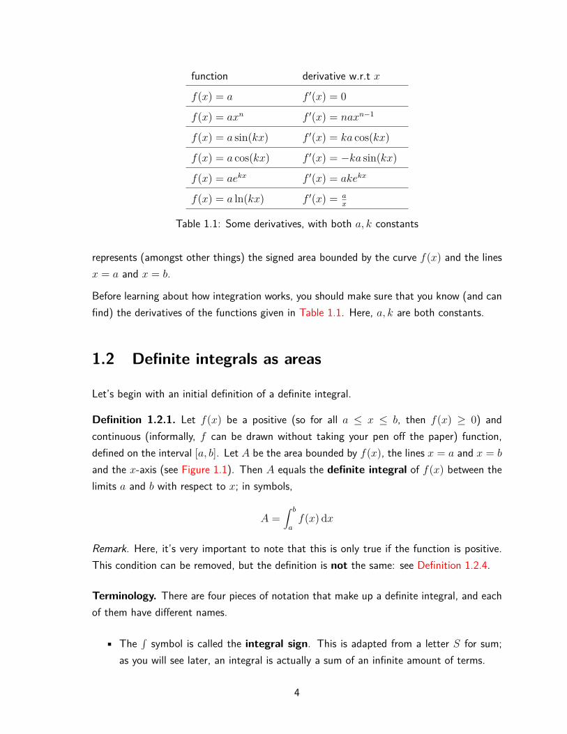
function derivative w.r.t x

f(x) = a f ′(x) = 0

f(x) = axn f ′(x) = naxn−1

f(x) = a sin(kx) f ′(x) = ka cos(kx)

f(x) = a cos(kx) f ′(x) = −ka sin(kx)

f(x) = aekx f ′(x) = akekx

f(x) = a ln(kx) f ′(x) = ax

Table 1.1: Some derivatives, with both a, k constants

represents (amongst other things) the signed area bounded by the curve f(x) and the linesx = a and x = b.

Before learning about how integration works, you should make sure that you know (and canfind) the derivatives of the functions given in Table 1.1. Here, a, k are both constants.

1.2 Definite integrals as areas

Let’s begin with an initial definition of a definite integral.

Definition 1.2.1. Let f(x) be a positive (so for all a ≤ x ≤ b, then f(x) ≥ 0) andcontinuous (informally, f can be drawn without taking your pen off the paper) function,defined on the interval [a, b]. Let A be the area bounded by f(x), the lines x = a and x = b

and the x-axis (see Figure 1.1). Then A equals the definite integral of f(x) between thelimits a and b with respect to x; in symbols,

A =∫ b

af(x) dx

Remark. Here, it’s very important to note that this is only true if the function is positive.This condition can be removed, but the definition is not the same: see Definition 1.2.4.

Terminology. There are four pieces of notation that make up a definite integral, and eachof them have different names.

• The ∫ symbol is called the integral sign. This is adapted from a letter S for sum;as you will see later, an integral is actually a sum of an infinite amount of terms.

4

x

f(x)

a b

Figure 1.1: The area of the shaded region is equal to the integral ∫ ba f(x) dx.

• The value a is called the lower limit and the value b is known as the upper limit.

• The function f(x) is called the integrand.

• The dx denotes the variable you are integrating with respect to. Here, the variable xdoesn’t have to be called x; for instance it can be called t or u. The important thingto remember is that the integral doesn’t change its value if you change the name ofthe variable throughout.

It is important to remember that in every integral, f(x) and dx are multiplied together.

In every definite integral you write, you should include every one of these pieces of notation.

Example 1.2.2. Consider the area bounded by f(x) = 2, the x-axis, and the lines x = 1and x = 3 (see Figure 1.2).

x

f(x)

1 3

2

Figure 1.2: The area of the shaded region is equal to the integral ∫ 31 2 dx

As the shaded region is a square with side length 2, the area of this region is A = 2 · 2 = 4.You can use Definition 1.2.1 to say that

∫ 3

12 dx = 4

5

Example 1.2.3. You are given the area bounded by f(x) = x, the x-axis, and the linesx = 0 and x = 2 (see Figure 1.2).

x

f(x)

0 2

Figure 1.3: The area of the shaded region is equal to the integral ∫ 20 x dx.

As the shaded region is a triangle with base and height both 2, the area is A = (2 ·2)/2 = 2.You can use Definition 1.2.1 to say that

∫ 2

0x dx = 2

However, evaluating areas gets more complicated if your curve is not a straight line. Forinstance, how would you work out the area bounded by f(x) = x2, the limits x = 0 andx = 1 and the x-axis, as seen in Figure 1.4? In other words, what is the value of the definiteintegral of f(x) = x2 between 0 and 1 with respect to x?

x

f(x)

0 1

Figure 1.4: What is ∫ 10 x

2 dx?

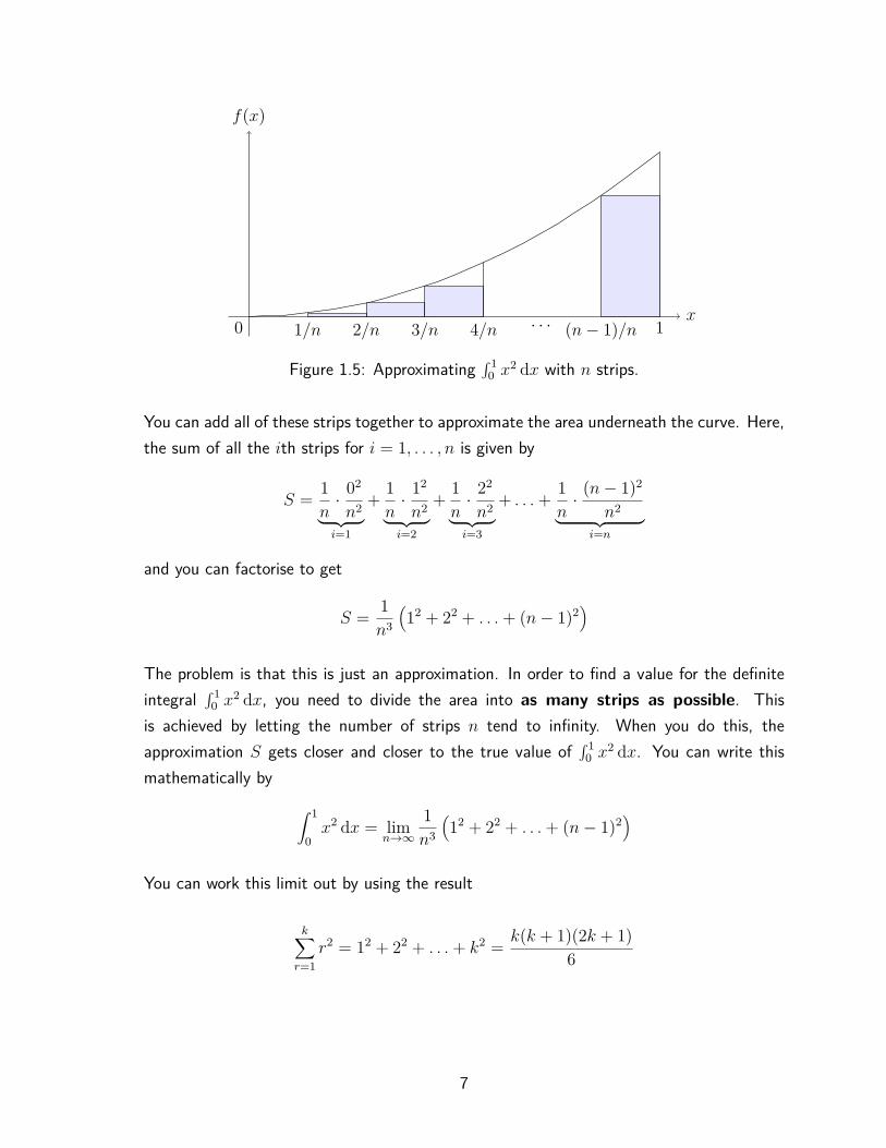
The idea is to approximate the area underneath the curve f(x) = x2 by dividing it into nrectangular strips, each of width 1/n. So for i = 1, . . . , n, the ith strip is a rectangle withwidth 1/n and height given by f((i − 1)/n) = [(i − 1)/n]2. This means that the area ofthe ith strip is (1/n) · [(i− 1)/n]2 (see Figure 1.5).

6

x

f(x)

0 11/n 2/n 3/n 4/n · · · (n− 1)/n

Figure 1.5: Approximating ∫ 10 x

2 dx with n strips.

You can add all of these strips together to approximate the area underneath the curve. Here,the sum of all the ith strips for i = 1, . . . , n is given by

S = 1n· 02

n2︸ ︷︷ ︸i=1

+ 1n· 12

n2︸ ︷︷ ︸i=2

+ 1n· 22

n2︸ ︷︷ ︸i=3

+ . . .+ 1n· (n− 1)2

n2︸ ︷︷ ︸i=n

and you can factorise to get

S = 1n3

(12 + 22 + . . .+ (n− 1)2

)

The problem is that this is just an approximation. In order to find a value for the definiteintegral ∫ 1

0 x2 dx, you need to divide the area into as many strips as possible. This

is achieved by letting the number of strips n tend to infinity. When you do this, theapproximation S gets closer and closer to the true value of ∫ 1

0 x2 dx. You can write this

mathematically by∫ 1

0x2 dx = lim

n→∞

1n3

(12 + 22 + . . .+ (n− 1)2

)

You can work this limit out by using the result

k∑r=1

r2 = 12 + 22 + . . .+ k2 = k(k + 1)(2k + 1)6

7

By setting k = (n− 1) in this result, you can see that∫ 1

0x2 dx = lim

n→∞

1n3

(n− 1)(n)(2n− 1)6

You can then reduce this in the same way you would any limit to get∫ 1

0x2 dx = lim

n→∞

(1− 1/n)(2− 1/n)6 = 1

3

However, this is just one example. It would be extremely useful to work out the definiteintegral of any positive, continuous function f(x) between any limits a and b. This canbe done like the process above: by dividing the interval [a, b] into n strips, working out thearea of each strip, adding up the area of all the strips and then letting n tend to infinityand working out the limit.

Definition 1.2.4. Let f(x) be a positive and continuous function, defined on the interval[a, b]. Set x0 = a and xk = a + k(b − a)/n for all k = 1, 2, . . . , n. Then the definiteintegral of f(x) between the limits a and b with respect to x is given by

∫ b

af(x) dx = lim

n→∞

b− an

n∑k=1

f(xk)

where

• (b− a)/n is the width of every strip;

• f(xk) is the height of the kth strip (the strip between xk and xk+1), and;

• b−an

∑nk=1 f(xk) is the sum of the areas of all n strips.

See Figure 1.6 for a diagram.

Example 1.2.5. You are asked to evaluate the definite integral ∫ 10 e

x dx.

Using the fact that a = 0 and b = 1 and f(x) = ex, and setting xk = k/n, the sum inDefinition 1.2.4 becomes

S = 1n

n∑k=1

ek/n

This is a geometric series. Using the formula for the sum of a geometric series

r + r2 + ...+ rn = rrn − 1r − 1

8

x

f(x)

a bx1 x2 x3 x4 · · · xn−1

Figure 1.6: Partitioning the interval [a, b] into n pieces to find the definite integral∫ ba f(x) dx. Not a very good approximation!

with r = e1/n you can obtainS = 1

ne1/n e− 1

e1/n − 1The goal now is to work out the limit of this expression as n tends to infinity. Here, youcan get ∫ 1

0ex dx = lim

n→∞S = lim

n→∞

e1/n

n

e− 1e1/n − 1

You can take (e− 1) out of the limit and rearrange and, using the expression

limn→∞

n(e1/n − 1

)= 1

gives ∫ 1

0ex dx = (e− 1) lim

n→∞

e1/n

n (e1/n − 1) = e− 1

1.3 Properties of definite integrals

You can use Definition 1.2.4 and the properties of sums and limits to show the followingproperties of definite integrals.

Proposition 1.3.1. Let∫ ba f(x) dx be a definite integral. Then the following properties

hold:

(1) For c such that a < c < b, then:

∫ b

af(x) dx =

∫ c

af(x) dx+

∫ b

cf(x) dx

9

(2) If k is some constant, then:

∫ b

akf(x) dx = k

∫ b

af(x) dx

(3) For a function g(x) where the definite integral exists on the interval [a, b]:

∫ b

af(x) + g(x) dx =

∫ b

af(x) dx+

∫ b

ag(x) dx

(4) If f(x) ≤ g(x) for all x between a and b, then:

∫ b

af(x) dx ≤

∫ b

ag(x) dx

(5) If a is some real number, then:∫ a

af(x) dx = 0

(6) Finally if a < b, then: ∫ b

af(x) dx = −

∫ a

bf(x) dx

Using properties (1) and (2) of Proposition 1.3.1, you can define a definite integral forfunctions that are negative. For instance, let f(x) be a function where f(x) ≥ 0 for all xbetween a and c, and f(x) ≤ 0 for all x between c and b.

You can use property (1) of Proposition 1.3.1 to get:∫ b

af(x) dx =

∫ c

af(x) dx+

∫ b

cf(x) dx.

As f(x) ≤ 0, it follows that −|f(x)| ≤ 0 between c and b. So using property (2) gives:∫ b

af(x) dx =

∫ c

af(x) dx+

∫ b

c−|f(x)| dx

=∫ c

af(x) dx−

∫ b

c|f(x)| dx

This shows that the definite integral is the area above the axis minus the area below theaxis. So regions where f(x) < 0 correspond to negative areas (see Figure 1.7).

Example 1.3.2. Let f(x) = sin(x) be defined between −π and π. Using property (1) of

10

x

f(x)

ab

c

Figure 1.7: The curve f(x) crosses the x-axis at x = c, so the shaded region below thex-axis has a negative area.

Proposition 1.3.1 gives:∫ π

−πsin(x) dx =

∫ 0

−πsin(x) dx+

∫ π

0sin(x) dx (1.1)

As sin(x) is an odd function, then sin(x) = − sin(x). You can use this, along with property(2) of Proposition 1.3.1 to see that

∫ 0

−πsin(x) dx =

∫ 0

−π− sin(−x) dx = −

∫ 0

−πsin(−x) dx

Here, −x is contained in the interval −π < −x < 0. Multiplying through by −1 givesπ > x > 0. So

−∫ 0

−πsin(−x) dx = −

∫ π

0sin(x) dx

Putting this in to Equation 1.1 gives∫ π

−πsin(x) dx = −

∫ π

0sin(x) dx+

∫ π

0sin(x) dx = 0

This result is illustrated in Figure 1.8; you can see that the areas are equal in size, but onopposite sides of the x-axis.

x

f(x)

−ππ

Figure 1.8: ∫ π−π sin(x) dx

11

Chapter 2

The Fundamental Theorem OfCalculus

2.1 From definite to indefinite

You may have wondered why the term ‘definite’ has been attached to integrals throughoutChapter 1. This is because the definite integral ∫ ba f(x) dx is an expression of a definitesigned area bounded by f(x), the x axis, the lower limit a and the upper limit b.

Now suppose instead of setting an upper limit b, this limit is allowed to vary. So here youcan write:

F (x) =∫ x

af(t) dt

It is important to say that the variable in the integral has changed to t; this doesn’t affectthe value of the integral as mentioned in the Terminology section after Definition 1.2.1.

The function F (x) represents the change of area expressed by the integral when x is allowedto change. This means that the area bounded by f(t), the t-axis, the lower limit a andthe upper limit x changes as x changes. In fact, you could say this area is not definite.Therefore, F (x) is known as the indefinite integral of f .

In this chapter, the Fundamental Theorem of Calculus (Theorem 2.2.2) says that F (x) =∫ xa f(t) dt is the antiderivative of f(x); that is, a function whose derivative is f(x). This

will show that integration is a reverse process of differentiation, and that you can evaluatedefinite integrals ∫ ba f(x) dx by considering the antiderivative of the integrand f(x) andcalculating the difference of the antiderivative at the two limits a and b.

12

2.2 The theorem

This section aims to show that the function F (x) as stated above acts as the antiderivativeof f(x). You have seen from the part of the course on differentiation that the derivative ofa function is defined to be

f ′(x) = limh→0

f(x+ h)− f(x)h

The aim is to demonstrate that F ′(x) = f(x) using this definition of derivative. So take

F (x) =∫ x

af(t) dt

as above, representing the area under the curve f(t) between the lines t = a and t = x. Itfollows that

F (x+ h) =∫ x+h

af(t) dt

(see Figure 2.1 for a picture).

x

f(x)

x+ hxa

Figure 2.1: An illustration of the areas ∫ xa f(t) dt and ∫ x+ha f(t) dt.

By Proposition 1.3.1 (1), you can write:

F (x+ h) =∫ x+h

af(t) dt =

∫ x

af(t) dt+

∫ x+h

xf(t) dt = F (x) +

∫ x+h

xf(t) dt

and soF (x+ h)− F (x) =

∫ x+h

xf(t) dt

The idea now is to ‘bound’ the area underneath f(t) between x and x + h between twoareas. To do this, set the minimum value of f(t) between x and x+h as m, and the similarmaximum value by M . The minimum area of ∫ x+h

x f(t) dt is given by the area of rectanglewith side lengths h and m; and the maximum area is given by the area of the rectangle with

13

side lengths h and M . You can see a diagram of this in Figure 2.2.

x

f(x)

Mm

x x+ h

Figure 2.2: Describing the rectangles hm (red rectangles, minimum area) and hM (blue andred rectangles together, maximum area). The value of ∫ x+h

x f(t) dt is somewhere betweenthe two.

So you can writehm ≤

∫ x+h

xf(t) dt ≤ hM.

Dividing through each term by h gives

m ≤ F (x+ h)− F (x)h

≤M.

As f(t) is continuous, when h tends towards 0 both the upper and the lower bounds tendto the value f(x). So, letting h→ 0 gives

f(x) ≤ limh→0

F (x+ h)− F (x)h

≤ f(x)

and sof(x) = lim

h→0

F (x+ h)− F (x)h

= F ′(x)

This statement is the first of the two parts of the Fundamental Theorem of Calculus. Hereis an example of how it can be used, illustrating the way forward for a proof of the secondpart.

Example 2.2.1. You are given the function

F (x) =∫ x

0et dt (2.1)

Using the above result, you can write

F ′(x) = ex

14

The idea now is to find F (x) such that F ′(x) = ex. You can look at Table 1.1 to see thatthe derivative of ex is ex, which is on the right hand side. However, you can also see inTable 1.1 that the derivative of a constant C is 0. So when you are finding F (x) such thatF ′(x) = ex, you need to be careful to include a constant term! So you can take

F (x) = ex + C

as a function whose derivative is ex.

You can substitute this into Equation 2.1 to get

ex + C =∫ x

0et dt

You now have enough information to find the constant C. You can set x = 0 to see that

e0 + C = 1 + C =∫ 0

0et dt = 0

and so C = −1, giving F (x) = ex − 1. Finally, evaluating F (x) at x = 1 gives:

F (1) =∫ 1

0et dt = e− 1

which is exactly the same result as you found in Example 1.2.5.

As has just been shown, the integral

F (x) =∫ x

af(t) dt

represents an antiderivative of f(x). Following the discussion in Example 2.2.1, this an-tiderivative is not unique. In fact, F (x) + C, where C is some constant, is also anantiderivative of f(x), as

ddx (F (x) + C) = F ′(x) + 0 = f(x)

So you can write thatF (x) + C =

∫ x

af(t) dt

To work out C, you can evaluate this function at x = a to get that:

F (a) + C =∫ a

af(t) dt = 0

15

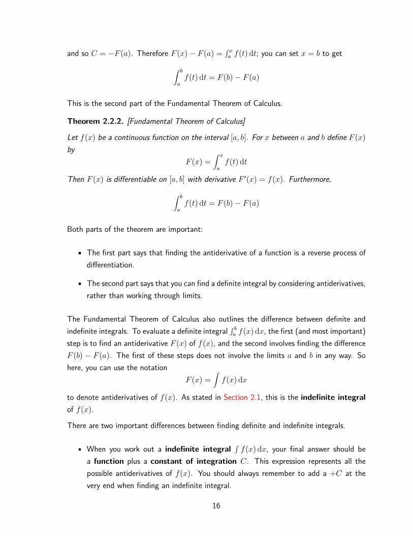
and so C = −F (a). Therefore F (x)− F (a) =∫ xa f(t) dt; you can set x = b to get

∫ b

af(t) dt = F (b)− F (a)

This is the second part of the Fundamental Theorem of Calculus.

Theorem 2.2.2. [Fundamental Theorem of Calculus]

Let f(x) be a continuous function on the interval [a, b]. For x between a and b define F (x)by

F (x) =∫ x

af(t) dt

Then F (x) is differentiable on [a, b] with derivative F ′(x) = f(x). Furthermore,

∫ b

af(t) dt = F (b)− F (a)

Both parts of the theorem are important:

• The first part says that finding the antiderivative of a function is a reverse process ofdifferentiation.

• The second part says that you can find a definite integral by considering antiderivatives,rather than working through limits.

The Fundamental Theorem of Calculus also outlines the difference between definite andindefinite integrals. To evaluate a definite integral ∫ ba f(x) dx, the first (and most important)step is to find an antiderivative F (x) of f(x), and the second involves finding the differenceF (b) − F (a). The first of these steps does not involve the limits a and b in any way. Sohere, you can use the notation

F (x) =∫f(x) dx

to denote antiderivatives of f(x). As stated in Section 2.1, this is the indefinite integralof f(x).

There are two important differences between finding definite and indefinite integrals.

• When you work out a indefinite integral∫f(x) dx, your final answer should be

a function plus a constant of integration C. This expression represents all thepossible antiderivatives of f(x). You should always remember to add a +C at thevery end when finding an indefinite integral.

16

• When you work out a definite integral∫ ba f(x) dx, you could follow this method:

Step 1: Find an antiderivative F (x) of f(x). You do not need a +C.

Step 2: The result F (x) can be put into square brackets, with the upper limit at the topright and the lower limit at the bottom right. So you can write:

∫ b

af(x) dx = [F (x)]ba

Step 3: Work out F (x) at x = b and then work out F (x) at x = a. You can thensubtract F (a) from F (b) to get

∫ b

af(x) dx = [F (x)]ba = F (b)− F (a)

The number at the end is the answer.

Your final answer should be a number. This quantity represents the signed areaunderneath the curve of f(x) between the lines x = a and x = b. There should beno variables in your answer, and you do not need a +C at the end.

2.3 Some antiderivatives

This section details some examples of finding antiderivatives. If you are unsure aboutderivatives of functions here, you could take the opportunity to re-familiarise yourself withTable 1.1 before continuing.

The idea of Table 1.1 is to provide a list of derivatives for common functions. As indef-inite integration is the reverse process of differentiation, it makes sense to write a list ofantiderivatives.

For instance, suppose you wanted to find the antiderivative of the function f(x) = axn,where a is a constant and n 6= −1. You can use the fact that integration is the opposite ofdifferentiation to say that the solution will be a function F (x) such that

ddx (F (x)) = axn

17

Taking F (x) = axn+1

n+1 , and using the power rule for differentiation gives:

ddx

(axn+1

n+ 1

)= a

n+ 1 · (n+ 1)xn = axn

which is f(x). Whenever you differentiate a constant, it goes to 0; so you could takeF (x) = axn+1

n+1 +C, differentiate it with respect to x, and still get f(x). So this means thatyou can write: ∫

axn dx = axn+1

n+ 1 + C for n 6= −1 (2.2)

A special case happens when n = 0; if this happens, then f(x) = ax0 = a is a constant.Integrating this using the formula above gives ∫ a dx =

∫ax0 dx = ax1

1 +C = ax+C andso ∫

a dx = ax+ C (2.3)

You may have asked yourself already why doesn’t this process work for n = −1? These arefunctions of the form f(x) = a

x. It is because if you do the process with n = −1, you end

up dividing by 0; which is not good. However, you can look at Table 1.1 and see that

ddx (a ln(x)) = a

x

However, you need to make sure that ln(x) is defined on only positive x. You can getaround this by writing ln |x| instead of ln(x); this ensures the value of the input is positive.This means you can write ∫

ax−1 dx = a ln |x|+ C (2.4)

You have already seen in Example 2.2.1 that an antiderivative for f(x) = ex is F (x) =ex + C. But what about f(x) = aekx? You are looking for a function F (x) such thatd

dx (F (x)) = aekx. Here, taking F (x) = 1kaekx + C, and differentiating with respect to x

using the rules in Table 1.1 gives

ddx

(1kaekx + C

)= aekx

and so you can write ∫aekx dx = 1

kaekx + C (2.5)

Finally, you can consider antiderivatives of a sin(kx) and a cos(kx). Using rules of differen-

18

function antiderivative w.r.t x notes

f(x) = a∫f(x) dx = ax+ C a constant (2.3)

f(x) = axn∫f(x) dx = ax(n+1)

n+ 1 + C n 6= −1 (2.2)

f(x) = ax−1∫f(x) dx = a ln |x|+ C (2.4)

f(x) = aekx∫f(x) dx = 1

kaekx + C (2.5)

f(x) = a cos(kx)∫f(x) dx = 1

ka sin(kx) + C (2.6)

f(x) = a sin(kx)∫f(x) dx = −1

ka cos(kx) + C (2.7)

Table 2.1: Some antiderivatives

tiation, you can say that

ddx

(−1ka cos kx

)= a sin(kx) and d

dx

(1ka sin kx

)= a cos(kx)

This means that you can write:

∫a cos(kx) dx = 1

ka sin kx+ C (2.6)

and ∫a sin(kx) dx = −1

ka cos kx+ C (2.7)

Summarising the boxed results, Table 2.1 gives a list of common antiderivatives that will beuseful throughout your mathematical career. Throughout, a, k, C are constants.

You can use the examples given in Table 2.1 to find some integrals that previously wereharder to find.

Example 2.3.1. You are asked to find the definite integral ∫ 20 x dx. To do this, you need

to find an antiderivative F (x) of f(x) = x, and then find out F (b) − F (a) where b = 2

19

and a = 0. You can use Equation 2.2 with a = 1 and n = 1 to get

∫ 2

0x dx =

[1 · x1+1

1 + 1

]2

0=[x2

2

]2

0

Using F (x) = x2/2, you can write that F (2) = 4/2 = 2 and F (0) = 0, so now you canevaluate the integral: ∫ 2

0x dx =

[x2

2

]2

0= 4

2 − 0 = 2

This is the same answer you got in Example 1.2.3.

It can be shown that properties (2) and (3) of Proposition 1.3.1 hold for indefinite integrals.So for any constant k (so nothing that involves a variable!) you can write that

∫kf(x) dx = k

∫f(x) dx

and for a continuous function g(x):∫f(x) + g(x) dx =

∫f(x) dx+

∫g(x) dx

Example 2.3.2. You are asked to find the indefinite integral ∫ 16− x2 dx. Here, you canuse the properties of indefinite integrals stated above (and a remark in Example 1.2.2) towrite ∫

16− x2 dx =∫

16 dx+∫−x2 dx = 16

∫dx−

∫x2 dx

So the problem is reduced to working out antiderivatives of 1 and x2. Using Equation 2.3with f(x) = 1 gives an antiderivative of 1x = x. Using Equation 2.2 with n = 2 gives x3/3as an antiderivative of x2. So you can write:

∫16− x2 dx = 16

∫1 dx−

∫x2 dx = 16x− x3

3 + C

You can notice here that you only need to add one constant of integration +C at the veryend of the working.

Example 2.3.3. You are asked to find the definite integral ∫ π−π sin(2x) + 2 cos(x) dx. Youcan use Equation 2.7 with a = 1 and k = 2 to say that an antiderivative for sin(2x) is−1

2 cos(2x). You can use Equation 2.6 with a = 2 and k = 1 to get that an antiderivative

20

for 2 cos(x) is 2 sin(x). Therefore, you can write∫ π

−πsin(2x) + 2 cos(x) dx =

[−1

2 cos(2x) + 2 sin(x)]π−π

You can now evaluate the value of this antiderivative at the limits π and −π. Here

−12 cos(2π) + 2 sin(π) = −1

2 · (1) + 2 · 0 = −12

and−1

2 cos(−2π) + 2 sin(−π) = −12 · (1) + 2 · 0 = −1

2You can put this all together to get that

∫ π

−πsin(2x) + 2 cos(x) dx =

[−1

2 cos(2x) + 2 sin(x)]π−π

=[−1

2

]−[−1

2

]= 0

This example shows that you do not have to write F (x) at any point when evaluating anintegral, nor do you have to split up the integral of two functions added together into twoparts before proceeding.

2.4 Summary of first two chapters

• The Fundamental Theorem of Calculus states that indefinite integration is the reverseprocess to differentiation, and that you can work out definite integrals (the limit ofsums of areas) by using the antiderivative of the integrand.

• Working out both indefinite and definite integrals involve using antiderivatives; youcan find these for common functions in Table 2.1.

• When you work out a indefinite integral∫f(x) dx, your answer should be a function

F (x) plus a constant of integration C. This expression represents all the possibleantiderivatives of f(x). You should always remember to add a +C at the end whenworking out an indefinite integral.

• When you work out a definite integral, your answer should be a number. Thisnumber represents the signed area underneath the curve of f(x) between the linesx = a and x = b. There should be no variables in your answer, and you do not needa +C.

21

Chapter 3

Integration by substitution

3.1 Techniques of calculus

You may have studied techniques for finding derivatives of composite functions using thechain rule, the product rule and the quotient rule. These rules are detailed in Table 3.1 forvarious operations on functions f(x) and g(x).

function derivative w.r.t x name

y(x) = f(g(x)) y′(x) = ddg (f(g(x))) · d

dx (g(x)) chain rule

y(x) = f(x) · g(x) y′(x) = g(x) · f ′(x) + f(x) · g′(x) product rule

y(x) = f(x)g(x) y′(x) = g(x) · f ′(x)− f(x) · g′(x)

(g(x))2 quotient rule (g 6= 0)

Table 3.1: Helpful rules for differentiation

Similar techniques exist for when you want to find antiderivatives of composite functions.This chapter is on integration by substitution, which is similar to the technique of thechain rule. This technique is discussed further in Chapter 4, when considering trigonometricfunctions in more detail. Chapter 5 is on integration by parts, which is similar to thetechnique of the product rule. Both techniques are very important for finding antiderivativesof a variety of functions.

22

3.2 How integration by substitution works

Suppose you are asked to integrate a composite function f(u(x)). You can write thefunction u(x) as a variable u here (see the terminology on page 4), and use the termsinterchangeably; but you should always remember that u is a function of x. Finding thisintegral of f(u(x)) = f(u) can be done in two different ways; one with respect to u andone with respect to x. Firstly, using the Fundamental Theorem of Calculus, you are lookingfor a function F (u) such that

ddu (F (u)) = f(u)

and so you can writeF (u) =

∫f(u) du

As u is a function of x, you can differentiate F (u(x)) with respect to x using the chainrule, to get

ddx (F (u(x))) = d

du (F (u(x))) · ddx (u(x)) = F ′(u(x)) · u′(x) = f(u(x)) · u′(x)

You can see from this that F (u(x)) is an antiderivative (with respect to x) of f(u(x))·u′(x).This means that you can write

F (u) =∫f(u) · u′(x) dx

This gives two expressions for F (u), which you can compare to get:

∫f(u(x)) · u′(x) dx =

∫f(u) du (3.1)

Equation 3.1 demonstrates the principle of integration by substitution for indefiniteintegrals. Essentially, you can choose a function u = u(x) of x, and ‘substitute’ this intothe left hand side of Equation 3.1. This is then equal to the right hand side which, onthe correct choice of u(x), should be an easier integral to solve. You should consider usingintegration by substitution (with substitution u = u(x)) where the integrand is a compositefunction f(u(x)) of x multiplied by a term that ‘looks like’ the derivative u′(x) of u(x).

The difficulty of integration by substitution lies in the correct choice of u = u(x). There isno general rule for choosing the ‘right’ substitution in a given integrand, so you will haveto decide on a correct substitution for every integration by substitution that you do. Youwill know that you have made the correct substitution when there is no mention of x in

23

your expression. A useful thing to remember is that the idea of this method is to makeintegration easier; so the integral on the right is something you know you can work out.This should motivate your choice for u.

One thing that you can notice is that integration by substitution at this stage is only usedin finding antiderivatives of composite functions. Suppose that you are using integration bysubstitution to evaluate a definite integral ∫ ba f(u(x)) dx. You need to be careful here asthe limits of the integral are defined in terms of x, and not in terms of u. To correct this,you need to evaluate the limits a and b in your chosen substitution u = u(x), and thensubstitute these values in the correct place. In other words:

∫ b

af(u(x)) · u′(x) dx =

∫ u(b)

u(a)f(u) du (3.2)

This is integration by substitution for definite integrals.

Another thing you can notice is that f(u) is present in both integrands in Equation 3.1 (andEquation 3.2), and that this implies that u′(x)dx = du. This expression can be rearranged;so you can write dx = du/u′(x). This technique is very useful; particularly if there is nou′(x) term immediately visible in the integrand.

You can follow these steps whenever you would need to use integration by substitution. Thismethod will be used throughout the examples given in Section 3.3.

3.2.1 Method for integration by substitution

Step 1: Choose a suitable u = u(x). Your choice of substitution should not be a constantfunction u(x) = a.

Step 2: Work out u′(x), and write down an expression for dx = du/u′(x). If you areconsidering a definite integral, work out u(a) and u(b) where a and b are the limitsof the integral.

Step 3: Now, you should

• replace every instance of u(x) with the letter u• replace dx with du/u′(x), and cancel;• (for definite integrals only) replace a with the value u(a) and b with u(b).

Warning: At this stage, the integral should be solely in terms of u. If there are still termscontaining x at this stage, stop and consider another choice of u.

24

Step 4: If you can, work out the integral. If you are considering a definite integral, then themethod stops here with the answer. if you are considering an indefinite integral,don’t forget the +C!

Step 5: (For indefinite integrals only) Your antiderivative should be in terms of u. Replaceevery instance of u with the original function u(x). The method stops here forindefinite integrals.

3.3 Examples

Throughout these examples, the properties of integrals as outlined in Proposition 1.3.1 areused without reference.

Example 3.3.1. You are asked to evaluate ∫ sin(3x + 9) dx. Since this is an indefiniteintegral, you have no limits to change but you must remember to do Step 5 of the methodin Subsection 3.2.1.

Step 1: You can integrate sin, so a good choice of substitution here would be u = 3x+ 9.

Step 2: Here, u′(x) = 3, and so dx = du/3. As this is an indefinite integral, you have nolimits to change.

Step 3: Replacing each instance of u(x) = 3x+ 9 with u, and replacing dx by du/3 gives∫

sin(3x+ 9) dx =∫

sin(u)13 du = 1

3

∫sin(u) du

Since there is no x left in the integral, you are OK to continue.

Step 4: Not forgetting the constant of integration, evaluating the integral using the appro-priate rule from Table 2.1 gives

13

∫sin(u) du = −1

3 cos(u) + C

Step 5: You need to substitute in 3x + 9 = u into your solution to get 13 cos(3x + 9). So

you can write ∫sin(3x+ 9) dx = −1

3 cos(3x+ 9) + C

which is the final answer.

25

Example 3.3.2. Say you are asked to evaluate ∫ 40

1(x/2−4)3 dx. Since this is a definite

integral, you must remember to change the limits of integration, but you don’t have to doStep 5 of the method in Subsection 3.2.1.

Step 1: You can integrate any function of the form xn, so a good choice of substitutionhere would be u = x/2− 4.

Step 2: Here, u′(x) = 1/2, and so dx = du/(1/2) = 2du. As this is a definite integral,you must remember to change the limits. You can do this by evaluating u at x = 0and x = 4. So here u(0) = −4 and u(4) = −2.

Step 3: Replacing each instance of u(x) = x/2 − 4 with u, replacing dx by 2du, andreplacing the lower limit 0 with −4 and the upper limit 4 with −2 gives

∫ 4

0

1(x/2− 4)3 dx =

∫ −2

−4

1u3 · 2 du = 2

∫ −2

−4u−3 du

As there are no terms involving x left in the integral, you are OK to continue andyou can now evaluate the integral.

Step 4: Evaluating the integral using the corresponding rule from Table 2.1 gives

2∫ −2

−4u−3 du = 2

[u−2

−2

]−2

−4=[−u−2

]−2

−4

So this means that

[−u−2

]−2

−4=[− 1

(−2)2

]−[− 1

(−4)2

]= −1

4 + 116 = − 3

16

which is the final answer.

Example 3.3.3. You are asked to evaluate ∫ sin3(x) cos(x) dx. Since this is an indefiniteintegral, you have no limits to change but you must remember to do Step 5 of the methodin Subsection 3.2.1.

Step 1: You can integrate un, so a good choice of substitution here would be u = sin(x).

Step 2: Here, u′(x) = cos(x), so you can write dx = du/ cos(x). Again, as this is anindefinite integral, you have no limits to change.

26

Step 3: Replacing each instance of u(x) = sin(x) with u, and replacing dx by du/ cos(x)gives ∫

sin3(x) cos(x) dx =∫u3 cos(x)

cos(x) du =∫u3 du

Since there is no x left in the integral, you are OK to continue.

Step 4: Not forgetting the constant of integration, evaluating the integral using the corre-sponding rule from Table 2.1 gives

∫u3 du = u4

4 + C

Step 5: You need to substitute in sin(x) = u into your solution to get 14 sin4(x). You can

write ∫sin(3x+ 9) dx = −1

3 cos(3x+ 9) + C

which is the final answer.

Example 3.3.4. You are asked to evaluate ∫ 1x

+ e√

x√x

dx. Since this is an indefinite integral,you have no limits to change but you must remember to do Step 5 of the method inSubsection 3.2.1. Here, you can integrate 1/x using a rule in Table 2.1 (giving ln |x|, butyou cannot integrate e

√x/√x so easily. The idea here is to split the integrand into two, using

integration by substitution on one of the parts. Using the techniques from Proposition 1.3.1can make your life easier in these circumstances. So by saying

∫ 1x

+ e√x

√x

dx =∫ 1x

dx+∫ e

√x

√x

dx = ln |x|+∫ e

√x

√x

dx

you can focus on evaluating the remaining integral by substitution.

Step 1: You can integrate ex, so a good choice of substitution here would be u =√x =

x1/2.

Step 2: Here, u′(x) = 12x−1/2 = 1

2x1/2 . This means that

dx = du/(1/2x1/2) = 2x1/2du

As x1/2 = u, you can write dx = 2udu. Since this is an indefinite integral, youhave no limits to change.

27

Step 3: Replacing each instance of u(x) =√x with u, and replacing dx by 2udu gives

∫ e√x

√x

dx =∫ eu

u· 2u du = 2

∫eu du

Since there is no x left in the integral, you are OK to continue.

Step 4: Not forgetting the constant of integration, evaluating the integral using the corre-sponding rule from Table 2.1 gives

2∫eu du = 2eu + C

Step 5: You need to substitute in √x = u into your solution to get 2e√x. So you can write

∫ e√x

√x

dx = 2e√x + C

which is the final answer.

So therefore, you can now integrate the entire expression. The final answer is

∫ 1x

+ e√x

√x

dx =∫ 1x

dx+∫ e

√x

√x

dx = ln |x|+ 2e√x + C.

Example 3.3.5. Say you are asked to evaluate ∫ π/40 x + cos(2x)2 sin(2x) dx. This is a

definite integral with two parts. Similar to the previous example, you can write∫ π/4

0x+ cos2(2x) sin(2x) dx =

∫ π/4

0x dx︸ ︷︷ ︸

(1)

+∫ π/4

0cos2(2x) sin(2x) dx︸ ︷︷ ︸

(2)

and work out both integrals one at a time.

So for (1), you can evaluate this using the rules in Table 2.1. Here

∫ π/4

0x dx =

[x2

2

]π/4

0= (π/4)2

2 − 02 = π2

32

For part (2) however, you need to use integration by substitution. As this is a definiteintegral, you must remember to change the limits of integration.

Step 1: You can integrate any function of the form xn, so a good choice of substitutionhere would be u = cos(2x).

28

Step 2: Here, u′(x) = −2 sin(2x), and so dx = du/(−2 sin(x)). As this is a definiteintegral, you must remember to change the limits. You can do this by evaluatingu at x = 0 and x = π/4. So here u(0) = cos(0) = 1 and u(π/4) = cos(π/2) = 0.

Step 3: By replacing each instance of cos(2x) with u, the term dx with du/(−2 sin(x)),and the lower limit 0 with 1 and the upper limit π/4 with 0 gives

∫ π/4

0cos2(2x) sin(2x) dx =

∫ 0

1

u2 sin(2x)−2 sin(2x) du = −1

2

∫ 0

1u2 du

As there are no terms involving x left in the integral, you are OK to continue andyou can now evaluate the integral.

Step 4: Using Proposition 1.3.1 (6), you can see that

−12

∫ 0

1u2 du = 1

2

∫ 1

0u2 du

Evaluating this integral using the corresponding rule from Table 2.1 gives

12

∫ 1

0u2 du = 1

2

[u3

3

]1

0=[u3

6

]1

0

So this means that [u3

6

]1

0=[−1

6

]− [0] = 1

6

which is the final answer for (2).

Putting the results of (1) and (2) together give

∫ π/4

0x+ cos2(2x) sin(2x) dx = π2

32 + 16

Remark. In these examples, the tradition has been to substitute dx with du/u′(x) andthen cancel through. However, sometimes it is convenient to replace u′(x)dx with du. Forinstance, you could have used this technique in Example 3.3.3 and Example 3.3.5.

Finally in this chapter, you can use integration by substitution in a more general setting,and demonstrate that it works as the ‘inverse’ of the chain rule of differentiation. Considerthe function y = ln(h(x)), where h is some non-zero function of x. Using the chain rule in

29

Table 3.1 with f = ln(x) and g = h(x) gives

dydx = 1

h(x)︸ ︷︷ ︸f ′(g(x))

·h′(x) = h′(x)h(x)

Now, for some non-zero function h, you can think about solving∫ h′(x)h(x) dx

You can use integration by substitution to do this, with a choice of substitution u = h(x).This means that u′(x) = h′(x), and so dx = du/h′(x). Replacing h(x) with u and dx withdu/h′(x) gives ∫ h′(x)

h(x) dx =∫ h′(x)u · h′(x) du =

∫ 1u

du

You can integrate this using the corresponding rule from Table 2.1 to get∫ 1u

du = ln |u|+ C

Substituting h(x) back in for u gives the following useful identity

∫ h′(x)h(x) dx = ln |h(x)|+ C (3.3)

You can notice that this reverses the differentiation performed above.

This equation is a valuable tool, as you can ‘spot’ the patterns of a function in the denom-inator and its derivative on the top. This will save you time in performing an integration bysubstitution. For instance, you can consider the indefinite integral

∫ 2xx2 + 1 dx

Here, you can see that the numerator h′(x) = 2x is precisely the derivative of the denomi-nator h(x) = x2 + 1. Therefore, you can use Equation 3.3 to say that

∫ 2xx2 + 1 dx = ln |x2 + 1|+ C.

30

Chapter 4

Trigonometry and integration

4.1 Previously in trigonometry...

So far in this portion on integration, you have seen the cos and the sin functions... but notmuch else. You may have seen at different points that there are four other trigonometricfunctions to consider; tan, sec, csc and cot. The definitions of these functions are given inTable 4.1 along with their derivatives. You can find the derivatives on your own by usingthe chain rule on each of the definitions of the functions.

function definition

f(x) = tan(x) f(x) = sin(x)cos(x)

f(x) = sec(x) f(x) = 1cos(x)

f(x) = csc(x) f(x) = 1sin(x)

f(x) = cot(x) f(x) = 1tan(x) = cos(x)

sin(x)

Table 4.1: Definitions of tan, sec, csc and cot

You may have studied the derivatives of all of the functions in Table 4.1 in previous partsof the course. Table 4.2 provides the derivatives of the six trigonometric functions you haveseen so far, as well as all the known antiderivatives.

31

function derivative w.r.t x ∫dx

f(x) = a cos(kx) f ′(x) = −ak sin(kx) (2.6)

f(x) = a sin(kx) f ′(x) = ak cos(kx) (2.7)

f(x) = a tan(kx) f ′(x) = ak

cos2(kx) = ak sec2(kx) (4.1)

f(x) = a sec(kx) f ′(x) = aksin(kx)cos2(kx) = ak sec(kx) tan(kx) (6.3)

f(x) = a csc(kx) f ′(x) = −ak cos(kx)sin2(kx) = −ak csc(kx) cot(kx) (4.3)

f(x) = a cot(kx) f ′(x) = − ak

sin2(kx) = −ak csc2(kx) (4.2)

Table 4.2: Derivatives and antiderivatives of trigonometric functions

Here, the references given in the antiderivative column refers to the equation in which theyare first presented.

The aim of this chapter is for you to expand your knowledge about integration of trigonomet-ric functions, using trigonometric identities to calculate examples, and the use of trigono-metric functions in integration by substitution.

To begin with, you should make sure that you know the derivative and antiderivative ofboth sin and cos functions (listed in Table 4.2).

4.2 Some more antiderivatives

This section is designed to find some more antiderivatives that you can use throughout yourintegration course. A good place to start would be to look at the functions outlined inTable 4.1, and work out antiderivatives for those.

Let’s begin with a tan(kx). Here, you can write∫a tan(kx) dx =

∫a

sin(kx)cos(kx) dx.

32

You can work this integral out using integration by substitution.

Here, you can integrate this expression using integration by substitution, with u = cos(kx).It follows that u′(x) = −k sin(kx) and so dx = du/− k sin(kx). Making the substitutiongives ∫

asin(kx)cos(kx) dx =

∫−a sin(kx)

u · k sin(kx) du =∫− a

kudu = −a

k

∫ 1u

du

You can integrate this expression using Equation 2.4 to get

−ak

∫ 1u

du = −ak

ln |u|+ C

Substituting u = cos(kx) back into this antiderivative, and using the laws of logarithmstogether with the fact that sec(kx) = 1

cos(kx) gives

∫a tan(kx) dx = −a

kln | cos(kx)|+ C = a

kln∣∣∣∣∣ 1cos(kx)

∣∣∣∣∣+ C = a

kln | sec(kx)|+ C

and so you can write∫a tan(kx) dx = a

kln | sec(kx)|+ C (4.1)

There is another way in which you can obtain this result. By Table 4.2, the derivative ofcos(kx) is − sin(kx), which is nearly equal to the numerator. So here, you can use the factthat −a/k · −k = a, together with Proposition 1.3.1 (2) to write that

∫a

sin(kx)cos(kx) dx =

∫(−ak) sin(kx)

−k cos(kx) dx = −ak

∫ −k sin(kx)cos(kx) dx

You can recognise that this integrand is a fraction with a function h(x) on the bottom andits derivative h′(x) on the top. Therefore, you can use Equation 3.3 to write

−ak

∫ −k sin(kx)cos(kx) dx = −a

kln | cos(kx)|+ C = a

kln | sec(kx)|+ C

and recover the result from Equation 4.1.

You can use a similar method to work out the antiderivative of a cot(kx). Here, you canuse Table 4.1 to write that

a cot(kx) = acos(kx)sin(kx)

You can integrate this by substitution, using u = sin(kx) as your choice of substitution.

33

This means that u′(x) = k cos(kx) and so dx = du/k cos(kx). Substituting these in andcancelling gives

∫a

cos(kx)sin(kx) dx =

∫a

cos(kx)u · k cos(kx) du = a

k

∫ 1u

du

You can integrate this using Equation 2.4 to write

a

k

∫ 1u

du = a

kln |u|+ C

Finally, you can substitute u = sin(kx) into this to write

∫a cot(kx) dx = a

kln | sin(kx)|+ C (4.2)

Remark. While the antiderivatives of tan and cot have been worked out with techniquesthat you have already studied up to this point, finding the indefinite integrals of sec(x) andcsc(x) with respect to x need some more work.

You can use the Fundamental Theorem of Calculus (Theorem 2.2.2) to state the antideriva-tives for those functions given in the second column of Table 4.2. These results are collectedin Table 4.3. You can check these antiderivatives by differentiating them and getting f(x)as an answer.

function antiderivative w.r.t x

f(x) = a sec2(kx)∫f(x) dx = a

ktan(kx) + C

f(x) = a sec(kx) tan(kx)∫f(x) dx = a

ksec(kx) + C

f(x) = a csc(kx) cot(kx)∫f(x) dx = −a

kcsc(kx) + C

f(x) = a csc2(kx)∫f(x) dx = −a

kcot(kx) + C

Table 4.3: Antiderivatives of some derivatives found in Table 4.2

34

Example 4.2.1. You are asked to integrate∫−4 tan(2x) + 4 sec2(x) dx

Here, you can use Proposition 1.3.1 (3) to say that∫−4 tan(2x) + 4 sec2(x) dx =

∫−4 tan(2x) dx+

∫4 sec2(x) dx

Using Equation 4.1 with a = −4 and k = 2 for the first integral, and using the result inTable 4.3 with a = 4 and k = 1 for the second integral, you can write

∫−4 tan(2x) + 4 sec2(x) dx =− −4

2 ln | sec(2x)|+ 41 tan(x) + C

=2 ln | sec(2x)|+ 4 tan(x) + C

= ln | sec2(2x)|+ 4 tan(x) + C

4.3 Using trigonometric identities

In your mathematical career, you may have come across a range of identities that relate twotrigonometric functions together. These trigonometric identities prove to be very useful inintegrating some functions that cannot be integrated directly or by substitution. Techniquesto do this are discussed in the next two sections.

The first set of these pairs together trigonometric functions in the square identities (orPythagorean identities; see Table 4.4):

functions identity

sin, cos cos2(x) + sin2(x) = 1

tan, sec 1 + tan2(x) = sec2(x)

cot, csc cot2(x) + 1 = csc2(x)

Table 4.4: Square identities of trigonometric functions

These are so called because you can derive the first of these from Pythagoras’ Theorem,

35

and the second and third of these identities from the first by dividing through by cos2(x)and sin2(x) respectively.

The second set of these are known as angle sum rules, and are particularly useful fordealing with powers of trigonometric functions. These are very useful when you take theangles A and B to be the same angle, giving the related double angle formulas (seeTable 4.5):

Sum rule double angle formula

sin(A±B) = sin(A) cos(B)± cos(A) sin(B) sin(2A) = 2 sin(A) cos(A)

cos(A±B) = cos(A) cos(B)∓ sin(A) sin(B) cos(2A) = cos2(A)− sin2(A)

tan(A±B) = tan(A)± tan(B)1∓ tan(A) tan(B) tan(2A) = 2 tan(A)

1− tan2(A)

Table 4.5: Sum rules of trigonometric functions

You can choose the angles A and B carefully in these rules in order to find expressions tohelp you solve integrals. For instance, taking A = 2x and B = x in the sum rules yieldthe triple angle formulas. Here, for instance, is the derivation of the formula for cos3(x),using the double angle formulas and the fact that sin2(x) = 1− cos2(x):

cos(3x) = cos(2x+ x) = cos(2x) cos(x)− sin(2x) sin(x)

= (cos2(x)− sin2(x)) cos(x)− (2 sin(x) cos(x)) sin(x)

= cos3(x)− sin2(x) cos(x)− 2 sin2(x) cos(x)

= cos3(x)− 3 sin2(x) cos(x)

= cos3(x)− 3(1− cos2(x)) cos(x)

= 4 cos3(x)− 3 cos(x). (*)

You should know, and be confident with manipulating the identities in Tables 4.4 and 4.5before continuing.

36

4.3.1 Examples

Example 4.3.1. You are asked to find ∫ π/40 tan2(x) dx. You can notice that you cannot

integrate this using substitution, as it is not of the form f(u(x)) · u′(x) for some functionu(x). However, you can see that you can write down the antiderivative of sec2(x) fromTable 4.3, and that tan2(x) = sec2(x)− 1 from Table 4.4. This means you can write

∫ π/4

0tan2(x) dx =

∫ π/4

0sec2(x)− 1 dx

You can integrate this to get∫ π/4

0sec2(x)− 1 dx = [tan(x)− x]π/4

0

=(

tan(π

4

)− π

4

)− (0 + 0)

=1− π

4

Example 4.3.2. You are asked to find ∫ sin2(x) dx. Again, you cannot integrate this usingsubstitution, and this is not something you can write down the antiderivative for. Here, youneed to use trigonometric identities to find a way to write sin2(x) in a form you know youcan integrate.

Here, you can notice that sin2(x) appears in the double angle formula for cos(2x), which iscos2(x)−sin2(x). Furthermore, sin2(x) appears in the square identity cos2(x)+sin2(x) = 1,which you can rewrite as cos2(x) = 1− sin2(x). Combining these gives

cos(2x) = cos2(x)− sin2(x)

= (1− sin2(x))− sin2(x)

= 1− 2 sin2(x)

Rearranging to make sin2(x) the subject gives

sin2(x) = 12 −

12 cos(2x)

and the right hand side of this equation is something that you can integrate. So now, youcan write ∫

sin2(x) dx =∫ 1

2 −12 cos(2x) dx

37

and integrate using Equation 2.3 and Equation 2.6 to get∫

sin2(x) dx =∫ 1

2 −12 cos(2x) dx = 1

2x−14 sin(2x) + C

Example 4.3.3. Now, you are asked to find ∫ 2 cos3(x) dx. Once again, you cannot usesubstitution or integrate directly to find the answer to this problem. This integrand is alittle harder to represent as something you can integrate directly as there is no trigonometricidentity in Tables 4.4 and 4.5 to use with cos3(x) in it. However, at the start of the section,it was demonstrated in Table * that

cos(3x) = 4 cos3(x)− 3 cos(x)

You can rearrange this to say that

cos3(x) = 14 cos(3x) + 3

4 cos(x)

which is something that you can integrate. Replacing the integrand gives∫

2 cos3(x) dx =∫ 1

2 cos(3x) + 32 cos(x) dx

and you can integrate this using Equation 2.6 to get∫

2 cos3(x) dx =∫ 1

2 cos(3x) + 32 cos(x) dx = 1

6 sin(3x) + 32 sin(x) + C

Finally in this section, nou can use trigonometric identities, together with some previousresults, to prove one of the final two antiderivatives of the functions from Table 4.1 not yetconsidered.

Example 4.3.4. You are asked to find ∫ a csc(kx) dx. You can use Table 4.1 and Propo-sition 1.3.1 (2) to write the integral as

∫a csc(kx) dx =

∫ a

sin(kx) dx

Now, you can use the sum rule for sin in Table 4.5 with A = B = kx/2 to write that

1sin(kx) = 1

2 sin(kx/2) cos(kx/2)

38

Next, you can use the fact that 1 = cos2(kx/2) + sin2(kx/2), and cancelling gives to write

12 sin(kx/2) cos(kx/2) = cos2(kx/2) + sin2(kx/2)

2 sin(kx/2) cos(kx/2) = cos(kx/2)2 sin(kx/2) + sin(kx/2)

2 cos(kx/2)

Finally, you can use Table 4.1 to write that

1sin(kx) = 1

2 cot(kx/2) + 12 tan(kx/2)

You know how to integrate cot and tan by Equations (4.2) and (4.1) respectively. Soreplacing the integrand gives

∫ a

sin(kx) dx =∫ a

2 cot(kx/2) + a

2 tan(kx/2) dx

and integrating using Equation 4.2 and Equation 4.1 gives∫ a

2 cot(kx/2) + a

2 tan(kx/2) dx = 2a2k ln | sin(kx/2)|+ 2a

2k ln | sec(kx/2)|+ C

Cancelling the 2’s in each term, and using the laws of logarithms together with the factthat sin(kx) sec(kx) = tan(kx) gives:

∫a csc(kx) dx = a

kln | tan(kx/2)|+ C (4.3)

Remark. This technique does not work in the case of integrating a sec(kx). This is becauseusing the double angle formula on cos(kx) in the same fashion as in Example 4.3.4 causesthe denominator to become cos2(kx/2)−sin2(kx/2); an expression that you cannot cancel.The technique to integrate a sec(kx) will be explored later.

4.4 Inverse functions: a different kind of substitution

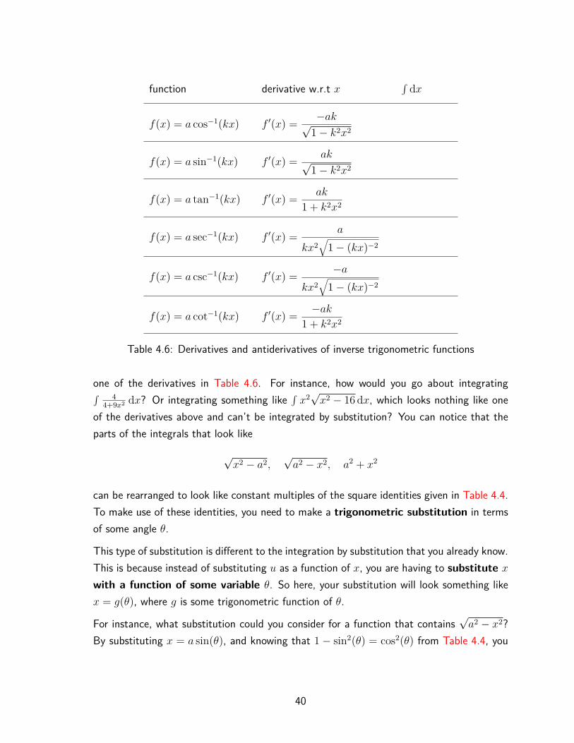
Every trigonometric function has an inverse. For instance, the inverse of sin(x) is sin−1(x).You may have seen in the differentiation part of the course that you can use implicit dif-ferentiation to find derivatives of these functions. A list of inverse trigonometric functionsand their derivatives are given in Table 4.6; this means that you can find antiderivatives foreach of these derivatives by the Fundamental Theorem of Calculus.

However, sometimes the integral you are considering does not come in the same form as

39

function derivative w.r.t x ∫dx

f(x) = a cos−1(kx) f ′(x) = −ak√1− k2x2

f(x) = a sin−1(kx) f ′(x) = ak√1− k2x2

f(x) = a tan−1(kx) f ′(x) = ak

1 + k2x2

f(x) = a sec−1(kx) f ′(x) = a

kx2√

1− (kx)−2

f(x) = a csc−1(kx) f ′(x) = −akx2

√1− (kx)−2

f(x) = a cot−1(kx) f ′(x) = −ak1 + k2x2

Table 4.6: Derivatives and antiderivatives of inverse trigonometric functions

one of the derivatives in Table 4.6. For instance, how would you go about integrating∫ 44+9x2 dx? Or integrating something like ∫ x2√x2 − 16 dx, which looks nothing like one

of the derivatives above and can’t be integrated by substitution? You can notice that theparts of the integrals that look like

√x2 − a2,

√a2 − x2, a2 + x2

can be rearranged to look like constant multiples of the square identities given in Table 4.4.To make use of these identities, you need to make a trigonometric substitution in termsof some angle θ.

This type of substitution is different to the integration by substitution that you already know.This is because instead of substituting u as a function of x, you are having to substitute xwith a function of some variable θ. So here, your substitution will look something likex = g(θ), where g is some trigonometric function of θ.

For instance, what substitution could you consider for a function that contains√a2 − x2?

By substituting x = a sin(θ), and knowing that 1− sin2(θ) = cos2(θ) from Table 4.4, you

40

can see that

√a2 − x2 =

√a2 − a2 sin2(θ) =

√a2(1− sin2(θ)) = a cos(θ)

Similarly, for functions that contain x2 + a2, you could consider the substitution a tan(θ).Then, using the fact that 1 + tan2(θ) = sec2(θ), you can write

x2 + a2 = a2 tan2(θ) + a2 = a2(tan2(θ) + 1) = a2 sec2(θ)

Finally, for functions that contain√x2 − a2 you could consider the substitution a sec(θ).

Then, using the identity tan2(θ) = sec2(θ)− 1, you can say that

√x2 − a2 =

√a2 sec2(θ)− a2 =

√a2(sec2(θ)− 1) = a tan(θ)

Warning. Of course, there are functions containing these types of expressions that do notrequire a trigonometric substitution. For instance,

∫x2 + a2 dx = x3

3 + a2x+ C

Some integrands containing these types of expression can be solved using a conventionalsubstitution rather than a trigonometric one. For instance, using the substitution u = x2−16gives that ∫

x√x2 − 16 dx = (x2 − 16)3/2

3 + C

Therefore, you should only use a trigonometric substitution unless you really have to! Thisis usually when one of the three expressions above is in the denominator of the integrand.

The choice of substitution is not the only thing you need to consider before making atrigonometric substitution. Because you are considering a function of θ, this has the effectof changing how you handle the dx term in the integral. Here, the correct substitution fordx is dx = g′(θ)dθ.

Furthermore, if you are considering a definite integral, you need to change the limits; again,this is slightly different to the usual process. As your limits a and b will be in terms of x,you need to change this into terms of θ. As x = g(θ), it follows that g−1(x) = θ, whereg−1 is the inverse trigonometric function of g. This means that you should replace a withg−1(a) and replace b with g−1(b).

This leads to a modified method for integration via a trigonometric substitution. The

41

principle is the same, with a few key differences.

4.4.1 Method for integration by trigonometric substitution

Step 1: Choose a suitable x = g(θ).

Step 2: Work out g′(θ) (the derivative of g(θ) with respect to θ, and write down theexpression dx = g′(θ)dθ. If you are considering a definite integral, work out anexpression for θ in terms of x (usually, this is the inverse function g−1(x) = θ),and then evaluate this expression at a and b where a and b are the limits of theintegral.

Step 3: Now, you should

• replace every instance of x with the function g(θ)

• replace dx with g′(θ)dθ, and cancel if you need to;

• (for definite integrals only) replace a with the value g−1(a) and b with g−1(b).

Warning: At this stage, the integral should be solely in terms of θ. If there are still termscontaining x at this stage, stop and consider another choice of g(θ).

Step 4: If you can, work out the integral. If you are considering a definite integral, then themethod stops here with the answer. if you are considering an indefinite integral,don’t forget the +C!

Step 5: (For indefinite integrals only) Your antiderivative should be in terms of θ. You canreplace every instance of θ with the inverse function g−1(x), or find an expressionfor the antiderivative h(θ) in terms of x if the alternative is too difficult (seeExample 4.4.2). The method stops here for indefinite integrals.

If you do require a trigonometric substitution, then the information about the choice youcould make is summarised in Table 4.7. The reason why these substitutions are suggestedis the fact that what results after the substitution x = g(θ) looks like a constant multipleof the derivative g′(θ) of g(θ).

4.4.2 Examples

Example 4.4.1. You are asked to find the integral ∫√21

1x2√

4−x2 dx.

42

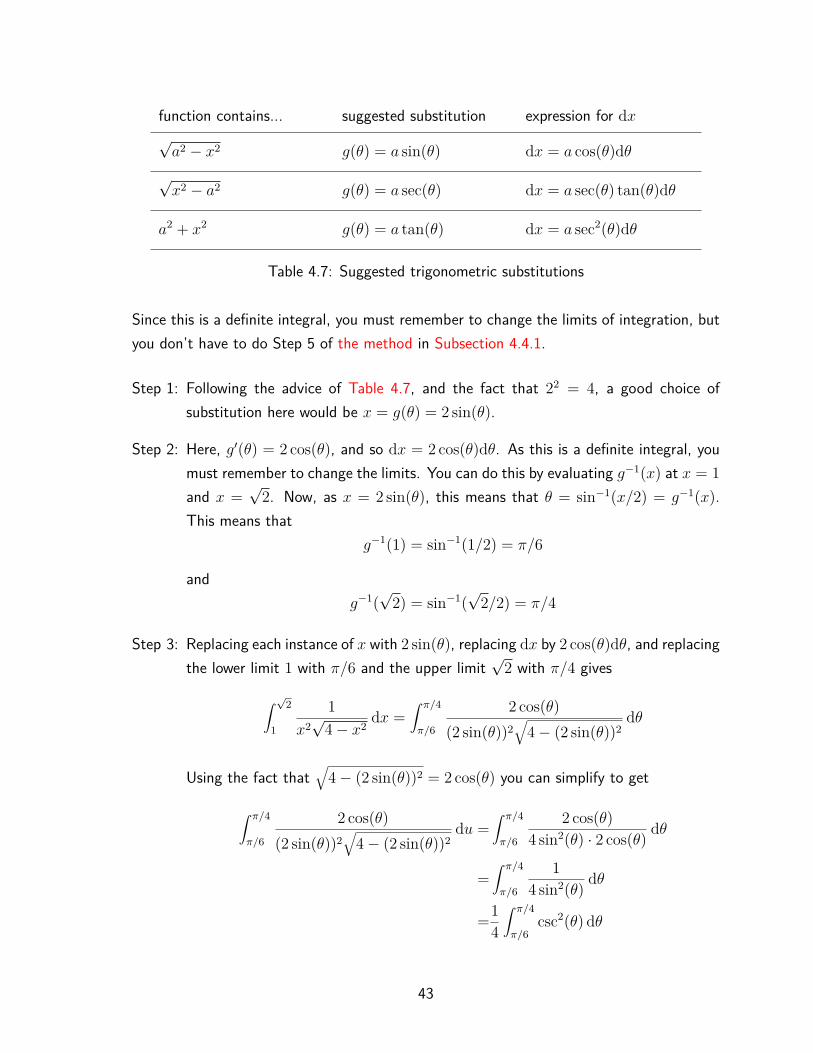
function contains... suggested substitution expression for dx√a2 − x2 g(θ) = a sin(θ) dx = a cos(θ)dθ√x2 − a2 g(θ) = a sec(θ) dx = a sec(θ) tan(θ)dθ

a2 + x2 g(θ) = a tan(θ) dx = a sec2(θ)dθ

Table 4.7: Suggested trigonometric substitutions

Since this is a definite integral, you must remember to change the limits of integration, butyou don’t have to do Step 5 of the method in Subsection 4.4.1.

Step 1: Following the advice of Table 4.7, and the fact that 22 = 4, a good choice ofsubstitution here would be x = g(θ) = 2 sin(θ).

Step 2: Here, g′(θ) = 2 cos(θ), and so dx = 2 cos(θ)dθ. As this is a definite integral, youmust remember to change the limits. You can do this by evaluating g−1(x) at x = 1and x =

√2. Now, as x = 2 sin(θ), this means that θ = sin−1(x/2) = g−1(x).

This means thatg−1(1) = sin−1(1/2) = π/6

andg−1(√

2) = sin−1(√

2/2) = π/4

Step 3: Replacing each instance of x with 2 sin(θ), replacing dx by 2 cos(θ)dθ, and replacingthe lower limit 1 with π/6 and the upper limit

√2 with π/4 gives

∫ √2

1

1x2√

4− x2dx =

∫ π/4

π/6

2 cos(θ)(2 sin(θ))2

√4− (2 sin(θ))2

dθ

Using the fact that√

4− (2 sin(θ))2 = 2 cos(θ) you can simplify to get

∫ π/4

π/6

2 cos(θ)(2 sin(θ))2

√4− (2 sin(θ))2

du =∫ π/4

π/6

2 cos(θ)4 sin2(θ) · 2 cos(θ) dθ

=∫ π/4

π/6

14 sin2(θ) dθ

=14

∫ π/4

π/6csc2(θ) dθ

43

As there are no terms involving x left in the integral, you are OK to continue andyou can now evaluate the integral.

Step 4: You can evaluate the integral using the corresponding rule from Table 4.3, whichgives

14

∫ π/4

π/6csc2(θ) dθ = 1

4 [− cot(θ)]π/4π/6

Using the fact that cot(π/6) =√

3 and cot(π/4) = 1, you can evaluate this to get

14 [− cot(θ)]π/4

π/6 = 14[−1− (−

√3)]

=√

3− 14

which is the final answer.

Example 4.4.2. You are asked to find the integral ∫ 4(x2+9)3/2 dx.

Since this is an indefinite integral, you have no limits to change but you must remember todo Step 5 of the method in Subsection 4.4.1.

Step 1: Following the advice of Table 4.7, and the fact that 32 = 9, a good choice ofsubstitution here would be x = g(θ) = 3 tan(θ).

Step 2: Here, g′(θ) = 3 sec2(θ), and so dx = 3 sec2(θ)dθ. As this is an indefinite integral,you have no limits to change.

Step 3: Replacing each instance of x with 3 tan(θ), and replacing dx by 3 sec2(θ)dθ gives

∫ 4(x2 + 9)3/2 dx = 4

∫ 3 sec2(θ)(9 tan2(θ) + 9)3/2 dθ

You can use the fact that tan2(x) + 1 = sec2(x) to simplify the integral to:

4∫ 3 sec2(θ)

(9 tan2(θ) + 9)3/2 dθ =12∫ sec2(θ)

93/2 · (sec2(θ))3/2 dθ

=1227

∫ 1(sec2(θ))1/2 dθ

=49

∫ 1sec(θ) dθ = 4

9

∫cos(θ) dθ

Since there is no x left in the integral, you are OK to continue.

Step 4: Not forgetting the constant of integration, evaluating the integral using Equa-tion 2.6 gives

49

∫cos(θ) dθ = 4

9 sin(θ) + C (*)

44

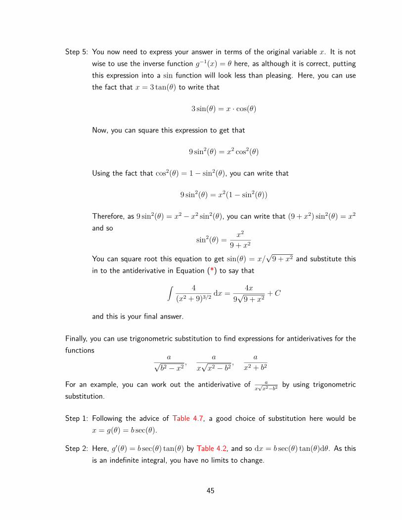
Step 5: You now need to express your answer in terms of the original variable x. It is notwise to use the inverse function g−1(x) = θ here, as although it is correct, puttingthis expression into a sin function will look less than pleasing. Here, you can usethe fact that x = 3 tan(θ) to write that

3 sin(θ) = x · cos(θ)

Now, you can square this expression to get that

9 sin2(θ) = x2 cos2(θ)

Using the fact that cos2(θ) = 1− sin2(θ), you can write that

9 sin2(θ) = x2(1− sin2(θ))

Therefore, as 9 sin2(θ) = x2 − x2 sin2(θ), you can write that (9 + x2) sin2(θ) = x2

and sosin2(θ) = x2

9 + x2

You can square root this equation to get sin(θ) = x/√

9 + x2 and substitute thisin to the antiderivative in Equation (*) to say that

∫ 4(x2 + 9)3/2 dx = 4x

9√

9 + x2+ C

and this is your final answer.

Finally, you can use trigonometric substitution to find expressions for antiderivatives for thefunctions

a√b2 − x2

,a

x√x2 − b2

,a

x2 + b2

For an example, you can work out the antiderivative of ax√x2−b2 by using trigonometric

substitution.

Step 1: Following the advice of Table 4.7, a good choice of substitution here would bex = g(θ) = b sec(θ).

Step 2: Here, g′(θ) = b sec(θ) tan(θ) by Table 4.2, and so dx = b sec(θ) tan(θ)dθ. As thisis an indefinite integral, you have no limits to change.

45

Step 3: Replacing each instance of x with b sec(θ), and replacing dx by b sec(θ) tan(θ)dθgives ∫ a

x√x2 − b2

dx = a∫ b sec(θ) tan(θ)b sec(θ)

√b2 sec2(θ)− b2

dθ

You can use the fact that sec2(x)− 1 = tan2(x) to simplify the integral to:

a∫ b sec(θ) tan(θ)b sec(θ)

√b2 sec2(θ)− b2

dθ =a∫ tan(θ)√

b2 tan2(θ)dθ

=ab

∫ tan(θ)tan(θ) dθ

=ab

∫dθ

Since there is no x left in the integral, you are OK to continue.

Step 4: Not forgetting the constant of integration, evaluating the integral using Equa-tion 2.3 gives

a

b

∫dθ = a

bθ + C

Step 5: You now need to express your answer in terms of the original variable x. Here, asyou only have to find an expression for θ, finding θ = g−1(x) will do. Here, youcan use the fact that x = b sec(θ) to write that

θ = sec−1(x/b)

And so ∫ a

x√x2 − b2

dx = a

bsec−1

(x

b

)+ C (4.4)

You can use similar techniques to show that

∫ a√b2 − x2

dx = a sin−1(x

b

)+ C (4.5)

and ∫ a

b2 + x2 dx = a

btan−1

(x

b

)+ C (4.6)

These expressions could also be found by using the Fundamental Theorem of Calculus on thederivatives in Table 4.6. Finally in this chapter, the information is summed up in Table 4.8.

46

function antiderivative w.r.t x

f(x) = a√b2 − x2

∫f(x) dx = a sin−1

(x

b

)+ C

f(x) = a

b2 + x2

∫f(x) dx = a

btan−1

(x

b

)+ C

f(x) = a

x√x2 − b2

∫f(x) dx = −a

bsec−1

(x

b

)+ C

Table 4.8: Summary of Equations (4.4), (4.5), and (4.6)

47

Chapter 5

Integration by parts

5.1 What is integration by parts?

Say you are given the integration ∫xex dx

How would you go about evaluating it? You can’t use Equation 2.5 as x is not a constant.Since the derivative of x is 1, you can’t use integration by substitution as x is not a constantmultiple of 1. This means a new approach has to be developed.

You can notice here that the integrand is the product of two functions, u(x) = x and v(x) =ex. The deep connection between differentiation and integration implies that evaluating thisintegral may be related to the product rule.

Chapter 3 asserted that integration by substitution is the integral version of the chain rule. Inthat chapter, it was mentioned that the integral version of the product rule of differentiation(see Table 3.1) is known as integration by parts. This is the second main technique offinding antiderivatives of functions, and is the technique to use on ∫ xex dx.

This chapter is dedicated to the technique of integration by parts: where it comes from,how to use it, and several examples detailing different ways to use it.

5.2 How integration by parts works

Let u(x) and v(x) be functions of x, and say that f(x) = u(x)v(x), the product of u(x)and v(x). Table 3.1 says that the derivative of f with respect to x is given by the product

48

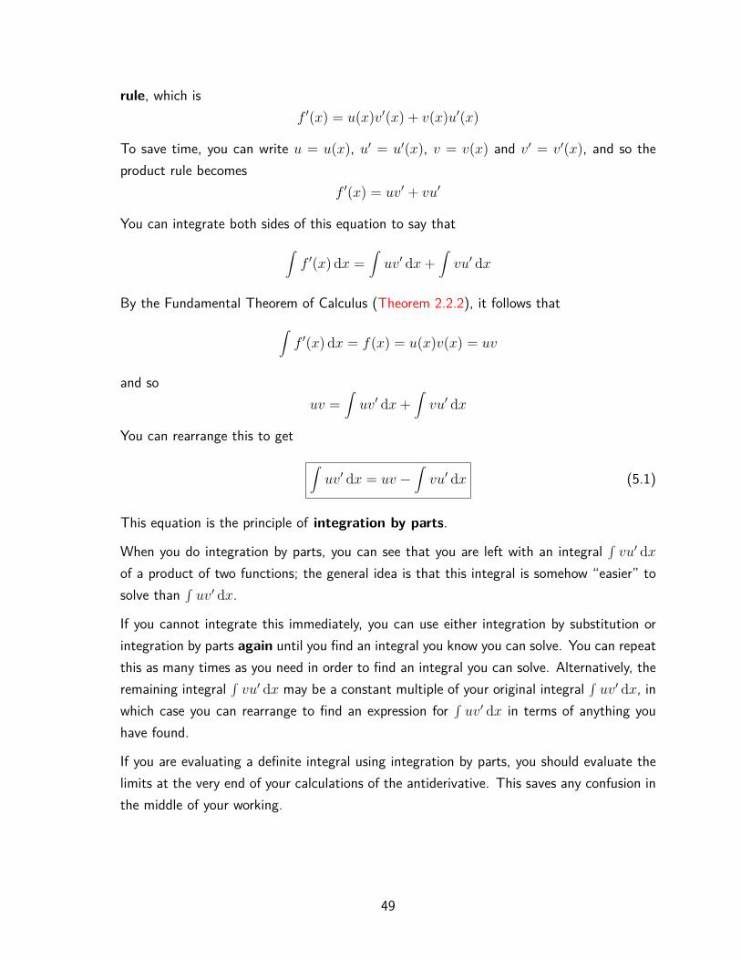
rule, which isf ′(x) = u(x)v′(x) + v(x)u′(x)

To save time, you can write u = u(x), u′ = u′(x), v = v(x) and v′ = v′(x), and so theproduct rule becomes

f ′(x) = uv′ + vu′

You can integrate both sides of this equation to say that∫f ′(x) dx =

∫uv′ dx+

∫vu′ dx

By the Fundamental Theorem of Calculus (Theorem 2.2.2), it follows that∫f ′(x) dx = f(x) = u(x)v(x) = uv

and souv =

∫uv′ dx+

∫vu′ dx

You can rearrange this to get∫uv′ dx = uv −

∫vu′ dx (5.1)

This equation is the principle of integration by parts.

When you do integration by parts, you can see that you are left with an integral ∫ vu′ dxof a product of two functions; the general idea is that this integral is somehow “easier” tosolve than ∫ uv′ dx.

If you cannot integrate this immediately, you can use either integration by substitution orintegration by parts again until you find an integral you know you can solve. You can repeatthis as many times as you need in order to find an integral you can solve. Alternatively, theremaining integral ∫ vu′ dx may be a constant multiple of your original integral ∫ uv′ dx, inwhich case you can rearrange to find an expression for ∫ uv′ dx in terms of anything youhave found.

If you are evaluating a definite integral using integration by parts, you should evaluate thelimits at the very end of your calculations of the antiderivative. This saves any confusion inthe middle of your working.

49

5.2.1 How to use integration by parts effectively

The idea is to take the product function you are asked to evaluate, name one of the functionsu and the other v′, and then work through the formula to find uv−∫ vu′ dx, where hopefullythe integral ∫ vu′ dx is easier to integrate than ∫ uv′ dx.

The difficulty in integration by parts is in the naming of the functions at the start; thatis, which function u to differentiate and which one v′ to integrate. As is the case withintegration by substitution, there is no general rule for choosing the functions u(x) andv′(x). However, here are a few hints you can use when doing integration by parts.

• If the function you are trying to integrate is of the form xng(x) (for n ≥ 1), theidea is to take u = xn and v′ = g(x) (as in Examples 5.2.1, 5.3.1 and 5.3.2). Thisway, the integral ∫ vu′ dx =

∫xn−1v dx, which is theoretically easier to evaluate than∫

uv′ dx. There are exceptions to this case; particularly where you cannot integratev(x) easily (see Example 5.3.3). Sometimes, it is not easy to decide which of thefunctions you can integrate; however, integrating by parts can often yield a solution(see Example 5.3.5).

• Sometimes, you may be confronted with a function f(x) that you cannot integrate atall, but you are able to differentiate it without much difficulty. In this case, you cantry integrating by parts with u = f(x) and v′ = 1; this may make the integral easierto evaluate (see Example 5.3.4).

• If you find that you do not know what to do with the integral ∫ vu′ dx, or that it looks‘more complicated’ than your original integral ∫ uv′ dx, it is best to stop immediately,and change your choices of u and v′. If this does not make the integration simpler,try another technique.

As with integration by substitution, there is a method that you can use to evaluate anintegral using integration by parts.

Step 1: Identify your choice of u(x) = u and v′(x) = v′ in the integrand.

Step 2: Work out u′ by differentiating u with respect to x, and work out v by integratingv′ with respect to x (you do not need a +C for this integral).

Step 3: Write down ∫uv′ dx = uv −

∫vu′ dx

with your values for u, u′, v and v′. Simplify if you can.

50

Step 4: There are a number of cases for ∫ vu′ dx, which are listed below:

Case 1: You can integrate∫vu′ dx directly or by substitution: In this case,

do what you need to do to find ∫ vu′ dx. You can then write your answerand proceed to Step 5 (see Example 5.2.1).

Case 2: You can integrate∫vu′ dx by parts: In this case, you need to start the

process over with ∫ vu′ dx, from Step 1. Here, using different letters forthese functions (such as f, g or a, b) at this stage is highly recommended.You can repeat this case as many times as you need (see Example 5.3.2).(You will find that if you have to repeat integration by parts more thanonce, you will have a lot of minus signs in your working. Take care tomake sure that your signs are correct!)

Case 3: Some part of the integral∫vu′ dx is a constant multiple of

∫uv′ dx:

In this case, you can write

K∫uv′ d = [uv + · · · ]

where the number of terms on the left hand side corresponds to howmany times you needed to integrate by parts. You can now proceed toStep 5 (see Example 5.3.5 and Example 5.3.6).

Case 4: After trying everything, you do not know what to do with∫vu′ dx:

In this case, you can try reversing your choices of u and v′, or use adifferent integration technique.

Remark. Sometimes, you are asked to do integration by parts on a function withan unknown power n, in order to find a reduction formula. In this case (and thiscase alone), you can leave an integral sign on the right hand side of the equation,almost always after an occurrence of Case 3.

Before continuing to Step 5 you should ensure that in any of these cases (apartfrom when you are finding a reduction formula), your answer on the right handside does not have an integral sign in it.

Step 5: If you are finding an indefinite integral, you should add the constant C on theright hand side. If you are evaluating a definite integral between limits a and b,you should evaluate this integral as normal.

To illustrate this method, you can use integration by parts on the following example.

51

Example 5.2.1. Suppose you are asked to find the integral ∫ 10 xe

x dx. This is a commonexample of an integral you can solve by integration by parts. This is a definite integral, soyou should aim to find the complete antiderivative in Step 4 before evaluating the limits inStep 5.

Step 1: Here, you can follow the advice at the beginning of Subsection 5.2.1 and take u = x

and v′ = ex.

Step 2: Now, differentiating u with respect to x gives u′ = 1. Integrating v′ = ex withrespect to x gives v = ex; remember that you do not need the +C here.

Step 3: You can now write that∫ 1

0xex dx =

[x · ex −

∫1 · ex dx

]1

0

=[xex −

∫ex dx

]1

0

Step 4: You can integrate ∫ ex dx directly (Case 1). Integrating this gives∫ex dx = ex

Substituting this into the above equation gives∫ 1

0xex dx = [xex − ex]10

which you can now evaluate as it does not have an integral sign in it.

Step 5: Here,

[x · ex − ex]10 =(1 · e1 − e1)− (0 · e0 − e0)

=1

Therefore you can write ∫ 1

0xex dx = 1

and this is your final answer.

Remark. Suppose that in Step 1 in Example 5.2.1 you picked u = ex and v′ = x; whichmeans that u′ = ex and v = x2/2. Putting these terms into the integration by parts formula

52

(Equation 5.1) gives: ∫ 1

0xex dx =

[x2ex

2 −∫ x2ex

2 dx]1

0

But this integral is harder to evaluate; and so this is not a good choice for u and v′.

Table 5.1 gives some recommended choices for integration by parts questions.

integral choice of u choice of v

∫axn cos(kx) dx u = axn v′ = cos(kx)

∫axn sin(kx) dx u = axn v′ = sin(kx)

∫axnekx dx u = axn v′ = ekx

∫axn ln(kx) dx u = ln(kx) v′ = axn

Table 5.1: Some recommended choices for u and v′ for common integration by parts ques-tions

5.3 Examples

The rest of this chapter is devoted to a range of different examples involving integration byparts.

Example 5.3.1. Suppose you are asked to evaluate ∫ −x csc2(x) dx. This is a definiteintegral, so you should aim to find the complete antiderivative in Step 4 before evaluatingthe limits in Step 5.

Step 1: Here, you can follow the advice at the beginning of Subsection 5.2.1 and take u = x.You can integrate − csc2(x) (see Table 4.3) and so you can take v′ = − csc2(x).It does not matter whether either u or v′ contains the minus sign; as long as it isnot forgotten!

Step 2: Now, differentiating u with respect to x gives u′ = 1. Integrating v′ = − csc2(x)

53

with respect to x gives v = cot(x) by Table 4.3; remember that you do not needthe +C here.

Step 3: You can now write that∫−x csc2(x) dx =

[x cot(x)−

∫cot(x) dx

]

Step 4: You can integrate cot(x) directly by Equation 4.2 with a = k = 1 (Case 1). Doingthis gives ∫

cot(x) dx = ln | sin(x)|

Substituting this into the above equation gives∫−x csc2(x) dx = [x cot(x)− ln | sin(x)|]

which does not have an integral sign in it; so you can proceed to Step 5.

Step 5: All that is left to do add the +C here; so you can write∫−x csc2(x) dx = x cot(x)− ln | sin(x)|+ C

and this is your final answer.

The next example details what happens when you need to integrate by parts more thanonce.

Example 5.3.2. Suppose you are asked to find the integral ∫ π/40 4x2 cos(2x) dx. This is

a definite integral, so you should aim to find the complete antiderivative in Step 4 beforeevaluating the limits in Step 5.

Step 1: Again you can follow the advice at the beginning of Subsection 5.2.1 and takeu = x2 and v′ = 4 cos(2x). Here, it does not matter whether the 4 goes in u orv′; as long as it goes in one of them.

Step 2: Now, differentiating u with respect to x gives u′ = 2x. Using Equation 2.6 witha = 4 and k = 2, you can integrate v′ = 4 cos(2x) with respect to x to getv = 2 sin(2x); remember that you do not need the +C here.

54

Step 3: You can now write that

∫ π/4

04x2 cos(2x) dx =

[x2 · 2 sin(2x)−

∫2x · 2 sin(2x) dx

]π/4

0

=[2x2 sin(2x)−

∫4x sin(2x) dx

]π/4

0(*)

Step 4: Here, you can notice that ∫ 4x sin(2x) dx is only integrable by parts (Case 2); sothis is what you need to do.

Step 1.1: Here, you are trying to integrate the indefinite integral ∫ 4x sin(2x) dx;you can take a = x and b′ = 4 sin(2x). Notice here that you can’t use uand v again in this working.

Step 1.2: Differentiating a = x with respect to x gives a′ = 1; integrating b′ =4 sin(2x) with respect to x gives b = −2 cos(2x). You should be carefulwith the minus signs here.

Step 1.3: Using the fact that − ∫ −2 cos(2x) dx =∫

2 cos(2x) dx, you can nowwrite that

∫4x sin(2x) dx =

[x · −2 cos(2x)−

∫1 · −2 cos(2x) dx

]=[−2x cos(2x) +

∫2 cos(2x) dx

]

Step 1.4: You can integrate 2 cos(2x) directly (Case 1). Doing this gives∫

2 cos(2x) dx = sin(2x)

Substituting this into the above equation gives∫

4x sin(2x) dx = [−2x cos(2x) + sin(2x)]

which does not have an integral sign in it. As you are finding this integralas part of another integral, you do not need a +C here.

You can substitute your expression for ∫ 4x sin(2x) dx into item * to get∫ π/4

04x2 cos(2x) dx =

[2x2 sin(2x)− [−2x cos(2x) + sin(2x)]

]π/4

0

=[2x2 sin(2x) + 2x cos(2x)− sin(2x)

]π/4

0

55

Finally, the right hand side of this integral does not have an integral sign in it; soyou can proceed to Step 5.

Step 5: Using the fact that 2 · π/4 = π/2, you can evaluate the limits to get

∫ π/4

04x2 cos(2x) dx =

[2(π

4

)2sin(π/2) + 2

(π

4

)cos(π/2)− sin(π/2)

]− [sin(0)]

=[π2

8 + 0− 1]− [0]

=π2

8 − 1

and this is your final answer.

The next two examples are slightly different, and it shows that integration by parts can beused in creative ways. They also provide antiderivatives for some common functions thathave not been found yet.

Example 5.3.3. Suppose you are asked to find the integral ∫ a ln(kx) dx. You do not knowto find the antiderivative of ln(x); but you know that the derivative of ln(kx) is 1

xfrom

Table 1.1. You can use integration by parts to find the antiderivative of a ln(kx).

Step 1: As discussed above, you do not know how to integrate ln(kx); but you know howto differentiate it. This means that you are forced to take u = ln(kx); here, youcan take v′ = a. Notice here that if a = 1, then you can take v′ = 1; this isperfectly acceptable!

Step 2: Now, differentiating u with respect to x gives u′ = 1x

by Table 1.1. Integratingv′ = a with respect to x gives v = ax.

Step 3: You can now write that∫a ln(kx) dx =

[ax ln(kx)−

∫ax · 1

xdx]

=[ax ln(kx)−

∫a dx

]

Step 4: You can integrate ∫ a dx directly to get ax (Case 1). Substituting this into theabove equation gives

∫a ln(kx) dx = [ax ln(kx)− ax]

56

As this expression does not have an integral sign in it, you can proceed to Step 5.

Step 5: Finally, you can write that∫a ln(kx) dx = a(x ln(kx)− x) + C (5.2)

Example 5.3.4. Suppose you are asked to find the integral ∫ sin−1(x) dx. You do not knowto find the antiderivative of sin−1(x); but you know that the derivative of sin−1(x) is 1√

1−x2

from Table 4.6. You can use integration by parts to find the antiderivative of sin−1(x).

Step 1: As discussed above, you do not know how to integrate sin−1(x); but you know howto differentiate it. This means that you are forced to take u = sin−1(x); here, youcan take v′ = 1.

Step 2: Now, differentiating u with respect to x gives u′ = 1√1−x2 by Table 1.1. Integrating

v′ = 1 with respect to x gives v = x.

Step 3: You can now write that

∫sin−1(x) dx =

[x sin−1(x)−

∫x · 1√

1− x2dx]

=[x sin−1(x)−

∫ x√1− x2

dx]

(**)

Step 4: You can integrate ∫ x√1−x2 dx using integration by substitution (Case 1).

Here, you can take the substitution u = 1−x2. This means that u′(x) = −2x, andso dx = du/− 2x. Replacing each instance of u(x) = 1− x2 with u and replacingdx by du/− 2x in the integral gives

∫ x√1− x2

dx =∫ x√

u · −2x du

=∫ 1−2√u

du

Integrating this expression using Equation 2.2 with a = −1/2 and n = −1/2 gives∫ 1√−2u

du = −u1/2

57

and substituting u = 1− x2 back into this gives the integral as∫ x√

1− x2dx = −

√1− x2

As you are finding this integral as part of another integral, you do not need a +Chere.

Finally, you can substitute this into item ** to get that

∫sin−1(x) dx =

[x sin−1(x) +

√1− x2

]As this expression does not have an integral sign in it, you can proceed to Step 5.

Step 5: Finally, you can write that∫

sin−1(x) dx = x sin−1(x) +√

1− x2 + C (5.3)

Remark. You can use a similar method to show that∫

tan−1(x) dx = x tan−1(x)− 12 ln |x2 + 1|+ C (5.4)

The next example of integration by parts demonstrate the need for Case 3 in Step 4 of themethod in Subsection 5.2.1

Example 5.3.5. Suppose you are asked to find the integral ∫ ex cos(x) dx. Here, the choiceof u and v′ is less clear, as neither choice is going to make the integral a lot easier to find.However, you know that if you integrate cos(x) twice, you get to − cos(x); so perhaps youcan find an expression for ∫ ex cos(x) dx after integrating by parts twice.

Step 1: It doesn’t matter too much which function you take to be u and which functionyou take to be v′ in this case. Here, you can take u = ex and v′ = cos(x).

Step 2: Now, differentiating u with respect to x gives u′ = ex, and integrating v′ = cos(x)with respect to x to get v = sin(x); remember that you do not need the +C here.

Step 3: You can now write that∫ex cos(x) dx =

[ex sin(x)−

∫ex sin(x) dx

](†)

58

Step 4: Here, you can notice that ∫ ex sin(x) dx is only integrable by parts (Case 2); so thisis what you need to do.

Step 1.1: You are trying to integrate the indefinite integral ∫ ex sin(x) dx; so hereyou can take a = ex and b′ = sin(x). Notice here that you can’t use uand v again in this working. It is also best to be consistent with yourchoices; so this means differentiating ex throughout and integrating theother term.

Step 1.2: Differentiating a = ex with respect to x gives a′ = ex; integrating b′ =sin(x) with respect to x gives b = − cos(x). You should be careful withthe minus signs here.

Step 1.3: Using the fact that − ∫ − cos(x) dx =∫

cos(x) dx, you can now writethat

∫ex sin(x) dx =

[−ex cos(x)−

∫−ex cos(x) dx

]=[−ex cos(x) +

∫ex cos(x) dx

]

Step 1.4: You can notice here that the integral ∫ ex cos(x) dx is a constant multipleof your original integral (Case 3). Therefore, you can return to the originalintegral.

You can substitute your expression for ∫ ex sin(x) dx into item † to get∫ex cos(x) dx =

[ex sin(x)−

[−ex cos(x) +

∫ex cos(x) dx

]]=ex sin(x) + ex cos(x)−

∫ex cos(x) dx

and so collecting the ∫ ex cos(x) dx terms together gives

2∫ex cos(x) dx = ex(sin(x) + cos(x))

There is no integral sign on the right hand side; so you can continue to Step 5.

Step 5: Dividing by 2 on both sides and adding the constant of integration gives

∫ex cos(x) dx = ex

2 (sin(x) + cos(x)) + C

and this is your final answer.

59

There are some instances of integration by parts where you do not know how many timesyou need to do this. This is usually when the power of the function is some number n; forinstance, in the functions sinn(x) and xnex. You can do integration by parts to find what iscalled a reduction formula; this formula provides an iterative process to find the integral.

Example 5.3.6. You are asked to find a reduction formula for the integral ∫ cosn(x) dx.This involves doing integration by parts. Even though this is an indefinite integral, you donot need a +C at the end unless you are working out the integral for a given n.

Step 1: You can follow the advice at the beginning of Subsection 5.2.1; as you don’t knowhow to integrate cosn(x), but you do know how to integrate cos(x), you shouldtake u = cosn−1(x) and v′ = cos(x). You can notice here that uv′ = cosn(x).

Step 2: Now, you can use the chain rule to differentiate u with respect to x; this givesu′ = −(n − 1) cosn−2(x) sin(x). You can integrate v′ = cos(x) with respect to xto get v = sin(x); remember that you do not need the +C here.

Step 3: You can now write that∫

cosn(x) dx =[cosn−1(x) · sin(x)−

∫−(n− 1) cosn−2(x) sin(x) · sin(x) dx

]=[cosn−1(x) sin(x) + (n− 1)

∫cosn−2(x) sin2(x) dx

]

Here, you can use the fact that 1− cos2(x) = sin2(x) to write that∫

cosn(x) dx =[cosn−1(x) sin(x) + (n− 1)

∫cosn−2(x)(1− cos2(x)) dx

]=[cosn−1(x) sin(x) + (n− 1)

(∫cosn−2(x) dx−

∫cosn(x) dx

)]

Step 4: After expanding the brackets, you can see that the integral −(n− 1)∫

cosn(x) dxis a constant multiple of your original integral (Case 3). You can take this termover to the left hand side and write that

n∫

cosn(x) dx = cosn−1(x) sin(x) + (n− 1)∫

cosn−2(x) dx

Since you are finding a reduction formula, it is OK to leave the integral sign on theright hand side and proceed to Step 5.

60

Step 5: Dividing through by n gives your final answer as∫

cosn(x) dx = 1n

cosn−1(x) sin(x) + n− 1n

∫cosn−2(x) dx

You can use this reduction formula with n = 5 (and again, with n = 3 for ∫ cos3(x) dx) tosay that

∫cos5(x) dx =1

5 cos4(x) sin(x) + 45

∫cos3(x) dx

=15 cos4(x) sin(x) + 4

5

[13 cos2(x) sin(x) + 2

3

∫cos(x) dx

]=1

5 cos4(x) sin(x) + 415 cos2(x) sin(x) + 8

15 sin(x) + C

61

Chapter 6

Integration using partial fractions

6.1 What are partial fractions?

In your mathematical education, you may have learned how to add and subtract algebraicfractions from each other. This is acheived by the technique of ‘cross-multiplication’. Forinstance

2x− 1 + 3

x+ 2 = 2(x+ 2) + 3(x− 1)(x− 1)(x+ 2) = 5x+ 1

x2 + x− 2Now, suppose you were asked to integrate this function. Which would you rather integrate:

∫ 2x− 1 + 3

x+ 2 dx or∫ 5x+ 1x2 + x− 2 dx ?

They are the same function, and so the integrals are the same. However, the integral onthe left seems easier to integrate than the one on the right; you can use integration bysubstitution on each of the terms, and your answer should involve ln. In fact:

∫ 2x− 1 + 3

x+ 2 dx = 2 ln |x− 1|+ 3 ln |x+ 2|+ C

However, this answer would not seem at all plausible if you started with ∫ 5x+1x2+x−2 dx.

The idea is to develop a method to reverse the technique of cross-multiplying algebraicfractions. This way, if you are asked to integrate a function like 5x+1

x2+x−2 , you can split it upinto smaller fractions that are easier to integrate. This technique is called partial fractiondecomposition. The final chapter in this course deals with the technique of integrationusing partial fractions.

62

6.2 Rational functions

You may remember from a previous course that a polynomial in x is a function f(x) thatis a finite sum of powers of x. For example,

f(x) = x3 + 3x2 − x+ 6

is a polynomial. If f(x) and g(x) are two polynomials with g(x) 6= 0, then the functionh(x) = f(x)

g(x) is called a rational function. You should be confident with how to factoriseand manipulate polynomial functions before continuing with this chapter of the course.

There are two types of polynomial that will appear as factors in the denominators of partialfractions.

• A linear polynomial is a function of the form ax + b, for some real numbers a, bwhere a is non zero.

• A quadratic polynomial is a function of the form ax2+bx+c, for some real numbersa, b, c with a not equal to 0.

You may have been asked to find roots of quadratic polynomials in the past. If a quadraticpolynomial f(x) has a real root, then it can be written as f(x) = (x− a)(x− b), where aand b are the real roots of the polynomial. If a quadratic polynomial g(x) has no real roots(so it has complex roots), it cannot be written in this way. If this happens, you can call thequadratic equation g(x) irreducible.

In this course, you will only be asked to consider partial fraction decomposition for rationalfunctions h(x) = f(x)

g(x) where the polynomial g(x) in the denominator has a larger power init than the polynomial f(x) in the numerator. In addition to this, you will only be askedto perform partial fraction decomposition on partial fractions whose denominator can befactorised into one of the following three cases:

(1) Fractions containing distinct, linear factors in the denominator: These includefunctions like

3x− 3(x− 4)(x+ 2) and −x2 − 1

(x− 5)(x+ 1)(x− 2)

(2) Fractions containing distinct, possibly repeated linear factors in the denomi-nator: These include functions like

2x+ 1(x− 1)2 and −5x+ 2

(x− 2)(x+ 1)2

63

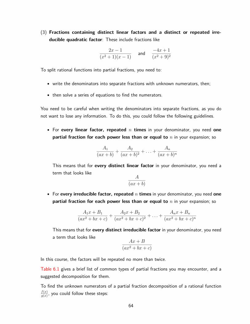
(3) Fractions containing distinct linear factors and a distinct or repeated irre-ducible quadratic factor: These include fractions like

2x− 1(x2 + 1)(x− 1) and −4x+ 1

(x2 + 9)2

To split rational functions into partial fractions, you need to:

• write the denominators into separate fractions with unknown numerators, then;

• then solve a series of equations to find the numerators.

You need to be careful when writing the denominators into separate fractions, as you donot want to lose any information. To do this, you could follow the following guidelines.

• For every linear factor, repeated n times in your denominator, you need onepartial fraction for each power less than or equal to n in your expansion; so

A1

(ax+ b) + A2

(ax+ b)2 + . . .+ An(ax+ b)n

This means that for every distinct linear factor in your denominator, you need aterm that looks like

A

(ax+ b)

• For every irreducible factor, repeated n times in your denominator, you need onepartial fraction for each power less than or equal to n in your expansion; so

A1x+B1

(ax2 + bx+ c) + A2x+B2

(ax2 + bx+ c)2 + . . .+ Anx+Bn

(ax2 + bx+ c)n

This means that for every distinct irreducible factor in your denominator, you needa term that looks like

Ax+B

(ax2 + bx+ c)

In this course, the factors will be repeated no more than twice.

Table 6.1 gives a brief list of common types of partial fractions you may encounter, and asuggested decomposition for them.

To find the unknown numerators of a partial fraction decomposition of a rational functionf(x)g(x) , you could follow these steps:

64

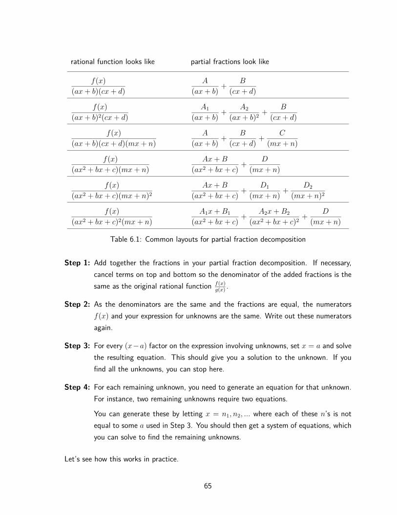
rational function looks like partial fractions look like

f(x)(ax+ b)(cx+ d)

A

(ax+ b) + B

(cx+ d)

f(x)(ax+ b)2(cx+ d)

A1

(ax+ b) + A2

(ax+ b)2 + B

(cx+ d)

f(x)(ax+ b)(cx+ d)(mx+ n)

A

(ax+ b) + B

(cx+ d) + C

(mx+ n)

f(x)(ax2 + bx+ c)(mx+ n)

Ax+B

(ax2 + bx+ c) + D

(mx+ n)

f(x)(ax2 + bx+ c)(mx+ n)2

Ax+B

(ax2 + bx+ c) + D1

(mx+ n) + D2

(mx+ n)2

f(x)(ax2 + bx+ c)2(mx+ n)

A1x+B1

(ax2 + bx+ c) + A2x+B2

(ax2 + bx+ c)2 + D

(mx+ n)

Table 6.1: Common layouts for partial fraction decomposition

Step 1: Add together the fractions in your partial fraction decomposition. If necessary,cancel terms on top and bottom so the denominator of the added fractions is thesame as the original rational function f(x)

g(x) .

Step 2: As the denominators are the same and the fractions are equal, the numeratorsf(x) and your expression for unknowns are the same. Write out these numeratorsagain.

Step 3: For every (x−a) factor on the expression involving unknowns, set x = a and solvethe resulting equation. This should give you a solution to the unknown. If youfind all the unknowns, you can stop here.

Step 4: For each remaining unknown, you need to generate an equation for that unknown.For instance, two remaining unknowns require two equations.

You can generate these by letting x = n1, n2, ... where each of these n’s is notequal to some a used in Step 3. You should then get a system of equations, whichyou can solve to find the remaining unknowns.

Let’s see how this works in practice.

65

Example 6.2.1. Suppose you are asked to decompose

−3x2 + 8x− 1(x− 1)2(x2 + 1)

into partial fractions. You can use the guidelines above to write your decomposition as

−3x2 + 8x− 1(x− 1)2(x2 + 1) = A1

(x− 1) + A2

(x− 1)2 + Bx+D

(x2 + 1)

in an attempt to split the left hand side into partial fractions. You now need to find thenumerators A1, A2, B and B; you can do this using the method above.

Step 1: You need to add together the partial decomposition back into a fraction. This canbe done by the usual method of adding fractions. So this becomes

−3x2 + 8x− 1(x− 1)2(x2 + 1) = A1

(x− 1) + A2

(x− 1)2 + Bx+D

(x2 + 1)

=A1(x− 1)2(x2 + 1) + A2(x− 1)(x2 + 1) + (Bx+D)(x− 1)3

(x− 1)3(x2 + 1)

At this stage, you need to make sure the denominators are the same. You cannotice there is an (x− 1) common to each of the terms, and an (x− 1)3 term onthe bottom. This means that you can write

−3x2 + 8x− 1(x− 1)2(x2 + 1) =A1(x− 1)2(x2 + 1) + A2(x− 1)(x2 + 1) + (Bx+D)(x− 1)3

(x− 1)3(x2 + 1)

=A1(x− 1)(x2 + 1) + A2(x2 + 1) + (Bx+D)(x− 1)2

(x− 1)2(x2 + 1)

Step 2: Now the denominators are the same, the numerators must also be the same. Soyou can write

−3x2 + 8x− 1 = A1(x− 1)(x2 + 1) + A2(x2 + 1) + (Bx+D)(x− 1)2

Step 3: To find some of the numerators, you can set each factor to equal 0 in turn. Forinstance, setting x = 1 throughout this equation gives

−3 + 8− 1 = 0 + A2(2) + 0 + 0

and so 4 = 2A2, giving A2 = 2. There are no more ways to set a linear factor

66

equal to 0 here, so you should proceed to Step 4.

Step 4: You have three numerators left to find in this case, and so you need to generatethree equations to find them. So setting x = 0, x = −1 and x = 2 (notice thatyou can’t set x = 1 here) gives

−1 =− A1 + 2 +D (x = 0)−12 =− 4A1 + 4− 4B + 4D (x = −1)

3 =5A1 + 10 + 2B +D (x = 2)

Solving this gives A1 = −1, B = 1, D = 4. So this means that

−3x2 + 8x− 1(x− 1)2(x2 + 1) = −1

(x− 1) + 2(x− 1)2 + x− 4

(x2 + 1)

Don’t worry; it is unlikely that you will be asked to find anything so complicated on atutorial sheet or exam! This example is just to illustrate the ways in which you can find thenumerators. You can find some easier examples in the integrations that follow in the nextsection.

6.3 Integration using partial fractions

The two most common types of partial fraction you are likely to integrate are of the form

a

bx+ cand a

(bx+ c)n

where n 6= 1 in the second term.

You can integrate both of these expressions this using the substitution u = bx+ c. Differ-entiating this gives u′(x) = b, and so dx = du/b.

Integrating the first term here gives∫ a

bx+ cdx =

∫ a

b · udu = a

b

∫ 1u

du = a

bln |u|+ C

and so ∫ a

bx+ cdx = a

bln |bx+ c|+ C (6.1)

67

Now, integrating the second term here gives∫ a

(bx+ c)n dx =∫ a

b · undu = a

b

∫u−n du = au−n+1

b(−n+ 1) + C

and so ∫ a

(bx+ c)n dx = a(bx+ c)1−n

b(1− n) + C (6.2)

for n 6= 1. You can use these results throughout the chapter. In addition to these, you alsoneed to be able to integrate by substitution effectively; see Chapter 3 for more details.

Note: In this examples section, all integrals considered are indefinite. If you are asked tofind a definite integral using partial fractions, you should evaluate the limits after calculatingthe antiderivative; in a similar fashion to integration by parts.

Example 6.3.1. You are asked to find the integral ∫ 5x+1x2+x−2 dx. Here, you can factorise

the denominator to getx2 + x− 2 = (x+ 2)(x− 1)

This means that the integral becomes∫ 5x+ 1x2 + x− 2 dx =

∫ 5x+ 1(x+ 2)(x− 1) dx

You can use the technique of partial fraction decomposition to find this integral. Using therecommended layout for the partial fraction decomposition as seen in Table 6.1, you canwrite

5x+ 1(x+ 2)(x− 1) = A

x+ 2 + B

x− 1Adding these fractions gives

5x+ 1(x+ 2)(x− 1) = A(x− 1) +B(x+ 2)

(x+ 2)(x− 1)

As the denominators are the same, the numerators are the same and so you can write

5x+ 1 = A(x− 1) +B(x+ 2) (*)

Here, you can set each factor to be equal to 0 in order to find A and B. Setting x = 1 andsubstituting it into Equation * gives 6 = 3B, and so B = 2. You can now set x = −2 and

68

substitute into Equation * to give −9 = −3A, and so A = 3. This means that

5x+ 1(x+ 2)(x− 1) = 3

x+ 2 + 2x− 1

and this is the same answer as in the introduction. Following this, the integral becomes∫ 5x+ 1x2 + x− 2 dx =

∫ 3x+ 2 + 2

x− 1 dx

You can see from the introduction that∫ 5x+ 1x2 + x− 2 dx =

∫ 3x+ 2 + 2

x− 1 dx = 3 ln |x+ 2|+ 2 ln |x− 1|+ C

and this is your final answer.

Example 6.3.2. You are asked to find∫ −3x2 + 8x− 1

(x− 1)2(x2 + 1) dx

You can split the integrand into partial fractions... which you have already done in Exam-ple 6.2.1. So this means the integral is

∫ −3x2 + 8x− 1(x− 1)2(x2 + 1) dx =

∫ −1(x− 1) + 2

(x− 1)2 + x− 4(x2 + 1) dx

You can integrate the first term using Equation 6.1 with a = −1 = c and b = 1 to get∫ −1x− 1 dx = − ln |x− 1|

Integrating the second term using Equation 6.2 with a = 2, b = 1, c = −1 and n = 2 gives∫ 2

(x− 1)2 dx = − 2(x− 1)

You cannot integrate the third term directly. In this case, you have to split the integral intotwo separate parts. You can do this by saying that

∫ x− 4x2 + 1 dx =

∫ x

x2 + 1 dx+∫ −4x2 + 1 dx

You can integrate the first of these terms using integration by substitution. Taking u =

69

x2 + 1, you can work through the method of integration by substitution to get∫ x

x2 + 1 dx = 12 ln |x2 + 1|

In the second of these integrals, you can use Equation 4.6 with a = −4 and b = 1 to get∫ −4x2 + 1 dx = −4 tan−1(x)

Collecting together these four antiderivatives, you can write that∫ −3x2 + 8x− 1

(x− 1)2(x2 + 1) dx = − ln |x− 1| − 2(x− 1) + 1

2 ln |x2 + 1| − 4 tan−1(x) + C

not forgetting the +C!

Example 6.3.3. You are asked to find∫ 2x2 + x− 7

(x− 2)(x+ 1)(x− 1) dx

You can do this using partial fractions. Following the recommended layout for the partialfraction decomposition as seen in Table 6.1, you can write

2x2 + x− 7(x− 2)(x+ 1)(x− 1) = A

x− 2 + B

x+ 1 + D

x− 1

Adding these fractions gives

2x2 + x− 7(x− 2)(x+ 1)(x− 1) = A(x+ 1)(x− 1) +B(x− 2)(x− 1) +D(x− 2)(x+ 1)

(x− 2)(x+ 1)(x− 1)

As the denominators are the same, the numerators are the same and so you can write

2x2 + x− 7 = A(x+ 1)(x− 1) +B(x− 2)(x− 1) +D(x− 2)(x+ 1) (†)

Here, you can set each factor to be equal to 0 in order to find A,B and D. So, settingx = 2 and substituting this into Equation † gives 3 = A(3)(1), and so A = 1. You cannow set x = −1 and substitute this into Equation † to get −6 = B(−3)(−2) = 6B, andso B = −1. Finally, you can set x = 1 and substitute this into Equation † to get that−4 = D(−1)(2) = −2D, and so D = 2. This means that

2x2 + x− 7(x− 2)(x+ 1)(x− 1) = 1

x− 2 −1

x+ 1 + 2x− 1

70

Following this, the integral becomes∫ 2x2 + x− 7

(x− 2)(x+ 1)(x− 1) dx =∫ 1x− 2 −

1x+ 1 + 2

x− 1 dx

You can use Equation 6.1 to integrate each of these terms to say that∫ 2x2 + x− 7

(x− 2)(x+ 1)(x− 1) dx =∫ 1x− 2 −

1x+ 1 + 2

x− 1 dx

= ln |x− 2| − ln |x+ 1|+ 2 ln |x− 1|+ C

Now, let’s look at an example with a repeated linear factor.

Example 6.3.4. You are asked to evaluate∫ 7x2 − 25x− 2

(x− 3)2(2x+ 1) dx

You can do this using partial fractions. Following the recommended layout for the partialfraction decomposition as seen in Table 6.1, you can write

7x2 − 25x− 2(x− 3)2(2x+ 1) = A1

(x− 3) + A2

(x− 3)2 + B

2x+ 1

Adding these fractions gives

7x2 − 25x− 2(x− 3)2(2x+ 1) = A1(x− 3)2(2x+ 1) + A2(x− 3)(2x+ 1) +B(x− 3)3

(x− 3)3(2x+ 1)

Here, the denominators are not the same. However, there is an (x − 3) term on the topand bottom of the right hand side, so you can cancel to get

7x2 − 25x− 2(x− 3)2(2x+ 1) = A1(x− 3)(2x+ 1) + A2(2x+ 1) +B(x− 3)2

(x− 3)2(2x+ 1)

So as the denominators are the same, the numerators are the same and therefore you canwrite

7x2 − 25x− 2 = A1(x− 3)(2x+ 1) + A2(2x+ 1) +B(x− 3)2 (‡)

Here, you can set each factor to be equal to 0 in order to find A1, A2 and B. So, settingx = 3 and substituting this into Equation ‡ gives

63− 75− 2 = 0 + A2(7) + 0

71

giving −14 = 7A2; so A2 = −2. You can now set x = −1/2 and substitute this intoEquation ‡ to get

74 + 25

2 − 2 = 494 B

Multiplying through by 4 on both sides gives

7 + 50− 8 = 49B

giving 49 = 49B; this means B = 1. There are no other factors you can set to be 0 inorder to find A1. However, you only need to generate one more equation. So here, you canset x = 0 and substitute this into Equation ‡ to get that −2 = A1(−3)(1)− 2 + 9, and so−9 = −3A1, giving A1 = 3. This means that

7x2 − 25x− 2(x− 3)2(2x+ 1) = 3

(x− 3) −2

(x− 3)2 + 12x+ 1

Following this, the integral becomes∫ 7x2 − 25x− 2

(x− 3)2(2x+ 1) dx =∫ 3

(x− 3) −2

(x− 3)2 + 12x+ 1 dx

You can use Equation 6.1 to integrate the first and third of these terms, and Equation 6.2to integrate the second to get

∫ 7x2 − 25x− 2(x− 3)2(2x+ 1) dx =

∫ 3(x− 3) −

2(x− 3)2 + 1

2x+ 1 dx

=3 ln |x− 3|+ 2x− 3 + 1

2 ln |2x+ 1|+ C

Example 6.3.5. Suppose you are asked to find the integral∫ x2 + 3x+ 2

x(x2 + 1) dx

You can use the technique of partial fraction decomposition to find this integral. Using therecommended layout for the partial fraction decomposition as seen in Table 6.1, you canwrite

x2 + 3x+ 2x(x2 + 1) = A

x+ Bx+D

x2 + 1

72

Adding these fractions gives

x2 + 3x+ 2x(x2 + 1) = A(x2 + 1) + (Bx+D)x

x(x2 + 1)

As the denominators are the same, the numerators are the same and so you can write

x2 + 3x+ 2 = A(x2 + 1) + (Bx+D)x (F)

Here, you can set one factor to be equal to 0 in order to find A. Setting x = 0 andsubstituting it into Equation F gives 2 = A. There are no other factors you can set to be0 in order to find B and D. As you need to find two unknowns, you need to generate twoequations. So taking x = 1 and x = −1 and substituting these into Equation F gives thesimultaneous equations

6 = 4 + (B +D) (x = 1)0 = 4− (−B +D) (x = −1)

Adding these two equations together cancels the D’s to give 6 = 8 + 2B; so B = −1. Thismeans that D = 3. You can therefore write:

x2 + 3x+ 2x(x2 + 1) = 2

x+ −x+ 3

x2 + 1

So the integral becomes∫ x2 + 3x+ 2

x(x2 + 1) dx =∫ 2x

+ −x+ 3x2 + 1 dx

The first of these you can integrate directly by Equation 6.1 to get∫ 2x

dx = 2 ln |x|

However, the second term is not integrable directly. Like in Example 6.3.2, you can splitthe integral up into two parts to get

∫ −x+ 3x2 + 1 dx =

∫ −xx2 + 1 dx+

∫ 3x2 + 1 dx

You can integrate the first of these using integration by substitution (with u = x2 +1). The

73

integrand of the second term is the derivative of 3 tan−1(x) (see Equation 4.6); and so youcan write (with some working omitted):

∫ −x+ 3x2 + 1 dx = −1

2 ln |x2 + 1|+ 3 tan−1(x)

At last, you can write your answer as∫ x2 + 3x+ 2

x(x2 + 1) dx = 2 ln |x| − 12 ln |x2 + 1|+ 3 tan−1(x) + C

6.3.1 And finally...

You can use the technique of partial fractions to find the as yet unconsidered antiderivativeof a sec(kx). You know that sec(x) = 1

cos(x) and so you can write

∫a sec(kx) dx =

∫ a

cos(kx) dx = a∫ 1

cos(kx) dx

Multiplying top and bottom of this fraction by cos(kx) gives

a∫ cos(kx)

cos2(kx) dx

As cos2(kx) = 1− sin2(kx), you can write

a∫

sec(kx) dx = a∫ cos(kx)

1− sin2(kx) dx

Now, you can integrate this by substitution by taking u = sin(kx). Using the chain rule, itfollows that u′(x) = k cos(kx) and so dx = du/k cos(kx). So the integral becomes

a∫ cos(kx)

1− sin2(kx) dx =a∫ cos(kx)

(1− u2) · k cos(kx) du

=a

k

∫ 11− u2 du

As 1 − u2 = (1 − u)(1 + u), you can integrate 11−u2 using partial fractions. Following the

advice in Table 6.1, you can write

11− u2 = A

1− u + B

1 + u

74

Adding these fractions together gives

11− u2 = A(1 + u) +B(1− u)

1− u2

As the denominators are the same, the numerators are the same and so you can write

1 = A(1 + u) +B(1− u) (�)

Here, you can set each factor to be equal to 0 in order to find A and B. Setting x = 1 andsubstituting it into Equation � gives 1 = 2A, and so A = 1/2. You can now set x = −1and substitute into Equation � to give 1 = −2B, and so B = −1/2. This means that

11− u2 = 1

2(1− u) −1

2(1 + u)

Following this, the integral becomes

a

k

∫ 11− u2 du = a

k

∫ 12(1− u) −

12(1 + u) du = a

k

∫ 12(u+ 1) −

12(u− 1) du

Integrating gives

a

k

∫ 11− u2 du = a

2k ln |u+ 1| − a

2k ln |u− 1|+ C

Combining the two logarithms using the laws of logs gives

a

k

∫ 11− u2 du = a

2k ln∣∣∣∣u+ 1u− 1

∣∣∣∣+ C

Substituting u = sin(x) back into this equation gives the integral as

∫a sec(kx) dx = a

2k ln∣∣∣∣∣sin(x) + 1sin(x)− 1

∣∣∣∣∣+ C

While this is a perfectly valid answer, you could find a way to simplify this. Here, multiplyingtop and bottom of the term inside the natural log by sin(x) + 1 and simplifying gives

(sin(x) + 1) · (sin(x) + 1)(sin(x)− 1) · (sin(x) + 1) = (sin(x) + 1)2

(sin2(x)− 1)

75

As sin2(x)− 1 = − cos2(x), you can write

sin(x) + 1sin(x)− 1 = (sin(x) + 1)2

− cos2(x)

Putting this expression into the natural log gives

∫a sec(kx) dx = a

2k ln∣∣∣∣∣(sin(x) + 1)2

− cos2(x)

∣∣∣∣∣+ C

You can use the properties of the absolute value to get rid of the minus sign in the denom-inator, giving that ∫

a sec(kx) dx = a

2k ln∣∣∣∣∣(sin(x) + 1)2

cos2(x)

∣∣∣∣∣+ C

Using the laws of logarithms, you can cancel the 12 by taking the square root of everything

inside the logarithm, writing that

∫a sec(kx) dx = a

kln∣∣∣∣∣(sin(x) + 1)

cos(x)

∣∣∣∣∣+ C

The final step in the course is to simplify the fraction to get∫a sec(kx) dx = a

kln |tan(x) + sec(x)|+ C (6.3)

76