moral hazard and optimal subsidiary structure ... - citeseerx
TRANSCRIPT

American Finance Association
Moral Hazard and Optimal Subsidiary Structure for Financial InstitutionsAuthor(s): Charles Kahn and Andrew WintonSource: The Journal of Finance, Vol. 59, No. 6 (Dec., 2004), pp. 2531-2575Published by: Blackwell Publishing for the American Finance AssociationStable URL: http://www.jstor.org/stable/3694781Accessed: 06/12/2008 14:03
Your use of the JSTOR archive indicates your acceptance of JSTOR's Terms and Conditions of Use, available athttp://www.jstor.org/page/info/about/policies/terms.jsp. JSTOR's Terms and Conditions of Use provides, in part, that unlessyou have obtained prior permission, you may not download an entire issue of a journal or multiple copies of articles, and youmay use content in the JSTOR archive only for your personal, non-commercial use.
Please contact the publisher regarding any further use of this work. Publisher contact information may be obtained athttp://www.jstor.org/action/showPublisher?publisherCode=black.
Each copy of any part of a JSTOR transmission must contain the same copyright notice that appears on the screen or printedpage of such transmission.
JSTOR is a not-for-profit organization founded in 1995 to build trusted digital archives for scholarship. We work with thescholarly community to preserve their work and the materials they rely upon, and to build a common research platform thatpromotes the discovery and use of these resources. For more information about JSTOR, please contact [email protected].
Blackwell Publishing and American Finance Association are collaborating with JSTOR to digitize, preserveand extend access to The Journal of Finance.
http://www.jstor.org
THE JOURNAL OF FINANCE * VOL. LIX, NO. 6 ? DECEMBER 2004
Moral Hazard and Optimal Subsidiary Structure for Financial Institutions
CHARLES KAHN and ANDREW WINTON*
ABSTRACT
Banks and related financial institutions often have two separate subsidiaries that make loans of similar type but differing risk, for example, a bank and a finance com- pany, or a "good bank/bad bank" structure. Such "bipartite" structures may prevent risk shifting, in which banks misuse their flexibility in choosing and monitoring loans to exploit their debt holders. By "insulating" safer loans from riskier loans, a bipartite structure reduces risk-shifting incentives in the safer subsidiary. Bipartite structures are more likely to dominate unitary structures as the downside from riskier loans is higher or as expected profits from the efficient loan mix are lower.
AT FIRST GLANCE, SOME SUBSIDIARY STRUCTURES that are common among financial institutions seem difficult to explain. For example, bank holding companies, such as Wells Fargo Inc. and Bank of America, often have both a commercial banking subsidiary and a finance company subsidiary. Both subsidiaries make loans, and the sectors to which they lend usually overlap: both may lend to consumers, or both may lend to commercial firms. On average, finance com- pany loans are more risky than commercial bank loans, but outside investors generally cannot observe the risk of any given loan at the time it is made. Pub- lic disclosure by the holding company is usually limited to broad sectors (e.g., "commercial loans" or "consumer loans"), and in any case the holding company's ex ante assessments of loan risk are in part subjective and costly to disclose in detail. Given the difficulties that outside investors have in distinguishing the quality of the various subsidiaries' loans, why is it often the case that these subsidiaries are funded separately from one another and from their parent?
A similar question arises with "good bank/bad bank" restructurings, such as Mellon Bank's creation of Grant Street Bank in 1988. In these restructurings, an institution with impaired loans or other illiquid assets writes down their
*Charles Kahn is from the University of Illinois at Urbana-Champaign. Andrew Winton is from the University of Minnesota. This is a substantial revision of an earlier paper entitled "Project Choice, Moral Hazard, and Optimal Subsidiary Structure for Financial Intermediaries." We are grateful to the late Herb Baer, Douglas Diamond, Paolo Fulghieri, Richard Green (the editor), Joseph Haubrich, Timothy Guinnane, John McMillan, Yossi Spiegel, Larry Wall, and an anony- mous referee for their comments, and to Sen Li for research assistance. We also thank seminar participants at Bellcore, the Federal Reserve Bank of Chicago, the Federal Reserve Bank of Cleve- land, the Federal Reserve Bank of New York, the Federal Reserve Bank of Philadelphia, INSEAD, New York University, Stanford University, the Stockholm School of Economics, Tulane University, Yale University, the University of Chicago, and the University of Texas.
2531
The Journal of Finance
reported value to an estimate of what they are worth, then puts them in a sep- arate structure. What seems odd is that the financial institution often retains its equity stake in the bad loans. Given that expected losses on the loans have been taken and that the loans are still owned by the institution, why bother placing them in a separately funded subsidiary?
Arguments based on different managerial practices for loans of differing risk do not seem relevant to the use of separate subsidiaries. Granted that riskier loans require more intensive monitoring than safer loans, this could be dealt with by simply having a separate department or division of the bank handle such loans. Indeed, many banks have asset-based lending groups whose busi- ness resembles that of commercial finance companies, and almost all banks have some form of loan workout group to handle impaired credits. Moreover, if the concern is one of providing information to investors about the perfor- mance of different divisions, as suggested by Holmstrom (1979), this can be provided in the institution's annual report (e.g., in the notes to the financial statements)-which, in fact, many institutions do.
In this paper, we suggest an explanation that is rooted in the role of banks and similar financial institutions as delegated monitors. These institutions raise funds from diffuse investors and then invest them in illiquid financial assets such as loans and privately placed bonds. Although such assets benefit from careful evaluation, selection, and monitoring, the quality and composition of the institution's assets are not easily observed by investors. Indeed, this is one rea- son why such institutions are typically highly levered-issuing debt mitigates some of the adverse selection and moral hazard problems between the institu- tion and its investors (Diamond (1984), Williamson (1986), DeMarzo and Duffie (1999), Bolton and Freixas (2000), Diamond and Rajan (2001)). Nevertheless, this combination of high leverage and asset opacity means that the institution may have incentive to engage in risk shifting, inefficiently increasing the over- all risk of its loans, because some of the downside is shared with debt holders, while shareholders pocket the upside. This increase in loan risk could come through deliberate selection or through shirking on screening or monitoring of loans, all of which are activities that are difficult for outside investors to observe.
We show that, when such risk shifting is a concern, the institution's incentives can often be improved by creating a structure with two subsidiaries, where one subsidiary is supposed to hold relatively safe loans and the other is supposed to hold relatively risky loans. In this "bipartite" structure, each subsidiary's debt has recourse only to that subsidiary's assets. This contrasts with a "unitary" structure in which all debt has equal recourse to all assets.
To see why a bipartite structure may dominate a unitary structure, it is easiest to start with the case of pure asset selection, in which the risk and quality of the loans that the institution holds are unobservable to outsiders. Regardless of subsidiary structure, the first-best outcome is for the institution to make all loans that are "efficient," that is, those that offer it an expected return in excess of the required return for their risk class. Some of these loans will be relatively safe, others relatively risky. Thus, there will be "bad" states of
2532

Moral Hazard and Optimal Subsidiary Structure
the world where the risky loans as a group perform more poorly than the safe loans.
Risk shifting by "asset substitution"-choosing riskier but inefficient loans- has a cost for shareholders, namely, the loss of any shareholder profits that an efficient portfolio would produce in bad states. As we will show below, a bipartite structure makes asset substitution more costly for shareholders. In a unitary structure, even if the institution holds the efficient portfolio, safer and riskier loans are mixed together. Although the riskier loans are "good" (efficient), in bad states their return is less than that of safer loans and less than their own required return. This reduces the institution's net return in bad states. By contrast, in a bipartite structure, the safer efficient loans are supposed to be held in a separate subsidiary. This insulates them from the downside of riskier efficient loans and may also reduce the debt rate that investors require from the subsidiary. Both these features increase the safe subsidiary's net return in bad states, reducing risk-shifting incentives. This improvement in incentives occurs even though asset risk per se cannot be contracted on; it is enough that investors can limit the size of each subsidiary and set financing rates based on each subsidiary's expected asset composition.
The bipartite structure's potential weakness lies in the risky subsidiary. By construction, this subsidiary is supposed to hold riskier loans and have a higher chance of default than the safe subsidiary. This may increase the institution's incentives to engage in risk shifting within the risky subsidiary. Nevertheless, such a limited amount of risk shifting is usually better than having the entire institution engage in risk shifting under a unitary structure.
The bipartite structure is most likely to dominate the unitary structure in situations where risk-shifting incentives are particularly high, for example, when the institution's mix of efficient loans includes a relatively large number of risky loans, or when the downside of these risky efficient loans is especially high, or when safer loans offer very low excess returns. All of these factors imply that a unitary structure will have low or negative net returns in bad states, encouraging risk shifting. In these circumstances, there will be great incentive gains to separating safe and risky loans into two subsidiaries. We demonstrate this both in the case where loans come in a few discrete types (Section II) and in the case where loan types vary continuously (Section III).
Our analysis assumes that the institution has some positive net present value lending opportunities: On average, it can earn rents or quasirents on its loans. For simplicity, we abstract from questions of market structure and take the institution's opportunity set as given, but this is not essential. Even if the institution faces competition for marginal loans, all our analysis requires is that there are some inframarginal loans on which it earns rents ex post. As discussed in Section I, this is consistent with evidence on bank informational quasi-rents from continuing relationships.
Although our discussion thus far has focused on a story of costless loan se- lection, in Section IV we show that the same intuition carries over to the cases of costly loan monitoring and costly loan screening. If the institution does not monitor loans, it saves costs, but its loans perform worse in bad states of the
2533
The Journal of Finance
world. Setting up two subsidiaries insulates safer loans from the downside riskier loans possess even when monitored; this reduces the temptation to forgo monitoring the safer loans. Similarly, setting up two subsidiaries reduces po- tential risk-shifting gains from not screening. Moreover, conditional on having screened, the institution could still engage in asset substitution; by discourag- ing this, a bipartite structure can further encourage screening.
In all three cases-loan selection, costly monitoring, and costly screening- the critical assumptions are that outside investors cannot directly observe the institution's actions and loan quality. Nonetheless, a bipartite structure in which safer loans are supposed to be separate from riskier loans can be self- fulfilling. The bipartite structure improves incentives, not because investors can better observe the institution's actions or loan quality, but because this structure reduces potential gains from risk shifting.
Our analysis initially assumes that the institution uses debt for all of its ex- ternal financing. This assumption is not necessary; as we show in Section V, all that is required is that equity is more costly than debt. Examples of such costs include the agency and signaling motivations for highly levered institutions, as well as the more traditional tax and financial distress costs from the corporate finance literature. Our analysis also assumes that investors cannot observe the institution's loan risk and quality or any actions that affect this risk and qual- ity, but only the distribution from which risk and quality are drawn. Again, in Section V we discuss how this assumption can be weakened; all that is required is that investors' knowledge of the institution's choice and action set is more precise than their ability to observe actual choices and actions in a timely fash- ion. As discussed above, both of our assumptions-that equity finance is costly for institutions and that outside investors have difficulty observing the institu- tion's actions in a timely fashion-are at the heart of the delegated monitoring theory of financial intermediation.
At the outset, we noted two examples where bipartite structures are used to separate loans of similar type but differing risk. We return to these exam- ples in Section VI. If the riskier segment of an institution's borrower base is large enough or risky enough, it could undermine the institution's incentives to choose or screen for safer loans. In this case, having a separately funded finance company subsidiary improves lending incentives. In the case of a "good bank/bad bank" structure, the institution already has a large number of im- paired loans. Even if these loans are written down to their fair value, re- coveries on them are much more uncertain than are repayments on healthy loans. By putting impaired loans in a separate subsidiary, the institution in- sulates the rest of its business from the impaired loans' downside, reducing risk-shifting incentives in the ongoing selection, screening, and monitoring of healthy loans.
As discussed in Section VI, our analysis also has implications beyond these two uses of bipartite structures. Several insurance companies have used "good bank/bad bank" structures to deal with policy lines where the risk of loss has increased substantially since the policies were sold. Securities firms routinely segregate their high-risk private equity investments in separately funded af- filiates. Again, the critical ingredient is that the financial claims placed in the
2534
Moral Hazard and Optimal Subsidiary Structure
"bad bank" or "risky sub" have enough downside to harm incentives throughout the rest of the institution.
Literature review. Our paper investigates how an institution can best choose its internal structure to pursue a given set of activities. This distinguishes our work from the large literature on costs and benefits of merging separate firms. This other literature focuses on benefits resulting from coinsurance and other synergies and costs resulting from increased internal agency problems and reduced transparency (see, e.g., Gertner, Scharfstein, and Stein (1994), Habib, Johnsen, and Naik (1997), Fluck and Lynch (1999), Boot and Schmeits (2000), Fulghieri and Hodrick (2003)). We also abstract from issues involving exploitation of government safety nets and conflicts of interest between differ- ent aspects of financial services, which are the focus of Santos (1998) and Shull and White (1998).
Closest to our paper are John (1993), Flannery, Houston, and Venkataraman (1993), and Chemmanur and John (1996). John shows that separating divisions into subsidiaries with their own debt finance can reduce underinvestment prob- lems within a firm, but increased diversification also reduces underinvestment problems, reducing gains from creating subsidiaries. Flannery et al. show nu- merically that by providing coinsurance, merging two independent firms can increase tax shields and reduce underinvestment but may exacerbate asset substitution. Chemmanur and John focus on the role of managerial control benefits rather than project return risk. They show that when these benefits vary widely across projects, project finance (akin to multisubsidiary structures in our model) sometimes dominates independent firms or unitary merged struc- tures in preventing loss of these benefits through outside takeover or financial distress.
Our paper differs from these in several critical respects. First, unlike Chemmanur and John, we focus on asset risk and returns. Unlike all three of these papers, our model is geared to key features of financial institutions. Our firm (institution) relies heavily on debt finance and is critically in the busi- ness of choosing, screening, or monitoring a large number of assets, rather than combining a few projects of fixed size. As a result, unlike nonfinancial firms, our firm has very high leverage and great flexibility in its choice of the size, risk, and return of any subsidiary structures it forms.
The rest of the paper is organized as follows. Section I outlines our model's key assumptions and supporting evidence for these assumptions. Sections II and III analyze the institution's lending decision when loan types are discrete and when loan types vary continuously, respectively. Section IV shows how our results apply to settings with costly loan screening and monitoring. Section V discusses additional considerations such as costly equity finance. Section VI discusses applications of our results, including separately funded finance subsidiaries and "good bank/bad bank" restructurings. Section VII concludes.
I. Model and Motivation
We begin by describing the key assumptions of our model, after which we discuss the assumptions' motivation and supporting evidence.
2535
The Journal of Finance
A. Key Assumptions
A financial institution raises money from investors and invests the proceeds in various loans or other assets. The institution's goal is to maximize the welfare of its initial owners, who are assumed to be risk neutral and (for simplicity) do not have any additional funds for investment. Additional funds are raised from risk-neutral investors who require an expected total return of r per unit borrowed.
Loans: Each loan requires one unit now and returns an amount next period that depends on the loan's type and the state of the world. There are two possible states of the world, 1 and 2; for simplicity, both are equally likely. Thus, a loan's type can be represented by (el, e2) , where ei > 0 is the loan's gross return in state i. We assume that for all types (el, e2), el > e2; that is, state 2 is a "bad" state for all loan types. Thus, our focus is on risk that is not easily diversifiable.
Loans-especially those that offer an expected return in excess of investors' required return r-are available in limited supply. Intuitively, the institution has some lending opportunities that offer rents or quasi-rents, whether from local market power, location advantages, or private information that the in- stitution has acquired-but these "positive NPV" opportunities are limited in number. For simplicity, we take the numbers of loans of different types and their returns as exogenous. Of course, in reality, these parameters would reflect over- all economic conditions and the degree of competition among institutions.
Funding: Initially, we assume that the institution must issue debt to fund all loans. As noted in the introduction, financial institutions such as banks, finance companies, and life insurers are all much more highly levered than nonfinancial firms. As we show in Section V, so long as equity finance involves additional costs relative to debt finance, allowing the institution to issue equity does not alter the thrust of our results.
Investors' information: We assume that investors can observe and contract on the size of the institution and its subsidiaries; however, although investors know the distribution of loan types that the institution has access to, they cannot observe the precise mix of loans that the institution chooses to make. This leaves open the possibility of risk shifting through asset substitution: the institution may claim it is going to invest in a set of loans of given risk, and then shift into a riskier mix once debt funding is in place.
Later in the paper, we extend our results by assuming that the institution may change its loans' returns via costly screening or monitoring, and that investors cannot observe these activities or their direct effects. In this case, the institution may raise funds at a rate that presumes that the institution will screen or monitor, after which it may shift risk by not screening or monitoring.
Our final assumption is that investors know the characteristics of the pool from which the institution chooses its loans. In reality, investors will have some uncertainty over these characteristics. So long as they have rational expecta- tions and their sense of the pool's characteristics is more precise than their knowledge of the institution's choices, our results should continue to have force. We discuss this in more depth in Section V.
2536
Moral Hazard and Optimal Subsidiary Structure
B. Discussion
We now provide our motivation for assuming that (1) investors find it diffi- cult to observe the precise mix and risk of the institution's loans in a timely fashion and (2) investors are concerned that the institution may engage in risk shifting. We also provide evidence for the importance of institutional risk shifting.
Loan opacity: Although investors often have some information about the composition of an institution's asset holdings, this information is typically avail- able only annually or quarterly with a lag and only for broad sector group- ings. For example, Wells Fargo's 2001 Annual Report gives no breakdown of its $48.6 billion average balance of commercial loans (out of $163 billion total loans), even in the footnotes or management's discussion of operations. This does not give much idea of the precise nature of the commercial loan portfolio. Moreover, an institution's screening or monitoring efforts affect the risk of its assets. Since these efforts are difficult for investors to observe directly, they present another channel by which the institution can unobservably increase its risk.
The nature of loan risk-small probability of large loss-also makes observa- tion of risk difficult. The provision for loan losses is the most forward-looking measure of this risk, but it is also the measure most vulnerable to manage- ment's manipulation. Actual loan charge-offs are the most accurate measure of losses, but also the most backward looking. Moreover, loan losses are concen- trated in sector downturns, which tend to occur at intervals of several years. The upshot is that it is difficult for outside investors to make timely and ac- curate assessments of an institution's loan portfolio risk until possible losses have become a reality.
In a study of bank credit ratings, Morgan (2002) finds evidence that is con- sistent with the relative opacity of a bank's loans and its actions. He finds that Moody's and Standard and Poor's, the two largest credit rating agencies, disagree on bank ratings significantly more often than they disagree on nonfi- nancial firms' ratings.1 Disagreements on banks are more common as loans are a larger fraction of bank assets, and as bank equity capital ratios are lower.2
Investor concern for risk shifting: There is a large literature documenting the effects of governmental deposit guarantees on bank risk taking. Gener- ally speaking, the evidence suggests that such guarantees tend to exacerbate risk taking, although this can be reduced to some extent by more stringent
1 Morgan finds similar results for insurance companies. Since insurers act as delegated monitors
of their portfolios of policies, this is consistent with insurers having more precise information about their portfolio exposures than outsiders have.
2Morgan also finds that disagreements are more common as trading account assets are a larger fraction of total assets. As argued by Myers and Rajan (1998), trading assets are highly liquid, allowing easy changes of risk via trading, which are hard for investors to control directly. Again, this is consistent with investor concerns about risk shifting. We return to this issue in Section VI.
2537
The Journal of Finance
regulation.3 Our results do have implications for regulators concerned about risk shifting. Our main point, however, is that investors themselves often care about bank risk shifting, and this affects an institution's ex ante choice of struc- tures that serve as commitments to avoid such inefficient behavior.
In fact, Keeley (1990) finds evidence that investors in bank liabilities are also concerned about potential risk shifting by banks. Drawing on the theoretical work of Marcus (1984), he predicts that banks with higher "franchise" or going- concern value should be less likely to engage in risk shifting; such value is lost in the event of financial distress, which increases shareholders' cost of taking on inefficient risky loans. Using a sample of U.S. banks from 1970 to 1986, he finds that, all else equal, banks with higher market-to-book ratios pay lower rates on their large CDs. Because market-to-book proxies for going-concern value, this is consistent with investor concern that banks with lower franchise value are more likely to engage in risk shifting.
Occurrence of institutional risk shifting: In a number of cases, institutions have engaged in significant risk shifting that has remained undetected until losses materialized. For example, as shown by Herring (1991), the well-known failure of Continental Illinois in 1984 was due to both lack of diversification and lax credit standards. Although Continental's problems developed over a number of years in the late 1970s and early 1980s, these problems only became public in July 1982, when the bank announced that it was holding over $1 billion in energy-related loans purchased from the just-failed Penn Square Bank.
For our purposes, Continental's case illustrates two key points. First, al- though outside analysts had a general sense of Continental's focus on energy- related loans, they did not know the details in a timely fashion. Second, the bank maintained investor confidence until the summer of 1982 because investors be- lieved that the bank's specialization in energy lending made it better at picking out good energy loans-a confidence that was admittedly misplaced.4
More recent cases show similar patterns. During 1989 to 1992, Citicorp had massive loan losses in a number of its U.S. operations, including highly- leveraged-transaction loans, commercial and residential real estate loans, and credit card loans. Later accounts (e.g., Hansell (1994)) suggest that rapid diver- sification and lax internal credit controls were to blame; yet, until loan losses began to surface in 1989, Citicorp's diversification strategy was widely viewed as a source of strength. Green Point Savings' experience with "low-doc" mort- gage loans during the same period also illustrates the discrepancy between
3 The clearest results come from studies of state-run deposit insurance schemes in the United States before the Great Depression and of the impact of the U.S. Comptroller of the Currency's "too big to fail" scheme in the wake of Continental Illinois's failure in 1984 (whereby the 11 largest banks in the country were effectively given 100% deposit insurance). The well-known U.S. savings and loan crisis in the 1980s shows a mixture of risk shifting and simple fraud, as suggested by Akerlof and Romer (1993). For further references and discussion, see Gorton and Winton (2003).
4 Continental's annual reports from 1978 to 1981 give no breakdown of commercial loans other than domestic versus foreign. Moreover, a search on LexisNexis for the period from January 1980 through June 1982 shows many references by Continental and outsiders to the bank's "leading position" and "strong growth" in energy loans, but no specifics on energy loan exposure (20% of total loans by year-end 1981) and no mention of Penn Square (3% of total loans by year-end 1981) (see also Herring (1991)).
2538
Moral Hazard and Optimal Subsidiary Structure
institutional behavior and investor perceptions; in this case, investors did not recognize the bank's superior monitoring skills until losses hit the entire "low- doc" loan market.5
Nor is unobservable risk shifting only a problem at government-insured banks and thrifts. A recent example concerns Household International, a large independent U.S. consumer finance company, which in 2002 was accused by the SEC of making "'false and misleading' statements concerning its policies for restructuring loans so that they are no longer considered delinquent" (Croft and Silverman (2003)). Such restructuring is a form of risk shifting: delinquent loans are essentially "rolled over," allowing the lender to gamble on the hope that the borrower will be able to repay a larger amount in the future. Since Household's liabilities had no government guarantee at the time (it was subse- quently acquired by HSBC, a U.K.-based bank holding company), this example shows that risk shifting concerns can arise from the very nature of delegated monitoring, which leads to a significant information asymmetry between finan- cial intermediaries and the diffuse debt holders that fund them.
Relative transparency of an institution's size and debt levels: Whereas risk is difficult for investors to measure, an institution's size and debt level are two simple numbers that are relatively easy to report and verify. As such, size and debt level can be embedded in debt covenants much more easily than risk can. Increases in an institution's size can only come about by issuing debt, issuing equity, or reinvesting free cash flow. Increases in debt are relatively easy to monitor; the other two actions reduce leverage and risk, all else equal. For simplicity, we have assumed that the difference is absolute; size and debt levels are perfectly observable, whereas actual loan composition and risk level are completely unobservable.
II. Institutional Structure with Discrete Loan Types We begin with the case where investment loans come in a few discrete types.
In this setting, we compare the performance of a unitary structure and a bi- partite structure, where the bipartite structure consists of a subsidiary that holds low-risk loans and does not default and a subsidiary that holds high-risk loans and defaults part of the time. We show that, if high-risk loans are rel- atively plentiful, the bipartite structure supports efficient lending more often than the unitary structure does. When high-risk loans are less plentiful, results are mixed: although in some cases the bipartite structure continues to be more likely to support efficient lending, there are also cases where a unitary struc- ture is better because the bipartite structure's risky subsidiary distorts lending
5 Requiring little verification of borrower income or asset levels, "low-doc" residential mortgage loans attracted a risky, low-income clientele. After an initial burst of popularity, rising defaults as the economy weakened in 1989 and 1990 led many lenders to withdraw from the business. Unlike other lenders, Green Point, a large New-York-based savings bank, had carefully monitored the quality of the real estate collateral itself and enforced stricter loan-to-value ratios; as a result, it was able to continue making these loans profitably throughout the early and mid 1990s (see Roosevelt (1990), United States Banker (1991), and Bird (1994)).
2539
The Journal of Finance
incentives. These results help motivate our more general analysis in Section III, where we extend our results to the case where loan types vary continuously.
Accordingly, suppose that loans fall into two risk classes, low and high. Within each class, there are two subtypes: those that have expected returns less than investors' required return r ("inefficient" or "negative-NPV" loans) and those that have expected returns greater than r ("efficient" or positive-NPV" loans). More precisely, low-risk loans return s in both states, where s = sb < r for inef- ficient low-risk loans and s = sg > r for efficient low-risk loans. High-risk loans return (1 + a)t in state 1 and (1 - a)t in state 2, where c e (0, 1], t = tb < r for inefficient high-risk loans, and t = tg > r for efficient high-risk loans. We also assume that
(1 - a)tg < r, (1)
so that efficient high-risk loans do have some downside risk.6 For brevity, we sometimes refer to loans by their expected return; for example, "Sg loans."
Let S* denote the mass of efficient low-risk loans that the institution has access to, and S the mass of inefficient low-risk loans it has access to; similarly, let T* and T denote the mass of efficient and inefficient high-risk loans it has access to, respectively. We will also assume that the inefficient loans of a given risk-class weakly outnumber the efficient loans in that class, i.e., S > S* and T > T*. This simplifies analysis without affecting the substance of our results.
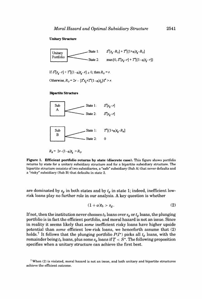
The first-best investment rule is to fund all loans with expected return greater than r, in which case the institution's size is I* = S* + T*. Because of the incen- tive problem already noted, however, this first-best rule may not be feasible. We first consider the case where the institution tries to fund the efficient portfolio in a unitary (single subsidiary) structure. If investors believe that the institution will choose the efficient portfolio, then they expect that gross portfolio returns (before debt payments) are S*sg + T*(1 + a)tg in state 1 and S*sg + T*(1 - a)tg in state 2, and so they require that the institution promise to pay a face value of
R =max r,2r S*sg + T*(l1- a)tg RU = max r,2r -?
per unit of debt. The upper part of Figure 1 displays these conditions. Nevertheless, given Ru, the institution may be tempted to shift into more
risky loans, defaulting in State 2 while maximizing state 1 returns. This leads to the following definition.
DEFINITION 1: The plunging portfolio of size I, P(I), is the portfolio of size I with maximum total state 1 return.
Thus, the most profitable deviation from the efficient portfolio is the plunging portfolio of size I*. This portfolio never puts any weight on sb loans, since these
6 If efficient loan returns always exceeded r, risk shifting would never be a problem.
2540
Moral Hazard and Optimal Subsidiary Structure
Unitary Structure
Unitary State : S*[s -Ru] + T*[(l+a)tg-Ru]
Portfolio --- State 2: max{O, S*[sg-r] + T[(l-a)tg-r]}
If S*[s,-r] + T[(l-a)tg-r] > O, thenRu= r.
Otherwise, Ru = 2r - [S*s,+T(1 -a)t]/ > r.
Bipartite Structure
Sub State 1: S'[sg-r]
_ - State 2: S'[sg-r]
Sub State 1: *r[(1+a)tg-RB] B
- State 2: 0
RB= 2r-(l-a)tg >Ru,
Figure 1. Efficient portfolio returns by state (discrete case). This figure shows portfolio returns by state for a unitary subsidiary structure and for a bipartite subsidiary structure. The bipartite structure consists of two subsidiaries, a "safe" subsidiary (Sub A) that never defaults and a "risky" subsidiary (Sub B) that defaults in state 2.
are dominated by sg in both states and by tg in state 1; indeed, inefficient low- risk loans play no further role in our analysis. A key question is whether
(1 + a)tb > g. (2)
If not, then the institution never chooses tb loans over Sg or tg loans, the plunging portfolio is in fact the efficient portfolio, and moral hazard is not an issue. Since in reality it seems likely that some inefficient risky loans have higher upside potential than some efficient low-risk loans, we henceforth assume that (2) holds.7 It follows that the plunging portfolio P(I*) picks all tg loans, with the remainder being tb loans, plus some sg loans if T < S*. The following proposition specifies when a unitary structure can achieve the first best.
7 When (2) is violated, moral hazard is not an issue, and both unitary and bipartite structures achieve the efficient outcome.
2541

The Journal of Finance
PROPOSITION 1 (Efficiency of the unitary structure):
(i) The unitary structure cannot support the efficient portfolio if the efficient portfolio is risky (that is, if the efficient portfolio's average state 2 return is less than the required return r).
(ii) The unitary structure supports the efficient portfolio if and only if
min{T, S*} [(1 + a)tb - Sg] < S*(Sg - r) + T*[(1 - a)tg - r]. (3)
(iii) The unitary structure is more likely to support the efficient portfolio as the risk of high-risk loans (a) decreases, as the number of efficient low-risk loans (S*) rises relative to the number of efficient high-risk loans (T*), as the expected returns of efficient loans (sg and tg) increase, or as the expected return of inefficient high-risk loans (tb) decreases.
The proofs of this and all subsequent propositions are given in the Appendix.
Note that the right-hand side of (3) is the state 2 payoff to the institution from the efficient portfolio, while the left-hand side is the increase in upside (state 1 return) from replacing min{T, S*} efficient low-risk (sg) loans with inef- ficient high-risk (tb) loans. Plunging is attractive when this increase in upside offsets the loss of any state 2 income that would accrue under efficient invest- ment. The second term on the right-hand side is negative; lumping high-risk tg loans together with low-risk sg loans weakens the institution's resistance to risk shifting. As the returns on efficient loans (sg and tg) increase, the temp- tation to plunge decreases. Increasing the numbers or riskiness of high-risk loans reduces the state 2 payoff and increases the upside from risk shifting, increasing this temptation. When the unitary portfolio defaults in state 2 (the right-hand side of (3) is negative), the unitary structure always succumbs to plunging.
The unitary structure is inefficient when the efficient portfolio's aggregate return in state 2 is too small, that is, when the downside of high-risk loans is too great relative to the returns from low-risk loans. One might then conjecture that separating these two groups into two subsidiaries might improve matters by isolating safer loans from the "contagion" of riskier loans. As we now show, this conjecture generally holds; the subsidiary with the safer loans is more immune to risk shifting than is a unitary structure.
Suppose the institution sets up two subs: one ("Sub A") is of size S* and is supposed to hold only the Sg loans; the other ("Sub B") is of size T* and is supposed to hold only the tg loans. If this arrangement is incentive compatible, Sub A pays r on its debt and never defaults, whereas Sub B pays RB = 2r - (1 - a)tg on its debt and defaults in state 2. The lower part of Figure 1 displays these results.
The question of whether this bipartite structure supports efficient investment is more complex than in the unitary case, since the institution has additional options for asset substitution by switching loans between subsidiaries. The next proposition establishes necessary and sufficient conditions for efficiency. Although the general statement is somewhat cumbersome, these conditions simplify considerably in a number of cases, as we will demonstrate shortly.
2542
Moral Hazard and Optimal Subsidiary Structure
PROPOSITION 2 (Efficiency of the bipartite structure): The bipartite structure supports efficient investment if and only if the following conditions hold:
(i) If S* < T* (efficient high-risk loans outnumber efficient low-risk loans) and 2T*(tg - r) > S*(1 + a)(tg - tb), then
min{T, S*}. [(1 + a)tb - Sg] < S*(sg - r), (4)
and
tg-Sg < 2(1 + (a)(tg-tb). (5)
(ii) If S* > T*, then (4), (5), and
min{S* - T*, T) [(1 + a)tb - Sg]
< S*(sg - r) + T* minsg - RB, RB - Sg}. (6)
(iii) If S* < T* and 2T*(tg - r) < S*(1 + a)(tg - tb), then (4), (5), and
S*[(1 + a)tg - Sg] < S*(sg - r) + 2T*(tg - r). (7)
In interpreting the proposition, note that the condition 2T*(tg - r) < S*(1 +
a)(tg - tb) is the condition that replacing S* of Sub B's tg loans with tb loans makes Sub B default all the time.
Condition (4) precludes plunging. This is weaker than the corresponding con- dition (3) for the unitary structure. Intuitively, under the target investment mix, efficient low-risk loans are "insulated" from the downside of high-risk loans, making it more costly to get risk shifting gains in Sub A. This can be seen in Figure 1: under efficient investment, Sub A has higher net returns in state 2 than does the unitary structure, and so the institution has more to lose by plunging in Sub A than by plunging in a unitary structure. Through Sub B, the status quo already has the institution "shifting" the downside on effi- cient risky loans (tg) to debt holders, but Sub B's debt is priced accordingly. Effectively, plunging in the unitary structure lets the institution extract value from all debt holders, whereas plunging in the bipartite structure only extracts value from the debt holders of Sub A and is more costly (since the foregone net returns in state 2 are higher).
Nevertheless, as already noted, the bipartite structure permits other forms of asset substitution. We call one possibility "asset rotation": inefficient loans are placed in Sub B and the efficient loans that they displace are moved into Sub A. Since Sub A replaces Sg loans with tg loans, and Sub B replaces tg loans with tb loans, so long as the rotation does not change the default probabilities of the two subsidiaries, the institution's profits change by (tg - Sg) - 2(1 + a)(tg - tb) per dollar shifted. Condition (5) implies that such asset rotation is not prof- itable. Note that (5) is equivalent to (1 + a)tb - Sg < Sg - (1 - a)tg; i.e., the gain in state 1 from taking tb loans rather than Sg loans must be less than the loss in state 2 from having tg loans rather than Sg loans in Sub A, the default-free subsidiary.
2543
The Journal of Finance
If S* < T* (efficient high-risk loans outnumber efficient low-risk loans), then rotating as many loans as possible in this fashion ends up filling Sub A with tg loans and Sub B with a mix of tg and tb loans. So long as the tb loans yield a net profit in state 1-that is, (1 + a)tb exceeds Sub B's promised debt rate RB- then this makes both subsidiaries default in state 2 only, and the "no plunging" condition (4) is sufficient to rule out this rotation. On the other hand, if(1 + a)tb is less than RB, Sub B may default all the time; if so, Sub B's debt holders don't get their promised return even in state 1, and the rotation creates additional risk shifting gains in Sub B. In this case, condition (7) is required to rule out rotation.
Condition (6) largely focuses on another type of asset-substitution that we call "flipping," in which the "safe subsidiary" (Sub A) is filled with high-risk loans, while the "risky subsidiary"(Sub B) is filled with low-risk loans. More specifically, a "flip" begins by swapping loans between Sub A and Sub B, after which any low-risk Sg loans remaining in Sub A are replaced by inefficient high- risk tb loans. When S* < T*, this is dominated by the asset-rotation strategy already described, but when the inequality is reversed, flipping may be better. Intuitively, when S* is small, the institution can plunge in both subsidiaries via asset rotation, but when S* exceeds T this is impossible. In the second case, it may be better to focus all high-risk loans on Sub A so as to maximize net state 1 returns; Sub B is then filled as needed with low-risk loans.8
Proposition 2 can be simplified in several cases. For example, when there are "plenty of bad high-risk loans to go around"-that is, T exceeds S*-the bipartite structure unequivocally dominates the unitary structure.
COROLLARY 1 (Bipartite v. Unitary structure with many high-risk loans): Sup- pose that S* < T, so that inefficient high-risk loans outnumber efficient low-risk loans. Then, whenever the unitary structure supports efficient investment, the bi- partite structure also does so. Moreover, there are parameter values such that the bipartite structure supports efficient investment, whereas the unitary structure does not.
Intuitively, we know from the discussion of condition (4) above that the bipar- tite structure is more proof against "plunging" than the unitary structure is. When T exceeds S*, there are enough bad high-risk loans to completely replace all low-risk ones, so both bipartite and unitary structures allow a total focus on high-risk loans, and the "no plunging" advantage of the bipartite structure is most telling.9
8 When S* is between T* and T, it can be shown that condition (6) only binds when (1 + a)tg is less than RB, in which case it is the analog of (7), ruling out asset rotations or flips that leave Sub B defaulting all the time.
9 Formally, we know that the "no plunging" condition (4) for a bipartite structure is weaker than the similar condition (3) for a unitary structure. When T exceeds S*, condition (6) or (7) (as appropriate) is also weaker than condition (3), and condition (4) implies that the "no rotation" condition (5) holds.
2544
Moral Hazard and Optimal Subsidiary Structure
When S* exceeds T, it is possible that the unitary structure may withstand plunging (so that condition (3) and thus (4) hold), and yet the bipartite structure succumbs to asset rotation. Nevertheless, if condition (5) is imposed, the bipar- tite structure continues to dominate the unitary structure over a significant range.
COROLLARY 2: Suppose that S* > T, so that efficient low-risk loans outnumber inefficient high-risk loans, and suppose that condition (5) holds, so that as- set rotation's marginal effect on the institution's profits is negative. If either (i) S* < 2T*, or (ii) sg < 3r - 2(1 - a)tg = RB + [r - (1- a)tg], then whenever the unitary structure supports efficient investment, the bipartite structure also does so. Moreover, there are parameter values such that the bipartite structure sup- ports efficient investment, whereas the unitary structure does not.
Recall that when S* > T, asset rotation may be dominated by flipping. The conditions of the corollary require that either (i) efficient low-risk loans are not too numerous, or else (ii) efficient low-risk loans are not too profitable. In these cases, the gains from a flipping strategy are limited; even if they exceed the gains to plunging in the bipartite structure (so that (6) is more binding than (4)), they will not exceed the even greater gains from plunging in a unitary structure.
It follows that there are two sets of circumstances in which a bipartite struc- ture opens the door to exploitative behavior that would not arise under a uni- tary structure. The first case occurs when efficient low-risk loans outnumber all high-risk loans (S* > T* + T) and the low-risk loans are fairly profitable. Here, a bipartite structure may open the door to flipping, whereas the unitary struc- ture may be efficient. Of course, if the number or net return of low-risk loans increases sufficiently, exploiting debt holders never pays, and either structure supports efficient investment.
The other case where the unitary structure dominates occurs when efficient low-risk loans outnumber inefficient high-risk loans and condition (5) is vio- lated. In this case, even if the unitary structure is efficient, the bipartite struc- ture succumbs to asset rotation, taking efficient high-risk loans into Sub A and replacing them in Sub B with inefficient high-risk loans. Our next result gives more details.
COROLLARY 3: Suppose that S* > T and that condition (5) does not hold, so that tg - Sg > (1 + a)(tg - tb). Then:
(i) The bipartite structure does not support efficient investment. Condition (5) is less likely to hold as high-risk loan returns tg and tb increase, as low-risk loan returns sg decrease, and as the risk of high-risk loans (a) decreases.
(ii) The unitary structure supports efficient investment if condition (3) holds. Condition (3) requires that
T* < S*. (8) Sg - (1 - a)tb
2545
The Journal of Finance
Condition (8) is more likely to hold as the number S* and return sg of efficient low-risk loans increase, as the number of efficient high-risk loans (T*) decreases, as the risk of high-risk loans (a) decreases, and as investors' required return r decreases.
Part (i) of the corollary follows from Proposition 2 and comparative statics on condition (5). In part (ii), condition (8) implies that rotating T* of tg loans into Sub A and T* of tb loans into Sub B does not increase Sub A's chance of default. If this were not true, then wholesale plunging in the bipartite structure would be attractive, but this would imply that plunging in the unitary structure would also be attractive, contradicting condition (3). If asset rotation is not to make Sub A default, then there cannot be too many efficient high-risk loans vis-a-vis efficient low-risk loans and low-risk loans' returns cannot be too low.
The upshot is that the bipartite structure is dominated by the unitary struc- ture when "cherry-picking" is possible, whereby the institution selects the best high-risk loans ("cherries") and keeps them in the safer subsidiary, replacing them in its risky subsidiary with inefficient high-risk loans ("lemons"). Since the risky subsidiary already has a significant chance of default, part of the cost of holding these "lemons" is borne by debt holders, mitigating the cost of this strategy (the institution loses 1(1 + a)(tg - tb) rather than tg - tb).
Looking ahead to the general analysis in Section III, Corollary 3 limits a bipartite structure's ability to support the efficient loan mix: when efficient high-risk loans are more profitable than some efficient low-risk loans, and there are inefficient high-risk loans whose expected return is close to that of the marginal efficient high-risk loans (tg - tb relatively small), shifting inefficient loans into Sub B and efficient high-risk loans into Sub A is attractive. Thus, in the continuous setting of Section III, a bipartite structure will have to either limit the size of its safe subsidiary so that only the most attractive low-risk loans are held, or else expand its risky subsidiary to admit some marginal inefficient loans.
If condition (3) does not hold, yet a bipartite structure is not efficient, another possible strategy is to change the size of the unitary structure. Inspection of (3) immediately shows that increasing size above I* only worsens matters: new loans are either Sb or tb, either of which reduces the institution's state 2 return net of r, increasing incentives to plunge. On the other hand, reducing the size of the unitary structure may be useful. For example, a unitary structure of size T* will only choose efficient loans, although these may consist entirely of high-risk tg loans.
Summary: Our analysis in this section suggests that a unitary structure works best when the spread in risk between different loan types (here a) is relatively small, high-risk loans are relatively few in number, average expected return of efficient loans (sg or tg) is high relative to the required return r, or the average expected return of inefficient loans (tb) is low. When these conditions do not hold, a bipartite structure may do better: the safe subsidiary (Sub A) is better protected from risk shifting than is the unitary structure, because its loans are insulated from the downside of efficient but high-risk loans; also, the
2546
Moral Hazard and Optimal Subsidiary Structure
debt of the risky subsidiary (Sub B) is already priced to reflect default risk from efficient high-risk loans. This is always true when inefficient high-risk loans are plentiful.
On the other hand, a bipartite structure may create problems. If efficient low-risk loans are sufficiently profitable and numerous, the bipartite structure may succumb to flipping even when a unitary structure supports efficient in- vestment. If efficient low-risk loans are only more numerous than inefficient high-risk loans, the bipartite structure may still be undermined by asset rota- tion if high-risk loans are sufficiently profitable relative to low-risk loans. In this second case, the critical weakness of a bipartite structure is that the risky subsidiary already defaults with some probability; this reduces the opportunity cost of taking on inefficient high-risk loans into this subsidiary, because some of this cost is borne by debt holders in states of default. As we show in the next section, when there are more risk classes of loans, this weakness means that the more risky subsidiary often engages in some inefficient risk shifting. Nev- ertheless, by limiting risk shifting to the risky subsidiary, a bipartite structure may still be able to dominate a unitary structure when the latter succumbs to wholesale plunging.
III. Institutional Structure with Continuous Loan Types
We now extend our analysis to continuous distributions of loan types, contin- uing to work in a two-state environment where both states are equally likely. As just suggested, the intuition from the discrete case continues to hold: when a unitary structure is subject to plunging, a bipartite structure often improves incentives by insulating safer loans from riskier loans and by containing risk shifting to the risky subsidiary; however, when the unitary structure with- stands plunging, the bipartite structure may create problems.
As before, a loan's type is characterized by its payoffs ei > 0 in each state i. Let F(el, e2) be the distribution of loans. As in the previous section, we continue to assume that all loans are positively correlated, in the sense that state 2 is always the "bad" state: el > e2 for all loans.
For any subsidiary A, we define the "size" (number of loans) of A as t(A) = fA dF(el, e2). As with discrete types, the first-best investment rule is to fund all loans for which 2(el + e2) > r. We denote the set of all such efficient loans as G*; as before, we denote the size 1(G*) of this set as I*.
A subsidiary structure specifies the loans in each subsidiary A, together with each subsidiary's debt face value RA per unit borrowed. The institution's payoff from subsidiary A is then
E max0, (ei - RA)dF(e1, e2)} (9) i=1,2 A
and the total payoff from a subsidiary structure is the sum of the payoffs from each subsidiary.
2547
The Journal of Finance
Again, our analysis focuses on whether a proposed subsidiary structure is incentive compatible, that is, immune to asset substitution. A subsidiary's debt is fairly priced if the expected per unit value of the debt is r; in other words, if
E max(, (ei -RA)dF(el,e2) = - (ei -r)dF(e1,e2). (10) i=1,2 A i=1,2 2
The institution's optimization problem is to find the subsidiary structure that maximizes its total payoff subject to the conditions that the structure is incen- tive compatible and that each subsidiary's debt is fairly priced. We have the following preliminary result:
PROPOSITION 3: If all loans are positively correlated, then the institution's opti- mization problem is solved by at most two subsidiaries, one of which does not default, the other of which defaults in state 2 only.
While the proof (together with additional technical details) is in the Appendix, the intuition is clear. Suppose we have a fairly priced subsidiary structure with more than two subsidiaries. Since each subsidiary is fairly priced, none can default in state 1, and so the subsidiaries can be divided into two groups: those that default in state 2 ("risky") and those that never default ("safe"). Consolidate all risky subsidiaries into a single safe subsidiary whose debt face value is the weighted average of the face values of the individual subsidiaries' debt, and do the same for the safe subsidiaries. It follows that the institution's expected payoff is the same as before. Moreover, it can be shown that if the old structure was incentive compatible, so is the new structure.
We next ask whether efficient investment can be supported by a unitary struc- ture of size I*; if so, this clearly solves the institution's maximization problem. Again, we must compare the expected payoff from a fairly priced subsidiary equal to G* with the payoff from switching to the plunging portfolio of size I*, P(I*), where again P(I*) is the portfolio of size I* with highest state 1 re- turn; for convenience, we will call it P*. We once more assume that there is some moral hazard, so that P* is not efficient (P* $ G*); this will generally be true when loan types are continuously distributed.10 We have the following result.
PROPOSITION 4 (When the unitary structure is efficient):
(i) A unitary structure supports the efficient portfolio if and only if
2 (ei - r)dF(el, e2) > f(ei - r)dF(ei, e2), (11) i=1,2
10P* being inefficient is equivalent to P* containing a set Z of size 1(Z) > 0 such that, for all loans in Z, l(el + e2) < r.
2548
Moral Hazard and Optimal Subsidiary Structure
or equivalently
JG* JP*\G* G\P*
where "P*\G*" means "the set of loans that are in P* but not G*," and similarly for "G*\P*."
(ii) If average state 2 returns for the efficient portfolio G* are less than the required return r, a unitary structure cannot support efficient investment.
(iii) The unitary structure is more likely to support efficient investment as efficient loans have higher average state 2 return, as inefficient loans in P* (loans in P*\G*) have lower average state 1 return, and as the marginal "safer" efficient loans (those in G*\P*) have higher average state 1 return.
The intuition here follows that in Proposition 1. In condition (12), the LHS is the state 2 return of the efficient portfolio less investors' required return r; the RHS is the increase in upside (state 1 return) from replacing efficient loans that have low state 1 returns (those in G*\P*) with inefficient loans that have high state 1 returns (those in P*\G*). Plunging is not attractive when the increase in upside from such substitution is less than the loss of state 2 income. Note that if the efficient unitary structure would default in state 2, there is no state 2 income to lose, so (12) cannot hold and the unitary structure succumbs to plunging.11
Suppose a unitary structure does in fact succumb to plunging. Can a bipartite structure do better? In order to answer this question, we must first examine the restrictions that incentive compatibility imposes on such structures when loan types are continuous. The following definition is useful in this regard.
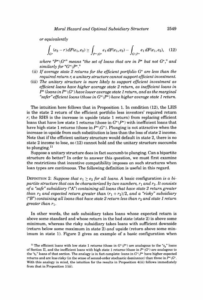
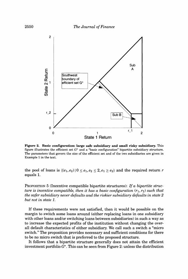
DEFINITION 2: Suppose that el > e2 for all loans. A basic configuration is a bi- partite structure that can be characterized by two numbers, r1 and r2. It consists of a "safe" subsidiary ("A") containing all loans that have state 2 return greater than r2 and expected return greater than (r1 + r2)/2, and a "risky" subsidiary ("B") containing all loans that have state 2 return less than r2 and state 1 return greater than rl.
In other words, the safe subsidiary takes loans whose expected return is above some standard and whose return in the bad state (state 2) is above some minimum, whereas the risky subsidiary takes loans with sufficient downside (return below some maximum in state 2) and upside (return above some min- imum in state 1). Figure 2 gives an example of a basic configuration when
1 The efficient loans with low state 1 returns (those in G*\P*) are analogous to the "sg" loans of Section II, and the inefficient loans with high state 1 returns (those in P*\G*) are analogous to the "tb" loans of that section. The analogy is in fact complete: loans in G*\P* have higher expected returns and are less risky (in the sense of second-order stochastic dominance) than those in P*\G*. With this analogy in mind, the intuition for the results in Proposition 4(iii) follows immediately from that in Proposition l(iii).
2549
The Journal of Finance
2
Sub A
s- Southwest Qy boundary of C 1 efficient set G* U)
0 rl
0 1 r
2 State 1 Return
Figure 2. Basic configuration: large safe subsidiary and small risky subsidiary. This figure illustrates the efficient set G* and a "basic configuration" bipartite subsidiary structure. The parameters that govern the size of the efficient set and of the two subsidiaries are given in
Example 1 in the text.
the pool of loans is {(el, e2) I0 < el, e2 < 2, el > e2} and the required return r equals 1.
PROPOSITION 5 (Incentive compatible bipartite structures): If a bipartite struc- ture is incentive compatible, then it has a basic configuration (rl, r2) such that the safer subsidiary never defaults and the riskier subsidiary defaults in state 2 but not in state 1.
If these requirements were not satisfied, then it would be possible on the margin to switch some loans around (either replacing loans in one subsidiary with other loans and/or switching loans between subsidiaries) in such a way as to increase the expected profits of the institution without changing the over- all default characteristics of either subsidiary. We call such a switch a "micro switch." The proposition provides necessary and sufficient conditions for there to be no micro switch that is preferred to the proposed structure.
It follows that a bipartite structure generally does not attain the efficient investment portfolio G*. This can be seen from Figure 2: unless the distribution
2550

Moral Hazard and Optimal Subsidiary Structure
of loan types has some very convenient holes in its support, either the risky subsidiary will contain some inefficient loans, or some efficient loans will not be in either subsidiary, or both. This bears out the claim at the end of Section II: because the risky subsidiary takes all loans whose upside (state 1 return) is over a certain hurdle rate rl, some inefficient loans with very high risk (low state 2 return but high state 1 return) are taken at the expense of efficient loans with somewhat lower risk. (In Figure 2, these efficient loans are "northeast" of the efficient set boundary, but have state 1 return below ri.)
The "cherry-picking" asset rotation described in Corollary 3 is in fact a type of microswitch. When tg - Sg > (1 + c)(tg - tb), this switch is profitable, and the bipartite structure does not support efficient investment; there is no basic configuration that can simultaneously include sg in the safe subsidiary and tg in the risky subsidiary while excluding tb from the risky subsidiary, so some "cherry-picking" or risk shifting in the riskier subsidiary cannot be prevented.
Note that a unitary structure can be thought of as a limiting form of a ba- sic configuration. Thus, Proposition 5 also gives some insight into incentive compatible structures for unitary portfolios. Either r2 = 0, in which case the structure takes all loans with expected return above some r1/2, or else r2 = oo, in which case the structure takes all loans with state 1 return above some rl. In other words, incentive-compatible unitary portfolios must either be efficient for their size (take all loans above some "hurdle rate" expected return) or else plunge (maximize state 1 return).
Nevertheless, although all incentive compatible structures are basic config- urations, the converse is not true; the institution may be tempted to engage in loan switches that change the risk of one or both subsidiaries. We call such switches "macro switches." In the case of the unitary structure, the relevant macro switch is the substitution of the plunging portfolio P* for the efficient portfolio G*.
Suppose that we have a proposed bipartite structure, where, as in Section II, A is the "safe" subsidiary and B is the "risky" subsidiary. Let ?(A) = S, C(B) = T, and S + T = I. As in Section II, the main macro switch that needs to be considered is that in which P(I), the plunging portfolio of size I, is selected and allocated across the two subsidiaries. The other switch that may need to be considered is the "basic configuration" that has safe subsidiary with size T and risky subsidiary with size S; that is, the roles of the two subsidiaries are switched, analogous to "flipping" in Section II.12
Without imposing further restrictions on the distribution of loan types, the general conditions for a bipartite structure to dominate a unitary structure are complex. The intuition, however, follows that from Section II. A bipar- tite structure is generally more resistant to "total" plunging (choosing P(I)) than is the unitary structure. Again, the bipartite structure segregates safer loans from riskier ones, making risk shifting in the safe subsidiary less attrac- tive. Meanwhile, the risky subsidiary already pays a higher rate, compensating
12 If a macro switch that makes both Sub A and Sub B default-free dominates plunging, then a unitary structure of size I is incentive compatible and preferable to the bipartite structure.
2551
The Journal of Finance
investors for some risk shifting. The downside to the bipartite structure is that, as previously discussed, it generally implies that there will be some inefficiency.
The upshot is that, from an efficiency point of view, the risky subsidiary should be as small as possible subject to incentive compatibility; however, in- centive compatibility will require that the risky subsidiary be large enough to discourage plunging. The following numerical examples illustrate these ideas.
Example 1: Suppose the required return is 1, and the pool of loans is dis- tributed uniformly over W = {(el, e2) 1 0 < el, e2 < 2, ei > e2}; for simplicity, we set the density equal to 1, so that ?(W)= 2. As illustrated in Figure 2, the efficient set is the triangle G* including all loans with expected return greater than 1, which has size 1. Nevertheless, a fairly priced unitary portfolio of G* is not incentive compatible: although this portfolio does not default in either state, it produces expected profit 0.333, whereas if the institution plunges and takes all loans with state 1 return above v/2, it earns expected profit 0.362, which is 8.6% greater.
As the size of the unitary portfolio is reduced below 1, incentives to plunge decrease. At a size of 0.853 (taking all loans with expected returns greater than 1.076), the institution earns expected profit 0.328 and is indifferent to plunging, and for smaller portfolios (higher hurdle rates) it strictly prefers not to plunge. Moreover, equilibrium profits for larger unitary portfolios (given that investors will expect that the institution will plunge) are lower than 0.328. Thus, the unitary portfolio of size 0.853 is the optimal unitary portfolio.
Nevertheless, this unitary structure is not optimal: there are bipartite struc- tures of total size 1 that are incentive compatible and produce higher profits. Of these, the best sets rl = 1.754 and r2 = 0.286, which results in safe subsidiary A with size C(A) = 0.930 and risky subsidiary B with size C(B) = 0.070; total expected profits are 0.332, or 1.2% higher than the expected profit from the best unitary structure.
Although this example suggests that the risky subsidiary B is small, in gen- eral this will depend on the precise distribution of loan types. In particular, if there is a large concentration of very risky loans-those with very low state 2 returns but moderate to high state 1 returns-incentive compatibility may require that the risky subsidiary be very large indeed. So long as there is some concentration of relatively profitable low-risk loans, however, it will be better to adapt a bipartite structure rather than a (small) unitary one. The next example illustrates these ideas.
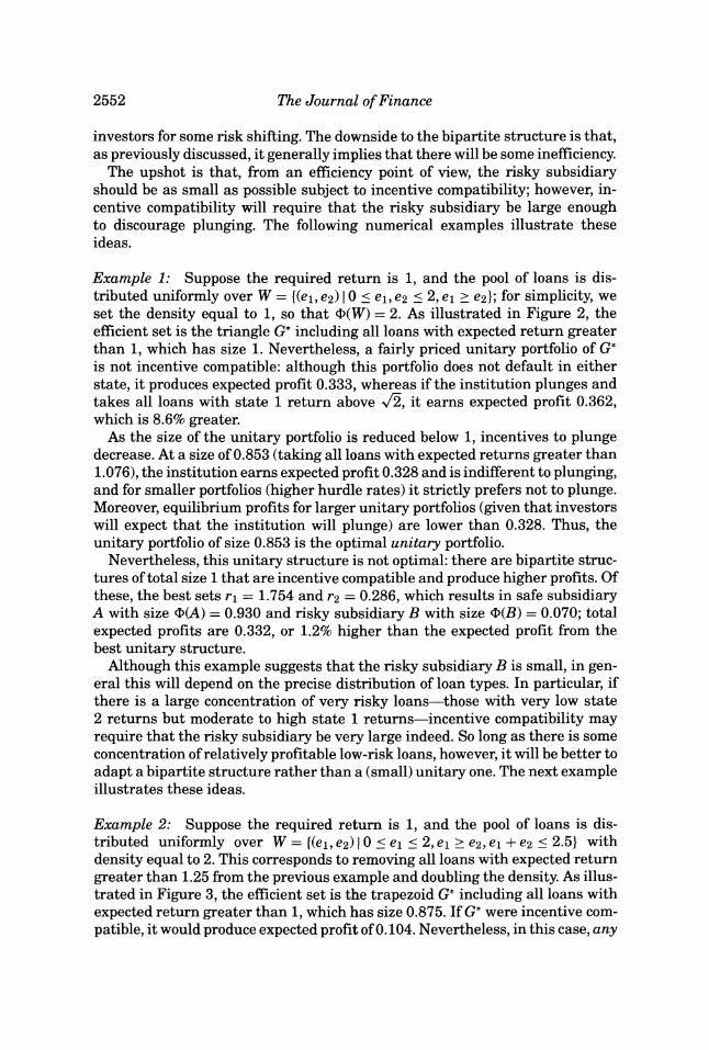
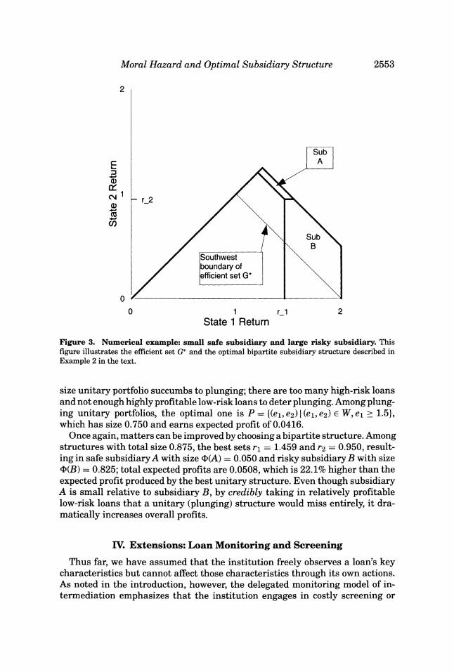
Example 2: Suppose the required return is 1, and the pool of loans is dis- tributed uniformly over W = {(el, e2)1 0 < el < 2, el > e2, el + e2 < 2.5} with density equal to 2. This corresponds to removing all loans with expected return greater than 1.25 from the previous example and doubling the density. As illus- trated in Figure 3, the efficient set is the trapezoid G* including all loans with expected return greater than 1, which has size 0.875. If G* were incentive com- patible, it would produce expected profit of 0.104. Nevertheless, in this case, any
2552
Moral Hazard and Optimal Subsidiary Structure
2
Sub A
(D
041 -2 Sub_
Southwest boundary of efficient set G*
0
0 1 r_ 2 State 1 Return
Figure 3. Numerical example: small safe subsidiary and large risky subsidiary. This
figure illustrates the efficient set G* and the optimal bipartite subsidiary structure described in
Example 2 in the text.
size unitary portfolio succumbs to plunging; there are too many high-risk loans and not enough highly profitable low-risk loans to deter plunging. Among plung- ing unitary portfolios, the optimal one is P = {(el, e2) (el, e2) E W, el > 1.5}, which has size 0.750 and earns expected profit of 0.0416.
Once again, matters can be improved by choosing a bipartite structure. Among structures with total size 0.875, the best sets r1 = 1.459 and r2 = 0.950, result- ing in safe subsidiary A with size ?F(A) = 0.050 and risky subsidiary B with size =>(B) = 0.825; total expected profits are 0.0508, which is 22.1% higher than the expected profit produced by the best unitary structure. Even though subsidiary A is small relative to subsidiary B, by credibly taking in relatively profitable low-risk loans that a unitary (plunging) structure would miss entirely, it dra- matically increases overall profits.
IV. Extensions: Loan Monitoring and Screening
Thus far, we have assumed that the institution freely observes a loan's key characteristics but cannot affect those characteristics through its own actions. As noted in the introduction, however, the delegated monitoring model of in- termediation emphasizes that the institution engages in costly screening or
2553
The Journal of Finance
monitoring of loans on behalf of less-informed investors. We now show that the results of the previous two sections cah be reinterpreted as an example of costly monitoring. We then discuss how similar logic can be used to reinterpret the model as one of costly screening, and how the model can be further generalized.
Until now, we have assumed that the return of a given loan is exogenous, but in reality, many loans give institutions control rights that can be used to improve returns. For example, loans and other private debt can be restructured or called when a borrower's situation deteriorates, limiting the downside to the lender. To get the value out of these control rights, the institution must monitor the situation and then act appropriately. To the extent that monitoring aims at avoiding or ameliorating bad outcomes, the highly levered institutions that are the focus of our paper may underinvest in monitoring. Essentially, borrowers are more likely to be in trouble when their sector or the economy as a whole is in trouble, so (ex post) monitoring is most valuable in bad states of the world. If in good states of the world the cost of monitoring outweighs its benefit, the institution may engage in risk shifting by not monitoring: it saves the cost in good states and defaults in bad states, leaving losses to debt holders (see Winton (2000) for detailed analysis).
Our model is easily adapted to such endogenous loan risk. Returning to the notation of Section II, suppose that both Sg and tg loans benefit from monitor- ing: if they are monitored, their returns (net of costs) are as given in Section II, and they are efficient; if they are not monitored, they become tb loans. Thus, monitoring Sg loans actually worsens returns in state 1 (due to the cost of mon- itoring loans that prove to be healthy anyway), but helps returns in state 2 (the institution intercepts problems before they become severe). By contrast, in this example, monitoring tg loans improves net returns in both states of the world; intuitively, some high-risk borrowers get in trouble even in good economic times, so monitoring has value even then.
All propositions from Section II now hold exactly with the additional assump- tion that T > S* + T*. (Note that investors will never lend more than S* + T* to the institution, since this is the number of efficient loans.) It follows that we are always in the case where Corollary 1 applies: A bipartite structure is always at least as good as a unitary structure. Intuitively, in this example, the institution has incentive to engage in risk shifting by not monitoring Sg loans. By insulating Sg loans from tg loans and in particular the downside of tg loans in state 2, a bipartite structure improves incentives to monitor the Sg loans.
Thus, our analysis easily extends to the case where the institution's role is that of a delegated monitor. In this case, the loans that should be segregated into a "risky subsidiary" are loans that are risky despite monitoring, but which benefit from monitoring even in relatively good times. Examples include many types of finance company loans, as well as loans that have been classified as "problem loans," so that their outcomes are already in doubt. As discussed in Section VI below, such loans are in fact often segregated from the rest of the institution.
With a slight change, our analysis in Section II can also be interpreted as one of costly loan screening. Briefly, suppose that, if the institution pays a
2554
Moral Hazard and Optimal Subsidiary Structure
screening cost, it observes loan types and subtypes. Thus, if the institution does screen, analysis proceeds precisely as in Section II; contingent on screening, the same circumstances govern whether a bipartite structure dominates a unitary structure, etc. If the institution does not screen, it gets a random mix of loans, which by definition includes some that are inefficient.13 If a bipartite structure strictly dominates a unitary structure conditional on screening, it is also more likely to encourage screening.
In the above discussion, we have tailored our examples to make them as close as possible to the analysis of Section II. It is clear, however, that the underlying principles hold more generally: Separate subsidiaries can be a way of encouraging targeted monitoring and screening.
V. Additional Considerations
As noted in the introduction, for tractability, our model has imposed several strong assumptions: The institution is entirely financed with debt, these debt holders know the characteristics of the institution's loan pool but cannot observe the institution's choices, and there are only two states of the world. Since real financial institutions do have equity capital, produce financial reports that on a regular basis reveal some information on loan composition, and operate in a world with many possible outcomes, we now discuss the impact of weakening these assumptions.
Equity capital: Because equity is junior to debt, it absorbs losses first. Thus, substituting equity capital for debt finance reduces a firm's risk shifting incen- tives. Nevertheless, as we have already discussed, equity capital has a number of costs relative to debt finance, so all else equal, an institution would like to use the smallest amount of equity consistent with achieving efficient investment. We now show that choosing subsidiary structure so as to reduce risk shifting incentives allows an institution to economize on costly equity finance.
We return to the setting of Section II, with discrete loan types. Denote by k the fraction of the institution's holdings that it chooses to finance via costly equity. If the institution uses a unitary structure, then the institution prefers efficient investment over plunging if and only if
T*[(l - a)tg - r] + S*(sg - r) + k(S* + T*)r > x[(l + a)tb - Sg]. (13)
At k equal to zero, condition (13) is equivalent to condition (3). Since the left side of (13) is increasing in k while the right side is constant, greater equity capital reduces the likelihood of risk shifting.
First, suppose that condition (3) does not hold-that is, without equity capital, the institution would prefer to plunge under a unitary structure. One can show that, for any capital ratio k, conditions similar to those in Proposition 2 and Corollary 1 determine when a bipartite structure dominates or is dominated by
13 It is also possible that, if the institution does not screen, adverse selection a la Stiglitz and Weiss (1981) leads Sg borrowers to drop out of the market. This would make the institution's mix of loans riskier, increasing the attractiveness of risk shifting by not screening.
2555
The Journal of Finance
a unitary structure.14 It follows that there are circumstances where a bipartite structure with capital ratio k in each subsidiary achieves efficient investment, whereas a unitary structure with the same capital ratio would not. In this case, a bipartite institution could reduce its capital in the safer subsidiary (Sub A) while maintaining efficiency, whereas the unitary institution would have to increase capital to achieve efficiency. Thus, the bipartite structure can allow the institution to economize on costly equity capital.
Of course, there are circumstances where the unitary structure achieves ef- ficiency, whereas the bipartite structure does not. Also, with more loan types, a bipartite structure generally will not achieve the first best. Nevertheless, be- cause equity capital is expensive, allowing a limited amount of risk shifting in the risky subsidiary and having a lower overall capital level can dominate having a unitary structure with sufficient capital to rule out plunging.
Better investor information on loan choices: As discussed in Section I, in- vestors usually do get some information about an institution's loan composition and quality, but with a lag, and with some remaining uncertainty over the quality and risk of the loans of a given class. To the extent the institution's debt holders can act on this information-either by demanding a short matu- rity or specific covenants on the debt-they can reduce the institution's scope for exploiting them through risk shifting.
Nevertheless, our model remains relevant for the reasons discussed in Sec- tion I. Although it is relatively easy to report broad classes of assets (corporate bonds, government bonds, commercial loans, consumer loans), it is difficult for investors to verify the precise breakdown and risk of the loans themselves un- til after losses (if any) are realized. This is partly because of the complexity of the institution's loan portfolio and partly because the risk of these loans is af- fected by the institution's screening and monitoring efforts, which are difficult to observe ex ante.
Furthermore, even if investors imposed highly detailed covenants governing the minutiae of the institution's loan choice and decisions, such covenants would be extremely cumbersome and hard to enforce. Again, one of the functions of financial intermediaries is to use superior skills in choosing which loans to make and how to monitor them. Any legal algorithm built into a debt contract is likely to be imperfect at best, become obsolescent as circumstances change, and be difficult to renegotiate when there are many diffuse debt holders. At best, under the detailed covenant approach, diffuse debt holders would abandon the benefits of delegated monitoring. By steering the institution's incentives in the right direction, an appropriate choice of subsidiary structure may well be a cheaper and less onerous means of preventing investor exploitation.
Incomplete information on the institution's choice set: We assume that in- vestors know the features of the institution's choice set: the population fre- quency of loans of varying types and the effect of screening or monitoring on loan returns. In reality, this information is only known imperfectly. For example,
14 The analysis is identical to that of Section II with debt holders' required return r replaced by debt holders' required return per dollar of institutional loans (1 - k)r.
2556

Moral Hazard and Optimal Subsidiary Structure
the distribution of risk types in loan pool is probably random. Thus, any structure-unitary or bipartite-will with positive probability either leave some efficient loans unfunded or fund some inefficient loans. This does not change the basic intuition of our results. Of course, in the limit, if the relative numbers of safer and riskier loans were too uncertain, investors could not be sure that a "safer" subsidiary of any significant size could in fact be made safe, ruling out significant gains from a bipartite structure.15
Our discussion of the relative precision of investor's information leads to predictions about when and where our model applies. For an economy in which investors have very limited information about loan types and risks, bipartite structures will not add value for the reasons just given. As this information becomes more and more precise, our results will apply with more and more force.
More than two states of the world: Our analysis has focused on a two-state example, with the further restriction that one state (state 2) is worse for all loans. Suppose we generalize to the case of n states of the world, with the proviso that, for all i E (1,..., n - 1}, all loans have weakly higher returns in state i than in state i + 1. In other words, we continue to assume that, regardless of the group of loans being focused on, states can unambiguously be ranked from "best" to "worst." It is easy to show that an optimal subsidiary structure will have at most n subsidiaries: one that never defaults, one that only defaults in state n, etc.
In practice, such an "n-partite" structure will be rather unwieldy, requiring ever more precise information about the distribution of loans that default in each group of states, and also requiring a host of "no-flipping" incentive com- patibility conditions. Moreover, given fixed costs of setting up and maintaining each subsidiary, so fine-tuned a structure is unlikely to be optimal.
By contrast, unitary and bipartite structures are still relatively easy to spec- ify: a unitary structure targets all efficient loans, whereas a bipartite structure merely divides efficient loans into a safer group and a riskier group. The critical tradeoffs between these two structures are unchanged. By isolating safer loans from riskier ones, a bipartite structure still reduces risk shifting incentives in the "safer" subsidiary. The price is that the riskier subsidiary is prone to risk shifting, but the scope of this is limited by the size of the riskier subsidiary. Thus, if the unitary structure does not prevent risk shifting, the bipartite structure will generally be more efficient. Again, this will be more likely as the number of riskier loans is higher, as the downside of efficient risky loans is greater, and as expected profits on efficient loans are lower.16
15 We should also emphasize that what is most critical for our results is not that investors know the proportion of loans that are good lending opportunities, but rather their absolute number. This can be seen from Corollary 1, which shows that the dominance of the bipartite structure holds as the relative proportion of bad opportunities increases without limit.
16 Having more than two states also creates a richer interaction between subsidiary structure and equity capital. By reducing the capital needed in the safer subsidiary, a bipartite structure allows more capital to be injected into the riskier subsidiary, reducing the set of states in which it defaults and thus making risk shifting in that subsidiary less attractive.
2557
The Journal of Finance
Diversifiable portfolio risk: We have assumed that risk is undiversifiable. Even if some risk can be diversified away, our results continue to hold so long as some risk is undiversifiable: It may be useful to segregate loans with more exposure to this risk from loans with'less exposure to this risk.
Our model can be extended to analyze an institution's decision to hold more or less diversified portfolios. Consider the case where, as in our analysis, there are two states of the world, but now some loans do worse in state 1 rather than state 2. In principle, the institution can dramatically reduce its risk by holding loans with "state 1 exposure" and loans with "state 2 exposure" in a unitary portfolio. Nevertheless, if the institution's choice of loans is not observable, investors will be concerned that the institution might raise funds and then plunge its portfolio towards one state or the other. The institution's incentive to do so is higher when there are more loans with very high exposure to one state or the other.
It is easy to show that, when plunging incentives are high, the efficient sub- sidiary structure is now "tripartite," consisting of a risky subsidiary that de- faults in state 1, a risky subsidiary that defaults in state 2, and a subsidiary that holds only relatively safe loans (i.e., those with little downside in either state) and never defaults. In this case, the institution's diversified portfolio does not consist of the riskiest loans-even though at first glance these loans would seem to offer the biggest gains to diversification.17
VI. Applications
We began this paper with two examples, bank holding companies that have separate commercial bank and finance company subsidiaries and good bank/bad bank restructurings. In this section, .we discuss the relationship between our results and these two examples in more detail. We also discuss the extent to which our results may help motivate other institutional arrangements.
Let us recall the main predictions of our model. First, an efficient bipartite structure requires that the risk of the two subsidiaries be significantly differ- ent. Second, a bipartite structure is more likely to be preferred to a unitary structure as the potential downside of efficient riskier loans is larger relative to the institution's overall size. It follows that, all else equal, the bipartite struc- ture is more likely to be preferred as the amount of riskier loans or their risk per dollar is higher. Third, the bipartite structure is more likely to be preferred as expected profit margins on efficient loans decrease. To the extent increased competition erodes the institution's potential profits on loans, increased com- petition encourages a bipartite structure. Fourth, an increase in the profitabil- ity of riskier loans relative to safer loans heightens the risk that a bipartite structure will induce "cherry-picking," particularly if riskier loans are a small part of the institution's asset base (Corollary 3).
17 Unlike our existing model, these results on diversification do not apply to monitoring or screen- ing of loans, but only to choice of loan concentrations. As such, we would expect that they apply most forcefully to less-developed financial markets, where it is more difficult for investors to iden- tify broad groupings of an institution's loan portfolio in a timely manner. For further analysis, see Kahn and Winton (2001).
2558
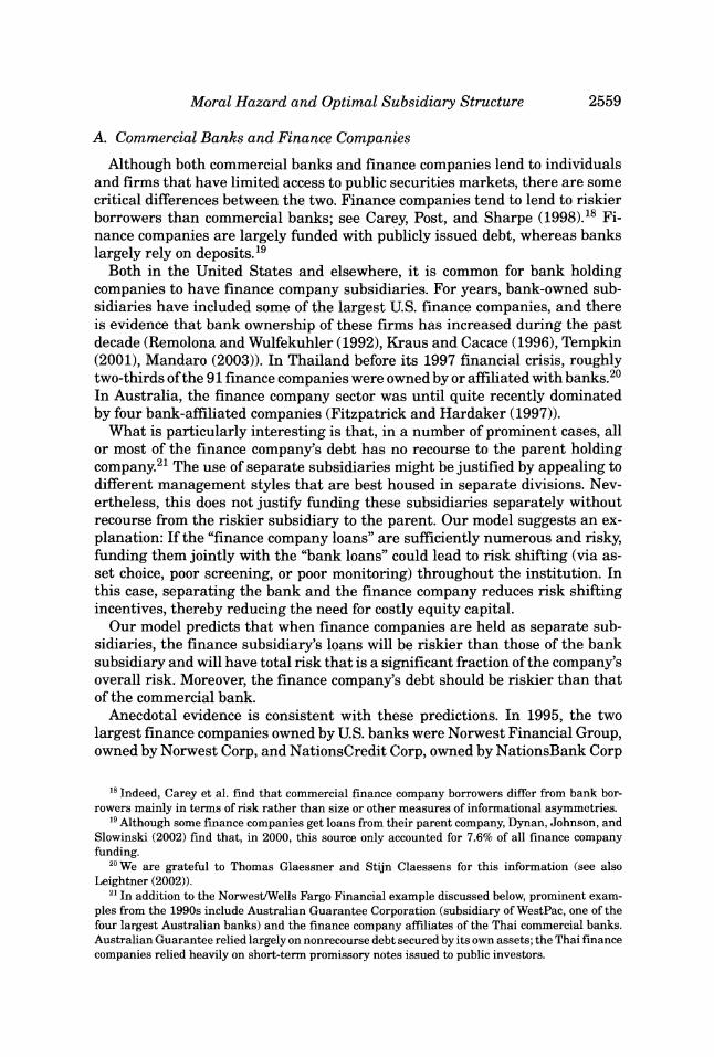
Moral Hazard and Optimal Subsidiary Structure
A. Commercial Banks and Finance Companies
Although both commercial banks and finance companies lend to individuals and firms that have limited access to public securities markets, there are some critical differences between the two. Finance companies tend to lend to riskier borrowers than commercial banks; see Carey, Post, and Sharpe (1998).18 Fi- nance companies are largely funded with publicly issued debt, whereas banks largely rely on deposits.19
Both in the United States and elsewhere, it is common for bank holding companies to have finance company subsidiaries. For years, bank-owned sub- sidiaries have included some of the largest U.S. finance companies, and there is evidence that bank ownership of these firms has increased during the past decade (Remolona and Wulfekuhler (1992), Kraus and Cacace (1996), Tempkin (2001), Mandaro (2003)). In Thailand before its 1997 financial crisis, roughly two-thirds of the 91 finance companies were owned by or affiliated with banks.20 In Australia, the finance company sector was until quite recently dominated by four bank-affiliated companies (Fitzpatrick and Hardaker (1997)).
What is particularly interesting is that, in a number of prominent cases, all or most of the finance company's debt has no recourse to the parent holding company.21 The use of separate subsidiaries might be justified by appealing to different management styles that are best housed in separate divisions. Nev- ertheless, this does not justify funding these subsidiaries separately without recourse from the riskier subsidiary to the parent. Our model suggests an ex- planation: If the "finance company loans" are sufficiently numerous and risky, funding them jointly with the "bank loans" could lead to risk shifting (via as- set choice, poor screening, or poor monitoring) throughout the institution. In this case, separating the bank and the finance company reduces risk shifting incentives, thereby reducing the need for costly equity capital.
Our model predicts that when finance companies are held as separate sub- sidiaries, the finance subsidiary's loans will be riskier than those of the bank subsidiary and will have total risk that is a significant fraction of the company's overall risk. Moreover, the finance company's debt should be riskier than that of the commercial bank.
Anecdotal evidence is consistent with these predictions. In 1995, the two largest finance companies owned by U.S. banks were Norwest Financial Group, owned by Norwest Corp, and NationsCredit Corp, owned by NationsBank Corp
8 Indeed, Carey et al. find that commercial finance company borrowers differ from bank bor- rowers mainly in terms of risk rather than size or other measures of informational asymmetries.
19 Although some finance companies get loans from their parent company, Dynan, Johnson, and Slowinski (2002) find that, in 2000, this source only accounted for 7.6% of all finance company funding.
20We are grateful to Thomas Glaessner and Stijn Claessens for this information (see also Leightner (2002)).
21 In addition to the Norwest/Wells Fargo Financial example discussed below, prominent exam- ples from the 1990s include Australian Guarantee Corporation (subsidiary of WestPac, one of the four largest Australian banks) and the finance company affiliates of the Thai commercial banks. Australian Guarantee relied largely on nonrecourse debt secured by its own assets; the Thai finance companies relied heavily on short-term promissory notes issued to public investors.
2559
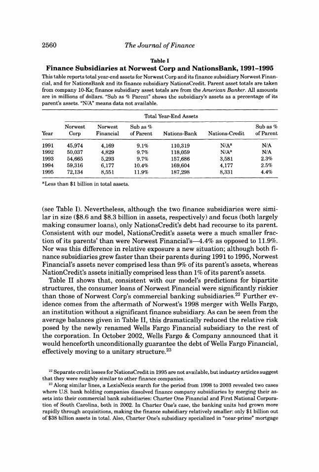
The Journal of Finance
Table I Finance Subsidiaries at Norwest Corp and NationsBank, 1991-1995
This table reports total year-end assets for Norwest Corp and its finance subsidiary Norwest Finan- cial, and for NationsBank and its finance subsidiary NationsCredit. Parent asset totals are taken from company 10-Ks; finance subsidiary asset totals are from the American Banker. All amounts are in millions of dollars. "Sub as % Parent" shows the subsidiary's assets as a percentage of its parent's assets. "N/A" means data not available.
Total Year-End Assets
Norwest Norwest Sub as % Sub as % Year Corp Financial of Parent Nations-Bank Nations-Credit of Parent
1991 45,974 4,169 9.1% 110,319 N/Aa N/A 1992 50,037 4,829 9.7% 118,059 N/Aa N/A 1993 54,665 5,293 9.7% 157,686 3,581 2.3% 1994 59,316 6,177 10.4% 169,604 4,177 2.5% 1995 72,134 8,551 11.9% 187,298 8,331 4.4%
aLess than $1 billion in total assets.
(see Table I). Nevertheless, although the two finance subsidiaries were simi- lar in size ($8.6 and $8.3 billion in assets, respectively) and focus (both largely making consumer loans), only NationsCredit's debt had recourse to its parent. Consistent with our model, NationsCredit's assets were a much smaller frac- tion of its parents' than were Norwest Financial's-4.4% as opposed to 11.9%. Nor was this difference in relative exposure a new situation; although both fi- nance subsidiaries grew faster than their parents during 1991 to 1995, Norwest Financial's assets never comprised less than 9% of its parent's assets, whereas NationCredit's assets initially comprised less than 1% of its parent's assets.
Table II shows that, consistent with our model's predictions for bipartite structures, the consumer loans of Norwest Financial were significantly riskier than those of Norwest Corp's commercial banking subsidiaries.22 Further ev- idence comes from the aftermath of Norwest's 1998 merger with Wells Fargo, an institution without a significant finance subsidiary. As can be seen from the average balances given in Table II, this dramatically reduced the relative risk posed by the newly renamed Wells Fargo Financial subsidiary to the rest of the corporation. In October 2002, Wells Fargo & Company announced that it would henceforth unconditionally guarantee the debt of Wells Fargo Financial, effectively moving to a unitary structure.23
22 Separate credit losses for NationsCredit in 1995 are not available, but industry articles suggest that they were roughly similar to other finance companies.
23 Along similar lines, a LexisNexis search for the period from 1998 to 2003 revealed two cases where U.S. bank holding companies dissolved finance company subsidiaries by merging their as- sets into their commercial bank subsidiaries: Charter One Financial and First National Corpora- tion of South Carolina, both in 2002. In Charter One's case, the banking units had grown more rapidly through acquisitions, making the finance subsidiary relatively smaller: only $1 billion out of $38 billion assets in total. Also, Charter One's subsidiary specialized in "near-prime" mortgage
2560
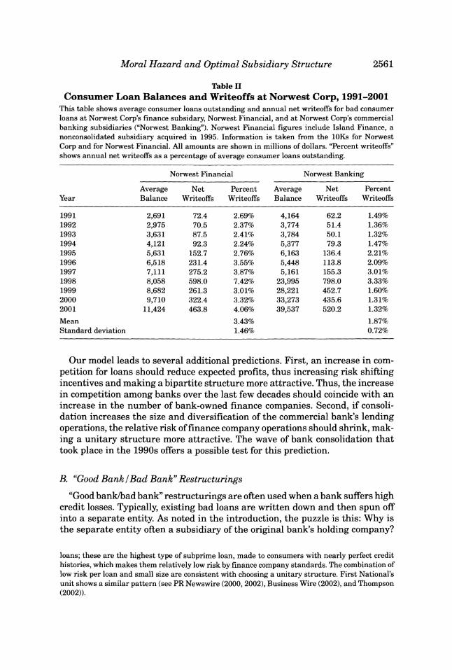
Moral Hazard and Optimal Subsidiary Structure
Table II Consumer Loan Balances and Writeoffs at Norwest Corp, 1991-2001
This table shows average consumer loans outstanding and annual net writeoffs for bad consumer loans at Norwest Corp's finance subsidary, Norwest Financial, and at Norwest Corp's commercial banking subsidiaries ("Norwest Banking"). Norwest Financial figures include Island Finance, a nonconsolidated subsidiary acquired in 1995. Information is taken from the lOKs for Norwest Corp and for Norwest Financial. All amounts are shown in millions of dollars. "Percent writeoffs" shows annual net writeoffs as a percentage of average consumer loans outstanding.
Norwest Financial Norwest Banking
Average Net Percent Average Net Percent Year Balance Writeoffs Writeoffs Balance Writeoffs Writeoffs
1991 2,691 72.4 2.69% 4,164 62.2 1.49% 1992 2,975 70.5 2.37% 3,774 51.4 1.36% 1993 3,631 87.5 2.41% 3,784 50.1 1.32% 1994 4,121 92.3 2.24% 5,377 79.3 1.47% 1995 5,631 152.7 2.76% 6,163 136.4 2.21% 1996 6,518 231.4 3.55% 5,448 113.8 2.09% 1997 7,111 275.2 3.87% 5,161 155.3 3.01% 1998 8,058 598.0 7.42% 23,995 798.0 3.33% 1999 8,682 261.3 3.01% 28,221 452.7 1.60% 2000 9,710 322.4 3.32% 33,273 435.6 1.31% 2001 11,424 463.8 4.06% 39,537 520.2 1.32% Mean 3.43% 1.87% Standard deviation 1.46% 0.72%
Our model leads to several additional predictions. First, an increase in com- petition for loans should reduce expected profits, thus increasing risk shifting incentives and making a bipartite structure more attractive. Thus, the increase in competition among banks over the last few decades should coincide with an increase in the number of bank-owned finance companies. Second, if consoli- dation increases the size and diversification of the commercial bank's lending operations, the relative risk of finance company operations should shrink, mak- ing a unitary structure more attractive. The wave of bank consolidation that took place in the 1990s offers a possible test for this prediction.
B. "Good Bank/Bad Bank" Restructurings "Good bank/bad bank" restructurings are often used when a bank suffers high
credit losses. Typically, existing bad loans are written down and then spun off into a separate entity. As noted in the introduction, the puzzle is this: Why is the separate entity often a subsidiary of the original bank's holding company?
loans; these are the highest type of subprime loan, made to consumers with nearly perfect credit histories, which makes them relatively low risk by finance company standards. The combination of low risk per loan and small size are consistent with choosing a unitary structure. First National's unit shows a similar pattern (see PR Newswire (2000, 2002), Business Wire (2002), and Thompson (2002)).
2561
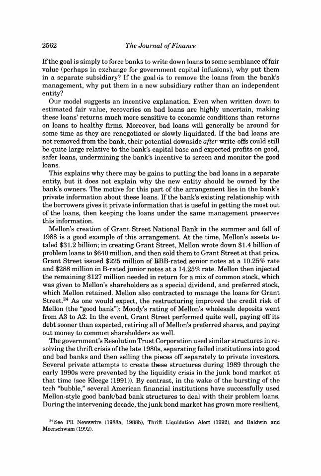
The Journal of Finance
If the goal is simply to force banks to write down loans to some semblance of fair value (perhaps in exchange for government capital infusions), why put them in a separate subsidiary? If the goallis to remove the loans from the bank's management, why put them in a new subsidiary rather than an independent entity?
Our model suggests an incentive explanation. Even when written down to estimated fair value, recoveries on bad loans are highly uncertain, making these loans' returns much more sensitive to economic conditions than returns on loans to healthy firms. Moreover, bad loans will generally be around for some time as they are renegotiated or slowly liquidated. If the bad loans are not removed from the bank, their potential downside after write-offs could still be quite large relative to the bank's capital base and expected profits on good, safer loans, undermining the bank's incentive to screen and monitor the good loans.
This explains why there may be gains to putting the bad loans in a separate entity, but it does not explain why the new entity should be owned by the bank's owners. The motive for this part of the arrangement lies in the bank's private information about these loans. If the bank's existing relationship with the borrowers gives it private information that is useful in getting the most out of the loans, then keeping the loans under the same management preserves this information.
Mellon's creation of Grant Street National Bank in the summer and fall of 1988 is a good example of this arrangement. At the time, Mellon's assets to- taled $31.2 billion; in creating Grant Street, Mellon wrote down $1.4 billion of problem loans to $640 million, and then sold them to Grant Street at that price. Grant Street issued $225 million of BBB-rated senior notes at a 10.25% rate and $288 million in B-rated junior notes at a 14.25% rate. Mellon then injected the remaining $127 million needed in return for a mix of common stock, which was given to Mellon's shareholders as a special dividend, and preferred stock, which Mellon retained. Mellon also contracted to manage the loans for Grant Street.24 As one would expect, the restructuring improved the credit risk of Mellon (the "good bank"): Moody's rating of Mellon's wholesale deposits went from A3 to A2. In the event, Grant Street performed quite well, paying off its debt sooner than expected, retiring all of Mellon's preferred shares, and paying out money to common shareholders as well.
The government's Resolution Trust Corporation used similar structures in re- solving the thrift crisis of the late 1980s, separating failed institutions into good and bad banks and then selling the pieces off separately to private investors. Several private attempts to create these structures during 1989 through the early 1990s were prevented by the liquidity crisis in the junk bond market at that time (see Kleege (1991)). By contrast, in the wake of the bursting of the tech "bubble," several American financial institutions have successfully used Mellon-style good bank/bad bank structures to deal with their problem loans. During the intervening decade, the junk bond market has grown more resilient,
24See PR Newswire (1988a, 1988b), Thrift Liquidation Alert (1992), and Baldwin and Meerschwam (1992).
2562
Moral Hazard and Optimal Subsidiary Structure
and securitization has made investors more comfortable with similar structures (see Sherer and Sapsford (2001), Agosta (2001)).
Given that a dollar of bad loans is far more risky than a dollar of finance company loans, our model predicts that it should take a smaller relative volume of bad loans to make a bipartite structure attractive. Most of our examples bear this out; whereas Norwest Bank's finance subsidiary was over 10% of its parent's size, Mellon's Grant Street Bank took on only 2% of the parent's assets, and the recent bad banks created by FleetBoston and Upstate National Bank concerned roughly 1% and 3%, respectively, of their total assets.
During the 1990s, many countries made use of good bank/bad bank structures to deal with banking crises; examples include Sweden, Mexico, and Thailand. Thailand is especially relevant to our model, because many of the "bad banks" were created privately rather than by the government (see Bennett (1993), Sherer and Sapsford (2001), Bangkok Post (2001)). Of course, banks will only opt for a private bipartite structure if a government bailout seems remote or bailout terms are sufficiently onerous.25 Recently, Mizuho Financial and UFJ Holdings (two large Japanese bank holding companies) announced that they plan to transfer problem loans from their bank subsidiaries to new "bad bank" subsidiaries; consistent with our analysis in Section V, the move was described as a bid to bolster bank capital (Economist (2002)). The Japanese banks seem to have been motivated by fresh falls in the Japanese stock market, eroding unrealized profits on equity holdings that regulators had allowed them to use in meeting capital requirements. With one regulatory subsidy removed and no other forthcoming, they had to focus on private solutions for reducing their risk of default.
To conclude this subsection, we note that other financial institutions have used good bank/bad bank structures. Beginning in the 1970s, property and ca- sualty insurers have used similar structures where the "bad bank" consists of discontinued insurance lines or policies with exceptionally problematic loss reserves. This process accelerated in the 1990s, with Cigna and other ma- jor insurers using such "bad banks" to house troubled asbestos- and other environmental-liability policies.26
To see how this fits our model, first note that property and casualty insurers are delegated monitors, screening and monitoring new policies on behalf of dis- persed policyholders. Their liabilities to policyholders give them high leverage (recently on the order of 65 to 70%). As such, policyholders face the risk that the insurers will engage in risk shifting by not screening and monitoring poli- cies, or even by building up unhealthy concentrations of risk through deliberate policy selection.27 Future losses on asbestos- and other environmental-liability policies are not only expected to be high, but face high "systematic" risk as well,
25 In Thailand's case, the use of private good bank/bad bank structures was a reaction to harsh terms for government aid.
26 For further discussion and examples, see Snyder and Simpson (1996) and Latza (1997). 27 Morgan (2002) finds that, just as rating agencies differ more on banks than on nonfinancial
firms, they differ more on their ratings of insurers as well. This is consistent with the notion that insurers suffer from opacity due to the diverse nature of their policy portfolios and policyholders' difficulty in observing the insurers' screening and monitoring.
2563
The Journal of Finance
because a change in legal ruling or outcome on one policy affects the expected amount of losses on other policies of the same type. Because of this high po- tential downside, keeping these policies in the main insurer could undermine the insurer's incentive to carefully screen, choose, and monitor other, healthier policy lines. By segregating the policies along with appropriate loss reserves, the insurer insulates the healthier policies from this "contagion," improving incentives.
Another example comes from real estate investment trusts (REITs), institu- tions that serve as delegated monitors of real estate properties for investors. In 1997, Prime Retail Inc. planned to acquire the 20 strongest factory-outlet centers of Horizon Group Inc., along with the assumption of $540 million of Horizon's debt; in return, three of Prime's weakest centers would be merged with Horizon's weakest 17 centers under Horizon's name, and Prime share- holders would receive equity in this new entity (Pacelle (1997)). Effectively, Prime would be the "good bank" and Horizon the "bad bank." Again, without this bipartite structure, the merged entity would face continuing risk from the weaker (hence riskier) properties, hurting incentives throughout the entire entity.
All of these examples have certain features in common with our predictions about when a bipartite structure will be adopted. The number of bad assets (and their risk) must be large relative to the institution's existing capital base and profit margins. Also, the existing bank is more likely to retain a claim on the new "bad bank" if its private information about the bad loans is critical to their ongoing monitoring. Thus, bad banks are more likely to be owned by the parent if the (bad) assets are more opaque.
C. Additional Applications Our results also help motivate other arrangements used by financial institu-
tions. In this subsection, we discuss how our results apply to the use of bipar- tite subsidiary structures by investment banks and the provision of recourse by originating banks in credit card securitizations.
Investment bank private-equity affiliates: Like commercial banks, investment banks face investor concerns over risk shifting. They are highly levered, and the bulk of their assets consists of marketable securities held both as inven- tories for their underwriting and broker/dealer activities and as proprietary trading positions. As noted by Myers and Rajan (1998), such assets are gener- ally quite liquid, allowing easy changes of risk via asset substitution that are difficult for investors to control directly. Morgan's (2002) finding that banks with a larger fraction of their assets in trading accounts are more likely to have ratings agency disagreements (see footnote 2) is consistent with this concern.
Given this situation, we should expect to see investment banks making use of bipartite structures to segregate assets whose risk is significantly higher than average. One common example concerns private equity finance. As doc- umented by Fenn, Liang, and Prowse (1995), many large U.S. investment banks have separately funded affiliates that provide private equity finance to a
2564
Moral Hazard and Optimal Subsidiary Structure
variety of businesses (venture capital targets, leveraged-buyout targets, dis- tressed firms that restructure). These affiliates are usually structured as lim- ited partnerships, with the investment bank as general partner; moreover, the stakes of the limited partners resemble convertible preferred stock, insofar as they participate in the partnership's potential upside but also have some down- side protection. As discussed by Fenn et al., this arrangement creates potential risk shifting concerns between the limited partners and the general partner.
Given that investment banks could in principle fund these equity investments through their main subsidiaries, why fund them separately?28 Our model sug- gests one reason, based on the fact that these private equity investments are much more risky than most publicly traded stocks, much less the Treasury securities and corporate bonds that make up the bulk of investment bank as- set holdings.29 Moreover, private equity investments are notoriously opaque and hard to monitor, even for limited partners in specialized funds (again, see Fenn (1995)). Given the high risk of private equity and the high leverage of investment banks, commingling these assets with an investment bank's other assets could easily increase risk shifting incentives throughout the institution. Putting private equity holdings in a "risky sub" (the affiliated private equity fund) avoids this worsening of incentives. Consistent with our model, the "debt" (limited partner funding) of the affiliates is much riskier than that of the rest of the investment bank, which typically consists of very short-term collateralized loans (e.g., repurchase agreements) and investment grade debt.30
Recourse in credit card securitizations: Credit card securitizations provide an example where the "cherry-picking" concerns outlined in Corollary 3 seem to apply. In such a securitization, credit card receivables are sold by the originating bank into a "special purpose entity" (SPE). The SPE finances itself largely by issuing debt collateralized by the receivables (asset-backed securities), though the originating bank injects some equity in the form of cash reserves. In most securitizations, the SPE would be completely without recourse to the originat- ing bank, forming a bipartite structure.31 By contrast, in the case of credit
28 The investment banks would have to comply with SEC capital requirements, which basically require that broker/dealers fund private equity holdings entirely with equity. (More precisely, they must subtract these holdings from both their assets and their capital base in calculating their capital ratios.) Since preferred stock counts as equity capital, in principle this could be met by having the erstwhile private equity fund's limited partners hold preferred stock in the investment bank.
29 For example, the bulk of returns on venture capital investments typically come from success- ful "exit strategies" such as an IPO or sale to a large corporation, but the IPO option depends heavily on favorable conditions in the public equity market. More generally, the illiquidity and associated information asymmetries that come with private equity also contribute to the risk of these investments.
30 Historically, large U.S. commercial bank holding companies also had private equity affili- ates, but regulation generally prevented the commercial bank itself from direct holdings of equity. Following the passage of the Gramm-Leach-Bliley Act, these banks now can (and often do) have investment bank affiliates, so our argument now applies to the holding companies' use of separate private equity affiliates.
31 This might improve the institution's lending incentives, as per our earlier analysis (see also Fulghieri (1993)).
2565
The Journal of Finance
cards, the structure usually allows limited recourse against the issuer in the form of requirements that the issuer inject additional receivables in the event of problems with the existing collateral.
One motivation for this effectively unitary structure may be concerns about "cherry-picking." Credit card loans are not only much riskier than most com- mercial bank loans, but also are much more profitable, with return on assets averaging 2 to 3% versus 1% or less on other loans. In addition, any one securi- tization is usually small in relation to the rest of the bank. This is exactly the situation where the "cherry-picking" concerns detailed in Corollary 3 may apply, in which case a unitary structure is more efficient than a bipartite structure. By giving investors the right to demand recourse against receivables held on the bank's balance sheet, they gain the ability to seize any "cherries" the bank may withhold, reducing the bank's incentive to engage in such risk shifting behavior.32
VII. Conclusion
The choice of subsidiary structure affects a financial institution's lending, monitoring, and screening decisions. When the aggregate downside from riskier loans is high or when the expected returns to the institution's target loan mix are low, a bipartite structure will insulate safer loans from the downside of riskier loans, reducing the institution's risk shifting incentives. This justifi- cation for multiple subsidiary structures helps motivate "good bank/bad bank" restructurings and separately funded finance company subsidiaries of commer- cial bank holding companies.
Appendix Define x = min{T, S*}, y = min{S* - T*, T}, andz = min{S*, T*}. Recall that
a risky portfolio or subsidiary is one that defaults in state 2.
Proof of Proposition 1: If the efficient portfolio is risky (Ru > r), then con- dition (2) implies that the plunging portfolio generates higher profits than the efficient portfolio, verifying (i). Also, Ru > r implies that the right-hand side of (3) is negative, whereas (2) implies that the left-hand side is positive. Thus, (3) is violated, confirming (ii) for this case.
If both the efficient portfolio and the plunging portfolio are safe, then the plunging portfolio is less profitable and so the efficient portfolio is incentive compatible. The plunging portfolio's state 2 return is
T*(l - a)tg + x(l - a)tb + (S* - x)sg. (Al)
32 By contrast, regulatory arbitrage is not a motivation for this recourse structure, since credit card SPEs typically have a higher internal capital ratio than the banks themselves are required to have. For further analysis and discussion, see Higgins and Mason (2003) and Calomiris and Mason (2003).
2566

Moral Hazard and Optimal Subsidiary Structure
The plunging portfolio is safe if and only if this expression exceeds (S* + T*)r, or, rearranging, if and only if
x[sg - (1 - a)tb] < T*[(1 - a)tg - r] + S*(sg - r). (A2)
Since Sg > tb, Sg - (1 - a)tb > (1 + a)tb - g, and so (3) holds whenever the plunging portfolio is safe.
We are left with the case where the efficient portfolio is safe (so Ru = r) but the plunging portfolio is risky. The plunging portfolio's state 1 return is
(S* - x)sg + T*tg(l + a) + xtb(l + a). (A3)
In this case, it follows that the institution prefers efficient investment over plunging if and only if
2[T*(1 + a)tg + (S* - x)sg + x(l + a)tb - (S* + T*)r]
< T*tg + S*sg - (S* + T*)r. (A4)
The left-hand side (LHS) of this inequality is the payoff of the plunging portfolio; the right-hand side (RHS) is the payoff of the efficient portfolio. Doubling both sides and rearranging, this inequality reduces to (3).
Finally, (iii) follows from basic comparative statics on (3). Q.E.D.
Proof of Proposition 2: We prove this by grouping potential deviations from the efficient portfolio by their effect on each subsidiary's default probability. Throughout, we refer to the efficient arrangement (sg assets in Sub A, tg as- sets in Sub B) as the "status quo." Expected profits under the status quo are S*(sg - r) + T*(tg - r).
(i) Both subsidiaries safe: In this case, the institution's total profits are (expected asset returns) - (S*r + T*RB). It is best to use only the Sg and tg assets, since these have the highest expected returns, so profits are (S*sg + T*tg) - (S*r + T*RB). Since RB > r, this is always dominated by the status quo.
(ii) Sub A safe, Sub B risky: First, note that such a deviation that simul- taneously puts Sg assets in Sub B and tb assets in Sub A is dominated: Switching these assets increases profits in Sub A by sg - tb and profits in Sub B by [(1 + a)tb - Sg ]. Also, having tg assets in Sub B and tb as- sets in Sub A is dominated: Switching these assets increases profits by 2(1- a)(tg - tb). Finally, having Sg assets in Sub B and some tb assets unused is dominated by switching the two.
Thus, the best such deviation moves tg assets into Sub A and tb assets into Sub B. (If one runs out of sg assets to replace in Sub A, then Sub A defaults in state 2 and we are in a different case; similarly, if one runs out of tg assets to move into Sub A, moving in tb assets hurts profits unless Sub A defaults in state 2.) This increases profits by (tg - sg) +
+(1 + a)(tb - tg), which is negative so long as condition (5) holds.
2567
The Journal of Finance
(iii) Both subsidiaries risky: In this case, it is best to plunge, using T*tg as- sets, xtb assets, and then Sg assets only as needed. This fails to dominate the status quo if and only if
2[T*(l + a)tg + (S* - x)sg + x(1 + a)tb - S*r - T*RB]
< S*(sg - r) + T*[(1 + )tg - RB]. (A5)
Doubling both sides and rearranging leads to (4). (iv) Sub A risky, Sub B safe ("flip" the subsidiaries): This can only occur if
Sg > RB = 2r - (1 - a)tg, in which case placing enough Sg assets in Sub B may make it safe. There are two subcases to consider.
(a) S* < T*: The best way to achieve the "flip" is to switch as many sg and tg assets as possible. To see this, note that if Sg > tg, profits in a safe Sub B are maximized by placing sg assets there, while profits in a risky Sub A are maximized by placing tg assets there (these have highest state 1 return). If sg < tg, then as in (ii) the only way to dominate this flip while preserving the subsidiaries' risk profile would be to rotate tg assets back into Sub B and tb assets into Sub A. This is ruled out by condition (5).
Once all Sg assets are in Sub B, it is best to leave any remaining tg assets in Sub B rather than replace them with tb assets, since tg assets do better in both states. This dominates the status quo if and only if
1S*[(1 + )tg - r] + [(T* - S*)tg + S*g - T*RB]
> S*(g - r) + T*(tg - r). (A6)
Doubling, substituting for RB, and rearranging, this is equivalent to
(S* - 2T*)[r - (1 - a)tg] > 0. (A7)
Since r > (1 - a)tg and S* < T*, this is a contradiction, and so a flip never dominates the status quo.
(b) S* > T*: Again, it is best to begin by switching as many Sg and tg assets as possible; that is, T* of each. Since Sub A is now risky, it is best to augment this by replacing as many remaining sg assets as possible with tb; i.e., replace y of them. Condition (5) rules out any further switches that leave the risk structure unchanged. This deviation dominates the status quo if and only if
[T*(1 + a)tg + (S* - T* - y)sg + y(l + O)tb - S*r] + T*(sg - R)
> S*(Sg - r) + T*(tg - r). (A8)
2568
Moral Hazard and Optimal Subsidiary Structure
Doubling, substituting for RB, and rearranging, this is equivalent to
y[(1 + a)tb - Sg] > S*(Sg - r) + T*[2r - Sg - (1 - a)tg]
= S*(sg - r) + T*(RB - g). (A9)
Thus the status quo is incentive compatible if and only if the reverse of (A9) holds. Since sg > RB, min{sg - RB, RB - Sg] = RB - Sg, so the reverse of (A9) is equivalent to condition (6) in the text.
(v) Sub A safe, Sub B defaults all the time: This requires that sg < RB; otherwise, it is impossible to make Sub B default all the time by using sg or tb assets, and we are in one of the previous cases. In this deviation, all profits come from Sub A. If sg > tg and Sub A is to be safe, profits are maximized by filling Sub A with sg assets. But the status quo does this and earns positive profits in Sub B, so it dominates any such deviation.
If instead sg < tg, Sub A's profits are maximized by replacingz of the Sg assets in Sub A with tg. (If Sub A now becomes risky, defaulting in state 2, further switches get risk shifting gains as well.) If Sub A now defaults (as is true when S* < T*), then we are in another case. Otherwise, since Sub B defaults all the time, profits from the deviation are (S* - T*)sg + T*tg - S*r = (S* - T*)(sg - r) + T*(tg - r), which is less than profits under the status quo. Thus, we can ignore this case.
(vi) Sub A risky, Sub B defaults all the time: Again, we must have sg < RB, and we can focus on maximizing profits in Sub A. There are two subcases.
(a) S* < T*: If Sub A is to be risky, its profits are maximized by filling it with tg. This dominates the status quo if and only if
[S*(l + a)tg - r] > S*(sg - r) + T*(tg - r). (A10)
Doubling and subtracting S*(sg - r) from both sides yields the re- verse of condition (7) in the text. The requirement that the deviation causes Sub A to default in state 2 yields the other condition for this subcase.
(b) S* > T*: Subject to failing in state 2, Sub A's profits are maximized by using T*of tg assets and y of tb assets. This dominates the status quo if and only if
2[T*(1 + a)tg + (S* - T* - y)sg + y(l + a)tb- S*r]
> S*(sg - r) + T*(tg - r). (All)
Doubling and rearranging gives
y[(l + a)tb - Sg] > S*(sg - r) + T*[(l - a)tg + Sg - 2r]. (A12)
On the right-hand side, the last term equals T* times g - RB =
min{sg - RB, RB - Sg]. The reverse of this inequality yields condition (6) in the text. Q.E.D.
2569

The Journal of Finance
Proof of Corollary 1: Since (1 - a)tg < r, (3) always implies that (4) holds strictly. Since S* < T, (4) becomes S*[(1 + a)tb - Sg] S*[sg - r]. Dividing by S* and rearranging gives -2sg < -r - (1 + a)tb, and so 2(tg - sg) < 2tg - r - (1 + a)tb. Also, (1 - a)tg < r implies 2tg - r < (1 + a)tg, so (4) implies 2(tg - sg) < (1 + a)(tg - tb), which is equivalent to (5). It remains to be shown that (3) implies that (7) or (6) holds, depending on whether or not S* < T*. Note that (3) is now equivalent to S*[(1 + a)tb - Sg] < S*[Sg - r] + T*[(1 - a)tg - r].
(i) S* < T*: If sg > RB, then conditions (4) and (5) are necessary and suffi- cient for bipartite efficiency. Otherwise, since (1 + a)tb > r, S*(1 + a)(tg -
tb) < T*[(1 + a)tg - r]; adding this to (3) gives condition (7). (ii) T* < S* < T: Now (6) is equivalent to
S*[(1 + a)tb - g] < S*(sg - r) + T*[(1 + )tb - Sg
+ minsg -RB, RB- Sg}]. (A13)
Condition (3) implies (6) if and only if the bracketed term on the RHS of (A13) exceeds (1 - a)tg - r. If sg < RB, this term equals (1 + a)tb - RB = (1 + a)tb + (1 - a)tg - 2r > (1 - a)tg - r, so (3) implies (6). If Sg > RB, this term equals (1 + a)tb - sg + RB - Sg. If this exceeds (1 - a)tg - r, we are done. Otherwise, (1 + a)tb - sg < Sg - RB + [(1 - a)tg - r] < sg -
RB, so (S*-T*)[(l + a)tb-sg] < (S* - T*)(sg - RB) < S*(sg - r) + T*(RB - sg), which is equivalent to (6).
Since (3) implies that (4) and (6) hold strictly, the last statement of the corol- lary follows. Q.E.D.
Proof of Corollary 2: Once again, (3) implies that (4) holds strictly.
(i) When S* < 2T*, S* - T* < T* < T. If sg < RB, the second term on the RHS of(6) equals T*(sg - RB) = T*[sg - r + (1 - a)tg - r] > T*[(1 - a)tg- r]. Thus, the RHS of(6) strictly exceeds the RHS of(3). Since S* - T* < T, the LHS of (6) is less than or equal to the LHS of (3); thus, (3) implies that (6) holds strictly.
If sg > RB, (6) is equivalent to T*[2sg -(1 + a)tb - RB] < S*[2sg - (1 + a)tb - r]. Since T* < S* and RB > r, this holds strictly.
(ii) IfS* > 2T*, the LHS of(6) is less than or equal to the LHS of(3), so (3) im- plies (6) if min{sg - RB, RB - Sg > (1 - a)tg - r. If sg < RB, this holds be- cause Sg - RB = Sg - r + [(1 - a)tg - r]. Otherwise, RB - Sg > (1 - a)tg -
r if and only ifsg < RB + (1 - a)tg - r]. Q.E.D.
Proof of Corollary 3:
(i) When (5) does not hold, the bipartite status quo is dominated by "asset rotation." The rest of this part follows from comparative statics on (5).
(ii) After rotating T* of tg assets into Sub A, Sub A's state 2 return is (S* - T*)sg + T*(1 - a)tg - S*r. This is positive if and only if (8) holds. If (8) does not hold, the rotation is attractive and gives Sub A zero profits in
2570
Moral Hazard and Optimal Subsidiary Structure
state 2. Thus, it pays to replace min{S* - T*, T - T*} = T - T* of the Sg assets that remain in Sub A with unused tb assets. Under this augmented rotation, the institution as a whole holds the plunging portfolio: x = T of the Sg assets are replaced with tb assets. Comparative statics on (8) are straightforward.
We want to show that if (8) does not hold, (3) does not hold. There are two subcases to consider.
(a) (1 + )tb > RB. The augmented rotation makes both subsidiaries default in state 2 only. Since this dominates the status quo, condi- tion (4) is violated, and so (3) is violated.
(b) (1 + a)tb < RB. The augmented rotation makes Sub A default in state 2 and Sub B default in both states. Since the rotation domi- nates the status quo, profits in Sub A must exceed those from the status quo:
2 [T*(1 + a)tg + (x - T*)(1 + a)tb + (S* - x)sg - S*r]
> S*(sg - r) + T*(tg - r), (A14)
where we have made use ofmin{S* - T*, T- T*} = min{S*, T) - T* x - T*. Doubling and rearranging gives
x[(1 + a)tb - Sg] > S*(sg - r) + T*[(1 - a)tg - r]
+ T*[(l + a)tb - r]. (A15)
Since (1 + a)tb - r > 0, this condition implies that condition (3) is violated. Q.E.D.
Proof of Proposition 3: We assume that the set of all possible loan types is some bounded set W, and the loan types form a non-atomic distribution function F(el, e2) with positive support almost everywhere on W. A subsidiary structure a = (A, B, C,..., K;RA, RB, RC, ..., RK) is a finite set of nonintersecting subsets of W(the "subsidiaries"A, B, C, ..., K), together with each subsidiary's debt face value per unit borrowed. We will say that a subsidiary structure a' mimics a if there is a one-to-one correspondence between the two sets of subsidiaries such that corresponding subsidiaries have the same size and debt face value. Under these circumstances, outside investors are unable to tell if a' has been substituted for a.
First, note that none of the original subsidiaries can default in both states and still issue fairly priced debt. Since el > e2 for all (el, e2) e W, it follows that each subsidiary defaults either in state 2 or not at all. Consolidate all subsidiaries Ak that do not default, and consolidate all subsidiaries Bj that default in state 2. Make the per unit face value of a consolidated subsidiary's debt equal the size- weighted average of the original subsidiaries' face values. Each consolidated subsidiary defaults in the same states as its original components, its debt is fairly priced, and the new structure produces the same expected profits as the original.
2571
The Journal of Finance
Now suppose that this consolidated structure is not incentive compatible; that is, there is another structure A', B' that mimics it and produces higher expected profits. Chop each (consolidated) subsidiary in this mimicking structure into new subsidiaries the size of the original components of that subsidiary, calling each new subsidiary A', and so on. We have
E E max 0, (ei- RHk)dF(el, e2)
= E E max 0,1 (ei-RH)dF(el,e2)}
H=A,B k i=1,2
L ?-maxV H=A,B i=1,2 0 -kRHk)dF(el e2)}
> H E max <0, f( e- RH)dF(el,e2)} H=A,B i=1,2
1 f/ H=A,B i=1,2
= E E^? ?1E/ M(ei-RH,)dF(el, e2) (A16) H=A,B i=1,2 k
which contradicts the assumed incentive compatibility of the original structure. Q.E.D.
Proof of Proposition 4: (i) That (11) is necessary and sufficient is obvious if the unitary portfolio G* does not default in state 2. If G* does default in state 2, then the LHS of (11) equals
1 fG*(el - RG)dF(e1, e2), where RG* is
the portfolio's fairly priced debt face value. By the definition of the plunging portfolio P*, this is no greater than 1 fp*(el - RG*)dF(el, e2), which is less than the RHS of (11), and so (11) is still necessary and sufficient. This proves (ii). Condition (12) follows by doubling both sides of(11) and then rearranging. The comparative statics in (iii) are obvious from condition (12). Q.E.D.
Proof of Proposition 5: That one subsidiary defaults in state 1 and the other does not default at all follows from Proposition 3. Let A be the default-free subsidiary, B be the other subsidiary, and C be the set of all assets not in- cluded in the structure. Consider asset switches of small size among these groups. If the amount of assets switched is sufficiently small, the switch will not affect the default probabilities of A and B. Let a = sup{el I (el, e2) E C} and d = inf{e1 I (el, e2) e B). Then a > a; otherwise one could switch assets between C and B and improve subsidiary B's return (recall that B defaults in state 2). Let b = sup{e2 I (el, e2) E B} and b = inf{e2 I (el, e2) e A}. Then b > b; otherwise a switch between A and B would increase A's state 2 return and leave the to- tal state 1 returns of A and B unaffected. Let c = sup{el + e2 I (el, e2) e C} and c = inf{e1 + e2 l (el, e2) E A). Then c > c; otherwise one could switch assets be- tween C and A and improve subsidiary A's expected return.
2572
Moral Hazard and Optimal Subsidiary Structure
Next, we claim that c > a + b. Suppose not. Using the definitions of , a, and b, there exists a = (al, a2) e A, b = (bl, b2) E B, and c = (Cl, c2) E C such that al + a2 < cl + b2. Currently, from these three assets, the institution receives expected revenue '(al + a2 + bl), since B defaults in state 2. If we switch asset c into B, asset b intoA, and asset a into C, the institution now receives (bl + b2 + ci), which is greater. Thus, the original structure was not incentive compatible.
A similar argument shows that c < a + b; otherwise, there exists a e A, b E B, and c e C such that switching c into A, a into B, and b into C improves the institution's expected return. Since i > a + b and c < a + b, there exist r1 and r2 such that a < rl < d, b < r2 < b, and c < ri + r2 < c, which (together with the definitions of a, a, etc.) means that A and B satisfy the definition of a basic configuration. Q.E.D.
REFERENCES
Agosta, Veronica, 2001, "Good-bank, bad-bank" idea revived in loan sale, American Banker, July 27, p. 5.
Akerlof, George, and Paul Romer, 1993, Looting: The economic underworld of bankruptcy for profit, Brookings Papers on Economic Activity, 1-60.
Baldwin, Michael, and David Meerschwam, 1992, Restructuring the Mellon Bank, in Samuel Hayes and David Meerschwam, eds.: Managing Financial Institutions: Cases within the Financial Services Industry (Dryden Press, Fort Worth).
Bangkok Post, 2001, Thai Rak Thai regulatory reform: Banks seek new policies; want help to boost capital and profits, Bangkok Post, January 15, p. 2.
Bennett, Rosemary, 1993, Good bank, bad bank, Euromoney, October, 67-77. Bird, Anat, 1994, Super community banking: Green Point wrings profits from low-doc loans, Amer-
ican Banker, January 12. Bolton, Patrick, and Xavier Freixas, 2000, Equity, bonds, and bank debt: Capital structure and
financial market equilibrium under asymmetric information, Journal of Political Economy 108, 324-351.
Boot, Arnoud, and Anjolein Schmeits, 2000, Market discipline and incentive problems in conglom- erate firms with applications to banking, Journal of Financial Intermediation 9, 240-273.
Business Wire, 2002, First National Corporation reports earnings results for third quarter and announces cash and stock dividend, Business Wire, October 18.
Calomiris, Charles, and Joseph Mason, 2003, Credit card securitization and regulatory arbitrage, Working paper, Columbia University.
Carey, Mark, Mitch Post, and Steven Sharpe, 1998, Does corporate lending by banks and finance companies differ? Evidence on specialization in private debt contracting, Journal of Finance 53, 845-878.
Chemmanur, Thomas, and Kose John, 1996, Optimal incorporation, structure of debt contracts, and limited-recourse project financing, Journal of Financial Intermediation 5, 372-408.
Croft, Jane, and Gary Silverman, 2003, HSBC target rapped by SEC, Financial Times, March 20, p. 29.
DeMarzo, Peter, and Darrell Duffie, 1999, A liquidity-based model of security design, Econometrica 67, 65-99.
Diamond, Douglas, 1984, Financial intermediation and delegated monitoring, Review of Economic Studies 51, 393-414.
Diamond, Douglas, and Raghuram Rajan, 2001, Liquidity risk, liquidity creation, and financial fragility: A theory of banking, Journal of Political Economy 109, 287-327.
Dynan, Karen, Kathleen Johnson, and Samuel Slowinski, 2002, Survey of finance companies, 2000, Federal Reserve Bulletin, January, pp. 1-14.
2573
The Journal of Finance
Economist, 2002, In a hole, digging deeper, Economist, December 12, pp. 66-67. Fenn, George, Nellie Liang, and Stephen Prowse, 1995, The economics of the private equity market,
Staff Study 168, Board of Governors of the Federal Reserve System. Fitzpatrick, Peter, and Ron Hardaker, 1997, Finance company finance, in Robert Bruce, Bruce
McKern, Ian Pollard, and Michael Skully, eds.: Handbook of Australian Corporate Finance, 5th edition (Butterworths, Sydney).
Flannery, Mark, Joel Houston, and Subramanyam Venkataraman, 1993, Financing multiple in- vestment projects, Financial Management 22, 161-172.
Fluck, Zsuzsanna, and Anthony Lynch, 1999, Why do firms merge and then divest? A theory of financial synergy, Journal of Business 72, 319-346.
Fulghieri, Paolo, 1993, Loan sales and balance sheet assets, in Victoria Conti and Rony Hamaui, eds.: Financial Markets' Liberalization and the Role of Banks (Cambridge University Press, Cambridge).
Fulghieri, Paolo, and Laurie Hodrick, 2003, Synergies and internal agency conflicts: The double- edged sword of mergers, Working Paper, University of North Carolina at Chapel Hill.
Gertner, Robert, David Scharfstein, and Jeremy Stein, 1994, Internal versus external capital mar- kets, Quarterly Journal of Economics 109, 1211-1230.
Gorton, Gary, and Andrew Winton, 2000, Liquidity provision, bank capital, and the macroeconomy, Working Paper No. 9806, Institute for Financial Studies, University of Minnesota.
Gorton, Gary, and Andrew Winton, 2003, Financial intermediation, in George Constantinides, Milton Harris, and Ren6 Stulz, eds.: Handbook of the Economics of Finance, Vol. 1A: Corporate Finance (Elsevier Science, Amsterdam).
Habib, Michel, D. Bruce Johnsen, and Narayan Naik, 1997, Spinoffs and information, Journal of Financial Intermediation 6, 153-176.
Hansell, Saul, 1994, Uniting the feudal lords at Citicorp, New York Times, January 16. Herring, Richard, 1991, Continental Illinois Bank and Trust Company, Salomon Center Case Study,
New York University. Higgins, Eric, and Joseph Mason, 2003, What is the value of recourse to asset backed securities?
A clinical study of credit card banks, Working paper, Drexel University. Holmstrom, Bengt, 1979, Moral hazard and observability, Bell Journal of Economics 10, 74-91. John, Teresa, 1993, Optimality of spin-offs and allocation of debt, Journal of Financial and Quan-
titative Analysis 28, 139-160. Kahn, Charles, and Andrew Winton, 2001, Moral hazard and optimal subsidiary structure for
financial institutions, Working paper, University of Minnesota. Keeley, Michael, 1990, Deposit insurance, risk, and market power in banking, American Economic
Review, 80, 1183-1200. Kleege, Stephen, 1991, Mellon inspires "bad bank" plans for property portfolios, American Banker,
February 5, p. 6. Kraus, James, and L. Michael Cacace, 1996, Norwest, NationsBank in top 20 finance firms, Amer-
ican Banker, June 21, p. 1. Latza, William, 1997, Reinsurance law and practice: New legal and business developments in a
changing global environment, International Insurance Monitor, 50 (1st Quarter). Leightner, Jonathan, 2002, The domestic effects of tight monetary policy in the wake of Thailand's
financial crisis, Journal of the Asia Pacific Economy 7, 242-266. Mandaro, Laura, 2003, Profitable but risky, subprime stress-tested, American Banker, April 2,
p. 1. Marcus, Alan, 1984, Deregulation and bank financial policy, Journal of Banking and Finance 8,
557-565. Morgan, Donald, 2002, Rating banks: Risk and uncertainty in an opaque industry, American Eco-
nomic Review 92, 874-888. Myers, Stewart, and Raghuram Rajan, 1998, The paradox of liquidity, Quarterly Journal of Eco-
nomics 113, 733-771. Pacelle, Mitchell, 1997, Horizon Group and Prime Retail to merge best, worst properties, Wall
Street Journal, November 14. PR Newswire, 1988a, Grant Street National Bank established, PR Newswire, October 21.
2574
Moral Hazard and Optimal Subsidiary Structure
PR Newswire, 1988b, D&P rates Grant Street National Bank extendible pay-through notes, PR Newswire, November 9.
PR Newswire, 2000, First National Corporation reports increased annual and fourth quarter earn- ings and declares dividend, PR Newswire, January 26.
PR Newswire, 2002, Charter One Financial, Inc. realigns near prime mortgage lending operations; assets of Charter One Credit to merge into bank, PR Newswire, April 30.
Remolona, Eli, and Kurt Wulfekuhler, 1992, Finance companies, bank competition, and niche mar- kets, Federal Reserve Bank of New York, Quarterly Review (Summer), 25-38.
Roosevelt, Phil, 1990, Home loans fall as bulwarks for bank portfolios, American Banker, November 13.
Santos, Joao, 1998, Securities activities in banking conglomerates: Should their location be regu- lated? Cato Journal 18, 93-117.
Sherer, Paul, and Jathon Sapsford, 2001, Deals & deal makers: FleetBoston plays "good bank/bad bank," dumps $1.35 billion in troubled loans, Wall Street Journal, January 10, p. C1.
Shull, Bernard, and Lawrence White, 1998, Of firewalls and subsidiaries: The right stuff for ex- panded bank activities, Working Paper No. CLB-98-017, New York University Center for Law and Business.
Snyder, John, and Eric Simpson, 1996, Perspective on good bank bad bank structures, Best's Review, Property-Casualty Edition 96 (March), 46-53.
Stiglitz, Joseph, and Andrew Weiss, 1981, Credit rationing in markets with imperfect information, American Economic Review 71, 393-410.
Tempkin, Adam, 2001, Muscling in: Banks take over ABS, Investment Dealers Digest, July 30. Thrift Liquidation Alert, 1992, Bad mortgages targeted for securitization, Thrift Liquidation Alert
May 18 (Harrison Scott Publications, Inc.). Thompson, Laura, 2002, First National of S.C. folds unit into bank, American Banker, December
3, p. 2. United States Banker, 1991, Low-doc loans low in popularity, United States Banker, January, p. 45. Wells Fargo & Company, 2002, 2001 Annual Report. Williamson, Stephen, 1986, Costly monitoring, financial intermediation, and equilibrium credit
rationing, Journal of Monetary Economics 18, 159-179. Winton, Andrew, 2000, Don't put all your eggs in one basket? Diversification and specialization in
lending, Working paper, University of Minnesota.
2575