Deep-Sea Research II 58 (2011) 1744–1753

Contents lists available at ScienceDirect

Deep-Sea Research II

0967-06

doi:10.1

n Corr

E-m

journal homepage: www.elsevier.com/locate/dsr2

Monitoring the Atlantic meridional overturning circulation

Darren Rayner a,n, Joel J.-M. Hirschi a, Torsten Kanzow b, William E. Johns c, Paul G. Wright a,Eleanor Frajka-Williams a, Harry L. Bryden a, Christopher S. Meinen d, Molly O. Baringer d,Jochem Marotzke e, Lisa M. Beal c, Stuart A. Cunningham a

a Ocean Observing and Climate Research Group, National Oceanography Centre, Southampton, United Kingdomb Ozeanzirkulation und Klimadynamik, Leibniz-Institut fur Meereswissenschaften an der Universitat Kiel, Kiel, Germanyc Division of Meteorology and Physical Oceanography, Rosenstiel School of Marine and Atmospheric Science, Miami, FL, USAd Physical Oceanography Division, National Oceanic and Atmospheric Administration, Atlantic Oceanographic and Meteorological Laboratory, Miami, FL, USAe Max-Planck-Institut fur Meteorologie, Hamburg, Germany

a r t i c l e i n f o

Article history:

Received 12 October 2010

Accepted 12 October 2010Available online 27 January 2011

Keywords:

Physical oceanography

Thermohaline circulation

Ocean circulation

Ocean currents

Mooring systems

Atlantic meridional overturning circulation

45/$ - see front matter & 2011 Elsevier Ltd. A

016/j.dsr2.2010.10.056

esponding author.

ail address: dr400@noc.soton.ac.uk (D. Rayne

a b s t r a c t

The rapid climate change programme (RAPID) has established a prototype system to continuously

observe the strength and structure of the Atlantic meridional overturning circulation (MOC) at 26.51N.

Here we provide a detailed description of the RAPID-MOC monitoring array and how it has evolved

during the first four deployment years, as well as an overview of the main findings so far. The RAPID-

MOC monitoring array measures: (1) Gulf Stream transport through Florida Strait by cable and repeat

direct velocity measurements; (2) Ekman transports by satellite scatterometer measurements; (3) Deep

Western Boundary Currents by direct velocity measurements; (4) the basin wide interior baroclinic

circulation from moorings measuring vertical profiles of density at the boundaries and on either side of

the Mid-Atlantic Ridge; and (5) barotropic fluctuations using bottom pressure recorders. The array

became operational in late March 2004 and is expected to continue until at least 2014. The first 4 years

of observations (April 2004–April 2008) have provided an unprecedented insight into the MOC

structure and variability. We show that the zonally integrated meridional flow tends to conserve

mass, with the fluctuations of the different transport components largely compensating at periods

longer than 10 days. We take this as experimental confirmation of the monitoring strategy, which was

initially tested in numerical models. The MOC at 26.51N is characterised by a large variability—even on

timescales as short as weeks to months. The mean maximum MOC transport for the first 4 years of

observations is 18.7 Sv with a standard deviation of 4.8 Sv. The mechanisms causing the MOC

variability are not yet fully understood. Part of the observed MOC variability consists of a seasonal

cycle, which can be linked to the seasonal variability of the wind stress curl close to the African coast.

Close to the western boundary, fluctuations in the Gulf Stream and in the North Atlantic Deep Water

(NADW) coincide with bottom pressure variations at the western margin, thus suggesting a barotropic

compensation. Ongoing and future research will put these local transport variations into a wider spatial

and climatic context.

& 2011 Elsevier Ltd. All rights reserved.

1. Introduction

Large variations in the Earth’s climate have occurred in thepast according to paleo records. Some of the variations during thelast 100,000 years were rapid, with 10 1C changes in Greenlandtemperature occurring over a period of 5– 25 years (Broecker andDenton, 1989; Dansgaard et al., 1993; Huber et al., 2006). Theserapid changes are generally attributed to changes in the strengthof the Atlantic meridional overturning circulation (MOC). The

ll rights reserved.

r).

Atlantic MOC carries warm upper waters northward through theAtlantic; the waters gradually cool on their journey northwardgiving up heat to the atmosphere; in the subpolar and polarregions the surface waters become cold and salty enough to sinkto the bottom forming cold deep waters; and this cold deep waterreturns southward through the Atlantic (Ganachaud and Wunsch,2002). The magnitude of the Atlantic MOC is estimated to beabout 17 Sv and it transports 1.3 PW of heat northward, anamount equal to a quarter of the maximum poleward heattransport of the combined global atmosphere-ocean heat trans-port required to balance the global heat budget (Bryden andImawaki, 2001). It is generally thought that switching off thisMOC – e.g. as hypothesised to be caused by the melting of ice caps

D. Rayner et al. / Deep-Sea Research II 58 (2011) 1744–1753 1745

in the early warming period at the end of the ice age – would leadto the rapid cooling of the northern Atlantic, and switching on theMOC would lead to the rapid warming found in paleo records.

The Earth’s climate has been remarkably stable for the past8000 years and this stable climate has coincided with, andarguably contributed to, the development of modern civilisationfrom prehistoric nomadic tribes to modern industrial society. Weare now performing a finite amplitude perturbation experimenton the climate system by doubling the amount of CO2 in theatmosphere. Will we perturb the climate out of its stable state?Because of its role in past rapid climate change events, theAtlantic meridional overturning circulation is a focus for under-standing present and future climate changes.

Coupled ocean-atmosphere climate models are in agreementthat the Atlantic MOC will decrease as CO2 builds up in theatmosphere (Cubasch et al., 2001; IPCC, 2007). Eleven coupledmodels run under greenhouse gas forcing where CO2 doublesevery 70 years, all show a decrease in the Atlantic MOC by 10–50%over 140 years (Gregory et al., 2005). The slowdown in the MOC isgradual, however, no model exhibits a sudden change in theoverturning circulation. On the other hand, experiments withcoupled models using a fixed CO2 level, where deep waterformation is turned off by adding freshwater to the surface watersof the northern Atlantic, exhibit a rapid shutdown of the MOCresulting in 4–8 1C reductions in air temperatures over the north-ern Atlantic and northwest Europe (Vellinga and Wood, 2002).Thus, our best models predict a weakening of the Atlantic MOCunder an increase in CO2 in the atmosphere and suggest that if theMOC abruptly shuts down there would be severe cooling over thenorthern Atlantic.

There is confusion about how the North Atlantic circulation ischanging. Some ocean observations suggest a slowdown of theMOC by as much as 30% over the last 50 years with the change instructure so that less North Atlantic Deep Water flows southward,and more upper waters are circulated in the subtropical gyre(Bryden et al., 2005). A possible weakening of the MOC issupported by observations of a cessation in the formation oflower North Atlantic Deep Water (Østerhus and Gammelsrod,1999), a decrease in the amount of cold dense overflow watersthrough the Faroe Bank Channel (Hansen et al., 2001), reducednorthward flow of upper waters through the subpolar gyre(Lherminier et al., 2006), and a freshening of northern Atlanticsurface and deep waters (Curry et al., 2003, Dickson et al., 2002).However other observations do not support a weakening MOC.Olsen et al. (2008) found that there was no trend in the FaroeBank Channel overflow, and Holliday et al. (2008) report areversal of the previously observed freshening trend of thenortheast North Atlantic and Nordic Seas—possibly caused by areduced contribution of water from the subpolar gyre (Hatunet al., 2005; Hakkinen and Rhines, 2004) or by surface watersfrom the Gulf Stream reaching the Rockall Trough through thesubtropical gyre (Hakkinen and Rhines, 2009). For more discus-sion on the evidence for the changing MOC, see Cunningham andMarsh (2010).

North Atlantic surface temperatures are increasing, even fasterthan temperatures in the North Pacific, for example. How can wereconcile warmer sea surface temperatures with a slowdown inthe MOC? Analyses of natural variability in coupled climatemodels run over 1000-year periods indicate that warmer Atlantictemperatures are significantly correlated with a stronger MOC.Warmer Atlantic sea surface temperatures (SSTs) could be a directresult of radiative heating due to the greenhouse effect associatedwith increased CO2 in the atmosphere (Cubasch et al., 2001; IPCC,2007). However, warmer SSTs could also be associated with highNorth Atlantic Oscillation (NAO) and Atlantic Multidecadal Oscil-lation (AMO) indices. The NAO index measures the strength of the

westerly winds over the northern Atlantic. This index hasincreased substantially from the 1970s to the 1990s and thelow frequency response to sustained NAO forcing is expected tobe warmer SSTs (Visbeck et al., 2003). The AMO is a naturaloscillation of 50–100-year period in the Atlantic, which combinesa strong MOC and warm SSTs (Delworth and Mann, 2000). Thewarmer SSTs in the past 25 years are then taken as evidence thatthe Atlantic MOC is presently in a strong phase (Knight et al.,2005). For comparison, the 11 coupled climate model runs withdoubling atmospheric CO2 over 70 years all show slowing of theAtlantic MOC but an overall warming of Atlantic temperature; thecooling associated with a gradual decrease of the MOC is smallerthan the warming associated with direct radiative forcing, soeverywhere in the Atlantic SSTs increase with time (Gregory et al.,2005). Thus, there are many views on the reason for an increase inSSTs in the North Atlantic, but it is possible that a cooling trendassociated with a slowdown in the Atlantic MOC is being maskedby direct radiative heating due to increased atmospheric CO2.However, even in this case, it is not yet understood why the NorthAtlantic region warms faster than, e.g. the North Pacific.

There is a clear need for observations of the Atlantic MOC andhow it is changing over time. The MOC is central to our under-standing of the present climate and how it might change in thefuture. Thus, it is essential to establish a baseline measure of theMOC strength and its seasonal to interannual variability to putwide-ranging and longer timeseries of Atlantic observations intoan overall context of Atlantic (and global) climate change.Comparison of a timeseries of the observed strength of the MOCwith SSTs, NAO index and AMO index would clarify the relation-ship between presently distinct phenomena. Finally, we want toknow if there is a trend in the strength of the MOC and whetherit is a significant decrease (or increase) in the overturningcirculation.

In this paper we describe an array deployed at 26.51N tocontinuously monitor the MOC, with a description of the observa-tional strategy and the pre-deployment design validation withnumerical models (Section 2). The array has evolved over timeand these changes are summarised in Section 2.5. A summary ofthe main scientific findings is given in Section 3 and in Section 4we provide a discussion of these results and place them in thewider context of measuring the MOC.

2. Monitoring programme

We initiated a monitoring project in 2004 with timeseriesmeasurements of the basin-scale overturning circulation at26.51N (Fig. 1) (Marotzke et al., 2002). The project was fundedfrom 2004 to 2008 in the framework of the Rapid Climate Change(RAPID) thematic programme of the Natural EnvironmentResearch Council (NERC), the National Science Foundation (NSF)Meridional Circulation and Heat Flux Array (MOCHA) and by theNOAA Office of Climate Observations. Funding has since beenextended by NERC, NSF and NOAA till 2014 as part of the RAPID-WATCH (Will the Atlantic Thermohaline Circulation Halt?) pro-gramme to provide a decade long timeseries of measurements.The main aim of the project is the development of an operational,cost-efficient observation system that continuously monitors thestrength and vertical structure of the Atlantic MOC at 26.51N.

2.1. Rationale for observing the MOC at 26.51N

The latitude of 26.51N for the monitoring array was chosen forthree reasons: it is close to the peak northward heat transport; itis the latitude of four modern hydrographic sections (five includ-ing one in 2004 immediately after the array was deployed);

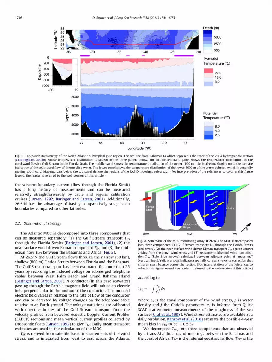
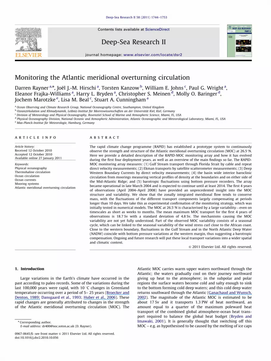
Fig. 1. Top panel: Bathymetry of the North Atlantic subtropical gyre region. The red line from Bahamas to Africa represents the track of the 2004 hydrographic section

(Cunningham, 2005b) whose temperature distribution is shown in the three panels below. The middle left hand panel shows the temperature distribution of the

northward flowing Gulf Stream in the Florida Strait. The middle panel shows the temperature distribution of the upper 1000 m—the isotherms sloping up to the east are

indicative of the southward flow of thermocline water. The lower panel shows the temperature distribution of the lower 5000 m of the water column, which is generally

moving southward. Magenta bars below the top panel denote the regions of the RAPID moorings sub-arrays. (For interpretation of the references to color in this figure

legend, the reader is referred to the web version of this article.)

D. Rayner et al. / Deep-Sea Research II 58 (2011) 1744–17531746

the western boundary current (flow through the Florida Strait)has a long history of measurements and can be measuredrelatively straightforwardly by cable and regular calibrationcruises (Larsen, 1992, Baringer and Larsen, 2001). Additionally,26.51N has the advantage of having comparatively steep basinboundaries compared to other latitudes.

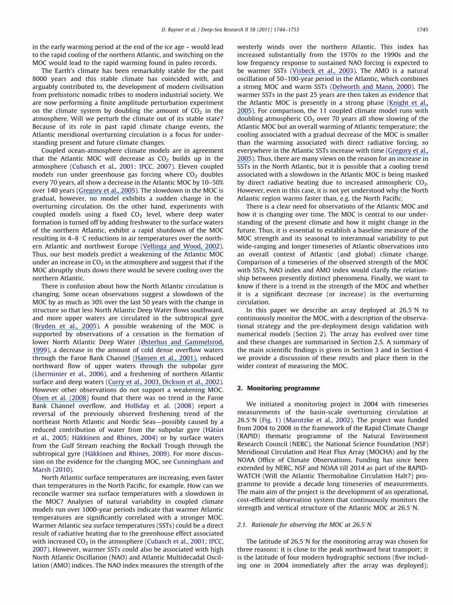
Fig. 2. Schematic of the MOC monitoring array at 261N. The MOC is decomposed

into three components: (1) Gulf Stream transport TGS through the Florida Straits

(red arrow), (2) the near-surface wind driven Ekman transport TEK (green arrow)

arising from the zonal wind stress and (3) geostrophic (thermal wind) contribu-

tion TINT (light blue arrows) calculated between adjacent pairs of ‘‘moorings’’

(vertical lines). Yellow arrows indicate a spatially constant velocity correction that

ensures mass balance across the section. (For interpretation of the references to

color in this figure legend, the reader is referred to the web version of this article.)

2.2. Observational strategy

The Atlantic MOC is decomposed into three components thatcan be measured separately: (1) The Gulf Stream transport TGS

through the Florida Straits (Baringer and Larsen, 2001), (2) thenear-surface wind driven Ekman component TEK and (3) the mid-ocean flow TMO between the Bahamas and Africa (Fig. 2).

At 26.51N the Gulf Stream flows through the narrow (80 km),shallow (800 m) Florida Straits between Florida and the Bahamas.The Gulf Stream transport has been estimated for more than 25years by recording the induced voltage on submerged telephonecables between West Palm Beach and Grand Bahama Island(Baringer and Larsen, 2001). A conductor (in this case seawater)passing through the Earth’s magnetic field will induce an electricfield perpendicular to the motion of the conductor. This inducedelectric field varies in relation to the rate of flow of the conductorand can be detected by voltage changes on the telephone cablerelative to an Earth ground. The voltage variations are calibratedwith direct estimates of the Gulf Stream transport from thevelocity profiles from Lowered Acoustic Doppler Current Profiler(LADCP) sections and mean vertical current profiles collected byDropsonde floats (Larsen, 1992) to give TGS. Daily mean transportestimates are used in the calculation of the MOC.

TEK is derived from satellite based measurements of the windstress, and is integrated from west to east across the Atlantic

according to

TEK ¼�

Z tx

rfdx

where tx is the zonal component of the wind stress, r is waterdensity and f the Coriolis parameter. tx is inferred from QuickSCAT scatterometer measurements of the roughness of the seasurface (Graf et al., 1998). Wind stress estimates are available at adaily resolution. Kanzow et al. (2010) estimate the possible 4-yearmean bias in TEK to be 70.5 Sv.

We decompose TMO into three components that are observedby a trans-Atlantic array of moorings between the Bahamas andthe coast of Africa. TINT is the internal geostrophic flow, TEXT is the

Fig. 3. Testing the MOC monitoring strategy in an eddy-permitting ocean model

(OCCAM; Webb 1996). The horizontal resolution is 0.251 in both longitude and

latitude. Top: placement of ‘‘moorings’’ (vertical lines) and area where velocity can

be calculated based on zonal density differences (blue area). Bottom: MOC at

26.51N and 1100 m depth (blue), reconstruction (red, see main text) and Ekman

contribution (green). (For interpretation of the references to color in this figure

legend, the reader is referred to the web version of this article.)

D. Rayner et al. / Deep-Sea Research II 58 (2011) 1744–1753 1747

zonally integrated reference-level contribution of the geostrophicflow and TWBW is the meridional transport over the continentalshelf west of the moorings WB1 and WB2—referred to as thewestern boundary wedge.

TINT is calculated from the difference in full depth densityprofiles on either side of the Atlantic basin with the profilesderived from temperature, conductivity and pressure measure-ments at discrete levels—hereafter referred to as geostrophicmoorings. In the west the continental shelf slope is steep andthe tall geostrophic mooring WB2 is placed close to the Bahamasescarpment. In the east the shelf slope is much more gradual so aseries of shorter moorings is distributed up the slope to minimisethe effects of bottom triangles where horizontal interpolationat depth would miss significant sections of the ocean (e.g.Whitworth and Peterson, 1985). This series of moorings is mergedto produce a single vertical density profile at the eastern bound-ary. The eastern and western density profiles give the geostrophicinternal transport (TINT) relative to the reference level (ZREF) using

TINT ðzÞ ¼�g=ðfrÞZ 0

ZREF

½rEðzuÞ�rW ðzuÞ�dz

where g is the Earth’s acceleration of gravity, rE the density in theeast and rW the density in the west. We use a reference level of�4740 m.

Bottom pressure recorders are used to compute the time-varying reference level meridional geostrophic velocities. Fromthese the vertically integrated external transport fluctuation(Ti

EXT ) integrated between two sites i and i+1 can be obtainedusing

TiEXT ¼Hi=ðfrÞ½Piþ1

BOT�PiBOT �

where H is the water column height and PBOT is the bottompressure at each site. As H is different for each site the deeper ofthe two is adjusted to the shallower one by removing the densityfluctuations below the depth of the shallower site found from thegeostrophic mooring nearest to the deeper site. The zonal trans-port integral TEXT is found by summing the contributions betweenadjacent moorings so that

TEXT ¼X

TiEXT

The western boundary wedge component (TWBW) is obtainedfrom interpolating and integrating direct velocity measurementsfrom current metres on moorings inshore of the westernmostdensity mooring (Johns et al., 2007). Currents in this regionconsist of the upper-ocean northward Antilles current and theupper and inshore fractions of the Deep Western BoundaryCurrent (DWBC).

If we assume there is no net mass transport across 26.51N thenwe can simplify this with the vertical integral of TMO equalling thevertical integral of the sum of TEK and TGS. This method does notuse TEXT and instead adds a barotropic transport profile to TINT tomaintain mass balance at each time step. Kanzow et al. (2007)show the validity of this approach.

The timeseries of the MOC—defined as the maximum north-ward upper-ocean transport is produced by summing TGS, TEK andTUMO transports, where TUMO is the upper mid-ocean transportfound by vertically integrating TMO down to the deepest north-ward velocity (�1100 m) on each day.

2.3. Array design tests in numerical models

Numerical ocean models are a valuable tool for testing the ad

hoc observational strategy. Prior to the deployment of the RAPID-MOC array we have used models to compare the MOC calculatedfrom the full meridional velocities to reconstructions based on

sub-sampled model data (Hirschi et al., 2003, Baehr et al., 2004,Hirschi and Marotzke, 2007). We obtain the reconstructions bysumming the modelled transport through the Florida Straits, theEkman transport calculated from the zonal wind stress used toforce the model at the surface and the geostrophic transportobtained from ‘‘moorings’’ deployed in the numerical model.Additionally, we add a spatially constant velocity correction sothat there is no net mass transport across the longitude-depthsection at 26.51N (Fig. 2). The high level of agreement foundbetween the simulated MOC and its estimate based on theproposed observing strategy provides a first indication for thesoundness of the approach (Fig. 3) (Hirschi et al., 2003, Baehret al., 2004, Hirschi and Marotzke, 2007).

2.4. Implementation and deployment of the array

The mooring array consists of three sub-arrays: one at thewestern boundary (east of the Bahamas), one at the easternboundary (west of Morocco) and one with moorings on eitherside of the Mid-Atlantic Ridge. The western boundary and easternboundary moorings provide endpoint density profiles used duringthe calculation of the ocean-wide zonally integrated geostrophicflow. The Mid-Atlantic Ridge moorings allow the contribution tothe MOC from the eastern and western basins to be distinguished.

A mooring to obtain a vertical density profile timeseriescomprises a series of self-logging conductivity, temperature anddepth instruments (CTDs) vertically distributed on an anchoredmooring wire supported by distributed buoyancy. Vertical instru-ment resolution increases at shallower depths where the highervertical density gradient requires more reference points for anaccurate interpolation of the density profile. The instruments aretypically set to record data at 15–30 min intervals with datasubsequently low-pass-filtered to remove tides. Moorings areserviced annually with the western boundary serviced in Springand the eastern boundary and Mid-Atlantic Ridge sub-arraysserviced in Autumn.

Fig. 4. Schematic of the three RAPID mooring sub-arrays as deployed in March and April 2004 (Cunningham, 2005a). Moorings are the vertical red lines and instruments

symbols are defined in the key on the right hand panel (CTD—conductivity, temperature, depth recorder; current meter—direct velocity measuring instrument;

BPR—bottom pressure recorder measuring the hydrostatic weight of water, ADCP—an acoustic Doppler current profiler and MMP limit is the profiling range of a profiling

self propelled CTD). Distribution of potential temperature was obtained on a trans-Atlantic hydrographic transect in 2004 following the deployment of the mooring arrays

(Cunningham, 2005b). (For interpretation of the references to color in this figure legend, the reader is referred to the web version of this article.)

Fig. 5. As Fig. 4 but for mooring deployments from 2009 to 2010.

D. Rayner et al. / Deep-Sea Research II 58 (2011) 1744–17531748

The western boundary sub-array is the most important: thelargest fluctuations in the Atlantic MOC occur here compared tothe rest of the ocean basin. Our key mooring WB2, measuringbetween 50 and 3800 m depth, is deployed as close as possible(o3 km) to the ‘‘wall’’ of the continental shelf. WB3 (50–4800 m;27 km offshore from WB2) and WB1 (50–1400 m; 7 km inshorefrom WB2) can be used as backups to provide the density profileif WB2 is lost. WB1, WB0 and WBA also use current meters todirectly measure the DWBC and the shallower Antilles current,allowing the flow inshore of the geostrophic array to be mea-sured. WB4 and WB5 are deployed offshore from the principalmoorings to monitor the offshore extent of the DWBC, thuscapturing thermal wind shear across the entire boundary current.

In the east, to minimise leakage through bottom triangles, aseries of shorter moorings (EBH1– EBH5) were deployed up theslope. As the array evolved this series was extended with EBHi atthe deeper end and a series of still smaller ‘‘mini-moorings’’,EBM1–EBM7, added at the inshore end to reduce risk of data lossthrough fishing activity.

The series of moorings in the east is merged to create a singleprofile as the counterpart to WB2. This is a change from our initialstrategy where we had the tall mooring EB2 deployed in deepwater—with its location chosen as a compromise between thedesire for full water depth and the nearness to the shelf break.

The contribution to MOC variability from the eastern andwestern basins can be distinguished by the Mid-Atlantic Ridgemoorings. MAR1 (up to 50 m depth) and MAR2 (up to 1100 m) aredeployed on the western flank of the ridge, with MAR3 (up to theridge crest at 2500 m) and MAR4 (up to 50 m) initially deployedon the eastern flank.

2.5. Evolution of the mooring array

The array as first deployed in 2004 consisted of 22 moorings(Fig. 4) with the primary geostrophic moorings being WB2 in thewest and EB2 in the east. EB3 was deployed 10 km from EB2 as abackup. The backup to WB2 was WB3, 24 km further offshore. Thevertical resolution of density measurements was 14 discretelevels at the 3900 m deep WB2 site and 13 discrete levels at the3500 m deep EB2 site. The array configuration has been progres-sively modified during subsequent deployments, with the currentconfiguration shown in Fig. 5.

WB2 is still our primary density mooring in the west but theinstrument vertical resolution has been increased to 22 (whenmerging the upper 1400 m with WB1) to allow better interpola-tion of the density profile. At the eastern margin EB2 wasrelocated offshore to the site of EB1 in 5100 m depth followingdamage to the mooring during the first year’s deployment—EB1was extended to 50 m depth to act as the backup and EB3 wasremoved from the array. Subsequently the work by Kanzow et al.(2010) demonstrated the importance of the continental sloperegion for capturing seasonal variability in the MOC so the focusfor the eastern boundary density profile is now the series of shortmoorings that steps up the slope. As such the EB2 site is lessimportant and so the EB1 backup mooring is not required.

The series of shorter moorings has changed slightly as thearray has evolved to try to minimise risk of loss through fishingactivity on the continental slope. The current design has a seriesof mini-moorings (EBM1, 4, 5 and 6) at the inshore end, whicheach consist of a single instrument, thereby spreading the risk oflosing all of the shallow data records. Experience has shown that

D. Rayner et al. / Deep-Sea Research II 58 (2011) 1744–1753 1749

the Mid-Atlantic Ridge moorings are relatively safe so the numberof geostrophic moorings deployed here has been reduced fromfour to three, with MAR4 being removed. The pressure gradientacross the ridge is monitored by the moorings profiling up to theridge crest, with MAR1 providing the upper water column profilefor both sides of the ridge.

In the western boundary sub-array WBH1 and WBH2 wereremoved from the array with WBH2 subsequently being rein-stated but with a different design to include current meters forbetter horizontal interpolation of direct velocity measurements ofthe Deep Western Boundary Current.

The bottom pressure recorders (BPRs) deployed in the firstyear were attached to drop off mechanisms to the bottom of themoorings by magnesium bolts. When these bolts corrode after acouple of hours the BPRs are dropped to the seabed to decouplethem from mooring motion. The BPR remained attached to themooring by a short length of rope so that when the main mooringwas recovered the BPR was recovered too. Due to the large andsomewhat unpredictable drift that pressure sensors can exhibitthe 1-year timeseries is often not enough to remove the driftsatisfactorily. The BPRs were removed from the moorings anddeployed on their own custom moorings – termed landers – thatmount the BPR on a stable frame on the seabed. These are nowdeployed for 2 years at a time with overlapping records of 1 yearso that the second half of the record (which is less affected bydrift) can be used for the calculations of TEXT.

Another change that has taken place in the array design is thedeployment of moorings MAR0 on the western flank of the Mid-Atlantic Ridge and WB6 640 km offshore of the Bahamas in thewestern boundary sub-array. These moorings are both at a depthof 5500 m and have been deployed to study the contribution tothe MOC variability from Antarctic Bottom Water.

2.6. The use of gliders in the array

Two autonomous glider missions have been undertaken toassess the contribution that autonomous gliders could make inmonitoring the MOC, with a specific focus on their use as asubstitute for moorings at the eastern boundary. This part of theRAPID array has suffered losses of instruments and data—largelydue to suspected fishing activity on the continental slope.Furthermore, the findings of Kanzow et al. (2010) mean that thedata from this area are more important than the first thought. It isexpected that gliders will be less susceptible to loss by fishing (inparticular trawling) than the moored instruments and henceimprove data return from this region. Another advantage ofgliders is that data may be retrieved in real-time via iridiumsatellite communications, thus further reducing the risk ofdata loss.

These glider missions took place between 15 September–24November 2008 and 21 May–21 July 2009, between the CanaryIslands and the coast of Morocco. The findings are being preparedfor a subsequent paper (Smeed et al., 2010).

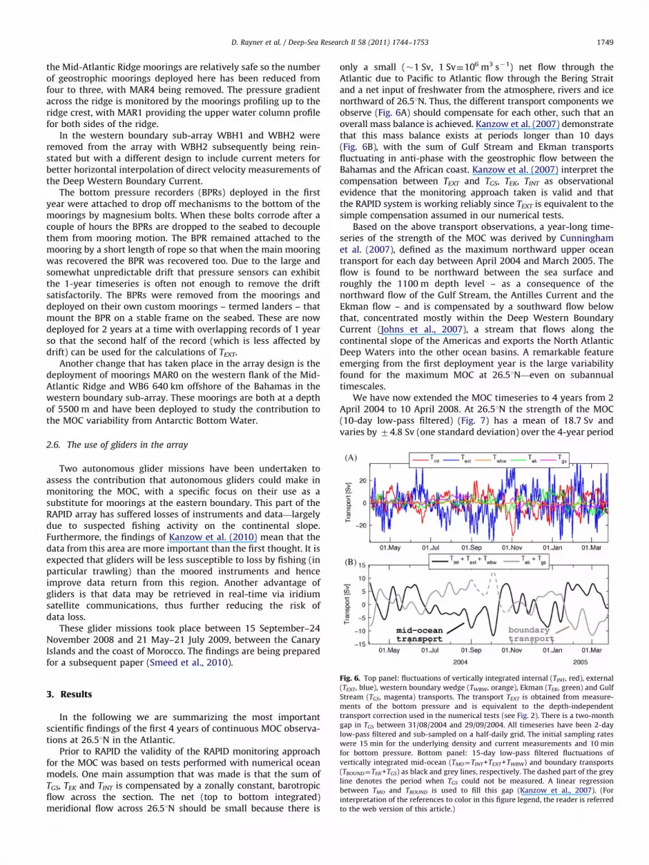
Fig. 6. Top panel: fluctuations of vertically integrated internal (TINT, red), external

(TEXT, blue), western boundary wedge (TWBW, orange), Ekman (TEK, green) and Gulf

Stream (TGS, magenta) transports. The transport TEXT is obtained from measure-

ments of the bottom pressure and is equivalent to the depth-independent

transport correction used in the numerical tests (see Fig. 2). There is a two-month

gap in TGS between 31/08/2004 and 29/09/2004. All timeseries have been 2-day

low-pass filtered and sub-sampled on a half-daily grid. The initial sampling rates

were 15 min for the underlying density and current measurements and 10 min

for bottom pressure. Bottom panel: 15-day low-pass filtered fluctuations of

vertically integrated mid-ocean (TMO¼TINT+TEXT+TWBW) and boundary transports

(TBOUND¼TEK+TGS) as black and grey lines, respectively. The dashed part of the grey

line denotes the period when TGS could not be measured. A linear regression

between TMO and TBOUND is used to fill this gap (Kanzow et al., 2007). (For

interpretation of the references to color in this figure legend, the reader is referred

to the web version of this article.)

3. Results

In the following we are summarizing the most importantscientific findings of the first 4 years of continuous MOC observa-tions at 26.51N in the Atlantic.

Prior to RAPID the validity of the RAPID monitoring approachfor the MOC was based on tests performed with numerical oceanmodels. One main assumption that was made is that the sum ofTGS, TEK and TINT is compensated by a zonally constant, barotropicflow across the section. The net (top to bottom integrated)meridional flow across 26.51N should be small because there is

only a small (�1 Sv, 1 Sv�106 m3 s�1) net flow through theAtlantic due to Pacific to Atlantic flow through the Bering Straitand a net input of freshwater from the atmosphere, rivers and icenorthward of 26.51N. Thus, the different transport components weobserve (Fig. 6A) should compensate for each other, such that anoverall mass balance is achieved. Kanzow et al. (2007) demonstratethat this mass balance exists at periods longer than 10 days(Fig. 6B), with the sum of Gulf Stream and Ekman transportsfluctuating in anti-phase with the geostrophic flow between theBahamas and the African coast. Kanzow et al. (2007) interpret thecompensation between TEXT and TGS, TEK, TINT as observationalevidence that the monitoring approach taken is valid and thatthe RAPID system is working reliably since TEXT is equivalent to thesimple compensation assumed in our numerical tests.

Based on the above transport observations, a year-long time-series of the strength of the MOC was derived by Cunninghamet al. (2007), defined as the maximum northward upper oceantransport for each day between April 2004 and March 2005. Theflow is found to be northward between the sea surface androughly the 1100 m depth level – as a consequence of thenorthward flow of the Gulf Stream, the Antilles Current and theEkman flow – and is compensated by a southward flow belowthat, concentrated mostly within the Deep Western BoundaryCurrent (Johns et al., 2007), a stream that flows along thecontinental slope of the Americas and exports the North AtlanticDeep Waters into the other ocean basins. A remarkable featureemerging from the first deployment year is the large variabilityfound for the maximum MOC at 26.51N—even on subannualtimescales.

We have now extended the MOC timeseries to 4 years from 2April 2004 to 10 April 2008. At 26.51N the strength of the MOC(10-day low-pass filtered) (Fig. 7) has a mean of 18.7 Sv andvaries by 74.8 Sv (one standard deviation) over the 4-year period

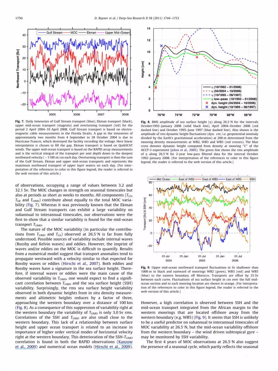
Fig. 8. RMS amplitude of sea surface height (Z) along 26.51N for the intervals

October1992–January 2008 (solid black line), April 2004–October 2006 (red

dashed line) and October 1995–June 1997 (blue dashed line). Also shown is the

amplitude of rms dynamic height fluctuations (dyn. cm; i.e. geopotential anomaly

divided by the Earth’s gravitational acceleration) at 200 m determined from the

mooring density measurements at WB2, WB3 and WB5 (red crosses). The blue

cross denotes dynamic height computed from density at mooring ‘‘C’’ of the

ACCP-3 experiment (Johns et al., 2005). The green line shows the rms amplitude

of Z along 26.51N for 2-year low-pass filtered data for the interval October

1992–January 2008. (For interpretation of the references to color in this figure

legend, the reader is referred to the web version of this article.)

Fig. 9. Upper mid-ocean northward transport fluctuations in Sv shallower than

1000 m in black and eastward of moorings WB2 (green), WB3 (red) and WB5

(blue) to the eastern boundary off Morocco. Transports are offset by 25 Sv

between each curve. Fluctuations of sea surface height in cm over the full mid-

ocean section and to each mooring location are shown in orange. (For interpreta-

tion of the references to color in this figure legend, the reader is referred to the

web version of this article.)

Fig. 7. Daily timeseries of Gulf Stream transport (blue), Ekman transport (black),

upper mid-ocean transport (magenta) and overturning transport (red) for the

period 2 April 2004–10 April 2008. Gulf Stream transport is based on electro-

magnetic cable measurements in the Florida Straits. A gap in the timeseries of

approximately two months from 4 September to 28 October 2004 is due to

Hurricane Frances, which destroyed the facility recording the voltage. Here linear

interpolation is chosen to fill the gap. Ekman transport is based on QuikSCAT

winds. The upper mid-ocean transport is based on the RAPID array measurements

and is the vertical integral of the transport per unit depth down to the deepest

northward velocity (�1100 m) on each day. Overturning transport is then the sum

of the Gulf Stream, Ekman and upper mid-ocean transports and represents the

maximum northward transport of upper layer waters on each day. (For inter-

pretation of the references to color in this figure legend, the reader is referred to

the web version of this article.)

D. Rayner et al. / Deep-Sea Research II 58 (2011) 1744–17531750

of observations, occupying a range of values between 3.2 and32.1 Sv. The MOC changes in strength on seasonal timescales butalso at periods as short as weeks to months. All components (TGS,TEK and TUMO) contribute about equally to the total MOC varia-bility (Fig. 7). Whereas it was previously known that the Ekmanand Gulf Stream transports can exhibit a large variability onsubannual to interannual timescales, our observations were thefirst to show that a similar variability is found for the mid-oceantransport TUMO.

The nature of the MOC variability (in particular the contribu-tions from TUMO and TGS) observed at 26.51N is far from fullyunderstood. Possible sources of variability include internal waves(Rossby and Kelvin waves) and eddies. However, the imprint ofwaves and/or eddies on the MOC is difficult to quantify. Resultsfrom a numerical model suggest that transport anomalies tend topropagate westward with a velocity similar to that expected forRossby waves or eddies (Hirschi et al., 2007). Both eddies andRossby waves have a signature in the sea surface height. There-fore, if internal waves or eddies were the main cause of theobserved variability in TUMO, one would expect to find a signifi-cant correlation between TUMO and the sea surface height (SSH)variability. Surprisingly, the rms sea surface height variabilityobserved in both dynamic heights from in situ density measure-ments and altimetric heights reduces by a factor of three,approaching the western boundary over a distance of 100 km(Fig. 8). As a consequence of this suppression of variability right atthe western boundary the variability of TUMO is only 3.0 Sv rms.Correlations of the SSH and TUMO are also small close to thewestern boundary. This lack of a relationship between surfaceheight and upper ocean transport is related to an increase inimportance of higher order vertical modes of horizontal velocityright at the western boundary. This deterioration of the SSH-TUMO

correlation is found in both the RAPID observations (Kanzowet al., 2009) and numerical ocean models (Hirschi et al., 2009).

However, a high correlation is observed between SSH and themid-ocean transport integrated from the African margin to thewestern moorings that are located offshore away from thewestern boundary (e.g. WB5) (Fig. 9). It seems that SSH is unlikelyto be a useful predictor on subannual to interannual timescales ofMOC variability at 26.51N, but the mid-ocean variability offshorefrom the western boundary – the wind driven subtropical gyre –may be monitored by SSH variability.

The first 4 years of MOC observations at 26.51N also suggestthe presence of a seasonal cycle, which partly reflects the seasonal

D. Rayner et al. / Deep-Sea Research II 58 (2011) 1744–1753 1751

cycle observed for the upper mid-ocean transport TUMO. Recentwork has shown that for TUMO this seasonal variability has itsorigin at both the eastern and western margins. The slightly largercontribution originates from the eastern margin and can beexplained by the heaving of isopycnals linked to the seasonalcycle of the wind-stress curl at the eastern margin (Kanzow et al.,2010; Chidichimo et al., 2010).

Bryden et al. (2009) show that at 4000 m depth at the westernboundary off Abaco, bottom pressure fluctuations compensateinstantaneously for baroclinic fluctuations in the strength andstructure of the Deep Western Boundary Current. Therefore,baroclinic fluctuations in the Deep Western Boundary Currentare compensated locally by bottom pressure fluctuations and sothere is no mid-ocean flow resulting from fluctuations in the DeepWestern Boundary Current. Residual bottom pressure fluctuationsat the western boundary (bottom pressure fluctuations minusbottom pressure, which account for baroclinic variability of theDeep Western Boundary Current) compensate for fluctuations inFlorida Current transport. Thus fluctuations in both the FloridaCurrent and Deep Western Boundary Currents are compensatedbarotropically very close to the western boundary.

4. Discussion and summary

The 4 years of MOC observations have already provided anunprecedented insight into the MOC variability. With the initialmeasurements we were also able to determine that the historicestimates of the strength of the MOC, based on synoptic ship-board expeditions (Bryden et al., 2005), were within the range ofsubannual variability of the MOC (Cunningham et al., 2007).

One aspect that needs to be better understood and which isthe subject of ongoing research is the climatic relevance of theMOC observations. A question of particular interest is whether wecan use the RAPID data to improve climate predictions (onseasonal to perhaps decadal timescales). On the way to addressthis question we will need to be able to put the local MOCobservations from 26.51N into a wider spatial context and try toestablish the meridional coherence of the observed MOC varia-bility. Does the meridional coherence depend on the frequency(i.e. are subannual signals mainly local to 26.51N while inter-annual and longer signals reflect processes affecting a largefraction of the North Atlantic basin (e.g. Bingham et al., 2007)?).

To address these points we will need to make use of observa-tions from other locations and numerical models. Numericalstudies suggest that fast propagating boundary waves can lead tomeridionally coherent MOC changes. This was found for idealisedmodel setups (e.g. Kawase, 1987, Johnson and Marshall, 2002) andin more realistic models (e.g. Bingham et al., 2007, Biastoch et al.,2008, Zhang, 2008). However, model results also suggest thatlocally, large high-frequency MOC variability could mask thecoherence (e.g. Hirschi et al., 2007). To assess whether meridionallycoherent MOC changes can be observed, the MOC transport from26.51N needs to be considered alongside data from other observingsystems. From 2000 to 2009 the Meridional Overturning VariabilityExperiment (MOVE) provided NADW observations at 161N in theAtlantic (e.g. Kanzow et al., 2006, 2008). Additionally, continuousobservations have been made at the western boundary at 401Nsince 2004 in the framework of the RAPID funded Western AtlanticVariability Experiment (WAVE, http://www.pol.ac.uk/home/research/theme10/rapidII.php, Hughes et al., 2002). Bottom pres-sure measurements are available at 26.51N, as well as at thelocations of MOVE and WAVE and can be used to test on whattimescales we find coherent signals between the different obser-ving systems. Model studies suggest a close link between bottompressure and MOC fluctuations (e.g. Roussenov et al., 2008). It

would also be instructive if we could compare transports, e.g. ofNADW at 26.51N and 161N, in terms of transports in isopycnalcoordinates as this could allow us to infer water mass changesbetween different latitudes. However, since the transports at26.51N and 161N are obtained from density observations at onlya few longitudes (‘‘end point method’’), the full zonal densitystructure is not available, which means that a projection oftransports onto density coordinates is not obvious.

One possible way to overcome the inability of ocean models toreproduce the observed ocean circulation and the inevitable gapsin observations is to assimilate the observed MOC and otherobservational ocean data into numerical models. There aredifferent data assimilation schemes (e.g. Wunsch and Stammer,1998, Kohl and Stammer, 2008, Smith and Haines, 2008,Balmaseda et al., 2007) that assimilate data from hydrographicsections, Argo floats or from satellites with the aim to produceocean states that are as close as possible to the real ocean (‘‘oceananalyses’’). Apart from providing global, physically consistentocean states that are useful for studying ocean processes(e.g. Kohl, 2005; Cabanes et al., 2008), the value of these oceananalyses lies in their potential use for improving climatepredictions. Smith et al. (2007) showed that the assimilation ofocean observations into their decadal prediction system(DePreSys) improved the forecast quality in a set of 10-yearhindcasts. Research done in the framework of RAPID-WATCH willestablish the value of the RAPID-MOC data from 26.51N, when it isused as an additional constraint in ocean models and forecastingsystems like DePreSys (Smith et al., 2010; Baehr, 2010).

The RAPID-MOC monitoring system is funded by NERC, NOAAand NSF for a total of 10 years through to 2014 and shoulddocument the size and structure of the subannual to interannualvariability in the Atlantic MOC. From a 10-year record, we cancompare the interannual variations in the MOC with Atlantic seasurface temperature variations and with the North AtlanticOscillation index and start to understand links between theAtlantic meridional overturning circulation and climate. Theobservational estimates of MOC variability will also serve as anew benchmark against which the variability in coupled climatemodels (which exhibit substantially different amplitude andstructure in MOC interannual variability) can be comparedand validated. With a 10-year record of MOC strength andstructure and by considering ocean observations from otherlocations in the North Atlantic (e.g. in the framework of the EUfunded Thermohaline Overturning—at Risk? (THOR) project), wecan also start to assess whether there is a statistically significanttrend in the strength of the MOC above the subannual andinterannual variability and we can build the groundwork forpredicting the course of Atlantic climate change over the next50 years.

Appendix

Data availability

Data from the RAPID project are logged with the BritishOceanographic Data Centre (BODC) on acquisition. Following theNERC data policy for RAPID-WATCH (http://www.bodc.ac.uk/projects/uk/rapid/data_policy/), data are made freely availablefrom the BODC website (http://www.bodc.ac.uk). Timeseries ofthe overturning and component transports, along with griddedmooring data, are available from the project webpage (http://www.noc.soton.ac.uk/rapidmoc).

The Florida Current cable data are made freely availableby the Atlantic Oceanographic and Meteorological Laboratory

D. Rayner et al. / Deep-Sea Research II 58 (2011) 1744–17531752

(http://www.aoml.noaa.gov/phod/floridacurrent/) and are fundedby the NOAA Office of Climate Observations.

The surface layer or Ekman contribution to the MOC iscalculated from winds obtained by the QuickSCAT satellite scat-terometer (SeaWinds on QuickSCAT. Mission, http://winds.jpl.nasa.gov/missions/quickscat/index.cfm).

References

Baehr, J., Hirschi, J., Beismann, J.-O., Marotzke, J., 2004. Monitoring the meridionaloverturning circulation in the North Atlantic: a model-based array designstudy. Journal of Marine Research 62, 283–312.

Baehr, J., 2010. Influence of the 261N RAPID/MOCHA array and Florida Currentcable observations on the ECCO-GODAE state estimate. Journal of PhysicalOceanography 40, 865–879.

Balmaseda, M., Smith, G., Haines, K., Anderson, D., Palmer, T., Vidard, A., 2007.Historical reconstruction of the Atlantic Meridional Overturning Circulationfrom the ECMWF operational ocean reanalysis. Geophysical Research Letters34, L23615.

Baringer, M.O., Larsen, J.C., 2001. Sixteen years of Florida Current transport at271N. Geophysical Research Letters 28, 3182–3197.

Biastoch, A., Boning, C.W., Lutjeharms, J.R.E., 2008. Agulhas leakage dynamicsaffects decadal variability in overturning circulation. Nature 456.

Bingham, R.J., Hughes, C.W., Roussenov, V., Williams, R.G., 2007. Meridionalcoherence of the North Atlantic meridional overturning circulation. Geophy-sical Research Letters 2007 (34), L23606.

Broecker, W.S., Denton, G.H., 1989. The role of ocean-atmosphere reorganisationsin glacial cycles. Geochimica et Cosmochimica Acta 53, 2465–2501.

Bryden, H.L., Imawaki, S., 2001. Ocean heat transport. In: Siedler, G., Church, J.,Gould, J. (Eds.), Ocean Circulation and Climate. Academic Press, pp. 455–474.

Bryden, H.L., Longworth, H.L., Cunningham, S.A., 2005. Slowing of the AtlanticMeridional Overturning Circulation at 251N. Nature 438, 655–657.

Bryden, H.L., Mujahid, A., Cunningham, S.A., Kanzow, T., 2009. Adjustment of thebasin-scale circulation at 261N to variations in Gulf Stream, Deep WesternBoundary Current and Ekman transports as observed by the RAPID array.Ocean Science 5, 421–433.

Cabanes, C., Lee, T., Fu, L.-T., 2008. Mechanisms of interannual variations of themeridional overturning circulation of the North Atlantic Ocean. Journal ofPhysical Oceanography 38, 467–480.

Chidichimo, M.P., Kanzow, T., Cunningham, S.A., Marotzke, J., 2010. The contribu-tion of eastern-boundary density variations to the Atlantic meridional over-turning circulation at 26.51N. Ocean Science 6, 475–490.

Cubasch, U., Meehl, G.A., Boer, G.J., Stouffer, R.J., Dix, M., Noda, A., Senior, C.A.,Raper, S., Yap, K.S., 2001. Projections of future climate change, Chapter 9. In:Houghton, J.T. (Ed.), Climate Change 2001: The Scientific Basis. CambridgeUniversity Press, pp. 525–582.

Cunningham, S.A., Kanzow, T.O., Rayner, D., Barringer, M.O., Johns, W.E., Marotzke,J., Longworth, H.R., Grant, E.M., Hirschi, J.J.-M., Beal, L.M., Meinen, C.S., Bryden,H.L., 2007. Temporal variability of the Atlantic Meridional OverturningCirculation at 26.51N. Science 317, 935–938.

Cunningham, S.A., 2005a. RRS Discovery Cruises 277 (26 Mar.–16 Apr. 2004) and278 (19 Mar.–30 Mar. 2004): monitoring the Atlantic Meridional OverturningCirculation at 26.51N. Cruise Report No. 53, 103pp.

Cunningham, S.A., 2005b. RRS Discovery Cruise 279, 04 Apr.–10 May 2004: atransatlantic hydrographic section at 24.51N. Cruise Report No. 54, 198pp.

Cunningham, S.A., Marsh, R., 2010. Observing and modeling changes in theAtlantic MOC. Wiley Interdisciplinary Reviews: Climate Change 1, 180–191.

Curry, R., Dickson, B., Yashayaev, I., 2003. A change in the freshwater balance of theAtlantic Ocean over the past four decades. Nature 426, 826–829.

Dansgaard, W., Johnsen, S.J., Clausen, H.B., Dahl-Jensen, D., Gundestrup, N.S.,Hammer, C.U., Hvidberg, C.S., Steffensen, J.P., Sveinbjornsdottir, A.E., Jouzel,J., Bond, G., 1993. Evidence for general instability of past climate from a250 kyr ice-core record. Nature 364, 218–220.

Delworth, T.L., Mann, M.E., 2000. Observed and simulated multidecadal variabilityin the Northern Hemisphere. Climate Dynamics 16, 661–676.

Dickson, R., Yashayaev, I., Meincke, J., Turrell, B., Dye, S., Holfort, J., 2002. Rapidfreshening of the deep North Atlantic Ocean over the past four decades. Nature416, 832–837.

Ganachaud, A., Wunsch, C., 2002. Large-scale ocean heat and freshwater transportsduring the World Ocean Circulation Experiment. Journal of Climate 16, 696–705.

Graf, J., Sasaki, C., Winn, C., Liu, T., Tsai, W., Freilich, M., Long, D., 1998. NASAscatterometer experiment. Acta Astronautica 43, 397–407.

Gregory, J.M., Dixon, K.W., Stouffer, R.J., Weaver, A.J., Driesschaert, E., Eby, M.,Fichefet, T., Hasumi, H., Hu, A., Jungclaus, J.H., Kamenkovich, I.V., Levermann, A.,Montoya, M., Murakami, S., Nawrath, S., Oka, A., Sokolov, A.P., Thorpe, R.B., 2005.A model intercomparison of changes in the Atlantic thermohaline circulation inresponse to increasing atmospheric CO2 concentration. Geophysical ResearchLetters 32, L12703. doi:10.1029/2005GL023209.

Hakkinen, S., Rhines, P.B., 2004. Decline of subpolar North Atlantic circulationduring the 1990s. Science 304, 555–559.

Hakkinen, S., Rhines, P.B., 2009. Shifting Surface Currents in the Northern NorthAtlantic Ocean. Journal of Geophysical Research 114, C04005. doi:10.1029/2008JC004883.

Hansen, B., Turrell, W.R., Østerhus, S., 2001. Decreasing outflow from the Nordicseas into the Atlantic Ocean through the Faroe Bank Channel since 1950.Nature 411, 927–930.

Hatun, H., Sandø, A.B., Drange, H., Hansen, B., Valdimarsson, H., 2005. Influence ofthe Atlantic Subpolar Gyre on the thermohaline circulation. Science 309,1841–1844.

Hirschi, J., Marotzke, J., 2007. Reconstructing the meridional overturning circula-tion from boundary densities and the zonal wind stress. Journal of PhysicalOceanography 37, 743–763.

Hirschi, J., Baehr, J., Marotzke, J., Stark, J., Cunningham, S.A., Beismann, J.-O., 2003.A monitoring design for the Atlantic meridional overturning circulation.Geophysical Research Letters 30. doi:10.1029/2002GL016776.

Hirschi, J.J.-M., Killworth, P.D., Blundell, J.R., 2007. Subannual, seasonal andinterannual variability of the North Atlantic Meridional Overturning Circula-tion. Journal of Physical Oceanography 37, 1246–1265.

Hirschi, J.J.-M., Killworth, P.D., Blundell, J.R., Cromwell, D., 2009. Sea Surface heightsignals as indicators for oceanic meridional mass transports. Journal ofPhysical Oceanography 39, 581–601. doi:10.1175/2008JPO3923.1.

Holliday, N.P., Hughes, S.L., Bacon, S., Beszczynska-Moller, A., Hansen, B., Lavin, A.,Loeng, H., Mork, K.A., Østerhus, S., Sherwin, T., Walczowski, W., 2008. Reversal ofthe 1960s to 1990s freshening trend in the northeast North Atlantic and NordicSeas. Geophysical Research Letters 35, L03614. doi:10.1029/2007GL032675.

Huber, C., Leuenberger, M., Spahni, R., Fluckiger, J., Schwander, J., Stocker, T.F.,Johnson, S., Landais, A., Jouzel, J., 2006. Isotope calibrated Greenland tempera-ture record over Marine Isotope Stage 3 and its relation to CH4. Earth andPlanetary Science Letters 243, 504–519. doi:10.1016/j.epsl.2006.01.002.

Hughes, C., D. Marshall and R. Williams. 2002. A monitoring array along thewestern margin of the North Atlantic, Research Proposal submitted to NaturalEnvironment Research Council.

IPCC, 2007. Summary for policymakers. In: Solomon, S., Qin, D., Manning, M., Chen,Z., Marquis, M., Averyt, K.B., Tignor, M., Miller, H.L. (Eds.), Climate Change 2007:The Physical Science Basis, Contribution of Working Group I to the FourthAssessment Report of the Intergovernmental Panel on Climate Change. Cam-bridge University Press, Cambridge, New York.

Johns, W.E., Kanzow, T., Zantopp, R., 2005. Estimating ocean transports withdynamic height moorings: an application in the Atlantic Deep WesternBoundary Current at 261N. Deep-Sea Research I 52, 1542–1567.

Johns, W.E., Beal, L.M., Baringer, M.O., Molina, J., Rayner, D., Cunningham, S.A.,Kanzow, T.O., 2007. Variability of shallow and Deep Western BoundaryCurrents off the Bahamas during 2004–2005: results from the 261N RAPID-MOC array. 2008. Journal of Physical Oceanography 38, 605–623.

Johnson, H.L., Marshall, D.P., 2002. A theory for the surface Atlantic response tothermohaline variability 32, 1121–1132.

Kanzow, T., Send, U., Zenk, W., Chave, A.D., Rhein, M., 2006. Monitoring theintegrated deep meridional flow in the tropical North Atlantic: long-termperformance of a geostrophic array. Deep Sea Research I 53, 528–546.

Kanzow, T., Cunningham, S.A., Rayner, D., Hirschi, J.J.-M., Johns, W.E., Baringer,M.O., Bryden, H.L., Beal, L.M., Meinen, C.S., Marotzke, J., 2007. Observed flowcompensation associated with the MOC at 26.51N in the Atlantic. Science 317,938–941.

Kanzow, T., Send, U., McCartney, M., 2008. On the variability of the deepmeridional transports in the tropical North Atlantic. Deep-Sea Research I 55,1601–1623.

Kanzow, T., Johnson, H., Marshall, D., Cunningham, S.A., Hirschi, J.J.-M., Mujahid,A., Bryden, H.L., Johns, W.E., 2009. Basin-wide integrated volume transports inan eddy-filled ocean. Journal of Physical Oceanography 39, 3091–3110.

Kanzow, T., Cunningham, S.A., Johns, W.E., Hirschi, J.J.-M., Marotzke, J., Baringer, M.O.,Meinen, C.S., Chidichimo, M.P., Atkinson, C., Beal, L.M., Bryden, H.L., Collins, J.,2010. Seasonal variability of the Atlantic meridional overturning circulation at26.51N. Journal of Climate 23, 5678–5698.

Kawase, M., 1987. Establishment of deep ocean circulation driven by deep-waterproduction. Journal of Physical Oceanography 17, 2294–2317.

Knight, J.R., Allan, R.J., Folland, C.K., Vellinga, M., Mann, M.E., 2005. A signature ofpersistent natural thermohaline circulation cycles in observed climate. Geo-physical Research Letters 32, L20708. doi:10.1029/2005GL024233.

Kohl, A., 2005. Anomalies of Meridional Overturning: mechanisms in the NorthAtlantic. Journal of Physical Oceanography 35, 1455–1472.

Kohl, A., Stammer, D., 2008. Variability of the Meridional Overturning in the NorthAtlantic from the 50-year GECCO State estimation. Journal of PhysicalOceanography 38, 1913–1930.

Larsen, J.C., 1992. Transport and heat flux of the Florida Current at 271N derived fromcross-stream voltages and profiling data: theory and observations. PhilosophicalTransactions of the Royal Society of London A 338, 169–236.

Lherminier, P., H. Mercier, C. Gourcuff, Treguier, A.M., 2006. MOC observationsbetween Greenland and Portugal in Summers 1997, 2002 and 2004. EGUAbstract, presented in Vienna in April.

Marotzke, J., Cunningham S.A., Bryden, H.L.. 2002. Monitoring the Atlanticmeridional overturning circulation at 26.51N, Research Proposal submittedto Natural Environment Research Council.

Olsen, S.M, Hansen, B., Quadfasel, D., Østerhus, S., 2008. Observed and modelledstability of overflow across the Greenland-Scotland ridge. Nature 455,519–522. doi:10.1038/nature07302.

Østerhus, S., Gammelsrod, T., 1999. The abyss of the Nordic Seas is warming.Journal of Climate 12, 3297–3304.

Roussenov, V.M., Williams, R.G., Hughes, C.W., Bingham, R., 2008. Boundary wavecommunication of bottom pressure and overturning changes for the North

D. Rayner et al. / Deep-Sea Research II 58 (2011) 1744–1753 1753

Atlantic. Journal of Geophysical Research 113, C08042. doi:10.1029/2007/JC004501.

Smeed, D.A. et al., 2010. Bellamite and Dynamite RAPID Deployment Report,National Oceanography Centre, Southampton, Cruise Report No. 44.

Smith, D.M., Cusack, S., Colman, A.W., Folland, C.K., Harris, G.R., Murphy, J.M.,2007. Improved surface temperature prediction for the coming decade from aglobal climate model. Science 317, 796–799.

Smith, G.C., Haines, K., 2008. Evaluation of the S(T) assimilation method with theargo dataset. Quarterly Journal of the Royal Meteorological Society 135,739–756.

Smith, G.C., Haines, K., Kanzow, T., Cunningham, S.A., 2010. Impact of hydro-graphic data assimilation on the modelled Atlantic meridional over- turningcirculation. Ocean Science 6, 761–774.

Vellinga, M., Wood, R.A., 2002. Global climatic impacts of a collapse of the Atlanticthermohaline circulation. Climatic Change 54, 251–267.

Visbeck, M., E.P. Chassignet, R. Curry, T. Delworth, Dickson, B., Krahmann, G., 2003.The ocean’s response to North Atlantic Oscillation variability. In: The NorthAtlantic Oscillation, J.W. Hurrell, Y. Kushnir, G. Ottersen, M. Visbeck (Eds.),Geophysical Monograph Series, vol. 134, pp. 113–146.

Webb, D.J., 1996. An ocean model code for array processor computers. Computers& Geosciences 22, 569–578.

Whitworth III, T., Peterson, R.G., 1985. Volume transport of the AntarcticCircumpolar Current from bottom pressure measurements. Journal of PhysicalOceanography 15, 810–816.

Wunsch, C., Stammer, D., 1998. Satellite altimetry, the marine geoid, and theoceanic general circulation. Annual Review of Earth and Planetary Sciences 26,219–253.

Zhang, 2008. Coherent surface-subsurface fingerprint of the Atlantic meridionaloverturning circulation. Geophysical Research Letters 35, L20705. doi:10.1029/2008GL035463.