modeling of heat transfer in rooms in the modelica buildings library

MODELING OF HEAT TRANSFER IN ROOMS IN THE MODELICA“BUILDINGS” LIBRARY

Michael Wetter, Wangda Zuo, Thierry Stephane NouiduiSimulation Research Group, Building Technologies Department

Environmental Energy Technologies Division, Lawrence Berkeley National LaboratoryBerkeley, CA 94720, USA

ABSTRACTThis paper describes the implementation of the

room heat transfer model in the free open-sourceModelica “Buildings” library. The model can beused as a single room or to compose a multizonebuilding model. We discuss how the model is de-composed into submodels for the individual heattransfer phenomena. We also discuss the mainphysical assumptions. The room model can beparameterized to use di↵erent modeling assump-tions, leading to linear or non-linear di↵erentialalgebraic systems of equations. We present nu-merical experiments that show how these assump-tions a↵ect computing time and accuracy for se-lected cases of the ANSI/ASHRAE Standard 140-2007 envelop validation tests.

INTRODUCTIONIn 2007, the Lawrence Berkeley National Lab-

oratory started the development of the free open-source Modelica “Buildings” library. The libraryconsists of component models for building energyand control systems to support

• rapid prototyping of new building systems,• analysis of the operation of existing buildings,• development and performance assessment ofbuilding control algorithms, and

• reuse of models during operation for energy-minimizing controls, fault detection and diag-nostics.

The library provides users with a collection ofopen-source models that they can use, extend andadjust to suit their individual needs.The use of equation-based modeling languages

in the building simulation community goes backto Sahlin and Sowell (1989) and Sowell, Buhl,and Nataf (1989). In contrast to these early de-velopments, nowadays such development can bedone using Modelica, an industry-driven, opennon-proprietary language and associated libraries,modeling, simulation and optimization environ-ments (Mattsson and Elmqvist 1997). The Mod-elica development and standardization is doneby various people from diverse application do-mains and scientific disciplines. Such a mod-

eling approach is di↵erent compared to conven-tional building simulation programs such as Ener-gyPlus, DOE-2, TRNSYS and ESP-r: Equation-based languages allow a model builder to declarea set of algebraic equations, ordinary di↵erentialequations and finite state machines that define thephysics of a component or the logic of a controlsequence. These equations need not be explicit orordered. A model translator analyzes these equa-tions, and using computer algebra, rearranges andsolves these systems of equations symbolically – asfar as possible – to reduce the number of variablesthat need to be iteratively solved for during thetime integration. Next, executable code is gener-ated, generally in the form of C-code, and linkedto numerical solvers. See Cellier and Kofman(2006) for details. Using the same model archi-tecture, di↵erent code can be generated for sim-ulation, for embedded systems and for optimiza-tion. Also, model linearization and state initial-ization, as for example needed by optimization-based control algorithms, are generally supportedby equation-based simulation programs. Thishigh-level model formulation leads to more flex-ible and intuitive model use as the compositionof system models can be done schematically us-ing acausal models instead of using a signal-flowchart. The decomposition of the system modelneed not follow primary and secondary HVACsystem loop structures or other non-intuitive con-straints that may be imposed by a simulation en-gine. Since the model formulation is independentof the solution scheme of the simulation engine,they are easier to exchange among users, moreconcise and faster to develop (Wetter 2011a). Inaddition, since domain-specific libraries can be de-veloped separately from the simulation engines,the e↵ort for engine development can be spreadacross various application domains.

The motivation for the development of the“Buildings” library is described in Wetter(2009a). The first versions of the library havebeen described in Wetter (2009c) and Wetter(2009b), and a recent update has been publishedin Wetter, Zuo, and Nouidui (2011). The here de-

Proceedings of Building Simulation 2011: 12th Conference of International Building Performance Simulation Association, Sydney, 14-16 November.

- 1096 -

scribed building envelope model is more compre-hensive than the one described in Wetter (2006b).In particular, the here described model containsa detailed window model, it can be interfaced di-rectly with TMY3 weather data and it contains amore detailed infrared radiation balance.This paper presents an overview of the main

packages in the library. Next, it describes themodel for heat transfer through the building en-velope and within a room to inform users aboutthe main physical assumptions and model struc-ture. Numerical experiments are presented to dis-cuss the e↵ect of di↵erent model configurations oncomputing time and model accuracy relative toresults reported in the ASNI/ASHRAE Standard140-2007 envelop validation.

OVERVIEW OF THE LIBRARYThe “Buildings” library version 0.12 contains

the following main packages:

Airflow: This package contains models for mul-tizone airflow and contaminant transport. Themodels compute air flow between di↵erentrooms and between a room and the exteriorenvironment. Each room volume is assumedto be completely mixed. The driving force forthe air flow are pressure di↵erences that can beinduced, e.g., by flow imbalance of the HVACsystem, density di↵erence across large openingssuch as doors or open windows, stack e↵ects inhigh rise buildings, and wind pressure on thebuilding facade. The physics of the models inthis package are described in Wetter (2006a).However, this package is a new implementationthat led to simpler models and more robust sim-ulation due to the use of the Modelica streamconnectors (Franke et al. 2009b) that have beenintroduced in the Modelica.Fluid package ofthe Modelica Standard Library in 2009 (Frankeet al. 2009a).

BoundaryConditions: This package containsmodels to read and compute boundary condi-tions, such as TMY3 weather data, solar irra-diation and sky temperatures.

Controls: This package contains blocks thatmodel continuous time and discrete time con-trollers. There are also blocks that can be usedto schedule set points.

Fluid: This is the largest package of the libraryand contains component models for air-basedand water-based HVAC systems. The packagecontains models such as chillers, cooling towers,heat exchangers, flow resistances, valves and airdampers, flow sources, pumps and fans, sen-sors and energy storage. A recent description

of these models can be found in Wetter, Zuo,and Nouidui (2011).

HeatTransfer: This package contains modelsfor steady-state and dynamic heat transferthrough opaque constructions such as multi-layered walls. It also contains models for heattransfer through glazing systems which will bedescribed in the next section.

Rooms: This package contains models for heattransfer in rooms and through the building en-velope. These models will be described in thenext section.

Utilities: This package contains utility modelssuch as for computing thermal comfort, to ex-change data with the Building Controls VirtualTest Bed (Wetter 2011b) or to compute psy-chrometric functions.

In total, the “Buildings” library contains about200 models and blocks, 70 functions and 200 ex-ample and test models.

ACAUSAL MODELSIn Modelica, models can be acausal using ports

where the input and output causality need not bespecified by the model developer. Rather, inputand output variables are determined by a codegenerator that employs symbolic algebra to de-termine a computationally e�cient solution se-quence.It is customary that the ports declare poten-

tial variables (temperature T , pressure p, electri-cal voltage U) and flow variables (heat flow rateQ, mass flow rate m, electrical current I) thatuniquely determine the boundary conditions. Inaddition, ports for fluid flow also have a streamvariable. Flow and stream variables are both usedfor conserved quantities, but stream variables (en-thalpy h, species concentration X and trace sub-stances C) are used for quantities that are car-ried by a flow variable (such as mass flow rate).The distinction between flow and stream variablessimplifies the numerical solution of fluid flow net-works (Franke et al. 2009b). The Modelica lan-guage specification allows multiple connections tobe made to a port, and a code generator will au-tomatically generate conservation equations. Forexample, suppose a model for heat conductancem1, heat convection m2, and heat radiation m3 allhave a heat port p with variables temperature T

and heat flow rate Q flow. Then, the Modelicastatements

connect(m1.p, m2.p);

connect(m1.p, m3,p);

are expanded by the code translator tothe equations m1.p.T = m2.p.T, m1.p.T =


- 1097 -

m3.p.T and 0 = m1.p.Q flow + m2.p.Q flow +

m3.p.Q flow.Consequently, a model for one-dimensional heat

conduction in a solid only needs to expose thevariables T and Q flow at its port. The port canthen be used to couple models for di↵erent bound-ary conditions, such as prescribed heat flow rateor temperature. Thus, in the following model de-scription, component models will be described insuch a way that the physical relations that con-nect their boundary conditions are stated, with-out specifying the equations for the boundary con-ditions as these can change from one applicationto another.

MODEL DESCRIPTIONThe model Buildings.Rooms.MixedAir is a

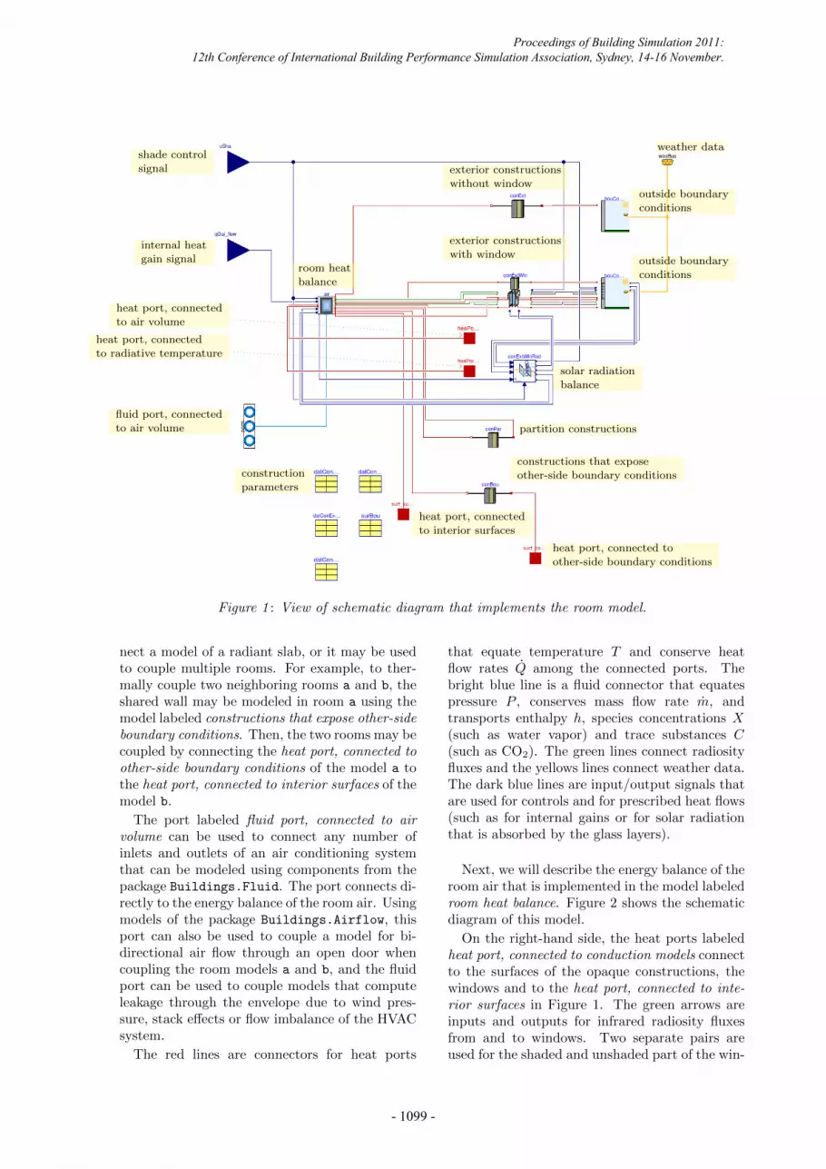
model of a room with completely mixed air. Theroom can have any number of constructions andsurfaces that participate in the heat exchangethrough convection, conduction, infrared radia-tion and solar radiation. Figure 1 shows theschematic model as implemented in Modelica.The following sections describe the models for thevarious heat transfer phenomena. Italics font isused to relate to the figure labels.There are four di↵erent models to compute heat

conduction through opaque constructions. Themodels exterior constructions without window andexterior constructions with window connect tomodels that compute the outside boundary condi-tions. The models partition constructions can beused for partitions within a thermal zone as it con-nects both surfaces to the room model, in whichthey will participate in the convective and radia-tive heat transfer balances. The models construc-tions that expose other-side boundary conditions

have one surface connected to the room heat bal-ance, and the other surface connected to the heat

port, connected to other-side boundary conditions.All of these models compute one-dimensional heatconduction through multi-layered materials. Ineach layer, the Fourier equation

⇢ c@T (x, t)

@t= k

@2T (x, t)

@x2, (1)

where ⇢ is the density, c is the specific heat capac-ity, T (x, t) is the temperature at location x andtime t and k is the heat conductivity, is solvedusing a finite volume model. If a user either setsc = 0 or ⇢ = 0, then steady-state heat conductionis computed for the respective layer. The spa-tial grid is auto-generated based on the materialproperties using the algorithm described in Wet-ter (2004).The models exterior constructions with win-

dow contain a heat conduction model for the

opaque part of the construction as describedabove, and a layer-by-layer window model thatis based on the TARCOG algorithm (TARCOG2006) which is also the basis of the WINDOW 6program (Mitchell et al. 2011). In the windowmodel, a solar radiation balance is solved for glaz-ing systems that can have multiple window panes.Optionally, the window can have either an interioror exterior shade.The model solar radiation balance implements

the solar radiation balance. Output of this modelis the solar radiation that is absorbed by eachglass and shading layer. This absorbed solar radi-ation is then used in a layer-by-layer heat transfermodel that computes infrared radiation exchange,heat conduction, and temperature and wind speeddependent convection.The models outside boundary conditions com-

pute the convective heat transfer and the radiativeheat transfer to the ambient and the sky. They areused for the exterior-facing surfaces of the opaqueconstructions and the windows.All these models are vectors of component mod-

els, i.e., there can be an arbitrary number of con-structions. Models that are not needed are re-moved automatically when executable code is gen-erated. The material properties and the geome-try of the constructions are defined in the datarecords labeled construction parameters. Depend-ing on these data records, heat conduction in thematerial layers of the constructions may be com-puted transient or steady-state, and the windowmodels may have di↵erent number of glass panes,optical properties and gas fills.The connector weather data can be used to cou-

ple weather data, which may be obtained fromTMY3 data (Wilcox and Marion 2008). Thereare also input signals for the control of the win-dow shade, and for specifying radiant, convectivesensible and latent heat gains. The port labeledheat port, connected to air volume may be used tocouple a sensor for the room air temperature, andit may be used to add a sensible convective heatflow to the room air. Similarly, the port labeledheat port, connected to radiative temperature maybe used to couple a sensor for the room radiativetemperature, and it may be used to add a radia-tive heat flow to the room air. The heat portlabeled heat port, connected to interior surfaces

specifies the temperature and heat flow rate ofa surface in the model room heat balance. Thissurface then participates in the convective andinfrared and solar radiation heat transfer in theroom.Therefore, this heat port may be used to con-


- 1098 -

exterior constructions

without window

partition constructions

constructions that expose

other-side boundary conditions

heat port, connected to

other-side boundary conditions

exterior constructions

with window

solar radiation

balance

outside boundary

conditions

outside boundary

conditions

room heat

balance

construction

parameters

weather data

shade control

signal

internal heat

gain signal

heat port, connected

to air volume


to radiative temperature


to interior surfaces

fluid port, connected

to air volume

Figure 1 : View of schematic diagram that implements the room model.

nect a model of a radiant slab, or it may be usedto couple multiple rooms. For example, to ther-mally couple two neighboring rooms a and b, theshared wall may be modeled in room a using themodel labeled constructions that expose other-side

boundary conditions. Then, the two rooms may becoupled by connecting the heat port, connected to

other-side boundary conditions of the model a tothe heat port, connected to interior surfaces of themodel b.

The port labeled fluid port, connected to air

volume can be used to connect any number ofinlets and outlets of an air conditioning systemthat can be modeled using components from thepackage Buildings.Fluid. The port connects di-rectly to the energy balance of the room air. Usingmodels of the package Buildings.Airflow, thisport can also be used to couple a model for bi-directional air flow through an open door whencoupling the room models a and b, and the fluidport can be used to couple models that computeleakage through the envelope due to wind pres-sure, stack e↵ects or flow imbalance of the HVACsystem.

The red lines are connectors for heat ports

that equate temperature T and conserve heatflow rates Q among the connected ports. Thebright blue line is a fluid connector that equatespressure P , conserves mass flow rate m, andtransports enthalpy h, species concentrations X(such as water vapor) and trace substances C(such as CO2). The green lines connect radiosityfluxes and the yellows lines connect weather data.The dark blue lines are input/output signals thatare used for controls and for prescribed heat flows(such as for internal gains or for solar radiationthat is absorbed by the glass layers).

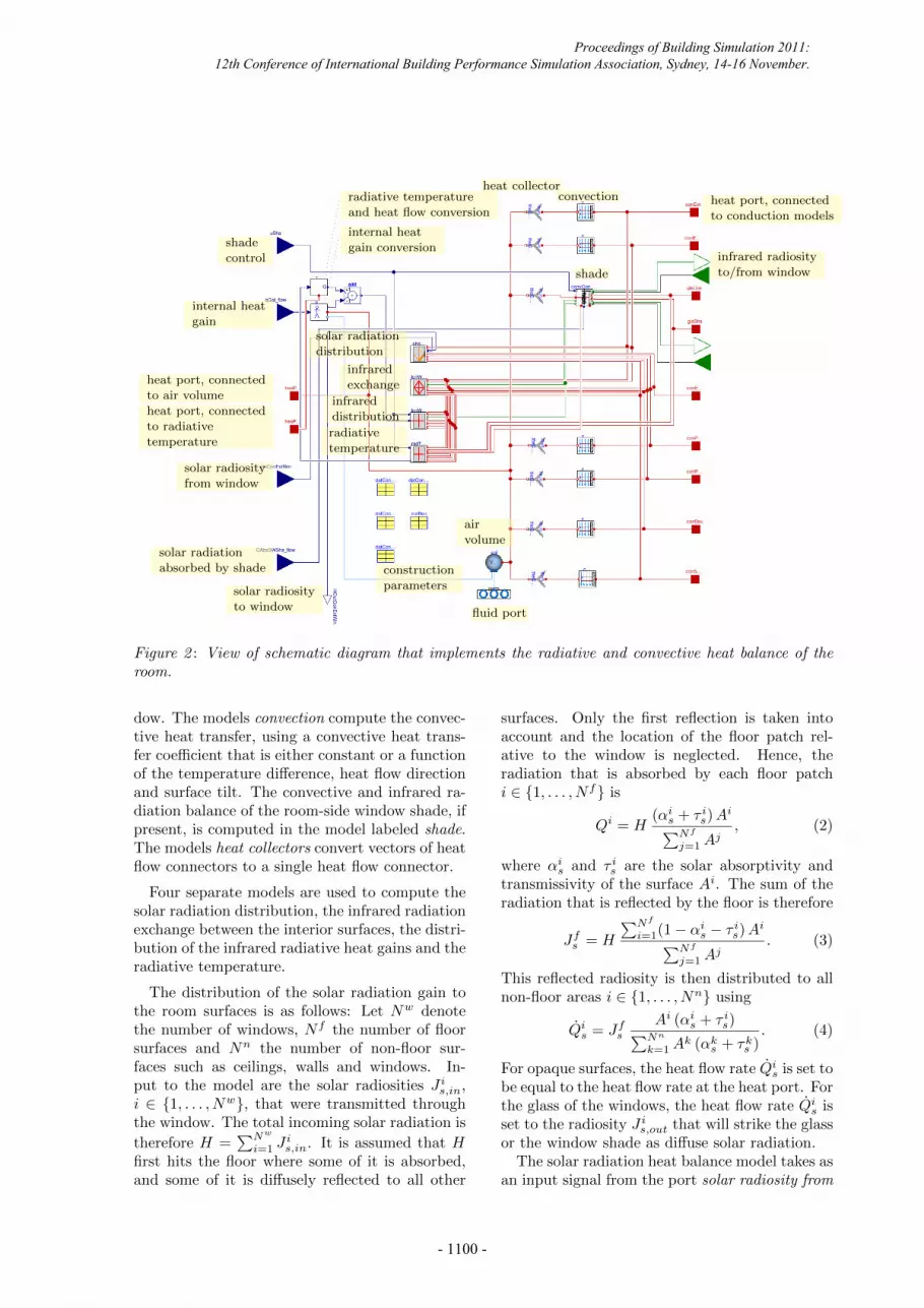
Next, we will describe the energy balance of theroom air that is implemented in the model labeledroom heat balance. Figure 2 shows the schematicdiagram of this model.

On the right-hand side, the heat ports labeledheat port, connected to conduction models connectto the surfaces of the opaque constructions, thewindows and to the heat port, connected to inte-

rior surfaces in Figure 1. The green arrows areinputs and outputs for infrared radiosity fluxesfrom and to windows. Two separate pairs areused for the shaded and unshaded part of the win-


- 1099 -


to conduction models

infrared radiosity

to/from window

convection

shade

heat collector

solar radiation

distribution

infrared

exchange

infrared

distribution

radiative

temperature

solar radiosity

from window

solar radiosity

to window

internal heat

gain

radiative temperature

and heat flow conversion

internal heat

gain conversion

construction

parameters

shade

control

solar radiation

absorbed by shade

fluid port

air

volume


to air volume


to radiative

temperature

Figure 2 : View of schematic diagram that implements the radiative and convective heat balance of the

room.

dow. The models convection compute the convec-tive heat transfer, using a convective heat trans-fer coe�cient that is either constant or a functionof the temperature di↵erence, heat flow directionand surface tilt. The convective and infrared ra-diation balance of the room-side window shade, ifpresent, is computed in the model labeled shade.The models heat collectors convert vectors of heatflow connectors to a single heat flow connector.

Four separate models are used to compute thesolar radiation distribution, the infrared radiationexchange between the interior surfaces, the distri-bution of the infrared radiative heat gains and theradiative temperature.

The distribution of the solar radiation gain tothe room surfaces is as follows: Let Nw denotethe number of windows, Nf the number of floorsurfaces and Nn the number of non-floor sur-faces such as ceilings, walls and windows. In-put to the model are the solar radiosities J i

s,in

,i 2 {1, . . . , Nw}, that were transmitted throughthe window. The total incoming solar radiation istherefore H =

PN

w

i=1 Ji

s,in

. It is assumed that Hfirst hits the floor where some of it is absorbed,and some of it is di↵usely reflected to all other

surfaces. Only the first reflection is taken intoaccount and the location of the floor patch rel-ative to the window is neglected. Hence, theradiation that is absorbed by each floor patchi 2 {1, . . . , Nf} is

Qi = H(↵i

s

+ ⌧ is

)Ai

PN

f

j=1 Aj

, (2)

where ↵i

s

and ⌧ is

are the solar absorptivity andtransmissivity of the surface Ai. The sum of theradiation that is reflected by the floor is therefore

Jf

s

= H

PN

f

i=1(1� ↵i

s

� ⌧ is

)Ai

PN

f

j=1 Aj

. (3)

This reflected radiosity is then distributed to allnon-floor areas i 2 {1, . . . , Nn} using

Qi

s

= Jf

s

Ai (↵i

s

+ ⌧ is

)P

N

n

k=1 Ak (↵k

s

+ ⌧ks

). (4)

For opaque surfaces, the heat flow rate Qi

s

is set tobe equal to the heat flow rate at the heat port. Forthe glass of the windows, the heat flow rate Qi

s

isset to the radiosity J i

s,out

that will strike the glassor the window shade as di↵use solar radiation.The solar radiation heat balance model takes as

an input signal from the port solar radiosity from


- 1100 -

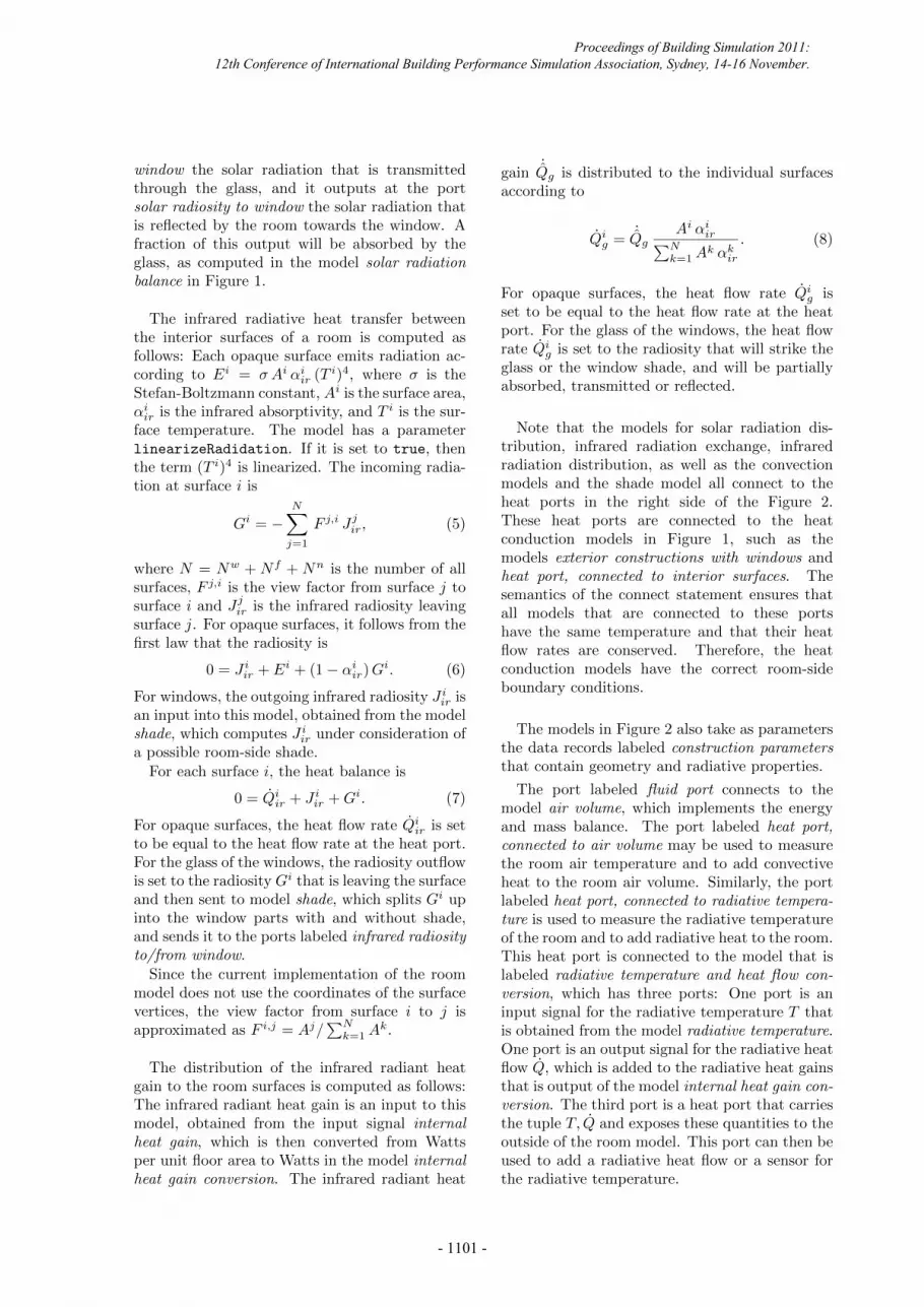
window the solar radiation that is transmittedthrough the glass, and it outputs at the portsolar radiosity to window the solar radiation thatis reflected by the room towards the window. Afraction of this output will be absorbed by theglass, as computed in the model solar radiation

balance in Figure 1.

The infrared radiative heat transfer betweenthe interior surfaces of a room is computed asfollows: Each opaque surface emits radiation ac-cording to Ei = �Ai ↵i

ir

(T i)4, where � is theStefan-Boltzmann constant, Ai is the surface area,↵i

ir

is the infrared absorptivity, and T i is the sur-face temperature. The model has a parameterlinearizeRadidation. If it is set to true, thenthe term (T i)4 is linearized. The incoming radia-tion at surface i is

Gi = �NX

j=1

F j,i Jj

ir

, (5)

where N = Nw + Nf + Nn is the number of allsurfaces, F j,i is the view factor from surface j tosurface i and Jj

ir

is the infrared radiosity leavingsurface j. For opaque surfaces, it follows from thefirst law that the radiosity is

0 = J i

ir

+ Ei + (1� ↵i

ir

)Gi. (6)

For windows, the outgoing infrared radiosity J i

ir

isan input into this model, obtained from the modelshade, which computes J i

ir

under consideration ofa possible room-side shade.For each surface i, the heat balance is

0 = Qi

ir

+ J i

ir

+Gi. (7)


ir

is setto be equal to the heat flow rate at the heat port.For the glass of the windows, the radiosity outflowis set to the radiosity Gi that is leaving the surfaceand then sent to model shade, which splits Gi upinto the window parts with and without shade,and sends it to the ports labeled infrared radiosity

to/from window.Since the current implementation of the room

model does not use the coordinates of the surfacevertices, the view factor from surface i to j isapproximated as F i,j = Aj/

PN

k=1 Ak.

The distribution of the infrared radiant heatgain to the room surfaces is computed as follows:The infrared radiant heat gain is an input to thismodel, obtained from the input signal internal

heat gain, which is then converted from Wattsper unit floor area to Watts in the model internalheat gain conversion. The infrared radiant heat

gain ˙Q

g

is distributed to the individual surfacesaccording to

Qi

g

= ˙Q

g

Ai ↵i

irPN

k=1 Ak ↵k

ir

. (8)


g

isset to be equal to the heat flow rate at the heatport. For the glass of the windows, the heat flowrate Qi

g

is set to the radiosity that will strike theglass or the window shade, and will be partiallyabsorbed, transmitted or reflected.

Note that the models for solar radiation dis-tribution, infrared radiation exchange, infraredradiation distribution, as well as the convectionmodels and the shade model all connect to theheat ports in the right side of the Figure 2.These heat ports are connected to the heatconduction models in Figure 1, such as themodels exterior constructions with windows andheat port, connected to interior surfaces. Thesemantics of the connect statement ensures thatall models that are connected to these portshave the same temperature and that their heatflow rates are conserved. Therefore, the heatconduction models have the correct room-sideboundary conditions.

The models in Figure 2 also take as parametersthe data records labeled construction parameters

that contain geometry and radiative properties.

The port labeled fluid port connects to themodel air volume, which implements the energyand mass balance. The port labeled heat port,

connected to air volume may be used to measurethe room air temperature and to add convectiveheat to the room air volume. Similarly, the portlabeled heat port, connected to radiative tempera-

ture is used to measure the radiative temperatureof the room and to add radiative heat to the room.This heat port is connected to the model that islabeled radiative temperature and heat flow con-

version, which has three ports: One port is aninput signal for the radiative temperature T thatis obtained from the model radiative temperature.One port is an output signal for the radiative heatflow Q, which is added to the radiative heat gainsthat is output of the model internal heat gain con-

version. The third port is a heat port that carriesthe tuple T, Q and exposes these quantities to theoutside of the room model. This port can then beused to add a radiative heat flow or a sensor forthe radiative temperature.


- 1101 -

APPLICATIONTo illustrate how di↵erent model formulations

a↵ect computing time, we run di↵erent cases ofthe BESTEST building envelope test (ASHRAE2007). These test cases have been selected be-cause they are widely known in the simulationcommunity. They are also used to evaluate theaccuracy of our model. Meanwhile, a more com-prehensive validation with a larger set of test casesis ongoing. All simulations have been done us-ing the Dymola 7.4 FD01 simulation program forModelica on Windows 7 using one 2.67 GHz In-tel Xeon processor. Unless noted otherwise, theradau solver has been used. We run the light-weight and heavy-weight test cases 600 and 900,as well as the free floating cases 600FF and 900FF.In the results denoted by “n”, the convective heattransfer is temperature and wind-speed depen-dent, and the radiative heat transfer is not lin-earized. In the results denoted by “l”, the convec-tion coe�cients are constant, and the equationsfor radiative heat transfer are linearized.

10�8 10�7 10�6 10�5 10�4

0

2

4 l: linearized convection &

radiation

n: nonlinear convection &

radiation

solver tolerance ✏

Eh

in[M

Wh/a]

600 n600 l900 n900 l

Figure 3 : Annual heating energy for case 600 and

900. The yellow boxes are minimum and maxi-

mum values reported in BESTEST.

10�8 10�7 10�6 10�5 10�4

0

2

4

6

8

l: linearized convection &

radiation


radiation


Ec

in[M

Wh/a]

600 n600 l900 n900 l

Figure 4 : Annual cooling energy for case 600 and

900. The yellow boxes are minimum and maxi-

mum values reported in BESTEST.

Figures 3 and 4 show that the results are withinthe range published in BESTEST for the solver

10�8 10�6 10�4

050

100150200250

l: linearized convection &

radiation


radiation


CPU

timein

[s] 600 n

600 l900 n900 l600FF n600FF l900FF n900FF l

Figure 5 : Computing time for an annual simula-

tion.

tolerances of 10k, for k 2 {�8, . . . ,�4}. Lin-earizing the radiative and convective heat transferequations caused a twofold reduction in comput-ing time. However, case 900 shows slightly highannual cooling energy if these equations are lin-earized. We recommend a solver tolerance of 10�5

to 10�6 to reduce the numerical approximationerror and the computing time. With ✏ = 10�4,the numerical approximation error is noticeable,and computing time is higher than for ✏ = 10�5

for some cases. No di↵erence in computing timecan be seen between the heavy-weight and light-weight buildings, which had 43 and 54 state vari-ables, respectively. For case 600n and 900n, thecoupled system of nonlinear equations had dimen-sion 12, the iteration variables were the room-sidesurface temperatures and radiosities. Dymola ob-tained analytical expressions for all Jacobian ma-trices. Cases 600l and 900l had no nonlinear equa-tions, except for the initialization problem. Forcase 600n with ✏ = 10�6, a majority of the com-puting time was spent to solve the 12 ⇥ 12 non-linear system of equations. For case 600n, with✏ = 10�6, the following additional experimentswere done: The solver was changed from radau todassl and lsodar, which changed computing timefrom 75s to 170s and 240s, respectively. The equa-tions for radiative heat transfer were linearized,which reduced computing time by 10%, decreasedannual energy for heating by 10% and increasedannual energy for cooling by 10%.

CONCLUSIONSFor the test cases 600 and 900, annual heating

and cooling energy consumption were within therange reported in the ANSI/ASHRAE Standard140-2007 envelope test. More extensive testing issubject of future work. The majority of comput-ing time was spent to solve the nonlinear system ofequations that obtains room-side surface temper-atures and radiosities. Linearizing the equationsfor convective and radiative heat transfer yieldeda twofold reduction in computing time.


- 1102 -

ACKNOWLEDGMENTSThis research was supported by the Assistant

Secretary for Energy E�ciency and RenewableEnergy, O�ce of Building Technologies of the U.S.Department of Energy, under Contract No. DE-AC02-05CH11231.We thank Slaven Peles from the United Tech-

nologies Research Center for his feedback duringthe model validation and for providing the modelthat served as a basis for the experiments.

REFERENCESASHRAE. 2007. ANSI/ASHRAE Standard 140-

2007, Standard Method of Test for the Evalua-tion of Building Energy Analysis Computer Pro-grams.

Cellier, Francois E., and Ernesto Kofman. 2006.Continuous System Simulation. Springer.

Franke, Rudiger, Francesco Casella, Martin Otter,Katrin Proelss, Michael Sielemann, and MichaelWetter. 2009a, September. “Standardizationof thermo-fluid modeling in Modelica.Fluid.”Edited by Francesco Casella, Proc. of the 7-thInternational Modelica Conference. Modelica As-sociation, Como, Italy.

Franke, Rudiger, Francesco Casella, Martin Otter,Michael Sielemann, Hilding Elmqvist, Sven ErikMattsson, and Hans Olsson. 2009b, September.“Stream Connectors – an Extension of Model-ica for Device-Oriented Modeling of ConvectiveTransport Phenomena.” Edited by FrancescoCasella, Proc. of the 7-th International ModelicaConference. Modelica Association, Como, Italy.

Mattsson, Sven Erik, and Hilding Elmqvist. 1997,April. “Modelica – An international e↵ortto design the next generation modeling lan-guage.” Edited by L. Boullart, M. Loccufier, andSven Erik Mattsson, 7th IFAC Symposium onComputer Aided Control Systems Design. Gent,Belgium.

Mitchell, Robin, Christian Kohler, Ling Zhu, Dar-iush Arasteh, John Carmody, Charlie Huizenga,and Dragan Curcija. 2011, January. “THERM6.3 / WINDOW 6.3 NFRC Simulation Manual.”Technical Report LBNL-48255, Lawrence Berke-ley National Laboratory, Berkeley, CA.

Sahlin, Per, and Edward F. Sowell. 1989, June. “ANeutral Format for Building Simulation Mod-els.” Proceedings of the Second InternationalIBPSA Conference. Vancouver, BC, Canada,147–154.

Sowell, Edward F., W. Fred Buhl, and Jean-MichelNataf. 1989, June. “Object-Oriented Program-mingg, Equation-Based Submodels, and SystemReduction in SPANK.” Proceedings of the Sec-ond International IBPSA Conference. Vancou-ver, BC, Canada, 141–146.

TARCOG (Carli, Inc.). 2006, October. TARCOG:Mathematical Models for Calculation of Thermal

Performance of Glazing Systems with or withoutShading Devices. Amherst, MA: Carli, Inc.

Wetter, Michael. 2004. “Simulation-Based BuildingEnergy Optimization.” Ph.D. diss., University ofCalifornia at Berkeley.

Wetter, Michael. 2006a, September. “Multizone Air-flow Model in Modelica.” Edited by ChristianKral and Anton Haumer, Proc. of the 5-th Inter-national Modelica Conference, Volume 2. Mod-elica Association and Arsenal Research, Vienna,Austria, 431–440.

Wetter, Michael. 2006b, September. “MultizoneBuilding Model for Thermal Building Simula-tion in Modelica.” Edited by Christian Kral andAnton Haumer, Proc. of the 5-th InternationalModelica Conference, Volume 2. Modelica Asso-ciation and Arsenal Research, Vienna, Austria,517–526.

Wetter, Michael. 2009a. “Modelica-based Model-ing and Simulation to Support Research and De-velopment in Building Energy and Control Sys-tems.” Journal of Building Performance Simu-lation 2 (2): 143–161 (June).

Wetter, Michael. 2009b. “A Modelica-based modellibrary for building energy and control systems.”Edited by Paul A. Strachan, Nick J. Kelly, andMichael Kummert, Proc. of the 11-th IBPSAConference. International Building PerformanceSimulation Association and University of Strath-clyde, 652–659.

Wetter, Michael. 2009c, September. “Modelica Li-brary for Building Heating, Ventilation and Air-Conditioning Systems.” Edited by FrancescoCasella, Proc. of the 7-th International ModelicaConference. Modelica Association, Como, Italy,393–402.

Wetter, Michael. 2011a. Chapter The Future ofBuilding System Modeling and Simulation ofBuilding Performance Simulation for Design andAutomation, edited by Jan L. M. Hensen andRoberto Lamberts. Oxon, OX: Taylor & Fran-cis.

Wetter, Michael. 2011b. “Co-simulation of build-ing energy and control systems with the BuildingControls Virtual Test Bed.” Journal of BuildingPerformance Simulation 4:185–203.

Wetter, Michael, Wangda Zuo, andThierry Stephane Nouidui. 2011, March.“Recent developments of the Modelica buildingslibrary for building heating, ventilation andair-conditioning systems.” Proc. of the 8-thInternational Modelica Conference. ModelicaAssociation, Dresden, Germany, 266–275.

Wilcox, S., and W. Marion. 2008, May. “UsersManual for TMY3 Data Sets.” Technical ReportNREL/TP-581-43156, NREL, Golden, CO.


- 1103 -

modeling of heat transfer in rooms in the modelica buildings library

Documents