modeling calendar effects in mbie's jobs online vacancies

MODELLING CALENDAR EFFECTS in MBIE’s JOBS ONLINE VACANCIES TIME SERIES

Anne Fale and Amapola Generosa - Ministry of Business, Innovation and Employment (MBIE)

1 Abstract

The Ministry of Business, Innovation and Employment release Jobs Online reports every month. These

reports discuss changes in job vacancies advertised online by businesses and organisations from the

private and public sectors through the two main internet job boards - SEEK and Trade Me Jobs. Jobs

Online presents its vacancy data in a Skilled Vacancy Index (SVI) and an All Vacancy Index (AVI). and

a The SVI breaks down the data by industry1 , occupation2 and region3. The indices indicate the

demand for labour.

This paper describes the change to the seasonal adjustment of the SEEK and Trade Me Jobs vacancies

series that are used to calculate the monthly SVI and AVI. The change in the process is the result of an

investigation into calendar effects in the series and comparisons of the performance of the day of the

week and Easter effects regression models. The outcome of this modelling framework was a better

identification of seasonal effects and a clearer picture of job vacancies, enhancing MBIE’s capacity to

monitor and report on job vacancies.

2 Background

Monthly time series like Jobs Online can be influenced by differences in the number of weekdays,

weekends in each month or holidays. These calendar effects introduce volatility into monthly time

series data and obscure important seasonal effects. These effects also make it difficult for Jobs Online

vacancies to be compared across months or for movements in one series to be compared across other

series. Job vacancies across industries, occupations and regions were also impacted in different ways

by seasonal effects, making valid comparison an issue. These issues meant that accurately adjusting

Jobs Online data for seasonal effects was important. For this reason, the Ministry, in consultation with

Statistics New Zealand, introduced a new process into the seasonal adjustment of Jobs Online data.

Job advertisements tended to rise in months with more weekdays and working days relative to other

months (see Figure 1). Job advertisements also vary according to the individual day of the week. A

month with more Mondays than Thursdays will have a different impact compared to the other way

around. In this case, months having different numbers of each day of the week from year to year, can

explain short-term movements in the Jobs Online series. Generally, in each month there are four full

weeks and additionally one, two or three days. Therefore, for each month, the given day of the week

occurs at least four times, but some days will occur five times. If the number and composition of these

extra days have an effect on data for the month, the days-of-the-week effect arose. This effect was

significant for time series in which daily activity depends on the day of the week like advertisements of

vacancies online.

1 The industries are accounting, HR, legal and administration; construction and engineering; information technology; healthcare

and medical; sales, retail, marketing and advertising; education and training; hospitality and tourism; and other. 2 The occupations are managers; professionals; and trades and technicians. 3 The regions are Auckland, Wellington, Canterbury, South Island (excluding Canterbury) and North Island (excluding Auckland

and Wellington).

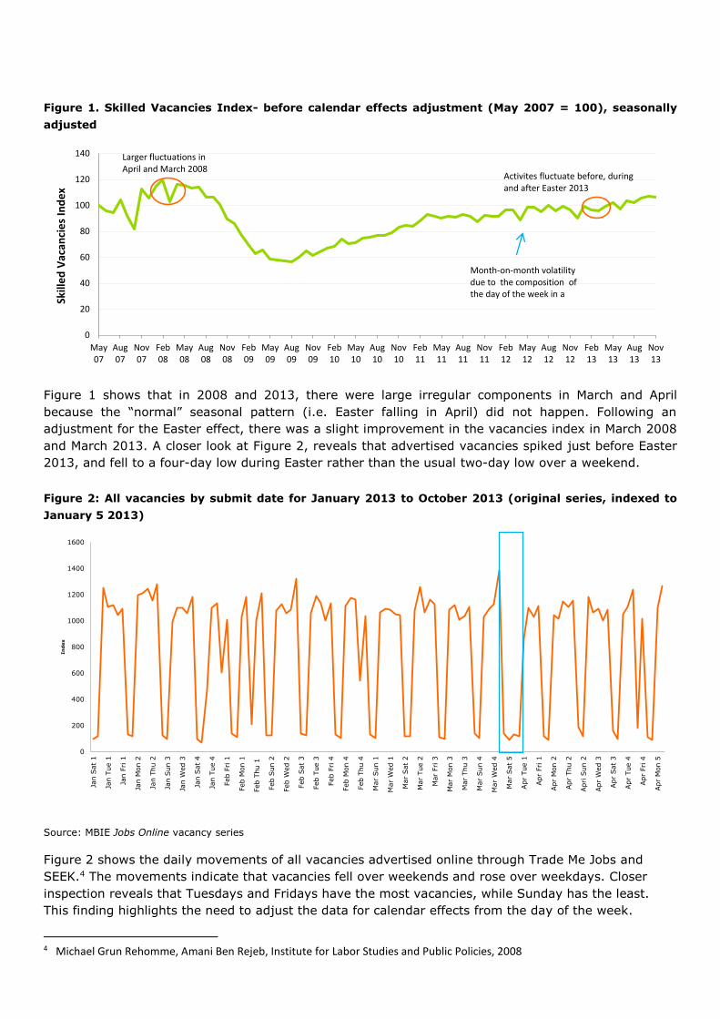
Figure 1. Skilled Vacancies Index- before calendar effects adjustment (May 2007 = 100), seasonally

adjusted

Figure 1 shows that in 2008 and 2013, there were large irregular components in March and April

because the “normal” seasonal pattern (i.e. Easter falling in April) did not happen. Following an

adjustment for the Easter effect, there was a slight improvement in the vacancies index in March 2008

and March 2013. A closer look at Figure 2, reveals that advertised vacancies spiked just before Easter

2013, and fell to a four-day low during Easter rather than the usual two-day low over a weekend.

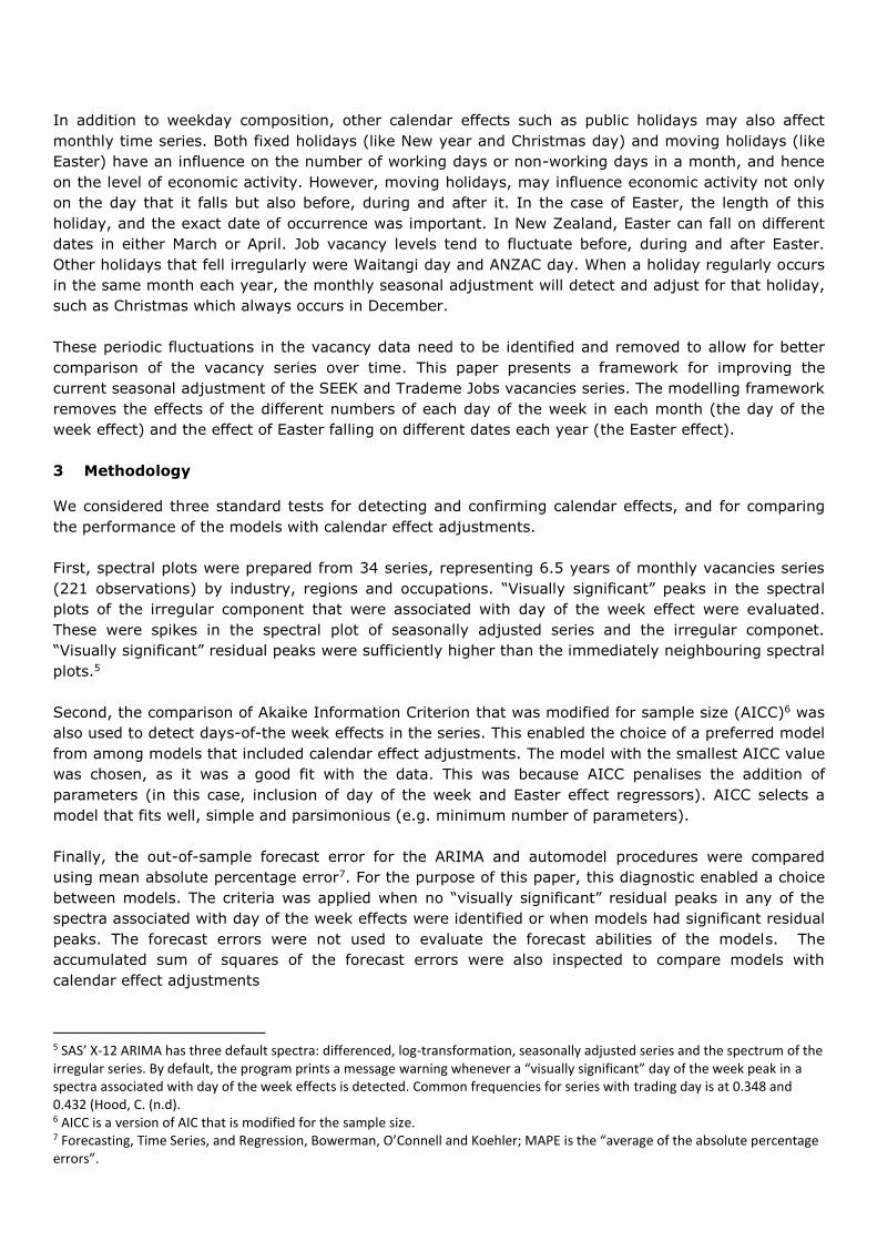
Figure 2: All vacancies by submit date for January 2013 to October 2013 (original series, indexed to

January 5 2013)

Source: MBIE Jobs Online vacancy series

Figure 2 shows the daily movements of all vacancies advertised online through Trade Me Jobs and

SEEK.4 The movements indicate that vacancies fell over weekends and rose over weekdays. Closer

inspection reveals that Tuesdays and Fridays have the most vacancies, while Sunday has the least.

This finding highlights the need to adjust the data for calendar effects from the day of the week.

4 Michael Grun Rehomme, Amani Ben Rejeb, Institute for Labor Studies and Public Policies, 2008

0

20

40

60

80

100

120

140

May07

Aug07

Nov07

Feb08

May08

Aug08

Nov08

Feb09

May09

Aug09

Nov09

Feb10

May10

Aug10

Nov10

Feb11

May11

Aug11

Nov11

Feb12

May12

Aug12

Nov12

Feb13

May13

Aug13

Nov13

Skill

ed

Vac

anci

es

Ind

ex

Month-on-month volatility due to the composition of the day of the week in a

Larger fluctuations inApril and March 2008

Activites fluctuate before, during and after Easter 2013

0

200

400

600

800

1000

1200

1400

1600

Jan S

at

1

Jan T

ue 1

Jan F

ri 1

Jan M

on 2

Jan T

hu 2

Jan S

un 3

Jan W

ed 3

Jan S

at

4

Jan T

ue 4

Feb F

ri 1

Feb M

on 1

Feb T

hu 1

Feb S

un 2

Feb W

ed 2

Feb S

at

3

Feb T

ue 3

Feb F

ri 4

Feb M

on 4

Feb T

hu 4

Mar

Sun 1

Mar

Wed 1

Mar

Sat

2

Mar

Tue 2

Mar

Fri 3

Mar

Mon 3

Mar

Thu 3

Mar

Sun 4

Mar

Wed 4

Mar

Sat

5

Apr

Tue 1

Apr

Fri 1

Apr

Mon 2

Apr

Thu 2

Apri S

un 2

Apr

Wed 3

Apr

Sat

3

Apr

Tue 4

Apr

Fri 4

Apr

Mon 5

In

dex

In addition to weekday composition, other calendar effects such as public holidays may also affect

monthly time series. Both fixed holidays (like New year and Christmas day) and moving holidays (like

Easter) have an influence on the number of working days or non-working days in a month, and hence

on the level of economic activity. However, moving holidays, may influence economic activity not only

on the day that it falls but also before, during and after it. In the case of Easter, the length of this

holiday, and the exact date of occurrence was important. In New Zealand, Easter can fall on different

dates in either March or April. Job vacancy levels tend to fluctuate before, during and after Easter.

Other holidays that fell irregularly were Waitangi day and ANZAC day. When a holiday regularly occurs

in the same month each year, the monthly seasonal adjustment will detect and adjust for that holiday,

such as Christmas which always occurs in December.

These periodic fluctuations in the vacancy data need to be identified and removed to allow for better

comparison of the vacancy series over time. This paper presents a framework for improving the

current seasonal adjustment of the SEEK and Trademe Jobs vacancies series. The modelling framework

removes the effects of the different numbers of each day of the week in each month (the day of the

week effect) and the effect of Easter falling on different dates each year (the Easter effect).

3 Methodology

We considered three standard tests for detecting and confirming calendar effects, and for comparing

the performance of the models with calendar effect adjustments.

First, spectral plots were prepared from 34 series, representing 6.5 years of monthly vacancies series

(221 observations) by industry, regions and occupations. “Visually significant” peaks in the spectral

plots of the irregular component that were associated with day of the week effect were evaluated.

These were spikes in the spectral plot of seasonally adjusted series and the irregular componet.

“Visually significant” residual peaks were sufficiently higher than the immediately neighbouring spectral

plots.5

Second, the comparison of Akaike Information Criterion that was modified for sample size (AICC)6 was

also used to detect days-of-the week effects in the series. This enabled the choice of a preferred model

from among models that included calendar effect adjustments. The model with the smallest AICC value

was chosen, as it was a good fit with the data. This was because AICC penalises the addition of

parameters (in this case, inclusion of day of the week and Easter effect regressors). AICC selects a

model that fits well, simple and parsimonious (e.g. minimum number of parameters).

Finally, the out-of-sample forecast error for the ARIMA and automodel procedures were compared

using mean absolute percentage error7. For the purpose of this paper, this diagnostic enabled a choice

between models. The criteria was applied when no “visually significant” residual peaks in any of the

spectra associated with day of the week effects were identified or when models had significant residual

peaks. The forecast errors were not used to evaluate the forecast abilities of the models. The

accumulated sum of squares of the forecast errors were also inspected to compare models with

calendar effect adjustments

5 SAS’ X-12 ARIMA has three default spectra: differenced, log-transformation, seasonally adjusted series and the spectrum of the irregular series. By default, the program prints a message warning whenever a “visually significant” day of the week peak in a spectra associated with day of the week effects is detected. Common frequencies for series with trading day is at 0.348 and 0.432 (Hood, C. (n.d). 6 AICC is a version of AIC that is modified for the sample size. 7 Forecasting, Time Series, and Regression, Bowerman, O’Connell and Koehler; MAPE is the “average of the absolute percentage errors”.

To adjust for day of the week and Easter effects in the indices, a straightforward use of ARIMA models

was insufficient. The X-12 ARIMA estimates the regARIMA8 separately. The pre-adjustment for

calendar effects involves removing from the time series calendar effects. It was achieved by including

the appropriate regression variables to the RegARIMA. The RegARIMA included calendar effects as

deterministic input variables. This part of X-12-ARIMA makes adjustments for calendar effects from the

original series (Catherine C. Hood, Catherine Hood Consulting, 2013).

For the purposes of this report we considered eight different models, these were:

1) ARIMA

a) No day of the week effect (NODWE)

b) Day of the week effect (DWE)

c) DWE and one part Easter regressor (one part Easter)

d) DWE and two part Easter regressor – before Easter and during Easter.

2) Auto model

a) No day of the week effect effect (NODWE)

b) Day of the week effect effect (DWE)

c) DWE and a one part Easter regressor

d) DWE and a two part Easter regressor.

The vacancy series were decomposed by the calendar effect factor, a seasonal component and a non-

seasonal component. The seasonal adjustment procedure included the day of the week and Easter

adjustments as regressors. Online vacancies were modelled using a six-day coefficient effect for the

day of the week (DWE) regressor, and a two-part Easter regressor. DWE estimates a separate

regression coefficient for six day of the week and has an implied coefficient for Sunday.9 Details in the

detection and modelling of day of the week effects were given in Soukop and Findley (2000).

The other deterministic variable, the Easter regressor, adjusted for Easter. The Easter effect was

modelled as two parts: a pre-Easter effect (days before Easter to Good Friday) and an Easter holiday

effect starting on Good Friday and lasting until Easter Monday.10 The approach using two Easter

regressors was similar to the approach taken in Australia, which also has a Monday holiday over Easter

(Norhayati Shuja, Mohd Alias Lazim, Yap Bee Wah, Department of Statistics Malaysia, 2007). Genhol11

was used to generate Easter regressors.

The seasonal adjustment procedure using an automatic model12 and ARIMA (0 1 1) (0 1 1)

specifications were applied to 6.5 years of monthly data from Trademe Jobs and SEEK. The monthly

data for skilled vacancies was broken down by industry, occupation groups and region. Comparing

results from the two proceduces in SAS allowed for evaluation of a ‘good fit’ for individual series. The

quality of the seasonally adjusted series was assessed on standard diagnostics for the presence of

seasonality. M and Q statistics13 were used to measure the stable and moving seasonality in each

series. These diagnostics were also used to identify seasonality, as a seasonally adjusted series should

8 A time series modelling (combines regression and ARIMA model) developed to identify and estimate outliers, trading day and holiday effects that may exist in the series. 9 We initially used the “TD1coef” in the context of the SAS programmes. TD1 coef assumes that the weeks and weekends are the same. However, further investigation has revealed that the “TD” (trading day) coefficient should be used. The TD, which assumes six-coefficients, was selected as the weekends differed to the weekday structure in the underlying data. 10 For details about this method, see Monsell (2010) and Monsell B, David F.Findley, Kellie Wills (2003). 11 Genhol is a programme developed by the US Census Bureau for creating holiday regressors. 12 This X-12 ARIMA procedure automatically selects the orders of differencing and ARIMA model. It is based largely on the TRAMO (time series regression with ARIMA noise, missing values, and outliers) method. 13 The M tests and Q test from the SAS diagnostics assess the quality of the seasonal adjustment. The M7 is the most important

diagnostic and compares the moving seasonality relative to the stable seasonality. The Q test is a weighted average of all of the M tests. The M tests indicate an issue if their value is greater than 1.

have no residual seasonal effects (Catherine C. Hood, Catherine Hood Consulting, June 18-21 2007).

Residual seasonality was further inspected using spectral graphs to identify the outliers in the series.

4 Empirical results

4.1 Detection day of the week and Easter effects

To confirm the presence of day of the week effects, we looked at the spectral graphs of the seasonally

adjusted and irregular series of 34 series were looked at. Spectral graphs were used to investigate the

seasonality and day of the week effect in the data. The graph shows that the seasonal and irregular

components of the Jobs Online series included day of the week peaks in the vacancy series. The

spectral plots14 shows that frequencies related to the day of the week effect were detected in skilled

vacancies, total vacancies; Wellington region; trades occupation and; in industries of accounting,

construction IT, sales, and hospitality (Catherine C. Hood, Catherine Hood Consulting, 2009);

(Raymond J. Soukup, David F. Findley, US Census Bureau). The results from spectrum analysis were

summarised in Table 4 and Table 5 in Appendix A. A sample of spectral plots showing seasonally

adjusted and irregular components series for vacancies in the sales industry were also presented in

Appendix B.

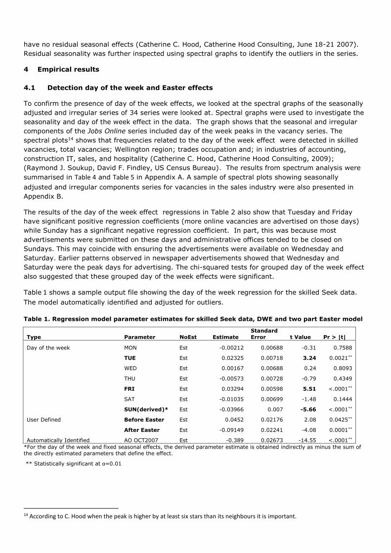
The results of the day of the week effect regressions in Table 2 also show that Tuesday and Friday

have significant positive regression coefficients (more online vacancies are advertised on those days)

while Sunday has a significant negative regression coefficient. In part, this was because most

advertisements were submitted on these days and administrative offices tended to be closed on

Sundays. This may coincide with ensuring the advertisements were available on Wednesday and

Saturday. Earlier patterns observed in newspaper advertisements showed that Wednesday and

Saturday were the peak days for advertising. The chi-squared tests for grouped day of the week effect

also suggested that these grouped day of the week effects were significant.

Table 1 shows a sample output file showing the day of the week regression for the skilled Seek data.

The model automatically identified and adjusted for outliers.

Table 1. Regression model parameter estimates for skilled Seek data, DWE and two part Easter model

Type Parameter NoEst Estimate Standard Error t Value Pr > |t|

Day of the week MON Est -0.00212 0.00688 -0.31 0.7588

TUE Est 0.02325 0.00718 3.24 0.0021**

WED Est 0.00167 0.00688 0.24 0.8093

THU Est -0.00573 0.00728 -0.79 0.4349

FRI Est 0.03294 0.00598 5.51 <.0001**

SAT Est -0.01035 0.00699 -1.48 0.1444

SUN(derived)* Est -0.03966 0.007 -5.66 <.0001**

User Defined Before Easter Est 0.0452 0.02176 2.08 0.0425**

After Easter Est -0.09149 0.02241 -4.08 0.0001**

Automatically Identified AO OCT2007 Est -0.389 0.02673 -14.55 <.0001**

*For the day of the week and fixed seasonal effects, the derived parameter estimate is obtained indirectly as minus the sum of the directly estimated parameters that define the effect.

** Statistically significant at α=0.01

14 According to C. Hood when the peak is higher by at least six stars than its neighbours it is important.

Results from identifying outliers through the automatic outlier detection function of X-12 ARIMA in SAS

confirmed the decreases in the March/April months where Easter fell over the past seven years. March

and April months at various years were often identified as additive outliers (ao), indicating a need to

make Easter adjustments. Easter effects were statistically significant in industries such as sales,

hospitality and accounting; in the Auckland and Canterbury regions; in trades occupation and; in

skilled and total vacancies. The regressions results in Table 1 also show that the Easter regressors (a

before and after user-defined regressors) were significant. The results of the chi-square tests on day of

the week and Easter effects regressors were summarised by Table 9 and Table 10 in Appendix E.

4.2 Model Selection

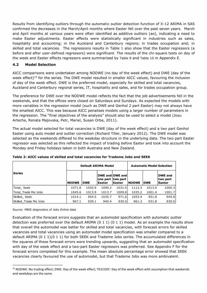
AICC comparisons were undertaken among NODWE (no day of the week effect) and DWE (day of the

week effect)15 for the series. The DWE model resulted in smaller AICC values, favouring the inclusion

of day of the week effect. DWE is the preferred model, especially for skilled and total vacancies,

Auckland and Canterbury regional series, IT, hospitality and sales, and for trades occupation group.

The preference for DWE over the NODWE model reflects the fact that the job advertisements fell in the

weekends, and that the offices were closed on Saturdays and Sundays. As expected the models with

more variables in the regression model (such as DWE and Genhol 2 part Easter) may not always have

the smallest AICC. This was because AICC penalises models using a larger number of parameters in

the regression. The “final objectives of the analysis” should also be used to select a model (Josu

Arteche, Renata Majovska, Petr, Mariel, Susan Orbe, 2011).

The actual model selected for total vacancies is DWE (day of the week effect) and a two part Genhol

Easter using auto model and outlier correction (Richard Tiller, January 2012). The DWE model was

selected as the weekends differed to the weekday structure in the underlying data. The two part Easter

regressor was selected as this reflected the impact of trading before Easter and took into account the

Monday and Friday holidays taken in both Australia and New Zealand.

Table 2: AICC values of skilled and total vacancies for Trademe Jobs and SEEK

Source: MBIE diagnostics of Jobs Online data

Evaluation of the forecast errors suggests that an automodel specification with automatic outlier

detection was preferred over the default ARIMA (0 1 1) (0 1 1) model. As an example the results show

that overall the automodel was better for skilled and total vacancies, with forecast errors for skilled

vacancies and total vacancies using an automodel model specification was smaller compared to a

default ARIMA (0 1 1)(0 1 1) for both SEEK and Trademe Jobs series. The accumulated differences in

the squares of these forecast errors were trending upwards, suggesting that an automodel specification

with day of the week effect and a two-part Easter regressors was preferred. See Appendix F for the

forecast errors completed for this example. The mean absolute percentage error showed that SEEK

vacancies clearly favoured the use of automodel, but that Trademe Jobs was more ambivalent.

15 NODWE: No trading effect; DWE: Day of the week effect; TD1COEF: Day of the week effect with assumption that weekends and weekdays are the same.

NODWE DWE

DWE and

one part

Easter

DWE and

two part

Easter NODWE DWE

DWE and

two part

Easter

Total_ Seek 1071.8 1020.9 1090.2 1031.0 1112.3 1013.0 1000.3

Total_Trade Me Jobs 1045.6 1013.9 1013.7 1009.8 1035.2 1001.4 1001.7

Skilled_ Seek 1014.1 954.5 1035.7 971.6 1053.4 951.8 945.8

Skilled_Trade Me Jobs 967.1 939.1 940.4 930.0 961.3 931.8 930.0

Series

Automatic Model SelectionDefault ARIMA Model

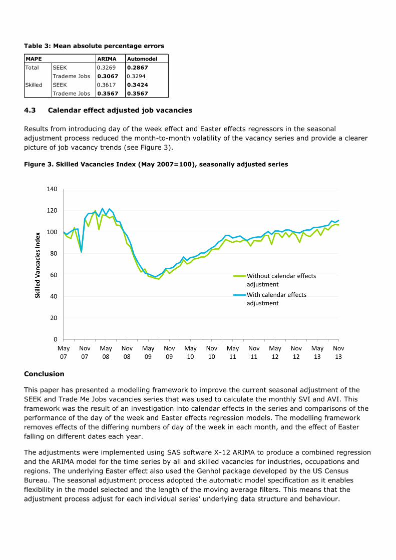
Table 3: Mean absolute percentage errors

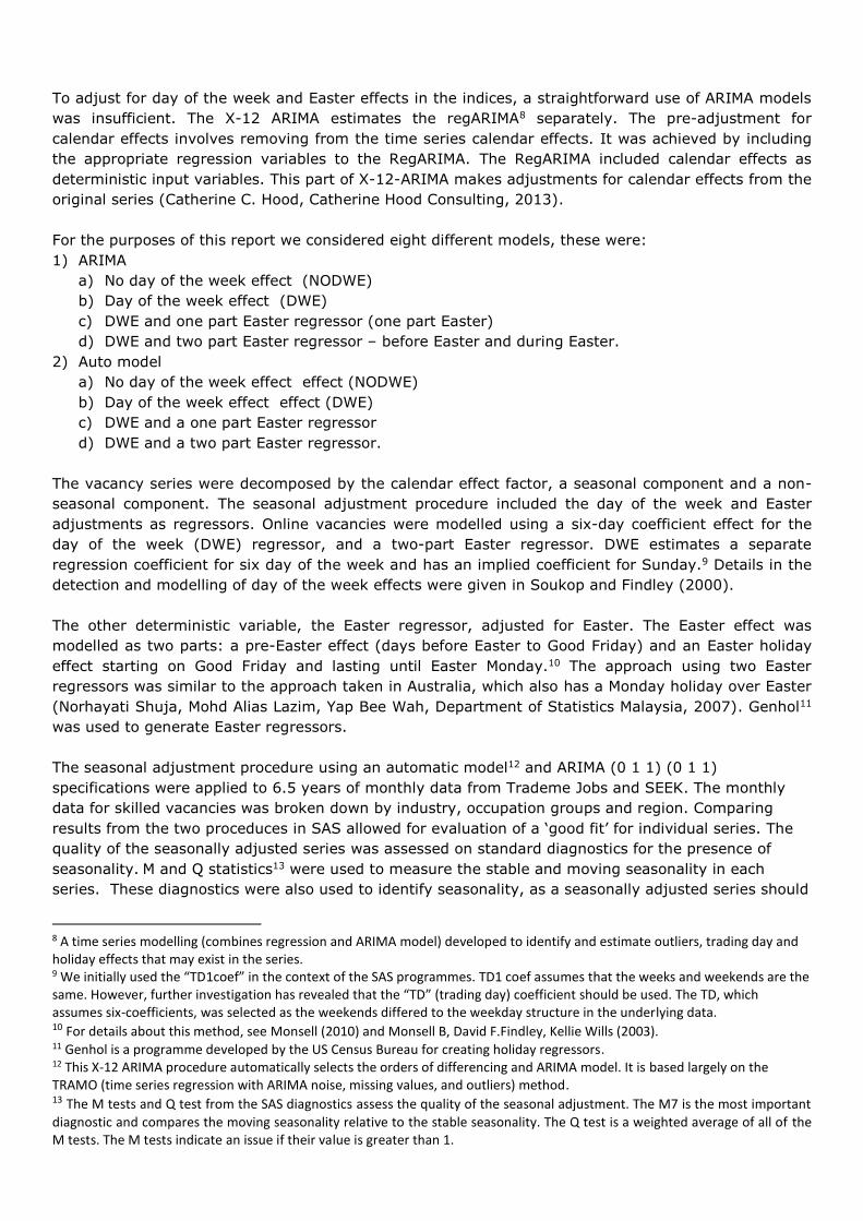
4.3 Calendar effect adjusted job vacancies

Results from introducing day of the week effect and Easter effects regressors in the seasonal

adjustment process reduced the month-to-month volatility of the vacancy series and provide a clearer

picture of job vacancy trends (see Figure 3).

Figure 3. Skilled Vacancies Index (May 2007=100), seasonally adjusted series

Conclusion

This paper has presented a modelling framework to improve the current seasonal adjustment of the

SEEK and Trade Me Jobs vacancies series that was used to calculate the monthly SVI and AVI. This

framework was the result of an investigation into calendar effects in the series and comparisons of the

performance of the day of the week and Easter effects regression models. The modelling framework

removes effects of the differing numbers of day of the week in each month, and the effect of Easter

falling on different dates each year.

The adjustments were implemented using SAS software X-12 ARIMA to produce a combined regression

and the ARIMA model for the time series by all and skilled vacancies for industries, occupations and

regions. The underlying Easter effect also used the Genhol package developed by the US Census

Bureau. The seasonal adjustment process adopted the automatic model specification as it enables

flexibility in the model selected and the length of the moving average filters. This means that the

adjustment process adjust for each individual series’ underlying data structure and behaviour.

ARIMA Automodel

Total SEEK 0.3269 0.2867

Trademe Jobs 0.3067 0.3294

Skilled SEEK 0.3617 0.3424

Trademe Jobs 0.3567 0.3567

MAPE

0

20

40

60

80

100

120

140

May07

Nov07

May08

Nov08

May09

Nov09

May10

Nov10

May11

Nov11

May12

Nov12

May13

Nov13

Skill

ed V

anca

cies

Ind

ex

Without calendar effectsadjustment

With calendar effectsadjustment

The final model selected adjusts for individual day of the week effect in each month and before and

during Easter effects. Standard statistical tests indicates that adjusting for these calendar effects in the

vacancies series was consistent with the data in each month from Trade Me Jobs and SEEK.

The outcome of this modelling framework was a better identification of seasonal effects and a clearer

picture of job vacancies, enhancing MBIE’s capacity to monitor and report on job vacancies.

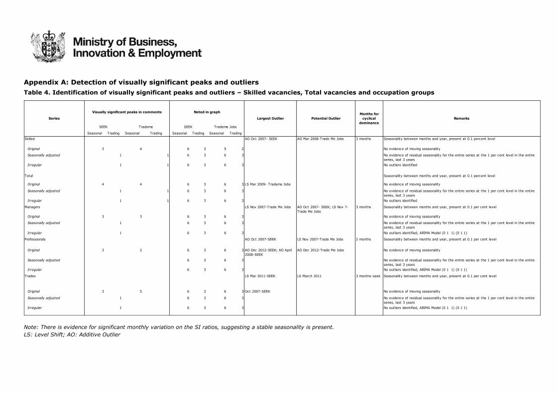
Appendix A: Detection of visually significant peaks and outliers

Table 4. Identification of visually significant peaks and outliers – Skilled vacancies, Total vacancies and occupation groups

Note: There is evidence for significant monthly variation on the SI ratios, suggesting a stable seasonality is present.

LS: Level Shift; AO: Additive Outlier

Seasonal Trading Seasonal Trading Seasonal Trading Seasonal Trading

Skilled AO Oct 2007- SEEK AO Mar 2008-Trade Me Jobs 3 months Seasonality between months and year, present at 0.1 percent level

Original 3 4 6 3 5 2 No evidence of moving seasonality

Seasonally adjusted 1 1 6 3 6 3 No evidence of residual seasonality for the entire series at the 1 per cent level in the entire

series, last 3 years

Irregular 1 1 6 3 6 3 No outliers identified

Total Seasonality between months and year, present at 0.1 percent level

Original 4 4 6 3 6 3 LS Mar 2009- Trademe Jobs No evidence of moving seasonality

Seasonally adjusted 1 1 6 3 6 3 No evidence of residual seasonality for the entire series at the 1 per cent level in the entire


Irregular 1 1 6 3 6 3 No outliers identified

Managers LS Nov 2007-Trade Me Jobs AO Oct 2007- SEEK; LS Nov 7-

Trade Me Jobs

3 months Seasonality between months and year, present at 0.1 per cent level

Original 3 3 6 3 6 3 No evidence of moving seasonality

Seasonally adjusted 1 6 3 6 3 No evidence of residual seasonality for the entire series at the 1 per cent level in the entire


Irregular 1 6 3 6 3 No outliers identified, ARIMA Model (0 1 1) (0 1 1)

Professionals AO Oct 2007-SEEK LS Nov 2007-Trade Me Jobs 2 months Seasonality between months and year, present at 0.1 per cent level

Original 3 2 6 3 6 3 AO Dec 2012-SEEK; AO April

2008-SEEK

AO Dec 2012-Trade Me Jobs No evidence of moving seasonality

Seasonally adjusted 6 3 6 3 No evidence of residual seasonality for the entire series at the 1 per cent level in the entire


Irregular 6 3 6 3 No outliers identified, ARIMA Model (0 1 1) (0 1 1)

Trades LS Mar 2011-SEEK LS March 2011 3 months-seek Seasonality between months and year, present at 0.1 per cent level

Original 3 5 6 3 6 3 Oct 2007-SEEK No evidence of moving seasonality

Seasonally adjusted 1 6 3 6 3 No evidence of residual seasonality for the entire series at the 1 per cent level in the entire


Irregular 1 6 3 6 3 No outliers identified, ARIMA Model (0 1 1) (0 1 1)

Series Largest Outlier Potential Outlier

Months for

cyclical

dominance

Remarks

SEEK Trademe

Visually significant peaks in comments

SEEK Trademe Jobs

Noted in graph

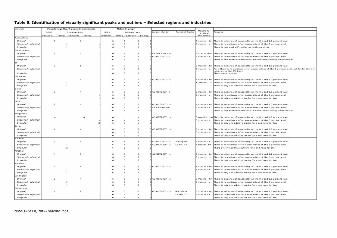
Table 5. Identification of visually significant peaks and outliers – Selected regions and industries

Note:s=SEEK; tm=Trademe Jobs

Variable

SEEK Trademe Jobs SEEK Trademe Jobs Largest Outlier Potential Outlier Remarks

Seasonal Trading Seasonal Trading Seasonal Trading Seasonal Trading

Accounting

Original 3 3 6 3 6 3 3 months - tm There is evidence of seasonality at the 0.1 and 1.0 percent level

Seasonally adjusted 1 1 6 3 6 3 3 months - s There is no evidence of an easter effect at the 5 percent level

Irregular 1 1 6 3 6 3 There is one level shift outlier for both s and tm

Construction

Original 1 2 1 6 3 6 3 LS NOV2007 - tm 3 months -tm There is evidence of seasonality at the 0.1 and 1.0 percent level

Seasonally adjusted 6 3 6 3 AO OCT2007 -s 2 months - s There is no evidence of an easter effect at the 5 percent level

Irregular 6 3 6 3 There is one additive outlier for s and one level shifting outlier for tm

IT

Original 2 1 6 3 6 3 2 months - tm There is evidence of seasonality at the 0.1 and 1.0 percent level

Seasonally adjusted 6 3 6 3 3 months - s For s there is no evidence of an easter effect at the 5 percent level, but for tm there is

evidence at the 5% level.

Irregular 6 3 6 3 There are no outliers

Education

Original 1 6 3 6 3 AO OCT2007 - s 4 months - tm There is evidence of seasonality at the 0.1 and 1.0 percent level

Seasonally adjusted 1 6 3 6 3 12 months - s There is no evidence of an easter effect at the 5 percent level

Irregular 1 6 3 6 3 There is only one additive outlier for s and none for tm.

Sales

Original 3 4 6 3 6 3 AO OCT2007- s 2 months - tm There is evidence of seasonality at the 0.1 and 1.0 percent level



Health

Original 2 1 1 6 3 6 3 AO OCT2007 - s 4 months - tm There is evidence of seasonality at the 0.1 and 1.0 percent level

Seasonally adjusted 6 3 6 3 LS JUL2007 -tm 5 months - s There is no evidence of an easter effect at the 5 percent level

Irregular 6 3 6 3 There is one additive outlier for s and one level shifting outlier for tm

Hospitality

Original AO OCT2007 - s 3 months - tm There is evidence of seasonality at the 0.1 and 1.0 percent level



Other

Original 4 4 6 3 6 3 AO OCT2007 - s 2 months - tm There is evidence of seasonality at the 0.1 and 1.0 percent level

Seasonally adjusted 6 3 6 3 3 months - s There is no evidence of an easter effect at the 5 percent level

Irregular 6 3 6 3 There is only one additive outlier for s and none for tm.

SIOther

Original 3 1 6 3 6 3 AO OCT2007 - s AO sep 07 4 months - s There is evidence of seasonality at the 0.1 and 1.0 percent level

Seasonally adjusted 1 6 3 6 3 AO MAR2008 - s LS nov 07 3 months -tm There is no evidence of an easter effect at the 5 percent level

Irregular 2 6 3 6 3 There are two additive outliers for s and none for tm.

NIOther


Seasonally adjusted 6 3 6 3 3 months - s There is no evidence of an easter effect at the 5 percent level

Irregular 6 3 6 3 There is only one additive outlier for s and none for tm.

Auckland




Wellington




Canterbury

Original 1 2 6 3 6 3 AO OCT2007 - s AO Feb 11 3 months - tm There is evidence of seasonality at the 0.1 and 1.0 percent level

Seasonally adjusted 1 6 3 6 3 LS Mar 11 3 months - s There is no evidence of an easter effect at the 5 percent level


Months for

cyclical

dominance

Visually significant peaks in comments Noted in graph

4 4 6 6

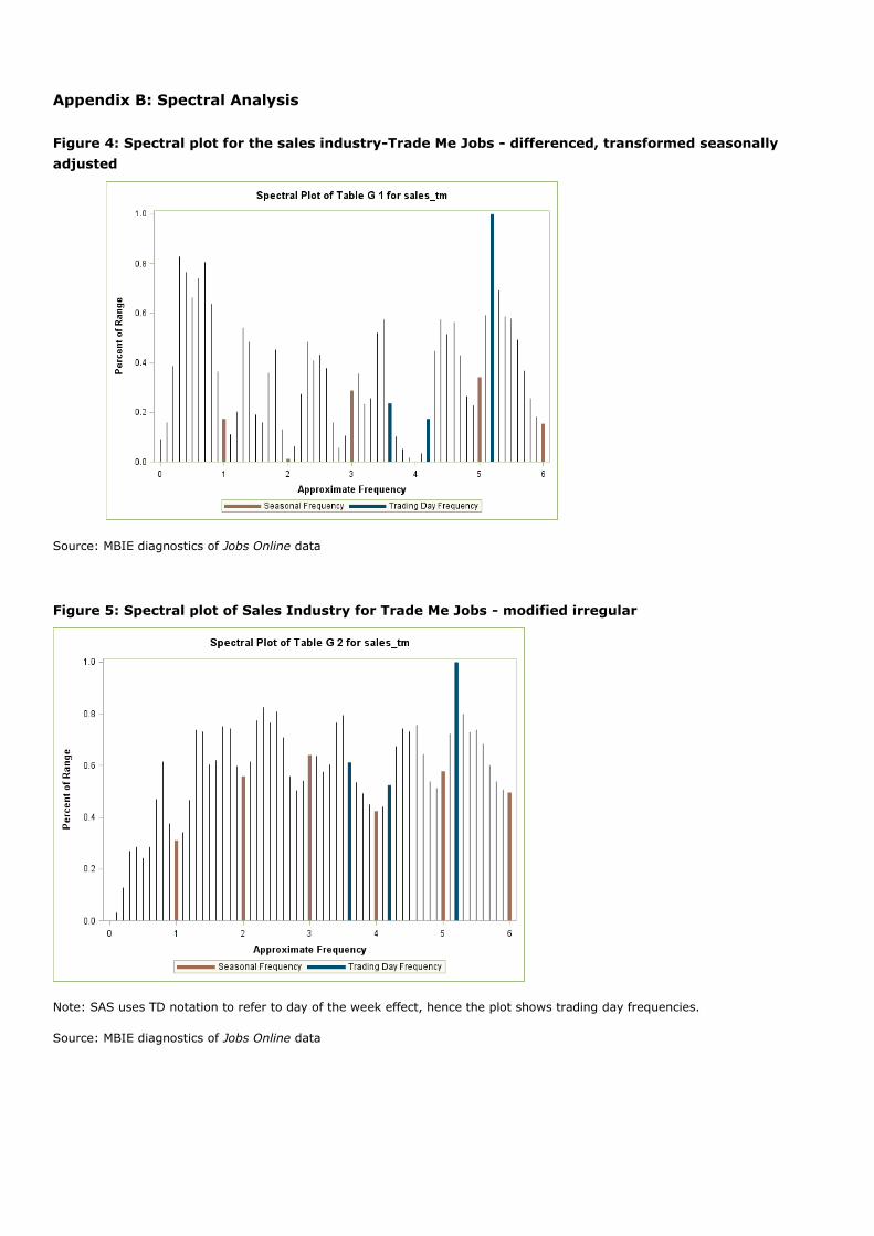
Appendix B: Spectral Analysis

Figure 4: Spectral plot for the sales industry-Trade Me Jobs - differenced, transformed seasonally

adjusted


Figure 5: Spectral plot of Sales Industry for Trade Me Jobs - modified irregular

Note: SAS uses TD notation to refer to day of the week effect, hence the plot shows trading day frequencies.


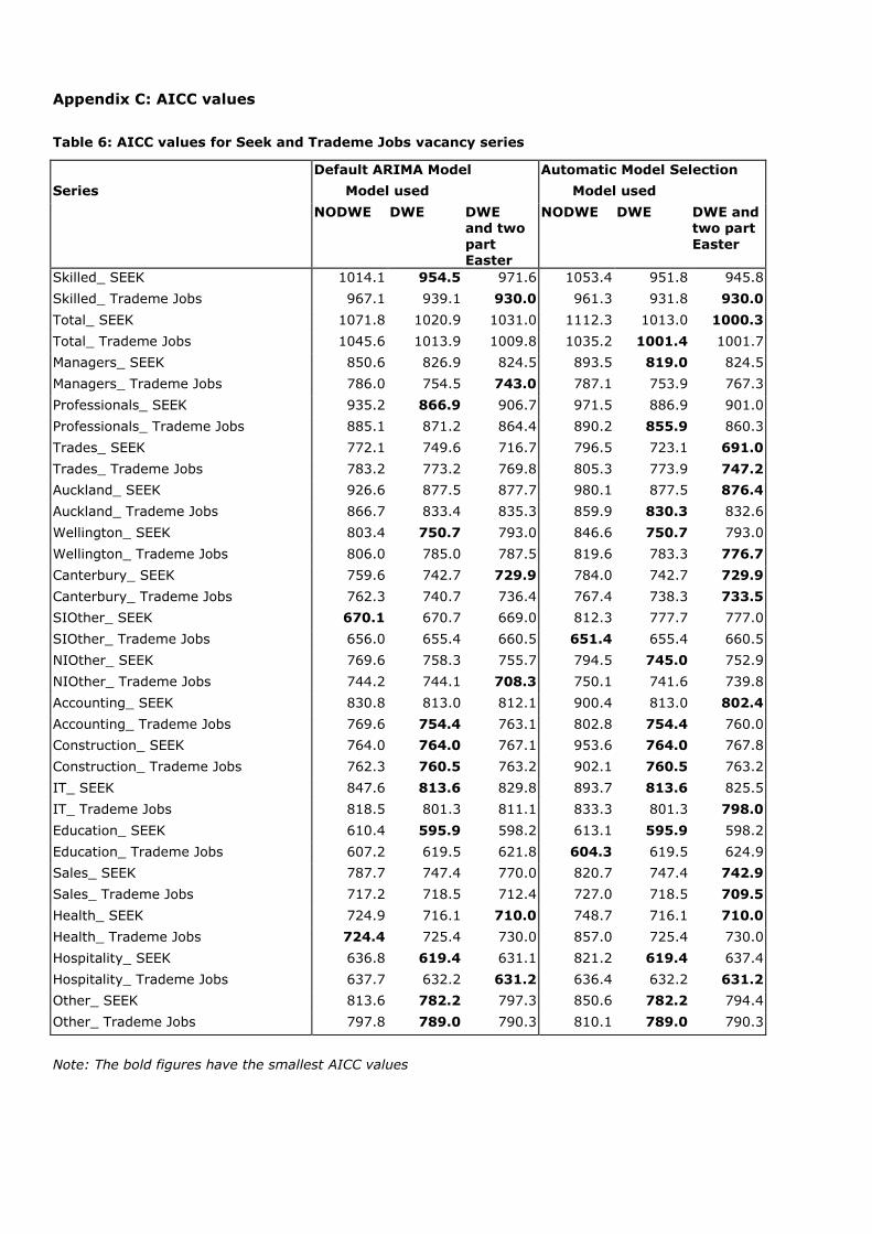
Appendix C: AICC values

Table 6: AICC values for Seek and Trademe Jobs vacancy series

Default ARIMA Model Automatic Model Selection

Series Model used Model used

NODWE DWE DWE and two

part Easter

NODWE DWE DWE and two part

Easter

Skilled_ SEEK 1014.1 954.5 971.6 1053.4 951.8 945.8

Skilled_ Trademe Jobs 967.1 939.1 930.0 961.3 931.8 930.0

Total_ SEEK 1071.8 1020.9 1031.0 1112.3 1013.0 1000.3

Total_ Trademe Jobs 1045.6 1013.9 1009.8 1035.2 1001.4 1001.7

Managers_ SEEK 850.6 826.9 824.5 893.5 819.0 824.5

Managers_ Trademe Jobs 786.0 754.5 743.0 787.1 753.9 767.3

Professionals_ SEEK 935.2 866.9 906.7 971.5 886.9 901.0

Professionals_ Trademe Jobs 885.1 871.2 864.4 890.2 855.9 860.3

Trades_ SEEK 772.1 749.6 716.7 796.5 723.1 691.0

Trades_ Trademe Jobs 783.2 773.2 769.8 805.3 773.9 747.2

Auckland_ SEEK 926.6 877.5 877.7 980.1 877.5 876.4

Auckland_ Trademe Jobs 866.7 833.4 835.3 859.9 830.3 832.6

Wellington_ SEEK 803.4 750.7 793.0 846.6 750.7 793.0

Wellington_ Trademe Jobs 806.0 785.0 787.5 819.6 783.3 776.7

Canterbury_ SEEK 759.6 742.7 729.9 784.0 742.7 729.9

Canterbury_ Trademe Jobs 762.3 740.7 736.4 767.4 738.3 733.5

SIOther_ SEEK 670.1 670.7 669.0 812.3 777.7 777.0

SIOther_ Trademe Jobs 656.0 655.4 660.5 651.4 655.4 660.5

NIOther_ SEEK 769.6 758.3 755.7 794.5 745.0 752.9

NIOther_ Trademe Jobs 744.2 744.1 708.3 750.1 741.6 739.8

Accounting_ SEEK 830.8 813.0 812.1 900.4 813.0 802.4

Accounting_ Trademe Jobs 769.6 754.4 763.1 802.8 754.4 760.0

Construction_ SEEK 764.0 764.0 767.1 953.6 764.0 767.8

Construction_ Trademe Jobs 762.3 760.5 763.2 902.1 760.5 763.2

IT_ SEEK 847.6 813.6 829.8 893.7 813.6 825.5

IT_ Trademe Jobs 818.5 801.3 811.1 833.3 801.3 798.0

Education_ SEEK 610.4 595.9 598.2 613.1 595.9 598.2

Education_ Trademe Jobs 607.2 619.5 621.8 604.3 619.5 624.9

Sales_ SEEK 787.7 747.4 770.0 820.7 747.4 742.9

Sales_ Trademe Jobs 717.2 718.5 712.4 727.0 718.5 709.5

Health_ SEEK 724.9 716.1 710.0 748.7 716.1 710.0

Health_ Trademe Jobs 724.4 725.4 730.0 857.0 725.4 730.0

Hospitality_ SEEK 636.8 619.4 631.1 821.2 619.4 637.4

Hospitality_ Trademe Jobs 637.7 632.2 631.2 636.4 632.2 631.2

Other_ SEEK 813.6 782.2 797.3 850.6 782.2 794.4

Other_ Trademe Jobs 797.8 789.0 790.3 810.1 789.0 790.3

Note: The bold figures have the smallest AICC values

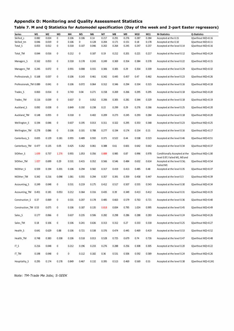
Appendix D: Monitoring and Quality Assessment Statistics

Table 7. M and Q Statistics for Automodel specification (Day of the week and 2-part Easter regressors)

Note: TM-Trade Me Jobs; S-SEEK

Series M1 M2 M3 M4 M5 M6 M7 M8 M9 M10 M11 M-Statistics Q-Statistics

Skilled_s 0.082 0.024 0 0.106 0.106 0.14 0.217 0.291 0.276 0.287 0.284 Accepted at the 0.15 Q(without M2)=0.16

Skilled_tm 0.046 0.019 0 0.106 0 0.128 0.204 0.171 0.151 0.18 0.178 Accepted at the 0.10 Q(without M2)=0.11

Total_S 0.053 0.012 0 0.318 0.107 0.046 0.202 0.264 0.245 0.247 0.237 Accepted at the level 0.14 Q(without M2)=0.16

Total_TM 0.044 0.016 0 0.212 0 0.187 0.19 0.212 0.201 0.221 0.217 Accepted at the level 0.12 Q(without M2)=0.24

Managers_S 0.162 0.053 0 0.318 0.178 0.243 0.249 0.369 0.354 0.384 0.378 Accepted at the level 0.22 Q(without M2)=0.15

Managers_TM 0.245 0.072 0 0.955 0.008 0.555 0.306 0.305 0.29 0.354 0.339 Accepted at the level 0.29 Q(without M2)=0.32

Professionals_S 0.168 0.037 0 0.106 0.143 0.461 0.342 0.445 0.457 0.47 0.462 Accepted at the level 0.23 Q(without M2)=0.26

Professionals_TM 0.089 0.041 0 0.106 0.072 0.064 0.312 0.346 0.294 0.334 0.315 Accepted at the level 0.16 Q(without M2)=0.18

Trades_S 0.063 0.014 0 0.743 0.04 0.271 0.158 0.269 0.266 0.295 0.295 Accepted at the level 0.18 Q(without M2)=0.20

Trades_TM 0.116 0.039 0 0.637 0 0.052 0.206 0.305 0.281 0.344 0.329 Accepted at the level 0.18 Q(without M2)=0.19

Auckland_S 0.092 0.028 0 0.849 0.192 0.238 0.22 0.299 0.29 0.276 0.266 Accepted at the level 0.25 Q(without M2)=0.20

Auckland_TM 0.148 0.055 0 0.318 0 0.402 0.209 0.273 0.245 0.293 0.284 Accepted at the level 0.18 Q(without M2)=0.20

Wellington_S 0.194 0.046 0 0.637 0.195 0.013 0.311 0.322 0.295 0.353 0.348 Accepted at the level 0.23 Q(without M2)=0.25

Wellington_TM 0.278 0.086 0 0.106 0.101 0.788 0.277 0.194 0.174 0.154 0.15 Accepted at the level 0.16 Q(without M2)=0.17

Canterbury_S 0.655 0.129 0.181 0.955 0.489 0.592 0.371 0.522 0.44 0.538 0.523 Accepted at the level 0.46 Q(without M2)=0.51

Canterbury_TM 0.477 0.135 0.05 0.425 0.262 0.061 0.388 0.61 0.601 0.642 0.642 Accepted at the level 0.34 Q(without M2)=0.37

SIOther_S 1.639 0.737 1.276 0.955 1.053 0.356 0.888 0.985 0.87 0.996 0.978 Conditionally Accepted at the

level 0.97; Failed M1, M3 and

Q(without M2)=1.00

SIOther_TM 1.027 0.699 0.29 0.531 0.415 0.352 0.566 0.546 0.484 0.632 0.614 Accepted at the level 0.56;

Failed M1

Q(without M2)=0.54

NIOther_S 0.559 0.194 0.201 0.106 0.294 0.582 0.317 0.419 0.413 0.485 0.48 Accepted at the level 0.35 Q(without M2)=0.37

NIOther_TM 0.342 0.216 0.098 1.061 0.355 0.294 0.357 0.391 0.359 0.458 0.447 Accepted at the level 0.3 Q(without M2)=0.39

Accounting_S 0.249 0.048 0 0.531 0.219 0.175 0.412 0.517 0.507 0.555 0.543 Accepted at the level 0.30 Q(without M2)=0.34

Accounting_TM 0.451 0.181 0.053 0.212 0.364 0.316 0.435 0.39 0.349 0.413 0.412 Accepted at the level 0.31 Q(without M2)=0.35

Construction_S 0.37 0.069 0 0.531 0.207 0.178 0.485 0.663 0.579 0.763 0.721 Accepted at the level 0.36 Q(without M2)=0.40

Construction_TM 0.53 0.075 0 0.106 0.187 0.135 0.818 0.834 0.795 1.024 0.995 Accepted at the level 0.45 Q(without M2)=0.49

Sales_S 0.177 0.066 0 0.637 0.235 0.506 0.282 0.298 0.286 0.288 0.283 Accepted at the level 0.24 Q(without M2)=0.26

Sales_TM 0.18 0.106 0 0.106 0.241 0.636 0.313 0.312 0.27 0.333 0.318 Accepted at the level 0.25 Q(without M2)=0.27

Health_S 0.641 0.629 0.88 0.106 0.721 0.538 0.376 0.474 0.445 0.469 0.419 Accepted at the level 0.53 Q(without M2)=0.52

Health_TM 0.748 0.383 0.338 0.106 0.518 0.013 0.528 0.725 0.679 0.74 0.726 Accepted at the level 0.47 Q(without M2)=0.48

IT_S 0.216 0.048 0 0.212 0.196 0.233 0.276 0.288 0.256 0.308 0.305 Accepted at the level 0.20 Q(without M2)=0.22

IT_TM 0.198 0.048 0 0 0.112 0.182 0.36 0.531 0.506 0.592 0.589 Accepted at the level 0.24 Q(without M2)=0.26

Hospitality_S 0.295 0.174 0.178 0.849 0.467 0.132 0.395 0.513 0.469 0.569 0.55 Accepted at the level 0.38 Q(without M2)=0.241

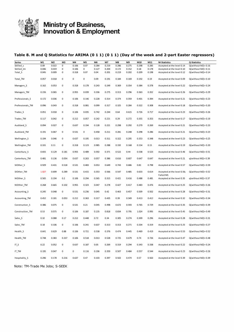
Table 8. M and Q Statistics for ARIMA (0 1 1) (0 1 1) (Day of the week and 2-part Easter regressors)

Note: TM-Trade Me Jobs; S-SEEK

Series M1 M2 M3 M4 M5 M6 M7 M8 M9 M10 M11 M-Statistics Q-Statistics

Skilled_s 0.09 0.022 0 0.106 0.07 0.284 0.219 0.286 0.275 0.298 0.285 Accepted at the level 0.14 Q(without M2)= 0.16

Skilled_tm 0.046 0.019 0 0.106 0 0.127 0.204 0.172 0.152 0.18 0.178 Accepted at the level 0.10 Q(without M2)= 0.11

Total_S 0.045 0.009 0 0.318 0.07 0.04 0.201 0.219 0.202 0.209 0.198 Accepted at the level 0.12 Q(without M2)= 0.14

Total_TM 0.057 0.018 0 0 0 0.09 0.191 0.184 0.169 0.192 0.19 Accepted at the level 0.09 Q(without M2)= 0.10

Managers_S 0.162 0.053 0 0.318 0.178 0.243 0.249 0.369 0.354 0.384 0.378 Accepted at the level 0.22 Q(without M2)= 0.24

Managers_TM 0.226 0.065 0 0.955 0.039 0.336 0.275 0.313 0.296 0.363 0.352 Accepted at the level 0.26 Q(without M2)= 0.29

Professionals_S 0.172 0.036 0 0.106 0.146 0.228 0.314 0.374 0.359 0.401 0.394 Accepted at the level 0.21 Q(without M2)= 0.23

Professionals_TM 0.096 0.043 0 0.318 0.081 0.099 0.317 0.325 0.284 0.322 0.308 Accepted at the level 0.18 Q(without M2)= 0.20

Trades_S 0.051 0.018 0 0.106 0.035 0.742 0.244 0.64 0.615 0.726 0.717 Accepted at the level 0.23 Q(without M2)= 0.26

Trades_TM 0.117 0.042 0 0.212 0.057 0.242 0.221 0.29 0.272 0.355 0.353 Accepted at the level 0.17 Q(without M2)= 0.19

Auckland_S 0.094 0.027 0 0.637 0.194 0.128 0.221 0.298 0.292 0.279 0.269 Accepted at the level 0.21 Q(without M2)= 0.23

Auckland_TM 0.191 0.067 0 0.531 0 0.458 0.211 0.281 0.248 0.298 0.286 Accepted at the level 0.21 Q(without M2)= 0.23

Wellington_S 0.194 0.046 0 0.637 0.195 0.013 0.311 0.322 0.295 0.353 0.348 Accepted at the level 0.23 Q(without M2)= 0.25

Wellington_TM 0.331 0.11 0 0.318 0.123 0.985 0.288 0.192 0.168 0.154 0.15 Accepted at the level 0.19 Q(without M2)= 0.20

Canterbury_S 0.655 0.129 0.181 0.955 0.489 0.592 0.371 0.522 0.44 0.538 0.523 Accepted at the level 0.46 Q(without M2)= 0.51

Canterbury_TM 0.481 0.136 0.054 0.637 0.263 0.057 0.386 0.616 0.607 0.647 0.647 Accepted at the level 0.21 q(without M2)= 0.39

SIOther_S 0.929 0.431 0.518 0.531 0.483 0.053 0.649 0.743 0.686 0.81 0.798 Accepted at the level 0.57 Q(without M2)= 0.59

SIOther_TM 1.027 0.699 0.289 0.531 0.415 0.353 0.566 0.547 0.485 0.633 0.614 Accepted at the level 0.56;

Failed M1

Q(without M2)= 0.52

NIOther_S 0.565 0.194 0.2 0.106 0.294 0.565 0.315 0.421 0.416 0.488 0.481 Accepted at the level 0.35 q(without M2)= 0.37

NIOther_TM 0.268 0.665 0.102 0.955 0.323 0.047 0.278 0.427 0.417 0.483 0.476 Accepted at the level 0.25 Q(without M2)= 0.26

Accounting_S 0.245 0.048 0 0.531 0.236 0.045 0.42 0.463 0.457 0.509 0.502 Accepted at the level 0.28 Q(without M2)= 0.31

Accounting_TM 0.452 0.181 0.053 0.212 0.363 0.317 0.435 0.39 0.349 0.413 0.412 Accepted at the level 0.32 Q(without M2)= 0.34

Construction_S 0.386 0.075 0 0.531 0.21 0.045 0.498 0.672 0.593 0.765 0.729 Accepted at the level 0.35 Q(without M2)= 0.39

Construction_TM 0.53 0.075 0 0.106 0.187 0.135 0.818 0.834 0.795 1.024 0.995 Accepted at the level 0.45 Q(without M2)= 0.49

Sales_S 0.32 0.088 0.17 0.212 0.448 0.72 0.34 0.305 0.274 0.309 0.296 Accepted at the level 0.28 Q(without M2)= 0.31

Sales_TM 0.18 0.106 0 0.106 0.241 0.637 0.313 0.313 0.271 0.334 0.319 Accepted at the level 0.25 Q(without M2)= 0.27

Health_S 0.641 0.629 0.88 0.106 0.721 0.538 0.376 0.474 0.445 0.469 0.419 Accepted at the level 0.53 Q(without M2)= 0.52

Health_TM 0.748 0.383 0.337 0.106 0.518 0.013 0.528 0.725 0.679 0.74 0.726 Accepted at the level 0.47 Q(without M2)= 0.48

IT_S 0.22 0.052 0 0.637 0.187 0.05 0.269 0.319 0.294 0.343 0.338 Accepted at the level 0.22 Q(without M2)= 0.24

IT_TM 0.195 0.047 0 0 0.116 0.196 0.359 0.507 0.484 0.557 0.544 Accepted at the level 0.23 Q(without M2)= 0.26

Hospitality_S 0.296 0.178 0.216 0.637 0.47 0.103 0.397 0.502 0.474 0.57 0.563 Accepted at the level 0.39 Q(without M2)= 0.39

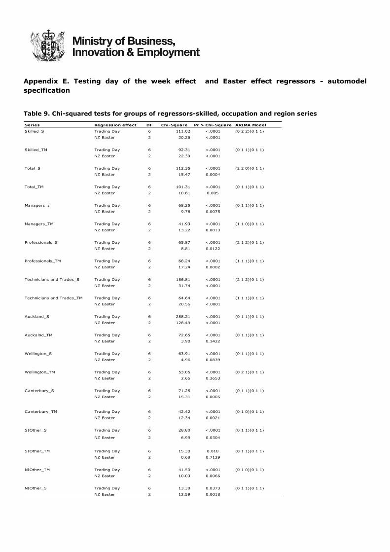
Appendix E. Testing day of the week effect and Easter effect regressors - automodel

specification

Table 9. Chi-squared tests for groups of regressors-skilled, occupation and region series

Series Regression effect DF Chi-Square Pr > Chi-Square ARIMA Model

Skilled_S Trading Day 6 111.02 <.0001 (0 2 2)(0 1 1)

NZ Easter 2 20.26 <.0001

Skilled_TM Trading Day 6 92.31 <.0001 (0 1 1)(0 1 1)

NZ Easter 2 22.39 <.0001

Total_S Trading Day 6 112.35 <.0001 (2 2 0)(0 1 1)

NZ Easter 2 15.47 0.0004

Total_TM Trading Day 6 101.31 <.0001 (0 1 1)(0 1 1)

NZ Easter 2 10.61 0.005

Managers_s Trading Day 6 68.25 <.0001 (0 1 1)(0 1 1)

NZ Easter 2 9.78 0.0075

Managers_TM Trading Day 6 41.93 <.0001 (1 1 0)(0 1 1)

NZ Easter 2 13.22 0.0013

Professionals_S Trading Day 6 65.87 <.0001 (2 1 2)(0 1 1)

NZ Easter 2 8.81 0.0122

Professionals_TM Trading Day 6 68.24 <.0001 (1 1 1)(0 1 1)

NZ Easter 2 17.24 0.0002

Technicians and Trades_S Trading Day 6 186.81 <.0001 (2 1 2)(0 1 1)

NZ Easter 2 31.74 <.0001

Technicians and Trades_TM Trading Day 6 64.64 <.0001 (1 1 1)(0 1 1)

NZ Easter 2 20.56 <.0001

Auckland_S Trading Day 6 288.21 <.0001 (0 1 1)(0 1 1)

NZ Easter 2 128.49 <.0001

Auckalnd_TM Trading Day 6 72.65 <.0001 (0 1 1)(0 1 1)

NZ Easter 2 3.90 0.1422

Wellington_S Trading Day 6 63.91 <.0001 (0 1 1)(0 1 1)

NZ Easter 2 4.96 0.0839

Wellington_TM Trading Day 6 53.05 <.0001 (0 2 1)(0 1 1)

NZ Easter 2 2.65 0.2653

Canterbury_S Trading Day 6 71.25 <.0001 (0 1 1)(0 1 1)

NZ Easter 2 15.31 0.0005

Canterbury_TM Trading Day 6 42.42 <.0001 (0 1 0)(0 1 1)

NZ Easter 2 12.34 0.0021

SIOther_S Trading Day 6 28.80 <.0001 (0 1 1)(0 1 1)

NZ Easter 2 6.99 0.0304

SIOther_TM Trading Day 6 15.30 0.018 (0 1 1)(0 1 1)

NZ Easter 2 0.68 0.7129

NIOther_TM Trading Day 6 41.50 <.0001 (0 1 0)(0 1 1)

NZ Easter 2 10.03 0.0066

NIOther_S Trading Day 6 13.38 0.0373 (0 1 1)(0 1 1)

NZ Easter 2 12.59 0.0018

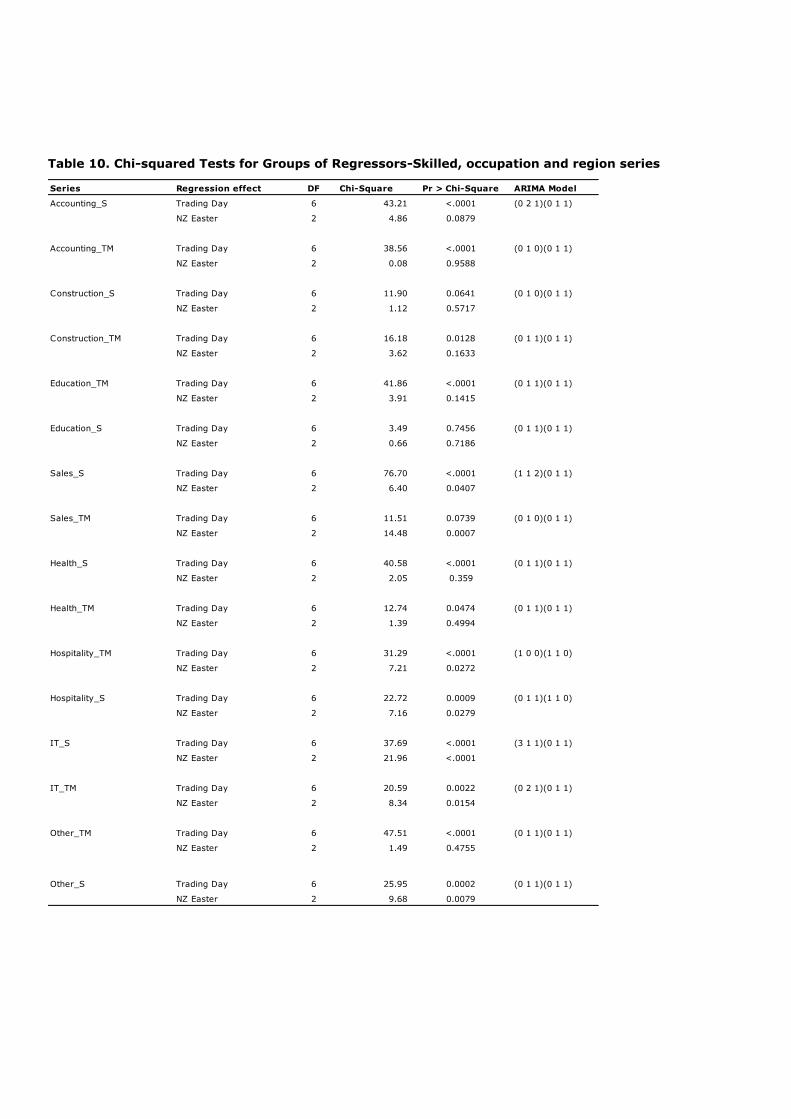
Table 10. Chi-squared Tests for Groups of Regressors-Skilled, occupation and region series

Series Regression effect DF Chi-Square Pr > Chi-Square ARIMA Model

Accounting_S Trading Day 6 43.21 <.0001 (0 2 1)(0 1 1)

NZ Easter 2 4.86 0.0879

Accounting_TM Trading Day 6 38.56 <.0001 (0 1 0)(0 1 1)

NZ Easter 2 0.08 0.9588

Construction_S Trading Day 6 11.90 0.0641 (0 1 0)(0 1 1)

NZ Easter 2 1.12 0.5717

Construction_TM Trading Day 6 16.18 0.0128 (0 1 1)(0 1 1)

NZ Easter 2 3.62 0.1633

Education_TM Trading Day 6 41.86 <.0001 (0 1 1)(0 1 1)

NZ Easter 2 3.91 0.1415

Education_S Trading Day 6 3.49 0.7456 (0 1 1)(0 1 1)

NZ Easter 2 0.66 0.7186

Sales_S Trading Day 6 76.70 <.0001 (1 1 2)(0 1 1)

NZ Easter 2 6.40 0.0407

Sales_TM Trading Day 6 11.51 0.0739 (0 1 0)(0 1 1)

NZ Easter 2 14.48 0.0007

Health_S Trading Day 6 40.58 <.0001 (0 1 1)(0 1 1)

NZ Easter 2 2.05 0.359

Health_TM Trading Day 6 12.74 0.0474 (0 1 1)(0 1 1)

NZ Easter 2 1.39 0.4994

Hospitality_TM Trading Day 6 31.29 <.0001 (1 0 0)(1 1 0)

NZ Easter 2 7.21 0.0272

Hospitality_S Trading Day 6 22.72 0.0009 (0 1 1)(1 1 0)

NZ Easter 2 7.16 0.0279

IT_S Trading Day 6 37.69 <.0001 (3 1 1)(0 1 1)

NZ Easter 2 21.96 <.0001

IT_TM Trading Day 6 20.59 0.0022 (0 2 1)(0 1 1)

NZ Easter 2 8.34 0.0154

Other_TM Trading Day 6 47.51 <.0001 (0 1 1)(0 1 1)

NZ Easter 2 1.49 0.4755

Other_S Trading Day 6 25.95 0.0002 (0 1 1)(0 1 1)

NZ Easter 2 9.68 0.0079

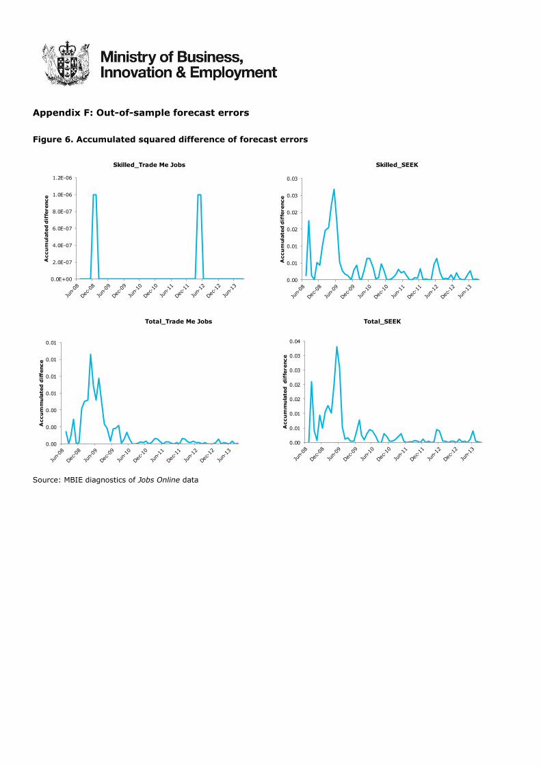
Appendix F: Out-of-sample forecast errors

Figure 6. Accumulated squared difference of forecast errors


Skilled_SEEKSkilled_Trade Me Jobs

Total_Trade Me Jobs Total_SEEK

0.0E+00

2.0E-07

4.0E-07

6.0E-07

8.0E-07

1.0E-06

1.2E-06

Accu

mula

ted d

iffe

rence

0.00

0.01

0.01

0.02

0.02

0.03

0.03

Accu

mula

ted d

iffe

rence

0.00

0.00

0.00

0.01

0.01

0.01

0.01

Accu

mm

ula

ted

dif

fence

0.00

0.01

0.01

0.02

0.02

0.03

0.03

0.04

Accu

mm

ula

ted

d

iffe

rence

References

Michael Grun Rehomme, Amani Ben Rejeb, Institute for Labor Studies and Public Policies. (2008). Modelling Moving

Feasts Determined by the Islamic Calendar: Application to Macroeconomic Tunisian Time Series. Paris,

France.

Bowerman, O'Connell and Koehler. (2005). Forecasting, Time Series, and Regression. United States of America:

Brooks Cole Cengage Learning.

Catherine C. Hood, Catherine Hood Consulting. (2009). Getting started with X12 ARIMA diagnostics – Spectral

Diagnostics. p1.

Catherine C. Hood, Catherine Hood Consulting. (2011). Case study: Fixing residual trading day effects in the

seasonality adjusted series.

Catherine C. Hood, Catherine Hood Consulting. (2013). Diagnostics FAQ.

Catherine C. Hood, Catherine Hood Consulting. (June 18-21 2007). Assessment of Diagnostics for the Presence of

seasonality. ICES-III, Montreal Quebec, Canada.

Catherine C. Hood, Roxanne Feldpausch, Catherine Hood Consulting. (2010). Experiences with User-defined

regressors for Seasonal Adjustment.

Catherine C. Hood, US Census Bureau, Washington DC. (2000). SAS programs to get the most from X12 ARIMAs

modelling and seasonal adjustment diagnostics. p1.

Catherine Hood Consulting. (25/11/2013). Seasonal Adjustment and Time Series FAQ.

http://catherinechhood.net/safaQdiagnostics.html, p2.

Central Bureau of Statistics. (2007). Seasonal Adjustment. Israel:

http://www.cbs.gov.il/publications/tseries/seasonal07/introduction.pdf.

James D Ryan, J. E. (n.d.). The Spectrum of Broadway: A SAS® PROC Spectra Inquiry. Paper 199-26, p1.

Josu Arteche, Renata Majovska, Petr, Mariel, Susan Orbe. (2011). Detection and Correction of calendar effects: An

Application to Industrial Production index of Alava. Journal of Applied Maths, Volume IV (2011), number III.

Monsell B, David F.Findley, Kellie Wills. (2003). Issues in Estimating Easter Regressors Using REGARIMA Models with

X-12 ARIMA. US Census Bureau.

Monsell, B. (2010). Issues in modelling and adjusting for calendar effects in economic time series.

http://www.census.gov/ts/papers/ices2007bcm.pdf. Retrieved from

http://www.census.gov/ts/papers/ices2007bcm.pdf

Norhayati Shuja, Mohd Alias Lazim, Yap Bee Wah, Department of Statistics Malaysia. (2007). Moving holiday effects

adjustment for Malaysian Economic Time Series.

Raymond J. Soukup, D. F. (2000). Detection and modelling of trading day effects.

Raymond J. Soukup, David F Findley, US Census Bureau. (2000). Detection and modelling of trading day effects.

Raymond J. Soukup, David F. Findley, US Census Bureau. (n.d.). On the spectrum diagnostics used by X12-ARIMA to

indicate the presence of trading day effects after modeling or adjustment.

www.census.gov/ts/papers/rr9903s.pdf.

Richard Tiller, Daniel Chow and Stuart Scott, Bureau of Labor Statistics. (2007). Empirical Evaluation of X-11 and

Model-based Seasonal Adjustment methods. Massachusetts Avenue, N.E., Washington, D.C. 20122.

Richard Tiller, T. E. (January 2012). Methodology for Seasonally Adjusting National Household Labor Force Series with

Revisions for 2012, Current Population Syrvey (CPS), Technical Documentation.

SAS/ETS®. (2013). The X-12 procedure: User defined regressors: SAS/ETS® 9.2 Users Guide.

http://support.sas.com/documentation/cdl/en/etsug/60372/HTML/default/etsug_x12_s,

http://support.sas.com/documentation/cdl/en/etsug/65545/HTML/default/etsug_x12.

Spider Financial. (2014). Adjusting for calendar effects, 2014.

http://www.spiderfinancial.com/support/documentation/numxl/tips-and-tricks/calendar-effects.

Statistics NZ, John Crequer, Barbara Clendon. (2008). Elucidating Easter’s Economic Effects. p8.

Tammy Jackson, Michael Leonard, SAS Institute, Inc. (2000). Seasonal adjustment using the X12 procedure.

United National Statistics Division (UNSD). (17 March 2010). Seasonal Adjustment and Time Series Issues. p15.

US Census Bureau. (2013). Running Genhol – Examples.

http://www.census.gov/srd/ww/genhol/genhol_examples.html.

US Census Bureau. (2013). Running the Genhol Utility. http://www.census.gov/srd/ww/genhol/genhol_run.html.

US Census Bureau. (2013). X-12-ARIMA Seasonal Adjustment program, Notes on centering holiday regressors.

http://www.census.gov/srd/ww/genhol/genhol_center.html.

Zhang, X., McLaren, C. H., and Leung, C. C. S. (2003). An Easter proximity effect: Modelling and adjustment.

Australian and New Zealand Journal of Statistics, 43.

modeling calendar effects in mbie's jobs online vacancies

Documents