modelado jerárquico de objetos 3d con superficies de
TRANSCRIPT
UNIVERSIDAD POLITÉCNICA DE MADRID
ESCUELA TÉCNICA SUPERIOR DE INGENIEROS
DE TELECOMUNICACIÓN
TESIS DOCTORAL
MODELADO JERÁRQUICO DE OBJETOS 3D
CON SUPERFICIES DE SUBDIVISIÓN
FRANCISCO MORÁN BURGOS
INGENIERO DE TELECOMUNICACIÓN
2001

DEPARTAMENTO DE SEÑALES, SISTEMAS Y RADIOCOMUNICACIONES
ESCUELA TÉCNICA SUPERIOR DE INGENIEROS
DE TELECOMUNICACIÓN
TESIS DOCTORAL
MODELADO JERÁRQUICO DE OBJETOS 3D
CON SUPERFICIES DE SUBDIVISIÓN
Autor: Francisco Morán Burgos
Ingeniero de Telecomunicación
Director: Narciso García Santos
Doctor Ingeniero de Telecomunicación
Octubre 2001


Tribunal nombrado por el Mgfco. y Excmo. Sr. Rector de la Universidad Politécnica de
Madrid, el día ....... de ............................ de 200... :
Presidente: .........................................................................................................
Vocal: .........................................................................................................
Vocal: .........................................................................................................
Vocal: .........................................................................................................
Secretario: .........................................................................................................
Realizado el acto de lectura y defensa de la Tesis el día ....... de ............................ de 200...
en Madrid.
Calificación: .........................................................................................................
EL PRESIDENTE EL SECRETARIO
LOS VOCALES


Agradecimientos
Ya los fenicios incluían secciones de agradecimientos en sus tesis, que empezaban invariablemente cantando las alabanzas de sus respectivos directores. Yo no voy a ser menos, y no por interés ni por parecer bien nacido, sino porque es de justicia agradecer a Narciso, verdadero maestro de malabares figurados, el tiempo que ha logrado sacarse de la manga para dirigir esta tesis, un diferencial de caspa de mosca en su universo de (pre)ocupaciones. Además, pocas personas hubieran sido capaces de tolerar mi perfeccionismo (en la pequeñez, desgraciadamente), mis salidas de tono y mis desáni-mos como Narciso: de Narciso se aprende, aparte de historia(s ;-), a no darse por vencido, a insistir.
También quiero agradecer a los miembros del tribunal de esta tesis que hayan aceptado formar parte de él, con independencia del juicio que emitan de ella, por supuesto. Los españoles, aun siendo mayoría, han visto bien enfrentarse a un documento que, además de ser abstruso (eso ellos aun no lo saben, pero yo sí…), está escrito en inglés, por deferencia a los extranjeros. Éstos, primeras figuras del mundo de los estándares internacionales de codificación de vídeo, de los que tanto he aprendido en las reuniones del MPEG, han dado a su vez el visto bueno a un posible y probablemente engorro-so desplazamiento a Madrid para asistir al correspondiente acto de presentación y defensa de la tesis, que se realizaría también en inglés. Thank you so much, Touradj, Gauthier and Michael. I hope you’ll understand the rest of this paragraph — oh, come on, compliments and acknowledgements are always easier to understand, no matter the language!
Siguiendo con los agradecimientos formales, no por ello menos sentidos, no me puedo olvidar de que mucho de lo que sé de superficies de subdivisión se lo debo a Peter (thank you so much for all you taught me about subdivision surfaces and multiresolution analysis techniques, and for your food forand thought Friday lunches, Peter) y a Miguel, que me acogieron calurosamente en CalTech. Tampoco me puedo olvidar de la tediosa labor de revisión crítica de partes de esta tesis o de docu-mentos previos que le han servido de base, lo que me permite volver a dar las gracias a Nacho, Gauthier y Michael, y el dárselas por primera vez a mi tío Manuel, el más caótico de los doctos Moranes, y a Chema, al que devuelvo su agradecimiento por corregir erratas tipográficas y otras minucias en su tesis.
Pero el agradecimiento bonito, bonito que puedo devolver ahora a Chema es el de los “13 años estando ahí”. A mí, ya ves, me salen dieciséis y pico, pero te siento tan ahí como tú me sentías a mí hace más de tres años, aunque de vez en cuando me toques los ficheros/alumnos o yo te toque otros colgajos, aunque no nos parezcamos en muchas cosas, aunque no nos veamos tanto fuera de la Escuela.
Ya entrado en la Escuela y sus aledaños, y está bien que haya sido de la mano de Chema porque él fue el principal responsable de mi abducción por el GTI hace diez años, tengo que nombrar honoris causa a: Martina, mi kleinecillä y artista potencial preferida; Aurora y Patricia, que vienen a ser Sta. Bendita y Sta. Paciencia; Ángel y Saúl, que seguramente no hicieron mal en largarse al mundo real, y con los que espero que no perdamos el contacto; Fernando, por ser un borde tan de pega y echarme

tantas manos con las máquinas (gracias también a José Miguel y a José, mis tablas de salvación en más de una ocasión cuando andaba perdido con el HP-UX o con los misterios de los routers); Na-cho, por meterme de vez en cuando en el cuerpo las ganas de volver a darle a las Mates, como en el Liceo; Carlos, por sus picos de acidez; y Luis, Guillermo y José Manuel, por contribuir a darle al GTI su color característico. Quiero mandar un fuerte abrazo a Enrique y agradecerle las charlas sobre gráficos y otras golosinas palosojos por las que compartimos el gusto — tranquilo, que ya tendrás ocasión de devolverme el agradecimiento en una sección como ésta cuando te toque escribir-la. He dejado para el final a los otros dos jotas de los (cada vez menos) indocumentados del GTI, para dedicarles también frases aparte, claro. Julián: esta vez, y sin que sirva de precedente, seré yo quien te agradezca esas partidas de mus en las que tanto aprendías de mí — por ejemplo, que no hace falta ligar tan buenas cartas (como tú) para cagarla (sí, eso), sino que es posible hacerlo con unas cartas vomitivas como las que me suelen entrar a mí. Jesús: comidas y vinos aparte, por las que lógicamente también serás recordado siempre, quiero decirte que cada vez admiro más tu capacidad de enfocarte y dedicar tiempo y energía sólo a las cosas importantes (lo que exige, para empezar, tener claro cuáles son), y tu ser un tío generoso y elegante sin darte cuenta siquiera, como para rizar el rizo en ese despiste marca de la casa.
De los (ex-)miembros del GTI, paso a los que han sido alumnos nuestros y nos han hecho y hacen pasar buenos ratos, aunque a mí en particular me hayan tenido que aburrir con cuestiones system-manageriles. No nombraré a nadie en concreto para no levantar suspicacias, salvo quizá a Clara, que es tan feliz que no se le puede querer mal. De entre los Proyectos Fin de Carrera que yo en concreto he dirigido, destaco, porque es tan justo y necesario como los agradecimientos del primer párrafo, el de Marcos, sin quien esta tesis no sería la que es: gracias por tus programas y por las horas que hemos pasado juntos quebrándonos la cabeza por temas técnicos relacionados con las mallas 3D o compartiendo dudas profesionales más genéricas.
Y llego ya al núcleo de la cebolla (del cebollo, en este caso) en el que se encuentran mis familiares y amigos, que están siempre ahí. Están siempre ahí mis padres y mis hermanos Ana y Uge, a los que pido perdón por escatimarles flores y agradecimientos, al menos en comparación con los que le dedico a Sara, como sabe todo el que me haya oído hablar más de cinco minutos — y es que es normal, porque eres muy buina: sin ti me hubiera sido imposible imprimir a tiempo los enemasún ejemplares de esta tesis, por ejemplo. Están siempre ahí Poe y el resto de mis tíos (Manuel: gracias otra vez), mi abuela, que es un solete, y mis primos, que me siguen dejando jugar a ser su primo mayor aunque vayan a ponerse a echar críos al mundo antes que yo. En este último lote (tranquila, que no te meto en él por lo de los críos, al menos de momento…) brilla especialmente mi prima Clara, que además de bellartista es una de mis confesoras predilectas. Pero igual de ahí han estado para mí, en los momentos importantes de renacimientos y otras penurias que he pasado durante todo este tiempo, Ferbiñe y Garbando, que tanto monta, monta tanto, y Mercedes, y muchos de los licea-nos con los que dentro de poco cenaré y jugaré a la lotería de Navidad como desde hace casi veinte años, aunque algunos estén, más que ahí, allá, debido a que se han exportado (hola, Felipe; hola, Luisa: pasa y saluda a Chema, que no se ha exportardo pero sí se ha invitado también, por derecho propio, a este apartado de amigos de siempre); o por ahí, debido sobre todo a que también se han puesto a repoblar el planeta (sí, Juan: te puedes dar por aludido… ;-).
En ese mismo núcleo también hay personajes (de ficción, o del Arte, como los muchos directores de cine o escritores culpables en parte de lo que he tardado en acabar esta tesis) e intangibles varios que me hacen fantasear con otras posibles vidas, alejadas de toda telequez o ingenierez, por muy bonitas que puedan ser algunas cosas de la teoría de la información y por muy optimizador nato que sea uno. A ellos, y a los que buscan y dudan y son incapaces de enfocar sus energías, pero no acaban de dejar de creer en ellas, dedico esta tesis sin dedicatoria.
Resumen
Las SSs (Superficies de Subdivisión) son un potente paradigma de modelado de objetos 3D (tri-Dimensionales) que establece un puente entre los dos enfoques tradicionales a la aproximación de superficies, basados en mallas poligonales y de parches alabeados, que conllevan problemas uno y otro. Los esquemas de subdivisión permiten definir una superficie suave (a tramos), como las más frecuentes en la práctica, como el límite de un proceso recursivo de refinamiento de una malla de control burda, que puede ser descrita muy compactamente. Además, la recursividad inherente a las SSs establece naturalmente una relación de anidamiento piramidal entre las mallas / NDs (Niveles de Detalle) generadas/os sucesivamente, por lo que las SSs se prestan extraordinariamente al AMRO (Análisis MultiResolución mediante Ondículas) de superficies, que tiene aplicaciones prácticas inmediatas e interesantísimas, como la codificación y la edición jerárquicas de modelos 3D.
Empezamos describiendo los vínculos entre las tres áreas que han servido de base a nuestro trabajo (SSs, extracción automática de NDs y AMRO) para explicar cómo encajan estas tres piezas del puzzle del modelado jerárquico de objetos de 3D con SSs. El AMRO consiste en descomponer una función en una versión burda suya y un conjunto de refinamientos aditivos anidados jerárquicamente llamados “coeficientes ondiculares”. La teoría clásica de ondículas estudia las señales clásicas nD: las definidas sobre dominios paramétricos homeomorfos a n o [0, 1]n, como el audio (n = 1), las imágenes (n = 2) o el vídeo (n = 3). En topologías menos triviales, como las variedades 2D (superfi-cies en el espacio 3D), el AMRO no es tan obvio, pero sigue siendo posible si se enfoca desde la perspectiva de las SSs. Basta con partir de una malla burda que aproxime a un bajo ND la superficie considerada, subdividirla recursivamente y, al hacerlo, ir añadiendo los coeficientes ondiculares, que son los detalles 3D necesarios para obtener aproximaciones más y más finas a la superficie original.
Pasamos después a las aplicaciones prácticas que constituyen nuestro principal desarrollo original y, en particular, presentamos una técnica de codificación jerárquica de modelos 3D basada en SSs, que actúa sobre los detalles 3D mencionados: los expresa en un referencial normal local; los organi-za según una estructura jerárquica basada en facetas; los cuantifica dedicando menos bits a sus componentes tangenciales, menos energéticas, y los “escalariza”; y los codifica finalmente gracias a una técnica similar al SPIHT (Set Partitioning In Hierarchical Trees) de Said y Pearlman. El resul-tado es un código completamente embebido y al menos dos veces más compacto, para superficies mayormente suaves, que los obtenidos con técnicas de codificación progresiva de mallas 3D publi-cadas previamente, en las que además los NDs no están anidados piramidalmente.
Finalmente, describimos varios métodos auxiliares que hemos desarrollado, mejorando técnicas previas y creando otras propias, ya que una solución completa al modelado de objetos 3D con SSs requiere resolver otros dos problemas. El primero es la extracción de una malla base (triangular, en nuestro caso) de la superficie original, habitualmente dada por una malla triangular fina con conecti-vidad arbitraria. El segundo es la generación de un remallado con conectividad de subdivisión de la malla original/objetivo mediante un refinamiento recursivo de la malla base, calculando así los detalles 3D necesarios para corregir las posiciones predichas por la subdivisión para nuevos vértices.


Sinopsis en español
Modelado jerárquico de objetos 3D con superficies de subdivisión a
Sinopsis en español
MOTIVACIÓN
Hay varias posibles maneras de modelar un objeto 3D (triDimensional), de las que la más sencilla consiste en describir únicamente la superficie que lo delimita, despreciando su interior. Éste es, además, el enfoque más comúnmente usado en el mundo de los gráficos 3D por ordenador, en el que el objetivo principal del modelado de los objetos es su posterior visualización. La razón es que el interior de la mayoría de los objetos no afecta sustancialmente a la manera en que la luz es reflejada por ellos, que es lo que ha de ser simulado durante el proceso de visualización. El problema funda-mental del DAO (Diseño Asistido por Ordenador) es precisamente el de representar verosímil y eficientemente superficies 3D complejas. Modelar superficies lineales a tramos, como la de un cubo, o aun alabeadas pero simples, como las de un cilindro o una esfera, es una tarea relativamente senci-lla, pero diseñar estructuras de datos y algoritmos para crear y manipular eficientemente aproxima-ciones fieles de formas 3D reales dista de ser evidente.
A su vez, hay varias posibles maneras de aproximar una superficie 3D, de las que la más sencilla consiste en teselarla con polígonos, lógicamente planos — de hecho, con triángulos, dado que los triángulos son los polígonos más sencillos. La mayoría de las aplicaciones comerciales de DAO son capaces de manejar mallas poligonales compuestas por triángulos o polígonos arbitrarios, que tam-bién son consideradas por los dos únicos estándares de jure para la descripción de escenas 3D sinté-ticas adoptados hasta la fecha por la ISO (International Organisation for Standardisation): VRML97, que normaliza un Virtual Reality Modelling Language [VRML1997], y MPEG-4, el estándar para aplicaciones multimedia interactivas del MPEG (Moving Picture Experts Group). Este último fue el primer estándar internacional que se propuso normalizar herramientas para SNHC (Synthetic/Natural Hybrid Coding), de las que ya incluyó algunas para la animación de caras y cuerpos de humanoides en sus dos primeras versiones [MPEG1998, MPEG1999]. Más importante en nuestro contexto es, sin embargo, que la versión 2 de MPEG-4 contiene herramientas para la codificación de objetos 3D genéricos, también descritos mediante aproximaciones de sus superficies con mallas poligonales. En cuanto a los estándares de facto, las mallas poligonales (y, más concre-tamente, las triangulares) son cada vez más comunes. Dada su sencillez, son la salida típica de los sistemas de digitalización 3D basados en láser, y la entrada típica de las tarjetas gráficas con acelera-ción hardware para la visualización 3D, razón esta última por la que también son la entrada preferi-da por las bibliotecas de funciones gráficas como OpenGL [Neider1993].
El problema de las mallas poligonales es que son sólo aproximaciones lineales a tramos de super-ficies arbitrariamente complejas, por lo que pueden dar lugar a errores de aproximación inaceptables salvo en caso de tener un número de elementos (polígonos, aristas, vértices) arbitrariamente grande. Así, uno se puede ver fácilmente enfrentado a mallas de cientos de miles o incluso millones de elementos cuyo almacenamiento y manejo pueden resultar extremadamente costosos — por no hablar de su transmisión… Y como las formas naturales tienden a ser suaves, la mayoría de los
Sinopsis en español
b Modelado jerárquico de objetos 3D con superficies de subdivisión
programas de DAO, aun dando soporte a las mallas poligonales, prefieren y favorecen el uso de aproximaciones de orden superior. De éstas, las más comunes siguen siendo probablemente las basadas en parches alabeados polinómicos o racionales, dispuestos en rejillas rectangulares regulares para definir productos tensoriales de curvas polinómicas de Bézier o [NUR]BSs ([Non-Uniform, Rational] B-Splines) [Bézier1986, Ramshaw1989, Farin1993].
La forma de una de estas primitivas de modelado suaves, polinómicas o racionales, se puede des-cribir muy compactamente gracias a la de un poliedro formado por unos pocos puntos de control. Por ejemplo, para especificar la forma de un parche bicúbico de Bézier, que permite representar exactamente superficies formadas como producto tensorial de dos funciones cúbicas, basta con dar las posiciones de sus 4×4 puntos de control, que forman una rejilla regular cuadrilateral. Esta com-pacidad en la descripción de una superficie es de mucha importancia, y no sólo porque ahorran memoria, tiempo de cálculo y ancho de banda a los ordenadores que deben manejar los datos corres-pondientes, sino también porque ahorran esfuerzo al pobre operador humano que tiene que editar la superficie. Ésta es la otra razón fundamental por la que los programas de DAO o de modelado y animación de objetos 3D usan parches alabeados: dada la ya de por sí abrumadora complejidad del interfaz de usuario de cualquier programa potente de modelado 3D, no tiene sentido alguno forzar al usuario a cambiar las posiciones individuales de toneladas de vértices, cuando moviendo unos pocos puntos de control se podría lograr resultados muy similares. Y esto tiene aun menos sentido cuando lo que se busca es la animación de esa superficie, que no es más que su edición repetida para definir su forma en distintos instantes clave, entre los que el programa es posiblemente capaz de realizar algún tipo de interpolación automáticamente.
Uno de los problemas principales de la versión 2 de MPEG-4 en este sentido es que sus objetos 3D genéricos, a diferencia de sus humanoides, fueron concebidos como estáticos, por lo que la única manera de animarlos es la proporcionada por el mecanismo general de BIFS (BInary Format for Scenes: uno de los componentes principales de la Parte 1 de MPEG-4, “Sistemas” [MPEG1998, MPEG1999]) para mover individualmente cada vértice de un conjunto posiblemente ingente de elementos semánticamente inconexos. El subgrupo de AFX (Animation Framework eXtension) de MPEG-SNHC trabaja actualmente en solucionar este problema con herramientas que serán añadidas en la futura versión 5 de MPEG-4 prevista para octubre de 2002 [MPEG2001, MPEG2001a, MPEG2001b].
Los parches alabeados son ciertamente una forma cómoda de modelar superficies suaves sin de-masiado detalle, pero también distan de ser la panacea en el campo de la aproximación de superficies 3D. Cuando se usan parches, en lugar de polígonos, como unidades elementales para el teselado de una superficie, la conservación de la suavidad en las fronteras entre distintos parches no es un pro-blema trivial, y ha de ser resuelto mediante la inclusión en los programas de modelado de enmaraña-dos mecanismos de “cosido de parches”, no siempre libres de errores. Por otra parte, las mallas de parches deben ser completamente regulares, por lo que definen inherentemente superficies homeo-morfas al plano. Para modelar con ellas superficies como la de una esfera, o mayormente suaves pero con alguna característica aislada de alta frecuencia (como puede ser el caso cuando existen detalles pequeños, bordes o elementos “vivos”: aristas o vértices no romos, marcando valles o picos abruptos), el precio a pagar es la incorporación en los algoritmos de mecanismos de “recorte de curvas o parches”, que también contribuyen a la complejidad y a la potencial falta de robustez del software de modelado. Además, se hace necesario introducir más parches y, consiguientemente, más puntos de control, con lo que se pierde parte de la ventaja lograda sobre las mallas poligonales.
Las SSs (Superficies de Subdivisión) [Warren1995, Schweitzer1996, Zorin2000] pueden ser con-sideradas como un puente entre los dos extremos descritos más arriba: polígonos y parches. Los esquemas de subdivisión establecen mecanismos sencillos y eficientes para construir una superficie límite suave a partir de un poliedro de control inicial burdo, cuya conectividad y geometría son progresivamente refinadas. Algunos esquemas son generalizaciones de los algoritmos de inserción
Sinopsis en español
Modelado jerárquico de objetos 3D con superficies de subdivisión c
de nudos de tipo NURBS, mientras que otros son completamente independientes de los splines, pero todos ellos forman un camino continuo entre las mallas poligonales y los parches, y son extremada-mente útiles para la manipulación de una superficie a distintos NDs (Niveles de Detalle).
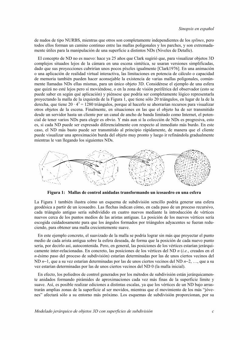
El concepto de ND no es nuevo: hace ya 25 años que Clark sugirió que, para visualizar objetos 3D complejos situados lejos de la cámara en una escena sintética, se usaran versiones simplificadas, dado que sus proyecciones cubrirían unos pocos píxeles igualmente [Clark1976]. En una animación o una aplicación de realidad virtual interactiva, las limitaciones en potencia de cálculo o capacidad de memoria también pueden hacer aconsejable la existencia de varias mallas poligonales, común-mente llamadas NDs ellas mismas, para un único objeto 3D. Considérese el ejemplo de una esfera que quizá no esté lejos pero sí moviéndose, o en la zona de visión periférica del observador (esto se puede saber en según qué aplicación) y piénsese que podría ser completamente lógico representarla proyectando la malla de la izquierda de la Figura 1, que tiene sólo 20 triángulos, en lugar de la de la derecha, que tiene 20 · 43 = 1280 triángulos, porque al hacerlo se ahorrarían recursos para visualizar otros objetos de la escena. Finalmente, en situaciones en las que el objeto ha de ser transmitido desde un servidor hasta un cliente por un canal de ancho de banda limitado como Internet, el poten-cial de tener varios NDs para elegir es obvio. Y más aun si la colección de NDs es progresiva, esto es, si cada ND puede ser expresado diferencialmente con respecto al inmediato más burdo. En este caso, el ND más basto puede ser transmitido al principio rápidamente, de manera que el cliente puede visualizar una aproximación burda del objeto muy pronto y luego ir refinándola gradualmente mientras le van llegando los siguientes NDs.
Figura 1: Mallas de control anidadas transformando un icosaedro en una esfera
La Figura 1 también ilustra cómo un esquema de subdivisión sencillo podría generar una esfera geodésica a partir de un icosaedro. Las flechas indican cómo, en cada paso de un proceso recursivo, cada triángulo antiguo sería subdividido en cuatro nuevos mediante la introducción de vértices nuevos cerca de los puntos medios de las aristas antiguas. La posición de los nuevos vértices sería escogida cuidadosamente para que los ángulos formados por triángulos adyacentes se fueran redu-ciendo, para obtener una malla crecientemente suave.
En este ejemplo concreto, el suavizado de la malla se podría lograr sin más que proyectar el punto medio de cada arista antigua sobre la esfera deseada, de forma que la posición de cada nuevo punto sería, por decirlo así, autocontenida. Pero, en general, las posiciones de los vértices estarían jerárqui-camente inter-relacionadas. En concreto, las posiciones de los vértices del ND n (i.e., creados en el n-ésimo paso del proceso de subdivisión) estarían determinadas por las de unos ciertos vecinos del ND n−1, que a su vez estarían determinadas por las de unos ciertos vecinos del ND n−2, …, que a su vez estarían determinadas por las de unos ciertos vecinos del ND 0 (la malla inicial).
En efecto, los poliedros de control generados por los métodos de subdivisión están jerárquicamen-te anidados formando pirámides de aproximaciones cada vez más finas de la superficie límite y suave. Así, es posible realizar ediciones a distintas escalas, ya que los vértices de un ND bajo arras-trarán amplias zonas de la superficie al ser movidos, mientras que el movimiento de los más “jóve-nes” afectará sólo a su entorno más próximo. Los esquemas de subdivisión proporcionan, por su
Sinopsis en español
d Modelado jerárquico de objetos 3D con superficies de subdivisión
propia naturaleza, los mandos para la edición multi-resolución que ni los polígonos ni los parches pueden ofrecer por separado.
VENTAJAS DE LOS ESQUEMAS JERÁRQUICOS
Nos parece muy importante hacer hincapié en la diferencia que hay entre esquemas de modelado meramente progresivos y verdaderamente jerárquicos. Una representación progresiva de un objeto 3D es aquella en la que es posible pasar de un ND al inmediato más fino porque están codificados incrementalmente; sin embargo, las diferencias entre uno y otro pueden estar repartidas arbitraria-mente por toda la superficie, y no hay relación alguna entre los elementos de un ND y los de los NDs contiguos. En el caso de una colección jerárquica, los NDs también pueden estar codificados diferencialmente, pero además sí existe una relación entre los elementos de un ND y sus inmediatos anterior y posterior. Esta relación, que para más señas es de anidamiento piramidal, tiene muchas aplicaciones teóricas y prácticas.
En particular, una pirámide de NDs es altamente aprovechable para representar y codificar (y, por ende, transmitir) jerárquicamente objetos 3D gracias a las técnicas de AMRO (Análisis Multi-Resolución mediante Ondículas). La idea principal en la que se basan estas técnicas es la descompo-sición de una función/señal en una parte burda, de baja resolución/frecuencia, y una colección de detalles cada vez más finos, y observables sólo a resoluciones/frecuencias cada vez mayores. El interés teórico de tener una tal descomposición de una señal en sub-bandas es obvio: permite ver tanto el bosque como las ramas. Las ventajas prácticas han quedado suficientemente probadas por la cantidad de investigación y el número de aplicaciones generadas por el AMRO de señales nD clási-cas en la última docena de años. Por “señales nD clásicas” entendemos aquellas definidas sobre dominios homeomorfos a n, o [0, 1]n a lo sumo, como audio (n = 1), imágenes (n = 2) o vídeo (n = 3). En dominios topológicamente triviales como esos, es fácil expresar la señal en bases de funciones que también están jerárquicamente anidadas por ser translaciones y dilaciones de una misma función madre.
Si bien es discutible que una de nuestras superficies 3D pueda ser considerada una “señal”, no lo es que pueda ser etiquetada como “verdaderamente 3D” puesto que, aunque pertenezca a un espacio 3D, sólo tiene dos grados de libertad — razón por la cual a veces se dice que las superficies son señales 2,5D, para gran disgusto de los amantes de los fractales… De hecho, un topólogo diría que nuestras superficies son variedades 2D (2D manifolds) de un espacio 3D. Y en topologías menos triviales como lo son las variedades, traslación y dilación pierden su significado, aunque el AMRO sigue siendo posible si se enfoca desde la perspectiva de los esquemas de subdivisión. Basta con partir de una malla burda aproximando pobremente (el ND inicial de) la superficie considerada, irla subdividiendo recursivamente y, al hacerlo, añadir los detalles necesarios para ir obteniendo cada vez mejores aproximaciones (sucesivos NDs) de la superficie.
Especialmente en el ámbito de la transmisión de señales, el concepto de multi-resolución es muy importante. No sólo permite, como se ha dicho, mandar primero una versión tosca de una señal que es posteriormente refinada, sino que además facilita una codificación más compacta de la informa-ción contenida por las señales suaves, cuya energía está concentrada en las bajas frecuencias. Los esquemas de codificación jerárquica y predictiva permiten expresar una señal aproximada sucesiva-mente como su versión más burda más un conjunto de errores de predicción, que son las diferencias entre la señal original y las predicciones basadas en sus versiones refinadas sucesivas. Los mecanis-mos de predicción son diseñados habitualmente de manera que generen errores de predicción peque-ños para señales mayormente suaves, que son las que más abundan en la práctica, y son por lo tanto capaces de transformar una señal posiblemente energética en un conjunto de errores de predicción de poca varianza. Después, se pueden aplicar técnicas de codificación estadística para comprimir efi-cientemente los errores de predicción y lograr, como resultado final, codificar la misma información con muchos menos datos.
Sinopsis en español
Modelado jerárquico de objetos 3D con superficies de subdivisión e
SUPERFICIES DE SUBDIVISIÓN
Una SS se define como el límite de un proceso de refinamiento recursivo aplicado a una malla de control enteramente compuesta por polígonos de un mismo tipo (todos ellos triángulos, cuadriláte-ros, etc.). El refinamiento progresivo de la malla de control es tanto topológico, porque enriquece su conectividad, como geométrico, porque suaviza su forma.
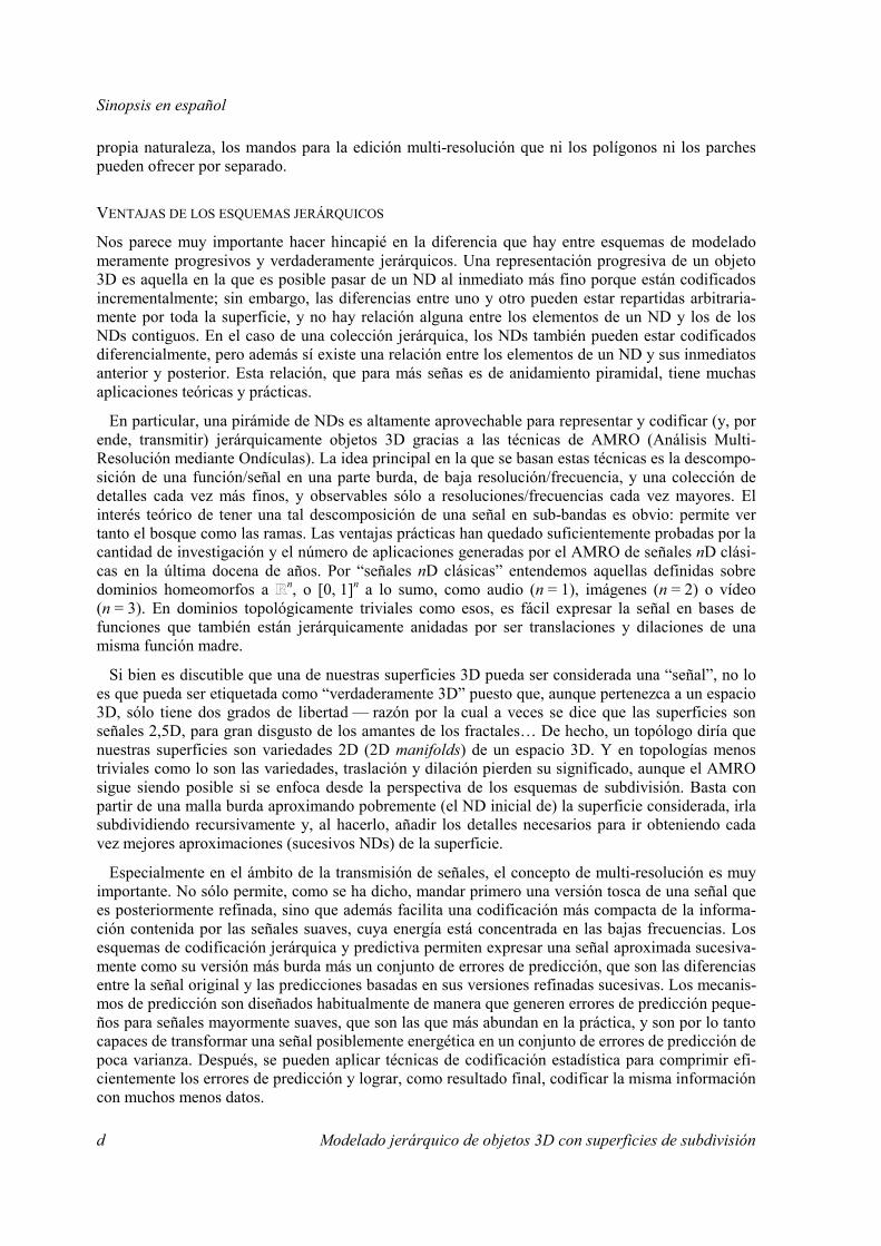
Es muy importante distinguir la conectividad (el grafo abstracto) de una malla, que describe sólo cómo sus vértices están interconectados, de su geometría (su forma 3D), que describe las posiciones espaciales de sus vértices. Un mismo grafo abstracto podría dar lugar a muy distintas formas 3D, de la misma manera que una misma forma 3D podría corresponder a distintos grafos abstractos.
Figura 2: Dos generaciones de la malla triangular de control de una SS (izquierda: grafo abstracto; derecha: forma 3D)
La Figura 2-izquierda muestra dos generaciones del grafo abstracto de una sencilla malla de control triangular: cada uno de los cinco triángulos iniciales, cuyos vértices son mostrados como circunfe-rencias, es subdividido en cuatro triángulos más pequeños por bisección de sus aristas. Los puntos medios de las aristas, mostrados como discos, son añadidos a la malla como nuevos vértices e inter-conectados formando cuatro nuevos triángulos que reemplazan al antiguo. Siendo nα
k el número de elementos α (α ∈ {v, a, t} para vértices, aristas y triángulos, respectivamente) de una malla de nivel k (k = 0 para la inicial), en este caso, nv
0 = 6, na0 = 10 y nt
0 = 5, mientras que nv1 = nv
0 + na0 = 16,
na1 = 2na
0 + 3nt0 = 35 y nt
1 = 4nt0 = 20.
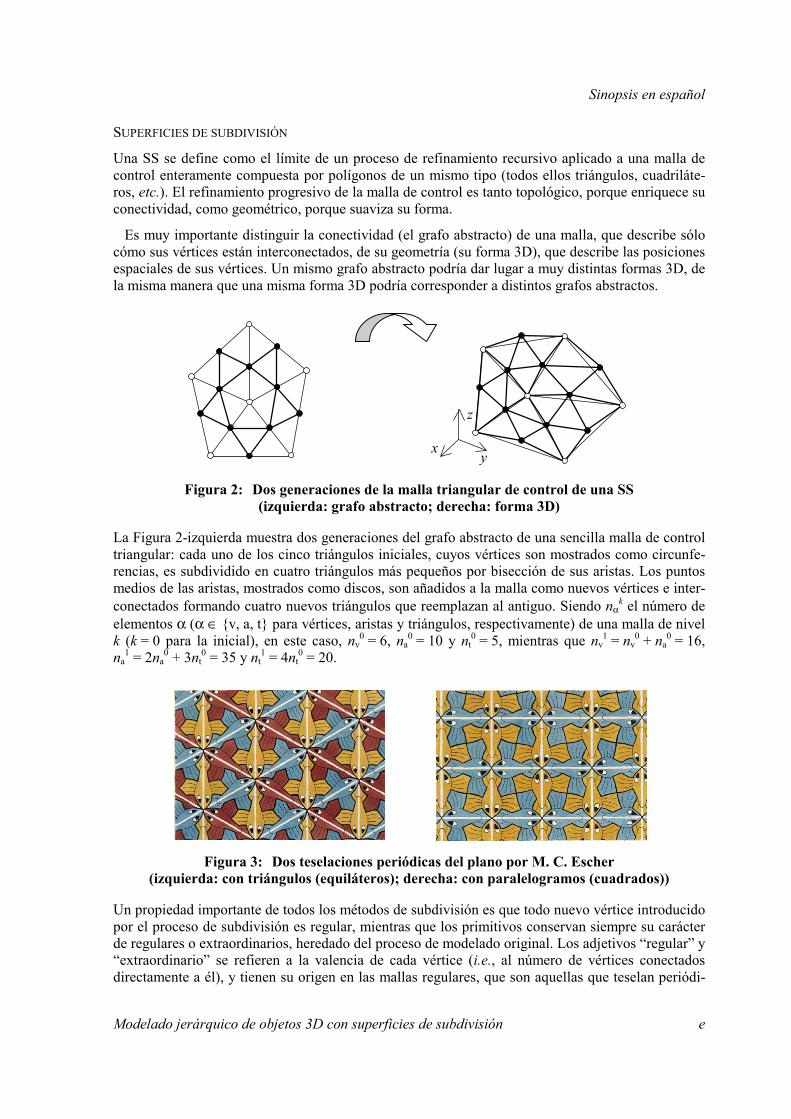
Figura 3: Dos teselaciones periódicas del plano por M. C. Escher (izquierda: con triángulos (equiláteros); derecha: con paralelogramos (cuadrados))
Un propiedad importante de todos los métodos de subdivisión es que todo nuevo vértice introducido por el proceso de subdivisión es regular, mientras que los primitivos conservan siempre su carácter de regulares o extraordinarios, heredado del proceso de modelado original. Los adjetivos “regular” y “extraordinario” se refieren a la valencia de cada vértice (i.e., al número de vértices conectados directamente a él), y tienen su origen en las mallas regulares, que son aquellas que teselan periódi-
z
yx
Sinopsis en español
f Modelado jerárquico de objetos 3D con superficies de subdivisión
camente el plano. En la Figura 3, que muestra las dos mallas regulares más sencillas, compuestas por triángulos (equiláteros, en el caso de la Figura 3-izquierda) y paralelogramos (cuadrados, en el caso de la Figura 3-derecha), se puede observar cómo los vértices regulares tienen respectivamente valen-cias seis y cuatro. Si no se considera una malla infinita, sino una con bordes, también cabe distinguir entre vértices fronterizos regulares y extraordinarios, teniendo los regulares valencia cuatro en mallas triangulares, y tres en mallas cuadrilaterales. Volviendo a la Figura 2-izquierda, se puede observar cómo los vértices iniciales, todos extraordinarios, no dejan de serlo tras la subdivisión, mientras que los vértices nuevos son todos regulares, ya sean interiores o de borde.
En la Figura 2-derecha se muestra cómo el grafo abstracto de la izquierda podría ser llevado al espacio 3D. Cada uno de los puntos iniciales tendría la posición arbitraria que le hubiera sido dada por el modelador, de manera que, en principio, las seis circunferencias de la Figura 2-derecha no serían coplanarias, y tampoco lo serían los cinco triángulos que definen, cuyas aristas se muestran con líneas finas. Si la malla fuera subdividida por un esquema interpolante, que es uno que no reco-loca los vértices antiguos, las circunferencias permanecerían en su sitio pero aparecerían nuevos vértices formando nuevos triángulos, cuyas aristas se muestran con líneas gruesas. Nótese que las imágenes de los puntos medios de las aristas del grafo abstracto, por la aplicación que lleva puntos de ese grafo al espacio 3D, no tendrían por qué ser los puntos medios de las aristas de la malla 3D. De hecho, es precisamente si no lo son cuando se logra suavizar progresivamente la forma 3D.
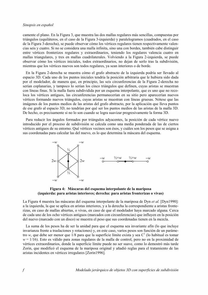
Para reducir los ángulos formados por triángulos adyacentes, la posición de cada vértice nuevo introducido por el proceso de subdivisión se calcula como una media ponderada de las de ciertos vértices antiguos de su entorno. Qué vértices vecinos son ésos, y cuáles son los pesos que se asigna a sus coordenadas para calcular las del nuevo, es lo que determina la máscara del esquema.
Figura 4: Máscaras del esquema interpolante de la mariposa (izquierda: para aristas interiores; derecha: para aristas fronterizas o vivas)
La Figura 4 muestra las máscaras del esquema interpolante de la mariposa de Dyn et al. [Dyn1990]: a la izquierda, la que se aplica en aristas interiores, y a la derecha la correspondiente a aristas fronte-rizas, en caso de mallas abiertas, o vivas, en caso de que el modelador haya marcado alguna. Cerca de cada uno de los ocho vértices antiguos (marcados con circunferencias) que influyen en la posición del nuevo (marcado con un disco) se muestra el peso que sus coordenadas tienen en la mezcla.
La suma de los pesos ha de ser la unidad para que el esquema sea invariante afín (lo que incluye invarianza frente a traslaciones y rotaciones) y, en este caso, varios pesos son función de un paráme-tro w, que debe ser menor que 1/8 para que la superficie límite exista y sea C1 (lo habitual es tomar w = 1/16). Esto es válido para zonas regulares de la malla de control, pero no en la proximidad de vértices extraordinarios, donde la superficie límite puede no ser suave, como lo demostró más tarde Zorin, que modificó el esquema de la mariposa original y añadió reglas para el tratamiento de las aristas incidentes en vértices irregulares [Zorin1996].
2w 2w
½
½
−w −w
−w −w
−w −w ½+w ½+w

Sinopsis en español
Modelado jerárquico de objetos 3D con superficies de subdivisión g
Figura 5: Máscaras del esquema aproximante de Loop (izquierda: para recolocar vértices antiguos; derecha: para aristas interiores)
Otro ejemplo notable, por comúnmente usado, es el esquema de subdivisión de Loop, que también actúa sobre mallas triangulares pero no es interpolante, sino aproximante [Loop1987]. Las máscaras para zonas regulares de la malla de control de este esquema son las mostradas en la Figura 5, en cuya parte izquierda se puede observar cómo un vértice antiguo sí es recolocado en función de las posiciones de sus seis vecinos. Con estas reglas, se consiguen superficies límite C2 en las zonas regulares de la malla. En las irregulares, hay que aplicar otras reglas: por ejemplo, para recolocar un vértice extraordinario de valencia K ≠ 6, se ha de tomar, por mor de simetría, β para cada uno de sus vecinos y 1−K β para él mismo, existiendo varias propuestas para β [Loop1987, Warren1995].
El análisis de la existencia y, en su caso, continuidad de la superficie límite en las zonas regulares de la malla de control se ve muy facilitado por las matrices de subdivisión, con las que también se logra “codificar” de manera compacta cómo actúa localmente el esquema correspondiente. En el caso del esquema de Loop, para averiguar la posición que ocupará en la superficie límite un vértice regular originalmente situado en P, es conveniente proceder como sigue.
Sean P1-6 las posiciones de los vecinos de P, y P' la suya propia tras un paso de subdivisión, i.e.,
P' = 1610 P +
161 (P1 + P2 + P3 + P4 + P5 + P6).
Esto se puede expresar de manera más compacta en forma matricial: siendo P el vector columna que contiene a P y P1-6 (cada uno de los cuales son puntos 3D), i.e., P = (P P1 P2 P3 P4 P5 P6)T, es:
P' = 161 (10 1 1 1 1 1 1) · P.
Siendo ahora P' el vector columna que contiene a P' y P'1-6 (que no son las siguientes posiciones de P1-6, sino los vecinos de P'), se puede codificar las reglas de subdivisión en una matriz fija S de dimensiones (1+6)×(1+6):
P' =
=
6
5
4
3
2
1
6
5
4
3
2
1
62000262620006026200600262060002626200026611111110
161
'''''''
PPPPPPP
PPPPPPP
= S · P.
3/83/8
1/8
1/81/161/16
1/16 1/16
1/161/16 10/16
Sinopsis en español
h Modelado jerárquico de objetos 3D con superficies de subdivisión
Como la mayoría de los esquemas de subdivisión son estacionarios (sus reglas no cambian a lo largo del proceso), también se puede escribir que P" = S · P' = S2 · P, etc., i.e.:
P(k) = S · P(k−1) = … = Sk−1 · P' = Sk · P.
Si el esquema está bien definido, los vecindarios formados por los puntos de P(k) van contrayéndose y convergen a un punto P∞, que es donde el punto de control inicialmente situado en P acaba en la superficie límite. Y la manera de averiguar si el esquema es convergente, y cuál es el vector normal a la superficie límite si ésta existe, la proporciona el análisis de autovalores y autovectores de la matriz S.
El análisis en la proximidad de vértices extraordinarios es algo más complicado y debe realizarse, mediante “mapas característicos” [Reif1995, Zorin2000], individualmente para cada posible valencia irregular, aunque afortunadamente no para cada posible configuración espacial.
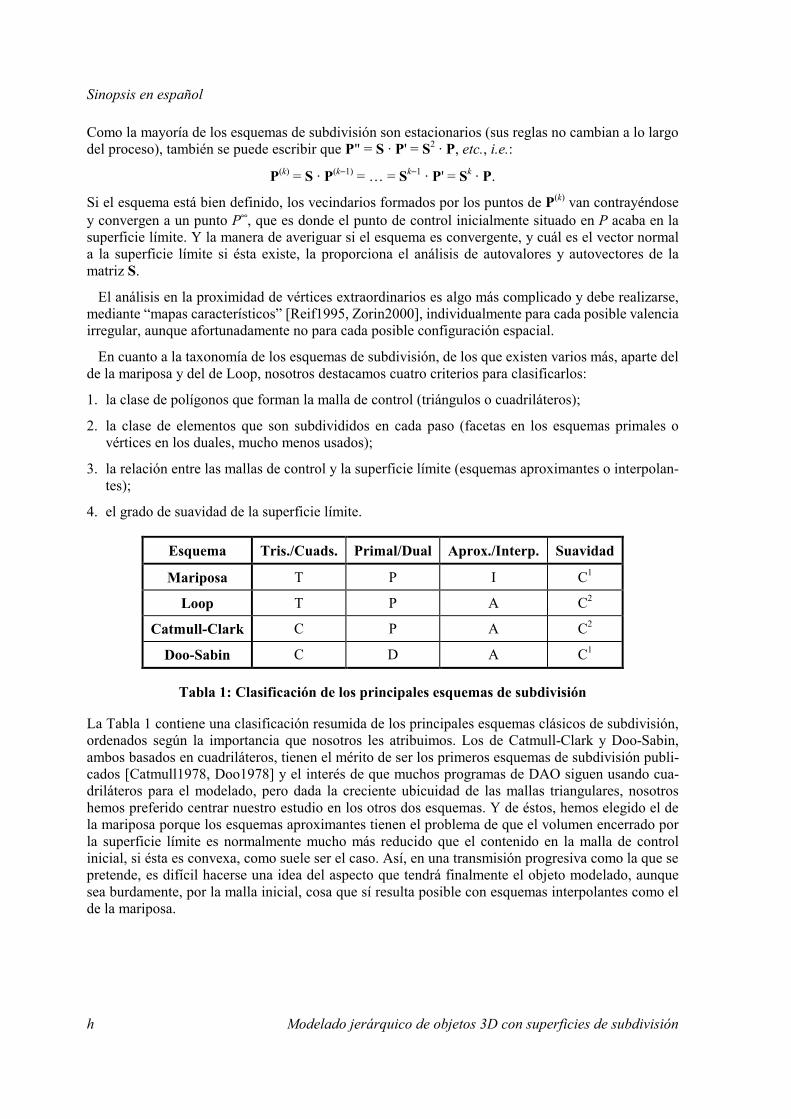
En cuanto a la taxonomía de los esquemas de subdivisión, de los que existen varios más, aparte del de la mariposa y del de Loop, nosotros destacamos cuatro criterios para clasificarlos:
1. la clase de polígonos que forman la malla de control (triángulos o cuadriláteros);
2. la clase de elementos que son subdivididos en cada paso (facetas en los esquemas primales o vértices en los duales, mucho menos usados);
3. la relación entre las mallas de control y la superficie límite (esquemas aproximantes o interpolan-tes);
4. el grado de suavidad de la superficie límite.
Esquema Tris./Cuads. Primal/Dual Aprox./Interp. Suavidad
Mariposa T P I C1
Loop T P A C2
Catmull-Clark C P A C2
Doo-Sabin C D A C1
Tabla 1: Clasificación de los principales esquemas de subdivisión
La Tabla 1 contiene una clasificación resumida de los principales esquemas clásicos de subdivisión, ordenados según la importancia que nosotros les atribuimos. Los de Catmull-Clark y Doo-Sabin, ambos basados en cuadriláteros, tienen el mérito de ser los primeros esquemas de subdivisión publi-cados [Catmull1978, Doo1978] y el interés de que muchos programas de DAO siguen usando cua-driláteros para el modelado, pero dada la creciente ubicuidad de las mallas triangulares, nosotros hemos preferido centrar nuestro estudio en los otros dos esquemas. Y de éstos, hemos elegido el de la mariposa porque los esquemas aproximantes tienen el problema de que el volumen encerrado por la superficie límite es normalmente mucho más reducido que el contenido en la malla de control inicial, si ésta es convexa, como suele ser el caso. Así, en una transmisión progresiva como la que se pretende, es difícil hacerse una idea del aspecto que tendrá finalmente el objeto modelado, aunque sea burdamente, por la malla inicial, cosa que sí resulta posible con esquemas interpolantes como el de la mariposa.
Sinopsis en español
Modelado jerárquico de objetos 3D con superficies de subdivisión i
TRABAJO PREVIO EN CODIFICACIÓN PROGRESIVA DE MALLAS 3D
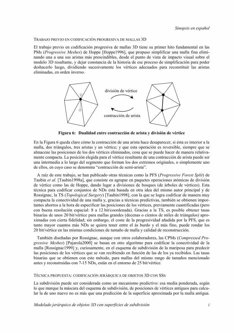
El trabajo previo en codificación progresiva de mallas 3D tiene su primer hito fundamental en las PMs (Progressive Meshes) de Hoppe [Hoppe1996], que propuso simplificar una malla fina elimi-nando una a una sus aristas más prescindibles, desde el punto de vista de impacto visual sobre el modelo 3D resultante, y dejar constancia de la historia de ese proceso de simplificación para poder deshacerlo luego, dividiendo sucesivamente los vértices adecuados para reconstituir las aristas eliminadas, en orden inverso.
Figura 6: Dualidad entre contracción de arista y división de vértice
En la Figura 6 queda claro cómo la contracción de una arista hace desaparecer, si ésta es interior a la malla, dos triángulos, tres aristas y un vértice; y que esta operación es reversible, siempre que se almacene las posiciones de los dos vértices eliminados, cosa que se puede hacer de manera relativa-mente compacta. La posición elegida para el vértice resultante de una contracción de arista puede ser una intermedia a lo largo del segmento que forman los dos extremos originales, o simplemente uno de ellos, en cuyo caso se denomina “contracción de semi-arista”.
A raíz de este trabajo, se han publicado otras técnicas como la PFS (Progressive Forest Split) de Taubin et al. [Taubin1998a], que consiste en agrupar en paquetes operaciones atómicas de división de vértice como las de Hoppe, dando lugar a divisiones de bosques (de árboles de vértices). Esta técnica para codificar conjuntos de NDs está basada en otra idea del mismo autor principal y de Rossignac, la TS (Topological Surgery) [Taubin1998], con la que se logra codificar de manera muy compacta la conectividad de una malla y, gracias a técnicas predictivas, también se obtienen impor-tantes ahorros a la hora de especificar las posiciones de los vértices, previamente cuantificadas (pero con buena resolución espacial: 8 a 12 bit/coordenada). Gracias a la TS, es posible obtener tasas binarias de unos 20 bit/vértice para mallas grandes (decenas o cientos de miles de triángulos) apro-ximadas con cierta fidelidad; sin embargo, el coste de la progresividad añadida por la PFS, que es tanto mayor cuantos más NDs se quiera tener entre el ás burdo y el más fino, puede rondar los 20 bit/vértice en las mismas condiciones de tamaño de malla y calidad de reconstrucción.
También diseñadas por Rossignac, aunque con otros colaboradores, las CPMs (Compressed Pro-gressive Meshes) [Pajarola2000] se basan en otro algoritmo para codificar la conectividad de la malla [Rossignac1999] y, curiosamente, en el esquema de subdivisión de la mariposa para predecir las posiciones de los vértices que se van recibiendo en función de las de los ya recibidos. Las tasas binarias que se obtienen con este método, para mallas del mismo rango de tamaños mencionado antes y reconstruidas con 7-15 NDs, están en el entorno de 25 bit/vértice.
TÉCNICA PROPUESTA: CODIFICACIÓN JERÁRQUICA DE OBJETOS 3D CON SSS
La subdivisión puede ser considerada como un mecanismo predictivo: esa media ponderada, según lo que marque la máscara del esquema de subdivisión, de posiciones de vértices antiguos para calcu-lar la de uno nuevo no es más que una predicción de la superficie aproximada por la malla antigua.
contracción de arista
división de vértice
Sinopsis en español
j Modelado jerárquico de objetos 3D con superficies de subdivisión
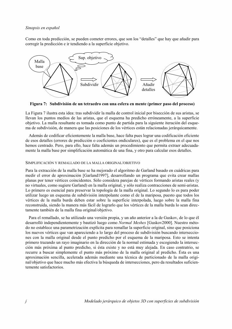
Como en toda predicción, se pueden cometer errores, que son los “detalles” que hay que añadir para corregir la predicción e ir tendiendo a la superficie objetivo.
Figura 7: Subdivisión de un tetraedro con una esfera en mente (primer paso del proceso)
La Figura 7 ilustra esta idea: tras subdividir la malla de control inicial por bisección de sus aristas, se llevan los puntos medios de las aristas, que el esquema ha predicho erróneamente, a la superficie objetivo. La malla resultante es tomada como punto de partida para la siguiente iteración del esque-ma de subdivisión, de manera que las posiciones de los vértices están relacionadas jerárquicamente.
Además de codificar eficientemente la malla base, hace falta pues lograr una codificación eficiente de esos detalles (errores de predicción o coeficientes ondiculares), que es el problema en el que nos hemos centrado. Pero, para ello, hace falta además un procedimiento que permita extraer adecuada-mente la malla base por simplificación automática de una fina, y otro para calcular esos detalles.
SIMPLIFICACIÓN Y REMALLADO DE LA MALLA ORIGINAL/OBJETIVO
Para la extracción de la malla base se ha mejorado el algoritmo de Garland basado en cuádricas para medir el error de aproximación [Garland1997], desarrollando un programa que evita crear mallas planas por tener vértices coincidentes. Sólo considera parejas de vértices formando aristas reales (y no virtuales, como sugiere Garland) en la malla original, y sólo realiza contracciones de semi-aristas. Lo primero es esencial para preservar la topología de la malla original. Lo segundo lo es para poder utilizar luego un esquema de subdivisión interpolante como el de la mariposa, puesto que todos los vértices de la malla burda deben estar sobre la superficie interpolada, luego sobre la malla fina reconstruida, siendo la manera más fácil de lograrlo que los vértices de la malla burda lo sean direc-tamente también de la malla fina original/objetivo.
Para el remallado, se ha utilizado una versión propia, y un año anterior a la de Guskov, de lo que él desarrolló independientemente y bautizó luego como Normal Meshes [Guskov2000]. Nuestro méto-do no establece una parametrización explícita para remallar la superficie original, sino que posiciona los nuevos vértices que van apareciendo a lo largo del proceso de subdivisión buscando interseccio-nes con la malla original desde el punto predicho por el esquema de la mariposa. Esto se intenta primero trazando un rayo imaginario en la dirección de la normal estimada y escogiendo la intersec-ción más próxima al punto predicho, si ésta existe y no está muy alejada. En caso contratrio, se recurre a buscar simplemente el punto más próximo de la malla original al predicho. Ésta es una aproximación sencilla, acelerada además mediante una técnica de particionado de la malla origi-nal/objetivo que hace mucho más efectiva la búsqueda de intersecciones, pero da resultados suficien-temente satisfactorios.
Sup. objetivoMalla base
Subdividir Añadir detalles

Sinopsis en español
Modelado jerárquico de objetos 3D con superficies de subdivisión k
RFERENCIAL LOCAL NORMAL PARA LOS DETALLES
Figura 8: Referencial de Frenet para los detalles
La Figura 8 muestra el referencial local normal que se ha de usar para expresar los detalles. Al tener éstos una componente normal predominante sobre las tangenciales, es fácil beneficiarse de que uno de los vectores de la base sea n durante su cuantificación, en la que se puede favorecer a la compo-nente normal, asignándole más bits del total destinado a cada detalle. Y esto es posible sin necesidad de que n sea la normal exacta a la superficie límite, sino que se puede aproximar, por ejemplo, por la media de las normales de los triángulos que comparten la arista, pesadas por sus áreas respectivas.
ORGANIZACIÓN JERÁRQUICA DE LOS DETALLES
Figura 9: Organización jerárquica de los detalles (idea básica)
La Figura 9 muestra el esquema espacial diseñado para lograr una organización jerárquica de los detalles. Para cada triángulo de la malla inicial, se elige al azar un vértice raíz, y en él se planta el árbol de detalles de nivel 0, del que colgarán los detalles de los vértices correspondientes a ese triángulo madre a lo largo del proceso de subdivisión. Cuando un triángulo es subdividido, ello crea cuatro nuevos árboles de detalles de un nivel superior, que son plantados como se indica.
CUANTIFICACIÓN Y “ESCALARIZACIÓN” DE LOS DETALLES PARA ADAPTARLOS AL SPIHT
Gracias a esta organización de los detalles, se puede utilizar una técnica de codificación muy similar al SPIHT (Set Partitioning In Hierarchical Trees) desarrollado por Said y Pearlman [Said1996], basado a su vez en los zerotrees de coeficientes ondiculares de Shapiro [Shapiro1993]. Sin embargo, los coeficientes ondiculares que ellos consideraban eran cantidades escalares, mientras que nuestros detalles son vectores 3D.
Para solucionar este problema, hemos diseñado mecanismos de cuantificación y “escalarización” de los detalles. Como ya hemos señalado, al tener los detalles una componente normal claramente más energética que las tangenciales, éstas se pueden cuantificar, adaptativamente, con varios bits menos que aquélla sin pérdida apreciable de calidad. En cuanto a la “escalarización” que propone-
TBTA
t1 = en
t2 = n×e
nivel 0 (árbol)nivel 1 (árbol)
nivel 2 (árbol)nivel 1 (árbol)
nivel 2 (hoja) Ts0 Ts1
Ts2
Ts3
Sinopsis en español
l Modelado jerárquico de objetos 3D con superficies de subdivisión
mos, consiste en entremezclar los bits de las distintas componentes de manera que, si se estima que el reparto de un total de 32 ha de ser de 14 para la normal más 9 para cada tangencial, se formen palabras binarias que tengan primero los 5 bits extra dedicados a la componente normal, y luego un bit de cada una.
Finalmente, tras aplicar el algoritmo del SPIHT reducimos la redundancia remanente aplicando codificación aritmética adaptativa, para así producir un código aun más compacto.
RESULTADOS
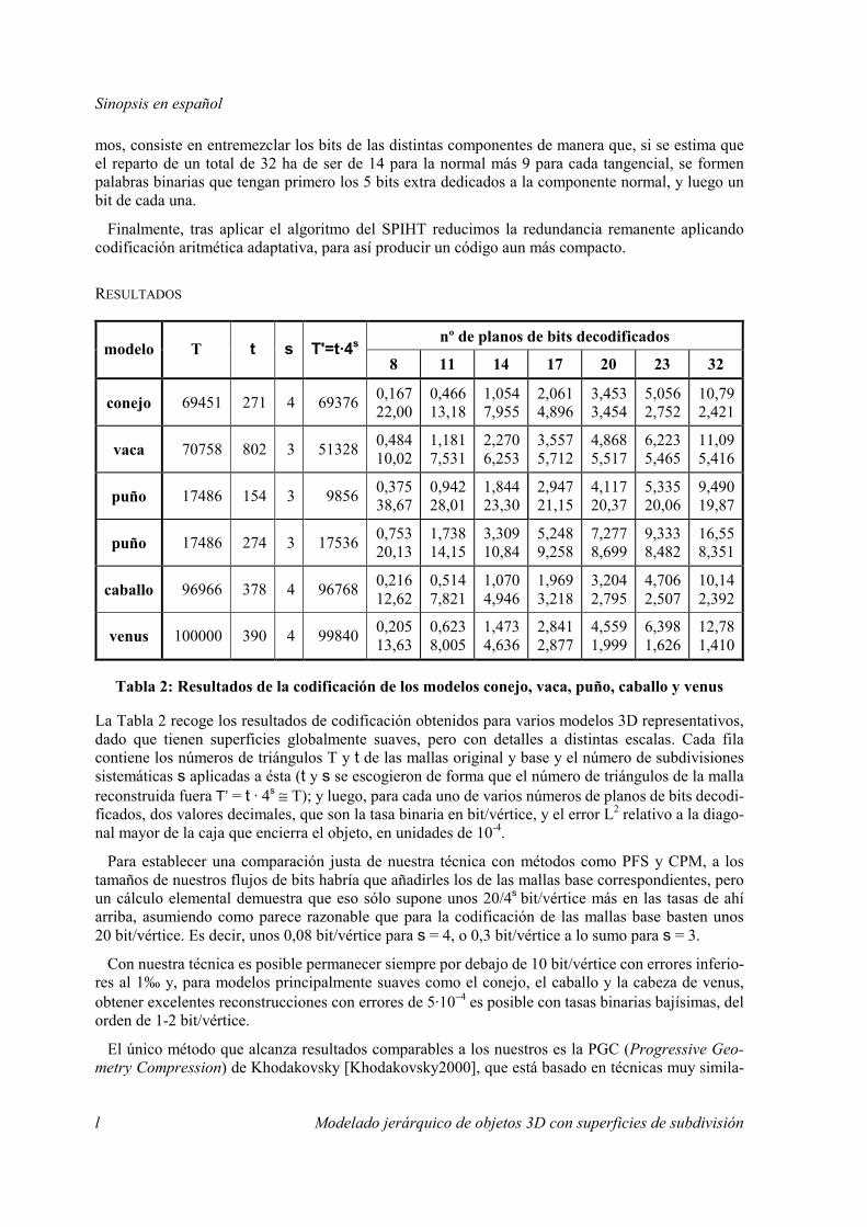
nº de planos de bits decodificados modelo T t s T'=t·4s
8 11 14 17 20 23 32
conejo 69451 271 4 69376 0,16722,00
0,46613,18
1,0547,955
2,0614,896
3,453 3,454
5,056 2,752
10,792,421
vaca 70758 802 3 51328 0,48410,02
1,1817,531
2,2706,253
3,5575,712
4,868 5,517
6,223 5,465
11,095,416
puño 17486 154 3 9856 0,37538,67
0,94228,01
1,84423,30
2,94721,15
4,117 20,37
5,335 20,06
9,49019,87
puño 17486 274 3 17536 0,75320,13
1,73814,15
3,30910,84
5,2489,258
7,277 8,699
9,333 8,482
16,558,351
caballo 96966 378 4 96768 0,21612,62
0,5147,821
1,0704,946
1,9693,218
3,204 2,795
4,706 2,507
10,142,392
venus 100000 390 4 99840 0,20513,63
0,6238,005
1,4734,636
2,8412,877
4,559 1,999
6,398 1,626
12,781,410
Tabla 2: Resultados de la codificación de los modelos conejo, vaca, puño, caballo y venus
La Tabla 2 recoge los resultados de codificación obtenidos para varios modelos 3D representativos, dado que tienen superficies globalmente suaves, pero con detalles a distintas escalas. Cada fila contiene los números de triángulos T y t de las mallas original y base y el número de subdivisiones sistemáticas s aplicadas a ésta (t y s se escogieron de forma que el número de triángulos de la malla reconstruida fuera T’ = t · 4s ≅ T); y luego, para cada uno de varios números de planos de bits decodi-ficados, dos valores decimales, que son la tasa binaria en bit/vértice, y el error L2 relativo a la diago-nal mayor de la caja que encierra el objeto, en unidades de 10-4.
Para establecer una comparación justa de nuestra técnica con métodos como PFS y CPM, a los tamaños de nuestros flujos de bits habría que añadirles los de las mallas base correspondientes, pero un cálculo elemental demuestra que eso sólo supone unos 20/4s bit/vértice más en las tasas de ahí arriba, asumiendo como parece razonable que para la codificación de las mallas base basten unos 20 bit/vértice. Es decir, unos 0,08 bit/vértice para s = 4, o 0,3 bit/vértice a lo sumo para s = 3.
Con nuestra técnica es posible permanecer siempre por debajo de 10 bit/vértice con errores inferio-res al 1‰ y, para modelos principalmente suaves como el conejo, el caballo y la cabeza de venus, obtener excelentes reconstrucciones con errores de 5·10−4 es posible con tasas binarias bajísimas, del orden de 1-2 bit/vértice.
El único método que alcanza resultados comparables a los nuestros es la PGC (Progressive Geo-metry Compression) de Khodakovsky [Khodakovsky2000], que está basado en técnicas muy simila-

Sinopsis en español
Modelado jerárquico de objetos 3D con superficies de subdivisión m
res, porque también está inspirado en el trabajo de Kolarov y Lynch [Kolarov1996], aunque fue desarrollado independientemente del nuestro y publicado un año más tarde.
CONCLUSIONES
Las SSs son un poderoso paradigma de modelado de objetos 3D que permite obtener a partir de una malla de control burda, que puede ser descrita de forma muy compacta, una superficie límite suave, como resultado de un proceso de subdivisión recursiva que va refinando tanto la conectividad como la geometría de la malla. Como la recursividad es inherente a las SSs, las sucesivas mallas que se van obteniendo a lo largo del proceso forman un conjunto de NDs piramidalmente anidados, que puede someterse fácilmente a técnicas de AMRO. De ello resultan inmediatamente interesantes aplicaciones potenciales como, por ejemplo, la codificación y la edición jerárquicas de objetos 3D.
En esta tesis, hemos empezado por describir las relaciones de parentesco entre las tres áreas de conocimiento que han servido de base (pese a no ser independientes) para nuestro trabajo: las SSs, la extracción automática de NDs y el AMRO. Hasta donde nosotros sabemos, éste es el primer trabajo de compilación y síntesis que explica cómo encajan esas tres piezas del rompecabezas del modelado jerárquico de objetos 3D con SSs. Se trata de modelar una superficie, cada vez más frecuentemente descrita por una malla poligonal de conectividad arbitraria en los últimos tiempos, empezando por extraer de ella una malla burda, que la aproxime con un bajo ND y que sirva como punto de partida para un proceso de subdivisión. Éste irá creando NDs cada vez más finos, que serán aproximaciones cada vez mejores de la superficie original si las posiciones predichas para los nuevos vértices por el esquema de subdivisión considerado se van corrigiendo gracias a unos detalles 3D (coeficientes ondiculares) obtenidos mediante técnicas de remallado.
Las aplicaciones prácticas del modelado jerárquico de objetos 3D con SSs constituyen sin embargo nuestra mayor aportación original. En particular, hemos diseñado un método de codificación jerár-quica de objetos 3D basado en SSs que ha dado lugar a publicaciones internacionales [Morán1999, Morán2000] y una propuesta al subgrupo de AFX de MPEG-SNHC [Morán2001] que está siendo considerada actualmente, para su eventual adopción en la futura versión 5 del estándar MPEG-4, prevista para octubre de 2002 [MPEG2001, MPEG2001a, MPEG2001b]. La técnica que propone-mos consiste en hallar los detalles mencionados más arriba, expresarlos en un referencial local normal, organizarlos en una estructura jerárquica basada en facetas, cuantificar mejor su componente normal, la más energética, que sus componentes tangenciales, que lo son menos, “escalarizarlos”, y finalmente codificarlos gracias a una técnica similar al SPIHT. El resultado es un código completa-mente embebido que produce mucho mejores resultados, en términos de eficiencia de compresión, que los de mecanismos de codificación progresiva de mallas 3D publicados anteriormente (PFS o CPM).
Finalmente, como una solución completa para el modelado jerárquico de objetos 3D con SSs re-quiere generar también un remallado de la superficie/malla original y el ND más burdo que servirá como punto de partida al proceso de subdivisión, hemos desarrollado además métodos auxiliares de simplificación automática y de remallado de mallas 3D, tanto mejorando técnicas ya publicadas como creando las nuestras propias.
Esta tesis está disponible en la red en “http://www.gti.ssr.upm.es./~fmb/pub/tesis.pdf.gz” y se pueden dirigir preguntas y comentarios relativos a ella a “[email protected]”.


Hierarchical Modelling of 3D Objects with Subdivision Surfaces
by
Francisco Morán Burgos
A dissertation submitted in partial fulfilment of the requirements for the degree of
Doctor of Philosophy
Universidad Politécnica de Madrid
October 2001
Advisor: Narciso García Santos

Abstract
SSs (Subdivision Surfaces) are a powerful 3D (three Dimensional) object modelling paradigm serving as a bridge between the two traditional approaches for approximating surfaces, polygons and curved (polynomial or rational) patches, which imply their own problems each. Subdivision schemes permit to define a (piecewise) smooth surface, like the ones most frequently found in practice, as the limit of the recursive refinement of a coarse polygonal control mesh, which can be described very compactly. Moreover, the recursiveness inherent to SSs establishes naturally a pyramidal nesting relationship between the successively generated meshes / LODs (Levels Of Detail). This makes SSs most suitable for the wavelet-based MRA (MultiResolution Analysis) of surfaces, which has imme-diate and most interesting practical applications such as hierarchical 3D model coding and editing.
We start by describing the linkage between the three main knowledge areas which have served as a basis for our work (SSs, automatic LOD extraction, and wavelet-based MRA) to explain how these three pieces of the puzzle of hierarchical modelling of 3D objects with SSs fit together. The wavelet-based MRA approach consists in decomposing a function into a coarse version of it and a set of hierarchically nested additive refinements, called “wavelet coefficients”. The classic wavelet theory applies to classic nD signals: those defined on parametric domains homeomorphic to n or [0, 1]n, such as audio (n = 1), still images (n = 2) or video (n = 3). In less trivial topological settings such as generic 2D manifolds (i.e., surfaces embedded in 3D space), wavelet-based MRA is not as obvious, but nevertheless possible if approached from the subdivision viewpoint. It suffices to start from a coarse mesh approximating the considered surface at a low LOD, subdivide it recursively and, while doing so, add the wavelet coefficients, which are the 3D details needed to obtain finer and finer approximations to the original surface.
We then turn to the practical applications which constitute our main original development and, specifically, we present a technique for truly hierarchical 3D model coding based on SSs, which acts on the 3D details mentioned above: it expresses them in a local normal frame; it organises them in a facet-based hierarchical set; it quantises them by attibuting lees bits to their less energetic tangential components and “scalarises” them; and it finally codes them thanks to a technique similar to the SPIHT (Set Partitioning In Hierarchical Trees) of Said and Pearlman. The result is a fully embedded code at least twice more compact, for mainly smooth surfaces, than those obtained with previously reported progressive 3D mesh coding techniques, in which the LODs are not pyramidally nested.
Finally, we describe some auxiliary methods that we have had to design, by improving previous techniques and creating our own, as a complete solution for the hierarchical modelling of 3D objects with SSs requires solving another two problems as well. The first is extracting a base mesh (made of triangles, in our case) from the input surface, usually given as a fine triangular mesh with arbitrary connectivity. The second is generating a subdivision connectivity remesh of the input/target mesh by recursively refining the base mesh, thus computing the 3D details that must be added to correct the positions predicted by the subdivision process for the new vertices.

Hierarchical modelling of 3D objects with subdivision surfaces i
Contents
Contents i
Figures v
Tables viii
Acronyms and abbreviations ix
0. Introduction 1 0.0. Motivation ................................................................................................................................. 1 0.1. Objectives and contributions..................................................................................................... 5 0.2. Outline of dissertation ............................................................................................................... 6
1. Background 7 1.0. Contents..................................................................................................................................... 7 1.1. A few topological considerations.............................................................................................. 7 1.2. Subdivision surfaces.................................................................................................................. 9
1.2.0. Intuitive definition .......................................................................................................... 9 1.2.1. A few examples............................................................................................................. 11
Dyn’s four-point scheme for curves.............................................................................. 11 Dyn’s butterfly scheme ................................................................................................. 11 Loop’s scheme .............................................................................................................. 12
1.2.2. Formal definition and analysis...................................................................................... 13 Smoothness of the limit surface: geometric and parametric continuities...................... 13 Parameterisation over the initial control mesh.............................................................. 15 Local subdivision matrices............................................................................................ 18 Analysis at extraordinary vertices................................................................................. 20
1.2.3. Taxonomy ..................................................................................................................... 21 Triangular vs. quadrilateral ........................................................................................... 22 Primal vs. dual............................................................................................................... 22 Interpolating vs. approximating .................................................................................... 24

ii Hierarchical modelling of 3D objects with subdivision surfaces
Smoothness of the limit surface .................................................................................... 25 Uniformity of the subdivision process .......................................................................... 25 Summary: classification of major subdivision schemes................................................ 27
1.2.4. A detailed example: the butterfly scheme revisited ...................................................... 27 Dyn’s (original) butterfly scheme ................................................................................. 27 Zorin’s modified butterfly scheme................................................................................ 28
1.2.5. Summary of advantages of subdivision surfaces .......................................................... 30 Advantages over polygons: compactness...................................................................... 30 Advantages over patches: arbitrary mesh connectivity................................................. 30 Advantages over both: harmonisation and truly hierarchical representation ................ 30
1.3. Automatic LOD extraction ...................................................................................................... 31 1.3.0. Motivation ..................................................................................................................... 31 1.3.1. Error metrics.................................................................................................................. 32 1.3.2. Brief taxonomy.............................................................................................................. 34
Static vs. dynamic.......................................................................................................... 34 Global vs. local.............................................................................................................. 35 Relationship between LODs.......................................................................................... 36
1.4. Wavelet-based multiresolution analysis .................................................................................. 37 1.4.0. Introduction ................................................................................................................... 37 1.4.1. First generation wavelets............................................................................................... 38
Haar’s transform of a discrete signal............................................................................. 38 Deslauriers-Dubuc’s interpolating subdivision ............................................................. 39 Scaling functions and wavelets ..................................................................................... 40 Other wavelets related to subdivision ........................................................................... 42
1.4.2. Second generation wavelets .......................................................................................... 43 Boundaries and irregular sampling on trivial topologies .............................................. 43 Non-trivial topologies: Lounsbery’s MRA of semi-regular meshes ............................. 44
1.4.3. Applications of wavelet-based multiresolution analysis ............................................... 45 Compression.................................................................................................................. 46 Editing........................................................................................................................... 47
2. Hierarchical 3D model coding with SSs 49 2.0. Contents................................................................................................................................... 49 2.1. Raw size of a 3D mesh ............................................................................................................ 49 2.2. Previous work on progressive 3D mesh coding ...................................................................... 50
2.2.0. Hoppe’s PM (Progressive Mesh) .................................................................................. 51 2.2.1. Taubin’s PFS (Progressive Forest Split) ....................................................................... 51 2.2.2. Rossignac’s CPM (Compressed Progressive Mesh) ..................................................... 52 2.2.3. Other.............................................................................................................................. 53
2.3. Truly hierarchical 3D model coding with SSs......................................................................... 53 2.3.0. Remeshing piecewise smooth surfaces is perfectly reasonable .................................... 54 2.3.1. Basic idea: subdivision regarded as a prediction mechanism ....................................... 54
Hierarchical modelling of 3D objects with subdivision surfaces iii
2.3.2. Prior art on hierarchical 3D model coding with subdivision surfaces .......................... 56 2.4. Proposed method for hierarchical 3D model coding with SSs................................................ 56
2.4.0. Base mesh extraction and remeshing ............................................................................ 57 2.4.1. Frenet coordinate frame for details ............................................................................... 57 2.4.2. Hierarchical organisation of details .............................................................................. 58
The general rule ............................................................................................................ 58 The exception................................................................................................................ 60
2.4.3. Coding algorithm .......................................................................................................... 60 Some nomenclature....................................................................................................... 60 The algorithm itself....................................................................................................... 61 Notes (and some more nomenclature)........................................................................... 62
2.4.4. Quantisation and “scalarisation” of details ................................................................... 62 2.4.5. Entropy coding.............................................................................................................. 63 2.4.6. Details bit-stream structure ........................................................................................... 64 2.4.7. Adaptive subdivision .................................................................................................... 64 2.4.8. Results........................................................................................................................... 66
3D models test set ......................................................................................................... 66 Non-duplication of details on mother edges ................................................................. 68 Arithmetic coding efficiency ........................................................................................ 68 Rate vs. distortion curves .............................................................................................. 69
2.4.9. Khodakovsky’s PGC (Progressive Geometry Compression)........................................ 76 2.5. Future work ............................................................................................................................. 78
2.5.0. Straightforward extensions ........................................................................................... 78 Meshes with properties ................................................................................................. 78 Non-triangular meshes .................................................................................................. 78 Surfaces with sharp features ......................................................................................... 79 Non-manifold and non-orientable surfaces................................................................... 79 Improved compression efficiency through tangential components subsampling ......... 80 Details set partitioning for error resilience and view-dependent coding ...................... 80
2.5.1. Animated models .......................................................................................................... 81 2.5.2. Truly 3D models ........................................................................................................... 81
3. LOD extraction and remeshing 83 3.0. Contents................................................................................................................................... 83 3.1. Previous work.......................................................................................................................... 83
3.1.0. LOD extraction ............................................................................................................. 83 Hoppe’s PM (Progressive Mesh) .................................................................................. 83 Garland’s quadrics ........................................................................................................ 84
3.1.1. Remeshing..................................................................................................................... 85 Eck’s extension of Lounsbery’s MRA of semi-regular meshes.................................... 85 Lee’s MAPS (Multiresolution Adaptive Parameterization of Surfaces)....................... 86
3.2. Proposed techniques................................................................................................................ 87

iv Hierarchical modelling of 3D objects with subdivision surfaces
3.2.0. LOD extraction.............................................................................................................. 87 Neutralisation of QSlim’s memory effect ..................................................................... 87 Own implementation of QSlim ..................................................................................... 88
3.2.1. Remeshing..................................................................................................................... 89 Estimation of normal vector.......................................................................................... 90 Ray intersection............................................................................................................. 90 Accelerated search through “voxelisation” of the input mesh ...................................... 91 Closest point instead of normal point............................................................................ 92
3.2.2. Results ........................................................................................................................... 93 3.2.3. Guskov’s NM (Normal Mesh) ...................................................................................... 94
3.3. Future work ............................................................................................................................. 95 3.3.0. Explicit parameterisation obtained during simplification ............................................. 95 3.3.1. Adaptive subdivision..................................................................................................... 95 3.3.2. Optimality of the base mesh.......................................................................................... 96
4. Conclusions 97 4.0. Contents................................................................................................................................... 97 4.1. Summary ................................................................................................................................. 97 4.2. Future work ............................................................................................................................. 99
5. References 101 5.0. Contents................................................................................................................................. 101 5.1. Books, theses and international standards ............................................................................. 101 5.2. Papers, technical reports and course notes ............................................................................ 103 5.3. Internet resources................................................................................................................... 110

Hierarchical modelling of 3D objects with subdivision surfaces v
Figures
Figure 1: Bicubic Bézier patches (left: planar graph; right: 3D shape) ............................................ 2 Figure 2: Nested control meshes turning an icosahedron into a sphere (three first steps)................ 3 Figure 3: Non-manifold mesh with three non-manifold edges......................................................... 8 Figure 4: Two periodic tesselations of the plane by M. C. Escher (left: with triangles; right:
with parallelograms) ......................................................................................................... 8 Figure 5: Non-manifold mesh with one non-manifold vertex .......................................................... 9 Figure 6: Two generations of a SS triangular control mesh (left: abstract graph; right: 3D
mapping) ......................................................................................................................... 10 Figure 7: The four-point subdivision scheme for curves (left: stencil; right: two generations
of a control polygon)....................................................................................................... 11 Figure 8: Stencils of the butterfly subdivision scheme (left: for regular edges; right: for
crease and boundary edges) ............................................................................................ 12 Figure 9: Stencils of Loop’s subdivision scheme (left: for repositioning old vertices; right:
for splitting edges) .......................................................................................................... 12 Figure 10: A hardly visually smooth curve with continuous tangent ............................................... 14 Figure 11: A smooth, but non-orientable (and “buggy”! ;-) Möbius’ strip by M. C. Escher ........... 14 Figure 12: Construction of a quartic three-directional box-spline triangular patch (left:
parametric domain; right: control net for the central triangle)........................................ 16 Figure 13: Treatment of non-manifold edges (top: original non-manifold mesh; centre and
bottom: two manifold meshes, subdivided separately) ................................................... 17 Figure 14: Two generations of the 1-ring of a vertex....................................................................... 18 Figure 15: Chaikin’s algorithm for building uniform quadratic B-splines (two first steps)............. 21 Figure 16: A periodic tiling of the plane not usable for subdivision purposes................................. 22 Figure 17: Primal and dual schemes for quadrilateral meshes (left: initial mesh; right-top
(primal): facets are split; right-bottom (dual): vertices are split) .................................... 23 Figure 18: A possible dual scheme for hexagonal meshes ............................................................... 23 Figure 19: The effect of an interpolating scheme (top: butterfly) vs. an approximating one
(bottom: Loop’s) on an octahedron................................................................................. 24

vi Hierarchical modelling of 3D objects with subdivision surfaces
Figure 20: Flag with heterogeneous curvature (left: initial mesh; centre and right: systematic and adaptive subdivision yielding around 3000 triangles each)...................................... 26
Figure 21: Stencils of the most common butterfly subdivision scheme (left: for normal interior edges; right: for crease and boundary edges) ..................................................... 27
Figure 22: Gradual smoothing achieved by the butterfly subdivision scheme (two first steps) ....... 28 Figure 23: Regular triangulation of a rectangular grid ..................................................................... 28 Figure 24: Incomplete smoothing of a tetrahedron by the original butterfly scheme....................... 29 Figure 25: Point to vertex (dpv), plane (dpp) and surface (dps) distances............................................ 32 Figure 26: Edge collapse and half-edge collapse.............................................................................. 35 Figure 27: The edge swap local remeshing operation ...................................................................... 36 Figure 28: Haar’s wavelet transforms (from left to right: forward; from right to left: inverse;
n.b.: the number of elements of each sequence is indicated inside the parentheses) ...... 38 Figure 29: Fundamental functions for Deslauriers-Dubuc’s interpolating subdivision scheme
with n = 1 (left: scaling function φ; right: wavelet ψ) ..................................................... 41 Figure 30: The duality between a vertex split and an edge collapse................................................. 51 Figure 31: Subdividing a tetrahedron with a sphere in mind (first step of the process) ................... 54 Figure 32: Hierarchical coding of a sphere with nested LODs (from left to right: levels 0
(base mesh), 1, 2 and 5)................................................................................................... 55 Figure 33: Numbering of new vertices and triangles........................................................................ 57 Figure 34: Frenet coordinate frame for details ................................................................................. 57 Figure 35: Hierarchical organisation of details (basic idea) ............................................................. 58 Figure 36: Hierarchical organisation of details (detail ;-)................................................................. 59 Figure 37: Local solution (right) to the potential crack problem (left) when one (top), two
(centre) or three (bottom) neighbours of the central triangle have children.................... 65 Figure 38: The solution to the crack problem applied to the waving flag of Figure 20 (base
(left) and adaptively subdivided non-conforming (centre) and conforming (right) meshes)............................................................................................................................ 66
Figure 39: The fist model (from left to right: input/target, base and reconstructed (level 3) meshes)............................................................................................................................ 67
Figure 40: The octahedron/cube model (left: target (wireframe) and base meshes; right: target and reconstructed (level 5) meshes) ...................................................................... 67
Figure 41: Rate vs. distortion curve for the bunny model................................................................. 71 Figure 42: Different stages of the progressive reconstruction of the bunny model (clockwise
from left-top: base mesh, reconstructed mesh after 8, 11, 17 and 23 bit-planes, and original mesh).................................................................................................................. 71
Figure 43: Rate vs. distortion curve for the cow model.................................................................... 72
Hierarchical modelling of 3D objects with subdivision surfaces vii
Figure 44: Different stages of the progressive reconstruction of the cow model (counter- clockwise: base mesh, reconstructed mesh after 8, 11, 17 and 23 bit-planes, and original mesh) ................................................................................................................. 72
Figure 45: Rate vs. distortion curves for the fist model.................................................................... 73 Figure 46: Different stages of the progressive reconstruction of the fist model (clockwise:
base mesh (t=274), reconstructed mesh after 8, 11, 17 and 23 bit-planes, and original mesh) ................................................................................................................. 73
Figure 47: Rate vs. distortion curve for the horse model.................................................................. 74 Figure 48: Different stages of the progressive reconstruction of the horse model (clockwise:
base mesh, reconstructed mesh after 8, 11, 17 and 23 bit-planes, and original mesh)............................................................................................................................... 74
Figure 49: Rate vs. distortion curve for the venus model ................................................................. 75 Figure 50: Different stages of the progressive reconstruction of the venus model (clockwise:
base mesh, reconstructed mesh after 8, 11, 17 and 23 bit-planes, and original mesh)............................................................................................................................... 75
Figure 51: Khodakovsky’s edge-based detail hierarchy................................................................... 76 Figure 52: Rate vs. distortion curves obtained with our technique and the PGC one for the
bunny, horse and venus models ...................................................................................... 77 Figure 53: A triangulated cube smoothed by the butterfly scheme .................................................. 79 Figure 54: Proposed 3D midpoint subdivision (left: of a tetrahedron; right: of the resulting
central octahedron only).................................................................................................. 82 Figure 55: Potential generation of flat meshes by Garland’s QSlim (from left to right:
original octahedron, correct pyramid and two (non-manifold and manifold) flat meshes) ........................................................................................................................... 89
Figure 56: Predicted midpoint (thick circle) and its normal projection (medium grey) and closest point (light grey) on the target curve................................................................... 89
Figure 57: Estimation of normal vector............................................................................................ 90 Figure 58: Different neighbourhoods of a central cell in orthogonal tilings of the plane (left:
4 + 4 neighbours) and the 3D space (right: 6 + 12 + 8 neighbours) ............................... 92

viii Hierarchical modelling of 3D objects with subdivision surfaces
Tables
Table 1: Classification of major subdivision schemes .................................................................. 27 Table 2: Effect of avoiding the duplication of details on mother edges for the fist model ........... 68 Table 3: Effect of arithmetic coding of the SPIHT bit-stream for the fist model.......................... 68 Table 4: Effect of arithmetic coding of the SPIHT bit-stream for the octahedron/cube
model............................................................................................................................... 69 Table 5: Summary of coding results for the bunny, cow, fist, horse and venus models ............... 70 Table 6: Summary of remeshing results for the bunny, cow, fist, horse and venus models.......... 93

Hierarchical modelling of 3D objects with subdivision surfaces ix
Acronyms and abbreviations
nD n Dimensional (for instance, “3D” stands for “three Dimensional”)
ACM Association for Computing Machinery
AFX (MPEG-SNHC) Animation Framework eXtension subgroup
a.k.a. also known as
BIFS (MPEG-4) BInary Format for Scenes
CA[G]D Computer-Aided [Geometric] Design
CalTech California Institute of Technology
cf. confer (compare with / see)
CODAP COmponent-based DAta Partitioning
CPM Compressed Progressive Mesh
CPU Central Processing Unit
DCT Discrete Cosine Transform
ed. edition
e.g. exempli gratia (for instance)
et al. et alii/ae (and others)
etc. et cetera (and so on)
FFT Fast Fourier’s Transform
GTI-UPM Grupo de Tratamiento de Imágenes de la Universidad Politécnica de Madrid (Image Processing Group of the Polytechnic University of Madrid)
i.e. id est (that is)
IBM Industrial Business Machines
ICIP (IEEE) International Conference on Image Processing
IEC International Engineering Consortium
IEEE Institute of Electrical and Electronics Engineers
INT Institut National des Télécommunications (National Telecommunications Insti-tute)

x Hierarchical modelling of 3D objects with subdivision surfaces
ISO International Organisation for Standardisation (see the footnote in page 1)
IWSNHC3DI International Workshop on Synthetic/Natural Hybrid Coding and 3D Imaging
KISS Keep It Simple, Stupid
LID, LIT, LSD Lists of Insignificant Details and Trees, and of Significant Details, respectively
LOD Level Of Detail
MAPS Multiresolution Adaptive Parameterization of Surfaces
MPEG Moving Picture Experts Group (formally, “ISO/IEC JTC1/SC29/WG11”: “ISO/IEC Joint Technical Commitee 1 / Sub-Commitee 29 / Work Group 11”)
MRA MultiResolution Analysis
N, E, S, W, NE, SE, SW, NW Oh, come on!
n.b. nota bene (note well)
NBPD Number of Bits Per Detail
NM Normal Mesh
[NUR]BS [Non-Uniform Rational] B-Spline
PFS Progressive Forest Split
PGC Progressive Geometry Compression
Ph.D. Philosophiae Doctor (Doctor of Philosophy)
PM Progressive Mesh
RAM Random Access Memory
RMS Root of Mean of Squares
SAIT Samsung Advanced Institute of Technology
SIGGRAPH (ACM) Special Interest Group on GRAPHics
SGI Silicon Graphics, Inc.
SNHC (MPEG) Synthetic/Natural Hybrid Coding ad-hoc group
SPIHT Set Partitioning In Hierarchical Trees
SS Subdivision Surface
TS Topological Surgery
URL Uniform Resource Locator
VRML Virtual Reality Modelling Language
vs. versus (against)
v.v. vice versa (the reverse)
Introduction
Hierarchical modelling of 3D objects with subdivision surfaces 1
0. Introduction
0.0. Motivation There are several possible ways of modelling a 3D (three Dimensional) object, of which the simplest is to describe only its bounding surface, without paying attention to its inner volume. This is also the most common approach when the main purpose of modelling the object is its subsequent rendering with a computer, because the interior of most objects does not affect substantially the way light is reflected off them, which is what has to be simulated during the rendering process. The fundamental problem of CA[G]D (Computer-Aided [Geometric] Design) is precisely that of realistically and efficiently representing complex 3D surfaces. Of course, modelling piecewise flat surfaces, such as that of a cube, or even curved but simple ones, such as those of a cylinder or a sphere, is a rather easy task. But designing data structures and algorithms for creating and manipulating efficiently accurate approximations of real 3D shapes is hardly straightforward.
In turn, there are several possible ways of approximating a 3D surface, of which the simplest is to tile it with flat polygons — in fact, with triangles, since triangles are the simplest polygons. Most commercial CAD applications support planar/polygonal meshes, made of triangles or arbitrary polygons, and so do the two de jure standards for describing synthetic 3D scenes that have been produced to date by the ISO (International Organisation for Standardisation)�: VRML97, which normalises a Virtual Reality Modelling Language [VRML1997], and MPEG-4, the standard for interactive multimedia applications from the Moving Picture Experts Group. The latter was the first international standard aiming at the normalisation of SNHC (Synthetic/Natural Hybrid Coding) tools, of which it already had some for human-like faces animation in its version 1 [MPEG1998] and then included some more for human-like bodies animation in its version 2 [MPEG1999]. Perhaps more importantly, MPEG-4 version 2 added tools for the coding of generic 3D objects, also de-scribed by approximating their bounding surfaces with flat polygon meshes. In what concerns de facto standards, planar (and, more specifically, triangular) meshes have recently become extremely commonplace as well. The main reason is probably the one already mentioned: simplicity. As a result, triangular meshes are the most typical output of laser-based 3D scanning systems, and the
� All references to the “present” found in this dissertation must be understood as the “end of 2001” and all URLs (Uniform Resource Locators) given for documents available on-line in the Internet are valid as of 20011002. The purist will like to know that ISO is not meant to be an acronym of “International Organisation for Standardisation”, but just a language-independent abbreviation derived from the Greek word isos (equal), as explained below “http://www.iso.org./”.

Introduction
2 Hierarchical modelling of 3D objects with subdivision surfaces
most typical input of accelerated rendering hardware — and, because of this, the preferred input of wide spread 3D graphic libraries like OpenGL [Neider1993].
The problem with planar meshes is that they are only piecewise linear approximations to arbitrar-ily complex surfaces, and can thus lead to unacceptable approximation errors unless their number of elements (triangles/polygons and, therefore, vertices) is arbitrarily large. So one may well end up having to deal with meshes of hundreds of thousands, or even millions, of elements, which can be extremely expensive to store and handle — let alone transmit… And natural shapes tend to be smooth, which is one of the reasons why most CAD programs, although supporting triangular meshes, prefer and encourage higher order approximations to 3D surfaces. The most common of these are probably still the ones based on polynomial or rational curved patches, put side by side on regular rectangular grids to define tensor products of polynomial Bézier curves or [NUR]BSs ([Non-Uniform, Rational] B-Splines) [Bézier1986, Ramshaw1989, Farin1993].
Figure 1: Bicubic Bézier patches (left: planar graph; right: 3D shape)
The shape of one of these smooth, polynomial or rational modelling primitives is rather compactly defined by that of a control polyhedron, formed by relatively few control points. In the case of a bicubic Bézier quadrilateral patch, the control net is a regular rectangular grid of 4×4 points such as the ones of Figure 1. The four corner vertices are always interpolated by the patch, whereas the other eight on the border of the control net and the four interior ones need not be: in general, they merely “pull” the patch towards them (see Figure 1-left), although exceptionally they may indeed lie on the surface, as is the case of four border ones in Figure 1-right. This compactness in the description of a surface is of great importance, and not only because of the savings in memory space, processing time and transmission bandwidth it may represent for the computers which have to handle the corre-sponding data, but also because the poor human operator who has to edit the surface can do so with much less effort. This is the other fundamental reason why CAD and 3D object modelling/animation software packages use patches: given the overwhelming complexity of the user interface of any powerful 3D object modeller, it makes no sense to force its users to change the position of tons of vertices individually, when by editing a few control points they could achieve very similar results. And it makes even less sense when what is sought is the animation of the 3D surface, which is nothing more than its repeated editing to define its shape at different times, probably corresponding to key-frames in between which the software package is able to perform some interpolation auto-matically.
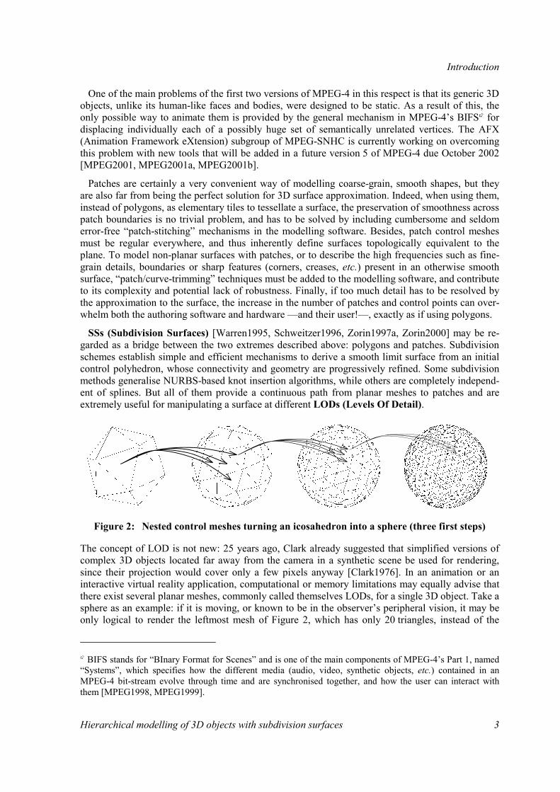
Introduction
Hierarchical modelling of 3D objects with subdivision surfaces 3
One of the main problems of the first two versions of MPEG-4 in this respect is that its generic 3D objects, unlike its human-like faces and bodies, were designed to be static. As a result of this, the only possible way to animate them is provided by the general mechanism in MPEG-4’s BIFS� for displacing individually each of a possibly huge set of semantically unrelated vertices. The AFX (Animation Framework eXtension) subgroup of MPEG-SNHC is currently working on overcoming this problem with new tools that will be added in a future version 5 of MPEG-4 due October 2002 [MPEG2001, MPEG2001a, MPEG2001b].
Patches are certainly a very convenient way of modelling coarse-grain, smooth shapes, but they are also far from being the perfect solution for 3D surface approximation. Indeed, when using them, instead of polygons, as elementary tiles to tessellate a surface, the preservation of smoothness across patch boundaries is no trivial problem, and has to be solved by including cumbersome and seldom error-free “patch-stitching” mechanisms in the modelling software. Besides, patch control meshes must be regular everywhere, and thus inherently define surfaces topologically equivalent to the plane. To model non-planar surfaces with patches, or to describe the high frequencies such as fine-grain details, boundaries or sharp features (corners, creases, etc.) present in an otherwise smooth surface, “patch/curve-trimming” techniques must be added to the modelling software, and contribute to its complexity and potential lack of robustness. Finally, if too much detail has to be resolved by the approximation to the surface, the increase in the number of patches and control points can over-whelm both the authoring software and hardware —and their user!—, exactly as if using polygons.
SSs (Subdivision Surfaces) [Warren1995, Schweitzer1996, Zorin1997a, Zorin2000] may be re-garded as a bridge between the two extremes described above: polygons and patches. Subdivision schemes establish simple and efficient mechanisms to derive a smooth limit surface from an initial control polyhedron, whose connectivity and geometry are progressively refined. Some subdivision methods generalise NURBS-based knot insertion algorithms, while others are completely independ-ent of splines. But all of them provide a continuous path from planar meshes to patches and are extremely useful for manipulating a surface at different LODs (Levels Of Detail).
Figure 2: Nested control meshes turning an icosahedron into a sphere (three first steps)
The concept of LOD is not new: 25 years ago, Clark already suggested that simplified versions of complex 3D objects located far away from the camera in a synthetic scene be used for rendering, since their projection would cover only a few pixels anyway [Clark1976]. In an animation or an interactive virtual reality application, computational or memory limitations may equally advise that there exist several planar meshes, commonly called themselves LODs, for a single 3D object. Take a sphere as an example: if it is moving, or known to be in the observer’s peripheral vision, it may be only logical to render the leftmost mesh of Figure 2, which has only 20 triangles, instead of the
� BIFS stands for “BInary Format for Scenes” and is one of the main components of MPEG-4’s Part 1, named “Systems”, which specifies how the different media (audio, video, synthetic objects, etc.) contained in an MPEG-4 bit-stream evolve through time and are synchronised together, and how the user can interact with them [MPEG1998, MPEG1999].
Introduction
4 Hierarchical modelling of 3D objects with subdivision surfaces
rightmost one, which has 20 · 43 = 1280 triangles, and save computing resources for rendering other objects in the scene. Finally, in situations where the object has to be transmitted from a server to a rendering client over a limited bandwidth communication channel such as the Internet, the benefits of having several LODs to choose from is obvious. And even more so if the LOD collection is progressive, that is, if each LOD may be easily expressed differentially, relative to the next coarser one. In such a case, the coarsest LOD can be transmitted quickly so that the client can start display-ing a rough approximation to the object very soon, while refinements keep being sent and incorpo-rated gradually to the rendered mesh.
Figure 2 also illustrates how a simple subdivision scheme could proceed to generate a geodesic sphere starting from an icosahedron. The arrows indicate how, at each step, every old triangle would be split into four new ones by inserting a new vertex near the midpoint of each old edge. Care would be taken, when positioning those new vertices, so that the angles between adjacent triangles would keep diminishing, so as to make the resulting mesh increasingly smooth.
In this example, the smoothing of the mesh could be easily accomplished by simply projecting the midpoint of each old edge onto the desired sphere, so the position of each new vertex would be, so to speak, self-contained. But, in the general case, vertex positions would be hierarchically related to one another. More specifically, the positions of vertices of LOD n (i.e., appearing at the nth subdivi-sion step) would be determined by those of some set of neighbour vertices of LOD n−1, which would in turn be determined by those of some set of neighbour vertices of LOD n−2, …, which would in turn be determined by those of the initial (LOD 0) vertices.
The control polyhedra generated by subdivision methods are indeed hierarchically nested and form a pyramid of finer and finer approximations to the smooth limit surface. Therefore, it is possible to perform both large-scale edits, in which the movement of a few vertices of a coarse control mesh drags a wide area of the surface, as well as minute detail modifications, in which only a few vertices of the finest meshes are displaced. Subdivision schemes provide, by their own nature, the multi-resolution editing handles that neither polygons nor patches alone can offer.
We will elaborate further on the important difference there is between merely progressive and truly hierarchical modelling, but the basic idea is quite simple. As stated above, a progressive repre-sentation of a 3D object is one in which it is possible to go from any given LOD to the next finer one because they are coded incrementally; however, the refinements are randomly located, and there is no relationship between the elements of one LOD and the immediate ones. In the hierarchical case, the LODs are also coded differentially; but, furthermore, there is a very clear pyramidal nesting of the elements of successive LODs, which has many theoretical and practical positive consequences.
In particular, such a pyramid of LODs is highly suitable for a truly hierarchical representation and coding (and, hence, transmission) of 3D models thanks to wavelet-based MRA (MultiResolution Analysis) techniques. The main idea behind MRA is to decompose a function or signal into a coarse, low resolution/frequency part, plus a collection of finer and finer details only observable at increas-ing resolutions/frequencies. The theoretical interest of having such a sub-band decomposition of a signal is obvious: it allows to “see both the forest and the trees”. Its practical potential has been sufficiently proven by the amount of research and the number of practical applications that wavelet-based MRA of classic nD signals has generated in the past dozen of years. By “classic nD signals” we mean 1D (e.g., audio), 2D (still image), and 3D (video) signals/functions, as opposed to those of our interest, 3D surfaces. The latter may arguably be called “signals”, but can hardly be labelled as “3D” ones, as they are certainly embedded in a 3D space but have only two degrees of freedom — in fact, this is why they are sometimes termed “2,5D signals”, much to the distaste of fractal lovers…
Especially for signal transmission purposes, multiresolution is a very important concept. Not only does it permit to send a coarse version of the signal first and progressively refine it afterwards, but it also enables a more compact coding of the information carried by signals whose energy is mostly
Introduction
Hierarchical modelling of 3D objects with subdivision surfaces 5
concentrated in their low frequency part. Indeed, predictive coding schemes allow to express a successively approximated signal as its coarsest version plus a set of prediction errors, which are the differences between the original signal and the predictions based on its successively refined ver-sions. The prediction mechanisms are usually designed to generate small prediction errors for mostly smooth signals, which are the ones encountered in practice, and are therefore able to transform a possibly energetic signal into a low variance set of prediction errors. Entropy coding techniques can finally be applied for efficiently compressing the prediction errors, the total result being that the same amount of information is represented with much less data.
It can be said that the roots of MRA are nearly two centuries old and can be found in a basic build-ing block of approximation theory: Fourier’s analysis and transform for representing periodic func-tions as harmonic trigonometric series [Fourier1822]. In the last few decades, and in the field of signal processing, other already classic space/frequency transforms such as the DCT (Discrete Cosine Transform) have been commonly used to represent signals in a multiresolution manner in many practical applications, notably those dealing with sub-band coding of the classic nD signals mentioned above. Even more recently (in the last dozen of years or so), wavelets have proven to be a powerful tool for defining bases of functional spaces with better resolution in the space and fre-quency domains than classic space/frequency transforms. And this, both in the contexts of approxi-mation theory and signal processing (see the book “Wavelets and Subband Coding” by Vetterli and Kovačević [Vetterli1995]); but also in others such as computer graphics, where they are starting to play an essential role in several areas like image compression and editing, global illumination, volume rendering and, very especially, hierarchical modelling of 3D objects.
0.1. Objectives and contributions At the time of setting the objectives of the research we would carry within the context of hierarchical modelling of 3D objects with SSs, we foresaw both theoretical and practical components, but with a special emphasis on the latter. We intended to focus primarily on the practical applications that could be —and are being!— derived in that context, notably truly hierarchical 3D model coding.
However, the theoretical aspects of our research, carried to gain a deep understanding of the fields related to our subject, have led us to a synthesis task which we now believe is as essential, in our work, as the technique for hierarchical 3D model coding we have devised. Besides, we are not aware of the existence of any previously published literature compiling and linking together the three main knowledge areas which have served as a basis for our work: SSs, automatic LOD extraction, and wavelet-based MRA. In fact, it would not be correct to say that they form a basis, since they are precisely not independent from each other, which is what we stress below by explaining how these three pieces of our puzzle fit together.
The practical applications of hierarchical modelling of 3D objects with SSs constitute nevertheless our main original development. In particular, we have devised and published a method for hierarchi-cal 3D model coding based on SSs that significantly outperforms previously reported ones, and is currently being considered inside the AFX subgroup of MPEG-SNHC for its adoption in a future version of the MPEG-4 standard.
But a complete solution for the hierarchical modelling of 3D objects with SSs requires as well ex-tracting a base mesh from the input surface, still most frequently given as a very fine mesh with arbitrary connectivity, which has to be remeshed. Consequently, we have designed some auxiliary methods dealing with automatic 3D mesh simplification and remeshing by improving previous techniques and by creating our own.

Introduction
6 Hierarchical modelling of 3D objects with subdivision surfaces
0.2. Outline of dissertation Given its subject, we have tried to make this dissertation as hierarchical as possible. Many concepts are structured in a pyramidal fashion: a coarse version of them is first introduced and later refined by adding details where needed. If our attempt at organising our exposition in a multiresolution manner has been successful, the reader will be able to quickly grasp the basic idea behind our techniques and then hopefully satisfy her possible wish for details afterwards.
The first chapter, “Background”, is a synthesis of the concepts needed to follow the rest of the dissertation. Apart from a brief introductory section explaining a few basic topological concepts, it contains three main sections, devoted to SSs, automatic LOD extraction, and wavelet-based MRA.
The second chapter, “Hierarchical 3D model coding with SSs”, describes the core of our work: the hierarchical 3D model coding scheme based on SSs we propose. It starts by defining the raw size of a 3D mesh, in order to have a reference for establishing compression efficiency comparisons be-tween 3D model coding techniques. It then reviews previous work on progressive 3D mesh coding before describing our proposal for truly hierarchical 3D model coding and the results we have ob-tained with it.
The third chapter, “LOD extraction and remeshing”, describes the aspects of our proposal for hier-archical modelling of 3D objects that deal with two auxiliary techniques, namely the extraction of the base mesh and the implicit remeshing of an arbitrary input mesh.
Finally, the fourth chapter, “Conclusions”, summarises the dissertation and the results we have obtained, and reflects our insight on potential threads for future research which could improve and complete our work.
This dissertation is available on-line at “http://www.gti.ssr.upm.es./~fmb/pub/PhD.pdf.gz”, and related questions and comments can be addressed to “[email protected]”.

Background
Hierarchical modelling of 3D objects with subdivision surfaces 7
1. Background
1.0. Contents This chapter is a synthesis of the concepts needed to follow the rest of the dissertation. Its first section introduces a few basic topological concepts. A second one is devoted to SSs and explains that they are a simple, efficient means of deriving a smooth shape from an initial coarse mesh, without having yet a particular target surface in mind. Especial attention is paid to the analysis of their geometric properties, and a taxonomy is established for subdivision schemes, of which the most common ones for triangular meshes are described in some depth. A third section reviews the essen-tial aspects of automatic LOD extraction, such as the notion of approximation error for surfaces and the modus operandi of the best 3D mesh simplification methods published to date. A closing section on wavelet-based MRA techniques gives some insight on how the different pieces of our puzzle fit together.
1.1. A few topological considerations We introduce below the few concepts from algebraic topology needed in our context and advise the reader interested in acquiring a deep understanding of the subject to study the classic “introductory” book by Massey [Massey1989], which is far more rigorous. In fact, the term “topology” itself will be used in this dissertation both for the connectivity of a planar mesh and for the properties of the curved surface approximated by that mesh, such as its openness/closeness, genus, etc. Nevertheless, this usage inconsistency will hopefully not lead to any ambiguities.
Let us concentrate first on planar meshes embedded in 3D space. It is very important to distinguish between the abstract graph of a mesh, which describes only how its vertices are interconnected, and the 3D mapping of that graph, which describes also its geometric shape. A given abstract graph could be mapped onto completely different shapes, and different abstract graphs could be mapped onto 3D meshes of different connectivity but with the exact same shape. In fact, triangular meshes are very commonly denoted as a pair (P, K), where P = {pi ∈ 3 | 1 ≤ i ≤ n} is a set of n 3D points, and K is a 2D abstract simplicial complex containing all the connectivity information. The complex K is a set of subsets of {1, 2, …, n} called simplices, where a simplex can be a singleton {i} (repre-senting vertex nr. i), a pair {i, j} (the edge whose endpoints are vertices i and j) or a triple {i, j, k} (the triangle delimited by vertices i, j and k). Any subset of a simplex of K must in turn be a simplex of K: if a triangle belongs to K, so must its edges and vertices. On the other hand, there cannot be

Background
8 Hierarchical modelling of 3D objects with subdivision surfaces
“dangling” edges or vertices either: each edge must belong to at least one triangle, and each vertex must belong to at least one edge (in fact, to two, if the previous rule is taken into account).
Figure 3: Non-manifold mesh with three non-manifold edges
An important property we will require meshes to have, at least in principle, is manifoldness. In a manifold mesh, among other things which will be explained below, each edge must belong to either one or two facets, but no more, so edges shared by three or more facets (called “non-manifold edges”) are not permitted. The quadrilateral mesh of Figure 3, meant to model a car hood and wind-shield, has three non-manifold edges along their joint, which have been highlighted.
Not surprisingly, an edge belonging to only one facet is said to be a border edge, whereas one shared by two facets is labelled as interior to the mesh. Those two adjectives apply as well for vertices, depending on whether they lie or not on the border of the mesh. Also rather logically, meshes are said to be closed, if they have no border edges, or open, if they do have any.
It is also worthwhile to discuss the number of facets that can share a vertex V; or, equivalently (if V is interior), the number of edges that can emanate from V, hence called V’s outdegree; or, also equivalently, the number of neighbour vertices V can have, hence called V’s valence. There are two clearly distinct categories of vertices, according to their valence: regular interior vertices of a trian-gular mesh have six outgoing/incident edges each, whereas those of a quadrilateral mesh have four; non-regular vertices are usually called extraordinary. In the case of open meshes, border vertices may as well be regular or extraordinary, the former having valence four in triangular meshes, and three in quadrilateral ones. Note that the adjective “regular” originates, in this context of a planar abstract graph, from the structure of a regular mesh (or grid), which is one that periodically tesse-lates the plane. No connection should be made with the regularity of the five perfect polyhedra, whose vertices are in fact all extraordinary from this point of view.
Figure 4: Two periodic tesselations of the plane by M. C. Escher (left: with triangles; right: with parallelograms)
The expression topologically regular setting is also commonly used to refer to regions of an arbi-trary graph where all vertices are regular and interior. Figure 4 consists of a couple of drawings

Background
Hierarchical modelling of 3D objects with subdivision surfaces 9
made in 1964 by the great Dutch artist M. C. Escher, who developed a certain addiction to plane tilings after visiting the South of Spain in 1922 and 1936 and being fascinated by the legacy of the Arabs. By forgetting for a moment the tantalising fish patterns and looking only at the white lines, the two simplest topologically regular settings can be observed. The corresponding tiles of the plane are triangles (equilateral, in Figure 4-left) and parallelograms (squares, in Figure 4-right).
Figure 5: Non-manifold mesh with one non-manifold vertex
The set of vertices directly connected to a vertex V constitutes what is called its 1-ring, its k-ring being recursively defined as the union of the 1-rings of all vertices in V’s (k−1)-ring (never counting V itself). Notice how the 1-rings of vertices of Figure 4, which are all regular, are formed by either six connected vertices forming hexagons, in the first case, or four linked vertices forming squares, in the second. The 1-ring of a vertex V may not be a proper, closed ring in that it may be incomplete, if V is a border vertex (sometimes such partial 1-rings are called “1-fans”). This is the case of most border vertices in the triangular mesh shown in Figure 5, which have either four or three neighbours, depending on their regularity. However, the central vertex of Figure 5 where the two cones touch, which has six neighbours, exhibits a more pathological type of singularity, as its 1-ring consists of more than one (partial) ring of connected neighbours, which is another forbidden situation in mani-fold meshes.
Let us finally add that analogies can of course be found in the case of surfaces for all which has been said for meshes: surfaces can as well be manifold or non-manifold, and open (i.e., with border) or closed (without). A manifold, closed, and connected surface delimits a single 3D volume, which may be simply connected or not: in the first case, the surface is topologically equivalent to a sphere and has genus zero (no handles), whereas in the second it is equivalent to a torus or any other shape with higher genus (one or more handles).
1.2. Subdivision surfaces
1.2.0. Intuitive definition A SS is defined as the limit of a recursive refinement process applied upon an arbitrary connec-tivity control mesh made entirely of planar polygons, generally of the same kind (all of them triangles, quadrilaterals, etc.). The progressive refinement of the control mesh is both topological, as its connectivity is made richer, and geometric, as its shape is made smoother. It is achieved by splitting its polygons or vertices and positioning new vertices so that the angles between adjacent facets are conveniently reduced.

Background
10 Hierarchical modelling of 3D objects with subdivision surfaces
Figure 6: Two generations of a SS triangular control mesh (left: abstract graph; right: 3D mapping)
Figure 6-left shows two generations of the abstract graph corresponding to a simple triangular con-trol mesh: each of the five initial triangles, whose vertices are shown as circles, is subdivided into four smaller triangles by splitting its edges at their midpoints�, which is why this process is known as midpoint subdivision. Those midpoints are added to the mesh as new vertices (shown as dots), and interconnected to form four new triangles that replace the old one. Old edges are also replaced by two new ones each, and three new edges interior to each old triangle are created. Letting nα
k denote the number of elements α (α ∈ {v, e, t} for vertices, edges, and triangles, respectively) of a mesh of level k (k = 0 for the initial mesh), in this case, nv
0 = 6, ne0 = 10 and nt
0 = 5, whereas nv
1 = nv0 + ne
0 = 16, ne1 = 2 ne
0 + 3 nt0 = 35 and nt
1 = 4 nt0 = 20.
A very important property of all subdivision methods is that the new vertices introduced by the subdivision process are all regular, while the primitive ones always keep their arbitrary initial va-lence. This is illustrated by Figure 6-left, in which the dots are all regular (interior ones have valence six; border ones have valence four), whereas the circles happen to be all extraordinary (the interior one has five neighbours; border ones have three each).
Figure 6-right shows how the control net on the left could be mapped onto its corresponding 3D mesh. Each initial point has the arbitrary 3D position given to it by the modeller so that, in principle, the six circles of Figure 6-right are not coplanar, nor are the five level 0 triangles they form, whose edges are shown as thin lines. If such a mesh is subdivided by an interpolating scheme, which is one that does not reposition old vertices (see section 1.2.3), the circles remain in their locations, but new vertices shown as dots appear and form level 1 triangles highlighted with thick lines. The images of the dots need not be the midpoints of the edges joining the images of the circles. In fact, it is pre-cisely by not mapping the midpoints of the abstract graph edges onto the midpoints of the 3D mesh edges that the geometric refinement (i.e., smoothing) of the initial control mesh is performed.
In order to reduce the angles between adjacent triangles, the position of each new vertex intro-duced by the subdivision process is calculated as a function of some old vertices in the vicinity of the considered edge. In fact, the position of old vertices themselves may be altered as well for that same purpose. As what is sought is a low-pass filtering of the 3D shape, usually some linear combi-nation is chosen: a new vertex position is then simply a weighted average of those of some nearby old vertices. It is important to stress that only some finite number of such nearby old vertices are used in the blend in most schemes, which are consequently said to have finite/compact support. Some attractive features of SSs such as local control are derived from this property.
� We will always assume that edges are split at their midpoints, because this is what major subdivision schemes do. However, this is not always the case: for instance, the 3 subdivision scheme [Kobbelt2000, Labsik2000] splits edges at one and two thirds of their length in order to subdivide each triangle into nine.
z
yx
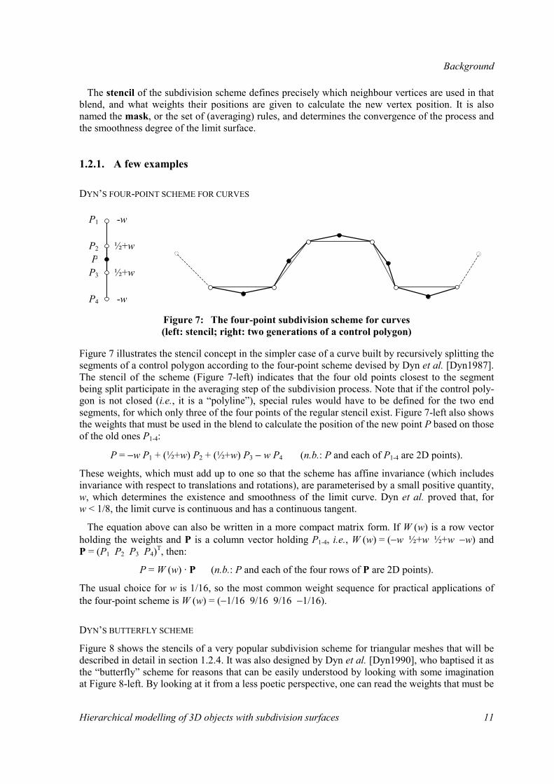
Background
Hierarchical modelling of 3D objects with subdivision surfaces 11
The stencil of the subdivision scheme defines precisely which neighbour vertices are used in that blend, and what weights their positions are given to calculate the new vertex position. It is also named the mask, or the set of (averaging) rules, and determines the convergence of the process and the smoothness degree of the limit surface.
1.2.1. A few examples
DYN’S FOUR-POINT SCHEME FOR CURVES
Figure 7: The four-point subdivision scheme for curves (left: stencil; right: two generations of a control polygon)
Figure 7 illustrates the stencil concept in the simpler case of a curve built by recursively splitting the segments of a control polygon according to the four-point scheme devised by Dyn et al. [Dyn1987]. The stencil of the scheme (Figure 7-left) indicates that the four old points closest to the segment being split participate in the averaging step of the subdivision process. Note that if the control poly-gon is not closed (i.e., it is a “polyline”), special rules would have to be defined for the two end segments, for which only three of the four points of the regular stencil exist. Figure 7-left also shows the weights that must be used in the blend to calculate the position of the new point P based on those of the old ones P1-4:
P = −w P1 + (½+w) P2 + (½+w) P3 − w P4 (n.b.: P and each of P1-4 are 2D points).
These weights, which must add up to one so that the scheme has affine invariance (which includes invariance with respect to translations and rotations), are parameterised by a small positive quantity, w, which determines the existence and smoothness of the limit curve. Dyn et al. proved that, for w < 1/8, the limit curve is continuous and has a continuous tangent.
The equation above can also be written in a more compact matrix form. If W (w) is a row vector holding the weights and P is a column vector holding P1-4, i.e., W (w) = (−w ½+w ½+w −w) and P = (P1 P2 P3 P4)T, then:
P = W (w) · P (n.b.: P and each of the four rows of P are 2D points).
The usual choice for w is 1/16, so the most common weight sequence for practical applications of the four-point scheme is W (w) = (−1/16 9/16 9/16 −1/16).
DYN’S BUTTERFLY SCHEME
Figure 8 shows the stencils of a very popular subdivision scheme for triangular meshes that will be described in detail in section 1.2.4. It was also designed by Dyn et al. [Dyn1990], who baptised it as the “butterfly” scheme for reasons that can be easily understood by looking with some imagination at Figure 8-left. By looking at it from a less poetic perspective, one can read the weights that must be
-w
-w
½+w
½+w
P1
P2
P3
P4
P

Background
12 Hierarchical modelling of 3D objects with subdivision surfaces
assigned to the positions of the eight old vertices (circles) to calculate the position of the new vertex (dot) that will be the image of the highlighted edge midpoint. As in the four-point scheme, those weights add up to one and are parameterised by a small w. In the words of the creators of both schemes, “w serves as a tension parameter in the sense that as w tends to zero the limit surface is tightened toward the piecewise linear control polyhedron”. In fact, by choosing w = 0, one would perform only a topological refinement of the mesh, but no geometric refinement at all, i.e., plain midpoint subdivision.
Figure 8: Stencils of the butterfly subdivision scheme (left: for regular edges; right: for crease and boundary edges)
As shown in Figure 8-right, the same stencil of the four-point scheme is in fact used to subdivide edges lying on the border of open meshes, or interior ones aligned with sharp features of the surface that have to be respected. The effect of taking into account only old vertices lying on a boundary or aligned with a crease, for the calculation of new vertex positions, is that the corresponding curve is smoothed as if it were isolated from the surrounding triangles in the mesh.
LOOP’S SCHEME
Figure 9: Stencils of Loop’s subdivision scheme (left: for repositioning old vertices; right: for splitting edges)
Figure 9 shows the stencils used for repositioning old vertices and inserting new ones by splitting edges in the case of another classical subdivision scheme for triangular meshes first studied by Loop in his Master thesis [Loop1987]. Note that those stencils are the ones used in the topologically regular setting, so other rules are needed for extraordinary and/or border vertices, and border edges. For instance, for repositioning extraordinary vertices of valence K ≠ 6, a weight β ≠ 1/16 must be assigned to each neighbour vertex position, and a weight of 1−K β to the central one. There are several possibilities for β:
2w 2w
½
½
−w −w
−w −w
−w −w ½+w ½+w
3/83/8
1/8
1/81/161/16
1/16 1/16
1/161/16 10/16
Background
Hierarchical modelling of 3D objects with subdivision surfaces 13
• Loop’s original proposal was β =
+−2π2cos
41
83
851
KK. In particular, this is β = 3/16 for
K = 3, β = 31/256 ≅ 1/8 for K = 4, β ≅ 1/12 for K = 5, and β = 1/16 for K = 6.
• Warren proposed later to keep β = 3/16 for K = 3, but to have simply β = 3/(8K) for K > 3, which also amounts to β = 1/16 for K = 6 [Warren1995].
1.2.2. Formal definition and analysis To define more precisely what the limit surface yielded by the recursive subdivision process is, and to analyse its existence and smoothness with some rigour, it is necessary to elaborate on a few key concepts:
• there are two definitions of surface smoothness which deserve some careful explanation;
• a SS can be represented as a function mapping elements of a 2D parametric domain to points in 3D space;
• the subdivision rules can be “coded” in local subdivision matrices which facilitate greatly the study of the existence and smoothness of the limit surface at regular vertices;
• the analysis of the behaviour of the limit surface at extraordinary vertices is more involved.
SMOOTHNESS OF THE LIMIT SURFACE: GEOMETRIC AND PARAMETRIC CONTINUITIES
The concept of surface smoothness is important in the field of computer graphics because piecewise smooth shapes are very common in real life and supposedly more pleasing to the subjective human eye. Intuitively speaking, a surface is smooth if it has no sharp features, like creases, peaks, corners, etc. More precisely, although still informally, a surface is considered to be smooth if it is indistin-guishable from a plane, when looking at any of its points from a sufficiently close distance. Many authors have devoted valuable efforts to the clarification of this intuitive idea of surface smoothness, and have introduced more formal, mathematical terms, such as surface continuity. Since the begin-nings of CA[G]D, when people started using parametric patches as elementary building blocks to model complex shapes, the main concern has been how to “stitch” together those internally smooth patches to obtain globally “seamless” surfaces [Bézier1986, Du1988, Farin1993]. The continuity of SSs was studied first by Ball and Storry [Ball1988] and, more recently and in deeper detail, by Reif [Reif1995], Warren [Warren1995], Schweitzer [Schweitzer1996] and Zorin [Zorin1997a].
The formal, although somewhat misleading, definition of geometric/visual continuity has tradi-tionally been the following: a surface is said to be G1-continuous (or simply G1) if and only if its tangent plane is continuous at any of its points. This is why G1-continuity is also known as tangent plane continuity. According to this definition, a polyhedron is not visually smooth, but merely G0, meaning it is just connected (if it were not, it would not even deserve the “G rating”). Its vertices and edges are the sharp features at which its tangent plane exhibits discontinuities — but those sharp features are precisely “chopped off” by the averaging step of the subdivision process! Higher order geometric continuities are rarely required in practical surface rendering applications, since tangent plane continuity is enough to produce aesthetically pleasing results. Nevertheless, G2-continuity, which requires that the tangent plane of the surface (or, equivalently, its osculating paraboloid) be well-defined everywhere, is sometimes desirable.
The reason why we believe this definition of visual continuity may be misleading is that it allows to argue that the surface formed by two hemispheres lying side by side on a plane is visually smooth,

Background
14 Hierarchical modelling of 3D objects with subdivision surfaces
as it can be said it has a well-defined tangent plane everywhere. Such a surface, which is non-manifold, is clearly not “indistinguishable from a plane” at the point where the two hemispheres touch.
Figure 10: A hardly visually smooth curve with continuous tangent
Figure 10 illustrates this with a simpler but analogous example, in which a curve has been obtained by replicating the unit semicircle «x2 + y2 = 1, y ≥ 0» centred at (2k+1, 0), k ∈ . Even if willing to accept that its tangent line is well-defined everywhere, one must admit that its normal vector n (defined consistently to always have ny ≥ 0, for instance) is definitely not: its orientation flips at the points (2k, 0), k ∈ , which is precisely why the curve can hardly be described as visually smooth. It must not be forgotten that a vector has an orientation, which has to be consistently chosen through-out the curve or surface — the latter being impossible in the case of non-orientable surfaces like the Möbius’ strip [Massey1989] depicted in Figure 11.
Figure 11: A smooth, but non-orientable (and “buggy”! ;-) Möbius’ strip by M. C. Escher
There is another definition of surface smoothness much less prone to misinterpretation, which is the main reason why it is useful to express a SS as a function defined over some parametric domain. The degree of parametric continuity of a surface states, in that simple and elegant way mathematicians have to put things, how many times it is differentiable — here is where they usually omit an essen-tial “for a given parameterisation S = S (u, v)” which is as obvious to them as forgettable by mere mortals… A parameterised surface is said to be Ck-continuous (or simply Ck) if and only if it is k times continuously differentiable at any of its points: a polyhedron is just C0, since it is not differen-tiable at all; a C1 surface would tolerate a single differentiation step; a C2 one would take two; etc.
The main problem with parametric continuity is that it depends on the (implicit or, at best, explicit) parameterisation of the surface, which can be any of infinitely many. So the finding of one or many parameterisations which are not differentiable some number of times does not prove there are none which indeed are. It may be possible to re-parameterise a non-Ck surface so that it does become Ck: with curves, this is usually achieved by using arc-length as the new parameter.
x
y
1
1
n’n

Background
Hierarchical modelling of 3D objects with subdivision surfaces 15
Another problem of parametric continuity is that some paradigmatic shapes do not have any global parameterisation, no matter how smooth they may be. The sphere, for instance, is not globally ho-meomorphic to a plane, although being locally so at any of its points. Unfortunately, when the surface associated to the initial control mesh is not topologically equivalent to the plane, there is simply no way to find a global parameterisation of it over a planar domain. It is important to bear in mind that smoothness is a local property of a surface, which is why it is required to have Gk or Ck-continuity “at any of its points” in order to be declared Gk/Ck-continuous itself as a whole. The topological properties of a surface, on the other hand, are intrinsically global. Among them are its openness/closeness, its number of borders (if it is open), its genus, its orientability, and the like [Massey1989].
Many formal studies of SSs have been devoted to find necessary and sufficient conditions to prove that a particular scheme yields Ck-continuous limit surfaces, or to build clever (and usually local) re-parameterisations of its most natural one. In fact, the latter is enough from the viewpoint of the intuitive definition of smoothness given above, which stated that a surface is smooth if it is indistin-guishable from the plane “when looking at any of its points from a sufficiently close distance” (i.e., locally).
Geometric and parametric continuities are only equivalent if non-manifolds are excluded from the set of surfaces under consideration. This amounts to requiring, in the case of geometric continuity, that the normal vector be well-defined and consistently oriented throughout the surface. Otherwise, geometric continuity would be weaker than the corresponding parametric continuity. For instance, C1 would be stronger than G1, as the existence of continuous first partial derivatives of a surface parameterisation implies the continuity of its tangent plane, whereas the opposite implication does not hold: in addition, the projection of the surface onto the tangent plane must be injective [Zo-rin1997a]. This is why we believe it would be wiser, and more general, to define a surface to be Gk-continuous (or simply Gk) if and only if its consistently oriented normal vector is k times continu-ously differentiable at any of its points. Note that the continuity of a surface normal vector implies that of its tangent plane, as the latter is uniquely characterised by the former, whereas the opposite is not true.
PARAMETERISATION OVER THE INITIAL CONTROL MESH
As already explained in section 1.2.0, the abstract graph of the initial control mesh is recursively refined by midpoint subdivision, thus generating a denser and denser graph, which is mapped to a finer and finer control mesh. At each subdivision step, the control mesh can be represented as a vector-valued piecewise linear function over a parametric domain, in which the abstract graph lives. This defines a sequence of functions from the parametric domain into 3 that, under some known conditions, converges uniformly to a limit mapping: the wanted limit surface.
Although it is not the case of all subdivision schemes, many are built with spline basis functions, and therefore that mapping is known in advance. For instance, when subdividing a completely regular mesh according to Loop’s scheme, a quartic three-directional box-spline patch is obtained [Loop1987]. It is possible to describe that box-spline with a global, explicit closed form expression as a function mapping a planar parametric domain into 3D space.
There are obviously only two independent variables in a planar domain, but it is very convenient to use three parametric/barycentric coordinates (u, v, w) for triangular graphs. This is the common practice when dealing with box-splines which, unlike tensor product splines, are defined on regular triangular (as opposed to rectangular) grids. Those three coordinates always satisfy «u + v + w = 1»: see Figure 12-left and note that, furthermore, inside the triangle, 0 ≤ u, v, w ≤ 1.
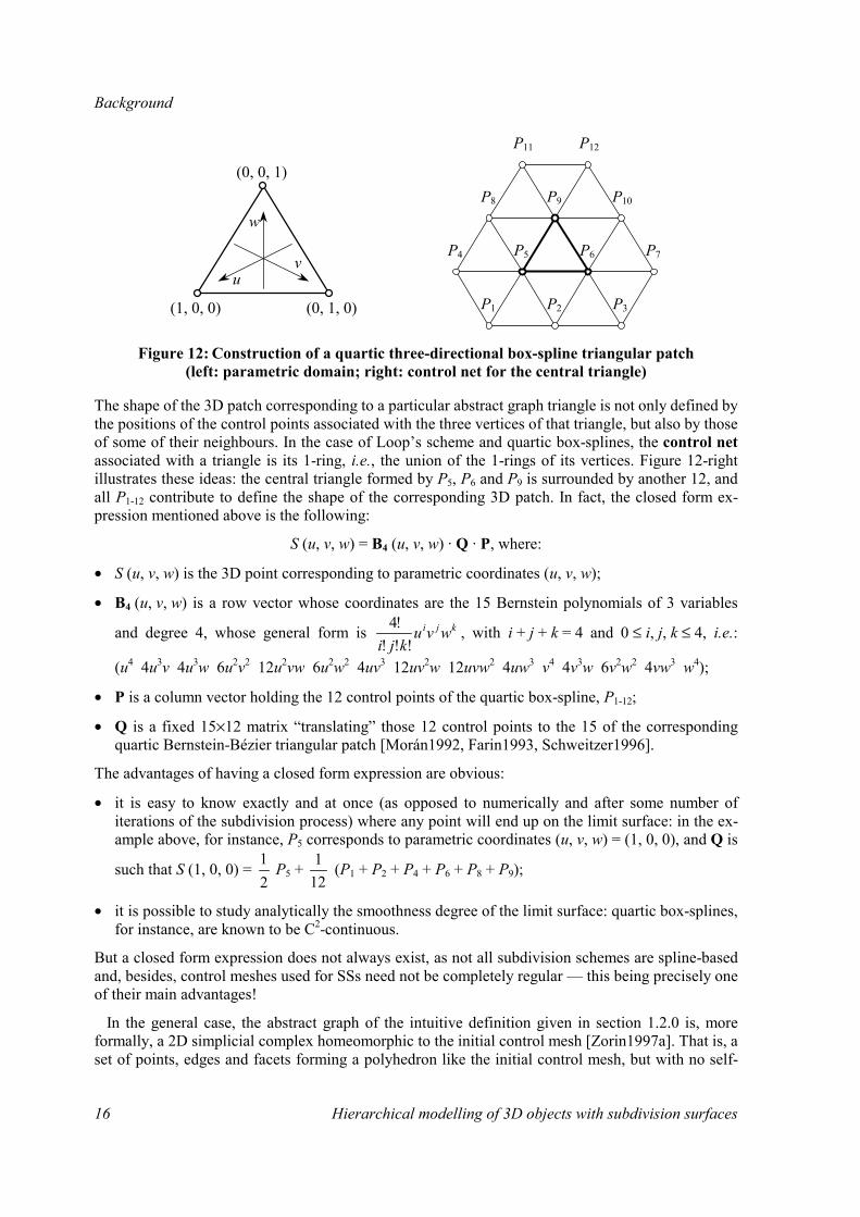
Background
16 Hierarchical modelling of 3D objects with subdivision surfaces
Figure 12: Construction of a quartic three-directional box-spline triangular patch (left: parametric domain; right: control net for the central triangle)
The shape of the 3D patch corresponding to a particular abstract graph triangle is not only defined by the positions of the control points associated with the three vertices of that triangle, but also by those of some of their neighbours. In the case of Loop’s scheme and quartic box-splines, the control net associated with a triangle is its 1-ring, i.e., the union of the 1-rings of its vertices. Figure 12-right illustrates these ideas: the central triangle formed by P5, P6 and P9 is surrounded by another 12, and all P1-12 contribute to define the shape of the corresponding 3D patch. In fact, the closed form ex-pression mentioned above is the following:
S (u, v, w) = B4 (u, v, w) · Q · P, where:
• S (u, v, w) is the 3D point corresponding to parametric coordinates (u, v, w);
• B4 (u, v, w) is a row vector whose coordinates are the 15 Bernstein polynomials of 3 variables
and degree 4, whose general form is kji wvukji !!!
!4 , with i + j + k = 4 and 0 ≤ i, j, k ≤ 4, i.e.:
(u4 4u3v 4u3w 6u2v2 12u2vw 6u2w2 4uv3 12uv2w 12uvw2 4uw3 v4 4v3w 6v2w2 4vw3 w4);
• P is a column vector holding the 12 control points of the quartic box-spline, P1-12;
• Q is a fixed 15×12 matrix “translating” those 12 control points to the 15 of the corresponding quartic Bernstein-Bézier triangular patch [Morán1992, Farin1993, Schweitzer1996].
The advantages of having a closed form expression are obvious:
• it is easy to know exactly and at once (as opposed to numerically and after some number of iterations of the subdivision process) where any point will end up on the limit surface: in the ex-ample above, for instance, P5 corresponds to parametric coordinates (u, v, w) = (1, 0, 0), and Q is
such that S (1, 0, 0) = 21
P5 + 121 (P1 + P2 + P4 + P6 + P8 + P9);
• it is possible to study analytically the smoothness degree of the limit surface: quartic box-splines, for instance, are known to be C2-continuous.
But a closed form expression does not always exist, as not all subdivision schemes are spline-based and, besides, control meshes used for SSs need not be completely regular — this being precisely one of their main advantages!
In the general case, the abstract graph of the intuitive definition given in section 1.2.0 is, more formally, a 2D simplicial complex homeomorphic to the initial control mesh [Zorin1997a]. That is, a set of points, edges and facets forming a polyhedron like the initial control mesh, but with no self-
P1 P2 P3
P7
P10
P12P11
P9
P6P5
P8
P4
w
uv
(0, 0, 1)
(0, 1, 0)(1, 0, 0)

Background
Hierarchical modelling of 3D objects with subdivision surfaces 17
intersections. The reason why the parametric domain must be a simple polyhedron is that, if it were allowed to have self-intersections, a vertex on it could be mapped to 3D in a non-unique way. But this is not really a limitation of the initial control mesh connectivity. It is only a requirement for the abstraction that must be made of it to build the parametric domain. It only means that, if the initial control mesh has any self-intersections, they must be removed to build the parametric domain, whose vertices can be displaced at will.
There is, nevertheless, a true limitation to the connectivity of the initial control mesh of a SS (and, hence, to the topology of the implied limit surface) which is not always made explicit in the litera-ture on the subject: it must be manifold. This is due to the fact that the stencils of the usual subdivi-sion schemes do not consider edges shared by more than two facets. But this limitation is reasonably easy to solve, though: if the initial control mesh is non-manifold, it can be cut into manifold pieces to be smoothed independently.
Figure 13: Treatment of non-manifold edges (top: original non-manifold mesh; centre and bottom: two manifold meshes, subdivided separately)
Figure 13 illustrate this procedure with the mesh of Figure 3, whose non-manifoldness is attacked by cutting the non-manifold mesh into two manifold ones, which can then be subdivided separately. Care has to be taken, however, to mark each originally non-manifold edge on both meshes it belongs to, in order to guarantee that it will be treated in the same way when subdividing them.
subdivide
cut

Background
18 Hierarchical modelling of 3D objects with subdivision surfaces
LOCAL SUBDIVISION MATRICES
Subdivision matrices are extremely helpful for “coding” the rules of a subdivision scheme in a compact way. Furthermore, they are also extremely useful for analysing the existence and tangent plane continuity of the limit surface.
When using Loop’s scheme, for instance, old vertices need not keep their positions. If we consider first the regular setting and denote the first two positions occupied by a control point as P and P', and those of its six closest neighbours as P1-6, we can write:
P' = 1610 P +
161 (P1 + P2 + P3 + P4 + P5 + P6).
As in the case of the four-point scheme, it is convenient to express the above in matrix form. Let P be a column vector having as coordinates P and P1-6, i.e., P = (P P1 P2 P3 P4 P5 P6)T; then:
P' = 161 (10 1 1 1 1 1 1) · P (n.b.: P' and each of the seven rows of P are 3D points).
Figure 14: Two generations of the 1-ring of a vertex
To describe the evolution of P’s 1-ring� as the subdivision process goes, it is also useful to define P' as the column vector holding P' and its 1-ring, formed by the six new vertices P'1-6 (see Figure 14 and note that P'k is not the next position of Pk, but the k-th neighbour of P'). It is then possible to code the subdivision rules in a fixed (1+6)×(1+6) matrix S:
P' =
=
6
5
4
3
2
1
6
5
4
3
2
1
62000262620006026200600262060002626200026611111110
161
'''''''
PPPPPPP
PPPPPPP
= S · P.
� Yes, we do mean “the evolution of the 1-ring of the control point initially located in P” — please bear with us as we try to make our already never-ending sentences easier to read, and note that this� is not “ P'' ”...
P5 P6
P, P'
P'6
P1P4
P3 P2
P'5
P'4
P'3 P'2
P'1
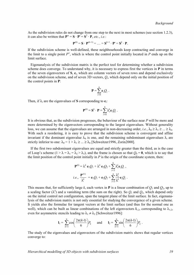
Background
Hierarchical modelling of 3D objects with subdivision surfaces 19
As the subdivision rules do not change from one step to the next in most schemes (see section 1.2.3), it can also be written that P" = S · P' = S2 · P, etc., i.e.:
P(k) = S · P(k−1) = … = Sk−1 · P' = Sk · P.
If the subdivision scheme is well-defined, these neighbourhoods keep contracting and converge in the limit to a single point P∞, which is where the control point initially located in P ends up on the limit surface.
Eigenanalysis of the subdivision matrix is the perfect tool for determining whether a subdivision scheme does converge. To understand why, it is necessary to express first the vertices in P in terms of the seven eigenvectors of S, ei, which are column vectors of seven rows and depend exclusively on the subdivision scheme, and of seven 3D vectors, Qi, which depend only on the initial position of the control points in P:
P =∑=
6
0iiiQe .
Then, if λi are the eigenvalues of S corresponding to ei:
P(k) = Sk · P =∑=
λ6
0iii
ki Qe .
It is obvious that, as the subdivision progresses, the behaviour of the surface near P will be more and more determined by the eigenvectors corresponding to the largest eigenvalues. Without generality loss, we can assume that the eigenvalues are arranged in non-decreasing order, i.e., λ0 ≥ λ1 ≥ ... ≥ λ6. With such a reordering, it is easy to prove that the subdivision scheme is convergent and affine invariant if the dominant eigenvalue λ0 is one, and the remaining subdominant eigenvalues λi are strictly inferior to one: λ0 = 1 > λ1 ≥ ... ≥ λ6 [Schweitzer1996, Zorin2000].
If the first two subdominant eigenvalues are equal and strictly greater than the third, as is the case of Loop’s scheme (1 > λ = λ1 = λ2 > λ3), and the frame is chosen so that Q0 = 0, which is to say that the limit position of the control point initially in P is the origin of the coordinate system, then:
P(k) = λk e1Q1 + λk e2Q2 +∑=
λ6
3iii
ki Qe ,
i.e., k
k
λ
)(P = e1Q1 + e2Q2 +∑= λ
λ6
3iiik
ki Qe .
This means that, for sufficiently large k, each vertex in P is a linear combination of Q1 and Q2, up to a scaling factor (λk) and a vanishing term (the sum on the right). So Q1 and Q2, which depend only on the initial control net configuration, span the tangent plane of the limit surface. In fact, eigenana-lysis of the subdivision matrix is not only essential for studying the convergence of a given scheme. It yields also the formulae for tangent vectors at the limit surface (and thus for the normal one as well), which can be built as linear combinations of the left eigenvectors l1,2, corresponding to λ1,2, even for asymmetric stencils leading to λ1 ≠ λ2 [Schweitzer1996]:
l1 = ∑=
6
1 6)1(π2cos
kkPk- and l2 = ∑
=
6
1 6)1(π2sin
kkPk- .
The study of the eigenvalues and eigenvectors of the subdivision matrix shows that regular vertices converge to:

Background
20 Hierarchical modelling of 3D objects with subdivision surfaces
P∞ = 21 P +
121 (P1 + P2 + P3 + P4 + P5 + P6),
which is of course the same value yielded by the closed form expression given before. Compare it with the effect that a single iteration of Loop’s scheme would have and remark that those two equa-tions can be rewritten so they differ only very slightly, if all vectors are now expressed relative to P:
P'−P = 161 (P1−P + P2−P + P3−P + P4−P + P5−P + P6−P) = ( )∑
=−
6
1161
kk PP ;
P∞−P = 121 (P1−P + P2−P + P3−P + P4−P + P5−P + P6−P) = ( )∑
=−
6
1121
kk PP .
The fact that any control point is always moved towards the barycentre of its neighbour vertices set, which is the obvious qualitative interpretation of the expressions above, is hardly surprising, given the symmetry of the stencils. The quantitative information they contain is that the repeated move-ment of P towards that barycentre in steps of 1/16 tends to a final displacement of 1/12 in the limit.
ANALYSIS AT EXTRAORDINARY VERTICES
In the vicinity of non-regular control vertices with valence K ≠ 6, an approach based on local subdi-vision matrices is equally valid. If the same weight β is assigned in the blend to the position of each of the K neighbours of the extraordinary vertex and P is defined as above, except for being a column vector with (1+K) rows now, then:
P' =
ββββ−
�������
�
K
K1 · P,
and the matrix form expression is exactly the same, although S is a (1+K)×(1+K) matrix now. If
Loop’s rule for β is chosen (β =
+−2π2cos
41
83
851
KK), the eigenanalysis of S shows that ex-
traordinary vertices converge in the limit to:
P∞ =
χχχχ−
NNMNNLK
h
K
K1 · P, with χ = 1
83
−
+
βK .
As before, it can be written:
P'−P = β ( )∑=
−K
kk PP
1 and P∞−P = χ ( )∑
=−
K
kk PP
1,
only now this is true for any valence of the central vertex (note that, for K = 6, β = 1/16 and χ = 1/12, as expected).
And, as before, there exist also formulae for tangent vectors at the limit surface, based on the left eigenvectors l1,2 corresponding to the two subdominant eigenvalues, λ1,2 [Schweitzer1996]:
l1 = ∑=
K
kkP
Kk-
1
)1(π2cos and l2 = ∑=
K
kkP
Kk-
1
)1(π2sin .
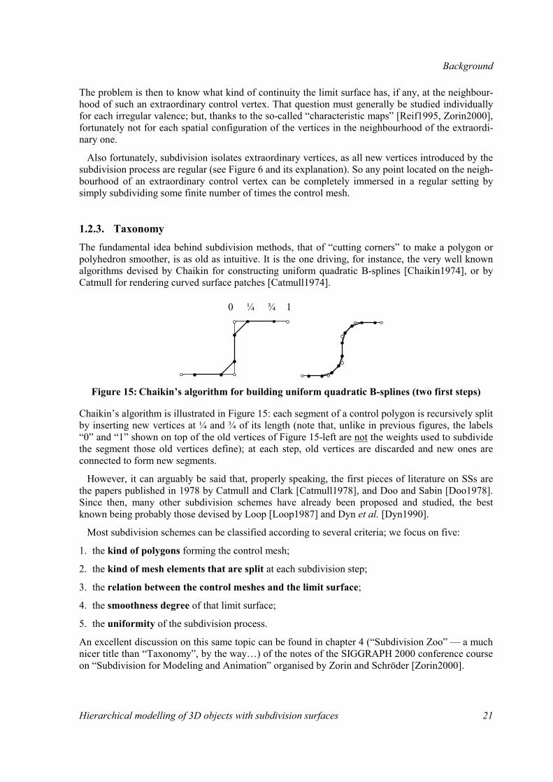
Background
Hierarchical modelling of 3D objects with subdivision surfaces 21
The problem is then to know what kind of continuity the limit surface has, if any, at the neighbour-hood of such an extraordinary control vertex. That question must generally be studied individually for each irregular valence; but, thanks to the so-called “characteristic maps” [Reif1995, Zorin2000], fortunately not for each spatial configuration of the vertices in the neighbourhood of the extraordi-nary one.
Also fortunately, subdivision isolates extraordinary vertices, as all new vertices introduced by the subdivision process are regular (see Figure 6 and its explanation). So any point located on the neigh-bourhood of an extraordinary control vertex can be completely immersed in a regular setting by simply subdividing some finite number of times the control mesh.
1.2.3. Taxonomy The fundamental idea behind subdivision methods, that of “cutting corners” to make a polygon or polyhedron smoother, is as old as intuitive. It is the one driving, for instance, the very well known algorithms devised by Chaikin for constructing uniform quadratic B-splines [Chaikin1974], or by Catmull for rendering curved surface patches [Catmull1974].
Figure 15: Chaikin’s algorithm for building uniform quadratic B-splines (two first steps)
Chaikin’s algorithm is illustrated in Figure 15: each segment of a control polygon is recursively split by inserting new vertices at ¼ and ¾ of its length (note that, unlike in previous figures, the labels “0” and “1” shown on top of the old vertices of Figure 15-left are not the weights used to subdivide the segment those old vertices define); at each step, old vertices are discarded and new ones are connected to form new segments.
However, it can arguably be said that, properly speaking, the first pieces of literature on SSs are the papers published in 1978 by Catmull and Clark [Catmull1978], and Doo and Sabin [Doo1978]. Since then, many other subdivision schemes have already been proposed and studied, the best known being probably those devised by Loop [Loop1987] and Dyn et al. [Dyn1990].
Most subdivision schemes can be classified according to several criteria; we focus on five:
1. the kind of polygons forming the control mesh;
2. the kind of mesh elements that are split at each subdivision step;
3. the relation between the control meshes and the limit surface;
4. the smoothness degree of that limit surface;
5. the uniformity of the subdivision process.
An excellent discussion on this same topic can be found in chapter 4 (“Subdivision Zoo” — a much nicer title than “Taxonomy”, by the way…) of the notes of the SIGGRAPH 2000 conference course on “Subdivision for Modeling and Animation” organised by Zorin and Schröder [Zorin2000].
0 1 ¼ ¾

Background
22 Hierarchical modelling of 3D objects with subdivision surfaces
TRIANGULAR VS. QUADRILATERAL
Perhaps the most obvious difference between subdivision schemes is based on the kind of polygons forming the control meshes, the only ones used in practice being triangles and quadrilaterals.
Consider first the abstract graph of the mesh and, more specifically, consider the topologically regular setting, to understand that only polygons that can periodically tessellate the plane are valid candidates (see Figure 4). But, of the polygons that can periodically tile the plane, only the ones that can be tessellated themselves in a self-similar, nesting fashion may be used for the recursive subdivi-sion process.
Figure 16: A periodic tiling of the plane not usable for subdivision purposes
And, of those, only convex ones: Figure 16 shows that L-shaped hexagons can indeed tile the plane and be subdivided in a nesting fashion, but we believe that they are not suitable for subdivision. All these restrictions limit the choice to triangles, parallelograms and convex hexagons. The latter can-not be subdivided self-similarly by splitting their edges, but could be used for dual subdivision schemes, as explained in the next section. However, only triangles and parallelograms are used in practice, as a matter of fact.
Consider now the control mesh living in 3D space. The term “quadrilaterals”, instead of “paral-lelograms”, must be used for the four-sided ones, because the facets of the abstract graph need not remain parallelograms when mapped onto the 3D shape — in fact, their vertices need not even remain coplanar! With triangles, this subtlety is not necessary, of course…
Flat triangle meshes seem to be increasingly more extended than any other kind of meshes, and most simplification methods work on and produce triangular meshes. Since it is the kind of polygons forming the base mesh which determine what kind of schemes may be applied to it, the latter could be a reason to prefer triangular schemes over quadrilateral ones. Nevertheless, those two kinds of schemes are, a priori, equally appropriate for the hierarchical modelling of 3D objects.
Among the classical subdivision schemes, the butterfly and Loop’s schemes operate on triangular meshes, whereas Catmull-Clark’s and Doo-Sabin’s schemes are defined for quadrilateral meshes. However, arbitrary polygonal meshes can be easily turned into quadrilateral ones [Catmull1978].
PRIMAL VS. DUAL
Not all subdivision schemes split the facets of the mesh: there exist also schemes which split its vertices. The former, however, are the most natural and most commonly used, which is why they are called primal, the latter being named dual. This classification is equally valid for subdivision schemes for curves, like the ones illustrated in Figure 7 (four-point) and Figure 15 (Chaikin’s), that are respectively primal and dual.
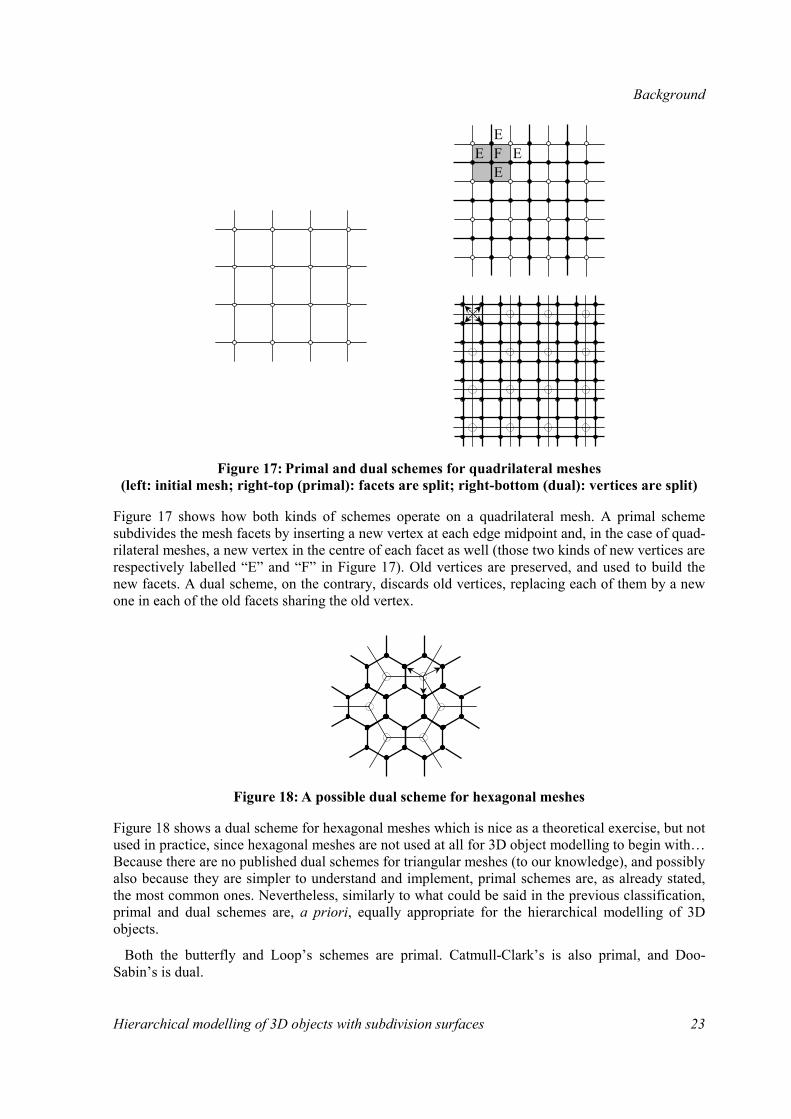
Background
Hierarchical modelling of 3D objects with subdivision surfaces 23
Figure 17: Primal and dual schemes for quadrilateral meshes (left: initial mesh; right-top (primal): facets are split; right-bottom (dual): vertices are split)
Figure 17 shows how both kinds of schemes operate on a quadrilateral mesh. A primal scheme subdivides the mesh facets by inserting a new vertex at each edge midpoint and, in the case of quad-rilateral meshes, a new vertex in the centre of each facet as well (those two kinds of new vertices are respectively labelled “E” and “F” in Figure 17). Old vertices are preserved, and used to build the new facets. A dual scheme, on the contrary, discards old vertices, replacing each of them by a new one in each of the old facets sharing the old vertex.
Figure 18: A possible dual scheme for hexagonal meshes
Figure 18 shows a dual scheme for hexagonal meshes which is nice as a theoretical exercise, but not used in practice, since hexagonal meshes are not used at all for 3D object modelling to begin with… Because there are no published dual schemes for triangular meshes (to our knowledge), and possibly also because they are simpler to understand and implement, primal schemes are, as already stated, the most common ones. Nevertheless, similarly to what could be said in the previous classification, primal and dual schemes are, a priori, equally appropriate for the hierarchical modelling of 3D objects.
Both the butterfly and Loop’s schemes are primal. Catmull-Clark’s is also primal, and Doo-Sabin’s is dual.
EE
EE F
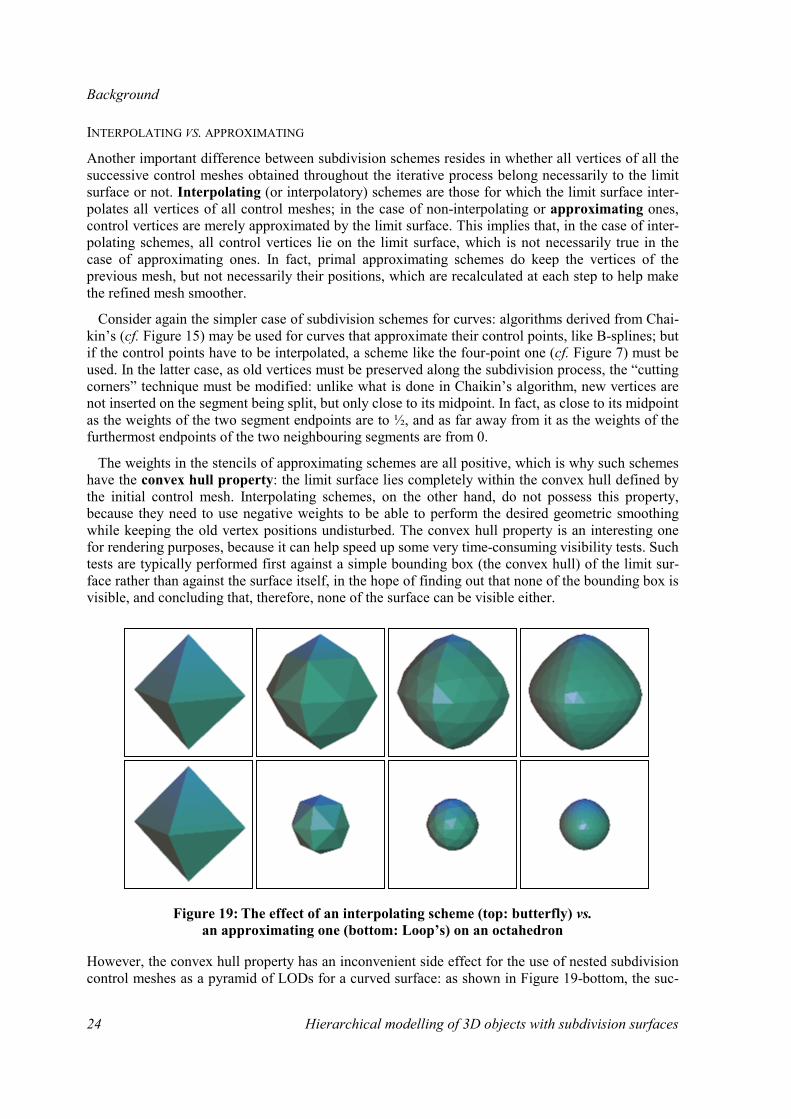
Background
24 Hierarchical modelling of 3D objects with subdivision surfaces
INTERPOLATING VS. APPROXIMATING
Another important difference between subdivision schemes resides in whether all vertices of all the successive control meshes obtained throughout the iterative process belong necessarily to the limit surface or not. Interpolating (or interpolatory) schemes are those for which the limit surface inter-polates all vertices of all control meshes; in the case of non-interpolating or approximating ones, control vertices are merely approximated by the limit surface. This implies that, in the case of inter-polating schemes, all control vertices lie on the limit surface, which is not necessarily true in the case of approximating ones. In fact, primal approximating schemes do keep the vertices of the previous mesh, but not necessarily their positions, which are recalculated at each step to help make the refined mesh smoother.
Consider again the simpler case of subdivision schemes for curves: algorithms derived from Chai-kin’s (cf. Figure 15) may be used for curves that approximate their control points, like B-splines; but if the control points have to be interpolated, a scheme like the four-point one (cf. Figure 7) must be used. In the latter case, as old vertices must be preserved along the subdivision process, the “cutting corners” technique must be modified: unlike what is done in Chaikin’s algorithm, new vertices are not inserted on the segment being split, but only close to its midpoint. In fact, as close to its midpoint as the weights of the two segment endpoints are to ½, and as far away from it as the weights of the furthermost endpoints of the two neighbouring segments are from 0.
The weights in the stencils of approximating schemes are all positive, which is why such schemes have the convex hull property: the limit surface lies completely within the convex hull defined by the initial control mesh. Interpolating schemes, on the other hand, do not possess this property, because they need to use negative weights to be able to perform the desired geometric smoothing while keeping the old vertex positions undisturbed. The convex hull property is an interesting one for rendering purposes, because it can help speed up some very time-consuming visibility tests. Such tests are typically performed first against a simple bounding box (the convex hull) of the limit sur-face rather than against the surface itself, in the hope of finding out that none of the bounding box is visible, and concluding that, therefore, none of the surface can be visible either.
Figure 19: The effect of an interpolating scheme (top: butterfly) vs. an approximating one (bottom: Loop’s) on an octahedron
However, the convex hull property has an inconvenient side effect for the use of nested subdivision control meshes as a pyramid of LODs for a curved surface: as shown in Figure 19-bottom, the suc-

Background
Hierarchical modelling of 3D objects with subdivision surfaces 25
cessive control meshes yielded by an approximating scheme like Loop’s are smaller and smaller. A “non-shrinking” smoothing filter such as Taubin’s [Taubin1995] can be used, but then the convex hull property is not verified — one cannot have everything! In this respect, although both interpolat-ing and approximating schemes could a priori be useful for the purposes of hierarchical modelling of 3D objects, interpolating ones seem a better choice, as they guarantee non-shrinking LODs.
Regarding implementation and computational complexity, interpolating schemes are in principle simpler and faster, since only rules for splitting edges are needed, whereas in the case of approximat-ing schemes, rules for repositioning old vertices must also be specified. But a deeper analysis shows that more things have to be considered: the number of old vertices needed to split an edge, for in-stance, is eight in the butterfly scheme (cf. Figure 8), as opposed to only four in Loop’s (cf. Figure 9-right). This increases not only the number of arithmetic operations needed to calculate the average position, but also, and perhaps more importantly, the complexity of the search for the neighbour vertices in the data structures holding the control mesh.
Another marginal advantage of interpolating schemes, derived from the fact that old vertices are never repositioned, is that they can handle meshes with non-manifold vertices.
Of the four classic subdivision schemes mentioned above, the butterfly scheme is interpolating, whereas Loop’s, Catmull-Clark’s and Doo-Sabin’s schemes are approximating.
SMOOTHNESS OF THE LIMIT SURFACE
Tangent plane continuity is normally enough to produce visually pleasing results, so it is not crucial to have limit surfaces with a continuity degree higher than one, at least from the rendering view-point. The reason why having smooth limit surfaces may be good for hierarchical 3D object model-ling purposes is the following. As it will be explained in detail in the next chapter, the technique we propose is based on regarding a subdivision scheme as a predictor: starting with a base mesh ex-tracted from a given surface, the chosen subdivision scheme yields a limit surface considered to be a prediction of the original one. In fact, each new vertex introduced at each step of the subdivision process is also regarded as a prediction, and the difference between the position where the scheme places it and the one it should have (in order to have the limit surface fit best the original one) is regarded as a prediction error. Our technique for hierarchical 3D object modelling works most efficiently if those prediction errors are kept small, as they are indeed if the subdivision rules place the new vertices close to the original surface. But the main purpose of the subdivision process is precisely the geometric refinement, i.e., the smoothing, of the base mesh. So our technique works best when that original, given surface is smooth, its specific continuity degree being in fact much less important than its having any.
The butterfly and Doo-Sabin’s schemes achieve C1-continuity in the regular setting, while Loop’s and Catmull-Clark’s are C2.
UNIFORMITY OF THE SUBDIVISION PROCESS
Yet another difference between subdivision schemes derives from the uniformity of the process, which, to begin with, can be systematic or adaptive. Up to here, we have only considered system-atic subdivision: at each step, all elements (faces or vertices) of the mesh are split. But there are situations in which this may make no sense, because there is little to gain by performing geometric refinement on mesh regions that are already smooth enough, and there is a lot to lose by multiplying (typically by four) its number of elements, as this has a direct impact on the processing and storage requirements of any practical application.

Background
26 Hierarchical modelling of 3D objects with subdivision surfaces
Figure 20: Flag with heterogeneous curvature (left: initial mesh; centre and right: systematic and adaptive subdivision yielding around 3000 triangles each)
Figure 20 shows a snapshot of a waving flag. The mesh on the left is the output of a FEM (Finite Element Method [Hughes1987]) program that simulates the effect that the air flow has on the flag. To do it, for each instant of the simulation, it meshes the flag with triangles and then calculates the pressure at each vertex to predict how it would move. The pressure at all other points is found by interpolation, so it is essential that the triangles be small, especially in those regions of the mesh where there are important variations of the pressure, i.e., in those areas where the curvature of the flag is high. In this sense, a mesh like the one on the right (created by subdividing more the triangles with less coplanar neighbours) could be much preferred to the one in the centre (created by system-atically subdividing twice the initial triangles), even if both meshes have approximately the same number of facets. Note, however, that both rendering applications and FEM analysis programs need that their input meshes be conforming, and that the one on the right is not, because some triangles have been subdivided while their neighbours have not. Luckily, this problem can be easily solved, as explained in section 2.4.7.
Even when the subdivision process is applied systematically to all elements of a mesh, it may be useful to have its coefficient stencils be adaptive. According to the terminology used by Guskov et al. [Guskov1999]:
• uniform schemes are those for which fixed weight masks are applied everywhere;
• semi-uniform schemes are those for which coefficients depend only on the local connectivity of the mesh;
• the coefficients, and possibly also the shape and size of the stencils of non-uniform schemes depend on the local connectivity and geometry of the mesh.
As these authors point out, uniform schemes can be used only over perfectly regular meshes, and semi-uniform ones are typically used on semi-regular meshes, which are those formed by subdivid-ing regularly a coarse, possibly irregular mesh. The latter is the most common case in practical applications, although a few non-uniform schemes have been described as well [Sederberg1998, Guskov1999].
Subdivision schemes could be also classified according to yet another kind of uniformity, which is orthogonal to the two already described, and which depends on whether the stencils and coefficients remain fixed or not as the subdivision process goes. Practically all known schemes are stationary, as the tools for studying the limit surface smoothness —and its very existence!— require it.

Background
Hierarchical modelling of 3D objects with subdivision surfaces 27
SUMMARY: CLASSIFICATION OF MAJOR SUBDIVISION SCHEMES
Scheme Triangles/Quads. Primal/Dual Approx./Interp. Smoothness
Butterfly T P I C1
Loop’s T P A C2
Catmull-Clark’s Q P A C2
Doo-Sabin’s Q D A C1
Table 1: Classification of major subdivision schemes
Table 1 summarises our classification of the four major subdivision schemes. Ck-continuity must be understood in the terms explained above, that is, k being the number of times that some local param-eterisation of the surface is differentiable at any regular vertex of any control mesh. Regarding uniformity, all schemes are considered to be systematic, semi-uniform and stationary, and designed to be applied to semi-regular meshes.
Since triangular meshes are the de facto standard in our context, as explained above, we discard studying further Catmull-Clark’s and Doo-Sabin’s schemes and will not refer to them again. Be-sides, as it has already be mentioned as well, we believe that the potential benefits of interpolating schemes vs. approximating ones are (arguably) more interesting than the extra degree of continuity that Loop’s scheme has to offer. This is why we choose to focus our study in the butterfly scheme, although most of the techniques and algorithms we have devised will also work with minor modifi-cations for Loop’s scheme.
1.2.4. A detailed example: the butterfly scheme revisited
DYN’S (ORIGINAL) BUTTERFLY SCHEME
The original butterfly scheme was devised in 1990 by Dyn et al. as an extension for surfaces of their own four-point subdivision scheme for curves. It is interpolating and able to reproduce cubic poly-nomials and, with w = 1/16 (see Figure 8 for the general case), it yields C1-continuous limit surfaces in the topologically regular setting [Dyn1990].
Figure 21: Stencils of the most common butterfly subdivision scheme (left: for normal interior edges; right: for crease and boundary edges)
1/81/8
½
½
−1/16−1/16
−1/16−1/16
−1/16 −1/16 9/16 9/16

Background
28 Hierarchical modelling of 3D objects with subdivision surfaces
Figure 21 shows the weights that must be assigned to the positions of the old vertices (circles) to calculate the position of the new vertex (dot) that will be the image of the highlighted edge midpoint, according to the most commonly used version of the butterfly scheme.
Figure 22: Gradual smoothing achieved by the butterfly subdivision scheme (two first steps)
Figure 22 shows the smoothing effect achieved by recursively and systematically subdividing the facets of a meshed chess queen according to the butterfly scheme, in just two steps. As it is easy to guess, the abstract graph of the original 3D mesh was a regular rectangular grid, except at its very top and bottom, where eight triangles closed each “pole” of the queen. The butterfly scheme operates on triangular meshes, so the original quadrilaterals had to be triangulated. But this can always be done very easily in such a way that all resulting vertices have exactly six neighbours each, in the particular case of rectangular grids, as illustrated by Figure 23. In other words, a rectangular grid can be easily triangulated and fed into a butterfly subdivider, which will produce a C1-continuous limit surface.
Figure 23: Regular triangulation of a rectangular grid
ZORIN’S MODIFIED BUTTERFLY SCHEME
Zorin explained in his Ph.D. dissertation [Zorin1997a] that, at extraordinary vertices with valences other than four, five and seven (i.e., at vertices with three or eight or more neighbours), the limit surfaces produced by the original butterfly scheme exhibit tangent plane discontinuities.

Background
Hierarchical modelling of 3D objects with subdivision surfaces 29
Figure 24: Incomplete smoothing of a tetrahedron by the original butterfly scheme
Figure 24 shows the effect of subdividing a tetrahedron with the original butterfly scheme. At the first subdivision step, the butterfly stencil (six triangles, 13 edges, eight vertices) has to be wrapped around the tetrahedron (four triangles, six edges, four vertices), so many stencil vertices correspond in fact to the same tetrahedron vertices. That is why the surface is not smoothed at all at the first step, which is merely a midpoint subdivision one. Nevertheless, the following four subdivision steps do refine also the geometry of the tetrahedron, which is somewhat smoothed, except at the initial vertices, where there is no tangent plane continuity whatsoever, because they have valence three.
To solve this problem, Zorin also proposed, together with Schröder and Sweldens, a modified but-terfly scheme to avoid those discontinuities, which works as follows [Zorin1996]:
• To subdivide edges connecting two regular vertices, it uses the original butterfly stencil.
• To subdivide edges connecting a regular vertex and an extraordinary one of valence K ≠ 6, it numbers those K neighbours from 0 (the regular vertex of the edge being subdivided) to K−1 by visiting them cyclically (in either a clockwise or anti-clockwise fashion: the order is immaterial due to the symmetry in the formulae below), and assigns them the following weights:
� K = 3: s0 = 5/12; s1,2 = −1/12;
� K = 4: s0 = 3/8; s1,3 = 0; s2 = −1/8;
� K ≥ 5: sk =
++41π4cos
21π2cos1
Kk
Kk
K, 0 ≤ k ≤ K−1.
• To subdivide edges connecting two extraordinary vertices, it takes the average of the values computed using the appropriate scheme of the previous paragraph for each endpoint.
• To subdivide edges that lie on an open mesh boundary, it uses the four-point rule.
Background
30 Hierarchical modelling of 3D objects with subdivision surfaces
• To subdivide edges that are incident to a boundary, it replaces the vertices missing in the original eight-point butterfly stencil with virtual ones constructed by reflecting existing interior ones across the boundary (see also [Zorin2000]).
The surfaces built according to this scheme do possess C1-continuity even at extraordinary vertices with three or strictly more than seven neighbours.
1.2.5. Summary of advantages of subdivision surfaces
ADVANTAGES OVER POLYGONS: COMPACTNESS
When a complex, smooth shape has to be closely approximated with a planar mesh, its number of polygons can grow boundless. It can easily reach the hundreds of thousands, thus turning the mesh pretty much useless in most systems, where its sheer size is completely unmanageable for storage and editing. On top of that, in the case of editing, a cruel and artificial need is imposed on the model-ler for moving one after another tons of semantically unrelated vertices, when it would be much easier and more natural to displace a few control points and have them drag some set of surrounding vertices.
SSs, like [NUR]BSs and other traditional patches, follow this latter approach. A small set of con-trol points define an initial, coarse mesh, which is recursively refined by a well known (and usually fixed) set of rules, so complex shapes are described with substantially less data. Furthermore, by modifying the positions of the initial control vertices, entire portions of the limit surface follow the edited vertices. In fact, since any mesh is the control one for the subsequent refinement levels, what has been just said for the initial control points is also true for any of the intermediate ones that keep appearing as the subdivision process goes.
ADVANTAGES OVER PATCHES: ARBITRARY MESH CONNECTIVITY
SSs are like patches in more than one way. In fact, some subdivision schemes generalise NURBS-based knot insertion algorithms [Warren1995, Schweitzer1996], and all of the commonly used ones are locally defined and have finite support. Regarding implementation issues, they also possess the numerical stability and code simplicity and efficiency of traditional patch families. Probably this is even more true in the case of subdivision schemes, because practical implementations of NURBSs must incorporate patch-stitching and curve-trimming algorithms which are hardly simple or efficient —or error-free!— for dealing with boundaries and sharp features like cusps, corners, creases, etc. SSs, on the other hand, are inherently as smooth as NURBSs but also easily extended to model objects with boundaries and sharp features [Schweitzer1996, Zorin2000].
But SSs have an obvious key advantage over patches: a SS initial control mesh can have any con-nectivity, whereas patch control meshes must be regular everywhere, and thus inherently define surfaces topologically equivalent to the plane. To model non-planar surfaces with patches, complex patch/curve-trimming mechanisms must be used. On the contrary, the vertices of a SS initial control mesh may have any valence. Therefore, the connectivity of the control mesh they define is arbitrary (except for the limitation of having to be manifold, which also affects NURBS), and so is the topol-ogy of the corresponding limit surface, which can be homeomorphic to the sphere, the torus, etc.
ADVANTAGES OVER BOTH: HARMONISATION AND TRULY HIERARCHICAL REPRESENTATION
Subdivision schemes harmonise the two ends of a spectrum represented by polygons and patches. Based on an initial control mesh, which can be described with a small amount of data, they allow to
Background
Hierarchical modelling of 3D objects with subdivision surfaces 31
derive a smooth limit surface by means of simple, efficient rules for recursively refining both the topology and the geometry of the planar mesh. The same concept of “control points” of patch-based modelling is inherent to SSs, which have nevertheless the versatility to model high frequency detail with little effort.
This ability to model and edit a surface at different LODs is precisely the most powerful feature of SSs, as it means having multiresolution handles for 3D object modelling and animation. In fact, the different LODs created by any subdivision scheme are hierarchically nested and form a pyramid of finer and finer approximations to the smooth limit surface, unlike what happens with other multi-resolution modelling schemes such as Hoppe’s progressive meshes [Hoppe1996]. This comes from the fact that subdivision is a recursive process and thus produces a truly hierarchical representation of the surface under approximation.
1.3. Automatic LOD extraction
1.3.0. Motivation The idea of having several meshes approximate a single 3D object is not new: 25 years ago, Clark already suggested that simpler versions of complex objects be used for those with lesser visual importance in a synthetic scene [Clark1976]. But it is essentially in the last decade that a lot of attention has been paid, both in the fields of academic research and commercial applications, to the problem of describing 3D objects with different LODs. The interest of having several planar meshes to choose from, for a given complex 3D object, is manifold… ;-)
• If rendering quality considerations are taken into account, an object located far away from the camera will be projected onto a few pixels on the screen, no matter which of its LODs is used. In fact, objects with “lesser visual importance” are not necessarily those with a small screen size: in contexts other than that of static images, like animations or immersive virtual reality applications, a moving object can be rendered with less care than its static version without affecting signifi-cantly the perceived quality, and so can an object which lies on the observer’s peripheral field of view.
• But even if the object is of no lesser visual importance in any way, there might be good reasons to use a simple LOD of it, such as the impossibility of achieving otherwise some user-specified frame rate, because of CPU or memory limitations. Again, in (interactive) real-time applications, computing resources may easily be exhausted even by relatively simple scenes, and a need may appear of prioritising the objects according to a rendering quality classification.
• Finally, in any client-server scenario in which a complex object has to be transmitted over a limited bandwidth communication channel such as the Internet, it may be simply essential to have a collection of LODs. Especially if the LOD set is progressive, as it is then possible to transmit quickly a coarse version of the object, so that the user at the client side gets a first grasp of the object appearance, while refinements are streamed and incorporated gradually (and maybe seamlessly) to the rendered mesh.
The growing interest in automatic LOD extraction for scene complexity management has led to an impressive amount of research in the field of polygonal simplification, i.e., generation of coarser and coarser planar meshes approximating an initial input one with a bigger and bigger error. As any planar mesh can be reduced to a triangular one (see [Seidel1991, O’Rourke1994, Ronfard1994, Shewchuck1996]), most LOD extraction algorithms take directly triangular meshes as their input.

Background
32 Hierarchical modelling of 3D objects with subdivision surfaces
1.3.1. Error metrics We find it necessary to pay some attention to the error metrics used to measure the quality of a given LOD with respect to the mesh it supposedly approximates, as no classification of simplification techniques can be described or understood without having done so.
The first comparison of two approximations to a 3D surface should probably be based on topologi-cal considerations: is it licit to approximate a thick slice of Swiss cheese at some point with a brick by “filling the holes” (of the volume, i.e., by removing the handles of the surface), or must all its LODs have a high genus? Some simplification techniques try to always respect the original topology but, as what matters the most is usually the preservation of global appearance, other techniques do not insist on respecting it exactly, especially when used to achieve drastic reductions of the initial triangle count.
Independently of whether topology is preserved or simplified, it is clear that some precise notion of distance must be established in order to compare 3D meshes. Some studies have been carried that consider subjective distances (e.g., viewpoint-dependent) or sophisticated objective ones (e.g., based on texture deviation metrics for meshes with attributes [Cohen1998, Cignoni1998a]). Nevertheless we believe that, for our purposes, it suffices to use simple objective distances based on geometric norms — besides, their being conceptually simple does unfortunately not mean that they can always be efficiently evaluated…
Figure 25: Point to vertex (dpv), plane (dpp) and surface (dps) distances
The point to vertex distance is based on the usual, Euclidean distance between two points (of a 3D space, in our case). It is the simplest of the distances described here and can be efficiently evaluated, but only makes sense for simplification techniques based on vertex clustering, such as the ones explained below. In Figure 25, it is shown as dpv = ||V − P|| (the corresponding oriented vector being dpv = V − P), where V is a vertex of a mesh, unlike P, a point which need not belong to the mesh or lie on its surface S.
The point to plane distance is also the common one: in Figure 25, it is dpp = ||dpp|| = ||P⊥ − P||, where P⊥ is the orthogonal projection of P onto the plane of interest (in this case, the one supporting the highlighted triangle). It can also be rather efficiently implemented thanks to tips and numerical recipes like the ones found in the “Graphics Gems” series [Gems1990, Gems1991, Gems1992, etc.], and is used directly in [Ronfard1996] and, more importantly, in [Garland1997].
Other simplification techniques, notably those by Hoppe [Hoppe1993, Hoppe1996], do not use the point to plane distance as such, but rather the point to surface distance, shown in Figure 25 as dps = ||dps|| = ||PS − P||, where PS is the closest point to P on S. More formally:
P
P⊥
PS
V
S
dppdpv
dps

Background
Hierarchical modelling of 3D objects with subdivision surfaces 33
dps = d (P, S) = SQ∈
min (||P − Q||).
The point to surface distance can be much more expensive to evaluate than the point to plane one, no matter what numerical shortcuts are used. The reason is that it requires to find, for all (or at least several) triangles of the mesh, the (3D) orthogonal projection P⊥ of the point P onto their supporting plane first, and then, if P⊥ does not lie within the triangle, a new (2D) projection PS of P⊥ onto some edge of the triangle. Note that the latter projection need not be an orthogonal one, if PS is one of the vertices of the triangle.
However, it is with surface to surface distances, which are the truly adequate ones for measuring appearance preservation, that things start getting desperately involved — this is a typical situation in which the simplicity and elegance of the mathematical expression of a concept are only surpassed by the “pain-in-the-neck-ness” of its computational implementation… Besides, numerical evaluations of surface to surface distances can only yield a posteriori results: the approximation error introduced by a simplification can only be evaluated after the fact.
Different authors have defined and used in their polygonal decimation techniques slightly different surface to surface distances. This is the case of Guéziec’s “tolerance volumes” [Guéziec1995] and of the “simplification envelopes” by Cohen et al. [Cohen1996]. But we understand by surface to sur-face distances the ones based on the Lp norms, which are usually defined for functional spaces, but can be expressed in terms of the point to surface distance as follows:
Lp (S1, S2) = max (lp (S1, S2), lp (S2, S1)), where lp (A, B) = p
Aa
p daBaA ∫
∈
)),((d)(area
1
(n.b.: area (A) is the area of A, and da is the corresponding differential).
In the limit (p → ∞), this becomes Hausdorff’s distance between surfaces S1 and S2:
L∞ (S1, S2) = H (S1, S2) = max (h (S1, S2), h (S2, S1)), where h (A, B) = Aa∈
max (d (a, B)).
The definitions are made in two steps because h (S1, S2), usually called “Hausdorff’s oriented dis-tance” from S1 to S2, is no symmetric function and therefore no proper distance, and the same can be said for lp (S1, S2): there exist surfaces for which lp (S1, S2) ≠ lp (S2, S1), hence the “symmetrisation” step of taking the maximum of both. Intuitively speaking, l1 (S1, S2) is the average “distance” from S1 to S2, l2 (S1, S2) the RMS (Root of Mean of Squares) one, etc.: as p increases, the points of S1 with the biggest contribution to the integral in lp (S1, S2) take an increasingly important role in the final result, so that peak values tend to predominate. In the limit, only the maximum contribution to the integral remains and the definition becomes that of Hausdorff’s oriented “distance”, which guaran-tees that every point of S1 is within h (S1, S2) of some point of S2 (and v.v. if the symmetric, true distance H (S1, S2) is used). In fact, precisely in order to filter out any exaggerated contributions of peak difference/error values over average ones, and to reflect best with an objective measure what is subjectively important in terms of overall shape appearance, the L2 norm is frequently used�.
The L1, L2 and L∞ surface to surface distances are implemented by means of uniform sampling and numerical integration in the Metro tool by Cignoni et al. [Cignoni1998]. As Metro’s binary code is publicly available, it is becoming a de facto standard for measuring the mentioned distances between two triangular meshes. The L1, L2 and L∞ distances reported by Metro are always relative, i.e., they are expressed as a percentage of the largest diagonal of the mesh bounding box.
� In other contexts, the reason why the L2 norm is frequently used is that it is differentiable.
Background
34 Hierarchical modelling of 3D objects with subdivision surfaces
1.3.2. Brief taxonomy We establish here a (by no means complete) classification of polygonal simplification techniques according to a couple of methodological criteria (whether they are static vs. dynamic, and global vs. local) and to the relationship existing among the different LODs they yield for a single 3D object. We introduce a few general concepts of mesh decimation and postpone a more detailed description of the techniques of interest in our context until section 3.1.0.
STATIC VS. DYNAMIC
Static simplification techniques are designed to work as a pre-processing step before storing (in archival applications) or publishing (in client-server scenarios) the 3D objects. This has been the traditional approach and is still commonly used: several fixed resolution LODs are created off-line for each object and then, at run-time, the most appropriate one is chosen.
Note that the LODs being predefined does not exclude adaptiveness. To begin with, the generation of the different LODs may be done adaptively in some sense, so that some parts of the considered object are approximated with a greater fidelity. This was already suggested, for instance, by Turk, who tried to detect and respect important features of the input surface, as indicated by maximal curvature regions [Turk1992]; by Guéziec, who also considered the possibility of having his toler-ance volumes be adaptive [Guéziec1995]; or by Cohen et al., whose simplification envelopes could fit more closely the surface under approximation in particularly intricate regions [Cohen1996]. Besides, there is certainly adaptiveness as well in the decision of which LOD must be used at run-time, which can be based on the screen coverage of the object, or the rendering capacity of the system, or the transmission bandwith of the channel, or some similar criterion.
Other benefits from the static simplification approach are that it uncouples the decimation and ren-dering processes, simplifying both (LOD creation need not address real-time rendering constraints and run-time rendering need only pick some LOD), and that it fits well current OpenGL-oriented graphics hardware (each LOD can be compiled into triangle strips and display lists, which can be rendered much faster than unorganised sets of triangles). However, static simplification methods are not well suited for some specific but important problems, such as terrain flyovers and display of massive� meshes, which are not infrequent in CAD applications and that have to be simplified drastically before rendering.
Dynamic simplification methods were designed to address such problems, but they are being used now in more and more general settings, especially since the apparition of Hoppe’s so-called “pro-gressive meshes” [Hoppe1996], described in sections 2.2.0 and 3.1.0. This approach consists in organising the data describing the collection of LODs for a given 3D object in such a way that any desired LOD may be extracted at run-time, which of course implies, from a programming point of view, designing data structures allowing it, like the ones by Luebke [Luebke1996].
The advantages of this approach are many, starting from the obvious improvement in flexibility and granularity, which also permit to have better fidelity approximations and smoother transitions among different LODs (see the description of “geomorphs” in section 2.2.0). Besides, dynamic simplification methods offer support for viewpoint-dependent refinement [Hoppe1997, Luebke1997, Xia1997]. “View-dependent LODs”, as they are called, can be seen as the ultimate step in dynamic simplification, which can be inter-object (objects of a scene are simplified more or less according to their relative visual importance) or even intra-object (the silhouette or curved regions of an individ-
� By current standards, a “massive” mesh is one with millions of triangles, a “large” one having tens to hun-dreds of thousands — this footnote will probably make people laugh already in 2003...

Background
Hierarchical modelling of 3D objects with subdivision surfaces 35
ual object are approximated better than its interior or flat regions). But perhaps even more impor-tantly, at least in the context of 3D object coding, dynamic LODs provide the best solution for progressive transmission of 3D meshes [Hoppe1996, Taubin1998a].
GLOBAL VS. LOCAL
Another aspect that differentiates simplification techniques with respect to their modus operandi is whether they consider the input mesh, and/or act upon it, globally or locally.
Global techniques do not retain, in general, any elements (vertices, edges or triangles) of the initial mesh. For instance, Turk’s re-tiling technique distributes new vertices at random on the surface of the original mesh and moves them to maximal curvature positions, then starts removing old vertices gradually so that the final output is a complete remesh built thanks to the new vertices [Turk1992]. Other techniques such as the already mentioned one by Cohen et al. [Cohen1996] do not even re-quire that their new vertices lie on the initial mesh surface, but allow them to lie within some offset of it instead.
Local techniques, on the other hand, base their decisions on geometric properties (curvature, edge length, etc.) of some small region of their input mesh, and alter it only partially, usually by applying to it some atomic operation designed to be iterated. The most common of such operations are the following:
• Vertex removal: a vertex is chosen as removable (for being too close to or too coplanar with its neighbours, for instance) and indeed removed from the mesh, and the resulting hole triangulated. This is a paradigmatic local and repeatable atomic operation used by several techniques, like the ones by Schroeder et al. [Schroeder1992], Li and Kuo [Li1998], and Lee et al. [Lee1998]. Its main caveat is that it can lead to bad aspect ratio triangles when iterated too much without care.
• Vertex clustering: a group of vertices located close to each other are merged into a single one, and the local mesh configuration updated accordingly. Rossignac and Borrel were the first, to our knowledge, to devise a method based on this approach [Rossignac1993], but the clearest example is probably that of Luebke’s “VDS (View-Dependent Simplification)” algorithm [Luebke1997]. VDS maintains a hierarchical vertex tree in which whole branches can “fold” (to have a vertex act as a proxy for a group of them) or unfold, and an active triangle list representing the current status of the mesh.
Figure 26: Edge collapse and half-edge collapse
• Edge collapse: an edge is chosen as discardable based on some local geometric criteria and its two endpoints are merged, which results in the mesh loosing two triangles, three edges and one vertex, in the general case. This mesh decimation operation, which is as paradigmatic as, and rather similar —but not equivalent!— to a vertex removal, is illustrated in Figure 26, which shows a portion of a mesh, consisting initially (Figure 26-centre) of eight triangles. When the
half-edge collapse
edge collapse

Background
36 Hierarchical modelling of 3D objects with subdivision surfaces
highlighted edge is collapsed, the resulting vertex is usually placed in some position along the old edge (Figure 26-left), which can be chosen optimally in some error-minimising sense, or stay in the same exact location as one of the old edge endpoints, and then the operation is called a half-edge collapse (Figure 26-right). The edge collapse is possibly the most common decimation op-eration [Hoppe1993, Hoppe1996, Ronfard1996].
• Vertex pair (a.k.a. virtual edge) collapse: exactly like a regular edge collapse, except that any pair of vertices can be merged, whether they form an edge or not. This implies that, unlike a true edge collapse, which in principle preserves the topology of the mesh being simplified, a virtual one can alter it to remove holes or handles. But this is seen more as an advantage than as a draw-back by many authors, notably Garland and Heckbert [Garland1997].
It is important to stress that the geometric criteria upon which local simplification techniques base their decisions could be, in principle, completely uncoupled from their atomic actions. For instance, the mesh simplification techniques by Hoppe and Garland, reviewed in some detail in section 3.1.0, perform both (virtual) edge collapses, but are based on different error metrics.
Figure 27: The edge swap local remeshing operation
Another noteworthy aspect regarding local mesh simplification techniques is that there exist local remeshing operations designed to be combined with some of the atomic decimation operations in order improve the resulting mesh quality — the aspect ratio of triangles, basically. In particular, vertex removals and (virtual) edge collapses are commonly followed by “edge swaps” like the one depicted in Figure 27. But, again, such remeshing operations are again independent from the mesh decimation operations themselves.
A special mention must be made to the multiresolution modelling and analysis techniques based on SSs, introduced in section 1.4.2 and described with more detail in section 3.1, which cannot be directly classified according to this criterion. The reason is that their way of extracting LODs from a given mesh relies on remeshing it to have the initial mesh follow a particular connectivity, instead of on following either a local or a global simplification approach. In fact, it could be argued that SS-based (remeshing and) LOD extraction techniques fall more into the global mesh simplification category, as they do not retain, in general, any elements of the initial mesh, which is what has been said above about global techniques. However, many of them use local polygonal simplification techniques for the generation of their base mesh.
RELATIONSHIP BETWEEN LODS
To close this taxonomy of mesh simplification techniques, we would like to pay some attention to the existing relationship between different LODs of a single 3D object, which can be simply none. Indeed, some simplification methods, especially global ones [Turk1992, Guéziec1995, Cohen1996], generate LODs corresponding to the same object that are independent from each other, even if it is possible to parameterise the approximation quality, or the target number of triangles of each LOD.
edge swap

Background
Hierarchical modelling of 3D objects with subdivision surfaces 37
This changed when Hoppe introduced the concept of progressive meshes [Hoppe1996] and, as a side effect, that of LOD continuum, an expression used to describe a collection of LODs with a very fine granularity, that is, in which any two consecutive LODs differ by only one or two triangles. Other researchers have built later upon this idea [Garland1997], but it is possible that a set of LODs be progressive without strictly forming a continuum: the only requirement is that LODs be incre-mentally expressed, with any granularity, so that one may go from the coarsest to the finest by traversing the whole collection. Section 2.1 describes other progressive LOD schemes which do not fall in the LOD continuum category [Taubin1998a, Li1998, Pajarola2000].
Finally, hierarchical LODs are the ones in which a pyramidal relationship of some kind exists between the elements (vertices, edges or triangles) of successive meshes. Of those, the ones based on SSs are of course the most interesting in the context of this dissertation, but other approaches have also been studied [DeFloriani1995, Barequet1996, Luebke1996, Luebke1997].
1.4. Wavelet-based multiresolution analysis
1.4.0. Introduction As already stated in the general introduction, the main idea behind MRA is to decompose a function or signal into a coarse, low resolution (i.e., frequency) part, plus a collection of finer and finer details only observable at increasing resolutions/frequencies. In the contexts of signal analysis, processing and transmission, sub-band decompositions of signals are of key relevance, because of their poten-tial benefits for practical applications. This is especially the case when there is a pyramidal nesting of the sub-bands forming a hierarchical multiresolution description.
Historically, MRA has been based on Fourier’s transform and, more recently, on the DCT, but in the last dozen of years or so, the interest of the research community has been captured by wavelets. The first and simplest wavelets were those devised by Haar nearly one century ago [Haar1910], but the finding of more general and well-behaved ones, and the coining of the term “wavelet” itself, had to wait until the 1980’s. The mathematical framework was provided by the so-called “French school”, from which Deslauriers and Dubuc introduced a process for interpolating data sampled at regularly spaced locations, e.g., at the integers, to obtain a smooth function defined on the entire real line [Deslauriers1987]. Daubechies published soon afterwards a method for building orthonormal, compactly supported wavelets [Daubechies1988]. In parallel, in the field of signal processing, wave-lets originated in the context of sub-band coding or, more precisely, in that of quadrature mirror filters. The connection between these two approaches was established by Mallat in “A theory for multiresolution signal decomposition: the wavelet representation” [Mallat1989]. Nowadays, wave-lets are also present in different subjects related to computer graphics, notably image compression and editing, global illumination, and hierarchical 3D object modelling.
An excellent introductory text on wavelets for computer graphics is the primer by Stollnitz and co-workers at the University of Washington [Stollnitz1994]. It begins presenting 1D and 2D Haar’s wavelet transforms with easy to follow examples, before proceeding with the mathematical frame-work and the matrix formulation needed to understand essential concepts of MRA as seen by Mallat, such as nested function spaces with orthogonal bases and the filter bank. It then explains how to extend that simplest MRA based on Haar’s wavelets in two directions: to have it handle functions defined in other topologies, more complex than the infinite real line or plane, and to analyse them with more sophisticated bases, such as the ones given by spline wavelets.

Background
38 Hierarchical modelling of 3D objects with subdivision surfaces
Another very enlightening material on the same subject is provided by the notes of the course “Wavelets in Computer Graphics” organised by Schröder and Sweldens for the SIGGRAPH 96 conference [Schröder1996]. Following their comprehensive understanding of the subject, we use the expressions “first vs. second generation wavelets” to refer to wavelets defined on trivial topologies (e.g., the infinite real line or plane) vs. those defined on more complex ones. Another key concept in their exposition is the lifting scheme invented by Sweldens [Sweldens1994], which enables to save computing resources for the calculation of the already extremely economic wavelet transforms. Even more importantly, and in the words of its author, “the main feature of the lifting scheme is that all constructions are derived in the spatial domain”. Not having to rely on Fourier’s analysis may or may not be seen as an advantage, depending on one’s mathematical background. But it is certainly beneficial to remain in the spatial domain when this leads, as in the case of the lifting scheme, to design wavelet constructions which can be generalised (more easily or at all) to non-trivial topolo-gies. This is why we will also try to avoid using concepts or nomenclature from the fields of tradi-tional sub-band coding or signal filtering in what follows.
1.4.1. First generation wavelets
HAAR’S TRANSFORM OF A DISCRETE SIGNAL
Consider first a 1D signal (e.g., an audio clip) sampled at 2n integer locations, with respective values sn,k: sn = {sn,k | 0 ≤ k < 2n}. Haar’s forward transform consists in taking the average (denoted as sn−1,k) and difference (dn−1,k) of every other pair of consecutive samples, sn,2k and sn,2k+1 (0 ≤ k < 2n−1):
sn−1,k = (sn,2k + sn,2k+1) / 2 and dn−1,k = sn,2k+1 − sn,2k.
In this way, two new sequences of 2n−1 elements are obtained from the original one: sn−1 represents a coarser resolution version of sn, and dn−1 contains the details needed to recover sn from sn−1 by apply-ing to each pair Haar’s inverse transform:
sn,2k = sn−1,k − dn−1,k / 2 and sn,2k+1 = sn−1,k + dn−1,k / 2.
Figure 28: Haar’s wavelet transforms (from left to right: forward; from right to left: inverse; n.b.: the number of elements of each sequence is indicated inside the parentheses)
This same operation can be repeated upon sn−1 to obtain sn−2 and dn−2 (each of which have 2n−2 ele-ments), and again upon sn−2 to obtain sn−3 and dn−3 (each of which have 2n−3 elements), …, until s0 and d0 (each of which have a single element) are obtained. Each step of the recursion yields a “twice coarser”, average-preserving version of the original signal, plus the detail(s) needed to go back to the previous resolution. This recursive procedure is illustrated in Figure 28, which can be interpreted from left to right (forward wavelet transform), with the arrows pointing as shown, or from right to left (inverse wavelet transform), with the arrows pointing the opposite way. The forward transform recursively splits sn (of 2n elements) into pair-wise averages and differences to produce (sj, dj) (of 2j elements each); the inverse transform recursively merges (sj, dj) starting from (s0, d0) to reconstruct sn in the end.
sn (2n) sn−1 (2n−1) sn−2 (2n−2) s2 (4) s1 (2) s0 (1) . . .
dn−1 (2n−1) dn−2 (2n−2) d1 (2) d0 (1)

Background
Hierarchical modelling of 3D objects with subdivision surfaces 39
Two very important computational features of wavelets in general (i.e., not only of Haar’s) that can be easily seen in the light of the above are:
• Memory efficiency: other than the single element of s0, namely s0,0, all that is needed to recover sn is the whole set of detail signals, dj (0 ≤ j < n), which have 2j elements each. Most interestingly, the “final cascaded” transform of sn, i.e., the set {s0,0, {dj,k | 0 ≤ j < n, 0 ≤ k < 2j}} formed by s0,0
and all dj,k, contains exactly as many elements as sn�, since 1 + ∑
−
=
1
02
n
j
j = 2n.
• Speed: thanks to its hierarchical structure, the whole wavelet transform can be computed in only O (N) operations (N = 2n). This has to be compared to the O (N2) cost a general linear transform would have, because of applying an N×N matrix to an N vector/sequence. When using techniques based on classic space/frequency transforms, the latter cost may come down to O (N log2 (N)) for the FFT (Fast Fourier’s Transform), but never to O (N).
Haar’s transform is easily generalised to process higher dimension signals. For instance, to act upon a discrete 2D signal (e.g., an image) represented by a 2n×2n matrix of samples, one can simply:
1. apply first Haar’s (1D) transform to each row of the matrix, to obtain a transformed row similar to the set described above, {s0,0, {dj,k | 0 ≤ j < n, 0 ≤ k < 2j}};
2. apply Haar’s (1D) transform to each column of the matrix containing those transformed rows.
This kind of wavelet transform or decomposition of a 2D signal is known as the “standard” one, as opposed to others which would alternate between operations on rows and columns (and obtain of course different results).
DESLAURIERS-DUBUC’S INTERPOLATING SUBDIVISION
Wavelets can also be built thanks to an interpolating subdivision mechanism first described by Deslauriers and Dubuc in 1987. This mechanism is based on the same idea that led Dyn et al. to design, also in 1987, their four-point scheme for interpolating an ordered set of 2D points with a smooth curve (see section 1.2.1). Consider again the case of a discrete 1D signal, but with a different goal in mind: suppose now that s0 = {s0,k = f (k) | k ∈ } is a sequence of regularly spaced samples from some unknown function f (the corresponding analog signal) which has to be reconstructed. Deslauriers and Dubuc proposed, as Dyn et al., to proceed by recursively subdividing the sampling intervals into two and inserting samples at all dyadic points, thus obtaining a sequence of sequences {sj | j ∈ }:
sj = {sj,k = f (xj,k) | k ∈ }, where xj,k = k 2−j.
The newly generated samples in sj+1 must be the result of some prediction based on old ones from sj, and the usual convention, when numbering the samples of sj+1, is to reserve the even indices for the samples taken from sj (sj+1,2k = sj,k), and to use the odd indices for predicted values (sj+1,2k+1).
The first predicted value that comes to mind is perhaps the average of its two neighbours:
sj+1,2k+1 = (sj+1,2k + sj+1,2k+2) / 2 = (sj,k + sj,k+1) / 2.
� However, it must be said, in all fairness, that more bits may be needed to represent the transformed data with the same accuracy as the original because, in principle, if a set of values can be encoded with B bits, their differences or averages will only fit in B+1 bits.
Background
40 Hierarchical modelling of 3D objects with subdivision surfaces
It is obvious that, if such a linear predictor is used, the function f obtained as the limit sequence s∞ is simply the piecewise linear interpolation of the initial set of samples. If a smoother function is desired, the obvious improvement consists in having sj+1,2k+1 depend on more of its neighbours, instead of on only two. For instance, one can take two neighbours on each side of sj+1,2k+1 in sj, let p be the unique cubic polynomial interpolating those four values (i.e., sj,k−1 = p (xj,k−1), sj,k = p (xj,k), sj,k+1 = p (xj,k+1), and sj,k+2 = p (xj,k+2)) and have the predicted value be sj+1,2k+1 = p (xj+1,2k+1). Deslauriers and Dubuc suggested to use, in general, 2n neighbours (n on each side), and thus a polynomial of degree 2n−1.
The connections between wavelets and subdivision should already start to be quite apparent: not surprisingly, the procedure described for n = 2 is equivalent to calculating the new value according to the four-point scheme described in section 1.2.1:
sj+1,2k+1 = −161 sj,k−1 +
169 sj,k +
169 sj,k+1 −
161 sj,k+2.
But in order to make these connections even more evident, and to define precisely what wavelets are, instead of using the term informally as we have done until now, some formalism is needed.
SCALING FUNCTIONS AND WAVELETS
MRA, as originally conceived by Mallat [Mallat1989], is based on three essential components:
1. An infinite sequence of nested vector spaces: {Vj | Vj ⊂ Vj+1 ∀ j ∈ }. The “vectors” of these spaces are in fact functions of “increasing resolution”. Strictly speaking, it is for this sequence of nested/scaled linear function spaces that the expression MRA should be reserved.
2. An inner product: <f, g> must be defined for any pair of functions f, g ∈ Vj (j ∈ ). The usual choice is the standard inner product, <f, g> = ∫ dxxgxf )()( . But what is important is that any choice of inner product implies a notion of orthogonality: two functions f and g are said to be or-thogonal if <f, g> = 0. And this in turn defines implicitly orthogonal complement function spaces, called wavelet spaces: Wj = Vj+1 \ Vj = {f ∈ Vj+1 | <f, g> = 0 ∀ g ∈ Vj}.
3. The third concept is derived from the first two: an infinite sequence of translated and dilated scaling functions and wavelets, forming bases for their respective function spaces. The bases of the wavelet spaces are especially interesting when they are orthogonal, in whatever sense is im-plied by the inner product, and up to whatever extent, as explained below.
It is easy to get an intuitive idea of what those nested vector spaces and their corresponding scaling function bases are by coming back to Deslaurier-Dubuc’s interpolating subdivision scheme and their idea that the different sj are nothing but successive approximations of an analog signal f.
For each n, a coefficient sj,k has a scaling function φj,k associated to it, which is defined as the limit sequence resulting from iterating the subdivision starting with {sj,l = δ (l−k)}, i.e., all coefficients sj,l being zero except for sj,k, which is one. It is not difficult to show that, if the sample locations are regularly spaced (xj,k = k 2−j), all scaling functions are translates and dilates of a single fundamental function φ = φ0,0, as stated by the refinement relation:
φj,k (x) = φ (2jx − k).

Background
Hierarchical modelling of 3D objects with subdivision surfaces 41
Figure 29: Fundamental functions for Deslauriers-Dubuc’s interpolating subdivision scheme with n = 1 (left: scaling function φφφφ; right: wavelet ψ)ψ)ψ)ψ)
For n = 1, φ0,0 is the piecewise linear “hat function” with support in [−1, 1] shown in Figure 29-left. It is the mother function of a basis for V0, the set formed by all functions f resulting from piecewise linear interpolation of a set of samples taken at integer locations (a particular s0). This means that φ0,0, together with its translates φ0,k (k ∈ *), forms a basis for V0, and therefore any function f in V0 can be expressed as a linear combination of {φ0,k | k ∈ }:
f = ∑+∞
−∞=φ
kkks ,0,0 .
Still for n = 1, φ1,0, which is exactly like φ0,0 but with support in [−½, ½] only, is the mother function of a basis for V1, the set formed by all functions f resulting from piecewise linear interpolation of a set of samples taken at multiples of ½ (a particular s1). V1 contains of course all functions in V0, but also many more which vary too quickly (i.e., which have too small details or, equivalently, too large frequencies) to be described by {φ0,k}. These “higher resolution” functions are precisely the ones belonging to W0 = V1 \ V0, whose basis is formed by wavelets such as ψ = ψ0,0, depicted in Figure 29-right, which has a slightly larger support than φ0,0 and whose maximum occurs at x1,1 = ½. The same refinement relation seen for the scaling functions is valid for the wavelets: ψj,k (x) = ψ (2jx − k).
In general, but still for n = 1, φj,0 has support in [−2−j, 2−j] only and is the mother function of a basis for Vj, the set of functions f interpolating piecewise linearly sets of samples taken at multiples of 2−j. Wj, whose basis mother function is ψj,0, captures the detail missed when trying to express a function in Vj+1 with the basis of Vj.
For n > 1, Deslauriers-Dubuc’s scaling functions have smoother shapes and larger supports (φ is zero outside [−(2n−1), 2n−1]), and form a basis in the space of polynomials of degree up to 2n−1. The corresponding wavelets are also smoother (but always “wigglier” than the scaling functions, which explains their name) and have also larger supports.
It is of theoretical and practical importance that the bases formed by wavelets be orthogonal, in the sense implied by the inner product: if {ψj,k} is a basis for Wj, it is said to be orthogonal if ∀ m ≠ n, <ψj,m, ψj,n> = 0 (if, furthermore, all ψj,k are normalised, {ψj,k} is said to be an orthonormal basis). As there is an infinite sequence of such bases, a need has arisen to distinguish between fully orthogonal and semiorthogonal bases. In the stricter fully orthogonal setting, every wavelet of every basis is orthogonal to every other: ∀ i ≠ j, ∀ m ≠ n, <ψi,m, ψj,n> = 0. In the more relaxed semiorthogonal setting, the requirement of orthogonality only applies between wavelets of different levels: ∀ i ≠ j, ∀ m, n, <ψi,m, ψj,n> = 0, but possibly without having orthogonal bases {ψj,k} at any level j. The reason why semiorthogonality may be convenient is that simultaneously fully orthogo-nal, compactly supported and symmetric wavelets do not exist [Daubechies1988]. The last two features of wavelets being of much importance for their practical applications, the first is sometimes not required. In fact, there is even another category of wavelets for which the orthogonality require-
0 1 2−1
0
1
0 1 2 −1
0
1¾
−¼
½
Background
42 Hierarchical modelling of 3D objects with subdivision surfaces
ment is dropped entirely, but which are nevertheless called biorthogonal wavelets because they satisfy another orthogonality relation [Vetterli1995]. In this case, the wavelet space Wj need not be the orthogonal complement of Vj in Vj+1, but is simply some complement of Vj in Vj+1.
Independently of how orthogonal the wavelet bases might be, it is crucial to observe that any func-tion f in Vn can be expressed as:
f = ∑ ∑∑−
=
+∞
−∞=
+∞
−∞=ψ+φ
1
0,,,0,0
n
j kkjkj
kkk ws ,
where wj,k are called the wavelet coefficients of f’s multiresolution representation.
OTHER WAVELETS RELATED TO SUBDIVISION
Donoho’s designed his average-interpolation wavelets [Donoho1992] by starting again from a sequence of regularly spaced samples from some unknown function g, s0 = {s0,k = g (k) | k ∈ }. However, instead of trying to reconstruct g itself, he looked at its samples s0,k as the averages over intervals [k, k+1] of another function f, the one of his interest:
s0,k = ∫+1
)(k
k
dxxf .
On second thoughts, the simplest prediction for an odd sample of sj in the case of Deslauriers-Dubuc’s interpolating subdivision could have been, most simply, sj+1,2k+1 = sj,k. This is exactly like performing Haar’s inverse transform with all details set to zero, and can also be done in this case, as it results in the limit in a function f whose averages over intervals [k, k+1] match indeed s0,k. The problem is that such a function is only piecewise constant; but, again, if smoother functions are desired, higher order (than zeroth, i.e., piecewise constant) polynomials can be constructed. For instance, consider the intervals to the left and to the right of a given central one [xj,k, xj,k+1] at a given level j, and let p be the unique quadratic polynomial such that:
sj,k−1 = ∫−
kj
kj
x
x
dxxp,
1,
)( , sj,k = ∫+1,
,
)(kj
kj
x
x
dxxp and sj,k+1 = ∫+
+
2,
1,
)(kj
kj
x
x
dxxp .
Now compute sj+1,2k and sj+1,2k+1 as the average of p over the left and right subintervals of [xj,k, xj,k+1], i.e., [xj+1,2k, xj+1,2k+1] = [xj,k, xj+1,2k+1] and [xj+1,2k+1, xj+1,2k+2] = [xj+1,2k+1, xj,k+1] respectively:
sj+1,2k = 2 ∫++ 12,1
,
)(kj
kj
x
x
dxxp and sj+1,2k+1 = 2 ∫+
++
1,
12,1
)(kj
kj
x
x
dxxp ,
where the integrals have been multiplied by two to compensate for the width of the subintervals, which is logically only half that of [xj,k, xj,k+1].
In general, Donoho’s average-interpolating wavelets require using 2n+1 intervals surrounding (and including) the central one to build a polynomial of degree 2n. Note that, except for the trivial case n = 0 (piecewise constant polynomial), this is not an interpolating construct, as in general sj+1,2k ≠ sj,k.
Let it finally be mentioned that there are yet other wavelets based on more general spline functions (Haar’s wavelets can be classified as zeroth order endpoint-interpolating uniform B-spline wavelets), which can also be constructed thanks to subdivision mechanisms [deBoor1978, deCasteljau1985, Ramshaw1989].
Background
Hierarchical modelling of 3D objects with subdivision surfaces 43
1.4.2. Second generation wavelets All scaling functions and wavelets described so far may be expressed as translates and dilates of some fixed mother function, but this is not always possible. The constructions explained above for finding sj+1 as a function of sj might simply not apply in non-trivial topological settings, except possibly in the cases of Haar’s transform or the simplest version of Deslauriers-Dubuc’s interpolat-ing subdivision scheme (the one with n = 1, i.e., considering just one neighbour on each side of the new sample to be predicted).
For instance, consider a simple case in which it is desired that the four-point scheme (Deslauriers-Dubuc’s interpolating subdivision with n = 2) act upon an initial sequence s0 not defined over the whole bi-infinite set , but over some finite set of integers, say [i, j] ∩ . Clearly, something must be done at the boundaries (i.e., to predict the first and last samples of s1), to compensate for the lack of s0,i−1 and s0,j+1. This and the like are situations of major practical importance, since real-world discrete nD signals are always defined over finite versions of n.
But the case of discrete/sampled 3D surfaces is even worse: for the mathematician (or the video-game addict), who can be aware that a two-way self-wrapping rectangle (or screen) is equivalent to a torus, “translation” may be a clear concept in a few non-trivial topologies, but certainly not in others. The generalisation of wavelets to non-translation/dilation invariant settings yields what are known as “second generation wavelets”.
BOUNDARIES AND IRREGULAR SAMPLING ON TRIVIAL TOPOLOGIES
When translation of a fixed mother scaling function is not possible beyond a boundary, one solution may consider having a set of scaling functions, such as the endpoint-interpolating non-uniform B-splines described in the primer of Stollnitz et al. [Stollnitz1994]. Another, perhaps simpler and more flexible, consists in adapting a general subdivision algorithm to have it handle boundaries correctly.
In the simple case described above in which the four-point scheme must be applied to an initial sequence s0 defined over [i, j] ∩ , there are at least two obvious ways of extending the algorithm to have it handle the left boundary, in which the problem is that s0,i−1 does not exist, and is required to predict s1,2i+1:
1. the same cubic polynomial used to predict s1,2i+3, which is based on s0,i, s0,i+1, s0,i+2 and s0,i+3, can be used to predict s1,2i+1, only evaluated at x1,2i+1 = (2i+1) / 2, instead of at x1,2i+3 = (2i+3) / 2;
2. s0,i−1 can be built by duplicating s0,i+1 at x0,i−1 = i−1, as if the boundary were a “virtual mirror”.
Of course, in both cases the treatment of the right boundary and of successive subdivision levels would be analogous.
Interval constructions such as these can be extended to work on discrete nD signals, defined on simple nD manifolds homeomorphic to discrete versions of [0, 1] n (what we term “trivial topologies with boundaries”), by proceeding as explained for the case of Haar’s transform. This is equivalent to building tensor products of the scaling functions and wavelets, and represents no problem for the subdivision algorithms.
But perhaps a more important advantage of looking at wavelet constructs from the subdivision viewpoint is that extending them to handle irregularly sampled, traditional nD signals requires no effort either, as subdivision does not require that the sampling locations be regularly spaced. In fact, the difference between the version of the interpolating scheme of Deslauriers and Dubuc with n = 2 and the four-point subdivision scheme of Dyn et al. resides precisely there: the latter was designed without assuming points would be regularly spaced — or even arbitrarily spaced along a principal direction, as they can be in completely arbitrary locations in the plane and form polygons in general!

Background
44 Hierarchical modelling of 3D objects with subdivision surfaces
NON-TRIVIAL TOPOLOGIES: LOUNSBERY’S MRA OF SEMI-REGULAR MESHES
Extensions of spline-based wavelets for handling surfaces topologically equivalent to the plane are straightforward, as just mentioned. The true pioneering achievement was that of Lounsbery and co-workers at the University of Washington, who extended the classic wavelet-based MRA to manifold surfaces of arbitrary topology [Lounsbery1993, Lounsbery1994, Lounsbery1997]. They did so by looking at a mesh as a set of samples of a signal (the surface), the sampling locations being the vertices of the corresponding abstract graph, and the values being their respective positions in 3D. They concluded that it should be possible to extract somehow low-pass and high-pass filtered ver-sions of a mesh, and succeeded in doing so by using subdivision mechanisms on triangular meshes. We will not describe their analysis and synthesis filters, as we do not use any such filters directly; instead, we will focus on making it clear how SSs allow to extend the concept of first generation wavelets.
Imagine that a base triangular mesh representing the coarsest version of the surface of interest has been obtained with automatic mesh simplification techniques such as the ones described in section 1.3. That base mesh, which is a simplicial complex K0 (the abstract graph) embedded in 3 (the 3D mapping) for the purist [Massey1989], will play the same role that s0 has been playing in the cases described above of first generation wavelets built with subdivision mechanisms. The only difference is that subdivision must not be understood now as bisection of intervals, but as quadrisection of triangles (cf. Figure 6). The recursive subdivision of the base mesh will refine K0 (of vertices {v0,k}) by introducing new vertices and yielding denser and denser complexes Kj (of vertices {vj,k}), exactly as in the case of a 1D signal the sets {xj,k} were denser and denser. And exactly in the same way the values of new samples had to be interpolated from those of old ones in the 1D case, the positions of new vertices have to be predicted from those of old ones now.
The simplest prediction rule, in the case of meshes, is that of midpoint subdivision. The analogy between the simplest version of Deslauriers-Dubuc’s interpolating subdivision (n = 1) and the poly-hedral midpoint subdivision is perfect, as midpoint subdivision places each new vertex halfway of the two endpoints of the edge being subdivided. So the predictor is exactly the same in both cases, the only difference being the one already pointed out between the Deslauriers-Dubuc’s interpolating subdivision scheme with n = 2 and the four-point scheme for curves: in the case of polyhedral mid-point subdivision, the sample locations are not regularly spaced — to begin with, because in Kj the notion of translation, and hence that of regular spacing, may be quite fuzzy!
Having chosen the midpoint subdivision prediction rule, Lounsbery et al. obtained the following:
• Nested spaces: V0 is the set formed by all 3D functions resulting from piecewise linear interpola-tion between the 3D positions corresponding to the vertices of K0. V1 contains also piecewise lin-ear functions, but which can vary “twice as quickly” on each edge of K0, as they are defined on K1, which has four times as many triangles as K0. In general, Vj (0 ≤ j < n) is the set formed by all piecewise linear functions interpolating the 3D positions corresponding to the vertices of Kj, which is created by j steps of recursive quadrisection of K0. Obviously, for large j, the functions in Vj are able to approximate much better a smooth function than the ones in V0.
• Scaling functions: φj,k (0 ≤ j < n, 0 ≤ k < nj, nj being the number of vertices in Kj) is the “k-th hat function on Kj”, which is defined as the unique piecewise linear function being one at vj,k and zero at all other vertices in Kj. φj,k can be pictured as a spike protruding from the 3D mapping of Kj, centred at vj,k, and as sharp (i.e., with as small a support) as j is large.
As for the inner product, the choice of Lounsbery et al. was:
<f, g> = ∫∈ 0
)()(K
dgfx
xxx ,
Background
Hierarchical modelling of 3D objects with subdivision surfaces 45
dx being the differential area of K0 embedded in 3. In fact, they simplified the integral above by treating all triangles of the abstract graph as equilateral and of unit area, so that “triangles of differ-ent geometric size and shape are weighted equally” [Lounsbery1997]. They reason behind this simplification, in spite of which they reportedly obtained good results, was that it leads to wavelet spaces Wj and functions ψj,k independent of the geometry, and thus allows for some algorithmic optimisations derived from the pre-computation of costly operations. It is probably noteworthy that Sweldens wrote that “the wavelets of Lounsbery et al. can be seen as a particular instance of the lifting scheme in case one wants to construct semiorthogonal wavelets” [Sweldens1994].
Of course, as in the 1D case, if smoother than piecewise linear limit functions/surfaces are desired, more sophisticated predictors than the one of midpoint subdivision can be used, such as the butterfly scheme or Loop’s. The reasons why smooth limit functions may be desirable will become clearer in the next section, where the potential benefits of wavelet-based MRA for data compression are ex-plained.
But independently of how smooth scaling functions and wavelets may be, it is again crucial to note that, as in the 1D case, because they form bases, any function/surface f in Vn can be expressed in terms of {φj,k} and {ψj,k}:
f = ∑ ∑∑−
=
−
=
−
=ψ+φ
1
0
1
0,,
1
0,0,0
0 n
j
n
kkjkj
n
kkk
j
ws ,
where the first term describes the shape of the coarsest mesh (the one corresponding to K0) and the second that of the successively refined meshes which approximate f better and better as j increases (the ones corresponding to Kj), thanks to the wavelet coefficients wj,k.
Before describing the main applications in which wavelet-based MRA is most useful, we feel it is only fair to mention two problems posed by its extension to surfaces, which have not been addressed for the moment. Both will deserve more attention in the following chapters, but we want to point them out already to clarify the need for LOD extraction and remeshing techniques.
1. Extraction of the base mesh: Lounsbery’s idea requires that a base mesh (i.e., a simplicial com-plex K0 together with its 3D mapping) be extracted from the original surface so as to have a coarsest version of it. As the subdivision process will not change the topological type of the base complex, K0 must be of the same topological type than the original surface. This means that, if the original surface is given in the form of a fine mesh, only topology preserving LOD extraction techniques can be used to obtain the base mesh.
2. Remeshing: since subdivision will not change the valence of K0’s vertices, nor will it introduce any extraordinary ones, all Kj will be semi-regular complexes, and their mappings will thus be semi-regular 3D meshes. This means that, if the original surface is given in the form of a fine mesh, which will most likely not have subdivision connectivity, it will have to be conveniently approximated by a mesh with subdivision connectivity, which will be the finest LOD in the ap-proximation (the 3D mapping of Kn).
1.4.3. Applications of wavelet-based multiresolution analysis A summary of the above might be that, whether in the first generation or in the second generation wavelets setting, a function f in the “finer” space Vn of a set of nested spaces Vj, can be expressed as a reduced set of samples plus a possibly long sequence of wavelet coefficients, or “details”. The former permit to obtain, thanks to the basis formed by the scaling functions of V0, a coarse version of f which is a function in V0; the latter, thanks to the bases formed by the wavelets, progressively refined versions of f belonging to Vj. This way of hierarchically modelling a function/signal (be it an

Background
46 Hierarchical modelling of 3D objects with subdivision surfaces
audio clip, an image or a surface) has great potential benefits for two practical applications: com-pression and multiresolution editing.
COMPRESSION
In this scenario, it is of key importance that the hierarchically modelled function be smooth, i.e., that there be some correlation between the samples of its highest resolution version (the one in Vn). If this is not the case, the wavelet representation of the function offers no advantages with respect to its efficient (i.e., compact) coding. But most functions/signals encountered in practice do exhibit some coherence, and therefore decomposing them into a coarse version and a sequence of details can lead to impressive savings, especially if lossy coding is considered.
The more obvious advantage of transmitting the details, instead of the full samples (e.g., sound amplitudes, colour values, vertex positions), is the one any predictive coding scheme would offer: a more compact code can be obtained by using the prediction errors rather than the predicted values themselves, since the former have a smaller variance than the latter if the prediction is accurate. Moreover, for smooth target functions, a smoothing prediction scheme will generally produce smaller and smaller prediction errors (and, therefore, more and more efficient code), as the subdivi-sion progresses.
However, the difference between other predictive coding schemes and the ones based on wavelets resides in the inherently hierarchical organisation of the set of details the latter produce. This was exploited to achieve surprisingly high coding efficiency by Shapiro to perform embedded image coding by using zerotrees of wavelet coefficients [Shapiro1993]. The way Shapiro suggested to proceed is the following:
• A wavelet transform of the image yields a compact multiresolution representation of the data in which most high-frequency coefficients are negligible relative to a certain threshold. This is true for the set of details obtained with any smoothing prediction scheme provided, of course, that the target function is mostly smooth itself.
• As significant coefficients are so much in the minority, the problem of designating the significant ones far outweighs that of coding their values. The idea behind zerotrees is precisely to obtain a compact multiresolution representation of what are commonly called “significance maps”, which are binary maps indicating the positions of significant coefficients. Given that the set of coeffi-cients resulting from the wavelet transform of most natural images is arranged in a hierarchical fashion and presents a self-similarity across different scales of the hierarchy, it is highly likely that all coefficients in a given tree will be zero relative to the considered threshold (hence the term “zerotree”). It is easy then to entropy code this fact efficiently by assigning it a symbol which will have a much higher probability than the rest.
• As in any other transmission scheme in which a set of coefficients has to be exchanged, there has to be a previous agreement by both encoder and decoder upon the order in which those coeffi-cients will appear in the stream. In this case, there is a predefined canonical hierarchy traversal order, but some of the ordering is driven by the bit-stream itself, as the subset partitioning algo-rithm from the encoder, which is of course exactly duplicated at the decoder, takes decisions based on the output/input symbols.
• An embedded code, which is one where the code for a coarser approximation of the data is a prefix of the code for any finer one, is obtained by transmitting first the most significant bits of the largest coefficients. In this way, the reconstruction error at the decoder decreases as quickly as possible.

Background
Hierarchical modelling of 3D objects with subdivision surfaces 47
Said and Pearlman later improved on these same ideas and designed the beautiful SPIHT (Set Partitioning In Hierarchical Trees) technique and coding algorithm [Said1996], which enabled them to outperform Shapiro’s compression results. Said and Pearlman only applied their technique to image coding, but it is also possible to design hierarchical arrangements for semi-regular com-plexes, as we will explain in detail in the next chapter, and then their algorithm can be used without any substantial modification to handle semi-regular meshes.
The SPIHT algorithm consists of several steps, each corresponding to a bit-plane, and each divided into a clever sorting pass, in which some details are classified as “significant” (relative to the consid-ered bit-plane/threshold), and a refinement pass, in which the actual bits of these significant details are input/output. The bits i/o by the successive sorting passes are used by the same SPIHT algorithm running “in sync” at both encoder and decoder to perform the subset partitioning (i.e., subtree ex-pansion), as in Shapiro’s algorithm.
EDITING
In parallel with the work of Lounsbery, Finkelstein and Salesin, also from the University of Wash-ington, developed a method for multiresolution curve design based on endpoint interpolating cubic B-splines scaling functions and wavelets [Finkelstein1994]. Their MRA technique for curves per-mits to edit them at different scales, thus modifying the overall “sweep” of a curve without affecting its “character” (fine details), or v.v., by acting upon wavelet coefficients of different levels. Even more interestingly, they defined “fractional-level” curves to avoid being restricted to have the most natural, discrete numbers of control points which are of the form 2k + 3 (k ∈ ) in the case of cubic B-splines. These fractional-level curves allow for continuous levels of smoothing.
The work of Lounsbery et al. described above opened the door to new techniques for multi-resolution editing of SSs of arbitrary topological type. The same team at the University of Washing-ton extended their concepts to have them handle completely irregular input meshes [Eck1995]. But other researchers have worked on the same subject too, notably Zorin from CalTech (California Institute of Technology), who devised a technique for “Interactive Multiresolution Mesh Editing” [Zorin1997] based on the same ideas.


Hierarchical 3D model coding with SSs
Hierarchical modelling of 3D objects with subdivision surfaces 49
2. Hierarchical 3D model coding with SSs
2.0. Contents This chapter describes the hierarchical 3D model coding scheme based on SSs that we propose and constitutes the core of our work. In order to have a reference for establishing compression efficiency comparisons between the various coding techniques presented afterwards, an initial section defines the raw size of a 3D mesh: the amount of data necessary to describe it in an uncompressed way, i.e., in a very self-explanatory fashion, without using any entropy coding techniques.
After analysing previous work on progressive 3D mesh coding in a second section, and before describing in a fourth section our proposal for truly hierarchical 3D model coding and the results that we have obtained with it, we devote a third section to discussing the important differences there are between the two pairs of words underlined above. On one hand, we term a LOD collection “merely progressive” if its LODs are incrementally coded, and reserve the “truly hierarchical” label for LOD sets in which there exists some pyramidal nesting of successive LODs. On the other hand, we be-lieve it makes little sense to put too much effort in the exact description of a particular planar mesh, as for most applications all that matters is the appearance of the piecewise smooth model/surface approximated by the mesh, and not the mesh itself.
In the last section we present straightforward extensions our proposed technique could benefit from, and future work that could conceivably be carried to further improve it.
2.1. Raw size of a 3D mesh It would not be fair to compare the sizes of binary bit-streams or files with those of any of the textual formats existing for 3D triangular meshes like, for instance, VRML97 [VRML1997]. However, what practically all those formats have in common, and can therefore serve as a starting point, is that they represent a triangular mesh by the means of two separate tables: a vertex table, which lists the three coordinates of each vertex; and a triangle table, which lists the indices in the vertex table of the three vertices forming each triangle. This reflects the fact that a mesh contains two separate kinds of information: connectivity (the triangle table) vs. geometry (the vertex one) — a distinction that we already made explicit in section 1.1, where we remarked the important difference between the ab-stract graph of a mesh and its 3D mapping.
King and Rossignac reviewed different techniques of coding those two kinds of information, both in lossless and lossy ways, in their paper entitled “Optimal Bit Allocation in Compressed 3D Mod-
Hierarchical 3D model coding with SSs
50 Hierarchical modelling of 3D objects with subdivision surfaces
els” [King1999]. Before reviewing ourselves some previous work on progressive 3D mesh coding, we try to give here some estimates of the raw size S of a triangular mesh with V vertices and T triangles. Li and Kuo based theirs on the assumption that 32 bit words are used for each of the three floating point coordinates of each vertex, and also for each of the three pointers to vertices of each triangle: S = 3 · 32 (V + T) bit [Li1998]. As typical triangular meshes, especially large ones, have a vast majority of regular (i.e., valence 6) vertices, the number of triangles is approximately twice that of vertices: T ≅ 2 V�. Li and Kuo concluded from this fact that S ≅ 288 V bit.
However, we find it more reasonable, as King and Rossignac, to argue that only 3 log2 (V) T bit are needed for the connectivity information, even without subjecting it to any sophisticated coding. Besides, 16 bit words for the coordinates are enough to resolve 1 mm details in models the size of a building, or 3 µm ones (around 100 DNA molecules) in a model of a human body. We thus find that a more reasonable estimate of the raw size of a triangular mesh might be:
S = 3 (16 V + log2 (V) T) ≅ 3 (16 + 2 log2 (V)) V bit.
This cuts down by half, with respect to Li’s estimate, the size of both the connectivity and geometry information for meshes of up to 216 = 65536 vertices: a rather large mesh of, say, one hundred thou-sand triangles could be trivially coded with approximately 144 V bit.
In the 3D mesh coding literature, it has become quite common to express bit-stream sizes in bits per vertex to compare the compression efficiency of different coding techniques. According to Li’s estimate, the raw size of a mesh would be 288 bit/vertex; according to the second one, it could be 144 bit/vertex or less for meshes of up to around 217 ≅ 131000 triangles.
Several lossless coding techniques have been developed in the last few years to represent com-pactly a mesh connectivity by exploiting redundancy in the triangle adjacency information. This is usually done by partitioning the mesh in “triangle strips”, a concept already present in the OpenGL API [Neider1993], and later generalised by Deering [Deering1995]. Some other coding techniques, usually lossy and based on quantisation and prediction methods, can be applied to the geometry information so that much less than 3 · 32 or even 3 · 16 bit/vertex are devoted to it. With those two kinds of techniques combined, it is not too difficult to build decent approximations to a generic mesh while remaining around 50 bit/vertex.
2.2. Previous work on progressive 3D mesh coding Excellent surveys on general (i.e., not necessarily progressive) 3D mesh coding methods can be found in the already mentioned paper by King and Rossignac [King1999], and the in notes of the course organised by Taubin on “3D Geometry Compression” for the SIGGRAPH 2000 conference [Taubin2000]. We review below the best progressive 3D mesh coding techniques published to date.
� It is quite easy to verify this informally by drawing an infinite —this is why it is only quite easy...— regular triangular grid and realising that the basic tile must have one vertex, three edges and two triangles. What is true in any (i.e., not necessarily regular) mesh is Euler’s relation: «E = V + T − 2», where E is the number of edges. In fact, Euler’s relation does not even require that the facets be triangles: they can be arbitrary convex polygons. However, if stated as above, it is only true for meshes with no borders or holes and genus zero, i.e., closed meshes with no handles, topologically equivalent to a sphere. For more general meshes with P convex polygons, genus G and B connected borders, the correct expression is: «E = V + P − 2 + 2 G + B».

Hierarchical 3D model coding with SSs
Hierarchical modelling of 3D objects with subdivision surfaces 51
2.2.0. Hoppe’s PM (Progressive Mesh) Hoppe’s paper on “Progressive Meshes” [Hoppe1996] described an automatic simplification method for decimating triangular meshes. The concept of PM representation is immediately derived from this simplification technique: any triangular mesh can be described incrementally starting with a coarse version of it, which is first obtained from the original one through a sequence of edge col-lapses, and later successively refined by a sequence of vertex splits to recover exactly the original mesh. In section 3.1.0, we will describe in more detail the simplification process, which we outline however in the rest of this paragraph to facilitate the understanding of the reconstruction one. The edges of the initial mesh are sorted according to some criteria determining to what extent they could be dispensed with, given that collapsing an edge means merging its two endpoints into a single one, so that the mesh looses generally one vertex, three edges and two triangles. An iterative procedure then starts which removes edges until the target number of facets is reached, collapsing always the most discardable edge and updating, after doing so, the places in the list of the few surrounding edges affected by this change.
Figure 30: The duality between a vertex split and an edge collapse
A vertex split, which is the inverse/dual operation to an edge collapse (see Figure 30), is specified by identifying two edges and a shared vertex in the current mesh. The vertex is split into two and the resulting cut is filled with two new triangles, in addition to which the mesh gains one vertex and three edges. A nice property of the vertex split is that the positions of the vertices involved in it can be interpolated as a continuous function of time from their initial common location to their respec-tive final ones. This kind of smooth visual transition, usually called “geomorph”, makes it possible to avoid the “popping” artefact that would occur when switching abruptly from one LOD to the next finer one — of course, geomorphs can also be used when performing an edge collapse for switching from one LOD to the next coarser one.
The PM representation thus consists of a base mesh and a sequence of vertex split records, each specifying which vertex and couple of edges incident to it must be split, and the local geometry changes. From such a representation, it is straightforward to extract a LOD of the mesh with any desired number of triangles by simply choosing the adequate prefix of the vertex split sequence. This makes PMs very attractive for progressive transmission: the base, coarse mesh is first transmitted quickly, and the sequence of vertex splits is then streamed, so that the receiver can reconstruct the original, fine mesh incrementally, and visually seamlessly, thanks to geomorphs. According to Hoppe himself, the PM technique allows to code a mesh with around 35 bit/vertex.
2.2.1. Taubin’s PFS (Progressive Forest Split) However important they may be conceptually, PMs are easily beaten in what concerns compression efficiency. Taubin’s research team at IBM developed a technique for the progressive coding of
edge collapse
vertex split

Hierarchical 3D model coding with SSs
52 Hierarchical modelling of 3D objects with subdivision surfaces
triangular meshes achieving better results in terms of compression of the connectivity information present in a mesh. Their PFS technique follows Hoppe’s approach in that a coarsest LOD is taken as the base mesh for an incremental refinement process in which arbitrarily located cuts are made to the current mesh and filled with new triangles. But, unlike in the PMs scheme, each cut can affect more than two edges and insert many more than two new triangles: in fact, this is precisely what enables the PFS technique to achieve better compression efficiency, “at the expense of reduced granularity”, as its authors themselves admit [Taubin1998a]. They also explain that “the forest split can be seen as a grouping of several consecutive edge (sic) split operations into a set, instead of a sequence” and that “the highest compression ratios are achieved by minimising the number of LODs”. As for compression efficiency, they state the following: “A forest split operation doubling the number n of triangles of a mesh requires a maximum of approximately 3,5 n bit to represent the connectivity changes, as opposed to approximately (5 + log2 (n)) n bit in PM”.
The PFS technique for multiresolution mesh representation is based on another idea by Taubin and Rossignac for efficiently compressing both connectivity and geometry of a single resolution 3D mesh, named TS (Topological Surgery) [Taubin1998]. TS constructs a spiralling triangle tree to cover the input mesh, much in the way one would peel an orange with a knife, and does it in such a manner that the connectivity information can be very compactly coded. A vertex spanning tree interlocked with the triangle tree is also created to define a precise order of traversal of the set of vertices. Thanks to this, predictive techniques can be used for the coding of geometry information, because unknown vertex locations can be estimated based upon those of previously visited neigh-bouring vertices. In order to increase compression efficiency, TS includes quantisation of vertex coordinates (to, e.g., 8-12 bit/coordinate, instead of the 32 mentioned above) and entropy coding of the whole bit-stream, which results in final bit rates of a little over 20 bit/vertex for good approximations of the input mesh. However, it must be emphasised that the PFS technique necessar-ily produces fatter bit-streams than the TS one as soon as there are several LODs in between the base and final meshes, so its final bit rates are in the neighbourhood of 30 bit/vertex for medium size meshes (T = O (10k)).
It is probably noteworthy that, although other competing proposals were extremely interesting (see section 2.2.3), both TS and PFS were adopted for the MPEG-4 version 2 standard [MPEG1999] practically without modifications or additions. In fact, the only significant addition was the CODAP (COmponent-based DAta Partitioning) technique for error resilience developed at SAIT (Samsung Advanced Institute of Technology).
2.2.2. Rossignac’s CPM (Compressed Progressive Mesh) After developing the TS technique with Taubin, Rossignac published another for compressing the connectivity information of triangular meshes, which he baptised “Edgebeaker” and based on an edge conquest mechanism [Rossignac1999]. Rossignac claims that, for large meshes homeomorphic to a tetrahedron, entropy coding of Edgebreaker results yields less than 3 bit/vertex. Regarding geometry coding, he uses 10-12 bit/coordinate for vertex positions and argues that his method “may be easily combined with a variety of vertex data compression schemes based on vertex estimates that are derived from the incidence graph and from the location of previously decoded vertices”.
More recently, Pajarola and Rossignac have also developed the CPM method [Pajarola2000], which uses Edgebreaker for coding its base mesh and some improvements over PFS for its progres-sive refinement, which also occurs thanks to batches of vertex splits. Interestingly enough, CPM uses the butterfly averaging rule for predicting the location of new vertices from those of neighbour-ing (and already decoded) ones, implicitly assuming that the recovered mesh is smooth. CPM re-portedly achieves bitrates in the range of 22-28 bit/vertex for medium (T = O (10k)) and large (T = O (100k)) size meshes progressively approximated with 7-15 LODs.
Hierarchical 3D model coding with SSs
Hierarchical modelling of 3D objects with subdivision surfaces 53
Even more recently, Pajarola and Rossignac have published other results obtained with a new technique named “SQUEEZE” [Pajarola2000a] which performs slightly worse than CPM in terms of compression efficiency, but apparently enables the decoder to decompress faster the bit-stream. The reasons for this are that its geometry predictor is simpler than the CPM one and that a high perform-ance Huffman decoder by Pajarola is used to read the prediction errors contained in the bit-stream.
2.2.3. Other The triangle mesh compression technique devised by Touma and Gotsman at the Technion (Israel Institute of Technology) must also be mentioned here, although it is not a progressive coding one, because it focuses on the compression of a single resolution 3D mesh [Touma1998]. It is thus a contender of TS (which it was as well in the context of proposals for MPEG-4 version 2) and usually outperforms it, needing typically 15-20 bit/vertex for good approximations of the input mesh. It sweeps the mesh with an edge conquest mechanism which generates, for each conquered vertex, a valence code; and, in presence of boundaries or other irregularities of the mesh, an exception code. The ordered list of those valence and exception codes is then entropy coded to yield extremely low bit counts for connectivity information. In fact, this technique is currently considered to be the best single resolution 3D mesh coding technique in terms of compression ratio, especially for mostly regular meshes, in which paractically the whole bit budget is spent in geometry information. It is therefore the best candidate to date for the coding of the coarsest LOD in any progressive coding scheme which does not depend on how its base mesh is coded, as is our case.
Another proposal which was evaluated by the SNHC ad-hoc group of MPEG for its inclusion in the set of 3D mesh coding tools of MPEG-4 version 2 was the technique for “Progressive Coding of 3-D Graphic Models” by Li and Kuo [Li1998]. Their approach is based on the interesting notion that, in the progressive refinement of a coarse mesh over a time interval, there should be, at any given instant, a balance between the approximation precision contributed by connectivity and ge-ometry. Consequently, they establish a formula to decide whether the next batch of bits in their completely embedded bit-stream should be used to add more vertices/triangles to the current LOD, or to further refine the positions of the already existing vertices. Their original idea of finding an optimal balance between having more accurately placed or simply more vertices was later pushed forward by King and Rossignac [King1999].
Yet another alternative to PFS and CPM is the technique by Cohen-Or and his co-workers from the Technion, which decimates a mesh based on an alternate 2- and 4-colouring approach, the choice being driven by the valences of vertices in the considered LOD [Cohen-Or1999]. It reportedly achieves up to 15% better compression ratios than CPM, but the aspect ratio of triangles may degen-erate, which results in progressive meshes of poorer visual quality.
2.3. Truly hierarchical 3D model coding with SSs The 3D mesh coding techniques described above are progressive in that LODs are incrementally described: it is always easy to go from a given LOD to the next finer one by means of a (set of) vertex split(s). However, the refinements are randomly located, and there is no relationship between the elements (facets, edges, vertices) of one LOD and those of its immediate coarser and finer ones. In what we call a “truly hierarchical” setting, the LODs are also coded differentially; but, what is more, there is a clear pyramidal nesting of successive LODs which can be conveniently exploited.
Besides, the techniques described above are 3D mesh coding ones, which insist on reproducing exactly a polygonal approximation to a usually complex 3D model. This leads us to argue that…

Hierarchical 3D model coding with SSs
54 Hierarchical modelling of 3D objects with subdivision surfaces
2.3.0. Remeshing piecewise smooth surfaces is perfectly reasonable Given that a majority of natural surfaces are piecewise smooth, the problem of automatic polygonal LOD generation should be that of finding how to approximate a given (piecewise smooth) target surface by coarser and coarser meshes, differing more and more from the target surface. However, due to the recent omnipresence of very fine triangular meshes, the input of automatic LOD extrac-tion programs is frequently not the original piecewise smooth surface itself, but some planar mesh approximating it.
That piecewise linear approximation is taken by the LOD generator as the target surface, but one must always keep in mind that it is definitely not: it is only a sort of “connect-the-dots” version of it, in which the “dots” (points) are samples of the real target surface, and are indeed connected in the simplest way, i.e., linearly. Of course, a linear approximation to the real surface can be good enough, according to some distance and error threshold sensibly chosen. But what is important is that one particular planar mesh is no better than any of infinitely many other approximating that real surface within the same tolerance, and probably with a similar number of elements.
As already stated, one of the properties of subdivision methods is that the surfaces associated to the successive meshes generated by the initial control mesh are all topologically equivalent. But, as two homeomorphic surfaces can be represented by meshes of different connectivities, it is rarely straightforward to extract automatically a base control mesh from a given, fine, target one by making four-to-one merges of its triangles. In fact, the topologies of all semi-regular meshes obtained by recursively and systematically splitting into four the triangles of a given base mesh follow the same simple pattern known as “subdivision connectivity”. Therefore, the problem of automatic LOD extraction has a simple solution, in an approach based on SSs, only if the abstract graph of the target mesh exhibits this same kind of connectivity. In most cases, the target mesh has to be remeshed by an either fully automatic [Eck1995] or partially user-driven [Krishnamurthy1996, Lee1998] method to have it conform to the subdivision connectivity rules.
2.3.1. Basic idea: subdivision regarded as a prediction mechanism The problem is then to find a base control mesh that yields, when the subdivision scheme is repeat-edly applied upon it some number of times, the given target mesh, most likely remeshed. Of course, that problem has generally no solution if stated as above, because one cannot expect the new vertices that appear at each stage of the subdivision process to lie precisely on the target surface as the old ones do (we are supposing that an interpolating subdivision scheme is used). But nothing prevents one from correcting slightly the positions of those new vertices after the standard subdivision rules have misplaced them, and to use that slightly modified mesh as the input one for the next step of the subdivision process.
Figure 31: Subdividing a tetrahedron with a sphere in mind (first step of the process)
Target surfaceBase mesh
Subdivide Add details

Hierarchical 3D model coding with SSs
Hierarchical modelling of 3D objects with subdivision surfaces 55
It is easy to imagine then a hierarchical 3D mesh transmission scenario, in which an initial, coarse mesh has already been efficiently transmitted somehow (possibly thanks to the technique by Touma and Gotsman) and is taken as the base mesh for the subdivision process. Then only the 3D details (or wavelet coefficients) to be added to the new vertices need to be sent. If both encoder and decoder have previously agreed upon a set of subdivision rules, those details can be considered to be predic-tion errors, as they measure the difference between the predicted vertices, that would result from the normal subdivision process, and the real ones, that do lie on the target surface. Figure 31 illustrates this idea: after subdividing the base mesh by splitting its edges, details are added to the new vertices (dots) to have them lie also on the target surface, and the whole process can be repeated upon the resulting mesh.
In fact, all subdivision schemes themselves can be viewed as operating exactly this way, in the sense that they all share a first step of topological refinement of the abstract graph, followed by a second step of geometric smoothing of the 3D surface. In the case of a primal subdivision scheme operating on triangular meshes, in the first of these steps, the density and connectivity of the mesh are enriched by splitting the edges of its abstract graph into two at their midpoints and connecting them together so that each original triangle is split into four. In the second, those new “abstract midpoints” (and perhaps also the old vertices, depending on whether the considered scheme is interpolating or not) are mapped to some 3D positions chosen so that the angles formed by neigh-bour triangles keep diminishing, and thus a smooth limit surface is obtained by iterating the process. The only differences between the second phase of geometric correction of the mesh in the regular subdivision process and in the one described above reside in their generality degree and goal: in the first case, a set of well-defined rules is used in every case to produce a smooth limit surface; in the second, an ad-hoc solution is used to have the limit surface match a particular target one.
Figure 32: Hierarchical coding of a sphere with nested LODs (from left to right: levels 0 (base mesh), 1, 2 and 5)
Figure 32 shows four LODs of a sphere obtained by recursively and systematically subdividing the facets of a tetrahedron and correcting the positions of the new vertices introduced at each step before proceeding with the next one. Note that the tetrahedron is the simplest object that may serve as a base mesh for any target surface homeomorphic to the sphere, although it could be more efficient to use a stretched octahedron as a starting point to model a bottle, for example (see also Figure 2).
A very important remark that is worth being made explicit is that the 3D details added to the new vertices are of course relative to their predicted position. By this we mean that, if the vertices from one generation are moved by editing the mesh at that LOD, the higher-frequency perturbations that could have been added at finer LODs, by means of correcting the positions of newer generation vertices, will follow the broader edits. This is much like what happens when increasing the overall brightness of an image. On the other hand, if a fine level edit is performed locally in some region of the mesh, none of the older generation vertices will be affected. This would be equivalent to altering only the high-frequencies of a small area of an image.

Hierarchical 3D model coding with SSs
56 Hierarchical modelling of 3D objects with subdivision surfaces
2.3.2. Prior art on hierarchical 3D model coding with subdivision surfaces As already explained in section 1.4.2, the pioneering work in this field was that of Lounsbery and co-workers from the University of Washington, which extended the classic wavelet-based MRA to surfaces of arbitrary topology [Lounsbery1993, Lounsbery1994, Lounsbery1997]. The main prob-lem they encountered was the need to have a semi-regular input mesh, that is, one with subdivision connectivity. This led Eck and other researchers from the same team to develop a fully automatic remeshing technique for building a smooth parameterisation of an arbitrary fine mesh over a much coarser one serving as the base domain, which is explained in section 3.1.1 [Eck1995].
At the same time Lounsbery, Eck, and other researchers at the University of Washington were obtaining these results, Sweldens designed the lifting scheme [Sweldens1994] and applied it with Schröder to a particular 2-manifold in “Spherical Wavelets: Efficiently Representing Functions on the Sphere” [Schröder1995]. This was arguably the first attempt to use second-generation wavelets especifically for compression purposes.
However, none of these compression schemes exploited fully the advantages of the hierarchical organisation of wavelet coefficients in the way Shapiro had with his zerotrees [Shapiro1993] or Said and Pearlman did later with their SPIHT technique [Said1996]. It was the team formed by Kolarov and Lynch which first combined the two approaches to compress scalar functions defined on any generic 2-manifold [Kolarov1996]. Their work triggered ours because their problem is very related to ours. In fact, its introduction states it explicitly: “[…] surfaces have information about illumina-tion, texture, etc. distributed about them. In this report we will focus on the representation of that distributed information, although it is clear that the techniques described herein are also applicable as well to the description of the geometry.”.
The team led by Schröder and Sweldens, reinforced with other researchers, has recently published some impressive compression results obtained with techniques quite similar to ours, but developed independently and published one year later:
• In “Normal Meshes” [Guskov2000] (see section 3.2.3), they show the potential benefits of locally aligning all or most detail vectors with the normal to the surface, in order to encode 3D vectors as scalar quantities. One of the remeshing techniques they use is “MAPS: Multiresolution Adaptive Parameterization of Surfaces” [Lee1998], a partially automatic procedure that may benefit from user input, and which is also described in section 3.1.1, as Eck’s.
• MAPS is also used in “Progressive Geometry Compression” [Khodakovsky2000], where they describe how a fine mesh can be hierarchically and efficiently compressed by using several types of wavelets. The main differences between their approach and ours will be explained in section 2.4.9 to respect the chronological order in our exposition.
2.4. Proposed method for hierarchical 3D model coding with SSs Our hierarchical 3D model coding technique based on SSs was presented in the 1999 edition of the IWSNHC3DI (International Workshop on Synthetic/Natural Hybrid Coding and 3D Imaging) [Morán1999]. We have made some important improvements and additions to it since then, like the ones presented at the year 2000 edition of the IEEE ICIP (International Conference on Image Proc-essing) [Morán2000]. Besides, the method described below has been submitted [Morán2001] for consideration inside the AFX subgroup of MPEG-SNHC, for its adoption in future version 5 of the MPEG-4 standard, to be released in October 2002 [MPEG2001, MPEG2001a, MPEG2001b].

Hierarchical 3D model coding with SSs
Hierarchical modelling of 3D objects with subdivision surfaces 57
2.4.0. Base mesh extraction and remeshing Given a finest LOD target mesh of arbitrary connectivity, we obtain a base mesh, the coarsest (level 0) LOD of our pyramid as explained in section 3.2.0. In the following, we will assume that the base mesh has been transmitted in some efficient way and is therefore known by the decoder.
We subdivide it then as many times as needed to obtain a small enough remeshing error, usually obtaining a number of triangles similar to that of the original target mesh. At each subdivision step, we displace the new (level l > 0) vertices to have them lie on the given mesh, as explained in section 3.2.1. Note that, when using an interpolating scheme, it is not necessary to reposition old vertices.
Figure 33: Numbering of new vertices and triangles
Figure 33 illustrates the numbering conventions we follow when subdividing a triangle. The three vertices v0, v1 and v2 of triangle T on the left, which is viewed “from above” (i.e., its oriented normal points towards the reader), are numbered counter-clockwise, the little dot inside T marking which is its first vertex. When T is subdivided, new midpoints m0, m1 and m2 are placed as shown and help form the four sons of T, of which three keep the same orientation as their mother (Ts0, Ts1 and Ts2), whereas the other (Ts3) is “upside down”�.
2.4.1. Frenet coordinate frame for details
Figure 34: Frenet coordinate frame for details
As we use only primal subdivision schemes, a new vertex appears and a detail vector is needed for each edge. It is important that detail vectors be expressed in a Frenet’s coordinate frame {n, t1, t2}, as shown in Figure 34. n must be (close to) the local normal to the surface (and therefore, t1 and t2 must span its tangent plane), and the frame must be tied to the coarser level mesh.
� We have been unable to ascertain the gender of triangles: we know for a fact that they are sons when they are born, but at some point they may become mothers, no matter whether they are normal or inverts...
TBTA
t1 = en
t2 = n×e
T
v0 v1
v2
Ts0 Ts1
Ts2
Ts3
v2
v0 v1 m0
m1m2

Hierarchical 3D model coding with SSs
58 Hierarchical modelling of 3D objects with subdivision surfaces
The first requirement states that one of the vectors of the base, n, must be the normal to the surface or close to it. By this we mean that it can be the exact limit one yielded by the formulae derived from the eigenanalysis of the particular subdivision scheme being used [Schweitzer1996, Zorin1997a] or an estimate computed, e.g., as an area-weighted average of the unit normals of the triangles sharing the edge (see section 3.2.1). In section 2.4.4 we explain the importance of this requirement: detail vectors are mostly aligned with the normal to the surface, so their normal component is the most energetic one, and deserves a more careful coding. Tangential components, on the other hand, can be treated worse and assigned a lesser portion of the total bit budget without greatly sacrificing the reconstruction quality.
The fundamental reason why the coordinate frames must be tied to the parent level is that express-ing details in such a way makes it possible to animate/edit the surface at different scales very easily [Zorin1997]. If a level l vertex is moved, its neighbour vertices of generation l’ > l implicitly follow it, so a local deformation of the surface is achieved. This kind of edit is very convenient, as it is local both in the space and frequency (level) domains, much as the one that would increase the brightness or sharpness of some region of a picture. But also from an operational point of view, in a hierarchi-cal transmission scenario like ours, it is essential that the calculation of the local frame be based on previous levels of the hierarchy, which will be coded first in general.
2.4.2. Hierarchical organisation of details
THE GENERAL RULE
Figure 35: Hierarchical organisation of details (basic idea)
Our hierarchical organisation of detail vectors is facet-based and its basic idea is shown in Figure 35. For each base mesh triangle, a level 0 detail tree in charge of covering all detail vectors of that triangle is rooted at an arbitrarily chosen root vertex (the lower-leftmost one in Figure 35). It can be any of the three vertices of the base mesh triangle as long as the choice is consistently made on both encoder and decoder. That choice also determines which detail subtrees will be sterile (marked as “leaf” in Figure 35): those planted on vertices appearing on the dead edge of the base mesh triangle, which is the one opposite to the root vertex.
When a triangle is subdivided, its detail tree gives birth to four new detail trees of a higher level, according to the layout described above. One of them is planted on the same vertex as the old detail tree, and will not carry any detail vector in the case of interpolating schemes, but could do so if an approximating scheme is used. The other three new detail trees are planted at the midpoints of the subdivided edges. Figure 36 illustrates this and also the labelling of detail trees, in which a digit is added at each subdivision level. An initial triangle, whose root vertex is again the lower-leftmost one, has been subdivided once (top-left), then recursively once more (top-right). When the level 0 triangle is split, level 1 detail trees 0, 1 and 2 (all three fertile), and 3 (sterile) are planted. Note that detail tree 0 is planted at the same location as the root detail tree. When the four corresponding level 1 triangles are subdivided, level 1 detail trees 1 and 2 give birth, respectively, to level 2 detail trees
level 0 (tree) level 1 (tree)
level 2 (tree)level 1 (leaf)
level 2 (leaf) Ts0 Ts1
Ts2
Ts3

Hierarchical 3D model coding with SSs
Hierarchical modelling of 3D objects with subdivision surfaces 59
10 (planted at the same location as detail tree 1), 11, 12 and 13, and 20, 21, 22 and 23. Of those, only 13 and 23 are sterile, but all four sons of detail tree 0, namely 00, 01, 02 and 03, are fertile. This is because if the subdivided triangle is not oriented like the originating base mesh one, which is the case of Ts3 in Figure 35, its detail tree does not give birth to any new ones. Instead, the sons of such an invert triangle will be “pollinated” by the detail trees planted on the edge the invert triangle shares with one of its neighbouring triangles: the one closest to the root vertex of the corresponding base mesh triangle.
Figure 36: Hierarchical organisation of details (detail ;-)
001
002 003
011
012 013
021
022 023
031
033032
101 11,110 111
113 112 103102
121 13
122 123
201 211 3
213212203202
221 23
222 223
12,120
1,10,1000,00,000
2,20,200
01,010
02,020 03,030
21,210
22,220
0 1
2 3
01
02 03
11
12 13
21
22 23
0,00 1,10
2,20 3

Hierarchical 3D model coding with SSs
60 Hierarchical modelling of 3D objects with subdivision surfaces
Figure 36-bottom illustrates this by subdividing once again the triangle: level 2 detail tree 03 will be responsible for covering the highlighted (level 2) central son of Ts3, which is the (level 1) central and invert son of the (level 0) initial triangle. And, exactly in the same way that detail tree 03 is fertile, all detail trees whose label ends in 3 but contains a 0 (e.g., level 3 detail trees 003, 013, 023, 033, 103 and 203) are fertile, because they are not planted on the dead edge of the initial triangle.
In short, the idea behind our organisation of details is that any fertile detail (sub)tree planted at a given vertex should cover the coarsest triangle that vertex belongs to, except for the other two verti-ces of that triangle. This is why, in Figure 35, Ts0 is coloured in red, Ts1 in green and Ts2 in blue. Ts3 has all three colours because it is mainly covered by detail trees planted on the edge Ts3 shares with Ts0, but its two other edges are covered by detail trees planted on Ts1 and Ts2.
THE EXCEPTION
Nevertheless, there is one important exception to this rule. Base mesh edges are in general shared by two mother triangles, so details of vertices lying on mother edges would be covered by two mother detail trees and therefore coded twice. To avoid this, the ordering of the base mesh triangles is used to resolve conflicts: vertices lying on mother edges are covered by the detail tree of the triangle with the lowest index in the base mesh. The savings one can expect to obtain by considering this excep-tion to the general rule are not negligible, especially for small subdivision depths. Section 2.4.8 gives a precise quantitative idea on the magnitude of those savings, but we also include here a more analytical insight.
It is easy to check that a triangle systematically subdivided n times has a total number of vertices V = (2n + 1) (2n−1 + 1), of which VB = 3 · 2n are border ones, so the ratio VB / V is greater than 10% for n < 6. For instance, for n = 3, which is enough to multiply by 43 = 64 the number of triangles of the base mesh, VB / V = 24 / 45 ≅ 53%. However, this is not the true “sin ratio” — the sin being the duplicate coding of details of vertices lying on mother edges…
It is also easy to find how many of those border vertices should be covered by each mother triangle (or, more precisely, how many details attached to vertices lying on mother edges covered by each mother detail tree). As already explained in section 2.1, in most triangular meshes the numbers of triangles T and edges E are approximately twice and thrice, respectively, that of vertices V. This is “exactly true” for an infinite regular triangular grid, and “very true” for any large triangular mesh, but it also holds “practically true” even for meshes with relatively few elements, so base meshes are likely to verify it as well. It is thus sensible to assume that, most frequently, E ≅ 1,5 T, so each mother triangle must cover 1,5 (instead of 3) mother edges on average. Therefore, the really mean-ingful ratio is not VB / V, but (VB / 2) / V, which is still around 27% for n = 3, but less than 9% for n = 5 (enough to multiply by 1024 the number of triangles of the base mesh).
2.4.3. Coding algorithm A hierarchical organisation of details like the one just described makes it possible to code them most compactly by following Said-Pearlman’s SPIHT algorithm [Said1996], as we have done closely. The notation and terminology we use is however slightly different.
SOME NOMENCLATURE
• The LID and LSD are our Lists of Insignificant and Significant Details (equivalent to Said-Pearlman’s Lists of Insignificant and Significant Pixels). Each detail d is assigned a codeword cw (d) of length NBPD (Number of Bits Per Detail) which is used for the significance tests, as explained in next section.

Hierarchical 3D model coding with SSs
Hierarchical modelling of 3D objects with subdivision surfaces 61
• The LIT is our List of Insignificant Trees (equivalent to Said-Pearlman’s List of Insignificant Sets). If dt is a detail tree in the LIT, it may be there to represent O (dt), the set of its direct off-spring, and is then said to be an entry of type A; or L (dt), the set of its little children or further descendants, in which case it is an entry of type B. D (dt) is the set of all descendants of detail tree dt: D (dt) = O (dt) ∪ L (dt). By abuse of notation, L (dt) and D (dt) are also used to represent the maximum codeword of all details in their respective sets.
THE ALGORITHM ITSELF
0. Initialisation:
[0. for each dt in all mother detail trees: compute D (dt) and L (dt) — only necessary in encoder;]
1. set LID = LSD = ∅; add all mother detail trees as type A entries of the LIT;
2. set n = NBPD − 4.
1. Sorting pass:
1. for each d in the LID:
1. i/o (input/output) b = nth bit of cw (d);
2. if b = 1: i/o sgn (d); move d to the end of the LSD;
2. for each dt in the LIT (including entries just appended in this same pass):
1. if dt is of type A:
1. i/o b = nth bit of D (dt);
2. if b = 1:
1. for each d’ in O (dt):
1. i/o b’ = nth bit of cw (d’);
2. if b’ = 1: i/o sgn (d’); append d’ to the LSD;
2’. if b’ = 0: append d’ to the LID;
2. if L (dt) ≠ ∅: move dt to the end of the LIT as a type B entry;
2’. if L (dt) = ∅: remove dt from the LIT;
1’. if dt is of type B:
1. i/o b = nth bit of L (dt);
2. if b = 1:
1. for each dt’ in O (dt): append dt’ to the LIT as a type A entry;
2. remove dt from the LIT.
2. Refinement pass:
1. for each d in the LSD (excluding entries just appended in this same pass): i/o nth bit of cw (d).
3. Threshold/bit-plane update:
1. decrement n by one; if n ≥ 0: go to step 1.
Hierarchical 3D model coding with SSs
62 Hierarchical modelling of 3D objects with subdivision surfaces
NOTES (AND SOME MORE NOMENCLATURE)
• Step 1.2.1.2.1 should read “for each unmarked d’ in O (dt)”. As explained at the end of the previous section, it is important to avoid coding twice the details corresponding to vertices lying on mother triangle edges. We have taken care of this in the following way: first, when triangles are subdivided and detail trees planted, it is very easy (in both encoder and decoder) to detect and mark details already covered; then, during step 1.2.1.2.1, marked details are simply skipped (no bits are i/o for them, and they are not added to either the LSD or the LID).
• If an interpolating scheme is used, step 1.2.1.2.1 should read “for each unmarked d’ in O (dt) pointed to by the three sons of dt which are not planted on the same vertex as dt”. Indeed, for in-terpolating schemes, only three sons of dt need to be added to either the LSD or the LID, as the first son of dt, which is the detail pointed to by dt itself, is already in one of those two lists. For the same reason, if an interpolating scheme is used, care has to be taken, when computing recur-sively D (dt) for all mother detail trees in step 0.0, not to consider the first son of each detail tree.
• We call the bits i/o during step 1.1.1 type 1 significance bits and those i/o by step 1.2.1.2.1.1 type 2 significance bits. The distinction we establish between them is not only based on the ob-vious fact that the former measure the significance of a detail, whereas the latter measure the sig-nificance of a set of details, but also on the more important fact (of course related to the first one) that the bits i/o in step 1.2.1.2.1.1 can be very easily and meaningfully grouped together. We will present later the specific vector and arithmetic coding techniques that we use to do so (cf. section 2.4.5) and the benefits that we obtain in terms of compression efficiency (cf. section 2.4.8). But the reader will probably understand already that it may make sense to form super-symbols with the significance bits involved in step 1.2.1.2.1.1 corresponding to sibling details.
• The sign bits i/o by steps 1.1.2 and 1.2.1.2.1.2 always go three by three, since each codeword contains three sign bits (see next section), so “i/o sgn (d)” means in fact “i/o the three leftmost bits of cw (d)”. In this case, the possibility of grouping bits before their encoding is even more obvious and meaningful, since it is an intra-detail grouping, instead of an inter-detail one. We have not made any distinctions between the sign bits i/o by both steps because the details to which they belong have all the same immediate destination: the LSD.
• Step 1.2.1.1 produces type A sorting bits and 1.2.1’.1 type B sorting bits. Although the differ-ence between those two kinds of sorting bits is not as clear as in the case of significance bits, we have chosen to treat them separately in what concerns their entropy coding (again, see section 2.4.5 for an elaborate explanation on this).
• Finally, step 2.1 yields refinement bits, which we always code individually.
2.4.4. Quantisation and “scalarisation” of details We quantise details uniformly and with a fixed total NBPD (Number of Bits Per Detail), which is typically 32. As our experiments show clearly, the most energetic component is the normal one, so we assign it more bits, say 14 (= 1+13, since it is a signed quantity) or 12, in order to represent it with a higher fidelity, and have the two tangential components share the rest, say 9 or 10 each. This share of NBPD is determined by the ratio dmaxN / dmaxT (dmaxN/T being the maximum magnitude of the normal/tangential component of all details), which is recalculated at each subdivision step or after each user’s edit of the mesh. In this way, we are able to dynamically redistribute the total bit budget between the normal and tangential components. Specifically, we assign nN bits to normal compo-nents and nT to tangential ones, in such a way that nN + 2 nT = NBPD and dmaxN ≥ 2∆ dmaxT, with ∆ = nN − nT ∈ . For instance, if NBPD = 32 and dmaxN ≤ 4 dmaxT, then normal components would be assigned two more bits than tangential ones, resulting in the 12+10+10 share mentioned above. But
Hierarchical 3D model coding with SSs
Hierarchical modelling of 3D objects with subdivision surfaces 63
if NBPD = 32 and dmaxN = 10 dmaxT, as the next possible value for ∆ is five, the 14+9+9 solution (which allows for a ratio dmaxN / dmaxT of up to 32 and is somehow an “overkill”) would be chosen.
The main problem we have encountered in adapting the SPIHT algorithm for our purposes is that our details are not scalar, positive quantities belonging to a given dynamic range, as are the coeffi-cients resulting from the wavelet transform of an image. Our details are instead 3D vectors whose components live in presumably symmetric but otherwise unknown intervals [−dmaxN/T, dmaxN/T]. There are two obvious possible ways of overcoming this difficulty:
• Three independent passes: treat each component separately with the standard, scalar magnitude test for significance of the SPIHT algorithm and produce three independent bit-streams first; then possibly interleave the bits of those three bit-streams to maintain progressivity.
• Space partitioning: partition 3D space around each detail vector origin using either spherical or cubic cells and decide whether the detail is significant or not depending on its magnitude; then use a binary version of Euler’s angles or octant numbering respectively for encoding the signs of the three components.
The way we have solved this problem is none of them. Instead, we have designed a “scalarisation” technique for our 3D details, performed by adequately interleaving the bits of their three components to form a single, scalar magnitude which is used in the significance tests of the SPIHT algorithm. This bit interleaving technique depends again on dmaxN / dmaxT. In the general case, nq, t1q and t2q being respectively the quantised normal and tangential components of a detail, their binary represen-tations could be written as:
nq = n0
n1
n3
n2
nNN
: bbbbs nn �−− , t1q = 11T
1T
1 t0
t1
n3
t2
t : bbbbs nn �−− and t2q = 222T
2T
2 t0
t1
t3
t2
t : bbbbs nn �−− ,
where the leftmost bit of each component, separated from the rest by a colon, is reserved for its sign. In the particular case of the “14+9+9” share, for instance, the above would become:
nq = n0
n1
n11
n12
n : bbbbs � , t1q = 11111 t0
t1
t6
t7
t : bbbbs � and t2q = 22222 t0
t1
t6
t7
t : bbbbs � ,
and the bit shuffling would yield the following codeword:
cw = 2121212121 t0
t0
n0
t1
t1
n1
t6
t6
n6
t7
t7
n7
n8
n9
n10
n11
n12
ttn :: bbbbbbbbbbbbbbbbbsss l ,
where the colons are meant to distinguish three parts: the three sign bits, the extra ∆ bits the normal component has been assigned, and the 3 nT bits which are properly speaking “shuffled” to follow the pattern “ 21 ttn
iii bbb ”. Except for its first three sign bits, all of a codeword is used for significance tests.
2.4.5. Entropy coding The bit-stream that results directly from the algorithm described above still contains a fair amount of redundancy that can be reduced through entropy coding. Arithmetic coding has long been known to be the best lossless compression method for sources of information with varying (or not known in advance) symbol probability tables, for which adaptive probability models are therefore needed. Besides, arithmetic coding allows to translate each symbol into a fractional number of bits, unlike traditional coding techniques like Huffman’s [Hamming1986]. We have adapted to our needs Wheeler’s implementation [Wheeler2001] of the arithmetic coding algorithm first proposed by Witten et al. [Witten1987], and use several adaptive probability models:
1. The first of them is for type 1 significance bits (those corresponding to details in the LID which may quit it to enter the LSD), which we consider individually. The corresponding alphabet has
Hierarchical 3D model coding with SSs
64 Hierarchical modelling of 3D objects with subdivision surfaces
therefore only two symbols, namely “0” and “1”, but note that, thanks to arithmetic coding, it is possible to code each of them in less than one bit — per bit!
2. The second is for type 2 significance bits, which correspond to groups of three sibling details which will each enter either the LSD or the LID, and whose common father detail tree is just about to quit the LIT. We have chosen to code these groups of three bits together by forming an eight symbol alphabet.
3. Sign bits (of details entering the LSD) always go three by three, as already explained, so vector coding makes even more sense in this case. We also form an alphabet of eight super-symbols and use for it our third probability model.
4. The fourth model is for type A sorting bits (those corresponding to type A detail trees in the LIT), which we consider individually, the corresponding alphabet being “{0, 1}”.
5. The same goes for type B sorting bits (those corresponding to type B detail trees in the LIT), which are dealt with by the fifth probability model, and
6. for refinement bits (those corresponding to “veteran” details in the LSD), that benefit from a sixth adaptive probability model.
In their SPIHT paper [Said1996], Said and Pearlman say they increased the coding efficiency by keeping together groups of up to four sibling coordinates in the lists, in order to perform vector coding also with what we call type 1 significance bits, all sorting bits and refinement bits. We dis-carded this possibility as it requires a much more complex algorithm and fails, in our experience, to give significantly better compression results (cf. section 2.4.8).
2.4.6. Details bit-stream structure The resulting structure of the details file/bit-stream, which is fully embedded except for the header, is the following (always bear in mind that the base mesh must have been transmitted beforehand):
0. Header (25 bytes): subdivision scheme and depth, scaling information, dmaxN/T;
1. significance/sign/sorting/refinement bits for bit-plane NBPD − 4;
2. significance/sign/sorting/refinement bits for bit-plane NBPD − 5;
…
NBPD − 4. significance/sign/sorting/refinement bits for bit-plane 1;
NBPD − 3. significance/sign/sorting/refinement bits for bit-plane 0.
2.4.7. Adaptive subdivision Up to now, only systematic subdivision of all triangles of the successive meshes has been described, but, of course, further savings can be obtained by having the subdivision mechanism be adaptive instead. Given that the main purpose of the proposed coding technique for 3D meshes is their final rendering, such an adaptiveness should be based on the effect on the perceived result. Although viewpoint-dependent criteria could be important for deciding whether to subdivide or not a given triangle, such as its screen size or its crossing the silhouette of the object, they are more expensive to evaluate [Clay1988, Morán1992]. Basing instead the adaptiveness of the subdivision on a viewpoint-independent geometric criterion, such as surface curvature, allows faster implementations.
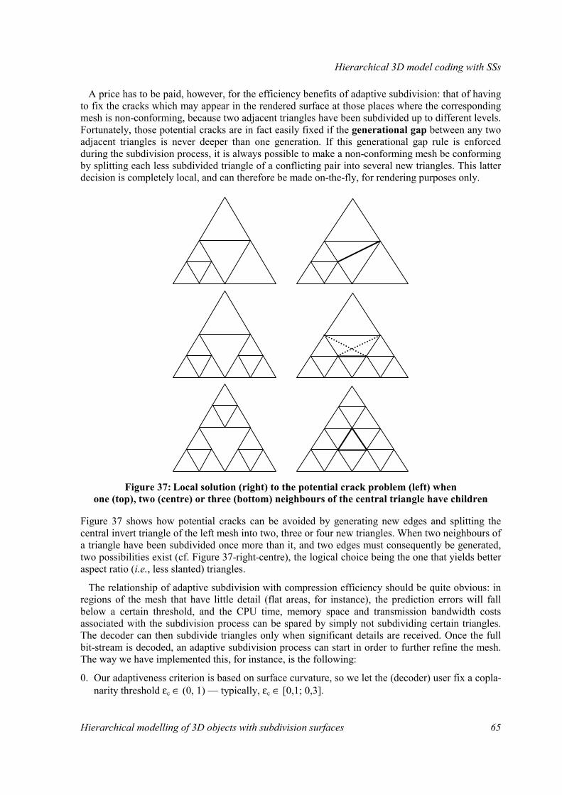
Hierarchical 3D model coding with SSs
Hierarchical modelling of 3D objects with subdivision surfaces 65
A price has to be paid, however, for the efficiency benefits of adaptive subdivision: that of having to fix the cracks which may appear in the rendered surface at those places where the corresponding mesh is non-conforming, because two adjacent triangles have been subdivided up to different levels. Fortunately, those potential cracks are in fact easily fixed if the generational gap between any two adjacent triangles is never deeper than one generation. If this generational gap rule is enforced during the subdivision process, it is always possible to make a non-conforming mesh be conforming by splitting each less subdivided triangle of a conflicting pair into several new triangles. This latter decision is completely local, and can therefore be made on-the-fly, for rendering purposes only.
Figure 37: Local solution (right) to the potential crack problem (left) when one (top), two (centre) or three (bottom) neighbours of the central triangle have children
Figure 37 shows how potential cracks can be avoided by generating new edges and splitting the central invert triangle of the left mesh into two, three or four new triangles. When two neighbours of a triangle have been subdivided once more than it, and two edges must consequently be generated, two possibilities exist (cf. Figure 37-right-centre), the logical choice being the one that yields better aspect ratio (i.e., less slanted) triangles.
The relationship of adaptive subdivision with compression efficiency should be quite obvious: in regions of the mesh that have little detail (flat areas, for instance), the prediction errors will fall below a certain threshold, and the CPU time, memory space and transmission bandwidth costs associated with the subdivision process can be spared by simply not subdividing certain triangles. The decoder can then subdivide triangles only when significant details are received. Once the full bit-stream is decoded, an adaptive subdivision process can start in order to further refine the mesh. The way we have implemented this, for instance, is the following:
0. Our adaptiveness criterion is based on surface curvature, so we let the (decoder) user fix a copla-narity threshold εc ∈ (0, 1) — typically, εc ∈ [0,1; 0,3].

Hierarchical 3D model coding with SSs
66 Hierarchical modelling of 3D objects with subdivision surfaces
1. All triangles in the current mesh receive the order of getting subdivided and, when each of them does, it checks whether it is coplanar enough to its up to three neighbours (to be precise, it checks whether the cosines of the angles its normal forms with those of its neighbours are all greater than 1−εc): if it is, the triangle simply ignores the order; otherwise, the triangle does follow the order, and propagates it to its neighbours if needed, so as to guarantee that the generational gap rule is always respected (this is done in such a way that dead-locks due to recurrence are avoided).
2. The previous step can be iterated a fixed number of times or until the number of triangles stops increasing.
Figure 38: The solution to the crack problem applied to the waving flag of Figure 20 (base (left) and adaptively subdivided non-conforming (centre) and conforming (right) meshes)
Figure 38 shows the same waving flag of Figure 20, which has been adaptively subdivided three times based on the curvature criterion described above, in order to get a mesh of approximately the same size of the one that two systematic subdivisions would yield (around 3000 triangles). When rendering the non-conforming mesh depicted in Figure 38-centre, cracks would appear on its sur-face, so the conforming mesh on its right has to be used instead.
2.4.8. Results
3D MODELS TEST SET
We have used around a dozen 3D models for developing our algorithms, then many more for “stress testing” them. Among the former are the fist (cf. Figure 39) and the octahedron/cube (cf. Figure 40) models. The sources for the latter were the following:
• “The Stanford 3D Scanning Repository” from the Stanford University [Stanford2001].
• The “Large Geometric Models Archive” from the Georgia Institute of Technology [GA-Tech2001].
• The original meshes used by the CalTech research team to test their PGC technique [Cal-Tech2001] (see section 2.4.9).
• The MPEG-SNHC 3D models repository of more than 1300 VRML meshes mirrored at the GTI-UPM (Grupo de Tratamiento de Imágenes de la Universidad Politécnica de Madrid: Image Processing Group of the Polytechnic University of Madrid) [GTI2001].

Hierarchical 3D model coding with SSs
Hierarchical modelling of 3D objects with subdivision surfaces 67
We wish to thank all those institutions (and, especially, their system managers… ;-) for sharing their 3D models collections. Some of them contain donations from other public organisms, such as the French INT (Institut National des Télécommunications: National Telecommunications Institute) and the Canadian National Research Council, or from private companies, like Cyberware, IBM and Ocnus Rope Company.
Figure 39: The fist model (from left to right: input/target, base and reconstructed (level 3) meshes)
The original fist mesh shown in Figure 39-left contained 8734 vertices and 17490 triangles. One of its vertices being duplicated, four of its triangles resulted to be flat and the mesh itself non-manifold. We simplified the original to obtain a base mesh of 79 vertices and 154 triangles, depicted in Figure 39-centre, which therefore has 9856 triangles when systematically subdivided three times (Figure 39-right). For a subdivision depth of four, the triangle count reaches 39424.
Figure 40: The octahedron/cube model (left: target (wireframe) and base meshes; right: target and reconstructed (level 5) meshes)
The octahedron/cube model was designed as a worse case scenario to test our algorithms. Figure 40-left shows an octahedron, the base mesh, inscribed in a cube, the target mesh, which is a specially stressful one, because it is everything but smooth and completely unaligned with the coarsest LOD. Even if in this case it is not really relevant, for the sake of completeness we will make it explicit that the target mesh has six vertices and twelve triangles, whereas the base mesh contains six vertices and eight triangles, that turn into 8192 when it is systematically subdivided five times, as shown in Figure 40-right.

Hierarchical 3D model coding with SSs
68 Hierarchical modelling of 3D objects with subdivision surfaces
NON-DUPLICATION OF DETAILS ON MOTHER EDGES
subdiv. depth 1 2 3 4
duplicated 14528 60072 195976 614160
zeroed 13184 57176 188464 597040
not duplicated 7632 39248 149392 521712
Table 2: Effect of avoiding the duplication of details on mother edges for the fist model
Table 2 contains the sizes of the bit-streams (in bits and excluding the 25 bytes header) generated by our technique for the fist model at different subdivision depths (of the butterfly subdivision scheme) and three functioning modes:
• duplicated: details attached to vertices lying on mother edges are simply coded twice;
• zeroed: the second time one of such vertices shared by two mother triangles is visited, its detail is zeroed — note that, although the zerotree-like technique by Said and Pearlman exploits this fact, the savings are negligible (less than 10% even with just one subdivision step);
• not duplicated: each detail is covered by only one mother detail tree, as explained at the end of section 2.4.2 — note that, in this case, the savings are really substantial, and range from a more than modest 15% (four subdivision steps) to an impressive 47% (one step).
Needless to say, all the results that follow were obtained with the version of our algorithms which avoids the replicated coding of details attached to vertices lying on mother edges.
ARITHMETIC CODING EFFICIENCY
subdiv. depth 1 2 3 4
no AC 7632 39248 149392 521712
AC2 (no reset) 7724 39460 147193 501643
AC2 7761 39220 144285 485807
AC4 7562 35584 133139 455014
AC5 7574 35269 128547 427003
AC6 6447 26040 82708 248084
Table 3: Effect of arithmetic coding of the SPIHT bit-stream for the fist model
Table 3 and Table 4 show the importance of using different adaptive probability models for coding the different kinds of bits generated by the SPIHT algorithm during the coding of the two 3D models of Figure 39 and Figure 40 respectively. The numbers shown are again the sizes of the respective bit-streams (in bits and excluding the 25 bytes header) and the rows correspond to:
• no AC: raw SPIHT bit-stream generated by the algorithm described in section 2.4.3;
• AC2: arithmetic coding with two probability models for significance bits (one for each type);
• AC4: AC2 + another two probability models for sorting bits (one for each type);
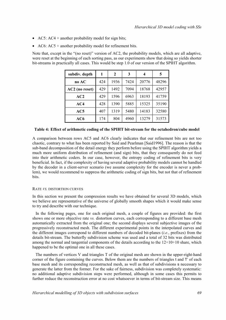
Hierarchical 3D model coding with SSs
Hierarchical modelling of 3D objects with subdivision surfaces 69
• AC5: AC4 + another probability model for sign bits;
• AC6: AC5 + another probability model for refinement bits.
Note that, except in the “(no reset)” version of AC2, the probability models, which are all adaptive, were reset at the beginning of each sorting pass, as our experiments show that doing so yields shorter bit-streams in practically all cases. This would be step 1.0 of our version of the SPIHT algorithm.
subdiv. depth 1 2 3 4 5
no AC 424 1936 7424 20776 48296
AC2 (no reset) 429 1492 7094 18768 42957
AC2 429 1596 6963 18193 41759
AC4 428 1390 5885 15325 35190
AC5 407 1319 5480 14183 32580
AC6 174 804 4960 13279 31573
Table 4: Effect of arithmetic coding of the SPIHT bit-stream for the octahedron/cube model
A comparison between rows AC5 and AC6 clearly indicates that our refinement bits are not too chaotic, contrary to what has been reported by Said and Pearlman [Said1996]. The reason is that the sub-band decomposition of the detail energy they perform before using the SPIHT algorithm yields a much more uniform distribution of refinement (and sign) bits, that they consequently do not feed into their arithmetic coders. In our case, however, the entropy coding of refinement bits is very beneficial. In fact, if the complexity of having several adaptive probability models cannot be handled by the decoder in a client-server scenario (we assume complexity for the encoder is never a prob-lem), we would recommend to suppress the arithmetic coding of sign bits, but not that of refinement bits.
RATE VS. DISTORTION CURVES
In this section we present the compression results we have obtained for several 3D models, which we believe are representative of the universe of globally smooth shapes which it would make sense to try and describe with our technique.
In the following pages, one for each original mesh, a couple of figures are provided: the first shows one or more objective rate vs. distortion curves, each corresponding to a different base mesh automatically extracted from the original one; the second displays several subjective images of the progressively reconstructed mesh. The different experimental points in the interpolated curves and the different images correspond to different numbers of decoded bit-planes (i.e., prefixes) from the details bit-stream. The butterfly subdivision scheme was used and a total of 32 bits was distributed among the normal and tangential components of the details according to the 12+10+10 share, which happened to be the optimal one in all these cases.
The numbers of vertices V and triangles T of the original mesh are shown in the upper-right-hand corner of the figure containing the curves. Below them are the numbers of triangles t and T’ of each base mesh and its corresponding reconstructed mesh, as well as that of subdivisions s necessary to generate the latter from the former. For the sake of fairness, subdivision was completely systematic: no additional adaptive subdivision steps were performed, although in some cases this permits to further reduce the reconstruction error at no cost whatsoever in terms of bit-stream size. This means
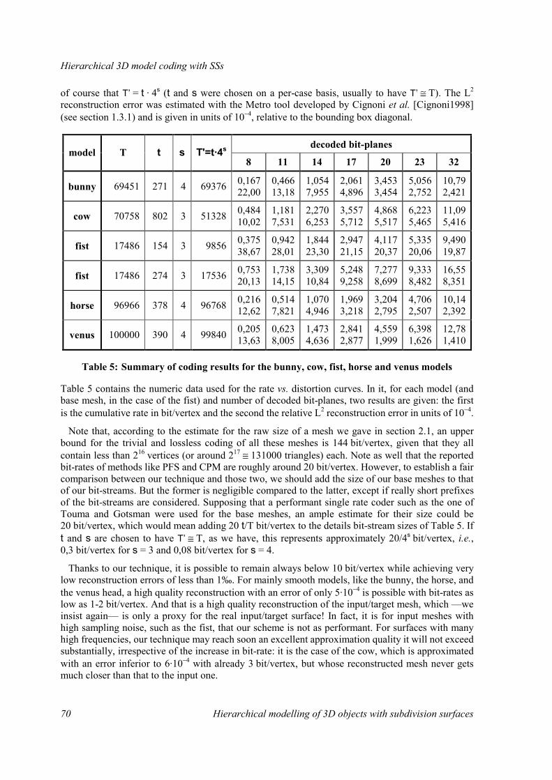
Hierarchical 3D model coding with SSs
70 Hierarchical modelling of 3D objects with subdivision surfaces
of course that T’ = t · 4s (t and s were chosen on a per-case basis, usually to have T’ ≅ T). The L2 reconstruction error was estimated with the Metro tool developed by Cignoni et al. [Cignoni1998] (see section 1.3.1) and is given in units of 10−4, relative to the bounding box diagonal.
decoded bit-planes model T t s T'=t·4s
8 11 14 17 20 23 32
bunny 69451 271 4 69376 0,16722,00
0,46613,18
1,0547,955
2,0614,896
3,453 3,454
5,056 2,752
10,792,421
cow 70758 802 3 51328 0,48410,02
1,1817,531
2,2706,253
3,5575,712
4,868 5,517
6,223 5,465
11,095,416
fist 17486 154 3 9856 0,37538,67
0,94228,01
1,84423,30
2,94721,15
4,117 20,37
5,335 20,06
9,49019,87
fist 17486 274 3 17536 0,75320,13
1,73814,15
3,30910,84
5,2489,258
7,277 8,699
9,333 8,482
16,558,351
horse 96966 378 4 96768 0,21612,62
0,5147,821
1,0704,946
1,9693,218
3,204 2,795
4,706 2,507
10,142,392
venus 100000 390 4 99840 0,20513,63
0,6238,005
1,4734,636
2,8412,877
4,559 1,999
6,398 1,626
12,781,410
Table 5: Summary of coding results for the bunny, cow, fist, horse and venus models
Table 5 contains the numeric data used for the rate vs. distortion curves. In it, for each model (and base mesh, in the case of the fist) and number of decoded bit-planes, two results are given: the first is the cumulative rate in bit/vertex and the second the relative L2 reconstruction error in units of 10−4.
Note that, according to the estimate for the raw size of a mesh we gave in section 2.1, an upper bound for the trivial and lossless coding of all these meshes is 144 bit/vertex, given that they all contain less than 216 vertices (or around 217 ≅ 131000 triangles) each. Note as well that the reported bit-rates of methods like PFS and CPM are roughly around 20 bit/vertex. However, to establish a fair comparison between our technique and those two, we should add the size of our base meshes to that of our bit-streams. But the former is negligible compared to the latter, except if really short prefixes of the bit-streams are considered. Supposing that a performant single rate coder such as the one of Touma and Gotsman were used for the base meshes, an ample estimate for their size could be 20 bit/vertex, which would mean adding 20 t/T bit/vertex to the details bit-stream sizes of Table 5. If t and s are chosen to have T’ ≅ T, as we have, this represents approximately 20/4s bit/vertex, i.e., 0,3 bit/vertex for s = 3 and 0,08 bit/vertex for s = 4.
Thanks to our technique, it is possible to remain always below 10 bit/vertex while achieving very low reconstruction errors of less than 1‰. For mainly smooth models, like the bunny, the horse, and the venus head, a high quality reconstruction with an error of only 5·10−4 is possible with bit-rates as low as 1-2 bit/vertex. And that is a high quality reconstruction of the input/target mesh, which —we insist again— is only a proxy for the real input/target surface! In fact, it is for input meshes with high sampling noise, such as the fist, that our scheme is not as performant. For surfaces with many high frequencies, our technique may reach soon an excellent approximation quality it will not exceed substantially, irrespective of the increase in bit-rate: it is the case of the cow, which is approximated with an error inferior to 6·10−4 with already 3 bit/vertex, but whose reconstructed mesh never gets much closer than that to the input one.
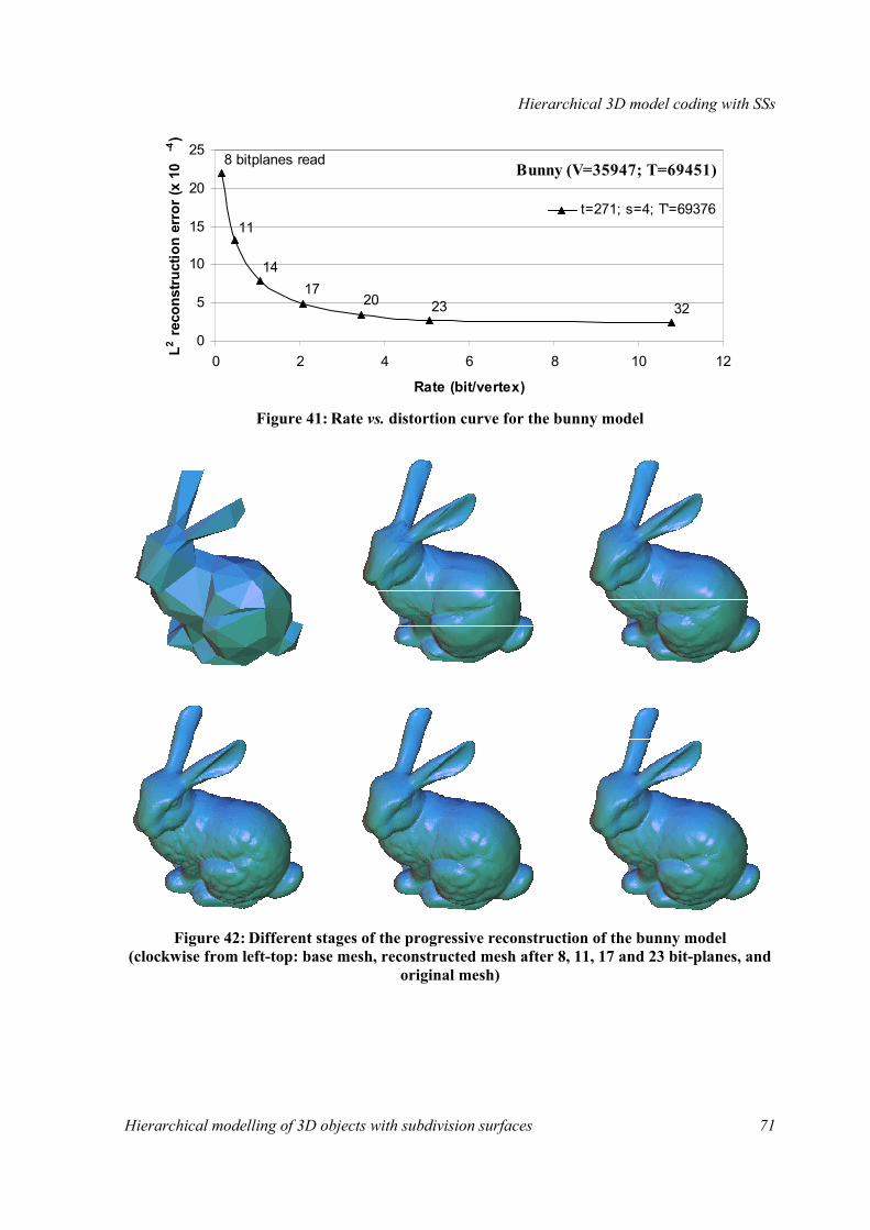
Hierarchical 3D model coding with SSs
Hierarchical modelling of 3D objects with subdivision surfaces 71
Figure 41: Rate vs. distortion curve for the bunny model
Figure 42: Different stages of the progressive reconstruction of the bunny model (clockwise from left-top: base mesh, reconstructed mesh after 8, 11, 17 and 23 bit-planes, and
original mesh)
Bunny (V=35947; T=69451)
32232017
14
8 bitplanes read
11
0
5
10
15
20
25
0 2 4 6 8 10 12
Rate (bit/vertex)
L2 reco
nstru
ctio
n er
ror (
x 10
-4)
t=271; s=4; T'=69376
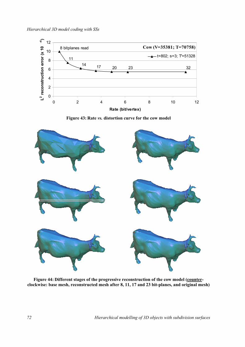
Hierarchical 3D model coding with SSs
72 Hierarchical modelling of 3D objects with subdivision surfaces
Figure 43: Rate vs. distortion curve for the cow model
Figure 44: Different stages of the progressive reconstruction of the cow model (counter- clockwise: base mesh, reconstructed mesh after 8, 11, 17 and 23 bit-planes, and original mesh)
Cow (V=35381; T=70758)
322320171411
8 bitplanes read
0
2
4
6
8
10
12
0 2 4 6 8 10 12
Rate (bit/vertex)
L2 reco
nstru
ctio
n er
ror (
x 10
-4)
t=802; s=3; T'=51328

Hierarchical 3D model coding with SSs
Hierarchical modelling of 3D objects with subdivision surfaces 73
Figure 45: Rate vs. distortion curves for the fist model
Figure 46: Different stages of the progressive reconstruction of the fist model (clockwise: base mesh (t=274), reconstructed mesh after 8, 11, 17 and 23 bit-planes, and original mesh)
Fist (V=8733; T=17486)8 bitplanes read
11
1417 20 23 32
3223201714
11
8
0
5
10
15
20
25
30
35
40
45
0 2 4 6 8 10 12 14 16 18
Rate (bit/vertex)
L2 reco
nstru
ctio
n er
ror (
x 10
-4) t=154; s=3; T'=9856 t=274; s=3; T'=17536

Hierarchical 3D model coding with SSs
74 Hierarchical modelling of 3D objects with subdivision surfaces
Figure 47: Rate vs. distortion curve for the horse model
Figure 48: Different stages of the progressive reconstruction of the horse model (clockwise: base mesh, reconstructed mesh after 8, 11, 17 and 23 bit-planes, and original mesh)
Horse (V=48485; T=96966)
32232017
14
11
8 bitplanes read
0
2
4
6
8
10
12
14
0 2 4 6 8 10 12
Rate (bit/vertex)
L2 reco
nstru
ctio
n er
ror (
x 10
-4)
t=378; s=4; T'=96768
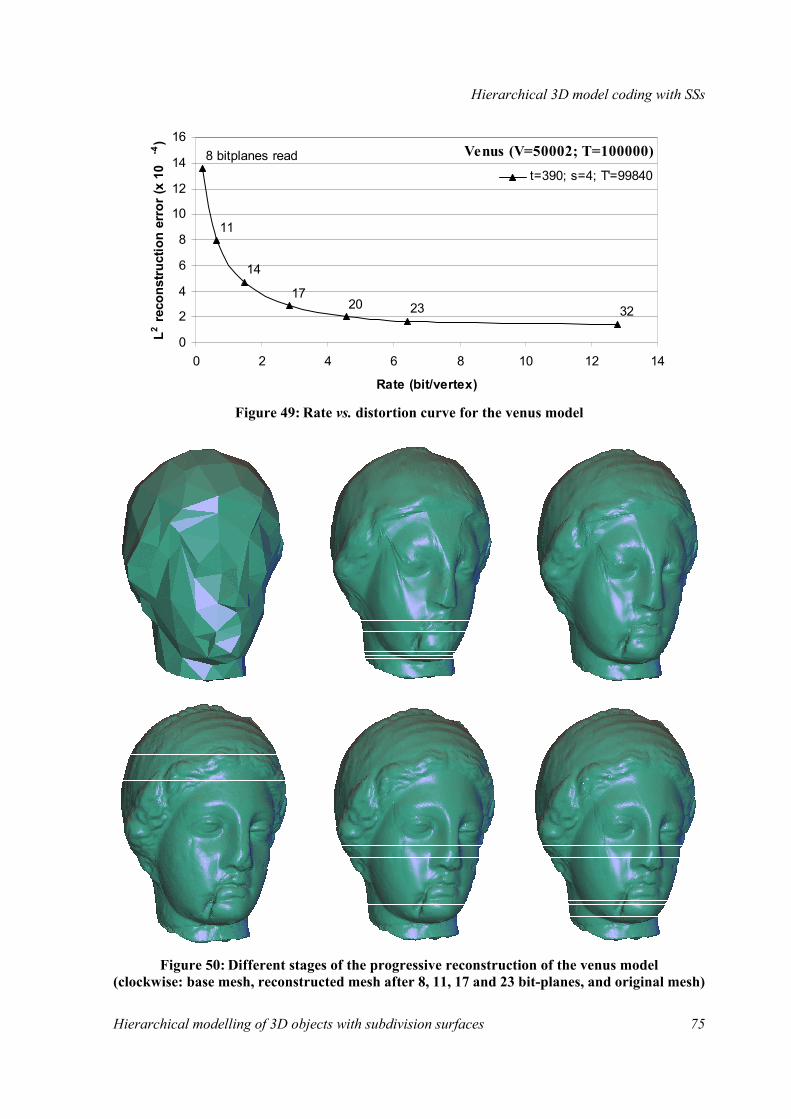
Hierarchical 3D model coding with SSs
Hierarchical modelling of 3D objects with subdivision surfaces 75
Figure 49: Rate vs. distortion curve for the venus model
Figure 50: Different stages of the progressive reconstruction of the venus model (clockwise: base mesh, reconstructed mesh after 8, 11, 17 and 23 bit-planes, and original mesh)
Venus (V=50002; T=100000)
32232017
14
11
8 bitplanes read
0
2
4
6
8
10
12
14
16
0 2 4 6 8 10 12 14
Rate (bit/vertex)
L2 reco
nstru
ctio
n er
ror (
x 10
-4)
t=390; s=4; T'=99840

Hierarchical 3D model coding with SSs
76 Hierarchical modelling of 3D objects with subdivision surfaces
2.4.9. Khodakovsky’s PGC (Progressive Geometry Compression) One year after we presented our technique at the IWSNHC3DI’99, Khodakovsky, Schröder and Sweldens published in SIGGRAPH 2000 a paper entitled “Progressive Geometry Compression” [Khodakovsky2000]. In it, they describe a method developed independently of ours but extremely similar, which is not too surprising, since it was inspired as well by the work of Kolarov and Lynch [Kolarov1996]. Indeed, they also propose to simplify a fine manifold mesh of arbitrary connectivity to extract a base mesh and to subdivide it later to yield a remesh approximating very closely the original input mesh. To achieve this, they also modify the positions of the midpoints predicted by the subdivision scheme with conveniently calculated wavelet coefficients, that they group hierarchically to be able to feed them into a SPIHT-like coder.
The main differences between their work and ours are the following:
• Base mesh extraction: They use directly Garland’s automatic mesh simplifier, whereas we use a slightly improved version of it (see section 3.2.0).
• Remeshing and obtention of wavelet coefficients: After having remeshed the input mesh thanks to MAPS, which establishes an explicit parameterisation of it over the mase domain, they com-pute the coefficients of one of several possible lifted or non-lifted wavelet transforms through the use of the corresponding analysis filters. As we explain in section 3.2.1, our solution is much simpler, because it does not require to obtain an explicit parameterisation of the input/target mesh over the base one.
• Subdivision scheme: Their best results are obtained with a lifted wavelet transform based on Loop’s approximating scheme, whereas our technique has been designed for the interpolating butterfly scheme.
Figure 51: Khodakovsky’s edge-based detail hierarchy
• Details set organisation: Their detail hierarchy is edge-based, instead of facet-based. Figure 51 shows how an edge of level l (left) gives birth, when the mesh is subdivided, to four edges of level l + 1 (right). This is a very elegant idea we wish we had had when we were struggling to build a consistent facet-based detail hierarchy…
• Detail quantisation: They also remark the importance of expressing details in a local normal frame, and assign systematically (not adaptively, as we do) two more bits to their normal compo-nent than to their tangential ones. Their way of dealing with the fact that details are 3D vectors, and not scalar values, is by interleaving the bits produced by three independent standard, scalar SPIHT coders.
Figure 52 shows the rate vs. distortion curves obtained with our technique (baptised “subdiv”) and Khodakovsky’s (PGC) for the bunny, horse and venus models. We argue that their slightly better results are most likely due to the finer quality of their remeshes, and not by the compression effi-ciency of their coding technique, as proven by the fact that our approximation errors never get as low as theirs, even for high bit-rates. However, MAPS remeshing is costly from the computational viewpoint, and so is the analysis filtering performed for finding the wavelet coefficients of PGC, so we wonder whether, in this case, “the price is worth the prize”…

Hierarchical 3D model coding with SSs
Hierarchical modelling of 3D objects with subdivision surfaces 77
Figure 52: Rate vs. distortion curves obtained with our technique and the PGC one for the bunny, horse and venus models
Bunny (V=35947; T=69451)
0
5
10
15
20
25
0 2 4 6 8 10 12
Rate (bit/vertex)
L2 reco
nstru
ctio
n er
ror (
x 10
-4)
subdiv (UPM) PGC (CalTech)
Horse (V=48485; T=96966)
0
2
4
6
8
10
12
14
0 2 4 6 8 10 12
Rate (bit/vertex)
L2 reco
nstru
ctio
n er
ror (
x 10
-4)
subdiv (UPM) PGC (CalTech)
Venus (V=50002; T=100000)
024
68
1012
1416
0 2 4 6 8 10 12 14
Rate (bit/vertex)
L2 reco
nstru
ctio
n er
ror (
x 10
-4)
subdiv (UPM) PGC (CalTech)

Hierarchical 3D model coding with SSs
78 Hierarchical modelling of 3D objects with subdivision surfaces
2.5. Future work
2.5.0. Straightforward extensions
MESHES WITH PROPERTIES
It is fairly common, when modelling 3D objects with planar meshes, to attach properties or attributes to their elements, as they can later be used by a rendering application to modify their appearance. Indeed, by attaching to each vertex, facet or corner (i.e., a vertex inside a particular facet) of a mesh one such attribute, that is, a normal vector, a colour, or a pair of texture coordinates, the modeller can help the renderer make the corresponding object look much more realistic — or completely the opposite, depending on what is sought. Most commercial CAD packages, 3D graphics libraries [Neider1993] and international standards [VRML1997, MPEG1998, MPEG1999] support attributes.
The main interest of our technique for hierarchical 3D model coding is the efficient description of their geometry. However, most of what is written above is perfectly valid for coding other attributes attached to vertices, instead of their positions. In fact, we believe that, since our detail hierarchy is facet-based, properties bound to facets could be coded equally well. And this, independently of the number of dimensions of such attributes (both normals and colours have three, whereas texture coordinates have only two).
The validity of our coding scheme for vertex properties other than their position should be hardly surprising, since it brings us back to what was our starting point: the technique devised by Kolarov and Lynch to compress scalar functions defined on 2-manifolds [Kolarov1996]. In their own words: “[…] surfaces have information about illumination, texture, etc. distributed about them. In this report we will focus on the representation of that distributed information, although it is clear that the techniques described herein are also applicable as well to the description of the geometry.”.
The only modification that must be introduced in the coding scheme described above affects our “scalarisation” technique, which should treat equally all components of vectorial attributes, at least in the absence of evidence proving that one component is more energetic than the rest. This is what happens with our detail vectors, and could also be the case for colours if they were expressed in a (Y, CR, CB) basis, as they are in the Digital Television world, but not if they are expressed in the (R, G, B) basis, which is the one most commonly used by the 3D Graphics community. In the latter case, as well as in that of (u, v) texture coordinates, there is no a priori reason to privilege any com-ponent, so both a homogeneous quantisation and, consequently, a simple bit interleaving should be employed for “scalarising” those vectorial properties.
NON-TRIANGULAR MESHES
If the input surface to the geometry coding algorithm is a mesh whose elements are not all triangles, but arbitrary polygons, our technique requires that they be triangulated. Triangulation of polygons is a fundamental problem in the relatively new field of Computational Geometry, but fortunately a rather simple one, so many general yet efficient solutions exist for it [Seidel1991, O’Rourke1994, Ronfard1994, Shewchuck1996]. And by “arbitrary” polygons and “general” solutions we mean exactly that: triangulation algorithms exist whose input polygons need not be convex, nor monotone, nor simply connected, nor even connected. Therefore, it is only fair to say that, in the unlikely case that the original mesh is made of arbitrary polygons (triangle meshes are the most common ones), a previous triangulation step is not much of a problem.

Hierarchical 3D model coding with SSs
Hierarchical modelling of 3D objects with subdivision surfaces 79
Figure 53: A triangulated cube smoothed by the butterfly scheme
However, it is also fair to make it explicit that the result of applying a subdivision scheme upon a previously triangulated mesh of arbitrary polygons may not be the expected one. Figure 53 illus-trates this undesirable side effect in the case of a cube whose six square facets have been triangulated by splitting them along their diagonals. When the resulting mesh is given to the butterfly subdivision scheme, the edges created by the triangulation step are not treated differently in the smoothing process, and the new vertices to which they give birth do not remain on their midpoints (cf. Figure 53-centre). This results in the artificial “humps” that can be seen in Figure 53-right, which are most likely unwanted. Note that the problem is not the smoothing of the surface (smoothing is the goal of SSs and the basis of our prediction mechanism), but the smoothing of the surface along those edges, which introduce arbitrary and unforeseeable privileged directions.
The way to prevent this from happening is to tag the edges created by the triangulation step so that the subdivision algorithm may preserve them unaltered, while smoothing the surface along the ones already present in the original mesh.
SURFACES WITH SHARP FEATURES
There is another situation which asks even more clearly for a tagging of the input mesh edges or vertices: when the surface under approximation exhibits sharp features (corners, cusps, creases, sharp edges, etc.) that must be preserved, the subdivision algorithm must also be told to respect them. This is also a relatively well studied problem [Schweitzer1996, Biermann2000, Zorin2000].
In particular, surfaces with a boundary yield meshes with border edges, which need not be tagged, as it is immediate to detect their not being shared by two triangles, but for which special subdivision rules must be used. Our implementation handles border edges in the most common way: they are smoothed using the four-point rule for curves (see, for instance, Figure 38).
NON-MANIFOLD AND NON-ORIENTABLE SURFACES
As already explained in the first chapter, subdivision schemes need to operate on manifold meshes, as they do not consider edges shared by more than two facets (or, in the case on approximating schemes, vertex 1-rings composed by more than one ring of linked vertices). Therefore, a non-manifold mesh must be cut into manifold pieces by replicating the conflicting vertices/edges and tagging them appropriately, so that they are treated in the same way when both pieces are smoothed independently (cf. Figure 13).
In this same way, even non-orientable meshes can be handled. An orientable mesh representing a Möbius strip (cf. Figure 11), for instance, could be constructed by simulating what must be done to

Hierarchical 3D model coding with SSs
80 Hierarchical modelling of 3D objects with subdivision surfaces
build one physically from a narrow rectangle of paper, whose short edges are NW-NE and SW-SE (the long ones being NW-SW and NE-SE):
1. To build a simple loop with the paper strip, the SW-SE edge must be made coincident with the NW-NE edge; to build a Möbius strip, a half-twist must be added before closing the loop, so that the SW corner is superimposed to the NE one, and the SE corner to the NW one. Analogously, a mesh modelling a Möbius strip must have a “jump edge” composed of two separate border edges coincident in space, although with “opposite directions”.
2. If the two border edges forming the composite jump edge are tagged adequately, the subdivision process can exclude them from being smoothed at all (even according to the four-point rule). The strip would be smoothed elsewhere, resulting in a shape similar to the one depicted in Figure 11.
IMPROVED COMPRESSION EFFICIENCY THROUGH TANGENTIAL COMPONENTS SUBSAMPLING
As it has been mentioned above, in the Digital Television world colours are expressed in the (Y, CR, CB) basis. This is not only done for maintaining a compatibility with monochrome receivers but, more importantly, because the luminance Y carries the most energy and is the most essential component of the signal to the human visual system. Having expressed the signal in that basis, it is immediate to code with different accuracy the luminance and the two chrominances (CR and CB). The chrominances are in fact treated with much less care than the luminance, as they are subsampled with respect to it at a ratio of 2:1 or 4:1, although quantised with a slightly larger number of levels (225 as opposed to 220).
Analogously, our detail vectors have one component which is clearly more energetic than the rest. In fact, in this case there is not even any subjective sensor such as a human eye involved, so it would be hardly surprising to see that some more compression efficiency can be gained by subsampling the tangential components with respect to the normal one, on top of quantising them more crudely.
DETAILS SET PARTITIONING FOR ERROR RESILIENCE AND VIEW-DEPENDENT CODING
Looking along this same line of enhancements of our hierarchical 3D model coding technique, it is not difficult to imagine that partitioning the set of details could be most beneficial for error resilient transmission over noisy channels or view-dependent coding. In our basic hierarchical 3D model coding scheme described above, a transmission error affecting some low level detail (and therefore appearing most likely at the beginning of the bit-stream) would be fatal, as all nearby vertices of a higher level would be ill-positioned. Likewise, having a predefined order for the traversal of the set of triangles forming the base mesh is convenient for compression efficiency purposes, but in a client-server scenario, it forces the rendering process on the client/decoder end to wait until the details associated with the visible parts of the object appear in the bit-stream. One could envisage client-driven transmission scenarios in which the client could request to the server, through a back-channel, the transmission of specific zones of the 3D object. But even in a pure broadcast context, with no back-channel, it could be desirable to give a chance to decoders with low computational resources to skip some portions of the bit-stream: indeed, the “wait” mentioned above is not a pas-sive one, as the client must keep decoding the bit-stream to check when “the details associated with the visible parts of the object appear”.
In all these cases, partitioning the details set, e.g., by considering independently the details lying on each base mesh triangle, could be helpful, and perhaps not too difficult to achieve by inserting markers in the bit-stream to delimit its different parts. Such a details set partitioning and bit-stream delimiting technique is under exam, as our basic hierarchical 3D model coding method itself, inside the AFX subgroup of MPEG-SNHC, for its adoption in version 5 of MPEG-4, due October 2002 [MPEG2001, MPEG2001a, MPEG2001b].

Hierarchical 3D model coding with SSs
Hierarchical modelling of 3D objects with subdivision surfaces 81
Nevertheless, the most challenging tracks of future research are, in our opinion, those dealing with the extension of the hierarchical modelling of surfaces to higher dimensions, that we introduce below. We think both of considering “3,5D surfaces” (i.e., time-varying surfaces embedded in 3D space) and truly 3D models representing the inner volume of the corresponding 3D objects (e.g., with tetrahedral meshes), which we see as hardly trivial problems, and have thus put outside this first section of “straighorward extensions” to our work.
2.5.1. Animated models As we have already said and repeated, some of the most attractive applications of hierarchical mod-elling are the ones derived from multiresolution editing or animation (which is nothing more than editing repeated over time). In fact, the potential of SS-based approaches to 3D object modelling has been largely proven by the number of them published so far [Zorin1997, Kobbelt1998, Lee1999], as opposed to the few existing interactive multiresolution editing techniques not based on SSs (a nota-ble exception being [Lee1999a]). Moreover, several commercial products exist already that feature SS-based character animation and are being used for the generation of entirely computer-generated films [DeRose1998]. It is then foreseeable that an extension of our work to have it consider the hierarchical modelling and coding of animated 3D objects could be of great importance. Defining a semantically and syntactically consistent way of representing the animated details, and designing an efficient mechanism for their hierarchical coding seem major tasks, but also potentially rewarding ones.
A hierarchical technique for animating 3D objects could fit perfectly with another tool developed by the AFX subgroup of MPEG-SNHC that will be included in MPEG-4 version 5: bone-based animation. The idea behind it is to define a set of (virtual, invisible) bones forming a skeleton and determining the shape of their (actual, visible) surrounding “skin”, usually modelled as a planar mesh. This is the same idea of having a set of control points determine the shape of a patch, but with an added benefit: if furthermore a set of rules for the joints between the bones is defined, it is possi-ble and very convenient to specify the position of only a few points of the skeleton, and have the system calculate automatically the others (and the shape of the skin) by using inverse kinematics. Bone-based animation bears a striking relationship to hierarchical 3D object modelling with SSs: it is easy to imagine bones acting somehow as “meta-control points” for the control mesh of a SS, in an even more hierarchical scheme.
2.5.2. Truly 3D models The FEM [Hughes1987] helps solve numerically some problems involving partial derivative equa-tions with no analytical solution: the domain in which the varying field under study (stress, pressure, temperature, etc.) is meshed with simple elementary cells, on whose vertices the field value is calcu-lated, and inside which it is interpolated. Thanks to this aproach, it is possible to approximate within an arbitrarily small error bound the exact solution to the problem by making the size of those ele-ments conveniently small, which is usually done be refining (i.e., splitting the elements of) a previ-ously obtained mesh.
When that domain is a surface, the elements used to partition it are triangular of quadrilateral, but when it is a solid 3D volume, it is most frequently meshed with tetrahedra, and not with parallelepi-peds, which are the only 3D elements which could be tesselated themselves in a self-similar, nesting fashion. This makes it impossible, at least in principle, to model hierarchically truly 3D objects, and in fact most published refinement schemes resort to simple bisection of tetrahedra and put special care in preventing the degeneration of their aspect ratio [Liu1994].
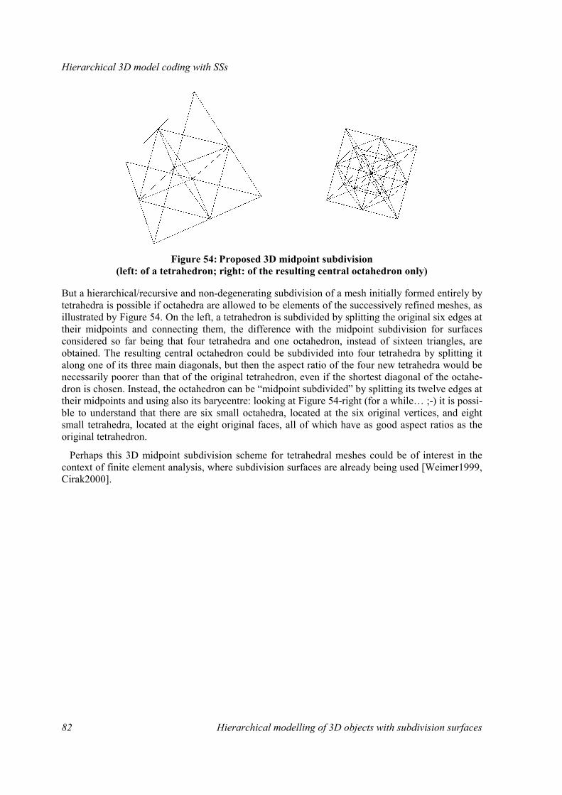
Hierarchical 3D model coding with SSs
82 Hierarchical modelling of 3D objects with subdivision surfaces
Figure 54: Proposed 3D midpoint subdivision (left: of a tetrahedron; right: of the resulting central octahedron only)
But a hierarchical/recursive and non-degenerating subdivision of a mesh initially formed entirely by tetrahedra is possible if octahedra are allowed to be elements of the successively refined meshes, as illustrated by Figure 54. On the left, a tetrahedron is subdivided by splitting the original six edges at their midpoints and connecting them, the difference with the midpoint subdivision for surfaces considered so far being that four tetrahedra and one octahedron, instead of sixteen triangles, are obtained. The resulting central octahedron could be subdivided into four tetrahedra by splitting it along one of its three main diagonals, but then the aspect ratio of the four new tetrahedra would be necessarily poorer than that of the original tetrahedron, even if the shortest diagonal of the octahe-dron is chosen. Instead, the octahedron can be “midpoint subdivided” by splitting its twelve edges at their midpoints and using also its barycentre: looking at Figure 54-right (for a while… ;-) it is possi-ble to understand that there are six small octahedra, located at the six original vertices, and eight small tetrahedra, located at the eight original faces, all of which have as good aspect ratios as the original tetrahedron.
Perhaps this 3D midpoint subdivision scheme for tetrahedral meshes could be of interest in the context of finite element analysis, where subdivision surfaces are already being used [Weimer1999, Cirak2000].

LOD extraction and remeshing
Hierarchical modelling of 3D objects with subdivision surfaces 83
3. LOD extraction and remeshing
3.0. Contents This chapter describes the aspects of our technique for hierarchical modelling of 3D objects that deal with the extraction of the base mesh and the implicit remeshing of an arbitrary (i.e., non semi-regular) input mesh. Its first section reviews, in chronological order, previous work on automatic LOD extraction and remeshing, whereas the second presents the solutions we propose for both problems. A final section on future work closes the chapter.
3.1. Previous work
3.1.0. LOD extraction Several comprehensive surveys on automatic LOD generation through polygonal simplification have already been published. We recommend those of Erikson [Erikson1996], Krus et al. [Krus1997], and the notes of the SIGGRAPH 2000 conference course organised by Luebke on “Advanced Issues in Level of Detail” [Luebke2000]. Lindstrom and Turk also compare the results and timings obtained with public domain implementations of the techniques described below and a few other mentioned in section 1.3 in their paper “Evaluation of Memoryless Simplification” [Lindstrom1999].
HOPPE’S PM (PROGRESSIVE MESH)
Hoppe’s probably most referenced paper so far, “Progressive Meshes” [Hoppe1996], made two essential contributions to the field of automatic LOD approximation of 3D meshes: it presented a triangular mesh simplification procedure based on successive edge collapses and, more importantly, it introduced the key concept of PM representation, already explained in section 2.2.0.
The expression “edge collapse” had already been coined in a previous research work on “Mesh Optimization” [Hoppe1993] carried by Hoppe and his co-workers at the University of Washington, and comes from the fact that each unitary simplification step collapses the two endpoints of some suitably chosen edge. As a result, the mesh looses one vertex and either three edges and the two triangles sharing the chosen edge (if it is an interior one), or two edges and one triangle (if the cho-sen edge lies on the boundary). The procedure is iterative:
LOD extraction and remeshing
84 Hierarchical modelling of 3D objects with subdivision surfaces
1. the edges of the initial mesh are sorted according to the criteria described below;
2. the most discardable edge is collapsed and the places in the sorted list of the few surrounding edges affected by this change are updated;
3. the previous step is repeated until the target number of facets (plus/minus one) is obtained.
Hoppe defined an explicit energy metric for measuring the accuracy of a simplified mesh, M, with respect to the original one, M0:
E (M) = Edist (M) + Espring (M) + Escalar (M) + Edisc (M).
In Hoppe’s own words, “the first two terms, Edist (M) and Espring (M), are identical to those in [Hoppe1993]” and “the next two are added to preserve attributes associated with M: Escalar (M) measures the accuracy of its scalar attributes, and Edisc (M) measures the geometric accuracy of its discontinuity curves”. In fact, all terms are important for preserving the surface shape, except for Escalar (M), which deals with properties attached to it (colours, normals, texture coordinates), but Hoppe poses the problem of minimising Edisc (M) as a particular one of minimising Edist (M), and thus reduces the optimisation problem basically to minimising:
• Edist (M), the “distance energy”, which measures the total squared distance from a set of points X formed by all the vertices of M0 (and possibly also some other points scattered at random on its surface) to the surface of M.
• Espring (M), the “spring energy”, that corresponds to placing on each edge of M an imaginary spring of rest length zero and a tension coefficient adaptively chosen as a function of the ratio of the number of points to the number of facets in the neighbourhood.
This non-linear combined minimisation problem is solved with an iterative procedure alternating between two steps, of which the first involves projecting the points in X onto M for finding some optimal parameterisations, and the second solving a least-squares problem for optimally placing the vertices of M. This is a computationally expensive algorithm, which can take tens to hundreds of minutes to simplify tens of thousands of triangles (Hoppe reported those results by running his program on a 150 MHz SGI Indigo2 with 128 MB of RAM which, in 1996, was a pretty powerful workstation).
As already explained in section 2.2.0, the PM representation allows to describe any triangular mesh in an incremental fashion, starting with a coarse version of it. The coarse mesh, obtained from the original one through a sequence of edge collapses, is refined by a sequence of vertex splits to recover exactly the original mesh. This is possible because the edge collapse operation is invertible: in fact, Hoppe gave baptised the atomic reconstruction operation as “vertex split” because that is precisely what the inverse/dual of an edge collapse is (see Figure 30). A nice property of vertex splits and edge collapses is that, thanks to geomorphs, the positions of the vertices involved in them can be interpolated as continuous functions of time, making thus possible to show smooth transitions between consecutive LODs.
PMs were initially conceived as a static, topology preserving LOD extraction technique. But Hoppe himself improved them by considering their viewpoint-dependent refinement [Hoppe1997] and, with the help of Popović, by extending the concept to handle completely arbitrary meshes, i.e., possibly non-regular, non-orientable, non-manifold, and/or of any dimensionality [Popović1997].
GARLAND’S QUADRICS
Garland and Heckbert improved on Hoppe’s PMs ideas and published a year later a paper entitled “Surface Simplification Using Quadric Error Metrics” [Garland1997]. The two main differential

LOD extraction and remeshing
Hierarchical modelling of 3D objects with subdivision surfaces 85
assets of their technique are that they generalise the iterative edge contraction concept to create that of iterative vertex pair contraction, and that they introduce the quadric error metric.
By collapsing arbitrary vertex pairs, also called “virtual edges”, and not only actual edges, their technique can join unconnected pieces of a model together: a topological simplification process they baptise as “aggregation” and for which they make a case by saying that overall shape is more impor-tant than topology for many applications such as rendering. Their algorithm selects a set of valid (i.e., contractible) vertex pairs during its initialisation step, formed by all real edges of the input mesh and by all virtual ones shorter than some threshold.
But even more important, both conceptually and computationally, is the difference regarding the error metric that allows their technique to classify vertex pairs as more or less essential for shape preservation. Following the work of Ronfard and Rossignac [Ronfard1996], Garland and Heckbert observe that each vertex V in a mesh is nothing but the intersection of a set of planes (those support-ing the triangles sharing V), and define the local approximation error of the mesh at V as the sum of the squared distances from V to its planes. Their main insight is to associate to each original vertex V its original set of planes, and to “encode” very compactly the plane equations associated to V as a quadric represented by a 4×4 matrix Q, which is symmetric and can thus be stored as a set of only ten values. During the iterative simplification process, when two vertices are merged together, their associated quadrics/matrices can be simply added to have the resulting quadric/matrix, associated to the new vertex, represent the union of the planes of the two old vertices. The local approximation error mentioned above, which can be calculated by pre- and post-multiplying Q by the homogeneous coordinates of V (assuming V should be the intersection of the planes represented by Q), and which is obviously zero everywhere initially, is what guides their minimisation algorithm. The net result of all this, regarding execution times, is an amazing increase in speed of easily two orders of magnitude over Hoppe’s simplification algorithm: Garland and Heckbert reported run times of tens of seconds to eliminate tens or hundreds of thousands of triangles, on a workstation very similar to Hoppe’s.
There is, unfortunately, one flaw in their setting, as confessed by themselves: when adding the matrices associated to two vertices belonging to the same initial triangle, its supporting plane be-comes “over-represented”. Even if this can only happen twice per original plane, it introduces an accumulative error in the error measured by the quadrics, which can be non-negligible after an important number of iterations. This is why different results can easily be obtained when simplifying an initial mesh by (i) contracting one thousand vertex pairs and by (ii) repeating ten contractions of one hundred vertex pairs (the output mesh of each step being, of course, the input one for the next iteration). The most correct results are obtained by using Garland’s technique in this second way, as it somehow prevents the cumulative memory effect.
In order to avoid this undesirable side effect, Lindstrom and Turk designed a technique equally based on edge collapses and quadrics but completely “memory-less”, with which they reportedly obtain better quality LODs than Garland’s, although not as quickly [Lindstrom1999].
3.1.1. Remeshing
ECK’S EXTENSION OF LOUNSBERY’S MRA OF SEMI-REGULAR MESHES
As already mentioned in section 1.4.2, the main problem met by Lounsbery et al. for extending the classic wavelet-based MRA techniques to manifold surfaces of arbitrary topology [Lounsbery1993, Lounsbery1994, Lounsbery1997] was the need to act upon input meshes with subdivision connec-tivity. This led Eck and a number of other researchers from the same team at the University of Washington to develop an automatic remeshing technique for building a smooth parameterisation of a fine mesh with arbitrary connectivity over a much coarser one serving as the base domain. Their
LOD extraction and remeshing
86 Hierarchical modelling of 3D objects with subdivision surfaces
extension of Lounsbery’s MRA of subdivision meshes rightly deserves its name, “Multiresolution Analysis of Arbitrary Meshes” [Eck1995], and has a number of applications, including multi-resolution mesh reconstruction [Eck1996], rendering [Certain1996] and editing [Zorin1997] — apart from compression, of course!
The basic idea behind Eck’s remeshing technique is that the original input fine arbitrary mesh M can be approximated within a controlled error tolerance by an equally fine but semi-regular mesh MN created by subdividing N times the coarse base mesh M0. The remeshing procedure consists thus of three steps:
1. Partitioning: M is partitioned through a heuristic Voronoi tiling algorithm into a number of regions, which are “more or less triangular” surface patches grouping contiguous triangles of M. This mesh partitioning determines of course the base mesh M0, but it also associates a triangular region Ti in the input mesh M to each triangle ti of K0, the abstract simplicial complex corresponding to M0.
2. Parameterisation: The key contribution of Eck’s work consists in finding a set of local map-pings ρi: ti → Ti establishing a smooth correspondence between abstract/parametric points in K0 and 3D points in M. Moreover, the mappings ρi are constructed to fit together continuously, so as to define a globally C0 parameterisation ρ: K0 → M.
3. Resampling: The easiest part of the remeshing consists in subdividing N times the base complex K0 recursively and systematically to obtain a semi-regular complex KN, whose vertices are simply mapped onto 3 as indicated by ρ. A mesh MN with subdivision connectivity is thus obtained, and N can be determined to have MN and M differ by no more than a user-specified remeshing tolerance (n.b.: Eck et al. chose the L∞ norm, instead of the L2 one, for measuring the mesh ap-proximation error).
Harmonic maps are used in the first two steps and special care is taken so that the resulting remesh can later be approximated with relatively few wavelet coefficients. Even if piecewise linear ap-proximations to the true harmonic maps are used, as Eck et al. suggest to do, this inevitably results in computationally intensive algorithms.
Another drawback of Eck’s technique is derived from the most attractive aspects of the Voronoi tiling algorithm: the locations of the cell centroids (or representative vertices of the triangular re-gions, in this case) are not known in advance, but rather dynamically discovered as the Voronoi diagram is built. Unfortunately, this also makes the partitioning step depend on a number of heuris-tics, and therefore fragile; besides, it provides no control over the number of facets in the base mesh.
LEE’S MAPS (MULTIRESOLUTION ADAPTIVE PARAMETERIZATION OF SURFACES)
A few years after Eck, Lee published, together with Sweldens, Schröder and other researchers, a technique named “MAPS: Multiresolution Adaptive Parameterization of Surfaces” [Lee1998] that overcame the problems of Eck’s remeshing method. Lee’s goal was the same as Eck’s: to obtain a subdivision connectivity remesh within guaranteed error bounds of a fine input triangular mesh of arbitrary connectivity.
However, Lee’s approach is radically different from Eck’s in that it does not derive the base mesh in a first step, and then construct the remesh thanks to a smooth parameterisation. Instead, MAPS builds the parameterisation while coarsening the fine input mesh through hierarchical smoothing, thus obtaining at the same time the mapping and its domain (i.e., the base mesh). The coarsening of the input mesh to obtain the base one is performed through successive removals of “maximally independent” sets of vertices (in which no vertex belongs to the 1-ring of any other), yielding a full LOD collection. Thanks to this coarsening procedure, MAPS avoids the potential problems of Eck’s

LOD extraction and remeshing
Hierarchical modelling of 3D objects with subdivision surfaces 87
heuristic Voronoi tiling algorithm, and is reportedly much faster for large meshes. The construction of the parameterisation is possible because each time a vertex V is removed, the resulting hole is triangulated and V is assigned some suitably chosen barycentric coordinates in one of the newly created, coarser triangles. Constrained Delaunay triangulations and conformal maps are used during this coarsening step.
Furthermore, MAPS considers the preservation of essential features of the input mesh, such as sharp edges or vertices, which should not be eliminated by the coarsening process. Those can be automatically detected by measuring local curvatures or dihedral angles and marking, respectively, the vertices or edges for which these quantities exceeded some threshold. But the user can also tag herself the feature vertices or lines of her choice, if they are not noticeable in the input mesh but are meaningful, for instance, in an editing application.
Finally, the resulting remesh is not the result of systematically subdividing the base mesh. Instead, an adaptive subdivision procedure is run in order to guarantee that no vertex assigned to a triangle would be further from that triangle than some chosen remeshing error ε. Starting with the triangles of the base mesh, all triangles are recursively inspected to see whether they satisfy the requirement above and, if any of the vertices mapped to a given triangle is further than ε from it, the triangle is subdivided.
MAPS has been used with most satisfactory results in more recent works of the team led by Schröder and Sweldens. For instance, Guskov developed within that team the concept of normal meshes [Guskov2000]: a set of pyramidally nested meshes in which each LOD is a normal offset from the immediate coarser one. For the sake of the chronological order in our exposition, we will present Guskov’s work and compare it with Eck’s and ours later, in section 3.2.3. Let it be said for the moment that Guskov’s approach needs of a remesher such as MAPS for building those normal meshes, whereas ours, which is much simpler, does not.
3.2. Proposed techniques Our hierarchical 3D model coding technique based on SSs, which was presented in the 1999 edition of the IWSNHC3DI [Morán1999], needed two auxiliary techniques: one to extract a coarse mesh from the input/target one, that would serve as a starting point for the subdivision procedure; and another to calculate the details (wavelet coefficients) that would later be coded, i.e., to produce an implicit remesh of the input/target mesh.
3.2.0. LOD extraction Garland’s automatic mesh simplification technique based on the quadric error metric [Garland1997] has proven to be extremely efficient for extracting high quality LODs, except perhaps for the mem-ory effect due to cumulative errors, a problem which is easily solved. Besides, the complete source code of Garland’s mesh simplifier, called “QSlim”, is publicly available on-line [Garland2001] and can thus be modified to suit the particular needs of any experienced user.
NEUTRALISATION OF QSLIM’S MEMORY EFFECT
We have found that, at least for our purposes, the undesirable memory effect can be very easily and effectively counteracted by using Garland’s original QSlim software wisely, without having to resort to more sophisticated methods such as Lindstrom’s [Lindstrom1999]. As explained above, if it is decided that the number of elements of a two thousand vertices mesh has to be cut down by half, the
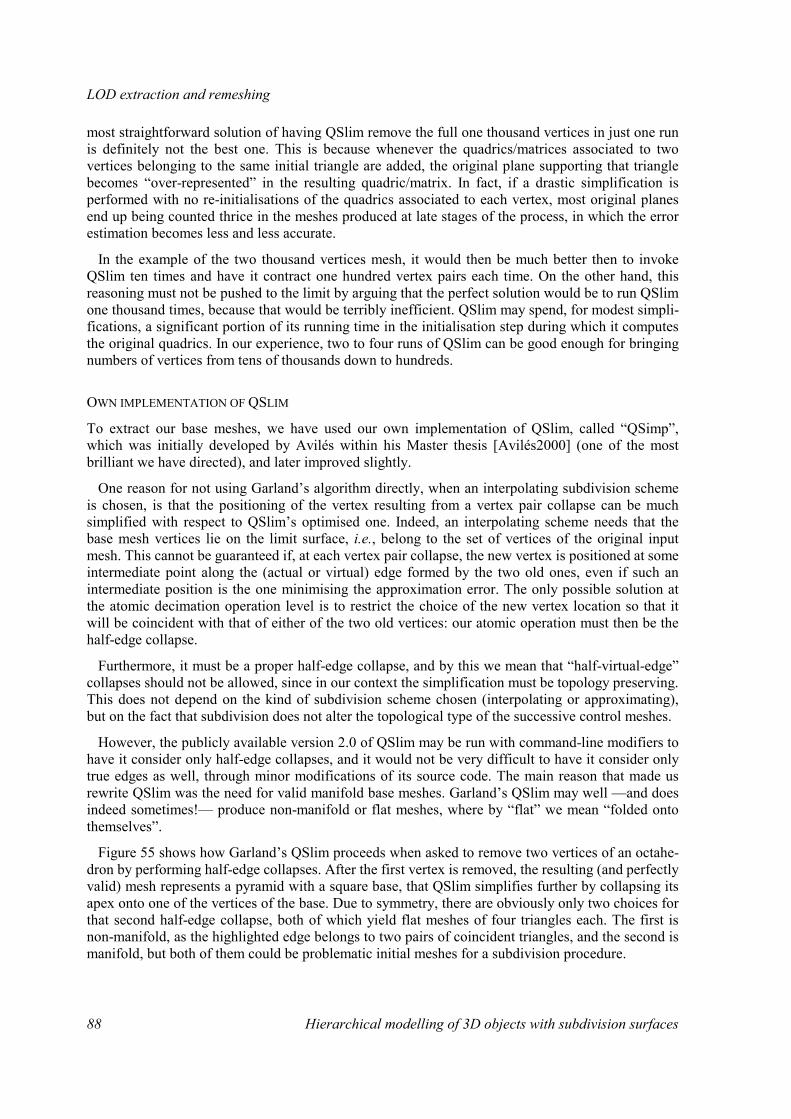
LOD extraction and remeshing
88 Hierarchical modelling of 3D objects with subdivision surfaces
most straightforward solution of having QSlim remove the full one thousand vertices in just one run is definitely not the best one. This is because whenever the quadrics/matrices associated to two vertices belonging to the same initial triangle are added, the original plane supporting that triangle becomes “over-represented” in the resulting quadric/matrix. In fact, if a drastic simplification is performed with no re-initialisations of the quadrics associated to each vertex, most original planes end up being counted thrice in the meshes produced at late stages of the process, in which the error estimation becomes less and less accurate.
In the example of the two thousand vertices mesh, it would then be much better then to invoke QSlim ten times and have it contract one hundred vertex pairs each time. On the other hand, this reasoning must not be pushed to the limit by arguing that the perfect solution would be to run QSlim one thousand times, because that would be terribly inefficient. QSlim may spend, for modest simpli-fications, a significant portion of its running time in the initialisation step during which it computes the original quadrics. In our experience, two to four runs of QSlim can be good enough for bringing numbers of vertices from tens of thousands down to hundreds.
OWN IMPLEMENTATION OF QSLIM
To extract our base meshes, we have used our own implementation of QSlim, called “QSimp”, which was initially developed by Avilés within his Master thesis [Avilés2000] (one of the most brilliant we have directed), and later improved slightly.
One reason for not using Garland’s algorithm directly, when an interpolating subdivision scheme is chosen, is that the positioning of the vertex resulting from a vertex pair collapse can be much simplified with respect to QSlim’s optimised one. Indeed, an interpolating scheme needs that the base mesh vertices lie on the limit surface, i.e., belong to the set of vertices of the original input mesh. This cannot be guaranteed if, at each vertex pair collapse, the new vertex is positioned at some intermediate point along the (actual or virtual) edge formed by the two old ones, even if such an intermediate position is the one minimising the approximation error. The only possible solution at the atomic decimation operation level is to restrict the choice of the new vertex location so that it will be coincident with that of either of the two old vertices: our atomic operation must then be the half-edge collapse.
Furthermore, it must be a proper half-edge collapse, and by this we mean that “half-virtual-edge” collapses should not be allowed, since in our context the simplification must be topology preserving. This does not depend on the kind of subdivision scheme chosen (interpolating or approximating), but on the fact that subdivision does not alter the topological type of the successive control meshes.
However, the publicly available version 2.0 of QSlim may be run with command-line modifiers to have it consider only half-edge collapses, and it would not be very difficult to have it consider only true edges as well, through minor modifications of its source code. The main reason that made us rewrite QSlim was the need for valid manifold base meshes. Garland’s QSlim may well —and does indeed sometimes!— produce non-manifold or flat meshes, where by “flat” we mean “folded onto themselves”.
Figure 55 shows how Garland’s QSlim proceeds when asked to remove two vertices of an octahe-dron by performing half-edge collapses. After the first vertex is removed, the resulting (and perfectly valid) mesh represents a pyramid with a square base, that QSlim simplifies further by collapsing its apex onto one of the vertices of the base. Due to symmetry, there are obviously only two choices for that second half-edge collapse, both of which yield flat meshes of four triangles each. The first is non-manifold, as the highlighted edge belongs to two pairs of coincident triangles, and the second is manifold, but both of them could be problematic initial meshes for a subdivision procedure.
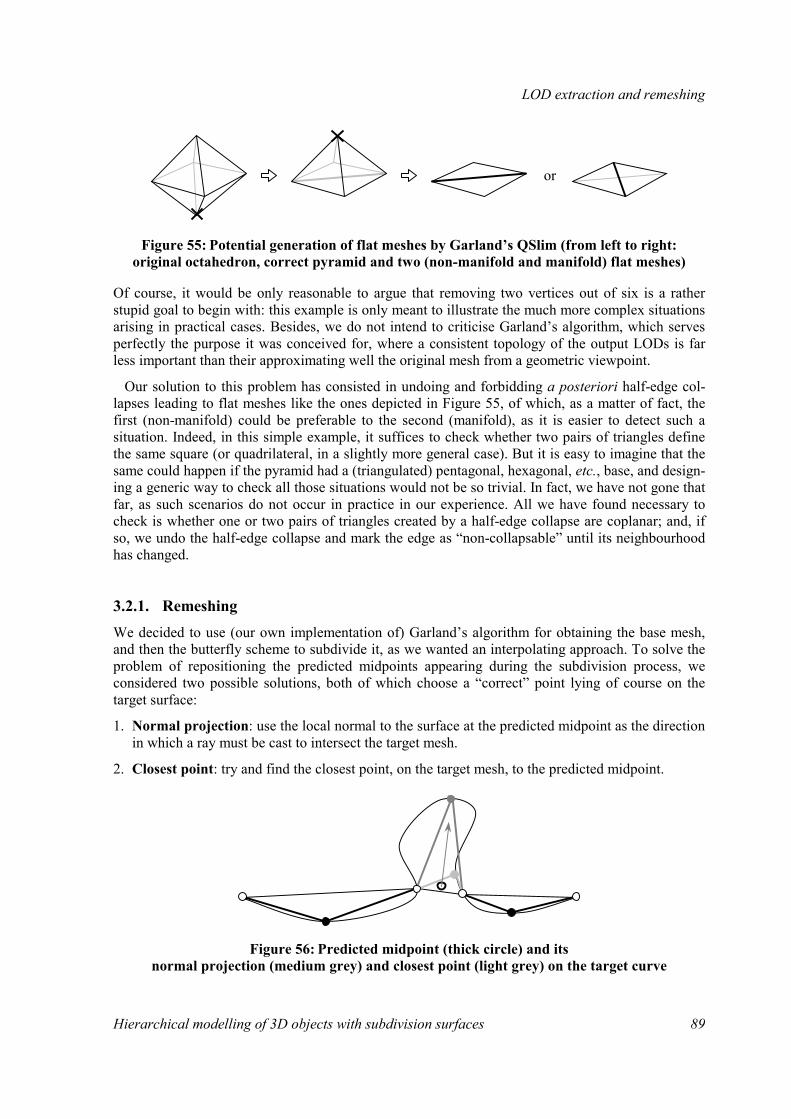
LOD extraction and remeshing
Hierarchical modelling of 3D objects with subdivision surfaces 89
Figure 55: Potential generation of flat meshes by Garland’s QSlim (from left to right: original octahedron, correct pyramid and two (non-manifold and manifold) flat meshes)
Of course, it would be only reasonable to argue that removing two vertices out of six is a rather stupid goal to begin with: this example is only meant to illustrate the much more complex situations arising in practical cases. Besides, we do not intend to criticise Garland’s algorithm, which serves perfectly the purpose it was conceived for, where a consistent topology of the output LODs is far less important than their approximating well the original mesh from a geometric viewpoint.
Our solution to this problem has consisted in undoing and forbidding a posteriori half-edge col-lapses leading to flat meshes like the ones depicted in Figure 55, of which, as a matter of fact, the first (non-manifold) could be preferable to the second (manifold), as it is easier to detect such a situation. Indeed, in this simple example, it suffices to check whether two pairs of triangles define the same square (or quadrilateral, in a slightly more general case). But it is easy to imagine that the same could happen if the pyramid had a (triangulated) pentagonal, hexagonal, etc., base, and design-ing a generic way to check all those situations would not be so trivial. In fact, we have not gone that far, as such scenarios do not occur in practice in our experience. All we have found necessary to check is whether one or two pairs of triangles created by a half-edge collapse are coplanar; and, if so, we undo the half-edge collapse and mark the edge as “non-collapsable” until its neighbourhood has changed.
3.2.1. Remeshing We decided to use (our own implementation of) Garland’s algorithm for obtaining the base mesh, and then the butterfly scheme to subdivide it, as we wanted an interpolating approach. To solve the problem of repositioning the predicted midpoints appearing during the subdivision process, we considered two possible solutions, both of which choose a “correct” point lying of course on the target surface:
1. Normal projection: use the local normal to the surface at the predicted midpoint as the direction in which a ray must be cast to intersect the target mesh.
2. Closest point: try and find the closest point, on the target mesh, to the predicted midpoint.
Figure 56: Predicted midpoint (thick circle) and its normal projection (medium grey) and closest point (light grey) on the target curve
or

LOD extraction and remeshing
90 Hierarchical modelling of 3D objects with subdivision surfaces
Figure 56 illustrates the difference between those two options in the simpler case of an open curve whose coarsest LOD is the polyline of three thin segments joining the four thin circles. When the intermediate segment is subdivided, its predicted midpoint, shown as a thick circle, can be projected onto the target curve along the normal direction (first solution, shown in medium grey) or by finding the closest point (second solution, shown in light grey). Very different results are obtained, contrary to what would happen when subdividing any of the other two segments, the reason being that the simplification was too careless in eliminating the central protuberance of the target curve.
The first option appeared more attractive, so we explored it first and will present it below before the second solution, which we also used nevertheless, as we will explain at the end of this section.
ESTIMATION OF NORMAL VECTOR
Each time an edge is subdivided and a new vertex appears, the local normal n to the surface at the location V predicted by the chosen subdivision scheme is needed to position the new vertex at V', the intersection of a ray cast from V in the direction of n with the input surface. Unfortunately, there is no efficient mechanism to calculate the exact normal to the limit surface obtained with the butterfly scheme [Zorin1997a], so we decided to approximate it, as already mentioned in section 2.4.1. The possibilities we considered were two: Loop’s formula, whose evaluation is less expensive than that of the butterfly scheme, or an area-weighted average of the unit normals of the triangles sharing the edge being subdivided.
Figure 57: Estimation of normal vector
Our choice was the second, for being computationally inexpensive and yielding, in our experience, very satisfactory results. If edge e shared by triangles TA (of oriented unit normal nA and area aA) and TB (nB, aB) is subdivided, as shown in Figure 57, we argue that a good enough approximation to the normal to the limit surface at the new vertex corresponding to e’s midpoint is simply:
n = (aA nA + aB nB) / (aA + aB).
But note well that, in a progressive transmission scenario as ours, all nA, aA, nB, and aB are estimates themselves, as the vertices positions could change until the whole bit-stream is taken into account. This means that the estimation of the normal vector for a given edge must indeed change while the bit-stream is being encoded or decoded, in a way previously agreed upon by encoder and decoder. Our implementation addresses this change in what would be step 1.0 of our version of the SPIHT algorithm presented section 2.4.3.
RAY INTERSECTION
A ray must be cast from the predicted midpoint V in the direction of n, seeking for its possible intersection(s) with the input/target surface. Note that “direction” must be understood here in the
TB (aB)e
nnBnA
TA (aA)

LOD extraction and remeshing
Hierarchical modelling of 3D objects with subdivision surfaces 91
Spanish or French sense, i.e., without an implied orientation: both n and −−−−n would be valid for this purpose, as the intersection point(s), if any, could lie on both sides of the predicted mesh.
In the first volume of the “Graphics Gems” series [Gems1990], Badouel describes an efficient way for establishing whether a ray cast from a point V hits a triangle T, and for finding the intersection point V' if it does:
1. It first determines whether the ray intersects the plane containing T and, if so, the distance d (V, V⊥), V⊥ being the orthogonal projection of V onto that plane (see Figure 25 in section 1.3.1). We have implemented this step with only six products and one division in the worst case, where “worst case” must be understood from the computational viewpoint and in fact corresponds to the best case in terms of hope of finding an intersection.
2. To check efficiently whether V⊥ belongs to T:
� It first projects T onto one of the three coordinate planes, (x, y), (y, z) or (z, x): the one T is “more parallel” to. For us, this is an immediate operation, as we store the normal of each tri-angle, which is thus directly available, and projecting onto the planes (x, y), (y, z) or (z, x) means simply discarding the z, x or y coordinate, respectively.
� Finally, it calculates the normalised parametric coordinates of V⊥ with respect to the projected triangle and verifies that both of them and also their sum belong to [0, 1]: if so, V⊥ is accepted as the sought V'; otherwise, it is rejected. We perform this check with another four products and one division in the worst case.
Problems of both conceptual and computational natures must be addressed. To begin with, such an intersection point V' may not exist (for instance, if the input mesh is open) or be unique (if the input mesh is closed, there are in general two intersection points). But, even if it does and is unique, or if several exist and the one yielding the shortest d (V, V') is chosen, it could lie on any triangle T of the input/target mesh. So a brute force search over the whole set of triangles should in principle be carried, as we do not establish an explicit parameterisation or partition the input mesh in any way: the KISS (Keep It Simple, Stupid) principle behind our approach certainly has advantages, but the input mesh is semantically unrelated to our base mesh and its successive refinements.
Having to examine all the triangles of the input mesh becomes soon an overwhelming task, even if our implementation of Badouel’s algorithm is efficient and permits to discard rapidly many candi-dates. Note that, as each subdivision step multiplies roughly by four the number of edges being split, and hence that of intersection points to be found, the computational requirements of this search process grow exponentially.
ACCELERATED SEARCH THROUGH “VOXELISATION” OF THE INPUT MESH
It is possible to accelerate the search process through a “voxelisation” of the input mesh, consisting in partitioning the bounding box of the input mesh in, say, 10×10×10 equal-sized cells/voxels, and memorising which triangles of the input mesh fall (mostly) in which cell before the subdivision process starts. In that way, when the subdivision process predicts later a midpoint and an intersection has to be found in its vicinity, the search can be conducted in concentrically growing neighbour-hoods. Note that by “concentrically” we do not mean “spherically”, as the neighbourhoods that are easiest to build and visit are the orthogonal ones aligned with the coordinate planes (hints for the navigation can be found in Samet’s books on spatial data structures [Samet1990, Samet1990a]).

LOD extraction and remeshing
92 Hierarchical modelling of 3D objects with subdivision surfaces
Figure 58: Different neighbourhoods of a central cell in orthogonal tilings of the plane (left: 4 + 4 neighbours) and the 3D space (right: 6 + 12 + 8 neighbours)
The notion of concentrically growing neighbourhoods can lead to ambiguity, as illustrated by Figure 58, which shows the different kinds of neighbourhoods in regular orthogonal tilings of 2D and 3D spaces. In the case of the plane, a central cell/pixel (P in Figure 58-left) has two types of neighbours, depending on whether, for jumping from one cell to the next, it is licit to cross only edges or also corners. Those two kinds of vicinities are usually referred to as 4- and 8-neighbourhoods, and con-tain cells {N, E, S, W} and {N, NE, E, SE, S, SW, W, NW} respectively. In the more complex case of 3D space, which is the one of our interest, there are three kinds of neighbourhoods containing 6, 18 and 26 cells/voxels (see Figure 58-right).
Which could be worse is that our concentric neighbourhoods can lead to sheer error if not used carefully, even if the ambiguity is eliminated by deciding to always take successive layers of the full 26-neighbourhoods. Indeed, reasoning again in the plane for simplicity, there are points of the di-agonal cells (NE, SE, SW and NW) which are further away from the central point of P than some of the cells in the second layer of P’s 4-neighbourhood. If it is decided that the search will consider successive layers of 8-neighbourhoods and stop as soon as an intersection point is found, any such point found in NE, for instance, will beat any point in the cell to the North of N, which will never be visited. So it is best to remain on the safe side by stopping the search only when no better solutions are found after visiting one layer beyond the last containing a candidate best solution.
On the other hand, spherical neighbourhoods would not be a good solution either, because they would have to be built for each predicted midpoint, and not once and for all, during the initialisation step of the subdivision procedure — not to mention that the mere decision of choosing the closest intersection point is far from flawless, especially for intricate input/target meshes…
In short, our voxelisation of the input mesh is an efficient mechanism for accelerating the search process, but must be used with care. A generally safe fallback solution consists in zeroing any detail whose estimate is wildly large with respect to the size of the triangle to which it is tied.
CLOSEST POINT INSTEAD OF NORMAL POINT
The algorithm for finding the normal projection of a predicted midpoint V onto the input/target mesh is not substantially different to the one explained in section 1.3.1 for calculating the point to surface distance. Indeed, if V' must be the closest point to V on the target mesh, V⊥ has to be found as well, and it has to be checked as well whether it lies within each considered triangle T. The only modifica-tion to be made to the algorithm described in page 90 is that V⊥ must not be rejected if it does not lie within T: instead, V' must be found by projecting V⊥ onto some edge of T (possibly not orthogonally, as V' can be one of T’s vertices).
Aware of this, and having our accelerated search mechanism in place, we found it only logical to consider that the “correct” position of a predicted midpoint V could be the closest point to it on the target mesh, instead of its normal projection onto it. Not really surprisingly, this approach did not
P
N NE NW
W E
SE S SW

LOD extraction and remeshing
Hierarchical modelling of 3D objects with subdivision surfaces 93
perform much worse than the previous one: for meshes with many intricate regions, or ill-simplified, as in the case of the curve of Figure 56, it is more difficult to reconstruct protuberances eliminated by a careless simplification process; but for generally smooth meshes simplified in a sound manner, it is not.
What does happen, however, is that this solution does not guarantee that the normal component of our details be much greater than the tangential one (dmaxN >> dmaxT: see section 2.4.4). If all predicted midpoints are repositioned in this way, it could result in dmaxN < dmaxT, and thus a bit share in which nN < nT should be chosen. To avoid this, and since the computation of the closest point includes that of the normal projection, what we do is look first for the latter, and resort to the former only if no solution is found, or if the corresponding detail is too large compared to the edge bearing it. We then apply the “safety net” suggested above, consisting in completely zeroing the detail, if the closest point is also too far away from the prediction — a fallback solution we have had to use only with our octahedron/cube model (see Figure 40 in section 2.4.8), but not with any of the other test meshes.
3.2.2. Results The results of our mesh simplification and remeshing tools are integrated in the ones reported in section 2.4.8, as both the extraction of a coarsest LOD and the implied remesh of the input/target mesh are needed by our hierarchical 3D model coding technique. However, we repeat below for convenience the results obtained for the bunny, cow, fist, horse and venus models.
model V T t s T'=t·4s e (10−−−−4)
bunny 35947 69451 271 4 69376 2,421
cow 35381 70758 802 3 51328 5,416
fist 8733 17486 154 3 9856 19,87
fist 8733 17486 274 3 17536 8,351
horse 48485 96966 378 4 96768 2,392
venus 50002 100000 390 4 99840 1,410
Table 6: Summary of remeshing results for the bunny, cow, fist, horse and venus models
The first three columns of each row of Table 6 contain the name of the model and the numbers of vertices V and triangles T of its original input mesh. The following two columns contain the num-bers of triangles t of our choice of base mesh and of systematic subdivision steps s, which permit to calculate the number of triangles T’ of the remesh (T’ = t · 4s), shown in the sixth column. Finally, the remeshing L2 error, relative to the bounding box diagonal and measured with the Metro tool of Cignoni et al. [Cignoni1998] (see section 1.3.1), is given in units of 10−4 in the last column.
These results can be considered excellent for a technique which cannot be simpler, compared to the previously published methods reviewed above. All errors are below 1‰, except for the first remesh of the fist, which contains approximately half as many triangles as the original mesh, and this for details quantised with only 32 bits for their three components.

LOD extraction and remeshing
94 Hierarchical modelling of 3D objects with subdivision surfaces
3.2.3. Guskov’s NM (Normal Mesh) One year after we presented our work, Guskov et al. published in the 2000 edition of SIGGRAPH “Normal Meshes” [Guskov2000], a paper describing a technique developed independently of ours but very similar in spirit. It aims at representing hierarchically closed manifold meshes in such a way that each LOD is expressed as a normal offset from the immediate coarser one. Guskov’s main insight consists in interpreting from the perspective of differential geometry what other researchers have already been exploiting to design predictive coding schemes for 3D meshes: the correlation between the positions of neighbouring vertices in a mesh approximating a smooth surface. Indeed, in a mesh resulting from the sampling of a smooth surface, samples/vertices which are close in the parameter space (i.e., “topologically nearby”) are also closely located in the 3D space. Instead of taking advantage of this from a merely operational viewpoint, to design a predictive coding scheme for the geometry of a mesh, such as the ones described in section 2.1, Guskov draws a more abstract conclusion. In his own words, “while vertex locations come as 3-dimensional quantities, […] locally two of those dimensions represent parametric information and only the third captures geometric, or shape information”. Consequently, he defines a NM as one which can be obtained, starting from a base mesh, by recursively inserting new vertices lying each on a line defined by a base point and normal direction depending only on neighbouring old vertices.
The basic idea for constructing a NM approximating a fine, arbitrary connectivity input one con-sists, as in the cases of Eck’s and Lee’s techniques, in subdividing a base mesh to obtain a remesh of the input one. But in the case of NMs, the details (wavelet coefficients) are strictly aligned with the local normal direction, and can therefore be expressed as scalar quantities, instead of as 3D vectors. The specific way Guskov suggests to proceed to build a NM is the following (in [Guskov2000], the algorithm is presented as having seven stages, but we have grouped them in only three, to establish a parallelism with Eck’s method):
1. Partitioning: A tentative version of the base mesh is first extracted with Garland’s simplification procedure based on quadrics, restricted to perform only half-edge collapses. An initial net of curves is obtained thanks to MAPS that partitions the input mesh into triangular patches, and a substantial effort is then spent in smoothing those curves and repositioning the base mesh vertices so that the resulting parameterisation is globally smooth.
2. Initial parameterisation: Much of the work needed for the construction of a (globally smooth) parameterisation is inherited from the previous stage. In fact, the parameterisation built in this stage by “filling in” the interior of the triangular patches delimited by the net of smoothed curves will be retouched in the next step.
3. “Piercing” and re-parameterisation: All vertices of the remesh lie on the input surface, so the interpolating butterfly scheme is also here the logical choice to predict the new vertex corre-sponding to an edge e being subdivided. The piercing procedure consists in finding, among the (possibly several) intersection points of the ray described above and the input mesh, the one that is closest, in the parametric domain, to the midpoint of e, M (also in the parametric domain). If no such intersection is found, or if its parametric coordinates are further away from M than some user-specified threshold, then M is chosen as an exceptional fall-back solution, and the three co-ordinates of the corresponding input mesh point recorded. But according to Guskov et al., in a vast majority of cases (over 90% for their test meshes), it is possible to find a convenient intersection point near M and therefore store a single scalar value, corresponding to its deviation from the predicted point in the normal direction.
The differences of Guskov’s technique with respect to Eck’s, other than the most important one of not having vectorial wavelet coefficients and having (mostly) scalar ones instead, are thus that:
• expensive and problematic Voronoi diagrams are replaced by MAPS;
LOD extraction and remeshing
Hierarchical modelling of 3D objects with subdivision surfaces 95
• the relative complexity of the parameterisation and remeshing steps is the opposite: in Eck’s case, harmonic maps are used to build a static parameterisation thanks to which the remeshing step is a mere matter of subsampling; in Guskov’s case, on the contrary, the parameterisation is only a seed for a non-trivial stage in which piercings of the input mesh are alternated with MAPS-based re-parameterisations of its successively refined triangular patches.
The main difference between Guskov’s technique and ours is that we do not establish any explicit parameterisation over the base mesh or reposition its vertices, as we were not aiming a priori at having completely normal detail vectors. This saves us an enormous computational load, but also prevents us from obtaining probably better compression ratios and, especially, better rate vs. distor-tion results. Indeed, if the tangential component of all our details were null (dmaxT = 0: see section 2.4.4), our “scalarisation” mechanism would automatically assign the normal component the whole bit budget (nN = NBPD; nT = 0). And then it would most likely suffice to decode only a few bit-planes of those NBPD (i.e., a few bits per vertex) to achieve very low reconstruction errors. This is why we put, immediately below, the finding of an explicit parameterisation as the first item in our list of ideas for future research, as we believe it would be worthwhile comparing its potential com-pression efficiency gains to its complexity.
3.3. Future work
3.3.0. Explicit parameterisation obtained during simplification Perhaps the most obvious shortcoming of our remeshing technique is the absence of an explicit parameterisation. As we obtain the vertices of our remesh when we subdivide recursively the base mesh, obtained previously and independently, we are uncoupling two processes which are intimately related: simplification and reconstruction, i.e., downsampling and upsampling.
It would be beneficial to take advantage of the information that can be gathered during the decima-tion of the input mesh, much as Lee’s MAPS does, although probably with a quadrics driven simpli-fication method acting through edge collapses. Lee himself, in collaboration with Hoppe, has already started to explore this path with “Displaced Subdivision Surfaces” [Lee2000], which is based on MAPS [Lee1998] and Hoppe’s early work [Hoppe1993, Hoppe1994].
3.3.1. Adaptive subdivision A problem related to the obtention of an explicit parameterisation is that of ill-simplificated meshes in which there is a very uneven distribution of the “parametric area”, among the triangles of the base domain, with respect to the 3D surface. Picture the base mesh as a collection of tissue patches that must be gradually stretched, as the subdivision progresses, to wrap the target mesh. Then understand that, if in some of the initial triangles there is enough tissue to cover their corresponding 3D patch, but in others there is not, adding more and more levels of systematic subdivision to facilitate the stretching of the deficient triangles leads to undue accumulation of tissue in the others. Take the curve of Figure 56 for instance: with just one or two subdivision steps, the two exterior segments of the base polyline will do a reasonably good job at approximating the target curve; on the contrary, the interior one would have to be subdivided thrice or more to fill the protuberance, even with the normal projection approach.
One could argue that the best solution to this problem is to prevent such a simplification from hap-pening in the first place. But a simpler solution could be given by adaptive subdivision, perhaps

LOD extraction and remeshing
96 Hierarchical modelling of 3D objects with subdivision surfaces
again à la MAPS. Note that this would be different from the adaptive subdivision considered in our current scheme, which only occurs after a number of systematic subdivision steps.
3.3.2. Optimality of the base mesh Another thread of research it might be interesting to follow concerns the optimality of the base mesh with respect to the following two aspects:
• Position of vertices: Given the topological type of an input surface or mesh, different base 3D meshes of that same topological type and a fixed number of vertices can be obtained by placing those vertices in different locations. Although all would be valid starting points for our hierarchi-cal 3D model coding technique, they would lead to different compression results, independently of the coding technique (Khodakovsky’s PGC or ours), because they establish different base do-mains and thus different (explicit or implicit) parameterisations. To put it in a graphical way, they “comb” the remesh differently, and that affects the degree of space/frequency correlation of the details, which is essential for obtaining good compression results. It would therefore be interest-ing to try and find out whether there exists a way for positioning optimally the vertices of the base mesh. Presumably, doing so would require some global mesh simplification technique, per-haps similar to the one devised by Turk [Turk1992], or taking from Rossignac’s [Rossignac1993] the concept of vertex clustering, which is not far from what could likely be achieved by vector quantisation techniques based on neural nets.
• Number of vertices: An even stronger challenge would be to try and optimise the number of vertices itself, instead of taking it for granted as above. All methods for hierarchical modelling of 3D objects based on SSs published so far, including ours, choose a somehow arbitrary number of vertices for their base mesh, based on obtaining, after a few (3-5) systematic splits, a number of triangles similar to that of their input mesh. The following question should be addressed: cannot the tetrahedron be the base mesh for all surfaces homeomorphic to the sphere?

Conclusions
Hierarchical modelling of 3D objects with subdivision surfaces 97
4. Conclusions
4.0. Contents This chapter closes our dissertation with a summary of our contributions, presented in its first sec-tion, but it also opens, in its second section, several doors leading to potential tracks —or avenues, in some cases!— for future research related to ours.
4.1. Summary The most common way of modelling a 3D object that has to be rendered with a computer is to describe only its bounding surface, as opposed to its inner volume, and the simplest way to do so is to approximate that surface with a polygonal (e.g., triangular) mesh. Planar meshes are the 3D object modelling approach preferred by many industrial applications, and supported by international stan-dards released to date. But approximating accurately smooth or piecewise smooth shapes, such as the ones most frequently found in the real world, can easily lead to planar meshes with a myriad of elements (vertices, edges, and facets). Such meshes can be unmanageable, in the contexts of render-ing or transmission applications, for the most capable computers or networks, and must therefore be simplified by automatic LOD extraction techniques approximating the original approximation with coarser and coarser meshes. What is worse, in applications such as editing, the countless elements of a huge triangular mesh, which are semantically unrelated to each other, must be repositioned indi-vidually in a cumbersome process. This is why other commercial applications in the fields of CAGD and computer-generated animation encourage the use of curved patches such as NURBSs, which are unfortunately problematic as well for modelling non-planar topologies or fine-grain details.
SSs are a powerful 3D object modelling paradigm that may be regarded as a bridge between the two extremes described above: polygons and patches. Subdivision schemes permit to derive a (piecewise) smooth limit surface through the recursive refinement of a coarse polygonal control mesh of arbitrary connectivity, which can be described very compactly. Moreover, the recursiveness inherent to SSs establishes naturally a pyramidal nesting between the successively generated meshes/LODs. This makes SSs most suitable for defining MRA tools to represent surfaces, which have immediate and most interesting applications such as hierarchical 3D model coding and editing.
In the first chapter of this dissertation we have described the linkage between the three main knowledge areas which have served as a basis for our work: SSs, automatic LOD extraction, and wavelet-based MRA. To the best of our knowledge, this is the first compilation and synthesis work

Conclusions
98 Hierarchical modelling of 3D objects with subdivision surfaces
explaining how these three pieces of the puzzle of hierarchical modelling of 3D objects with SSs fit together. The classic wavelet theory applies to classic nD signals, i.e., those defined on parametric domains homeomorphic to n or [0, 1]n, such as audio (n = 1), still images (n = 2) or video (n = 3). In such topologically trivial domains, it is easy to express the signal in bases of functions which are hierarchically nested because of being dilates and translates of a single mother function. In non-trivial topological settings such as generic 2D manifolds (i.e., surfaces embedded in 3D space), translation and dilation loose their meaning, but wavelet-based MRA of surfaces is nevertheless possible if approached from the subdivision viewpoint. It suffices to:
1. extract a coarse mesh, approximating the considered surface at a low LOD, thanks to a (prefera-bly automatic) mesh simplification technique;
2. use that coarse mesh as the seed for a recursive subdivision process, during which the 3D details (i.e., wavelet coefficients) needed to obtain finer and finer approximations to the original shape are added to the new vertex positions predicted by the considered subdivision scheme.
The practical applications of hierarchical modelling of 3D objects with SSs constitute nevertheless our main original development. In particular, we have devised the method for truly hierarchical 3D model coding based on SSs that is described in the second chapter. Our technique has led to two international publications [Morán1999, Morán2000], and is currently being considered inside the AFX subgroup of MPEG-SNHC for its adoption in the future version 5 of the MPEG-4 standard, due October 2002 [Morán2001]. It consists in representing compactly the 3D details mentioned in the step 2 above by:
a. expressing them in a local normal coordinate frame;
b. organising them in a facet-based hierarchical set;
c. quantising them in such a manner that their normal component, which carries the most energy one, is treated better than their tangential components and “scalarising” them for
d. feeding the set they form into an algorithm similar to the SPIHT designed by Said and Pearlman, followed by selective arithmetic coding of the symbol types exhibiting the highest correlation.
The final outcome is a fully embedded code much more compact than those of previously published progressive 3D mesh coding methods such as Taubin’s PFS or Rossignac’s CPM, which typically achieve bit-rates of around 20 bit/vertex for good reconstructions. With our method, it possible to remain typically below 10 bit/vertex while achieving very low reconstruction errors of less than 1‰ (L2 error relative to the bounding box diagonal). For mainly smooth models, like the ones most frequently found in practice, high quality reconstructions with errors in the order of units of 10−4 can be obtained with rates as low as 1-2 bit/vertex. Besides, such progressive 3D mesh coding methods insist on representing exactly (up to some quantisation error affecting vertex positions) a particular planar mesh, which is only a first order approximation of a usually piecewise smooth surface, and whose vertices are semantically unrelated. Our hierarchical 3D model coding technique inherently defines a smooth limit surface, and does so by producing truly pyramidally nested control meshes, thus providing naturally multiresolution editing/animation handles.
Finally, in the third chapter we describe the auxiliary methods we have had to design to offer a complete solution for the hierarchical modelling of 3D objects with SSs. We have built on Garland’s popular 3D mesh simplification technique based on quadrics, to improve it and have an automatic LOD extractor better suited to solve the problem mentioned in step 1 above. We have designed as well an implicit remeshing method for computing the details required by step a of our hierarchical 3D model coding technique. It is much simpler than previous approaches, such as Eck’s or Lee’s MAPS, as it does not establish an explicit parameterisation of the input/target mesh over the base domain (the coarsest level mesh), and yet it has proven to be effective enough for our needs.

Conclusions
Hierarchical modelling of 3D objects with subdivision surfaces 99
4.2. Future work Apart from the desirable extensions described in section 2.5.0, thanks to which our hierarchical 3D model coding technique would be able to handle meshes with properties (normals, colours, textures) and surfaces with sharp features and/or non-manifold and/or non-orientable, we see several direc-tions in which research related to ours could conceivably carry on:
• Regarding our hierarchical 3D model coding technique:
� Our detail vectors have one component (the normal one) which is clearly more energetic than the rest (the two tangential ones). Probably more compression efficiency can be obtained by spatially subsampling the tangential components with respect to the normal one, on top of quantising them more crudely.
� If a low level detail is decoded erroneously, e.g., because of having been transmitted over a noisy channel, the reconstructed positions of all nearby vertices of higher LODs will be wrong. Also, a client-driven transmission scenario can be imagined in which the client could request to the server, through a back-channel, the exclusive transmission of the visible areas of a 3D object. Error resilience and view-dependent coding are two certainly interesting goals which could be achieved by considering independently the details lying on each base mesh triangle and consequently partitioning the bit-stream through the insertion of markers.
• Regarding hierarchical modelling (and maybe coding as well) of more complex objects:
� An extension considering animated surfaces could be of great importance, not only theoreti-cally, but also in terms of its potential for practical applications. Currently, there are several 3D object modelling and animation software vendors which are starting to include SS mod-ules in their flagship products, but this is a market with plenty of proprietary solutions and few common standards, if any. If a homogeneous solution based on SSs were designed to handle the hierarchical modelling (and hopefully coding) of both static and dynamic objects, it could have a remarkable commercial success.
� Tetrahedral meshes of 3D solids are widely used in the FEM world, where refinement by sub-division is approached in a non-recursive/hierarchical manner. Perhaps our proposal of a 3D midpoint subdivision scheme for tetrahedral meshes could be further developed and used in the context of finite element analysis, where subdivision surfaces have already raised interest.
• Regarding our auxiliary techniques for automatic LOD extraction and remeshing:
� It would be certainly beneficial to take advantage of the information that can be gathered dur-ing the decimation of the input mesh, much as Lee’s MAPS does, although probably with a quadrics driven simplification method acting through edge collapses. Another interesting characteristic of MAPS that is worth being adopted is its adaptiveness: thanks to it, it is possi-ble to solve partially the problems encountered when trying to reconstruct through systematic subdivision and with a spatially homogeneous low error an intricate input mesh after having ill-simplified it.
� Finally, it could be worth trying to find out whether there exists a way for positioning opti-mally a given number of vertices defining the base mesh, an even stronger challenge being to try and optimise the number of vertices itself, instead of taking it for granted.


References
Hierarchical modelling of 3D objects with subdivision surfaces 101
5. References
5.0. Contents Although we realise it may make this chapter somewhat more difficult to browse, we have decided to divide it into three different sections: the first contains books or book chapters, Ph.D. or Master theses, and released international standards; the second lists journal or conference papers, technical reports or working drafts for international standards, and course notes; the third is devoted to publi-cations that are only available on-line�. The fussy reader must be warned that a few of the references listed below are not explicitly mentioned in the dissertation, and that we have chosen not to stan-dardise in any way the capitalisation or spelling of the words in the titles, or to complete in any way the initials in the names of the authors: both words and names are shown as originally published.
5.1. Books, theses and international standards [Avilés2000] Marcos Avilés Rodrigálvarez: “Simplificación automática de mallas 3D”, pro-
yecto fin de carrera, Universidad Politécnica de Madrid, mayo 2000.
[Bézier1986] Pierre E. Bézier: “Courbes et surfaces”, volume 4 de “Mathématiques et CAO”, Hermès Publishing, 1986.
[Catmull1974] Edwin E. Catmull: “A Subdivision Algorithm for Computer Display of Curved Surfaces”, Ph.D. thesis, University of Utah, December 1974.
[deBoor1978] Carl de Boor: “A Practical Guide to Splines”, Springer-Verlag, 1978.
[deCasteljau1985] Paul de Faget de Casteljau: “Formes à pôles”, volume 2 de “Mathématiques et CAO”, Hermès Publishing, 1985.
[Deslauriers1987] G. Deslauriers et S. Dubuc: “Interpolation dyadique”, pages 44-55 de “Fractals: dimensions non entières et applications” (édité par G. Cherbit et J.-P. Kahane), Masson, 1987.
� All URLs given for documents available on-line in the Internet are valid as of 20011002.

References
102 Hierarchical modelling of 3D objects with subdivision surfaces
[Du1988] Wen-Hui Du: “Étude sur la représentation de surfaces complexes: applicaction à la reconstruction de surfaces échantillonnées”, thèse de doctorat, École Nationale Supérieure des Télécommunications de Paris, Octobre 1988.
[Farin1993] Gerald E. Farin: “Curves and Surfaces for Computer Aided Geometric Design: A Practical Guide” (3rd ed.), Academic Press, 1993.
[Foley1997] James D. Foley, Andries van Dam, Steven K. Feiner and John F. Hughes: “Com-puter Graphics: Principles and Practice” (2nd edition in C), Addison-Wesley, 1997.
[Fourier1822] J. Fourier: “Théorie analytique de la chaleur”, Firmin Didot, Père et Fils, 1822.
[Gems1990] Several authors: “Graphics Gems” (edited by Andrew S. Glassner), Academic Press, 1990.
[Gems1991] Several authors: “Graphics Gems II” (edited by James Arvo), Academic Press, 1991.
[Gems1992] Several authors: “Graphics Gems III” (edited by David Kirk), Academic Press, 1992.
[Hamming1986] Richard W. Hamming: “Coding and Information Theory” (2nd ed.), Prentice-Hall, 1986.
[Hughes1987] Thomas J. R. Hughes: “The Finite Element Method: Linear Static and Dynamic Finite Element Analysis”, Prentice-Hall, 1987.
[Loop1987] Charles Loop: “Smooth Subdivision Surfaces Based on Triangles”, Master thesis, University of Utah, August 1987.
[Lounsbery1994] John Michael Lounsbery: “Multiresolution Analysis for Surfaces of Arbitrary Topological Type”, Ph.D. thesis, University of Washington, September 1994.
[Massey1989] W. S. Massey: “Algebraic Topology: an Introduction” (8th ed.), Springer-Verlag, 1989.
[Morán1992] Francisco Morán Burgos: “Desarrollo e integración de herramientas de visualiza-ción de objetos 3-D reales modelados por recubrimientos superficiales aproxima-dos”, proyecto fin de carrera, Universidad Politécnica de Madrid, junio 1992.
[MPEG1998] MPEG (Moving Picture Experts Group, formally ISO/IEC JTC1/SC29/WG11): “ISO/IEC 14496 Information technology — Coding of audio-visual objects” (a.k.a. “MPEG-4 version 1”), ISO/IEC standard, October 1998. In fact, this is when the work regarding the three main Parts of the Standard was finalised, but they were not released by ISO until the beginning of 1999. These three main Parts of MPEG-4 must be individually referred to as “ISO/IEC 14496-1:1999 In-formation technology — Coding of audio-visual objects — Part 1: Systems”, “ISO/IEC 14496-2:1999 […] — Part 2: Visual” and “ISO/IEC 14496-3:1999 […] — Part 3: Audio”. Parts 4 (Conformance testing), 5 (Reference software) and 6 (DMIF: Delivery Multimedia Integration Framework) were released in 2000.

References
Hierarchical modelling of 3D objects with subdivision surfaces 103
[MPEG1999] MPEG (Moving Picture Experts Group, formally ISO/IEC JTC1/SC29/WG11): “ISO/IEC 14496/Amd 1 Extensions” (a.k.a. “MPEG-4 version 2”), ISO/IEC standard, December 1999. Again, this is the date in which several backward compatible extensions to MPEG-4 version 1 were frozen, but ISO released them in the first months of 2000 as “ISO/IEC 14496-2:1999/Amd 1:2000 Visual ex-tensions” and “ISO/IEC 14496-3:1999/Amd 1:2000 Audio extensions”.
[Neider1993] Jackie Neider, Tom Davis and Mason Woo: “OpenGL Programming Guide”, Addison-Wesley, 1993.
[O’Rourke1994] Joseph O’Rourke: “Computational geometry in C”, Cambridge University Press, 1994.
[Samet1990] Hanan Samet: “The Design and Analysis of Spatial Data Structures”, Addison-Wesley, 1990.
[Samet1990a] Hanan Samet: “Applications of Spatial Data Structures”, Addison-Wesley, 1990.
[Schweitzer1996] Jean E. Schweitzer: “Analysis and Application of Subdivision Surfaces”, Ph.D. thesis, University of Washington, August 1996.
[Shannon1949] Claude E. Shannon and Warren Weaver: “The Mathematical Theory of Communication”, University of Illinois Press, 1949.
[Vetterli1995] Martin Vetterli and Jelena Kovačević: “Wavelets and Subband Coding”, Pren-tice-Hall, 1995.
[VRML1997] VRML (Virtual Reality Modelling Language) Consortium Inc. (now Web3D Consortium Inc.) and ISO/IEC JTC1/SC24: “ISO/IEC 14772-1:1997” (a.k.a. “VRML97”), ISO/IEC standard, December 1997.
[Zorin1997a] Denis N. Zorin: “Subdivision and Multiresolution Surface Representations”, Ph.D. thesis, California Institute of Technology, September 1997 — presented in 1998.
5.2. Papers, technical reports and course notes [Ball1988] A. A. Ball and D. J. T. Storry: “Conditions for tangent plane continuity over
recursively generated B-spline surfaces”, ACM Transactions on Graphics, 7-2, 83-102, April 1988.
[Barequet1996] Gill Barequet, Bernard Chazelle, Leonidas J. Guibas, Joseph S. B. Mitchell and Ayellet Tal: “BOXTREE: A Hierarchical Representation for Surfaces in 3D”, EUROGRAPHICS ’96 conference proceedings (Computer Graphics Forum, 15-3), C387-C396, August 1996.
[Biermann2000] Henning Biermann, Adi Levin and Denis Zorin: “Piecewise Smooth Subdivision Surfaces with Normal Control”, ACM SIGGRAPH 2000 conference proceed-ings�, 113-120, July 2000.
� Note that the ACM SIGGRAPH conference proceedings are published as special numbers of the journal “ACM SIGGRAPH Computer Graphics”, and are thus sometimes referred to as “ACM SIGGRAPH Computer Graphics, Annual Conference Series”.

References
104 Hierarchical modelling of 3D objects with subdivision surfaces
[Catmull1978] E. Catmull and J. Clark: “Recursively generated B-spline surfaces on arbitrary topological meshes”, Computer-Aided Design, 10-6, 350-355, November 1978.
[Certain1996] Andrew Certain, Jovan Popović, Tony DeRose, Tom Duchamp, David Salesin and Werner Stuetzle: “Interactive Multiresolution Surface Viewing”, ACM SIG-GRAPH 96 conference proceedings, 91-98, August 1996.
[Chaikin1974] G. M. Chaikin: “An algorithm for high speed curve generation”, Computer Graphics Image Processing, 3-4, 346-349, December 1974.
[Ciampalini1997] A. Ciampalini, P. Cignoni, C. Montani and R. Scopigno: “Multiresolution deci-mation based on global error”, The Visual Computer, 13-5, 228-246, May 1997.
[Cignoni1998] P. Cignoni, C. Rocchini and R. Scopigno: “Metro: measuring error on simplified surfaces”, Computer Graphics Forum, 17-2, 167-174, June 1998. Binary code for SGI workstations running IRIX (SGI’s UNIX) is publicly available on-line at “http://vcg.iei.pi.cnr.it./metro.html”.
[Cignoni1998a] P. Cignoni, C. Montani, C. Rocchini and R. Scopigno: “A general method for preserving attribute values on simplified meshes”, IEEE Visualization ’98 con-ference proceedings, 59-66, October 1998.
[Cirak2000] Fehmi Cirak, Michael Ortiz and Peter Schröder: “Subdivision Surfaces: A New Paradigm for Thin-Shell Finite-Element Analysis”, submitted to International Journal on Numerical Methods in Engineering, August 2000.
[Clark1976] J. H. Clark: “Hierarchical Geometric Models for Visible Surface Algorithms”, Communications of the ACM, 19-10, 547-554, October 1976.
[Clay1988] Reed D. Clay and Henry P. Moreton: “Efficient Adaptive Subdivision of Bézier Surfaces”, EUROGRAPHICS ’88 conference proceedings (Computer Graphics Forum, 7-3), C357-C371, September 1988.
[Cohen1996] Jonathan Cohen, Amitabh Varshney, Dinesh Manocha, Greg Turk, Hans Weber, Pankaj Agarwal, Frederick Brooks and William Wright: “Simplification Enve-lopes”, ACM SIGGRAPH 96 conference proceedings, 119-128, August 1996.
[Cohen1998] Jonathan Cohen, Marc Olano and Dinesh Manocha: “Appearance-Preserving Simplification”, ACM SIGGRAPH 98 conference proceedings, 115-122, July 1998.
[Cohen-Or1999] Daniel Cohen-Or, David Levin and Offir Remez: “Progressive compression of arbitrary triangular meshes”, IEEE Visualization ’99 conference proceedings, 67-72, October 1999.
[Daubechies1988] Ingrid Daubechies: “Orthonormal Bases of Compactly Supported Wavelets”, Communications on Pure and Applied Mathematics, XLI, 909-996, October 1988.
[Deering1995] Michael Deering: “Geometry Compression”, ACM SIGGRAPH 95 conference proceedings, 13-20, August 1995.
[DeFloriani1995] L. De Floriani and E. Puppo: “Hierarchical Triangulation for Multiresolution Surface Description”, ACM Transactions on Graphics, 14-4, 363-411, October 1995.
[DeRose1998] Tony DeRose, Michael Kass and Tien Truong: “Subdivision Surfaces in Charac-ter Animation”, ACM SIGGRAPH 98 conference proceedings, 85-94, July 1998.
References
Hierarchical modelling of 3D objects with subdivision surfaces 105
[Desbrun1999] Mathieu Desbrun, Mark Meyer, Peter Schröder and Alan Barr: “Implicit Fairing of Irregular Meshes using Diffusion and Curvature Flow”, ACM SIGGRAPH 99 conference proceedings, 317-324, August 1999.
[Donoho1992] David L. Donoho: “Interpolating Wavelet Transforms”, technical report (54 pages), Stanford University, October 1992.
[Doo1978] D. Doo and M. Sabin: “Behaviour of recursive division surfaces near extraordi-nary points”, Computer-Aided Design, 10-6, 356-360, November 1978.
[Dyn1987] Nira Dyn, David Levin and John A. Gregory: “A four-point interpolatory subdi-vision scheme for curve design”, Computer-Aided Geometric Design, 4, 257-268, July 1987.
[Dyn1990] Nira Dyn, David Levin and John A. Gregory: “A Butterfly Subdivision Scheme for Surface Interpolation with Tension Control”, ACM Transactions on Graphics, 9-2, 160-169, April 1990.
[Dyn1992] Nira Dyn, David Levin and D. Liu: “Interpolatory convexity-preserving subdivi-sion schemes for curves and surfaces”, Computer-Aided Design, 24-4, 211-216, April 1992.
[Eck1995] Matthias Eck, Tony DeRose, Tom Duchamp, Hugues Hoppe, Michael Lounsbery and Werner Stuetzle: “Multiresolution Analysis of Arbitrary Meshes”, ACM SIG-GRAPH 95 conference proceedings, 173-182, August 1995.
[Eck1996] Matthias Eck and Hugues Hoppe: “Automatic Reconstruction of B-Spline Sur-faces of Arbitrary Topological Type”, ACM SIGGRAPH 96 conference proceed-ings, 325-334, August 1996.
[Erikson1996] Carl Erikson: “Polygonal Simplification: An Overview”, technical report (32 pages), University of North Carolina at Chapel Hill, February 1996.
[Finkeltstein1994] Adam Finkelstein and David H. Salesin: “Multiresolution Curves”, ACM SIG-GRAPH 94 conference proceedings, 261-268, July 1994.
[Garland1997] Michael Garland and Paul S. Heckbert: “Surface Simplification Using Quadric Error Metrics”, ACM SIGGRAPH 97 conference proceedings, 209-216, August 1997.
[Grosso1998] Roberto Grosso and Thomas Ertl: “Progressive Iso-Surface Extraction from Hierarchical 3D Meshes”, EUROGRAPHICS ’98 conference proceedings (Com-puter Graphics Forum, 17-3), C125-C135, September 1998.
[Guéziec1995] André Guéziec: “Surface Simplification with Variable Tolerance”, MRCAS (Medical Robotics and Computer Assisted Surgery) ’95 symposium proceedings, 132-139, November 1995.
[Guéziec1999] André Guéziec, Frank Bossen, Gabriel Taubin and Claudio Silva: “Efficient compression of non-manifold meshes”, Computational Geometry: Theory and Applications, 14-1-3, 137-166, November 1999.
[Gumhold1998] Stefan Gumhold and Wolfgang Straßer: “Real Time Compression of Triangle Mesh Connectivity”, ACM SIGGRAPH 98 conference proceedings, 133-140, July 1998.

References
106 Hierarchical modelling of 3D objects with subdivision surfaces
[Guskov1999] Igor Guskov, Wim Sweldens and Peter Schröder: “Multiresolution Signal Proc-essing for Meshes”, ACM SIGGRAPH 99 conference proceedings, 325-334, Au-gust 1999.
[Guskov2000] Igor Guskov, Kiril Vidimče, Wim Sweldens and Peter Schröder: “Normal Meshes”, ACM SIGGRAPH 2000 conference proceedings, 95-102, July 2000.
[Haar1910] Alfred Haar: “Zur Theorie der orthogonalen Funktionensysteme”, Mathematische Annalen, 69, 331-371, 1910.
[Hoppe1993] Hugues Hoppe, Tony DeRose, Tom Duchamp, John McDonald and Werner Stuetzle: “Mesh Optimization”, ACM SIGGRAPH 93 conference proceedings, 19-26, August 1993.
[Hoppe1994] Hugues Hoppe, Tony DeRose, Tom Duchamp, Mark Halstead, Hubert Jin, John McDonald, Jean Schweitzer and Werner Stuetzle: “Piecewise Smooth Surface Reconstruction”, ACM SIGGRAPH 94 conference proceedings, 295-302, July 1994.
[Hoppe1996] Hugues Hoppe: “Progressive Meshes”, ACM SIGGRAPH 96 conference proceedings, 99-108, August 1996.
[Hoppe1997] Hugues Hoppe: “View-Dependent Refinement of Progressive Meshes”, ACM SIGGRAPH 97 conference proceedings, 189-198, August 1997.
[Karni2000] Zachi Karni and Craig Gotsman: “Spectral Compression of Mesh Geometry”, ACM SIGGRAPH 2000 conference proceedings, 279-286, July 2000.
[Khodakovsky2000] Andrei Khodakovsky, Peter Schröder and Wim Sweldens: “Progressive Geome-try Compression”, ACM SIGGRAPH 2000 conference proceedings, 271-278, July 2000.
[King1999] Davis King and Jarek Rossignac: “Optimal Bit Allocation in Compressed 3D Models”, Computational Geometry: Theory and Applications, 14-1-3, 91-118, November 1999.
[Kobbelt1996] Leif Kobbelt: “Interpolatory Subdivision on Open Quadrilateral Nets with Arbi-trary Topology”, EUROGRAPHICS ’96 conference proceedings (Computer Graphics Forum, 15-3), C409-C420, August 1996.
[Kobbelt1998] Leif Kobbelt, Swen Campagna, Jens Vorsatz and Hans-Peter Seidel: “Interactive Multiresolution Modeling on Arbitrary Meshes”, ACM SIGGRAPH 98 confer-ence proceedings, 105-114, July 1998.
[Kobbelt2000] Leif Kobbelt: “ 3 -Subdivision”, ACM SIGGRAPH 2000 conference proceed-ings, 103-112, July 2000.
[Kolarov1996] Krasimir Kolarov and William Lynch: “Compression of Scalar Functions De-fined on 2-Manifolds”, technical report (25 pages), Interval Research Corpora-tion, September 1996.
[Krishnamurthy1996] Venkat Krishnamurthy and Marc Levoy: “Fitting Smooth Surfaces to Dense Polygon Meshes”, ACM SIGGRAPH 96 conference proceedings, 313-324, Au-gust 1996.
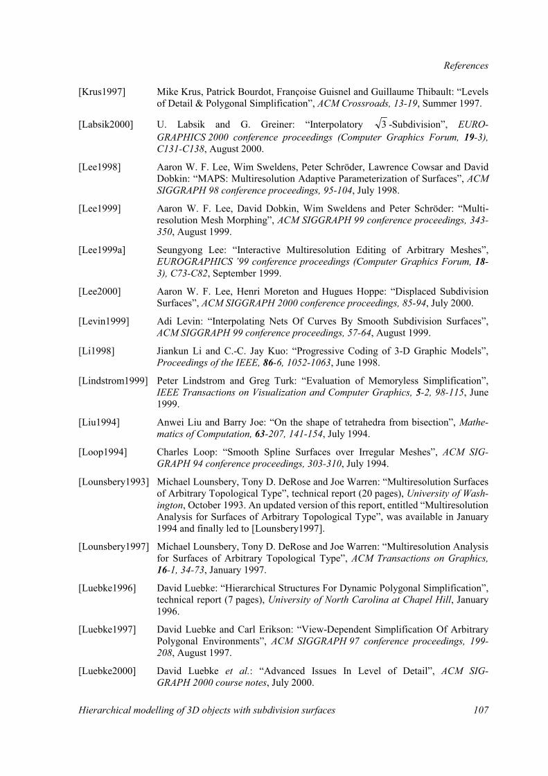
References
Hierarchical modelling of 3D objects with subdivision surfaces 107
[Krus1997] Mike Krus, Patrick Bourdot, Françoise Guisnel and Guillaume Thibault: “Levels of Detail & Polygonal Simplification”, ACM Crossroads, 13-19, Summer 1997.
[Labsik2000] U. Labsik and G. Greiner: “Interpolatory 3 -Subdivision”, EURO-GRAPHICS 2000 conference proceedings (Computer Graphics Forum, 19-3), C131-C138, August 2000.
[Lee1998] Aaron W. F. Lee, Wim Sweldens, Peter Schröder, Lawrence Cowsar and David Dobkin: “MAPS: Multiresolution Adaptive Parameterization of Surfaces”, ACM SIGGRAPH 98 conference proceedings, 95-104, July 1998.
[Lee1999] Aaron W. F. Lee, David Dobkin, Wim Sweldens and Peter Schröder: “Multi-resolution Mesh Morphing”, ACM SIGGRAPH 99 conference proceedings, 343-350, August 1999.
[Lee1999a] Seungyong Lee: “Interactive Multiresolution Editing of Arbitrary Meshes”, EUROGRAPHICS ’99 conference proceedings (Computer Graphics Forum, 18-3), C73-C82, September 1999.
[Lee2000] Aaron W. F. Lee, Henri Moreton and Hugues Hoppe: “Displaced Subdivision Surfaces”, ACM SIGGRAPH 2000 conference proceedings, 85-94, July 2000.
[Levin1999] Adi Levin: “Interpolating Nets Of Curves By Smooth Subdivision Surfaces”, ACM SIGGRAPH 99 conference proceedings, 57-64, August 1999.
[Li1998] Jiankun Li and C.-C. Jay Kuo: “Progressive Coding of 3-D Graphic Models”, Proceedings of the IEEE, 86-6, 1052-1063, June 1998.
[Lindstrom1999] Peter Lindstrom and Greg Turk: “Evaluation of Memoryless Simplification”, IEEE Transactions on Visualization and Computer Graphics, 5-2, 98-115, June 1999.
[Liu1994] Anwei Liu and Barry Joe: “On the shape of tetrahedra from bisection”, Mathe-matics of Computation, 63-207, 141-154, July 1994.
[Loop1994] Charles Loop: “Smooth Spline Surfaces over Irregular Meshes”, ACM SIG-GRAPH 94 conference proceedings, 303-310, July 1994.
[Lounsbery1993] Michael Lounsbery, Tony D. DeRose and Joe Warren: “Multiresolution Surfaces of Arbitrary Topological Type”, technical report (20 pages), University of Wash-ington, October 1993. An updated version of this report, entitled “Multiresolution Analysis for Surfaces of Arbitrary Topological Type”, was available in January 1994 and finally led to [Lounsbery1997].
[Lounsbery1997] Michael Lounsbery, Tony D. DeRose and Joe Warren: “Multiresolution Analysis for Surfaces of Arbitrary Topological Type”, ACM Transactions on Graphics, 16-1, 34-73, January 1997.
[Luebke1996] David Luebke: “Hierarchical Structures For Dynamic Polygonal Simplification”, technical report (7 pages), University of North Carolina at Chapel Hill, January 1996.
[Luebke1997] David Luebke and Carl Erikson: “View-Dependent Simplification Of Arbitrary Polygonal Environments”, ACM SIGGRAPH 97 conference proceedings, 199-208, August 1997.
[Luebke2000] David Luebke et al.: “Advanced Issues In Level of Detail”, ACM SIG-GRAPH 2000 course notes, July 2000.
References
108 Hierarchical modelling of 3D objects with subdivision surfaces
[Mallat1989] Stéphane Mallat: “A theory for multiresolution signal decomposition: the wavelet representation”, IEEE Transactions on Pattern Analysis and Machine Intelli-gence, 11-7, 674-693, July 1989.
[Morán1999] Francisco Morán: “Hierarchical 3D mesh coding with subdivision surfaces”, IWSNHC3DI (International Workshop on Synthetic/Natural Hybrid Coding and Three Dimensional Imaging) ’99 proceedings, 189-192, September 1999.
[Morán2000] Francisco Morán and Narciso García: “Hierarchical coding of 3D models with subdivision surfaces”, IEEE ICIP (International Conference on Image Process-ing) 2000 proceedings, II, 911-914, September 2000.
[Morán2001] Francisco Morán and Michael Steliaros: “Truly Hierarchical Coding of 3D Models with Subdivision Surfaces”, proposal for ISO/IEC standard (14 pages), MPEG-SNHC input document MPEG2001/M7465, July 2001.
[MPEG2001] MPEG (Moving Picture Experts Group, formally ISO/IEC JTC1/SC29/WG11): “Animation Framework eXtension Core Experiments description”, MPEG-SNHC output document WG11/N4220, July 2001 — work in progress towards “ISO/IEC 14496-1/Amd 4” (a.k.a. “MPEG-4 Systems version 5”), ISO/IEC standard due October 2002.
[MPEG2001a] MPEG (Moving Picture Experts Group, formally ISO/IEC JTC1/SC29/WG11): “Animation Framework eXtension Verification Model version 4.0”, MPEG-SNHC output document WG11/N4221, July 2001 — work in progress towards “ISO/IEC 14496-1/Amd 4” (a.k.a. “MPEG-4 Systems version 5”), ISO/IEC stan-dard due October 2002.
[MPEG2001b] MPEG (Moving Picture Experts Group, formally ISO/IEC JTC1/SC29/WG11): “Animation Framework eXtension Working Draft version 3.0”, MPEG-Systems output document WG11/N4272, July 2001 — work in progress towards “ISO/IEC 14496-1/Amd 4” (a.k.a. “MPEG-4 Systems version 5”), ISO/IEC standard due October 2002.
[Pajarola2000] Renato Pajarola and Jarek Rossignac: “Compressed Progressive Meshes”, IEEE Transactions on Visualization and Computer Graphics, 6-1, 79-93, March 2000.
[Pajarola2000a] Renato Pajarola and Jarek Rossignac: “Squeeze: Fast and Progressive Decom-pression of Triangle Meshes”, Computer Graphics International conference pro-ceedings, 173-182, June 2000.
[Peters1997] Jörg Peters and Ahmad Nasri: “Computing Volumes of Solids Enclosed by Recursive Subdivision Surfaces”, EUROGRAPHICS ’97 conference proceedings (Computer Graphics Forum, 16-3), C89-C94, September 1997.
[Popović1997] Jovan Popović and Hugues Hoppe: “Progressive Simplicial Complexes”, ACM SIGGRAPH 97 conference proceedings, 217-224, August 1997.
[Ramshaw1989] Lyle Ramshaw: “Blossoms Are Polar Forms”, technical report (46 pages), Digi-tal Equipment Corporation Systems Research Center, January 1989.
[Reif1995] Ulrich Reif: “A unified approach to subdivision algorithms near extraordinary points”, Computer-Aided Geometric Design, 12-2, 153-174, March 1995.
[Ronfard1994] Rémi Ronfard and Jarek Rossignac: “Triangulating multiply-connected poly-gons: A simple, yet efficient algorithm”, EUROGRAPHICS ’94 conference pro-ceedings (Computer Graphics Forum, 13-3), C281-C292, September 1994.
References
Hierarchical modelling of 3D objects with subdivision surfaces 109
[Ronfard1996] Rémi Ronfard and Jarek Rossignac: “Full-range approximation of triangulated polyhedra”, EUROGRAPHICS ’96 conference proceedings (Computer Graphics Forum, 15-3), C67-C76, August 1996.
[Rossignac1993] Jarek Rossignac and Paul Borrel: “Multi-resolution 3D approximations for ren-dering complex scenes”, Geometric Modeling in Computer Graphics conference proceedings, 455-465, June 1993.
[Rossignac1999] Jarek Rossignac: “Edgebreaker: Connectivity compression for triangle meshes”, IEEE Transactions on Visualization and Computer Graphics, 5-1, 47-61, March 1999.
[Said1996] Amir Said and William A. Pearlman: “A New, Fast and Efficient Image Codec Based on Set Partitioning in Hierarchical Trees”, IEEE Transactions on Circuits and Systems for Video Technology, 6-3, 243-250, June 1996.
[Schroeder1992] William J. Schroeder, Jonathan A. Zarge and William E. Lorensen: “Decimation of Triangle Meshes”, ACM SIGGRAPH 92 conference proceedings, 65-70, July 1992.
[Schröder1995] Peter Schröder and Wim Sweldens: “Spherical Wavelets: Efficiently Represent-ing Functions on the Sphere”, ACM SIGGRAPH 95 conference proceedings, 161-172, August 1995.
[Schröder1996] Peter Schröder, Wim Sweldens et al.: “Wavelets in Computer Graphics”, ACM SIGGRAPH 96 course notes, August 1996.
[Sederberg1998] Thomas W. Sederberg, Jianmin Zheng, David Sewell and Malcolm Sabin: “Non-Uniform Recursive Subdivision Surfaces”, ACM SIGGRAPH 98 conference pro-ceedings, 387-394, July 1998.
[Seidel1991] Raimund Seidel: “A simple and fast incremental randomized algorithm for computing trapezoidal decompositions and for triangulating polygons”, Compu-tational Geometry: Theory and Applications, 1-1, 51-64, July 1991.
[Shapiro1993] Jerome M. Shapiro: “Embedded Image Coding Using Zerotrees of Wavelet Coefficients”, IEEE Transactions on Signal Processing, 41-12, 3445-3462, De-cember 1993.
[Shewchuck1996] Jonathan Richard Shewchuk: “Triangle: Engineering a 2D Quality Mesh Genera-tor and Delaunay Triangulator”, ACM First Workshop on Applied Computational Geometry Proceseding, 124-133, May 1996. The source code is publicly avail-able on-line at “http://www.cs.cmu.edu./~quake/triangle.html”.
[Stollnitz1994] Eric J. Stollnitz, Tony D. DeRose and David H. Salesin: “Wavelets for Computer Graphics: A Primer”, technical report (42 pages), University of Washington, Oc-tober 1994. A slightly updated version of this work was published in two parts in IEEE Computer Graphics and Applications, 15-3, 76-84, May 1995, and 15-4, 75-85, July 1995. The version we used is however still publicly available on-line at “ftp://ftp.cs.washington.edu./pub/graphics/WaveletPrimer.ps.Z”.
[Sweldens1994] Wim Sweldens: “The lifting scheme: A custom-design construction of bior-thogonal wavelets”, technical report (29 pages), University of South Carolina, November 1994.
[Taubin1995] Gabriel Taubin: “A Signal Processing Approach to Fair Surface Design”, ACM SIGGRAPH 95 conference proceedings, 351-358, August 1995.

References
110 Hierarchical modelling of 3D objects with subdivision surfaces
[Taubin1998] Gabriel Taubin and Jarek Rossignac: “Geometric Compression Through Topological Surgery”, ACM Transaction on Graphics, 17-2, 84-115, April 1998.
[Taubin1998a] Gabriel Taubin, André Guéziec, William Horn and Francis Lazarus: “Progressive Forest Split Compression”, ACM SIGGRAPH 98 conference proceedings, 123-132, July 1998.
[Taubin2000] Gabriel Taubin, Jarek Rossignac et al.: “3D Geometry Compression”, ACM SIG-GRAPH 2000 course notes, July 2000.
[Touma1998] Costa Touma and Craig Gotsman: “Triangle mesh compression”, Graphics Interface ’98 conference proceedings, 26-34, June 1998.
[Turk1992] Greg Turk: “Re-Tiling Polygonal Surfaces”, ACM SIGGRAPH 92 conference proceedings, 55-64, July 1992.
[Warren1995] Joe Warren: “Subdivision Methods for Geometric Design”, technical report (110 pages), Rice University, November 1995.
[Weimer1998] Henrik Weimer and Joe Warren: “Subdivision Schemes for Thin Plate Splines”, EUROGRAPHICS ’98 conference proceedings (Computer Graphics Forum, 17-3), C303-C313, September 1998.
[Weimer1999] Henrik Weimer and Joe Warren: “Subdivision Schemes for Fluid Flow”, ACM SIGGRAPH 99 conference proceedings, 111-120, August 1999.
[Witten1987] Ian H. Witten, Radford M. Neal and John G. Cleary: “Arithmetic coding for data compression”, Communications of the ACM, 30-6, 520-540, June 1987.
[Xia1997] Julie C. Xia, Jihad El-Sana, Amitabh Varshney: “Adaptive Real-Time Level-of-detail-based Rendering for Polygonal Models”, IEEE Transactions on Visualiza-tion and Computer Graphics, 3-2, 171-183, June 1997.
[Zorin1996] Denis Zorin, Peter Schröder and Wim Sweldens: “Interpolating Subdivision for Meshes with Arbitrary Topology”, ACM SIGGRAPH 96 conference proceedings, 189-192, August 1996.
[Zorin1997] Denis Zorin, Peter Schröder and Wim Sweldens: “Interactive Multiresolution Mesh Editing”, ACM SIGGRAPH 97 conference proceedings, 259-268, August 1997.
[Zorin2000] Denis Zorin, Peter Schröder et al.: “Subdivision for Modeling and Animation”, ACM SIGGRAPH 2000 course notes, July 2000.
5.3. Internet resources [CalTech2001] California Institute of Technology Multi-Res Modeling Group: “Progressive
Geometry Compression Software” (and test data set), publicly available on-line at “http://www.multires.caltech.edu./software/pgc/”.
[Garland2001] Michael Garland: “QSlim 2.0”, publicly available on-line at “http://graphics.cs.uiuc.edu./~garland/software/qslim.html”.
[GATech2001] Georgia Institute of Technology: “Large Geometric Models Archive”, publicly available on-line at “http://www.cc.gatech.edu./projects/large_models/”.

References
Hierarchical modelling of 3D objects with subdivision surfaces 111
[GTI2001] Grupo de Tratamiento de Imágenes de la Universidad Politécnica de Madrid: “MPEG-SNHC 3D models repository @ GTI-UPM”, available on-line (password required) at “http://www.gti.ssr.upm.es./~mpeg/snhc/3Dmodels/”.
[Google2001] Google: “Google” (Internet resources search engine), publicly available on-line at “http://www.google.com./”.
[Merriam2001] Merriam-Webster: “Merriam-Webster OnLine” (English Dictionary and Thesau-rus), publicly available on-line at “http://www.m-w.com./”.
[NECI2001] NECI (Nippon Electric Company Research Institute, Inc.): “ResearchIndex: The NECI Scientific Literature Digital Library”, publicly available on-line at “http://citeseer.nj.nec.com./”.
[Stanford2001] Stanford University Computer Graphics Laboratory: “The Stanford 3D Scanning Repository”, publicly available on-line at “http://graphics.stanford.edu./data/3Dscanrep/”.
[Wheeler2001] Fred Wheeler: “Adaptive Arithmetic Coding Source Code”, publicly available on-line at “http://www.cipr.rpi.edu./wheeler/ac/”.
This dissertation is available on-line at “http://www.gti.ssr.upm.es./~fmb/pub/PhD.pdf.gz”, and related questions or comments can be addressed to “[email protected]”.