Model-on-Demand Predictive Control for Nonlinear Hybrid SystemsWith Application to Adaptive Behavioral Interventions

Naresh N. Nandola and Daniel E. Rivera

Abstract— This paper presents a data-centric modeling andpredictive control approach for nonlinear hybrid systems.System identification of hybrid systems represents a challengingproblem because model parameters depend on the mode oroperating point of the system. The proposed algorithm appliesModel-on-Demand (MoD) estimation to generate a local linearapproximation of the nonlinear hybrid system at each time step,using a small subset of data selected by an adaptive bandwidthselector. The appeal of the MoD approach lies in the fact thatmodel parameters are estimated based on a current operatingpoint; hence estimation of locations or modes governed byautonomous discrete events is achieved automatically. The localMoD model is then converted into a mixed logical dynamical(MLD) system representation which can be used directly ina model predictive control (MPC) law for hybrid systemsusing multiple-degree-of-freedom tuning. The effectiveness ofthe proposed MoD predictive control algorithm for nonlinearhybrid systems is demonstrated on a hypothetical adaptivebehavioral intervention problem inspired by Fast Track, a real-life preventive intervention for improving parental functionand reducing conduct disorder in at-risk children. Simulationresults demonstrate that the proposed algorithm can be usefulfor adaptive intervention problems exhibiting both nonlinearand hybrid character.

Index Terms— Nonlinear hybrid systems; Model PredictiveControl; Model-on-Demand; optimized behavioral interventions

I. I NTRODUCTION

Hybrid systems are characterized by interaction betweencontinuous and discrete dynamics [1], [2]. In recent years,significant emphasis has been given to modeling and controlof nonlinear hybrid systems based on first principles models[2], [3], [4]. However, this is only useful for small andwell understood systems. On the other hand, data-drivenmodeling is critical in many practical applications. Consider,for example, adaptive interventions in behavioral health,which are receiving increasing attention as a means toaddress the prevention and treatment of chronic, relapsingdisorders such as drug abuse [5]. In an adaptive intervention,dosages of intervention components are assigned based onthe values of tailoring variables that reflect some measureof outcome or adherence. In practice, these problems arehybrid in nature because dosages of intervention componentscorrespond to discrete values. The dynamics of these systemscan be complex and highly uncertain, with many factors thatcontribute to these dynamics not well understood. Moreover,these interventions have to be implemented on a population

N. N. Nandola and D.E. Rivera are with the Control Systems En-gineering Laboratory, School for Engineering of Matter, Transport, andEnergy, Arizona State University, Tempe, AZ 85287-6106, USA. Email:nnandola@asu.edu,daniel.rivera@asu.edu.

or cohort that may display significant levels of interindividualvariability. Thus, a data-driven modeling and control formu-lation which achieves robust performance is essential. Thispaper is an attempt to focus on these issues for nonlinearhybrid systems.

Identification theory for continuous systems is well un-derstood in the literature (see for example [6]). However,hybrid system identification is challenging due to presenceof discrete events. A number of identification approaches forlinear hybrid systems have been proposed in the literature [7],[8], [9], [10]. An identification scheme for nonlinear hybridsystems has been presented in [11]. However, it addressesonly a particular class of nonlinear hybrid systems whichare linear and separable in the discrete variables. Moreover,locations or modes of the hybrid systems are assumed tobe known beforehand. There has been significant interest indata-centric dynamic modeling frameworks such as Just-in-Time modeling [12], Model-on-Demand (MoD) estimation[13], [14] and more recently, Direct Weight Optimization(DWO) [15] for continuous systems. These modeling ap-proaches enable nonlinear estimation and can be a promisingapproach for identification of nonlinear hybrid systems.

This paper presents a Model-on-Demand Predictive Con-trol (MoDPC) formulation for nonlinear hybrid systems.The proposed scheme represents a significant extension ofearlier work by the authors [4] which develops a modelpredictive control (MPC) formulation for hybrid systemsthat is amenable for achieving robust performance. ThisMPC formulation offers a multiple-degree-of-freedom tuningarrangement that enables the user to adjust the speed ofsetpoint tracking, measured disturbance rejection and un-measured disturbance rejection independently in the closed-loop system. Consequently, controller tuning is more flexibleand intuitive than relying on move suppression weights astraditionally used in MPC schemes. The work in this paperextends this MPC formulation to the control of nonlinearhybrid systems that involve both state and control eventsusing a data-centric MoD approach. In this approach, theMoD estimator is executed at each sampling instant inorder to generate a linear local polynomial model at thecurrent operating point from a subset of available data asdetermined by a crossvalidation data measure. This model isthen converted into a mixed logical and dynamical (MLD)model [1] for linear hybrid systems, which is used by themultiple-degree-of-freedom MPC algorithm [4]. By system-atically achieving model estimation from data through theMoD algorithm, without substantially increasing computa-tional burden or increasing problem complexity, the hybrid

Paper FrB02.2, 49th IEEE Conference on Decision and Control, Atlanta, GA, December 15-17, 2010.

PREPRINT

MoDMPC approach described in this paper has the potentialto make this integrated modeling and control much moreaccessible in practice.

The paper is organized as follows: Section 2 developsthe identification scheme for nonlinear hybrid systems usingMoD approach. MoDMPC formulation for nonlinear hybridsystems is presented in Section 3. Section 4 discuss a casestudy problem of a hypothetical adaptive intervention basedon Fast Trackprogram and simulation results. A summaryand conclusions is presented in Section 5.

II. I DENTIFICATION OF NONLINEAR HYBRID SYSTEM

USING MODEL-ON-DEMAND APPROACH

Consider a nonlinear hybrid system that can be describedby following set of differential algebraic equations,

x(t) = F [x(t), u(t), s(t)] (1)

s(t) = G[x(t), u(t), y(t)] (2)

y(t) = H[x(t)] (3)

wherex represents a vector for states,u is a vector for inputs(both continuous and discrete),y is the measured outputs, andfunction vectorG[·] is a set of event generating functions.The functionG[·] can be classified into an autonomous eventgenerating function which is governed by the states of thesystem (i.e. G[x]) and a non-autonomous (or deterministic)event generating function that governed by the inputs and theoutputs of the system (i.e. G[u(t), y(t)]). In (2), ‘s’ representsthe discrete variables that can take finite integer valuesevaluated byG[·]. Upon occurrence of an event, ‘s’ takes anew value and the hybrid system transits from one location(or mode) to anther. Thus, a new value of ‘s’ corresponds toa new location of the hybrid system. Each of these locationsis governed by individual nonlinear dynamics characterizedby states and inputs of the system. The challenge in theidentification of hybrid systems lies in the fact that themodel parameters depend on the mode or location [11],[9]. In case of hybrid systems with only non-autonomous(or deterministic) events, locations of the subsystems areknown a priori, and the identification problem consists ofestimating model parameters for all locations. In the presenceof autonomous events, the identification problem requiresthe simultaneous identification of location (or mode) of thesystem and estimation of model parameters, which is difficultproblem to solve due to its mixed integer and nonlinearnature.

A Model-on-Demand (MoD) approach [16] that generatesa model “on demand” relevant to the region of interest usingsubset of neighborhood data around current operating pointcan be an useful tool for identification of such systems.Model-on-Demand is a data-centric, nonlinear black-box es-timation method which enhances the classical local modelingproblem. In MoD, an adaptive bandwidth selector determinesthe size of data to be used for the local regression. Thedata is weighted using a kernel or weighting function. Alocal regression is performed using a linear or quadraticmodel to estimate the plant output at each time step; all

observations are stored on a database and the models arebuilt ‘on demand’ as the actual need arises. Local modelingtechniques such as the MoD predictor use only small portionsof data, relevant to the region of interest around currentoperating point defined by regressors, to determine a model.Thus, MoD automatically considers the current operatinglocation of the hybrid system and correspondingly estimatesthe model parameters. The variance/bias tradeoff inherent toall modeling is optimized locally by adapting the numberof data and their relative weighting. As a consequence,the non-convex and mixed integer optimization problemassociated with global modeling of nonlinear hybrid systemscan be avoided. A Matlab-based tool for MoD estimation isavailable in the public domain [17].

A. Model on Demand Estimation

The MoD modeling formulation is described with a SISOprocess based on the approach of [16]. Consider a SISOprocess with nonlinear ARX structure, i.e.,

y(k) = m(ϕ(k))+e(k), k = 1, ... ,N (4)

wherem(·) is an unknown nonlinear mapping ande(k) is anerror term modeled as random variables with zero mean andvarianceσ2

k . The MoD predictor attempts to estimate outputpredictions based on a local neighborhood of the regressorspaceϕ(t). The regressor vector is of the form

ϕ(t)= [y(t−1) ... y(t−na) u(t−nk) ... u(t−nb−nk)]T

(5)wherena, nb, andnk denote the number of previous outputsand inputs and the degree of delays in the model.

A local estimate ˆy can be obtained from the solution ofthe weighted regression problem

β = argminβ

N

∑k=1

ℓ(y(k)−m(ϕ(k), β))×W

(‖ϕ(k)−ϕ(t)‖M

h

)

(6)where ℓ(·) is a quadratic norm function,‖u‖M ,

√uTMu

is a scaled distance function on the regressor space,h is abandwidth parameter controlling the size of the local neigh-borhood, which is determined via Akaike’s FPE criteria andW(·) is a window function (usually referred to as the kernel)assigning weights to each remote data point according toits distance fromϕ(t) [16]. The window is typically a bell-shaped function with bounded support. These weights canbe chosen to minimize the point-wise mean square error ofthe estimate. Assuming a local model structure

m(ϕ(t), β ) = β0 + β T1 (ϕ(k)−ϕ(t)) (7)

which is linear in the unknown parameters, an estimate caneasily be computed using least squares methods. Ifβ0 andβ1 denote the minimizers of (6) using the model from (7), aone-step ahead prediction is given by

y(k) = α + β T1 ϕ(k) (8)

where α = β0 − β T1 ϕ(t). Each local regression problem

produces a single prediction ˆy(k) corresponding to the cur-rent regression vectorϕ(t). To obtain predictions at other

Paper FrB02.2, 49th IEEE Conference on Decision and Control, Atlanta, GA, December 15-17, 2010.

PREPRINT

operating points in the regressor space, the weights changeand a new optimization problem must be solved. This standsin contrast to the global modeling approach where themodel is fitted to data only once and then discarded. Thebandwidthh controls the neighborhood size and criticallyimpacts the resulting estimate since it governs the tradeoffbetween bias and variance errors of the estimate. Traditionalbandwidth selectors produce a single global bandwidth; inMoD estimation, a bandwidth is computed adaptively at eachprediction.

B. From time series MoD model to MLD model

A standard practice in obtaining MIMO models involvesperforming identification for each individual output of thesystem (as described above) and stacking these together toobtain a MIMO model comprising multiple linear polynomi-als (one for each output) of the form (8). This polynomialmodel can be rearranged in the following piecewise affine(PWA) form:

x(k) = Ax(k−1)+B1u(k−1)+ f (9)

y(k) = Cx(k)+d′(k)+ ν(k) (10)

Here A, B1 and C are state space matrices that can begenerated from the elements ofβ1, while f is a constantaffine term derived fromα. d′ andν represent unmeasureddisturbances and measurement noise signals, respectively.Because disturbances are an inherent part of any process,it is necessary to incorporate these in the controller modelthat defines the control system. It should be noted that thematricesA, B1, C and f vary at each time step based oncurrent operating point. Hence the effect of the autonomousevents are automatically captured and the model representsthe dynamics of current location of the system. At this stage,any deterministic logical condition on inputs or outputs (i.e.non-autonomous events) can be included in the model. Theselogical conditions are than converted into linear constraintsto obtain the standard MLD form [1] given below:

x(k) = Ax(k−1)+B1u(k−1)+B2δ (k−1)

+B3z(k−1)+ f (11)

y(k) = Cx(k)+d′(k)+ ν(k) (12)

E5 ≥ E2δ (k−1)+E3z(k−1)

−E4y(k−1)−E1u(k−1) (13)

δ andz are discrete and continuous auxiliary variables thatare introduced in order to convert logical/discrete decisionsinto their equivalent linear inequality constraints summarizedin (13) (for details, see [1]).

III. M ODEL-ON-DEMAND PREDICTIVE CONTROL FOR

HYBRID SYSTEMS

The MLD model (11)-(13) estimated through a MoDapproach is used to formulate the hybrid model predictivecontrol (MPC) law presented in [4]. The controller model(11)-(13) lumps the effect of all unmeasured disturbances onthe outputs only, which is a common practice in the process

control literature [18]. We considerd′, the unmeasureddisturbance, as a stochastic signal, described as follows,

xw(k) = Awxw(k−1)+Bww(k−1) (14)

d′(k) = Cwxw(k) (15)

whereAw has all eigenvalues inside the unit circle andw(k)is a vector of integrated white noise. Here, it is assumed thatthe disturbance effect is uncorrelated. Thus,Bw =Cw = I andAw = diag{α1, α1, · · · , αny} whereny is number of outputs.In order to take advantage of well understood properties ofwhite noise signal considering difference form of disturbanceand system models and augmenting them as follows,

X(k) = A X(k−1)+B1∆u(k−1)

+B2∆δ (k−1)+B3∆z(k−1)

+Bw∆w(k−1) (16)

y(k) = C X(k) (17)

Here X(k) = [∆xT(k) ∆xTw(k) yT(k)]T , ∆ ∗ (k) = ∗(k)−

∗(k− 1) and ∆w(k) is white noise sequence. AugmentedmatricesA , Bi (i = 1,2,3) andC are given in [4].

A. MPC Problem

In this work, we use a quadratic cost function of the form,

min{[u(k+i)]m−1

i=0 , [δ (k+i)]p−1i=0 , [z(k+i)]p−1

i=0 }J

△=

p

∑i=1

‖Qy(y(k+ i)−yr)‖22 +

m−1

∑i=0

‖Q∆u(∆u(k+ i))‖22

+m−1

∑i=0

‖Qu(u(k+ i)−ur)‖22 +

p−1

∑i=0

‖Qd(δ (k+ i)− δr)‖22

+p−1

∑i=0

‖Qz(z(k+ i)−zr)‖22 (18)

subjected to mixed integer constraints according to (13) andvarious process and safety constraints,

ymin ≤ y(k+ i) ≤ ymax, 1≤ i ≤ p (19)

umin ≤ u(k+ i) ≤ umax, 0≤ i ≤ m−1 (20)

∆umin ≤ ∆u(k+ i) ≤ ∆umax, 0≤ i ≤ m−1 (21)

p is the prediction horizon andm is the control horizon.umin, umax, ∆umin, ∆umax, and ymin, ymax are lower andupper bound on inputs, move sizes, and outputs, respectively.(·)r stands for reference trajectory and‖ · ‖2 is for 2-norm.Qy, Q∆u, Qu, Qd, andQz are penalty weights on the controlerror, move size, control signal, auxiliary binary variablesand auxiliary continuous variables, respectively.

The MPC problem (18)-(21) is governed by both binaryand continuous decision variables hence it is a mixed integerquadratic program (miqp). Moreover, it requires future pre-dictions of the outputs and the mixed integer constraints in(13), which can be obtain by propagating (13), (16) and (17)for p steps in future. These multi-step predictions are thenused to convert aforementioned MPC problem to a standardmiqp (for details, see [4]). This problem can be solved using

Paper FrB02.2, 49th IEEE Conference on Decision and Control, Atlanta, GA, December 15-17, 2010.

PREPRINT

any miqp solver available in the market. In this work, wehave used theTomlab-CPLEXsolver. It should be noted thatthe algorithm also requires externally generated referencetrajectories and estimate of (disturbance free) initial statesX(k) that influence the robust performance of the proposedformulation.

The output reference trajectory is generated using anasymptotically step (a Type-I filter per [19]) as follows,

yr(k+ i)ytarget

=(1−α j

r )q

q−α jr

, 1≤ j ≤ ny, 1≤ i ≤ p (22)

The setpoint tracking speed can be adjusted by choosingα jr

between [0,1) for each individual output. The smaller thevalue for α j

r , the faster the response for particular setpointtracking. Thus, setpoint tracking speed can be adjusted foreach output individually.

The states of the system can be estimated from thecurrent measurements,y(k) while rejecting the unmeasureddisturbance using a Kalman filter as follows:

X(k|k−1) = A X(k−1|k−1)+B1∆u(k−1)

+B2∆δ (k−1)+B3∆z(k−1) (23)

X(k|k) = X(k|k−1)

+K f (y(k)−C X(k|k−1)) (24)

HereK f is the filter gain, an optimal value of which can befound by solving an algebraic Riccati equation. We use theparametrization of filter gain [18] as follows,

K f = [0 Fb Fa]T (25)

where

Fa = diag{( fa)1, · · · ,( fa)ny} (26)

Fb = diag{( fb)1, · · · ,( fb)ny} (27)

( fb) j =( fa) j

2

1+ α j −α j( fa) j, 1≤ j ≤ ny (28)

( fa) j is a tuning parameter that lies between 0 and 1.While the unmeasured disturbances are rejected using thestate observer presented in (23)-(28), the speed of rejectionis proportional to the tuning parameter( fa) j . As ( fa) j

approaches zero, the state estimator increasingly ignores theprediction error correction, and the control solution is mainlydetermined by the deterministic model, (23). On the otherhand, the state estimator tries to compensate for all predictionerror as( fa) j approaches to 1, with a corresponding increasein the aggressiveness of the control action. In practice,the judicious selection of( fa) j requires making the propertradeoff between performance and robustness.

IV. CASE STUDY: ADAPTIVE INTERVENTIONS

As a representative case study of a time-varying adaptivebehavioral intervention we examine theFast Trackprogram[20]. Fast Trackwas a multi-year, multi-component programdesigned to prevent conduct disorders in at-risk children.Youth showing conduct disorder are at increased risk forincarceration, injury, depression, substance abuse, and death

Intervention

Dosage

(Manipulated

Variable)

( Delay Time)

Parental Function

(Controlled

Variable)

Exogenous

Depletion

Effects

(Disturbance

Variable)

θ(Gain)

Outflow

Controller/

Decision

Rules

Measured Parental

Function

(Feedback Signal)

Parental Function Target

(Setpoint Signal)

Inflow

PFGoal

I(k)

PFmeas(k)

PF (k)

D(k)LT

KI

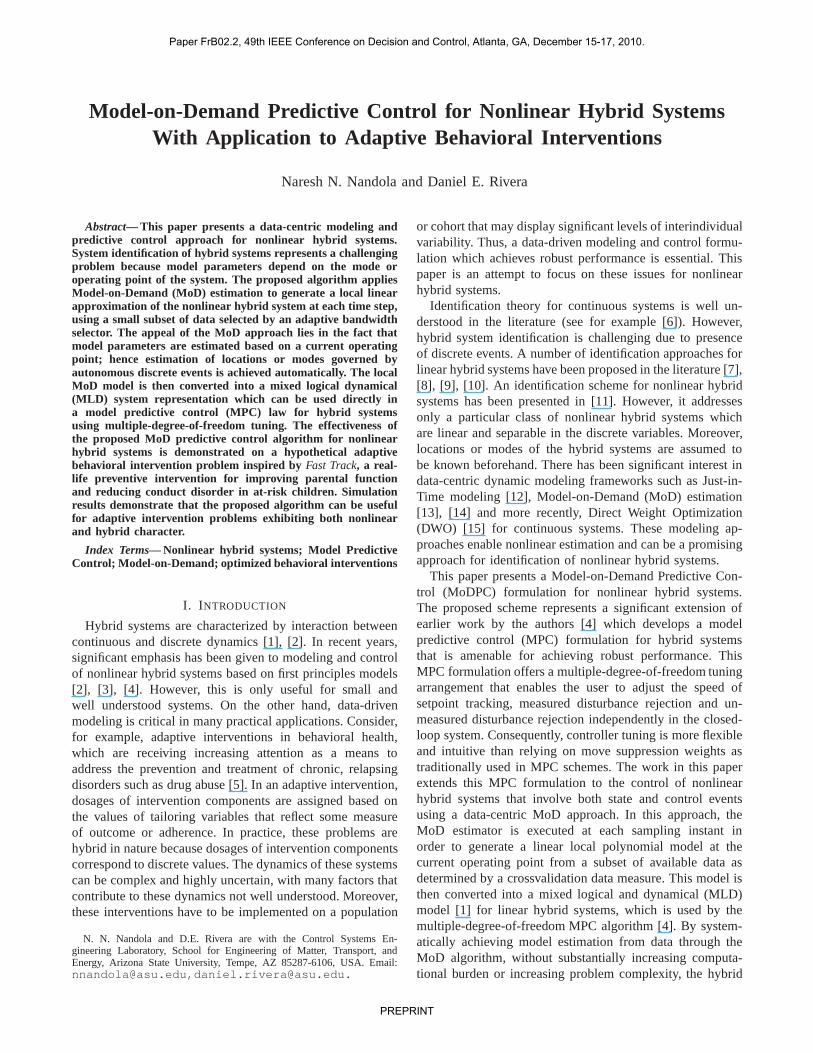
Fig. 1. Fluid analogy corresponding to the hypothetical adaptive interven-tion. Parental functionPF(k) is treated as material (inventory) in a tank,which is depleted by disturbancesD(k) and replenished by interventiondosageI(k), which is the manipulated variable.

by homicide or suicide. InFast Track, some interventioncomponents were delivered universally to all participants,while other specialized components were delivered adap-tively. In this paper we focus on a hypothetical adaptiveintervention described in [5] for assigning family counseling,which was provided to families on the basis of parentalfunctioning. There are several possible levels of intensity,or doses, of family counseling. The idea is to vary thedoses of family counseling depending on the needs of thefamily, in order to avoid providing an insufficient amountof counseling for very troubled families, or wasting coun-seling resources on families that may not need them orbe stigmatized by excessive counseling. The decision aboutwhich dose of counseling to offer each family is basedprimarily on the family’s level of functioning, assessed by afamily functioning questionnaire completed by the parents.As described in [5], based on the questionnaire and theclinician’s assessment, family functioning is determined tofall in one of the following categories: very poor, poor, nearthreshold, or at/above threshold. A corresponding decisionrule that can be applied is as follows: families with very poorfunctioning are given weekly counseling; families with poorfunctioning are given biweekly counseling; families withnear threshold functioning are given monthly counseling;and families at or above threshold are given no counseling.Family functioning is reassessed at a review interval of onemonths, at which time the intervention dosage may change.This goes on for four years.

Rivera et al. [21] analyzed the intervention by means ofa fluid analogy, represented in Figure 1. Parental functionPF(k) is treated as fluid in a tank, which is depleted byexogenous disturbancesD(k). The tank is replenished bythe interventionI(k), which is the manipulated variable.The use of fluid analogy enables developing a mathematicalmodel of the open-loop dynamics of the intervention usingthe principle of conservation of mass. This model can bedescribed by nonlinear difference equations which relatesparental functionPF(k) with the interventionI(k) as follows:

PF(k+T) = PF(k)+KI (k)I(k−θ )−D(k) (29)

Paper FrB02.2, 49th IEEE Conference on Decision and Control, Atlanta, GA, December 15-17, 2010.

PREPRINT

0 20 40 60 80 1000.05

0.1

0.15

0.2

0.25

0.3

PF (%)

KI

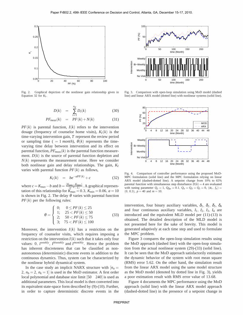
Fig. 2. Graphical depiction of the nonlinear gain relationship given inEquation 32 forKI .

D(k) =nd

∑i=1

Di(k) (30)

PFmeas(k) = PF(k)+N(k) (31)

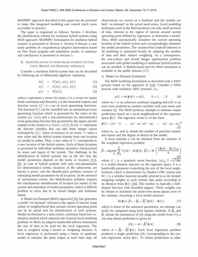
PF(k) is parental function,I(k) refers to the interventiondosage (frequency of counselor home visits),KI (k) is thetime-varying intervention gain,T represent the review periodor sampling time (= 1 month), θ (k) represents the time-varying time delay between intervention and its effect onparental function,PFmeas(k) is the parental function measure-ment.D(k) is the source of parental function depletion andN(k) represents the measurement noise. Here we considerboth nonlinear gain and delay relationships. The gain,KI

varies with parental functionPF(k) as follows,

KI (k) = be−aPF(k) +c (32)

wherec= Kmax−b andb= (Kmin−Kmax)(e−a−1)

. A graphical represen-tation of this relationship forKmax= 0.3, Kmin = 0.06, a= 10is shown in Fig. 2. The delayθ varies with parental functionPF(k) per the following rules:

θ =

0; 0≤ PF(k) ≤ 251; 25< PF(k) ≤ 502; 50< PF(k) ≤ 753; 75< PF(k) ≤ 100

(33)

Moreover, the interventionI(k) has a restriction on thefrequency of counselor visits, which requires imposing arestriction on the interventionI(k) such that it takes only fourvalues: 0, Iweekly, IbiweeklyandImonthly. Hence the problemhas inherent discreteness that can be classified as non-autonomous (deterministic) discrete events in addition to thecontinuous dynamics. Thus, system can be characterized bythe nonlinear hybrid dynamical system.

In the case study an implicit NARX structure with[na =2, nb = 2, nk = 1] is used in the MoD estimator. A first orderlocal polynomial and database size limit[50 240] is used asadditional parameters. This local model is then converted intoits equivalent state-space form described by (9)-(10). Further,in order to capture deterministic discrete events in the

0 50 100 150 2000

50

100

time (Month)

PF

(%

)

0 50 100 150 200

No Visit

Monthly

Bi−Weekly

Weekly

time (Month)

Inte

rven

tion

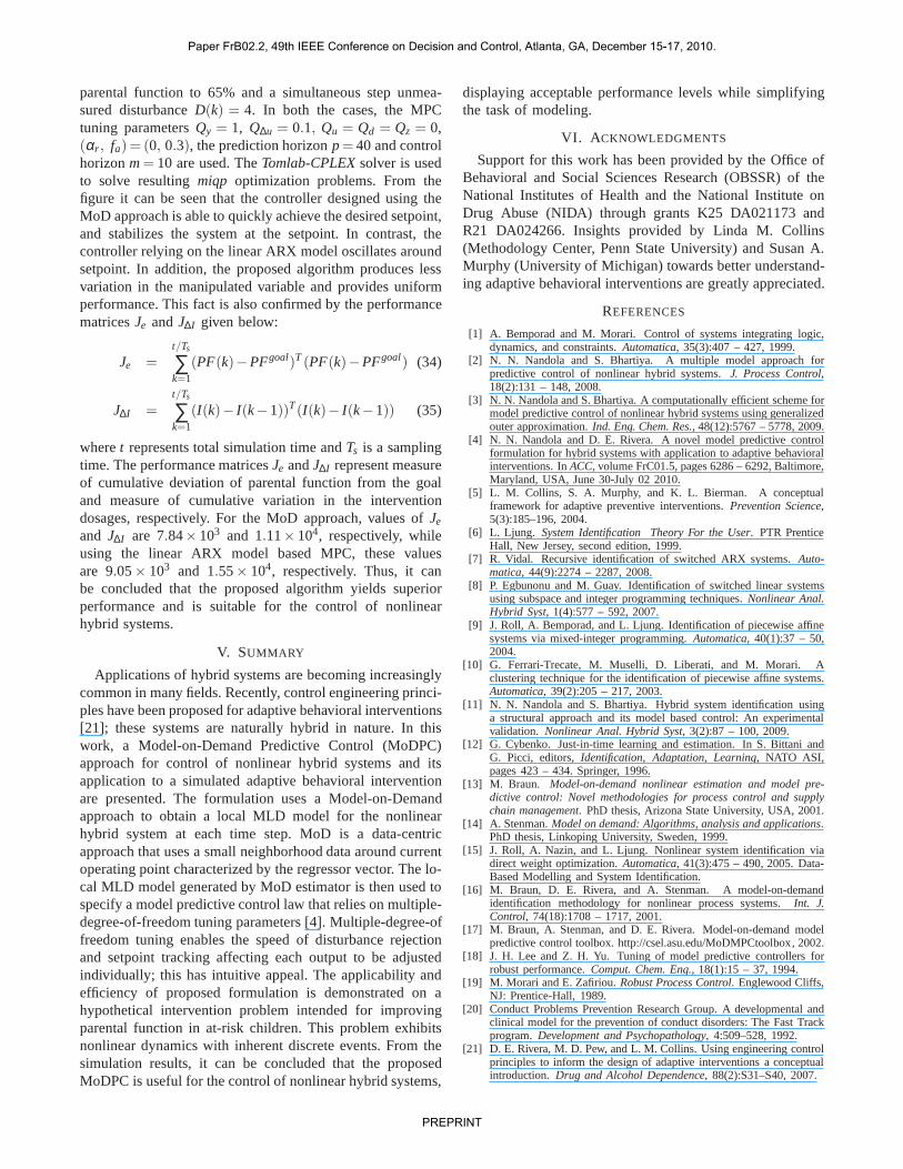
Fig. 3. Comparison with open-loop simulation using MoD model (dashedline) and linear ARX model (dotted line) with nonlinear systems (solid line).

0 4 8 12 16 20 24 28 32 36 40 44 480

20

40

60

80

PF

(%

)

time (Month)

0 4 8 12 16 20 24 28 32 36 40 44 48

No Visit

Monthly

Bi−Weekly

Weekly

time (Month)

Inte

rven

tion

MODARX

Fig. 4. Comparison of controller performance using the proposed MoD-MPC formulation (solid line) and the MPC formulation relying on linearARX model (dashed-dotted line). A setpoint change from 10% to 65%parental function with simultaneous step disturbanceD(k) = 4 are evaluatedwith tuning parameterQy = 1, Q∆u = 0.1, Qu = Qd = Qz = 0, (αr , fa) =(0, 0.3), p = 40 andm= 10.

intervention, four binary auxiliary variables,δ1, δ2, δ3, δ4

and four continuous auxiliary variables,I1, I2, I3, I4 areintroduced and the equivalent MLD model per (11)-(13) isobtained. The detailed description of the MLD model isnot presented here for the sake of brevity. This model isgenerated adaptively at each time step and used to formulatethe MPC problem.

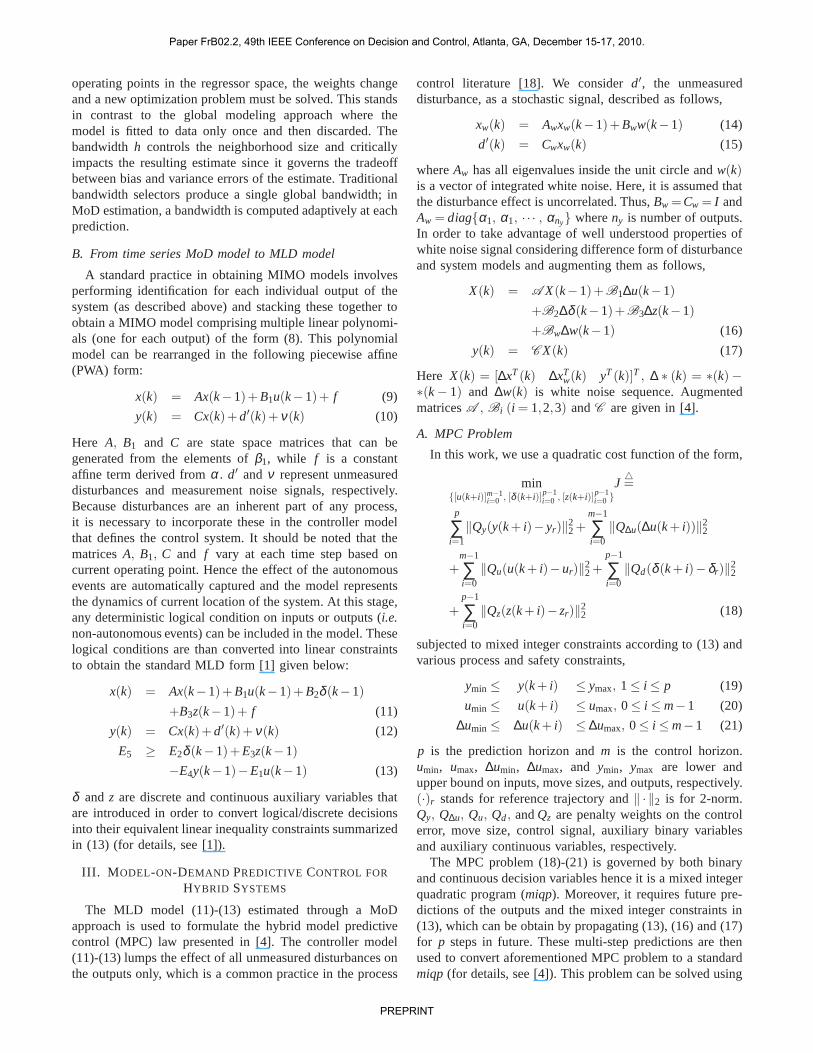
Figure 3 compares the open-loop simulation results usingthe MoD approach (dashed line) with the open-loop simula-tion from the actual nonlinear system (29)-(33) (solid line).It can be seen that the MoD approach satisfactorily estimatesthe dynamic behavior of the system with root mean square(RMS) error 5.62. On the other hand, the simulation resultfrom the linear ARX model using the same model structureas the MoD model (denoted by dotted line in Fig. 3), yieldsa poor estimation result with RMS error value of 13.68.

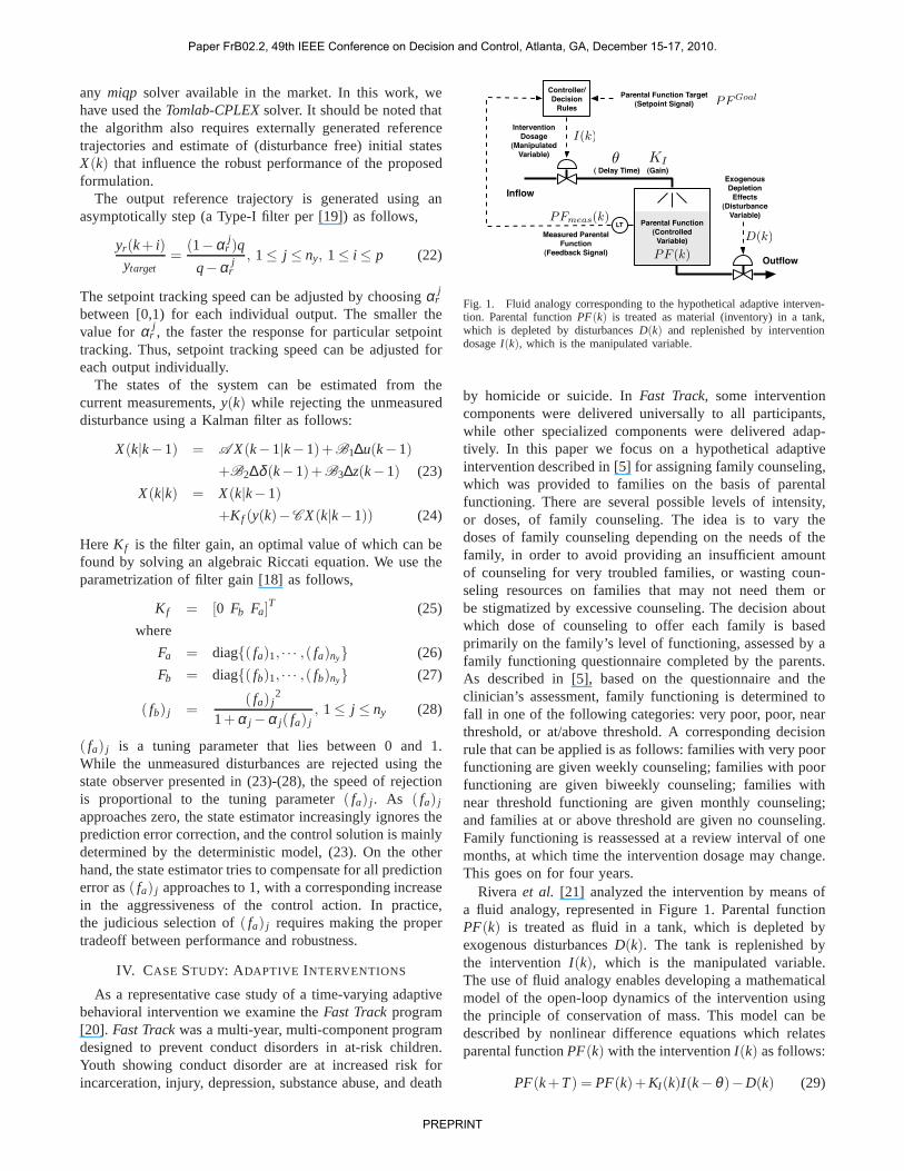
Figure 4 documents the MPC performance using the MoDapproach (solid line) with the linear ARX model approach(dashed-dotted line) in the presence of a setpoint change in

Paper FrB02.2, 49th IEEE Conference on Decision and Control, Atlanta, GA, December 15-17, 2010.

PREPRINT

parental function to 65% and a simultaneous step unmea-sured disturbanceD(k) = 4. In both the cases, the MPCtuning parametersQy = 1, Q∆u = 0.1, Qu = Qd = Qz = 0,(αr , fa) = (0, 0.3), the prediction horizonp= 40 and controlhorizonm= 10 are used. TheTomlab-CPLEXsolver is usedto solve resultingmiqp optimization problems. From thefigure it can be seen that the controller designed using theMoD approach is able to quickly achieve the desired setpoint,and stabilizes the system at the setpoint. In contrast, thecontroller relying on the linear ARX model oscillates aroundsetpoint. In addition, the proposed algorithm produces lessvariation in the manipulated variable and provides uniformperformance. This fact is also confirmed by the performancematricesJe andJ∆I given below:

Je =t/Ts

∑k=1

(PF(k)−PFgoal)T(PF(k)−PFgoal) (34)

J∆I =t/Ts

∑k=1

(I(k)− I(k−1))T(I(k)− I(k−1)) (35)

wheret represents total simulation time andTs is a samplingtime. The performance matricesJe andJ∆I represent measureof cumulative deviation of parental function from the goaland measure of cumulative variation in the interventiondosages, respectively. For the MoD approach, values ofJe

and J∆I are 7.84× 103 and 1.11× 104, respectively, whileusing the linear ARX model based MPC, these valuesare 9.05× 103 and 1.55× 104, respectively. Thus, it canbe concluded that the proposed algorithm yields superiorperformance and is suitable for the control of nonlinearhybrid systems.

V. SUMMARY

Applications of hybrid systems are becoming increasinglycommon in many fields. Recently, control engineering princi-ples have been proposed for adaptive behavioral interventions[21]; these systems are naturally hybrid in nature. In thiswork, a Model-on-Demand Predictive Control (MoDPC)approach for control of nonlinear hybrid systems and itsapplication to a simulated adaptive behavioral interventionare presented. The formulation uses a Model-on-Demandapproach to obtain a local MLD model for the nonlinearhybrid system at each time step. MoD is a data-centricapproach that uses a small neighborhood data around currentoperating point characterized by the regressor vector. The lo-cal MLD model generated by MoD estimator is then used tospecify a model predictive control law that relies on multiple-degree-of-freedom tuning parameters [4]. Multiple-degree-offreedom tuning enables the speed of disturbance rejectionand setpoint tracking affecting each output to be adjustedindividually; this has intuitive appeal. The applicability andefficiency of proposed formulation is demonstrated on ahypothetical intervention problem intended for improvingparental function in at-risk children. This problem exhibitsnonlinear dynamics with inherent discrete events. From thesimulation results, it can be concluded that the proposedMoDPC is useful for the control of nonlinear hybrid systems,

displaying acceptable performance levels while simplifyingthe task of modeling.

VI. A CKNOWLEDGMENTS

Support for this work has been provided by the Office ofBehavioral and Social Sciences Research (OBSSR) of theNational Institutes of Health and the National Institute onDrug Abuse (NIDA) through grants K25 DA021173 andR21 DA024266. Insights provided by Linda M. Collins(Methodology Center, Penn State University) and Susan A.Murphy (University of Michigan) towards better understand-ing adaptive behavioral interventions are greatly appreciated.

REFERENCES

[1] A. Bemporad and M. Morari. Control of systems integrating logic,dynamics, and constraints.Automatica, 35(3):407 – 427, 1999.

[2] N. N. Nandola and S. Bhartiya. A multiple model approach forpredictive control of nonlinear hybrid systems.J. Process Control,18(2):131 – 148, 2008.

[3] N. N. Nandola and S. Bhartiya. A computationally efficient scheme formodel predictive control of nonlinear hybrid systems using generalizedouter approximation.Ind. Eng. Chem. Res., 48(12):5767 – 5778, 2009.

[4] N. N. Nandola and D. E. Rivera. A novel model predictive controlformulation for hybrid systems with application to adaptive behavioralinterventions. InACC, volume FrC01.5, pages 6286 – 6292, Baltimore,Maryland, USA, June 30-July 02 2010.

[5] L. M. Collins, S. A. Murphy, and K. L. Bierman. A conceptualframework for adaptive preventive interventions.Prevention Science,5(3):185–196, 2004.

[6] L. Ljung. System Identification Theory For the User. PTR PrenticeHall, New Jersey, second edition, 1999.

[7] R. Vidal. Recursive identification of switched ARX systems.Auto-matica, 44(9):2274 – 2287, 2008.

[8] P. Egbunonu and M. Guay. Identification of switched linear systemsusing subspace and integer programming techniques.Nonlinear Anal.Hybrid Syst, 1(4):577 – 592, 2007.

[9] J. Roll, A. Bemporad, and L. Ljung. Identification of piecewise affinesystems via mixed-integer programming.Automatica, 40(1):37 – 50,2004.

[10] G. Ferrari-Trecate, M. Muselli, D. Liberati, and M. Morari. Aclustering technique for the identification of piecewise affine systems.Automatica, 39(2):205 – 217, 2003.

[11] N. N. Nandola and S. Bhartiya. Hybrid system identification usinga structural approach and its model based control: An experimentalvalidation. Nonlinear Anal. Hybrid Syst, 3(2):87 – 100, 2009.

[12] G. Cybenko. Just-in-time learning and estimation. In S. Bittani andG. Picci, editors,Identification, Adaptation, Learning, NATO ASI,pages 423 – 434. Springer, 1996.

[13] M. Braun. Model-on-demand nonlinear estimation and model pre-dictive control: Novel methodologies for process control and supplychain management. PhD thesis, Arizona State University, USA, 2001.

[14] A. Stenman.Model on demand: Algorithms, analysis and applications.PhD thesis, Linkoping University, Sweden, 1999.

[15] J. Roll, A. Nazin, and L. Ljung. Nonlinear system identification viadirect weight optimization.Automatica, 41(3):475 – 490, 2005. Data-Based Modelling and System Identification.

[16] M. Braun, D. E. Rivera, and A. Stenman. A model-on-demandidentification methodology for nonlinear process systems.Int. J.Control, 74(18):1708 – 1717, 2001.

[17] M. Braun, A. Stenman, and D. E. Rivera. Model-on-demand modelpredictive control toolbox. http://csel.asu.edu/MoDMPCtoolbox, 2002.

[18] J. H. Lee and Z. H. Yu. Tuning of model predictive controllers forrobust performance.Comput. Chem. Eng., 18(1):15 – 37, 1994.

[19] M. Morari and E. Zafiriou.Robust Process Control. Englewood Cliffs,NJ: Prentice-Hall, 1989.

[20] Conduct Problems Prevention Research Group. A developmental andclinical model for the prevention of conduct disorders: The Fast Trackprogram.Development and Psychopathology, 4:509–528, 1992.

[21] D. E. Rivera, M. D. Pew, and L. M. Collins. Using engineering controlprinciples to inform the design of adaptive interventions a conceptualintroduction. Drug and Alcohol Dependence, 88(2):S31–S40, 2007.

Paper FrB02.2, 49th IEEE Conference on Decision and Control, Atlanta, GA, December 15-17, 2010.

PREPRINT