Mining the impact of evolution categorieson object-oriented metrics

Henrique Rocha • Cesar Couto • Cristiano Maffort • Rogel Garcia •

Clarisse Simoes • Leonardo Passos • Marco Tulio Valente

Published online: 29 August 2012� Springer Science+Business Media, LLC 2012

Abstract Despite the relevance of the software evolution phase, there are few charac-

terization studies on recurrent evolution growth patterns and on their impact on software

properties, such as coupling and cohesion. In this paper, we report a study designed to

investigate whether the software evolution categories proposed by Lanza can be used to

explain not only the growth of a system in terms of lines of code (LOC), but also in terms

of metrics from the Chidamber and Kemerer (CK) object-oriented metrics suite. Our

results show that high levels of recall (ranging on average from 52 to 72 %) are achieved

when using LOC to predict the evolution of coupling and size. For cohesion, we have

achieved smaller recall rates (\27 % on average).

Keywords Software evolution categories � Patterns of evolution � Object-oriented

metrics � CK metrics � Evolution matrix

H. Rocha � C. Couto � C. Maffort � R. Garcia � C. Simoes � M. T. Valente (&)Department of Computer Science, UFMG, Belo Horizonte, Brazile-mail: mtov@dcc.ufmg.br

H. Rochae-mail: hrocha@dcc.ufmg.br

C. Coutoe-mail: cesarfmc@dcc.ufmg.br

C. Mafforte-mail: maffort@dcc.ufmg.br

R. Garciae-mail: rogelgarcia@dcc.ufmg.br

C. Couto � C. MaffortDepartment of Computing, CEFET-MG, Minas Gerais, Brazil

L. PassosDepartment of Electrical and Computer Engineering, University of Waterloo, Waterloo, ON, Canadae-mail: lpassos@gsd.uwaterloo.ca

123

Software Qual J (2013) 21:529–549DOI 10.1007/s11219-012-9186-7

1 Introduction

As expressed by the Laws of Software Evolution (Lehman et al. 1997), evolution usually

contributes to increased software size and complexity and therefore has negative impacts

on both internal quality factors (like coupling, cohesion, readability, modularity, and

separation of concerns) as well as in external quality factors (like correctness, robustness,

and efficiency). However, despite the importance of the evolution phase, there are few

studies in the literature aiming to evaluate the main patterns that describe the growth of

software systems. This observation contrasts with the amount of work about the patterns of

evolution in other research areas. For example, patterns are widely used to model the

evolution of biological (Pagel 1999; Ledyard 1950) and financial systems (Lo et al. 2000).

One study of patterns in software evolution is the work of Lanza proposing a catego-

rization of classes based on recurrent patterns detected when investigating techniques for

the visualization of object-oriented systems (Lanza 2001). The categories proposed by

Lanza rely on a vocabulary mostly taken from the astronomy domain to model the evo-

lution of classes. For example, the proposed categorization covers the following phe-

nomena: rapid growth in class size (supernova), rapid decrease in class size (white dwarf),

rapid growth followed by rapid decrease in class size or vice versa (pulsar), class stability

(stagnant), and limited class lifetime (dayfly).

Our central goal in this paper is to investigate the impact of the evolution categories

proposed by Lanza on the behavior of classical metrics commonly used to evaluate

properties of object-oriented systems, such as coupling, cohesion, and size. More specif-

ically, our goal is to investigate whether the occurrence of a given evolution category

(measured in terms of lines of code) implies an equivalent bevahior in metrics that are part

of the well-known Chidamber and Kemerer (CK) metrics suite (Chidamber and Kemerer

1994). Stated otherwise, we investigate whether the proposed categories can be used to

model not only the evolution of a system in terms of lines of code but also in terms of

coupling, cohesion, and size. An eventual correlation between evolution categories mea-

sured in terms of size and evolution categories measured using the metrics considered in

the paper emphasizes the importance of the former over the latter, showing that it is

possible to predict the evolution of well-known software metrics by evaluating the evo-

lution of a single size metric: lines of code (LOC).

To summarize, our contributions are threefold. The first contribution is a formal defi-

nition for the categories proposed by Lanza (Sect. 2). Our intention is to provide a rigorous

specification for the criteria we describe in the paper when searching for evolution cate-

gories. The second contribution is a study—reported in Sects. 3 and 4—showing that at

least four evolution categories are recurrent: stagnants, supernovas, white dwarfs, and

dayflies. To reach this conclusion, we mined for the evolution categories in several ver-

sions of 10 open-source Java-based systems, comprising in most cases more than 3 years of

evolution. Our third contribution is a study showing an important correlation between

evolution categories measured in terms of LOC and evolution categories assessing size,

coupling, and, to a less extent, cohesion (Sect. 5). Next, Sect. 6 discusses threats to validity,

Sect. 7 presents related work, and Sect. 8 provides concluding remarks.

2 Formal definition

In this section, we provide a formal definition for the categories originally proposed by

Lanza to describe the ways that a class can evolve over its lifetime (Lanza 2001). The

530 Software Qual J (2013) 21:529–549

123

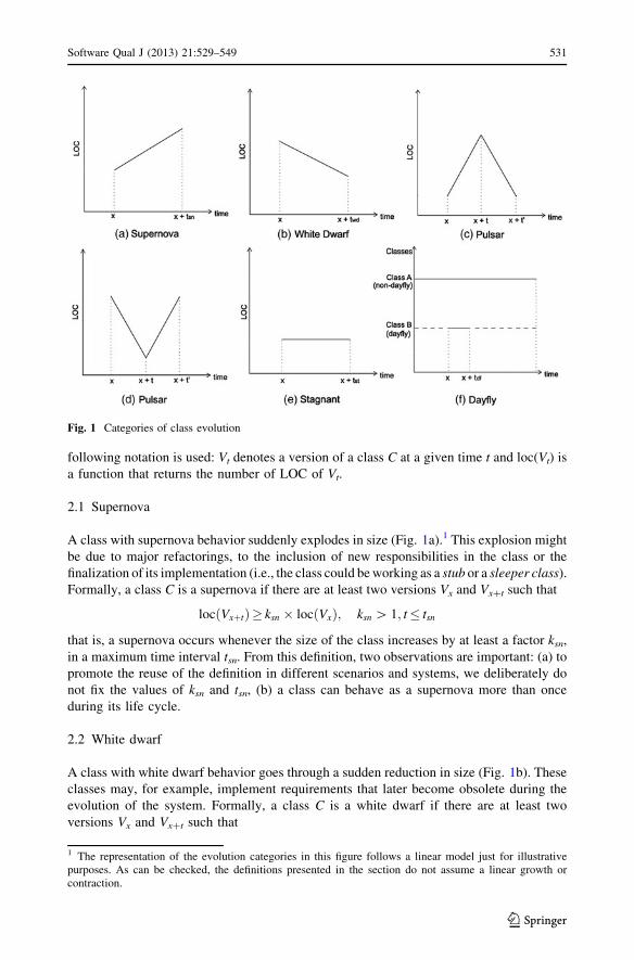
following notation is used: Vt denotes a version of a class C at a given time t and loc(Vt) is

a function that returns the number of LOC of Vt.

2.1 Supernova

A class with supernova behavior suddenly explodes in size (Fig. 1a).1 This explosion might

be due to major refactorings, to the inclusion of new responsibilities in the class or the

finalization of its implementation (i.e., the class could be working as a stub or a sleeper class).

Formally, a class C is a supernova if there are at least two versions Vx and Vx?t such that

locðVxþtÞ� ksn � locðVxÞ; ksn [ 1; t� tsn

that is, a supernova occurs whenever the size of the class increases by at least a factor ksn,

in a maximum time interval tsn. From this definition, two observations are important: (a) to

promote the reuse of the definition in different scenarios and systems, we deliberately do

not fix the values of ksn and tsn, (b) a class can behave as a supernova more than once

during its life cycle.

2.2 White dwarf

A class with white dwarf behavior goes through a sudden reduction in size (Fig. 1b). These

classes may, for example, implement requirements that later become obsolete during the

evolution of the system. Formally, a class C is a white dwarf if there are at least two

versions Vx and Vx?t such that

1 The representation of the evolution categories in this figure follows a linear model just for illustrativepurposes. As can be checked, the definitions presented in the section do not assume a linear growth orcontraction.

Fig. 1 Categories of class evolution

Software Qual J (2013) 21:529–549 531

123

locðVxþtÞ� kwd � locðVxÞ; kwd\1; t� twd

that is, a white dwarf happens whenever the size of the class decreases by at least a factor

kwd, at a time t lower than a maximum time twd.

2.3 Pulsar

A class with pulsar behavior is a class whose size increases and then suddenly decreases or

vice versa (Fig. 1c, d). The growth can occur either by adding or refactoring code.

Decreases are more likely due to refactorings and restructuring of the class. Formally, a

class C has a pulsar including a growth cycle between versions Vx and Vx?t and a shrinking

cycle between versions Vx?t and Vxþt0 , where t \ t0 B tps, if

locðVxþtÞ� ð1þ kpsÞ � locðVxÞ^locðVxþt0 Þ � ð1� kpsÞ � locðVxþtÞ; 0\kps\1

Alternatively, a class with a pulsar behavior can include a decrease cycle between versions

Vx and Vx?t and a cycle of growth between versions Vx?t and Vxþt0 , where t \ t0 B tps, if

locðVxþtÞ� ð1� kpsÞ � locðVxÞ^locðVxþt0 Þ � ð1þ kpsÞ � locðVxþtÞ; 0\kps\1

In these definitions, tps represents the maximum time frame for detecting a pulsar (i.e., the

cycles of growth and decrease must occur in this time window) and kps denotes the

minimum factor that characterizes both the growth (1 ? kps) and the decrease (1 - kps)

phases of a pulsar.

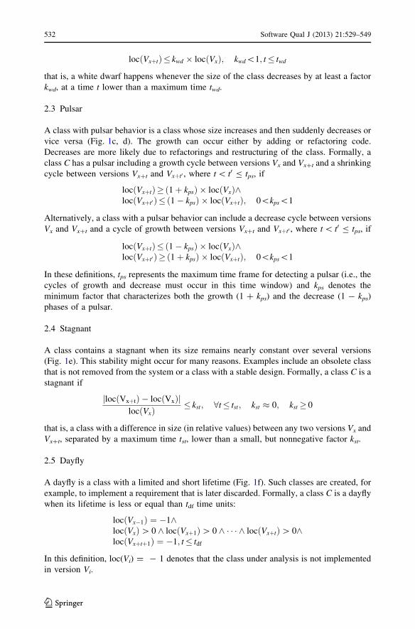
2.4 Stagnant

A class contains a stagnant when its size remains nearly constant over several versions

(Fig. 1e). This stability might occur for many reasons. Examples include an obsolete class

that is not removed from the system or a class with a stable design. Formally, a class C is a

stagnant if

jlocðVxþtÞ � locðVxÞjlocðVxÞ

� kst; 8t� tst; kst � 0; kst � 0

that is, a class with a difference in size (in relative values) between any two versions Vx and

Vx?t, separated by a maximum time tst, lower than a small, but nonnegative factor kst.

2.5 Dayfly

A dayfly is a class with a limited and short lifetime (Fig. 1f). Such classes are created, for

example, to implement a requirement that is later discarded. Formally, a class C is a dayfly

when its lifetime is less or equal than tdf time units:

locðVx�1Þ ¼ �1^locðVxÞ[ 0 ^ locðVxþ1Þ[ 0 ^ � � � ^ locðVxþtÞ[ 0^locðVxþtþ1Þ ¼ �1; t� tdf

In this definition, loc(Vi) = - 1 denotes that the class under analysis is not implemented

in version Vi.

532 Software Qual J (2013) 21:529–549

123

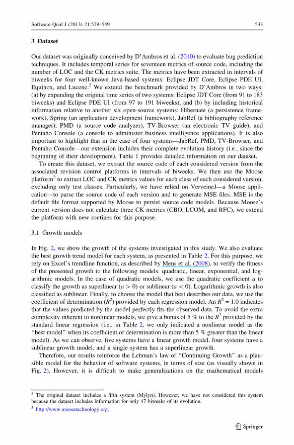
3 Dataset

Our dataset was originally conceived by D’Ambros et al. (2010) to evaluate bug prediction

techniques. It includes temporal series for seventeen metrics of source code, including the

number of LOC and the CK metrics suite. The metrics have been extracted in intervals of

biweeks for four well-known Java-based systems: Eclipse JDT Core, Eclipse PDE UI,

Equinox, and Lucene.2 We extend the benchmark provided by D’Ambros in two ways:

(a) by expanding the original time series of two systems: Eclipse JDT Core (from 91 to 183

biweeks) and Eclipse PDE UI (from 97 to 191 biweeks), and (b) by including historical

information relative to another six open-source systems: Hibernate (a persistence frame-

work), Spring (an application development framework), JabRef (a bibliography reference

manager), PMD (a source code analyzer), TV-Browser (an electronic TV guide), and

Pentaho Console (a console to administer business intelligence applications). It is also

important to highlight that in the case of four systems—JabRef, PMD, TV-Browser, and

Pentaho Console—our extension includes their complete evolution history (i.e., since the

beginning of their development). Table 1 provides detailed information on our dataset.

To create this dataset, we extract the source code of each considered version from the

associated revision control platforms in intervals of biweeks. We then use the Moose

platform3 to extract LOC and CK metrics values for each class of each considered version,

excluding only test classes. Particularly, we have relied on VerveineJ—a Moose appli-

cation—to parse the source code of each version and to generate MSE files. MSE is the

default file format supported by Moose to persist source code models. Because Moose’s

current version does not calculate three CK metrics (CBO, LCOM, and RFC), we extend

the platform with new routines for this purpose.

3.1 Growth models

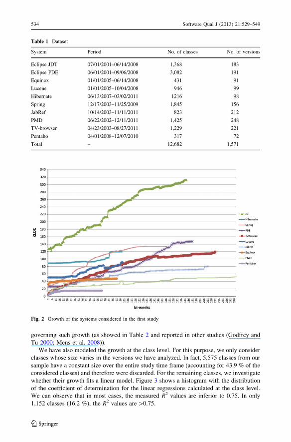
In Fig. 2, we show the growth of the systems investigated in this study. We also evaluate

the best growth trend model for each system, as presented in Table 2. For this purpose, we

rely on Excel’s trendline function, as described by Mens et al. (2008), to verify the fitness

of the presented growth to the following models: quadratic, linear, exponential, and log-

arithmic models. In the case of quadratic models, we use the quadratic coefficient a to

classify the growth as superlinear (a [ 0) or sublinear (a \ 0). Logarithmic growth is also

classified as sublinear. Finally, to choose the model that best describes our data, we use the

coefficient of determination (R2) provided by each regression model. An R2 = 1.0 indicates

that the values predicted by the model perfectly fits the observed data. To avoid the extra

complexity inherent to nonlinear models, we give a bonus of 5 % to the R2 provided by the

standard linear regression (i.e., in Table 2, we only indicated a nonlinear model as the

‘‘best model’’ when its coefficient of determination is more than 5 % greater than the linear

model). As we can observe, five systems have a linear growth model, four systems have a

sublinear growth model, and a single system has a superlinear growth.

Therefore, our results reinforce the Lehman’s law of ‘‘Continuing Growth’’ as a plau-

sible model for the behavior of software systems, in terms of size (as visually shown in

Fig. 2). However, it is difficult to make generalizations on the mathematical models

2 The original dataset includes a fifth system (Mylyn). However, we have not considered this systembecause the dataset includes information for only 47 biweeks of its evolution.3 http://www.moosetechnology.org.

Software Qual J (2013) 21:529–549 533

123

governing such growth (as showed in Table 2 and reported in other studies (Godfrey and

Tu 2000; Mens et al. 2008)).

We have also modeled the growth at the class level. For this purpose, we only consider

classes whose size varies in the versions we have analyzed. In fact, 5,575 classes from our

sample have a constant size over the entire study time frame (accounting for 43.9 % of the

considered classes) and therefore were discarded. For the remaining classes, we investigate

whether their growth fits a linear model. Figure 3 shows a histogram with the distribution

of the coefficient of determination for the linear regressions calculated at the class level.

We can observe that in most cases, the measured R2 values are inferior to 0.75. In only

1,152 classes (16.2 %), the R2 values are [0.75.

Fig. 2 Growth of the systems considered in the first study

Table 1 Dataset

System Period No. of classes No. of versions

Eclipse JDT 07/01/2001–06/14/2008 1,368 183

Eclipse PDE 06/01/2001–09/06/2008 3,082 191

Equinox 01/01/2005–06/14/2008 431 91

Lucene 01/01/2005–10/04/2008 946 99

Hibernate 06/13/2007–03/02/2011 1216 98

Spring 12/17/2003–11/25/2009 1,845 156

JabRef 10/14/2003–11/11/2011 823 212

PMD 06/22/2002–12/11/2011 1,425 248

TV-browser 04/23/2003–08/27/2011 1,229 221

Pentaho 04/01/2008–12/07/2010 317 72

Total – 12,682 1,571

534 Software Qual J (2013) 21:529–549

123

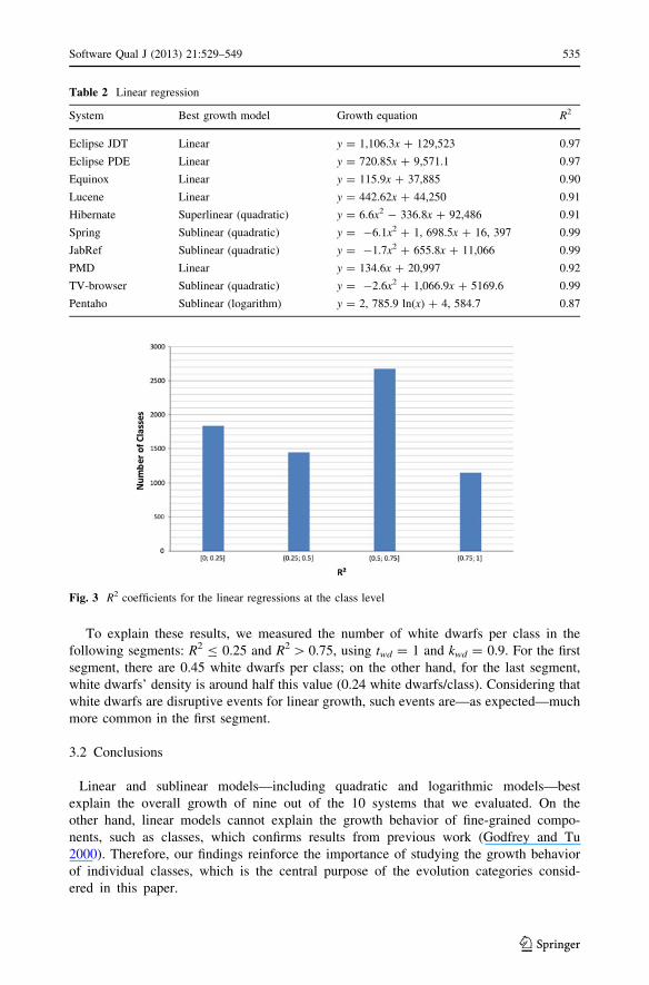
To explain these results, we measured the number of white dwarfs per class in the

following segments: R2 B 0.25 and R2 [ 0.75, using twd = 1 and kwd = 0.9. For the first

segment, there are 0.45 white dwarfs per class; on the other hand, for the last segment,

white dwarfs’ density is around half this value (0.24 white dwarfs/class). Considering that

white dwarfs are disruptive events for linear growth, such events are—as expected—much

more common in the first segment.

3.2 Conclusions

Linear and sublinear models—including quadratic and logarithmic models—best

explain the overall growth of nine out of the 10 systems that we evaluated. On the

other hand, linear models cannot explain the growth behavior of fine-grained compo-

nents, such as classes, which confirms results from previous work (Godfrey and Tu

2000). Therefore, our findings reinforce the importance of studying the growth behavior

of individual classes, which is the central purpose of the evolution categories consid-

ered in this paper.

Fig. 3 R2 coefficients for the linear regressions at the class level

Table 2 Linear regression

System Best growth model Growth equation R2

Eclipse JDT Linear y = 1,106.3x ? 129,523 0.97

Eclipse PDE Linear y = 720.85x ? 9,571.1 0.97

Equinox Linear y = 115.9x ? 37,885 0.90

Lucene Linear y = 442.62x ? 44,250 0.91

Hibernate Superlinear (quadratic) y = 6.6x2 - 336.8x ? 92,486 0.91

Spring Sublinear (quadratic) y = -6.1x2 ? 1, 698.5x ? 16, 397 0.99

JabRef Sublinear (quadratic) y = -1.7x2 ? 655.8x ? 11,066 0.99

PMD Linear y = 134.6x ? 20,997 0.92

TV-browser Sublinear (quadratic) y = -2.6x2 ? 1,066.9x ? 5169.6 0.99

Pentaho Sublinear (logarithm) y = 2, 785.9 ln(x) ? 4, 584.7 0.87

Software Qual J (2013) 21:529–549 535

123

4 Mining for categories of class evolution

In this section, we describe a study to check whether the categories of evolution—as

formalized in Sect. 2—are actually found in real software evolution settings.

4.1 Tool support

To mine for the five categories of evolution, we implemented a small Java system that

searches for the categories using the definition proposed in Sect. 2. The input of this

program is a table whose rows are the classes that existed in at least one version of the

target system and the columns represent the biweeks considered in the study. A cell

(r, c) in this table contains the size (in LOC) of the class in row r at the biweek

represented by column c. The output of the program is a list of the classes that match

each of the categories of evolution considered in the paper. For each matching category,

the program also outputs some information (for example, for a supernova, it outputs the

initial and final biweeks of the supernova, with the size of the class in both versions and

the growth rate).

4.2 Parameters calibration and estimation

A critical decision when mining for the evolution categories is setting the parameters used

in the formal definitions presented in Sect. 2. To help in this decision, we tested several

possible values using the systems in our dataset as input,4 aiming to check how our results

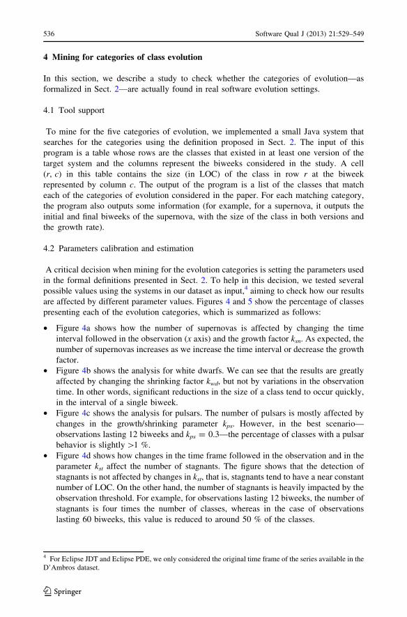
are affected by different parameter values. Figures 4 and 5 show the percentage of classes

presenting each of the evolution categories, which is summarized as follows:

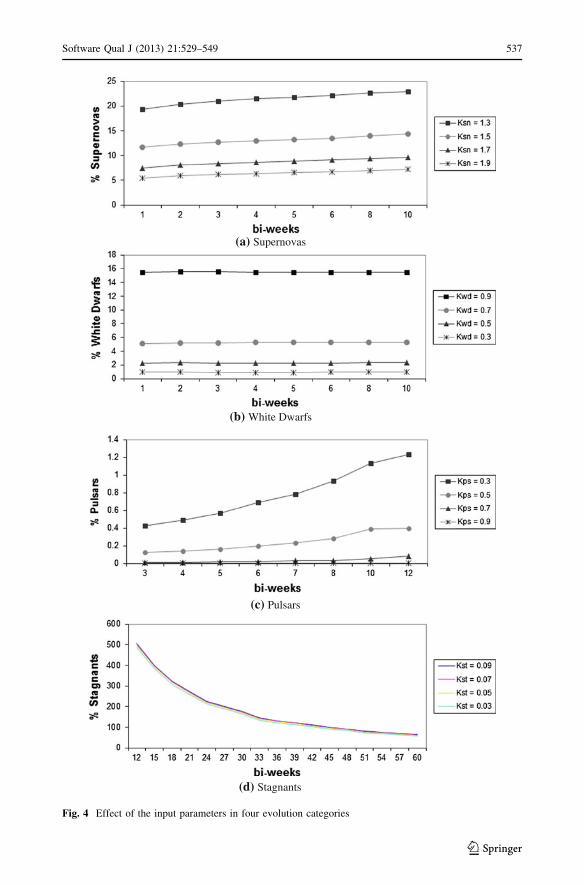
• Figure 4a shows how the number of supernovas is affected by changing the time

interval followed in the observation (x axis) and the growth factor ksn. As expected, the

number of supernovas increases as we increase the time interval or decrease the growth

factor.

• Figure 4b shows the analysis for white dwarfs. We can see that the results are greatly

affected by changing the shrinking factor kwd, but not by variations in the observation

time. In other words, significant reductions in the size of a class tend to occur quickly,

in the interval of a single biweek.

• Figure 4c shows the analysis for pulsars. The number of pulsars is mostly affected by

changes in the growth/shrinking parameter kps. However, in the best scenario—

observations lasting 12 biweeks and kps = 0.3—the percentage of classes with a pulsar

behavior is slightly [1 %.

• Figure 4d shows how changes in the time frame followed in the observation and in the

parameter kst affect the number of stagnants. The figure shows that the detection of

stagnants is not affected by changes in kst, that is, stagnants tend to have a near constant

number of LOC. On the other hand, the number of stagnants is heavily impacted by the

observation threshold. For example, for observations lasting 12 biweeks, the number of

stagnants is four times the number of classes, whereas in the case of observations

lasting 60 biweeks, this value is reduced to around 50 % of the classes.

4 For Eclipse JDT and Eclipse PDE, we only considered the original time frame of the series available in theD’Ambros dataset.

536 Software Qual J (2013) 21:529–549

123

(a) Supernovas

(b) White Dwarfs

(c) Pulsars

(d) Stagnants

Fig. 4 Effect of the input parameters in four evolution categories

Software Qual J (2013) 21:529–549 537

123

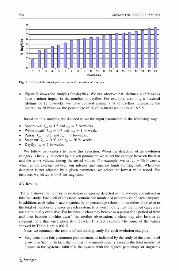
• Figure 5 shows the analysis for dayflies. We can observe that lifetimes [12 biweeks

have a minor impact in the number of dayflies. For example, assuming a maximal

lifetime of 12 bi-weeks, we have counted around 7 % of dayflies. Increasing the

interval to 20 biweeks, the percentage of dayflies increases to around 8.5 %.

Based on this analysis, we decided to set the input parameters in the following way:

• Supernova: ksn = 1.5 and tsn = 5 bi-weeks.

• White dwarf: kwd = 0.7 and twd = 1 bi-week.

• Pulsar: kps = 0.5, and tps = 7 bi-weeks.

• Stagnant: kst = 0.03 and tst = 36 bi-weeks.

• Dayfly: tdf = 7 bi-weeks.

We follow two criteria to make this selection. When the detection of an evolution

category is heavily impacted by a given parameter, we select the average between the best

and the worst values, among the tested values. For example, we set tst = 36 biweeks,

which is the average between our inferior and superior limits for stagnants. When the

detection is not affected by a given parameter, we select the lowest value tested. For

instance, we set kst = 0.03 for stagnants.

4.3 Results

Table 3 shows the number of evolution categories detected in the systems considered in

this first study. Each cell of this table contains the number of occurrences of each category.

In addition, each value is accompanied by its percentage (shown in parenthesis) relative to

the total of number of classes in each system. It is worth noting that the mined categories

are not mutually exclusive. For instance, a class may behave as a pulsar for a period of time

and then become a white dwarf. As another observation, a class may also behave as

stagnant more than once along its lifecycle. This fact explains why some of the values

showed in Table 1 are [100 %.

Next, we comment the results of our mining study for each evolution category:

• Stagnants are a fairly common phenomenon, as indicated by the study of the class-level

growth in Sect. 3. In fact, the number of stagnants usually exceeds the total number of

classes in the systems. JabRef is the system with the highest percentage of stagnants

Fig. 5 Effect of the input parameters in the number of dayflies

538 Software Qual J (2013) 21:529–549

123

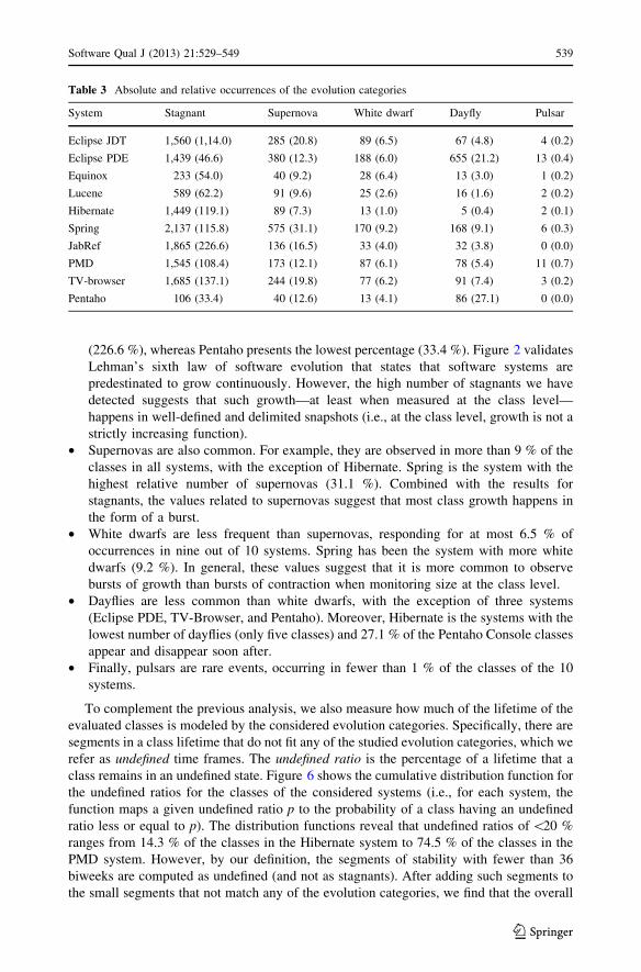
(226.6 %), whereas Pentaho presents the lowest percentage (33.4 %). Figure 2 validates

Lehman’s sixth law of software evolution that states that software systems are

predestinated to grow continuously. However, the high number of stagnants we have

detected suggests that such growth—at least when measured at the class level—

happens in well-defined and delimited snapshots (i.e., at the class level, growth is not a

strictly increasing function).

• Supernovas are also common. For example, they are observed in more than 9 % of the

classes in all systems, with the exception of Hibernate. Spring is the system with the

highest relative number of supernovas (31.1 %). Combined with the results for

stagnants, the values related to supernovas suggest that most class growth happens in

the form of a burst.

• White dwarfs are less frequent than supernovas, responding for at most 6.5 % of

occurrences in nine out of 10 systems. Spring has been the system with more white

dwarfs (9.2 %). In general, these values suggest that it is more common to observe

bursts of growth than bursts of contraction when monitoring size at the class level.

• Dayflies are less common than white dwarfs, with the exception of three systems

(Eclipse PDE, TV-Browser, and Pentaho). Moreover, Hibernate is the systems with the

lowest number of dayflies (only five classes) and 27.1 % of the Pentaho Console classes

appear and disappear soon after.

• Finally, pulsars are rare events, occurring in fewer than 1 % of the classes of the 10

systems.

To complement the previous analysis, we also measure how much of the lifetime of the

evaluated classes is modeled by the considered evolution categories. Specifically, there are

segments in a class lifetime that do not fit any of the studied evolution categories, which we

refer as undefined time frames. The undefined ratio is the percentage of a lifetime that a

class remains in an undefined state. Figure 6 shows the cumulative distribution function for

the undefined ratios for the classes of the considered systems (i.e., for each system, the

function maps a given undefined ratio p to the probability of a class having an undefined

ratio less or equal to p). The distribution functions reveal that undefined ratios of \20 %

ranges from 14.3 % of the classes in the Hibernate system to 74.5 % of the classes in the

PMD system. However, by our definition, the segments of stability with fewer than 36

biweeks are computed as undefined (and not as stagnants). After adding such segments to

the small segments that not match any of the evolution categories, we find that the overall

Table 3 Absolute and relative occurrences of the evolution categories

System Stagnant Supernova White dwarf Dayfly Pulsar

Eclipse JDT 1,560 (1,14.0) 285 (20.8) 89 (6.5) 67 (4.8) 4 (0.2)

Eclipse PDE 1,439 (46.6) 380 (12.3) 188 (6.0) 655 (21.2) 13 (0.4)

Equinox 233 (54.0) 40 (9.2) 28 (6.4) 13 (3.0) 1 (0.2)

Lucene 589 (62.2) 91 (9.6) 25 (2.6) 16 (1.6) 2 (0.2)

Hibernate 1,449 (119.1) 89 (7.3) 13 (1.0) 5 (0.4) 2 (0.1)

Spring 2,137 (115.8) 575 (31.1) 170 (9.2) 168 (9.1) 6 (0.3)

JabRef 1,865 (226.6) 136 (16.5) 33 (4.0) 32 (3.8) 0 (0.0)

PMD 1,545 (108.4) 173 (12.1) 87 (6.1) 78 (5.4) 11 (0.7)

TV-browser 1,685 (137.1) 244 (19.8) 77 (6.2) 91 (7.4) 3 (0.2)

Pentaho 106 (33.4) 40 (12.6) 13 (4.1) 86 (27.1) 0 (0.0)

Software Qual J (2013) 21:529–549 539

123

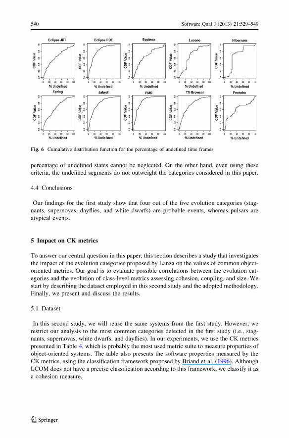
percentage of undefined states cannot be neglected. On the other hand, even using these

criteria, the undefined segments do not outweight the categories considered in this paper.

4.4 Conclusions

Our findings for the first study show that four out of the five evolution categories (stag-

nants, supernovas, dayflies, and white dwarfs) are probable events, whereas pulsars are

atypical events.

5 Impact on CK metrics

To answer our central question in this paper, this section describes a study that investigates

the impact of the evolution categories proposed by Lanza on the values of common object-

oriented metrics. Our goal is to evaluate possible correlations between the evolution cat-

egories and the evolution of class-level metrics assessing cohesion, coupling, and size. We

start by describing the dataset employed in this second study and the adopted methodology.

Finally, we present and discuss the results.

5.1 Dataset

In this second study, we will reuse the same systems from the first study. However, we

restrict our analysis to the most common categories detected in the first study (i.e., stag-

nants, supernovas, white dwarfs, and dayflies). In our experiments, we use the CK metrics

presented in Table 4, which is probably the most used metric suite to measure properties of

object-oriented systems. The table also presents the software properties measured by the

CK metrics, using the classification framework proposed by Briand et al. (1996). Although

LCOM does not have a precise classification according to this framework, we classify it as

a cohesion measure.

Fig. 6 Cumulative distribution function for the percentage of undefined time frames

540 Software Qual J (2013) 21:529–549

123

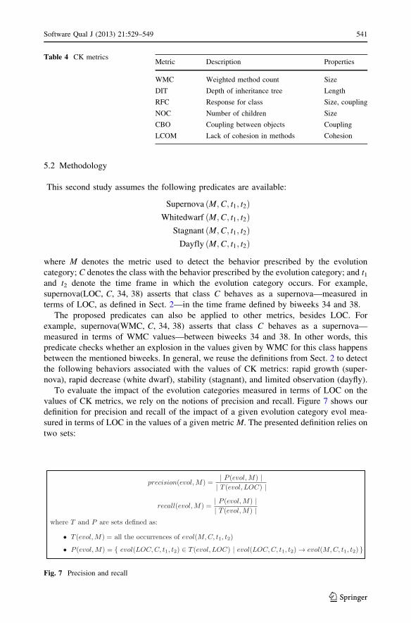
5.2 Methodology

This second study assumes the following predicates are available:

Supernova ðM;C; t1; t2ÞWhitedwarf ðM;C; t1; t2Þ

Stagnant ðM;C; t1; t2ÞDayfly ðM;C; t1; t2Þ

where M denotes the metric used to detect the behavior prescribed by the evolution

category; C denotes the class with the behavior prescribed by the evolution category; and t1and t2 denote the time frame in which the evolution category occurs. For example,

supernova(LOC, C, 34, 38) asserts that class C behaves as a supernova—measured in

terms of LOC, as defined in Sect. 2—in the time frame defined by biweeks 34 and 38.

The proposed predicates can also be applied to other metrics, besides LOC. For

example, supernova(WMC, C, 34, 38) asserts that class C behaves as a supernova—

measured in terms of WMC values—between biweeks 34 and 38. In other words, this

predicate checks whether an explosion in the values given by WMC for this class happens

between the mentioned biweeks. In general, we reuse the definitions from Sect. 2 to detect

the following behaviors associated with the values of CK metrics: rapid growth (super-

nova), rapid decrease (white dwarf), stability (stagnant), and limited observation (dayfly).

To evaluate the impact of the evolution categories measured in terms of LOC on the

values of CK metrics, we rely on the notions of precision and recall. Figure 7 shows our

definition for precision and recall of the impact of a given evolution category evol mea-

sured in terms of LOC in the values of a given metric M. The presented definition relies on

two sets:

Table 4 CK metricsMetric Description Properties

WMC Weighted method count Size

DIT Depth of inheritance tree Length

RFC Response for class Size, coupling

NOC Number of children Size

CBO Coupling between objects Coupling

LCOM Lack of cohesion in methods Cohesion

Fig. 7 Precision and recall

Software Qual J (2013) 21:529–549 541

123

• T(evol, M): set containing all the occurrences of a given evolution category evol

measured in terms of the metric M;

• P(evol, M): set containing the occurrences of the evolution categories in T(evol, LOC)

that have caused an equivalent behavior in the values of the metric M. Therefore,

Pðevol;MÞ � Tðevol;LOCÞ.

To illustrate this definition, suppose that in a given system, we have detected 100

supernovas in terms of LOC (i.e., |T(supernova, LOC)| = 100) and 120 supernovas in

terms of the CBO metric (i.e., |T(supernova, CBO)| = 120); suppose also that 80 of the

supernovas detected in terms of LOC have also been detected in terms of the CBO metric,

for the same class and at the same time interval (i.e., |P(supernova, CBO)| = 80).

Therefore, precision(supernova, CBO) = 80/100 and recall(supernova, CBO) = 80/120.

To simplify analysis and provide a single model showing the correlation between LOC

and CK metrics, we also rely on the F measure (or F1 score) that combines precision and

recall in a single weighted average:

F1score ¼ 2� precision� recall

precisionþ recall

In the best case, precision = recall = 1.0 and therefore F1 score = 1.0. The worst case

happens when precision = 0.0 or recall = 0.0, and therefore F1 score = 0.0.

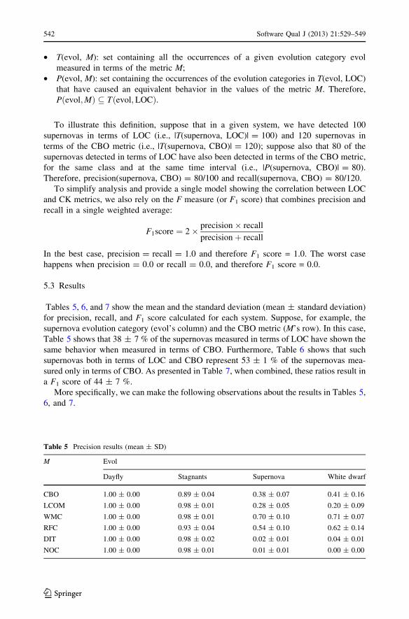
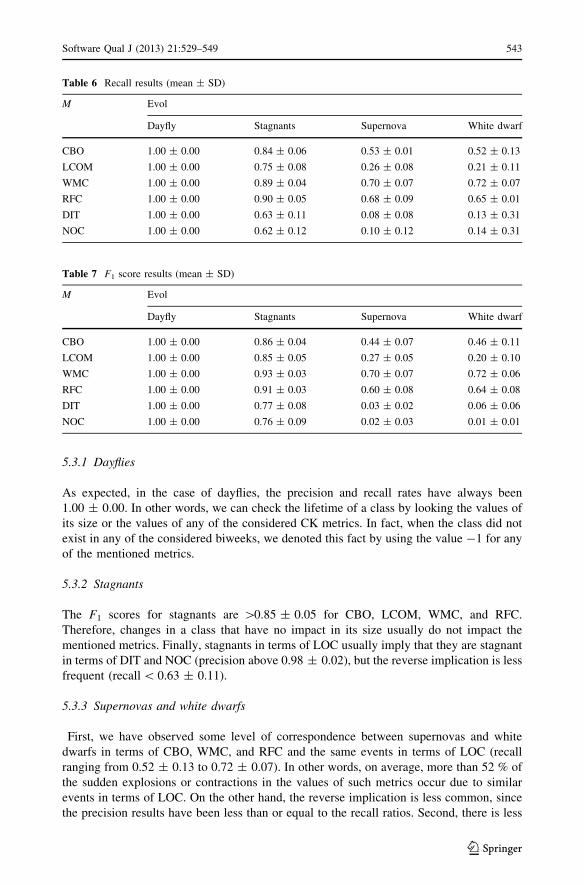
5.3 Results

Tables 5, 6, and 7 show the mean and the standard deviation (mean ± standard deviation)

for precision, recall, and F1 score calculated for each system. Suppose, for example, the

supernova evolution category (evol’s column) and the CBO metric (M’s row). In this case,

Table 5 shows that 38 ± 7 % of the supernovas measured in terms of LOC have shown the

same behavior when measured in terms of CBO. Furthermore, Table 6 shows that such

supernovas both in terms of LOC and CBO represent 53 ± 1 % of the supernovas mea-

sured only in terms of CBO. As presented in Table 7, when combined, these ratios result in

a F1 score of 44 ± 7 %.

More specifically, we can make the following observations about the results in Tables 5,

6, and 7.

Table 5 Precision results (mean ± SD)

M Evol

Dayfly Stagnants Supernova White dwarf

CBO 1.00 ± 0.00 0.89 ± 0.04 0.38 ± 0.07 0.41 ± 0.16

LCOM 1.00 ± 0.00 0.98 ± 0.01 0.28 ± 0.05 0.20 ± 0.09

WMC 1.00 ± 0.00 0.98 ± 0.01 0.70 ± 0.10 0.71 ± 0.07

RFC 1.00 ± 0.00 0.93 ± 0.04 0.54 ± 0.10 0.62 ± 0.14

DIT 1.00 ± 0.00 0.98 ± 0.02 0.02 ± 0.01 0.04 ± 0.01

NOC 1.00 ± 0.00 0.98 ± 0.01 0.01 ± 0.01 0.00 ± 0.00

542 Software Qual J (2013) 21:529–549

123

5.3.1 Dayflies

As expected, in the case of dayflies, the precision and recall rates have always been

1.00 ± 0.00. In other words, we can check the lifetime of a class by looking the values of

its size or the values of any of the considered CK metrics. In fact, when the class did not

exist in any of the considered biweeks, we denoted this fact by using the value -1 for any

of the mentioned metrics.

5.3.2 Stagnants

The F1 scores for stagnants are [0.85 ± 0.05 for CBO, LCOM, WMC, and RFC.

Therefore, changes in a class that have no impact in its size usually do not impact the

mentioned metrics. Finally, stagnants in terms of LOC usually imply that they are stagnant

in terms of DIT and NOC (precision above 0.98 ± 0.02), but the reverse implication is less

frequent (recall \ 0.63 ± 0.11).

5.3.3 Supernovas and white dwarfs

First, we have observed some level of correspondence between supernovas and white

dwarfs in terms of CBO, WMC, and RFC and the same events in terms of LOC (recall

ranging from 0.52 ± 0.13 to 0.72 ± 0.07). In other words, on average, more than 52 % of

the sudden explosions or contractions in the values of such metrics occur due to similar

events in terms of LOC. On the other hand, the reverse implication is less common, since

the precision results have been less than or equal to the recall ratios. Second, there is less

Table 6 Recall results (mean ± SD)

M Evol

Dayfly Stagnants Supernova White dwarf

CBO 1.00 ± 0.00 0.84 ± 0.06 0.53 ± 0.01 0.52 ± 0.13

LCOM 1.00 ± 0.00 0.75 ± 0.08 0.26 ± 0.08 0.21 ± 0.11

WMC 1.00 ± 0.00 0.89 ± 0.04 0.70 ± 0.07 0.72 ± 0.07

RFC 1.00 ± 0.00 0.90 ± 0.05 0.68 ± 0.09 0.65 ± 0.01

DIT 1.00 ± 0.00 0.63 ± 0.11 0.08 ± 0.08 0.13 ± 0.31

NOC 1.00 ± 0.00 0.62 ± 0.12 0.10 ± 0.12 0.14 ± 0.31

Table 7 F1 score results (mean ± SD)

M Evol

Dayfly Stagnants Supernova White dwarf

CBO 1.00 ± 0.00 0.86 ± 0.04 0.44 ± 0.07 0.46 ± 0.11

LCOM 1.00 ± 0.00 0.85 ± 0.05 0.27 ± 0.05 0.20 ± 0.10

WMC 1.00 ± 0.00 0.93 ± 0.03 0.70 ± 0.07 0.72 ± 0.06

RFC 1.00 ± 0.00 0.91 ± 0.03 0.60 ± 0.08 0.64 ± 0.08

DIT 1.00 ± 0.00 0.77 ± 0.08 0.03 ± 0.02 0.06 ± 0.06

NOC 1.00 ± 0.00 0.76 ± 0.09 0.02 ± 0.03 0.01 ± 0.01

Software Qual J (2013) 21:529–549 543

123

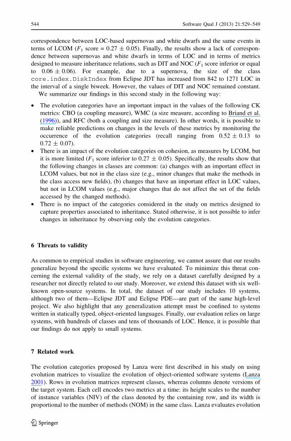
correspondence between LOC-based supernovas and white dwarfs and the same events in

terms of LCOM (F1 score = 0.27 ± 0.05). Finally, the results show a lack of correspon-

dence between supernovas and white dwarfs in terms of LOC and in terms of metrics

designed to measure inheritance relations, such as DIT and NOC (F1 score inferior or equal

to 0.06 ± 0.06). For example, due to a supernova, the size of the class

core.index.DiskIndex from Eclipse JDT has increased from 842 to 1271 LOC in

the interval of a single biweek. However, the values of DIT and NOC remained constant.

We summarize our findings in this second study in the following way:

• The evolution categories have an important impact in the values of the following CK

metrics: CBO (a coupling measure), WMC (a size measure, according to Briand et al.

(1996)), and RFC (both a coupling and size measure). In other words, it is possible to

make reliable predictions on changes in the levels of these metrics by monitoring the

occurrence of the evolution categories (recall ranging from 0.52 ± 0.13 to

0.72 ± 0.07).

• There is an impact of the evolution categories on cohesion, as measures by LCOM, but

it is more limited (F1 score inferior to 0.27 ± 0.05). Specifically, the results show that

the following changes in classes are common: (a) changes with an important effect in

LCOM values, but not in the class size (e.g., minor changes that make the methods in

the class access new fields), (b) changes that have an important effect in LOC values,

but not in LCOM values (e.g., major changes that do not affect the set of the fields

accessed by the changed methods).

• There is no impact of the categories considered in the study on metrics designed to

capture properties associated to inheritance. Stated otherwise, it is not possible to infer

changes in inheritance by observing only the evolution categories.

6 Threats to validity

As common to empirical studies in software engineering, we cannot assure that our results

generalize beyond the specific systems we have evaluated. To minimize this threat con-

cerning the external validity of the study, we rely on a dataset carefully designed by a

researcher not directly related to our study. Moreover, we extend this dataset with six well-

known open-source systems. In total, the dataset of our study includes 10 systems,

although two of them—Eclipse JDT and Eclipse PDE—are part of the same high-level

project. We also highlight that any generalization attempt must be confined to systems

written in statically typed, object-oriented languages. Finally, our evaluation relies on large

systems, with hundreds of classes and tens of thousands of LOC. Hence, it is possible that

our findings do not apply to small systems.

7 Related work

The evolution categories proposed by Lanza were first described in his study on using

evolution matrices to visualize the evolution of object-oriented software systems (Lanza

2001). Rows in evolution matrices represent classes, whereas columns denote versions of

the target system. Each cell encodes two metrics at a time: its height scales to the number

of instance variables (NIV) of the class denoted by the containing row, and its width is

proportional to the number of methods (NOM) in the same class. Lanza evaluates evolution

544 Software Qual J (2013) 21:529–549

123

matrices using two Smalltalk systems, in which supernovas, white dwarfs, pulsars, stag-

nants, and dayfly classes are visually identified in terms of NIV and NOM. The evaluated

systems, however, are not representative of industrial-strength object-oriented systems.

Lanza and Ducasse (2003) propose the use of polymetric views, which contrary to

Lanza’s evolution matrices, can encode up to five metrics measurements. A polymetric

view is a graph representing a given relationship between source code entities (e.g.,

classes), where nodes encode metric measurements by means of colors, position, and size.

Colors are in gray scale, with white standing as the least value and black the maximum

metric measurement. Positions are (x and y) coordinates, and node size encodes two

measurements by its size and width. Polymetric views are designed to assist developers in

understanding the structure and the design quality of software systems, along with infor-

mation on how these two properties evolve over time. The authors argue that such an

approach help detecting evolution patterns in terms of class, method, and attribute metrics,

but excluded CK metrics from their analysis.

Godfrey and Tu (2000) study the Linux Kernel and its evolution over 96 versions,

showing that it follows a super-linear rate, contradicting Lehman and Turki’s hypothesis of

an inverse square growth rate (Lehman et al. 1998). Israeli and Feitelson perform a larger

study, with the analysis of 810 Linux kernel releases over 14 years (Israeli and Feitelson

2010). Their analysis suggests that the kernel agrees with Lehman’s Law of Software

Evolution. In particular, the authors report strong evidence toward continuing growth and

change laws, but anecdotal evidence of the self-regulation and feedback system laws.

Gonzalez-Barahona et al. (2009) study the evolution of the Debian Linux distribution,

opposed to studies focusing on the kernel alone, and point out that the package mean size

in Debian is often constant across stable releases. However, the number of packages and

the LOC size of the distribution (the sum of all LOC in each source file) doubles at each

release. They also find that 7 % of packages from version 2.0 are still present in version

4.0, and that around 18 % of such packages remained unchanged (something we would

characterize as a stagnant behavior).

Herraiz and Hassan (2010) investigate the correlation between LOC and other soft-

ware metrics. In particular, the authors analyze how LOC/SLOC measurement of C files

in Arch Linux packages correlates with McCabe’s control flow complexity and Hal-

stead’s metrics. Overall, they find a high correlation (C84 %) between size and Hal-

stead’s metrics, but an average correlation (60 %) between SLOC and McCabe’s

cyclomatic complexity for non-header files. Finally, a low correlation between McCabe’s

complexity and SLOC/LOC is present. As discussed by the authors, this is expected, as

header files do not contain control flow information. Similar results are reported in

Herraiz et al. (2007), but with FreeBSD as a subject of analysis. Altogether, these works

measure correlations between metric values taken from a single version of the target

systems, which are restricted to the domain of operating systems. Opposed to that, we use

different versions of the systems in our experiments, thus taking into account the tem-

poral variations over the metric values. Furthermore, our target systems comprise a rich

set of applications from different domains.

El Emam et al. (2001) points out the potential confounding effect of class size on CK

metrics when predicting fault-proneness (El Emam et al. 2001). Subramanyan and

Krishnan further investigates such effect (Subramanyam and Krishnan 2003), but opposed

to Eman, show a strong association of defects to a subset of CK metrics, even after

controlling for size. Their results, however, are dependent on the programing language. In

future work, we also intend to investigate correlations between evolution categories and

bugs, similar to the ones we investigate regarding CK metrics.

Software Qual J (2013) 21:529–549 545

123

8 Conclusions

Our findings from the studies reported in this paper can be summarized as follows:

• The first study (Sect. 4) shows that stagnants, supernovas, white dwarfs, and dayflies

are probable events in the lifetime of classes.

• The second study (Sect. 5) shows that by monitoring only the occurrence of the

evolution categories, we can make reliable predictions of the values of metrics

designed to measure coupling (CBO), both coupling and size (RFC), size (WMC), and

to a less extent cohesion (LCOM). On the other hand, there is no connection between

the evolution categories considered in the paper and properties derived from

inheritance relations (as measured by NOC and DIT metrics).

As further work, we have the following plans: (a) to consider external software quality

metrics, such as number of warnings raised by static analysis tools (Araujo et al. 2011) and

number of bugs (Hora et al. 2012), (b) to consider the use of evolution categories as an

independent variable in bug prediction models (Couto et al. 2012), (c) to investigate how

software evolution categories in general (and their particular relations to software metrics as

investigated in this paper) can be incorporated in software quality monitoring tools and

models.

The dataset with the software metrics time series used in this paper is available at:

http://java.llp.dcc.ufmg.br/sqj2013.

Acknowledgments This research has been supported by the grants from FUNDEP/Santander, CAPES,FAPEMIG, and CNPq. We thank Marco D’Ambros for making the dataset with the historical values of theOO metrics publicly available and Andre Hora and Nicolas Anquetil for helping us with the Mooseplatform.

References

Araujo, J. E., Souza, S., & Valente, M. T. (2011). Study on the relevance of the warnings reported by javabug-finding tools. IET Software, 5(4), 366–374.

Briand, L. C., Morasca, S., & Basili, V. R. (1996). Property-based software engineering measurement. IEEETransactions on Software Engineering, 22(1), 68–86.

Chidamber, S. R., & Kemerer, C. F. (1994). A metrics suite for object oriented design. IEEE Transactionson Software Engineering, 20(6), 476–493.

Couto, C., Araujo, J. E., Silva, C., & Valente, M. T. Static correspondence and correlation between fielddefects and warnings reported by a bug finding tool. Software Quality Journal (to appear).

Couto, C., Silva, C., Valente, M. T., Bigonha, R., & Anquetil, N. (2012). Uncovering causal relationshipsbetween software metrics and bugs. In 16th European conference on software maintenance andreengineering (CSMR), pp. 223–232.

D’Ambros, M., Lanza, M., & Robbes, R. (2010). An extensive comparison of bug prediction approaches. In7th working conference on mining software repositories (MSR), pp. 31–41.

El Emam, K., Benlarbi, S., Goel, N., & Rai, S. N. (2001). The confounding effect of class size on thevalidity of object-oriented metrics. IEEE Transactions on Software Engineering, 27, 630–650.

Godfrey, M. W., & Tu, Q. (2000). Evolution in open source software: A case study. In Internationalconference on software maintenance (ICSM), pp. 131–142.

Gonzalez-Barahona, J. M., Robles, G, Michlmayr, M., Amor Juan, J., & German, D. M. (2009) Macro-levelsoftware evolution: A case study of a large software compilation. Empirical Software Engineering, 14,262–285.

Herraiz, I., Gonzalez-Barahona, J. M., & Robles, G. (2007). Towards a theoretical model for softwaregrowth. In International workshop on mining software repositories, p. 21.

546 Software Qual J (2013) 21:529–549

123

Herraiz, I., & Hassan, A. E. (2010). Making software: What really works, and why we believe it? In I.Herraiz (Ed.), Beyond lines of code: Do we need more complexity metrics? (pp. 435–451). Sebastopol,CA: O’Reilly Media.

Hora, A., Anquetil, N., Ducasse, S., Bhatti, M. U., Couto, C., Valente, M. T., & Martins, J. (2012).BugMaps: A tool for the visual exploration and analysis of bugs. In 16th European conference onsoftware maintenance and reengineering (CSMR), pp. 523–526.

Israeli, A., & Feitelson, D. G. (2010). The linux kernel as a case study in software evolution. Journal ofSystems and Software, 83(3), 485–501.

Lanza, M. (2001). The evolution matrix: Recovering software evolution using software visualization tech-niques. In 4th international workshop on principles of software evolution (IWPSE), pp. 37–42.

Lanza, M., & Ducasse, S. (2003). Polymetric views—A lightweight visual approach to reverse engineering.IEEE Transactions on Software Engineering, 29, 782–795.

Ledyard Stebbins, G. (1950). Variation and evolution in plants. New York: Columbia University Press.Lehman, M. M., Perry, D. E., & Ramil, J. F. (1998). Implications of evolution metrics on software main-

tenance. In International conference on software maintenance (ICSM), pp. 208–217.Lehman, M. M., Ramil, J. F., Wernick, P. D., Perry, D. E., & Turski, W. M. (1997). Metrics and laws of

software evolution-the nineties view. In 4th international software metrics symposium, pp. 20–32.Lo, A. W., Mamaysky, H., & Wang, J. (2000). Foundations of technical analysis: Computational algorithms,

statistical inference, and empirical implementation. Journal of Finance, 40, 1705–1765.Mens, T., Fernandez-Ramil, J., & Degrandsart, S. (2008). The evolution of eclipse. In International con-

ference on software maintenance (ICSM), pp. 386–395.Pagel, M. (1999). Inferring the historical patterns of biological evolution. Nature, 401(6756), 877–884.Subramanyam, R., & Krishnan, M. S. (2003). Empirical analysis of CK metrics for object-oriented design

complexity: Implications for software defects. IEEE Transactions on Software Engineering, 29,297–310.

Author Biographies

Henrique Rocha is a PhD student in the Computer Science Depart-ment at the Federal University of Minas Gerais, Brazil. He is also alecturer at COTEMIG and UNIPAC. His research interests includesoftware engineering, software maintenance and evolution, program-ming languages, digital games, and game theory. Rocha has a master’sdegree in Electrical Engineering from the Pontifical Catholic Univer-sity of Minas Gerais, Brazil.

Software Qual J (2013) 21:529–549 547

123

Cesar Couto is a PhD student in the Computer Science Department atthe Federal University of Minas Gerais, Brazil. He is also a lecturer inthe Department of Computing at CEFET-MG, Brazil. His researchinterests include software maintenance and evolution, software quality,and programming languages. Couto has a master’s degree in ComputerScience from the Federal University of Minas Gerais.

Cristiano Maffort is a PhD student in the Computer ScienceDepartment at the Federal University of Minas Gerais, Brazil. He isalso a lecturer in the Department of Computing at CEFET-MG, Brazil.His research interests include software architecture and softwaremaintenance and evolution. Maffort has a master’s degree in Infor-matics from the Pontifical Catholic University of Minas Gerais, Brazil.

Rogel Garcia is a Master’s student in the Computer Science Depart-ment at the Federal University of Minas Gerais, Brazil. His currentresearch interests are in the interplay between software architectureand workflow management systems. Garcia is also a software architectconsultant and the leading architect of an open source framework forweb applications, called Next (http://www.nextframework.org).

548 Software Qual J (2013) 21:529–549

123

Clarisse Simoes is an undergraduate student in Electrical Engineeringat the Federal University of Minas Gerais, Brazil. Her research inter-ests include web development, software maintenance and evolution,and software quality.

Leonardo Passos is a PhD student in the Electrical and ComputerEngineering Department at the University of Waterloo, Canada. Hisresearch interests include programming languages and software prod-uct lines. Passos has a master’s degree in Computer Science from theFederal University of Minas Gerais, Brazil.

Marco Tulio Valente is an assistant professor in the Computer Sci-ence Department at the Federal University of Minas Gerais, Brazil. Hisresearch interests include software architecture, software remodular-ization and software maintenance and evolution. Valente has a PhD incomputer science from the Federal University of Minas Gerais. He is amember of the ACM, the IEEE Computer Society, and the BrazilianComputer Society.

Software Qual J (2013) 21:529–549 549

123