Milk Marketing Order Winners and Losers

Hayley H. Chouinard*

School of Economic Sciences Washington State University

PO Box 646210 Pullman, WA 99164-6210

Email: chouinard@wsu.edu Telephone: (509) 335-8739

Fax: (509) 335-1173

David E. Davis Department of Economics

South Dakota State University

Jeffrey T. LaFrance School of Economic Sciences Washington State University

Jeffrey M. Perloff

Agricultural and Resource Economics University of California – Berkeley

Abstract

Determining the impacts on consumers of government policies affecting the demand for food products requires a theoretically consistent micro-level demand model. We estimate a system of demands for weekly city-level dairy product purchases by nonlinear three stage least squares to account for joint determination between quantities and prices. We analyze the distributional effects of federal milk marketing orders, and find results that vary substantially across demographic groups. Families with young children suffer, while wealthier childless couples benefit. We also find that households with lower incomes bear a greater regulatory burden due to marketing orders than those with higher income levels.

*Corresponding author.

Milk Marketing Order Winners and Losers

1. Introduction

The U.S. dairy industry has been subjected to more government intervention and regula-

tion than almost any other domestic industry. There are three major areas of this market

intervention: the dairy price support program; import quotas on dairy products; and Fed-

eral milk marketing orders (FMMOs). For several decades, these three policy instruments

were closely connected and operated jointly to establish farm, wholesale, and retail prices

for milk and manufactured products. But over the past two decades, price supports have

become essentially irrelevant to market outcomes in the dairy industry and trade policy

has been renegotiated in the Uruguay Round of the General Agreement on Trades and

Tariffs (Cox, Coleman, Chavas, and Zhu 2005). On the other hand, the Federal Agricul-

ture Improvement and Reform Act of 1996 mandated reforms to the FMMO program.

These reforms include changing the way that minimum prices paid to farmers are deter-

mined and reducing the number of FMMOs through consolidation from 42 to no less than

10 and more than 14 by January 2000. The period 1997–1999 was a significant transition

period for these reforms, and so far the effects of these reforms on the consumers of dairy

products have not yet been analyzed thoroughly.

To better understand the distributional effects on consumers due to the FMMO pro-

gram during this period, this paper investigates an econometric model of the retail de-

mand for 14 dairy products. The model analyzes weekly city–level purchases of dairy

products matched with demographic characteristics of the purchasing households in 22

cities across the U.S. during the transition period 1997–1999 of the FMMO program. The

model is flexible with respect to estimated price and income effects, and satisfies the

conditions that are necessary and sufficient for the existence of a rational, representative

consumer in each city.

There are four important gains that can be expected from the approach taken in this

paper. First, a higher level of disaggregation of products included in the empirical model

increases the degree of substitution across goods. For example, whole milk, 2%, 1%, and

nonfat beverage milk should be close substitutes. Indeed, if the price of 2% milk is higher

than the average of the prices of whole and nonfat milk, then mixing two half gallons of

each of the latter types would give approximately 1.9% milk at a lower cost than a gallon

of 2% milk. A similar argument applies to the price of 1% milk relative to the average

price of 2% and nonfat milk. Thus, we expect ex ante that the estimated own–price elas-

ticities of demand will increase in the empirical model, and this is precisely what we find

relative to the extant literature.

Second, nonlinear three–stage least squares estimation methods are used to account

for simultaneous determination of prices and quantities. This also should increase the

point estimates for the own–price elasticities of demand, and improve the bias, consis-

tency, and precision of those estimates.

Third, the model chosen for the empirical analysis is associated with a null hypothesis

of zero for each price and income elasticity, which is the appropriate null in a valid statis-

tical analysis. This contrasts to a null hypothesis of negative unity for the own–price elas-

ticity and positive unity for the income elasticity in the Almost Ideal Demand System.

2

Thus, we expect that the inferences drawn from the model specification employed in this

paper to be less biased and inconsistent.

Fourth, the functional form for the dependent and independent variables, i.e., linear in

quantities, prices, and income, rather than budget shares as dependent variables with the

natural logarithms of prices and income on the right–hand side of the demand equations

generates a demand model with a much larger region of economic regularity (LaFrance,

Beatty, and Pope 2005). Thus, ex ante, the empirical model can be expected to be more

useful for welfare and other economic analyses than alternative functional forms.

To set the stage for this analysis, a brief history of the evolution of domestic Federal

policy in the dairy industry is presented next. This is followed by a description of the

model and its properties, a description of the data and its use in the empirical model, the

estimation techniques and results, a simulation analysis of the welfare effects of FMMOs

during this period, and our summary and conclusions.

2. A Brief History of Federal Domestic Dairy Policy

The origins of Federal dairy policy can be traced to the Agricultural Adjustment Acts of

1933 and 1935 as part of the New Deal in the Great Depression. Permanent authorization

for the dairy price support program is the Agricultural Act of 1949, which is the last per-

manent farm bill. The FMMO program is authorized by the Agricultural Marketing

Agreement Act of 1937. With high support prices relative to world prices up until the mid

to late 1990’s, import quotas have been used to prevent imports of dairy products from

overwhelming the price support program. This section reviews the history and evolution

of domestic policy in the U.S. dairy industry.

3

The Dairy Price Support Program

The Agricultural Act of 1949 specifies that farm milk prices are to be supported at be-

tween 75 and 90 percent of parity and authorizes the Secretary of Agriculture to deter-

mine the specific price support level within this range. Parity is defined by the index of

prices paid by farmers for commodities and services, interest, taxes, and wages relative to

the base period 1910–14. For example, this index reached 2,244 in January 2008 and the

parity price equivalent for manufacturing grade milk was $40.40 per hundred pounds

(cwt) of farm milk (NASS, USDA, Agricultural Prices, January 2008), while the parity

price for all milk was $43.76/cwt in January 2008 and $47.10/cwt in April 2008 (NASS,

USDA, Agricultural Prices, April 2008).

Farm milk prices are supported indirectly through government purchases of butter,

cheese, and nonfat dry milk from the processors of these products by the Commodity

Credit Corporation (CCC). The purchase prices for these products are pre–announced and

determined by formulas that include a manufacturing “make margin” intended to cover

the cost of a processing plant of average efficiency to convert milk into these products

and an estimated “yield factor” for each product that converts a cwt of milk into a pound

of butter, cheese, or nonfat dry milk. The objective of these administratively determined

CCC purchase prices is to achieve a farm–level price received for manufacturing milk at

least equal to the support price.

Before 1977, support prices were set once a year and were effective throughout the

marketing year. But the Food and Agriculture Act of 1977 required midyear adjustments

in the support price, added the prices of land and fixed inputs to the calculations for sup-

4

port prices, dramatically increasing milk support prices twice a year during this period of

rapid commodity price inflation. As a result, large surpluses of dairy products developed

(LaFrance and de Gorter 1985), and the Agriculture and Food Act of 1981 broke away

from parity pricing altogether, setting the manufacturing milk support price nominally at

$13.10/cwt. As a result of continuing surpluses, the 1983 Dairy and Tobacco Adjustment

Act lowered the support price again to $12.60/cwt and allowed for additional reductions

if net government removals of manufactured dairy products remained high.

These reductions in the nominal support price for farm milk continued throughout the

1980s. The Food Security Act of 1985 set the support price at $11.60/cwt for the 1986

calendar year, $11.35 for January–September, 1987, and $11.10/cwt through the end of

1989. On January 1, 1990, the support price was reduced further to $10.10/cwt because

CCC purchases of manufactured dairy products were projected to exceed 5 billion pounds

in terms of farm milk equivalent weight. The support price for manufacturing milk has

been quite steady since this date, fluctuating slightly between $10.35 and $9.90/cwt, and

current legislation continues the support price at the latter level through 2012.

Since 1990, the farm milk support price has been set low enough that it seldom af-

fects the market prices received for manufacturing grade milk. Thus, during the transition

period of 1997–1999 for the FMMO program, the price support program had little to no

impact on farm, wholesale, or retail prices for milk and dairy products. However, al-

though the 1949 Agricultural Act has been suspended by omnibus farm bill amendments

since 1972, it remains the last piece of permanent farm legislation. In the event that an

expiring farm bill is not extended or replaced by a new one, Federal policies in the dairy

5

industry will revert to the 1949 regulations, with the attendant disrupting impacts on both

demand and supply that would result from a more than fourfold increase in the farm price

for manufacturing grade milk. Nevertheless, given the evolution of the dairy price sup-

port program, we can safely ignore it in our analysis of the distributional impacts on con-

sumers of the FMMO program.

Federal Milk Marketing Orders

FMMOs divide the country into geographic regions. First handlers of milk (manufactur-

ers or processors) in each region are required to pay to farmers at least the minimum price

for four classes of milk defined by the Federal government.1 Class I is the milk used for

fluid beverage products.2 Class II milk is used to produce soft dairy products such as ice

cream, cottage cheese, and yogurt. Class III milk goes into hard dairy products such as

butter and cheese. Class III–A milk is used to manufacture nonfat dry milk. The original

objectives of milk marketing orders focused on equalizing the market power of buyers

and sellers, and to provide market stability. In reality, these marketing orders allow the

Federal government, acting for milk producers, to price discriminate.

FMMOs set minimum prices that must be paid by processors to dairy farmers or their

cooperatives for Grade A milk. Grade A milk meets the sanitary requirements to be le-

gally sold as a fluid product. Markets where FMMOs are in place are those where the

producers of two–thirds of the milk marketed in a given demand area or two–thirds of the

1 Berck and Perloff (1985) present a theory of how marketing order prices are set and how they affect milk prices. 2 Only grade A milk may be used for the Class I market. When milk marketing orders were introduced in the 1930s, one of the justifications was to reduce the variability in the availability of Grade A milk. How-ever, today nearly all of the milk produced in the United States meets the Grade A standards, so this ration-ale is outdated.

6

number of producers that market milk in that area have elected to come under a Federal

order.

Only Grade A milk is regulated under FMMOs. However, over 85 percent of all milk

currently produced in the United States is Grade A. FMMOs regulate over 80 percent of

the Grade A milk produced in the United States. The USDA (1984) estimates that virtu-

ally all Grade B milk (milk that can only be used to make manufactured dairy products)

produced in the United States would qualify as Grade A if a market existed for the addi-

tional fluid grade milk. State milk marketing orders that mimic the FMMO program con-

trol virtually all remaining Grade A milk produced in the country.

Two major provisions of FMMOs are classified pricing according to use and the

pooling of revenue from the sale of milk to obtain a single blend price to be paid to dairy

farmers. Milk used for fluid products is Class I. Milk used for soft manufactured products

(ice cream, cottage cheese, and yogurt) is Class II. Milk used for hard manufactured

products (butter, cheese, nonfat dry milk, and canned milk) is Class III.3

FMMOs set minimum prices based on specified relationships to the price of Grade B

milk in Minnesota and Wisconsin, where more than a third of the Grade B milk in the

U.S. is produced. The average price paid for Grade B milk obtained from a monthly sur-

vey of 100 processing plants in Wisconsin and 62 plants in Minnesota that produce but-

3 In 22 of the 34 FMMOs in operation during 1997–1999, a fourth class, Class III–A, for nonfat dry milk also was in effect. The minimum price for Class III–A milk was based on a formula that used the Chicago Mercantile Exchange (CME) price for nonfat dry milk minus a make margin intended to reflect the cost of production at an average efficiency processing plant, with the difference multiplied by a yield factor that is intended to represent the average yield in pounds of nonfat milk solids from a hundred pounds of milk. This class became Class IV in all FMMOs on January 1, 2000, as part of the final order for the milk marketing order reforms. Both butter and nonfat dry milk are included in the new Class IV. We do not include nonfat dry milk in our analysis and our sample period is 1997–1999. Hence, we focus only on Classes I, II, and III.

7

ter, cheese, and nonfat dry milk is used to calculate the Minnesota–Wisconsin price, or

the Base Month Price (BMP). These plants purchase approximately 80 percent of the

Grade B milk sold in these two states.

The price of Grade B milk is presumed to be a competitive price because manufactur-

ing grade milk is not directly regulated by Federal or state milk marketing orders.4 The

Basic Formula Price (BFP) was used to determine the minimum prices for all classes of

milk in all FMMOs until the end of October, 1999.5 The BFP is calculated by adjusting

the previous month’s BMP to 3.5% butterfat content using a dairy product price formula.

The formula uses information contained in reports by the National Agricultural Statistics

Service (NASS) on CME and National Cheese Exchange (NCE) prices for grade AA or

A butter (CME), 40–pound blocks of Cheddar cheese (CME or NCE), nonfat dry milk

(CME), and dried whey (CME), yield factors for each of these products, and a weighted

average of American cheese and nonfat dry milk production in Minnesota and Wisconsin.

The NASS central market exchange prices are published weekly by the USDA Agricul-

tural Marketing Service in Dairy Market News. During the period 1997–1999, the yield

factors used in the FMMO calculations are: butter, 4.27 lbs/cwt; Cheddar cheese, 9.87

lbs/cwt; dry buttermilk, 0.42 lbs/cwt; nonfat dry milk, 8.07 lbs/cwt; and whey cream but-

ter, 0.238 lbs/cwt.

4 However, as discussed above, the Federal dairy price support program provided a floor on the price of Grade B milk from 1949 until 1990, though this was not a binding price floor during 1997–1999. 5 From the early 1960s until June 1, 1995, the Minnesota–Wisconsin price was the BPF for all milk market-ing orders (ERS, USDA, 1996). Federal milk order reform replaced the BFP with a dairy products compo-nents based formula beginning on November 1, 1999.

8

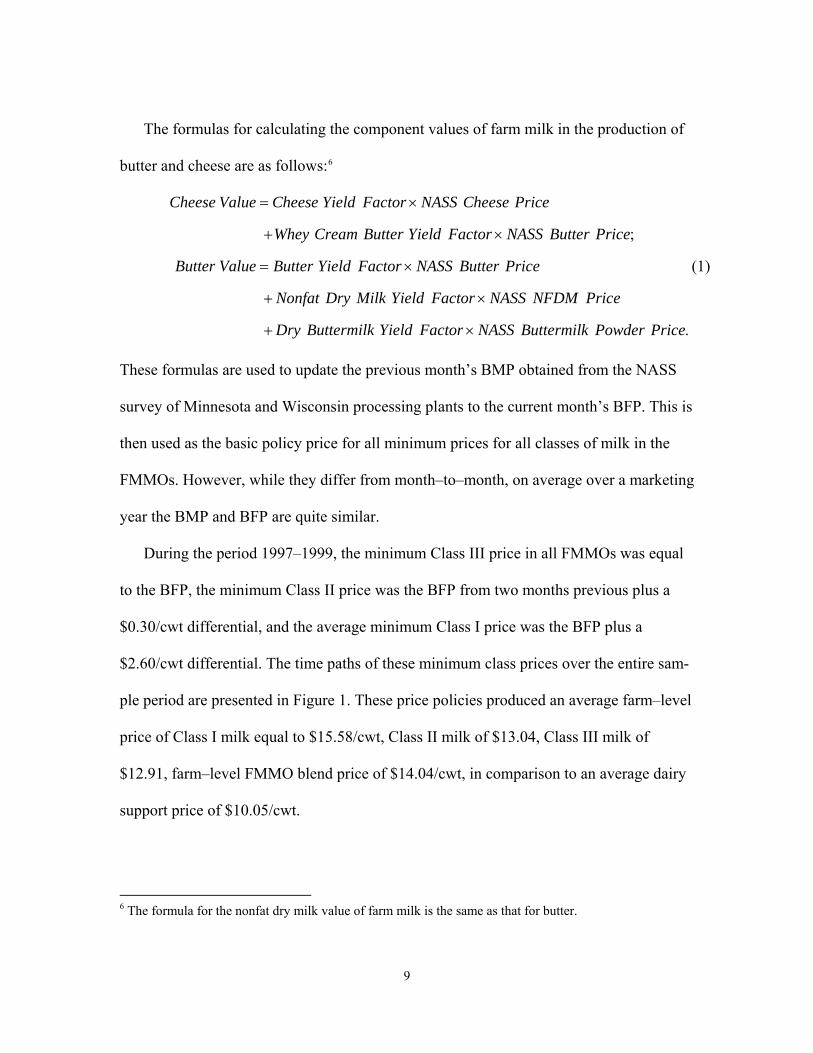
The formulas for calculating the component values of farm milk in the production of

butter and cheese are as follows:6

;

Cheese Value Cheese Yield Factor NASS Cheese Price

Whey Cream Butter Yield Factor NASS Butter Price

Butter Value Butter Yield Factor NASS Butter Price

Nonfat Dry Milk Yield Factor NASS NFDM Price

Dry Buttermilk Yield Factor N

= ×

+ ×

= ×

+ ×

+ × .ASS Buttermilk Powder Price

(1)

These formulas are used to update the previous month’s BMP obtained from the NASS

survey of Minnesota and Wisconsin processing plants to the current month’s BFP. This is

then used as the basic policy price for all minimum prices for all classes of milk in the

FMMOs. However, while they differ from month–to–month, on average over a marketing

year the BMP and BFP are quite similar.

During the period 1997–1999, the minimum Class III price in all FMMOs was equal

to the BFP, the minimum Class II price was the BFP from two months previous plus a

$0.30/cwt differential, and the average minimum Class I price was the BFP plus a

$2.60/cwt differential. The time paths of these minimum class prices over the entire sam-

ple period are presented in Figure 1. These price policies produced an average farm–level

price of Class I milk equal to $15.58/cwt, Class II milk of $13.04, Class III milk of

$12.91, farm–level FMMO blend price of $14.04/cwt, in comparison to an average dairy

support price of $10.05/cwt.

6 The formula for the nonfat dry milk value of farm milk is the same as that for butter.

9

3. The Economic Model

We assume that city–level weekly average purchases of dairy products can be modeled

with a representative consumer. We use a generalized Almost Ideal Demand System that

is linear and quadratic in prices and linear in income (LQ–IDS), is flexible with respect to

price and income effects, and satisfies the conditions that are necessary and sufficient for

the existence of a rational, representative consumer (LaFrance 2004). The demand equa-

tions for the LQ–IDS can be written in matrix form as

( )½m ′ ′ ′= + + + − − −q As Bp p p As p Bα γ α p

, (2)

where q is the vector of quantities demanded, α and γ are vectors of parameters, A is a

matrix of parameters, is a symmetric matrix of parameters, p is the vector of

normalized final consumer prices for dairy products, m is normalized income, and s is a

vector of demographic variables. All prices and income are normalized by a positive–

valued, increasing, concave, and linearly homogeneous function of the prices of all other

goods.

′=B B

7

To identify and predict the impacts of dairy product prices on consumer welfare,

we need to compare the utility level at the initial prices to the utility level at the final

prices. Suppose that dairy product prices change from p0 to p1. The equivalent variation,

ev, is the change in income at the original price vector, p0, that is just necessary to bring

the consumer to the new utility level at the final price vector, p1. For the demand model

in equation (2), the equivalent variation for such as price change is

7 This model can be thought of either as an incomplete demand system (LaFrance and Hanemann 1989) or as a complete system in which the demand for the n+1st good, x, has a different functional form than the demands for q, i.e., ( )(1 ) (1 ½ ) .x m′ ′ ′ ′ ′= − − − − −p p p As p pγ α γ Bp

10

( ) ( )0 1( )1 1 1 1 0 0 0 0½ ½ev m e m−′′ ′ ′ ′ ′ ′= − − − − − − −p pp p As p Bp p p As p Bpγα α . (3)

For this model, the compensating variation is proportional to the equivalent variation,

. Hence, we focus only on the equivalent variation. 1 0(cv ev e −′= × p pγ )

To better understand the distributional effects of FMMOs, note that the marginal

effect of a change in the kth demographic variable on the equivalent variation for the

change in dairy product prices from p0 to p1 is

0 1( )0 1

1

n

jk j jk j

ev a p p es

′ −

=

∂ ⎡ ⎤= −⎣ ⎦∂ ∑ p pγ . (4)

This depends on the coefficients on the variables sk in the demands for dairy products, the

size of the relative prices changes, and the vector of income coefficients. Therefore, we

expect a priori that the welfare effects of marketing orders for dairy products vary sys-

tematically across consumer characteristics. This is precisely what we find in the empiri-

cal work reported below.

4. Data and Variable Definitions

Consumer prices and quantities are obtained from individual scanner data. These prices

are adjusted for the effects of retail sales taxes by calculating real, after–tax prices facing

consumers. We use robust nonlinear three stage least squares estimation to account for

the joint determination of city–level quantities and prices. We carefully select instruments

to obtain a best estimator in this class. We also include several weekly city–level demo-

graphic variables to avoid the problem with scanner data due to omitted variables bias:

ethnicity; home ownership; employment status; occupation; ages and numbers of children

in the household; education and ages of household heads; and income.

11

The quantity data are city–level weekly average household purchases of fourteen

dairy products calculated from weekly Information Resources Incorporated’s (IRI) Info-

scan™ scanner data for the three–year period January 1, 1997 through December 30,

1999 for 23 U.S. cities.8 The city populations range from 50,000 to 10 million. Each re-

gion of the country is represented with several cities. IRI records both purchase price and

quantity information at the Universal Product Code (UPC) level for a panel of customers

for a number of grocery stores in each city. We group the UPC code data into 14 prod-

ucts: non–fat milk, 1% milk, 2% milk, whole milk, dairy cream including half and half,

coffee creamers, butter and margarine, ice cream including frozen yogurt and ice milk,

cooking yogurt (plain and vanilla yogurt), flavored yogurt (all other yogurt that is not

categorized as cooking yogurt), cream cheese, shredded and grated cheese, American and

other processed cheese, and natural cheese. The dependent variable in the demand system

is the average quantity purchased per household in each city in each week for each of the

fourteen dairy products.

The consumer prices of dairy products are city–level weekly average prices. Given a

generic city, the jth product category, and the tth week, define the city’s average price for

product j in week t by

( )11 , 1,...,14j j

j j jjj

n njt i t i kkip p q q j=== Σ∑ =

, (5)

8 Atlanta, Boston, Cedar Rapids (IA), Chicago, Denver, Detroit, Eau Claire (WI), Grand Junction (CO), Houston, Kansas City, Los Angeles, Memphis, Midland (TX), Minneapolis/St. Paul, New York, Philadel-phia, Pittsburgh, Pittsfield (MA), San Francisco/Oakland, Seattle/Tacoma, St. Louis, Tampa/St. Petersburg, and Visalia (CA).

12

where nj is the number of unique UPC codes for that dairy product, , 1,...,ji jq i n= j , is the

average quantity purchased per household per week in the given city of the dairy product

with UPC code ij,9 andji tp is the retail price of that good in week t. To reflect the effects

of sales taxes and inflation, we adjusted the reported prices in two ways. We first multi-

plied each price by one plus the state–level retail sales tax on food items to account for

the effects of sales taxes on the final retail prices paid by consumers. We then deflated by

the regional consumer price index for all items except food for all urban consumers, not

seasonally adjusted (the nonfood CPI). The nonfood CPI was multiplied by one plus the

general retail sales tax rate in the state where the city is located.10

We match each household’s price and quantity data with household–level weekly

measures of several demographic variables. The first is the household’s annual income

bracket. There are eight income brackets with midpoints from $7,500 to $200,000.11 We

constructed an estimate of the city–level average weekly household income by taking the

sum of the products of the proportion of households in each income bracket times the

midpoint of that income bracket, using the number of households that purchased a given

dairy product as a fraction of the number households that purchased at least one dairy

9 The average quantity weights are calculated over all 156 weeks in the sample period. 10 If the general ad valorem retail sales tax rate in the state is τ, then the after–tax nonfood CPI is (1+τ)CPI. Retail sales tax rates are taken from the Council of State Governments (1997–1999) and the regional non-food CPI’s are from the Bureau of Labor Statistics (1997–1999), with 1982 as the base year. We linearly interpolated monthly nonfood CPI data to obtain weekly series. We matched each IRI city to one of four CPI regions: Northeast, South, Midwest, and West. 11 The last category is top coded as income at or above $100,000 per year. We arbitrarily set $200,000 as the conditional mean of the top income category. This amount is roughly the mean income level of all U.S. households that earned at least $100,000 per year in the years 1997–1999. We calculated this national aver-age conditional mean income using the full household income samples in the March supplement of the Continuing Population Survey for each of these three years.

13

product in that city during that week as weights. We deflated the city–level average

household income with that city’s after–tax nonfood CPI. We divided these measures of

deflated average annual household income by 52 to estimate the deflated average weekly

income per household for each city and week in our sample.

We constructed weekly city–level aggregate measures of several other demographic

variables in a manner similar to the calculations for weekly average household income. If

a household purchased any dairy product in a given week, then we included that house-

hold’s demographic characteristics to calculate the city–level aggregates, so that the

demographic variables vary week–to–week and city–by–city as averages of dairy–

product purchasing households’ demographic characteristics. These demographic vari-

ables include ethnic group, home ownership, employment status, occupation, whether the

household has children under 18, has young children (ages 0–5.9), has medium aged

children (ages 6–11.9), or has older children (ages 12–17.9), the number of young, me-

dium, and older children in the household, number of individuals in each household,

years of education of male and female heads of household, and ages of the heads of

household. Table 1 presents summary statistics for weekly household income and the

other demographic variables included in the model. Not shown in the table, but included

in the empirical model, are city–level fixed effects.

5. Model Estimates

We estimate the demand system by nonlinear three stage least squares (NL3SLS) to ac-

count for joint determination between quantities and prices (Deaton 1988). The instru-

ments used in the first stage price equations include city–level fixed effects, the demo-

14

graphic and income variables in the demand equations, the current and lagged deflated

wholesale price of milk by city, the Herfindahl–Hirschman market power index (HHI) for

grocery stores in the city, squared household income, squared wholesale milk price,

squared HHI, and interactions between the race, home ownership, and income variables

with the wholesale milk price and the HHI. These instruments produced coefficients of

multiple determination ranging from 0.691 to 0.956 for the deflated average prices, indi-

cating a reasonably strong instrument set.12

In equation (2), each structural parameter enters each demand equation through the

income term, ½m ′ ′ ′− − −p p As p Bpα . In this expression, market prices interact with

each parameter. Amemyia (1985) showed that best NL3SLS estimators are obtained if

and only if the set of instrumental variables can be expressed as a linear combination of

the expected values of the partial derivatives of the structural equations with respect to

the structural parameters, conditional on the instrument set. To meet this requirement, we

need a set of instrumental variables for each demand equation that includes a constant,

city–level fixed effects dummies, demographic variables including average weekly

household income, predicted prices, own– and cross–product second–order interactions

between predicted prices, and interactions between predicted prices and the city dummies

and the demographic variables. Thus, we need 856 instruments for the 819 structural pa-

rameters with a total of 3588 cross–section/time–series observations per demand equation

and 14 demand equations, for a total of 50,162 observations.

12 We also tried additional instruments, such as the market shares of each of the eight largest firms in each city and the squared market share variables, with similar results.

15

We used White’s robust heteroskedasticity consistent covariance matrix estimator in

the NL3SLS system estimates to calculate robust, asymptotically consistent standard er-

rors. Table 2 presents summary statistics for each of the fourteen dependent variables and

the models error variances and goodness of fit measures. As can be seen from this table,

this demand model fits the available data reasonably well.

Because we estimated the LQ–IDS demand model for the fourteen dairy products us-

ing a large number of demographic variables, it is impractical to report all of the coeffi-

cient estimates in a table, or series of tables.13 Many coefficients on the demographic

variables are statistically different from zero at a 5% significance level in some, but gen-

erally not all, equations. However, the demographic variables are collectively strongly

statistically significant. Rather than try to describe the effects of all of the demographic

variables on quantities demanded variable by variable, we turn to their effects on the

price elasticities of demand and the distribution of the welfare effects due to marketing

orders.

As the prices of dairy products change, households that consume dairy products alter

the mix of dairy products that they demand. Table 3 shows the own– and cross–price

elasticities for dairy products calculated at the mean of all of the variables (from table 1).

In each row, each cell shows the price elasticity for the product due to a change in the

price listed at the top of the corresponding column. All of the own–price elasticities are

negative, statistically significant, and with one exception – 1% milk – are inelastic. The

magnitudes of the point estimates for the own–price elasticities are comparable to those

13 A complete list of empirical results is available from the authors on request.

16

reported in the previous literature, although for the reasons discussed in the introduction,

are larger in absolute value. The own–price elasticities of demand for the four types of

fresh milk (1%, 2%, non–fat, and whole) range from –0.628 for nonfat milk to –2.05 for

1% milk.14 The demands for other dairy products are less elastic, and the demand for but-

ter is the least elastic, with an estimated own–price elasticity of demand of –0.295. There

are roughly equal numbers of positive and negative cross–price elasticities of demand.

All of these are close to zero – generally below 0.15 in absolute value and none are larger

than 0.3 in absolute value. Most cross–price elasticities of demand are not statistically

different from zero at a 5% significance level.

Table 4 reports the income elasticities, also evaluated at the sample means of the data.

All of the income elasticities are negative, and eight are statistically different from zero at

the 5% significance level. The estimated income elasticities fall generally in the range of

other estimated income elasticities for dairy products15.

6. Distribution of the Consumer Welfare Effects of Eliminating FMMOs

One important use of a carefully estimated demand system is the ability to conduct useful

welfare analysis of government policies. We apply the results of estimating the model

above to investigate distributional the effects on consumers from FMMOs. During the

14 Again, recall that mixing two half gallons of nonfat and 2% milk produces a gallon of 1% milk, so that this variety, in particular, has a ready substitute available in the market. Hence, one would expect it to have an elastic demand curve. 15 See Heien and Roheim Wessells (1990), Park, Holcomb, Raper and Capp (1996), Huang and Lin (2000), Gould, Cox and Perali (1990) and Bergtold, Akobudu and Petersen (2004). In a recent study of U.S. food demand over the 20th century, LaFrance (2008) finds that the income elasticities of demand for many food items have decreased over time and that those for all five dairy products studied – milk, butter, cheese, ice cram and frozen yogurt, and other dairy products – turned negative in the mid–1990s.

17

1990s, milk production was affected by 31 Federal marketing orders and 4 state orders, of

which only the Virginia and California orders completely replace the Federal orders.

Other studies have examined the effects on consumers of eliminating or changing

milk marketing orders, although none of them have looked at the distributional effects

across demographic and income groups. LaFrance and de Gorter (1985) find that raw

milk prices would fall nearly 40% in the absence of marketing orders. A retail pass–

through of 50% suggests retail prices would decrease 20% (LaFrance 1991, 1993). Some

estimate that eliminating the New England Dairy Compact, which acted much like a mar-

keting order, would result in a 4% – 70% decrease in fresh milk prices (Cotterill 2003).

LaFrance and de Gorter (1985) and Dardis and Bedore (1990) estimated that con-

sumer surplus losses due to marketing orders averaged nearly $700 million dollars annu-

ally in constant 1967 dollars (approximately $3.6 billion per year in constant 2000 dol-

lars) during the 1970s and the mid–1980s. Dardis and Bedore (1990) pointed out that the

consumers with the lowest incomes are the hardest hit by this type of price discrimination

policy. Heien (1977), Ippolito and Masson (1978) and Masson and Eisenstat (1980) find

social costs involving milk marketing orders of $175 million, $25 million and $70 million

per year, also in constant 1967 dollars.

As discussed in Section 3 above, we expect a priori that the welfare effects of price

changes will vary substantially across demographic characteristics. If marketing orders

for dairy products were eliminated, so that prices for fresh milk products fall and prices

for processed dairy products rise, consumers in some demographic groups therefore may

gain while others would lose. We use the empirical estimates of the demand model in (2)

18

to analyze the differential welfare effects of this contrapositive policy question. We simu-

late the weekly equivalent variation per household – the change in weekly income that a

household would be willing to accept in lieu of experiencing the price changes associated

with eliminating the marketing order. Households benefit from the policy change if the

equivalent variation is positive and suffer a loss when the equivalent variation is negative.

To analyze the economic and distributional effects of FMMOs, we examine three

cases taken from the literature. For FFMO policies in effect prior to the marketing order

reforms of the FAIR Act, combining the farm–level results of LaFrance and de Gorter

(1985), –18% for fluid milk and +11% for manufacturing milk, with the farm–to–retail

price elasticities of LaFrance (1993) – 1.0 for Fluid milk milk, 0.33 for butter, 0.16 for

cheese, 0.00 for ice cream and frozen yogurt, and 0.14 for other dairy products – one pre-

dicts that on average fluid milk prices decrease –18%, butter prices increase 3%, cheese

prices increase 2%, frozen dairy product prices remain unchanged, and all other dairy

product prices increase 1%. More recently, Kawaguchi, Suzuki, and Kaiser (2001) pre-

dict that moving from FMMOs to competition would decrease farm–level fluid milk

prices an average of 16% and increase farm–level manufacturing milk prices an average

2.5%. Combining these estimates with the farm–to–retail price elasticities taken from

LaFrance (1993) implies prices changes of –16% for fluid milk, +1% for butter, +0.4%

for cheese, 0% for frozen dairy products, and +0.35% for all other dairy products. Cox

and Chavas (2001) simulate regional retail price changes eliminating the FMMOs and

moving to a competitive market in their Scenario 2. This simulation predicts that average

fluid milk prices decrease 15%, soft dairy product (yogurt, cottage cheese, cream cheese)

19

prices increase 0.6%, butter prices decrease 7.6%, cheese prices decrease between 0.1%

(Italian cheese) to 0.5% (American processed cheese), frozen dairy product prices (ice

cream and frozen yogurt) prices decrease 2.2%, and other manufactured dairy product

(nonfat dry milk, canned and condensed milk, dry whole milk, and dry whey) prices in-

crease 1.9%.

Although the predictions are nearly identical for the impacts of eliminating FMMOs

on the retail prices of fluid milk, they differ in terms of the size and sign of the retail price

effects for manufactured products. In an effort to bracket the consumer welfare effects,

we simulate three cases, with retail fluid milk prices falling by 20% in each case.16 Table

5 displays the results on the average quantities demanded for each of these cases. The

first column simulates no change in the retail prices of any manufacturing dairy products,

the second column simulates a 5% increase in the retail prices of all manufactured dairy

products, and the third column uses the average increase or decrease in each manufac-

tured dairy product taken from the above three combined sources in the literature.

Table 5 shows the simulated average quantities purchased (evaluated at the mean of

the explanatory variables) for each of the scenarios. As expected, if fluid milk prices de-

crease and manufactured dairy product prices remain unchanged, quantities purchased of

fresh milk products rise and those for processed dairy products fall. In all simulations, the

quantity purchased of 1%, 2%, non–fat, and whole milk increase substantially. In the

16 Other simulation experiments showed that smaller or larger cuts in the retail prices of milk fluid beverage products have proportional effects. For example, a 10% cut in fluid milk prices has almost exactly half as large an ev effect as a 20% decrease.

20

scenarios where some or all processed prices rise, the corresponding quantities purchased

of these products fall by comparatively modest amounts.

Given the estimated changes in the quantities purchased of fresh fluid milk and proc-

essed dairy products in the scenarios when the prices, we expect some dairy consumers to

benefit and others to lose. Table 6 presents the simulated welfare effects across several

demographic groups by holding all but one demographic variable fixed at the sample

means and changing one characteristic at a time. The first column of this table presents

the obvious result that if the retail prices of processed dairy products do not change, then

all consumers benefit from a drop in fresh milk prices. Moving down the rows in this

column reveals that, as one would expect, these economic gains vary considerably across

different types of households. The second column shows that if the prices of all manufac-

tured dairy products increase by 5%, then the economic gains to each demographic group

decrease, with wealthy households and childless couples (yuppies) losing. The third col-

umn shows that if prices of processed dairy products change by the average predictions

gleaned from the literature, then all but the wealthiest of consumers would gain from

eliminating the Federal milk marketing order program, and in most cases by considerably

more than is predicted for the simulation in which retail prices for manufactured products

do not change as a result of moving from FMMOs to a free market for dairy products.

The first row of table 6 shows the equivalent variation for a family with average

demographic characteristics. Given that the price of fresh milk falls 20%, such a typical

household’s weekly equivalent variation is $1.44 if the prices of processed goods do not

change, 63¢ if they rise by 5%, –17¢ if they rise by 10%, and –$1.75 if they rise by 20%.

21

The next two rows show how the results vary by race. The second row of table 6 shows

the equivalent variation for a white household. The third row shows the equivalent varia-

tion for a comparable non–white family, which is simulated by setting the variable for

White equal to zero and the variables for Black, Asian, and Hispanic equal to the propor-

tion of the sample of each of these nonwhite groups divided by the fraction of all house-

holds that are not White. For example, the simulated equivalent variation for a nonwhite

family (the third row) is 96¢/week for a 0% price change in processed goods. The corre-

sponding equivalent variations for a white family (the second row) is $1.50. Nonwhite

families always benefit less than White families in all of the simulations.

The above result that the welfare effects of changes in dairy product prices vary with

the race of the household may be due to varying incidences of lactose intolerance. In the

United States, the prevalence of lactose intolerance are relatively low for whites: 5% for

Caucasians of northern European and Scandinavian descent (although 70% for North

American Jews), 45% for African American children and 79% for African American

adults, 55% for Mexican American males, to 90% for Asian Americans, and 98% for

Southeast Asians (Nutrigenomics 2005).

Table 6 also shows how welfare changes as we vary one variable at a time for in-

come, education, presence of children, and whether the household has a child in each age

group. In all of the simulations, lower income families benefit more than wealthier fami-

lies from eliminating FMMOs. Similarly, more educated families fare better than less

educated ones. Families with children under six years of age or with older children be-

tween 12 and 18 years of age benefit more than others from eliminating marketing orders.

22

Perhaps the most striking experiments are those in the last two rows of table 6, where

we compare the equivalent variations of two types of families by varying several charac-

teristics at once. In the next to last row, we examine a family with three small children.

The parents are 35 years old, they have a deflated income of $20,000, the wife is not em-

ployed, the husband works in a non–professional occupation, they have three children

under the age of six, and they rent their dwelling. In contrast, in the last row, is a childless

couple. They are 30 years old, have a higher income of $60,000, are working profession-

als, and own their dwelling. The family with three children gains more from eliminating

FMMOs than virtually any other group, presumably because their children consume rela-

tively large amounts of fresh milk. In contrast, the childless, wealthier couple only bene-

fits if the increase in processed dairy product prices is less than 5%. Moreover, even if

there is no increase in the retail prices for manufactured dairy products, the benefit to the

young family with three children is 82% greater than that for the childless couple. In gen-

eral, if the 20% drop in the fresh milk price is offset by a 0% or 5% increase in the proc-

essed products prices, nearly all consumer groups benefit, with the exception of the

wealthiest members of the population.

Finally, our simulations show that FMMO regulations are highly regressive. We de-

fine the regulatory burden of the FMMO program as a household’s annual equivalent

variation from removing the marketing order divided by its annual income. We look at

the regulatory burden associated with a 20% decrease in fluid milk prices and a 5% in-

crease in manufacturing prices. Figure 2 compares the regulatory burden as a function of

23

income for white and for non–white families.17 The equivalent variation of removing the

marketing order is positive at low incomes – consumers benefit from removing it – so

there is a regulatory burden (loss) from imposing marketing orders for milk. For white

families, the burden falls from 0.61% at an income of $7,500, to 0.44% at $10,000,

0.19% at $20,000, 0.11% at $30,000, 0.04% at $50,000, 0.01% at $75,000. At higher in-

comes, the burden is slightly negative, ranging from –0.002% at $85,000 to –0.04 at

$200,000.

The curve for nonwhite families lies strictly below that for white families, although

both curves fall with income. At $7,500, the regulatory burden of a nonwhite family is

about half that of a white family. At the average real income, $25,000, the regulatory

burden is about a third for the non–white family as for a white one. Perhaps this differ-

ence has to do with higher rates of lactose intolerance among nonwhites.

7. Conclusions

We presented and estimated a dairy demand system for households that consume dairy

products, using an exactly aggregable, theoretically consistent demand model, scanner

data, and matching household–level demographic variables. We estimated this model us-

ing nonlinear three stage least squares to account for the possibility of measurement er-

rors and simultaneous equations bias, and calculated robust standard errors to account for

heteroskedasticity of an unknown form. We then used the empirical results of this model

to simulate the welfare effects of eliminating Federal milk marketing orders for various

demographic groups.

17 Simulations for the other two scenarios have the same regressive structure.

24

There are substantial differences across demographic groups in welfare effects from

eliminating market orders. Virtually all consumers benefit from eliminating milk market-

ing orders, except for the wealthiest members of the population. Poorer families with

young children gain more from eliminating this policy–induced price discrimination than

richer families with no children or older children. That is, as predicted, orphans and

young families with small children suffer from milk marketing orders while childless

yuppies benefit. Finally, marketing orders are a highly regressive policy tool. Households

with lower income levels pay a larger percentage of their incomes as a result of the milk

marketing order regulations than do those with higher income levels.

25

References

Amemyia, T. 1985. Advanced Econometrics. Cambridge, MA: Harvard University Press. Berck, P., and J.M. Perloff. 1985. “A Dynamic Analysis of Marketing Orders, Voting,

and Welfare.” American Journal of Agricultural Economics 67: 487–96. Bergtold, J., E. Akobundu, and E.B. Peterson. 2004. “The FAST Method: Estimating Un-

conditional Demand Elasticities for Processed Foods in the Presence of Fixed Ef-fects.” Journal of Agricultural and Resource Economics 29: 276–95.

Bureau of Labor Statistics. 1997–1999. “Consumer Price Index—All Urban Consumers, All Products Less Food.”

Council of State Governments. 1997–1999. “Food and Drug Sales Tax Exemptions.” The Book of the States 31–33.

Cotterill, R.W. 2003. “The Impact of the Northeastern Dairy Compact on New England Consumers: A Report from the Milk Policy Wars.” Food Marketing Policy Center Research Report 77.

Cox, T.L., Coleman, J.R., Chavas, J.–P., and Y. Zhu. “An economic Analysis of the Ef-fects on the World Dairy Sector of Extending Uruguay Round Agreement to 2005.” Canadian Journal of Agricultural Economics 47: 169-183.

Cox, T.L. and J.–P. Chavas. 2001. “An Interregional Analysis of Price discrimination and Domestic Policy Reform in the U.S. Dairy Industry.” American Journal of Agricul-tural Economics 83: 89-106.

Dardis, R., and B. Bedore. 1990. “Consumer and Welfare Losses from Milk Marketing Orders.” Journal of Consumer Affairs 24:366–80.

Deaton, A. 1988. “Quality, Quantity, and Spatial Variation of Price.” American Eco-nomic Review 87:418–430.

Dobson, W.D. and R.A. Cropp. 1995. “Economic Impacts of the GATT Agreement on the U.S. Dairy Industry.” Marketing and Policy Briefing Paper Series, Paper No. 50, Department of Agricultural Economics, University of Wisconsin–Madison.

Gould, B.W., T.L. Cox and F. Perali. 1990. “The Demand for Fluid Milk Products in the U.S.: A Demand Systems Approach.” Western Journal of Agricultural Economics 15:1–12.

Heien, D.M. 1977. “The Cost of the U. S. Dairy Price Support Program: 1949–74.” The Review of Economics and Statistics. 59(1):1–8.

Heien, D.M., and C. Roheim Wessells. 1990. “Demand Systems Estimation with Micro-data: A Censored Regression Approach.” Journal of Business and Economic Statis-tics 8:365–71.

Huang, K.S., and B. Lin. 2000. “Estimation of Food Demand and Nutrient Elasticities from Household Survey Data.” Tech. Bull. No. 1887, USDA, Economic Research Service, Washington DC, August.

Ippolito, R.A. and R.T. Masson. 1978. “The Social Cost of Government Regulation of Milk.” Journal of Law and Economics, 21(1):33–65.

Kawaguchi, T. Suzuki, N. and H.M. Kaiser. 2001. “Evaluating Class I Differentials in the New Federal Milk Marketing Order System.” Agribusiness 17: 527–538.

26

LaFrance, J.T. 1991. “Consumer’s Surplus versus Compensating Variation Revisited.” American Journal of Agricultural Economics 73: 1496–1507.

LaFrance, J.T. 1993. “Weak Separability in Applied Welfare Analysis.” American Jour-nal of Agricultural Economics 75: 770–775.

. 2004. “Integrability of the Linear Approximate Almost Ideal Demand System.” Economics Letters 84: 297–303.

. 2008. “The Structure of U.S. Food Demand.” Journal of Econometrics 147: 336–349.

LaFrance, J.T., T.K.M. Beatty, and R.D. Pope. 2005. “Building Gorman’s Nest.” 9th World Congress of the Econometrics Society, London, United Kingdom.

LaFrance, J.T., and H. de Gorter. 1985. “Regulation in a Dynamic Market: The U.S. Dairy Industry.” American Journal of Agricultural Economics 67: 821–32.

Masson, R.T., and P.M. Eisenstat. 1980. “Welfare Impacts of Milk Orders and the Anti-trust Immunities for Cooperatives.” American Journal of Agricultural Economics 62:270–78.

Nutrigenomics.ucdavis.edu/lactoseintolerance.htm. 2005. Park, J.L., R.B. Holcomb, K.C. Raper, and O. Capps, Jr. 1996. “A Demand System

Analysis of Food Commodities by U.S. Households Segmented by Income.” Ameri-can Journal of Agricultural Economics 78:290–300.

27

Table 1. Summary Statistics of the Households that Purchase Dairy Products.

Variable Mean Standard

Error Household size 2.816 0.176 Weekly income 471.839 84.690 Own house 0.826 0.074 Race/ethnicity

Share white 0.880 0.110 Share black 0.054 0.075 Share hispanic 0.045 0.063 Share asian 0.014 0.032

Male head of household Age 54.200 2.080 Years of education 12.900 0.492 Share unemployed 0.030 0.012 Share employed part time 0.037 0.010 Share employed full time 0.650 0.051 Share nonprofessional occupation 0.356 0.113 Share technical education 0.110 0.058

Female head of household Age 53.551 2.124 Years of education 13.373 0.398 Share unemployed 0.226 0.046 Share employed part time 0.170 0.035 Share employed full time 0.366 0.051 Share nonprofessional occupation 0.430 0.076 Share technical education 0.068 0.039

Children Children present in hh 0.350 0.058 Average number of young children ages 0–5.9 0.133 0.041 Average number of middle children ages 6–11.9 0.249 0.050 Average number of older children ages 12–18 0.307 0.064 Share of hh with children with young children 0.309 0.059 Share of hh with children with middle children 0.524 0.039 Share of hh with children with older children 0.562 0.060

28

Table 2. equation Summary Statistics

Dairy Product Average Quantity Purchased Regression Equation

Mean (ounces)

Standard ErrorError

Variance

R2

1% Milk 151.409 77.692 3553.0 .41

2% Milk 137.592 24.049 107.7 .81 Nonfat Milk 127.630 25.798 101.8 .85 Whole Milk 121.439 27.128 169.4 .77

Fresh Cream 15.298 3.080 3.9 .59 Coffee Additives 30.249 5.194 12.6 .53 Natural Cheese 13.417 2.418 2.2 .63 Processed Cheese 15.780 2.2551 2.1 .68 Shredded Cheese 11.834 1.759 1.1 .64 Cream Cheese 11.405 1.641 1.9 .30 Butter 18.302 3.929 11.0 .29 Ice Cream 79.484 12.936 90.1 .46 Cooking Yogurt 22.060 5.937 25.9 .26 Other Yogurt 33.882 4.480 9.7 .52

Notes: “Cooking yogurt” is defined as plain and vanilla yogurt. “Other yogurt” is yogurt of all other flavors.

29

30

FC

CA

N C

PC

ShCh

rh Bu

Ice Cre

YoCoo

t av

Table 3. Price Elasticities of Demand for Dairy Products of Households that Consume Dairy Products Calculated at the Mean of the Explanatory Variables

Dairy Product

1% Milk 2% Milk Nonfat Milk

Whole Milk

resh ream

offee dditives

atural heese

rocessed heese

redded CCeese

eam eese tter am

gurt king Fl

Yogurored

1% Milk –2.052* 0.019 0.110* 0.168* –0.038 –0.046* 0.051 0.016 –0.043 0.011 0.095 0.016 –0.113* .010 1 2% Milk 0.018 –0.742* 0.079* 0.022 – – 0. 0.0 –0. .04 0.0

0 0.091* –0.048 –0. –0. 0. .21 0.00– – –– 0. 0. 0.004 –0.016 0 –0.496* –0.014 –0. 0. 0.1 0.01 0.14

–0.176* 0.052 – 0.0 0.004 0.137* –0. 0. 0.2 0.05 –0.0

0 – – .0 0.1 –0.2 0.00. –0 –0. .1 0.04 0.0

– 0 0.077 0.196* 0.0 0. .18 0.09– 0.084 0.520* 0.0

0 0.103* 0.066 –0. 0. .1 –0.0 0.8

0.050* 0.045 163* 0.105* 0.025 –0.013 32* 098* 00

5 – 31 Nonfat Milk 0.115* 0.084* –0.628* –0.022 .089* –0.098* 0.008 013 062* – 023 1* 0 Whole Milk 0.181* 0.025 –0.022 –0.652* 0.036 0.072* 0.222* –0.098* –0.047 0.006 0.001 0.023 –0.069 0.030 Fresh Cream –0.063 –0.084* 0.139* –0.056 0.407* 022 101 0.274* 0.118* 0.173* –0.139 0.035 Coffee Additives –0.071* –0.070 0.130* –0.103* .020 0.007 –0.056 082* – 016 37* 9 4* Natural Cheese 0.042 0.140* –0.039 –0.007 0.641* 132* 0.040 –0.015 0.014 0.104 –0.035 0.052 Processed Cheese 0.013 0.094* –0.083* –0.082* .147* –0.734* –0.009 122* – 019 75 7 28 Shredded Cheese –0.038 0.020 0.006 –0.038 0.060* –0.031 0.039 –0.008 –0.404* –0.082* 0.022 0.036 0.068 0.044 Cream Cheese 0.014 –0.019 –0.018 0.006 .149* 0.076* 0.026 –0.194* –0.138* –0.515* 0 64* 28* 25* –

–12

Butter 0.093 0.033* –0.056* 0.001 0.003 –0.009 019 .019 0.029 0.045* 295* 0–

36* 7 38* Ice Cream 0.010 –0.062* –0.013 0.013 0.006 .058* 0.028 0.057* 87* 741* 0 7* 0* Yogurt Cooking –0.196* 0.079 0.348* –0.111 –0.147 0.023 0.071 0.113 0.142* –0.276*

––0.911* –

–70

Yogurt Flavored 0.011 –0.035 –0.001 0.029 .023 –0.034 0.057 009 044* 0 54* 44 08*

Notes: The table shows the price elasticity given that the price of the good shown in the column changes. An asterisk denotes that we can reject the null hypothesis that the elasticity is zero at the 5% significance level.

31

Table 4. Income Elasticities for Households that Consume Dairy Products Dairy Product Income Elasticity Standard Error

1% Milk –0.558 0.468

2% Milk –0.221* 0.058 Nonfat Milk –0.239* 0.059 Whole Milk –0.484* 0.075 Fresh Cream –0.205* 0.098 Coffee Additives –0.071 0.087 Natural Cheese –0.209* 0.077 Processed Cheese –0.040 0.066 Shredded Cheese –0.115 0.068 Cream Cheese –0.109 0.091 Butter –0.676* 0.127 Ice Cream –0.406* 0.082 Yogurt Cooking –0.327 0.182 Yogurt Flavored –0.151* 0.071

Note: An asterisk denotes that we can reject the null hypothesis that the elasticity is zero at the 5% significance level.

Table 5. Percent Change in Quantity Given Fresh Milk and Processed Product Prices

Change by Various Percentages (at the Means of the Explanatory Variables).

Dairy Product Percent Change Percent Change Percent Change

Price Quantity Price Quantity Price Quantity 1% Milk –20 32.9 –20 32.7 –15.5 25.0 2 % Milk –20 12.2 –20 12.9 –15.5 9.5 Nonfat Milk –20 8.8 –20 9.6 –15.5 7.4 Whole Milk –20 9.2 –20 6.8 –15.5 6.8 Fresh Cream 0 1.3 +5 2.1 1.25 0.8 Coffee Additives 0 2.2 +5 0.6 1.25 1.1 Natural Cheese 0 0.6 +5 –0.9 0.5 0.2 Processed Cheese 0 1.1 +5 –0.3 0.5 0.5 Shredded Cheese 0 1.0 +5 –0.3 0.5 0.5 Cream Cheese 0 0.3 +5 –3.8 0.5 –1.1 Butter 0 –1.4 +5 –1.8 –3.0 –0.3 Ice Cream 0 1.0 +5 1.2 –1.0 1.9

Yogurt Cooking 0 –2.4 +5 –5.3 1.25 –4.2

Yogurt Flavored 0 –0.1 +5 –2.7 1.25 –1.0

32

Table 6. Equivalent Variation ($/week) for Demographic Group of Households that Con-

sume Dairy Products Given Fresh Milk and Processed Product Prices Change by Various

Percentages

Demographic Group

Milk prices decrease 20%

Processed product prices no change

Milk prices decrease 20%

Processed product prices increase 5%

Milk, processed product prices

change the average of the literature

Mean 1.44 0.63 2.94

White 1.50 0.68 2.96

Non–white 0.96 0.23 2.10

Income=$10,000 1.73 0.80 3.84

Income=$30,000 1.33 0.56 2.63

Income=$50,000 0.94 0.33 1.41

Income=$70,000 0.54 0.09 0.20

Income=$90,000 0.15 –0.14 –0.92

Education=10 Years 1.19 0.47 1.95

Education=16 Years 1.41 0.53 3.62

Young Child (0–5.9) 1.68 0.76 3.88

Middle Child (6–11.9) 0.84 0.17 1.65

Older Child (12–18) 2.00 1.13 2.57

No Children 1.69 0.84 2.83

Family with 3 Childrena 1.25 0.70 5.77

Childless Coupleb 0.22 –0.37 3.34

a Heads of household are 35 years old, they have a real income of $20,000, the wife is not employed, the husband works in a non–professional occupation, they have three children under 6 years of age, and they rent their dwelling. b Heads of household are 30 years old, they have a real income of $60,000, both are working professionals, and they own their dwelling.

33

Figure 1. Federal Milk Marketing Order Minimum Prices, 1997-1999.

1997 1998 1999 2000Month

9

10

11

12

13

14

15

16

17

18

19

20

21

Min

imum

Cla

ss P

rices

($/c

wt)

Support PriceClass I PriceClass II PriceClass III Price

34

35

0 25 50 75 100 125 150 175 200

Income ($1,000/year)

-0.1

0.0

0.1

0.2

0.3

0.4

0.5

0.6

% o

f Inc

ome

White

Non-White

Figure 2. Distribution of Regulatory Burden for Federal Milk Marketing Orders.