Structure and Geometry in Sequence-ProcessingNeural Networks

by

Miguel Ángel Del Río Fernández

B.S., Massachusetts Institute of Technology (2019)

Submitted to the Department of Electrical Engineering and ComputerScience

in partial fulfillment of the requirements for the degree of

Masters of Engineering in Computer Science

at the

MASSACHUSETTS INSTITUTE OF TECHNOLOGY

February 2020

c○ Massachusetts Institute of Technology 2020. All rights reserved.

Author . . . . . . . . . . . . . . . . . . . . . . . . . . . . . . . . . . . . . . . . . . . . . . . . . . . . . . . . . . . . . . . .Department of Electrical Engineering and Computer Science

January 29𝑡ℎ, 2020

Certified by. . . . . . . . . . . . . . . . . . . . . . . . . . . . . . . . . . . . . . . . . . . . . . . . . . . . . . . . . . . .SueYeon Chung

Research Affiliate/Fellow in Computation, Department of Brain andCognitive SciencesThesis Supervisor

Accepted by . . . . . . . . . . . . . . . . . . . . . . . . . . . . . . . . . . . . . . . . . . . . . . . . . . . . . . . . . . .Katrina LaCurts

Chairman, Department Committee on Graduate Theses

2

Structure and Geometry in Sequence-Processing Neural

Networks

by

Miguel Ángel Del Río Fernández

Submitted to the Department of Electrical Engineering and Computer Scienceon January 29𝑡ℎ, 2020, in partial fulfillment of the

requirements for the degree ofMasters of Engineering in Computer Science

Abstract

Recent success of state-of-the-art neural models on various natural language process-

ing (NLP) tasks has spurred interest in understanding their representation space. In

the following chapters we will use various techniques of representational analysis to

understand the nature of neural-network based language modelling. To introduce the

concept of linguistic probing, we explore how various language features affect model

representations and long-term behavior through the use of linear probing techniques.

To tease out the geometrical properties of BERT’s internal representations, we task

the model with 5 linguistic abstractions (word, part-of-speech, combinatory categor-

ical grammar, dependency parse tree depth, and semantic tag). By using a Mean

Field theory backed manifold capacity (MFT) metric, we show that BERT entangles

linguistic information when contextualizing a normal sentence but detangles the same

information when it must form a token prediction. To mend our findings to those

of previous works that used linear probing, we reproduce the prior results and show

that linear separation between classes follows the trends we present. To show that

linguistic structure of a sentence is being geometrically embedded in BERT represen-

tations, we swap words in sentences such that the underlying tree structure becomes

perturbed. By using canonical correlation analysis (CCA) to compare sentence repre-

3

sentations, we find that the distance between swapped words is directly proportional

to the decrease in geometric similarity of model representations.

Thesis Supervisor: SueYeon ChungTitle: Research Affiliate/Fellow in Computation, Department of Brain and CognitiveSciences

4

Acknowledgments

I would like to thank the staff and students here at MIT who have supported me

through my journey. In particular, I’d like to thank Brandi Adams for providing me

with an open ear and the assistance through the Master’s program. Thanks to Rakesh

Kumar and Julia Hopkins who were my two GRTs in Undergrad; without them MIT

would have been much harder and a lot less fun - thanks for being there for me and

all of D-Entry.

I’d also like to thank the institution. I could not be the person I am toady without

help of MIT and culture that it cares about so deeply; this place has truly been my

home-away-from-home for the past four and a half years. My deepest gratitude goes

to the committee for the consideration of this Thesis and for the support you provide

to all of us in the program.

Finally, I would like to thank all my family and friends at home for all the love,

patience, and support they’ve provided me over the last 22 years (and those to come).

To those close to me: it truly takes a village to raise a child - thank you for being

the people I look up to, for caring about me, and for motivating me to do more. To

my siblings: Michelle and Mauricio, thank you for making me laugh hard, giving me

reasons to smile wide, and being the best siblings I could have ever asked for. To my

parents: Mamá y Papá, gracias por todo el amor y apoyo que me han dado a través

de toda mi vida - los admiro y agradezco por todos los sacrificios que han hecho por

nosotros para que salgamos adelante. Gracias por ayudarme a cumplir mis suenos.

Este esfuerzo lo dedico a ustedes, porque sin ustedes no seria posible - los quiero

mucho!

5

The work in Chapter 3 was done in collaboration with Jon Gauthier and Jenn Hu

under broad supervision by Roger Levy and SueYeon Chung. The work and continu-

ation of Chapter 3 could be submitted for publication at a future date.

The work in Chapter 4 and Chapter 5 was done in collaboration with Hang Le,

Jonathan Mamou, Cory Stephenson, Hanlin Tang, Yoon Kim, and SueYeon Chung.

This work and the continuation of Chapter 4 and Chapter 5 could be submitted for

publication at a future date.

The funding source for this work was provided in part through an Intel research grant.

6

7

8

Contents

1 Introduction 21

1.1 Background . . . . . . . . . . . . . . . . . . . . . . . . . . . . . . . . 21

1.2 Methods and Techniques . . . . . . . . . . . . . . . . . . . . . . . . . 23

1.2.1 Principle Component Analysis . . . . . . . . . . . . . . . . . . 23

1.2.2 Uniform Manifold Approximation and Projection . . . . . . . 24

1.2.3 Linear Probes . . . . . . . . . . . . . . . . . . . . . . . . . . . 24

1.2.4 Mean Field Theory . . . . . . . . . . . . . . . . . . . . . . . . 27

1.2.5 Canonical Correlational Analysis . . . . . . . . . . . . . . . . 27

1.3 Models . . . . . . . . . . . . . . . . . . . . . . . . . . . . . . . . . . . 28

1.3.1 Basic Recurrent Neural Networks . . . . . . . . . . . . . . . . 28

1.3.2 Attention and the Transformer . . . . . . . . . . . . . . . . . 30

1.3.3 Pre-trained Models . . . . . . . . . . . . . . . . . . . . . . . . 30

2 Linear Probing of Simple Sequence Models 35

2.1 Background . . . . . . . . . . . . . . . . . . . . . . . . . . . . . . . . 35

2.2 Model . . . . . . . . . . . . . . . . . . . . . . . . . . . . . . . . . . . 36

2.3 2-Add Regression Task . . . . . . . . . . . . . . . . . . . . . . . . . . 37

2.3.1 Description . . . . . . . . . . . . . . . . . . . . . . . . . . . . 37

2.3.2 Implementation . . . . . . . . . . . . . . . . . . . . . . . . . . 37

2.3.3 Information Encoding . . . . . . . . . . . . . . . . . . . . . . 38

2.4 Discussion . . . . . . . . . . . . . . . . . . . . . . . . . . . . . . . . . 43

3 Manipulations of Language Model Behavior 47

3.1 Background . . . . . . . . . . . . . . . . . . . . . . . . . . . . . . . . 47

9

3.1.1 Representational questions . . . . . . . . . . . . . . . . . . . . 48

3.1.2 Behavioral work . . . . . . . . . . . . . . . . . . . . . . . . . . 49

3.1.3 Representational analysis . . . . . . . . . . . . . . . . . . . . . 49

3.2 Model . . . . . . . . . . . . . . . . . . . . . . . . . . . . . . . . . . . 50

3.3 Methods . . . . . . . . . . . . . . . . . . . . . . . . . . . . . . . . . . 50

3.3.1 Garden-path Stimuli . . . . . . . . . . . . . . . . . . . . . . . 50

3.3.2 Behavioral Study . . . . . . . . . . . . . . . . . . . . . . . . . 51

3.3.3 Representation: Correlational Study . . . . . . . . . . . . . . 52

3.3.4 Representation: causal study . . . . . . . . . . . . . . . . . . . 53

3.4 Discussion . . . . . . . . . . . . . . . . . . . . . . . . . . . . . . . . . 55

4 Studying the Geometry of Language Manifolds 59

4.1 Background . . . . . . . . . . . . . . . . . . . . . . . . . . . . . . . . 59

4.2 Model . . . . . . . . . . . . . . . . . . . . . . . . . . . . . . . . . . . 60

4.3 Methods . . . . . . . . . . . . . . . . . . . . . . . . . . . . . . . . . . 60

4.3.1 Data and Task Definition . . . . . . . . . . . . . . . . . . . . 60

4.3.2 Sampling Techniques . . . . . . . . . . . . . . . . . . . . . . . 62

4.3.3 Model Feature Extraction . . . . . . . . . . . . . . . . . . . . 64

4.4 Analysis Methods . . . . . . . . . . . . . . . . . . . . . . . . . . . . . 65

4.4.1 Mean Field Theory . . . . . . . . . . . . . . . . . . . . . . . . 65

4.4.2 Linear Probes . . . . . . . . . . . . . . . . . . . . . . . . . . . 65

4.4.3 Dimensionality Reduction . . . . . . . . . . . . . . . . . . . . 66

4.5 Results . . . . . . . . . . . . . . . . . . . . . . . . . . . . . . . . . . . 66

4.5.1 Linear Capacity . . . . . . . . . . . . . . . . . . . . . . . . . . 66

4.5.2 Linear Probe Analysis . . . . . . . . . . . . . . . . . . . . . . 67

4.5.3 Visualizing the Transformer . . . . . . . . . . . . . . . . . . . 67

4.5.4 Geometric Properties of Task Manifolds . . . . . . . . . . . . 68

4.6 Discussion . . . . . . . . . . . . . . . . . . . . . . . . . . . . . . . . . 69

5 Observing Hierarchical Structure in Model Representations 75

5.1 Background . . . . . . . . . . . . . . . . . . . . . . . . . . . . . . . . 75

10

5.2 Model . . . . . . . . . . . . . . . . . . . . . . . . . . . . . . . . . . . 76

5.3 Methods . . . . . . . . . . . . . . . . . . . . . . . . . . . . . . . . . . 76

5.3.1 Data . . . . . . . . . . . . . . . . . . . . . . . . . . . . . . . . 76

5.3.2 Textual Manipulations . . . . . . . . . . . . . . . . . . . . . . 76

5.3.3 Model Feature Extraction . . . . . . . . . . . . . . . . . . . . 83

5.3.4 Analytical Techniques . . . . . . . . . . . . . . . . . . . . . . 85

5.4 Results . . . . . . . . . . . . . . . . . . . . . . . . . . . . . . . . . . . 85

5.4.1 Phrasal Manipulations . . . . . . . . . . . . . . . . . . . . . . 85

5.4.2 Structural Manipulations . . . . . . . . . . . . . . . . . . . . . 87

5.5 Discussion . . . . . . . . . . . . . . . . . . . . . . . . . . . . . . . . . 89

6 Conclusion 95

A Figures 99

B Tables 133

C Miscellaneous 143

11

12

List of Figures

A-1 Figures depicting variable model, first number running parsing. Every

figure is colored such that dark red equates to 100 and dark blue is -100. 99

A-2 Figures depicting variable model, first number categorical parsing. Ev-

ery figure is colored such that dark red equates to 100 and dark blue

is -100. . . . . . . . . . . . . . . . . . . . . . . . . . . . . . . . . . . . 100

A-3 Figures depicting fixed model, first number running parsing. Every

figure is colored such that dark red equates to 100 and dark blue is -100.101

A-4 Figures depicting fixed model, first number categorical parsing. Every

figure is colored such that dark red equates to 100 and dark blue is -100.102

A-5 Figures depicting variable model, second number running parsing. Ev-

ery figure is colored such that dark red equates to 100 and dark blue

is -100. . . . . . . . . . . . . . . . . . . . . . . . . . . . . . . . . . . . 103

A-6 Figures depicting variable model, second number categorical parsing.

Every figure is colored such that dark red equates to 100 and dark blue

is -100. . . . . . . . . . . . . . . . . . . . . . . . . . . . . . . . . . . . 104

A-7 Figures depicting fixed model, second number running parsing. Every

figure is colored such that dark red equates to 100 and dark blue is -100.105

A-8 Figures depicting fixed model, second number categorical parsing. Ev-

ery figure is colored such that dark red equates to 100 and dark blue

is -100. . . . . . . . . . . . . . . . . . . . . . . . . . . . . . . . . . . . 106

A-9 Figures depicting possible schemes by which the variable model is stor-

ing information. We compare the final layer predictions (a) to the

running sum (b) and categorical sum (c) schemes. . . . . . . . . . . 107

13

A-10 Figures depicting possible schemes by which the fixed model is storing

information. We compare the final layer predictions (a) to the running

sum (b) and categorical sum (c) schemes. . . . . . . . . . . . . . . . 108

A-11 Surprisal at VBD given sentence prefix, averaged across 69 most fre-

quent VBD tokens. . . . . . . . . . . . . . . . . . . . . . . . . . . . . 109

A-12 Item with correct surprisal pattern at VBD given sentence prefix, av-

eraged across 69 most frequent VBD tokens. . . . . . . . . . . . . . . 110

A-13 Item with incorrect surprisal pattern at VBD given sentence prefix,

averaged across 69 most frequent VBD tokens. . . . . . . . . . . . . . 111

A-14 Model surprisals for different regions of the RC stimuli. Replicated

from [1] but using the averaged surprisal metric (see Section 3.3.2) at

Disambiguation. . . . . . . . . . . . . . . . . . . . . . . . . . . . . . . 112

A-15 Singular significance using 𝑦 gradient step. . . . . . . . . . . . . . . . 113

A-16 Smoothed significance using 𝑦 gradient step. . . . . . . . . . . . . . . 114

A-17 Singular significance using regression loss gradient step. . . . . . . . . 115

A-18 Smoothed significance using regression loss gradient step. . . . . . . . 116

A-19 Contexualization / Unmasked (Left) and Prediction / Masked (Right)

of CWR Manifolds: Manifolds defined by Input gets entangled (in-

formation gets dissipated), those defined by Output gets untangled

(information emerges). . . . . . . . . . . . . . . . . . . . . . . . . . . 117

A-20 Linear Separability of CWR Manifolds: Effect of Conflicting Labels . 118

A-21 Geometric entangling vs. untangling of POS Manifolds via UMAP

visualization. Left is the Contextualizing / Unmasked mode of BERT

while the right is the Predictive / Masked mode. . . . . . . . . . . . . 119

A-22 Quantifying Geometric entangling vs. Untangling of CWR Manifolds

with MFT Geometry of POS. . . . . . . . . . . . . . . . . . . . . . . 120

A-23 Comparing unmasked BERTBase representations between "Normal"

sentences and various n-gram shuffles. . . . . . . . . . . . . . . . . . . 121

14

A-24 Comparing masked BERTBase representations between "Normal" sen-

tences and various n-gram shuffles. (Note that the embedding and

BERT1 layer are not included due to these matrices having too low

rank to apply CCA.) . . . . . . . . . . . . . . . . . . . . . . . . . . . 122

A-25 Comparing unmasked BERTBase representations between "Normal"

sentences and those same sentences with "real" and "fake" phrase swaps.123

A-26 Comparing special cases of unmasked BERTBase representations dur-

ing a real/fake phrase swap. . . . . . . . . . . . . . . . . . . . . . . . 124

A-27 Comparing masked BERTBase representations between "Normal" sen-

tences and those same sentences with "real" and "fake" phrase swaps. 125

A-28 Comparing unmasked BERTBase representations between the original

sentences and those same sentences with a pair of swapped words,

conditioned on the location of swap - either both words within the

same phrase or across multiple phrases. . . . . . . . . . . . . . . . . . 126

A-29 Comparing BERTBase representations between the original sentences

and those same sentences with a pair of swapped words, conditioned

on depth difference between the swapped words. . . . . . . . . . . . . 127

A-30 Comparing BERTBase representations between the original sentences

and those same sentences with a pair of swapped words, conditioned

on distance between the swapped words. . . . . . . . . . . . . . . . . 128

A-31 Comparing BERTBase representations, reduced down to 400 dimen-

sions via PCA, between the original sentences and those same sen-

tences with a pair of swapped words, conditioned on distance between

the swapped words. . . . . . . . . . . . . . . . . . . . . . . . . . . . . 129

A-32 Conditioning PCA’d BERTBase representations of different distance

swaps on the location of each word with respect to the swap. . . . . . 130

C-1 Comparing the number of CCG-Tag samples in Unique and Curated

sampling. . . . . . . . . . . . . . . . . . . . . . . . . . . . . . . . . . 153

15

16

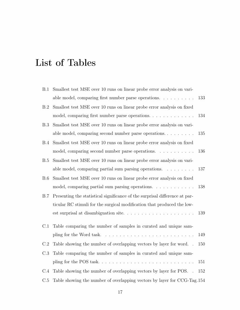
List of Tables

B.1 Smallest test MSE over 10 runs on linear probe error analysis on vari-

able model, comparing first number parse operations. . . . . . . . . . 133

B.2 Smallest test MSE over 10 runs on linear probe error analysis on fixed

model, comparing first number parse operations. . . . . . . . . . . . . 134

B.3 Smallest test MSE over 10 runs on linear probe error analysis on vari-

able model, comparing second number parse operations. . . . . . . . . 135

B.4 Smallest test MSE over 10 runs on linear probe error analysis on fixed

model, comparing second number parse operations. . . . . . . . . . . 136

B.5 Smallest test MSE over 10 runs on linear probe error analysis on vari-

able model, comparing partial sum parsing operations. . . . . . . . . 137

B.6 Smallest test MSE over 10 runs on linear probe error analysis on fixed

model, comparing partial sum parsing operations. . . . . . . . . . . . 138

B.7 Presenting the statistical significance of the surprisal difference at par-

ticular RC stimuli for the surgical modification that produced the low-

est surprisal at disambiguation site. . . . . . . . . . . . . . . . . . . . 139

C.1 Table comparing the number of samples in curated and unique sam-

pling for the Word task. . . . . . . . . . . . . . . . . . . . . . . . . . 149

C.2 Table showing the number of overlapping vectors by layer for word. . 150

C.3 Table comparing the number of samples in curated and unique sam-

pling for the POS task. . . . . . . . . . . . . . . . . . . . . . . . . . . 151

C.4 Table showing the number of overlapping vectors by layer for POS. . 152

C.5 Table showing the number of overlapping vectors by layer for CCG-Tag.154

17

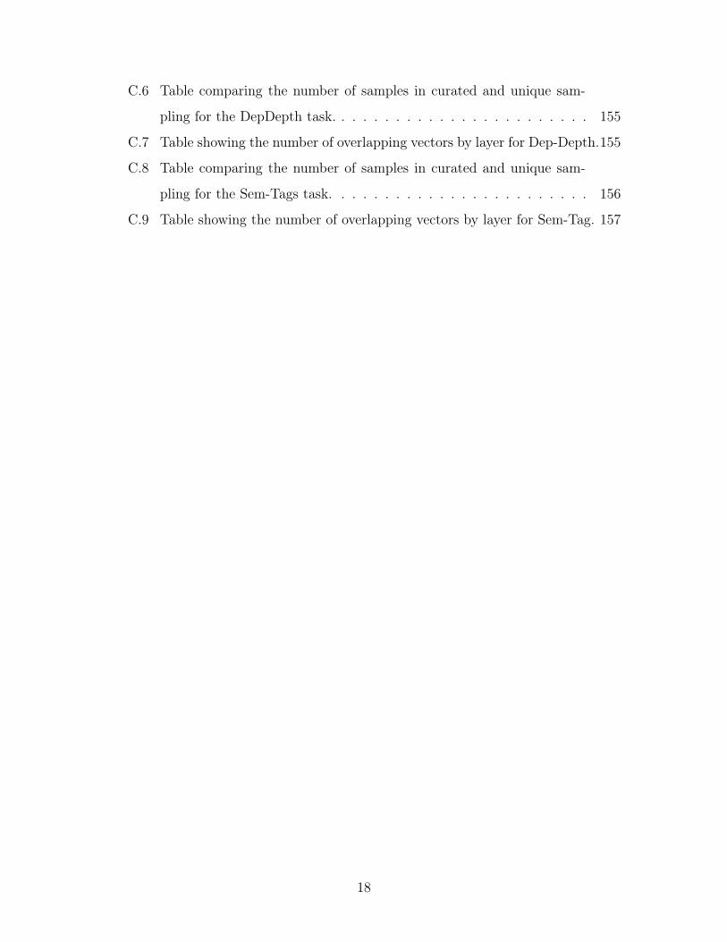
C.6 Table comparing the number of samples in curated and unique sam-

pling for the DepDepth task. . . . . . . . . . . . . . . . . . . . . . . . 155

C.7 Table showing the number of overlapping vectors by layer for Dep-Depth.155

C.8 Table comparing the number of samples in curated and unique sam-

pling for the Sem-Tags task. . . . . . . . . . . . . . . . . . . . . . . . 156

C.9 Table showing the number of overlapping vectors by layer for Sem-Tag. 157

18

19

20

Chapter 1

Introduction

1.1 Background

Machine learning as a science is not something inherently new. In reality, before

machine learning existed, many of the foundations already existed for a long period

as part of statistics and neuroscience. Pinpointing an exact year or person that began

the era of machine learning is difficult to say the least. Mathematically, the work done

by Thomas Bayes and Pierre-Simon Laplace provided the foundations of inference and

Bayes’ Theorem which are at the core of many modern, artificial intelligence (A.I.)

systems. Pragmatically, the work by Warren McCulloch and Walter Pitts originated

the idea of neurons and even provided an electrical circuit that could simulate a

neural network. This would inevitably lead to Frank Rosenblatt’s creation of the

perceptron - the basis for all modern deep neural networks. Finally, the conceptual

vision of Alan Turing’s "Universal Machine" and his Turing Test truly sparked many

scientist’s imagination of waht future computers could one day do - leading us into

the A.I. Revolution as we know it. While each of these people have had significant

impact in the origins of the field, it is the combined efforts of the research community

that has shaped what now dominates our society.

Over many decades, the field of machine learning and artificial intelligence has

developed and experienced many research slow-downs or "winters". During the peri-

ods of large activity however, major progress has always been made to improve upon

21

these intelligent systems. The first major change came in 1952, when Arthur Samuels

working for International Business Machines Coporation (IBM) was the first to ever

develop a computer program that learned to played checkers; for the first time, the

term machine learning was coined and is used to describe a computer that can adapt

its strategy. In 1959, Stanford developed MADALINE, a neural network that learned

to adaptively filter echoes from phone calls. Then, for the first time ever in 1985,

Terry Sejnowski and Charles Rosenberg developed an artificial neural network that

could learn to speak called NETTalk. IBM’s DeepBlue, in 1997, was the first com-

puter ever to learn chess and defeat a chess master. And it is here, at the beginning of

the 21st Century where the major boom in machine learning we are now experiencing

began - with the sufficient computational power and mathematical tools to develop

modern deep neural networks.

These major improvements have been felt through the various sub-fields of ma-

chine learning as well as many other areas of science. So called, "expert-systems"

have shown great promise in new medical applications even improving over the best

human doctors [2]. State-of-the-art language models are able to create text that is

extremely difficult to distinguish from human writing [3]. Never before seen human

faces can now be generated using the newest neural models [4]. The list of results from

recent research is long and awe-inspiring, but all suffer from a lack of explainability -

as in no one knows exactly how and why neural models achieve these spectacles.

The black-box nature of more complicated machine learning models has halted

major progress in real-world applications. For example, medical applications need to

be able to explain why a diagnosis was given - this prevents many modern machine

learning techniques from being used simply because no one can really be sure of what

the model learned[5]. This is only one of the many reasons we must ask: what does a

machine learning model know? Recent research has focused on studying these neural

models in hopes of finding an answer:

In [?], the authors studied a convolutional neural network (CNN) model and found

which pixels in an image were most important to make a prediction. The work done

in [6] explored a similar concept by looking at the gradients of the convolutional

22

layers, finding the general areas that a model found most useful when classifying.

Psycholinguists in [7] observed recurrent neural (RNN) models and determined that

long-term subject-verb dependencies are represented in the model’s feature represen-

tations. Work on abstracting language has shown promise in the recent years as well;

similar to the work performed on humans in [8], a group in Stanford found that un-

der certain data projections, we can find an approximate, linguistic tree structure in

neural language models[9]. Researchers have even found that these neural language

models are learning our cultural biases based on the data we train them on [10].

As a research community, we have only just scratched the surface and begun the

exploration of neural networks. In this work, we take our own approach to answer

the question: "what does a machine learning model learn?" We will explore the

principles of how information is represented and studied in simple models trained

on simple tasks. We then move on to larger, more well defined models trained on

language. First, we will show that these models learn to distribute information across

various features and that information can be distorted with simple operations. Next,

we take a new approach to a common technique and show that we’ve only just begun

to understand the complex mechanisms behind modern language models. Finally we

will take a step back and show that these models are capable of learning higher-level,

implicit structures.

1.2 Methods and Techniques

1.2.1 Principle Component Analysis

Principle Component Analysis (PCA)[11] is a statistical technique that finds orthog-

onal vectors (also known as principle components) that can describe data variance.

By definition, the principle components found by PCA are ordered such that the

explained variance decreases with each consecutive components (in other words the

first principle component describes the direction of the biggest, linear variance in the

data while the second explains the second most, and so on). For this work, we rely

23

on the implementation provided by Sci-Kit Learn [12]1

1.2.2 Uniform Manifold Approximation and Projection

Uniform Manifold Approximation and Projection (UMAP)[13], like PCA, is a di-

mensionality reduction technique but unlike it, primarily focuses on preserving non-

linearities that exist within the data. The foundation of the algorithm assumes the

data has the following properties:

1. The data is uniformly distributed on Riemannian manifold;

2. The Riemannian metric is locally constant (or can be approximated as such);

3. The manifold is locally connected.

A good tutorial on this technique is provided by the paper authors2. We also use

their implementation (umap-learn) for our work3

1.2.3 Linear Probes

Throughout the work, we use a variety of linear probes - in particular, both Chapter 2

and Chapter 3 use a linear regression model while Chapter 4 uses a linear classifier

via a "Softmax Linear Layer" and a Support Vector Machine (SVM). The following

will give detail to these probes.

Linear Regression

The purpose of linear regression is to find a linear function that best maps some input

space to some output space. More formally, for some data point, x ∈ R𝑛 and output,

𝑦, we wish to find a function of the following form:

𝑦 ≈ 𝑓(x) = 𝛽1𝑥1 + 𝛽2𝑥2 + ...+ 𝛽𝑛𝑥𝑛 (1.1)

1https://scikit-learn.org/stable/modules/generated/sklearn.decomposition.PCA.html2https://umap-learn.readthedocs.io/en/latest/how𝑢𝑚𝑎𝑝𝑤𝑜𝑟𝑘𝑠.ℎ𝑡𝑚𝑙3https://umap-learn.readthedocs.io/

24

where 𝑥𝑖 corresponds to the 𝑖𝑡ℎ component of x. Now suppose our dataset has 𝑚

samples, and each sample has 𝑛 features. We can define a dataset matrix 𝑋 ∈ R𝑚x𝑛

corresponds to all the data samples and vector 𝑦 ∈ R𝑚x1 corresponds to all the desired

outputs. The previous can equation can be re-written as:

𝑋𝛽 ≈ 𝑦 (1.2)

where 𝛽 ∈ R𝑛x1 describes the linear coefficients of 𝑓(𝑥). Our goal is to estimate

𝛽 - this is typically done via Ordinary Least Squares (OLS) as follows:

𝑋𝛽 ≈ 𝑦 (1.3)

𝑋𝑇𝑋𝛽 = 𝑋𝑇𝑦 (1.4)

(𝑋𝑇𝑋)−1(𝑋𝑇𝑋)𝛽 = (𝑋𝑇𝑋)−1𝑋𝑇𝑦 (1.5)

𝛽 = (𝑋𝑇𝑋)−1𝑋𝑇𝑦 (1.6)

Therefore, our best estimate of a linear mapping from input space to output space is

𝛽.

For the implementation of Linear Regression, we use the code provided by Sci-kit

learn[12]4

Softmax Linear Layer Classification

Given some data set with 𝑚 samples each with 𝑛 features, X ∈ R𝑚x𝑛, the class each

belongs to, 𝑦 ∈ R𝑚x1, and a pre-set number of classes, 𝑐, the softmax linear layer

must learn a transformation matrix, 𝑀 ∈ R𝑛x𝑐 such that for any data point, 𝑥𝑖, the

correct class 𝑦𝑖 has the highest probability. More formally:

∀𝑖 ∈ [1,𝑚], argmax(𝜎(𝑋𝑀)𝑖) = 𝑦𝑖 (1.7)

where 𝜎(·) is the softmax activation function (see appendix C.1).4https://scikit-learn.org/stable/modules/generated/sklearn.linear𝑚𝑜𝑑𝑒𝑙.𝐿𝑖𝑛𝑒𝑎𝑟𝑅𝑒𝑔𝑟𝑒𝑠𝑠𝑖𝑜𝑛.ℎ𝑡𝑚𝑙

25

In Chapter 4, we use this probe with very specific parameters and training regime

to match the work done in [14]. This probe is optimized using the Adam optimizer[15]

with a learning rate of 0.0001. The probe is trained for 50 epochs using early stopping

with a patience of 3. We also perform this operation for 10 different probes trained

on the same task with different data splits and report the results from the probe that

performs best under their respective test sets.

The code we wrote for this is written using Pytorch[16].

Support Vector Machines

Support Vector Machines (SVMs) are commonly used classifiers in the field of machine

learning. At their most basic, the idea is to find a plane that separates two classes

such that the distance between the class boundaries is maximized (i.e. we wish to

maximize the margin defined by the SVM’s hyperplane). These models are solved

through optimization of the primal formulation:

min𝑤∈𝐼Ω𝑅𝐷

𝜆[|𝑤|]2+𝐶𝑁∑𝑖=1

max(0, 1− 𝑦𝑖𝑓(𝑥𝑖)) (1.8)

where our dataset lies in D dimensions and the hyperplane learned by the model is

𝑓(𝑥) = 𝑤𝑇𝑥+ 𝑏.

This will result in a "hard" margin classifier meaning that the data must be linearly

separable in order for a hyperplane to be found. We can relax these constraints and

allow for some slack on the data, resulting in a "soft" margin classifier formulated by

the optimization of:

min𝑤∈𝐼Ω𝑅𝐷

,𝜉∈𝐼Ω𝑅+𝜆[|𝑤|]2+𝐶

𝑁∑𝑖=1

𝜉𝑖, (1.9)

subject to 1− 𝑦𝑖𝑓(𝑥𝑖) ≥1− 𝜉𝑖∀𝑖 ∈ [1, 𝑁 ] (1.10)

where our dataset lies in D dimensions and the hyperplane learned by the model is

𝑓(𝑥) = 𝑤𝑇𝑥+ 𝑏.

26

For the implementation of SVM, we use the code provided by Sci-kit learn[12]5

1.2.4 Mean Field Theory

Originating from the work by Chung et al.[17, 18, 19, 20], the mean field theory

(MFT) technique is used to quantify the amount of invariant object information by

measuring various geometrical properties of the internal representations - specifically,

this technique seeks to find the radius, dimension, and manifold capacity of pre-

defined data manifolds as they are represented over a model. With these measures, we

are able to measure the linear separability present within a model’s representations

and understand what about the geometry of this representations promotes model

behavior.

1.2.5 Canonical Correlational Analysis

Canonical Correlational Analysis (CCA) is a technique used to estimate the relation-

ship between two sets of data. It finds a coefficient vector such that we maximize the

covariance between two given datasets. Quoting T. R. Knapp, "virtually all of the

commonly encountered parametric tests of significance can be treated as special cases

of canonical-correlation analysis". Simply put, this metric can be used to estimate

the similarity between two datasets such that a result of 1 means the datasets are the

same and a result of 0 means that they are completely different.

5https://scikit-learn.org/stable/modules/generated/sklearn.svm.SVC.html

27

1.3 Models

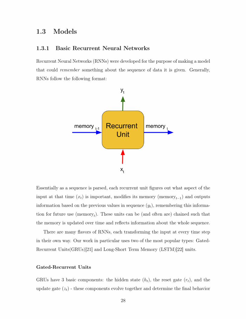
1.3.1 Basic Recurrent Neural Networks

Recurrent Neural Networks (RNNs) were developed for the purpose of making a model

that could remember something about the sequence of data it is given. Generally,

RNNs follow the following format:

Essentially as a sequence is parsed, each recurrent unit figures out what aspect of the

input at that time (𝑥𝑡) is important, modifies its memory (memory𝑡−1) and outputs

information based on the previous values in sequence (𝑦𝑡), remembering this informa-

tion for future use (memory𝑡). These units can be (and often are) chained such that

the memory is updated over time and reflects information about the whole sequence.

There are many flavors of RNNs, each transforming the input at every time step

in their own way. Our work in particular uses two of the most popular types: Gated-

Recurrent Units(GRUs)[21] and Long-Short Term Memory (LSTM)[22] units.

Gated-Recurrent Units

GRUs have 3 basic components: the hidden state (ℎ𝑡), the reset gate (𝑟𝑡), and the

update gate (𝑧𝑡) - these components evolve together and determine the final behavior

28

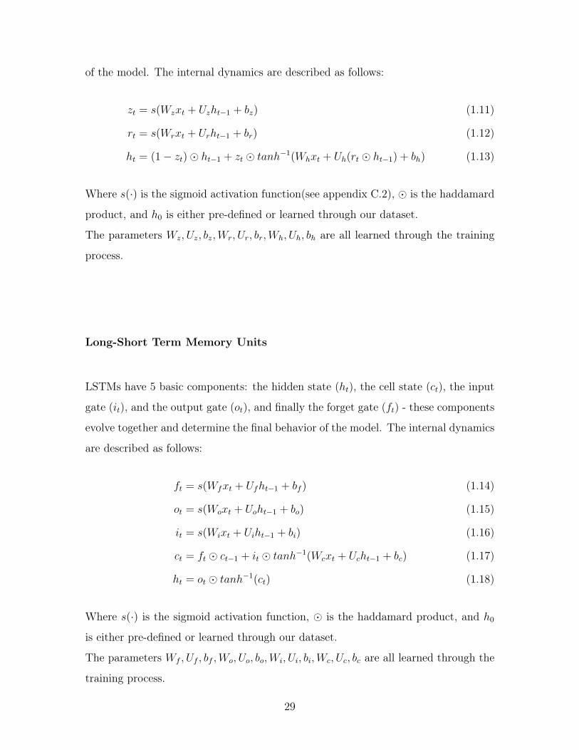
of the model. The internal dynamics are described as follows:

𝑧𝑡 = 𝑠(𝑊𝑧𝑥𝑡 + 𝑈𝑧ℎ𝑡−1 + 𝑏𝑧) (1.11)

𝑟𝑡 = 𝑠(𝑊𝑟𝑥𝑡 + 𝑈𝑟ℎ𝑡−1 + 𝑏𝑟) (1.12)

ℎ𝑡 = (1− 𝑧𝑡)⊙ ℎ𝑡−1 + 𝑧𝑡 ⊙ 𝑡𝑎𝑛ℎ−1(𝑊ℎ𝑥𝑡 + 𝑈ℎ(𝑟𝑡 ⊙ ℎ𝑡−1) + 𝑏ℎ) (1.13)

Where 𝑠(·) is the sigmoid activation function(see appendix C.2), ⊙ is the haddamard

product, and ℎ0 is either pre-defined or learned through our dataset.

The parameters 𝑊𝑧, 𝑈𝑧, 𝑏𝑧,𝑊𝑟, 𝑈𝑟, 𝑏𝑟,𝑊ℎ, 𝑈ℎ, 𝑏ℎ are all learned through the training

process.

Long-Short Term Memory Units

LSTMs have 5 basic components: the hidden state (ℎ𝑡), the cell state (𝑐𝑡), the input

gate (𝑖𝑡), and the output gate (𝑜𝑡), and finally the forget gate (𝑓𝑡) - these components

evolve together and determine the final behavior of the model. The internal dynamics

are described as follows:

𝑓𝑡 = 𝑠(𝑊𝑓𝑥𝑡 + 𝑈𝑓ℎ𝑡−1 + 𝑏𝑓 ) (1.14)

𝑜𝑡 = 𝑠(𝑊𝑜𝑥𝑡 + 𝑈𝑜ℎ𝑡−1 + 𝑏𝑜) (1.15)

𝑖𝑡 = 𝑠(𝑊𝑖𝑥𝑡 + 𝑈𝑖ℎ𝑡−1 + 𝑏𝑖) (1.16)

𝑐𝑡 = 𝑓𝑡 ⊙ 𝑐𝑡−1 + 𝑖𝑡 ⊙ 𝑡𝑎𝑛ℎ−1(𝑊𝑐𝑥𝑡 + 𝑈𝑐ℎ𝑡−1 + 𝑏𝑐) (1.17)

ℎ𝑡 = 𝑜𝑡 ⊙ 𝑡𝑎𝑛ℎ−1(𝑐𝑡) (1.18)

Where 𝑠(·) is the sigmoid activation function, ⊙ is the haddamard product, and ℎ0

is either pre-defined or learned through our dataset.

The parameters 𝑊𝑓 , 𝑈𝑓 , 𝑏𝑓 ,𝑊𝑜, 𝑈𝑜, 𝑏𝑜,𝑊𝑖, 𝑈𝑖, 𝑏𝑖,𝑊𝑐, 𝑈𝑐, 𝑏𝑐 are all learned through the

training process.

29

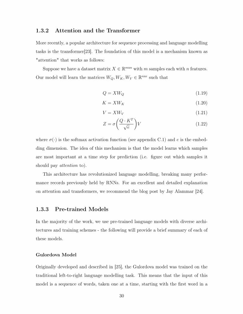
1.3.2 Attention and the Transformer

More recently, a popular architecture for sequence processing and language modelling

tasks is the transformer[23]. The foundation of this model is a mechanism known as

"attention" that works as follows:

Suppose we have a dataset matrix 𝑋 ∈ R𝑚x𝑛 with 𝑚 samples each with 𝑛 features.

Our model will learn the matrices 𝑊𝑄,𝑊𝐾 ,𝑊𝑉 ∈ R𝑛x𝑒 such that

𝑄 = 𝑋𝑊𝑄 (1.19)

𝐾 = 𝑋𝑊𝐾 (1.20)

𝑉 = 𝑋𝑊𝑉 (1.21)

𝑍 = 𝜎

(𝑄 ·𝐾𝑇

√𝑒

)𝑉 (1.22)

where 𝜎(·) is the softmax activation function (see appendix C.1) and 𝑒 is the embed-

ding dimension. The idea of this mechanism is that the model learns which samples

are most important at a time step for prediction (i.e. figure out which samples it

should pay attention to).

This architecture has revolutionized language modelling, breaking many perfor-

mance records previously held by RNNs. For an excellent and detailed explanation

on attention and transformers, we recommend the blog post by Jay Alammar [24].

1.3.3 Pre-trained Models

In the majority of the work, we use pre-trained language models with diverse archi-

tectures and training schemes - the following will provide a brief summary of each of

these models.

Gulordova Model

Originally developed and described in [25], the Gulordova model was trained on the

traditional left-to-right language modelling task. This means that the input of this

model is a sequence of words, taken one at a time, starting with the first word in a

30

sentence and end terminating after the last word.

Architecturally, the model only has two stacked, LSTM layers, with 650 and 200

hidden units respectively. An implementation of this model can be found in the

colorless green repository.6

BERT Base Cased

The Bidirectional Encoder Representations from Transformers (BERT) Base model[26]

was developed by researchers at Google AI in 2018. It has been able to perform far

better than many other models on traditional natural language processing (NLP)

Tasks such as question answering (SQuAd), natural language inference (MNLI), and

on the general language understanding evaluation (GLUE) benchmark. Unlike most

models, BERT is first trained on the masked language modelling task and then on a

next sentence prediction task. This unique training sequence means that: BERT is

fed the whole sentence at once and some words are replaced with something different

(either a randomly chosen word or the special "[MASK]" token) which allows the

model to capture distant relationships among words and prevents the model from

relying too much on any token for it’s prediction.

This model has quite a deep architecture with a many internal components. The

first layer is an embedding layer that generates vectors from tokens via a convolutional

tranformation. Every layer after that is based on the tranformer architecture (for the

specifc changes, see the original paper). In total, there is 1 Embedding layer and 12

Tranformer layers, each with 768 hidden units.

An excellent repository that includes a frozen model and great tutorials is the

huggingface repository 7[27]. We use this repository for our implementation of BERT.

6(https://github.com/facebookresearch/colorlessgreenRNNs)7https://github.com/huggingface/transformers

31

32

33

34

Chapter 2

Linear Probing of Simple Sequence

Models

2.1 Background

Artificial Neural Networks are often thought of as black-boxes; information is passed

in one end and an output comes out the other, giving scientists little clue to what hap-

pens in-between. That process of transforming data however, is crucial to understand

how or what the model has learned. It is known that neural networks can approxi-

mate any function[28] but our choice of optimization, activation function, number of

neurons, number of layers, and the type of layer will greatly affect how that transfor-

mation is learned. Recent work at New York University (NYU) has shown that the

choice of update rule, a type of optimization technique, for Recurrent Neural Net-

works (RNNs) has significant impact in how easily a task is learned[29]. Other work

has explored the importance of various components in a Long-Short Term Memory

(LSTM) network[30] and it has been found that the addition of these components

simplifies optimization[31].

Parallel investigations into what a model learns have also taken great strides for-

ward. Early work exploring deep Convolutional Neural Networks (CNNs) showed that

early layers in the model focus on identifying "low-level features" of an image such as

edges and simple shapes while later layers have broader views of images [32]. Most

35

recently, researchers at Google Brain and Brown University[33] measured where infor-

mation about words and various aspects of these words are found in a state-of-the-art

language model.

These studies have always had to limit themselves due to the complex nature

of real-world data; dealing with the intricacies of an image or human language are

by no means an easy task. For this reason, researchers have used artificial data to

augment our understanding of neural networks. David Sussilo and Omri Barak, for

example, explored the non-linear dynamics of RNNs in their work[34] to show that

the model had learned efficient representations based on its assigned task. In another

experiment[35], researchers generated their own artificial language and were able to

probe fore specific knowledge required by their design. Fully controlling the data that

a model learns is what makes artificial data or "toy tasks" so useful.

Inspired by these tasks, we begin our explorations into the geometric nature of

sequence-processing neural networks by showing an example of current techniques

used to analyze these models. In particular, we are motivated by the artificial lan-

guage of [35] and, in this chapter, develop our own task that mimics this work: the

2-Add Regression. Through this task we will explore what information is internally

stored, how this information is stored, and the operations that the model learns. On

top of this, we use our tasks to study how the choice of data and the presentation of

that data affects the model’s ability to learn a task.

2.2 Model

In our following explorations, we used a 1 layer network with 100 Gated-Recurrent

Units (GRUs)[21]. The model was trained for 5 epochs using stochastic gradient

descent (SGD)[36] to minimize the mean-squared error (MSE).

We chose GRUs due to their proven capability and performance. We also de-

cided to stick close to the model used in the investigation[35] that inspired the 2-Add

Regression Task.

36

2.3 2-Add Regression Task

2.3.1 Description

For some integers, 𝑛1 and 𝑛2, let 𝑠 = 𝑛1 + 𝑛2. The task for our model is: given a

sequence of characters describing the addition of 𝑛1 and 𝑛2, predict the sum 𝑠

2.3.2 Implementation

In order to implement the addition task, we define a vocabulary V={0,1,2,...,8,9,+,-

,=}. Each character in a sample is one-hot encoded according to V and passed, in

sequence, to the recurrent model. When the ’=’ character is passed into the model,

we use linear regression on the hidden state to predict 𝑠. Our numbers 𝑛1 and 𝑛2 are

drawn uniformly at random from [−100, 100]. The dataset we developed consists of

20,000 random samples from the task space.

When implementing the task, there are two possible ways of parsing a number:

fixed length parsing in which we force all numbers to have the same number of

characters (i.e. 7 is parsed as +007 and -62 is -062) or variable length parsing in

which the quantity of characters to describe a number depends on its value (i.e. 7

is parsed as 7 and -62 is -62). These variations are crucial distinctions, particularly

because of the expected structure each implies. By having a fixed length number, the

data now has a set structure such that characters 1-4 will always belong to the first

number and characters 6-9 will always belong to the second number. This structure

potentially allows each character to be interpreted by its place value - we call this a

categorical parse. A variable length number, will instead result in unknown length

sequences. This implies that at any point in the series one could be expected to return

or remember some value - we call this interpretation a running parse.

In our explorations, we study both fixed and variable length numbers; training

the model on a fixed length resulted in a final test MSE of 0.016 while variable length

resulted in a final test MSE of 1.913. As we explore the information encoded in the

model’s hidden state space, we will recall these two parse interpretations and attempt

37

to measure the most likely operation.

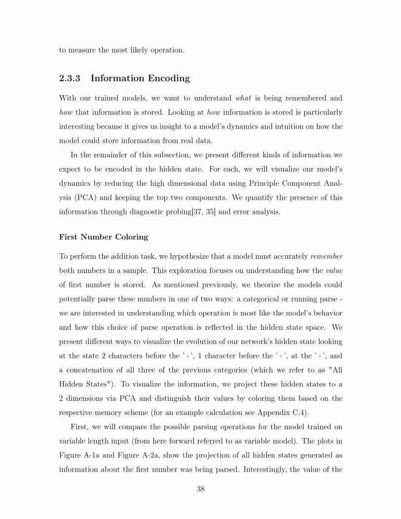
2.3.3 Information Encoding

With our trained models, we want to understand what is being remembered and

how that information is stored. Looking at how information is stored is particularly

interesting because it gives us insight to a model’s dynamics and intuition on how the

model could store information from real data.

In the remainder of this subsection, we present different kinds of information we

expect to be encoded in the hidden state. For each, we will visualize our model’s

dynamics by reducing the high dimensional data using Principle Component Anal-

ysis (PCA) and keeping the top two components. We quantify the presence of this

information through diagnostic probing[37, 35] and error analysis.

First Number Coloring

To perform the addition task, we hypothesize that a model must accurately remember

both numbers in a sample. This exploration focuses on understanding how the value

of first number is stored. As mentioned previously, we theorize the models could

potentially parse these numbers in one of two ways: a categorical or running parse -

we are interested in understanding which operation is most like the model’s behavior

and how this choice of parse operation is reflected in the hidden state space. We

present different ways to visualize the evolution of our network’s hidden state looking

at the state 2 characters before the ’+’, 1 character before the ’+’, at the ’+’, and

a concatenation of all three of the previous categories (which we refer to as "All

Hidden States"). To visualize the information, we project these hidden states to a

2 dimensions via PCA and distinguish their values by coloring them based on the

respective memory scheme (for an example calculation see Appendix C.4).

First, we will compare the possible parsing operations for the model trained on

variable length input (from here forward referred to as variable model). The plots in

Figure A-1a and Figure A-2a, show the projection of all hidden states generated as

information about the first number was being parsed. Interestingly, the value of the

38

first number seems to be presented along an axis such that a clear visual separation

between positive and negative first numbers exists. Looking at plots b,c, and d in

both Figure A-1 and Figure A-2 we see the evolution of hidden states as we approach

the ’+’ character. The distinction we saw in Figure A-1a is even more obvious as

the model recieves more information and the hidden state evolve; two completely

distinct clusters place the value of the first number on a gradient (see Figure A-1d

and Figure A-2d). Visually, the different parsing operation seem constant apart from

the difference in color intensity we see in Figure A-1b.

In order to quantify the differences of these two parses, we train 10 linear regressors

at each view (all hidden states, 2 characters before ’+’, 1 character before ’+’, and

at the ’+’ character). We claim that whichever operation results in a lower test MSE

overall must be most similar to the model’s true operation at that scale. We present

these results in Table B.1. Overall we find that the running parse on "All Hidden

States" has lower test MSE - this seems to imply that the information about the first

number could be remembered via a running parse.

We now observe the parsing operations on the model trained on the fixed length

input (from here forward referred to as the fixed model). As was the case in the

variable model, very little difference is seen among the coloring of the four different

views when we compare Figure A-3 and Figure A-4. Observing the evolution of the

hidden states, it seems that the model evolves two distinct clusters between positive

and negative first number values. Unique to this model however, the PCA on all

hidden states (shown in Figure A-3a and Figure A-4a) is not as visibly separable in

the way that the variable model was on the same view. Two possible interpretations

of this:

1. Information is rotating - when a new character is introduced into the model,

stored information moves to a different location or set of dimensions. This

would mean that PCA would not be able to capture the information because

each time step would store the information in a unique way.

2. Not enough dimensions - due to the low-dimensional projection, it’s possible

39

that the information is visibly separable but only in a higher dimension. This

would mean that we would not be able to see the separability because we lack

the figure to do this.

We believe the most likely answer is a combination of both interpretations; from

figures b,c,d in Figure A-3 and Figure A-4 it seems that the information about the

first number is easily readable and separable so information might be rotating but

without fully viewing the data, we won’t know for certain. Instead, we attempt to

quantify this by using a linear probe. If the probe can predict the first number’s

value when trained on all states, then we can claim that this information is present

but requires higher dimensions to view. We present the lowest test MSE for these

analyses in Table B.2. It seems that the linear probe trained on all hidden states

performs better with a categorical parse scheme; this potentially implies that overall

hidden states are encoding information about the first number in a categorical way.

We cannot yet claim this as a fact. It’s possible that this information is signal

of something else - potentially information about the addition. We will check this

by performing similar experiments on the second number parse operation and the

addition parse operation.

Second Number Coloring

As with the first number value, we hypothesize that the second number value is being

stored in the the hidden state. We take a look at the hidden states where we expect

the information about the second number to be present - that is hidden states from 2

characters before ’=’, 1 character before ’=’, and at the ’=’ character. We include

the concatenation of all three categories (which we name "All Hidden States"). To

visualize the information, we project these hidden states to a lower dimension via

PCA and distinguish their values by coloring them based on their respective memory

scheme (for an example calculation see Appendix C.5).

We present the variable model’s hidden state colored by the running parse of the

second number in Figure A-5 and by the categorical parse of the second number in

Figure A-6. Visually, it would again seem that the variable number is using it’s feature

40

space to encode information - this time about the second number. By comparing the

running and categorical parse figures, it would seem that the running parse on all

hidden states (Figure A-5a) has a slight gradient property to it that is not seen in the

categorical parse (Figure A-6a). We turn to linear probing to quantify the differences;

we present the MSE on test data for the best of 10 probes on Table B.1. From the

results of probing, it would seem to imply that little, if any, information about the

second number can be linearly extracted from the hidden states.

We repeat these experiments on the fixed model’s hidden states. The figures of

the four hidden state views (2 characters before ’=’, 1 character before ’=’, at the

’=’ character, and the concatenation of all three categories referred to as "All Hidden

States") on running second number parse are in Figure A-7 and categorical second

number parse in Figure A-8. Visually, the hidden state in this case seems to be more

problematic for linear separability. There does seem to be some distinction between

positive and negative numbers but there is a large amount of overlap at all views

between positive and negative numbers. We quantify these results using the best of

10 linear regressors on test data and present the resuls on test data in Table B.4. Like

the variable model, we also find the linear probes perform poorly.

This is particularly counter-intuitive due to the clear visual separation we saw in

the PCA and the good performance on the first number regression. It is possible that

the PCA separation only clearly distinguishes between positive and negative numbers,

and does not clearly separate value which would still make linear regression a difficult

task. At the same time, the performance on the first number regression, could result

from the hidden state not storing either number value but only the sum of the two

numbers. Without information about the second number, as the first is being parsed

the partial sum is essentially the first number meaning the accuracy we had could

result from an internal, partial sum operation.

Partial Summing

We begin our exploration with a simple hypothesis that the model’s hidden state is

storing the partial sum. Similar to number parsing, we theorize two possible ways by

41

which a model could learn to add two numbers from a character sequence:

1. Running Sum

For some sample in our dataset, 𝑥 + 𝑦 = 𝑧, let 𝐶1...𝑛 be the sequence 𝑛 of

characters representing this addition. At time 𝑡, the model has seen characters

𝐶1...𝑡 - the running sum at time 𝑡 then is sum if the full sequence were 𝐶1...𝑡,’=’.

(Note that if the sequence has non numeric characters as the final character (s),

such as ’+’, ’-’, or ’=’, we calculate the sum as if it ended on the last numeric

character. For an example of this calculation see the example in Appendix C.6)

2. Categorical Sum

For some line in our dataset, 𝑥+𝑦 = 𝑧, let 𝐶1...𝑛 be the sequence 𝑛 of characters

representing this addition such that we fix the number of 𝑥 and 𝑦. By the nature

of having fixed length variables, each time-step corresponds to a different place

value of either 𝑥 or 𝑦, so at time 𝑡, the model has seen characters 𝐶1...𝑡 - the

categorical sum is the sum if the remaining characters corresponding to either

𝑥 or 𝑦 are zeros. (Note that if the sequence has non numeric characters as the

final character (s), such as ’+’ or ’-’ we simply append the necessary zeros to

fill 𝑥 and 𝑦 and calculate the sum. For an example of this calculation see the

example in Appendix C.7).

We try to visualize these potential summing operations by performing PCA on

all hidden states over all characters and projecting the vectors into low dimensional

space. This will give us a reasonable way to see the model’s hidden state evolution

at once.

In Figure A-9, we present three different coloring schemes to distinguish the vari-

able model’s hidden states: first the "intermediate prediction" scheme in Figure A-9a

which colors each hidden state using the prediction from the model’s final linear re-

gressor, followed by the running sum scheme in Figure A-9b and the categorical sum

scheme in Figure A-9c both of which are described above. There seems to be no

strong, visual distinction between the running sum and categorical sum. That being

42

said, the schemes seem to be separating the information about the number as a gradi-

ent along the first principle component very similar to the coloring shown by the the

intermediate prediction figure. We verify these observations, by training 10 different

linear regressors on the full set of hidden states and present the results on test data

in Table B.5. These results imply that the difference between the two schemes on

individual time steps is minimal - more-over the results are not promising that either

partial sum operation is the underlying behavior.

For the fixed model, we repeat the experiment and present the visualizations in

Figure A-10. In this case, we do see a clear visual distinction between the running sum

(Figure A-10b) and categorical sum(Figure A-10c) coloring schemes. In particular,

Figure A-10b clearly has positive and negative values mapped all over the space while

Figure A-10c has a more defined gradient (with few exceptions). Visually, we see that

the categorical sum scheme is more similar to the intermediate prediction (Figure A-

10a) than the running sum is. Again, we quantify these observations and present

them in Table B.6. Despite the visual distinction, it seems that both operations

perform poorly in prediction the partial sum.

2.4 Discussion

It would seem that, despite the promising visuals, we are unable to claim much about

the operations used to store information in the hidden state representation of our

model. This experiment was fruitful however by confirming that the choice of data

and the internal structure that the data has will greatly impact performance. The

models even learned very distinct ways to represent their data internally. But clearly,

the model is learning something because it performs relatively well when it must

predict the sum of the two numbers.

Following the example of previous works was not enough - ultimately be it the

complexity of our model or the simplicity of our probe the information eluded us.

It is possible that the signal was in fact present through every hidden state but we

simply missed it. Perhaps if we had used a more complex, non-linear probe the

43

information could have been captured? But this brings more issues than solutions:

Which non-linearity is appropriate? How do we avoid capturing noise that is present?

What interpretations can we get from studying the probe? What’s more, whatever

choice we make could work well for one of the models but not the other. The probing

techniques used in this chapter are consistent with state-of-the-art work currently

being done. Based on our results in the toy example, we see that some probes can

lack the substance to fully understand a model. Without a more formal methodology

that can understand the complicated geometries and non-linearities present in neural

models, we will only ever be able to scratch the surface of neural information.

44

45

46

Chapter 3

Manipulations of Language Model

Behavior

3.1 Background

Psycholinguists have developed broad theories attempting to explain how humans

process sentences like those in Examples (1) and (2).

(1) The woman brought the sandwich tripped.

(2) The woman given the sandwich tripped.

These special sentences are known as "garden path" sentences for the method in

which they lead a reader down one interpretation but suddenly change due to an

unexpected, but grammatically correct word.

For our purposes, the psycholinguistic theories contrast in two important ways:

Computational mechanism: How do readers deal with multiple possible inter-

pretations of a sentence? They may incrementally construct a single analysis

(serial theories) or revise multiple candidate analyses at the same time (parallel

theories).

Modularity: Which cues enter into the initial analysis of a sentence? Readers may

exploit only syntactic cues (modular theories), or both semantic and syntactic

cues (nonmodular theories).

47

With all theories, proving that any one mechanism is truly the human mechanism

is difficult. There is no easy way to observe all neurons, interpret the observations,

and prove a theory is correct. Instead by looking at neural-network based models, we

could potentially gain useful insight into human language mechanisms. These models

can easily be manipulated, stopped, and observed at any point during sentence parsing

giving psycholinguists a unique view of the network’s inner-workings.

These same theories, then, can be applied to our artificial subjects. And the

questions now become a matter of measurement and interpretation.

3.1.1 Representational questions

While processing theories differ in mechanistic accounts, they each assume large

amounts of competence knowledge: they assume, for example, that a reader can

recognize words as nouns or verbs, and that a reader knows that the two alternative

analyses of Examples (1) and (2) consist of a “main verb analysis” and a “relative

clause analysis.” To the extent that recurrent neural-network based language mod-

els (RNNLMs) produce consistent prediction behavior on minimal pair examples like

Examples (1) and (2), we expect that their predictions must be derived from some

approximation of this competence knowledge.

But how could concepts like “verb” or “relative clause analysis” be learned from

text corpora without any syntactic annotations? Furthermore, how could continuous

neural network hardware serve to represent such structured knowledge?

We focus on the ambiguous relative clause constructions (as in Example (1)) be-

cause they offer a window into these mechanistic and representational questions.

First, because incremental parsing of sentences like Example (1) license multiple

possible interpretations, we can use them to arbitrate between serial and parallel

processing theories.

Second, because we expect models to have similar representational structure allow-

ing it to distinguish main-verb and RRC analysis, we believe using these ambiguous

structures will illuminate the distributed representation within the language model.

48

3.1.2 Behavioral work

The idea of studying Neural Network based Language Models as psycholinguistic is

not a new area. Work such as [38] studied the capabilities of LSTM based models to

capture long term ’number agreement’. They found that these models were extremely

accurate (less than 1% error) at representing the quantity, but began to fail more

when intervening or conflicting nouns appeared between the subject and verb. The

work of [39] studied the ability of state-of-the-art RNNs to represent relationships

of filler-gap constraints and showed that they are able to learn and generalize about

empty syntactic positions. More recently, [1] compared four different language models

finding promising results that even models tasked with next-word prediction had

comparable syntactic state generalization as models trained specifically to predict

sentence structure.

3.1.3 Representational analysis

Due to the high dimensional nature of language modelling, work in the area of repre-

sentational analysis has focused heavily on finding novel ways to extract useful infor-

mation about the model’s state at any given timestep. In [37] the idea of diagnostic

classifiers was developed to explore how a GRU model was encoding information over

time. This idea was then used in [40] to visualize and manipulate subject plurality

encoding within an LSTM language model.

More recent work has shifted to finding specific units that encode this information

as opposed to relying on the distributed nature of diagnostic classifiers. In [41], two

units in the Gulordova langauge model (GRNN) were found to have the highest impact

on the accuracy of predicting the right verb. Through further experimentation and

evaluation, it was found that these units almost perfectly encode information about

singular and plural subjects.

49

3.2 Model

The language model we use in this paper is described in the supplementary material

of [25]. What we call “GRNN”, is a stacked LSTM with two hidden layers of 650

hidden units each, trained on a subset of English Wikipedia with 90 million tokens.1

GRNN has been the subject of a number of psycholinguistic studies, and has been

shown to produce human-like behavior for subject-verb agreement [25], subordination,

and multiple types of garden-pathing [1].

3.3 Methods

3.3.1 Garden-path Stimuli

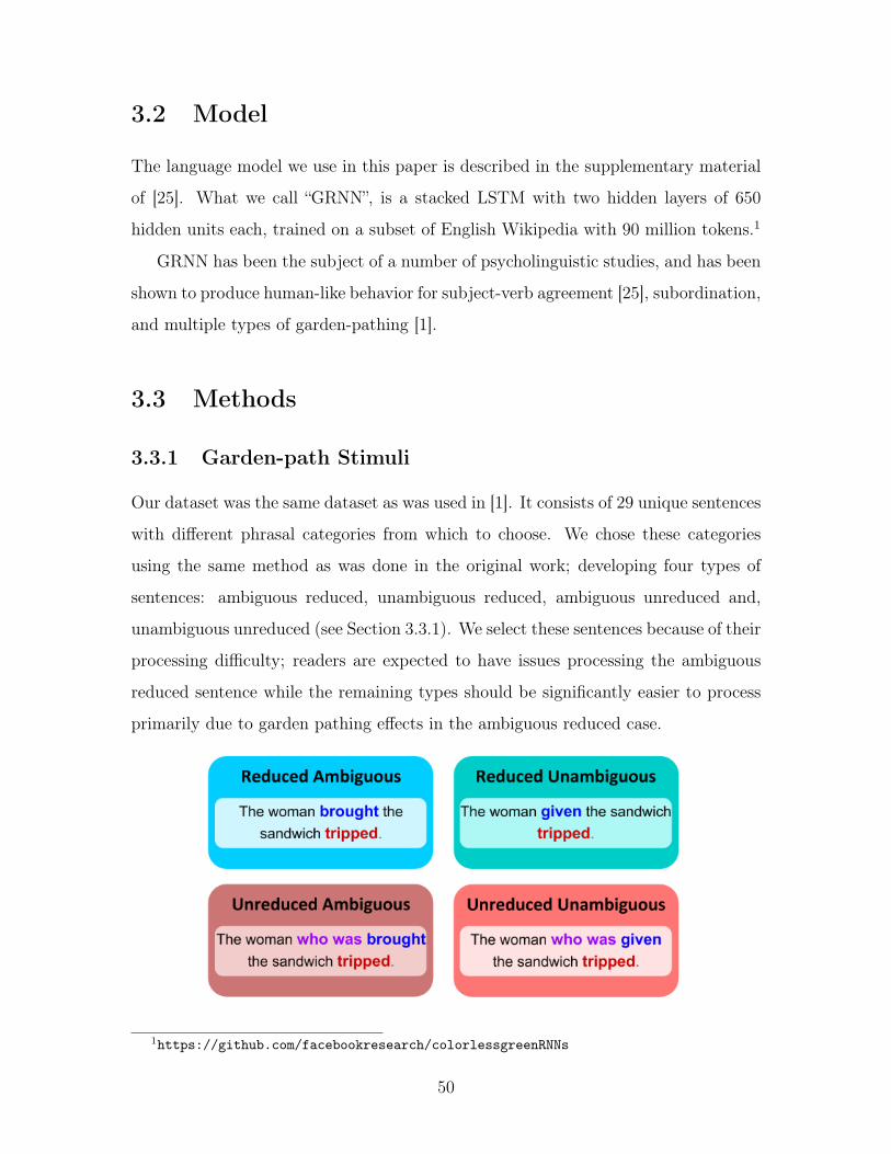
Our dataset was the same dataset as was used in [1]. It consists of 29 unique sentences

with different phrasal categories from which to choose. We chose these categories

using the same method as was done in the original work; developing four types of

sentences: ambiguous reduced, unambiguous reduced, ambiguous unreduced and,

unambiguous unreduced (see Section 3.3.1). We select these sentences because of their

processing difficulty; readers are expected to have issues processing the ambiguous

reduced sentence while the remaining types should be significantly easier to process

primarily due to garden pathing effects in the ambiguous reduced case.

1https://github.com/facebookresearch/colorlessgreenRNNs

50

3.3.2 Behavioral Study

We measure the effect of these processing difficulties via a model’s ability to predict

the next word by utilizing the concept of surprisal[42] - in essence, if the model is

unlikely to predict the next word then it is more "surprised" than if the token is

the only possibility. In our case, if the models learn the correct generalization, then

they should not assign higher surprisal at the main verb when the relative clause

is ambiguous than when it is unambiguous (either by the presence of a “who was”

phrase or by the form of the relative clause verb). In previous work, each item has

a single word or phrase in the disambiguating main verb position. If the model is

truly learning to expect a main verb however, then this pattern should hold for any

main verb at the disambiguating position. Beyond this, by considering a larger set of

possible verbs, we reduce the possibility of noise caused by any one infrequent verb

in our corpus.

We selected the most frequent tokens tagged[43] as VBD (past tense verb) in the

GRNN training corpus. After cleaning these verbs by hand to remove ambiguous

forms, we had a list of 69 VBD tokens. We then measured the surprisal at the main

verb by averaging the surprisal at each of these VBD tokens.

Figure A-11 shows the patterns of surprisal averaged over these VBD contin-

uations and all items. As expected, surprisal is lower when the relative clause is

unreduced than when it is reduced. Furthermore, when the relative clause is reduced,

the surprisal at the unambiguous verb is lower than at the ambiguous verb. While

these patterns hold on average between items, the pattern can vary within individual

items. Figure A-12 shows an item with the correct pattern, while Figure A-13 shows

an item with an incorrect pattern. While the surprisal is still lower in the unreduced

relative clause condition, the surprisal is higher in the unambiguous reduced condi-

tion than the ambiguous reduced condition. This shows that unigrams can profoundly

affect our surprisal values, suggesting that looking at a single lexical item is not suffi-

cient for measuring a model’s expectation for an entire part of speech. We therefore

recreate the temporal surprisal plot from [1] using the averaged VBD surprisal at dis-

ambiguation instead of the surprisal as defined from the items in their dataset. As we

51

can see in Figure A-14 the pairwise-relationships among sentence category surprisals

at the "Disambiguator" site stay the same as in [1] (as in from most surprising to

least the order remained ambiguous reduced, unambiguous reduced, ambiguous unre-

duced, unambiguous unreduced) but we see that the surprisals of all four cases have

increased. We claim that this figure is more representative of the model’s predictive

capabilities as it evaluates the model’s general ability to disambiguate.

3.3.3 Representation: Correlational Study

If a model had units responsible for determining the presence of relative clause, we

would expect information to be encoded within the cell state which could predict how

the model will react upon seeing the disambiguating verb. We tested this theory by

using the cell states immediately after entering the relative clause to predict the the

metric as described in Section 3.3.2. Assuming this is true, we should expect there

to be some units in previous temporal steps that are correlated with the metric at

the disambiguation site. This correlation could then be picked up by a linear model.

Therefore, we attempt to train a model to regress on the cell state and predict the

average surprisal.

We used a ridge regression model and explored different penalization parameters

over the set of {0.01,0.1,0.2,0.5,1,5,10}. Using 10-fold cross validation, we trained on

all the reduced conditions, and determined the best model was the one that had the

highest 𝑅2 score on the validation fold. In the end we found the best model used

a penalization parameter of 0.1 and got scores 𝑅2 scores of 0.928 on the reduced

ambiguous condition and 0.968 on the reduced unambiguous condition.

Using this linear probe, we then claim units are correlated if their corresponding

coefficients are statistically significant compared to the average unit - their significance

would imply that the value of these units are important to determine the surprisal

metric down the line.

We considered two methods to determine significance.

1. Singular Significance - A unit is significant if the corresponding coefficient is

three standard deviations away from the mean coefficient value on the best regression

52

model, which is equivalent to saying the coefficient is significant at the 0.003 level.

This method resulted in 6 highly correlated units with the surprisal metric, [ 39, 189

281, 328, 329, 474].

2. Smoothed Significance - A unit is only truly significant if it is frequently

found significant over all models in the cross validation. In this method, we look for

units with coefficient values that are three standard deviations away from the mean

coefficient value on each model. We then keep a count of the number of times each

unit is found significant. Using these counts, we claim a unit is truly significant only if

the unit occurs 3 standard deviations more than the mean number of unit occurrences.

This method resulted in 1 unit highly correlated with the surprisal metric, [281].

Having the smoothed significance units as a subset of singular significance is a

sanity check since we’d expect the best performing model to capture the true trends

of significance over all training data.

3.3.4 Representation: causal study

Using Section 3.3.3 as a starting point, we explored the idea that these units were

not only correlated with the model’s surprisal at disambiguation but rather truly

caused the surprise. If this were true, it would allow cell state editing at the re-

duced ambiguous verb site which could, in turn, be used to decrease verb surprisal at

disambiguation.

To test this theory, we looked at the significant units identified and modified cell

states via a gradient descent step

𝑥′ = 𝑥− 𝜆𝜕𝑓

𝜕𝑥(3.1)

where 𝜆 is some set learning rate, 𝑥 the cell state at the ambiguous reduced verb

site, and 𝑓 some loss function.

We considered two loss functions and produced plots for each:

1. 𝑦 loss

Using our best regression model with coefficient vector 𝑏 and bias 𝑏0, the predicted

53

surprisal metric, 𝑦, from cell state 𝑥 is as follows:

𝑦 = 𝑏𝑇𝑥+ 𝑏0 (3.2)

If we set our loss function 𝑓 to be the predicted surprisal metric 𝑦, we expect to

modify 𝑥 to minimize the predicted surprisal 𝑦.

The resulting loss gradient would be

𝜕𝑓

𝜕𝑥= 𝑏 (3.3)

2. Regression loss

Using Ridge Regression, the loss function each model is trained on is

||𝑦 − 𝑏𝑇𝑥||22 + 𝛼||𝑏||22 (3.4)

where 𝑏 is the coefficient vector, 𝑦 the targets, 𝑥 the cell state used for training, and

𝛼 the penalization parameter.

Setting this as our loss function 𝑓 would mean that we push 𝑥 closer to the targets

𝑦. Since we wish to reduce surprisal, we could set the targets to be 𝑦 = 0 and use 𝑏

from our best regression model.

The resulting loss gradient would be

𝜕𝑓

𝜕𝑥= 2(𝑏𝑇𝑥)(𝑏) (3.5)

Regardless of the loss function chosen, we want to observe the causality of par-

ticular units, and thus will perform this surgery only on units found significant via a

method as described in Section 3.3.3.

We present the model surprisals using both significance methods and gradient

steps over different regions of the RC stimuli post surgery: for Singular Significance

with 𝑦 update see Figure A-15, for Smoothed Significance with 𝑦 update see Figure A-

16, for Singular Significance with the regression update see Figure A-17, for Smoothed

54

Significance with regression update see Figure A-18. These show the original plot,

labelled as Ambiguous Reduced True along with surgeries performed with different

learning rates labelled as Ambiguous Reduced 𝜆 where 𝜆 is some number. We can

see clearly from the figures that the surgically modified plots always have a lower

surprisal at the disambiguation site than the unmodified plot (and are not too different

anywhere else). To further show that this surgery was indeed successful and causal,

we performed a paired t-test between the modified and unmodified surprisals (see

Table B.7).

We can clearly see from the figures and the paired t-test: the model is making

significant changes at the disambiguation site and not significantly different anywhere

else.

3.4 Discussion

We begin by looking at Figures Figure A-15, Figure A-16, Figure A-17, Figure A-18

to explore the different significance methods and gradients.

Between singular significance and smoothed significance, it seems that smoothed

significance finds the units that most correlated with being in an RC while singular

significance finds units that are correlated with being in an RC but include some noise.

One particularly interesting yet counter-intuitive result we found was that smoothed

significant units performed the same regardless of the learning rate - one theory we

came up with when seeing these results is that this unit we found could be a flag unit,

acting as a sort of switch marking the beginning of a relative clause. If this were true,

the other units found to be significant could potentially be useful in identifying the

relative clause and could explain the variable interpretations of sentences/clauses. We

believe that developing a complete neural circuit explaining these results would be an

interesting direction to explore in future work. Ultimately, we believe that using the

singular significance is better for surgical modifications precisely because the variance

the extra units provide could be useful to adapt to different contexts.

Comparing 𝑦 loss and regression loss, it seems clear that regression loss is

55

able to change the surprisal values more than 𝑦 loss. One explanation could be that

the value at which we minimize the prediction is different - regression loss minimizes

if the predicted surprisal has a value of 0 while 𝑦 loss would minimize if the predicted

surprisal is the same as the surprisal metric. Future work could also focus on different

formulas for updating the cell state as it seems that this greatly impacts how units

are changed with respect to each other.

These surgeries have an interesting implication - by being able to extract the

surprisal signal and modifying it at a distance without significant impact elsewhere

in the model means that the model must be behaving in a non-linear way. In other

words, we can extract and play with the information being passed through a model

but really lack the full story of what goes on internally - just using these linear probes

cannot know how this information is changing or where it is even present.

56

57

58

Chapter 4

Studying the Geometry of Language

Manifolds

4.1 Background

The most common technique to explore the stored information of a neural model’s

internal representations has been through linear probing methods. Such is the case

of a group at Stanford [14] that used a linear softmax probe trained on a fixed BERT

model to predict various linguistic tasks. This group showed that these probes are

capable of state-of-the-art performance in their respective tasks. We must ask: why

are these linear models performing so well? Is this due to information being linearly

available at a given location? Or is it due to something else about the probe or

dataset?

These set of questions are relatively new to the field, yet very important. Un-

derstanding where information is most available (and why) is crucial to advance of

machine learning and the improvement of our models. As of now, the most supported

theory is that the location where our linear probes achieve the highest accuracy is

the location of greatest, linear separability and therefore the location where specific

information is most easily transferred. Accuracy however, is not the full story; simply

because some probe achieved good results does not measure how present information

is or explain why this layer in particular is capable of linear presentation. In this

59

work, we show the discrepancies that can occur by using a linear probe. We also

present a metric backed by mathematical theory[17] that can be applied and be used,

itself, as a probe of information giving details about the shape of data, quantitatively

answering the how and why a layer is most capable of presenting information.

4.2 Model

Our main interest was to understand how state-of-the-art language models were learn-

ing implicit structures in English! As such, we focused our work on a single model -

the Bidirectional Encoder Representations from Transformers or BERT Base model

[26]. The implementation, documentation, and many other important details of the

model can be found in the hugging face repository[27]1. A brief description of the

model is provided in Section 1.3.3.

4.3 Methods

4.3.1 Data and Task Definition

In order to align our work with what has already been done, we felt it necessary to

replicate some recent work on the same topic. Because we were inspired by the work

of Liu et al.[14], we chose a subset of the tasks used in their work. Primarily, the

dataset used is the University of Pennsylvania’s "Penn Treebank" (PTB)[44], from

which many abstract syntactic properties of a sentence can be extracted.

The lowest level of abstraction we look at is the Word category. In this case,

we wish to understand how the model is transforming the information about a word

(regardless of case, position, or use) through its various layers. To generate this, each

word has a tag corresponding to itself, but every setting character to lower-case.

One step higher than this is the word’s part-of-speech (POS) category. In this

case, the PTB dataset provides sentence tree structures such that we can extract the

POS tag for a word by traversing up the tree by one node.1https://github.com/huggingface/transformers

60

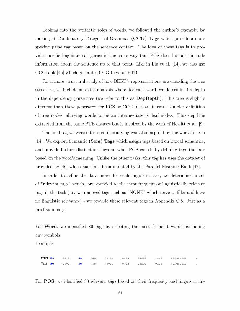
Looking into the syntactic roles of words, we followed the author’s example, by

looking at Combinatory Categorical Grammar (CCG) Tags which provide a more

specific parse tag based on the sentence context. The idea of these tags is to pro-

vide specific linguistic categories in the same way that POS does but also include

information about the sentence up to that point. Like in Liu et al. [14], we also use

CCGbank [45] which generates CCG tags for PTB.

For a more structural study of how BERT’s representations are encoding the tree

structure, we include an extra analysis where, for each word, we determine its depth

in the dependency parse tree (we refer to this as DepDepth). This tree is slightly

different than those generated for POS or CCG in that it uses a simpler definition

of tree nodes, allowing words to be an intermediate or leaf nodes. This depth is

extracted from the same PTB dataset but is inspired by the work of Hewitt et al. [9].

The final tag we were interested in studying was also inspired by the work done in

[14]. We explore Semantic (Sem) Tags which assign tags based on lexical semantics,

and provide further distinctions beyond what POS can do by defining tags that are

based on the word’s meaning. Unlike the other tasks, this tag has uses the dataset of

provided by [46] which has since been updated by the Parallel Meaning Bank [47].

In order to refine the data more, for each linguistic task, we determined a set

of "relevant tags" which corresponded to the most frequent or linguistically relevant

tags in the task (i.e. we removed tags such as "NONE" which serve as filler and have

no linguistic relevance) - we provide these relevant tags in Appendix C.8. Just as a

brief summary:

For Word, we identified 80 tags by selecting the most frequent words, excluding

any symbols.

Example:

For POS, we identified 33 relevant tags based on their frequency and linguistic im-

61

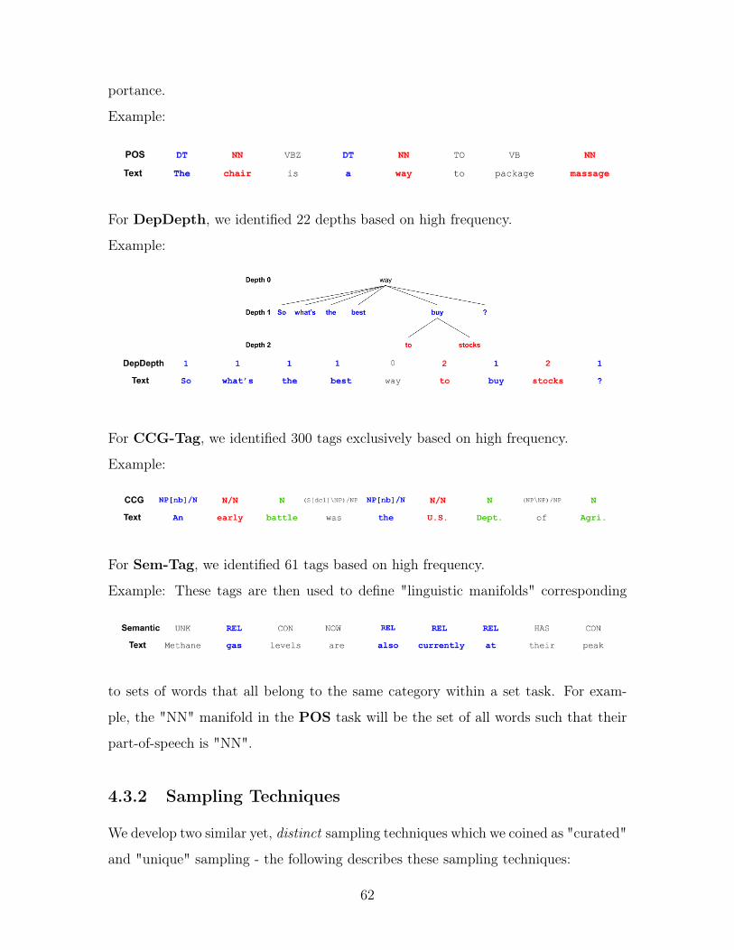
portance.

Example:

For DepDepth, we identified 22 depths based on high frequency.

Example:

For CCG-Tag, we identified 300 tags exclusively based on high frequency.

Example:

For Sem-Tag, we identified 61 tags based on high frequency.

Example: These tags are then used to define "linguistic manifolds" corresponding

to sets of words that all belong to the same category within a set task. For exam-

ple, the "NN" manifold in the POS task will be the set of all words such that their

part-of-speech is "NN".

4.3.2 Sampling Techniques

We develop two similar yet, distinct sampling techniques which we coined as "curated"

and "unique" sampling - the following describes these sampling techniques:

62

To perform curated sampling, we first specify a maximum and minimum number

(MAX and MIN respectively) of words each "manifold" must have to be included

in the sample. First, we identify every word in the dataset that maps to one of

the "relevant tags". Once all manifolds have been identified, one of three things

will occur with each manifold: if the manifold has more words than MAX then we

randomly select MAX words from the manifold and remove the rest, if the manifold

has between MIN and MAX words then the manifold is left alone, and finally if the

manifold has less than MIN words the manifold is removed entirely from the analysis.

In our sampling we always set MIN to be at least 2 and MAX to 50 - these settings

ensure that the manifold properties are meaningful and computationally feasible.

Unique sampling is nearly identical to curated sampling but with the added con-

straint that each word included in the sample must result in a unique vector when

first ingested by the word model. As mentioned previously, in this project we chose

to work with BERT which uses both the word and position to create the embedding -

in terms of sampling, this means that each word at a given position is assigned to one

manifold. This creates a new problem: there are some word, position combinations

can belong to multiple manifolds. We deal with this multiclass problem by selecting

one of the manifold tags uniformly at random for each combination.

We investigated the impact of using either sampling technique. Unique sampling

ensured that there was no overlap whatsoever in any layer. Curated sampling on

the other hand showed major overlap in some tasks at the embedding layer and a

reduced, but constant overlap in later layers (see Table C.2 for Word, Table C.4 for

POS, Table C.7 for DepDepth, Table C.5 for CCG-Tag, and Table C.9 for Sem-Tag).

While the overlap at the embedding was expected due to the sampling technique, the

later layer overlap was perplexing. Further investigation showed that these overlaps

were caused by duplicate sentences in the dataset having multiple tags associated

to them. While these issues are problematic to the separability of the data, it did

not significantly impact the results of our metrics. For future analyses however, we

present solely the plots that used unique sampling.

63

4.3.3 Model Feature Extraction

BERT has some interesting subtleties that we had to deal with before being able to

extract features:

∙ Contextualization - because BERT uses attention as the main mechanism by

which the vectors are transformed, it requires the full sentence to generate each

embedding vector. This means that word included in the sample requires that

we feed the full sentence that the word came from. The difficulty with this

is in computation time: depending on the sample, generating the vectors can

take a long time and the tensor generated can be very large. We dealt with

this issue by reusing the tensor whenever possible (in the case that two words

from the same sentence are included in the sample) and removing unnecessary

dimensions of the tensor before performing any operations on it (we do this by

removing all dimensions that are not related to the needed word)

∙ Tokenization - the design of BERT included a "subword" tokenization tech-

nique by which certain words are split into multiple tokens before being passed

into the model to allow the model to deal with unseen words:

swimming → ["swimming"]

reiterating → ["re##","iter","at","##ing"]

The question for us is: how do we deal with these subword-tokens? Previous

work[14] has explored using the right-most subword-token to represent the full

word (for our purposes we refer to this choice of representation as "right").

In this work, we explore the right representation but also look at word repre-

sentation that takes the average of all subword-token representations (for our

purposes we refer to this choice of representation as "avg"). After experiment-

ing with both, we ultimately found there to be little difference in our analyses

between right and avg representations - as such we chose to only present the

results from avg.

64

∙ Special Tokens - BERT provides a flag by which we can add special "start"

and "end" tokens to each sentence. In each experiment, we ensured these special

tags were always included.

∙ Masking - part of BERT’s training includes "masking" random words in a

sentence and training the model to predict the correct word that was "masked".

On the implementation side, this means that BERT has two different modes:

(1) the normal, unmasked mode where it can contextualize words and (2) the

masked cased where it must be predictive. In our experimentation, we explored

how BERT changes when a word is masked versus when it is left normally.

The model is always fed a full sentence but when masking, the sampled word

is hidden with "[MASK]". If multiple words in a sentence are included in the

sample, we feed the sentence multiple times ensuring that each time the sentence

fed only masks one word at a time.

4.4 Analysis Methods

4.4.1 Mean Field Theory

We use the Mean Field Theory (MFT) manifold analysis metric developed by Chung

et al. [17]. This metric is built on the assumption that the data has a large number of

manifolds and as such works best when more are included in the analysis (in practice,

we found that having a set of at least 20 manifolds was sufficient). Through this

analysis, we are able to capture the linear separability among linguistic manifolds

and quantifies how separation is achieved geometrically in a language model’s learned

representations.

4.4.2 Linear Probes

We repeat and extend the linear analyses done in [14] through an implementation of

their softmax probe and a support vector machine (SVM). To implement the softmax

probe, we use PyTorch[16] and follow the specifications provided in [14] of a linear

65

transformation followed by a softmax activation, optimizing with Adam[15] with the

default parameters, a batch size of 80 over 50 epochs, and early stopping with a

patience of 3. For thoroughness, we train 10 different softmax probes and report the

results from the model showing the best, test performance. For the SVM, we use the

implementation provided by Scikit-Learn[12] for a support vector classifier to measure

not only model accuracy but also the separability among classes via measuring the

SVM’s, positive margins.

4.4.3 Dimensionality Reduction

To visualize the different tasks, we turn to a novel dimensionality reduction technique,

Uniform Manifold Approximation and Projection (UMAP) [13], which respects higher

dimensional properties of data and projects vectors to reflect these relationships.

Previous work by a team at Google Brain [48] has shown the power of this technique

and inspired us to do the same. By reducing the set of manifolds we generated, we

hope to visualize how the model transforms the data.

4.5 Results

4.5.1 Linear Capacity

We begin our analysis by measuring the linear capacity of BERT’s representations.

Using the tasks identified earlier, we generate sets of relevant manifolds and run the

MFT metric.

Looking at Figure A-19, the general trend is that contextualization decreases the

linear capacity while prediction increases it. This implies that earlier layers contain

the most information, readily available about the task in question. The inverse nature

between contextualization and prediction also implies that their function is opposing.

The one task that seems to be inverted is Dependency Tree Parse Depth; we postulate

that this is a result of the linguistic difference in tasks: POS, Word, CCG-Tag, Sem-

Tag are all directly related to the word while DepDepth is more about the location

66

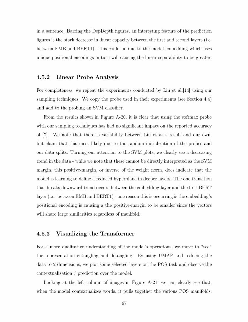
in a sentence. Barring the DepDepth figures, an interesting feature of the prediction

figures is the stark decrease in linear capacity between the first and second layers (i.e.

between EMB and BERT1) - this could be due to the model embedding which uses

unique positional encodings in turn will causing the linear separability to be greater.

4.5.2 Linear Probe Analysis

For completeness, we repeat the experiments conducted by Liu et al.[14] using our

sampling techniques. We copy the probe used in their experiments (see Section 4.4)

and add to the probing an SVM classifier.

From the results shown in Figure A-20, it is clear that using the softmax probe

with our sampling techniques has had no significant impact on the reported accuracy

of [?]. We note that there is variability between Liu et al.’s result and our own,

but claim that this most likely due to the random initialization of the probes and

our data splits. Turning our attention to the SVM plots, we clearly see a decreasing

trend in the data - while we note that these cannot be directly interpreted as the SVM

margin, this positive-margin, or inverse of the weight norm, does indicate that the

model is learning to define a reduced hyperplane in deeper layers. The one transition

that breaks downward trend occurs between the embedding layer and the first BERT

layer (i.e. between EMB and BERT1) - one reason this is occurring is the embedding’s

positional encoding is causing a the positive-margin to be smaller since the vectors

will share large similarities regardless of manifold.

4.5.3 Visualizing the Transformer

For a more qualitative understanding of the model’s operations, we move to "see"

the representation entangling and detangling. By using UMAP and reducing the

data to 2 dimensions, we plot some selected layers on the POS task and observe the

contextualization / prediction over the model.

Looking at the left column of images in Figure A-21, we can clearly see that,

when the model contextualizes words, it pulls together the various POS manifolds.

67

In particular, we see that the nnp and in classes are being pulled in closer as we

get to deeper and deeper layers. Generally the manifolds also seem to be spreading

out over a larger area which ultimately results in significant overlap (particularly in

the last layer). This means that the model’s representations are being pushed closer

to one another thereby reducing: the distance between each manifold and the linear

separability.

Looking at the images in the right column of Figure A-21, we can observe how the

model’s predictive mode causes the POS manifolds to emerge. In the earliest layer, we

clearly see that the different manifolds overlap everywhere - visually making it hard

to distinguish between them all. The deeper layers clearly separate these manifolds;

note that each subsequent transformation is causing the manifolds to be more and

more separable, reducing their overlap.

This visualization lines up with the prediction from Manifold Capacity we saw in

Figure A-19. As the model contextualizes words, information about the words begins

to push the representations closer together resulting in greater entanglement - at the

same time, when the model must predict a word the surrounding information helps

tease out the relevant information, improving the quality of prediction, reducing the

possible choices, and ultimately de-tangling the manifolds.

4.5.4 Geometric Properties of Task Manifolds

We now turn back to the MFT metric for a more quantitative understanding of the

task manifold’s transformations.

In Figure A-22, we see various aspects of the manifolds geometry. Looking at

the left column, we see that as the model contextualizes text the average manifold

radius and dimension increase; practically this explains why the linear separability

is decreasing in deeper layers - the distance between manifolds is becoming smaller

because the average manifold is growing. As expected, the inverse trend is observed

in the prediction setting - as we transform the data through deeper layers the aver-

age manifold is shrinking and reducing in dimension, focusing in on a more specific

prediction.

68

4.6 Discussion

We began our exploration into BERT’s representations by comparing the model’s two

modes: contextualization of text given a sentence and word prediction of a masked

word. Intuitively, we expect that when the model contextualizes the importance of

individual words goes away and the focus shifts to representing meaning in context.

At the same time when the model predicts, we expect that it will focus on specifying

the correct word choice that fits under the "[MASK]" token. We turn our attention to

Figure A-19 in which the left column of shows the "unmasked" or contextualization

setting and the right column shows the "masked" or prediction setting. Looking

over the many tasks we fed BERT, we can see that the general trend of the linear

capacity decreases when the model contextualizes but increases when the model must

predict the word - exactly our hypothesis. These results in fact, line up with previous

work[49] which shows that a transformer based model will generate representations

such that: mutual information is lost when compared to original tokens and gained

when comparing to the tokens that are prediction targets.

Our results imply that, given a normal sentence, linguistic information about a

word is most separable in the earliest layers of BERT - this seems to contradict

the results of [14] that showed that this information is most present in the model’s

middle layers. To investigate this, we focused in on the POS task in which they show

that the 7th transformer layer was the most performant. The important difference

between our methodology and theirs is the distribution sampling: Liu et al. use the

full PTB training file which has a non-uniform distribution of the manifolds while we

try to ensure that all manifolds have roughly the same number of sample; this could

potentially result in a biased probe that can achieve high accuracy by predicting based

on the model distribution and not based on the vectors being fed into the model. A

more subtle, but important distinction comes from the nature of language: a word at

a given position can belong to multiple classes depending on the context. This causes

a major problem for the linear probe by making data inseparable, particularly in the

embedding and early transformer layers where these words have not yet been put into

69

context - this could potentially explain the reduced accuracy in the early layers shown

by Liu et al. We reproduce these linear probe results using their softmax probe, as

described in Section 4.4, and include a further analysis of the manifold margins in

Figure A-20.

The left column of Figure A-20 shows the linear probes results using curated sam-

pling while the right shows the linear probes using unique sampling - the important

difference here is that the curated sampling technique does not guarantee that the

data generated is separable while the unique sampling does. Along with the accuracy

of the softmax probe, we provide a measure of SVM positive-margin via plotting the

average, inverse of the weight norm, over multiple runs. First, we note that the two

sampling techniques do not seem to impact the softmax probe’s accuracy significantly

and we claim that the slight variations that are observed between the two plots re-

sult from the random seed used for the particular probe. Second, we note that in

both cases, the SVM’s positive-margins seem to be decreasing over time. Generally,

the trend indicates that the smallest positive-margin occurs at the last layer while

the largest positive-margins are in the early layers, regardless of sampling technique.

We claim therefore, the probe used by Liu et al. is capable of reading out linguistic

information from BERT vectors, but is not telling the full story - in fact, we see

from the positive-margins that despite the linear accuracy trend, linear separability

is decreasing.

This reduction of linear separability in higher layers is also evident when we visu-

alize the data as it moves through the various model layers. By using UMAP[13], we

reduced the data to 2 dimensions and clearly see the entanglement and detanglement

of POS manifolds in Figure A-21.

By observing the geometric properties of these manifolds in Figure A-22, we got

a more analytical picture of the transformations shown in Figure A-21. In the left

column, we can see the geometric properties of the manifolds defined by the input

token (i.e. the contextualization of words) and in the right column, those same

properties for manifolds defined by the output token (i.e. the prediction of words).

Generally, we see that the trends are inverted when we directly compare the two modes

70

of BERT: when the model contextualizes information, the radius and dimension of

information increases while the same decrease as we predict a word. This intuitively

makes sense - by increasing the dimension and radius of a manifold, more information

can be captured and broader context can be extracted while a reduced manifold,

implied by the smaller dimension and radius, will decrease the number of possible

choices thereby improving the quality of prediction.

With this new MFT metric, for the first time in the field of natural language

processing, we can get a clear picture of the how linguistic information is structured

in a language model. Most notable, the information is quantified in various ways

giving us intuitive explanations for our results. We also see that the new metric is

more capable of describing the model’s information dynamics than the traditional

linear probe. But with the success of knowing that language models are capable of

learning abstract linguistical concepts - we now ask: how much does the model know

about sentence structure?

71

72

73

74

Chapter 5

Observing Hierarchical Structure in

Model Representations

5.1 Background

The ability to speak and understand a language is a necessity to traverse the modern

world. This means learning to take abstract ideas and formulating them into a coher-

ent, organized sentences. Such a difficult task is expected of every one of us. Most

importantly, this daunting task essentially requires we do this on our own even as

children. While some language can be learned by mimicking the bits of conversation

we over hear when we are young, the ability to generate our own proper sentences

involves knowing how to use the difference among words to our advantage. Trying

to understand how this structure can be learned through the implied relationships

among words has always been a curiosity in the field of Linguistics. People have

studied this phenomena in humans [50, 51] showing the deep links between long term

cognitive ability and the ability to learn these implied structures. On the machine

learning front, work in model explainability has begun to explore these ideas via prob-

ing for specific structure [9] or implying that structure must exists because of probe

performance[14]. In this work, we focus on showing that these implied relationships

are being learned, not by probing for a specific structure or via implications due to

probe performance but rather by perturbing sentences in various ways and showing

75

the impact these results have on final model predictions.

5.2 Model

Our main interest was to understand how state-of-the-art language models were learn-

ing implicit structures in English. As such, we focused our work on a single model -

the Bidirectional Encoder Representations from Transformers or BERT Base model

[26]. The implementation, documentation, and many other important details of the

model can be found in the hugging face repository[27]1. A brief description of the

model is provided in Section 1.3.3.

5.3 Methods

5.3.1 Data

For our analysis, we chose to use the University of Pennsylvania’s "Penn Treebank"

(PTB)[44] in order to best match our previous work. This dataset provides an easy

way to extract sentence tree structure and thus was perfect for the purpose of this

analysis. In every case where we consider the phrasal boundary, we use the sentence’s

constituency tree to define the start and end of phrases.

5.3.2 Textual Manipulations

Grammatical

For this analysis we wish to answer the question: does BERT care about phrases

and grammatical structure? We explore this idea by altering our dataset - swapping

different sets of words to tease out the how important correct grammar is to the

model. We selected a comparison between a frozen, pre-trained and an untrained

BERT model to be the baseline analysis. In what follows, we provide descriptions of

1https://github.com/huggingface/transformers

76

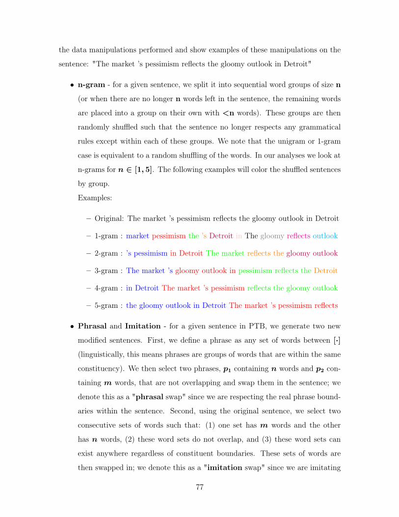
the data manipulations performed and show examples of these manipulations on the

sentence: "The market ’s pessimism reflects the gloomy outlook in Detroit"

∙ n-gram - for a given sentence, we split it into sequential word groups of size n

(or when there are no longer n words left in the sentence, the remaining words

are placed into a group on their own with <n words). These groups are then

randomly shuffled such that the sentence no longer respects any grammatical

rules except within each of these groups. We note that the unigram or 1-gram

case is equivalent to a random shuffling of the words. In our analyses we look at

n-grams for 𝑛 ∈ [1, 5]. The following examples will color the shuffled sentences

by group.

Examples:

– Original: The market ’s pessimism reflects the gloomy outlook in Detroit

– 1-gram : market pessimism the ’s Detroit in The gloomy reflects outlook

– 2-gram : ’s pessimism in Detroit The market reflects the gloomy outlook

– 3-gram : The market ’s gloomy outlook in pessimism reflects the Detroit

– 4-gram : in Detroit The market ’s pessimism reflects the gloomy outlook

– 5-gram : the gloomy outlook in Detroit The market ’s pessimism reflects

∙ Phrasal and Imitation - for a given sentence in PTB, we generate two new

modified sentences. First, we define a phrase as any set of words between [·]

(linguistically, this means phrases are groups of words that are within the same

constituency). We then select two phrases, 𝑝1 containing 𝑛 words and 𝑝2 con-

taining 𝑚 words, that are not overlapping and swap them in the sentence; we

denote this as a "phrasal swap" since we are respecting the real phrase bound-

aries within the sentence. Second, using the original sentence, we select two

consecutive sets of words such that: (1) one set has 𝑚 words and the other

has 𝑛 words, (2) these word sets do not overlap, and (3) these word sets can

exist anywhere regardless of constituent boundaries. These sets of words are

then swapped in; we denote this as a "imitation swap" since we are imitating

77

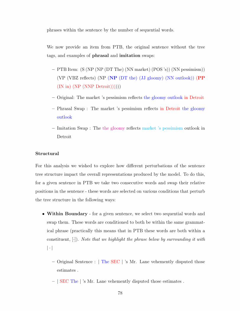
phrases within the sentence by the number of sequential words.

We now provide an item from PTB, the original sentence without the tree

tags, and examples of phrasal and imitation swaps:

– PTB Item: (S (NP (NP (DT The) (NN market) (POS ’s)) (NN pessimism))

(VP (VBZ reflects) (NP (NP (DT the) (JJ gloomy) (NN outlook)) (PP

(IN in) (NP (NNP Detroit))))))

– Original: The market ’s pessimism reflects the gloomy outlook in Detroit

– Phrasal Swap : The market ’s pessimism reflects in Detroit the gloomy

outlook

– Imitation Swap : The the gloomy reflects market ’s pessimism outlook in

Detroit

Structural

For this analysis we wished to explore how different perturbations of the sentence

tree structure impact the overall representations produced by the model. To do this,

for a given sentence in PTB we take two consecutive words and swap their relative

positions in the sentence - these words are selected on various conditions that perturb

the tree structure in the following ways:

∙ Within Boundary - for a given sentence, we select two sequential words and

swap them. These words are conditioned to both be within the same grammat-

ical phrase (practically this means that in PTB these words are both within a

constituent, [·]). Note that we highlight the phrase below by surrounding it with

| · |

– Original Sentence : | The SEC | ’s Mr. Lane vehemently disputed those

estimates .

– | SEC The | ’s Mr. Lane vehemently disputed those estimates .

78

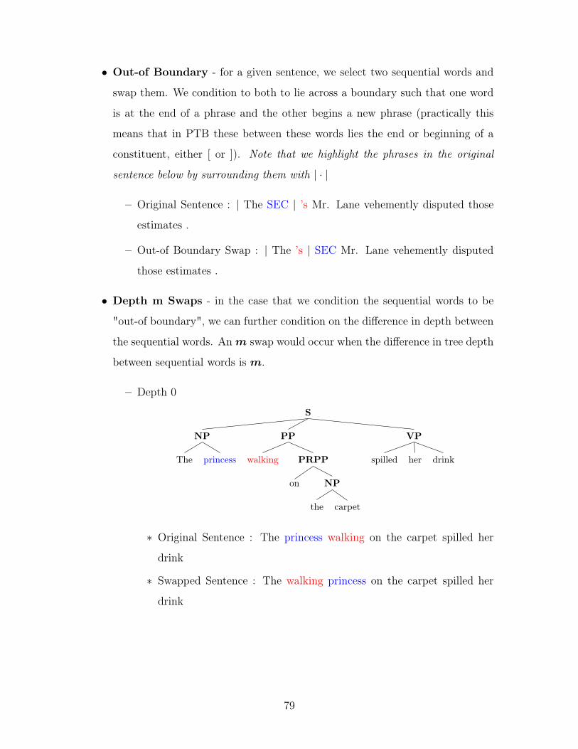
∙ Out-of Boundary - for a given sentence, we select two sequential words and

swap them. We condition to both to lie across a boundary such that one word

is at the end of a phrase and the other begins a new phrase (practically this

means that in PTB these between these words lies the end or beginning of a

constituent, either [ or ]). Note that we highlight the phrases in the original

sentence below by surrounding them with | · |

– Original Sentence : | The SEC | ’s Mr. Lane vehemently disputed those

estimates .

– Out-of Boundary Swap : | The ’s | SEC Mr. Lane vehemently disputed

those estimates .

∙ Depth m Swaps - in the case that we condition the sequential words to be

"out-of boundary", we can further condition on the difference in depth between

the sequential words. An 𝑚 swap would occur when the difference in tree depth

between sequential words is 𝑚.

– Depth 0

S

VP

drinkherspilled

PP

PRPP

NP

carpetthe

on

walking

NP

princessThe

* Original Sentence : The princess walking on the carpet spilled her

drink

* Swapped Sentence : The walking princess on the carpet spilled her

drink

79

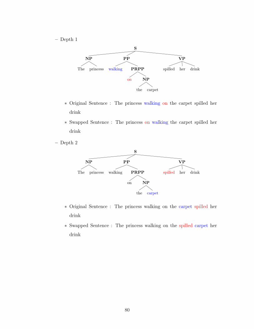
– Depth 1

S

VP

drinkherspilled

PP

PRPP

NP

carpetthe

on

walking

NP

princessThe

* Original Sentence : The princess walking on the carpet spilled her

drink

* Swapped Sentence : The princess on walking the carpet spilled her

drink

– Depth 2

S

VP

drinkherspilled

PP

PRPP

NP

carpetthe

on

walking

NP

princessThe

* Original Sentence : The princess walking on the carpet spilled her

drink

* Swapped Sentence : The princess walking on the spilled carpet her

drink

80

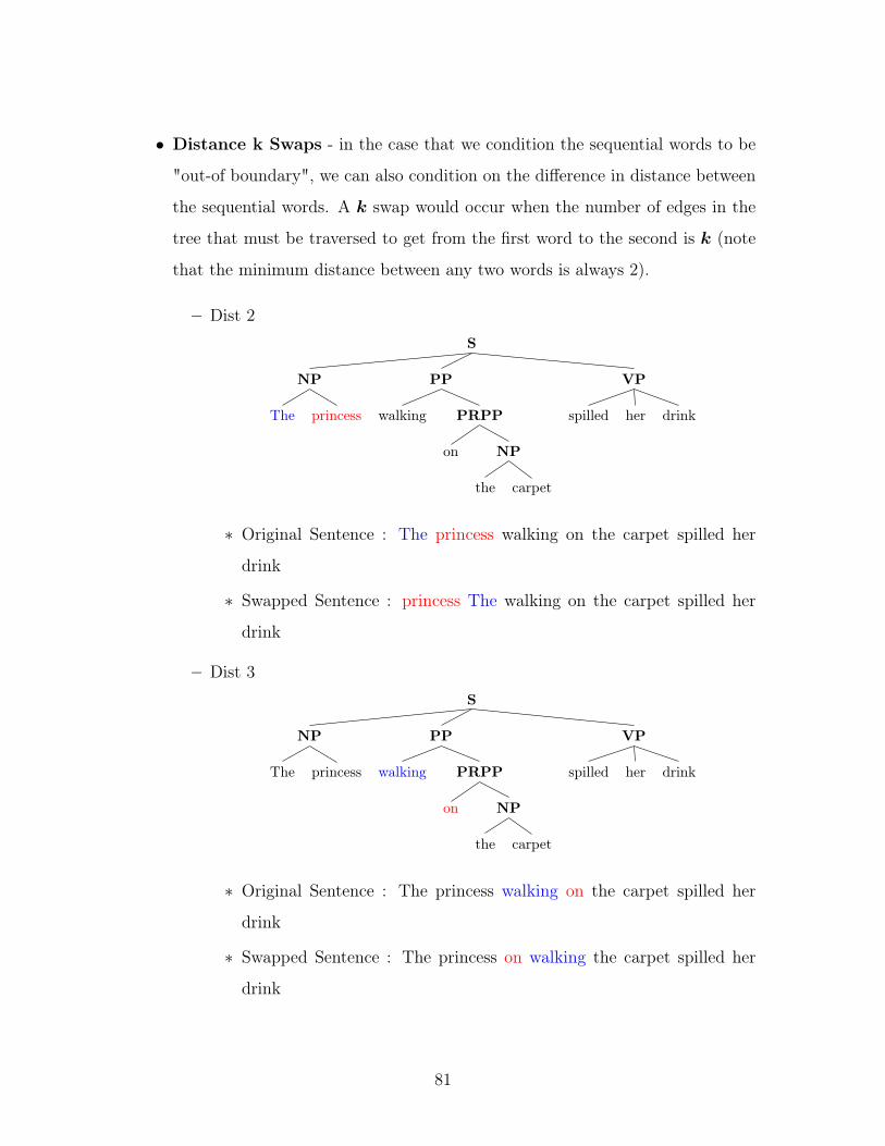
∙ Distance k Swaps - in the case that we condition the sequential words to be

"out-of boundary", we can also condition on the difference in distance between

the sequential words. A 𝑘 swap would occur when the number of edges in the

tree that must be traversed to get from the first word to the second is 𝑘 (note

that the minimum distance between any two words is always 2).

– Dist 2S

VP

drinkherspilled

PP

PRPP

NP

carpetthe

on

walking

NP

princessThe

* Original Sentence : The princess walking on the carpet spilled her

drink

* Swapped Sentence : princess The walking on the carpet spilled her

drink

– Dist 3S

VP

drinkherspilled

PP

PRPP

NP

carpetthe

on

walking

NP

princessThe

* Original Sentence : The princess walking on the carpet spilled her

drink

* Swapped Sentence : The princess on walking the carpet spilled her

drink

81

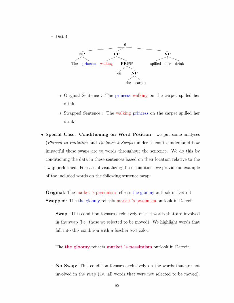
– Dist 4

S

VP

drinkherspilled

PP

PRPP

NP

carpetthe

on

walking

NP

princessThe

* Original Sentence : The princess walking on the carpet spilled her

drink

* Swapped Sentence : The walking princess on the carpet spilled her

drink

∙ Special Case: Conditioning on Word Position - we put some analyses

(Phrasal vs Imitation and Distance k Swaps) under a lens to understand how

impactful these swaps are to words throughout the sentence. We do this by

conditioning the data in these sentences based on their location relative to the

swap performed. For ease of visualizing these conditions we provide an example

of the included words on the following sentence swap:

Original: The market ’s pessimism reflects the gloomy outlook in Detroit

Swapped: The the gloomy reflects market ’s pessimism outlook in Detroit

– Swap: This condition focuses exclusively on the words that are involved

in the swap (i.e. those we selected to be moved). We highlight words that

fall into this condition with a fuschia text color.

The the gloomy reflects market ’s pessimism outlook in Detroit

– No Swap: This condition focuses exclusively on the words that are not

involved in the swap (i.e. all words that were not selected to be moved).

82

We highlight words that fall into this condition with a fuschia text color.

The the gloomy reflects market ’s pessimism outlook in Detroit

– Shift: This condition focuses exclusively on the words that are in a dif-

ferent position as a result of the swap but do not belong to the swap. We

define a word’s position as the number of words needed to reach the be-

ginning of the sentence. We highlight words that fall into this condition

with a fuschia text color.

The the gloomy reflects market ’s pessimism outlook in Detroit

– No Shift: This condition focuses exclusively on the words that are in a

the same position after the swap and do not belong to the swap. We define

a word’s position as the number of words needed to reach the beginning

of the sentence. We highlight words that fall into this condition with a

fuschia text color.

The the gloomy reflects market ’s pessimism outlook in Detroit

5.3.3 Model Feature Extraction

BERT has some interesting subtleties that we had to deal with before being able to

extract features:

∙ Contextualization - because BERT uses attention as the main mechanism by

which the vectors are transformed, it requires the full sentence to generate each

embedding vector. This means that word included in the sample requires that

we feed the full sentence that the word came from. The difficulty with this

is in computation time: depending on the sample, generating the vectors can

83

take a long time and the tensor generated can be very large. We dealt with

this issue by reusing the tensor whenever possible (in the case that two words

from the same sentence are included in the sample) and removing unnecessary

dimensions of the tensor before performing any operations on it (we do this by

removing all dimensions that are not related to the needed word)

∙ Tokenization - the design of BERT included a "subword" tokenization tech-

nique by which certain words are split into multiple tokens before being passed

into the model to allow the model to deal with unseen words:

swimming → ["swimming"]

reiterating → ["re##","iter","at","##ing"]

The question for us is: how do we deal with these subword-tokens? Previous

work[14] has explored using the right-most subword-token to represent the full

word (for our purposes we refer to this choice of representation as "right").

In this work, we explore the right representation but also look at word repre-

sentation that takes the average of all subword-token representations (for our

purposes we refer to this choice of representation as "avg"). After experiment-

ing with both, we ultimately found there to be little difference in our analyses

between right and avg representations - as such we chose to only present the

results from avg.

∙ Special Tokens - BERT provides a flag by which we can add special "start"

and "end" tokens to each sentence. In each experiment, we ensured these special

tags were always included.

∙ Masking - part of BERT’s training includes "masking" random words in a

sentence and training the model to predict the correct word that was "masked".

On the implementation side, this means that BERT has two different modes:

(1) the normal, unmasked mode where it can contextualize words and (2) the

masked cased where it must be predictive. In our experimentation, we explored

how BERT changes when a word is masked versus when it is left normally.

84

The model is always fed a full sentence but when masking, the sampled word

is hidden with "[MASK]". If multiple words in a sentence are included in the

sample, we feed the sentence multiple times ensuring that each time the sentence

fed only masks one word at a time.

5.3.4 Analytical Techniques

For this analysis, we rely on the implementations and explanations of Canonical Cor-

relation Analysis (CCA) developed by a team in Google [52]. When using CCA, we

measure the correlation between tensors by taking the average of the correlation coef-

ficients (we denote this as the "Mean CCA"). We also experimented using Projection

weighted CCA (PWCCA)[53] which has previously been found to be an improved

estimate to the true correlation between tensors but found there to be no notable,

qualitative differences between it and Mean CCA in this case. We provide similar

plots using PWCCA in the appendix. In situations when there is insufficient samples

to use CCA, we use Principle Component Analysis (PCA)[11] to reduce the feature

size of each vector in the tensor. After looking at the experiments of [54, 55, 56], we

decided to use a rule of thumb approach to determine the reduced number of com-

ponents we need; we select the number of components such that the we can explain

roughly 90% of the variance (In our experiments, this meant 400 components for the

BERT Base model). We use Mean CCA to perform direct comparisons between two

tensors corresponding to the same layer or between two tensors where one is fixed to

be the final layer and the other varies over all layers.

5.4 Results

5.4.1 Phrasal Manipulations

n-grams

We first compare the unmasked representations generated by: (1) BERT Base having

been fed n-gram shuffles, as previously described, to (2) a BERT Base model that

85

was fed the normal sentence.

We see in Figure A-23 that all conditions (with the exception of the baseline

against the untrained BERT model) have a high correlation at the embedding layer

and taper off at different rates over deepr layers. We note that the near 1 correlation

at the embedding layer is due strictly caused by BERT’s embedding mechanism which

uses a combination of a learned, per-token encoding and positional encoding to de-

termine each representation; in our case this means that the only difference between

each condition at the embedding layer is the different positional encodings due to the

word shuffling. The initial major qualitative divergence in representation caused by

the manipulations seems to occur at around BERT2 where the lines begin separate

in correlation. Roughly at BERT10, we believe all conditions converge to their final

representations based on the approximately equal correlation in subsequent layers.

Considering this plot, it seems that the manipulation greatly impact the final repre-

sentation of the model such that keeping larger chunks of the sentence together (i.e.

larger n-grams like 4,5-grams) causes less change to the final representations than

smaller sentence chunks (i.e. smaller n-grams like 1,2-grams).

We now look to the masked representations to understand how well the model

is able approximate the true word when it must predict. Again, we see a similar

pattern in Figure A-24 with the masked representations that we saw in the unmasked

mode - there is a clear distinction between the conditions, with larger n-grams result-

ing in higher correlated representations than smaller n-grams. That being said, the

difference in representation is significantly more marked here being that the n-gram

shuffles cause the correlations to become constant early on and not just at the final

layers.

Phrasal vs Imitation Swaps

Having seen the effects of non-grammatical shuffles of a sentence, we move on to

understand the effects of phrasal swaps. The following plots contain our baseline,

correlations between normal sentences and those sentence with a phrasal swap, and

finally correlations between normal sentences and those sentence with a imitation

86

phrase swap.

The distinction between "Phrasal" and "Imitation" swaps as shown in Figure A-25

seems to be much more subtle than the n-gram shuffles. In particular, the correla-

tions seem to be qualitatively different at a later layer namely around BERT5. The

divergence clearly shows that the model’s representations with a phrasal swap result

in representations that are more similar to the normal sentence than those produced

with an imitation swap. We investigate this further by conditioning the the represen-

tations based on their location in reference to the swapped words; we primarily focus

on the words that were involved in the swap (Swap) vs those that were not (No

Swap) and the words that were moved to a different position in the sentence due to

the swap (Shift) vs those that were not (No Shift). We can see these conditions in

Figure A-26

The main thing to notice is that in every condition, the phrasal swap always re-

sults in a more correlated representation that the imitation swap; this further cements

the idea that phrasal phrase swaps result in less perturbation to the model’s repre-

sentations than imitation phrase swaps. The plot also shows that the conditions "No

Swap" and "No Shift" where the words aren’t as impacted with the swap result in

higher correlations than the conditions where we include the swap / shift.

Again we turn to the masked context in Figure A-27 and find a similar result to

the n-gram figures - the masking causes earlier separation of the representations but

most importantly here, we still see clearly that phrasal swap resulted in markedly

more correlated representations than the imitation phrase swap.

5.4.2 Structural Manipulations

Within vs Out-of Phrase

In our first experiment on the structural manipulations, we explore how similar repre-

sentations of word swaps are to the original representations conditioning on the swap

being "within" and "out-of" phrase.

Looking at Figure A-28, it is evident that the distinction between the conditions

87

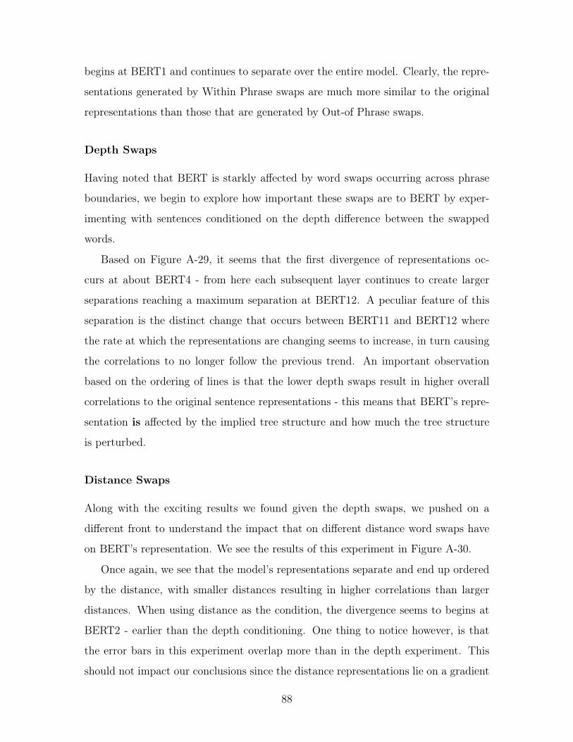
begins at BERT1 and continues to separate over the entire model. Clearly, the repre-

sentations generated by Within Phrase swaps are much more similar to the original

representations than those that are generated by Out-of Phrase swaps.

Depth Swaps

Having noted that BERT is starkly affected by word swaps occurring across phrase

boundaries, we begin to explore how important these swaps are to BERT by exper-

imenting with sentences conditioned on the depth difference between the swapped

words.

Based on Figure A-29, it seems that the first divergence of representations oc-

curs at about BERT4 - from here each subsequent layer continues to create larger

separations reaching a maximum separation at BERT12. A peculiar feature of this

separation is the distinct change that occurs between BERT11 and BERT12 where

the rate at which the representations are changing seems to increase, in turn causing

the correlations to no longer follow the previous trend. An important observation

based on the ordering of lines is that the lower depth swaps result in higher overall

correlations to the original sentence representations - this means that BERT’s repre-

sentation is affected by the implied tree structure and how much the tree structure

is perturbed.

Distance Swaps

Along with the exciting results we found given the depth swaps, we pushed on a

different front to understand the impact that on different distance word swaps have

on BERT’s representation. We see the results of this experiment in Figure A-30.

Once again, we see that the model’s representations separate and end up ordered

by the distance, with smaller distances resulting in higher correlations than larger

distances. When using distance as the condition, the divergence seems to begins at

BERT2 - earlier than the depth conditioning. One thing to notice however, is that

the error bars in this experiment overlap more than in the depth experiment. This

should not impact our conclusions since the distance representations lie on a gradient

88

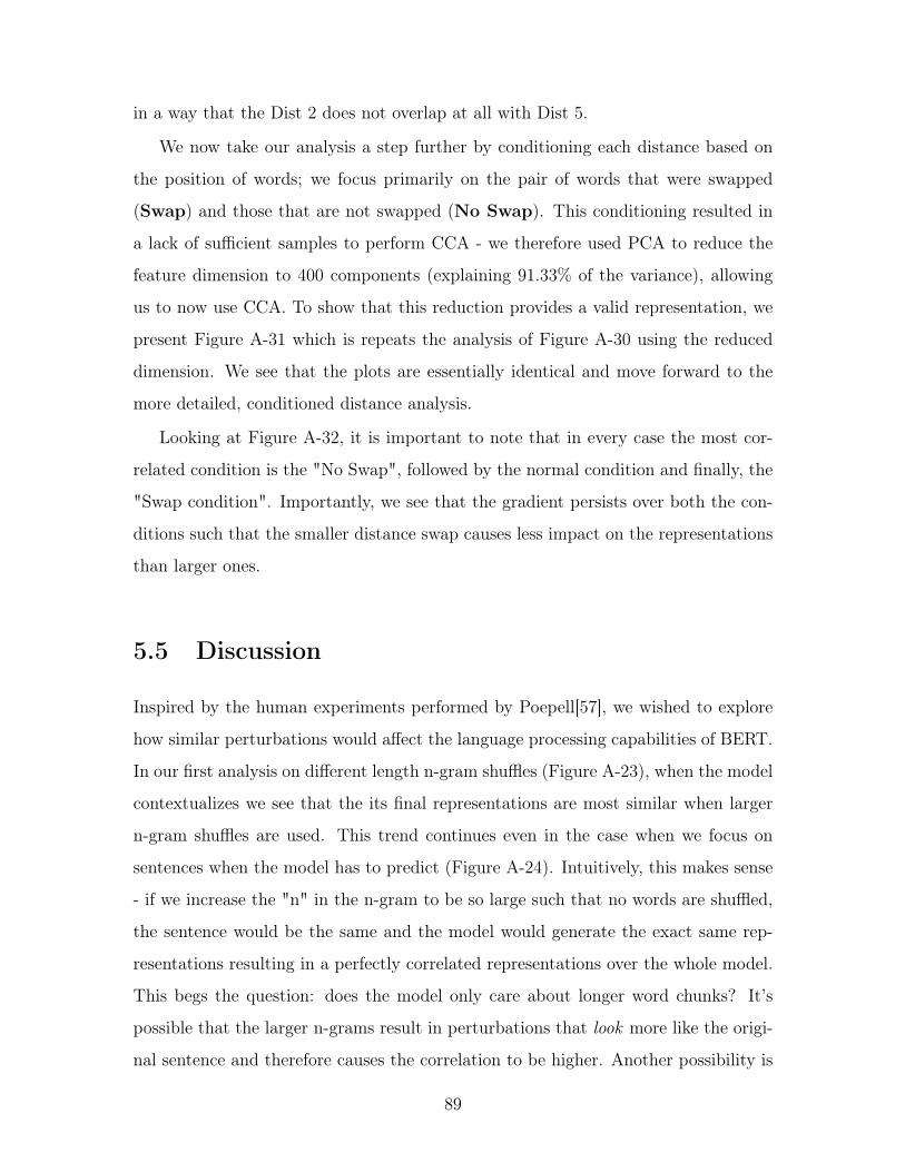
in a way that the Dist 2 does not overlap at all with Dist 5.

We now take our analysis a step further by conditioning each distance based on

the position of words; we focus primarily on the pair of words that were swapped

(Swap) and those that are not swapped (No Swap). This conditioning resulted in

a lack of sufficient samples to perform CCA - we therefore used PCA to reduce the

feature dimension to 400 components (explaining 91.33% of the variance), allowing

us to now use CCA. To show that this reduction provides a valid representation, we

present Figure A-31 which is repeats the analysis of Figure A-30 using the reduced

dimension. We see that the plots are essentially identical and move forward to the

more detailed, conditioned distance analysis.

Looking at Figure A-32, it is important to note that in every case the most cor-

related condition is the "No Swap", followed by the normal condition and finally, the

"Swap condition". Importantly, we see that the gradient persists over both the con-

ditions such that the smaller distance swap causes less impact on the representations

than larger ones.

5.5 Discussion

Inspired by the human experiments performed by Poepell[57], we wished to explore

how similar perturbations would affect the language processing capabilities of BERT.

In our first analysis on different length n-gram shuffles (Figure A-23), when the model

contextualizes we see that the its final representations are most similar when larger

n-gram shuffles are used. This trend continues even in the case when we focus on

sentences when the model has to predict (Figure A-24). Intuitively, this makes sense

- if we increase the "n" in the n-gram to be so large such that no words are shuffled,

the sentence would be the same and the model would generate the exact same rep-

resentations resulting in a perfectly correlated representations over the whole model.

This begs the question: does the model only care about longer word chunks? It’s

possible that the larger n-grams result in perturbations that look more like the origi-

nal sentence and therefore causes the correlation to be higher. Another possibility is

89

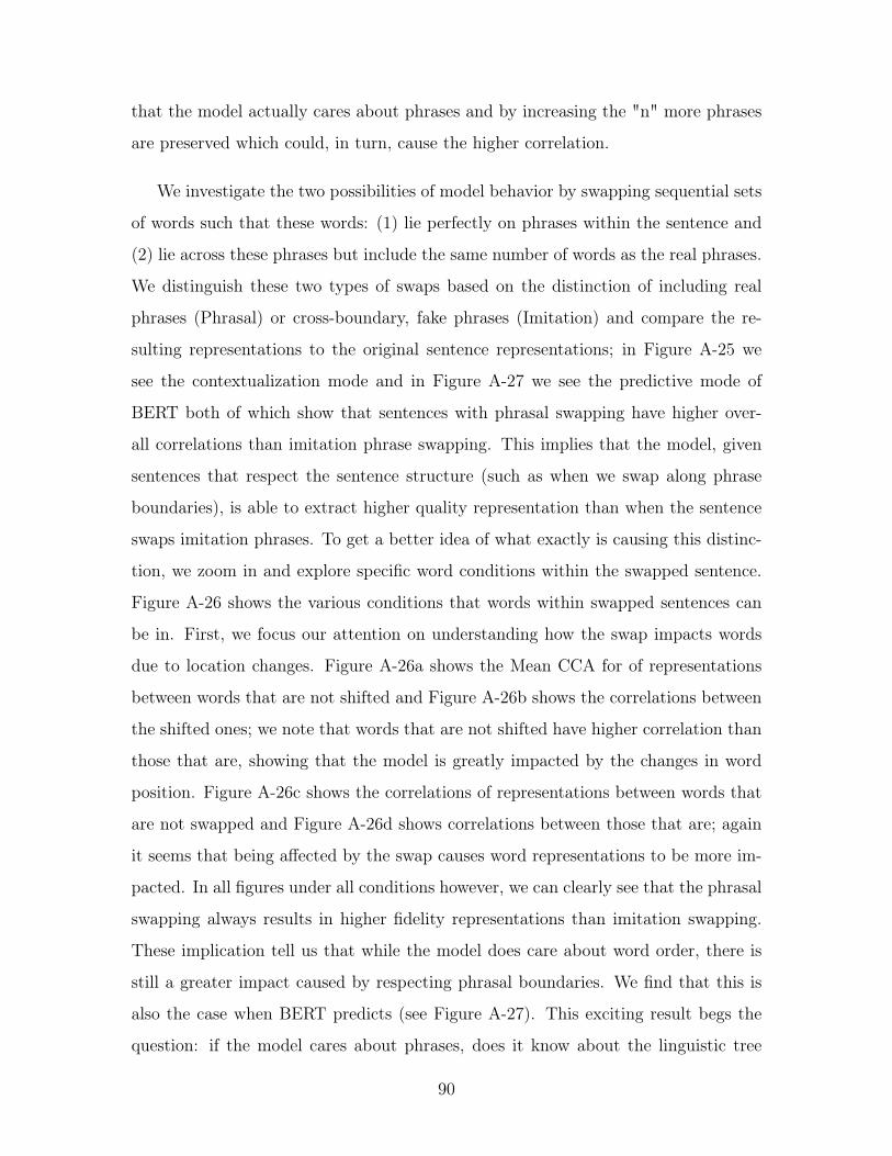
that the model actually cares about phrases and by increasing the "n" more phrases

are preserved which could, in turn, cause the higher correlation.

We investigate the two possibilities of model behavior by swapping sequential sets

of words such that these words: (1) lie perfectly on phrases within the sentence and

(2) lie across these phrases but include the same number of words as the real phrases.

We distinguish these two types of swaps based on the distinction of including real

phrases (Phrasal) or cross-boundary, fake phrases (Imitation) and compare the re-

sulting representations to the original sentence representations; in Figure A-25 we

see the contextualization mode and in Figure A-27 we see the predictive mode of

BERT both of which show that sentences with phrasal swapping have higher over-

all correlations than imitation phrase swapping. This implies that the model, given

sentences that respect the sentence structure (such as when we swap along phrase

boundaries), is able to extract higher quality representation than when the sentence

swaps imitation phrases. To get a better idea of what exactly is causing this distinc-

tion, we zoom in and explore specific word conditions within the swapped sentence.

Figure A-26 shows the various conditions that words within swapped sentences can

be in. First, we focus our attention on understanding how the swap impacts words

due to location changes. Figure A-26a shows the Mean CCA for of representations

between words that are not shifted and Figure A-26b shows the correlations between

the shifted ones; we note that words that are not shifted have higher correlation than

those that are, showing that the model is greatly impacted by the changes in word

position. Figure A-26c shows the correlations of representations between words that

are not swapped and Figure A-26d shows correlations between those that are; again

it seems that being affected by the swap causes word representations to be more im-

pacted. In all figures under all conditions however, we can clearly see that the phrasal

swapping always results in higher fidelity representations than imitation swapping.

These implication tell us that while the model does care about word order, there is

still a greater impact caused by respecting phrasal boundaries. We find that this is

also the case when BERT predicts (see Figure A-27). This exciting result begs the

question: if the model cares about phrases, does it know about the linguistic tree

90

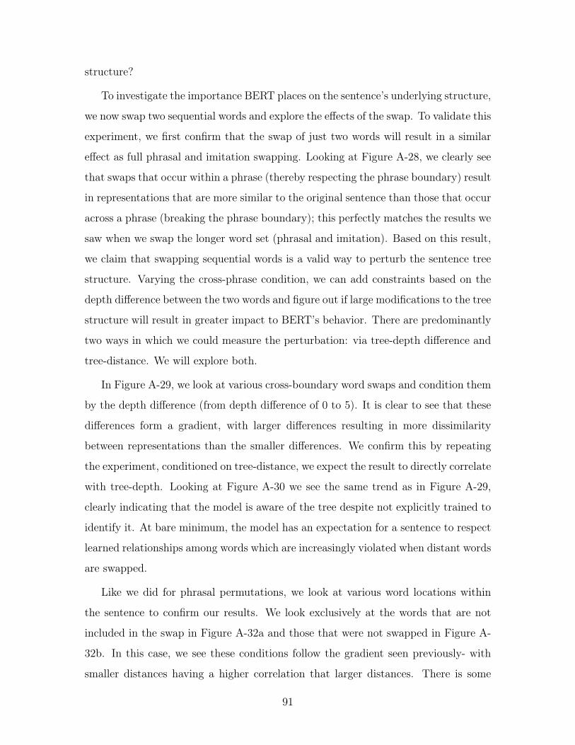
structure?

To investigate the importance BERT places on the sentence’s underlying structure,

we now swap two sequential words and explore the effects of the swap. To validate this

experiment, we first confirm that the swap of just two words will result in a similar

effect as full phrasal and imitation swapping. Looking at Figure A-28, we clearly see

that swaps that occur within a phrase (thereby respecting the phrase boundary) result

in representations that are more similar to the original sentence than those that occur

across a phrase (breaking the phrase boundary); this perfectly matches the results we

saw when we swap the longer word set (phrasal and imitation). Based on this result,

we claim that swapping sequential words is a valid way to perturb the sentence tree

structure. Varying the cross-phrase condition, we can add constraints based on the

depth difference between the two words and figure out if large modifications to the tree

structure will result in greater impact to BERT’s behavior. There are predominantly

two ways in which we could measure the perturbation: via tree-depth difference and

tree-distance. We will explore both.

In Figure A-29, we look at various cross-boundary word swaps and condition them

by the depth difference (from depth difference of 0 to 5). It is clear to see that these

differences form a gradient, with larger differences resulting in more dissimilarity

between representations than the smaller differences. We confirm this by repeating

the experiment, conditioned on tree-distance, we expect the result to directly correlate

with tree-depth. Looking at Figure A-30 we see the same trend as in Figure A-29,

clearly indicating that the model is aware of the tree despite not explicitly trained to

identify it. At bare minimum, the model has an expectation for a sentence to respect

learned relationships among words which are increasingly violated when distant words

are swapped.

Like we did for phrasal permutations, we look at various word locations within

the sentence to confirm our results. We look exclusively at the words that are not

included in the swap in Figure A-32a and those that were not swapped in Figure A-

32b. In this case, we see these conditions follow the gradient seen previously- with

smaller distances having a higher correlation that larger distances. There is some

91

interesting behavior near the middle layers of BERT but, the variance in this case is

too high to known for certain is due to the conditioning. These results imply that the

model is being impacted significantly by the different distances and confirms that all

words in the sentence are affected proportionally to the distance difference between

swapped words.

We return the the question posed earlier: does BERT know about tree structure?

Based on these experiment we claim that BERT understands that sentences have

structural relationships within them. Note that this is not the same as knowing the

tree structure but rather it means that it understands that there are an high-level

relationships among sets of words in a sentence. It is also impacted by changes in

the sentence that break these learned relationship. Even if the model only knows

about these relationship and not the tree this is not a real problem - as has been

shown in previous work [50, 51, 57] humans often do not know about a sentence’s

linguistic tree structure despite being able to communicate perfectly fine in a language.

These results do bring hope for the future: knowing language models are capable of

recognizing these complex interactions among words shows that the current state-of-

the-art language models are improving and might soon be able to generate human

language without any interaction.

92

93

94

Chapter 6

Conclusion

In this work, we explored various aspects of sequential models and their internal

representations. In Chapter 2 we looked at some of the simplest RNNs available to

test their ability to learn a task and express relevant information within the model’s

representations. We showed that while some information is readily available, many

times this information can be hidden - due to our probe lacking complexity or the

model using an unknown mechanism. In Chapter 3 we turned to a more complex

study of language to understand mechanisms by which language models learn to store

linguistic information. By using linear probes and "surgical operations" of the model,

we showed that the information can be affected changing the model’s behavior in the

long run. In Chapter 4 we tried to understand how different linguistic information is

represented over a whole model. Through this analysis, we find that a contextualizing

model will result in the information being dissipated while a predictive model will

result in the information emerging as we get to deeper layers. Finally in Chapter 5, we

explained the importance of sentence structure to a language model. By performing

various structural perturbations over several sentences we found that, despite not

being explicitly trained to learn a sentence’s tree, the model is keenly aware of a

grammar and is directly impacted by any change to the underlying structure. Along

with this, we also showed that linear probes do not fully detail internal information.

In fact, we saw that this information can be extracted but is often non-linear and has

properties that our simple probes cannot pick up.

95

We return to the question asked at the beginning of our work: "what does a ma-

chine learning model know?". The ability to distinguish between different grammati-

cal structures (see Chapter 3 and Chapter 5) as well as showing some understanding of

abstract linguistic concepts (see Chapter 4) implies that our observed language mod-

els do have a grasp on language. Most interesting is that this information is learned

entirely through the implicit relationships found in sentences. This is quite similar

to the way we, as humans, learn language: listening to others, reading text, and

modifying our speech when we make mistakes. Eventually, we learn to understand

and generate perfectly grammatical and complex sentences. There still seems to be

something missing from language models that is necessary to generate language that

is human-like. Work such as those we have cited throughout the thesis are necessary

steps toward achieving greater knowledge of neural-model behavior and improving

current models. Understanding how the current state-of-the-art models perform and

learn will help us improve future models, by focusing our efforts on areas that previ-

ous model’s performance have shown to be problematic. We hope that this work will

add to the overall knowledge in the subject and serve others as a stepping stone - not

only toward improving Natural Language Processing and language models but also

providing a guide for future analyses into human language and our ability to acquire

it.

96

97

98

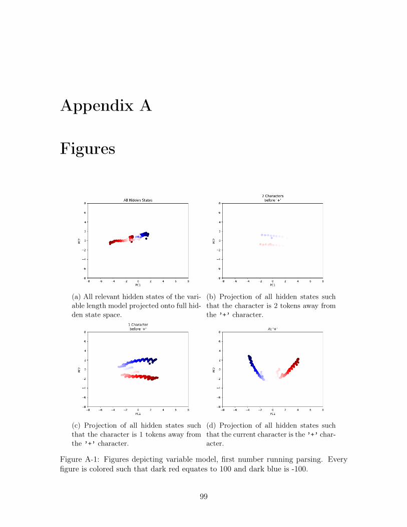
Appendix A

Figures

(a) All relevant hidden states of the vari-able length model projected onto full hid-den state space.

(b) Projection of all hidden states suchthat the character is 2 tokens away fromthe ’+’ character.

(c) Projection of all hidden states suchthat the character is 1 tokens away fromthe ’+’ character.

(d) Projection of all hidden states suchthat the current character is the ’+’ char-acter.

Figure A-1: Figures depicting variable model, first number running parsing. Everyfigure is colored such that dark red equates to 100 and dark blue is -100.

99

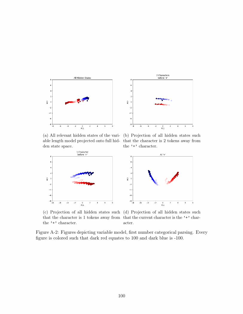
(a) All relevant hidden states of the vari-able length model projected onto full hid-den state space.

(b) Projection of all hidden states suchthat the character is 2 tokens away fromthe ’+’ character.

(c) Projection of all hidden states suchthat the character is 1 tokens away fromthe ’+’ character.

(d) Projection of all hidden states suchthat the current character is the ’+’ char-acter.

Figure A-2: Figures depicting variable model, first number categorical parsing. Everyfigure is colored such that dark red equates to 100 and dark blue is -100.

100

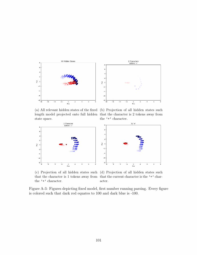
(a) All relevant hidden states of the fixedlength model projected onto full hiddenstate space.

(b) Projection of all hidden states suchthat the character is 2 tokens away fromthe ’+’ character.

(c) Projection of all hidden states suchthat the character is 1 tokens away fromthe ’+’ character.

(d) Projection of all hidden states suchthat the current character is the ’+’ char-acter.

Figure A-3: Figures depicting fixed model, first number running parsing. Every figureis colored such that dark red equates to 100 and dark blue is -100.

101

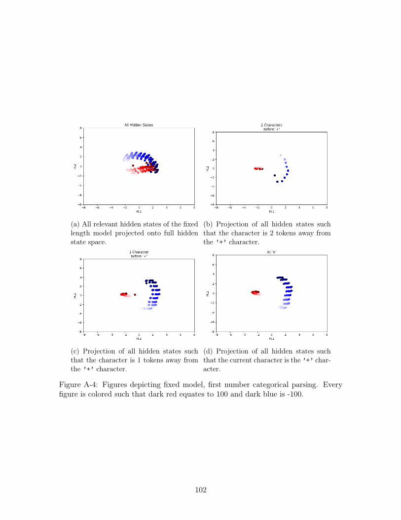
(a) All relevant hidden states of the fixedlength model projected onto full hiddenstate space.

(b) Projection of all hidden states suchthat the character is 2 tokens away fromthe ’+’ character.

(c) Projection of all hidden states suchthat the character is 1 tokens away fromthe ’+’ character.

(d) Projection of all hidden states suchthat the current character is the ’+’ char-acter.

Figure A-4: Figures depicting fixed model, first number categorical parsing. Everyfigure is colored such that dark red equates to 100 and dark blue is -100.

102

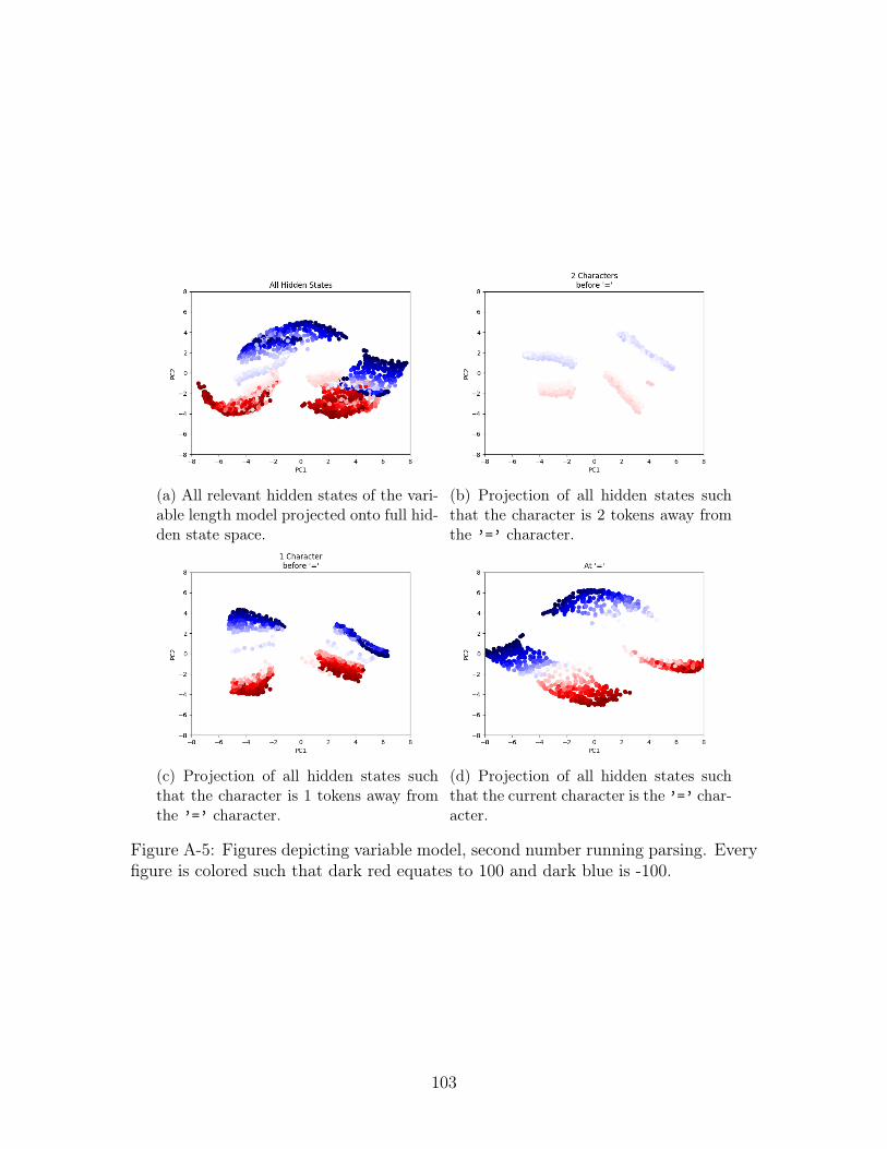
(a) All relevant hidden states of the vari-able length model projected onto full hid-den state space.

(b) Projection of all hidden states suchthat the character is 2 tokens away fromthe ’=’ character.

(c) Projection of all hidden states suchthat the character is 1 tokens away fromthe ’=’ character.

(d) Projection of all hidden states suchthat the current character is the ’=’ char-acter.

Figure A-5: Figures depicting variable model, second number running parsing. Everyfigure is colored such that dark red equates to 100 and dark blue is -100.

103

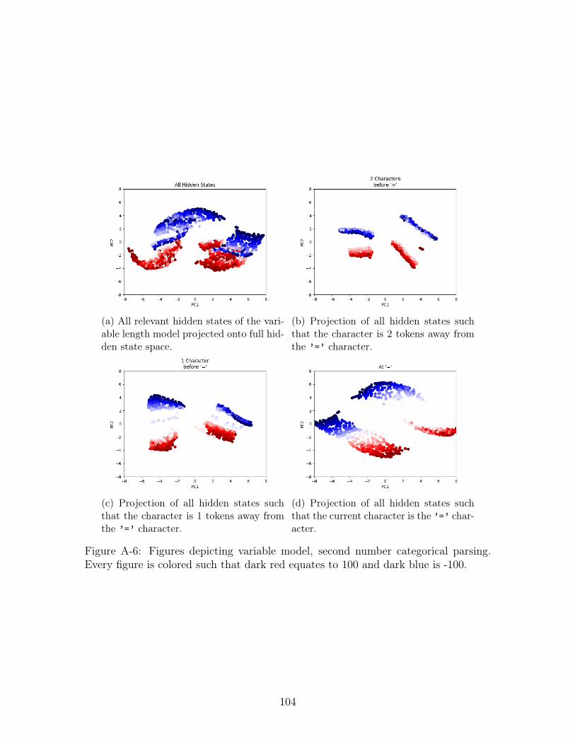
(a) All relevant hidden states of the vari-able length model projected onto full hid-den state space.

(b) Projection of all hidden states suchthat the character is 2 tokens away fromthe ’=’ character.

(c) Projection of all hidden states suchthat the character is 1 tokens away fromthe ’=’ character.

(d) Projection of all hidden states suchthat the current character is the ’=’ char-acter.

Figure A-6: Figures depicting variable model, second number categorical parsing.Every figure is colored such that dark red equates to 100 and dark blue is -100.

104

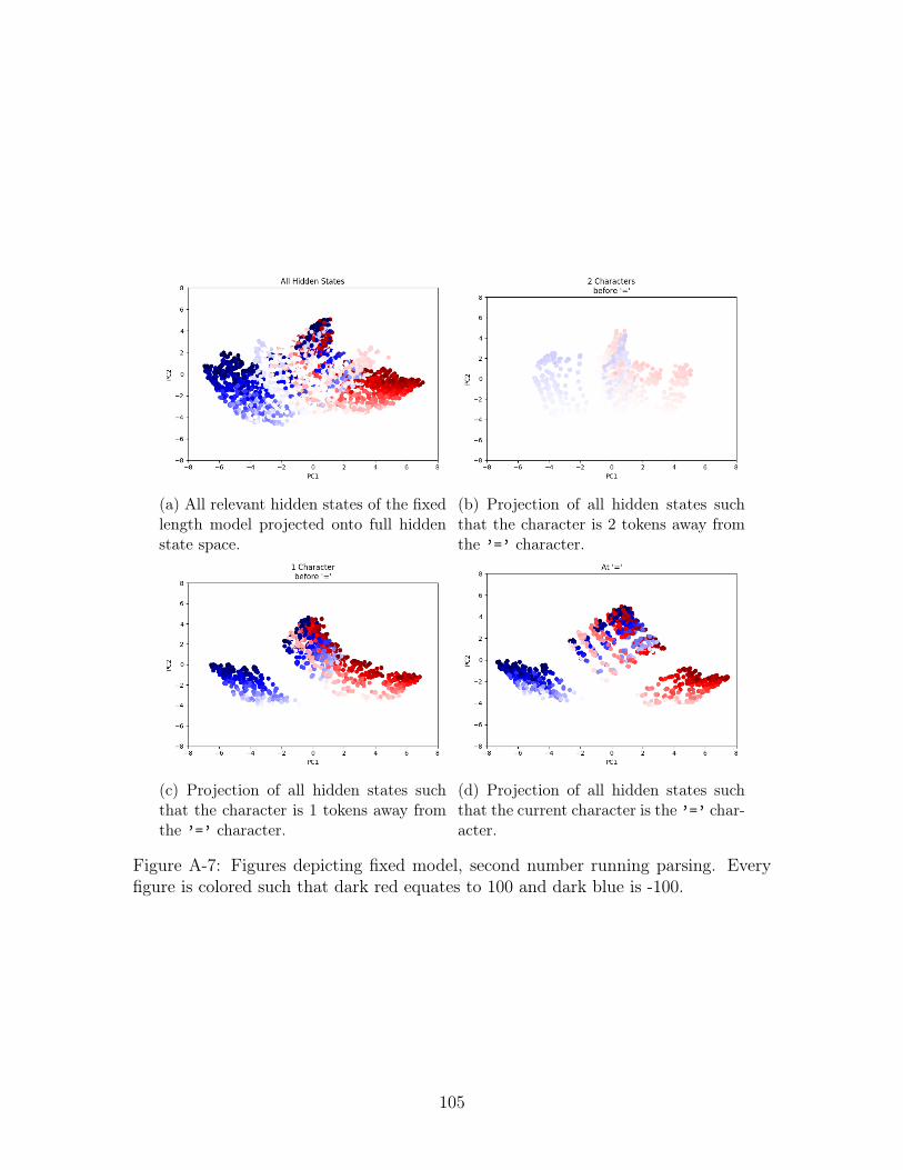
(a) All relevant hidden states of the fixedlength model projected onto full hiddenstate space.

(b) Projection of all hidden states suchthat the character is 2 tokens away fromthe ’=’ character.

(c) Projection of all hidden states suchthat the character is 1 tokens away fromthe ’=’ character.

(d) Projection of all hidden states suchthat the current character is the ’=’ char-acter.

Figure A-7: Figures depicting fixed model, second number running parsing. Everyfigure is colored such that dark red equates to 100 and dark blue is -100.

105

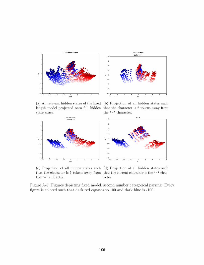
(a) All relevant hidden states of the fixedlength model projected onto full hiddenstate space.

(b) Projection of all hidden states suchthat the character is 2 tokens away fromthe ’=’ character.

(c) Projection of all hidden states suchthat the character is 1 tokens away fromthe ’=’ character.

(d) Projection of all hidden states suchthat the current character is the ’=’ char-acter.

Figure A-8: Figures depicting fixed model, second number categorical parsing. Everyfigure is colored such that dark red equates to 100 and dark blue is -100.

106

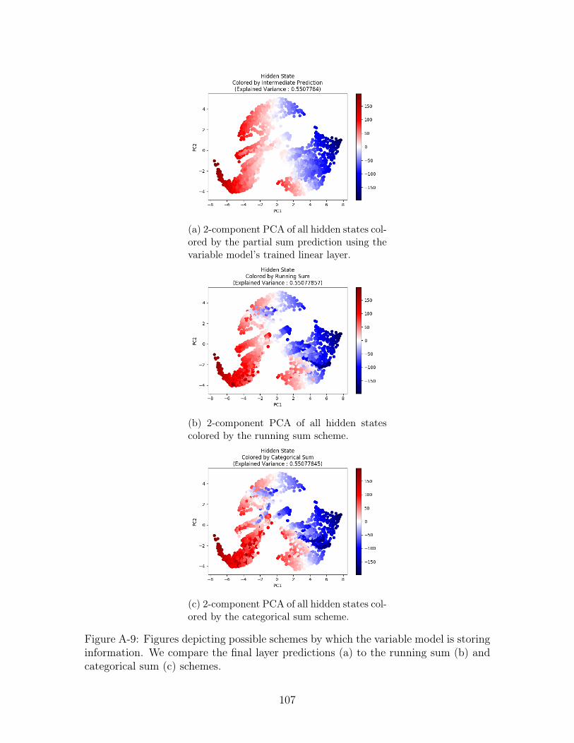
(a) 2-component PCA of all hidden states col-ored by the partial sum prediction using thevariable model’s trained linear layer.

(b) 2-component PCA of all hidden statescolored by the running sum scheme.

(c) 2-component PCA of all hidden states col-ored by the categorical sum scheme.

Figure A-9: Figures depicting possible schemes by which the variable model is storinginformation. We compare the final layer predictions (a) to the running sum (b) andcategorical sum (c) schemes.

107

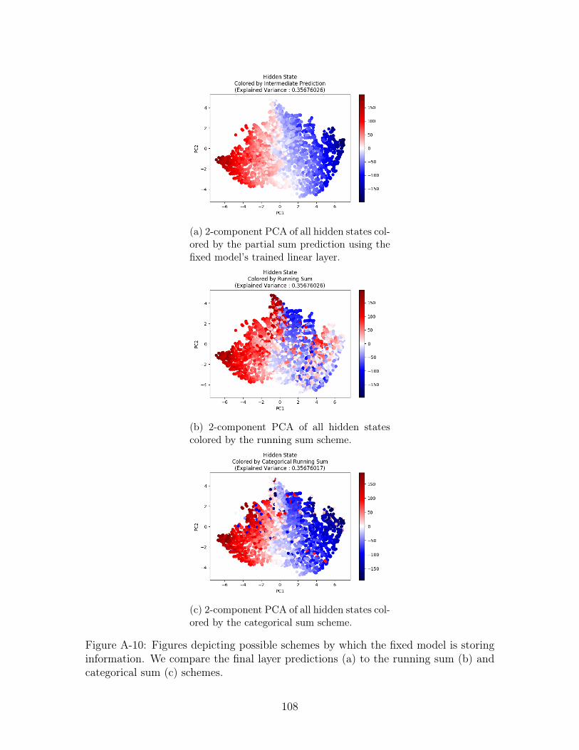
(a) 2-component PCA of all hidden states col-ored by the partial sum prediction using thefixed model’s trained linear layer.

(b) 2-component PCA of all hidden statescolored by the running sum scheme.

(c) 2-component PCA of all hidden states col-ored by the categorical sum scheme.

Figure A-10: Figures depicting possible schemes by which the fixed model is storinginformation. We compare the final layer predictions (a) to the running sum (b) andcategorical sum (c) schemes.

108

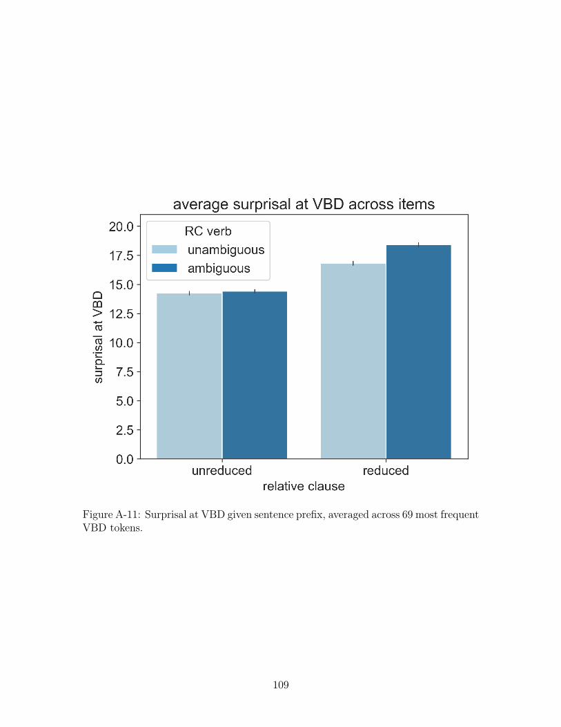
Figure A-11: Surprisal at VBD given sentence prefix, averaged across 69 most frequentVBD tokens.

109

Figure A-12: Item with correct surprisal pattern at VBD given sentence prefix, aver-aged across 69 most frequent VBD tokens.

110

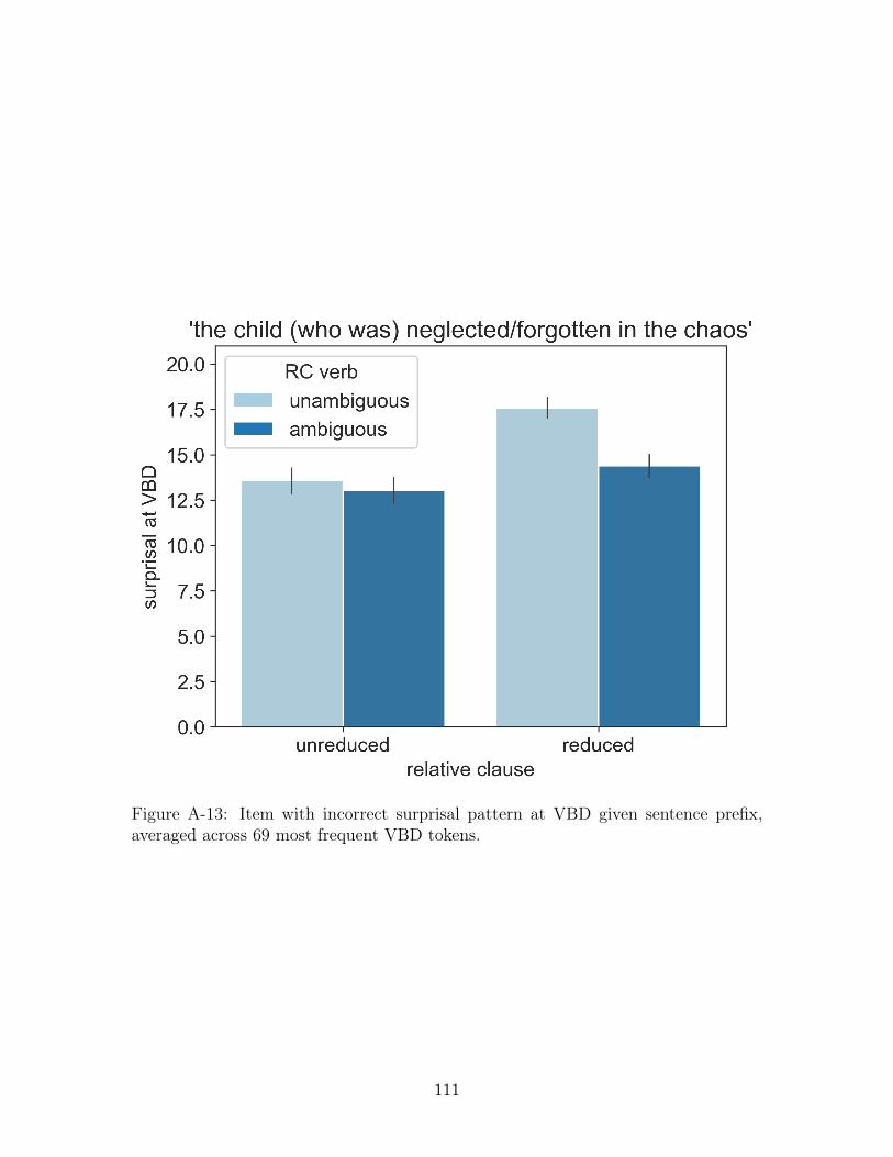
Figure A-13: Item with incorrect surprisal pattern at VBD given sentence prefix,averaged across 69 most frequent VBD tokens.

111

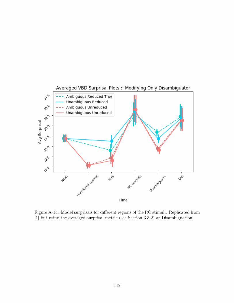
Figure A-14: Model surprisals for different regions of the RC stimuli. Replicated from[1] but using the averaged surprisal metric (see Section 3.3.2) at Disambiguation.

112

Figure A-15: Singular significance using 𝑦 gradient step.

113

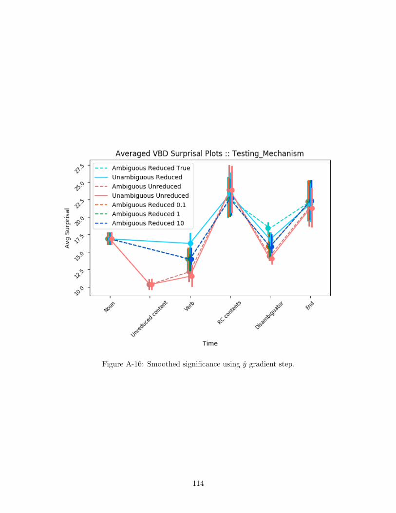
Figure A-16: Smoothed significance using 𝑦 gradient step.

114

Figure A-17: Singular significance using regression loss gradient step.

115

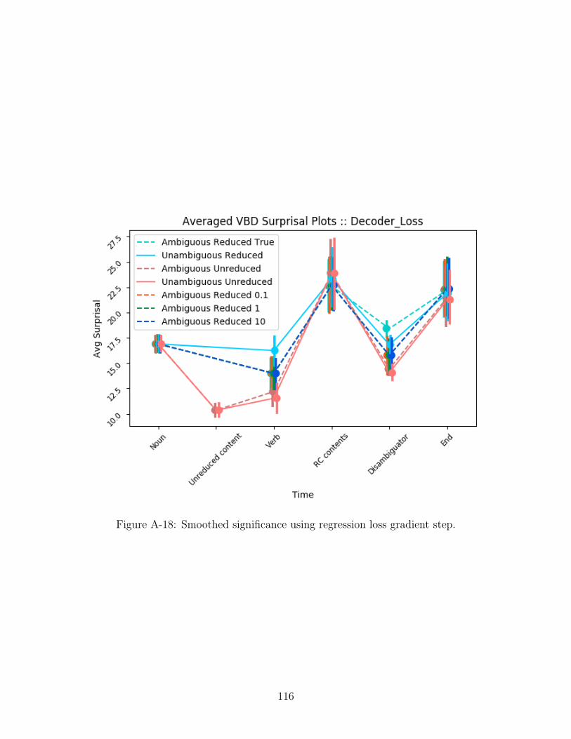
Figure A-18: Smoothed significance using regression loss gradient step.

116

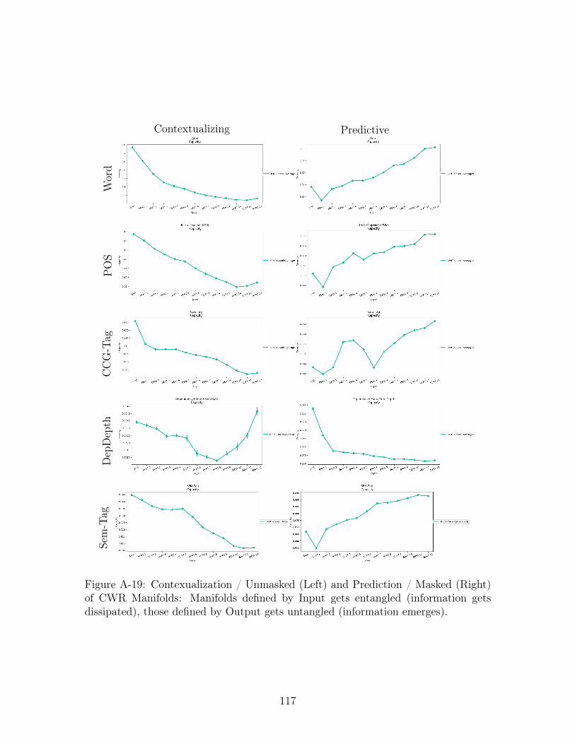
Contextualizing Predictive

Wor

dP

OS

CC

G-T

agD

epD

epth

Sem

-Tag

Figure A-19: Contexualization / Unmasked (Left) and Prediction / Masked (Right)of CWR Manifolds: Manifolds defined by Input gets entangled (information getsdissipated), those defined by Output gets untangled (information emerges).

117

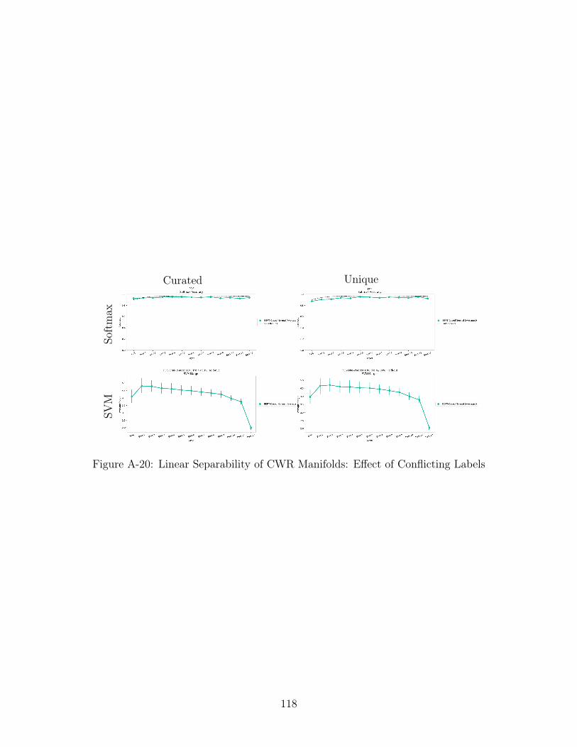
Curated Unique

Soft

max

SVM

Figure A-20: Linear Separability of CWR Manifolds: Effect of Conflicting Labels

118

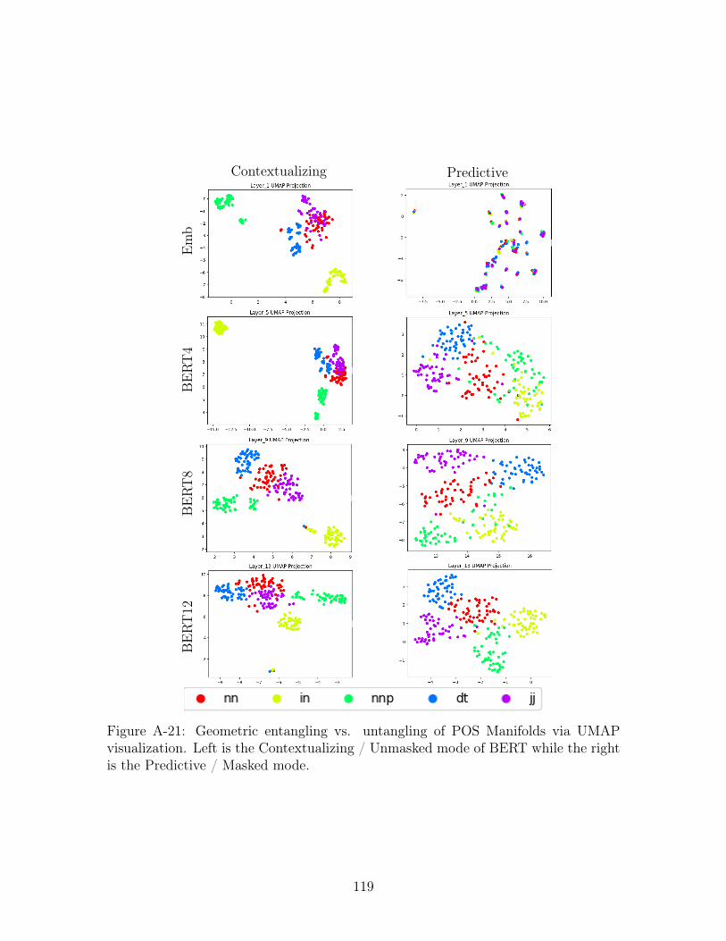
Contextualizing PredictiveE

mb

BE

RT

4B

ERT

8B

ERT

12

Figure A-21: Geometric entangling vs. untangling of POS Manifolds via UMAPvisualization. Left is the Contextualizing / Unmasked mode of BERT while the rightis the Predictive / Masked mode.

119

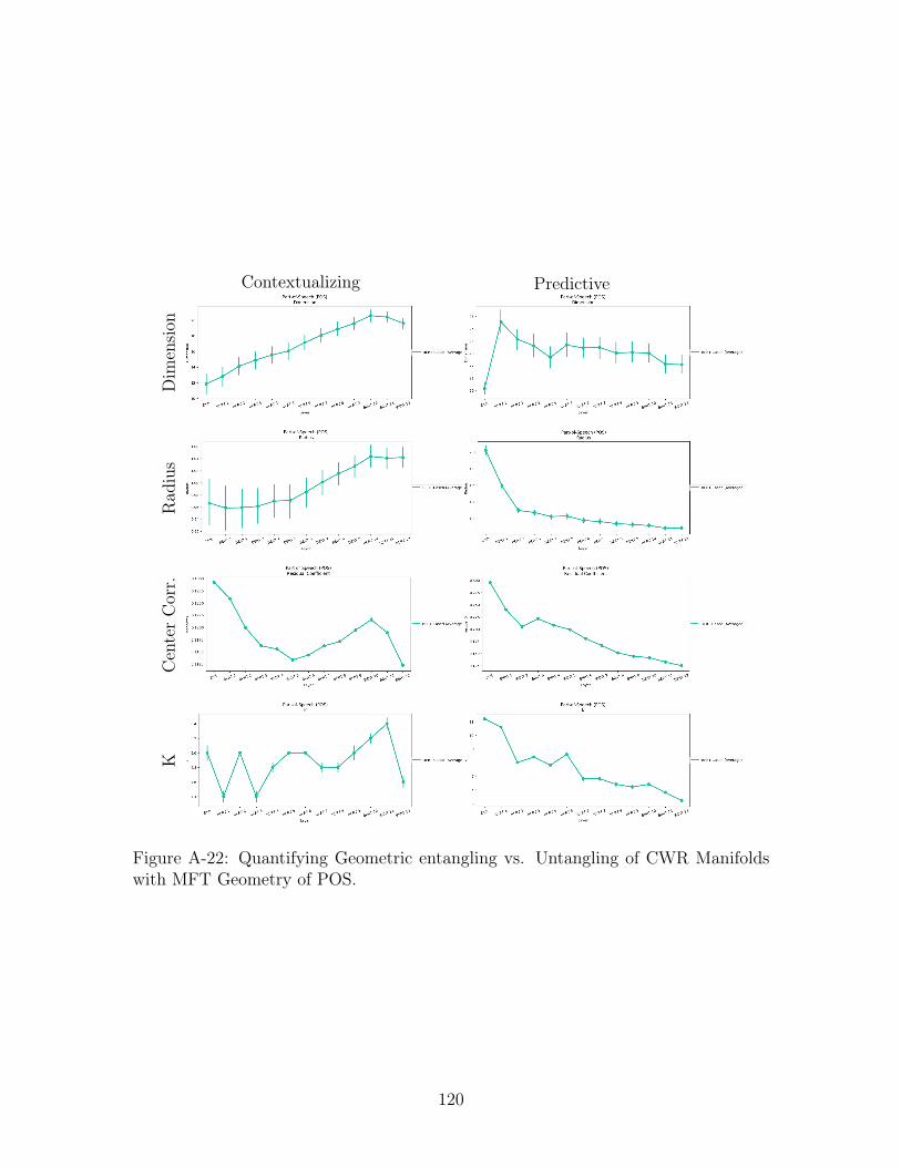
Contextualizing Predictive

Dim

ensi

onR

adiu

sC

ente

rC

orr.

K

Figure A-22: Quantifying Geometric entangling vs. Untangling of CWR Manifoldswith MFT Geometry of POS.

120

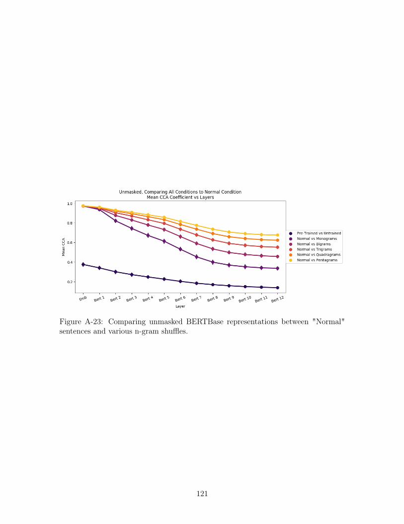
Figure A-23: Comparing unmasked BERTBase representations between "Normal"sentences and various n-gram shuffles.

121

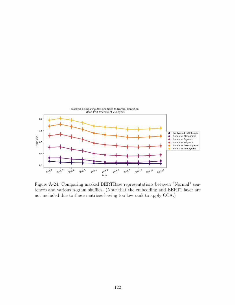
Figure A-24: Comparing masked BERTBase representations between "Normal" sen-tences and various n-gram shuffles. (Note that the embedding and BERT1 layer arenot included due to these matrices having too low rank to apply CCA.)

122

Figure A-25: Comparing unmasked BERTBase representations between "Normal"sentences and those same sentences with "real" and "fake" phrase swaps.

123

(a) Correlation between words that werenot shifted in the sentence due toreal/fake phrase swaps.

(b) Correlation between words that wereshifted in the sentence due to real/fakephrase swaps.

(c) Correlation between words that werenot swapped in the sentence due toreal/fake phrase swaps.

(d) Correlation between words that wereswapped in the sentence due to real/fakephrase swaps.

(e) Correlation between all conditionswhen real swaps occur.

(f) Correlation between all conditionswhen fake swaps occur.

Figure A-26: Comparing special cases of unmasked BERTBase representations duringa real/fake phrase swap.

124

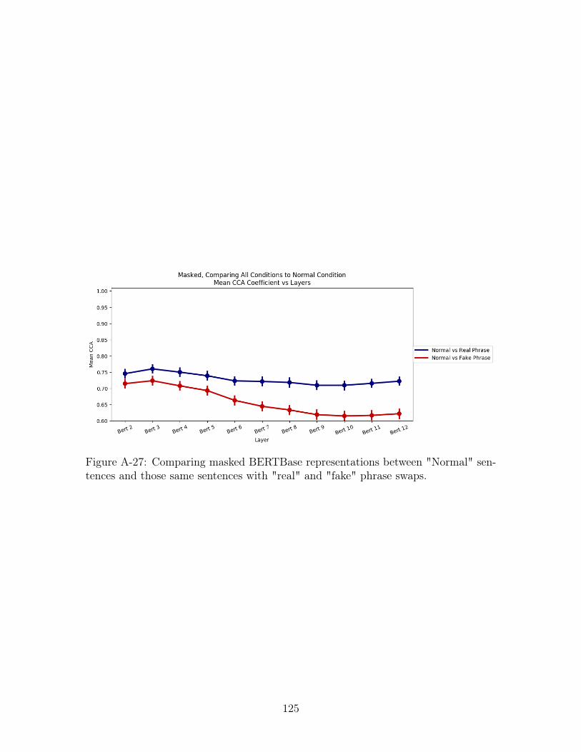
Figure A-27: Comparing masked BERTBase representations between "Normal" sen-tences and those same sentences with "real" and "fake" phrase swaps.

125

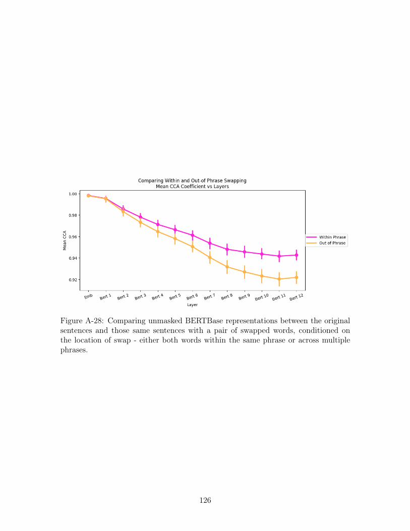
Figure A-28: Comparing unmasked BERTBase representations between the originalsentences and those same sentences with a pair of swapped words, conditioned onthe location of swap - either both words within the same phrase or across multiplephrases.

126

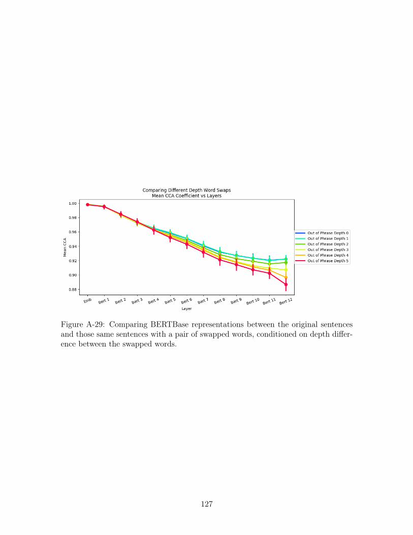
Figure A-29: Comparing BERTBase representations between the original sentencesand those same sentences with a pair of swapped words, conditioned on depth differ-ence between the swapped words.

127

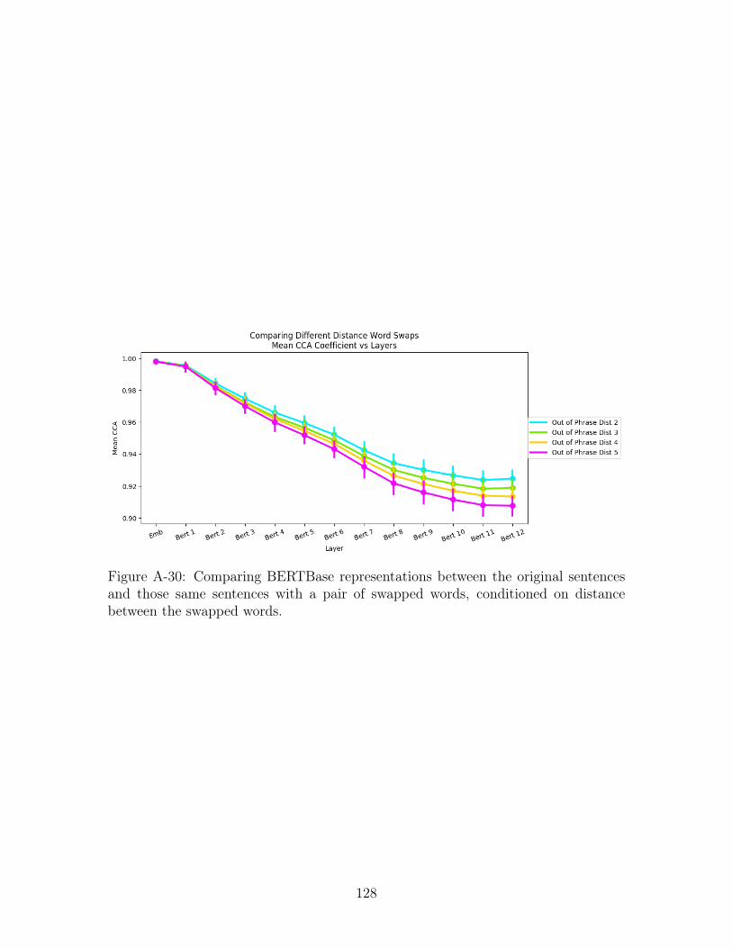
Figure A-30: Comparing BERTBase representations between the original sentencesand those same sentences with a pair of swapped words, conditioned on distancebetween the swapped words.

128

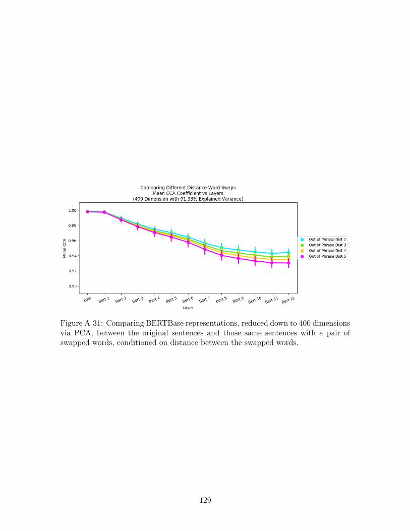
Figure A-31: Comparing BERTBase representations, reduced down to 400 dimensionsvia PCA, between the original sentences and those same sentences with a pair ofswapped words, conditioned on distance between the swapped words.

129

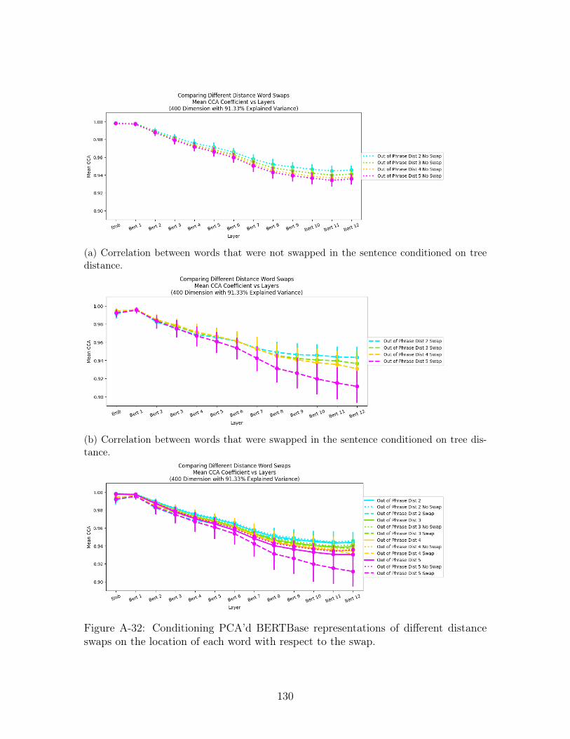
(a) Correlation between words that were not swapped in the sentence conditioned on treedistance.

(b) Correlation between words that were swapped in the sentence conditioned on tree dis-tance.

Figure A-32: Conditioning PCA’d BERTBase representations of different distanceswaps on the location of each word with respect to the swap.

130

131

132

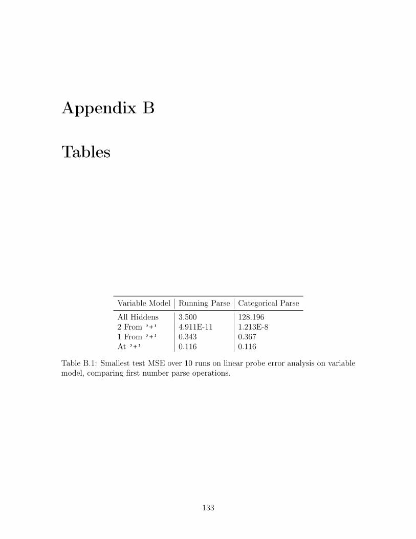
Appendix B

Tables

Variable Model Running Parse Categorical Parse

All Hiddens 3.500 128.1962 From ’+’ 4.911E-11 1.213E-81 From ’+’ 0.343 0.367At ’+’ 0.116 0.116

Table B.1: Smallest test MSE over 10 runs on linear probe error analysis on variablemodel, comparing first number parse operations.

133

Fixed Model Running Parse Categorical Parse

All Hiddens 18.333 0.3532 From ’+’ 1.658E-12 1.972E-101 From ’+’ 0.005 0.005At ’+’ 0.003 0.003

Table B.2: Smallest test MSE over 10 runs on linear probe error analysis on fixedmodel, comparing first number parse operations.

134

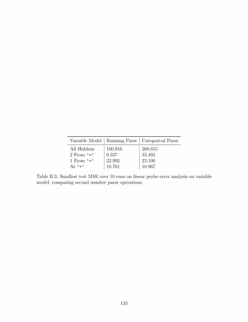
Variable Model Running Parse Categorical Parse

All Hiddens 100.916 268.6552 From ’=’ 0.337 33.4931 From ’=’ 22.992 23.100At ’=’ 10.761 10.967

Table B.3: Smallest test MSE over 10 runs on linear probe error analysis on variablemodel, comparing second number parse operations.

135

Fixed Model Running Parse Categorical Parse

All Hiddens 148.515 163.5192 From ’=’ 0.582 68.0271 From ’=’ 54.996 55.021At ’=’ 96.908 96.879

Table B.4: Smallest test MSE over 10 runs on linear probe error analysis on fixedmodel, comparing second number parse operations.

136

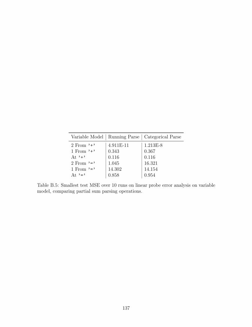
Variable Model Running Parse Categorical Parse

2 From ’+’ 4.911E-11 1.213E-81 From ’+’ 0.343 0.367At ’+’ 0.116 0.1162 From ’=’ 1.045 16.3211 From ’=’ 14.302 14.154At ’=’ 0.858 0.954

Table B.5: Smallest test MSE over 10 runs on linear probe error analysis on variablemodel, comparing partial sum parsing operations.

137

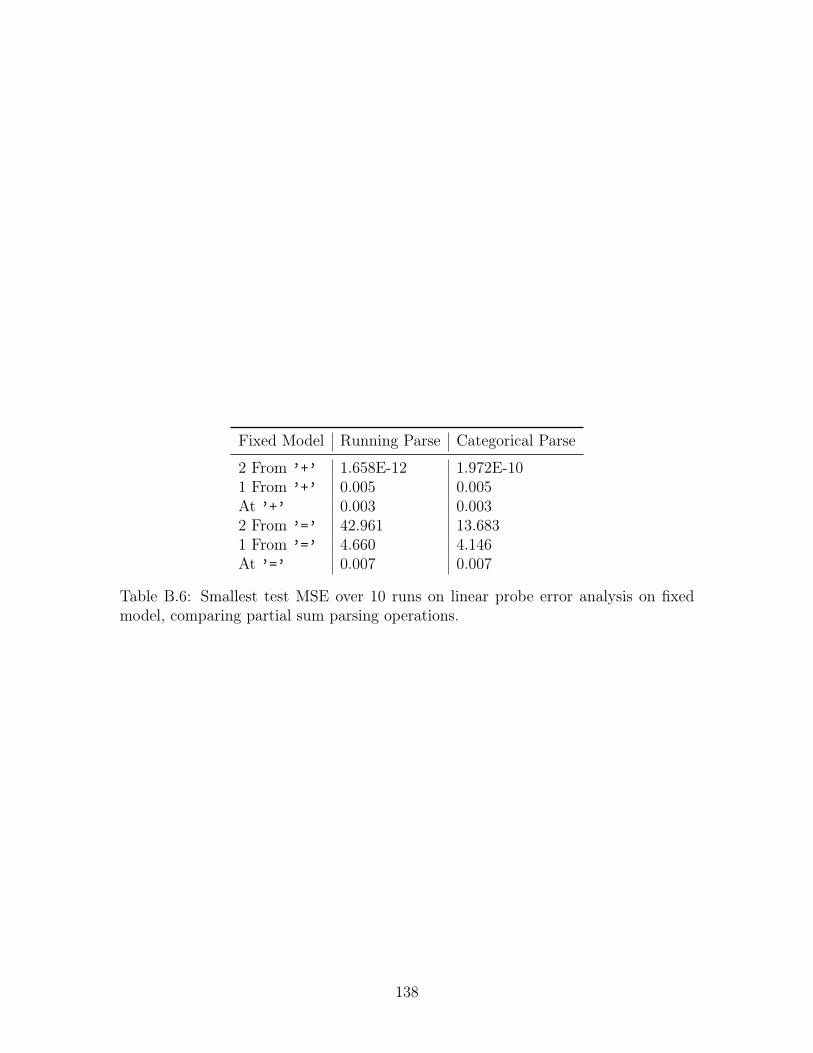
Fixed Model Running Parse Categorical Parse

2 From ’+’ 1.658E-12 1.972E-101 From ’+’ 0.005 0.005At ’+’ 0.003 0.0032 From ’=’ 42.961 13.6831 From ’=’ 4.660 4.146At ’=’ 0.007 0.007

Table B.6: Smallest test MSE over 10 runs on linear probe error analysis on fixedmodel, comparing partial sum parsing operations.

138

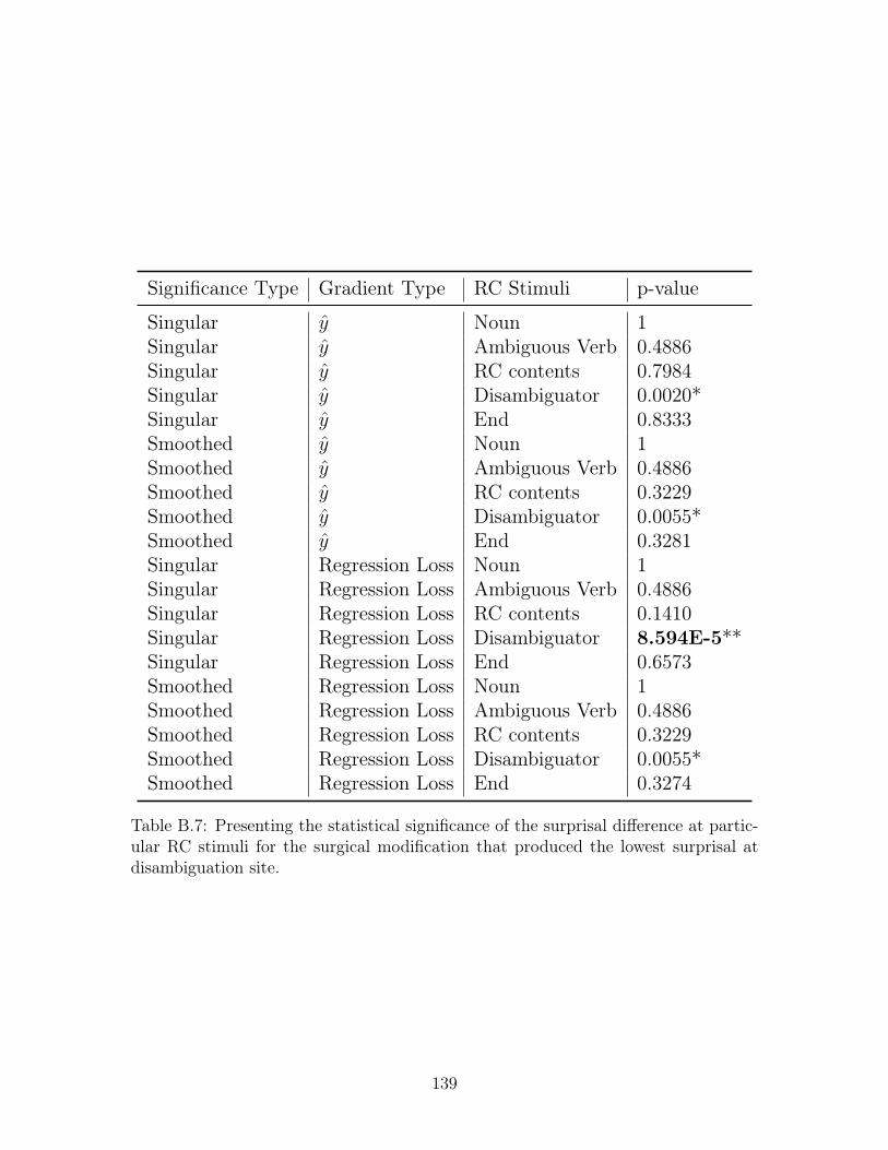
Significance Type Gradient Type RC Stimuli p-value

Singular 𝑦 Noun 1Singular 𝑦 Ambiguous Verb 0.4886Singular 𝑦 RC contents 0.7984Singular 𝑦 Disambiguator 0.0020*Singular 𝑦 End 0.8333Smoothed 𝑦 Noun 1Smoothed 𝑦 Ambiguous Verb 0.4886Smoothed 𝑦 RC contents 0.3229Smoothed 𝑦 Disambiguator 0.0055*Smoothed 𝑦 End 0.3281Singular Regression Loss Noun 1Singular Regression Loss Ambiguous Verb 0.4886Singular Regression Loss RC contents 0.1410Singular Regression Loss Disambiguator 8.594E-5**Singular Regression Loss End 0.6573Smoothed Regression Loss Noun 1Smoothed Regression Loss Ambiguous Verb 0.4886Smoothed Regression Loss RC contents 0.3229Smoothed Regression Loss Disambiguator 0.0055*Smoothed Regression Loss End 0.3274

Table B.7: Presenting the statistical significance of the surprisal difference at partic-ular RC stimuli for the surgical modification that produced the lowest surprisal atdisambiguation site.

139

140

141

142

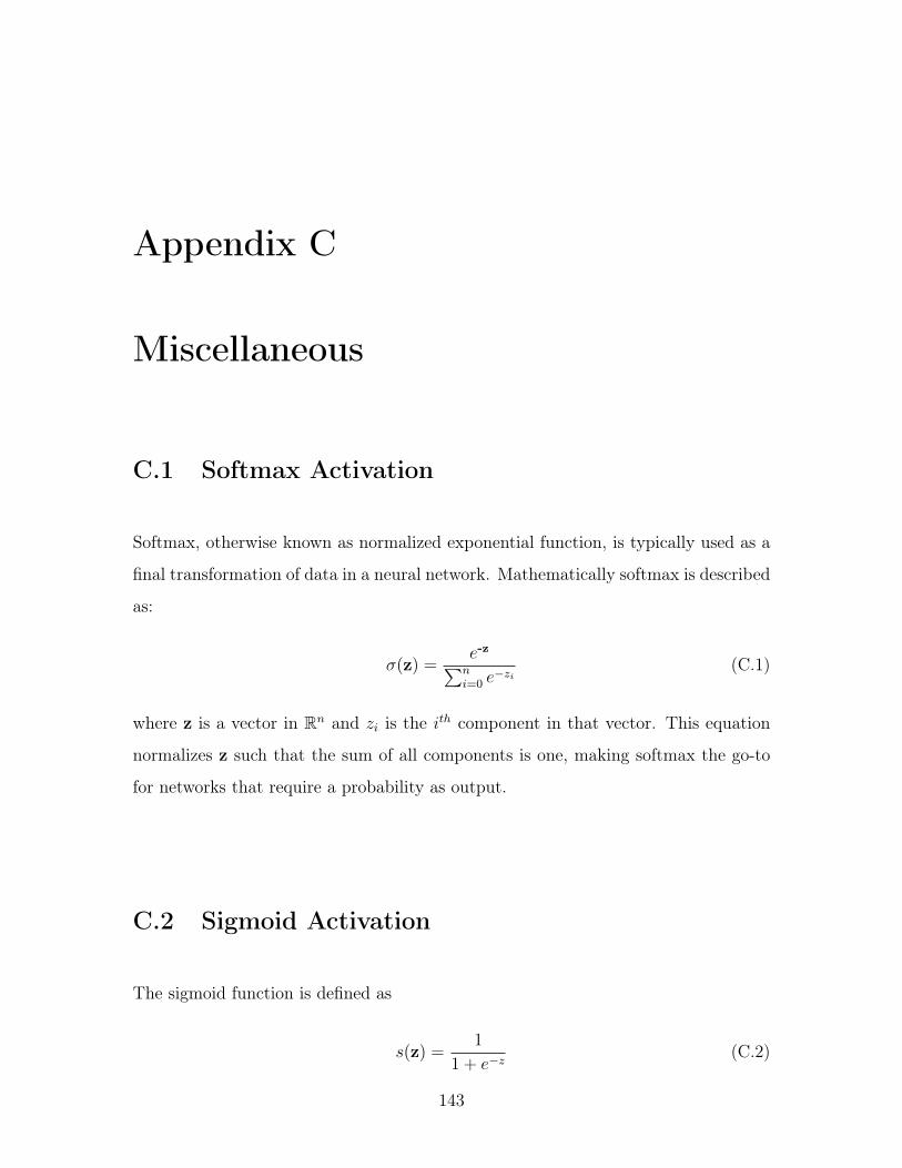
Appendix C

Miscellaneous

C.1 Softmax Activation

Softmax, otherwise known as normalized exponential function, is typically used as a

final transformation of data in a neural network. Mathematically softmax is described

as:

𝜎(z) =𝑒-z∑𝑛

𝑖=0 𝑒−𝑧𝑖

(C.1)

where z is a vector in R𝑛 and 𝑧𝑖 is the 𝑖𝑡ℎ component in that vector. This equation

normalizes z such that the sum of all components is one, making softmax the go-to

for networks that require a probability as output.

C.2 Sigmoid Activation

The sigmoid function is defined as

𝑠(z) =1

1 + 𝑒−𝑧(C.2)

143

C.3 Mean-Squared Error

Mean-Squared Error (MSE) is a measure of how accurately a linear model matches

some data distribution. The formula for MSE is as follows: for some true values, 𝑦,

and predicted values 𝑦 the MSE is

𝑀𝑆𝐸 =1

𝑛

𝑛∑𝑖=0

(𝑦 − 𝑦)2 (C.3)

This metric in particular is great for measuring how well a linear prediction model

fits data.

144

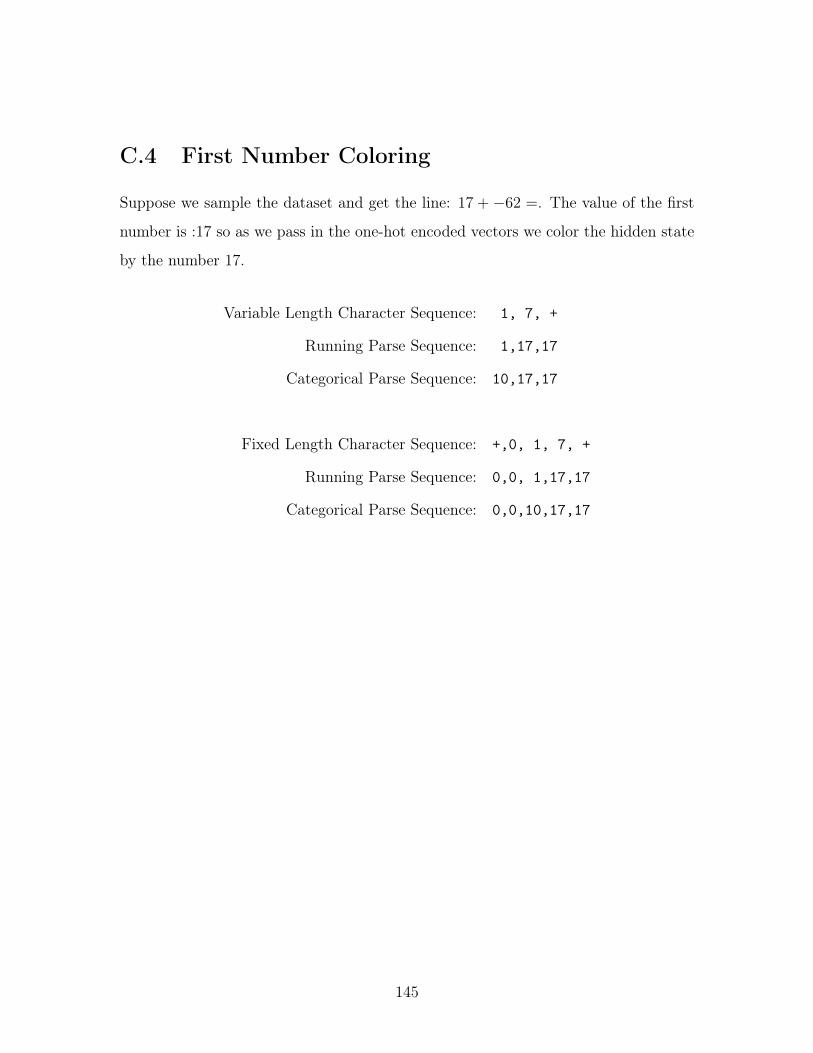
C.4 First Number Coloring

Suppose we sample the dataset and get the line: 17 +−62 =. The value of the first

number is :17 so as we pass in the one-hot encoded vectors we color the hidden state

by the number 17.

Variable Length Character Sequence: 1, 7, +

Running Parse Sequence: 1,17,17

Categorical Parse Sequence: 10,17,17

Fixed Length Character Sequence: +,0, 1, 7, +

Running Parse Sequence: 0,0, 1,17,17

Categorical Parse Sequence: 0,0,10,17,17

145

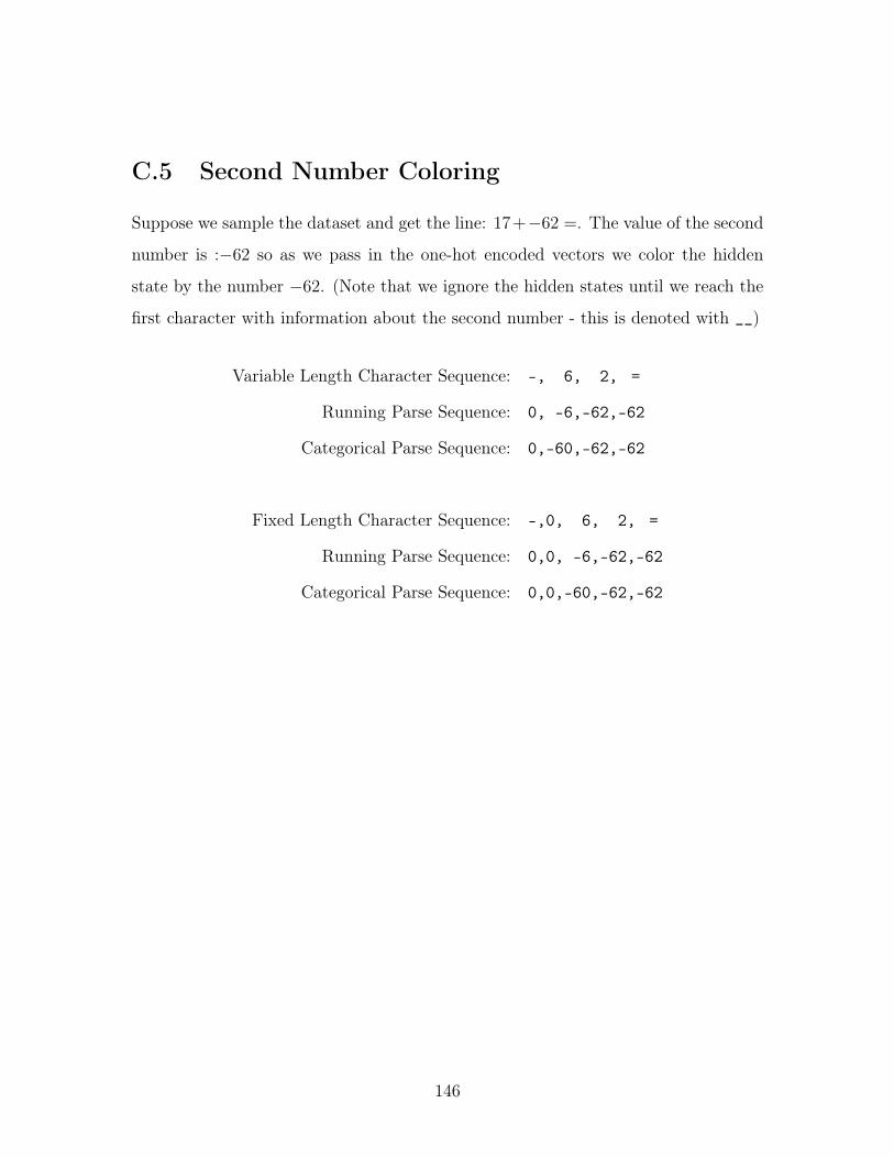
C.5 Second Number Coloring

Suppose we sample the dataset and get the line: 17+−62 =. The value of the second

number is :−62 so as we pass in the one-hot encoded vectors we color the hidden

state by the number −62. (Note that we ignore the hidden states until we reach the

first character with information about the second number - this is denoted with __)

Variable Length Character Sequence: -, 6, 2, =

Running Parse Sequence: 0, -6,-62,-62

Categorical Parse Sequence: 0,-60,-62,-62

Fixed Length Character Sequence: -,0, 6, 2, =

Running Parse Sequence: 0,0, -6,-62,-62

Categorical Parse Sequence: 0,0,-60,-62,-62

146

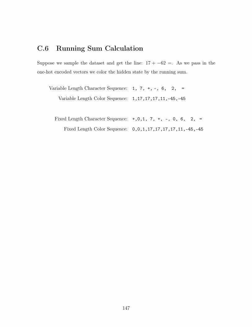
C.6 Running Sum Calculation

Suppose we sample the dataset and get the line: 17 + −62 =. As we pass in the

one-hot encoded vectors we color the hidden state by the running sum.

Variable Length Character Sequence: 1, 7, +, -, 6, 2, =

Variable Length Color Sequence: 1,17,17,17,11,-45,-45

Fixed Length Character Sequence: +,0,1, 7, +, -, 0, 6, 2, =

Fixed Length Color Sequence: 0,0,1,17,17,17,17,11,-45,-45

147

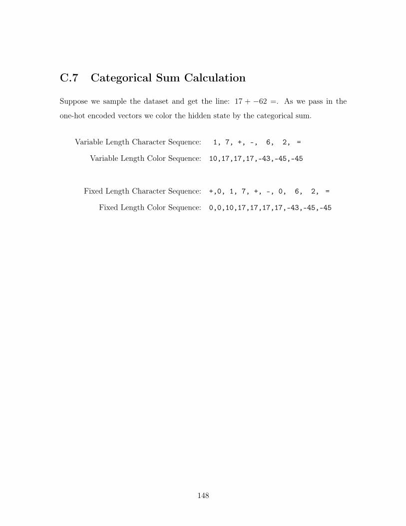
C.7 Categorical Sum Calculation

Suppose we sample the dataset and get the line: 17 + −62 =. As we pass in the

one-hot encoded vectors we color the hidden state by the categorical sum.

Variable Length Character Sequence: 1, 7, +, -, 6, 2, =

Variable Length Color Sequence: 10,17,17,17,-43,-45,-45

Fixed Length Character Sequence: +,0, 1, 7, +, -, 0, 6, 2, =

Fixed Length Color Sequence: 0,0,10,17,17,17,17,-43,-45,-45

148

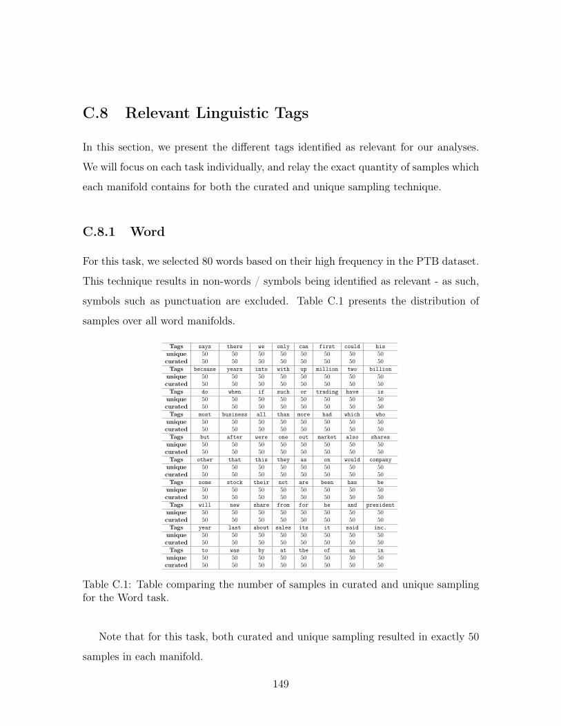
C.8 Relevant Linguistic Tags

In this section, we present the different tags identified as relevant for our analyses.

We will focus on each task individually, and relay the exact quantity of samples which

each manifold contains for both the curated and unique sampling technique.

C.8.1 Word

For this task, we selected 80 words based on their high frequency in the PTB dataset.

This technique results in non-words / symbols being identified as relevant - as such,

symbols such as punctuation are excluded. Table C.1 presents the distribution of

samples over all word manifolds.

Tags says there we only can first could hisunique 50 50 50 50 50 50 50 50curated 50 50 50 50 50 50 50 50Tags because years into with up million two billion

unique 50 50 50 50 50 50 50 50curated 50 50 50 50 50 50 50 50Tags do when if such or trading have is

unique 50 50 50 50 50 50 50 50curated 50 50 50 50 50 50 50 50Tags most business all than more had which who

unique 50 50 50 50 50 50 50 50curated 50 50 50 50 50 50 50 50Tags but after were one out market also shares

unique 50 50 50 50 50 50 50 50curated 50 50 50 50 50 50 50 50Tags other that this they as on would company

unique 50 50 50 50 50 50 50 50curated 50 50 50 50 50 50 50 50Tags some stock their not are been has be

unique 50 50 50 50 50 50 50 50curated 50 50 50 50 50 50 50 50Tags will new share from for he and president

unique 50 50 50 50 50 50 50 50curated 50 50 50 50 50 50 50 50Tags year last about sales its it said inc.

unique 50 50 50 50 50 50 50 50curated 50 50 50 50 50 50 50 50Tags to was by at the of an in

unique 50 50 50 50 50 50 50 50curated 50 50 50 50 50 50 50 50

Table C.1: Table comparing the number of samples in curated and unique samplingfor the Word task.

Note that for this task, both curated and unique sampling resulted in exactly 50

samples in each manifold.

149

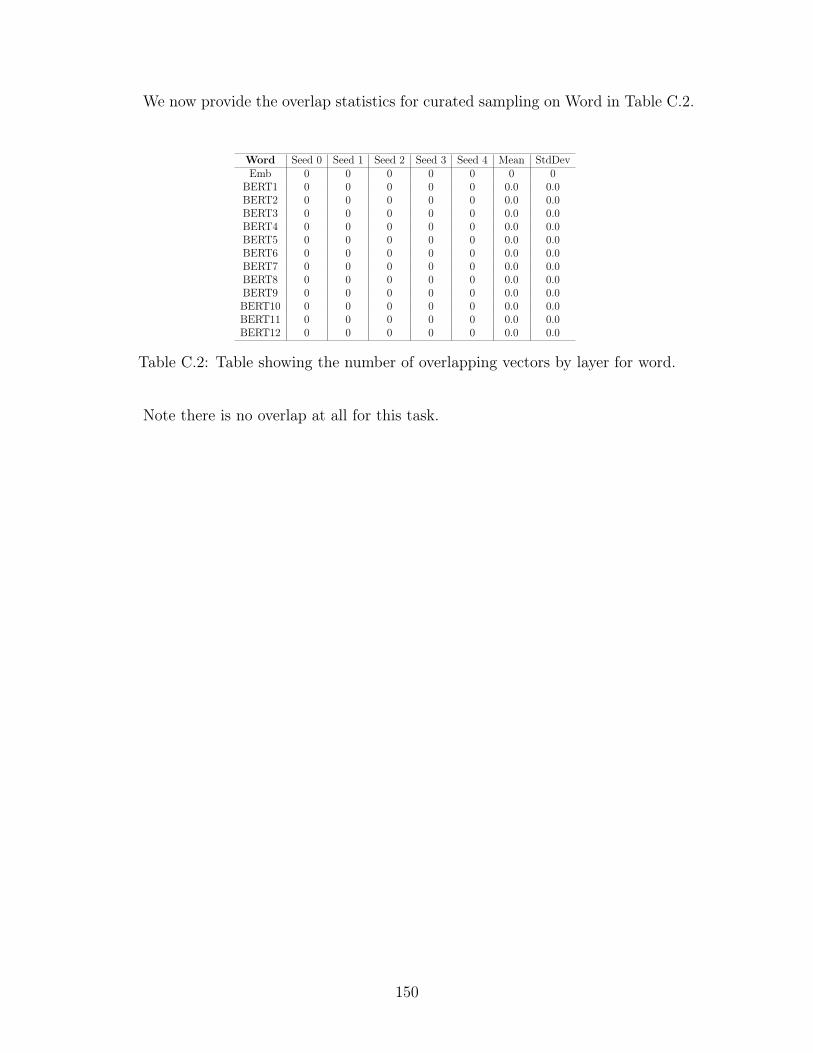
We now provide the overlap statistics for curated sampling on Word in Table C.2.

Word Seed 0 Seed 1 Seed 2 Seed 3 Seed 4 Mean StdDevEmb 0 0 0 0 0 0 0

BERT1 0 0 0 0 0 0.0 0.0BERT2 0 0 0 0 0 0.0 0.0BERT3 0 0 0 0 0 0.0 0.0BERT4 0 0 0 0 0 0.0 0.0BERT5 0 0 0 0 0 0.0 0.0BERT6 0 0 0 0 0 0.0 0.0BERT7 0 0 0 0 0 0.0 0.0BERT8 0 0 0 0 0 0.0 0.0BERT9 0 0 0 0 0 0.0 0.0BERT10 0 0 0 0 0 0.0 0.0BERT11 0 0 0 0 0 0.0 0.0BERT12 0 0 0 0 0 0.0 0.0

Table C.2: Table showing the number of overlapping vectors by layer for word.

Note there is no overlap at all for this task.

150

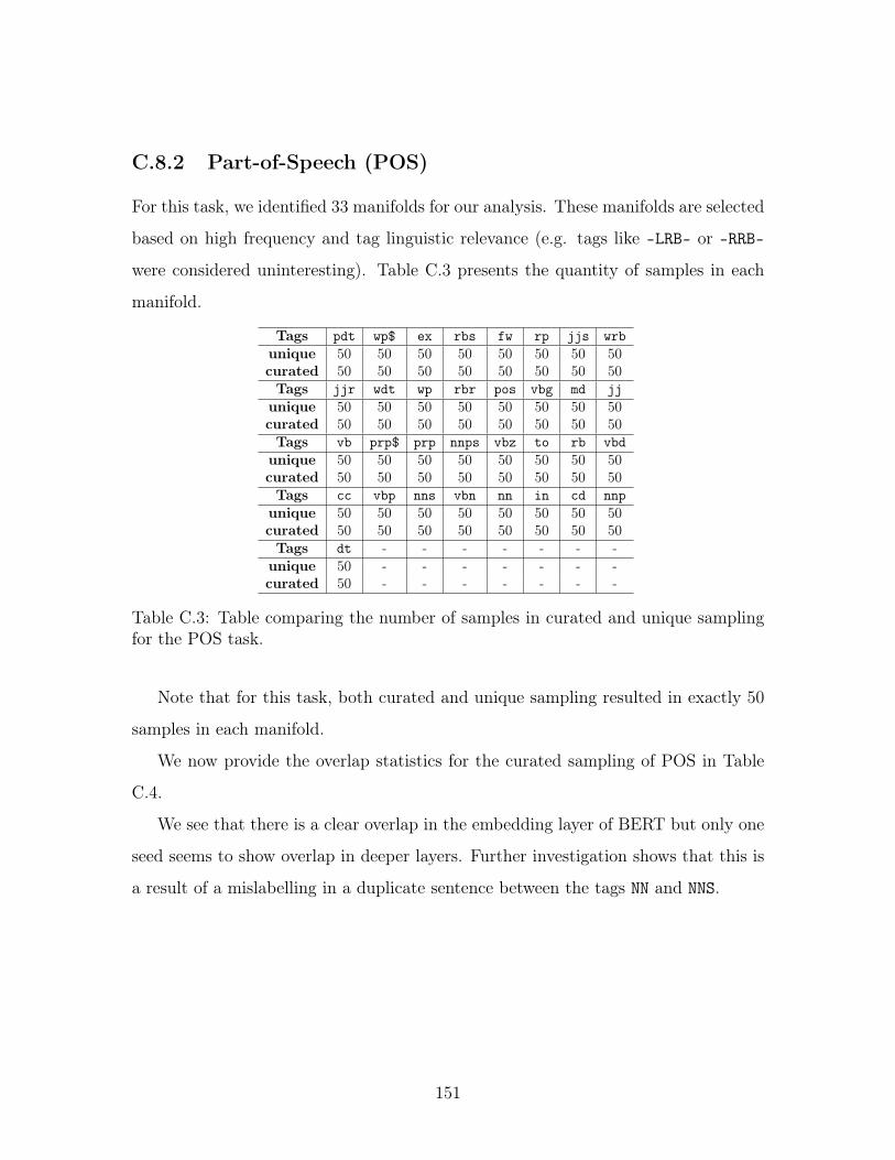
C.8.2 Part-of-Speech (POS)

For this task, we identified 33 manifolds for our analysis. These manifolds are selected

based on high frequency and tag linguistic relevance (e.g. tags like -LRB- or -RRB-

were considered uninteresting). Table C.3 presents the quantity of samples in each

manifold.

Tags pdt wp$ ex rbs fw rp jjs wrbunique 50 50 50 50 50 50 50 50curated 50 50 50 50 50 50 50 50Tags jjr wdt wp rbr pos vbg md jj

unique 50 50 50 50 50 50 50 50curated 50 50 50 50 50 50 50 50Tags vb prp$ prp nnps vbz to rb vbd

unique 50 50 50 50 50 50 50 50curated 50 50 50 50 50 50 50 50Tags cc vbp nns vbn nn in cd nnp

unique 50 50 50 50 50 50 50 50curated 50 50 50 50 50 50 50 50Tags dt - - - - - - -

unique 50 - - - - - - -curated 50 - - - - - - -

Table C.3: Table comparing the number of samples in curated and unique samplingfor the POS task.

Note that for this task, both curated and unique sampling resulted in exactly 50

samples in each manifold.

We now provide the overlap statistics for the curated sampling of POS in Table

C.4.

We see that there is a clear overlap in the embedding layer of BERT but only one

seed seems to show overlap in deeper layers. Further investigation shows that this is

a result of a mislabelling in a duplicate sentence between the tags NN and NNS.

151

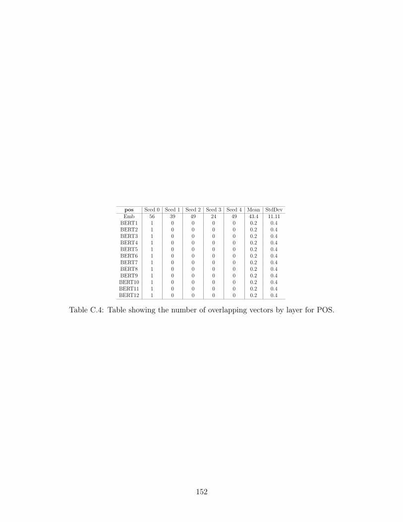
pos Seed 0 Seed 1 Seed 2 Seed 3 Seed 4 Mean StdDevEmb 56 39 49 24 49 43.4 11.11

BERT1 1 0 0 0 0 0.2 0.4BERT2 1 0 0 0 0 0.2 0.4BERT3 1 0 0 0 0 0.2 0.4BERT4 1 0 0 0 0 0.2 0.4BERT5 1 0 0 0 0 0.2 0.4BERT6 1 0 0 0 0 0.2 0.4BERT7 1 0 0 0 0 0.2 0.4BERT8 1 0 0 0 0 0.2 0.4BERT9 1 0 0 0 0 0.2 0.4BERT10 1 0 0 0 0 0.2 0.4BERT11 1 0 0 0 0 0.2 0.4BERT12 1 0 0 0 0 0.2 0.4

Table C.4: Table showing the number of overlapping vectors by layer for POS.

152

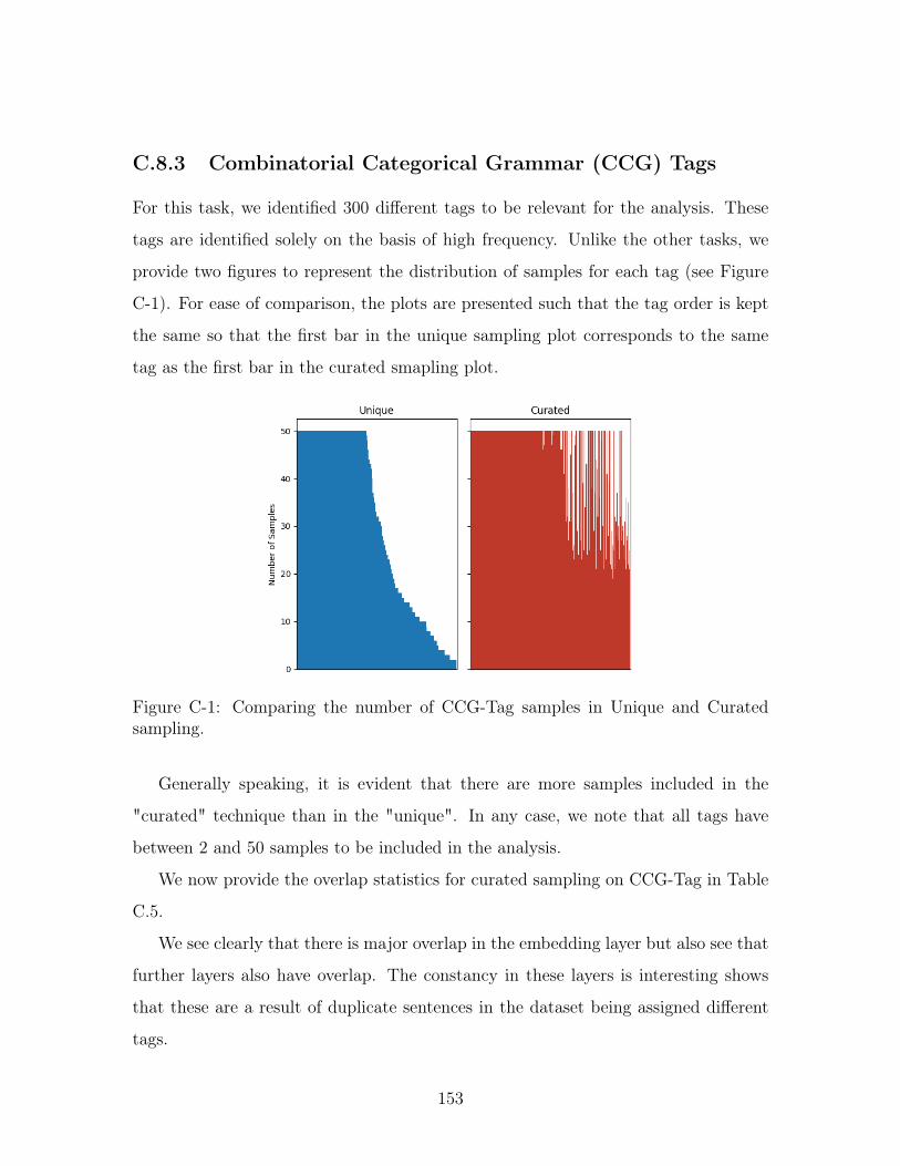
C.8.3 Combinatorial Categorical Grammar (CCG) Tags

For this task, we identified 300 different tags to be relevant for the analysis. These

tags are identified solely on the basis of high frequency. Unlike the other tasks, we

provide two figures to represent the distribution of samples for each tag (see Figure

C-1). For ease of comparison, the plots are presented such that the tag order is kept

the same so that the first bar in the unique sampling plot corresponds to the same

tag as the first bar in the curated smapling plot.

Figure C-1: Comparing the number of CCG-Tag samples in Unique and Curatedsampling.

Generally speaking, it is evident that there are more samples included in the

"curated" technique than in the "unique". In any case, we note that all tags have

between 2 and 50 samples to be included in the analysis.

We now provide the overlap statistics for curated sampling on CCG-Tag in Table

C.5.

We see clearly that there is major overlap in the embedding layer but also see that

further layers also have overlap. The constancy in these layers is interesting shows

that these are a result of duplicate sentences in the dataset being assigned different

tags.

153

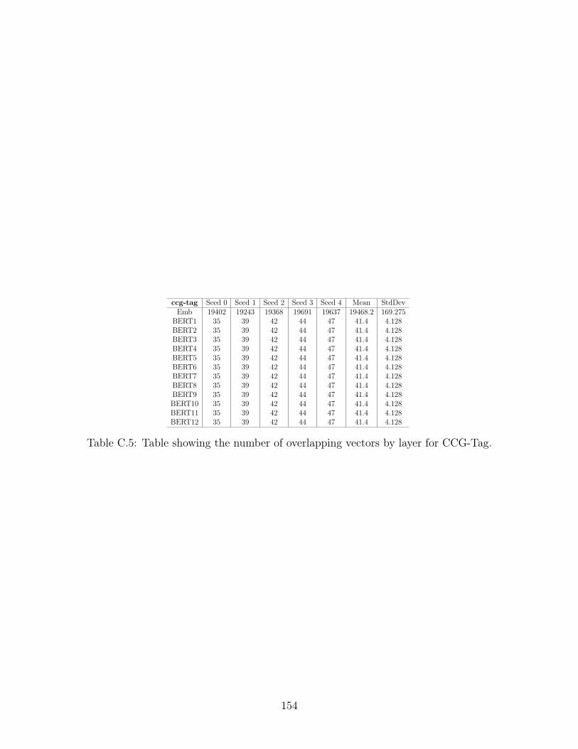
ccg-tag Seed 0 Seed 1 Seed 2 Seed 3 Seed 4 Mean StdDevEmb 19402 19243 19368 19691 19637 19468.2 169.275

BERT1 35 39 42 44 47 41.4 4.128BERT2 35 39 42 44 47 41.4 4.128BERT3 35 39 42 44 47 41.4 4.128BERT4 35 39 42 44 47 41.4 4.128BERT5 35 39 42 44 47 41.4 4.128BERT6 35 39 42 44 47 41.4 4.128BERT7 35 39 42 44 47 41.4 4.128BERT8 35 39 42 44 47 41.4 4.128BERT9 35 39 42 44 47 41.4 4.128BERT10 35 39 42 44 47 41.4 4.128BERT11 35 39 42 44 47 41.4 4.128BERT12 35 39 42 44 47 41.4 4.128

Table C.5: Table showing the number of overlapping vectors by layer for CCG-Tag.

154

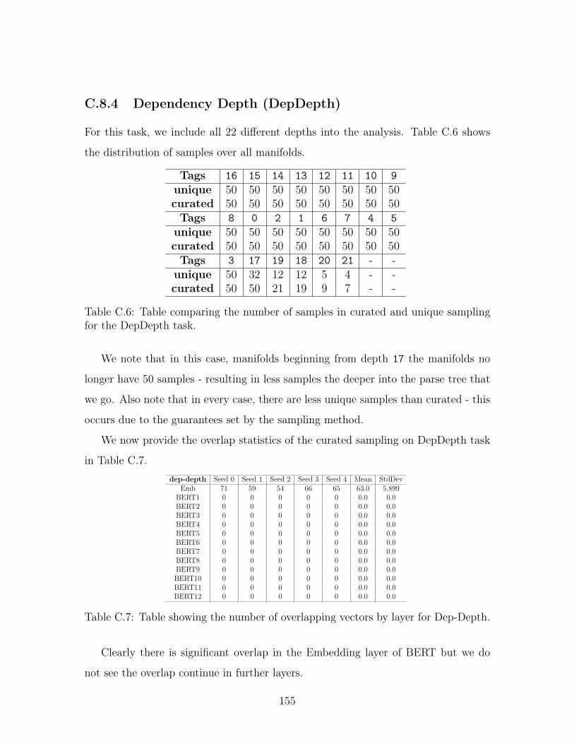
C.8.4 Dependency Depth (DepDepth)

For this task, we include all 22 different depths into the analysis. Table C.6 shows

the distribution of samples over all manifolds.

Tags 16 15 14 13 12 11 10 9unique 50 50 50 50 50 50 50 50curated 50 50 50 50 50 50 50 50Tags 8 0 2 1 6 7 4 5

unique 50 50 50 50 50 50 50 50curated 50 50 50 50 50 50 50 50Tags 3 17 19 18 20 21 - -

unique 50 32 12 12 5 4 - -curated 50 50 21 19 9 7 - -

Table C.6: Table comparing the number of samples in curated and unique samplingfor the DepDepth task.

We note that in this case, manifolds beginning from depth 17 the manifolds no

longer have 50 samples - resulting in less samples the deeper into the parse tree that

we go. Also note that in every case, there are less unique samples than curated - this

occurs due to the guarantees set by the sampling method.

We now provide the overlap statistics of the curated sampling on DepDepth task

in Table C.7.dep-depth Seed 0 Seed 1 Seed 2 Seed 3 Seed 4 Mean StdDev

Emb 71 59 54 66 65 63.0 5.899BERT1 0 0 0 0 0 0.0 0.0BERT2 0 0 0 0 0 0.0 0.0BERT3 0 0 0 0 0 0.0 0.0BERT4 0 0 0 0 0 0.0 0.0BERT5 0 0 0 0 0 0.0 0.0BERT6 0 0 0 0 0 0.0 0.0BERT7 0 0 0 0 0 0.0 0.0BERT8 0 0 0 0 0 0.0 0.0BERT9 0 0 0 0 0 0.0 0.0BERT10 0 0 0 0 0 0.0 0.0BERT11 0 0 0 0 0 0.0 0.0BERT12 0 0 0 0 0 0.0 0.0

Table C.7: Table showing the number of overlapping vectors by layer for Dep-Depth.

Clearly there is significant overlap in the Embedding layer of BERT but we do

not see the overlap continue in further layers.

155

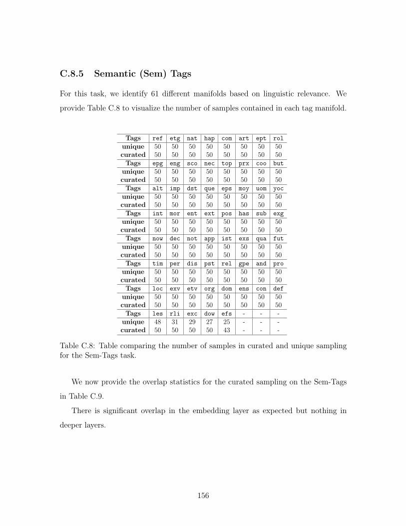
C.8.5 Semantic (Sem) Tags

For this task, we identify 61 different manifolds based on linguistic relevance. We

provide Table C.8 to visualize the number of samples contained in each tag manifold.

Tags ref etg nat hap com art ept rolunique 50 50 50 50 50 50 50 50curated 50 50 50 50 50 50 50 50Tags epg eng sco nec top prx coo but

unique 50 50 50 50 50 50 50 50curated 50 50 50 50 50 50 50 50Tags alt imp dst que eps moy uom yoc

unique 50 50 50 50 50 50 50 50curated 50 50 50 50 50 50 50 50Tags int mor ent ext pos has sub exg

unique 50 50 50 50 50 50 50 50curated 50 50 50 50 50 50 50 50Tags now dec not app ist exs qua fut

unique 50 50 50 50 50 50 50 50curated 50 50 50 50 50 50 50 50Tags tim per dis pst rel gpe and pro

unique 50 50 50 50 50 50 50 50curated 50 50 50 50 50 50 50 50Tags loc exv etv org dom ens con def

unique 50 50 50 50 50 50 50 50curated 50 50 50 50 50 50 50 50Tags les rli exc dow efs - - -

unique 48 31 29 27 25 - - -curated 50 50 50 50 43 - - -

Table C.8: Table comparing the number of samples in curated and unique samplingfor the Sem-Tags task.

We now provide the overlap statistics for the curated sampling on the Sem-Tags

in Table C.9.

There is significant overlap in the embedding layer as expected but nothing in

deeper layers.

156

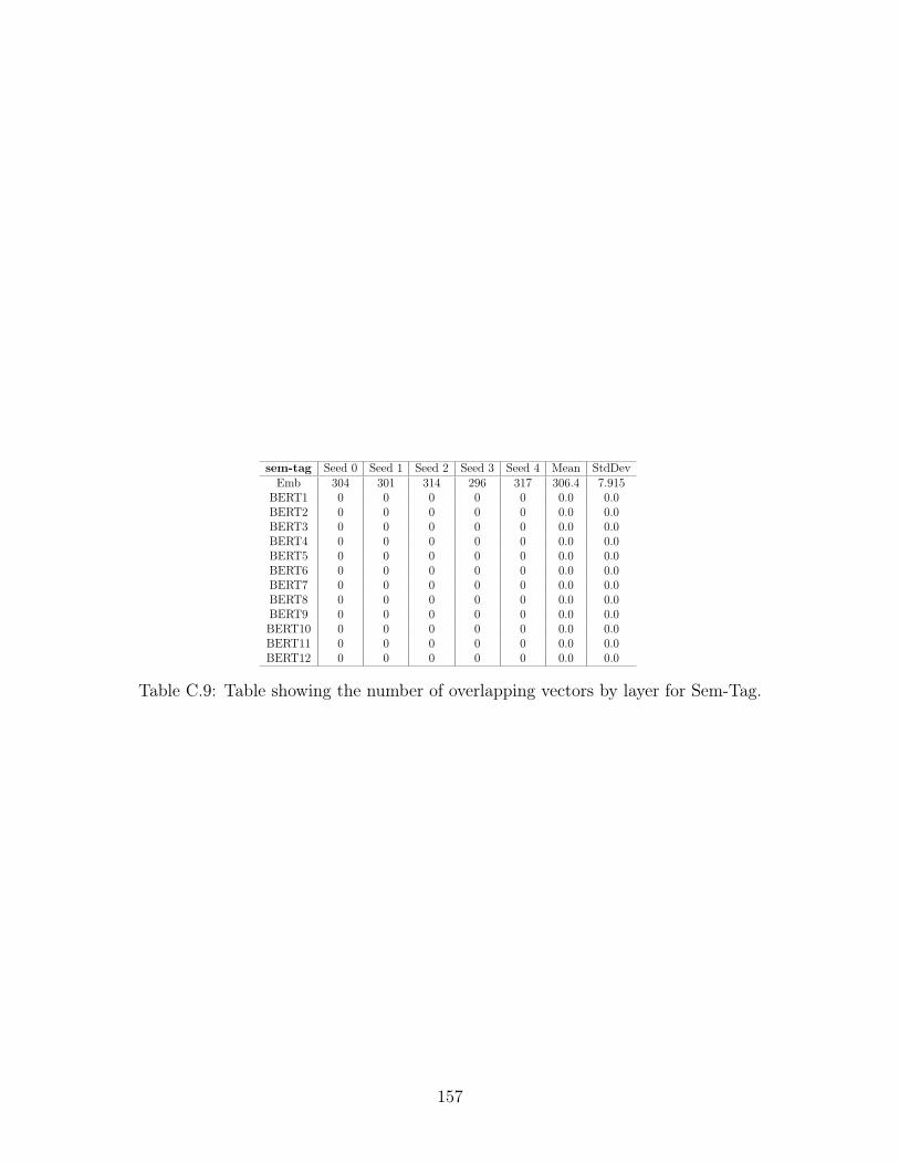
sem-tag Seed 0 Seed 1 Seed 2 Seed 3 Seed 4 Mean StdDevEmb 304 301 314 296 317 306.4 7.915

BERT1 0 0 0 0 0 0.0 0.0BERT2 0 0 0 0 0 0.0 0.0BERT3 0 0 0 0 0 0.0 0.0BERT4 0 0 0 0 0 0.0 0.0BERT5 0 0 0 0 0 0.0 0.0BERT6 0 0 0 0 0 0.0 0.0BERT7 0 0 0 0 0 0.0 0.0BERT8 0 0 0 0 0 0.0 0.0BERT9 0 0 0 0 0 0.0 0.0BERT10 0 0 0 0 0 0.0 0.0BERT11 0 0 0 0 0 0.0 0.0BERT12 0 0 0 0 0 0.0 0.0

Table C.9: Table showing the number of overlapping vectors by layer for Sem-Tag.

157

158

159

160

Bibliography

[1] Richard Futrell, Ethan Wilcox, Takashi Morita, Peng Qian, Miguel Ballesteros,and Roger Levy. Neural language models as psycholinguistic subjects: Repre-sentations of syntactic state. CoRR, abs/1903.03260, 2019.

[2] Fei Gao, Teresa Wu, Jing Li, Bin Zheng, Lingxiang Ruan, Desheng Shang, andBhavika Patel. SD-CNN: A shallow-deep CNN for improved breast cancer diag-nosis. Computerized Medical Imaging and Graphics, 70:53–62, December 2018.

[3] Alec Radford, Jeffrey Wu, Rewon Child, David Luan, Dario Amodei, and IlyaSutskever. Language Models are Unsupervised Multitask Learners. page 24.

[4] Tero Karras, Samuli Laine, and Timo Aila. A Style-Based Generator Architec-ture for Generative Adversarial Networks. arXiv:1812.04948 [cs, stat], December2018. arXiv: 1812.04948.

[5] Alfredo Vellido. Societal Issues Concerning the Application of Artificial Intelli-gence in Medicine. Kidney Diseases, 5(1):11–17, 2019.

[6] Ramprasaath R. Selvaraju, Michael Cogswell, Abhishek Das, RamakrishnaVedantam, Devi Parikh, and Dhruv Batra. Grad-CAM: Visual Explanationsfrom Deep Networks via Gradient-based Localization. arXiv:1610.02391 [cs],October 2016. arXiv: 1610.02391.

[7] Mario Giulianelli, Jack Harding, Florian Mohnert, Dieuwke Hupkes, and WillemZuidema. Under the Hood: Using Diagnostic Classifiers to Investigate and Im-prove how Language Models Track Agreement Information. arXiv:1808.08079[cs], August 2018. arXiv: 1808.08079.

[8] Matthew J. Nelson, Imen El Karoui, Kristof Giber, Xiaofang Yang, LaurentCohen, Hilda Koopman, Sydney S. Cash, Lionel Naccache, John T. Hale,Christophe Pallier, and Stanislas Dehaene. Neurophysiological dynamics ofphrase-structure building during sentence processing. Proceedings of the Na-tional Academy of Sciences, page 201701590, April 2017.

[9] John Hewitt and Christopher D Manning. A Structural Probe for Finding Syntaxin Word Representations. page 10.

[10] Marc-Etienne Brunet, Colleen Alkalay-Houlihan, Ashton Anderson, andRichard S. Zemel. Understanding the origins of bias in word embeddings. CoRR,abs/1810.03611, 2018.

161

[11] Svante Wold, Kim Esbensen, and Paul Geladi. Principal component analysis.Chemometrics and intelligent laboratory systems, 2(1-3):37–52, 1987.

[12] F. Pedregosa, G. Varoquaux, A. Gramfort, V. Michel, B. Thirion, O. Grisel,M. Blondel, P. Prettenhofer, R. Weiss, V. Dubourg, J. Vanderplas, A. Passos,D. Cournapeau, M. Brucher, M. Perrot, and E. Duchesnay. Scikit-learn: Machinelearning in Python. Journal of Machine Learning Research, 12:2825–2830, 2011.

[13] Leland McInnes, John Healy, and James Melville. UMAP: Uniform ManifoldApproximation and Projection for Dimension Reduction. arXiv e-prints, pagearXiv:1802.03426, Feb 2018.

[14] Nelson F. Liu, Matt Gardner, Yonatan Belinkov, Matthew E. Peters, andNoah A. Smith. Linguistic knowledge and transferability of contextual repre-sentations. CoRR, abs/1903.08855, 2019.

[15] Diederik Kingma and Jimmy Ba. Adam: A method for stochastic optimization.International Conference on Learning Representations, 12 2014.

[16] Adam Paszke, Sam Gross, Francisco Massa, Adam Lerer, James Bradbury, Gre-gory Chanan, Trevor Killeen, Zeming Lin, Natalia Gimelshein, Luca Antiga,Alban Desmaison, Andreas Kopf, Edward Yang, Zachary DeVito, Martin Rai-son, Alykhan Tejani, Sasank Chilamkurthy, Benoit Steiner, Lu Fang, Junjie Bai,and Soumith Chintala. Pytorch: An imperative style, high-performance deeplearning library. In H. Wallach, H. Larochelle, A. Beygelzimer, F. dAlché-Buc,E. Fox, and R. Garnett, editors, Advances in Neural Information ProcessingSystems 32, pages 8024–8035. Curran Associates, Inc., 2019.

[17] SueYeon Chung, Uri Cohen, Haim Sompolinsky, and Daniel D Lee. Learning datamanifolds with a cutting plane method. Neural computation, 30(10):2593–2615,2018.

[18] SueYeon Chung, Daniel D. Lee, and Haim Sompolinsky. Linear readout of objectmanifolds. Phys. Rev. E, 93:060301, Jun 2016.

[19] SueYeon Chung, Daniel D. Lee, and Haim Sompolinsky. Classification and ge-ometry of general perceptual manifolds. Phys. Rev. X, 8:031003, Jul 2018.

[20] Uri Cohen, SueYeon Chung, Daniel D. Lee, and Haim Sompolinsky. Separabilityand geometry of object manifolds in deep neural networks. bioRxiv, 2019.

[21] Kyunghyun Cho, Bart Van Merrienboer, Caglar Gulcehre, Dzmitry Bahdanau,Fethi Bougares, Holger Schwenk, and Yoshua Bengio. Learning phrase represen-tations using rnn encoder–decoder for statistical machine translation. Proceedingsof the 2014 Conference on Empirical Methods in Natural Language Processing(EMNLP), 2014.

[22] Sepp Hochreiter and Jürgen Schmidhuber. Long short-term memory. Neuralcomputation, 9(8):1735–1780, 1997.

162

[23] Ashish Vaswani, Noam Shazeer, Niki Parmar, Jakob Uszkoreit, Llion Jones,Aidan N Gomez, Łukasz Kaiser, and Illia Polosukhin. Attention is all you need.In Advances in neural information processing systems, pages 5998–6008, 2017.

[24] Jay Alammar. The illustrated transformer.

[25] Kristina Gulordava, Piotr Bojanowski, Edouard Grave, Tal Linzen, and MarcoBaroni. Colorless green recurrent networks dream hierarchically. In Proceed-ings of the 2018 Conference of the North American Chapter of the Associationfor Computational Linguistics: Human Language Technologies, Volume 1 (LongPapers), pages 1195–1205, New Orleans, Louisiana, June 2018. Association forComputational Linguistics.

[26] Kenton Lee Jacob Devlin, Ming-Wei Chang and Kristina Toutanova. Bert:Pre-training of deep bidirectional transformers for language understanding.abs/1810.04805, 2018.

[27] Thomas Wolf, Lysandre Debut, Victor Sanh, Julien Chaumond, Clement De-langue, Anthony Moi, Pierric Cistac, Tim Rault, R’emi Louf, Morgan Funtowicz,and Jamie Brew. Huggingface’s transformers: State-of-the-art natural languageprocessing. ArXiv, abs/1910.03771, 2019.

[28] Balázs Csanád Csáji. Approximation with artificial neural networks. 2001.

[29] Owen Marschall, Kyunghyun Cho, and Cristina Savin. A unified frameworkof online learning algorithms for training recurrent neural networks. CoRR,abs/1907.02649, 2019.

[30] Klaus Greff, Rupesh K Srivastava, Jan Koutník, Bas R Steunebrink, and JürgenSchmidhuber. Lstm: A search space odyssey. IEEE transactions on neuralnetworks and learning systems, 28(10):2222–2232, 2016.

[31] Jascha Sohl-Dickstein BJasmine Collins and David Sussillo. Capacity and train-ability in recurrent neural networks. 2016.

[32] Matthew D. Zeiler and Rob Fergus. Visualizing and understanding convolutionalnetworks. 2014.

[33] Dipanjan Das Ian Tenney and Ellie Pavlick. Bert rediscovers the classical nlppipeline. abs/1905.05950, 2019.

[34] David Sussillo and Omri Barak. Opening the black box: Low-dimensional dy-namics in high-dimensional recurrent neural networks. Neural Computation,25(3):626–649, 2013. PMID: 23272922.

[35] Sara Veldhoen, Dieuwke Hupkes, and Willem Zuidema. Diagnostic classifiers:Revealing how neural networks process hierarchical structure. In Pre-Proceedingsof the Workshop on Cognitive Computation: Integrating Neural and SymbolicApproaches (CoCo @ NIPS 2016), 2016.

163

[36] J. Kiefer and J. Wolfowitz. Stochastic estimation of the maximum of a regressionfunction. Collected Papers, page 60–64, 1985.

[37] Dieuwke Hupkes, Sara Veldhoen, and Willem Zuidema. Visualisation and ’di-agnostic classifiers’ reveal how recurrent and recursive neural networks processhierarchical structure. 2017.

[38] Tal Linzen, Emmanuel Dupoux, and Yoav Goldberg. Assessing the ability oflstms to learn syntax-sensitive dependencies, 2016.

[39] Ethan Wilcox, Roger P. Levy, Takashi Morita, and Richard Futrell. What dornn language models learn about filler–gap dependencies? In Proceedings of theWorkshop on Analyzing and Interpreting Neural Networks for NLP, 2018.

[40] Mario Giulianelli, Jack Harding, Florian Mohnert, Dieuwke Hupkes, and WillemZuidema. Under the hood: Using diagnostic classifiers to investigate and improvehow language models track agreement information, 2018.

[41] Yair Lakretz, German Kruszewski, Theo Desbordes, Dieuwke Hupkes, StanislasDehaene, and Marco Baroni. The emergence of number and syntax units in lstmlanguage models, 2019.

[42] Roger Levy. Expectation-based syntactic comprehension. Cognition, 106:1126–77, 04 2008.

[43] Edward Loper and Steven Bird. Nltk: The natural language toolkit. In In Pro-ceedings of the ACL Workshop on Effective Tools and Methodologies for TeachingNatural Language Processing and Computational Linguistics. Philadelphia: As-sociation for Computational Linguistics, 2002.

[44] Mitchell Marcus, Grace Kim, Mary Ann Marcinkiewicz, Robert MacIntyre, AnnBies, Mark Ferguson, Karen Katz, and Britta Schasberger. The penn treebank:Annotating predicate argument structure. In Proceedings of the Workshop onHuman Language Technology, HLT ’94, pages 114–119, Stroudsburg, PA, USA,1994. Association for Computational Linguistics.

[45] Julia Hockenmaier and Mark Steedman. CCGbank: A corpus of CCG derivationsand dependency structures extracted from the Penn treebank. ComputationalLinguistics, 33(3):355–396, 2007.

[46] Johannes Bjerva, Barbara Plank, and Johan Bos. Semantic tagging with deepresidual networks. In Proceedings of COLING 2016, the 26th International Con-ference on Computational Linguistics: Technical Papers, pages 3531–3541, Os-aka, Japan, December 2016. The COLING 2016 Organizing Committee.

[47] Lasha Abzianidze, Johannes Bjerva, Kilian Evang, Hessel Haagsma, Rik van No-ord, Pierre Ludmann, Duc-Duy Nguyen, and Johan Bos. The parallel meaningbank: Towards a multilingual corpus of translations annotated with composi-tional meaning representations. In Proceedings of the 15th Conference of the

164

European Chapter of the Association for Computational Linguistics: Volume 2,Short Papers, pages 242–247, Valencia, Spain, April 2017. Association for Com-putational Linguistics.

[48] Andy Coenen, Emily Reif, Ann Yuan, Been Kim, Adam Pearce, Fernanda Viégas,and Martin Wattenberg. Visualizing and Measuring the Geometry of BERT.arXiv e-prints, page arXiv:1906.02715, Jun 2019.

[49] Elena Voita, Rico Sennrich, and Ivan Titov. The Bottom-up Evolution of Repre-sentations in the Transformer: A Study with Machine Translation and LanguageModeling Objectives. arXiv e-prints, page arXiv:1909.01380, Sep 2019.

[50] Jenny R. Saffran, Ann Senghas, and John C. Trueswell. The acquisitionof language by children. Proceedings of the National Academy of Sciences,98(23):12874–12875, 2001.

[51] Christopher M. Conway, David B. Pisoni, Esperanza M. Anaya, JenniferKarpicke, and Shirley C. Henning. Implicit sequence learning in deaf childrenwith cochlear implants. Developmental Science, 14(1):69–82, 2011.

[52] Maithra Raghu, Justin Gilmer, Jason Yosinski, and Jascha Sohl-Dickstein. Svcca:Singular vector canonical correlation analysis for deep learning dynamics and in-terpretability. In I. Guyon, U. V. Luxburg, S. Bengio, H. Wallach, R. Fergus,S. Vishwanathan, and R. Garnett, editors, Advances in Neural Information Pro-cessing Systems 30, pages 6076–6085. Curran Associates, Inc., 2017.

[53] Ari Morcos, Maithra Raghu, and Samy Bengio. Insights on representational sim-ilarity in neural networks with canonical correlation. In S. Bengio, H. Wallach,H. Larochelle, K. Grauman, N. Cesa-Bianchi, and R. Garnett, editors, Advancesin Neural Information Processing Systems 31, pages 5732–5741. Curran Asso-ciates, Inc., 2018.

[54] Yang Song, Peter J. Schreier, David Ramírez, and Tanuj Hasija. Canonicalcorrelation analysis of high-dimensional data with very small sample support.CoRR, abs/1604.02047, 2016.

[55] William R. Zwick and Wayne F. Velicer. Comparison of five rules for determiningthe number of components to retain. Psychological Bulletin, 99(3):432–442, 1986.

[56] Heungsun Hwang, Kwanghee Jung, Yoshio Takane, and Todd Woodward. A uni-fied approach to multiple-set canonical correlation analysis and principal com-ponents analysis. The British journal of mathematical and statistical psychology,66:308–321, 05 2013.

[57] Nai Ding, Lucia Melloni, Hang Zhang, Xing Tian, and David Poeppel. Cor-tical tracking of hierarchical linguistic structures in connected speech. Natureneuroscience, 19, 12 2015.

165

166

167