JOURNAL OF GEOPHYSICAL RESEARCH, VOL. 99, NO. A4, PAGES 6321-6329, APRIL 1, 1994

Middle and upper atmosphere radar observations of ionospheric density gradients produced by gravity wave packets

W. L. Oliver, 2 S. Fukao, l Y. Yamamoto, • T. Takami, 2 M.D. Yamanaka,• M. Yamamoto,• T. Nakamura,• and T. Tsuda•

Abstract. By observing the ionospheric F region simultaneously in multiple beams with the middle and upper atmosphere (MU) radar, we have been able to track the passage of gravity waves and measure the horizontal electron density gradients that they produce. Our previous work on this topic, on one day of observations, verified that the gradient structure and fluctuations were consistent with a gravity wave source. The present work (1) looks at several days of observation to confirm the routine existence of these gradient structures; (2) identifies individual wave packets; (3) finds evidence that long trains of gravity wave fluctuations are composed of several juxtaposed wave packets of one or two cycles each rather than a single wave of many cycles; (4) finds that during quiet periods strong waves are present only during the daytime, but during disturbed periods they are present day and night; and (5) notes several other characterizations.

1. Introduction

The Japanese middle and upper atmosphere (MU) radar [Fukao et al., 1985a, b] is the newest of the large atmo- spheric radars capable of detecting the incoherent scatter (IS) from the free electrons of the ionosphere [Sato et al., 1989]. IS observations began in December 1985. A number of papers quantifying the behavior of the ionosphere and thermosphere over the MU radar have been published since 1988. Of particular interest as predecessors of the present paper are those that have dealt with the passage of waves over the radar. Because the MU radar is an active phased- array system and hence can observe in different pointing direction essentially simultaneously, the MU radar has proved to be effective in distinguishing unambiguously be- tween local temporal variations and spatial variations flow- ing over the radar; that is, it routinely detects horizontal wave motion. This capability has been used by Oliver et al. [ 1988] to characterize the gravity wave launched by the large magnetic storm of February 6-8, 1986, later simulated by Oliver and Hagan [1991], by Takami et al. [1991, also F layer tilts and the traveling plateau observed with the middle and upper atmosphere radar, submitted to Journal of Geo- physical Research, 1994] to characterize the average behav- ior of waves above the radar and the ionospheric structures that they produce, and by Fukao et al. [ 1993] to characterize the ionospheric gradients caused by these waves. This latter paper may be considered as the forerunner of the current

1Radio Atmospheric Science Center, Kyoto University, Kyoto, Jal•an.

•Center for Space Physics and Department of Electrical, Com- puter and Systems Engineering, Boston University, Boston, Mas- sachusetts.

Copyright 1994 by the American Geophysical Union.

Paper number 94JA00171. 0148-0227/94/94JA-00171 $05.00

paper as it showed from one day's observation that the ionospheric gradients measured with the MU radar are consistent in every way with production by a gravity wave source. W. L. Oliver et al. (MU radar observations of the dispersion relation for ionospheric gravity waves, submitted to Journal of Atmospheric and Terrestrial Physics, 1994) looks at the gravity wave dispersion relation derived from MU radar measurements.

The current paper looks more closely at the propagation of the gravity waves and gravity wave packets and the horizon- tal density gradient structures that they produce, using more days of observation and extended analysis methods.

2. Gravity Wave Experiments Because the MU radar can observe in multiple directions

just as easily as it can observe in one, MU radar IS experiments are routinely carried out in the four cardinal magnetic azimuths (355 ø, 85 ø, 175 ø, 265 ø, where 5.7øW is true magnetic north), all at 20 ø from zenith. For the F region wave and horizontal gradient studies addressed in this paper, we normally run a high-time-resolution backscattered-power experiment using the longest pulse possible with the MU radar, 512/xs. This maximizes signal strength for our search for the often small density fluctuations caused by the waves. It also gives a poor height resolution of 72 km, but in practice this has not hindered our analysis owing to the large vertical wavelengths of the wave structures. The backscattered signal power is sampled every 4.8 km in range, but neigh- boring samples are not independent. Data are written to tape every 20 s but were integrated to 2-min averages for the present study as no organized wave motion with periods less than the natural oscillating frequency of the atmosphere (about 15 min at these altitudes) is expected. While it is desirable to measure the drift velocity and temperature signatures of the waves also, these "spectral" measure- ments are much less accurate with the MU radar, and we

6321

6322 OLIVER ET AL.' IONOSPHERIC GRADIENTS PRODUCED BY WAVES

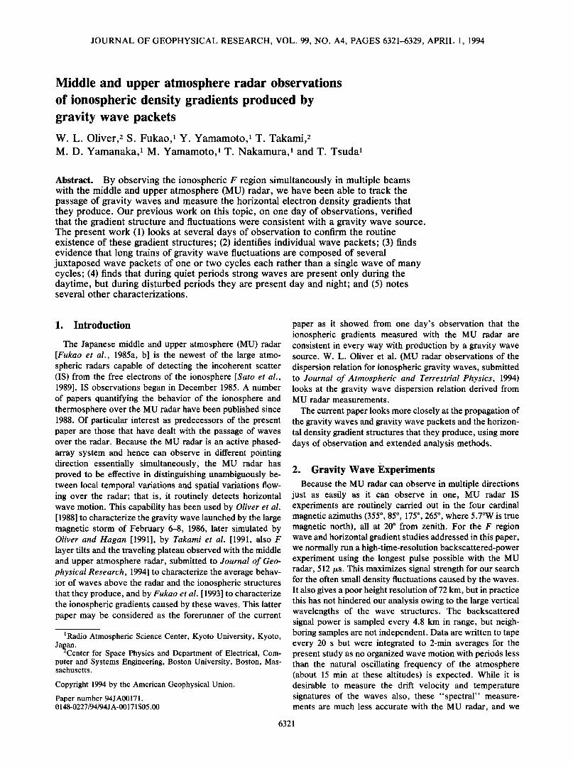
Cross Correlation

15-NOV-1990 08:01 - 15-NOV-1990 09:00

Altitude ß 228(km)

1.0-

0.0

-0.5

-60 -40 -20 0 20 40 60

Time Lag (min.)

North-South

East-West

Figure 1. Cross correlations between the north and south (solid line) and the east and west (dashed line) electron density time series for a selected set of data. The values r x and ry are the correlation time delays between the east and west beams and between the north and south beams.

have opted to settle for the high accuracy and good time resolution of the density measurements only.

3. Density Gradient and Wave Propagation Vectors

We will work with two wave-related horizontal vectors

and their meridional and zonal components or their magni- tudes and phases in this paper. The first is a density gradient vector, whose components are the meridional and zonal gradients in electron density. The second is a wave propa- gation vector, whose magnitude and phase are the speed and azimuthal direction of the wave phase progression. Let us first define these vectors then note what information each

gives.

3.1. Density Gradient Vector

The experiment measures the backscattered power S versus altitude z in the magnetic east (e), west (w), north (n), and south (s) directions. Let d(z) be the horizontal distance between the east and west beams and between the

north and south beams at altitude z, and let x and y represent the zonal and meridional directions. We compute the hori- zontal density gradients in the east-west and north-south directions as

dS S e( Z) -- S w(Z) Gx(z) = = (1)

t(z)

dS Sn( z) -- S s( Z) Gy(Z) = = (2)

dy d(z)

These values may be considered to be the x and y compo- nents of a density gradient vector. We should note here that the electron density is proportional to the product of the power and the factor 1 + Te/Ti, where T e and T i are the electron and ion temperatures. We will not distinguish here between power and electron density perturbations. At night the pertinent temperature ratio is unity, and there is no need to so distinguish. During the day, however, both T e and T i will have wave-induced perturbations dependent primarily upon the perturbations in the neutral concentrations (for Ti) and the electron concentration (for Te). However, each of the different neutral constituents and the neutral temperature have perturbations with different and situation-dependent relationships with the wave phase, and so the relationship between the T e and T i perturbations is not at all clear. We do not intend to digress further on this point here, but we do wish the reader to keep in mind that our so-called "electron density" gradients may also have a substantial component of "temperature" gradients affecting them too.

Table 1. Dates, Times, and Magnetic Conditions for the Experiments

Kp Three-Hourly Time Interval, UT

Day 1 2 3 4 5 6 7 8 Ap

March 14-17, 1989 14 9 8- [8- 6- 5 5+ 8- 7+ 158 15 7- 6 5- 5 4+ 5- 4 3 49 16 2 5 5+ 7- 5+ 5 5 4- 50 17 4+ 5+ 5+] 4+ 4+ 4+ 4- 3- 34

April 18-21, 1990 18 5 [5+ 3 3- 3+ 2+ 3- 4- 24 19 3- 1+ 1+ 1+ 2- 2+ 3 3 9 20 3+ 2+ 2+ 2 3- 3+ 5 4- 18 21 5-] 4+ 3- 2- 1+ 1 1- 1+ 13

November 11-16, 1990 11 3+ 3- 3- 3 [3+ 2- 2- 2- 12 12 1+ 3- 1- 1 1- 2- 1+ 1- 5 13 1+ 1 1+ 1- 0+ 1- 0+ 0+ 3 14 1 0 0+ 1- 0+ 0 0 0 1 15 1- 1- 0+ 0+ 1- 1 2- 1- 3 16 2+] 3 4- 3+ 4 3+ 3- 3+ 17

Brackets denote the radar operating period. Kp was not smaller than 4 during the 24 hours before the April radar experiment.

OLIVER ET AL.' IONOSPHERIC GRADIENTS PRODUCED BY WAVES 6323

Meridional Component Period (min.)

1000 100 10 Ii,11, , , , I,,,,. , , , I,,,,,

1CT 2• 10 • 1't• 10 '3 10 '=

Frequency (Hz)

Zonal Component Period (min.)

lOOO lOO lO Jllll i I I I I,,,, , , , i Ill,,,

10- • 10 • 10 4 10 '3 10- =

Frequency (Hz)

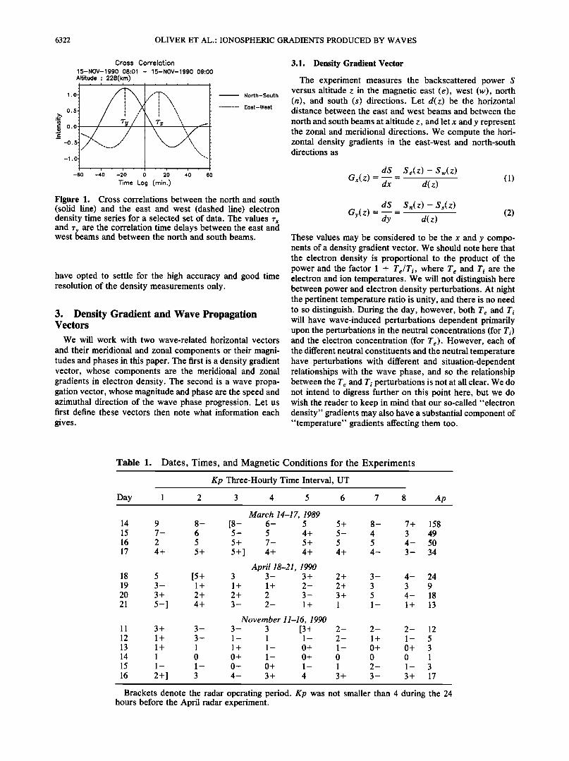
Figure 2. Power spectrum of the time series of the hori- zontal gradient of the electron density averaged over 246.7- 300.8 km altitude for the period 0801-1558 LT on November 15, 1990.

3.2. Wave Propagation Vector

When a wave perturbs the electron density, we can determine its horizontal propagation direction and speed by observing the times lags between the responses seen in the four radar beams. For a wave propagating at altitude z with speed v and direction 0 measured clockwise from north, the time lag r x between the east and west beams and the time lag ry between the north and south beams are

d sin 0 d cos 0

r x = • ry = (3)

where d is the distance between diagonal beams at altitude z. These equations may be inverted easily to give v and 0 in terms of rx, ry, and d

v = 2 2 0 = arctan -- (4) T x q- Ty Ty

v and 0 are the magnitude and phase of a wave propagation vector. Figure 1 shows the cross correlations of the density time series for the north and south beams and for the east

and west beams for a certain 1-hour sequence of data and identifies rx and ry. The cross-correlation value here is normalized to the autocorrelation to maintain a maximum

correlation magnitude of about unity. Both the density gradient and wave propagation vectors

are computed from the same data, the former from differ-

ences between the four beams at the same time, the latter by correlating time series in different beams. The former exists in both static and dynamic cases, the latter only when a wave propagates. Each can be determined at each altitude of measurement. The former pertains to the effect of the wave upon the ionosphere, the latter to the wave itself. At the F region altitudes of interest in this study viscosity is expected to render gravity wave propagation largely height indepen- dent, so we expect little variation with altitude for our wave vectors. A few apparent exceptions will be noted.

4. Density Gradient Results We present results for three long experiments whose

dates, times, and magnetic conditions are summarized in Table 1. We have here a very disturbed period, a moderately disturbed period, and a very quiet period. For any of these periods we wish to do a spectral analysis of the time series of observations to determine the periods at which density perturbations occur. As explained by Fukao et al. [1993], if we apply the spectral analysis directly to the density (power) data, we do indeed capture the periods of propagating waves, but we also capture the periods of temporal varia- tions occurring in all beams simultaneously (due, for exam- ple, to global scale wind or electric field changes), which are not due to waves. We therefore apply the spectral analysis to the horizontal density gradient to assure that we capture information on only the propagating perturbations (this is analogous to the moving target indicator (MTI) technique in which the difference between two radar measurements is

used to detect target motion). An example of this spectral analysis is shown in Figure 2. Here all of the data for November 15, 1990, have been Fourier-analyzed. The short- period limit of the spectrum is set by the 2-min data integration, while the long end is set by the 24-hour window of data used. We see that the meridional component has a distinct peak in its spectrum, while the zonal component does not. This means that the strongest waves are traveling meridionally, and this is the more usual result that we encounter. Every distinct maximum that we have seen in these spectra (10 days of observation) has occurred within the range 60-120 min, though clearly a broad spectrum of waves is present.

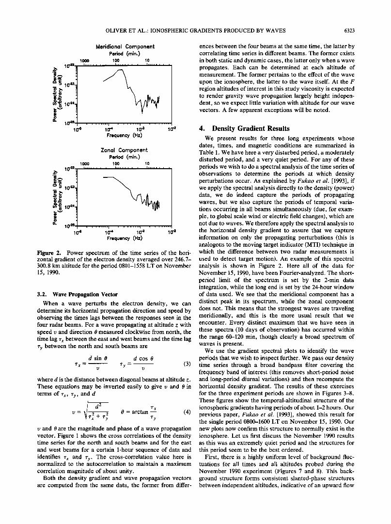
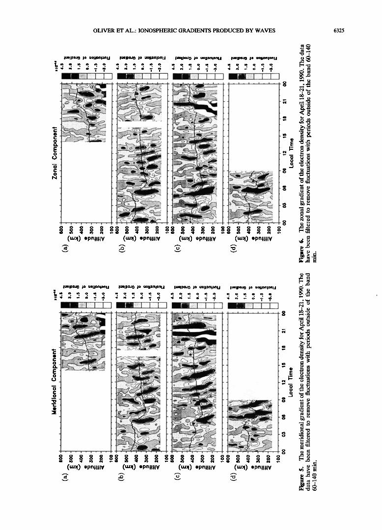
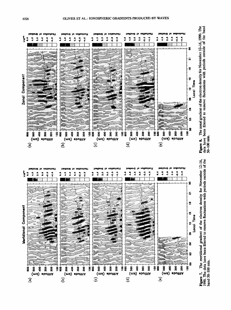
We use the gradient spectral plots to identify the wave periods that we wish to inspect further. We pass our density time series through a broad bandpass filter covering the frequency band of interest (this removes short-period noise and long-period diurnal variations) and then recompute the horizontal density gradient. The results of these exercises for the three experiment periods are shown in Figures 3-8. These figures show the temporal-altitudinal structure of the ionospheric gradients having periods of about 1-2 hours. Our previous paper, Fukao et al. [1993], showed this result for the single period 0800-1600 LT on November 15, 1990. Our new plots now confirm this structure to normally exist in the ionosphere. Let us first discuss the November 1990 results as this was an extremely quiet period and the structures for this period seem to be the best ordered.

First, there is a highly uniform level of background fluc- tuations for all times and all altitudes probed during the November 1990 experiment (Figures 7 and 8). This back- ground structure forms consistent slanted-phase structures between independent altitudes, indicative of an upward flow

6324 OLIVER ET AL.: IONOSPHERIC GRADIENTS PRODUCED BY WAVES

o N

L-X.-; ..........

• ½ , --

.::::..:. ............... ...½ :...:..-....',,,•,• • • •.:..--.. •: :•

...... ' ":""'•;::E'-iiii?c:•.":: ........;;;;i: i l- •'-•i:.-'." ::::::::::::::::::::::::::::::::::::::::::: '•ii',:'.:::..'iE-'..ii::i•.i::.;..;-:: ' •11]i.•....,.;...;...; :;:;:' ...::.;:•½i!..':.-'i•!•i;?•:•'•: •:•' :.?????;:;i!?i:;.':'i'

-' -'.'-'---'.' ..:.-'.:•i•!i•.;:'.-::.:::::::::i .... .:::::•ii•½•ii?,;iiii!i:•L :'.!::...:' ....

,

- i ß ! ß i ß !

0 0 0 0 0 O0 0 0 0 0 0 0 0 0 0 0 0 0 0 0 0 0

(mH) epnl!llV (mH) epnl!llV (mH) epnl!llV (mH) epnl!llV

c..) o

o

o

• E E -'o o

r'

o

E o

0 0 0 0 0 O0 0 0 0 0 0 0 0 0 0 0 O0 0 0 0 0 0 0 0 0 0 O0 0 0 0 0 0 0 0 0 0 0 O0 0 0 0 0

(tU>l) epnl!llV (tU>l) epnuIIV (tU>l) epnuIIV (tU>l) epnl!llV

OLIVER ET AL.: IONOSPHERIC GRADIENTS PRODUCED BY WAVES 6325

o

o

o

o N

o u c•

ß • ß • ' • ß • ß 0 0 0 0 0 0 0 O0 0 0 0 0 O0 0 0 0 0 0 0 0 0 0 0 0 •::• -• o o o o o oo o o o o oo o o o o oo o o o o o •

(m•l) epnl!11¾ (m•l) epnl!11¾ (m•l) epnl!11¾ (m•l) epnl!11¾ • 8

ß i ß i ß i ß i

0 0 0 0 0 O0 0 0 0 0 O0 0 0 0 0 O0 0 0 0 0 0 0 0 0 0 O0 0 0 0 0 O0 0 0 0 0 O0 0 0 0 0 0

op.mv op.m:v op..v

6326 OLIVER ET AL.: IONOSPHERIC GRADIENTS PRODUCED BY WAVES

.,.C3 tuelp•J9 jo UOltDnlonli tuelP•J9 Jo UOllDnlonli lUelpzu9 jo UOllDnlonli tuelpzu0 jo UOllDnlonli lUelpi•J9 jo UOllDnlonli

0 0 0 0 0 0 0 0 0 0 0 0 0 0 0 0 0 0 0 0 0 0 0 0 0 0 0 0 0 0 (• •

OLIVER ET AL.: IONOSPHERIC GRADIENTS PRODUCED BY WAVES 6327

of gravity-wave energy. Further, the phase fronts tend to become vertical at higher altitudes (the expected product of high viscosity), again a feature expectable for gravity waves. During this quiet November 1990 period the stronger density gradients appeared only during the daytime, but even then there were periods when the stronger perturbations ceased or appeared to cease. We will show later in this paper that these waves existed for only one or two cycles, even for the apparently long and uniform wave train of November 15.

The moderately disturbed April 1990 period (Figures 5 and 6) shows wave structures day and night, but they appear more sporadically on the plots. There is some noticeable pattern of perturbation structures occurring in pairs. The background structure is not as well ordered here as for the quiet November 1990 case.

The highly disturbed March 1989 case (Figures 3 and 4) much more closely resembles the moderately disturbed case than the quiet case. The background structure is better organized than the moderately disturbed case. There is not a good correlation between the magnetic activity and the strength of the density gradients seen, or at least the global index Kp may not be a good indicator of local conditions.

5. Wave Propagation Results We have used the time series in the four radar beams,

band filtered as explained in the previous section, to deter- mine the wave propagation vector via (4). These results are shown in Figures 9-11. The arrows on these plots represent

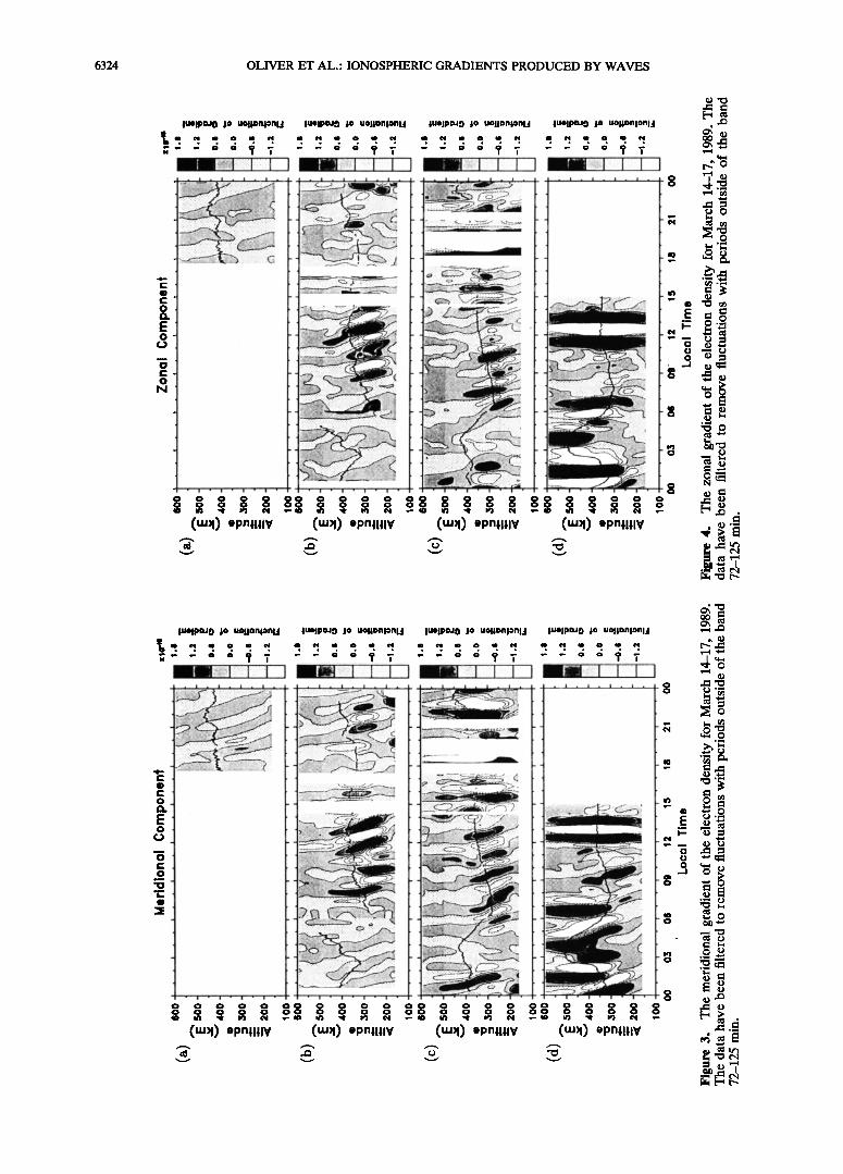
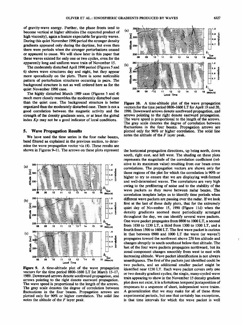
Figure 9. A time-altitude plot of the wave propagation vectors for the time period 0800-1600 LT for March 15-17, 1989. Downward arrows denote southward propagation, and arrows pointing to the right denote eastward propagation. The wave speed is proportional to the length of the arrows. The gray scale denotes the degree of correlation between fluctuations in the four beams. Propagation arrows are plotted only for 90% or higher correlation. The solid line notes the altitude of the F layer peak.

08 09

6 •/• ß ß • ß , i , , • , , ] , , , . ./A •/'/•; ..: •;.:•::|•:F,(:• .::::'::-":v'•:'•: ' ß •'•x:•\•¾ ':•;'::' ' :•I •. o •:/Z :'" ::" •?•½•:•:-•::?• ,.•:•:•'":•.'.:':•.• ': .... •:• ........ •:•,• •'":'; •:"

.... . . . ?.• ............ .•.•.-.:.•E ...... • .X :-•-:•-•-..• ...... •.:•.• ........................ '•½'•:'Z": ' [x'-xX' • •':' ' :* • 0 • • ""'•::';":•;:•:•-•' •;'•:•::•:'.• :::'' 'k•½'•'z •:'.-':,•_•" .'•:';*d""-:"* .-- "•;?:-.•½•;•:,:.• ..... ½../.z;.• ,,::•::. ;•,x.N.:.&,:.:x•..,:•....: •:.. o 7 .... •:;•..,½Z•::.:.:-;• • .... /..½.•:•.: .•:--:;X•x•:-•,,•x'• ..... :..•:... r•/•: •:: -•f•...';;•;½ • ;•.•.• ..... ':Z•:;•:•:i•:l "x.•'•-•:- .... •'- ß :•;(:• •'•'.' ':',::•-"• :':":T': ' '. .... : ,-:t't. '; t t '.'.. ';" :": ':, • ..... ..:..:: .... :•..:;..:..._.. .... ... •.,.. ::.. .... ..:..;...., . .:...r• [ Z•

/10 11 12 13 14 15 16 250(m/8) Local •me

Figure 10. A time-altitude plot of the wave propagation vectors for the time period 0800-1600 LT for April 19 and 20, 1990. Downward arrows denote southward propagation, and arrows pointing to the right denote eastward propagation. The wave speed is proportional to the length of the arrows. The gray scale denotes the degree of correlation between fluctuations in the four beams. Propagation arrows are plotted only for 90% or higher correlation. The solid line notes the altitude of the F layer peak.

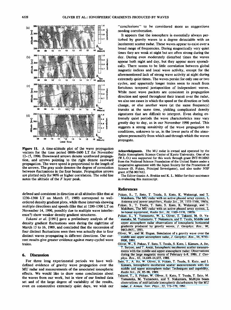
the horizontal propagation directions, up being north, down south, right east, and left west. The shading on these plots represents the magnitude of the correlation coefficient (rel- ative to its maximum value) resulting from our beam cross correlations. The propagation vectors are shown only for those regions of the plot for which the correlation is 90% or higher to try to ensure that we are displaying well-formed and well-determined waves. The correlations are very high owing to the prefiltering of noise and to the stability of the wave packets as they move between radar beams. The correlation template helps us to identify time periods when different wave packets are passing over the radar. If we look first at the last of these daily plots, that for the extremely quiet day of November 15, 1990 (Figure 11d) when the density gradients seemed most periodically arranged throughout the day, we can identify several wave packets. One wave packet propagates from 0800 to 1000 LT, a second from 1030 to 1230 LT, a third from 1300 to 1500 LT, and a fourth from 1500 to 1600 LT. The first wave packet is curious in that between 0900 and 1000 LT the wave (or waves?) propagates toward the northwest above 250 km altitude and changes abruptly to south-southeast below that altitude. The last of the four wave packets propagates northward, but its zonal component changes smoothly from west to east with increasing altitude. Wave packet identification is not always unambiguous. The first of the packets just identified could be two packets, and an additional smaller packet might be identified near 1230 LT. Each wave packet covers only one or two density gradient cycles; the single, many-cycled wave train appearing to show in the November 15 density gradient plot does not exist, it is a fortuitous temporal juxtaposition of responses to a sequence of short, independent wave trains. A generalization that we may make for all of these three experimental periods, but one that certainly has exceptions, is that time intervals for which the wave packet is well

6328 OLIVER ET AL.' IONOSPHERIC GRADIENTS PRODUCED BY WAVES

08 09 10 11 12 13 14 15 16

.:, --:-:•',•:,.'•.•:•:- -:•:• •' .--"-:!•-.;.•.:• .... i•.•:•:•!i ..... ':• iii!:::.• l.•, ....... '•: . • •.•:,::.•....• ......... '"• .'?, ............. ,• ............ o.e •.•::•:-..:::F•.::•-.•.•:•.•.--. •. - •..,. -. :::;.::• ;....•.• ....... .= '-

250 ............ .., .... ......... ........ ..... .::;.• .... .-•y::•?:- .::. • !•:•:.- •:.•-• .... •:.• •:•,.•:•:•:•:.),•::..-•:•i:.. .... •... 200• . ,

•(•/.)

350'•'._:...•.. ß L' ß ".• ..... •r...' •,.'.,:,,'.' ./ .... •.o •.•..-•.•::::-•:,.• • .... :-,-•-.• ;•..:..,•,•..•.•:.•?:•:"-: ;.:..::•.:: ......... •.• : .......... -•.::•.:. . •:• .... ..:..:•:•.;..:•--.•.•:• .:•:•. • • ..... :/•:. -• '• •-;•:•.:..- •::....:....:::, :j:•::.:• ;-'...-.•:' . ..•::::• E '•:•:.•:•:• ::•,. - •-•'...:..::;:•:•:•:-•;7• t •:" :?: :•:• ' •:::•:•::L:' .' O. 9 ._

_250 200 ..... z.'::•:'•:: • j L

• • .... • ' '•1 "•' • ß '/•1/' ' •1,/1•11.•i •'•

550• ' ' •.' .... .•'' • ß ß • , ß : ß ß ,•- •: 1,0

•3oo-•R":-:x ..... ',.':'"::•-•-'- :. •::-' •.•.-z.----'•: '- :..:-,. :.•:•:-• ............ -

• 200 •:•- •-•:":'• t'?-'-' t-'.'7•-'7:' _-::.: -:- ..• .................. r,,•l,,,,. ,... ,- ........ • • 10 11 12 13 14 15 16 •/.)

Locol •me

"conclusions" to be considered more as suggestions needing corroboration.

It appears that the ionosphere is essentially always per- turbed by gravity waves to a degree detectable with an incoherent scatter radar. These waves appear to exist over a broad range of frequencies. During magnetically very quiet times they are weak at night but are often strong during the day. During even moderately disturbed times the waves appear both night and day, but they appear more sporadi- cally. There seems to be little correlation between global magnetic indices and local wave activity, except for the aforementioned lack of strong wave activity at night during extremely quiet times. The waves persist for only one or two cycles, and apparently longer trains seem to result from fortuitous temporal juxtaposition of independent waves. While most wave packets are consistent in propagation direction and speed throughout their transit over the radar, we also see cases in which the speed or the direction or both change, or else another wave (at the same frequency) transits at the same time, yielding complicated density signatures that are difficult to interpret. Even during ex- tremely quiet periods the wave characteristics may vary greatly day to day, as in our November 1990 period. This suggests a strong sensitivity of the wave propagation to conditions, unknown to us, in the lower parts of the atmo- sphere presumably from which and through which the waves propagate.

Figure 1i. A time-altitude plot of the wave propagation vectors for the time period 0800-1600 LT for November 12-15, 1990. Downward arrows denote southward propaga- tion, and arrows pointing to the right denote eastward propagation. The wave speed is proportional to the length of the arrows. The gray scale denotes the degree of correlation between fluctuations in the four beams. Propagation arrows are plotted only for 90% or higher correlation. The solid line notes the altitude of the F layer peak.

Acknowledgments. The MU radar is owned and operated by the Radio Atmospheric Science Center of Kyoto University. One of us (W.L.O.) was supported for this work through grant INT-9116063 from the National Science Foundation of the United States under a

cooperative agreement with the Japan Society for the Promotion of Science (S. Fukao, Principal Investigator), and also under NSF grant ATM-9017612.

The Editor thanks A. Brekke and K. L. Miller for their assistance

in evaluating this manuscript.

defined and consistent in direction at all altitudes (like that at 1230-1300 LT on March 17, 1989) correspond to well- ordered density gradient plots, while those intervals showi ng multiple directions and speeds (like that at 1200-1300 LT on November 14, 1990, possibly due to multiple wave interfer- ence?) show weaker density gradient structures.

Takami et al. [1991] gave a preliminary analysis of the density gradient fluctuations seen during the nighttime of March 15 to 16, 1989, and concluded that the succession of four distinct fluctuations seen then was actually due to four distinct waves propagating in different directions. Our cur- rent results give greater evidence against many-cycled wave trains.

6. Discussion

For three long experimental periods we have well- defined evidence of gravity wave propagation over the MU radar and measurements of the associated ionospheric effects. We would like to draw some conclusions about

the waves from our work, but in view of our limited data set and of the large degree of variability of the results, even on consecutive extremely quiet days, we wish our

References

Fukao, S., T. Sato, T. Tsuda, S. Kato, K. Wakasugi, and T. Makihara, The MU radar with an active phased array system, 1, Antenna and power amplifiers, Radio Sci., 20, 1155-1168, 1985a.

Fukao, S., T. Tsuda, T. Sato, S. Kato, K. Wakasugi, and T. Makihara, The MU radar with an active phased array system, 2, In-house equipment, Radio Sci., 20, 1169-1176, 1985b.

Fukao, S., Y. Yamamoto, W. L. Oliver, T. Takami, M.D. Ya- manaka, M. Yamamoto, T. Nakamura, and T. Tsuda, Middle and upper atmosphere radar observations of ionospheric horizontal gradients produced by gravity waves, J. Geophys. Res., 98, 9443-9451, 1993.

Oliver, W., and M. Hagan, Simulation of a gravity wave over the middle and upper atmosphere radar, J. Geophys. Res., 96, 9793- 9800, 1991.

Oliver, W., S. Fukao, T. Sato, T. Tsuda, S. Kato, I. Kimura, A. Ito, T. Saryou, and T. Araki, Ionospheric incoherent scatter measure- ments with the middle and upper atmosphere radar: Observations during the large magnetic storm of February 6-8, 1986, J. Geo- phys. Res., 93, 14,649-14,655, 1988.

Sato, T., A. Ito, W. Oliver, S. Fukao, T. Tsuda, S. Kato, and I. Kimura, Ionospheric incoherent scatter measurements with the middle and upper atmosphere radar: Techniques and capability, Radio Sci., 24, 85-98, 1989.

Takami, T., S. Fukao, W. Oliver, S. Kato, T. Tsuda, T. Sato, M. Yamanaka, M. Yamamoto, and T. Nakamura, Multiple beam observations of mid-latitude ionospheric disturbances by the MU radar, J. Atmos. Terr. Phys., 53, 773-779, 1991.

OLIVER ET AL.: IONOSPHERIC GRADIENTS PRODUCED BY WAVES 6329

S. Fukao, T. Nakamura, T. Tsuda, M. Yamamoto, Y. Yamamoto, and M.D. Yamanaka, Radio Atmospheric Science Center, Kyoto University, Uji, Kyoto 611, Japan. (e-mail: Internet.fukao@ kurasc.kyoto-u.ac.jp; nakamura@kurasc.kyoto-u.ac.jp; tsuda@ kurasc. kyoto-u.ac.jp; yamamoto@kurasc. kyoto-u.ac.jp; yamamo@ kurasc.kyoto-u.ac.jp; yamanaka@kurasc.kyoto-u.ac.jp)

W. L. Oliver and T. Takami, Department of Electrical, Computer

and Systems Engineering, Boston University, 44 Cummington Street, Boston, MA 02215. (e-mail: Internet.wlo@buenga.bu.edu; takami@buenga.bu.edu)

(Received August 2, 1993; revised December 8, 1993; accepted January 14, 1994.)