Microwave response of anisotropic magnetorheological elastometers, model andexperiments

A. Butera∗ and N. AlvarezCentro Atomico Bariloche (CNEA) and Instituto Balseiro (U. N. Cuyo), 8400 Bariloche, Rıo Negro, Argentina.

G. JorgeDepartamento Fısica, Facultad de Ciencias Exactas y Naturales.Universidad de Buenos Aires, Argentina.

M. M. Ruiz, J. L. Mietta, R. M. NegriINQUIMAE, Facultad de Ciencias Exactas y Naturales,Universidad de Buenos Aires, Argentina.

(Dated: October 15, 2012)

We present ferromagnetic resonance measurements of Fe3O4 nanoparticles which have been dis-persed in an elastomeric polymer (PDMS) at two different concentrations (5% and 15% w/w),and then cured in the presence of a uniform magnetic field. With this procedure it is possibleto align the particles forming unidimensional needle-like cylindrical agglomerates with a relativelyhigh lenght/diameter ratio. The dynamical response of this nanostructured composite has beencharacterized using ferromagnetic resonance at K-band (24 GHz) and Q-band (34 GHz). In bothcases we have observed an anisotropic behavior in the resonance field when the external magneticfield is rotated from the direction of the needles to the perpendicular plane. However, the measuredvariation is considerable lower than the values expected for an array of perfectly homogeneous longcylinders in which the elongated shape causes a uniaxial anisotropy. Results have been analyzedusing the standard Smit and Beljers formalism, considering a phenomenological shape factor, P ,that accounts for the reduced anisotropy. Also an ellipticity factor in the cross section of the needles,r, and gaussian fluctuations of the shape factor, σP , are needed to explain the observed angularvariation of the linewidth. The values of these parameters are consistent with data obtained at K-and Q- bands, supporting the proposed model, although some differences have been found for thetwo studied concentrations.

PACS numbers:Keywords: ferromagnetic resonance, magnetite, nanoparticles, elastometers.

I. INTRODUCTION

Iron oxides, and particularly magnetite (Fe3O4), have been extensively studied since research in magnetic materi-als started. Magnetite crystallizes in a spinel structure and orders ferrimagnetically below 840 K with a saturationmagnetization Ms ∼ 480 emu/cm3 when in bulk form.[1] This material was also studied in systems with reduced di-mensions, particularly nanoparticles,[2–4] thin films,[5] and structured multilayers[6] in order to induce new magneticcharacteristics, absent in bulk samples. These engineered materials, with novel magnetic properties, open a broadspectrum of new potential applications. One of these engineered systems consists in the preparation of magnetorhe-ological elastometers (MRE), in which magnetic nanoparticles are dispersed in an organic elastic matrix and thencured in the presence of an external applied field in order to induce anisotropic transport and magnetic properties.These elastomeric polymers are very attractive due to their potential use in flexible electronics, including pressureand magnetic field sensors. For these applications oxide nanoparticles (typically Fe3O4 or CoFe2O4) are agglomeratedand then covered with a metallic shell, such as Ag, forming a core/shell structure of micrometer size.[7, 8] When theparticles are introduced in a polymer matrix and then cured in the presence of a magnetic field, they tend to alignin the shape of needle-like elongated cylinders with a morphological length/diameter aspect ratio in the range of 100,which is responsible for the observed anisotropic magnetic response.

We have performed a detailed study using Ferromagnetic Resonance (FMR) techniques in order to get a deeperunderstanding of the observed magnetic behavior and correlate these results with the microstructure of the composite.This technique is specially suitable for the determination of magnetic anisotropies and the distribution of magneticparameters, through the analysis of the resonance field, the linewidth, and the lineshape.

∗Electronic address: butera@cab.cnea.gov.ar; Also at Consejo Nacional de Investigaciones Cientıficas y Tecnicas and Instituto deNanociencia y Nanotecnologıa, Argentina.

2

II. EXPERIMENTAL DETAILS

The synthesis of the magnetic particles and the preparation of the MRE was explained in detail in Ref. 7. Briefly,Fe3O4 nanoparticles were obtained by chemical co-precipitation of a solution of hydrated FeCl3 and FeCl2 in HClmixed with NaOH. After several steps of washing and centrifugation, it was possible to obtain magnetite nanoparticlesof the correct crystalline phase with an average diameter of 13 nm and a relatively narrow size distribution. Theparticles were then dispersed in a polydimethylsiloxane (PDMS) matrix and cured at 75◦C for 4 hours in the presenceof a uniform dc magnetic field of 3000 Oe. As already mentioned, the magnetite nanoparticles tend to agglomerateforming needle-like cylinders. Two different dispersions, 5% and 15% w/w Fe3O4 in PDMS, were prepared to accountfor possible effects of interactions among needles. The average diameter, length and separation among cylinders is 51µm, 3 mm, 100 µm for Fe3O4:PDMS 15%, and 20 µm, 3 mm, 120 µm for Fe3O4:PDMS 5%. As can be seen in Fig.1 (and in more detail in Fig. 4 of Ref. 7) the cylinders have a granular texture and their cross section is generallyelliptical with a transverse aspect ratio that can be higher than two. This fact will be important when describing theangular variation of the FMR spectra for different directions of the applied magnetic field. Due to their very smallvolume, individual magnetite particles are superparamagnetic at room temperature, and consequently they can notreach saturation. Magnetization vs. field loops give magnetization values M ∼ 50 emu/gr and M ∼ 55 emu/gr at 8kOe and 12 kOe, respectively, which are approximately one half of the room temperature saturation magnetization ofbulk magnetite,[1] Ms ∼ 92 emu/gr. Considering δ = 5.2 gr/cm3 the magnetization values at the given fields are thenMs ∼ 260 emu/cm3 and ∼ 286 emu/cm3. These values are similar to the magnetization reported[3] in nanoparticlesof comparable size at the same fields.

FIG. 1: Scanning electron microscopy images of the structured PDMS-Fe3O4 composites. The upper panel (a) shows a lateralview of the needles formed by magnetite nanoparticles in a 15% w/w composite, after alignment in an external magnetic field.The bottom panel (b) is a top view of one the inorganic needles in which a non circular cross section (with aspect ratio r = b/c)can be observed.

Ferromagnetic resonance spectra have been acquired at room temperature with a commercial Bruker ESP 300

3

spectrometer at frequencies of 24 GHz (K-Band) and 34 GHz (Q-Band). The samples were cut in slabs of approxi-mately 2 mm x 2 mm and a thickness of a fraction of a millimeter. Two different cuts were made from the originalsample, trying to maintain the needles laying within or perpendicular to the surface of the slab. The samples wereplaced at the center of a resonant cavity where the derivative of the absorbed power was measured using a standardfield modulation and lock-in detection technique with amplitudes in the range 5 − 20 Oe. The slab plane could beeither parallel or perpendicular to the excitation microwave field, according to the desired angular variation. Angularvariations with respect to the external DC field were made around the slab normal or within the slab plane. Themaximum available DC field was 19 kOe.

III. EXPERIMENTAL RESULTS AND MODEL

Room temperature FMR measurements were made in 5% and 15% Fe3O4:PDMS samples at both K-band andQ-band frequencies. The external applied field was rotated from the direction of alignment of the needles to aperpendicular axis in order to study the magnetic anisotropy of the composite. We show schematically in Fig. 2the vectors and angles that will be used in the expression of the free energy for a single cylinder. As we will seelater, interactions among needles do not seem to be significant, so that the measured spectra can be described as thesuperposition of individually resonating entities. The average orientation of the cylinders formed by the magnetitenanoparticles is always assumed to be parallel to the x− axis, the direction where the curing field was applied. Themagnetic field ~H for the FMR experiment is rotated in the xy plane and characterized by the angle ϕH and the vector~M is given by the polar and azimuthal angles θ and ϕ, respectively. In one of the used geometries (which we will callin-plane), the slab is placed in the xy plane so that the field variation tests the anisotropy within the slab. In theother geometry (called out-of-plane) we placed the sample in the xz plane to consider the anisotropy perpendicularto the slab. These experiments were made in order to account for possible dipolar interactions among cylinders whichcan give an effective demagnetization factor related to the shape of the slab. Cylinders are not necessarily alignedparallel to a single axis as determined in the observation of Scanning Electron Microscopy (SEM) micrographs (seeFig. 1). It is then necessary to use the angles ψc, θc, and φc to account for possible misalignments of the needles anddifferent orientations of the cylinder elliptical cross section with respect to the applied magnetic field. The angles θc,and φc are assumed to be close to 0, while ψc can, in principle, vary randomly in the range [0, 2π].

FIG. 2: Schematics of the different vectors and angles involved in the description on the free energy. Cylinders (formed by theagglomeration of nanoparticles) are assumed to be on average aligned with the x−axis, so that both θc and φc are almost zero,but ψc can vary randomly in the range [0 − 2π]. Slabs containing the cylinders can be in the xy plane (in-plane geometry) orin the yz plane (out-of-plane configuration). The cross section of the cylinder may have an ellipticity given by r = b/c.

We show in Fig. 3 the K-band FMR spectra of 5% Fe3O4:PDMS samples measured for different angles betweenthe external field and the direction of alignment of the cylinders in the elastometer. We defined ϕH = 0 as the angle

4

� � �

��⊥������ �ϕ����� �

�

�χ������� �������

�����������������

!���"�#$%&�'

()*��

��++������ �

ϕ���

FIG. 3: FMR spectra of 5% Fe3O4:PDMS as a function of the angle between the external field and the direction of alignmentof the cylinders. Data have been measured at 300 K at K-band. Spectra at Q-band are similar, but with a center field around11.8 kOe.

when H is parallel to the needles. Spectra for other samples or frequencies are relatively similar, so we show onlythese data as an example of the overall observed behavior. The following main features can be seen in the spectra:

i) the resonance field, Hr, is minimum when H is applied parallel to the long axis of the cylinders and maximumin the perpendicular direction, giving a 180◦ symmetry. This fact is a strong indication that curing the composite inthe presence of an external field produces an easy magnetization axis parallel to the cylinders.

ii) The difference between these two fields is almost independent of frequency and varies slightly with the geometry(in-plane or out-of-plane), indicating that interactions among cylinders are relatively low and affect only marginallythe FMR response. We have observed a small dependence with the filler concentration, with the difference Hr⊥(ϕH =90◦)−Hr‖(ϕH = 0◦) being larger for the 5% sample. It is then possible to use a model of individual resonating entitiesto explain the observed spectra. However, changes in Hr are considerably lower than those expected from a simplemodel of a perfectly aligned group of cylinders, for which an upper limit[9] of Hr⊥−Hr‖ due to the shape anisotropyis given by (3/2)2πMs. This estimation can be obtained from the appropriate expressions for Hr in uniaxial systemsin the limit of low anisotropy compared to the resonance field, Hr⊥ = ω/γ +πMs and Hr‖ = ω/γ−2πMs. In our casethis yields Hr⊥−Hr‖ ∼ 2500 Oe, using an average reduced value for Ms = 265 emu/cm3. The observed experimentalvalue of Hr⊥ −Hr‖ ∼ 600 Oe is considerable lower than that expected from the mentioned simple model, indicatingthat the effective shape anisotropy of the composite could not be described as that of a perfect homogeneous cylinder.

iii) The linewidth is also anisotropic, the maximum value of ∆H is found for ϕH = 90◦ and the minimum mayoccur at ϕH = 0 or at an intermediate angle, depending on the magnetite concentration in the composite. Frequencydoes not influence this behavior. To explain this variation it is necessary to take into account the ellipticity in thecross section of the needles and possible fluctuations in the shape anisotropy.

iv) The line shape is almost symmetrical, but the low field part is somewhat higher and narrower than the high fieldpart. This observation suggests that additional effects, such as magnetocrystalline anisotropy, should be accountedfor in order to fully describe the observed experimental behavior. These effects will be further discussed and explainedwhen the cubic anisotropy term is considered in the model.

Figures 4 and 5 show the angular variation of the resonance field and the linewidth extracted from the measuredspectra for the two filler concentrations at 24 GHz and 34 GHz. As already stated differences between the two samplesare relatively small but, as we will show later, can be understood within a mean field model that includes fluctuationsin the anisotropy parameters. The almost sinusoidal dependence of the angular variation of the resonance field at Kand Q bands is consistent with an effective anisotropy field considerable lower than the working frequency in units offield. In uniaxial systems the anisotropy is HA ∼ 2/3

(Hr⊥ −Hr‖

)which yields HA ∼ 400 Oe for our samples, while

the expected resonance fields are around 8500 Oe and 12000 Oe for K- and Q-bands, respectively, for g ∼ 2.To explain the observed behavior we have used the Smit and Beljers[10] formalism to calculate the resonant modes,

starting with a free energy that considers the Zeeman effect, the cubic magnetocrystalline anisotropy and the cylin-

5

���

���

���

���

���

� �� � �����

���

��

��

� �

�

�

���

�� �

����

����

����

�� ��� ���

��������� !"#$

��������� !"#$

���

�

�

%��

�&��

'(��

��

��

ϕ)����*+����

FIG. 4: Resonance field (a) and peak to peak linewidth (b) taken from the experimental data of 5% and 15% Fe3O4:PDMSsamples as a function of the angle between the external field and the direction of alignment of the cylinders. In this case thedirection of alignment of the cylinders is within the PDMS slab (in-plane geometry). The corresponding spectra were measuredat 300 K and at K-band (24 GHz). The continuous line are best fits obtained from the proposed model and the parametersgiven in Table I.

drical shape of the needles,

F = − ~M · ~H + Kc(α21α

22 + α2

2α23 + α2

3α21) +

12

~M ·N · ~M. (1)

In a fixed coordinate system the magnetization vector is given by ~M = M(cos ϕ sin θ, sin ϕ sin θ, cos θ) and the externalfield ~H = H(cos ϕH , sin ϕH , 0) is assumed to rotate in the xy plane. Kc is the cubic magnetocrystalline anisotropy,which for bulk magnetite[1] is Kc ∼ −1.35 × 105 emu/cm3, and αi are the directional cosines. We will leave forthe moment the discussion of the effects of the magnetocrystalline anisotropy of the individual grains forming theneedles and discuss first the shape effects. If long enough circular cylinders were aligned parallel to the x-axis, thedemagnetization tensor N would be diagonal with elements Nxx = 0, Nyy = Nzz = 2π. However, the needles arecomposed by an agglomeration of individual particles so that the demagnetization factors could differ considerable fromthese values. To treat this situation[11–14] a shape parameter P is often used, with P = 1 for perfectly homogeneouscylinders formed by closely packed spherical nanoparticles, and P = 0 if the particles (assumed spherical) are farapart so that the dipolar interaction does not contribute to the shape. Intermediate values of P serve to quantify the“cylindricity” of the needles. Taking into account the shape factor, the demagnetization tensor is still diagonal, butnow it has the values Nxx = 4

3π(1 − P ), Nyy = Nzz = 43π(1 + P/2). As expected, for P = 1 we recover the shape

factors for a perfect cylinder and for P = 0 we obtain the demagnetization factors for a sphere. We mentioned thatthe cylinder cross section is elliptical rather than circular, so that if r = b/c is the ratio between the two axes, theresultant tensor elements are Nxx = 4

3π(1−P ), Nyy = 43π(1 + P/2)2/(r + 1), Nzz = 4

3π(1 + P/2)2r/(r + 1). In a realsample the long axis of the needles is not necessarily aligned with the x−axis, so that in the fixed reference frame thedemagnetization tensor Nf will not remain diagonal. If Nd is the diagonal demagnetization tensor, the relationship

6

����

����

����

����

�� � � ����

���

��

� �

�

�

���

�� �

����

����

����

��

��� ���

���

�

�

���

����

!��

��

��

ϕ"����#$����

���%���&��'()*+

��%���&��'()*+

FIG. 5: Room temperature Q-band resonance field (a) and linewidth (b) for 5% and 15% Fe3O4:PDMS samples as a function ofthe angle between the external field and the direction of alignment of the cylinders which, in this case, was perpendicular to thePDMS slab (out-of-plane geometry). The continuous lines are best fits obtained from the proposed model and the parametersreported in Table I.

between both is

Nf = RNdR−1, (2)

where R = RxRyRz is the rotation matrix composed of three consecutive anticlockwise rotations by angles φc, θc andψc around the axis z, y, and x, respectively, as shown in Fig. 2. With this election the angles φc, θc can be used tolocalize the long axis of the cylinder, while ψc gives the orientation of b, the larger axis of the elliptical cross section ofthe cylinder. It is possible to find complete expressions for Nf for any values of the three angles, but we are assumingthat the needles are mostly parallel to the x−axis, so that approximate expressions may be used for φc ∼ θc ∼ 0. Inthis case we obtain:

Nf =

Nxx Nxy Nxz

Nyx Nyy Nyz

Nzx Nzy Nzz

, (3)

with

Nxx =43π(1− P ) = 4π −Nyy −Nzz. (4)

Nyy =4π

3(1 + r)[(2 + P )

(r + (1− r) cos2 ψc

)− (1 + 2P + r − rP ) θcφc sin 2ψc

].

Nzz =4π

3(1 + r)[(2 + P )

(1 + (r − 1) cos2 ψc

)+ (1 + 2P + r − rP ) θcφc sin 2ψc

].

7

Nxy = Nyx =4π

3(1 + r)[(1− P − r − 2rP ) θc sin ψc − (1 + 2P + r − rP )φc cos ψc] .

Nxz = Nzx =4π

3(1 + r)[− (1− P − r − 2rP ) θc cos ψc − (1 + 2P + r − rP ) φc sin ψc] .

Nyz = Nzy =4π

3(1 + r)[(2 + P ) (1− r) sin ψc cosψc + (1 + 2P + r − rP ) θcφc cos 2ψc] .

The explicit form for the free energy of Eq. (1) (without the cubic term) is then

F = −MH cos (ϕ− ϕH) sin θ +12M2

[sin2 θ

(Nxx cos2 ϕ + Nyy sin2 ϕ

)(5)

+Nzz cos2 θ + Nxy sin2 θ sin 2ϕ + sin 2θ (Nxz cos ϕ + Nyz sinϕ)].

From this expression for the free energy, it is possible to calculate the angular derivatives evaluated at the equilibriumangles,

∂2F

∂θ2= M

[H cos (ϕ− ϕH) sin θ − 2M sin 2θ (Nxz cos ϕ + Nyz sinϕ)+M cos 2θ

(Nxx cos2 ϕ + Nyy sin2 ϕ + Nxy sin 2ϕ−Nzz

)]

(6)

∂2F

∂ϕ2= M

[H cos (ϕ− ϕH) sin θ − M

2 sin 2θ (Nxz cosϕ + Nyz sin ϕ)−M sin2 θ (2Nxy sin 2ϕ + (Nxx −Nyy) cos 2ϕ)

]

∂2F

∂θ∂ϕ= M

[sin (ϕ− ϕH) cos θ + M cos 2θ (Nyz cosϕ−Nxz sin ϕ)

+M2 sin 2θ (2Nxy cos 2ϕ + (Nyy −Nxx) sin 2ϕ)

],

Replacing Eqs. 4 and 6 in the Smit and Beljers [10] formulae,

(ω

γ

)2

=1

M2 sin2 θ

[∂2F

∂θ2

∂2F

∂ϕ2− ∂2F

∂θ∂ϕ

], (7)

∆ω

γ=

α

2M

(∂2F

∂θ2+

1sin2 θ

∂2F

∂ϕ2

), (8)

it is possible to arrive to the dispersion relation and the damping expression for the resonance modes. In the aboveexpression γ = gµB/~, with µB the Bohr magneton.

The parameters involved in the model are: the magnetization (M), the g−value, the damping parameter (α), theshape factor (P ), and the cross section ratio of the cylinders (r). Each of these parameters modifies the resonancespectra (mostly) in the following ways: the g−value is related to the “center of gravity” of the angular variation ofthe resonance field. The magnetization M is proportional to the maximum difference between the resonance fieldperpendicular and parallel to the axis of the needle. As already mentioned, in systems with relatively low anisotropy[9]compared with ω/γ, which holds in this case for both frequencies, Hr⊥ − Hr‖ ∼ 3πM. As the measured differenceis around 1/4 smaller than the expected value, the factor P is introduced to account for the reduced anisotropycompared to that of a perfect cylinder.

To explain the angular variation of the linewidth, ∆H, we need to consider at least the following effects: one is theelliptical cross section, which is assumed to be randomly oriented with respect to the axis of the cylinder, giving aminimum parallel to the cylinder axis and a maximum in the perpendicular orientation. Another effect arises frompossible fluctuations in the shape parameter, P, which tends to increase ∆H mainly in the direction parallel to theeasy axis. The misalignment of the cylinders with respect the the easy direction also contributes to an enhancementthe linewidth.

There are numerous reports[3, 6, 15–18] of the FMR linewidth in Fe3O4, spanning from ∆H ∼ 150 Oe[17] to 1500Oe.[15, 18] In most cases the origin of a broadened line is due to extrinsic or inhomogeneous contributions, so that themeasured peak to peak linewidth for Lorentzian-like lines is usually written as the sum of an intrinsic term (which in afirst approximation increases linearly with frequency) and a frequency independent contribution, ∆H ∼ (2/

√3)αω/γ+

∆H0. From the lowest reported value[17] for the linewidth at X- band (ν ∼ 9.5 GHz) it is possible to estimate α . 0.04for the intrinsic damping parameter. As can be seen in Figs. 4 and 5 the linewidth is almost the same for K- and Q-bands indicating that the line broadening in our samples arises mainly from the inhomogeneous contribution. Because

8

the needles are formed by a collection of randomly oriented individual nanoparticles, a contribution to the linewidthdue to the sum of particles resonating at different fields must be taken into account. Note also that the magnitudeof M and Kc can vary from particle to particle which will also change the linewidth and the lineshape. All thesevariables affect the FMR spectrum in different ways and could be taken into account with appropriate models,[9, 19]but in a first approximation it is enough to consider the random distribution of cubic magnetocrystalline axes toaccount for the average linewidth and the asymmetry in the lineshape.

We have made computer simulations of the FMR spectra of a set of randomly oriented nanoparticles for the casesof a positive or a negative cubic magnetocrystalline anisotropy field, Hc. The first case corresponds to materialslike Fe, in which the easy axes are parallel to the 〈100〉 directions. Magnetite, on the other hand, has negativeanisotropy indicating that the directions of easy magnetization are aligned with the 〈111〉 axes. In Fig. 6 we showthe expected spectrum for both cases. It can be seen that although the particles are randomly oriented the lineshapeis not symmetric, similar to the observed behavior in uniaxial systems[20] with positive or negative anisotropy. Inparticular, negative cubic anisotropy produces an asymmetry in which the low field part of the line is narrower andhigher than the high field region. The opposite behavior is predicted for materials with positive cubic anisotropy.We have already shown (see Fig. 3) that the composites have slightly asymmetric resonant lines, which are thencompatible with the predictions made for negative Hc, as expected for Fe3O4. The asymmetry in the experimentalspectra is lower than that of the simulated results, suggesting that fluctuations in M, Hc or even a non-randomdistribution of the anisotropy axes should be taken into account. However, in the case of negative cubic anisotropy,the magnetocrystalline effects do not predict an angular variation of the resonant field and linewidth[22] that matchesthe observed behavior, even if a nonrandom distribution of crystalline axes is assumed. This prediction indicates thatthe cubic axes are at random and the most important anisotropy effects are produced by the shape and the ellipticalcross section of the cylinders.

� � � �����

���

�

��

��

�

�

χ��� �����������

�� ����

��������������

�������������

FIG. 6: Simulated spectra of materials with cubic magnetocrystalline anisotropy composed of randomly oriented particles. Forthe simulation we have used M = 265 emu/cm3, Hc = ±540 Oe, g = 2.055, α = 0.06, ω = 24 GHz and averaged the spectra of30000 individual particles.

For the above mentioned reasons the effects of the magnetocrystalline anisotropy can be included in an effectivelinewidth which we have chosen to match the observed value parallel to the needle axis, ∆H‖ ∼ 750 Oe. At K-bandthis yields an effective alpha value α ∼ 0.13. As we are assuming ∆H = 2/

√3 αω

γ and the measured linewidth doesnot change with frequency, the value of α should be frequency dependent. From this value of α it is possible toestimate the damping constant α = α−√3/2 ∆H/ ω

γ ∼ α−√3/2 ∆H0/ωγ , which holds when ∆H ∼ ∆H0, i.e. when

the major contribution to the linewidth is due to inhomogeneous broadening.To simulate the angular variation of Hr and ∆H we have used a Lorentzian-like lineshape that can be deduced from

the scalar magnetic susceptibility (which gives the microwave response of the system to the microwave perturbationfield). Following Refs. [11, 23] χ can be written as:

χ = χ′ + iχ′′ =1 + α2

(ωγ

)2

−(

ω0γ

)2

+ iω0γ

∆ωγ

9

[l2

(∂2F

∂θ2+ iα′

)+ m2

(1

sin2 θ

∂2F

∂ϕ2+ iα′

)

+2lm∂2F

∂θ∂ϕ

1sin θ

], (9)

with ω0/2π = ν the microwave excitation frequency, α′ = ω0γ M α

1+α2 , and l = 0, m = − sin θ when the microwave fieldis applied in the z direction (as in the present case). The absorbed power is proportional to χ′′, the imaginary partof the scalar susceptibility, and hence the line shape can be written as:

χ′′ (ω) = −ω0

γ

α

((ωγ

)2

−(

ω0γ

)2)

M sin2 θ − (1 + α2

)∆ωγ

∂2F∂ϕ2

((ωγ

)2

−(

ω0γ

)2)2

+(

ω0γ

∆ωγ

)2. (10)

To obtain the average susceptibility it is necessary to integrate χ′′ in the angular variables ψc (which is chosento have a random distribution in the interval [0, 2π]), θc and φc and other parameters which could have a variationaround an average value. For θc, φc, P , and r we have assumed a gaussian distribution centered at an average valuewith a width σθc, σφc, σP , and σr. Other sources of line broadening are included in the α parameter.

The FMR response was simulated by adding a minimum of 5× 104 spectra in which the angular variables and thefree parameters were generated with their corresponding distribution functions. This number of spectra was found tobe enough to converge to an average spectrum in which the addition of more spectra did not change significantly thelineshape. The initial field for each spectrum always started at 0 Oe and the maximum field was varied depending onthe values of the parameters used in the simulation. This field was chosen large enough so that a negligible absorptionwas computed for fields above this value, and 20 kOe was found to be enough in most cases. When evaluatingthe spectra the total field span was divided in 1200 steps. The value of M was estimated from the magnetizationmeasurements as a function of the applied field reported in Ref. [7]. We observed a small field dependence whichgives M = 265 emu/cm3 for K-band fields (H ∼ 8500 Oe) and M = 290 emu/cm3 for Q-band (H ∼ 12000 Oe). Dueto the superparamagnetic nature of the particles at room temperature the magnetization is not completely saturatedat the fields where the absorptions are observed. Thermal effects are usually introduced into the free energy, Eq. 1,by replacing different powers of M by their corresponding expressions corrected by thermal fluctuations.[21] In thepresent case M must be replaced by MsL1(x) and M2 by M2

s L2(x), with x = µH/kBT , L1(x) = coth(x)− 1/x andL2(x) = 1 − 3L1(x)/x. For our samples the resonant fields are always larger than 8 kOe and in this field regionL2(x) ∼ L2

1(x). With this approximation all powers of M(H, T ) in Eq. 1 should be replaced by the correspondingpower of MsL1(x) which, for a fixed temperature, is equivalent to using the value of M(H) from the hysteresis loop.

The rest of the parameters (P, g, α, and r) were varied until a reasonable fit of the angular variations of Figs. 4and 5 was obtained. In a first approach σθc, σφc, σP , and σr were fixed to zero and only one of them was allowed tochange in order to analyze how fluctuations influence the angular variations.

In Fig. 7 we present simulations for the angular variation of ∆H as a function of the angle ϕH between the externalfield and the x−axis with the parameters indicated in the figure caption. Angular variations of Hr (not shown) arealmost unaffected by gaussian fluctuations in P , θc, φc or r. This is not unexpected because the average value of Hr

does not change if the distribution function is symmetric. In Fig.7 (a) we show the effects of a gaussian distribution ofthe shape parameter P with a width σP . Changes in ∆H are strongly dependent on the value of σP , especially whenthe field is applied parallel to the easy axis of the cylinder. For σP = 0 the linewidth grows monotonically with theangle ϕH , but for σP > 0 the width ∆H‖ increases considerable, and the minimum occurs at an intermediate angle.The differences between the easy and the hard axes are essentially due to the nonuniformity of Eq. 7 as a functionof ϕH , yielding in general a maximum linewidth when ϕH = 0, a minimum at an intermediate angle, and a relativemaximum along the hard axis.[22] In this special case, the random orientation of ψc for a fixed value of r = b/cgives the largest contribution to ∆H for ϕH = 90◦, and hence the effect of σP is less important in this direction.This correction seems to be enough to explain the angular variation of Figs. 4 and 5 with values of σP ∼ 0.1 − 0.3,particularly for the samples with larger Fe3O4 concentration.

In Fig. 7 (b) we show the effects of changing the aspect ratio of the cylinders while keeping other parameters fixed.It is observed that increasing r broadens ∆H⊥ and, as expected, produces no changes in ∆H‖. We have also simulatedthe influence of fluctuations in the parameter r by an amount σr in the range 0 ≤ σr ≤ 0.6 and found that the angularvariations of the resonant field and the linewidth remain almost unaffected. This implies that fluctuations in the crosssection of the cylinders (which are effectively observed in SEM micrographs) will not reflect in the lineshape if theperpendicular axes of the needles are randomly distributed.

10

The other effect that we have considered is the misalignment of the cylinders with respect to the x−axis. To accountfor this correction the angles θc and φc are assumed to be gaussian distributed around zero with the same dispersion,σθc = σφc. Again this contribution produces little changes on the curves Hr vs. ϕH but, as shown in Fig. 7 (c), thelinewidth tends to increase at intermediate angles. This behavior is a consequence of the dependence of the linewidthwith |∂Hr/∂θc| (and |∂Hr/∂φc|) which tends to be zero for H parallel or perpendicular to the easy axis and maximumat an intermediate angle.[22] Note, however, that the values of σθc and σφc should be considerably large (σθc ≥ 20◦)in order to produce a significant variation in ∆H.

���

���

���

����

�

�

��� �������

� �

���

���

���

����

���

����

�����

�����

�����

�

�

∆������

� �� �� ��

���

���

���

�������

�σθ�����σθ������σθ�����σθ�����

�

�

ϕ�������

FIG. 7: Angular variation of the linewidth when fluctuations in different parameters are allowed. For the simulations we haveused ω/2π = 24 GHz, M = 265 emu/cm3, g = 2.055, α = 0.15, P = 0.6, σP = 0, r = 2, θc = φc = 0, σθc = σφc = 0, ψc

random in [0, 2π], and averaged the spectra of 50000 individual particles. Panel (a) shows the effects of a gaussian distributionof width σP ≥ 0 on ∆H; in panel (b) the influence of different values of r is analyzed, and in panel (c) we present the influenceof a gaussian distribution of width σθc = σφc on the linewidth.

To summarize the results predicted by the computational simulations on the angular variation of the linewidth, wehave found that: i) fluctuations in the shape factor P increase ∆H‖ considerably and do not modify ∆H⊥ appreciably.ii) Different values of r only change ∆H close to the normal to the cylinders. iii) The misalignment of the needlesenhances the linewidth at intermediate angles, but relatively large values of σθc and σφc are needed to producesignificant effects.

In Table I we present the parameters we have used to fit the angular variations of Figs. 4 and 5. A very goodagreement is obtained for both the resonance field and the linewidth in the two samples and frequencies. For bothfrequencies it is observed that the 5% sample has P values approximately 10% larger than the more concentratedelastometer. This probably originates in the already mentioned higher lenght/diameter aspect ratio of the dilutedsamples which is compatible with a larger value of P. Values of σP also differ in the two samples, being larger in the15% composite by a factor of two. This is indicating that as the concentration increases, the cylinders tend to formwith higher variations in their aspect ratio.

The cross section aspect ratio r has a average value < r > ∼ 1.9 very similar to what it is observed in SEM pictures.The present measurements are not adequate to account for possible fluctuations in this parameter, which are indeed

11

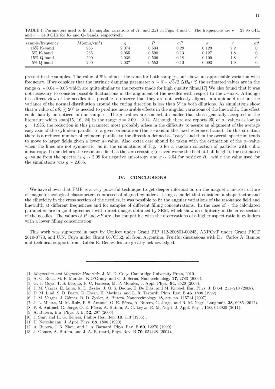
TABLE I: Parameters used to fit the angular variations of Hr and ∆H in Figs. 4 and 5. The frequencies are ν = 23.95 GHzand ν = 34.0 GHz for K- and Q- bands, respectively.

sample/frequency M(emu/cm3) g P σP α r σθ15% K-band 265 2.074 0.534 0.28 0.129 2.2 05% K-band 265 2.055 0.590 0.13 0.127 1.8 015% Q-band 290 2.038 0.506 0.18 0.100 1.8 05% Q-band 290 2.037 0.552 0.10 0.093 1.9 0

present in the samples. The value of α is almost the same for both samples, but shows an appreciable variation withfrequency. If we consider that the intrinsic damping parameter α ∼ α−√3/2 ∆H0/

ωγ the estimated values are in the

range α ∼ 0.04−0.05 which are quite similar to the reports made for high quality films.[17] We also found that it wasnot necessary to consider possible fluctuations in the alignment of the needles with respect to the x−axis. Althoughin a direct view of the needles it is possible to observe that they are not perfectly aligned in a unique direction, thevariance of the normal distribution around the curing direction is less than 5o in both dilutions. As simulations showthat a value of σθc & 20◦ is needed to produce measurable effects in the angular variations of the linewidth, this effectcould hardly be noticed in our samples. The g−values are somewhat smaller that those generally accepted in theliterature which span[15, 16, 24] in the range g = 2.09 − 2.14. Although there are reports[25] of g−values as low asg = 1.985, the reduction in this parameter most probably arises in the difficulty to assure an alignment of the averageeasy axis of the cylinders parallel to a given orientation (the x−axis in the fixed reference frame). In this situationthere is a reduced number of cylinders parallel to the direction defined as ”easy” and then the overall spectrum tendsto move to larger fields given a lower g−value. Also, extra care should be taken with the estimation of the g−valuewhen the lines are not symmetric, as in the simulations of Fig. 6 for a random collection of particles with cubicanisotropy. If one defines the resonance field as the zero crossing (or even worse the field at half height), the estimatedg−value from the spectra is g ∼ 2.09 for negative anisotropy and g ∼ 2.04 for positive Hc, while the value used forthe simulations was g ∼ 2.055.

IV. CONCLUSIONS

We have shown that FMR is a very powerful technique to get deeper information on the magnetic microstructureof magnetorheological elastometers composed of aligned cylinders. Using a model that considers a shape factor andthe ellipticity in the cross section of the needles, it was possible to fit the angular variations of the resonance field andlinewidth at different frequencies and for samples of different filling concentrations. In the case of r the calculatedparameters are in good agreement with direct images obtained by SEM, which show an ellipticity in the cross sectionof the needles. The values of P and σP are also compatible with the observations of a higher aspect ratio in cylinderswith a lower filling concentration.

This work was supported in part by Conicet under Grant PIP 112-200801-00245, ANPCyT under Grant PICT2010-0773, and U.N. Cuyo under Grant 06/C352, all from Argentina. Fruitful discussions with Dr. Carlos A. Ramosand technical support from Ruben E. Benavides are greatly acknowledged.

[1] Magnetism and Magnetic Materials, J. M. D. Coey, Cambridge University Press, 2010.[2] A. G. Roca, M. P. Morales, K.O’Grady, and C. J. Serna, Nanotechnology 17, 2783 (2006).[3] G. F. Goya, T. S. Berquo, F. C. Fonseca, M. P. Morales, J. Appl. Phys., 94, 3520 (2003).[4] J. M. Vargas, E. Lima, R. D. Zysler, J. G. S. Duque, E. De Biasi and M. Knobel, Eur. Phys. J. B 64, 211–218 (2008).[5] D. M. Lind, S. D. Berry, G. Chern, H. Mathias, and L. R. Testardi, Phys. Rev. B 45, 1838 (1992).[6] J. M. Vargas, J. Gomez, R. D. Zysler, A. Butera, Nanotechnology 18, art. no. 115714 (2007).[7] J. L. Mietta, M. M. Ruiz, P. S. Antonel, O. E. Perez, A. Butera, G. Jorge, and R. M. Negri, Langmuir, 28, 6985 (2012).[8] P. S. Antonel, G. Jorge, O. E. Perez, A. Butera, A. G. Leyva, R. M. Negri. J. Appl. Phys., 110, 043920 (2011).[9] A. Butera, Eur. Phys. J. B, 52, 297 (2006).

[10] J. Smit and H. G. Beljers, Philips Res. Rep. 10, 113 (1955) .[11] U. Netzelmann, J. Appl. Phys. 68, 1800 (1990).[12] A. Butera, J. N. Zhou, and J. A. Barnard, Phys. Rev. B 60, 12270 (1999).[13] J. Gomez, A. Butera, and J. A. Barnard, Phys. Rev. B 70, 054428 (2004).

12

[14] M. Spasova, U. Wiedwald, R. Ramchal, M. Farle, M. Hilgendorff, M. Giersig, J. Magn. Magn. Mater. 40, 240 (2002).[15] L.R. Bickford Jr., Physical Review 78, 449 (1950).[16] J. J. Krebs, D. M. Lind, and S. D. Berry, J. Appl. Phys. 73, 6457 (1993).[17] P.A.A. van der Heijden, M.G. van Opstal, C.H.W. Swiiste, P.H.J. Bloemen, J.M. Gaines, W.J.M. de Jonge, J. Magn.

Magn. Mater. 182, 71 (1998).[18] T. Bodziony, N. Guskos, J. Typek, Z. Roslaniec, U. Narkiewicz, M. Kwiatkowska, M. Maryniak, Reviews on Advanced

Materials Science 8, 86 (2004).[19] A. Butera, S. S. Kang, D.E. Nikles, and J.W. Harrell, Physica B 354, 108 (2004). A. Butera, J. L. Weston, J.A. Barnard,

J. Magn. Magn. Mater.284, 17 (2004).[20] J. Curiale, R.D. Sanchez, C.A. Ramos, A.G. Leyva, A. Butera, J. Magn. Magn. Mater. 320, e218 (2008).[21] E. De Biasi, C. A. Ramos and R. D. Zysler, J. Magn. Magn. Mater. 235, 262 (2003).[22] A. Butera, J. Gomez, J. L. Weston, J. A. Barnard, J. Appl. Phys. 98, 033901 (2005).[23] E. P. Valstyn, J. P. Hanton, and A. H. Morrish, Phys. Rev. 128, 2078 (1962).[24] B. Aktas, Thin Solid Films, 307, 250 (1997).[25] Y. Koseoglu, B. Aktas, Phys. Status Solidi C, 1, 3516 (2004).