microsimulation as a tool for the evaluation of public policies
TRANSCRIPT


m i c r o s i m u l a t i o n a s a t o o l f o r t h e e v a l u a t i o n o f p u b l i c p o l i c i e s


Microsimulation as a Tool for the Evaluation
of Public Policies Methods and Applications
Amedeo Spadaro (ed.)
The BBVA Foundation’s decision to publish this book does not imply any responsibility for its content, or for the inclusion therein of any supplementary documents or information facilitated by the authors.
No part of this publication, including the cover design, may be reproduced, stored in a retrieval system or transmitted in any form or by any means, electronic, mechanical, photocopying, recording or otherwise, without the prior written permission of the copyright holder.
cataloguing-in-publication data
Microsimulation as a tool for the evaluation of public
policies : methods and applications / Amedeo Spadaro
(ed). — Bilbao : Fundación BBVA, 2007.
357 p. ; 24 cm
isbn 978-84-96515-17-8
1. Método de evaluación 2. Simulación I. Spadaro,
Amedeo II. Fundación BBVA, ed.
303.001.57
Microsimulation as a Tool for the Evaluation of Public Policies: Methods and Applications
p u b l i s h e d b y:© Fundación BBVA, 2007 Plaza de San Nicolás, 4. 48005 Bilbao
c o v e r i l l u s t r at i o n: © Germán aparicio fernández, 2007 ASR 10, 1998 Aquatint and etching, 272 x 700 mm Collection of Contemporary Graphic Art Fundación BBVA – Calcografía Nacional
i s b n: 978-84-96515-17-8l e g a l d e p o s i t n o. : m-4596-2007
p r i n t e d b y: Ibersaf Industrial, s.l. Huertas, 47 bis. 28014 Madrid
Printed in Spain
The books published by the BBVA Foundation are produced with 100% recycled paper made from recovered cellulose fibre (used paper) rather than virgin cellulose, in conformity with the environmental standards required by current legislation.
The paper production process complies with European environmental laws and regulations, and has both Nordic Swan and Blue Angel accreditation.
c o n T E n T S
Introduction, Amedeo Spadaro . . . . . . . . . . . . . . . . . . . . . . . . . . . . . . . . . . . . . . . . . . . . . . . . . . . . . . . . . . . . . 13
1. Microsimulation as a Tool for the Evaluation of Public Policies Amedeo Spadaro
1.1. Introduction . . . . . . . . . . . . . . . . . . . . . . . . . . . . . . . . . . . . . . . . . . . . . . . . . . . . . . . . . . . . . . . . . . . . . . . . . . . . . . . 17
1.2. Arithmetical microsimulation and tax incidence analysis . . . . . . . . . . . . 23
1.3. Behavioural microsimulation . . . . . . . . . . . . . . . . . . . . . . . . . . . . . . . . . . . . . . . . . . . . . . . . . . . . . . 32
1.4 Microsimulation and normative policy evaluation . . . . . . . . . . . . . . . . . . . . . . . 40
1.5. Recent extensions and directions for future research . . . . . . . . . . . . . . . . . 45
1.5.1. Macroeconomic analysis and microsimulation
models . . . . . . . . . . . . . . . . . . . . . . . . . . . . . . . . . . . . . . . . . . . . . . . . . . . . . . . . . . . . . . . . . . . . . . . . . . . . . . 46
1.5.2. Introducing dynamics . . . . . . . . . . . . . . . . . . . . . . . . . . . . . . . . . . . . . . . . . . . . . . . . . . . . . . . . 50
1.5.3. Firms, institutions and investment climate . . . . . . . . . . . . . . . . . . . . . . . . . 53
1.6. Conclusions . . . . . . . . . . . . . . . . . . . . . . . . . . . . . . . . . . . . . . . . . . . . . . . . . . . . . . . . . . . . . . . . . . . . . . . . . . . . . . . . 54
References . . . . . . . . . . . . . . . . . . . . . . . . . . . . . . . . . . . . . . . . . . . . . . . . . . . . . . . . . . . . . . . . . . . . . . . . . . . . . . . . . . . . . . . . 55
2. Direct Taxation and Behavioural Microsimulation: A Review of Applications in Italy and Norway Rolf Aaberge and Ugo colombino
2.1. Introduction . . . . . . . . . . . . . . . . . . . . . . . . . . . . . . . . . . . . . . . . . . . . . . . . . . . . . . . . . . . . . . . . . . . . . . . . . . . . . . . 61
2.2. The microeconometric model . . . . . . . . . . . . . . . . . . . . . . . . . . . . . . . . . . . . . . . . . . . . . . . . . . . . 61
2.3. Labour supply elasticity . . . . . . . . . . . . . . . . . . . . . . . . . . . . . . . . . . . . . . . . . . . . . . . . . . . . . . . . . . . . . . 64
2.4. A simulation of some reform proposals . . . . . . . . . . . . . . . . . . . . . . . . . . . . . . . . . . . . . 65
2.5. An empirical exercise in optimal taxation . . . . . . . . . . . . . . . . . . . . . . . . . . . . . . . . . . . 68
2.6. Integrating the micro and the CGE model . . . . . . . . . . . . . . . . . . . . . . . . . . . . . . . . . 70
2.7. Out-of-sample predictions . . . . . . . . . . . . . . . . . . . . . . . . . . . . . . . . . . . . . . . . . . . . . . . . . . . . . . . . . . . 71
References . . . . . . . . . . . . . . . . . . . . . . . . . . . . . . . . . . . . . . . . . . . . . . . . . . . . . . . . . . . . . . . . . . . . . . . . . . . . . . . . . . . . . . . . 72
3. Growth, Distribution and Poverty in Madagascar: Learning from a Microsimulation Model in a General Equilibrium Framework Denis cogneau and Anne-Sophie Robilliard
3.1. Introduction . . . . . . . . . . . . . . . . . . . . . . . . . . . . . . . . . . . . . . . . . . . . . . . . . . . . . . . . . . . . . . . . . . . . . . . . . . . . . . . 73
3.2. Modelling income distribution . . . . . . . . . . . . . . . . . . . . . . . . . . . . . . . . . . . . . . . . . . . . . . . . . . . 75
3.2.1. Functional distribution vs. personal distribution . . . . . . . . . . . . . . . . 76
3.2.2. The representative agent assumption . . . . . . . . . . . . . . . . . . . . . . . . . . . . . . . . 77
3.3. Microeconomic specifications of the model . . . . . . . . . . . . . . . . . . . . . . . . . . . . . . . . 78
3.3.1. Production and labour allocation . . . . . . . . . . . . . . . . . . . . . . . . . . . . . . . . . . . . . . 78
3.3.1.1. Agricultural households . . . . . . . . . . . . . . . . . . . . . . . . . . . . . . . . . . . . . . . . 79
3.3.1.2. Non-agricultural households . . . . . . . . . . . . . . . . . . . . . . . . . . . . . . . . . 81
3.3.2. Disposable income, savings and consumption . . . . . . . . . . . . . . . . . . . . 81
3.4. Description of the general equilibrium framework . . . . . . . . . . . . . . . . . . . . . 82
3.5. An application to Madagascar . . . . . . . . . . . . . . . . . . . . . . . . . . . . . . . . . . . . . . . . . . . . . . . . . . . . . 83
3.5.1. Estimation results . . . . . . . . . . . . . . . . . . . . . . . . . . . . . . . . . . . . . . . . . . . . . . . . . . . . . . . . . . . . . . 85
3.5.1.1. Agricultural production function . . . . . . . . . . . . . . . . . . . . . . . . . . 85
3.5.1.2. Informal and formal wage equations . . . . . . . . . . . . . . . . . . . . 88
3.5.2. Calibration, parameters and algorithm . . . . . . . . . . . . . . . . . . . . . . . . . . . . . . 89
3.5.2.1. Parameter calibration . . . . . . . . . . . . . . . . . . . . . . . . . . . . . . . . . . . . . . . . . . . 90
3.5.2.2. Potential wage equation . . . . . . . . . . . . . . . . . . . . . . . . . . . . . . . . . . . . . . . . 91
3.5.2.3. Heterogeneity . . . . . . . . . . . . . . . . . . . . . . . . . . . . . . . . . . . . . . . . . . . . . . . . . . . . . . . 92
3.5.2.4. Algorithm and solution . . . . . . . . . . . . . . . . . . . . . . . . . . . . . . . . . . . . . . . . . 92
3.6. Impact of growth shocks on poverty and inequality . . . . . . . . . . . . . . . . . . . . 92
3.6.1. Some descriptive elements . . . . . . . . . . . . . . . . . . . . . . . . . . . . . . . . . . . . . . . . . . . . . . . . . 93
3.6.2. Description of growth shocks . . . . . . . . . . . . . . . . . . . . . . . . . . . . . . . . . . . . . . . . . . . . . 95
3.6.3. Ex ante and ex post decomposition of the impact
of growth shocks . . . . . . . . . . . . . . . . . . . . . . . . . . . . . . . . . . . . . . . . . . . . . . . . . . . . . . . . . . . . . . . . 96
3.6.4. Decomposition of microeconomic results by group . . . . . . . . . . . 102
3.7. Conclusions . . . . . . . . . . . . . . . . . . . . . . . . . . . . . . . . . . . . . . . . . . . . . . . . . . . . . . . . . . . . . . . . . . . . . . . . . . . . . . . . 108
References . . . . . . . . . . . . . . . . . . . . . . . . . . . . . . . . . . . . . . . . . . . . . . . . . . . . . . . . . . . . . . . . . . . . . . . . . . . . . . . . . . . . . . . . 110
4. Microsimulation of Healthcare Policies nuria Badenes and Ángel López
4.1. Introduction . . . . . . . . . . . . . . . . . . . . . . . . . . . . . . . . . . . . . . . . . . . . . . . . . . . . . . . . . . . . . . . . . . . . . . . . . . . . . . . 113
4.2. Microsimulation models in health economics . . . . . . . . . . . . . . . . . . . . . . . . . . . . . 114
4.2.1. Australia . . . . . . . . . . . . . . . . . . . . . . . . . . . . . . . . . . . . . . . . . . . . . . . . . . . . . . . . . . . . . . . . . . . . . . . . . . . . 115
4.2.2. Canada . . . . . . . . . . . . . . . . . . . . . . . . . . . . . . . . . . . . . . . . . . . . . . . . . . . . . . . . . . . . . . . . . . . . . . . . . . . . . . 116
4.2.3. United States . . . . . . . . . . . . . . . . . . . . . . . . . . . . . . . . . . . . . . . . . . . . . . . . . . . . . . . . . . . . . . . . . . . . . 118
4.2.4. Europe . . . . . . . . . . . . . . . . . . . . . . . . . . . . . . . . . . . . . . . . . . . . . . . . . . . . . . . . . . . . . . . . . . . . . . . . . . . . . . 120
4.2.4.1. France . . . . . . . . . . . . . . . . . . . . . . . . . . . . . . . . . . . . . . . . . . . . . . . . . . . . . . . . . . . . . . . . . . 120
4.2.4.2. Netherlands . . . . . . . . . . . . . . . . . . . . . . . . . . . . . . . . . . . . . . . . . . . . . . . . . . . . . . . . . . 120
4.2.4.3. Norway . . . . . . . . . . . . . . . . . . . . . . . . . . . . . . . . . . . . . . . . . . . . . . . . . . . . . . . . . . . . . . . . . 121
4.2.4.4. United Kingdom . . . . . . . . . . . . . . . . . . . . . . . . . . . . . . . . . . . . . . . . . . . . . . . . . . . 121
4.2.4.5. Sweden . . . . . . . . . . . . . . . . . . . . . . . . . . . . . . . . . . . . . . . . . . . . . . . . . . . . . . . . . . . . . . . . . 122
4.3. Microsimulation à la carte . . . . . . . . . . . . . . . . . . . . . . . . . . . . . . . . . . . . . . . . . . . . . . . . . . . . . . . . . . . 123
4.4. Empirical application: a microsimulation model
for taxation policies in Spain . . . . . . . . . . . . . . . . . . . . . . . . . . . . . . . . . . . . . . . . . . . . . . . . . . . . . 126
4.4.1. Objectives of the study . . . . . . . . . . . . . . . . . . . . . . . . . . . . . . . . . . . . . . . . . . . . . . . . . . . . . . . 126
4.4.2. Methodology . . . . . . . . . . . . . . . . . . . . . . . . . . . . . . . . . . . . . . . . . . . . . . . . . . . . . . . . . . . . . . . . . . . . 128
4.4.3. Coverage type and use of healthcare services . . . . . . . . . . . . . . . . . . . . 130
4.4.4. An econometric model for the use probability
of healthcare services . . . . . . . . . . . . . . . . . . . . . . . . . . . . . . . . . . . . . . . . . . . . . . . . . . . . . . . . 132
4.5. Simulation of healthcare savings under different
double coverage scenarios . . . . . . . . . . . . . . . . . . . . . . . . . . . . . . . . . . . . . . . . . . . . . . . . . . . . . . . . . . 136
4.5.1. Evaluation of the cost of visits to the public network. . . . . . . . . . 136
4.5.2. Simulation of healthcare costs and savings under
diverse double coverage scenarios . . . . . . . . . . . . . . . . . . . . . . . . . . . . . . . . . . . . . 139
4.5.2.1. Simulation of diverse scenarios . . . . . . . . . . . . . . . . . . . . . . . . . . . . . 140
4.6. Summary and conclusions . . . . . . . . . . . . . . . . . . . . . . . . . . . . . . . . . . . . . . . . . . . . . . . . . . . . . . . . . . 144
References . . . . . . . . . . . . . . . . . . . . . . . . . . . . . . . . . . . . . . . . . . . . . . . . . . . . . . . . . . . . . . . . . . . . . . . . . . . . . . . . . . . . . . . . 145
5. Microsimulation in the Analysis of Environmental Tax Reforms. An Application for Spain Xavier Labandeira, José M. Labeaga and Miguel Rodríguez
5.1. Introduction . . . . . . . . . . . . . . . . . . . . . . . . . . . . . . . . . . . . . . . . . . . . . . . . . . . . . . . . . . . . . . . . . . . . . . . . . . . . . . . 149
5.2. Integrating micro and macroeconomic models . . . . . . . . . . . . . . . . . . . . . . . . . . 152
5.3. Details of the integrated micro-macro model . . . . . . . . . . . . . . . . . . . . . . . . . . . . . . 155
5.3.1. The Applied General Equilibrium Model . . . . . . . . . . . . . . . . . . . . . . . . . 157
5.3.2. A microeconomic model for household energy demand . . . 161
5.4. Results obtained via the integrated micro-macro model . . . . . . . . . . . . . 165
5.4.1. Description of the reform . . . . . . . . . . . . . . . . . . . . . . . . . . . . . . . . . . . . . . . . . . . . . . . . . . 165
5.4.2. Results . . . . . . . . . . . . . . . . . . . . . . . . . . . . . . . . . . . . . . . . . . . . . . . . . . . . . . . . . . . . . . . . . . . . . . . . . . . . . . . 165
5.5. Conclusions . . . . . . . . . . . . . . . . . . . . . . . . . . . . . . . . . . . . . . . . . . . . . . . . . . . . . . . . . . . . . . . . . . . . . . . . . . . . . . . . 171
Appendix: Production and consumption structures . . . . . . . . . . . . . . . . . . . . . . . . . . 173
References . . . . . . . . . . . . . . . . . . . . . . . . . . . . . . . . . . . . . . . . . . . . . . . . . . . . . . . . . . . . . . . . . . . . . . . . . . . . . . . . . . . . . . . . 175
6. Microsimulation and Economic Rationality: An Application of the Collective Model to Evaluate Tax Reforms in Spain Raquel carrasco and Javier Ruiz-castillo
6.1. Introduction . . . . . . . . . . . . . . . . . . . . . . . . . . . . . . . . . . . . . . . . . . . . . . . . . . . . . . . . . . . . . . . . . . . . . . . . . . . . . . . 177
6.2. The data . . . . . . . . . . . . . . . . . . . . . . . . . . . . . . . . . . . . . . . . . . . . . . . . . . . . . . . . . . . . . . . . . . . . . . . . . . . . . . . . . . . . . 182
6.3. The baseline system . . . . . . . . . . . . . . . . . . . . . . . . . . . . . . . . . . . . . . . . . . . . . . . . . . . . . . . . . . . . . . . . . . . . 187
6.4. The construction of a collective world . . . . . . . . . . . . . . . . . . . . . . . . . . . . . . . . . . . . . . . . 190
6.4.1. Efficient household allocations . . . . . . . . . . . . . . . . . . . . . . . . . . . . . . . . . . . . . . . . . . 190
6.4.2. Empirical specification and identification of the
collective model . . . . . . . . . . . . . . . . . . . . . . . . . . . . . . . . . . . . . . . . . . . . . . . . . . . . . . . . . . . . . . . . 192
6.4.3. A summary . . . . . . . . . . . . . . . . . . . . . . . . . . . . . . . . . . . . . . . . . . . . . . . . . . . . . . . . . . . . . . . . . . . . . . . . 197
6.5. Estimation results . . . . . . . . . . . . . . . . . . . . . . . . . . . . . . . . . . . . . . . . . . . . . . . . . . . . . . . . . . . . . . . . . . . . . . . 198
6.5.1. The singles model . . . . . . . . . . . . . . . . . . . . . . . . . . . . . . . . . . . . . . . . . . . . . . . . . . . . . . . . . . . . . 198
6.5.1.1. Missing wages . . . . . . . . . . . . . . . . . . . . . . . . . . . . . . . . . . . . . . . . . . . . . . . . . . . . . . . 198
6.5.1.2. Marginal propensities . . . . . . . . . . . . . . . . . . . . . . . . . . . . . . . . . . . . . . . . . . . 201
6.5.2. The construction of the collective world . . . . . . . . . . . . . . . . . . . . . . . . . . . . 207
6.5.2.1. Missing wages . . . . . . . . . . . . . . . . . . . . . . . . . . . . . . . . . . . . . . . . . . . . . . . . . . . . . . . 210
6.5.2.2. Preference parameters . . . . . . . . . . . . . . . . . . . . . . . . . . . . . . . . . . . . . . . . . . 211
6.6. The unitary model for couples . . . . . . . . . . . . . . . . . . . . . . . . . . . . . . . . . . . . . . . . . . . . . . . . . . . 220
6.7. The analysis of tax reform . . . . . . . . . . . . . . . . . . . . . . . . . . . . . . . . . . . . . . . . . . . . . . . . . . . . . . . . . . 223
6.7.1. The 1999 tax reform . . . . . . . . . . . . . . . . . . . . . . . . . . . . . . . . . . . . . . . . . . . . . . . . . . . . . . . . . 223
6.7.2. The consequences of the 1999 tax reform.
The static case . . . . . . . . . . . . . . . . . . . . . . . . . . . . . . . . . . . . . . . . . . . . . . . . . . . . . . . . . . . . . . . . . . . 226
6.7.3. The consequences of the 1999 tax reform
according to the collective model . . . . . . . . . . . . . . . . . . . . . . . . . . . . . . . . . . . . . . 231
6.8. Conclusions . . . . . . . . . . . . . . . . . . . . . . . . . . . . . . . . . . . . . . . . . . . . . . . . . . . . . . . . . . . . . . . . . . . . . . . . . . . . . . . . 239
References . . . . . . . . . . . . . . . . . . . . . . . . . . . . . . . . . . . . . . . . . . . . . . . . . . . . . . . . . . . . . . . . . . . . . . . . . . . . . . . . . . . . . . . . 242
7. Microsimulation and Macroeconomic Analysis: An Integrated Approach. An Application for Evaluating Reforms in the Italian Agricultural Sector Riccardo Magnani, Eleonora Matteazzi and Federico Perali
7.1. Introduction . . . . . . . . . . . . . . . . . . . . . . . . . . . . . . . . . . . . . . . . . . . . . . . . . . . . . . . . . . . . . . . . . . . . . . . . . . . . . . . 245
7.2. Data . . . . . . . . . . . . . . . . . . . . . . . . . . . . . . . . . . . . . . . . . . . . . . . . . . . . . . . . . . . . . . . . . . . . . . . . . . . . . . . . . . . . . . . . . . 247
7.3. The micro-macro experiment . . . . . . . . . . . . . . . . . . . . . . . . . . . . . . . . . . . . . . . . . . . . . . . . . . . . . 248
7.4. The macro applied general equilibrium model . . . . . . . . . . . . . . . . . . . . . . . . . . 249
7.5. Distributional impact at the macro level . . . . . . . . . . . . . . . . . . . . . . . . . . . . . . . . . . . . . 254
7.6. The micro applied general equilibrium model . . . . . . . . . . . . . . . . . . . . . . . . . . . 259
7.7. The collective farm-household model . . . . . . . . . . . . . . . . . . . . . . . . . . . . . . . . . . . . . . 259
7.8. Description of household social accounting matrices . . . . . . . . . . . . . . . 268
7.9. Modelling labour market failures . . . . . . . . . . . . . . . . . . . . . . . . . . . . . . . . . . . . . . . . . . . . . 273
7.10. An example: the impact of changes in off-farm wages . . . . . . . . . . . . . . 274
7.11. Microsimulation results . . . . . . . . . . . . . . . . . . . . . . . . . . . . . . . . . . . . . . . . . . . . . . . . . . . . . . . . . . . . 277
7.12. Distributional impact at the micro level in the case
of labour market failure . . . . . . . . . . . . . . . . . . . . . . . . . . . . . . . . . . . . . . . . . . . . . . . . . . . . . . . . . . 286
7.13. Conclusions . . . . . . . . . . . . . . . . . . . . . . . . . . . . . . . . . . . . . . . . . . . . . . . . . . . . . . . . . . . . . . . . . . . . . . . . . . . . . 288
References . . . . . . . . . . . . . . . . . . . . . . . . . . . . . . . . . . . . . . . . . . . . . . . . . . . . . . . . . . . . . . . . . . . . . . . . . . . . . . . . . . . . . . . . 289
8. Child Poverty and Family Transfers in Southern Europe Manos Matsaganis, cathal o’Donoghue, Horacio Levy,
Manuela coromaldi, Magda Mercader-Prats, carlos Farinha Rodrigues,
Stefano Toso and Panos Tsakloglou 8.1. Introduction . . . . . . . . . . . . . . . . . . . . . . . . . . . . . . . . . . . . . . . . . . . . . . . . . . . . . . . . . . . . . . . . . . . . . . . . . . . . . . . 293
8.2. Child poverty and household composition . . . . . . . . . . . . . . . . . . . . . . . . . . . . . . . . 295
8.3. Family transfers and child poverty . . . . . . . . . . . . . . . . . . . . . . . . . . . . . . . . . . . . . . . . . . . . . . 299
8.4. Target efficiency . . . . . . . . . . . . . . . . . . . . . . . . . . . . . . . . . . . . . . . . . . . . . . . . . . . . . . . . . . . . . . . . . . . . . . . . . 308
8.5. Reforming family transfers . . . . . . . . . . . . . . . . . . . . . . . . . . . . . . . . . . . . . . . . . . . . . . . . . . . . . . . . . 311
8.6. Conclusions . . . . . . . . . . . . . . . . . . . . . . . . . . . . . . . . . . . . . . . . . . . . . . . . . . . . . . . . . . . . . . . . . . . . . . . . . . . . . . . . 319
References . . . . . . . . . . . . . . . . . . . . . . . . . . . . . . . . . . . . . . . . . . . . . . . . . . . . . . . . . . . . . . . . . . . . . . . . . . . . . . . . . . . . . . . . 321
9. Microsimulation and Normative Analysis of Public Policies Amedeo Spadaro and Xisco oliver
9.1. Introduction . . . . . . . . . . . . . . . . . . . . . . . . . . . . . . . . . . . . . . . . . . . . . . . . . . . . . . . . . . . . . . . . . . . . . . . . . . . . . . . 323
9.2. The model . . . . . . . . . . . . . . . . . . . . . . . . . . . . . . . . . . . . . . . . . . . . . . . . . . . . . . . . . . . . . . . . . . . . . . . . . . . . . . . . . . 326
9.3. The data, the microsimulation model and the main
features of redistribution systems . . . . . . . . . . . . . . . . . . . . . . . . . . . . . . . . . . . . . . . . . . . . . . . . 329
9.3.1. The 1998 and 1999 Spanish redistribution systems . . . . . . . . . . . . 330
9.4. Results . . . . . . . . . . . . . . . . . . . . . . . . . . . . . . . . . . . . . . . . . . . . . . . . . . . . . . . . . . . . . . . . . . . . . . . . . . . . . . . . . . . . . . . . 332
9.5. Conclusions . . . . . . . . . . . . . . . . . . . . . . . . . . . . . . . . . . . . . . . . . . . . . . . . . . . . . . . . . . . . . . . . . . . . . . . . . . . . . . . . 336
References . . . . . . . . . . . . . . . . . . . . . . . . . . . . . . . . . . . . . . . . . . . . . . . . . . . . . . . . . . . . . . . . . . . . . . . . . . . . . . . . . . . . . . . . 337
List of Figures and Graphs . . . . . . . . . . . . . . . . . . . . . . . . . . . . . . . . . . . . . . . . . . . . . . . . . . . . . . . . . . . . . . 339
List of Tables . . . . . . . . . . . . . . . . . . . . . . . . . . . . . . . . . . . . . . . . . . . . . . . . . . . . . . . . . . . . . . . . . . . . . . . . . . . . . . . . . . . . . . 341
Index . . . . . . . . . . . . . . . . . . . . . . . . . . . . . . . . . . . . . . . . . . . . . . . . . . . . . . . . . . . . . . . . . . . . . . . . . . . . . . . . . . . . . . . . . . . . . . . . . . . 347
About the Authors . . . . . . . . . . . . . . . . . . . . . . . . . . . . . . . . . . . . . . . . . . . . . . . . . . . . . . . . . . . . . . . . . . . . . . . . . . . . 353

[ 13 ]
Introduction
Amedeo Spadaro Paris-Jourdan Sciences Economiques (Paris), FEDEA (Madrid)
and University of the Balearic Islands (Palma de Mallorca)
THIS has been a time of rapid development for the research field dealing with the evaluation of public policies. Microsimulation techniques—based on the representation of individuals’ behaviour when confronted with real or hypothetical changes in their eco-nomic or institutional environment—have become a much used instrument in this context for their ability to provide an a priori assessment of differing scenarios and facilitate decision making. On the basis of extremely accurate and rich models calibrated on representative samples of individuals, households or firms, simula-tion techiques permit precise predictions of the impact of a given policy on the population.
The workshop on “Microsimulation as a tool for the evaluation of public policies: methods and applications”, organised under the aegis of the BBVA Foundation on 15-16 November 2004, brought together some of the leading international experts in the field to share their experiences and map out new directions for the analysis and application of these innovative techniques as an input to public decision making. The present volume assembles the different contributions made at this event.
In the opening chapter, Amedeo Spadaro offers an introduc-tion to the use of microsimulation as a technique for the evalu-ation of public policies, discussing the theoretical foundations of the different types of microsimulation and reviewing recent developments in the field.
The second chapter is given over to microsimulation with behavioural responses. Authors Rolf Aaberge and Ugo Colombino present some applications of this type of model, as recently developed by themselves for evaluating tax reforms in Italy and Norway. They
[ 14 ] m i c r o s i m u l at i o n a s a t o o l f o r t h e e va l u at i o n o f p u b l i c p o l i c i e s
explain both the difficulties encountered and the potential of these instruments for identifying the effects of such reforms.
In the third chapter, Denis Cogneau and Anne-Sophie Robilliard use a fully integrated microsimulation model within a general equilibrium framework for the ex ante evaluation of the impact of different growth strategies on poverty and inequality in Madagascar. They show that, given the complexity of the general equilibrium effects and the wide range of household positions in markets for factors and goods, partial equilibrium analysis or the use of a representative households approach would limit the robustness of the evaluation exercise.
Microsimulation has revealed itself to be a powerful tool in many economic areas, and health economics are no exception. In the fourth chapter, Nuria Badenes and Ángel López review some of the microsimulation models that may be most useful in this sphere. After defining the scope of microsimulation in the health economics field and looking at models developed in different countries, the authors give an example of the use of microsimula-tion models constructed à la carte for solving a specific problem: an assessment of savings generated by dual coverage through the use of private healthcare in preference to the equivalent public service.
In our fifth chapter, Xavier Labandeira, José M. Labeaga and Miguel Rodríguez put forward a methodology to evaluate the re-distributive and efficiency effects of the reform of indirect taxes on energy consumption. They propose a microeconomic model to gauge the varied effects on household energy demand. This model is integrated through prices with a Computable General Equilibrium Model (CGE), which can identify the effects of a policy on social welfare, relative prices and levels of sectoral and institutional activity. The results are then fed into a microeco-nomic model in order to disaggregate the impact of the policy in question on the welfare of sample households and aggregate the findings to the reference population.
The evaluation of tax reforms through microsimulation mod-els usually starts from the classic hypothesis that resource alloca-tion within a household is the work of a benign dictator. In the sixth chapter, Javier Ruiz Castillo and Raquel Carrasco present
i n t r o d u c t i o n [ 15 ]
the results of a series of research projects which seek to go beyond this approach by introducing the collective model in microsimula-tion with behavioural reactions. The text discusses the implemen-tation of collective rationality in a microsimulation model with reference to Spain’s recent reform of personal income tax.
In chapter 7, Riccardo Magnani, Eleonora Matteazzi and Federico Perali employ an integrated micro-macro simulation model to assess the impact of agricultural sector reforms and international trade agreements on Italy’s rural population. The analysis they conduct shows how macro approaches based on general economic equilibrium can be compatible with micro ap-proaches involving the simulation of individual behaviour. This chapter also provides some general insights into the statistical specifications of samples, the interpretation of data and tech-niques for constructing integrated micro-macro models for appli-cation in the distributive analysis of macroeconomic policies.
Chapter 8 describes an excellent team project which demon-strates the importance of multi-country microsimulation models in defining supranational policies for the fight against poverty. The authors present the results of EUROMOD, a research project financed by the European Union, aimed at the construction of an arithmetic microsimulation model for the then 15 EU member countries. This tool has since served to detect child poverty prob-lems in Europe’s southern countries and to identify possible rem-edies at the European level (or coordinated between countries).
Microsimulation has largely been applied to the positive evalu-ation of reforms. In the closing chapter, Amedeo Spadaro and Xisco Oliver look at how this technique can also be used for nor-mative analysis. Microsimulation models, they explain, can help us identify the best possible redistribution policy (in the sense of maximising a given social welfare function). The application presented also shows how the preferences of social planners can be divined through the observation of a tax reform.

[ 17 ]
Microsimulation as a Tool for the Evaluation of Public Policies
Amedeo Spadaro Paris-Jourdan Sciences Economiques (Paris), FEDEA (Madrid)
and University of the Balearic Islands (Palma de Mallorca)
1.1.Introduction
The analysis of public policies (in terms of alternatives and effects) is one of the major tasks of economists. Identifying the winners and losers of a tax reform or evaluating the impact on poverty of the introduction of a new subsidy requires powerful tools allow-ing for the measurement of aggregate effects on the economy as well as the impact on individual or household welfare.
The construction of such tools is always characterized by a trade off between the simplicity of their use, an in-depth descrip-tion of the complexity of the socioeconomic system and, most importantly, the possibility to fully capture the agent’s heteroge-neity. The first property is required in order to be able to manage and control the tool and understand why we get a certain result. The second and the third properties are necessary to optimise the accuracy of the analysis. The standard representative agent approach, commonly used in the analysis of most public policies, gives more weight to the simplicity factor. Without questioning its validity as a powerful approach for economic analysis,1 the representative agent approach is not useful to evaluate the ef-fects of public policies taking into account the heterogeneity of the population. Imagine that you are dealing with an income tax reform that determines changes in the consumption or labour supply patterns of the population. These behavioural effects dif-
1 More specifically, we want to highlight the importance of the representative agent approach.
1.
[ 18 ] m i c r o s i m u l at i o n a s a t o o l f o r t h e e va l u at i o n o f p u b l i c p o l i c i e s
fer from one agent to another depending on his or her individual characteristics and preferences: a robust analysis of the effects of such a measure cannot be conducted without a model taking into account the heterogeneity of individual behaviour. This necessity has pushed applied economists towards the use of microsimula-tion models (MSMs).
MSMs are tools that allow simulation of the effects of a policy on a sample of agents (individuals or households) at individual level. The microsimulation approach is based on the representa-tion of individual behaviour when agents face different economic and institutional frameworks.
The simulation approach has been widely used in sciences like mathematics or physics. Its use as a tool for the analysis of and support for public decision-making processes is more re-cent. Although it was as early as 1957 when the seminal paper by Orcutt2 planted the seed of microsimulation as an instrument for economic analysis, it was only in the 1980s that the use of microsimulation tools increased substantially. This was due to the growing availability of large and detailed data sets on individual and household socioeconomic characteristics and the constant expansion of the computing capacity of the PC (as well as its ac-cessibility in terms of cost). These factors have greatly increased the spread of MSMs among researchers and in the planning services of government administrations. MSMs have thus become an increasingly powerful instrument for evaluating redistribution and social policies.3
The importance of microsimulation in the analysis of public policies owes to several of its qualities.
The first and most important is the possibility to fully exploit the rich information contained in the data set about the heterogene-ity of individuals and/or households. Working with some “typical agent” (i.e., a typical household or a typical worker) is often the first approach used when evaluating the impact of fiscal and social
2 See Orcutt (1957), Orcutt, Greenberger, Korbel and Rivlin (1961), Orcutt, Merz and Quinke (1986).
3 For a detailed description of the “history” and developments of microsimulation in economic analysis, see Atkinson and Sutherland (1988), Merz (1991), Citro and Hanusheck (1991), Harding (1996), Gupta and Kapur (2000).
m i c r o s i m u l at i o n a s a t o o l f o r t h e e va l u at i o n o f p u b l i c p o l i c i e s [ 19 ]
policies. It certainly gives us a general idea about the performance of the new institutional policy framework, but may also conceal important effects of the new system depending on certain char-acteristics that are not so frequently observed in the population. Agents differ in age, sex, economic status, family composition, geographical location, etc., and each of these dimensions can be a major determinant of the net effects of a policy. The richness of information contained in the micro dataset should be completely exploited in the simulation analysis in order to identify all pos-sible effects of a policy both in ex ante and ex post analyses.
The second one, closely related to the first, concerns the pos-sibility of identifying the winners and losers of a reform. This is probably the basic and simplest result that an MSM must provide, and the first analysis that is normally performed when running a simulation of a reform. Reforms of fiscal or social policies do not affect all agents in the same way. It is not easy, for example, to anticipate, without a detailed micro analysis, the impact of a small change in the progressivity of income tax given that the net effect on disposable income results from the interaction of the income tax mechanism with other redistribution instruments such as social contributions or minimum income schemes. Even if no behavioural responses are considered, the knowledge of who wins or loses as a result of a reform gives us a first approximation to the welfare effects of the measure simulated, and helps policy makers have an idea about its political feasibility.
The third quality relates to its ability to fully characterize re-distribution mechanisms. The equity-efficiency trade-off is at the core of redistribution policy design. And an MSM should be able to provide a clear and detailed picture of its functioning. The reduction (increase) in inequality produced by a reform of the redistribution mechanism can be assessed by simply looking at the difference in the disposable income distribution of the popu-lation before and after the reform. The efficiency (inefficiency) effects can be assessed directly by measuring behavioural changes (in a model including behavioural reactions) or indirectly by looking at changes in the distribution of effective marginal tax rates after reform (in a model without behavioural reactions). The size of the inefficiency will also depend on the number of
[ 20 ] m i c r o s i m u l at i o n a s a t o o l f o r t h e e va l u at i o n o f p u b l i c p o l i c i e s
people affected by the reform. MSMs can give us all this kind of information.
The last quality concerns the possibility of accurately evaluat-ing the aggregate financial cost/benefit of a reform. The results obtained with the MSM at the individual level can be aggregated (using the weights contained in the datasets where necessary) at the macro level, allowing the analyst to examine the effect of the policy on government budget constraints.
The common structure of an MSM is composed of three elements: 1) the micro dataset, containing the economic and sociodemographic variables at an individual level; 2) the rules of the policies to be simulated (i.e., the budget constraint that each agent faces); 3) the theoretical model representing the behaviour of the agents. A taxonomy of MSMs can be built under different dimensions. The most important are the inclusion of agent be-haviour reactions, the representation of the timing of decisions and the partial versus general equilibrium focus.
An MSM that replicates the institutional framework without simulating the behavioral responses of the agent is called arith-metical. These types of model simply reproduce the budget con-straint that agents face and are often used to simulate changes in tax-benefits policies. They compute, starting from the gross income and sociodemographic characteristics of an agent, the disposable income of that agent under a given tax-benefit system. With such models, the analysis of reform is limited to first order effects. The models that go beyond arithmetical analysis include the simulation of agent behaviour. In these types of models, called behavioural MSMs, a detailed representation of the indi-vidual economic decision problem is included. Given the prices, wages and the institutional redistribution system, they simulate the optimal consumption demand and labour supply for each agent. With behavioural MSMs, second order effects of a reform can be measured and a more detailed welfare analysis can be per-formed (as we will see later on).
Timing issues are treated in different ways depending on the object under analysis. Imagine that you are interested in evaluat-ing the effects of an income tax reform introducing more deduc-tions depending on the number of children in a household. If
m i c r o s i m u l at i o n a s a t o o l f o r t h e e va l u at i o n o f p u b l i c p o l i c i e s [ 21 ]
you are interested in the short-term redistribution effects of such a measure, you will simply need an MSM simulating the new budget constraint for households with children to be able to characterise the new distribution of disposable income. If you want to analyse the long-term effects of the reform, you will need to simulate the impact on fertility decisions of such a measure. This means that your MSM must contain an algorithm that computes for each year, the number of children in each household as an endogenous vari-able. MSMs containing inter-temporal behavioural decisions such as ageing, marriage, fertility, inter-temporal consumption and sav-ings, retirement decisions, etc., are called dynamic MSMs in oppo-sition to the static MSM, in which no time issues are considered.
The Walrasian general equilibrium theory, according to which prices and quantities are determined by the equilibrium between demand and supply in each market, has inspired the construc-tion of simulation models reproducing the mechanics of the instantaneous equilibrium underlying the Walrasian world. They are called Computable General Equilibrium Models (CGE)4 and have been widely used in taxation, redistribution and interna-tional trade. This type of model allows a detailed analysis of the impact of a public policy on prices and quantities of equilibrium. They are less useful for distributional analysis, given that they are normally based on the representative agent approach. The reason for this is that the burden of computing the general equi-librium with many agents and many goods is enormous and not always manageable (mathematically speaking). Basic versions of MSMs, on the contrary, are based on many agents, but frequently do not take into account general equilibrium effects: gross prices and wages are fixed and changes in net prices and wages are de-termined by changes in taxation and redistribution mechanisms and are fully shifted to consumers and workers. They work in a so-called partial equilibrium framework. In these MSMs, the loss in accounting for general equilibrium effects is compensated by the gain in considering explicitly agent heterogeneity. As we will see later on, several recent attempts have been made to build in-tegrated CGE-MSM models, but this dichotomy is still present.
4 See Shoven and Walley (1984) for an introduction to and survey on CGE.
[ 22 ] m i c r o s i m u l at i o n a s a t o o l f o r t h e e va l u at i o n o f p u b l i c p o l i c i e s
MSM models have been used in many fields. The first models were built in the US and Europe for the analysis of direct and indirect taxation incidence, and, more generally, for the evalu-ation of redistribution and social policies.5 More recently, given the increasing availability of household income surveys, the use of MSM techniques has been extended to the analysis of social policies in less developed countries (LDC). The debate on the distributional, poverty and other social effects of growth-enhanc-ing public policies implemented by national governments and international institutions has made the ex ante and ex post evalu-ation of such policies a fundamental objective for economist and policy makers. For this reason, an increasing number of MSMs simulating the social policies and/or the fiscal systems of LDC have been built both at national (government services, universi-ties) and international (multilateral and aid agencies) level.6 The use of MSMs is also frequent in health economics: models have been built to evaluate the equity-efficiency impact of new health system financing mechanisms or to simulate the optimal alloca-tion of medical resources (i.e., equipment, physician teams, wait-ing lists, etc.).7
Independently from the field of application and from the nature of the MSM used, a good microsimulation policy analysis going beyond the simple identification of aggregate financial ef-fects needs to be supported by an economic background (even if very simple). For this reason, instead of focusing on technical details related to the construction of an MSM,8 in this chapter I want to discuss microsimulation techniques and their economic theoretical background as a tool for the analysis of public policies.
5 Orcutt et al. (1986), Atkinson and Sutherland (1988), Merz (1991), Citro and Hanusheck (1991), Symons and Warren (1996), Harding (1996), Redmond et al. (1998), Sutherland (1998, 2001), Gupta and Kapur (2000), Blundell and MaCurdy (1999) and Creedy and Duncan (2002) among others, provide detailed descriptions of most of the MSMs built in developed countries for direct and indirect fiscal reforms and redistribution and social policy analysis (under both static and dynamic approaches).
6 Bourguignon and Pereira da Silva (2003) present a detailed description of the application of MSMs for poverty and inequality analysis in LDC.
7 See Gruber (2000), Zabinski (1999), Klein et al. (1993). See Breuil-Genier (1998) for a detailed survey on the application of MSMs to health economics.
8 The interested reader can see Merz (1991), Sutherland (1998) or Redmond et al. (1998).
m i c r o s i m u l at i o n a s a t o o l f o r t h e e va l u at i o n o f p u b l i c p o l i c i e s [ 23 ]
Particular emphasis will be given to the use of microsimulation models in tax incidence, redistribution and poverty analysis. We will also discuss recent developments in normative public policy analysis carried out with microsimulation techniques.
The structure of the chapter is the following. In section 1.2, I discuss the use of arithmetical MSMs for tax incidence analysis as an archetypical example of microsimulation analysis. I will analyse the underlying theoretical framework and discuss some applications to the analysis of direct taxation reforms. In section 1.3, I will discuss behavioural microsimulation, the theory and its application to the ex ante marginal incidence of redistribution policies. Section 1.4 is devoted to the use of microsimulation as a tool for normative evaluation of public policies. In section 1.5, I present a discussion on directions for future research. Section 1.6 is given over to general conclusions.
1.2.Arithmeticalmicrosimulationandtaxincidenceanalysis
What happens to individual welfare when consumer prices change because of a VAT reform? What are the aggregate fi-nancial and welfare effects? Who is better and who is worse off? Identifying the winners and the losers of a reform and its finan-cial cost is the aim of tax incidence analysis, and one of the main tasks that can be performed with MSMs. A comprehensive analy-sis would require an in-depth knowledge of individual behaviour responses in terms of consumption and labour supply, and also a good understanding of the general equilibrium mechanics of the economy. This information is not often available or can only be acquired at a high cost. In such a case, could we still perform a good incidence analysis of a given public policy? When the re-form we want to evaluate is marginal,9 the answer is affirmative;
9 A marginal reform is commonly considered as a new situation differing from the reference one only in small changes in the structural parameters. An increase of 1% in the UK marginal income tax rate is a marginal reform, if compared to the complete replacement of income tax with, for example, a basic income-flat tax redistribution mechanism.
[ 24 ] m i c r o s i m u l at i o n a s a t o o l f o r t h e e va l u at i o n o f p u b l i c p o l i c i e s
otherwise, it is negative. Regardless of the object of the reform (direct or indirect taxation), the starting point of such analysis is a good theoretical framework allowing us to interpret the results in terms of welfare.
The basic underlying theory of incidence analysis (for both indirect and direct taxation) is the duality consumer theory. To measure household welfare gains and losses from a reform, let’s define Vi(p, yi ) and Ei(p, Ū) as the indirect utility function and the expenditure function of household i resulting from the following optimisation problems:
{ } ( ))y(p, xU=ypx s.t. )U(x Max=)y(p,V i M
iiiii ≤
and(1.1)
{ } ),U(p,px=U )U(x s.t. px Min=)U(p,E Hiii ≥ (1.2)
where p is the price vector, yi is the household i’s income, U(x) is the direct utility function, Ū is an exogenous utility level, xM(p,y) and xH(p,Ū) are respectively the Marshallian and Hicksian de-mand functions [solutions of the problem (1.1) and (1.2)].
The marginal incidence analysis of public policies affecting household income can be performed by using the Marshallian framework (problem 1). By differentiating V( ) holding constant the prices p, we obtain that ∆V = Vy ∆y and, as we can always nor-malize Vy to one without loss of generality, we obtain that a first approximation of the household welfare effects of the policy is
∆V = ∆y. (1.3)
If the policy to be analysed induces a change in prices (for example, an indirect tax reform) we can use the concept of com-pensating variation (cV); that is, the amount of income needed to just keep the household utility constant at the pre-reform level (situation 0) given the post-reform price vector (situation 1). Analytically, cV is defined as follows:
cV = E(p1,U0 ) – E(p0 ,U0 ). (1.4)
This money metric measure of welfare change is very useful for our purposes. If we can estimate the household expenditure
m i c r o s i m u l at i o n a s a t o o l f o r t h e e va l u at i o n o f p u b l i c p o l i c i e s [ 25 ]
function, we can directly calculate the cV and thus evaluate how much real income declines/increases because of tax reform. When we do not have an estimation of the expenditure function, as is often the case, we can compute an approximation of the cV in the following way.
To improve the exposition, we assume for the moment that the policy change affects only the price of the j good (pj ). Using Shepard’s lemma, giving us the relation
),(=),(
Upxp
UpE H
j
j
∂
∂
and expanding à la Taylor equation (1.4) we can write an approxi-mation of cV as:
....,+),(
21
+),( 20000 j
j
H
jj
H
j pp
UpxpUpxCV Δ
∂∂
Δ=~ (1.5)
where ∆pj is the change in price j caused by the reform.The first term of equation (1.5) is the change in household
expenditure necessary to keep household utility constant at the initial level without changing consumption patterns. This term is the first order approximation of the compensating variation not considering behavioural responses (they are included in the second term of the Taylor expansion). For a reform implying changes in more than one price, the aggregate effect on house-hold welfare is simply given by the sum of the first order effects as in (1.5) induced by each price change:
∑ Δj
jH
j pUpxCV ),(= 00 . (1.6)
If the reform to be analysed is a marginal one, we can use as a first approximation equation (1.6) to compute the net welfare effects. By looking at graph 1.1, showing a Hicksian demand, the true cV (equation 1.4) and the first order approximation of cV (first term of equation 1.5), we can easily understand why we can use (1.6) only in the analysis of marginal reforms. The cV computed by equation (1.4) is the area from p0 to p1 under the Hicksian demand curve. The first term of equation (1.5) is the
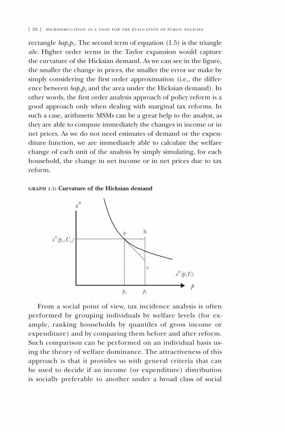
[ 26 ] m i c r o s i m u l at i o n a s a t o o l f o r t h e e va l u at i o n o f p u b l i c p o l i c i e s
rectangle bap0p1. The second term of equation (1.5) is the triangle abc. Higher order terms in the Taylor expansion would capture the curvature of the Hicksian demand. As we can see in the figure, the smaller the change in prices, the smaller the error we make by simply considering the first order approximation (i.e., the differ-ence between bap0p1 and the area under the Hicksian demand). In other words, the first order analysis approach of policy reform is a good approach only when dealing with marginal tax reforms. In such a case, arithmetic MSMs can be a great help to the analyst, as they are able to compute immediately the changes in income or in net prices. As we do not need estimates of demand or the expen-diture function, we are immediately able to calculate the welfare change of each unit of the analysis by simply simulating, for each household, the change in net income or in net prices due to tax reform.
graph1.1:CurvatureoftheHicksiandemand
From a social point of view, tax incidence analysis is often performed by grouping individuals by welfare levels (for ex-ample, ranking households by quantiles of gross income or expenditure) and by comparing them before and after reform. Such comparison can be performed on an individual basis us-ing the theory of welfare dominance. The attractiveness of this approach is that it provides us with general criteria that can be used to decide if an income (or expenditure) distribution is socially preferable to another under a broad class of social
m i c r o s i m u l at i o n a s a t o o l f o r t h e e va l u at i o n o f p u b l i c p o l i c i e s [ 27 ]
welfare functions.10 A comprehensive redistribution analysis of tax reforms (limited to first order effects) will be rounded off by computing inequality, poverty and polarization indexes (Esteban and Ray 1994). All these social welfare comparison measures can easily be computed by using arithmetical MSM. Most of them incorporate routines that automatically compute the standard measures (Gini, Atkinson, Theil, Kakwani, Reynolds-Smolensky, poverty headcount, poverty gap, etc.) and give a picture of the Lorenz and concentration curves before and after the reform.
There is an emerging body of literature applying arithmeti-cal MSM techniques in the analysis of tax reforms. Atkinson and Sutherland (1988), Merz (1991), Citro and Hanusheck (1991), Harding (1996), Gupta and Kapur (2000) and Sutherland (1998) among others, present a detailed revision of MSMs and their use in Europe and the United States. Arithmetical MSMs have also been used extensively to review indirect tax incidence (Creedy 1999). Bourguignon and Pereira da Silva (2003) present a de-tailed description of the application of MSMs for poverty and inequality analysis in LDC.
Particular attention has been given in Europe to the analysis of policy reforms at domestic and European level in an attempt to hasten the convergence of social policies. Atkinson, Bourguignon and Chiappori (1988), for example, analyse the redistribution impact of a reform in which, for a given sample of French house-holds, the French tax system is replaced by the UK’s tax system. De Lathouwer (1996) simulates the implementation of the un-employment benefit scheme enforced in the Netherlands on a sample of Belgian households, thus reflecting the importance of the sociodemographic characteristics of the population on the resulting effects. Callan and Sutherland (1997) compare the effects of different types of fiscal and social policies on the welfare of households in certain EEC countries. Bourguignon, O’Donoghue, Sastre-Descals, Spadaro and Utili (1997) use a mi-
10 For a complete survey on welfare dominance theory, see Lambert (1993). See also Atkinson (1970), Sen (1973), Kolm (1969), Shorrocks (1983), Foster and Shorrocks (1988), Bourguignon (1979), Atkinson and Bourguignon (1987), Sen (1992), Bourguignon and Fields (1997), Bourguignon and Chakravarty (2003) and Zhenhg (1997).
[ 28 ] m i c r o s i m u l at i o n a s a t o o l f o r t h e e va l u at i o n o f p u b l i c p o l i c i e s
crosimulation model to simulate the effects of the enforcement of the same child benefit scheme on the populations of France, the UK and Italy. They show that this policy can have a strong impact on the reduction of poverty in those countries.
Recently, the European Union financed EUROMOD, a research project involving researchers from the EU 15 coun-tries11 with the objective of building a European-wide MSM. This model has been used in several papers providing esti-mates of the distributional impact of changes to personal tax and transfer policy taking place at either the domestic or the European level.12
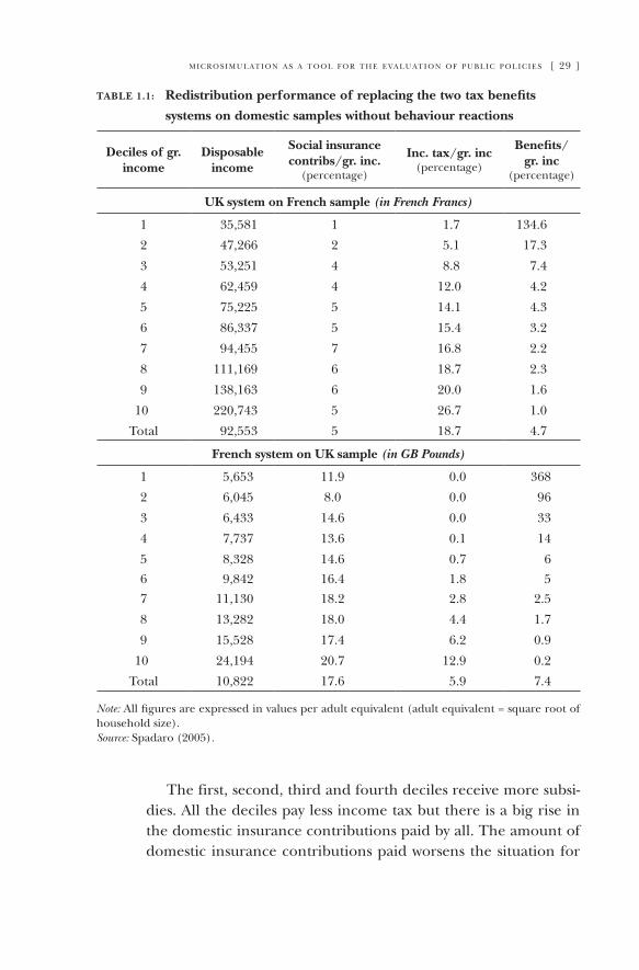
As an example of the application of arithmetical MSMs to tax reforms, we present the results of simulations performed in Spadaro (2005) consisting of applying 1995 French and British redistribution systems to two samples of households extracted from the INSEE Households Budget Survey 1989 and from the NSO 1994 Family Expenditure Survey. Simulations are per-formed using a prototype version of EUROMOD that replicates social contributions levied on wages (for employers and em-ployees) and on self-employed workers; social contributions on other types of income (unemployment benefits, income from pensions and capital returns); income taxes; family benefits and social assistance mechanisms. The results are shown in table 1.1, which shows the percentage changes in disposable income, social insurance contributions, income tax and family benefits observed by deciles of reference households’ equivalent gross income. Enforcing the UK system on the French population leads to a reduction in disposable income for the lower five deciles and an increase in income for the top five deciles. The reason for the negative effects on poor households is the reduc-tion of means-tested benefits. On the other side of the income distribution scale, rich households perform better because of the reduction in social security contributions. In the scenario based on the enforcement of the French tax-benefits system on the UK sample, the effects are the just opposite.
11 For a detailed description, see Sutherland (2001).12 Downloadable at: http://www.iser.essex.ac.uk/msu/emod.
m i c r o s i m u l at i o n a s a t o o l f o r t h e e va l u at i o n o f p u b l i c p o l i c i e s [ 29 ]
table1.1: Redistributionperformanceofreplacingthetwotaxbenefits
systemsondomesticsampleswithoutbehaviourreactions
Decilesofgr.income
Disposableincome
Socialinsurancecontribs/gr.inc.
(percentage)
Inc.tax/gr.inc(percentage)
Benefits/gr.inc
(percentage)
UKsystemonFrenchsample(in French Francs)
1 35,581 1 1.7 134.6
2 47,266 2 5.1 17.3
3 53,251 4 8.8 7.4
4 62,459 4 12.0 4.2
5 75,225 5 14.1 4.3
6 86,337 5 15.4 3.2
7 94,455 7 16.8 2.2
8 111,169 6 18.7 2.3
9 138,163 6 20.0 1.6
10 220,743 5 26.7 1.0
Total 92,553 5 18.7 4.7
FrenchsystemonUKsample(in GB Pounds)
1 5,653 11.9 0.0 368
2 6,045 8.0 0.0 96
3 6,433 14.6 0.0 33
4 7,737 13.6 0.1 14
5 8,328 14.6 0.7 66 9,842 16.4 1.8 57 11,130 18.2 2.8 2.5
8 13,282 18.0 4.4 1.7
9 15,528 17.4 6.2 0.9
10 24,194 20.7 12.9 0.2
Total 10,822 17.6 5.9 7.4
note: All figures are expressed in values per adult equivalent (adult equivalent = square root of household size).Source: Spadaro (2005).
The first, second, third and fourth deciles receive more subsi-dies. All the deciles pay less income tax but there is a big rise in the domestic insurance contributions paid by all. The amount of domestic insurance contributions paid worsens the situation for
[ 30 ] m i c r o s i m u l at i o n a s a t o o l f o r t h e e va l u at i o n o f p u b l i c p o l i c i e s
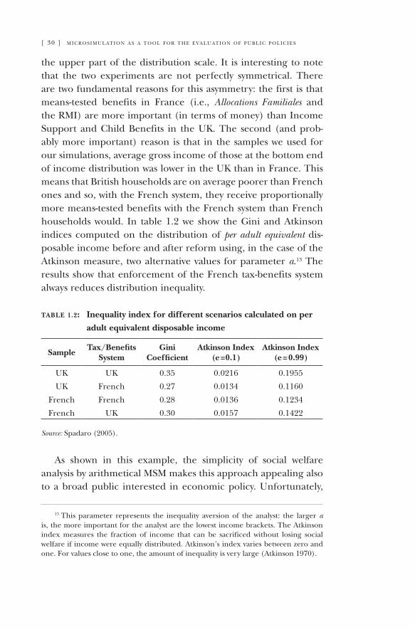
the upper part of the distribution scale. It is interesting to note that the two experiments are not perfectly symmetrical. There are two fundamental reasons for this asymmetry: the first is that means-tested benefits in France (i.e., Allocations Familiales and the RMI) are more important (in terms of money) than Income Support and Child Benefits in the UK. The second (and prob-ably more important) reason is that in the samples we used for our simulations, average gross income of those at the bottom end of income distribution was lower in the UK than in France. This means that British households are on average poorer than French ones and so, with the French system, they receive proportionally more means-tested benefits with the French system than French households would. In table 1.2 we show the Gini and Atkinson indices computed on the distribution of per adult equivalent dis-posable income before and after reform using, in the case of the Atkinson measure, two alternative values for parameter a.13 The results show that enforcement of the French tax-benefits system always reduces distribution inequality.
table1.2: Inequalityindexfordifferentscenarioscalculatedonper
adultequivalentdisposableincome
SampleTax/Benefits
SystemGini
CoefficientAtkinsonIndex
(e=0.1)AtkinsonIndex
(e=0.99)
UK UK 0.35 0.0216 0.1955
UK French 0.27 0.0134 0.1160
French French 0.28 0.0136 0.1234
French UK 0.30 0.0157 0.1422
Source: Spadaro (2005).
As shown in this example, the simplicity of social welfare analysis by arithmetical MSM makes this approach appealing also to a broad public interested in economic policy. Unfortunately,
13 This parameter represents the inequality aversion of the analyst: the larger a is, the more important for the analyst are the lowest income brackets. The Atkinson index measures the fraction of income that can be sacrificed without losing social welfare if income were equally distributed. Atkinson’s index varies between zero and one. For values close to one, the amount of inequality is very large (Atkinson 1970).
m i c r o s i m u l at i o n a s a t o o l f o r t h e e va l u at i o n o f p u b l i c p o l i c i e s [ 31 ]
there are various potential sources of inaccuracy (see Sahn and Younger 2003). The first comes from the assumption, often made when using arithmetical MSMs for tax-incidence analysis, that tax changes work through completely to consumer prices. This would be true only in the case of perfectly competitive markets (which is far from reality). A second source of inaccuracy is the fact that indirect tax reforms often concern intermediate goods and not final sales. In both cases, in order to be able to fully characterise the tax incidence on consumers, we need a model taking into ac-count the production side of the economy.
Tax evasion and non take-up of benefits are other important sources of inaccuracy that are strictly related to the ex ante nature of MSM analysis. Models are normally built under the hypothesis that taxpayers declare all their income and that any household that is entitled to a certain benefit receives financial assistance. In reality, we know that tax evasion is common prac-tice (in some countries more than in others). We also know that, for multiple reasons (lack of information, social stigma, com-plexity of administrative procedures, etc.), some households do not claim social assistance even though they are entitled to it by law.14
The most important source of inaccuracy is the absence of efficiency concerns in the above analysis. The absence of behavioural reactions prevents the analyst from considering the eventual efficiency costs (gains) of a public policy reform. Demand responses may be ignored as a first approximation when evaluating the welfare effects of a marginal tax reform. On the contrary, when the reform to be evaluated is specifically designed to induce changes in agent behaviour, when reform is not marginal or when we want to evaluate the change of the government’s budget constraint and its effects on redistribu-tion performance, we need to have an MSM that can reproduce agents’ behaviour.
14 About the take-up problem see Hancock, Pudney and Sutherland (2003). Using Econometric Models of Benefit Take-up by British Pensioners in Microsimulation Models, a paper presented at the International Microsimulation Conference on Population, Ageing and Health: Modelling Our Future, held in Canberra, Australia, in December 2003.
[ 32 ] m i c r o s i m u l at i o n a s a t o o l f o r t h e e va l u at i o n o f p u b l i c p o l i c i e s
1.3.Behaviouralmicrosimulation
This section is devoted to a discussion on behavioural MSMs and, in particular, their application in ex ante marginal incidence analysis of redistribution policies.
As with arithmetical analysis, behavioural evaluation of poli-cies often relies on household surveys. Nevertheless, they use data in a different way. The point is not to count how much everyone is receiving or paying but to generate a model representing the likely behaviour of agents as a function of variables directly af-fected by the policies being evaluated. This may be done through the estimation of a structural econometric model on the cross-section of households provided by the household survey and/or through the calibration of a model with a given structure so as to make it consistent with what is observed in the survey and supposedly corresponding to the status quo.
Tax benefit models with labour supply response in developed countries are the archetypical example of ex ante marginal inci-dence analysis. Changes in the tax benefit system in these models affect the budget constraint of households. They modify their disposable income with unchanged labour supply, but through income effects—and also through changes in the after tax price of labour—they also modify labour supply decisions. By how much is determined through a behavioural model, which is gen-erally estimated econometrically across households observed in the status quo.
The whole behavioural MSM approach comprises three steps: specifying the logical economic structure of the model being used, estimating the model and simulating it. These are consid-ered in turn using as an implicit reference the first model of this type developed by Hausman (1980, 1981, 1985).
The logical economic structure is that of the textbook utility maximizing consumption. An economic agent with character-istics z chooses his/her volume of consumption c and his/her labour supply L, so as to maximize his/her preferences rep-resented by the utility function u( ) under a budget constraint that incorporates the whole tax benefit system. Formally, this is represented by:
m i c r o s i m u l at i o n a s a t o o l f o r t h e e va l u at i o n o f p u b l i c p o l i c i e s [ 33 ]
Max u (c, L; z; ß, ε) s.t. c ≤ y0 + wL + nT(wL, L, y0; z; γ), L ≥ 0. (1.7)
In the budget constraint, y0 stands for (exogenous) non-la-bour income, w for the wage rate and nT( ) for the tax benefit schedule. Taxes and benefits depend on the characteristics of the agent, his/her non-labour income and his/her labour income wL. They may also depend directly on the quantity of labour be-ing supplied, as in workfare programmes. γ stands for the param-eters of the tax-benefit system—various tax rates, means-testing of benefits, etc. Likewise, ß and ε are coefficients that parameterise preferences. The solution of the programme yields the following labour supply function:
L = F(w, y0; z; ß, ε; γ). (1.8)
This function is non-linear. In particular, it is equal to zero for some subsets of the space of its arguments (participation condi-tion).
Suppose that a sample of agents i is observed in some household survey. The problem now is to estimate the function F( ) above or, equivalently, the preference parameters ß and ε, since all the other variables or tax-benefit parameters are actually observed. To do so, it is assumed that the set of coefficients ß is common to all agents, whereas ε is idiosyncratic. It is not observed but some assumptions can be made concerning its statistical distribution in the sample. This leads to the following econometric specification:
Li = F(zi, wi, y0i; ß, εi ; γ), (1.9)
where εi plays the usual role of the random term in standard regressions.
Estimation proceeds as with standard models, minimizing the role of the idiosyncratic preference term in explaining cross-sec-tional differences in labour supply. This leads to a set of estimates
iβ̂ for the common preference parameters and iε̂ for the idiosyn-cratic preference terms. By definition of the latter, it is true for each observation in the sample that:
[ 34 ] m i c r o s i m u l at i o n a s a t o o l f o r t h e e va l u at i o n o f p u b l i c p o l i c i e s
).;,;y γ,w,F(zLiiii
ˆ=0iβ ε̂ (1.10)
It is now possible to simulate alternative tax-benefit systems. This simply requires modifying the set of parameters γ.15 In the absence of general equilibrium effects, the change in labour sup-ply due to moving to the set of parameters γs is given by:
).;, ;y ,w ,− F(z);, ;y ,w ,F(z − LL i0iii
si0iiii
s
iγεβγεβ ˆˆˆˆ= (1.11)
The change in disposable income may also be computed for every agent. It is given by:
).;z;L,Lw,NT(y
);z;L,Lw,NT(y)L(LwCC
iiii0i
s
i
s
i
s
ii0ii
s
iii
si
γγ+=− −
−−
(1.12)
Then, one may also derive changes in any measure of indi-vidual welfare.
Several drawbacks of the preceding model must be empha-sized. In general, its estimation is not that easy. It is highly non-linear because of the non-linearity of the budget constraint and possibly its non-convexity due to the tax-benefit schedule nT( ) and corner solutions at L = 0. Functional forms must be chosen for preferences, which may introduce some arbitrariness in the whole procedure. Finally, it may be feared that imposing full economic rationality and a functional form for preferences se-verely restricts the estimates that are obtained. There has been a debate on this point ever since this model first appeared in the literature—see in particular MaCurdy, Green and Paarsch (1990).
It turns out that simpler and less restrictive specifications may be used that considerably weaken the preceding critiques. In par-ticular, specifications used in recent works consider labour supply as a discrete variable that may take only a few alternative values, and evaluate the utility of the agent for each of these values and the corresponding disposable income given by the budget con-straint. As before, the behavioural rule is then simply that agents
15 Assuming a structural specification of the nT( ) function general enough for all reforms to be represented by a change in parameters γ.
m i c r o s i m u l at i o n a s a t o o l f o r t h e e va l u at i o n o f p u b l i c p o l i c i e s [ 35 ]
choose the value that leads to the highest level of utility. However, the utility function may be specified in a very general way. In par-ticular, its parameters may be allowed to vary with the different quantities of labour that may be supplied, no restriction being imposed on these coefficients. Such a representation is therefore as close as possible to what is revealed by data.
Formally, a specification that generalizes what is most often found in the recent tax and supply-supply literature is the follow-ing:
Li = Dj if Uij = f (zi; wi,ci
j; β j,εij) ≥ f (zi; wi,ci
k; βk,εik) for all k ≠j, (1.13)
where Dj is the duration of work in the jth alternative and Uij the
utility associated with that alternative and cij the disposable in-
come given by the budget constraint in (1.7):
c j = y0 + wL + nT(wD, D, y0; z; γ). (1.14)
When the function f( ) is linear with respect to its common preference parameters and idiosyncratic terms are assumed to be iid with a double exponential distribution, this model is the standard multinomial logit. It may also be noted that it encom-passes the initial model (1.7). It is sufficient to make the following substitution:
f (zi; wi,cij; β j,εi
j)= u(cij,D j; zi, β,εi
j). (1.15)
This specification, which involves restrictions across the vari-ous supply-supply alternatives, is actually the one that is most often used.
Even under its more general form, the preceding specification might still be found to be restrictive because it relies on some utility maximizing assumption. Two remarks can be made in this respect. First, it must be clear that ex ante incidence analysis can-not dispense with such a basic assumption. The ex ante nature of the analysis requires assumptions to be made about the way agents choose between alternatives. Assuming that agents maximize some criterion defined in a different way for each alternative is not really restric-tive. Second, it is clear that if no restriction is imposed across alternatives, then the utility maximizing assumption is compatible with the most flexible representation of the way in which labour
[ 36 ] m i c r o s i m u l at i o n a s a t o o l f o r t h e e va l u at i o n o f p u b l i c p o l i c i e s
supply choices observed in a survey are related to individual char-acteristics, including the wage rate and the disposable income defined by the tax benefit system, nT( ).
That model (1.13) can be interpreted as representing utility maximizing behaviour is to some extent secondary, although this of course permits counterfactual simulations to be implemented in a simple way. What is more important is that this model fits the data as closely as possible. Interestingly enough, the only restric-tion with respect to this objective in the general expression (1.13) is the assumption that the income effect in each alternative—i.e., the j
ic argument in f( )—depends on disposable income as given by the budget constraint and the tax-benefit schedule, nT( ). The economic structure of this model thus lies essentially in the income effect. If it were not for that property, it would simply be a reduced form model aimed at fitting the data as well as possible.
In effect, the restriction that income effect must be propor-tional to disposable income seems to be a minimal assumption to ensure that this representation of cross-sectional differences in supply-supply behaviour may represent at the same time a rational choice among various supply-supply alternatives. This remark also makes perfectly clear that, within this framework, the simulated effect of a reform of the tax benefit system, nT( ), on individual labour supply is estimated on the basis of the cross-sec-tional disposable income effect in the status quo.
The role of idiosyncratic terms iε̂ or jiε̂ in the whole approach
must not be downplayed. They represent the unobserved heteroge-neity of agents’ labour supply behaviour. Thus, they may be respon-sible for some heterogeneity in responses to reform of taxes and benefits. We can see in (1.15) that agents who are otherwise identical might react differently to a change in disposable income, despite the fact that these changes are the same for all of them. All that is need-ed is for the idiosyncratic terms j
iε̂ to be different among them.Estimates of idiosyncratic terms result directly from the
econometric estimation of common preference parameters, β̂ orj
iβ̂ .16 Note, however, that it is possible to use a calibration rather
16 They would be standard residuals with specification (1.9) and most likely pseudo residuals in the discrete formulation (1.13).
m i c r o s i m u l at i o n a s a t o o l f o r t h e e va l u at i o n o f p u b l i c p o l i c i e s [ 37 ]
than an estimation approach. With the former, some of the coef-ficients β̂ or
jiβ̂ would not be estimated but given arbitrary values
deemed reasonable by the analyst. Then, as in the standard esti-mation procedure, estimates of the idiosyncratic terms would be obtained by imposing the coincidence of predicted choices under the status quo and actual choices.
It is important to emphasize that there is some ambiguity about who the agents behind the labour supply model (1.7) should be. Traditionally, the literature considers individuals, even though the welfare implications of the analysis concern households. Extending the model to households requires considering simul-taneously the labour supply decisions of all members of working age. This makes analysis more complex.
Examples of the application of the preceding model are nu-merous. A survey is provided in Blundell and MaCurdy (1999) and in Creedy and Duncan (2002). The discrete approach underlined above is best illustrated by van Soest (1995) and Aaberge et al. (1999). For an application of the calibration ap-proach, see Spadaro (2005).
A nice application of behavioural MSMs, which clearly illus-trates the potential of this approach, is the work of Blundell et al. (2000) evaluating the likely effect of the introduction of the Working Families Tax Credit (WTFC) in the UK. They estimate separately a discrete labour supply model for married couples and single parents using a sample of UK households drawn from the 1995 and 1996 Family Resources Survey. The particularity of the model estimation is that it allows for childcare costs varying with working hours. They then use the estimated model to simu-late labour supply responses under the new budget constraint using the TAXBEN MSM developed at the Institute for Fiscal Studies. The results of the analysis show that the introduction of behavioural responses reduces by 14% the estimated cost of the WFTC programme in the purely arithmetical scenario. This is mostly due to the increase in labour force participation of single mothers.
In addition to labour supply and consumption patterns, there are other dimensions of household behaviour that matter from a welfare point of view and may be affected by transfers and other
[ 38 ] m i c r o s i m u l at i o n a s a t o o l f o r t h e e va l u at i o n o f p u b l i c p o l i c i e s
public policies. Demand for schooling or health care are among them. Progresa in Mexico, Bolsa Escola in Brazil and similar condi-tional cash transfer programmes in several other countries offer a clear example of policies that can be evaluated ex ante by behav-ioural MSMs.
To have an idea about the possible application of behavioural MSMs to this type of policies, consider the Bolsa Escola pro-gramme in Brazil. It consists of a transfer to households whose income per capita is below 90 Reais (approximately US$ 45) per month, on condition that they send all their children between 6 and 15 to school. The monthly transfer is equal to 15 Reais per child going to school but is limited to 45 Reais per household. This may be considered as a conditional cash transfer programme because it combines cash transfers based on a means test and some additional conditionality—i.e., having children of school age actually going to school. As the main occupational alternative to school is work, this really is a labour supply problem similar to the one analysed above. Bourguignon, Ferreira and Leite (2003) estimate a child labour supply discrete model on all children aged 10 to 15 in households surveyed in the Brazilian sample, PnAD. After estimating all coefficients of the discrete model of the labour supply-schooling decision, the Bolsa Escola programme has been simulated on each of the households in the PnAD. The results show that the programme is indeed effective in reducing the number of poor children not going to school. Their propor-tion in the population of poor 10-15 children goes down from 8.9 per cent without the programme to 3.7 under the simulated programme. Interestingly enough, the proportion of children both going to school and engaging in some labour market activ-ity tends to increase, which suggests that the programme has little effect on child labour when children are already going to school. Another useful result of the MSM analysis in the paper is that the expected effect of the Bolsa Escola programme on poverty turns out to be rather limited. The poverty headcount goes down by only 1.3 per cent, reflecting the moderate size of the programme, the rather large dispersion of welfare levels in the poor segment of the population and the negative (child) labour supply effect of the programme.
m i c r o s i m u l at i o n a s a t o o l f o r t h e e va l u at i o n o f p u b l i c p o l i c i e s [ 39 ]
Despite the appeal of this methodology, surprisingly few ap-plications are available in developing countries. In most cases, applying it only requires a structural model of some dimension of household behaviour that permits a change to be simulated in one or several policy parameters. For instance, Younger (2002) uses this kind of approach to analyse the consequences of reduc-ing uniformly the distance to school in rural Peru. Todd and Volpin (2002) apply similar techniques to evaluate the effects of the child schooling programme Progresa in Mexico.
Some limitation of the preceding approach, which has not been mentioned explicitly before, must be stressed. First, this ap-proach is difficult to implement because it generally requires the estimation of an original behavioural model that fits the policy to be evaluated or designed, and of course the corresponding micro data. Because of this, it is unlikely that an analysis conducted in a given country for a particular policy can be applied without substantial modification to another country or another type of policy. The methodological investment behind this approach may thus be considerable. Because of this, it must be preceded by a pure arithmetical microsimulation based on simpler assumptions. Secondly, we have the fact that the behavioural approach rests necessarily on a structural model that requires a minimal set of assumptions. In general, there is no way these assumptions may be tested. In the labour supply model with a discrete choice rep-resentation, the basic assumption is that net disposable income, as given by the tax-benefit system, is what matters for occupational decisions. A reduced form model would say that the exogenous idiosyncratic determinants of the budget constraint are what matters. Econometrically, the difference may be tenuous but the implications in terms of microsimulation are huge. Finally, the strongest hypothesis is that cross-sectional income effects, as esti-mated on the basis of a standard household survey, coincide with the income effects that will be produced by the programme under study or reforms in the same. In other words, time income effects for a given agent should coincide with the effect of cross-sectional income differences. Here again, this is a hypothesis that is hard to test and yet absolutely necessary for ex ante analysis. Nothing is possible without it. The only test one can think of would be to
[ 40 ] m i c r o s i m u l at i o n a s a t o o l f o r t h e e va l u at i o n o f p u b l i c p o l i c i e s
combine ex ante and ex post analysis. For instance, one could try to run some ex ante analysis on a household survey taken prior to the implementation of the reform, and then compare it with the results obtained in the ex post evaluations conducted for that programme. Coincidence would support the hypothesis that cross-sectional and time individual specific income effects are identical.
Because of some potentially strong hypotheses, there is cer-tainly some uncertainty about the predictions that come out of ex ante marginal incidence analysis based on behavioural MSMs. That said, this tool is necessary to optimise the design of policies likely to generate strong behavioural responses. A pure account-ing approach to marginal incidence analysis is an indispensable first step. However, although it may be considered a cutting edge technique, introducing behaviour on an ex ante basis is highly desirable in several fields of public policy.
1.4.Microsimulationandnormativepolicyevaluation
One of the major benefits of extending the framework of policy evaluation analysis to second order effects by including agent be-haviour reactions is that it allows us to perform comparative social welfare analysis of policy scenarios both in a positive and normative way. By using an MSM we are able to characterize the true budget constraint faced by agents, improving the reality of the rational decision-making process representation.17
Starting from the computation of the individual utility func-tion, we can evaluate any social welfare function (previously de-fined). Calling the individual indirect utility function V(p,y), as in section 1, we can write a social welfare function (SWF) as:
17 Offering his opinions on the subject, Mirrlees (1986 chap. 24, p. 1198) states: “[...] There are, it seems to me, only two promising approaches to making well based recommendations about public policy. One is to use a welfare function of some form and develop the theory of optimal policy. The other is to model the existing state of affairs in some manageable way, and on that basis to display the likely effects of changes in government policy, these effects being displayed in sufficient detail to make rational choice among alternative policies possible. If a welfare function were used to evaluate the changes predicted, the second approach would come fairly close to the first, and in fact, there is a closer theoretical relationship.”
m i c r o s i m u l at i o n a s a t o o l f o r t h e e va l u at i o n o f p u b l i c p o l i c i e s [ 41 ]
∑=
=n
iSWF
1G[Vi(p,yi)], (1.16)
where n is the number of agents in the population and G[Vi ] is the social perception of individual welfare. In other words, G[Vi ] is the weight the government puts on the welfare of individual i. The concavity of G[ ] gives us the level of aversion to inequality embedded in the social welfare function.
With such a framework, we can perform a social evaluation of a policy implementation by evaluating the SWF before and after the reform. This is a positive approach used in several papers ap-plying behavioural MSMs to the evaluation of fiscal reforms. In most of these works,18 following a methodology proposed by King (1983), the indirect utility function Vi( ) has been replaced by the money metric utility function ye defined as (using the same nota-tion as in section 1.1).
ye= E(p1,Vi(p0,y)). (1.17)
The advantage of using (1.17) is that it does not depend on the cardinalization of the utility functions used. A drawback is that equivalent income function is not guaranteed to be concave. This means that the SWF could favour inequality increasing transfers.19
An alternative route is to use behavioural MSMs for normative analysis of public policies. In several situations, instead of being concerned with the comparison of two or more given situations (for example, before and after reform), we want to solve the problem of finding the optimal redistribution policy, i.e., the policy that maximises a SWF under certain efficiency and/or ag-gregate budget constraints. This is a normative approach widely known in public economic theory.
Probably the most interesting (for our purposes) theoreti-cal contributions are optimal taxation models (Ramsey 1927; Atkinson and Stiglitz 1980; Diamond and Mirrlees 1971a 1971b;
18 A recent survey is found in Aaberge, Colombino and Strøm (1998a). See also Aaberge, Colombino and Strøm (1998b, 1999, 2000, 2001), Aaberge, Colombino, Strøm and Wennemo (2000) and Aaberge, Colombino and Wennemo (2002).
19 Blackorby and Donaldson (1988) give the conditions that satisfy the concavity of SWF under this approach: the individual utility function must be quasi-homothetic.
[ 42 ] m i c r o s i m u l at i o n a s a t o o l f o r t h e e va l u at i o n o f p u b l i c p o l i c i e s
and Mirrlees 1971). These models highlight the trade-off between equity and efficiency that characterises public decisions regard-ing redistribution policies. Concerning optimal direct taxation, the work of Mirrlees (1971), extended by many other authors (Tuomala 1990), shows that optimal income tax depends funda-mentally on government aversion to inequality, on the behaviour of economic agents in terms of effort supply and on the distribu-tion pattern of the population’s productivities. Optimal indirect taxation’s main results are that government must levy more tax on goods whose demand is less elastic to prices (Ramsey 1927) and, concerning equity, must tax more the goods consumed in a higher proportion by richer agents (Diamond and Mirrlees 1971a; 1971b).
In both frameworks, the problem addressed is that of a govern-ment that, using as a control variable the tax function, wants to maximise a social welfare function as in (1.16) under an aggre-gate budget constraint defining exogenously the average redistri-bution. Agents take as given the tax function and price levels, and decide the optimal level of consumption and/or labour supply by maximising their utility function. Solving such a social planner problem gives us the redistribution mechanism that achieves the equity objectives of the government by minimizing the efficiency negative effects of the resource reallocation.
With behavioural MSMs it is now possible to test, in reality, the predictions for these theoretical models. The first intuitive application of behavioural MSMs in this field is the computation of the optimal redistribution policy. If the optimal redistribution problem is mathematically simple (for example, when the tax instrument is linear with one or two brackets),20 and if the compu-tational power of the machine is higher, we can perform optimal tax calculation starting from the specification of a social welfare function. This computational approach is largely used in dynamic optimal taxation papers (Judd et al. 2000).
Another possible direction, easier to follow, is to define a dis-crete set of possible redistribution mechanisms allowing for the same aggregate average redistribution and, by simulating each
20 As in Stern (1976) and in Slemrod et al. (1994).
m i c r o s i m u l at i o n a s a t o o l f o r t h e e va l u at i o n o f p u b l i c p o l i c i e s [ 43 ]
alternative with a behavioural MSM, to compute individual and social welfare functions. By this means, it is possible to look for the best redistribution policy in a framework very similar to the optimal tax framework. An example of this approach is found in Spadaro (2005), in which direct redistribution systems, inspired by the 1995 French and UK ones, are simulated on samples of French and UK households in order to find the best of all possible alternatives. The main difficulty that such a simulation must overcome when applied to real redistribution systems is the constraint that average redistri-bution must remain unchanged under each redistribution scheme. A frequently used methodology (see, for example, Bourguignon et al. 1997) dealing with this problem is to redistribute as a subsidy/tax proportional to consumption the eventual surplus/deficit. This lump sum subsidy/tax has an effect on the labour supply of indi-viduals (the so-called third round effect) that must be taken into account in optimal tax calculation. It is thus necessary to iterate the problem several times in order to find the proportional tax rate that satisfies the aggregate net tax receipt constraint.
This type of social evaluation of public policies is a discrete version of the original theoretical models, in the sense that it analyses a discrete set of redistribution instruments. A continuous version of the analysis, more similar in content to the Diamond and Mirrlees (1971a, 1971b) and Mirrlees (1971) frameworks, is one where MSMs are used to characterize redistribution systems. The effective marginal tax rate (together with the average tax rate) gives us a complete characterization of the redistribution performance of a given tax-benefits system. This characteriza-tion is then used as an input of the optimal tax model, which is inverted in order to recover the implicit social welfare function embedded in the true redistribution system analysed.21 In other words, instead of taking the social welfare function as given and deriving the optimal schedule of effective marginal tax rates along the income or consumption patterns, the same process is run in reverse. This approach has been used by Bourguignon and Spadaro (2002) for direct taxes, and by Christiansen and Jansen
21 The inversion of the optimal problem is a methodology applied in economics for the first time by Kurz (1968) to growth models.
[ 44 ] m i c r o s i m u l at i o n a s a t o o l f o r t h e e va l u at i o n o f p u b l i c p o l i c i e s
(1978) and Ahmad and Stern (1984) for indirect taxes. In these works, the focus is on the social welfare function that optimizes the effective marginal tax rates schedule corresponding to the redistribution system actually in place. In effect, the approach described is simply a way of reading the redistribution schedule characterized by the MSM.
Christiansen and Jansen (1978) specify a parametric social welfare function making it possible to separate and quantify three different effects by inverting the optimal tax model starting from the Norwegian data and indirect tax system. First, it provides a condensed quantitative measure of the degree of income inequal-ity aversion. Second, a set of parameters evaluates the external social costs induced by the consumption of certain commodities. Finally, the function allows estimation of implicit equivalent in-come scales. The authors consider the results a source of informa-tion about an important part of Norwegian tax policy.
Ahmad and Stern (1984) apply the inversion of the optimal problem approach to look at the possibility of a Pareto-improv-ing indirect tax reform in India. After giving the theoretical conditions for the existence of a Pareto social welfare function maximizing the optimal tax problem assumed to be behind the observed indirect tax system, they microsimulate indirect tax reforms showing that taxes on cereals, fuel and light are less so-cially desirable than a tax on clothing (for a class of Pareto social welfare functions).
More recently, Kaplanoglou and Newbery (2003) apply the same approach as in Ahmad and Stern (1984) to assess the distri-butional and efficiency aspects of the Greek indirect tax system, identifying welfare improving directions of reform simply by re-placing the present tax system with the UK’s.
Bourguignon and Spadaro (2002) show how the character-istics of any given redistribution system for any country may be expressed in social welfare terms and, by using the EUROMOD MSM, analyze the social welfare properties of the redistribution system of France, UK and Spain in 1995. Interestingly, they find that revealed social preferences satisfy the usual regularity as-sumption—positive and decreasing marginal social welfare—as long as the wage elasticity of labour supply is below a given thresh-
m i c r o s i m u l at i o n a s a t o o l f o r t h e e va l u at i o n o f p u b l i c p o l i c i e s [ 45 ]
old. For Spain and the UK, this threshold stands reasonably above the range of available econometric estimates of the wage elasticity of labour supply. In the case of France, however, the threshold is much lower, so it cannot be ruled out that revealed social prefer-ences are non-Paretian beyond a certain income level.
An application of inversion of the optimal labour income tax problem has also been performed by Oliver and Spadaro (2002). They analyse how social preferences on inequality have changed with the 1999 reform of income tax in Spain.
The methodology discussed in this section must be considered as a first attempt to compare alternative real tax-benefits systems in a normative framework. The nature of the results must be con-sidered as exploratory for several reasons. First, the election of a particular functional form or a particular dataset always influences result (see Stern 1976, 1986). For this reason, when applying mi-crosimulation techniques for normative analysis, it is important to look at the results of the application of different functional forms and/or the key parameters of the model. Second, results always depend on the statistical properties of the sub-sample used in the simulations, as well as the numerical computation techniques em-ployed. It is therefore important to perform a robustness analysis of the simulations (see Spadaro 2005).
Despite its limitations, this type of normative social welfare evaluation based on the use of behavioural MSMs is useful for the practical interest of reading present tax-benefit systems through the social preferences they reveal. Such an approach is very useful for the comparative analysis of different countries’ fiscal reforms, and to measure the extent of their similarities in social policies. It also allows different states’ policies to be simulated in other countries, helping identify and draw on the most beneficial inter-national practices.
1.5.Recentextensionsanddirectionsforfutureresearch
Microsimulation techniques are not necessarily restricted to the analysis of fiscal and social policies. They also have potential uses
[ 46 ] m i c r o s i m u l at i o n a s a t o o l f o r t h e e va l u at i o n o f p u b l i c p o l i c i e s
in analyzing the heterogeneity of the effects of every change in agents’ economic environment. For this reason, several research directions can be defined. A first important direction would consist of ensuring that adequate, issue-specific, macroeconomic frameworks are chosen and adapted to provide a guide for mi-crosimulations while fully utilizing the heterogeneity found in household surveys. Thus combining macro modelling with MSM techniques would allow an integrated macro-micro analysis of redistribution policies. A second direction consists of extending the MSM analysis to a dynamic framework. A third interesting re-search direction is the extension of the work done in household MSM to the analysis of firms’ behaviour. In the sections that fol-low, we look briefly into these three issues.
1.5.1. MacroeconomicanalysisandmicrosimulationmodelsOne of the most promising directions of research consists of
seeking a true integration between macro models and the MSM approach. The problem is how to do this. In this section, we ex-plore three possibilities but also stress some difficulties.
A first possible approach is to use microsimulation techniques to build a link between the macro environment and micro vari-ables influencing individual behaviour. This approach is very similar to the one used by Juhn, Murphy and Pierce (1993) to analyse the effects of changes in the US labour market on wage distribution. The basic model (inspired by the Oaxaca-Blinder methodology) is based on a parametric representation of the way in which individual earnings are linked to household or individual sociodemographic characteristics or endowments, and the market returns of such characteristics (which are influenced by the macroeconomic environment as well as by the redistribu-tion mechanism) (see Oaxaca 1973 and Blinder 1973).
The model sets the agent’s wage as follows:
w(i)= X(i)b(i) + e(i), (1.18)
where i = 1, 2 represents the period of observation. In other words, the wage observed in period t is supposed to depend linearly on a vector of his/her observed characteristics, X(i), and on some unobserved characteristics summarized by the
m i c r o s i m u l at i o n a s a t o o l f o r t h e e va l u at i o n o f p u b l i c p o l i c i e s [ 47 ]
residual term, e(i). The coefficients b(i) simply map individual characteristics X into wage w. The components of X are seen as individual endowments; the b’s may be interpreted as rates of return on those endowments or as the prices of the ser-vices associated with them. The microsimulation they perform consists of computing the wages that the agents would earn in period 1 if the parameters b( ) were those of period 2. In other words, they analyse the difference between w(1) and the microsimulation:
w(0) = X(1)b(2) + e(1). (1.19)
The change b(1) to b(2) plays here the same role as a change in the tax system in arithmetical MSMs. It can be due to changes in the institutional/political framework, to macroeconomic shocks or simply to the structural evolution of the economy (tech-nological progress, etc.).
Bourguignon, Fournier and Gurgand (2001) and Bourguignon, Ferreira and Leite (2003) have generalized this approach to the household income generation process. In this case, the MSM behind the model is a little bit complicated, but it also improves the ways we can link the macroeconomic framework with micro-economic agent behaviour.
A second possible approach concerns the full integration of MSMs within Computable General Equilibrium models (CGE). CGEs are often based on the assumption of representative agents (households or individuals). The first possibility would be to move from representative to real households within the CGE approach. Theoretically, this can be done. We simply need to replace a small number of representative households by the full sample in the household survey. However, this requires the speci-fication of a behavioural model at individual or household level. This could be done by estimating the structural form of micro models of occupational choices, labour supply and consump-tion behaviour while allowing for appropriate individual fixed effects (along the lines described in section 1.2.) This would also generally require the assumption that all individuals operate in perfect markets and are unconstrained in their choices. It is likely that advances in computational capability will make it easier to
[ 48 ] m i c r o s i m u l at i o n a s a t o o l f o r t h e e va l u at i o n o f p u b l i c p o l i c i e s
build and estimate this type of model in the future. Of course, there may be intermediate solutions between working with a few representative household groups and several thousands of real households. For instance, one might be satisfied expanding the original representative household approach to several hundreds of households, defined for instance on the basis of the clusters typically found in household survey samples. In any case, most of the work to achieve full integration in these models still needs to be done (see Savard 2003; Aaberge et al. 2004).
A third possibility, also following the route of integrating an MSM with a CGE, is to implement a sequential approach (also called top-down approach). This alternative generalizes the micro-simulation approach described for the ex ante marginal incidence analysis of taxation and public spending (section 1.1). But now, the incidence analysis is made on the basis of changes in consumer/producer prices, wages and sectoral employment levels as predict-ed by some (disaggregated) macroeconomic model. The idea is to have the changes in the coefficients of earnings, self-employment income, occupational choice functions and prices provided by a macro model (for example, a CGE) and to use it as an input for an MSM that distributes the effects of the macro changes among households (Chen and Ravallion 2003).
The basic difficulty is to achieve consistency between the micro and macro levels of analysis. Implementing price and wage changes obtained with a macro model at the micro level is not difficult and essentially mirrors the standard incidence analysis. Implementing changes in occupation—due for instance to the contraction of the formal sector and employment substitution in the informal sector—is a more difficult proposition. A method for doing so has been developed by Bourguignon, Robilliard and Robinson (2001) (see also Ferreira et al. 2002; Labandeira and Labeaga 1999) in a model that simulates the effects of the 1997 crisis in Indonesia. They propose a model in which the household (real) income generation model consists of a set of equations that describe the earnings and the occupational status of its members according to the labour market segment where they operate. These equa-tions are estimated econometrically on a sample of observations for a given base year. They are all idiosyncratic, in the sense that
m i c r o s i m u l at i o n a s a t o o l f o r t h e e va l u at i o n o f p u b l i c p o l i c i e s [ 49 ]
they incorporate fixed individual effects identified by standard regression residuals. A microsimulation would then consist of modifying all or part of these equations (following an approach very similar to the one described in section 1.2.) For instance, one might want to analyse the effect on poverty of changing the price of farm products—i.e., modifying the corresponding self-employment income function in the appropriate proportion—or wages in a particular labour market segment, or of modifying occupational choice behaviour in favour of some specific occupa-tion, e.g., wage work.
Suppose that a macro model (CGE, econometric, pure fore-casts) gives counterfactual information on the variables entering the household income model, but at the aggregate level. In other words, the macro model yields information on linkage variables like the aggregate level of wages by labour segment, the price of the output of self-employment sectors, the aggregate level of em-ployment by type of occupation, the structure of consumer prices. The idea is to modify some parameters in the equations of the household (real) income generation model so as to make the aggregate results of the microsimulation consistent with the linkage variables.22
This operation is easy for variables like wage or self-employ-ment income. It is sufficient to multiply the equations by some parameter until the mean wage or self-employment income in the microsimulation framework coincides with the value of the linkage variables provided by the macromodel. Things get more complicated with occupational choices because the correspond-ing functions are not linear. Yet, tâtonnement may be undertaken on specific parameters of these functions so as to ensure that the aggregate employment structure resulting from the microsimula-tion is consistent with the information provided by the macro-model through the linkage variables. No feedback is actually necessary for the idiosyncratic consumer price index.
The top-down route can be easily combined with standard marginal incidence analyses of changes in public expenditures, taxation and safety nets that could accompany the macro shocks and policies being studied. Note, however, that it does not permit
22 These parameters are the equivalent of b(i) in equation (1.18).
[ 50 ] m i c r o s i m u l at i o n a s a t o o l f o r t h e e va l u at i o n o f p u b l i c p o l i c i e s
identification of the feedback effect of these accompanying mea-sures (e.g., safety nets) at the macro level.
Interestingly, this approach can work with very different types of macro frameworks. The choice will depend on the specific issue being studied and the availability of modelling tools. CGE models will of course typically be used to study the effect of struc-tural reforms like trade policies or indirect taxation, whereas dis-aggregated macroeconometric models might be preferred when dealing with aggregate demand issues or financial or exchange rate crises.
1.5.2. IntroducingdynamicsMuch of what we have just said about the possible linkage
between micro and macro phenomena refers to a static frame-work. Both the intermediate disaggregated multi-sector CGE-like model and the MSM framework are likely to rely on some kind of medium-run equilibrium assumptions. This is certainly true for the allocation of flexible factors of production across sectors in the intermediate model. However, it is also true for occupational choices and earning equations in MSMs. Even though the usual residuals of econometric estimation reflect ad-justment mechanisms, they are interpreted in the MSM frame-work as individual fixed effects and are thus transformed into a kind of permanent component. Such a static framework may be inappropriate in situations where dynamics are important for the object of the analysis like, for instance, in pension system reforms or the analysis of the poverty effects of macroeconomic crises.
We can take dynamics into account directly at the macro level by using augmented or inter-temporal CGE models to get macro predictions and, as explained in section 1.5.1, to translate them to a micro framework using prices and wages as an MSM input. They may be a good tool but rely on assumptions about expecta-tions formation that are unrealistic, and make them more fit for the analysis of very long-run phenomena (Browning, Hansen and Heckman 1999).
m i c r o s i m u l at i o n a s a t o o l f o r t h e e va l u at i o n o f p u b l i c p o l i c i e s [ 51 ]
A good alternative is to make microsimulation truly dynamic.23 In dynamic MSMs, the objective is to reproduce individual life cycle paths consistent with observed social phenomena. This es-sentially involves “updating each attribute for each micro-unit for each time interval” (Caldwell 1990, 5). Such updating can be probabilistic or behavioural.
Probabilistic updating is done by using transition matrix methods or by using random processes to simulate changes in the agent’s attributes. The transition matrix methods start from the description of the population by a state vector St giving the partition of the population at time t in a number J of classes. The updating of the state vector for each time period is done by apply-ing a transition matrix Mt whose elements mij give the (exogenous) probability for an agent in class j at time t to be in class i at time t+1. This type of updating consists of a chain of matrices products
St+n= St ∏Mh.t+n−1
h=t
The main problem with this updating approach is that aug-menting the number of partitions J implies the exponential growth of the size of the transition matrix and consequently of the problems of numerical computation. From an operational point of view, the size of J is normally not large enough to ensure complete accounting for agent heterogeneity. Instead of using transition matrix methods, a possible probabilistic alternative is to apply the updating process for each period directly to individual data. For variables that can be considered deterministic, it is suf-ficient to clearly specify the updating rule. For example, in the case of age it is sufficient to define the rule: age(t+1)= age(t)+1. For variables following stochastic processes, the updating can be done by pseudo-random lotteries. The idea is the following: imagine that we can model the probability P(t) to become unemployed at t+1 (being employed at t) as a function of a vector of variables X(t) including, for example, individual variables such age, sex, etc., and
23 On dynamic microsimulation of household behaviour, see Harding (1993), O’Donoghue (1999) and Zaidi and Rake (2001). See also Dupont, Hagneré and Touzé (2003) for a survey on dynamic MSM applied to pensions system analysis.
[ 52 ] m i c r o s i m u l at i o n a s a t o o l f o r t h e e va l u at i o n o f p u b l i c p o l i c i e s
also economic environmental variables such as unemployment rate, growth rate, etc.; we can then compute P(t) for each agent as P(t)= f[X(t)]. The next step is to extract a random variable R in a uniform distribution of support [0;1] and to update the oc-cupational status of each individual by comparing R with P(t). It is immediately obvious that the choice of comparison rule is a key pa-rameter of the analysis. In the example, if you are concerned with a particular unemployment rate (say 10%) then you will fix the rule in such a way as to guarantee that only 10% of potential workers will be unemployed. The main advantage to this method is that it is applied to each agent in the sample and keeps intact all the in-formation about population heterogeneity. On the downside, this method produces stochastic results that reduce the robustness of the analysis conducted on subsamples of small size. For this rea-son, it is important when presenting the results of different types of simulations to perform robustness analyses by the Montecarlo or Bootstrapping methods (Bradley and Tibshirani 1993).
In behavioural updating, agents change their characteristics as the result of endogenous mechanisms within the model. This means that one must model the decision-making process on labour supply, consumption, savings, marriage, fertility, etc., in function of some exogenous (for the agent) variables, along the lines explained in section 1.2.24 As for static behavioural models, a weakness of this behavioural updating approach is that the results are strongly influenced by the functional forms chosen at individual level for the simulations.
The general problem with dynamic MSMs is that their con-struction presents several difficulties. Besides the intrinsic diffi-culty of estimating econometrically dynamic individual behaviour, the large data requirement, the difficult task of validation and the amount of resources (financial and personal) consumed, make them a less frequent option than static MSMs.25 However, despite these difficulties, it seems likely that dynamic MSMs will become more numerous in the future. A key reason is that they allow the
24 For an in-depth description of this type of updating and its advantages/disadvantages, see Klevmarken (1997).
25 This explains why most dynamic MSMs to date have been built by public administration services or public research institutions.

m i c r o s i m u l at i o n a s a t o o l f o r t h e e va l u at i o n o f p u b l i c p o l i c i e s [ 53 ]
analysis of policy issues that are on the agenda of any government, including, for instance, the social and economic implications of population ageing. Health issues also seem to be gaining greater prominence given that the evolution of the socioeconomic situa-tion seems to be one of the strongest predictors of health status. Several policies of interest may be simulated in such a framework, but they are for the moment limited in scope. Here again, more work is needed to see how we can go in that direction.
1.5.3. Firms,institutionsandinvestmentclimateWhile allowing for a much more detailed representation of
occupational choices, income generation, etc., the MSM ap-proach remains circumscribed to the activity, income and/or expenditure of households in the economy, i.e., it ultimately deals with private consumption, the labour market and possibly wealth accumulation. The techniques developed to microsimulate the demand side of the economy can be extended to the production side by building a corporate behaviour MSM using industrial survey instead of household survey data. Van Tongeren (1995) presents a detailed explanation of the methods and results of corporate MSMs.
With such MSMs we can run analysis of public policies at three levels at least. The first level is the incidence analysis level. For a sample of firms, this would simply consist of measuring the subsi-dies and taxes on their income (profit) and investment. With sim-ple assumptions about average tax rates, the average incidence analysis conducted for household (in section 1.1) could be repli-cated. The second level includes the modelling of firms’ output and demand for inputs (capital and labour) as dependent upon the levels of subsidies and taxes. In particular, the relationship between firms’ output and investment levels could be fed back into the economy’s price levels and hence into the type of analysis conducted with households. Of course, if we want to pursue this direction, we should be aware at all times that the demographics of firm creation and destruction are more complex than that of a population of households. The third level would involve, as with households, choosing a macroeconomic framework and adapt-ing it to provide a guide for firm microsimulations. The ability to
[ 54 ] m i c r o s i m u l at i o n a s a t o o l f o r t h e e va l u at i o n o f p u b l i c p o l i c i e s
disaggregate the productive sectors in the macro model by size of firm could be of significant importance. In particular, accounting for different investment, borrowing or hiring behaviour by differ-ent sized firms within the same sector could help us understand the interaction between small, medium and larger enterprises. This could have implications both at the macroeconomic level and for distribution (e.g., wage differentiation, profit distribu-tion, exit and entry of firms).
A behavioural MSM for companies is particularly useful when we want to evaluate the effect of policies involving changes in their institutional environment (this is particularly important in developing countries). Starting from incidence analysis of the in-vestment climate variables on firms’ investment, pricing and hiring behaviour identified by such an MSM, we could measure, firstly, the different types of effects of the investment climate on the level and structure of economic activity and then its effect on the real-location of resources at the micro level.
1.6.Conclusions
The efficiency and sustainability of reforms could be greatly enhanced by systematically evaluating their full distributional impact. This is easily done in some instances, under the assump-tion of no behavioural response, as long as satisfactory house-hold and community surveys are available. Simple microsimula-tion tools can be developed on that basis, and indeed should be used more systematically. Extending the analysis to cover some dimension of household behavioural responses and the poten-tial macroeconomic effects of reform requires investing more in microeconomic and macroeconomic modelling. Several at-tempts in this direction show the benefits that policy makers could draw from this kind of instrument. Such techniques also broaden the range of reforms that can be precisely evaluated from a distributional point of view, but other applications must be developed and existing methods must be improved. This calls for more research effort.
m i c r o s i m u l at i o n a s a t o o l f o r t h e e va l u at i o n o f p u b l i c p o l i c i e s [ 55 ]
References
aaberge, R., U., colombino, H. holmøy, B. strøm and T. Wennemo. Population age-ing and fiscal sustainability: An integrated micro-macro analysis of required tax changes. Working Paper CHILD 6, 2004.
aaberge, R., U. colombino and S. strøm. “Social Evaluation of Individual Welfare Effects from Income Taxation.” Statistics norway, Discussion Paper 230 (1998a).
—. “Evaluating Alternative Tax Reforms in Italy with a Model of Joint Labour Supply of Married Couples.” Structural change and Economic Dynamics 9: 415–433.
—. “Labour Supply in Italy: An Empirical Analysis of Joint Household Decisions, with Taxes and Quantity Constraints.” Journal of Applied Econometrics 14: 1999, 403–422.
—. “Labour supply responses and welfare effects from replacing current tax rules by a flat tax: empirical evidence from Italy, Norway and Sweden.” Journal of Population Economics 13(4): 595–621.
—. Do More Equal Slices Shrink the cake? An Empirical Evaluation of Tax–Transfer Reform Proposals in Italy. Working Paper CHILD 19, 2001.
ahmad, E. and N. stern. “The Theory of Reform and Indian Direct Taxes.” Journal of Public Economics 25.
atkinson, A. “On the Measurement of Inequality.” Journal of Economic Theory, vol. 2.atkinson, A. and F. bourguignon. “Income Distribution and Differences in Needs.”
In G. R. Feiwel (ed.). Arrow and the Foundation of the Theory of Economic Policy. London: MacMillan, 1987.
atkinson A., F. bourguignon and P. A. chiappori. “What Do We Learn About Tax Reforms from International Comparisons? France and Britain.” European Economic Review 32, 1988.
atkinson, A. and J. stiglitz. Lectures on Public Economics. McGraw Hill International Editions, 1980.
atkinson, A. and H. sutherland. Tax Benefit Models. ST/STICERD, LSE. London, 1988.
blackorby, C. and D. donaldson. “Money Metric Utility: A Harmless Normalisation?” Journal of Economic Theory 46 (1998): 120–1209.
blinder, A. “Wage Discrimination: Reduced Form and Structural Estimates.” Journal of Human Resources 8 (1973): 436–455.
blundell, R., A. duncan, J. mccrae and C. meghir. “The Labour Market Impact of The Working Families’ Tax Credit.” Fiscal Studies 21(1), 2000.
blundell, r. W. and t. macurdy. “Labour Supply: a Review of Alternative Approaches.” Handbook of Labour Economics vol. 3. Ashenfelter and Card eds. North Holland, 1999.
bourguignon, f. “Decomposable Inequality Measures.” Econometrica 47 (1979): 901–920.
bourguignon, f. and s. r. chakravarty. “The Measurement of Multidimensional Poverty.” Journal of Economic Inequality, 1 (2003): 25–49.
bourguignon, f., f. ferreira and p. leite “Beyond Oaxaca–Blinder: Accounting for Differences in Household Income Distributions Across Countries.” World Bank. Policy Research Working Paper 2828, 2002.
bourguignon, f. and g. fields. “Discontinous Losses from Poverty, Generalized Measures and Optimal Transfer to Poors.” Journal of Public Economics 63 (1997): 155–175.
[ 56 ] m i c r o s i m u l at i o n a s a t o o l f o r t h e e va l u at i o n o f p u b l i c p o l i c i e s
bourguignon, f., m. fournier and m. gurgand. “Fast Development with a Stable Income Distribution: Taiwan, 1979–1994.” Review of Income and Wealth 47 no. 2 (2001): 1–25.
bourguignon, f., c. o’donoghue, J. sastre, a. spadaro and f. utili. Eur3: A Prototype European Tax-benefits Model. DAE Working Paper no. 9723. Micro-simulation Unit, Cambridge University, 1997.
bourguignon, f. and l. pereira da silva. The Impact of Economic Policies on Poverty and Income Distribution: Evaluation Techniques and Tools. The World Bank, 2003.
bourguignon, f., a. s. robillard and s. robinson. “Crisis and Income Distribution: A Micro Macro Model for Indonesia.” The World Bank. Mimeo, 2001.
bourguignon, f. and a. spadaro. “Tax-Benefit Revealed Social Preferences: Are Tax Authorities Non-Paretian?” DELTA. Mimeo, 2002.
bradley, e. and J. tibshirani. An Introduction to the Bootstrap. New York: Chapman and Hall eds., 1993.
breuil-grenier, p. “Les enseignements théoriques et pratiques des microsimulations“Les enseignements théoriques et pratiques des microsimulations en économie de la santé.” Economie et Statistique 315 (1998): 73–94.
broWning, m., l. p. hansen and J. heckman. “Micro Data and General Equilibrium Models.” In Handbook of Macroeconomics vol. 1. Taylor and Woodford eds., North Holland, 1999.
caldWell, s. b. “Static, Dynamic and Mixed Microsimulation.” Working Paper Department of Sociology, Cornell University, 1990.
chen, s. and m. ravallion. “Households Welfare Impacts of China’s Accession to the World Trade Organization.” World Bank. Policy Research Working Paper 3040, 2003.
christiansen, V. and E. Jansen. “Implicit Social Preferences in the Norwegian System of Indirect Taxation.” Journal of Public Economics, vol. 10 (1978): 217–245.
citro, C. and E. hanushek. “Improving Information for Social Policy Decision—The Uses of Microsimulation Modelling.” Washington DC: National Academic Press, 1991.
creedy, J. “Modelling Indirect Taxes and Tax Reform.” USA: Edward Elgar, 1999.creedy, J. and A. duncan. “Behavioural Microsimulation with Labour Supply
Responses.” Journal of Economic Surveys 16 (2002): 1–38.de lathouWer, L. “A Case Study of Unemployment Scheme for Belgium and The
Netherlands.” Microsimulation and Public Policy. Amsterdam: North Holland, Harding editor, 1996.
diamond, P. “Optimal Income Taxation: An Example with a U-Shaped Pattern of Optimal Marginal Tax Rate.” American Economic Review, vol. 88, 1 (1998): 83–95.
diamond, P. and J. mirrlees. “Optimal Taxation and Public Production: I–-Production Efficiency.” American Economic Review, vol. 61, iss. 1 (1971a): 8–27.
dupont, G., C. hagneré and V. touzé. “Les modèles de microsimulation dynamique dans l’analyse des réformes des systèmes de retraites: une tentative de bilan.” Mimeo, 2003.
esteban, J. M. and D. Ray. “On the Measurement of Polarization.” Econometrica 62 (1994): 819–852.
ferreira, F., P. leite, perera da silva and P. picchetti. “Financial Volatility and Income Distribution: Assessing Winners and Losers of the Brazilian 1999 Devaluation Using a Macro-Financial Econometric Model Linked to
m i c r o s i m u l at i o n a s a t o o l f o r t h e e va l u at i o n o f p u b l i c p o l i c i e s [ 57 ]
Microsimulations.” Paper presented at the FIPE-World Bank Conference July 2002, São Paolo (Brasil), 2002.
forster, J. and A. shorrocks. “Poverty Orderings.” Econometrica 56 (1998): 173–177.gruber, J. “Tax Subsidies for Health Insurance: Evaluating the Costs and Benefits.”
NBER Working Paper 7553, 2000.gupta, A. and V. kapur. Microsimulation in Government Policy and Forecasting. Amsterdam:
North Holland, 2000.harding, A. Lifetime Income Distribution and Redistribution. Applications of a Microsimulation
model. Amsterdam: North Holland, 1993.—. Microsimulation and Public Policy. Amsterdam: North Holland, 1996.hausman, J. “Labour Supply.” In How Taxes Affect Economic Behaviour. Aaron and
Pechman eds. Washington DC: Brookings Institution, 1981.—.“The Effect of Wages, Taxes and Fixed Costs on Women’s Labour Force
Participation.” Journal of Public Economics, 14 (1980): 161–194.—.“The Econometrics of Nonlinear Budget Set.” Econometrica 53 (1985): 1255–82.Judd K., F. kubler and K. schmedders. “Computational Methods for Dynamic
Equilibria with Heterogeneous Agents.” Stanford University, Mimeo, 2000.Juhn, c., k. murphy and b. pierce. “Wage Inequality and the Rise in Returns to Skill.”
The Journal of Political Economy, vol. 10, no. 2 (1993): 410–442.kaplanoglou, G. and D. neWbery. “Indirect Taxation in Greece: Evaluation and
Possible Reform.” International Tax and Public Finance 10 (2003): 511–533.king, M. A. “Welfare Analysis of Tax Reforms Using Households Data.” Journal of Public
Economics 21 (1983): 183–214.klein, R. W., R. S. dittus, S. D. roberts and J. R. Wilson. “Simulation Modelling and
Health Care Decision Making.” Medical Decision Making, 13 no. 4 (1993): 347–354.klevmarken, N. A. “Modelling Behavioural Response in EUROMOD.” Microsimulation
Unit Working Paper MU9702. Cambridge University, 1997.kolm, S. “The Optimal Production of Social Justice.” In Public Economics. New York:
Mac Millan, 1969.kurz, M. “On the Inverse Optimal Problem.” In H. W. Kuhn and G. P. Szego.
Mathematical Systems Theory and Economics. Springer-Verlag 1968: 189–202.labandeira, X. and J. M. labeaga. “Combining input-output analysis and micro-simu-
lation to assess the effects of carbon taxation on Spanish households.” Fiscal Studies 20 no. 3 (1999): 303–318.
lambert, P. The Distribution and Redistribution of Income. A Mathematical Analysis. Oxford: Basil Blackwell, 1993.
macurdy, T. E., D. green and H. paarsch. “Assessing Empirical Approaches for Analysing Taxes and Labour Supply.” Journal of Human Resources, vol. 25 no. 3 (1990).
merz, J. “Microsimulation—A Survey of Principles, Developments and Applications.” International Journal of Forecasting: 7 (1991) 77–104.
mirrlees, J. A. “An Exploration of the Theory of Optimal Income Taxation.” Review of Economic Studies 39 (1971): 175–208.
—.“The Theory of Optimal Taxation.” Handbook of Mathematical Economics, vol. III.Amsterdam: North Holland. Arrow and Intriligator eds. 1986.
o’donoghue, C. “Dynamic Microsimulation: A Methodological Survey.” Brazilian Electronic Economic Journal, 1999.
[ 58 ] m i c r o s i m u l at i o n a s a t o o l f o r t h e e va l u at i o n o f p u b l i c p o l i c i e s
oaxaca, R. “Male-Female Wage Differentials in Urban Labour Markets.” International Economic Review 14 (1973): 673–709.
oliver, X. and A. spadaro. “Are Spanish Governments Really Averse to Inequality? An Empirically-Based Normative Analysis of the 1998 and 1999 Spanish Tax-Benefit Systems.” Universitat de les Illes Balears. Mimeo, 2002.
orcutt, G. “A New Type of Socio-Economic System.” Review of Economic and Statistics 58 (1957): 773–797.
orcutt, G., M. greenberger, J. korbel and A. rivlin. Microanalysis of Socio-Economic Systems: A Simulation Study. New York: Harper and Row, 1961.
orcutt, G., J. merz and H. Quinke. Microanalytic Simulation Models to Support Social and Financial Policy. Amsterdam: North Holland, 1986.
ramsey, F. “A Contribution to the Theory of Taxation.” Economic Journal 37, 1927.redmond, G., H. sutherland and W. M. sutherland. The Arithmetic of Tax and Social
Security Reform. Cambridge: Cambridge University Press, 1998.sahn, D. and S. younger. Estimating the Incidence of Indirect Taxes in Developing countries.
Bourguignon and Pereira da Silva, 2003.savard, L. Poverty and Income Distribution in a cGE-Household Micro-Simulation Model:
Top-Down/ Bottom-Up Approach. CIRPÉE Working Paper 03–43, 2003.sen, A. K. on Economic Inequality. Oxford: Clarendon Press, 1973.—. Inequality Reexamined. Cambridge MA: Harvard University Press, 1992.shorrocks, A. “Ranking Income Distribution.” Economica 50 (1983): 3–17.shoven, J. and J. Whalley. “Applied General-Equilibrium Models of Taxation and
International Trade: an Introduction and Survey.” Journal of Economic Literature 22 (1984): 1007–1051.
slemrod, J. S., S. yitzhaki and J. mayshar. “The Optimal Two-bracket Linear Income Tax.” Journal of Public Economics 53 no. 2 (1994): 269–290.
spadaro, A. “Microsimulation and Normative Policy Evaluation: An Application to some EU Tax-Benefits System.” Journal of Public Economic Theory 7(4), 2005.
stern, N. “On the Specification of Labour Supply Functions.” In Unemployment, Search and Labour Supply. Walker and Blundell eds. Cambridge University Press, 1986.
—. “On the Specification of Models of Optimum Income Taxation.” Journal of Public Economics 6, 1976.
sutherland, H. “Final Report EUROMOD: An Integrated European Benefit-Tax Model.” EUROMOD Working Paper, EM9/01, 2001.
—.“Les modèles statiques de microsimulation en Europe dans les années 90.” Economie et Statistique 315, 1998.
symons, E. and N. Warren. Modelling consumer Behaviour Response to commodity Tax Reforms. Harding A., 1996.
todd, P. and K. Wolpin. “Using Experimental Data to Validate a Dynamic Behavioural Model of Child Schooling and Fertility: Assessing the Impact of a School Subsidy Program in Mexico.” Mimeo, 2002.
tuomala, M. optimal Income Tax and Redistribution. Oxford University Press, 1990.van soest, A. “A Structural Model of Family Labour Supply: a Discrete Choice
Approach.” Journal of Human Resources 30 (1995): 63–88.van tongeren, F. “Microsimulation Modelling of the Corporate Firm. Exploring
Micro-Macro Economic Relations.” Lecture notes in Economics and Mathematical Systems, vol. 427. Berlin: Springer Verlag, 1995.

m i c r o s i m u l at i o n a s a t o o l f o r t h e e va l u at i o n o f p u b l i c p o l i c i e s [ 59 ]
younger, S. “Benefits on the Margin: Observation on the Average vs Marginal Benefit Incidence.” Mimeo, Cornell University, 2002.
zabinski, D. “Medical Savings Accounts: Microsimulation Results from a Model with Adverse Selection.” Journal of Health Economics 19 (1999): 195–218.
zaidi, A. and K. rake. “Dynamic Microsimulation Models: A Review and some Lessons for SAGE.” SAGE Discussion Paper 2, 2001.
zhenhg, B. “Aggregate Poverty Measures.” Journal of Economic Surveys 11 (1997): 123–163.

[ 61 ]
Direct Taxation and Behavioural Microsimulation: a Review of applications in Italy and Norway
Rolf Aaberge Statistics Norway
Ugo Colombino Turin University
2.1. Introduction
In this contribution we illustrate various applications of a behav-ioural microsimulation model that we have been developed dur-ing the last few years. Behavioural models are complex and costly tools to develop, use and maintain, but also very powerful ones as we wish to show through the examples that follow. In section 2.2 we present the main features of the microeconometric model. In section 2.3 we comment upon the labour supply elasticities implied by the estimates. In section 2.4 we illustrate a simulation of behav-ioural and welfare effects of some tax reform proposals. In section 2.5 we report on an exercise where we look for the optimal tax system. In section 2.6 we report on an ongoing project aimed at in-tegrating the microeconometric model and a Computable General Equilibrium model. Lastly, in section 2.7, we show an out-of-sample test of the model, where we compare predictions of a model esti-mated on 1994 data to the observed effects of reform in 2001.
2.2. The microeconometric model
Over the last ten years, together with other colleagues, we have developed a structural model of labour supply1 which features: si-
1 See for example aaberge, Colombino and Strøm (1999), aaberge, Colombino, Strøm and Wennemo (2000) and their references.
2.
[ 62 ] m i c r o s i m u l at i o n a s a t o o l f o r t h e e va l u at i o n o f p u b l i c p o l i c i e s
multaneous treatment of spouses’ decisions, exact representation of complex tax rules, quantity constraints on the choice of hours of work, choice among jobs that differ with respect to hours, wage rate and other characteristics.
We assume that agents choose among jobs, each job being de-fined by a wage rate w, hours of work h and other characteristics z. as an example of z, think of commuting time or the specific skills involved in the job. For expository simplicity, the text that follows considers a single person household, although the model we es-timate considers both singles and married couples. The problem solved by the agent is:
max U (C,h,z)h,w,j
s.t.C = ƒ (wh,I)(h,w,z) ∈ B, (2.1)
where I is an unearned income, C is a net income and ƒ( ) is the tax-benefit rule that transforms gross income into net income.
Set B is the opportunity set, i.e., it contains all the opportunities available to the household. For generality we also include non-market opportunities into B; a non-market opportunity is a job with w = 0 and h = 0. agents can differ not only in their preferences and in their wage (as in the traditional model) but also in the number of available jobs of a different nature. Note that for the same agent, wage rates (unlike in the traditional model) can differ from job to job. as analysts, we do not know exactly what opportunities are contained in B. Therefore we use probability density functions to represent B. Let us denote with p(h,w) the density of jobs of type (h,w). By specifying a probability density function on B, we can for example allow for the fact that jobs with working hours in a certain range are more or less likely to be found, possibly depending on agents’ characteristics; or for the fact that for different agents the relative number of market opportunities may differ.
From expression (2.1) it is clear that what we adopt is a choice model; choice, however, is constrained by the number and the characteristics of jobs in the opportunity set. Therefore the mod-el is also compatible with the case of involuntary unemployment,
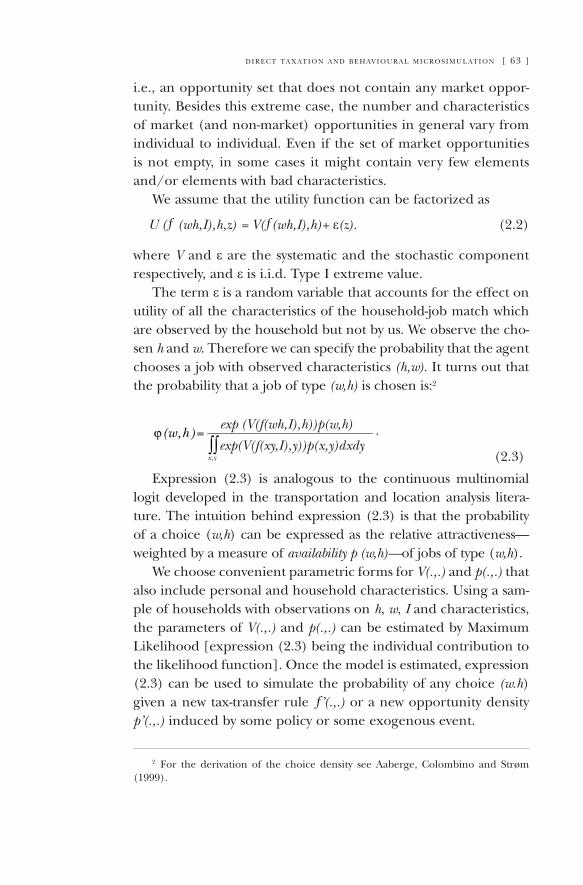
d i r e c t ta x at i o n a n d b e h av i o u r a l m i c r o s i m u l at i o n [ 63 ]
i.e., an opportunity set that does not contain any market oppor-tunity. Besides this extreme case, the number and characteristics of market (and non-market) opportunities in general vary from individual to individual. Even if the set of market opportunities is not empty, in some cases it might contain very few elements and/or elements with bad characteristics.
We assume that the utility function can be factorized as
U (ƒ (wh,I),h,z) = V(ƒ(wh,I),h)+ ε(z). (2.2)
where V and ε are the systematic and the stochastic component respectively, and ε is i.i.d. Type I extreme value.
The term ε is a random variable that accounts for the effect on utility of all the characteristics of the household-job match which are observed by the household but not by us. We observe the cho-sen h and w. Therefore we can specify the probability that the agent chooses a job with observed characteristics (h,w). It turns out that the probability that a job of type (w,h) is chosen is:2
( , )=w hϕ∫∫
exp (V(f(wh,I),h))p(w,h)
exp(V(f(xy,I),y))p(x,y)dxdyx,y
.
(2.3)
Expression (2.3) is analogous to the continuous multinomial logit developed in the transportation and location analysis litera-ture. The intuition behind expression (2.3) is that the probability of a choice (w,h) can be expressed as the relative attractiveness—weighted by a measure of availability p (w,h)—of jobs of type (w,h).
We choose convenient parametric forms for V(.,.) and p(.,.) that also include personal and household characteristics. Using a sam-ple of households with observations on h, w, I and characteristics, the parameters of V(.,.) and p(.,.) can be estimated by Maximum Likelihood [expression (2.3) being the individual contribution to the likelihood function]. Once the model is estimated, expression (2.3) can be used to simulate the probability of any choice (w.h) given a new tax-transfer rule ƒ’(.,.) or a new opportunity density p’(.,.) induced by some policy or some exogenous event.
2 For the derivation of the choice density see aaberge, Colombino and Strøm (1999).
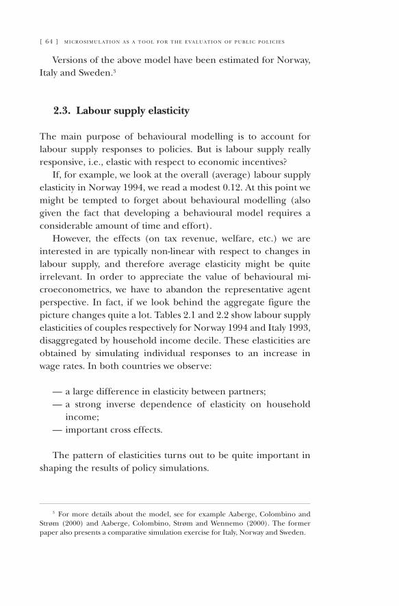
[ 64 ] m i c r o s i m u l at i o n a s a t o o l f o r t h e e va l u at i o n o f p u b l i c p o l i c i e s
Versions of the above model have been estimated for Norway, Italy and Sweden.3
2.3. Labour supply elasticity
The main purpose of behavioural modelling is to account for labour supply responses to policies. But is labour supply really responsive, i.e., elastic with respect to economic incentives?
If, for example, we look at the overall (average) labour supply elasticity in Norway 1994, we read a modest 0.12. at this point we might be tempted to forget about behavioural modelling (also given the fact that developing a behavioural model requires a considerable amount of time and effort).
However, the effects (on tax revenue, welfare, etc.) we are interested in are typically non-linear with respect to changes in labour supply, and therefore average elasticity might be quite irrelevant. In order to appreciate the value of behavioural mi-croeconometrics, we have to abandon the representative agent perspective. In fact, if we look behind the aggregate figure the picture changes quite a lot. Tables 2.1 and 2.2 show labour supply elasticities of couples respectively for Norway 1994 and Italy 1993, disaggregated by household income decile. These elasticities are obtained by simulating individual responses to an increase in wage rates. In both countries we observe:
a large difference in elasticity between partners;a strong inverse dependence of elasticity on household income;important cross effects.
The pattern of elasticities turns out to be quite important in shaping the results of policy simulations.
3 For more details about the model, see for example aaberge, Colombino and Strøm (2000) and aaberge, Colombino, Strøm and Wennemo (2000). The former paper also presents a comparative simulation exercise for Italy, Norway and Sweden.
——
—
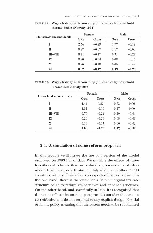
d i r e c t ta x at i o n a n d b e h av i o u r a l m i c r o s i m u l at i o n [ 65 ]
table 2.1: Wage elasticity of labour supply in couples by household income decile (Norway 1994)
Household income decileFemale Male
Own Cross Own Cross
I 2.54 –0.29 1.77 –0.12
II 0.97 –0.67 1.17 –0.08
III–VIII 0.41 –0.47 0.31 –0.24
IX 0.20 –0.34 0.08 –0.14
X 0.26 –0.10 0.05 –0.42
All 0.52 –0.42 0.39 –0.23
table 2.2: Wage elasticity of labour supply in couples by household
income decile (Italy 1993)
Household income decileFemale Male
Own Cross Own Cross
I 4.44 0.82 0.32 0.06
II 2.31 –0.15 0.17 0.00
III–VIII 0.73 –0.24 0.10 –0.04
IX 0.20 –0.20 0.08 –0.03
X 0.13 –0.17 0.06 –0.02
All 0.66 –0.20 0.12 –0.02
2.4. A simulation of some reform proposals
In this section we illustrate the use of a version of the model estimated on 1993 Italian data. We simulate the effects of three hypothetical reforms that are stylised representations of ideas under debate and consideration in Italy as well as in other OECD countries, with a differing focus on aspects of the tax regime. On the one hand, there is the quest for a flatter marginal tax rate structure so as to reduce disincentives and enhance efficiency. On the other hand, and specifically in Italy, it is recognised that the system of basic income support provides transfers that are not cost-effective and do not respond to any explicit design of social or family policy, meaning that the system needs to be rationalised
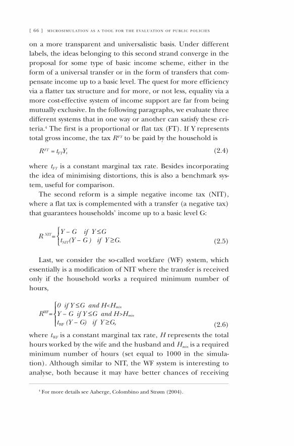
[ 66 ] m i c r o s i m u l at i o n a s a t o o l f o r t h e e va l u at i o n o f p u b l i c p o l i c i e s
on a more transparent and universalistic basis. Under different labels, the ideas belonging to this second strand converge in the proposal for some type of basic income scheme, either in the form of a universal transfer or in the form of transfers that com-pensate income up to a basic level. The quest for more efficiency via a flatter tax structure and for more, or not less, equality via a more cost-effective system of income support are far from being mutually exclusive. In the following paragraphs, we evaluate three different systems that in one way or another can satisfy these cri-teria.4 The first is a proportional or flat tax (FT). If Y represents total gross income, the tax RFT to be paid by the household is
R FT = tFTY, (2.4)
where tFT is a constant marginal tax rate. Besides incorporating the idea of minimising distortions, this is also a benchmark sys-tem, useful for comparison.
The second reform is a simple negative income tax (NIT), where a flat tax is complemented with a transfer (a negative tax) that guarantees households’ income up to a basic level G:
Y − G if Y ≤GtNIT(Y − G ) if Y ≥G.R NIT=
(2.5)
Last, we consider the so-called workfare (WF) system, which essentially is a modification of NIT where the transfer is received only if the household works a required minimum number of hours,
0 if Y ≤G and H<Hmin
Y − G if Y ≤G and H>Hmin
tWF (Y − G) if Y ≥G,RWF=
(2.6)where tWF is a constant marginal tax rate, H represents the total hours worked by the wife and the husband and Hmin is a required minimum number of hours (set equal to 1000 in the simula-tion). although similar to NIT, the WF system is interesting to analyse, both because it may have better chances of receiving
4 For more details see aaberge, Colombino and Strøm (2004).
.
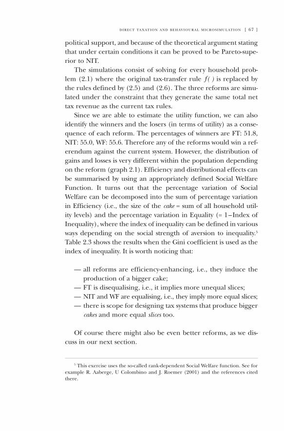
d i r e c t ta x at i o n a n d b e h av i o u r a l m i c r o s i m u l at i o n [ 67 ]
political support, and because of the theoretical argument stating that under certain conditions it can be proved to be Pareto-supe-rior to NIT.
The simulations consist of solving for every household prob-lem (2.1) where the original tax-transfer rule ƒ( ) is replaced by the rules defined by (2.5) and (2.6). The three reforms are simu-lated under the constraint that they generate the same total net tax revenue as the current tax rules.
Since we are able to estimate the utility function, we can also identify the winners and the losers (in terms of utility) as a conse-quence of each reform. The percentages of winners are FT: 51.8, NIT: 55.0, WF: 55.6. Therefore any of the reforms would win a ref-erendum against the current system. However, the distribution of gains and losses is very different within the population depending on the reform (graph 2.1). Efficiency and distributional effects can be summarised by using an appropriately defined Social Welfare Function. It turns out that the percentage variation of Social Welfare can be decomposed into the sum of percentage variation in Efficiency (i.e., the size of the cake = sum of all household util-ity levels) and the percentage variation in Equality (= 1 – Index of Inequality), where the index of inequality can be defined in various ways depending on the social strength of aversion to inequality.5
Table 2.3 shows the results when the Gini coefficient is used as the index of inequality. It is worth noticing that:
all reforms are efficiency-enhancing, i.e., they induce the production of a bigger cake;FT is disequalising, i.e., it implies more unequal slices;NIT and WF are equalising, i.e., they imply more equal slices;there is scope for designing tax systems that produce bigger cakes and more equal slices too.
Of course there might also be even better reforms, as we dis-cuss in our next section.
5 This exercise uses the so-called rank-dependent Social Welfare function. See for example R. aaberge, U Colombino and J. Roemer (2001) and the references cited there.
—
———
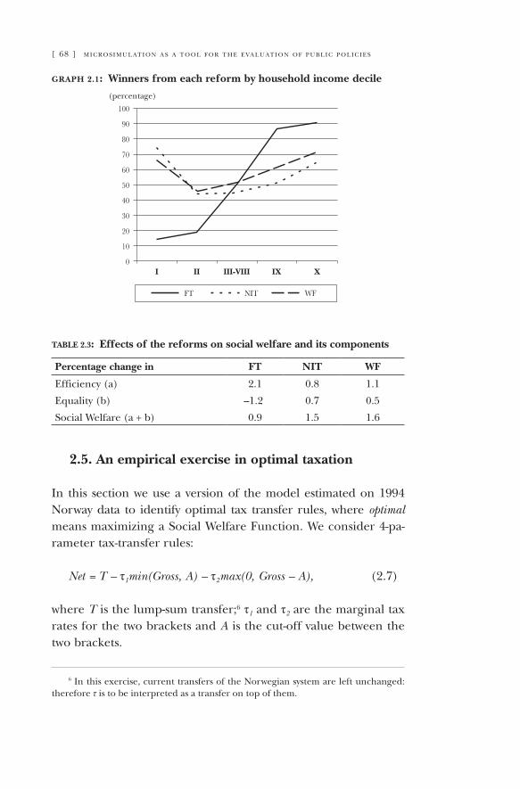
[ 68 ] m i c r o s i m u l at i o n a s a t o o l f o r t h e e va l u at i o n o f p u b l i c p o l i c i e s
graph 2.1: Winners from each reform by household income decile
(percentage)
table 2.3: Effects of the reforms on social welfare and its components
Percentage change in FT NIT WF
Efficiency (a) 2.1 0.8 1.1
Equality (b) –1.2 0.7 0.5
Social Welfare (a + b) 0.9 1.5 1.6
2.5. An empirical exercise in optimal taxation
In this section we use a version of the model estimated on 1994 Norway data to identify optimal tax transfer rules, where optimal means maximizing a Social Welfare Function. We consider 4-pa-rameter tax-transfer rules:
Net = T – τ1min(Gross, A) – τ2max(0, Gross – A), (2.7)
where T is the lump-sum transfer;6 τ1 and τ2 are the marginal tax rates for the two brackets and A is the cut-off value between the two brackets.
6 In this exercise, current transfers of the Norwegian system are left unchanged: therefore τ is to be interpreted as a transfer on top of them.
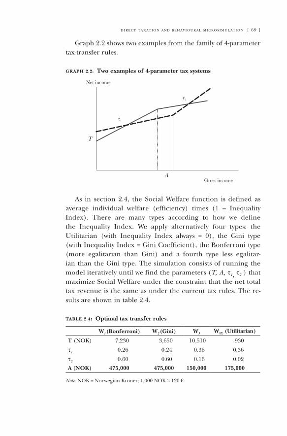
d i r e c t ta x at i o n a n d b e h av i o u r a l m i c r o s i m u l at i o n [ 69 ]
Graph 2.2 shows two examples from the family of 4-parameter tax-transfer rules.
graph 2.2: Two examples of 4-parameter tax systems
as in section 2.4, the Social Welfare function is defined as average individual welfare (efficiency) times (1 – Inequality Index). There are many types according to how we define the Inequality Index. We apply alternatively four types: the Utilitarian (with Inequality Index always = 0), the Gini type (with Inequality Index = Gini Coefficient), the Bonferroni type (more egalitarian than Gini) and a fourth type less egalitar-ian than the Gini type. The simulation consists of running the model iteratively until we find the parameters (T, A, τ1, τ2 ) that maximize Social Welfare under the constraint that the net total tax revenue is the same as under the current tax rules. The re-sults are shown in table 2.4.
table 2.4: Optimal tax transfer rules
W1 (Bonferroni) W2 (Gini) W3 W∞ (Utilitarian)
T (NOK) 7,230 3,650 10,510 930
τ1 0.26 0.24 0.36 0.36
τ2 0.60 0.60 0.16 0.02
A (NOK) 475,000 475,000 150,000 175,000
Note: NOK = Norwegian Kroner; 1,000 NOK ≈ 120 €.
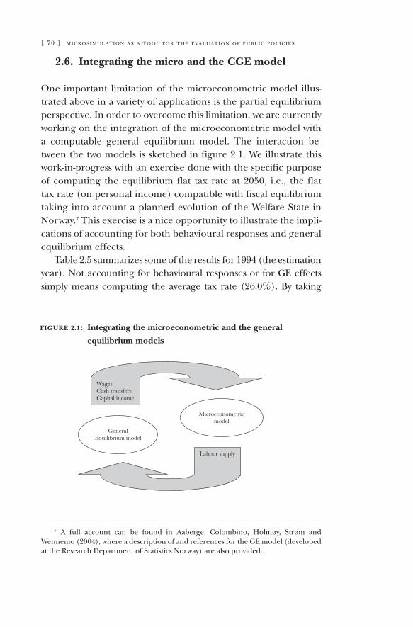
[ 70 ] m i c r o s i m u l at i o n a s a t o o l f o r t h e e va l u at i o n o f p u b l i c p o l i c i e s
2.6. Integrating the micro and the CGE model
One important limitation of the microeconometric model illus-trated above in a variety of applications is the partial equilibrium perspective. In order to overcome this limitation, we are currently working on the integration of the microeconometric model with a computable general equilibrium model. The interaction be-tween the two models is sketched in figure 2.1. We illustrate this work-in-progress with an exercise done with the specific purpose of computing the equilibrium flat tax rate at 2050, i.e., the flat tax rate (on personal income) compatible with fiscal equilibrium taking into account a planned evolution of the Welfare State in Norway.7 This exercise is a nice opportunity to illustrate the impli-cations of accounting for both behavioural responses and general equilibrium effects.
Table 2.5 summarizes some of the results for 1994 (the estimation year). Not accounting for behavioural responses or for GE effects simply means computing the average tax rate (26.0%). By taking
7 a full account can be found in aaberge, Colombino, Holmøy, Strøm and Wennemo (2004), where a description of and references for the GE model (developed at the Research Department of Statistics Norway) are also provided.
figure 2.1: Integrating the microeconometric and the general
equilibrium models
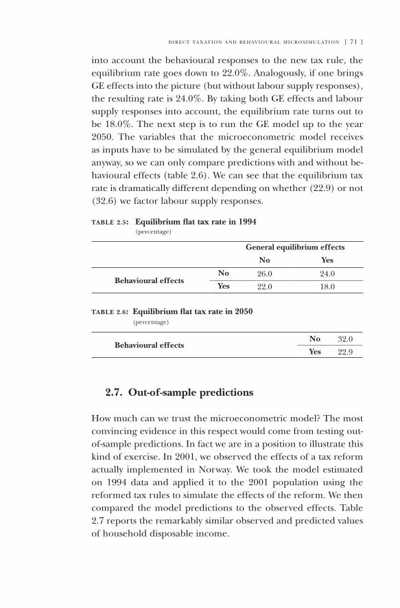
d i r e c t ta x at i o n a n d b e h av i o u r a l m i c r o s i m u l at i o n [ 71 ]
into account the behavioural responses to the new tax rule, the equilibrium rate goes down to 22.0%. analogously, if one brings GE effects into the picture (but without labour supply responses), the resulting rate is 24.0%. By taking both GE effects and labour supply responses into account, the equilibrium rate turns out to be 18.0%. The next step is to run the GE model up to the year 2050. The variables that the microeconometric model receives as inputs have to be simulated by the general equilibrium model anyway, so we can only compare predictions with and without be-havioural effects (table 2.6). We can see that the equilibrium tax rate is dramatically different depending on whether (22.9) or not (32.6) we factor labour supply responses.
table 2.5: Equilibrium flat tax rate in 1994 (percentage)
General equilibrium effects
No Yes
Behavioural effectsNo 26.0 24.0Yes 22.0 18.0
table 2.6: Equilibrium flat tax rate in 2050 (percentage)
Behavioural effectsNo 32.0
Yes 22.9
2.7. Out-of-sample predictions
How much can we trust the microeconometric model? The most convincing evidence in this respect would come from testing out-of-sample predictions. In fact we are in a position to illustrate this kind of exercise. In 2001, we observed the effects of a tax reform actually implemented in Norway. We took the model estimated on 1994 data and applied it to the 2001 population using the reformed tax rules to simulate the effects of the reform. We then compared the model predictions to the observed effects. Table 2.7 reports the remarkably similar observed and predicted values of household disposable income.
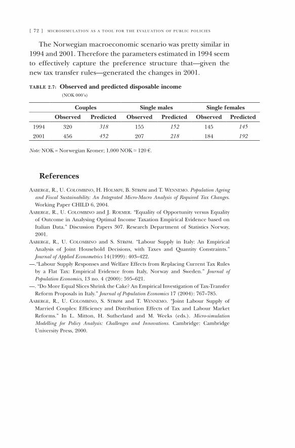
[ 72 ] m i c r o s i m u l at i o n a s a t o o l f o r t h e e va l u at i o n o f p u b l i c p o l i c i e s
The Norwegian macroeconomic scenario was pretty similar in 1994 and 2001. Therefore the parameters estimated in 1994 seem to effectively capture the preference structure that—given the new tax transfer rules—generated the changes in 2001.
table 2.7: Observed and predicted disposable income (NOK 000’s)
Couples Single males Single females
Observed Predicted Observed Predicted Observed Predicted
1994 320 318 155 152 145 145
2001 456 452 207 218 184 192
Note: NOK = Norwegian Kroner; 1,000 NOK ≈ 120 €.
References
aaberge, r., u. colombino, h. holmøy, b. strøm and t. Wennemo. Population Ageing and Fiscal Sustainability: An Integrated Micro-Macro Analysis of Required Tax Changes. Working Paper CHILD 6, 2004.
aaberge, r., u. colombino and J. roemer. “Equality of Opportunity versus Equality of Outcome in analysing Optimal Income Taxation Empirical Evidence based on Italian Data.” Discussion Papers 307. Research Department of Statistics Norway, 2001.
aaberge, r., u. colombino and s. strøm. “Labour Supply in Italy: an Empirical analysis of Joint Household Decisions, with Taxes and Quantity Constraints.” Journal of Applied Econometrics 14(1999): 403–422.
—.“Labour Supply Responses and Welfare Effects from Replacing Current Tax Rules by a Flat Tax: Empirical Evidence from Italy, Norway and Sweden.” Journal of Population Economics, 13 no. 4 (2000): 595–621.
—. “Do More Equal Slices Shrink the Cake? an Empirical Investigation of Tax-Transfer Reform Proposals in Italy.” Journal of Population Economics 17 (2004): 767–785.
aaberge, r., u. colombino, s. strøm and t. Wennemo. “Joint Labour Supply of Married Couples: Efficiency and Distribution Effects of Tax and Labour Market Reforms.” In L. Mitton, H. Sutherland and M. Weeks (eds.). Micro-simulation Modelling for Policy Analysis: Challenges and Innovations. Cambridge: Cambridge University Press, 2000.
[ 73 ]
Growth, Distribution and Poverty in Madagascar: Learning from a Microsimulation Model in a General Equilibrium Framework
Denis Cogneau Anne-Sophie Robilliard
IRD, DIAL (Paris)
3.1. Introduction
The nature of the links between economic growth, poverty and income distribution is central to the study of economic develop-ment. A number of approaches have been taken to analyze these links. This debate has also contributed to raising the question of how to construct suitable tools to analyze the impact of macroeco-nomic policies on poverty and income distribution. More recently, this led to the development of tools for counterfactual analysis to study the impact of structural adjustment policies. Among these tools, computable general equilibrium (CGE) models are widely used, because of their ability to produce disaggregated results at the microeconomic level, within a consistent macroeconomic framework (Adelman and Robinson 1988; Dervis et al. 1982; Taylor 1990; Bourguignon et al. 1991; De Janvry et al. 1991). Despite this ability, CGE models rest on the assumption of the representative agent, for both theoretical and practical reasons. From the theoretical point of view, the existence and uniqueness of equilibrium in the Arrow Debreu model are warranted only when the excess demand of the economy has certain properties (Kirman 1992; Hildenbrand 1998). The assumption that the representative agent has a quasi-concave utility function ensures that these properties are met at the individual level, which, in turn, makes it possible to give microeconomic foundations to the model without having to solve distributional problems. From a
3.
[ 74 ] m i c r o s i m u l at i o n a s a t o o l f o r t h e e va l u at i o n o f p u b l i c p o l i c i e s
practical point of view, several reasons justify resorting to this as-sumption. On the one hand, the construction of macroeconomic models with heterogeneous agents presupposes the availability of representative microeconomic data at the domestic level; a construction which is often problematic given the difficulty of reconciling household survey data and national accounts data. In addition, the solution of numerical models of significant size was until recently limited by the data-processing resources and software available.
The study of income distribution within this framework re-quires, initially, identifying groups whose characteristics and be-haviours are homogeneous. Generating overall distribution from the distribution among several representative groups requires several assumptions, in particular on the form of the income distri-bution function within each group. The most common assumption in the applied models is that within-group distribution of income has an endogenous average (given by the model) as well as fixed variance and higher moments. It is widely agreed that it would be far more satisfactory to endogenize the income variance within each group, since its contribution to the total inequality is generally significant, whatever the relevance of the classification considered. This consideration led to the development of microsimulation models.
Microsimulation models, which were pioneered by the work of Orcutt (1957), are much less widely used than applied com-putable general equilibrium models. In the mid-1970s various teams of researchers developed microsimulation models on the basis of surveys. Most of them tackled questions related to the distributive impact of welfare programs or tax policies. Since then, many applications have been implemented in developed countries to evaluate the impact of fiscal reforms, or health care financing, or to study issues related to demographic dynam-ics (Harding 1993). Another path pursued recently consists of models based on household surveys carried out at various dates, built to identify and analyze the determinants of the evolution of inequality (Bourguignon et al., 1998; Alatas and Bourguignon 1999). Microsimulation models can be complex depending on whether individual or household behaviour is taken into account
g r o w t h, d i s t r i b u t i o n a n d p o v e rt y i n m a d a g a s c a r [ 75 ]
and represented. The majority of analyses based on microsimula-tion models are conducted within a framework of partial equilib-rium. General equilibrium effects have been incorporated simply by coupling an aggregate CGE model with a microsimulation model in a sequential way (Meagher 1993), but this framework prevents agents’ reactions at the micro level from being taken into account. To our knowledge, only Van Tongeren (1994) and Cogneau (1999) have carried out the full integration of a micro-simulation model within a general equilibrium framework; the former to analyze the behaviour of Dutch companies within a domestic framework, the latter to study the labour market in the town of Antananarivo (Madagascar). Building on this last model, we develop a microsimulation model within a general equilibrium framework for the Malagasy economy as a whole. This model is built on microeconomic data to explicitly represent the h etero-geneity of qualifications, preferences and labour allocation as well as consumption preferences at the microeconomic level. In addition, relative prices are determined endogenously through market-clearing mechanisms for goods and factors. The modelling choices were driven by a desire to make the best possible use of the microeconomic information derived from the household data.
The chapter is organized as follows. In section 3.2, we discuss the modelling of income distribution. The methodology is then described. The microeconomic basis of the model is presented in section 3.3, the general equilibrium framework is sketched in sec-tion 3.4, and the presentation of the results of the estimates of be-havioural functions, as well as the calibration of the model are pre-sented in section 3.5. Lastly, the results of simulations with various growth shock scenarios are presented and analyzed in section 3.6.
3.2. Modelling income distribution
Among the tools used for counterfactual analysis of the impact of policies and macroeconomic shocks on poverty and income dis-tribution, computable general equilibrium models appeal because of their ability to produce relatively disaggregated results at microeco-nomic level within a consistent macroeconomic framework.
[ 76 ] m i c r o s i m u l at i o n a s a t o o l f o r t h e e va l u at i o n o f p u b l i c p o l i c i e s
3.2.1. Functional distribution vs. personal distributionApplied general equilibrium models, initially built on the ba-
sis of Social Accounting Matrices (SAM) with one representative household, have been gradually enriched from the microeconomic point of view by constructing SAM increasingly disaggregated at the household account level. This development has allowed analyses to be conducted based on a typology of households characterized by different levels of income. The first two gen-eral equilibrium models used to study the distributive impact of various macroeconomic policies in developing economies are the Adelman and Robinson model for Korea (1978) and that of Lysy and Taylor for Brazil (1980). The two models produced different results. The differences were initially attributed to differences in the structural characteristics of both economies and the speci-fications of the models. Subsequently, Adelman and Robinson (1988) used the same two models again, and determined that the differences were mainly due to different definitions of income distribution and not to different macroeconomic closures. The neoclassical approach focuses on the size distribution of income, essentially individualistic, while the Latin American structuralist school is built on a Marxian vision that considers society to be made up of classes characterized by their endowment in factors of production and whose interests are divergent. While the latter defends the functional approach of income distribution, which characterizes households by their production factor endowment, the former more often adopts the personal approach, which is based on a classification of households according to their income level. The most common approach today is to use the extended functional classification, which takes into account several criteria for classifying households.
In order to go from income distribution among groups of households to an indicator of overall inequality or poverty, it is necessary to specify income distribution within the groups consid-ered. The most common approach is to assume that within each group income has a lognormal distribution with an endogenous average (given by the model) and a fixed variance (Adelman and Robinson 1988). More recently, Decaluwé et al. (1999) proposed a numerical model, applied to an African prototype economy that
g r o w t h, d i s t r i b u t i o n a n d p o v e rt y i n m a d a g a s c a r [ 77 ]
distinguishes four household groups and estimates income distri-bution laws for each group that envisage more complex forms of distribution than the normal law. However it does not allow us to relax the assumption of fixed within-group variance of income, whose contribution to overall inequality is often quite significant (in general, more than 50% of total variance).
3.2.2. The representative agent assumptionDisaggregation of the SAM does not allow applied general
equilibrium models to relax the representative agent assumption, but leads to a multiplication of representative agents. The wide-spread use of this assumption is due to the desire to give microeco-nomic foundations to the aggregated behaviour, and to establish a framework of analysis in which equilibrium is unique and stable. According to Kirman (1992), this assumption raises many problems. First of all, there is no plausible justification for the assumption that the aggregate of several individuals, even if they are optimizing agents, acts like an individual optimizing agent. Individual optimization does not necessarily generate collective rationality, nor does the fact that the community shows some ra-tionality imply that the individuals who make it up act rationally. In addition, even if it is accepted that the choices of the aggregate can be regarded as those of an optimizing individual, the reaction of the representative agent to a modification of the parameters in the initial model may be different from the reactions of the individuals that this agent represents. Thus we may find cases of two situations where the representative agent prefers the second, while each individual prefers the first. Finally, trying to explain the behaviour of a group by that of an individual is constraining. The sum of the simple and plausible economic behaviour of a multitude of individuals can generate complex dynamics, whereas building a model of an individual whose behaviour corresponds to these complex dynamics can result in considering an agent whose characteristics are very particular. In other words, the dynamic complexity of the behaviour of an aggregate can emerge from the aggregation of heterogeneous individuals with simple behaviours.
Our approach makes it possible to relax the representative agent assumption in two ways. The first is by using information
[ 78 ] m i c r o s i m u l at i o n a s a t o o l f o r t h e e va l u at i o n o f p u b l i c p o l i c i e s
at the microeconomic level—at the household or individual level according to the variable being considered. The second is by estimating behavioural equations starting from the same micro-economic data. The estimated functions form part of the model, which allows some of the behaviour to be endogenized. The unexplained portion—the error term or fixed effect—remains exogenous but is preserved, making it possible to take into ac-count elements of unexplained heterogeneity.
3.3. Microeconomic specifications of the model
Microeconomic specifications constitute the foundations of the model. From this perspective, our approach can be thought of as a bottom-up approach. Microeconomic modelling choices were guided by concern about using and explaining empirical obser-vations. Agricultural households occupy a central place in the model, and particular care was given to the specification of their labour allocation behaviour.
3.3.1. Production and labour allocationWe model labour allocation of households among various
activities. Three sectors are considered: formal, informal, and agricultural. Individuals can be wage workers or self-employed. Thus, we distinguish three types of activities:
agricultural activity; informal activity;wage-earning in the formal sector.
One of the original characteristics of the model is that it explicitly models the fact that agricultural households are pro-ducers. Traditionally, computable general equilibrium models represent the behaviour of sectors that hire workers and pay value-added to households through the production factor ac-counts. This specification does not allow for the heterogeneity of producers, nor does it permit us to represent interactions be-tween production and consumption decisions.
i)ii)iii)
g r o w t h, d i s t r i b u t i o n a n d p o v e rt y i n m a d a g a s c a r [ 79 ]
3.3.1.1. Agricultural householdsLabour allocation models for agricultural households are the
subject of an ongoing literature which focuses on estimating the parameters of labour supply and demand (Skoufias 1994), on the question of the separability of behaviours, on characterizing the types of rationing faced by these households (Benjamin 1992), and on the substitutability of various types of work (Jacoby 1992, 1993). Our approach does not constitute a contribution to these questions, but makes use of the theoretical developments and empirical results of this work to construct the microeconomic foundations of the model.
Traditionally, modelling the choices of labour allocation is considered in a context where wage activities are dominant. The existence of one or several labour markets makes it pos-sible to refer to exogenous prices in estimating model equations. Agricultural households have two fundamental characteristics which justify the extension of traditional producer and consumer models: the dominant use of family labour and the fact that households consume an often significant part of their own pro-duction. Standard labour market models traditionally distinguish entities that supply work (households) from entities that require work (companies). This representation is not well suited to de-scribe the operation of the rural labour market where agricultur-al households are institutions that supply and require work at the same time. On the production side, the level of each activity, and consequently the level of labour demand, is determined by the maximization of profits. On the consumption side, the demand for leisure, and consequently labour supply, is determined by the maximization of utility.
The separability of demand and labour supply behaviour de-pends on the existence and operation of the labour market: if it exists and operates perfectly, then the household independently maximizes profits (which determines its labour demand) and utility (which determines its labour supply). In this case, the mar-ginal productivity of on-farm labour is equal to the market wage, and depends neither on the household’s endowment of produc-tion factors nor on its consumer preferences. If, on the contrary, the market does not exist, each household balances its own la-
[ 80 ] m i c r o s i m u l at i o n a s a t o o l f o r t h e e va l u at i o n o f p u b l i c p o l i c i e s
bour supply and demand, linking its consumer preferences and its producer behaviour. In this case, the marginal productivity of on-farm labour depends on the characteristics of the household. These characteristics comprise not only observable elements like endowment of production factors, demographic composition and levels of education and professional experience of members, but also non observable characteristics such as the preference for on- or off-farm work.
Neither of these two models satisfactorily explains the real operation of the markets, either in Madagascar or in the majority of developing countries. Many surveys indicate the simultaneous existence of a rural labour market and different marginal produc-tivities among households. For instance, larger farmers typically exhibit a higher marginal labour productivity. Various explana-tions of this phenomenon were proposed within the framework of studies on the inverse relationship between farm size and land productivity. In his work on labour allocation in agricultural households, Benjamin (1992) analyzes three rationing schemes: constraints on off-farm labour supply, rationing on the labour demand side and different marginal productivity between family and wage work.
In our model, off-farm and hired labour are treated in an asymmetrical way. This approach is justified by the observation that even households that hire agricultural wage labour can have low marginal productivities of labour, lower than the average observed agricultural wage. We thus made the assumption that hired labour is complementary to family labour. The validity of this assumption is reinforced by the seasonal nature of the use of agricultural wage labour in Madagascar. Hiring is particularly important at the time of rice transplanting in irrigated fields. This operation must be carried out quickly, ideally in one day for each field, so the seedlings grow at the same pace and appropriate wa-ter control can be assured. Typically, rice-grower households call upon paid work or mutual aid during this period. The technical coefficient relative to non-family work is nevertheless specific to each household, since the quantity of auxiliary work depends on the demographic characteristics of the household and the size of the farm.
g r o w t h, d i s t r i b u t i o n a n d p o v e rt y i n m a d a g a s c a r [ 81 ]
On the off-farm employment side, agricultural households have several possibilities, including agricultural or informal wage work, or an informal handicraft or commercial activity. Since these activities are very labour intensive even when not wage-earning, we have treated them as activities with constant returns to labour. Again, empirical observations determined the choices of specification. It was necessary to find a model that explained the observation that households supplying off-farm labour have low marginal productivities of on-farm labour. Among the possible models of rationing, we chose to consider that there are transaction costs and/or elements of preference which explain this observation. The labour alloca-tion model thus becomes discrete. Households that do not supply work off-farm have a marginal productivity of on-farm labour higher than their potential off-farm wages, adjusted for costs. Households that supply off-farm labour have a marginal productivity that is equal to their off-farm wages, adjusted for transaction costs. Since the supply of formal wage labour is completely rationed on the demand side, it does not enter ex-plicitly into the labour allocation model. An exogenous shock on formal labour demand will nevertheless have an impact on the time available for agricultural and informal activities. It will also have an impact on household income, which in turn affects total labour supply.
3.3.1.2. Non-agricultural householdsNon-agricultural households supply informal and/or formal
wage work. Their demand for leisure and consequently their to-tal labour supply depends on their wage rate and income apart from labour income. Since the supply of formal wage work is completely rationed on the demand side, the potential impact of an exogenous shock on formal labour demand or on the formal wage rate is the same as that described above for agricultural households.
3.3.2. Disposable income, savings and consumptionHousehold income comes from various sources: agricultural
activities, informal activities, formal wages, dividends of formal
[ 82 ] m i c r o s i m u l at i o n a s a t o o l f o r t h e e va l u at i o n o f p u b l i c p o l i c i e s
capital, income from sharecropping, and transfers from other households and from the government. Apart from income from the formal sector and transfers, all income flows are endogenous in the model. Part of total income is saved and the saving rate is endogenous. It is an increasing function of total income. Final consumption is represented through a linear expenditure sys-tem (LES). This specification makes it possible to distinguish and take into account necessary expenditures and supernumer-ary expenditures. Finally, each activity consumes intermediate goods. The technical coefficients for the agricultural sector are household-specific.
3.4. Description of the general equilibrium framework
The general equilibrium framework is made up of equilibrium equations for goods and factor markets. This framework makes it possible to take into account indirect effects through changes in relative prices. Macroeconomic closures are nevertheless not specified explicitly. The implicit assumptions are that govern-ment savings and total investment are flexible, that the exchange rate is fixed and foreign savings are flexible.
The model is a static model with three sectors: agricultural, informal and formal. The agricultural sector produces two types of goods, a tradable good that is exported and a non-tradable good. The two other sectors each produce one type of good. The informal good is a non-tradable good, while the formal good is tradable. The production factors are labour, land and formal capital. Total labour supply is endogenous and deter-mined at the household level. The levels of agricultural and in-formal production are also determined at the household level, as is agricultural labour demand. Informal labour demand is determined at the aggregate level by the demand for informal goods and for agricultural wage labour. The supply of informal labour is determined at the individual level through the labour allocation model described earlier. Formal labour demand is
g r o w t h, d i s t r i b u t i o n a n d p o v e rt y i n m a d a g a s c a r [ 83 ]
exogenous. Capital stocks (land, cattle and agricultural capital for the agricultural sector, formal capital for the formal sector) are specific and fixed for agricultural and formal activities, while the capital used in the informal sector is integrated into work. Capital and labour are substitutable in agricultural technology represented through a Cobb-Douglas specification. The formal labour market operates with exogenous demand at fixed prices. The allocation of work between agricultural and informal pro-duction is determined at the microeconomic level, according to the labour allocation model described in section 3.3.
Although the model is based on information at the household level, an aggregate social accounting matrix (SAM) with 13 ac-counts can be derived from the source data (table 3.1). In this ag-gregated SAM, the labour factor is disaggregated into three types of work: agricultural family work, informal wage work and formal wage work. The household account is disaggregated into two ac-counts, one for urban households and the other for rural house-holds. The formal sector account is an aggregate of private and public formal activities accounts, while the last account (RES) is an aggregate of the accounts of formal firms, government, sav-ing-investment and the rest of the world. This matrix summarizes the model accounts, which include 4,500 households, of which approximately 3,500 are agricultural producers. Thus, there are thousands of household, factor, and activity accounts in the full model SAM.
3.5. An application to Madagascar
Some of the microeconomic functions were estimated on cross-sectional data: the agricultural production function and the informal income equation at the household level and the formal wage equation at the individual level. On the consumption side, parameters for the linear expenditure system and the labour sup-ply function could not be estimated but were calibrated instead using estimates found in the literature and data derived from the household survey and the SAM.
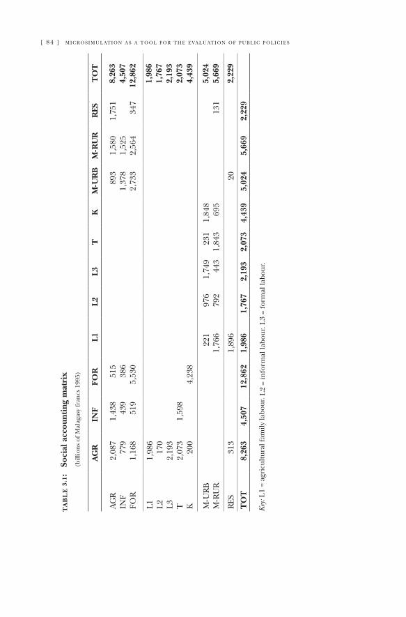
[ 84 ] m i c r o s i m u l at i o n a s a t o o l f o r t h e e va l u at i o n o f p u b l i c p o l i c i e s
ta
bl
e 3
.1:
Soci
al a
ccou
ntin
g m
atri
x
(bill
ions
of
Mal
agas
y fr
ancs
199
5)
AG
RIN
FFO
RL1
L2L3
TK
M-U
RB
M-R
UR
RES
TO
T
AG
RIN
FFO
R
2,0
87 779
1,16
8
1,43
843
951
9
515
386
5,53
0
893
1,37
82,
733
1,58
01,
525
2,56
4
1,75
1
347
8,26
34,
507
12,8
62
L1 L2 L3 T K
1,98
617
02,
193
2,07
320
01,
598
4,23
8
1,98
61,
767
2,19
32,
073
4,43
9
M-U
RB
M-R
UR
221
1,76
697
679
21,
749
443
231
1,84
31,
848
695
131
5,02
45,
669
RES
313
1,89
620
2,22
9
TO
T8,
263
4,50
712
,862
1,98
61,
767
2,19
32,
073
4,43
95,
024
5,66
92,
229
Key
: L1
= ag
ricu
ltura
l fam
ily la
bour
. L2
= in
form
al la
bour
. L3
= fo
rmal
labo
ur.
g r o w t h, d i s t r i b u t i o n a n d p o v e rt y i n m a d a g a s c a r [ 85 ]
3.5.1. Estimation resultsThe econometric techniques implemented are inspired as far as
possible by econometric work on household labour allocation. The complexity of the methods used is nevertheless limited by the need to estimate functions on the whole sample of households and not just on a sub-sample. Thus, in the case of the agricultural produc-tion function, we did not differentiate types of labour according to qualification or gender, because we could not find a well-behaved neoclassical function which permits null quantities of one of the production factors. The estimation of a function with several types of labour would also have made it possible to write the labour al-location model at the level of individuals and not of households. To our knowledge, only Newman and Gertler (1994) have implement-ed a complete estimation of a time allocation model for agricul-tural households with an arbitrary number of members. However, their specification relies on the use of only part of the available in-formation, since the model estimation relies only on the observed marginal productivity data, i.e., wages, and uses the Kuhn-Tucker conditions to estimate the marginal productivity of on-farm family labour. The comparison of wages and productivities derived from the estimate of an agricultural production function based on the EPM93 data shows that these conditions do not appear to hold.
3.5.1.1. Agricultural production functionFollowing Jacoby (1993) and Skoufias (1994), we considered
an agricultural production function and derived the marginal pro-ductivity of agricultural labour for each household. Agricultural households are defined as all those that draw an income from land. Other agricultural factors include agricultural equipment and livestock. The Cobb-Douglas function has advantages in terms of interpretation and handiness.1 Aside from the homogeneity of
1 The search for a function making it possible to take into account null quantities of inputs led us to consider estimating a quadratic function embedded in a Cobb-Douglas function. The quadratic form makes it possible to consider several types of work and null quantities of factors. We abandoned this approach for two reasons. One is that the estimation results are much less satisfactory from an econometric point of view. The other is that the function is much less handy analytically, which considerably complicates the writing of the model.
[ 86 ] m i c r o s i m u l at i o n a s a t o o l f o r t h e e va l u at i o n o f p u b l i c p o l i c i e s
family work, the assumptions related to the use of a Cobb-Douglas function are strong: the contributions of the production factors are strongly separable, and the marginal rate of substitution between factors is equal to 1 and does not depend on the other factors.
The logarithm of agricultural value added is regressed on the logarithms of the four production factors (work in hours, land in hectares, endowment in value, livestock in value), and the average level of education of the household, as well as on variables char-acterizing the cultivated land (share of irrigated surface, share of surface in property, share of cash crop cultures) and on regional dummy variables. Because of the endogeneity of certain explana-tory variables, the ordinary least squares estimate (OLS) is likely to give biased results. The endogeneity bias can result from the overlap of production and input allocation decisions, and from fixed effects of unobserved heterogeneity. The multiplicity of the endogeneity sources does not permit determination of the bias direction a priori. Since capital stock, acreage and livestock are considered fixed over the period considered (one year of pro-duction) and intermediate consumptions are deducted from the value of the production—which amounts to assuming that they are complementary—the only variable that needs to be instrumented is the use of family work. The instrumental variables (IV) must be correlated with the explanatory variables but not with the residuals of the production function. The selected IV are the demographic structure of the household and the age of the household head. The results of the estimates by OLS and IV methods are presented in table 3.2. The first stage of the estimate—regression of the vari-able instrumented on the instrumental variables—indicates that the instruments are relatively powerful in explaining the variation in the quantities of family work applied to agricultural activity. The results of the over-identification test allow us to reject the null hy-pothesis of correlation between the residuals of the IV estimate and the instruments, while the results of the Durbin-Wu-Hausman test show that the family work coefficient in the production function estimated by the IV is significantly different from the coefficient estimated by the OLS. The comparison of the results of estimates by the OLS and the IV shows that the coefficient of family work (corresponding to its contribution to agricultural value-added)
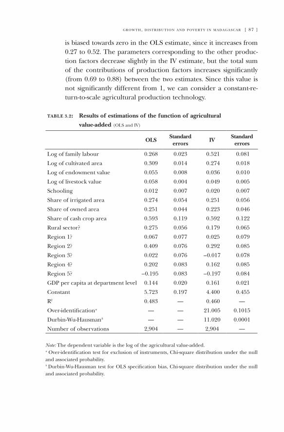
g r o w t h, d i s t r i b u t i o n a n d p o v e rt y i n m a d a g a s c a r [ 87 ]
is biased towards zero in the OLS estimate, since it increases from 0.27 to 0.52. The parameters corresponding to the other produc-tion factors decrease slightly in the IV estimate, but the total sum of the contributions of production factors increases significantly (from 0.69 to 0.88) between the two estimates. Since this value is not significantly different from 1, we can consider a constant-re-turn-to-scale agricultural production technology.
table 3.2: Results of estimations of the function of agricultural
value-added (OLS and IV)
OLSStandard
errorsIV
Standard errors
Log of family labour 0.268 0.023 0.521 0.081
Log of cultivated area 0.309 0.014 0.274 0.018
Log of endowment value 0.055 0.008 0.036 0.010
Log of livestock value 0.058 0.004 0.049 0.005
Schooling 0.012 0.007 0.020 0.007
Share of irrigated area 0.274 0.054 0.251 0.056
Share of owned area 0.251 0.044 0.223 0.046
Share of cash crop area 0.593 0.119 0.592 0.122
Rural sector? 0.275 0.056 0.179 0.065
Region 1? 0.067 0.077 0.025 0.079
Region 2? 0.409 0.076 0.292 0.085
Region 3? 0.022 0.076 –0.017 0.078
Region 4? 0.202 0.083 0.162 0.085
Region 5? –0.195 0.083 –0.197 0.084
GDP per capita at department level 0.144 0.020 0.161 0.021
Constant 5.723 0.197 4.400 0.455
R2 0.483 — 0.460 —
Over-identificationa — — 21.005 0.1015
Durbin-Wu-Hausmanb — — 11.020 0.0001
Number of observations 2,904 — 2,904 —
Note: The dependent variable is the log of the agricultural value-added.a Over-identification test for exclusion of instruments, Chi-square distribution under the null and associated probability.b Durbin-Wu-Hausman test for OLS specification bias, Chi-square distribution under the null and associated probability.
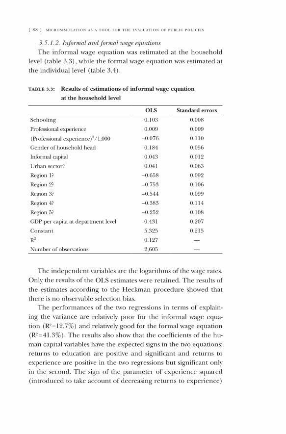
[ 88 ] m i c r o s i m u l at i o n a s a t o o l f o r t h e e va l u at i o n o f p u b l i c p o l i c i e s
3.5.1.2. Informal and formal wage equationsThe informal wage equation was estimated at the household
level (table 3.3), while the formal wage equation was estimated at the individual level (table 3.4).
table 3.3: Results of estimations of informal wage equation
at the household level
OLS Standard errors
Schooling 0.103 0.008
Professional experience 0.009 0.009
(Professional experience)2/1,000 –0.076 0.110
Gender of household head 0.184 0.056
Informal capital 0.043 0.012
Urban sector? 0.041 0.063
Region 1? –0.658 0.092
Region 2? –0.753 0.106
Region 3? –0.544 0.099
Region 4? –0.383 0.114
Region 5? –0.252 0.108
GDP per capita at department level 0.431 0.207
Constant 5.325 0.215
R2 0.127 —
Number of observations 2,605 —
The independent variables are the logarithms of the wage rates. Only the results of the OLS estimates were retained. The results of the estimates according to the Heckman procedure showed that there is no observable selection bias.
The performances of the two regressions in terms of explain-ing the variance are relatively poor for the informal wage equa-tion (R2 =12.7%) and relatively good for the formal wage equation (R2 = 41.3%). The results also show that the coefficients of the hu-man capital variables have the expected signs in the two equations: returns to education are positive and significant and returns to experience are positive in the two regressions but significant only in the second. The sign of the parameter of experience squared (introduced to take account of decreasing returns to experience)
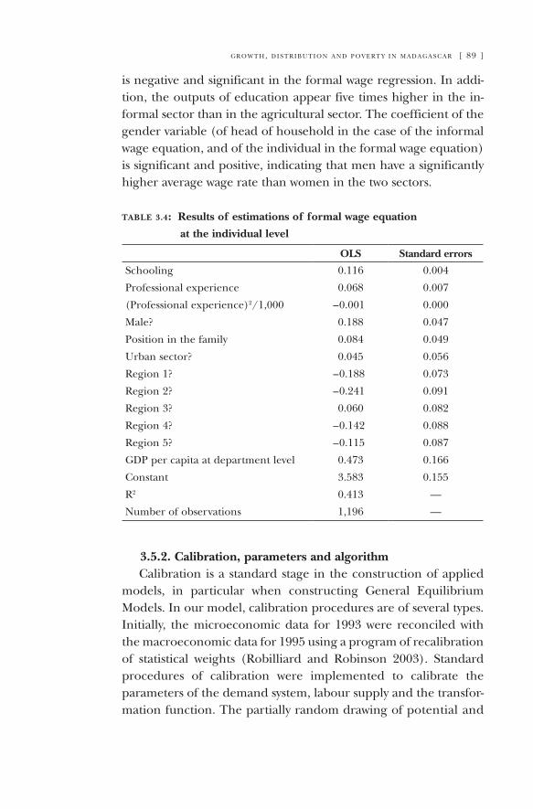
g r o w t h, d i s t r i b u t i o n a n d p o v e rt y i n m a d a g a s c a r [ 89 ]
is negative and significant in the formal wage regression. In addi-tion, the outputs of education appear five times higher in the in-formal sector than in the agricultural sector. The coefficient of the gender variable (of head of household in the case of the informal wage equation, and of the individual in the formal wage equation) is significant and positive, indicating that men have a significantly higher average wage rate than women in the two sectors.
table 3.4: Results of estimations of formal wage equation
at the individual level
OLS Standard errors
Schooling 0.116 0.004
Professional experience 0.068 0.007
(Professional experience)2/1,000 –0.001 0.000
Male? 0.188 0.047
Position in the family 0.084 0.049
Urban sector? 0.045 0.056
Region 1? –0.188 0.073
Region 2? –0.241 0.091
Region 3? 0.060 0.082
Region 4? –0.142 0.088
Region 5? –0.115 0.087
GDP per capita at department level 0.473 0.166
Constant 3.583 0.155
R2 0.413 —
Number of observations 1,196 —
3.5.2. Calibration, parameters and algorithmCalibration is a standard stage in the construction of applied
models, in particular when constructing General Equilibrium Models. In our model, calibration procedures are of several types. Initially, the microeconomic data for 1993 were reconciled with the macroeconomic data for 1995 using a program of recalibration of statistical weights (Robilliard and Robinson 2003). Standard procedures of calibration were implemented to calibrate the parameters of the demand system, labour supply and the transfor-mation function. The partially random drawing of potential and
[ 90 ] m i c r o s i m u l at i o n a s a t o o l f o r t h e e va l u at i o n o f p u b l i c p o l i c i e s
reservation wages is non standard and constitutes an innovative step, characteristic of microsimulation models with endogenous microeconomic behaviours.
3.5.2.1. Parameter calibrationThe linear expenditure system (LES) was calibrated for each
household given the budgetary shares derived from household data and the SAM, the income elasticity of agricultural and formal demand and the Frisch parameter. Price elasticities and LES param-eters were derived from the calibration process. The outcome of this process is that minimal expenditures are specific to each household, as are propensities to consume supernumerary income. This speci-fication leads to individual demand functions whose aggregation is not perfect, i.e., whose aggregate cannot be described through a function of the same type as the individual function. Only a specifi-cation based on marginal propensities to consume supernumerary income equal for all households allows perfect aggregation.
The labour supply function was calibrated for each household by reference to the price and income elasticities drawn from Jacoby (1993). The savings function was calibrated by reference to the income elasticity of the marginal propensity to save. Finally, the autonomous agricultural demand was calibrated by reference to the price elasticity of demand. Other calibrations include in-come derived from sharecropping and formal capital.
Finally, we use the Armington assumption of imperfect substi-tutability between agricultural goods produced for the local market and those produced for export. The formalization of this assump-tion is based on the specification of a function with constant elastic-ity of transformation (CET) for each agricultural household. The calibration of the CET function is based on the production data de-rived from the household survey, but also requires the definition of the substitution elasticity between production for the local market and exports. For this parameter, which could not be estimated in the absence of long data series on production and price, an average value was selected. Thereafter, various simulations were carried out to test the sensitivity of the results of the model to the value of this parameter. The values of guesstimated parameters of the reference simulation are presented in table 3.5.
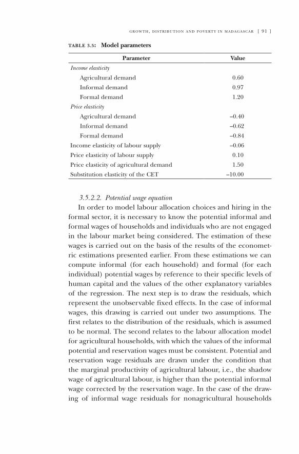
g r o w t h, d i s t r i b u t i o n a n d p o v e rt y i n m a d a g a s c a r [ 91 ]
table 3.5: Model parameters
Parameter Value
Income elasticity
Agricultural demand 0.60
Informal demand 0.97
Formal demand 1.20
Price elasticity
Agricultural demand –0.40
Informal demand –0.62
Formal demand –0.84
Income elasticity of labour supply –0.06
Price elasticity of labour supply 0.10
Price elasticity of agricultural demand 1.50
Substitution elasticity of the CET –10.00
3.5.2.2. Potential wage equationIn order to model labour allocation choices and hiring in the
formal sector, it is necessary to know the potential informal and formal wages of households and individuals who are not engaged in the labour market being considered. The estimation of these wages is carried out on the basis of the results of the economet-ric estimations presented earlier. From these estimations we can compute informal (for each household) and formal (for each individual) potential wages by reference to their specific levels of human capital and the values of the other explanatory variables of the regression. The next step is to draw the residuals, which represent the unobservable fixed effects. In the case of informal wages, this drawing is carried out under two assumptions. The first relates to the distribution of the residuals, which is assumed to be normal. The second relates to the labour allocation model for agricultural households, with which the values of the informal potential and reservation wages must be consistent. Potential and reservation wage residuals are drawn under the condition that the marginal productivity of agricultural labour, i.e., the shadow wage of agricultural labour, is higher than the potential informal wage corrected by the reservation wage. In the case of the draw-ing of informal wage residuals for nonagricultural households
[ 92 ] m i c r o s i m u l at i o n a s a t o o l f o r t h e e va l u at i o n o f p u b l i c p o l i c i e s
and individual formal wages, only the assumption of normal dis-tribution is retained.
3.5.2.3. HeterogeneityThe model allows for various sources of heterogeneity at the
household level. These differ in their demographic character-istics, their endowments of physical and human capital, their position in the labour market, and their consumption and labour supply preferences. The conservation of the residuals in the microeconomic equations makes it possible to take into account unexplained elements of heterogeneity.
3.5.2.4. Algorithm and solutionThe model was written using the GAUSS software package. The
solution algorithm is a loop with decreasing steps that seeks the equi-librium prices that will clear excess demand for the agricultural good and informal labour. At each step, all the microeconomic functions of behaviour are recomputed with new prices. Since the process of labour allocation for agricultural households is discrete, these can “switch” from a state of autarky (where they do not participate in the wage labour market) to a state of multi-activity, according to the respective values of the implicit on-farm wage (which depends on the price of the agricultural good) and of the corrected market wage (which depend on the price of informal labour). Individual demand and supply are then aggregated to obtain the functions of excess de-mand that we wish to clear. Solution time depends on the magnitude of the shocks and the computational capacities available.
3.6. Impact of growth shocks on poverty and inequality
The first set of simulations relates to a number of growth shocks corresponding to various development strategies. The impact of these shocks on poverty and inequality is analyzed. The compara-tive statics of the model are studied through an analysis of the results at aggregate level. The ex ante/ex post decomposition of the results underscores the importance of the general equilib-
g r o w t h, d i s t r i b u t i o n a n d p o v e rt y i n m a d a g a s c a r [ 93 ]
rium effects, while reading the microeconomic results through a detailed classification of households allows us to evaluate the contribution of endogenizing the within-group variance of in-come. Some results of sensitivity tests for guesstimated parameters are also presented.
3.6.1. Some descriptive elementsMicroeconomic data are provided by the EPM (Enquête
Permanente auprès des Ménages) survey of 1993; a national survey of the SDA type (social dimension of adjustment) cover-ing 4,508 households. This survey was carried out by the INSTAT (Institut National de la Statistique) on behalf of the Malagasy government. The macroeconomic data correspond to those of the Social Accounting Matrix of Madagascar for the year 1995 (Razafindrakoto and Roubaud 1997). This SAM, in addition, was used as the base for a computable general equilibrium model ap-plied to Madagascar (Dissou, Haggblade et al. 1999). The reconcili-ation of the microeconomic data of 1993 with the macroeconomic data of 1995 was carried out using a program of recalibration of statistical weights (Robilliard and Robinson 2003). The results of the model thus correspond to the Malagasy economy of 1995 and are presented in constant 1995 Malagasy francs. The figures in table 3.6 show that income structure differs greatly between rural households, whose income is dominated by agricultural production, and urban households, whose income is dominated by formal production factors. Consumption patterns also differ since the agricultural budget share is 17.9% in the urban sector and 27.9% in the rural sector.
Table 3.7 presents various indicators of poverty and inequal-ity as well as the distribution of the poor between the rural and urban sector.
Several indicators are used for this descriptive analysis and will be used again for the analysis of the results. The three indicators of poverty depend on the definition of a poverty line. Following several analyses of poverty in Madagascar, we took the per capita caloric line corresponding to the poverty line used at national level, and which amounts to 248,000 Malagasy francs of 1993. This threshold corresponds to a per capita income sufficient
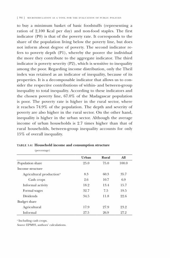
[ 94 ] m i c r o s i m u l at i o n a s a t o o l f o r t h e e va l u at i o n o f p u b l i c p o l i c i e s
to buy a minimum basket of basic foodstuffs (representing a ration of 2,100 Kcal per day) and non-food staples. The first indicator (P0) is that of the poverty rate. It corresponds to the share of the population living below the poverty line, but does not inform about degree of poverty. The second indicator re-fers to poverty depth (P1), whereby the poorer the individual the more they contribute to the aggregate indicator. The third indicator is poverty severity (P2), which is sensitive to inequality among the poor. Regarding income distribution, only the Theil index was retained as an indicator of inequality, because of its properties. It is a decomposable indicator that allows us to con-sider the respective contributions of within- and between-group inequality to total inequality. According to these indicators and the chosen poverty line, 67.0% of the Madagascar population is poor. The poverty rate is higher in the rural sector, where it reaches 74.9% of the population. The depth and severity of poverty are also higher in the rural sector. On the other hand, inequality is higher in the urban sector. Although the average income of urban households is 2.7 times higher than that of rural households, between-group inequality accounts for only 15% of overall inequality.
table 3.6: Household income and consumption structure (percentage)
Urban Rural All
Population share 25.0 75.0 100.0
Income structure
Agricultural productiona 8.3 60.3 35.7
Cash crops 2.6 10.7 6.9
Informal activity 18.2 13.4 15.7
Formal wages 32.7 7.5 19.5
Dividends 34.5 11.8 22.6
Budget share
Agricultural 17.9 27.9 23.2
Informal 27.5 26.9 27.2
a Including cash crops.Source: EPM93, authors’ calculations.
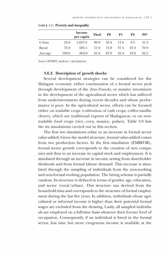
g r o w t h, d i s t r i b u t i o n a n d p o v e rt y i n m a d a g a s c a r [ 95 ]
table 3.7: Poverty and inequality
Income per capita
Theil P0 P1 P2 P0*
Urban 25.0 1,627.6 90.9 43.4 17.6 9.5 41.3
Rural 75.0 605.1 51.0 74.9 37.4 23.3 70.9
Average 100.0 863.0 81.6 67.0 32.4 19.8 62.5
Source: EPM93, authors’ calculations.
3.6.2. Description of growth shocksSeveral development strategies can be considered for the
Malagasy economy: either continuation of a formal sector push through development of the Zone Franche, or massive investment in the development of the agricultural sector which has suffered from underinvestment during recent decades and whose perfor-mance is poor. In the agricultural sector, efforts can be focused either on tradable crops (cultivation of cash crops, coffee-vanilla-cloves), which are traditional exports of Madagascar, or on non-tradable food crops (rice, corn, manioc, pulses). Table 3.8 lists the six simulations carried out in this section.
The first two simulations relate to an increase in formal sector value-added. Given the model structure, formal value-added comes from two production factors. In the first simulation (EMBFOR), formal sector growth corresponds to the creation of new compa-nies and thus to an increase in capital stock and employment. It is simulated through an increase in income arising from shareholder dividends and from formal labour demand. This increase is simu-lated through the sampling of individuals from the non-working and non-formal working population. The hiring scheme is partially random. Its structure is defined in terms of gender, age, education, and sector (rural/urban). This structure was derived from the household data and corresponds to the structure of formal employ-ment during the last five years. In addition, individuals whose agri-cultural or informal income is higher than their potential formal wages are excluded from the drawing. Lastly, all sampled individu-als are employed on a full-time basis whatever their former level of occupation. Consequently, if an individual is hired in the formal sector, less time but more exogenous income is available at the
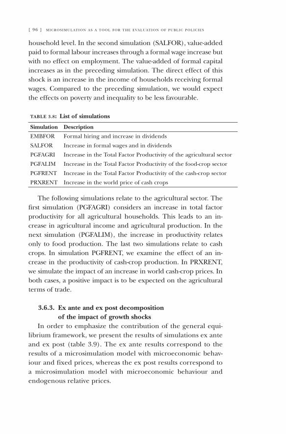
[ 96 ] m i c r o s i m u l at i o n a s a t o o l f o r t h e e va l u at i o n o f p u b l i c p o l i c i e s
household level. In the second simulation (SALFOR), value-added paid to formal labour increases through a formal wage increase but with no effect on employment. The value-added of formal capital increases as in the preceding simulation. The direct effect of this shock is an increase in the income of households receiving formal wages. Compared to the preceding simulation, we would expect the effects on poverty and inequality to be less favourable.
table 3.8: List of simulations
Simulation Description
EMBFOR Formal hiring and increase in dividends
SALFOR Increase in formal wages and in dividends
PGFAGRI Increase in the Total Factor Productivity of the agricultural sector
PGFALIM Increase in the Total Factor Productivity of the food-crop sector
PGFRENT Increase in the Total Factor Productivity of the cash-crop sector
PRXRENT Increase in the world price of cash crops
The following simulations relate to the agricultural sector. The first simulation (PGFAGRI) considers an increase in total factor productivity for all agricultural households. This leads to an in-crease in agricultural income and agricultural production. In the next simulation (PGFALIM), the increase in productivity relates only to food production. The last two simulations relate to cash crops. In simulation PGFRENT, we examine the effect of an in-crease in the productivity of cash-crop production. In PRXRENT, we simulate the impact of an increase in world cash-crop prices. In both cases, a positive impact is to be expected on the agricultural terms of trade.
3.6.3. Ex ante and ex post decomposition of the impact of growth shocks
In order to emphasize the contribution of the general equi-librium framework, we present the results of simulations ex ante and ex post (table 3.9). The ex ante results correspond to the results of a microsimulation model with microeconomic behav-iour and fixed prices, whereas the ex post results correspond to a microsimulation model with microeconomic behaviour and endogenous relative prices.
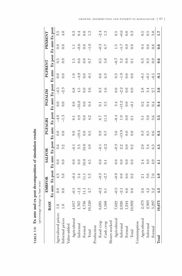
g r o w t h, d i s t r i b u t i o n a n d p o v e rt y i n m a d a g a s c a r [ 97 ]
ta
bl
e 3
.9:
Ex
ante
and
ex
post
dec
ompo
sitio
n of
sim
ulat
ion
resu
lts
(per
cent
age
chan
ge v
s. b
ase
year
)
BA
SEE
MB
FOR
SAL
FOR
PG
FAG
RI
PG
FAL
IMP
GFR
EN
TP
RX
RE
NT
Ex
ante
Ex
post
Ex
ante
Ex
post
Ex
ante
Ex
post
Ex
ante
Ex
post
Ex
ante
Ex
post
Ex
ante
Ex
post
Agr
icul
tura
l pri
ces
1.0
0.0
4.3
0.0
3.6
0.0
–4.0
0.0
–4.5
0.0
0.5
0.0
3.5
Info
rmal
pri
ces
1.0
0.0
3.8
0.0
3.2
0.0
–1.3
0.0
–2.3
0.0
0.9
0.0
4.0
Valu
e-ad
ded
Agr
icul
tura
l4,
017
–0.1
–0.4
0.0
–0.1
9.9
8.1
8.0
6.8
1.9
1.5
1.1
0.3
Info
rmal
1,76
7–1
.23.
40.
03.
3–1
9.4
4.9
–16.
04.
5–4
.90.
6–8
.60.
4Fo
rmal
4,73
611
.111
.110
.010
.00.
00.
00.
00.
00.
00.
00.
00.
0To
tal
10,5
204.
75.
34.
54.
90.
54.
20.
43.
6-0
.10.
7–1
.01.
3Pr
oduc
tion
Food
cro
p6,
695
–0.2
–0.3
0.0
–0.1
9.9
8.7
9.1
8.3
0.8
0.5
–0.3
–2.4
Cas
h cr
op1,
568
0.1
–2.7
0.1
–2.2
9.7
11.5
3.5
5.6
6.3
5.8
6.7
1.3
Hou
rs w
orke
dA
gric
ultu
ral
7,62
2–0
.5–0
.90.
0–0
.33.
6–0
.43.
40.
60.
3–0
.71.
50.
5In
form
al2,
026
–2.1
0.8
0.0
2.2
–13.
91.
9–1
3.2
–2.2
–1.0
3.2
–5.7
–0.6
Form
al1,
244
6.6
6.6
0.0
0.0
0.0
0.0
0.0
0.0
0.0
0.0
0.0
0.0
Tota
l10
,892
0.0
0.2
0.0
0.2
0.0
0.1
–0.1
0.0
0.0
0.1
0.0
0.3
Con
sum
ptio
nA
gric
ultu
ral
2,47
32.
62.
12.
42.
00.
33.
10.
22.
8–0
.10.
30.
40.
5In
form
al2,
903
4.2
3.6
4.0
3.4
0.5
3.6
0.4
3.4
–0.1
0.3
0.6
0.5
Form
al5,
297
5.2
7.0
4.9
6.3
0.6
3.6
0.4
2.7
–0.1
0.9
0.8
3.0
Tot
al10
,673
4.3
4.9
4.1
4.5
0.5
3.5
0.4
3.0
-0.1
0.6
0.6
1.7
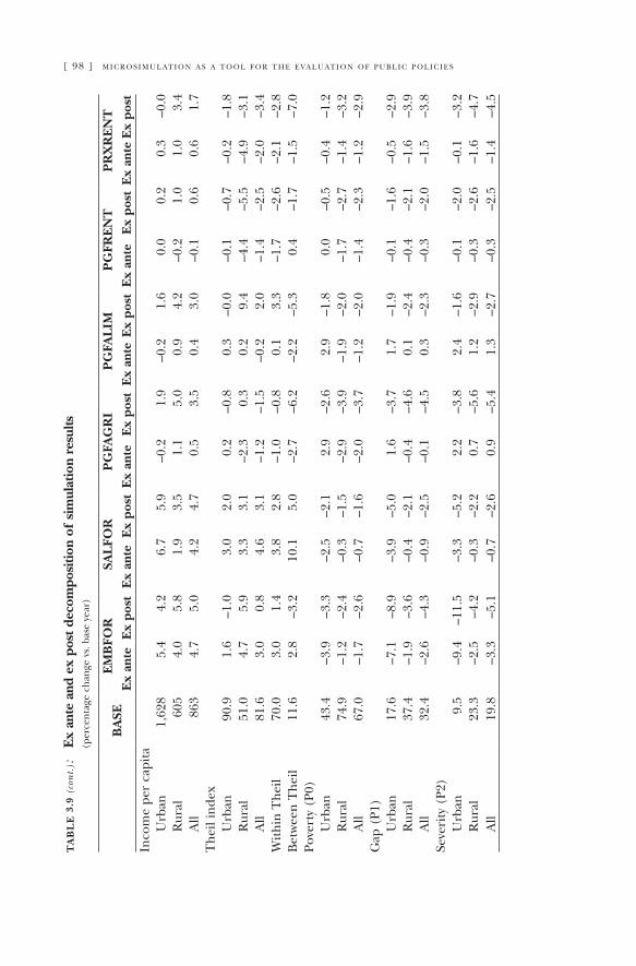
[ 98 ] m i c r o s i m u l at i o n a s a t o o l f o r t h e e va l u at i o n o f p u b l i c p o l i c i e st
ab
le 3
.9 (
con
t.):
Ex
ante
and
ex
post
dec
ompo
sitio
n of
sim
ulat
ion
resu
lts
(p
erce
ntag
e ch
ange
vs.
bas
e ye
ar)
BA
SEE
MB
FOR
SAL
FOR
PG
FAG
RI
PG
FAL
IMP
GFR
EN
TP
RX
RE
NT
Ex
ante
Ex
post
Ex
ante
Ex
post
Ex
ante
Ex
post
Ex
ante
Ex
post
Ex
ante
Ex
post
Ex
ante
Ex
post
Inco
me
per
capi
taU
rban
1,62
85.
44.
26.
75.
9–0
.21.
9–0
.21.
60.
00.
20.
3–0
.0R
ural
605
4.0
5.8
1.9
3.5
1.1
5.0
0.9
4.2
–0.2
1.0
1.0
3.4
All
863
4.7
5.0
4.2
4.7
0.5
3.5
0.4
3.0
–0.1
0.6
0.6
1.7
The
il in
dex
Urb
an90
.91.
6–1
.03.
02.
00.
2–0
.80.
3–0
.0–0
.1–0
.7–0
.2–1
.8R
ural
51.0
4.7
5.9
3.3
3.1
–2.3
0.3
0.2
9.4
–4.4
–5.5
–4.9
–3.1
All
81.6
3.0
0.8
4.6
3.1
–1.2
–1.5
–0.2
2.0
–1.4
–2.5
–2.0
–3.4
With
in T
heil
70.0
3.0
1.4
3.8
2.8
–1.0
–0.8
0.1
3.3
–1.7
–2.6
–2.1
–2.8
Bet
wee
n T
heil
11.6
2.8
–3.2
10.1
5.0
–2.7
–6.2
–2.2
–5.3
0.4
–1.7
–1.5
–7.0
Pove
rty
(P0)
Urb
an43
.4–3
.9–3
.3–2
.5–2
.12.
9–2
.62.
9–1
.80.
0–0
.5–0
.4–1
.2R
ural
74.9
–1.2
–2.4
–0.3
–1.5
–2.9
–3.9
–1.9
–2.0
–1.7
–2.7
–1.4
–3.2
All
67.0
–1.7
–2.6
–0.7
–1.6
–2.0
–3.7
–1.2
–2.0
–1.4
–2.3
–1.2
–2.9
Gap
(P1
)U
rban
17.6
–7.1
–8.9
–3.9
–5.0
1.6
–3.7
1.7
–1.9
–0.1
–1.6
–0.5
–2.9
Rur
al37
.4–1
.9–3
.6–0
.4–2
.1–0
.4–4
.60.
1–2
.4–0
.4–2
.1–1
.6–3
.9A
ll32
.4–2
.6–4
.3–0
.9–2
.5–0
.1–4
.50.
3–2
.3–0
.3–2
.0–1
.5–3
.8Se
veri
ty (
P2)
Urb
an9.
5–9
.4–1
1.5
–3.3
–5.2
2.2
–3.8
2.4
–1.6
–0.1
–2.0
–0.1
–3.2
Rur
al23
.3–2
.5–4
.2–0
.3–2
.20.
7–5
.61.
2–2
.9–0
.3–2
.6–1
.6–4
.7A
ll19
.8–3
.3–5
.1–0
.7–2
.60.
9–5
.41.
3–2
.7–0
.3–2
.5–1
.4–4
.5
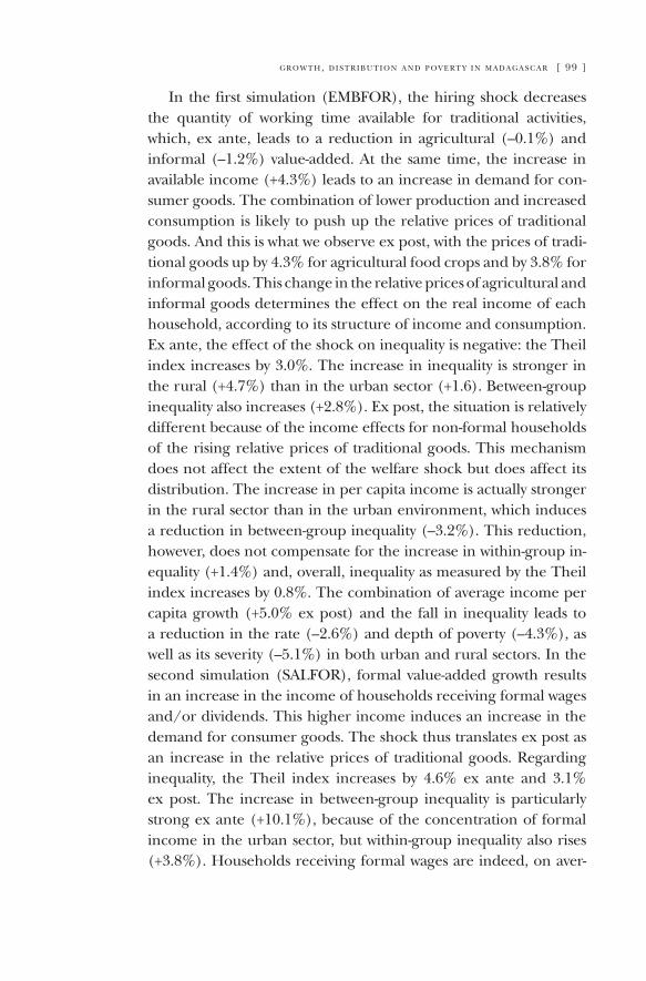
g r o w t h, d i s t r i b u t i o n a n d p o v e rt y i n m a d a g a s c a r [ 99 ]
In the first simulation (EMBFOR), the hiring shock decreases the quantity of working time available for traditional activities, which, ex ante, leads to a reduction in agricultural (–0.1%) and informal (–1.2%) value-added. At the same time, the increase in available income (+4.3%) leads to an increase in demand for con-sumer goods. The combination of lower production and increased consumption is likely to push up the relative prices of traditional goods. And this is what we observe ex post, with the prices of tradi-tional goods up by 4.3% for agricultural food crops and by 3.8% for informal goods. This change in the relative prices of agricultural and informal goods determines the effect on the real income of each household, according to its structure of income and consumption. Ex ante, the effect of the shock on inequality is negative: the Theil index increases by 3.0%. The increase in inequality is stronger in the rural (+4.7%) than in the urban sector (+1.6). Between-group inequality also increases (+2.8%). Ex post, the situation is relatively different because of the income effects for non-formal households of the rising relative prices of traditional goods. This mechanism does not affect the extent of the welfare shock but does affect its distribution. The increase in per capita income is actually stronger in the rural sector than in the urban environment, which induces a reduction in between-group inequality (–3.2%). This reduction, however, does not compensate for the increase in within-group in-equality (+1.4%) and, overall, inequality as measured by the Theil index increases by 0.8%. The combination of average income per capita growth (+5.0% ex post) and the fall in inequality leads to a reduction in the rate (–2.6%) and depth of poverty (–4.3%), as well as its severity (–5.1%) in both urban and rural sectors. In the second simulation (SALFOR), formal value-added growth results in an increase in the income of households receiving formal wages and/or dividends. This higher income induces an increase in the demand for consumer goods. The shock thus translates ex post as an increase in the relative prices of traditional goods. Regarding inequality, the Theil index increases by 4.6% ex ante and 3.1% ex post. The increase in between-group inequality is particularly strong ex ante (+10.1%), because of the concentration of formal income in the urban sector, but within-group inequality also rises (+3.8%). Households receiving formal wages are indeed, on aver-
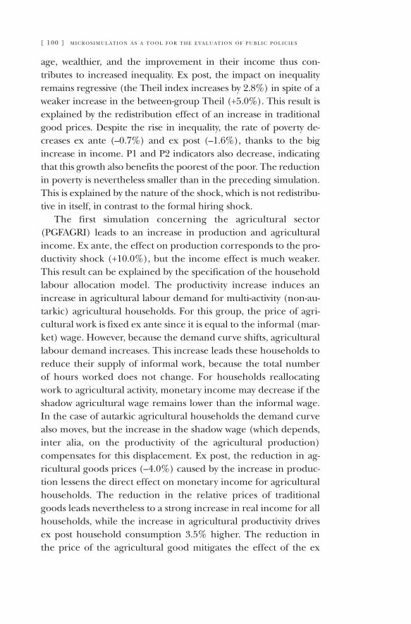
[ 100 ] m i c r o s i m u l at i o n a s a t o o l f o r t h e e va l u at i o n o f p u b l i c p o l i c i e s
age, wealthier, and the improvement in their income thus con-tributes to increased inequality. Ex post, the impact on inequality remains regressive (the Theil index increases by 2.8%) in spite of a weaker increase in the between-group Theil (+5.0%). This result is explained by the redistribution effect of an increase in traditional good prices. Despite the rise in inequality, the rate of poverty de-creases ex ante (–0.7%) and ex post (–1.6%), thanks to the big increase in income. P1 and P2 indicators also decrease, indicating that this growth also benefits the poorest of the poor. The reduction in poverty is nevertheless smaller than in the preceding simulation. This is explained by the nature of the shock, which is not redistribu-tive in itself, in contrast to the formal hiring shock.
The first simulation concerning the agricultural sector (PGFAGRI) leads to an increase in production and agricultural income. Ex ante, the effect on production corresponds to the pro-ductivity shock (+10.0%), but the income effect is much weaker. This result can be explained by the specification of the household labour allocation model. The productivity increase induces an increase in agricultural labour demand for multi-activity (non-au-tarkic) agricultural households. For this group, the price of agri-cultural work is fixed ex ante since it is equal to the informal (mar-ket) wage. However, because the demand curve shifts, agricultural labour demand increases. This increase leads these households to reduce their supply of informal work, because the total number of hours worked does not change. For households reallocating work to agricultural activity, monetary income may decrease if the shadow agricultural wage remains lower than the informal wage. In the case of autarkic agricultural households the demand curve also moves, but the increase in the shadow wage (which depends, inter alia, on the productivity of the agricultural production) compensates for this displacement. Ex post, the reduction in ag-ricultural goods prices (–4.0%) caused by the increase in produc-tion lessens the direct effect on monetary income for agricultural households. The reduction in the relative prices of traditional goods leads nevertheless to a strong increase in real income for all households, while the increase in agricultural productivity drives ex post household consumption 3.5% higher. The reduction in the price of the agricultural good mitigates the effect of the ex
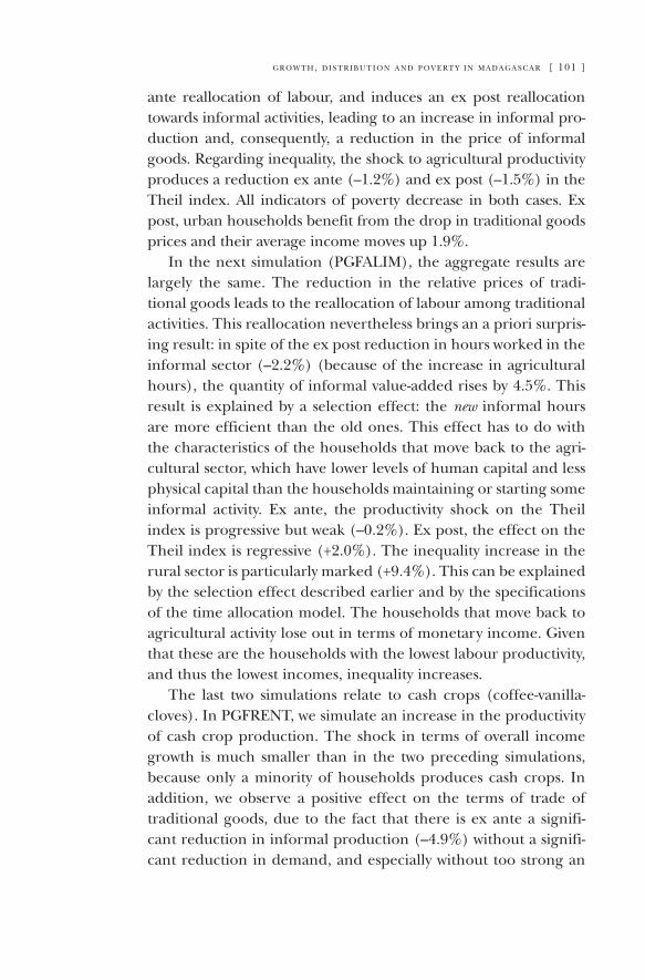
g r o w t h, d i s t r i b u t i o n a n d p o v e rt y i n m a d a g a s c a r [ 101 ]
ante reallocation of labour, and induces an ex post reallocation towards informal activities, leading to an increase in informal pro-duction and, consequently, a reduction in the price of informal goods. Regarding inequality, the shock to agricultural productivity produces a reduction ex ante (–1.2%) and ex post (–1.5%) in the Theil index. All indicators of poverty decrease in both cases. Ex post, urban households benefit from the drop in traditional goods prices and their average income moves up 1.9%.
In the next simulation (PGFALIM), the aggregate results are largely the same. The reduction in the relative prices of tradi-tional goods leads to the reallocation of labour among traditional activities. This reallocation nevertheless brings an a priori surpris-ing result: in spite of the ex post reduction in hours worked in the informal sector (–2.2%) (because of the increase in agricultural hours), the quantity of informal value-added rises by 4.5%. This result is explained by a selection effect: the new informal hours are more efficient than the old ones. This effect has to do with the characteristics of the households that move back to the agri-cultural sector, which have lower levels of human capital and less physical capital than the households maintaining or starting some informal activity. Ex ante, the productivity shock on the Theil index is progressive but weak (–0.2%). Ex post, the effect on the Theil index is regressive (+2.0%). The inequality increase in the rural sector is particularly marked (+9.4%). This can be explained by the selection effect described earlier and by the specifications of the time allocation model. The households that move back to agricultural activity lose out in terms of monetary income. Given that these are the households with the lowest labour productivity, and thus the lowest incomes, inequality increases.
The last two simulations relate to cash crops (coffee-vanilla-cloves). In PGFRENT, we simulate an increase in the productivity of cash crop production. The shock in terms of overall income growth is much smaller than in the two preceding simulations, because only a minority of households produces cash crops. In addition, we observe a positive effect on the terms of trade of traditional goods, due to the fact that there is ex ante a signifi-cant reduction in informal production (–4.9%) without a signifi-cant reduction in demand, and especially without too strong an
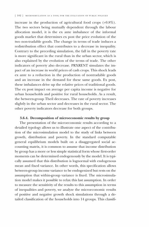
[ 102 ] m i c r o s i m u l at i o n a s a t o o l f o r t h e e va l u at i o n o f p u b l i c p o l i c i e s
increase in the production of agricultural food crops (+0.8%). The two sectors being mutually dependent through the labour allocation model, it is the ex ante imbalance of the informal goods market that determines ex post the price evolution of the two non-tradable goods. The change in terms of trade induces a redistribution effect that contributes to a decrease in inequality. Contrary to the preceding simulation, the fall in the poverty rate is more significant in the rural than in the urban sector, which is also explained by the evolution of the terms of trade. The other indicators of poverty also decrease. PRXRENT simulates the im-pact of an increase in world prices of cash crops. This shock leads ex ante to a reduction in the production of nontradable goods and an increase in the demand for these same goods. Ex post, these imbalances drive up the relative prices of traditional goods. The ex post impact on average per capita income is negative for urban households and positive for rural households. As a result, the between-group Theil decreases. The rate of poverty increases slightly in the urban sector and decreases in the rural sector. The other poverty indicators decrease for both groups.
3.6.4. Decomposition of microeconomic results by groupThe presentation of the microeconomic results according to a
detailed typology allows us to illustrate one aspect of the contribu-tion of the microsimulation model to the study of links between growth, distribution and poverty. In the standard computable general equilibrium models built on a disaggregated social ac-counting matrix, it is common to assume that income distribution by group has a more or less simple statistical form whose first-order moments can be determined endogenously by the model. It is typi-cally assumed that this distribution is lognormal with endogenous mean and fixed variance. In other words, this specification allows between-group income variance to be endogenized but rests on the assumption that within-group variance is fixed. The microsimula-tion model makes it possible to relax this last assumption. In order to measure the sensitivity of the results to this assumption in terms of inequalities and poverty, we analyze the microeconomic results of positive and negative growth shock simulations through a de-tailed classification of the households into 14 groups. This classifi-
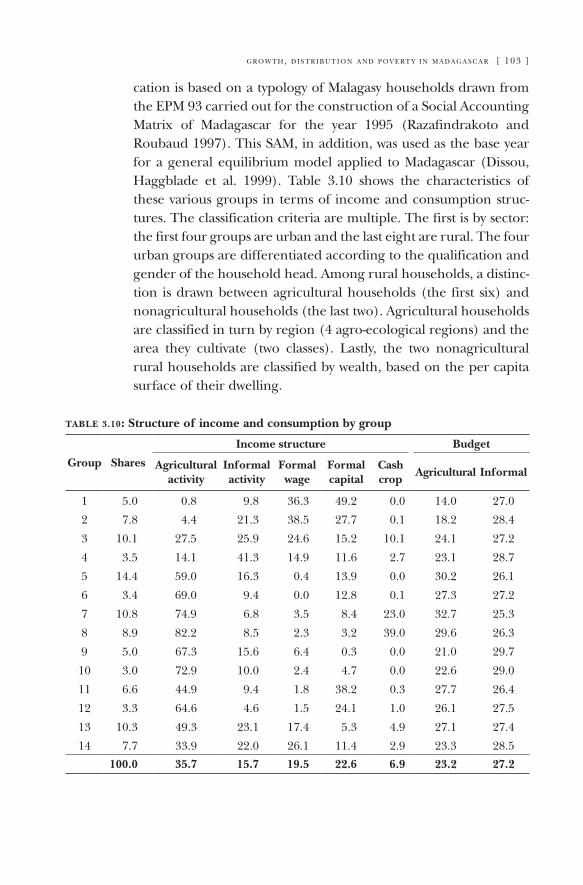
g r o w t h, d i s t r i b u t i o n a n d p o v e rt y i n m a d a g a s c a r [ 103 ]
cation is based on a typology of Malagasy households drawn from the EPM 93 carried out for the construction of a Social Accounting Matrix of Madagascar for the year 1995 (Razafindrakoto and Roubaud 1997). This SAM, in addition, was used as the base year for a general equilibrium model applied to Madagascar (Dissou, Haggblade et al. 1999). Table 3.10 shows the characteristics of these various groups in terms of income and consumption struc-tures. The classification criteria are multiple. The first is by sector: the first four groups are urban and the last eight are rural. The four urban groups are differentiated according to the qualification and gender of the household head. Among rural households, a distinc-tion is drawn between agricultural households (the first six) and nonagricultural households (the last two). Agricultural households are classified in turn by region (4 agro-ecological regions) and the area they cultivate (two classes). Lastly, the two nonagricultural rural households are classified by wealth, based on the per capita surface of their dwelling.
table 3.10: Structure of income and consumption by group
Group Shares
Income structure Budget
Agricultural activity
Informal activity
Formal wage
Formal capital
Cash crop
Agricultural Informal
1 5.0 0.8 9.8 36.3 49.2 0.0 14.0 27.0
2 7.8 4.4 21.3 38.5 27.7 0.1 18.2 28.4
3 10.1 27.5 25.9 24.6 15.2 10.1 24.1 27.2
4 3.5 14.1 41.3 14.9 11.6 2.7 23.1 28.7
5 14.4 59.0 16.3 0.4 13.9 0.0 30.2 26.1
6 3.4 69.0 9.4 0.0 12.8 0.1 27.3 27.2
7 10.8 74.9 6.8 3.5 8.4 23.0 32.7 25.3
8 8.9 82.2 8.5 2.3 3.2 39.0 29.6 26.3
9 5.0 67.3 15.6 6.4 0.3 0.0 21.0 29.7
10 3.0 72.9 10.0 2.4 4.7 0.0 22.6 29.0
11 6.6 44.9 9.4 1.8 38.2 0.3 27.7 26.4
12 3.3 64.6 4.6 1.5 24.1 1.0 26.1 27.5
13 10.3 49.3 23.1 17.4 5.3 4.9 27.1 27.4
14 7.7 33.9 22.0 26.1 11.4 2.9 23.3 28.5
100.0 35.7 15.7 19.5 22.6 6.9 23.2 27.2
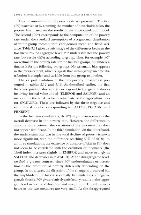
[ 104 ] m i c r o s i m u l at i o n a s a t o o l f o r t h e e va l u at i o n o f p u b l i c p o l i c i e s
Two measurements of the poverty rate are presented. The first (P0) is arrived at by counting the number of households below the poverty line, based on the results of the microsimulation model. The second (P0*) corresponds to the computation of the poverty rate under the standard assumption of a lognormal distribution of within-group income, with endogenous mean and fixed vari-ance. Table 3.11 gives a static image of the differences between the two measures. At aggregate level, P0* underestimates the poverty rate, but results differ according to group. Thus, for example, P0* overestimates the poverty rate for the first two groups, but underes-timates it for the following two groups. No systematic bias appears in the measurement, which suggests that within-group income dis-tribution is complex and variable from one group to another.
The ex post evolution of the two poverty measures is pre-sented in tables 3.12 and 3.13. As described earlier, the first three are positive shocks and correspond to the growth shocks involving formal value-added (EMBFOR and SALFOR) and an increase in the total factor productivity of the agriculture sec-tor (PGFAGRI). These are followed by the three negative and symmetrical shocks corresponding to SALFOR, PGFAGRI and PRXRENT.
In the first two simulations, d(P0*) slightly overestimates the overall decrease in the poverty rate. However, the difference in absolute value between the variations of the two measures does not appear significant. In the third simulation, on the other hand, the underestimation bias in the total decline of poverty is much more significant, with the difference reaching 30% of d(P0). In all three simulations, the existence or absence of bias in P0* does not seem to be correlated with the evolution of inequality (the Theil index increases slightly in EMBFOR and more strongly in SALFOR, and decreases in PGFAGRI). At the disaggregated level, we find a greater contrast, since P0* underestimates or overes-timates the evolution of poverty differently depending on the group. In most cases, the direction of the change is preserved but the amplitude of the bias varies greatly. In simulations of negative growth shocks, P0* gives relatively satisfactory results at the aggre-gate level in terms of direction and magnitude. The differences between the two measures are very small. At the disaggregated
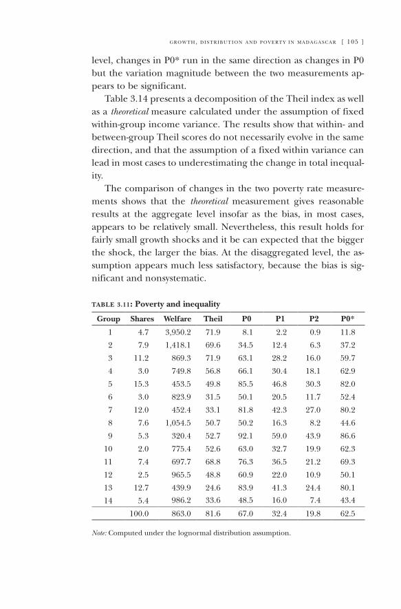
g r o w t h, d i s t r i b u t i o n a n d p o v e rt y i n m a d a g a s c a r [ 105 ]
level, changes in P0* run in the same direction as changes in P0 but the variation magnitude between the two measurements ap-pears to be significant.
Table 3.14 presents a decomposition of the Theil index as well as a theoretical measure calculated under the assumption of fixed within-group income variance. The results show that within- and between-group Theil scores do not necessarily evolve in the same direction, and that the assumption of a fixed within variance can lead in most cases to underestimating the change in total inequal-ity.
The comparison of changes in the two poverty rate measure-ments shows that the theoretical measurement gives reasonable results at the aggregate level insofar as the bias, in most cases, appears to be relatively small. Nevertheless, this result holds for fairly small growth shocks and it be can expected that the bigger the shock, the larger the bias. At the disaggregated level, the as-sumption appears much less satisfactory, because the bias is sig-nificant and nonsystematic.
table 3.11: Poverty and inequality
Group Shares Welfare Theil P0 P1 P2 P0*
1 4.7 3,950.2 71.9 8.1 2.2 0.9 11.8
2 7.9 1,418.1 69.6 34.5 12.4 6.3 37.2
3 11.2 869.3 71.9 63.1 28.2 16.0 59.7
4 3.0 749.8 56.8 66.1 30.4 18.1 62.9
5 15.3 453.5 49.8 85.5 46.8 30.3 82.0
6 3.0 823.9 31.5 50.1 20.5 11.7 52.4
7 12.0 452.4 33.1 81.8 42.3 27.0 80.2
8 7.6 1,054.5 50.7 50.2 16.3 8.2 44.6
9 5.3 320.4 52.7 92.1 59.0 43.9 86.6
10 2.0 775.4 52.6 63.0 32.7 19.9 62.3
11 7.4 697.7 68.8 76.3 36.5 21.2 69.3
12 2.5 965.5 48.8 60.9 22.0 10.9 50.1
13 12.7 439.9 24.6 83.9 41.3 24.4 80.1
14 5.4 986.2 33.6 48.5 16.0 7.4 43.4
100.0 863.0 81.6 67.0 32.4 19.8 62.5
Note: Computed under the lognormal distribution assumption.
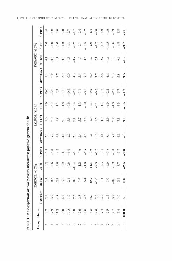
[ 106 ] m i c r o s i m u l at i o n a s a t o o l f o r t h e e va l u at i o n o f p u b l i c p o l i c i e s
ta
bl
e 3
.12:
Com
pari
son
of tw
o po
vert
y m
easu
res:
pos
itive
gro
wth
sho
cks
Gro
upSh
ares
EM
BFO
R (
+10%
)SA
LFO
R (
+10%
)P
GFA
GR
I (+
10%
)
d(W
elfa
re)
d(T
heil)
d(P
0)d
(P0*
)d(
Wel
fare
)d(
The
il)d(
P0)
d(P
0*)
d(W
elfa
re)
d(T
heil)
d(P
0)d
(P0*
)
14.
72.
11.
46.
2–2
.87.
21.
0–3
.0–1
0.0
1.4
–0.1
–5.6
–2.4
27.
93.
00.
3–2
.6–3
.85.
72.
0–3
.7–5
.22.
2–0
.8–2
.0–2
.8
311
.24.
8–2
.4–3
.6–4
.24.
31.
8–1
.1–2
.32.
7–1
.1–2
.6–2
.0
43.
05.
0–5
.6–5
.9–6
.13.
02.
5–1
.3–1
.63.
0–0
.8–1
.3–2
.0
515
.31.
62.
1–0
.8–0
.42.
03.
8–0
.8–0
.36.
0–1
.7–4
.1–2
.7
63.
02.
30.
6–1
0.4
–2.1
2.7
2.1
–10.
4–2
.14.
5–0
.7–8
.2–4
.7
712
.02.
81.
6–1
.2–1
.03.
43.
7–1
.3–1
.15.
4–1
.0–2
.1–2
.4
87.
64.
35.
4–1
.0–3
.54.
03.
5–0
.8–3
.57.
23.
5–1
6.5
–6.2
95.
359
.920
.2–1
1.5
–7.9
1.6
1.9
–0.1
–0.2
6.0
–1.7
–2.0
–1.4
102.
02.
6–1
.6–2
.3–2
.21.
31.
5–0
.1–0
.57.
72.
7–1
.2–4
.0
117.
43.
01.
4–2
.3–1
.44.
24.
9–1
.7–1
.23.
6–2
.7–2
.7–2
.9
122.
52.
31.
0–4
.3–1
.83.
42.
9–4
.3–2
.24.
4–1
.4–1
4.3
–4.8
1312
.73.
7–0
.8–0
.9–1
.85.
22.
2–1
.8–2
.12.
51.
8–0
.6–0
.9
145.
43.
02.
1–3
.7–2
.74.
33.
1–3
.5–3
.72.
8–0
.4–4
.8–3
.8
010
0.0
5.0
0.8
–2.6
–2.8
4.7
3.1
–1.6
–1.7
3.5
–1.5
–3.7
–2.6
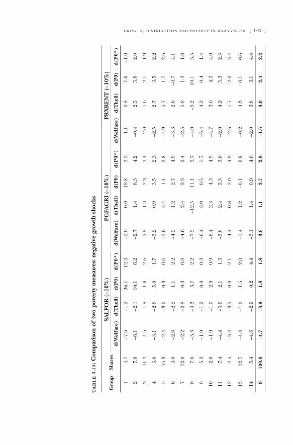
g r o w t h, d i s t r i b u t i o n a n d p o v e rt y i n m a d a g a s c a r [ 107 ]
ta
bl
e 3
.13:
Com
pari
son
of tw
o po
vert
y m
easu
res:
neg
ativ
e gr
owth
sho
cks
Gro
upSh
ares
SAL
FOR
(–1
0%)
PG
FAG
RI
(–10
%)
PR
XR
EN
T (–
10%
)
d(W
elfa
re)
d(T
heil)
d(P
0)d
(P0*
)d(
Wel
fare
)d(
The
il)d(
P0)
d(P
0*)
d(W
elfa
re)
d(T
heil)
d(P
0)d
(P0*
)
14.
7–7
.6–1
.236
.112
.3–2
.00.
019
.83.
31.
10.
87.
6–1
.0
27.
9–6
.1–2
.110
.16.
2–2
.71.
48.
34.
2–0
.42.
55.
82.
0
311
.2–4
.5–1
.81.
82.
6–2
.91.
32.
32.
4–2
.01.
62.
11.
9
43.
0–3
.1–2
.85.
01.
7–3
.20.
93.
52.
3–2
.52.
73.
52.
2
515
.3–2
.4–3
.00.
30.
6–5
.64.
41.
42.
8–4
.95.
71.
72.
6
63.
0–2
.6–2
.21.
12.
2–4
.21.
22.
74.
9–3
.32.
6–0
.74.
1
712
.0–2
.2–2
.80.
30.
8–4
.62.
42.
32.
4–2
.55.
81.
31.
8
87.
6–3
.3–9
.33.
72.
2–7
.5–1
2.5
11.1
5.7
–4.0
–5.2
10.1
3.5
95.
3–1
.9–1
.20.
00.
3–6
.43.
90.
51.
7–5
.44.
20.
41.
4
102.
0–1
.9–1
.02.
90.
9–6
.42.
34.
34.
9–4
.73.
04.
34.
0
117.
4–4
.4–5
.62.
11.
3–3
.82.
45.
33.
0–2
.04.
95.
32.
5
122.
5–3
.4–3
.50.
02.
1–4
.40.
82.
04.
9–2
.61.
72.
03.
4
1312
.7–4
.4–1
.01.
52.
0–1
.41.
2–0
.10.
8–0
.24.
30.
10.
6
145.
4–4
.6–2
.90.
24.
4–3
.11.
40.
94.
8–2
.03.
83.
14.
4
010
0.0
–4.7
–3.9
1.8
1.8
–3.6
1.1
2.7
2.9
–1.6
3.0
2.4
2.2
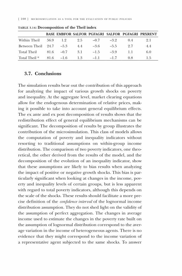
[ 108 ] m i c r o s i m u l at i o n a s a t o o l f o r t h e e va l u at i o n o f p u b l i c p o l i c i e s
table 3.14: Decomposition of the Theil index
BASE EMBFOR SALFOR PGFAGRI SALFOR PGFAGRI PRXRENT
Within Theil 56.9 1.2 2.5 –0.7 –3.2 0.4 2.1
Between Theil 24.7 –5.3 4.4 –3.6 –5.5 2.7 4.4
Total Theil 81.6 –0.7 3.1 –1.5 –3.9 1.1 6.0
Total Theil * 81.6 –1.6 1.3 –1.1 –1.7 0.8 1.5
3.7. Conclusions
The simulation results bear out the contribution of this approach for analyzing the impact of various growth shocks on poverty and inequality. At the aggregate level, market clearing equations allow for the endogenous determination of relative prices, mak-ing it possible to take into account general equilibrium effects. The ex ante and ex post decomposition of results shows that the redistribution effect of general equilibrium mechanisms can be significant. The decomposition of results by group illustrates the contribution of the microsimulation. This class of models allows the computation of poverty and inequality indicators without resorting to traditional assumptions on within-group income distribution. The comparison of two poverty indicators, one theo-retical, the other derived from the results of the model, and the decomposition of the evolution of an inequality indicator, show that these assumptions are likely to bias results when analyzing the impact of positive or negative growth shocks. This bias is par-ticularly significant when looking at changes in the income, pov-erty and inequality levels of certain groups, but is less apparent with regard to total poverty indicators, although this depends on the scale of the shocks. These results should facilitate a more pre-cise definition of the confidence interval of the lognormal income distribution assumption. They do not shed light on the validity of the assumption of perfect aggregation. The changes in average income used to estimate the changes in the poverty rate built on the assumption of lognormal distribution correspond to the aver-age variation in the income of heterogeneous agents. There is no evidence that they might correspond to the income variation of a representative agent subjected to the same shocks. To answer
g r o w t h, d i s t r i b u t i o n a n d p o v e rt y i n m a d a g a s c a r [ 109 ]
this question would call for a model with representative agents comparable to the disaggregated model.
The analysis of the impact of various growth shocks on poverty and inequality also highlights the complexity of the mechanisms connecting macroeconomic shocks and income distribution, start-ing from a model that embraces considerable inter-household di-versity, but otherwise considers only three sectors and four goods. Although not standard, the microeconomic specifications selected are nevertheless derived from a model of rational behaviour and the rationing schemes selected are relatively simple. Even so, the impact of growth shocks on individual households is a complex matter, which depends on the structural characteristics of each as well as on the structural characteristics of the economy.
Although the relative mean income and price changes are significant, the impact of the various growth shocks on overall poverty and inequality indicators appears relatively small; a result which concurs with the findings of studies on the evolution of inequality over time (Li, Squire and Zou 1998). There are several explanations for this. First of all, the descriptive analysis of house-hold income shows how income sources are diversified. This diversification itself constitutes a first line of protection against risk insofar as the income from different sources is not directly correlated. Secondly, reallocation between different activities reinforces this protection strategy, while making it possible for households to react to significant price shocks. The existence of transaction costs weakens the size of these reactions. Finally, the inertia of total indicators is explained by the unequal distribution of production factors. These inequalities will not disappear with-out proactive policies that give poor households access to educa-tion and credit. This inertia nevertheless masks the importance of redistribution among household groups. Analyzing the results through the filter of a classification into distinct socioeconomic groups shows that the evolution of poverty and inequality indica-tors can differ from one group to other.
Concerning the limits of the model, the extreme aggrega-tion of goods and sectors does not allow us to study the impact of more specific policies on poverty and income distribution. More precisely, the economic impact of certain macroeconomic
[ 110 ] m i c r o s i m u l at i o n a s a t o o l f o r t h e e va l u at i o n o f p u b l i c p o l i c i e s
policies or liberalization campaigns may depend on the trad-ability of the goods produced by the economy. One contribution of applied general equilibrium models is their capacity to factor these structural effects through the disaggregation of activities and goods. Several reasons explain why this capacity is lacking in the microsimulation model as developed up to now. First of all, there remains a problem of data and estimation. To include more goods we would have to be able to connect the income of each household to each type of good represented. And this is a difficult operation given the quality of the available data. We would also need to develop a labour allocation model with sev-eral goods, which considerably complicates model writing. Lastly, it seemed to us interesting initially to develop a simple model to highlight structural effects like those described above. Another possible extension of the model relates to the explicit modelling of macroeconomic closures. This extension would require the further integration of the model within a general equilibrium framework, adding government and savings-investment accounts. Finally, building a dynamic model constitutes another model development stage. The introduction of the temporal dimension would allow us to take account of demographic effects, which are of fundamental importance in the evolution of inequality and poverty. The extensions described above can be envisaged as a magic triangle whose nodes would be: i) the heterogeneity of products, ii) the heterogeneity of agents, and iii) the temporal dimension. The relative weight assigned to these three poles of disaggregation will vary according to the problem at hand.
References
adelman, i., and s. robinson. “Macroeconomic Adjustment and Income Distribution: Alternative Models Applied to Two Economies.” Journal of Development Economics 29(1): 23–44.
—. Income Distribution Policy: A Computable General Equilibrium Model of South Korea. Stanford: Stanford University Press, 1978.
alatas, v. and f. bourguignon. “The evolution of income distribution during Indonesia's fast growth: 1980-1996.” Mimeo, 1999.
benjamin, d.“Household Composition, Labour Markets and Labour Demand: Testing for Separation in Agricultural Household Models.” Econometrica 60 (March 1992): 287–322.

g r o w t h, d i s t r i b u t i o n a n d p o v e rt y i n m a d a g a s c a r [ 111 ]
bourguignon, f., m. fournier and m. gurgand. “Distribution, development and education: Taiwan, 1979–1992.” Mimeo. Paris: DELTA, 1998.
bourguignon, f., j. de melo and c. morrisson. “Poverty and Income Distribution During Adjustment: Issues and Evidence from the OECD Project.” World Development 19(11): 1485–1508.
cogneau, d. “La formation du revenue des ménages à Antananarivo: une microsimulation en équilibre general pour la fin du siècle.” Economie de Madagascar 4 (1999): 131–155.
decaluwé, b., a. patry, l. savard and e. thorbecke. “Poverty Analysis within a General Equilibrium Framework.” CREFA Working Paper 9909. Université Laval, 1999.
de janvry, a., e. sadoulet and a. fargeix. “Politically Feasible and Equitable Adjustment: Some Alternatives for Ecuador.” World Development 19(11): 1577–1594.
dervis, k., j. de melo and s. robinson. General Equilibrium Models for Development Policy. Cambridge: Cambridge University Press, 1982.
harding, a. Microsimulation and Public Policy. Amsterdam: Elsevier, 1993.hildenbrand, w. “How relevant are specifications of behavioural relations on the
micro-level for modelling the time path of population aggregates?” European Economic Review 42: 437–458.
jacoby, h. “Productivity of Men and Women and the Sexual Division of Labour in Peasant Agriculture of the Peruvian Sierra.” Journal of Development Economics 37 (1992): 265–287.
—. “Shadow Wages and Peasant Family Labour Supply: An Econometric Application to the Peruvian Sierra.” Review of Economic Studies 60 (October 1993): 903–922.
kirman, a. “Whom or What Does the Representative Individual Represent?” Journal of Economic Perspectives 6(2): 117–136.
li, h., l. squire and h. Zou. “Explaining International and Intertemporal Variations in Income Inequality.” Economic Journal 108: 26–43.
lysy, f. and l. taylor. “The general equilibrium model of income distribution.” In L. Taylor, E. Bacha, E. Cardoso and F. Lysy (eds.). Models of growth and distribution for Brazil. Oxford: Oxford University Press, 1980.
meagher, g. a. “Forecasting Changes in the Distribution of Income: An Applied General Equilibrium Approach.” In A. Harding (ed.). Microsimulation and Public Policy. Amsterdam: Elsevier, 1993.
newman, j. l. and p. j. gertler. “Family Productivity, Labour Supply, and Welfare in a Low Income Country.” The Journal of Human Resources XXIX(4): 989–1026.
orcutt, g. “A new type of socio-economic system.” Review of Economics and Statistics 58: 773–797.
raZafindrakoto, m. and f. roubaud. “Une Matrice de Comptabilité Sociale pour Madagascar.” MADIO Working Paper, 9744/E. Antananarivo, 1997.1997..
robilliard, a. s. and s. robinson. “Reconciling Household Surveys and National Accounts Data Using Cross-Entropy Estimation.” Review of Income and Wealth 49(3): 395–406.
skoufias, e.“Using Shadow Wages to Estimate Labour Supply of Agricultural Households.” American Journal of Agricultural Economics 76 (May 1994): 215–227.
taylor, l. Socially Relevant Policy Analysis. Structuralist Computable General Equilibrium Models for the Developing World. Cambridge: The MIT Press, 1990.
van tongeren, f. “Microsimulation versus Applied General Equilibrium Models.” Paper presented at the 5th International Conference on CGE Modelling, 27–29 October, 1994, University of Waterloo (Canada).

[ 113 ]
Microsimulation of Healthcare Policies
Nuria Badenes Complutense University of Madrid
Ángel López Polytechnic University of Cartagena
4.1. Introduction
Microsimulation has become a powerful tool in many fields of economics, and health economics is no exception. It can be part of the programming carried out by a researcher in order to resolve a specific problem, although it is increasingly common to come across coordinated efforts where models are constructed by teams. The advantage of constructing large models is that these can be improved, refined or incorporated into other models. The proliferation of microsimulation models thus exemplifies the advantages of the division and specialisation of work, in such a way that today it is no longer necessary to know how to construct the tool in order to be able to use it, and researchers’ efforts can be focussed on what each one does best: programming, designing improvements for microsimulation models or applying models for decision making.
This chapter reviews the microsimulation models that can be used in the field of health economics and highlights one applica-tion for the technique’s use. The chapter is structured as follows: following this introduction, the second section sets out the limits of what the concept of microsimulation comprises in the field of health economics and reviews by country the models that have been developed by different teams. The third section shows some examples of work using ad hoc microsimulation models created to resolve specific problems. The fourth section details the results of the application of one of these models, which was created to estimate the savings derived from the use of private healthcare services to the detriment of the equivalent services in the public system generated by double coverage.
4.
[ 114 ] m i c r o s i m u l at i o n a s a t o o l f o r t h e e va l u at i o n o f p u b l i c p o l i c i e s
4.2. Microsimulation models in health economics
Microsimulation models are computer models that operate from the level of the individual upwards. Starting from the individual behaviour of representative groups, these models simulate what occurs in larger populations in order to reach conclusions ap-plicable to larger groups. Starting from the behaviour at the individual level, it is possible to incorporate different responses, and this is what makes these models different from aggregate models, in which the explanatory variables represent group properties.
There are areas of public economics in which microsimula-tion has been extensively used as a decision making instrument, such as the distributional analysis of taxation and transfer poli-cies. In other fields, such as health economics, microsimulation is only just beginning to advance, although its applicability and potential are both considerable.
The field of health economics is very broad and difficult to define and the efforts in creating models are still modest. When we refer to microsimulation in this field it should be clear that we are essentially referring to healthcare financing and pharmaceu-tical expenditure models, healthcare management models and models that study healthcare demand and the economic impact of behaviour related to the health and ageing of the population. In many cases we will not find specific healthcare models but tax-benefit models which include variables related to healthcare expenditure and services, or pension models in which health status is one more variable to be taken into account.
Given the broad scope of application of microsimulation in health economics, it is not surprising that current and po-tential users of this relatively new work method are many and varied: the public sector, private sector, individuals, business and academia. Decision making increasingly has to be based on the quantification of hypothetical scenarios, and this is something that interests everyone.
As stated, it is increasingly common to find working groups that have joined forces to construct microsimulation models. Tax-benefit models were the pioneers in developing microsimulation.
m i c r o s i m u l at i o n o f h e a lt h c a r e p o l i c i e s [ 115 ]
Although these models may simply analyse the after effects of a given policy, they can also be improved so that they include the response of the parties affected by that policy. Initially, tax-benefit models were confined to analysing distributional issues related to taxes and transfers, but it is more and more common to find models that incorporate individual behavioural responses to a given policy relating to health, or models created specifically to analyse healthcare policies.
Models that analyse the cost in pensions or healthcare of population ageing are a fairly recent development that goes one step further and incorporates a dynamic element. The construc-tion of dynamic models is not an easy task as regards either the construction of the models or estimating the probabilities of each future scenario considered. This may be one explanation for the proliferation of multidisciplinary working teams composed of researchers from different countries.
The most significant microsimulation models for health eco-nomics are detailed below, by country and institution. In many cases they are not specific healthcare models, but models con-structed for other purposes. Nevertheless, the models consider issues related to healthcare expenditure, health insurance or pensions. We will not attempt to give an exhaustive explanation of how the models work or the assumptions that they incorporate (see Zaidi and Rake 2002), but just a general overview of which tools are currently available in the field of health economics.
4.2.1. AustraliaThe National Centre for Social and Economic Modelling
(NATSEM) at the University of Canberra has begun to apply mi-crosimulation techniques to issues related to healthcare policy. According to Brown and Harding (2002) the PBS microsimula-tion model (Pharmaceutical Benefits Scheme) has been in de-velopment since 1997. This model is based on STINMOD, an earlier static model for analysing taxation and transfer policies also developed by NATSEM. Data from the National Health Survey were added to this model in relation to the use of pre-scribed medicines according to socioeconomic characteristics. Therefore, taking into account the age, gender and the subsidy

[ 116 ] m i c r o s i m u l at i o n a s a t o o l f o r t h e e va l u at i o n o f p u b l i c p o l i c i e s
level of patients who are prescribed medication, the model is capable of calculating:
simulated expenditure on the PBS according to household characteristics;government expenditure under the Pharmaceutical Benefits Scheme;the remaining out-of-pocket cost (contribution per patient co-payment) for the two consumer groups in Australia: general and those that receive benefit.
Also from NATSEM is DYNAMOD-2, a microsimulation model designed to forecast the characteristics of the Australian popula-tion 50 years into the future. The model operates with 1% of the population (150,000 observations) and generates the histories of the population taking into account demographic events (fertility, mortality, formation and separation of couples, as well as migra-tory phenomena). It also considers educational levels, employ-ment levels and income.
In addition to the official and academic fields, the Oakleigh-based company Laerdal offers various microsimulation models for educational purposes, including MicroSim Inhospital and MicroSim Prehospital. The former optimises economic and train-ing resources in hospitals, while the latter specifically focuses on the situation prior to hospitalisation (emergency doctors, para-medics, ambulances).
4.2.2. CanadaCanada has developed various microsimulation models
related to health economics. The Population Health Model (POHEM) is used by the Ministry of Statistics and is strictly a health model. Canadians also have LifePaths which can be used for analysing health policies, despite being a more general model.
POHEM is a longitudinal microsimulation health and illness model. It simulates representative populations using equations from sub-models developed by the Canadian Ministry of Statistics and allows alternative healthcare policies to be rationally com-
—
—
—
m i c r o s i m u l at i o n o f h e a lt h c a r e p o l i c i e s [ 117 ]
pared through an approach that captures the interactions caused by illness.
LifePaths is a dynamic longitudinal model of individuals and families. Using incorporated behavioural equations as well as a variety of micro historical databases, the model creates statistically representative samples that cover complete life periods of indi-viduals. The behavioural equations of the model generate the discrete events that comprise the individual’s complete history, at sub-annual resolution. In addition to these longitudinal capabili-ties, LifePaths is capable of analysing refined and representative results taking into account a set of overlapping cohorts from 1971 onwards. LifePaths is used to analyse, develop and calculate the cost of programmes that have a fundamental longitudinal com-ponent, especially those that require evaluation at individual or household level. It can also be used to analyse social issues with a longitudinal nature such as intergenerational justice or the most appropriate timing for the allocation of certain resources over a lifetime.
In addition to the above models, the Canadian Ministry of Health has others such as HTSIM (Health and Tax Microsimulation model) and the supply and demand models PHARMSIM and HHR (Health Human Resources).
HTSIM allows the implications of the income tax system for households with subsidised healthcare spending to be developed and evaluated. The advantage of this model over existing ones is that it provides a better explanation of healthcare expenditure, as regards both expenses covered by the fiscal system and those that are not recognised.
The PHARMSIM model is currently under construction. Its principal objective is to analyse the usage patterns of medications and the distributional impact of medical insurance plans.
The HHR supply and demand models are also currently un-der construction. Their objective is to allow the Health Ministry to forecast expenditure and resource use by means of a series of complex equations, including the employment situation, age and gender of healthcare personnel. They seek to construct a non-mechanical model that incorporates agent behaviour. The HHR demand model will foreseeably be constructed in accordance
[ 118 ] m i c r o s i m u l at i o n a s a t o o l f o r t h e e va l u at i o n o f p u b l i c p o l i c i e s
with MD use, as well as the demands of patients of other health-care professionals.
Canada took CORSIM, a dynamic model previously devel-oped by the United States, and adapted it to Canadian data to create DYNACAN—a dynamic, longitudinal and stochastic microsimulation model.1 DYNACAN can carry out simulations on different demographic and income aspects, as well as other characteristics which allow the evolution of contributors and beneficiaries in the pension system to be analysed. It is therefore possible to study the sustainability of the existing system and the consequences of alternative actions by the Human Resources Development Canada department (HRDC), the principal user of the model.
4.2.3. United StatesJonathan Gruber, affiliated to the MIT and NBER, has recently
developed a microsimulation model whose first version is ex-plained in Gruber (2000). The model takes a representative sam-ple of the North American population, which contains informa-tion about insurance products offered by employers, healthcare coverage, income, demographics and the state of health declared by survey respondents.2 This model can calculate the effects of various medical insurance policy alternatives on the distribution of healthcare costs and expenditure in the public and private sec-tors. The model assumes certain behavioural traits for companies, families and individuals in the face of changes in the absolute and relative prices of healthcare insurance.
In the 1970s, the Urban Institute in Washington began to de-velop a dynamic microsimulation tool, which it revised during the 1980s and continues improving today. The institute’s objective was to determine how current and proposed retirement policies, demographic trends and practices of the private sector influence the security and decision making of elderly Americans, provid-
1 A stochastic model based on Monte Carlo simulations of random number generation for event generation. It is longitudinal because it forecasts the life of individuals/families (and their pensions) throughout the lifecourse and dynamic because it takes into account that household characteristics can change over time.
2 The sample comes from the 1997 Current Population Survey (CPS).
m i c r o s i m u l at i o n o f h e a lt h c a r e p o l i c i e s [ 119 ]
ing a tool for politicians to tackle potential crises. Known as DYNASIM3, it consists of a dynamic microsimulation model that analyses the long-term distributional consequences of retire-ment and population ageing. The model works with a represen-tative sample3 from which demographic events are simulated, such as population growth, family creation, education or health. Although it is not strictly a healthcare model, it does tackle population ageing, one of the principal problems of interest in health economics.
The Urban Institute also has the TRIM3 model (Transfer Income Model), created from an earlier version of a microsimula-tion model (RIM, Reforms and Income Maintenance) developed in 1969. This static model attempts to enable researchers to work with microdata in the simulation of a wide variety of in-come and taxation programmes, but specifically includes health programmes that impact the North American population—the reason the Department of Health and Human Services financed the initiative. Specifically, TRIM3 allows policy alternatives to be simulated relative to the following programmes:
Medicaid; SCHIP (State Health Insurance Programs);Medicare;ESI (Employer Sponsored-Health Insurance).
In 1987 Cornell University began to develop its CORSIM model, whose most recent version CORSIM 4.1 was launched in 2002. CORSIM has been the benchmark for the construc-tion of other dynamic models such as the POLISIM model of the U.S. Social Security administration, SVERIGE in Sweden and DYNACAN in Canada. It is a dynamic model relating to the U.S. population that uses the recent past to simulate what will hap-pen in the future with the focus on government policies, and especially those related to social security programmes. The data that it incorporates on individuals and households refer to basic
3 Data on families and individuals taken from the Survey of Income and Program Participation panels in 1990 and 1993, which are then aged on a yearly basis.
————
[ 120 ] m i c r o s i m u l at i o n a s a t o o l f o r t h e e va l u at i o n o f p u b l i c p o l i c i e s
demographic characteristics such as births, deaths, marriage, di-vorce, emigration and immigration. It also includes educational levels, economic, income and employment information, accu-mulation of wealth and debt and contributions to pension plans. This model has been extensively used by the U.S. Social Security administration.
4.2.4. EuropeWithin the group of tax-benefit models, EUROMOD is one
of the most ambitious in terms of coverage, since it includes 15 European Union countries (Germany, Austria, Belgium, Denmark, Spain, Finland, France, Greece, the Netherlands, Ireland, Italy, Luxemburg, Portugal and the United Kingdom) coordinated via a microsimulation unit. It is a static microsimulation model that allows the distributional impact of taxation and transfer policies to be estimated, both at individual country and European level. Although not created as a health economics model, it uses health-related concepts to evaluate consolidated social policies in the European Union. It is possible to simulate policies relating to social contributions and social welfare for all the aforementioned countries, but policies on disabilities or pensions can only be simu-lated for selected countries (Sutherland 2001).
In addition to this combined country initiative, microsimula-tion models applicable to health economics are available for a number of individual European countries.
4.2.4.1. FranceLike other European countries, France has developed a dy-
namic model, DESTINIE, to simulate pension sustainability, al-though it is not a healthcare model as such. The problem is that public and private pension schemes operate differently and the model assumes that everyone takes out a private pension plan. DESTINIE began to be developed at the end of the 1990s, but is expected to be extended in the future to the public sector.
4.2.4.2. NetherlandsJan Nelissen developed a microsimulation model for the
Netherlands with the name of NEDYMAS, whose objective is to
m i c r o s i m u l at i o n o f h e a lt h c a r e p o l i c i e s [ 121 ]
compare the degree of vertical redistribution of social security schemes in the income of four 10-year cohorts born between 1930 and 1960. This required a cross-sectional sampling from the point in time when the first cohort entered the job market. Since this data was not available, it was generated hypothetically with the same characteristics as the census. This model is therefore similar to cohort models, although it does not assume a static position, but simply attempts to model the conditions in which in-dividuals live (and will live). Starting with this cross-sectional data and simulating the birth of future generations, the model allows for analysis of lifelong redistributional effects of the tax-benefit models on a group of cohorts. This Dutch model is not a specific health economics tool, but it is a useful instrument to evaluate the sustainability of the pensions system linked to ageing.
4.2.4.3. NorwayThe Norwegian Statistics Department uses various energy,
taxation, macroeconomic, regional and population microsimula-tion models. The group of population models includes MOSART, a dynamic microsimulation model that allows long-term forecasts to be made, and analyses changes in population and the labour force, public aid for education and social security benefits. The model was created by Fredriksen (1998) in the Norwegian Ministry of Statistics for the study of different options to deal with the challenge of financing future public expenditure. The input data represent 12% of the Norwegian population and the same data are used to estimate transition probabilities to various situa-tions such as disability, rehabilitation or employment.
4.2.4.4. United KingdomThe Department of Social Policy of the London School of
Economics, in conjunction with the Institute of Gerontology of King’s College London and the Sciences Institute of the University of Southampton, created SAGE (Social Policy in an Ageing Society) in November 1999. The objective of this group is to investigate the future of social policy in an ageing society. One of the keys towards achieving this objective lies in the construc-tion and use of a dynamic microsimulation model that allows
[ 122 ] m i c r o s i m u l at i o n a s a t o o l f o r t h e e va l u at i o n o f p u b l i c p o l i c i e s
the impact of different policy options to be evaluated. SAGE is not devoted to the study of health economics, but the policies analysed and included in its models do take health into account as a variable.
SAGE has developed a family of static microsimulation models to evaluate policies that impact income and pensions in the later part of the life course, such as RITA (Retirement Income Trajectory Analysis model). This type of simulation is called “hypothetical” be-cause it can disclose the cost of pensions under the existing system or under a range of alternative hypothetical scenarios.
The SAGE research group has also created a dynamic micro-simulation model called SAGEMOD, which allows a sample of the British population to be projected up to 2020 simulating the principal events that occur in the life of individuals. By using cen-suses, panel data and cross-sectional data, the simulated events include birth, death, education, marriage, divorce, employment, income, health status, retirement, disability and informal care. The probabilities of these events occurring are estimated from the separate study of the probabilities for each.
The microsimulation unit at the University of Cambridge has created various microsimulation models for intercountry comparative purposes. One is the aforementioned EUROMOD and another is POLIMOD, both designed to determine the effects of changes in income tax and social security policies on income distribution.
Another model applicable to the United Kingdom is PENSIM, created to forecast the income of pensioners once they have retired. The first version of the dynamic model was made by Hancock el al. (1992), and then Curry (1996) developed the model now in use by the Department of Social Security. The introduction of a new extended version, PENSIM2, is being con-sidered for disability simulation, among other possibilities.
4.2.4.5. SwedenSweden has the SVERIGE model, created to simulate the be-
haviour of the Swedish population in demographic and economic terms. It is an example of dynamic microsimulation along the lines of the CORSIM model. Its reference point is the entire Swedish population of 1990, from which it simulates different events
m i c r o s i m u l at i o n o f h e a lt h c a r e p o l i c i e s [ 123 ]
throughout the life course of the nine million individuals consid-ered. Included in these events are education, energy consump-tion and migrations, but it also considers that individuals become ill, retire, receive pensions and die, and is therefore capable of analysing numerous actions related to health economics.
4.3. Microsimulation à la carte
Microsimulation models described in the above section stem from the efforts of many researchers and have taken considerable time to perfect. At times, the researcher does not want to embark on a large-scale project but simply to carry out a specific investigation. Hence, the literature also offers examples of work where micro-simulation is used as a tool but is not the primary objective. That is to say, researchers may create microsimulation models as tools applicable to the work of others. From an initial version, time and effort are invested in improving the model’s operation, increasing calculation speed, integrating the calculation tool with similar tools in the same or different countries or extending the model’s func-tionality. Once these models are in place, it is easy to obtain results in microsimulation terms without actually having to create the tool. Consider for instance the papers spawned by a highly extensive microsimulator project such as EUROMOD, which has a series of working papers (see http://www.iser.essex.ac.uk/msu/emod), or SAGE within the London School of Economics (http://www.lse.ac.uk/collections/SAGE/discussionPapers.htm).
On other occasions, the effort required to create a model may not compensate the researcher who wishes to make use of micro-data but for whom the intended output is not a tool. Tracking down works of these characteristics is an arduous task, since in-dividual programmes used for microsimulations by a particular researcher are not easily available in the same way as the models described in the previous section. Nevertheless, for the last few years it has been possible to find researchers who use microsimu-lation as a means to obtain results that allow knowledge in vari-ous disciplines to be advanced, and in particular in relation to health from both a medical and an economic perspective.
[ 124 ] m i c r o s i m u l at i o n a s a t o o l f o r t h e e va l u at i o n o f p u b l i c p o l i c i e s
Microsimulation has been applied to the study of as many different issues within the field of health economics as there are areas which generate interest. A recurrent theme in this research area is the analysis of the efficiency and equity of healthcare ex-penditure.
These issues, of great interest in the field of public sector eco-nomics in general, are of even more interest in the area of health, where problems of efficiency linked to adverse selection and moral hazard can be of particular importance in terms of expen-diture. Cost effectiveness, cost efficiency and cost-benefit analyses of the different ways of allocating healthcare expenditure are of enormous relevance in efficiency studies. Similarly, when speak-ing of equity one should not limit the analysis to monetary in-come, since the problem becomes much more serious when users are both disadvantaged and face difficulties accessing healthcare services. Overdemand for health services, the cost related to an ageing population and the favourable tax treatment of insurance are also recurrent issues in the area of health economics.
Various examples of work on these relevant questions in which ad hoc microsimulation models have been designed are described below, although the list is not exhaustive. We refer to models made for a particular purpose, either because the researchers do not form part of a team, because no such model exists or because the development of a more extensive model would not make sense for resolving the problem addressed by the study.
Healthcare insurance has been studied recurrently in the lit-erature. Chernick el al. (1987) study the correlation between the fact that the health insurance provided by employers is subsidised and that insurance is taken out above the optimum level, creating an excess of demand for healthcare services and rapid growth in expenditure in the medical sector. They calculate the elasticity of demand for medical insurance and medical services using a static microsimulation model applied to the United States. They conclude that the removal of subsidies would cause a reduction in demand for healthcare insurance of about 20% and a reduction in demand for healthcare services of about 5%.
The issue of medical insurance in the U.S. is also tackled by Zabinski el al. (1999), who use a microsimulation model con-
m i c r o s i m u l at i o n o f h e a lt h c a r e p o l i c i e s [ 125 ]
templating adverse selection to consider what would happen if the tax advantages of certain types of medical insurance were extended to the market as a whole. Among their conclusions is that the biggest losers would be the poorest and families with most children. More recently, Pauly and Herring (2000) take up the issue of the design of an insurance premium policy for em-ployees that reduces the inefficiency linked to the problem of adverse selection. They propose the efficient premium contribution whereby you would offer limited, but more generous coverage, and achieve an efficient allocation between individuals differing for reasons of risk. Applied to the Spanish case, López Nicolás (2001) analyses the consequences of the tax expenditure policy linked to medical insurance in Spain, as detailed in the empiri-cal application in this chapter. In López and Vera (2002) a mi-crosimulation routine is constructed based on a discrete choice model applied to data from Catalonia, in order to determine if tax subsidies for private medical insurance are self-financing. The conclusion is that, applied to 1999, the elimination of those subsidies implies an increase of 69.2 million euros in annual tax revenue, compared to an increase in costs for the public sector of 8.9 million euros annually.
Microdata analysis allows the study of inequality, a core issue in economics. Wagstaff and van Doorslaer (1997), pioneers in the study of inequalities linked to health, use Aronson’s method to break down the redistributional effect of the Dutch health-care financing system into three components: progressivity, horizontal equity and reranking.
Medical research on the suitability of certain diagnostic and treatment policies can use microsimulation as a decision making resource. An example is the study carried out by Boer el al. (1998) comparing the cost effectiveness of two possible changes to the breast cancer diagnostic programme in the United Kingdom: to reduce the screening period from every three to two years or to increase the screening age from 64 to 69. The histories of women without screening and with either of the screening policies being considered were simulated with microdata. Both policies would contribute to a reduction in mortality, with little difference in cost.
[ 126 ] m i c r o s i m u l at i o n a s a t o o l f o r t h e e va l u at i o n o f p u b l i c p o l i c i e s
Another example of applying microsimulation techniques to medical research is found in Cronin el al. (1998). Given the impossibility of resolving complex mathematical problems, this paper presents a cancer detecting application for a microsimu-lation model previously applied to the engineering field. A structure and set of parameter values are specified with associ-ated uncertainty. A Bayesian approach is adopted and a para-metric probability distribution is assumed to mathematically express the uncertainty linked to the parameters. Then follow three steps. First, design of a simulation experiment to achieve good coverage of the parameters. Second, modelling a set of responses for the result sought, as a function of the model parameters based on the results of the simulation. Third, sum-marising the variability of the result sought, including the vari-ability due to parameter uncertainty, using the combination of the possible responses and the probability distributions of the parameters. This model was applied to research into the effect of the specific prostate antigen on the prostate cancer mortality rate.
More recently, Lubitz et al. (2003) estimated the relationship between the state of health of the elderly (especially at 70) and the life expectancy and accumulated healthcare expenditure from this age until death. The study used American data from 1992 to 1998. In this case, microsimulation was necessary to estimate life expectancy in different states of health. The study concluded that accumulated healthcare expenditure for elderly people with a better state of health, despite their greater longevity, was similar to those in poor health. Health campaigns designed for people under 65 can improve health and longevity without increasing healthcare expenditure.
4.4. Empirical application: A microsimulation model for taxation policies in Spain
4.4.1. Objectives of the studyPrivate health insurance is an important ingredient for health-
care systems in the majority of OECD countries. Regardless of
m i c r o s i m u l at i o n o f h e a lt h c a r e p o l i c i e s [ 127 ]
the institutional arrangements for each country, public policies invariably have to consider the implications of private health insurance in terms of equity of access and efficiency in the provi-sion of healthcare services, quality, innovation, and the costs to users. In relation to the latter, in some countries private health insurance has been used as an instrument to shift the demand for healthcare services towards private providers, and thereby free up the public network. A typical setup consists of allowing private insurance to cover the same contingencies as the public network (therefore offering double coverage). This is the case in Australia, Ireland, the United Kingdom and Spain (Colombo and Tapay 2004). Tax breaks for holding private policies are justified under this viewpoint and in fact, exist in the majority of countries either through personal or corporate income tax (although some, like the UK, have removed them).
In this study, an empirical strategy is presented to evaluate whether the subsidies for private healthcare insurance are self-financing. In other words, do they produce reductions in the use of the public network on a sufficient scale to cover the tax expen-diture incurred? We illustrate this strategy with an application for Spain. The Spanish national health system provides free (mainly financed through general taxes) and universal treatment to the Spanish population. Apart from this public coverage, approxi-mately 10% of the population benefits from additional coverage via private insurance. The Spanish tax system treats the holding of private insurance generously. Until 1999, 15 cents of every euro spent on healthcare services (including insurance policies) were deductible for personal income tax purposes. Since 1999, tax re-lief is not directly available for the purchase of private insurance, but companies may offer policies to their employees as tax-free non-cash compensation. This involves a subsidy of 35 cents for every euro (the standard corporate tax rate) spent on healthcare insurance by the company.
We analyse the patterns of usage of private services to the detriment of equivalent public health services as a result of double coverage. In Spain, data from the 1997 National Health Survey suggest that holding dual coverage does not create two differentiated classes in the population of healthcare service users,
[ 128 ] m i c r o s i m u l at i o n a s a t o o l f o r t h e e va l u at i o n o f p u b l i c p o l i c i e s
but there seems to be a greater mobility between the two systems among those users who have the choice. As such, according to this data source, 13.85% of the population with double coverage visited a private provider in the fortnight prior to the survey, while 10.5% of this group visited a public provider. Conversely, the lack of double coverage does appear to create two types of users: in this population group only 1.46% visited a private provider in the 15 days before the survey while 23.38% visited a public provider. These circumstances lend weight to the view that the network of private providers reinforces the public service network. It may also be presumed that without double coverage, the public system would have to absorb a large part of the demand for care currently met by private providers contracted under supplemental policies. It is therefore interesting to quantify the savings in public expenditure that double healthcare coverage potentially generates. This will help to formulate tax policies that, if this is indeed the case, generate a positive externality associated with freeing up the public network. Although there is no evidence of the magnitude of this effect, previous studies suggest that demand for private healthcare services is highly sensitive to changes in price (with price elasticity of –1.4), and the public sector could therefore have demand pressure on its services alleviated or increased depending on changes in the cost of private healthcare (see López Nicolás 1998). This study attempts to quantify this saving using a microsimulation model of the behaviour of healthcare service consumers in Spain.
4.4.2. Methodology In general, when discussing microsimulation models it is
common to specify if they are static or dynamic. The crucial difference between them is that the latter contain an individual behavioural model that allows us to incorporate consumer reac-tions to changes in tax policies.
Various factors have to be taken into account in deciding on one or the other. First, there is no doubt that evaluation of the effects of reforms, assuming that these do not cause changes to consumers’ behaviour (level one effects) prior to being put into practice, offers useful results for any institution responsible for making tax and/or healthcare policy decisions. Also, factoring behaviour is a task
m i c r o s i m u l at i o n o f h e a lt h c a r e p o l i c i e s [ 129 ]
that requires the specification and estimation of relatively complex econometric models. For this reason, the majority of dynamic mod-els now available only contemplate one side of the market and not both. All these reasons favor the choice of static models. However, any economic reform will have effects on individual behaviour, and it is appropriate to take these reactions into account, especially knowing that the authorities may make changes aimed at altering the response of economic agents in order to, for example, incentiv-ise job search by the unemployed, private savings or a reduction in harmful consumption. The construction of static simulation models should therefore be seen as an intermediate stage on the road to achieving a dynamic model. In these circumstances it is important to break with the tendency to identify two separate research paths in the field of economic policy microsimulation: one path choos-ing static models and the other choosing dynamic models. This distinction is meaningless, since a static simulation model is just a dynamic model with the pre-imposed assumption that the reform to be simulated will generate a zero reaction from individuals, i.e., static models are specific types of dynamic models.
Also, in this specific project the objectives pursued make it necessary to estimate changes in the behaviour of healthcare service consumers under various healthcare coverage scenarios. A dynamic microsimulation model will therefore be used subject to the following sequential process:
Specification of an econometric model on the probability at the individual level of using the healthcare services for medi-cal visits in Spain, dealing with two types of providers, the public and private networks, and distinguishing between coverage types (public only and/or public + private).Estimation of the model from National Health Survey data.Incorporation of the econometric model into a simula-tion routine that allows for the probability of each of the services being used to be predicted for each of the com-ponents in the sample, as well as set types of user-specified individuals.Simulation/prediction of the probabilities of using the dif-ferent types of services.
—
——
—
[ 130 ] m i c r o s i m u l at i o n a s a t o o l f o r t h e e va l u at i o n o f p u b l i c p o l i c i e s
Estimate of healthcare costs associated to each type of ser-vice and of the socioeconomic characteristics of individu-als, using databases of payments to medical professionals by a mutual society representative of the situation in Spain.Calculation of expected savings per sampling unit under a double coverage scenario using the estimates to generate counterfactual analyses.Application of the results to the general population using relevant sample weightings.
4.4.3. Coverage type and use of healthcare services Double coverage is understood as a situation where a health
services user can access the services provided by the public net-work of the National Health Service and additionally via a volun-tary affiliation mutual insurer. According to data from the 1997 National Health Survey shown in table 4.1, this group comprises 7.16% of the adult population. Conversely, the second group is considered to be individuals that only have coverage from the public network, representing 83.94% of the adult population. These two groups cover 91.1% of the entire adult population rep-resented by the survey. The remaining adult population (8.9%) principally comprises users covered exclusively by obligatory af-filiation mutual societies (MUFACE, ISFAS, PAMEM, MUNPAL, Mútua del Poder Judicial) and, to a small extent, individuals covered exclusively by voluntary affiliation mutual societies and those declaring that they are covered by charity, a health manage-ment organisation or other types of coverage.
This study will use the information first on the group of individuals that only access the public network, and then on the group with double coverage as defined above. Given the size of these groups, they are clearly highly representative of the Spanish population. Also, the objectives of the study advo-cate analysing the behaviour of individuals with double cover-age against only those with sole access to the National Health Service. This is because individuals covered solely by an obliga-tory affiliation mutual association have a service that is more comparable to the service enjoyed by users with dual coverage via their private policy, in terms of waiting times, compensation
—
—
—
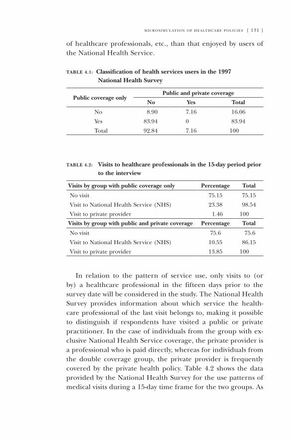
m i c r o s i m u l at i o n o f h e a lt h c a r e p o l i c i e s [ 131 ]
of healthcare professionals, etc., than that enjoyed by users of the National Health Service.
table 4.1: Classification of health services users in the 1997 National Health Survey
Public coverage onlyPublic and private coverage
No Yes Total
No 8.90 7.16 16.06
Yes 83.94 0 83.94
Total 92.84 7.16 100
table 4.2: Visits to healthcare professionals in the 15-day period prior to the interview
Visits by group with public coverage only Percentage Total
No visit 75.15 75.15
Visit to National Health Service (NHS) 23.38 98.54
Visit to private provider 1.46 100
Visits by group with public and private coverage Percentage Total
No visit 75.6 75.6
Visit to National Health Service (NHS) 10.55 86.15
Visit to private provider 13.85 100
In relation to the pattern of service use, only visits to (or by) a healthcare professional in the fifteen days prior to the survey date will be considered in the study. The National Health Survey provides information about which service the health-care professional of the last visit belongs to, making it possible to distinguish if respondents have visited a public or private practitioner. In the case of individuals from the group with ex-clusive National Health Service coverage, the private provider is a professional who is paid directly, whereas for individuals from the double coverage group, the private provider is frequently covered by the private health policy. Table 4.2 shows the data provided by the National Health Survey for the use patterns of medical visits during a 15-day time frame for the two groups. As
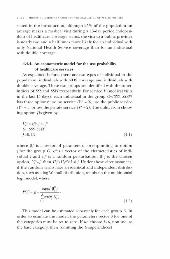
[ 132 ] m i c r o s i m u l at i o n a s a t o o l f o r t h e e va l u at i o n o f p u b l i c p o l i c i e s
stated in the introduction, although 25% of the population on average makes a medical visit during a 15-day period indepen-dent of healthcare coverage status, the visit to a public provider is nearly two and a half times more likely for an individual with only National Health Service coverage than for an individual with double coverage.
4.4.4. An econometric model for the use probability of healthcare services
As explained before, there are two types of individual in the population: individuals with NHS coverage and individuals with double coverage. These two groups are identified with the super-indices of SSS and SSYP respectively. For service V (medical visits in the last 15 days), each individual in the group G={SSS, SSYP} has three options: use no service (Yi
G = 0), use the public service
(YiG = 1) or use the private service (Yi
G = 2). The utility from choos-ing option J is given by
UijG = xi
G βjG+ εji
G G = SSS, SSYPJ = 0,1,2, (4.1)
where βjG is a vector of parameters corresponding to option
j for the group G, xiG is a vector of the characteristics of indi-
vidual I and εjiG is a random perturbation. If j is the chosen
option, YiG= j, then Uij
G>UikG "k ≠ j. Under these circumstances,
if the random terms have an identical and independent distribu-tion, such as a log-Weibull distribution, we obtain the multinomial logit model, where
( )
( )∑J
0=k
Gk
Gi
G
j
G
iGi
βxexp
βxexp=j)=P(Y .
(4.2)
This model can be estimated separately for each group G. In order to estimate the model, the parameters vector β for one of the categories must be set to zero. If we choose j = 0, non use, as the base category, then (omitting the G superindices)

m i c r o s i m u l at i o n o f h e a lt h c a r e p o l i c i e s [ 133 ]
).βexp(x=0)=P(Y2)=P(Y
)βexp(x=0)=P(Y1)=P(Y
2ii
i
1ii
i
(4.3)
The expressions exp(xi βj) are the relative risk (to the base op-tion) of option j for individual i.
To interpret the results of the estimation with this model, note that a change in any of the components of the characteristics vec-tor, x3 for example, implies a change in the probability of choos-ing the three options and a change in relative risks according to equations 1 and 2 respectively. As can be seen, since these expres-sions are non-linear, the effect of a change in one explanatory variable on the probability of choosing any option and therefore, in the relative risk, is not constant but depends on the configura-tion of the remaining explanatory variables.
As regards the explanatory variables that we use to specify the systematic part of the model, it bears mention that the National Health Survey combines information on a wide range of health indicators with socioeconomic status variables. This provides confidence in our estimates to a greater degree than would be expected if only socioeconomic or health indicators were available, since in any of these cases the possibility of bias for unobserved differences would be relatively high. Our specification therefore captures the effect of the following factors:
Gender: Modelled using a fictitious variable with a value of 1 for men (dman).
Age: Modelled using a linear term and a quadratic term (age, age2).
Self-perception of state of health: Modelled using two fictitious variables that indicate good health, and poor or very poor health (dhea2 dbadh respectively). The omitted category is very good health.
Limitations on activity in the last year: Modelled using a fictitious variable with a value of 1 if affirmative (dlimit).
Presence of chronic illnesses: Modelled using a fictitious variable, with a value of 1 for hypertension, high cholesterol, diabe-
[ 134 ] m i c r o s i m u l at i o n a s a t o o l f o r t h e e va l u at i o n o f p u b l i c p o l i c i e s
tes, asthma, cardiopathy and allergies (dcr1-dcr5 and dcr7 respectively).
Severity of chronic illnesses: Modelled using a fictitious variable with a value of 1 in the event that the chronic illness limits normal activity (dcrinter).
Accidents: Modelled using a fictitious variable with a value of 1 in the event of having suffered an accident in the previous year (dacci).
Hearing or sight problems: Modelled using fictitious variables, with a value of 1 in the event of hearing or sight problems (dhear, dsight respectively).
Smoker status: Modelled using a fictitious variable with a value of 1 for a current smoker or for having been a regular smoker in the past (devsmok).
Sports: Modelled using a fictitious variable that is activated if the individual does not regularly practice sports (dnos-port).
Household income level: Modelled using fictitious variables, with a value of 1 if the household income is between 150,000 and 300,000 pesetas per month and more than 300,000 pesetas per month (d300 and dm300, respective-ly). The omitted category corresponds to individuals with monthly household income less than 150,000 pesetas and also includes a fictitious variable with a value of 1 if the income variable has not been stated by the interviewee (dincmiss).
Marital status: Modelled using a fictitious variable with a value of 1 if the individual is married (dmarried).
Level of education: Modelled using a fictitious variable with a value of 1 if the individual has university studies (duniv).
Employment status: Modelled using fictitious variables, with a value of 1 if the individual is employed, receiving a retire-ment pension or unemployed with previous experience (demploy, dpensi, dunemp). The omitted category consists of the unemployed without work experience, those unem-ployed and not seeking work and housewives.
Occupational category: Modelled using fictitious variables, with a value of 1 in the event that the individual is a business
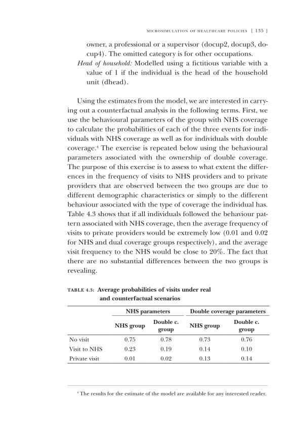
m i c r o s i m u l at i o n o f h e a lt h c a r e p o l i c i e s [ 135 ]
owner, a professional or a supervisor (docup2, docup3, do-cup4). The omitted category is for other occupations.
Head of household: Modelled using a fictitious variable with a value of 1 if the individual is the head of the household unit (dhead).
Using the estimates from the model, we are interested in carry-ing out a counterfactual analysis in the following terms. First, we use the behavioural parameters of the group with NHS coverage to calculate the probabilities of each of the three events for indi-viduals with NHS coverage as well as for individuals with double coverage.4 The exercise is repeated below using the behavioural parameters associated with the ownership of double coverage. The purpose of this exercise is to assess to what extent the differ-ences in the frequency of visits to NHS providers and to private providers that are observed between the two groups are due to different demographic characteristics or simply to the different behaviour associated with the type of coverage the individual has. Table 4.3 shows that if all individuals followed the behaviour pat-tern associated with NHS coverage, then the average frequency of visits to private providers would be extremely low (0.01 and 0.02 for NHS and dual coverage groups respectively), and the average visit frequency to the NHS would be close to 20%. The fact that there are no substantial differences between the two groups is revealing.
table 4.3: Average probabilities of visits under real and counterfactual scenarios
NHS parameters Double coverage parameters
NHS groupDouble c.
groupNHS group
Double c. group
No visit 0.75 0.78 0.73 0.76
Visit to NHS 0.23 0.19 0.14 0.10
Private visit 0.01 0.02 0.13 0.14
4 The results for the estimate of the model are available for any interested reader.

[ 136 ] m i c r o s i m u l at i o n a s a t o o l f o r t h e e va l u at i o n o f p u b l i c p o l i c i e s
The similarity in average frequency is reflected in the figures shown on the right hand section of the table. We can see here that if all individuals followed the behaviour associated with the double coverage pattern, visits to private providers would be more frequent than to NHS providers for the group that currently only has NHS coverage.
The counterfactual analysis shown in the previous table suggests that differences in the states of health and socioeconomic character-istics of the two population groups are not determinant in explain-ing the differences in visit patterns. On the contrary, holding or not holding double coverage is the factor which, according to our estimates, explains nearly all of these differences. This suggests that an individual with NHS coverage who takes out a private policy will increase his/her visits to private providers to the detriment of some of the visits that were previously made to the NHS and, also, that an individual who ceases to have private health insurance will increase his/her visits to the NHS to the detriment of some of the visits previ-ously made to private providers. Specifically, these results show that tax and healthcare policy decisions that affect the likelihood of in-dividuals taking out double coverage will have an important impact on the workload borne by the public network. For the same reason, we believe that one way of controlling pressure on public networks could be to apply policies that affect people’s willingness to take out dual coverage. The second part of this study seeks to quantify the economic effect on the public network of changing the current situ-ation to diverse scenarios in which the proportion of the population with double coverage differs from at present. The results will form the benefit element in a hypothetical cost-benefit analysis of policies designed to encourage the acquisition of insurance through tax deductions or other measures.
4.5. Simulation of healthcare savings under different double coverage scenarios
4.5.1. Evaluation of the cost of visits to the public networkIn order to evaluate healthcare savings or the increase in
healthcare costs associated with changes in the proportion of in-
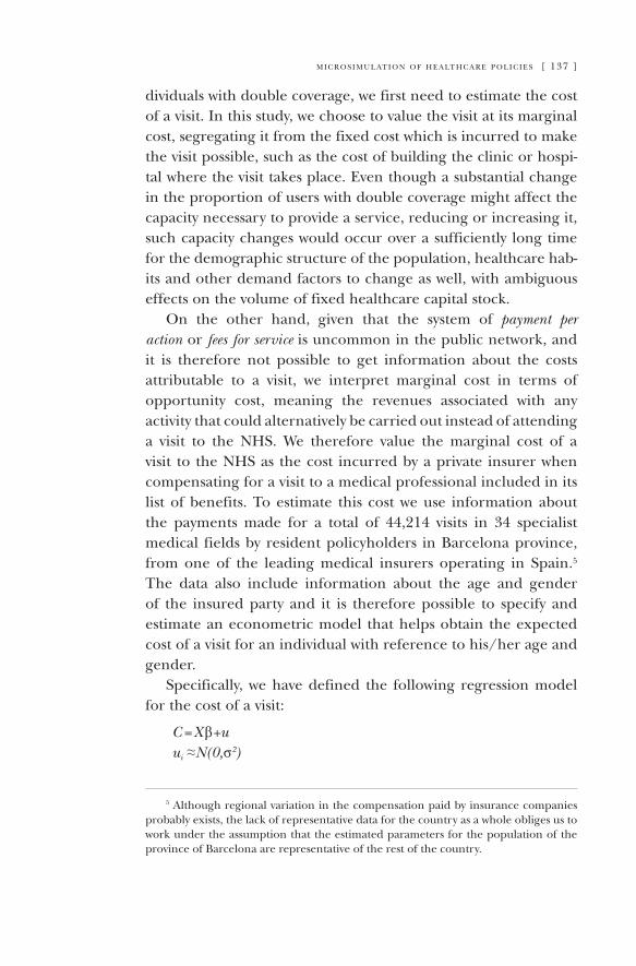
m i c r o s i m u l at i o n o f h e a lt h c a r e p o l i c i e s [ 137 ]
dividuals with double coverage, we first need to estimate the cost of a visit. In this study, we choose to value the visit at its marginal cost, segregating it from the fixed cost which is incurred to make the visit possible, such as the cost of building the clinic or hospi-tal where the visit takes place. Even though a substantial change in the proportion of users with double coverage might affect the capacity necessary to provide a service, reducing or increasing it, such capacity changes would occur over a sufficiently long time for the demographic structure of the population, healthcare hab-its and other demand factors to change as well, with ambiguous effects on the volume of fixed healthcare capital stock.
On the other hand, given that the system of payment per action or fees for service is uncommon in the public network, and it is therefore not possible to get information about the costs attributable to a visit, we interpret marginal cost in terms of opportunity cost, meaning the revenues associated with any activity that could alternatively be carried out instead of attending a visit to the NHS. We therefore value the marginal cost of a visit to the NHS as the cost incurred by a private insurer when compensating for a visit to a medical professional included in its list of benefits. To estimate this cost we use information about the payments made for a total of 44,214 visits in 34 specialist medical fields by resident policyholders in Barcelona province, from one of the leading medical insurers operating in Spain.5
The data also include information about the age and gender of the insured party and it is therefore possible to specify and estimate an econometric model that helps obtain the expected cost of a visit for an individual with reference to his/her age and gender.
Specifically, we have defined the following regression model for the cost of a visit:
C = X β+uui ≈N(0,σ2)
5 Although regional variation in the compensation paid by insurance companies probably exists, the lack of representative data for the country as a whole obliges us to work under the assumption that the estimated parameters for the population of the province of Barcelona are representative of the rest of the country.
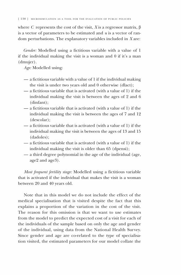
[ 138 ] m i c r o s i m u l at i o n a s a t o o l f o r t h e e va l u at i o n o f p u b l i c p o l i c i e s
where C represents the cost of the visit, X is a regressor matrix, β is a vector of parameters to be estimated and u is a vector of ran-dom perturbations. The explanatory variables included in X are:
Gender: Modelled using a fictitious variable with a value of 1 if the individual making the visit is a woman and 0 if it’s a man (dmujer).
Age: Modelled using:
a fictitious variable with a value of 1 if the individual making the visit is under two years old and 0 otherwise (dlact);a fictitious variable that is activated (with a value of 1) if the individual making the visit is between the ages of 2 and 6 (dinfant);a fictitious variable that is activated (with a value of 1) if the individual making the visit is between the ages of 7 and 12 (descolar);a fictitious variable that is activated (with a value of 1) if the individual making the visit is between the ages of 13 and 15 (dadoles);a fictitious variable that is activated (with a value of 1) if the individual making the visit is older than 65 (dpensi);a third degree polynomial in the age of the individual (age, age2 and age3).
Most frequent fertility stage: Modelled using a fictitious variable that is activated if the individual that makes the visit is a woman between 20 and 40 years old.
Note that in this model we do not include the effect of the medical specialisation that is visited despite the fact that this explains a proportion of the variation in the cost of the visit. The reason for this omission is that we want to use estimates from the model to predict the expected cost of a visit for each of the individuals of the sample based on only the age and gender of the individual, using data from the National Health Survey. Since gender and age are co-related to the type of specialisa-tion visited, the estimated parameters for our model collate the
—
—
—
—
—
—
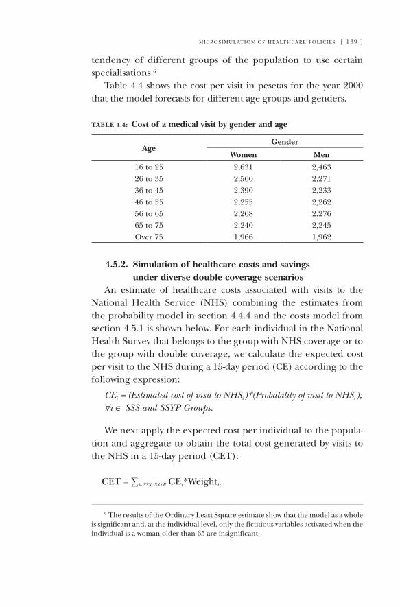
m i c r o s i m u l at i o n o f h e a lt h c a r e p o l i c i e s [ 139 ]
tendency of different groups of the population to use certain specialisations.6
Table 4.4 shows the cost per visit in pesetas for the year 2000 that the model forecasts for different age groups and genders.
table 4.4: Cost of a medical visit by gender and age
AgeGender
Women Men
16 to 25 2,631 2,46326 to 35 2,560 2,27136 to 45 2,390 2,23346 to 55 2,255 2,26256 to 65 2,268 2,27665 to 75 2,240 2,245Over 75 1,966 1,962
4.5.2. Simulation of healthcare costs and savings under diverse double coverage scenarios
An estimate of healthcare costs associated with visits to the National Health Service (NHS) combining the estimates from the probability model in section 4.4.4 and the costs model from section 4.5.1 is shown below. For each individual in the National Health Survey that belongs to the group with NHS coverage or to the group with double coverage, we calculate the expected cost per visit to the NHS during a 15-day period (CE) according to the following expression:
CEi = (Estimated cost of visit to NHSi )*(Probability of visit to NHSi ); "i ∈ SSS and SSYP Groups.
We next apply the expected cost per individual to the popula-tion and aggregate to obtain the total cost generated by visits to the NHS in a 15-day period (CET):
CET = ∑i∈SSS, SSYP CEi*Weighti.
6 The results of the Ordinary Least Square estimate show that the model as a whole is significant and, at the individual level, only the fictitious variables activated when the individual is a woman older than 65 are insignificant.
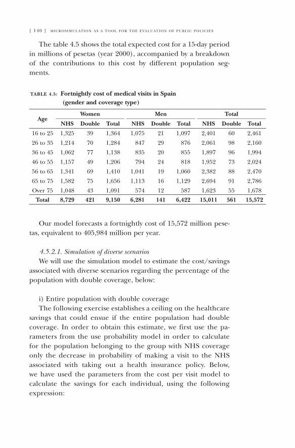
[ 140 ] m i c r o s i m u l at i o n a s a t o o l f o r t h e e va l u at i o n o f p u b l i c p o l i c i e s
The table 4.5 shows the total expected cost for a 15-day period in millions of pesetas (year 2000), accompanied by a breakdown of the contributions to this cost by different population seg-ments.
table 4.5: Fortnightly cost of medical visits in Spain (gender and coverage type)
AgeWomen Men Total
NHS Double Total NHS Double Total NHS Double Total
16 to 25 1,325 39 1,364 1,075 21 1,097 2,401 60 2,461
26 to 35 1,214 70 1,284 847 29 876 2,061 98 2,160
36 to 45 1,062 77 1,138 835 20 855 1,897 96 1,994
46 to 55 1,157 49 1,206 794 24 818 1,952 73 2,024
56 to 65 1,341 69 1,410 1,041 19 1,060 2,382 88 2,470
65 to 75 1,582 75 1,656 1,113 16 1,129 2,694 91 2,786
Over 75 1,048 43 1,091 574 12 587 1,623 55 1,678
Total 8,729 421 9,150 6,281 141 6,422 15,011 561 15,572
Our model forecasts a fortnightly cost of 15,572 million pese-tas, equivalent to 405,984 million per year.
4.5.2.1. Simulation of diverse scenariosWe will use the simulation model to estimate the cost/savings
associated with diverse scenarios regarding the percentage of the population with double coverage, below:
i) Entire population with double coverageThe following exercise establishes a ceiling on the healthcare
savings that could ensue if the entire population had double coverage. In order to obtain this estimate, we first use the pa-rameters from the use probability model in order to calculate for the population belonging to the group with NHS coverage only the decrease in probability of making a visit to the NHS associated with taking out a health insurance policy. Below, we have used the parameters from the cost per visit model to calculate the savings for each individual, using the following expression:
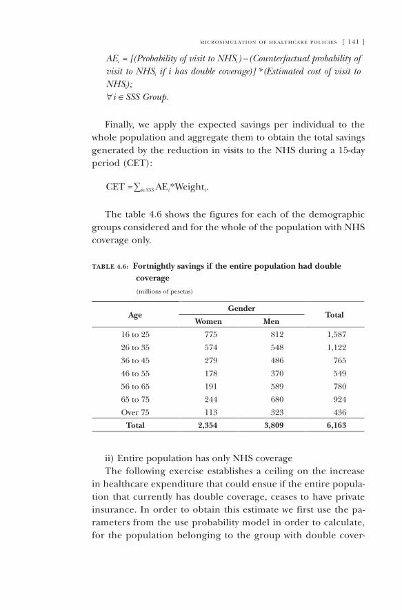
m i c r o s i m u l at i o n o f h e a lt h c a r e p o l i c i e s [ 141 ]
AEi = [(Probability of visit to NHSi ) – (Counterfactual probability of visit to NHSi if i has double coverage)] * (Estimated cost of visit to NHSi);"i ∈SSS Group.
Finally, we apply the expected savings per individual to the whole population and aggregate them to obtain the total savings generated by the reduction in visits to the NHS during a 15-day period (CET):
CET = ∑i∈SSS AEi*Weighti.
The table 4.6 shows the figures for each of the demographic groups considered and for the whole of the population with NHS coverage only.
table 4.6: Fortnightly savings if the entire population had double coverage
(millions of pesetas)
AgeGender
TotalWomen Men
16 to 25 775 812 1,587
26 to 35 574 548 1,122
36 to 45 279 486 765
46 to 55 178 370 549
56 to 65 191 589 780
65 to 75 244 680 924
Over 75 113 323 436
Total 2,354 3,809 6,163
ii) Entire population has only NHS coverage The following exercise establishes a ceiling on the increase
in healthcare expenditure that could ensue if the entire popula-tion that currently has double coverage, ceases to have private insurance. In order to obtain this estimate we first use the pa-rameters from the use probability model in order to calculate, for the population belonging to the group with double cover-
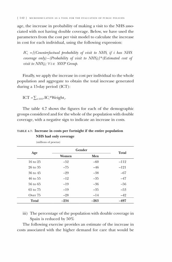
[ 142 ] m i c r o s i m u l at i o n a s a t o o l f o r t h e e va l u at i o n o f p u b l i c p o l i c i e s
age, the increase in probability of making a visit to the NHS asso-ciated with not having double coverage. Below, we have used the parameters from the cost per visit model to calculate the increase in cost for each individual, using the following expression:
ICi = [(Counterfactual probability of visit to NHSi if i has NHS coverage only) – (Probability of visit to NHSi)]* (Estimated cost of visit to NHSi); "i ∈ SSYP Group.
Finally, we apply the increase in cost per individual to the whole population and aggregate to obtain the total increase generated during a 15-day period (ICT):
ICT = ∑i∈SSYP ICi*Weighti.
The table 4.7 shows the figures for each of the demographic groups considered and for the whole of the population with double coverage, with a negative sign to indicate an increase in costs.
table 4.7: Increase in costs per fortnight if the entire population
NHS had only coverage
(millions of pesetas)
AgeGender
TotalWomen Men
16 to 25 –52 –60 –112
26 to 35 –75 –46 –121
36 to 45 –29 –38 –67
46 to 55 –12 –35 –47
56 to 65 –19 –36 –56
65 to 75 –19 –35 –53
Over 75 –28 –14 –42
Total –234 –263 –497
iii) The percentage of the population with double coverage in Spain is reduced by 50%
The following exercise provides an estimate of the increase in costs associated with the higher demand for care that would be
m i c r o s i m u l at i o n o f h e a lt h c a r e p o l i c i e s [ 143 ]
generated if the proportion of the population with double cover-age decreased to a point corresponding to 3.5%.
To carry out this simulation, which reflects a more plausible scenario compared to the previous examples, we must make a series of additional assumptions that merit more discussion. The question raised is “which individuals within the double coverage group would drop their insurance cover and join the group with NHS coverage only?” The answer is clear: it depends on the circumstance causing such a change in the behavioural patterns of the population. It could be reasoned, for instance, that an increase in the perceived quality of public healthcare services would make some individuals abandon double coverage. A similar effect might also be caused by an increase in the price of private insurance policies. Nevertheless, individuals who change due to a modification in their perception of the quality of the public network will differ from those who abandon double coverage due to an increase in price in respects which influence the frequency of visits and the cost of each visit. One of the limitations of the model that we have created, estimated and incorporated into a simulation routine is precisely that it takes no account of the decision-making stage of purchasing double coverage. This is primarily due to the fact that the objective of the exercise is to quantify the costs associated with different scenarios, regardless of how those scenarios are arrived at. The incorporation of a model for the first decision stage of purchasing private insurance will resolve this limitation in the future but, in order to address our present objectives and given that there are various healthcare and tax policy alternatives that influence the likelihood of taking out a private policy, we will randomly take individuals from the double coverage group and assign them to the NHS only coverage group until the abovementioned percentage has been reached. Below, we have calculated the increase in costs for this ex double coverage group using the following expression:
ICi = [(Counterfactual probability of visit to NHSi if i has NHS cover-age only) – (Probability of visit to NHSi )]*(Estimated cost of visit to NHSi); "i ∈ “ex double coverage” Group.
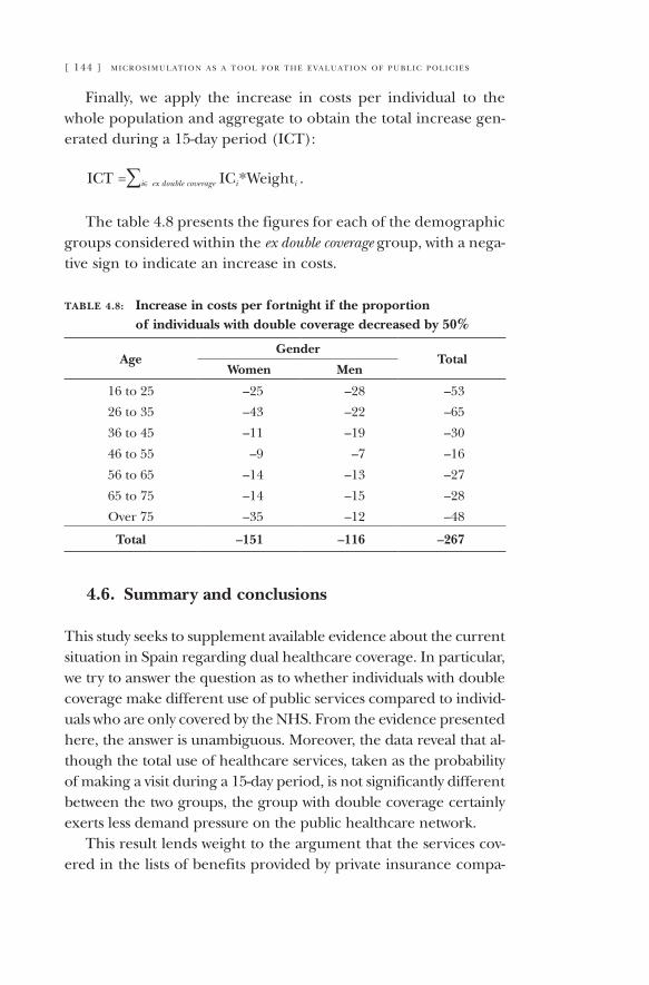
[ 144 ] m i c r o s i m u l at i o n a s a t o o l f o r t h e e va l u at i o n o f p u b l i c p o l i c i e s
Finally, we apply the increase in costs per individual to the whole population and aggregate to obtain the total increase gen-erated during a 15-day period (ICT):
ICT =∑i∈ ex double coverage ICi*Weighti .
The table 4.8 presents the figures for each of the demographic groups considered within the ex double coverage group, with a nega-tive sign to indicate an increase in costs.
table 4.8: Increase in costs per fortnight if the proportion of individuals with double coverage decreased by 50%
AgeGender
TotalWomen Men
16 to 25 –25 –28 –53
26 to 35 –43 –22 –65
36 to 45 –11 –19 –30
46 to 55 –9 –7 –16
56 to 65 –14 –13 –27
65 to 75 –14 –15 –28
Over 75 –35 –12 –48
Total –151 –116 –267
4.6. Summary and conclusions
This study seeks to supplement available evidence about the current situation in Spain regarding dual healthcare coverage. In particular, we try to answer the question as to whether individuals with double coverage make different use of public services compared to individ-uals who are only covered by the NHS. From the evidence presented here, the answer is unambiguous. Moreover, the data reveal that al-though the total use of healthcare services, taken as the probability of making a visit during a 15-day period, is not significantly different between the two groups, the group with double coverage certainly exerts less demand pressure on the public healthcare network.
This result lends weight to the argument that the services cov-ered in the lists of benefits provided by private insurance compa-
m i c r o s i m u l at i o n o f h e a lt h c a r e p o l i c i e s [ 145 ]
nies reinforce the public healthcare system. As such, the second objective of the work has been to quantify the savings generated for the NHS by the decrease in demand due to double coverage. Our results suggest that if the entire population had double cov-erage healthcare savings could total 160,000 million pesetas per year (base 2000). Alternatively, if the population that currently has double coverage decided to switch to NHS-only coverage, the increase in demand for NHS services could generate an additional 12,922 million in costs every year. If the percentage of the popu-lation with double coverage in Spain fell by 50%, the increase in costs could be approximately half of this 12,922 million.
These estimates help contextualise the importance of double coverage with regard to the public sector’s interest in policies af-fecting the externality of public network decongestion. However, this work poses a series of additional questions that must be re-solved in future research. The first is “how do we develop measures that influence the propensity of part of the population to take out double coverage?” And once these measures have been chosen, “what sort of individuals are most influenced by these measures?” The answer to such questions is important because there is evi-dence that individuals are sensitive to factors other than and in addition to price when taking out a private healthcare policy, including the perception of quality of the public health system and, more specifically, waiting times. Furthermore, as stated, the use patterns of price-sensitive individuals differ from the use pat-terns of individuals who are sensitive to the perception of quality, and measures taken to influence the purchase of double coverage should be clear about which population group they are targeting. This observation clearly suggests the lines of research that could most usefully be followed in the near future.
References
besley t., J. hall and i. preston. “Private and public health insurance in the UK.” European Economic Review 42 no. 3-5 (1998): 491–497.
boer, R., H. de Koning, A. threlfall, P. Warmerdam, A. street, E. friedman and C. Woodman. “Cost Effectiveness of Shortening Screening Interval or Extending Age Range of NHS Breast Screening Programme: Computer Simulation Study.” British Medical Journal 317 (7155): 376–379.
[ 146 ] m i c r o s i m u l at i o n a s a t o o l f o r t h e e va l u at i o n o f p u b l i c p o l i c i e s
broWn, L., A. abello, B. phillips and A. harding. “Moving towards an Improved Microsimulation Model of the Australian Pharmaceutical Benefits Scheme.” The Australian Economic Review 37 (1): 41–61.
broWn, L. and A. harding. “Social Modelling and Public Policy: Application of Microsimulation Modelling in Australia.” Journal of Artificial Societies and Social Simulation 5 (4): 2002.
chernicK H. A., M. R. holmer and D. H. Weinberg. “Tax policy toward health insur-ance and the demand for medical services.” Journal of Health Economics 6 (1): 1–25.
colombo, F. and N. tapay. “Private health insurance in OECD countries. The benefits and costs for individuals and health systems.” OECD Health Working Paper no. 15. Paris: OECD, 2004.
cronin, K., J. M. legler and R. etzioni. “Assessing uncertainty in microsimulation modeling with application to cancer screening interventions.” Statistics in Medicine 17: 2509–2523.
curry, C. “PENSIM: A Dynamic Simulation Model of Pensioners’ Incomes.” Government Economic Service Working Paper no. 129, 1996.
evandrou, M., J. falKingham, P. Johnson and K. raKe. “SAGE: Simulating Social Policy for an Ageing Society. A Research Agenda.” SAGE Discussion Paper no. 1. 2001.
favreault, M. and K. smith. A Primer on the Dynamic Simulation of Income Model (DYNASIM3). Washington, DC: The Urban Institute, 2004.
fredriKsen, D. Projections of Population, Education, Labour Supply and Public Pension Benefits: Analyses with the Dynamic Microsimulation Model MOSART. Oslo: Social and Economics Studies, Statistics Norway, 1998.
gruber, J. “Microsimulation Estimates of the Effects of Tax Subsidies for Health Insurance.” National Tax Journal 53(3), Part I (2000): 329–342.
hancocK, R., J. mallender and S. pudney. “Constructing a Computer Model for Simulating the Future Distribution of Pensioners’ Incomes for Great Britain.” In R. Hancock and H. Sutherland (eds.). Microsimulation Models for Public Policy Analysis: New Frontiers. London: STICER, 1992: 33–66.
King, A., H. bæKgaard and M. robinson. “DYNAMOD-2: An overview.” Technical Paper no. 19. NATSEM University of Canberra, 1999.
lópez nicolás, A. Unobserved Heterogeneity and Censoring in the Demand for Private Health Care. Health Economics 7 (1998): 429–437.
—. “Seguros sanitarios y gasto público en España. Un modelo de microsimulación para las políticas de gastos fiscales en sanidad.” Papeles de Trabajo del Instituto de Estudios Fiscales (Serie Economía) 12. Madrid: Instituto de Estudios Fiscales, 2001.
lópez nicolás, A., J. garcía villar, G. lópez casasnovas and J. puig Junoy. ¿Es posible reducir el gasto sanitario a través del subsidio a los seguros sanitarios privados? La doble cobertura sanitaria en Catalunya. Estimación de patrones de utilización de servicios sanitarios y simulación de costes asociados a la asistencia sanitaria. Servei Català de la Salut, 2000.
lópez nicolás, A. and M. vera. “Are Tax Subsidies for Private Medical Insurance Self-financing? Evidence from a Microsimulation Model for Outpatient Episodes in a NHS Context.” Working Paper 632. Dept. Economics and Business. Universitat Pompeu Fabra, 2002.
lubitz, J., C. liming, E. KramaroW and H. lentzner. “Health, Life Expectancy, and Health Care Spending among the Elderly.” The New England Journal of Medicine 349 (September 11, 2003): 1048–1055.
m i c r o s i m u l at i o n o f h e a lt h c a r e p o l i c i e s [ 147 ]
morrison R. and B. dussault. “A full-fledged Canadian actuarial stochastic model designed for the fiscal and policy analysis of social security schemes.” In http://www.actuaries.org/members/en/committees/SOCSEC/documents/dynacan.pdf. 2000.
nelissen, J. “Labour market, income formation and social security in the microsimula-tion model NEDYMAS.” Economic Modelling 10 no. 3 (1993): 225–272.
—. “Social Security and Lifetime Income Redistribution: a microsimulation approach.” In Harding, A. (ed.), Microsimulation and Public Policy. Amsterdam: North Holland, 1996.
orcutt, H. and A. glazer. “Microanalytic Modelling and Simulation.” In B. Bergmann, G. Eliasson and G. H. Orcutt, editors. Micro Simulation Models: Methods and Applications. IUI Conference Reports 1980: 1. Stockholm: Industrial Institute for Economic and Social Research, 1980.
pauly M. V. and B. J. herring. “An efficient employer strategy for dealing with adverse selection in multiple-plan offerings: an MSA example.” Journal of Health Economics 19 no. 4 (2000): 513–528.
propper C. “The demand for private health care in the UK.” Journal of Health Economics 19 no. 6 (2000): 855–876.
spielauer. “Dynamic Microsimulation of Health Care Demand, Health Care Finance and the Economic Impact of Health Behavior. Part I: Background and a Comparison with Cell-Based Models”. IIASA IR-02-032. In http://www.iiasa.ac.at/Publications/Documents/IR-02-032.pdf.
—. “Dynamic Microsimulation of Health Care Demand, Health Care Finance and the Economic Impact of Health Behavior. Part II: Survey and Review”. IIASA IR, 2002. In http://www.iiasa.ac.at/Publications/Documents/IR-02-036.pdf. 2002.
sutherland, H. “EUROMOD: An Integrated European Benefit-Tax Model.” Final Report. EUROMOD Working Paper EM9/01, June 2001.
Wagstaff, A. and E. van doorslaer. “Progressivity, horizontal equity and reranking in health care finance: a decomposition analysis for the Netherlands.” Journal of Health Economics, 16 no. 5 (1997): 499–516.
zabinsKi, D., T. M. selden, J. F. moeller and J. S. banthin. “Medical savings accounts: Microsimulation results from a model with adverse selection.” Journal of Health Economics 18 no. 2 (1999): 195–218.
zaidi, A. and K. raKe. “Dynamic Microsimulation Models: A Review and some Lessons from SAGE.” SAGE Discussion paper no. 2. ESRC-Sage Research Group, LSE SAGE/DP2, 2002.

[ 149 ]
Microsimulation in the Analysis of Environmental Tax Reforms. An Application for Spain
Xavier LabandeiraREDE and Department of Applied Economics, University of Vigo
José M. LabeagaFEDEA (Madrid) and Department of Economic Analysis II – UNED
Miguel RodríguezREDE and Department of Applied Economics, University of Vigo
5.1. Introduction
During recent decades numerous economic policies have been in-troduced, such as trade liberalisation or changes to the tax system; subsidies that have had important implications for the efficiency of the economy, but also for inequality, poverty and, in general, the welfare of individuals. Internationally, there has been a signifi-cant effort to improve the efficiency of the economy by reducing international trade barriers. Its impact on inequality and poverty must be closely analysed, due to the correlation between globalisa-tion and redistribution (Dollard, David and Kraay 2000).
Tax reforms introduced in numerous countries since the be-guining of the 1980s have represented a change in the hierarchy of taxation principles in favour of efficiency, horizontal equity and simplicity (Gago and Labandeira 2000). Recently, proposals to modify taxation of energy, or more generally, to introduce en-
5.
This work has benefited from comments and suggestions by Melchor Fernández, Alberto Gago, Antonio Gómez, José M. González-Páramo, Baltasar Manzano, Clemente Polo, Pere Riera and Amedeo Spadaro. We acknowledge the receipt of financing from the Ministry of Science and Technology (Projects BEC-2002 04394 C02-02 and SEC-2002-03095) and the Galician Regional Government (Project PGIDIT03PXIC30008PN). Any errors or omissions are our sole responsibility.
[ 150 ] m i c r o s i m u l at i o n a s a t o o l f o r t h e e va l u at i o n o f p u b l i c p o l i c i e s
vironmental taxes have sought to attain efficiency improvements. However, it is important to remember that these measures also have effects on distribution (Speck 1999).
The distributional consequences of a specific public policy are often a fundamental factor in determining its acceptability. In many cases, law and policymakers introduce special measures to marshal political support from citizens or corporate execu-tives. Obviously, this type of action can derail achievement of the primary efficiency objectives that should guide decision making. That is why we need a simultaneous analysis of the efficiency and distributional issues associated to public policies is necessary.
Currently, microeconomic models represent the most usual approach to analysing distributional aspects. Such methods re-quire the use of microeconomic databases that contain data on individuals, households or firms. The most interesting aspect of the use of this data is that it allows the large disparity existing between economic agents to be taken into account. In the case of families, this disparity is related to their income, the actual composition of the household and its preferences. The main drawback of microsimulation models is that their partial equi-librium setting does not allow relative prices to be endogenised, which leads to potentially biased results. Furthermore, they are not the most appropriate framework for analysing efficiency as-pects deriving from public policies. As such, a trade-off must be acknowledged between the analysis of distributional effects and efficiency, and it will be up to researchers to choose from the diversity of instruments available.
Applied general equilibrium models (AGEM) permit analysis of the impacts of policy measures on an economy-wide scale. Established on microeconomic fundamentals, they allow the interaction between all component sectors and institutions of the economy to be studied. AGEM are therefore a powerful in-strument for analysing the efficiency and other macroeconomic effects of public policies already in place or measures that may be put into practice. Nevertheless, despite their potential they are not capable of evaluating the distributional effects of such policies on households and therefore lack the ability to calculate welfare related aspects. This problem is common to instruments
m i c r o s i m u l at i o n i n t h e a n a ly s i s o f e n v i r o n m e n ta l ta x r e f o r m s [ 151 ]
based on the existence of representative consumers or even ag-gregate models with a significant number of representative con-sumers (Bourguignon, Robilliard and Robinson 2003). Grouping households or individuals according to specific characteristics, such as occupation, income source or place of residence, consti-tutes a limitation in the sense that it misses out on much of the heterogeneity existing between households belonging to these standard groups.
In this study, we propose a methodology to evaluate the dis-tributional and efficiency effects of public policies without losing the heterogeneity between households provided by the surveys. We have therefore created a model at microeconomic level for the purposes of adjusting the demand for household energy. We integrate this model via prices with an AGEM that allows us to un-derstand changes brought about by a given social welfare policy, and to identify the relative prices and levels of sector and institu-tional activity. We can then integrate the results into a microeco-nomic model in order to unbundle the effects of that policy on the welfare of households in the sample and, if appropriate, to aggregate the results at the population level.
In order to illustrate how the simulation instrument works, we propose to evaluate the effects of a tax reform that consists of rais-ing indirect taxes on coal, electricity, hydrocarbons and natural gas by 20%. The reform and its timing can be justified as follows:
there are initiatives at EU level to control greenhouse gases following the ratification of the Kyoto protocol in April 2002;1
this is a typical measure that will have an impact on both efficiency and the distribution of income (Bovenberg and Goulder 2002). The extra tax receipts obtained from the tax increase will be used to reduce indirect taxes on other goods so as to achieve a zero net tax revenue impact in real terms. The results of these tax changes suggest an improvement in the levels of sector activity and, therefore, in the activity of
1 For example, the European carbon market in 2005 or the tax harmonisation of energy goods in the EU.
—
—
[ 152 ] m i c r o s i m u l at i o n a s a t o o l f o r t h e e va l u at i o n o f p u b l i c p o l i c i e s
the Spanish economy as a whole. They do not, however, pro-duce significant changes in the prices of capital and labour. Therefore, all the distributional effects occur via changes in the prices of goods and services. In this way we find signifi-cant distributional consequences, which in our opinion jus-tifies the use of integrated models for the global economic analysis of public policies.
This chapter contains four sections apart from the introduction. In section 5.2 we attempt to explain why it is desirable, on some occasions, to integrate micro and macro economic models, and we review the available empirical evidence. Section 5.3 explains how the two parts that comprise the integrated model work. Section 5.4 presents the policies that we simulate and analyses the results. Section 5.5 establishes a series of conclusions and makes some eco-nomic policy recommendations.
5.2. Integrating micro and macroeconomic models
If we follow the reasoning of the previous section, it is logical to think that the integration of micro and macro models will provide the benefits of both methodologies. Both procedures are comple-mentary since AGEMs do not offer the differentiation that micro-simulation models provide (generally microeconometric models) and microsimulation instruments do not have some interesting characteristics of AGEMs (Aaberge, Colombino, Holmoy, Strom and Wennemo 2004).
The simplest integration procedure consists of adding macroeconomic aspects to a microeconomic model, but without constructing an AGEM. This can be done, for example, by combining a microsimulation instrument with an input-output table. Yet decisions about the content of the individual components must be made in advance. What form should the microeconomic model have? We could consider purely arithmetic models but also models that incorporate agent behaviour. Figure 5.1 illustrates both possibilities, which are differentiated by the ability to include (or not) an econometric model, or more specifically,
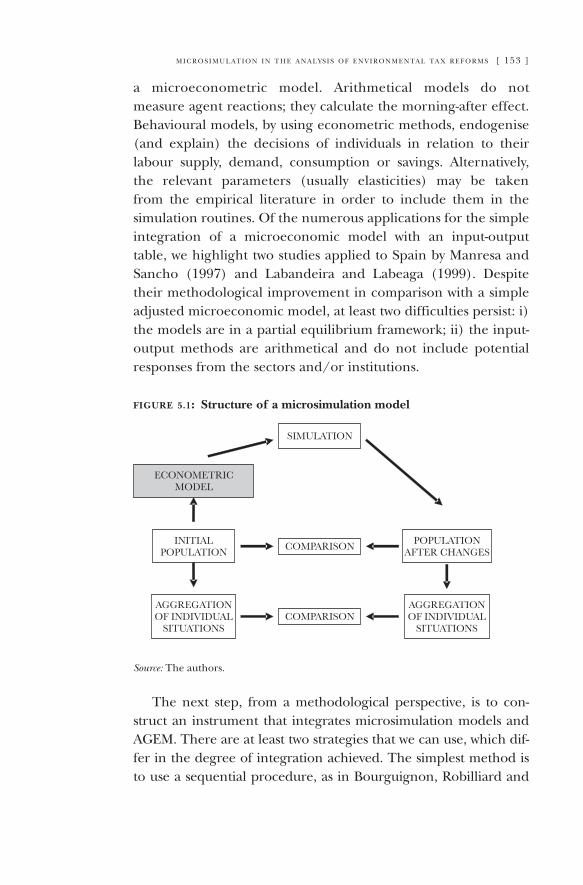
m i c r o s i m u l at i o n i n t h e a n a ly s i s o f e n v i r o n m e n ta l ta x r e f o r m s [ 153 ]
a microeconometric model. Arithmetical models do not measure agent reactions; they calculate the morning-after effect. Behavioural models, by using econometric methods, endogenise (and explain) the decisions of individuals in relation to their labour supply, demand, consumption or savings. Alternatively, the relevant parameters (usually elasticities) may be taken from the empirical literature in order to include them in the simulation routines. Of the numerous applications for the simple integration of a microeconomic model with an input-output table, we highlight two studies applied to Spain by Manresa and Sancho (1997) and Labandeira and Labeaga (1999). Despite their methodological improvement in comparison with a simple adjusted microeconomic model, at least two difficulties persist: i) the models are in a partial equilibrium framework; ii) the input-output methods are arithmetical and do not include potential responses from the sectors and/or institutions.
figure 5.1: Structure of a microsimulation model
Source: The authors.
The next step, from a methodological perspective, is to con-struct an instrument that integrates microsimulation models and AGEM. There are at least two strategies that we can use, which dif-fer in the degree of integration achieved. The simplest method is to use a sequential procedure, as in Bourguignon, Robilliard and
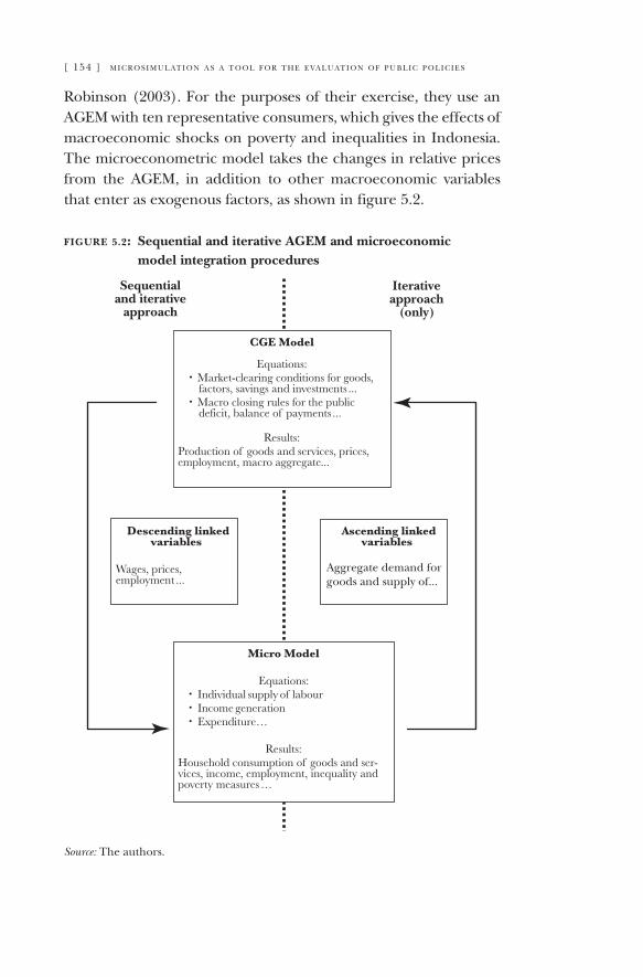
[ 154 ] m i c r o s i m u l at i o n a s a t o o l f o r t h e e va l u at i o n o f p u b l i c p o l i c i e s
Robinson (2003). For the purposes of their exercise, they use an AGEM with ten representative consumers, which gives the effects of macroeconomic shocks on poverty and inequalities in Indonesia. The microeconometric model takes the changes in relative prices from the AGEM, in addition to other macroeconomic variables that enter as exogenous factors, as shown in figure 5.2.
figure 5.2: Sequential and iterative AGEM and microeconomic model integration procedures
Sequentialand iterative
approach
Iterativeapproach
(only)
Source: The authors.
m i c r o s i m u l at i o n i n t h e a n a ly s i s o f e n v i r o n m e n ta l ta x r e f o r m s [ 155 ]
The principal advantage of sequential integration is that it provides information about the impact on household welfare at a microeconomic level, allowing the model to maintain a high degree of flexibility. Nevertheless, there is still the problem of guaranteeing the consistency between both components. Note that this consistency cannot always be guaranteed unless feed-back effects between components are included. In this respect, Savard (2003) proposes an innovation on the methodology of Bourguignon, Robilliard and Robinson (2003), which allows two-way relations between the microeconomic model and the AGEM, forcing consistent solutions to be obtained through the conver-gence of final results. The behaviour of households is accordingly fixed when the AGEM simulations are carried out. The results of these simulations are an input for the microeconometric model (or for the simulation instrument), which allows the effects of re-form at a microeconomic level to be calculated. Once responses from the households obtained via the micro model are available, information is used as an input to the AGEM, providing new val-ues for the variables previously considered as exogenous (figure 5.2). The procedure does not end with this stage but follows an iterative process until convergence is achieved in the results pro-vided by both components.
For our purposes, what interests most about the Bourguignon, Robilliard and Robinson (2003) proposal is the possibility of comparing results obtained under various scenarios, first using the simulation instruments individually and then using the inte-grated model. These authors find highly significant differences, not only in the magnitude of the changes but also in their sign. Savard (2003) also provides very different results between the two procedures as regards distribution and poverty aspects, in an ex-ercise which simulates a trade policy reform in the Philippines.
5.3. Details of the integrated micro-macro model
This section is wholly dedicated to describing the procedure we use in this paper. Its fundamental methodological contribution is to evaluate the effects of a tax reform influencing energy goods
[ 156 ] m i c r o s i m u l at i o n a s a t o o l f o r t h e e va l u at i o n o f p u b l i c p o l i c i e s
on the efficiency of economic sectors (and the overall efficiency of the economy) and its consequences for individual welfare. The empirical exercise integrates an AGEM specifically designed to simulate environmental tax policies and a household micro-simulation model based on a previously estimated demand model (Labandeira, Labeaga and Rodríguez 2006). We therefore use a top-down procedure in order to study the macroeconomic effects of policies and a bottom-up method to analyse their distribu-tional effects. Similarly to Bourguignon, Robilliard and Robinson (2003), we take the changes in prices and income provided by the AGEM as exogenous variables in order to carry out simulations using the microsimulation model. Bearing in mind this opera-tion, we first calculate the relative prices for each good using the AGEM Pinew
AGEM/PibaseAGEM. The new relative prices resulting from the
reform, PinewMIC, that will be used as an input to the microsimula-
tion instrument are calculated by multiplying the pre-reform prices, Pibase
MIC, by the percentage changes in the corresponding variables derived from the AGEM:
PinewMIC = (Pinew
AGEM/PibaseAGEM)Pibase
MIC. (5.1)
As a result, integration between both modules occurs sequen-tially. We are interested in analysing potential policies with a sector-based impact on the supply and demand for goods and services, and minimal effects on income. In relation to income, the only simulation we conduct relates to the expenditure of each household, leaving aside the income generation process at an ag-gregate level. Given the assumed effects that reforms will have on income, the sequential method used is no worse then the iterative alternative.
A primary objective of our analysis is to obtain complete information, with the highest possible degree of differentia-tion, on welfare and distribution effects of changes in taxation. Inconsistencies can certainly occur between survey data and ag-gregate data: the objectives behind constructing both data sourc-es do not prevent these problems occurring, either in the data sources for Spain or for other countries. Although the samples from the Continuous Family Budget Survey (ECPF), which is the base used in the analysis, are representative of the population,
m i c r o s i m u l at i o n i n t h e a n a ly s i s o f e n v i r o n m e n ta l ta x r e f o r m s [ 157 ]
the sampling processes are not entirely successful in minimising the impact of these problems. Since the ECPF provides factors for elevating the survey data to population level, we use these fac-tors to obtain aggregate figures, which we collate with the figures from Spanish National Accounts (Symons, Proops and Gay 1994, or Bourguignon, Robilliard and Robinson 2003).
5.3.1. The Applied General Equilibrium Model2 In order to evaluate the efficiency effects of energy and environ-
mental policies, we use a static AGEM whose structure is described below. First, sectors and institutions are separated out as much as available information allows. This disaggregation is important inso-far as we wish to factor energy consumption heterogeneity. It is es-pecially important in the case of the energy sector for the purposes of this exercise, since this sector provides different intermediate in-puts for production (electrical services, heating, transport services, etc.) and these inputs exhibit important differences in relation to CO2 emission factors.3 We should not forget that the effectiveness of environmental policies and their cost efficiency depend on two key factors: the price of the energy required to protect the environ-ment and the substitution between energy sources (from dirty to clean energies, depending on the emission factors).
The 17 production sectors in the model produce with constant returns to scale and minimise costs in a competitive context. The production function, which is specifically designed to accommo-date environmental policies, is a succession of constant elasticity of substitution functions (CES), as shown in figure 5.A.1.4 As is nor-mal in AGEM models, the total production for sector i arises from combining intermediate inputs and a good composed of labour, capital and various sources of energy using a Leontief technique.
2 The notation criterion conforms to the following convention: endogenous variables are expressed in capital letters and exogenous variables in capital letters with a line over the letter.
3 CO2 emission factors in Spain are: 98 kg/GJ for coal; 73 kg/GJ for refined petroleum products and 55 kg/GJ for natural gas.
4 The AGEM used incorporates various modifications in relation to the AGEM used by Böhringer, Ferris and Rutherford (1997), although in essence it is the same model.
[ 158 ] m i c r o s i m u l at i o n a s a t o o l f o r t h e e va l u at i o n o f p u b l i c p o l i c i e s
We use the Armington method to model international trans-actions in goods. Imported and domestic goods are imperfect substitutes in terms of production. The total supply of goods and services from the economy is therefore a combination obtained from different sources using CES functions. The maximisation of profits by each sector, which is determined via a constant elastic-ity transformation function, distributes the supply of goods and services between domestic consumption and the foreign market.5
Since our case is a small economy and most of Spain’s trade in goods is with EU countries, the exchange rate is fixed (in fact, most foreign trade is with Eurozone countries) and agents face exogenous prices from the rest of the world.6
The supply of capital is inelastic (distributed exogenously be-tween institutions) and has perfect mobility between sectors, but it is not allowed to be mobile internationally. Households offer labour so that they maximise their utility. Labour is also mobile between sectors, although not internationally.
The public sector collects direct taxes (personal income tax from households and also taxes on sector wages) and indirect taxes (on production and consumption). The provision of capital from the government (KG), transfers to other institutions (TRG) and the public deficit (DP) are exogenous variables. The con-sumption of government goods and services (DiG) is determined via a Cobb-Douglas type function in which PDi are domestic prices. A balance must therefore exist between total public ex-penditure, capital income and tax revenue (REV) that fulfils the following budget restriction:
DP = r·KG + TRG + REV −∑PDi·DGi,17
i=1(5.2)
in which r is the price of capital services.
5 For a detailed description of the treatment of international trade in AGEMs, see Shoven and Whalley (1992).
6 We will assume that the policies simulated have no significant impact on the euro exchange rate, given that the countries that trade most with Spain belong to the Monetary Union and therefore any impact on the Spanish economy will be relatively limited.
m i c r o s i m u l at i o n i n t h e a n a ly s i s o f e n v i r o n m e n ta l ta x r e f o r m s [ 159 ]
The representative household has a fixed amount of time that it divides between leisure (LS) and work. It maximises utility (W) which is a function of leisure and of a good comprising remaining goods and savings (UA), subject to the budget constraint.7
W = sUB LS + (1− sUB)UA
σUB–1
σUB σUB–1
σUB
σUB–1
σUB .
.
(5.3)
We assume, as in Böhringer and Rutherford (1997), that con-sumers have a marginal propensity to save based on their dispos-able income (YH). Disposable income comprises income from capi-tal, salaries (W is the nominal salary and SCH are social security contributions) and transfers, an amount from which income tax must be subtracted (TH is the tax rate). The consumption of goods and services is defined by a structure of nested CES functions, as shown in figure 5.A.2, which focuses especially on the demand for energy goods. An important contribution of the AGEM is the distinction between energy for household uses, energy for private transport and other energy products.8
YH = (1–TH)[r·KH + w(1−SCH)·(TIME − LS) + TRH]. (5.4)
The AGEM is a model structure based on the Walrasian equi-librium concept. This means that for any simulated policy the model finds a set of market-clearing prices and quantities (of goods, labour and capital).9 The total saving for the economy (SAVINGS) is defined endogenously and is equal to the sum of savings generated by all institutions. The macroeconomic equilib-rium of the model continues to be defined by the exogenous ca-pacity/requirement of the economy to finance/be financed by the
7 σUB is the elasticity of substitution and SUB is the proportion that leisure represents in welfare.
8 This distinction is common in microeconomic models. Other non-energy goods are a composite good for which a Cobb-Douglas formula is also chosen.
9 There are no quantity adjustments in the supply of capital from the economy because the capital stock of all institutions is an exogenous variable. The only changes occur in the use of capital by the production sectors. The equilibrium condition is obtained from changes in the price of capital services (r).
[ 160 ] m i c r o s i m u l at i o n a s a t o o l f o r t h e e va l u at i o n o f p u b l i c p o l i c i e s
foreign sector (CAPNEC). This capacity/requirement arises from the difference between national savings, the public deficit and internal investment, which are aggregated via a Leontief function of the different goods used in gross capital formation, INVi:
SAVINGS + DP –∑ PDi·INVi = CAPNEC.17
i=1
(5.5)
International prices PXMi, transfers between the foreign sector and other institutions and the consumption of goods and services by foreign residents in Spain (DiRM) are considered exogenous variables. Exports (EXPi) and imports (IMPi) must therefore satisfy the restriction faced by the foreign sector:
∑ PXMi·EXPi + TRRM + CNR −∑ PXMi·IMPi = CAPNEC
where CNR = ∑PDi·DiRM .
17 17
i=1i=1
17
i=1(5.6)
The model is also capable of simulating CO2 emissions from different energy sources. Emissions are generated only during production processes which use fossil fuels. There is therefore a technological relationship between the consumption of fossil fuels in physical units and emissions, whose parameters for coal, refined petroleum products and natural gas are θC, θR and θG re-spectively. For example, given the technology, the corresponding CO2 emissions for sector i will be:
CO2i = θC COALi + θR REFi + θG GASi. (5.7)
To employ an AGEM it is essential to construct in advance a National Accounting Matrix. We base our own on the 1995 National Accounts (NAM-95) for the Spanish economy.10 We also extend the available database with environmental data relating fossil fuel consumption and emissions for each production sec-
10 The NAM-95 that we use is based on a NAM published by Fernández and Manrique (2004). For a more detailed description of the procedure see Rodríguez (2003). The 1995 Spanish National Accounts follow the European System of Accounts (ESA-95).
m i c r o s i m u l at i o n i n t h e a n a ly s i s o f e n v i r o n m e n ta l ta x r e f o r m s [ 161 ]
tor and institution considered. Unfortunately, there is no source that provides data to the required level of detail. Therefore, we had to estimate environmental data using diverse sources such as the Andalusian Statistics Institute (IEA) (1998) or the Spanish Statistics Institute (INE) (2002a, 2002b).
Using the information obtained from the NAM-95, some mod-el parameters such as tax rates, technical production and con-sumption coefficients and the parameters of the utility function are obtained through calibration. As is well known, the criterion for calibrating the model is that the AGEM replicates the NAM-95 information as an equilibrium, which is used as the benchmark with which to compare the results of the simulations.11
Other model parameters are taken from the literature as an alternative to calibrating them. For example, labour supply elasticity is set at 0.4, similar to that obtained by Labeaga and Sanz (2001). In running the simulation for the initial situation, we follow the procedure used by Ballard, Shoven and Whalley (1985) to obtain the elasticity of labour supply, and assume that leisure represents a third of the available hours (Parry, Williams and Goulder 1999). In all cases, since this elasticity value is central to the results obtained, sensitivity analysis has been carried out, increasing and decreasing this value by 50%. From this analysis we can conclude that the results provided by the AGEM are robust at different elasticity values.
5.3.2. A microeconomic model for household energy demand
In order to evaluate the distributional effects of implement-ing environmental tax policy measures, we use a microsimulation model based on a household energy demand system (Labandeira, Labeaga and Rodríguez 2006). This section describes the most important characteristics of the model and presents the principal results. The theoretical model underpinning econometric esti-mation is the quadratic extension of the Almost Ideal Demand
11 For a brief description of the methodology, see Shoven and Whalley (1992). The AGEM was programmed in GAMS/MPSGE. The method proposed by Rutherford (1999) is used for the calibration, employing the PATH algorithm.
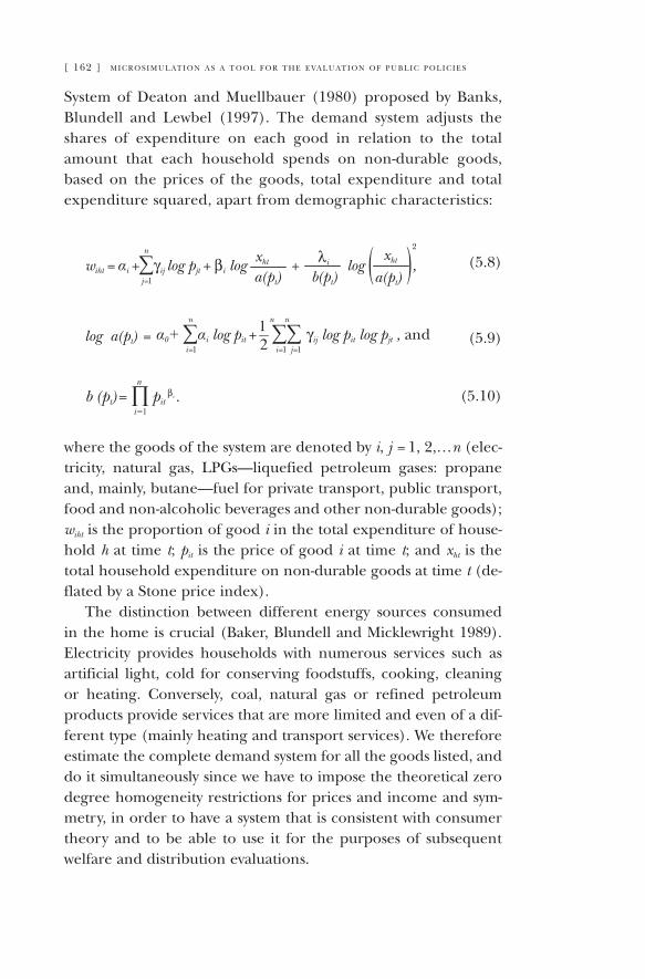
[ 162 ] m i c r o s i m u l at i o n a s a t o o l f o r t h e e va l u at i o n o f p u b l i c p o l i c i e s
System of Deaton and Muellbauer (1980) proposed by Banks, Blundell and Lewbel (1997). The demand system adjusts the shares of expenditure on each good in relation to the total amount that each household spends on non-durable goods, based on the prices of the goods, total expenditure and total expenditure squared, apart from demographic characteristics:
))
wiht = αi +∑γij log pjt + βi log + log ,n
j=1 a(pt) b(pt)xht xhtλi
a(pt)
2
(5.8)
log a(pt) = α0+ ∑αi log pit + ∑∑ γij log pit log pjt , and12
n n n
j=1i=1i=1(5.9)
b (pt)= ∏ pit βi .
n
i=1(5.10)
where the goods of the system are denoted by i, j = 1, 2,…n (elec-tricity, natural gas, LPGs—liquefied petroleum gases: propane and, mainly, butane—fuel for private transport, public transport, food and non-alcoholic beverages and other non-durable goods); wiht is the proportion of good i in the total expenditure of house-hold h at time t; pit is the price of good i at time t; and xht is the total household expenditure on non-durable goods at time t (de-flated by a Stone price index).
The distinction between different energy sources consumed in the home is crucial (Baker, Blundell and Micklewright 1989). Electricity provides households with numerous services such as artificial light, cold for conserving foodstuffs, cooking, cleaning or heating. Conversely, coal, natural gas or refined petroleum products provide services that are more limited and even of a dif-ferent type (mainly heating and transport services). We therefore estimate the complete demand system for all the goods listed, and do it simultaneously since we have to impose the theoretical zero degree homogeneity restrictions for prices and income and sym-metry, in order to have a system that is consistent with consumer theory and to be able to use it for the purposes of subsequent welfare and distribution evaluations.
m i c r o s i m u l at i o n i n t h e a n a ly s i s o f e n v i r o n m e n ta l ta x r e f o r m s [ 163 ]
Among the demographic characteristics that influence de-mand for the goods considered, we include dummy variables for the level of education of the head of the household, the geo-graphic location of the household and ownership of the home, as well as variables that control family composition by age and a trend with which we seek to control patterns over time in the distribution of expenses, which in the case of energy sources can take into account technical advances that improve the efficiency of energy producing devices.
The data we use originate from a combination of micro-economic data sources containing information on house-hold spending, income and demographic characteristics. Specifically, we combine the Family Budget Survey from 1973–1974 and 1980–1981 and the ECPF for the 1985–1995 period. All these surveys were carried out by the INE. The 1973–1974 Family Budget Survey provides information on more than 170 goods, while the 1980-81 survey contains more than 600 goods and services. The sample size of both is approximately 24,000 households. The ECPF sample that we use has information on 26,000 households and more than 270 goods and services. To make the three data sources compatible, we aggregate the goods into standardized groups according to the definitions given in the surveys. To construct demographic variables, we use the same definitions in the three surveys in order to pro-duce the same variables.
Our decision to combine these three surveys responds to a primary objective. In general, it is hard to identify price effects when estimating complete demand systems. This is due to the limited variation and the high collinearity between the price series of different goods. Our experience is that even when the system is estimated for a relatively long period such as 1985–95, the multi-collinearity in the price series does not allow for pre-cise estimates of either the price coefficients or the cross effects. But combining data for a time-period such as that covered by the three surveys (1973–1995) allows us to adequately identify the price responses. The obvious disadvantage of such a long period is that we have to assume no changes in demand pat-terns for Spanish households or else take this fact into account
[ 164 ] m i c r o s i m u l at i o n a s a t o o l f o r t h e e va l u at i o n o f p u b l i c p o l i c i e s
when estimating the system. Moreover, if the objective is to use the estimated parameters to simulate tax measures affecting the price of goods, then estimating the effects accurately is of key importance.
The estimation results show the importance of adjusting con-sumer behaviour using microeconomic data. Differences also in the demand for goods need to be taken into account, such as ac-cess to energy sources like natural gas that are available to urban households but not to households in rural areas. Other goods like public transport are also harder to access in rural areas. Therefore, households in rural areas have to move around by pri-vate vehicle with the resulting purchases of fuel, while those in ur-ban areas can substitute private for public transport services when relative prices change. The results of the model also demonstrate the importance of household composition in the consumption of goods, since, for example, households of retired people spend less on transport services because they can use subsidised public services in place of private ones.
We can identify significant income effects on the consumption of the goods making up the system. Among energy sources, LPG is preferred by low income households because it represents a cheap substitute for natural gas. Furthermore, the use of petrol or diesel for vehicles is associated with the ownership of one or more vehicles, which is a decision correlated to household income. The price elasticity of all goods forming part of the system is negative, as required by the theory. Energy goods are relatively inelastic while price elasticity for the group of other non-durable goods is much more pronounced.12
We use the same methodology as Baker, Blundell and Micklewright (1989) and Labeaga and López (1994) to carry out the simulations, which are run with annual data for 1995 taken from the Continuous Family Budget Survey. The proce-dure used allows changes in demand, tax payments and welfare measures to be obtained. In this study, we provide equivalent
12 For further information about the construction and description of the database and the results, see Labandeira, Labeaga and Rodríguez (2006). More details on the microsimulation model are given in Labandeira, Labeaga and Rodríguez (2004).
m i c r o s i m u l at i o n i n t h e a n a ly s i s o f e n v i r o n m e n ta l ta x r e f o r m s [ 165 ]
variations following the procedure described in Banks, Blundell and Lewbel (1997).
5.4. Results obtained via the integrated micro-macro model
5.4.1. Description of the reformIn this study we analyse the effects of a green tax reform
consisting of a 20% increase in the indirect taxes charged on the consumption of energy goods: electricity, refined petroleum products, natural gas and coal. The revenues generated are used to finance a general reduction in value added tax (VAT) rates (ex-cept on the aforementioned energy goods). The objective of the reform is therefore to increase taxation on energy goods while the public budget remains unchanged in real terms.
The reason behind the reform relates to the relatively low taxation of energy products in Spain compared to other EU mem-bers. The European Commission has made frequent proposals to harmonise and increase taxation on energy products, although to date it has not achieved meaningful advances. An additional ob-jective of the reform is to contribute to the control over Spanish greenhouse gas emissions (GHG). The EU has ratified the Kyoto protocol, which establishes an 8% reduction in European GHG by 2010 based on emissions from 1990. The internal rule for distrib-uting this reduction among EU members (burden sharing agree-ment) resulted in Spain being permitted to increase its emissions by 15% during the same period. But by the end of 2005, they had increased by more than 45%.
5.4.2. ResultsThe green tax reform produces a positive effect on eco-
nomic activity, increasing gross domestic product (GDP) by 1%. Demand for labour remains unchanged and there are no sig-nificant effects on wage levels and capital returns in real terms.13 The effects of reform on main macroeconomic variables are
13 Prices relative to the consumer price index (CPI).
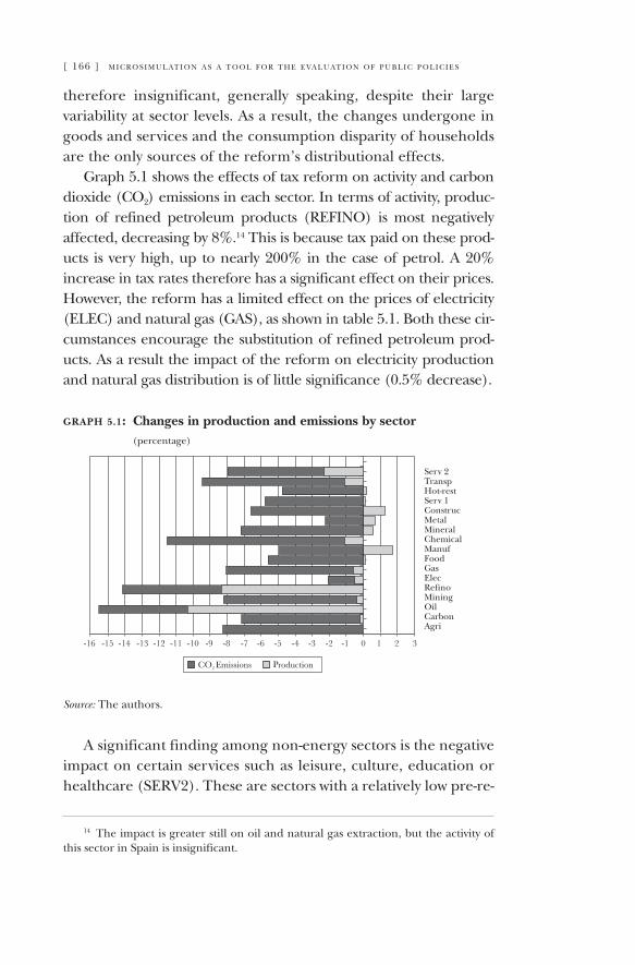
[ 166 ] m i c r o s i m u l at i o n a s a t o o l f o r t h e e va l u at i o n o f p u b l i c p o l i c i e s
therefore insignificant, generally speaking, despite their large variability at sector levels. As a result, the changes undergone in goods and services and the consumption disparity of households are the only sources of the reform’s distributional effects.
Graph 5.1 shows the effects of tax reform on activity and carbon dioxide (CO2) emissions in each sector. In terms of activity, produc-tion of refined petroleum products (REFINO) is most negatively affected, decreasing by 8%.14 This is because tax paid on these prod-ucts is very high, up to nearly 200% in the case of petrol. A 20% increase in tax rates therefore has a significant effect on their prices. However, the reform has a limited effect on the prices of electricity (ELEC) and natural gas (GAS), as shown in table 5.1. Both these cir-cumstances encourage the substitution of refined petroleum prod-ucts. As a result the impact of the reform on electricity production and natural gas distribution is of little significance (0.5% decrease).
graph 5.1: Changes in production and emissions by sector (percentage)
Serv 2TranspHot-restServ 1ConstrucMetalMineralChemicalManufFoodGasElecRefinoMiningOilCarbonAgri
Source: The authors.
A significant finding among non-energy sectors is the negative impact on certain services such as leisure, culture, education or healthcare (SERV2). These are sectors with a relatively low pre-re-
14 The impact is greater still on oil and natural gas extraction, but the activity of this sector in Spain is insignificant.
m i c r o s i m u l at i o n i n t h e a n a ly s i s o f e n v i r o n m e n ta l ta x r e f o r m s [ 167 ]
form taxation which therefore benefit little from the reduction in indirect taxation. Activity in the transport services (TRANSP) and chemicals (CHEMICAL) sectors also decreased, both of them highly dependent on the consumption of refined petroleum products. Nevertheless, the simulated tax reform is capable of generating significant improvements in certain sectors, encour-aged by the reduction in indirect taxes. Some manufacturing sectors (MANUF) and the construction sector (CONSTRUC) are positively impacted, with approximate increases of 1.5%, while activity in mineral product (MINERAL) and metal (METAL) sec-tors increases by 0.7%.
The 20% hike in tax rates on the consumption of certain energy goods allows Spanish CO2 emissions to be reduced by 5.7%. Its dis-tribution across sectors is highly unequal, as shown by figure 5.3. On the one hand, the emissions from oil refining, chemical products and transport services sectors decline by more than 9%, while those from electrical and mineral products sectors fall by a modest 2%. We should not forget that nuclear and hydroelectric power stations account for more than half of Spain’s electricity production.
Table 5.1 shows the percentage changes in relative post-reform prices, which will be introduced as an input into the household energy demand model. The reform causes a significant increase (23.35%) in fuel prices, although the effects on remaining energy goods are much less. This is due to the relatively modest tax on these goods (16% on electricity or natural gas and 7% on LPGs). Changes in energy goods prices produce a small increase in the price of public transport services (1.4%) and decreases in the prices of food and other goods (0.83% and 1.09% respectively). This latter finding will have important consequences for the reform’s distribution effects.
Changes in households’ average expenditure on each of these goods are also collated in table 5.1. The largest increase occurs in fuels (17.6%); a lower amount than the increase in fuel prices, indicating a fall in consumption. The increase in electricity prices compared to gas encourages some substitution between household energies. Expenditure on electricity falls by 6.5% while that on gas moves up by more than 10%. Expenditure on private transport services, foodstuffs and other goods also
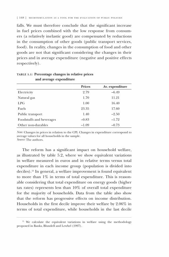
[ 168 ] m i c r o s i m u l at i o n a s a t o o l f o r t h e e va l u at i o n o f p u b l i c p o l i c i e s
falls. We must therefore conclude that the significant increase in fuel prices combined with the low response from consum-ers (a relatively inelastic good) are compensated by reductions in the consumption of other goods (public transport services, food). In reality, changes in the consumption of food and other goods are not that significant considering the changes in their prices and in average expenditure (negative and positive effects respectively).
table 5.1: Percentage changes in relative prices and average expenditure
Prices Av. expenditure
Electricity 2.79 –6.49
Natural gas 1.70 11.21
LPG 1.00 16.40
Fuels 23.35 17.60
Public transport 1.40 –2.50
Foodstuffs and beverages –0.83 –1.72
Other non-durables –1.09 –0.73
Note: Changes in prices in relation to the CPI. Changes in expenditure correspond to average values for all households in the sample.Source: The authors.
The reform has a significant impact on household welfare, as illustrated by table 5.2, where we show equivalent variations in welfare measured in euros and in relative terms versus total expenditure in each income group (population is divided into deciles).15 In general, a welfare improvement is found equivalent to more than 1% in terms of total expenditure. This is reason-able considering that total expenditure on energy goods (higher tax rates) represents less than 10% of overall total expenditure for the majority of households. Data from the table also show that the reform has progressive effects on income distribution. Households in the first decile improve their welfare by 2.06% in terms of total expenditure, while households in the last decile
15 We calculate the equivalent variations in welfare using the methodology proposed in Banks, Blundell and Lewbel (1997).
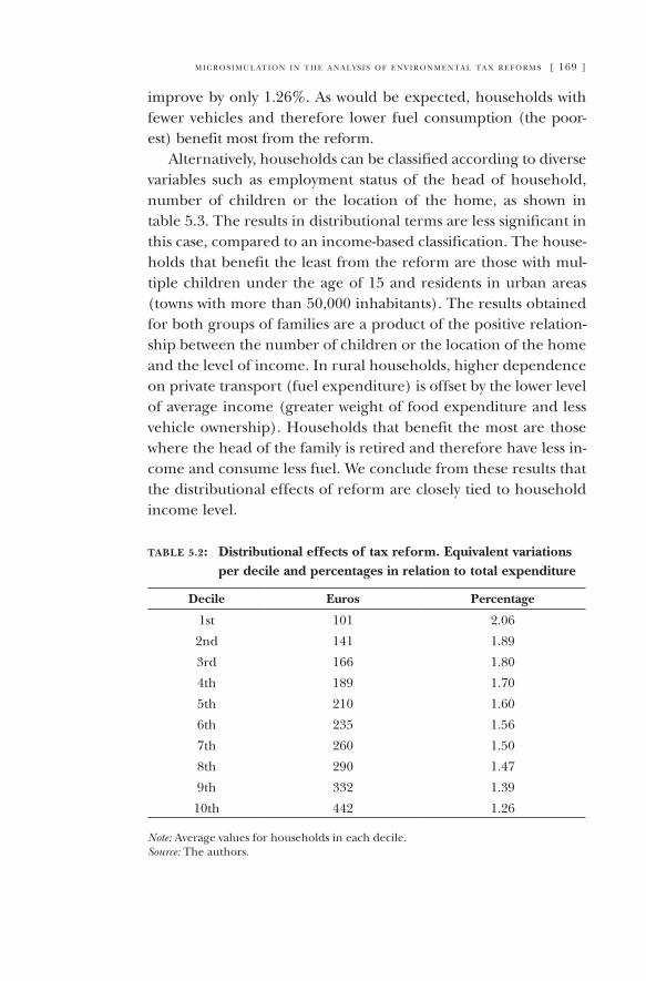
m i c r o s i m u l at i o n i n t h e a n a ly s i s o f e n v i r o n m e n ta l ta x r e f o r m s [ 169 ]
improve by only 1.26%. As would be expected, households with fewer vehicles and therefore lower fuel consumption (the poor-est) benefit most from the reform.
Alternatively, households can be classified according to diverse variables such as employment status of the head of household, number of children or the location of the home, as shown in table 5.3. The results in distributional terms are less significant in this case, compared to an income-based classification. The house-holds that benefit the least from the reform are those with mul-tiple children under the age of 15 and residents in urban areas (towns with more than 50,000 inhabitants). The results obtained for both groups of families are a product of the positive relation-ship between the number of children or the location of the home and the level of income. In rural households, higher dependence on private transport (fuel expenditure) is offset by the lower level of average income (greater weight of food expenditure and less vehicle ownership). Households that benefit the most are those where the head of the family is retired and therefore have less in-come and consume less fuel. We conclude from these results that the distributional effects of reform are closely tied to household income level.
table 5.2: Distributional effects of tax reform. Equivalent variations per decile and percentages in relation to total expenditure
Decile Euros Percentage
1st 101 2.06
2nd 141 1.89
3rd 166 1.80
4th 189 1.70
5th 210 1.60
6th 235 1.56
7th 260 1.50
8th 290 1.47
9th 332 1.39
10th 442 1.26
Note: Average values for households in each decile.Source: The authors.
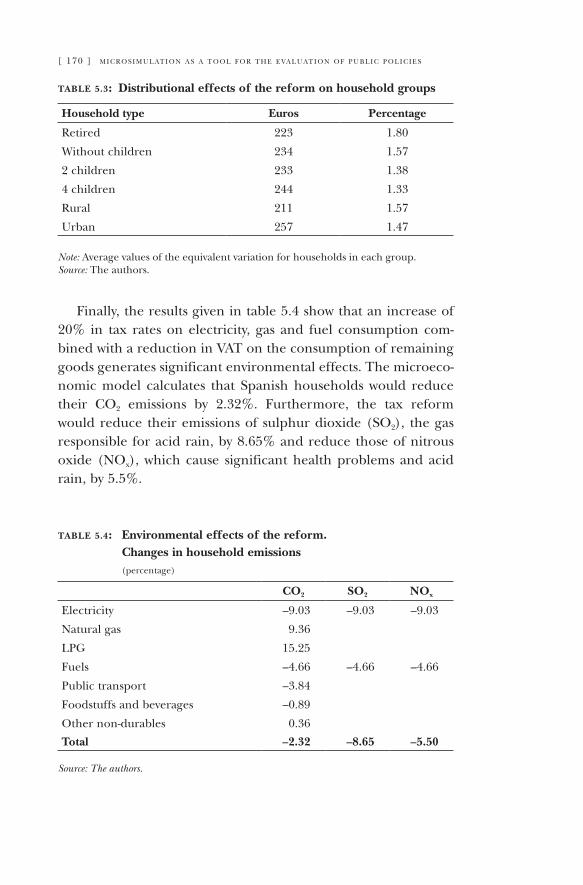
[ 170 ] m i c r o s i m u l at i o n a s a t o o l f o r t h e e va l u at i o n o f p u b l i c p o l i c i e s
table 5.3: Distributional effects of the reform on household groups
Household type Euros Percentage
Retired 223 1.80
Without children 234 1.57
2 children 233 1.38
4 children 244 1.33
Rural 211 1.57
Urban 257 1.47
Note: Average values of the equivalent variation for households in each group.Source: The authors.
Finally, the results given in table 5.4 show that an increase of 20% in tax rates on electricity, gas and fuel consumption com-bined with a reduction in VAT on the consumption of remaining goods generates significant environmental effects. The microeco-nomic model calculates that Spanish households would reduce their CO2 emissions by 2.32%. Furthermore, the tax reform would reduce their emissions of sulphur dioxide (SO2), the gas responsible for acid rain, by 8.65% and reduce those of nitrous oxide (NOx), which cause significant health problems and acid rain, by 5.5%.
table 5.4: Environmental effects of the reform. Changes in household emissions (percentage)
CO2 SO2 NOx
Electricity –9.03 –9.03 –9.03
Natural gas 9.36
LPG 15.25
Fuels –4.66 –4.66 –4.66
Public transport –3.84
Foodstuffs and beverages –0.89
Other non-durables 0.36
Total –2.32 –8.65 –5.50
Source: The authors.
m i c r o s i m u l at i o n i n t h e a n a ly s i s o f e n v i r o n m e n ta l ta x r e f o r m s [ 171 ]
5.5. Conclusions
Public policies that pursue economic improvements in terms of efficiency tend to cause secondary positive or negative effects on income distribution. However, the analytical methodologies used to study both effects are different. General equilibrium methods are the most appropriate for analysing the efficiency of public policies. But when they include a representative household no distributional analysis can be carried out. More disaggregated models can also produce incorrect results according to the em-pirical evidence in the literature. Microeconomic models are ap-propriate for distribution analysis but not efficiency analysis, due to their partial equilibrium approach.
In this paper, we used a new methodological approach inte-grating different analytical methods to study the effects of public policies. In particular, we integrate a static general equilibrium model which allows us to evaluate the effects of a reform on the efficiency and activity of economic sectors, with a household en-ergy microeconomic demand model that allows us to disaggregate results by different types of household. To illustrate the suitability of the proposed methodology, we simulate a policy consisting of a green tax reform with a 20% tax increase on the consumption of different energy goods. The tax revenues obtained are used to finance a reduction in the tax charge on remaining goods and services in the economy, the objective being a zero public budget impact.
Our results indicate that reform contributes to significantly reducing pollutant emissions. It also provides other benefits apart from environmental ones, such as a modest increase in production. As expected, the effects of the reform differ by sec-tor: while overall production increases, production in energy intensive sectors falls. The effects on prices also vary by sector, with significant increases in the prices of energy intensive sec-tors and modest price reductions in goods that form a more important part of the household shopping basket. Since no significant changes in income are detected, price changes and household heterogeneity are the only sources for changes in income distribution.
[ 172 ] m i c r o s i m u l at i o n a s a t o o l f o r t h e e va l u at i o n o f p u b l i c p o l i c i e s
The distributional consequences are significant. In general, there is a welfare improvement but with distributional conse-quences. On average, the ratio between the equivalent variation and total expenditure is greater than 1% for all households. This figure is 63 percent higher for the poorest households (first decile in the distribution) than for the richest (last decile). Following the green tax reform, households where the principal earner is retired also benefit more than the average. This result is interesting because most evidence available at international level suggests that taxes on energy goods are regressive, although this evidence is generally obtained from partial equilibrium models.
The study also has some methodological implications. It shows that analysis can be significantly improved by integrating different methods. The AGEM allows for richer and more detailed studies on the macroeconomic effects of public policies. Integrated with a microsimulation model at the household or individual level, it fills out results to the greatest possible heterogeneity, allowing welfare analysis to be carried out at individual level.
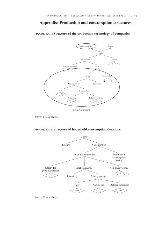
m i c r o s i m u l at i o n i n t h e a n a ly s i s o f e n v i r o n m e n ta l ta x r e f o r m s [ 173 ]
Appendix: Production and consumption structures
figure 5.A.1: Structure of the production technology of companies
Source: The authors.
figure 5.A.2: Structure of household consumption decisions
Source: The authors.
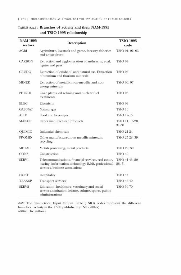
[ 174 ] m i c r o s i m u l at i o n a s a t o o l f o r t h e e va l u at i o n o f p u b l i c p o l i c i e s
table 5.A.1: Branches of activity and their NAM-1995 and TSIO-1995 relationship
NAM-1995 sectors
Description TSIO-1995 code
AGRI Agriculture, livestock and game, forestry, fisheries and aquaculture
TSIO 01, 02, 03
CARBON Extraction and agglomeration of anthracite, coal, lignite and peat
TSIO 04
CRUDO Extraction of crude oil and natural gas. Extraction of uranium and thorium minerals
TSIO 05
MINER Extraction of metallic, non-metallic and non-energy minerals
TSIO 06, 07
PETROL Coke plants, oil refining and nuclear fuel treatments
TSIO 08
ELEC Electricity TSIO 09
GAS NAT Natural gas TSIO 10
ALIM Food and beverages TSIO 12-15
MANUF Other manufactured products TSIO 11, 16-20, 31-38
QUIMIO Industrial chemicals TSIO 21-24
PROMIN Other manufactured non-metallic minerals, recycling
TSIO 25-28, 39
METAL Metals processing, metal products TSIO 29, 30
CONS Construction TSIO 40
SERV1 Telecommunications, financial services, real estate, leasing, information technology, R&D, professional services, business associations
TSIO 41-43, 50-58, 71
HOST Hospitality TSIO 44
TRANSP Transport services TSIO 45-49
SERV2 Education, healthcare, veterinary and social services, sanitation, leisure, culture, sports, public administrations
TSIO 59-70
Note: The Symmetrical Input Output Table (TSIO) codes represent the different branches activity in the TSIO published by INE (2002a).Source: The authors.
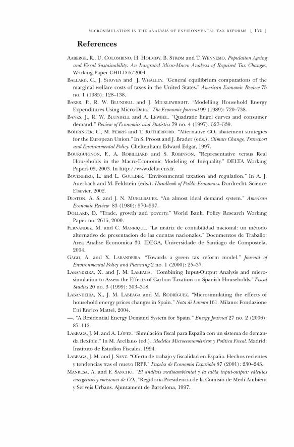
m i c r o s i m u l at i o n i n t h e a n a ly s i s o f e n v i r o n m e n ta l ta x r e f o r m s [ 175 ]
References
aaberge, r., u. colombino, h. holmøy, b. strøm and T. Wennemo. Population Ageing and Fiscal Sustainability: An Integrated Micro-Macro Analysis of Required Tax Changes, Working Paper CHILD 6/2004.
ballard, c., J. shoven and J. Whalley. “General equilibrium computations of the marginal welfare costs of taxes in the United States.” American Economic Review 75 no. 1 (1985): 128–138.
baker, p., r. W. blundell and J. mickleWright. “Modelling Household Energy Expenditures Using Micro-Data.” The Economic Journal 99 (1989): 720–738.
banks, J., R. W. blundell and A. leWbel. “Quadratic Engel curves and consumer demand.” Review of Economics and Statistics 79 no. 4 (1997): 527–539.
böhringer, C., M. ferris and T. rutherford. “Alternative CO2 abatement strategies for the European Union.” In S. Proost and J. Brader (eds.). Climate Change, Transport and Environmental Policy. Cheltenham: Edward Edgar, 1997.
bourguignon, F., A. robilliard and S. robinson. “Representative versus Real Households in the Macro-Economic Modeling of Inequality.” DELTA Working Papers 05, 2003. In http://www.delta.ens.fr.
bovenberg, L. and L. goulder. “Environmental taxation and regulation.” In A. J. Auerbach and M. Feldstein (eds.). Handbook of Public Economics. Dordrecht: Science Elsevier, 2002.
deaton, a. s. and J. n. muellbauer. “An almost ideal demand system.” American Economic Review 83 (1980): 570–597.
dollard, d. “Trade, growth and poverty.” World Bank. Policy Research Working Paper no. 2615, 2000.
fernández, m. and c. manrique. “La matriz de contabilidad nacional: un método alternativo de presentacion de las cuentas nacionales.” Documentos de Traballo: Area Analise Economica 30. IDEGA, Universidade de Santiago de Compostela, 2004.
gago, a. and x. labandeira. “Towards a green tax reform model.” Journal of Environmental Policy and Planning 2 no. 1 (2000): 25–37.
labandeira, X. and J. M. labeaga. “Combining Input-Output Analysis and micro-simulation to Assess the Effects of Carbon Taxation on Spanish Households.” Fiscal Studies 20 no. 3 (1999): 303–318.
labandeira, x., J. m. labeaga and m. rodríguez. “Microsimulating the effects of household energy prices changes in Spain.” Nota di Lavoro 161. Milano: Fondazione Eni Enrico Mattei, 2004.
—. “A Residential Energy Demand System for Spain.” Energy Journal 27 no. 2 (2006): 87–112.
labeaga, J. m. and a. lópez. “Simulación fiscal para España con un sistema de deman-da flexible.” In M. Arellano (ed.). Modelos Microeconométricos y Política Fiscal. Madrid: Instituto de Estudios Fiscales, 1994.
labeaga, J. m. and J. sanz. “Oferta de trabajo y fiscalidad en España. Hechos recientes y tendencias tras el nuevo IRPF.” Papeles de Economía Española 87 (2001): 230–243.
manresa, A. and F. sancho. “El análisis medioambiental y la tabla input-output: cálculos energéticos y emisiones de CO2 .” Regidoria-Presidencia de la Comisió de Medi Ambient y Serveis Urbans. Ajuntament de Barcelona, 1997.

[ 176 ] m i c r o s i m u l at i o n a s a t o o l f o r t h e e va l u at i o n o f p u b l i c p o l i c i e s
parry, i., r. Williams and l. goulder. “When Can Carbon Abatement Policies Increase Welfare? The Fundamental Role of Distorted Factor Markets.” Journal of Environmental Economics and Management 37 (1999): 52–84.
rutherford, t. “Applied General Equilibrium Modeling with MPSGE as a GAMS subsystem: an overview of the Modeling Framework and Syntax.” Computational Economics 14 (1999): 1–46.
savard, l. “Poverty and Income Distribution in a CGE-Household Micro-Simulation Model: Top-Down/ Bottom-Up Approach.” CIRPÉE Working paper 03-43, 2003.
shoven, J. and J. Whalley. Applying general equilibrium. Cambridge: Cambridge University Press, 1992.
speck, S. “Energy and Carbon Taxes and their Distributional Implications.” Energy Policy 27 (1999): 659–667.
symons, E., J. proops and P. gay. “Carbon Taxes, Consumer Demand and Carbon Dioxide Emissions: A Simulation Analysis for the UK.” Fiscal Studies 15 no. 2 (1994): 19–43.
[ 177 ]
Microsimulation and Economic Rationality: an application of the Collective Model to Evaluate Tax Reforms in Spain
Raquel Carrasco and Javier Ruiz-CastilloCarlos III University (Madrid)
6.1. Introduction
The incidence of the tax system on labour supplies is a classic topic in the evaluation of fiscal policy. This chapter studies the impact of an important reform of personal income tax in Spain using a collective model of household labour supply.1 The reform was introduced in 1999 by the centre-right government that came into power in 1996 after 14 years of socialist governments. The main novelties of the 1999 tax system are the reduction in the number of tax brackets, the lowering of marginal tax rates and the introduction of a large standard deduction from the tax base depending on family composition.
In the unitary model, it is assumed that, regardless of their composition, households behave as single decision-making units. In this way, standard tools of consumer analysis can then be
6.
We are grateful for comments and advice from all participants in the one-year project “Welfare analysis of fiscal and social security reforms in Europe: Does the representation of family decision processes matter?”, partly financed by the EU, General Directorate of Employment and Social affairs, grant VS/2000/0778. In particular, we would like to thank Denis Beninger and François Laisney for providing continuous assistance as well as the programmes used in this work. We are also in debt to Maite Martinez who decisively helped to adapt one of the programmes to our goals. Thanks also to Miriam Beblo, Denis Beninger, François Laisney and Frederic Vermeulen for careful reading of a preliminary version. The authors are solely responsible for all remaining shortcomings.
1 This study is part of a research project using a common methodology in seven European countries: Belgium, Denmark, France, Germany, Italy, Spain and the United Kingdom.

[ 178 ] m i c r o s i m u l at i o n a s a t o o l f o r t h e e va l u at i o n o f p u b l i c p o l i c i e s
applied at the household level. Observable joint household consumption and individual labour supplies in multi-person households are assumed to result from the maximization of a single utility function representing household preferences. In the overall budget constraint, household income results from the pooling of all household members’ incomes. In this setup, where households are treated as a black box, the intra-household redis-tribution of resources cannot be reconstructed. Consequently, nothing is said about the individual welfare enjoyed by each household member.
It has been known for some time that the strong implication of the unitary model about the symmetry of the Slutsky matrix is regularly rejected for household data (Blundell 1988; Blundell et al. 1993; and Browning and Meghir 1991). More recently, there has been mounting empirical evidence rejecting the income pool-ing property of the unitary model (see, for instance, the papers quoted in Browning and Chiappori 1998).
as an alternative to the methodological and empirical shortcomings of the standard approach, a new literature on household economics has developed during the last twenty years (Manser and Brown 1980). Its main feature is the recog-nition that a household is formed by several individuals, pos-sibly with different preferences, who engage in some form of intra-household bargaining process to arrive at all household decisions. In this paper, only the so-called collective approach to household behaviour, originating in Chiappori (1988, 1992) will be considered.2 The assumption that characterizes this approach is that household decisions are Pareto efficient. This assumption alone has testable implications for house-hold demand functions that can be seen as a generalization of the Slutsky symmetry and negativeness in the unitary case (Browning and Chiappori 1998). Furthermore, within a col-lective framework, household demands and labour supplies should be sensitive to the intra-household distribution of re-sources, and more generally to any environmental variable that
2 For a summary of this approach, see Bourguignon and Chiappori (1992), and for a more recent survey, see Vermeulen (2000).
m i c r o s i m u l at i o n a n d e c o n o m i c r at i o n a l i t y [ 179 ]
may influence the decision process—the EEPs in McElroy’s (1990) terminology or the distribution factors in Browning et al. (1994). Interestingly enough, the restrictions of different collective models have not been rejected in several empirical studies (Vermeulen 2000).
Thus, the stage is set for the evaluation of policy measures according to a unitary or a collective model of the household. Ideally, one would have to estimate structural models under the two approaches and a common version of the base tax system. Then, the two sets of behavioural parameter estimates would be used to obtain predictions after a tax reform. Unfortunately, this strategy is not possible at this point. The estimation of house-hold labour supply decisions is operational for unitary models of the household in the realistic case of discrete choices (Van Soest 1995; Bingley and Walker 1997; and Blundell et al. 1998). However, the identification and the estimation of a full collec-tive model of the household including labour non-participation, the presence of children and non-linear taxation is still in its infancy.3
To circumvent this problem, this paper proposes a simplified application of the collective approach. The methodology origi-nates in Beninger and Laisney (2001), where fiscal reforms are simulated on an artificially created dataset. The population of tax units consists only of singles and couples where labour sup-ply decisions are treated as a discrete choice problem. Here a dataset is created where couples’ behaviour under the baseline tax system results from a fully deterministic labour supply model that exhibits some fundamental ingredients of the collective approach. The collective world is constructed following a mixed strategy. Some preference parameters are estimated from the singles sample, while some other key parameters of the collec-tive model are calibrated so as to replicate the observed data on couples’ labour supply. a unitary model is then estimated in this
3 The only attempt to model the (female) participation decision, but with linear taxation and convex budget sets, is Blundell et al. (1998). See also Donni (2002) for a model with nonlinear budget constraints resulting in convex budget sets. For the issue of female labour participation in the context of cross-section data on commodity expenditures, see Zamora (2000).
[ 180 ] m i c r o s i m u l at i o n a s a t o o l f o r t h e e va l u at i o n o f p u b l i c p o l i c i e s
collective world where household members behave according to collective rationality. In this way, it is possible to study whether the two models lead to substantially different predictions on house-hold consumption and male and female labour supplies before and after a common tax reform.
The Spanish data come from the first three waves of the European Community Household Panel (ECHP), collected during 1994 to 1996. In line with the remaining countries in the inter-national project to which this paper belongs, the sample selected consists of people of 25-55 years of age, excluding the retired, the registered unemployed, the self-employed and those working in the agricultural sector. Thus, the tax units selected are singles and couples, with or without children under 16, where the adults are either employed in a salaried job or non-participants in the labour market.
The baseline personal tax system is the one of 1994. The available data permits the modeling of a 1994 stylized tax system, where married people are allowed to fill in either two individual tax returns or a joint return. The remaining features of the 1994 tax system can be summarized as follows:
certain deductions from wage earnings; two graduated tariffs for individual and joint returns, both consisting of 18 tax brackets with a minimum and a maxi-mum marginal tax rate of 20% and 56%, respectively; a minimum exempted income of approximately 2,405 eu-ros, for individual tax units and 4,810 euros, for couples; and certain tax credits depending on the number of children and other circumstances of the tax unit.
The 1999 tax system also permits married people to fill in individual or joint returns and maintains a deduction from wage earnings. The two distinctive features of the reform are (i) the substitution of tax credits by a standard deduction from the tax base of 3,307 euros per adult, plus 1,203 euros for the first and second child, and 1,803 euros for the third and remaining chil-dren; and (ii) a unique graduated tariff for individual and joint
i)ii)
iii)
iv)
m i c r o s i m u l at i o n a n d e c o n o m i c r at i o n a l i t y [ 181 ]
tax returns consisting of only 6 tax brackets with a minimum and a maximum marginal tax rate of 18% and 48%, respectively.4
The first important finding of the paper is that the unitary model performs very badly on the dataset constructed under the collective approach. This is partly due to the mistaken assumption that households behave as single decision makers when the da-taset has been constructed according to a collective model. The implication for future research is that more effort is warranted in making the collective approach operational.
Regarding the collective framework, the paper first evaluates the 1999 tax reform maintaining constant the behaviour pre-dicted by the deterministic collective model. Consistently with other static exercises, it is found that the 1999 tax system leads to an increase in mean disposable income and a reduction of the redistributive effect on the pre-tax income distribution.5
The more interesting results take into account individuals’ re-sponses to changes in the tax system. an important finding is that female bargaining power depends, among other variables, on the earnings potential of the members of the couple. In turn, this variable partially depends on the tax system parameters. Thus, in the collective framework any tax reform affects spouses’ labour supplies through two channels. First, through changes in the overall budget constraint, the only channel available in a unitary world. Second, through changes in females’ bargaining power, a distinctive feature of the collective approach.
When labour supplies are allowed to vary, the decrease in tax revenues and average tax rates is smaller than in the static case, the redistributive effect is larger than in 1994, and there is a 14.8 social welfare increase, defined in the space of disposable incomes. Moreover, the issue of changes in the intra-household distribution of resources—about which the unitary model is silent—can also be analyzed within the collective approach. In particular, correspond-ing to the increase in females’ power index induced by the tax
4 as explained in section 6.7, rather than estimating the growth of 1994 gross incomes until 1999 for the tax units in the sample, the standard deductions and the tax brackets of the 1999 reform are expressed at 1994 prices using the official 15.15 % inflation rate between the two periods according to the Consumer Price Index.
5 See, for instance, Castañer et al. (2000).
[ 182 ] m i c r o s i m u l at i o n a s a t o o l f o r t h e e va l u at i o n o f p u b l i c p o l i c i e s
reform, all females in the couples sample experience a utility gain, while essentially all men are seen to experiment a utility loss.
The rest of this chapter is organized in seven sections. Section 6.2 discusses sample selection and other data prob-lems. Section 6.3 presents the baseline 1994 tax system. Section 6.4 describes how to construct a collective world. Section 6.5 presents the results on the estimation of the singles model and the construction of the collective world for the Spanish econ-omy. Section 6.6 reports the estimation of the unitary model on the collectively generated dataset. Section 6.7 evaluates the tax reform in the collective world, and section 6.8 summarizes the findings.
6.2. The data
as indicated in the introduction, data come from the ECHP. The main focus of this study is the evaluation of tax reforms through their impact on labour supply. It is well known that the labour behaviour of the registered unemployed, the self-employed and those working in the agricultural sector is particularly difficult to estimate. Therefore, together with the retired, households containing persons of these characteristics are excluded from the analysis. Furthermore, the labour behaviour of those close to the normal retirement age of 65 years might be heavily influenced by early retirement provisions, which are an important part of all the social security systems of the European countries participat-ing in this study. Therefore, the tax units selected are households with or without children under 16, where the adults are 25-55 years of age and either employed in a salaried job or voluntarily unemployed.
There are basically three problems with the type of informa-tion available in Spain and with the sample selected according to these criteria. First, three waves of the ECHP, conducted in 1994, 1995 and 1996, were available at the time of the project. In a given ECHP wave dated in year t, individual characteristics refer to the moment the interview is conducted, namely, during the last quarter of that year. However, annual income is reported in
m i c r o s i m u l at i o n a n d e c o n o m i c r at i o n a l i t y [ 183 ]
answer to a retrospective question that refers to the year t – 1. To overcome this discrepancy, individuals interviewed during two consecutive waves have been considered. In this way, individual characteristics recorded during the last quarter of year t can be matched with income information referring to this year, but re-corded during the second wave, that is, during the last quarter of year t + 1.
Secondly, as in other Southern European countries, the percentage of people living in single person households and satisfying the above selection criteria is very low. In particular, among the people interviewed in 1994 for which information in the second wave is available, there are only 70 females and 86 males in this situation. In an attempt to increase the sample size, new individuals in single person households in 1995 who had other living arrangements in 1994 have also been considered. Unfortunately, those for whom there is also information in 1996 about the income earned during 1995 sum only 19 females and 20 males.6 Finally, single parents with children under 16 are also considered. a total of 46 females and 3 males fulfil this condi-tion. Therefore, the final sample of tax units consisting of single person households, with or without children under 16, comprises 135 females and 109 males. From now on, these tax units will be referred to as singles.
a classical difficulty in studies of tax reform with micro data from household surveys is that the definition of a household need not coincide with the definition of a tax unit. Therefore, in line with the remaining countries in this international project, the second type of tax unit studied—which will be referred to as couples—consists of households which can be easily identified as tax units and satisfy the selected criterion already discussed, that is, households with two adults 25-55 years of age, either employed in a salaried job or voluntary unemployed, with and without children under 16. Households of more complex composition, with either additional older,
6 People interviewed during the last quarter of 1996 cannot be considered because there is no information on income earned that year but reported in the unavailable 1997 wave.
[ 184 ] m i c r o s i m u l at i o n a s a t o o l f o r t h e e va l u at i o n o f p u b l i c p o l i c i e s
younger members, or both, are excluded from the analysis. as in other Southern European countries, a large propor-tion of households in Spain belong to this excluded category. Consequently, the ECHP sample of couples thus defined con-sists of only 975 observations.7
The third problem with Spanish data has to do with the fact that most income information refers to income net of (i) with-holdings retained at the income source on account of personal income tax, and (ii) the employee’s contribution to social secu-rity. Withholdings refer both to capital income, wage income and some public transfers that are considered part of labour income. These public transfers include old age and disability pensions, pensions granted to widows and orphans, the unemployment subsidy and other minor public subsidies granted to needy fami-lies.8
Given the graduated tariff in Spanish income tax, firms are instructed to practice withholdings on wage income according to a complex formula that takes into account the number of de-pendent children. In addition, there is a single 25% withhold-ing rate on capital income, and a relatively small withholding rate on the public transfers described above. The employee’s contribution to social security refers only to wage income, var-ies across a number of professional categories and is subject to a ceiling.
Fortunately, the Instituto de Estudios Fiscales (IEF)—a public entity in the Ministry of Finance devoted to research on fiscal matters and other activities—has a programme to compute an estimate of gross income from the information available in the ECHP about the net income described above, and the number of
7 The 244 singles and the 975 couples represent 15.6 and 11.7%, respectively, of all households interviewed during two consecutive years in the three available waves of the ECHP. Naturally, for the reasons mentioned in the text, it is impossible to know the percentage that this sample represents relative to the total number of tax units which are legally required to fill in a tax return in the year of reference 1994.
8 In addition, as will be seen below, the ECHP provides information about property income, which is part of taxable income but is not subject to withholdings, as well as certain non-taxable public transfers including students’ scholarships and some minor housing subsidies.
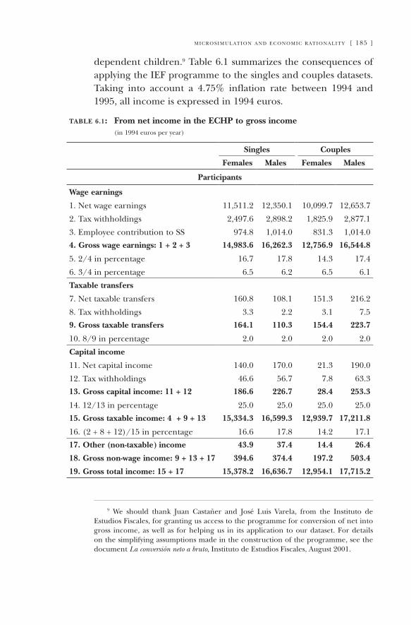
m i c r o s i m u l at i o n a n d e c o n o m i c r at i o n a l i t y [ 185 ]
dependent children.9 Table 6.1 summarizes the consequences of applying the IEF programme to the singles and couples datasets. Taking into account a 4.75% inflation rate between 1994 and 1995, all income is expressed in 1994 euros.
table 6.1: From net income in the ECHP to gross income (in 1994 euros per year)
Singles Couples
Females Males Females Males
Participants
Wage earnings
1. Net wage earnings 11,511.2 12,350.1 10,099.7 12,653.7
2. Tax withholdings 2,497.6 2,898.2 1,825.9 2,877.1
3. Employee contribution to SS 974.8 1,014.0 831.3 1,014.0
4. Gross wage earnings: 1 + 2 + 3 14,983.6 16,262.3 12,756.9 16,544.8
5. 2/4 in percentage 16.7 17.8 14.3 17.4
6. 3/4 in percentage 6.5 6.2 6.5 6.1
Taxable transfers
7. Net taxable transfers 160.8 108.1 151.3 216.2
8. Tax withholdings 3.3 2.2 3.1 7.5
9. Gross taxable transfers 164.1 110.3 154.4 223.7
10. 8/9 in percentage 2.0 2.0 2.0 2.0
Capital income
11. Net capital income 140.0 170.0 21.3 190.0
12. Tax withholdings 46.6 56.7 7.8 63.3
13. Gross capital income: 11 + 12 186.6 226.7 28.4 253.3
14. 12/13 in percentage 25.0 25.0 25.0 25.0
15. Gross taxable income: 4 + 9 + 13 15,334.3 16,599.3 12,939.7 17,211.8
16. (2 + 8 + 12)/15 in percentage 16.6 17.8 14.2 17.1
17. Other (non-taxable) income 43.9 37.4 14.4 26.4
18. Gross non-wage income: 9 + 13 + 17 394.6 374.4 197.2 503.4
19. Gross total income: 15 + 17 15,378.2 16,636.7 12,954.1 17,715.2
9 We should thank Juan Castañer and José Luis Varela, from the Instituto de Estudios Fiscales, for granting us access to the programme for conversion of net into gross income, as well as for helping us in its application to our dataset. For details on the simplifying assumptions made in the construction of the programme, see the document La conversión neto a bruto, Instituto de Estudios Fiscales, august 2001.
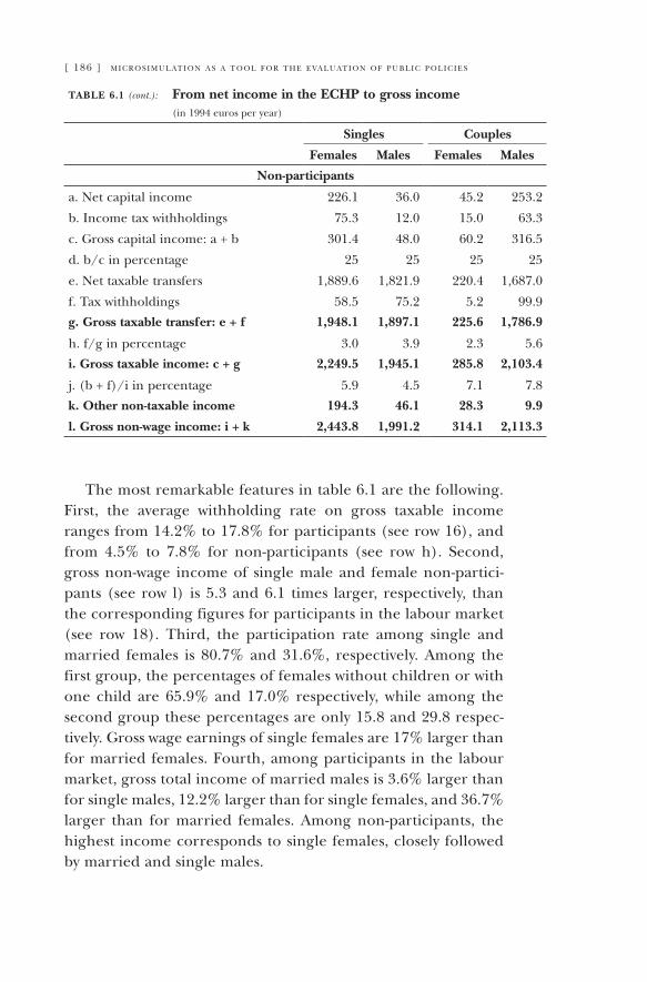
[ 186 ] m i c r o s i m u l at i o n a s a t o o l f o r t h e e va l u at i o n o f p u b l i c p o l i c i e s
table 6.1 (cont.): From net income in the ECHP to gross income (in 1994 euros per year)
Singles Couples
Females Males Females Males
Non-participants
a. Net capital income 226.1 36.0 45.2 253.2
b. Income tax withholdings 75.3 12.0 15.0 63.3
c. Gross capital income: a + b 301.4 48.0 60.2 316.5
d. b/c in percentage 25 25 25 25
e. Net taxable transfers 1,889.6 1,821.9 220.4 1,687.0
f. Tax withholdings 58.5 75.2 5.2 99.9
g. Gross taxable transfer: e + f 1,948.1 1,897.1 225.6 1,786.9
h. f/g in percentage 3.0 3.9 2.3 5.6
i. Gross taxable income: c + g 2,249.5 1,945.1 285.8 2,103.4
j. (b + f)/i in percentage 5.9 4.5 7.1 7.8
k. Other non-taxable income 194.3 46.1 28.3 9.9
l. Gross non-wage income: i + k 2,443.8 1,991.2 314.1 2,113.3
The most remarkable features in table 6.1 are the following. First, the average withholding rate on gross taxable income ranges from 14.2% to 17.8% for participants (see row 16), and from 4.5% to 7.8% for non-participants (see row h). Second, gross non-wage income of single male and female non-partici-pants (see row l) is 5.3 and 6.1 times larger, respectively, than the corresponding figures for participants in the labour market (see row 18). Third, the participation rate among single and married females is 80.7% and 31.6%, respectively. among the first group, the percentages of females without children or with one child are 65.9% and 17.0% respectively, while among the second group these percentages are only 15.8 and 29.8 respec-tively. Gross wage earnings of single females are 17% larger than for married females. Fourth, among participants in the labour market, gross total income of married males is 3.6% larger than for single males, 12.2% larger than for single females, and 36.7% larger than for married females. among non-participants, the highest income corresponds to single females, closely followed by married and single males.
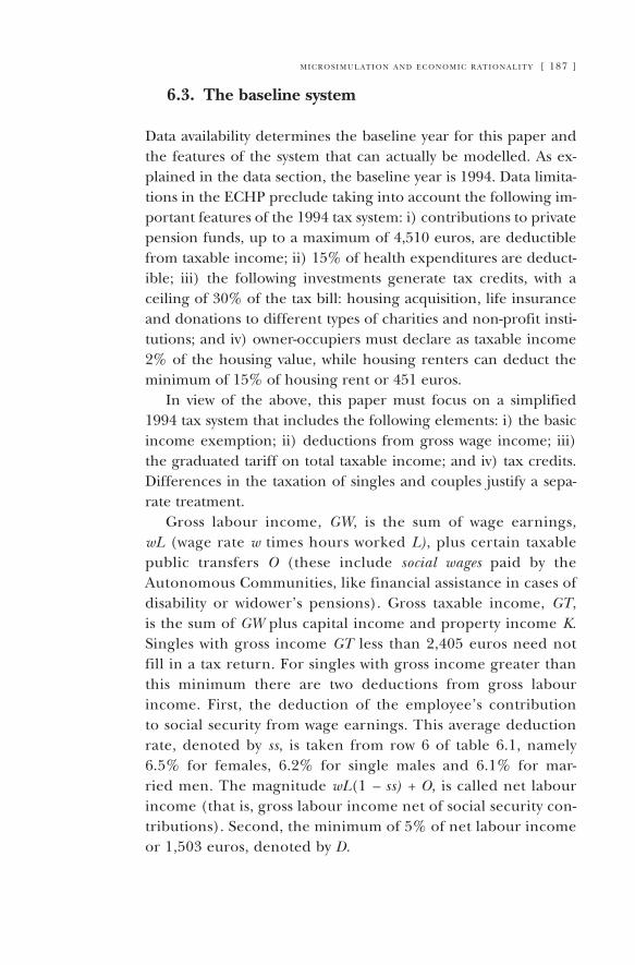
m i c r o s i m u l at i o n a n d e c o n o m i c r at i o n a l i t y [ 187 ]
6.3. The baseline system
Data availability determines the baseline year for this paper and the features of the system that can actually be modelled. as ex-plained in the data section, the baseline year is 1994. Data limita-tions in the ECHP preclude taking into account the following im-portant features of the 1994 tax system: i) contributions to private pension funds, up to a maximum of 4,510 euros, are deductible from taxable income; ii) 15% of health expenditures are deduct-ible; iii) the following investments generate tax credits, with a ceiling of 30% of the tax bill: housing acquisition, life insurance and donations to different types of charities and non-profit insti-tutions; and iv) owner-occupiers must declare as taxable income 2% of the housing value, while housing renters can deduct the minimum of 15% of housing rent or 451 euros.
In view of the above, this paper must focus on a simplified 1994 tax system that includes the following elements: i) the basic income exemption; ii) deductions from gross wage income; iii) the graduated tariff on total taxable income; and iv) tax credits. Differences in the taxation of singles and couples justify a sepa-rate treatment.
Gross labour income, GW, is the sum of wage earnings, wL (wage rate w times hours worked L), plus certain taxable public transfers O (these include social wages paid by the autonomous Communities, like financial assistance in cases of disability or widower’s pensions). Gross taxable income, GT, is the sum of GW plus capital income and property income K. Singles with gross income GT less than 2,405 euros need not fill in a tax return. For singles with gross income greater than this minimum there are two deductions from gross labour income. First, the deduction of the employee’s contribution to social security from wage earnings. This average deduction rate, denoted by ss, is taken from row 6 of table 6.1, namely 6.5% for females, 6.2% for single males and 6.1% for mar-ried men. The magnitude wL(1 – ss) + O, is called net labour income (that is, gross labour income net of social security con-tributions). Second, the minimum of 5% of net labour income or 1,503 euros, denoted by D.
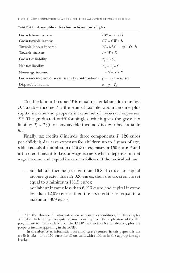
[ 188 ] m i c r o s i m u l at i o n a s a t o o l f o r t h e e va l u at i o n o f p u b l i c p o l i c i e s
table 6.2: A simplified taxation scheme for singles
Gross labour income GW = wL + O
Gross taxable income GT = GW + K
Taxable labour income W = wL(1 – ss) + O - D
Taxable income I = W + K
Gross tax liability Tg = T(I)
Net tax liability Tn = Tg – C
Non-wage income y = O + K + P
Gross income, net of social security contributions g = wL(1 – ss) + y
Disposable income x = g – Tn
Taxable labour income W is equal to net labour income less D. Taxable income I is the sum of taxable labour income plus capital income and property income net of necessary expenses, K.10 The graduated tariff for singles, which gives the gross tax liability Tg = T(I) for any taxable income I is described in table 6.3.
Finally, tax credits C include three components: i) 120 euros per child; ii) day care expenses for children up to 3 years of age, which equals the minimum of 15% of expenses or 150 euros;11 and iii) a credit meant to favour wage earners which depends on net wage income and capital income as follows. If the individual has:
net labour income greater than 10,824 euros or capital income greater than 12,026 euros, then the tax credit is set equal to a minimum 151.5 euros; net labour income less than 6,013 euros and capital income less than 12,026 euros, then the tax credit is set equal to a maximum 409 euros;
10 In the absence of information on necessary expenditures, in this chapter K is taken to be the gross capital income resulting from the application of the IEF programme to the raw data from the ECHP (see section 6.2 for details), plus the property income appearing in the ECHP.
11 In the absence of information on child care expenses, in this paper this tax credit is taken to be 150 euros for all tax units with children in the appropriate age bracket.
—
—
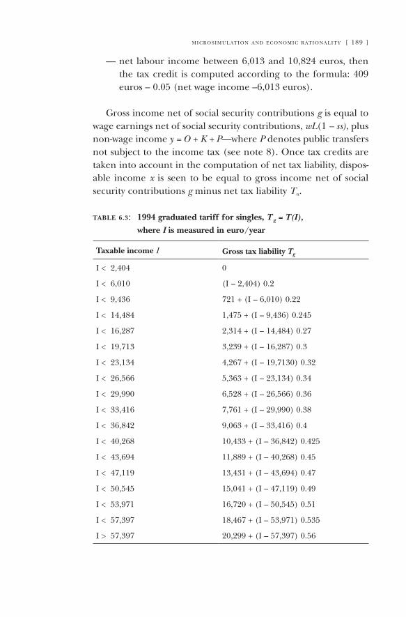
m i c r o s i m u l at i o n a n d e c o n o m i c r at i o n a l i t y [ 189 ]
net labour income between 6,013 and 10,824 euros, then the tax credit is computed according to the formula: 409 euros – 0.05 (net wage income –6,013 euros).
Gross income net of social security contributions g is equal to wage earnings net of social security contributions, wL(1 – ss), plus non-wage income y = O + K + P—where P denotes public transfers not subject to the income tax (see note 8). Once tax credits are taken into account in the computation of net tax liability, dispos-able income x is seen to be equal to gross income net of social security contributions g minus net tax liability Tn.
table 6.3: 1994 graduated tariff for singles, T g = T(I), where I is measured in euro/year
Taxable income I Gross tax liability Tg
I < 2,404 0
I < 6,010 (I – 2,404) 0.2
I < 9,436 721 + (I – 6,010) 0.22
I < 14,484 1,475 + (I – 9,436) 0.245
I < 16,287 2,314 + (I – 14,484) 0.27
I < 19,713 3,239 + (I – 16,287) 0.3
I < 23,134 4,267 + (I – 19,7130) 0.32
I < 26,566 5,363 + (I – 23,134) 0.34
I < 29,990 6,528 + (I – 26,566) 0.36
I < 33,416 7,761 + (I – 29,990) 0.38
I < 36,842 9,063 + (I – 33,416) 0.4
I < 40,268 10,433 + (I – 36,842) 0.425
I < 43,694 11,889 + (I – 40,268) 0.45
I < 47,119 13,431 + (I – 43,694) 0.47
I < 50,545 15,041 + (I – 47,119) 0.49
I < 53,971 16,720 + (I – 50,545) 0.51
I < 57,397 18,467 + (I – 53,971) 0.535
I > 57,397 20,299 + (I – 57,397) 0.56
—
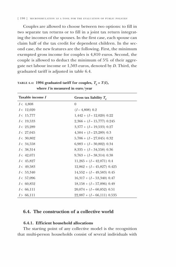
[ 190 ] m i c r o s i m u l at i o n a s a t o o l f o r t h e e va l u at i o n o f p u b l i c p o l i c i e s
Couples are allowed to choose between two options: to fill in two separate tax returns or to fill in a joint tax return integrat-ing the incomes of the spouses. In the first case, each spouse can claim half of the tax credit for dependent children. In the sec-ond case, the new features are the following. First, the minimum exempted gross income for couples is 4,810 euros. Second, the couple is allowed to deduct the minimum of 5% of their aggre-gate net labour income or 1,503 euros, denoted by D. Third, the graduated tariff is adjusted in table 6.4.
table 6.4: 1994 graduated tariff for couples, Tg = T(I),
where I is measured in euro/year
Taxable income I Gross tax liability Tg
I < 4,808 0
I < 12,020 (I – 4,808) 0.2
I < 15,777 1,442 + (I – 12,020) 0.22
I < 19,533 2,366 + (I – 15,777) 0.245
I < 23,289 3,377 + (I – 19,533) 0.27
I < 27,045 4,504 + (I – 23,289) 0.3
I < 30,802 5,706 + (I – 27,045) 0.32
I < 34,558 6,983 + (I – 30,802) 0.34
I < 38,314 8,335 + (I – 34,558) 0.36
I < 42,071 9,763 + (I – 38,314) 0.38
I < 45,827 11,265 + (I – 42,071) 0.4
I < 49,583 12,862 + (I – 45,827) 0.425
I < 53,340 14,552 + (I – 49,583) 0.45
I < 57,096 16,317 + (I – 53,340) 0.47
I < 60,852 18,158 + (I – 57,096) 0.49
I < 66,111 20,074 + (I – 60,852) 0.51
I > 66,111 22,887 + (I – 66,111) 0.535
6.4. The construction of a collective world
6.4.1. Efficient household allocationsThe starting point of any collective model is the recognition
that multi-person households consist of several individuals with
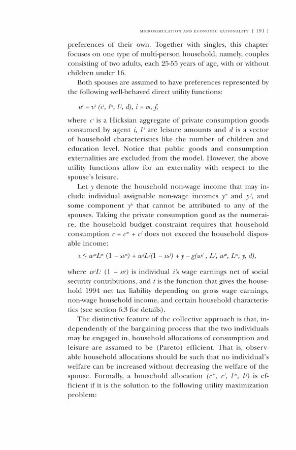
m i c r o s i m u l at i o n a n d e c o n o m i c r at i o n a l i t y [ 191 ]
preferences of their own. Together with singles, this chapter focuses on one type of multi-person household, namely, couples consisting of two adults, each 25-55 years of age, with or without children under 16.
Both spouses are assumed to have preferences represented by the following well-behaved direct utility functions:
ui = v i (c i, l m, l f, d), i = m, f,
where c i is a Hicksian aggregate of private consumption goods consumed by agent i, l i are leisure amounts and d is a vector of household characteristics like the number of children and education level. Notice that public goods and consumption externalities are excluded from the model. However, the above utility functions allow for an externality with respect to the spouse’s leisure.
Let y denote the household non-wage income that may in-clude individual assignable non-wage incomes y m and y f, and some component y h that cannot be attributed to any of the spouses. Taking the private consumption good as the numerai-re, the household budget constraint requires that household consumption c = c m + c f does not exceed the household dispos-able income:
c ≤ w mLm (1 – ssm) + w fL f(1 – ss f) + y – g(w f , L f, wm, Lm, y, d),
where w iLi (1 – ss i) is individual i’s wage earnings net of social security contributions, and t is the function that gives the house-hold 1994 net tax liability depending on gross wage earnings, non-wage household income, and certain household characteris-tics (see section 6.3 for details).
The distinctive feature of the collective approach is that, in-dependently of the bargaining process that the two individuals may be engaged in, household allocations of consumption and leisure are assumed to be (Pareto) efficient. That is, observ-able household allocations should be such that no individual’s welfare can be increased without decreasing the welfare of the spouse. Formally, a household allocation (c m, c f, l m, l f) is ef-ficient if it is the solution to the following utility maximization problem:
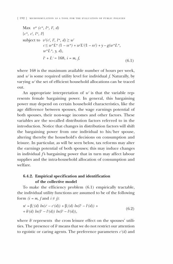
[ 192 ] m i c r o s i m u l at i o n a s a t o o l f o r t h e e va l u at i o n o f p u b l i c p o l i c i e s
Max v m (c m, l m, l f, d)
(6.1)
{c m, c f, l m, l f}
subject to v f(c f, l f, l m, d) ≥ u f
c ≤ w mLm (1 – ss m) + w fL f(1 – ss f) + y – g(w mL m, w mL m, y, d),
l i + L i = 168, i = m, f,
where 168 is the maximum available number of hours per week, and u f is some required utility level for individual f. Naturally, by varying u f the set of efficient household allocations can be traced out.
an appropriate interpretation of u f is that the variable rep-resents female bargaining power. In general, this bargaining power may depend on certain household characteristics, like the age difference between spouses, the wage earnings potential of both spouses, their non-wage incomes and other factors. These variables are the so-called distribution factors referred to in the introduction. Notice that changes in distribution factors will shift the bargaining power from one individual to his/her spouse, altering thereby the household's decisions on consumption and leisure. In particular, as will be seen below, tax reforms may alter the earnings potential of both spouses; this may induce changes in individual f’s bargaining power that in turn may affect labour supplies and the intra-household allocation of consumption and welfare.
6.4.2. Empirical specification and identification of the collective model
To make the efficiency problem (6.1) empirically tractable, the individual utility functions are assumed to be of the following form (i = m, f and i ≠ j):
ui = βci(d) ln(ci – c i(d)) + βl
i(d) ln(l i – l i(d)) + + δi(d) ln(l i – l i(d)) ln(l j – l j(d)),
(6.2)
where δi represents the cross leisure effect on the spouses’ utili-ties. The presence of δi means that we do not restrict our attention to egoistic or caring agents. The preference parameters c i(d) and
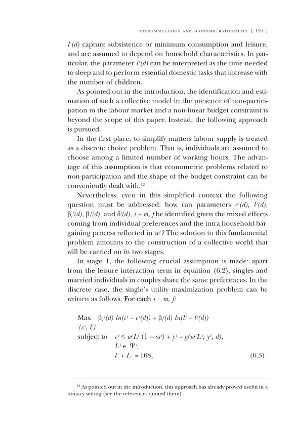
m i c r o s i m u l at i o n a n d e c o n o m i c r at i o n a l i t y [ 193 ]
l i(d) capture subsistence or minimum consumption and leisure, and are assumed to depend on household characteristics. In par-ticular, the parameter l i(d) can be interpreted as the time needed to sleep and to perform essential domestic tasks that increase with the number of children.
as pointed out in the introduction, the identification and esti-mation of such a collective model in the presence of non-partici-pation in the labour market and a non-linear budget constraint is beyond the scope of this paper. Instead, the following approach is pursued.
In the first place, to simplify matters labour supply is treated as a discrete choice problem. That is, individuals are assumed to choose among a limited number of working hours. The advan-tage of this assumption is that econometric problems related to non-participation and the shape of the budget constraint can be conveniently dealt with.12
Nevertheless, even in this simplified context the following question must be addressed: how can parameters c i(d), l i(d), βc
i(d), βli(d), and δi(d), i = m, f be identified given the mixed effects
coming from individual preferences and the intra-household bar-gaining process reflected in u f ? The solution to this fundamental problem amounts to the construction of a collective world that will be carried on in two stages.
In stage 1, the following crucial assumption is made: apart from the leisure interaction term in equation (6.2), singles and married individuals in couples share the same preferences. In the discrete case, the single’s utility maximization problem can be written as follows. For eachFor each i = m, f:
Max βc i(d) ln(c i – c i(d)) + βli(d) ln(l i – l i(d))
{c i, l i}subject to c i ≤ w iL i (1 – ss i) + y i – g(w iL i, y i, d),
L i ∈ Ψ i, l i + L i = 168, (6.3)
12 as pointed out in the introduction, this approach has already proved useful in a unitary setting (see the references quoted there).
[ 194 ] m i c r o s i m u l at i o n a s a t o o l f o r t h e e va l u at i o n o f p u b l i c p o l i c i e s
where y i = O i + K i is the non-wage income of agent i, h is the func-tion that gives the net tax liability (see section 6.3 for a discus-sion) and Ψ i is the set of alternatives among which individual i can choose his/her working hours.
This model can be estimated on data from the two samples of male and female singles discussed in section 6.2. Two remarks are in order. First, the estimation requires gross wages for all individuals. Thus, using information about their individual characteristics, standard techniques are used to predict non-par-ticipants’ gross wages. Second, although in principle the mini-mum consumption and leisure terms c i(d) and l i(d), i = m, f, can be estimated from the data, for convenience they will be fixed according to the criteria explained in the next section. Thus, the outcome of stage 1 consists of parameter estimates for βc
i(d) and βl
i(d), i = m, f (see section 6.5 for results.)For couples, minimum consumption and leisure terms are
also set equal for both males and females and are fixed according to the criteria explained in the next section. at this point, the leisure interaction terms δi(d) and the individual’s f bargaining power uf remain to be identified. For this purpose, a calibration exercise is performed in stage 2.13
This stage consists of two rounds. In the first one, for each couple the parameters δ m and δ f are made equal, δ m = δf = δ, and are allowed to vary in a grid of discrete choices denoted by ∆. For each δ in ∆, a number of utility pairs (u km(δ), u kf(δ)), k = 1,…, K, in the utility possibility frontier is computed for each couple. The utility pair whose associated allocation of consumption and leisures best fits the observed labour supplies is selected. This choice determines an estimate of the power index of individual f —denoted by µ—depending on the given δ. Finally, the δ that provides the best fits, to labour supplies is selected. The outcome of the first round is an optimal household allocation and an opti-mal power index µ for each couple.
The power index thus calibrated is then regressed on the vec-tor of demographic characteristics d, and a vector z of explana-
13 This procedure was jointly elaborated by M. Beblo, D. Beninger, F. Laisney and F. Vermeulen.
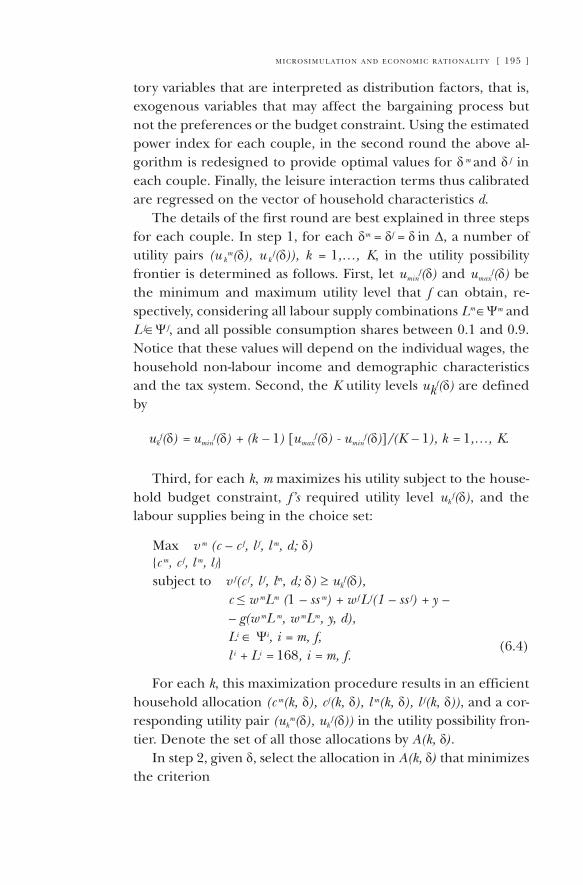
m i c r o s i m u l at i o n a n d e c o n o m i c r at i o n a l i t y [ 195 ]
tory variables that are interpreted as distribution factors, that is, exogenous variables that may affect the bargaining process but not the preferences or the budget constraint. Using the estimated power index for each couple, in the second round the above al-gorithm is redesigned to provide optimal values for δ m and δ f in each couple. Finally, the leisure interaction terms thus calibrated are regressed on the vector of household characteristics d.
The details of the first round are best explained in three steps for each couple. In step 1, for each δm = δf = δ in ∆, a number of utility pairs (u km(δ), u k
f(δ)), k = 1,…, K, in the utility possibility frontier is determined as follows. First, let umin
f(δ) and umaxf(δ) be
the minimum and maximum utility level that f can obtain, re-spectively, considering all labour supply combinations Lm ∈Ψm and L f∈Ψ f, and all possible consumption shares between 0.1 and 0.9. Notice that these values will depend on the individual wages, the household non-labour income and demographic characteristics and the tax system. Second, the K utility levels uk
f(δ) are defined by
ukf(δ) = umin
f(δ) + (k – 1) [umaxf(δ) - umin
f(δ)]/(K – 1), k = 1,…, K.
Third, for each k, m maximizes his utility subject to the house-hold budget constraint, f’s required utility level uk
f(δ), and the labour supplies being in the choice set:
Max v m (c – c f, l f, l m, d; δ){c m, c f, l m, l f}subject to v f(c f, l f, lm, d; δ) ≥ uk
f(δ),c ≤ w mLm (1 – ss m) + w f L f(1 – ss f) + y –– g(w mL m, w mLm, y, d),Li ∈ Ψi, i = m, f,l i + Li = 168, i = m, f.
(6.4)
For each k, this maximization procedure results in an efficient household allocation (c m(k, δ), c f(k, δ), l m(k, δ), l f(k, δ)), and a cor-responding utility pair (uk
m(δ), uk f(δ)) in the utility possibility fron-
tier. Denote the set of all those allocations by A(k, δ).In step 2, given δ, select the allocation in A(k, δ) that minimizes
the criterion
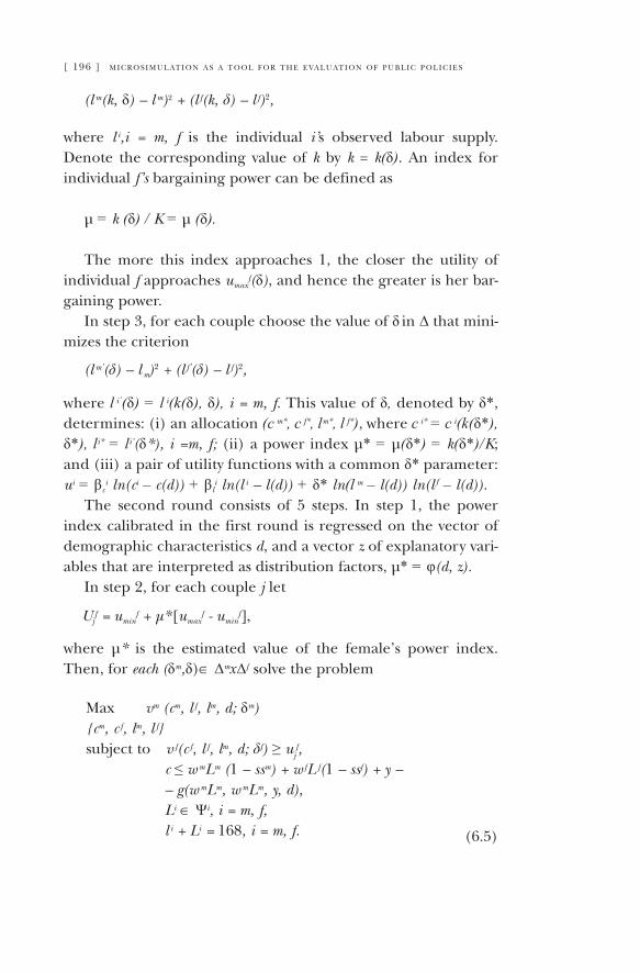
[ 196 ] m i c r o s i m u l at i o n a s a t o o l f o r t h e e va l u at i o n o f p u b l i c p o l i c i e s
(l m(k, δ) – l m)2 + (l f(k, δ) – l f)2,
where l i,i = m, f is the individual i’s observed labour supply. Denote the corresponding value of k by k = k(δ). an index for individual f’s bargaining power can be defined as
µ = k (δ) / K = µ (δ).
The more this index approaches 1, the closer the utility of individual f approaches umax
f(δ), and hence the greater is her bar-gaining power.
In step 3, for each couple choose the value of δ in ∆ that mini-mizes the criterion
(l m’(δ) – l m)2 + (l f’(δ) – l f)2,
where l i’(δ) = l i(k(δ), δ), i = m, f. This value of δ, denoted by δ*, determines: (i) an allocation (c m*, c f*, lm*, l f*), where c i* = c i(k(δ*), δ*), li* = li’(δ*), i =m, f; (ii) a power index µ* = µ(δ*) = k(δ*)/K; and (iii) a pair of utility functions with a common δ* parameter: ui = βc
i ln(ci – c(d)) + βli ln(l i – l(d)) + δ* ln(l m – l(d)) ln(l f – l(d)).
The second round consists of 5 steps. In step 1, the power index calibrated in the first round is regressed on the vector of demographic characteristics d, and a vector z of explanatory vari-ables that are interpreted as distribution factors, µ* = φ(d, z).
In step 2, for each couple j let
Ujf = umin
f + µ* [umaxf - umin
f ],
where µ* is the estimated value of the female’s power index. Then, for each (δm,δ)∈ ∆mx∆f solve the problem
Max vm (cm, l f, lm, d; δm){cm, c f, lm, l f}subject to v f(c f, l f, lm, d; δf) ≥ uj
f,c ≤ w mLm (1 – ssm) + w fL f(1 – ssf) + y – – g(w mLm, w mLm, y, d),Li ∈ Ψi, i = m, f,l i + Li = 168, i = m, f. (6.5)
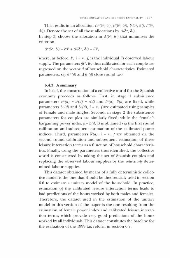
m i c r o s i m u l at i o n a n d e c o n o m i c r at i o n a l i t y [ 197 ]
This results in an allocation (cm(δm, δf), c f(δm, δ f), lm(δm, δ f), l f(δm, δ f)). Denote the set of all those allocations by A(δm, δ f).In step 3, choose the allocation in A(δm, δ f) that minimizes the criterion
(lm(δm, δf) – lm)2 + (l f(δm, δ f) – l f )2,
where, as before, l i , i = m, f, is the individual i’s observed labour supply. The parameters (δ m, δ f) thus calibrated for each couple are regressed on the vector d of household characteristics. Estimated parameters, say δ m(d) and δ f(d) close round two.
6.4.3. A summaryIn brief, the construction of a collective world for the Spanish
economy proceeds as follows. First, in stage 1 subsistence parameters c m(d) = c f(d) = c(d) and l m(d), l f(d) are fixed, while parameters βc
i(d) and βli(d), i = m, f are estimated using samples
of female and male singles. Second, in stage 2 the subsistence parameters for couples are similarly fixed, while the female’s bargaining power index µ= φ(d, z) is obtained via the first round calibration and subsequent estimation of the calibrated power indices. Third, parameters δi(d), i = m, f are obtained via the second round calibration and subsequent estimation of these leisure interaction terms as a function of household characteris-tics. Finally, using the parameters thus identified, the collective world is constructed by taking the set of Spanish couples and replacing the observed labour supplies by the collectively deter-mined labour supplies.
This dataset obtained by means of a fully deterministic collec-tive model is the one that should be theoretically used in section 6.6 to estimate a unitary model of the household. In practice, estimation of the calibrated leisure interaction terms leads to bad predictions of the hours worked by both males and females. Therefore, the dataset used in the estimation of the unitary model in this version of the paper is the one resulting from the estimation of female power index and calibrated leisure interac-tion terms, which provide very good predictions of the hours worked by all individuals. This dataset constitutes the baseline for the evaluation of the 1999 tax reform in section 6.7.
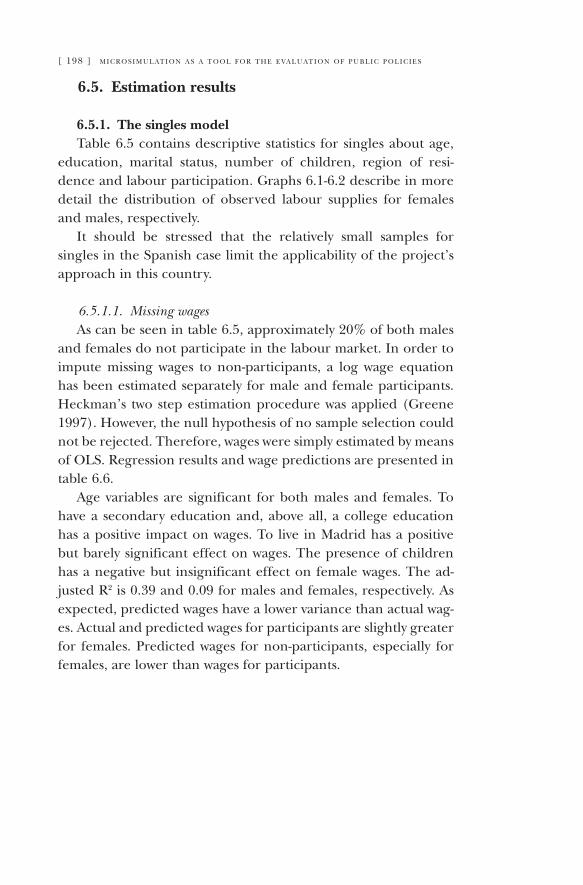
[ 198 ] m i c r o s i m u l at i o n a s a t o o l f o r t h e e va l u at i o n o f p u b l i c p o l i c i e s
6.5. Estimation results
6.5.1. The singles modelTable 6.5 contains descriptive statistics for singles about age,
education, marital status, number of children, region of resi-dence and labour participation. Graphs 6.1-6.2 describe in more detail the distribution of observed labour supplies for females and males, respectively.
It should be stressed that the relatively small samples for singles in the Spanish case limit the applicability of the project’s approach in this country.
6.5.1.1. Missing wagesas can be seen in table 6.5, approximately 20% of both males
and females do not participate in the labour market. In order to impute missing wages to non-participants, a log wage equation has been estimated separately for male and female participants. Heckman’s two step estimation procedure was applied (Greene 1997). However, the null hypothesis of no sample selection could not be rejected. Therefore, wages were simply estimated by means of OLS. Regression results and wage predictions are presented in table 6.6.
age variables are significant for both males and females. To have a secondary education and, above all, a college education has a positive impact on wages. To live in Madrid has a positive but barely significant effect on wages. The presence of children has a negative but insignificant effect on female wages. The ad-justed R2 is 0.39 and 0.09 for males and females, respectively. as expected, predicted wages have a lower variance than actual wag-es. actual and predicted wages for participants are slightly greater for females. Predicted wages for non-participants, especially for females, are lower than wages for participants.
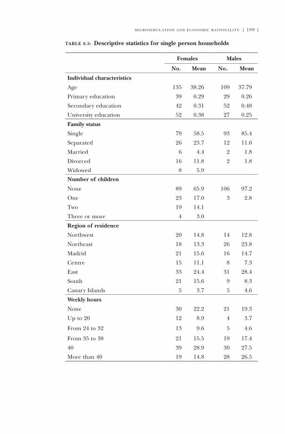
m i c r o s i m u l at i o n a n d e c o n o m i c r at i o n a l i t y [ 199 ]
table 6.5: Descriptive statistics for single person households
Females Males
No. Mean No. Mean
Individual characteristics
age 135 38.26 109 37.79
Primary education 39 0.29 29 0.26
Secondary education 42 0.31 52 0.48
University education 52 0.38 27 0.25
Family status
Single 79 58.5 93 85.4
Separated 26 23.7 12 11.0
Married 6 4.4 2 1.8
Divorced 16 11.8 2 1.8
Widowed 8 5.9
Number of children
None 89 65.9 106 97.2
One 23 17.0 3 2.8
Two 19 14.1
Three or more 4 3.0
Region of residence
Northwest 20 14.8 14 12.8
Northeast 18 13.3 26 23.8
Madrid 21 15.6 16 14.7
Centre 15 11.1 8 7.3
East 33 24.4 31 28.4
South 21 15.6 9 8.3
Canary Islands 5 3.7 5 4.6
Weekly hours
None 30 22.2 21 19.3
Up to 20 12 8.9 4 3.7
From 24 to 32 13 9.6 5 4.6
From 35 to 38 21 15.5 19 17.4
40 39 28.9 30 27.5
More than 40 19 14.8 28 26.5
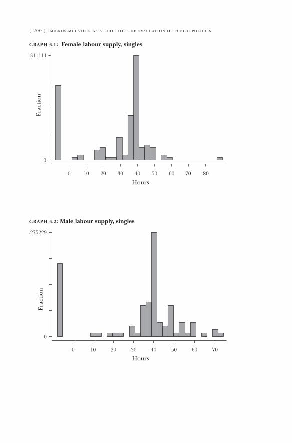
[ 200 ] m i c r o s i m u l at i o n a s a t o o l f o r t h e e va l u at i o n o f p u b l i c p o l i c i e s
graph 6.1: Female labour supply, singles
graph 6.2: Male labour supply, singles
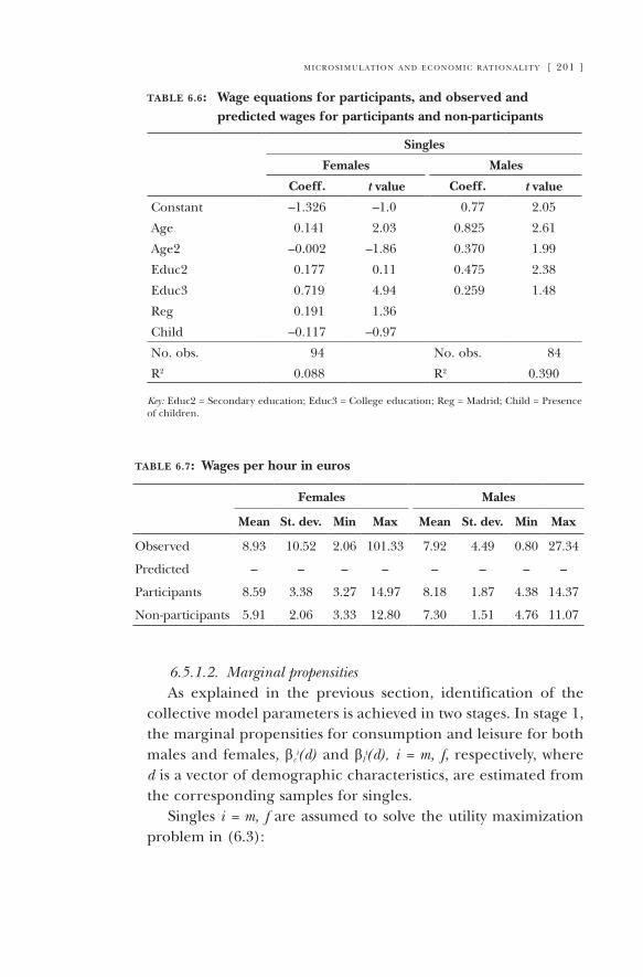
m i c r o s i m u l at i o n a n d e c o n o m i c r at i o n a l i t y [ 201 ]
table 6.6: Wage equations for participants, and observed and predicted wages for participants and non-participants
Singles
Females Males
Coeff. t value Coeff. t value
Constant –1.326 –1.0 0.77 2.05
age 0.141 2.03 0.825 2.61
age2 –0.002 –1.86 0.370 1.99
Educ2 0.177 0.11 0.475 2.38
Educ3 0.719 4.94 0.259 1.48
Reg 0.191 1.36
Child –0.117 –0.97
No. obs. 94 No. obs. 84
R2 0.088 R2 0.390
Key: Educ2 = Secondary education; Educ3 = College education; Reg = Madrid; Child = Presence of children.
table 6.7: Wages per hour in euros
Females Males
Mean St. dev. Min Max Mean St. dev. Min Max
Observed 8.93 10.52 2.06 101.33 7.92 4.49 0.80 27.34
Predicted – – – – – – – –
Participants 8.59 3.38 3.27 14.97 8.18 1.87 4.38 14.37
Non-participants 5.91 2.06 3.33 12.80 7.30 1.51 4.76 11.07
6.5.1.2. Marginal propensitiesas explained in the previous section, identification of the
collective model parameters is achieved in two stages. In stage 1, the marginal propensities for consumption and leisure for both males and females, βc
i(d) and βli(d), i = m, f, respectively, where
d is a vector of demographic characteristics, are estimated from the corresponding samples for singles.
Singles i = m, f are assumed to solve the utility maximization problem in (6.3):
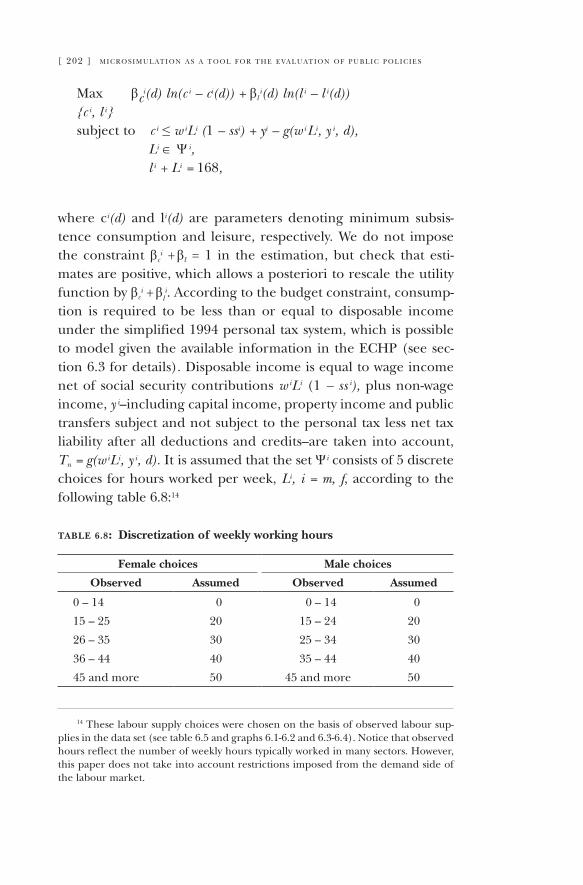
[ 202 ] m i c r o s i m u l at i o n a s a t o o l f o r t h e e va l u at i o n o f p u b l i c p o l i c i e s
Max βci(d) ln(c i – c
i(d)) + βl i(d) ln(l i – l i(d))
{c i, l i }subject to c i ≤ w iLi (1 – ssi) + yi – g(w i Li, y i, d),
Li ∈ Ψ i,l i + Li = 168,
where ci(d) and li(d) are parameters denoting minimum subsis-tence consumption and leisure, respectively. We do not impose the constraint βc
i + βl = 1 in the estimation, but check that esti-
mates are positive, which allows a posteriori to rescale the utility function by βc
i + βli. according to the budget constraint, consump-
tion is required to be less than or equal to disposable income under the simplified 1994 personal tax system, which is possible to model given the available information in the ECHP (see sec-tion 6.3 for details). Disposable income is equal to wage income net of social security contributions w iLi (1 – ss i), plus non-wage income, y i–including capital income, property income and public transfers subject and not subject to the personal tax less net tax liability after all deductions and credits–are taken into account, Tn = g(w iLi, y i, d). It is assumed that the set Ψ i consists of 5 discrete choices for hours worked per week, Li, i = m, f, according to the following table 6.8:14
table 6.8: Discretization of weekly working hours
Female choices Male choices
Observed Assumed Observed Assumed
0 – 14 0 0 – 14 0
15 – 25 20 15 – 24 20
26 – 35 30 25 – 34 30
36 – 44 40 35 – 44 40
45 and more 50 45 and more 50
14 These labour supply choices were chosen on the basis of observed labour sup-plies in the data set (see table 6.5 and graphs 6.1-6.2 and 6.3-6.4). Notice that observed hours reflect the number of weekly hours typically worked in many sectors. However, this paper does not take into account restrictions imposed from the demand side of the labour market.
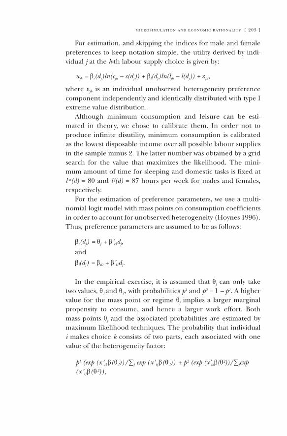
m i c r o s i m u l at i o n a n d e c o n o m i c r at i o n a l i t y [ 203 ]
For estimation, and skipping the indices for male and female preferences to keep notation simple, the utility derived by indi-vidual j at the h-th labour supply choice is given by:
ujh = βc(dj )ln(cjh – c(dj )) + βl(dj )ln(ljh – l(dj )) + εjh,
where εjh is an individual unobserved heterogeneity preference component independently and identically distributed with type I extreme value distribution.
although minimum consumption and leisure can be esti-mated in theory, we chose to calibrate them. In order not to produce infinite disutility, minimum consumption is calibrated as the lowest disposable income over all possible labour supplies in the sample minus 2. The latter number was obtained by a grid search for the value that maximizes the likelihood. The mini-mum amount of time for sleeping and domestic tasks is fixed at l m(d) = 80 and l f(d) = 87 hours per week for males and females, respectively.
For the estimation of preference parameters, we use a multi-nomial logit model with mass points on consumption coefficients in order to account for unobserved heterogeneity (Hoynes 1996). Thus, preference parameters are assumed to be as follows:
βc(dj ) = θj + β’c1dj,
and
βl(dj ) = βl0 + β’l1dj.
In the empirical exercise, it is assumed that θj can only take two values, θ1 and θ2, with probabilities p1 and p2 = 1 – p1. a higher value for the mass point or regime θj implies a larger marginal propensity to consume, and hence a larger work effort. Both mass points θj and the associated probabilities are estimated by maximum likelihood techniques. The probability that individual i makes choice k consists of two parts, each associated with one value of the heterogeneity factor:
p1 (exp (x’ikβ(θ1))/ ∑j exp (x’ijβ(θ1)) + p2 (exp (x’ikβ(θ2))/ ∑jexp(x’ijβ(θ2)),
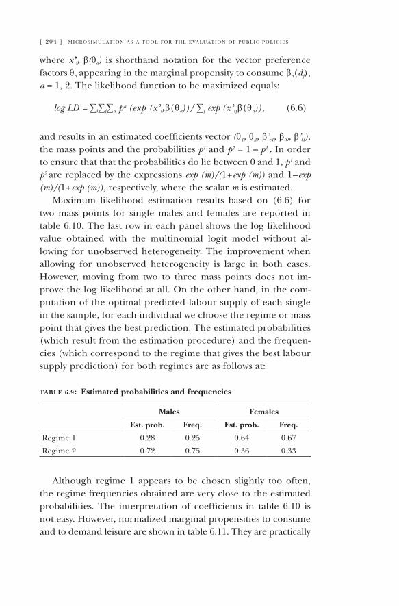
[ 204 ] m i c r o s i m u l at i o n a s a t o o l f o r t h e e va l u at i o n o f p u b l i c p o l i c i e s
where x’ik β(θa) is shorthand notation for the vector preference factors θa appearing in the marginal propensity to consume βa(dj), a = 1, 2. The likelihood function to be maximized equals:
log LD = ∑i ∑j ∑a p a (exp (x’ikβ(θa))/ ∑j exp (x’ijβ(θa)), (6.6)
and results in an estimated coefficients vector (θ1, θ2, β’c1, βl0, β’l1), the mass points and the probabilities p1 and p2 = 1 – p1 . In order to ensure that that the probabilities do lie between 0 and 1, p1 and p2 are replaced by the expressions exp (m)/(1+ exp (m)) and 1– exp (m)/(1+ exp (m)), respectively, where the scalar m is estimated.
Maximum likelihood estimation results based on (6.6) for two mass points for single males and females are reported in table 6.10. The last row in each panel shows the log likelihood value obtained with the multinomial logit model without al-lowing for unobserved heterogeneity. The improvement when allowing for unobserved heterogeneity is large in both cases. However, moving from two to three mass points does not im-prove the log likelihood at all. On the other hand, in the com-putation of the optimal predicted labour supply of each single in the sample, for each individual we choose the regime or mass point that gives the best prediction. The estimated probabilities (which result from the estimation procedure) and the frequen-cies (which correspond to the regime that gives the best labour supply prediction) for both regimes are as follows at:
table 6.9: Estimated probabilities and frequencies
Males Females
Est. prob. Freq. Est. prob. Freq.
Regime 1 0.28 0.25 0.64 0.67
Regime 2 0.72 0.75 0.36 0.33
although regime 1 appears to be chosen slightly too often, the regime frequencies obtained are very close to the estimated probabilities. The interpretation of coefficients in table 6.10 is not easy. However, normalized marginal propensities to consume and to demand leisure are shown in table 6.11. They are practically
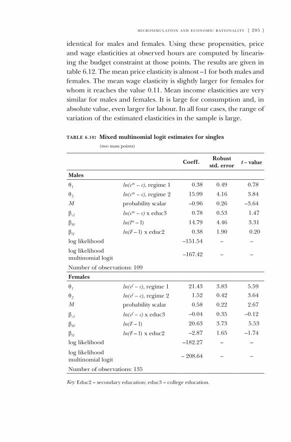
m i c r o s i m u l at i o n a n d e c o n o m i c r at i o n a l i t y [ 205 ]
identical for males and females. Using these propensities, price and wage elasticities at observed hours are computed by linearis-ing the budget constraint at those points. The results are given in table 6.12. The mean price elasticity is almost –1 for both males and females. The mean wage elasticity is slightly larger for females for whom it reaches the value 0.11. Mean income elasticities are very similar for males and females. It is large for consumption and, in absolute value, even larger for labour. In all four cases, the range of variation of the estimated elasticities in the sample is large.
table 6.10: Mixed multinomial logit estimates for singles (two mass points)
Coeff.Robust
std. error t – value
Males
θ1 ln(c m – c), regime 1 0.38 0.49 0.78
θ2 ln(c m – c), regime 2 15.99 4.16 3.84
M probability scalar –0.96 0.26 –3.64
βc1 ln(c m – c) x educ3 0.78 0.53 1.47
βl0 ln(l m – l) 14.79 4.46 3.31
βl1 ln(l f – l) x educ2 0.38 1.90 0.20
log likelihood –151.54 – –
log likelihood multinomial logit –167.42 – –
Number of observations: 109
Females
θ1 ln(c f – c), regime 1 21.43 3.83 5.59
θ2 ln(c f – c), regime 2 1.52 0.42 3.64
M probability scalar 0.58 0.22 2.67
βc1 ln(c f – c) x educ3 –0.04 0.35 –0.12
βl0 ln(l f – l) 20.63 3.73 5.53
βl1 ln(l f – l) x educ2 –2.87 1.65 –1.74
log likelihood –182.27 – –
log likelihood multinomial logit – 208.64 – –
Number of observations: 135
Key: Educ2 = secondary education; educ3 = college education.
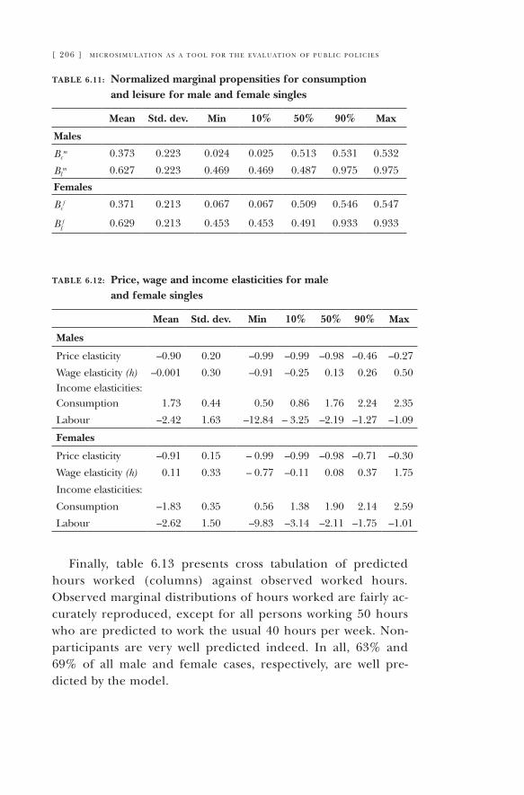
[ 206 ] m i c r o s i m u l at i o n a s a t o o l f o r t h e e va l u at i o n o f p u b l i c p o l i c i e s
table 6.11: Normalized marginal propensities for consumption and leisure for male and female singles
Mean Std. dev. Min 10% 50% 90% Max
Males
Bcm 0.373 0.223 0.024 0.025 0.513 0.531 0.532
Blm 0.627 0.223 0.469 0.469 0.487 0.975 0.975
Females
Bcf 0.371 0.213 0.067 0.067 0.509 0.546 0.547
Blf 0.629 0.213 0.453 0.453 0.491 0.933 0.933
table 6.12: Price, wage and income elasticities for male and female singles
Mean Std. dev. Min 10% 50% 90% Max
Males
Price elasticity –0.90 0.20 –0.99 –0.99 –0.98 –0.46 –0.27
Wage elasticity (h) –0.001 0.30 –0.91 –0.25 0.13 0.26 0.50Income elasticities:Consumption 1.73 0.44 0.50 0.86 1.76 2.24 2.35
Labour –2.42 1.63 –12.84 – 3.25 –2.19 –1.27 –1.09
Females
Price elasticity –0.91 0.15 – 0.99 –0.99 –0.98 –0.71 –0.30
Wage elasticity (h) 0.11 0.33 – 0.77 –0.11 0.08 0.37 1.75
Income elasticities:
Consumption –1.83 0.35 0.56 1.38 1.90 2.14 2.59
Labour –2.62 1.50 –9.83 –3.14 –2.11 –1.75 –1.01
Finally, table 6.13 presents cross tabulation of predicted hours worked (columns) against observed worked hours. Observed marginal distributions of hours worked are fairly ac-curately reproduced, except for all persons working 50 hours who are predicted to work the usual 40 hours per week. Non-participants are very well predicted indeed. In all, 63% and 69% of all male and female cases, respectively, are well pre-dicted by the model.
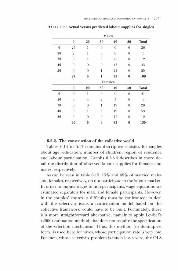
m i c r o s i m u l at i o n a n d e c o n o m i c r at i o n a l i t y [ 207 ]
table 6.13: Actual versus predicted labour supplies for singles
Males
0 20 30 40 50 Total
0 25 1 0 0 0 26
20 2 1 0 0 0 3
30 0 4 0 8 0 12
40 0 0 0 43 0 43
50 0 0 1 24 0 25
27 6 1 75 0 109
Females
0 20 30 40 50 Total
0 40 1 0 0 0 41
20 0 4 2 3 0 9
30 0 0 1 19 0 20
40 0 1 3 49 0 53
50 0 0 0 12 0 12
40 6 6 83 0 135
6.5.2. The construction of the collective worldTables 6.14 to 6.17 contains descriptive statistics for singles
about age, education, number of children, region of residence and labour participation. Graphs 6.3-6.4 describes in more de-tail the distribution of observed labour supplies for females and males, respectively.
as can be seen in table 6.15, 15% and 68% of married males and females, respectively, do not participate in the labour market. In order to impute wages to non-participants, wage equations are estimated separately for male and female participants. However, in the couples’ context a difficulty must be confronted: to deal with the selectivity issue, a participation model based on the collective framework would have to be built. Fortunately, there is a more straightforward alternative, namely to apply Lewbel’s (2000) estimation method, that does not require the specification of the selection mechanism. Thus, this method (in its simplest form) is used here for wives, whose participation rate is very low. For men, whose selectivity problem is much less severe, the OLS
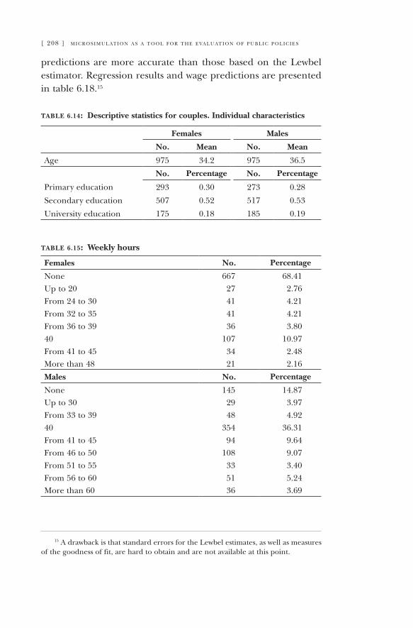
[ 208 ] m i c r o s i m u l at i o n a s a t o o l f o r t h e e va l u at i o n o f p u b l i c p o l i c i e s
predictions are more accurate than those based on the Lewbel estimator. Regression results and wage predictions are presented in table 6.18.15
table 6.14: Descriptive statistics for couples. Individual characteristics
Females Males
No. Mean No. Mean
age 975 34.2 975 36.5
No. Percentage No. Percentage
Primary education 293 0.30 273 0.28
Secondary education 507 0.52 517 0.53
University education 175 0.18 185 0.19
table 6.15: Weekly hours
Females No. Percentage
None 667 68.41Up to 20 27 2.76From 24 to 30 41 4.21From 32 to 35 41 4.21From 36 to 39 36 3.8040 107 10.97From 41 to 45 34 2.48More than 48 21 2.16
Males No. Percentage
None 145 14.87Up to 30 29 3.97From 33 to 39 48 4.9240 354 36.31From 41 to 45 94 9.64From 46 to 50 108 9.07From 51 to 55 33 3.40From 56 to 60 51 5.24More than 60 36 3.69
15 a drawback is that standard errors for the Lewbel estimates, as well as measures of the goodness of fit, are hard to obtain and are not available at this point.
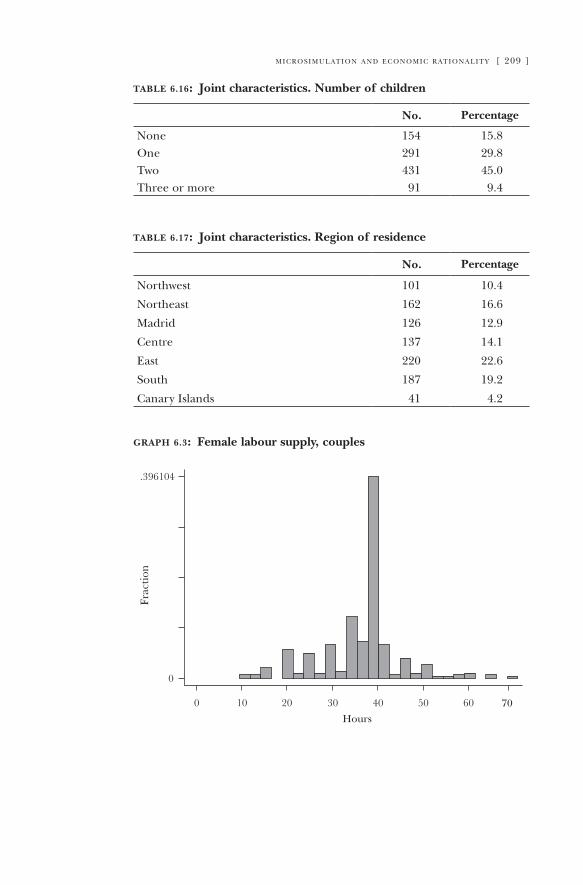
m i c r o s i m u l at i o n a n d e c o n o m i c r at i o n a l i t y [ 209 ]
table 6.16: Joint characteristics. Number of children
No. Percentage
None 154 15.8One 291 29.8Two 431 45.0Three or more 91 9.4
table 6.17: Joint characteristics. Region of residence
No. Percentage
Northwest 101 10.4
Northeast 162 16.6
Madrid 126 12.9
Centre 137 14.1
East 220 22.6
South 187 19.2
Canary Islands 41 4.2
graph 6.3: Female labour supply, couples
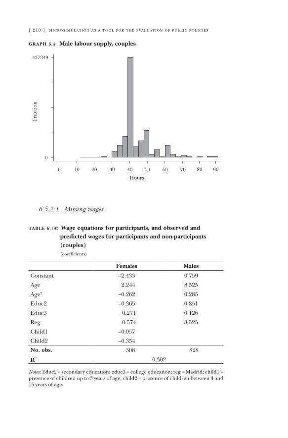
[ 210 ] m i c r o s i m u l at i o n a s a t o o l f o r t h e e va l u at i o n o f p u b l i c p o l i c i e s
graph 6.4: Male labour supply, couples
70 80
Hours
6.5.2.1. Missing wages
table 6.18: Wage equations for participants, and observed and predicted wages for participants and non-participants (couples) (coefficients)
Females Males
Constant –2.433 0.759
age 2.244 8.525
age2 –0.262 0.285
Educ2 –0.365 0.851
Educ3 0.271 0.126
Reg 0.574 8.525
Child1 –0.057
Child2 –0.354
No. obs. 308 828
R2 0.302
Notes: Educ2 = secondary education; educ3 = college education; reg = Madrid; child1 = presence of children up to 3 years of age; child2 = presence of children between 4 and 15 years of age.
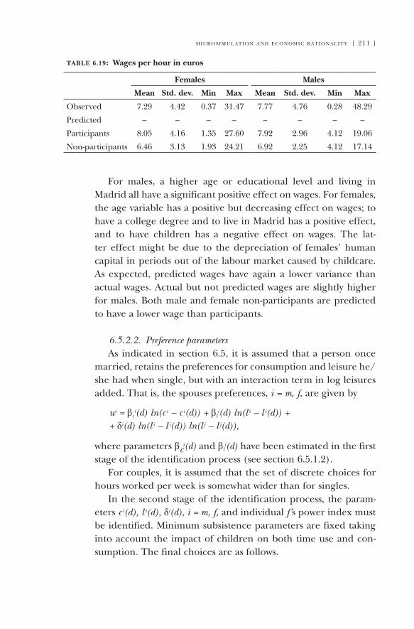
m i c r o s i m u l at i o n a n d e c o n o m i c r at i o n a l i t y [ 211 ]
table 6.19: Wages per hour in euros
Females Males
Mean Std. dev. Min Max Mean Std. dev. Min Max
Observed 7.29 4.42 0.37 31.47 7.77 4.76 0.28 48.29
Predicted – – – – – – – –
Participants 8.05 4.16 1.35 27.60 7.92 2.96 4.12 19.06
Non-participants 6.46 3.13 1.93 24.21 6.92 2.25 4.12 17.14
For males, a higher age or educational level and living in Madrid all have a significant positive effect on wages. For females, the age variable has a positive but decreasing effect on wages; to have a college degree and to live in Madrid has a positive effect, and to have children has a negative effect on wages. The lat-ter effect might be due to the depreciation of females’ human capital in periods out of the labour market caused by childcare. as expected, predicted wages have again a lower variance than actual wages. actual but not predicted wages are slightly higher for males. Both male and female non-participants are predicted to have a lower wage than participants.
6.5.2.2. Preference parametersas indicated in section 6.5, it is assumed that a person once
married, retains the preferences for consumption and leisure he/she had when single, but with an interaction term in log leisures added. That is, the spouses preferences, i = m, f, are given by
ui = βci(d) ln(c i – c i(d)) + βl
i(d) ln(l i – l i(d)) + + δi(d) ln(l i – l i(d)) ln(l j – l j(d)),
where parameters βci(d) and βl
i(d) have been estimated in the first stage of the identification process (see section 6.5.1.2).
For couples, it is assumed that the set of discrete choices for hours worked per week is somewhat wider than for singles.
In the second stage of the identification process, the param-eters c i(d), l i(d), δi(d), i = m, f, and individual f’s power index must be identified. Minimum subsistence parameters are fixed taking into account the impact of children on both time use and con-sumption. The final choices are as follows.
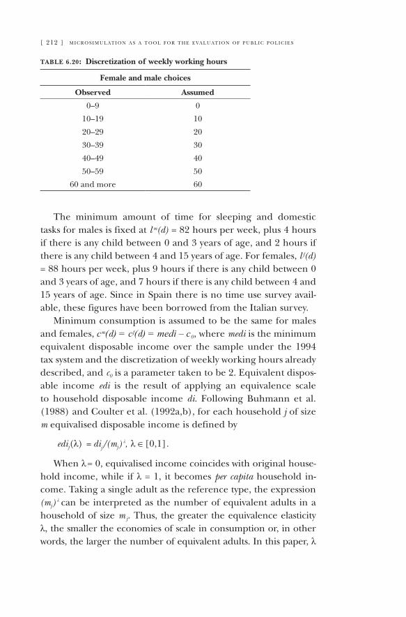
[ 212 ] m i c r o s i m u l at i o n a s a t o o l f o r t h e e va l u at i o n o f p u b l i c p o l i c i e s
table 6.20: Discretization of weekly working hours
Female and male choices
Observed Assumed
0–9 0
10–19 10
20–29 20
30–39 30
40–49 40
50–59 50
60 and more 60
The minimum amount of time for sleeping and domestic tasks for males is fixed at l m(d) = 82 hours per week, plus 4 hours if there is any child between 0 and 3 years of age, and 2 hours if there is any child between 4 and 15 years of age. For females, l f(d) = 88 hours per week, plus 9 hours if there is any child between 0 and 3 years of age, and 7 hours if there is any child between 4 and 15 years of age. Since in Spain there is no time use survey avail-able, these figures have been borrowed from the Italian survey.
Minimum consumption is assumed to be the same for males and females, cm(d) = cf(d) = medi – c0, where medi is the minimum equivalent disposable income over the sample under the 1994 tax system and the discretization of weekly working hours already described, and c0 is a parameter taken to be 2. Equivalent dispos-able income edi is the result of applying an equivalence scale to household disposable income di. Following Buhmann et al. (1988) and Coulter et al. (1992a,b), for each household j of size m equivalised disposable income is defined by
edij(λ) = dij/(mj ) λ, λ ∈[0,1].
When λ = 0, equivalised income coincides with original house-hold income, while if λ = 1, it becomes per capita household in-come. Taking a single adult as the reference type, the expression (mj ) λ can be interpreted as the number of equivalent adults in a household of size m j. Thus, the greater the equivalence elasticity λ, the smaller the economies of scale in consumption or, in other words, the larger the number of equivalent adults. In this paper, λ
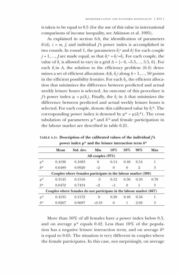
m i c r o s i m u l at i o n a n d e c o n o m i c r at i o n a l i t y [ 213 ]
is taken to be equal to 0.5 (for the use of this value in international comparisons of income inequality, see atkinson et al. 1995).
as explained in section 6.6, the identification of parameters δi(d), i = m, f, and individual f’s power index is accomplished in two rounds. In round 1, the parameters δj
m and δjf for each couple
j = 1,…, J are made equal, so that δjm = δj
f = δj. For each couple, the value of δj
is allowed to vary in a grid ∆ = {– 6, –5.5,…, 5.5, 6}. For each δj
in ∆, the solution to the efficiency problem (6.4) deter-mines a set of efficient allocations A(k, δj ) along k = 1,…, 50 points in the efficient possibility frontier. For each δj, the efficient alloca-tion that minimizes the difference between predicted and actual weekly leisure hours is selected. an outcome of this procedure is f’s power index µ = µ(δj ). Finally, the δj
in ∆ that minimizes the difference between predicted and actual weekly leisure hours is selected. For each couple, denote this calibrated value by δj*. The corresponding power index is denoted by µ* = µ(δj*). The cross tabulation of parameters µ* and δ* and female participation in the labour market are described in table 6.21.
table 6.21: Description of the calibrated values of the individual f’s
power index µ* and the leisure interaction term δ*
Mean Std. dev. Min 10% 50% 90% Max
All couples (975)
µ* 0.4196 0.1683 0 0.14 0.48 0.54 1
δ* 0.6489 0.9920 –2 0 0 2 3
Couples where females participate in the labour market (308)
µ* 0.3145 0.1516 0 0.12 0.30 0.50 0.78
δ* 0.0472 0.7434 –2 –1 0 1 3
Couples where females do not participate in the labour market (667)
µ* 0.4535 0.1572 0 0.28 0.48 0.56 1
δ* 0.9267 0.9697 –0.33 0 1 2.02 3
More than 50% of all females have a power index below 0.5, and on average µ* equals 0.42. Less than 10% of the popula-tion has a negative leisure interaction term, and on average δ* is equal to 0.65. The situation is very different in couples where the female participates. In this case, not surprisingly, on average
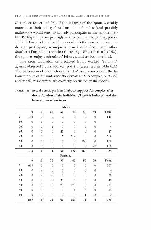
[ 214 ] m i c r o s i m u l at i o n a s a t o o l f o r t h e e va l u at i o n o f p u b l i c p o l i c i e s
δ* is close to zero (0.05). If the leisures of the spouses weakly enter into their utility functions, then females (and possibly males too) would tend to actively participate in the labour mar-ket. Perhaps more surprisingly, in this case the bargaining power shifts in favour of males. The opposite is the case when women do not participate, a majority situation in Spain and other Southern European countries: the average δ* is close to 1 (0.93), the spouses enjoy each others’ leisures, and µ* becomes 0.45.
The cross tabulation of predicted hours worked (columns) against observed hours worked (rows) is presented in table 6.22. The calibration of parameters µ* and δ* is very successful: the la-bour supplies of 943 males and 936 females in 975 couples, or 96.7% and 96.0%, respectively, are correctly predicted by the model.
table 6.22: Actual versus predicted labour supplies for couples after
the calibration of the individual f’s power index µ* and the
leisure interaction term
Males
0 10 20 30 40 50 60 Total
0 145 0 0 0 0 0 0 145
10 0 1 0 0 0 0 0 1
20 0 0 4 0 0 0 0 4
30 0 0 0 27 0 0 0 27
40 0 0 0 5 514 0 0 519
50 0 0 0 0 13 156 0 169
60 0 0 0 0 0 13 97 110145 1 4 32 527 169 97 975
Females
0 10 20 30 40 50 60 Total
0 667 0 0 0 0 0 0 667
10 0 4 0 0 0 0 0 4
20 0 2 29 0 0 0 0 30
30 0 0 2 37 0 0 0 40
40 0 0 0 23 178 0 0 201
50 0 0 0 0 11 13 0 24
60 0 0 0 0 0 1 8 9
667 6 31 60 189 14 8 975

m i c r o s i m u l at i o n a n d e c o n o m i c r at i o n a l i t y [ 215 ]
Round 2 begins by regressing a logistic transformation the power index µj* on a vector d of demographic characteristics and a vector z of explanatory variables interpreted as distribution fac-tors. These variables capture the way that the tax benefit system influences the relative earning power of spouses. If these turn out to contribute significantly to the prediction of the power index, they will allow us to describe changes in the power index induced by tax reforms. Three distribution factors are included: (i) the difference between male minus female age, denoted by dage; (ii) the logarithm of the difference between female and male non-labour incomes, denoted by lndif, and (iii) the ratio of female to male marginal contribution to household earnings when switch-ing from non-participation in the labour market to working 40 hours per week, denoted by mgcontr. More specifically, this vari-able is defined as follows. Let pf k and pm
k denote the observed sample frequencies of (discretised) weekly labour supplies h k of wives and husbands, respectively. Denote Rmk fk’ the household dis-posable income when the husband works hk hours and the wife works hk’ hours. Variable yf40 is defined as:
yf40 = ∑k pmk (Rmk
f40 – Rmk f 0 )
that measures the expected increase in household disposable income if the wife switches form 0 to 40 hours, the expectation being taken over male hours distribution. Defining ym40 similarly, we consider the ratio mgcontr = yf40/ym40. Table 6.23 gives sum-mary statistics for these variables and shows that there is impor-tant variation across households.
table 6.23: Descriptive statistics for variables used in predicting power index
No. Mean St. dev. Min Max
Yf40 975 197.74 50.66 20.12 753.37
Ym40 975 227.03 95.80 50.16 1,061.97
mgcontr 975 1.09 0.91 0.05 11.53
Dage 975 2.26 3.30 –13 18
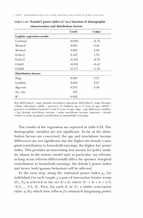
[ 216 ] m i c r o s i m u l at i o n a s a t o o l f o r t h e e va l u at i o n o f p u b l i c p o l i c i e s
table 6.24: Female’s power index ω* as a function of demographic
characteristics and distribution factors
Coeff. t value
Logistic regression results
Constant –0.949 –2.73
Meduc2 0.045 0.46
Meduc3 0.082 0.60
Feduc2 0.167 1.72
Feduc3 –0.105 –0.78
Child1 –0.034 –0.42
Child2 –0.117 –1.35
Distribution factors
Dage 0.069 0.27
Lndifinc 0.002 0.67
Mgcontr 0.275 6.40
No. obs. 975
R2 0.042
Keys: M(F)educ2 = male (female) secondary education; M(F)educ3 = male (female) college education; child1 = presence of children up to 3 years of age; child2 = presence of children between 4 and 15 years of age; dage = age difference; lndifinc = log (female non-labour income – male non-labour income; mgcontr = female relative to male marginal contributions to household’s earnings.
The results of the regression are reported in table 6.24. The demographic variables are not significant. as far as the distri-bution factors are concerned, the age and non-labour income differences are not significant, but the higher the female’s mar-ginal contribution to household earnings, the higher her power index. This provides an interesting new avenue for policy analy-sis, absent in the unitary model and, in particular, tax reforms: as long as tax reforms differentially affect the spouses’ marginal contribution to household earnings, the female’s power index and hence both spouses behaviour will be affected.
In the next step, using the estimated power index µj, for individual f in each couple j, a pair of interaction leisure terms (δm
j, δfj) is selected in the set ∆m x ∆f, where ∆m = ∆f = ∆ = {–3,
–2.5,…, 2.5, 3}. First, for each δfj in ∆m, a utility reservation
value upf(δf
j) which best reflects f’s estimated bargaining power
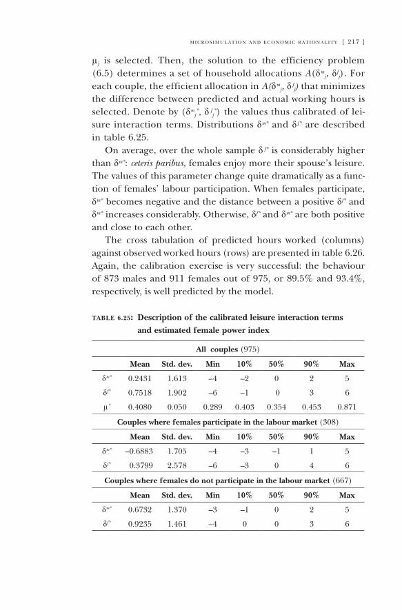
m i c r o s i m u l at i o n a n d e c o n o m i c r at i o n a l i t y [ 217 ]
µj is selected. Then, the solution to the efficiency problem (6.5) determines a set of household allocations A(δm
j, δfj). For
each couple, the efficient allocation in A(δmj, δ fj) that minimizes
the difference between predicted and actual working hours is selected. Denote by (δm
j*, δ fj*) the values thus calibrated of lei-
sure interaction terms. Distributions δm* and δ f* are described in table 6.25.
On average, over the whole sample δ f* is considerably higher than δm*: ceteris paribus, females enjoy more their spouse’s leisure. The values of this parameter change quite dramatically as a func-tion of females’ labour participation. When females participate, δm* becomes negative and the distance between a positive δf* and δm* increases considerably. Otherwise, δf* and δm* are both positive and close to each other.
The cross tabulation of predicted hours worked (columns) against observed worked hours (rows) are presented in table 6.26. again, the calibration exercise is very successful: the behaviour of 873 males and 911 females out of 975, or 89.5% and 93.4%, respectively, is well predicted by the model.
table 6.25: Description of the calibrated leisure interaction terms
and estimated female power index
All couples (975)
Mean Std. dev. Min 10% 50% 90% Max
δm* 0.2431 1.613 –4 –2 0 2 5
δf* 0.7518 1.902 –6 –1 0 3 6
µ* 0.4080 0.050 0.289 0.403 0.354 0.453 0.871
Couples where females participate in the labour market (308)
Mean Std. dev. Min 10% 50% 90% Max
δm* –0.6883 1.705 –4 –3 –1 1 5
δf* 0.3799 2.578 –6 –3 0 4 6
Couples where females do not participate in the labour market (667)
Mean Std. dev. Min 10% 50% 90% Max
δm* 0.6732 1.370 –3 –1 0 2 5
δf* 0.9235 1.461 –4 0 0 3 6
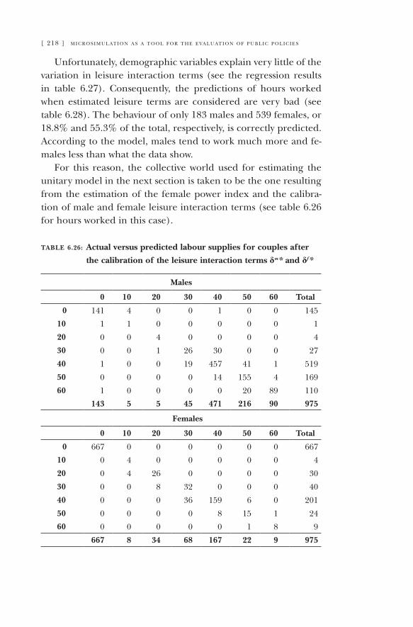
[ 218 ] m i c r o s i m u l at i o n a s a t o o l f o r t h e e va l u at i o n o f p u b l i c p o l i c i e s
Unfortunately, demographic variables explain very little of the variation in leisure interaction terms (see the regression results in table 6.27). Consequently, the predictions of hours worked when estimated leisure terms are considered are very bad (see table 6.28). The behaviour of only 183 males and 539 females, or 18.8% and 55.3% of the total, respectively, is correctly predicted. according to the model, males tend to work much more and fe-males less than what the data show.
For this reason, the collective world used for estimating the unitary model in the next section is taken to be the one resulting from the estimation of the female power index and the calibra-tion of male and female leisure interaction terms (see table 6.26 for hours worked in this case).
table 6.26: Actual versus predicted labour supplies for couples after
the calibration of the leisure interaction terms δm* and δf*
Males
0 10 20 30 40 50 60 Total
0 141 4 0 0 1 0 0 145
10 1 1 0 0 0 0 0 1
20 0 0 4 0 0 0 0 4
30 0 0 1 26 30 0 0 27
40 1 0 0 19 457 41 1 519
50 0 0 0 0 14 155 4 169
60 1 0 0 0 0 20 89 110
143 5 5 45 471 216 90 975
Females
0 10 20 30 40 50 60 Total
0 667 0 0 0 0 0 0 667
10 0 4 0 0 0 0 0 4
20 0 4 26 0 0 0 0 30
30 0 0 8 32 0 0 0 40
40 0 0 0 36 159 6 0 201
50 0 0 0 0 8 15 1 24
60 0 0 0 0 0 1 8 9
667 8 34 68 167 22 9 975
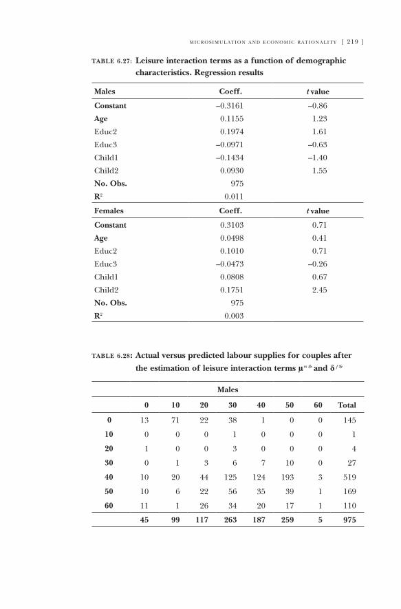
m i c r o s i m u l at i o n a n d e c o n o m i c r at i o n a l i t y [ 219 ]
table 6.27: Leisure interaction terms as a function of demographic characteristics. Regression results
Males Coeff. t value
Constant –0.3161 –0.86
Age 0.1155 1.23
Educ2 0.1974 1.61
Educ3 –0.0971 –0.63
Child1 –0.1434 –1.40
Child2 0.0930 1.55
No. Obs. 975
R2 0.011
Females Coeff. t value
Constant 0.3103 0.71
Age 0.0498 0.41
Educ2 0.1010 0.71
Educ3 –0.0473 –0.26
Child1 0.0808 0.67
Child2 0.1751 2.45
No. Obs. 975
R2 0.003
table 6.28: Actual versus predicted labour supplies for couples after
the estimation of leisure interaction terms µm* and δ f*
Males
0 10 20 30 40 50 60 Total
0 13 71 22 38 1 0 0 145
10 0 0 0 1 0 0 0 1
20 1 0 0 3 0 0 0 4
30 0 1 3 6 7 10 0 27
40 10 20 44 125 124 193 3 519
50 10 6 22 56 35 39 1 169
60 11 1 26 34 20 17 1 110
45 99 117 263 187 259 5 975

[ 220 ] m i c r o s i m u l at i o n a s a t o o l f o r t h e e va l u at i o n o f p u b l i c p o l i c i e s
table 6.28 (cont.): Actual versus predicted labour supplies for couples
after the estimation of leisure interaction terms µm*
and δ f*
Females
0 10 20 30 40 50 60 Total
0 499 33 118 17 0 0 0 667
10 3 0 1 0 0 0 0 4
20 5 2 8 14 1 0 0 30
30 8 4 5 20 3 0 0 40
40 35 22 64 68 12 0 0 201
50 3 6 7 7 0 0 0 24
60 3 1 3 1 0 0 0 9
556 68 208 127 16 0 0 975
6.6. The unitary model for couples
In order to quantify the distortions derived from the unitary model when the collective approach is appropriate, an empirical specification of the former is needed. The option is to extend couples’ Stone-Geary utility function by means of a leisure in-teraction term. Moreover, each couple has a finite set of labour supply choices. Thus, the utility derived by household j at the h-th labour supply choice is given by:
ujh = βc(dj )ln(cjh – c(dj )) + βlm(dj )ln(l mjh – l(dj)) +
+ βl f(dj )ln(l fjh – l(dj )) + δ(dj )ln(l mjh – l(dj )) ln(l fjh – l(dj )) + εjh ,
where disturbance is assumed to be drawn from a type I extreme value distribution. Preference heterogeneity across households is dealt with via the preference factors βk(dj). as in the singles model, it is assumed that there is only unobserved preference heterogene-ity with regard to the marginal propensity to consume βc(dj). Thus, preference parameters are assumed to be of the following form:
βc(dj) = θj + β’c1dj, βl
m(dj) = βml0 + βm’l1dj ,
βl f(dj) = β fl0 + β f’l1dj,
m i c r o s i m u l at i o n a n d e c o n o m i c r at i o n a l i t y [ 221 ]
where it is assumed that θj can only take two values, θ1 and θ2, with probabilities p1 and p2 = 1 – p1. This empirical model can be estimated by means of maximum likelihood techniques. The re-sults are shown in table 6.29. among the explanatory variables we include information concerning the regimes chosen in the calibra-tion of the collective model. This can be seen as a sort of observed unobservable heterogeneity, and the corresponding variables turn out to be highly significant (variables reg1f and reg2m). Children have a negative, although non-significant impact on the cross leisure interaction term.
These parameter estimates give rise to a considerable number of badly behaved direct utility functions. There are 429 households exhibiting negative marginal utilities of consumption or leisure. Therefore, one problem with these unitary estimates is that they lack any economic meaning for many households. It turns out that viola-tions of the restriction of positive marginal utilities heavily depend on the parameter associated with the leisure interaction term.
Of course, rejections of unitary behavioural restrictions could be expected beforehand. as shown earlier, the wife’s bargaining power index depends significantly on wage variables and non-labour incomes. This feature makes the collective model distinct from the unitary model. It implies that observed (multi-person) household behaviour cannot be considered as resulting from the maximization of unique rational preferences, subject to a budget constraint. Note further that simulated data come from a perfectly deterministic collective model. Nowhere in the model is there un-observed preference heterogeneity. By means of observed wages, non-labour income and other household characteristics, the la-bour supply of the household members can be exactly predicted, along the lines of the collective model. Putting collectively gener-ated data in the straitjacket of the unitary model may indeed result in a strong rejection of unitary theoretical implications.
as regards predictions with the unitary model, table 6.30 shows that the unitary model does not perform well in predicting labour supplies. Predictions are correct only for 35% of the wives and for 55% of the husbands. The table gives the labour supply predictions in using the regime chosen for each couple. Some large discrep-ancies occur. For instance, more than 50% of non-working women
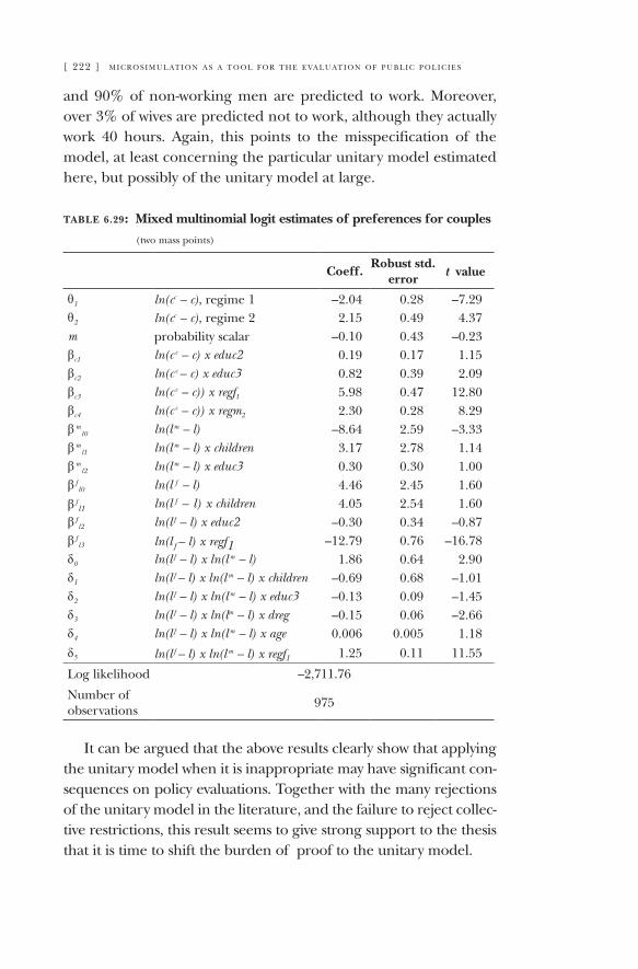
[ 222 ] m i c r o s i m u l at i o n a s a t o o l f o r t h e e va l u at i o n o f p u b l i c p o l i c i e s
and 90% of non-working men are predicted to work. Moreover, over 3% of wives are predicted not to work, although they actually work 40 hours. again, this points to the misspecification of the model, at least concerning the particular unitary model estimated here, but possibly of the unitary model at large.
table 6.29: Mixed multinomial logit estimates of preferences for couples
(two mass points)
Coeff.Robust std.
error t value
θ1 ln(cc – c), regime 1 –2.04 0.28 –7.29θ2 ln(cc – c), regime 2 2.15 0.49 4.37m probability scalar –0.10 0.43 –0.23βc1 ln(c c – c) x educ2 0.19 0.17 1.15βc2 ln(c c – c) x educ3 0.82 0.39 2.09βc3 ln(c c – c)) x regf1 5.98 0.47 12.80βc4 ln(c c – c)) x regm2 2.30 0.28 8.29β m
l0 ln(l m – l) –8.64 2.59 –3.33β m
l1 ln(l m – l) x children 3.17 2.78 1.14β m
l2 ln(l m – l) x educ3 0.30 0.30 1.00β f l0 ln(l f – l) 4.46 2.45 1.60β f l1 ln(l f – l) x children 4.05 2.54 1.60β f l2 ln(l f – l) x educ2 –0.30 0.34 –0.87β f l3 ln(l f – l) x regf1 –12.79 0.76 –16.78δ0 ln(l f – l) x ln(l m – l) 1.86 0.64 2.90δ1 ln(l f – l) x ln(l m – l) x children –0.69 0.68 –1.01δ2 ln(l f – l) x ln(l m – l) x educ3 –0.13 0.09 –1.45δ3 ln(l f – l) x ln(lm – l) x dreg –0.15 0.06 –2.66δ4 ln(l f – l) x ln(l m – l) x age 0.006 0.005 1.18δ5 ln(l f – l) x ln(l m – l) x regf1 1.25 0.11 11.55
Log likelihood –2,711.76
Number of observations 975
It can be argued that the above results clearly show that applying the unitary model when it is inappropriate may have significant con-sequences on policy evaluations. Together with the many rejections of the unitary model in the literature, and the failure to reject collec-tive restrictions, this result seems to give strong support to the thesis that it is time to shift the burden of proof to the unitary model.
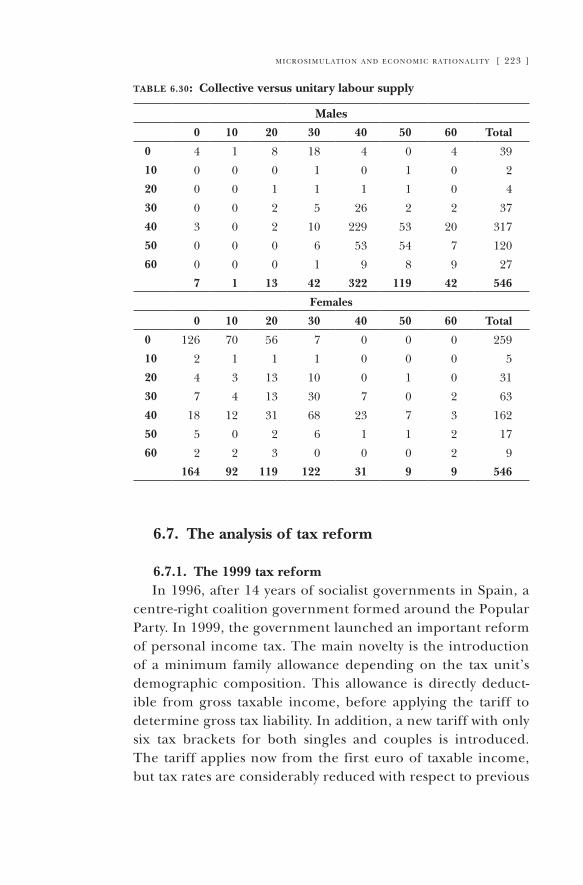
m i c r o s i m u l at i o n a n d e c o n o m i c r at i o n a l i t y [ 223 ]
table 6.30: Collective versus unitary labour supply
Males
0 10 20 30 40 50 60 Total
0 4 1 8 18 4 0 4 39
10 0 0 0 1 0 1 0 2
20 0 0 1 1 1 1 0 4
30 0 0 2 5 26 2 2 37
40 3 0 2 10 229 53 20 317
50 0 0 0 6 53 54 7 120
60 0 0 0 1 9 8 9 27
7 1 13 42 322 119 42 546
Females
0 10 20 30 40 50 60 Total
0 126 70 56 7 0 0 0 259
10 2 1 1 1 0 0 0 5
20 4 3 13 10 0 1 0 31
30 7 4 13 30 7 0 2 63
40 18 12 31 68 23 7 3 162
50 5 0 2 6 1 1 2 17
60 2 2 3 0 0 0 2 9
164 92 119 122 31 9 9 546
6.7. The analysis of tax reform
6.7.1. The 1999 tax reformIn 1996, after 14 years of socialist governments in Spain, a
centre-right coalition government formed around the Popular Party. In 1999, the government launched an important reform of personal income tax. The main novelty is the introduction of a minimum family allowance depending on the tax unit’s demographic composition. This allowance is directly deduct-ible from gross taxable income, before applying the tariff to determine gross tax liability. In addition, a new tariff with only six tax brackets for both singles and couples is introduced. The tariff applies now from the first euro of taxable income, but tax rates are considerably reduced with respect to previous
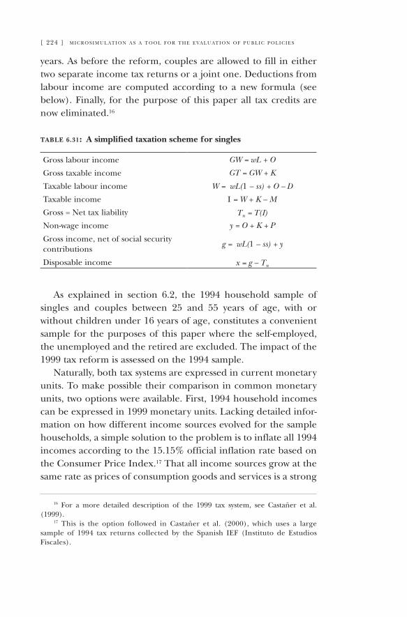
[ 224 ] m i c r o s i m u l at i o n a s a t o o l f o r t h e e va l u at i o n o f p u b l i c p o l i c i e s
years. as before the reform, couples are allowed to fill in either two separate income tax returns or a joint one. Deductions from labour income are computed according to a new formula (see below). Finally, for the purpose of this paper all tax credits are now eliminated.16
table 6.31: A simplified taxation scheme for singles
Gross labour income GW = wL + O
Gross taxable income GT = GW + K
Taxable labour income W = wL(1 – ss) + O – D
Taxable income I = W + K – M
Gross = Net tax liability Tn = T(I)
Non-wage income y = O + K + P
Gross income, net of social security contributions
g = wL(1 – ss) + y
Disposable income x = g – Tn
as explained in section 6.2, the 1994 household sample of singles and couples between 25 and 55 years of age, with or without children under 16 years of age, constitutes a convenient sample for the purposes of this paper where the self-employed, the unemployed and the retired are excluded. The impact of the 1999 tax reform is assessed on the 1994 sample.
Naturally, both tax systems are expressed in current monetary units. To make possible their comparison in common monetary units, two options were available. First, 1994 household incomes can be expressed in 1999 monetary units. Lacking detailed infor-mation on how different income sources evolved for the sample households, a simple solution to the problem is to inflate all 1994 incomes according to the 15.15% official inflation rate based on the Consumer Price Index.17 That all income sources grow at the same rate as prices of consumption goods and services is a strong
16 For a more detailed description of the 1999 tax system, see Castañer et al. (1999).
17 This is the option followed in Castañer et al. (2000), which uses a large sample of 1994 tax returns collected by the Spanish IEF (Instituto de Estudios Fiscales).
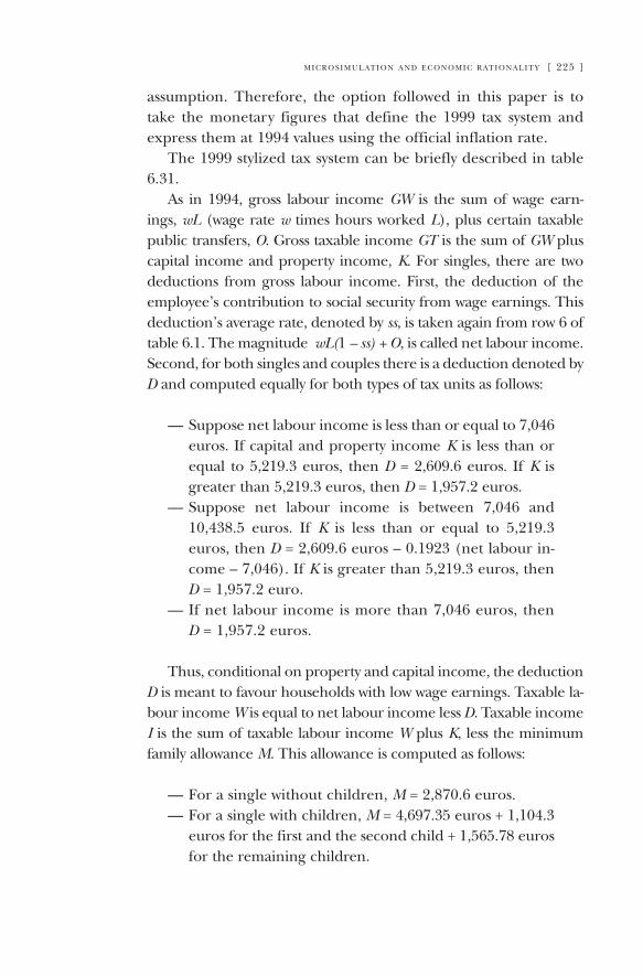
m i c r o s i m u l at i o n a n d e c o n o m i c r at i o n a l i t y [ 225 ]
assumption. Therefore, the option followed in this paper is to take the monetary figures that define the 1999 tax system and express them at 1994 values using the official inflation rate.
The 1999 stylized tax system can be briefly described in table 6.31.
as in 1994, gross labour income GW is the sum of wage earn-ings, wL (wage rate w times hours worked L), plus certain taxable public transfers, O. Gross taxable income GT is the sum of GW plus capital income and property income, K. For singles, there are two deductions from gross labour income. First, the deduction of the employee’s contribution to social security from wage earnings. This deduction’s average rate, denoted by ss, is taken again from row 6 of table 6.1. The magnitude wL(1 – ss) + O, is called net labour income. Second, for both singles and couples there is a deduction denoted by D and computed equally for both types of tax units as follows:
Suppose net labour income is less than or equal to 7,046 euros. If capital and property income K is less than or equal to 5,219.3 euros, then D = 2,609.6 euros. If K is greater than 5,219.3 euros, then D = 1,957.2 euros.Suppose net labour income is between 7,046 and 10,438.5 euros. If K is less than or equal to 5,219.3 euros, then D = 2,609.6 euros – 0.1923 (net labour in-come – 7,046). If K is greater than 5,219.3 euros, then D = 1,957.2 euro.If net labour income is more than 7,046 euros, then D = 1,957.2 euros.
Thus, conditional on property and capital income, the deduction D is meant to favour households with low wage earnings. Taxable la-bour income W is equal to net labour income less D. Taxable income I is the sum of taxable labour income W plus K, less the minimum family allowance M. This allowance is computed as follows:
For a single without children, M = 2,870.6 euros.For a single with children, M = 4,697.35 euros + 1,104.3 euros for the first and the second child + 1,565.78 euros for the remaining children.
—
—
—
——
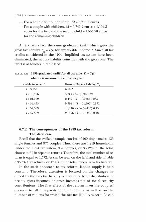
[ 226 ] m i c r o s i m u l at i o n a s a t o o l f o r t h e e va l u at i o n o f p u b l i c p o l i c i e s
For a couple without children, M = 5,741.2 euros.For a couple with children, M = 5,741.2 euros + 1,104.3 euros for the first and the second child + 1,565.78 euros for the remaining children.
all taxpayers face the same graduated tariff, which gives the gross tax liability Tg = T(I) for any taxable income X. Since all tax credits considered in the 1994 simplified tax system have been eliminated, the net tax liability coincides with the gross one. The tariff is as follows in table 6.32.
table 6.32: 1999 graduated tariff for all tax units Tn = T(I), where I is measured in euros per year
Taxable income, I Gross = Net tax liability, Tn
I < 3,130 0.18 I
I < 10,956 563 + (I – 3,130) 0.24
I < 21,390 2,442 +(I – 10,956) 0.283
I < 34,433 5,394 + (I – 21,390) 0.372
I < 57,389 10,246 + (I – 34,433) 0.45
I > 57,389 20,576 + (I – 57,389) 0.48
6.7.2. The consequences of the 1999 tax reform. The static case
Recall that the available sample consists of 109 single males, 135 single females and 975 couples. Thus, there are 1,219 households. Under the 1994 tax system, 352 couples, or 36.12% of the total, choose to fill in separate returns. Therefore, the total number of re-turns is equal to 1,572. as can be seen on the left-hand side of table 6.33, 269 tax returns, or 17.1% of the total involve zero tax liability.
In the static approach to tax reform, labour supply is held constant. Therefore, attention is focused on the changes in-duced by the two tax liability vectors on a fixed distribution of pre-tax gross incomes, or gross incomes net of social security contributions. The first effect of the reform is on the couples’ decision to fill in separate or joint returns, as well as on the number of returns for which the net tax liability is zero. as can
——
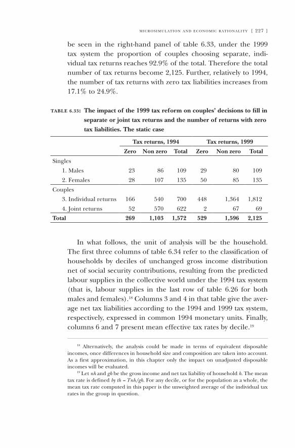
m i c r o s i m u l at i o n a n d e c o n o m i c r at i o n a l i t y [ 227 ]
be seen in the right-hand panel of table 6.33, under the 1999 tax system the proportion of couples choosing separate, indi-vidual tax returns reaches 92.9% of the total. Therefore the total number of tax returns become 2,125. Further, relatively to 1994, the number of tax returns with zero tax liabilities increases from 17.1% to 24.9%.
Tax returns, 1994 Tax returns, 1999
Zero Non zero Total Zero Non zero Total
Singles
1. Males 23 86 109 29 80 109
2. Females 28 107 135 50 85 135
Couples
3. Individual returns 166 540 700 448 1,364 1,812
4. Joint returns 52 570 622 2 67 69
Total 269 1,103 1,572 529 1,596 2,125
In what follows, the unit of analysis will be the household. The first three columns of table 6.34 refer to the classification of households by deciles of unchanged gross income distribution net of social security contributions, resulting from the predicted labour supplies in the collective world under the 1994 tax system (that is, labour supplies in the last row of table 6.26 for both males and females).18 Columns 3 and 4 in that table give the aver-age net tax liabilities according to the 1994 and 1999 tax system, respectively, expressed in common 1994 monetary units. Finally, columns 6 and 7 present mean effective tax rates by decile.19
18 alternatively, the analysis could be made in terms of equivalent disposable incomes, once differences in household size and composition are taken into account. as a first approximation, in this chapter only the impact on unadjusted disposable incomes will be evaluated.
19 Let nh and gh be the gross income and net tax liability of household h. The mean tax rate is defined by th = Tnh/gh. For any decile, or for the population as a whole, the mean tax rate computed in this paper is the unweighted average of the individual tax rates in the group in question.
table 6.33: The impact of the 1999 tax reform on couples’ decisions to fill in
separate or joint tax returns and the number of returns with zero
tax liabilities. The static case
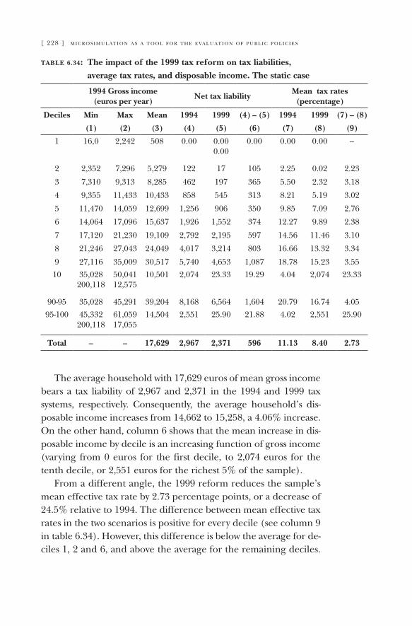
[ 228 ] m i c r o s i m u l at i o n a s a t o o l f o r t h e e va l u at i o n o f p u b l i c p o l i c i e s
table 6.34: The impact of the 1999 tax reform on tax liabilities,
average tax rates, and disposable income. The static case
1994 Gross income (euros per year)
Net tax liabilityMean tax rates
(percentage)
Deciles Min Max Mean 1994 1999 (4) – (5) 1994 1999 (7) – (8)
(1) (2) (3) (4) (5) (6) (7) (8) (9)
1 16,0 2,242 508 0.00 0.00 0.00
0.00 0.00 0.00 –
2 2,352 7,296 5,279 122 17 105 2.25 0.02 2.23
3 7,310 9,313 8,285 462 197 365 5.50 2.32 3.18
4 9,355 11,433 10,433 858 545 313 8.21 5.19 3.02
5 11,470 14,059 12,699 1,256 906 350 9.85 7.09 2.76
6 14,064 17,096 15,637 1,926 1,552 374 12.27 9.89 2.38
7 17,120 21,230 19,109 2,792 2,195 597 14.56 11.46 3.10
8 21,246 27,043 24,049 4,017 3,214 803 16.66 13.32 3.34
9 27,116 35,009 30,517 5,740 4,653 1,087 18.78 15.23 3.5510 35,028
200,11850,041 12,575
10,501 2,074 23.33 19.29 4.04 2,074 23.33
90-95 35,028 45,291 39,204 8,168 6,564 1,604 20.79 16.74 4.0595-100 45,332
200,11861,059 17,055
14,504 2,551 25.90 21.88 4.02 2,551 25.90
Total – – 17,629 2,967 2,371 596 11.13 8.40 2.73
The average household with 17,629 euros of mean gross income bears a tax liability of 2,967 and 2,371 in the 1994 and 1999 tax systems, respectively. Consequently, the average household’s dis-posable income increases from 14,662 to 15,258, a 4.06% increase. On the other hand, column 6 shows that the mean increase in dis-posable income by decile is an increasing function of gross income (varying from 0 euros for the first decile, to 2,074 euros for the tenth decile, or 2,551 euros for the richest 5% of the sample).
From a different angle, the 1999 reform reduces the sample’s mean effective tax rate by 2.73 percentage points, or a decrease of 24.5% relative to 1994. The difference between mean effective tax rates in the two scenarios is positive for every decile (see column 9 in table 6.34). However, this difference is below the average for de-ciles 1, 2 and 6, and above the average for the remaining deciles.
m i c r o s i m u l at i o n a n d e c o n o m i c r at i o n a l i t y [ 229 ]
The difference in average tax rates for the sample’s richest 10% is slightly greater than 4 percentage points.
The above facts appear to indicate that the redistributive effect of the 1999 tax system is of a smaller order of magnitude than the one achieved by the 1994 tax system. as will be seen below, this is indeed the case. But then, how can reform be evaluated in social welfare terms? For any income distribution x, this paper uses the following social evaluation function studied in Herrero and Villar (1989):
S(x) = ∑ h αh xh = m(x)(1 – I(x))
where αh = (1 – ln (xh/µ(x))/H;m(x) = mean of income distribution x;I(x) = (1/H) ∑h {xh/m(x)}log{xh/m(x)}.
The function S is a weighted sum of individual incomes, where the household whose income coincides with the mean of the population receives a weight equal to 1/H, and households with income above or below the mean receive weights increasingly smaller or greater, re-spectively, than 1/H. Moreover, it can be expressed as mean income, m(x), times an adjustment factor (1 – I(x)), which varies inversely with the degree of income inequality according to a well behaved member of the general entropy family of inequality indices.20 Finally, although this property will not be used further ahead, this function possesses a convenient additive decomposability property. 21
Let g be the before tax gross income distribution (net of social security contributions) and x and r be the after tax disposable income distributions corresponding to the 1994 and 1999 tax systems, respectively. Using the inequality index I already intro-duced, the redistributive effect of the two tax systems, RE-1994
20 among the continuous, S-convex, scale independent inequality indices that are invariant to population replications, the members of this family are the only ones which are additively decomposable for any partition of the population (see Shorrocks 1980, 1984).
21 In particular, for any partition of the population, the function S can be decom-posed into two terms: (i) the weighted average of social welfare in each subgroup, with weights equal to the subgroups’ demographic importance, less (ii) a term equal to the between-group income inequality times the distribution mean. For applications in the income distribution literature, see Garner et al. (1999), Ruiz-Castillo (1998), Ruiz-Castillo and Sastre (2001).

[ 230 ] m i c r o s i m u l at i o n a s a t o o l f o r t h e e va l u at i o n o f p u b l i c p o l i c i e s
and RE-1999, can be computed as the percentage change in in-come inequality induced by the corresponding vector of net tax liabilities, that is:
RE-1994 = 100 (I(g) – I(x))/I(g) = = 100 (0.3146 – 0.2584)/0.3146 = 17.8
RE-1999 = 100 (I(g) – I(r))/I(g) = = 100 (0.3146 – 0.2658)/0.3146 = 15.5.
as conjectured, the 1999 tax system has a smaller redistributive effect than the 1994 tax system. However, as we already observed, tax reform leads to an increase in mean disposable income. Using the social evaluation function S, the social welfare consequences of the increase in disposable income and the increase in income inequality induced by the tax reform can be assessed with the help of the following expression:
S(r) – S(x) = m(r)(1– I(r)) – m(x)(1 – I(x)) == (m(r) – m(x))(1– I(r)) + (I(x) – I(r))m(x).
(6.7)
The first term in equation (6.7) is the change in mean dispos-able income, which has been shown to be positive, weighted by the 1999 adjustment factor (1 – I(r)). The second term is the change in disposable income inequality, weighted by the 1994 mean income m(x). It turns out that
100 (S(r) - S(x))/S(x) = 100 (11,207 – 10,879)/10,879 = 3.01.
That is, as long as the evaluation is limited to a comparison of the two disposable income distributions, the 1999 tax re-form induces a 3.01% increase in social welfare.
It should be pointed out that the increase in household dis-posable incomes amounts to a decrease of equal size in 1999 tax revenues, which would lead to a reduction in publicly provided goods and services relative to the 1994 situation. The possible social welfare cost of such a reduction can be assessed in terms of equation (6.7). On one hand, the reduction in public expendi-tures can be assumed to be equivalent to a certain loss of house-hold incomes, although possibly by an inferior amount than the loss in tax revenues. Denote the average loss by a(m(r)–m(x)), where a ∈(0, 1). The closer a is to 1, the smaller the positive con-
m i c r o s i m u l at i o n a n d e c o n o m i c r at i o n a l i t y [ 231 ]
tribution to the social welfare change by the first term in equation (6.7). On the other hand, the way the loss in public expenditures is distributed among households has some bearing on the question. Denote this effect by bI(r). If the reduction in public expenditures is distributed in proportion to disposable incomes in the 1999 dis-tribution r, then the parameter b will be equal to 1. However, if this reduction is borne in equal absolute amounts by all households, or in greater absolute amounts by the poor, then b > 1. Conversely, if the reduction is borne in greater amounts by the rich, then b < 1. Thus, the larger b is the greater will be the negative contribution to the change in social welfare by the second term in equation (6.7).
This subsection assumes that households view passively the 1999 tax reform. However, faced with new tax incentives, house-holds will typically respond with behavioural changes that will affect labour supply, gross income and hence disposable income. In the next subsection, these effects will be examined according to the collective model.
6.7.3. The consequences of the 1999 tax reform according to the collective model
In the collective model, the 1999 tax reform induces two types of behavioural changes. First, the new tax system provides new incentives through changes in the budget constraint of every household. Second, as far as couples are concerned, changes in the marginal contribution of males and females to household earnings has an effect on the estimated female’s power index; in turn, this effect gives rise to a second round of changes in labour supplies. The detailed changes in labour supplies, operating only through the budget constraint, are reported in table 6.35.
Only 5 out of 109 single males and 15 out of 135 single females increase their labour supply. In addition, one single female choos-es to reduce hers. as far as couples are concerned, 219 males and 253 females are seen to increase their labour supply, while 133 males and 41 females decrease their labour supply. Thus, 352 married males and 294 married females or 36.1% and 30.2%, respectively, experience some change.
Changes in the estimated female’s power index induced by the 1999 tax reform are presented in graph 6.5. It can be seen that for
[ 232 ] m i c r o s i m u l at i o n a s a t o o l f o r t h e e va l u at i o n o f p u b l i c p o l i c i e s
all the couples, women turn out to be favoured from that point of view by the reform we consider. On average, the female power index increases from 0.41 to 0.57. The consequences for labour supply are shown in table 6.36.
The changes are very important. Essentially, males tend to exert a much larger work effort, while the opposite is the case for females. In particular, 531 males but only 69 females increase their labour supply relative to the 1994 situation. at the same time, only 73 males but 211 females reduce their labour supply. Consequently, 604 married males and 288 married females, or 61.9% and 29.5% of the total, respectively, change their behaviour relative to 1994.
By way of a summary, the first three columns of table 6.37 record the mean hours worked under the 1994 tax system and the two situations under the 1999 tax system, namely before and after the change in the female power index. On average, male and female singles, as well as married males and females, increase their hours worked in response to changes in the tax system operating through the budget constraint (see columns 1 and 2 in table 6.37). Such in-creases are moderate, ranging from approximately 2% for single and married males to 6.3% and 18.4% for single and married females. On the other hand, changes induced in couples by the increase in the female power index are dramatic (see column 3 in table 6.37). The combined effect of the two channels relative to the initial 1994 situation lead to an average increase of 13.1% in hours worked by married males, and a 21.9% decrease by married females.
Naturally, these behavioural changes have an impact on mean before tax income (gross income net of social security contribu-tions) and mean after tax income (disposable income), which are presented in columns 4 to 9 in table 6.38. Before tax income for the whole sample increases by 4.8% as a consequence of changes in budget constraint. For couples, whose mean increase in before tax income is 5.3%, the second channel adds a 0.8% increase (see columns 4 to 6 in table 6.38). Relative to 1994, after tax incomes for the whole sample increase on average by 9.6% after changes in budget constraint. However, disposable income remains essen-tially the same when the consequences of change in the female power index are taken into account (see columns 7 to 9 in the table 6.38).
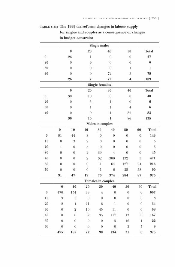
m i c r o s i m u l at i o n a n d e c o n o m i c r at i o n a l i t y [ 233 ]
table 6.35: The 1999 tax reform: changes in labour supply
for singles and couples as a consequence of changes
in budget constraint
Single males
0 20 40 50 Total
0 26 1 0 0 27
20 0 6 0 0 6
30 0 0 0 1 1
40 0 0 72 3 75
26 7 72 4 109
Single females
0 20 30 40 Total
0 30 10 0 0 40
20 0 5 1 0 6
30 0 1 1 4 6
40 0 0 1 82 83
30 16 1 86 135
Males in couples
0 10 20 30 40 50 60 Total
0 91 44 8 0 0 0 0 143
10 0 3 2 0 0 0 0 5
20 1 0 5 0 0 0 0 5
30 0 0 2 39 4 0 0 45
40 0 0 2 32 300 132 5 471
50 0 0 0 1 64 127 24 216
60 0 0 0 1 6 25 58 90
91 47 19 73 374 284 87 975
Females in couples
0 10 20 30 40 50 60 Total
0 470 154 39 4 0 0 0 667
10 3 5 0 0 0 0 0 8
20 2 4 21 6 1 0 0 34
30 0 2 10 45 11 0 0 68
40 0 0 2 35 117 13 0 167
50 0 0 0 0 5 16 1 22
60 0 0 0 0 0 2 7 9
475 165 72 90 134 31 8 975
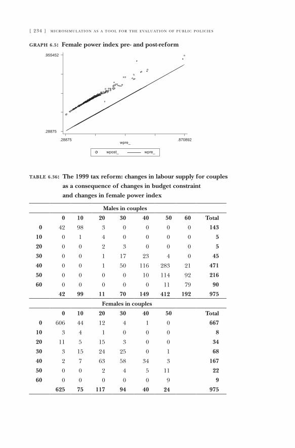
[ 234 ] m i c r o s i m u l at i o n a s a t o o l f o r t h e e va l u at i o n o f p u b l i c p o l i c i e s
graph 6.5: Female power index pre- and post-reform
table 6.36: The 1999 tax reform: changes in labour supply for couples
as a consequence of changes in budget constraint
and changes in female power index
Males in couples
0 10 20 30 40 50 60 Total
0 42 98 3 0 0 0 0 143
10 0 1 4 0 0 0 0 5
20 0 0 2 3 0 0 0 5
30 0 0 1 17 23 4 0 45
40 0 0 1 50 116 283 21 471
50 0 0 0 0 10 114 92 216
60 0 0 0 0 0 11 79 90
42 99 11 70 149 412 192 975
Females in couples
0 10 20 30 40 50 Total
0 606 44 12 4 1 0 667
10 3 4 1 0 0 0 8
20 11 5 15 3 0 0 34
30 3 15 24 25 0 1 68
40 2 7 63 58 34 3 167
50 0 0 2 4 5 11 22
60 0 0 0 0 0 9 9
625 75 117 94 40 24 975
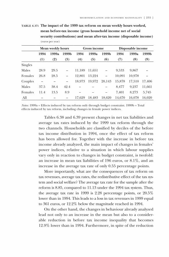
m i c r o s i m u l at i o n a n d e c o n o m i c r at i o n a l i t y [ 235 ]
table 6.37: The impact of the 1999 tax reform on mean weekly hours worked,
mean before-tax income (gross household income net of social
security contributions) and mean after-tax income (disposable income) (euros per year)
Mean weekly hours Gross income Disposable income
1994 1999a 1999b 1994 1999a 1999b 1994 1999a 1999b
(1) (2) (3) (4) (5) (6) (7) (8) (9)
Singles
Males 28.9 29.5 – 11,189 11,651 – 9,533 9,867 –
Females 26.8 28.5 – 12,801 13,224 – 10,091 10,978 –
Couples – – – 18,973 19,972 20,143 15,878 17,510 17,406
Males 37.5 38.4 42.4 – – – 8,477 9,237 11,661
Females 11.4 13.5 8.9 – – – 7,401 8,273 5,745
all – – – 17,629 18,483 18,620 14,670 16,078 16,020
Notes: 1999a = Effects induced by tax reform only through budget constraint. 1999b = Total effects induced by tax reform, including changes in female power indices.
Tables 6.38 and 6.39 present changes in net tax liabilities and average tax rates induced by the 1999 tax reform through the two channels. Households are classified by deciles of the before tax income distribution in 1994, once the effect of tax reform has been allowed for. Together with the increase in before tax income already analyzed, the main impact of changes in females’ power indices, relative to a situation in which labour supplies vary only in reaction to changes in budget constraint, is twofold: an increase in mean tax liabilities of 196 euros, or 8.1%, and an increase in the average tax rate of only 0.55 percentage points.
More importantly, what are the consequences of tax reform on tax revenues, average tax rates, the redistributive effect of the tax sys-tem and social welfare? The average tax rate for the sample after the reform is 8.85, compared to 11.13 under the 1994 tax system. Thus, the average tax rate in 1999 is 2.28 percentage points, or 20.5% lower than in 1994. This leads to a loss in tax revenues in 1999 equal to 361 euros, or 12.2% below the magnitude reached in 1994.
On the other hand, the changes in behaviour already analyzed lead not only to an increase in the mean but also to a consider-able reduction in before tax income inequality that becomes 12.9% lower than in 1994. Furthermore, in spite of the reduction
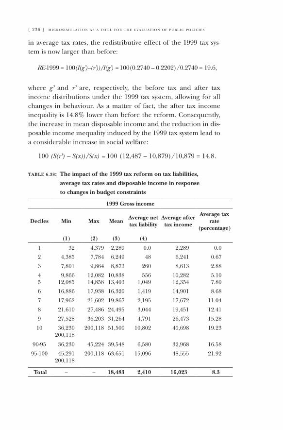
[ 236 ] m i c r o s i m u l at i o n a s a t o o l f o r t h e e va l u at i o n o f p u b l i c p o l i c i e s
in average tax rates, the redistributive effect of the 1999 tax sys-tem is now larger than before:
RE-1999 = 100(I(g’)–(r’))/I(g’) = 100(0.2740 – 0.2202)/0.2740 = 19.6,
where g’ and r’ are, respectively, the before tax and after tax income distributions under the 1999 tax system, allowing for all changes in behaviour. as a matter of fact, the after tax income inequality is 14.8% lower than before the reform. Consequently, the increase in mean disposable income and the reduction in dis-posable income inequality induced by the 1999 tax system lead to a considerable increase in social welfare:
100 (S(r’) – S(x))/S(x) = 100 (12,487 – 10,879)/10,879 = 14.8.
table 6.38: The impact of the 1999 tax reform on tax liabilities,
average tax rates and disposable income in response
to changes in budget constraints
1999 Gross income
Deciles Min Max MeanAverage net tax liability
Average after tax income
Average tax rate
(percentage)
(1) (2) (3) (4)
1 32 4,379 2,289 0.0 2,289 0.0
2 4,385 7,784 6,249 48 6,241 0.67
3 7,801 9,864 8,873 260 8,613 2.88
4 9,866 12,082 10,838 556 10,282 5.105 12,085 14,858 13,403 1,049 12,354 7.80
6 16,886 17,938 16,320 1,419 14,901 8.68
7 17,962 21,602 19,867 2,195 17,672 11.04
8 21,610 27,486 24,495 3,044 19,451 12.41
9 27,528 36,203 31,264 4,791 26,473 15.28
10 36,230 200,118
200,118 51,500 10,802 40,698 19.23
90-95 36,230 45,224 39,548 6,580 32,968 16.58
95-100 45,291 200,118
200,118 63,651 15,096 48,555 21.92
Total – – 18,483 2,410 16,023 8.3
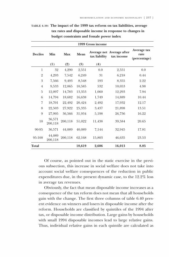
m i c r o s i m u l at i o n a n d e c o n o m i c r at i o n a l i t y [ 237 ]
table 6.39: The impact of the 1999 tax reform on tax liabilities, average
tax rates and disposable income in response to changes in
budget constraints and female power index
1999 Gross income
Deciles Min Max MeanAverage net tax liability
Average after tax income
Average tax rate
(percentage)
(1) (2) (3) (4)
1 32 4,290 2,551 0.0 2,551 0.0
2 4,293 7,542 6,249 31 6,218 0.44
3 7,566 9,493 8,548 193 8,355 2.22
4 9,533 12,065 10,585 532 10,053 4.98
5 12,097 14,783 13,353 1,060 12,293 7.94
6 14,794 18,682 16,638 1,749 14,889 10.44
7 18,701 22,492 20,424 2,492 17,932 12.17
8 22,503 27,922 25,335 3,437 21,898 13.51
9 27,995 36,566 31,934 5,198 26,736 16.22
10 36,571 200,118 200,118 51,022 11,438 39,584 20.65
90-95 36,571 44,089 40,089 7,144 32,945 17.81
95-100 44,089 200,118 200,118 62,168 15,803 46,635 23.53
Total 18,619 2,606 16,013 8.85
Of course, as pointed out in the static exercise in the previ-ous subsection, this increase in social welfare does not take into account social welfare consequences of the reduction in public expenditures due, in the present dynamic case, to the 12.2% loss in average tax revenues.
Obviously, the fact that mean disposable income increases as a consequence of the tax reform does not mean that all households gain with the change. The first three columns of table 6.40 pres-ent evidence on winners and losers in disposable income after the reform. Households are classified by quintiles of the 1994 after tax, or disposable income distribution. Large gains by households with small 1994 disposable incomes lead to large relative gains. Thus, individual relative gains in each quintile are calculated as
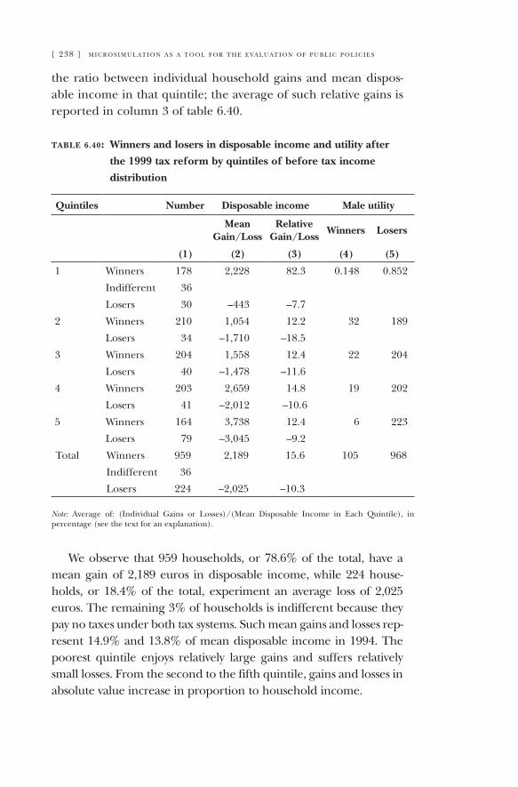
[ 238 ] m i c r o s i m u l at i o n a s a t o o l f o r t h e e va l u at i o n o f p u b l i c p o l i c i e s
the ratio between individual household gains and mean dispos-able income in that quintile; the average of such relative gains is reported in column 3 of table 6.40.
table 6.40: Winners and losers in disposable income and utility after
the 1999 tax reform by quintiles of before tax income
distribution
Quintiles Number Disposable income Male utility
Mean Gain/Loss
Relative Gain/Loss
Winners Losers
(1) (2) (3) (4) (5)
1 Winners 178 2,228 82.3 0.148 0.852
Indifferent 36
Losers 30 –443 –7.7
2 Winners 210 1,054 12.2 32 189
Losers 34 –1,710 –18.5
3 Winners 204 1,558 12.4 22 204
Losers 40 –1,478 –11.6
4 Winners 203 2,659 14.8 19 202
Losers 41 –2,012 –10.6
5 Winners 164 3,738 12.4 6 223
Losers 79 –3,045 –9.2
Total Winners 959 2,189 15.6 105 968
Indifferent 36
Losers 224 –2,025 –10.3
Note: average of: (Individual Gains or Losses)/(Mean Disposable Income in Each Quintile), in percentage (see the text for an explanation).
We observe that 959 households, or 78.6% of the total, have a mean gain of 2,189 euros in disposable income, while 224 house-holds, or 18.4% of the total, experiment an average loss of 2,025 euros. The remaining 3% of households is indifferent because they pay no taxes under both tax systems. Such mean gains and losses rep-resent 14.9% and 13.8% of mean disposable income in 1994. The poorest quintile enjoys relatively large gains and suffers relatively small losses. From the second to the fifth quintile, gains and losses in absolute value increase in proportion to household income.
m i c r o s i m u l at i o n a n d e c o n o m i c r at i o n a l i t y [ 239 ]
The availability of a collective model permits to go beyond gains and losses in household disposable income and toward gains and losses in utility for individual males and females. In this respect, it has already been observed that, on average, tax reform induces an increase of hours worked by both single males and females (see col-umns 1 and 2 in table 6.36). Less leisure implies a utility decrease, but larger disposable income for consumption (see columns 7 and 9 in table 6.36) works in the opposite direction. Within couples, the situation of males and females is very different. after reform, males work on average considerably harder but enjoy a 37.6% increase in consumption, while females reduce their average labour supply but experience a 22.4% decrease in consumption.
The final question is: how do these changes in leisure and consumption affect the utility of the 1,084 males and 1,110 fe-males in the sample? It turns out that all females in the sample experience a utility gain as a consequence of reform. Columns 4 and 5 in table 6.40 classify males in each quintile of the 1994 household disposable income as winners, indifferent or losers in utility space. Only 9.8% of all males in the sample enjoy a utility increase. It should be noticed that 102 out of the 105 winners are single males. That is to say, practically all married men lose utility as a consequence of reform. In any case, 55.2% of the gainers, including the 3 married males, belong to households classified in the poorest 20% according to 1994 household disposable income. The conclusion is clear: the increase in female power indices induced by reform translates into utility gains for them and utility losses for practically all their spouses.
6.8. Conclusions
This chapter has made two contributions. In the first place, it has presented a collective model of household labour supply behav-iour, allowing for labour participation, the presence of children and non-linear taxation. In the second place, the model has been used to simulate an important tax reform in Spain using data from the first three waves of the ECHP. However, many caveats must be stressed in this concluding section.
[ 240 ] m i c r o s i m u l at i o n a s a t o o l f o r t h e e va l u at i o n o f p u b l i c p o l i c i e s
as pointed out in the introduction, at present we do not know how to identify and estimate a collective model with the above characteristics. Consequently, only a certain application of the collective approach has been presented under the base-line 1994 tax system. Marginal propensities for consumption and leisure have been estimated for single males and females. Using these estimates for married individuals, a leisure interac-tion term and an index of female bargaining power have been calibrated so as to replicate observed labour supply in couples as well as possible. Female power index has been estimated as a function of demographic variables and a set of distribution fac-tors. This has led to the calibration of a leisure interaction term for each member of each couple. The dataset thus obtained, which replicates very well the observed behaviour in 1994, has been used to estimate a unitary model of similar characteristics to the collective one.
The first conclusion of the paper is that when a unitary model is estimated on data obtained from a deterministic collective model, the results lack economic meaning. To us, this is an indi-cation that unitary models do not provide a convincing basis for policy evaluations. Instead, more resources should be put towards identifying and estimating collective models under complex situ-ations like the one considered in this paper.
The results of the singles model and the simplified approach to collective decision making provide some hints on essential aspects that have not received sufficient attention in the chapter. When single, males and females appear to behave very similarly as far as labour supply is concerned. However, when married, these individuals alter their behaviour dramatically. In particular, as is well known from many previous studies, married females in Southern European countries tend not to participate in the labour market and generally exert much less market work effort than their husbands. In the simplified approach presented in this paper, differences in labour supply behaviour are simply cap-tured through the calibration of a leisure interaction term and a female power index. It is true that, in the spirit of the collective approach, this index is partly explained by distribution factors, including a key variable capturing the differential contribution
m i c r o s i m u l at i o n a n d e c o n o m i c r at i o n a l i t y [ 241 ]
by males and females to household earnings. This is encouraging and very useful for the purpose at hand, namely the evaluation of a tax reform with potentially important effects on such marginal contributions.
However, high female labour participation in couples is as-sociated in this paper with a negative leisure interaction term for males and a low female power index. Similarly, low female labour participation is associated with a high leisure interaction term for females and a high female power index. It remains to be seen if this inverse relationship between female labour participation and bargaining power is maintained once household production and time use within the household are appropriately taken care of in an explicit collective model for the spouses’ labour participa-tion.
The second part of the paper evaluates the tax reform that took place in Spain in 1999. This exercise has important limita-tions: (i) given the nature of the data, only a stylized modeling of the tax system has been possible, excluding the key role of tax deductions and allowances granted for pension funds, health expenditures, investments in housing acquisition, life insurance and charity contributions; (ii) rather than evaluating the 1999 tax reform on data for that year, it has been necessary to convert the 1999 tax parameters into 1994 monetary units; (iii) the samples of singles and couples have been selected with a focus on wage earners (or potential earners) that form easily identifiable tax units, namely households with adults between 25 and 55 years old with or without children below 16 years of age. This sample represents only a very small part of the total population; (iv) the available income data refer to income net of both social secu-rity contributions and income tax withholdings. Therefore, gross earnings had to be estimated in the paper.
Notwithstanding the above limitations, the results obtained are very interesting indeed. First, in the static case taken as a bench-mark, the 1999 tax reform leads to a decrease in tax revenues and average tax rates, as well as to a smaller redistributive effect than the 1994 tax system. Taking into account only the impact on the mean and the inequality of disposable income, social wel-fare in 1999 increases by approximately 3%. Second, it has been
[ 242 ] m i c r o s i m u l at i o n a s a t o o l f o r t h e e va l u at i o n o f p u b l i c p o l i c i e s
confirmed that labour supply considerations are an essential part of tax reform evaluation. When only the effects of the 1999 tax reform through reactions to changes in the budget constraint are considered, single and married individuals of both genders tend to exert a larger work effort. Third, couples’ behaviour changes dramatically as a consequence of the increase in the female power index induced by the tax reform: while males exert a considerably larger market work effort, females do the opposite.22 Fourth, in the case where labour supplies are allowed to vary, the before tax income distribution under the 1999 tax system presents a larger mean and a smaller inequality than the corresponding distribu-tion under the 1994 tax system. Further, the decrease in tax rev-enues and average tax rates is now smaller than in the static case, the redistributive effect is larger than in 1994 and there is a 14.8% increase in social welfare. Fifth, single males and females are shown to experience a utility increase as a consequence of the tax reform. More importantly, corresponding to the increase in the female power index, all females in the sample of couples experi-ence a utility gain, while essentially all men are seen to experiment a utility loss.
These results should suffice to justify the interest of evaluating tax and other reforms by means of a collective model of house-hold labour supply.
References
atkinson, a. b., l. rainwater and T. smeeding. Income Distribution in OECD Countries: the Evidence from the Luxembourg Income Study (LIS). Paris: OECD, 1995.
beninger, d. and f. laisney. “Comparison between Unitary and Collective Models of Household Labour Supply with Taxation.” Mimeo. Manheim: ZEW, 2001.
bingley, p., and i. walker. “The Labour Supply, Unemployment, and Participation of Lone Mothers in In-Work Transfer Programs.” Economic Journal 107 (1997): 1375–1390.
blundell, r. “Consumer Behaviour: Theory and Empirical Evidence.” Economic Journal 98 (1998): 16–65.
blundell, r., c. meghir, e. symons, and i. walke. “Labour Supply Specification and the Evaluation of Tax Reforms.” Journal of Public Economics 36 (1998): 23–52.
22 It should be pointed out that the amount of observed changes may depend on the fact that a partially calibrated data set has been used. Perhaps in a new version of the paper a fully estimated data set may give rise to fewer changes.
m i c r o s i m u l at i o n a n d e c o n o m i c r at i o n a l i t y [ 243 ]
blundell, r., p. pashardes and g. weber. “What Do We Learn about Consumer Demand Patterns from Micro Data?” American Economic Review 83 (1993): 57.
bourguignon, F. and p. a. chiappori. “Collective Models of Household Behaviour. an Introduction.” European Economic Review 36 (1992): 355–364.
browning, m., f. bourguignon, p. a. chiappori and v. lechene. “Income and Outcomes: a Structural Model of Intra-Household allocation.” Journal of Political Economy 102 (1994): 1067–1096.
browning, m. and p. a. chiappori. “Efficient Intra-Household allocations: a General Characterization and Empirical Tests.” Econometrica 66 no. 6 (1998): 1241–1278.
browning, m. and c. meghir. “The Effects of Male and Female Labour Supply on Commodity Demands.” Econometrica 59 (1991): 925–951.
buhmann, b., l. rainwater, g. schmaus and t. smeeding. “Equivalence Scales, Well-Being, Inequality and Poverty: Sensitivity Estimates across Ten Countries Using the Luxembourg Income Study Database.” Review of Income and Wealth 34 (1998): 115-142.
castañer, J. m., J. onrubia and r. paredes. “análisis de los efectos recaudatorios y redistributivos de la reforma del IRPF por Comunidades autónomas.” Hacienda Pública Española 150 (1999): 79–108.
—.“Efectos de la reforma del IRPF sobre la renta disponible, su distribución y sobre el bienestar social.” Economistas 84 (2000), 183–199.
coulter, f., f. cowell and s. Jenkins. “Differences in Needs and assessment of Income Distributions.” Bulletin of Economic Research 44 (1992a): 77–124.
—.“Equivalence Scale Relativities and the Extent of Inequality and Poverty.” Economic Journal 102 (1992b): 1067-1082.
donni, o. “Collective Household Labour Supply: Nonparticipation and Income Taxation.” Journal of Public Economics, 2002.
garner, t., J. ruiz-castillo and m. sastre. “The Influence of Demographics and Household Specific Price Indices on Expenditure Based Inequality and Welfare: a Comparison of Spain and the United States.” Working Paper 99-63. Universidad Carlos III de Madrid, 1999.
herrero, c. and a. villar. “Comparaciones de renta real y evaluación del bienestar.” Revista de Economía Pública 2 (1989): 79–101.
hoynes, h. “Welfare Transfers in Two-Parent Families: Labour Supply and Welfare Participation under aFDC-UP.” Econometrica 64 (1996): 295–332.
manser, m., and m. brown. “Marriage and Household Decision-Making: a Bargaining analysis.” International Economic Review 21 (1980): 31–44.
mcelroy, m. “The Empirical Content of Nash-Bargained Household Behaviour.” Journal of Human Resources 25 (1990): 559–583.
ruiz-castillo, J. “a Simplified Model for Social Welfare analysis. an application to Spain, 1973-74 to 1980-81.” Review of Income and Wealth 44 (1998): 123–141.
ruiz-castillo, J. and m. sastre. “Distributive Implications of Member Level Income aggregation within the Household: an approximation Through Income Mobility Indexes.” Economics of Transition 9 (2) 2001: 487– 513.
shorrocks, a. f. “The Class of additively Decomposable Inequality Measures,” Econometrica 48 (1980): 613–625.
—. “Inequality Decomposition by Population Subgroups.” Econometrica 52 (1984): 1369-1388.
van soest, a. “a Structural Model of Family Labour Supply: a Discrete Choice approach.” Journal of Human Resources 30 (1995): 63–88.

[ 244 ] m i c r o s i m u l at i o n a s a t o o l f o r t h e e va l u at i o n o f p u b l i c p o l i c i e s
vermeulen, f. “Collective households: Principles and Main Results.” Discussion Paper Series DPS 00.28. Center for Economic Studies, Katholike Universiteit Leuven, 2000.
zamora, b. “Participación laboral de la mujer y bienes públicos en el marco de los modelos colectivos del hogar (Female Labour Participation and Public Goods in the Collective Model of the Household).” Unpublished PhD dissertation, Universidad Carlos III, 2000.
[ 245 ]
Microsimulation and Macroeconomic Analysis: An Integrated Approach. An Application for Evaluating Reforms in the Italian Agricultural Sector
Riccardo Magnani and Eleonora MatteazziUniversity of Verona and University of Cergy-Pontoise
Federico PeraliUniversity of Verona and CHILD
7.1. Introduction
The general equilibrium impac of reforms on Italian agriculture is here developed both at the macro and micro level of analysis. The Applied General Equilibrium model (AGE) is based on a social accounting matrix that incorporates seven farm-house-hold types, one rural household type and three urban classes of households. This macro level of analysis is statistically linked to the micro level of analysis, represented by the farm-household, because the aggregate SAM at the core of the general equilibri-um model is constructed from the aggregation of the household level microdata.
The microlevel of the farm-household analysis is carried out by first estimating a microeconometric model of the farm-house-hold, and, in sequence, constructing a farm-household general equilibrium model using the estimated elasticities of the econo-metric model and the average data of each farm-household type. The simulations of the application are behavioural both at the macro and micro level.
7.
The authors wish to thank Antonella Finizia. The research has been carried out with the financial contribution of the Italian Ministry of Agriculture and Forestry Policies.
[ 246 ] m i c r o s i m u l at i o n a s a t o o l f o r t h e e va l u at i o n o f p u b l i c p o l i c i e s
This application seeks to evaluate the macro distributional impact of agricultural reforms and trade agreements on policy-relevant farm, rural and urban household types in Italy by de-scribing households’ behavioural response to policy changes. The analysis contributes to improving our knowledge on the possibility to make the macro and micro level of analysis as complementary as possible in order to understand the welfare consequences of policy changes both at the household and in-dividual level. The application intends also to reveal something about the transition from a macro description of the economy, where most markets function, to a micro understanding of the farm-household economy, where most markets fail or are absent. At the micro level, most policy changes are likely to induce internal reallocations of income and other resources, such as time, affecting households’ real adjustment capabili-ties in a way which is not obvious in situations where markets are missing. The Italian case study also sheds lights on some of the conditions in survey design, data interpretation and model building for the micro-macro approach to be applied in distributional analysis for other developed and developing countries.
Figure 7.1 describes the micro-macro link between the general equilibrium model at the macro level of the economy and the general equilibrium at the micro level of the household economy that differentiates for individual behaviour. The dashed set dia-gram emphasizes the fact that the primitive macro-micro link is the one aggregating all household individuals into the family seen as a macro-society. Then, households at the micro level ag-gregate up to the macro level of the whole economy. As shown in the right panel of the figure, households can aggregate also at the intermediate level of a community, such as a village, or a territory like a natural park, an industrial district or a region. Statistical consistency across levels of aggregation is ensured by the peculiar design of the underlying information source, which is the same across levels.
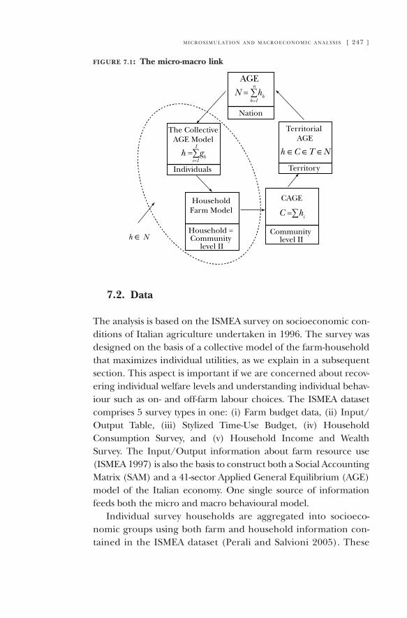
m i c r o s i m u l at i o n a n d m a c r o e c o n o m i c a n a ly s i s [ 247 ]
figure 7.1: The micro-macro link
7.2. Data
The analysis is based on the ISMEA survey on socioeconomic con-ditions of Italian agriculture undertaken in 1996. The survey was designed on the basis of a collective model of the farm-household that maximizes individual utilities, as we explain in a subsequent section. This aspect is important if we are concerned about recov-ering individual welfare levels and understanding individual behav-iour such as on- and off-farm labour choices. The ISMEA dataset comprises 5 survey types in one: (i) Farm budget data, (ii) Input/Output Table, (iii) Stylized Time-Use Budget, (iv) Household Consumption Survey, and (v) Household Income and Wealth Survey. The Input/Output information about farm resource use (ISMEA 1997) is also the basis to construct both a Social Accounting Matrix (SAM) and a 41-sector Applied General Equilibrium (AGE) model of the Italian economy. One single source of information feeds both the micro and macro behavioural model.
Individual survey households are aggregated into socioeco-nomic groups using both farm and household information con-tained in the ISMEA dataset (Perali and Salvioni 2005). These
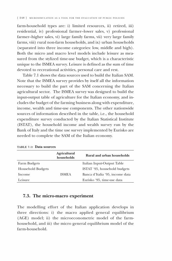
[ 248 ] m i c r o s i m u l at i o n a s a t o o l f o r t h e e va l u at i o n o f p u b l i c p o l i c i e s
farm-household types are: i) limited resources, ii) retired, iii) residential, iv) professional farmer–lower sales, v) professional farmer–higher sales, vi) large family farms, vii) very large family farms, viii) rural non-farm households, and ix) urban households (separated into three income categories: low, middle and high). Both the micro and macro level models include leisure as mea-sured from the stylized time-use budget, which is a characteristic unique to the ISMEA survey. Leisure is defined as the sum of time devoted to recreational activities, personal care and rest.
Table 7.1 shows the data sources used to build the Italian SAM. Note that the ISMEA survey provides by itself all the information necessary to build the part of the SAM concerning the Italian agricultural sector. The ISMEA survey was designed to build the input-output table of agriculture for the Italian economy, and in-cludes the budget of the farming business along with expenditure, income, wealth and time-use components. The other nationwide sources of information described in the table, i.e., the household expenditure survey conducted by the Italian Statistical Institute (ISTAT), the household income and wealth survey run by the Bank of Italy and the time use survey implemented by Eurisko are needed to complete the SAM of the Italian economy.
table 7.1: Data sources
Agricultural households
Rural and urban households
Farm Budgets Italian Input-Output Table
Household Budgets ISTAT ‘95, household budgets
Income ISMEA Banca d’Italia ‘95, income data
Leisure Eurisko ‘95, time-use data
7.3. The micro-macro experiment
The modelling effort of the Italian application develops in three directions: i) the macro applied general equilibrium (AGE) model; ii) the microeconometric model of the farm-household, and iii) the micro general equilibrium model of the farm-household.
m i c r o s i m u l at i o n a n d m a c r o e c o n o m i c a n a ly s i s [ 249 ]
The estimated functional form of the microeconometric mod-el, described in Menon and Perali (2004), is the statistical basis for the mathematical programming general equilibrium model of the farm-household, which serves in its benchmark formula-tion as a standard microsimulation model. Each farm-household is then treated as a miniature economy within a general equilib-rium framework that is best suited to analyze the micro impact of macro policies under non competitive conditions. This study, therefore, illustrates only the macro and micro dimensions of the applied general equilibrium approach adopted in the study.
7.4. The macro applied general equilibrium model
The AGE model includes 41 sectors and places particular empha-sis on the agricultural sector: agriculture is disaggregated into 23 agricultural sectors, agro-industry into nine sectors, other indus-tries into seven sectors and services into two sectors. Each sector produces a single output using intermediate goods and primary factors according to a two-level CES production function. The agri-cultural sectors use 10 production factors: land (broken down into three types), agricultural capital, labour (split into independent farm labour and dependent labour) and animals (split into four types), while other sectors use two production factors: non agricul-tural capital and labour. The AGE distinguishes two institutional sectors, households and government. The MEG includes seven farm-household types describing the agricultural sector, one rural household type and three urban categories. This classification per-mits an accurate distributional and welfare analysis of the impact of agricultural policies upon policy relevant farm-household types. International trade is factored in the model by considering two trade areas: the European Union (EU) and the rest of the world (RoW). The model incorporates the main features of the CAP re-form (OECD 1988; Weyerbrock 1998; De Muro and Salvatici 2001) and is designed to compare the social desirability of total versus partial decoupling options proposed by the reform. The results of the ex ante policy analysis were used by the Italian government to support the decision adopted in July 2004 in favour of a totally
[ 250 ] m i c r o s i m u l at i o n a s a t o o l f o r t h e e va l u at i o n o f p u b l i c p o l i c i e s
decoupled scheme. The MEG model is comparable to other na-tional models used for policy analysis such as the French MEGAAF (Gohin, Gouyoumard, La Mouël 1999, 2002; Gohin 2002) and Adelman and Robinson (1978), De Melo (1988), Hertel (1999), Shoven and Whalley (1984) for general references of general equi-librium models applied to agricultural policies.
Total decoupling gives the market back both the allocative and the redistributive function, thus favouring greater efficiency in the use of resources in activities and areas of greater comparative advantage. Income levels of farming households are maintained by granting a non distortive lump sum corresponding to the amount of premiums received in the reference situation for the years 2001-2002. In general, a totally decoupled scheme would mitigate the problem of distributive justice associated with cou-pled payments, which by design benefit mainly large producers. The adjustment process induced by reform may encourage farm-ers to adopt least cost practices and activities, with the objective of minimizing the use of labour and other agriculture inputs. The increase in pasture production at the expense of durum wheat in the Italian south is one instance of such a change.
An example may help to describe this behavioural reaction to decoupling. In the central region of Italy, cereal farmers traditionally face the choice of planting either soft or durum wheat. In the pre-reform context coupled premiums were giving durum wheat a comparative advantage over soft wheat in terms of lower cost to returns ratio. Under a decoupled scheme, the terms of convenience are inverted. However, neither durum nor soft wheat would be produced by a rational farm, because both crops have higher costs than gross returns. It is therefore more allocatively efficient to switch, for example, to low cost pasture production while receiving the lump-sum payment based on the cereal production of the reference situation. This new con-figuration frees resources in surplus such as labour and other inputs available for more efficient uses in other sectors of the economy. Agricultural surplus labour may give rise to unemploy-ment, especially in the south, where employment opportunities are lacking. The farm enterprise keeps farming but at an activity level low in input use. We term farm-households adopting this
m i c r o s i m u l at i o n a n d m a c r o e c o n o m i c a n a ly s i s [ 251 ]
behaviour as deactivated. This reaction is in line with the spirit of the reform.
The model is described in detail in Finizia, Magnani and Perali (2004). We analyze the general equilibrium effects at the aggre-gate level of the agricultural sector by focusing our attention on the impact upon:
activity portfolio and value added composition; changes in production prices;balance of trade of the primary sector; land prices;labour demand and remuneration, and farm-household incomes.
Results have been aggregated in order to conform with the speci-fications of the econometric and micro general equilibrium model. The simulation is therefore interested in changes in the price of aggregate products crops, milk, beef, fruit, used in the econometric ap-plication and adopted in the micro-general equilibrium model as a result of the implementation of a totally decoupled reform.
Macro results under the total decoupling scenario are de-scribed in table 7.2, which presents percentage change in pro-duction (Xs) and domestic consumption prices (Pd), and in table 7.3 describing percentage changes in factor prices. Impact on production and consumption prices is described in detail to show that the small effect on both production level and price is the effect of the weighted aggregation masking large fluctuations for wheat, fodder, soy beans and other industrial crops. The fruit and vegetable sector shows a very small impact because it is not directly involved in the reform. The reduction in the magnitudes of the effects due to aggregation also reduces considerably the policy space of micro-analysis. This is the price that must be paid for the econometric difficulties that make the microeconometric model intractable if the level of disaggregation of 23 agricultural sectors, as in the macro model, is to be maintained. Further, be-cause the CAP reform has a surgical impact mainly concentrated on agriculture, only the macro effects of decoupling on agricul-ture are transmitted at the micro level of the farm-household.
i)ii)iii)iv)v)vi)

[ 252 ] m i c r o s i m u l at i o n a s a t o o l f o r t h e e va l u at i o n o f p u b l i c p o l i c i e s
Another factor limiting policy analysis comes from the fact that the effects on production are not differentiated by farm-house-hold type, since production technology is the same for all farm types. Incorporating this feature would require the enlargement of the model to host 23 activities for each farm type, allowing for each type to adopt an optimal subset of activities. This exercise is left for future developments of the model.
The impact of reform on hired labour is negligible, while de-mand for farm labour decreases slightly. Demand for agricultural capital decreases markedly. Interestingly, lower demand for agri-cultural inputs coupled with higher costs in the chemical industry has a positive impact on the environment. Higher land prices are expected to curb sale land property transactions but may activate the rental market. The land market may also suffer from legal con-flicts due to the unclear definition of property and rental rights in the reference situation, leading to higher transaction costs.
The set of macro results aggregated in the group of crops, fruits and vegetables, milk and livestock products presented in tables 7.2 and 7.3 serves as the basis for simulation at the micro level, where prices, endogenous at the macro level, become exogenous.
table 7.2: Change in production (Xs) and domestic consumption prices
(Pd) under a total decoupling scenario. Detailed
and aggregate results
(percentage)
XsProduction
PdDomestic
PriceWeight
Weighted Xs
Weighted Pd
Crops
1 Soft wheat –27.64 0.60 5.36 –1.48 0.03
2 Durum wheat –36.11 0.60 8.29 –2.99 0.05
3 Rice 0.20 –1.06 3.20 0.01 –0.03
4 Corn –0.71 –1.15 18.81 –0.13 –0.22
5 Fodder 16.32 –10.49 10.89 1.78 –1.14
6 Dry hay 30.36 –15.25 7.26 2.20 –1.11
7 Potatoes 1.80 –0.83 3.38 0.06 –0.03
8 Tomatoes 1.86 –0.77 4.17 0.08 –0.03
9 Other vegetables –0.52 0.27 25.75 –0.13 0.07
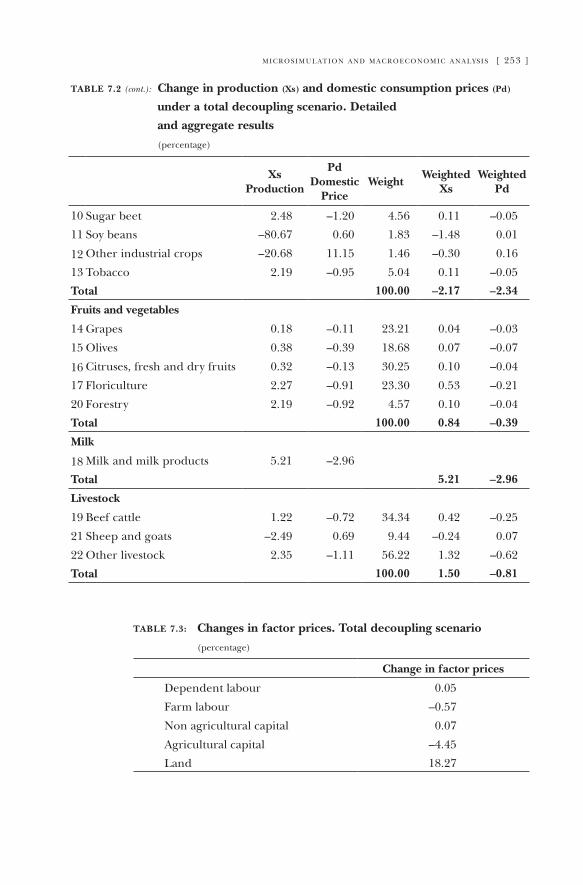
m i c r o s i m u l at i o n a n d m a c r o e c o n o m i c a n a ly s i s [ 253 ]
table 7.2 (cont.): Change in production (Xs) and domestic consumption prices (Pd)
under a total decoupling scenario. Detailed
and aggregate results
(percentage)
XsProduction
PdDomestic
PriceWeight
Weighted Xs
Weighted Pd
10 Sugar beet 2.48 –1.20 4.56 0.11 –0.05
11 Soy beans –80.67 0.60 1.83 –1.48 0.01
12 Other industrial crops –20.68 11.15 1.46 –0.30 0.16
13 Tobacco 2.19 –0.95 5.04 0.11 –0.05
Total 100.00 –2.17 –2.34
Fruits and vegetables
14 Grapes 0.18 –0.11 23.21 0.04 –0.03
15 Olives 0.38 –0.39 18.68 0.07 –0.07
16 Citruses, fresh and dry fruits 0.32 –0.13 30.25 0.10 –0.04
17 Floriculture 2.27 –0.91 23.30 0.53 –0.21
20 Forestry 2.19 –0.92 4.57 0.10 –0.04
Total 100.00 0.84 –0.39
Milk
18 Milk and milk products 5.21 –2.96
Total 5.21 –2.96
Livestock
19 Beef cattle 1.22 –0.72 34.34 0.42 –0.25
21 Sheep and goats –2.49 0.69 9.44 –0.24 0.07
22 Other livestock 2.35 –1.11 56.22 1.32 –0.62
Total 100.00 1.50 –0.81
table 7.3: Changes in factor prices. Total decoupling scenario
(percentage)
Change in factor prices
Dependent labour 0.05
Farm labour –0.57
Non agricultural capital 0.07
Agricultural capital –4.45
Land 18.27
[ 254 ] m i c r o s i m u l at i o n a s a t o o l f o r t h e e va l u at i o n o f p u b l i c p o l i c i e s
7.5. Distributional impact at the macro level
Macroanalysis has shown that the Italian economy is fairly insulat-ed from the effects derived from the implementation of the CAP reform. This fact holds both for farm and non farm households and for firms in general. Considering the compensating effect of the lump-sum farm payment, this result comes as no surprise. The question that we now address is to evaluate the distributive impact at macro level stemming from the adoption of scenarios that worsen the total decoupling scenario, simulating, fairly realistically:
a 50% reduction in the single farm payment;international prices of all industrial goods (sectors 33-39 in the model) increase 20%, simulating the effect produced by global shocks such as those generated by the volatility of financial markets and the political instability of oil mar-kets.
We also inquire whether the real dimension of the distributive impact was hidden by the aggregate level of the analysis, which considered only the impact on household income, neglecting its components associated with time use either in agricultural or non agricultural activities and leisure. We term this distribution of in-come as functional, describing the proportion of labour income going to different types of the same factor. This approach unveils quite a differentiated response pattern.
Table 7.4 reports the impact of policy scenarios on welfare levels and factor prices. The relative change in equivalent varia-tion is large for urban households and medium and large family farms as a result of the adoption of a totally decoupled scheme. The 50% reduction in the single farm payment causes a relative loss for all farm household types, while urban households benefit to a considerable extent. Compared to the CAP scenario, farm wages decrease slightly, but the value of land is seriously affected because of the reduction in the single farm payment. On the other hand, the increase in international industrial prices harms all household categories, especially the urban one. As expected,
——
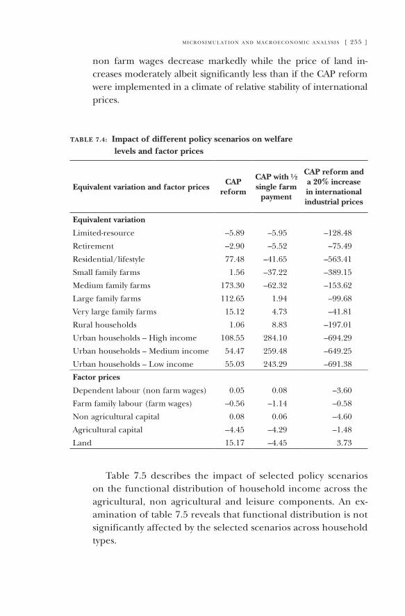
m i c r o s i m u l at i o n a n d m a c r o e c o n o m i c a n a ly s i s [ 255 ]
non farm wages decrease markedly while the price of land in-creases moderately albeit significantly less than if the CAP reform were implemented in a climate of relative stability of international prices.
table 7.4: Impact of different policy scenarios on welfare levels and factor prices
Equivalent variation and factor pricesCAP
reform
CAP with ½ single farm
payment
CAP reform and a 20% increase in international industrial prices
Equivalent variation
Limited-resource –5.89 –5.95 –128.48
Retirement –2.90 –5.52 –75.49
Residential/lifestyle 77.48 –41.65 –563.41
Small family farms 1.56 –37.22 –389.15
Medium family farms 173.30 –62.32 –153.62
Large family farms 112.65 1.94 –99.68
Very large family farms 15.12 4.73 –41.81
Rural households 1.06 8.83 –197.01
Urban households – High income 108.55 284.10 –694.29
Urban households – Medium income 54.47 259.48 –649.25
Urban households – Low income 55.03 243.29 –691.38
Factor prices
Dependent labour (non farm wages) 0.05 0.08 –3.60
Farm family labour (farm wages) –0.56 –1.14 –0.58
Non agricultural capital 0.08 0.06 –4.60
Agricultural capital –4.45 –4.29 –1.48
Land 15.17 –4.45 3.73
Table 7.5 describes the impact of selected policy scenarios on the functional distribution of household income across the agricultural, non agricultural and leisure components. An ex-amination of table 7.5 reveals that functional distribution is not significantly affected by the selected scenarios across household types.
[ 256 ] m i c r o s i m u l at i o n a s a t o o l f o r t h e e va l u at i o n o f p u b l i c p o l i c i e s
Tables 7.6 and 7.7 summarize the level of inequality of the ex post distribution for both total farm and off-farm income and extended income, considering all household categories and farm-household categories respectively. In table 7.7, where only farm-household types are considered, total income is split into farm and non-farm income. Both tables show a more equitable distribution of extended income thanks to the efficient reorga-nization of activities within the household. Table 7.6 shows that the distribution of society’s income is not significantly affected across scenarios. However, if we focus on the differential distri-bution of farm and non-farm income, as depicted in table 7.7, the distribution of off-farm income becomes significantly more unequal as a consequence of the CAP reform. This negative impact on the distribution of off-farm incomes across farm-household types is slightly curbed in the scenarios considering a 50% reduction of the lump-sum transfer and an increase in industrial prices.
The policy question of interest now moves from the macro to the micro dimension, where we describe behavioural re-sponses and how they vary across different household types. Further, we inquire how strongly the shocks stemming from a) the CAP reform and a likely reduction of the level of the single farm payment, and b) international industrial prices exert their effects at the micro level. The objective is to describe the behavioural response of different farm-household types to the shocks generated by the deregulation of European agriculture and the greater openness of international markets. The micro analysis is conducted to help identify who wins, who loses and by how much, and to ascertain how the macro effect differs from the micro effect. We implement the micro phase of the investigation by estimating a microeconometric model speci-fied within the collective theory of the household, and then constructing the corresponding general equilibrium model of the farm-household.
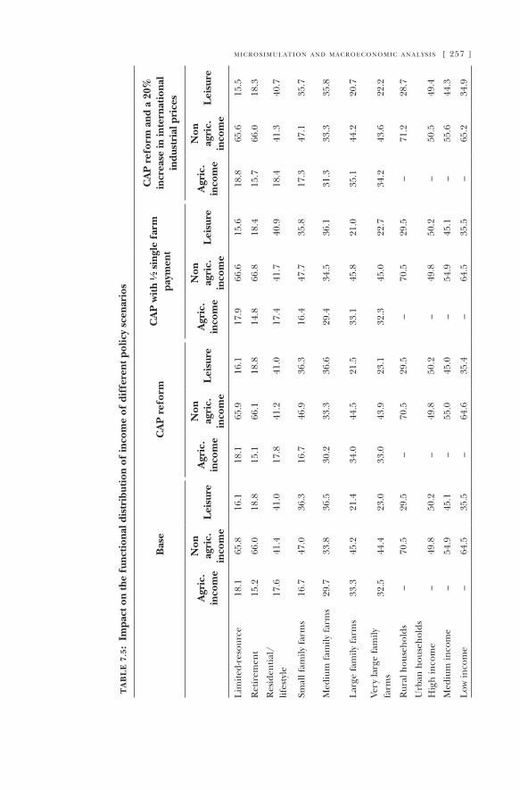
m i c r o s i m u l at i o n a n d m a c r o e c o n o m i c a n a ly s i s [ 257 ]
ta
bl
e 7
.5:
Impa
ct o
n th
e fu
ncti
onal
dis
trib
utio
n of
inco
me
of d
iffe
rent
pol
icy
scen
ario
s
Bas
eC
AP
ref
orm
CA
P w
ith
½ s
ingl
e fa
rm
paym
ent
CA
P r
efor
m a
nd a
20%
in
crea
se in
inte
rnat
iona
l in
dust
rial
pri
ces
Agr
ic.
inco
me
Non
ag
ric.
in
com
eL
eisu
reA
gric
.in
com
e
Non
ag
ric.
in
com
eL
eisu
reA
gric
.in
com
e
Non
ag
ric.
in
com
eL
eisu
reA
gric
.in
com
e
Non
ag
ric.
in
com
eL
eisu
re
Lim
ited-
reso
urce
18.1
65.8
16.1
18.1
65.9
16.1
17.9
66.6
15.6
18.8
65.6
15.5
Ret
irem
ent
15.2
66.0
18.8
15.1
66.1
18.8
14.8
66.8
18.4
15.7
66.0
18.3
Res
iden
tial/
lif
esty
le17
.641
.441
.017
.841
.241
.017
.441
.740
.918
.441
.340
.7
Smal
l fam
ily f
arm
s16
.747
.036
.316
.746
.936
.316
.447
.735
.817
.347
.135
.7
Med
ium
fam
ily f
arm
s29
.733
.836
.530
.233
.336
.629
.434
.536
.131
.333
.335
.8
Lar
ge f
amily
far
ms
33.3
45.2
21.4
34.0
44.5
21.5
33.1
45.8
21.0
35.1
44.2
20.7
Very
larg
e fa
mily
fa
rms
32.5
44.4
23.0
33.0
43.9
23.1
32.3
45.0
22.7
34.2
43.6
22.2
Rur
al h
ouse
hold
s–
70.5
29.5
–70
.529
.5–
70.5
29.5
–71
.228
.7
Urb
an h
ouse
hold
s H
igh
inco
me
–49
.850
.2–
49.8
50.2
–49
.850
.2–
50.5
49.4
Med
ium
inco
me
–54
.945
.1–
55.0
45.0
–54
.945
.1–
55.6
44.3
Low
inco
me
–64
.535
.5–
64.6
35.4
–64
.535
.5–
65.2
34.9

[ 258 ] m i c r o s i m u l at i o n a s a t o o l f o r t h e e va l u at i o n o f p u b l i c p o l i c i e s
ta
bl
e 7
.6:
Dis
trib
utio
nal i
mpa
ct in
ter
ms
of G
ini c
oeffi
cien
ts o
n al
l hou
seho
ld c
ateg
orie
s
Gin
i – F
ull e
cono
my
(all
hous
ehol
d cl
asse
s)
Bas
eC
AP
ref
orm
CA
P w
ith
½ s
ingl
e fa
rm
paym
ent
CA
P r
efor
m a
nd a
20%
in
crea
se in
inte
rnat
iona
l in
dust
rial
pri
ces
Tot
al f
arm
and
off
-fa
rm in
com
eE
xten
ded
inco
me
Tot
al f
arm
and
of
f-fa
rm in
com
eE
xten
ded
inco
me
Tot
al f
arm
and
of
f-fa
rm in
com
eE
xten
ded
inco
me
Tot
al f
arm
an
d of
f-fa
rm
inco
me
Ext
ende
d in
com
e
Gin
i0.
546
0.51
60.
546
0.51
60.
546
0.51
50.
547
0.51
7
ta
bl
e 7
.7:
Dis
trib
utio
nal i
mpa
ct in
ter
ms
of G
ini c
oeff
icie
nts
on f
arm
-hou
seho
ld c
lass
es
Gin
i – A
gric
ultu
ral e
cono
my
(far
m-h
ouse
hold
cat
egor
ies)
Bas
eC
AP
ref
orm
CA
P w
ith
½ s
ingl
e fa
rm p
aym
ent
CA
P r
efor
m a
nd a
20%
incr
ease
in
inte
rnat
iona
l ind
ustr
ial p
rice
s
Farm
inco
me
Tot
al f
arm
an
d o
ff-f
arm
in
com
e
Ext
ende
din
com
eFa
rmin
com
e
Tot
al f
arm
an
d of
f-fa
rm
inco
me
Ext
ende
din
com
eFa
rmin
com
e
Tot
al f
arm
an
d of
f-fa
rm
inco
me
Ext
ende
din
com
eFa
rmin
com
e
Tot
al f
arm
and
of
f-fa
rm
inco
me
Ext
ende
din
com
e
Gin
i0.
623
0.65
90.
543
0.62
20.
758
0.53
60.
622
0.69
80.
536
0.62
00.
697
0.53
8
m i c r o s i m u l at i o n a n d m a c r o e c o n o m i c a n a ly s i s [ 259 ]
7.6. The micro applied general equilibrium model
The general equilibrium approach to the modelling of the farm-household micro-society is a powerful tool to describe the be-havioural responses of both farms and households to economic and social policies, and to evaluate their impact on welfare lev-els. The household enterprise (Becker 1965), be it a farm or a firm, is the micro-level mirror image of the macroeconomy. At the household level, production and consumption decisions are non separable. This property of the decision making process has been empirically tested (Benjamin 1992; Benjamin and Kimhi 2003; Chayanov 1986; Lambert and Magnac 1994; Lofgren and Robinson 1999; Pavoni and Perali 2000; Singh, Squire and Strauss 1986; Taylor and Adelman 2003). These studies reject the separability assumption both in a static and in a dynamic setting. It should be stressed that the farm/firm household model is intrinsically non separable. The household endowment of time is in fact allocated to farming activities, off-farm employ-ment and domestic production. Farm production is partly sold and partly consumed by the household. This is the structural cause explaining why production and consumption decisions are interlocked in the microeconomy of a household enterprise. As far as information about domestic production is available and modelled, urban households are household enterprises just as rural households are.
7.7. The collective farm-household model
This research proposes a collective representation of the farm-household model as initially proposed by Caiumi and Perali (1997). Unitary models of the household use a household wel-fare function where each individual has the same preferences and weight. Collective models, on the other hand, use the sec-ond fundamental welfare theorem to decentralize Pareto-effi-cient household economies and identify the rule governing in-tra-household resource allocation and individual preferences. Knowledge of welfare levels of household members offers the
[ 260 ] m i c r o s i m u l at i o n a s a t o o l f o r t h e e va l u at i o n o f p u b l i c p o l i c i e s
possibility to account for gender and inter-generational differ-ences in the evaluation of policy impacts.
The elasticities come from an econometric study conducted by Menon and Perali (2004), where production and consumption technologies have been jointly estimated along with household domestic production. The objective of microsimulation is to es-timate the impact of agricultural reforms at the farm-household level. Special attention is devoted to measuring the behavioural response to a macro policy in terms of changes in production, consumption, labour patterns and welfare levels both at the household and individual level.
In a collective framework, each household can be seen as a household-enterprise producing domestic public goods by transforming factors which are in part non market goods. The family/firm model presented in this section is general, since it describes the household as involved both in production, in a family-owned business and in consumption. It embraces both urban and rural households as regards location of both the household and the entrepreneurial activity. When family-owned business activities are not undertaken, then the household sells labour either to the job market or to the household. In this case, the general model of a family/firm reduces to a family engaged in household production. The family/firm model is a miniature general equilibrium model where the household enterprise fully reproduces the characteristics of a macro society at the micro level.
Whether the domestic goods, from farming or activities un-dertaken within the home, are marketable has important impli-cations for the structure of the model. If markets are complete, the domestic production can be sold on the market, or the same goods and services can be bought on the market at a given price. Since households are price takers for every commodity including labour, production decisions are taken independently from consumption and labour supply decisions. If markets are incomplete, the price of the domestic good is endogenous to household behaviour and the separation of property between production and consumption decisions no longer holds. In both cases, the value of labour not employed outside the family is
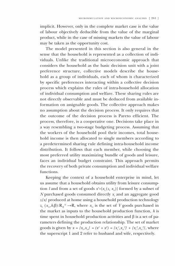
m i c r o s i m u l at i o n a n d m a c r o e c o n o m i c a n a ly s i s [ 261 ]
implicit. However, only in the complete market case is the value of labour objectively deducible from the value of the marginal product, while in the case of missing markets the value of labour may be taken as the opportunity cost.
The model presented in this section is also general in the sense that the household is represented as a collection of indi-viduals. Unlike the traditional microeconomic approach that considers the household as the basic decision unit with a joint preference structure, collective models describe the house-hold as a group of individuals, each of whom is characterized by specific preferences interacting within a collective decision process which explains the rules of intra-household allocation of individual consumption and welfare. These sharing rules are not directly observable and must be deduced from available in-formation on assignable goods. The collective approach makes no assumption about the decision process. It only requires that the outcome of the decision process is Pareto efficient. The process, therefore, is a cooperative one. Decisions take place in a way resembling a two-stage budgeting process. Assuming that the workers of the household pool their incomes, total house-hold income is then allocated to single members according to a predetermined sharing rule defining intra-household income distribution. It follows that each member, while choosing the most preferred utility maximizing bundle of goods and leisure, faces an individual budget constraint. This approach permits the recovery of both private consumption and individual welfare functions.
Keeping the context of a household enterprise in mind, let us assume that a household obtains utility from leisure consump-tion l and from a set of goods x*={xz,(zx xzz)} formed by a subset of N purchased goods consumed directly xz and an aggregate good z{x} produced at home using a household production technology zx (xzz,h;β):R+
N →R, where xzz is the set of V goods purchased in the market as inputs to the household production function, h is time spent in household production activities and β is a set of pa-rameters defining the production relationship. The set of market goods is given by x = {xz,xzz} = (x1 + x2) = {xz
1,xzz2} + {xz
2,xzz2}, where
the superscript 1 and 2 refer to husband and wife, respectively.
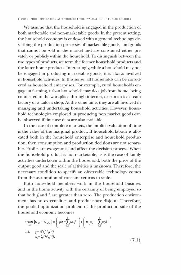
[ 262 ] m i c r o s i m u l at i o n a s a t o o l f o r t h e e va l u at i o n o f p u b l i c p o l i c i e s
We assume that the household is engaged in the production of both marketable and non-marketable goods. In the present setting, the household economy is endowed with a general technology de-scribing the production processes of marketable goods, and goods that cannot be sold in the market and are consumed either pri-vately or publicly within the household. To distinguish between the two types of products, we term the former household products and the latter home products. Interestingly, while a household may not be engaged in producing marketable goods, it is always involved in household activities. In this sense, all households can be consid-ered as household enterprises. For example, rural households en-gage in farming, urban households may do a job from home, being connected to the workplace through internet, or run an ice-cream factory or a tailor’s shop. At the same time, they are all involved in managing and undertaking household activities. However, house-hold technologies employed in producing non market goods can be observed if time-use data are also available.
In the case of complete markets, the implicit valuation of time is the value of the marginal product. If household labour is allo-cated both in the household enterprise and household produc-tion, then consumption and production decisions are not separa-ble. Profits are exogenous and affect the decision process. When the household product is not marketable, as is the case of family activities undertaken within the household, both the price of the output good and the scale of activities is unknown. Therefore, the necessary condition to specify an observable technology comes from the assumption of constant returns to scale.
Both household members work in the household business and in the home activity with the certainty of being employed so that both fi and hi are greater than zero. The production environ-ment has no externalities and products are disjoint. Therefore, the pooled optimization problem of the production side of the household economy becomes
s.t. q= Ψ(f 1,f 2) zx= (h1,f 2),ζ
pq w f p z w h∑ ∑{ }2 2
, 1 1
maxi i x
i iM NM i z x i
f h i i
π π= =
+ = + −
−
(7.1)
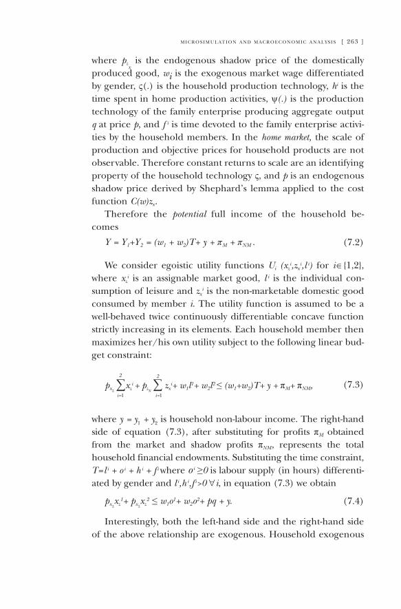
m i c r o s i m u l at i o n a n d m a c r o e c o n o m i c a n a ly s i s [ 263 ]
where pzx is the endogenous shadow price of the domestically
produced good, wi is the exogenous market wage differentiated by gender, ς(.) is the household production technology, hi is the time spent in home production activities, ψ(.) is the production technology of the family enterprise producing aggregate output q at price p, and f i is time devoted to the family enterprise activi-ties by the household members. In the home market, the scale of production and objective prices for household products are not observable. Therefore constant returns to scale are an identifying property of the household technology ς, and p is an endogenous shadow price derived by Shephard’s lemma applied to the cost function C(w)zx.
Therefore the potential full income of the household be-comes
Y = Y1+Y2 = (w1 + w2)T+ y + πM + πNM . (7.2)
We consider egoistic utility functions Ui (xzi,zx
i,l i) for i ∈{1,2}, where xz
i is an assignable market good, l i is the individual con-sumption of leisure and zx
i is the non-marketable domestic good consumed by member i. The utility function is assumed to be a well-behaved twice continuously differentiable concave function strictly increasing in its elements. Each household member then maximizes her/his own utility subject to the following linear bud-get constraint:
pxz ∑xz
i + pzx ∑ zx
i+ w1l1+ w2l2 ≤ (w1+w2)T+ y + πM+ πNM,2 2
i=1 i=1
(7.3)
where y = y1 + y2 is household non-labour income. The right-hand side of equation (7.3), after substituting for profits πM obtained from the market and shadow profits πNM, represents the total household financial endowments. Substituting the time constraint, T= l i + o i + h i + f i where o i ≥0 is labour supply (in hours) differenti-ated by gender and l i,h i,f i>0 ∀i, in equation (7.3) we obtain
pxzxz
1+ pxzxz
2 ≤ w1o1+ w2o2+ pq + y. (7.4)
Interestingly, both the left-hand side and the right-hand side of the above relationship are exogenous. Household exogenous

[ 264 ] m i c r o s i m u l at i o n a s a t o o l f o r t h e e va l u at i o n o f p u b l i c p o l i c i e s
income Y is given by the sum of income obtained from labour supplied outside the household, non wage income y and total re-turns earned from the family enterprise. In our set up, we assume that all household production is sold in the home market at an implicit endogenous price.
The full income version of the budget constraint, where the value of consumption cannot exceed the value of household’s endowment plus household returns, would have to be rewritten as
pxz∑xz
i + pzx ∑zx
i+ w1l1+ w2l2 ≤ (w1o1+ w2o2+ pq + y) +
+ pzxzx + (w1l1+ w2l2),
2 2
i=1 i=1
(7.5)
where the price of the household good pzx is endogenous.
Within a collective framework, and slightly generalizing the structure of both the household and home technology, we can describe the Paretian programme:
Max {U1(xz1,zx
1,l1;d)|U 2 (xz2,zx
2,l 2;d) = u2 }
or
Max {µU1(xz1,zx
1,l1;d) + (1 – µ)U 2(xz2,zx
2,l 2;d)}, (7.6)
subject to the following additional constraints:
∑ ∑ pxzxzj
i+∑ ∑ pxzzxzzk
i=∑wioi+∑ρi(pq−rF)+∑ yi=Y2 N
i=1
2
i=1
2
i=1
2
i=1
2
i=1
V
k=1j=1 Budget
qj = ξ (F,f,d) Household enterprise
zi = ζ (xi,hi,d) Household technology
li = T– hi – oi – fi Time
xzji ≤ x; xzzk
i ≤ x; x,o i,l i,f i,h i,zx,yi,Y ≥0 Capacity and non-negativity
where u2 is the level of utility of member 2 before decisions are made by member 1 that must be maintained to ensure Pareto effi-
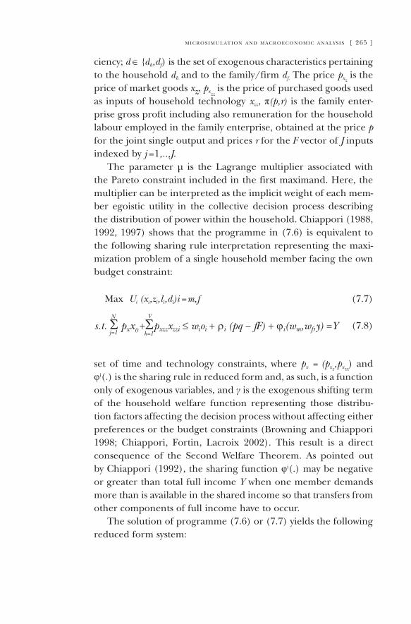
m i c r o s i m u l at i o n a n d m a c r o e c o n o m i c a n a ly s i s [ 265 ]
ciency; d ∈ {dh,df) is the set of exogenous characteristics pertaining to the household dh and to the family/firm df. The price pxz
is the price of market goods xz, pxzz
is the price of purchased goods used as inputs of household technology xzz, π(p,r) is the family enter-prise gross profit including also remuneration for the household labour employed in the family enterprise, obtained at the price p for the joint single output and prices r for the F vector of J inputs indexed by j = 1,..,J.
The parameter µ is the Lagrange multiplier associated with the Pareto constraint included in the first maximand. Here, the multiplier can be interpreted as the implicit weight of each mem-ber egoistic utility in the collective decision process describing the distribution of power within the household. Chiappori (1988, 1992, 1997) shows that the programme in (7.6) is equivalent to the following sharing rule interpretation representing the maxi-mization problem of a single household member facing the own budget constraint:
Max Ui (xi,zi,li,di)i = m,f (7.7)
s.t. Σ pxx0 +Σpxzzxzzi ≤ wioi + ρi (pq − fF) + ϕi(wm,wf,y) =Y j=1 k=1
N V
(7.8)
set of time and technology constraints, where px = (pxz,pxzz
) and φi(.) is the sharing rule in reduced form and, as such, is a function only of exogenous variables, and γ is the exogenous shifting term of the household welfare function representing those distribu-tion factors affecting the decision process without affecting either preferences or the budget constraints (Browning and Chiappori 1998; Chiappori, Fortin, Lacroix 2002). This result is a direct consequence of the Second Welfare Theorem. As pointed out by Chiappori (1992), the sharing function φi(.) may be negative or greater than total full income Y when one member demands more than is available in the shared income so that transfers from other components of full income have to occur.
The solution of programme (7.6) or (7.7) yields the following reduced form system:
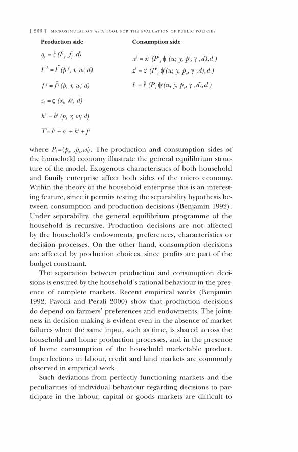
[ 266 ] m i c r o s i m u l at i o n a s a t o o l f o r t h e e va l u at i o n o f p u b l i c p o l i c i e s
Production side Consumption side
qj = ξ (Fj, fj, d)xi = xi (Pi
i φ (w, y, pi, γ ,d),d )˜˜ zi = zi (P i
i φi(w, y, px, γ ,d),d )˜
f j = f j (p, r, w; d)˜ li = li (P i φi(w, y, px, γ ,d),d )˜
zi = ς (xi, hi, d)
hi = hi (p, r, w; d)˜
T= l i + oi + hi + f i
where Pi =(px ,pz,wi). The production and consumption sides of the household economy illustrate the general equilibrium struc-ture of the model. Exogenous characteristics of both household and family enterprise affect both sides of the micro economy. Within the theory of the household enterprise this is an interest-ing feature, since it permits testing the separability hypothesis be-tween consumption and production decisions (Benjamin 1992). Under separability, the general equilibrium programme of the household is recursive. Production decisions are not affected by the household’s endowments, preferences, characteristics or decision processes. On the other hand, consumption decisions are affected by production choices, since profits are part of the budget constraint.
The separation between production and consumption deci-sions is ensured by the household’s rational behaviour in the pres-ence of complete markets. Recent empirical works (Benjamin 1992; Pavoni and Perali 2000) show that production decisions do depend on farmers’ preferences and endowments. The joint-ness in decision making is evident even in the absence of market failures when the same input, such as time, is shared across the household and home production processes, and in the presence of home consumption of the household marketable product. Imperfections in labour, credit and land markets are commonly observed in empirical work.
Such deviations from perfectly functioning markets and the peculiarities of individual behaviour regarding decisions to par-ticipate in the labour, capital or goods markets are difficult to
m i c r o s i m u l at i o n a n d m a c r o e c o n o m i c a n a ly s i s [ 267 ]
model within an econometric model, especially if the model de-scribes production and consumption choices jointly. This is not the case if the estimated model is transferred into a mathematical programming environment that treats corner solutions in a natu-ral way. By so doing, a researcher can pool the statistical power of econometric microsimulation models with the mathematical precision of a programming tool capable of implementing corner choices at the individual level.
The farm-household programming model exactly reproduces the collective farm-household theoretical model underlying the econometric specification. It is calibrated on the elasticities esti-mated in the econometric model (Menon and Perali 2004). For the sake of policy simulations, the programming approach, as compared to the econometric tool, enjoys the flexibility of any general equilibrium model that can produce timing and relevant results by applying simple adaptations to the model without the need to re-estimate the econometric model. The farm-household programming model plays the role of a policy lab that simulates the micro impact of macro policy changes under several assump-tions about market functioning and degree of openness. When the farm-household is treated as a closed economy and (shadow) prices are endogenously determined, then the solution comes from a general equilibrium. Policy impacts are evaluated under more realistic assumptions where some markets clear and others fail. The farm-household models are adapted to disaggregate farm-household types in order to compare differential policy impacts.
Farm-household models use translog technologies to describe both production and consumption preferences and are calibrat-ed on the household social accounting matrix specific to each farm-household type: the average, the less professional, which is the mean of the limited-resources, pension, residential and small, and the professional farm-household formed by medium and large farm-households. The model uses the estimated econometric parameters. Therefore, the need for calibration is reduced to a minimum limited to the calibration of the intercepts of demand and production equations to match the levels of the household SAMs.
[ 268 ] m i c r o s i m u l at i o n a s a t o o l f o r t h e e va l u at i o n o f p u b l i c p o l i c i e s
7.8. Description of household social accounting matrices
The household produces four outputs (crops, beef, milk, and fruit, olives and grapes) using hired labour, chemicals, materials, capital stock and family labour. The production is sold on the mar-ket. The production factors are demanded on the market and re-munerated from the value added. The household economy, which is decentralized in husband and wife, spends the full income, derived as the sum of off-farm income, domestic income, the re-muneration of family labour, the value of leisure and non labour income, to i) purchase market goods (food, clothing and other goods) and ii) consume domestic goods and leisure. The economy acquires the assets produced from the household, pays the family off-farm and non-labour income and gains from the factor supply, the selling of market goods and household savings. This account-ing scheme of the farm-household economy is reported in table 7.8 for professional farms grouping the medium, large and very large farm-households, and in table 7.9 for the non-professional farms grouping the limited-resource, retired, residential, small-farm type.
It should be remarked that the distinction between professional and less professional farm-households is of interest because profes-sional farm-households are the elected recipients of agricultural policies, while less professional farm-households are the subject of in-terest of rural policies, which interestingly enough can be financed by the modulation of agricultural policy. This distinction between farm-household types can be useful to gauge the differential effects of coupling agricultural with rural policies.
The Micro General Equilibrium collective model of the farm-household incorporates the complete set of variables and equa-tions describing the technology of farm production and house-hold consumption as estimated in the microeconometric model. The dual production function as argument has been derived from the estimated cost function describing the farm technology.
The links between the farm-household and the rest of the economy are described in the farm-households SAM presented in tables 7.8 and 7.9.
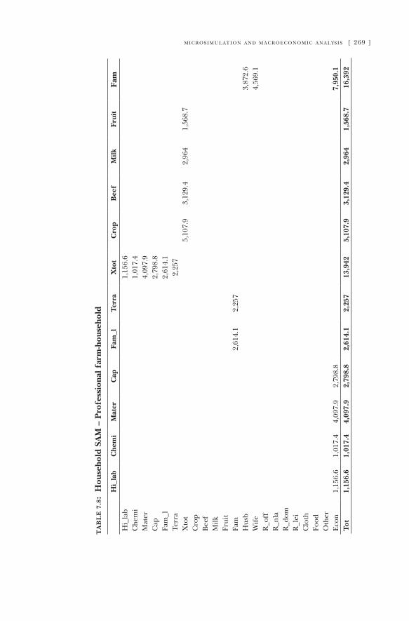
m i c r o s i m u l at i o n a n d m a c r o e c o n o m i c a n a ly s i s [ 269 ]
ta
bl
e 7
.8:
Hou
seho
ld S
AM
– P
rofe
ssio
nal f
arm
-hou
seho
ld
H
i_la
bC
hem
iM
ater
Cap
Fam
_lT
erra
Xto
tC
rop
Bee
fM
ilkFr
uit
Fam
Hi_
lab
1,15
6.6
C
hem
i
1,
017.
4
Mat
er
4,
097.
9
Cap
2,79
8.8
Fa
m_l
2,61
4.1
Te
rra
2,25
7
Xto
t
5,10
7.9
3,12
9.4
2,96
41,
568.
7
Cro
p
B
eef
Milk
Frui
t
Fa
m
2,
614.
12,
257
Hus
b
3,87
2.6
Wife
4,
569.
1R
_off
R_n
la
R
_dom
R_l
ei
C
loth
Food
Oth
er
Eco
n1,
156.
61,
017.
44,
097.
92,
798.
8
7,95
0.1
Tot
1,15
6.6
1,01
7.4
4,09
7.9
2,79
8.8
2,61
4.1
2,25
713
,942
5,10
7.9
3,12
9.4
2,96
41,
568.
716
,392
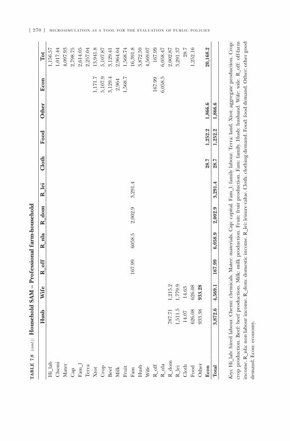
[ 270 ] m i c r o s i m u l at i o n a s a t o o l f o r t h e e va l u at i o n o f p u b l i c p o l i c i e st
ab
le 7
.8 (
cont
.):
Hou
seho
ld S
AM
– P
rofe
ssio
nal f
arm
-hou
seho
ld
H
usb
Wif
eR
_off
R_n
laR
_dom
R_l
eiC
loth
Food
Oth
erE
con
Tot
Hi_
lab
1,
156.
57C
hem
i
1,01
7.44
Mat
er
4,09
7.93
Cap
2,
798.
75Fa
m_l
2,
614.
05Te
rra
2,
257.
04X
tot
1,17
1.7
13,9
41.8
Cro
p
5,
107.
95,
107.
87B
eef
3,12
9.4
3,12
9.41
Milk
2,96
42,
964.
04Fr
uit
1,56
8.7
1,56
8.74
Fam
16
7.99
6058
.52,
002.
93,
291.
4
16
,391
.8H
usb
3,87
2.59
Wife
4,56
9.07
R_o
ff
16
7.99
167.
99R
_nla
6,05
8.5
6,05
8.47
R_d
om
787.
711,
215.
2
2,
002.
87R
_lei
1,
511.
51,
779.
9
3,
291.
37C
loth
14
.07
14.6
3
28
.7Fo
od
626.
0862
6.08
1,25
2.16
Oth
er93
3.38
933.
28E
con
28.7
1,25
2.2
1,86
6.6
20,1
68.2
Tot
al3,
872.
64,
569.
116
7.99
6,05
8.9
2,00
2.9
3,29
1.4
28.7
1,25
2.2
1,86
6.6
Key
s: H
i_la
b: h
ired
labo
ur. C
hem
i: ch
emic
als.
Mat
er: m
ater
ials
. Cap
: cap
ital.
Fam
_l: f
amily
labo
ur. T
erra
: lan
d. X
tot:
aggr
egat
e pr
oduc
tion.
Cro
p:
crop
pro
duct
ion.
Bee
f: be
ef p
rodu
ctio
n. M
ilk:
milk
pro
duct
ion.
Fru
it: f
ruit
prod
uctio
n. F
am:
fam
ily.
Hus
b: h
usba
nd.
Wife
: w
ife.
R_o
ff:
off-f
arm
in
com
e. R
_nla
: non
labo
ur in
com
e. R
_dom
: dom
estic
inco
me.
R_l
ei: l
eisu
re v
alue
. Clo
th: c
loth
ing
dem
and.
Foo
d: fo
od d
eman
d. O
ther
: oth
er g
ood
dem
and.
Eco
n: e
cono
my.
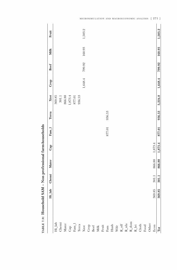
m i c r o s i m u l at i o n a n d m a c r o e c o n o m i c a n a ly s i s [ 271 ]
ta
bl
e 7
.9:
Hou
seho
ld S
AM
– N
on p
rofe
ssio
nal f
arm
-hou
seho
lds
H
i_la
bC
hem
iM
ater
Cap
Fam
_lT
erra
Xto
tC
rop
Bee
fM
ilkFr
uit
Hi_
lab
369.
85
C
hem
i
30
1.1
Mat
er
86
6.88
Cap
1,87
3.4
Fam
_l
87
7.01
Terr
a
93
6.53
Xto
t
1,64
8.4
799.
9216
0.93
1,50
3.2
Cro
p
Bee
f
Milk
Fr
uit
Fa
m
87
7.01
936.
53
Hus
b
Wife
R
_off
R
_nla
R
_dom
R
_lei
C
loth
Fo
od
Oth
er
Eco
n36
9.85
301.
186
6.88
1,87
3.4
T
ot36
9.85
301.
186
6.88
1,87
3.4
877.
0193
6.53
5,22
4.8
1,64
8.4
799.
9216
0.93
1,50
3.2
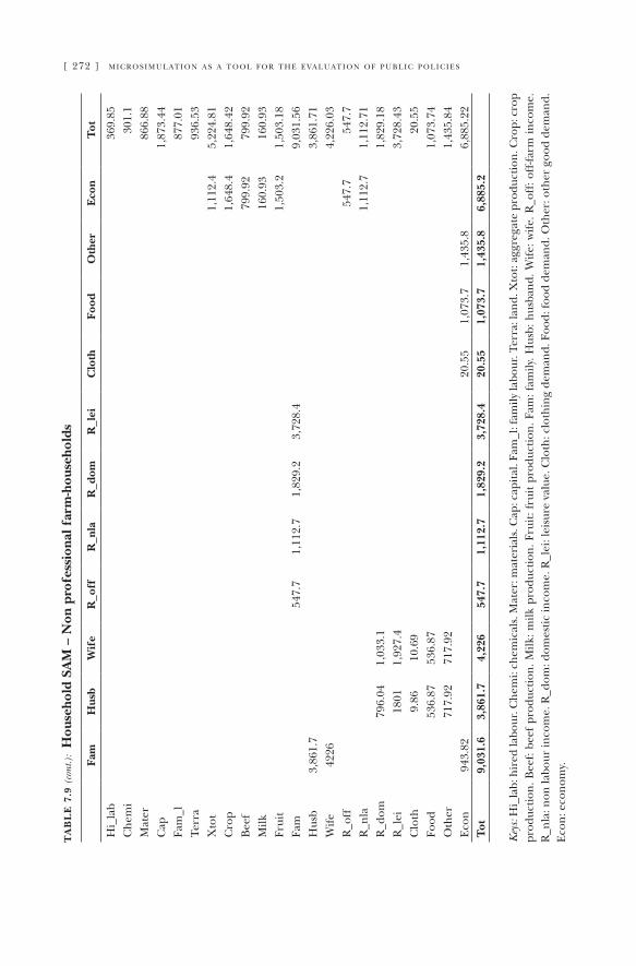
[ 272 ] m i c r o s i m u l at i o n a s a t o o l f o r t h e e va l u at i o n o f p u b l i c p o l i c i e st
ab
le 7
.9 (
cont
.):
Hou
seho
ld S
AM
– N
on p
rofe
ssio
nal f
arm
-hou
seho
lds
Fa
mH
usb
Wif
eR
_off
R_n
laR
_dom
R_l
eiC
loth
Food
Oth
erE
con
Tot
Hi_
lab
36
9.85
Che
mi
30
1.1
Mat
er
866.
88C
ap
1,87
3.44
Fam
_l
877.
01Te
rra
93
6.53
Xto
t
1,
112.
45,
224.
81C
rop
1,64
8.4
1,64
8.42
Bee
f
79
9.92
799.
92M
ilk
16
0.93
160.
93Fr
uit
1,50
3.2
1,50
3.18
Fam
54
7.7
1,11
2.7
1,82
9.2
3,72
8.4
9,03
1.56
Hus
b3,
861.
7
3,
861.
71W
ife42
26
4,
226.
03R
_off
547.
754
7.7
R_n
la
1,
112.
71,
112.
71R
_dom
79
6.04
1,03
3.1
1,82
9.18
R_l
ei
1801
1,92
7.4
3,72
8.43
Clo
th
9.86
10.6
9
20
.55
Food
53
6.87
536.
87
1,
073.
74O
ther
71
7.92
717.
92
1,
435.
84E
con
943.
82
20
.55
1,07
3.7
1,43
5.8
6,
885.
22T
ot9,
031.
63,
861.
74,
226
547.
71,
112.
71,
829.
23,
728.
420
.55
1,07
3.7
1,43
5.8
6,88
5.2
Key
s: H
i_la
b: h
ired
labo
ur. C
hem
i: ch
emic
als.
Mat
er: m
ater
ials
. Cap
: cap
ital.
Fam
_l: f
amily
labo
ur. T
erra
: lan
d. X
tot:
aggr
egat
e pr
oduc
tion.
Cro
p: c
rop
prod
uctio
n. B
eef:
beef
pro
duct
ion.
Milk
: milk
pro
duct
ion.
Fru
it: f
ruit
prod
uctio
n. F
am: f
amily
. Hus
b: h
usba
nd. W
ife: w
ife. R
_off
: off
-farm
inco
me.
R
_nla
: non
labo
ur in
com
e. R
_dom
: dom
estic
inco
me.
R_l
ei: l
eisu
re v
alue
. Clo
th: c
loth
ing
dem
and.
Foo
d: fo
od d
eman
d. O
ther
: oth
er g
ood
dem
and.
E
con:
eco
nom
y.
m i c r o s i m u l at i o n a n d m a c r o e c o n o m i c a n a ly s i s [ 273 ]
7.9. Modelling labour market failures
All markets function perfectly, except the labour market. As we saw in the econometric analysis, the on-farm wage differs sig-nificantly from the off-farm wage, because of nonseparability. We model failure in the labour market as a Mixed Complementarity Problem (MCP) (Löfgren and Robinson 1997, 1999). An MCP model consists of a set of simultaneous equations that are a mix of equalities and inequalities, with each inequality linked to a bounded variable in a complementarity-slackness condition (Rutherford 1995).
Mixed complementarity problems can be represented as a complementarity between a variable and an equation, where the variable is non zero only if the equation is a strictly binding constraint and, conversely, the constraint is binding when the variable is zero. In other words, complementarity conditions state that either the non negative variable must be zero or the corresponding inequality must hold with equality, or both.
For example, if we consider the professional farm-house-hold type, characterized by an endogenous on-farm wage greater than the exogenous off-farm wage, the farm household will supply on-farm labour at the fixed upper bound only if the on-farm wage is greater than the off-farm wage. However, if the on-farm wage is less than or equal to the off-farm wage, the family labour supply decreases. For the non professional farm-household type, the situation is a mirror of the previous one. The farm household increases the on-farm labour supply only if the on-farm wage is greater than or equal to the off-farm wage; otherwise, it supplies an amount of on-farm labour equal to the fixed lower bound corresponding to the observed level. This Kuhn-Tucker rule applies to both the husband and the wife.
The associated complementarity-slackness condition is:
FS_labg (w_offg–wage_on) = 0, g ∈ G {husband, wife}
where: FS_labg= 0 if w_off –wage_on, and FS_labg> 0 if w_off –wage_on.
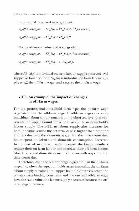
[ 274 ] m i c r o s i m u l at i o n a s a t o o l f o r t h e e va l u at i o n o f p u b l i c p o l i c i e s
Professional: observed wage gradient:
w_off < wage_on → FS_labg = FS_labg0 (Upper bound)
w_off ≥ wage_on → FS_labg < FS_labg0
Non professional: observed wage gradient:
w_off > wage_on → FS_labg = FS_labg0 (Lower bound)
w_off ≤ wage_on → FS_labg > FS_labg0
where FS_labg0 is individual on farm labour supply: observed level (upper or lower bound); FS_labg is individual on farm labour sup-ply; w_off, the off-farm wage, and wage_on the on-farm wage.
7.10. An example: the impact of changes in off-farm wages
For the professional household farm type, the on-farm wage is greater than the off-farm wage. If off-farm wages decrease, individual labour supply remains at the observed level that rep-resents the upper bound for a professional farm household’s labour supply. The off-farm labour supply also increases for both individuals since the off-farm wage is higher than both the leisure value and the domestic wage. For the time constraint, hours spent on leisure and domestic consumption decrease. In the case of an off-farm wage increase, the family members reduce their on-farm labour and increase their off-farm labour. Also, leisure and domestic demands increase with respect to the time constraint.
Therefore, when the off-farm wage is greater than the on-farm wage, i.e., when the equation holds as an inequality, the on-farm labour supply remains at the upper bound. Conversely, when the equation is a binding constraint and the on- and off-farm wage have the same value, the labour supply decreases because the off-farm wage increases.
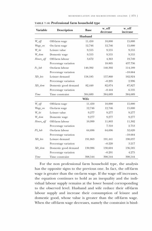
m i c r o s i m u l at i o n a n d m a c r o e c o n o m i c a n a ly s i s [ 275 ]
table 7.10: Professional farm household type
Variable Description Base w_off decrease
w_off increase
Husband
W_off Off-farm wage 11,450 10,000 15,000
Wage_on On farm wage 12,746 12,746 15,000
W_lei Leisure value 9,555 9,555 9,555
W_dom Domestic wage 9,555 9,555 9,555
Hours_off Off-farm labour 3,672 4,363 19,749
Percentage variation 18.805 437.736
Fs_lab On-farm labour 140,392 140,392 114,189
Percentage variation –18.664
XD_leis Leisure demand 158,185 157,860 162,924
Percentage variation –0.205 2.996
XD_dom Domestic good demand 82,440 82,074 87,827
Percentage variation –0.444 6.535
Time Time constraint 384,689 384,689 384,689
Wife
W_off Off-farm wage 11,450 10,000 15,000
Wage_on On-farm wage 12,746 12,746 15,000
W_lei Leisure value 9,277 9,277 9,277
W_dom Domestic wage 9,277 9,277 9,277
Hours_off Off-farm labour 10,999 11,803 11,302
Percentage variation 7.310 2.753
FS_lab On-farm labour 64,696 64,696 52,620
Percentage variation –18.664
XD_leis Leisure demand 191,863 191,441 198,037
Percentage variation –0.220 3.217
XD_dom Domestic good demand 130,986 130,604 136,585
Percentage variation –0.291 4.275
Time Time constraint 398,544 398,544 398,544
For the non professional farm household type, the analysis has the opposite signs to the previous one. In fact, the off-farm wage is greater than the on-farm wage. If the wage off increases, the equation continues to hold as an inequality and the indi-vidual labour supply remains at the lower bound corresponding to the observed level. Husband and wife reduce their off-farm labour supply and increase their consumption of leisure and domestic good, whose value is greater than the off-farm wage. When the off-farm wage decreases, namely the constraint is bind-
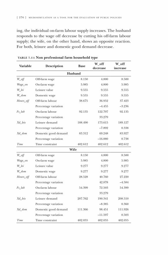
[ 276 ] m i c r o s i m u l at i o n a s a t o o l f o r t h e e va l u at i o n o f p u b l i c p o l i c i e s
ing, the individual on-farm labour supply increases. The husband responds to the wage off decrease by cutting his off-farm labour supply; the wife, on the other hand, shows an opposite reaction. For both, leisure and domestic good demand decrease.
table 7.11: Non professional farm household type
Variable Description BaseW_off
decreaseW_off
increase
Husband
W_off Off-farm wage 8.150 4.800 8.500
Wage_on On-farm wage 5.985 4.800 5.985
W_lei Leisure value 9.555 9.555 9.555
W_dom Domestic wage 9.555 9.555 9.555
Hours_off Off-farm labour 38.675 36.952 37.423
Percentage variation –4.455 –3.236
Fs_lab On-farm labour 92.135 122.797 92.135
Percentage variation 33.279
Xd_leis Leisure demand 188.490 173.615 189.127
Percentage variation –7.892 0.338
Xd_dom Domestic good demand 83.312 69.248 83.927
Percentage variation –16.880 0.738
Time Time constraint 402.612 402.612 402.612
Wife
W_off Off-farm wage 8.150 4.800 8.500
Wage_on On-farm wage 5.985 4.800 5.985
W_lei Leisure value 9.277 9.277 9.277
W_dom Domestic wage 9.277 9.277 9.277
Hours_off Off-farm labour 28.528 40.760 27.220
Percentage variation 42.878 –4.584
Fs_lab On-farm labour 54.399 72.503 54.399
Percentage variation 33.279
Xd_leis Leisure demand 207.762 190.341 208.510
Percentage variation –8.385 0.360
Xd_dom Domestic good demand 111.366 98.451 111.926
Percentage variation –11.597 0.503
Time Time constraint 402.055 402.055 402.055
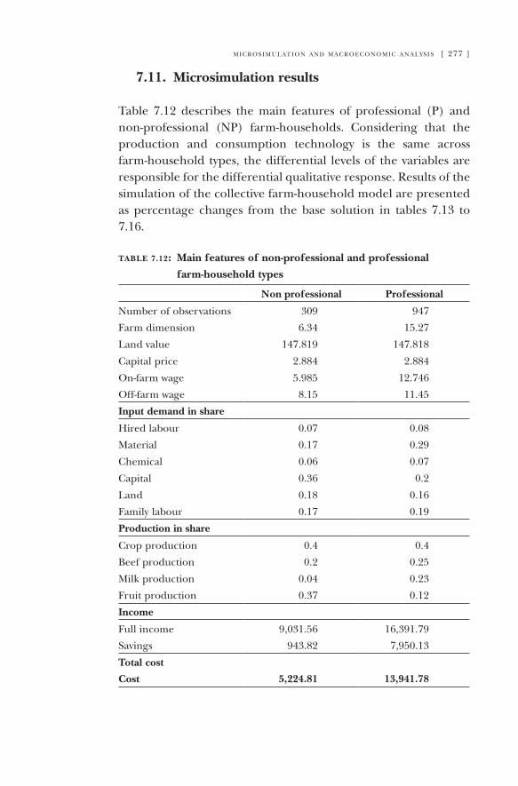
m i c r o s i m u l at i o n a n d m a c r o e c o n o m i c a n a ly s i s [ 277 ]
7.11. Microsimulation results
Table 7.12 describes the main features of professional (P) and non-professional (NP) farm-households. Considering that the production and consumption technology is the same across farm-household types, the differential levels of the variables are responsible for the differential qualitative response. Results of the simulation of the collective farm-household model are presented as percentage changes from the base solution in tables 7.13 to 7.16.
table 7.12: Main features of non-professional and professional
farm-household types
Non professional Professional
Number of observations 309 947
Farm dimension 6.34 15.27
Land value 147.819 147.818
Capital price 2.884 2.884
On-farm wage 5.985 12.746
Off-farm wage 8.15 11.45
Input demand in share
Hired labour 0.07 0.08
Material 0.17 0.29
Chemical 0.06 0.07
Capital 0.36 0.2
Land 0.18 0.16
Family labour 0.17 0.19
Production in share
Crop production 0.4 0.4
Beef production 0.2 0.25
Milk production 0.04 0.23
Fruit production 0.37 0.12
Income
Full income 9,031.56 16,391.79
Savings 943.82 7,950.13
Total cost
Cost 5,224.81 13,941.78
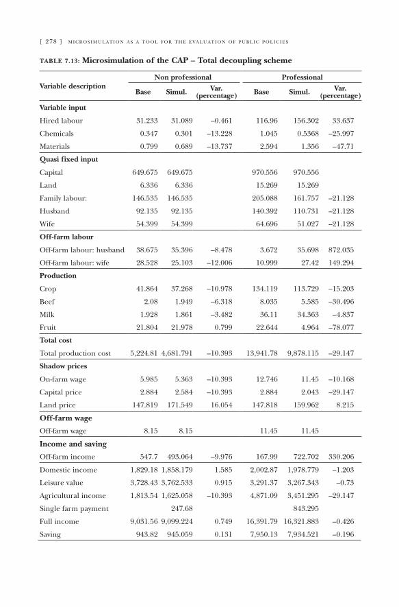
[ 278 ] m i c r o s i m u l at i o n a s a t o o l f o r t h e e va l u at i o n o f p u b l i c p o l i c i e s
table 7.13: Microsimulation of the CAP – Total decoupling scheme
Variable descriptionNon professional Professional
Base Simul. Var. (percentage) Base Simul. Var.
(percentage)
Variable input
Hired labour 31.233 31.089 –0.461 116.96 156.302 33.637
Chemicals 0.347 0.301 –13.228 1.045 0.5368 –25.997
Materials 0.799 0.689 –13.737 2.594 1.356 –47.71
Quasi fixed input
Capital 649.675 649.675 970.556 970.556
Land 6.336 6.336 15.269 15.269
Family labour: 146.535 146.535 205.088 161.757 –21.128
Husband 92.135 92.135 140.392 110.731 –21.128
Wife 54.399 54.399 64.696 51.027 –21.128
Off-farm labour
Off-farm labour: husband 38.675 35.396 –8.478 3.672 35.698 872.035
Off-farm labour: wife 28.528 25.103 –12.006 10.999 27.42 149.294
Production
Crop 41.864 37.268 –10.978 134.119 113.729 –15.203
Beef 2.08 1.949 –6.318 8.035 5.585 –30.496
Milk 1.928 1.861 –3.482 36.11 34.363 –4.837
Fruit 21.804 21.978 0.799 22.644 4.964 –78.077
Total cost
Total production cost 5,224.81 4,681.791 –10.393 13,941.78 9,878.115 –29.147
Shadow prices
On-farm wage 5.985 5.363 –10.393 12.746 11.45 –10.168
Capital price 2.884 2.584 –10.393 2.884 2.043 –29.147
Land price 147.819 171.549 16.054 147.818 159.962 8.215
Off-farm wage
Off-farm wage 8.15 8.15 11.45 11.45
Income and saving
Off-farm income 547.7 493.064 –9.976 167.99 722.702 330.206
Domestic income 1,829.18 1,858.179 1.585 2,002.87 1,978.779 –1.203
Leisure value 3,728.43 3,762.533 0.915 3,291.37 3,267.343 –0.73
Agricultural income 1,813.54 1,625.058 –10.393 4,871.09 3,451.295 –29.147
Single farm payment 247.68 843.295
Full income 9,031.56 9,099.224 0.749 16,391.79 16,321.883 –0.426
Saving 943.82 945.059 0.131 7,950.13 7,934.521 –0.196
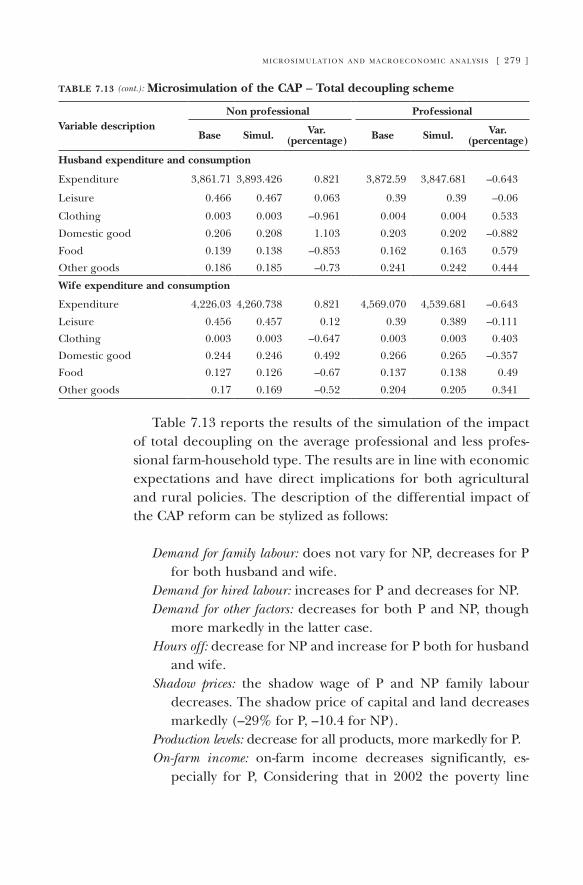
m i c r o s i m u l at i o n a n d m a c r o e c o n o m i c a n a ly s i s [ 279 ]
table 7.13 (cont.): Microsimulation of the CAP – Total decoupling scheme
Variable descriptionNon professional Professional
Base Simul. Var. (percentage) Base Simul. Var.
(percentage)
Husband expenditure and consumption
Expenditure 3,861.71 3,893.426 0.821 3,872.59 3,847.681 –0.643
Leisure 0.466 0.467 0.063 0.39 0.39 –0.06
Clothing 0.003 0.003 –0.961 0.004 0.004 0.533
Domestic good 0.206 0.208 1.103 0.203 0.202 –0.882
Food 0.139 0.138 –0.853 0.162 0.163 0.579
Other goods 0.186 0.185 –0.73 0.241 0.242 0.444
Wife expenditure and consumption
Expenditure 4,226.03 4,260.738 0.821 4,569.070 4,539.681 –0.643
Leisure 0.456 0.457 0.12 0.39 0.389 –0.111
Clothing 0.003 0.003 –0.647 0.003 0.003 0.403
Domestic good 0.244 0.246 0.492 0.266 0.265 –0.357
Food 0.127 0.126 –0.67 0.137 0.138 0.49
Other goods 0.17 0.169 –0.52 0.204 0.205 0.341
Table 7.13 reports the results of the simulation of the impact of total decoupling on the average professional and less profes-sional farm-household type. The results are in line with economic expectations and have direct implications for both agricultural and rural policies. The description of the differential impact of the CAP reform can be stylized as follows:
Demand for family labour: does not vary for NP, decreases for P for both husband and wife.
Demand for hired labour: increases for P and decreases for NP.Demand for other factors: decreases for both P and NP, though
more markedly in the latter case.Hours off: decrease for NP and increase for P both for husband
and wife.Shadow prices: the shadow wage of P and NP family labour
decreases. The shadow price of capital and land decreases markedly (–29% for P, –10.4 for NP).
Production levels: decrease for all products, more markedly for P.On-farm income: on-farm income decreases significantly, es-
pecially for P, Considering that in 2002 the poverty line
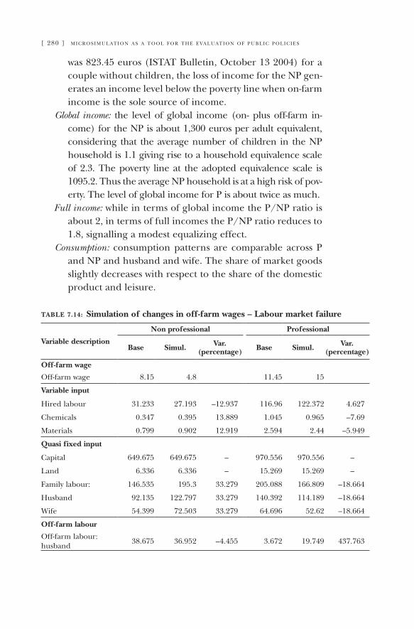
[ 280 ] m i c r o s i m u l at i o n a s a t o o l f o r t h e e va l u at i o n o f p u b l i c p o l i c i e s
was 823.45 euros (ISTAT Bulletin, October 13 2004) for a couple without children, the loss of income for the NP gen-erates an income level below the poverty line when on-farm income is the sole source of income.
Global income: the level of global income (on- plus off-farm in-come) for the NP is about 1,300 euros per adult equivalent, considering that the average number of children in the NP household is 1.1 giving rise to a household equivalence scale of 2.3. The poverty line at the adopted equivalence scale is 1095.2. Thus the average NP household is at a high risk of pov-erty. The level of global income for P is about twice as much.
Full income: while in terms of global income the P/NP ratio is about 2, in terms of full incomes the P/NP ratio reduces to 1.8, signalling a modest equalizing effect.
Consumption: consumption patterns are comparable across P and NP and husband and wife. The share of market goods slightly decreases with respect to the share of the domestic product and leisure.
table 7.14: Simulation of changes in off-farm wages – Labour market failure
Variable description
Non professional Professional
Base Simul. Var. (percentage) Base Simul. Var.
(percentage)
Off-farm wage
Off-farm wage 8.15 4.8 11.45 15
Variable input
Hired labour 31.233 27.193 –12.937 116.96 122.372 4.627
Chemicals 0.347 0.395 13.889 1.045 0.965 –7.69
Materials 0.799 0.902 12.919 2.594 2.44 –5.949
Quasi fixed input
Capital 649.675 649.675 – 970.556 970.556 –
Land 6.336 6.336 – 15.269 15.269 –
Family labour: 146.535 195.3 33.279 205.088 166.809 –18.664
Husband 92.135 122.797 33.279 140.392 114.189 –18.664
Wife 54.399 72.503 33.279 64.696 52.62 –18.664
Off-farm labour
Off-farm labour: husband 38.675 36.952 –4.455 3.672 19.749 437.763
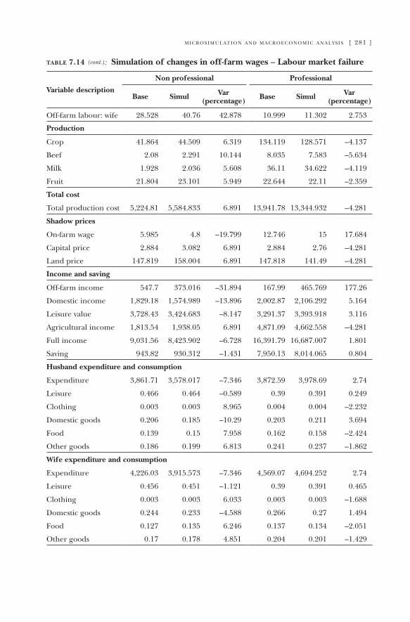
m i c r o s i m u l at i o n a n d m a c r o e c o n o m i c a n a ly s i s [ 281 ]
table 7.14 (cont.): Simulation of changes in off-farm wages – Labour market failure
Variable description
Non professional Professional
Base Simul Var (percentage) Base Simul Var
(percentage)
Off-farm labour: wife 28.528 40.76 42.878 10.999 11.302 2.753
Production
Crop 41.864 44.509 6.319 134.119 128.571 –4.137
Beef 2.08 2.291 10.144 8.035 7.583 –5.634
Milk 1.928 2.036 5.608 36.11 34.622 –4.119
Fruit 21.804 23.101 5.949 22.644 22.11 –2.359
Total cost
Total production cost 5,224.81 5,584.833 6.891 13,941.78 13,344.932 –4.281
Shadow prices
On-farm wage 5.985 4.8 –19.799 12.746 15 17.684
Capital price 2.884 3.082 6.891 2.884 2.76 –4.281
Land price 147.819 158.004 6.891 147.818 141.49 –4.281
Income and saving
Off-farm income 547.7 373.016 –31.894 167.99 465.769 177.26
Domestic income 1,829.18 1,574.989 –13.896 2,002.87 2,106.292 5.164
Leisure value 3,728.43 3,424.683 –8.147 3,291.37 3,393.918 3.116
Agricultural income 1,813.54 1,938.05 6.891 4,871.09 4,662.558 –4.281
Full income 9,031.56 8,423.902 –6.728 16,391.79 16,687.007 1.801
Saving 943.82 930.312 –1.431 7,950.13 8,014.065 0.804
Husband expenditure and consumption
Expenditure 3,861.71 3,578.017 –7.346 3,872.59 3,978.69 2.74
Leisure 0.466 0.464 –0.589 0.39 0.391 0.249
Clothing 0.003 0.003 8.965 0.004 0.004 –2.232
Domestic goods 0.206 0.185 –10.29 0.203 0.211 3.694
Food 0.139 0.15 7.958 0.162 0.158 –2.424
Other goods 0.186 0.199 6.813 0.241 0.237 –1.862
Wife expenditure and consumption
Expenditure 4,226.03 3,915.573 –7.346 4,569.07 4,694.252 2.74
Leisure 0.456 0.451 –1.121 0.39 0.391 0.465
Clothing 0.003 0.003 6.033 0.003 0.003 –1.688
Domestic goods 0.244 0.233 –4.588 0.266 0.27 1.494
Food 0.127 0.135 6.246 0.137 0.134 –2.051
Other goods 0.17 0.178 4.851 0.204 0.201 –1.429
[ 282 ] m i c r o s i m u l at i o n a s a t o o l f o r t h e e va l u at i o n o f p u b l i c p o l i c i e s
Table 7.14 describes results of the analysis of the labour mar-ket failure. We simulate situations that are likely to occur for farm-households belonging to the Professional or Non-profes-sional groups, but that are close to being part of the other group if the wage differential changes its sign. This switching regime is ensured by the mixed complementarity condition. The results show that professional and non-professional farm-households react to changes in off-farm wages as expected from theory pre-dictions.
Table 7.15 describes the simulation of a change in the intra-household distribution of resources, where the distribution of power passes from the observed situation of 57% percent of full income being under control of the woman to a fair distribution of power where both wife and husband control 50% of full income. The changes are significant in almost all variables. Behavioural changes in allocation of time and labour at the individual level are of special policy interest. As a consequence of the power shift, the husband’s on-farm employment decreases by 10.3% corre-sponding to a reduction in the husband’s contribution to farm income of 11.9%, while the wife’s on-farm employment increases by 28.6% generating a 26.2% increase in on-farm income. The reallocation of power gives the husband greater control over the level of expenditure and the consumption of leisure, which both increase by about 7.3%.
In general, the reform in the short run may affect the distribu-tion of power by changing the relative price of leisure and other goods. On the other hand, a change in the distribution of power may be a powerful and useful tool to correct part of the undesir-able effects of the reform.
Table 7.16 reports the impact at the micro level of changes in the international trade scenario, including the one half reduction in the level of the single farm payment. In line with the previous scenarios, the impact is markedly differentiated across farm-household types. With respect to the CAP scenario of total decoupling (table 7.13), the non professional farm-household reacts to the new trade environment and to the one half reduction of the single farm payment by slightly increas-ing off-farm employment, because the on-farm shadow wage
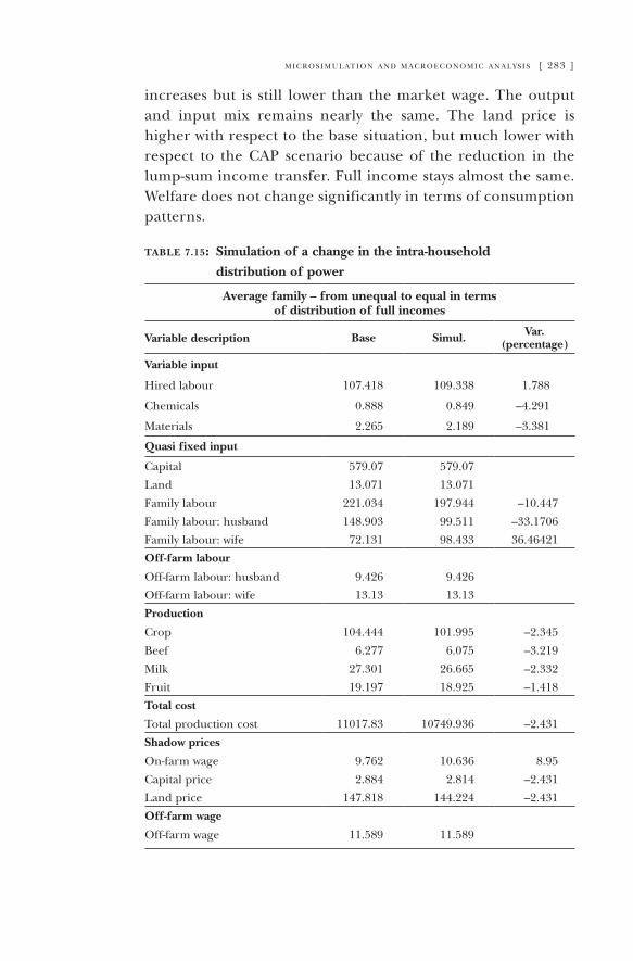
m i c r o s i m u l at i o n a n d m a c r o e c o n o m i c a n a ly s i s [ 283 ]
increases but is still lower than the market wage. The output and input mix remains nearly the same. The land price is higher with respect to the base situation, but much lower with respect to the CAP scenario because of the reduction in the lump-sum income transfer. Full income stays almost the same. Welfare does not change significantly in terms of consumption patterns.
table 7.15: Simulation of a change in the intra-household
distribution of power
Average family – from unequal to equal in terms of distribution of full incomes
Variable description Base Simul. Var. (percentage)
Variable input
Hired labour 107.418 109.338 1.788
Chemicals 0.888 0.849 –4.291
Materials 2.265 2.189 –3.381
Quasi fixed input
Capital 579.07 579.07
Land 13.071 13.071
Family labour 221.034 197.944 –10.447
Family labour: husband 148.903 99.511 –33.1706
Family labour: wife 72.131 98.433 36.46421
Off-farm labour
Off-farm labour: husband 9.426 9.426
Off-farm labour: wife 13.13 13.13
Production
Crop 104.444 101.995 –2.345
Beef 6.277 6.075 –3.219
Milk 27.301 26.665 –2.332
Fruit 19.197 18.925 –1.418
Total cost
Total production cost 11017.83 10749.936 –2.431
Shadow prices
On-farm wage 9.762 10.636 8.95
Capital price 2.884 2.814 –2.431
Land price 147.818 144.224 –2.431
Off-farm wage
Off-farm wage 11.589 11.589
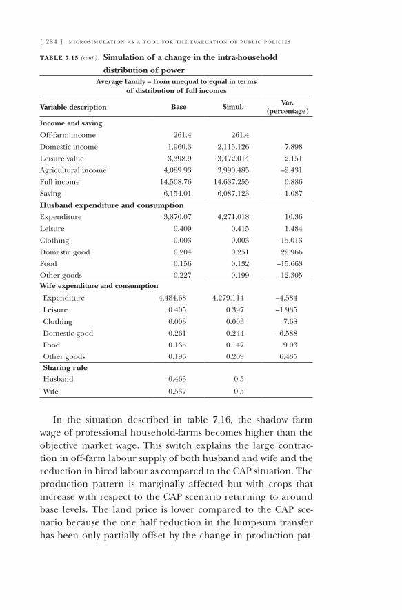
[ 284 ] m i c r o s i m u l at i o n a s a t o o l f o r t h e e va l u at i o n o f p u b l i c p o l i c i e s
table 7.15 (cont.): Simulation of a change in the intra-household
distribution of powerAverage family – from unequal to equal in terms
of distribution of full incomes
Variable description Base Simul. Var. (percentage)
Income and saving
Off-farm income 261.4 261.4
Domestic income 1,960.3 2,115.126 7.898
Leisure value 3,398.9 3,472.014 2.151
Agricultural income 4,089.93 3,990.485 –2.431
Full income 14,508.76 14,637.255 0.886
Saving 6,154.01 6,087.123 –1.087
Husband expenditure and consumptionExpenditure 3,870.07 4,271.018 10.36
Leisure 0.409 0.415 1.484
Clothing 0.003 0.003 –15.013
Domestic good 0.204 0.251 22.966
Food 0.156 0.132 –15.663
Other goods 0.227 0.199 –12.305Wife expenditure and consumption
Expenditure 4,484.68 4,279.114 –4.584
Leisure 0.405 0.397 –1.935
Clothing 0.003 0.003 7.68
Domestic good 0.261 0.244 –6.588
Food 0.135 0.147 9.03
Other goods 0.196 0.209 6.435Sharing ruleHusband 0.463 0.5
Wife 0.537 0.5
In the situation described in table 7.16, the shadow farm wage of professional household-farms becomes higher than the objective market wage. This switch explains the large contrac-tion in off-farm labour supply of both husband and wife and the reduction in hired labour as compared to the CAP situation. The production pattern is marginally affected but with crops that increase with respect to the CAP scenario returning to around base levels. The land price is lower compared to the CAP sce-nario because the one half reduction in the lump-sum transfer has been only partially offset by the change in production pat-
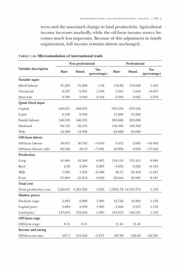
m i c r o s i m u l at i o n a n d m a c r o e c o n o m i c a n a ly s i s [ 285 ]
terns and the associated change in land productivity. Agricultural income increases markedly, while the off-farm income source be-comes much less important. Because of this adjustment in family organization, full income remains almost unchanged.
table 7.16: Microsimulation of international trade
Variable description
Non professional Professional
Base Simul.Var.
(percentage)Base Simul.
Var. (percentage)
Variable input
Hired labour 31.233 31.699 1.49 116.96 118.648 1.443
Chemicals 0.347 0.351 1.339 1.045 1.044 –0.057
Materials 0.799 0.816 2.164 2.594 2.627 1.278
Quasi fixed input
Capital 649.675 649.675 970.556 970.556
Land 6.336 6.336 15.269 15.269
Family labour: 146.535 146.535 205.088 205.088
Husband 92.135 92.135 140.392 140.392
Wife 54.399 54.399 64.696 64.696
Off-farm labour
Off-farm labour: 38.675 36.763 –4.943 3.672 2.005 –45.402
Off-farm labour: wife 28.528 26.53 –7.001 10.999 9.059 –17.642
Production
Crop 41.864 42.268 0.967 134.119 135.412 0.964
Beef 2.08 2.084 0.203 8.035 8.022 –0.163
Milk 1.928 1.916 –0.588 36.11 35.443 –1.847
Fruit 21.804 21.854 0.229 22.644 22.685 0.181
Total cost
Total production cost 5,224.81 5,324.325 1.905 1,3941.78 14,103.374 1.159
Shadow prices
On-farm wage 5.985 6.099 1.905 12.746 12.894 1.159
Capital price 2.884 2.939 1.905 2.884 2.917 1.159
Land price 147.819 150.634 1.905 147.818 149.531 1.159
Off-farm wage
Off-farm wage 8.15 8.15 11.45 11.45
Income and saving
Off-farm income 547.7 515.843 –5.817 167.99 126.68 –24.591
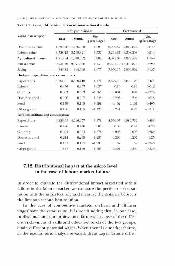
[ 286 ] m i c r o s i m u l at i o n a s a t o o l f o r t h e e va l u at i o n o f p u b l i c p o l i c i e s
table 7.16 (cont.): Microsimulation of international trade
Variable description
Non professional Professional
Base Simul.Var.
(percentage)Base Simul.
Var. (percentage)
Domestic income 1,829.18 1,846.083 0.924 2,002.87 2,019.876 0.849
Leisure value 3,728.43 3,748.321 0.533 3,291.37 3,308.298 0.514
Agricultural income 1,813.54 1,848.082 1.905 4,871.09 4,927.549 1.159
Full income 9,031.56 9,071.038 0.437 16,391.79 16,440.873 0.299
Saving 943.82 944.549 0.077 7,950.13 7,960.982 0.137
Husband expenditure and consumption
Expenditure 3,861.71 3,880.212 0.479 3,872.59 3,890.128 0.453
Leisure 0.466 0.467 0.037 0.39 0.39 0.042
Clothing 0.003 0.003 –0.562 0.004 0.004 –0.373
Domestic good 0.206 0.207 0.645 0.203 0.205 0.618
Food 0.139 0.138 –0.499 0.162 0.161 –0.405
Other goods 0.186 0.185 –0.427 0.241 0.24 –0.311
Wife expenditure and consumption
Expenditure 4,226.03 4,246.277 0.479 4,569.07 4,589.762 0.453
Leisure 0.456 0.456 0.07 0.39 0.39 0.078
Clothing 0.003 0.003 –0.378 0.003 0.003 –0.282
Domestic good 0.244 0.245 0.287 0.266 0.267 0.25
Food 0.127 0.127 –0.391 0.137 0.137 –0.343
Other goods 0.17 0.169 –0.304 0.204 0.204 –0.239
7.12. Distributional impact at the micro level in the case of labour market failure
In order to evaluate the distributional impact associated with a failure in the labour market, we compare the perfect market so-lution with the imperfect one and measure the distance between the first and second best solution.
In the case of competitive markets, on-farm and off-farm wages have the same value. It is worth noting that, in our case, professional and non-professional farmers, because of the differ-ent endowment of skills and education levels of the two groups, attain different potential wages. When there is a market failure, as the econometric analysis revealed, these wages assume differ-
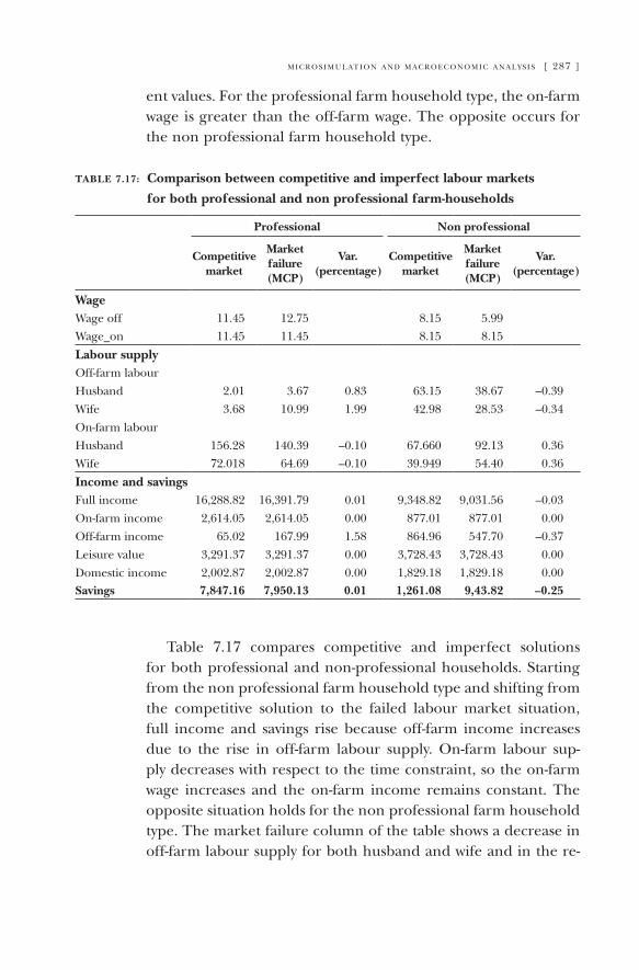
m i c r o s i m u l at i o n a n d m a c r o e c o n o m i c a n a ly s i s [ 287 ]
ent values. For the professional farm household type, the on-farm wage is greater than the off-farm wage. The opposite occurs for the non professional farm household type.
table 7.17: Comparison between competitive and imperfect labour markets
for both professional and non professional farm-households
Professional Non professional
Competitive market
Market failure (MCP)
Var. (percentage)
Competitive market
Market failure (MCP)
Var. (percentage)
Wage Wage off 11.45 12.75 8.15 5.99 Wage_on 11.45 11.45 8.15 8.15
Labour supply Off-farm labour Husband 2.01 3.67 0.83 63.15 38.67 –0.39Wife 3.68 10.99 1.99 42.98 28.53 –0.34On-farm labour Husband 156.28 140.39 –0.10 67.660 92.13 0.36Wife 72.018 64.69 –0.10 39.949 54.40 0.36
Income and savings Full income 16,288.82 16,391.79 0.01 9,348.82 9,031.56 –0.03On-farm income 2,614.05 2,614.05 0.00 877.01 877.01 0.00Off-farm income 65.02 167.99 1.58 864.96 547.70 –0.37Leisure value 3,291.37 3,291.37 0.00 3,728.43 3,728.43 0.00Domestic income 2,002.87 2,002.87 0.00 1,829.18 1,829.18 0.00Savings 7,847.16 7,950.13 0.01 1,261.08 9,43.82 –0.25
Table 7.17 compares competitive and imperfect solutions for both professional and non-professional households. Starting from the non professional farm household type and shifting from the competitive solution to the failed labour market situation, full income and savings rise because off-farm income increases due to the rise in off-farm labour supply. On-farm labour sup-ply decreases with respect to the time constraint, so the on-farm wage increases and the on-farm income remains constant. The opposite situation holds for the non professional farm household type. The market failure column of the table shows a decrease in off-farm labour supply for both husband and wife and in the re-
[ 288 ] m i c r o s i m u l at i o n a s a t o o l f o r t h e e va l u at i o n o f p u b l i c p o l i c i e s
lated off-farm income, full income and savings, and an increase in on-farm labour supply. Consequently, the on-farm wage decreases compared to the off-farm wage. In general, judging by the level of full income and savings, competitive markets are welfare dete-riorating for professional households and welfare improving for non professional farm-households.
7.13. Conclusions
This research has developed a general equilibrium model for the Italian economy to evaluate the macro effects of the CAP re-form to be transmitted at the micro level of analysis, in order to estimate the behavioural and welfare impact on farm-households within a farm-household general equilibrium model. The micro general equilibrium collective model is not calibrated, because it incorporates as such the econometric model of the farm-house-hold and the estimated technologies of production and consump-tion. The macro-micro link is fully carried out in our experiment because the macro effect is evaluated at the micro level both at the household and at the individual level, as a result of the econo-metric estimation of the rule governing the intra-household pro-cess of resource allocation.
The micro-macro link built in the present research has the virtue of allowing an exact statistical aggregation (Stoker 1993) between the micro and macro level of analysis. For this to hap-pen, it is necessary to run the policy microsimulation at the level of each farm-household type identified also at the macro level. This statistical consistency across levels of aggregation is ensured by the peculiar design of the underlying information source, which is the same across levels. Therefore, embedded in the mi-cro-macro approach adopted in this study is the potential for a natural micro-macro closure.
The approach also suffers from another type of aggregation problem. At the macro level, the effects on production are not differentiated by farm-household type, because production tech-nology is the same for all farm types. The incorporation of this feature would require the enlargement of the model to host 23
m i c r o s i m u l at i o n a n d m a c r o e c o n o m i c a n a ly s i s [ 289 ]
activities for each farm type, allowing the possibility for each type to adopt an optimal subset of activities. This exercise is left for future developments of the model.
The macro shock from the CAP reform generates significantly different behavioural responses at the micro level of professional and non-professional farm-households. The reform impacts differ-ently upon husbands and wives employed in agriculture. Demand for farm labour decreases in both professional and non-profession-al farm-households, but wives reduce their involvement in farming activities by more than double the proportion of the husband. Women in both professional and non-professional farm-house-holds show more flexibility. Both professional and non-professional farms suffer a reduction in global income, but the loss of income and of welfare can be critical for non-professional farm-households that are more exposed to the risk of poverty. In this sense, non-pro-fessional farm-households are a more appropriate target for rural rather than agricultural policies. In general, competitive markets are welfare deteriorating for professional households and welfare improving for non professional farm-households.
Micro and macro results are generally consistent. Behavioural responses at the micro level reveal a differentiated pattern that calls for targeted policies. The household’s capability to adjust to changes by reallocating its resources acts as a powerful cushion against the risk of incurring welfare losses. From a policy perspec-tive, it is fundamental to realize that this mitigation effect only works if output and factor markets function properly. Otherwise, households would not be able to compensate negative effects by selling their resources off farm or acquiring resources through land, labour and capital markets. As a suggestion for future re-search, incorporating these aspects in the modelling framework is crucial for a full understanding of the real impact of reforms.
References
adelman, i. and s. robinson. Income Distribution Policy: A Computable General Equilibrium Model of South Korea. Stanford: Stanford University Press, 1978.
becker, G. s. “A Theory of Allocation of Time.” Economic Journal 75 no. 299 (1965): 493–517.
[ 290 ] m i c r o s i m u l at i o n a s a t o o l f o r t h e e va l u at i o n o f p u b l i c p o l i c i e s
benjamin, c. and a. kimhi. “Farm Work, Off-Farm Work, and Hired Farm Labour: Estimating a Discrete-Choice Model of French Farm Couples. Labour Decisions.” Working Paper, 2003.
benjamin, d. “Household Composition, Labour Markets, and Labour Demand: Testing for Separation in Agricultural Household Models.” Econometrica 60 no. 2 (1992): 287–322.
browninG, m. and p. a. chiappori. “Efficient Intra-household Allocations: A General Characterization and Empirical Tests.” Econometrica 66 no. 6 (1998): 1241–1278.
caiumi, a. and f. perali. “Female Labor Force Participation: A Comparison between Urban and Rural Families.” American Journal of Agricultural Economics 79 (1997): 595–601.
chayanov, a. v. The Theory of Peasant Economy. Madison: The University of Wisconsin Press (original edition 1926), 1986.
chiappori, p. a. “Rational Household Labor Supply.” Econometrica 56 no. 1 (1988): 63–90.
—.“Collective Labor Supply and Welfare.” Journal of Political Economy 100 no. 3 (1992): 437–467.
—.“Introducing Household Production in Collective Models of Labor Supply.” Journal of Political Economy 105 (1997): 191–209.
chiappori, p. a., b. fortin and G. lacroix. “Marriage Market, Divorce Legislation, and Household Labor Supply.” Journal of Political Economy 110 no. 1 (2002): 37–72.
de melo, j. “Computable General Equilibrium Models for Trade Policy Analysis in Development Countries: A Survey.” Journal of Policy Modeling 10 (1988): 469–503.
de muro, p. and l. salvatici. “La PAC nei Modelli Multisettoriali.” In Anania G. (a cura di), Valutare gli effetti della PAC. Rome: INEA, 2001.
finizia, a., r. maGnani and f. perali. A General Equilibrium Analysis of the Mid Term Review of the CAP on the Italian Economy. Rome: Franco Angeli, 2004.
Gohin, a. Le Proposition de Révision à Mi-Parcours de la PAC: Evaluation des Impacts sur l’Agriculture Française à Partir du Modèle MEGAAF. Research Report 02-01. Rennes: INRA, 2002.
Gohin, a., h. Guyomard and c. le mouël. “L’Analyse des Politiques Agricoles: l’Ap-port de l’Equilibre Général Calculable.” Economie Rurale 25 (1999): 4–10.
—.Tariff Protection Elimination and Common Agricultural Policy Reform: Implications of Changes in Methods of Import Demand Modelling. Working Paper 02-01. Rennes: INRA, 2002.
hertel, t. w. Applied General Equilibrium Analysis of Agricultural and Resources Policies, Staff Paper 99-2. Dept. of Agricultural Economics, Purdue University, 1999.
lambert, S. and t. maGnac. “Measurement of Implicit Prices of Family Labour in Agriculture: an Application to Cote d’Ivoire.” In F. Caillavet, H. Guyomard and R. Lifran (eds.). Agricultural Household Modelling and Family Economics. Amsterdam: Elsevier Science B. V., 1994.
löfGren, h. and s. robinson. The Mixed Complementarity Approach to Specifying Agricultural Supply in Computable General Equilibrium Models. TMD Discussion Paper, 20. Washington, D.C.: IFPRI, 1997.
—.To Trade or Not to Trade: Non-Separable Farm Household Models in Partial and General Equilibrium. TMD Discussion Paper no. 37. Washington, D.C.: IFPRI, 1999.
menon, m. and f. perali. “Estimation of a Collective Farm-Household Model.” Working Paper, Dipartimento di Scienze Economiche, Università degli studi di Verona, 2004.
m i c r o s i m u l at i o n a n d m a c r o e c o n o m i c a n a ly s i s [ 291 ]
oecd. Quantifying the Economy Wide Effects of Agricultural Policies. A General Equilibrium Model. Working Paper 55, 1988.
pavoni, n. and f. perali. “Analisi Dinamica dell’Azienda-Famiglia.” In F. Perali (ed.). Microeconomia Applicata. Rome: Carocci, 2000.
perali, f. and C. salvioni. Agricoltura e ruralità secondo l’indagine socioeconomica dell’agricoltura italiana, ISMEA, 1995. Franco Angeli editore, 2005.
rutherford, t. “Extension of GAMS for Complementarity Problem Arising in Applied Economic Analysis.” Journal of Economic Dynamics and Control 19 (1995): 1299–1324.
shoven, J. and J. whalley. “Applied General-Equilibrium Models of Taxation and International Trade: An Introduction and Survey.” Journal of Economic Literature 22 (1984): 1007–1051.
sinGh, i. j., l. squire and j. strauss. Agricultural Household Models: Extensions, Applications, and Policy. Baltimore: John Hopkins Press, 1986.
stoker, T. “Empirical Approaches to the Problem of Aggregation over Individuals.” Journal of Economic Literature 31 (1993): 1827–1874.
taylor, e. and i. adelman. “Agricultural Household Models: Genesis, Evolution, and Extensions." Review of Economics of the Household 1 (2003): 33–58.
weyerbrock, s. “Reform of the European Union’s Common Agricultural Policy: How to reach GATT-compatibility.” European Economic Review 42 (1998): 375–411.

[ 293 ]
Child poverty and family transfers in southern europe
Manos Matsaganis, Athens university of economics and business
Cathal O’Donoghue, Rural economy Research Centre at Galway
Horacio Levy, university of essex
Manuela Coromaldi, university of Rome “tor Vergata”
Magda Mercader-Prats, Autonomous university of barcelona
Carlos Farinha Rodrigues, technical university of Lisbon
Stefano Toso, university of bologna
Panos Tsakloglou, Athens university of economics and business
8.1. Introduction
Over the last decade or so, fighting child poverty has been assigned a higher priority by policy makers in europe (and beyond). At the March 2000 Lisbon summit, the european Commission submitted a proposal to halve child poverty by 2010. the proposal was not endorsed by the Council, but the social Inclusion process confirmed the greater visibility of anti-poverty policy at eu level. Indeed, drawing up biennial National Action plans since 2001 has been in many countries the opportunity for initiatives specifically targeted at children. Recently, the March 2005 brussels summit made explicit refer-
8.
the original paper was written as part of the MICResA (Micro Analysis of the european social Agenda) project, financed by the european Commission under the Improving Human potential programme (seRD-2001-00099), coordinated by Holly sutherland, now at the university of essex. the authors wish to thank project participants for their comments and suggestions. special thanks are due to Michael förster and an anonymous referee for their thorough review of the manuscript. Obviously, the authors alone are responsible for errors concerning use of the model and interpretation of results. As euROMOD is continually being improved and updated, the results presented here should be viewed as work in progress. the version used here was 17A.
[ 294 ] m i c r o s i m u l at i o n a s a t o o l f o r t h e e va l u at i o n o f p u b l i c p o l i c i e s
ence to the need to “target groups such as children in poverty” (Ceu 2005: 11). In britain, the Labour government commit-ted itself to halving child poverty by the year 2010. A variety of policy instruments have been employed, including substantial improvements in universal Child benefit and in the child supplements to means-tested Income support, as well as the extensive use of in-work benefits (piachaud and sutherland 2001; brewer 2003). In the united states, the Clinton admin-istration greatly expanded the scope of earned Income tax Credit, which has now become the main instrument for the provision of income support to families (Moffitt 2002).
the drive to reduce child poverty is of particular interest in southern europe. If anything, familialism has long been identified as a special ingredient of south european welfare states (ferrera 1996; Rhodes 1996; saraceno 1997). At first glance, it might be thought that in such a context families and children are well looked after. Rather paradoxically perhaps, this is not always the case. On the one hand, family activism in the domain of social policy has proved far from fully effective in terms of preventing child poverty. the mobilisation of family resources to bail out relatives at risk of poverty requires that such resources are adequate in the first place, even when the existence of families or their willingness to help is not an issue. On the other hand, the subsidiary role of the state in family policy has often meant that formal programmes of public assistance to poor children are meagre or not available at all (Matsaganis et al. 2003).
this chapter aims to assess the impact of family transfers on child poverty in Greece, Italy, spain and portugal. family trans-fers are broadly defined as all income transfers that are specifical-ly targeted at families with children, irrespective of whether they are provided through social security or through the tax system. these include contributory family allowances, non-contributory child benefits and tax relief for dependent children.
the analysis relies on euROMOD, a cross-country compara-tive benefit-tax model for the 15 older members of the eu. the model simulates a variety of policies, including social insurance contributions, income taxes, social assistance benefits, unemploy-ment benefits, housing benefits, family benefits and, where pos-
c h i l d p o v e rt y a n d fa m i ly t r a n s f e r s i n s o u t h e r n e u r o p e [ 295 ]
sible, social insurance benefits. the data used in this chapter are derived from the bank of Italy's Household Income survey and from the european Community Household panel (eCHp) for the other three countries. Income data were updated to 1998 using appropriate adjustment factors by country and income source. policy rules also refer to 1998. Microsimulation models allow us-ers to evaluate the impact of existing tax and benefit measures and to simulate the impact of alternative policy reforms. both features are brought to use here.
the structure of the chapter is as follows. the next section re-views the incidence of child poverty by family type. section 8.8 as-sesses the distributional impact of existing family transfers. section 8.4 estimates target efficiency of family transfers. section 8.5 simu-lates the effects of alternative reforms. the chapter concludes with a discussion of key findings and their policy implications.
8.2. Child poverty and household composition
the importance of the family has long been identified as an out-standing feature of southern europe. In this part of the world, families function as an informal but effective social safety net across a whole range of policy areas (including child care, care for the elderly, unemployment assistance, housing and social assistance).
Resource pooling between family members need not operate within households, but it usually does. As a matter of fact, the common assumption of equal sharing of resources on which most current research on poverty—including research presented here—rests may not fully capture what actually goes on inside many south european families. there is evidence that low income families go to very considerable lengths to ensure that their children appear less different to their peers than might have been expected on the basis of family income alone (for example, by spending a larger share of the family budget on expensive clothing and footwear).
As youth joblessness remained high, such resource pooling in-tensified. Remarkably, the proportion of young persons aged 25-29 still living with their parents rose between 1990 and 2000 from 43% to 58% in Greece, from 46% to 62% in Italy, from 51% to 62% in
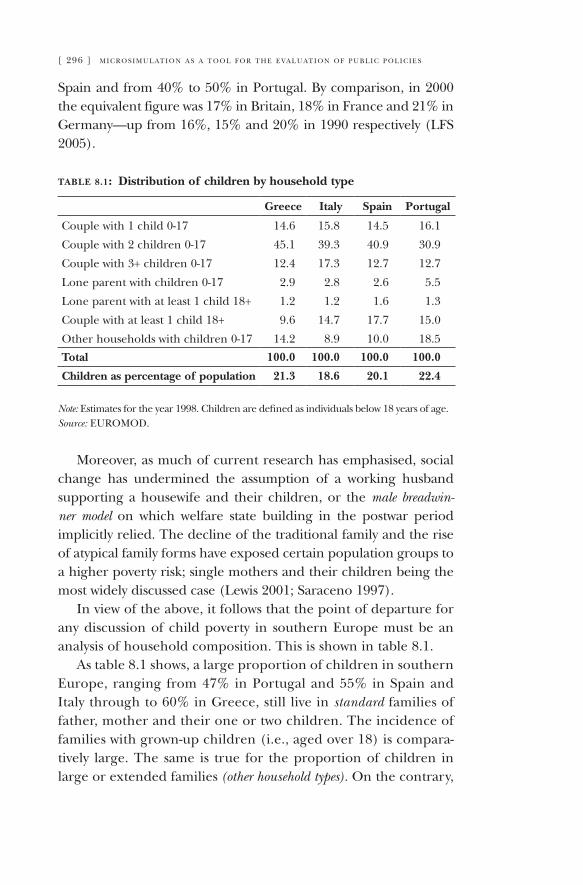
[ 296 ] m i c r o s i m u l at i o n a s a t o o l f o r t h e e va l u at i o n o f p u b l i c p o l i c i e s
spain and from 40% to 50% in portugal. by comparison, in 2000 the equivalent figure was 17% in britain, 18% in france and 21% in Germany—up from 16%, 15% and 20% in 1990 respectively (Lfs 2005).
table 8.1: Distribution of children by household type
Greece Italy Spain Portugal
Couple with 1 child 0-17 14.6 15.8 14.5 16.1
Couple with 2 children 0-17 45.1 39.3 40.9 30.9
Couple with 3+ children 0-17 12.4 17.3 12.7 12.7
Lone parent with children 0-17 2.9 2.8 2.6 5.5
Lone parent with at least 1 child 18+ 1.2 1.2 1.6 1.3
Couple with at least 1 child 18+ 9.6 14.7 17.7 15.0
Other households with children 0-17 14.2 8.9 10.0 18.5
Total 100.0 100.0 100.0 100.0
Children as percentage of population 21.3 18.6 20.1 22.4
Note: estimates for the year 1998. Children are defined as individuals below 18 years of age.Source: euROMOD.
Moreover, as much of current research has emphasised, social change has undermined the assumption of a working husband supporting a housewife and their children, or the male breadwin-ner model on which welfare state building in the postwar period implicitly relied. the decline of the traditional family and the rise of atypical family forms have exposed certain population groups to a higher poverty risk; single mothers and their children being the most widely discussed case (Lewis 2001; saraceno 1997).
In view of the above, it follows that the point of departure for any discussion of child poverty in southern europe must be an analysis of household composition. this is shown in table 8.1.
As table 8.1 shows, a large proportion of children in southern europe, ranging from 47% in portugal and 55% in spain and Italy through to 60% in Greece, still live in standard families of father, mother and their one or two children. the incidence of families with grown-up children (i.e., aged over 18) is compara-tively large. the same is true for the proportion of children in large or extended families (other household types). On the contrary,
c h i l d p o v e rt y a n d fa m i ly t r a n s f e r s i n s o u t h e r n e u r o p e [ 297 ]
lone parent families account for a relatively low share of the child population, especially if one focuses on those with children below 18 (single parent families with older children are likely to include more widows than never-married mothers).
In the light of the above, when analysing child poverty in south-ern europe it is useful to distinguish between poverty rates and contribution to aggregate child poverty. the former is simply the proportion of children in a certain household type that are below the poverty line. the latter is a function of the population share of each household type calculated as the number of poor children in a certain household type as a proportion of all poor children.1
the implications of this distinction are more clearly brought out in table 8.2. In terms of poverty rates, child poverty rates are highest in large and lone parent families. In this sense, there is nothing re-markable about child poverty in southern europe compared to the rest of europe. In terms of contribution to aggregate child poverty, a very different picture emerges. In the case of lone parent families this is clearly limited: from about 8% of all poor children in Italy to 15% in portugal. Large families account for a higher share of poor children. Yet, a very substantial proportion of children in poverty (ranging from 29% in portugal to 48% in Greece) live in standard families of couples with one or two children.Naturally, headcount rates tell only part of the story. for instance, a look at the income gap ratio, or the average income shortfall of poor families from the poverty line as seen in table 8.3, reveals that the depth of child poverty is greatest in Greece and smallest in portugal. Remember that the opposite is true with respect to the poverty rate (17% in Greece vs. 23% in portugal). In other words, while proportionally fewer children find themselves below the poverty line in Greece compared to the other south european countries, those who do have lower relative incomes on average.
the picture changes again if a poverty indicator is adopted that attaches greater weight to larger income gaps, such as the
1 Note that any estimates of child poverty by household type is sensitive to the equivalence scale used. Other things being equal, the lower the household economies of scale implicit in the equivalence scale used with respect to children, the higher the headcount poverty rate and the contribution to aggregate child poverty of children living in larger households.
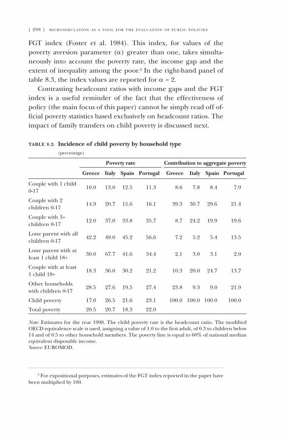
[ 298 ] m i c r o s i m u l at i o n a s a t o o l f o r t h e e va l u at i o n o f p u b l i c p o l i c i e s
fGt index (foster et al. 1984). this index, for values of the poverty aversion parameter (α) greater than one, takes simulta-neously into account the poverty rate, the income gap and the extent of inequality among the poor.2 In the right-hand panel of table 8.3, the index values are reported for α = 2.
Contrasting headcount ratios with income gaps and the fGt index is a useful reminder of the fact that the effectiveness of policy (the main focus of this paper) cannot be simply read off of-ficial poverty statistics based exclusively on headcount ratios. the impact of family transfers on child poverty is discussed next.
table 8.2: Incidence of child poverty by household type (percentage)
Poverty rate Contribution to aggregate poverty
Greece Italy Spain Portugal Greece Italy Spain Portugal
Couple with 1 child 0-17
10.0 13.0 12.5 11.3 8.6 7.8 8.4 7.9
Couple with 2 children 0-17
14.9 20.7 15.6 16.1 39.3 30.7 29.6 21.4
Couple with 3+ children 0-17
12.0 37.0 33.8 35.7 8.7 24.2 19.9 19.6
Lone parent with all children 0-17
42.2 49.0 45.2 56.6 7.2 5.2 5.4 13.5
Lone parent with at least 1 child 18+
30.0 67.7 41.6 34.4 2.1 3.0 3.1 2.0
Couple with at least 1 child 18+
18.3 36.0 30.2 21.2 10.3 20.0 24.7 13.7
Other households with children 0-17
28.5 27.6 19.5 27.4 23.8 9.3 9.0 21.9
Child poverty 17.0 26.5 21.6 23.1 100.0 100.0 100.0 100.0
total poverty 20.5 20.7 18.3 22.0
Note: estimates for the year 1998. the child poverty rate is the headcount ratio. the modified OeCD equivalence scale is used, assigning a value of 1.0 to the first adult, of 0.3 to children below 14 and of 0.5 to other household members. the poverty line is equal to 60% of national median equivalent disposable income.Source: euROMOD.
2 for expositional purposes, estimates of the fGt index reported in the paper have been multiplied by 100.
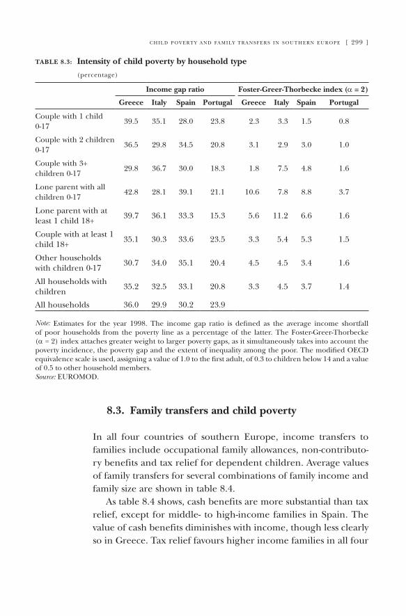
c h i l d p o v e rt y a n d fa m i ly t r a n s f e r s i n s o u t h e r n e u r o p e [ 299 ]
table 8.3: Intensity of child poverty by household type
(percentage)
Income gap ratio Foster-Greer-Thorbecke index (α = 2)
Greece Italy Spain Portugal Greece Italy Spain Portugal
Couple with 1 child 0-17
39.5 35.1 28.0 23.8 2.3 3.3 1.5 0.8
Couple with 2 children 0-17
36.5 29.8 34.5 20.8 3.1 2.9 3.0 1.0
Couple with 3+ children 0-17
29.8 36.7 30.0 18.3 1.8 7.5 4.8 1.6
Lone parent with all children 0-17
42.8 28.1 39.1 21.1 10.6 7.8 8.8 3.7
Lone parent with at least 1 child 18+
39.7 36.1 33.3 15.3 5.6 11.2 6.6 1.6
Couple with at least 1 child 18+
35.1 30.3 33.6 23.5 3.3 5.4 5.3 1.5
Other households with children 0-17
30.7 34.0 35.1 20.4 4.5 4.5 3.4 1.6
All households with children
35.2 32.5 33.1 20.8 3.3 4.5 3.7 1.4
All households 36.0 29.9 30.2 23.9
Note: estimates for the year 1998. the income gap ratio is defined as the average income shortfall of poor households from the poverty line as a percentage of the latter. the foster-Greer-thorbecke (α = 2) index attaches greater weight to larger poverty gaps, as it simultaneously takes into account the poverty incidence, the poverty gap and the extent of inequality among the poor. the modified OeCD equivalence scale is used, assigning a value of 1.0 to the first adult, of 0.3 to children below 14 and a value of 0.5 to other household members.Source: euROMOD.
8.3. Family transfers and child poverty
In all four countries of southern europe, income transfers to families include occupational family allowances, non-contributo-ry benefits and tax relief for dependent children. Average values of family transfers for several combinations of family income and family size are shown in table 8.4.
As table 8.4 shows, cash benefits are more substantial than tax relief, except for middle- to high-income families in spain. the value of cash benefits diminishes with income, though less clearly so in Greece. tax relief favours higher income families in all four
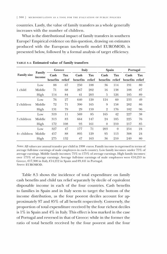
[ 300 ] m i c r o s i m u l at i o n a s a t o o l f o r t h e e va l u at i o n o f p u b l i c p o l i c i e s
countries. Lastly, the value of family transfers as a whole generally increases with the number of children.
What is the distributional impact of family transfers in southern europe? empirical evidence on this question, drawing on estimates produced with the european tax-benefit model euROMOD, is presented below, followed by a formal analysis of target efficiency.
table 8.4: Estimated value of family transfers
Family sizeFamily income
Greece Italy Spain Portugal
Cash benefits
Tax relief
Cash benefits
Tax relief
Cash benefits
Tax relief
Cash benefits
Tax relief
1 childLow 88 67 250 188 36 114 191 80
Middle 71 68 267 202 16 138 188 87High 114 84 41 203 5 126 185 89
2 childrenLow 76 27 640 120 124 60 233 49
Middle 72 71 390 165 9 158 202 86High 131 79 29 159 2 176 182 96
3 childrenLow 319 11 569 85 165 42 227 38
Middle 313 83 664 147 24 185 225 76High 172 108 93 161 0 210 217 85
4+ childrenLow 327 47 177 71 203 0 254 24
Middle 457 88 895 129 95 113 308 24High 275 132 47 163 36 210 249 80
Notes: All values are annual transfer per child in 1998 euros. family income is expressed in terms of average full-time earnings of male employees in each country. Low family incomes: under 75% of average earnings. Middle family incomes: 75% to 175% of average earnings. High family incomes: over 175% of average earnings. Average full-time earnings of male employees were €10,253 in Greece, €17,300 in Italy, €14,212 in spain and €9,441 in portugal.Source: euROMOD.
table 8.5 shows the incidence of total expenditure on family cash benefits and child tax relief separately by decile of equivalent disposable income in each of the four countries. Cash benefits to families in spain and in Italy seem to target the bottom of the income distribution, as the four poorest deciles account for ap-proximately 97 and 85% of all benefit respectively. Conversely, the proportion of total expenditure received by the four richest deciles is 1% in spain and 4% in Italy. this effect is less marked in the case of portugal and reversed in that of Greece: while in the former the ratio of total benefit received by the four poorest and the four
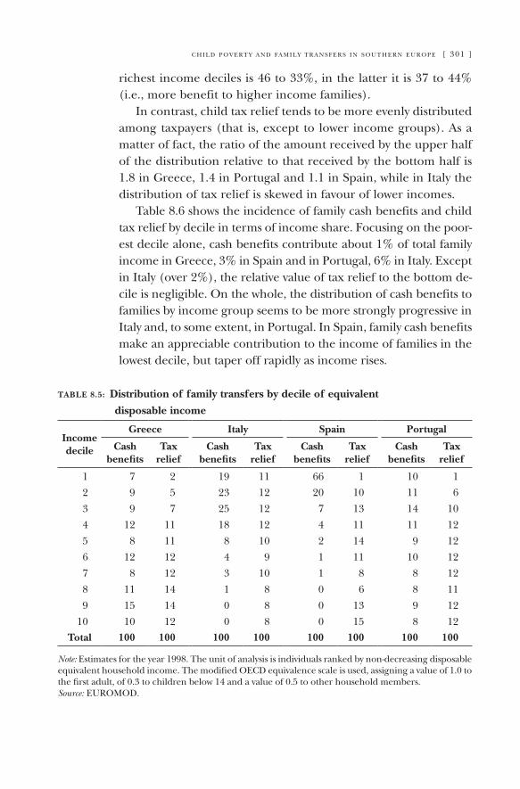
c h i l d p o v e rt y a n d fa m i ly t r a n s f e r s i n s o u t h e r n e u r o p e [ 301 ]
richest income deciles is 46 to 33%, in the latter it is 37 to 44% (i.e., more benefit to higher income families).
In contrast, child tax relief tends to be more evenly distributed among taxpayers (that is, except to lower income groups). As a matter of fact, the ratio of the amount received by the upper half of the distribution relative to that received by the bottom half is 1.8 in Greece, 1.4 in portugal and 1.1 in spain, while in Italy the distribution of tax relief is skewed in favour of lower incomes.
table 8.6 shows the incidence of family cash benefits and child tax relief by decile in terms of income share. focusing on the poor-est decile alone, cash benefits contribute about 1% of total family income in Greece, 3% in spain and in portugal, 6% in Italy. except in Italy (over 2%), the relative value of tax relief to the bottom de-cile is negligible. On the whole, the distribution of cash benefits to families by income group seems to be more strongly progressive in Italy and, to some extent, in portugal. In spain, family cash benefits make an appreciable contribution to the income of families in the lowest decile, but taper off rapidly as income rises.
table 8.5: Distribution of family transfers by decile of equivalent
disposable income
Income decile
Greece Italy Spain Portugal
Cash benefits
Tax relief
Cash benefits
Tax relief
Cash benefits
Tax relief
Cash benefits
Tax relief
1 7 2 19 11 66 1 10 12 9 5 23 12 20 10 11 6
3 9 7 25 12 7 13 14 10
4 12 11 18 12 4 11 11 12
5 8 11 8 10 2 14 9 12
6 12 12 4 9 1 11 10 12
7 8 12 3 10 1 8 8 12
8 11 14 1 8 0 6 8 11
9 15 14 0 8 0 13 9 12
10 10 12 0 8 0 15 8 12Total 100 100 100 100 100 100 100 100
Note: estimates for the year 1998. the unit of analysis is individuals ranked by non-decreasing disposable equivalent household income. the modified OeCD equivalence scale is used, assigning a value of 1.0 to the first adult, of 0.3 to children below 14 and a value of 0.5 to other household members.Source: euROMOD.
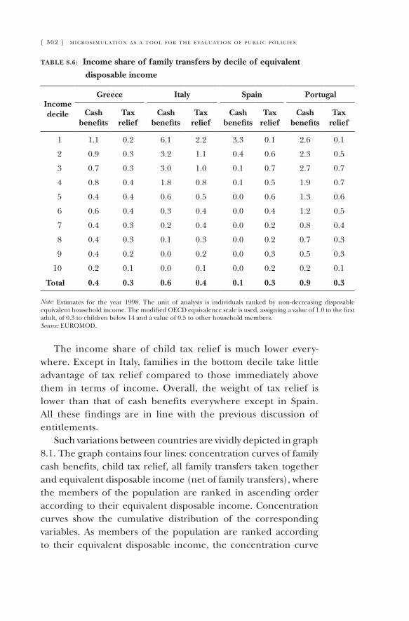
[ 302 ] m i c r o s i m u l at i o n a s a t o o l f o r t h e e va l u at i o n o f p u b l i c p o l i c i e s
table 8.6: Income share of family transfers by decile of equivalent
disposable income
Income decile
Greece Italy Spain Portugal
Cash benefits
Tax relief
Cash benefits
Tax relief
Cash benefits
Tax relief
Cash benefits
Tax relief
1 1.1 0.2 6.1 2.2 3.3 0.1 2.6 0.1
2 0.9 0.3 3.2 1.1 0.4 0.6 2.3 0.5
3 0.7 0.3 3.0 1.0 0.1 0.7 2.7 0.7
4 0.8 0.4 1.8 0.8 0.1 0.5 1.9 0.7
5 0.4 0.4 0.6 0.5 0.0 0.6 1.3 0.6
6 0.6 0.4 0.3 0.4 0.0 0.4 1.2 0.5
7 0.4 0.3 0.2 0.4 0.0 0.2 0.8 0.4
8 0.4 0.3 0.1 0.3 0.0 0.2 0.7 0.3
9 0.4 0.2 0.0 0.2 0.0 0.3 0.5 0.3
10 0.2 0.1 0.0 0.1 0.0 0.2 0.2 0.1
Total 0.4 0.3 0.6 0.4 0.1 0.3 0.9 0.3
Note: estimates for the year 1998. the unit of analysis is individuals ranked by non-decreasing disposable equivalent household income. the modified OeCD equivalence scale is used, assigning a value of 1.0 to the first adult, of 0.3 to children below 14 and a value of 0.5 to other household members.Source: euROMOD.
the income share of child tax relief is much lower every-where. except in Italy, families in the bottom decile take little advantage of tax relief compared to those immediately above them in terms of income. Overall, the weight of tax relief is lower than that of cash benefits everywhere except in spain. All these findings are in line with the previous discussion of entitlements.
such variations between countries are vividly depicted in graph 8.1. the graph contains four lines: concentration curves of family cash benefits, child tax relief, all family transfers taken together and equivalent disposable income (net of family transfers), where the members of the population are ranked in ascending order according to their equivalent disposable income. Concentration curves show the cumulative distribution of the corresponding variables. As members of the population are ranked according to their equivalent disposable income, the concentration curve
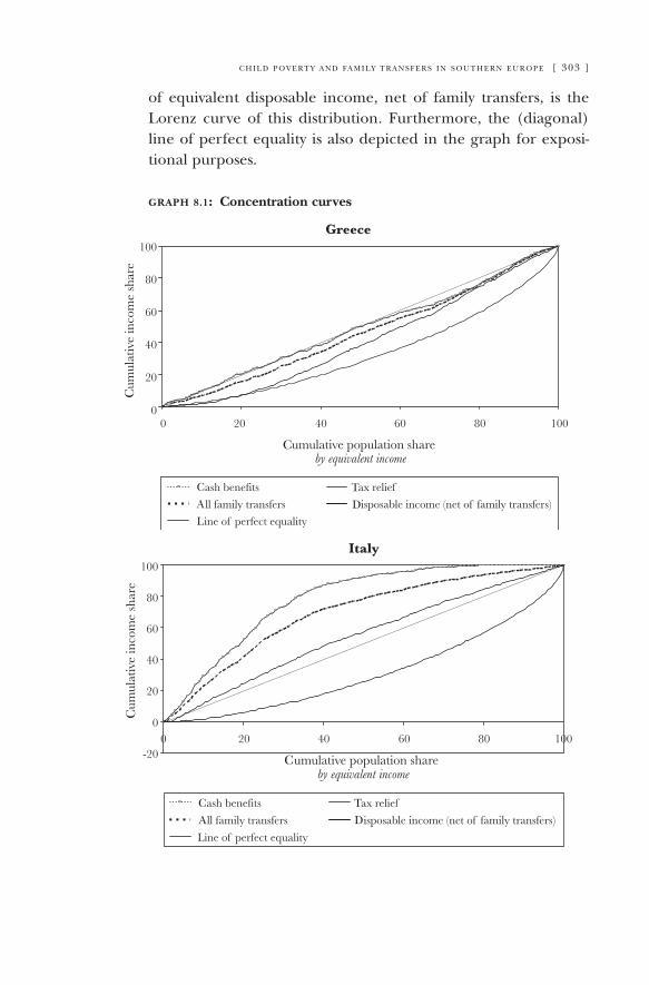
c h i l d p o v e rt y a n d fa m i ly t r a n s f e r s i n s o u t h e r n e u r o p e [ 303 ]
of equivalent disposable income, net of family transfers, is the Lorenz curve of this distribution. furthermore, the (diagonal) line of perfect equality is also depicted in the graph for exposi-tional purposes.
graph 8.1: Concentration curves
L
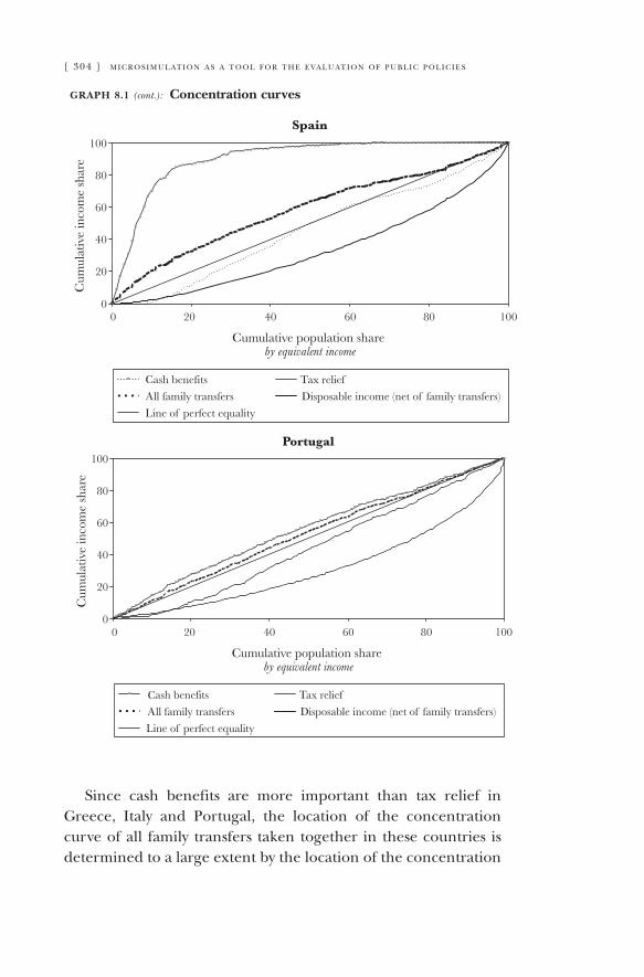
[ 304 ] m i c r o s i m u l at i o n a s a t o o l f o r t h e e va l u at i o n o f p u b l i c p o l i c i e s
graph 8.1 (cont.): Concentration curves
L
L
since cash benefits are more important than tax relief in Greece, Italy and portugal, the location of the concentration curve of all family transfers taken together in these countries is determined to a large extent by the location of the concentration
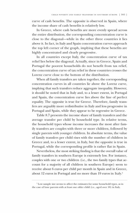
c h i l d p o v e rt y a n d fa m i ly t r a n s f e r s i n s o u t h e r n e u r o p e [ 305 ]
curve of cash benefits. the opposite is observed in spain, where the income share of cash benefits is relatively low.
In Greece, where cash benefits are more evenly spread across the entire distribution, the corresponding concentration curve is close to the diagonal—while in the other three countries it lies above it. In fact, in Italy and spain concentration curves approach the top left corner of the graph, implying that these benefits are highly concentrated and clearly progressive.
In all countries except Italy, the concentration curve of tax relief lies below the diagonal. Actually, since in Greece, spain and portugal the poorest households do not benefit from tax relief, the concentration curve of tax relief in these countries crosses the Lorenz curve close to the bottom of the distribution.
When all family transfers are taken together, the corresponding concentration curves in all countries lie above the Lorenz curve, implying that such transfers reduce aggregate inequality. However, it should be noted that in Italy and, to a lesser extent, in portugal and spain, the concentration curve lies above the line of perfect equality. the opposite is true for Greece. therefore, family trans-fers are arguably more redistributive in Italy and less progressive in portugal and spain, while they appear to be regressive in Greece.
table 8.7 presents the income share of family transfers and the average transfer per child by household type. In relative terms, the household types whose income increases the most after fam-ily transfers are couples with three or more children, followed by single parents with younger children. In absolute terms, the value of family transfers per child rises with the number of children in Greece and, to a lesser extent, in Italy, but the opposite is true in portugal, while the corresponding profile is rather flat in spain.
Nevertheless, the most striking finding is that the overall value of family transfers in southern europe is extremely low. for instance, couples with one or two children (i.e., the two family types that ac-count for a majority of all children in southern europe) seem to receive about 6 euros per child per month in spain and in Greece, about 12 euros in portugal and no more than 19 euros in Italy.3
3 Low sample size seems to affect the estimates for some household types, as in the case of lone parents with at least one older child (i.e., aged over 18) in Italy.
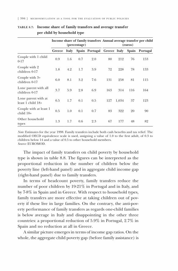
[ 306 ] m i c r o s i m u l at i o n a s a t o o l f o r t h e e va l u at i o n o f p u b l i c p o l i c i e s
table 8.7: Income share of family transfers and average transfer
per child by household type
Income share of family transfers (percentage)
annual average transfer per child (euros)
Greece Italy Spain Portugal Greece Italy Spain Portugal
Couple with 1 child 0-17
0.9 1.6 0.7 2.0 80 212 76 153
Couple with 2 children 0-17
1.8 4.2 1.7 3.9 72 228 78 133
Couple with 3+ children 0-17
6.0 8.1 3.2 7.6 131 258 81 115
Lone parent with all children 0-17
3.7 5.9 2.8 6.9 163 314 116 164
Lone parent with at least 1 child 18+
0.5 1.7 0.1 0.5 127 1,034 37 123
Couple with at least 1 child 18+
0.5 1.0 0.1 0.7 83 322 20 90
Other household types
1.3 1.7 0.6 2.3 67 177 48 82
Note: estimates for the year 1998. family transfers include both cash benefits and tax relief. the modified OeCD equivalence scale is used, assigning a value of 1.0 to the first adult, of 0.3 to children below 14 and a value of 0.5 to other household members.Source: euROMOD.
the impact of family transfers on child poverty by household type is shown in table 8.8. the figures can be interpreted as the proportional reduction in the number of children below the poverty line (left-hand panel) and in aggregate child income gap (right-hand panel) due to family transfers.
In terms of headcount poverty, family transfers reduce the number of poor children by 19-21% in portugal and in Italy, and by 7-8% in spain and in Greece. With respect to household types, family transfers are more effective at taking children out of pov-erty if these live in large families. On the contrary, the anti-pov-erty performance of family transfers as regards one-child families is below average in Italy and disappointing in the other three countries: a proportional reduction of 5.9% in portugal, 2.7% in spain and no reduction at all in Greece.
A similar picture emerges in terms of income gap ratios. On the whole, the aggregate child poverty gap (before family assistance) is
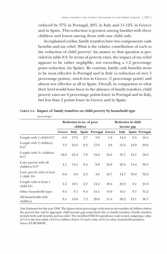
c h i l d p o v e rt y a n d fa m i ly t r a n s f e r s i n s o u t h e r n e u r o p e [ 307 ]
reduced by 37% in portugal, 28% in Italy and 11-12% in Greece and in spain. this reduction is greatest among families with three children and lowest among those with one child only.
As explained earlier, family transfers have two components: cash benefits and tax relief. What is the relative contribution of each to the reduction of child poverty? An answer to that question is pro-vided in table 8.9. In terms of poverty rates, the impact of tax relief appears to be rather negligible, not exceeding a 1.2 percentage point reduction (in spain). by contrast, family cash benefits seem to be most effective in portugal and in Italy (a reduction of over 5 percentage points), much less in Greece (1 percentage point) and almost not effective at all in spain. Overall, in comparison to what their level would have been in the absence of family transfers, child poverty rates are 6 percentage points lower in portugal and in Italy, but less than 2 points lower in Greece and in spain.
table 8.8: Impact of family transfers on child poverty by household type
(percentage)
reduction in no. of poor children
reduction in child income gap
Greece Italy Spain Portugal Greece Italy Spain Portugal
Couple with 1 child 0-17 0.0 17.6 2.7 5.9 1.9 14.4 8.5 16.4
Couple with 2 children 0-17
3.3 25.6 9.2 17.6 4.8 31.6 12.0 29.6
Couple with 3+ children 0-17
32.0 23.4 7.8 34.6 34.0 35.7 18.1 58.0
Lone parent with all children 0-17
4.1 14.1 8.4 9.8 16.8 29.4 14.4 39.3
Lone parent with at least 1 child 18+
0.0 0.0 2.3 4.0 16.7 14.7 10.0 32.6
Couple with at least 1 child 18+
5.5 10.1 5.7 14.4 10.4 22.3 9.1 21.0
Other household types 9.4 8.1 9.4 24.1 14.0 16.1 9.7 31.2
All households with children
8.1 19.0 7.3 20.8 11.4 28.2 12.1 36.7
Note: estimates for the year 1998. the figures show percentage reduction in the number of children below the poverty line and in aggregate child income gap respectively due to family transfers. family transfers include both cash benefits and tax relief. the modified OeCD equivalence scale is used, assigning a value of 1.0 to the first adult, of 0.3 to children below 14 and a value of 0.5 to other household members.Source: euROMOD.
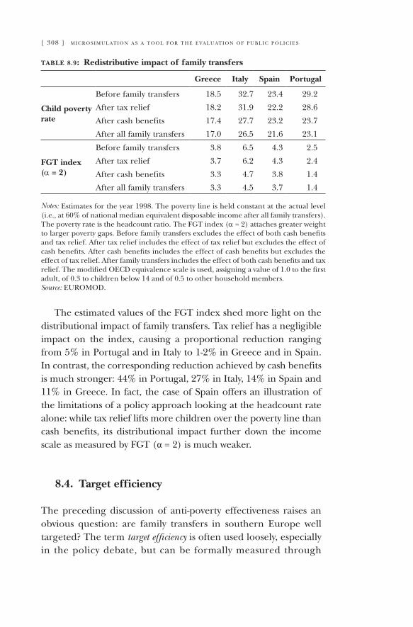
[ 308 ] m i c r o s i m u l at i o n a s a t o o l f o r t h e e va l u at i o n o f p u b l i c p o l i c i e s
table 8.9: redistributive impact of family transfers
Greece Italy Spain Portugal
Child poverty rate
before family transfers 18.5 32.7 23.4 29.2
After tax relief 18.2 31.9 22.2 28.6
After cash benefits 17.4 27.7 23.2 23.7
After all family transfers 17.0 26.5 21.6 23.1
FGT index (α = 2)
before family transfers 3.8 6.5 4.3 2.5
After tax relief 3.7 6.2 4.3 2.4
After cash benefits 3.3 4.7 3.8 1.4
After all family transfers 3.3 4.5 3.7 1.4
Notes: estimates for the year 1998. the poverty line is held constant at the actual level (i.e., at 60% of national median equivalent disposable income after all family transfers). the poverty rate is the headcount ratio. the fGt index (α = 2) attaches greater weight to larger poverty gaps. before family transfers excludes the effect of both cash benefits and tax relief. After tax relief includes the effect of tax relief but excludes the effect of cash benefits. After cash benefits includes the effect of cash benefits but excludes the effect of tax relief. After family transfers includes the effect of both cash benefits and tax relief. the modified OeCD equivalence scale is used, assigning a value of 1.0 to the first adult, of 0.3 to children below 14 and of 0.5 to other household members.Source: euROMOD.
the estimated values of the fGt index shed more light on the distributional impact of family transfers. tax relief has a negligible impact on the index, causing a proportional reduction ranging from 5% in portugal and in Italy to 1-2% in Greece and in spain. In contrast, the corresponding reduction achieved by cash benefits is much stronger: 44% in portugal, 27% in Italy, 14% in spain and 11% in Greece. In fact, the case of spain offers an illustration of the limitations of a policy approach looking at the headcount rate alone: while tax relief lifts more children over the poverty line than cash benefits, its distributional impact further down the income scale as measured by fGt (α = 2) is much weaker.
8.4. Target efficiency
the preceding discussion of anti-poverty effectiveness raises an obvious question: are family transfers in southern europe well targeted? the term target efficiency is often used loosely, especially in the policy debate, but can be formally measured through
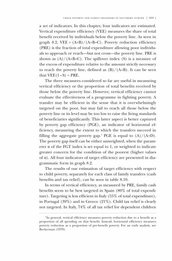
c h i l d p o v e rt y a n d fa m i ly t r a n s f e r s i n s o u t h e r n e u r o p e [ 309 ]
a set of indicators. In this chapter, four indicators are estimated. Vertical expenditure efficiency (Vee) measures the share of total benefit received by individuals below the poverty line. As seen in graph 8.2, Vee = (A+b)/(A+b+C). poverty reduction efficiency (pRe) is the fraction of total expenditure allowing poor individu-als to approach or reach—but not cross—the poverty line. pRe is shown as (A)/(A+b+C). the spillover index (s) is a measure of the excess of expenditure relative to the amount strictly necessary to reach the poverty line, defined as (b)/(A+b). It can be seen that Vee(1 – s) = pRe.
the three measures considered so far are useful in measuring vertical efficiency or the proportion of total benefits received by those below the poverty line. However, vertical efficiency cannot evaluate the effectiveness of a programme in fighting poverty. A transfer may be efficient in the sense that it is overwhelmingly targeted on the poor, but may fail to reach all those below the poverty line or its level may be too low to raise the living standards of beneficiaries significantly. this latter aspect is better captured by poverty gap efficiency (pGe), an indicator of horizontal ef-ficiency, measuring the extent to which the transfers succeed in filling the aggregate poverty gap.4 pGe is equal to (A)/(A+D). the poverty gap itself can be either unweighted, when the param-eter α of the fGt index is set equal to 1, or weighted to indicate greater concern for the condition of the poorest (higher values of α). All four indicators of target efficiency are presented in dia-grammatic form in graph 8.2.
the results of our estimation of target efficiency with respect to child poverty, separately for each class of family transfers (cash benefits and tax relief), can be seen in table 8.10.
In terms of vertical efficiency, as measured by pRe, family cash benefits seem to be best targeted in spain (80% of total expendi-ture). targeting is less efficient in Italy (55% of total expenditure), in portugal (39%) and in Greece (21%). Child tax relief is clearly not targeted. In Italy, 74% of all tax relief for dependent children
4 In general, vertical efficiency measures poverty reduction due to a benefit as a proportion of all spending on that benefit. Instead, horizontal efficiency measures poverty reduction as a proportion of pre-benefit poverty. for an early analysis, see beckerman (1979).
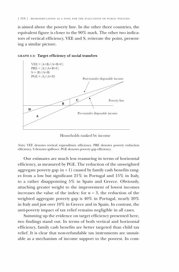
[ 310 ] m i c r o s i m u l at i o n a s a t o o l f o r t h e e va l u at i o n o f p u b l i c p o l i c i e s
is aimed above the poverty line. In the other three countries, the equivalent figure is closer to the 90% mark. the other two indica-tors of vertical efficiency, Vee and s, reiterate the point, present-ing a similar picture.
graph 8.2: Target efficiency of social transfers
Notes: Vee denotes vertical expenditure efficiency. pRe denotes poverty reduction efficiency. s denotes spillover. pGe denotes poverty gap efficiency.
Our estimates are much less reassuring in terms of horizontal efficiency, as measured by pGe. the reduction of the unweighted aggregate poverty gap (α = 1) caused by family cash benefits rang-es from a low but significant 21% in portugal and 15% in Italy, to a rather disappointing 5% in spain and Greece. Obviously, attaching greater weight to the improvement of lowest incomes increases the value of the index: for α = 3, the reduction of the weighted aggregate poverty gap is 40% in portugal, nearly 20% in Italy and just over 10% in Greece and in spain. In contrast, the anti-poverty impact of tax relief remains negligible in all cases.
summing up the evidence on target efficiency presented here, two findings stand out. In terms of both vertical and horizontal efficiency, family cash benefits are better targeted than child tax relief. It is clear that non-refundable tax instruments are unsuit-able as a mechanism of income support to the poorest. In com-
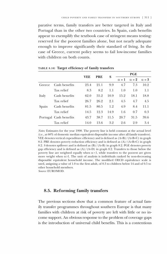
c h i l d p o v e rt y a n d fa m i ly t r a n s f e r s i n s o u t h e r n e u r o p e [ 311 ]
parative terms, family transfers are better targeted in Italy and portugal than in the other two countries. In spain, cash benefits appear to exemplify the textbook case of stringent means testing: reserved for the poorest families alone, but not nearly adequate enough to improve significantly their standard of living. In the case of Greece, current policy seems to fail low-income families with children on both counts.
table 8.10: Target efficiency of family transfers
VEE PrE SPGE
α = 1 α = 2 α = 3
Greece Cash benefits 23.4 21.1 9.9 4.7 7.3 10.2
tax relief 8.3 8.2 1.1 1.0 1.0 1.1
Italy Cash benefits 62.0 55.2 10.9 15.2 18.1 18.8
tax relief 26.7 26.2 2.1 4.5 4.7 4.5
spain Cash benefits 81.5 80.5 1.2 4.9 8.4 11.1
tax relief 14.5 12.3 14.9 1.6 0.7 0.3
portugal Cash benefits 43.7 38.7 11.5 20.7 31.5 39.6
tax relief 14.0 13.6 3.2 2.6 2.9 3.4
Notes: estimates for the year 1998. the poverty line is held constant at the actual level (i.e., at 60% of domestic median equivalent disposable income after all family transfers). Vee denotes vertical expenditure efficiency and is defined as (A+b)/(A+b+C) in graph 8.2. pRe denotes poverty reduction efficiency and is defined as (A)/(A+b+C) in graph 8.2. S denotes spillover and is defined as (b)/(A+b) in graph 8.2. pGe denotes poverty gap efficiency and is defined as (A)/(A+D) in graph 8.2. transfers to those below the poverty line are weighted equally when α = 1, while transfers to the poorest are given more weight when α>1. the unit of analysis is individuals ranked by non-decreasing disposable equivalent household income. the modified OeCD equivalence scale is used, assigning a value of 1.0 to the first adult, of 0.3 to children below 14 and of 0.5 to other household members.Source: euROMOD.
8.5. reforming family transfers
the previous sections show that a common feature of actual fam-ily transfer programmes throughout southern europe is that many families with children at risk of poverty are left with little or no in-come support. An obvious response to the problem of coverage gaps is the introduction of universal child benefits. this is a contentious
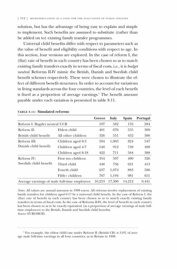
[ 312 ] m i c r o s i m u l at i o n a s a t o o l f o r t h e e va l u at i o n o f p u b l i c p o l i c i e s
solution, but has the advantage of being easy to explain and simple to implement. such benefits are assumed to substitute (rather than be added on to) existing family transfer programmes.
universal child benefits differ with respect to parameters such as the value of benefit and eligibility conditions with respect to age. In this section, four versions are explored. In the case of reform I, the (flat) rate of benefit in each country has been chosen so as to match existing family transfers exactly in terms of fiscal costs, i.e., it is budget neutral. Reforms II-IV mimic the british, Danish and swedish child benefit schemes respectively. these were chosen to illustrate the ef-fect of different benefit structures. In order to account for variations in living standards across the four countries, the level of each benefit is fixed as a proportion of average earnings.5 the benefit amount payable under each variation is presented in table 8.11.
table 8.11: Simulated reforms
Greece Italy Spain Portugal
Reform I: bugdet neutral uCb 197 582 135 284
Reform II: eldest child 401 676 555 369
british child benefit All other children 326 551 452 300
Reform III: Children aged 0-3 594 1,003 824 547Danish child benefit Children aged 4-7 540 912 749 498
Children aged 8-18 422 711 584 388
Reform IV: first two children 354 597 490 326swedish child benefit third child 448 756 621 413
fourth child 637 1,074 883 586
fifth+ children 707 1,194 981 651
Average earnings of male full-time employees 10,253 17,300 14,212 9,441
Notes: All values are annual amounts in 1998 euros. All reforms involve replacement of existing family transfers for children aged 0-17 by a universal child benefit. In the case of Reform I, the (flat) rate of benefit in each country has been chosen so as to match exactly existing family transfers in terms of fiscal costs. In the case of Reforms II-IV, the level of benefit in each country has been chosen so as to be exactly equivalent (as a proportion of average earnings of male full-time employees) to the british, Danish and swedish child benefits.Source: euROMOD.
5 for example, the eldest child rate under Reform II (british Cb) is 3.9% of aver-age male full-time earnings in all four countries, as in britain in 1998.
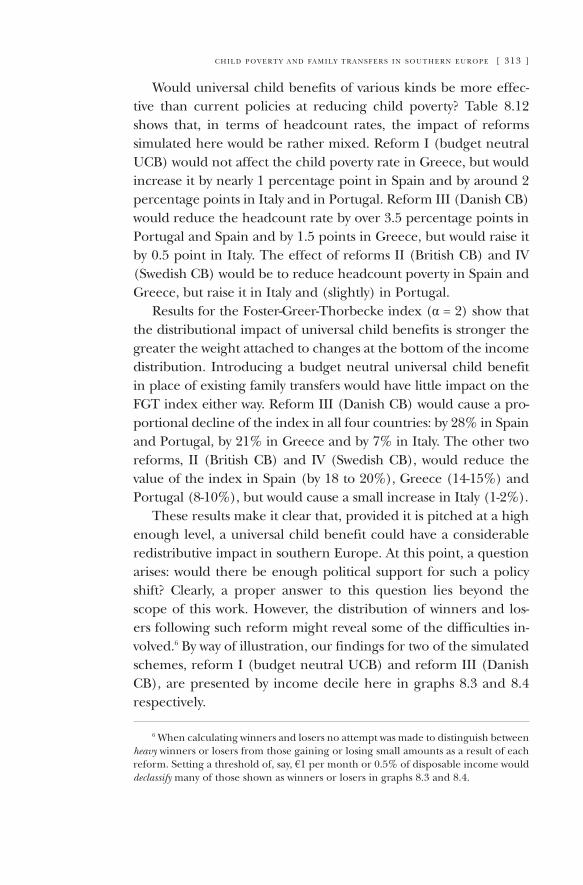
c h i l d p o v e rt y a n d fa m i ly t r a n s f e r s i n s o u t h e r n e u r o p e [ 313 ]
Would universal child benefits of various kinds be more effec-tive than current policies at reducing child poverty? table 8.12 shows that, in terms of headcount rates, the impact of reforms simulated here would be rather mixed. Reform I (budget neutral uCb) would not affect the child poverty rate in Greece, but would increase it by nearly 1 percentage point in spain and by around 2 percentage points in Italy and in portugal. Reform III (Danish Cb) would reduce the headcount rate by over 3.5 percentage points in portugal and spain and by 1.5 points in Greece, but would raise it by 0.5 point in Italy. the effect of reforms II (british Cb) and IV (swedish Cb) would be to reduce headcount poverty in spain and Greece, but raise it in Italy and (slightly) in portugal.
Results for the foster-Greer-thorbecke index (α = 2) show that the distributional impact of universal child benefits is stronger the greater the weight attached to changes at the bottom of the income distribution. Introducing a budget neutral universal child benefit in place of existing family transfers would have little impact on the fGt index either way. Reform III (Danish Cb) would cause a pro-portional decline of the index in all four countries: by 28% in spain and portugal, by 21% in Greece and by 7% in Italy. the other two reforms, II (british Cb) and IV (swedish Cb), would reduce the value of the index in spain (by 18 to 20%), Greece (14-15%) and portugal (8-10%), but would cause a small increase in Italy (1-2%).
these results make it clear that, provided it is pitched at a high enough level, a universal child benefit could have a considerable redistributive impact in southern europe. At this point, a question arises: would there be enough political support for such a policy shift? Clearly, a proper answer to this question lies beyond the scope of this work. However, the distribution of winners and los-ers following such reform might reveal some of the difficulties in-volved.6 by way of illustration, our findings for two of the simulated schemes, reform I (budget neutral uCb) and reform III (Danish Cb), are presented by income decile here in graphs 8.3 and 8.4 respectively.
6 When calculating winners and losers no attempt was made to distinguish between heavy winners or losers from those gaining or losing small amounts as a result of each reform. setting a threshold of, say, €1 per month or 0.5% of disposable income would declassify many of those shown as winners or losers in graphs 8.3 and 8.4.
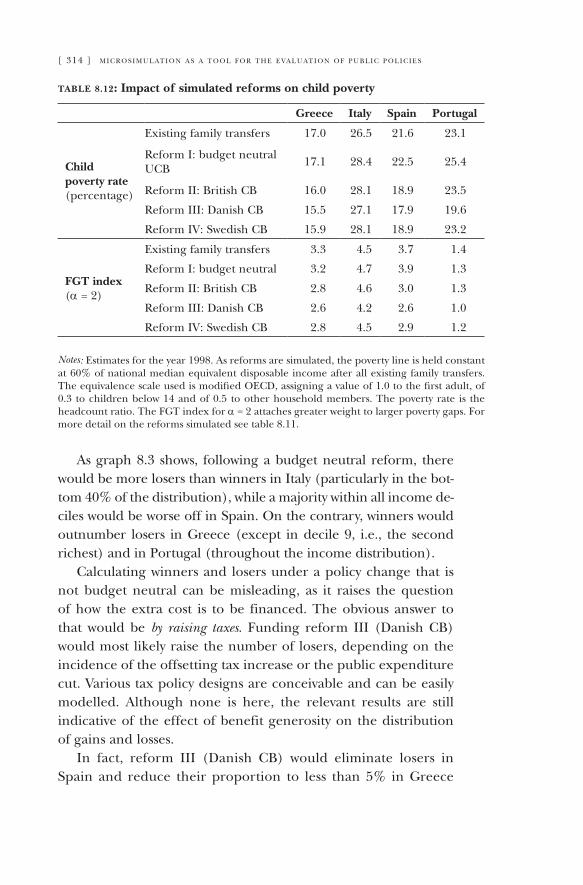
[ 314 ] m i c r o s i m u l at i o n a s a t o o l f o r t h e e va l u at i o n o f p u b l i c p o l i c i e s
table 8.12: Impact of simulated reforms on child poverty
Greece Italy Spain Portugal
Child poverty rate (percentage)
existing family transfers 17.0 26.5 21.6 23.1
Reform I: budget neutral uCb 17.1 28.4 22.5 25.4
Reform II: british Cb 16.0 28.1 18.9 23.5
Reform III: Danish Cb 15.5 27.1 17.9 19.6
Reform IV: swedish Cb 15.9 28.1 18.9 23.2
FGT index (α = 2)
existing family transfers 3.3 4.5 3.7 1.4
Reform I: budget neutral 3.2 4.7 3.9 1.3
Reform II: british Cb 2.8 4.6 3.0 1.3
Reform III: Danish Cb 2.6 4.2 2.6 1.0
Reform IV: swedish Cb 2.8 4.5 2.9 1.2
Notes: estimates for the year 1998. As reforms are simulated, the poverty line is held constant at 60% of national median equivalent disposable income after all existing family transfers. the equivalence scale used is modified OeCD, assigning a value of 1.0 to the first adult, of 0.3 to children below 14 and of 0.5 to other household members. the poverty rate is the headcount ratio. the fGt index for α = 2 attaches greater weight to larger poverty gaps. for more detail on the reforms simulated see table 8.11.
As graph 8.3 shows, following a budget neutral reform, there would be more losers than winners in Italy (particularly in the bot-tom 40% of the distribution), while a majority within all income de-ciles would be worse off in spain. On the contrary, winners would outnumber losers in Greece (except in decile 9, i.e., the second richest) and in portugal (throughout the income distribution).
Calculating winners and losers under a policy change that is not budget neutral can be misleading, as it raises the question of how the extra cost is to be financed. the obvious answer to that would be by raising taxes. funding reform III (Danish Cb) would most likely raise the number of losers, depending on the incidence of the offsetting tax increase or the public expenditure cut. Various tax policy designs are conceivable and can be easily modelled. Although none is here, the relevant results are still indicative of the effect of benefit generosity on the distribution of gains and losses.
In fact, reform III (Danish Cb) would eliminate losers in spain and reduce their proportion to less than 5% in Greece
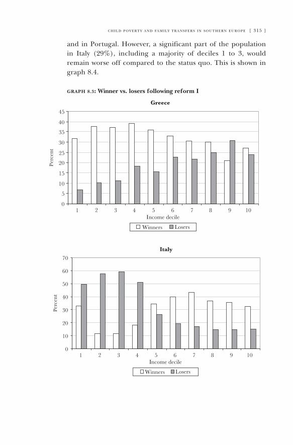
c h i l d p o v e rt y a n d fa m i ly t r a n s f e r s i n s o u t h e r n e u r o p e [ 315 ]
and in portugal. However, a significant part of the population in Italy (29%), including a majority of deciles 1 to 3, would remain worse off compared to the status quo. this is shown in graph 8.4.
graph 8.3: Winner vs. losers following reform I
P
LW
I
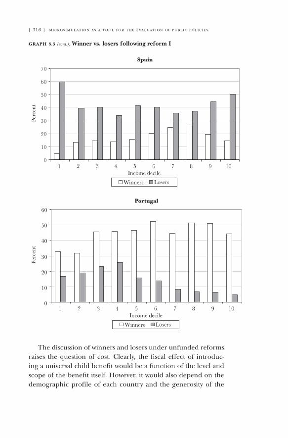
[ 316 ] m i c r o s i m u l at i o n a s a t o o l f o r t h e e va l u at i o n o f p u b l i c p o l i c i e s
graph 8.3 (cont.): Winner vs. losers following reform I
the discussion of winners and losers under unfunded reforms raises the question of cost. Clearly, the fiscal effect of introduc-ing a universal child benefit would be a function of the level and scope of the benefit itself. However, it would also depend on the demographic profile of each country and the generosity of the
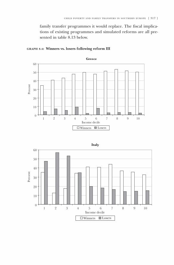
c h i l d p o v e rt y a n d fa m i ly t r a n s f e r s i n s o u t h e r n e u r o p e [ 317 ]
family transfer programmes it would replace. the fiscal implica-tions of existing programmes and simulated reforms are all pre-sented in table 8.13 below.
graph 8.4: Winners vs. losers following reform III
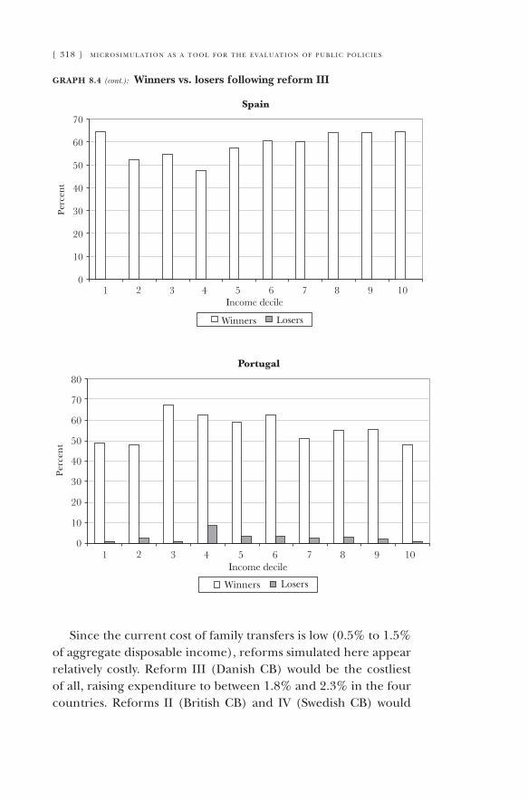
[ 318 ] m i c r o s i m u l at i o n a s a t o o l f o r t h e e va l u at i o n o f p u b l i c p o l i c i e s
graph 8.4 (cont.): Winners vs. losers following reform III
since the current cost of family transfers is low (0.5% to 1.5% of aggregate disposable income), reforms simulated here appear relatively costly. Reform III (Danish Cb) would be the costliest of all, raising expenditure to between 1.8% and 2.3% in the four countries. Reforms II (british Cb) and IV (swedish Cb) would

c h i l d p o v e rt y a n d fa m i ly t r a n s f e r s i n s o u t h e r n e u r o p e [ 319 ]
have a softer fiscal impact, bringing expenditure on income transfers to families with children to between 1.4% and 1.8% of disposable income.
table 8.13: Fiscal effects of simulated reforms
Greece Italy Spain Portugal
existing family transfers 0.9 1.3 0.5 1.5
Reform I: budget neutral uCb 0.9 1.3 0.5 1.5
Reform II: british Cb 1.6 1.4 1.8 1.8
Reform III: Danish Cb 2.1 1.8 2.4 2.3
Reform IV: swedish Cb 1.7 1.4 1.8 1.8
Notes: estimates for the year 1998. fiscal costs are expressed as a proportion of aggregate (non-equivalised) disposable income. for more detail on the reforms simulated, see table 8.11.Source: euROMOD.
8.6. Conclusions
the purpose of this chapter was to evaluate the impact of family transfers taking into account both cash benefits and tax relief. As the preceding analysis shows, existing programmes seem to per-form at best modestly in terms of poverty reduction. Many poor families with children are ineligible for benefits (as in the case of Italy) or receive low sums (as in spain and, to some extent, in portugal), or both (as in Greece). Needless to say, this effect is even more pronounced with respect to tax benefits, as non-re-fundable schemes exclude poor families by design.7
the analysis presented here assumes 100% take up of all benefits. In real life, the take up of benefits may be incomplete, often significantly so (Hernanz et al. 2004). Non-take up is known to be high when benefits are of low value, means-tested or poorly administered. However, family transfers in southern europe are
7 More recently, refundable tax credit schemes were actually introduced in Greece in 2002 (for low-income families with children aged 6-16 at school) and in spain in 2003 (for working mothers with children aged below 3). Although estimating their effect is a subject for future research, these schemes seem unlikely to alter the regres-sive nature of tax relief for dependent children in the two countries.
[ 320 ] m i c r o s i m u l at i o n a s a t o o l f o r t h e e va l u at i o n o f p u b l i c p o l i c i e s
likely to show at least one of these characteristics. In a few words, the redistributive performance of income transfers to families with children, shown to be weak under the assumption of full take up, is probably even weaker.
In view of the above, the scope for improving the redistribu-tive performance of income transfers to families with children through redesigning the structure of benefits is ample. Would universal benefits improve on the anti-poverty performance of existing schemes?
Our results show that replacing current policies by universal child benefits would not reduce the number of children in pov-erty by much—and could even increase it. this can happen if cur-rent policies provide relatively generous benefits to a substantial proportion of families on low incomes (e.g., in Italy, where fam-ily transfers are both income tested and categorically targeted). Nonetheless, where existing policies leave coverage gaps, uni-versal child benefits will improve the position of families at the bottom of the income scale but ineligible for current assistance. bringing in the fGt index reveals that the performance of re-forms improves when a poverty measure is adopted that registers improvements at the bottom of the income distribution.
Among the child benefits simulated that are actually in oper-ation elsewhere in europe, the Danish scheme clearly emerges ahead of the rest in terms of generosity: it would be the costliest, but also the one with the highest impact on child poverty in all countries of southern europe. On the other hand, the british and swedish schemes, although very different in terms of inter-nal logic (the former paying a higher rate to the elder child, the latter rising in value with family size), would have quite similar effects on child poverty and fiscal costs in the four countries studied.
In general, a trade off operates between fiscal cost and poverty reduction, since more generous benefits have a stronger distribu-tional impact at a higher fiscal cost. In any case, current expendi-ture on family transfers in southern europe is too low to expect significant improvements in terms of poverty reduction through a simple reallocation of public spending within this policy area alone. On the whole, a judicious combination of a universal (even
c h i l d p o v e rt y a n d fa m i ly t r a n s f e r s i n s o u t h e r n e u r o p e [ 321 ]
if low) income base with more targeted (but non-categorical) policies could be an effective way to improve coverage and reduce poverty at a reasonable cost to the tax payer.
the final conclusion concerns the methodology used. Important policy questions, such as that posed here (“What is the effect on child poverty of income transfers to families?”), are too complex—and to some extent counterfactual—to answer without resorting to a benefit-tax model like euROMOD. While micro-simulation models are clearly not immune from limitations of their own, some of which are discussed here, the ability to simu-late the full impact of policy reforms is their unique advantage.
references
beckerman, W. “Impact of income-maintenance payments on poverty in britain, 1975.” Economic Journal 89 (354): 261–279, 1979.
breWer, m. “the New tax Credits.” Ifs briefing Note 35. London: Institute of fiscal studies, 2003.
Presidency Conclusions of the Brussels European Council, 22-23 March. 7619/1/05 Rev. 1. brussels: Council of the european union, 2005.
ferrera, m. “the southern model of welfare in social europe.” Journal of European Social Policy 6 no. 1(1996): 17–37.
foster, J. e., J. Greer and e. thorbecke. “A class of decomposable poverty measures.” Econometrica 52 (1984): 761–766.
hernanz, v., f. malherbet and m. pellizzar. Take-up of Welfare Benefits in OECD Countries: A Review of the Evidence. OeCD social, employment and Migration Working paper 17. paris: OeCD, 2004.
leWis, J. “the Decline of the Male breadwinner Model: the Implications for Work and Care.” Social Politics 8 no. 2 (2001): 152–170.
lfs. European Community Labour Force Survey. eurostat, 2005.matsaGanis, m., m. ferrera, l. capucha and L. moreno. “Mending Nets in the
south: Anti-poverty policies in Greece, Italy, portugal and spain.” Social Policy and Administration 37 no. 6 (2003): 639–655.
moffitt, r. Means-tested Transfer Programs in the US. Chicago: university of Chicago press, 2002.
piachaud, d. and h. sutherland. “Child poverty in britain and the New Labour Government.” Journal of Social Policy 30 no. 1 (2001): 95–118.
rhodes, m. “southern european welfare states: identity, problems and prospects for reform.” South European Society and Politics 1 no. 3 (1996): 1–22.
saraceno, c. “family Change, family policies and the Restructuring of Welfare.” In: Family, Market and Community: Equity and Efficiency in Social Policy. OeCD social policy series 21. paris: OeCD, 1997.

[ 323 ]
Microsimulation and Normative Analysis of Public Policies
Amedeo SpadaroParis-Jourdan Sciences Economiques (Paris), FEDEA(Madrid)
and University of the Balearic Islands (Palma de Mallorca)
Xisco Oliver University of the Balearic Islands, Palma de Mallorca
9.1. Introduction
Microsimulation models are powerful tools to evaluate public redistribution policies. With the development of PC computa-tional capacity and the increasing availability of large datasets on household economic and sociodemographic variables, it is possible to perform an in-depth evaluation of the welfare effects of fiscal reforms. This evaluation of public policy practice has been widely used all around the world. Atkinson, Bourguignon and Chiappori (1988), for example, analyze the redistributive impact of a reform in which, for a given sample of French house-holds, the French tax system is replaced by the UK tax system. De Lathouwer (1996) simulates the effects of taxation of the unemployment benefit system, enforced in the Netherlands, on a sample of Belgian households, thus reflecting the importance of the sociodemographic characteristics of the population on the resulting effects. Callan and Sutherland (1997) compare the effects of different types of fiscal and social policies on the welfare of households in certain EEC countries. Bourguignon et
9.
The authors wish to acknowledge financial support from EC-DGXII (Targeted Socioeconomic Research Programme contract ERBFMBICT960879), Spanish Government MCYT (Programa nacional de promoción general del conocimiento, BEC2000-0415 and SEC2002-02606) and the BBVA Foundation. The usual disclaim-ers apply.
[ 324 ] m i c r o s i m u l at i o n a s a t o o l f o r t h e e va l u at i o n o f p u b l i c p o l i c i e s
al. (1997) use a microsimulation model to simulate the impact of certain reforms, undertaken at European level, on the popula-tions of France, the UK and Italy.
In Spain, microsimulation studies are becoming the refer-ences for academic and political debate about the future of the redistribution system. Castañer et al. (2000) use the panel data of the Spanish Instituto de Estudios Fiscales to look at the implications of reform in terms of redistribution and welfare, showing that the 1999 reform of the income tax regime reduces total redistribution, mainly as a result of the reduction of tax re-ceipts. Levy and Mercader-Prats (2002) focus on the analysis of the withholding mechanism and its effects on the efficiency of the new income tax system, showing that the 1999 reforms fails to reduce the compliance costs for taxpayers. Using another da-tabase, Sanchís and Sanchís (2001) simulate the new PIT system, taking into account the effects on household consumption of a VAT increase introduced to compensate for the fall in income tax revenue that the reforms entailed.
Microsimulation analysis has been also implemented for the normative evaluation of public policies. In several situations, instead of comparing two or more given situations (for example, before and after a reform), what concerns us is to solve the problem of finding the optimal redistribution policy, i.e., the policy that maximizes a social welfare function under certain efficiency and/or aggregate budget constraints. This is a normative approach, widely known in public economic theory.
If the optimal redistribution problem is mathematically simple (for example, when the tax instrument is linear with one or two brackets) and the computational power of the machine suffices, we can perform optimal tax calculations starting from the specification of a social welfare function. This computational approach is widely used in dynamic optimal taxation papers (Judd et al. 2000).
Another possible direction, easier to follow, is to define a discrete set of possible redistribution mechanisms allowing for the same aggregate average redistribution and, by simulating each alternative with a behavioural microsimulation model, to compute individual and social welfare functions. In this way, it is possible to look for the best redistribution policy in a framework
m i c r o s i m u l at i o n a n d n o r m at i v e a n a ly s i s o f p u b l i c p o l i c i e s [ 325 ]
very similar to the optimal tax one. An example of this approach is presented in Spadaro (2005), in which direct redistribution systems inspired by the 1995 French and UK ones are simulated on samples of French and UK households in order to identify the best of all possible alternatives.
This type of social evaluation of public policies is a discrete version of the original theoretical models, in the sense that it analyses a discrete set of redistribution instruments. A continuous version of the analysis, more similar to the frameworks developed by Diamond and Mirrlees (1971a, 1971b) and Mirrlees (1971), is one in which microsimulation models are used to characterize redistribution systems. The effective marginal tax rate (together with the average tax rate) gives us a complete characterization of the redistribution performance of a given tax-benefits system. This characterization is then used as an input of the optimal tax model, which is inverted in order to recover the implicit social welfare function embedded in the true redistribution system ana-lysed. In other words, instead of taking the social welfare function as given and deriving the optimal schedule of effective marginal tax rates across income or consumption patterns, the same pro-cess is run in reverse.
In a recent paper, Bourguignon and Spadaro (2000b) follow this direction. They start from the observed distribution of a population’s gross and disposable income and from observed marginal tax rates as computed in standard tax-benefit models. They show that, under a set of simplifying assumptions, it is pos-sible to identify the social welfare function that would optimise the observed marginal tax rate schedule.
In this chapter, we use the methodology of Bourguignon and Spadaro (2000b) in order to analyse whether the 1999 changes to the Spanish redistribution system reveal a change in social pref-erences on inequality. We compare the results of its application on the 1998 and 1999 PIT systems, using the Eurostat (ECHP) dataset on the income and sociodemographic characteristics of Spanish households.
The objective of what follows is to highlight the usefulness of an arithmetical microsimulation model as an instrument for the normative analysis of real redistribution systems.
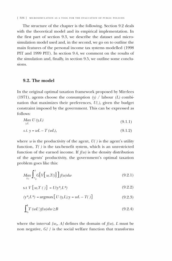
[ 326 ] m i c r o s i m u l at i o n a s a t o o l f o r t h e e va l u at i o n o f p u b l i c p o l i c i e s
The structure of the chapter is the following. Section 9.2 deals with the theoretical model and its empirical implementation. In the first part of section 9.3, we describe the dataset and micro-simulation model used and, in the second, we go on to outline the main features of the personal income tax systems modelled (1998 PIT and 1999 PIT). In section 9.4, we comment on the results of the simulation and, finally, in section 9.5, we outline some conclu-sions.
9.2. The model
In the original optimal taxation framework proposed by Mirrlees (1971), agents choose the consumption (y) / labour (L) combi-nation that maximizes their preferences, U(.), given the budget constraint imposed by the government. This can be expressed as follows:
Max U (y,L)y,L (9.1.1)
s.t. y = wL – T (wL), (9.1.2)
where w is the productivity of the agent, U( ) is the agent’s utility function, T( ) is the tax-benefit system, which is an unrestricted function of the earned income. If f(w) is the density distribution of the agents’ productivity, the government’s optimal taxation problem goes like this:
Max G{V[w,T()}]f(w)dw∫w0
A
T()(9.2.1)
s.t V [w,T ( )] = U(y*,L*) (9.2.2)
(y*,L*) = argmax[U (y,L);y = wL – T( )] (9.2.3)
∫A
w0T (wL*)f(w)dw ≥B (9.2.4)
where the interval [w0, A] defines the domain of f(w), L must be non negative, G{ } is the social welfare function that transforms
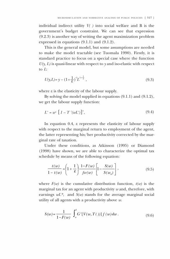
m i c r o s i m u l at i o n a n d n o r m at i v e a n a ly s i s o f p u b l i c p o l i c i e s [ 327 ]
individual indirect utility V( ) into social welfare and B is the government’s budget constraint. We can see that expression (9.2.3) is another way of writing the agent maximization problem expressed in equations (9.1.1) and (9.1.2).
This is the general model, but some assumptions are needed to make the model tractable (see Tuomala 1990). Firstly, it is standard practice to focus on a special case where the function U(y, L) is quasi-linear with respect to y and iso-elastic with respect to L:
U(y,L)= y – (1+ ) L ,1ε
1ε–1 1+
(9.3)
where ε is the elasticity of the labour supply.By solving the model supplied in equations (9.1.1) and (9.1.2),
we get the labour supply function:
L* = w ε [1 – T '(wL*)]ε, (9.4)
In equation 0.4, ε represents the elasticity of labour supply with respect to the marginal return to employment of the agent, the latter representing his/her productivity corrected by the mar-ginal rate of taxation.
Under these conditions, as Atkinson (1995) or Diamond (1998) have shown, we are able to characterize the optimal tax schedule by means of the following equation:
−
−
+=
− )(
)(1
)(
)(111
)(1
)(
0wS
wS
w
wF
wt
wtε fw
, (9.5)
where F(w) is the cumulative distribution function, t(w) is the marginal tax for an agent with productivity w and, therefore, with earnings wL*, and S(w) stands for the average marginal social utility of all agents with a productivity above w.
[ ]∫−=
A
wdw .wfTwVG
wFwS )()) (,('
)(11
)( (9.6)

[ 328 ] m i c r o s i m u l at i o n a s a t o o l f o r t h e e va l u at i o n o f p u b l i c p o l i c i e s
Once the optimal tax schedule has been characterized, let us invert the usual problem and define φ(.) as:
[ ])(
)()(1)(
0wS
wSwFw −=φ . (9.7)
Then, we can rewrite equation (9.7) as follows:
[ ]εε
+⋅ ⋅
−−−=
1
)(
)(1
)()(1)(
wwf
wt
wtwFwφ (9.8)
And, by normalizing the welfare function G(.) in such a way that the mean marginal social welfare is equal to 1, S(w0) = 1, it is easy to show (after some straightforward calculations) that:
) ) [ ])()('
(,('wfw
TwVG −=φ . (9.9)
This formula gives us the marginal social welfare weight of an agent characterized by productivity w under a certain redistribu-tion system T(.), a given distribution of productivities f(w) and some hypotheses regarding ε.
Before applying the inversion procedure just described, some work on the data must be performed, as follows. First, to retain the logic of the optimal taxation model (in this case, an optimal labour income tax model), all households for which unearned income (including pension and unemployment benefits) repre-sented more than 10 per cent of their total income were elimi-nated from the sample.1
Second, to compute f(w), we have used the process described in Bourguignon and Spadaro (2000a). Basically, the idea is to invert the individual utility maximization problem (equations 9.1.1 and 9.1.2) and to recover the implicit productivity of each household by observing the gross earned income wl and the ef-fective marginal tax rate t(w), and by making certain hypotheses
1 This filtering reduces the number of households used in our computations from 6,420 to 2,718, divided by category as follows: singles (326), couples (1,456), couples + 1 child (423), couples + 2 children (513). Of course the new sample is not representa-tive of the whole population but it is representative of the working population.
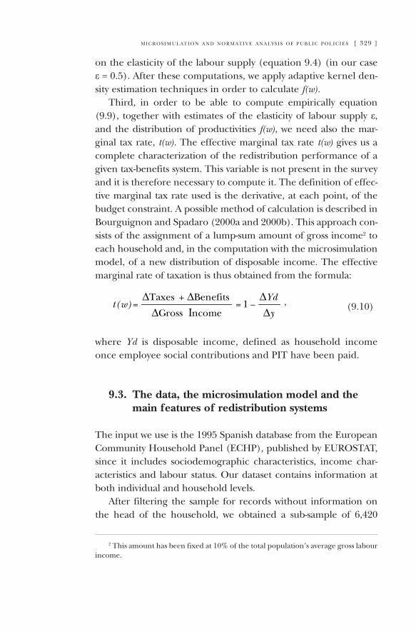
m i c r o s i m u l at i o n a n d n o r m at i v e a n a ly s i s o f p u b l i c p o l i c i e s [ 329 ]
on the elasticity of the labour supply (equation 9.4) (in our case ε = 0.5). After these computations, we apply adaptive kernel den-sity estimation techniques in order to calculate f(w).
Third, in order to be able to compute empirically equation (9.9), together with estimates of the elasticity of labour supply ε, and the distribution of productivities f(w), we need also the mar-ginal tax rate, t(w). The effective marginal tax rate t(w) gives us a complete characterization of the redistribution performance of a given tax-benefits system. This variable is not present in the survey and it is therefore necessary to compute it. The definition of effec-tive marginal tax rate used is the derivative, at each point, of the budget constraint. A possible method of calculation is described in Bourguignon and Spadaro (2000a and 2000b). This approach con-sists of the assignment of a lump-sum amount of gross income2 to each household and, in the computation with the microsimulation model, of a new distribution of disposable income. The effective marginal rate of taxation is thus obtained from the formula:
y
Yd
ncomeGross
BenefitsTaxeswt
∆∆
−=∆
∆+∆= 1
I )( . (9.10)
where Yd is disposable income, defined as household income once employee social contributions and PIT have been paid.
9.3. The data, the microsimulation model and the main features of redistribution systems
The input we use is the 1995 Spanish database from the European Community Household Panel (ECHP), published by EUROSTAT, since it includes sociodemographic characteristics, income char-acteristics and labour status. Our dataset contains information at both individual and household levels.
After filtering the sample for records without information on the head of the household, we obtained a sub-sample of 6,420
2 This amount has been fixed at 10% of the total population’s average gross labour income.
,
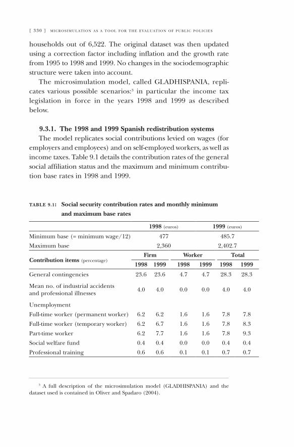
[ 330 ] m i c r o s i m u l at i o n a s a t o o l f o r t h e e va l u at i o n o f p u b l i c p o l i c i e s
households out of 6,522. The original dataset was then updated using a correction factor including inflation and the growth rate from 1995 to 1998 and 1999. No changes in the sociodemographic structure were taken into account.
The microsimulation model, called GLADHISPANIA, repli-cates various possible scenarios:3 in particular the income tax legislation in force in the years 1998 and 1999 as described below.
9.3.1. The 1998 and 1999 Spanish redistribution systemsThe model replicates social contributions levied on wages (for
employers and employees) and on self-employed workers, as well as income taxes. Table 9.1 details the contribution rates of the general social affiliation status and the maximum and minimum contribu-tion base rates in 1998 and 1999.
table 9.1: Social security contribution rates and monthly minimum
and maximum base rates
1998 (euros) 1999 (euros)
Minimum base (= minimum wage/12) 477 485.7
Maximum base 2,360 2,402.7
Contribution items (percentage)Firm Worker Total
1998 1999 1998 1999 1998 1999
General contingencies 23.6 23.6 4.7 4.7 28.3 28.3
Mean no. of industrial accidents and professional illnesses 4.0 4.0 0.0 0.0 4.0 4.0
Unemployment
Full-time worker (permanent worker) 6.2 6.2 1.6 1.6 7.8 7.8
Full-time worker (temporary worker) 6.2 6.7 1.6 1.6 7.8 8.3
Part-time worker 6.2 7.7 1.6 1.6 7.8 9.3
Social welfare fund 0.4 0.4 0.0 0.0 0.4 0.4
Professional training 0.6 0.6 0.1 0.1 0.7 0.7
3 A full description of the microsimulation model (GLADHISPANIA) and the dataset used is contained in Oliver and Spadaro (2004).
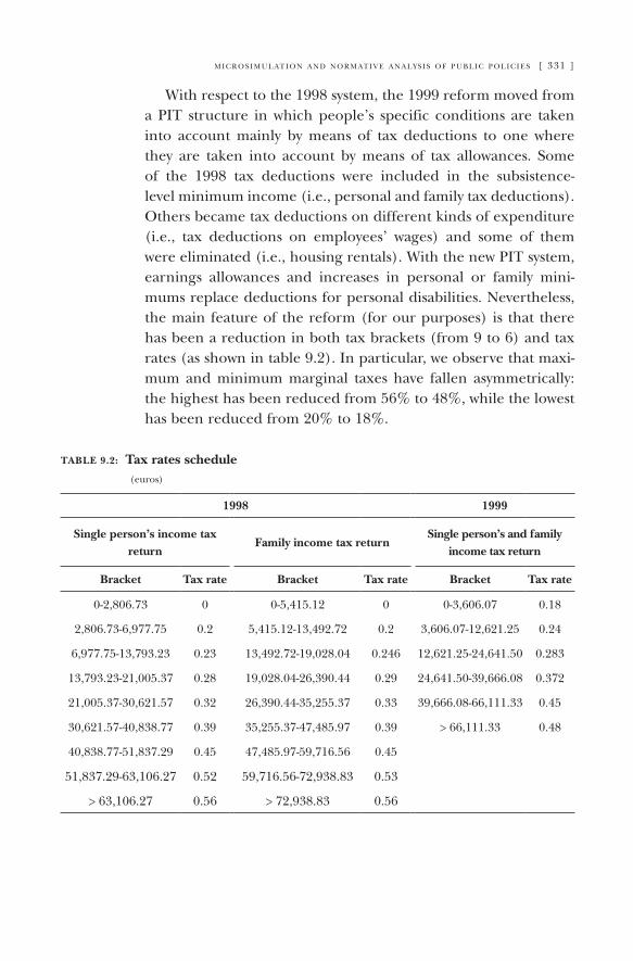
m i c r o s i m u l at i o n a n d n o r m at i v e a n a ly s i s o f p u b l i c p o l i c i e s [ 331 ]
With respect to the 1998 system, the 1999 reform moved from a PIT structure in which people’s specific conditions are taken into account mainly by means of tax deductions to one where they are taken into account by means of tax allowances. Some of the 1998 tax deductions were included in the subsistence-level minimum income (i.e., personal and family tax deductions). Others became tax deductions on different kinds of expenditure (i.e., tax deductions on employees’ wages) and some of them were eliminated (i.e., housing rentals). With the new PIT system, earnings allowances and increases in personal or family mini-mums replace deductions for personal disabilities. Nevertheless, the main feature of the reform (for our purposes) is that there has been a reduction in both tax brackets (from 9 to 6) and tax rates (as shown in table 9.2). In particular, we observe that maxi-mum and minimum marginal taxes have fallen asymmetrically: the highest has been reduced from 56% to 48%, while the lowest has been reduced from 20% to 18%.
table 9.2: Tax rates schedule (euros)
1998 1999
Single person’s income tax return
Family income tax returnSingle person’s and family
income tax return
Bracket Tax rate Bracket Tax rate Bracket Tax rate
0-2,806.73 0 0-5,415.12 0 0-3,606.07 0.18
2,806.73-6,977.75 0.2 5,415.12-13,492.72 0.2 3,606.07-12,621.25 0.24
6,977.75-13,793.23 0.23 13,492.72-19,028.04 0.246 12,621.25-24,641.50 0.283
13,793.23-21,005.37 0.28 19,028.04-26,390.44 0.29 24,641.50-39,666.08 0.372
21,005.37-30,621.57 0.32 26,390.44-35,255.37 0.33 39,666.08-66,111.33 0.45
30,621.57-40,838.77 0.39 35,255.37-47,485.97 0.39 > 66,111.33 0.48
40,838.77-51,837.29 0.45 47,485.97-59,716.56 0.45
51,837.29-63,106.27 0.52 59,716.56-72,938.83 0.53
> 63,106.27 0.56 > 72,938.83 0.56
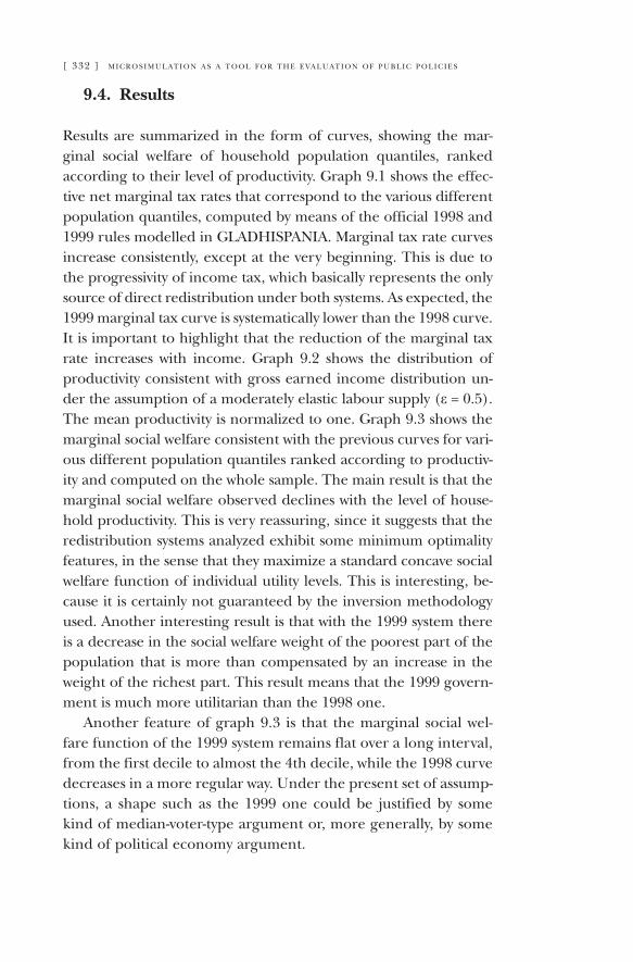
[ 332 ] m i c r o s i m u l at i o n a s a t o o l f o r t h e e va l u at i o n o f p u b l i c p o l i c i e s
9.4. Results
Results are summarized in the form of curves, showing the mar-ginal social welfare of household population quantiles, ranked according to their level of productivity. Graph 9.1 shows the effec-tive net marginal tax rates that correspond to the various different population quantiles, computed by means of the official 1998 and 1999 rules modelled in GLADHISPANIA. Marginal tax rate curves increase consistently, except at the very beginning. This is due to the progressivity of income tax, which basically represents the only source of direct redistribution under both systems. As expected, the 1999 marginal tax curve is systematically lower than the 1998 curve. It is important to highlight that the reduction of the marginal tax rate increases with income. Graph 9.2 shows the distribution of productivity consistent with gross earned income distribution un-der the assumption of a moderately elastic labour supply (ε = 0.5). The mean productivity is normalized to one. Graph 9.3 shows the marginal social welfare consistent with the previous curves for vari-ous different population quantiles ranked according to productiv-ity and computed on the whole sample. The main result is that the marginal social welfare observed declines with the level of house-hold productivity. This is very reassuring, since it suggests that the redistribution systems analyzed exhibit some minimum optimality features, in the sense that they maximize a standard concave social welfare function of individual utility levels. This is interesting, be-cause it is certainly not guaranteed by the inversion methodology used. Another interesting result is that with the 1999 system there is a decrease in the social welfare weight of the poorest part of the population that is more than compensated by an increase in the weight of the richest part. This result means that the 1999 govern-ment is much more utilitarian than the 1998 one.
Another feature of graph 9.3 is that the marginal social wel-fare function of the 1999 system remains flat over a long interval, from the first decile to almost the 4th decile, while the 1998 curve decreases in a more regular way. Under the present set of assump-tions, a shape such as the 1999 one could be justified by some kind of median-voter-type argument or, more generally, by some kind of political economy argument.
m i c r o s i m u l at i o n a n d n o r m at i v e a n a ly s i s o f p u b l i c p o l i c i e s [ 333 ]
graph 9.1: Marginal taxes for workers 1998 and 1999 (kernel estimation)
-
graph 9.2: kernel density estimation of productivities
(w = 1)
graph 9.3: Marginal social welfare functions. Whole sample
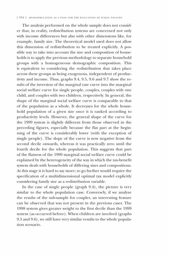
[ 334 ] m i c r o s i m u l at i o n a s a t o o l f o r t h e e va l u at i o n o f p u b l i c p o l i c i e s
The analysis performed on the whole sample does not consid-er that, in reality, redistribution systems are concerned not only with income differences but also with other dimensions like, for example, family size. The theoretical model used does not allow this dimension of redistribution to be treated explicitly. A pos-sible way to take into account the size and composition of house-holds is to apply the previous methodology to separate household groups with a homogeneous demographic composition. This is equivalent to considering the redistribution that takes place across these groups as being exogenous, independent of produc-tivity and income. Thus, graphs 9.4, 9.5, 9.6 and 9.7 show the re-sults of the inversion of the marginal rate curve into the marginal social welfare curve for single people, couples, couples with one child, and couples with two children, respectively. In general, the shape of the marginal social welfare curve is comparable to that of the population as a whole. It decreases for the whole house-hold population of a given size once it is ranked according to productivity levels. However, the general shape of the curve for the 1999 system is slightly different from those observed in the preceding figures, especially because the flat part at the begin-ning of the curve is considerably lower (with the exception of single people). The slope of the curve is now negative from the second decile onwards, whereas it was practically zero until the fourth decile for the whole population. This suggests that part of the flatness of the 1999 marginal social welfare curve could be explained by the heterogeneity of the way in which the tax-benefit system deals with households of differing sizes and compositions. At this stage it is hard to say more; to go further would require the specification of a multidimensional optimal tax model explicitly considering family size as a redistribution variable.
In the case of single people (graph 9.4), the picture is very similar to the whole population case. Conversely, if we analyze the results of the sub-sample for couples, an interesting feature can be observed that was not present in the previous cases. The 1998 system gives greater weight to the first decile than the 1999 system (as occurred before). When children are involved (graphs 9.5 and 9.6), we still have very similar results to the whole popula-tion scenario.
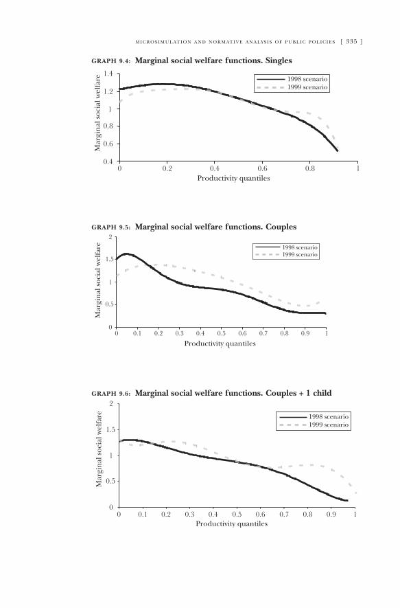
m i c r o s i m u l at i o n a n d n o r m at i v e a n a ly s i s o f p u b l i c p o l i c i e s [ 335 ]
graph 9.4: Marginal social welfare functions. Singles
graph 9.5: Marginal social welfare functions. Couples
graph 9.6: Marginal social welfare functions. Couples + 1 child
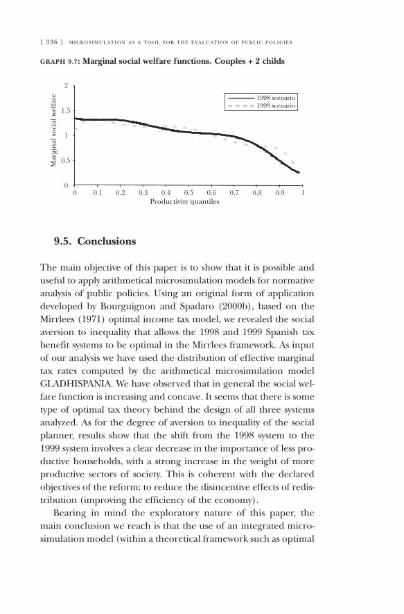
[ 336 ] m i c r o s i m u l at i o n a s a t o o l f o r t h e e va l u at i o n o f p u b l i c p o l i c i e s
graph 9.7: Marginal social welfare functions. Couples + 2 childs
9.5. Conclusions
The main objective of this paper is to show that it is possible and useful to apply arithmetical microsimulation models for normative analysis of public policies. Using an original form of application developed by Bourguignon and Spadaro (2000b), based on the Mirrlees (1971) optimal income tax model, we revealed the social aversion to inequality that allows the 1998 and 1999 Spanish tax benefit systems to be optimal in the Mirrlees framework. As input of our analysis we have used the distribution of effective marginal tax rates computed by the arithmetical microsimulation model GLADHISPANIA. We have observed that in general the social wel-fare function is increasing and concave. It seems that there is some type of optimal tax theory behind the design of all three systems analyzed. As for the degree of aversion to inequality of the social planner, results show that the shift from the 1998 system to the 1999 system involves a clear decrease in the importance of less pro-ductive households, with a strong increase in the weight of more productive sectors of society. This is coherent with the declared objectives of the reform: to reduce the disincentive effects of redis-tribution (improving the efficiency of the economy).
Bearing in mind the exploratory nature of this paper, the main conclusion we reach is that the use of an integrated micro-simulation model (within a theoretical framework such as optimal
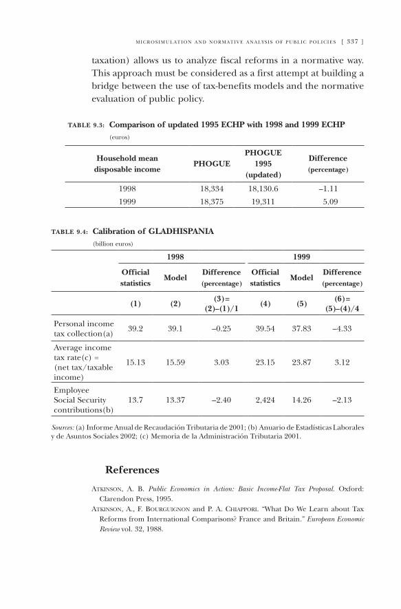
m i c r o s i m u l at i o n a n d n o r m at i v e a n a ly s i s o f p u b l i c p o l i c i e s [ 337 ]
taxation) allows us to analyze fiscal reforms in a normative way. This approach must be considered as a first attempt at building a bridge between the use of tax-benefits models and the normative evaluation of public policy.
table 9.3: Comparison of updated 1995 ECHP with 1998 and 1999 ECHP (euros)
Household mean disposable income
PHOGUE PHOGUE
1995 (updated)
Difference(percentage)
1998 18,334 18,130.6 –1.11
1999 18,375 19,311 5.09
table 9.4: Calibration of GLADHISPANIA (billion euros)
1998 1999
Official statistics
ModelDifference(percentage)
Official statistics
ModelDifference(percentage)
(1) (2)(3) =
(2)–(1)/1(4) (5)
(6) = (5)–(4)/4
Personal income tax collection(a) 39.2 39.1 –0.25 39.54 37.83 –4.33
Average income tax rate(c) = (net tax/taxable income)
15.13 15.59 3.03 23.15 23.87 3.12
Employee Social Security contributions(b)
13.7 13.37 –2.40 2,424 14.26 –2.13
Sources: (a) Informe Anual de Recaudación Tributaria de 2001; (b) Anuario de Estadísticas Laborales y de Asuntos Sociales 2002; (c) Memoria de la Administración Tributaria 2001.
References
atkinson, a. b. Public Economics in Action: Basic Income-Flat Tax Proposal. Oxford: Clarendon Press, 1995.
atkinson, a., f. bourguignon and p. a. chiappori. “What Do We Learn about Tax Reforms from International Comparisons? France and Britain.” European Economic Review vol. 32, 1988.
[ 338 ] m i c r o s i m u l at i o n a s a t o o l f o r t h e e va l u at i o n o f p u b l i c p o l i c i e s
bourguignon, F., C. o’donoghue, J. sastre, A. spadaro and F. utili. “Eur3: A Prototype European Tax-benefits Model.” DAE Working Paper no. 9723. Micro-simu-lation Unit. Cambridge University, 1997.
bourguignon, f. and a. spadaro. “Redistribution and Labour Supply Incentives: An Application of the Optimal Tax Theory.” Paper presented at the 56th Congress of the IIPF. Seville: 28-31 August, 2000a.
—. “Social Preferences Revealed through Effective Marginal Tax Rates.” Working Paper DELTA no. 29, 2000b.
callan, t. and h. sutherland. “The Impact of Comparable Policies in European Countries: Microsimulation Approaches.” European Economic Review, Papers and Proceedings, 1997.
castañer, J. m., J. onrubia and r. paredes. “Efectos de la reforma del I.R.P.F. sobre la renta disponible, su distribución y sobre el bienestar social.” Economistas 84 (2000): 183–199.
de lathouwer, l. “A Case Study of Unemployment Scheme for Belgium and The Netherlands.” In Harding (ed.). Microsimulation and Public Policy. Amsterdam: North Holland, 1996.
diamond, p. “Optimal Income Taxation: An Example with a U-Shaped Pattern of Optimal Marginal Tax Rate.” American Economic Review, 88 no. 1 (1998): 83–95.
Judd, k., f. kubler and k. schmedders. “Computational Methods for Dynamic Equilibria with Heterogeneous Agents.” Mimeo, Stanford University, 2000.
levy, h., m. mercader-prats. “Simplifying the Personal Income Tax System: Lessons from the 1998 Spanish Reform.” Fiscal Studies 23 no. 3 (2002): 419–443.
mirrlees, J. a. “An Exploration of the Theory of Optimal Income Taxation.” Review of Economic Studies 39 (1971): 175–208.
oliver, X. and a. spadaro. “A Technical Description of GLADHISPANIA: A Spanish Micro-Simulation Tax-Benefit Model.” DEA Working Papers no. 7. Universitat de les Illes Balears, 2004.
sanchís, J. a. and a. s. sanchís. “Análisis de simulación de los efectos distributivos de la reforma del IRPF de 1999.” In J. M. Labeaga and Magda Mercader (coords.). Desigualdad, redistribución y bienestar: una aproximación a partir de la microsimulación de reformas fiscales. Instituto de Estudios Fiscales, 2001.
spadaro, a. “Microsimulation and Normative Policy Evaluation: an Application to Some EU Tax-Benefits System.” Journal of Public Economic Theory 7 no. 4, 2005.
tuomala, m. Optimal Income Tax and Redistribution. Oxford University Press, 1990.
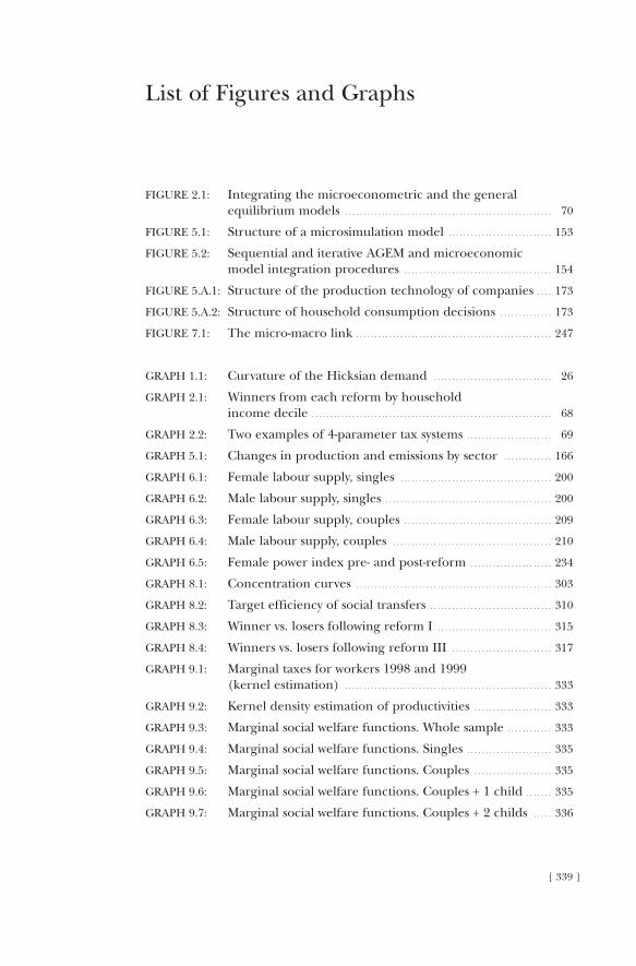
[ 339 ]
List of Figures and Graphs
FiGure 2.1: integrating the microeconometric and the general equilibrium models . . . . . . . . . . . . . . . . . . . . . . . . . . . . . . . . . . . . . . . . . . . . . . . . . . . . . . . . 70
FiGure 5.1: Structure of a microsimulation model . . . . . . . . . . . . . . . . . . . . . . . . . . . . 153
FiGure 5.2: Sequential and iterative AGeM and microeconomic model integration procedures . . . . . . . . . . . . . . . . . . . . . . . . . . . . . . . . . . . . . . . . 154
FiGure 5.A.1: Structure of the production technology of companies . . . . 173
FiGure 5.A.2: Structure of household consumption decisions . . . . . . . . . . . . . . 173
FiGure 7.1: The micro-macro link . . . . . . . . . . . . . . . . . . . . . . . . . . . . . . . . . . . . . . . . . . . . . . . . . . . . . 247
GrAph 1.1: Curvature of the hicksian demand . . . . . . . . . . . . . . . . . . . . . . . . . . . . . . . . 26
GrAph 2.1: Winners from each reform by household income decile . . . . . . . . . . . . . . . . . . . . . . . . . . . . . . . . . . . . . . . . . . . . . . . . . . . . . . . . . . . . . . . . . 68
GrAph 2.2: Two examples of 4-parameter tax systems . . . . . . . . . . . . . . . . . . . . . . . 69
GrAph 5.1: Changes in production and emissions by sector . . . . . . . . . . . . . 166
GrAph 6.1: Female labour supply, singles . . . . . . . . . . . . . . . . . . . . . . . . . . . . . . . . . . . . . . . . . 200
GrAph 6.2: Male labour supply, singles . . . . . . . . . . . . . . . . . . . . . . . . . . . . . . . . . . . . . . . . . . . . . 200
GrAph 6.3: Female labour supply, couples . . . . . . . . . . . . . . . . . . . . . . . . . . . . . . . . . . . . . . . . 209
GrAph 6.4: Male labour supply, couples . . . . . . . . . . . . . . . . . . . . . . . . . . . . . . . . . . . . . . . . . . . 210
GrAph 6.5: Female power index pre- and post-reform . . . . . . . . . . . . . . . . . . . . . . 234
GrAph 8.1: Concentration curves . . . . . . . . . . . . . . . . . . . . . . . . . . . . . . . . . . . . . . . . . . . . . . . . . . . . . 303
GrAph 8.2: Target efficiency of social transfers . . . . . . . . . . . . . . . . . . . . . . . . . . . . . . . . . 310
GrAph 8.3: Winner vs. losers following reform i . . . . . . . . . . . . . . . . . . . . . . . . . . . . . . . 315
GrAph 8.4: Winners vs. losers following reform iii . . . . . . . . . . . . . . . . . . . . . . . . . . . 317
GrAph 9.1: Marginal taxes for workers 1998 and 1999 (kernel estimation) . . . . . . . . . . . . . . . . . . . . . . . . . . . . . . . . . . . . . . . . . . . . . . . . . . . . . . . . 333
GrAph 9.2: Kernel density estimation of productivities . . . . . . . . . . . . . . . . . . . . . 333
GrAph 9.3: Marginal social welfare functions. Whole sample . . . . . . . . . . . . 333
GrAph 9.4: Marginal social welfare functions. Singles . . . . . . . . . . . . . . . . . . . . . . . 335
GrAph 9.5: Marginal social welfare functions. Couples . . . . . . . . . . . . . . . . . . . . . 335
GrAph 9.6: Marginal social welfare functions. Couples + 1 child . . . . . . . 335
GrAph 9.7: Marginal social welfare functions. Couples + 2 childs . . . . . 336

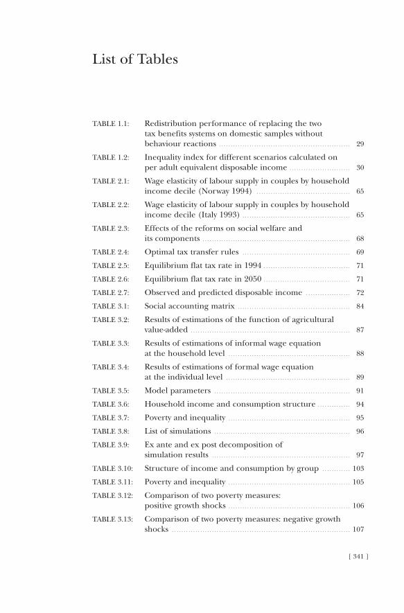
[ 341 ]
List of Tables
TabLe 1.1: Redistribution performance of replacing the two tax benefits systems on domestic samples without behaviour reactions . . . . . . . . . . . . . . . . . . . . . . . . . . . . . . . . . . . . . . . . . . . . . . . . . . . . . . . . 29�
TabLe 1.2: Inequality index for different scenarios calculated on per adult equivalent disposable income . . . . . . . . . . . . . . . . . . . . . . . . . . 30
TabLe 2.1: Wage elasticity of labour supply in couples by household income decile (Norway 19�9�4) . . . . . . . . . . . . . . . . . . . . . . . . . . . . . . . . . . . . . . . . 65
TabLe 2.2: Wage elasticity of labour supply in couples by household income decile (Italy 19�9�3) . . . . . . . . . . . . . . . . . . . . . . . . . . . . . . . . . . . . . . . . . . . . . . 65
TabLe 2.3: effects of the reforms on social welfare and its components . . . . . . . . . . . . . . . . . . . . . . . . . . . . . . . . . . . . . . . . . . . . . . . . . . . . . . . . . . . . . . . 68
TabLe 2.4: Optimal tax transfer rules . . . . . . . . . . . . . . . . . . . . . . . . . . . . . . . . . . . . . . . . . . . . . . 69�
TabLe 2.5: equilibrium flat tax rate in 19�9�4 . . . . . . . . . . . . . . . . . . . . . . . . . . . . . . . . . . . . . 71
TabLe 2.6: equilibrium flat tax rate in 2050 . . . . . . . . . . . . . . . . . . . . . . . . . . . . . . . . . . . . . 71
TabLe 2.7: Observed and predicted disposable income . . . . . . . . . . . . . . . . . . . 72
TabLe 3.1: Social accounting matrix . . . . . . . . . . . . . . . . . . . . . . . . . . . . . . . . . . . . . . . . . . . . . . . . 84
TabLe 3.2: Results of estimations of the function of agricultural value-added . . . . . . . . . . . . . . . . . . . . . . . . . . . . . . . . . . . . . . . . . . . . . . . . . . . . . . . . . . . . . . . . . . . . 87
TabLe 3.3: Results of estimations of informal wage equation at the household level . . . . . . . . . . . . . . . . . . . . . . . . . . . . . . . . . . . . . . . . . . . . . . . . . . . . 88
TabLe 3.4: Results of estimations of formal wage equation at the individual level . . . . . . . . . . . . . . . . . . . . . . . . . . . . . . . . . . . . . . . . . . . . . . . . . . . . . 89�
TabLe 3.5: Model parameters . . . . . . . . . . . . . . . . . . . . . . . . . . . . . . . . . . . . . . . . . . . . . . . . . . . . . . . . . . 9�1
TabLe 3.6: Household income and consumption structure . . . . . . . . . . . . . . 9�4
TabLe 3.7: Poverty and inequality . . . . . . . . . . . . . . . . . . . . . . . . . . . . . . . . . . . . . . . . . . . . . . . . . . . . 9�5
TabLe 3.8: List of simulations . . . . . . . . . . . . . . . . . . . . . . . . . . . . . . . . . . . . . . . . . . . . . . . . . . . . . . . . . . 9�6
TabLe 3.9�: ex ante and ex post decomposition of simulation results . . . . . . . . . . . . . . . . . . . . . . . . . . . . . . . . . . . . . . . . . . . . . . . . . . . . . . . . . . . 9�7
TabLe 3.10: Structure of income and consumption by group . . . . . . . . . . . . 103
TabLe 3.11: Poverty and inequality . . . . . . . . . . . . . . . . . . . . . . . . . . . . . . . . . . . . . . . . . . . . . . . . . . . . 105
TabLe 3.12: Comparison of two poverty measures: positive growth shocks . . . . . . . . . . . . . . . . . . . . . . . . . . . . . . . . . . . . . . . . . . . . . . . . . . . . 106
TabLe 3.13: Comparison of two poverty measures: negative growth shocks . . . . . . . . . . . . . . . . . . . . . . . . . . . . . . . . . . . . . . . . . . . . . . . . . . . . . . . . . . . . . . . . . . . . . . . . . . . . 107
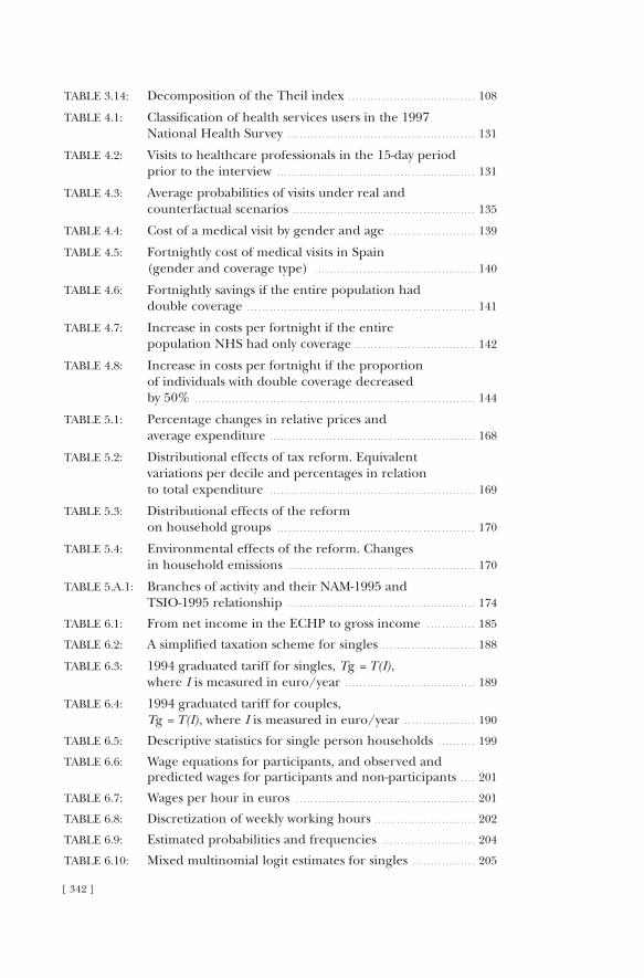
[ 342 ]
TabLe 3.14: Decomposition of the Theil index . . . . . . . . . . . . . . . . . . . . . . . . . . . . . . . . . . 108
TabLe 4.1: Classification of health services users in the 19�9�7 National Health Survey . . . . . . . . . . . . . . . . . . . . . . . . . . . . . . . . . . . . . . . . . . . . . . . . . . 131
TabLe 4.2: Visits to healthcare professionals in the 15-day period prior to the interview . . . . . . . . . . . . . . . . . . . . . . . . . . . . . . . . . . . . . . . . . . . . . . . . . . . . . 131
TabLe 4.3: average probabilities of visits under real and counterfactual scenarios . . . . . . . . . . . . . . . . . . . . . . . . . . . . . . . . . . . . . . . . . . . . . . . . . 135
TabLe 4.4: Cost of a medical visit by gender and age . . . . . . . . . . . . . . . . . . . . . . . 139�
TabLe 4.5: Fortnightly cost of medical visits in Spain (gender and coverage type) . . . . . . . . . . . . . . . . . . . . . . . . . . . . . . . . . . . . . . . . . . . 140
TabLe 4.6: Fortnightly savings if the entire population had double coverage . . . . . . . . . . . . . . . . . . . . . . . . . . . . . . . . . . . . . . . . . . . . . . . . . . . . . . . . . . . . . 141
TabLe 4.7: Increase in costs per fortnight if the entire population NHS had only coverage . . . . . . . . . . . . . . . . . . . . . . . . . . . . . . . . 142
TabLe 4.8: Increase in costs per fortnight if the proportion of individuals with double coverage decreased by 50% . . . . . . . . . . . . . . . . . . . . . . . . . . . . . . . . . . . . . . . . . . . . . . . . . . . . . . . . . . . . . . . . . . . . . . . . . . . 144
TabLe 5.1: Percentage changes in relative prices and average expenditure . . . . . . . . . . . . . . . . . . . . . . . . . . . . . . . . . . . . . . . . . . . . . . . . . . . . . . . 168
TabLe 5.2: Distributional effects of tax reform. equivalent variations per decile and percentages in relation to total expenditure . . . . . . . . . . . . . . . . . . . . . . . . . . . . . . . . . . . . . . . . . . . . . . . . . . . . . . . 169�
TabLe 5.3: Distributional effects of the reform on household groups . . . . . . . . . . . . . . . . . . . . . . . . . . . . . . . . . . . . . . . . . . . . . . . . . . . . . 170
TabLe 5.4: environmental effects of the reform. Changes in household emissions . . . . . . . . . . . . . . . . . . . . . . . . . . . . . . . . . . . . . . . . . . . . . . . . . . 170
TabLe 5.a.1: branches of activity and their NaM-19�9�5 and TSIO-19�9�5 relationship . . . . . . . . . . . . . . . . . . . . . . . . . . . . . . . . . . . . . . . . . . . . . . . . . . 174
TabLe 6.1: From net income in the eCHP to gross income . . . . . . . . . . . . . 185
TabLe 6.2: a simplified taxation scheme for singles . . . . . . . . . . . . . . . . . . . . . . . . . 188
TabLe 6.3: 19�9�4 graduated tariff for singles, Tg = T(I), where I is measured in euro/year . . . . . . . . . . . . . . . . . . . . . . . . . . . . . . . . . . . 189�
TabLe 6.4: 19�9�4 graduated tariff for couples, Tg = T(I), where I is measured in euro/year . . . . . . . . . . . . . . . . . . . 19�0
TabLe 6.5: Descriptive statistics for single person households . . . . . . . . . . 19�9�
TabLe 6.6: Wage equations for participants, and observed and predicted wages for participants and non-participants . . . . 201
TabLe 6.7: Wages per hour in euros . . . . . . . . . . . . . . . . . . . . . . . . . . . . . . . . . . . . . . . . . . . . . . . . 201
TabLe 6.8: Discretization of weekly working hours . . . . . . . . . . . . . . . . . . . . . . . . . . . 202
TabLe 6.9�: estimated probabilities and frequencies . . . . . . . . . . . . . . . . . . . . . . . . . 204
TabLe 6.10: Mixed multinomial logit estimates for singles . . . . . . . . . . . . . . . . . 205
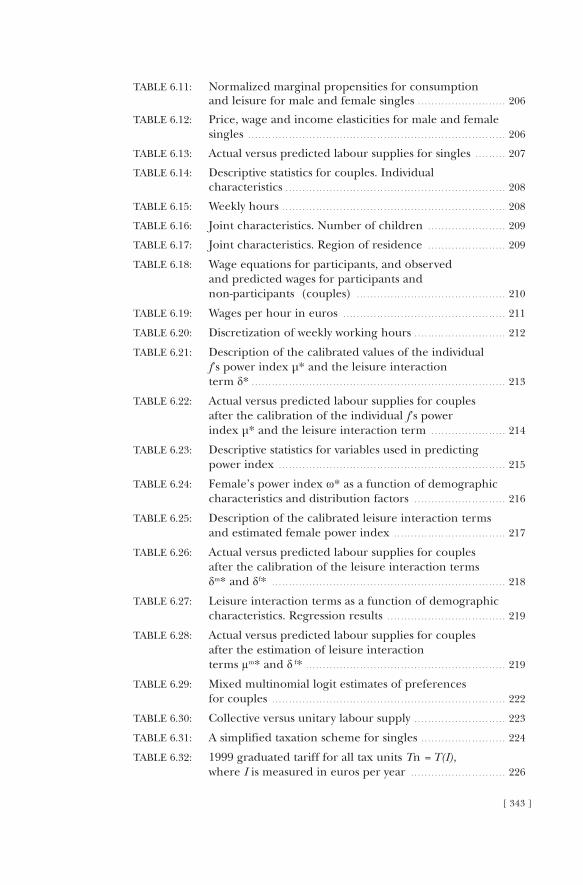
[ 343 ]
TabLe 6.11: Normalized marginal propensities for consumption and leisure for male and female singles . . . . . . . . . . . . . . . . . . . . . . . . . . 206
TabLe 6.12: Price, wage and income elasticities for male and female singles . . . . . . . . . . . . . . . . . . . . . . . . . . . . . . . . . . . . . . . . . . . . . . . . . . . . . . . . . . . . . . . . . . . . . . . . . . . . 206
TabLe 6.13: actual versus predicted labour supplies for singles . . . . . . . . . 207
TabLe 6.14: Descriptive statistics for couples. Individual characteristics . . . . . . . . . . . . . . . . . . . . . . . . . . . . . . . . . . . . . . . . . . . . . . . . . . . . . . . . . . . . . . . . . 208
TabLe 6.15: Weekly hours . . . . . . . . . . . . . . . . . . . . . . . . . . . . . . . . . . . . . . . . . . . . . . . . . . . . . . . . . . . . . . . . . . 208
TabLe 6.16: Joint characteristics. Number of children . . . . . . . . . . . . . . . . . . . . . . . 209�
TabLe 6.17: Joint characteristics. Region of residence . . . . . . . . . . . . . . . . . . . . . . . 209�
TabLe 6.18: Wage equations for participants, and observed and predicted wages for participants and non-participants (couples) . . . . . . . . . . . . . . . . . . . . . . . . . . . . . . . . . . . . . . . . . . . . 210
TabLe 6.19�: Wages per hour in euros . . . . . . . . . . . . . . . . . . . . . . . . . . . . . . . . . . . . . . . . . . . . . . . . 211
TabLe 6.20: Discretization of weekly working hours . . . . . . . . . . . . . . . . . . . . . . . . . . . 212
TabLe 6.21: Description of the calibrated values of the individual f’s power index µ* and the leisure interaction term δ* . . . . . . . . . . . . . . . . . . . . . . . . . . . . . . . . . . . . . . . . . . . . . . . . . . . . . . . . . . . . . . . . . . . . . . . . . . . 213
TabLe 6.22: actual versus predicted labour supplies for couples after the calibration of the individual f’s power index µ* and the leisure interaction term . . . . . . . . . . . . . . . . . . . . . . 214
TabLe 6.23: Descriptive statistics for variables used in predicting power index . . . . . . . . . . . . . . . . . . . . . . . . . . . . . . . . . . . . . . . . . . . . . . . . . . . . . . . . . . . . . . . . . . . 215
TabLe 6.24: Female’s power index ω* as a function of demographic characteristics and distribution factors . . . . . . . . . . . . . . . . . . . . . . . . . . . 216
TabLe 6.25: Description of the calibrated leisure interaction terms and estimated female power index . . . . . . . . . . . . . . . . . . . . . . . . . . . . . . . . . 217
TabLe 6.26: actual versus predicted labour supplies for couples after the calibration of the leisure interaction terms δm* and δf* . . . . . . . . . . . . . . . . . . . . . . . . . . . . . . . . . . . . . . . . . . . . . . . . . . . . . . . . . . . . . . . . . . . . . 218
TabLe 6.27: Leisure interaction terms as a function of demographic characteristics. Regression results . . . . . . . . . . . . . . . . . . . . . . . . . . . . . . . . . . . 219�
TabLe 6.28: actual versus predicted labour supplies for couples after the estimation of leisure interaction terms µm* and δ f* . . . . . . . . . . . . . . . . . . . . . . . . . . . . . . . . . . . . . . . . . . . . . . . . . . . . . . . . . . . 219�
TabLe 6.29�: Mixed multinomial logit estimates of preferences for couples . . . . . . . . . . . . . . . . . . . . . . . . . . . . . . . . . . . . . . . . . . . . . . . . . . . . . . . . . . . . . . . . . . . . . 222
TabLe 6.30: Collective versus unitary labour supply . . . . . . . . . . . . . . . . . . . . . . . . . . . 223
TabLe 6.31: a simplified taxation scheme for singles . . . . . . . . . . . . . . . . . . . . . . . . . 224
TabLe 6.32: 19�9�9� graduated tariff for all tax units Tn = T(I), where I is measured in euros per year . . . . . . . . . . . . . . . . . . . . . . . . . . . . 226
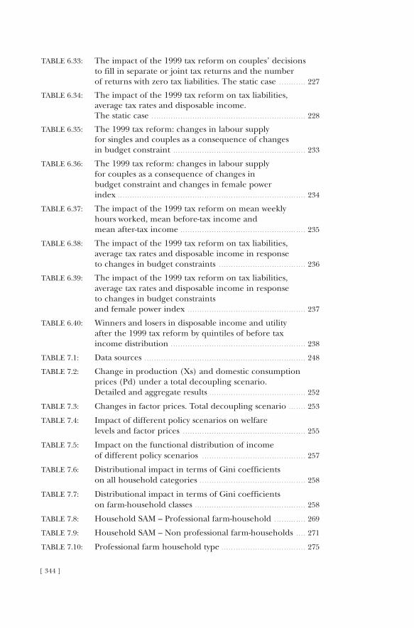
[ 344 ]
TabLe 6.33: The impact of the 19�9�9� tax reform on couples’ decisions to fill in separate or joint tax returns and the number of returns with zero tax liabilities. The static case . . . . . . . . . . . 227
TabLe 6.34: The impact of the 19�9�9� tax reform on tax liabilities, average tax rates and disposable income. The static case . . . . . . . . . . . . . . . . . . . . . . . . . . . . . . . . . . . . . . . . . . . . . . . . . . . . . . . . . . . . . . . . 228
TabLe 6.35: The 19�9�9� tax reform: changes in labour supply for singles and couples as a consequence of changes in budget constraint . . . . . . . . . . . . . . . . . . . . . . . . . . . . . . . . . . . . . . . . . . . . . . . . . . . . . . . 233
TabLe 6.36: The 19�9�9� tax reform: changes in labour supply for couples as a consequence of changes in budget constraint and changes in female power index . . . . . . . . . . . . . . . . . . . . . . . . . . . . . . . . . . . . . . . . . . . . . . . . . . . . . . . . . . . . . . . . . . . . . . . . . . . . . . 234
TabLe 6.37: The impact of the 19�9�9� tax reform on mean weekly hours worked, mean before-tax income and mean after-tax income . . . . . . . . . . . . . . . . . . . . . . . . . . . . . . . . . . . . . . . . . . . . . . . . . . . . 235
TabLe 6.38: The impact of the 19�9�9� tax reform on tax liabilities, average tax rates and disposable income in response to changes in budget constraints . . . . . . . . . . . . . . . . . . . . . . . . . . . . . . . . . . . . 236
TabLe 6.39�: The impact of the 19�9�9� tax reform on tax liabilities, average tax rates and disposable income in response to changes in budget constraints and female power index . . . . . . . . . . . . . . . . . . . . . . . . . . . . . . . . . . . . . . . . . . . . . . . . . 237
TabLe 6.40: Winners and losers in disposable income and utility after the 19�9�9� tax reform by quintiles of before tax income distribution . . . . . . . . . . . . . . . . . . . . . . . . . . . . . . . . . . . . . . . . . . . . . . . . . . . . . . . . 238
TabLe 7.1: Data sources . . . . . . . . . . . . . . . . . . . . . . . . . . . . . . . . . . . . . . . . . . . . . . . . . . . . . . . . . . . . . . . . . . . 248
TabLe 7.2: Change in production (Xs) and domestic consumption prices (Pd) under a total decoupling scenario. Detailed and aggregate results . . . . . . . . . . . . . . . . . . . . . . . . . . . . . . . . . . . . . . . . 252
TabLe 7.3: Changes in factor prices. Total decoupling scenario . . . . . . . 253
TabLe 7.4: Impact of different policy scenarios on welfare levels and factor prices . . . . . . . . . . . . . . . . . . . . . . . . . . . . . . . . . . . . . . . . . . . . . . . . . . . 255
TabLe 7.5: Impact on the functional distribution of income of different policy scenarios . . . . . . . . . . . . . . . . . . . . . . . . . . . . . . . . . . . . . . . . . . . 257
TabLe 7.6: Distributional impact in terms of Gini coefficients on all household categories . . . . . . . . . . . . . . . . . . . . . . . . . . . . . . . . . . . . . . . . . . . . 258
TabLe 7.7: Distributional impact in terms of Gini coefficients on farm-household classes . . . . . . . . . . . . . . . . . . . . . . . . . . . . . . . . . . . . . . . . . . . . . . 258
TabLe 7.8: Household SaM – Professional farm-household . . . . . . . . . . . . . 269�
TabLe 7.9�: Household SaM – Non professional farm-households . . . . 271
TabLe 7.10: Professional farm household type . . . . . . . . . . . . . . . . . . . . . . . . . . . . . . . . . . . 275
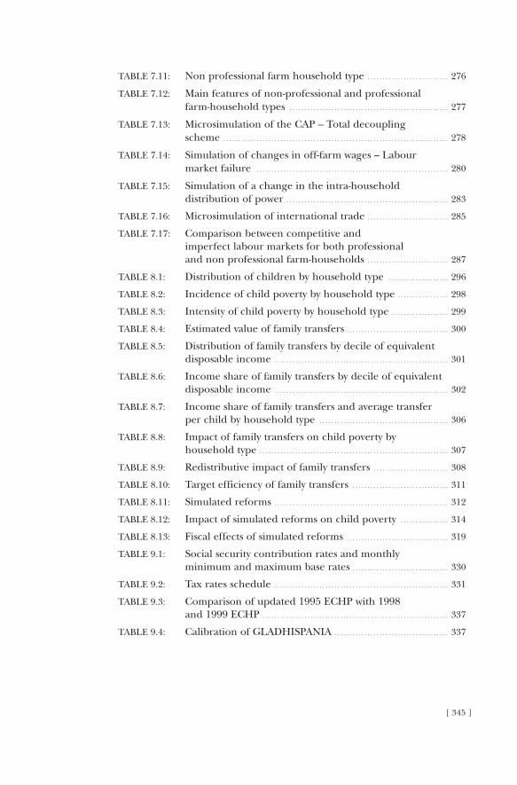
[ 345 ]
TabLe 7.11: Non professional farm household type . . . . . . . . . . . . . . . . . . . . . . . . . . . 276
TabLe 7.12: Main features of non-professional and professional farm-household types . . . . . . . . . . . . . . . . . . . . . . . . . . . . . . . . . . . . . . . . . . . . . . . . . . . . . 277
TabLe 7.13: Microsimulation of the CaP – Total decoupling scheme . . . . . . . . . . . . . . . . . . . . . . . . . . . . . . . . . . . . . . . . . . . . . . . . . . . . . . . . . . . . . . . . . . . . . . . . . . . 278
TabLe 7.14: Simulation of changes in off-farm wages – Labour market failure . . . . . . . . . . . . . . . . . . . . . . . . . . . . . . . . . . . . . . . . . . . . . . . . . . . . . . . . . . . . . . . . 280
TabLe 7.15: Simulation of a change in the intra-household distribution of power . . . . . . . . . . . . . . . . . . . . . . . . . . . . . . . . . . . . . . . . . . . . . . . . . . . . . . 283
TabLe 7.16: Microsimulation of international trade . . . . . . . . . . . . . . . . . . . . . . . . . . . 285
TabLe 7.17: Comparison between competitive and imperfect labour markets for both professional and non professional farm-households . . . . . . . . . . . . . . . . . . . . . . . . . . . 287
TabLe 8.1: Distribution of children by household type . . . . . . . . . . . . . . . . . . . . 29�6
TabLe 8.2: Incidence of child poverty by household type . . . . . . . . . . . . . . . . . 29�8
TabLe 8.3: Intensity of child poverty by household type . . . . . . . . . . . . . . . . . . . 29�9�
TabLe 8.4: estimated value of family transfers . . . . . . . . . . . . . . . . . . . . . . . . . . . . . . . . . . 300
TabLe 8.5: Distribution of family transfers by decile of equivalent disposable income . . . . . . . . . . . . . . . . . . . . . . . . . . . . . . . . . . . . . . . . . . . . . . . . . . . . . . . . . . 301
TabLe 8.6: Income share of family transfers by decile of equivalent disposable income . . . . . . . . . . . . . . . . . . . . . . . . . . . . . . . . . . . . . . . . . . . . . . . . . . . . . . . . . . 302
TabLe 8.7: Income share of family transfers and average transfer per child by household type . . . . . . . . . . . . . . . . . . . . . . . . . . . . . . . . . . . . . . . . . . . 306
TabLe 8.8: Impact of family transfers on child poverty by household type . . . . . . . . . . . . . . . . . . . . . . . . . . . . . . . . . . . . . . . . . . . . . . . . . . . . . . . . . . . . . . . 307
TabLe 8.9�: Redistributive impact of family transfers . . . . . . . . . . . . . . . . . . . . . . . . . 308
TabLe 8.10: Target efficiency of family transfers . . . . . . . . . . . . . . . . . . . . . . . . . . . . . . . . 311
TabLe 8.11: Simulated reforms . . . . . . . . . . . . . . . . . . . . . . . . . . . . . . . . . . . . . . . . . . . . . . . . . . . . . . . . . . 312
TabLe 8.12: Impact of simulated reforms on child poverty . . . . . . . . . . . . . . . . 314
TabLe 8.13: Fiscal effects of simulated reforms . . . . . . . . . . . . . . . . . . . . . . . . . . . . . . . . . . 319�
TabLe 9�.1: Social security contribution rates and monthly minimum and maximum base rates . . . . . . . . . . . . . . . . . . . . . . . . . . . . . . . . 330
TabLe 9�.2: Tax rates schedule . . . . . . . . . . . . . . . . . . . . . . . . . . . . . . . . . . . . . . . . . . . . . . . . . . . . . . . . . . 331
TabLe 9�.3: Comparison of updated 19�9�5 eCHP with 19�9�8 and 19�9�9� eCHP . . . . . . . . . . . . . . . . . . . . . . . . . . . . . . . . . . . . . . . . . . . . . . . . . . . . . . . . . . . . . . 337
TabLe 9�.4: Calibration of GLaDHISPaNIa . . . . . . . . . . . . . . . . . . . . . . . . . . . . . . . . . . . . . . 337

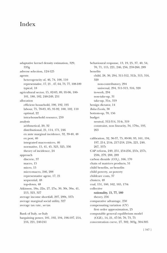
[ 347 ]
adaptative kernel density estimation, 329, 333g
adverse selection, 124-125agents heterogeneity of, 46, 74, 108, 110 representative, 17, 21 , 47, 64, 73, 77, 108-109 typical, 18agricultural sector, 15, 82-83, 89, 95-96, 100-
101, 180, 182, 248-249, 251allocation efficient household, 190, 192, 195 labour, 75, 78-83, 85, 91-92, 100, 102, 110 optimal, 22 intra-household resource, 259analysis arithmetical, 20, 32 distributional, 21, 114, 171, 246 ex ante marginal incidence, 32, 39-40, 48 ex post, 40 integrated macro-micro, 46 normative, 15, 41, 45, 323, 325, 336 theory of incidence, 24approach discrete, 37 macro, 15 micro, 15 micro-macro, 246, 288 representative agent, 17, 21 sequential, 48 top-down, 48Atkinson, 18n, 22n, 27, 27n, 30, 30t, 30n, 41,
213, 323, 327average income shortfall, 297, 299t, 337taverage marginal social utility, 327average tax rate, see tax
Bank of Italy, see Italybargaining power, 181, 192, 194, 196-197, 214,
216, 221, 240-241
behavioural response, 13, 19, 25, 37, 40, 54, 70, 71, 115, 221, 246, 256, 259-260, 289
benefits child, 28, 30, 294, 311-312, 312t, 313, 316,
320 non-contributory, 294 universal, 294, 311-313, 316, 320 in-work, 294 non-take-up, 31 take-up, 31n, 319benign dictator, 14Bolsa Escola, 38bottom-up, 78, 156budget neutral, 312-314, 314t, 319 constraint, non linearity, 34, 179n, 193,
263
calibration, 32, 36-37, 75, 89-90, 93, 161, 194, 197, 214, 214t, 217-218, 218t, 221, 240, 267, 337t
CAP reform, 249, 251, 254-256, 255t, 257t, 258t, 279, 288, 289
carbon dioxide (CO2), 166, 170chain of matrices products, 51child benefits, see benefitschild poverty, see povertychildcare costs, 37clusters, 48coal, 151, 160, 162, 165, 174tcollective rationality, 15, 77, 180rationality, 15, 77, 180 theory, 256comparative advantage, 250compensating variation (CV) first order approximation, 25computable general equilibrium model
(CGE), 14, 21, 47-50, 70, 73, 75concentration curve, 27, 302, 303g, 304-305
Index
[ 348 ]
conditional cash transfer programmes, 38constant return to scale, 87, 157, 262-263Continous Family Budget Survey (ECPF),
156-157, 163contribution to aggregate child poverty, see
poverty contributory family allowances, 294corner solutions, 34, 267CORSIM, 118-119, 122CORSIM 4.1, 119cost function, 263-268Council, 293coverage double, 113, 127-128, 130-132, 135-137,
135t, 139-145, 141t, 144t dual, 14, 127, 130, 135-136cross-section of households, see householdcross-sectional differences, 33, 36, 39
data interpretation, 246decision making process, 18, 40, 52, 259decoupling, 249-251, 252t, 253t, 254, 278t,
279, 282DESTINIE, 120developing countries, 39, 54, 80, 246development strategies, 92, 95distributional impact, 28, 54, 117, 120,
246, 254, 258t, 286, 295, 300, 308, 313, 320
distribution double exponential, 35 functional, 76, 255, 257t income, 19, 28, 30, 73-77, 94, 102, 104,
108-109, 122, 168, 171 intra-household, 178, 181, 283t uniform, 52duality consumer theory, 24DYNACAN, 118-119dynamic framework, 46DYNASIM3, 119
earned income tax credit, 294econometric model, see model specification, 33, 267 techniques, 85economic growth, 73
economy miniature, 249 production side of, 31effects efficiency, 14, 19, 151, 157 first order, 20, 25, 27 redistributive, 181, 229-230, 235-236, 241-
242 second order, 20, 40 short-term redistribution, 21efficiency horizontal, 309-310 vertical, 3009-310 expenditure, see VEEefficient premium contribution, 125energy, 14, 121, 123, 149, 151, 155, 157, 159-
168, 171-172 energy consumption, 14, 123, 157environmental, 52, 149, 157, 161, 170t, 171,
178equality, 66-67, 68t, 273, 303, 305equity of access, 127 efficiency, 42, 124 trade-off, 19 impact, 22equivalence scale, 212, 280, 297nequivalent disposable income, 30, 30t, 212,
227n, 300, 301t, 302t, 302-303equivalent variation, 172, 254, 255temployer sponsored-health insurance (ESI), 19EUROMOD, 15, 28, 44, 122-123, 293n, 294,
300, 321European Commission, 165, 293European Community Household Panel
(ECHP), 180, 182, 184, 185t, 187, 188n, 202, 239, 295, 329, 337t
European Union (UE), 15, 28, 120, 249european-wide MSM, 28Eurostat, 325, 329evaluation positive, 15 behavioural, 32 ex ante, 14, 22 ex post, 22, 40 normative, of public policies, 23, 324, 337exact statistical aggregation, see statisticalfamilialism, 294
[ 349 ]
family activism, 294 low-income, 295, 311, 319, 320 resources survey, 37 transfers, target efficiency of, 295, 311farm wages, 254-255FGT index, 298, 308-309, 308t, 313, 314t, 320financial cost/benefit, 20firms behaviour, 46first order approximation, see compensating
variationFoster-Greer-Thorbecke index, 299tframework dynamic, 46 optimal taxation, 326function cost, 263, 268 expenditure, 24-26 Hicksian demand, 24 household expenditure, 24-25 iso-elastic, 327 Marshallian demand, 24 Pareto, 44 quasi-linear, 327 social welfare, see welfare utility, 35, 63, 67, 73, 161, 178, 191-192,
196, 202, 214, 220-221, 263, 326 indirect, 24, 40-41 individual, 40, 41n
Gini coefficient, 30t, 67, 69, 258tGLADHISPANIA, 330, 332, 336, 337t
headcount poverty rate, 297n rates, 297-298, 308, 313health economics, 14, 22, 113-116, 119-124healthcare financing, 114, 125 management models, 114 private, 14, 113, 127-128, 145health human resources (HHR), 117 Hicksian demand, 24-26, 26ghousehold agricultural, 78-81, 85, 90-92, 96, 100, 103,
248t
consumption survey, 22, 295 cross-section of, 348 enterprise, 259-262, 264, 266 farm, 284 income and wealth survey, 247 income survey, 22, 295 labour supply, 177, 179, 239, 242 production, 241, 260-262, 264, 266 SAM, 267, 269t, 272t technology, 262-265 typical, 18health and tax microsimulation model
(HTSIM), 117Human Resources Development Canada
Department (HRDC), 118
idiosyncratic preference term, 33incidence analysis theory of, 24income distribution, 19, 28, 30, 73-77, 94, 102, 104,
108-109, 122, 168, 171, 181, 227, 229-230, 235-237, 238t, 242, 261, 300, 313-314, 320, 332
effect, 32, 36, 39-40, 99-100, 164 equivalent disposable, 30, 30t, 212, 227n,
300, 301t, 302t, 302-303 extended, 256, 258t full, 263-265, 268, 277t, 278t, 280, 281t,
282-283, 283t, 285, 286t, 287-288, 287t gap, 297-298, 299t, 306, 307t support, 30, 65-66, 294, 310-311 tax, see taxinequality aggregate, 305 governments’ aversion to, 42 index, 30t, 69, 229innovation, 127input/output table, 152-153, 247-248INSEE Households Budget Survey, 28Institute for Fiscal Studies/Instituto de
Estudios Fiscales, 37insurance private health, 126-127, 136integrated CGE-MSM, see modelinternational trade agreements, see Italyinter-temporal behavioural decisions, 21investment climate, 53-54
[ 350 ]
in-work benefits, see benefitsItaly Bank of, household income survey, 295 international trade agreements, 15 tax reform, 13
Kakwani, 27Kuhn-Tucker, 85, 273Kyoto protocol, 151, 165
labour supply, 17, 20, 23, 32-34, 36-39, 42-45, 47, 52, 61, 64, 65t, 71, 79-83, 89-90, 92, 153, 161, 177, 179, 182, 193, 195-196, 200g, 202-204, 209g, 210, 220-221, 223t, 226, 231-232, 233t, 234t, 239-240, 242, 260, 263, 273-276, 284, 287-288, 327-329, 332
land market, 252, 266leisure, 79, 81, 159, 161, 166, 191-195, 197,
201-206, 211, 213-214, 216-218, 219t, 220-221, 239-241, 248, 254-255, 257t, 261, 263, 268, 274-276, 275t, 276t, 278t, 280, 281t, 282, 284t, 286t, 287t
less developed countries (LDC), 22, 27link micro-macro, 246, 247f, 288linkage variables, 49liquified petroleum gases (LPG), 162, 164,
167, 168t, 170tLisbon summit, 293long-term effects, 21Lorenz curve, 303, 305low-income families, see family
macro modelling, 46male breadwinner model, 296marginal social welfare mean, 328 weight, 328Marshallian demand, 24mathematical programming, 249, 267median-voter-type argument, 332Medicaid, 119Medicare, 119microsimulation different types, theoretical foundations, 13 firm, 53 multi-country, 15 techniques, 13, 22-23, 45-46, 115, 126techniques, 13, 22-23, 45-46, 115, 126
microsimulation models (MSM) arithmetical, 325, 336 behavioural, 61 corporate behaviour, 53 dynamic, 119, 121-122, 129 European-wide, 28 integrated CGE-MSM, 21 static, 120, 122, 124
Mirrlees, 40n, 41-43, 325-326, 336MIT, 118mixed complementarity problem (MCP), 273,
287tmodel behavioural, 32, 39, 47, 52, 61, 64, 128,
153, 247 building, 246 collective, 15, 177, 179, 181, 190, 192-193,
197, 201, 221, 231, 239-242, 247, 259, 261, 268, 288
cross-country comparative benefit-tax, 294 econometric, 50, 61, 70-71, 129, 132, 137,
152-155, 245, 248-249, 251, 256, 267-268, 288
estructural econometric, 32 healthcare management, 114 integrated CGE-MSM, 21 male breadwinner, 296 microeconomic, 9, 14, 78, 150-153, 154f,
155, 159n, 161, 170-171 miniature general equilibrium, 260 multidimensional optimal tax, 334 pharmaceutical expenditure, 114 tax benefit, 32, 114-115, 120-121, 300, 325MOSART, 121multilateral and aid agencies, 22multinomial logit, 35, 63, 132, 203-204, 205t,
222t
national accounting matrix (NAM), 160national action plans, 293National Centre for Social and Economic
Modelling (NATSEM), 115natural gas, 151, 160, 162, 164-167, 168t, 170t,
174tNBER, 118NEDYMAS, 120 negative income tax, see tax
[ 351 ]
non-take-up of benefits, see benefitsnon-convexity, 34non-linearity, see budget constraintNorway tax reforms, 13, 61, 121NSO 1994 Family Expenditure Survey, 28
Orcutt, 18, 18n, 22n, 74out-of-sample predictions, 71
Pareto improving indirect, see tax reformPareto social welfare, see functionPareto-efficient, 191, 259, 261pharmaceutical benefits scheme (PBS), 115-116PENSIM, 122PENSIM2, 122pension system reforms, 50, 118perfect equality, see equalityPHARMSIM, 117PNAD, 38POHEM, 116polarization index, 27policy antipoverty, 293 lab, 267 makers, 19, 22, 54, 293 optimal redistribution, 41-42, 324 social, see social policyPOLIMOD, 122POLISIM, 119population ageing, 53, 115, 119poverty analysis, 23 aversion parameter, 298 child aggregate gap, 297, 306 contribution to aggregate, 298t, 297,
297n rate, 308t, 313, 314t target groups, 294, 297, 320 gap efficiency (PGE), 309 weighted aggregated, 310 unweighted aggregated, 309-310 headcount, 27 rate, 94, 102, 104-105, 108, 297-298, 298t,
307 reduction efficiency (PRE), 309
Progresa, 38-39progressivity, see income taxpseudo-random lotteries, 51public assistance to poor children, 294public policies growth-enhancing, 22 normative analysis of, 41, 323, 336
quality, 110, 127, 143, 145
random processes, 51recursive, 266refined petroleum products, 160, 162, 165-
167reforms and income maintenance (RIM), 119resource allocation, see allocationresource pooling, 295retirement income trajectory analysis (RITA),
122revealed social preferences non-Paretian, 45Reynolds-Smolensky, 27
SAGEMOD, 122shadow price, 263, 267, 278t, 279, 281t, 283t,
285tsharing rule, 261, 265, 284tShepard’s lemma, 25short-term redistribution, see effectssingle farm payment, 254, 255t, 256, 257t,
258t, 278t, 282social accounting matrix (SAM), 83, 84t, 93,
102-103, 245, 247, 267-268social inclusion process, 293social perception of individual welfare, see
welfaresocial planners, 15social policy, 22n, 121, 294Social Policy in an Ageing Society (SAGE)
121-123social welfare, see welfaresocioeconomic system, 17south European welfare states, see welfaresouthern Europe, 293Spanish households sociodemographic characteristics of, 325Spanish national health system, 127
[ 352 ]
Spanish redistribution system, 325, 330spillover index, 309State Health Insurance Programs (SCHIP),
119state vector, 51statistical specifications, 15STINMOD, 115subsidiary role, 294subsidies, 29, 53, 124-125, 127, 149, 184survey design, 246SVERIGE, 119, 122
take-up benefits, see benefitstarget efficiency, 295, 300, 308-309, 310g,
311gtarget groups, see child povertytâtonnement, 49tax credit, 180, 187-190, 224, 226, 319n evasion, 31 expenditure, 125, 127 flat, 23n, 66, 70, 71t incidence, 23, 26-27, 31 income, 15, 17, 19-20, 23n, 28-29, 42, 45,
66, 117, 122, 127, 158-159, 177, 184, 186t, 189, 223-224, 241, 294, 324, 326, 328, 330, 331t, 332, 336, 337t
optimal, 42, 336 progressitivity of, 19, 332 negative, 66 indirect, 24, 27, 31, 44 reform,reform, see Pareto, Norway, Italy optimaloptimal model, 43-44, 325, 334model, 43-44, 325, 334 schedule, 327schedule, 327 rate average, 43, 70, 235, 236t, 237t, 325 effective marginal, 12, 43, 44, 325, 328-
329, 336 relief for dependent children, 294, 299,
309, 319n value added, see VATtaxation direct, 22-24, 42, 61
incidence, 22 optimal government’s problem, 326 indirect, 42 model, 41, 328TAXBEN MSM, 37tax-benefit model, 32, 114-115, 120-121, 300, 325 system, 20, 32-34, 36, 39, 45, 215, 226, 334,
336Taylor expansion, 25-26Theil, 27, 94, 99-102, 104-105, 108ttime-use, 211-212, 241, 247-248, 254, 262top-down approach, 48 route, 49transition matrix methods, 51transfer income model (TRIM3), 119
universal child benefits, see benefitsupdating behavioural, 52 probabilistic, 51 process, 51Urban Institute, 118-119
value added tax (VAT), 23, 165, 170, 324vertical expenditure efficiency (VEE), 309-310
Walrasian general equilibrium theory, 21wealth, 53, 103, 120, 247-248welfare dominance, theory of, 26, 27n individual, 41 money metric measure of, 24 social, 15, 40-44, 67-69, 324-326, 330t, 332,
333g, 335g, 336, 336g south European states, 294winners and losers, 17, 19, 237, 238t, 313-314,
316withholding mechanism, 324workfare, 33, 66working families tax credit (WTFC), 37worker, typical, 18
About the Authors
Amedeo SpAdAro holds a PhD from the Ecole des Hautes Etudes en Sciences
Sociales in Paris. He is currently on the research staff of Paris-Jourdan Sciences
Economiques (PSE) and FEDEA (Madrid). He is also professor of public eco-
nomics at the University of the Balearic Islands (Palma de Mallorca). A train-
ing research mobility fellow (European Community Programme, 1996-99)
and fellow of the Ecole Normale Superieure (Paris, 1995), in January 2000 he
received the award for the best PhD dissertation on public economics from the
Instituto de Estudios Fiscales in Madrid. His research interest lies in the theo-
retical and empirical analysis of the reform of redistribution systems, based on
the normative analysis of labour income taxation models and, on the applied
side, the construction of microsimulation models with behavioural reactions
and the treatment of microdata on the income and sociodemographic charac-
teristics of European households. He has contributed articles to the Journal of
Economic Inequality, Journal of Public Economics, Journal of Public Economic Theory,
among other publications, and is currently participating (as coordinator in
some cases) in research projects focused on tax reforms and their impact on
household welfare.
rolf AAberge is senior research fellow in the Research Department of
Statistics Norway. He is a graduate in mathematics and statistics from the
University of Oslo. His current research activities are concerned with labour
supply and taxation, public finance, income distribution and social welfare,
poverty, econometrics and statistical methods, and include management of
a four-year international research programme on evaluation of welfare and
tax policies in welfare states. He has published in economic journals such as
Journal of Economic Theory, Journal of Applied Econometrics, Journal of Population
Economics, Social Choice and Welfare, Journal of Public Economics, Review of Income
and Wealth, Public Choice, and in statistical journals such as Biometrika, Metrika,
Scandinavian Journal of Statistics and Biometrics.
NuriA bAdeNeS plá holds a PhD in economics from the Complutense
University of Madrid and is currently an associate professor at the same
university. Her research is primarily concerned with the design and use of
microsimulation models for the evaluation of public policy. She is a partner
in a number of international research projects and networks, and has pub-
lished extensively in national and international journals.
rAquel CArrASCo holds a PhD in economics from CEMFI and is cur-
rently associate professor in the Department of Economics of Carlos III
University in Madrid. Her work focuses mainly on applied microeconomet-
rics, labour economics and theoretical econometrics. She has published
in economic journals such as the Economic Journal, Journal of Econometrics,
Journal of Business and Economics Statistics and the Oxford Bulletin of Economics
and Statistics.
deNiS CogNeAu has a PhD in economics from the Ecole des Hautes Etudes
en Sciences Sociales (Paris) and is a permanent researcher at the IRD
(Institut de Recherche pour le Développement) and DIAL (Développement
et Insertion Internationale). His specialisation is development economics
and the economics of inequality. He has published several papers and books
on development and social policy issues with particular attention to the
problems of the African continent.
ugo ColombiNo is professor of microeconomics at the University of Turin
(Italy), a research professor at Statistics Norway (Oslo) and Vice-President
of CHILD (Centre for Household, Income, Labour and Demographic eco-
nomics). His research interests centre on the microeconometrics of labour
supply with taxes, and the evaluation of fiscal reforms. He has contributed
articles to a number of economic journals.
mANuelA CoromAldi is a researcher at “Tor Vergata” University (Rome),
where her current focus is on questions of inequality, poverty and social
exclusion. She has participated in several conferences and workshops and is
a partner in a number of international research projects and networks. She
has published various articles in books and journals.
CArloS fAriNhA rodrigueS is a senior research officer at CISEP (Research
Centre on the Portuguese Economy), attached to the Higher Institute of
Economics and Management (ISEG/Technical University of Lisbon), in the
areas of income distribution, social inequalities and social policy.

XAvier lAbANdeirA holds a European doctorate in economics from the
University of Vigo and is currently engaged in research and teaching ac-
tivities at the same university. His research interest centres on the applied
analysis of regulatory policies in the environmental field, with particular
regard to taxation. The results of his work have been presented at national
and international congresses and published in scientific journals.
JoSé mAríA lAbeAgA has a PhD in economics from the Autonomous
University of Barcelona. He is currently professor of fundamentals of eco-
nomic analysis at the Spanish open university (UNED) and a researcher at
FEDEA (Madrid). His main research focus is the analysis of economic mod-
els applied to individual data, and he has also worked on the microsimula-
tion of reforms in direct and indirect taxation. He has published widely and
is currently a partner in various research projects in Spain and Europe.
horACio levy Copello is senior research officer at the Institute for Social
and Economic Research, University of Essex (UK). His research focuses on
questions of inequality, poverty, social exclusion, labour economics, educa-
tion, welfare comparisons and social policy. He has participated in several
conferences and workshops, and is a partner in a number of international
research projects and networks. He has published articles in journals and
books at both national and international level.
áNgel lópez NiColáS is a professor at the Technical University of Cartagena
and a researcher at CRES (Barcelona). His research at present is mainly con-
cerned with the microeconometrics of labour supply with taxes and the evalu-
ation of fiscal reforms, as well as health economics and the microeconometrics
of demand. His work has appeared in a number of international journals.
riCCArdo mAgNANi holds a PhD in political economy from the University of
Verona and a master’s in international economy from the University of Cergy-
Pontoise. His main lines of research are the theory of general equilibrium
applied to the analysis of economic policy and pension system reforms.
eleoNorA mAtteAzzi is a PhD student at the University of Verona (Italy).
Her research focuses on the construction and use of integrated micro-macro
simulation models for the evaluation of public policies.
mANoS mAtSAgANiS is professor in the Department of International and
European Economic Studies of Athens University of Economics and

Business. He was previously a research officer in the London School
of Economics Welfare State Programme, and adjunct professor in the
Economics Department of the University of Crete. His research interests
are the political economy of welfare reform, the microeconomic analysis of
social policy, the economics of social assistance and health economics. He
has published extensively in peer-reviewed journals.
mAgdA merCAder-prAtS is professor in the Department of Applied
Economics of the Autonomous University of Barcelona. Her research
involves the design and use of microsimulation models for the evaluation
of public policy, with particular emphasis on the economics of inequality
and poverty. She has published in a number of international economic
journals.
CAthAl o’doNoghue teaches economics at the National University of
Ireland (Galway). His research involves the design and use of microsimu-
lation models for the evaluation of public policy, in which field he has
acted as a consultant to a range of national and international organisa-
tions. He is a research associate of the Economic and Social Research
Institute (Dublin) the Department of Applied Economics at ULB
Brussels, DAE at the University of Cambridge, and ICER research fel-
low at the University of Turin and a SAGE visiting fellow at the London
School of Economics.
XiSCo oliver is professor of economics at the University of the Balearic
Islands (Palma de Mallorca). His research focuses on the theoretical and
empirical analysis of the reform of redistribution systems, on inequality,
poverty, social exclusion, labour economics, education, welfare comparisons
and social policy. He has paricipated in several conferences and workshops.
He is a partner in a number of international research projects and networks
and has published articles in journals and books both at national and inter-
national level.
federiCo perAli holds a PhD in economic development from the University
of Wisconsin (US) and is currently professor of economic policy at the
University de Verona (Italy). His specialist fields are the analysis of welfare,
poverty, the microeconomic behaviour of consumers and the conduct of
households and family businesses. He has acted as a consultant for a large
number of international organisations.
ANNe-Sophie robilliArd has a PhD in development economics from the
University of Paris I Panthéon-Sorbonne and is a permanent researcher
at DIAL (Développement et Insertion Internationale) (Paris). Her work
has mainly focused on the use of simulation models for the evaluation of
development and social policy impacts in least developed countries (LDC).
She has authored a number of papers and books published at international
level.
miguel rodríguez has a PhD in economics from the University of Vigo,
where he currently holds the post of associate professor. His research activ-
ity centres on the theoretical and applied analysis of the effects of environ-
mental tax reforms, with a focus on the construction and use of integrated
micro-macro simulation models.
JAvier ruiz-CAStillo holds a PhD in economics from Northwestern
University and is currently a professor in the Department of Economics of
Carlos III University (Madrid). His areas of research interest are welfare
economics, public economics and microeconomics, and he has authored
numerous contributions in his specialist field in international journals.
StefANo toSo is professor of economics in the Faculty of Political Sciences
of the University of Bologna. His research focuses on questions of inequality,
poverty, social exclusion, labour economics, education, welfare comparisons
and social policy. He has participated in several conferences and workshops
and is partner in a number of international research projects and networks.
He has published in journals and books at both national and international
level.
pANoS tSAkloglou is a professor in the Department of International
and European Economic Studies at Athens University of Economics and
Business. His research focuses on questions of inequality, poverty, social ex-
clusion, labour economics, education, welfare comparisons and social policy.
He has participated in a large number of conferences and workshops and
has lectured as visiting professor at a number of European universities. A
partner in a number of international research projects and networks, he has
also published extensively in international journals.
