1Department of Economics, Göteborg University, Box 640, S-405 30 Göteborg. E-mail:

Olof.Johansson@economics.gu.se, Fredrik.Carlsson@economics.gu.se, Dinky.Daruvala@kau.se

We are most grateful to two anonymous referees and the editor for very constructive comments. We have

also received valuable comments from Susanna Lundström and seminar participants at Göteborg University,

Karlstad University, The Trade Union Institute for Economic Research (FIEF), Resources for the Future (RFF)

and University of Maryland. Financial support from the Swedish Transport and Communications Research

Board (KFB) is gratefully acknowledged.

Revised version forthcoming in Economic Journal 2002.http//www.blackwellpublishers.co.uk/asp/journal.asp?ref=0013-0133

MEASURING HYPOTHETICAL GRANDPARENTS’

PREFERENCES FOR EQUALITY AND

RELATIVE STANDINGS1

Olof Johansson-StenmanFredrik CarlssonDinky Daruvala

Working Papers in Economics no 42May 2001

Department of Economics Göteborg University

Abstract

Individuals’ aversion to risk and inequality, and their concern for relative standing, are measured

through experimental choices between hypothetical societies. It is found that on average

individuals are both fairly inequality-averse and have a strong concern for relative income. The

results are used to illustrate welfare consequences based on a utilitarian SWF and a modified

CRRA utility function. It is shown that the social marginal utility of income may then become

negative, even at income levels that are far from extreme.

Key words: Well-being, Veil of ignorance, distributional considerations, welfare theory

JEL-classification: C91, D63

1

I. Introduction

The aim of this paper is twofold: (i) To measure the concavity of individual utility functions in

terms of their Arrow-Pratt measure of relative risk aversion (or social inequality aversion), where

utility is seen as a cardinal measure of individual well-being. (ii) To measure the extent to which

individual well-being is a function of absolute and relative income. In public policy the degree of

concavity of the utility function is central for the trade-off between efficiency and equity (see

Atkinson and Stiglitz 1980, or Myles 1995). Relative income effects may also have important

policy implications. For example, public goods, such as environmental quality, should typically

be over-provided relative to the basic Samuelson (1954) rule in the case where relative private

consumption matters for utility (Howarth 1996, Ng 1987, and Ng and Wang 1993). Relative

income effects and status are also important for explaining much of actual behaviour, both in

experiments (Fehr and Schmidt 1999) and in real life (Frank 1985a, Weiss and Fershtman 1998).

We also show that a simultaneous analysis of equity and relative-income effects provides new

insights, and that a utilitarian social welfare function (SWF) may actually be decreasing in income

for a sufficiently high individual income.

1.1 Choosing Behind a Veil of Ignorance and the Social Welfare Function

In order to measure individuals’ relative risk aversion we will utilize hypothetical choices behind

a so-called ‘veil of ignorance’. The idea of choosing behind a veil of ignorance has frequently

been used in welfare theory and moral philosophy, and is also linked with the notion of the

‘impartial spectator’ as discussed by Adam Smith. Vickrey (1945) and Harsanyi (1955) argued

that given a choice between different alternatives, people who are (hypothetically) behind a veil

of ignorance, and hence ignorant of their future position and characteristics in society, would

choose the alternative that maximizes expected utility. Hence, if all individuals were located behind

2See also the rejoinders by Harsanyi (1975a, 1977) and the discussions by Broome (1991), Kaplow (1995), Ng

(1981, 1999) and Weymark (1991) on this issue.

2

such a veil of ignorance, then, given a choice between different SWFs, each individual would

again choose the one which maximizes its expected utility. As demonstrated by Harsanyi (1955),

this happens to be the (unweighted) classical utilitarian SWF. The ethical significance of these

results has been debated intensively. For example, Sen (1976, 1977, 1986) has objected to

Harsanyi’s theorems, claiming that they are not really about utilitarianism, since utility is not

defined independently of individual choice.2 Further, Rawls (1971), who first used the terminology

‘veil of ignorance’, rejected all kinds of utilitarianism and argued that each individual would

instead adopt an extreme risk-averse strategy and select the alternative that provides the best of

the worst possible outcomes (in terms of ‘primary goods’, including income). The arguments for

this extreme risk-averse ‘maxi-min’ strategy are not very clear, however, and they have been

criticized strongly by many economists including Arrow (1973), Harsanyi (1975b), and Ng

(1990). From the experimental results in this paper we found that most individuals do not follow

the strategy proposed by Rawls, but that some actually do.

This discussion, although certainly important, is nevertheless beyond the main scope of this

paper. In the welfare analysis we take an additive utilitarian SWF as given, and the arguments for

equality based on this paper must thus be centred around the concavity of the utility functions (in

income) and, as will be shown, the relative income effects.

1.2 Relative Risk Aversion

As is well known, there is no general consensus in economics about the exact shape of individual

utility functions. In conventional static ordinal consumer theory under certainty, nothing can be

revealed about the concavity of the utility function, since the consumer choice is independent of

3

any monotonically increasing transformation of the utility function (e.g. Samuelson 1947). In the

presence of uncertainty, where individuals maximize expected utility, or in the case of

intertemporal choices, this is no longer true and we clearly need some kind of cardinal measure

of utility. The literature on measuring relative risk aversion is rather extensive and although there

is a considerable variation in the results, values in the interval 0.5 - 2 are often referred to. A

common reference is Blanchard and Fischer (1989, p. 44) who claim that the results from studies

based on consumption choices over time (where interest rates differ) vary greatly, but are often

around or larger than unity. Stern (1977) summarized much of the extensive literature during the

seventies and found larger values (around 4-5) from many studies based on savings behaviour.

He also made estimations based on the actual tax system in UK under the assumption of “equal

sacrifice” and found a relative risk aversion of about two. Similarly, Christiansen and Jansen

(1978) estimated the implicit social preferences based on indirect taxation in Norway, and argued

that the most reliable estimates of the relative risk aversion were around unity.

The idea behind this paper is to let individuals choose between alternative societies with

different income distributions behind a veil of ignorance. The more concave the utility function,

the larger is the relative risk aversion; thus the individual will be willing to trade-off more in terms

of expected income in order to achieve a more equal income distribution. The only empirical

studies we are aware of that utilizes the idea of choices behind a veil of ignorance for measuring

inequality aversion are Johannesson and Gerdtham (1995, 1996), who discuss the inequality

aspect of health care. It is difficult, however, to compare these results to those in other studies

(including the present one) due to the unconventional functional form used. Others, such as

Bukszar and Knetsch (1997), utilize choice behind a veil of ignorance to measure attitudes to

different rules for the distribution of benefits within a group. These experiments are generally not

discussed in relation to an actual income distribution; thus, they do not allow for estimating the

4

concavity of the utility function.

1.3 The Importance of Relative Income or Status

There is a growing awareness in mainstream economics that individual utility may also partly

depend on relative income, i.e. the individual’s income compared to the incomes of other

members of society, and not solely on absolute income; for classic contributions in economics,

see Veblen (1899), Duesenberry (1949), Hirsch (1976), and Frank (1985a, b). Still, although

early economists such as Adam Smith and John Stuart Mill discussed relative income effects, it

has for a long time been unconventional to include these in economic modelling. In a recent book,

Mason (1998) provides a thorough and informative historical overview of conspicuous

consumption (made famous by Veblen) in economics, where he discusses in depth how it came

to be that such issues were considered to be outside the domain of mainstream economics. This

was not an obvious development and in the beginning of this century both Edgeworth and Pigou

(among others) argued that status is important for explaining consumer behaviour, and should also

be included in social welfare analysis.

There is a substantial psychological literature on the measurement of individual well-being,

or happiness; see Oswald (1998) for a recent survey. The well-known conclusion by Easterlin

(1974, 1995) and others from these studies is that stated happiness appears to increase with

income in a given country (or area) for a specific time-period. However, happiness in a society

does not appear to increase over time even though income does. Similarly, the level of happiness

in the countries studied appears to be about the same, although income varies greatly. A utility

framework consistent with these findings is that utility is a function of relative, rather than absolute

3 Kenny (1999) argue that there may actually also be a link from happiness to growth, since some elements

of social capital, such as trust, are important both for happiness and for growth.

5

income.3

A possible weakness in these psychological studies is the link between stated happiness

and actual happiness. Brekke (1997) and Osmani (1993) argue that people may respond to such

questions relating to what they consider to be an average norm of happiness, and that this norm

may also be dependent on income. If so, happiness may depend primarily on the absolute level

of income even though this is not reflected by the survey responses. Although psychologists have

tried to correct for such possibilities, there is clearly a need for more empirical research using

other methods. Frank (1985a, pp. 32-33) argued, partly based on introspection, that it is most

likely that utility depends positively on both relative and absolute income, a view which is

supported by the results in this paper.

Economists are generally sceptical towards statements of well-being and prefer instead

to rely on consumer choices. However, for obvious reasons, it is difficult to observe the utility

derived from relative income by observing consumer behaviour, since individuals can only to a

very limited extent choose the income of others in their surroundings. This is presumably the main

reason why so little work has been done in this area, and why the unrealistic assumption of non-

interdependency is still dominant. Our strategy is therefore to utilize hypothetical choices where

the individuals’ own income as well as mean income in society varies. The greater the importance

of relative income, the more the individual will be willing to trade-off in terms of own income in

order to achieve a better relative standing.

This remainder of this paper is organised as follows: Section 2 describes the models

underlying the experiments on risk (or inequality) aversion and positionality. Section 3 presents

the experimental set-ups, while section 4 presents the results of the experiments. Section 5

6

illustrates welfare consequences of preferences that are both risk-averse and positional, while

section 6 draws conclusions.

2. The Model

2.1 The CRRA Utility Function

It is common in applied welfare economics to assume a special class of utility functions

characterized by constant relative risk aversion (CRRA) as proposed by Atkinson (1970):

(1)u

y

y

= −≠

=

−1

11

1

η

ηη

η

,

ln ,

where y is individual disposable income and is the relative risk aversion.η = − ′′ ′yu u/

Alternatively, assuming a classical utilitarian SWF where welfare , can bew u yi i= ∑ ( ) η

interpreted as the constant social inequality aversion, defined as . Utility is seen− yw

y

wy

∂∂

∂∂

2

2

throughout the paper as an (imperfect) measure of individual well-being and the marginal utility

of income is given by:

(2)µ ∂∂

η= = −u

yy

which is clearly decreasing in income for > 0. = 0 implies that utility is proportional toη η

income, while 6 4 corresponds to extreme risk aversion of maxi-min type. In the case ofη

uncertainty regarding income, the expected utility for an individual is given by:

(3)E u u y f y yy

y

( ) ( ) ( )

min

max

= ∫ d

4 For equal to 1 and 2, respectively, we have: -1 andη E u

y y y y

y y( )

ln lnmax max min min

max min

=−−

.E uy y

y y( )

ln lnmax min

max min

= −−−

7

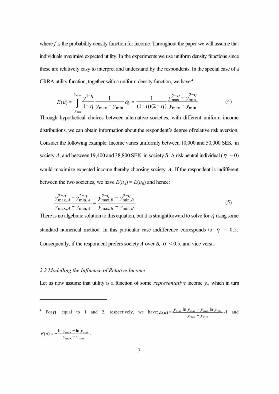
where f is the probability density function for income. Throughout the paper we will assume that

individuals maximise expected utility. In the experiments we use uniform density functions since

these are relatively easy to interpret and understand by the respondents. In the special case of a

CRRA utility function, together with a uniform density function, we have:4

(4)E uy

y yy

y y

y yy

y

( )( )( )max min

max min

max minmin

max

=− −

=− −

−−

− − −

∫1 2 2

1

1 1

1 2

η η η

η η ηd

Through hypothetical choices between alternative societies, with different uniform income

distributions, we can obtain information about the respondent’s degree of relative risk aversion.

Consider the following example: Income varies uniformly between 10,000 and 50,000 SEK in

society A, and between 19,400 and 38,800 SEK in society B. A risk neutral individual ( = 0)η

would maximize expected income thereby choosing society A. If the respondent is indifferent

between the two societies, we have E(uA) = E(uB) and hence:

(5)y y

y y

y y

y yA A

A A

B B

B B

max, min,

max, min,

max, min,

max, min,

2 2 2 2− − − −−

−=

−

−

η η η η

There is no algebraic solution to this equation, but it is straightforward to solve for using someη

standard numerical method. In this particular case indifference corresponds to = 0.5.η

Consequently, if the respondent prefers society A over B, < 0.5, and vice versa. η

2.2 Modelling the Influence of Relative Income

Let us now assume that utility is a function of some representative income yr, which in turn

5In this case utility is unaffected by how much higher or lower the income is compared to others’ income;

what is important is the fraction of the population with a lower (or higher) income.

8

depends on both absolute income and relative income in the following fashion:

(6)y yy

y

y

yr =

=−1 γ

γ

γ

where is the average (mean) income in society and ? is the degree of positionality. Thus, =y γ

0 corresponds to the conventional assumption that utility does not depend on relative income,

whereas at the other extreme, = 1, corresponds to the case where utility depends only on theγ

positional effect from the individual’s income relative to the average income in society, as

proposed e.g. by Easterlin (1974, 1995).

The formulation in (6) is of course quite restrictive, and other types of positional effects

could be considered. For example, Clark and Oswald (1998) discuss different theoretical

implications of ratio comparison formulations, of which (6) is an example, as well as additive

comparison formulations of positionality, where utility depends on the difference between

individual income and mean income. Frank (1985b) analyses a third case where an individual’s

utility depends on her income rank in society (as well as of absolute income).5 One related

possibility is that the concern for relative standing depends on whether the individual is above or

below some critical income level, such as the mean income, i.e. reflecting a kind of endowment

effect. The formulation in (6) should therefore be seen as a first step chosen mainly for its relative

simplicity in estimation, rather than as the most accurate description of reality. However, although

beyond the main scope of this paper, we undertook two additional experiments reported in

Section 4.2 in order to shed some light also on the functional form issue.

Assuming that each individual maximizes a utility function that is a function of representative

income of the form given in (6), we can through hypothetical choices between alternative societies

6 To avoid confusion we will use , instead of , to denote the relative risk aversion parameter when theρ η

degree of positionality, , is greater than zero.γ

9

obtain information about their degree of positionality. Consider the following example: In society

A, the average income is 30,000 SEK, while the individual’s own income is 25,000 SEK. In

society B, the average income is 20,000 SEK, and the individual’s income is 23,000 SEK. If an

individual is indifferent between the two societies, we have that . Thus,y yrA rB=

implying that . Hence, if the respondenty y y yA A B Bγ γ= γ =

≈ln,

,ln

,

,.

23 000

25 000

20 000

30 0000 2

is indifferent in the above example, we have that = 0.2 and, consequently, if A is preferred <γ γ

0.2, and vice versa.

2.3 A Reinterpretation of the Relative Risk Aversion Parameter

If positional externalities exist, the interpretation of as being a measure of relative risk aversionη

and inequality aversion simultaneously will change. In this case we have that utility is a function

of yr, instead of y; therefore, substituting y with yr in (1) we get:6

(7)u

y y

y

yy

y

r

r

=−

=−

≠

= =

− −

−

1 1

11 11

1

ρ ρ

ρ γ

γ

ρ ρρ

ρ

( )( )

,

ln ln ,

Relative risk aversion in terms of y, is still given by , if is seen as fixed. But the interpretationρ y

of as social inequality aversion is now clearly incorrect (if social inequality aversion is definedρ

as ). Indeed, as we will show in Section 5, it is not even obvious that welfare− yw

y

wy

∂∂

∂∂

2

2

7 For equal to 1 and 2, respectively, we have: and ρ E u

y y y yy y

y( )ln ln

lnmax max min min

max min

=−− − −γ

1

.E uy yy y

y( )ln ln

max min

max min

= −−−

γ

10

is increasing in an individual’s income.

Given the choice between alternative societies with different uniform income distributions,

an individual maximizes:7

(8)E uy y

y y y( )

( )( )

max min

max min( )

=− −

−−

− −

−1

1 2

12 2

1ρ ρ

ρ ρ

ρ γ

implying that the individual is indifferent between societies A and B if:

(9)

y y

y y y

y y

y y y

A A

A A A

B B

B B B

max, min,

max, min,( )

max, min,

max, max,( )

2 2

1

2 2

1

1 1− −

−

− −

−

−−

=−−

ρ ρ

ρ γ

ρ ρ

ρ γ

It can be shown that relative risk aversion is generally decreasing in . Hence, indifferenceγ

between the two societies A and B implies a lower relative risk aversion compared to the case

where = 0. γ

3. The Experiments

A total of 374 students from The University of Karlstad and Göteborg University took part in the

main experiments. Participation was voluntary and there was no show-up fee paid. The degree

of participation was approximately 90% although this varied between the groups. The experiment

consisted of three sections, (i) the risk aversion experiment, (ii) the positional experiment, and (iii)

questions regarding the respondent’s socioeconomic status. The students were given verbal

information before each section, in addition to the printed information. The total time for

conducting the experiment, including our instructions, varied between 25 and 40 minutes, mainly

8 From the focus groups we learned that this was especially difficult for the respondents to understand;

therefore it was carefully and repeatedly explained to them.

11

due to the difference in class sizes.

In the experiments the respondents made repeated choices between two societies,

characterized by different income distributions (the risk aversion experiment), and absolute and

relative incomes (the positional experiment). The respondents were given information about the

approximate level of consumption possible given different incomes, and were told that all goods

and prices were constant over the alternative societies.8 In both societies there was essentially no

welfare state and all individual welfare was provided through private insurance systems. The

respondents were also informed that there were no dynamic effects, such as higher growth, of any

specific income distribution. To minimize problems with learning and order effects, the

respondents were encouraged to go back and change their responses.

3.1 Hypothetical Grandchildren and Preference Elicitation

There are many reasons why one may question whether the individual is able to disregard her

personal circumstances and environment in the experiment. Furthermore, it is possible that utility

may also be a function of income changes over time (i.e. positional in the time-dimension, see e.g.

Frank and Hutchens, 1993). Therefore we instructed the respondents to consider the well-being

of their imagined grandchild. Their task was then to choose the alternative that would be in the

best interest of their grandchild. They were frequently reminded that they should not choose the

society that they considered to be the best society on the whole, but the society in which their

grandchild would be the most content.

Our hypothesis is that the respondents will either use their own preferences while choosing

on their grandchild’s behalf, since they have no (or very limited) information regarding their

9Our interpretation is also supported by expressed responses from pre-tests and focus groups.

10 In order to make the set-up more realistic, respondents were told that in both societies there are a small

number of individuals with very low incomes (the homeless, destitute etc.) and a small number of individuals

with extremely high incomes (top-executives, stars etc.). Since these two groups are equally large in both

societies the respondents were told to disregard them in their choices.

12

grandchild’s preferences, or, alternatively, that the respondents believe that their grandchild’s

preferences would be similar to their own preferences. This need not always be perfectly correct,

however. If, for example, the respondent believes that her own preferences are somewhat

extreme, then when forming expectations of her grandchild’s preferences she may adjust her

responses towards the mean. Still, in the subsequent econometric analysis, the parameters

associated with characteristics of the respondents have the expected signs and are of a

reasonable magnitude which supports our hypothesis to some degree.9

There may also be more general problems associated with preference elicitation from

hypothetical surveys or experiments. For example, it may be argued that these do not fully reveal

the true preferences, and that the responses to a certain degree also reflect a “purchase of moral

satisfaction” (cf. Kahneman and Knetsch, 1992). If so, the answers may be biased in (what the

respondent thinks is) an ‘ethical’ direction. If making the ethical choice implies selecting the more

equitable outcome, and not receiving utility from being richer than other people, respectively, then

this would imply a bias upwards for risk aversion and downwards for positionality.

3.2 Risk (Inequality) Aversion Experiment

In this experiment the respondents made choices between two societies, A and B, described only

by their income distribution. The respondents were told that they do not know the position of their

grandchild, and that they should place equal probability on all outcomes for their grandchild. Both

societies have a uniform income distribution,10 and for society A, monthly income always varies

11 There is a possibility of ordering effects here, i.e. their answers may depend on the order in which the

choices are made. This was tested in one of the pilot studies, with 54 respondents. For the relative risk-

aversion experiment the reversed order implied no significant difference. For the positional experiment there

was a significant difference; reversed order was associated with a higher degree of positionality. However,

the number of inconsistent responses was also significantly higher, and the task appeared slightly more

difficult to understand. Therefore, we chose only to include the order presented here.

12 The notion of relative risk premium is used since the comparison is not between a risk-free and a risky

alternative, but between two risky alternatives.

13

uniformly between 10,000 and 50,000 SEK; hence average income is 30,000 SEK/month. Given

the utility function in (1) we create another society, society B, with a different uniform income

distribution. The distribution in this society corresponds to a certain level of risk aversion when

the respondent is indifferent between society A and B. There are eight different B societies, and

thus the respondents made eight pair-wise choices. The societies in the experiments are presented

in Table 1, which is also the order in which the societies were presented in the experiment.11

[Table 1 about here]

The respondents’ choice of societies reflects their relative risk aversion. If, for example, an

individual chooses society B in the first pair-wise alternative, her relative risk aversion is at least

zero. If she then also chooses B in the second alternative, but A in the third alternative, we know

that her risk aversion is greater than 0.5 and less than 1. The table also reports the relative risk

premium when the respondent is indifferent between the societies, i.e. the difference between the

mean incomes of the two societies. This measure can be seen as the amount of money the

respondent is willing to trade-off for increased equality (and hence reduced risk) in society B.12

The respondents were given the information about the societies’ incomes and their distributions

both as numbers in pair-wise choices (as in Table 1) and in a diagram describing the income

distributions for the two societies (they did not receive any information about implicit relative risk

aversion); see appendix.

14

3.3 Positional Experiment

In this experiment the respondents were again required to make repeated choices between two

societies, A and B, described by the average income and their grandchild’s income. Thus, the

respondents now know the position of their grandchild. Here, all A and B societies have the same

degree of income inequality. The society A alternative is fixed with average income at 30,000

SEK/month and the grandchild’s income at 25,000 SEK/month. Society A is compared with

seven different B societies with varying individual and average incomes; thus, the respondents

made seven pair-wise selections where the objective was to choose the society that is best for

their grandchild.

Given a utility function which is a function of relative income of the form given in (6), the

individual and average incomes in society B correspond to a certain degree of positionality when

the respondent is indifferent between the two societies. The societies in the experiments are

presented in Table 2, in the same order as in the experiment.

[Table 2 about here]

The information was presented to the respondents as numbers in pair-wise choices, where the

degree of positionality is reflected in their choice of societies in a similar way as in the risk

aversion experiment. Table 2 also reports the relative positional premium when the respondent

is indifferent between the societies, i.e. the difference between the grandchild’s incomes in the two

societies. This can be seen as the amount of money that the individual is willing to trade-off in

order to obtain the improved relative standing in society B.

13 Seven of the respondents (or about 2%) are inconsistent in the sense that they switched from choosing

society A and then in a later choice alternative chose society B, e.g. implying a risk aversion parameter that

is smaller than, say, 0.2, and larger than, say, 0.6. There could be several reasons for these responses

including learning- or fatigue effects, or that the respondent has some other functional form of the utility

function.

15

4. Results

4.1 Descriptive Results of the Experiments

There were 367 consistent responses for the risk/inequality-aversion experiment,13 the results of

which are presented in Table 3.

[Table 3 about here]

The median relative risk aversion, given that there are no positional effects, is in the interval

between two and three. The respondents are fairly evenly distributed among the categories,

although 43% of the respondents have a risk aversion between one and five. Furthermore, a

considerable number of respondents (17%) were found to have zero or negative risk aversion.

19% exhibit rather extreme risk aversion ( ), compatible with the Rawlsian maxi-minη > 8

strategy, which is unquestionably a non-negligible fraction, but still a minority.

Given the discussion in Section 2.3 concerning the relative risk aversion measure, the results

of the experiment can be reinterpreted. We can calculate the relative risk aversion for a given

degree of positionality ( ) by solving for in equation (9). We then assume that all individualsγ ρ

have the same degree of positionality equal to 0.35, corresponding to the median value in the

second experiment. As can be seen in table 3, is lower than and the difference between themρ η

increases for larger values of . To see why, consider the choice between the society A and aη

specific B-society in the case with positionality. Since utility depends negatively on mean income

(eq. 7), and mean income is lower in B, a lower relative risk aversion is needed to prefer B,

14 There were 18 inconsistent responses in this experiment. Thus, this experiment seems somewhat more

difficult than the previous one, although 4.8% invalid responses is still fairly low.

16

compared to the non-positional case. A natural comparison can be made to the recent literature

on the equity-premium puzzle, where the results indicate that the seemingly unreasonably high

degrees of risk aversion may be reduced substantially when allowing for relative-income effects

and habit formation (Abel 1999; Campbell and Cochrane 1999), or (myopic) loss aversion

(Benartzi and Thaler, 1995).

Amiel et al. (1999) estimated social inequality aversion using a ’leaky-bucket experiment’

(Atkinson, 1980) on students. In this experiment the respondents were instructed to state the

amount of ‘lost money’ that they were willing to accept for transfers from a rich person to a

poorer one. The median relative risk aversion was estimated to be between 0.1 and 0.22, which

completely contrasts our results. However, the specific circumstances are very different from this

study, making a relevant comparison of the results difficult. For example, even an individual who

is generally positive toward large income re-distributions through taxes and transfers, despite large

associated inefficiency costs, may oppose simply taking 1000 dollars from a rich person in the

street and giving it to a poor one.

For the positional experiment there are 358 consistent responses,14 and the results are

presented in Table 4.

[Table 4 about here]

The median degree of positionality is between 0.2 and 0.5, and almost 30% of the respondents

are within this category. Still, a substantial fraction of the respondents are either not positional at

all ( ), or completely positional ( ).γ ≤ 0 γ ≥ 1

The importance of relative standing was verified in a similar hypothetical survey by Solnick

and Hemenway (1998), where the influence of relative standing for different goods such as own

15 We are indebted to an anonymous referee for proposing this test. The remaining 13 respondents were

inconsistent in at least one of the sets and therefore excluded from the analysis.

17

income, education and intelligence was tested. Their (single) question on income was similar to

ours, and where indifference between their alternatives implies a degree of positionality of 0.33.

They found that on average 48% of the respondents preferred the society with a higher relative

but lower absolute income, which is perfectly consistent with our findings.

4.2 On the Structure of Positional Concern

As mentioned earlier, the functional form adopted for positional concern is far from obvious, and

we performed some crude tests in order to gain some insight into this issue. First, we feared that

the respondents might adapt a heuristic choice-rule based on a reference point, and always

choose society A when the grandchild’s income is lower than mean income (choices 5-7 in Table

2). Therefore we let 1/3 of the respondents choose between a modified set of societies A and B,

where the grandchild’s income in society B is always larger than the mean income in B, and where

indifference reflects the same degree of positionality as in Table 2. However, we found no

significant difference between the two versions of the questionnaire.

Second, we performed another experiment based on 3 different sets of questions with 103

respondents, of which 90 were consistent.15 In each set the average income in the societies are

the same as before, i.e. 30,000 SEK/month in A and 20,000 SEK/month in B. The difference is

the grandchild’s income. In the first set (Low income), the grandchild’s income is much lower than

the average income. The second set (Medium income) is the same as before, while in the third

set (High income) the grandchild’s income is much higher than the average income. The implicit

positionality ( ) associated with indifference between A and B is the same for each respectiveγ

16For non-extreme responses we use the mid-value in each interval when calculating the mean. For the extreme

responses, we chose the degree of positionality implied by indifference in the extreme cases.

1716% were equally positional only in the Low and Medium income sets, 18% only in the Low and High

income sets, and 9% only in the Medium and High income sets. The remaining 38% chose alternatives which

imply different values of in all three sets. γ

18

choice in all sets, given the assumed functional form. For example, to test whether is larger orγ

smaller than 0.5 in the low-income set, the grandchild’s income is set to 15,000 SEK/month in

A and 12,240 SEK/month in B; in the high income set the grandchild’s income is instead 60,000

SEK/month in A and 48,960 SEK/month in B. If the functional form adopted is a good

approximation of the true one for most respondents, we would not expect the responses between

different sets to vary systematically. If, on the other hand, an additive-comparison formulation of

positionality such as is more accurate, we would expect people( )y y y y y yr = − + − = −( )1 δ δ δ

to be less positional (in terms of ) in the set with higher income, and vice versa. The results ofγ

the experiment are presented in Table 5, together with the implied degree of positionality for both

the ratio- and additive-comparison utility function.16

[Table 5 about here]

We see that the median degree of positionality ( ) is the same for all three sets for the ratio-γ

comparison utility function. The mean is highest for the Medium income set and lowest for High

income, but the differences are relatively small. For the additive-comparison function, both

median and mean increase strongly with income. These results indicate that the ratio-δ

comparison function performs better than the additive-comparison function. Still, only 19% of the

respondents chose alternatives consistent with the same degree of positionality, in terms of ,γ

in all three sets.17 The results should therefore not be seen to imply that the chosen functional form

18 The premium is calculated as the difference between the mean income in society A and the average of the

mean income levels in the B-societies where the respondent switches from B to A. For the extreme cases η

< 0 and 6 4 we set the relative risk premiums to -500 and 15,500, respectively. Since there is a considerableη

share of extreme responses we have tested for both higher and lower corresponding relative risk premiums.

However, the results turned out to be quite robust, and there was no change in terms of significant

parameters.

19 A left-wing party implies the Social Democrats, the Left Party itself and the Green Party. A lower fraction

than expected said that they would vote for a left-wing political party, “if an election was held today”, which

may partly be explained by the fact that business students were over-represented in the sample.

19

is always the most appropriate one. Just as there is a large heterogeneity with respect to the

degree of positionality, it seems reasonable that also the functional form may differ between

individuals. This is clearly an important area for future research.

4.3 Econometric Analysis

We now turn to the question concerning which factors determine the degree of relative risk

aversion and positionality. As the dependent variable in the regression for the risk aversion

experiment we use the relative risk premium when the respondent is indifferent between the two

societies (see Table 3).18

[Table 6 about here]

Left-wing voters19 are seen to be significantly more risk-averse than others, while business

students tend to be the least risk-averse among different student groups. We see that a large

fraction believed that their future grandchild would have a slightly higher income than average,

which may not be surprising given that the respondents are university students. As we might

expect, this affects their behaviour in the experiment; respondents who believe that their

grandchild will earn more than the mean income are less risk-averse. Thus, even if the

20 This is done by solving equations (5) and (9) for the partial effects on and respectively. Again, thereη ρ

is no algebraic solution, so this is solved numerically.

21 This is calculated as for the relative risk premium. For the extreme cases < 0 and > 1 we set the relativeγ γ

positional premium to -500 and 8,850, respectively. Again we tested for other values for the extreme cases, but

with no changes with respect to significant variables.

20

respondents were told that they do not know the position of their grandchild, they have some

difficulties with liberating themselves from their own expectations. Because of the complexity of

the experiment we have also tested whether there are any enumerator effects, i.e. if the results of

the experiments differ between instructors; however, the corresponding dummy variable used was

insignificant in all estimations.

The coefficients in the regressions can also be converted into partial effects in terms of the

relative risk aversion.20 We calculate the corresponding partial effects for both and atη ρ

sample means. Thus, at the sample mean, left party voters have a relative risk aversion ( ) whichρ

is 1.08 units higher, while business students have a relative risk aversion which is 0.59 units lower

than others.

As the dependent variable for the positional experiment we use the relative positional

premium when the respondent is indifferent between the societies (see Table 4).21

[Table 7 about here]

We see that left-wing voters are also found to be significantly more positional than others, while

technology and law students are less positional than others. Again, using equation (7), the

coefficients can be converted into partial effects in terms of the degree of positionality. For

example, at sample means, the degree of positionality is 0.075 units higher for left-wing voters and

0.15 units lower for law students.

The idea that the study of economics may be important for values and behaviours has been

21

discussed by many including Frank et al. (1993, 1996), who argued that studying economics

seems to decrease the probability of cooperation in social dilemmas. Here we see no effect from

studying economics on relative risk aversion, despite the common emphasis in economics on

efficiency rather than equity. However, there is a significant negative effect on positionality,

indicating a likely influence of the dominating micro-economic assumption that utility and well-

being do not depend on relative consumption. Thus, it is possible that students of economics have

been taught that relative income should not matter, and therefore that it would be irrational to

include such aspects. An alternative explanation is selection-bias, in that less positional individuals

may be over-represented among economics students.

Although the number of siblings does not affect the degree of relative risk aversion, there

seems to be an effect with respect to positionality. This is a possible indication that preferences

for relative status are acquired in childhood and that the presence of siblings leads to a higher

awareness of relative status. Whether people live in urban or rural areas or whether they

frequently attend religious services do not appear to significantly affect either risk aversion or

positionality.

5. Welfare Implications

In this section we will show that interesting welfare implications follow when individuals are both

risk-averse and positional. Let us first consider the general case where and alsou u y y y= ( , / )

a utilitarian SWF. Without positional considerations (or other externalities), an income increase

for any individual will always increase welfare (assuming non-satiation of utility). However, this

is not necessarily true in the general case, since an income increase for one individual implies

reduced relative consumption for all others. Consider a marginal income increase for an individual

22Since we have for .β

γργ ργk ky

y= −

− −1

∂β∂ γρ

ρ

γ ργk

k y

k

y

y

y= − <

− −

− −

1

1 0 γ ρ, ≥ 0

22

k and the corresponding change in social welfare:

(10)

( ) ( )( )

( ) ( )( )

( ) ( )λ

∂∂

∂∂

∂∂

∂∂

∂∂

∂∂

∂∂

α β β αβ β

βββ

≡ = + +

= + −

= + − −

−∑

∑

w

y

u y y y

y

u y y y

y y

y y

y

u y y y

y y

y y

y

y

y

y n

y

y y

y

y

k

k k

k

k k

k

k

k

i i

i

i

ki

k k ii

i kk

k

, / , /

/

/ , /

/

/

cov ,1 1

1

where is the social marginal utility of income, is the marginal utility of absolute incomeλ α k

(holding relative income fixed), and is the marginal utility of relative income (holding absoluteβk

income fixed). Hence, a sufficient condition for a positive marginal welfare change is that β βk ≥

and that the normalized covariance between y and is less than or equal to zero. If the individualβ

marginal utility of relative income decreases in income (for any given mean income), the latter

condition is fulfilled.

If we assume a functional form of the utility function according to (7) then the marginal utility

of relative income is decreasing in income.22 However, social welfare may still decrease in income

for large incomes (i.e. for small and , since both these are decreasing in income). Theα k βk

welfare change of an increase in income in this case is:

(11)

λ∂∂

γ γ

γ

ρ

ρ γρ

ρ γρ

ρ γ

ρ γρ

ρ

≡ = − −

= −

−

−−

− +−

− +

−−

−

−∑

∑

w

y

y

yy

y ny

y n

yy

y

y

n

k

kk ii

ki

i

k(1 ) (1 ) (1 )

(1 )

1

1

1

1

1

1 1

1

For = 0 (the non-positional case) this expression is always positive and it is straightforwardγ

23 From (11) we have that when goes to zero: for .ρ ( )∂

∂ γγwy yk

= − >1

1 0 γ < 1

24 In the graphs we have chosen parameter values as follows: = 0.73 and = 10, corresponding to ak1 k2

mean income in the society of 28,700 SEK/month. The implied Gini-coefficient is equal to 0.395, or the same

as the before-tax income Gini-coefficient for UK in 1996. Note that SMRS is invariant to any monotonic

transformation of the SWF, implying that the SWF can be seen as ordinal.

23

to see that the same holds for = 0.23 Thus, in order for social welfare to decrease in individualρ

income, the signs of the positionality-parameter as well as that of the relative risk aversion

parameter must be positive.

Assuming that the estimated parameters apply even outside the experimental conditions,

we can easily illustrate the welfare implications of an income change for individuals with different

income levels by imposing a more realistic income distribution into (11). Since the log-normal

distribution function (Aitchison and Brown, 1957) appears to be the most frequently used function

for describing actual income distributions on a national level, we impose this function into (11) to

obtain:

(12)λ∂∂

γπρ γ

ρρ

≡ = −

−

−−

− −

∞

∫w

y yy

y

y

ke y

kk

y k k1

21

1

2

0

22

12

( )

(ln ) / ( )d

where k1 and k2 are constants. We can then calculate the social marginal rate of substitution

(SMRS) for 2 individuals i, j with different incomes:

(13)SMRS

y

y

y k

y

ye y

y k

y

ye y

i ji

j

j

i

i y k k

j y k k

,

(ln ) /( )

(ln ) / ( )

≡ =

−

−

− −

∞

− −∞

∫

∫λλ

γπ

γπ

ρ

ρ

ρ

12

12

1

2

0

1

2

0

22

12

22

12

d

d

where the first factor equals SMRS in the absence of positionality. Using a specific log-normal

income distribution,24 and for a degree of positionality corresponding to the median value =γ

24

0.35, Figure 1 plots the SMRS between the income levels for two individuals, where income is

10,000 SEK/month for the reference individual, as a function of income for different levels of

relative risk aversion .ρ

[Figure 1 about here]

For example, we see that SMRS is roughly equal to 0.1 at when income y is equal toρ =1

50,000, implying that taking 10 SEK from the richer person and giving 1 SEK to the poorer

would keep social welfare constant, ceteris paribus. We also see that the critical income at

which marginal social utility becomes negative is roughly 45,000 SEK for the median relative risk

aversion of 1.72. Of course there are large differences depending on the degree of relative risk

aversion, but it is interesting to see that for a broad range of risk aversion the social marginal utility

of income becomes negative at income levels which are not at all extreme. For the conservative

estimate where the relative risk aversion is equal to 1, the critical income is 80,000 SEK, which

is less than three times the mean income. With a relative risk aversion equal to 3, the critical

income is 24,000, i.e. lower than the mean income. Figure 2 depicts SMRS for different degrees

of positionality, with a given relative risk aversion = 1.72.ρ

[Figure 2 about here]

We see that SMRS decreases rapidly in income in all cases. If individuals are completely non-

positional, social marginal utility is always positive. In the somewhat extreme case when the

degree of positionality is 0.9, the critical income for which SMRS becomes negative is roughly

26,000 SEK, which is again below the mean income level in the society.

6. Conclusions

We have found that the individuals in our sample are rather risk (or inequality) averse, although

25

the results are not extreme in comparison to earlier studies. Further, we found that most of the

individuals in our sample were willing to trade-off a non-negligible amount of money for increasing

their grandchild’s relative standing in the society.

It is possible, however, that individual utility is a function not only of absolute and relative

consumption, but also of inequality per se. This would imply a utility function of the

type , where is a measure of income inequality, e.g. the coefficient of variationu y y y( , , )ξ ξ

or the Gini-coefficient. If so, the estimated relative risk aversion may be overstated, and may in

part reflect the individuals’ willingness to pay for living in a more equal society. Reasons for this

might be that a more equal society is considered safer to live in, or that the presence of poor

people causes discomfort. On the other hand, some individuals may not be able to disregard the

link between a more equal income distribution and government intervention through, for example,

re-distributive taxes. Individuals who are not in favour of such policies might then have

understated their relative risk aversion in the experiment.

We also illustrated how a simultaneous treatment of relative risk aversion and concern for

position in society can affect the welfare implications of an increase in incomes, given a utilitarian

SWF. Even with quite conservative parameters of relative risk aversion and positionality, the

marginal social utility of income becomes negative above certain non-extreme income levels. At

these income levels it may then seem rational to increase taxes even if no one else would benefit

in terms of increased consumption. Hence, taking money from the very rich and throwing them

into the sea would be welfare improving, if no indirect effects would occur. Still, one may question

the functional form chosen, the ethics underlying a utilitarian SWF, or simply argue that the

respondents’ ‘true’ preferences are not revealed in this experimental setting. Alternatively it could

be claimed that increased taxes on the rich would be so distorting that it may even lead to lower

consumption for other groups. Further, there are of course public-choice reasons that make

26

extreme tax-increases for the rich difficult to implement.

To our knowledge this is the first attempt to measure relative risk aversion behind a veil of

ignorance, and also the first simultaneous treatment of risk aversion and concern for relative

standing. There are several interesting areas for future research. Firstly, measuring individuals’

aversion to inequality per se, thus separating this effect from risk aversion. Secondly, to extend

the treatment of positionality, for example by allowing it to depend on the consumption of goods

other than income, or by including moments of the income distribution other than average income.

Finally, to undertake similar studies in other countries, where the preferences for equality and

status may differ.

References

Abel, A.B. (1999). ‘Risk premia and term premia in general equilibrium’, Journal of Monetary

Economics, vol. 43, pp. 3-33.

Aitchison, J. and Brown, J. (1957). The Log-Normal Distribution, Cambridge: Cambridge

University Press.

Amiel, Y., Creedy, J. and Hurn, S. (1999). ‘Measuring attitudes towards inequality ’,

Scandinavian Journal of Economics, vol. 101, pp. 83-96.

Arrow, K. (1973). ‘Some ordinalist-utilitarian notes on Rawl’s theory of justice’, Journal of

Philosophy, vol. 70, pp. 245-63.

Atkinson, A.B. (1970). ‘On the measurement of inequality’, Journal of Economic Theory, vol.

2:, pp. 244-63.

Atkinson, A.B. (1980). ‘On the measurement of inequality’, in (A.B. Atkinson, ed.) Wealth

Income and Inequality, Oxford: Oxford University Press.

27

Atkinson, A.B. and Stiglitz, J.E. (1980). Lectures in Public Economics, Singapore: McGraw

Hill.

Benartzi, S. and Thaler, R. H. (1995). ‘Myopic loss aversion and the equity premium puzzle’,

Quarterly Journal of Economics, vol. 110, pp. 73-92.

Blanchard, O. and Fischer, S. (1989). Lectures on Macroeconomics, Cambridge: MIT Press.

Brekke, K.-A. (1997). Economic Growth and the Environment, Cheltenham: Edward Elgar.

Broome, J. (1991). Weighing Goods, Cambridge Mass.: Basil Blackwell.

Bukszar, E. and Knetsch, J. (1997). ‘Fragile redistribution behind a veil of ignorance’, Journal

of Risk and Uncertainty, vol. 14, pp. 63-74.

Campbell, J. Y. and Cochrane, J. H. (1999). ‘By force of habit: A consumption-based

explanation of aggregate stock market behavior’ Journal of Political Economy, vol. 107,

pp. 205-51.

Christiansen, V. and Jansen, E. (1978). ‘Implicit social preferences in the Norwegian system of

indirect taxation’, Journal of Public Economics, vol. 10, pp. 217-45.

Clark, A. and Oswald, A. (1998). ‘Comparison-concave utility and following behaviour in social

and economic settings’, Journal of Public Economics, vol. 70, pp. 133-55.

Duesenberry, J.S. (1949). Income, Saving, and the Theory of Consumer Behaviour,

Cambridge: Harvard University Press.

Easterlin, R.A. (1974). ‘Does economic growth enhance the human lot? Some empirical

evidence’, in (P.A. David and M. Reder, eds.) Nations and Households in Economic

Growth: Essays in Honour of Moses Abramovitz, Palo Alto: Stanford University Press,

pp. 89-125.

Easterlin, R.A. (1995). ‘Will raising the incomes of all increase the happiness of all?’ Journal of

Economic Behaviour and Organization, vol. 27, pp. 35-47.

28

Fehr, E. and Schmidt, K. (1999). A theory of fairness, competition, and cooperation, Quarterly

Journal of Economics, vol. 114, pp. 817-68.

Frank, R.H. (1985a). Choosing the Right Pond. Human Behaviour and the Quest for Status,

New York: Oxford University Press.

Frank, R.H. (1985b). ‘The demand for unobservable and other nonpositional goods’, American

Economic Review, vol. 75, pp. 101-16.

Frank, R.H., Gilovich, T.D. and Regan, D.T. (1993). ‘Does studying economics inhibit

cooperation’, Journal of Economic Perspectives, vol. 7, pp. 159-71.

Frank, R.H., Gilovich, T.D. and Regan, D.T. (1996). ‘Do economists make bad citizens?’,

Journal of Economic Perspectives, vol. 10, pp. 187-92.

Frank, R.H. and Hutchens, R.M. (1993). ‘Wages, seniority, and the demand for rising

consumption profiles’, Journal of Economic Behavior and Organization, vol. 21, pp.

251-76.

Harsanyi, J.C. (1955). ‘Cardinal welfare, individualistic ethics, and interpersonal comparisons of

utility’, Journal of Political Economy, vol. 63, pp. 309-21

Harsanyi, J.C. (1975a). ‘Non-linear social welfare functions: Do economists have a special

exemption from Bayesian rationality?’, Theory and Decision, vol. 6, pp. 311-32.

Harsanyi, J.C. (1975b). ‘Can the maximum principle serve as a basis for morality? A critique of

John Rawl's theory’, American Political Science Review, vol. 69, pp. 594-606.

Harsanyi, J.C. (1977). ‘Non-linear social welfare functions: A rejoinder to Professor Sen’, in (R.

Butts and J Hintikka, eds.) Logic, Methodology and Philosophy of Science, Dordrecht:

Reidel.

Hirsch, F. (1976). Social Limits to Growth, Cambridge: Harvard University Press.

29

Howarth, R.B. (1996). ‘Status effects and environmental externalities’, Ecological Economics,

vol. 16, pp. 25-34.

Johannesson, M. and Gerdtham. U. (1995). ‘A pilot test of using the veil of ignorance approach

to estimate a social welfare function for income’, Applied Economics Letters, vol. 2, pp.

400-2.

Johannesson, M. and Gerdtham, U. (1996). ‘A note on the estimation of the equality-efficiency

trade-off for QALYs’, Journal of Health Economics, vol. 15, pp. 359-68.

Kahneman, D. and Knetsch, J.L. (1992). ‘Valuing public goods: The purchase of moral

satisfaction’, Journal of Environmental Economics and Management, vol. 22, pp.

57-70.

Kaplow, L. (1995). ‘A fundamental objection to tax equity norms: a call for utilitarianism’,

National Tax Journal, vol. 48, pp. 497-514.

Kenny, C. (1999). ‘Does growth cause happiness, or does happiness cause growth?’, Kyklos,

vol. 52, pp. 3-26.

Mason, R. (1998). The Economics of Conspicuous Consumption - Theory and Thought

Since 1700, Cheltenham: Edward Elgar.

Myles, G. (1995). Public Economics, Cambridge: Cambridge University Press.

Ng, Y.-K. (1981). ‘Bentham or Nash? On the acceptable form of social welfare functions’,

Economic Record, vol. 57, pp. 231-50.

Ng, Y.-K. (1987). ‘Relative-income effects and the appropriate level of public expenditure’,

Oxford Economic Papers, vol. 39, pp. 293-300.

Ng, Y.-K. (1990). ‘Welfarism and utilitarianism: a rehabilitation’, Utilitas, vol. 2, pp. 171-93.

Ng, Y.-K. (1999). ‘Utility, informed preference, or happiness: following Harsanyi’s argument to

its logical conclusion. Social Choice and Welfare, vol. 16, pp. 197-216.

30

Ng, Y.-K. and Wang, J.. (1993). ‘Relative income, aspiration, environmental quality, individual

and political myopia - why may the rat-race for meeting growth be welfare-reducing?’,

Mathematical Social Sciences, vol. 26, pp. 3-23.

Osmani, S. (1993). ‘Comment on B.M.S. van Praag: The relativity of the welfare concept’, in

(M. Nussbaum and A. Sen, eds.) The Quality of Life, Oxford: Oxford University Press.

Oswald, A.J. (1998). ‘Happiness and economic performance’, Economic Journal, vol. 107,

pp. 1815-31.

Rawls, J. (1971). A Theory of Justice, Cambridge Mass.: Harvard University Press.

Samuelson, P.A. (1947). Foundation of Economic Analysis, Cambridge Mass.: Harvard

University Press.

Samuelson, P.A. (1954). ‘The pure theory of public expenditure’, Review of Economics and

Statistics, vol. 36, pp. 387-89.

Sen, A.K. (1976). ‘Welfare inequalities and Rawlsian axiomatics’, Theory and Decision, vol.

7, pp. 243-62.

Sen, A.K. (1977). ‘Non-linear social welfare functions: A reply to professor Harsanyi’, in (R.

Butts and J. Hintikka, eds.) Logic, Methodology and Philosophy of Science, Dordrecht:

Reidel.

Sen, A.K. (1986). ‘Social choice theory’ in (K.J. Arrow and M.D. Intrilligator, eds.) Handbook

of Mathematical Economics III, Amsterdam: North-Holland.

Solnick, S. and Hemenway, D. (1998). ‘Is more always better?: A survey on positional

concerns’, Journal of Economic Behavior & Organization, vol. 37, pp. 373-83.

Stern, N. (1977). ‘The marginal valuation of income’, in (M.J. Artis and A.R. Nobay, eds.)

Studies In Modern Economic Analysis, London: Blackwell.

Veblen, T. (1899). The Theory of the Leisure Class, New York: Macmillan.

31

Vickrey, W. (1945). ‘Measuring marginal utility by reactions to risk’ Econometrica, vol. 13, pp.

215-36.

Weiss, Y. and Fershtman, C. (1998). ‘Social status and economic performance: A survey’,

European Economic Review, vol. 42, pp. 801-20.

Weymark, J.A. (1991). ‘A reconsideration of the Harsanyi-Sen debate on utilitarianism’ in (J.

Elster and J.E. Roemer, eds.) Interpersonal Comparisons of Well-being, Cambridge:

Cambridge University Press.

Table 1

Societies in the relative risk aversion experiment

Minimum

income

Mean

Income

Maximum

income

Relative risk premium if

indifference between Aand B

Relative risk aversion

if indifference

between A and B

Society A 10000 30000 50000

Society B1 20000 30000 40000 0 = 0η

Society B2 19400 29100 38800 900 = 0.5η

Society B3 18800 28200 37600 1800 = 1η

Society B4 17200 25800 34400 4200 = 2η

Society B5 15800 23700 31600 6300 = 3η

Society B6 13600 20400 27200 9600 = 5 η

Society B7 12200 18300 24400 11700 = 8η

Society B8 10000 15000 20000 15000 6 4η

Table 2

Societies in the relative-income experiment

Average

income

Grandchild’s

income

Relative positional

premium if indifference

between A and B

Degree of positionality if

indifference between A and B

Society A 30000 25000

Society B1 20000 25000 0 = 0γ

Society B2 20000 24000 1000 = 0.1γ

Society B3 20000 23000 2000 = 0.2γ

Society B4 20000 20400 4600 = 0.5γ

Society B5 20000 18400 6600 = 0.75γ

Society B6 20000 17400 7600 = 0.9γ

Society B7 20000 16650 8350 = 1γ

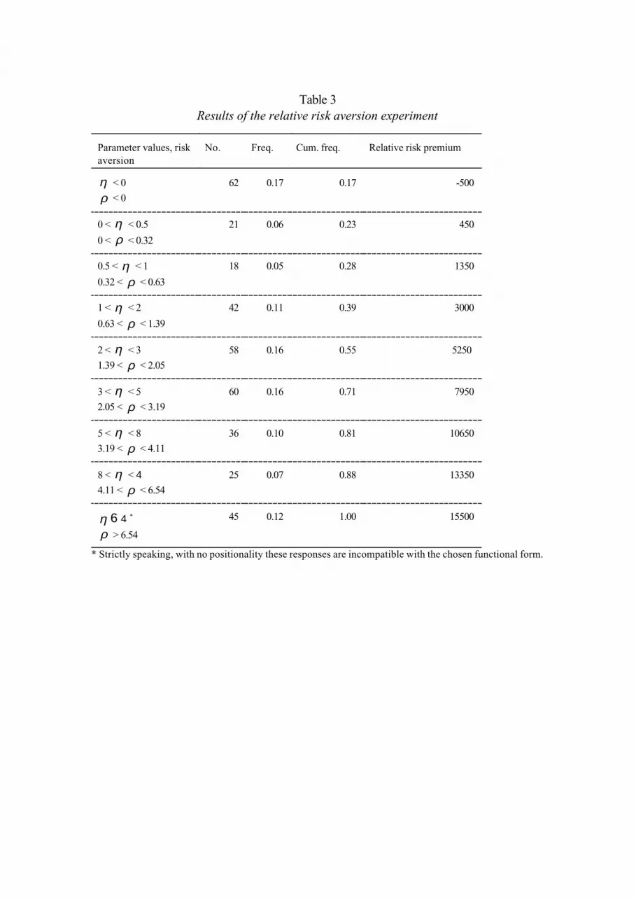
Table 3

Results of the relative risk aversion experiment

Parameter values, risk

aversion

No. Freq. Cum. freq. Relative risk premium

< 0η < 0ρ

62 0.17 0.17 -500

0 < < 0.5η0 < < 0.32ρ

21 0.06 0.23 450

0.5 < < 1η0.32 < < 0.63ρ

18 0.05 0.28 1350

1 < < 2η0.63 < < 1.39ρ

42 0.11 0.39 3000

2 < < 3η1.39 < < 2.05ρ

58 0.16 0.55 5250

3 < < 5η2.05 < < 3.19ρ

60 0.16 0.71 7950

5 < < 8η3.19 < < 4.11ρ

36 0.10 0.81 10650

8 < < 4 η4.11 < < 6.54ρ

25 0.07 0.88 13350

6 4 *η > 6.54 ρ

45 0.12 1.00 15500

* Strictly speaking, with no positionality these responses are incompatible with the chosen functional form.

Table 4

Results of the relative-income experiment

Parameter values ,positionality

No. Freq. Cum. freq. Relative positional premium

γ < 0 64 0.18 0.18 -500

0 < < 0.1 42 0.12 0.30 50γ

0.1 < < 0.2 30 0.08 0.38 1500γ

0.2 < < 0.5 101 0.28 0.66 3300γ

0.5 < < 0.75 52 0.15 0.81 5600γ

0.75 < < 0.9 14 0.04 0.85 7100γ

0.9 < < 1 20 0.06 0.91 7975γ

γ > 1 33 0.09 1.00 8850

Table 5

Results of experiment on the structure of positional concern

Low income Medium income High income

Parameter values ,positionality

Freq.

(Cum. freq.)

Parameter values ,positionality

Freq.

(Cum. freq.)

Parameter values ,positionality

Freq.

(Cum. freq.)

γ < 0

δ < 0

0.04

(0.04)

γ < 0

δ < 0

0.10

(0.10)

γ < 0

δ < 0

0.28

(0.28)

0 < < 0.1γ0 < < 0.06δ

0.21

(0.26)

0 < < 0.1γ0 < < 0.1δ

0.10

(0.20)

0 < < 0.1γ0 < < 0.24δ

0.18

(0.46)

0.1 < < 0.2γ0.06 < < 0.12δ

0.21

(0.47)

0.1 < < 0.2γ0.1 < < 0.2δ

0.09

(0.29)

0.1 < < 0.2γ0.24 < < 0.48δ

0.02

(0.48)

0.2 < < 0.5γ0.12 < < 0.28δ

0.21

(0.68)

0.2 < < 0.5γ0.2 < < 0.46δ

0.36

(0.64)

0.2 < < 0.5γ0.48 < < 1.10δ

0.30

(0.78)

0.5 < < 0.75γ0.28 < < 0.4δ

0.14

(0.82)

0.5 < < 0.75γ0.46 < < 0.66δ

0.14

(0.79)

0.5 < < 0.75γ1.10 < < 1.58δ

0.07

(0.84)

0.75 < < 0.9γ0.4 < < 0.46δ

0.03

(0.86)

0.75 < < 0.9γ0.66 < < 0.76δ

0.07

(0.86)

0.75 < < 0.9γ1.58 < < 1.82δ

0.03

(0.87)

0.9 < < 1γ0.46 < < 0.5δ

0.10

(0.96)

0.9 < < 1γ0.76 < < 0.83δ

0.11

(0.97)

0.9 < < 1γ1.82 < < 2δ

0.07

(0.94)

γ > 1

δ > 0.5

0.04

(1.00)

γ > 1

δ > 0.83

0.03

(1.00)

γ > 1

δ > 2

0.06

(1.00)

Median [0.2- 0.5] Median [0.2- 0.5] Median [0.2- 0.5]γ γ γ

Mean 0.37 Mean 0.43 Mean 0.31γ γ γ

Median [0.06-0.12] Median [0.2-0.46] Median [0.48-1.10]δ δ δ

Mean 0.2 Mean 0.38 Mean 0.65δ δ δ

Table 6

OLS estimates of relative risk premium

Variable Coefficient P-value Mean Partial effect

on , = 0η γPartial effect on

, = 0.35ρ γ

Intercept 7127.96 0.00

Female 490.12 0.39 0.47 0.27 0.16

No. of siblings -319.03 0.17 1.53 -0.18 -0.11

Left 3119.77 0.00 0.26 1.99 1.08

Education: - Technology

- Nurse

- Business

- Law

-528.69

806.38

-1803.82

-124.13

0.57

0.44

0.03

0.90

0.17

0.12

0.39

0.16

-0.29

0.47

-0.99

-0.07

-0.17

0.27

-0.59

-0.04

At least one semester in

economics

-63.97 0.94 0.12 -0.036 -0.02

Frequent church visitor 1747.76 0.14 0.05 0.97 0.58

Grandchild will earn

more than the mean

-1593.05 0.00 0.55 -0.9 -0.53

Area: Big city 933.88 0.22 0.17 0.54 0.31

R-squared 0.15

Breusch-Pagan13.33 ~ *χ chr.( . ; ) .0 05 12

221026=

* Using the Breush-Pagan test we can thus not reject the hypothesis of homoskedasticity.

Table 7

OLS estimates of relative positional premium

Variable Coefficient P-value Mean Partial effect on γ

Intercept 3142.68 0.00

Female 471.92 0.17 0.47 0.053

No. of siblings 259.76 0.06 1.53 0.029

Left 663.17 0.07 0.26 0.075

Education: - Technology

- Nurse

- Business

- Law

-1346.69

168.21

-21.69

-1042.27

0.02

0.79

0.96

0.06

0.17

0.12

0.40

0.16

-0.149

0.019

-0.002

-0.115

At least one semester in

economics

-1263.34 0.01 0.13 -0.139

Frequent church visitor -893.62 0.21 0.05 -0.101

Area: Big city 299.57 0.51 0.17 0.034

R-squared 0.08

Breusch-Pagan13.36 ~ *χ chr.( . ; ) .0 05 10

218307=

* Using the Breush-Pagan test we can again not reject the hypothesis of homoskedasticity.

Figure text:

Fig. 1. Social marginal rate of substitution for different parameters of relative risk aversion for a constant degree of positionality (=0.35).

Fig. 2. Social marginal rate of substitution for different degrees of positionality for aconstant relative risk aversion (=1.72).

-0,2

0,0

0,2

0,4

0,6

0,8

1,0

0 10000 20000 30000 40000 50000 60000 70000 80000 90000

Income, yρ= 3 ρ=1.72

ρ=1ρ=0.5

f(y)

SMRSy,y=10,000

-0,2

0

0,2

0,4

0,6

0,8

1

0 10000 20000 30000 40000 50000 60000 70000 80000 90000

SMRSy,y=10,000

γ=0

γ=0.35

γ=0.9

f(y)

Income, y