mathematics and visualization
TRANSCRIPT


Mathematics and Visualization
Series EditorsGerald FarinHans-Christian HegeDavid HoffmanChristopher R. JohnsonKonrad PolthierMartin Rumpf
For further volumes:http://www.springer.com/series/4562


Michael Breuß ! Alfred BrucksteinPetros MaragosEditors
Innovations for ShapeAnalysis
Models and Algorithms
With 227 Figures, 170 in color
123

EditorsMichael BreußInst. for Appl. Math. and Scient. CompBrandenburg Technical UniversityCottbus, Germany
Petros MaragosSchool of Electrical and Computer
EngineeringNational Technical University of AthensAthens, Greece
Alfred BrucksteinDepartment of Computer ScienceTechnion-Israel Institute of TechnologyHaifa, Israel
ISBN 978-3-642-34140-3 ISBN 978-3-642-34141-0 (eBook)DOI 10.1007/978-3-642-34141-0Springer Heidelberg New York Dordrecht London
Library of Congress Control Number: 2013934951
Mathematical Subject Classification (2010): 68U10
c! Springer-Verlag Berlin Heidelberg 2013This work is subject to copyright. All rights are reserved by the Publisher, whether the whole or part ofthe material is concerned, specifically the rights of translation, reprinting, reuse of illustrations, recitation,broadcasting, reproduction on microfilms or in any other physical way, and transmission or informationstorage and retrieval, electronic adaptation, computer software, or by similar or dissimilar methodologynow known or hereafter developed. Exempted from this legal reservation are brief excerpts in connectionwith reviews or scholarly analysis or material supplied specifically for the purpose of being enteredand executed on a computer system, for exclusive use by the purchaser of the work. Duplication ofthis publication or parts thereof is permitted only under the provisions of the Copyright Law of thePublisher’s location, in its current version, and permission for use must always be obtained from Springer.Permissions for use may be obtained through RightsLink at the Copyright Clearance Center. Violationsare liable to prosecution under the respective Copyright Law.The use of general descriptive names, registered names, trademarks, service marks, etc. in this publicationdoes not imply, even in the absence of a specific statement, that such names are exempt from the relevantprotective laws and regulations and therefore free for general use.While the advice and information in this book are believed to be true and accurate at the date ofpublication, neither the authors nor the editors nor the publisher can accept any legal responsibility forany errors or omissions that may be made. The publisher makes no warranty, express or implied, withrespect to the material contained herein.
Printed on acid-free paper
Springer is part of Springer Science+Business Media (www.springer.com)

We dedicate this book to our families.
To Doris, Sonja, Johannes, Christian,Jonathan and Dominik,Christa and Gerhard
To Rita and Ariel with love
To Rena, Monica and Sevasti,Agelis and Sevasti


Preface
Shape understanding remains one of the most intriguing problems in computervision and human perception. This book is a collection of chapters on shapeanalysis, by experts in the field, highlighting several viewpoints, including modelingand algorithms, in both discrete and continuous domains. It is a summary of researchpresentations and discussions on these topics at a Dagstuhl workshop in April 2011.
The content is grouped into three main areas:
Part I – Discrete Shape AnalysisPart II – Partial Differential Equations for Shape AnalysisPart III – Optimization Methods for Shape Analysis
The chapters contain both new results and tutorial sections that survey various areasof research.
It was a pleasure for us to have had the opportunity to collaborate and exchangescientific ideas with our colleagues who participated in the Dagstuhl Workshop onShape Analysis and subsequently contributed to this collection. We hope that thisbook will promote new research and further collaborations.
Cottbus, Haifa and Athens Michael BreußAlfred Bruckstein
Petros Maragos
vii

Acknowledgments
We would like to express our thanks to the many people who supported thepublication of this book.
First of all, we would like to thank the staff of Schloss Dagstuhl for theirprofessional help in all aspects. The breathtaking Dagstuhl atmosphere was the basisthat made our workshop such a unique and successful meeting.
This book would never have attained its high level of quality without a rigorouspeer-review process. Each chapter has been reviewed by at least two researchersin one or more stages. We would like to thank Alexander M. Bronstein, OliverDemetz, Jean-Denis Durou, Laurent Hoeltgen, Yong Chul Ju, Margret Keuper,Reinhard Klette, Jan Lellmann, Jose Alberto Iglesias Martınez, Pascal Peter, LuisPizarro, Nilanjan Ray, Christian Rossl, Christian Schmaltz, Simon Setzer, SibelTari, Michael Wand, Martin Welk, Benedikt Wirth, and Laurent Younes for theirdedicated and constructive help in this work.
Moreover, we would like to thank the editors of the board of the Springer seriesMathematics and Visualization for the opportunity to publish this book at an idealposition in the scientific literature. We are also grateful to Ruth Allewelt fromSpringer-Verlag for her practical and very patient support.
Finally, we would like to thank Anastasia Dubrovina for producing the nice coverimage for the book.
ix


Contents
Part I Discrete Shape Analysis
1 Modeling Three-Dimensional Morse and Morse-SmaleComplexes . . . . . . . . . . . . . . . . . . . . . . . . . . . . . . . . . . . . . . . . . . . . . . . . . . . . . . . . . . . . . . . . . . . 3Lidija Comic, Leila De Floriani, and Federico Iuricich1.1 Introduction .. . . . . . . . . . . . . . . . . . . . . . . . . . . . . . . . . . . . . . . . . . . . . . . . . . . . . . . . . . 31.2 Background Notions . . . . . . . . . . . . . . . . . . . . . . . . . . . . . . . . . . . . . . . . . . . . . . . . . 51.3 Related Work . . . . . . . . . . . . . . . . . . . . . . . . . . . . . . . . . . . . . . . . . . . . . . . . . . . . . . . . . 91.4 Representing Three-Dimensional Morse and Morse-
Smale Complexes . . . . . . . . . . . . . . . . . . . . . . . . . . . . . . . . . . . . . . . . . . . . . . . . . . . . 101.4.1 A Dimension-Independent Compact
Representation for Morse Complexes . . . . . . . . . . . . . . . . . . . . . 101.4.2 A Dimension-Specific Representation for 3D
Morse-Smale Complexes .. . . . . . . . . . . . . . . . . . . . . . . . . . . . . . . . . . 131.4.3 Comparison . . . . . . . . . . . . . . . . . . . . . . . . . . . . . . . . . . . . . . . . . . . . . . . . . 14
1.5 Algorithms for Building 3D Morse and Morse-SmaleComplexes . . . . . . . . . . . . . . . . . . . . . . . . . . . . . . . . . . . . . . . . . . . . . . . . . . . . . . . . . . . . 151.5.1 A Watershed-Based Approach for Building
the Morse Incidence Graph . . . . . . . . . . . . . . . . . . . . . . . . . . . . . . . . 151.5.2 A Boundary-Based Algorithm . . . . . . . . . . . . . . . . . . . . . . . . . . . . . 181.5.3 A Watershed-Based Labeling Algorithm .. . . . . . . . . . . . . . . . . 191.5.4 A Region-Growing Algorithm . . . . . . . . . . . . . . . . . . . . . . . . . . . . . 201.5.5 An Algorithm Based on Forman Theory . . . . . . . . . . . . . . . . . . 211.5.6 A Forman-Based Approach for Cubical Complexes .. . . . . 221.5.7 A Forman-Based Approach for Simplicial Complexes . . . 241.5.8 Analysis and Comparison . . . . . . . . . . . . . . . . . . . . . . . . . . . . . . . . . . 25
1.6 Simplification of 3D Morse and Morse-Smale Complexes . . . . . . . . 261.6.1 Cancellation in 3D .. . . . . . . . . . . . . . . . . . . . . . . . . . . . . . . . . . . . . . . . . 271.6.2 Removal and Contraction Operators . . . . . . . . . . . . . . . . . . . . . . . 29
1.7 Concluding Remarks . . . . . . . . . . . . . . . . . . . . . . . . . . . . . . . . . . . . . . . . . . . . . . . . . 31References .. . . . . . . . . . . . . . . . . . . . . . . . . . . . . . . . . . . . . . . . . . . . . . . . . . . . . . . . . . . . . . . . . . . 32
xi
xii Contents
2 Geodesic Regression and Its Application to Shape Analysis . . . . . . . . . . . 35P. Thomas Fletcher2.1 Introduction .. . . . . . . . . . . . . . . . . . . . . . . . . . . . . . . . . . . . . . . . . . . . . . . . . . . . . . . . . . 352.2 Multiple Linear Regression . . . . . . . . . . . . . . . . . . . . . . . . . . . . . . . . . . . . . . . . . . 362.3 Geodesic Regression . . . . . . . . . . . . . . . . . . . . . . . . . . . . . . . . . . . . . . . . . . . . . . . . . 37
2.3.1 Least Squares Estimation. . . . . . . . . . . . . . . . . . . . . . . . . . . . . . . . . . . 382.3.2 R2 Statistics and Hypothesis Testing . . . . . . . . . . . . . . . . . . . . . . 40
2.4 Testing the Geodesic Fit . . . . . . . . . . . . . . . . . . . . . . . . . . . . . . . . . . . . . . . . . . . . . 412.4.1 Review of Univariate Kernel Regression . . . . . . . . . . . . . . . . . . 432.4.2 Nonparametric Kernel Regression on Manifolds . . . . . . . . . 442.4.3 Bandwidth Selection . . . . . . . . . . . . . . . . . . . . . . . . . . . . . . . . . . . . . . . 44
2.5 Results: Regression of 3D Rotations . . . . . . . . . . . . . . . . . . . . . . . . . . . . . . . . 452.5.1 Overview of Unit Quaternions . . . . . . . . . . . . . . . . . . . . . . . . . . . . . 452.5.2 Geodesic Regression of Simulated Rotation Data . . . . . . . . 45
2.6 Results: Regression in Shape Spaces . . . . . . . . . . . . . . . . . . . . . . . . . . . . . . . . 462.6.1 Overview of Kendall’s Shape Space . . . . . . . . . . . . . . . . . . . . . . . 472.6.2 Application to Corpus Callosum Aging . . . . . . . . . . . . . . . . . . . 48
2.7 Conclusion .. . . . . . . . . . . . . . . . . . . . . . . . . . . . . . . . . . . . . . . . . . . . . . . . . . . . . . . . . . . 51References .. . . . . . . . . . . . . . . . . . . . . . . . . . . . . . . . . . . . . . . . . . . . . . . . . . . . . . . . . . . . . . . . . . . 51
3 Segmentation and Skeletonization on Arbitrary GraphsUsing Multiscale Morphology and Active Contours . . . . . . . . . . . . . . . . . . . . 53Petros Maragos and Kimon Drakopoulos3.1 Introduction .. . . . . . . . . . . . . . . . . . . . . . . . . . . . . . . . . . . . . . . . . . . . . . . . . . . . . . . . . . 533.2 Multiscale Morphology on Graphs . . . . . . . . . . . . . . . . . . . . . . . . . . . . . . . . . . 55
3.2.1 Background on Lattice and Multiscale Morphology .. . . . . 553.2.2 Background on Graph Morphology.. . . . . . . . . . . . . . . . . . . . . . . 573.2.3 Multiscale Morphology on Graphs . . . . . . . . . . . . . . . . . . . . . . . . 60
3.3 Geodesic Active Contours on Graphs . . . . . . . . . . . . . . . . . . . . . . . . . . . . . . . 613.3.1 Constant-Velocity Active Contours on Graphs .. . . . . . . . . . . 633.3.2 Direction of the Gradient on Graphs. . . . . . . . . . . . . . . . . . . . . . . 643.3.3 Curvature Calculation on Graphs . . . . . . . . . . . . . . . . . . . . . . . . . . 673.3.4 Convolution on Graphs . . . . . . . . . . . . . . . . . . . . . . . . . . . . . . . . . . . . . 683.3.5 Active Contours on Graphs: The Algorithm .. . . . . . . . . . . . . 69
3.4 Multiscale Skeletonization on Graphs. . . . . . . . . . . . . . . . . . . . . . . . . . . . . . . 703.5 Conclusions .. . . . . . . . . . . . . . . . . . . . . . . . . . . . . . . . . . . . . . . . . . . . . . . . . . . . . . . . . . 72References .. . . . . . . . . . . . . . . . . . . . . . . . . . . . . . . . . . . . . . . . . . . . . . . . . . . . . . . . . . . . . . . . . . . 74
4 Refined Homotopic Thinning Algorithms and QualityMeasures for Skeletonisation Methods . . . . . . . . . . . . . . . . . . . . . . . . . . . . . . . . . . . 77Pascal Peter and Michael Breuß4.1 Introduction .. . . . . . . . . . . . . . . . . . . . . . . . . . . . . . . . . . . . . . . . . . . . . . . . . . . . . . . . . . 774.2 Algorithms .. . . . . . . . . . . . . . . . . . . . . . . . . . . . . . . . . . . . . . . . . . . . . . . . . . . . . . . . . . . 79
4.2.1 New Algorithm: Flux-Ordered AdaptiveThinning (FOAT) . . . . . . . . . . . . . . . . . . . . . . . . . . . . . . . . . . . . . . . . . . . 80
4.2.2 New Algorithm: Maximal Disc Thinning (MDT) . . . . . . . . 81
Contents xiii
4.3 Analysis of MAT Algorithms . . . . . . . . . . . . . . . . . . . . . . . . . . . . . . . . . . . . . . . . 824.3.1 Quality Criteria . . . . . . . . . . . . . . . . . . . . . . . . . . . . . . . . . . . . . . . . . . . . . 834.3.2 Graph Matching for Invariance Validation . . . . . . . . . . . . . . . . 84
4.4 Experiments . . . . . . . . . . . . . . . . . . . . . . . . . . . . . . . . . . . . . . . . . . . . . . . . . . . . . . . . . . 854.5 Conclusions .. . . . . . . . . . . . . . . . . . . . . . . . . . . . . . . . . . . . . . . . . . . . . . . . . . . . . . . . . . 90References .. . . . . . . . . . . . . . . . . . . . . . . . . . . . . . . . . . . . . . . . . . . . . . . . . . . . . . . . . . . . . . . . . . . 90
5 Nested Sphere Statistics of Skeletal Models . . . . . . . . . . . . . . . . . . . . . . . . . . . . . 93Stephen M. Pizer, Sungkyu Jung, DibyendusekharGoswami, Jared Vicory, Xiaojie Zhao, Ritwik Chaudhuri,James N. Damon, Stephan Huckemann, and J.S. Marron5.1 Object Models Suitable for Statistics. . . . . . . . . . . . . . . . . . . . . . . . . . . . . . . . 945.2 Skeletal Models of Non-branching Objects . . . . . . . . . . . . . . . . . . . . . . . . . 955.3 Obtaining s-Reps Suitable for Probabilistic Analysis . . . . . . . . . . . . . . 98
5.3.1 Fitting Unbranched s-Reps to ObjectDescription Data . . . . . . . . . . . . . . . . . . . . . . . . . . . . . . . . . . . . . . . . . . . . 99
5.3.2 Achieving Correspondence of Spoke Vectors . . . . . . . . . . . . . 1025.4 The Abstract Space of s-Reps and Common
Configurations of s-Rep Families in that Space. . . . . . . . . . . . . . . . . . . . . 1035.4.1 The Abstract Space of s-Reps . . . . . . . . . . . . . . . . . . . . . . . . . . . . . . 1035.4.2 Families of s-Rep Components on Their Spheres . . . . . . . . . 104
5.5 Training Probability Distributions in Populationsof Discrete s-Reps . . . . . . . . . . . . . . . . . . . . . . . . . . . . . . . . . . . . . . . . . . . . . . . . . . . . 1045.5.1 Previous Methods for Analyzing Data on a Sphere . . . . . . . 1045.5.2 Training Probability Distributions on s-Rep
Components Living on Spheres: PrincipalNested Spheres. . . . . . . . . . . . . . . . . . . . . . . . . . . . . . . . . . . . . . . . . . . . . . 107
5.5.3 Compositing Component Distributions into anOverall Probability Distribution . . . . . . . . . . . . . . . . . . . . . . . . . . . 108
5.6 Analyses of Populations of Training Objects . . . . . . . . . . . . . . . . . . . . . . . 1105.7 Extensions and Discussion . . . . . . . . . . . . . . . . . . . . . . . . . . . . . . . . . . . . . . . . . . . 112References .. . . . . . . . . . . . . . . . . . . . . . . . . . . . . . . . . . . . . . . . . . . . . . . . . . . . . . . . . . . . . . . . . . . 113
6 3D Curve Skeleton Computation and Use for DiscreteShape Analysis . . . . . . . . . . . . . . . . . . . . . . . . . . . . . . . . . . . . . . . . . . . . . . . . . . . . . . . . . . . . . . 117Gabriella Sanniti di Baja, Luca Serino, and Carlo Arcelli6.1 Introduction .. . . . . . . . . . . . . . . . . . . . . . . . . . . . . . . . . . . . . . . . . . . . . . . . . . . . . . . . . . 1176.2 Notions and Definitions . . . . . . . . . . . . . . . . . . . . . . . . . . . . . . . . . . . . . . . . . . . . . . 121
6.2.1 Distance Transform.. . . . . . . . . . . . . . . . . . . . . . . . . . . . . . . . . . . . . . . . 1226.2.2 Centers of Maximal Balls and Anchor Points . . . . . . . . . . . . . 124
6.3 The Curve Skeleton . . . . . . . . . . . . . . . . . . . . . . . . . . . . . . . . . . . . . . . . . . . . . . . . . . 1256.3.1 Final Thinning and Pruning .. . . . . . . . . . . . . . . . . . . . . . . . . . . . . . . 126
6.4 Object Decomposition . . . . . . . . . . . . . . . . . . . . . . . . . . . . . . . . . . . . . . . . . . . . . . . 1286.4.1 Skeleton Partition . . . . . . . . . . . . . . . . . . . . . . . . . . . . . . . . . . . . . . . . . . . 1296.4.2 Simple Regions, Bumps and Kernels . . . . . . . . . . . . . . . . . . . . . . 1296.4.3 Merging . . . . . . . . . . . . . . . . . . . . . . . . . . . . . . . . . . . . . . . . . . . . . . . . . . . . . 131
xiv Contents
6.5 Discussion and Conclusion . . . . . . . . . . . . . . . . . . . . . . . . . . . . . . . . . . . . . . . . . . 132References .. . . . . . . . . . . . . . . . . . . . . . . . . . . . . . . . . . . . . . . . . . . . . . . . . . . . . . . . . . . . . . . . . . . 134
7 Orientation and Anisotropy of Multi-component Shapes . . . . . . . . . . . . . . 137Jovisa Zunic and Paul L. Rosin7.1 Introduction .. . . . . . . . . . . . . . . . . . . . . . . . . . . . . . . . . . . . . . . . . . . . . . . . . . . . . . . . . . 1387.2 Shape Orientation . . . . . . . . . . . . . . . . . . . . . . . . . . . . . . . . . . . . . . . . . . . . . . . . . . . . 1387.3 Orientation of Multi-component Shapes . . . . . . . . . . . . . . . . . . . . . . . . . . . . 142
7.3.1 Experiments . . . . . . . . . . . . . . . . . . . . . . . . . . . . . . . . . . . . . . . . . . . . . . . . 1467.4 Boundary-Based Orientation . . . . . . . . . . . . . . . . . . . . . . . . . . . . . . . . . . . . . . . . 149
7.4.1 Experiments .. . . . . . . . . . . . . . . . . . . . . . . . . . . . . . . . . . . . . . . . . . . . . . . . 1517.5 Anisotropy of Multi-component Shapes . . . . . . . . . . . . . . . . . . . . . . . . . . . . 1527.6 Conclusion .. . . . . . . . . . . . . . . . . . . . . . . . . . . . . . . . . . . . . . . . . . . . . . . . . . . . . . . . . . . 156References .. . . . . . . . . . . . . . . . . . . . . . . . . . . . . . . . . . . . . . . . . . . . . . . . . . . . . . . . . . . . . . . . . . . 156
Part II Partial Differential Equations for Shape Analysis
8 Stable Semi-local Features for Non-rigid Shapes . . . . . . . . . . . . . . . . . . . . . . . 161Roee Litman, Alexander M. Bronstein,and Michael M. Bronstein8.1 Introduction .. . . . . . . . . . . . . . . . . . . . . . . . . . . . . . . . . . . . . . . . . . . . . . . . . . . . . . . . . . 162
8.1.1 Related Work . . . . . . . . . . . . . . . . . . . . . . . . . . . . . . . . . . . . . . . . . . . . . . . 1628.1.2 Main Contribution . . . . . . . . . . . . . . . . . . . . . . . . . . . . . . . . . . . . . . . . . . 163
8.2 Diffusion Geometry . . . . . . . . . . . . . . . . . . . . . . . . . . . . . . . . . . . . . . . . . . . . . . . . . . 1638.2.1 Diffusion on Surfaces . . . . . . . . . . . . . . . . . . . . . . . . . . . . . . . . . . . . . . 1648.2.2 Volumetric Diffusion . . . . . . . . . . . . . . . . . . . . . . . . . . . . . . . . . . . . . . . 1658.2.3 Computational Aspects . . . . . . . . . . . . . . . . . . . . . . . . . . . . . . . . . . . . . 166
8.3 Maximally Stable Components . . . . . . . . . . . . . . . . . . . . . . . . . . . . . . . . . . . . . . 1678.3.1 Component Trees . . . . . . . . . . . . . . . . . . . . . . . . . . . . . . . . . . . . . . . . . . . 1688.3.2 Maximally Stable Components . . . . . . . . . . . . . . . . . . . . . . . . . . . . 1688.3.3 Computational Aspects . . . . . . . . . . . . . . . . . . . . . . . . . . . . . . . . . . . . . 169
8.4 Weighting Functions . . . . . . . . . . . . . . . . . . . . . . . . . . . . . . . . . . . . . . . . . . . . . . . . . 1698.4.1 Scale Invariance . . . . . . . . . . . . . . . . . . . . . . . . . . . . . . . . . . . . . . . . . . . . 170
8.5 Descriptors. . . . . . . . . . . . . . . . . . . . . . . . . . . . . . . . . . . . . . . . . . . . . . . . . . . . . . . . . . . . 1718.5.1 Point Descriptors . . . . . . . . . . . . . . . . . . . . . . . . . . . . . . . . . . . . . . . . . . . 1718.5.2 Region Descriptors . . . . . . . . . . . . . . . . . . . . . . . . . . . . . . . . . . . . . . . . . 172
8.6 Results . . . . . . . . . . . . . . . . . . . . . . . . . . . . . . . . . . . . . . . . . . . . . . . . . . . . . . . . . . . . . . . . 1738.6.1 Datasets . . . . . . . . . . . . . . . . . . . . . . . . . . . . . . . . . . . . . . . . . . . . . . . . . . . . . 1738.6.2 Detector Repeatability . . . . . . . . . . . . . . . . . . . . . . . . . . . . . . . . . . . . . . 1768.6.3 Descriptor Informativity.. . . . . . . . . . . . . . . . . . . . . . . . . . . . . . . . . . . 182
8.7 Conclusions .. . . . . . . . . . . . . . . . . . . . . . . . . . . . . . . . . . . . . . . . . . . . . . . . . . . . . . . . . . 187References .. . . . . . . . . . . . . . . . . . . . . . . . . . . . . . . . . . . . . . . . . . . . . . . . . . . . . . . . . . . . . . . . . . . 187
Contents xv
9 A Brief Survey on Semi-Lagrangian Schemesfor Image Processing . . . . . . . . . . . . . . . . . . . . . . . . . . . . . . . . . . . . . . . . . . . . . . . . . . . . . . . 191Elisabetta Carlini, Maurizio Falcone, and Adriano Festa9.1 Introduction .. . . . . . . . . . . . . . . . . . . . . . . . . . . . . . . . . . . . . . . . . . . . . . . . . . . . . . . . . . 1919.2 An Introduction to Semi-Lagrangian Schemes
for Nonlinear PDEs . . . . . . . . . . . . . . . . . . . . . . . . . . . . . . . . . . . . . . . . . . . . . . . . . . 1929.3 Shape from Shading .. . . . . . . . . . . . . . . . . . . . . . . . . . . . . . . . . . . . . . . . . . . . . . . . . 1989.4 Nonlinear Filtering via MCM .. . . . . . . . . . . . . . . . . . . . . . . . . . . . . . . . . . . . . . 204
9.4.1 SL Approximation for the Nonlinear FilteringProblem via MCM .. . . . . . . . . . . . . . . . . . . . . . . . . . . . . . . . . . . . . . . . . 205
9.5 Segmentation via the LS Method . . . . . . . . . . . . . . . . . . . . . . . . . . . . . . . . . . . . 2099.5.1 SL Scheme for Segmentation via the LS
Method . . . . . . . . . . . . . . . . . . . . . . . . . . . . . . . . . . . . . . . . . . . . . . . . . . . . . 2109.6 The Motion Segmentation Problem . . . . . . . . . . . . . . . . . . . . . . . . . . . . . . . . . 212
9.6.1 SL Scheme for the Motion Segmentation Problem . . . . . . . 2149.7 Conclusions .. . . . . . . . . . . . . . . . . . . . . . . . . . . . . . . . . . . . . . . . . . . . . . . . . . . . . . . . . . 215References .. . . . . . . . . . . . . . . . . . . . . . . . . . . . . . . . . . . . . . . . . . . . . . . . . . . . . . . . . . . . . . . . . . . 216
10 Shape Reconstruction of Symmetric Surfaces UsingPhotometric Stereo . . . . . . . . . . . . . . . . . . . . . . . . . . . . . . . . . . . . . . . . . . . . . . . . . . . . . . . . . 219Roberto Mecca and Silvia Tozza10.1 Introduction to the Shape from Shading: Photometric
Stereo Model and Symmetric Surfaces. . . . . . . . . . . . . . . . . . . . . . . . . . . . . . 21910.2 Condition of Linear Independent Images for the
SfS-PS Reconstruction .. . . . . . . . . . . . . . . . . . . . . . . . . . . . . . . . . . . . . . . . . . . . . . 22110.2.1 Normal Vector Approach .. . . . . . . . . . . . . . . . . . . . . . . . . . . . . . . . . . 22110.2.2 PDE Approach .. . . . . . . . . . . . . . . . . . . . . . . . . . . . . . . . . . . . . . . . . . . . . 222
10.3 Linear Dependent Image Reconstruction . . . . . . . . . . . . . . . . . . . . . . . . . . . 22710.4 Reduction of the Number of the Images Using Symmetries . . . . . . . 230
10.4.1 Symmetric Surfaces . . . . . . . . . . . . . . . . . . . . . . . . . . . . . . . . . . . . . . . . 23010.4.2 Uniqueness Theorem for the Symmetric Surfaces . . . . . . . . 23210.4.3 Surfaces with Four Symmetry Straight Lines . . . . . . . . . . . . . 236
10.5 Numerical Tests . . . . . . . . . . . . . . . . . . . . . . . . . . . . . . . . . . . . . . . . . . . . . . . . . . . . . . 23710.5.1 Numerical Computation of Linear Dependent Images. . . . 23710.5.2 Shape Reconstruction for Symmetric Surfaces . . . . . . . . . . . 238
10.6 Conclusion and Perspectives. . . . . . . . . . . . . . . . . . . . . . . . . . . . . . . . . . . . . . . . . 241References .. . . . . . . . . . . . . . . . . . . . . . . . . . . . . . . . . . . . . . . . . . . . . . . . . . . . . . . . . . . . . . . . . . . 242
11 Remeshing by Curvature Driven Diffusion . . . . . . . . . . . . . . . . . . . . . . . . . . . . . . 245Serena Morigi and Marco Rucci11.1 Introduction .. . . . . . . . . . . . . . . . . . . . . . . . . . . . . . . . . . . . . . . . . . . . . . . . . . . . . . . . . . 24511.2 Adaptive Mesh Regularization.. . . . . . . . . . . . . . . . . . . . . . . . . . . . . . . . . . . . . . 24711.3 Adaptive Remeshing (AR) Algorithm.. . . . . . . . . . . . . . . . . . . . . . . . . . . . . . 251
11.3.1 Calculating Gradient and Divergence Operators . . . . . . . . . . 25311.4 Remeshing Results . . . . . . . . . . . . . . . . . . . . . . . . . . . . . . . . . . . . . . . . . . . . . . . . . . . 25411.5 Conclusions .. . . . . . . . . . . . . . . . . . . . . . . . . . . . . . . . . . . . . . . . . . . . . . . . . . . . . . . . . . 260References .. . . . . . . . . . . . . . . . . . . . . . . . . . . . . . . . . . . . . . . . . . . . . . . . . . . . . . . . . . . . . . . . . . . 261
xvi Contents
12 Group-Valued Regularization for Motion Segmentationof Articulated Shapes . . . . . . . . . . . . . . . . . . . . . . . . . . . . . . . . . . . . . . . . . . . . . . . . . . . . . . 263Guy Rosman, Michael M. Bronstein,Alexander M. Bronstein, Alon Wolf, and Ron Kimmel12.1 Introduction .. . . . . . . . . . . . . . . . . . . . . . . . . . . . . . . . . . . . . . . . . . . . . . . . . . . . . . . . . . 264
12.1.1 Main Contribution . . . . . . . . . . . . . . . . . . . . . . . . . . . . . . . . . . . . . . . . . . 26412.1.2 Relation to Prior Work . . . . . . . . . . . . . . . . . . . . . . . . . . . . . . . . . . . . . 265
12.2 Problem Formulation.. . . . . . . . . . . . . . . . . . . . . . . . . . . . . . . . . . . . . . . . . . . . . . . . 26612.2.1 Articulation Model . . . . . . . . . . . . . . . . . . . . . . . . . . . . . . . . . . . . . . . . . 26612.2.2 Motion Segmentation.. . . . . . . . . . . . . . . . . . . . . . . . . . . . . . . . . . . . . . 26612.2.3 Lie-Groups .. . . . . . . . . . . . . . . . . . . . . . . . . . . . . . . . . . . . . . . . . . . . . . . . . 268
12.3 Regularization of Group-Valued Functions on Surfaces . . . . . . . . . . . 27012.3.1 Ambrosio-Tortorelli Scheme . . . . . . . . . . . . . . . . . . . . . . . . . . . . . . . 27012.3.2 Diffusion of Lie-Group Elements . . . . . . . . . . . . . . . . . . . . . . . . . . 271
12.4 Numerical Considerations . . . . . . . . . . . . . . . . . . . . . . . . . . . . . . . . . . . . . . . . . . . 27212.4.1 Initial Correspondence Estimation . . . . . . . . . . . . . . . . . . . . . . . . . 27212.4.2 Diffusion of Lie-Group Elements . . . . . . . . . . . . . . . . . . . . . . . . . . 27312.4.3 Visualizing Lie-Group Clustering on Surfaces . . . . . . . . . . . . 274
12.5 Results . . . . . . . . . . . . . . . . . . . . . . . . . . . . . . . . . . . . . . . . . . . . . . . . . . . . . . . . . . . . . . . . 27512.6 Conclusion .. . . . . . . . . . . . . . . . . . . . . . . . . . . . . . . . . . . . . . . . . . . . . . . . . . . . . . . . . . . 277References .. . . . . . . . . . . . . . . . . . . . . . . . . . . . . . . . . . . . . . . . . . . . . . . . . . . . . . . . . . . . . . . . . . . 278
13 Point Cloud Segmentation and Denoising via ConstrainedNonlinear Least Squares Normal Estimates . . . . . . . . . . . . . . . . . . . . . . . . . . . . . 283Edward Castillo, Jian Liang, and Hongkai Zhao13.1 Introduction .. . . . . . . . . . . . . . . . . . . . . . . . . . . . . . . . . . . . . . . . . . . . . . . . . . . . . . . . . . 28313.2 PCA as Constrained Linear Least Squares . . . . . . . . . . . . . . . . . . . . . . . . . . 28513.3 Normal Estimation via Constrained Nonlinear Least Squares . . . . . 28713.4 Incorporating Point Cloud Denoising into the NLSQ
Normal Estimate. . . . . . . . . . . . . . . . . . . . . . . . . . . . . . . . . . . . . . . . . . . . . . . . . . . . . . 28813.5 Generalized Point Cloud Denoising and NLSQ
Normal Estimation . . . . . . . . . . . . . . . . . . . . . . . . . . . . . . . . . . . . . . . . . . . . . . . . . . . 29113.6 Combined Point Cloud Declustering, Denoising,
and NLSQ Normal Estimation. . . . . . . . . . . . . . . . . . . . . . . . . . . . . . . . . . . . . . . 29213.7 Segmentation Based on Point Connectivity . . . . . . . . . . . . . . . . . . . . . . . . . 29213.8 Conclusions .. . . . . . . . . . . . . . . . . . . . . . . . . . . . . . . . . . . . . . . . . . . . . . . . . . . . . . . . . . 297References .. . . . . . . . . . . . . . . . . . . . . . . . . . . . . . . . . . . . . . . . . . . . . . . . . . . . . . . . . . . . . . . . . . . 297
14 Distance Images and the Enclosure Field: Applicationsin Intermediate-Level Computer and Biological Vision . . . . . . . . . . . . . . . . 301Steven W. Zucker14.1 Introduction .. . . . . . . . . . . . . . . . . . . . . . . . . . . . . . . . . . . . . . . . . . . . . . . . . . . . . . . . . . 301
14.1.1 Figure, Ground, and Border Ownership . . . . . . . . . . . . . . . . . . . 30214.1.2 Soft Closure in Visual Psychophysics . . . . . . . . . . . . . . . . . . . . . 30414.1.3 Intermediate-Level Computer Vision . . . . . . . . . . . . . . . . . . . . . . 304
14.2 Global Distance Information Signaled Locally . . . . . . . . . . . . . . . . . . . . . 305
Contents xvii
14.3 Mathematical Formulation .. . . . . . . . . . . . . . . . . . . . . . . . . . . . . . . . . . . . . . . . . . 30814.4 Edge Producing Model . . . . . . . . . . . . . . . . . . . . . . . . . . . . . . . . . . . . . . . . . . . . . . . 309
14.4.1 Density Scale Space . . . . . . . . . . . . . . . . . . . . . . . . . . . . . . . . . . . . . . . . 31214.5 Distance Images Support Airport Recognition . . . . . . . . . . . . . . . . . . . . . 31214.6 The Enclosure Field Conjecture . . . . . . . . . . . . . . . . . . . . . . . . . . . . . . . . . . . . . 315
14.6.1 Inferring Coherent Borders. . . . . . . . . . . . . . . . . . . . . . . . . . . . . . . . . 31714.6.2 Feedback Projections via Specialized Interneurons .. . . . . . 31714.6.3 Local Field Potentials Carry the Enclosure Field . . . . . . . . . 319
14.7 Summary and Conclusions . . . . . . . . . . . . . . . . . . . . . . . . . . . . . . . . . . . . . . . . . . 321References .. . . . . . . . . . . . . . . . . . . . . . . . . . . . . . . . . . . . . . . . . . . . . . . . . . . . . . . . . . . . . . . . . . . 321
Part III Optimization Methods for Shape Analysis
15 Non-rigid Shape Correspondence Using Pointwise SurfaceDescriptors and Metric Structures . . . . . . . . . . . . . . . . . . . . . . . . . . . . . . . . . . . . . . . 327Anastasia Dubrovina, Dan Raviv, and Ron Kimmel15.1 Introduction .. . . . . . . . . . . . . . . . . . . . . . . . . . . . . . . . . . . . . . . . . . . . . . . . . . . . . . . . . . 32715.2 Related Work . . . . . . . . . . . . . . . . . . . . . . . . . . . . . . . . . . . . . . . . . . . . . . . . . . . . . . . . . 32815.3 Matching Problem Formulation . . . . . . . . . . . . . . . . . . . . . . . . . . . . . . . . . . . . . 329
15.3.1 Quadratic Programming Formulation . . . . . . . . . . . . . . . . . . . . . 33115.3.2 Hierarchical Matching .. . . . . . . . . . . . . . . . . . . . . . . . . . . . . . . . . . . . . 331
15.4 On the Choice of Metric and Descriptors . . . . . . . . . . . . . . . . . . . . . . . . . . . 33215.4.1 Laplace-Beltrami Operator . . . . . . . . . . . . . . . . . . . . . . . . . . . . . . . . . 33315.4.2 Choice of Metric . . . . . . . . . . . . . . . . . . . . . . . . . . . . . . . . . . . . . . . . . . . . 33415.4.3 Choice of Descriptors . . . . . . . . . . . . . . . . . . . . . . . . . . . . . . . . . . . . . . 335
15.5 Matching Ambiguity Problem .. . . . . . . . . . . . . . . . . . . . . . . . . . . . . . . . . . . . . . 33515.6 Results . . . . . . . . . . . . . . . . . . . . . . . . . . . . . . . . . . . . . . . . . . . . . . . . . . . . . . . . . . . . . . . . 33715.7 Conclusions .. . . . . . . . . . . . . . . . . . . . . . . . . . . . . . . . . . . . . . . . . . . . . . . . . . . . . . . . . . 339References .. . . . . . . . . . . . . . . . . . . . . . . . . . . . . . . . . . . . . . . . . . . . . . . . . . . . . . . . . . . . . . . . . . . 340
16 A Review of Geometry Recovery from a Single ImageFocusing on Curved Object Reconstruction . . . . . . . . . . . . . . . . . . . . . . . . . . . . . 343Martin R. Oswald, Eno Toppe, Claudia Nieuwenhuis,and Daniel Cremers16.1 Introduction .. . . . . . . . . . . . . . . . . . . . . . . . . . . . . . . . . . . . . . . . . . . . . . . . . . . . . . . . . . 34316.2 Single View Reconstruction . . . . . . . . . . . . . . . . . . . . . . . . . . . . . . . . . . . . . . . . . 344
16.2.1 Image Cues. . . . . . . . . . . . . . . . . . . . . . . . . . . . . . . . . . . . . . . . . . . . . . . . . . 34416.2.2 Priors . . . . . . . . . . . . . . . . . . . . . . . . . . . . . . . . . . . . . . . . . . . . . . . . . . . . . . . . 346
16.3 Classification of High-Level Approaches . . . . . . . . . . . . . . . . . . . . . . . . . . . 34816.3.1 Curved Objects . . . . . . . . . . . . . . . . . . . . . . . . . . . . . . . . . . . . . . . . . . . . . 34916.3.2 Piecewise Planar Objects and Scenes . . . . . . . . . . . . . . . . . . . . . . 35316.3.3 Learning Specific Objects . . . . . . . . . . . . . . . . . . . . . . . . . . . . . . . . . . 35516.3.4 3D Impression from Scenes . . . . . . . . . . . . . . . . . . . . . . . . . . . . . . . . 358
16.4 General Comparison of High-Level Approaches . . . . . . . . . . . . . . . . . . . 360
xviii Contents
16.5 Comparison of Approaches for Curved SurfaceReconstruction.. . . . . . . . . . . . . . . . . . . . . . . . . . . . . . . . . . . . . . . . . . . . . . . . . . . . . . . 36316.5.1 Theoretical Comparison .. . . . . . . . . . . . . . . . . . . . . . . . . . . . . . . . . . . 36316.5.2 Experimental Comparison.. . . . . . . . . . . . . . . . . . . . . . . . . . . . . . . . . 364
16.6 Conclusion .. . . . . . . . . . . . . . . . . . . . . . . . . . . . . . . . . . . . . . . . . . . . . . . . . . . . . . . . . . . 375References .. . . . . . . . . . . . . . . . . . . . . . . . . . . . . . . . . . . . . . . . . . . . . . . . . . . . . . . . . . . . . . . . . . . 375
17 On Globally Optimal Local Modeling: From MovingLeast Squares to Over-parametrization . . . . . . . . . . . . . . . . . . . . . . . . . . . . . . . . . . 379Shachar Shem-Tov, Guy Rosman, Gilad Adiv, Ron Kimmel,and Alfred M. Bruckstein17.1 Introduction .. . . . . . . . . . . . . . . . . . . . . . . . . . . . . . . . . . . . . . . . . . . . . . . . . . . . . . . . . . 37917.2 The Local Modeling of Data . . . . . . . . . . . . . . . . . . . . . . . . . . . . . . . . . . . . . . . . . 38117.3 Global Priors on Local Model Parameter Variations . . . . . . . . . . . . . . . 38217.4 The Over-parameterized Functional . . . . . . . . . . . . . . . . . . . . . . . . . . . . . . . . 383
17.4.1 The Over-parameterized FunctionalWeaknesses . . . . . . . . . . . . . . . . . . . . . . . . . . . . . . . . . . . . . . . . . . . . . . . . . 384
17.5 The Non-local Over-parameterized Functional . . . . . . . . . . . . . . . . . . . . . 38517.5.1 The Modified Data Term: A Non-local
Functional Implementing MLS . . . . . . . . . . . . . . . . . . . . . . . . . . . . 38517.5.2 The Modified Regularization Term . . . . . . . . . . . . . . . . . . . . . . . . 38717.5.3 Effects of the Proposed Functional Modifications . . . . . . . . 38817.5.4 Euler-Lagrange Equations.. . . . . . . . . . . . . . . . . . . . . . . . . . . . . . . . . 392
17.6 Implementation . . . . . . . . . . . . . . . . . . . . . . . . . . . . . . . . . . . . . . . . . . . . . . . . . . . . . . 39317.6.1 Initialization . . . . . . . . . . . . . . . . . . . . . . . . . . . . . . . . . . . . . . . . . . . . . . . . 393
17.7 Experiments and Results . . . . . . . . . . . . . . . . . . . . . . . . . . . . . . . . . . . . . . . . . . . . 39417.7.1 1D Experiments. . . . . . . . . . . . . . . . . . . . . . . . . . . . . . . . . . . . . . . . . . . . . 39417.7.2 1D Results . . . . . . . . . . . . . . . . . . . . . . . . . . . . . . . . . . . . . . . . . . . . . . . . . . 39617.7.3 2D Example .. . . . . . . . . . . . . . . . . . . . . . . . . . . . . . . . . . . . . . . . . . . . . . . . 401
17.8 Conclusion .. . . . . . . . . . . . . . . . . . . . . . . . . . . . . . . . . . . . . . . . . . . . . . . . . . . . . . . . . . . 403References .. . . . . . . . . . . . . . . . . . . . . . . . . . . . . . . . . . . . . . . . . . . . . . . . . . . . . . . . . . . . . . . . . . . 404
18 Incremental Level Set Tracking . . . . . . . . . . . . . . . . . . . . . . . . . . . . . . . . . . . . . . . . . . . 407Shay Dekel, Nir Sochen, and Shai Avidan18.1 Introduction .. . . . . . . . . . . . . . . . . . . . . . . . . . . . . . . . . . . . . . . . . . . . . . . . . . . . . . . . . . 40718.2 Background .. . . . . . . . . . . . . . . . . . . . . . . . . . . . . . . . . . . . . . . . . . . . . . . . . . . . . . . . . . 408
18.2.1 Integrated Active Contours . . . . . . . . . . . . . . . . . . . . . . . . . . . . . . . . . 40918.2.2 Building the PCA Eigenbase .. . . . . . . . . . . . . . . . . . . . . . . . . . . . . . 41118.2.3 Dynamical Statistical Shape Model. . . . . . . . . . . . . . . . . . . . . . . . 413
18.3 PCA Representation Model . . . . . . . . . . . . . . . . . . . . . . . . . . . . . . . . . . . . . . . . . . 41418.4 Motion Estimation . . . . . . . . . . . . . . . . . . . . . . . . . . . . . . . . . . . . . . . . . . . . . . . . . . . 41518.5 Results . . . . . . . . . . . . . . . . . . . . . . . . . . . . . . . . . . . . . . . . . . . . . . . . . . . . . . . . . . . . . . . . 41618.6 Conclusions .. . . . . . . . . . . . . . . . . . . . . . . . . . . . . . . . . . . . . . . . . . . . . . . . . . . . . . . . . . 419References .. . . . . . . . . . . . . . . . . . . . . . . . . . . . . . . . . . . . . . . . . . . . . . . . . . . . . . . . . . . . . . . . . . . 419

Contents xix
19 Simultaneous Convex Optimization of Regions and RegionParameters in Image Segmentation Models . . . . . . . . . . . . . . . . . . . . . . . . . . . . . 421Egil Bae, Jing Yuan, and Xue-Cheng Tai19.1 Introduction .. . . . . . . . . . . . . . . . . . . . . . . . . . . . . . . . . . . . . . . . . . . . . . . . . . . . . . . . . . 42119.2 Convex Relaxation Models . . . . . . . . . . . . . . . . . . . . . . . . . . . . . . . . . . . . . . . . . . 425
19.2.1 Convex Relaxation for Potts Model . . . . . . . . . . . . . . . . . . . . . . . 42519.2.2 Convex Relaxation for Piecewise-Constant
Mumford-Shah Model . . . . . . . . . . . . . . . . . . . . . . . . . . . . . . . . . . . . . . 42619.2.3 Jointly Convex Relaxation over Regions and
Region Parameters . . . . . . . . . . . . . . . . . . . . . . . . . . . . . . . . . . . . . . . . . . 42819.3 Some Optimality Results . . . . . . . . . . . . . . . . . . . . . . . . . . . . . . . . . . . . . . . . . . . . 430
19.3.1 L1 Data Fidelity . . . . . . . . . . . . . . . . . . . . . . . . . . . . . . . . . . . . . . . . . . . . 43019.3.2 Optimality of Relaxation for n D 2 . . . . . . . . . . . . . . . . . . . . . . . . 431
19.4 Algorithms .. . . . . . . . . . . . . . . . . . . . . . . . . . . . . . . . . . . . . . . . . . . . . . . . . . . . . . . . . . . 43219.5 Numerical Experiments . . . . . . . . . . . . . . . . . . . . . . . . . . . . . . . . . . . . . . . . . . . . . . 43319.6 Conclusions and Future Work . . . . . . . . . . . . . . . . . . . . . . . . . . . . . . . . . . . . . . . 434
19.6.1 Conclusions .. . . . . . . . . . . . . . . . . . . . . . . . . . . . . . . . . . . . . . . . . . . . . . . . 43619.7 Proofs . . . . . . . . . . . . . . . . . . . . . . . . . . . . . . . . . . . . . . . . . . . . . . . . . . . . . . . . . . . . . . . . . 436References .. . . . . . . . . . . . . . . . . . . . . . . . . . . . . . . . . . . . . . . . . . . . . . . . . . . . . . . . . . . . . . . . . . . 437
20 Fluctuating Distance Fields, Parts, Three-Partite Skeletons . . . . . . . . . . . 439Sibel Tari20.1 Shapes Are Continuous . . . . . . . . . . . . . . . . . . . . . . . . . . . . . . . . . . . . . . . . . . . . . . 43920.2 Fluctuating Distance Field ! . . . . . . . . . . . . . . . . . . . . . . . . . . . . . . . . . . . . . . . . 442
20.2.1 Formulation . . . . . . . . . . . . . . . . . . . . . . . . . . . . . . . . . . . . . . . . . . . . . . . . . 44220.2.2 Illustrative Results . . . . . . . . . . . . . . . . . . . . . . . . . . . . . . . . . . . . . . . . . . 44820.2.3 ! and the AT/TSP Field . . . . . . . . . . . . . . . . . . . . . . . . . . . . . . . . . . . . 451
20.3 Three Partite Skeletons. . . . . . . . . . . . . . . . . . . . . . . . . . . . . . . . . . . . . . . . . . . . . . . 45520.3.1 Why Three Partite Skeletons?. . . . . . . . . . . . . . . . . . . . . . . . . . . . . . 459
20.4 Summary and Concluding Remarks . . . . . . . . . . . . . . . . . . . . . . . . . . . . . . . . . 463References .. . . . . . . . . . . . . . . . . . . . . . . . . . . . . . . . . . . . . . . . . . . . . . . . . . . . . . . . . . . . . . . . . . . 464
21 Integrated DEM Construction and Calibrationof Hyperspectral Imagery: A Remote Sensing Perspective . . . . . . . . . . . . 467Christian Wohler and Arne Grumpe21.1 Introduction .. . . . . . . . . . . . . . . . . . . . . . . . . . . . . . . . . . . . . . . . . . . . . . . . . . . . . . . . . . 46821.2 Reflectance Modelling . . . . . . . . . . . . . . . . . . . . . . . . . . . . . . . . . . . . . . . . . . . . . . . 46921.3 DEM Construction . . . . . . . . . . . . . . . . . . . . . . . . . . . . . . . . . . . . . . . . . . . . . . . . . . . 471
21.3.1 The Error Functional . . . . . . . . . . . . . . . . . . . . . . . . . . . . . . . . . . . . . . . 47121.3.2 Variational Optimisation Scheme . . . . . . . . . . . . . . . . . . . . . . . . . . 47221.3.3 Initialisation by an Extended
Photoclinometry Scheme . . . . . . . . . . . . . . . . . . . . . . . . . . . . . . . . . . . 47421.4 Results of DEM Construction . . . . . . . . . . . . . . . . . . . . . . . . . . . . . . . . . . . . . . . 47521.5 Calibration of Hyperspectral Imagery .. . . . . . . . . . . . . . . . . . . . . . . . . . . . . . 477
21.5.1 Preprocessing and Normalisation ofReflectance Spectra . . . . . . . . . . . . . . . . . . . . . . . . . . . . . . . . . . . . . . . . . 478

xx Contents
21.5.2 Extraction of Spectral Parameters . . . . . . . . . . . . . . . . . . . . . . . . . 48021.5.3 Topography Dependence of Spectral Parameters . . . . . . . . . 48321.5.4 Empirical Topography Correction . . . . . . . . . . . . . . . . . . . . . . . . . 484
21.6 Results of Topography Correctionand Final DEM Construction . . . . . . . . . . . . . . . . . . . . . . . . . . . . . . . . . . . . . . . . 485
21.7 Summary and Conclusion. . . . . . . . . . . . . . . . . . . . . . . . . . . . . . . . . . . . . . . . . . . . 489References .. . . . . . . . . . . . . . . . . . . . . . . . . . . . . . . . . . . . . . . . . . . . . . . . . . . . . . . . . . . . . . . . . . . 489
Index . . . . . . . . . . . . . . . . . . . . . . . . . . . . . . . . . . . . . . . . . . . . . . . . . . . . . . . . . . . . . . . . . . . . . . . . . . . . . . . 493

List of Contributors
Gilad Adiv Rafael, Haifa, Israel
Carlo Arcelli Institute of Cybernetics “E. Caianiello”, Pozzuoli (Naples), Italy
Shai Avidan Department of Electrical Engineering, Tel Aviv University, Tel Aviv,Israel
Egil Bae Department of Mathematics, University of California, Los Angeles, USA
Michael Breuß Applied Mathematics and Computer Vision Group, BTU Cottbus,Cottbus, Germany
Faculty of Mathematics and Computer Science, Mathematical Image AnalysisGroup, Saarland University, Saarbrucken, Germany
Alexander M. Bronstein School of Electrical Engineering, Faculty of Engineer-ing, Tel Aviv University, Tel Aviv, Israel
Michael M. Bronstein Faculty of Informatics, Institute of Computational Science,Universita della Svizzera Italiana, Lugano, Switzerland
Alfred Bruckstein Department of Computer Science Technion-Israel Institute ofTechnology Haifa, Israel
Elisabetta Carlini Dipartimento di Matematica “G. Castelnuovo”, Sapienza –Universita di Roma, Roma, Italy
Edward Castillo Department of Radiation Oncology, University of Texas MDAnderson Cancer Center, Houston, USA
Department of Computational and Applied Mathematics, Rice University, Houston,USA
Ritwik Chaudhuri University of North Carolina, Chapel Hill, USA
Lidija Comic Faculty of Technical Sciences, University of Novi Sad, Novi Sad,Serbia
xxi
xxii List of Contributors
Daniel Cremers Department of Computer Science, Institut fur Informatik, TUMunchen, Garching bei Munchen, Germany
James N. Damon University of North Carolina, Chapel Hill, USA
Leila De Floriani Department of Computer Science, University of Genova,Genova, Italy
Shay Dekel Department of Electrical Engineering, Tel Aviv University, Tel Aviv,Israel
Kimon Drakopoulos Massachusetts Institute of Technology, Cambridge, USA
Anastasia Dubrovina Technion, Israel Institute of Technology, Haifa, Israel
Maurizio Falcone Dipartimento di Matematica “G. Castelnuovo”, Sapienza –Universita di Roma, Roma, Italy
Adriano Festa Dipartimento di Matematica “G. Castelnuovo”, Sapienza –Universita di Roma, Roma, Italy
P. Thomas Fletcher University of Utah, Salt Lake City, USA
Dibyendusekhar Goswami University of North Carolina, Chapel Hill, USA
Arne Grumpe Image Analysis Group, Dortmund University of Technology,Dortmund, Germany
Stephan Huckemann Institute for Mathematical Stochastics, University ofGottingen, Gottingen, Germany
Federico Iuricich Department of Computer Science, University of Genova,Genova, Italy
Sungkyu Jung University of Pittsburgh, Pittsburgh, USA
Ron Kimmel Department of Computer Science, Technion, Haifa, Israel
Jian Liang Department of Mathematics, University of California, Irvine, USA
Roee Litman School of Electrical Engineering, Tel Aviv University, Tel Aviv,Israel
Petros Maragos School of Electrical and Computer Engineering, National Tech-nical University of Athens, Athens, Greece
J.S. Marron Department of Statistics and Operations Research, University ofNorth Carolina, Chapel Hill, USA
Roberto Mecca Dipartimento di Matematica “G. Castelnuovo”, Sapienza –University of Rome, Rome, Italy
Serena Morigi Department of Mathematics-CIRAM, University of Bologna,Bologna, Italy

List of Contributors xxiii
Claudia Nieuwenhuis Department of Computer Science, Institut fur Informatik,TU Munchen, Garching bei Munchen, Germany, [email protected]
Martin R. Oswald Department of Computer Science, Institut fur Informatik, TUMunchen, Garching bei Munchen, Germany
Pascal Peter Faculty of Mathematics and Computer Science, Mathematical ImageAnalysis Group, Saarland University, Saarbrucken, Germany
Stephen M. Pizer University of North Carolina, Chapel Hill, USA
Dan Raviv Technion, Israel Institute of Technology, Haifa, Israel
Paul L. Rosin School of Computer Science & Informatics, Cardiff University,Cardiff, UK
Guy Rosman Department of Computer Science, Technion, Haifa, Israel
Marco Rucci Department of Mathematics-CIRAM, University of Bologna,Bologna, Italy
Gabriella Sanniti di Baja Institute of Cybernetics “E. Caianiello”, CNR, Pozzuoli(Naples), Italy
Shachar Shem-Tov Technion – Israel Institute of Technology, Haifa, Israel
Luca Serino Institute of Cybernetics “E. Caianiello”, CNR, Pozzuoli (Naples),Italy
Nir Sochen Department of Applied Mathematics, Tel Aviv University, Tel Aviv,Israel
Xue-Cheng Tai Department of Mathematics, University of Bergen, Norway
Sibel Tari Middle East Technical University, Ankara, Turkey
Eno Toppe Department of Computer Science, Institut fur Informatik, TUMunchen, Garching bei Munchen, Germany
Silvia Tozza Dipartimento di Matematica “G. Castelnuovo”, Sapienza – Universityof Rome, Rome, Italy
Jared Vicory University of North Carolina, Chapel Hill, USA
Christian Wohler Image Analysis Group, Dortmund University of Technology,Dortmund, Germany
Alon Wolf Department of Mechanical Engineering, Technion – Israel Institute ofTechnology, Haifa, Israel
Jing Yuan Computer Science Department, University of Western Ontario, Canada
Hongkai Zhao Department of Mathematics, University of California, Irvine, USA
Xiaojie Zhao University of North Carolina, Chapel Hill, USA

xxiv List of Contributors
Steven W. Zucker Computer Science, Biomedical Engineering and Applied Math-ematics, Yale University, New Haven, USA
Jovisa Zunic Computer Science, University of Exeter, Exeter, UK
Mathematical Institute Serbian Academy of Sciences and Arts, Belgrade, Serbia

Part IDiscrete Shape Analysis

Chapter 1Modeling Three-Dimensional Morseand Morse-Smale Complexes
Lidija Comic, Leila De Floriani, and Federico Iuricich
Abstract Morse and Morse-Smale complexes have been recognized as a suitabletool for modeling the topology of a manifold M through a decomposition of Minduced by a scalar field f defined over M . We consider here the problem ofrepresenting, constructing and simplifying Morse and Morse-Smale complexes in3D. We first describe and compare two data structures for encoding 3D Morseand Morse-Smale complexes. We describe, analyze and compare algorithms forcomputing such complexes. Finally, we consider the simplification of Morse andMorse-Smale complexes by applying coarsening operators on them, and we discussand compare the coarsening operators on Morse and Morse-Smale complexesdescribed in the literature.
1.1 Introduction
Topological analysis of discrete scalar fields is an active research field incomputational topology. The available data sets defining the fields are increasing insize and in complexity. Thus, the definition of compact topological representationsfor scalar fields is a first step in building analysis tools capable of analyzingeffectively large data sets. In the continuous case, Morse and Morse-Smalecomplexes have been recognized as convenient and theoretically well foundedrepresentations for modeling both the topology of the manifold domainM , and thebehavior of a scalar field f overM . They segment the domainM of f into regionsassociated with critical points of f , which encode the features of both M and f .
L. Comic (!)Faculty of Technical Sciences, University of Novi Sad, Trg D. Obradovica 6, Novi Sad, Serbiae-mail: [email protected]
L. De Floriani ! F. IuricichDepartment of Computer Science, University of Genova, via Dodecaneso 35, Genova, Italye-mail: [email protected]; [email protected]
M. Breuß et al. (eds.), Innovations for Shape Analysis, Mathematics and Visualization,DOI 10.1007/978-3-642-34141-0 1, © Springer-Verlag Berlin Heidelberg 2013
3
4 L. Comic et al.
Morse and Morse-Smale complexes have been introduced in computer graphicsfor the analysis of 2D scalar fields [5, 20], and specifically for terrain modelingand analysis, where the domain is a region in the plane, and the scalar field is theelevation function [14,39]. Recently, Morse and Morse-Smale complexes have beenconsidered as a tool to analyze also 3D functions [21,24]. They are used in scientificvisualization, where data are obtained through measurements of scalar field valuesover a volumetric domain, or through simulation, such as the analysis of mixingfluids [8]. With an appropriate selection of the scalar function, Morse and Morse-Smale complexes are also used for segmenting molecular models to detect cavitiesand protrusions, which influence interactions between proteins [9, 35]. Morsecomplexes of the distance function have been used in shape matching and retrieval.
Scientific data, obtained either through measurements or simulation, is usuallyrepresented as a discrete set of vertices in a 2D or 3D domain M , together withfunction values given at those vertices. Algorithms for extracting an approximationof Morse and Morse-Smale complexes from a sampling of a (continuous) scalar fieldon the vertices of a simplicial complex ˙ triangulating M have been extensivelystudied in 2D [1,6,9,13,20,37,39]. Recently, some algorithms have been proposedfor dealing with scalar data in higher dimensions [11, 19, 21, 26, 27].
Although Morse and Morse-Smale complexes represent the topology of M andthe behavior of f in a much more compact way than the initial data set at fullresolution, simplification of these complexes is a necessary step for the analysis ofnoisy data sets. Simplification is achieved by applying the cancellation operatoron f [33], and on the corresponding Morse and Morse-Smale complexes. In2D [6, 20, 24, 39, 43], a cancellation eliminates critical points of f , reduces theincidence relation on the Morse complexes, and eliminates cells from the Morse-Smale complexes. In higher dimensions, surprisingly, a cancellation may introducecells in the Morse-Smale complex, and may increase the mutual incidences amongcells in the Morse complex.
Simplification operators, together with their inverse refinement ones, form abasis for the definition of a multi-resolution representation of Morse and Morse-Smale complexes, crucial for the analysis of the present-day large data sets. Severalapproaches for building such multi-resolution representations in 2D have beenproposed [6,7,15]. In higher dimensions, such hierarchies are based on a progressivesimplification of the initial full-resolution model.
Here, we briefly review the well known work on extraction, simplification, andmulti-resolution representation of Morse and Morse-Smale complexes in 2D. Then,we review in greater detail and compare the extension of this work to three andhigher dimensions. Specifically, we compare the data structure introduced in [25]for encoding 3D Morse-Smale complexes with a 3D instance of the dimension-independent data structure proposed in [11] for encoding Morse complexes. Wereview the existing algorithms for the extraction of an approximation of Morse andMorse-Smale complexes in three and higher dimensions. Finally, we review andcompare the two existing approaches in the literature to the simplification of thetopological representation given by Morse and Morse-Smale complexes, withoutchanging the topology of M . The first approach [24] implements a cancellation
1 Modeling Three-Dimensional Morse and Morse-Smale Complexes 5
operator defined for Morse functions [33] on the corresponding Morse-Smalecomplexes. The second approach [10] implements only a well-behaved subsetof cancellation operators, which still forms a basis for the set of operators thatmodify Morse and Morse-Smale complexes on M in a topologically consistentmanner. These operators also form a basis for the definition of a multi-resolutionrepresentation of Morse and Morse-Smale complexes.
1.2 Background Notions
We review background notions on Morse theory and Morse complexes for C2
functions, and some approaches to discrete representations for Morse and Morse-Smale complexes.
Morse theory captures the relationships between the topology of a manifold Mand the critical points of a scalar (real-valued) function f defined on M [33, 34].An n-manifold M without boundary is a topological space in which each pointp has a neighborhood homeomorphic to Rn. In an n-manifold with boundary,each point p has a neighborhood homeomorphic to Rn or to a half-space RnC Df.x1; x2; : : : ; xn/ 2 Rn W xn ! 0g [30].
Let f be a C2 real-valued function (scalar field) defined over a manifold M .A pointp 2 M is a critical point of f if and only if the gradientrfD. @f
@x1; : : : ; @f
@xn/
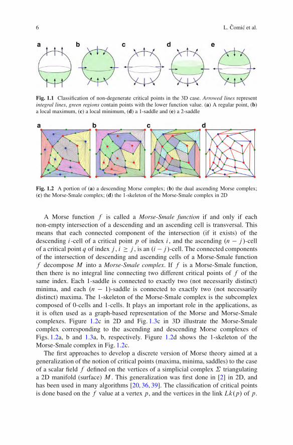
(in some local coordinate system around p) of f vanishes at p. Function f is saidto be a Morse function if all its critical points are non-degenerate (the Hessianmatrix Hesspf of the second derivatives of f at p is non-singular). For a Morsefunction f , there is a neighborhood of each critical point p D .p1; p2; : : : ; pn/ off , in which f .x1; x2; : : : ; xn/ D f .p1; p2; : : : ; pn/"x21": : :"x2i Cx2iC1C: : :Cx2n[34]. The number i is equal to the number of negative eigenvalues of Hesspf , andis called the index of critical point p. The corresponding eigenvectors point in thedirections in which f is decreasing. If the index of p is i , 0 # i # n, p is calledan i -saddle. A 0-saddle is called a minimum, and an n-saddle is called a maximum.Figure 1.1 illustrates a neighborhood of a critical point in three dimensions.
An integral line of a function f is a maximal path that is everywhere tangentto the gradient rf of f . It follows the direction in which the function has themaximum increasing growth. Two integral lines are either disjoint, or they are thesame. Each integral line starts at a critical point of f , called its origin, and ends atanother critical point, called its destination. Integral lines that converge to a criticalpoint p of index i cover an i -cell called the stable (descending) cell of p. Dually,integral lines that originate at p cover an (n" i )-cell called the unstable (ascending)cell of p. The descending cells (or manifolds) are pairwise disjoint, they cover M ,and the boundary of every cell is a union of lower-dimensional cells. Descendingcells decompose M into a cell complex !d , called the descending Morse complexof f on M . Dually, the ascending cells form the ascending Morse complex !a off on M . Figures 1.2a, b and 1.3a, b show an example of a descending and dualascending Morse complex in 2D and 3D, respectively.
6 L. Comic et al.
Fig. 1.1 Classification of non-degenerate critical points in the 3D case. Arrowed lines representintegral lines, green regions contain points with the lower function value. (a) A regular point, (b)a local maximum, (c) a local minimum, (d) a 1-saddle and (e) a 2-saddle
Fig. 1.2 A portion of (a) a descending Morse complex; (b) the dual ascending Morse complex;(c) the Morse-Smale complex; (d) the 1-skeleton of the Morse-Smale complex in 2D
A Morse function f is called a Morse-Smale function if and only if eachnon-empty intersection of a descending and an ascending cell is transversal. Thismeans that each connected component of the intersection (if it exists) of thedescending i -cell of a critical point p of index i , and the ascending .n " j /-cellof a critical point q of index j , i ! j , is an .i " j /-cell. The connected componentsof the intersection of descending and ascending cells of a Morse-Smale functionf decompose M into a Morse-Smale complex. If f is a Morse-Smale function,then there is no integral line connecting two different critical points of f of thesame index. Each 1-saddle is connected to exactly two (not necessarily distinct)minima, and each .n " 1/-saddle is connected to exactly two (not necessarilydistinct) maxima. The 1-skeleton of the Morse-Smale complex is the subcomplexcomposed of 0-cells and 1-cells. It plays an important role in the applications, asit is often used as a graph-based representation of the Morse and Morse-Smalecomplexes. Figure 1.2c in 2D and Fig. 1.3c in 3D illustrate the Morse-Smalecomplex corresponding to the ascending and descending Morse complexes ofFigs. 1.2a, b and 1.3a, b, respectively. Figure 1.2d shows the 1-skeleton of theMorse-Smale complex in Fig. 1.2c.
The first approaches to develop a discrete version of Morse theory aimed at ageneralization of the notion of critical points (maxima, minima, saddles) to the caseof a scalar field f defined on the vertices of a simplicial complex ˙ triangulatinga 2D manifold (surface) M . This generalization was first done in [2] in 2D, andhas been used in many algorithms [20, 36, 39]. The classification of critical pointsis done based on the f value at a vertex p, and the vertices in the link Lk.p/ of p.
1 Modeling Three-Dimensional Morse and Morse-Smale Complexes 7
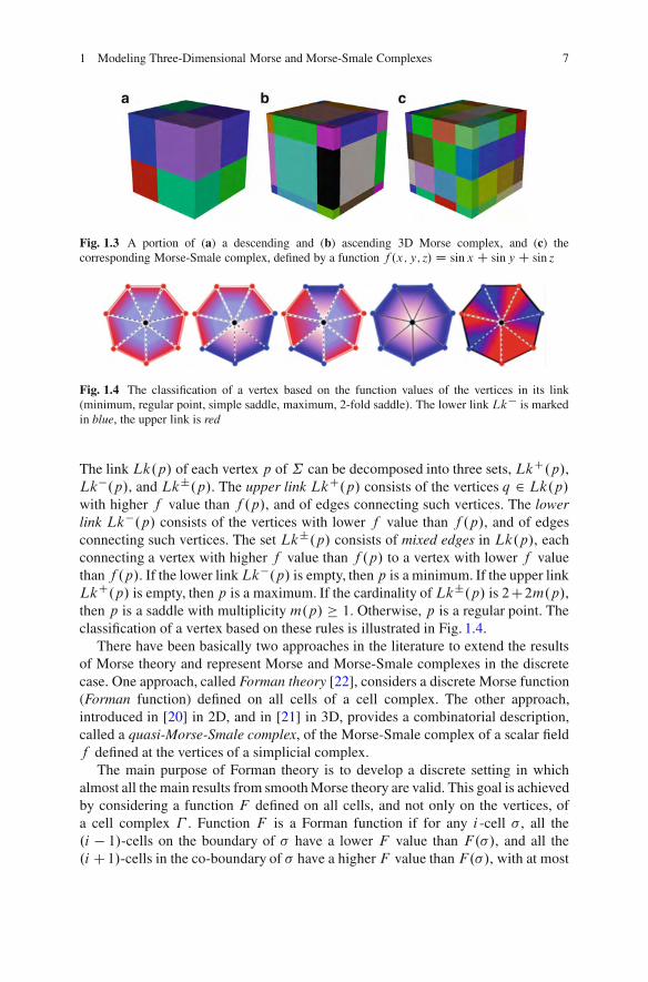
Fig. 1.3 A portion of (a) a descending and (b) ascending 3D Morse complex, and (c) thecorresponding Morse-Smale complex, defined by a function f .x; y; z/D sin x C siny C sin z
Fig. 1.4 The classification of a vertex based on the function values of the vertices in its link(minimum, regular point, simple saddle, maximum, 2-fold saddle). The lower link Lk! is markedin blue, the upper link is red
The link Lk.p/ of each vertex p of ˙ can be decomposed into three sets, LkC.p/,Lk".p/, and Lk˙.p/. The upper link LkC.p/ consists of the vertices q 2 Lk.p/with higher f value than f .p/, and of edges connecting such vertices. The lowerlink Lk".p/ consists of the vertices with lower f value than f .p/, and of edgesconnecting such vertices. The set Lk˙.p/ consists of mixed edges in Lk.p/, eachconnecting a vertex with higher f value than f .p/ to a vertex with lower f valuethan f .p/. If the lower linkLk".p/ is empty, then p is a minimum. If the upper linkLkC.p/ is empty, then p is a maximum. If the cardinality of Lk˙.p/ is 2C2m.p/,then p is a saddle with multiplicity m.p/ ! 1. Otherwise, p is a regular point. Theclassification of a vertex based on these rules is illustrated in Fig. 1.4.
There have been basically two approaches in the literature to extend the resultsof Morse theory and represent Morse and Morse-Smale complexes in the discretecase. One approach, called Forman theory [22], considers a discrete Morse function(Forman function) defined on all cells of a cell complex. The other approach,introduced in [20] in 2D, and in [21] in 3D, provides a combinatorial description,called a quasi-Morse-Smale complex, of the Morse-Smale complex of a scalar fieldf defined at the vertices of a simplicial complex.
The main purpose of Forman theory is to develop a discrete setting in whichalmost all the main results from smooth Morse theory are valid. This goal is achievedby considering a function F defined on all cells, and not only on the vertices, ofa cell complex ! . Function F is a Forman function if for any i -cell " , all the.i " 1/-cells on the boundary of " have a lower F value than F."/, and all the.iC1/-cells in the co-boundary of " have a higher F value than F."/, with at most

8 L. Comic et al.
Fig. 1.5 (a) Forman function F defined on a 2D simplicial complex, and (b) the correspondingdiscrete gradient vector field. Each simplex is labelled by its F value
one exception. If there is such an exception, it defines a pairing of cells of ! , calleda discrete (or Forman) gradient vector field V . Otherwise, i -cell " is a critical cell ofindex i . Similar to the smooth Morse theory, critical cells of a Forman function canbe cancelled in pairs. In the example in Fig. 1.5a, a Forman function F defined on a2D simplicial complex is illustrated. Each simplex is labelled by its function value.Figure 1.5b shows the Forman gradient vector field defined by Forman function Fin Fig. 1.5a. Vertex labelled 0 and edge labelled 6 are critical simplexes of F .
Forman theory finds important applications in computational topology, computergraphics, scientific visualization, molecular shape analysis, and geometric model-ing. In [32], Forman theory is used to compute the homology of a simplicial complexwith manifold domain, while in [9], it is used for segmentation of molecularsurfaces. Forman theory can be used to compute Morse and Morse-Smale complexesof a scalar field f defined on the vertices of a simplicial or cell complex, byextending scalar field f to a Forman function F defined on all cells of the complex[12, 27, 31, 38].
The notion of a quasi-Morse-Smale complex in 2D and 3D has been introducedin [20, 21] with the aim of capturing the combinatorial structure of a Morse-Smalecomplex of a Morse-Smale function f defined over a manifold M . In 2D, a quasi-Morse-Smale complex is defined as a complex whose 1-skeleton is a tripartite graph,since the set of its vertices is partitioned into subsets corresponding to critical points(minima, maxima, and saddles). A vertex corresponding to a saddle has four incidentedges, two of which connect it to vertices corresponding to minima, and the othertwo connect it to maxima. Each region (2-cell of the complex) is a quadrangle whosevertices are a saddle, a minimum, a saddle, and a maximum. In 3D, vertices of aquasi-Morse-Smale complex are partitioned into four sets corresponding to criticalpoints. Each vertex corresponding to a 1-saddle is the extremum vertex of two edgesconnecting it to two vertices corresponding to minima, and dually for 2-saddles andmaxima. Each 2-cell is a quadrangle, and there are exactly four 2-cells incident ineach edge connecting a vertex corresponding to a 1-saddle to a vertex correspondingto a 2-saddle.
1 Modeling Three-Dimensional Morse and Morse-Smale Complexes 9
1.3 Related Work
In this section, we review related work on topological representations of 2D scalarfields based on Morse or Morse-Smale complexes. We concentrate on three topicsrelevant to the work presented here, namely: computation, simplification and multi-resolution representation of Morse and Morse-Smale complexes.
Several algorithms have been proposed in the literature for decomposing thedomain of a 2D scalar field f into an approximation of a Morse or a Morse-Smalecomplex. For a review of the work in this area see [4]. Algorithms for decomposingthe domain M of field f into an approximation of a Morse, or of a Morse-Smale,complex can be classified as boundary-based [1, 6, 20, 37, 39], or region-based[9, 13]. Boundary-based algorithms trace the integral lines of f , which start atsaddle points and converge to minima and maxima of f . Region-based methodsgrow the 2D cells corresponding to minima and maxima of f , starting from thosecritical points.
One of the major issues that arise when computing a representation of a scalarfield as a Morse, or as a Morse-Smale, complex is the over-segmentation due tothe presence of noise in the data sets. Simplification algorithms eliminate lesssignificant features from these complexes. Simplification is achieved by applyingan operator called cancellation, defined in Morse theory [33]. It transforms a Morsefunction f into Morse function g with fewer critical points. Thus, it transforms aMorse-Smale complex into another, with fewer vertices, and it transforms a Morsecomplex into another, with fewer cells. It enables also the creation of a hierarchicalrepresentation. A cancellation in 2D consists of collapsing a maximum-saddlepair into a maximum, or a minimum-saddle pair into a minimum. Cancellation isperformed in the order usually determined by the notion of persistence. Intuitively,persistence measures the importance of the pair of critical points to be cancelled,and is equal to the absolute difference in function values between the paired criticalpoints [20]. In 2D Morse-Smale complexes, the cancellation operator has beeninvestigated in [6, 20, 39, 43]. In [15], the cancellation operator in 2D has beenextended to functions that may have multiple saddles and macro-saddles (saddlesthat are connected to each other).
Due to the large size and complexity of available scientific data sets, amulti-resolution representation is crucial for their interactive exploration. Therehave been several approaches in the literature to multi-resolution representationof the topology of a scalar field in 2D [6, 7, 15]. The approach in [6] is basedon a hierarchical representation of the 1-skeleton of a Morse-Smale complex,generated through the cancellation operator. It considers the 1-skeleton at fullresolution and generates a sequence of simplified representations of the complexby repeatedly applying a cancellation operator. In [7], the inverse anticancellationoperator to the cancellation operator in [6] has been defined. It enables a definitionof a dependency relation between refinement modifications, and a creation of amulti-resolution model for 2D scalar fields. The method in [15] creates a hierarchyof graphs (generalized critical nets), obtained as a 1-skeleton of an overlay of

10 L. Comic et al.
ascending and descending Morse complexes of a function with multiple saddles andsaddles that are connected to each other. Hierarchical watershed approaches havebeen developed to cope with the increase in size of both 2D and 3D images [3].
There have been two attempts in the literature to couple the multi-resolutiontopological model provided by Morse-Smale complexes with the multi-resolutionmodel of the geometry of the underlying simplicial mesh. The approach in [6] firstcreates a hierarchy of Morse-Smale complexes by applying cancellation operatorsto the full-resolution complex, and then, by Laplacian smoothing, it constructsthe smoothed function corresponding to the simplified topology. The approachin [16] creates the hierarchy by applying half-edge contraction operator, whichsimplifies the geometry of the mesh. When necessary, the topological representationcorresponding to the simplified coarser mesh is also simplified. The data structureencoding the geometrical hierarchy of the mesh, and the data structure encodingthe topological hierarchy of the critical net are interlinked. The hierarchical criticalnet is used as a topological index to query the hierarchical representation of thegeometry of the simplicial mesh.
1.4 Representing Three-Dimensional Morseand Morse-Smale Complexes
In this section, we describe and compare two data structures for representing thetopology and geometry of a scalar field f defined over the vertices of a simplicialcomplex ˙ with manifold domain in 3D. The topology of scalar field f (and ofits domain ˙) is represented in the form of Morse and Morse-Smale complexes.The two data structures encode the topology of the complexes in essentially thesame way, namely in the form of a graph, usually called an incidence graph. Thedifference between the two data structures is in the way they encode the geometry:the data structure in [11] (its 3D instance) encodes the geometry of the 3-cells ofthe descending and ascending complexes; the data structure in [25] encodes thegeometry of the ascending and descending 3-, 2- and 0-cells in the descending andascending Morse complexes, and that of the 1-cells in the Morse-Smale complexes.
1.4.1 A Dimension-Independent Compact Representationfor Morse Complexes
The incidence-based representation proposed in [11] is a dual representation for theascending and the descending Morse complexes !a and !d . The topology of bothcomplexes is represented by encoding the immediate boundary and co-boundaryrelations of the cells in the two complexes in the form of a Morse Incidence Graph(MIG). The Morse incidence graph provides also a combinatorial representation of
1 Modeling Three-Dimensional Morse and Morse-Smale Complexes 11
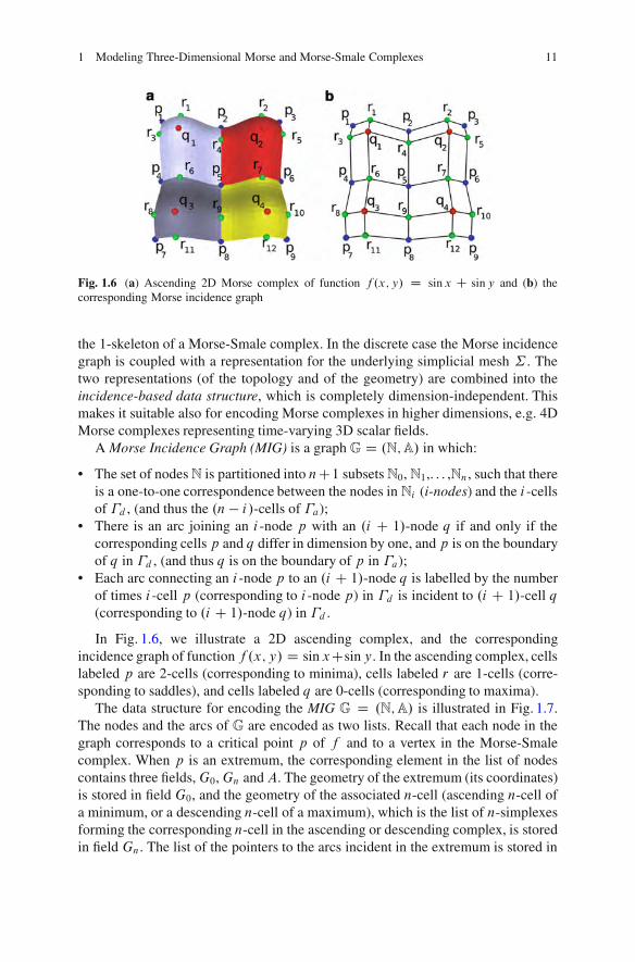
Fig. 1.6 (a) Ascending 2D Morse complex of function f .x; y/ D sin x C sin y and (b) thecorresponding Morse incidence graph
the 1-skeleton of a Morse-Smale complex. In the discrete case the Morse incidencegraph is coupled with a representation for the underlying simplicial mesh ˙ . Thetwo representations (of the topology and of the geometry) are combined into theincidence-based data structure, which is completely dimension-independent. Thismakes it suitable also for encoding Morse complexes in higher dimensions, e.g. 4DMorse complexes representing time-varying 3D scalar fields.
A Morse Incidence Graph (MIG) is a graph G D .N;A/ in which:
• The set of nodes N is partitioned into nC1 subsets N0, N1,. . . ,Nn, such that thereis a one-to-one correspondence between the nodes in Ni (i-nodes) and the i -cellsof !d , (and thus the .n " i/-cells of !a);
• There is an arc joining an i -node p with an .i C 1/-node q if and only if thecorresponding cells p and q differ in dimension by one, and p is on the boundaryof q in !d , (and thus q is on the boundary of p in !a);
• Each arc connecting an i -node p to an .i C 1/-node q is labelled by the numberof times i -cell p (corresponding to i -node p) in !d is incident to .i C 1/-cell q(corresponding to .i C 1/-node q) in !d .
In Fig. 1.6, we illustrate a 2D ascending complex, and the correspondingincidence graph of function f .x; y/ D sin xCsin y. In the ascending complex, cellslabeled p are 2-cells (corresponding to minima), cells labeled r are 1-cells (corre-sponding to saddles), and cells labeled q are 0-cells (corresponding to maxima).
The data structure for encoding the MIG G D .N;A/ is illustrated in Fig. 1.7.The nodes and the arcs of G are encoded as two lists. Recall that each node in thegraph corresponds to a critical point p of f and to a vertex in the Morse-Smalecomplex. When p is an extremum, the corresponding element in the list of nodescontains three fields,G0,Gn andA. The geometry of the extremum (its coordinates)is stored in field G0, and the geometry of the associated n-cell (ascending n-cell ofa minimum, or a descending n-cell of a maximum), which is the list of n-simplexesforming the corresponding n-cell in the ascending or descending complex, is storedin field Gn. The list of the pointers to the arcs incident in the extremum is stored in
12 L. Comic et al.
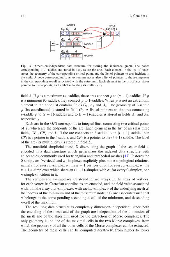
Fig. 1.7 Dimension-independent data structure for storing the incidence graph. The nodescorresponding to i -saddles are stored in lists, as are the arcs. Each element in the list of nodesstores the geometry of the corresponding critical point, and the list of pointers to arcs incident inthe node. A node corresponding to an extremum stores also a list of pointers to the n-simplexesin the corresponding n-cell associated with the extremum. Each element in the list of arcs storespointers to its endpoints, and a label indicating its multiplicity
field A. If p is a maximum (n-saddle), these arcs connect p to .n" 1/-saddles. If pis a minimum (0-saddle), they connect p to 1-saddles. When p is not an extremum,element in the node list contains fields G0, A1 and A2. The geometry of i -saddlep (its coordinates) is stored in field G0. A list of pointers to the arcs connectingi -saddle p to .i C 1/-saddles and to .i " 1/-saddles is stored in fields A1 and A2,respectively.
Each arc in the MIG corresponds to integral lines connecting two critical pointsof f , which are the endpoints of the arc. Each element in the list of arcs has threefields, CP1, CP2 and L. If the arc connects an i -saddle to an .i C 1/-saddle, thenCP1 is a pointer to the i -saddle, and CP2 is a pointer to the .iC1/-saddle. The labelof the arc (its multiplicity) is stored in field L.
The manifold simplicial mesh ˙ discretizing the graph of the scalar field isencoded in a data structure which generalizes the indexed data structure withadjacencies, commonly used for triangular and tetrahedral meshes [17]. It stores the0-simplexes (vertices) and n-simplexes explicitly plus some topological relations,namely: for every n-simplex " , the nC 1 vertices of " ; for every n-simplex " , thenC 1 n-simplexes which share an .n" 1/-simplex with " ; for every 0-simplex, onen-simplex incident in it.
The vertices and n-simplexes are stored in two arrays. In the array of vertices,for each vertex its Cartesian coordinates are encoded, and the field value associatedwith it. In the array of n-simplexes, with each n-simplex " of the underlying mesh˙the indexes of the minimum and of the maximum node in G are associated such that" belongs to the corresponding ascending n-cell of the minimum, and descendingn-cell of the maximum.
The resulting data structure is completely dimension-independent, since boththe encoding of the mesh and of the graph are independent of the dimension ofthe mesh and of the algorithm used for the extraction of Morse complexes. Theonly geometry is the one of the maximal cells in the two Morse complexes, fromwhich the geometry of all the other cells of the Morse complexes can be extracted.The geometry of these cells can be computed iteratively, from higher to lower

1 Modeling Three-Dimensional Morse and Morse-Smale Complexes 13
Fig. 1.8 Dimension-specific data structure for storing the incidence graph. Nodes and arcs arestored in lists. Each element in the list of nodes stores the geometry of the corresponding criticalpoint, tag indicating the index of the critical point, geometry of the associated 2- or 3-cell inthe Morse complex, and a pointer to one incident arc. Each element in the list of arcs stores thegeometry of the arc, two pointers to its endpoints, and two pointers to the next arcs incident in thetwo endpoints
dimensions, by searching for the k-simplexes that are shared by .k C 1/-simplexesbelonging to different .k C 1/-cells.
The incidence-based data structure encodes also the topology of theMorse-Smale complex. The arcs in the graph (i.e., pairs of nodes connected throughthe arc) correspond to 1-cells in the Morse-Smale complex. Similarly, pairs of nodesconnected through a path of length k correspond to k-cells in the Morse-Smalecomplex. The geometry of these cells can be computed from the geometry of thecells in the Morse complex through intersection. For example, the intersection ofascending n-cells corresponding to minima and descending n-cells correspondingto maxima defines n-cells in the Morse-Smale complex.
1.4.2 A Dimension-Specific Representation for 3DMorse-Smale Complexes
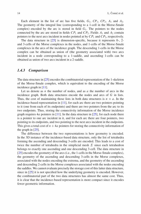
In [25] a data structure for 3D Morse-Smale complexes is presented. The topologyof the Morse-Smale complex (actually of its 1-skeleton) is encoded in a datastructure equivalent to the Morse incidence graph. The geometry is referred tofrom the elements of the graph, arcs and nodes. We illustrate this data structure inFig. 1.8.
The data structure encodes the nodes and arcs of the incidence graph in twoarrays. Each element in the list of nodes has four fields, G0, TAG, G2=G3 and A.The geometry (coordinates) of the corresponding critical point is stored in field G0.The index of the critical point is stored in field TAG. A reference to the geometryof the associated Morse cell (depending on the index of p) is stored in field G2=G3:a descending 3-cell is associated with a maximum; an ascending 3-cell is associatedwith a minimum; a descending 2-cell is associated with a 2-saddle; an ascending2-cell is associated with a 1-saddle. A pointer to an arc incident in the node (the firstone in the list of such arcs) is stored in field A. Thus, the geometry of 0-, 2-, and3-cells in the Morse complexes is referenced from the nodes.
14 L. Comic et al.
Each element in the list of arc has five fields, G1, CP1, CP2, A1 and A2.The geometry of the integral line (corresponding to a 1-cell in the Morse-Smalecomplex) encoded by the arc is stored in field G1. The pointers to the nodesconnected by the arc are stored in fields CP1 and CP2. Fields A1 and A2 containpointers to the next arcs incident in nodes pointed at by CP1 and CP2, respectively.
The data structure in [25] is dimension-specific, because it represents 0-, 2-and 3-cells of the Morse complexes in the nodes, and 1-cells of the Morse-Smalecomplexes in the arcs of the incidence graph. The descending 1-cells in the Morsecomplex can be obtained as union of (the geometry associated with) two arcsincident in a node corresponding to a 1-saddle, and ascending 1-cells can beobtained as union of two arcs incident in a 2-saddle.
1.4.3 Comparison
The data structure in [25] encodes the combinatorial representation of the 1-skeletonof the Morse-Smale complex, which is equivalent to the encoding of the Morseincidence graph in [11].
Let us denote as n the number of nodes, and as a the number of arcs in theincidence graph. Both data structures encode the nodes and arcs of G in lists.Thus, the cost of maintaining those lists in both data structures is n C a. In theincidence-based representation in [11], for each arc there are two pointers pointingto it (one from each of its endpoints) and there are two pointers from the arc to itstwo endpoints. Thus, storing the connectivity information of the Morse incidencegraph requires 4a pointers in [11]. In the data structure in [25], for each node thereis a pointer to one arc incident in it, and for each arc there are four pointers, twopointing to its endpoints, and two pointing to the next arcs incident in the endpoints.This gives a total cost of nC 4a pointers for storing the connectivity information ofthe graph in [25].
The difference between the two representations is how geometry is encoded.In the 3D instance of the incidence-based data structure, only the list of tetrahedraforming the ascending and descending 3-cells are encoded. This leads to a cost oftwice the number of tetrahedra in the simplicial mesh ˙ since each tetrahedronbelongs to exactly one ascending and one descending 3-cell. The data structure in[25] encodes the geometry of the arcs (i.e., the 1-cells in the Morse-Smale complex),the geometry of the ascending and descending 3-cells in the Morse complexes,associated with the nodes encoding the extrema, and the geometry of the ascendingand descending 2-cells in the Morse complexes associated with the nodes encodingthe saddles. We cannot evaluate precisely the storage cost of this latter data structure,since in [25] it is not specified how the underlying geometry is encoded. However,the combinatorial part of the two data structures has almost the same cost. Thus,it is clear that the incidence-based representation is more compact since it encodesfewer geometric information.
1 Modeling Three-Dimensional Morse and Morse-Smale Complexes 15
1.5 Algorithms for Building 3D Morse and Morse-SmaleComplexes
In this section, we describe and compare algorithms for extracting Morse andMorse-Smale complexes from a scalar field f defined on the vertices of a manifoldsimplicial mesh ˙ in 3D. Similarly to the 2D case, extraction and classificationof critical points is a usual preprocessing step. An algorithm performing this task isproposed in [21]. For each vertex p of˙ , the lower linkLk".p/ of p is considered.It consists of the vertices q in the linkLk.p/ of p such that f .q/ < f .p/, and of thesimplexes of Lk.p/ defined by these vertices. Vertex p is classified as a minimumif its lower link is empty. It is classified as a maximum if its lower link is the same asLk.p/. Otherwise, p is classified based on the Betti numbers ofLk".p/ as a criticalpoint composed of multiple 1- and 2-saddles. Intuitively, the Betti numbers ˇ0 andˇ1 of Lk".p/ count the number of connected components and holes in Lk".p/,respectively.
The algorithms presented here can be classified, according to the approach theyuse, as region-based [11, 26], boundary-based [19, 21], or based on Forman theory[27, 31, 38]. Region-based algorithms extract only the minima and maxima of f ,and do not explicitly extract saddle points. Boundary-based algorithms [19,21] firstextract and classify critical points of f (minima, maxima, and multiple 1- and 2-saddles) in the preprocessing step (using the method in [21]), and then compute theascending and descending 1- and 2-cells associated with saddles. The algorithms in[27, 31, 38] construct a Forman gradient vector field V and its critical cells startingfrom a scalar field f .
The output of the algorithm in [26] is a decomposition of the vertices of˙ into 0-,1-, 2- and 3-cells of the Morse complexes of f . Algorithms in [19, 21] produce 3-,2-, 1- and 0-cells of the Morse and Morse-Smale complexes composed of tetrahedra,triangles, edges and vertices of ˙ , respectively. The output of the algorithms basedon Forman theory [27,31,38] (Forman gradient vector field V ) can be used to obtainalso the decomposition of the underlying mesh K into descending cells associatedwith critical cells of V . Each descending cell of a critical i -cell " is composed ofall i -cells of K that are reachable by tracing gradients paths of V starting fromthe boundary of " . The algorithms in [11, 27] produce the graph encoding theconnectivity of Morse and Morse-Smale complexes. In [27], an algorithm basedon Forman theory has been developed to obtain the nodes and arcs of the graph. Thealgorithm in [11] obtains the graph starting from any segmentation of the tetrahedraof ˙ in descending and ascending 3-cells of the Morse complexes of f .
1.5.1 A Watershed-Based Approach for Building the MorseIncidence Graph
In [11], a two-step algorithm is described for the construction of the Morse incidencegraph of a scalar field f , defined on the vertices of a simplicial complex ˙ with

16 L. Comic et al.
a manifold carrier. The first step is the decomposition of ˙ in descending andascending n-cells of the Morse complexes. In [11], this decomposition is obtainedby extending the well-known watershed algorithm based on simulated immersionfrom image processing to n-dimensional manifold simplicial meshes [40]. Thefirst step of the algorithm is, thus, dimension-independent. The second step ofthe algorithm, developed for the 2D and 3D cases, consists of the construction ofthe Morse incidence graph.
The watershed algorithm by simulated immersion has been introduced in [40] forsegmenting a 2D image into regions of influence of minima, which correspond toascending 2-cells. We describe the extension of this algorithm from images to scalarfields defined at the vertices of a simplicial mesh in arbitrary dimension. The verticesof the simplicial mesh ˙ are sorted in increasing order with respect to the values ofthe scalar field f , and are processed level by level in increasing order of functionvalues. For each minimum m, an ascending region A.m/ is iteratively constructedthrough a breadth-first traversal of the 1-skeleton of the simplicial mesh ˙ (formedby its vertices and edges). For each vertex p, its adjacent, and already processed,vertices in the mesh are examined. If they all belong to the same ascending regionA.m/, or some of them are watershed points, then p is marked as belonging toA.m/.If they belong to two or more ascending regions, then p is marked as a watershedpoint. Vertices that are not connected to any previously processed vertex are newminima and they start a new ascending region.
Each maximal simplex " (an n-simplex if we consider an n-dimensional simpli-cial mesh) is assigned to an ascending region based on the labels of its vertices. If allvertices of " , that are not watershed points, belong to the same region A.m/, then" is assigned to A.m/. If the vertices belong to different ascending regions A.mi/,then " is assigned to the region corresponding to the lowest minimum.
Descending regions associated with maxima are computed in a completelysimilar fashion.
The algorithm proposed in [11] for the construction of the Morse incidence graphof f works on a segmentation produced by the watershed algorithm, althoughany other segmentation algorithm can be used. In the (dimension-independent)preprocessing step, for each descending region in !d , a maximum node in theincidence graph is created, and for each ascending region in !a, a minimum node iscreated. The algorithm for the construction of saddle nodes is based on inspectingthe adjacencies between the regions corresponding to maxima and minima, and isdeveloped for the 2D and the 3D case.
In the 2D case, after the preprocessing step, two steps are performed: (i) creationof the nodes corresponding to saddles, and (ii) creation of the arcs of the incidencegraph. To create the saddle nodes, 1-cells of the ascending (or of the descending)complex need to be created. Each 1-cell is a chain of edges of the triangle mesh.Each edge e of ˙ is inspected, and is classified with respect to such chain of edgesbased on the labels of the ascending regions to which the two triangles separated bye belong. Each connected component of edges separating two ascending regions issubdivided into topological 1-cells. Thus, if necessary, new saddle nodes are created.Each saddle node (1-cell) p is connected to the two minima it separates. The arcs
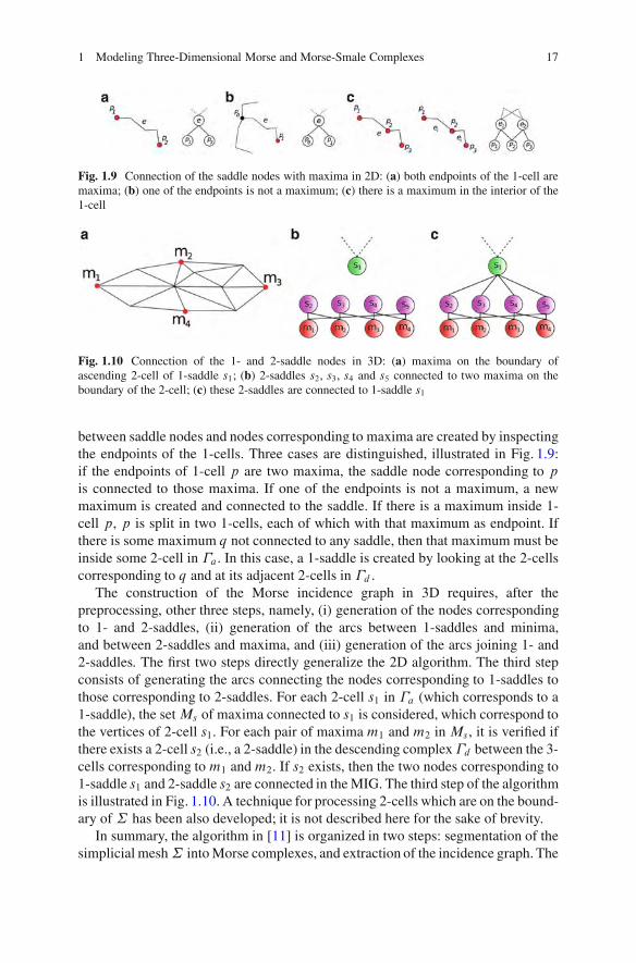
1 Modeling Three-Dimensional Morse and Morse-Smale Complexes 17
Fig. 1.9 Connection of the saddle nodes with maxima in 2D: (a) both endpoints of the 1-cell aremaxima; (b) one of the endpoints is not a maximum; (c) there is a maximum in the interior of the1-cell
Fig. 1.10 Connection of the 1- and 2-saddle nodes in 3D: (a) maxima on the boundary ofascending 2-cell of 1-saddle s1; (b) 2-saddles s2, s3, s4 and s5 connected to two maxima on theboundary of the 2-cell; (c) these 2-saddles are connected to 1-saddle s1
between saddle nodes and nodes corresponding to maxima are created by inspectingthe endpoints of the 1-cells. Three cases are distinguished, illustrated in Fig. 1.9:if the endpoints of 1-cell p are two maxima, the saddle node corresponding to pis connected to those maxima. If one of the endpoints is not a maximum, a newmaximum is created and connected to the saddle. If there is a maximum inside 1-cell p, p is split in two 1-cells, each of which with that maximum as endpoint. Ifthere is some maximum q not connected to any saddle, then that maximum must beinside some 2-cell in !a. In this case, a 1-saddle is created by looking at the 2-cellscorresponding to q and at its adjacent 2-cells in !d .
The construction of the Morse incidence graph in 3D requires, after thepreprocessing, other three steps, namely, (i) generation of the nodes correspondingto 1- and 2-saddles, (ii) generation of the arcs between 1-saddles and minima,and between 2-saddles and maxima, and (iii) generation of the arcs joining 1- and2-saddles. The first two steps directly generalize the 2D algorithm. The third stepconsists of generating the arcs connecting the nodes corresponding to 1-saddles tothose corresponding to 2-saddles. For each 2-cell s1 in !a (which corresponds to a1-saddle), the setMs of maxima connected to s1 is considered, which correspond tothe vertices of 2-cell s1. For each pair of maxima m1 and m2 in Ms , it is verified ifthere exists a 2-cell s2 (i.e., a 2-saddle) in the descending complex!d between the 3-cells corresponding to m1 and m2. If s2 exists, then the two nodes corresponding to1-saddle s1 and 2-saddle s2 are connected in the MIG. The third step of the algorithmis illustrated in Fig. 1.10. A technique for processing 2-cells which are on the bound-ary of ˙ has been also developed; it is not described here for the sake of brevity.
In summary, the algorithm in [11] is organized in two steps: segmentation of thesimplicial mesh˙ into Morse complexes, and extraction of the incidence graph. The
18 L. Comic et al.
first step is dimension-independent. It is based on the extension of a watershed algo-rithm for intensity images to scalar fields defined on simplicial complexes in arbi-trary dimension. The second step, developed for the 2D and 3D cases, constructs thenodes and arcs of the MIG encoding the Morse complexes generated at the first step.
1.5.2 A Boundary-Based Algorithm
The algorithm proposed in [21] builds a quasi-Morse-Smale complex (see Sect. 1.2),a complex that reflects the combinatorial structure of the Morse-Smale complex, butin which the arcs and quadrangles (1- and 2-cells) may not be those of maximalascent and descent. The quasi-Morse-Smale complex is constructed during twosweeps over a simplicial complex˙ triangulating a 3-manifoldM . The first sweep(in the direction of decreasing function value) computes the descending 1- and2-cells and the second sweep (in the direction of increasing function value) theascending 1- and 2-cells of the Morse complexes. The algorithm is boundary-based,as it computes the 1- and 2-cells which bound the 3-cells in the Morse complexes.During the first sweep, the descending 1- and 2-cells are computed simultaneously.A 1-cell is built as follows:
• If a current vertex p in the sweep is a 1-saddle, a descending 1-cell is started.The two arcs of the corresponding 1-cell are initialized by edges from p to thelowest vertex in each connected component of the lower link of p, as illustratedin Fig. 1.11a.
• If there is a descending arc ending at a current vertex p, it is expanded by addingan edge from p to the lowest vertex in its lower link. If p is a 1-saddle, lateran ascending 2-cell will start at p and each descending arc is extended to thelowest vertex in the specific connected component of the lower link of p that isnot separated from the arc by the ascending 2-cell.
• If p is a minimum, it becomes a node of the Morse-Smale complex, and thedescending arcs end at p.
A 2-cell is built as follows:
• If a current vertex p in the sweep is a 2-saddle, a descending 2-cell is started.A cycle of edges in the lower link is constructed, which contains the lowest vertexin the lower link of p. Triangles determined by p and edges of the cycle formthe initial descending 2-cell of p, as illustrated in Fig. 1.11b. Initially, the entireboundary of the descending 2-cell is unfrozen.
• A 2-cell is expanded by constructing a shortest-path tree in the lower link of thecurrent (highest) vertex q on the unfrozen boundary of the 2-cell associated with2-saddle p, and connecting q to the edges of this tree. If q is a critical point(a 1-saddle or a minimum), it is declared frozen together with its two incidentedges on the boundary.
• When the complete boundary of a 2-cell is frozen the 2-cell is completed.
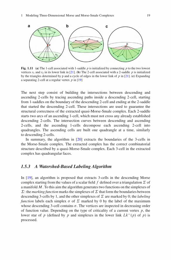
1 Modeling Three-Dimensional Morse and Morse-Smale Complexes 19
Fig. 1.11 (a) The 1-cell associated with 1-saddle p is initialized by connecting p to the two lowestvertices s1 and s2 in its lower link in [21]. (b) The 2-cell associated with a 2-saddle p is initializedby the triangles determined by p and a cycle of edges in the lower link of p in [21]. (c) Expandinga separating 2-cell at a regular vertex p in [19]
The next step consist of building the intersections between descending andascending 2-cells by tracing ascending paths inside a descending 2-cell, startingfrom 1-saddles on the boundary of the descending 2-cell and ending at the 2-saddlethat started the descending 2-cell. These intersections are used to guarantee thestructural correctness of the extracted quasi-Morse-Smale complex. Each 2-saddlestarts two arcs of an ascending 1-cell, which must not cross any already establisheddescending 2-cells. The intersection curves between descending and ascending2-cells, and the ascending 1-cells decompose each ascending 2-cell intoquadrangles. The ascending cells are built one quadrangle at a time, similarlyto descending 2-cells.
In summary, the algorithm in [20] extracts the boundaries of the 3-cells inthe Morse-Smale complex. The extracted complex has the correct combinatorialstructure described by a quasi-Morse-Smale complex. Each 3-cell in the extractedcomplex has quadrangular faces.
1.5.3 A Watershed-Based Labeling Algorithm
In [19], an algorithm is proposed that extracts 3-cells in the descending Morsecomplex starting from the values of a scalar field f defined over a triangulation˙ ofa manifoldM . To this aim the algorithm generates two functions on the simplexes of˙ : the marking function marks the simplexes of˙ that form the boundaries betweendescending 3-cells by 1, and the other simplexes of˙ are marked by 0; the labelingfunction labels each simplex " of ˙ marked by 0 by the label of the maximumwhose descending 3-cell contains " . The vertices are inspected in decreasing orderof function value. Depending on the type of criticality of a current vertex p, thelower star of p (defined by p and simplexes in the lower link Lk".p/ of p) isprocessed.
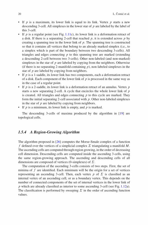
20 L. Comic et al.
• If p is a maximum, its lower link is equal to its link. Vertex p starts a newdescending 3-cell. All simplexes in the lower star of p are labeled by the label ofthis 3-cell.
• If p is a regular point (see Fig. 1.11c), its lower link is a deformation retract ofa disk. If there is a separating 2-cell that reached p, it is extended across p bycreating a spanning tree in the lower link of p. The spanning tree is constructedso that it contains all vertices that belong to an already marked simplex (i.e., toa simplex which is part of the boundary between two descending 3-cells). Alltriangles and edges connecting p to this spanning tree are marked (extendinga descending 2-cell between two 3-cells). Other non-labeled (and non-marked)simplexes in the star of p are labeled by copying from the neighbors. Otherwise(if there is no separating 2-manifold containing p), non-labeled simplexes in thestar of p are labeled by copying from neighbors.
• If p is a 1-saddle, its lower link has two components, each a deformation retractof a disk. Each component of the lower link of p is processed in the same way asin the case of a regular point.
• If p is a 2-saddle, its lower link is a deformation retract of an annulus. Vertex pstarts a new separating 2-cell. A cycle that encircles the whole lower link of pis created. All triangles and edges connecting p to this cycle are marked. Theyform the initial separating 2-cell associated with p. Other non-labeled simplexesin the star of p are labeled by copying from neighbors.
• If p is a minimum, its lower link is empty, and p is marked.
The descending 3-cells of maxima produced by the algorithm in [19] aretopological cells.
1.5.4 A Region-Growing Algorithm
The algorithm proposed in [26] computes the Morse-Smale complex of a functionf defined over the vertices of a simplicial complex˙ triangulating a manifold M .The ascending cells are computed through region growing, in the order of decreasingcell dimension. Descending cells are computed inside the ascending 3-cells, usingthe same region-growing approach. The ascending and descending cells of alldimensions are composed of vertices (0-simplexes) of ˙ .
The computation of the ascending 3-cells consists of two steps. First, the set ofminima of f are identified. Each minimum will be the origin for a set of verticesrepresenting an ascending 3-cell. Then, each vertex p of ˙ is classified as aninternal vertex of an ascending cell, or as a boundary vertex. This depends on thenumber of connected components of the set of internal vertices in the lower link ofp which are already classified as interior to some ascending 3-cell (see Fig. 1.12a).The classification is performed by sweeping ˙ in the order of ascending functionvalues.
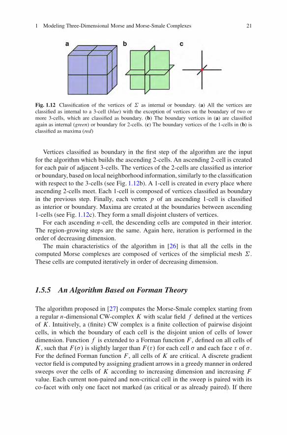
1 Modeling Three-Dimensional Morse and Morse-Smale Complexes 21
Fig. 1.12 Classification of the vertices of ˙ as internal or boundary. (a) All the vertices areclassified as internal to a 3-cell (blue) with the exception of vertices on the boundary of two ormore 3-cells, which are classified as boundary. (b) The boundary vertices in (a) are classifiedagain as internal (green) or boundary for 2-cells. (c) The boundary vertices of the 1-cells in (b) isclassified as maxima (red)
Vertices classified as boundary in the first step of the algorithm are the inputfor the algorithm which builds the ascending 2-cells. An ascending 2-cell is createdfor each pair of adjacent 3-cells. The vertices of the 2-cells are classified as interioror boundary, based on local neighborhood information, similarly to the classificationwith respect to the 3-cells (see Fig. 1.12b). A 1-cell is created in every place whereascending 2-cells meet. Each 1-cell is composed of vertices classified as boundaryin the previous step. Finally, each vertex p of an ascending 1-cell is classifiedas interior or boundary. Maxima are created at the boundaries between ascending1-cells (see Fig. 1.12c). They form a small disjoint clusters of vertices.
For each ascending n-cell, the descending cells are computed in their interior.The region-growing steps are the same. Again here, iteration is performed in theorder of decreasing dimension.
The main characteristics of the algorithm in [26] is that all the cells in thecomputed Morse complexes are composed of vertices of the simplicial mesh ˙ .These cells are computed iteratively in order of decreasing dimension.
1.5.5 An Algorithm Based on Forman Theory
The algorithm proposed in [27] computes the Morse-Smale complex starting froma regular n-dimensional CW-complex K with scalar field f defined at the verticesof K . Intuitively, a (finite) CW complex is a finite collection of pairwise disjointcells, in which the boundary of each cell is the disjoint union of cells of lowerdimension. Function f is extended to a Forman function F , defined on all cells ofK , such that F."/ is slightly larger than F.#/ for each cell " and each face # of " .For the defined Forman function F , all cells of K are critical. A discrete gradientvector field is computed by assigning gradient arrows in a greedy manner in orderedsweeps over the cells of K according to increasing dimension and increasing Fvalue. Each current non-paired and non-critical cell in the sweep is paired with itsco-facet with only one facet not marked (as critical or as already paired). If there

22 L. Comic et al.
Fig. 1.13 (a) Construction of the Forman gradient vector field, and (b) of the incidence graph
are several of such co-facets the lowest is taken. If there is no such co-facet, a cellcannot be paired, and it is critical. This pairing defines a discrete gradient vectorfield, as illustrated in Fig. 1.13a.
The 1-skeleton of the Morse-Smale complex is computed starting from thisgradient vector field. Critical cells ofF (and not critical points of f ) and the discretegradient paths connecting them determine the nodes and arcs in the 1-skeleton ofthe Morse-Smale complex (incidence graph), as illustrated in Fig. 1.13b. In [23],this algorithm has been extended to extract topological 2- and 3-cells from a regularhexahedral 3D mesh.
The order in which the cells in K are processed by the algorithm is notcompletely deterministic, since there could be many different i -cells in K with thesame value of function F . As a consequence, some unnecessary critical cells maybe produced by the algorithm.
1.5.6 A Forman-Based Approach for Cubical Complexes
In [38], a dimension-independent algorithm is proposed for constructing a Formangradient vector field on a cubical complex K with scalar field values given at thevertices, and applications to the 2D and 3D images are presented.
The algorithm processes the lower star of each vertex v in K independently. Foreach cell " in the lower star, the value max
p2"f .p/ D f max."/ is considered. An
ascending order$ is generated based on the values f max."/ and the dimension of" , such that each cell " comes after its faces in the order. If the lower star of vertexv is v itself, then v is a local minimum and it is added to the set C of critical cells.Otherwise, the first edge e in $ is chosen and vertex v is paired with edge e (thevector field V at v is defined as V.v/ D e).
The star of v is processed using two queues, PQone and PQzero, correspondingto i -cells with one and zero unpaired faces, respectively. All edges in the star of vdifferent from e are added to PQzero. All cofaces of e are added to PQone if thenumber of unpaired faces is equal to one.
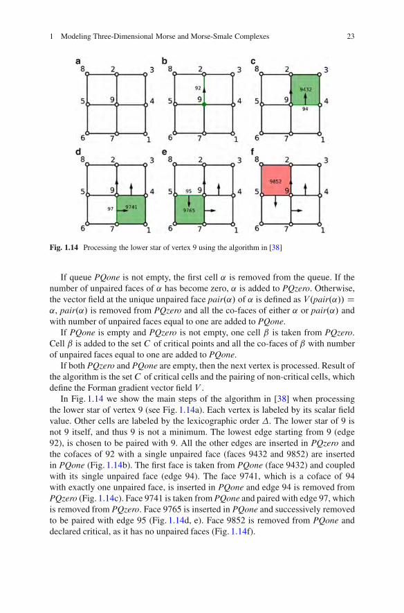
1 Modeling Three-Dimensional Morse and Morse-Smale Complexes 23
Fig. 1.14 Processing the lower star of vertex 9 using the algorithm in [38]
If queue PQone is not empty, the first cell ˛ is removed from the queue. If thenumber of unpaired faces of ˛ has become zero, ˛ is added to PQzero. Otherwise,the vector field at the unique unpaired face pair.˛/ of ˛ is defined as V.pair.˛// D˛, pair.˛/ is removed from PQzero and all the co-faces of either ˛ or pair.˛/ andwith number of unpaired faces equal to one are added to PQone.
If PQone is empty and PQzero is not empty, one cell ˇ is taken from PQzero.Cell ˇ is added to the set C of critical points and all the co-faces of ˇ with numberof unpaired faces equal to one are added to PQone.
If both PQzero and PQone are empty, then the next vertex is processed. Result ofthe algorithm is the set C of critical cells and the pairing of non-critical cells, whichdefine the Forman gradient vector field V .
In Fig. 1.14 we show the main steps of the algorithm in [38] when processingthe lower star of vertex 9 (see Fig. 1.14a). Each vertex is labeled by its scalar fieldvalue. Other cells are labeled by the lexicographic order $. The lower star of 9 isnot 9 itself, and thus 9 is not a minimum. The lowest edge starting from 9 (edge92), is chosen to be paired with 9. All the other edges are inserted in PQzero andthe cofaces of 92 with a single unpaired face (faces 9432 and 9852) are insertedin PQone (Fig. 1.14b). The first face is taken from PQone (face 9432) and coupledwith its single unpaired face (edge 94). The face 9741, which is a coface of 94with exactly one unpaired face, is inserted in PQone and edge 94 is removed fromPQzero (Fig. 1.14c). Face 9741 is taken from PQone and paired with edge 97, whichis removed from PQzero. Face 9765 is inserted in PQone and successively removedto be paired with edge 95 (Fig. 1.14d, e). Face 9852 is removed from PQone anddeclared critical, as it has no unpaired faces (Fig. 1.14f).
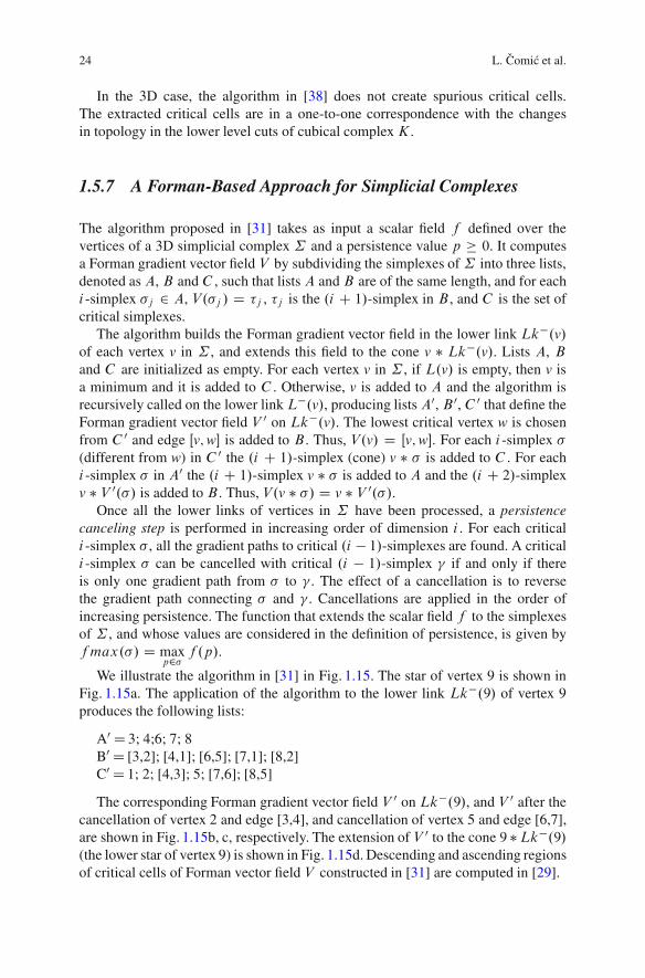
24 L. Comic et al.
In the 3D case, the algorithm in [38] does not create spurious critical cells.The extracted critical cells are in a one-to-one correspondence with the changesin topology in the lower level cuts of cubical complexK .
1.5.7 A Forman-Based Approach for Simplicial Complexes
The algorithm proposed in [31] takes as input a scalar field f defined over thevertices of a 3D simplicial complex ˙ and a persistence value p ! 0. It computesa Forman gradient vector field V by subdividing the simplexes of˙ into three lists,denoted as A, B and C , such that lists A and B are of the same length, and for eachi -simplex "j 2 A, V."j / D #j , #j is the .i C 1/-simplex in B , and C is the set ofcritical simplexes.
The algorithm builds the Forman gradient vector field in the lower link Lk".v/of each vertex v in ˙ , and extends this field to the cone v $ Lk".v/. Lists A, Band C are initialized as empty. For each vertex v in ˙ , if L.v/ is empty, then v isa minimum and it is added to C . Otherwise, v is added to A and the algorithm isrecursively called on the lower link L".v/, producing lists A0, B 0, C 0 that define theForman gradient vector field V 0 on Lk".v/. The lowest critical vertex w is chosenfrom C 0 and edge Œv;w% is added to B . Thus, V.v/ D Œv;w%. For each i -simplex "(different from w) in C 0 the .i C 1/-simplex (cone) v $ " is added to C . For eachi -simplex " in A0 the .i C 1/-simplex v $ " is added to A and the .i C 2/-simplexv $ V 0."/ is added to B . Thus, V.v $ "/ D v $ V 0."/.
Once all the lower links of vertices in ˙ have been processed, a persistencecanceling step is performed in increasing order of dimension i . For each criticali -simplex " , all the gradient paths to critical .i " 1/-simplexes are found. A criticali -simplex " can be cancelled with critical .i " 1/-simplex & if and only if thereis only one gradient path from " to & . The effect of a cancellation is to reversethe gradient path connecting " and & . Cancellations are applied in the order ofincreasing persistence. The function that extends the scalar field f to the simplexesof ˙ , and whose values are considered in the definition of persistence, is given byfmax."/ D max
p2"f .p/.
We illustrate the algorithm in [31] in Fig. 1.15. The star of vertex 9 is shown inFig. 1.15a. The application of the algorithm to the lower link Lk".9/ of vertex 9produces the following lists:
A0D 3; 4;6; 7; 8B0D [3,2]; [4,1]; [6,5]; [7,1]; [8,2]C0D 1; 2; [4,3]; 5; [7,6]; [8,5]
The corresponding Forman gradient vector field V 0 on Lk".9/, and V 0 after thecancellation of vertex 2 and edge [3,4], and cancellation of vertex 5 and edge [6,7],are shown in Fig. 1.15b, c, respectively. The extension of V 0 to the cone 9 $Lk".9/(the lower star of vertex 9) is shown in Fig. 1.15d. Descending and ascending regionsof critical cells of Forman vector field V constructed in [31] are computed in [29].
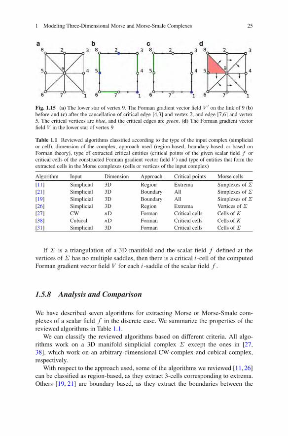
1 Modeling Three-Dimensional Morse and Morse-Smale Complexes 25
Fig. 1.15 (a) The lower star of vertex 9. The Forman gradient vector field V 0 on the link of 9 (b)before and (c) after the cancellation of critical edge [4,3] and vertex 2, and edge [7,6] and vertex5. The critical vertices are blue, and the critical edges are green. (d) The Forman gradient vectorfield V in the lower star of vertex 9
Table 1.1 Reviewed algorithms classified according to the type of the input complex (simplicialor cell), dimension of the complex, approach used (region-based, boundary-based or based onForman theory), type of extracted critical entities (critical points of the given scalar field f orcritical cells of the constructed Forman gradient vector field V ) and type of entities that form theextracted cells in the Morse complexes (cells or vertices of the input complex)
Algorithm Input Dimension Approach Critical points Morse cells
[11] Simplicial 3D Region Extrema Simplexes of ˙[21] Simplicial 3D Boundary All Simplexes of ˙[19] Simplicial 3D Boundary All Simplexes of ˙[26] Simplicial 3D Region Extrema Vertices of ˙[27] CW nD Forman Critical cells Cells of K[38] Cubical nD Forman Critical cells Cells of K[31] Simplicial 3D Forman Critical cells Cells of ˙
If ˙ is a triangulation of a 3D manifold and the scalar field f defined at thevertices of ˙ has no multiple saddles, then there is a critical i -cell of the computedForman gradient vector field V for each i -saddle of the scalar field f .
1.5.8 Analysis and Comparison
We have described seven algorithms for extracting Morse or Morse-Smale com-plexes of a scalar field f in the discrete case. We summarize the properties of thereviewed algorithms in Table 1.1.
We can classify the reviewed algorithms based on different criteria. All algo-rithms work on a 3D manifold simplicial complex ˙ except the ones in [27,38], which work on an arbitrary-dimensional CW-complex and cubical complex,respectively.
With respect to the approach used, some of the algorithms we reviewed [11, 26]can be classified as region-based, as they extract 3-cells corresponding to extrema.Others [19, 21] are boundary based, as they extract the boundaries between the
26 L. Comic et al.
3-cells corresponding to extrema. The algorithms in [27, 31, 38] compute a Formangradient vector field V starting from scalar field f .
The algorithms differ also in the type of critical points they extract beforeproducing the segmentation of the input mesh: some algorithms [19,21] first classifyall critical points of scalar field f (extrema and saddles); others [11, 26] extractonly extrema of f , and obtain the other nodes in the Morse incidence graph fromthe adjacency relation between 3-cells associated with extrema. The algorithms in[27,31,38] extract the critical cells of a Forman gradient vector field V (and not thecritical points of scalar field f ) defined through f .
Finally, another difference among the algorithms is given by the entities used inthe segmentation process: the algorithms in [11, 19, 21] assign the simplexes of ˙to cells in the Morse complexes; the algorithm in [26] assigns the vertices of ˙ tocells in the Morse complexes; the algorithms in [27, 31, 38] assign the cells of thecell complexK to cells in the descending Morse complex.
The algorithm in [20] computes the segmentation of the 3D simplicial mesh withthe correct combinatorial structure described by the quasi-Morse-Smale complex.The algorithm in [19] produces 3-cells in the descending Morse complex, which aretopological cells. In the 3D case, the algorithm in [38] computes the critical cells ofthe Forman gradient vector field V that are in a one-to-one correspondence with thechanges in topology in the lower level cuts ofK . If˙ is a triangulation of a manifoldM , and scalar field f has no multiple saddles, then the algorithm in [31] produces acritical i -cell of the Forman gradient vector field for each i -saddle of scalar field f .There are no formal claims about the critical cells of Forman gradient vector fieldcomputed by the algorithm in [26].
1.6 Simplification of 3D Morse and Morse-Smale Complexes
Although Morse and Morse-Smale complexes encode compactly the behavior of ascalar field f and the topology of its domain, simplification of these complexes isan important issue for two major reasons. The first is the over-segmentation (thepresence of a large number of small and insignificant regions) produced by Morseand Morse-Smale complexes which is due to the presence of noise in the data sets,both in case they are obtained through measurements or as a result of a simulationalgorithm. Simplification of the complexes through elimination of pairs of criticalpoints can be used to eliminate noise. Each simplification is performed guided bypersistence, which measures the importance of the pair of eliminated critical points,and is equal to the absolute difference in function values between them. Usually byusing a threshold on persistence equal to 5–10 % of the maximum persistence value,a reduction of the storage cost in the representation of the Morse or Morse-Smalecomplexes can be obtained which amounts to 10–20 % for 2D data sets, and 5–10 %for 3D ones.
Even after a simplification which removes insignificant regions considered tobe noise, and leaves regions that correspond to actual features of the scalar field,
1 Modeling Three-Dimensional Morse and Morse-Smale Complexes 27
the size of Morse and Morse-Smale complexes can still be large, due to thehuge size and amount of available scientific data. Thus, the second requirementis to reduce the size of the complexes at different levels of resolution, whileretaining information on important structural features of the field and guaranteeingthe topological correctness of the simplified representations. The size of a Morsecomplex is about 0.4–3 % the size of the underlying simplicial mesh in 2D andabout 2–8 % in 3D. For large 3D data sets (which have 15M tetrahedra), the size ofa Morse complex can be up to 50 MBytes.
We describe here two approaches to the simplification of Morse andMorse-Smale complexes in 3D proposed in the literature. The first approach [24]applies the cancellation operator of critical points of a Morse function f [33] onthe Morse-Smale complexes of f . The second approach [10] applies a new setof simplification operators, called removal and contraction, which, together withtheir inverse refinement ones, form a minimally complete basis of operators forperforming any topologically consistent simplification on Morse and Morse-Smalecomplexes.
Both cancellation and removal/contraction operators eliminate a pair of criticalpoints of scalar field f , i.e., a pair of cells in the Morse complexes and apair of vertices from the Morse-Smale complex. The difference between the twoapproaches to simplification is that cancellation often introduces a large numberof cells (of dimension higher than zero) in the Morse-Smale complex, while thisnever happens with removal/contraction. Cancellation operator applied on largedata sets can create complexes that exceed practical memory capabilities [28].Removal/contraction operator, on the other hand, reduces the size of the complexesat each step of the simplification process.
1.6.1 Cancellation in 3D
In this section, we review the cancellation operator, which simplifies a Morsefunction f defined on a manifold M by eliminating its critical points in pairs [33].Two critical points p and q can be cancelled if
1. p is an i -saddle and q is an .i C 1/-saddle, and2. p and q are connected through a unique integral line of f .
After the cancellation of p and q, each critical point t of index at least i C 1, whichwas connected through integral line of f to i -saddle p becomes connected to eachcritical point r of index at most i , which was connected to .iC1/-saddle q before thecancellation. Equivalently, in a descending (and, symmetrically, ascending) Morsecomplex, an i -cell p and an .i C 1/-cell q can be simultaneously cancelled if cellp appears exactly once on the boundary of cell q. After the cancellation, each cell rwhich was on the boundary of .i C 1/-cell q becomes part of the boundary of eachcell t which was in the co-boundary of i -cell p. In the Morse-Smale complex, thereis a new k-cell for each two cells t and r that become incident to each other in theMorse complexes after the cancellation and that differ in dimension by k.
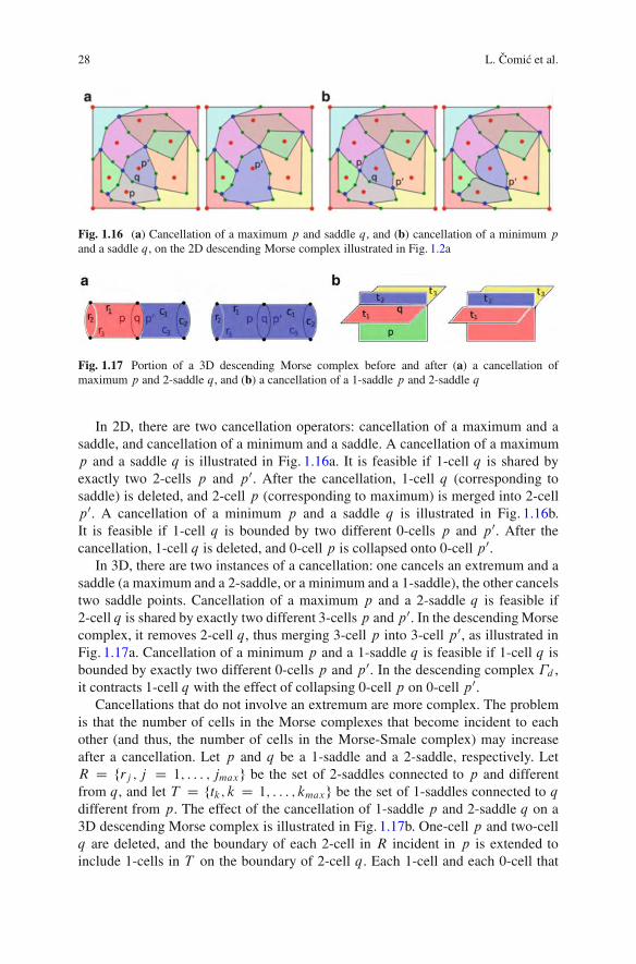
28 L. Comic et al.
Fig. 1.16 (a) Cancellation of a maximum p and saddle q, and (b) cancellation of a minimum pand a saddle q, on the 2D descending Morse complex illustrated in Fig. 1.2a
Fig. 1.17 Portion of a 3D descending Morse complex before and after (a) a cancellation ofmaximum p and 2-saddle q, and (b) a cancellation of a 1-saddle p and 2-saddle q
In 2D, there are two cancellation operators: cancellation of a maximum and asaddle, and cancellation of a minimum and a saddle. A cancellation of a maximump and a saddle q is illustrated in Fig. 1.16a. It is feasible if 1-cell q is shared byexactly two 2-cells p and p0. After the cancellation, 1-cell q (corresponding tosaddle) is deleted, and 2-cell p (corresponding to maximum) is merged into 2-cellp0. A cancellation of a minimum p and a saddle q is illustrated in Fig. 1.16b.It is feasible if 1-cell q is bounded by two different 0-cells p and p0. After thecancellation, 1-cell q is deleted, and 0-cell p is collapsed onto 0-cell p0.
In 3D, there are two instances of a cancellation: one cancels an extremum and asaddle (a maximum and a 2-saddle, or a minimum and a 1-saddle), the other cancelstwo saddle points. Cancellation of a maximum p and a 2-saddle q is feasible if2-cell q is shared by exactly two different 3-cells p and p0. In the descending Morsecomplex, it removes 2-cell q, thus merging 3-cell p into 3-cell p0, as illustrated inFig. 1.17a. Cancellation of a minimum p and a 1-saddle q is feasible if 1-cell q isbounded by exactly two different 0-cells p and p0. In the descending complex !d ,it contracts 1-cell q with the effect of collapsing 0-cell p on 0-cell p0.
Cancellations that do not involve an extremum are more complex. The problemis that the number of cells in the Morse complexes that become incident to eachother (and thus, the number of cells in the Morse-Smale complex) may increaseafter a cancellation. Let p and q be a 1-saddle and a 2-saddle, respectively. LetR D frj ; j D 1; : : : ; jmaxg be the set of 2-saddles connected to p and differentfrom q, and let T D ftk; k D 1; : : : ; kmaxg be the set of 1-saddles connected to qdifferent from p. The effect of the cancellation of 1-saddle p and 2-saddle q on a3D descending Morse complex is illustrated in Fig. 1.17b. One-cell p and two-cellq are deleted, and the boundary of each 2-cell in R incident in p is extended toinclude 1-cells in T on the boundary of 2-cell q. Each 1-cell and each 0-cell that
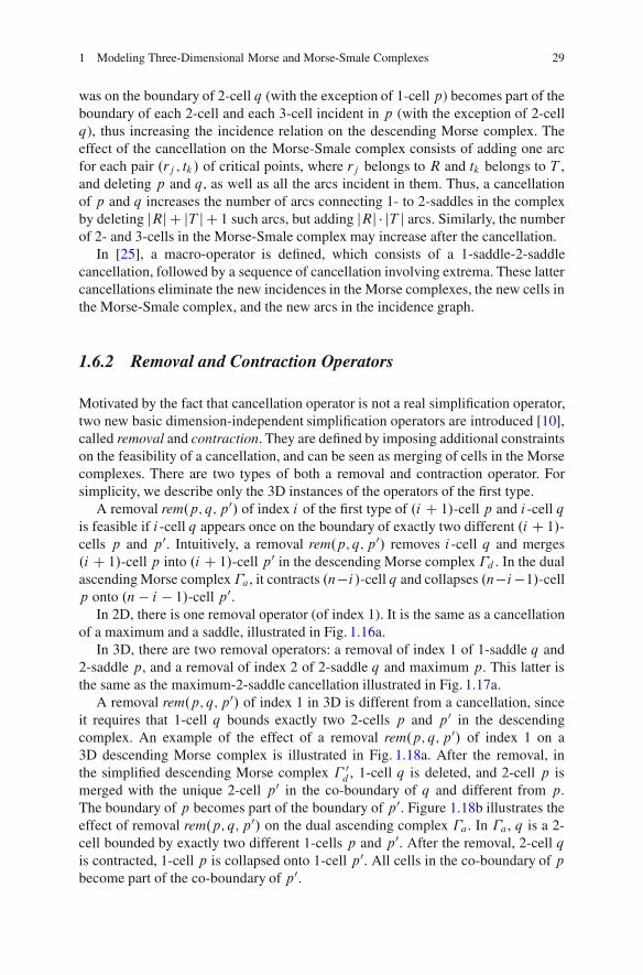
1 Modeling Three-Dimensional Morse and Morse-Smale Complexes 29
was on the boundary of 2-cell q (with the exception of 1-cell p) becomes part of theboundary of each 2-cell and each 3-cell incident in p (with the exception of 2-cellq), thus increasing the incidence relation on the descending Morse complex. Theeffect of the cancellation on the Morse-Smale complex consists of adding one arcfor each pair .rj ; tk/ of critical points, where rj belongs to R and tk belongs to T ,and deleting p and q, as well as all the arcs incident in them. Thus, a cancellationof p and q increases the number of arcs connecting 1- to 2-saddles in the complexby deleting jRj C jT j C 1 such arcs, but adding jRj % jT j arcs. Similarly, the numberof 2- and 3-cells in the Morse-Smale complex may increase after the cancellation.
In [25], a macro-operator is defined, which consists of a 1-saddle-2-saddlecancellation, followed by a sequence of cancellation involving extrema. These lattercancellations eliminate the new incidences in the Morse complexes, the new cells inthe Morse-Smale complex, and the new arcs in the incidence graph.
1.6.2 Removal and Contraction Operators
Motivated by the fact that cancellation operator is not a real simplification operator,two new basic dimension-independent simplification operators are introduced [10],called removal and contraction. They are defined by imposing additional constraintson the feasibility of a cancellation, and can be seen as merging of cells in the Morsecomplexes. There are two types of both a removal and contraction operator. Forsimplicity, we describe only the 3D instances of the operators of the first type.
A removal rem.p; q; p0/ of index i of the first type of .i C 1/-cell p and i -cell qis feasible if i -cell q appears once on the boundary of exactly two different .i C 1/-cells p and p0. Intuitively, a removal rem.p; q; p0/ removes i -cell q and merges.i C 1/-cell p into .i C 1/-cell p0 in the descending Morse complex !d . In the dualascending Morse complex!a, it contracts .n"i/-cell q and collapses .n"i"1/-cellp onto .n " i " 1/-cell p0.
In 2D, there is one removal operator (of index 1). It is the same as a cancellationof a maximum and a saddle, illustrated in Fig. 1.16a.
In 3D, there are two removal operators: a removal of index 1 of 1-saddle q and2-saddle p, and a removal of index 2 of 2-saddle q and maximum p. This latter isthe same as the maximum-2-saddle cancellation illustrated in Fig. 1.17a.
A removal rem.p; q; p0/ of index 1 in 3D is different from a cancellation, sinceit requires that 1-cell q bounds exactly two 2-cells p and p0 in the descendingcomplex. An example of the effect of a removal rem.p; q; p0/ of index 1 on a3D descending Morse complex is illustrated in Fig. 1.18a. After the removal, inthe simplified descending Morse complex ! 0d , 1-cell q is deleted, and 2-cell p ismerged with the unique 2-cell p0 in the co-boundary of q and different from p.The boundary of p becomes part of the boundary of p0. Figure 1.18b illustrates theeffect of removal rem.p; q; p0/ on the dual ascending complex !a. In !a, q is a 2-cell bounded by exactly two different 1-cells p and p0. After the removal, 2-cell qis contracted, 1-cell p is collapsed onto 1-cell p0. All cells in the co-boundary of pbecome part of the co-boundary of p0.
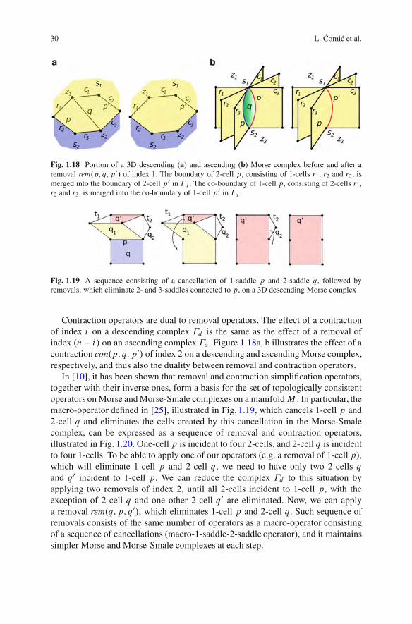
30 L. Comic et al.
Fig. 1.18 Portion of a 3D descending (a) and ascending (b) Morse complex before and after aremoval rem.p; q; p0/ of index 1. The boundary of 2-cell p, consisting of 1-cells r1, r2 and r3, ismerged into the boundary of 2-cell p0 in !d . The co-boundary of 1-cell p, consisting of 2-cells r1,r2 and r3, is merged into the co-boundary of 1-cell p0 in !a
Fig. 1.19 A sequence consisting of a cancellation of 1-saddle p and 2-saddle q, followed byremovals, which eliminate 2- and 3-saddles connected to p, on a 3D descending Morse complex
Contraction operators are dual to removal operators. The effect of a contractionof index i on a descending complex !d is the same as the effect of a removal ofindex .n" i/ on an ascending complex !a. Figure 1.18a, b illustrates the effect of acontraction con.p; q; p0/ of index 2 on a descending and ascending Morse complex,respectively, and thus also the duality between removal and contraction operators.
In [10], it has been shown that removal and contraction simplification operators,together with their inverse ones, form a basis for the set of topologically consistentoperators on Morse and Morse-Smale complexes on a manifoldM . In particular, themacro-operator defined in [25], illustrated in Fig. 1.19, which cancels 1-cell p and2-cell q and eliminates the cells created by this cancellation in the Morse-Smalecomplex, can be expressed as a sequence of removal and contraction operators,illustrated in Fig. 1.20. One-cell p is incident to four 2-cells, and 2-cell q is incidentto four 1-cells. To be able to apply one of our operators (e.g. a removal of 1-cell p),which will eliminate 1-cell p and 2-cell q, we need to have only two 2-cells qand q0 incident to 1-cell p. We can reduce the complex !d to this situation byapplying two removals of index 2, until all 2-cells incident to 1-cell p, with theexception of 2-cell q and one other 2-cell q0 are eliminated. Now, we can applya removal rem.q; p; q0/, which eliminates 1-cell p and 2-cell q. Such sequence ofremovals consists of the same number of operators as a macro-operator consistingof a sequence of cancellations (macro-1-saddle-2-saddle operator), and it maintainssimpler Morse and Morse-Smale complexes at each step.

1 Modeling Three-Dimensional Morse and Morse-Smale Complexes 31
Fig. 1.20 A sequence consisting of removals, which eliminate 2- and 3-saddles connected to p,followed by a removal of index 1 that eliminates 1-saddle p and 2-saddle q on a 3D descendingMorse complex
Fig. 1.21 (a) Field behavior for the Bucky Ball data set. (b) The incidence graph at full resolution,and the incidence graph after (c) 200 and (d) 400 simplifications
We have developed a simplification algorithm on the Morse complexes based onthe removal and contraction simplification operators. Simplifications are applied inincreasing order of persistence [20]. Our simplification algorithm can be applied notonly to scalar fields representing the elevation, but to any scalar field, such as forexample a discrete distortion [42], which generalizes the notion of curvature.
In Fig. 1.21, we illustrate the result of our simplification algorithm on a 3D BuckyBall data set, depicted in Fig. 1.21a, which represents a carbon molecule having 60atoms arranged as a truncated icosahedron. The full-resolution graph is shown inFig. 1.21b. The incidence graphs after 200 and 400 simplifications are shown inFig. 1.21c, d, respectively.
1.7 Concluding Remarks
The problem of modeling and simplifying Morse and Morse-Smale complexes in 2Dhas been extensively studied in the literature. Here, we have reviewed some recentwork which extends these results to three and higher dimensions. We have describedand compared data structures for representing Morse and Morse-Smale complexes.We have described and compared algorithms for extracting these complexes startingfrom the values of a scalar field f given at the vertices of a simplicial or a cellcomplex triangulating a manifold M . Finally, we have described and comparedexisting simplification operators on Morse and Morse-Smale complexes.

32 L. Comic et al.
Simplification operators, together with their inverse refinement ones, form a basisfor the definition of a multi-resolution model of Morse and Morse-Smale complexes[18].
The next challenge is how to extract representations of the geometry of thefield which is compatible with the reduced incidence graph extracted from themultiresolution model [6, 16, 41].
Acknowledgements This work has been partially supported by the Italian Ministry of Educationand Research under the PRIN 2009 program, and by the National Science Foundation under grantnumber IIS-1116747.
References
1. Bajaj, C.L., Shikore, D.R.: Topology preserving data simplification with error bounds. Comput.Graph. 22(1), 3–12 (1998)
2. Banchoff, T.: Critical points and curvature for embedded polyhedral surfaces. Am. Math. Mon.77(5), 475–485 (1970)
3. Beucher, S.: Watershed, hierarchical segmentation and waterfall algorithm. In: Proceedingsof the Mathematical Morphology and Its Applications to Image Processing, Fontainebleau,France, pp. 69–76 (1994)
4. Biasotti, S., De Floriani, L., Falcidieno, B., Frosini, P., Giorgi, D., Landi, C., Papaleo, L.,Spagnuolo, M.: Describing shapes by geometrical-topological properties of real functions.ACM Comput. Surv. 40, Article 12 (2008)
5. Bremer, P.-T., Edelsbrunner, H., Hamann, B., Pascucci, V.: A multi-resolution data structurefor two-dimensional Morse functions. In: Proceedings IEEE Visualization 2003, Seattle,pp. 139–146. IEEE Computer Society (2003)
6. Bremer, P.-T., Edelsbrunner, H., Hamann, B., Pascucci, V.: A topological hierarchy forfunctions on triangulated surfaces. Trans. Vis. Comput. Graph. 10(4), 385–396 (2004)
7. Bremer, P.-T., Pascucci, V., Hamann, B.: Maximizing adaptivity in hierarchical topologicalmodels. In: Belyaev, A.G., Pasko, A.A., Spagnuolo, M. (eds.) Proceedings of the Interna-tional Conference on Shape Modeling and Applications 2005 (SMI ’05), Cambridge, MA,pp. 300–309. IEEE Computer Society, Los Alamitos (2005)
8. Bremer, P.-T., Weber, G.H., Pascucci, V., Day, M.S., Bell, J.B.: Analyzing and tracking burningstructures in lean premixed hydrogen flames. IEEE Trans. Vis. Comput. Graph. 16(2), 248–260(2010)
9. Cazals, F., Chazal, F., Lewiner, T.: Molecular shape analysis based upon the Morse-Smalecomplex and the connolly function. In: Proceedings of the Nineteenth Annual Symposium onComputational Geometry, San Diego, pp. 351–360. ACM, New York (2003)
10. Comic, L., De Floriani, L.: Dimension-independent simplification and refinement of Morsecomplexes. Graph. Models 73(5), 261–285 (2011)
11. Comic, L., De Floriani, L., Iuricich, F.: Building morphological representations for 2D and3D scalar fields. In: Puppo, E., Brogni, A., De Floriani, L. (eds.) Eurographics Italian ChapterConference, Genova, pp. 103–110. Eurographics (2010)
12. Comic, L., Mesmoudi, M.M., De Floriani, L.: Smale-like decomposition and Forman theoryfor discrete scalar fields. In: DGCI, Nancy, pp. 477–488 (2011)
13. Danovaro, E., De Floriani, L., Mesmoudi, M.M.: Topological analysis and characterization ofdiscrete scalar fields. In: Asano, T., Klette, R., Ronse, C. (eds.) Geometry, Morphology, andComputational Imaging. Lecture Notes in Computer Science, vol. 2616, pp. 386–402. Springer,Berlin Heidelberg (2003)

1 Modeling Three-Dimensional Morse and Morse-Smale Complexes 33
14. Danovaro, E., De Floriani, L., Magillo, P., Mesmoudi, M.M., Puppo, E.: Morphology-driven simplification and multiresolution modeling of terrains. In: Hoel, E., Rigaux, P. (eds.)Proceedings ACM GIS 2003 – The 11th International Symposium on Advances in GeographicInformation Systems, New Orleans, pp. 63–70. ACM (2003)
15. Danovaro, E., De Floriani, L., Vitali, M., Magillo, P.: Multi-scale dual Morse complexes forrepresenting terrain morphology. In: GIS ’07: Proceedings of the 15th Annual ACM Interna-tional Symposium on Advances in Geographic Information Systems, Seattle, Washington, WA,pp. 1–8. ACM, New York (2007)
16. Danovaro, E., De Floriani, L., Magillo, P., Vitali, M.: Multiresolution Morse triangulations.In: Elber, G., Fischer, A., Keyser, J., Kim, M.-S. (eds.) Symposium on Solid and PhysicalModeling, Haifa, pp. 183–188. ACM (2010)
17. De Floriani, L., Hui, A.: Shape representations based on cell and simplicial complexes. In:Eurographics 2007, Prague, Czech Republic, State-of-the-Art Report, Sept 2007
18. Comic, L., De Floriani, L., Iuricich, F.: Dimension-independent multi-resolution Morsecomplexes. Comput. Graph. 36(5), 541–547 (2012)
19. Edelsbrunner, H., Harer, J.: The persistent Morse complex segmentation of a 3-manifold. In:Magnenat-Thalmann, N. (ed.) 3DPH, Zermatt. Lecture Notes in Computer Science, vol. 5903,pp. 36–50. Springer (2009)
20. Edelsbrunner, H., Harer, J., Zomorodian, A.: Hierarchical Morse complexes for piecewiselinear 2-manifolds. In: Proceedings of the 17th ACM Symposium on Computational Geometry,Medford, pp. 70–79 (2001)
21. Edelsbrunner, H., Harer, J., Natarajan, V., Pascucci, V.: Morse-Smale complexes for piecewiselinear 3-manifolds. In: Proceedings of the 19th ACM Symposium on Computational Geometry,San Diego, pp. 361–370 (2003)
22. Forman, R.: Morse theory for cell complexes. Adv. Math. 134, 90–145 (1998)23. Gyulassy, A., Pascucci, V.: Computing simply-connected cells in three-dimensional Morse-
Smale complexes. In: Peikert, R., Hauser, H., Carr, H., Fuchs, R. (eds.) Topological Methodsin Data Analysis and Visualization: Theory, Algorithms, and Applications. Mathematics andVisualization, pp. 31–46. Springer, Heidelberg (2012)
24. Gyulassy, A., Natarajan, V., Pascucci, V., Bremer, P.-T., Hamann, B.: Topology-based simpli-fication for feature extraction from 3D scalar fields. In: Proceedings IEEE Visualization’05,Minneapolis, Minnesota, MN, pp. 275–280. ACM (2005)
25. Gyulassy, A., Natarajan, V., Pascucci, V., Bremer, P.-T., Hamann, B.: A topological approach tosimplification of three-dimensional scalar functions. IEEE Trans. Vis. Comput. Graph. 12(4),474–484 (2006)
26. Gyulassy, A., Natarajan, V., Pascucci, V., Hamann, B.: Efficient computation of Morse-Smalecomplexes for three-dimensional scalar functions. IEEE Trans. Vis. Comput. Graph. 13(6),1440–1447 (2007)
27. Gyulassy, A., Bremer, P.-T., Hamann, B., Pascucci, V.: A practical approach to Morse-Smalecomplex computation: scalability and generality. IEEE Trans. Vis. Comput. Graph. 14(6),1619–1626 (2008)
28. Gyulassy, A., Bremer, P.-T., Hamann, B., Pascucci, V.: Practical considerations in Morse-Smalecomplex computation. In: Pascucci, V., Tricoche, X., Hagen, H., Tierny, J. (eds.) TopologicalMethods in Data Analysis and Visualization: Theory, Algorithms, and Applications. Mathe-matics and Visualization, pp. 67–78. Springer, Heidelberg (2011)
29. Jerse, G., Mramor Kosta, N.: Ascending and descending regions of a discrete Morse function.Comput. Geom. Theory Appl. 42(6–7), 639–651 (2009)
30. Kelley, J.L.: General Topology. Van Nostrand, Princeton (1955)31. King, H., Knudson, K., Mramor, N.: Generating discrete Morse functions from point data. Exp.
Math. 14(4), 435–444 (2005)32. Lewiner, T., Lopes, H., Tavares, G.: Applications of Forman’s discrete Morse theory to
topology visualization and mesh compression. Trans. Vis. Comput. Graph. 10(5), 499–508(2004)

34 L. Comic et al.
33. Matsumoto, Y.: An Introduction to Morse Theory. Translations of Mathematical Monographs,vol. 208. American Mathematical Society, Providence (2002)
34. Milnor, J.: Morse Theory. Princeton University Press, Princeton (1963)35. Natarajan, V., Wang, Y., Bremer, P.-T., Pascucci, V., Hamann, B.: Segmenting molecular
surfaces. Comput. Aided Geom. Des. 23(6), 495–509 (2006)36. Ni, X., Garland, M., Hart, J.C.: Fair Morse functions for extracting the topological structure of
a surface mesh. In: International Conference on Computer Graphics and Interactive TechniquesACM SIGGRAPH, Los Angeles, pp. 613–622 (2004)
37. Pascucci, V.: Topology diagrams of scalar fields in scientific visualization. In: Rana, S. (ed.)Topological Data Structures for Surfaces, pp. 121–129. Wiley, Chichester/Hoboken (2004)
38. Robins, V., Wood, P.J., Sheppard, A.P.: Theory and algorithms for constructing discrete Morsecomplexes from grayscale digital images. IEEE Trans. Pattern Anal. Mach. Intell. 33(8),1646–1658 (2011)
39. Takahashi, S., Ikeda, T., Kunii, T.L., Ueda, M.: Algorithms for extracting correct critical pointsand constructing topological graphs from discrete geographic elevation data. Comput. Graph.Forum 14, 181–192 (1995)
40. Vincent, L., Soille, P.: Watershed in digital spaces: an efficient algorithm based on immersionsimulation. IEEE Trans. Pattern Anal. Mach. Intell. 13(6), 583–598 (1991)
41. Weinkauf, T., Gingold, Y.I., Sorkine, O.: Topology-based smoothing of 2D scalar fields with1-continuity. Comput. Graph. Forum 29(3), 1221–1230 (2010)
42. Weiss, K., De Floriani, L., Mesmoudi, M.M.: Multiresolution analysis of 3D images based ondiscrete distortion. In: 20th International Conference on Pattern Recognition (ICPR), Istanbul,pp. 4093–4096 (2010)
43. Wolf, G.W.: Topographic surfaces and surface networks. In: Rana, S. (ed.) Topological DataStructures for Surfaces, pp. 15–29. Wiley, Chichester/Hoboken (2004)
Chapter 2Geodesic Regression and Its Applicationto Shape Analysis
P. Thomas Fletcher
Abstract In this chapter, I present a regression method for modeling therelationship between a manifold-valued random variable and a real-valuedindependent parameter. The principle is to fit a geodesic curve, parameterized by theindependent parameter, that best fits the data. Error in the model is evaluated as thesum-of-squared geodesic distances from the model to the data, and this provides anintrinsic least squares criterion. Geodesic regression is, in some sense, the simplestparametric model that one could choose, and it provides a direct generalizationof linear regression to the manifold setting. A generalization of the coefficient ofdetermination and a resulting hypothesis test for determining the significance of theestimated trend is developed. Also, a diagnostic test for the quality of the fit of theestimated geodesic is demonstrated. While the method can be generally appliedto data on any manifold, specific examples are given for a set of syntheticallygenerated rotation data and an application to analyzing shape changes in the corpuscallosum due to age.
2.1 Introduction
Regression analysis is a fundamental statistical tool for determining how a measuredvariable is related to one or more potential explanatory variables. The mostwidely used regression model is linear regression, due to its simplicity, ease ofinterpretation, and ability to model many phenomena. However, if the responsevariable takes values on a nonlinear manifold, a linear model is not applicable.Such manifold-valued measurements arise in many applications, including thoseinvolving directional data, transformations, tensors, and shape. For example, inbiology and medicine it is often critical to understand processes that change
P.T. Fletcher (!)University of Utah, Salt Lake City, 84112 UT, USAe-mail: [email protected]
M. Breuß et al. (eds.), Innovations for Shape Analysis, Mathematics and Visualization,DOI 10.1007/978-3-642-34141-0 2, © Springer-Verlag Berlin Heidelberg 2013
35
36 P.T. Fletcher
the shape of anatomy. The difficulty is that shape variability is inherently high-dimensional and nonlinear. An effective approach to capturing this variability hasbeen to parameterize shape as a manifold, or shape space.
Statistical analysis of manifold data has been developed by several authors. Theseminal work of Frechet [10] generalized the concept of expectation from linearspaces to general metric spaces. This opened up the possibility of computing asample mean statistic from a set of data on a manifold using the geodesic distance asmetric. The Frechet mean of a set of points, y1; : : : ; yN ; in a Riemannian manifoldM is given by
! D arg miny2M
NX
iD1d.y; yi /
2;
where d is the geodesic distance between points on M . This equation generalizesthe principle of least squares to the metric space setting. Karcher [12] providedconditions guaranteeing the existence and uniqueness of the Frechet mean, whichwere later improved by Kendall [14]. Second-order statistics such as generalizationsof principal components analysis [8] and Gaussian covariances [21] have also beendeveloped and applied in the domain of image analysis. Related work includesstatistical analysis of directional data (e.g., spheres) [16] and analysis on shapemanifolds [5], where statistics are derived from probability distributions on specificmanifolds (for example, the Fisher-von Mises distribution on spheres).
Several works have studied the regression problem on manifolds. Jupp andKent [11] propose an unrolling method on shape spaces. Regression analysis onthe group of diffeomorphisms has been proposed as growth models by Miller [18],nonparametric regression by Davis et al. [2], and second-order splines by Trouveand Vialard [23]. Durrleman et al. [6] construct spatiotemporal image atlases fromlongitudinal data. Finally, Shi et al. [22] proposed a semiparametric model withmultiple covariates for manifold response data. None of these methods provide adirect generalization of linear regression to manifolds. The purpose of this workis to develop such a generalization, called geodesic regression, which models therelationship between an independent scalar variable with a dependent manifold-valued random variable as a geodesic curve. Like linear regression, the advantagesof this model are its simplicity and ease of interpretation. As will be shown, thegeodesic regression model also leads to a straightforward generalization of the R2
statistic and a hypothesis test for significance of the estimated geodesic trend. Thischapter is an expanded exposition of the geodesic regression method first introducedin [7]. Niethammer et al. [20] independently proposed geodesic regression for thecase of diffeomorphic transformations of image time series.
2.2 Multiple Linear Regression
Before formulating geodesic regression on general manifolds, we begin byreviewing multiple linear regression in Rn. Here we are interested in the relationshipbetween a non-random independent variable X 2R and a random dependent
2 Geodesic Regression and Its Application to Shape Analysis 37
variable Y taking values in Rn. A multiple linear model of this relationship isgiven by
Y D ˛ CXˇ C "; (2.1)
where ˛ 2 Rn is an unobservable intercept parameter, ˇ 2 Rn is an unobservableslope parameter, and " is an Rn-valued, unobservable random variable representingthe error. Geometrically, this is the equation of a one-dimensional line throughRn (plus noise), parameterized by the scalar variable X . For the purposes ofgeneralizing to the manifold case, it is useful to think of ˛ as the starting pointof the line and ˇ as a velocity vector.
Given realizations of the above model, i.e., data .xi ; yi / 2 R ! Rn, for i D1; : : : ; N , the least squares estimates, O ; O; for the intercept and slope are computedby solving the minimization problem
. O ; O/ D arg min.˛;ˇ/
NX
iD1kyi " ˛ " xiˇk2 : (2.2)
This equation can be solved analytically, yielding
O D1N
Pxi yi " Nx NyPx2i " Nx2
;
O D Ny " Nx O;
where Nx and Ny are the sample means of the xi and yi , respectively. If the errorsin the model are drawn from distributions with zero mean and finite variance,then these estimators are unbiased and consistent. Furthermore, if the errors arehomoscedastic (equal variance) and uncorrelated, then the Gauss-Markov theoremstates that they will have minimal mean-squared error amongst all unbiased linearestimators.
2.3 Geodesic Regression
Let y1; : : : ; yN be points on a smooth Riemannian manifold M , with associatedscalar values x1; : : : ; xN 2 R. The goal of geodesic regression is to find a geodesiccurve # onM that best models the relationship between the xi and the yi . Just as inlinear regression, the speed of the geodesic will be proportional to the independentparameter corresponding to the xi . Estimation will be set up as a least-squaresproblem, where we want to minimize the sum-of-squared Riemannian distancesbetween the model and the data. A schematic of the geodesic regression model isshown in Fig. 2.1.
Before formulating the model, we review a few basic concepts of Riemanniangeometry. We will write an element of the tangent bundle as the pair .p; v/ 2 TM ,
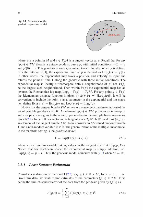
38 P.T. Fletcher
Fig. 2.1 Schematic of thegeodesic regression model
where p is a point in M and v 2 TpM is a tangent vector at p. Recall that for any.p; v/ 2 TM there is a unique geodesic curve # , with initial conditions #.0/ D pand # 0.0/ D v. This geodesic is only guaranteed to exist locally. When # is definedover the interval å 0; 1$, the exponential map at p is defined as Expp.v/ D #.1/.In other words, the exponential map takes a position and velocity as input andreturns the point at time 1 along the geodesic with these initial conditions. Theexponential map is locally diffeomorphic onto a neighborhood of p. Let V.p/be the largest such neighborhood. Then within V.p/ the exponential map has aninverse, the Riemannian log map, Logp W V.p/ ! TpM . For any point q 2 V.p/the Riemannian distance function is given by d.p; q/ D kLogp.q/k. It will beconvenient to include the point p as a parameter in the exponential and log maps,i.e., define Exp.p; v/ D Expp.v/ and Log.p; q/ D Logp.q/.
Notice that the tangent bundle TM serves as a convenient parameterization of theset of possible geodesics on M . An element .p; v/ 2 TM provides an intercept pand a slope v, analogous to the � and � parameters in the multiple linear regressionmodel (2.1). In fact, � is a vector in the tangent space T� Rn # Rn, and thus .� ; � / isan element of the tangent bundle TRn. Now consider anM -valued random variableY and a non-random variableX 2R. The generalization of the multiple linear modelto the manifold setting is the geodesic model,
Y D Exp.Exp.p;Xv/; "/; (2.3)
where " is a random variable taking values in the tangent space at Exp.p;Xv/.Notice that for Euclidean space, the exponential map is simply addition, i.e.,Exp.p; v/ D p C v. Thus, the geodesic model coincides with (2.1) when M D Rn.
2.3.1 Least Squares Estimation
Consider a realization of the model (2.3): .xi ; yi / 2 R ! M , for i D 1; : : : ; N .Given this data, we wish to find estimates of the parameters .p; v/ 2 TM . First,define the sum-of-squared error of the data from the geodesic given by .p; v/ as
E.p; v/ D 1
2
NX
iD1d.Exp.p; xiv/; yi /2: (2.4)
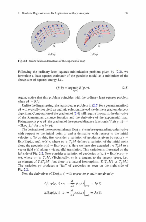
2 Geodesic Regression and Its Application to Shape Analysis 39
dpExp dvExp
Fig. 2.2 Jacobi fields as derivatives of the exponential map
Following the ordinary least squares minimization problem given by (2.2), weformulate a least squares estimator of the geodesic model as a minimizer of theabove sum-of-squares energy, i.e.,
. Op; Ov/ D arg min.p;v/
E.p; v/: (2.5)
Again, notice that this problem coincides with the ordinary least squares problemwhenM D Rn.
Unlike the linear setting, the least squares problem in (2.5) for a general manifoldM will typically not yield an analytic solution. Instead we derive a gradient descentalgorithm. Computation of the gradient of (2.4) will require two parts: the derivativeof the Riemannian distance function and the derivative of the exponential map.Fixing a pointp 2M , the gradient of the squared distance function isrxd.p; x/2 D"2Logx.p/ for x 2 V.p/.
The derivative of the exponential map Exp.p; v/ can be separated into a derivativewith respect to the initial point p and a derivative with respect to the initialvelocity v. To do this, first consider a variation of geodesics given by c1.s; t/ DExp.Exp.p; su1/; tv.s//, where u1 2 TpM defines a variation of the initial pointalong the geodesic %.s/ D Exp.p; su1/. Here we have also extended v 2 TpM to avector field v.s/ along % via parallel translation. This variation is illustrated on theleft side of Fig. 2.2. Next consider a variation of geodesics c2.s; t/DExp.p; su2 Ctv/, where u2 2 TpM . (Technically, u2 is a tangent to the tangent space, i.e.,an element of Tv.TpM/, but there is a natural isomorphism Tv.TpM/ # TpM .)The variation c2 produces a “fan” of geodesics as seen on the right side ofFig. 2.2.
Now the derivatives of Exp.p; v/ with respect to p and v are given by
dpExp.p; v/ $ u1 Dd
dsc1.s; t/
���sD0D J1.1/
dvExp.p; v/ $ u2 Dd
dsc2.s; t/
���sD0D J2.1/;
40 P.T. Fletcher
where Ji .t/ are Jacobi fields along the geodesic #.t/ D Exp.p; tv/. Jacobi fieldsare solutions to the second order equation
D2
dt2J.t/CR.J.t/; # 0.t// # 0.t/ D 0; (2.6)
where R is the Riemannian curvature tensor. For more details on the derivation ofthe Jacobi field equation and the curvature tensor, see for instance [3]. The initialconditions for the two Jacobi fields above are J1.0/ D u1; J 01.0/ D 0 and J2.0/D 0,J 02.0/ D u2, respectively. If we decompose the Jacobi field into a componenttangential to # and a component orthogonal, i.e., J D J> C J?, the tangentialcomponent is linear: J>.t/ D u>1 C tu>2 . Therefore, the only challenge is to solvefor the orthogonal component.
Finally, the gradient of the sum-of-squares energy in (2.4) is given by
rp E.p; v/ D "NX
iD1dpExp.p; xiv/&Log.Exp.p; xiv/; yi /;
rvE.p; v/ D "NX
iD1xi dvExp.p; xiv/&Log.Exp.p; xiv/; yi /;
where we have taken the adjoint of the exponential map derivative, e.g., definedby hdpExp.p; v/u;wi D hu; dpExp.p; v/&wi. As we will see in the next section,formulas for Jacobi fields and their respective adjoint operators can often be derivedanalytically for many useful manifolds.
2.3.2 R2 Statistics and Hypothesis Testing
In regression analysis the most basic question one would like to answer is whetherthe relationship between the independent and dependent variables is significant.A common way to test this is to see if the amount of variance explained by the modelis high. For geodesic regression we will measure the amount of explained varianceusing a generalization of the R2 statistic, or coefficient of determination, to themanifold setting. To do this, we first define predicted values of yi and the errors "i as
Oyi D Exp. Op; xi Ov/;O"i D Log. Oyi ; yi /;
where . Op; Ov/ are the least squares estimates of the geodesic parameters definedabove. Note that the Oyi are points along the estimated geodesic that are the bestpredictions of the yi given only the xi . The O"i are the residuals from the modelpredictions to the true data.
2 Geodesic Regression and Its Application to Shape Analysis 41
Now to define the total variance of data, y1; : : : ; yN 2 M , we use the Frechetvariance, intrinsically defined by
var.yi / D miny2M
1
N
NX
iD1d.y; yi /
2:
The unexplained variance is the variance of the residuals, var. O"i / D 1N
P kO"ik2.From the definition of the residuals, it can be seen that the unexplained variance isthe mean squared distance of the data to the model, i.e., var.O"i / D 1
N
Pd. Oyi ; yi /2.
Using these two variance definitions, the generalization of the R2 statistic is thengiven by
R2 D 1 " unexplained variancetotal variance
D 1 " var.O"i /var.yi /
: (2.7)
Frechet variance coincides with the standard definition of variance when M D Rn.Therefore, it follows that the definition ofR2 in (2.7) coincides with theR2 for linearregression when M D Rn. Also, because Frechet variance is always nonnegative,we see that R2 % 1, and that R2 D 1 if and only if the residuals to the modelare exactly zero, i.e., the model perfectly fits the data. Finally, it is clear that theresidual variance is always smaller than the total variance, i.e., var.O"i / % var.yi /.This is because we could always choose Op to be the Frechet mean and v D 0 toachieve var.O"i / D var.yi /. Therefore, R2 & 0, and it must lie in the interval Œ0; 1$,as is the case for linear models.
We now describe a permutation test for testing the significance of the estimatedslope term, Ov. Notice that if we constrain v to be zero in (2.5), then the resulting leastsquares estimate of the intercept, Op; will be the Frechet mean of the yi . The desiredhypothesis test is whether the fraction of unexplained variance is significantlydecreased by also estimating v. The null hypothesis is H0 W R2 D 0, which is thecase if the unexplained variance in the geodesic model is equal to the total variance.Under the null hypothesis, there is no relationship between the X variable and theY variable. Therefore, the xi are exchangeable under the null hypothesis, and a per-mutation test may randomly reorder the xi data, keeping the yi fixed. Estimating thegeodesic regression parameters for each random permutation of the xi , we can cal-culate a sequence ofR2 values,R21; : : : ; R
2m, which approximate the sampling distri-
bution of theR2 statistic under the null hypothesis. Computing the fraction of theR2kthat are greater than the R2 estimated from the unpermuted data gives us a p-value.
2.4 Testing the Geodesic Fit
In any type of regression analysis, a choice is made as to the type of modelthat is fit to the data, whether it be linear, polynomial, or perhaps nonparametric.An important step in the analysis is to verify that the selected model is in fact
42 P.T. Fletcher
appropriate. In linear regression, for example, one would want to test severalassumptions: (1) that the trend in the data is truly linear, (2) that the error ishomoscedastic, (3) that the model fit is not led astray by outliers, (4) that the errorsare Gaussian distributed, etc. Several graphical and quantitative heuristic tests havebeen developed to test these assumptions. For a detailed treatment of these methods,see [9].
In this section we develop a diagnostic test of the model assumptions for geodesicregression. We focus on the following question: is a geodesic curve an appropriatemodel for the relationship between the independent and dependent variables? Ageodesic curve is, in some sense, the “straightest” path one can take on a manifold.This begs the question if a more flexible model would do a better job at fitting thedata. This is analogous to the model selection problem for real-valued data whenone is making the choice between a linear model and something more flexible, suchas a higher-order polynomial model. Of course, if a model is made more flexiblethere is a danger that the data will be overfit. One way to test if a model is “flexibleenough” is to plot the residuals of the model versus the independent variable. Ifthe model has captured the relationship between the independent and dependentvariables, then the residuals should show no obvious trend. If they do show atrend, then a more flexible model is needed to capture the relationship between thedata. However, for regression on manifolds, this is a difficult test to apply becausethe residuals are high-dimensional tangent vectors and are thus difficult to plotversus the independent variable. One solution might be to plot the magnitude ofthe residuals instead, but this loses most of the information contained in the residualvectors.
Instead, we will use nonparametric regression as a comparison model to testif a geodesic is sufficient to capture the relationships in the data. Nonparametricregression models, such as the kernel regression method described below, arehighly flexible. Because there is no parametric model assumed for the functionalrelationship between the independent and dependent variables, these models canadapt to highly complex functions given enough data. Given a method to visualizethe results of a manifold-valued regression, the diagnostic test is as follows. First,compute both a geodesic regression and a nonparametric regression of the data.Second, visualize the results of both regression methods. If the nonparametricregression trend is similar to the estimated geodesic, then this provides strongevidence that the geodesic model is sufficient. If the nonparametric trend deviatessignificantly from the estimated geodesic, then this indicates that the geodesic modelis too inflexible to capture the relationship between the two variables.
An example of this procedure is given for synthesized univariate data in Fig. 2.3.The left figure shows data generated from a noisy linear trend. In this case the linearmodel and the nonparametric model give similar answers. The right figure showsdata generated from a noisy nonlinear (sinusoidal) trend. Here the nonparametricregression adapts to the nonlinearities in the data, and the inadequacy of thelinear trend can be seen as a difference between the two regression models. Ofcourse, in the univariate case we can easily see that a linear trend is inadequatejust by plotting the data even without comparing it to a nonparametric regression.
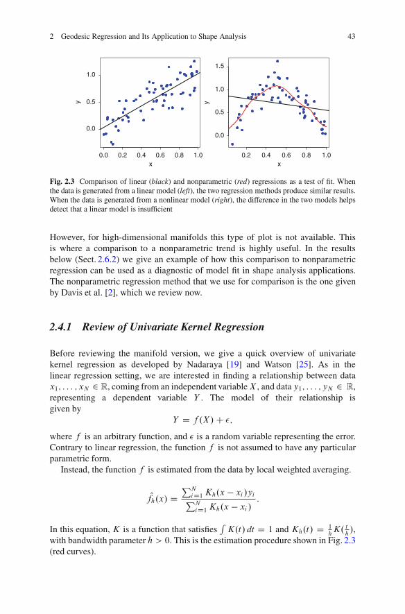
2 Geodesic Regression and Its Application to Shape Analysis 43
0.0 0.2 0.4 0.6 0.8 1.0
0.0
0.5
1.0
x
y
0.2 0.4 0.6 0.8 1.0
0.0
0.5
1.0
1.5
x
y
Fig. 2.3 Comparison of linear (black) and nonparametric (red) regressions as a test of fit. Whenthe data is generated from a linear model (left), the two regression methods produce similar results.When the data is generated from a nonlinear model (right), the difference in the two models helpsdetect that a linear model is insufficient
However, for high-dimensional manifolds this type of plot is not available. Thisis where a comparison to a nonparametric trend is highly useful. In the resultsbelow (Sect. 2.6.2) we give an example of how this comparison to nonparametricregression can be used as a diagnostic of model fit in shape analysis applications.The nonparametric regression method that we use for comparison is the one givenby Davis et al. [2], which we review now.
2.4.1 Review of Univariate Kernel Regression
Before reviewing the manifold version, we give a quick overview of univariatekernel regression as developed by Nadaraya [19] and Watson [25]. As in thelinear regression setting, we are interested in finding a relationship between datax1; : : : ; xN 2 R, coming from an independent variableX , and data y1; : : : ; yN 2 R,representing a dependent variable Y . The model of their relationship isgiven by
Y D f .X/C ";where f is an arbitrary function, and " is a random variable representing the error.Contrary to linear regression, the function f is not assumed to have any particularparametric form.
Instead, the function f is estimated from the data by local weighted averaging.
Ofh.x/ DPN
iD1 Kh.x " xi /yiPNiD1 Kh.x " xi /
:
In this equation, K is a function that satisfiesRK.t/ dt D 1 and Kh.t/ D 1
hK. t
h/,
with bandwidth parameter h > 0. This is the estimation procedure shown in Fig. 2.3(red curves).
44 P.T. Fletcher
2.4.2 Nonparametric Kernel Regression on Manifolds
The regression method of Davis et al. [2] generalizes the Nadaraya-Watson kernelregression method to the case where the dependent variable lives on a Riemannianmanifold, i.e., yi 2 M . Here the model is given by
Y D Exp.f .X/; "/;
where f W R ! M defines a curve on M , and " 2 Tf.X/M is an error term. As inthe univariate case, there are no assumptions on the parametric form of the curve f .
Motivated by the definition of the Nadaraya-Watson estimator as a weightedaveraging, the manifold kernel regression estimator is defined using a weightedFrechet sample mean as
Ofh.x/ D arg miny2M
PNiD1 Kh.x " xi /d.y; yi /2PN
iD1 Kh.x " xi /:
Notice that when the manifold under study is a Euclidean vector space, equippedwith the standard Euclidean norm, the above minimization results in the Nadaraya-Watson estimator.
2.4.3 Bandwidth Selection
It is well known within the kernel regression literature that kernel width plays acrucial role in determining regression results [24]. In particular, it is important toselect a bandwidth that captures relevant population-wide changes without eitheroversmoothing and missing relevant changes or undersmoothing and biasing theresults based on individual noisy data points. The ‘Goldie Locks’ method of tuningthe bandwidth until the results are most pleasing is a common subjective methodfor bandwidth selection. However, non-subjective methods may be required, forexample, when kernel regression is part of a larger statistical study. A numberof automatic kernel bandwidth selection techniques have been proposed for thispurpose [24].
One classic method for automatic bandwidth selection is based on least squarescross-validation. This method is easily extended to the manifold regression settingin the following way. The least squares cross-validation estimate for the optimalbandwidth h is defined as
OhLSCV D arg minh2RC
1
N
NX
iD1d!Of .i/h .xi /; yi
"2;
2 Geodesic Regression and Its Application to Shape Analysis 45
where
Of .i/h .t/ D arg min
y2M
PNjD1;j¤i Kh.x " xj /d.y; yj /2PN
jD1;j¤i Kh.x " xj /
!
is the manifold kernel regression estimator with the i -th observation left out. Thiscross-validation method was used to select the bandwidth for the kernel regressionexample in Fig. 2.3.
2.5 Results: Regression of 3D Rotations
2.5.1 Overview of Unit Quaternions
We represent 3D rotations as the unit quaternions, Q1. A quaternion is denoted asq D .a; v/, where a is the “real” component and v D biCcjCdk. Geodesics in therotation group are given simply by constant speed rotations about a fixed axis. Lete D .1; 0/ be the identity quaternion. The tangent space TeQ1 is the vector spaceof quaternions of the form .0; v/. The tangent space at an arbitrary point q 2 Q1
is given by right multiplication of TeQ1 by q. The Riemannian exponential map isExpq..0; v/ $ q/ D .cos.'=2/; 2v $ sin.'=2/='/ $ q, where ' D 2kvk. The log map isgiven by Logq..a; v/ $ q/ D .0; 'v=kvk/ $ q, where ' D arccos.a/.
Being a unit sphere, Q1 has constant sectional curvatureK D 1. In this case theorthogonal component of the Jacobi field equation (2.6) along a geodesic #.t/ hasthe analytic solution
J.t/? D u1.t/ cos .Lt/C u2.t/sin .Lt/L
;
where u1; u2 are parallel vector fields along # , with initial conditions u1.0/ D J.0/?and u2.0/ D J 0.0/?, and L D k# 0k. While the Jacobi field equation gives usthe differential of the exponential map, we really need the adjoint of this operatorfor geodesic regression. However, from the above equation it is clear that dpExpand dvExp are both self-adjoint operators. That is, the above Jacobi field equationprovides us both the differential and its adjoint.
2.5.2 Geodesic Regression of Simulated Rotation Data
To test the geodesic regression least squares estimation on Q1, synthetic rotationdata was simulated according to the geodesic model (2.3). The intercept was theidentity rotation: p D .1; 0; 0; 0/, and the slope was a rotation about the z-axis:v D .0; 0; 0;(=4/. The xi data were drawn from a uniform distribution on Œ0; 1$.

46 P.T. Fletcher
N
MSE
(p)
4 8 16 32 64 128 256
0.0
0.2
0.4
0.6
0.8
N
MSE
(v)
4 8 16 32 64 128 256
0.0
0.5
1.0
1.5
2.0
2.5
3.0
3.5
Fig. 2.4 Results for simulated rotation data: MSE of the geodesic regression estimates for theintercept (left) and slope (right) as a function of sample size
The errors in the model were generated from an isotropic Gaussian distribution inthe tangent space, with ) D (=8. The resulting data .xi ; yi / were used to computeestimates of the parameters . Op; Ov/. This experiment was repeated 1,000 times eachfor sample sizes N D 2k , k D 2; 3; : : : ; 8. We would expect that as the sample sizeincreases, the mean squared error (MSE) in the estimates . Op; Ov/, relative to the trueparameters, would approach zero. The MSE is defined as
MSE. Op/ D 1
M
MX
iD1d. Opi ; p/2; MSE.Ov/ D 1
M
MX
iD1kOvi $ . Op!1i p/ " vk2;
whereM D 1,000 is the number of repeated trials, and . Opi ; Ovi / is the estimate fromthe i th trial. Notice the multiplication by . Op!1i p/ in the second equation is a right-translation of Ovi to the tangent space of p. Figure 2.4 shows plots of the resultingMSE for the slope and intercept estimates. As expected, the MSE approaches zero assample size increases, indicating at least empirically that the least squares estimatesare consistent.
2.6 Results: Regression in Shape Spaces
One area of medical image analysis and computer vision that finds the mostwidespread use of Riemannian geometry is the analysis of shape. Dating back tothe groundbreaking work of Kendall [13] and Bookstein [1], modern shape analysisis concerned with the geometry of objects that is invariant to rotation, translation,and scale. This typically results in representing an object’s shape as a point in anonlinear Riemannian manifold, or shape space. Recently, there has been a greatamount of interest in Riemannian shape analysis, and several shape spaces for2D and 3D objects have been proposed [8, 15, 17, 26]. We choose here to useKendall’s shape space, but geodesic regression is applicable to other shape spaces
2 Geodesic Regression and Its Application to Shape Analysis 47
as well. It could also be applied to spaces of diffeomorphisms, using the Jacobifield calculations given by Younes [27]. In fact, Niethammer et al. [20] recentlyindependently developed geodesic regression for diffeomorphic transformations ofimage time series. They solve the gradient descent problem with an elegant controltheory approach, constraining the regression curve to be a geodesic using Lagrangemultipliers. The resulting update to the geodesic’s initial conditions involves anumerical integration of an adjoint equation backwards along the geodesic withjump conditions at the data points.
2.6.1 Overview of Kendall’s Shape Space
We begin with derivations of the necessary computations for geodesic regression onKendall’s shape space. A configuration of k points in the 2D plane is considered asa complex k-vector, z 2 Ck . Removing translation, by requiring the centroid to bezero, projects this point to the linear complex subspace V D fz 2 Ck WP zi D 0g,which is equivalent to the space Ck!1. Next, points in this subspace are deemedequivalent if they are a rotation and scaling of each other, which can be representedas multiplication by a complex number, *ei' , where * is the scaling factor and ' isthe rotation angle. The set of such equivalence classes forms the complex projectivespace, CPk!2. As Kendall points out, there is no unique way to identify a shapewith a specific point in complex projective space. However, if we consider thatthe geodesic regression problem only requires computation of exponential/log mapsand Jacobi fields, we can formulate these computations without making an explicitidentification of shapes with points in CPk!2.
Thus, we think of a centered shape x 2V as representing the complex line Lx Dfz $ x W z 2 Cnf0g g, i.e., Lx consists of all point configurations with the same shapeas x. A tangent vector at Lx 2V is a complex vector, v 2 V , such that hx; vi D 0.The exponential map is given by rotating (within V ) the complex line Lx by theinitial velocity v, that is,
Expx.v/ D cos ' $ x C kxk sin ''
$ v; ' D kvk: (2.8)
Likewise, the log map between two shapes x; y 2 V is given by finding the initialvelocity of the rotation between the two complex lines Lx and Ly . Let (x.y/ Dx $ hx; yi=kxk2 denote the projection of the vector y onto x. Then the log map isgiven by
Logx.y/ D' $ .y " (x.y//ky " (x.y/k
; ' D arccosjhx; yijkxkkyk : (2.9)
Notice that we never explicitly project a shape onto CPk!2. This has the effect thatshapes computed via the exponential map (2.8) will have the same orientation andscale as the base point x. Also, tangent vectors computed via the log map (2.9) arevalid only at the particular representation x (and not at a rotated or scaled version
48 P.T. Fletcher
of x). This works nicely for our purposes and implies that shapes along the estimatedgeodesic will have the same orientation and scale as the intercept shape, Op.
The sectional curvature of CPk!2 can be computed as follows. Let u;w beorthonormal vectors at a point p 2 CPk!2. These vectors may be thought of asvectors in Ck!1 # R2k!2. Writing the vector w as w D .w1; : : : ;w2k!2/, define theoperator
j.w/ D ."wk; : : : ;"w2k!2;w1; : : : ;wk!1/:
(This is just multiplication by i Dp"1 if we take w as a complex vector with the
k " 1 real coordinates listed first.) Using this operator, the sectional curvature isgiven by
K.u;w/ D 1C 3hu; j.w/i2:When k D 3, CP1 is the space of triangle shapes and is isomorphic to the sphere,S2, and thus has constant sectional curvature, K D 1. For k > 3, CPk!2 hassectional curvature in the interval K 2 Œ1; 4$. Furthermore, let u 2 TpCPk!2 beany unit length vector. If we decompose the tangent space into an orthonormal basise1; : : : ; e2k!2, such that e1 D j.u/, then we have K.u; e1/ D 4 and K.u; ei / D 1for i > 1. This leads to the following procedure for computing the Jacobi fieldequation on CPk!2 along a geodesic # . Given initial conditions for J.0/? andJ 0.0/?, decompose J.0/? D u1 C w1, so that u1 is orthogonal to j.# 0/ and w1is tangential to j.# 0/. Do the same for J 0.0/? D u2 C w2. As before, extend thesevectors to parallel fields, ui .t/;wi .t/, along # . Then the orthogonal component ofthe Jacobi field along # is given by
J.t/? D u1.t/ cos .Lt/C u2.t/sin .Lt/L
C w1.t/ cos .2Lt/C w2.t/sin .2Lt/2L
:
As was the case for rotations, both dpExp and dvExp are self-adjoint operators.
2.6.2 Application to Corpus Callosum Aging
The corpus callosum is the major white matter bundle connecting the two hemi-spheres of the brain. A midsagittal slice from a magnetic resonance image (MRI)with segmented corpus callosum is shown in Fig. 2.5. Several studies have shownthat the volume of the corpus callosum decreases with normal aging [4]. However,less is known about how the shape of the corpus callosum changes with age.Understanding shape changes may provide a deeper understanding of the anatomicaland biological processes underlying aging. For example, does the corpus callosumshrink uniformly in size, or do certain regions deteriorate faster than others? Thistype of question can be answered by geodesic regression in shape spaces.
To understand age-related changes in the shape of the corpus callosum, geodesicregression was applied to corpus callosum shape data derived from the OASISbrain database (www.oasis-brains.org). The data consisted of MRI from 32 subjects
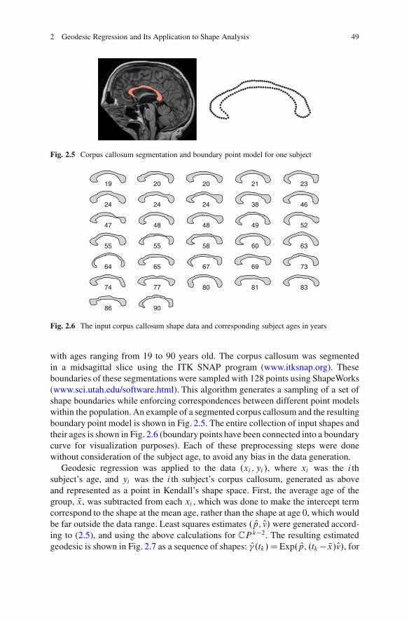
2 Geodesic Regression and Its Application to Shape Analysis 49
Fig. 2.5 Corpus callosum segmentation and boundary point model for one subject
19 20 20 21 23
24 24 24 38 46
47 48 48 49 52
55 55 58 60 63
64 65 67 69 73
74 77 80 81 83
86 90
Fig. 2.6 The input corpus callosum shape data and corresponding subject ages in years
with ages ranging from 19 to 90 years old. The corpus callosum was segmentedin a midsagittal slice using the ITK SNAP program (www.itksnap.org). Theseboundaries of these segmentations were sampled with 128 points using ShapeWorks(www.sci.utah.edu/software.html). This algorithm generates a sampling of a set ofshape boundaries while enforcing correspondences between different point modelswithin the population. An example of a segmented corpus callosum and the resultingboundary point model is shown in Fig. 2.5. The entire collection of input shapes andtheir ages is shown in Fig. 2.6 (boundary points have been connected into a boundarycurve for visualization purposes). Each of these preprocessing steps were donewithout consideration of the subject age, to avoid any bias in the data generation.
Geodesic regression was applied to the data .xi ; yi /, where xi was the i thsubject’s age, and yi was the i th subject’s corpus callosum, generated as aboveand represented as a point in Kendall’s shape space. First, the average age of thegroup, Nx, was subtracted from each xi , which was done to make the intercept termcorrespond to the shape at the mean age, rather than the shape at age 0, which wouldbe far outside the data range. Least squares estimates . Op; Ov/ were generated accord-ing to (2.5), and using the above calculations for CPk!2. The resulting estimatedgeodesic is shown in Fig. 2.7 as a sequence of shapes: O#.tk/DExp. Op; .tk" Nx/Ov/, for
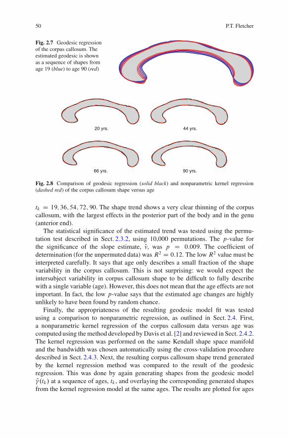
50 P.T. Fletcher
Fig. 2.7 Geodesic regressionof the corpus callosum. Theestimated geodesic is shownas a sequence of shapes fromage 19 (blue) to age 90 (red)
20 yrs.
66 yrs. 90 yrs.
44 yrs.
Fig. 2.8 Comparison of geodesic regression (solid black) and nonparametric kernel regression(dashed red) of the corpus callosum shape versus age
tk D 19; 36; 54; 72; 90. The shape trend shows a very clear thinning of the corpuscallosum, with the largest effects in the posterior part of the body and in the genu(anterior end).
The statistical significance of the estimated trend was tested using the permu-tation test described in Sect. 2.3.2, using 10,000 permutations. The p-value forthe significance of the slope estimate, Ov, was p D 0:009. The coefficient ofdetermination (for the unpermuted data) was R2 D 0:12. The low R2 value must beinterpreted carefully. It says that age only describes a small fraction of the shapevariability in the corpus callosum. This is not surprising: we would expect theintersubject variability in corpus callosum shape to be difficult to fully describewith a single variable (age). However, this does not mean that the age effects are notimportant. In fact, the low p-value says that the estimated age changes are highlyunlikely to have been found by random chance.
Finally, the appropriateness of the resulting geodesic model fit was testedusing a comparison to nonparametric regression, as outlined in Sect. 2.4. First,a nonparametric kernel regression of the corpus callosum data versus age wascomputed using the method developed by Davis et al. [2] and reviewed in Sect. 2.4.2.The kernel regression was performed on the same Kendall shape space manifoldand the bandwidth was chosen automatically using the cross-validation proceduredescribed in Sect. 2.4.3. Next, the resulting corpus callosum shape trend generatedby the kernel regression method was compared to the result of the geodesicregression. This was done by again generating shapes from the geodesic modelO#.tk/ at a sequence of ages, tk , and overlaying the corresponding generated shapesfrom the kernel regression model at the same ages. The results are plotted for ages
2 Geodesic Regression and Its Application to Shape Analysis 51
tk D 20; 44; 66; and 90 (Fig. 2.8). Both regression methods give strikingly similarresults. The two regression models at other values of ages, not shown, are alsoclose to identical. This indicates that a geodesic curve does capture the relationshipbetween age and corpus callosum shape, and that the additional flexibility offeredby the nonparametric regression does not change the estimated trend. However, eventhough both methods provide a similar estimate of the trend, the geodesic regressionhas the advantage that it is simpler to compute and easier to interpret, from thestandpoint of the R2 statistic and hypothesis test demonstrated above.
2.7 Conclusion
We introduced a geodesic regression analysis method for Riemannian manifolds.The geodesic regression model is the natural generalization of linear regression andis parameterized by an intercept and slope term. We also developed a generalizationof the R2 statistic and a permutation test for the significance of the estimatedgeodesic trend. There are several avenues for future work. First, the hypothesistest presented here could be extended to test for group differences, for example,to test if age-related anatomical changes are different in a disease populationcompared to controls. Second, theoretical properties of geodesic regression, such asunbiasedness and consistency, would be of interest. Finally, regression diagnosticsand model selection procedures need to be developed to assess the appropriatenessof a geodesic model for a particular data set.
References
1. Bookstein, F.L.: Size and shape spaces for landmark data in two dimensions (with discussion).Stat. Sci. 1(2), 181–242 (1986)
2. Davis, B., Fletcher, P.T., Bullitt, E., Joshi, S.: Population shape regression from random designdata. In: Proceedings of IEEE International Conference on Computer Vision (2007)
3. do Carmo, M.: Riemannian Geometry. Birkhauser, Boston (1992)4. Driesen, N., Raz, N.: The influence of sex, age, and handedness on corpus callosum
morphology: a meta-analysis. Psychobiology 23(3), 240–247 (1995)5. Dryden, I., Mardia, K.: Statistical Shape Analysis. Wiley, Chichester (1998)6. Durrleman, S., Pennec, X., Trouve, A., Gerig, G., Ayache, N.: Spatiotemporal atlas estimation
for developmental delay detection in longitudinal datasets. In: Medical Image Computing andComputer-Assisted Intervention, pp. 297–304 (2009)
7. Fletcher, P.T.: Geodesic regression on Riemannian manifolds. In: MICCAI Workshop onMathematical Foundations of Computational Anatomy, pp. 75–86 (2011)
8. Fletcher, P.T., Lu, C., Joshi, S.: Statistics of shape via principal geodesic analysis on Lie groups.In: IEEE CVPR, pp. 95–101 (2003)
9. Fox, J.: Applied Regression Analysis, Linear Models, and Related Methods. Sage, ThousandOaks (1997)
10. Frechet, M.: Les elements aleatoires de nature quelconque dans un espace distancie. Ann. Inst.H. Poincare 10(3), 215–310 (1948)
52 P.T. Fletcher
11. Jupp, P.E., Kent, J.T.: Fitting smooth paths to spherical data. Appl. Stat. 36(1), 34–46 (1987)12. Karcher, H.: Riemannian center of mass and mollifier smoothing. Commun. Pure Appl. Math.
30, 509–541 (1977)13. Kendall, D.G.: Shape manifolds, Procrustean metrics, and complex projective spaces. Bull.
Lond. Math. Soc. 16, 18–121 (1984)14. Kendall, W.S.: Probability, convexity, and harmonic maps with small image I: uniqueness and
fine existence. Proc. Lond. Math. Soc. 3(61), 371–406 (1990)15. Klassen, E., Srivastava, A., Mio, W., Joshi, S.: Analysis of planar shapes using geodesic paths
on shape spaces. IEEE PAMI 26(3), 372–383 (2004)16. Mardia, K.V.: Directional Statistics. Wiley, Chichester (1999)17. Michor, P.W., Mumford, D.: Riemannian geometries on spaces of plane curves. J. Eur. Math.
Soc. 8, 1–48 (2006)18. Miller, M.: Computational anatomy: shape, growth, and atrophy comparison via diffeomor-
phisms. NeuroImage 23, S19–S33 (2004)19. Nadaraya, E.A.: On estimating regression. Theory Probab. Appl. 10, 186–190 (1964)20. Niethammer, M., Huang, Y., Viallard, F.-X.: Geodesic regression for image time-series. In:
Proceedings of Medical Image Computing and Computer Assisted Intervention (2011)21. Pennec, X.: Intrinsic statistics on Riemannian manifolds: basic tools for geometric measure-
ments. J. Math. Imaging Vis. 25(1), 127–154 (2006)22. Shi, X., Styner, M., Lieberman, J., Ibrahim, J., Lin, W., Zhu, H.: Intrinsic regression models
for manifold-valued data. J. Am. Stat. Assoc. 5762, 192–199 (2009)23. Trouve, A., Vialard, F.-X.: A second-order model for time-dependent data interpolation: splines
on shape spaces. In: MICCAI STIA Workshop (2010)24. Wand, M.P., Jones, M.C.: Kernel Smoothing. Number 60 in Monographs on Statistics and
Applied Probabilitiy. Chapman & Hall/CRC, London/New York (1995)25. Watson, G.S.: Smooth regression analysis. Sankhya 26, 101–116 (1964)26. Younes, L.: Computable elastic distances between shapes. SIAM J. Appl. Math. 58, 565–586
(1998)27. Younes, L.: Jacobi fields in groups of diffeomorphisms and applications. Q. Appl. Math. 65,
113–113 (2006)
Chapter 3Segmentation and Skeletonization on ArbitraryGraphs Using Multiscale Morphologyand Active Contours
Petros Maragos and Kimon Drakopoulos
Abstract In this chapter we focus on formulating and implementing on abstractdomains such as arbitrary graphs popular methods and techniques developed forimage analysis, in particular multiscale morphology and active contours. To thisgoal we extend existing work on graph morphology to multiscale dilation anderosion and implement them recursively using level sets of functions defined onthe graph’s nodes. We propose approximations to the calculation of the gradient andthe divergence of vector functions defined on graphs and use these approximationsto apply the technique of geodesic active contours for object detection on graphs viasegmentation. Finally, using these novel ideas, we propose a method for multiscaleshape skeletonization on arbitrary graphs.
3.1 Introduction
Graph-theoretic approaches have become commonplace in computer vision. Exam-ples include the graph-cut approaches to segmentation [7,8,16,24] and the statisticalinference on discrete-space visual data with graphical models [42]. In most ofthese cases, the image graphs are regular grids that result from uniform samplingof continuous space. In addition, in nowadays science and technology there existboth low-level and high-level visual data as well as many other types of datadefined on arbitrary graphs with irregular spacing among their vertices. Examples
P. Maragos (!)National Technical University of Athens, School of Electrical and Computer Engineering,Athens 15773, Greecee-mail: [email protected]
K. DrakopoulosMassachusetts Institute of Technology, 77 Massachusetts Avenue, Cambridge,MA 02139-4307, USAe-mail: [email protected]
M. Breuß et al. (eds.), Innovations for Shape Analysis, Mathematics and Visualization,DOI 10.1007/978-3-642-34141-0 3, © Springer-Verlag Berlin Heidelberg 2013
53
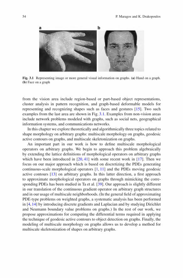
54 P. Maragos and K. Drakopoulos
Fig. 3.1 Representing image or more general visual information on graphs. (a) Hand on a graph.(b) Face on a graph
from the vision area include region-based or part-based object representations,cluster analysis in pattern recognition, and graph-based deformable models forrepresenting and recognizing shapes such as faces and gestures [15]. Two suchexamples from the last area are shown in Fig. 3.1. Examples from non-vision areasinclude network problems modeled with graphs, such as social nets, geographicalinformation systems, and communications networks.
In this chapter we explore theoretically and algorithmically three topics related toshape morphology on arbitrary graphs: multiscale morphology on graphs, geodesicactive contours on graphs, and multiscale skeletonization on graphs.
An important part in our work is how to define multiscale morphologicaloperators on arbitrary graphs. We begin to approach this problem algebraicallyby extending the lattice definitions of morphological operators on arbitrary graphswhich have been introduced in [20, 41] with some recent work in [17]. Then wefocus on our major approach which is based on discretizing the PDEs generatingcontinuous-scale morphological operators [1, 11] and the PDEs moving geodesicactive contours [13] on arbitrary graphs. In this latter direction, a first approachto approximate morphological operators on graphs through mimicking the corre-sponding PDEs has been studied in Ta et al. [39]. Our approach is slightly differentin our translation of the continuous gradient operator on arbitrary graph structuresand in our usage of multiscale neighborhoods. (In the general field of approximatingPDE-type problems on weighted graphs, a systematic analysis has been performedin [4, 14] by introducing discrete gradients and Laplacian and by studying Dirichletand Neumann boundary value problems on graphs.) In the rest of our work, wepropose approximations for computing the differential terms required in applyingthe technique of geodesic active contours to object detection on graphs. Finally, themodeling of multiscale morphology on graphs allows us to develop a method formultiscale skeletonization of shapes on arbitrary graphs.
3 Segmentation and Skeletonization on Graphs 55
3.2 Multiscale Morphology on Graphs
In this section we first review some basic concepts from lattice-based morphology.Then, we focus our review on (1) multiscale morphological image operators ona Euclidean domain, either defined algebraically or generated by nonlinear PDEs,and (2) on defining morphological operators on arbitrary graphs. Finally, we connectthese two areas and define multiscale morphological operators on graphs.
3.2.1 Background on Lattice and Multiscale Morphology
A general formalization [19,37] of morphological operators views them as operatorson complete lattices. A complete lattice is a set L equipped with a partial ordering! such that .L ;!/ has the algebraic structure of a partially ordered set wherethe supremum and infimum of any of its subsets exist in L . For any subset K "L , its supremum
WK and infimum
VK are defined as the lowest (with respect
to !) upper bound and greatest lower bound of K , respectively. The two mainexamples of complete lattices used respectively in morphological shape and imageanalysis are: (i) the power set P.E/DfX W X " Eg of all binary images or shapesrepresented by subsetsX of some domain E where the
W=V
lattice operations arethe set union/intersection, and (ii) the space of all graylevel image signals f W E !T where T is a continuous or quantized sublattice of RDR [ f#1;1g and theW=V
lattice operations are the supremum/infimum of sets of real numbers. Anoperator on L is called increasing if f ! g implies .f / ! .g/. Increasingoperators are of great importance; among them four fundamental examples are:
ı is dilation” ı._
i2Ifi / D
_
i2Iı.fi / (3.1)
" is erosion” ".^
i2Ifi / D
^
i2I".fi / (3.2)
˛ is opening” ˛ is increasing, idempotent, and anti-extensive (3.3)
ˇ is closing” ˇ is increasing, idempotent, and extensive (3.4)
where I is an arbitrary index set, idempotence of an operator means that 2D ,and anti-extensivity and extensivity of operators ˛ and ˇ means that ˛.f / ! f !ˇ.f / for all f . Operator products mean composition: ! .f /D!. .f //. Thenotation r means r-fold composition.Dilations and erosions come in pairs .ı; "/ called adjunctions if
ı.f /!g” f !".g/ (3.5)

56 P. Maragos and K. Drakopoulos
Such pairs are useful for constructing openings ˛D ı" and closings ˇD "ı. Theabove definitions allow broad classes of signal operators to be studied under theunifying lattice framework.
In Euclidean morphology, the domain E becomes the d -dimensional Euclideanspace Ed where EDR or EDZ. In this case, the most well-known morphologicaloperators are the translation-invariant Minkowski dilations˚, erosions$, openingsı, and closings %, which are simple special cases of their lattice counterparts. IfXCbDfx C b W x 2 Xg denotes the translation of a set/shape X " Ed by b 2 Ed ,the simple Minkowski set operators areX˚BD S
b2B XCb,X$BDTb2B X!b ,
and XıBD .X $B/˚B . The set B usually has a simple shape and small size, inwhich case it is called a structuring element. By denoting with rBDfrb W b 2 Bgthe r-scaled homothetic of B , where r & 0, we can define multiscale translation-invariant morphological set operators on Rd :
ırB.X/,X ˚ rB; "rB.X/,X $ rB; ˛rB.X/,XırB (3.6)
Similarly, if .f ˚ B/.x/D Wb2B f .x # b/, .f $ B/.x/D
Vb2B f .x C b/, and
.f ıB/.x/D .f $ B/ ˚ B are the unit-scale Minkowski translation-invariant flat(i.e. unweighted) function operators, their multiscale counterparts are
ırB.f /,f ˚ rB; "rB.f /,f $ rB; ˛rB.f /,f ırB (3.7)
If B is convex, then [30]
rB D B ˚ B ˚ ' ' '˚ B„ ƒ‚ …r times
; r D 0; 1; 2; : : : (3.8)
This endows the above multiscale dilations and erosions with a semigroup property,which allows them to be generated recursively:
ı.rC1/B D ıBırB; ".rC1/B D "B"rB; r D 0; 1; 2; : : : (3.9)
and create the simplest case of a morphological scale-space [11, 28].For digital shapes and images, the above translation-invariant morphological
operators can be extended to multiple scales by using two alternative approaches.The first is an algebraic approach where ifB "Zd is a unit-scale discrete structuringgraph, we define its scaled version rB for integer scales as in (3.8) and use (3.9)for producing multiscale morphological operators that agree with their continuousversions in (3.6) and (3.7) if B is convex. The second approach [1, 11] models thedilation and erosion scale-space functions u.x; t/D f ˚ tB and v.x; t/D f $ tBas generated by the nonlinear partial differential equations (PDEs)
@tu D krukB; @t v D #krvkB (3.10)
3 Segmentation and Skeletonization on Graphs 57
where for a convex B " R2, k.x1; x2/kB D sup.a1;a2/2B a1x1 C a2x2. These PDEscan be implemented using the numerical algorithms of [32], as explored in [35].In case of a shape X , the above PDEs can still be used to generate its multiscalemorphological evolutions by treating u as the level function whose zero level setcontains the evolving shape. Such PDE-based shape evolutions have been studied indetail by Kimia et al. [23]. Modern numerical algorithms for morphological PDEscan be found in [9, 10].
3.2.2 Background on Graph Morphology
We consider an undirected graph GD .V;E/ without loops and multiple edges,where V DV.G/ and EDE.G/ are the sets of its vertices (also called nodes) andedges, respectively. We denote edges by pairs .v;w/ of vertices; these are symmetric,i.e. .v;w/D .w; v/, since the graph is undirected. If V 0 " V and E 0 " E, the pairG0D .V 0; E 0/ is called a subgraph of G. A graph vertex mapping " W V ! V 0 iscalled a graph homomorphism fromG to G0 if " is one-to-one and preserves edges,i.e. .v;w/ 2 E implies .".v/; ".w// 2 E 0. If " is a bijection, then it is called agraph isomorphism; if in addition G0DG, then it is called a graph automorphismor symmetry of G. The set of all such symmetries forms under composition thesymmetry group Sym.G/ of a graph. Symmetries play the role of ‘generalizedtranslations’ on a graph.
ShapesX "V and image functions f WV !T defined on a graphG with valuesin a complete lattice T will be denoted by .X jG/ and .f jG/, respectively, and maybe referred to as binary graphs and multilevel graphs. In case of multilevel graphs,the values of the functions .f jG/ may be discrete, e.g. T Df0; 1; : : : ; m # 1g, orcontinuous, e.g. T DR. Similarly a graph operator for shapes or functions will bedenoted by .'jG/. The argumentG will be omitted if there is no risk of confusion.A graph operator is called increasing if it is increasing in its first argument (shapeor function), i.e. X " Y implies .X jG/ " .Y jG/, and G-increasing if itincreases in G, i.e., G0 " G implies .f jG0/ ! .f jG/ for all graph functions.f jG/. A graph operator is called invariant under graph symmetries # 2 Sym.G/if # D # .
Henceforth and until mentioned otherwise, we shall focus our discussion onbinary graph operators. Given a graph GD .V;E/, the binary graph dilations anderosions on P.V / can be defined via a graph neighborhood function N W V !P.V / which assigns at each vertex v a neighborhood N.v/. Taking the union ofall such neighborhoods for the vertices of a shape X " V creates a graph dilationof X ; then, by using (3.5) we also find its adjunct erosion:
ıN .X jG/,[
v2XN.v/; "N .X jG/, fv 2 V W N.v/ " Xg (3.11)
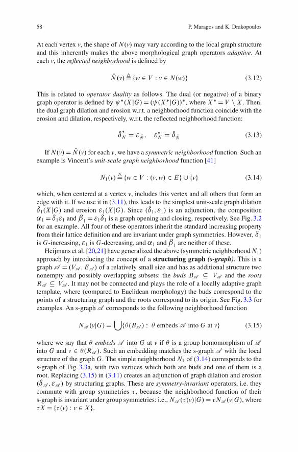
58 P. Maragos and K. Drakopoulos
At each vertex v, the shape of N.v/ may vary according to the local graph structureand this inherently makes the above morphological graph operators adaptive. Ateach v, the reflected neighborhood is defined by
LN.v/, fw 2 V W v 2 N.w/g (3.12)
This is related to operator duality as follows. The dual (or negative) of a binarygraph operator is defined by ".X jG/D . .X"jG//", where X"DV n X . Then,the dual graph dilation and erosion w.r.t. a neighborhood function coincide with theerosion and dilation, respectively, w.r.t. the reflected neighborhood function:
ı"N D " LN ; ""N D ı LN (3.13)
IfN.v/D LN.v/ for each v, we have a symmetric neighborhood function. Such anexample is Vincent’s unit-scale graph neighborhood function [41]
N1.v/, fw 2 V W .v;w/ 2 Eg [ fvg (3.14)
which, when centered at a vertex v, includes this vertex and all others that form anedge with it. If we use it in (3.11), this leads to the simplest unit-scale graph dilationı1.X jG/ and erosion "1.X jG/. Since .ı1; "1/ is an adjunction, the composition˛1D ı1"1 and ˇ1D "1ı1 is a graph opening and closing, respectively. See Fig. 3.2for an example. All four of these operators inherit the standard increasing propertyfrom their lattice definition and are invariant under graph symmetries. However, ı1is G-increasing, "1 is G-decreasing, and ˛1 and ˇ1 are neither of these.
Heijmans et al. [20,21] have generalized the above (symmetric neighborhoodN1)approach by introducing the concept of a structuring graph (s-graph). This is agraph A D .VA ; EA / of a relatively small size and has as additional structure twononempty and possibly overlapping subsets: the buds BA " VA and the rootsRA " VA . It may not be connected and plays the role of a locally adaptive graphtemplate, where (compared to Euclidean morphology) the buds correspond to thepoints of a structuring graph and the roots correspond to its origin. See Fig. 3.3 forexamples. An s-graph A corresponds to the following neighborhood function
NA .vjG/D[f".BA / W " embeds A into G at vg (3.15)
where we say that " embeds A into G at v if " is a group homomorphism of Ainto G and v 2 ".RA /. Such an embedding matches the s-graph A with the localstructure of the graph G. The simple neighborhoodN1 of (3.14) corresponds to thes-graph of Fig. 3.3a, with two vertices which both are buds and one of them is aroot. Replacing (3.15) in (3.11) creates an adjunction of graph dilation and erosion.ıA ; "A / by structuring graphs. These are symmetry-invariant operators, i.e. theycommute with group symmetries # , because the neighborhood function of theirs-graph is invariant under group symmetries: i.e.,NA .#.v/jG/D #NA .vjG/, where#X Df#.v/ W v 2 Xg.
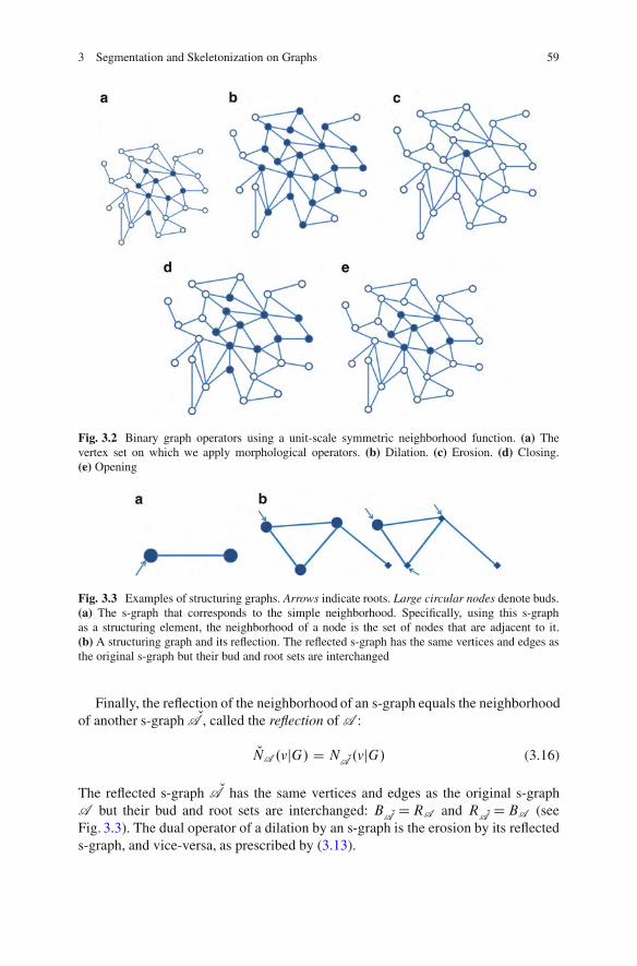
3 Segmentation and Skeletonization on Graphs 59
Fig. 3.2 Binary graph operators using a unit-scale symmetric neighborhood function. (a) Thevertex set on which we apply morphological operators. (b) Dilation. (c) Erosion. (d) Closing.(e) Opening
Fig. 3.3 Examples of structuring graphs. Arrows indicate roots. Large circular nodes denote buds.(a) The s-graph that corresponds to the simple neighborhood. Specifically, using this s-graphas a structuring element, the neighborhood of a node is the set of nodes that are adjacent to it.(b) A structuring graph and its reflection. The reflected s-graph has the same vertices and edges asthe original s-graph but their bud and root sets are interchanged
Finally, the reflection of the neighborhood of an s-graph equals the neighborhoodof another s-graph LA , called the reflection of A :
LNA .vjG/ D N LA .vjG/ (3.16)
The reflected s-graph LA has the same vertices and edges as the original s-graphA but their bud and root sets are interchanged: B LA DRA and R LA DBA (seeFig. 3.3). The dual operator of a dilation by an s-graph is the erosion by its reflecteds-graph, and vice-versa, as prescribed by (3.13).

60 P. Maragos and K. Drakopoulos
All the previously defined binary graph operators are increasing and can beextended to multilevel graphs. Specifically, a multilevel graph .f jG/ can also berepresented by its level sets Xh.f jG/Dfv 2 V W f .v/ & hg, h 2 T :
.f jG/.v/ D supfh 2 T W v 2 Xh.f jG/g (3.17)
By applying an increasing binary graph operator to all level sets and usingthreshold superposition, we can extend to a flat operator on multilevel graphs:
.f jG/.v/ D supfh 2 T W v 2 .Xh.f /jG/g (3.18)
For example, if .X jG/ is a set dilation by the s-graph A , the correspondingfunction operator is
ıA .f jG/.v/ D maxw2NA .vjG/
f .w/ (3.19)
Two useful choices for the function values are either discrete with T Df0; 1; : : : ;m # 1g, or continuous with T DR.
3.2.3 Multiscale Morphology on Graphs
We need to discuss the notion of scale in graph morphology in order to obtainthe graph counterparts of multiscale dilation and erosion defined in Sect. 3.2.1.Consider a graph GD .V;E/ and a nonempty subset X " V of its vertices. LetA be an s-graph. One approach could be to define the dilation at scale r D 1; 2; : : :of a vertex subset X w.r.t. the s-graph A by ırA .X jG/ where rA denotes ther-fold graph dilation of the s-graph with itself. This approach would encounterthe problem presented in Fig. 3.4. Specifically the scaled versions of the s-graphhave complicated structure and in general, it would be highly unlikely to find anappropriate embedding in the graph at every node of X to calculate the dilation ofthe set.
Thus, we propose the following alternative new definition of the scaled versionsof graph dilation and erosion in order to overcome the issues mentioned. We definerecursively the graph dilation of X at integer scale r D 1; 2; : : : with respect to thes-graph A by
ırA .X j G/ D ıA .ır!1A .X j G/ j G/ (3.20)
Essentially, we interchange the order with which we apply the dilation operators; inthe classic framework in order to get the r-scale dilation we first find the r-scalingof the structuring graph and then perform the dilation with the set, whereas in ourdefinition we dilate the set X with the structuring graph r times. Generalizing thisnotion of scale to multilevel dilation of a function f W V ! T we get the followingdefinition. The dilation of f at integer scales r will be given at each v 2 V by

3 Segmentation and Skeletonization on Graphs 61
Fig. 3.4 Left: a structuringgraph. Right: The scaled byrD 2 version of the s-graph.A scaling of a simple s-graphhas increasingly complicatedstructure and therefore, forlarger scales it is difficult orimpossible to find anembedding to an arbitrarygraph at each node. This factnecessitates an alternativedefinition of scale on graphs
!r .v/, ıA .!r!1.f j G/ j G/.v/; !1.v/ D ıA .f j G/.v/ (3.21)
This provides a recursive computation of the multiscale dilations of a functionf W V ! T and leads us to the following Proposition which offers an alternativerecursive computation that involves a simple morphological gradient on a graph.
Proposition 3.1. Given a graph GD .V;E/, the evolution of the multiscale dila-tion of a function f W V ! T by an s-graph A is described by the followingdifference equation at each vertex v 2 V :
!rC1.v/# !r .v/ D maxw2NA .vjG/
f!r .w/ # !r .v/g: (3.22)
Proof. By combining (3.21) with (3.19) we get
!rC1.v/ D ıA .!r .f j G//.v/ D maxw2NA .vjG/
f!r .w/# !r .v/g C !r .v/
ut
3.3 Geodesic Active Contours on Graphs
Kass et al. in [22] introduced the concept of energy minimizing snakes” drivenby forces that pull it towards special features in the image like edges or lines.Specifically, the goal is to find in an image areas that are naturally distinguishedfrom their background. The classical approach consists of a gradual deformationof an original curve towards the edges of those objects through the minimization,between successive time steps, of energy functionals which depend on the shape ofthe curve itself, its distance from the salient image features and finally terms thatstabilize the snakes near local minima.
62 P. Maragos and K. Drakopoulos
The main disadvantage of this initial approach is that the curve dynamics incurreddo not allow changing the topology of the original contour; for example if theoriginal curve contains two distinct objects the original snake will not be separatedin two independent snakes. Heuristic solutions have been proposed in [31] but atopology-free approach has been given independently by Caselles et al. [12] andMalladi et al. [27]. These models are based on the theory of the curve evolution andgeometric flows and the curve is propagating by means of a velocity that containstwo terms, one related to the regularity of the curve and the other shrinks or expandstowards the boundary. Finally, the curve dynamics take the form of a geometric flow(PDE) and can be implemented conveniently using the level set methods proposedby Osher and Sethian [32] that can accommodate changes in the topology betweensuccessive curves.
In particular let C.q/ W Œ0; 1$ ! R2 be parameterized planar curve and letI W Œ0; 1$2 ! RC be the image in which one needs to detect the objects’ boundaries.Note that we denote the curve by C.'/ when we interpret it as a vector-valuedfunction and by C when we interpret it as a set of points. The energy functionalassociated with C can be written as follows:
E.C / D ˛Z 1
0
kC0.q/k2 dq # %Z 1
0
g.krI.C.q//k/ dq a;% & 0 (3.23)
Let g W Œ0;C1/ ! RC be a strictly decreasing function such that g.r/ ! 0as r ! 1. Caselles et al. in [13] show that the problem of finding the minimumenergy curve as defined in (3.23) is equivalent to finding the minimum length curvein a Riemannian space induced from image I , whose length is given by
LR DZ 1
0
g.krI.C.q//k/kC0.q/kdq DZ L.C/
0
g.krI.C.q//k/ ds; (3.24)
where L.C / is the Euclidean length of the curve C . Furthermore, it is shown that acurve which is governed from the dynamics
@C.t/@tD g.I / ' & ' N# .rg ' N/ ' N (3.25)
where & is the Euclidean curvature and N is the unit inward normal, moves in thedirection of the gradient of the length LR.
Assume now that the curve C.t/ is a level set of a function u W R2 ( RC ! R.Namely, C.t/ is the set of points x for which u.x; t/ is equal to a constant (forexample uD 0). It is shown that if the function u.x; t/ satisfies
@[email protected] /kruk.c C &/Crg.I / ' ru; (3.26)
then the corresponding level set satisfies (3.25).

3 Segmentation and Skeletonization on Graphs 63
Our goal is to approximate all terms in the right hand side of (3.26) on graphs andfinally construct a difference equation which would approximate the active contourdynamics for edge detection. The next subsection is devoted to the analysis of thesimplest case of curve evolution on graphs, that is the constant velocity motionintroducing useful ideas from graph morphology operators. Observe that this casecorresponds to approximating the first term of the RHS of (3.26). Subsequently, wewill approximate the rest of the terms participating in the curve dynamics to end upwith a geodesic active contour model on graphs.
3.3.1 Constant-Velocity Active Contours on Graphs
We derive the difference equation that describes the evolution of the contour of aset that expands with constant velocity on a graph. In the continuous case, a contourundergoing such an evolution corresponds to the boundary of the multiscale dilationof the set by a unit disk. If this set is given as a level set of a graylevel functionu W R2 (RC ! R, then the evolution of u is described by
@u@tD kruk: (3.27)
Consider a subsetX of V . Let A be a structuring graph. Imitating the continuouscase, the constant velocity expansion of X corresponds to its r-scale dilation,denoted by Xr . If X is given as the level set of an original graylevel functionu0 W X ! R and Xr is the level set of the r-scale graylevel function ur W X ! R,then the difference equation that governs ur , by using Proposition 3.1, is
urC1.v/# ur .v/ D maxw2NA .vjG/
fur .w/ # ur .v/g: (3.28)
The above expression is a discrete equivalent of the gradient magnitude ongraphs. Similar expressions are being used in the literature, [4, 14, 39]. Our workextends previous results to more general structuring elements and exploits therevealed insight to approximate other geometric properties of differential operatorson graphs in the next sections. In order to account for topological inhomogeneitiesof the graph one could calculate the gradient as the maximum rate of increaseand its direction as the direction of the edge along which the rate of increase islarger. Therefore, (3.28) is the graph counterpart of (3.27), which implies theapproximation of kruk at node v by maxw2NA .vjG/fu.w/# u.v/g.
Summarizing, let X be a set of nodes whose contour expands with constantvelocity c. Then, to implement its evolution on a graph we proceed as follows:

64 P. Maragos and K. Drakopoulos
1. Let u0 be the signed distance function from X , defined by
u0.v/ D(
minw2GnX dE.w; v/ if v 2 X;#minw2X dE.w; v/ if v … X;
where X is the zero level set of u0, and dE.w; v/ corresponds to theEuclidean distance between the nodes w and v.
2. Evolve ur according to the following, at scales r D 1; 2; : : :
urC1.v/# ur .v/ D c ' maxw2NA .vjG/
fur .w/ # ur .v/g: (3.29)
3. The set Xr D fv 2 X W ur .v/ & 0g corresponds to the r-scale dilationof X .
Figure 3.5 illustrates the results for the constant velocity expansion of a circularcontour. Throughout this chapter for all our simulations we are using the simplestructuring graph of Fig. 3.3a that generates the simple neighborhood. Moreover weembed our shapes on a geometric random graph on the unit square. The geometricrandom graph is characterized by two parameters; the number of nodes N anda radius '. N nodes are being placed uniformly at random on the unit squareindependently from one another. If the Euclidean distance between those two nodesis less than ' then there is an edge between them. Typical values for N is 6,000–10,000 while ' ranges from 0.015 to 0.04. Given the number of nodes, the parameter' affects the expected degree of a node and is proportional to the square root of itsvalue.
3.3.2 Direction of the Gradient on Graphs
Observing Eq. (3.26), in order to obtain a model for active contours on graphs,we need to define, except from the magnitude of the gradient vector which we havealready done in the previous section, its direction and also a characterization for thecurvature of the corresponding curve.
Beginning from the first, trusting our intuition from real analysis, it would makesense to choose as the direction of the gradient on graphs the direction of the edgethat corresponds to the maximum difference of the values of the function u. Inother words, let a function u be defined on the set of nodes v 2 V of the graphGD .V;E/. Then

3 Segmentation and Skeletonization on Graphs 65
Fig. 3.5 Constant velocity evolution of a circular contour on a geometric random graph on theunit square. The structuring graph is an edge
rukruk .v/ D ev Ow; Ow D argmaxw2NA .vjG/fu.w/# u.v/g: (3.30)
where evw is the unit vector in the direction of the edge .v;w/. Although thisapproximation looks intuitive it does not work well in practice. In fact, considerthe setting depicted in Fig. 3.6. Such a scenario is fairly usual in a graph structuredue to its discrete nature. In other words choosing an edge out of finitely many cancreate asymmetries which vastly influence the result. Specifically, by using the edgeindicated in the figure for our calculations neglects the values of the function for therest of the nodes in one’s neighborhood. Note that in the continuous case such anissue does not occur under the continuity and differentiability assumptions that areusually made.

66 P. Maragos and K. Drakopoulos
Fig. 3.6 Illustration of thedisadvantages of choosing themaximum increase directionas the gradient direction.Observe that all directionsyield approximately the sameincrease but only one edge ischosen. This happens exactlybecause of the discrete natureof the graph’s structure.Alternatively, we propose aweighted average of edgedirections where the weightsare the function differencesalong each edge
Taking the above into account we propose to approximate the gradient directionon graphs through a weighted average of the direction of all edges in a node’sneighborhood, where weights will be the normalized corresponding differences,that is
rukruk .v/,
Pw2NA .vjG/.u.w/# u.v//evw
kPw2NA .vjG/.u.w/# u.v//evwk(3.31)
Finally, depending on the application, especially in those instances where thereis evident nonuniformity in the values of the function u within the neighborhood ofa vertex v one may need to control the influence of the edges with large increases.In those cases we may need to use the following expression as the direction of thegradient:
rukruk .v/,
X
w2NA .vjG/sign.u.w/ # u.v// evw
.maxs2NA .vjG/fku.s/!u.v/kg!ku.w/!u.v/k/pC(!!!!!!
X
w2NA .vjG/sign.u.w/ # u.v// evw
.maxs2NA .vjG/fku.s/!u.v/kg!ku.w/!u.v/k/pC(
!!!!!!
(3.32)
Essentially, under (3.32) the edges along which the change in the value ofthe function is closer to the maximum contribute more to the gradient direction.By changing the parameter p we can adjust how strongly such edges affect thefinal outcome. Finally, ( is a small constant that guarantees that the denominatorsin (3.32) are well defined. In the special case where (D 0 only the direction ofmaximum increase survives. For our simulations we have used the empirical valuespD 0:7 and (D 0:05.
3 Segmentation and Skeletonization on Graphs 67
Having determined a meaning for the gradient of a function on a graph the onlyterm remaining to be given a meaning on our more abstract graph structure is thecurvature of the contour of each level set of the function u.
3.3.3 Curvature Calculation on Graphs
In the continuous case the curvature of a curve given as the contour of a level set ofa function u can be computed using
& D div" rukruk
#: (3.33)
On the other hand we have derived expressions for the term rukruk on a graph.
Therefore, the remaining step is to propose an expression for the computation of thedivergence of a function on a graph. Consider a vector function F W R2 ! R2. Thedivergence of F at a point x is defined as
divF.x/ D limS!fxg
H) .S/ F ' nd`jS j ; (3.34)
where S is a two dimensional region, ) .S/ its boundary, n the outward unit normalto that boundary, and jS j its enclosed area.
To study the graph case consider Fig. 3.7. We can conclude that a goodapproximation for computing the divergence of F on a graph is the following
divF.v/ DP
w2NA .vjG/ LwF.w/ ' evw
S.v/(3.35)
where
• Lw corresponds to the length of the perpendicular to edge evw,• S.v/ corresponds to the area between the perpendicular to the edges lines,
as illustrated in Fig. 3.7.At this point we can perform all the necessary calculations to compute the
curvature of the contour of the level set of a graylevel function u on a graph. Toillustrate the behavior of the expression proposed consider a circular shaped contouras in Fig. 3.8. We would expect the curvature for all points on the circle to be apositive number, if we were working in the continuous setting. On a graph, thecurvature cannot be expected to be constant but the average value should be positiveand the curvature at each point should oscillate around the average. This behavior iscaptured in Fig. 3.8.
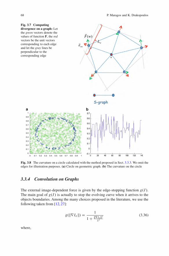
68 P. Maragos and K. Drakopoulos
Fig. 3.7 Computingdivergence on a graph: Letthe green vectors denote thevalues of function F, the redvectors be the unit vectorscorresponding to each edgeand let the gray lines beperpendicular to thecorresponding edge
0 0.1 0.2 0.3 0.4 0.5 0.6 0.7 0.8 0.9 10
0.1
0.2
0.3
0.4
0.5
0.6
0.7
0.8
0.9
1
a b
Fig. 3.8 The curvature on a circle calculated with the method proposed in Sect. 3.3.3. We omit theedges for illustration purposes. (a) Circle on geometric graph. (b) The curvature on the circle
3.3.4 Convolution on Graphs
The external image-dependent force is given by the edge-stopping function g.I /.The main goal of g.I / is actually to stop the evolving curve when it arrives to theobjects boundaries. Among the many choices proposed in the literature, we use thefollowing taken from [12, 27]:
g.krI*k/ D1
1C krI*k2%2
(3.36)
where,

3 Segmentation and Skeletonization on Graphs 69
I* D I )G* ; G* .x; y/ D1
2+*2exp
"#x
2 C y22*2
#: (3.37)
In order to compute the smoothed version I* of I we need to define theconvolution operation on graphs. Let GD .V;E/ denote the underlying graph. LetdE.v;w/ denote the Euclidean distance between vertices v and w. For each v;w 2 Vdefine the functionGw
* .v/ as follows:
Gw* .v/ D
1p2+*2
exp"#dE.v;w/
2
2*2
#: (3.38)
The smoothed version I* can be computed by mimicking the continuous convolu-tion operation as follows:
I* .v/ DX
w2VI.v/Gw
* .v/: (3.39)
3.3.5 Active Contours on Graphs: The Algorithm
Here we combine all the previous approximations to the PDE for geodesic activecontours and summarize the algorithm for automatic graph segmentation.
Consider a graph GD .V;E/ and let a function I W V ! R assign a real valueto each of the graph nodes.
Algorithm-Active Contour on Graphs
1. Compute the smoothed version I* of I as described in Sect. 3.3.4.2. Compute the magnitude of rI* as described in Sect. 3.3.1 and then
compute the function g.krI*k/.3. Initiate the algorithm with a set of nodes that contains the objects to be
found and let !o denote the signed distance function from the contour ofthe determined set.
4. For each r 2 N computer!r!1, kr!r!1k and the curvature & at each nodev as described in Sects. 3.3.1 and 3.3.3. Iterate according to the followingdifference equation:
!rC1 # !r D g.krI*k/kr!r!1k.c C &/C g.krI*k/ ' r!r!1; c & 0(3.40)
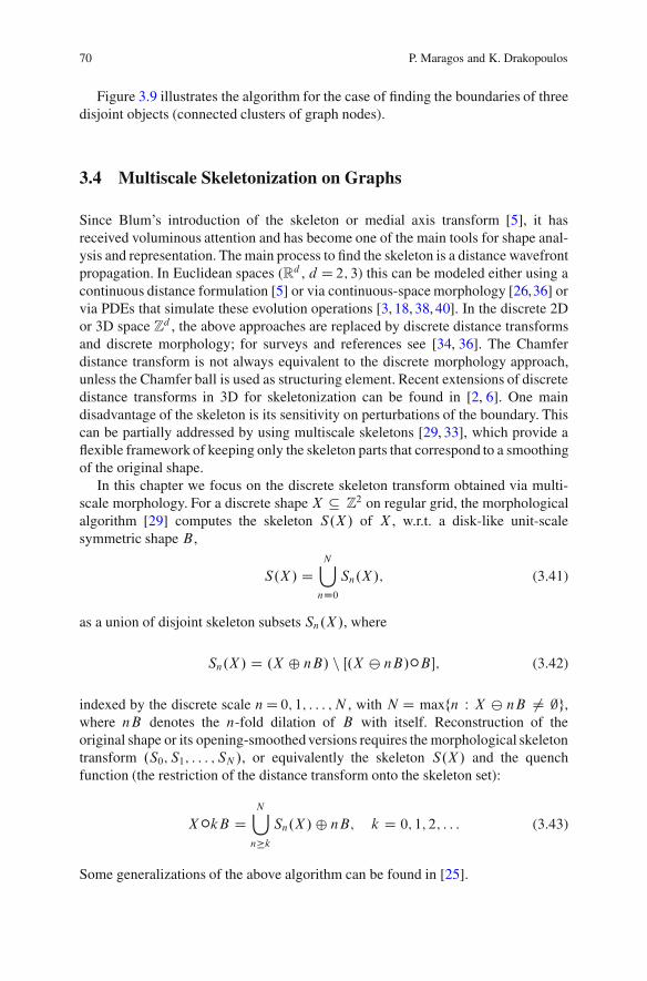
70 P. Maragos and K. Drakopoulos
Figure 3.9 illustrates the algorithm for the case of finding the boundaries of threedisjoint objects (connected clusters of graph nodes).
3.4 Multiscale Skeletonization on Graphs
Since Blum’s introduction of the skeleton or medial axis transform [5], it hasreceived voluminous attention and has become one of the main tools for shape anal-ysis and representation. The main process to find the skeleton is a distance wavefrontpropagation. In Euclidean spaces (Rd , d D 2; 3) this can be modeled either using acontinuous distance formulation [5] or via continuous-space morphology [26,36] orvia PDEs that simulate these evolution operations [3, 18, 38, 40]. In the discrete 2Dor 3D space Zd , the above approaches are replaced by discrete distance transformsand discrete morphology; for surveys and references see [34, 36]. The Chamferdistance transform is not always equivalent to the discrete morphology approach,unless the Chamfer ball is used as structuring element. Recent extensions of discretedistance transforms in 3D for skeletonization can be found in [2, 6]. One maindisadvantage of the skeleton is its sensitivity on perturbations of the boundary. Thiscan be partially addressed by using multiscale skeletons [29, 33], which provide aflexible framework of keeping only the skeleton parts that correspond to a smoothingof the original shape.
In this chapter we focus on the discrete skeleton transform obtained via multi-scale morphology. For a discrete shape X " Z2 on regular grid, the morphologicalalgorithm [29] computes the skeleton S.X/ of X , w.r.t. a disk-like unit-scalesymmetric shape B ,
S.X/ DN[
nD0Sn.X/; (3.41)
as a union of disjoint skeleton subsets Sn.X/, where
Sn.X/ D .X ˚ nB/ n Œ.X $ nB/ıB$; (3.42)
indexed by the discrete scale nD 0; 1; : : : ; N , with N D maxfn W X $ nB ¤ ;g,where nB denotes the n-fold dilation of B with itself. Reconstruction of theoriginal shape or its opening-smoothed versions requires the morphological skeletontransform .S0; S1; : : : ; SN /, or equivalently the skeleton S.X/ and the quenchfunction (the restriction of the distance transform onto the skeleton set):
XıkB DN[
n#kSn.X/˚ nB; k D 0; 1; 2; : : : (3.43)
Some generalizations of the above algorithm can be found in [25].
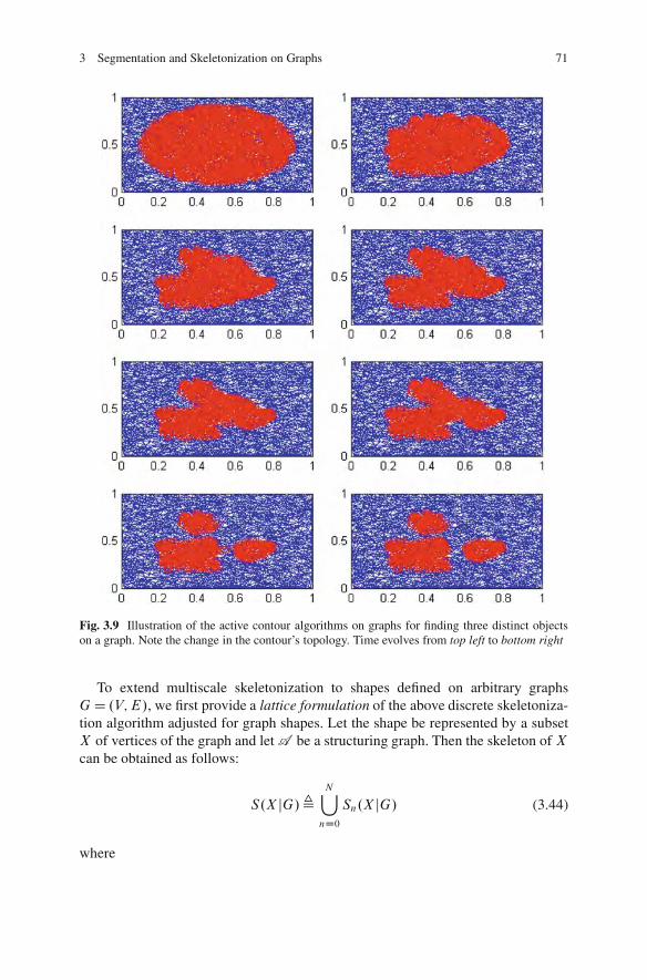
3 Segmentation and Skeletonization on Graphs 71
Fig. 3.9 Illustration of the active contour algorithms on graphs for finding three distinct objectson a graph. Note the change in the contour’s topology. Time evolves from top left to bottom right
To extend multiscale skeletonization to shapes defined on arbitrary graphsGD .V;E/, we first provide a lattice formulation of the above discrete skeletoniza-tion algorithm adjusted for graph shapes. Let the shape be represented by a subsetX of vertices of the graph and let A be a structuring graph. Then the skeleton of Xcan be obtained as follows:
S.X jG/,N[
nD0Sn.X jG/ (3.44)
where
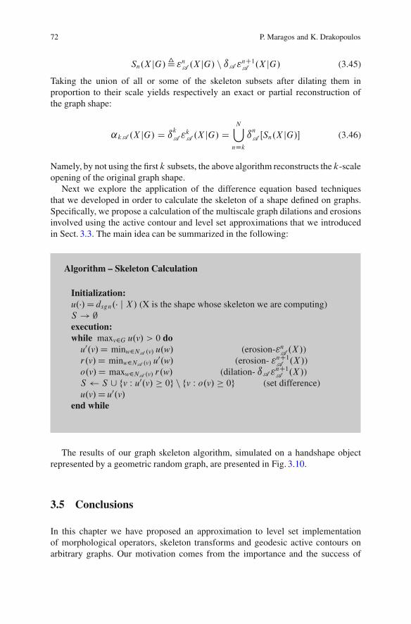
72 P. Maragos and K. Drakopoulos
Sn.X jG/, "nA .X jG/ n ıA "nC1A .X jG/ (3.45)
Taking the union of all or some of the skeleton subsets after dilating them inproportion to their scale yields respectively an exact or partial reconstruction ofthe graph shape:
˛kA .X jG/ D ıkA "kA .X jG/ DN[
nDkınA ŒSn.X jG/$ (3.46)
Namely, by not using the first k subsets, the above algorithm reconstructs the k-scaleopening of the original graph shape.
Next we explore the application of the difference equation based techniquesthat we developed in order to calculate the skeleton of a shape defined on graphs.Specifically, we propose a calculation of the multiscale graph dilations and erosionsinvolved using the active contour and level set approximations that we introducedin Sect. 3.3. The main idea can be summarized in the following:
Algorithm – Skeleton Calculation
Initialization:u.'/Ddsgn.' j X/ (X is the shape whose skeleton we are computing)S ! ;execution:while maxv2G u.v/ > 0 do
u0.v/D minw2NA .v/ u.w/ (erosion-"nA .X/)r.v/D minw2NA .v/ u0.w/ (erosion- "nC1A .X/)o.v/D maxw2NA .v/ r.w/ (dilation- ıA "nC1A .X/)S S [ fv W u0.v/ & 0g n fv W o.v/ & 0g (set difference)u.v/D u0.v/
end while
The results of our graph skeleton algorithm, simulated on a handshape objectrepresented by a geometric random graph, are presented in Fig. 3.10.
3.5 Conclusions
In this chapter we have proposed an approximation to level set implementationof morphological operators, skeleton transforms and geodesic active contours onarbitrary graphs. Our motivation comes from the importance and the success of
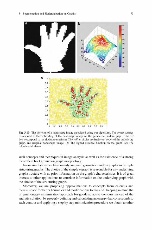
3 Segmentation and Skeletonization on Graphs 73
0 0.1 0.2 0.3 0.4 0.5 0.6 0.7 0.8 0.9 10
0.1
0.2
0.3
0.4
0.5
0.6
0.7
0.8
0.9
1
a b
c
Fig. 3.10 The skeleton of a handshape image calculated using our algorithm. The green squarescorrespond to the embedding of the handshape image on the geometric random graph. The reddots correspond to the skeleton transform. The yellow circles are irrelevant nodes of the underlyinggraph. (a) Original handshape image. (b) The signed distance function on the graph. (c) Thecalculated skeleton
such concepts and techniques in image analysis as well as the existence of a strongtheoretical background on graph morphology.
In our simulations we have mainly assumed geometric random graphs and simplestructuring graphs. The choice of the simple s-graph is reasonable for any underlyinggraph structure with no prior information on the graph’s characteristics. It is of greatinterest to other applications to correlate information on the underlying graph withthe choice of the structuring graph.
Moreover, we are proposing approximations to concepts from calculus andthere is space for better heuristics and modifications to this end. Keeping in mind theoriginal energy minimization approach for geodesic active contours instead of theanalytic solution, by properly defining and calculating an energy that corresponds toeach contour and applying a step by step minimization procedure we obtain another
74 P. Maragos and K. Drakopoulos
approach to geodesic active contours. On the other hand, since the latter involvesa minimization problem at each time step it is computationally less efficient but itmay yield more accurate results.
Finally, regarding the application of the above ideas that we have introducedto multiscale shape skeletonization on arbitrary graphs, one research direction ofinterest is how to analyze or guarantee the connectedness of the resulting skeleton.
References
1. Alvarez, L., Guichard, F., Lions, P.L., Morel, J.M.: Axioms and fundamental equations ofimage processing. Arch. Ration. Mech. 123(2), 199–257 (1993)
2. Arcelli, C., Sanniti di Baja, G., Serino, L.: Distance-driven skeletonization in voxel images.IEEE Trans. Pattern Anal. Mach. Intell. 33(4), 709–720 (2011)
3. Aslan, C., Erdem, A., Erdem, E., Tari, S.: Disconnected skeleton: shape at its absolute scale.IEEE Trans. Pattern Anal. Mach. Intell. 30(12), 2188–2203 (2008)
4. Bensoussan, A., Menaldi, J.: Difference equations on weighted graphs. J. Convex Anal. 12(1),13–44 (2005)
5. Blum, H.: A transformation for extracting new descriptors of shape. In: Proceedings of aSymposium on Models for the Perception of Speech and Visual Forms, Boston, Nov. 1964.MIT, Cambridge MA (1967)
6. Borgefors, G., Nystrom, I., Sanniti di Baja, G.: Discrete skeletons from distance transforms in2D and 3D. In: Siddiqi, K., Pizer, S. (eds.) Medial Representations: Mathematics, Algorithmsand Applications. Springer, Dordrecht (2008)
7. Boykov, Y., Kolmogorov, V.: An experimental comparison of Min-Cut/Max-Flow Algorithmsfor energy minimization in vision. IEEE Trans. Pattern Anal. Mach. Intell. 26(9), 1124–1137(2004)
8. Boykov, Y., Veksler, O., Zabih, R.: Fast approximate energy minimization via graph cuts. IEEETrans. Pattern Anal. Mach. Intell. 23(11), 1222–1239 (2001)
9. Breuß, M., Weickert, J.: A shock-capturing algorithm for the differential equations of Dilationand Erosion. J. Math. Imaging Vis. 25, 187–201 (2006)
10. Breuß, M., Weickert, J.: Highly accurate schemes for PDE-based morphology with generalconvex structuring elements. Int. J. Comput. Vis. 92(2), 132–145 (2011)
11. Brockett, R.W., Maragos, P.: Evolution equations for continuous-scale morphological filtering.IEEE Trans. Signal Process. 42(12), 3377–3386 (1994)
12. Caselles, V., Catte, F., Coll, T., Dibos, F.: A geometric model for active contours in imageprocessing. Numerische Mathematik 66(1), 1–31 (1993)
13. Caselles, V., Kimmel, R., Sapiro, G.: Geodesic active contours. Int. J. Comput. Vis. 22(1),61–79 (1997)
14. Chung, S.-Y., Berenstein, C.A.: Omega-Harmonic functions and inverse conductivity problemson networks. SIAM J. Appl. Math. 65, 1200–1226 (2005)
15. Cootes, T.F., Edwards, G.J., Taylor, C.J.: Active appearance models. IEEE Trans. Pattern Anal.Mach. Intell. 23(6), 681–685 (2001)
16. Couprie, C., Grady, L., Najman, L., Talbot, H.: Power watershed: a unifying graph-basedoptimization framework. IEEE Trans. Pattern Anal. Mach. Intell. 33(7), 1384–1399 (2011)
17. Cousty, J., Najman, L., Serra, J.: Some morphological operators in graph spaces. In: Proceed-ings of the International Symposium on Mathematical Morphology. Lecture Notes in ComputerScience, 5720. Springer, Berlin/New York (2009)
18. Hassouna, M.S., Farag, A.A.: Variational curve skeletons using gradient vector flow. IEEETrans. Pattern Anal. Mach. Intell. 31(12), 2257–2274 (2009)
19. Heijmans, H.J.A.M.: Morphological Image Operators. Academic, Boston (1994)
3 Segmentation and Skeletonization on Graphs 75
20. Heijmans, H.J.A.M., Nacken, P., Toet, A., Vincent, L.: Graph morphology. J. Vis. Commun.Image Represent. 3(1), 24–38 (1992)
21. Heijmans, H.J.A.M., Vincent, L.: Graph morphology in image analysis. In: Dougherty, E.R.(ed.) Mathematical Morphology in Image Processing. Marcel Dekker, New York (1993)
22. Kass, M., Witkin, A., Terzopoulos, D.: Snakes: active contour models. Int. J. Comput. Vis.1(4), 321–331 (1988)
23. Kimia, B., Tannenbaum, A., Zucker, S.: On the evolution of curves via a function of curvature.I. The classical case. J. Math. Anal. Appl. 163, 438–458 (1992)
24. Komodakis, N., Paragios, N., Tziritas, G.: MRF energy minimization and beyond via dualdecomposition. IEEE Trans. Pattern Anal. Mach. Intell. 33, 531–552 (2011)
25. Kresch, R., Malah, D.: Skeleton-based morphological coding of binary images. IEEE Trans.Image Process. 7(10), 1387–1399 (1998)
26. Lantuejoul, C.: Skeletonization in quantitative metallography. In: Haralick, R.M., Simon, J.C.(eds.) Issues of Digital Image Processing. Sijthoff and Noordhoff, Groningen (1980)
27. Malladi, R., Sethian, J.A., Vemuri, B.C.: A Fast Level Set based Algorithm for Topology-Independent Shape Modeling. J. Math. Imaging Vis. 6, 269–289 (1996)
28. Maragos, P.: Pattern spectrum and multiscale shape representation. IEEE Trans. Pattern Anal.Mach. Intell. 11, 701–716 (1989)
29. Maragos, P., Schafer, R.W.: Morphological skeleton representation and coding of binaryimages. IEEE Trans. Acoust. Speech Signal Process. 34, 1228–1244 (1986)
30. Matheron, G.: Random Sets and Integral Geometry. Wiley, New York (1975)31. McInerney, T., Terzopoulos, D.: Topologically adaptable snakes. In: Proceedings of the Int’l
Conference on Computer Vision, pp. 840–845 (1995)32. Osher, S., Sethian, J.A.: Fronts propagating with curvature dependent speed: algorithms based
on Hamilton-Jacobi formulations. J. Comput. Phys. 79, 12–49 (1988)33. Pizer, S.M., Siddiqi, K., Szekely, G., Damon, J.N., Zucker, S.W.: Multiscale medial loci and
their properties. Int. J. Comput. Vis. 55(2/3), 155–179 (2003)34. Rosenfeld, A., Kak, A.C.: Digital Picture Processing: Vol I and II. Academic, New York/
London/Paris (1982)35. Sapiro, G., Kimmel, R., Shaked, D., Kimia, B., Bruckstein, A.: Implementing continuous-scale
morphology via curve evolution. Pattern Recognit. 26(9), 1363–1372 (1993)36. Serra, J.: Image Analysis and Mathematical Morphology. Academic, London/New York (1982)37. Serra, J. (ed.): Image Analysis and Mathematical Morphology. Volume 2: Theoretical
Advances. Academic, London/New York (1988)38. Siddiqi, K., Buix, S., Tannenbaum, A., Zucker, W.: Hamilton-Jacobi skeletons. Int. J. Comput.
Vis. 48(3), 215–231 (2002)39. Ta, V.-T., Elmoataz, A., Lezoray, O.: Nonlocal PDEs-based morphology on weighted graphs
for image and data processing. IEEE Trans. Image Process. 20(6), 1504–1516 (2011)40. Tari, S.: Hierarchical shape decomposition via level sets. In: Proceedings of the Interna-
tional Symposium on Mathematical Morphology. Lecture Notes in Computer Science, 5720.Springer, Berlin/New York (2009)
41. Vincent, L.: Graphs and mathematical morphology. Signal Process. 16(4), 365–388 (1989)42. Yedidia, J.S., Freeman, W.T., Weiss, Y.: Constructing free energy approximations and general-
ized belief propagation algorithms. IEEE Trans. Inf. Theory 51(7), 2282–2312 (2005)

Chapter 4Refined Homotopic Thinning Algorithmsand Quality Measures for SkeletonisationMethods
Pascal Peter and Michael Breuß
Abstract Topological skeletons are shape descriptors that have been appliedsuccessfully in practical applications. However, many skeletonisation methods lackaccessibility, mainly due to the need for manual parameter adjustment and theshortage of tools for comparative analysis.In this paper we address these problems. We propose two new homotopy-preservingthinning algorithms: Flux-ordered adaptive thinning (FOAT) extends existing flux-based thinning methods by a robust automatic parameter adjustment, maximal discthinning (MDT) combines maximal disc detection on Euclidean distance maps withhomotopic thinning. Moreover, we propose distinct quality measures that allow toanalyse the properties of skeletonisation algorithms. Tests of the new algorithmsand quality assessment tools are conducted on the widely used shape databaseCE-Shape-1.
4.1 Introduction
Shape analysis is a central problem for many applications in image processing andcomputer vision, such as object recognition or segmentation, see e.g. [27] for anoverview. While boundary descriptors are a classic instrument for object represen-tation, specific tasks in shape analysis demand alternative shape representations
P. Peter (!)Faculty of Mathematics and Computer Science, Mathematical Image Analysis Group,Saarland University, Campus E1.1, 66041 Saarbrucken, Germanye-mail: [email protected]
M. BreußFaculty of Mathematics and Computer Science, Mathematical Image Analysis Group,Saarland University, Campus E1.1, 66041 Saarbrucken, Germany
Applied Mathematics and Computer Vision Group, BTU Cottbus, Platz der Deutschen Einheit 1,HG 2.51, 03046 Cottbus, Germanye-mail: [email protected]; [email protected]
M. Breuß et al. (eds.), Innovations for Shape Analysis, Mathematics and Visualization,DOI 10.1007/978-3-642-34141-0 4, © Springer-Verlag Berlin Heidelberg 2013
77
78 P. Peter and M. Breuß
that unite geometrical and topological information. The widely-used medial axistransform (MAT) is such a shape descriptor. Initially, the MAT was introduced in1967 by Blum [3] as a mathematical tool for modelling the biological problem ofshape vision. It represents a shape by a thin set of lines or arcs that are centred inthe shape, eliminating superfluous information of local symmetries. Intuitively, theMAT resembles bone structures, thus motivating the alternative term (topological)skeleton. Due to its useful properties, including equivalence to the shape boundary,homotopy to the original shape and invariance under Euclidean transformations,the MAT has been used for numerous practical applications; examples are objectrecognition [22, 28, 32] or medical imaging [31]. However, the results of existingskeletonisation algorithms largely depend on model parameters that often need tobe manually adjusted. Moreover, the literature is lacking comprehensive qualityanalysis tools that allow to quantify important features of skeletonisation algorithms.
In this work, we deal with these problems. We propose here two new thinningalgorithms for MAT computation, we call them FOAT and MDT. Both FOAT andMDT are robust w.r.t. the choice of parameters. In addition, MDT is particularlyeasy to understand and implement, and thus it is especially appealing for users.Moreover, we present new methods for comparative analysis of MAT algorithms.
Previous work. Algorithms for MAT computation are plentiful and diverse, bothin their methods and their theoretical background. In general, three classes can bedistinguished: Voronoi-based methods [10,18] that exploit the similarity of the MATand Voronoi diagrams, approaches related to the distance map [15, 21], thinningalgorithms [19, 33] and morphological approaches [2, 12, 16, 24].
In our paper we focus on combinations of thinning algorithms and distance mapmethods with further enhancements by additional pruning steps. In particular, theHamilton-Jacobi method by Siddiqi et al. [29] combines thinning and distance mapmethods with physical concepts of Hamiltonian mechanics, and it forms the basisfor one of our algorithms. We also propose a new algorithm combining maximaldisc detection using exact Euclidean distance maps with homotopic thinning. Themethod of Pudney [20] is similar to ours, but uses a different maximal disc detectionmethod based on Chamfer distance maps. For mathematical definitions of thinningand pruning operators see [23].
Despite the large number of publications on MAT computation, systematiccomparisons of existing methods are rare. Comparative studies of MAT algorithmsare usually performed by evaluating them in the context of a particular application,e.g. for the purpose of object recognition. An example for such a comparisonstrategy is the matching approach by Siddiqi et al. [30], see also [1, 6, 9, 14, 32]for related approaches. One reason for this kind of indirect comparative studies isthe lack of formal quality criteria for skeletonisation algorithms. However, from amore general point of view it is of interest to measure the qualities of skeletonsindependently from a specific application. In order to achieve this goal, we proposeways to assess in how far discrete algorithms mimic structural properties of thecorresponding continuous-scale MAT. For this purpose, we also aim to quantifyuseful properties of the discrete skeletons. An additional problem, especially in the
4 Homotopic Thinning Algorithms and Quality Measures for Skeletonisation 79
context of practical applications, is that many algorithms like the Hamilton-Jacobimethod [29] require manual parameter adjustment for optimal results.
Our contribution. We address the aforementioned issues by proposing refinedthinning algorithms that combine several state-of-the-art methods, and by introduc-ing quality measures that allow to assess meaningful properties of MAT algorithms:
(i) Flux-Ordered Adaptive Thinning (FOAT) extends the Hamilton-Jacobi method[29] with a secondary MAT detection (SMD) step. This allows an automatic,robust adaption of input parameters to individual shapes.
(ii) Maximal Disc Thinning (MDT) is an extension of the maximal disc detectionmethod of Remy and Thiel [21]. It combines the latter with the homotopypreserving thinning steps of the Hamilton-Jacobi method [29]. This methodis homotopy preserving as well as largely independent of input parameters.
(iii) Quality Criteria are proposed that quantify useful properties of discrete skele-tons in a new way, namely exactness of reconstruction, skeleton minimalityand skeleton complexity. These new quality measures allow to distinguishimportant properties of MAT schemes.
(iv) Comparative Skeleton Graph Matching is employed as a means to test MATalgorithms for invariances. Skeletons are transformed into graphs that can becompared using a graph matching method [26] in a similar way as in objectrecognition approaches.
Tests of both the newly proposed algorithms and the quality measures wereconducted on CE-Shape-1, a widely-used image database consisting of 1; 400shapes, which was specifically designed for testing shape descriptors [13].
Paper organisation. In Sect. 4.2 we present our new skeletonisation algorithmsalong with general information about thinning methods. Quality assessment toolsare discussed in Sect. 4.3. Section 4.4 contains the results of experiments conductedwith the new algorithms and quality criteria. The paper is concluded by Sect. 4.5.
4.2 Algorithms
The algorithms described in the following paragraphs operate on a binary imageu W ˝ ! R2 ! f0; 1g. In the image domain ˝ , the points of the shape form theobject domain O D fx 2 ˝ j u.x/ D 0g. The points of the skeleton ˙ ! O areexactly the centres of inscribed circles, that are tangent to the object boundary in atleast two points. The distance map D of the object boundary @O is defined as
D W ˝ ! RC0 ; D.x/ D miny2@Ojy " xj (4.1)
Homotopic thinning. Both of the new algorithms are thinning methods that sharethe same set of thinning rules. In each thinning step, the smallest point in terms ofthe thinning order >thin is deleted from the object domain O , until only the skeleton
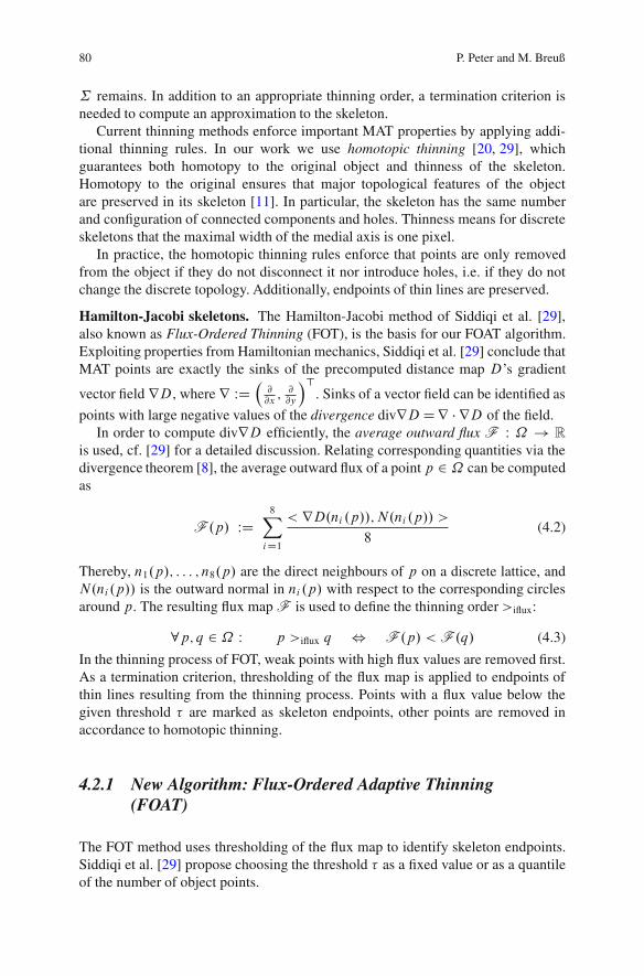
80 P. Peter and M. Breuß
˙ remains. In addition to an appropriate thinning order, a termination criterion isneeded to compute an approximation to the skeleton.
Current thinning methods enforce important MAT properties by applying addi-tional thinning rules. In our work we use homotopic thinning [20, 29], whichguarantees both homotopy to the original object and thinness of the skeleton.Homotopy to the original ensures that major topological features of the objectare preserved in its skeleton [11]. In particular, the skeleton has the same numberand configuration of connected components and holes. Thinness means for discreteskeletons that the maximal width of the medial axis is one pixel.
In practice, the homotopic thinning rules enforce that points are only removedfrom the object if they do not disconnect it nor introduce holes, i.e. if they do notchange the discrete topology. Additionally, endpoints of thin lines are preserved.
Hamilton-Jacobi skeletons. The Hamilton-Jacobi method of Siddiqi et al. [29],also known as Flux-Ordered Thinning (FOT), is the basis for our FOAT algorithm.Exploiting properties from Hamiltonian mechanics, Siddiqi et al. [29] conclude thatMAT points are exactly the sinks of the precomputed distance map D’s gradient
vector field rD, where r WD!@@x; @@y
">. Sinks of a vector field can be identified as
points with large negative values of the divergence divrDDr # rD of the field.In order to compute divrD efficiently, the average outward flux F W ˝ ! R
is used, cf. [29] for a detailed discussion. Relating corresponding quantities via thedivergence theorem [8], the average outward flux of a point p 2 ˝ can be computedas
F .p/ WD8X
iD1
< rD.ni .p//;N.ni .p// >8
(4.2)
Thereby, n1.p/; : : : ; n8.p/ are the direct neighbours of p on a discrete lattice, andN.ni.p// is the outward normal in ni .p/ with respect to the corresponding circlesaround p. The resulting flux map F is used to define the thinning order >iflux:
8p; q 2 ˝ W p >iflux q , F .p/ < F .q/ (4.3)
In the thinning process of FOT, weak points with high flux values are removed first.As a termination criterion, thresholding of the flux map is applied to endpoints ofthin lines resulting from the thinning process. Points with a flux value below thegiven threshold ! are marked as skeleton endpoints, other points are removed inaccordance to homotopic thinning.
4.2.1 New Algorithm: Flux-Ordered Adaptive Thinning(FOAT)
The FOT method uses thresholding of the flux map to identify skeleton endpoints.Siddiqi et al. [29] propose choosing the threshold ! as a fixed value or as a quantileof the number of object points.
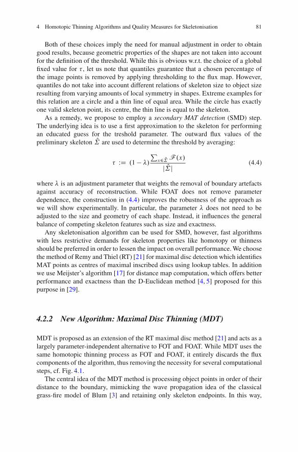
4 Homotopic Thinning Algorithms and Quality Measures for Skeletonisation 81
Both of these choices imply the need for manual adjustment in order to obtaingood results, because geometric properties of the shapes are not taken into accountfor the definition of the threshold. While this is obvious w.r.t. the choice of a globalfixed value for ! , let us note that quantiles guarantee that a chosen percentage ofthe image points is removed by applying thresholding to the flux map. However,quantiles do not take into account different relations of skeleton size to object sizeresulting from varying amounts of local symmetry in shapes. Extreme examples forthis relation are a circle and a thin line of equal area. While the circle has exactlyone valid skeleton point, its centre, the thin line is equal to the skeleton.
As a remedy, we propose to employ a secondary MAT detection (SMD) step.The underlying idea is to use a first approximation to the skeleton for performingan educated guess for the treshold parameter. The outward flux values of thepreliminary skeleton O are used to determine the threshold by averaging:
! WD .1 " "/P
x2 O F .x/
j O j(4.4)
where " is an adjustment parameter that weights the removal of boundary artefactsagainst accuracy of reconstruction. While FOAT does not remove parameterdependence, the construction in (4.4) improves the robustness of the approach aswe will show experimentally. In particular, the parameter " does not need to beadjusted to the size and geometry of each shape. Instead, it influences the generalbalance of competing skeleton features such as size and exactness.
Any skeletonisation algorithm can be used for SMD, however, fast algorithmswith less restrictive demands for skeleton properties like homotopy or thinnessshould be preferred in order to lessen the impact on overall performance. We choosethe method of Remy and Thiel (RT) [21] for maximal disc detection which identifiesMAT points as centres of maximal inscribed discs using lookup tables. In additionwe use Meijster’s algorithm [17] for distance map computation, which offers betterperformance and exactness than the D-Euclidean method [4, 5] proposed for thispurpose in [29].
4.2.2 New Algorithm: Maximal Disc Thinning (MDT)
MDT is proposed as an extension of the RT maximal disc method [21] and acts as alargely parameter-independent alternative to FOT and FOAT. While MDT uses thesame homotopic thinning process as FOT and FOAT, it entirely discards the fluxcomponents of the algorithm, thus removing the necessity for several computationalsteps, cf. Fig. 4.1.
The central idea of the MDT method is processing object points in order of theirdistance to the boundary, mimicking the wave propagation idea of the classicalgrass-fire model of Blum [3] and retaining only skeleton endpoints. In this way,
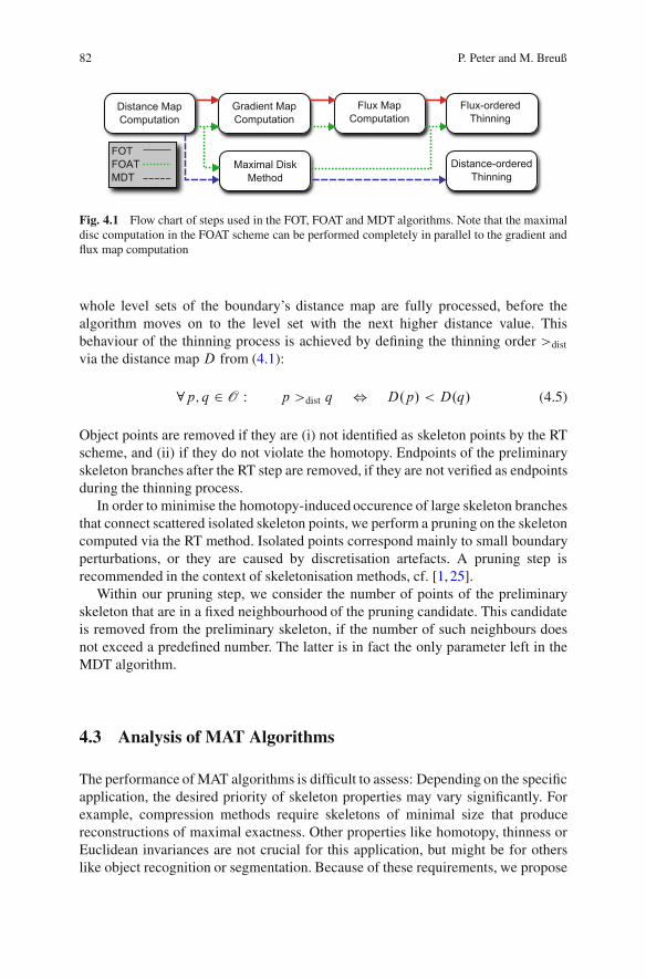
82 P. Peter and M. Breuß
Fig. 4.1 Flow chart of steps used in the FOT, FOAT and MDT algorithms. Note that the maximaldisc computation in the FOAT scheme can be performed completely in parallel to the gradient andflux map computation
whole level sets of the boundary’s distance map are fully processed, before thealgorithm moves on to the level set with the next higher distance value. Thisbehaviour of the thinning process is achieved by defining the thinning order >dist
via the distance map D from (4.1):
8p; q 2 O W p >dist q , D.p/ < D.q/ (4.5)
Object points are removed if they are (i) not identified as skeleton points by the RTscheme, and (ii) if they do not violate the homotopy. Endpoints of the preliminaryskeleton branches after the RT step are removed, if they are not verified as endpointsduring the thinning process.
In order to minimise the homotopy-induced occurence of large skeleton branchesthat connect scattered isolated skeleton points, we perform a pruning on the skeletoncomputed via the RT method. Isolated points correspond mainly to small boundaryperturbations, or they are caused by discretisation artefacts. A pruning step isrecommended in the context of skeletonisation methods, cf. [1, 25].
Within our pruning step, we consider the number of points of the preliminaryskeleton that are in a fixed neighbourhood of the pruning candidate. This candidateis removed from the preliminary skeleton, if the number of such neighbours doesnot exceed a predefined number. The latter is in fact the only parameter left in theMDT algorithm.
4.3 Analysis of MAT Algorithms
The performance of MAT algorithms is difficult to assess: Depending on the specificapplication, the desired priority of skeleton properties may vary significantly. Forexample, compression methods require skeletons of minimal size that producereconstructions of maximal exactness. Other properties like homotopy, thinness orEuclidean invariances are not crucial for this application, but might be for otherslike object recognition or segmentation. Because of these requirements, we propose
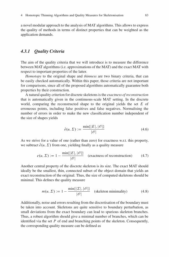
4 Homotopic Thinning Algorithms and Quality Measures for Skeletonisation 83
a novel modular approach to the analysis of MAT algorithms. This allows to expressthe quality of methods in terms of distinct properties that can be weighted as theapplication demands.
4.3.1 Quality Criteria
The aim of the quality criteria that we will introduce is to measure the differencebetween MAT algorithms (i.e. approximations of the MAT) and the exact MAT withrespect to important properties of the latter.
Homotopy to the original shape and thinness are two binary criteria, that canbe easily checked automatically. Within this paper, those criteria are not importantfor comparisons, since all of the proposed algorithms automatically guarantee bothproperties by their construction.
A natural quality criterion for discrete skeletons is the exactness of reconstructionthat is automatically given in the continuous-scale MAT setting. In the discreteworld, comparing the reconstructed shape to the original yields the set E oferroneous points, including false positives and false negatives. Normalising thenumber of errors in order to make the new classification number independent ofthe size of shapes yields
Oe.u; ˙/ WD minfjEj; jOjgjOj (4.6)
As we strive for a value of one (rather than zero) for exactness w.r.t. this property,we subtract Oe.u; ˙/ from one, yielding finally as a quality measure
e.u; ˙/ WD 1 " minfjEj; jOjgjOj (exactness of reconstruction) (4.7)
Another central property of the discrete skeleton is its size. The exact MAT shouldideally be the smallest, thin, connected subset of the object domain that yields anexact reconstruction of the original. Thus, the size of computed skeletons should beminimal. This defines the quality measure
m.u; ˙/ WD 1 " minfj˙ j; jOjgjOj (skeleton minimality) (4.8)
Additionally, noise and errors resulting from the discretisation of the boundary mustbe taken into account. Skeletons are quite sensitive to boundary perturbation, assmall deviations from the exact boundary can lead to spurious skeleton branches.Thus, a robust algorithm should give a minimal number of branches, which can beidentified via the set P of end and branching points of the skeleton. Consequently,the corresponding quality measure can be defined as
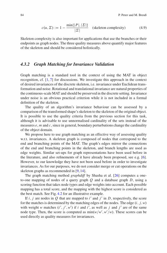
84 P. Peter and M. Breuß
c.u; ˙/ WD 1 " minfjP j; j˙ jgj˙ j (skeleton complexity) (4.9)
Skeleton complexity is also important for applications that use the branches or theirendpoints as graph nodes. The three quality measures above quantify major featuresof the skeleton and should be considered holistically.
4.3.2 Graph Matching for Invariance Validation
Graph matching is a standard tool in the context of using the MAT in objectrecognition, cf. [1, 7] for discussions. We investigate this approach in the contextof desired invariances of the discrete skeleton, i.e. invariance under Euclidean trans-formation and noise. Rotational and translational invariance are natural properties ofthe continuous-scale MAT and should be preserved in the discrete setting. Invarianceunder noise is an obvious practical criterion while it is not included in a formaldefinition of the skeleton.
The quality of an algorithm’s invariance behaviour can be assessed by acomparison of the transformed shape’s skeleton to the skeleton of the original object.It is possible to use the quality criteria from the previous section for this task,although it is advisable to use unnormalised cardinality of the sets instead of themeasures e,m and c, since in general, boundary perturbations change the cardinalityof the object domain.
We propose here to use graph matching as an effective way of assessing qualityw.r.t. invariances. A skeleton graph is composed of nodes that correspond to theend and branching points of the MAT. The graph’s edges mirror the connectionsof the end and branching points in the skeleton, and branch lengths are used asedge weights. Similar set-ups for graph representations have been used before inthe literature, and also refinements of it have already been proposed, see e.g. [6].However, to our knowledge they have not been used before in order to investigateinvariances. As for our purposes, we do not consider merge or cut operations on theskeleton graphs as recommended in [9, 14].
The graph matching method graphdiff by Shasha et al. [26] computes a one-to-one mapping of nodes of a query graph Q and a database graph D, using ascoring function that takes node types and edge weights into account. Each possiblemapping has a total score, and the mapping with the highest score is considered asthe best match. See Fig. 4.2 for an illustrative example.
If i; j are nodes in Q that are mapped to i 0 and j 0 in D, respectively, the scorefor the matches is determined by the matching edges of the nodes. The edge .i; j;w/with weight w matches .i 0; j 0;w0/ if i and i 0, as well as j and j 0 are of the samenode type. Then, the score is computed as min.w=w0;w0=w/. These scores can beused directly as quality measures for invariances.
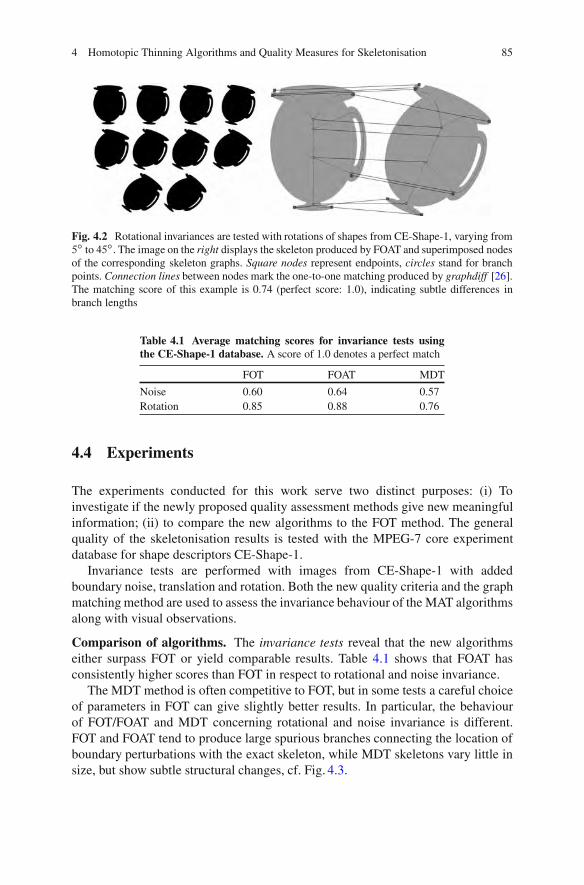
4 Homotopic Thinning Algorithms and Quality Measures for Skeletonisation 85
Fig. 4.2 Rotational invariances are tested with rotations of shapes from CE-Shape-1, varying from5ı to 45ı. The image on the right displays the skeleton produced by FOAT and superimposed nodesof the corresponding skeleton graphs. Square nodes represent endpoints, circles stand for branchpoints. Connection lines between nodes mark the one-to-one matching produced by graphdiff [26].The matching score of this example is 0.74 (perfect score: 1.0), indicating subtle differences inbranch lengths
Table 4.1 Average matching scores for invariance tests usingthe CE-Shape-1 database. A score of 1.0 denotes a perfect match
FOT FOAT MDT
Noise 0.60 0.64 0.57Rotation 0.85 0.88 0.76
4.4 Experiments
The experiments conducted for this work serve two distinct purposes: (i) Toinvestigate if the newly proposed quality assessment methods give new meaningfulinformation; (ii) to compare the new algorithms to the FOT method. The generalquality of the skeletonisation results is tested with the MPEG-7 core experimentdatabase for shape descriptors CE-Shape-1.
Invariance tests are performed with images from CE-Shape-1 with addedboundary noise, translation and rotation. Both the new quality criteria and the graphmatching method are used to assess the invariance behaviour of the MAT algorithmsalong with visual observations.
Comparison of algorithms. The invariance tests reveal that the new algorithmseither surpass FOT or yield comparable results. Table 4.1 shows that FOAT hasconsistently higher scores than FOT in respect to rotational and noise invariance.
The MDT method is often competitive to FOT, but in some tests a careful choiceof parameters in FOT can give slightly better results. In particular, the behaviourof FOT/FOAT and MDT concerning rotational and noise invariance is different.FOT and FOAT tend to produce large spurious branches connecting the location ofboundary perturbations with the exact skeleton, while MDT skeletons vary little insize, but show subtle structural changes, cf. Fig. 4.3.
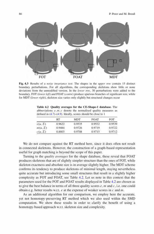
86 P. Peter and M. Breuß
Fig. 4.3 Results of a noise invariance test. The shapes in the upper row contain 15 distinctboundary perturbations. For all algorithms, the corresponding skeletons show little or nonedeviations from the unmodified version. In the lower row, 30 perturbations were added to theboundary. FOT (lower left) and FOAT (centre) produce spurious branches of significant size, whilefor MDT (lower right), skeleton size varies only slightly but structural changes occur
Table 4.2 Quality averages for the CE-Shape-1 database. Theabbreviations e;m; c denote the normalised quality measures asdefined in (4.7)–(4.9). Ideally, scores should be close to 1
RT MDT FOAT FOT
e.u; ˙/ 0.9622 0.9535 0.9532 0.9539m.u; ˙/ 0.9484 0.9726 0.9719 0.9722c.u; ˙/ 0.8803 0.9708 0.9715 0.9712
We do not compare against the RT method here, since it does often not resultin connected skeletons. However, the construction of a graph-based representationuseful for graph matching is beyond the scope of this paper.
Turning to the quality averages for the shape database, these reveal that FOATproduces skeletons that are of slightly simpler structure than the ones of FOT, whileskeleton exactness and absolute size is in average slightly higher. The MDT schemeconfirms its tendency to produce skeletons of minimal length, staying neverthelessquite accurate but introducing some small structures that result in a slightly highercomplexity as FOT and FOAT, see Table 4.2. Let us note in this context that theparameters used for the FOT and FOAT results displayed in Table 4.2 are chosen asto give the best balance in terms of all three quality scores e;m and c, i.e. one couldobtain e.g. better results w.r.t. e at the expense of weaker scores in c andm.
As an additional algorithm for our comparison, we employ here the accurate,yet not homotopy-preserving RT method which we also used within the SMDcomputation. We show these results in order to clarify the benefit of using ahomotopy-based approach w.r.t. skeleton size and complexity.

4 Homotopic Thinning Algorithms and Quality Measures for Skeletonisation 87
Table 4.3 Comparison of methods for the CE-Shape-1 database.Parameters for FOT and FOAT are chosen as to match the accuracye.u; ˙/ D 0:9535 of the MDT method
MDT FOAT FOT
m.u; ˙/ 0.9726 0.9719 0.9723c.u; ˙/ 0.9708 0.9714 0.9716
Table 4.4 Parameter sensitivity for the CE-Shape-1 database. Thetable gives the maximal deviation in the measures e;m; c as by (4.7)–(4.9)when varying the parameter in an interval of length 0:1. Ideally, scoresshould be as small as possible
e.u; ˙/ m.u; ˙/ c.u; ˙/
FOT 0.0095 0.0210 0.0470FOAT 0.0079 0.0017 0.0010
All of the algorithms work on average with high precision. However, let us alsopoint out that due to the size of 1,400 shapes in our test database, one may inferthat the first three to four digits after the comma in the error bear significance: Ascomputational results of the three algorithms are similar for many shapes leading toabout the same error measure contributing in (4.7)–(4.9), deviations from this rulemay be significant but do not show their influence in the first one or two digits.
Making algorithms even more comparable. With our new quality measures wehave the tools at hand to study how the algorithms perform at a common level ofaccuracy. To this end, we have performed a systematic parameter search for FOTand FOAT that gives a uniform exactness score of e.u; ˙/D 0:9535, matchingthe exactness of the MDT method (which is parameter-free). The result is givenin Table 4.3. We observe that MDT favors in comparison to the other schemesskeletons that are of more minimal size but of more complex structure. Moreover,a bit surprisingly, we observe that at the accuracy of the MDT method – or, moregenerally speaking, at a given average accuracy – FOT seems to slightly outperformFOAT.
Robustness vs. parameter choice. By the results documented in Table 4.3, onemay come to the conclusion that the FOAT method may be not better than thealready existing FOT scheme. However, having at hand the new rigorous measuresfor the quality of algorithms, we can now perform a systematic study of thesensitivity of the FOT and FOAT methods vs. the parameter choice. To this end,we have sampled a window of length 0:1 around the optimal parameter choiceemployed before and studied the deviation in the error measures. As by Table 4.4we observe that the FOAT method is generally much less sensitive to parametervariations than the FOT scheme; w.r.t. skeleton minimality and complexity it turnsout that this can be measured to be in the order of a considerable factor of 10 and40, respectively. Moreover, for FOT deviations appear already in the second digitafter the comma which indicates a considerable difference.

88 P. Peter and M. Breuß
Fig. 4.4 The lizard shape is an example of skeletons that are similar in size and exactness ofreconstruction, but vary in complexity. FOAT (middle) and MDT (right) feature less branchesin the small details of the lizard such as in its toes. FOT (left) produces additional branches, inparticular for jagged edges that result from the discretisation of the shape boundary, as it strives inthis example for a very exact representation
Fig. 4.5 The skeletons of the elephant shape reveal the improved adaption capabilities of FOAT(middle) and MDT (right) to individual shapes. Similar to Fig. 4.4, FOT (left) produces spuriousbranches at jagged edges (e.g. at the feet of the elephant), but omits branches that would give arefined reconstruction of the elephant’s head and back
The score differences illustrate the distinctive behaviours of the algorithms.When attempting to fine tune the threshold parameter ! (see Sect. 4.2) or whenmaking use of the same value of ! for different shapes, FOT easily producesmore and larger branches at narrow regions of a shape. There, additional skeletonpoints increase size and complexity, but yield only slight differences in exactnessof reconstruction, see Fig. 4.4. On some shapes however, FOT also omits largebranches, thus losing boundary information. Both effects can occur simultaneously,as displayed in Fig. 4.5.
A refined analysis of the new MDT algorithm. We now illustrate that the newquality measures can be useful to infer information about the properties of analgorithm if a related method is at hand.
Let us recall that, by construction, the MDT algorithm relies on the RT method.The latter gives as observable via Table 4.2 in average considerably more accurateskeletons than the MDT scheme. While the RT method is missing thinness,homotopy and connectivity, one may wonder why the loss in the accuracy qualityscore is relatively large as in the second digit after the comma. The question arises,if there is a general loss of accuracy for the shapes in our database (which wouldindicate a shortcoming of qualities like thinness, homotopy and connectedness), orif it is due to a few outliers that diminish the average quality score.

4 Homotopic Thinning Algorithms and Quality Measures for Skeletonisation 89
Fig. 4.6 Comparison of skeletonisation results illustrating the MDT algorithm. Top row. Thealgorithm of Remy and Thiel without pruning. Second row. The algorithm of Remy and Thiel withan additional pruning step. Third row. The new MDT scheme including pruning. Note that notall branches of the pruned RT skeleton are preserved during the MDT thinning phase due to thethinning order. For these selected shapes the problem appears that important branches are pruned.Bottom row. Result of modified MDT algorithm which will give a better accuracy for such shapes
90 P. Peter and M. Breuß
We now investigate this issue. For an illustration of the evolution step introducedby the MDT algorithm in comparison to the RT method, we present some typicalskeletonisation results, cf. Fig. 4.6. By adding the homotopy-preserving thinningcomponent, we clearly obtain thin, connected skeletons with no spurious points.However, in very few cases as in the car or the camel example given here, asignificant branch can be missing because of the general tendency of the MDTalgorithm towards producing skeletons as minimal as possible. In such singularcases the accuracy is obviously highly diminished; in turn one can infer by the highaverage accuracy score in Table 4.2 that these cases are very rare.
As a proof-of-concept that one can easily give a remedy for such rare cases(that can in principle be identified e.g. by computing individually for each shapethe reconstruction error e, or by a more local procedure) we propose to fine tune thebasic MDT method as follows. In a first step, the modified MDT scheme uses the RTpilot points to construct a preliminary skeleton that is homotopic, but not necessarilythin. This skeleton is then thinned according to homotopy preserving thinning rulesthat do obey the distance ordering, but do not remove skeleton endpoints, i.e. nobranches are deleted from the preliminary skeleton. Finally, branches of very smalllength are removed with a simple graph based pruning algorithm. See the last rowof Fig. 4.6 for typical results of this procedure.
4.5 Conclusions
In this paper we have proposed two new MAT algorithms, FOAT and MDT,based on homotopic thinning. The FOAT scheme relies on a robustification of thethresholding step in FOT. The MDT scheme is with the exception of the pruningstep parameter-free. As it is also relatively easy to implement and gives in generalresults of good quality, it is in our opinion an attractive algorithm for applications.
Additionally, we have proposed quality assessment techniques that give aninsight into properties of MAT algorithms. Moreover, they allow to perform asystematic parameter sensitivity analysis, and to analyse construction steps in analgorithm. The quality measures are easy to evaluate and can be applied with anyMAT method. However, the evaluation of the invariance tests as proposed here isnot straightforward for MAT methods that do not preserve homotopy since it relieson graph matching.
References
1. Bai, X., Latecki, L.J.: Path similarity skeleton graph matching. IEEE Trans. Pattern Anal.Mach. Intell. 30(7), 1282–1292 (2008)
2. Bloomberg, D.S.: Connectivity-preserving morphological image transformations. In: Pro-ceedings of the SPIE Visual Communications and Image Processing ’91: Image ProcessingConference, Boston, MA, pp. 302–334 (1991)

4 Homotopic Thinning Algorithms and Quality Measures for Skeletonisation 91
3. Blum, H.: A transformation for extracting new descriptors of shape. In: Wathen-Dunn, W. (ed.)Models for the Perception of Speech and Visual Form, pp. 362–380. MIT, Cambridge, MA(1967)
4. Borgefors, G.: Distance transformations in arbitrary dimensions. Comput. Vis. Graph. ImageProcess. 27(3), 321–345 (1984)
5. Danielsson, P.E.: Euclidean distance mapping. Comput. Vis. Graph. Image Process. 14, 227–248 (1980)
6. Demirci, F., Shoukoufandeh, A., Keselman, Y., Bretzner, L., Dickinson, S.: Object recognitonas many-to-many feature matching. Int. J. Comput. Vis. 69(2), 203–222 (2006)
7. Di Ruberto, C.: Recognition of shapes by attributed skeletal graphs. Pattern Recognit. 37(1),21–31 (2004)
8. Dimitrov, P., Damon, J., Siddiqi, K.: Flux invariants for shape. In: Proceedings of the IEEEConference on Computer Vision and Pattern Recognition, Madison, WI, pp. 835–841 (2003)
9. Geiger, D., Liu, T., Kohn, R.V.: Representation and self-similarity of shapes. IEEE Trans.Pattern Anal. Mach. Intell. 25(1), 86–99 (2003)
10. Kimmel, R., Shaked, D., Kiryati, N., Bruckstein, A.M.: Skeletonization via distance maps andlevel sets. Comput. Vis. Image Underst. 62, 382–391 (1995)
11. Kong, T.Y., Rosenfeld, A.: Digital topology: introduction and survey. Comput. Vis. Graph.Image Process. 48, 357–393 (1989)
12. Lantuejoul, C.: Skeletonization in quantitative metallography. In: Haralick, R.M., Simon, J.C.(eds.) Issues in Digital Image Processing, pp. 107–135. Sijthoff and Noordoff, Amsterdam(1980)
13. Latecki, L., Lakamper, R., Eckhardt, U.: Shape descriptors for non-rigid shapes with a singleclosed contour. In: Proceedings of the IEEE Conference on Computer Vision and PatternRecognition, Hilton Head Island, South Carolina, pp. 424–429 (1967)
14. Liu, T., Geiger, D.: Approximate tree matching and shape similarity. In: Proceedings of the 7thIEEE Conference on Computer Vision, Kerkyra, Greece, pp. 456–462 (1999)
15. Malandain, G., Fernandez-Vidal, S.: Euclidean skeletons. Image Vis. Comput. 16(5), 317–327(1998)
16. Maragos, P., Schafer, R.W.: Morphological skeleton representation and coding of binaryimages. IEEE Trans. Acoust. Speech Signal Process. 34(5), 1228–1244 (1986)
17. Meijster, A., Roerdink, J.B.T.M., Hesselink, W.H.: A general algorithm for computing distancetransforms in linear time. In: Goutsias, J., Vincent, L., Bloomberg, D.S. (eds.) MathematicalMorphology and Its Applications to Image and Signal Processing. Volume 18 of ComputationalImaging and Vision, pp. 362–380. Springer, Dordrecht (2002)
18. Ogniewicz, R.L., Kubler, O.: Hierarchic Voronoi skeletons. Pattern Recognit. 28, 343–359(1995)
19. Palagyi, K., Nemeth, G.: Fully parallel 3D thinning algorithms based on sufficient conditionsfor topology preservation. In: Proceedings of the International Conference on Discrete Geom-etry for Computer Imagery. Volume 5810 of Lecture Notes in Computer Science, pp. 481–492.Springer, Berlin (2009)
20. Pudney, C.: Distance-ordered homotopic thinning: a skeletonization algorithm for 3D digitalimages. Comput. Vis. Image Underst. 72, 404–413 (1998)
21. Remy, E., Thiel, E.: Exact medial axis with euclidean distance. Image Vis. Comput. 23, 167–175 (2005)
22. Sebastian, T.B., Klein, P.N., Kimia, B.B.: Recognition of shapes by editing their shock graphs.IEEE Trans. Pattern Anal. Mach. Intell. 26, 550–571 (2004)
23. Serra, J. (ed.): Image Analysis and Mathematical Morphology, vol. 1. Academic, London(1982)
24. Serra, J. (ed.): Image Analysis and Mathematical Morphology, vol. 2. Academic, London(1988)
25. Shaked, D., Bruckstein, A.: Pruning medial axes. Comput. Vis. Image Underst. 69(2), 156–169(1998)

92 P. Peter and M. Breuß
26. Shasha, D., Wang, J.: Graphdiff: approximate graph matcher and clusterer. http://cs.nyu.edu/shasha/papers/agm.html (2000). Accessed 29 December 2011
27. Siddiqi, K., Pizer, S.M. (eds.): Medial Representations: Mathematics, Algorithms and Appli-cations. Volume 37 of Computational Imaging. Springer, Dordrecht (2008)
28. Siddiqi, K., Shokoufandeh, A., Dickinson, S.J., Zucker, S.W.: Shock graphs and shapematching. Int. J. Comput. Vis. 35, 13–32 (1999)
29. Siddiqi, K., Bouix, S., Tannenbaum, A., Zucker, S.W.: Hamilton-Jacobi skeletons. Int.J. Comput. Vis. 48, 215–231 (2002)
30. Siddiqi, K., Zhang, J., Macrini, D., Dickinson, S., Shokoufandeh, A.: 3D model retrievalusing medial surfaces. In: Siddiqi, K., Pizer, S.M. (eds.) Medial Representations: Mathematics,Algorithms and Applications. Volume 37 of Computational Imaging, pp. 309–325. Springer,Dordrecht (2008)
31. Sorantin, E., Halmai, C., Erdohelyi, B., Palagyi, K., Nyul, L., Olle, K., Geiger, B.,Lindbichler, F., Friedrich, G., Kiesler, K.: Spiral-CT-based assessment of tracheal stenosesusing 3-D-skeletonization. Med. Imaging 21, 263–273 (2002)
32. Zhu, S.C., Yuille, A.L.: Forms: a flexible object recognition and modeling system. Int.J. Comput. Vis. 20(3), 187–212 (1996)
33. Zhu, Y., Seneviratne, L.D., Earles, S.W.E.: A fast boundary based thinning algorithm. In:Proceedings of IAPR Workshop on Machine Vision Applications, Kawasaki, Japan, pp. 548–551 (1994)
Chapter 5Nested Sphere Statistics of Skeletal Models
Stephen M. Pizer, Sungkyu Jung, Dibyendusekhar Goswami, Jared Vicory,Xiaojie Zhao, Ritwik Chaudhuri, James N. Damon, Stephan Huckemann,and J.S. Marron
Abstract We seek a form of object model that exactly and completely capturesthe interior of most non-branching anatomic objects and simultaneously is wellsuited for probabilistic analysis on populations of such objects. We show that certainnearly medial, skeletal models satisfy these requirements. These models are firstmathematically defined in continuous three-space, and then discrete representationsformed by a tuple of spoke vectors are derived. We describe means of fitting theseskeletal models into manual or automatic segmentations of objects in a way stableenough to support statistical analysis, and we sketch means of modifying thesefits to provide good correspondences of spoke vectors across a training populationof objects. Understanding will be developed that these discrete skeletal modelslive in an abstract space made of a Cartesian product of a Euclidean space and acollection of spherical spaces. Based on this understanding and the way objectschange under various rigid and nonrigid transformations, a method analogous toprincipal component analysis called composite principal nested spheres will beseen to apply to learning a more efficient collection of modes of object variation
S.M. Pizer (!) ! D. Goswami ! J. Vicory ! X. Zhao ! R. Chaudhuri ! J.N. DamonUniversity of North Carolina, Chapel Hill, NC, USAe-mail: [email protected]
S. JungUniversity of Pittsburgh, Pittsburgh, PA, USAe-mail: [email protected]
S. HuckemannInstitute for Mathematical Stochastics, University of Gottingen, Goldschmidtstrasse 7,37077 Gottingen, Germanye-mail: [email protected]
J.S. MarronDepartment of Statistics and Operations Research, University of North Carolina,Chapel Hill, NC 27599, USAe-mail: [email protected]
M. Breuß et al. (eds.), Innovations for Shape Analysis, Mathematics and Visualization,DOI 10.1007/978-3-642-34141-0 5, © Springer-Verlag Berlin Heidelberg 2013
93
94 S.M. Pizer et al.
about a new and more representative mean object than those provided by otherrepresentations and other statistical analysis methods. The methods are illustratedby application to hippocampi.
5.1 Object Models Suitable for Statistics
The objective of statistics on a population of 3D (or 2D) objects is to producesuch entities as the mean object and a shape space spanned by principal modes ofvariation of the object. These statistical descriptors are derived from training cases,each typically given by a pile of object boundary contours. Statistics on objectshas been applied to quite a variety of types of geometric model derived from theboundary cases:
1. Boundary point distribution models [4, 8, 17]. This popular form of model hasbeen analyzed by principal component analysis (PCA), although Kendall [16] hasshown this is not strictly appropriate because such models live in a space formedby a Cartesian product of a Euclidean space and a quotient of a high-dimensionalsphere modulo the rotation group. However, even the correct analysis ignores theshape of the object interior and, partially as a result, has difficulty limiting itsshape space to models whose boundaries do not cross themselves.
2. Deformation-of-atlas models, wherein the displacement of each voxel in the atlasis provided [1, 21] . These models have an enormous dimension, with the resultthat the statistical analysis is expensive and unstable with respect to the samplinginto training cases and to noise in those training cases.
3. Implicit models, such as level surfaces of pseudo-signed-distance functions [18,31] that do not live in Euclidean feature spaces but are often analyzed (by PCA)as if they did.
4. Skeletal models. While skeletal modeling is common, as summarized in thebook by Siddiqi and Pizer [27], work on statistics of skeletal models has beenthe major topic of only one group, namely ours. That work emphasized thatskeletal models, like those in the first two categories, live on abstract manifoldsthat are curved. Work on skeletal and other object models that live on abstractmanifolds have been the subject of study of Fletcher [10]. Our previous work onskeletal model statistics, on which Fletcher was an early contributor, is laid out inChaps. 8 and 9 of Siddiqi and Pizer [27]. The strength of skeletal models is thatthey richly model the object interior and boundary and that they yield an object-relative coordinate system for the object interiors. The difficulty with generalskeletal models, and especially the medial models that are their most commonform, is that even for objects that do not intuitively feel like a tree of figures, themodel takes the form of the tree. However, the branching structure of the treedoes not stay the same over the object population. This makes statistical analysisof these models very difficult. In our previous work we have solved this problemby using skeletal models whose boundaries are only approximately that of thetraining cases but which have no branches.
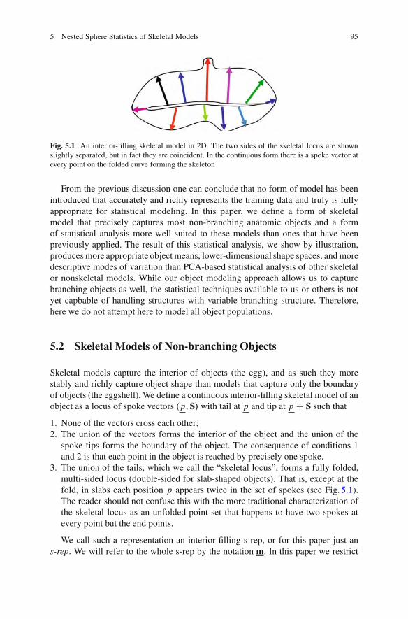
5 Nested Sphere Statistics of Skeletal Models 95
Fig. 5.1 An interior-filling skeletal model in 2D. The two sides of the skeletal locus are shownslightly separated, but in fact they are coincident. In the continuous form there is a spoke vector atevery point on the folded curve forming the skeleton
From the previous discussion one can conclude that no form of model has beenintroduced that accurately and richly represents the training data and truly is fullyappropriate for statistical modeling. In this paper, we define a form of skeletalmodel that precisely captures most non-branching anatomic objects and a formof statistical analysis more well suited to these models than ones that have beenpreviously applied. The result of this statistical analysis, we show by illustration,produces more appropriate object means, lower-dimensional shape spaces, and moredescriptive modes of variation than PCA-based statistical analysis of other skeletalor nonskeletal models. While our object modeling approach allows us to capturebranching objects as well, the statistical techniques available to us or others is notyet capbable of handling structures with variable branching structure. Therefore,here we do not attempt here to model all object populations.
5.2 Skeletal Models of Non-branching Objects
Skeletal models capture the interior of objects (the egg), and as such they morestably and richly capture object shape than models that capture only the boundaryof objects (the eggshell). We define a continuous interior-filling skeletal model of anobject as a locus of spoke vectors .p;S/ with tail at p and tip at p C S such that
1. None of the vectors cross each other;2. The union of the vectors forms the interior of the object and the union of the
spoke tips forms the boundary of the object. The consequence of conditions 1and 2 is that each point in the object is reached by precisely one spoke.
3. The union of the tails, which we call the “skeletal locus”, forms a fully folded,multi-sided locus (double-sided for slab-shaped objects). That is, except at thefold, in slabs each position p appears twice in the set of spokes (see Fig. 5.1).The reader should not confuse this with the more traditional characterization ofthe skeletal locus as an unfolded point set that happens to have two spokes atevery point but the end points.
We call such a representation an interior-filling s-rep, or for this paper just ans-rep. We will refer to the whole s-rep by the notation m. In this paper we restrict
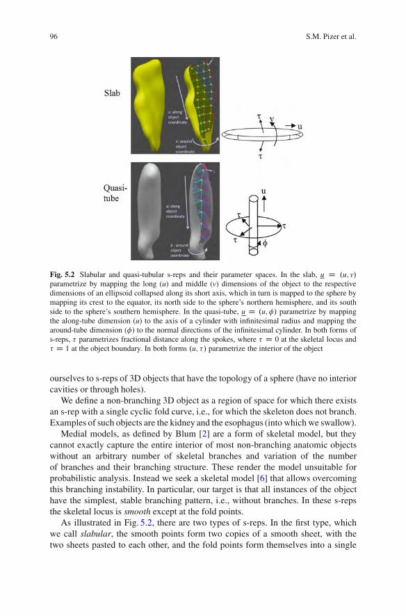
96 S.M. Pizer et al.
Fig. 5.2 Slabular and quasi-tubular s-reps and their parameter spaces. In the slab, u D .u; v/parametrize by mapping the long (u) and middle (v) dimensions of the object to the respectivedimensions of an ellipsoid collapsed along its short axis, which in turn is mapped to the sphere bymapping its crest to the equator, its north side to the sphere’s northern hemisphere, and its southside to the sphere’s southern hemisphere. In the quasi-tube, u D .u; !/ parametrize by mappingthe along-tube dimension (u) to the axis of a cylinder with infinitesimal radius and mapping thearound-tube dimension (!) to the normal directions of the infinitesimal cylinder. In both forms ofs-reps, " parametrizes fractional distance along the spokes, where " D 0 at the skeletal locus and" D 1 at the object boundary. In both forms .u; "/ parametrize the interior of the object
ourselves to s-reps of 3D objects that have the topology of a sphere (have no interiorcavities or through holes).
We define a non-branching 3D object as a region of space for which there existsan s-rep with a single cyclic fold curve, i.e., for which the skeleton does not branch.Examples of such objects are the kidney and the esophagus (into which we swallow).
Medial models, as defined by Blum [2] are a form of skeletal model, but theycannot exactly capture the entire interior of most non-branching anatomic objectswithout an arbitrary number of skeletal branches and variation of the numberof branches and their branching structure. These render the model unsuitable forprobabilistic analysis. Instead we seek a skeletal model [6] that allows overcomingthis branching instability. In particular, our target is that all instances of the objecthave the simplest, stable branching pattern, i.e., without branches. In these s-repsthe skeletal locus is smooth except at the fold points.
As illustrated in Fig. 5.2, there are two types of s-reps. In the first type, whichwe call slabular, the smooth points form two copies of a smooth sheet, with thetwo sheets pasted to each other, and the fold points form themselves into a single
5 Nested Sphere Statistics of Skeletal Models 97
smooth cyclic curve, called the end curve. In the second type, which we call quasi-tubular, the smooth points take the form of a bent cylinder of infinitesimal radius,i.e., a cylinder whose surface is made up of copies of an axis curve with all the copycurves pasted to each other, and the fold points consist of two discrete points, calledthe end points. In both types a continuum of spokes, formed by vectors with tails onthe skeletal locus and tips on the object boundary, cover the interior of the object.
Such s-reps capture all non-branching anatomic objects in the human body. Thisincludes not only slabular objects such as the kidney, most muscles, the heart, andthe bladder, and quasi-tubular objects, such as the esophagus and the rectum, butalso folded slabular objects such as the cerebral cortex and folded quasi-tubularobjects such as the intestines. These models capture objects with small pimplesand dimples; the main objects not captured are objects with hook-shaped or curvyprotrusions and indentations and those that branch multiple times.
In slabular s-reps the skeletal locus forms a two-sided sheet p.u/ with a cyclicfold curve. The parametrization u has the topology of a sphere. In this work, for slab-ular s-reps we will parametrize by the sphere and let the equator of the parametrizingsphere map onto the fold of skeletal locus. Thus we will refer to the north and southsides of the sheet. For each u a spoke S.u/ exists with its tail on p.u/ and its tipon an object boundary point b.u/. u parametrizes the skeletal locus along the objectand across and around the object; it also parametrizes the spokes S.u/, which passwithin the object, as well as the object boundary b.u/. The lengths of the spokes,jS.u/j, which we will call r.u/, and the directions of the spokes U.u/ D S.u/=r.u/are also defined. Thus u parametrizes the whole s-rep m.u/ D .p.u/;U.u/; r.u//.
In quasi-tubular s-reps the skeletal locus forms a collapsed (infinitesimal radius)bent cylinder with hemispherical caps at both ends, such that the axis of the cylinderis a space curve and the spokes emanating from each axis-orthogonal cut of thecylinder end in a common plane. Here the parametrization u is typically on theunit-radius, possibly hemispherically capped right-circular cylinder (Fig. 5.2); itparametrizes the axis of (forming) the skeletal locus by the along-cylinder scalarvariable u, and it parametrizes the angle around the circular tubular cross sectionsby another cyclic scalar variable !. As with the slabular s-rep, u parametrizes thespokes S.u/, their directions U.u/, their lengths r.u/, and the object boundaryb.u/. Quasi-tubular s-reps are used to model roughly tubular objects such as theesophagus, but they can also be used to model objects like muscles whose cross-sections are star-shaped but not roughly tubular.
For both slabular and quasi-tubular s-reps the position along a spoke from itstip to its tail is parametrized by the proportion-of-spoke-length variable " , so theunion of the interior and the boundary of the object is parametrized by .u; "/. In theremainder of this paper we restrict ourselves to slabular s-reps.
The mathematical theory of skeletal models is presented in Damon’s Chap. 3 ofthe book Medial Representations by Siddiqi and Pizer [27] and more completely inDamon’s papers: [6, 7]. There the geometry of our class of s-reps is shown to beneatly divisible into (a) the differential geometry of the two sides and fold of theskeletal locus p.u/ and (b) a variant of differential geometry, which we call radial
98 S.M. Pizer et al.
geometry, of the (tail-less) spokes S.u/ with respect to motions on the tangent planeof the skeletal locus. The radial geometry of the spoke directions U.u/ is of specialinterest; it can be divided into a radial shape operator Srad.u/ applicable at non-fold medial points and an edge shape operator SE.u/ (for u on the equator of theparametrizing sphere or the ends of the parametrizing cylinder) applicable at thefold curve. Each of these operators are represented by a 2 ! 2 matrix. These shapeoperators describe U.u/ motion in a way analogous to the way the ordinary shapeoperator from differential geometry describes the motion of boundary normals.There are special matters dealing with the appropriate coordinate system in whichto describe U.u/ motion and the need for projection of that motion onto the tangentplane to p.u/, but we will not go into those in this paper.
Damon shows that an interior-filling locus .p.u/;U.u/; r.u// has no locallycrossing spokes (is geometrically legal) if and only if for all u the positive eigen-values of Srad.u/< 1=r.u/ and any positive generalized eigenvalue of .SE.u/; J / <1=r.u/, where J is the 2 ! 2 matrix all of whose elements are 0 but for the upperleft element, which is 1.
Discrete s-reps sample m.u/ into a network of spoke vectors. In our work withslabular s-reps the sampling is into a northm! n grid of spokes, a southm! n gridof spokes, for some m, n, and a cyclic chain of 2m C 2n " 4 edge (crest) spokes(Fig. 5.2). These are organized into anm!n grid of “skeletal atoms”, each consistingof two or three spokes with a common tail position. For interior grid points there aretwo spokes, one on the north side and one on the south side. For exterior grid pointsthere are three spokes, one on the north side, one on the south side, and a crest spokebisecting the other two.
Interpolation of a continuous s-rep from a discrete s-rep proceeds accordingto the method of Han [11], in which p.u/, r.u/, and U.u/ are interpolated in anintertwined way. The spokes are interpolated using the fact that Srad.u/ or SE.u/times a small step vector on the tangent plane to the skeletal locus at p.u/ allowsthe calculation of the spoke direction swing corresponding to that step. The rSrad.u/or rSE.u/ matrix is first interpolated and then the implied spoke swing and lengthscaling for various small steps is integrated. The skeletal axis positions p.u/ areinterpolated using a Hermite-like interpolation using both the discrete positions andskeletal sheet normals there, where the normal is computed as the difference of thetwo spoke direction vectors with a common skeletal sheet position. This relation forthe normal holds only for Blum medial sheets, but given the “as medial as possible”criterion for skeletal sheets discussed below, it is sensible to use it for the skeletalsheet interpolation.
5.3 Obtaining s-Reps Suitable for Probabilistic Analysis
There are three properties necessary for making a population of s-reps suitable forprobabilistic analysis. The first is that the branching topology of all members of thepopulation should be the same. There is nice, albeit not yet usable, work on statistics
5 Nested Sphere Statistics of Skeletal Models 99
of trees with variable branching topology [28,30], but this is beyond the scope of thispaper. In this paper we restrict the branching situation further to having no skeletalbranches at all. This requires branching objects such as blood vessels to be treatedby compositing single branch components, but this, too, is beyond the scope of thispaper. This is the reason for the restriction mentioned in Sect. 5.1 to skeletal locithat are smooth except at the fold curve.
The second property needed to do probabilistic analysis is that small deforma-tions in the objects yield small deformations in the skeletal model. This can bemade to occur when the process of fitting s-reps into the data describing the objecthas certain behaviors. These will be discussed in Sect. 5.3.1.
The third property needed to do probabilistic analysis is that each spoke inone s-rep in the training population be at a position, orientation, and length thatgeometrically corresponds to that of the same spoke in the other training s-reps.Accomplishing this is discussed in Sect. 5.3.2.
5.3.1 Fitting Unbranched s-Reps to Object Description Data
Typically object data is provided in the form of a tiled object boundary, a pile ofparallel planes each containing a boundary contour, or a binary discrete image. Tofit s-reps to such data, we first transform the data into a signed distance image,where the distance is negative inside the object and positive outside and where thezero level curve of distance represents the object boundary. We have methods, usingconstrained flow controlled by the Laplacian of curvature, that yield a distanceimage representing a smooth boundary staying within a half-voxel of the objectdata [22].
Our objective is to study shape variability by statistical means, so the pair ofdistance images for many population samples of our object will be provided. For anyobject sample there are very many s-reps that can be fitted to this data. In particular,the skeletal locus could in principle be anywhere across the short dimension of theobject. In the extreme it could be along one side of the object, such that the objectwas covered by lines going from one side of the object (e.g., the south side) to theother side of the object. Since our goal is to do statistical analysis of the fitted s-reps,we need to fit s-reps that have as little variability over the training cases as possible.
The closer the skeletal locus is to bisecting the top and bottom sides, the wider therange of pimples and dimples on the boundary that could be accommodated. Moreimportantly, we can more stably constrain the geometry of the skeletal locus if wemake it bisect the two sides. However, as indicated earlier, the Blum medial locuswill not do, because it generates branches for pimples and dimples. So in brief, wewant a skeletal locus smooth but at the folds that is space filling and, within thoseconstraints, as medial as possible. The following section gives properties of trulymedial fits that can be used in measuring how medial an s-rep is. The propertiesare described in the form of penalties that contribute to a weighted sum that isminimized in the fitting process.

100 S.M. Pizer et al.
5.3.1.1 As Medial as Possible
The following medial properties should be approximate targets for an as-medial-as-possible s-rep. Each property yields a penalty term in the aforementioned weightedsum. Some depend on the input signed distance imageD.x/, and some involve therelation between the north (south) side spoke S.u/ and S.v/, its counterpart on theother side of the (double-sided) skeletal sheet with the same p.u/ value.
1. Equal r.u/ values for the northside and southside spokes at the same p.u/: in thefitting of a discrete s-rep we penalize according to jr.u/" r.v/j/.
2. Spokes are boundary normals: in the fitting we penalize according to the devia-tion from boundary normality, i.e., cos"1.brD.x/ #U.u// at the spoke end, where,given a vector W, bW is the unit vector in the direction of W.
3. The (interpolated) skeletal locus p.u/ bisects S.u/ and S.v/. Equivalently, thenormal to p.u/ is in the same direction as U.u/ " U.v/: in the fitting, for eachspoke we penalize according to the angle between the normal to p.u/ andU.u/"U.v/. This penalty has not yet been implemented in our code to fit s-repsto objects.
4. End curves’ spokes are at crests of the zero level curve of the distance imagethat forms the object boundary; this involves three properties, all involving theprincipal directions w1 and w2 and the associated principal curvature #1 of thelevel surface at the spoke end, where #1 is the lesser (more negative, i.e., moreconvex) principal curvature:
(a) The spoke end is at an extremum of #1 along the integral curve of w1, so thedirectional derivative of #1 in the w1 direction should be zero. In the fittingwe have attempted to penalize according to the magnitude of that directionalderivative. However, the high order derivative of the distance function thatthis involves proved to be unstable, so for now this term is not included inthe penalty list.
(b) The plane of the spoke and its infinitesimally near neighbors along theprincipal curve of w1 should be orthogonal to w2. We penalize accordingto the angle between w2 and U.u/ ! U.v/, the normal to the plane of thespokes at that end curve point.
(c) The boundary implied by the s-rep at the spoke end and the level surface ofthe distance at the spoke end should agree in the first principal curvature. Wehave not yet implemented a penalty for deviating from this condition, but ina future implementation we plan also to penalize according to the magnitudeof the difference between the two relevant radii of curvature.
This method of forcing spokes into the distance function’s crest is good whenthere is a strong crest for the end curve to fit into, but in some objects this crest isweak or, even worse, the object has more than one crest and we wish the s-rep tofit between them. This situation is illustrated in Fig. 5.3, where the skeletal sheetbisects the twin crests on the right side of the object, instead of favoring one crestover the other.
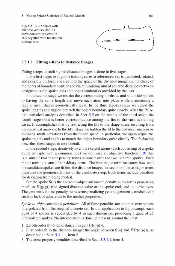
5 Nested Sphere Statistics of Skeletal Models 101
Fig. 5.3 A 2D object withmultiple vertices (the 2Dcorrespondent to a crest in3D), together with the desiredskeletal sheet
5.3.1.2 Fitting s-Reps to Distance Images
Fitting s-reps to such signed distance images is done in five stages.In the first stage, to align the training cases, a reference s-rep is translated, rotated,
and possibly uniformly scaled into the space of the distance image via matching ofmoments of boundary positions or via minimizing sum of squared distances betweendesignated s-rep spoke ends and object landmarks provided by the user.
In the second stage we restrict the corresponding northside and southside spokesto having the same length and move each atom into place while maintaining aregular array that is geometrically legal. In the third (spoke) stage we adjust thespoke lengths and angles to match the object boundary quite closely. After the PCA-like statistical analysis described in Sect. 5.5 on the results of the third stage, thefourth stage obtains better correspondence among the fits to the various trainingcases. It accomplishes that by restricting the fits to the shape space resulting fromthe statistical analysis. In the fifth stage we tighten the fit to the distance function byallowing small deviations from the shape space; in particular, we again adjust thespoke lengths and angles to match the object boundary quite closely. The followingdescribes these stages in more detail.
In the second stage, iteratively over the skeletal atoms (each consisting of a spokeduple or triple with a common hub) we optimize an objective function [19] thatis a sum of two major penalty terms summed over the two or three spokes. Eachmajor term is a sum of subsidiary terms. The first major term measures how wellthe candidate spokes are fit into the distance image; the second of these major termsmeasures the geometric fitness of the candidate s-rep. Both terms include penaltiesfor deviation from being medial.
For the spoke S.u/ the spoke-to-object-mismatch penalty sums terms penalizingmisfit to D.b.u// (the signed distance value at the spoke end) and its derivatives.The geometric fitness penalty sums terms penalizing general geometric misbehaviorsuch as lack of adherence to the medial properties.
Spoke-to-object mismatch penalties: All of these penalties are summed over spokesinterpolated from the original discrete set. In our application to hippocampi, eachquad of 4 spokes is subdivided by 4 in each dimension, producing a quad of 25interpolated spokes. No interpolation is done, at present, around the crest.
1. Zeroth order fit to the distance image: jD.b.u//j.2. First order fit to the distance image: the angle between S.u/ and rD.b.u//), as
described in Sect. 5.3.1.1, item 2.3. The crest property penalties described in Sect. 5.3.1.1, item 4.

102 S.M. Pizer et al.
Geometric fitness penalties:
1. S-rep irregularity: To achieve roughly uniform coverage of the object interiorand, given the crest-fitting of the end spokes, to provide approximate correspon-dence of spokes across cases, a penalty for each spoke is applied proportionalto its difference from the average of its neighbors. At present, the average iscalculated in a way consistent with the principal geodesic analysis approachdescribed in Sect. 5.5.1.1.
2. Illegality of spoke crossings: a penalty is added for Srad or SE values for a spokebeing greater than the reciprocal of their spoke lengths (see Sect. 5.2).
3. Deviation from medial properties, as described in items 1 and 3 of Sect. 5.3.1.1.4. The distance between S.u/ and the result of the first stage for that spoke. The
distance measure reflects positional deviations at the spoke end.
In the third, i.e., spoke, stage the spoke tail p.u/ is fixed, and the optimization isonly over the spoke direction U.u/ and the spoke length r.u/. The spoke-to-objectmismatch penalties are as above, but the geometric fitness penalty is only on themagnitude of the difference of both the spoke direction and the spoke length fromthe result at the first stage.
In the fourth stage the optimization is over the shape space determined by the sta-tistical analysis of those third stage fits that are adequately good, and the intializationis always from the mean s-rep of those fits. In that stage the geometric atypicalitypenalty is the negative log prior density (up to a constant multiplier and additiveconstant) of being in a population of s-reps, given by the Mahalanobis distancefunction also determined from the statistical analysis. In Sects. 5.5.2 and 5.5.3 wedescribe how to compute a set of eigenmodes vi of s-reps and associated principalvariances $2i , using the actual abstract space in which an s-rep falls. Any s-rep inthat population is designated by a tuple of scores ˛ of the respective eigenmodes,and
Pi .˛
2i =$
2i / forms the Mahalanobis distance of that s-rep.
The fifth, spoke, stage is just like the third stage, but on and relative to the resultsof the fourth stage.
In all of the stages conjugate gradient optimization of the objective function isapplied.
Figure 5.4 shows some sample hippocampus fits by this method, as described inSect. 5.6.
5.3.2 Achieving Correspondence of Spoke Vectors
The previous work on achieving correspondence in training populations of anatomicobject models has involved shifting points on object boundaries in point-distributionmodels (PDMs) [3, 5, 20]. We find the most attractive method is that of Cateset al. [3] and Oguz et al. [20], which minimizes a sum of two entropy terms:H.z/ " ˛
Pi H.xi /. The first term measures the tightness of the probability
distribution on the representation entities, here possibly including not only theboundary points but also derived values such as curvature. The second term sums
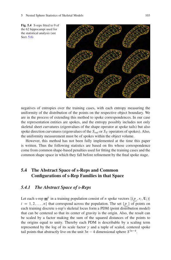
5 Nested Sphere Statistics of Skeletal Models 103
Fig. 5.4 S-reps fitted to 9 ofthe 62 hippocampi used forthe statistical analysis (seeSect. 5.6)
negatives of entropies over the training cases, with each entropy measuring theuniformity of the distribution of the points on the respective object boundary. Weare in the process of extending this method to spoke correspondences. In our casethe representation entities are spokes, and the entropy possibly includes not onlyskeletal sheet curvatures (eigenvalues of the shape operator at spoke tails) but alsospoke direction curvatures (eigenvalues of the Srad or SE operators of spokes). Also,the uniformity measurement must be of spokes within the object volume.
However, this method has not been fully implemented at the time this paperis written. Thus the following statistics are based on fits whose correspondencecome from common shape-based penalties used for fitting the training cases and thecommon shape space in which they fall before refinement by the final spoke stage.
5.4 The Abstract Space of s-Reps and CommonConfigurations of s-Rep Families in that Space
5.4.1 The Abstract Space of s-Reps
Let each s-rep mk in a training population consist of n spoke vectors f.pi; ri ;Ui /j
i D 1; 2; : : : ; ng that correspond across the population. The set fpig of points on
each training discrete s-rep’s skeletal locus form a PDM (point distribution model)that can be centered so that its center of gravity is the origin. Also, the result canbe scaled by a factor making the sum of the squared distances of the points tothe origins equal to unity. Thereby each PDM is describable by a scaling termrepresented by the log of its scale factor % and a tuple of scaled, centered spoketail points that abstractly live on the unit 3n " 4 dimensional sphere S3n"4.

104 S.M. Pizer et al.
Each spoke direction Ui abstractly lives on the unit two-sphere. Each log ri value,as well as log % , abstractly live in Euclidean space. Thus a discrete s-rep lives inRnC1 !S3n"4 ! .S2/n, i.e., the Cartesian product of nC 2 manifolds, one of whichis Euclidean and all of the rest of which are spheres. If the number of training casesN is less than 3n"4, the space of the scaled, centered spoke tails is restricted to theintersection of S3n"4 with the Euclidean space of dimensionN " 1 passing throughthe center of S3n"4, i.e., in SN"1. Also in that case, the n radii live in RN"1. In theexperiment on hippocampi reported in Sect. 5.5, N D 62 and n D 66. Thus eachhippocampus s-rep is a point in the composite space R62 ! S61 ! .S2/66.
5.4.2 Families of s-Rep Components on Their Spheres
The statistical analysis method we will describe in Sect. 5.5 involves includesanalysis on each of the here, 67 component spherical spaces, then compositingthe analyzed information with one another and with the Euclidean space data, andanalyzing the composited data. Therefore, it is of interest to consider how the s-repdata points distribute themselves on each sphere.
Certain basic transformations of the objects can be expected: global rigid rota-tions, rotational folding about an axis, and twisting about an axis. We have shown[24] the following behaviors of the spoke-direction points on S2 under these trans-formations. For each transformation each spoke moves on a small circle on S2 aboutthe rotational axis of the transformation; different spokes move on different smallcircles, but all the circles share the same axis. In rotational folding and twistingdifferent spoke-direction points rotate in opposite directions as the fold or twistprogresses.
Also, for rigid rotation the points on S3n"4 or SN"1 (here S61), each describingthe tuple of skeletal points for a separate training s-rep, move on a small circle(1-sphere).
We have experimentally confirmed (see Fig. 5.5) the relevance of these ideas, byobserving that real data s-rep spokes tend to arrange themselves near small circles.
We will now examine methods for statistically analyzing such data on ad -dimensional sphere in a PCA-like fashion, to describe the data by a suitablenotion of mean and a shape space formed from a limited number of eigenmodesof variation.
5.5 Training Probability Distributions in Populationsof Discrete s-Reps
5.5.1 Previous Methods for Analyzing Data on a Sphere
To understand the methods we will describe, it is useful to describe two approachesto PCA in a d -dimensional Euclidean space. The two approaches are called
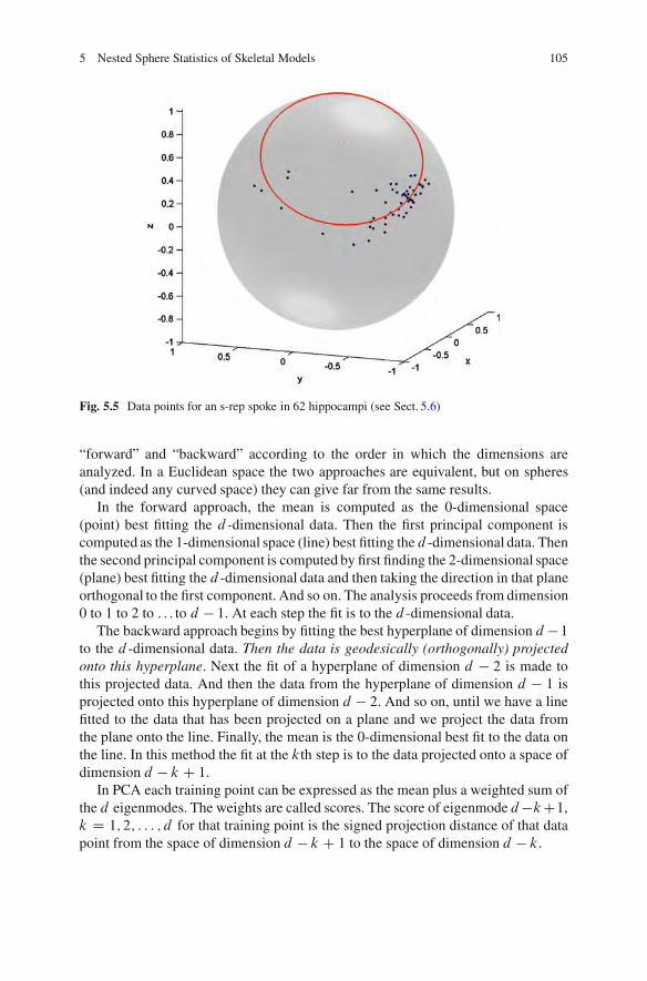
5 Nested Sphere Statistics of Skeletal Models 105
Fig. 5.5 Data points for an s-rep spoke in 62 hippocampi (see Sect. 5.6)
“forward” and “backward” according to the order in which the dimensions areanalyzed. In a Euclidean space the two approaches are equivalent, but on spheres(and indeed any curved space) they can give far from the same results.
In the forward approach, the mean is computed as the 0-dimensional space(point) best fitting the d -dimensional data. Then the first principal component iscomputed as the 1-dimensional space (line) best fitting the d -dimensional data. Thenthe second principal component is computed by first finding the 2-dimensional space(plane) best fitting the d -dimensional data and then taking the direction in that planeorthogonal to the first component. And so on. The analysis proceeds from dimension0 to 1 to 2 to . . . to d " 1. At each step the fit is to the d -dimensional data.
The backward approach begins by fitting the best hyperplane of dimension d " 1to the d -dimensional data. Then the data is geodesically (orthogonally) projectedonto this hyperplane. Next the fit of a hyperplane of dimension d " 2 is made tothis projected data. And then the data from the hyperplane of dimension d " 1 isprojected onto this hyperplane of dimension d " 2. And so on, until we have a linefitted to the data that has been projected on a plane and we project the data fromthe plane onto the line. Finally, the mean is the 0-dimensional best fit to the data onthe line. In this method the fit at the kth step is to the data projected onto a space ofdimension d " k C 1.
In PCA each training point can be expressed as the mean plus a weighted sum ofthe d eigenmodes. The weights are called scores. The score of eigenmode d"kC1,k D 1; 2; : : : ; d for that training point is the signed projection distance of that datapoint from the space of dimension d " k C 1 to the space of dimension d " k.
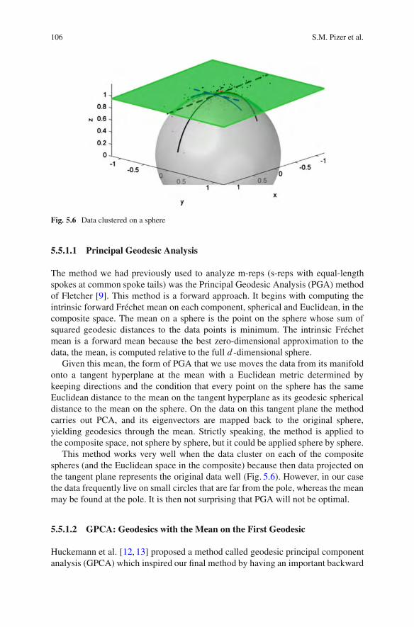
106 S.M. Pizer et al.
Fig. 5.6 Data clustered on a sphere
5.5.1.1 Principal Geodesic Analysis
The method we had previously used to analyze m-reps (s-reps with equal-lengthspokes at common spoke tails) was the Principal Geodesic Analysis (PGA) methodof Fletcher [9]. This method is a forward approach. It begins with computing theintrinsic forward Frechet mean on each component, spherical and Euclidean, in thecomposite space. The mean on a sphere is the point on the sphere whose sum ofsquared geodesic distances to the data points is minimum. The intrinsic Frechetmean is a forward mean because the best zero-dimensional approximation to thedata, the mean, is computed relative to the full d -dimensional sphere.
Given this mean, the form of PGA that we use moves the data from its manifoldonto a tangent hyperplane at the mean with a Euclidean metric determined bykeeping directions and the condition that every point on the sphere has the sameEuclidean distance to the mean on the tangent hyperplane as its geodesic sphericaldistance to the mean on the sphere. On the data on this tangent plane the methodcarries out PCA, and its eigenvectors are mapped back to the original sphere,yielding geodesics through the mean. Strictly speaking, the method is applied tothe composite space, not sphere by sphere, but it could be applied sphere by sphere.
This method works very well when the data cluster on each of the compositespheres (and the Euclidean space in the composite) because then data projected onthe tangent plane represents the original data well (Fig. 5.6). However, in our casethe data frequently live on small circles that are far from the pole, whereas the meanmay be found at the pole. It is then not surprising that PGA will not be optimal.
5.5.1.2 GPCA: Geodesics with the Mean on the First Geodesic
Huckemann et al. [12, 13] proposed a method called geodesic principal componentanalysis (GPCA) which inspired our final method by having an important backward
5 Nested Sphere Statistics of Skeletal Models 107
component. They realized that the Frechet mean may be far from the best fittinggreat circle. Hence, if the data lives on or near a circle on a sphere, the mean shouldbe computed on that circle after projection of the data onto it. Their method foundthe best fitting geodesic (great) circle on the sphere, projected the data onto that,and found the Frechet mean on that great circle of the projected points. This is abackward mean, since it computed after projection from the original d -space onto a1-dimensional subspace.
The method of Huckemann et al. on a d -sphere then went on to compute principalgeodesic circles through the mean in a forward fashion, in a way quite similar toPCA, albeit on a sphere. Its weakness for our data comes from two problems. First,it fits great circles, whereas our data live near small circles. Second, it is backwardonly at the first step, whereas the fully backward method of Jung [15] described nextappears superior.
5.5.1.3 Composite Principal Nested Spheres
A method better recognizing the loci along which the s-reps tend naturally to varyis the Composite Principal Nested Spheres (CPNS) method of Jung et al. [15]. Itconsists of (1) component by component estimation of principal modes of eachof the spherical manifolds separately, each producing scores that are suitable forEuclidean analysis; then (2) compositing those analyses with one another and theEuclidean data, followed by PCA on the result.
5.5.2 Training Probability Distributions on s-Rep ComponentsLiving on Spheres: Principal Nested Spheres
We begin by describing the principal nested spheres (PNS) approach that is appliedto the data on each sphere separately. This method has already been describedin [15]. As suggested, the approach is backwards analysis, and at each step thebest fitting subsphere of one dimension lower is fit, irrespective of whether thatsubsphere is a great or small subsphere.
The approach begins with the data on the d -dimensional sphere. The bestsubsphere of d " 1 dimensions is fit by an analytical computation. As illustratedin Fig. 5.7, the result is formed by (and recorded as) the pole (axis) position w1
of the subsphere on the d -sphere and its latitude (angle from the pole) 1. Thenit projects the data onto the subsphere of dimension d " 1. The process beginsanew, finding the .d " 2/-dimensional subsphere best fitting the data that has beenprojected onto the .d " 1/-dimensional sphere. The process repeats itself until a1-sphere (a not necessarily great circle) with points on it has been arrived at. Thefinal step is to find the mean (best-fitting 0-sphere) as the best fitting point to(geodesic mean of) the data points that have been projected onto the circle.

108 S.M. Pizer et al.
Fig. 5.7 Computation of subsphere, projection, and scores in principal nested spheres
The mean is successively projected forward through the dimensions 2; 3; : : : ; dusing the subsphere-to-sphere transformations that have been recorded. The result-ing point on the d-sphere gives the place in the data space which is the backwardsmean of the shape component that was analyzed on this sphere.
As with PCA, we record the score of the j th data point relative to the projectionof the subsphere of dimension d " k C 1, k D 1; 2; : : : ; d , to the subsphereof dimension d " k as the signed projection distance zd"kC1;j of that data pointbetween those two spheres (see Fig. 5.7). The random variable zd"kC1;! is a 0-meanvariable that can be understood as being in Euclidean space. Thus, the d!N arrayZwith elements k; j being zd"kC1;j represents the Euclideanized, 0-mean distributionof the respective shape component of the data on the d -sphere.
5.5.3 Compositing Component Distributions into an OverallProbability Distribution
In our method of analysis of CPNS the distribution of the 62-case s-rep data oneach of the component spheres is analyzed by PNS. The compositing approach hasalready been described in [14]; here we detail it for analysis of s-reps. In that case,with 67 spheres, this yields 67 Z arrays. One of them (for the spoke tail points)is 61 ! 62 and the other 66 (for the spoke directions) are 2 ! 62. We must nowaccount for the correlations between the various s-rep components, including boththose that live on spheres and those that live in a Euclidean space. To prepare forthat, for each s-rep the Euclidean components,kD 1; 2; : : : ; 67, each of the form loglength or log scale factor, must each have their mean computed (in the ordinary wayof summing the entries across the data items and dividing by the number of entries,62) and then subtracting that mean from each data item’s corresponding component.(Strictly speaking, that data lives in a 62-dimensional space, but the SVD analysisto follow is insensitive to using the original 67 dimensions.) Call the result of thisthe 67 ! 62 array ZEuclidean.
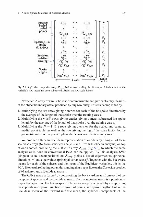
5 Nested Sphere Statistics of Skeletal Models 109
Fig. 5.8 Left: the composite array Zcomp before row scaling for N s-reps. * indicates that thevariable’s row mean has been subtracted. Right: the row scale factors
Next eachZ array row must be made commensurate; we give each entry the unitsof the object boundary offset produced by any row entry. This is accomplished by
1. Multiplying the two rows giving z entries for each of the 66 spoke directions bythe average of the length of that spoke over the training cases;
2. Multiplying the n (66) rows giving entries giving a mean-subtracted log spokelength by the average of the length of that spoke over the training cases;
3. Multiplying the N " 1 (61) rows giving z entries for the scaled and centeredmedial point tuple, as well as the row giving the log of the scale factor, by thegeometric mean of the point tuple scale factors over the training cases.
We produce a 0-mean Euclidean representation of our data by piling all of thesescaled Z arrays (67 from spherical analysis and 1 from Euclidean analysis) on topof one another, producing the 260 ! 62 array Zcomp (Fig. 5.8), to which the sameanalysis as is done in conventional PCA can be applied. By this analysis, SVD(singular value decomposition) on Zcomp yields a list of eigenvectors (principaldirections) vi and eigenvalues (principal variances) $2i . Together with the backwardmeans for each of the spheres and the mean of the Euclidean variables, this is thePCA-like result reflecting our understanding that s-reps live on the Cartesian productof 67 spheres and a Euclidean space.
The CPNS mean is formed by compositing the backward means from each of thecomponent spheres and the Euclidean mean. Each component mean is a point on itsrespective sphere or Euclidean space. The mean s-rep is achieved by compositingthese points into spoke directions, spoke tail points, and spoke lengths. Unlike theEuclidean mean or the forward intrinsic mean, the spherical components of the
110 S.M. Pizer et al.
CPNS mean live not only on their spheres but on all the best fitting subspheres. Ittherefore can be expected that the CPNS mean is more representative of the trainingshapes than any of the forward means.
From the CPNS analysis, we can choose a number of eigenmodes that captures adesired fraction of the total variance. This forms a shape space for s-reps as impliedby the training cases. Every s-rep in the shape space is given by a tuple ˛ of scores ofthe eigenmodes, with associated Mahalanobis distance˙i.˛
2i =$
2i /. Given ˛, one can
form the vector˙i˛ivi and then apply the row scale factors computed in preparingfor the SVD. The entries in the resulting column vector can be divided into thetuples corresponding to each s-rep component, just as the columns in the arrayZcomp
were divided. Each component will have its value unscaled by the row scale factorspreviously discussed. The Euclidean components are then ready for adding theirmean. Each group of components from a spherical space is ready for projectioninto its successive spherical spaces represented by the latitude angles i and polardirections wi , beginning with the backwards mean for that sphere. Compositing theresults on each of the 68 spaces into spoke directions, spoke tails, and spoke lengthsyields an s-rep that can be displayed or used to provide s-rep-relative coordinatesfor the points in the image space in which an s-rep was originally fit.
The results of a CPNS analysis on hippocampi, some of which were illustratedin Fig. 5.4, are described in the following section.
5.6 Analyses of Populations of Training Objects
We analyze 62 left hippocampi segmented from MR images. These are from control(normal) individuals in a study of schizophrenia [26]. Each had an initial model thathad been fit years ago using an earlier version of the first three stages of the s-repfitting program; these fits were neither tight with the object boundary nor did theysatisfy the spoke-to-boundary orthogonality and crest fitting objectives. These initialmodels were each translationally, rotationally, and scale aligned to their distancefunctions, and the resulting models were fit using the geometric (atom-by-atom andspoke) stages described as the second and third stages in Sect. 5.3.1.2. Our objectivewas to compare fitting using CPNS followed by statistical analysis via CPNS withfitting using PGA followed by statistical analysis via PGA.
Fifty of the third-stage fits were chosen as satisfactory, and this set was dealtwith in both ways. Fifteen eigennmodes were chosen from each set as the dominanteigenmodes. The result was two shape spaces, one with a mean and eigenmodesbased on PGA on the 50 fits and one with a mean and eigenmodes based on CPNS ofthe same 50 fits. Following this analysis, two applications, one PGA-based and oneCPNS-based, of the fourth (shape space) and fifth (spoke) stages (see Sect. 5.3.1.2)were applied to produce the two sets of fitted s-reps that we wished to compare. Ineach application, each of the 62 hippocampi was initialized by the mean appropriatefor that set, and it was first translated, rotated, and scaled into the hippocampusdistance image to be fit. That result was taken as the initialization of an optimization
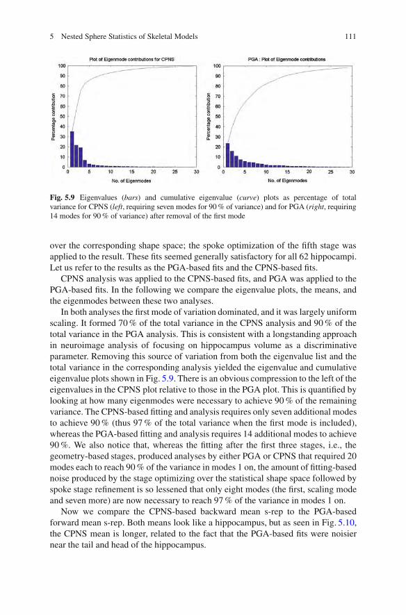
5 Nested Sphere Statistics of Skeletal Models 111
Fig. 5.9 Eigenvalues (bars) and cumulative eigenvalue (curve) plots as percentage of totalvariance for CPNS (left, requiring seven modes for 90 % of variance) and for PGA (right, requiring14 modes for 90 % of variance) after removal of the first mode
over the corresponding shape space; the spoke optimization of the fifth stage wasapplied to the result. These fits seemed generally satisfactory for all 62 hippocampi.Let us refer to the results as the PGA-based fits and the CPNS-based fits.
CPNS analysis was applied to the CPNS-based fits, and PGA was applied to thePGA-based fits. In the following we compare the eigenvalue plots, the means, andthe eigenmodes between these two analyses.
In both analyses the first mode of variation dominated, and it was largely uniformscaling. It formed 70 % of the total variance in the CPNS analysis and 90 % of thetotal variance in the PGA analysis. This is consistent with a longstanding approachin neuroimage analysis of focusing on hippocampus volume as a discriminativeparameter. Removing this source of variation from both the eigenvalue list and thetotal variance in the corresponding analysis yielded the eigenvalue and cumulativeeigenvalue plots shown in Fig. 5.9. There is an obvious compression to the left of theeigenvalues in the CPNS plot relative to those in the PGA plot. This is quantified bylooking at how many eigenmodes were necessary to achieve 90 % of the remainingvariance. The CPNS-based fitting and analysis requires only seven additional modesto achieve 90 % (thus 97 % of the total variance when the first mode is included),whereas the PGA-based fitting and analysis requires 14 additional modes to achieve90 %. We also notice that, whereas the fitting after the first three stages, i.e., thegeometry-based stages, produced analyses by either PGA or CPNS that required 20modes each to reach 90 % of the variance in modes 1 on, the amount of fitting-basednoise produced by the stage optimizing over the statistical shape space followed byspoke stage refinement is so lessened that only eight modes (the first, scaling modeand seven more) are now necessary to reach 97 % of the variance in modes 1 on.
Now we compare the CPNS-based backward mean s-rep to the PGA-basedforward mean s-rep. Both means look like a hippocampus, but as seen in Fig. 5.10,the CPNS mean is longer, related to the fact that the PGA-based fits were noisiernear the tail and head of the hippocampus.

112 S.M. Pizer et al.
Fig. 5.10 Impliedboundaries of CPNS (cyan)and PGA (yellow) means ofthe 62 left hippocampi ofnormal individuals
Finally, we compare the two analyses in terms of the shape changes shown bytheir eigenmodes. Because the contrast is too complex to show here, we summarizewhat we have observed. Beyond the first, largely scaling, eigenmode, none of thefollowing four eigenmodes from the PGA set qualitatively match any of the follow-ing four eigenmodes from the CPNS set, and vice versa. Roughly, the CPNS eigen-modes seem to capture more in the way of bendings and twistings, and the PGAeigenmodes seem to capture more in the way of rotations and small variations ineccentricity. We suggest that the reason is that CPNS by its design is more sensitiveto changes in local directions (e.g., of spokes), so, relative to PGA, its preliminaryshape space enables more efficient modeling of variations of that type. Moreover,its use in the final statistical analysis senses those variations more efficiently.
5.7 Extensions and Discussion
The method of composite principal nested spheres applies to any data that are bestanalyzed as a composite of components lying on spheres and possibly includingEuclidean components. The analyses of such data done so far have suggested thatCPNS can provide more efficient analysis (fewer eigenmodes), stabler s-rep fitting,and possibly more information about twisting and bending changes than PGA andother forward methods. We have seen that fitting a geometric model, here an s-rep,to object segmentations is significantly improved by the use of a shape space basedon CPNS-based analysis on preliminary fittings; the improvement is both in termsof quality of fit and in terms of making a second statistical analysis on the modelsinformative.
Shape analysis via CPNS extends beyond s-reps to essentially every other repre-sentation of shape. Shape inherently involves directions and curvatures (derivativeson directions). As a result, it can be expected that CPNS will provide similaradvantages when applied to other representations of shape. The following list somecandidate representations suitable for CPNS analysis.
5 Nested Sphere Statistics of Skeletal Models 113
• Point distribution models (PDMs), made of a large tuple of boundary (andpossibly other) points. On ten lung PDMs for ten phases of a patient’s respiration,CPNS required only required one to two eigenmodes vs. three for PCA. As withs-reps, CPNS required fewer modes than the forward method, here PCA.
• Point and normal distribution models: i.e., boundary point PDMs with a boundarynormal supplied with each point
• Quasi-tube s-reps• Branching objects• Multi-object complexes• Warps, i.e., displacement vector images or time-indexed velocity vector images
representing diffeomorphisms or other invertible deformations.• Fiber conglomerates, such as those studied by Savadjiev et al. [23].• Tensor images• Covariance matrices
The method of s-rep fitting followed by correspondence improvement andCPNS analysis requires a variety of improvements, listed in the following, togetherwith testing on many more shape populations. Once verified, it seems suitablefor applications in segmentation by posterior optimization [27, Chap. 9], hypothesistesting [29], and classification [25].
Improvements in s-rep fitting needed include spoke interpolations at the crestusing the Srad and SE matrices [11], fittings into multi-crest distance images, andgeneralization of entropy-based correspondence optimization [3] to spokes.
Acknowledgements We thank Jorn Schulz for studying the effects of global rotation, folding, andtwisting on skeletal spoke vectors; Martin Styner for the hippocampus data; and Anna Snyder forhelp with the references.
References
1. Arsigny, V., Commowick, O., Pennec, X., Ayache, N.: A log-Euclidean framework for statisticson diffeomorphisms. In: Medical Image Computing and Computer-Assisted Intervention,vol. 9, pp. 924–931. Springer, Berlin/Heidelberg (2006)
2. Blum, H.: A transformation for extracting new descriptors of shape. In: Wathen-Dunn, W. (ed.)Models for the Perception of Speech and Visual Form. MIT, Cambridge, MA (1967)
3. Cates, J., Fletcher, P.T., Styner, M.E., Shenton, R.T.W.: Shape modeling and analysis withentropy-based particle systems. Inf. Process. Med. Imaging 20, 333–345 (2007)
4. Cootes, T.F., Taylor, C., Cooper, D., Graham, J.: Training models of shape from sets ofexamples. In: Hogg, D., Boyle, R. (eds.) Proceedings of British Machine Vision Conference,pp. 9–18. Springer, Berlin (1992)
5. Cootes, T.F., Twining, C.J., Petrovic, V.S., Babalola, K.O., Taylor, C.J.: Computing accuratecorrespondences across groups of images. IEEE Trans. Pattern Anal. Mach. Intell. 32, 1994–2005 (2010)
6. Damon, J.: Smoothness and geometry of boundaries associated to skeletal structures I:sufficient conditions for smoothness. Ann. Inst. Fourier 53, 1001–1045 (2003)
114 S.M. Pizer et al.
7. Damon, J.: Swept regions and surfaces: modeling and volumetric properties. Conf. Computa-tional Alg. Geom. 2006, in honor of Andre Galligo. Spl. Issue Theor. Comp. Sci. 392, 66–91(2008)
8. Dryden, I.L., Mardia, K.V.: Statistical Shape Analysis. Wiley, Chichester (1998)9. Fletcher, P.T., Lu, C., Pizer, S.M., Joshi, S.: Principal geodesic analysis for the study of
nonlinear statistics of shape. IEEE Trans. Med. Imaging 23, 995–1005 (2004)10. Fletcher, P.T., Venkatasubramanian, S., Joshi, S.: The geometric median on Riemmanian
manifolds with application to robust atlas estimation. NeuroImage 45(1), S143–S152 (2009)11. Han, Q., Pizer, S.M., Damon, J.N.: Interpolation in discrete single figure medial objects. In:
Computer Vision and Pattern Recognition (CVPR) – Workshop on Mathematical Methods inBiomedical Image Analysis (MMBIA). IEEE Press (2006)
12. Huckemann, S., Ziezold, H.: Principal component analysis for Riemannian manifolds, with anapplication to triangular shape spaces. Adv. Appl. Probab. 38(2), 299–319 (2006)
13. Huckemann, S., Hotz, T., Munk, A.: Intrinsic shape analysis: geodesic PCA for Riemannianmanifolds modulo isometric lie group actions. Stat. Sin. 20(1), 1–58 (2010)
14. Jung, S., Liu, X., Marron, J.S., Pizer, S.M.: Generalized PCA via the backward stepwiseapproach in image analysis. In: Angeles, J. (ed.) Brain, Body and Machine: Proceedingsof an International Symposium on the 25th Anniversary of McGill University Centre forIntelligent Machines. Advances in Intelligent and Soft Computing, vol. 83, pp. 111–123.Springer, Berlin/Heidelberg (2010)
15. Jung, S., Dryden, I.L., Marron, J.S.: Analysis of principal nested spheres. Biometrika. 99(3),551–568 (2012)
16. Kendall, D.G., Barden, D., Carne, T.K., Le, H.: Shape and Shape Theory. Wiley, Chichester(1999)
17. Kurtek, S., Ding, Z., Klassen, E., Srivastava, A.: Parameterization-invariant shape statisticsand probabilistic classification of anatomical surfaces. Inf. Process. Med. Imaging 22, 147–158 (2011)
18. Leventon, M., Faugeras, O., Grimson, E., Kikinis, R., Wells, W.: Knowledge-based segmen-tation of medical images. In: Osher, S., Paragios, N. (eds.) Geometric Level Set Methods inImaging, Vision, and Graphics. Springer, New York (2003)
19. Merck, D., Tracton, G., Saboo, R., Levy, J., Chaney, E., Pizer, S.M., Joshi, S.: Training modelsof anatomic shape variability. Med. Phys. 35, 3584–3596 (2008)
20. Oguz, I., Cates, J., Fletcher, T., Whitaker, R., Cool, D., Aylward, S., Styner, M.: Entropy-basedparticle systems and local features for cortical correspondence optimization. In: Proceedingsof the IEEE International Symposium on Biomedical Imaging (ISBI), pp. 1637–1641. IEEEPress (2008)
21. Pennec, X.: Statistical computing on manifolds: from Riemannian geometry to computationalanatomy. Emerg. Trends Vis. Comput. 5416, 347–386 (2008)
22. Saboo, R., Niethammer, M., North, M., Pizer, S.M.: Anti-aliasing discretely sampledobject boundaries using fourth-order Laplacian of curvature flow. http://midag.cs.unc.edu/bibliography.html (2011). Accessed 3 Mar. 2012
23. Savadjiev, P., Campbell, J.S.W., Descoteaux, M., Deriche, R., Pike, G., Siddiqi, K.: Labelingof ambiguous sub-voxel fibre bundle configurations in high angular resolution diffusion MRI.NeuroImage 41(1), 58–68 (2008)
24. Schulz, J., Jung, S., Huckemann, S.: A collection of internal reports submitted to UNC-Gottingen study group on s-rep change under rotational transformations. University of NorthCarolina at Chapel Hill (2011)
25. Sen, S.K., Foskey, M., Marron, J.S., Styner, M.A.: Support vector machine for data onmanifolds: an application to image analysis. In: Proceedings of the IEEE InternationalSymposium on Biomedical Imaging (ISBI), pp. 1195–1198. IEEE Press (2008)
26. Shi, X., Styner, M., Lieberman, J., Ibrahim, J.G., Lin, W., Zhu, H.: Intrinsic regression modelsfor manifold-valued data. In: Medical Image Computing and Computer-Assisted Intervention,vol. 5762, pp. 192–199. Springer, Berlin/Heidelberg (2009)

5 Nested Sphere Statistics of Skeletal Models 115
27. Siddiqi, K., Pizer, S.: Medial Representations: Mathematics, Algorithms and Applications.Springer, Dordrecht (2008)
28. Sorensen, P., Lo, J., Petersen, A., Dirksen, A., de Bruijne, M.: Dissimilarity-based classificationof anatomical tree structures. Inf. Process. Med. Imaging 22, 475–485 (2011)
29. Terriberry, T., Joshi, S., Gerig, G.: Hypothesis testing with nonlinear shape models. Inf.Process. Med. Imaging 19, 15–26 (2005)
30. Wang, H., Marron, J.S.: Object oriented data analysis: sets of trees. Ann. Stat. 35(5), 1849–1873 (2007)
31. Yang, J., Staib, L., Duncan, J.: Neighbor-constrained segmentation with 3D deformablemodels. Inf. Process. Med. Imaging 18, 198–209 (2003)

Chapter 63D Curve Skeleton Computation and Usefor Discrete Shape Analysis
Gabriella Sanniti di Baja, Luca Serino, and Carlo Arcelli
Abstract A discrete 3D curve skeletonization algorithm is described, based oniterated voxel removal guided by the distance transform of the object and on anchorpoint selection. The criterion suggested for anchor point selection guarantees thatthe obtained curve skeleton reflects object’s shape quite well since it consists ofcurves symmetrically placed within the regions intuitively perceived as composingthe object. Then, the use of the curve skeleton for object decomposition in the frame-work of the structural approach to shape analysis is discussed. A suitable partitionof the skeleton is presented that originates object decomposition in accordance withhuman intuition.
6.1 Introduction
The skeleton of an object is a subset of the object with lower dimensionality,symmetrically placed within the object, characterized by the same topology asthe object, and reflecting the geometrical features of the object itself. In the caseof 3D objects, two different kinds of skeleton can be considered, namely thesurface skeleton, consisting of the union of surfaces and curves aligned alongthe principal symmetry planes and axes of the object, and the curve skeleton,exclusively consisting of curves aligned along the principal symmetry axes of theobject. Obviously, the curve skeleton can be computed only for objects rid ofcavities. In fact, to guarantee that the skeleton and the object have the same topology,a closed surface surrounding any cavity of the object should be present in theskeleton, which therefore would not be characterized by linear structure. Moreover,the curve skeleton should be used only to represent objects with the main symmetry
G. Sanniti di Baja (!) ! L. Serino ! C. ArcelliInstitute of Cybernetics “E. Caianiello”, CNR, Via Campi Flegrei 34,80078 Pozzuoli (Naples), Italye-mail: [email protected]; [email protected]; [email protected]
M. Breuß et al. (eds.), Innovations for Shape Analysis, Mathematics and Visualization,DOI 10.1007/978-3-642-34141-0 6, © Springer-Verlag Berlin Heidelberg 2013
117
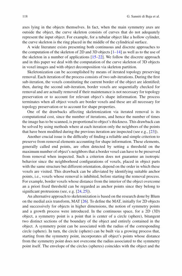
118 G. Sanniti di Baja et al.
axes lying in the objects themselves. In fact, when the main symmetry axes areoutside the object, the curve skeleton consists of curves that do not adequatelyrepresent the input object. For example, for a tubular object like a hollow cylinder,the curve skeleton is the ring placed in the middle of the cylindrical surface.
A wide literature exists presenting both continuous and discrete approaches tothe computation of the skeleton of 2D and 3D objects [1–14] as well as to the use ofthe skeleton in a number of applications [15–22]. We follow the discrete approachand in this paper we deal with the computation of the curve skeleton of 3D objectsin voxel images and with object decomposition via skeleton partition.
Skeletonization can be accomplished by means of iterated topology preservingremoval. Each iteration of the process consists of two sub-iterations. During the firstsub-iteration, the voxels constituting the current border of the object are identified;then, during the second sub-iteration, border voxels are sequentially checked forremoval and are actually removed if their maintenance is not necessary for topologypreservation or to account for relevant object’s shape information. The processterminates when all object voxels are border voxels and these are all necessary fortopology preservation or to account for shape properties.
One of the drawbacks affecting skeletonization via iterated removal is itscomputational cost, since the number of iterations, and hence the number of timesthe image has to be scanned, is proportional to object’s thickness. This drawback canbe solved by using methods where at each iteration only the neighbors of the pointsthat have been modified during the previous iteration are inspected (see e.g., [23]).
Another crucial issue is the difficulty of finding a reliable and simple criterion topreserve from removal elements accounting for shape information. These elements,generally called end points, are often detected by setting a threshold on themaximum number of object’s neighbors that a border voxel can have to be preservedfrom removal when inspected. Such a criterion does not guarantee an isotropicbehavior since the neighborhood configurations of voxels, placed in object partswith the same structure but different orientation, depend on the order in which thesevoxels are visited. This drawback can be alleviated by identifying suitable anchorpoints, i.e., voxels whose removal is inhibited, before starting the removal process.For example, border voxels whose distance from the interior of the object overcomean a priori fixed threshold can be regarded as anchor points since they belong tosignificant protrusions (see, e.g. [24, 25]).
An alternative approach to skeletonization is based on the research done by Blumon the medial axis transform, MAT [26]. To define the MAT, initially for 2D objectsand successively for objects in higher dimensions, the notion of symmetry pointsand a growth process were introduced. In the continuous space, for a 2D (3D)object, a symmetry point is a point that is center of a circle (sphere), bitangenttwo distinct sections of the boundary of the object and entirely contained in theobject. A symmetry point can be associated with the radius of the correspondingcircle (sphere). In turn, the circle (sphere) can be built via a growing process that,starting from the symmetry point, incorporates all object’s points whose distancefrom the symmetry point does not overcome the radius associated to the symmetrypoint itself. The envelope of the circles (spheres) coincides with the object and the

6 3D Curve Skeleton Computation and Use for Discrete Shape Analysis 119
MAT is the locus of the centers, associated with the corresponding radii. Blum alsostudied the geometric properties of the MAT and showed the usefulness of the MATfor shape analysis [27].
MAT computation is rather heavy, especially in 3D, so that it is of interest askeletonization method based on the computation of a reasonably good approxima-tion of the MAT. A possible solution in the discrete space is to resort to the useof the distance transform of the object X , DT.X/, and to the selection of the setof centers of maximal balls, CMB.X/. In fact, DT.X/ is a multi-valued replica ofthe object, where each voxel of the object is assigned the value of its distance fromthe boundary. Thus, each object voxel in DT.X/ can be interpreted as the centerof a ball with radius equal to the distance value of the voxel itself and touchingthe object boundary. As the name suggests, a voxel of CMB.X/ is a voxel whoseassociated ball is maximal, i.e., is not included by any other single ball, touches theobject boundary in at least two different parts, and is obviously totally included inthe object. Moreover, the union of all the maximal balls coincides with the object.This indicates that CMB.X/ consists of symmetry points and constitutes a discreteapproximation of the MAT.
As we will see in more detail in the following sections, the set CMB.X/ doesnot satisfy all the properties expected for the skeleton. We note that, except forthe case of 3D objects having tubular shape, voxels of CMB.X/ do concentratealong symmetry planes rather than along symmetry axes, so that not all voxelsof CMB.X/ are of interest for curve skeletonization. Moreover, CMB.X/ is notnecessarily characterized by the same topology as the represented object. Thus, onone side skeletonization needs to accept as skeleton elements other voxels besidesthose of CMB.X/ in order to obtain a topologically correct result. On the other side,skeletonization should not accept all voxels of CMB.X/ as skeleton voxels so as tooriginate a skeleton with a linear structure easy to manage and still able to representthe object sufficiently well. Of course, accepting only a subset of CMB.X/ in theskeleton also means that the union of the balls associated with the voxels of theskeleton does not coincide with the object itself.
Actually, the voxels of CMB.X/ are generally not all equally important. Forexample, a number of voxels of CMB.X/ do not carry shape information, sincethey are due only to the discrete nature of the digital space. In this respect, letus consider a cylinder with its main axis oriented along one of the three axes ina Cartesian coordinate system. In the continuous space, sections of the cylinderperpendicular to such an axis are circles and, for sections sufficiently far apart fromthe bases of the cylinder, the distance transform appears as consisting of concentriccircular wave-fronts, each including points with the same distance value. For eachof these sections only one center of maximal ball exists, which is the symmetrypoint placed along the main symmetry axis of the cylinder. In the digital space,the circular sections of the cylinder are unavoidably transformed into polygonalshapes and the distance transform appears as due to the propagation of a polygonalwave-front. Since voxels of CMB.X/ are located where the wave-front folds uponitself, besides the centers of maximal balls along the main axis, also other centersof maximal balls are detected. These are due to the existence of weak convexities

120 G. Sanniti di Baja et al.
in correspondence with the vertices of the polygonal wave-front. This fact causesfolding of the wave-front upon itself.
More in general, voxels of CMB.X/ can be found in correspondence of objectparts characterized by different properties, not all equally important for the specifictask. Thus, it is profitable to devise criteria to select an appropriate subset ofCMB.X/, depending on the object properties of interest for the task at hand [28].Once suitable criteria to filter out irrelevant centers of maximal balls are used, thenthe surviving voxels of CMB.X/ can be taken as anchor points and skeletonizationcan be accomplished by using iterated voxel removal to guarantee a topologicallycorrect result.
In this paper, we describe a skeletonization method based on the selection ofanchor points in the distance transform and on iterated voxel removal. Besides usingthe distance transform to identify the subset of CMB.X/ whose voxels are taken asanchor points, we also exploit it to strongly reduce the computational cost of iteratedvoxel removal. In fact, we avoid repeated inspections of the image by directlyaccessing in increasing distance value order the voxels that undergo removal. Thecurve skeleton CS of an object X is computed in two phases.
During the first phase, the Pseudo Surface Skeleton PSS is detected by followingthe strategy suggested in [14]. The set PSS is a subset of X and is used as inputto the second phase. To obtain PSS, the distance transform of X is computed andsuitable centers of maximal balls are taken as anchor points. Topology preservingremoval operations are then applied to object voxels that are not anchor points toget an at most two-voxel thick set. Final thinning is performed to gain unit thicknessand pruning of peripheral lines is done for trimming out negligible details.
During the second phase, a classification of the voxels of PSS into curve, internal,junction, extended junction, branching and edge voxels is done. The distancetransform of PSS is then computed. Voxels that are classified as branching orjunction voxels, and centers of maximal balls of PSS are taken as anchor points.Topology preserving removal operations are then applied to reduce PSS to an atmost two-voxel thick set of curves. Final thinning and pruning complete the secondcurve skeletonization phase.
Though the union of the balls associated with the voxels of the curve skeletongenerally provides only a rough version of the input object, the curve skeleton is ofinterest in the framework of the structural approach to object analysis to reduce thecomplexity of the recognition task. In particular, the skeleton can be used for objectdecomposition (see e.g., [29–32]).
As discussed in [33–36], the human visual system is likely to represent objectswith complex shape in terms of simpler parts, by decomposing the objects into partsand by organizing object representation in terms of the parts and of their spatialrelationships. Such a structured representation is characterized by a significantlygreater robustness under changes in viewing conditions.
Decomposition guided by skeleton partition has been followed particularly forobjects than can be perceived as articulated in parts with tubular shape, where a one-to-one correspondence exists between the individual curves composing the skeletonand the individual parts of the object. In this case, the object can be interpreted as
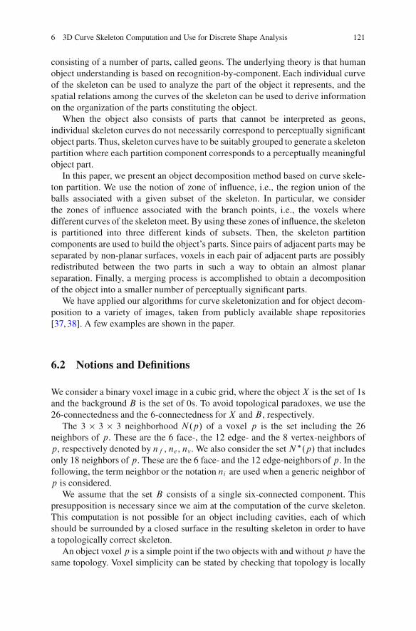
6 3D Curve Skeleton Computation and Use for Discrete Shape Analysis 121
consisting of a number of parts, called geons. The underlying theory is that humanobject understanding is based on recognition-by-component. Each individual curveof the skeleton can be used to analyze the part of the object it represents, and thespatial relations among the curves of the skeleton can be used to derive informationon the organization of the parts constituting the object.
When the object also consists of parts that cannot be interpreted as geons,individual skeleton curves do not necessarily correspond to perceptually significantobject parts. Thus, skeleton curves have to be suitably grouped to generate a skeletonpartition where each partition component corresponds to a perceptually meaningfulobject part.
In this paper, we present an object decomposition method based on curve skele-ton partition. We use the notion of zone of influence, i.e., the region union of theballs associated with a given subset of the skeleton. In particular, we considerthe zones of influence associated with the branch points, i.e., the voxels wheredifferent curves of the skeleton meet. By using these zones of influence, the skeletonis partitioned into three different kinds of subsets. Then, the skeleton partitioncomponents are used to build the object’s parts. Since pairs of adjacent parts may beseparated by non-planar surfaces, voxels in each pair of adjacent parts are possiblyredistributed between the two parts in such a way to obtain an almost planarseparation. Finally, a merging process is accomplished to obtain a decompositionof the object into a smaller number of perceptually significant parts.
We have applied our algorithms for curve skeletonization and for object decom-position to a variety of images, taken from publicly available shape repositories[37, 38]. A few examples are shown in the paper.
6.2 Notions and Definitions
We consider a binary voxel image in a cubic grid, where the objectX is the set of 1sand the background B is the set of 0s. To avoid topological paradoxes, we use the26-connectedness and the 6-connectedness for X and B , respectively.
The 3 ! 3 ! 3 neighborhood N.p/ of a voxel p is the set including the 26neighbors of p. These are the 6 face-, the 12 edge- and the 8 vertex-neighbors ofp, respectively denoted by nf , ne , nv. We also consider the set N ".p/ that includesonly 18 neighbors of p. These are the 6 face- and the 12 edge-neighbors of p. In thefollowing, the term neighbor or the notation ni are used when a generic neighbor ofp is considered.
We assume that the set B consists of a single six-connected component. Thispresupposition is necessary since we aim at the computation of the curve skeleton.This computation is not possible for an object including cavities, each of whichshould be surrounded by a closed surface in the resulting skeleton in order to havea topologically correct skeleton.
An object voxel p is a simple point if the two objects with and without p have thesame topology. Voxel simplicity can be stated by checking that topology is locally
122 G. Sanniti di Baja et al.
preserved. Thus, if we denote by cp the number of 26-connected object componentsin N.p/, and by c"p the number of six-connected background components having pas face-neighbor and computed inN ".p/, a voxel p is simple if cp D 1 and c"p D 1[39, 40].
A path linking two voxels p and q is a sequence of unit moves from p to qthrough voxels that are face-, edge- or vertex-neighbors of each other. To give areasonably good approximation of the Euclidean length of the path, the unit movestowards face- edge- and vertex-neighbors encountered along the path should bemeasured by different weights, suitably taking into account the different Euclideanlengths of these moves. The integer weights wf D 3, weD 4 and wvD 5 are adequateto provide a good approximation of the length of the path [41].
Though efficient algorithms exist to compute the Euclidean distance between twovoxels p and q (e.g., see [42]), when following discrete approaches, the distancebetween p and q is preferably defined as the length of a shortest path linking pto q [43]. In this work, we resort to the use of the h3; 4; 5i weighted distance thatcombines the simplicity of path-based distances with a reasonable approximationto the Euclidean distance. The main reason for preferring a path-based distance tothe true Euclidean distance is that with the former metric strong constraints existon the distance values that are possible for neighboring voxels, which will allow usto devise easily local operations for various tasks, e.g., for center of maximal balldetection.
The curve skeleton CS of a 3D object X is a set union of curves, symmetricallyplaced within X , with the same topology of X and reflecting the main geometricalfeatures of X . CS may be two-voxel thick at the intersection of curves. A voxelp of the skeleton is an end point when it has only one neighboring skeleton voxelin N.p/. A voxel p of the skeleton is a branch point when it has more than twoneighboring skeleton voxels in N.p/.
6.2.1 Distance Transform
The distance transform DT.X/ is a labeled replica of an objectX , where each voxelp of X is labeled with the length of a shortest path, entirely consisting of voxels ofX , connecting p to the boundary ofX . In the following, we will denote by d.p/ thedistance value of p in DT.X/.
DT.X/ can be interpreted as due to a local propagation process from theboundary of X towards the innermost part of X . During propagation, each internalvoxel p of X receives distance information from those of its neighbors that arecloser to the boundary than p, and propagates distance information to its objectneighbors that are farther than p from the boundary.
The object boundary is composed by the object voxels delimiting the object itself.For an object consisting of three-dimensional manifolds, the boundary is a set unionof closed surfaces that in the discrete space includes all and only the object’s voxelswith at least a face-neighbor in the background, while the internal voxels are the
6 3D Curve Skeleton Computation and Use for Discrete Shape Analysis 123
object’s voxels having no face-neighbors in B . In turn, when X consists of two-dimensional manifolds, its boundary will be a set union of curves. To identify theboundary ofX in this latter case, we need to classify the voxels ofX . To this aim, weuse a modified version of the classification scheme introduced in [14] and classifyas follows the voxels of an object X consisting exclusively of intersecting surfacesand curves:
• An object voxel with at most two disjoint object neighbors is a curve voxel.• A not yet classified object voxel with a neighboring curve voxel is a branching
voxel.• A not yet classified voxelp is a branching voxel if cp¤ 1 andp has a neighboring
branching voxel, or if the object neighbors of p are all branching voxels.• An object voxel p with c"p ¤ 1 is an internal voxel.• An internal voxel p with more than two 6-connected components of background
voxels in N.p/ face- or edge-adjacent to p, or being any of the eight internalvoxels in a 2 ! 2 ! 2 configuration is re-classified as junction voxel.
• An internal voxel having a face- or an edge-neighbor classified as junction voxel,is re-classified as extended junction voxel.
• Any other object voxel is an edge voxel.
The boundary of a set X consisting exclusively of intersecting surfaces andcurves, is the set of edge voxels, branching voxels and curve voxels. Branchingvoxels and junction voxels are the voxels where curves and surfaces intersectand will act as barriers to the propagation of distance information. Extendedjunction voxels are internal voxels playing also the role of junction voxels inpresence of intersecting surfaces, where voxels of a surface have edge-neighbors inanother surface. Differently from the junction voxels, which will neither receive norpropagate distance information, the extended junction voxels are allowed to receive,but are not allowed to propagate, this information to their neighbors. Due to thepresence of barriers, voxels internal in one of the surfaces constitutingX will receivedistance information exclusively from the edge voxels delimiting that surface.
The above classification allows us also to distinguish peripheral and internalsurfaces. The first are surfaces at least partially delimited by edge voxels, the latterare completely surrounded by junction voxels.
For the computation of DT.X/, boundary voxels are assigned the minimaldistance value, which is equal to 3 when using the h3; 4; 5i weighted distance.Distance information is then propagated to the internal voxels of X . If X consistsof three-dimensional manifolds, DT.X/ can be computed by means of the standardtwo-scan algorithm [41]. When X consists exclusively of surfaces and curves, anordered propagation algorithm, e.g., [44], is more convenient due to the presence ofjunction voxels and branching voxels acting as barriers to the propagation.
For the sake of clarity, we point out that when X consists exclusively of surfacesand curves, more than one application of distance transformation may be necessaryto obtain the complete DT.X/. In fact, the internal voxels belonging to internalsurfaces cannot be reached by the distance information propagated from theboundary, due to the role of barriers played by the junction voxels and by the
124 G. Sanniti di Baja et al.
extended junction voxels. To assign distance values also to the internal voxels ofinternal surfaces, we change the status of some particular junction voxels into thatof delimiting junction voxels. These particular voxels are the junction voxels havingboth neighboring voxels already reached by the propagated distance information,and neighboring extended junction voxels not yet labeled with distance value. Thedelimiting junction voxels are taken as constituting a new set of boundary voxelsfrom which to compute the distance transform for internal surfaces. The extendedjunction voxels that are neighbors of delimiting junction voxels change their statusinto that of internal voxels. To guarantee some continuity in distance values, thedelimiting junction voxels are assigned a value related to the maximum distancevalue, max, assigned during the previous application of distance transformation.Namely, delimiting junction voxels are set to maxC wv.
6.2.2 Centers of Maximal Balls and Anchor Points
Any voxel p in the distance transform can be interpreted as the center of a ball withradius d.p/. The ball associated to p can be constructed by applying to p the reversedistance transformation [45].
A center of maximal ball is any voxel p whose associated ball is included in theobject, but is not included by any other single ball in the object. The set of centersof maximal balls, CMB.X/, is computed by comparing the distance value d.p/ ofeach p of X , with the distance values of the neighbors of p, by taking into accountthe weights wf , we and wv [46]. In detail, p is a center of maximal ball if for eachof its neighbors ni there results
d.ni /" d.p/ < wi (6.1)
We note that the distance value 3 must be replaced by the equivalent value 1 beforedetecting the centers of maximal balls. In fact, balls with radii 3 and 1 are identicaland replacement of 3 by 1 is necessary to avoid the erroneous detection as center ofmaximal ball of a voxel whose associated ball is not maximal (see [1] Chap. 5, fordetails on the equivalent values).
We also note that when X exclusively consists of surfaces and curves, ratherthan talking of balls we should more correctly talk of geodesic discs. The geodesicdisc associated with a voxel p of X can be obtained by considering the intersectionbetween X and the ball associated to p by the reverse distance transformation. Ifthe intersection consists of more than one connected component, the geodesic discassociated to p is the component that includes p.
In principle, at least during the first phase of skeletonization, we should take asanchor points all centers of maximal balls of X since they are symmetry points.However, we are aware that the curve skeleton ofX could include almost all centersonly when X is composed by parts with tubular shape. Moreover, if all centersare taken as anchor points, the structure of the set resulting at the end of the first
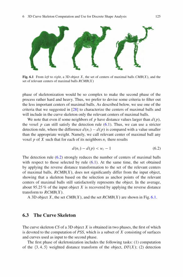
6 3D Curve Skeleton Computation and Use for Discrete Shape Analysis 125
Fig. 6.1 From left to right, a 3D object X , the set of centers of maximal balls CMB.X/, and theset of relevant centers of maximal balls RCMB.X/
phase of skeletonization would be so complex to make the second phase of theprocess rather hard and heavy. Thus, we prefer to devise some criteria to filter outthe less important centers of maximal balls. As described below, we use one of thecriteria that we suggested in [28] to characterize the centers of maximal balls andwill include in the curve skeleton only the relevant centers of maximal balls.
We note that even if some neighbors of p have distance values larger than d.p/,the voxel p can still satisfy the detection rule (6.1). Thus, we can use a stricterdetection rule, where the difference d.ni / " d.p/ is compared with a value smallerthan the appropriate weight. Namely, we call relevant center of maximal ball anyvoxel p of X such that for each of its neighbors ni there results
d.ni /" d.p/ < wi " 1 (6.2)
The detection rule (6.2) strongly reduces the number of centers of maximal ballswith respect to those selected by rule (6.1). At the same time, the set obtainedby applying the reverse distance transformation to the set of the relevant centersof maximal balls, RCMB.X/, does not significantly differ from the input object,showing that a skeleton based on the selection as anchor points of the relevantcenters of maximal balls still satisfactorily represents the object. In the average,about 95:25% of the input object X is recovered by applying the reverse distancetransform to RCMB.X/.
A 3D object X , the set CMB.X/, and the set RCMB.X/ are shown in Fig. 6.1.
6.3 The Curve Skeleton
The curve skeleton CS of a 3D objectX is obtained in two phases, the first of whichis devoted to the computation of PSS, which is a subset of X consisting of surfacesand curves used as input to the second phase.
The first phase of skeletonization includes the following tasks: (1) computationof the h3; 4; 5i weighted distance transform of the object, DT.X/; (2) detection
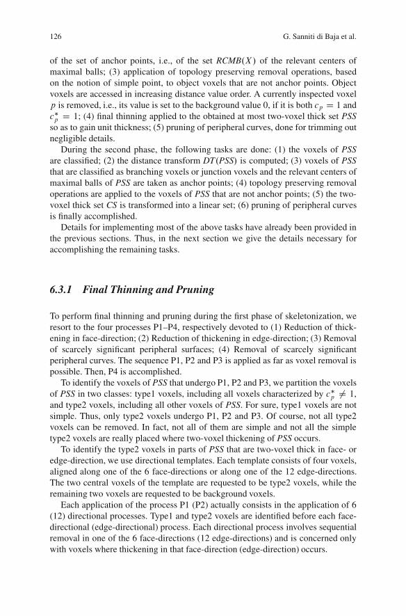
126 G. Sanniti di Baja et al.
of the set of anchor points, i.e., of the set RCMB.X/ of the relevant centers ofmaximal balls; (3) application of topology preserving removal operations, basedon the notion of simple point, to object voxels that are not anchor points. Objectvoxels are accessed in increasing distance value order. A currently inspected voxelp is removed, i.e., its value is set to the background value 0, if it is both cp D 1 andc"p D 1; (4) final thinning applied to the obtained at most two-voxel thick set PSSso as to gain unit thickness; (5) pruning of peripheral curves, done for trimming outnegligible details.
During the second phase, the following tasks are done: (1) the voxels of PSSare classified; (2) the distance transform DT.PSS/ is computed; (3) voxels of PSSthat are classified as branching voxels or junction voxels and the relevant centers ofmaximal balls of PSS are taken as anchor points; (4) topology preserving removaloperations are applied to the voxels of PSS that are not anchor points; (5) the two-voxel thick set CS is transformed into a linear set; (6) pruning of peripheral curvesis finally accomplished.
Details for implementing most of the above tasks have already been provided inthe previous sections. Thus, in the next section we give the details necessary foraccomplishing the remaining tasks.
6.3.1 Final Thinning and Pruning
To perform final thinning and pruning during the first phase of skeletonization, weresort to the four processes P1–P4, respectively devoted to (1) Reduction of thick-ening in face-direction; (2) Reduction of thickening in edge-direction; (3) Removalof scarcely significant peripheral surfaces; (4) Removal of scarcely significantperipheral curves. The sequence P1, P2 and P3 is applied as far as voxel removal ispossible. Then, P4 is accomplished.
To identify the voxels of PSS that undergo P1, P2 and P3, we partition the voxelsof PSS in two classes: type1 voxels, including all voxels characterized by c"p ¤ 1,and type2 voxels, including all other voxels of PSS. For sure, type1 voxels are notsimple. Thus, only type2 voxels undergo P1, P2 and P3. Of course, not all type2voxels can be removed. In fact, not all of them are simple and not all the simpletype2 voxels are really placed where two-voxel thickening of PSS occurs.
To identify the type2 voxels in parts of PSS that are two-voxel thick in face- oredge-direction, we use directional templates. Each template consists of four voxels,aligned along one of the 6 face-directions or along one of the 12 edge-directions.The two central voxels of the template are requested to be type2 voxels, while theremaining two voxels are requested to be background voxels.
Each application of the process P1 (P2) actually consists in the application of 6(12) directional processes. Type1 and type2 voxels are identified before each face-directional (edge-directional) process. Each directional process involves sequentialremoval in one of the 6 face-directions (12 edge-directions) and is concerned onlywith voxels where thickening in that face-direction (edge-direction) occurs.
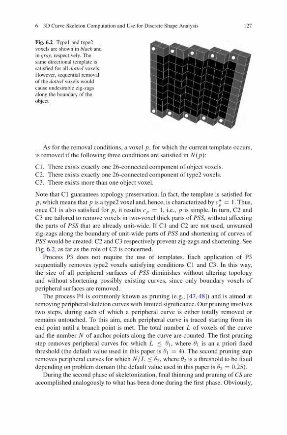
6 3D Curve Skeleton Computation and Use for Discrete Shape Analysis 127
Fig. 6.2 Type1 and type2voxels are shown in black andin gray, respectively. Thesame directional template issatisfied for all dotted voxels.However, sequential removalof the dotted voxels wouldcause undesirable zig-zagsalong the boundary of theobject
As for the removal conditions, a voxel p, for which the current template occurs,is removed if the following three conditions are satisfied in N.p/:
C1. There exists exactly one 26-connected component of object voxels.C2. There exists exactly one 26-connected component of type2 voxels.C3. There exists more than one object voxel.
Note that C1 guarantees topology preservation. In fact, the template is satisfied forp, which means that p is a type2 voxel and, hence, is characterized by c"p D 1. Thus,once C1 is also satisfied for p, it results cp D 1, i.e., p is simple. In turn, C2 andC3 are tailored to remove voxels in two-voxel thick parts of PSS, without affectingthe parts of PSS that are already unit-wide. If C1 and C2 are not used, unwantedzig-zags along the boundary of unit-wide parts of PSS and shortening of curves ofPSS would be created. C2 and C3 respectively prevent zig-zags and shortening. SeeFig. 6.2, as far as the role of C2 is concerned.
Process P3 does not require the use of templates. Each application of P3sequentially removes type2 voxels satisfying conditions C1 and C3. In this way,the size of all peripheral surfaces of PSS diminishes without altering topologyand without shortening possibly existing curves, since only boundary voxels ofperipheral surfaces are removed.
The process P4 is commonly known as pruning (e.g., [47, 48]) and is aimed atremoving peripheral skeleton curves with limited significance. Our pruning involvestwo steps, during each of which a peripheral curve is either totally removed orremains untouched. To this aim, each peripheral curve is traced starting from itsend point until a branch point is met. The total number L of voxels of the curveand the number N of anchor points along the curve are counted. The first pruningstep removes peripheral curves for which L # !1, where !1 is an a priori fixedthreshold (the default value used in this paper is !1 D 4). The second pruning stepremoves peripheral curves for which N=L # !2, where !2 is a threshold to be fixeddepending on problem domain (the default value used in this paper is !2 D 0:25).
During the second phase of skeletonization, final thinning and pruning of CS areaccomplished analogously to what has been done during the first phase. Obviously,
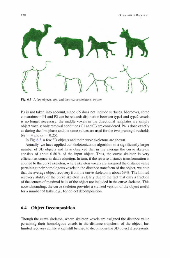
128 G. Sanniti di Baja et al.
Fig. 6.3 A few objects, top, and their curve skeletons, bottom
P3 is not taken into account, since CS does not include surfaces. Moreover, someconstraints in P1 and P2 can be relaxed: distinction between type1 and type2 voxelsis no longer necessary; the middle voxels in the directional templates are simplyobject voxels; only removal conditions C1 and C3 are considered. P4 is done exactlyas during the first phase and the same values are used for the two pruning thresholds(!1 D 4 and !2 D 0:25).
In Fig. 6.3, a few 3D objects and their curve skeletons are shown.Actually, we have applied our skeletonization algorithm to a significantly larger
number of 3D objects and have observed that in the average the curve skeletonconsists of about 0:80% of the input object. Thus, the curve skeleton is veryefficient as concerns data reduction. In turn, if the reverse distance transformation isapplied to the curve skeleton, where skeleton voxels are assigned the distance valuepertaining their homologous voxels in the distance transform of the object, we notethat the average object recovery from the curve skeleton is about 69%. The limitedrecovery ability of the curve skeleton is clearly due to the fact that only a fractionof the centers of maximal balls of the object are included in the curve skeleton. Thisnotwithstanding, the curve skeleton provides a stylized version of the object usefulfor a number of tasks, e.g., for object decomposition.
6.4 Object Decomposition
Though the curve skeleton, where skeleton voxels are assigned the distance valuepertaining their homologous voxels in the distance transform of the object, haslimited recovery ability, it can still be used to decompose the 3D object it represents.
6 3D Curve Skeleton Computation and Use for Discrete Shape Analysis 129
To this aim, we first partition the curve skeleton into three types of subsets, that wecall simple curves, complex sets, and single points. Then, we recover the object partsassociated to the skeleton parts. The recovered object parts are respectively calledsimple regions, bumps and kernels. Kernels can be interpreted as a sort of mainbodies of the object, from which simple regions and bumps protrude. Finally, weperform a merging process, aimed at reducing the number of object regions to theperceptually most relevant ones.
6.4.1 Skeleton Partition
To partition the curve skeleton, we apply the reverse distance transformation tothe branch points. As a result, we obtain a number of regions, that we call zonesof influence, which is at most equal to the number of branch points. Actually, thenumber of zones of influence is generally smaller than the number of branch points.In fact, the balls associated to branch points that are neighbors of each other or arecloser to each other than the sum of the corresponding radii overlap and merge intoa single connected component.
The simple curves of the partition are constituted by the connected componentsof skeletal voxels that are not included in any zone of influence. The single pointsof the partition, if any, are constituted by the end points of the skeleton that resultto be included in zones of influence. When single points exist in the partition, theskeleton branches that can be traced from each of the corresponding end pointsuntil a branch point is encountered are called linking branches. Finally, the complexsets of the partition are constituted by the connected components of all the skeletalvoxels included in the zones of influence, except for the end points.
Figure 6.4 shows the partition into simple curves, single points and complex setsfor the skeletons of the test objects.
6.4.2 Simple Regions, Bumps and Kernels
The construction of the simple regions, bumps and kernels into which the object canbe seen as decomposed requires four steps.
During the first step, the reverse distance transformation is applied to eachindividual skeleton partition component, by taking into account the following issues:(i) voxels that can be recovered from more than one individual partition componentare assigned to the kernel they are closer to, so as to originate a decomposition intodisjoint regions; (ii) linking branches do not take part in recovery, i.e., the reversedistance transformation is not applied to the linking branches. In fact, if a linkingbranch contributes, together with the other branches in a complex set, to the recoveryof the corresponding kernel, the bump protruding from that kernel is characterizedby a very small volume and the perceptual relevance of the bump is not enhanced.
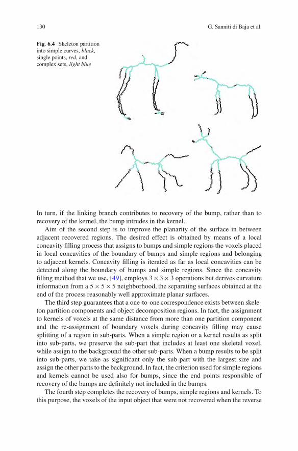
130 G. Sanniti di Baja et al.
Fig. 6.4 Skeleton partitioninto simple curves, black,single points, red, andcomplex sets, light blue
In turn, if the linking branch contributes to recovery of the bump, rather than torecovery of the kernel, the bump intrudes in the kernel.
Aim of the second step is to improve the planarity of the surface in betweenadjacent recovered regions. The desired effect is obtained by means of a localconcavity filling process that assigns to bumps and simple regions the voxels placedin local concavities of the boundary of bumps and simple regions and belongingto adjacent kernels. Concavity filling is iterated as far as local concavities can bedetected along the boundary of bumps and simple regions. Since the concavityfilling method that we use, [49], employs 3! 3! 3 operations but derives curvatureinformation from a 5 ! 5 ! 5 neighborhood, the separating surfaces obtained at theend of the process reasonably well approximate planar surfaces.
The third step guarantees that a one-to-one correspondence exists between skele-ton partition components and object decomposition regions. In fact, the assignmentto kernels of voxels at the same distance from more than one partition componentand the re-assignment of boundary voxels during concavity filling may causesplitting of a region in sub-parts. When a simple region or a kernel results as splitinto sub-parts, we preserve the sub-part that includes at least one skeletal voxel,while assign to the background the other sub-parts. When a bump results to be splitinto sub-parts, we take as significant only the sub-part with the largest size andassign the other parts to the background. In fact, the criterion used for simple regionsand kernels cannot be used also for bumps, since the end points responsible ofrecovery of the bumps are definitely not included in the bumps.
The fourth step completes the recovery of bumps, simple regions and kernels. Tothis purpose, the voxels of the input object that were not recovered when the reverse
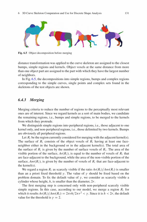
6 3D Curve Skeleton Computation and Use for Discrete Shape Analysis 131
Fig. 6.5 Object decomposition before merging
distance transformation was applied to the curve skeleton are assigned to the closestbumps, simple regions and kernels. Object voxels at the same distance from morethan one object part are assigned to the part with which they have the largest numberof neighbors.
In Fig. 6.5, the decompositions into simple regions, bumps and complex regionscorresponding to the simple curves, single points and complex sets found in theskeletons of the test objects are shown.
6.4.3 Merging
Merging criteria to reduce the number of regions to the perceptually most relevantones are of interest. Since we regard kernels as a sort of main bodies, we candidatethe remaining regions, i.e., bumps and simple regions, to be merged to the kernelsfrom which they protrude.
We distinguish simple regions into peripheral regions, i.e., those adjacent to onekernel only, and non-peripheral regions, i.e., those delimited by two kernels. Bumpsare obviously all peripheral regions.
LetRi be the region currently considered for merging with the adjacent kernel(s).The surface of Ri consists of the object voxels of Ri having at least one face-neighbor either in the background or in the adjacent kernel(s). The total area ofthe surface of Ri is given by the number of surface voxels of Ri . The area of thevisible portion of the surface, Av.Ri /, is equal to the number of voxels of Ri thatare face-adjacent to the background, while the area of the non-visible portion of thesurface, Anv.Ri /, is given by the number of voxels of Ri that are face-adjacent tothe kernel(s).
We regard a region Ri as scarcely visible if the ratio Av.Ri /=Anv.Ri / is smallerthan an a priori fixed threshold " . The value of " should be fixed based on theproblem domain. To fix the default value of " , we consider as scarcely visible acylinder whose height, h, is smaller than the diameter, 2r .
The first merging step is concerned only with non-peripheral scarcely visiblesimple regions. In this case, according to our model, we merge a region Ri forwhich it results Av.Ri /=Anv.Ri / D 2#rh=2#r2 < " . Since it is h < 2r , the defaultvalue for the threshold is " D 2.
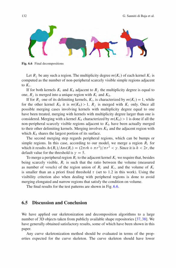
132 G. Sanniti di Baja et al.
Fig. 6.6 Final decompositions
Let Rj be any such a region. The multiplicity degreem.Ki/ of each kernelKi iscomputed as the number of non-peripheral scarcely visible simple regions adjacentto Ki .
If for both kernels Ki and Kh adjacent to Rj the multiplicity degree is equal toone, Rj is merged into a unique region with Ki and Kh.
If for Rj one of its delimiting kernels, Ki , is characterized by m.Ki/D 1, whilefor the other kernel Kh it is m.Kh/>1, Rj is merged with Ki only. Once allpossible merging cases involving kernels with multiplicity degree equal to onehave been treated, merging with kernels with multiplicity degree larger than one isconsidered. Merging with a kernelKh characterized by m.Kh/> 1 is done if all thenon-peripheral scarcely visible regions adjacent to Kh have been actually mergedto their other delimiting kernels. Merging involvesKh and the adjacent region withwhichKh shares the largest portion of its surface.
The second merging step regards peripheral regions, which can be bumps orsimple regions. In this case, according to our model, we merge a region Ri forwhich it results Av.Ri /=Anv.Ri / D .2#rhC#r2/=#r2 < " . Since it is h < 2r , thedefault value for the threshold is " D 5.
To merge a peripheral regionRi to the adjacent kernelKi we require that, besidesbeing scarcely visible, Ri is such that the ratio between the volume (measuredas number of voxels) of the region union of Ri and Ki , and the volume of Ki
is smaller than an a priori fixed threshold $ (set to 1:2 in this work). Using thevisibility criterion also when dealing with peripheral regions is done to avoidmerging elongated and narrow regions that satisfy the condition on volume.
The final results for the test patterns are shown in Fig. 6.6.
6.5 Discussion and Conclusion
We have applied our skeletonization and decomposition algorithms to a largenumber of 3D objects taken from publicly available shape repositories [37, 38]. Wehave generally obtained satisfactory results, some of which have been shown in thispaper.
Any curve skeletonization method should be evaluated in terms of the prop-erties expected for the curve skeleton. The curve skeleton should have lower
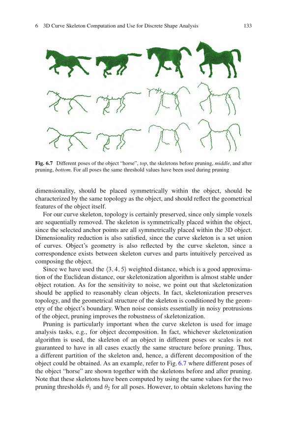
6 3D Curve Skeleton Computation and Use for Discrete Shape Analysis 133
Fig. 6.7 Different poses of the object “horse”, top, the skeletons before pruning, middle, and afterpruning, bottom. For all poses the same threshold values have been used during pruning
dimensionality, should be placed symmetrically within the object, should becharacterized by the same topology as the object, and should reflect the geometricalfeatures of the object itself.
For our curve skeleton, topology is certainly preserved, since only simple voxelsare sequentially removed. The skeleton is symmetrically placed within the object,since the selected anchor points are all symmetrically placed within the 3D object.Dimensionality reduction is also satisfied, since the curve skeleton is a set unionof curves. Object’s geometry is also reflected by the curve skeleton, since acorrespondence exists between skeleton curves and parts intuitively perceived ascomposing the object.
Since we have used the h3; 4; 5i weighted distance, which is a good approxima-tion of the Euclidean distance, our skeletonization algorithm is almost stable underobject rotation. As for the sensitivity to noise, we point out that skeletonizationshould be applied to reasonably clean objects. In fact, skeletonization preservestopology, and the geometrical structure of the skeleton is conditioned by the geom-etry of the object’s boundary. When noise consists essentially in noisy protrusionsof the object, pruning improves the robustness of skeletonization.
Pruning is particularly important when the curve skeleton is used for imageanalysis tasks, e.g., for object decomposition. In fact, whichever skeletonizationalgorithm is used, the skeleton of an object in different poses or scales is notguaranteed to have in all cases exactly the same structure before pruning. Thus,a different partition of the skeleton and, hence, a different decomposition of theobject could be obtained. As an example, refer to Fig. 6.7 where different poses ofthe object “horse” are shown together with the skeletons before and after pruning.Note that these skeletons have been computed by using the same values for the twopruning thresholds !1 and !2 for all poses. However, to obtain skeletons having the

134 G. Sanniti di Baja et al.
Fig. 6.8 Decomposition for different poses of “horse” before merging, top, and after merging,bottom
same structure after pruning a value for !1 larger than that suggested in this work asdefault value has been used. Namely, for the various poses of “horse” we have usedthe thresholds !1 D 6 and !2 D 0:25.
We point out that our partition of the skeleton has a key role in obtaining adecomposition of the object where the surfaces separating adjacent object parts cutthe object in correspondence with negative minima of curvature along the boundaryof the object. In particular, complex sets are crucial to obtain a perceptuallysignificant decomposition.
For the different poses of “horse”, the decompositions obtained before and aftermerging are shown in Fig. 6.8. The default values have been used for the thresholds" and $ .
Both curve skeletonization and object decomposition algorithms are easy toimplement, have limited computational cost and produce results in agreement withhuman intuition.
References
1. Siddiqi, K., Pizer, S.M. (eds.): Medial Representations: Mathematics, Algorithms and Appli-cations. Springer, Berlin (2008)
2. Arcelli, C., Sanniti di Baja, G.: A width-independent fast thinning algorithm. IEEE Trans.PAMI 7, 463–474 (1985)
3. Lam, L., Lee, S.W., Suen, C.Y.: Thinning methodologies-a comprehensive survey. IEEE Trans.PAMI 14(9), 869–885 (1992)
4. Arcelli, C., Sanniti di Baja, G.: Euclidean skeleton via center-of-maximal-disc extraction.Image Vis. Comput. 11, 163–173 (1993)
5. Kimmel, R., Shaked, D., Kiryati, N., Bruckstein, A.: Skeletonization via distance maps andlevel sets. CVIU 62(3), 382–391 (1995)
6. Sanniti di Baja, G., Thiel, E.: Skeletonization algorithm running on path-based distance maps.Image Vis. Comput. 14, 47–57 (1996)
7. Chuang, J., Tsai, C., Ko, M.-C.: Skeletonization of three-dimensional object using generalizedpotential field. IEEE Trans. PAMI 22(11), 1241–1251 (2000)

6 3D Curve Skeleton Computation and Use for Discrete Shape Analysis 135
8. Svensson, S., Nystrom, I., Sanniti di Baja, G.: Curve skeletonization of surface-like objects in3D images guided by voxel classification. Pattern Recognit. Lett. 23(12), 1419–1426 (2002)
9. Xie, W., Thompson, R.P., Perucchio, R.: A topology-preserving parallel 3D thinning algorithmfor extracting the curve skeleton. Pattern Recognit. 36(7), 1529–1544 (2003)
10. Bouix, S., Siddiqi, K., Tannenbaum, A.: Flux driven automatic centerline extraction. Med.Image Anal. 9, 209–221 (2005)
11. Lohou, Ch., Bertrand, G.: Two symmetrical thinning algorithms for 3D binary images, basedon P-simple points. Pattern Recognit. 40(8), 2301–2314 (2007)
12. Couprie, M., Coeurjolly, D., Zrour, R.: Discrete bisector function and Euclidean skeleton in2D and 3D. Image Vis. Comput. 25(10), 1543–1556 (2007)
13. Ju, T., Baker, M.L., Chiu, W.: Computing a family of skeletons of volumetric models for shapedescription. Comput.-Aided Des. 39(5), 352–360 (2007)
14. Arcelli, C., Sanniti di Baja, G., Serino, L.: Distance driven skeletonization in voxel images.IEEE Trans. PAMI 33(4), 709–720 (2011)
15. Thibault, D., Gold, C.M.: Terrain reconstruction from contours by skeleton generation. GeoInf. 4(4), 349–373 (2000)
16. He, T., Hong, L., Chen, D., Liang, Z.: Reliable path for virtual endoscopy: ensuring completeexamination of human organs. IEEE Trans. Vis. Comput. Graph. 7(4), 333–342 (2001)
17. Gagvani, N., Silver, D.: Animating volumetric models. Academic Press Professional. Graph.Models 63(6), 443–458 (2001)
18. Wade, L., Parent, R.E.: Automated generation of control skeletons for use in animation. Vis.Comput. 18(2), 97–110 (2002)
19. Fridman, Y., Pizer, S.M., Aylward, S., Bullitt, E.: Extracting branching tubular object geometryvia cores. Med. Image Anal. 8(3), 169–176 (2004)
20. Chaturvedi, A., Lee, Z.: Three-dimensional segmentation and skeletonization to build anairway tree data structure for small animals. Phys. Med. Biol. 50(7), 1405–1419 (2005)
21. Sadleir, R.J.T., Whelan, P.F.: Fast colon centerline calculation using optimized 3D topologicalthinning. Comput. Med. Imaging Graph. 29(4), 251–258 (2005)
22. Cornea, N.D., Silver, D.: Curve-skeleton properties, applications, and algorithms. IEEE Trans.Vis. Comput. Graph. 13(3), 530–548 (2007)
23. Verwer, B.J.H., Van Vliet, L.J., Verbeek, P.W.: Binary and grey-value skeletons: metrics andalgorithms. IJPRAI 7(5), 1287–1308 (1993)
24. Arcelli, C., Sanniti di Baja, G.: A thinning algorithm based on prominence detection. PatternRecognit. 13, 225–235 (1981)
25. Svensson, S., Borgefors, G., Nystrom, I.: On reversible skeletonization using anchor-pointsfrom distance transforms. J. Vis. Commun. Image Represent. 10, 379–397 (1999)
26. Blum, H.: A transformation for extracting new descriptors of shape. In: Wathen-Dunn, W.(ed.) Models for the Perception of Speech and Visual Form, pp. 362–380. MIT, Cambridge,MA (1967)
27. Blum, H., Nagel, R.: Shape description using weighted symmetric axis features. PatternRecognit. 10(3), 167–180 (1978)
28. Serino, L., Arcelli, C., Sanniti di Baja, G.: A characterization of centers of maximal balls in theh 3,4,5 i weighted distance transform of 3D digital objects. In: Proceeding of the Workshop onApplications of Discrete Geometry and Mathematical Morphology, pp. 12–16 (2010)
29. Sanniti di Baja, G., Thiel, E.: (3,4)-weighted skeleton decomposition for pattern representationand description. Pattern Recognit. 27, 1039–1049 (1994)
30. Cornea, N.D., Silver, D., Yuan, X., Balasubramanian, R.: Computing hierarchical curve-skeletons of 3D objects. Vis. Comput. 21(11), 945–955 (2005)
31. Lien, J.-M., Geyser, J., Amato, N.M.: Simultaneous shape decomposition and skeletonization.In: Proceedings of the 2006 ACM Symposium on Solid and Physical Modeling, pp. 219–228.ACM, New York (2006)
32. Serino, L., Sanniti di Baja, G., Arcelli, C.: Object decomposition via curvilinear skeletonpartition. In: Proceedings of ICPR 2010, Istanbul, pp. 4081–4084. IEEE Computer Society,Washington, DC (2010)
136 G. Sanniti di Baja et al.
33. Marr, D., Nishihara, H.K.: Representation and recognition of three-dimensional shapes. Proc.R. Soc. Lond. B 200, 269–294 (1978)
34. Hoffman, D.D., Richards, W.A.: Parts of recognition. Cognition 18, 65–96 (1984)35. Biederman, I.: Recognition-by-components: a theory of human image understanding. Psychol.
Rev. 94, 115–147 (1987)36. Singh, M., Hoffman, D.D.: Part-based representations of visual shape and implications for
visual cognition. In: Shipley, T., Kellman, P. (eds.) From Fragments to Objects: Segmentationand Grouping in Vision, pp. 401–459. Elsevier, New York (2001)
37. AIM@SHAPE Shape Repository. http://shapes.aimatshape.net/viewmodels.php38. Shilane, P., Min, P., Kazhdan, M., Funkhouser, T.: The Princeton Shape Benchmark. Shape
Modeling International, Genova (2004)39. Saha, P.K., Chaudhuri, B.B.: Detection of 3D simple points for topology preserving transfor-
mations with application to thinning. IEEE Trans. PAMI 16(10), 1028–1032 (1994)40. Bertrand, G., Malandain, G.: A new characterization of three-dimensional simple points.
Pattern Recognit. Lett. 15(2), 169–175 (1994)41. Borgefors, G.: On digital distance transforms in three dimensions. CVIU 64(3), 368–376
(1996)42. Breu, H., Gil, J., Kirkpatrick, D., Werman, M.: Linear time Euclidean distance algorithms.
IEEE Trans. PAMI 17(5), 529–533 (1995)43. Yamashita, M., Ibaraki, T.: Distances defined by neighborhood sequences. Pattern Recognit.
19(3), 237–246 (1986)44. Piper, J., Granum, E.: Computing distance transformations in convex and non-convex domains.
Pattern Recognit. 20(6), 599–615 (1987)45. Nystrom, I., Borgefors, G.: Synthesising Objects and Scenes Using the Reverse Distance
Transformation in 2D and 3D. Lecture Notes in Computer Science, vol. 974, pp. 441–446.Springer, Berlin (1995)
46. Svensson, S., Sanniti di Baja, G.: Using distance transforms to decompose 3D discrete objects.Image Vis. Comput. 20, 529–540 (2002)
47. Shaked, D., Bruckstein, A.M.: Pruning medial axes. CVIU 69(2), 156–169 (1998)48. Svensson, S., Sanniti di Baja, G.: Simplifying curve skeletons in volume images. CVIU 90(3),
242–257 (2003)49. Borgefors, G., Sanniti di Baja, G.: Analyzing non-convex 2D and 3D patterns. CVIU 63(1),
145–157 (1996)
Chapter 7Orientation and Anisotropy of Multi-componentShapes
Jovisa Zunic and Paul L. Rosin
Abstract There are many situations in which several single objects are betterconsidered as components of a multi-component shape (e.g. a shoal of fish), butthere are also situations in which a single object is better segmented into naturalcomponents and considered as a multi-component shape (e.g. decomposition ofcellular materials onto the corresponding cells). Interestingly, not much research hasbeen done on multi-component shapes. Very recently, the orientation and anisotropyproblems were considered and some solutions have been offered. Both problemshave straightforward applications in different areas of research which are based ona use of image based technologies, from medicine to astrophysics.
The object orientation problem is a recurrent problem in image processing andcomputer vision. It is usually an initial step or a part of data pre-processing, implyingthat an unsuitable solution could lead to a large cumulative error at the end of thevision system’s pipeline. An enormous amount of work has been done to developdifferent methods for a spectrum of applications. We review the new idea for theorientation of multi-component shapes, and also its relation to some of the methodsfor determining the orientation of single-component shapes. We also show how theanisotropy measure of multi-component shapes, as a quantity which indicates howconsistently the shape components are oriented, can be obtained as a by-product ofthe approach used.
J. Zunic (!)Computer Science, University of Exeter, Exeter EX4 4QF, UK
Mathematical Institute Serbian Academy of Sciences and Arts, Belgrade, Serbiae-mail: [email protected]
P.L. RosinSchool of Computer Science and Informatics, Cardiff University, Cardiff, CF24 3AA, UKe-mail: [email protected]
M. Breuß et al. (eds.), Innovations for Shape Analysis, Mathematics and Visualization,DOI 10.1007/978-3-642-34141-0 7, © Springer-Verlag Berlin Heidelberg 2013
137
138 J. Zunic and P.L. Rosin
7.1 Introduction
Shape is one of the object characteristics which enables many numerical character-izations suitable for computer supported manipulations. Because of that, differentshape concepts are intensively used in object recognition, object identification orobject classification tasks. Many approaches to analyse and characterise shapes havebeen developed. Some of them are very generic, like moment invariants or Fourierdescriptors, while others relate to specific object characteristics, e.g. descriptorslike convexity, compactness, etc. Another distinction among these approaches isbased on which points of shapes are used for analysis. Some approaches use allshape points (area-based ones), other use boundary information only (boundary-based ones), but there are methods which use only specific shape points (convexhull vertices or boundary corners) or hybrid methods (shape compactness is oftencomputed from the relation between shape perimeter and shape area).
In the most research and applications to date, shapes are treated as single objects,even if very often several objects form a group (vehicles on the road, group ofpeople, etc.), and thus, it could be beneficial to consider them as multi-componentshapes.
It is not difficult to imagine situations in which it is better to decompose a singleshape into its naturally defined components and then, by treating it as a multi-component shape, take some advantage over those methods that treat it as a singleshape. There are many more situations where a multi-component shape approachmay be appropriate – e.g., when analysing video sequences, multiple instances ofobjects over time can be grouped together and analysed as a multi-component shape.Several situations where it can be useful to treat objects as multi-component onesare displayed in Fig. 7.1.
Here we consider the multi-component shape orientation problem. We overviewrecently introduced methods (area-based and boundary-based) for the computa-tion of orientation of multi-component shapes and its relation to the most standardshape orientation method (based on the computation of the axis of the least secondmoment of inertia). As a by-product of the new method for the computation oforientation of compound shapes, an anisotropy measure of such shapes can bederived. This is a first shape measure defined for multi-component shapes and itindicates the consistency of a set of shape component orientations.
All discussions are illustrated with suitably selected experiments. Strict proofsare omitted and for them the readers are referred to the source references.
7.2 Shape Orientation
Computation of shape orientation is a common problem which appears in a largenumber of applications in both 2D and 3D, and also in higher-dimensional spaces.Due to the variety of shapes as well as to the diversity of applications, there is
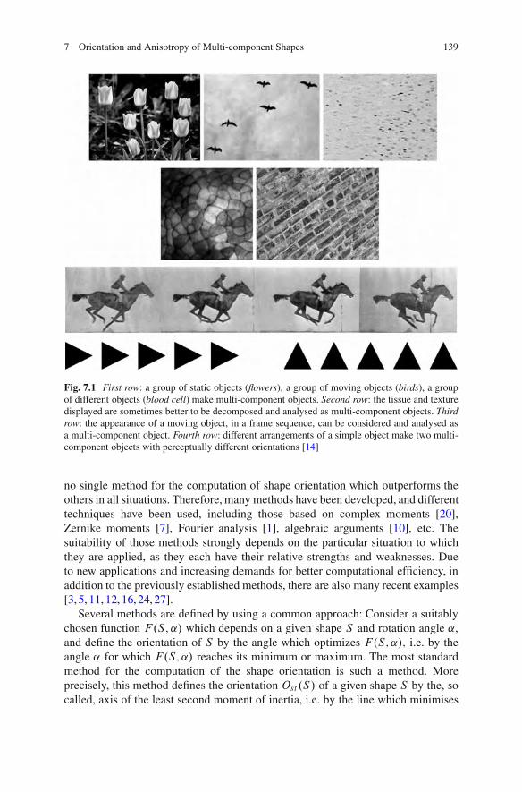
7 Orientation and Anisotropy of Multi-component Shapes 139
Fig. 7.1 First row: a group of static objects (flowers), a group of moving objects (birds), a groupof different objects (blood cell) make multi-component objects. Second row: the tissue and texturedisplayed are sometimes better to be decomposed and analysed as multi-component objects. Thirdrow: the appearance of a moving object, in a frame sequence, can be considered and analysed asa multi-component object. Fourth row: different arrangements of a simple object make two multi-component objects with perceptually different orientations [14]
no single method for the computation of shape orientation which outperforms theothers in all situations. Therefore, many methods have been developed, and differenttechniques have been used, including those based on complex moments [20],Zernike moments [7], Fourier analysis [1], algebraic arguments [10], etc. Thesuitability of those methods strongly depends on the particular situation to whichthey are applied, as they each have their relative strengths and weaknesses. Dueto new applications and increasing demands for better computational efficiency, inaddition to the previously established methods, there are also many recent examples[3, 5, 11, 12, 16, 24, 27].
Several methods are defined by using a common approach: Consider a suitablychosen function F.S; ˛/ which depends on a given shape S and rotation angle ˛,and define the orientation of S by the angle which optimizes F.S; ˛/; i.e. by theangle ˛ for which F.S; ˛/ reaches its minimum or maximum. The most standardmethod for the computation of the shape orientation is such a method. Moreprecisely, this method defines the orientation Ost .S/ of a given shape S by the, socalled, axis of the least second moment of inertia, i.e. by the line which minimises
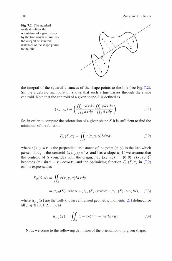
140 J. Zunic and P.L. Rosin
. .
..
..
Fig. 7.2 The standardmethod defines theorientation of a given shapeby the line which minimizesthe integral of squareddistances of the shape pointsto the line
the integral of the squared distances of the shape points to the line (see Fig. 7.2).Simple algebraic manipulation shows that such a line passes through the shapecentroid. Note that the centroid of a given shape S is defined as
.xS ; yS / D!RR
S xdxdyRRS dxdy
RRS ydxdyRRS dxdy
": (7.1)
So, in order to compute the orientation of a given shape S it is sufficient to find theminimum of the function
Fst .S; ˛/ DZZ
S
r.x; y; ˛/2dxdy (7.2)
where r.x; y; ˛/2 is the perpendicular distance of the point .x; y/ to the line whichpasses thought the centroid .xS ; yS / of S and has a slope ˛: If we assume thatthe centroid of S coincides with the origin, i.e., .xS ; yS / D .0; 0/; r.x; y; ˛/2
becomes .x ! sin ˛ " y ! cos˛/2; and the optimizing function Fst .S; ˛/ in (7.2)can be expressed as
Fst .S; ˛/ DZZ
S
r.x; y; ˛/2dxdy
D !2;0.S/ ! sin2 ˛ C !0;2.S/ ! cos2 ˛ " !1;1.S/ ! sin.2˛/; (7.3)
where !p;q.S/ are the well-known centralised geometric moments [21] defined, forall p; q 2 f0; 1; 2; : : :g; as
!p;q.S/ DZZ
S
.x " xS/p.y " yS/qdxdy: (7.4)
Now, we come to the following definition of the orientation of a given shape.

7 Orientation and Anisotropy of Multi-component Shapes 141
Definition 7.1. The orientation of a given shape S is determined by the angle ˛where the function Fst .S; ˛/ reaches its minimum.
This standard method defines the shape orientation in a natural way – by theline which minimizes the integral of the squared distances of shape points to thisline. Such a definition matches our perception of what the shape orientation shouldbe. Also, there is a simple formula for the computation of such orientation. It is easyto check [21] that the angle which minimizes Fst .S; ˛/ satisfies the equation
tan.2 !O.S// D 2 ! !1;1.S/!2;0.S/" !0;2.S/
: (7.5)
These are desirable properties, but there are some drawbacks too. The mainproblem is that there are many situations where the method fails [23,28] or does notperform satisfactorily. The situations were the method fails are easy to characterise.Indeed, considering the first derivative of Fst .S; ˛/ (see (7.3))
dFst .S; ˛/
d˛D .!2;0.S/" !0;2.S// ! sin.2˛/ " 2!1;1.S/ ! cos.2˛/; (7.6)
and looking for the conditions when dFst .S; ˛/=d˛ vanishes, it is easy to see thatfor all shapes S satisfying
!2;0.S/" !0;2.S/ D 0 and !1;1.S/ D 0 (7.7)
the function Fst .S; ˛/ is constant and consequently does not tell which angleshould be selected as the shape’s orientation. N -fold rotationally symmetric shapesare shapes which satisfy (7.7) but there are many other (irregular) shapes whichsatisfy (7.7) and consequently could not be oriented by the standard method givenby Definition 7.1.
In order to overcome such problems, [23] suggested a modification of theoptimizing function Fst .S; ˛/ by increasing the exponent in (7.2). The methodfrom [23] defines the orientation of a given shape S whose centroid coincides withthe origin, by the angle which minimizes
FN .S; ˛/ DZZ
S
r.x; y; ˛/2N dxdy (7.8)
for a certain exponent 2N . In such a way, the class of shapes whose orientationcan be computed is expanded. On the other hand, there is not a closed formula(analogous to (7.5)) for the computation of the shape orientation by using FN .S; ˛/;for an arbitraryN .
Notice that difficulties in the computation of the shape orientation can be causedby the nature of certain shapes. While for many shapes their orientations areintuitively clear and can be computed relatively easily, the orientation of some othershapes may be ambiguous or ill defined. Problems related to the estimation of thedegree to which a shape has a distinct orientation are considered in [29].
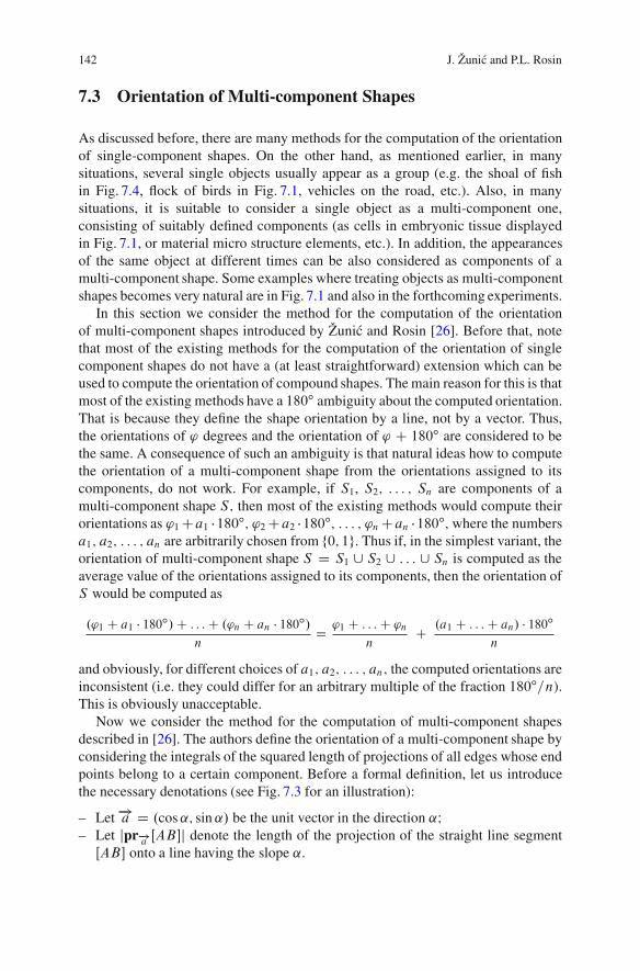
142 J. Zunic and P.L. Rosin
7.3 Orientation of Multi-component Shapes
As discussed before, there are many methods for the computation of the orientationof single-component shapes. On the other hand, as mentioned earlier, in manysituations, several single objects usually appear as a group (e.g. the shoal of fishin Fig. 7.4, flock of birds in Fig. 7.1, vehicles on the road, etc.). Also, in manysituations, it is suitable to consider a single object as a multi-component one,consisting of suitably defined components (as cells in embryonic tissue displayedin Fig. 7.1, or material micro structure elements, etc.). In addition, the appearancesof the same object at different times can be also considered as components of amulti-component shape. Some examples where treating objects as multi-componentshapes becomes very natural are in Fig. 7.1 and also in the forthcoming experiments.
In this section we consider the method for the computation of the orientationof multi-component shapes introduced by Zunic and Rosin [26]. Before that, notethat most of the existing methods for the computation of the orientation of singlecomponent shapes do not have a (at least straightforward) extension which can beused to compute the orientation of compound shapes. The main reason for this is thatmost of the existing methods have a 180ı ambiguity about the computed orientation.That is because they define the shape orientation by a line, not by a vector. Thus,the orientations of ' degrees and the orientation of ' C 180ı are considered to bethe same. A consequence of such an ambiguity is that natural ideas how to computethe orientation of a multi-component shape from the orientations assigned to itscomponents, do not work. For example, if S1, S2; : : : ; Sn are components of amulti-component shape S; then most of the existing methods would compute theirorientations as '1Ca1 !180ı; '2Ca2 !180ı; : : : ; 'nCan !180ı; where the numbersa1; a2; : : : ; an are arbitrarily chosen from f0; 1g: Thus if, in the simplest variant, theorientation of multi-component shape S D S1 [ S2 [ : : : [ Sn is computed as theaverage value of the orientations assigned to its components, then the orientation ofS would be computed as
.'1 C a1 ! 180ı/C : : :C .'n C an ! 180ı/n
D '1 C : : :C 'nn
C .a1 C : : :C an/ ! 180ın
and obviously, for different choices of a1; a2; : : : ; an; the computed orientations areinconsistent (i.e. they could differ for an arbitrary multiple of the fraction 180ı=n).This is obviously unacceptable.
Now we consider the method for the computation of multi-component shapesdescribed in [26]. The authors define the orientation of a multi-component shape byconsidering the integrals of the squared length of projections of all edges whose endpoints belong to a certain component. Before a formal definition, let us introducethe necessary denotations (see Fig. 7.3 for an illustration):
– Let "!a D .cos˛; sin ˛/ be the unit vector in the direction ˛I– Let jpr!!a ŒAB"j denote the length of the projection of the straight line segmentŒAB" onto a line having the slope ˛.
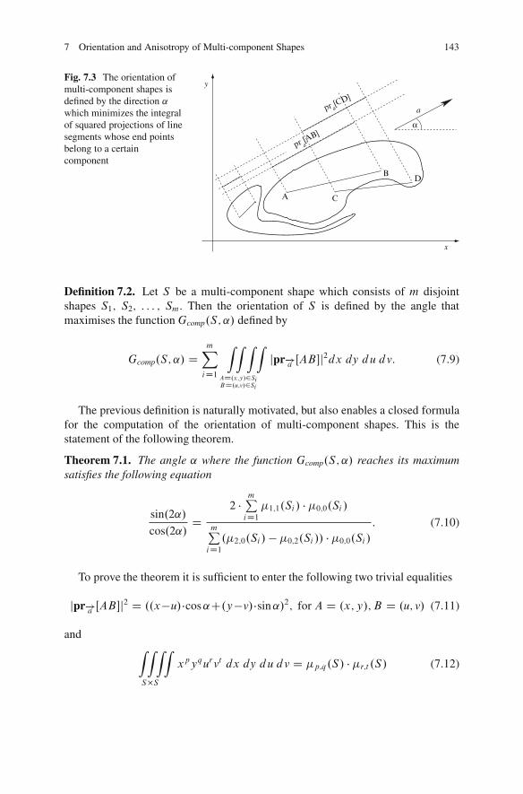
7 Orientation and Anisotropy of Multi-component Shapes 143
x
y
A
B
C
D
!
a
pr [AB]
pr [CD]
a
a
Fig. 7.3 The orientation ofmulti-component shapes isdefined by the direction �which minimizes the integralof squared projections of linesegments whose end pointsbelong to a certaincomponent
Definition 7.2. Let S be a multi-component shape which consists of m disjointshapes S1; S2; : : : ; Sm: Then the orientation of S is defined by the angle thatmaximises the functionGcomp.S; � / defined by
Gcomp.S; � / DmX
iD1
Z Z
AD.x;y/2SiBD.u;v/2Si
Z Zjpr!!a å AB"j2dx dy du dv: (7.9)
The previous definition is naturally motivated, but also enables a closed formulafor the computation of the orientation of multi-component shapes. This is thestatement of the following theorem.
Theorem 7.1. The angle � where the function Gcomp.S; � / reaches its maximumsatisfies the following equation
sin.2� /cos.2� /
D2 !
mPiD1
!1;1.Si / ! !0;0.Si /mPiD1.!2;0.Si / " !0;2.Si // ! !0;0.Si /
: (7.10)
To prove the theorem it is sufficient to enter the following two trivial equalities
jpr!!a å AB"j2 D ..x"u/!cos � C.y"v/!sin � /2; for A D .x; y/; B D .u; v/ (7.11)
andZ Z
S"S
ZZxpyqurvt dx dy du dv D !p;q.S/ ! !r;t .S/ (7.12)

144 J. Zunic and P.L. Rosin
into the optimizing function Gcomp.S; ˛/: After that, simple calculus applied to the
equationdGcomp.S; ˛/
d˛D 0 establishes the proof. For more details we refer to [26].
The orientation of multi-component shapes computed by optimizing the functionGcomp.S; ˛/ is theoretically well founded and because of that it can be wellunderstood. Some of properties are a direct consequence of the definition and canbe proved by using basic calculus. We list some of them.
Property 7.1. If the method given by Definition 7.2 is applied to a single compo-nent shape, then the computed orientation is the same as the orientation computedby the standard definition, i.e. by the optimizing the function Fst .S; ˛/ (see (7.2)and (7.5)). Note that the optimizing function G.S; ˛/ D Gcomp.S; ˛/, specified forsingle component shapes, and the optimizing function Fst .S; ˛/ are different, butthey are connected with the following, easily provable, equality
G.S; ˛/C 2 ! !0;0.S/ ! Fst .S; ˛/ D 2 ! !0;0.S/ ! .!2;0.S/C !0;2.S//: (7.13)
Since the right-hand side of (7.13) does not depend on ˛ we deduce that themaximum of G.S; ˛/ and the minimum of Fst .S; ˛/ are reached at the same point.In other words, the direction ˛ which defines the orientation of S by applying thestandard method is the same as the direction which defines the orientation of S ifthe Definition 7.2 is applied to single component shapes.
Property 7.2. As it is expected, there are situations where the method given byDefinition 7.2 fails. Due to the definition of the optimizing function Gcomp.S; ˛/,a simple characterization of such situations is possible. Indeed, by using (7.11)we deduce:
Gcomp.S; ˛/ D cos2 ˛ !mX
iD12!0;0.Si /!2;0.Si /C sin2 ˛ !
mX
iD12!0;0.Si /!0;2.Si /
C sin.2˛/ !mX
iD12!0;0.Si /!1;1.Si /: (7.14)
The last equality says immediately that the first derivativedGcomp.S; ˛/
d˛is iden-
tically equal to zero (i.e. Gcomp.S; ˛/ is constant) if and only if the following twoconditions are satisfied
mX
iD1!0;0.Si / ! !1;1.Si / D 0 and
mX
iD1!0;0.Si / ! .!2;0.Si /" !0;2.Si // D 0:
(7.15)
So, under the conditions in (7.15) the optimizing function is constant and nodirection can be selected as the shape orientation.
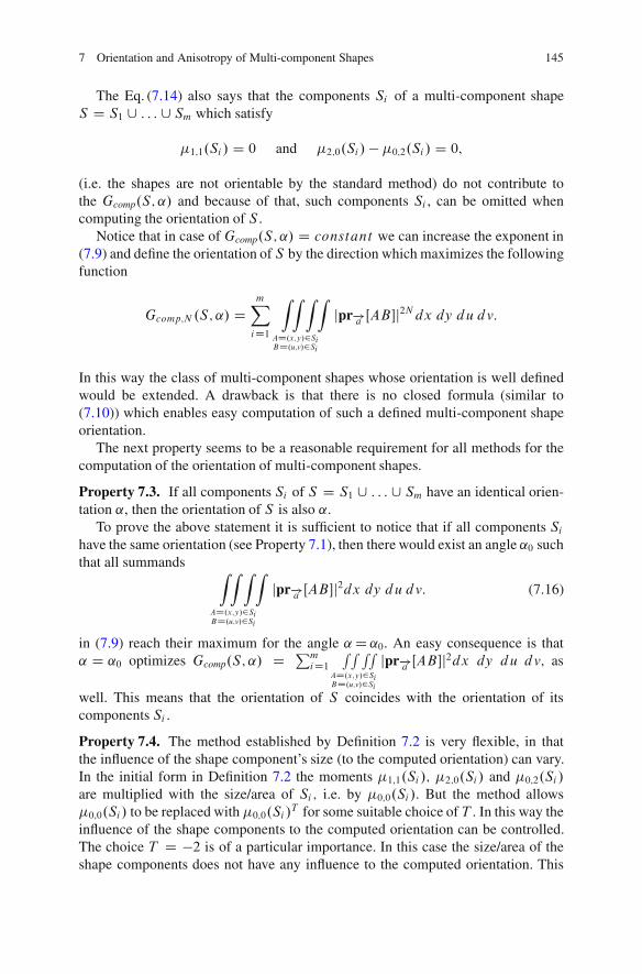
7 Orientation and Anisotropy of Multi-component Shapes 145
The Eq. (7.14) also says that the components Si of a multi-component shapeS D S1 [ : : : [ Sm which satisfy
!1;1.Si / D 0 and !2;0.Si / " !0;2.Si / D 0;
(i.e. the shapes are not orientable by the standard method) do not contribute tothe Gcomp.S; ˛/ and because of that, such components Si , can be omitted whencomputing the orientation of S .
Notice that in case of Gcomp.S; ˛/ D constant we can increase the exponent in(7.9) and define the orientation of S by the direction which maximizes the followingfunction
Gcomp;N .S; ˛/ DmX
iD1
Z Z
AD.x;y/2SiBD.u;v/2Si
Z Zjpr!!a ŒAB"j2N dx dy du dv:
In this way the class of multi-component shapes whose orientation is well definedwould be extended. A drawback is that there is no closed formula (similar to(7.10)) which enables easy computation of such a defined multi-component shapeorientation.
The next property seems to be a reasonable requirement for all methods for thecomputation of the orientation of multi-component shapes.
Property 7.3. If all components Si of S D S1 [ : : : [ Sm have an identical orien-tation ˛, then the orientation of S is also ˛:
To prove the above statement it is sufficient to notice that if all components Sihave the same orientation (see Property 7.1), then there would exist an angle ˛0 suchthat all summands Z Z
AD.x;y/2SiBD.u;v/2Si
Z Zjpr!!a ŒAB"j2dx dy du dv: (7.16)
in (7.9) reach their maximum for the angle ˛D ˛0. An easy consequence is that˛ D ˛0 optimizes Gcomp.S; ˛/ D
PmiD1
RRAD.x;y/2SiBD.u;v/2Si
RRjpr!!a ŒAB"j2dx dy du dv; as
well. This means that the orientation of S coincides with the orientation of itscomponents Si :
Property 7.4. The method established by Definition 7.2 is very flexible, in thatthe influence of the shape component’s size (to the computed orientation) can vary.In the initial form in Definition 7.2 the moments !1;1.Si /; !2;0.Si / and !0;2.Si /are multiplied with the size/area of Si ; i.e. by !0;0.Si /. But the method allows!0;0.Si / to be replaced with !0;0.Si /T for some suitable choice of T . In this way theinfluence of the shape components to the computed orientation can be controlled.The choice T D "2 is of a particular importance. In this case the size/area of theshape components does not have any influence to the computed orientation. This
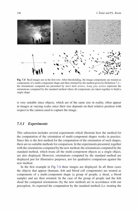
146 J. Zunic and P.L. Rosin
Fig. 7.4 Real images are in the first row. After thresholding, the image components are treated ascomponents of a multi-component shape and then oriented by the method given by Definition 7.2 –the orientations computed are presented by short dark arrows. Long grey arrows represent theorientations computed by the standard method where all components are taken together to build asingle shape
is very suitable since objects, which are of the same size in reality, often appearin images at varying scales since their size depends on their relative position withrespect to the camera used to capture the image.
7.3.1 Experiments
This subsection includes several experiments which illustrate how the method forthe computation of the orientation of multi-component shapes works in practice.Since this is the first method for the computation of the orientation of such shapes,there are no suitable methods for comparison. In the experiments presented, togetherwith the orientations computed by the new method, the orientations computed by thestandard method, which treats all the multi-component objects as a single object,are also displayed. However, orientations computed by the standard method aredisplayed just for illustrative purposes, not for qualitative comparison against thenew method.
In the first example in Fig. 7.4 three images are displayed. In all three casesthe objects that appear (humans, fish and blood cell components) are treated ascomponents of a multi-component shape (a group of people, a shoal, a bloodsample) and are then oriented. In the case of the group of people and the fishshoal the computed orientations (by the new method) are in accordance with ourperception. As expected the computation by the standard method (i.e. treating the
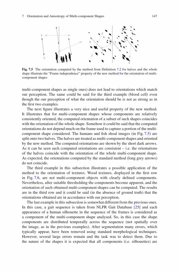
7 Orientation and Anisotropy of Multi-component Shapes 147
Fig. 7.5 The orientation computed by the method from Definition 7.2 for halves and the wholeshape illustrate the “Frame independence” property of the new method for the orientation of multi-component shapes
multi-component shapes as single ones) does not lead to orientations which matchour perception. The same could be said for the third example (blood cell) eventhough the our perception of what the orientation should be is not as strong as inthe first two examples.
The next figure illustrates a very nice and useful property of the new method.It illustrates that for multi-component shapes whose components are relativelyconsistently oriented, the computed orientation of a subset of such shapes coincideswith the orientation of the whole shape. Somehow it could be said that the computedorientations do not depend much on the frame used to capture a portion of the multi-component shape considered. The humans and fish shoal images (in Fig. 7.5) aresplit onto two halves. The halves are treated as multi-component shapes and orientedby the new method. The computed orientations are shown by the short dark arrows.As it can be seen such computed orientations are consistent – i.e. the orientationsof the halves coincide with the orientation of the whole multi-component shape.As expected, the orientations computed by the standard method (long grey arrows)do not coincide.
The third example in this subsection illustrates a possible application of themethod to the orientation of textures. Wood textures, displayed in the first rowin Fig. 7.6, are not multi-component objects with clearly defined components.Nevertheless, after suitable thresholding the components become apparent, and theorientation of such obtained multi-component shapes can be computed. The resultsare in the third row and it could be said (in the absence of ground truth) that theorientations obtained are in accordance with our perception.
The last example in this subsection is somewhat different from the previous ones.In this case, a gait sequence is taken from NLPR Gait Database [25] and eachappearance of a human silhouette in the sequence of the frames is considered asa component of the multi-component shape analysed. So, in this case the shapecomponents are distributed temporally across the sequence (not spatially overthe image, as in the previous examples). After segmentation many errors, whichtypically appear, have been removed using standard morphological techniques.However, several large errors remain and the task was to detect them. Due tothe nature of the shapes it is expected that all components (i.e. silhouettes) are

148 J. Zunic and P.L. Rosin
Fig. 7.6 Texture images, in the first row, are thresholded and their orientation is then computedas the orientation of multi-component shapes which correspond to the black-and-white imagesin the second row. The images in the third row are re-oriented in accordance with the computedorientations
Fig. 7.7 The extracted silhouettes from a gait sequence are displayed (the first row) andunderneath is an intensity coding of each silhouette to show its degree of being an outlier (darkmeans high likelihood). A magnified view of the most outlying silhouette and its neighbours is inthe third row
fairly consistently oriented if they are extracted properly. Thus, we make thehypothesis that the silhouettes with orientations inconsistent with the majority ofsilhouettes suffer from segmentation errors. The difference in multi-componentshape orientation caused by removing the least consistent component has been usedas a criterion to find possible outliers. In the example given, due to the errors in theprocessing chain that produced the sequence of binary images, the person’s leadingleg has been displaced and this silhouette/frame has been detected as an outlier, asshown in Fig. 7.7.
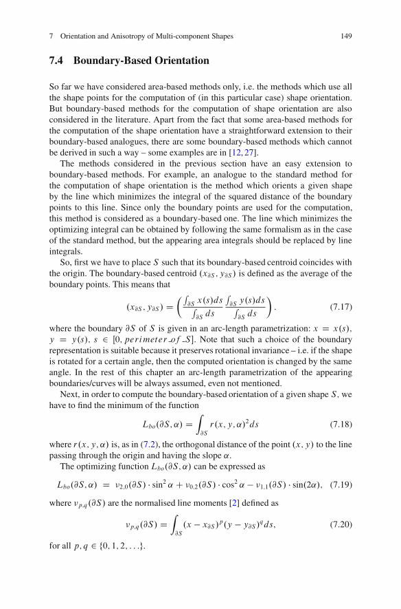
7 Orientation and Anisotropy of Multi-component Shapes 149
7.4 Boundary-Based Orientation
So far we have considered area-based methods only, i.e. the methods which use allthe shape points for the computation of (in this particular case) shape orientation.But boundary-based methods for the computation of shape orientation are alsoconsidered in the literature. Apart from the fact that some area-based methods forthe computation of the shape orientation have a straightforward extension to theirboundary-based analogues, there are some boundary-based methods which cannotbe derived in such a way – some examples are in [12, 27].
The methods considered in the previous section have an easy extension toboundary-based methods. For example, an analogue to the standard method forthe computation of shape orientation is the method which orients a given shapeby the line which minimizes the integral of the squared distance of the boundarypoints to this line. Since only the boundary points are used for the computation,this method is considered as a boundary-based one. The line which minimizes theoptimizing integral can be obtained by following the same formalism as in the caseof the standard method, but the appearing area integrals should be replaced by lineintegrals.
So, first we have to place S such that its boundary-based centroid coincides withthe origin. The boundary-based centroid .x@S ; y@S / is defined as the average of theboundary points. This means that
.x@S ; y@S / D!R
@S x.s/dsR@S ds
R@S y.s/dsR@S ds
": (7.17)
where the boundary @S of S is given in an arc-length parametrization: x D x.s/;y D y.s/; s 2 Œ0; perimeter of S ": Note that such a choice of the boundaryrepresentation is suitable because it preserves rotational invariance – i.e. if the shapeis rotated for a certain angle, then the computed orientation is changed by the sameangle. In the rest of this chapter an arc-length parametrization of the appearingboundaries/curves will be always assumed, even not mentioned.
Next, in order to compute the boundary-based orientation of a given shape S; wehave to find the minimum of the function
Lbo.@S; ˛/ DZ
@S
r.x; y; ˛/2ds (7.18)
where r.x; y; ˛/ is, as in (7.2), the orthogonal distance of the point .x; y/ to the linepassing through the origin and having the slope ˛:
The optimizing function Lbo.@S; ˛/ can be expressed as
Lbo.@S; ˛/ D #2;0.@S/ ! sin2 ˛ C #0;2.@S/ ! cos2 ˛ " #1;1.@S/ ! sin.2˛/; (7.19)
where #p;q.@S/ are the normalised line moments [2] defined as
#p;q.@S/ DZ
@S
.x " x@S /p.y " y@S /qds; (7.20)
for all p; q 2 f0; 1; 2; : : :g.
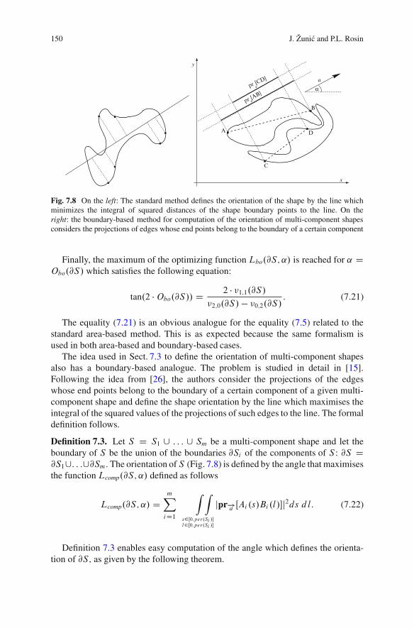
150 J. Zunic and P.L. Rosin
y
!a
pr [AB]
a
B
A
pr [CD]
a
x
D
C
Fig. 7.8 On the left: The standard method defines the orientation of the shape by the line whichminimizes the integral of squared distances of the shape boundary points to the line. On theright: the boundary-based method for computation of the orientation of multi-component shapesconsiders the projections of edges whose end points belong to the boundary of a certain component
Finally, the maximum of the optimizing function Lbo.@S; � / is reached for � DObo.@S/ which satisfies the following equation:
tan.2 !Obo.@S// D2 ! #1;1.@S/
#2;0.@S/ " #0;2.@S/: (7.21)
The equality (7.21) is an obvious analogue for the equality (7.5) related to thestandard area-based method. This is as expected because the same formalism isused in both area-based and boundary-based cases.
The idea used in Sect. 7.3 to define the orientation of multi-component shapesalso has a boundary-based analogue. The problem is studied in detail in [15].Following the idea from [26], the authors consider the projections of the edgeswhose end points belong to the boundary of a certain component of a given multi-component shape and define the shape orientation by the line which maximises theintegral of the squared values of the projections of such edges to the line. The formaldefinition follows.
Definition 7.3. Let S D S1 [ : : : [ Sm be a multi-component shape and let theboundary of S be the union of the boundaries @Si of the components of S : @S D@S1[: : :[@Sm: The orientation of S (Fig. 7.8) is defined by the angle that maximisesthe function Lcomp.@S; � / defined as follows
Lcomp.@S; � / DmX
iD1
Z
s2 å 0;per.Si /"l2 å 0;per.Si /"
Zjpr!!a å Ai .s/Bi .l/"j2ds d l: (7.22)
Definition 7.3 enables easy computation of the angle which defines the orienta-tion of @S; as given by the following theorem.

7 Orientation and Anisotropy of Multi-component Shapes 151
Theorem 7.2. Let S be a multi-component shape whose boundary is @S D @S1[ : : : [ @Sm. The angle ˛ where the function Lcomp.@S; ˛/ reaches its maximumsatisfies the following equation
tan.2˛/ D2 !
mPiD1
#1;1.@Si/ ! #0;0.@Si /mPiD1.#2;0.@Si /" #0;2.@Si // ! !0;0.@Si /
: (7.23)
Being derived in an analogous way as the area-based method for the computationof the multi-component shapes, the method given by Definition 7.3 also satisfiesthe Properties 7.1–7.4 listed in Sect. 7.3, before the experimental section. It is worthmentioning that the method also enables the control of the influence of the perimeterof the shape components to the computed orientation. If, for some applications, suchan influence should be ignored then the moments #1;1.@Si /; #2;0.@Si/; and #0;2.@Si /which appear in (7.23) should be multiplied by .#0;0.@Si//!2.
To close this section, let us mention that (in general) boundary-based approachesto define the orientation of shapes allow some extra generalizations. One suchgeneralisation was considered in [12]. Therein the shape orientation is computedbased on the projections of the tangent vectors at the shape boundary points,weighted by the suitably chosen function of the boundary curvature at the corre-sponding points. The advantage of such an approach is not only that the boundarycurvature, as an important shape feature, is involved in the computation of theshape orientation. This also provides an easy approach to overcome situations werethe orientations are not computable. It is sufficient to modify the curvature basedweighting function, and shapes which were not “orientable” by an initial choice ofthe weighting function can become orientable with another choice. The computationof the shape orientation remains possible by a closed form formula whether theweighting function is changed or not. For more details see [12].
7.4.1 Experiments
In this section we have two examples to illustrate how the boundary-based method(established by Definition 7.3) works.
First we consider the embryonic tissue displayed in Fig. 7.9. Cell boundariesare extracted and then the boundary-based method for the computation of theorientation of multi-component shapes is applied. The orientations are computed forthe whole image and also separately for the upper and lower parts. The computedorientations are consistent (presented by short dark arrows) which actually impliesthat the tissue displayed has an inherent consistent orientation. The orientationscomputed by the boundary-based analogue (by optimizing Lbo.@S; ˛/ from (7.18)),are different (long grey arrows), as it was expected.
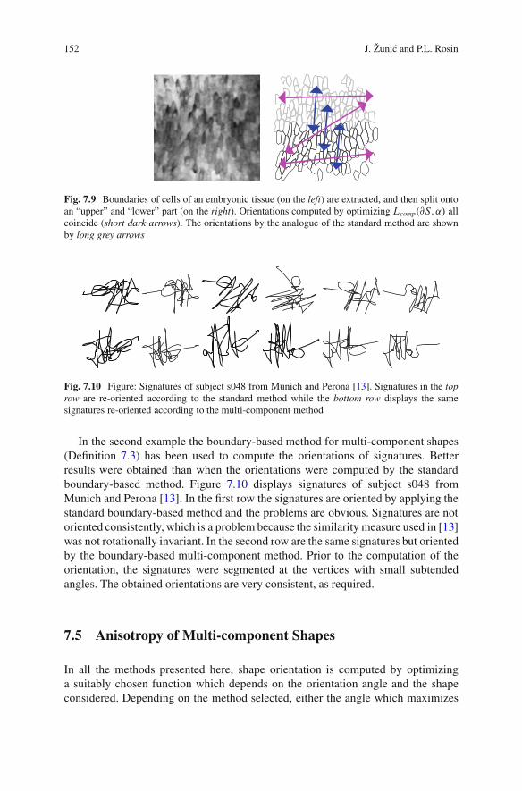
152 J. Zunic and P.L. Rosin
Fig. 7.9 Boundaries of cells of an embryonic tissue (on the left) are extracted, and then split ontoan “upper” and “lower” part (on the right). Orientations computed by optimizing Lcomp.@S; � / allcoincide (short dark arrows). The orientations by the analogue of the standard method are shownby long grey arrows
Fig. 7.10 Figure: Signatures of subject s048 from Munich and Perona [13]. Signatures in the toprow are re-oriented according to the standard method while the bottom row displays the samesignatures re-oriented according to the multi-component method
In the second example the boundary-based method for multi-component shapes(Definition 7.3) has been used to compute the orientations of signatures. Betterresults were obtained than when the orientations were computed by the standardboundary-based method. Figure 7.10 displays signatures of subject s048 fromMunich and Perona [13]. In the first row the signatures are oriented by applying thestandard boundary-based method and the problems are obvious. Signatures are notoriented consistently, which is a problem because the similarity measure used in [13]was not rotationally invariant. In the second row are the same signatures but orientedby the boundary-based multi-component method. Prior to the computation of theorientation, the signatures were segmented at the vertices with small subtendedangles. The obtained orientations are very consistent, as required.
7.5 Anisotropy of Multi-component Shapes
In all the methods presented here, shape orientation is computed by optimizinga suitably chosen function which depends on the orientation angle and the shapeconsidered. Depending on the method selected, either the angle which maximizes
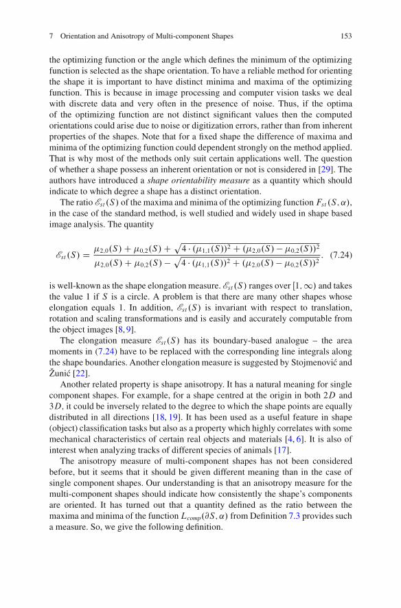
7 Orientation and Anisotropy of Multi-component Shapes 153
the optimizing function or the angle which defines the minimum of the optimizingfunction is selected as the shape orientation. To have a reliable method for orientingthe shape it is important to have distinct minima and maxima of the optimizingfunction. This is because in image processing and computer vision tasks we dealwith discrete data and very often in the presence of noise. Thus, if the optimaof the optimizing function are not distinct significant values then the computedorientations could arise due to noise or digitization errors, rather than from inherentproperties of the shapes. Note that for a fixed shape the difference of maxima andminima of the optimizing function could dependent strongly on the method applied.That is why most of the methods only suit certain applications well. The questionof whether a shape possess an inherent orientation or not is considered in [29]. Theauthors have introduced a shape orientability measure as a quantity which shouldindicate to which degree a shape has a distinct orientation.
The ratio Est .S/ of the maxima and minima of the optimizing functionFst .S; ˛/,in the case of the standard method, is well studied and widely used in shape basedimage analysis. The quantity
Est .S/ D!2;0.S/C !0;2.S/C
p4 ! .!1;1.S//2 C .!2;0.S/" !0;2.S//2
!2;0.S/C !0;2.S/"p4 ! .!1;1.S//2 C .!2;0.S/" !0;2.S//2
: (7.24)
is well-known as the shape elongation measure. Est .S/ ranges over Œ1;1/ and takesthe value 1 if S is a circle. A problem is that there are many other shapes whoseelongation equals 1. In addition, Est .S/ is invariant with respect to translation,rotation and scaling transformations and is easily and accurately computable fromthe object images [8, 9].
The elongation measure Est .S/ has its boundary-based analogue – the areamoments in (7.24) have to be replaced with the corresponding line integrals alongthe shape boundaries. Another elongation measure is suggested by Stojmenovic andZunic [22].
Another related property is shape anisotropy. It has a natural meaning for singlecomponent shapes. For example, for a shape centred at the origin in both 2D and3D; it could be inversely related to the degree to which the shape points are equallydistributed in all directions [18, 19]. It has been used as a useful feature in shape(object) classification tasks but also as a property which highly correlates with somemechanical characteristics of certain real objects and materials [4, 6]. It is also ofinterest when analyzing tracks of different species of animals [17].
The anisotropy measure of multi-component shapes has not been consideredbefore, but it seems that it should be given different meaning than in the case ofsingle component shapes. Our understanding is that an anisotropy measure for themulti-component shapes should indicate how consistently the shape’s componentsare oriented. It has turned out that a quantity defined as the ratio between themaxima and minima of the functionLcomp.@S; ˛/ from Definition 7.3 provides sucha measure. So, we give the following definition.

154 J. Zunic and P.L. Rosin
Definition 7.4. Let S1; : : : ; Sm be components of a compound shape S . Then theanisotropy A .S/ of S is defined as
A .S/ D max˛2Œ0;2$/ Lcomp.@S; ˛/
min˛2Œ0;2$/ Lcomp.@S; ˛/D max˛2Œ0;2$/ Lcomp.@S1 [ : : : [ Sm; ˛/
min˛2Œ0;2$/ Lcomp.@S1 [ : : : [ Sm; ˛/:
(7.25)
The anisotropy measure A .S/ for multi-component shapes ranges over Œ1;1/and is invariant with respect to translations, rotations and scaling transformations.It also enables an explicit formula for its computation. By basic calculus it can beshown that the maxima and minima of Lcomp.@S; ˛/ are:
max˛2Œ0;2$/
Lcomp.@S; ˛/ D C CpA2 C B2; min
˛2Œ0;2$/Lcomp.@S; ˛/ D C "
pA2 C B2
where the quantities A; B; and C are
A DmPiD1.#2;0.@Si /" !0;2.@Si// ! #0;0.@Si /;
B DmPiD1
2 ! #1;1.@Si / ! #0;0.@Si /;
C DmPiD1.#2;0.@Si /C #0;2.@Si // ! #0;0.@Si/:
We illustrate how the anisotropy measure A .S/ acts by two examples. Noticethat the anisotropy measure, as defined here, also depends on the elongation of theshape components, not only on their orientations. This also seems acceptable, e.g.a stereotype for a multi-component shape with a high anisotropy A .S/ is a shapewhose components have high elongations and the same orientation.
The first example is in Fig. 7.11. The shapes in both rows are treated as a multiplecomponent object (e.g. a herd of cattle and a group of cars). The anisotropy was firstcomputed for just the cattle, giving a value of 3:49: The anisotropy of the cattle’sshadows alone increases to 7:57 since the shadows are more consistently orientated,and are also slightly more elongated. Merging the cattle and their shadows produceseven more elongated regions, which lead to an increase of the herd’s anisotropy to12.08. The anisotropy of the cars (in the second row) is 1:38, which is very small.This is to be expected since the orientations of the individual cars vary strongly.
The second example which indicates how the anisotropy measure A .S/ acts isin Fig. 7.12, in which anisotropy is used to select appropriate elongated regions toenable skew correction of the document. The first image (on the left) in the first rowis the original image. Its components are letters whose orientations vary strongly, butalso many of the letters have a low elongation. This results in a very low anisotropyof this image, as it can be seen from the graph given in the second row.
After blurring is applied to the image the characters start to merge into words,which are both more consistently oriented and more elongated. This leads to an
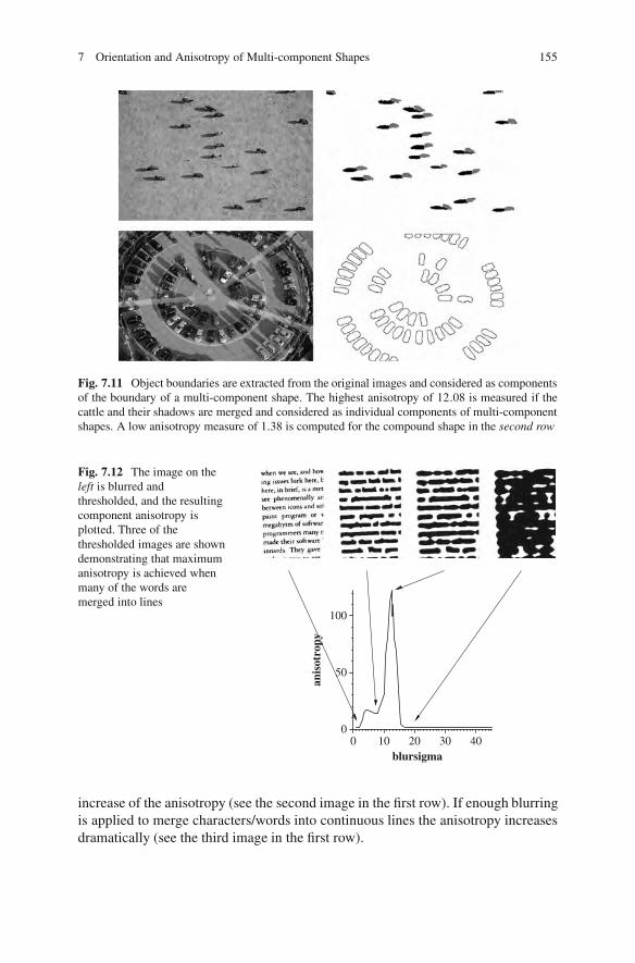
7 Orientation and Anisotropy of Multi-component Shapes 155
Fig. 7.11 Object boundaries are extracted from the original images and considered as componentsof the boundary of a multi-component shape. The highest anisotropy of 12:08 is measured if thecattle and their shadows are merged and considered as individual components of multi-componentshapes. A low anisotropy measure of 1:38 is computed for the compound shape in the second row
0 10 20 30 40blursigma
0
50
100
anis
otro
py
Fig. 7.12 The image on theleft is blurred andthresholded, and the resultingcomponent anisotropy isplotted. Three of thethresholded images are showndemonstrating that maximumanisotropy is achieved whenmany of the words aremerged into lines
increase of the anisotropy (see the second image in the first row). If enough blurringis applied to merge characters/words into continuous lines the anisotropy increasesdramatically (see the third image in the first row).
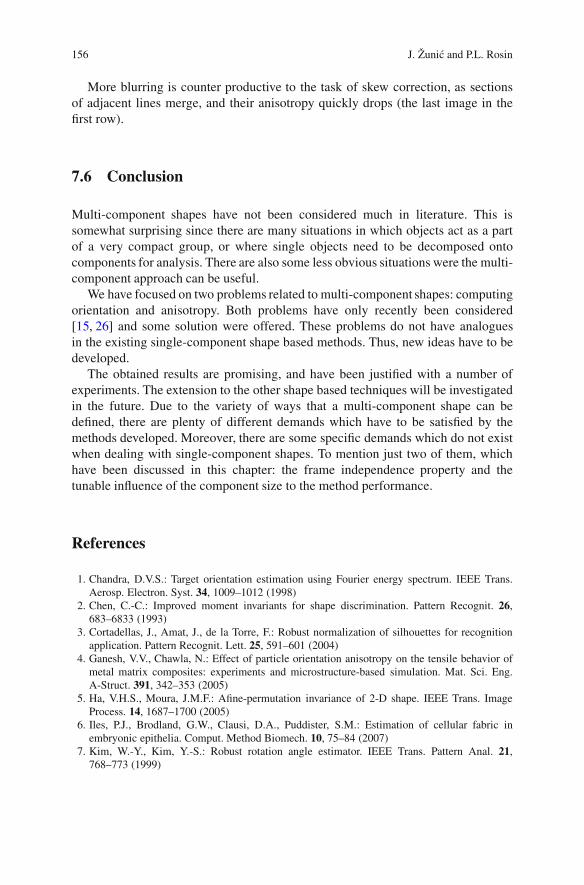
156 J. Zunic and P.L. Rosin
More blurring is counter productive to the task of skew correction, as sectionsof adjacent lines merge, and their anisotropy quickly drops (the last image in thefirst row).
7.6 Conclusion
Multi-component shapes have not been considered much in literature. This issomewhat surprising since there are many situations in which objects act as a partof a very compact group, or where single objects need to be decomposed ontocomponents for analysis. There are also some less obvious situations were the multi-component approach can be useful.
We have focused on two problems related to multi-component shapes: computingorientation and anisotropy. Both problems have only recently been considered[15, 26] and some solution were offered. These problems do not have analoguesin the existing single-component shape based methods. Thus, new ideas have to bedeveloped.
The obtained results are promising, and have been justified with a number ofexperiments. The extension to the other shape based techniques will be investigatedin the future. Due to the variety of ways that a multi-component shape can bedefined, there are plenty of different demands which have to be satisfied by themethods developed. Moreover, there are some specific demands which do not existwhen dealing with single-component shapes. To mention just two of them, whichhave been discussed in this chapter: the frame independence property and thetunable influence of the component size to the method performance.
References
1. Chandra, D.V.S.: Target orientation estimation using Fourier energy spectrum. IEEE Trans.Aerosp. Electron. Syst. 34, 1009–1012 (1998)
2. Chen, C.-C.: Improved moment invariants for shape discrimination. Pattern Recognit. 26,683–6833 (1993)
3. Cortadellas, J., Amat, J., de la Torre, F.: Robust normalization of silhouettes for recognitionapplication. Pattern Recognit. Lett. 25, 591–601 (2004)
4. Ganesh, V.V., Chawla, N.: Effect of particle orientation anisotropy on the tensile behavior ofmetal matrix composites: experiments and microstructure-based simulation. Mat. Sci. Eng.A-Struct. 391, 342–353 (2005)
5. Ha, V.H.S., Moura, J.M.F.: Afine-permutation invariance of 2-D shape. IEEE Trans. ImageProcess. 14, 1687–1700 (2005)
6. Iles, P.J., Brodland, G.W., Clausi, D.A., Puddister, S.M.: Estimation of cellular fabric inembryonic epithelia. Comput. Method Biomech. 10, 75–84 (2007)
7. Kim, W.-Y., Kim, Y.-S.: Robust rotation angle estimator. IEEE Trans. Pattern Anal. 21,768–773 (1999)
7 Orientation and Anisotropy of Multi-component Shapes 157
8. Klette, R., Zunic, J.: Digital approximation of moments of convex regions. Graph. ModelImage Process. 61, 274–298 (1999)
9. Klette, R., Zunic, J.: Multigrid convergence of calculated features in image analysis. J. Math.Imaging Vis. 13, 173–191 (2000)
10. Lin, J.-C.: The family of universal axes. Pattern Recognit. 29, 477–485 (1996)11. Martinez-Ortiz, C., Zunic, J.: Points position weighted shape orientation. Electron. Lett. 44,
623–624 (2008)12. Martinez-Ortiz, C., Zunic, J.: Curvature weighted gradient based shape orientation. Pattern
Recognit. 43, 3035–3041 (2010)13. Munich M.E., Perona. P.: Visual identification by signature tracking. IEEE Trans. Pattern Anal.
25, 200–217 (2003)14. Palmer, S.E.: What makes triangles point: local and global effects in configurations of
ambiguous triangles. Cognit. Psychol. 12, 285–305 (1980)15. Rosin, P.L., Zunic, J.: Orientation and anisotropy of multi component shapes from boundary
information. Pattern Recognit. 44, 2147–2160 (2011)16. Rosin, P.L., Zunic, J.: Measuring squareness and orientation of shapes. J. Math. Imaging Vis.
39, 13–27 (2011)17. Russell, J., Hasler, N., Klette, R., Rosenhahn, B.: Automatic track recognition of footprints for
identifying cryptic species. Ecology 90, 2007–2013 (2009)18. Saha, P.K., Wehrli, F.W.: A robust method for measuring trabecular bone orientation anisotropy
at in vivo resolution using tensor scale. Pattern Recognit. 37, 1935–1944 (2004)19. Scharcanski, J., Dodson, C.T.J.: Stochastic texture image estimators for local spatial anisotropy
and its variability. IEEE Trans. Instrum. Meas. 49, 971–979 (2000)20. Shen, D., Ip, H.H.S.: Generalized affine invariant normalization. IEEE Trans. Pattern Anal. 19,
431–440 (1997)21. Sonka, M., Hlavac, V., Boyle, R.: Image Processing, Analysis, and Machine Vision. Thomson-
Engineering, Toronto (2007)22. Stojmenovic, M., Zunic, J.: Measuring elongation from shape boundary. J. Math. Imaging Vis.
30, 73–85 (2008)23. Tsai, W.H., Chou, S.L.: Detection of generalized principal axes in rotationally symmetric
shapes. Pattern Recognit. 24, 95–104 (1991)24. Tzimiropoulos, G., Mitianoudis, N., Stathaki, T.: A unifying approach to moment based shape
orientation and symmetry classification. IEEE Trans. Image Process. 18, 125–139 (2009)25. Wang, L., Tan, T.N., Hu, W.M., Ning, H.Z.: Automatic gait recognition based on statistical
shape analysis. IEEE Trans. Image Process. 12, 1120–1131 (2003)26. Zunic, J, Rosin, P.L.: An alternative approach to computing shape orientation with an
application to compound shapes. Int. J. Comput. Vis. 81, 138–154 (2009)27. Zunic, J., Stojmenovic, M.: Boundary based shape orientation. Pattern Recognit. 41,
1785–1798 (2008)28. Zunic, J., Kopanja, L., Fieldsend, J.E.: Notes on shape orientation where the standard method
does not work. Pattern Recognit. 39, 856–865 (2006)29. Zunic, J., Rosin, P.L., Kopanja, L.: On the orientability of shapes. IEEE Trans. Image Process.
15, 3478–3487 (2006)

Part IIPartial Differential Equations
for Shape Analysis
Chapter 8Stable Semi-local Features for Non-rigid Shapes
Roee Litman, Alexander M. Bronstein, and Michael M. Bronstein
Abstract Feature-based analysis is becoming a very popular approach for geomet-ric shape analysis. Following the success of this approach in image analysis, there isa growing interest in finding analogous methods in the 3D world. Maximally stablecomponent detection is a low computation cost and high repeatability method forfeature detection in images.In this study, a diffusion-geometry based framework forstable component detection is presented, which can be used for geometric featuredetection in deformable shapes.
The vast majority of studies of deformable 3D shapes models them as the two-dimensional boundary of the volume of the shape. Recent works have shown thata volumetric shape model is advantageous in numerous ways as it better capturesthe natural behavior of non-rigid deformations. We show that our framework easilyadapts to this volumetric approach, and even demonstrates superior performance.
A quantitative evaluation of our methods on the SHREC’10 and SHREC’11feature detection benchmarks as well as qualitative tests on the SCAPE datasetshow its potential as a source of high-quality features. Examples demonstratingthe drawbacks of surface stable components and the advantage of their volumetriccounterparts are also presented.
R. Litman (!) ! A.M. BronsteinSchool of Electrical Engineering, Tel Aviv University, Tel Aviv, Israele-mail: [email protected]; [email protected]
M.M. BronsteinInstitute of Computational Science, Faculty of Informatics, Universita della Svizzera Italiana,Lugano, Switzerlande-mail: [email protected]
M. Breuß et al. (eds.), Innovations for Shape Analysis, Mathematics and Visualization,DOI 10.1007/978-3-642-34141-0 8, © Springer-Verlag Berlin Heidelberg 2013
161

162 R. Litman et al.
8.1 Introduction
Following their success in image analysis, many feature-based methods have foundtheir way into the world of 3D shape analysis. Feature descriptors play a major rolein many applications of shape analysis, such as assembling fractured models [16] incomputational archeology, or finding shape correspondence [36].
Some shape feature-works are inspired by and follow methods in image analysis,for example the histogram of intrinsic gradients used in [41] is similar in principleto the scale invariant feature transform (SIFT) [21] which has recently becomeextremely popular in image analysis. The concept of “bags of features” [32] wasintroduced as a way to construct global shape descriptors that can be efficientlyused for large-scale shape retrieval [27, 37].
Other features were developed natively for 3D, as they rely on properties like theshape normal field, as in the popular spin image [17]. Another example is a familyof methods based on the heat kernel [4, 35], describing the local heat propagationproperties on a shape. These methods are deformation-invariant due to the fact thatheat diffusion geometry is intrinsic, thus making descriptors based on it applicablein deformable shape analysis.
8.1.1 Related Work
The focus of this work is on another class of feature detection methods, one thatfinds stable components (or regions) in the analyzed image or shape. The origins ofthis approach are also in the image processing literature, this time in the form of thewatershed transform [9, 39].
Matas et al. [22] introduced the stable component detection concept to thecomputer vision and image analysis community in the form of the maximally stableextremal regions (MSER) algorithm. This approach represents intensity level setsas a component tree and attempts to find level sets with the smallest area variationacross intensity. The use of area ratio as the stability criterion makes this approachaffine-invariant, which is an important property in image analysis, as it approximatesviewpoint transformations. This algorithm can be made very efficient [25] in certainsettings, and was shown to have superior performance in a benchmark done byMikolajczyk et al. [24]. A deeper inspection of the notion of region stability wasdone by Kimmel et al. [18], also proposing an alternative stability criteria. TheMSER algorithm was also expanded to gray-scale volumetric images in [12], thoughthis approach was tested only in a qualitative way, and not evaluated as a featuredetector.
Methods similar to MSER have been explored in the works on topologicalpersistence [13]. Persistence-based clustering [7] was used by Skraba et al. [33]to perform shape segmentation. More recently, Dey et al. [10] researched thepersistence of the Heat Kernel Signature [35] for detecting features from partial
8 Stable Semi-local Features for Non-rigid Shapes 163
shape data. In Digne et al. [11], extended the notion of vertex-weighted componenttrees to meshes and proposed to detect MSER regions using the mean curvature.The approach was tested only in a qualitative way, and not evaluated as a featuredetector.
A part of this study was published in the proceedings of the Shape ModelingInternational (SMI’11) conference [20].
8.1.2 Main Contribution
The contributions of our framework are three-fold:First, in Sect. 8.3 we introduce a generic framework for stable component detec-
tion, which unifies vertex- and edge-weighted graph representations (as opposed tovertex-weighting used in image and shape maximally stable component detectors[11, 12, 22]). Our results (see Sect. 8.6) show that the edge-weighted formulation ismore versatile and outperforms its vertex-weighted counterpart in terms of featurerepeatability.
Second, in Sect. 8.2 we introduce diffusion geometric weighting functionssuitable for both vertex- and edge-weighted component trees. We show that suchfunctions are invariant under a large class of transformations, in particular, non-rigid inelastic deformations, making them especially attractive in non-rigid shapeanalysis. We also show several ways of constructing scale-invariant weightingfunctions. In addition, following Raviv et al. [29], we show that the suggestedframework performs better on volumetric data removing the (sometimes) unwantedinsensitivity to volume-changing transformations inherent to the surface model (seeFig. 8.8 for an illustration).
Third, in Sect. 8.6 we show a comprehensive evaluation of different settingsof our method on a standard feature detection benchmark comprising shapesundergoing a variety of transformations. We also present a qualitative evaluationon the SCAPE dataset of scanned human bodies and demonstrate that our meth-ods are capable of matching features across distinct data such as synthetic andscanned shapes.
8.2 Diffusion Geometry
Diffusion geometry is an umbrella term referring to geometric analysis of diffusionor random walk processes [8]. Let us consider the shape of a 3D physical object,modeled as a connected and compact region X ! R3. The boundary of the region@X is a closed connected two-dimensional Riemannian manifold. In many applica-tion in graphics, geometry processing, and pattern recognition, one seeks geometricquantities that are invariant to inelastic deformations of the object X [19, 30, 35].Traditionally in the computer graphics community, 3D shapes are modeled by
164 R. Litman et al.
considering their 2D boundary surface @X , and deformations as isometries of @Xpreserving its Riemannian metric structure. In the following, we refer to suchdeformations as boundary isometries, as opposed to a smaller class of volumeisometries preserving the metric structure inside the volume X (volume isometriesare necessarily boundary isometries, but not vice versa – see Fig. 8.8 for anillustration). Raviv et al. [29] argued that the latter are more suitable for modelingrealistic shape deformations that boundary isometries, which preserve the area of@X , but not necessarily the volume of X .
8.2.1 Diffusion on Surfaces
Recent line of works [4, 8, 19, 26, 30, 31, 35] studied intrinsic description of shapesby analyzing heat diffusion processes on @X , governed by the heat equation
!@
@tC!@X
"u.t; x/ D 0; (8.1)
where u.t; x/ W Œ0;1/ " @X ! Œ0;1" is the heat value at a point x in time t ,and !@X is the positive-semidefinite Laplace-Beltrami operator associated with theRiemannian metric of @X . The solution of (8.1) is derived from
u.x; t/ DZ
@X
ht .x; y/u0.y/da.y/ (8.2)
and is unique given the initial condition u.0; x/ D u0.x/, and a boundary conditionif the manifold @X has a boundary. The Green‘s function ht .x; y/ is called the heatkernel and represents the amount of heat transferred on @X from x to y in time t dueto the diffusion process. The heat kernel is the non-shift-invariant impulse responseof (8.1), i.e ht.x; x0/ it is the solution to a point initial condition u.0; x/ D ı.x; x0/.A probabilistic interpretation of the heat kernel ht .x; y/ is the transition probabilitydensity of a random walk of length t from the point x to the point y. In particular,the diagonal of the heat kernel or the auto-diffusivity function ht .x; x/ describes theamount of heat remaining at point x after time t . Its value is related to the GaussiancurvatureK.x/ through
ht .x; x/ #1
4# t
!1C 1
6K.x/t C O.t2/
": (8.3)
which describes the well-known fact that heat tends to diffuse slower at points withpositive curvature, and faster at points with negative curvature. Due to this relation,the auto-diffusivity function was used by Sun et al. [35] as a local surface descriptorreferred to as heat kernel signature (HKS). Being intrinsic, the HKS is invariant toboundary isometries of @X .
8 Stable Semi-local Features for Non-rigid Shapes 165
The heat kernel is easily computed using the spectral decomposition of theLaplace-Beltrami operator [19],
ht .x; y/ DX
i"0e#$i t%i .x/%i .y/; (8.4)
where %0 D const;%1;%2; : : : and $0 D 0 $ $1 $ $2 : : : denote, respectively, theeigenfunctions and eigenvalues of !@X operator satisfying !@X%i D $i%i .
The parameter t can be given the meaning of scale, and the family fht gt of heatkernels can be thought of as a scale-space of functions on @X . By integrating overall scales, a scale-invariant version of (8.4) is obtained,
c.x; y/ DZ 1
0
ht .x; y/dt DX
i"0
!Z 1
0
e#$i tdt"%i .x/%i .y/ (8.5)
DX
i"1
1
$i%i .x/%i .y/
This kernel is referred to as the commute-time kernel and can be interpreted as thetransition probability density of a random walk of any length. Similarly, c.x; x/express the probability density of remaining at a point x after any time
It is worthwhile noting that both the heat kernel and the commute time kernelsconstitute a family of low pass filters. In Aubry et al. [2], argued that for someshape analysis tasks kernels acting as band-pass filters might be advantageous. Theproposed “wave kernel signature” is related to the physical model of a quantumparticle on a manifold described by the Schrodinger equation. The study of thisalternative model is beyond the scope of this paper.
8.2.2 Volumetric Diffusion
Instead of considering diffusion processes on the boundary surface @X , Ravivet al. [29] considered diffusion inside the volume X , arising from the Euclideanvolumetric heat equation with Neumann boundary conditions,
!@
@tC!
"U.t; x/ D 0 x 2 int.X/I
hrU.t; x/; n.x/i D 0 x 2 @X: (8.6)
Here, U.t; x/ W Œ0;1/ " R3 ! Œ0;1" is the volumetric heat distribution, ! is theEuclidean positive-semidefinite Laplacian, and n.x/ is the normal to the surface @Xat point x. The heat kernel of the volumetric heat equation (8.6) is given, similarlyto (8.4) by
166 R. Litman et al.
Ht.x; y/ DX
i"0e#&i t˚i .x/˚i .y/; (8.7)
where ˚i and &i are the eigenfunctions and eigenvalues of ! satisfying !˚i D&i%i and the boundary conditions hr˚i.x/; n.x/i D 0. A volumetric version ofthe commute-time kernel can be created in a similar manner by integration over allvalues of t , yielding C.x; y/ D P
i"1=2i ˚i .x/˚i .y/. The diagonal of the heat
kernel Ht.x; x/ gives rise to the volumetric HKS (vHKS) descriptor [29], which isinvariant to volume isometries of X .
8.2.3 Computational Aspects
Both the boundary of an object discretized as a mesh and the volume enclosedby it discretized on a regular Cartesian grid can be represented in the form of anundirected graph. In the former case, the vertices of the mesh form the vertex setV while the edges of the triangles constitute the edge set E. In the latter case, thevertices are the grid point belonging to the solid, and the edge set is constructedusing the standard 6- or 26-neighbor connectivity of the grid (for points belonging tothe boundary, some of the neighbors do not exist). With some abuse of notation, wewill denote the graph by X D .V;E/ treating, whenever possible, both cases in thesame way. Due to the possibility to express all the diffusion-geometric constructionsin the spectral domain, their practical computation boils down to the ability todiscretize the Laplacian.
8.2.3.1 Surface Laplace-Beltrami Operator
In the case of 2D surfaces, the discretization of the Laplace-Beltrami operator ofthe surface @X and can be written in the generic matrix-vector form as !@X f DA#1Wf, where f D .f .vi // is a vector of values of a scalar function f W @X ! Rsampled on V D fv1; : : : ; vN g ! @X , W D diag
#Pl¤i wi l
$% .wij / is a zero-mean
N " N matrix of weights, and A D diag.ai / is a diagonal matrix of normalizationcoefficients [14, 40]. Very popular in computer graphics is the cotangent weightscheme [23, 28], where
wij D%.cot˛ij C cotˇij /=2 .vi ; vj / 2 EI
0 else;(8.8)
where ˛ij and ˇij are the two angles opposite to the edge between vertices vi andvj in the two triangles sharing the edge, and ai are the discrete area elements.The eigenfunctions and eigenvalues of !@X are found by solving the generalizedeigendecomposition problem W%i D A%i$i [19]. Heat kernels are approximatedby taking a finite number of eigenpairs in the spectral expansion.

8 Stable Semi-local Features for Non-rigid Shapes 167
8.2.3.2 Volumetric Laplacian
In the 3D case, we used a ray shooting method to create rasterized volumetricshapes, i.e. every shape is represented as arrays of voxels on a regular Cartesian grid,allowing us to use the standard Euclidean Laplacian. The Laplacian was discretizedusing a 6-neighborhood stencil. We use the finite difference scheme to evaluate thesecond derivative in each direction in the volume, and enforced boundary conditionsby zeroing the derivative outside the shape.
The construction of the Laplacian matrix under these conditions boils down tothis element-wise formula (up to multiplicative factor):
.!/ij D(%1 if i ¤ j and .vi ; vj / 2 E%Pk¤j .!/kj if i D j
8.3 Maximally Stable Components
Let us now we go over some preliminary graph-theory terms, needed to cover thetopic of the component-tree. As mentioned, we treat the discretization of a shape asan undirected graphX D .V;E/ with the vertex set V and edge set E. Two verticesv1 and v2 are said to be adjacent if .v1; v2/ 2 E. A path is an ordered sequence ofvertices # D fv1; : : : ; vkg such that for any i D 1; : : : ; k % 1, vi is adjacent to viC1.In this case, every pair of vertices on # are linked in X . If every pair of verticesin X is linked, the graph is said to be connected. A subgraph of X is every graphfor which Y D .V 0 & V;E 0 & E/, and will be denoted by Y & X . Such Y willbe a (connected) component of X if it is a maximal connected subgraph of X (i.e.for any connected subgraph Z, Y & Z & X implies Y D Z). A subset of thegraph edges E 0 & E, induces the graph Y D .V 0; E 0/ where V 0 D fv 2 V W 9v0 2V; .v; v0/ 2 E 0g, i.e. V 0 is a vertex set is made of all vertices belonging to an edgein E 0.
A component tree can be built only on a weighted graph. A graph is called vertex-weighted if it is equipped with a scalar function f W V ! R. Similarly, an edge-weighted graph is one that is equipped with a function d W E ! R defined on theedge set. In what follows, we will assume both types of weights to be non-negative.
In order to define the MSER algorithm on images, some regular connectivity(e.g., four-neighbor) was used. Gray-scale images may be represented as vertex-weighted graphs where the intensity of the pixels is used as weights. Using afunction measuring dissimilarity of pairs of adjacent pixels one can obtain edgeweights, as done by Forssen in [15]. Edge weighting is more general than vertexweighting, which is limited to scalar (gray-scale) images.
168 R. Litman et al.
8.3.1 Component Trees
The `-cross-section of a graph X is the sub-graph created by using only weightssmaller or equal to ` (assuming ` ' 0). If the graph has a vertex-weightf W V ! R,its `-cross-section is the graph induced by E` D f.v1; v2/ 2 E W f .v1/; f .v2/ $ `g.Similarly, for a graph with an edge-weightd W E ! R the `-cross-section is inducedby the edge subset E` D fe 2 E W d.e/ $ `g. A connected component of the`-cross-section is called the `-level-set of the weighted graph.
The altitude of a componentC , denoted by `.C /, is defined as the minimal ` forwhich C is a component of the `-cross-section. Altitudes establish a partial orderrelation on the connected components of X as any component C is contained in acomponent with higher altitude.
The set of all such pairs .`.C /; C / therefore forms a tree called the componenttree. The component tree is a data structure containing the nesting hierarchy thelevel-sets of a weighted graph. Note that the above definitions are valid for bothvertex- and edge-weighted graphs.
8.3.2 Maximally Stable Components
Since we represent a discretized smooth manifold (or a compact volume) by anundirected graph, a measure of area (or volume) can associate with every subset ofthe vertex set, and therefore also with every component. Even though we are dealingwith both surface and volume, w.l.o.g we will refer henceforth only to surface areaas a measure of a component C , which will be denoted by A.C /. When dealingwith regular sampling, like in the case images, the area of C can be thought of asits cardinality (i.e. the number of pixels in it). In the case of non-regular samplinga better discretization is needed, and a discrete area element da.v/ is associatedwith each vertex v in the graph. The area of a component in this case is defined asA.C / DPv2C da.v/.
The process of detection is done on a sequence of nested components f.`; C`/gforming a branch in the component tree. We define the stability of C` as a derivativealong the latter branch:
s.`/ D Change in altitude% Change in area
D A.C`/dd`A.C`/
: (8.9)
In other words, the less the area of a component changes with the change of `, themore stable it is. A componentC`! is called maximally stable if the stability functionhas a local maximum at `$. As mentioned before, maximally stable components arewidely known in the computer vision literature under the name of maximally stableextremal regions or MSERs for short [22], with s.`$/ usually referred to as the regionscore.
8 Stable Semi-local Features for Non-rigid Shapes 169
Pay attention that while in their original definition, both MSERs and theirvolumetric counterpart [12] were defined on a component tree of a vertex-weightedgraph, while the latter definition allows for edge-weighted graphs as well andtherefore more general. The importance of such an extension will become evidentin the sequel. Also, the original MSER algorithm [22] assumes the vertex weightsto be quantized, while our formulation is suitable for scalar fields whose dynamicrange is unknown a priori (this has some disadvantages, as will be seen up next).
8.3.3 Computational Aspects
Najman et al. [25] introduced quasi-linear time algorithm for the construction ofvertex-weighted component trees, and its adaptation to the edge-weighted case isquite straightforward. The algorithm is based on the observation that the vertexset V can be partitioned into disjoint sets which are merged together as one goesup in the tree. Maintaining and updating such a partition can be performed veryefficiently using the union-find algorithm and related data structures. The resultingtree construction complexity is O.N log logN/. However, since the weights mustbe sorted prior to construction, the latter complexity is true only if the weights arequantized over a known range (which is not the case in weights we used), otherwisethe complexity becomesO.N logN/.
The stability function (8.9) contains a derivative along a branch of the compo-nent tree. Given a branch of the tree is a sequence of nested components C`1 &C`2 & ( ( ( & C`K , the derivative was approximated using finite differences scheme:
s.`k/ #A.C`k /
A.C`kC1/% A.C`k"1 /
.`kC1 % `k#1/: (8.10)
Starting from the leaf nodes, a single pass over every branch of the component treeis in order to evaluate the function and detected its local maxima. Next, we filterout maxima with too low values of s (more details about this in the detector resultsection). Finally, we keep only the bigger of two nested maximally stable regions ifthey are overlapping by more that a predefined threshold.
8.4 Weighting Functions
Unlike images where pixel intensities are a natural vertex weight, 3D shapesgenerally do not have any such field. This could be a possible reason why MSERwas shown to be extremely successful as a feature detector in images, but equivalenttechniques for 3D shapes are quite rare. This method was recently proposed in[11], but due to the fact it uses mean curvature it is not deformation invariant andtherefore not suitable for the analysis deformable shape. The diffusion geometricframework used in [33] is more appropriate for this task, as it allows a robust way
170 R. Litman et al.
to analyze deformable shapes. We follow this approach and show that it allows theconstruction both vertex and edge weights suitable for the definition of maximallystable components with many useful properties.
Note that even though all of the following weighting functions are defined onthe surface of the shape (usually by using ht .x; y/), they are easily adapted to thevolumetric model (usually by using Ht.x; y/ instead).
The discrete auto-diffusivity function is a trivial vertex-weight when usingdiffusion geometry, and can be directly used given its value on a vertex v:
f .v/ D ht .v; v/: (8.11)
As will be with all diffusion geometric weights, the latter weights are intrinsic.Therefore, maximally stable components defined this way are invariant to non-rigidbending. In images, weighting functions are based on intensity values and thereforecontain all the data needed abut the image. The above weighting function, however,does not capture the complete intrinsic geometry of the shape, and depends on thescale parameter t .
Every scalar field may also be used as an edge-weight simply by usingd.v1; v2/ D jf .v1/ % f .v2/j. As mentioned, edge weights are a more flexible andallow us more freedom in selecting how to incorporate the geometric information.For example, a vector-valued field defined on the vertices of the graph can be usedto define an edge weighting scheme by weighting an edge by the distance betweenits vertices’ values, as done in [15].
There are ways to define edge weights without the usage of vector field definedon the vertices. Lets take the discrete heat kernel ht .v1; v2/ as an example. Takinga weight function inversely proportional to its value is metric-like in essence, sinceit represents random-walk probability between v1 and v2. The resulting edge weightwill be
d.v1; v2/ D1
ht .v1; v2/: (8.12)
This function also contains fuller information about the shape’s intrinsic geometry,for small values of t .
8.4.1 Scale Invariance
All of the three latter weighting functions are based on the heat kernel, and thereforeare not scale invariant. If we globally scale the shape by a factor a > 0, both the timeparameter and the kernel itself will be scaled by a2, i.e. the scaled heat kernel willbe a2ha2t .v1; v2/. The volumetric heat kernel Ht.v1; v2/ will be scaled differentlyand will become a3Ha2t .v1; v2/ (this is why C.v1; v2/ is constructed using theeigenvalues with a power of %3=2).
The commute time kernel is scale invariant, and could be used as a replacementto the heat kernel. However, the numerical computation of the commute time kernel
8 Stable Semi-local Features for Non-rigid Shapes 171
is more difficult as its coefficients decay polynomially (8.5), very slow compared toht .v1; v2/ whose coefficients decay exponentially (8.4). The slower decay translatesto the need of many more eigenfunctions of the Laplacian for c.v1; v2/ to achievethe same accuracy as ht .v1; v2/.
Let us point out that there is some invariance to scale, originating in the waythe detector operates over the component tree (this is also notable in the detectorresult section). As noted by Matas et al. [22], the MSER detector is invariant to anymonotonic transformation on the weights (originally pixel-intensities), a fact thatcan be harnessed to gain scale invariance in our detector. In practice, it is sufficientfor us to limit the effect scaling on the weights to a monotonous transformationinstead of completely undoing its effect. Such a weighting function will not be scaleinvariant by itself, nor the stability function (8.9) computed on such a componenttree. However, the local maxima of (8.9), namely the stable components, will remainunaffected. An alternative to this approach would be designing a more sophisticatedscale-invariant stability function. We intend to explore both of these options infollow up studies.
8.5 Descriptors
Usually, when using a feature-based approach, feature detection is followed byattaching a descriptor to each of the features. Once descriptors are manifested,we can measure similarity between a pair of features, which in turn, enables us toperform tasks like matching and retrieval. Since our detected feature are componentsof the shape, we first create a point-wise descriptor of the form ˛ W V ! Rq andthen aggregate al the point-descriptors into a single region descriptor.
8.5.1 Point Descriptors
We consider a descriptor suitable for non-rigid shapes proposed in [35] – theheat kernel signature (HKS) HKS is computed by sampling the values ofthe discrete auto-diffusivity function at vertex v at multiple times, ˛.v/ D.ht1.v; v/; : : : ; htq .v; v//, where t1; : : : ; tq are some fixed time values. The resultingdescriptor is a vector of dimensionality q at each vertex. Since the heat kernel is anintrinsic quantity, the HKS is invariant to isometric transformations of the shape.
8.5.1.1 Scale-Invariant Heat Kernel Signature
The fact that HKS is based on ht .v; v/, means it also inherits the drawback of itsdependence on the scaling of the shape. As mentioned, scaling the shape globallyby a factor a > 0 will result in the scaled heat kernel a2ha2t .v1; v2/. A way of ren-dering ht .v; v/ scale invariant was introduced in [4], by performing a sequence of
172 R. Litman et al.
transformations on it. First, we sample the heat kernel with logarithmical spacingin time. Then, we take the logarithm of the samples and preform a numericalderivative (with respect to time of the heat kernel) to undo the multiplicativeconstant. Finally, we perform the discrete Fourier transform followed by takingthe absolute value, to undo the scaling of the time variable. Note that the lattersequence of transformations will also work on Ht.v; v/, as the effect of scalingdiffers only in the power of the multiplicative constant.
This yields the modified heat kernel of the form
Oh!.v; v/ DˇˇF
%@ loght .v; v/@ log t
&.!/
ˇˇ (8.13)
where! denotes the frequency variable of the Fourier transform. The scale-invariantversion of the HKS descriptor (SI-HKS) is obtained by replacing ht with Oh! , yield-ing ˛.v/ D . Oh!1.v; v/; : : : ; Oh!q .v; v//, where !1; : : : ; !q are some fixed frequencyvalues.
8.5.1.2 Vocabulary Based Descriptors
Another method for the descriptor construction is following the bag of featuresparadigm [32]. Ovsjanikov et al. [27] used this approach to create a globalshape descriptor using point-wise descriptors. In the bag of features approach weperform off-line clustering of the descriptor space, resulting in a fixed “geometricvocabulary” ˛1; : : : ; ˛p . We then take any point descriptor ˛.v/, and represent itusing the vocabulary by means of vector quantization. This results in a new point-wise p-dimensional vector '.v/, where each of its elements follow a distributionof the form Œ'.v/"l / e#k˛.v/#˛lk
2=2(2 . The vector is then normalized in such away that the elements '.v/ sum to one. Setting ( D 0 is a special case named“hard vector quantization” where the descriptor boils down to a query result for thenearest neighbor of ˛.v/ in the vocabulary. In other words, we will get Œ'.v/"l D 1for ˛l being the closest vocabulary element to ˛.v/ in the descriptor space, and zeroelsewhere.
8.5.2 Region Descriptors
After creating a descriptor ˛.v/ at each vertex v 2 V , we need to gather the infor-mation from a subset of vertices, i.e. componentC ! V . This will result in a regiondescriptor. The simplest way to do this is by computing the average of ˛ in C ,weighted by the discrete area elements:
ˇ.C / DX
v2C˛.v/da.v/: (8.14)
8 Stable Semi-local Features for Non-rigid Shapes 173
The resulting region descriptor ˇ.C / is a vector of the same dimensionality q as thepoint descriptor ˛.
Other methods to create region descriptors from point descriptors such as theregion covariance descriptors [38], are beyond the scope of this text. The lattermethod may provide higher discriminativity due to the incorporation of spatialcontexts.
8.6 Results
8.6.1 Datasets
The proposed approaches were tested both qualitatively and quantitatively. Alldatasets mentioned below were given as triangular meshes, i.e. as 2D manifolds. Inthe following experiments, meshes were down-sampled to at most 10; 000 vertices.For the computation of the volumetric regions, meshes were rasterized in a cubewith variable number of voxels per dimension (usually around 100–130) in orderfor the resulting shapes to contain approximately 45,000 voxels.
8.6.1.1 Data for Quantitative Tests
While almost every data set can be used for a qualitative evaluation, only datasetswith additional ground-truth data can be used to quantify the performance of thealgorithm. We chose two such data sets: the SHREC’10 [6] and SHREC’11 [3]feature detection and description benchmarks.
SHREC’10[6] was used for evaluation only of the 2D version of the algorithm.The dataset consisted of three shape classes (human, dog, and horse), with simulatedtransformations applied to them. Shapes are represented as triangular meshes withapproximately 10,000–50,000 vertices.
Each shape class is given in a so-called “native” form, coined null, and alsoin nine categories of transformations: isometry (non-rigid almost inelastic defor-mations), topology (welding of shape vertices resulting in different triangulation),micro holes and big holes simulating missing data and occlusions, global and localscaling, additive Gaussian noise, shot noise, and downsampling (less than 20 %of the original points). All mentioned transformations appeared in five differentstrengths, and are combined with isometric deformations. The total number oftransformations per shape class is 45C 1 null shape, i.e. 138 shapes in total.
Vertex-wise correspondence between the transformed and the null shapes wasgiven and used as the ground-truth in the evaluation of region detection repeatability.Since all shapes exhibit intrinsic bilateral symmetry, best results over the ground-truth correspondence and its symmetric counterpart were used.

174 R. Litman et al.
SHREC’11 [3] was used for the comparison between the surface and volumetricapproaches, due to the fact that results of both methods were too similar onSHREC’10. Having a wider and more challenging range and strength of transfor-mations present in the SHREC’11 corpus was needed to emphasize the difference.The SHREC’11 dataset was constructed along the guidelines of its predecessor,SHREC’10. It contains one class of shapes (human) given in a null form, and alsoin 11 categories of transformations, in transformation appeared in five differentstrengths combined with isometric deformations. The strength of transformationis more challenging, in comparison to SHREC’10. The total number of shapes is55C 1 null shape.
Most of the transformations appear also in SHREC’10: isometry, micro holesand big holes, global, additive Gaussian noise, shot noise, and downsampling.Two transformations were discarded (topology and local scaling) and some newones were introduced: affine transformation, partial (missing parts), rasterization(simulating non-pointwise topological artifacts due to occlusions in 3D geometryacquisition), and view (simulating missing parts due to 3D acquisition artifacts).Some of the mentioned transformations are not compatible with our volumetricrasterization method. We did not include in our experiments the following trans-formations: big holes, partial and view.
Vertex-wise correspondence were given like in SHREC’10, including bilateralsymmetry. Volumetric ground-truth had to be synthesized, however. For thatpurpose, the surface voxels of two shapes were first matched using the groundtruthcorrespondences; then, the interior voxels were matched using an onion-peelprocedure.
8.6.1.2 Data for Qualitative Tests
In addition to the already mentioned sets, three more datasets without groundtruthcorrespondence were used to demonstrate the performance of the proposed methodvisually:
TOSCA [5] The dataset contains 80 high-resolution nonrigid shapes in a varietyof poses, including cat, dog, wolves, horse, 6 centaur, gorilla, female figures, andtwo different male figures. Shapes have a varying number vertices, usually about50,000. This dataset gives a good example of the potential of the detected featuresto be used for partial-matching of shapes (see Figs. 8.1–8.3).
SCAPE[1] The dataset contains watertight scanned human figures, containingaround 12.5 K vertices, in various poses. This dataset gives a hint on performanceof the detector on real life (not synthetic) data. Figure 8.7 shows that the detectedcomponents are consistent and remain invariant under pose variations.
Deformation Transfer for Triangle Meshes dataset by Sumner et al.[34]contains a few shapes, out of which we chose two animated sequences of ahorse shape represented as a triangular mesh with approximately 8.5 K vertices.
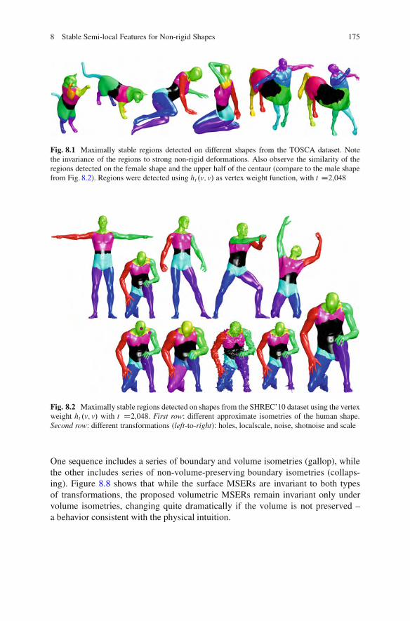
8 Stable Semi-local Features for Non-rigid Shapes 175
Fig. 8.1 Maximally stable regions detected on different shapes from the TOSCA dataset. Notethe invariance of the regions to strong non-rigid deformations. Also observe the similarity of theregions detected on the female shape and the upper half of the centaur (compare to the male shapefrom Fig. 8.2). Regions were detected using ht .v; v/ as vertex weight function, with t D2,048
Fig. 8.2 Maximally stable regions detected on shapes from the SHREC’10 dataset using the vertexweight ht .v; v/ with t D2,048. First row: different approximate isometries of the human shape.Second row: different transformations (left-to-right): holes, localscale, noise, shotnoise and scale
One sequence includes a series of boundary and volume isometries (gallop), whilethe other includes series of non-volume-preserving boundary isometries (collaps-ing). Figure 8.8 shows that while the surface MSERs are invariant to both typesof transformations, the proposed volumetric MSERs remain invariant only undervolume isometries, changing quite dramatically if the volume is not preserved –a behavior consistent with the physical intuition.
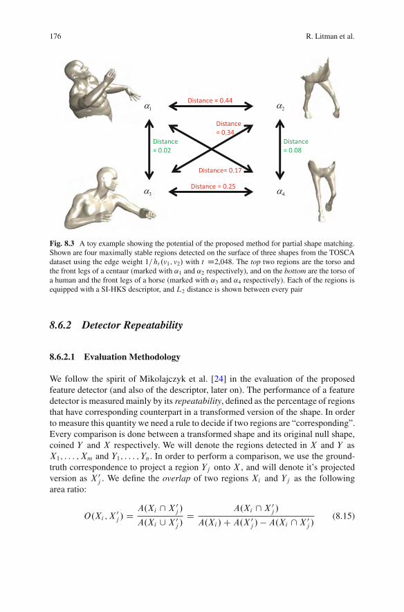
176 R. Litman et al.
Fig. 8.3 A toy example showing the potential of the proposed method for partial shape matching.Shown are four maximally stable regions detected on the surface of three shapes from the TOSCAdataset using the edge weight 1=ht .v1; v2/ with t D2,048. The top two regions are the torso andthe front legs of a centaur (marked with � 1 and � 2 respectively), and on the bottom are the torso ofa human and the front legs of a horse (marked with � 3 and � 4 respectively). Each of the regions isequipped with a SI-HKS descriptor, and L2 distance is shown between every pair
8.6.2 Detector Repeatability
8.6.2.1 Evaluation Methodology
We follow the spirit of Mikolajczyk et al. [24] in the evaluation of the proposedfeature detector (and also of the descriptor, later on). The performance of a featuredetector is measured mainly by its repeatability, defined as the percentage of regionsthat have corresponding counterpart in a transformed version of the shape. In orderto measure this quantity we need a rule to decide if two regions are “corresponding”.Every comparison is done between a transformed shape and its original null shape,coined Y and X respectively. We will denote the regions detected in X and Y asX1; : : : ; Xm and Y1; : : : ; Yn. In order to perform a comparison, we use the ground-truth correspondence to project a region Yj onto X , and will denote it’s projectedversion as X 0j . We define the overlap of two regions Xi and Yj as the followingarea ratio:
O.Xi ;X0j / D
A.Xi \ X 0j /A.Xi [ X 0j /
DA.Xi \ X 0j /
A.Xi /C A.X 0j /% A.Xi \X 0j /(8.15)
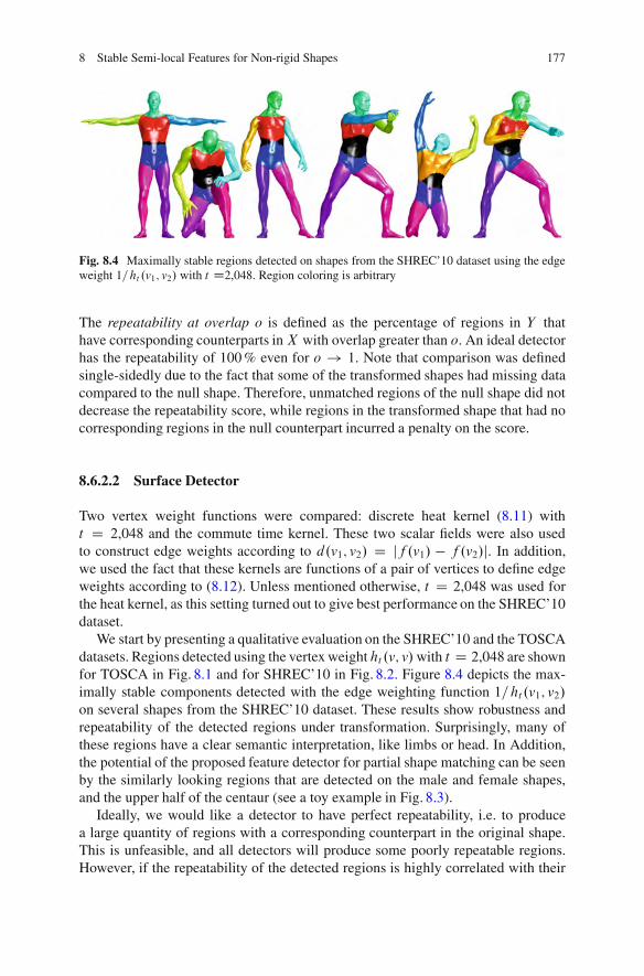
8 Stable Semi-local Features for Non-rigid Shapes 177
Fig. 8.4 Maximally stable regions detected on shapes from the SHREC’10 dataset using the edgeweight 1=ht .v1; v2/ with t D2,048. Region coloring is arbitrary
The repeatability at overlap o is defined as the percentage of regions in Y thathave corresponding counterparts in X with overlap greater than o. An ideal detectorhas the repeatability of 100 % even for o ! 1. Note that comparison was definedsingle-sidedly due to the fact that some of the transformed shapes had missing datacompared to the null shape. Therefore, unmatched regions of the null shape did notdecrease the repeatability score, while regions in the transformed shape that had nocorresponding regions in the null counterpart incurred a penalty on the score.
8.6.2.2 Surface Detector
Two vertex weight functions were compared: discrete heat kernel (8.11) witht D 2,048 and the commute time kernel. These two scalar fields were also usedto construct edge weights according to d.v1; v2/ D jf .v1/ % f .v2/j. In addition,we used the fact that these kernels are functions of a pair of vertices to define edgeweights according to (8.12). Unless mentioned otherwise, t D 2,048 was used forthe heat kernel, as this setting turned out to give best performance on the SHREC’10dataset.
We start by presenting a qualitative evaluation on the SHREC’10 and the TOSCAdatasets. Regions detected using the vertex weight ht .v; v/with t D 2,048 are shownfor TOSCA in Fig. 8.1 and for SHREC’10 in Fig. 8.2. Figure 8.4 depicts the max-imally stable components detected with the edge weighting function 1=ht.v1; v2/on several shapes from the SHREC’10 dataset. These results show robustness andrepeatability of the detected regions under transformation. Surprisingly, many ofthese regions have a clear semantic interpretation, like limbs or head. In Addition,the potential of the proposed feature detector for partial shape matching can be seenby the similarly looking regions that are detected on the male and female shapes,and the upper half of the centaur (see a toy example in Fig. 8.3).
Ideally, we would like a detector to have perfect repeatability, i.e. to producea large quantity of regions with a corresponding counterpart in the original shape.This is unfeasible, and all detectors will produce some poorly repeatable regions.However, if the repeatability of the detected regions is highly correlated with their
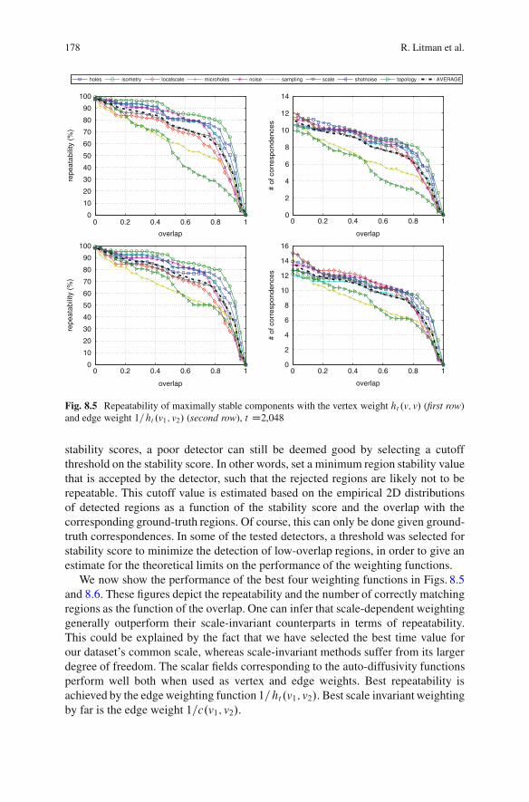
178 R. Litman et al.
holes isometry localscale microholes noise sampling scale shotnoise topology AVERAGE
0 0.2 0.4 0.6 0.8 10
10
20
30
40
50
60
70
80
90
100
overlap
repe
atab
ility
(%
)
0 0.2 0.4 0.6 0.8 10
2
4
6
8
10
12
14
overlap
# of
cor
resp
onde
nces
0 0.2 0.4 0.6 0.8 10
10
20
30
40
50
60
70
80
90
100
overlap
repe
atab
ility
(%
)
0 0.2 0.4 0.6 0.8 10
2
4
6
8
10
12
14
16
overlap
# of
cor
resp
onde
nces
Fig. 8.5 Repeatability of maximally stable components with the vertex weight ht .v; v/ (first row)and edge weight 1=ht .v1; v2/ (second row), t D2,048
stability scores, a poor detector can still be deemed good by selecting a cutoffthreshold on the stability score. In other words, set a minimum region stability valuethat is accepted by the detector, such that the rejected regions are likely not to berepeatable. This cutoff value is estimated based on the empirical 2D distributionsof detected regions as a function of the stability score and the overlap with thecorresponding ground-truth regions. Of course, this can only be done given ground-truth correspondences. In some of the tested detectors, a threshold was selected forstability score to minimize the detection of low-overlap regions, in order to give anestimate for the theoretical limits on the performance of the weighting functions.
We now show the performance of the best four weighting functions in Figs. 8.5and 8.6. These figures depict the repeatability and the number of correctly matchingregions as the function of the overlap. One can infer that scale-dependent weightinggenerally outperform their scale-invariant counterparts in terms of repeatability.This could be explained by the fact that we have selected the best time value forour dataset’s common scale, whereas scale-invariant methods suffer from its largerdegree of freedom. The scalar fields corresponding to the auto-diffusivity functionsperform well both when used as vertex and edge weights. Best repeatability isachieved by the edge weighting function 1=ht.v1; v2/. Best scale invariant weightingby far is the edge weight 1=c.v1; v2/.
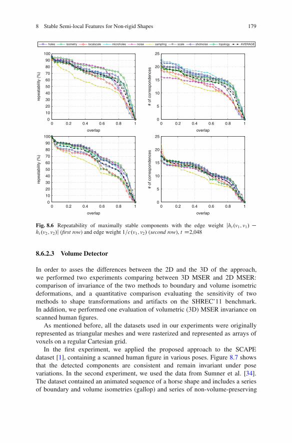
8 Stable Semi-local Features for Non-rigid Shapes 179
holes isometry localscale microholes noise sampling scale shotnoise topology AVERAGE
0 0.2 0.4 0.6 0.8 10
10
20
30
40
50
60
70
80
90
100
overlap
repe
atab
ility
(%
)
0 0.2 0.4 0.6 0.8 10
5
10
15
20
25
overlap
# of
cor
resp
onde
nces
0 0.2 0.4 0.6 0.8 10
10
20
30
40
50
60
70
80
90
100
overlap
repe
atab
ility
(%
)
0 0.2 0.4 0.6 0.8 10
5
10
15
20
25
overlap
# of
cor
resp
onde
nces
Fig. 8.6 Repeatability of maximally stable components with the edge weight jht .v1; v1/ #ht .v2; v2/j (first row) and edge weight 1=c.v1; v2/ (second row), t D2,048
8.6.2.3 Volume Detector
In order to asses the differences between the 2D and the 3D of the approach,we performed two experiments comparing between 3D MSER and 2D MSER:comparison of invariance of the two methods to boundary and volume isometricdeformations, and a quantitative comparison evaluating the sensitivity of twomethods to shape transformations and artifacts on the SHREC’11 benchmark.In addition, we performed one evaluation of volumetric (3D) MSER invariance onscanned human figures.
As mentioned before, all the datasets used in our experiments were originallyrepresented as triangular meshes and were rasterized and represented as arrays ofvoxels on a regular Cartesian grid.
In the first experiment, we applied the proposed approach to the SCAPEdataset [1], containing a scanned human figure in various poses. Figure 8.7 showsthat the detected components are consistent and remain invariant under posevariations. In the second experiment, we used the data from Sumner et al. [34].The dataset contained an animated sequence of a horse shape and includes a seriesof boundary and volume isometries (gallop) and series of non-volume-preserving
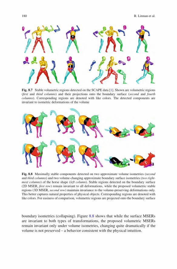
180 R. Litman et al.
Fig. 8.7 Stable volumetric regions detected on the SCAPE data [1]. Shown are volumetric regions(first and third columns) and their projections onto the boundary surface (second and fourthcolumns). Corresponding regions are denoted with like colors. The detected components areinvariant to isometric deformations of the volume
Fig. 8.8 Maximally stable components detected on two approximate volume isometries (secondand third columns) and two volume-changing approximate boundary surface isometries (two right-most columns) of the horse shape (left column). Stable regions detected on the boundary surface(2D MSER, first row) remain invariant to all deformations, while the proposed volumetric stableregions (3D MSER, second row) maintain invariance to the volume-preserving deformations only.This better captures natural properties of physical objects. Corresponding regions are denoted withlike colors. For easiness of comparison, volumetric regions are projected onto the boundary surface
boundary isometries (collapsing). Figure 8.8 shows that while the surface MSERsare invariant to both types of transformations, the proposed volumetric MSERsremain invariant only under volume isometries, changing quite dramatically if thevolume is not preserved – a behavior consistent with the physical intuition.
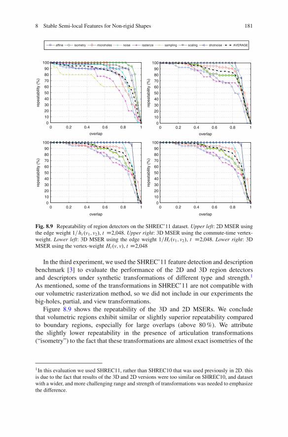
8 Stable Semi-local Features for Non-rigid Shapes 181
affine isometry microholes noise rasterize sampling scaling shotnoise AVERAGE
0 0.2 0.4 0.6 0.8 10
10
2030
40
5060
70
8090
100
overlap
repe
atab
ility
(%
)
0 0.2 0.4 0.6 0.8 10
1020
30
40
50
60
70
8090
100
overlap
repe
atab
ility
(%
)
0 0.2 0.4 0.6 0.8 10
1020
30
40
50
60
70
8090
100
overlap
repe
atab
ility
(%
)
0 0.2 0.4 0.6 0.8 10
1020
30
40
50
60
70
8090
100
overlap
repe
atab
ility
(%
)
Fig. 8.9 Repeatability of region detectors on the SHREC’11 dataset. Upper left: 2D MSER usingthe edge weight 1=ht .v1; v2/, t D2,048. Upper right: 3D MSER using the commute-time vertex-weight. Lower left: 3D MSER using the edge weight 1=Ht .v1; v2/, t D2,048. Lower right: 3DMSER using the vertex-weight Ht.v; v/, t D2,048
In the third experiment, we used the SHREC’11 feature detection and descriptionbenchmark [3] to evaluate the performance of the 2D and 3D region detectorsand descriptors under synthetic transformations of different type and strength.1
As mentioned, some of the transformations in SHREC’11 are not compatible withour volumetric rasterization method, so we did not include in our experiments thebig-holes, partial, and view transformations.
Figure 8.9 shows the repeatability of the 3D and 2D MSERs. We concludethat volumetric regions exhibit similar or slightly superior repeatability comparedto boundary regions, especially for large overlaps (above 80 %). We attributethe slightly lower repeatability in the presence of articulation transformations(“isometry”) to the fact that these transformations are almost exact isometries of the
1In this evaluation we used SHREC11, rather than SHREC10 that was used previously in 2D. thisis due to the fact that results of the 3D and 2D versions were too similar on SHREC10, and datasetwith a wider, and more challenging range and strength of transformations was needed to emphasizethe difference.

182 R. Litman et al.
boundary, while being only approximate isometries of the volume. Another reasonfor the latter degradation may be local topology changes that were manifested inthe rasterization of the shapes in certain isometries. These topology changes appearonly in the volumetric detector, and they affected the quality of detected regionsin their vicinity. Although the construction of the MSER feature detector is notaffine-invariant, excellent repeatability under affine transformation is observed. Webelieve that this and other invariance properties are related to the properties of thecomponent trees (which are stronger than those of the weighting functions) andintend to investigate this phenomenon in future studies.
8.6.3 Descriptor Informativity
8.6.3.1 Evaluation Methodology
In these experiments, we aim to evaluate the informativity of region descriptors.This is done by measuring the relation between the overlap of two regions and theirdistance in the descriptor space.
Keeping the notation from the previous section, we set a minimum overlap ) D0:75 deeming two regions Yi and Xj matched, i.e. if oij D O.X 0i ; Xj / ' ) (X 0i isthe projection of Yi on the null shape X ). This threshold is needed to constitute thematching ground-truth.
Given a region descriptor ˇ on each of the regions, we set a threshold * on thedistance between the descriptors of Yi andXj in order to classify them as positives,i.e. if dij D kˇ.Yi/ % ˇ.Xj /k $ * . For simplicity we assume the distance betweenthe descriptors to be the standard Euclidean distance. We define the true positiverate (TPR) and false positive rate (FPR) as the ratios
TPR D jfdij $ *gjjfoij ' )gjI FPR D jfdij > *gjjfoij < )gj
The receiver operator characteristic (ROC) curve is obtained a set of pairs.FPR;TPR/, created by varying the threshold * . The false negative rate definedas FNR D 1 % TPR. The equal error rate (EER) is the point on the ROC curve forwhich the false positive and false negative rates coincide. EER is used as a scalarmeasure for the descriptor informativity, where ideal descriptors have EER D 0.
Another descriptor performance criterion is created by finding for each Xi itsnearest neighbor in the descriptor space Yj!.i/, namely j $.i/ D arg minj dij . Wethen define the matching score, as the ratio of correct first matches for a givenoverlap ), and m, the total number of regions in X :
score.)/ D jfoij!.i/ ' )gjm
: (8.16)
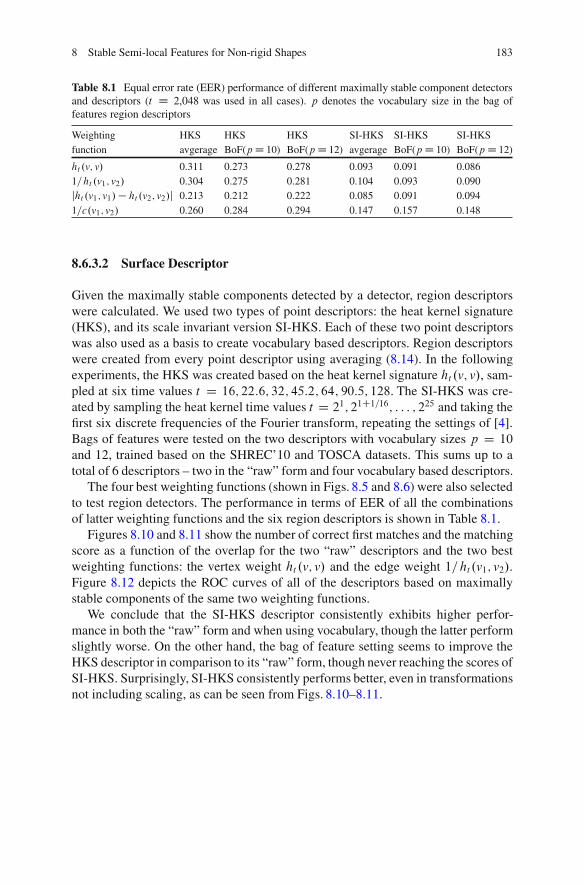
8 Stable Semi-local Features for Non-rigid Shapes 183
Table 8.1 Equal error rate (EER) performance of different maximally stable component detectorsand descriptors (t D 2,048 was used in all cases). p denotes the vocabulary size in the bag offeatures region descriptors
Weighting HKS HKS HKS SI-HKS SI-HKS SI-HKSfunction avgerage BoF(pD 10) BoF(pD 12) avgerage BoF(pD 10) BoF(pD 12)
ht .v; v/ 0.311 0.273 0.278 0.093 0.091 0.0861=ht .v1; v2/ 0.304 0.275 0.281 0.104 0.093 0.090jht .v1; v1/# ht .v2; v2/j 0.213 0.212 0.222 0.085 0.091 0.0941=c.v1; v2/ 0.260 0.284 0.294 0.147 0.157 0.148
8.6.3.2 Surface Descriptor
Given the maximally stable components detected by a detector, region descriptorswere calculated. We used two types of point descriptors: the heat kernel signature(HKS), and its scale invariant version SI-HKS. Each of these two point descriptorswas also used as a basis to create vocabulary based descriptors. Region descriptorswere created from every point descriptor using averaging (8.14). In the followingexperiments, the HKS was created based on the heat kernel signature ht .v; v/, sam-pled at six time values t D 16; 22:6; 32; 45:2; 64; 90:5; 128. The SI-HKS was cre-ated by sampling the heat kernel time values t D 21; 21C1=16; : : : ; 225 and taking thefirst six discrete frequencies of the Fourier transform, repeating the settings of [4].Bags of features were tested on the two descriptors with vocabulary sizes p D 10and 12, trained based on the SHREC’10 and TOSCA datasets. This sums up to atotal of 6 descriptors – two in the “raw” form and four vocabulary based descriptors.
The four best weighting functions (shown in Figs. 8.5 and 8.6) were also selectedto test region detectors. The performance in terms of EER of all the combinationsof latter weighting functions and the six region descriptors is shown in Table 8.1.
Figures 8.10 and 8.11 show the number of correct first matches and the matchingscore as a function of the overlap for the two “raw” descriptors and the two bestweighting functions: the vertex weight ht .v; v/ and the edge weight 1=ht.v1; v2/.Figure 8.12 depicts the ROC curves of all of the descriptors based on maximallystable components of the same two weighting functions.
We conclude that the SI-HKS descriptor consistently exhibits higher perfor-mance in both the “raw” form and when using vocabulary, though the latter performslightly worse. On the other hand, the bag of feature setting seems to improve theHKS descriptor in comparison to its “raw” form, though never reaching the scores ofSI-HKS. Surprisingly, SI-HKS consistently performs better, even in transformationsnot including scaling, as can be seen from Figs. 8.10–8.11.
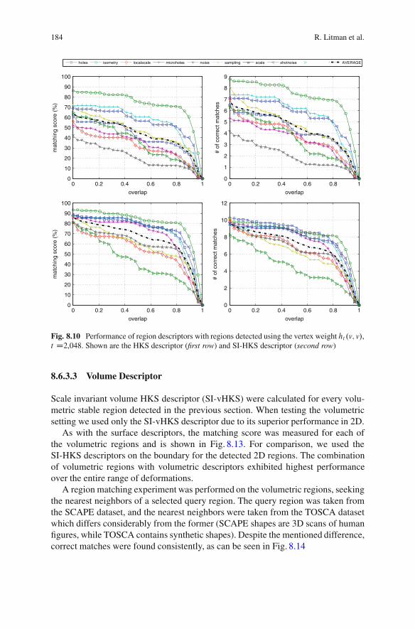
184 R. Litman et al.
holes isometry localscale microholes noise sampling scale shotnoise AVERAGE
0 0.2 0.4 0.6 0.8 10
10
20
30
40
50
60
70
80
90
100
overlap
mat
chin
g sc
ore
(%)
0 0.2 0.4 0.6 0.8 10
1
2
3
4
5
6
7
8
9
overlap
# of
cor
rect
mat
ches
0 0.2 0.4 0.6 0.8 10
10
20
30
40
50
60
70
80
90
100
overlap
mat
chin
g sc
ore
(%)
0 0.2 0.4 0.6 0.8 10
2
4
6
8
10
12
overlap
# of
cor
rect
mat
ches
Fig. 8.10 Performance of region descriptors with regions detected using the vertex weight ht .v; v/,t D2,048. Shown are the HKS descriptor (first row) and SI-HKS descriptor (second row)
8.6.3.3 Volume Descriptor
Scale invariant volume HKS descriptor (SI-vHKS) were calculated for every volu-metric stable region detected in the previous section. When testing the volumetricsetting we used only the SI-vHKS descriptor due to its superior performance in 2D.
As with the surface descriptors, the matching score was measured for each ofthe volumetric regions and is shown in Fig. 8.13. For comparison, we used theSI-HKS descriptors on the boundary for the detected 2D regions. The combinationof volumetric regions with volumetric descriptors exhibited highest performanceover the entire range of deformations.
A region matching experiment was performed on the volumetric regions, seekingthe nearest neighbors of a selected query region. The query region was taken fromthe SCAPE dataset, and the nearest neighbors were taken from the TOSCA datasetwhich differs considerably from the former (SCAPE shapes are 3D scans of humanfigures, while TOSCA contains synthetic shapes). Despite the mentioned difference,correct matches were found consistently, as can be seen in Fig. 8.14
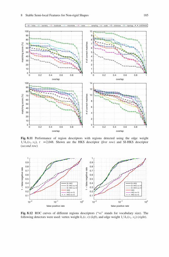
8 Stable Semi-local Features for Non-rigid Shapes 185
holes isometry localscale microholes noise sampling scale shotnoise topology AVERAGE
0 0.2 0.4 0.6 0.8 10
10
20
30
40
50
60
70
80
90
100
overlap
mat
chin
g sc
ore
(%)
0 0.2 0.4 0.6 0.8 10
1
2
3
4
5
6
7
8
9
10
overlap
# of
cor
rect
mat
ches
0 0.2 0.4 0.6 0.8 10
10
20
30
40
50
60
70
80
90
100
overlap
mat
chin
g sc
ore
(%)
0 0.2 0.4 0.6 0.8 10
2
4
6
8
10
12
14
overlap
# of
cor
rect
mat
ches
Fig. 8.11 Performance of region descriptors with regions detected using the edge weight1=ht .v1; v2/, t D2,048. Shown are the HKS descriptor (first row) and SI-HKS descriptor(second row)
10!2 10!1 100
0.1
0.2
0.3
0.4
0.5
0.6
0.7
0.8
0.9
1
false positive rate
1 !
fals
e ne
getiv
e ra
te
SI!HKSSI!HKS vs=10SI!HKS vs=12HKSHKS vs=10HKS vs=12
10!2 10!1 100
0.1
0.2
0.3
0.4
0.5
0.6
0.7
0.8
0.9
1
false positive rate
1 !
fals
e ne
getiv
e ra
te
SI!HKSSI!HKS vs=10SI!HKS vs=12HKSHKS vs=10HKS vs=12
Fig. 8.12 ROC curves of different regions descriptors (“vs” stands for vocabulary size). Thefollowing detectors were used: vertex weight ht .v; v/ (left), and edge weight 1=ht .v1; v2/ (right).

186 R. Litman et al.
affine isometry microholes noise rasterize sampling scaling shotnoise AVERAGE
0 0.2 0.4 0.6 0.8 10
10
20
30
40
50
60
70
80
90
100
overlap
mat
chin
g sc
ore
(%)
0 0.2 0.4 0.6 0.8 10
10
20
30
40
50
60
70
80
90
100
overlap
mat
chin
g sc
ore
(%)
0 0.2 0.4 0.6 0.8 10
10
20
30
40
50
60
70
80
90
100
overlap
mat
chin
g sc
ore
(%)
0 0.2 0.4 0.6 0.8 10
10
20
30
40
50
60
70
80
90
100
overlap
mat
chin
g sc
ore
(%)
Fig. 8.13 Matching score of descriptors based on the 2D and 3D regions detected with thedetectors shown in Fig. 8.9. Shown are the 2D SI-HKS (upper left) 3D SI-vHKS (upper rightand two bottom plots) descriptors
Fig. 8.14 Examples of closest matches found for different query regions from the SCAPE dataseton the TOSCA dataset. Shown from left to right are: query, 1st, 2nd, 4th, 10th, and 15th matches.Edge-weight 1=Ht .v1; v2/ was used as the detector; average SI-vHKS was used as the descriptor

8 Stable Semi-local Features for Non-rigid Shapes 187
8.7 Conclusions
A generic framework for the detection of stable non-local features in deformableshapes is presented. This approach is based on a popular image analysis tool calledMSER, where we maximize a stability criterion in a component tree representationof the shape. The framework is designed to unify the vertex or edge weights, unlikemost of its predecessors. The use of diffusion geometry as the base of the weightingscheme make to detector invariant to non-rigid bending, global scaling and othershape transformations, a fact that makes this approach applicable in the challengingsetting of deformable shape analysis.
The approach was shown to work with volumetric diffusion geometric analysis.In all experiments, our volumetric features exhibited higher robustness to defor-mation compared to similar features computed on the two-dimensional boundaryof the shape. We also argue and exemplify that unlike features constructed fromthe boundary surface of the shape, our volumetric features are not invariant tovolume-changing deformations of the solid object. We believe that this is thedesired behavior in many applications, as volume isometries better model naturaldeformations of objects than boundary isometries.
We showed experimentally the high repeatability of the proposed features, whichmakes them a good candidate for a wide range of shape representation and retrievaltasks.
Acknowledgements We are grateful to Dan Raviv for providing us his volume rasterizationand Laplacian disretization code. M. M. Bronstein is partially supported by the Swiss High-Performance and High-Productivity Computing (HP2C) grant. A. M. Bronstein is partiallysupported by the Israeli Science Foundation and the German-Israeli Foundation.
References
1. Anguelov, D., Srinivasan, P., Koller, D., Thrun, S., Rodgers, J., Davis, J.: SCAPE: shapecompletion and animation of people. TOG 24(3), 408–416 (2005)
2. Aubry, M., Schlickewei, U., Cremers, D.: The wave kernel signature-a quantum mechanicalapproach to shape analyis. In: Proceedings of the CVPR, Colorado Springs (2011)
3. Boyer, E., Bronstein, A.M., Bronstein, M.M., Bustos, B., Darom, T., Horaud, R., Hotz, I.,Keller, Y., Keustermans, J., Kovnatsky, A., Litman, R., Reininghaus, J., Sipiran, I., Smeets, D.,Suetens, P., Vandermeulen, D., Zaharescu, A., Zobel, V.: Shrec ’11: Robust feature detectionand description benchmark. In: Proceedings of the 3DOR, Llandudno, pp. 71–78 (2011)
4. Bronstein, M.M., Kokkinos, I.: Scale-invariant heat kernel signatures for non-rigid shaperecognition. In: Computer Vision and Pattern Recognition, San Francisco, pp. 1704–1711(2010)
5. Bronstein, A., Bronstein, M.M., Bronstein, M., Kimmel, R.: Numerical Geometry of Non-rigidShapes. Springer, New York (2008)
6. Bronstein, A., Bronstein, M.M., Bustos, B., Castellani, U., Crisani, M., Falcidieno, B.,Guibas, L.J., Kokkinos, I., Murino, V., Ovsjanikov, M., et al.: SHREC 2010: robust featuredetection and description benchmark. In: Eurographics Workshop on 3D Object Retrieval(2010)
188 R. Litman et al.
7. Chazal, F., Guibas, L.J., Oudot, S.Y., Skraba, P.: Persistence-based clustering in riemannianmanifolds. Research Report RR-6968, INRIA (2009)
8. Coifman, R.R., Lafon, S.: Diffusion maps. Appl. Comput. Harmonic Anal. 21(1), 5–30 (2006)9. Couprie, M., Bertrand, G.: Topological grayscale watershed transformation. In: SPIE Vision
Geometry V Proceedings, San Diego, vol. 3168, pp. 136–146 (1997)10. Dey, T.K., Li, K., Luo, C., Ranjan, P., Safa, I., Wang, Y.: Persistent heat signature for pose-
oblivious matching of incomplete models. Comput. Graph. Forum 29(5), 1545–1554 (2010)11. Digne, J., Morel, J.-M., Audfray, N., Mehdi-Souzani, C.: The level set tree on meshes. In:
Proceedings of the Fifth International Symposium on 3D Data Processing, Visualization andTransmission, Paris (2010)
12. Donoser, M., Bischof, H.: 3d segmentation by maximally stable volumes (msvs). In: Proceed-ings of the 18th International Conference on Pattern Recognition, vol. 1, pp. 63–66. IEEEComputer Society, Los Alamitos (2006)
13. Edelsbrunner, H., Letscher, D., Zomorodian, A.: Topological persistence and simplification.Discret.Comput. Geom. 28(4), 511–533 (2002)
14. Floater, M.S., Hormann, K.: Surface parameterization: a tutorial and survey. In: Advances inMultiresolution for Geometric Modelling, vol. 1, pp. 157–186. Springer, Berlin (2005)
15. Forssen, P.E.: Maximally stable colour regions for recognition and matching. In: Proceedingsof the CVPR, Minneapolis, pp. 1–8 (2007)
16. Huang, Q.X., Flory, S., Gelfand, N., Hofer, M., Pottmann, H.: Reassembling fractured objectsby geometric matching. ACM Trans. Graph. 25(3), 569–578 (2006)
17. Johnson, A.E., Hebert, M.: Using spin images for efficient object recognition in cluttered 3Dscenes. Trans. PAMI 21(5), 433–449 (1999)
18. Kimmel, R., Zhang, C., Bronstein, A.M., Bronstein, M.M.: Are mser features really interest-ing? IEEE Trans. PAMI 33(11), 2316–2320 (2011)
19. Levy, B.: Laplace-Beltrami eigenfunctions towards an algorithm that understands geometry.In: Proceedings of the IEEE International Conference on Shape Modeling and Applications2006, pp. 13. IEEE Computer Society, Los Alamitos (2006)
20. Litman, R., Bronstein, A.M., Bronstein, M.M.: Diffusion-geometric maximally stable compo-nent detection in deformable shapes. Comput. Graph. 35, 549–560 (2011)
21. Lowe, D.: Distinctive image features from scale-invariant keypoint. IJCV 60(2), 91–110 (2004)22. Matas, J., Chum, O., Urban, M., Pajdla, T.: Robust wide-baseline stereo from maximally stable
extremal regions. Image Vis. Comput. 22(10), 761–767 (2004)23. Meyer, M., Desbrun, M., Schroder, P., Barr, A.H.: Discrete differential-geometry operators for
triangulated 2-manifolds. In: Visualization and Mathematics III, pp. 35–57. Springer, Berlin(2003)
24. Mikolajczyk, K., Tuytelaars, T., Schmid, C., Zisserman, A., Matas, J., Schaffalitzky, F.,Kadir, T., Gool, L.V.: A comparison of affine region detectors. IJCV 65(1), 43–72 (2005)
25. Najman, L., Couprie, M.: Building the component tree in quasi-linear time. IEEE Trans. ImageProc. 15(11), 3531–3539 (2006)
26. Ovsjanikov, M., Sun, J., Guibas, L.: Global intrinsic symmetries of shapes. Comput. Graph.Forum 27(5), 1341–1348 (2008)
27. Ovsjanikov, M., Bronstein, A.M., Bronstein, M.M., Guibas, L.J.: Shape google: a computervision approach to isometry invariant shape retrieval. In: Computer Vision Workshops (ICCVWorkshops), Kyoto, pp. 320–327 (2009)
28. Pinkall, U., Polthier, K.: Computing discrete minimal surfaces and their conjugates. Exp. Math.2(1), 15–36 (1993)
29. Raviv, D., Bronstein, M.M., Bronstein, A.M., Kimmel, R.: Volumetric heat kernel signatures.In: Proceedings of the ACM Workshop on 3D Object Retrieval, Firenze, pp. 39–44 (2010)
30. Reuter, M., Wolter, F.-E., Peinecke, N.: Laplace-spectra as fingerprints for shape matching.In: Proceedings of the ACM Symposium on Solid and Physical Modeling, Cambridge,pp. 101–106 (2005)
31. Rustamov, R.M.: Laplace-Beltrami eigenfunctions for deformation invariant shape representa-tion. In: Proceedings of the SGP, Barcelona, pp. 225–233 (2007)
8 Stable Semi-local Features for Non-rigid Shapes 189
32. Sivic, J., Zisserman, A.: Video google: A text retrieval approach to object matching in videos.In: Proceedings of the CVPR, Madison, vol. 2, pp. 1470–1477 (2003)
33. Skraba, P. Ovsjanikov, M., Chazal, F., Guibas, L.: Persistence-based segmentation ofdeformable shapes. In: Proceedings of the NORDIA, San Francisco, pp. 45–52 (2010)
34. Sumner, R.W., Popovic, J.: Deformation transfer for triangle meshes. ACM Transactions onGraphics (Proceedings of the SIGGRAPH), Los Angeles, vol. 23, pp. 399–405 (2004)
35. Sun, J., Ovsjanikov, M., Guibas, L.: A concise and provably informative multi-scale signaturebased on heat diffusion. Comput. Graph. Forum 28, 1383–1392 (2009)
36. Thorstensen, N., Keriven, R.: Non-rigid shape matching using geometry and photometry.In: Computer Vision – ACCV 2009, Xi’an, vol. 5996, pp. 644–654 (2010)
37. Toldo, R., Castellani, U., Fusiello, A.: Visual vocabulary signature for 3d object retrieval andpartial matching. In: Proceedings of the 3DOR, Munich, pp. 21–28 (2009)
38. Tuzel, O., Porikli, F., Meer, P.: Region covariance: a fast descriptor for detection and clas-sification. In: Computer Vision ECCV 2006. Lecture Notes in Computer Science, vol. 3952,pp. 589–600. Springer, Berlin/Heidelberg (2006)
39. Vincent, L., Soille, P.: Watersheds in digital spaces: an efficient algorithm based on immersionsimulations. IEEE Trans. PAMI, 13(6), 583–598 (2002)
40. Wardetzky, M., Mathur, S., Kaelberer, F., Grinspun, E.: Discrete laplace operators: no freelunch. In: Proceedings of the of Eurographics Symposium on Geometry Processing, Barcelona,pp. 33–37 (2007)
41. Zaharescu, A., Boyer, E., Varanasi, K., Horaud, R.: Surface feature detection and descriptionwith applications to mesh matching. In: Proceedings of the CVPR, Miami, pp. 373–380 (2009)
Chapter 9A Brief Survey on Semi-Lagrangian Schemesfor Image Processing
Elisabetta Carlini, Maurizio Falcone, and Adriano Festa
Abstract In this survey we present some semi-Lagrangian schemes for the approx-imation of weak solutions of first and second order differential problems relatedto image processing and computer vision. The general framework is given by thetheory of viscosity solutions and, in some cases, of calculus of variations. Theschemes proposed here have interesting stability properties for evolutive problemssince they allow for large time steps, can deal with degenerate problems and aremore accurate if compared to standard finite difference/element methods of the sameorder. Several examples on classical problems will illustrate these properties.
9.1 Introduction
Nonlinear Partial Differential Equations (PDEs) appear in many classical imageprocessing problems and there is a need for accurate and efficient numericalmethods to solve them. Usually we have to deal with several difficulties, includingthe fact that in most cases these are degenerate problems with non smooth solutions.Classical methods (Finite Elements, Finite Differences) must be modified and oftenstabilized to solve this kind of problems (the interested reader will find in the booksby Strikwerda [46] and Brenner and Scott [6] a comprehensive introduction to theseclassical techniques and well as some recent results). The goal of this paper is topresent semi-Lagrangian (SL in the sequel) approximation techniques and illustratetheir properties through the solution of some classical image processing problems.
SL methods were introduced long time ago for linear advection problems. As faras we know the first example is the Courant-Isaacson and Rees scheme [19] whichdates back to the 1960s. However, their application to nonlinear problems is more
E. Carlini (!) !M. Falcone ! A. FestaDipartimento di Matematica “G. Castelnuovo”, Sapienza – Universita di Roma,P. Aldo Moro, 2 – 00185 Roma, Italye-mail: [email protected]; [email protected]; [email protected]
M. Breuß et al. (eds.), Innovations for Shape Analysis, Mathematics and Visualization,DOI 10.1007/978-3-642-34141-0 9, © Springer-Verlag Berlin Heidelberg 2013
191

192 E. Carlini et al.
recent as well as the analysis of their mathematical properties in terms of consis-tency, stability, convergence and convergence rates. A comprehensive introductionto this class of schemes can be found in the book by Falcone and Ferretti [32].
Let us just recall here some of the motivations which make semi-Lagrangianschemes an interesting alternative to more classical finite differences and finiteelements techniques. The first and perhaps more interesting point is that, due tothe fact that they mimic the method of characteristics, they allow for large timesteps in evolutive problems. This property is particularly useful when one looksfor the limiting behavior for t going to infinity in order to recover the solutionof the corresponding stationary problem. The second important property is thatthey introduce only a small numerical viscosity so that their smoothing effect onthe solution is very limited. The third property to be mentioned is that they havea natural interpretation in terms of the representation formula for some nonlinearproblems. One example is the solution of the eikonal equation where the Hopf-Laxformula applies (see the next section for details). Roughly speaking they can beinterpreted as a discrete Hopf-Lax formula and this means that their accuracy can beincreased to high-order. Finally, they can work on structured and unstructured grids.Although the latter are not very popular among the image processing communitythey are a natural choice in other fields of applications like fluid dynamics,meteorology, geophysics. The details regarding the analytical properties of theschemes will not be illustrated here since this survey is mainly intended to presentthe schemes and their potential via the solution of some test problems.
In the next section we will briefly describe how the schemes are derived forsome first and second order problems which come from image processing. Wewill consider some simplified models in order to introduce the main ideas of SLapproximation and to explain how the methods are constructed. The followingsections are devoted to some classical problems in image processing: Shape fromShading, nonlinear filtering, segmentation and optical flow. For each of them we willintroduce the model which we are going to approximate, present the correspondingSL scheme and illustrate some numerical experiments.
9.2 An Introduction to Semi-Lagrangian Schemesfor Nonlinear PDEs
We will consider three classical examples to show the main features and propertiesof the SL approximation: Shape from Shading (SfS in the sequel), segmentationvia the level set (LS) method and nonlinear filtering via Mean Curvature Motion(MCM). It is worth to note that they all lead to nonlinear (and possibly degenerate)partial differential models.
Let us start with the Shape from Shading problem. This is an inverse problemwhere we want to compute the surface corresponding to a single image. A simplemodel for this problem can be derived (see the next section for more details)
9 A Brief Survey on Semi-Lagrangian Schemes for Image Processing 193
assuming that the light source is at infinity in the direction !, the surface isLambertian, and that we can neglect perspective deformations. We consider thenthe equation which appears in most of the papers and corresponds to frontal lightsource at infinity, i.e. ! D .0; 0; 1/ and
jru.x/j D f .x/ for x 2 ˝; (9.1)
where I W ˝ ! R2 ! Œ0; 1! represents the brightness function of the image and
f .x/ Ds
1
I.x/2" 1: (9.2)
This is an eikonal equation, a first order stationary nonlinear pde. In order tosolve (9.1) we must provide some boundary conditions on @˝ and/or add someinformations to select a unique solution. In fact, the equation just depends on thegradient so that if u is a solution also uC constant is a solution and we need to fixthe height of the surface at least at the boundary to select a solution. For an imagecontaining an “occluding boundary”, it is usual to consider this boundary as @˝and the domain of reconstruction will be the region ˝ enclosed by the occludingboundary.
Another classical problem is the segmentation problem, where we want to detectthe boundaries of objects represented in a picture. A very popular method forsegmentation is based on the level set method, this application is often called “activecontour” since the segmentation is obtained following the evolution of a simplecurve (a circle for example) in its normal direction. Starting from a circle inside anobject we follow its evolution until the curve touches the borders of the object. Itis important to know that the LS method has had a great success for the analysisof front propagation problems for its capability to handle many different physicalphenomena within the same theoretical framework. Moreover, LS methods allowto develop the analysis of interface propagation also after the onset of singularities(as for example, when there is a topological change in the front). See the books bySethian [45] and Osher and Fedkiw [42].
In the LS methods the unknown is a “representation” function u WR2 # Œ0; T !!Rof the interface, the position of the interface "t at time t is given by the 0-level setof u.:; t/, i.e.
"t WD fx W u.x; t/ D 0g:The model equation corresponding to the LS method (see e.g.[43] for details) is
!ut C c.x; t/jruj D 0 .x; t/ 2 R2 # Œ0; T !u.x/ D u0.x/ x 2 R2 (9.3)
where u0 must be a representation function for the initial front @˝0, where ˝0 is agiven open bounded subset of R2, this means
194 E. Carlini et al.
8<
:
u0.x/ > 0 for x 2 R2 n˝0
u0.x/ D 0 for x 2 @˝0 WD "0u0.x/ < 0 for x 2 ˝0:
(9.4)
Note that usually the scalar velocity c W R2#Œ0; T !! R is given and it represents thevelocity of the front in its normal direction #.x; t/ WD ru.x;t/
jru.x;t/j . However, the sameapproach applies to other scalar velocities. For example one can use it to describeisotropic and anisotropic front propagation, Mean Curvature Motion (MCM) andother situations when the velocity depends on some geometrical properties of thefront. In summary, this corresponds to the following choices:
c.x; t/ isotropic growth with time varying velocity (9.5)
c.x; t; #/ anisotropic growth, i.e. dependent on the normal direction (9.6)
c.x; t; k/ Mean Curvature Motion (9.7)
where k D k.x; t/ is the mean curvature to the front at time t . There are evenmodels where the velocity is obtained by convolution (nonlocal velocity).
Since the borders of objects inside a given image I are characterized by the factthat there is a rapid change in the values of I , in the segmentation problem one cantake the gradient of I as an indicator of the edges. If jrI j is large this means thatwe are at an edge. For this reason, a popular choice of the velocity when we applyLS methods to the segmentation problem is
c.x/ WD .1C jrI.x/jp/"1 where p $ 1:
With this choice, the velocity is 1 inside the region where the gray level is constantand rapidly decreases to 0 when x is close to an edge (which corresponds to a jumpin the I derivative).
Another problem we will consider is nonlinear filtering. A classical model totreat this problem is to consider (9.3) with the velocity given by Mean Curvaturec.x; t/ D k.x; t/, see [34]. In this case one gets
8<
:ut .x; t/ D div
" ru.x; t/jru.x; t/j
#jru.x; t/j .x; t/ 2 R2 # Œ0; T !
u.x; 0/ D I0.x/(9.8)
where I0 is a starting noisy image. This equation, in the level set formalism,represents the Mean Curvature Motion of curves, since each level set of u movesin normal direction with a speed proportional to their mean curvature. The goal isto recover a new image reducing the noise. Note that the evolutive equation is notwell defined at all points where the gradient vanishes so it is a singular parabolicequation. This implies that classical finite difference and finite element methodsmust be adapted in order to deal with the singularities (see [43] for a finite differencescheme and [15, 41] for two convergence results).
9 A Brief Survey on Semi-Lagrangian Schemes for Image Processing 195
Let us now turn our attention to the construction of the semi-Lagrangian schemesfor the above model equations. For readers’ convenience, we will start from thelinear advection equation:
ut C b.x; t/ % ru D f .x; t/ .x; t/ 2 R2 # .0; T /: (9.9)
Here, b W R2 # .0; T / ! R2 is a vectorfield (the drift) and f W R2 # .0; T / ! Ris the source term. We look for the unique solution u W R2 # .0; T / ! R of (9.9)satisfying the initial condition
u.x; 0/ D u0.x/ x 2 R2: (9.10)
A simple case corresponds to f .x; t/ & 0 and b.x; t/ & c (constant). Then, thesolution u is given by the representation formula
u.x; t/ D u0.x " c t/ .x; t/ 2 R2 # Œ0; T / (9.11)
which can be easily obtained by the method of characteristics. The representationformula (9.11) contains an important information: the solution at the point x attime t only depends on the initial value at the point x " ct which is called thefoot of the characteristic passing through .x; t/ (more details on the method ofcharacteristics can be found on many classical books presenting the basic theoryof partial differential equations, e.g. [28]). A typical choice is to build a space gridwith constant step $x
G$x WD fxj W xj D .j1$x; j2$x/ for j1 2 Z; j2 2 Zg: (9.12)
This grid is called lattice. In order to build an approximation scheme for (9.9) andmore in general for evolutive problems, we need to consider a space-time grid
G$x;$t WD f.xj ; tn/ W xj D .j1$x; j2$x/; tn D n$t; for j1 2 Z; j2 2 Z; n 2 Ng(9.13)
where in the simplest case $t is a constant time step. Naturally for numericalpurposes the number of nodes of our grids has to be finite and we will considerthe intersections of our grids with the computational domain˝ .
The basic idea behind all finite difference approximations is to replace everyderivative by an incremental ratio. Thus, one obtains a finite dimensional problemwhose unknown are the values of the numerical solution at all the nodes of thelattice, so that the value unj associated to the node .xj ; tn/ should be regarded as anapproximation of u.xj ; tn/. For the time derivative it is natural to choose the forwardincremental ratio
ut .x; t/ 'u.x; t C$t/ " u.x; t/
$t: (9.14)

196 E. Carlini et al.
For finite difference, it is well known that dealing with advection problems we needto consider the incremental ratio in the up-wind direction, so that we must takethe first node on the left (right) if the velocity is positive (negative). This choiceguarantees the stability of the approximation scheme as well as a good fit withthe physics behind the model. When b.xj ; tn/ is positive, this corresponds to thefollowing up-wind scheme for the left hand side of the advection equation
ut .xj ; tn/C b.xj ; tn/ % ru.xj ; tn/ 'u.xj ; tn C$t / " u.xj ; tn/
$tC
"b1.xj ; tn/u.xj1!1;j2 ; tn/" u.xj1;j2 ; tn/
$x" b2.xj ; tn/
u.xj1;j2!1; tn/" u.xj1;j2 ; tn/$x
:
(9.15)
Adopting the standard notation unj D u.xj ; tn/, we write the scheme in the standardexplicit time marching form
unC1j D unj C$t
$xb.xj ; tn/ % .unj1"1;j2 " unj ; u
nj1;j2"1 " unj /: (9.16)
Semi-Lagrangian schemes are based on a different way to construct the approx-imation of (9.9), in particular this affects the discretization of the advection termb.x; t/ % ru. Since this is a directional derivative, we can write
b.xj ; tn/ % ru.xj ; tn/ ' "un.xj " ıb.xj ; tn// " unj
ı; (9.17)
where ı is a “small” positive parameter, and un denotes an extension of thenumerical solution (at time tn) to be computed outside of the grid. Coupling theforward finite difference in time with this approximation we get
unC1j " unj$t
"un.xj " ıb.xj ; tn// " unj
ıD 0; (9.18)
and finally, choosing ı D $t , we obtain the scheme
unC1j D un.xj "$tb.xj ; tn//: (9.19)
This is the semi-Lagrangian scheme for (9.9) for f .x; t/ D 0. Note that, forb.x; t/ & c (9.18) can be easily interpreted as a discrete version of the representa-tion formula (9.11). Even in this simple case, the value at the point xj " $tc doesnot belong to the grid G$x and must be obtained by interpolation on the values at thegrid nodes. We will denote by ˘Œw! the interpolation operator which reconstructslocally the values of a function w only known on G$x. There are many possiblechoices for ˘ , e.g. linear, bilinear or cubic interpolation (see also [32] for moregeneral choices). A very popular choice is the piecewise linear interpolation whichproduces a monotone first order scheme.
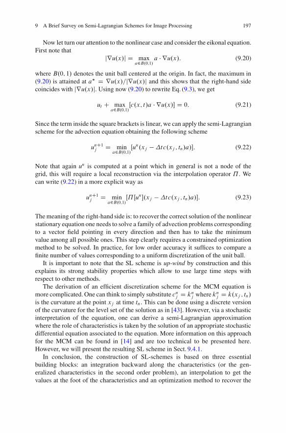
9 A Brief Survey on Semi-Lagrangian Schemes for Image Processing 197
Now let turn our attention to the nonlinear case and consider the eikonal equation.First note that
jru.x/j D maxa2B.0;1/
a % ru.x/: (9.20)
where B.0; 1/ denotes the unit ball centered at the origin. In fact, the maximum in(9.20) is attained at a# D ru.x/=jru.x/j and this shows that the right-hand sidecoincides with jru.x/j. Using now (9.20) to rewrite Eq. (9.3), we get
ut C maxa2B.0;1/
Œc.x; t/a % ru.x/! D 0: (9.21)
Since the term inside the square brackets is linear, we can apply the semi-Lagrangianscheme for the advection equation obtaining the following scheme
unC1j D mina2B.0;1/
Œun.xj "$tc.xj ; tn/a/!: (9.22)
Note that again un is computed at a point which in general is not a node of thegrid, this will require a local reconstruction via the interpolation operator ˘ . Wecan write (9.22) in a more explicit way as
unC1j D mina2B.0;1/
Œ˘Œun!.xj "$tc.xj ; tn/a/!: (9.23)
The meaning of the right-hand side is: to recover the correct solution of the nonlinearstationary equation one needs to solve a family of advection problems correspondingto a vector field pointing in every direction and then has to take the minimumvalue among all possible ones. This step clearly requires a constrained optimizationmethod to be solved. In practice, for low order accuracy it suffices to compare afinite number of values corresponding to a uniform discretization of the unit ball.
It is important to note that the SL scheme is up-wind by construction and thisexplains its strong stability properties which allow to use large time steps withrespect to other methods.
The derivation of an efficient discretization scheme for the MCM equation ismore complicated. One can think to simply substitute cnj D knj where knj D k.xj ; tn/is the curvature at the point xj at time tn. This can be done using a discrete versionof the curvature for the level set of the solution as in [43]. However, via a stochasticinterpretation of the equation, one can derive a semi-Lagrangian approximationwhere the role of characteristics is taken by the solution of an appropriate stochasticdifferential equation associated to the equation. More information on this approachfor the MCM can be found in [14] and are too technical to be presented here.However, we will present the resulting SL scheme in Sect. 9.4.1.
In conclusion, the construction of SL-schemes is based on three essentialbuilding blocks: an integration backward along the characteristics (or the gen-eralized characteristics in the second order problem), an interpolation to get thevalues at the foot of the characteristics and an optimization method to recover the
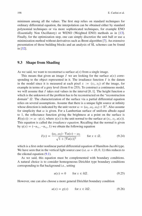
198 E. Carlini et al.
minimum among all the values. The first step relies on standard techniques forordinary differential equation, the interpolation can be obtained either by standardpolynomial techniques or via more sophisticated techniques, for example ENO(Essentially Non Oscillatory) or WENO (Weighted ENO) methods as in [13].Finally, for the optimization step, one can simply discretize the unit ball or use aminimization method without derivatives such as Brent algorithm [7]. An extensivepresentation of those building blocks and an analysis of SL schemes can be foundin [32].
9.3 Shape from Shading
As we said, we want to reconstruct a surface u.x/ from a single image.This means that given an image I we are looking for the surface u.x/ corre-
sponding to the object represented in it. The irradiance function I is the datumin the model since it is measured at each pixel x WD .x1; x2/ of the image, forexample in terms of a grey level (from 0 to 255). To construct a continuous model,we will assume that I takes real values in the interval Œ0; 1!. The height function uwhich is the unknown of the problem has to be reconstructed on the “reconstructiondomain” ˝ . The characterization of the surface via a partial differential equationrelies on several assumptions. Assume that there is a unique light source at infinitywhose direction is indicated by the unit vector ! D .!1; !2; !3/ 2 R3. Also assumefor simplicity that ! is given. For a Lambertian surface of uniform albedo equalto 1, the reflectance function giving the brightness at a point on the surface isR.#.x// WD ! % #.x/, where #.x/ is the unit normal to the surface at .x1; x2; u.x//.This equation is called the irradiance equation. Recalling that the normal is givenby #.x/ D ."ux1 ;"ux2 ; 1/ we obtain the following equation
I.x/ D .!1; !2/ % ru.x/ " !3p1C jru.x/j2
for x 2 ˝; (9.24)
which is a first order nonlinear partial differential equation of Hamilton-Jacobi type.We have seen that in the vertical light source case (i.e. ! D .0; 0; 1/) this reduces tothe eikonal equation (9.1).
As we said, this equation must be complemented with boundary conditions.A natural choice is to consider homogeneous Dirichlet type boundary conditionscorresponding to flat background i.e., setting
u.x/ D 0 for x 2 @˝: (9.25)
However, one can also choose a more general Dirichlet boundary condition
u.x/ D g.x/ for x 2 @˝: (9.26)
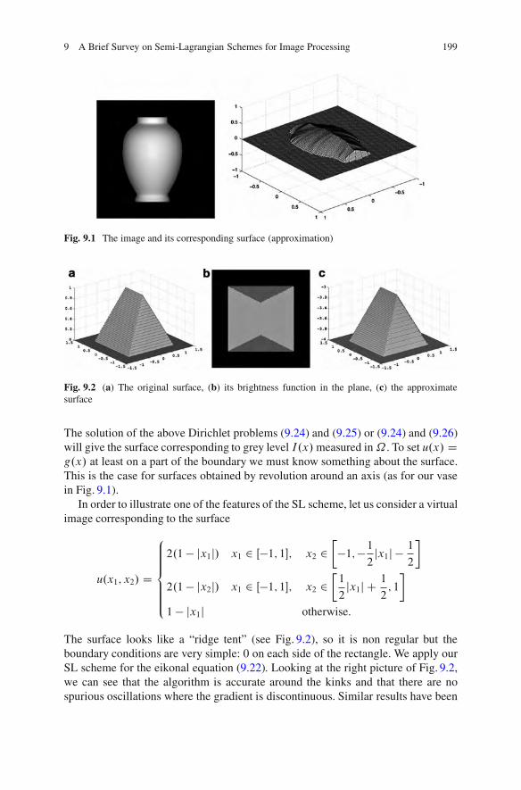
9 A Brief Survey on Semi-Lagrangian Schemes for Image Processing 199
Fig. 9.1 The image and its corresponding surface (approximation)
Fig. 9.2 (a) The original surface, (b) its brightness function in the plane, (c) the approximatesurface
The solution of the above Dirichlet problems (9.24) and (9.25) or (9.24) and (9.26)will give the surface corresponding to grey level I.x/measured in˝ . To set u.x/ Dg.x/ at least on a part of the boundary we must know something about the surface.This is the case for surfaces obtained by revolution around an axis (as for our vasein Fig. 9.1).
In order to illustrate one of the features of the SL scheme, let us consider a virtualimage corresponding to the surface
u.x1; x2/ D
8ˆˆ<
ˆˆ:
2.1" jx1j/ x1 2 Œ"1; 1!; x2 2$"1;"1
2jx1j "
1
2
%
2.1" jx2j/ x1 2 Œ"1; 1!; x2 2$1
2jx1j C
1
2; 1
%
1 " jx1j otherwise:
The surface looks like a “ridge tent” (see Fig. 9.2), so it is non regular but theboundary conditions are very simple: 0 on each side of the rectangle. We apply ourSL scheme for the eikonal equation (9.22). Looking at the right picture of Fig. 9.2,we can see that the algorithm is accurate around the kinks and that there are nospurious oscillations where the gradient is discontinuous. Similar results have been
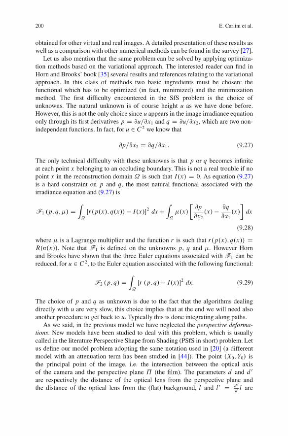
200 E. Carlini et al.
obtained for other virtual and real images. A detailed presentation of these results aswell as a comparison with other numerical methods can be found in the survey [27].
Let us also mention that the same problem can be solved by applying optimiza-tion methods based on the variational approach. The interested reader can find inHorn and Brooks’ book [35] several results and references relating to the variationalapproach. In this class of methods two basic ingredients must be chosen: thefunctional which has to be optimized (in fact, minimized) and the minimizationmethod. The first difficulty encountered in the SfS problem is the choice ofunknowns. The natural unknown is of course height u as we have done before.However, this is not the only choice since u appears in the image irradiance equationonly through its first derivatives p D @u=@x1 and q D @u=@x2, which are two non-independent functions. In fact, for u 2 C2 we know that
@p=@x2 D @q=@x1: (9.27)
The only technical difficulty with these unknowns is that p or q becomes infiniteat each point x belonging to an occluding boundary. This is not a real trouble if nopoint x in the reconstruction domain ˝ is such that I.x/ D 0. As equation (9.27)is a hard constraint on p and q, the most natural functional associated with theirradiance equation and (9.27) is
F1 .p; q;%/ DZ
˝
Œr.p.x/; q.x// " I.x/!2 dxCZ
˝
%.x/
$@p
@x2.x/ " @q
@x1.x/
%dx
(9.28)
where % is a Lagrange multiplier and the function r is such that r.p.x/; q.x// DR.n.x//. Note that F1 is defined on the unknowns p, q and %. However Hornand Brooks have shown that the three Euler equations associated with F1 can bereduced, for u 2 C2, to the Euler equation associated with the following functional:
F2 .p; q/ DZ
˝
Œr .p; q/ " I.x/!2 dx: (9.29)
The choice of p and q as unknown is due to the fact that the algorithms dealingdirectly with u are very slow, this choice implies that at the end we will need alsoanother procedure to get back to u. Typically this is done integrating along paths.
As we said, in the previous model we have neglected the perspective deforma-tions. New models have been studied to deal with this problem, which is usuallycalled in the literature Perspective Shape from Shading (PSfS in short) problem. Letus define our model problem adopting the same notation used in [20] (a differentmodel with an attenuation term has been studied in [44]). The point .X0; Y0/ isthe principal point of the image, i.e. the intersection between the optical axisof the camera and the perspective plane ˘ (the film). The parameters d and d 0
are respectively the distance of the optical lens from the perspective plane andthe distance of the optical lens from the (flat) background, l and l 0 D d 0
dl are
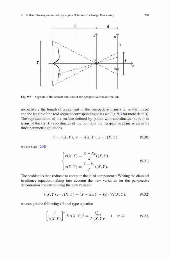
9 A Brief Survey on Semi-Lagrangian Schemes for Image Processing 201
Fig. 9.3 Diagram of the optical lens and of the perspective transformation
respectively the length of a segment in the perspective plane (i.e. in the image)and the length of the real segment corresponding to it (see Fig. 9.3 for more details).The representation of the surface defined by points with coordinates .x; y; z/ interms of the .X; Y / coordinates of the points in the perspective plane is given bythree parametric equations
x D r.X; Y /; y D s.X; Y /; z D t.X; Y / (9.30)
where (see [20])8ˆ<
ˆ:
r.X; Y / D X " X0d
t.X; Y /
s.X; Y / D Y " Y0d
t.X; Y /:
(9.31)
The problem is then reduced to compute the third component t . Writing the classicalirradiance equation, taking into account the new variables for the perspectivedeformation and introducing the new variable
t .X; Y / WD t.X; Y /C .X "X0; Y " Y0/ % rt.X; Y /; (9.32)
we can get the following eikonal type equation
$d
t.X; Y /
%2jrt.X; Y /j2 D I 2max
I 0.X; Y /2" 1 in ˝ (9.33)
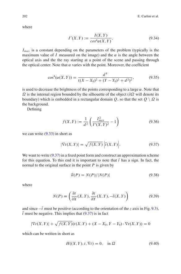
202 E. Carlini et al.
where
I 0.X; Y / WD I.X; Y /
cos4˛.X; Y /; (9.34)
Imax is a constant depending on the parameters of the problem (typically is themaximum value of I measured on the image) and the ˛ is the angle between theoptical axis and the the ray starting at a point of the scene and passing throughthe optical center. Note that ˛ varies with the point. Moreover, the coefficient
cos4.˛.X; Y // D d4
..X "X0/2 C .Y " Y0/2 C d2/2; (9.35)
is used to decrease the brightness of the points corresponding to a large ˛. Note that˝ is the internal region bounded by the silhouette of the object (@˝ will denote itsboundary) which is embedded in a rectangular domain Q, so that the set Q n ˝ isthe background.
Defining
f .X; Y / WD 1
d2
"I 2max
I 0.X; Y /2" 1
#(9.36)
we can write (9.33) in short as
jrt.X; Y /j Dpf .X; Y /
ˇˇt .X; Y /
ˇˇ: (9.37)
We want to write (9.37) in a fixed point form and construct an approximation schemefor this equation. To this end it is important to note that Nt has a sign. In fact, thenormal to the original surface in the point P is given by
bn.P / D N.P /=jN.P /j (9.38)
where
N.P / &"@t
@X.X; Y /;
@t
@Y.X; Y /;"Nt.X; Y /
#(9.39)
and since "Nt must be positive (according to the orientation of the z axis in Fig. 9.3),Nt must be negative. This implies that (9.37) is in fact
jrt.X; Y /j Cpf .X; Y /.t.X; Y /C .X "X0; Y " Y0/ % rt.X; Y // D 0
which can be written in short as
H..X; Y /; t;rt/ D 0; in ˝ (9.40)

9 A Brief Survey on Semi-Lagrangian Schemes for Image Processing 203
Fig. 9.4 A real photograph of one page, 128 $ 128 pixels (left) and reconstructed surface withDirichlet boundary conditions (right)
where the HamiltonianH represents the left-hand side of (9.40). It should be notedthat, with respect to the classical SfS problem without perspective, we have anadditional term which is linear in rt .
Let us consider equation (9.40) complemented with the Dirichlet boundarycondition
t D g.X; Y / on @˝; where " d 0 ( g ( 0 (9.41)
The arguments presented in Sect. 9.2 for the approximation of the directionalderivative lead to the standard semi-Lagrangian scheme for (9.40) which we writein a fixed point form as
t.X; Y / D F Œt !.X; Y /; in ˝ (9.42)
where the operator F is defined as
F Œt !.X; Y / WD 1
1C ı infa2B.0;1/
(t
.X; Y /C ı
"apf" .X; Y /
!!); on ˝:
(9.43)
and B.0; 1/ is the unit ball in R2. Introducing a space discretization, and definingxj D .Xj1 ; Yj2/, we can write for every node xj 2 ˝ \ G$x Eq. (9.42)
t.xj / D F Œt !.xj / WD1
1C ı infa2B.0;1/
(˘Œt !
xj C ı
"a
pf .xj /
" xj!!)
(9.44)
which gives the fully discrete semi-Lagrangian scheme for the PSfS problem.Naturally, this equation must be complemented with the boundary conditions (9.41).
In the following test we start from a real photograph where the effect ofperspective is visible. The surface is a sheet of paper with the shape of a roof tile.For this image the parameter values are: l D 6:91mm, d D 5:8mm, l 0D 200mm,d 0D l 0
ld D 167:87mm, $xD 0:05mm. We note that we performed a light cor-
rection in the preprocessing step, so we can assume ImaxD 1 during computation.Figure 9.4 shows the photograph (128 # 128 pixels) and the surface reconstructed

204 E. Carlini et al.
using Dirichlet boundary conditions (t D 0 on the left and right sides of the boundaryand t D g on the top and the bottom). We can see that the solution is quite goodconsidering the fact that light source (flash camera) is not far from the object andthat direction of light source is not perfectly vertical as the mathematical modelwould have required.
9.4 Nonlinear Filtering via MCM
The aim of this section is to present two classical methods based on Mean CurvatureMotion for image restoration. These models can be written in the following generalform:
8ˆˆ<
ˆˆ:
ut .x; t/ D div" ru.x; t/jru.x; t/j
#ˇjru.x; t/j .x; t/ 2 ˝ # .0; T !
u.x; 0/ D I0.x/ x 2 ˝@u.x; t/@#
D 0 .x; t/ 2 @˝ # .0; T !
(9.45)
where #.x/ is the normal direction at the point x. We will consider the case ˇ D 1corresponding to classical Mean Curvature Motion (MCM) and the case ˇ D 1=3corresponding to Affine Morphological Scale Space (AMSS). Here fu.x; t/gt%0represents a family of successive restored versions of the initial noisy image I0.The variable t is called the scale variable and, as t increases, we expect u.x; t/be a smoothed image, in which the noise has been removed. The model is ableto preserve significant features, like edges and corners, which are typically lostwhen using linear PDE-methods based on the heat equation where the smoothingeffect is isotropic. In curvature-related diffusion, the smoothing effect is anisotropic,i.e. the diffusion depends on the image and is not constant in all directions. Themodel with ˇD 1 corresponds to “pure” anisotropic diffusion and it was introducedfor image processing by Alvarez et al. in [1]. The term div
&ru.x;t/jru.x;t/j
'jru.x; t/j
represents a degenerate diffusion term, which diffuses in the direction orthogonalto the gradient ru and does not diffuse in the direction of ru. In fact, denoting by
&.ru/ D&rujruj
'?the unit vector orthogonal to ru, a formulation of the previous
equation with respect to &.ru/ would be:
ut D &.ru/>D2u&.ru/;
where D2u is the Hessian matrix with respect to x. This equation admits a uniquecontinuous viscosity solution, if u.x; 0/ is bounded uniformly continuous, see[18, 29].
In the paper [2] by Alvarez et al., a connection between scale space analysisand PDEs is proved, the authors also show that the MCM operator satisfies mostly
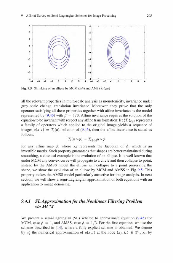
9 A Brief Survey on Semi-Lagrangian Schemes for Image Processing 205
Fig. 9.5 Shrinking of an ellipse by MCM (left) and AMSS (right)
all the relevant properties in multi-scale analysis as monotonicity, invariance undergrey scale change, translation invariance. Moreover, they prove that the onlyoperator satisfying all these properties together with affine invariance is the modelrepresented by (9.45) with ˇ D 1=3. Affine invariance requires the solution of theequation to be invariant with respect any affine transformation: let fTtgt%0 representsa family of operators which applied to the original image yields a sequence ofimages u.x; t/ D Tt.u/, solution of (9.45), then the affine invariance is stated asfollows:
Tt.u ı '/ D Tt !jJ' ju ı 'for any affine map ', where J' represents the Jacobian of ', which is aninvertible matrix. Such property guarantees that shapes are better maintained duringsmoothing, a classical example is the evolution of an ellipse. It is well known thatunder MCM any convex curve will propagate to a circle and then collapse to point,instead by the AMSS model the ellipse will collapse to a point preserving theshape, we show the evolution of an ellipse by MCM and AMSS in Fig. 9.5. Thisproperty makes the AMSS model particularly attractive for image analysis. In nextsection, we will show a semi-Lagrangian approximation of both equations with anapplication to image denoising.
9.4.1 SL Approximation for the Nonlinear Filtering Problemvia MCM
We present a semi-Lagrangian (SL) scheme to approximate equation (9.45) forMCM, case ˇ D 1, and AMSS, case ˇ D 1=3. For the first equation, we use thescheme described in [14], where a fully explicit scheme is obtained. We denoteby unj the numerical approximation of u.x; t/ at the node .xj ; tn/ 2 G$x;$t , by
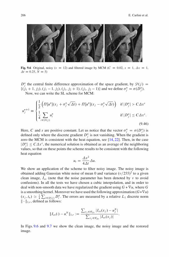
206 E. Carlini et al.
Fig. 9.6 Original, noisy (( D 12) and filtered image by MCM (C D 0:02, s D 1, $x D 1,$t D 0:25, N D 5)
Dnj the central finite difference approximation of the space gradient, by D.j / Df.j1 C 1; j2/; .j1 " 1; j2/; .j1; j2 C 1/; .j1; j2 " 1/g and we define &nj D &.Dn
j /.Now, we can write the SL scheme for MCM:
unC1j &
8ˆ<
ˆ:
1
2
&˘Œun!.xj C &nj
p$t/C˘Œun!.xj " &nj
p$t/
'if jDn
j j > C$xs
1
4
X
i2D.j /
uni if jDnj j ( C$xs:
(9.46)
Here, C and s are positive constant. Let us notice that the vector &nj D &.Dnj / is
defined only where the discrete gradient Dnj is not vanishing. When the gradient is
zero the MCM is consistent with the heat equation, see [14, 22]. Then, in the casejDn
j j ( C$xs , the numerical solution is obtained as an average of the neighboringvalues, so that on these points the scheme results to be consistent with the followingheat equation
ut D$x2
4$t$u:
We show an application of the scheme to filter noisy image. The noisy image isobtained adding Gaussian white noise of mean 0 and variance .(=255/2 to a givenclean image, Iex (note that the noise parameter has been denoted by ( to avoidconfusions). In all the tests we have chosen a cubic interpolation, and in order todeal with non-smooth data we have regularized the gradient usingG )ru, whereGis a smoothing kernel. Moreover we have used the following approximation .G)ru/.xj ; tn/ ' 1
4
Pi2D.j / D
ni . The errors are measured by a relative L1 discrete norm
k % k1;r , defined as follows:
kIex.%/" uN! k1;r WDP
xj2G$x jIex.xj /" uNj jPxj2G$x jIex.xj /j
:
In Figs. 9.6 and 9.7 we show the clean image, the noisy image and the restoredimage.
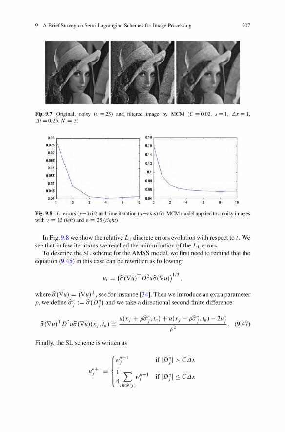
9 A Brief Survey on Semi-Lagrangian Schemes for Image Processing 207
Fig. 9.7 Original, noisy ((D 25) and filtered image by MCM (C D 0:02, sD 1, $xD 1,$tD 0:25, N D 5)
Fig. 9.8 L1 errors (y"axis) and time iteration (x"axis) for MCM model applied to a noisy imageswith ( D 12 (left) and ( D 25 (right)
In Fig. 9.8 we show the relativeL1 discrete errors evolution with respect to t . Wesee that in few iterations we reached the minimization of the L1 errors.
To describe the SL scheme for the AMSS model, we first need to remind that theequation (9.45) in this case can be rewritten as following:
ut D(b&.ru/>D2ub&.ru/
)1=3;
whereb&.ru/ D .ru/?, see for instance [34]. Then we introduce an extra parameter), we defineb&nj WD b&.Dn
j / and we take a directional second finite difference:
b&.ru/>D2ub&.ru/.xj ; tn/ 'u.xj C )b&nj ; tn/C u.xj " )b&nj ; tn/" 2unj
)2: (9.47)
Finally, the SL scheme is written as
unC1j &
8ˆ<
ˆ:
wnC1j if jDnj j > C$x
1
4
X
i2D.j /
wnC1i if jDnj j ( C$x
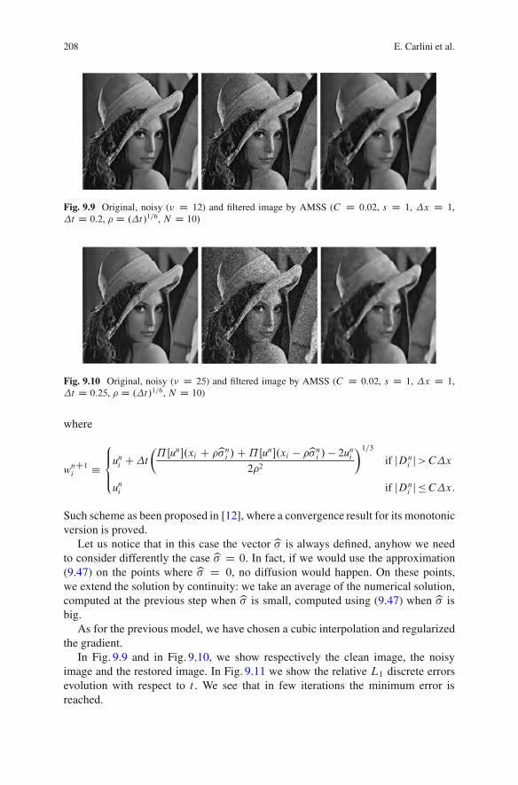
208 E. Carlini et al.
Fig. 9.9 Original, noisy (( D 12) and filtered image by AMSS (C D 0:02, s D 1, $x D 1,$t D 0:2, ) D .$t /1=6, N D 10/
Fig. 9.10 Original, noisy (( D 25) and filtered image by AMSS (C D 0:02, s D 1, $x D 1,$t D 0:25, ) D .$t /1=6, N D 10)
where
wnC1i &
8<
:
uni C$t"˘Œun!.xi C )b&ni /C˘Œun!.xi " )b&ni / " 2uni
2)2
#1=3if jDn
i j>C$x
uni if jDni j(C$x:
Such scheme as been proposed in [12], where a convergence result for its monotonicversion is proved.
Let us notice that in this case the vector b& is always defined, anyhow we needto consider differently the case b& D 0. In fact, if we would use the approximation(9.47) on the points where b& D 0, no diffusion would happen. On these points,we extend the solution by continuity: we take an average of the numerical solution,computed at the previous step when b& is small, computed using (9.47) when b& isbig.
As for the previous model, we have chosen a cubic interpolation and regularizedthe gradient.
In Fig. 9.9 and in Fig. 9.10, we show respectively the clean image, the noisyimage and the restored image. In Fig. 9.11 we show the relative L1 discrete errorsevolution with respect to t . We see that in few iterations the minimum error isreached.

9 A Brief Survey on Semi-Lagrangian Schemes for Image Processing 209
Fig. 9.11 Errors for MCM model for noisy images (left ( D 1, right ( D 25)
9.5 Segmentation via the LS Method
The segmentation problem in computer vision, as formulated by Mumford and Shah[40], can be defined in the following way: given an observed image I0 W ˝ ! Œ0; 1!,find a decomposition of disjoint open sets ˝ D S
i ˝i and C D Si @˝i , such
that I0 varies smoothly within each ˝i and rapidly or discontinuously across theboundaries of ˝i . We denote by jC j the length of curves which belong to C .
A classical way to solve this problem is solving the following minimizationproblem:
infI;CFMS.I; C / (9.48)
where
FMS.I; C / D *Z
˝
.I " I0/2dxC (Z
˝nCjrI j2dxC %jC j (9.49)
and %; ( are fixed parameters of weight for the different terms of the functional.For a minimum .I#; C #/, I# is an optimal piecewise smooth approximation of theinitial image I0, and C # approximates the edges of I0. I# will be smooth on˝ nCand will have its discontinuities on C #.
Theoretical results of existence of minimizers for this problem can be found inMumford and Shah [40], Morel and Solimini [38] and De Giorgi et al. [26].
A reduced case can be obtained by restricting the segmentation image I topiecewise constant functions, i.e. for ci D mean.I0/ in ˝i then I & ci insideeach ˝i . In this event, for the special case i D f0; 1g (that is the classical case ofsegmenting one object from the background image) the problem (9.48) becomesminimizing
EMS.c0; c1; C / D *Z
˝0
.I0 " c0/2dxC *Z
˝1
.I0 " c1/2dxC %jC j: (9.50)
210 E. Carlini et al.
We want now to use LS methods to solve this problem. LS methods are a very usefultool for computing evolving contours since they accommodate topological changesand allow to compute on a simple structured grid. For LS methods the curve Cis defined as the zero-level set of a sufficiently regular function ' called level setfunction, i.e. '.x/ < 0 for x 2 ˝0 and '.x/ > 0 for x 2 ˝1.
In this formulation, denoting by H.'/ the usual Heaviside function, (9.50)becomes (see [17])
EVC .c0; c1;'/ D *
Z
˝
.I0 " c0/2H.'/dxC *Z
˝
.I0 " c1/2.1 "H.'//dx
C%Z
˝
jrH.'/jdx: (9.51)
ConsideringH+ and ı+ two C1 regular approximations of the Heaviside functionHand of the delta function so thatH 0+ D ı+, we can write the Euler-Lagrange equationcorresponding to the energyEVC obtaining
@'
@tD ı+.'/
$%div
" r'jr'j
#" *.I0 " c0/2 C *.I0 " c1/2
%
where c0 DR˝ I.x/H.'/dxR˝ H.'/dx
; c1 DR˝ I.x/.1 "H.'//dxR
˝.1 "H.'//dx: (9.52)
This is a time dependent equation converging to a steady solution witch is aminimizer of the functional (9.50).
A standard rescaling can be made, as in Zhao et al. [49], by replacing ı.'/ byjr'j. This time rescaling does not affect the steady state solution, but helps remov-ing stiffness near the zero level sets of '. Finally, we get the following nonlinearevolution equation:
@'
@tD jr'j
$% div
" r'jr'j
#" *.I0 " c0/2 C *.I0 " c1/2
%(9.53)
which is solved for t tending to C1, yielding the solution of the segmentationproblem.
9.5.1 SL Scheme for Segmentation via the LS Method
In this section, we describe a SL approximation for Eq. (9.53). This equation hasa first-order and a second-order term, which we approximate using SL schemesintroduced in previous sections. We call c.x/ the speed of propagation of the first-order term,
c.x/ D "*.I0 " c0/2 C *.I0 " c1/2; (9.54)

9 A Brief Survey on Semi-Lagrangian Schemes for Image Processing 211
and using (9.20) we obtain
@'
@tD % div
" r'jr'j
#jr'j C c.x/ max
a2B.0;1/fa % r'g : (9.55)
As in every SL approximation, we want to build first an approximation of thedirectional derivative. This implies that the velocity c.x/ will appear directly insidethe argument of the unknown function '. For this particular problem, we have totake care of the change of sign of the velocity since will produce a sign change alsoin our scheme. We can rewrite (9.55) as
@'
@tD
8ˆ<
ˆ:
% div" r'jr'j
#jr'j C max
a2B.0;1/fc.x/a % r'g ; where c.x/ $ 0
% div" r'jr'j
#jr'j " max
a2B.0;1/f"c.x/a % r'g ; where c.x/ < 0:
(9.56)
Next, we define 'nj D '.xj ; tn/ where .xj ; tn/ 2 G$x;$t .Using, the schemes (9.46) for the second order term, and (9.22) for the first order
term, and explicit Euler finite differences for the temporal derivative, Eq. (9.56)becomes
'nC1j " 'nj$t
D %
!1
2˘ Œ'n! .xj C &nj
p$t/C 1
2˘ Œ'n! .xj " &nj
p$t/
*" 'nj
$t
" sign(c.xj /
)min
a2B.0;1/
˘Œ'n!.xj C ac.xj /$t/ " 'nj"$t ; (9.57)
where we have used the fact that "max."p/ D min.p/ and mina2B.0;1/.a % f / Dmina2B.0;1/."a % f / to simplify the notations.
Then, we get the fully discrete SL scheme:
'nC1j D 'nj C %!1
2˘ Œ'n! .xj C &nj
p$t/C 1
2˘ Œ'n! .xj " &nj
p$t /" 'nj
*
Csign(c.xj /
) !min
a2B.0;1/˚˘Œ'n!.xj C ac.xj /$t/
+" 'nj
*; (9.58)
and coherently with (9.46) in the case of discrete space gradient jDnj j ( C$xs .
We used this scheme to segment a variety of images, the results are shown inFigs. 9.12–9.14.
The most interesting feature of this approach is that the method is very rapid.While in classical finite difference schemes the information runs just one pixel foriteration, in this case we take information from a larger set. In particular to computethe value on the grid point xj we use all the values on the grid nodes that are

212 E. Carlini et al.
Fig. 9.12 Segmentation:% D 0:1, * D 104,two iterations
Fig. 9.13 Segmentation:% D 1, * D 0:3 # 104 ,two iterations
Fig. 9.14 Segmentation:% D 1, * D 0:3 # 104 ,two iterations
contained in a ball centered in xj with radius c.xj /. This is the reason of the rapidconvergence of the scheme. In our tests we found the correct segmentation of theimage always after 3 or less iterations. However, this is an experimental observation,a detailed treatment of SL scheme performances on this problem is still missing.
9.6 The Motion Segmentation Problem
Optical flow is the motion field in an image sequence; this problem belongs to themore general problem of motion estimation. Motion estimation and segmentationare strongly related topics that can increase the performances from each other. Inparticular segmentation can help us to solve the classical ambiguity near motionboundaries.
9 A Brief Survey on Semi-Lagrangian Schemes for Image Processing 213
Both topics are traditional in computer vision. Various approaches to optical flowcomputation have been suggested in [5], especially variational techniques based onmodifications of the method of Horn and Schunck [36] have yielded very convincingresults.
Also in segmentation, variational techniques perform well. As we showed in theprevious section, segmentation can be obtained minimizing the functional (9.48). Inrecent years the functional optimization is computed using LS methods [43].
In [3] and in [10], the authors propose to compute optical flow couplingestimators for optical flow and segmentation problem in a Mumford and Shah-like functional. Due to the presence of unspecified discontinuities in the integrationdomain, the minimization of this kind of functionals is difficult and we are going tosolve it using level set techniques.
We will use the studied semi-Lagrangian schemes for the Mean CurvatureMotion in this situation, to compute the front propagation of a level set function.Later, we compare the results for this application, in terms of accuracy and speed.The variational model which we use, is based on the optical flow functionalused in various works (for a short summary the dedicated section in [9]) and thesegmentation model presented in [16].
Given two images I0.x/; I1.x/ W˝!R, we have to find, at each point x 2˝ theoptical flow vector w.x/ W R2!R2 that describes the shift of the pixel at x in theimage I0 to the new location x C w in the image I1. Let us assume the followingclassical constraints: I0.x C w/D I1.x/ this is grey level constancy. It means thata pixel does not change its brightness from an image to the next. The secondimportant principle is gradient constancy, an assumption that makes the modelrobust with respect to global additive illumination changes in the scene. So, ourterm of consistency with the data is
fof .w/ D kjI0.x C w/" I1.x/j2 C , jrI0.x C w/" rI1.x/j2: (9.59)
The minimization of an optical flow functional with only the image constancyassumptions is ill-posed, to overcome this problem, a smoothness term regularizingthe flow field is considered. The typical smoothness term as in [36] is
sof .w/ D jrwj2: (9.60)
Using this term, nevertheless, we introduce regularization of the field and the knownambiguities along the discontinuities. For this reason, we place the smoothness termin a Mumford-Shah-like functional that provide to add regularization only in theregions of regularity of the solution.
Finally, calling " the discontinuity set of the optical flow, and j" j the length ofthe curve, we want to minimize the following functional
E.w;" / DZ
˝
kjI0.x C w/ " I1.x/j2 C , jrI0.x C w/ " rI1.x/j2dx
C%Z
˝n"jrwj2dxC (j" j: (9.61)
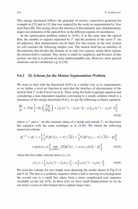
214 E. Carlini et al.
This energy functional follows the principle of motion competition proposed forexample in [23] and in [3], that was inspired by the work on segmentation by Veseand Chan [48]. This energy drives the interface of discontinuity and, simultaneously,makes an estimation of the optical flow in the different regions of smoothness.
In the optimization problem related to (9.61), if at the same time the opticalflow, the number or regions separated by " and the position of the curve " areall unknown, then minimization can be hard. For this reason, in the next sectionwe will consider the following simpler case. The motion field has an interface ofdiscontinuity that divides the domain ˝ in only two regions; inside these regionsthe motion field is constant. This choice is made for simplicity, and because, in thissection, our aim is to present an easly understandable case. However, more generalsituations can be considered, e.g. in [10].
9.6.1 SL Scheme for the Motion Segmentation Problem
We want to deal with the functional (9.61) in a similar way as in segmentation,so we define a level set function ' such that the interface of discontinuity of themotion field " is the 0-level set of '. Then, using the Euler-Lagrange equation andconsidering a time dependent equation converging to a steady solution which is aminimizer of the energy functional (9.61), we get the following evolutive equation:
@'
@tD jr'j
$( div
" r'jr'j
#C Œfof .wC/ " fof .w"/! " %
,sof .wC/" sof .w"/
-%
(9.62)
where, wC and w" are the constant values of w inside and outside " : we discretizethis equation with the same technique as in (9.58). We obtain the followingnumerical scheme:
'nC1j D 'nj C (!1
2˘ Œ'n! .xj C &nj
p$t/C 1
2˘ Œ'n! .xj " &nj
p$t /" 'nj
*
Csign.c.xj //!
mina2B.0;1/
˚˘Œ'n!.xj C ac.xj /$t/
+" 'nj
*; (9.63)
where the first-order velocity term c.xj / is
c.xj / Dhfof .wCj / " fof .w"j /
i" %
hsof .wCj / " sof .w"j /
i: (9.64)
We used this scheme for two simple tests obtaining the results shown in Fig. 9.15and 9.16. The first is a synthetic sequence where a ball is moving on a background,the second one is a small box taken from a more complicated real sequence(available on the site [47]). In these tests we have small displacements so we donot need a coarse-to-fine framework to capture larger ones.
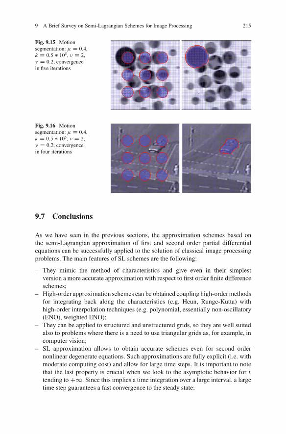
9 A Brief Survey on Semi-Lagrangian Schemes for Image Processing 215
Fig. 9.15 Motionsegmentation: % D 0:4,k D 0:5 # 105 , ( D 2,, D 0:2, convergencein five iterations
Fig. 9.16 Motionsegmentation: % D 0:4,- D 0:5 # 105, ( D 2,, D 0:2, convergencein four iterations
9.7 Conclusions
As we have seen in the previous sections, the approximation schemes based onthe semi-Lagrangian approximation of first and second order partial differentialequations can be successfully applied to the solution of classical image processingproblems. The main features of SL schemes are the following:
– They mimic the method of characteristics and give even in their simplestversion a more accurate approximation with respect to first order finite differenceschemes;
– High-order approximation schemes can be obtained coupling high-order methodsfor integrating back along the characteristics (e.g. Heun, Runge-Kutta) withhigh-order interpolation techniques (e.g. polynomial, essentially non-oscillatory(ENO), weighted ENO);
– They can be applied to structured and unstructured grids, so they are well suitedalso to problems where there is a need to use triangular grids as, for example, incomputer vision;
– SL approximation allows to obtain accurate schemes even for second ordernonlinear degenerate equations. Such approximations are fully explicit (i.e. withmoderate computing cost) and allow for large time steps. It is important to notethat the last property is crucial when we look to the asymptotic behavior for ttending toC1. Since this implies a time integration over a large interval. a largetime step guarantees a fast convergence to the steady state;

216 E. Carlini et al.
– SL schemes have shown to be rather robust when applied to non smooth data, asnoisy images. Moreover, in the time marching evolution there is less need for are-initialization in order to keep the level sets and acceleration techniques (suchas Fast Marching methods, [24, 45]) can be implemented.
A detailed analysis of these methods for first order model problems can be foundin the book [32] and some of the results for second order problems can be found in[12,14]. We conclude observing that there are still many open problems in the theoryof SL schemes, e.g. in the construction and analysis of high-order approximationsand acceleration methods (fast sweeping, fast marching). We are confident that thesemethods will be also useful for new challenging applications in image processing.
References
1. Alvarez, L., Lions, P.L., Morel, J.M.: Image selective smoothing and edge detection bynonlinear diffusion. SIAM J. Numer. Anal. 29, 845–866 (1992)
2. Alvarez, L., Guichard, F., Lions, P.L., Morel, J.M.: Axioms and fundamental equations ofimage processing. Arch. Ration. Mech. 123, 199–257 (1993)
3. Amiaz, T., Kiryati, N.: Piecewise-smooth dense optical flow via level sets. Int. J. Comput. Vis.68(2), 111–124 (2006)
4. Barles, G.: Solutions de Viscosite des Equations d’Hamilton–Jacobi. Springer, New York(1998)
5. Barron, J.L., Fleet, D.J., Beauchemin, S.S.: Performance of optical flow techniques. Int.J. Comput. Vis. 12, 75–104 (1996)
6. Brenner S.C., Scott, L.R.: The Mathematical Theory of Finite Element Methods, 3rd edn.Springer, New York (2008)
7. Brent, R.: Algorithms for Minimization Without Derivatives. Pentice–Hall, Englewood Cliffs(1973)
8. Breuss, M., Cristiani, E., Durou, J.D., Falcone, M., Vogel, O.: Numerical algorithms forperspective shape from shading. Kybernetika 46, 207–225 (2010)
9. Brox, T., Bruhn, A., Papenberg, N., Weickert, J.: High Accuracy Optical Flow EstimationBased on a Theory for Warping. Lecture Notes in Computer Science, pp. 25–36. Springer,Berlin (2004)
10. Brox, T., Bruhn, A., Weickert, J.: Variational segmentation with level sets. In: ComputerVision-ECCV, Graz, pp. 471–483 (2006)
11. Camilli, F., Falcone, M.: An approximation scheme for the maximal solution of the shape-from-shading model. In: Proceedings ICIP 96, vol. I, pp. 49–52. IEEE, Piscataway (1996)
12. Carlini, E., Ferretti, R.: A semi-Lagrangian approximation for the AMSS model of imageprocessing. submitted to Applied Numerical Mathematics (in press)
13. Carlini, E., Ferretti, R., Russo, G.: A weighted essentially non oscillatory, large time-stepscheme for Hamilton Jacobi equations. SIAM J. Sci. Comput. 27(3), 1071–1091 (2005)
14. Carlini, E., Falcone, M., Ferretti, R.: Convergence of a large time-step scheme for meancurvature motion. Interface Free Bound. 12, 409–441 (2010)
15. Catte, F., Dibos, F., Koepfler, G.: A morphological scheme for mean curvature motion andapplications to anisotropic diffusion and motion of level sets. SIAM J. Numer. Anal. 32, 1895–1909 (1995)
16. Chan, T., Vese, L.: Active contours without edges. IEEE Trans. Image Process. 10(2), 266–277(2001)

9 A Brief Survey on Semi-Lagrangian Schemes for Image Processing 217
17. Chan, T., Sandberg, B., Vese, L.: Active contours without edges for vector-valued images. J.Vis. Commun. Image R. 11(2), 130–141 (2000)
18. Chen, Y.G., Giga, Y., Goto, S.: Uniqueness and existence of viscosity solutions of generalizedmean curvature flow equation. J. Diff. Geom. 33, 749–786 (1991)
19. Courant, R., Isaacson, E., Rees, M.: On the solution of nonlinear hyperbolic differentialequations by finite differences. Commun. Pure Appl. Math. 5, 243–255 (1952)
20. Courteille, F., Crouzil, A., Durou, J.D., Gurdjos, P.: Towards shape from shading under realisticphotographic conditions, Int. C. Patt. Recog.- ICPR 2004, Cambridge, vol. 2, pp. 277–280(2004)
21. Crandall, M.G., Lions, P.L.: Two approximations of solutions of Hamilton–Jacobi equations.Math. Comput. 43, 1–19 (1984)
22. Crandall, M.G., Ishii, H., Lions, P.L.: User’s guide to viscosity solutions of second order partialdifferential equations. Bull. Am. Math. Soc. 27, 1–67 (1992)
23. Cremers, D., Soatto, S.: Motion competition: a variational framework for piecewise parametricmotion segmentation. Int. J. Comput. Vis. 63, 249–265 (2005)
24. Cristiani, E., Falcone, M.: Fast semi-Lagrangian schemes for the eikonal equation andapplications. SIAM J. Numer. Anal. 45(5), 1979–2011 (2007)
25. Cristiani, E., Falcone, M., Seghini, A.: Numerical solution of the shape-from-shading problem.In: Proceedings of Science POS (CSTNA2005) 008, 1–17, Electronic Journal site http://pos.sissa.it/
26. De Giorgi, E.: New functionals in calculus of variations, nonsmooth optimization and relatedtopics. In: Proceedings of the Fourth Course of the International School of Mathematics, Erice(1988)
27. Durou, J.D., Falcone, M., Sagona, M.: Numerical methods for shape from shading: a newsurvey with benchmarks. Comput. Vis. Image Underst. Elsevier 109, 22–43 (2008)
28. Evans, L.C.: Partial Differential Equations. AMS, Providence (2010)29. Evans, L.C., Spruck, J.: Motion of level sets by mean curvature. Int. J. Diff. Geom. 33, 635–681
(1991)30. Falcone, M.: The minimum time problem and its applications to front propagation. In: Motion
by Mean Curvature and Related Topics. De Gruyter Verlag, Berlino (1994)31. Falcone, M., Ferretti, R.: Convergence analysis for a class of high-order semi-Lagrangian
advection schemes. SIAM J. Numer. Anal. 35(3), 909–940 (1998)32. Falcone, M., Ferretti, R.: Semi-Lagrangian Approximation Schemes for Linear and Hamilton-
Jacobi Equations. SIAM, in preparation33. Falcone, M., Sagona, M., Seghini, A.: A global algorithm for the Shape-from-Shading problem
with black shadows. Numerical Mathematics and Advanced Applications ENUMATH 2001,pp. 503–512. Springer, Milano (2003)
34. Guichard, F., Morel, J.M.: Image Analysis and P.D.E.s. IPAM GBM Tutorial, March 27–April 6(2001)
35. Horn, B.K.P., Brooks M.J. (eds.): Shape from Shading. MIT, Cambridge (1989)36. Horn, B.K.P., Schunck, B.: Determinig optical flow. Artif. Intell. 17, 185–203 (1981)37. Lions, P.L., Rouy, E., Tourin, A.: A viscosity solution approach to shape from shading. Numer.
Math. 64, 323–353 (1993)38. Morel, J.M., Solimini, S.: Segmentation of images by variational methods: a constructive
approach. Rev. Mat. Univ. Compl. de Madr. 1, 169–182 (1988)39. Mumford, D., Shah, J.: Boundary detection by minimizing functional. In: Proceedings of the
CVPR, pp. 22–26. IEEE, Silver Spring (1985)40. Mumford, D., Shah, J.: Optimal approximations by piecewise smooth functions and associated
variational problems. Comm. Pure Appl. Math. XLII, 577–685 (1989)41. Oberman, A.M.: A convergent monotone difference scheme for motion of level sets by mean
curvature. Numer. Math. 99, 365–379 (2004)42. Osher, S.J., Fedkiw, R.P.: Level Set Methods and Dynamic Implicit Surfaces. Applied
Mathematical Sciences, vol. 153. Springer, New York (2003)

218 E. Carlini et al.
43. Osher, S.J., Sethian, J.A.: Front propagating with curvature-dependent speed: algorithms basedon Hamilton-Jacobi formulation. J. Comput. Phys. 79, 12–49 (1988)
44. Prados, E., Faugeras, O.: Perspective Shape-from-Shading and viscosity solutions. In: Proceed-ings of ICCV’03, pp. 826–831. IEEE, Los Alamitos (2003)
45. Sethian, J.A.: Level Set Methods and Fast Marching Methods Evolving Interfaces in Com-putational Geometry, Fluid Mechanics, Computer Vision, and Materials Science. CambridgeMonograph on Applied and Computational Mathematics. Cambridge University Press,Cambridge (1999)
46. Strikwerda, J.C.: Finite Difference Schemes and Partial Differential Equations, 2nd edn. SIAM,Philadelphia (2004)
47. Univeritat Kalsruhe. http://i21www.ira.uka.de/image sequences/48. Vese, L., Chan, T.: A multiphase level set framework for image segmentation using the
Mumford and Shah model. Int. J. Comput. Vis. 50, 271–293 (2002)49. Zhao, H., Chan, T., Merriman, B., Osher, S.J.: A variational level set approach to multiphase
motion. J. Comput. Phys. 127, 179–195 (1996)
Chapter 10Shape Reconstruction of Symmetric SurfacesUsing Photometric Stereo
Roberto Mecca and Silvia Tozza
Abstract The reconstruction of a 3D surface through one gray scale digital imagedoes not admit a unique solution in the orthographic Shape from Shading (SfS)framework. With the aim to make this type of problem well-posed it is possible touse the Photometric Stereo (PS) technique. It allows to add information about thesurface introducing other images of the object taken from the same point of viewbut modifying, for each photo, the direction of the light source. The methods thatuse the PS technique with the orthographic model of SfS need of, at least, threeimages. However, even if three images are used, there is the possibility that theSfS-PS problem continues to be ill-posed. This is the case when the three imagesare taken using three coplanar light vectors. This work analyses this kind of ill-posedness in order to understand how it is possible to establish a connection amongthe images that do not guarantee uniqueness. A further result in this paper is givenby a geometrical characterization of the surfaces for which it is possible to solve theclassic SfS problem.
10.1 Introduction to the Shape from Shading: PhotometricStereo Model and Symmetric Surfaces
The Shape from Shading (SfS) problem consists on the 3D reconstruction of anobject starting from only one gray scale photo. In the framework of the shape recon-struction the classical orthographic SfS problem fails its aims using only one digital
R. Mecca (!) ! S. TozzaDipartimento di Matematica “G. Castelnuovo”, Sapienza – University of Rome, Rome, Italye-mail: [email protected]; [email protected]
M. Breuß et al. (eds.), Innovations for Shape Analysis, Mathematics and Visualization,DOI 10.1007/978-3-642-34141-0 10, © Springer-Verlag Berlin Heidelberg 2013
219
220 R. Mecca and S. Tozza
image for the reconstruction of the corresponding surface. Our contribution is givenby the SfS model where we are considering the following hypotheses:
1. The light sources are at infinity;2. The surface is Lambertian;3. The optical point is sufficiently far from the surface so that perspective deforma-
tions can be neglected.
In this case the SfS model is given by the following irradiance equation:
!.x; y/.n.x; y/ ! !/ D I.x; y/ (10.1)
where !.x; y/ is the albedo (supposed constant and equal to one), n.x; y/ D.n1.x; y/; n2.x; y/; n3.x; y// is the unit outgoing normal to the unknown surfacez D u.x; y/, ! D .!1; !2; !3/ D .e!;!3/ is the direction of the light source andI W ˝ ! Œ0; 1" is the image function.
Under the previous assumptions this inverse problem is ill-posed due to theconcave/convex ambiguity. Many papers show the impossibility to have a uniquesolution for this SfS model (see [2, 5]). In order to avoid this ambiguity we can addinformation of the surface considering other data of the same type.
The Shape from Shading problem with the Photometric-Stereo techniques (SfS-PS) uses more than one image of the same surface taken from the same point ofview, but using a different light source for each image, that is:
n.x; y/ ! !i D Ii .x; y/: (10.2)
Let us clarify by now the meaning of coplanar light sources: since we considereach light source as a unit vector in R3, we will talk about coplanar light sourceswith the same meaning of coplanar unit vectors. That is, we will say that three ormore light sources are coplanar if the representing vectors are coplanar.
There are many possible approaches to model the SfS-PS problem (e.g. [11, 12,15]). The main two ways that allow to reconstruct the surface are the normal vectorfield approach [6] and the differential approach [13] which we briefly describe later.
The main difference between these approaches is that the first one is a localapproach that works pixel by pixel in order to find the normal vector field of theunknown surface and then it reconstructs the surface z D u.x; y/ all over the domainusing the gradient field [6]. The second approach instead works globally: it is basedon a differential problem that, using only two images, can recognize the shape of theobject but, as we will see, this differential problem is well-posed only if the Dirichletboundary condition (i.e. the height of the surface on the boundary) is known. Inorder to use it we need to approximate the boundary condition and another imagemust be added making the problem well-posed with three images.
We emphasize one more time that both approaches need three image functionsand our goal is to characterize this kind of functions with the aim to reduce thenumber of images needed considering the symmetry of the surface. There are severalprevious studies [3, 7] where this geometric constraint is used together with the

10 Shape Reconstruction of Symmetric Surfaces Using Photometric Stereo 221
photometric features. In particular there are works that focus on this field detectingthe symmetries in the images [8, 14]. Other papers in which a single image ofa symmetric object can be regarded as two images of another object taken fromtwo different points of view and two different illumination directions [20] or othersimilar approaches as [9, 10].
In Sect. 10.2 we recall the local and the differential approach. We explain theimpossibility to solve the SfS-PS problem with both approaches using three imagesobtained with three coplanar light source vectors. In this section we give a definitionof linear dependent images used in all the subsequent sections. In Sect. 10.3 weintroduce an algorithm for the “artificial” reconstruction of linear dependent images.Finally in Sect. 10.4 we study how it is possible to reduce the number of necessaryimages for the shape reconstruction of a symmetric surface. The main result in thissection is the theorem that explains how to solve the SfS problem (with only oneimage) through the SfS-PS formulation when the surface under observation has atleast four axes of symmetry. In the last section we present some numerical testsrelated to the algorithms presented.
10.2 Condition of Linear Independent Images for the SfS-PSReconstruction
We recall briefly the mathematical formulation of the approaches introduced in theprevious section.
10.2.1 Normal Vector Approach
As we have anticipated, the local approach solves the problem finding the outgoingnormal vector to the surface locally, that is pixel by pixel [4, 6]. This means that,once we discretize the image domain ˝ with an uniform lattice ˝d D ˝d [ @˝d ,the following system is solved for every .xi ; yj / 2 ˝d :
8ˆ<
ˆ:
!01n1.xi ; yj /C !02n2.xi ; yj /C !03n3.xi ; yj / D I1.xi ; yj /!001 n1.xi ; yj /C !002 n2.xi ; yj /C !003 n3.xi ; yj / D I2.xi ; yj /!0001 n1.xi ; yj /C !0002 n2.xi ; yj /C !0003 n3.xi ; yj / D I3.xi ; yj /:
(10.3)
As explained before, next step for this method is to approximate the values of theheight of the surface starting from the knowledge of its gradient field (i.e. knowingru.xi ; yj /8.xi ; yj / 2 ˝d ) [6]. In fact, using the definition of the outgoing normalvector:
n.x; y/ D ."ru.x; y/; 1/p1C jjru.x; y/jj2
D
!" @u
@x.x; y/;" @u
@y.x; y/; 1
"
p1C jjru.x; y/jj2
; (10.4)
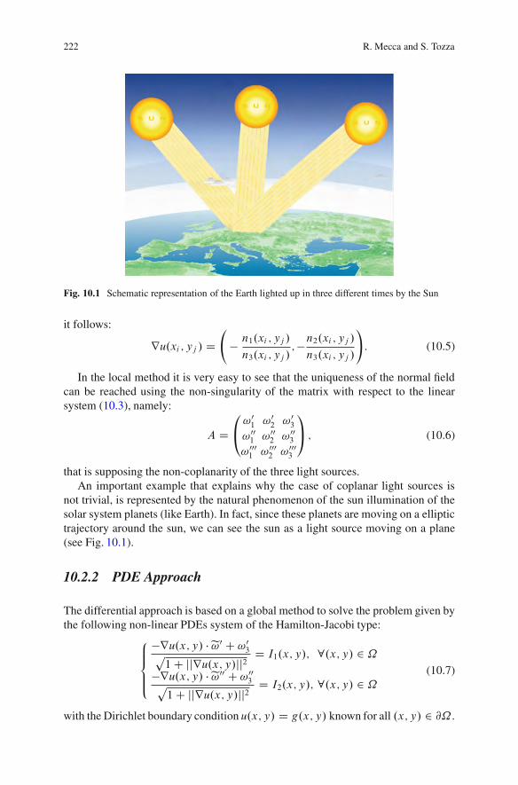
222 R. Mecca and S. Tozza
Fig. 10.1 Schematic representation of the Earth lighted up in three different times by the Sun
it follows:
ru.xi ; yj / D " n1.xi ; yj /n3.xi ; yj /
;"n2.xi ; yj /n3.xi ; yj /
!: (10.5)
In the local method it is very easy to see that the uniqueness of the normal fieldcan be reached using the non-singularity of the matrix with respect to the linearsystem (10.3), namely:
A D
0
@!01 !02 !03!001 !002 !003!0001 !0002 !0003
1
A ; (10.6)
that is supposing the non-coplanarity of the three light sources.An important example that explains why the case of coplanar light sources is
not trivial, is represented by the natural phenomenon of the sun illumination of thesolar system planets (like Earth). In fact, since these planets are moving on a elliptictrajectory around the sun, we can see the sun as a light source moving on a plane(see Fig. 10.1).
10.2.2 PDE Approach
The differential approach is based on a global method to solve the problem given bythe following non-linear PDEs system of the Hamilton-Jacobi type:
8ˆ<
ˆ:
"ru.x; y/ !e!0 C !03p1C jjru.x; y/jj2
D I1.x; y/; 8.x; y/ 2 ˝"ru.x; y/ !e!00 C !003p1C jjru.x; y/jj2
D I2.x; y/; 8.x; y/ 2 ˝(10.7)
with the Dirichlet boundary condition u.x; y/ D g.x; y/ known for all .x; y/ 2 @˝ .
10 Shape Reconstruction of Symmetric Surfaces Using Photometric Stereo 223
This system can also be studied eliminating the non-linearity [13]. We can thenconsider the following hyperbolic problem:
(b.x; y/ ! ru.x; y/ D f .x; y/; a.e. .x; y/ 2 ˝
u.x; y/ D g.x; y/; 8.x; y/ 2 @˝(10.8)
where
b.x; y/ D .I2.x; y/!01 " I1.x; y/!001 ; I2.x; y/!02 " I1.x; y/!002 / (10.9)
andf .x; y/ D I2.x; y/!03 " I1.x; y/!003 : (10.10)
For the differential method some other passages have to be done in order tosee the necessity to have non-coplanar light sources. It is clear that only takingpictures is not possible to get the height of the surface on the boundary points (i.e.the boundary condition g.x; y/).
This supplementary information is necessary to make (10.8) well-posed andthat is why we need to compute it. In fact the approximation of the Dirichletboundary condition g.x; y/ binds us to use another image (we call it I3, as inthe previous approach). This step allows us to start solving the problem with thesame starting data set (i.e. !0, !00, !000 and the respective images I1, I2, I3) for bothapproaches.
It is clear that we can approximate the boundary condition g.x; y/ using theprevious local method that is using (10.3) for all pixels .xi ; yj / 2 @˝d . Withthe aim to emphasize that also using the differential approach the condition ofnon-coplanarity is required, we use the combinations of the three images in thehyperbolic model in order to approximate the boundary condition.
We consider the following system of hyperbolic equations:
8<
:
b.1;2/.x; y/ ! ru.x; y/ D f .1;2/.x; y/; a.e. .x; y/ 2 ˝b.1;3/.x; y/ ! ru.x; y/ D f .1;3/.x; y/; a.e. .x; y/ 2 ˝b.2;3/.x; y/ ! ru.x; y/ D f .2;3/.x; y/; a.e. .x; y/ 2 ˝
(10.11)
where
b.h;k/.x; y/ D .Ik.x; y/!h1 " Ih.x; y/!k1 ; Ik.x; y/!h2 " Ik.x; y/!k2 /
andf .x; y/.h;k/ D Ik.x; y/!h3 " Ih.x; y/!k3
where .h; k/ is the combination of two of the first three natural integer withoutrepetition. In other words .h; k/ contains the indices (and the respective lightsources) of the images we are using. Then, using these equations, a way toapproximate the boundary condition is to choose two of the previous three equations
224 R. Mecca and S. Tozza
and to consider them in a generic boundary point .xi ; yj / 2 @˝d obtaining thefollowing linear system:
8ˆ<
ˆ:
b.1;2/1 .xi ; yj /
@[email protected] ; yj /C b.1;2/2 .xi ; yj /
@[email protected] ; yj / D f .1;2/.xi ; yj /
b.1;3/1 .xi ; yj /
@[email protected] ; yj /C b.1;3/2 .xi ; yj /
@[email protected] ; yj / D f .1;3/.xi ; yj /:
(10.12)
It permits to compute the gradient field of u on the boundary points and then wecan approximate the value of the height of u using some well know algorithm [4,6].
Considering the coefficient matrix of the latter linear system it is possible to finda relation between the non-singularity of the matrix A (from (10.6)) and the matrixof the linear system (10.12) proving the following proposition:
Proposition 10.1. Let
L.xi ; yj / D b.1;2/1 .xi ; yj / b
.1;2/2 .xi ; yj /
b.1;3/1 .xi ; yj / b
.1;3/2 .xi ; yj /
!: (10.13)
Then det.L.xi ; yj // D 0 8.xi ; yj / 2 ˝d if and only if !0, !00, !000 are coplanar.
Proof. ()) Let us prove that: det.L.xi ; yj // D 0 implies !0, !00, !000 coplanar.We generalize the proof by simplifying the notation instead of considering the
dependence on a specific point .xi ; yj /. We explicit the functions that appear in thematrix L in terms of the images and of the light sources and we obtain:
det.L/ D !01!02I2I3 " !01!0002 I1I2 " !001 !02I1I3 C !001 !0002 .I1/2"
" Œ!01!02I2I3 " !0001 !02I1I2 " !01!002 I1I3 C !0001 !002 .I1/2"D I1Œ"!01!0002 I2 " !001 !02I3 C !001 !0002 I1 C !0001 !02I2 C !01!002 I3 " !0001 !002 I1"D I1Œ."!01!0002 C!0001 !02/I2C ."!001 !02C!01!002 /I3C ."!0001 !002 C!001 !0002 /I1":
(10.14)
Let us consider the case where the three images I1, I2 and I3 are defined by thesurface u and the respective light sources as follows:
I1.x; y/ D"!01 @u
@x.x; y/ " !02 @u
@y.x; y/C !03p
1C jjru.x; y/jj2;
I2.x; y/ D"!001 @u
@x.x; y/ " !002 @u
@y.x; y/C !003p
1C jjru.x; y/jj2;
I3.x; y/ D"!0001 @u
@x.x; y/ " !0002 @u
@y.x; y/C !0003p
1C jjru.x; y/jj2:
(10.15)
10 Shape Reconstruction of Symmetric Surfaces Using Photometric Stereo 225
Replacing the previous equalities in (10.14) we have:
det.L/ D
I1
#1
p1Cjjru.x; y/jj2
$#@u@x.!01!
001 !0002 "!02!001 !0001 /C
@u@y.!01!
002 !0002 " !02!002 !0001 /"
!01!003 !0002 C !02!003 !0001 C
@u@x.!02!
001 !0001 " !01!002 !0001 /C
@u@y.!02!
001 !0002 " !01!002 !0002 /"
!02!001 !0003 C !01!002 !0003 C
@u@x.!01!
002 !0001 " !01!001 !0002 /C
@u@y.!02!
002 !0001 " !02!001 !0002 /"
!03!002 !0001 C !03!001 !0002
$: (10.16)
Since the common denominator (1Cjjru.x; y/jj2) is always different from zero, wecan continue the computation considering only the numerator of (10.16). Explicit I1using (10.15) we can write as follows:
@u@x
#" !01
%" !01!003 !0002 C !02!003 !0001 " !02!001 !0003
C !01!002 !0003 " !03!002 !0001 C !03!001 !0002&$
C @u@y
#" !02
%" !01!003 !0002 C !02!003 !0001 " !02!001 !0003
C !01!002 !0003 " !03!002 !0001 C !03!001 !0002&$
C !03%" !01!003 !0002 C !02!003 !0001 " !02!001 !0003 C !01!002 !0003 " !03!002 !0001 C !03!001 !0002
&:
(10.17)
With the aim to prove the coplanarity of !000 with respect to !0 and !00, we definethe direction parameters of the plane generated by these last two vectors:
s D !02!003 " !03!002 ;l D !03!001 " !01!003 ;m D !01!002 " !02!001 :
(10.18)
The direction parameters .s; l; m/ of a plane represent a vector orthogonal to it,therefore, orthogonal to every vector v D .v1; v2; v3/ belonging to the plane. Thismeans that:
sv1 C lv2 Cmv3 D 0: (10.19)
226 R. Mecca and S. Tozza
Now, considering det.L/.x; y/ (without denominator) as a polynomial in thevariables # D @u
@x.x; y/ and $ D @u
@y.x; y/, we have:
det.L/.#; $/ D
#
#" !01
!!0001%!02!
003 " !03!002
&C !0002
%!03!
001 " !01!003
&C !0003
%!01!
002 " !02!001
&"$C
$
#" !02
!!0001%!02!
003 " !03!002
&C !0002
%!03!
001 " !01!003
&C !0003
%!01!
002 " !02!001
&"$C
!03!!0001%!02!
003 " !03!002
&C !0002
%!03!
001 " !01!003
&C !0003
%!01!
002 " !02!001
&":
(10.20)
Since det.L/ D 0 8.#; $/ then this means that all the coefficients are zero:
!0001%!02!
003 " !03!002
&C !0002
%!03!
001 " !01!003
&C !0003
%!01!
002 " !02!001
&D 0 (10.21)
which implies the coplanarity.(() Let us prove now that: !0, !00, !000 coplanar implies det.L/ D 0.We start seeing how, considering two images I1 and I2 obtained by the light
vectors !0 and !00, it is possible to get all the images obtainable with a light vectorthat is coplanar to the first two (i.e. considering the vectorial equality !000 D ˛!0 Cˇ!00), that is I3 D ˛I1 C ˇI2 as ˛ and ˇ change. Considering the image definitionof the orthographic SfS model we can write:
I3 D" @u@x!0001 " @u
@y!0002 C !0003p
1C jjrujj2
D" @u@x.˛!01 C ˇ!001 / " @u
@y.˛!02 C ˇ!002 /C .˛!03 C ˇ!003 /p1C jjrujj2
D ˛" @u@x!01 " @u
@y!02 C !03p
1C jjrujj2C ˇ" @u@x!001 " @u
@y!002 C !003p
1C jjrujj2
D ˛I1 C ˇI2: (10.22)
We continue replacing in (10.14) the coplanarity equality !000 D ˛!0Cˇ!00 and,in consequence, I3 with ˛I1 C ˇI2. We obtain:
det.L/ D
" !01.˛!02 C ˇ!002 /I1I2 " !001 !02I1.˛I1 C ˇI2/C !001 .˛!02 C ˇ!002 /.I1/2C
.˛!01 C ˇ!001 /!02I1I2 C !01!002 I1.˛I1 C ˇI2/" .˛!01 C ˇ!001 /!002 .I1/2 D
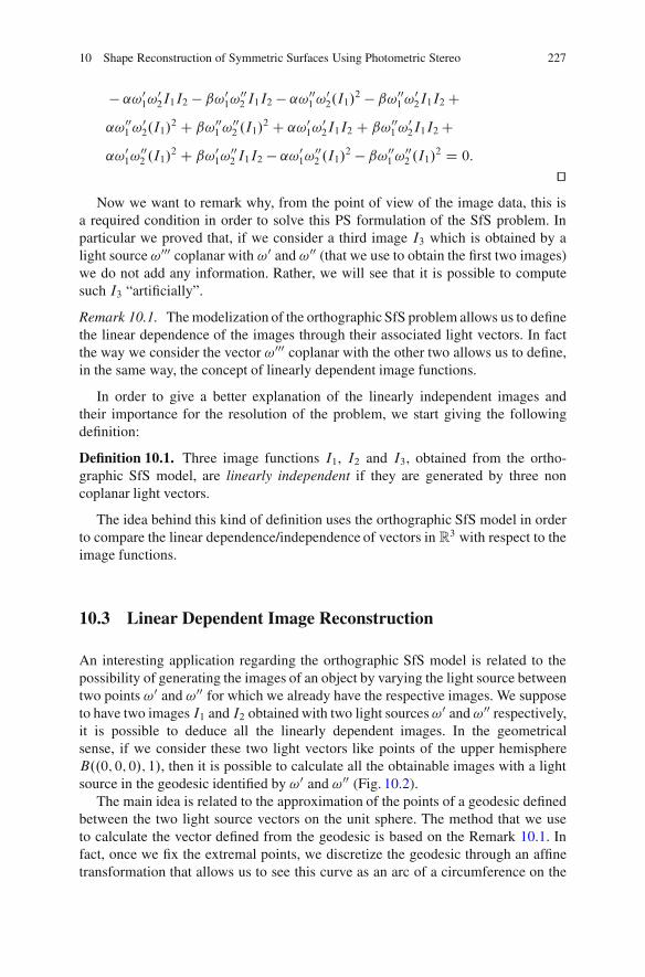
10 Shape Reconstruction of Symmetric Surfaces Using Photometric Stereo 227
" ˛!01!02I1I2 " ˇ!01!002 I1I2 " ˛!001 !02.I1/2 " ˇ!001 !02I1I2C
˛!001 !02.I1/
2 C ˇ!001 !002 .I1/2 C ˛!01!02I1I2 C ˇ!001 !02I1I2C
˛!01!002 .I1/
2 C ˇ!01!002 I1I2 " ˛!01!002 .I1/2 " ˇ!001 !002 .I1/2 D 0:ut
Now we want to remark why, from the point of view of the image data, this isa required condition in order to solve this PS formulation of the SfS problem. Inparticular we proved that, if we consider a third image I3 which is obtained by alight source !000 coplanar with !0 and !00 (that we use to obtain the first two images)we do not add any information. Rather, we will see that it is possible to computesuch I3 “artificially”.
Remark 10.1. The modelization of the orthographic SfS problem allows us to definethe linear dependence of the images through their associated light vectors. In factthe way we consider the vector !000 coplanar with the other two allows us to define,in the same way, the concept of linearly dependent image functions.
In order to give a better explanation of the linearly independent images andtheir importance for the resolution of the problem, we start giving the followingdefinition:
Definition 10.1. Three image functions I1, I2 and I3, obtained from the ortho-graphic SfS model, are linearly independent if they are generated by three noncoplanar light vectors.
The idea behind this kind of definition uses the orthographic SfS model in orderto compare the linear dependence/independence of vectors in R3 with respect to theimage functions.
10.3 Linear Dependent Image Reconstruction
An interesting application regarding the orthographic SfS model is related to thepossibility of generating the images of an object by varying the light source betweentwo points !0 and !00 for which we already have the respective images. We supposeto have two images I1 and I2 obtained with two light sources!0 and !00 respectively,it is possible to deduce all the linearly dependent images. In the geometricalsense, if we consider these two light vectors like points of the upper hemisphereB..0; 0; 0/; 1/, then it is possible to calculate all the obtainable images with a lightsource in the geodesic identified by !0 and !00 (Fig. 10.2).
The main idea is related to the approximation of the points of a geodesic definedbetween the two light source vectors on the unit sphere. The method that we useto calculate the vector defined from the geodesic is based on the Remark 10.1. Infact, once we fix the extremal points, we discretize the geodesic through an affinetransformation that allows us to see this curve as an arc of a circumference on the
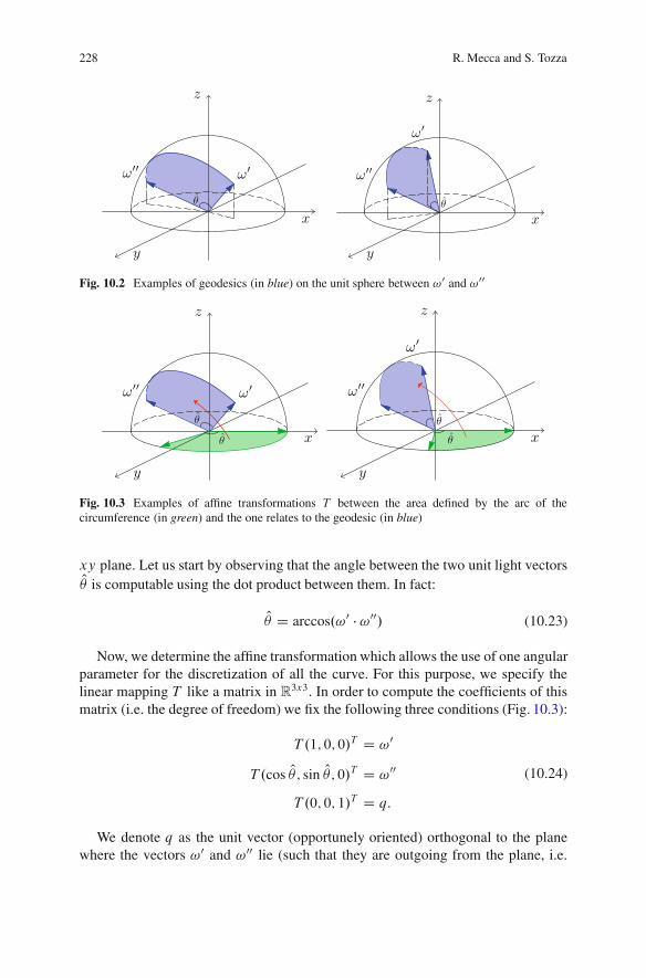
228 R. Mecca and S. Tozza
Fig. 10.2 Examples of geodesics (in blue) on the unit sphere between !0 and !00
Fig. 10.3 Examples of affine transformations T between the area defined by the arc of thecircumference (in green) and the one relates to the geodesic (in blue)
xy plane. Let us start by observing that the angle between the two unit light vectorsO% is computable using the dot product between them. In fact:
O% D arccos.!0 ! !00/ (10.23)
Now, we determine the affine transformation which allows the use of one angularparameter for the discretization of all the curve. For this purpose, we specify thelinear mapping T like a matrix in R3x3. In order to compute the coefficients of thismatrix (i.e. the degree of freedom) we fix the following three conditions (Fig. 10.3):
T .1; 0; 0/T D !0
T .cos O% ; sin O% ; 0/T D !00
T .0; 0; 1/T D q:
(10.24)
We denote q as the unit vector (opportunely oriented) orthogonal to the planewhere the vectors !0 and !00 lie (such that they are outgoing from the plane, i.e.
10 Shape Reconstruction of Symmetric Surfaces Using Photometric Stereo 229
q3 > 0). We consider the plane, generated by the vectors !0 and !00, to have thefollowing direction parameters:
s D !02!003 " !03!002l D !03!001 " !01!003m D !01!002 " !02!001 :
(10.25)
We consider the normalization of the vector .s; l; m/ like a possible vector qdepending on the sign of m. If m < 0 we take the opposite direction to thenormalization.
Let us make explicit the condition imposed by (10.24) writing the coefficients ofthe matrix that represents the transformation:
T D
0
BBB@
!01!001 "!0
1 cos O%sin O% q1
!02!002 "!0
2 cos O%sin O% q2
!03!003 "!0
3 cos O%sin O% q3
1
CCCA: (10.26)
If we consider an angle % such that 0 < % < O% , we obtain a third light source N!using just the previous application:
T .cos %; sin %; 0/T D N!: (10.27)
Now, if we have built N! coplanar to the previous two light vectors, then we haveN! D ˛!0 C ˇ!00. The next step is to determine the coefficients ˛; ˇ 2 R. We writethe previous equality and we obtain the following overdetermined linear system:
8ˆ<
ˆ:
N!1 D ˛!01 C ˇ!001N!2 D ˛!02 C ˇ!002N!3 D ˛!03 C ˇ!003
(10.28)
With the aim to calculate the coefficients that determine the third light source, wesolve the following linear system of two equations in two unknowns:
C
'˛
ˇ
(D b (10.29)
where C 2 R2#2 and clearly b 2 R2.Selecting two of the three equations of (10.28) in order to avoid singularity, the
matrix C depends on the first two light vectors that we can express in sphericalcoordinates as follows:
!0 D .cos %1 sin '1; sin %1 sin '1; cos'1/
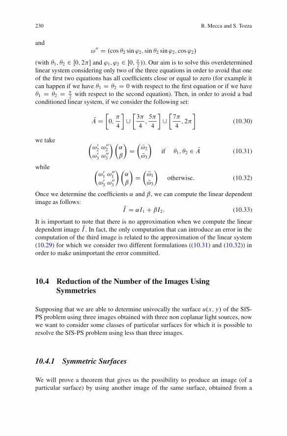
230 R. Mecca and S. Tozza
and!00 D .cos %2 sin '2; sin %2 sin'2; cos'2/
(with %1; %2 2 Œ0; 2&" and '1; '2 2 Œ0; &2 /). Our aim is to solve this overdeterminedlinear system considering only two of the three equations in order to avoid that oneof the first two equations has all coefficients close or equal to zero (for example itcan happen if we have %1 D %2 D 0 with respect to the first equation or if we have%1 D %2 D &
2with respect to the second equation). Then, in order to avoid a bad
conditioned linear system, if we consider the following set:
NA D#0;&
4
$[#3&
4;5&
4
$[#7&
4; 2&
$(10.30)
we take '!02 !
002
!03 !003
('˛
ˇ
(D'N!2N!3
(if %1; %2 2 NA (10.31)
while '!01 !
001
!03 !003
('˛
ˇ
(D'N!1N!3
(otherwise. (10.32)
Once we determine the coefficients ˛ and ˇ, we can compute the linear dependentimage as follows:
NI D ˛I1 C ˇI2: (10.33)
It is important to note that there is no approximation when we compute the lineardependent image NI . In fact, the only computation that can introduce an error in thecomputation of the third image is related to the approximation of the linear system(10.29) for which we consider two different formulations ((10.31) and (10.32)) inorder to make unimportant the error committed.
10.4 Reduction of the Number of the Images UsingSymmetries
Supposing that we are able to determine univocally the surface u.x; y/ of the SfS-PS problem using three images obtained with three non coplanar light sources, nowwe want to consider some classes of particular surfaces for which it is possible toresolve the SfS-PS problem using less than three images.
10.4.1 Symmetric Surfaces
We will prove a theorem that gives us the possibility to produce an image (of aparticular surface) by using another image of the same surface, obtained from a
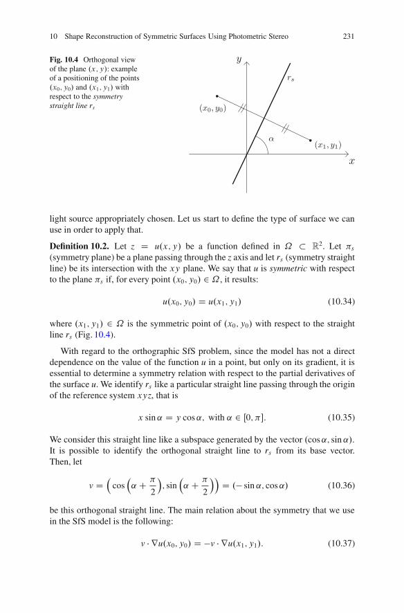
10 Shape Reconstruction of Symmetric Surfaces Using Photometric Stereo 231
Fig. 10.4 Orthogonal viewof the plane .x; y/: exampleof a positioning of the points.x0; y0/ and .x1; y1/ withrespect to the symmetrystraight line rs
light source appropriately chosen. Let us start to define the type of surface we canuse in order to apply that.
Definition 10.2. Let z D u.x; y/ be a function defined in # R2. Let &s(symmetry plane) be a plane passing through the z axis and let rs (symmetry straightline) be its intersection with the xy plane. We say that u is symmetric with respectto the plane &s if, for every point .x0; y0/ 2 , it results:
u.x0; y0/ D u.x1; y1/ (10.34)
where .x1; y1/ 2 is the symmetric point of .x0; y0/ with respect to the straightline rs (Fig. 10.4).
With regard to the orthographic SfS problem, since the model has not a directdependence on the value of the function u in a point, but only on its gradient, it isessential to determine a symmetry relation with respect to the partial derivatives ofthe surface u. We identify rs like a particular straight line passing through the originof the reference system xyz, that is
x sin � D y cos � ; with � 2 å 0;&": (10.35)
We consider this straight line like a subspace generated by the vector .cos � ; sin � /.It is possible to identify the orthogonal straight line to rs from its base vector.Then, let
v D!
cos!� C &
2
"; sin
!� C &
2
""D ." sin � ; cos � / (10.36)
be this orthogonal straight line. The main relation about the symmetry that we usein the SfS model is the following:
v ! ru.x0; y0/ D "v ! ru.x1; y1/: (10.37)

232 R. Mecca and S. Tozza
10.4.2 Uniqueness Theorem for the Symmetric Surfaces
We aim at obtaining further information relative to the symmetric surfaces bydeducing the grey scale values of an image corresponding to a particular lightsource whose position depends on the symmetry straight line rs . These information,together with a third image, allow us to resolve the SfS-PS problem using threeimages linearly independent.
Theorem 10.1. Let u.x; y/ be a symmetric surface with respect to any straight liners such that .0; 0/ 2 rs . Let !0 and !00ded be two light vectors such that:
1. e! 0 is orthogonal with respect to the symmetry straight line rs;2. e! 00ded D "e! 0 (that is !00ded D ."e! 0; !03/ since the light vectors are constrained to
be taken in the upper hemisphere).
Then it is possible to deduce the image associated to the light source !00ded only byI1 as follows:
I ded2 .x0; y0/ D I1.x1; y1/: (10.38)
Proof. Considering the image definition of the SfS problem, we have:
I ded2 .x0; y0/ D
"e! 00ded ! ru.x0; y0/C !00ded 3p1C jjru.x0; y0/jj2
$$D e!0 ! ru.x0; y0/C !03p1C jjru.x0; y0/jj2
$D
D "e!0 ! ru.x1; y1/C !03p1C jjru.x0; y0/jj2
D "e!0 ! ru.x1; y1/C !03p1C jjru.x1; y1/jj2
D I1.x1; y1/ (10.39)
where in $$ we use the assumption 2 of the theorem, whereas in $, as the surface issymmetric, we exploit (10.37). In the last equality we consider furthermore that thenormal vector in the point .x0; y0/ has the same norm as in .x1; y1/. ut
Let us explain with an example the previous theorem considering the symmetricsurface of Fig. 10.5 that we will use again in the numerical test section.
It is clear that its symmetry straight line rs drown in Fig. 10.5b defined by theangle ˛ D 3&
4, permits us to apply the previous theorem starting with a first light
source !0 having its projection on the xy planee! 0 orthogonal to rs . For example wecan choose %1 D &
4and, with the only aim to avoid shadows, we choose '1 D 0:1
obtaining the image I1 shown in Fig. 10.6 (on the left). Theorem 10.1 says that wecan deduce (and not approximate) a second image I ded
2 shown in Fig. 10.6 (on theright) associated to the light source !00ded D ."!0; !03/. In this example the anglesthat define the polar coordinates of !00ded are %ded
2 D %1 C & D 5&4
and 'ded2 D '1.
As we will remark the deduced image will help to have the sufficient information(about the three linear independent images) in order to solve the SfS-PS problemusing less than three images.
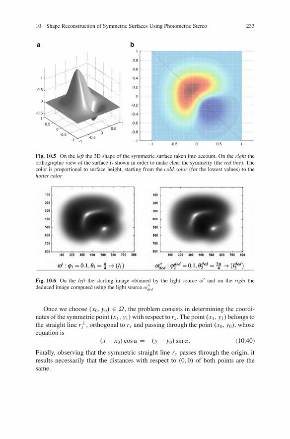
10 Shape Reconstruction of Symmetric Surfaces Using Photometric Stereo 233
1
1
0.8
0.6
0.4
0.2
0
-0.2
-0.4
-0.6
-0.8
-1-1 -0.5 0 0.5 1
0.5
0
-0.51
0.50
-0.5-1 -1
-0.50
0.51
a b
Fig. 10.5 On the left the 3D shape of the symmetric surface taken into account. On the right theorthographic view of the surface is shown in order to make clear the symmetry (the red line). Thecolor is proportional to surface height, starting from the cold color (for the lowest values) to thehotter color
Fig. 10.6 On the left the starting image obtained by the light source !0 and on the right thededuced image computed using the light source !00
ded
Once we choose .x0; y0/ 2 , the problem consists in determining the coordi-nates of the symmetric point .x1; y1/with respect to rs . The point .x1; y1/ belongs tothe straight line r?s , orthogonal to rs and passing through the point .x0; y0/, whoseequation is
.x " x0/ cos � D ".y " y0/ sin � : (10.40)
Finally, observing that the symmetric straight line rs passes through the origin, itresults necessarily that the distances with respect to .0; 0/ of both points are thesame.
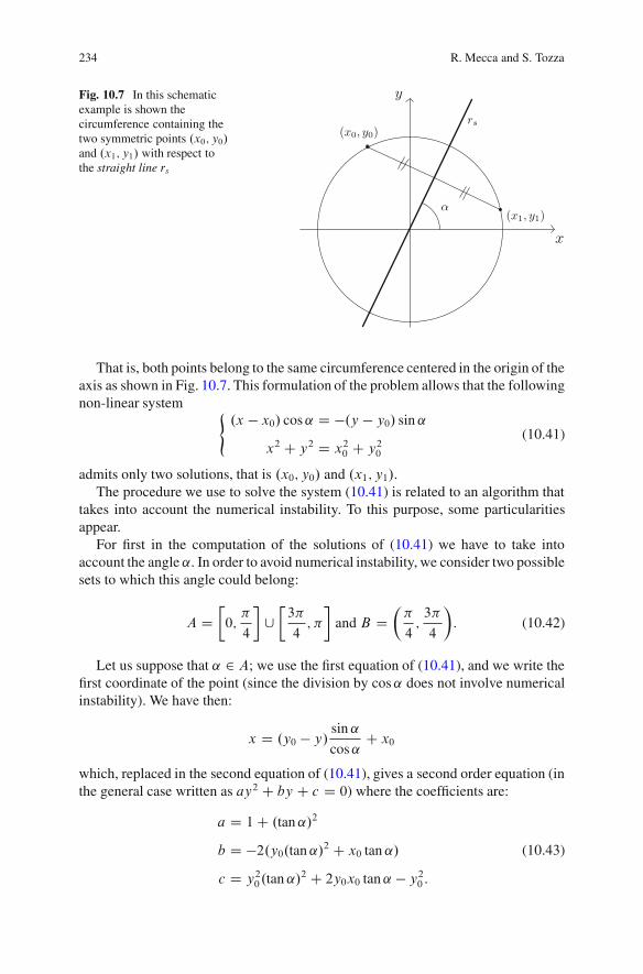
234 R. Mecca and S. Tozza
Fig. 10.7 In this schematicexample is shown thecircumference containing thetwo symmetric points .x0; y0/and .x1; y1/ with respect tothe straight line rs
That is, both points belong to the same circumference centered in the origin of theaxis as shown in Fig. 10.7. This formulation of the problem allows that the followingnon-linear system (
.x " x0/ cos � D ".y " y0/ sin �
x2 C y2 D x20 C y20(10.41)
admits only two solutions, that is .x0; y0/ and .x1; y1/.The procedure we use to solve the system (10.41) is related to an algorithm that
takes into account the numerical instability. To this purpose, some particularitiesappear.
For first in the computation of the solutions of (10.41) we have to take intoaccount the angle � . In order to avoid numerical instability, we consider two possiblesets to which this angle could belong:
A D#0;&
4
$[#3&
4;&
$and B D
'&
4;3&
4
(: (10.42)
Let us suppose that � 2 A; we use the first equation of (10.41), and we write thefirst coordinate of the point (since the division by cos � does not involve numericalinstability). We have then:
x D .y0 " y/sin �cos �
C x0
which, replaced in the second equation of (10.41), gives a second order equation (inthe general case written as ay2 C by C c D 0) where the coefficients are:
a D 1C .tan � /2
b D "2.y0.tan � /2 C x0 tan � /
c D y20.tan � /2 C 2y0x0 tan � " y20 :
(10.43)
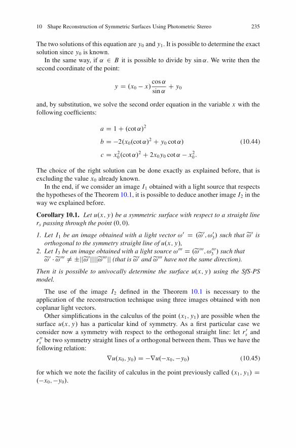
10 Shape Reconstruction of Symmetric Surfaces Using Photometric Stereo 235
The two solutions of this equation are y0 and y1. It is possible to determine the exactsolution since y0 is known.
In the same way, if ˛ 2 B it is possible to divide by sin ˛. We write then thesecond coordinate of the point:
y D .x0 " x/cos˛sin ˛
C y0
and, by substitution, we solve the second order equation in the variable x with thefollowing coefficients:
a D 1C .cot˛/2
b D "2.x0.cot˛/2 C y0 cot˛/
c D x20.cot˛/2 C 2x0y0 cot˛ " x20 :
(10.44)
The choice of the right solution can be done exactly as explained before, that isexcluding the value x0 already known.
In the end, if we consider an image I1 obtained with a light source that respectsthe hypotheses of the Theorem 10.1, it is possible to deduce another image I2 in theway we explained before.
Corollary 10.1. Let u.x; y/ be a symmetric surface with respect to a straight liners passing through the point .0; 0/.
1. Let I1 be an image obtained with a light vector !0 D .e! 0; !03/ such that e!0 isorthogonal to the symmetry straight line of u.x; y/,
2. Let I3 be an image obtained with a light source !000 D .e! 000; !0003 / such thate! 0 !e!000 ¤ ˙jje!0jjjje!000jj (that is e!0 and e!000 have not the same direction).
Then it is possible to univocally determine the surface u.x; y/ using the SfS-PSmodel.
The use of the image I2 defined in the Theorem 10.1 is necessary to theapplication of the reconstruction technique using three images obtained with noncoplanar light vectors.
Other simplifications in the calculus of the point .x1; y1/ are possible when thesurface u.x; y/ has a particular kind of symmetry. As a first particular case weconsider now a symmetry with respect to the orthogonal straight line: let r 0s andr 00s be two symmetry straight lines of u orthogonal between them. Thus we have thefollowing relation:
ru.x0; y0/ D "ru."x0;"y0/ (10.45)
for which we note the facility of calculus in the point previously called .x1; y1/ D."x0;"y0/.
236 R. Mecca and S. Tozza
10.4.3 Surfaces with Four Symmetry Straight Lines
A very interesting particular case is related to the surfaces with four symmetrystraight lines. In relation to these surfaces, in fact, it is possible to solve the classicalSfS problem considering only one image generated from any light source. For thiscase the constraint concerning the light sources direction vanishes. As before, wefollow the procedure of reconstructing the missing information (that is the threelinear independent images). Now, because of the particular surface geometry, we areable to obtain the necessary three images only from one. That is we can reconstructthe two missing images (generated with non coplanar light vectors) starting fromonly one image of the surface lighted up by any light source.
Let us consider the image I1 and let !0 be its relative light source. The other twoimages can be calculated in the following way:
I2.x; y/ D I1."x;"y/ with !00 D ."e! 0; !03/I3.x; y/ D I1."y; x/ with !000 D .!02;"!01; !03/:
(10.46)
Relating to the third image, we use .v1; v2/ !ru.x; y/ D ".v2;"v1/ !ru."y; x/,where .v1; v2/ is any vector of the plane .x; y/. The choice of the light placing,together with the way of determining the images, is not unique. The aim of thisconstruction is to obtain linearly independent reconstructed images for which theuniqueness of solution for the SfS problem stands.
We can adapt to this particular situation based on symmetries the uniquenesstheorem in [13] that proves the uniqueness of a Lipschitz solution (i.e. a solution inthe Sobolev space W 1;1.˝/) relatively to the differential approach:
Theorem 10.2. Let I.x; y/ be an image of the surface u.x; y/ 2 W 1;1.˝/, withfour straight lines of symmetry obtained by the SfS model such that 0 < I.x; y/ $1 8.x; y/ 2 ˝ with the light source !. Then it is possible to determine this surfaceunivocally solving the SfS classic problem.
The procedure followed until now is a constructive proof of the previous theoremand allows to solve, for a particular class of surfaces, the classical SfS problempassing through the SfS-PS one. Furthermore, our analysis of the problem allowsus to give also a numerical method for the approximation of this unique weaksolution.
Remark 10.2. Following this procedure it is possible to prove the uniquenessof a weak solution of the classic SfS problem even the surface is radial bysymmetries.
Remark 10.3. For both cases (one or four axes) the construction of the other imagescan be done only if the light source of the first image is not vertical. This meansthat in this case, even using this image deduction technique, the concave/convexambiguity cannot be solved.
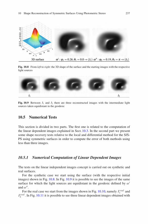
10 Shape Reconstruction of Symmetric Surfaces Using Photometric Stereo 237
Fig. 10.8 From left to right: the 3D shape of the surface and the starting images with the respectivelight sources
Fig. 10.9 Between I1 and I2 there are three reconstructed images with the intermediate lightsources taken equidistant in the geodesic
10.5 Numerical Tests
This section is divided in two parts. The first one is related to the computation ofthe linear dependent images explained in Sect. 10.3. In the second part we presentsome shape recovery tests relative to the local and differential method for the SfS-PS using symmetric surfaces in order to compute the error of both methods usingless than three images.
10.5.1 Numerical Computation of Linear Dependent Images
The tests on the linear independent images concept is carried out on synthetic andreal surfaces.
For the synthetic case we start using the surface (with the respective initialimages) shown in Fig. 10.8. In Fig. 10.9 it is possible to see the images of the samesurface for which the light sources are equidistant in the geodesic defined by !0
and !00.For the real case we start from the images shown in Fig. 10.10, namely I real1 and
I real2 . In Fig. 10.11 it is possible to see three linear dependent images obtained with

238 R. Mecca and S. Tozza
Fig. 10.10 Real starting data
Fig. 10.11 The results of the computation using our algorithm. The three images on the middleare lighted up from equidistant light sources in the geodesic defined by the starting images
the algorithm explained in the previous section. Also in this case we are consideringthree light sources equidistant in the geodesic defined by !0real and !00real .
10.5.2 Shape Reconstruction for Symmetric Surfaces
Let us start the numerical tests by studying several surfaces. Every single one is ofa typology that allows us to apply each variant of the previous results explained.These surfaces have symmetries that allows us to apply all the previous techniquesthat solve the SfS-PS problem.
The different typologies of the three surfaces represented in Fig. 10.12 are suchthat their geometrical characteristics differentiate the number of necessary imagesfor their tridimensional reconstruction. In fact:
• vsymm.x; y/, used also in the previous numerical test, is a surface with onesymmetry axis (the straight line y C x D 0) for which we need two images;
• vlip.x; y/ is a Lipschitz surface with four axis of symmetry (that is y D ˙x,y D 0, x D 0). For its reconstruction we need only one image;
• vrad.x; y/ is a particular case of the previous type of surfaces. In this radial casethe curves where it is not differentiable are concentric circles.
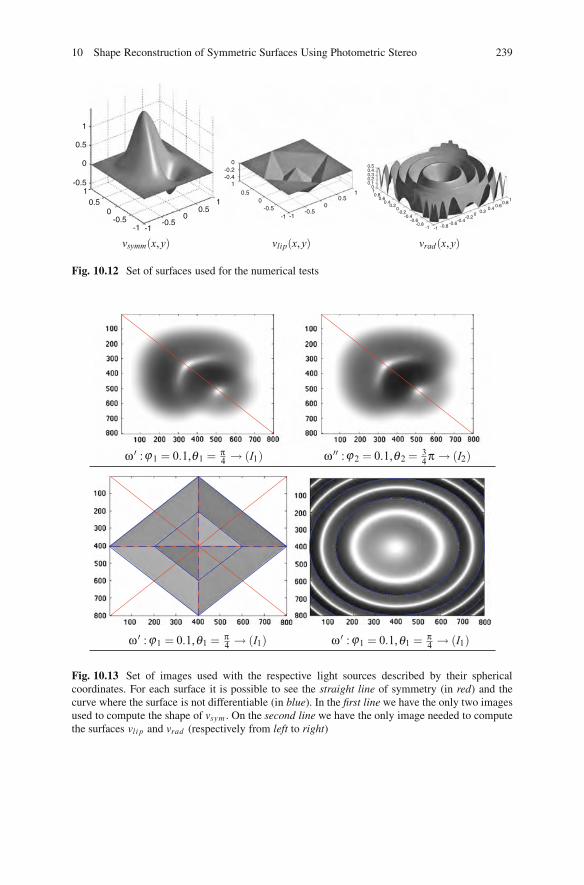
10 Shape Reconstruction of Symmetric Surfaces Using Photometric Stereo 239
1
0.5
0
-0.51
0.50
-0.5-1 -1
-0.50
0.51
vsymm(x, y) vlip(x, y) vrad(x, y)
0-0.2-0.4
110.5
0.500-0.5 -0.5
-1 -1
0.50.40.30.20.1
01
10.8
0.80.6
0.60.4
0.40.2
0.200-0.2
-0.2-0.4-0.4-0.6
-0.6-0.8-1 -1 -0.8
Fig. 10.12 Set of surfaces used for the numerical tests
! ! : 1 = 0.1, 1 = "4 " (I1) ! !! : 2 = 0.1, 2 = 3
4 " " (I2)
! ! : 1 = 0.1, 1 = "4 " (I1) ! ! : 1 = 0.1, 1 = "
4 " (I1)
j
j
j
j
q
q
q
q
Fig. 10.13 Set of images used with the respective light sources described by their sphericalcoordinates. For each surface it is possible to see the straight line of symmetry (in red) and thecurve where the surface is not differentiable (in blue). In the first line we have the only two imagesused to compute the shape of vsym . On the second line we have the only image needed to computethe surfaces vlip and vrad (respectively from left to right)
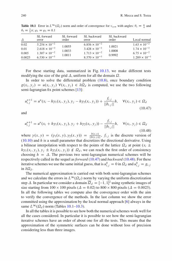
240 R. Mecca and S. Tozza
Table 10.1 Error in L1.˝d / norm and order of convergence for vsym with angles: %1 D &4
and%2 D 3
4& ; '1 D '2 D 0:1
SL forward SL forward SL backward SL backward' error order error order Local normal
0:02 5:254# 10!2
1.0055 6:856 # 10!2
1.0021 1:63 # 10!2
0:01 2:618# 10!2
1.00333:428 # 10!2
1.00081:74 # 10!2
0:005 1:307# 10!2
1.0011 1:713 # 10!2
0.9992 6:75 # 10!2
0:0025 6:530# 10!3 8:570 # 10!3 1:289 # 10!1
For these starting data, summarized in Fig. 10.13, we make different testsmodifying the size of the grid', uniform for all the domain˝ .
In order to solve the differential problem (10.8), once boundary conditiong.xi ; yj / D u.xi ; yj / 8.xi ; yj / 2 @˝d is computed, we use the two followingsemi-lagrangian fix point schemes [13]:
unC1i;j D un.xi " h(1.xi ; yj /; yj " h(2.xi ; yj //Cfi;j
jjbi;j jjh; 8.xi ; yj / 2 ˝d
(10.47)and
unC1i;j D un.xi C h(1.xi ; yj /; yj C h(2.xi ; yj // "fi;j
jjbi;j jjh; 8.xi ; yj / 2 ˝d
(10.48)where (.x; y/ D .(1.x; y/; (2.x; y// D b.x;y/
jjb.x;y/jj , fi;j is the discrete version of(10.10) and h is a small parameter that discretizes the directional derivative. Usinga bilinear interpolation with respect to the points of the lattice ˝d at point .xi ˙h(1.xi ; yj /; yj ˙ h(2.xi ; yj // … ˝d , we can reach the first order of consistencychoosing h D '. The previous two semi-lagrangian numerical schemes will berespectively called in the sequel as forward (10.47) and backward (10.48). For theseiterative schemes we use the same initial guess, that is u0i;j D 0 in˝d and u0i;j D gi;jin @˝d .
The numerical approximation is carried out with both semi-lagrangian schemesand we calculate the errors in L1.˝d / norm by varying the uniform discretizationstep'. In particular we consider a domain˝d D Œ"1; 1"2 using synthetic images ofsize starting from 100 % 100 pixels (' D 0:02) to 800 % 800 pixels (' D 0:0025).In all the following tables we compute also the convergence order with the aimto verify the convergence of the methods. In the last column we show the errorcommitted using the approximation by the local normal approach [6] always in thesame L1.˝d / norm (Tables 10.1–10.3).
In all the tables it is possible to see how both the numerical schemes work well forall the cases considered. In particular it is possible to see how the semi-lagrangianiterative schemes have an order of about one for all the tests. This means that theapproximation of the symmetric surfaces can be done without loss of precisionconsidering less than three images.
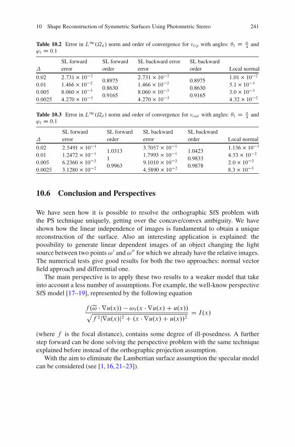
10 Shape Reconstruction of Symmetric Surfaces Using Photometric Stereo 241
Table 10.2 Error in L1.˝d / norm and order of convergence for vlip with angles: %1 D &4
and'1 D 0:1
SL forward SL forward SL backward error SL backward' error order error order Local normal
0:02 2:731# 10!2
0.8975 2:731 # 10!2
0.8975 1:01# 10!2
0:01 1:466 # 10!2
0.8630 1:466 # 10!2
0.8630 5:1# 10!3
0:005 8:060 # 10!3
0.91658:060 # 10!3
0.91653:0# 10!3
0:0025 4:270# 10!3 4:270 # 10!3 4:32# 10!2
Table 10.3 Error in L1.˝d / norm and order of convergence for vrad with angles: %1 D &4
and'1 D 0:1
SL forward SL forward SL backward SL backward' error order error order Local normal
0:02 2:5491 # 10!1
1.0313 3:7057 # 10!1
1.0423 1:136 # 10!1
0:01 1:2472 # 10!1
11:7993 # 10!1
0.98334:53# 10!2
0:005 6:2360 # 10!2
0.9963 9:1010 # 10!2
0.9878 2:0# 10!2
0:0025 3:1280 # 10!2 4:5890 # 10!2 8:3# 10!3
10.6 Conclusion and Perspectives
We have seen how it is possible to resolve the orthographic SfS problem withthe PS technique uniquely, getting over the concave/convex ambiguity. We haveshown how the linear independence of images is fundamental to obtain a uniquereconstruction of the surface. Also an interesting application is explained: thepossibility to generate linear dependent images of an object changing the lightsource between two points !0 and !00 for which we already have the relative images.The numerical tests give good results for both the two approaches: normal vectorfield approach and differential one.
The main perspective is to apply these two results to a weaker model that takeinto account a less number of assumptions. For example, the well-know perspectiveSfS model [17–19], represented by the following equation
f .e! ! ru.x// " !3.x ! ru.x/C u.x//pf 2jru.x/j2 C .x ! ru.x/C u.x//2
D I.x/
(where f is the focal distance), contains some degree of ill-posedness. A furtherstep forward can be done solving the perspective problem with the same techniqueexplained before instead of the orthographic projection assumption.
With the aim to eliminate the Lambertian surface assumption the specular modelcan be considered (see [1, 16, 21–23]).
242 R. Mecca and S. Tozza
References
1. Blinn, J.F.: Models of light reflection for computer synthesized pictures. Comput. Graph. 11(2),192–198 (1977)
2. Brooks, M.J., Chojnacki, W., Kozera, R.: Impossible and ambiguous shading patterns. Int. J.Comput. Vis. 7(2), 119–126 (1992)
3. Cham, T.-J., Cipolla, R.: Symmetry detection through local skewed symmetries. Image Vis.Comput. 13(5), 439–450 (1995)
4. Durou, J.-D., Courteille, F.: Integration of a normal field without boundary condition. In:Proceedings of the First International Workshop on Photometric Analysis For ComputerVision, Rio de Janeiro (2007)
5. Durou, J.-D., Falcone, M., Sagona, M.: Numerical methods for shape from shading: a newsurvey with benchmarks. Comput. Vis. Image Underst. 109(1), 22–43 (2008)
6. Durou, J.-D., Aujol, J.-F., Courteille, F.: Integrating the normal field of a surface in the presenceof discontinuities. In: Proceedings of the Energy Minimization Method in Computer Visionand Pattern Recognition 2009. Lecture Notes in Computer Science, vol. 5681, pp. 261–273.Springer, Berlin (2009)
7. Friedberg, S.A.: Finding axes of skewed symmetry. Comput. Vis. Graph. Image Process. 34(2),138–155 (1986)
8. Gofman, Y., Kiryati, N.: Detecting symmetries in grey level images: the global optimizationapproach. In: Proceedings of the International Conference on Pattern Recognition, SanFrancisco (1996)
9. Gordon, G.G.: Shape from symmetry. In: Proceedings of SPIE Intellent Robots and ComputerVision VIII, Philadelphia (1989)
10. Gordon, G.G.: 3d reconstruction from a single view of an object ant its image in a plane mirror.In: Proceedings of International Conference on Pattern Recognition, Brisbane (1998)
11. Kozera, R.: Existence and uniqueness in photometric stereo. Appl. Math. Comput. 44(1), 103(1991)
12. Kozera, R.: Uniqueness in shape from shading revisited. J. Math. Imaging Vis. 7(2), 123–138(1997)
13. Mecca, R.: Uniqueness for shape from shading via photometric stereo technique. In: Proceed-ings of the 18th IEEE International Conference on Image Processing, Brussels, pp. 2994–2997(2011)
14. Mukherjee, D.P., Zisserman, A., Brady, J.M.: Shape from symmetry – detecting and exploitingsymmetry in affine images. Technical report, report no. OUEL 1988/93. Department ofEngineering Science, University of Oxford
15. Onn, R., Bruckstein, A.M.: Integrability disambiguates surface recovery in two-image photo-metric stereo. Int. J. Comput. Vis. 5(1), 105–113 (1990)
16. Phong, B.T.: Illumination for computer generated pictures. Commun. ACM 18(6), 311–317(1975)
17. Prados, E., Faugeras, O.: Perspective shape from shading and viscosity solutions. In: Proceed-ings of the 9th IEEE International Conference on Computer Vision, Nice, vol. 2, pp. 826–831(2003)
18. Prados, E., Faugeras, O.: Shape from shading: a well-posed problem? In: Proceedings of theIEEE International Conference on Computer Vision and Pattern Recognition, San Diego, vol.2, pp. 870–877 (2005)
19. Prados, E., Camilli, F., Faugeras, O.: A viscosity solution method for shape-from-shadingwithout image boundary data. Math. Model. Numer. Anal. 40, 393–412 (2006)
20. Shimshoni, I., Moses, Y., Lindenbaum, M.: Shape reconstruction of 3d bilaterally symmetricsurfaces. Int. J. Comput. Vis. 39(2), 97–110 (2000)
21. Torrance, K.E., Sparrow, E.M.: Theory for off-specular reflecion from roughened surfaces. J.Opt. Soc. Am. 57(9), 1105–1114 (1967)

10 Shape Reconstruction of Symmetric Surfaces Using Photometric Stereo 243
22. Tsai, P.S., Shah, M.: Shape from shading using linear approximation. Image Vis. Comput. J.(Elsevier, Oxford) 12(8), 487–498 (1994)
23. Vogel, O., Breuss, M., Weickert, J.: Perspective shape from shading with non-lambertianreflectance. In: Rigoll, G. (ed.) Pattern Recognition. Lecture Notes in Computer Science, vol.5096, pp. 517–526. Springer, Berlin (2008)
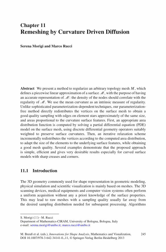
Chapter 11Remeshing by Curvature Driven Diffusion
Serena Morigi and Marco Rucci
Abstract We present a method to regularize an arbitrary topology mesh M , whichdefines a piecewise linear approximation of a surface M , with the purpose of havingan accurate representation of M : the density of the nodes should correlate with theregularity of M . We use the mean curvature as an intrinsic measure of regularity.Unlike sophisticated parameterization-dependent techniques, our parameterization-free method directly redistributes the vertices on the surface mesh to obtain agood quality sampling with edges on element stars approximately of the same size,and areas proportional to the curvature surface features. First, an appropriate areadistribution function is computed by solving a partial differential equation (PDE)model on the surface mesh, using discrete differential geometry operators suitablyweighted to preserve surface curvatures. Then, an iterative relaxation schemeincrementally redistributes the vertices according to the computed area distribution,to adapt the size of the elements to the underlying surface features, while obtaininga good mesh quality. Several examples demonstrate that the proposed approachis simple, efficient and gives very desirable results especially for curved surfacemodels with sharp creases and corners.
11.1 Introduction
The 3D geometry commonly used for shape representation in geometric modeling,physical simulation and scientific visualization is mainly based on meshes. The 3Dscanning devices, medical equipments and computer vision systems often performa uniform acquisition without any a priori knowledge of the surface properties.This may lead to raw meshes with a sampling quality usually far away fromthe desired sampling distribution needed for subsequent processing. Algorithms
S. Morigi (!) !M. RucciDepartment of Mathematics-CIRAM, University of Bologna, Bologna, Italye-mail: [email protected]; [email protected]
M. Breuß et al. (eds.), Innovations for Shape Analysis, Mathematics and Visualization,DOI 10.1007/978-3-642-34141-0 11, © Springer-Verlag Berlin Heidelberg 2013
245

246 S. Morigi and M. Rucci
for mesh simplification, denoising (fairing), decimation and remeshing representfundamental preliminary steps in mesh processing.
In particular, remeshing refers to the improvement process of the mesh quality interms of redistribution of the sampling, connectivity of the geometry, and trianglequality, in order to satisfy mesh property requirements while maintaining surfacefeatures. The reader is referred to [1] and the references therein for a survey onremeshing techniques.
Some remeshing techniques are parameterization-dependent, i.e. they associatethe mesh with a planar parameterization, and apply the algorithms on this plane. Forarbitrary genus objects, this involves also the creation of an atlas of parametrization,a well known complex process that inevitably introduces some metric distortion andmay lead to the loss of important feature information [2, 4, 9].
In contrast, parameterization-free methods avoid these problems by workingdirectly on the surface mesh and performing local modifications on the mesh. Aparameterization-free method has been proposed in [5] for direct remeshing usingarea-equalizing weights in multiresolution modeling, and in [11], several tangentialvelocity strategies are introduced to regularize geometric surface flows.
Isotropic remeshing methods based on Centroidal Voronoi Tessellation (CVT)require to repeatedly compute a geodesic Voronoi diagram which is a complex andtime-consuming step in this approach [4]. Several interesting proposals have beenpresented for this type of methods, both parameterization-based strategies [3], whichcompute the CVT on the 2D parametric domain, and parameterization-free methods,based on the intersection between a 3D Voronoi diagram and an input mesh surface,see [18].
In [1] the remeshing methods are classified by their end goal rather than bythe algorithmic strategy they employ. The techniques are classified into five cate-gories: structured, compatible, high quality, feature and error-driven remeshing. Thestructured and compatible remeshing methods aim to obtain a given connectivitystructure, the main goals for the high quality remeshing methods are the shape of theelements as well as the vertex distribution, while the end goal of feature remeshingis to preserve sharp features when producing the resulting meshes.
The proposed remeshing strategy is an adaptive, parameterization-free techniquedesigned to produce a good compromise of high quality and feature remeshingtechniques. High quality remeshing amounts to generating a mesh with well-shapedelements, uniform or isotropic sampling and smooth gradation sampling. Goodquality elements mainly lead to minimizing numerical instabilities in subsequentcomputations. However, we relaxed the uniform sampling property in order to adaptthe size of the elements to the underlying surface features.
The proposed remeshing algorithm alternates equalization of edge lengths andvertex valence, which generate a new connectivity, with mesh regularization, whichmodifies the distribution of the vertices on the surface to satisfy given mesh qualityrequirements. While the techniques that explicitly modify the connectivity, such ase.g. edge split, collapse, and flip, are widely used, the potential of the regularizationstep is still not much investigated.
11 Remeshing by Curvature Driven Diffusion 247
We present a new method to regularize an unstructured triangle mesh M , whichdefines a piecewise linear approximation of a curved surface M , with the purpose ofhaving an accurate representation of M : the density of the vertices should correlatewith the regularity of M . We cannot rely on parameterization to quantify regularityof M because this concept would not be invariant under reparameterization andfurthermore we do not assume any parameterization is given. Therefore, we usedthe mean curvature as a measure of regularity. To improve the regularization ofthe mesh M , the points X.t/ on the surface M are geometrically evolved using atangential flow
@X
@tD !!!T ; (11.1)
where ! is the velocity in the tangent direction!!T . The new resulting sampling
adapts itself to the sharper features of the surface. This motivates us to name theproposed method Adaptive Remeshing (AR).
In order to satisfy high quality remeshing we investigate the design of tangentialvelocities that aim to keep all edges on element stars approximatively of the samesize and all areas proportional to the surface features. To achieve this aim, weuse a two-step approach. First, we compute an area distribution function drivenby a mean curvature map of the surface mesh. Then the mesh vertices are movedon the tangential plane to satisfy edge equalization and area distribution qualityrequirements. The process is iterated until a significant improvement in triangleshape is obtained.
The organization of this chapter is as follows. The adaptive mesh regularizationis described in Sect. 11.2, and the proposed adaptive remeshing algorithm togetherwith its numerical aspects is discussed in Sect. 11.3. Numerical examples andcomments are provided in Sect. 11.4, and the paper is concluded in Sect. 11.5.
11.2 Adaptive Mesh Regularization
The AR method alternates equalization of edge lengths and vertex valence, whichgenerate a new connectivity, with adaptive mesh regularization, which modifies thedistribution of the vertices on the surface.
The mesh connectivity regularization is based on classical tools for meshes and itwill be briefly discussed in Sect. 11.3, while, in the following, we will focus on theproposed adaptive mesh regularization method, which consists of a two-step PDEmodel.
In the first step, the vertex area distribution function A.X/ defined on the meshM with vertex setX D fXignv
iD1, is diffused over the mesh, constrained by the meancurvature map. In the second step, the vertex position is tangentially relocated toobtain edges on element stars approximatively of the same size, and all the vertexareas proportional to the surface features.
248 S. Morigi and M. Rucci
Let A0 be the initial vertex area distribution function computed as the Voronoiarea at each vertex on the mesh M , with vertex set X0. Then in STEP 1, the vertexarea distribution function A.X/ is diffused on M by solving
@A
@tD 4wH
M A.X/; A.0/ D A0: (11.2)
In (11.2) the operator 4wHM is the weighted Laplace-Beltrami operator discretized
on the mesh M . The space discretization on M of the Laplace-Beltrami"M is theconnectivity matrix L 2 R.nv"nv/ with elements
Lij D 1Pj2N.i/ wij
8<
:
!Pj2N.i/ wij i D jCwij i ¤ j; j 2 N.i/0 otherwise
(11.3)
where N.i/ is the set of one-ring neighbor vertices of vertex Xi . The weights wijare positive numbers defined as in [14]
wij D .cot˛ij C cotˇij /; (11.4)
where ˛ij and ˇij are the two angles opposite to the edge in the two triangles sharingthe edge .Xj ;Xi/, see Fig. 11.1.
In order to solve (11.2), the weighted Laplace-Beltrami operator 4wHM is dis-
cretized by the matrix LwH with elements
LijwH D1P
j2N.i/ wij
8<
:
!Pj2N.i/ wijWij i D jCwijWij i ¤ j; j 2 N.i/0 otherwise:
(11.5)
The weight Wij depends on a similarity measure between the i th and the j thvertex, and it is defined in terms of mean curvature values H on the mesh M asfollows
Wij D 1Pj2N.i/ Wij
e#D.Xi ;Xj /=# ;
D.Xi ; Xj / D kH.Xi/ !H.Xj /k22; j 2 N.i/;(11.6)
where # is a filtering parameter which controls the decay of the exponential functionand therefore the decay of the weights as function of the Euclidean distance betweenmean curvature values. Since H.X/ is normalized to one, we can fix the value for# in order to identify a significant change in the curvature between vertices Xi andXj . For example, for # D 0:1 we identify as a curvature change when the meancurvature values in the two vertices differ more than 10%. The use of smaller #leads to detect more sharper features.
More details on the weights defined in (11.6) are provided in [12], where theauthors apply a weighted Laplace-Beltrami operator in the context of surface fairing.
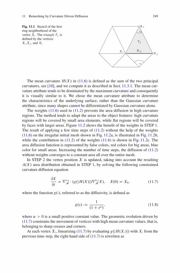
11 Remeshing by Curvature Driven Diffusion 249
Fig. 11.1 Stencil of the firstring neighborhood of thevertex Xi . The triangle Tj isdefined by the verticesXi ,Xj , and X`
The mean curvature H.X/ in (11.6) is defined as the sum of the two principalcurvatures, see [10], and we compute it as described in Sect. 11.3.1. The mean cur-vature attribute tends to be dominated by the maximum curvature and consequentlyit is visually similar to it. We chose the mean curvature attribute to determinethe characteristics of the underlying surface, rather than the Gaussian curvatureattribute, since many shapes cannot be differentiated by Gaussian curvature alone.
The weights (11.6) used in (11.2) prevents the area diffusion in high curvatureregions. The method tends to adapt the areas to the object features: high curvatureregions will be covered by small area elements, while flat regions will be coveredby faces with larger areas. Figure 11.2 shows the benefit of the weights in STEP 1.The result of applying a few time steps of (11.2) without the help of the weights(11.6) on the irregular initial mesh shown in Fig. 11.2a, is illustrated in Fig. 11.2b,while the contribution in (11.2) of the weights (11.6) is shown in Fig. 11.2c. Thearea diffusion function is represented by false colors, red colors for big areas, bluecolor for small areas. Increasing the number of time steps, the diffusion of (11.2)without weights converges to a constant area all over the entire mesh.
In STEP 2 the vertex position X is updated, taking into account the resultingA.X/ area distribution obtained in STEP 1, by solving the following constrainedcurvature diffusion equation
@X
@tD rwA
M " .g.jH.X/j/rwAMX/; X.0/ D X0; (11.7)
where the function g."/, referred to as the diffusivity, is defined as
g.s/ WD 1
.1C s� / ; (11.8)
where � > 0 is a small positive constant value. The geometric evolution driven by(11.7) constrains the movement of vertices with high mean curvature values, that is,belonging to sharp creases and corners.
At each vertex Xi , linearizing (11.7) by evaluating g.jH.Xi/j/ with Xi from theprevious time-step, the right-hand side of (11.7) is rewritten as
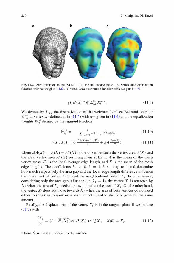
250 S. Morigi and M. Rucci
Fig. 11.2 Area diffusion in AR STEP 1: (a) the flat shaded mesh; (b) vertex area distributionfunction without weights (11.6); (c) vertex area distribution function with weights (11.6)
g.jH.Xoldi /j/4wA
MXnewi : (11.9)
We denote by LwA the discretization of the weighted Laplace Beltrami operator4wA
M at vertex Xi defined as in (11.5) with wij given in (11.4) and the equalizationweights W A
ij defined by the sigmoid function
W Aij D 1P
j2N.i/ W Aij
1
1Ce!f .Xi ;Xj /=# (11.10)
f .Xi ; Xj / D $1"A.Xj /#"A.Xi /
AC $2.Eij#EiE
/; (11.11)
where "A.X/ D A.X/ ! Ad.X/ is the offset between the vertex area A.X/ andthe ideal vertex area Ad.X/ resulting from STEP 1, A is the mean of the meshvertex areas, Ei is the local average edge length, and E is the mean of the meshedge lengths. The coefficients $i > 0, i D 1; 2, sum up to 1 and determinehow much respectively the area gap and the local edge length difference influencethe movement of vertex Xi toward the neighborhood vertex Xj . In other words,considering only the area gap influence (i.e. $1 D 1), the vertex Xi is attracted byXj when the area of Xi needs to grow more than the area of Xj . On the other hand,the vertexXi does not move towardsXj when the area of both vertices do not needeither to shrink or to grow or when they both need to shrink or grow by the sameamount.
Finally, the displacement of the vertex Xi is in the tangent plane if we replace(11.7) with
@Xi
@tD .I !!!N i
!!N Ti /g.jH.Xi/j/4wA
MXi; X.0/ D X0; (11.12)
where!!N is the unit normal to the surface.

11 Remeshing by Curvature Driven Diffusion 251
11.3 Adaptive Remeshing (AR) Algorithm
The AR algorithm iterates on the two stages of mesh connectivity regularizationand adaptive mesh regularization approaching to a mesh with a smooth gradation ofvertex density depending on mean curvature values and represented by well-shapedtriangles.
We terminate the process and accept X.i/ as the resulting mesh as soon as thedifference of area variance between consecutive iterations is sufficiently small;specifically, we acceptX.i/ when for the first time
"Var.A/ WD jVar.A.X.i/// ! Var.A.X.i#1///j < 1 " 10#6:
The regularization of mesh connectivity (named STEP 0) aims to perform anadjustment of edge lengths and vertex valences, and is implemented by applying thefollowing basic tools:
1. Specify target edge length L 2 ŒLmin; Lmax %2. Split all edges longer than Lmax3. Collapse all edges shorter than Lmin
4. Flip edges to promote valence 6 (or 4 on boundaries).
These are commonly used tools to obtain mesh connectivity regularization, and werefer the reader to [5] for more details.
The adaptive mesh regularization stage is a two-step process which implementsthe PDEs (11.2) and (11.12), named in the sequel STEP 1 and STEP 2, to relax thevertex position according to a computed area distribution.
The following algorithm summarizes the computations required by our method.
Adaptive Remeshing AlgorithmGiven an initial position vector X0,Compute LwH .X0/; A.X0/; set X.0/ D X0, i=1While "Var.A/ < 1 " 10#6STEP 0: MESH CONNECTIVITY REGULARIZATIONSTEP 1: AREA REGULARIZATION:Set A.0/ D A.X.i#1//.I ! dtLwH /A
.nC1/ D A.n/Compute LwA.X
.i#1//, g.jH.i#1/j/STEP 2: VERTEX TANGENTIAL UPDATE:Set X.0/ D X.i#1/
For n D 1; " " " ; nMAX
X.nC1/ D .I C dt.I !!!N!!N T /g.jH.i#1/j/LwA/X.n/
end fori=i+1
end while
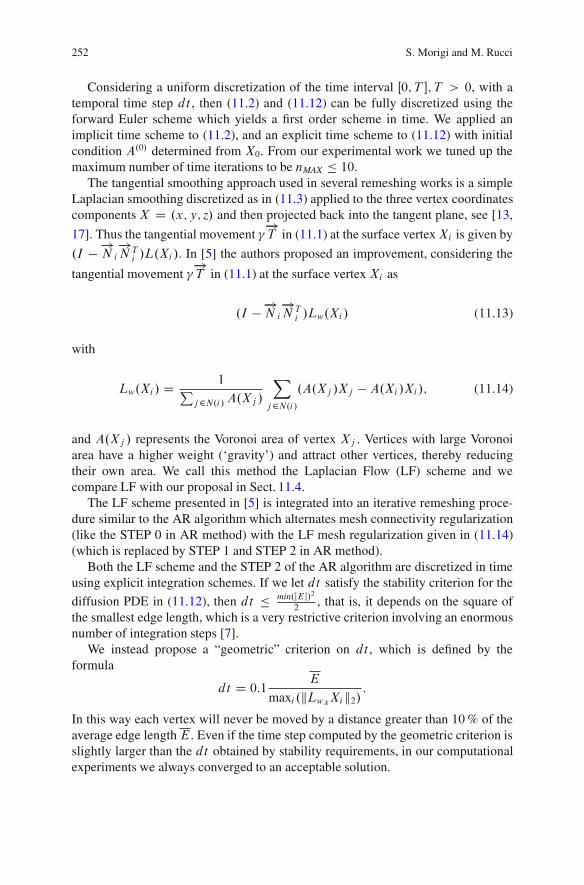
252 S. Morigi and M. Rucci
Considering a uniform discretization of the time interval Œ0; T %; T > 0, with atemporal time step dt , then (11.2) and (11.12) can be fully discretized using theforward Euler scheme which yields a first order scheme in time. We applied animplicit time scheme to (11.2), and an explicit time scheme to (11.12) with initialcondition A.0/ determined from X0. From our experimental work we tuned up themaximum number of time iterations to be nMAX # 10.
The tangential smoothing approach used in several remeshing works is a simpleLaplacian smoothing discretized as in (11.3) applied to the three vertex coordinatescomponents X D .x; y; z/ and then projected back into the tangent plane, see [13,17]. Thus the tangential movement !
!!T in (11.1) at the surface vertexXi is given by
.I ! !!N i!!N Ti /L.Xi /. In [5] the authors proposed an improvement, considering the
tangential movement !!!T in (11.1) at the surface vertex Xi as
.I !!!N i!!N Ti /Lw.Xi/ (11.13)
with
Lw.Xi / D1P
j2N.i/ A.Xj /
X
j2N.i/.A.Xj /Xj !A.Xi /Xi/; (11.14)
and A.Xj / represents the Voronoi area of vertex Xj . Vertices with large Voronoiarea have a higher weight (‘gravity’) and attract other vertices, thereby reducingtheir own area. We call this method the Laplacian Flow (LF) scheme and wecompare LF with our proposal in Sect. 11.4.
The LF scheme presented in [5] is integrated into an iterative remeshing proce-dure similar to the AR algorithm which alternates mesh connectivity regularization(like the STEP 0 in AR method) with the LF mesh regularization given in (11.14)(which is replaced by STEP 1 and STEP 2 in AR method).
Both the LF scheme and the STEP 2 of the AR algorithm are discretized in timeusing explicit integration schemes. If we let dt satisfy the stability criterion for thediffusion PDE in (11.12), then dt # min.jEj/2
2, that is, it depends on the square of
the smallest edge length, which is a very restrictive criterion involving an enormousnumber of integration steps [7].
We instead propose a “geometric” criterion on dt , which is defined by theformula
dt D 0:1 E
maxi .kLwAXik2/:
In this way each vertex will never be moved by a distance greater than 10% of theaverage edge length E. Even if the time step computed by the geometric criterion isslightly larger than the dt obtained by stability requirements, in our computationalexperiments we always converged to an acceptable solution.
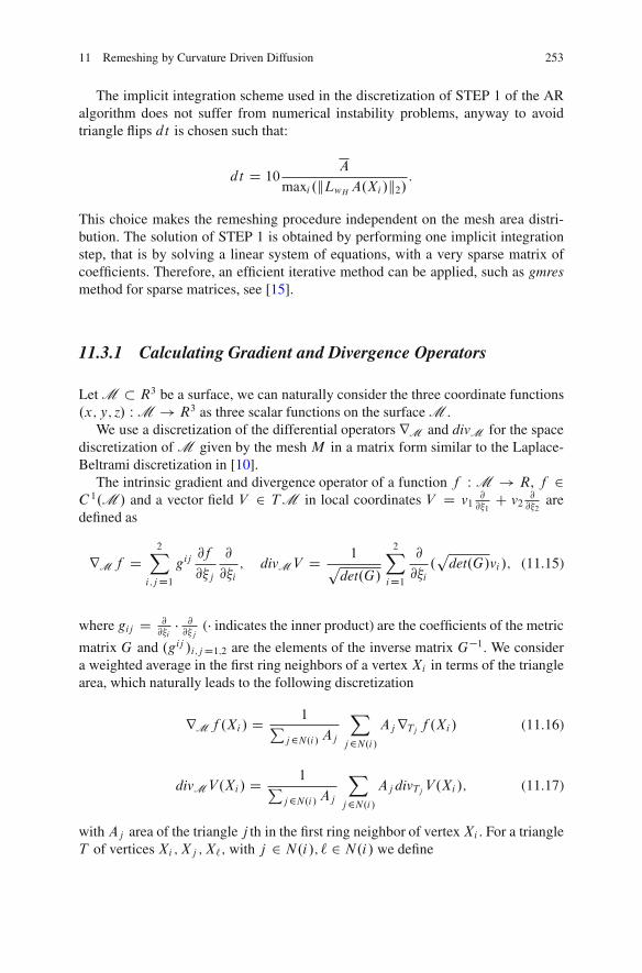
11 Remeshing by Curvature Driven Diffusion 253
The implicit integration scheme used in the discretization of STEP 1 of the ARalgorithm does not suffer from numerical instability problems, anyway to avoidtriangle flips dt is chosen such that:
dt D 10 A
maxi .kLwH A.Xi/k2/:
This choice makes the remeshing procedure independent on the mesh area distri-bution. The solution of STEP 1 is obtained by performing one implicit integrationstep, that is by solving a linear system of equations, with a very sparse matrix ofcoefficients. Therefore, an efficient iterative method can be applied, such as gmresmethod for sparse matrices, see [15].
11.3.1 Calculating Gradient and Divergence Operators
Let M $ R3 be a surface, we can naturally consider the three coordinate functions.x; y; z/ WM ! R3 as three scalar functions on the surface M .
We use a discretization of the differential operators rM and divM for the spacediscretization of M given by the mesh M in a matrix form similar to the Laplace-Beltrami discretization in [10].
The intrinsic gradient and divergence operator of a function f W M ! R, f 2C1.M / and a vector field V 2 TM in local coordinates V D v1 @
@&1C v2 @
@&2are
defined as
rMf D2X
i;jD1gij
@f
@&j
@
@&i; divMV D 1
pdet.G/
2X
iD1
@
@&i.p
det.G/vi /; (11.15)
where gij D @@&i" @@&j
(" indicates the inner product) are the coefficients of the metric
matrix G and .gij /i;jD1;2 are the elements of the inverse matrix G#1. We considera weighted average in the first ring neighbors of a vertex Xi in terms of the trianglearea, which naturally leads to the following discretization
rMf .Xi / D1P
j2N.i/ Aj
X
j2N.i/AjrTj f .Xi / (11.16)
divMV.Xi/ D1P
j2N.i/ Aj
X
j2N.i/Aj divTj V .Xi /; (11.17)
with Aj area of the triangle j th in the first ring neighbor of vertexXi . For a triangleT of verticesXi ;Xj ;X`; with j 2 N.i/; ` 2 N.i/ we define

254 S. Morigi and M. Rucci
rTj f .Xi / DP
k2i;j;`$Tj!!! Xk
Tjf .Xk/; (11.18)
where k varies in the set of the vertices of Tj , and
!!! XjT D g11.Xj !Xi/C g12.X` !Xi/;!!! X`T D g21.Xj !Xi/C g22.X` !Xi/;!!! Xi
T D !.!!!XjT C !!!
X`T /:
(11.19)
The mean curvature vector field, used in the similarity weights (11.6), isapproximated on a vertex Xi of the mesh, by H.Xi/ D divM .rM .Xi//. Thediscretization of the Laplace, gradient and divergence operators at the vertex Xidepends on the elements of its first ring neighborhood. The measure of meancurvature at the vertex Xi depends on its two-ring neighbors. Therefore, thismeasure of mean curvature is more reliable than the mean curvature computed bydiscretizing the relation"M .X/ D !2H.X/!!N .X/, mostly because it is computedon a wider stencil which allows to better identify the features of the mesh, thusimproving the efficacy of the weights in (11.6) and the quality of the diffusivityfunction in (11.7).
Moreover, instead of the linearization defined in (11.9), we can compute a moreaccurate approximation of the non-linear diffusion equation (11.7) by applying thediscretization of the gradient and divergence operators on the mesh proposed in(11.16) and (11.17), respectively.
11.4 Remeshing Results
To our knowledge, there are no standard measures for evaluating and comparing theefficacy of remeshing techniques. Instead, comparison is often based on a qualitativeevaluation of the final results and it is strictly related to the specific end goal theremeshing is used for. In [16] the authors measure the quality of a remeshed modelby measuring the geometric properties of the resulting triangles, but this approachslightly limits the global overview on the benefits of the remeshing algorithm.
In our work, to assess the quality of the mesh generated by the proposed ARalgorithm, we introduce the following measures:
Area Variance,
Var.A.X// WDnvX
iD1.A.Xi /! A/2; (11.20)
where A is the average vertex area for a mesh with nv vertices.Mean curvature variation,

11 Remeshing by Curvature Driven Diffusion 255
"H D kH !H0k2=kH0k2; (11.21)
where H and H0 are the mean curvature maps of the remeshed and the originalmeshes, respectively. For each vertex Xi on the original mesh, the differenceH.Xj / ! H0.Xi/ is computed with respect to the nearest vertex Xj on theremeshed mesh.
Variation of local edge length variance,
"Var.E/ D kVar.E/ ! Var.E0/k2=kVar.E0/k2; (11.22)
where the local edge length variance of the vertex Xi is computed asVar.E/i D 1
di
Pj2N.i/.Eij !Ei/
2.
Hausdorff distance,
dH.X0;X/ D maxf supx2X0
infy2X
d.x; y/; supy2X
infx2X0
d.x; y/ g; (11.23)
is a measure of distance between the remeshed and the original meshes, see [6].
The goal of our remeshing strategy is to minimize the area variance (Var.A.X//),while preserving the mean curvature values and the shape of the original mesh, thatis minimizing ("H ) and the average one-sided Hausdorff distance dh. Moreover,the variation of mean curvature variance ("Var.H/) is a value that should bepreserved, and the variation of area variance ("Var.A/) and the variation of edgevariance ("Var.E/) provide a measure of the quality of the resulting mesh.
The parameters ˛ in the diffusion function g."/ in (11.8), and # in (11.6) arechosen to be 0:05, while the parameter # in (11.10) is 0:1. All experiments wereperformed on Intel Core i7-720QM Quad-Core 1.6 GHz machine, with 4 GB/RAMand Nvidia G335M graphics card in a linux environment. The visualization is basedon OpenGL library and the application is written using C language. Numericalcomputations are performed using the “meschach” matrix library.
We compare the AR algorithm with the LF method defined in [5], when appliedto the meshes shown in Figs. 11.3a–11.7a. In the reported experiments we omitthe mesh connectivity regularization stage integrated in both AR (STEP 0) and LFmethods in order to effectively point out the performances of the mesh regularizationstage in the AR algorithm. Moreover, we noticed that the features of the mesh geteasily compromised if the operations involved in the mesh connectivity stage arenot performed adaptively, as we do in STEP 0 of the AR algorithm. In particular,in STEP 0 of the AR method the flip tool is applied only when the deviation incurvature normals is acceptable. This improves further on the results obtained bythe AR method, but it makes more difficult to distinguish the benefit of the meshregularization stage inside the entire iterative process.
A qualitative comparison is illustrated in Figs. 11.3–11.7. In Figs. 11.3–11.6 thearea distribution function A is visualized using false colors superimposed onto
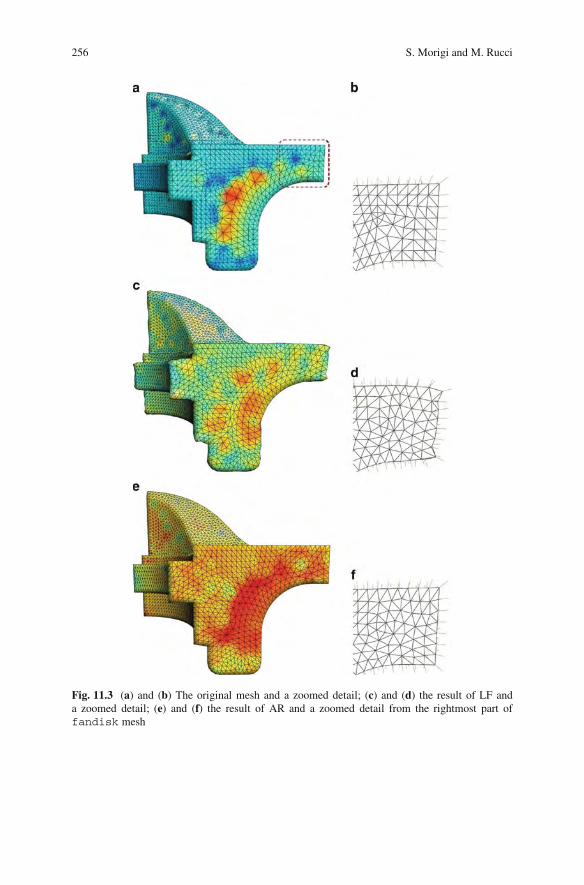
256 S. Morigi and M. Rucci
Fig. 11.3 (a) and (b) The original mesh and a zoomed detail; (c) and (d) the result of LF anda zoomed detail; (e) and (f) the result of AR and a zoomed detail from the rightmost part offandisk mesh
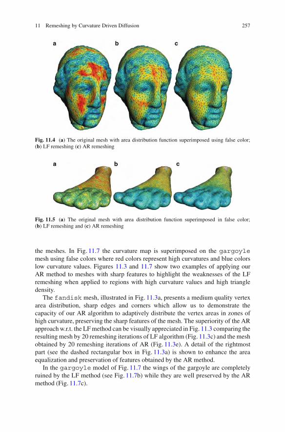
11 Remeshing by Curvature Driven Diffusion 257
Fig. 11.4 (a) The original mesh with area distribution function superimposed using false color;(b) LF remeshing (c) AR remeshing
Fig. 11.5 (a) The original mesh with area distribution function superimposed in false color;(b) LF remeshing and (c) AR remeshing
the meshes. In Fig. 11.7 the curvature map is superimposed on the gargoylemesh using false colors where red colors represent high curvatures and blue colorslow curvature values. Figures 11.3 and 11.7 show two examples of applying ourAR method to meshes with sharp features to highlight the weaknesses of the LFremeshing when applied to regions with high curvature values and high triangledensity.
The fandisk mesh, illustrated in Fig. 11.3a, presents a medium quality vertexarea distribution, sharp edges and corners which allow us to demonstrate thecapacity of our AR algorithm to adaptively distribute the vertex areas in zones ofhigh curvature, preserving the sharp features of the mesh. The superiority of the ARapproach w.r.t. the LF method can be visually appreciated in Fig. 11.3 comparing theresulting mesh by 20 remeshing iterations of LF algorithm (Fig. 11.3c) and the meshobtained by 20 remeshing iterations of AR (Fig. 11.3e). A detail of the rightmostpart (see the dashed rectangular box in Fig. 11.3a) is shown to enhance the areaequalization and preservation of features obtained by the AR method.
In the gargoyle model of Fig. 11.7 the wings of the gargoyle are completelyruined by the LF method (see Fig. 11.7b) while they are well preserved by the ARmethod (Fig. 11.7c).
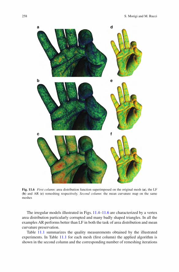
258 S. Morigi and M. Rucci
Fig. 11.6 First column: area distribution function superimposed on the original mesh (a), the LF(b) and AR (c) remeshing respectively. Second column: the mean curvature map on the samemeshes
The irregular models illustrated in Figs. 11.4–11.6 are characterized by a vertexarea distribution particularly corrupted and many badly shaped triangles. In all theexamples AR performs better than LF in both the task of area distribution and meancurvature preservation.
Table 11.1 summarizes the quality measurements obtained by the illustratedexperiments. In Table 11.1 for each mesh (first column) the applied algorithm isshown in the second column and the corresponding number of remeshing iterations
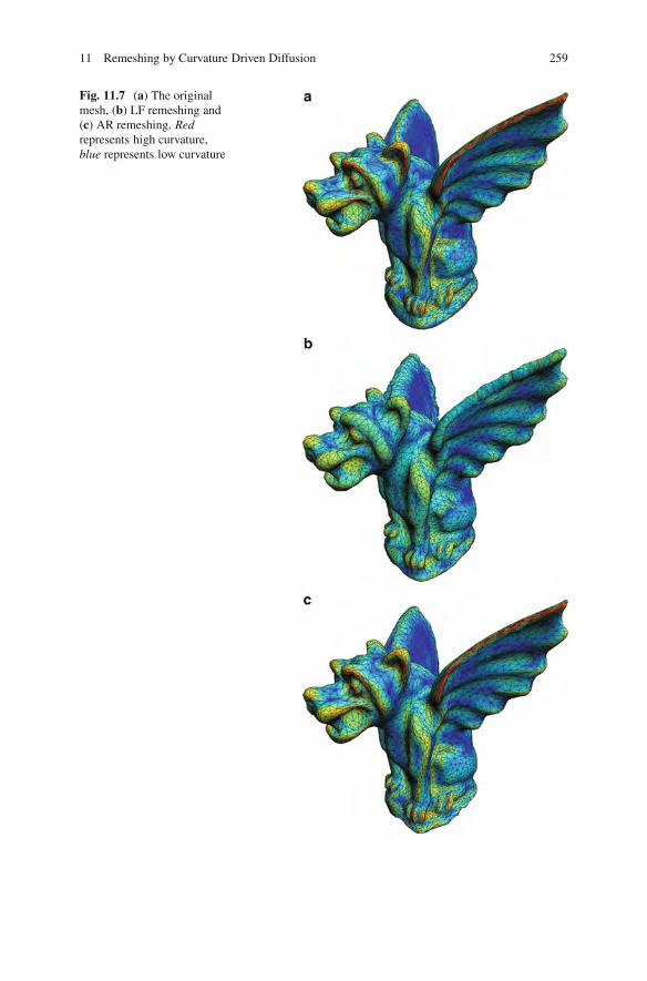
11 Remeshing by Curvature Driven Diffusion 259
Fig. 11.7 (a) The originalmesh, (b) LF remeshing and(c) AR remeshing. Redrepresents high curvature,blue represents low curvature

260 S. Morigi and M. Rucci
Table 11.1 Quality measurements for the remeshing tests
Mesh Method # its Var.A/ "H % "Var.E/% "Var.A/% "Var.H/% dh
Hand AR 5 0.0000077 17:8 77.2 61.2 5.9 0.002Hand LF 5 0.0000096 40:3 78.4 51.6 47.1 0.003Gargoyle AR 10 0.0015316 26:4 63.7 47.5 14.3 0.007Gargoyle LF 10 0.0015180 69:0 81.6 48.0 59.7 0.016Fandisk AR 20 0.0002583 4:7 51.7 55.2 0.8 0.005fandisk LF 20 0.0003982 30:3 74.4 31.0 5.9 0.013Igea AR 20 0.0001252 12:9 57.3 41.4 5.2 0.004Igea LF 20 0.0001248 27:5 64.9 41.5 34.3 0.005Foot AR 10 0.0007397 13:1 92.8 65.4 3.7 0.007Foot LF 10 0.0007995 28:2 93.0 62.7 22.5 0.008
Fig. 11.8 The area variance Var.A/ (left) and the mean curvature changing"H (right) as functionof the remeshing iterations
(its) is in the third column. The results reported in Table 11.1 show that the ARmethod successfully produces well-shaped triangles while preserving the meancurvature map of the original mesh better than the LF method.
The plots in Fig. 11.8 (left and right) show the area variance Var.A/ and themean curvature variation "H as functions of the number of remeshing iterationswhen the LF method and the AR method are applied to the fandisk mesh. Whenthe AR algorithm is applied, the area variance Var.A/ rapidly decreases, while themean curvature of the mesh is preserved. The comparison with the LF methodhighlights a strong effect on the mean curvature of the resulting mesh and a non-convergent behavior in the minimization of the area variance. This aspect requiresfurther theoretical investigation.
11.5 Conclusions
We presented a new adaptive remeshing scheme based on the idea of improvingmesh quality by a series of local modifications of the mesh geometry and con-nectivity. The fundamental quality criteria we pursued are: faces of good quality,and adaptive mesh resolution to preserve the surface structural characteristics.
11 Remeshing by Curvature Driven Diffusion 261
To satisfy the last requirement the size of the faces is adapted to the local meancurvature (big enough for smoothed parts and smaller for sharp features). Theproposed AR algorithm iterates a connectivity regularization, which is merelybased on elementary mesh operations such as edge collapse, flip, and split, witha mesh regularization method. Our contribution to the family of parameterization-free remeshing techniques is a curvature-based mesh regularization technique whichallows the control of both triangle quality and vertex sampling over the mesh, as afunction of the surface mesh curvature. The first step approaches to an appropriatearea distribution function computed by solving an evolutive PDE diffusion modelusing discrete differential geometry operators suitably weighted to preserve surfacecurvatures. The area distribution is then applied in the second step of the ARalgorithm to redistribute the vertices.
Future work will include operations on the mesh in order to produce a mesh thathas a semi-regular structure, namely, with subdivision connectivity. This operationswill be integrated in STEP 0 of the AR algorithm.
Acknowledgements This work is supported by MIUR-Prin Grant 20083KLJEZ and by ex 60 %project by the University of Bologna: Funds for selected research topics.
References
1. Alliez, P., Ucelli, G., Gotsman, C., Attene, M.: Recent advances in remeshing of surfaces.In: De Floriani, L., Spagnuolo, M. (eds.) Shape Analysis and Structuring. Mathematics andVisualization, pp. 53–82. Springer (2008)
2. Alliez, P., Meyer, M., Desbrun, M.: Interactive geometry remeshing. ACM Trans. Graph. 21(3),347–354 (2002)
3. Alliez, P., de Verdiere, E.C., Devillers, O., Isenburg, M.: Centroidal Voronoi Diagrams forisotropic surface remeshing. Graph. Models 67(3), 204–231 (2005)
4. Alliez, P., de Verdiere, E.C., Devillers, O., Isenburg, M.: Isotropic surface remeshing. In:Proceedings of the Shape Modeling International 2003 (SMI ’03), pp. 49–58. IEEE ComputerSociety, Washington, DC (2003)
5. Botsch, M., Kobbelt, L.: A remeshing approach to multiresolution modeling. In: Scopigno,R., Zorin, D. (eds.) Proceedings of 2nd Eurographics Symposium on Geometry Processing,Eurographics, pp. 189–196. ACM, New York (2004)
6. Cignoni, P., Callieri, M., Corsini, M., Dellepiane, M., Ganovelli, F., Ranzuglia, G., MeshLab,G.: An open-source mesh processing tool. In: Sixth Eurographics, pp. 47–48, (2008)
7. M. Desbrun, M. Meyer, P. Schroder, A.H. Barr, Implicit Fairing of Irregular Meshes usingDiffusion and Curvature Flow, Computer Graphics (SIGGRAPH 99 Proceedings), 317-324,(1999)
8. do Carmo, M.P.: Riemannian Geometry. Birkhauser, Boston/Basel/Berlin (1993)9. Hormann, K., Labsik, U., Greiner, G.: Remeshing triangulated surfaces with optimal parame-
terizations. Comput. Aided Des. 33(11), 779–788 (2001)10. Meyer, M., Desbrun, M., Schroeder, P., Barr, A.: Discrete differential geometry operators for
triangulated 2-manifolds. In: Proceedings of the VisMath ’02, Berlin-Dahlem, Germany, pp.237–242 (2002)
11. Morigi, S.: Geometric surface evolution with tangential contribution. J. Comput. Appl. Math.233, 1277–1287 (2010)

262 S. Morigi and M. Rucci
12. Morigi, S., Rucci, M., Sgallari, F.: Nonlocal surface fairing. In: Bruckstein, A.M., et al. (eds.):SSVM 2011, LNCS 6667, pp. 38–49. Springer, Berlin/Heidelberg (2011)
13. Ohtake, Y., Belyaev, A.G., Bogaevski, I.A.: Mesh regularization and adaptive smoothing.Comput. Aided Des. 33, 789–800 (2001)
14. Pinkall, U., Polthier, K.: Computing discrete minimal surfaces and their conjugates. Exp. Math.2, 15–36 (1993)
15. Saad, Y.: Iterative Methods for Sparse Linear Systems. SIAM, Philadelphia (2003)16. Surazhsky, V., Gotsman, C.: Explicit surface remeshing. In: Proceedings of the 2003
Eurographics/ACM SIGGRAPH Symposium on Geometry Processing, Aachen, Germany,pp. 20–30 (2003)
17. Xu, G., Pan, Q., Bajaj, C.L.: Discrete surface modelling using partial differential equations.CAGD 23(2), 125–145 (2006)
18. Yan, D.-M., Levy, B., Liu, Y., Sun, F., Wang, W.: Isotropic Remeshing with fast and exactcomputation of restricted Voronoi Diagram. Proc. Eurograph. Symp. Geom. Process. 28(5),1445–1454 (2009)
Chapter 12Group-Valued Regularization for MotionSegmentation of Articulated Shapes
Guy Rosman, Michael M. Bronstein,Alexander M. Bronstein, Alon Wolf, and Ron Kimmel
Abstract Motion-based segmentation is an important tool for the analysis ofarticulated shapes. As such, it plays an important role in mechanical engineering,computer graphics, and computer vision. In this chapter, we study motion-basedsegmentation of 3D articulated shapes. We formulate motion-based surface seg-mentation as a piecewise-smooth regularization problem for the transformationsbetween several poses. Using Lie-group representation for the transformation ateach surface point, we obtain a simple regularized fitting problem. An Ambrosio-Tortorelli scheme of a generalized Mumford-Shah model gives us the segmentationfunctional without assuming prior knowledge on the number of parts or even thearticulated nature of the object. Experiments on several standard datasets comparethe results of the proposed method to state-of-the-art algorithms.
G. Rosman (!) ! R. KimmelDepartment of Computer Science, Israel Institute of Technology, 32000, Haifa, Israele-mail: [email protected]; [email protected]
M.M. BronsteinInstitute of Computational Science, Faculty of Informatics, Universita della Svizzera italiana,Lugano, Switzerlande-mail: [email protected]
A.M. BronsteinSchool of Electrical Engineering, Faculty of Engineering, Tel Aviv University, Ramat Aviv69978, Israele-mail: [email protected]
A. WolfDepartment of Mechanical Engineering, Technion – Israel Institute of Technology,Haifa, 32000, Israele-mail: [email protected]
M. Breuß et al. (eds.), Innovations for Shape Analysis, Mathematics and Visualization,DOI 10.1007/978-3-642-34141-0 12, © Springer-Verlag Berlin Heidelberg 2013
263
264 G. Rosman et al.
12.1 Introduction
Articulated objects segmentation is a key problem in biomechanics [1], mechanicalengineering, computer vision [8,30,38,41,54], and computer graphics [6,35,37,39,59, 64, 65]. Related problems of deformation analysis [4, 63] and motion segmen-tation [5, 22] have also been studied extensively in these disciplines. Algorithmssolving these problems try to infer the articulated motion of an object, given severalinstances of the object in different poses. Simultaneously, the segmentation ofthe object into rigid parts takes place along with motion estimation between thecorresponding parts in the various poses.
Most motion analysis techniques make some assumptions on the object to besegmented. These usually concern the number or location of rigid parts in thearticulated object. This can be in the form of a skeleton describing the topologyof the shape, or some other prior on the object structure. Such priors are usuallyformulated in an ad hoc manner, but not based on the kinematic model commonlyassumed for near-rigid objects [1,4]. In cases where such a prior is not available forthe objects in question, or where assumptions about the data are only approximate,this can lead to errors in the segmentation and motion estimation.
Another common assumption, especially in graphics applications, is that ofknown correspondences. In computer graphics, the problem is usually referred toas dynamic mesh segmentation. While a matching technique between poses can becombined with existing motion segmentation tools, a more complete formulationfor motion segmentation should handle the correspondence problem implicitly.
Clearly, the above assumptions are often too limiting in real-world applications,and should be avoided as part of the basic problem formulation. We would likeinstead to apply the intuition often used when studying real-life near-rigid objects,about the existence of a representative rigid motion existing for each body part. Wewish, however, to avoid detecting the articulated parts in advance. Furthermore, insome object, a clear partition into rigid parts may not exist for all of the surface.We wish to obtain reasonable results in such a case. In other words, we wouldlike to obtain a “soft” segmentation of the surface, without knowing the number orlocation of regions in advance, an explicit analysis of the surface features, or havingadditional priors on the various object parts. Also, we strive towards a formulationof motion segmentation that incorporates an implicit handling of the correspondenceproblem, given a reasonable initialization.
12.1.1 Main Contribution
In this chapter we try to remedy the shortcoming of existing approaches toarticulated motion estimation by combining the two tasks of motion estimationand segmentation into a single functional. This scheme has been described in arecent conference paper [50] and we now slightly expand upon it. Unlike existingmethods, we propose a principled variational approach, attempting to find a rigid
12 Group-Valued Regularization for Motion Segmentation of Articulated Shapes 265
transformation at each surface point, between the instance surfaces, such that theoverall transformation is described by a relatively sparse set of such transformations,each matching a rigid part of the object. The functional we propose regularizes themotion between the surfaces, and is guided by the fact that the parameters of themotion transformations
(i) Should describe the motion at each point with sufficient accuracy.(ii) Should vary smoothly within the (unknown) rigid parts.
(iii) Can vary abruptly between rigid parts.
We see our main contribution in these:
A new framework: First, we propose an axiomatic variational framework forarticulated motion segmentation. While focusing on the segmentation problem inthis chapter, our framework is more general and the proposed functionals can beeasily incorporated into other applications such as motion estimation, tracking,and surface denoising.Variational segmentation: We claim that using the right parameterization, takenfrom the specific domain of rigid motion analysis, we can formulate thearticulated motion segmentation problem as a generalization of classical toolsin variational computer vision. This allows for an elegant and simple solutionwithin the proposed framework, obtaining results competitive with domain-specific state-of-the-art tools.A novel visualization algorithm: Third, we suggest a spatially-coherent algorithmfor spatial visualization of group valued data on manifolds, which draws from thesame variational principles.
12.1.2 Relation to Prior Work
Several previous works have attempted motion based segmentation of surfaces.We mention but a few of these. Kompatsiaris et al. [38] use an estimation of therigid motion at each segment in order to segment the visible surface in a coarse-to-fine manner. Arcila et al. [6] iteratively refine the segmentation for segmentswhose transformation error is too large. Wuhrer and Brunton [64] use a dual treerepresentation of the surface with weights between triangles set according to thedihedral angles. Lee et al. [39] use a similar graph-based formulation, looking atdeformation matrices around each triangle.
The scheme we propose involves diffusing the transformations between posesalong the surface, in the spirit of the Ambrosio-Tortorelli scheme [2] for Mumford-Shah segmentation [43]. The diffusion component of our scheme is a diffusionprocess of Lie-group elements, which has recently attracted significant attentionin other applications [25, 28, 56]. In diffusing transformations on the surface, ourwork is similar to that of Litke et al. [40], although the parameterization of themotion and of the surface is different. In addition, we do not make an assumption
266 G. Rosman et al.
on the surface topology; to that end, the proposed method diffuses transformationsalong the surface, rather than representing the surface in an evenly sampled 2Dparametrization plane. When dealing with real-life deformable objects that seldomadmit regular global parametrization, such an assumption could be too restrictive.
The idea of combining soft segmentation and motion estimation has beenattempted before in the case of optical flow computation (see, e.g., [3,18]). In opticalflow fields, however, the motion field is merely expected to be piecewise smooth.For truly articulated objects one would expect piecewise-constant flow fields, whenexpressed in the correct parametrization.
Finally, the functional can be extended with priors from general mesh segmen-tation techniques. These are usually based on the geometry of the surface itself,and obtain remarkable results for a variety of objects. We point the reader to[9,21,36,55], and references therein, for additional examples of mesh segmentationalgorithms. We do not, however, use an additional prior as such an addition willprevent the isolated examination of the principles shown in this chapter.
12.2 Problem Formulation
We now proceed to define the problem we try to solve and the proposed model.
12.2.1 Articulation Model
We denote byX a two-manifold representing a three-dimensional shape. We assumeX to have several embeddings into R3. Each of these embedding constitutes a poseof the surface. In the following, we will denote by x W X ! R3 the embedding ofX into R3, and use synonymously the notation x and x referring to a point on themanifold and its Euclidean embedding coordinates, for a specific pose.
In the setting of rigid motion segmentation, we assume that X represents anarticulated shape, i.e., it can be decomposed into rigid parts S1; : : : ; Sp. These aretransformed between different poses of the objects by a rigid transformation. Thistransformation, a rotation and a translation, is an isometry of R3. The rigid partsare connected by nonrigid joints J1; : : : ; Jq , such that X D Sp
iD1 Si [SqkD1 Jk .
An articulation Y D AX is obtained by applying rigid motions Ti 2 Iso.R3/to the rigid parts, and non-rigid deformations Qk to the joints, such that AX DSpiD1 Ti Si [
SqkD1 QkJk .
12.2.2 Motion Segmentation
The problem of motion-based segmentation can be described as follows: given twoarticulations of the shape, X and Y , extract its rigid parts. An extension to the case

12 Group-Valued Regularization for Motion Segmentation of Articulated Shapes 267
of multiple shape poses is straightforward. We therefore consider in the followingonly a pair of shapes for the sake of simplicity and without loss of generality.A strongly related question attempts to determine, given these articulations, themotion parameters linking the poses of the object.
Assuming that the correspondence between the two poses X and Y is known,given a point x 2 X and its correspondent point y.x/ 2 Y , we can find a motion g 2G such that gx D y, where G is some representation of coordinate transformationsin R3. This motion g may change, in the setting described above, for each surfacepoint. We therefore consider g to be a function g W X ! G. We will simultaneouslyuse gx 2 R3 to denote the action of g.x/ on the coordinates of the point x, as wellas consider the mapping given by g W X ! G and its properties.
We note that typical representations of motion in R3 contain more than threedegrees of freedom. In this sense, they are over-parameterized [45], and thus somemeasure of regularity is required in order to avoid ambiguity as well as favor ameaningful solution. On the other hand, we note that since the articulated partsof the shape move rigidly, if we choose an appropriate motion representation (asdetailed below), two points x; x0 2 Si will undergo the same transformation, fromwhich it follows that g.x/jx2Si D const. One possibility is to adopt a constrainedminimization approach, forcing g.X/ D Y , where g.X/ is a notation for the setg.x/x.x/ for all x 2 X . This approach, however, needs to somehow handle the setof joints, for which such a constraint may be meaningless. In general, restricting thefeasible set of solutions by such constraints or even constraints involving an error inthe data may be harmful for the overall result. In order to avoid this, another possibleapproach is to take an unconstrained, yet regularized, variational formulation,
mingWX!G
!ED.g/C ".g/; (12.1)
where " denotes a smoothness term operating on the motion parameters field. Thisterm is expected to be small for fields g which are piecewise constant on themanifoldX . While an appropriate parameterization of motion g, and regularizationterm ".g/ are crucial, we also require a data term that will encourage consistencyof the transformation field g with the known surface poses. Specifically, we wish tofavor a transformation field where the point x is taken by its transformation g.x/ to apoint on the other surface.ED.g/ is our fitting term which measures this consistencywith the data.
ED.g/ DZ
X
kg.x/x ! y.x/k2da; (12.2)
where y.x/ 2 R3 denotes the coordinate of the point y.x/ 2 Y corresponding tox, g.x/ is the transformation at x, and da is a measure on X . We have assumed inthe discussion so far that the correspondence between X and Y is known, which isusually not true. We can solve for the correspondence as part of the optimizationin an efficient manner. We will mention this issue in Sect. 12.4.1. We use the
268 G. Rosman et al.
term corresponding point y.x/ since, as in the case of iterative closest point (ICP)algorithms [13,67], several approaches for pruning erroneous or ineffective matchesexist [53].
Minimizing the functional with respect to g; y.x/ from a reasonable initialsolution allows recovery of the articulated parts by clustering g into regions of equalvalue. Yet another choice of a data term is a semi-local fitting term, is a semi-localone,
ED;SL.g/ DZ
X
Z
y2N .x/
kg.x/x0 ! y.x0/k2da0da; (12.3)
where N .x/ denotes a small neighborhood around the point x (we took N .x/ to bethe 12 nearest neighbors). This fitting term, by itself, formulates a local ICP process.The functional (12.1) equipped with the semi-local data term can be consideredas the geometrical fitting equivalent of the combined global-local approach for opticflow estimation [17].
The simplest representation of motion is a linear motion model, affectivelysetting G to be the group of translation, or G D R3. This results in the motionmodel gx D xC t D y for some t 2 R3. However, such a simplistic model fails tocapture the piecewise constancy of the motion field in most cases. Instead of turningto a higher order approximation model such as the affine over-parameterized model[46], or to more elaborate smoothness priors [60], we look for a relatively simplemodel that will capture natural motions with a simple smoothness prior. Thus weturn to a slightly different motion model, naturally occurring in motion research.
12.2.3 Lie-Groups
One parametrization often used in computer vision and robotics [28, 37, 42, 61] isthe representation of rigid motions by the Lie-group SE.3/ and the correspondingLie-algebra se.3/, respectively. In general, given two coordinate frame, an elementin SE.3/ describes the transformation between them. Works by Brockett [14], Parket al. [47] and Zefran et al. [69, 70] strongly relate Lie-groups, both in their globaland differential description, to robotics and articulated motions. We give a very briefintroduction to the subject and refer the reader to standard literature on the subject(e.g., [29, 44]) for more information.
Lie-groups are topological groups with a smooth manifold structure such that thegroup action G "G 7! G and the group inverse are differentiable maps.
For every Lie-group, we can canonically associate a Lie-algebra g. A Lie-algebrais as a vector space endowed with a Lie brackets operator Œ#; ## W G"G!G,describing the local structure of the group. The Lie-algebra associated with aLie-group can be mapped diffeomorphically via the exponential map onto aneighborhood of the identity operator and its tangent space.
12 Group-Valued Regularization for Motion Segmentation of Articulated Shapes 269
This property will allow us express neighboring elements in the Lie-group in avector space, and thereby define derivatives, regularity, and diffusion operators onthe group valued data.
In this chapter, we are specifically interested in the special orthogonal (rotation)matrix group SO.3/ and the Euclidean group SE.3/ to represent rigid motions. Thesecan be represented in matrix forms, where SO.3/ is given as
SO.3/ D˚R 2 R3"3;RTR D I
!; (12.4)
and SE.3/ is given by
SE.3/ D"#
R0 1
$;R 2 SO.3/; t 2 R3
%: (12.5)
The Lie-algebra of SO.3/, so.3/ consists of skew-symmetric matrices,
so.3/ D˚A 2 R3"3;AT D !A
!; (12.6)
whereas the Lie-algebra of SE.3/ can be identified with the group of 4 " 4 matricesof the form
se.3/ D"#
A0 0
$;A 2 so.3/; t 2 R3
%; (12.7)
where so.3/ is the set of 3 " 3 skew-symmetric matrices.In order to obtain piecewise constant description over the surface for the
relatively simple case of articulated object, we would like the points at each objectpart to have the same representative. Under the assumption of G D SE.3/, thisdesired property holds. We note, however, that the standard parameterization ofsmall rigid motions has six degrees of freedom, while the number of degreesof freedom required to describe the motion of point is mere three. Thus, thisparameterization clearly constitutes an over-parameterized motion field [46] forarticulated surfaces.
We now turn to the regularization term, ".g/, and note that the formulationgiven in Eq. (12.1) bears much resemblance to total variation (TV) regularizationcommon in signal and image processing [51]. Total variation regularization doesnot, however, favor distinct discontinuity sets. This property of TV regularizationis related to the staircasing effect. Furthermore, in the scalar case, discontinuitysets form closed curves, which may not be the case in some surfaces with largejoint areas. Instead, a model that better suits our segmentation problem is theMumford-Shah segmentation model [43]. This model can be implemented usingan Ambrosio-Tortorelli scheme [2], which can be easily generalized for the case ofmaps between general manifolds such as maps from surfaces into motion manifolds.We further describe the regularization chosen in Sect. 12.3.

270 G. Rosman et al.
We also note that due to the non-Euclidean structure of the group, special careshould be taken when parameterizing such a representation [28, 37, 42, 56], asdiscussed in Sect. 12.4.2.
12.3 Regularization of Group-Valued Functions on Surfaces
Ideally, we would like the transformation field defined on the articulated surface tobe piecewise smooth, if not piecewise constant. Therefore, a suitable regularizationof the transformation parameters is required. Since the Lie-groupG as a Riemannianmanifold, it is only natural to turn to regularization functionals defined on mapsbetween manifolds of the form g W X ! G.
A classical functional defined over such maps is the well-known Dirichlet energy[26],
"DIR.g/ D1
2
Z
X
hrg;rgig.x/da D 1
2
Z
X
tr&g#1rg
'2da; (12.8)
where rg denotes the intrinsic gradient of g on X , h#; #ig.x/ is the Riemannianmetric on G at a point g.x/, and da is the area element of X . This functional is themore general form of the Tikhonov regularization (for Euclidean spaces X and G),and its properties are well defined for general manifolds, as studied by Eells [26].
Minimizers of the Dirichlet energy are called harmonic maps. These result froma diffusion process, and are often used for surface matching [62, 68].
12.3.1 Ambrosio-Tortorelli Scheme
Unfortunately, the Dirichlet energy favors smooth maps defined on X , whereasour desired solution has discontinuities at the boundaries of rigid parts. We would,intuitively, want to prevent diffusion across these discontinuity curves. This can beobtained by adding a diffusivity function v W X ! Œ0; 1# to the Dirichlet functional,leading to the generalized Ambrosio-Tortorelli scheme [2] for Mumford-Shahregularization [43].
"AT.g/ DZ
X
1
2v2hrg;rgig C $hrv;rvi C .1 ! v/2
4$
!da; (12.9)
where $ is a small positive constant. This allows us to extend our outlook inseveral ways. The Mumford-Shah functional replaces the notion of a set of regionswith closed simple boundary curves with general discontinuity sets. It furthermoregeneralizes our notion of constant value regions with that of favored smoothness

12 Group-Valued Regularization for Motion Segmentation of Articulated Shapes 271
inside the areas defined by these discontinuity curves. This is in order to handleobjects which deviate from articulated motion, for example in flexible regions orjoints.
Furthermore, the generalized Ambrosio-Tortorelli scheme allows us to explicitlyreason about places in the flow where the nonlinear nature of the data manifoldmanifests itself. Suppose we have a solution .g$; v$/ satisfying our piecewise-constancy assumptions of g, and a diffusivity function with 0 at region boundariesand 1 elsewhere. At such a solution, we expect two neighboring points whichbelong to different regions to have a very small diffusivity value v connecting them,effectively nullifying the interaction between far-away group elements which isdependent on the mapping used for the logarithm map at each point, and hencecan be inaccurate [32, 42]. While such a solution .g$; v$/ may not be a minimizerof the functional, it serves well to explain the intuition motivating the choice of thefunctional.
12.3.2 Diffusion of Lie-Group Elements
In order to efficiently compute the Euler-Lagrange equation corresponding to thegeneralized Ambrosio-Tortorelli functional (12.9), we transform the neighborhoodof each point into the corresponding Lie-algebra elements before applying thediffusion operator. Using Lie-algebra representation of differential operators forrigid motion has been used before in computer vision [56], numerical PDEcomputations [32], path planning and optimal control theory [37, 42].
The Euler-Lagrange equation for the generalized Dirichlet energy measuring themap between two manifolds is given as [26]
%Xg˛ C & ˛
ˇ'
˝rgˇ;rg'
˛g.x/D 0; (12.10)
where ˛; ˇ ' enumerate the local coordinates of our group manifold, se.3/, and weuse Einstein’s notation according to which corresponding indices are summed over.& ˛ˇ' are the Christoffel symbols of SE.3/, which express the Riemannian metric’s
local derivatives. We refer the reader to [24] for an introduction to Riemanniangeometry. Finally,%X denotes the Laplace-Beltrami operator on the surface X .
In order to avoid computation of the Christoffel symbols, we transform thepoint and its neighbors using the logarithm map at that point in SE.3/. Thediffusion operation is now affected only by the structure of the surface X . Afterapplying the diffusion operator, we use the exponential map in order to return tothe usual representation of the transformation. While this approach may suffer atdiscontinuities, where the logarithm and exponential maps are less accurate, it isat these continuities that we expect the diffusivity function v to be very small,preventing numerical instability. In practice, as we will demonstrate, this did notpose a significant problem.

272 G. Rosman et al.
Algorithm 1 Articulated surface segmentation and matching1: Given an initial correspondence.2: for k D 1; 2; : : : ; until convergence do3: Update gkC1=2; vkC1 w.r.t. the diffusion term, according to Eq. (12.12).4: Obtain gkC1 according to the data term, using Eq. (12.15).5: Update ykC1.x/, the current estimated correspondence of the deformed surface.6: end for
12.4 Numerical Considerations
We now describe the algorithm for articulated motion estimation based on theminimization of the functional
E.g; v/ D !EDATA.g/C "AT .g; v/; (12.11)
where EDATA.g/ is the matching term defined by Eq. (12.2), and "AT .g; v/ isdefined in Eq. (12.9). The main steps of the algorithm are outlined as Algorithm 1.Throughout the algorithm we parameterize g.x/ based on the first surface, given asa triangulated mesh, with vertices fxi gNiD1, and an element from SE.3/ defined ateach vertex. The triangulation is used merely to obtain a more consistent numericaldiffusion operator, and can be avoided, for example by point-cloud based Laplacianapproximations [10]. Special care is made in the choice of coordinates during theoptimization as explained in Sect. 12.4.2.
12.4.1 Initial Correspondence Estimation
As in other motion segmentation and registration algorithms, some initialization ofthe matching between the surfaces must be used. One approach [6] is to use nonrigidsurface matching for initialization. Another possibility, in the case of high frameraterange scanners [65], is to exploit temporal consistency by 3D tracking. Yet anotherpossible source for initial matches incorporates motion capture marker systems.Such sparse initial correspondence lends itself to interpolation of the motion field,in order to initialize a local ICP algorithm, and match the patch around each sourcepoint to the target mesh. In Fig. 12.4, we use 30 matched points for initialization.This number of points is within the scope of current motion capture marker systems,or of algorithms for global nonrigid surface matching such as spectral methods[34,41,49,52], or the generalized multidimensional scaling (GMDS) algorithm [15].
We expect that a better initial registration, as can be obtained e.g. using asmoothness assumption, or by pruning unsuitable candidates [53], will reduce thenumber of markers needed.
12 Group-Valued Regularization for Motion Segmentation of Articulated Shapes 273
12.4.2 Diffusion of Lie-Group Elements
Rewriting the optimization over the functional in Eq. (12.11) in a fractional stepapproach [66], we update the parameters w.r.t. each term of the functional in asuitable representation. The treatment of regularized data fitting in a fractionalstep approach with respect to different forces has been used before for rigid bodymotion [20], and is also similar to the approach taken by Thirion’s demons algorithm[48, 58] for registration.
Using the transformation described in Sect. 12.3, the update step with respect tothe regularization now becomes
gkC1=2 D gkexp#!dt ı"AT
ı Qg
$; vkC1 D vk ! dt ı"AT
ıv(12.12)
where exp.A/ D I C AC A2=2(C A3=3(C : : : denotes the matrix exponential, Qgdenotes the logarithm transform of g, and dt denotes the time step. ı"AT
ı Qg denotes thevariation of the regularization term "AT .g/w.r.t. the Lie-algebra local representationof the solution, describing the Euler-Lagrange descent direction. g.x/ and theneighboring transformations are parameterized by a basis for matrices in se.3/, afterapplying the logarithm map at g.x/. The descent directions are given by
ı"AT
ı QgiD v2%X. Qgi /C v hrv;r Qgi i (12.13)
ı"AT
ıvD hrg;rgig.x/vC 2$%X.v/C
.v ! 1/2$
;
where Qgi denote the components of the logarithmic representation of g. Thediscretization we use for %X is a cotangent one suggested by [23], which has beenshown to be convergent for relatively smooth and well-parameterized surfaces. It isexpressed as
%X .u/ $3
Ai
X
j2N1.i/
cot˛ij C cotˇij2
(uj ! ui
); (12.14)
for a given function u on the surface X , where N1.i/ denotes the mesh neighborsof point i , and ˛ij ; ˇij are the angles opposing the edge ij in its neighboring faces.Ai denotes the area of the one-ring around i in the mesh. After a gradient descentstep w.r.t. the diffusion term, we take a step w.r.t. the data term.
gkC1 D PSE.3/#gkC1=2 ! dt ıEDATA
ıg
$; (12.15)

274 G. Rosman et al.
where PSE.3/.#/ denotes a projection onto the group SE.3/ obtained by correctingthe singular values of the rotation matrix [12]. We compute the gradient w.r.t. abasis for small rotation and translation matrices comprised of the regular basisfor translation and the skew-matrix approximation of small rotations. We thenreproject the update onto the manifold. This keeps the inaccuracies associated withthe projecting manifold-constrained data [19, 28, 32, 42] at a reasonable level, andleads to a first-order accuracy method. As noted by Belta and Kumar [11] in thecontext of trajectory planning and ODEs over Lie-groups, this method is reasonablyaccurate. In practice the time-step is limited in our case by the data-fitting ICP termand the explicit diffusion scheme. We expect improved handling of these terms toallow faster implementation of the proposed method.
Finally, we note that we may not know in advance the points y.x/ which matchX in Y . The correspondence can be updated based on the current transformations inan efficient manner similarly to the ICP algorithm. In our implementation we usedthe ANN library [7] for approximate nearest-neighbor search queries. We did notincorporate, however, any selective pruning of the matching candidates. These areoften used in order to robustify such the ICP algorithm against ill-suited matchesbut are beyond the scope of this chapter.
12.4.3 Visualizing Lie-Group Clustering on Surfaces
Finally, we need to mention the approach taken to visualize the transformationsas the latter belong to a six-dimensional non-Euclidean manifold. Motivatedby the widespread use of vector quantization in such visualizations, we use aclustering algorithm with spatial regularization. Instead of minimizing the Lloyd-Max quantization [33] cost function, we minimize the function
EVIS.gi ; Ri/ DX
i
Z
Ri
kg ! gik2daCZ
@Ri
v2.s/ds; (12.16)
where @Ri denotes the set of boundaries between partition regions fRigNiD1, gi arethe group representatives for each region, and v2.s/ denotes the diffusivity termalong the region boundary. The representation of members in SE.3/ is done viaits embedding into R12, with some weight given to spatial location, by lookingat the product space R3 " SE.3/ % R15. Several (about 50) initializations areperformed, as is often customary in clustering, with the lowest cost hypothesis kept.The visualization is detailed as Algorithm 2
While this visualization algorithm coupled with a good initialization at each pointcan be considered as a segmentation algorithm in its own right, it is less general as itassumes a strict separation between the parts. One possible question that can be raiseconcerned the meaning behind vector quantization of points belonging to a manifoldthrough its embedding into Euclidean space. In our case, since we are dealing with
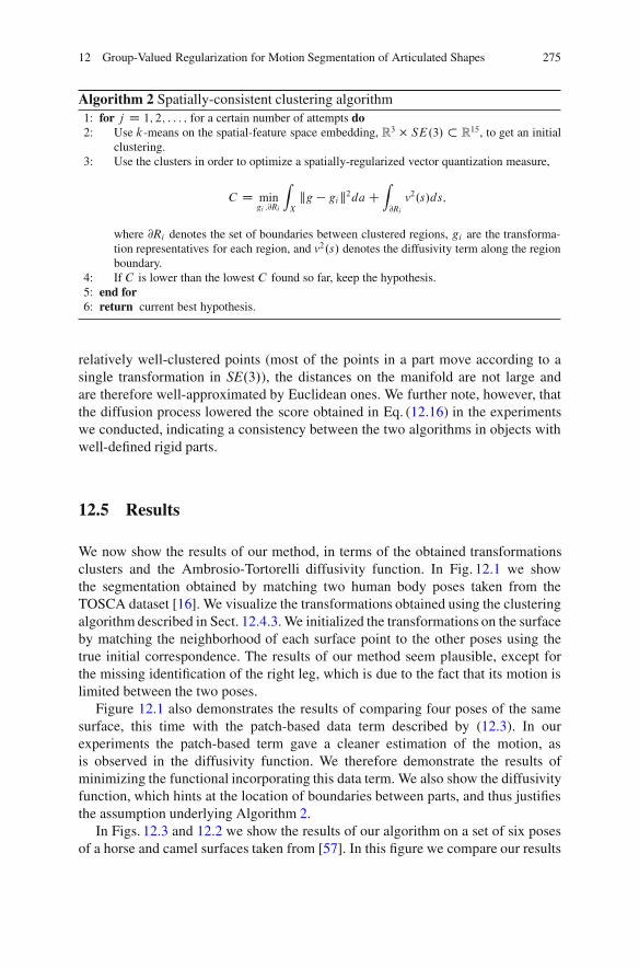
12 Group-Valued Regularization for Motion Segmentation of Articulated Shapes 275
Algorithm 2 Spatially-consistent clustering algorithm1: for j D 1; 2; : : : ; for a certain number of attempts do2: Use k-means on the spatial-feature space embedding, R3 " SE.3/ % R15, to get an initial
clustering.3: Use the clusters in order to optimize a spatially-regularized vector quantization measure,
C D mingi ;@Ri
Z
Xkg # gik2daC
Z
@Ri
v2.s/ds;
where @Ri denotes the set of boundaries between clustered regions, gi are the transforma-tion representatives for each region, and v2.s/ denotes the diffusivity term along the regionboundary.
4: If C is lower than the lowest C found so far, keep the hypothesis.5: end for6: return current best hypothesis.
relatively well-clustered points (most of the points in a part move according to asingle transformation in SE.3/), the distances on the manifold are not large andare therefore well-approximated by Euclidean ones. We further note, however, thatthe diffusion process lowered the score obtained in Eq. (12.16) in the experimentswe conducted, indicating a consistency between the two algorithms in objects withwell-defined rigid parts.
12.5 Results
We now show the results of our method, in terms of the obtained transformationsclusters and the Ambrosio-Tortorelli diffusivity function. In Fig. 12.1 we showthe segmentation obtained by matching two human body poses taken from theTOSCA dataset [16]. We visualize the transformations obtained using the clusteringalgorithm described in Sect. 12.4.3. We initialized the transformations on the surfaceby matching the neighborhood of each surface point to the other poses using thetrue initial correspondence. The results of our method seem plausible, except forthe missing identification of the right leg, which is due to the fact that its motion islimited between the two poses.
Figure 12.1 also demonstrates the results of comparing four poses of the samesurface, this time with the patch-based data term described by (12.3). In ourexperiments the patch-based term gave a cleaner estimation of the motion, asis observed in the diffusivity function. We therefore demonstrate the results ofminimizing the functional incorporating this data term. We also show the diffusivityfunction, which hints at the location of boundaries between parts, and thus justifiesthe assumption underlying Algorithm 2.
In Figs. 12.3 and 12.2 we show the results of our algorithm on a set of six posesof a horse and camel surfaces taken from [57]. In this figure we compare our results

276 G. Rosman et al.
Fig. 12.1 Segmenting a human figure. Top row: the set of poses used. Bottom row, left to right:the transformations obtained from the two left most poses, the transformations obtained from allfour poses using Eq. (12.3) as a data term, and the Ambrosio-Tortorelli diffusivity function basedon four poses
Fig. 12.2 Segmenting a camel dynamic surface motion based on six different poses. Top row: theposes used. Bottom row, left to right: a visualization of the transformations of the surface obtainedby our method and the diffusivity function v
to those of Wuhrer and Brunton [64], obtained on a similar set of poses with tenframes. The results of our method seem to be quite comparable to those obtainedby Wuhrer and Brunton, despite the fact that we use only six poses. We also notethat both the diffusion scheme and the visualization algorithm gave a meaningfulresult for the tail part, which is not rigid and does not have a piecewise-rigid motionmodel.
In Fig. 12.4 we demonstrate our algorithm, with an initialization of 30 simulatedmotion capture marker points, where the displacement is known. The relativelymonotonous motion range available in the dynamic mesh sequence leads to a lesscomplete, but still quite meaningful, segmentation of the horse, except for its head.
We also note the relatively low number of poses required for segmentation – inboth Figs. 12.3 and 12.4 we obtain good results despite the fact that we use only afew poses, six and eight respectively.

12 Group-Valued Regularization for Motion Segmentation of Articulated Shapes 277
Fig. 12.3 Segmenting a horse dynamic surface motion based on six different poses. Top row: theposes used. Bottom row, left to right: a visualization of the transformations of the surface obtainedby our method, and the segmentation results obtained by [64], and the diffusivity function v
Fig. 12.4 Segmenting a horse dynamic surface motion with a given sparse initial correspondences.Top row: the eight random poses used. Bottom row, left to right: the set of points used forinitializing the transformations, and a visualization of the transformations obtained, and thediffusivity function v
Finally, in Fig. 12.4 we demonstrate initialization of our method based on a sparsepoint set, with 30 known correspondence points. The points are arbitrarily placedusing farthest point sampling [27,31]. This demonstrates a possibility of initializingthe algorithm using motion capture markers, coupled with a 3D reconstructionpipeline, for object part analysis. While the examples shown in this chapter aresynthetic, this example shows that the algorithm can be initialized with data obtainedin a realistic setup.
12.6 Conclusion
In this chapter we present a new method for motion-based segmentation ofarticulated objects, in a variational framework. The method is based on minimizing ageneralized Ambrosio-Tortorelli functional regularizing a map from the surface onto
278 G. Rosman et al.
the Lie-group SE.3/. The results shown demonstrate the method’s effectiveness,and compare it with state-of-the-art articulated motion segmentation algorithms.The functional we suggest can be easily tailored to specific problems where it canbe contrasted and combined with domain-specific algorithms for articulated objectanalysis. In future work we intend to adapt the proposed algorithm to real datafrom range scanners, and explore initialization methods as well as use the proposedframework in other applications such as articulated surfaces tracking and denoising.
References
1. Alexander, E.J., Bregler, C., Andriacchi, T.P.: Non-rigid modeling of body segments forimproved skeletal motion estimation. Comput. Model. Eng. Sci. 4, 351–364 (2003)
2. Ambrosio, L., Tortorelli, V.M.: Approximation of functional depending on jumps by ellipticfunctional via & -convergence. Commun. Pure Appl. Math. 43(8), 999–1036 (1990)
3. Amiaz, T., Kiryati, N.: Piecewise-smooth dense optical flow via level sets. Int. J. Comput. Vis.68(2), 111–124 (2006)
4. Andersen, M.S., Benoit, D.L., Damsgaarda, M., Ramsey, D.K., Rasmussen, J.: Do kinematicmodels reduce the effects of soft tissue artefacts in skin marker-based motion analysis? An invivo study of knee kinematics. J. Biomech. 43, 268–273 (2010)
5. Anguelov, D., Koller, D., Pang, H.-C., Srinivasan, P., Thrun, S.: Recovering articulated objectmodels from 3D range data. In: Proceedings of the Conference on Uncertainty in ArtificialIntelligence, pp. 18–26. AUAI Press, Arlington (2004)
6. Arcila, R., Kartik Buddha, S., Hetroy, F., Denis, F., Dupont, F.: A framework for motion-based mesh sequence segmentation. In: International Conference on Computer Graphics,Visualisation and Compter Vision, Plzen, Czech Republic, 2010
7. Arya, S., Mount, D.M., Netanyahu, N.S., Silverman, R., Wu, A.Y.: An optimal algorithm forapproximate nearest neighbor searching fixed dimensions. J. ACM 45(6), 891–923 (1998)
8. Ashbrook, A.P., Fisher, R.B., Robertson, C., Werghi, N.: Segmentation of range data into rigidsubsets using surface patches. In International Conference on Computer Vision, pp. 201–206.IEEE Computer Society, Washington, DC (1998)
9. Attene, M., Katz, S., Mortara, M., Patane, G., Spagnuolo, M., Tal, A.: Mesh segmentation – acomparative study. In: Proceedings of the IEEE International Conference on Shape Modelingand Applications, pp. 7–18. IEEE Computer Society, Washington, DC (2006)
10. Belkin, M., Sun, J., Wang, Y.: Constructing Laplace operator from point clouds in Rd . In:Proceedings of the Twentieth Annual ACM-SIAM Symposium on Discrete Algorithms, SODA’09, pp. 1031–1040. Society for Industrial and Applied Mathematics, Philadelphia (2009)
11. Belta, C., Kumar, V.: On the computation of rigid body motion. Electron. J. Comput. Kinemat.1 (2001)
12. Belta, C., Kumar, V.: An SVD-based project method for interpolation on se(3). IEEE Trans.Robot. Autom. 18(3), 334–345 (2002)
13. Besl, P.J., McKay, N.D.: A method for registration of 3D shapes. IEEE Trans. Pattern Anal.Mach. Intell. 14(2), 239–256 (1992)
14. Brockett, R.: Robotic manipulators and the product of exponential formula. In: Fuhrman,P. (ed.) Proceedings of the Mathematical Theory of Networks and Systems, pp. 120–129.Springer (1984)
15. Bronstein, A.M., Bronstein, M.M., Kimmel, R.: Generalized multidimensional scaling: aframework for isometry-invariant partial surface matching. Proc. Natl. Acad. Sci. USA 103(5),1168–1172 (2006)
16. Bronstein, A.M., Bronstein, M.M., Kimmel, R.: Numerical geometry of non-rigid shapes.Springer, New York (2008)
12 Group-Valued Regularization for Motion Segmentation of Articulated Shapes 279
17. Bruhn, A., Weickert, J., Schnorr, C.: Lucas/Kanade meets Horn/Schunck: combining local andglobal optic flow methods. Int. J. Comput. Vis. 61(3), 211–231 (2005)
18. Brune, C., Maurer, H., Wagner, M.: Detection of intensity and motion edges within optical flowvia multidimensional control. SIAM J. Imag. Sci. 2(4), 1190–1210 (2009)
19. Celledoni, E., Owren, B.: Lie group methods for rigid body dynamics and time integration onmanifolds. Comput. Methods Appl. Mech. Eng. 19, 421–438 (1999)
20. Celledoni, E., Fasso, F., Safstrom, N., Zanna, A.: The exact computation of the free rigid bodymotion and its use in splitting methods. SIAM J. Sci. Comput. 30(4), 2084–2112 (2008)
21. Chen, X., Golovinskiy, A., Funkhouser, T.: A benchmark for 3D mesh segmentation. ACMTrans. Graph. 28(3), Article 73 (2009)
22. Daniel Cremers and Steffano Soatto: Motion competition: a variational framework for piece-wise parametric motion segmentation. Int. J. Comput. Vis. 62(3), 249–265 (2005)
23. Desbrun, M., Meyer, M., Schroder, P., Barr, A.H.: Implicit fairing of irregular meshesusing diffusion and curvature flow. SIGGRAPH Proceedings of the 26th Annual Conferenceon Computer Graphics and Interactive Techniques, pp. 317–324. ACM/Addison-Wesley,New York (1999)
24. do Carmo, M.P.: Riemannian Geometry. Birkhauser Verlag, Boston (1992)25. Duits, R., Burgeth, B.: Scale spaces on Lie groups. In: Scale Space and Variational Methods in
Computer Vision. LNCS, vol. 4485, pp. 300–312. Springer, Berlin/Heidelberg (2007)26. Eells, J. Jr., Sampson, J.H.: Harmonic mappings of Riemannian manifolds. Am. J. Math. 86(1),
106–160 (1964)27. Gonzalez T.F.: Clustering to minimize the maximum intercluster distance. Theor. Comput. Sci.
38, 293–306 (1985)28. Gur, Y., Sochen, N.A.: Regularizing flows over lie groups. J. Math. Imag. Vis. 33(2), 195–208
(2009)29. Hall, B.C.: Lie Groups, Lie Algebras,and Representations, An Elementary Introduction.
Springer-Verlag, 2004.30. Hauberg, S., Sommer, S., Pedersen, K.S.: Gaussian-like spatial priors for articulated tracking.
In: European Conference on Computer Vision. LNCS, vol. 6311, pp. 425–437. Springer,Berlin/New York (2010)
31. Hochbaum, D., Shmoys, D.: A best possible approximation for the k-center problem. Math.Oper. Res. 10(2), 180–184 (1985)
32. Iserles, A., Munthe-Kaas, H.Z., Nørsett, S.P., Zanna, A.: Lie group methods. Acta Numer. 9,215–365 (2000)
33. Jain, A.K.: Fundamentals of Digital Image Processing. Prentice-Hall, Upper Saddle River(1989)
34. Jain, V., Zhang, H.: Robust 3D shape correspondence in the spectral domain. In: Proceedings ofShape Modeling International, pp. 118–129. IEEE Computer Society, Washington DC (2006)
35. James, D.L., Twigg, C.D.: Skinning mesh animations. SIGGRAPH 24(3), 399–407 (2005)36. Kalogerakis, E., Hertzmann, A., Singh, K.: Learning 3D mesh segmentation and labeling.
ACM Trans. Graph. 29(4), Article 102 (2010)37. Kobilarov, M., Crane, K., Desbrun, M.: Lie group integrators for animation and control of
vehicles. ACM Trans. Graph. 28(2), 1–14 (2009)38. Kompatsiaris, I., Tzovaras, D., Strintzis, M.G.: Object articulation based on local 3D motion
estimation. In: Proceedings of ECMAST, pp. 378–391. Springer, London (1999)39. Lee, T.-Y., Wang, Y.-S., Chen, T.-G.: Segmenting a deforming mesh into near-rigid compo-
nents. Vis. Comput. 22(9), 729–739 (2006)40. Litke, N., Droske, M., Rumpf, M., Schroder, P.: An image processing approach to sur-
face matching. In: Proceedings of the Eurographics Symposium on Geometry processing,pp. 207–216. Eurographics Association, Aire-la-Ville (2005)
41. Mateus, D., Horaud, R., Knossow, D., Cuzzolin, F., Boyer, E.: Articulated shape matchingusing Laplacian eigenfunctions and unsupervised point registration. In: CVPR. IEEE ComputerSociety (2008)
42. Muller, A., Terze, Z.: Differential-geometric modelling and dynamic simulation of multibodysystems. Strojarstvo 51(6), 597–612 (2009)
280 G. Rosman et al.
43. Mumford, D., Shah, J.: Optimal approximations by piecewise smooth functions and associatedvariational problems. Commun. Pure Appl. Math. 42(5), 577–685 (1989)
44. Murray, R.M., Li, Z., Sastry, S.S.: A Mathematical Introduction to Robotic Manipulation,1 edn. CRC, Boca Raton (1994)
45. Nir, T., Kimmel, R., Bruckstein, A.M.: Variational approach for joint optic-flow computationand video restoration. Technical Report CIS-05, Technion, 2005
46. Nir, T., Bruckstein, A.M., Kimmel, R.: Over-parameterized variational optical flow. Int.J. Comput. Vis. 76(2), 205–216 (2008)
47. Park, F.C., Bobrow, J.E., Ploen, S.R.: A Lie group formulation of robot dynamics. Int. J. Robot.Res. 14, 609–618 (1995)
48. Pennec, X., Cachier, P., Ayache, N.: Understanding the “demon’s algorithm”: 3D non-rigid registration by gradient descent. In: MICCAI Proceedings of the Second InternationalConference on Medical Image Computing and Computer-Assisted Intervention, pp. 597–605.Springer, London (1999)
49. Raviv, D., Dubrovina, A., Kimmel, R.: Hierarchical shape matching. In: Bruckstein, A.M.,ter Haar Romeny, B., Bronstein, A.M., Bronstein, M.M. (eds.) Scale Space and VariationalMethods in Computer Vision. LNCS, vol. 6667, pp. 604–615 (2011)
50. Rosman, G., Bronstein, M.M., Bronstein, A.M., Wolf, A., Kimmel, R.: Group-valued regular-ization framework for motion segmentation of dynamic non-rigid shapes. In: Scale Space andVariational Methods in Computer Vision, pp. 725–736 (2011)
51. Rudin, L.I., Osher, S., Fatemi, E.: Nonlinear total variation based noise removal algorithms.Phys. D Lett. 60, 259–268 (1992)
52. Ruggeri, M.R., Patane, G., Spagnuolo, M., Saupe, D.: Spectral-driven isometry-invariantmatching of 3D shapes. Int. J. Comput. Vis. 89(2–3), 248–265 (2010)
53. Szymon Rusinkiewicz and Marc Levoy: Efficient variants of the ICP algorithm. In: ThirdInternational Conference on 3D Digital Imaging and Modeling (3DIM), pp. 145–152. IEEEComputer Society (2001)
54. Sapp, B., Toshev, A., Taskar, B.: Cascaded models for articulated pose estimation. In: EuropeanConference Computer Vision, pp. 406–420. Springer, Berlin/New York (2010)
55. Shamir, A.: A survey on mesh segmentation techniques. Comput. Graph. Forum 27(6), 1539–1556 (2008)
56. Subbarao, R., Meer, P.: Nonlinear mean shift over Riemannian manifolds. Int. J Comput. Vis.84(1), 1–20 (2009)
57. Sumner, R.W., Popovic, J.: Deformation transfer for triangle meshes. In: SIGGRAPH,pp. 399–405. ACM, New York (2004)
58. Thirion, J.P.: Image matching as a diffusion process: an analogy with Maxwell’s demons. Med.Image Anal. 2(3), 243–260 (1998)
59. Tierny, J., Vandeborre, J.-P., Daoudi, M.: Fast and precise kinematic skeleton extraction of 3Ddynamic meshes. In: ICPR. IEEE Computer Society (2008)
60. Trobin, W., Pock, T., Cremers, D., Bischof, H.: An Unbiased Second-Order Prior for High-Accuracy Motion Estimation, pp. 396–405. Springer, Berlin/New York (2008)
61. Tuzel, O., Porikli, F., Meer, P.: Learning on lie groups for invariant detection and tracking. In:CVPR. IEEE Computer Society (2008)
62. Wang, S., Wang, Y., Jin, M., Gu, X.D., Samaras, D.: Conformal geometry and its applicationson 3D shape matching, recognition, and stitching. IEEE Trans. Pattern Anal. Mach. Intell.29(7), 1209–1220 (2007)
63. Wolf, A., Sharf, I., Rubin, M.B.: Using Cosserat point theory for estimating kinematics andsoft-tissue deformation during gait analysis. In: Lenarcic, J., Stanisic, M.M. (eds.) Advancesin Robot Kinematics: Motion in Man and Machine, pp. 63–70. Springer, Netherlands (2010)
64. Wuhrer, S., Brunton, A.: Segmenting animated objects into near-rigid components. Vis.Comput. 26, 147–155 (2010)
65. Yamasaki, T., Aizawa, K.: Motion segmentation for time-varying mesh sequences based onspherical registration. EURASIP J. Appl. Signal Process. 1–9, (2009). Article 346425

12 Group-Valued Regularization for Motion Segmentation of Articulated Shapes 281
66. Yanenko, N.N.: The Method of Fractional Steps: Solution of Problems of MathematicalPhysics in Several Variables. Springer, Berlin/New York (1971). Translated from Russian
67. Yang, C., Medioni, G.: Object modelling by registration of multiple range images. Image Vis.Comput. 10, 145–155 (1992)
68. Zhang, D., Hebert, M.: Harmonic maps and their applications in surface matching. In: CVPR,vol. 2, pp. 524–530. IEEE Computer Society (1999)
69. Zefran, M., Kumar, V., Croke, C.: On the generation of smooth three-dimensional rigid bodymotions. IEEE Trans. Robot. Autom. 14(4), 576–589 (1998)
70. Zefran, M., Kumar, V., Croke, C.: Metrics and connections for rigid-body kinematics. Int.J. Robot. Res. 18(2), 242 (1999)
Chapter 13Point Cloud Segmentation and Denoisingvia Constrained Nonlinear Least SquaresNormal Estimates
Edward Castillo, Jian Liang, and Hongkai Zhao
Abstract We first introduce a surface normal estimation procedure for point cloudscapable of handling geometric singularities in the data, such as edges and corners.Our formulation is based on recasting the popular Principal Component Analysis(PCA) method as a constrained nonlinear least squares (NLSQ) problem. In contrastto traditional PCA, the new formulation assigns appropriate weights to neighboringpoints automatically during the optimization process in order to minimize thecontributions of points located across singularities. We extend this strategy to pointcloud denoising by combining normal estimation, point projection, and declusteringinto one NLSQ formulation. Finally, we propose a point cloud segmentationtechnique based on surface normal estimates and local point connectivity. Inaddition to producing consistently oriented surface normals, the process segmentsthe point cloud into disconnected components that can each be segmented furtherinto piecewise smooth components as needed.
13.1 Introduction
Two key processing tools for unstructured point cloud data are surface normalestimation and segmentation. Surface normal estimation is utilized by severalapplications such as reconstruction [5, 6, 20], local feature size estimation [10, 26],computer aided design [24], and inside-outside queries, while segmentation is
E. Castillo (!)Department of Radiation Oncology, University of Texas, MD Anderson Cancer Center, Houston,TX, USA
Department of Computational and Applied Mathematics, Rice University, Houston, TX, USAe-mail: [email protected]
J. Liang ! H. ZhaoDepartment of Mathematics, University of California, Irvine, CA, USAe-mail: [email protected]; [email protected]
M. Breuß et al. (eds.), Innovations for Shape Analysis, Mathematics and Visualization,DOI 10.1007/978-3-642-34141-0 13, © Springer-Verlag Berlin Heidelberg 2013
283
284 E. Castillo et al.
useful for efficient point cloud representation and classification [15, 30]. However,depending on the method, segmentation often requires surface normal estimates asa prerequisite.
As described in [11], surface normal estimation methods can be classifiedalgorithmically as either numerical or combinatorial. Combinatorial methods arebased on the information obtained from a Delaunay triangulation procedure appliedto the point cloud. Consequently, combinatorial methods such as the algorithmproposed in [2], are known to be sensitive to noise. Though noise robustness hasbeen incorporated into the combinatorial methodology [9], the approach in generalbecomes infeasible for large data sets due to the computational cost required by theDelaunay triangulation [11]. On the other hand, numerical methods are based onthe optimization of a fitting model defined on a subset of point contained in a localneighborhood.
The most common approach employed by numerical methods is to first determinea subset of data points representing the local neighbors of a given point p. Asdescribed in [13], the estimated surface normal for the point p is then the normalto the plane that best fits the neighboring data points in the least squares sense.The least squares fitting plane is determined using Principal Component Analysis(PCA). As such, the entire procedure is often referred to as PCA. Since the methodis based on a least squares formulation, PCA is known to be stable in the presenceof noise. However, near geometric singularities such as corners or edges, wherethe normal is discontinuous, the PCA fails to produce sharp normal estimatessince neighboring points are used nondistinctively to compute the planar fit. Theeffect is rounded or smoothed normal estimates along edges. Adjustments to thebasic PCA procedure, such as distance weighting [1, 27], varying neighborhoodsizes [23, 26], and higher-order fitting [18, 24, 32], have been suggested to improvethe accuracy near geometric discontinuities. However, such approaches fail toaddress the fundamental problem of determining which points contained in a givenneighborhood should contribute to the normal computation.
In this work, we first introduce a surface normal approximation method basedon recasting the popular PCA formulation as a constrained nonlinear least squares(NLSQ) problem that is designed to produce accurate surface normal estimates neargeometric singularities. Our constrained NLSQ method incorporates the weightof each point contribution into the normal estimate problem formulation as anunknown quantity. In another word, our formulation can be viewed as a robuststatistic strategy, i.e., points belonging to a different smooth patch across a geometricsingularity can be seen as outliers in the sense of robust statistics [17]. Bysimultaneously optimizing the weights and the normal, essentially only neighbor-ing points from the same smooth piece contribute to the normal estimate. Thisconstrained NLSQ formulation has the benefit of being simpler than neighborhoodreorganization methods such as [6] and can be implemented with almost the sameefficiency as the standard PCA. In addition, we extend the constrained NLSQmethodology to address point cloud denoising by combining normal estimation,point projection, and declustering together into one formulation.
Next we introduce a point cloud segmentation scheme that utilizes the esti-mated surface normals computed by our constrained NLSQ approach. Point cloud
13 Point Cloud Segmentation and Denoising 285
segmentation methods are typically categorized as either a region growing methodor border-based method. Region growing methods, such as those described in[4,28,30,31], are based on growing segmented regions from preselected seed pointlocations according to a given consistency or continuity rule. Though known to berobust to noise, the main difficulties associated with region growing are the seedpoint selection criteria and the monitoring of the growing process. Border-basedmethods on the other hand [7, 8, 15, 19], rely on identifying the points locatedalong edges. The full segmentation is then computed from the detected edges byapplying a filling process or meshing. However, due to noise or spatially unevenpoint distributions, such methods often detect disconnected edges that make itdifficult for a filling procedure to identify closed segments.
Our segmentation procedure is based on first constructing an adjacency matrixrepresenting the point connectivity of the full data set from unoriented surfacenormal estimates according to an angular continuity measure. The connectedcomponents present in the adjacency matrix constitute the initial segmentation. Asa result, the method does not require a filling process or region growing procedure.Additionally, the point connectivity information represented by the adjacencymatrix provides a means for consistently orienting the surface normal estimates,even for data sets representing multiple closed surfaces. A finer segmentation canthen be obtained from the initial connected components by classifying the orientedsurface normals according to both their direction and the local geometry informationcontained in the adjacency matrix.
Here is the outline. First, we reformulate the standard PCA as a constrained leastsquares problem in Sect. 13.2. Then, we derive our constrained NLSQ formulationfor normal estimation in Sect. 13.3. This formulation is extended to point clouddenoising in Sects. 13.4–13.6. Our point cloud segmentation algorithm based onsurface normal estimates and point connectivity is described in Sect. 13.7.
13.2 PCA as Constrained Linear Least Squares
PCA is a popular method for computing surface normal approximations from pointcloud data [13]. Given a point cloud data set D D fxi gniD1, the PCA surface normalapproximation for the point p 2 D is typically computed by first determining theK-nearest neighbors, xk 2 D, of p. Given the K-neighbors, the approximate surfacenormal is then the eigenvector associated with the smallest eigenvalue of thesymmetric positive semi-definite matrix:
P DKX
kD1.xk ! Np/T .xk ! Np/; (13.1)
where Np is the local data centroid, Np D . 1K/PK
kD1 xk .The PCA normal approximation, also referred to as total least squares [23],
is accurate when the underlying surface is smooth, but tends to smear acrosssingularities, such as corners or edges as illustrated in Fig. 13.1. The smearing is
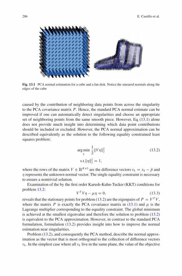
286 E. Castillo et al.
Fig. 13.1 PCA normal estimation for a cube and a fan disk. Notice the smeared normals along theedges of the cube
caused by the contribution of neighboring data points from across the singularityto the PCA covariance matrix P . Hence, the standard PCA normal estimate can beimproved if one can automatically detect singularities and choose an appropriateset of neighboring points from the same smooth piece. However, Eq. (13.1) alonedoes not provide much insight into determining which data point contributionsshould be included or excluded. However, the PCA normal approximation can bedescribed equivalently as the solution to the following equality constrained leastsquares problem:
arg min!
1
2kV!k22 (13.2)
s.t.k!k22 D 1;
where the rows of the matrix V 2 RK"3 are the difference vectors vk D xk ! Np and! represents the unknown normal vector. The single equality constraint is necessaryto ensure a nontrivial solution.
Examination of the by the first order Karush-Kuhn-Tucker (KKT) conditions forproblem 13.2:
V T V! ! "! D 0; (13.3)
reveals that the stationary points for problem (13.2) are the eigenpairs ofP D V T V ,where the matrix P is exactly the PCA covariance matrix in (13.1) and " is theLagrange multiplier corresponding to the equality constraint. The global minimumis achieved at the smallest eigenvalue and therefore the solution to problem (13.2)is equivalent to the PCA approximation. However, in contrast to the standard PCAformulation, formulation (13.2) provides insight into how to improve the normalestimation near singularities.
Problem (13.2), and consequently the PCA method, describe the normal approx-imation as the vector that is most orthogonal to the collection of difference vectorsvk . In the simplest case where all vk live in the same plane, the value of the objective
13 Point Cloud Segmentation and Denoising 287
function V T ! at the solution !# is zero, and !# is orthogonal to the plane. From thisperspective, it is not necessary to compute the local centroid, since utilizing thedifference vectors ak D xk ! p, as opposed to the vectors vk D xk ! Np, yieldsthe same result. Moreover, the magnitude of the inner product between !# and eachdifference vector quantifies the “planar deviation” of each local neighbor. Thus,monitoring this quantity provides a means for determining which data points, if any,are contributing from across a discontinuity.
13.3 Normal Estimation via Constrained NonlinearLeast Squares
The PCA method produces poor normal approximations near surface discontinuitiesbecause the method equally weights the erroneous contributions of points positionedacross the singularity into the normal calculation. However, utilizing the PCAequivalent, constrained least squares formulation (13.2), such contributions can bedetected by examining the magnitude of the orthogonality mismatch, jaTk !j, whereak D xk ! p. In the language of robust statistics, points with large orthogonalitymismatch are considered outliers.
Assuming noise free data, large orthogonality mismatches correspond to neigh-boring points that highly deviate from the local least squares fitted plane. Conse-quently, large orthogonality mismatches indicate that the corresponding neighborsare potentially positioned across a discontinuity. Thus, we propose a dynamicweighting scheme that adaptively determines the weight of each point contributionas a function of the orthogonality mismatch. Incorporating this strategy intoformulation (13.2) results in the following constrained nonlinear least squaresformulation:
arg min!
1
2
KX
kD1e$#.a
Tk !/
2 !aTk !
"2(13.4)
s.t. k!k2 D 1:
While traditional weighting schemes place emphasis on proximity [1, 27], theweighting term e$#.a
Tk !/
2adaptively deflates the contribution of terms with high
orthogonality mismatch at a rate defined by the parameter #. In this way, formu-lation (13.4) is designed to compute the surface normal estimate using only theneighboring points positioned on the same smooth surface component. Naturally,setting # to zero results in the original PCA linear least squares problem (13.2),with the exception that the difference vectors are taken from the data point p andnot the centroid Np.
At first glance, formulation (13.4) appears to be substantially more difficultto solve than the small eigenvalue problem associated with the PCA approach.
288 E. Castillo et al.
However, the equality constraint is easily absorbed into the objective function byrepresenting the unknown surface normal ! in spherical coordinates with magnitudeset to unity:
!.$; %/ D
2
4cos.$/ cos.%/cos.$/ sin.%/
sin.$/
3
5 :
Substituting the spherical coordinate representation of the unknown surface normalinto formulation (13.4) results in the following unconstrained nonlinear least squaresproblem for only two variables:
min$;%
1
2
KX
kD1e$#.a
Tk !.$;%//
2 #aTk !.$; %/
$2: (13.5)
Applying formulation (13.4) to the examples shown in Fig. 13.1 results in significantimprovement in the surface normal estimates at singularities, as illustrated byFig. 13.2. Moreover, the computational cost is comparable to that of standard PCA.
In general, computing the k-nearest neighbors represents the main computationalcost associated with normal estimation. For the city example containing 1.99 millionpoints and illustrated in Fig. 13.8, the nearest neighbor calculation (tree basedsorting method with O.n log n/ complexity) required 66 s on a Dell PrecisionM6400 laptop. The normal calculations utilizing our nonlinear least squares methodrequired 39 s whereas the PCA normal calculation required 24 s.
13.4 Incorporating Point Cloud Denoising into the NLSQNormal Estimate
Point cloud denoising is naturally an important task in many applications. Thenoise associated with a data point can be viewed as a perturbation of the point’strue location. Hence, for a given noise polluted point Qp, the task of denoising canbe viewed as finding the projection of the point Qp onto the underlying surface.However, the underlying surface is unknown and has to be inferred from thenoisy point cloud itself. Developing methods for projecting points onto curves andsurfaces is an active area of research with applications in computer graphics andvision (see [14]). Work has also been done for the problem of projecting points ontopoint cloud represented surfaces [3, 22], based on first determining a “projectiondirection”. The goal here is to couple point cloud denoising with the surface normalestimation together. The motivation for this approach is the idea that a denoisedpoint cloud improves surface normal estimation, which in turn provides a betterprojection direction for point cloud denoising.

13 Point Cloud Segmentation and Denoising 289
Fig. 13.2 Nonlinear least squares normal estimation for a cube and a fan disk. Notice theimprovement in the normal estimation along the edges of the cube compared to standard PCA(Fig. 13.1)
Given a surface normal estimate ! at Qp, we wish to determine a projection along !that minimizes the orthogonality mismatch energy (formulation (13.5) with # D 0):
arg mint
1
2
KX
kD1
#.xk ! . Qp C t!//T !
$2: (13.6)
Rearranging terms and taking advantage of the fact that k!k D 1, the problemreduces to a simple least squares problem for the scalar value t :
arg mint
1
2kA! ! tk22; (13.7)
where the rows of A are the difference vectors ak D xk ! Qp, and the denoisedlocation is given by the solution t# as p# D Qp C .t#/!.
As is the case for most denoising procedures, naively applying (13.7) to cleandata will result in over smoothing and the loss of sharp surface features. However,given a bound T for the distance between Qp and the underlying surface, datafidelity can easily be incorporated into the formulation by way of linear inequalityconstraints. Specifically,
arg mint
1
2kA! ! tk22; (13.8)
s.t. jt j < T:
Single variable calculus dictates that the solution to problem (13.8) is achieved ateither the unconstrained minimum tunc D . 1
K/PK
kD1 aTk !, or at one of the bounds
!T or T .

290 E. Castillo et al.
Fig. 13.3 Constrainednonlinear least squaresnormal estimation for a noisycube. Three percent (in termof cube size) randomperturbation was added to theoriginal data. The estimatednormals are still quiteaccurate even at edges
For the typical case where ! is not known, the noise in the data can lead toinaccurate PCA or NLSQ surface normal approximations. However, both noiserobustness and robustness to surface discontinuities can be incorporated into oneNLSQ framework by coupling the denoising formulation (13.8) with the NLSQformulation (13.5) (Fig. 13.3):
arg min$;%;t
1
2
KX
kD1e$#.a
Tk !.$;%/$t /2
#aTk !.$; %/ ! t
$2(13.9)
s.t. jt j " T:
Our numerical approach for solving Problem (13.9) is based on reformulatingthe two linear constraints as a pair of log-barrier functions:
L1.t/ D ! ln%T ! tT
&;
L2.t/ D ! ln%T C tT
&;
designed so that L1.0/ D L2.0/ D 0 and L1.T / D L2.!T / D 1. Problem (13.9)with the inequality constraints replaced by the log-barrier functions, comprise astandard, unconstrained, and nonlinear least squares problem. Our current imple-mentation utilizes the MINPACK software package, which employs the Levenberg-Marquardt Quasi-Newton trust region algorithm, using exact values for the gradientof the objective function. The initial guess used for the optimization routine iscomputed by solving problems (13.5) and (13.8) for #, h D 0, respectively. It is
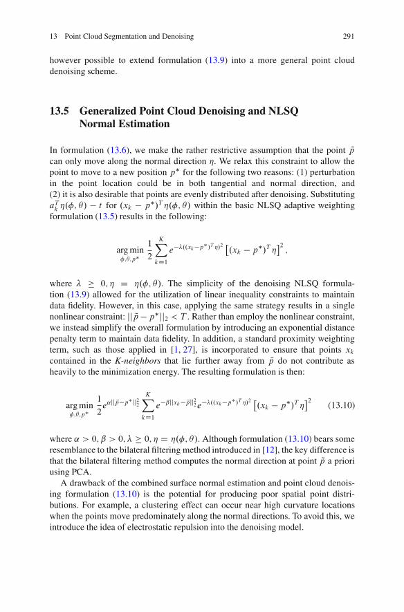
13 Point Cloud Segmentation and Denoising 291
however possible to extend formulation (13.9) into a more general point clouddenoising scheme.
13.5 Generalized Point Cloud Denoising and NLSQNormal Estimation
In formulation (13.6), we make the rather restrictive assumption that the point Qpcan only move along the normal direction !. We relax this constraint to allow thepoint to move to a new position p# for the following two reasons: (1) perturbationin the point location could be in both tangential and normal direction, and(2) it is also desirable that points are evenly distributed after denoising. SubstitutingaTk !.$; %/ ! t for .xk ! p#/T !.$; %/ within the basic NLSQ adaptive weightingformulation (13.5) results in the following:
arg min$;%;p!
1
2
KX
kD1e$#..xk$p
!/T !/2 #.xk ! p#/T !$2;
where # # 0; ! D !.$; %/. The simplicity of the denoising NLSQ formula-tion (13.9) allowed for the utilization of linear inequality constraints to maintaindata fidelity. However, in this case, applying the same strategy results in a singlenonlinear constraint: jj Qp ! p#jj2 < T . Rather than employ the nonlinear constraint,we instead simplify the overall formulation by introducing an exponential distancepenalty term to maintain data fidelity. In addition, a standard proximity weightingterm, such as those applied in [1, 27], is incorporated to ensure that points xkcontained in the K-neighbors that lie further away from Qp do not contribute asheavily to the minimization energy. The resulting formulation is then:
arg min$;%;p!
1
2e˛jj Qp$p
! jj22KX
kD1e$ˇjjxk$ Qpjj
22 e$#..xk$p
!/T !/2 #.xk ! p#/T !$2
(13.10)
where ˛ > 0; ˇ > 0;# # 0; ! D !.$; %/. Although formulation (13.10) bears someresemblance to the bilateral filtering method introduced in [12], the key difference isthat the bilateral filtering method computes the normal direction at point Qp a prioriusing PCA.
A drawback of the combined surface normal estimation and point cloud denois-ing formulation (13.10) is the potential for producing poor spatial point distri-butions. For example, a clustering effect can occur near high curvature locationswhen the points move predominately along the normal directions. To avoid this, weintroduce the idea of electrostatic repulsion into the denoising model.
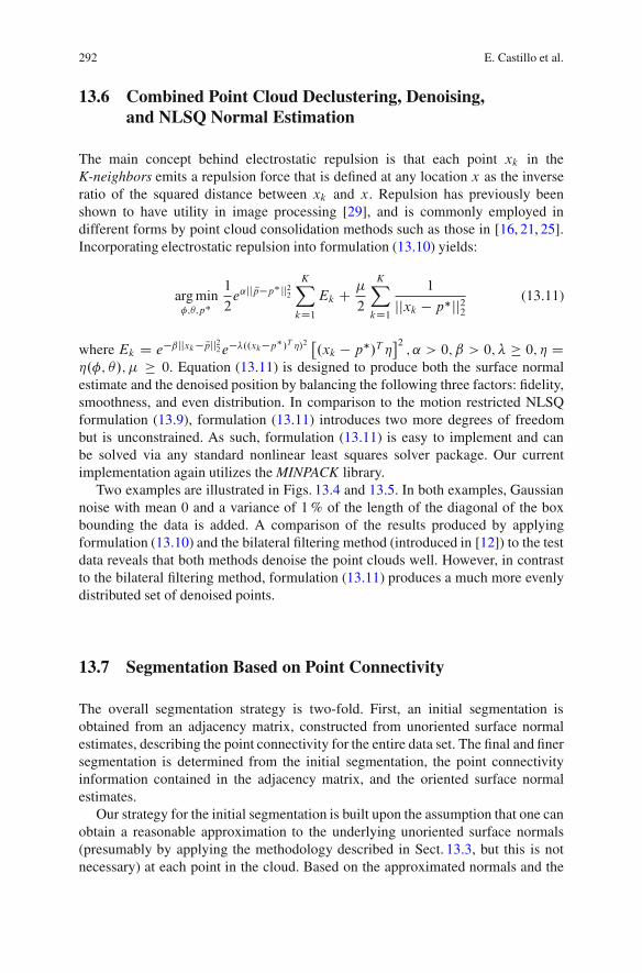
292 E. Castillo et al.
13.6 Combined Point Cloud Declustering, Denoising,and NLSQ Normal Estimation
The main concept behind electrostatic repulsion is that each point xk in theK-neighbors emits a repulsion force that is defined at any location x as the inverseratio of the squared distance between xk and x. Repulsion has previously beenshown to have utility in image processing [29], and is commonly employed indifferent forms by point cloud consolidation methods such as those in [16, 21, 25].Incorporating electrostatic repulsion into formulation (13.10) yields:
arg min$;%;p!
1
2e˛jj Qp$p
! jj22KX
kD1Ek C
"
2
KX
kD1
1
jjxk ! p#jj22(13.11)
where Ek D e$ˇjjxk$ Qpjj22 e$#..xk$p
!/T !/2 #.xk ! p#/T !$2; ˛ > 0; ˇ > 0;# # 0; ! D
!.$; %/;" # 0. Equation (13.11) is designed to produce both the surface normalestimate and the denoised position by balancing the following three factors: fidelity,smoothness, and even distribution. In comparison to the motion restricted NLSQformulation (13.9), formulation (13.11) introduces two more degrees of freedombut is unconstrained. As such, formulation (13.11) is easy to implement and canbe solved via any standard nonlinear least squares solver package. Our currentimplementation again utilizes the MINPACK library.
Two examples are illustrated in Figs. 13.4 and 13.5. In both examples, Gaussiannoise with mean 0 and a variance of 1% of the length of the diagonal of the boxbounding the data is added. A comparison of the results produced by applyingformulation (13.10) and the bilateral filtering method (introduced in [12]) to the testdata reveals that both methods denoise the point clouds well. However, in contrastto the bilateral filtering method, formulation (13.11) produces a much more evenlydistributed set of denoised points.
13.7 Segmentation Based on Point Connectivity
The overall segmentation strategy is two-fold. First, an initial segmentation isobtained from an adjacency matrix, constructed from unoriented surface normalestimates, describing the point connectivity for the entire data set. The final and finersegmentation is determined from the initial segmentation, the point connectivityinformation contained in the adjacency matrix, and the oriented surface normalestimates.
Our strategy for the initial segmentation is built upon the assumption that one canobtain a reasonable approximation to the underlying unoriented surface normals(presumably by applying the methodology described in Sect. 13.3, but this is notnecessary) at each point in the cloud. Based on the approximated normals and the

13 Point Cloud Segmentation and Denoising 293
Fig. 13.4 Nonlinear least squares denoising for a noisy sphere. (Upper left) is the noisy data,(upper middle) is the denoised result using bilateral filter, (upper right) is the zoom in front partof (upper middle), (lower left) is the denoised result using formulation (13.10), (lower middle) isthe denoised result using formulation (13.11) and (lower right) is the zoom in front part of (lowermiddle)
Fig. 13.5 Nonlinear least squares denoising for a noisy torus. (Upper left) is the noisy data, (uppermiddle) is the denoised result using bilateral filter, (upper right) is the zoom in upper right quarterof (upper middle), (lower left) is the denoised result using formulation (13.10), (lower middle) isthe denoised result using formulation (13.11) and (lower right) is the zoom in upper right quarterof (lower middle)
K-nearest neighbor information, a symmetric adjacency matrix A is built such thatAi;j D 1 if the data points i; j are “connected”, or in terms of graph theory, thereexist an edge between the two points. Ai;j D 0 otherwise. The initial segmentationthen is given by the connected components of the undirected graph represented byA.

294 E. Castillo et al.
* !
Fig. 13.6 Two dimensionalrepresentation of a data pointand its tangent plane
Fig. 13.7 The black pointand blue point are connectedto one another. The red pointis not connected to eitherpoint
Of course, the nature of “connected component segmentation” is dictated by thecriteria governing the placement of edges between points. Specifically, given pointsxi and xj , the corresponding adjacency matrix entryAi;j D 1 if both are a k-nearestneighbor of each other, and if the line xj ! xi lies within a user defined angle %(see Fig. 13.6) of the tangent plane associated with the unoriented surface normalapproximation for xi , and vice versa (see Fig. 13.7). In this way, point proximity, aswell as local geometry are taken into account when determining point connectivity.Or put another way, neighboring points are connected if the local geometry estimate,represented by the associated surface normal approximations, are compatible withthe location of xi and xj in R3.
Based on this criteria, the process of segmenting the point cloud according to theconnected components of A can be considered an edge detection scheme. However,a serendipitous characteristic of this methodology is its innate ability to account forthe possibility of multiple closed surfaces, or disconnected components, within agiven data set. For a smoothly varying surface, such as a sphere, the correspondingadjacency matrix is comprised of one connected component. However, for the cylin-der or city data depicted in Figs. 13.8 and 13.9, this is not the case. Consequently, theassociated adjacency matrices contain several connected components (point cloudsegments) and the resulting segmentations break the data sets into piecewise smoothcomponents.
A finer segmentation can be obtained from the connected component segmen-tation by first traversing the connectivity information contained in A to orient theapproximated surface normals in the same manner as the minimum spanning tree
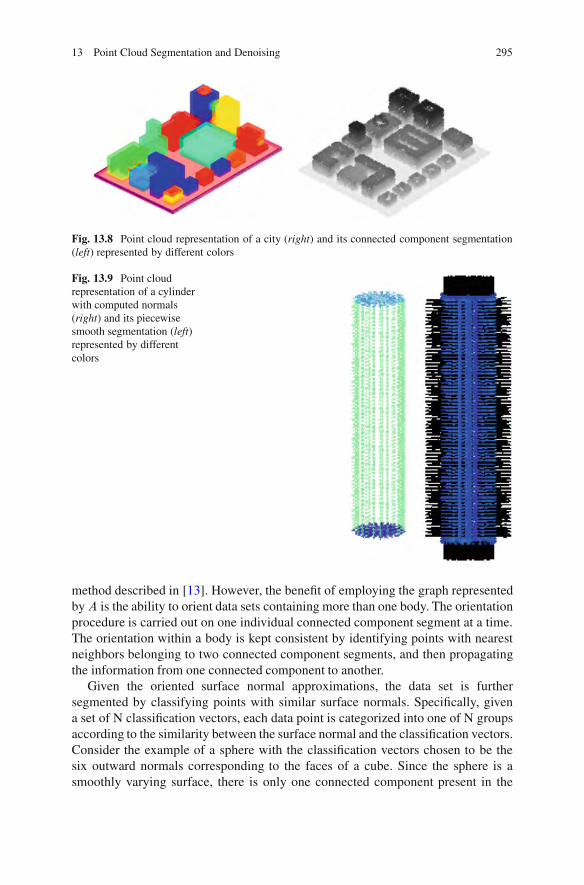
13 Point Cloud Segmentation and Denoising 295
Fig. 13.8 Point cloud representation of a city (right) and its connected component segmentation(left) represented by different colors
Fig. 13.9 Point cloudrepresentation of a cylinderwith computed normals(right) and its piecewisesmooth segmentation (left)represented by differentcolors
method described in [13]. However, the benefit of employing the graph representedbyA is the ability to orient data sets containing more than one body. The orientationprocedure is carried out on one individual connected component segment at a time.The orientation within a body is kept consistent by identifying points with nearestneighbors belonging to two connected component segments, and then propagatingthe information from one connected component to another.
Given the oriented surface normal approximations, the data set is furthersegmented by classifying points with similar surface normals. Specifically, givena set of N classification vectors, each data point is categorized into one of N groupsaccording to the similarity between the surface normal and the classification vectors.Consider the example of a sphere with the classification vectors chosen to be thesix outward normals corresponding to the faces of a cube. Since the sphere is asmoothly varying surface, there is only one connected component present in the
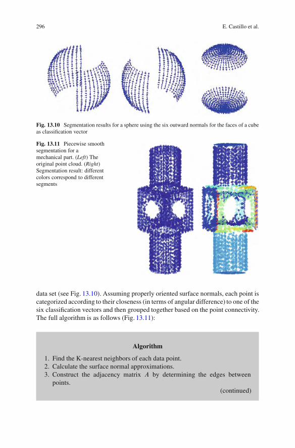
296 E. Castillo et al.
Fig. 13.10 Segmentation results for a sphere using the six outward normals for the faces of a cubeas classification vector
Fig. 13.11 Piecewise smoothsegmentation for amechanical part. (Left) Theoriginal point cloud. (Right)Segmentation result: differentcolors correspond to differentsegments
data set (see Fig. 13.10). Assuming properly oriented surface normals, each point iscategorized according to their closeness (in terms of angular difference) to one of thesix classification vectors and then grouped together based on the point connectivity.The full algorithm is as follows (Fig. 13.11):
Algorithm
1. Find the K-nearest neighbors of each data point.2. Calculate the surface normal approximations.3. Construct the adjacency matrix A by determining the edges between
points.(continued)

13 Point Cloud Segmentation and Denoising 297
(continued)4. Determine the initial segmentation by finding the connected components
of A.5. Orient the surface normal approximations.6. (Optional) Refine the segmentation according to N classification vectors.
13.8 Conclusions
A robust surface normal approximation strategy for point clouds using a constrainednonlinear least squares (NLSQ) formulation is developed. The formulation isdesigned to improve normal estimation near geometric singularities, such as edgesand corners, by employing a nonlinear adaptive weighting scheme. The weightingscheme is designed to incorporate only neighboring points positioned on the samesmooth surface component into the surface normal computation. This approachgeneralizes to the broader problem of outlier detection. More specifically, the NLSQformulation finds neighboring points that are the most consistent with one anotherin terms of the orthogonality mismatch. A byproduct of this procedure is then thedetermination of the inconsistent points, which can be considered as outlier data.
Using the NLSQ surface normal formulation as a foundation, we also derivea new point cloud processing strategy that combines denoising, declustering, andsurface normal estimation into one formulation.
The point cloud segmentation procedure introduced in this paper is based ona simple point connectivity criteria and the connected components present in therepresentative adjacency matrix. This approach allows for surface normal orienta-tion even when the data set contains more than one closed surface. Furthermore, afiner segmentation that splits the point cloud into piecewise smooth regions can beachieved.
Acknowledgements The authors acknowledge ARO/MURI award W911NF-07-1-0185 and NGANURI Award HM1582-10-1-0012 for support with this work.
References
1. Alexa, M., Behr, J., Cohen-Or, D., Fleishman, S., Levin, D., Silva, C.T.: Computing andrendering point set surfaces. IEEE Trans. Vis. Comput. Graph. 9, 3–15 (2003)
2. Amenta, N., Bern, M.: Surface reconstruction by voronoi filtering. In: Proceedings of theFourteenth Annual Symposium on Computational Geometry. ACM, New York (1998)

298 E. Castillo et al.
3. Azariadis, P.: Parameterization of clouds of unorganized points using dynamic base surfaces.Comput. Aided Des. 36, 607–623 (2004)
4. Besl, P.J., Jain, R.C.: Segmentation through variable-order surface fitting. IEEE Trans. PatternAnal. Mach. Intell. 10, 167–192 (1988)
5. Boissonnat, J.D., Cazals, F.: Smooth surface reconstruction via natural neighbor interpolationof distance functions. In: Proceedings of 16th Annual Symposium on Computational Geome-try, pp. 223–232. ACM, New York (2000)
6. Calderon, F., Ruiz, U., Rivera, M.: Surface-normal estimation with neighborhood reorga-nization for 3d reconstruction. In: Proceedings of the Congress on Pattern Recognition12th Iberoamerican Conference on Progress in Pattern Recognition, Image Analysis andApplications, pp. 321–330. Springer, Berlin/Heidelberg (2007)
7. Canny, J.: A computational approach to edge detection. IEEE Trans. Pattern Anal. Mach. Intell.8, 679–698 (1986)
8. Demarsin, K., Vanderstraeten, D., Volodine, T., Roose, D.: Detection of closed sharp edgesin point clouds using normal estimation and graph theory. Comput. Aided Des. 39, 276–283(2007)
9. Dey, T.K., Goswami, S.: Provable surface reconstruction from noisy samples. Comput. Geom.Theory Appl. 35, 124–141 (2006)
10. Dey, T., Sun, J.: Normal and feature approximations from noisy point clouds. In: FSTTCS2006: Foundations of Software Technology and Theoretical Computer Science, vol. 4337, pp.21–32. Springer, Berlin/Heidelberg (2006)
11. Dey, T.K., Li, G., Sun, J.: Normal estimation for point clouds: a comparison study for a voronoibased method. In: Proceedings Eurographics/IEEE VGTC Symposium Point-Based Graphics,vol. 0, pp. 39–46 (2005)
12. Fleishman, S., Drori, I., Cohen-or, D.: Bilateral mesh denoising. ACM Trans. Graph. 22, 950–953 (2003)
13. Hoppe, H., DeRose, T., Duchamp, T., McDonald, J., Stuetzle, W.: Surface reconstruction fromunorganized points. In: Proceedings of ACM Siggraph, pp. 71–78. ACM, New York (1992)
14. Hu, S., Wallner, J.: A second order algorithm for orthogonal projection onto curves andsurfaces. Comput. Aided Graph. Des. 22(3), 251–260 (2005)
15. Huang, J., Menq, C.-H.: Automatic data segmentation for geometric feature extraction fromunorganized 3-D coordinate points. IEEE Trans. Robot. Autom. 17, 268–278 (2001)
16. Huang, H., Li, D., Zhang, H., Ascher, U., Cohen-Or, D.: Consolidation of unorganized pointclouds for surface reconstruction. ACM Trans. Graph. 28, 176:1–176:7 (2009)
17. Huber, P.J.: Robust Statistics. Wiley, New York (2004)18. Klasing, K., Althoff, D., Wollherr, D., Buss, M.: Comparison of surface normal estimation
methods for range sensing applications. In: IEEE International Conference on Robotics andAutomation, 2009. ICRA ’09. IEEE, Piscataway (2009)
19. Lee, Y., Park, S., Jun, Y., Choi, W.C.: A robust approach to edge detection of scanned pointdata. Int. J. Adv. Manuf. Technol. 23, 263–271 (2004)
20. Leung, S., Zhao, H.: A grid based particle method for evolution of open curves and surfaces. J.Comput. Phys. 228, 2993–3024 (2009)
21. Lipman, Y., Cohen-Or, D., Levin, D., Tal-Ezer, H.: Parameterization-free projection forgeometry reconstruction. ACM Trans. Graph. 26, Article no 22 (2007)
22. Liu, Y.S., Paul, J.C., Yong, J.H., Yu, P.Q., Zhang, H., Sun, J.G., Ramani, K.: Automaticleast-squares projection of points onto point clouds with applications in reverse engineering.Comput. Aided Des. 38, 1251–1263 (2006)
23. Mitra, N., Nguyen, A., Guibas, L.: Estimating surface normals in noisy point cloud data. In:Spec. Issue Int. J. Comput. Geom. Appl. 14, 261–276 (2004)
24. OuYang, D., Feng, H.-Y.: On the normal vector estimation for point cloud data from smoothsurfaces. Comput. Aided Des. 37, 1071–1079 (2005)
25. Pauly, M., Gross, M., Kobbelt, L.P.: Efficient simplification of point-sampled surfaces. In:Proceedings of the conference on Visualization 2002. VIS 2002. IEEE Computer Society,Washington, DC (2002)

13 Point Cloud Segmentation and Denoising 299
26. Pauly, M., Keiser, R., Gross, M.: Multi-scale feature extraction on point-sampled surfaces.Comput. Graph. Forum 22, 281–289 (2003)
27. Pauly, M., Keiser, R., Kobbelt, L.P., Gross, M.: Shape modeling with point-sampled geometry.ACM Trans. Graph. 22, 641–650 (2003)
28. Rabbani, T., Van Den Heuvel, F., Vosselmann, G.: Segmentation of point clouds usingsmoothness constrain. ISPRS Comm. V Symp. Image Eng. Vis. Metrol. 36, 248–253 (2006)
29. Schmaltz, C., Gwosdek, P., Bruhn, A., Weickert, J.: Electrostatic halftoning. Comput. Graph.Forum 29, 2313–2327 (2010)
30. Vosselman, G.: Advanced point cloud processing. In: Fritsch, D. (ed.) Photogrammetric Week’09, pp. 137–146. Wichmann, Heidelberg (2009)
31. Vosselman, G., Gorte, B., Rabbani, T., Sithole, G.: Recongnising structure in laser scannerpoint clouds. Int. Arch. Photogramm. Remote Sens. Spat. Inf. Sci. 46, 33–38 (2004)
32. Yang, M., Lee, E.: Segmentation of measured point data using parametric quadric surfaceapproximation. Computer A 31, 449–457 (1999)
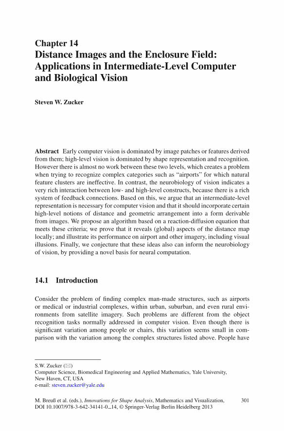
Chapter 14Distance Images and the Enclosure Field:Applications in Intermediate-Level Computerand Biological Vision
Steven W. Zucker
Abstract Early computer vision is dominated by image patches or features derivedfrom them; high-level vision is dominated by shape representation and recognition.However there is almost no work between these two levels, which creates a problemwhen trying to recognize complex categories such as “airports” for which naturalfeature clusters are ineffective. In contrast, the neurobiology of vision indicates avery rich interaction between low- and high-level constructs, because there is a richsystem of feedback connections. Based on this, we argue that an intermediate-levelrepresentation is necessary for computer vision and that it should incorporate certainhigh-level notions of distance and geometric arrangement into a form derivablefrom images. We propose an algorithm based on a reaction-diffusion equation thatmeets these criteria; we prove that it reveals (global) aspects of the distance maplocally; and illustrate its performance on airport and other imagery, including visualillusions. Finally, we conjecture that these ideas also can inform the neurobiologyof vision, by providing a novel basis for neural computation.
14.1 Introduction
Consider the problem of finding complex man-made structures, such as airportsor medical or industrial complexes, within urban, suburban, and even rural envi-ronments from satellite imagery. Such problems are different from the objectrecognition tasks normally addressed in computer vision. Even though there issignificant variation among people or chairs, this variation seems small in com-parison with the variation among the complex structures listed above. People have
S.W. Zucker (!)Computer Science, Biomedical Engineering and Applied Mathematics, Yale University,New Haven, CT, USAe-mail: [email protected]
M. Breuß et al. (eds.), Innovations for Shape Analysis, Mathematics and Visualization,DOI 10.1007/978-3-642-34141-0 14, © Springer-Verlag Berlin Heidelberg 2013
301

302 S.W. Zucker
arms and legs and heads; airports have runways and buildings and access roads.Arms and legs have bilateral symmetry; airports do not. In fact, the wide scopefor arrangement variation is what makes airports so much more complex thanfaces, say, as a category. Humans, however, can readily detect airports as wellas faces, which suggests that there is a level (or several levels) of structure to befound at which objects such as airports can be described. We discuss, in this paper,one such structure: distance measures derived from arrangement information aboutedge elements. It captures the notion that airports consist of elongated structuresthat are separated from other, possibly more dense structure. For computer visionapplications we realize this structure as a distance image.
Another motivation for considering these distance images derives from visualpsychophysics and physiology. Gestalt psychologists [21] identified the conceptsof figure and ground, and it is now common in computer vision to seek image“segmentations” that delimit such figures. Typically in computer vision a boundarycompletely encloses the figure, so these boundaries are defined by closed curves.
Gestalt psychologists have refined this notion in two subtle but important ways.First, they showed that a key property of the figure is that it “owns” the boundary.Secondly, they showed that the boundary need not be closed, continuous, or evenconnected; this suggests more of a field of points, an enclosure field, than the rigidcharacteristic function defining inside/outside sought in computer vision.
To unify these two ideas – distance images in computer vision and enclosurefields in visual psychophysics – we first develop the concept of border-ownership, aGestalt notion of how the border belongs to the figure and not to the background. Tocompute it there is an “information at a distance” problem: how do distant edges“inform” whether a given edge is part of the figure or part of the background?Computer vision seeks to solve this with a global segmentation; we take a differenttack, by deriving a partial differential equation that summarizes aspects of thedistance property inherent in border ownership. Several of its relevant propertiesare sketched, and its usefulness is demonstrated on the airport problem.
14.1.1 Figure, Ground, and Border Ownership
Rubin, in a seminal 1915 publication [32], introduced the notions of figure andground; see Fig. 14.1a. Note: as the figure shifts from the vase to the faces, theborder appears to shift as well; it “belongs” to the figure.
It is now known that such border-ownership effects exist in neurobiology. Whilemany in computer vision are aware of the existence of neurons early in the corticalvisual system that are selective for “edges” and their orientation, it is not widelyknown that, for many such cells, the response can be modulated depending onthe border-ownership sense. To explain this, recall that so-called “edge detectingneurons” were first identified using stimuli of light and dark regions as they wouldarise from ideal, step edges [19]. Now, consider a neuron that responds vigorously
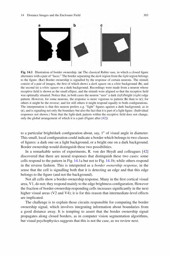
14 Distance Images and the Enclosure Field 303
Fig. 14.1 Illustration of border ownership. (a) The classical Rubin vase, in which a closed figurealternates with a pair of “faces.” The border separating the dark region from the light region belongsto the figure. (b,c) Border ownership is signalled by the response of certain neurons. The stimuliconsist of a pair of images, the first of which shows a dark square on a white background (b), andthe second (c) a white square on a dark background. Recordings were made from a neuron whosereceptive field is shown as the small ellipse, and the stimuli were aligned so that the receptive fieldwas optimally situated. Notice that, in both cases the neuron “sees” a dark (left)/bright (right) edgepattern. However, for some neurons, the response is more vigorous to pattern (b) than to (c); forothers it might be the reverse; and for still others it might respond equally to both configurations.The interpretation is that this neuron prefers e.g. “light” figures against a dark background, as in(c), and is signaling not only the boundary but also the fact that it is part of a light figure. (Individualresponses not shown.) Note that the light-dark pattern within the receptive field does not change,only the global arrangement of which it is a part (Figure after [42])
to a particular bright/dark configuration about, say, 1ı of visual angle in diameter.This small, local configuration could indicate a border which belongs to two classesof figures: a dark one on a light background, or a bright one on a dark background.Border ownership would distinguish these two possibilities.
In a remarkable series of experiments, R. von der Heydt and colleagues [42]discovered that there are neural responses that distinguish these two cases: somecells respond to the pattern in Fig. 14.1a but not to Fig. 14.1b; while others respondin the reverse fashion. This is interpreted as a border ownership response, in thesense that the cell is signalling both that it is detecting an edge and that this edgebelongs to the figure (and not the background).
Not all cells show a border-ownership response. Many in the first cortical visualarea, V1, do not; they respond mainly to the edge brightness configuration. Howeverthe fraction of border-ownership responding cells increases significantly in the nexthigher visual areas (V2 and V4); it is for this reason that intermediate-level effectsare implicated.
The challenge is to explain those circuits responsible for computing the borderownership signal, which involves integrating information about boundaries froma good distance away. It is tempting to assert that the border ownership signalpropagates along closed borders, as in computer vision segmentation algorithms,but visual psychophysics suggests that this is not the case, as we review next.

304 S.W. Zucker
14.1.2 Soft Closure in Visual Psychophysics
Visual search tasks, in which the subject seeks to find that figure which differs froman array of background distractors, provides another, “softer” view of closure; seeFig. 14.2.
While closure makes the search easy – closed figures often pop out from theothers [37] – the effect persists even if the boundary is broken (Fig. 14.2b). Evena small amount of contour “pointing” toward it’s continuation helps to support theperceptual organization of closure.
In effect there is a local/global stress implicit in computing closure and border-ownership. Global figural effects influence local border ownership, but figureimplies borders are known. Models have recently been developed that reflect thisstress, in which an approximate skeleton of the (global) shape influences the localcalculation of border ownership. To relax the need for exact boundaries to reveal theskeleton, a Bayesian approach has been attempted [17], although how this might berealized biologically remains unclear.
The concept of closure needs to be relaxed to reflect that perceptual closure onlyhints at mathematical closure. And this holds in both directions: while one mightpredict that mathematical closure implies perceptual closure, this is not necessarilythe case. Closed contours exist that are too complex [12] to assess without tracingalong [38]. Moreover, border ownership can shift along a contour [17]. More thantopology is required.
14.1.3 Intermediate-Level Computer Vision
Border ownership computations have not been a focus in computer vision. Ratherthe emphasis has been on object recognition systems and, e.g., the tradeoff betweenwithin-class or category variation relative to between-class/category variation.While scale-invariant features (e.g. [24]) and interest detectors can limit some of thewithin-class variation, an important trend is revealing that edge and shape featuresworking together can improve performance; see e.g. [14,15]. These may involve notonly organizing edge fragments into object boundary parts, but also their relativearrangement as captured by the centroid [27,28]. Such techniques follow a “bottomup” strategy, by which increasingly more context is involved in the recognition [39].
Centroids suggest involving higher-level shape features directly, and it is thisobservation that reveals a connection to border ownership. Skeleton points areextrema of the distance map and the centroid is related to shock-based formulations[35]. Computing such skeletons requires a (relatively) closed boundary, which isbarely plausible for shape categories such as cups and airplanes given photometricvariation, and relates back to Bayesian perceptual models [17]. But man-madestructures, such as airports and sports complexes are much less structured: althoughrunways are straight, there are huge variations in the buildings, parking facilities
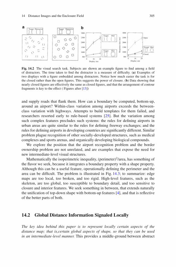
14 Distance Images and the Enclosure Field 305
Target Distractor Target
Target
Target
Distractor
3000
2500
2000
1500
1000
500
3000
2500
2000
1500
1000
5008 16 24
Display size
8 16 24Display size
Dist
Target Dist
Dist
Res
pons
e tim
e (m
s) Open
Closed
a b
Fig. 14.2 The visual search task. Subjects are shown an example figure to find among a fieldof distractors. The time taken to find the distractor is a measure of difficulty. (a) Examples oftwo displays with a figure embedded among distractors. Notice how much easier the task is forthe closed rather than the open figures. This suggests the power of closure. (b) Data showing thatnearly closed figures are effectively the same as closed figures, and that the arrangement of contourfragments is key to the effect ( Figures after [13])
and supply roads that flank them. How can a boundary be computed, bottom-up,around an airport? Within-class variation among airports exceeds the between-class variation with highways. Attempts to build templates for them failed, andresearchers resorted early to rule-based systems [25]. But the variation amongsuch complex features precludes such systems: the rules for defining airports inurban areas are quite similar to the rules for defining freeway exchanges; and therules for defining airports in developing countries are significantly different. Similarproblem plague recognition of other socially-developed structures, such as medicalcomplexes and sports arenas, and organically developing biological compounds.
We explore the position that the airport recognition problem and the borderownership problem are not unrelated, and are examples that expose the need fornew intermediate-level visual structures.
Mathematically the isoperimetric inequality, (perimeter)2/area, has something ofthe flavor we seek, because it integrates a boundary property with a shape property.Although this can be a useful feature, operationally defining the perimeter and thearea can be difficult. The problem is illustrated in Fig. 14.3; to summarize: edgemaps are too local, too broken, and too rigid. High-level features, such as theskeleton, are too global, too susceptible to boundary detail, and too sensitive toclosure and interior features. We seek something in between, that extends naturallythe unification of top-down shape with bottom-up features [4], and that is reflectiveof the better parts of both.
14.2 Global Distance Information Signaled Locally
The key idea behind this paper is to represent locally certain aspects of thedistance map; that is,certain global aspects of shape, so that they can be usedin an intermediate-level manner. This provides a middle-ground between abstract

306 S.W. Zucker
a b c d
Fig. 14.3 The quest for intermediate-level vision is to find useful representational structuresbetween edges (a), reflecting local, bottom-up processing, and global shape features such asthe medial axis (b). While informative, edges are incomplete; ideally, skeletons need completeboundaries. We recall that each medial axis, or skeleton point, is the center of a maximal inscribeddisc and also a singularity of the distance map. Both of these properties will be exploited bydifferent approaches to border ownership. We seek a representation that captures aspects of bothboundaries and their arrangement. For organically-and industrially-developed structures, such asairports (c, d), the relevant structure is captured by an abstract combination of edge and distanceeffects, rather than only local image properties
high-level representations such as skeletons and templates and the lower-levels oflayered images. The representation is derived from a partial differential equation,and leads to a non-linear scale space for distances, estimated over increasingly largerdomains. We note that there are many applications of pde’s in scale space analysis(e.g., [16]) but none, to our knowledge, that relate the solutions to properties of thedistance map.
As a warm-up, we note that there are many problems in developmental biologythat involve signalling of distant events, and we borrow heavily from a plantexample: A young leaf in a developing plant consists of a network of veins thatform cycles surrounding domains of cells. A problem arises when the domain ofcells enlarges to exceed the nutrient delivery capability of the existing vasculature:how do the “starving” cells in the center of the domain signal the need to form newveins? What is the nature of the signal, how is it generated, and what is the value thatcan be “read out” as a new vein instruction. The local task (a particular cell musttransform from a ground cell to a vascular one) requires global information (distanceto the nearest vein). To make this even more complicated, the signal must be readby those cells adjacent to existing veins, so that the network remains connected.
A theoretical solution to this problem has been developed in [8–10], and we taketheir model as a starting point for this paper; the intuition is shown in Fig. 14.4.The key idea is that cells in the developing leaf all produce a hormone called auxinat the same rate. This hormone then diffuses from cell to cell and is cleared awayat the existing veins. The result is a differential equation (stated in the next section),the equilibria of which carry information about the distance from the veins to thefurthest cell. Two properties are salient: the concentration of the hormone peaks atthe furthest cells; and the magnitude of the gradient peaks at the existing vasculature.It is this gradient peak that provides the signal for plant development.
We interpret the hormone concentration function in [8–10] as a kind of distanceimage; that is, an image whose value at certain points corresponds to properties of
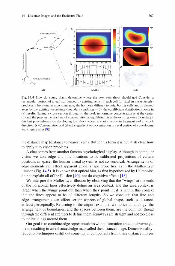
14 Distance Images and the Enclosure Field 307
Left RightMiddle
Low
High
Low
High
Dif
fere
nce
Con
cent
ratio
n
5 10 15 20 25 30 35 40
0
5
10
ac
d
eb
15
20
25
30
0
5
10
15
20
Roots (Consumption)
Leaves (Production)
Con
cent
ratio
n gr
adie
nt
Con
cent
ratio
n
areole
D
Fig. 14.4 How do young plants determine where the next vein shoot should go? Consider arectangular portion of a leaf, surrounded by existing veins. If each cell (or pixel in the rectangle)produces a hormone at a constant rate, the hormone diffuses to neighboring cells and is clearedaway by the existing vasculature (boundary condition D 0), the equilibrium distribution shown in(a) results. Taking a cross section through it, the peak in hormone concentration is at the center(b) and the peak in the gradient of concentration at equilibrium is at the existing veins (boundary);this last peak informs the developing leaf about where to start a new vein fragment and in whichdirection. (c) Concentration and (d and e) gradient of concentration in a real portion of a developingleaf (Figure after [8])
the distance map (distance to nearest vein). But in this form it is not at all clear howto apply it to vision problems.
A clue comes from another famous psychological display. Although in computervision we take edge and line locations to be calibrated projections of certainpositions in space, the human visual system is not so veridical. Arrangements ofedge elements can effect apparent global shape properties, as in the Muller-Lyerillusion (Fig. 14.5). It is known that optical blur, as first hypothesized by Helmholtz,do not explain all of the illusion [40], nor do cognitive effects [18].
We interpret the Muller-Lyer illusion by observing that the “wings” at the endsof the horizontal lines effectively define an area context, and this area context islarger when the wings point out than when they point in; it is within this contextthat the lines appear to be of different lengths. So we conclude that line andedge arrangements can effect certain aspects of global shape, such as distance,at least perceptually. Returning to the airport example, we notice an analogy: thearrangement of boundaries, and the spaces between them, are the common threadthrough the different attempts to define them. Runways are straight and not too closeto the buildings around them.
Our goal is to combine edge representations with information about their arrange-ment, resulting in an enhanced edge map called the distance image. Dimensionality-reduction techniques distill out some major components from these distance images
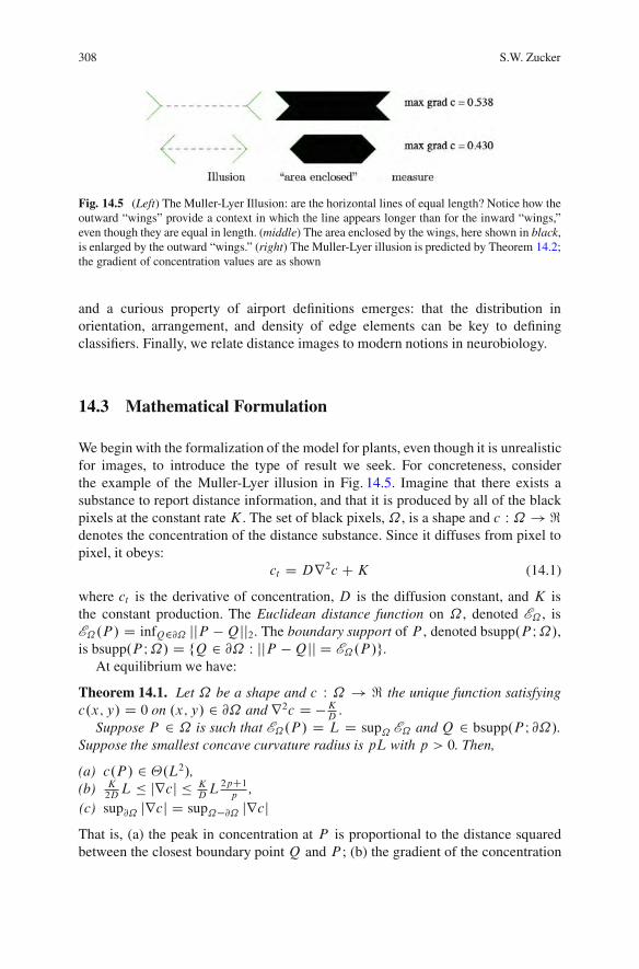
308 S.W. Zucker
Fig. 14.5 (Left) The Muller-Lyer Illusion: are the horizontal lines of equal length? Notice how theoutward “wings” provide a context in which the line appears longer than for the inward “wings,”even though they are equal in length. (middle) The area enclosed by the wings, here shown in black,is enlarged by the outward “wings.” (right) The Muller-Lyer illusion is predicted by Theorem 14.2;the gradient of concentration values are as shown
and a curious property of airport definitions emerges: that the distribution inorientation, arrangement, and density of edge elements can be key to definingclassifiers. Finally, we relate distance images to modern notions in neurobiology.
14.3 Mathematical Formulation
We begin with the formalization of the model for plants, even though it is unrealisticfor images, to introduce the type of result we seek. For concreteness, considerthe example of the Muller-Lyer illusion in Fig. 14.5. Imagine that there exists asubstance to report distance information, and that it is produced by all of the blackpixels at the constant rate K . The set of black pixels, ˝ , is a shape and c W ˝ ! <denotes the concentration of the distance substance. Since it diffuses from pixel topixel, it obeys:
ct D Dr2c CK (14.1)
where ct is the derivative of concentration, D is the diffusion constant, and K isthe constant production. The Euclidean distance function on ˝ , denoted E˝ , isE˝.P / D infQ2@˝ jjP !Qjj2. The boundary support of P , denoted bsupp.P I˝/,is bsupp.P I˝/ D fQ 2 @˝ W jjP !Qjj D E˝.P /g:
At equilibrium we have:
Theorem 14.1. Let ˝ be a shape and c W ˝ ! < the unique function satisfyingc.x; y/ D 0 on .x; y/ 2 @˝ and r2c D !K
D:
Suppose P 2 ˝ is such that E˝.P / D L D sup˝ E˝ and Q 2 bsupp.P I @˝/.Suppose the smallest concave curvature radius is pL with p > 0. Then,
(a) c.P / 2 !.L2/,(b) K
2DL " jrcj " K
DL2pC1
p,
(c) sup@˝ jrcj D sup˝!@˝ jrcjThat is, (a) the peak in concentration at P is proportional to the distance squaredbetween the closest boundary point Q and P ; (b) the gradient of the concentration
14 Distance Images and the Enclosure Field 309
reports the (approximate) length between P and Q; and (c) the largest gradientvalue is on the boundary. In other words, properties of the global distance map arerepresented locally by the concentration of the hormone.
Uniqueness follows from classical results, and the proof is based on twofunctions that sandwich c, one from above and one from below, and that take on thesame values at the boundary. Shapes can be thought of as bounded by two contours,an “inner edge” and an “outer edge.” The results hold even when the initializingfunction is non-smooth, a point that is important below, although the gradient ofthe concentration and sandwiching functions are shown to remain perpendicular tothe boundary. Not all first derivatives exist (consider medial axis points) althoughdivergence conditions can be defined. The full proof of Theorem 14.1 is in [9].Discretization and numerical issues are also important: c is defined on a continuousdomain although cells are discrete; see [9, 10].
One more conceptual point from the plant model is important. From a math-ematical perspective we typically think of the boundary (vein cells) as fixing theconcentration c D 0: However for plants we can think of the vein cells as having alarger diffusion coefficient between them than between the ground cells, so that ineffect the concentration remains at 0 because the hormone diffuses away so fast thatits concentrations is effectively 0. Such non-isotropic diffusions are also developedin [9, 10].
14.4 Edge Producing Model
We are now ready to develop the model for computer vision applications, and we dothis in two steps, the first with plants and the second with images
In the first step we imagine a dual model to the one above for plants: instead ofhaving all of the ground cells produce the hormone and the veins clear it away,now imagine that only the veins produce the hormone and that it diffuses intothe interior tissue. (This is relevant in the development of the root.) To ensure afinite equilibrium concentration, suppose the substance is destroyed (metabolized)everywhere proportional to concentration.
This results in a reaction diffusion equation (writing the continuous version),ct D Dr2c C " ! ˛c, with three terms: the change in concentration at a pixeldepends on the amount that enters by diffusion, with the amount produced there(" W ˝ ! < is the production rate) and with the amount destroyed there (˛ > 0 isthe destruction constant).
It is shown in [9, 10] that this dual model enjoys all of the properties fromTheorem 14.1, and this is the model that we develop for computational vision.
We proceed as follows (step 2). Imagine that cells are pixels, and the vein cellsare pixels at which edges have been detected. Thus the network of veins is replacedby a network of edges, and it is these edge pixels that each produce a unit of thesubstance per unit of time; non-edge pixels produce no substance. It is important to
310 S.W. Zucker
realize that this “substance” is not a simple measure of distance; it is an abstractionof a function that integrates distance and arrangement information from the edgepixels. Nevertheless, we will picture the equilibrium of this substance as a “distanceimage.”
Proposition 14.1. Consider the dynamical system
@c
@tD Dr2c C "˝ ! ˛c: (14.2)
Suppose that it acts over a domain ˝ which is a shape as in Theorem 14.1 and onwhich we impose a zero-flux boundary condition (Neumann). Let "˝ W ˝ ! <. Inthis version the diffusion is constant between regular and edge pixels, although theproduction term is not. Then the following holds.
(a) If ˛ > 0, then limt!1 c D c˛ for a unique steady-state c˛ .(b) Let ˛ D 0 and R D
R"˝d˝=
Rd˝ be the average production. Then
limt!1 ct D R and c converges to c˛ C cst: whenever R D 0. Further, rc˛ isunique even when R ¤ 0.
(c) If A;B 2 <, then the transformation "˝ 7! A"˝C˛B induces a unique trans-formation of the steady state c˛ 7! Ac˛ C B and vice versa. It follows that thegradient of c˛ is only affected if A ¤ 1: rc˛ 7! Arc˛ .
Remarks. (i) There is a variational form which may be related to the Ambrosio-Tortorelli functional [1, 36]. (ii) In part (c), if the destruction term is not linear, e.g.˛c C ˇc2, then the gradient might be affected by B as well.
Proof. Parts (a) and (b). To show existence we prove that the dynamical systemachieves ct D 0 as t ! 1. Consider the dynamical system ct t D Dr2ct ! ˛ct .The boundary conditions are inherited: since no flux goes through the boundary,there must be no change of concentration in time, i.e. rct # n D 0 on @˝ . Theunique solution of this system is ct D 0.
To prove uniqueness, suppose u1 and u2 both satisfy the equation given theboundary conditions and ct D 0. ThusDr2u1 C "˝ ! ˛u1 D Dr2u2 C "˝ ! ˛u2which gives rise to Dr2v ! ˛v D 0 where v D u1 ! u2 and rv # n D 0 where nis the normal to the boundary. Since v is elliptic and ˛ > 0, v vanishes everywhereand uniqueness follows (see [6, pp. 329 and 321]). The same reference shows that if˛ D 0, then this uniqueness is up to an additive constant u D u1 C cst; that is, onlyru is unique.
Now to show the convergence in (b) whenever R D 0, note that ct t D Dr2ctassuming ˛ D 0. This has a steady-state s.t. ct D cst: everywhere. Also,
Rct DR
"˝d˝ which shows that ct D R.Part (c). Let c˛ satisfy Eq. (14.2) for ct D 0 and a production function ".˛/˝ . Then,
Dr2c˛ ! ˛c˛ D !".˛/˝ . Suppose c D Ac˛ C B satisfies the equation for some "˝ .Since this c is unique, the following verification proves the claim.

14 Distance Images and the Enclosure Field 311
Dr2c ! ˛c D !"˝ D Dr2.Ac˛ C B/ ! ˛.Ac˛ C B/) ADr2c˛ ! A˛c˛ ! ˛B D !"˝) A.!".˛/˝ / D !"˝ C ˛B) "˝ D A.".˛/˝ /C ˛B
The other direction is derived similarly and the result follows. utWe now generalize from a single, constant diffusion constant D to one defined
on edge pixels and the another on non-edge pixels. Note that the Laplacian operatornow is sub-Riemannian; i.e., it is non-homogeneous in the diffusion constants.
Proposition 14.2. Let ˝ be a shape with two components˝ D ˝0 [˝1 such that˝0 \ ˝1 D @˝0. Let D0 and D1 be the diffusion coefficients inside ˝0 and ˝1
respectively. IfR˝0"˝dvC
R˝1"˝dv D 0 and "˝.˝0/ D K
R˝0
dv > 0, then
limD0=D1!0
c˛ D cK
where cK satisfies Theorem 14.1 for the shape ˝0 by setting cK.@˝0/ D 0.
Proof. The convergence of the system derives from Proposition 14.1(b). AsD0=D1 ! 0 the relative speed of diffusion in ˝1 increases to infinity. Thus, theconcentration over ˝1 will tend to a constant and, consequently, so will c.@˝0/ Dc.˝0 \ ˝1/. The conditions of Theorem 14.1 are therefore satisfied and the claimfollows. utTheorem 14.2. Suppose that ˝ is a region in an image and that "˝ takes a valueof 1 at edge pixels and 0 everywhere else. Let the perimeterP be the number of edgepixels and the area A be the total number of pixels in˝ , i.e.
R˝ d˝ D A. Denote by
c1 D lim˛!0 c˛ and assume that the diffusion coefficient between non-edge pixelsD D 1 and that the diffusion coefficient between edge pixels is much larger thanD.Then, for each pixelQ that is not an edge pixel
jrc1.Q/j DP
AL and jr2c1.Q/j D
P
A
Proof. The derivatives of c1 are well defined and unique as Proposition 14.1shows. They are approximated by c˛ to any precision provided that a sufficientlysmall ˛ is chosen. Thus, given an arbitrary but fixed precision, suppose that ˛satisfies that requirement. According to Proposition 14.1(c), we may transformthe production function by writing: "new D !"˝ C ˛B where ˛B D P
A. Thus,R
˝ "newd˝D !R˝ "˝ d˝ C
R˝PA
d˝ D !P C P D 0: Hence, according toProposition 14.2, this transformed setup is equivalent to cK where K D P
Aand
the claims are true for cK due to Theorem 14.1. The result for c1 follows fromProposition 14.1(c) by observing that rc1 D !rcK . ut
312 S.W. Zucker
The gradient of concentration that emerges in this last result, and that scales withL, is precisely what was shown in Fig. 14.5.
14.4.1 Density Scale Space
Displaying the concentration function c.x; y/ reveals our “distance image”. Byvarying the destruction constant, ˛, a scale space is created; notice how these captureseveral aspects of edge density (Fig. 14.6). Although this bears some resemblanceto image scale spaces [20], there are fundamental differences. In particular, theinterpretation of the gradient and the Laplacian of concentration in isoperimetricterms is completely novel.
To demonstrate that the Laplacian of concentration across scale can be usefulfor classification, we build a vector of four values of ˛ as input to a standard linearclassifier. The result for this toy experiment is in Fig. 14.7. Although experimentsremain to be done on recognition of standard object databases, we believe these willdemonstrate a role for distance images. The advantage of using the centroid alreadypoints in this direction. For computer vision applications it is more interesting todemonstrate that distance images are relevant for airport and other complex featurerecognition.
14.5 Distance Images Support Airport Recognition
We now demonstrate our first application of distance images by applying themto airport recognition. Following a standard approach in machine learning, weuse Laplacian eigenmaps [2] to reveal structure in a dataset of distance imagesfrom airports. (To remain focused on distance images, we ignore other sources ofinformation which could also be useful.)
Laplacian eigenmaps are applied as follows. Let a data point be a vectorizedpatch of regular or distance images at three scales. The edge map was obtained withthe Matlab Canny operator, and the scales were (˛D 1:0; 0:01; 0:0033; the large˛D 1:0 is essentially the original edge map); patch sizeD .17 $ 17/. Formally, letX Dfx1; x2; : : : ; xN g be the set of data points (typically ND 10,000), with eachxi 2 <nD867. We seek to find a projection of these data into much lower dimension,under the assumption that they are not randomly distributed throughout <n butrather that they lie on (or near) a lower-dimensional manifold embedded in <n.
The structure of the data are revealed via a symmetric, positivity-preserving,and positive semi-definite kernel k.x; y/, which provides a measure of similaritybetween data points. (We use a Gaussian kernel, the value for which can be truncatedto 0 for all but very similar points.) The intuition is that the natural structureamong these “distance images” can be revealed by examining their low-dimensionalembedding in significant eigenfunction coordinates. Then nearby points can beclustered to reveal airport structure.
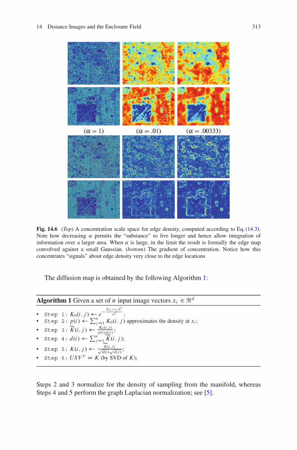
14 Distance Images and the Enclosure Field 313
Fig. 14.6 (Top) A concentration scale space for edge density, computed according to Eq. (14.3).Note how decreasing ˛ permits the “substance” to live longer and hence allow integration ofinformation over a larger area. When ˛ is large, in the limit the result is formally the edge mapconvolved against a small Gaussian. (bottom) The gradient of concentration. Notice how thisconcentrates “signals” about edge density very close to the edge locations
The diffusion map is obtained by the following Algorithm 1:
Algorithm 1 Given a set of n input image vectors xi 2 <d
• Step 1: K0.i; j / e! kxi!xj k2#2 ;
• Step 2: p.i/ PnjD1 K0.i; j / approximates the density at xi ;
• Step 3:eK.i; j / K0.i;j /p.i/p.j /
;
• Step 4: d.i/ PnjD1
eK.i; j /;• Step 5: K.i; j / eK.i;j /p
d.i/pd.j /
;
• Step 6: USV T D K (by SVD of K);
Steps 2 and 3 normalize for the density of sampling from the manifold, whereasSteps 4 and 5 perform the graph Laplacian normalization; see [5].

314 S.W. Zucker
Target selection Best Rectangle Best Rectangle Best Rectangle
Target selection Best Rectangle Best Rectangle Best Rectangle
Target selection Best Rectangle Best Rectangle Best Rectangle
Target selection Best Rectangle Best Rectangle Best Rectangle
Fig. 14.7 Classification of the truck image with pose, orientation, and scale differences using theP/A measure, which is related to the Laplacian of concentration
The result of applying Algorithm 1 to the distance map images is illustratedin Fig. 14.8. Notice how a boomerang-shaped “manifold” is revealed, the basiccoordinates of which are edge density (going along it) and edge orientation (goingaround it). These two dimensions codify our intuition that airports are defined by acertain collection of oriented edges (runways, etc.) arranged in a particular fashionrelative to surrounding context.
To test the usefulness of the distance-images, we collected a set of 20 airportimages from Google images by randomly spinning the globe, half of which were fortraining and half for testing. Our goal is to compare distance images against standardimage patches for airport detection to demonstrate “proof of concept.” Since normalimage blur also collects information from a neighborhood around a point, our three-scale distance image patches were compared against the original image patch plustwo blurred versions (comparable scales).
We interactively placed a rough outline around airports in the ten trainingimages; patches from within this outline are the red points in Fig. 14.8 for thedistance images. (The traditional blurred images are not shown.) To use this traininginformation operationally, we built a characteristic function in embedded patchcoordinates that defined “airport.”
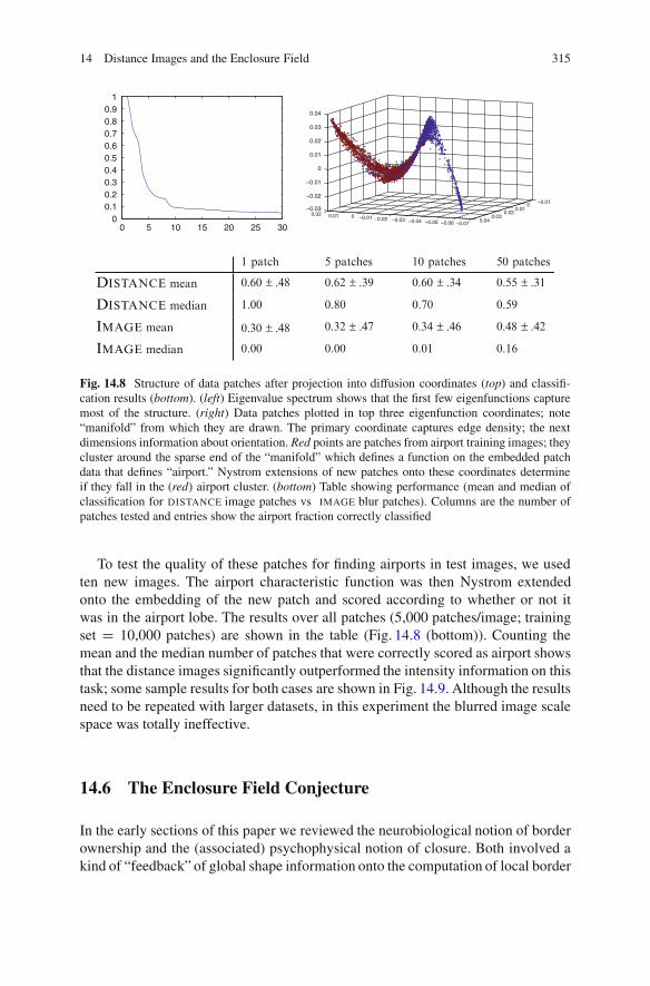
14 Distance Images and the Enclosure Field 315
0 5 10 15 20 25 300
0.10.20.30.40.50.60.70.80.9
1
!0.07!0.06!0.05!0.04!0.03!0.02!0.0100.010.02
!0.0100.01
0.020.03
0.04
!0.03
!0.02
!0.01
0
0.01
0.02
0.03
0.04
1 patch 5 patches 10 patches 50 patches
DISTANCE mean 0.60 ± .48 0.62 ± .39 0.60 ± .34 0.55 ± .31
DISTANCE median 1.00 0.80 0.70 0.59
IMAGE mean 0.30 ± .48 0.32 ± .47 0.34 ± .46 0.48 ± .42
IMAGE median 0.00 0.00 0.01 0.16
Fig. 14.8 Structure of data patches after projection into diffusion coordinates (top) and classifi-cation results (bottom). (left) Eigenvalue spectrum shows that the first few eigenfunctions capturemost of the structure. (right) Data patches plotted in top three eigenfunction coordinates; note“manifold” from which they are drawn. The primary coordinate captures edge density; the nextdimensions information about orientation. Red points are patches from airport training images; theycluster around the sparse end of the “manifold” which defines a function on the embedded patchdata that defines “airport.” Nystrom extensions of new patches onto these coordinates determineif they fall in the (red) airport cluster. (bottom) Table showing performance (mean and median ofclassification for DISTANCE image patches vs IMAGE blur patches). Columns are the number ofpatches tested and entries show the airport fraction correctly classified
To test the quality of these patches for finding airports in test images, we usedten new images. The airport characteristic function was then Nystrom extendedonto the embedding of the new patch and scored according to whether or not itwas in the airport lobe. The results over all patches (5,000 patches/image; trainingset D 10,000 patches) are shown in the table (Fig. 14.8 (bottom)). Counting themean and the median number of patches that were correctly scored as airport showsthat the distance images significantly outperformed the intensity information on thistask; some sample results for both cases are shown in Fig. 14.9. Although the resultsneed to be repeated with larger datasets, in this experiment the blurred image scalespace was totally ineffective.
14.6 The Enclosure Field Conjecture
In the early sections of this paper we reviewed the neurobiological notion of borderownership and the (associated) psychophysical notion of closure. Both involved akind of “feedback” of global shape information onto the computation of local border
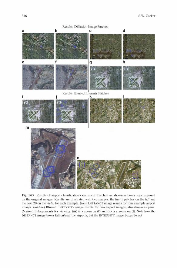
316 S.W. Zucker
Results: Diffusion Image Patches
Results: Blurred Intensity Patches
a b c d
e f g h
ki j l
m
n
Fig. 14.9 Results of airport classification experiment. Patches are shown as boxes superimposedon the original images. Results are illustrated with two images: the first 5 patches on the left andthe next 20 on the right, for each example. (top) DISTANCE image results for four example airportimages. (middle) Blurred INTENSITY image results for two airport images, also shown as pairs.(bottom) Enlargements for viewing: (m) is a zoom on (f) and (n) is a zoom on (l). Note how theDISTANCE image boxes fall on/near the airports, but the INTENSITY image boxes do not
14 Distance Images and the Enclosure Field 317
inferences. With the background we have now developed, it becomes possible toassert that there may be a relationship between the equilibrium solution of thedistance pde and neural computation. This is our second application of the distanceimage idea. To develop it, we first briefly describe a traditional view, which servesas a basis for the more elaborate conjecture.
14.6.1 Inferring Coherent Borders
As shown in Fig. 14.1, visual cortex contains neurons selective for local edgeorientation. These cells are arranged in networks that could implement a geometricnotion of border coherence. Since the large number of neurons that are sensitive toboundary segments cover all (discretely sampled) positions and orientations, thesecan be arranged as columns of cells selective for all orientations at a point; theninteractions between the cells in these columns could excite those cells that formsmooth boundaries and inhibit others. Since borders of objects are mostly smooth,locally defined orientations can be interpreted as contour tangents. Fitting tangentstogether requires a notion of curvature: how much does the tangent rotate as it istransported from one position along a curve to a nearby one. One model [3] for suchcurvature-mediated connections is outlined in Fig. 14.10, where the circuits runningbetween columns reinforce one another to provide the “flow” of tangents along thecurve.
Such models of neural computation provide consistent local edge elements, butdo not yet incorporate the more global inferences involved in glueing them togetherto form shapes. Nevertheless, there is substantial evidence that border ownershipand other shape related signals are available as early as V2 and, in some cases, V1[22, 23, 29, 43].
To establish the shape context feedback, there are two possibilities. First, onecan assert that the same class of long-range horizontal connections incorporated forborder consistency above provide the signals, as in [34,41], but the timing of borderownership signals argues strongly against this class of model; see [7]. Instead they(and others, e.g. [33]) argue that higher-level vision areas are involved. Cells in thesuperficial layers of V1, for example, project to V2, and V2 projects to V4 (amongother areas). Finally V4 projects to inferotemporal (IT) cortex, where much of visualshape analysis is believed to reside. Most importantly, there is a back projection foreach of these forward projections; see Fig. 14.11a. We now turn to a description ofsuch feedback.
14.6.2 Feedback Projections via Specialized Interneurons
Feedback projections could provide the more global information, and these areshown in Fig. 14.11 as arriving in layer I and forming synapses with apical dendrites
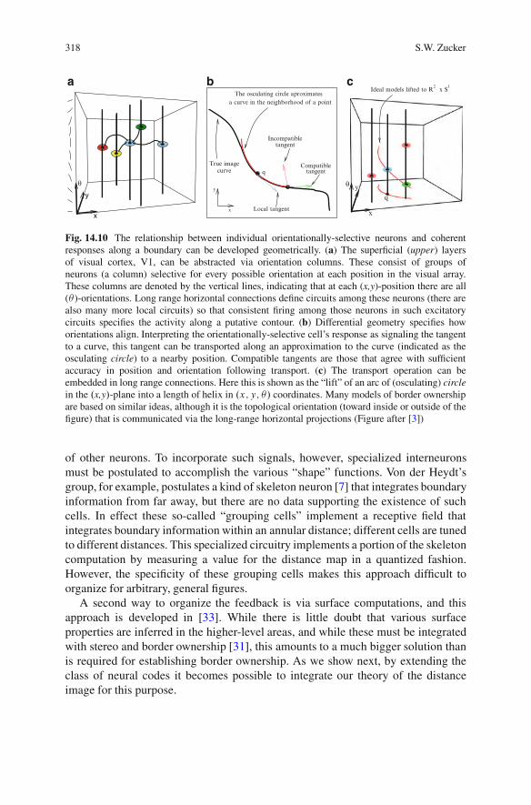
318 S.W. Zucker
!
x
yy
x
curveTrue image
The osculating circle aproximatesa curve in the neighborhood of a point
tangent
tangentCompatible
Incompatible
Local tangent
q
x
y
!
Ideal models lifted to R2 x S1
qy
x
!
a b c
Fig. 14.10 The relationship between individual orientationally-selective neurons and coherentresponses along a boundary can be developed geometrically. (a) The superficial (upper) layersof visual cortex, V1, can be abstracted via orientation columns. These consist of groups ofneurons (a column) selective for every possible orientation at each position in the visual array.These columns are denoted by the vertical lines, indicating that at each (x,y)-position there are all($ )-orientations. Long range horizontal connections define circuits among these neurons (there arealso many more local circuits) so that consistent firing among those neurons in such excitatorycircuits specifies the activity along a putative contour. (b) Differential geometry specifies howorientations align. Interpreting the orientationally-selective cell’s response as signaling the tangentto a curve, this tangent can be transported along an approximation to the curve (indicated as theosculating circle) to a nearby position. Compatible tangents are those that agree with sufficientaccuracy in position and orientation following transport. (c) The transport operation can beembedded in long range connections. Here this is shown as the “lift” of an arc of (osculating) circlein the .x,y/-plane into a length of helix in .x; y; $/ coordinates. Many models of border ownershipare based on similar ideas, although it is the topological orientation (toward inside or outside of thefigure) that is communicated via the long-range horizontal projections (Figure after [3])
of other neurons. To incorporate such signals, however, specialized interneuronsmust be postulated to accomplish the various “shape” functions. Von der Heydt’sgroup, for example, postulates a kind of skeleton neuron [7] that integrates boundaryinformation from far away, but there are no data supporting the existence of suchcells. In effect these so-called “grouping cells” implement a receptive field thatintegrates boundary information within an annular distance; different cells are tunedto different distances. This specialized circuitry implements a portion of the skeletoncomputation by measuring a value for the distance map in a quantized fashion.However, the specificity of these grouping cells makes this approach difficult toorganize for arbitrary, general figures.
A second way to organize the feedback is via surface computations, and thisapproach is developed in [33]. While there is little doubt that various surfaceproperties are inferred in the higher-level areas, and while these must be integratedwith stereo and border ownership [31], this amounts to a much bigger solution thanis required for establishing border ownership. As we show next, by extending theclass of neural codes it becomes possible to integrate our theory of the distanceimage for this purpose.
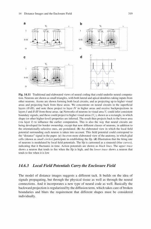
14 Distance Images and the Enclosure Field 319
a b
c d
Fig. 14.11 Traditional and elaborated views of neural coding that could underlie neural computa-tion. Neurons are shown as small triangles, with both lateral and apical dendrites taking inputs fromother neurons. Axons are shown forming both local circuits, and as projecting up to higher visualareas and projecting back from these areas. We concentrate on neural circuits in the superficiallayers (II-III), and note these project to layer IV in higher areas and receive backprojections inlayers I and II-III from those areas. (a) Networks of neurons in visual area Vi could infer consistentboundary signals, and these could project to higher visual areas (Vj ), shown as a rectangle, in whichshape (or other higher-level) properties are inferred. The result then projects back to the lower area(via layer I) to influence the earlier computation. This is also the way that neural circuits arebeing developed for border ownership, except that now different classes of neurons, in addition tothe orientationally-selective ones, are postulated. (b) An elaborated view in which the local fieldpotential surrounding each neuron is taken into account. This field potential could correspond tothe “distance” signal in the paper. (c) An even more elaborated view of the anatomy, in which glialcells (shown as small circles) participate in establishing the lfp. (d) Illustration that the firing rateof neurons is modulated by local field potentials. The lfp is cartooned as a sinusoid (blue curves),indicating that it fluctuates in time. Action potentials are shown as black lines. The upper traceshows a neuron that tends to fire when the lfp is high, and the lower trace shows a neuron thattends to fire when it is low
14.6.3 Local Field Potentials Carry the Enclosure Field
The model of distance images suggests a different tack. It builds on the idea ofsignals propagating, but through the physical tissue as well as through the neuralconnections. And it incorporates a new type of neural code as well. Basically thebackward projection is regularized by the diffusion term, which takes care of brokenboundaries and blurs the requirement that different shapes must be consideredindividually.
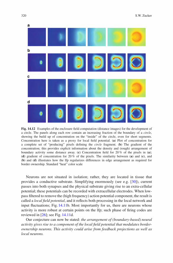
320 S.W. Zucker
Fig. 14.12 Examples of the enclosure field computation (distance images) for the development ofa circle. The panels along each row contain an increasing fraction of the boundary of a circle,showing the build up of concentration on the “inside” of the circle, even for short segments.Concentration here is taken as a proxy for local field potential. (a) Plot of concentration fora complete set of “producing” pixels defining the circle fragment. (b) The gradient of theconcentration; this provides explicit information about the density and (rough) arrangement ofboundary activity some distance away. (c) Concentration field for 20 % of the pixels in (a);(d) gradient of concentration for 20 % of the pixels. The similarity between (a) and (c), and(b) and (d) illustrates how the lfp regularizes differences in edge arrangement as required forborder ownership. Standard “heat” color scale
Neurons are not situated in isolation; rather, they are located in tissue thatprovides a conductive substrate. Simplifying enormously (see e.g. [30]), currentpasses into both synapses and the physical substrate giving rise to an extra-cellularpotential; these potentials can be recorded with extracellular electrodes. When low-pass filtered to remove the (high frequency) action potential component, the result iscalled a local field potential, and it reflects both processing in the local network andinput fluctuations; Fig. 14.11b. Most importantly for us, there are neurons whoseactivity is more robust at certain points on the lfp; such phase of firing codes arereviewed in [26]; see Fig. 14.11d.
Our conjecture can now be stated: the arrangement of (boundary-based) neuralactivity gives rise to a component of the local field potential that modulates border-ownership neurons. This activity could arise from feedback projections as well aslocal neurons.
14 Distance Images and the Enclosure Field 321
We stress that this is a novel view of neural computation, in which the lfp signalcarries different information (coding distant activity about shape) from the spikingnetwork signal (about local edges); the resulting system requires both.
The connection between this idea and distance maps is that the concentrationequation derives from neurons embedded in a linear resistive medium:
ct D "„ƒ‚…charge=ion injection
C Dr2c„ƒ‚…diffusion
! ˛c„ƒ‚…resistive loss(14.3)
Clearly neural tissue is non-linear so that more biophysically plausible modelswill be necessary, but this is sufficient to at least illustrate the principles; seeFig. 14.12. Finally, we note that the glial cells, which richly surround the pyramidalneurons and outnumber them by perhaps an order of magnitude, are now knownto have channels that allow them to participate in regulating the lfp. This furthersuggests an important computational role for it. See [44].
14.7 Summary and Conclusions
We developed a structural coupling between local edge information and more globalarrangement information by postulating a pde whose equilibria provided localsignals about global properties of the distance map. A computer vision applicationof these ideas to locating airports demonstrated that these properties are useful, anda biological interpretation suggested a richer view of neural computation involvingthe local field potential for border ownership.
Much more remains to be done with both the recognition of complex structuresand understanding border ownership. Nevertheless, by considering these two prob-lems together we emphasize how ideas from biology can influence computer vision,and vice versa.
Acknowledgements The computer vision content in this paper was in [11]; I thank P. Dimitrovand M. Lawlor for permission to reuse that material here. S. Tari pointed out the possibleconnection to Ambrosio-Tortorelli. Research supported by AFOSR, ARO, NIH/NIAAA and NSF.
References
1. Ambrosio, L., Tortorelli, V.: On the approximation of functionals depending on jumps byelliptic functionals via? %-convergence. Commun. Pure Appl. Math. 43(8), 999–1036 (1990)
2. Belkin, M., Niyogi, P.: Laplacian eigenmaps for dimensionality reduction and data representa-tion. Neural Comput. 6(15), 1373–1396 (2003)
3. Ben-Shahar, O., Zucker, S.W.: Geometrical computations explain projection patterns of long-range horizontal connections in visual cortex. Neural Comput. 16(3), 445–4476 (2003)
4. Borenstein, E., Ullman, S.: Combined top-down/bottom-up segmentation. IEEE Trans. PatternAnal. Mach. Intell. 30(12), 2109–2125 (2008)
322 S.W. Zucker
5. Coifman, R., Lafon, S., Lee, A., Maggioni, M., Nadler, B., Warner, F., Zucker, S.W.: Geometricdiffusions as a tool for harmonic analysis and structure definition of data: Diffusion maps. Proc.Nat. Acad. Sci. USA 102, 7426–7431 (2005)
6. Courant, R., Hilbert, D.: Methods of Mathematical Physics, vol. 2. Interscience, New York(1962)
7. Craft, E., Schutze, H., Niebur, E., von der Heydt, R.: A neural model of figure-groundorganization. J Neurophysiol. 97(6), 4310–4326 (2007)
8. Dimitrov, P., Zucker, S.W.: A constant production hypothesis that predicts the dynamics of leafvenation patterning. Proc. Nat. Acad. Sci. USA 13(24), 9363–9368 (2006)
9. Dimitrov, P., Zucker, S.W.: Distance maps and plant development #1: Uniform production andproportional destruction. arXiv.org, arXiv:0905.4446v1 (q-bio.QM), 1–39 (2009)
10. Dimitrov, P., Zucker, S.W.: Distance maps and plant development #2: Facilitated transport anduniform gradient. arXiv.org, arXiv:0905.4662v1 (q-bio.QM)(24), 1–46 (2009)
11. Dimitrov, P., Lawlor, M., Zucker, S.W.: Distance images and intermediate-level vision. In:Bruckstein, A.M., ter Haar Romeny, B.M., Bronstein, A.M., Bronstein, M.M. (eds.). ThirdInternational Conference on Scale Space and Variational Methods in Computer Vision. LectureNotes in Computer Science, vol. 1, pp. 653664. Springer (2011)
12. Dubuc, B., Zucker, S.W.: Complexity, confusion, and perceptual grouping. part i: the curve likerepresentation. Int. J. Comput. Vis. 42(1), 55–82 (2001)
13. Elder, J., Zucker, S.W.: Contour closure and the perception of shape. Vis. Res. 33(7), 981–991(1993)
14. Ferrari, V., Jurie, F., Schmid, C.: From images to shape models for object detection. Int.J. Comput. Vis. 87(3), 284–303 (2010)
15. Fidler, S., Leonardis, A.: Towards scalable representations of object categories: learninga hierarchy of parts. In: Proceedings of the 2007 IEEE Computer Society Conference onComputer Vision and Pattern Recognition (CVPR 2007), 1823 June 2007, Minneapolis, MNIEEE Computer Society (2007)
16. Florack, L.M.J., ter Haar Romeny, B.M., Viergever, M.A., Koenderink, J.J.: The Gaussianscale-space paradigm and the multiscale local jet. Int. J. Comput. Vis. 18(1), 61–75 (1996)
17. Froyen, V., Feldman, J., Singh, M.: A bayesian framework for figure-ground interpretation.Adv. Neural Inf. Process. Syst. 23, 631–639 (2010).
18. Gregory, R.L.: Eye and Brain. McGraw Hill, New York (1966)19. Hubel, D.H., Wiesel, T.N.: Functional architecture of macaque monkey visual cortex. Proc. R.
Soc. Lond. B 198, 1–59 (1977)20. Koenderink, J.J.: The structure of images. Biol. Cybern. 50, 363–370 (1984)21. Koffka, K.: Principles of Gestalt Psychology. Harcourt, Brace & World, New York (1935)22. Lamme, V.A.F.: The neurophysiology of figure ground segregation in primary visual cortex.
J. Neurosci. 15, 1605–1615 (1995)23. Lee, T.S., Mumford, D., Romeo, R., Lamme, V.A.F.: The role of the primary visual cortex in
higher level vision. Vis. Res. 38, 2429–2454 (1998)24. Lowe, D.: Distinctive image features from scale-invariant keypoints. Int. J. Comput. Vis. 60,
91–110 (2004)25. McKeown, D.M., Harvey, W.A., McDermott, J.: Rule-based interpretation of aerial imagery.
IEEE Trans. Pattern Anal. Mach. Intell. 7(5), 570–585 (1985)26. Montemurro, M.A., Rasch, M.J., Murayama, Y., Logothetis, N.K., Panzeri, S.: Phase-of-firing
coding of natural visual stimuli in primary visual cortex. Curr. Biol. 18(5), 375–380 (2008)27. Opelt, A., Pinz, A., Zisserman, A.: A boundary-fragment-model for object detection. In:
Leonardis, A., Bischof, H., Pinz, A. (eds.) ECCV (2). Lecture Notes in Computer Science,vol. 3952, pp. 575–588. Springer, Berlin/Heidelberg (2006)
28. Opelt, A., Pinz, A., Zisserman, A.: Learning an alphabet of shape and appearance for multi-class object detection. Int. J. Comput. Vis. 80(1), 16–44 (2008)
29. Orban, G.A.: Higher order visual processing in macaque extrastriate cortex. Physiol. Rev.88(1), 59–89 (2008)
30. Plonsey, R.: Bioelectric Phenomena. McGraw-Hill, New York (1969)
14 Distance Images and the Enclosure Field 323
31. Qiu, F., von der Heydt, R.: Figure and ground in the visual cortex: V2 combines stereoscopiccues with gestalt rules. Neuron 47, 155–166 (2005)
32. Rubin, E.: Synsoplevede Figurer. Gyldendalske Boghandel, Nordisk Forlag, Denmark (1915)33. Sajda, P., Finkel, L.: Intermediate-level visual representations and the construction of surface
perception. J. Cognit. Neurosci. 7, 267–291 (1995)34. Sakai, K., Nishimura, H.: Determination of border ownership based on the surround context of
contrast. Neurocomputing 58, 843–848 (2004)35. Siddiqi, K., Shokoufandeh, A., Dickinson, S.J., Zucker, S.W.: Shock graphs and shape
matching. Int. J. Comput. Vis. 35(1), 13–32 (1999)36. Tari, S., Genctav, M.: From a modified ambrosio-tortorelli to a randomized part hierarchy
tree. In: Third International Conference on Scale Space and Variational Methods in ComputerVision, vol. 1. Springer, Berlin/Heidelberg (2011)
37. Treisman, A., Gelade, G.: A feature-integration theory of attention. Cognit. Psychol. 12(1),97–136 (1980)
38. Ullman, S.: Visual routines. In: Fischler, M.A., Firschein, O. (eds.) Readings in ComputerVision: Issues, Problems, Principles, and Paradigms, pp. 298–328. Morgan Kaufmann, SanFrancisco (1987)
39. Ullman, S., Epshtein, B.: Visual classification by a hierarchy of extended fragments. In: Ponce,J., Hebert, M., Schmid, C., Zisserman, A. (eds.) Toward Category-Level Object Recognition.Lecture Notes in Computer Science, vol. 4170, pp. 321–344. Springer, Berlin/New York (2006)
40. Ward, L.M., Coren, S.: The effect of optically induced blur on the magnitude of the mueller-lyer illusion. Bull. Psychon. Soc. 7(5), 483–484 (1976)
41. Zhaoping, L.: Border ownership from intracortical interactions in visual area v2. Neuron 47,143–153 (2005)
42. Zhou, H., Friedman, H.S., von der Heydt, R.: Coding of border ownership in monkey visualcortex. J. Neurosci. 20, 6594–6611 (2000)
43. Zipser, K., Lamme, V.A.F., Schiller, P.H.: Contextual modulation in primary visual cortex.J. Neurosci. 16(22), 7376–7389 (1996)
44. Zucker, S.W.: Local field potentials and border ownership: a conjecture about computation invisual cortex. J. Physiol. (Paris) 106, 297–315 (2012)

Part IIIOptimization Methods for Shape Analysis
Chapter 15Non-rigid Shape Correspondence UsingPointwise Surface Descriptors and MetricStructures
Anastasia Dubrovina, Dan Raviv, and Ron Kimmel
Abstract Finding a correspondence between two non-rigid shapes is one of thecornerstone problems in the field of three-dimensional shape processing. Wedescribe a framework for marker-less non-rigid shape correspondence, based onmatching intrinsic invariant surface descriptors, and the metric structures of theshapes. The matching task is formulated as a quadratic optimization problemthat can be used with any type of descriptors and metric. We minimize it usinga hierarchical matching algorithm, to obtain a set of accurate correspondences.Further, we present the correspondence ambiguity problem arising when matchingintrinsically symmetric shapes using only intrinsic surface properties. We show thatwhen using isometry invariant surface descriptors based on eigendecompositionof the Laplace-Beltrami operator, it is possible to construct distinctive sets ofsurface descriptors for different possible correspondences. When used in a properminimization problem, those descriptors allow us to explore a number of possiblecorrespondences between two given shapes.
15.1 Introduction
Three-dimensional shape processing became increasingly popular in the last decade.One of its corner-stone tasks is detecting a correspondence between two givenshapes. It is essential for shape comparison, retrieval, shape morphing and defor-mation, or shape calculus [5], etc. The most interesting yet complex task isautomatic non-rigid shape matching. In this work we address the problem of
A. Dubrovina (!) ! D. RavivTechnion, Israel Institute of Technology, Haifa, Israele-mail: [email protected],[email protected]
R. KimmelTechnion, Department of Computer Science, Israel Institute of Technology, Haifa, Israele-mail: [email protected]
M. Breuß et al. (eds.), Innovations for Shape Analysis, Mathematics and Visualization,DOI 10.1007/978-3-642-34141-0 15, © Springer-Verlag Berlin Heidelberg 2013
327
328 A. Dubrovina et al.
matching non-rigid approximately isometric shapes. We perform the matching usingcertain surface properties that remain invariant under isometric transformations. Inparticular, we use two types of such properties – pointwise surface descriptors, anddistances measured between pairs of points on the surface. We show how thesetwo properties can be incorporated into a measure of dissimilarity between theshapes, which can be written as a quadratic function of the correspondence. Wethen minimize this dissimilarity measure in order to find the minimal dissimilaritycorrespondence.
Another important issue we address here is the correspondence ambiguity presentwhen matching intrinsically symmetric shapes. In this case, there may exist severalcorrespondences minimizing the proposed dissimilarity measure. We show that thisambiguity can be resolved by constructing distinct sets of symmetry-aware surfacedescriptors. By employing them within the proposed framework it is possible to findseveral matchings between the shapes.
The rest of the paper is organized as follows: in the next section we review therelated work on matching non-rigid shapes. In Sect. 15.3 we describe the proposedproblem formulation. In Sect. 15.4 we describe the possible choices of metric anddescriptors. In Sect. 15.5 we describe the correspondence ambiguity problem andthe construction of the symmetry-aware surface descriptors. In Sect. 15.6 we presentthe matching results obtained with the proposed framework combined with differentdescriptors and distances measures. We summarize the paper and discuss futureresearch directions in Sect. 15.7.
15.2 Related Work
Zigelman et al. [43] and Elad and Kimmel [9] suggested a method for matchingisometric shapes by embedding them into a Euclidian space using multidimensionalscaling (MDS), thus obtaining isometry invariant representations, followed by rigidshape matching in that space. Since it is generally impossible to embed a non-flat2D manifold into a flat Euclidean domain without introducing some errors, theinherited embedding error affects the matching accuracy of all methods of thistype. For that end, Jain et al. [13], Mateus et al. [19] and Sharma and Horaud[34] suggested alternative isometry-invariant shape representations, obtained byusing eigendecomposition of discrete Laplace operators. The Global Point Signature(GPS) suggested by Rustamov [33] for shape comparison employs the discreteLaplace-Beltrami operator, which, at least theoretically, captures the shape’s geome-try more faithfully. The Laplace-Beltrami operator was later employed by Sun et al.[35], and Ovsjanikov et al. [25], to construct their Heat Kernel Signature (HKS)and Heat Kernel Maps, respectively. Zaharescu et al. [41] suggested an extension of2D descriptors for surfaces, and used them to perform the matching. While linearmethods, such as [25, 41] produce good results, once distortions start to appear,ambiguity increases, and alternative formulations should be thought of. Addingthe proposed approach as a first step in one of the above linear dense matching
15 Non-Rigid Shape Correspondence Using Surface Descriptors and Metric Structures 329
algorithms can improve the final results. Hu and Hua [12] used the Laplace-Beltramioperator for matching using prominent features, and Dubrovina and Kimmel[8] suggested employing surface descriptors based on its eigendecomposition,combined with geodesic distances, in a quadratic optimization formulation of thematching problem. The above methods, incorporating pairwise constraints, tendto be slow due to high computational complexity. Wang et al. [40] used a similarproblem formulation, casted as a graph labeling problem, and experimented withdifferent surface descriptors and metrics.
Memoli and Sapiro [22], Bronstein et al. [4], and Memoli [20, 21] comparedshapes using different approximations of the Gromov-Hausdorff distance [10].Bronstein et al. [6] used the approach suggested in [4] with diffusion geometry,in order to match shapes with topological noise, and Thorstensen and Keriven [37]extended it to handle surfaces with textures. The methods in [20–22] were intendedfor surface comparison rather than matching, and as such they do not producecorrespondence between shapes. At the other end, the GMDS algorithm [6] resultsin a non-convex optimization problem, therefore it requires good initializations inorder to obtain meaningful solutions, and can be used as a refinement step for mostother shape matching algorithms. Other algorithms employing geodesic distances toperform the matching were suggested by Anguelov et al. [1], who optimized a jointprobabilistic model over the set of all possible correspondences to obtain a sparseset of corresponding points, and by Tevs et al. [36] who proposed a randomizedalgorithm for matching feature points based on geodesic distances between them.Zhang et al. [42] performed the matching using extremal curvature feature pointsand a combinatorial tree traversal algorithm, but its high complexity allowed themto match only a small number of points. Lipman and Funkhouser [18] used thefact that isometric transformation between two shapes is equivalent to a Mobiustransformation between their conformal mappings, and obtained this transformationby comparing the respective conformal factors. However, there is no guarantee thatthis result minimizes the difference between pairwise geodesic distances of matchedpoints.
Self-similarity and symmetry detection are particular cases of the correspon-dence detection problem. Instead of detecting the non-rigid mapping between twoshapes, [14, 17, 24, 28] search for a mapping from the shape to itself, and thus areable to detect intrinsic symmetries.
15.3 Matching Problem Formulation
The suggested problem formulation is based on comparison of shape propertiesthat remain approximately invariant under non-rigid !-isometric transformations,specifically – distances between the points on the shape, and pointwise surfacedescriptors defined at every point of the shape. We assume to be given shapes repre-sented by sampled surfaces, which is one of the common 3D shape representations.
330 A. Dubrovina et al.
In this work shapes were represented by triangular meshes, but the followingdiscussion is not limited to some specific sampled surface representation.
Given a shape X , we assume that is endowed with a distance measure dX WX ! X ! RC [ f0g, and a set of pointwise d -dimensional surface descriptorsfX W X ! Rd . Given two shapes X and Y , we define a correspondence betweenthem by a mapping P W X ! Y ! f0; 1g, such that
P.x; y/ D!1; x 2 X corresponds to y 2 Y ;0; otherwise
(15.1)
We can measure the dissimilarity introduced by the mapping P into the surfacedescriptors and the metric structures by
dis.P / DX
x2Xy2Y
kfX.x/ " fY .y/kF P.x; y/C ˛ #X
x;Qx2Xy; Qy2Y
jdX.x; Qx/ " dY .y; Qy//jP.x; y/P. Qx; Qy/; (15.2)
where k#kF is a norm in the descriptor space. The first term of the dissimilaritymeasure is a linear function of the mapping P , and it expresses the pointwisesurface descriptor dissimilarity. This term provides a The second term of dis.P /is a quadratic function of the mapping P , and it expresses the metric structuredissimilarity. The parameter ˛ $ 0 determines the relative weight of the secondterm in the total dissimilarity measure.
Note that by setting ˛D 0 we obtain the linear matching method used by[25, 41]. When the descriptors of different points on the shape are not uniqueor sufficiently distinct, say due to numerical inaccuracies, the correspondencesobtained by minimizing only the linear part of the dissimilarity measure may notbe consistent in terms of pairwise relationships between f the matched points. Byadding the quadratic term in Eq. (15.2) we ensure that the optimal correspondencepreserves also these pairwise relationships. On the other hand, by choosing ˛ % 1we obtain a problem similar to the one addressed in [4, 20, 22], and, since theproblem is non-convex, a good initialization is required in order to obtain a close-to-global minimizer. This is achieved by adding the linear term as in Eq. (15.2).
The optimal matching, which we denote by P ", is obtained by minimizing thedissimilarity
P " D argminP WX#Y!f0;1g fdis.P /g : (15.3)
In order to avoid a trivial solution P " & 0, we constrain P to the space of validcorrespondences. Note that the above problem formulation allows us to considerdifferent types of possible correspondences between the two shapes. For example,when a bijective mapping from X to Y is required, the constraints on P are
X
x2XP.x; y/ D 1;8y 2 Y;
X
y2YP.x; y/ D 1;8x 2 X: (15.4)
15 Non-Rigid Shape Correspondence Using Surface Descriptors and Metric Structures 331
For a surjective mapping we relax the constraints to be
X
x2XP.x; y/ D 1;8y 2 Y: (15.5)
Thus, the resulting optimization problem is
P " D argminP WX#Y!f0;1g fdis.P /g s:t: suitable constrains on P. (15.6)
15.3.1 Quadratic Programming Formulation
When the two shapes X and Y are represented by a finite number of points N , themapping P is a binary matrix of size N2. In order to convert the problem into amore convenient quadratic programming form we reshape the matrix P by takingits columns and concatenating them, thus obtaining a vector p of dimension N2,referred to as a correspondence vector. Thus, k-th entry of the vector p correspondsto some entry .i; j / in the matrix P – we will denote these corresponding indicesby .ik; jk/. The vector entry pk encodes the correspondence between the points xikand yjk .
Similarly, we introduce the following notations for the metric and the descriptordissimilarity
bk D""fX.xik /" fY .yjk /
""F
; Qkl D""dX.xik ; xmk /" dY .yjl ; ynl //
"" :
(15.7)
The vector b 2 RN2represents the pointwise descriptor dissimilarity, and the matrix
Q 2 RN2#N2represents the metric structure dissimilarity.
Lastly, we re-write optimization problem (15.6) in the quadratic programmingform
p" D argminp2f0;1gN2
˚bT p C " # pTQp
#s.t. Sp D 1; (15.8)
where Sp D 1 is the matrix form of the constraints in Eqs. (15.4) or (15.5).
15.3.2 Hierarchical Matching
The optimization problem in Eq. (15.8) belongs to the class of NP -hard IntegerQuadratic Programming (IQP) problems. There exist different techniques forapproximating its solution, [2, 38] among them, which are able to solve onlymoderate size IQPs. The implication on the matching problem is that the algorithmwill be able to find only small number of correspondences – up to several tens
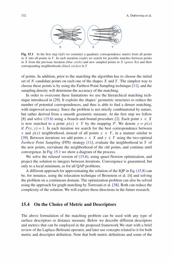
332 A. Dubrovina et al.
Fig. 15.1 In the first step (left) we construct a quadratic correspondence matrix from all pointsin X into all points in Y . In each iteration (right) we search for possible matches between pointsin X from the previous iteration (blue circle) and new sampled points in X (green Xs) and theircorresponding neighborhoods (black circles) in Y
of points. In addition, prior to the matching the algorithm has to choose the initialset of N candidate points on each one of the shapes X and Y . The simplest way tochoose these points is by using the Farthest Point Sampling technique [11], and thesampling density will determine the accuracy of the matching.
In order to overcome these limitations we use the hierarchical matching tech-nique introduced in [29]. It exploits the shapes’ geometric structures to reduce thenumber of potential correspondences, and thus is able to find a denser matching,with improved accuracy. Since the problem is not strictly combinatorial by nature,but rather derived from a smooth geometric measure. At the first step we follow[8] and solve (15.6) using a branch-and-bound procedure [2]. Each point x 2 Xis now matched to a point p.x/ 2 Y by the mapping P . We denote yDp.x/if P.x; y/D 1. In each iteration we search for the best correspondence betweenx and p.x/ neighborhood, instead of all points y 2 Y , in a manner similar to[39]. Between iterations we add points x 2 X and y 2 Y using the two-optimalFarthest Point Sampling (FPS) strategy [11], evaluate the neighborhood in Y ofthe new points, reevaluate the neighborhood of the old points, and continue untilconvergence. In Fig. 15.1 we show a diagram of the process.
We solve the relaxed version of (15.6), using quazi-Newton optimization, andproject the solution to integers between iterations. Convergence is guaranteed, butonly to a local minimum, as for all QAP problems.
A different approach for approximating the solution of the IQP in Eq. (15.8) canbe, for instance, using the relaxation technique of Bronstein et al. [4] and solvingthe problem on a continuous domain. The optimization problem can also be solvedusing the approach for graph matching by Torresani et al. [38]. Both can reduce thecomplexity of the solution. We will explore these directions in the future research.
15.4 On the Choice of Metric and Descriptors
The above formulation of the matching problem can be used with any type ofsurface descriptors or distance measure. Below we describe different descriptorsand metrics that can be employed in the proposed framework.We start with a briefreview of the Laplace-Beltrami operator, and later use concepts related to it for bothmetric and descriptor definition. Note that both metric definitions and some of the
15 Non-Rigid Shape Correspondence Using Surface Descriptors and Metric Structures 333
descriptor definitions are given in terms of continuous surface representation (or 2DRiemannian manifolds). For each one of them we state the discrete approximationwe used for numerical evaluation.
15.4.1 Laplace-Beltrami Operator
The Laplace-Beltrami operator is a generalization of the Laplacian operator fromflat domain to compact Riemannian manifolds. Given a manifold M , its Laplace-Beltrami operator#M is given by
#Xf D "divX .rXf / ; f W X ! R: (15.9)
The divergence and the gradient operators, divX and rX respectively, are defined bythe intrinsic geometry of the manifold X . Explicitly, the Laplace-Beltrami operatorof a function f W X ! R defined on the manifold X equipped with a Riemannianmetric g is given by
#Xf D "1
pdet g
X
j;k
@
@xj
$gjk
pdet g
@f
@xk
%: (15.10)
In the above equation, det g D det.gij / and the gjk are the elements of g$1. Formore details see [30].
Consider the Laplace-Beltrami operator eigenvalue problem given by
#X$i D "i$i : (15.11)
f$i g are the eigenfunctions of #X , corresponding to the eigenvalues f"i g. Thespectrum of the Laplace-Beltrami operator consists of positive eigenvalues (see, forexample, [30]). When X is a connected manifold without boundary, then #X hasadditional eigenvalue equal to zero, with corresponding constant eigenfunction. Wecan order the eigenvalues as follows
0 D "0 < "1 ' "2 ' "3 ' : : : (15.12)
The set of corresponding eigenfunctions given by
f$1;$2;$3; : : :g (15.13)
forms an orthonormal basis defined on X with inner product induced by themetric g.
There exist various approximations for the Laplace-Beltrami operator. In thiswork we used the cotangent weight scheme [23, 26].
334 A. Dubrovina et al.
15.4.2 Choice of Metric
Geodesic distance: The simplest intrinsic metric defined on a surface X is thegeodesic metric. It measures the lengths of the shortest paths on the surface X
dX.x; x0/ D inf
%2& .x;x0/`.%/: (15.14)
& .x; x0/ is the set of all admissible paths between the points x and x0 on the surfaceX , with a length of a path % given by `.%/. In order to calculate the geodesicdistances we used the fast marching method [15], which simulates a wavefrontpropagation on a triangular mesh, and associates the front arrival time with thedistance traveled by it.
Diffusion geometry: The diffusion of heat on surface X is governed by the heatequation, $
#X C@
@t
%u.x; t/ D 0; (15.15)
where a scalar field u W X ! Œ0;1/! R is the heat profile at location x and time t ,and#X is the Laplace-Beltrami operator.
The heat kernel ht .x; z/ describes the amount of heat transferred from a pointheat source located at x to another point z at time t , and can be written as
ht .x; z/ D1X
iD0e$"i t$i .x/$i .z/: (15.16)
The diffusion distance can then be defined as a cross-talk between two heatkernels [3, 7]
d2X;t .x; y/ D kht .x; #/ " ht .y; #/k2L2.X/
DZ
X
jht.x; z/ " ht .y; z/j2d z
D1X
iD0e$2"i t .$i .x/ " $i .y//2 : (15.17)
Since the heat flow on the surface is governed entirely by its intrinsic geometry,the diffusion distance defined above is an intrinsic property of the surface, and,according to [3, 7], also fulfills the metric axioms.
We approximate the diffusion distances using a finite number of the eigenvaluesand the eigenvectors of the discretized Laplace-Beltrami operator. Specifically, weused several hundred eigenvalues with the smallest magnitude and their correspond-ing eigenvectors.
15 Non-Rigid Shape Correspondence Using Surface Descriptors and Metric Structures 335
15.4.3 Choice of Descriptors
Distance histograms: Given a shape X and the corresponding distance dX , thedistance histogram descriptor [27, 28, 32] is constructed as follows
fX.x/ D hist fdX.x; Qx/ j dX.x; Qx/ ' dmax; Qx 2 Xg ; (15.18)
where dmax controls the local support of the descriptor. If two shapes are representedby differently sampled surfaces, the descriptors can be normalized to have L1-normequal to one. The descriptor comparison can be performed using either an Lp-norm,or some measure of distances between histograms, such as the earth movingdistances (EMD) [31].
Heat kernel signatures and heat kernel maps: Local descriptors based on the heatequation were presented by Sun et al. in [35] and Ovsjanikov et al. in [25]. Theheat kernel signature (HKS) is constructed using the diagonal of the heat kernelht .x; x/ (15.16) at multiple times t
fX.x/ D&ht1.x; x/; ht2 .x; x/; : : : ; htd .x; x/
': (15.19)
The heat kernel map (HKM) is constructed using the heat kernel values with a pre-specified heat source x0
fX.x/ D&ht1.x0; x/; ht2 .x0; x/; : : : ; htd .x0; x/
': (15.20)
For the latter descriptors, the heat sources chosen for the two shapes we want tomatch must be in correspondence in order to produce consistent descriptors. Onecan choose the heat source x0 either as proposed by the authors of [25], or bysome different method. Both HKS and HKM remains invariant under isometricdeformations of X , and are insensitive to topological noise at small scales.
To compute HKS and HKM we used eigenvalues and eigenfunction of thediscretized Laplace-Beltrami operator, similar to the diffusion distance calculation.
15.5 Matching Ambiguity Problem
The matching ambiguity problem arises when matching intrinsically symmetricshapes [24,27,28]. Given a shapeX , we say that it is intrinsically symmetric if thereexists a mapping S W X ! X that preserves all the geodesic distances between thecorresponding points
dX .x; Qx/ D dX .S.x/; S. Qx// ; 8x; Qx 2 X: (15.21)

336 A. Dubrovina et al.
If the shape X is intrinsically symmetric, and S W X ! X is its intrinsicsymmetry, then the surface descriptors mentioned in the previous section are alsosymmetric functions with respect to S . That is, for each of their components f .i/
X
the following holds
f.i/X .x/ D f .i/
X .S.x// : (15.22)
From the Eq. (15.21) and the above property of the descriptors it follows that ifP ".x; y/ D argmin fdis.P /g, then P ".S.x/; y/ also minimizes the dissimilaritydis.P /, with the same minimal value. Thus, when matching intrinsically symmetricshapes, the optimization problem (15.8) has multiple solutions, and by minimizingdis.P / we can obtain only one of them.
In order to overcome the above problem, a technique for construction ofsymmetry-aware surface descriptors was suggested in [8]. These descriptors arebased on the eigendecomposition of the Laplace-Beltrami operator, and exploit theimportant property of the eigenfunctions of #X , described by Ovsjanikov et al.in [24]. As stated in Theorem 3.1. of [24], eigenfunctions corresponding to non-repeating eigenvalues of the Laplace-Beltrami operator of an intrinsically symmetricshape exhibit reflection symmetry, with respect to the shape’s intrinsic symmetry.That is, such an eigenfunction $ can be either symmetric of anti-symmetric withrespect to S
$.x/ D $.S.x// or $.x/ D "$.S.x//: (15.23)
As described in [8], the symmetry-aware surface descriptors are constructed asfollows
fX.x/ D Œ$X1 .x/;$X2 .x/; : : : ;$Xd .x/'; (15.24)
and
fY .y/ D Œs1$Y1 .y/; s2$Y2 .y/; : : : ; s3$Yd .y/': (15.25)
In the above,˚$Xi#diD1 and
n$Yj
odjD1
are the eigenfunctions corresponding to the first
d non-repeating eigenvalues of the Laplace-Beltrami operators of the two shapes,
respectively. The values ofn$Yj
odjD1
are then multiplied by the sign sequence˚sj#djD1, to obtain consistent descriptors for X and Y .
Figure 15.2 shows an example of two human shapes colored according to thevalues of the first three eigenfunctions of their corresponding Laplace-Beltramioperators. It is easy to see that the eigenfunctions of the lower shape have to bemultiplied by a sequence ŒC;";C', in order to be equal to the eigenfunctions ofthe upper shape in the corresponding points. But it is also possible to multiply themby a sequence ŒC;C;"', and thus obtain eigenfunctions reflectionally symmetricto the eigenfunctions of the upper shape. In general, the number of different signsequences, and thus different sets of descriptors for the shape Y , is determined bythe number of intrinsic symmetries of the shape. Using these sets of descriptors inthe optimization problem (15.6) allows us to find several different correspondences
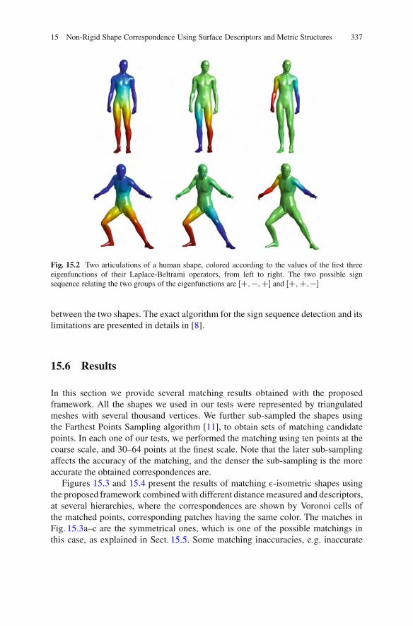
15 Non-Rigid Shape Correspondence Using Surface Descriptors and Metric Structures 337
Fig. 15.2 Two articulations of a human shape, colored according to the values of the first threeeigenfunctions of their Laplace-Beltrami operators, from left to right. The two possible signsequence relating the two groups of the eigenfunctions are ŒC;$;C' and ŒC;C;$'
between the two shapes. The exact algorithm for the sign sequence detection and itslimitations are presented in details in [8].
15.6 Results
In this section we provide several matching results obtained with the proposedframework. All the shapes we used in our tests were represented by triangulatedmeshes with several thousand vertices. We further sub-sampled the shapes usingthe Farthest Points Sampling algorithm [11], to obtain sets of matching candidatepoints. In each one of our tests, we performed the matching using ten points at thecoarse scale, and 30–64 points at the finest scale. Note that the later sub-samplingaffects the accuracy of the matching, and the denser the sub-sampling is the moreaccurate the obtained correspondences are.
Figures 15.3 and 15.4 present the results of matching !-isometric shapes usingthe proposed framework combined with different distance measured and descriptors,at several hierarchies, where the correspondences are shown by Voronoi cells ofthe matched points, corresponding patches having the same color. The matches inFig. 15.3a–c are the symmetrical ones, which is one of the possible matchings inthis case, as explained in Sect. 15.5. Some matching inaccuracies, e.g. inaccurate
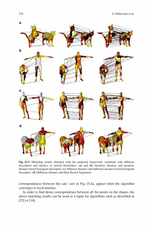
338 A. Dubrovina et al.
Fig. 15.3 Matching results obtained with the proposed framework combined with differentdescriptors and metrics, at several hierarchies. (a) and (b) Geodesic distance and geodesicdistance-based histogram descriptor; (c) diffusion distance and diffusion distance-based histogramdescriptor; (d) Diffusion distance and Heat Kernel Signatures
correspondences between the cats’ ears in Fig. 15.4a, appear when the algorithmconverges to local minima.
In order to find dense correspondence between all the points on the shapes, theabove matching results can be used as a input for algorithms such as described in[25] or [16].
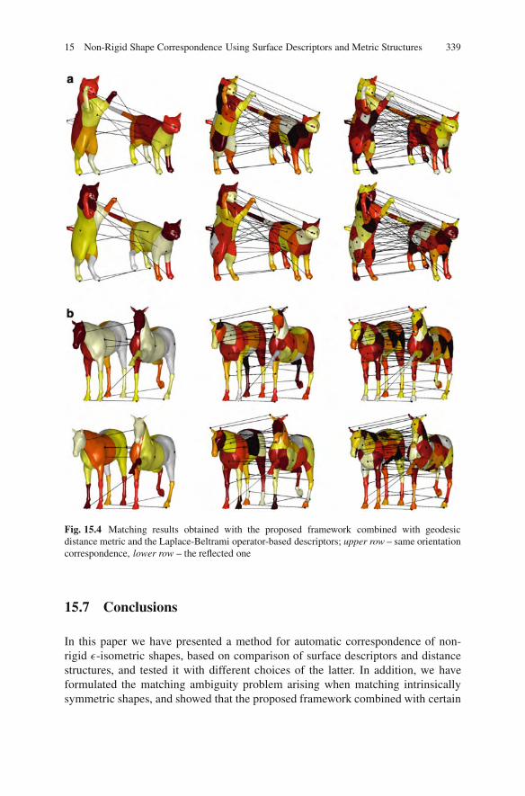
15 Non-Rigid Shape Correspondence Using Surface Descriptors and Metric Structures 339
Fig. 15.4 Matching results obtained with the proposed framework combined with geodesicdistance metric and the Laplace-Beltrami operator-based descriptors; upper row – same orientationcorrespondence, lower row – the reflected one
15.7 Conclusions
In this paper we have presented a method for automatic correspondence of non-rigid !-isometric shapes, based on comparison of surface descriptors and distancestructures, and tested it with different choices of the latter. In addition, we haveformulated the matching ambiguity problem arising when matching intrinsicallysymmetric shapes, and showed that the proposed framework combined with certain
340 A. Dubrovina et al.
descriptors allows us to detect multiple possible correspondences. In future workwe intend to adapt the proposed framework for partial shape matching and extend itto shapes that are not necessarily !-isometric.
Acknowledgements This research was supported by European Community’s FP7- ERC program,grant agreement no. 267414.
References
1. Anguelov, D., Srinivasan, P., Pang, H.-C., Koller, D., Thrun, S.: The correlated correspondencealgorithm for unsupervised registration of nonrigid surfaces. In: Proceedings of the NeuralInformation Processing Systems (NIPS) Conference, vol. 17, pp. 33–40. MIT Press, Cam-bridge (2004)
2. Bemporad, A.: Hybrid Toolbox - User’s Guide (2004). http://www.dii.unisi.it/hybrid/toolbox.3. Berard, P., Besson, G., Gallot, S.: Embedding Riemannian manifolds by their heat kernel.
Geom. Funct. Anal. 4(4), 373–398 (1994)4. Bronstein, A.M., Bronstein, M.M., Kimmel, R.: Generalized multidimensional scaling: a
framework for isometry-invariant partial surface matching. Proc. Natl. Acad. Sci. (PNAS)103(5), 1168–1172 (2006)
5. Bronstein, A.M., Bronstein, M.M., Kimmel, R.: Numerical Geometry of Non-rigid Shapes.Springer, New York (2008)
6. Bronstein, A.M., Bronstein, M.M., Kimmel, R., Mahmoudi, M., Sapiro, G.: A Gromov-Hausdorff framework with diffusion geometry for topologically-robust non-rigid shapematching. Int. J. Comput. Vis. (IJCV) 89(2–3), 266–286 (2009)
7. Coifman, R.R., Lafon, S.: Diffusion maps. Appl. Comput. Harmon. Anal. 21, 5–30 (2006)8. Dubrovina, A., Kimmel, R.: Matching shapes by eigendecomposition of the Laplace-Beltrami
operator. In: International Symposium on 3D Data Processing Visualization and Transmission(3DPVT) (2010)
9. Elad, A., Kimmel, R.: On bending invariant signatures for surfaces. IEEE Trans. Pattern Anal.Mach. Intell. (PAMI) 25(10), 1285–1295 (2003)
10. Gromov, M.: Structures Metriques Pour Les Varietes Riemanniennes. Textes Math. 1 (1981).Cedic
11. Hochbaum, D.S., Shmoys, D.B.: A best possible heuristic for the k-center problem. Math.Oper. Res. 10(2), 180–184 (1985)
12. Hu, J., Hua, J.: Salient spectral geometric features for shape matching and retrieval. Vis.Comput. 25(5–7), 667–675 (2009)
13. Jain, V., Zhang, H., Van Kaick, O.: Non-rigid spectral correspondence of triangle meshes. Int.J. Shape Model. 13(1), 101–124 (2007)
14. Kim, V., Lipman, Y., Chen, X., Funkhouser, T.: Mobius transformations for global intrinsicsymmetry analysis. In: Proceedings of the Eurographics Symposium on Geometry Processing(SGP). Wiley Online Library (2010)
15. Kimmel, R., Sethian, J.A.: Computing geodesic paths on manifolds. Proc. Natl. Acad. Sci.(PNAS) 95, 8431–8435 (1998)
16. Kraevoy, V., Sheffer, A.: Cross-parameterization and compatible remeshing of 3D models.ACM Trans. Graph. (Proc. SIGGRAPH) 23(3), 861–869 (2004)
17. Lipman, Y., Chen, X., Daubechies, I., Funkhouser, T.: Symmetry factored embedding anddistance. In ACM Transactions on Graphics (Proc. SIGGRAPH) 29(4), 103 (2010)
18. Lipman, Y., Funkhouser, T.: Mobius voting for surface correspondence. ACM Trans. Graph.(Proc. SIGGRAPH) 28(3), 72:1–72:12 (2009). Article number 72. ACM, New York

15 Non-Rigid Shape Correspondence Using Surface Descriptors and Metric Structures 341
19. Mateus, D., Horaud, R.P., Knossow, D., Cuzzolin, F., Boyer, E.: Articulated shape matchingusing Laplacian eigenfunctions and unsupervised point registration. In: Proceedings of theIEEE Conference on Computer Vision and Pattern Recognition (CVPR) (2008)
20. Memoli, F.: On the use of Gromov-Hausdorff distances for shape comparison. In: Point BasedGraphics 2007, pp. 81–90. The Eurographics Association (2007)
21. Memoli, F.: Spectral Gromov-Wasserstein distances for shape matching. In: Workshop onNon-Rigid Shape Analysis and Deformable Image Alignment (ICCV workshop, NORDIA’09),Kyoto, Japan 2009
22. Memoli, F., Sapiro, G.G.: A theoretical and computational framework for isometry invariantrecognition of point cloud data. Found. Comput. Math. 5(3), 313–347 (2005)
23. Meyer, M., Desbrun, M., Schroder, P., Barr, A.: Discrete differential geometry operators fortriangulated 2-manifolds. In: Hege, H.-C., Polthier, K. (eds.) Visualization and MathematicsIII, pp. 35–57 (2003)
24. Ovsjanikov, M., Sun, J., Guibas, L.: Global intrinsic symmetries of shapes. Comput. Graph.Forum 27(5), 1341–1348 (2008)
25. Ovsjanikov, M., Merigot, Q., Memoli, F., Guibas, L.: One point isometric matching withthe heat kernel. In: Eurographics Symposium on Geometry Processing (SGP). Wiley OnlineLibrary (2010)
26. Pinkall, U., Polthier, K.: Computing discrete minimal surfaces and their conjugates. Exp. Math.2, 15–36 (1993)
27. Raviv, D., Bronstein, A.M., Bronstein, M.M., Kimmel, R.: Symmetries of non-rigid shapes. In:IEEE 11th International Conference on Computer Vision (ICCV 2007), pp. 1–7 (2007)
28. Raviv, D., Bronstein, A.M., Bronstein, M.M., Kimmel, R.: Full and partial symmetries of non-rigid shapes. Int. J. Comput. Vis. (IJCV) 89(1), 18–39 (2010)
29. Raviv, D., Dubrovina, A., Kimmel, R.: Hierarchical matching of non-rigid shapes. In: Interna-tion Conference on Scale Space and Variational Methods (SSVM). Springer (2011)
30. Rosenberg, S.: The Laplacian on a Riemannian manifold: an Introduction to Analysis onManifolds. Cambridge University Press, Cambridge (1997)
31. Rubner, Y., Tomasi, C., Guibas, L.J.: The earth mover’s distance as a metric for image retrieval.Int. J. Comput. Vision 40, 99–121 (2000)
32. Ruggeri, M.R., Saupe, D.: Isometry-invariant matching of point set surfaces. In: Proceedingsof the Eurographics 2008 Workshop on 3D Object Retrieval. The Eurographics Association(2008)
33. Rustamov, R.M.: Laplace-Beltrami eigenfunctions for deformation invariant shape representa-tion. In Proceedings of SGP, pp. 225–233 Eurographics Association, Aire-la-Ville (2007)
34. Sharma, A., Horaud, R.P.: Shape matching based on diffusion embedding and on mutualisometric consistency. In: Proceedings of the Workshop on Nonrigid Shape Analysis andDeformable Image Alignment (NORDIA) (2010)
35. Sun, J., Ovsjanikov, M., Guibas, L.: A concise and provably informative multi-scale signaturebased on heat diffusion. In: Proceedings of the Eurographics Symposium on GeometryProcessing (SGP). Wiley Online Library (2009)
36. Tevs, A., Bokeloh, M., Wand, M., Schilling, A., Seidel, H.-P.: Isometric registration ofambiguous and partial data. In: Proceedings of the IEEE Conference on Computer Vision andPattern Recognition (CVPR) pp. 1185–1192 (2009)
37. Thorstensen, N., Keriven, R.: Non-rigid shape matching using geometry and photometry. In:Asian Conference on Computer Vision, pp. 1–12. Springer (2009)
38. Torresani, L., Kolmogorov, V., Rother, C.: Feature correspondence via graph matching: Modelsand global optimization. In: Proceedings of the 10th European Conference on Computer Vision(ECCV ’08), pp. 596–609. Springer, Berlin/Heidelberg (2008)
39. Wang, C., Bronstein, M.M., Paragios, N.: Discrete minimum distortion correspondenceproblems for non-rigid shape matching. Technical report, INRIA Research Report 7333,Mathematiques Appliquees aux Systemes, Ecole Centrale Paris, 2010

342 A. Dubrovina et al.
40. Wang, C., Bronstein, M.M., Paragios, N.: Discrete minimum distortion correspondence prob-lems for non-rigid shape matching. Technical report, Int. Conf. Scale Space and VariationalMethods (SSVM) (2011)
41. Zaharescu, A., Boyer, E., Varanasi, K., Horaud, R.P.: Surface feature detection and descriptionwith applications to mesh matching. In: Proceedings of the IEEE Conference on ComputerVision and Pattern Recognition (CVPR), (2009)
42. Zhang, H., Sheffer, A., Cohen-Or, D., Zhou, Q., van Kaick, O., Tagliasacchi, A.: Deformation-driven shape correspondence. Comput. Graph. Forum (Proc. SGP) 27(5), 1431–1439 (2008)
43. Zigelman, G., Kimmel, R., Kiryati, N.: Texture mapping using surface flattening via multi-dimensional scaling. IEEE Trans. Vis. Comput. Graph. 8(2), 198–207 (2002)

Chapter 16A Review of Geometry Recovery from a SingleImage Focusing on Curved ObjectReconstruction
Martin R. Oswald, Eno Toppe, Claudia Nieuwenhuis, and Daniel Cremers
Abstract Single view reconstruction approaches infer the structure of 3D objectsor scenes from 2D images. This is an inherently ill-posed problem. An abundanceof reconstruction approaches has been proposed in the literature, which can becharacterized by the additional assumptions they impose to make the reconstructionfeasible. These assumptions are either formulated by restrictions on the recon-structable object domain, by geometric or learned shape priors or by requiringuser input. In this chapter, we examine a representative set of state-of-the-artreconstruction approaches, which are applicable to real-world images. We classifythe approaches according to their reconstruction objective and compare them basedon a variety of important criteria. Finally, we show experimental comparisons forfive curved object reconstruction approaches.
16.1 Introduction
Estimating 3D geometry from images has been a core research topic in ComputerVision for several decades. For the case of multiple input images a large variety ofmethods has been developed which are able to deliver high quality reconstructionresults. For the special case that only a single still image is available the problemgets considerably more difficult. For specific assumptions imposed on the image avariety of methods to estimate 3D geometry exist in literature. However, a thoroughcomparison has not been carried out so far.
The reason for this lies partly in the significant diversity of existing approacheswhich in turn is due to the inherent ill-posedness of the underlying problem: duringimage formation, depth is irrecoverably lost. In their effort to make the problem
M.R. Oswald (!) ! E. Toppe ! C. Nieuwenhuis ! D. CremersDepartment of Computer Science, Institut fur Informatik, TU Munchen, Boltzmannstr. 3,Garching bei Munchen, Germanye-mail: [email protected]; [email protected]; [email protected]; [email protected]
M. Breuß et al. (eds.), Innovations for Shape Analysis, Mathematics and Visualization,DOI 10.1007/978-3-642-34141-0 16, © Springer-Verlag Berlin Heidelberg 2013
343
344 M.R. Oswald et al.
tractable, single view methods have come up with an abundance of very differentassumptions, methods and priors to infer the geometry of a depicted scene or object.The reconstruction precision of such approaches exceeds that of plausible estimatesonly in very few cases. Consequently, the reconstruction objectives are of verydifferent nature, which makes a comparison difficult.
In this chapter we give a brief survey on the subject of single view reconstruction.We provide an introduction to the field and examine basic image information andassumptions that are used in order to compensate for ill-posedness. We then review,categorize and compare existing state-of-the-art approaches. Finally, we give adetailed theoretical and experimental comparison of five single view reconstructionmethods for curved surfaces.
16.2 Single View Reconstruction
Single view reconstruction has the objective of recovering geometric informationfrom a single photograph or synthetic image. The geometric information that is tobe retrieved can be of very different manifestation reaching from purely relationalinformation, sparse metrics or dense depth information to a complete 3D model ofa single object or even a scene. This circumstance in combination with the inherentill-posedness of the problem is the main reason for the strong diversity that iswitnessed among the works in single view reconstruction and it is by no meansa straightforward task to develop a taxonomy let alone a comparison.
A first approach will therefore be on the one hand to give an overview onthe different types of image information (‘image cues’) used in the differentreconstruction processes. On the other hand we will review the priors that areassumed in order to overcome the ill-posedness. This will also serve as a briefsurvey on existing works. Later in Sect. 16.3, we will classify a number of high-level approaches and compare them in Sect. 16.4. We will then narrow down furtherconsideration to a subclass of methods that concentrates on reconstructing curvedobjects which will form the basis for our comparison in Sect. 16.5.
16.2.1 Image Cues
Approaches to single view reconstruction extract specific higher or lower levelinformation contained in the input image either automatically or with the help ofuser input. This information then is interpreted to infer geometric relations of thedepicted object or scene. In the following we list the most important categories andgive prominent references.
Shading The problem of Shape from Shading (SfS) is to infer a surface (heightfield) from a single gray level image by using the gradual variation of shading that
16 A Review of Single View Reconstruction Methods 345
is induced by the surface interaction of light. Some approaches also co-estimatelighting conditions and reflection properties. In general, the goal is to find a solutionto the following image formation model
R.n.x// D I.x/ ; (16.1)
where I is the image, n is the normal field of the surface and R is the reflectancefunction which is dependent on the object. In most SfS approaches a Lambertianreflectance model is assumed. There are, however, other models which also includethe specular case (e.g. Wang et al. [56]). SfS is an ill-posed problem, althoughthere has been progress on deriving conditions for unique solutions by Prados andFaugeras [42].
As shown by Durou et al. [12] and Zhang et al. [62] reconstruction fromreal world images is limited in the sense that each approach exhibits special andsometimes unrealistic requirements on lighting conditions or reflection properties.Especially the presence of texture is an issue. Work has been done, however, toincorporate interreflection [39], shadowing and perspective projection [7] just toname a few. One of the first minimization approaches to SfS is by Ikeuchi andHorn [24]. For a current survey see Durou et al. [12].
Shadow The shadow that is thrown by objects conveys geometric informationrelative to the viewpoint of the light source. This information can be used to narrowdown possible reconstruction results. Often point light sources have to be assumedas soft shadows do not provide enough information. Furthermore, shadow is notalways thrown on known geometry, which makes the problem even more complex.Apart from reconstruction ambiguities, it is not straightforward to extract shadowborders from images. References include works by Daum and Dudek [9], Kenderand Smith [29], Yu and Chang [60], and Hatzitheodorou [16].
Contour Edges Contour edges are salient structures in the image that are inducedby surface discontinuities, occlusion, object boundaries or reflectance changes. Theygive evidence for geometry and relative pose/position of objects. Junction points orcorners, where multiple contour edges meet or end, are also of importance for singleview reconstruction.
Subclasses of contour edge-based methods are contour-based and silhouette-based reconstruction methods. Shape from Contour approaches try to infer geometrygiven the object contours alone. However, reconstructions are in most cases ambigu-ous. Especially, smooth surfaces often do not exhibit sufficient contour lines in theimage. Shape from Contour approaches based on closed contour drawings includeHoraud et al. [19], Ulupinar et al. [53], and Li et al. [33]. Karpenko et al. [27, 28]interpret user line drawings. Other single view reconstruction approaches that usecontour edges for reconstruction include [10, 14, 17, 30, 47, 48].
Silhouette Closely related to Shape from Contour are approaches that infergeometry given the object silhouette. The silhouette is the image of the contourgenerator and the contour generator is the set of visible points on a surface, whoseimage rays are tangent to the surface.
346 M.R. Oswald et al.
The goal of silhouette based approaches is to find a geometric reconstruction,whose projection into the image plane agrees with the silhouette. As there are alwaysinfinitely many objects that are silhouette consistent this cue suffers from inherentambiguity if used alone.
There are several silhouette based single view reconstruction algorithms that wewill consider in more detail later. These include works by Prasad et al. [44, 45],Oswald et al. [41], and Toppe et al. [52]. Related to these approaches are a class ofsketch based modeling tools e.g. by Igarashi et al. [23], Karpenko et al. [27], andNealen et al. [40].
Texture Besides geometry, the appearance of real world objects is also determinedby texture. Although a complete distinction from shading is not possible, texture isconsidered as an inherent property of an object rather than a result of an interactionof light and geometry.
If one assumes objects to have a regular and known texture it is possible to infertheir geometry from the way the texture is deformed after image projection. TheseShape from Texture approaches, obviously, impose strong constraints on the recon-structable objects. An example constitutes the work of Malik and Rosenholtz [37].
Further single view reconstruction algorithms that use texture cues include Superet al. [50], Hassner and Basri [15], and Vetter et al. [55]. Approaches that combinetexture and contour edges for reconstruction by considering so-called ‘superpixels’are Hoiem et al. [17] and Saxena et al. [48].
Defocus Due to physical aspects of image formation, the sharpness of a depictedobject correlates with its distance to the camera. This fact can be used to infer adense depth map from an image. However, the accuracy of such methods is limitedand camera calibration is necessary. References include works from Levin [32] andBae and Durand [1].
Location The location of objects in the image can infer semantic knowledge ofthe objects. For example, ground, floor or sky can be identified more easily fromtheir location in the image. This information can be helpful for 3D reconstructions.Hoiem et al. [17] reconstruct vertical objects by distinguishing them from the groundand the sky. Delage et al. [10] use a Bayesian network to identify floor pixels.
16.2.2 Priors
Priors are of utter importance in single view reconstruction in order to compensatefor the problem of ill-posedness. Depending on the ultimate reconstruction goaland the target group of objects, different priors or a combination of them can beapplied. Priors can either be chosen in fixed form, or they can be gained by learning.Furthermore, there are low-level and high-level priors. In the following we will listpriors that are most frequently assumed in single view reconstruction.
16 A Review of Single View Reconstruction Methods 347
Smoothness Smoothness can be defined as the small spatial change of someproperty. In single view reconstruction we are often not able to infer a dense recon-struction. It is therefore good practice to choose among the possible reconstructionsurfaces those which tend to be smooth. Smoothness naturally plays a significantrole in the reconstruction of curved surfaces as in [41, 45, 52, 63].
Smoothness in a wider sense can also be learned as the consistency of objectsurfaces. Hoiem et al. [17] use a machine learning approach to find image featuresindicating the assignment of neighboring superpixels to the same object. Saxenaet al. [48] use image cues and geometric relations to learn the relative depth ofneighboring superpixels.
Geometric Relations Basic geometric relations are often encountered specificallyin man-made environments. As a prior they can help to dissolve ambiguities inthe reconstruction process. As part of those basic geometric relations we considere.g. coplanarity, collinearity, perpendicularity and symmetry. An early work whichmakes use of such simple rules is the one of Lowe [36]. By assuming planes tobe parallel or perpendicular one can also derive camera parameters (see Criminisiet al. [8]). This is even more important, as perspective projection is not angle-preserving and the image of parallel lines will not necessarily be parallel. We canoften assume objects to stand vertically on the ground plane [10, 14, 17].
Symmetric objects exhibit identical sections, which are projected to differentlocations in the input image. Knowing that these parts possess similar geometricand reflectance properties one can interpret their respective projections as viewsof the same object part from different observation points. This can be seen as aweak multiview scenario providing more information for reconstruction [18]. Also,occluded geometry can be inferred from this prior [14].
Volume/Area With smoothness as a prior on its own, solutions tend to be trivialor flat depending on the reconstruction approach. Adding a volume prior to thereconstruction process will ensure an inflation of the object surface and will stillresult in a certain compactness of the solution due to the smoothness assumption.Volume priors can be found in Li et al. [33] and Toppe et al. [52].
Semantic Relations Semantic relations infer high-level knowledge on the relativeposition and inner structure of different objects and their depth values. Han andZhu [14], for example, infer occluded points based on semantic human knowledge,e.g. that leaves are connected to the plant. Koutsourakis et al. [30] introducesemantic knowledge to ensure the consistency of different floors. Finally, knowledgeon the location of the ground and the sky represents an important cue for 3Dreconstruction. The ground is often used as starting point for the reconstruction asobjects, especially walls, are usually perpendicular to this plane [10, 14, 17].
Shape Priors Shape priors impose high-level knowledge on the objects to bereconstructed. Among commonly used priors, full shape priors usually impose thestrongest restrictions. On the one hand, this leads to a rather limited applicability ofthe approach. On the other hand, the reconstructions are usually of high quality andwork automatically without user input.

348 M.R. Oswald et al.
Shape priors can be defined or learned. In [30], Koutsourakis et al. define afull shape grammar for the reconstruction of facades. This limits the approachto the reconstruction of buildings in urban environments. In contrast, Rother andSapiro [46] and Chen and Cipolla [4] shape priors are learned from a databaseof sample objects. Hence, they are not a-priori limited to a specific object class.However, their choice of samples intrinsically limits their approach to the objectclasses represented in the database.
The representation of shape priors ranges from specified sets of grammar rulesover parametric models to probabilistic priors. In [4], Chen and Cipolla learn depthmaps of human bodies by means of principal component analysis. This modelimposes strong assumptions on the 3D object, but the dimension of the state spaceis reduced and only valid 3D reconstructions are obtained. In contrast, Rother andSapiro [46] impose less strong assumptions on the learned model. For each objectclass a shape prior is learned as the relative occupancy frequency of each voxel inthe object.
16.3 Classification of High-Level Approaches
In this section we will examine selected works in the field of single view recon-struction. Due to the abundance and diversity of approaches we selected algorithmswith respect to the following criteria: the chosen approaches are applicable to realworld images that are not taken under special or unrealistic material or lightingconditions. We rather concentrate on approaches inferring objects from ordinaryphotographs where reconstruction plausibility is more important than precision. Theselection, furthermore, focuses on works that are representative and state-of-the-art.We provide a classification and examine differences and similarities.
For classification we found several categories ranging from application domainover image cues and shape priors to user input and 3D representation (see below).However, these categories are not suitable to partition the set of approaches dueto strong overlap. Instead, we think that the most important information for eachsingle view reconstruction approach is its application domain, i.e. the set of objectsand scenes, which can be reconstructed. We introduce the literature sorted by thefollowing reconstruction categories:
• Curved Objects• Piecewise Planar Objects• Learning Specific Objects• 3D Impression from Scenes
More categories will follow in the next subsection. We distinguish between objectsand scenes. Reconstructions of scenes aim at producing 3D impressions or depthmaps from the whole scene contained in the image. In contrast, object reconstructionapproaches concentrate on single objects within the scene. Approaches that recon-struct curved objects principally aim at producing arbitrary, mostly smooth objects.

16 A Review of Single View Reconstruction Methods 349
Often, minimal surface approaches are used, which try to minimize the surfaceof the object given a fixed area or volume. The second class consists of methodsthat concentrate on piecewise planar objects such as buildings and man-madeenvironments. Furthermore, we distinguish arbitrary curved and planar objects fromlearning specific objects. Approaches in this class cannot reconstruct arbitraryobjects, but are inherently limited to specific object classes by shape informationlearned from sample databases. Finally, we discuss methods that do not aim toreconstruct exact or plausible 3D geometry but rather provide a pleasing 3DImpression from Scenes. In the following, we will present and classify related workon single view reconstruction.
16.3.1 Curved Objects
16.3.1.1 Zhang et al.
Zhang et al. [63] proposed a method for interactive depth map editing based on aninput image. The depth map reconstruction is the result of minimizing a thin plateenergy [11], which favors smooth surfaces and penalizes bending. User input comesas a variety of constraints on the thin plate energy that can be placed interactivelyinto the depth map. These comprise of position constraints, surface normals, surfaceor normal discontinuities, planar region constraints or curves on which curvature ortorsion is minimized.
From a mathematical point of view the thin plate energy for a continuous functionf on a two dimensional rectangular domain Œ0; 1!2 is defined as:
E.f / DZ 1
0
Z 1
0
"˛.u; v/
!!!!@2f
@u2
!!!!2
C 2ˇ.u; v/!!!!@2f
@uv
!!!!2
C ".u; v/!!!!@2f
@v2
!!!!2#
du dv ;
(16.2)
where functions ˛; ˇ; " W Œ0; 1!2 7! f0; 1g extend the thin plate model withweighting functions which can be used to define local surface discontinuities. Zhanget al. [63] discretize this minimization problem by introducing a function gi;j thatsamples values of the depth map function f W Œ0; 1!2 7! IR on a discrete rectangulargrid, that is, gi;j D f .id; jd/, with d being the distance between neighboring gridpoints. For efficiency and accuracy the grid resolution can be locally refined by theuser. By stacking all values gi;j into a single vector g and by discretizing the partialderivatives of g, the energy in Eq. (16.2) can be written in matrix form as
gTCg subject to Ag D b ; (16.3)
where the condition Ag D b may contain any constraints on the surface that canbe expressed in linear form. For a detailed description on how the constraints are

350 M.R. Oswald et al.
incorporated into this quadratic optimization problem we refer to [63]. A descriptionof these constraints from the user’s point of view is given later together with theexperimental comparison (Sect. 16.5.2).
16.3.1.2 Prasad et al.
The works [45] and [44] of Prasad et al. introduce a framework for single viewreconstruction of curved surfaces. The method is related to the one by Zhanget al. [63] but aims at reconstructing closed surfaces.
The main idea involves computing a parametric minimal surface by globallyminimizing the same thin plate energy (Eq. (16.2)) as Zhang et al. [63] the differencebeing, however, that they minimize with respect to a parametrized 3D surface f WŒ0; 1!2 7! IR3 instead of a depth map. As a result, function domain and imagedomain are no longer equivalent. For implementation purposes, the discretizationof the optimization problem with constraints is done similar to Zhang et al. (seeEq. (16.3)).
The choice of constraints is mostly different from Zhang et al. [63]. The mainsource of reconstruction information is the silhouette: Prasad et al. [45] use the factthat normals along the contour generator c.t/ can be inferred from the 2D silhouetteas by definition they are parallel to the viewing plane for a smooth surface. Thisleads to the constraints
#.f .u.t/; v.t/// D c.t/ (16.4)
n.c.t//f .u.t/; v.t// D 0 8t 2 Œ0; 1! ; (16.5)
where n.c.t// is the normal at the point c.t/ in IR3 and # the orthographic projectionfunction. The user has to determine the coordinates .u.t/; v.t// of the contourgenerator in parameter space. This is done by placing lines within the grid of theparameter space and setting them in correspondence with the parts of the contourgenerator. Similar to Zhang et al. [63] the user can employ position constraints todefine the object inflation locally. Also, surface discontinuities can be optionallyspecified to relax the surface smoothness along curves in the parameter space.
Important to note is that in order to define the topology of the object, the user hasto define which parts of the parameter space boundary are connected. For example,the connection of the left and right boundary defines a cylindrical shape of thefunction domain.
16.3.1.3 Oswald et al.
The variational single view approach by Oswald et al. [41] computes closed curvedminimal surface reconstructions. The input comprises of a side view of an objectand its silhouette which is obtained by interactive segmentation of the input image.
16 A Review of Single View Reconstruction Methods 351
An object reconstruction is achieved by searching for a smooth minimal surface thatcomplies with a shape based on the silhouette distance function.
The minimal object surface is represented by indicator function u W V 7! f0; 1gdefining object interior (u D 1) and exterior (u D 0) and is found by minimizingthe following convex energy
E.u/ DZ
V
g.x/jru.x/j d3x„ ƒ‚ …
smoothness term
CZ
V
u.x/"$vol.x/C $sil.x/
#d3x
„ ƒ‚ …data term
; (16.6)
where V ! IR3 is the reconstruction domain and the data term promotes volumeinflation via $vol and silhouette consistency via $sil. Function g W V 7! IRC is usedto locally adapt the smoothness of the surface if desired by the user – its defaultvalue is g " 1. Given the input silhouette S ! ˝ ! V as part of the image plane˝ a height map h W ˝ 7! IR is defined
h.p/ D min˚%cutoff ; %offset C %factor # dist.p; @S/k
$(16.7)
with the help of the silhouette distance function dist.p; @S/ D mins2@S kp $ sk,which returns the distance of any point p 2 ˝ to the silhouette boundary @S . Theparameters k;%cutoff;%offset;%factor modify the shape of h.
Now, the data term can be expressed in terms of h so that the object locallyhas a depth proportional to the silhouette distance. Using an implicit surfacerepresentation the data term can thus be written as
$vol.x/ D($1 if dist.x;˝/ % h.#.x//C1 otherwise ;
(16.8)
where # W V 7! ˝ is the orthographic projections of 3D points onto ˝ . Silhouetteconsistency is brought forward by
$sil.x/ D
8ˆ<
ˆ:
$1 if &S .#.x// D 1 and x 2 ˝C1 if &S .#.x// D 00 otherwise ;
(16.9)
where characteristic function &S W ˝ 7! f0; 1g indicates exterior or interior of thesilhouette, respectively. The convex energy in Eq. (16.6) is minimized with the helpof convex relaxation techniques and the global optimum defines the reconstructedobject.
16.3.1.4 Toppe et al.
Very similar to Oswald et al. [41], the variational single view approach by Toppeet al. [52] also computes closed curved minimal surface reconstructions. It followsthe same work flow and also requires an object silhouette as input.
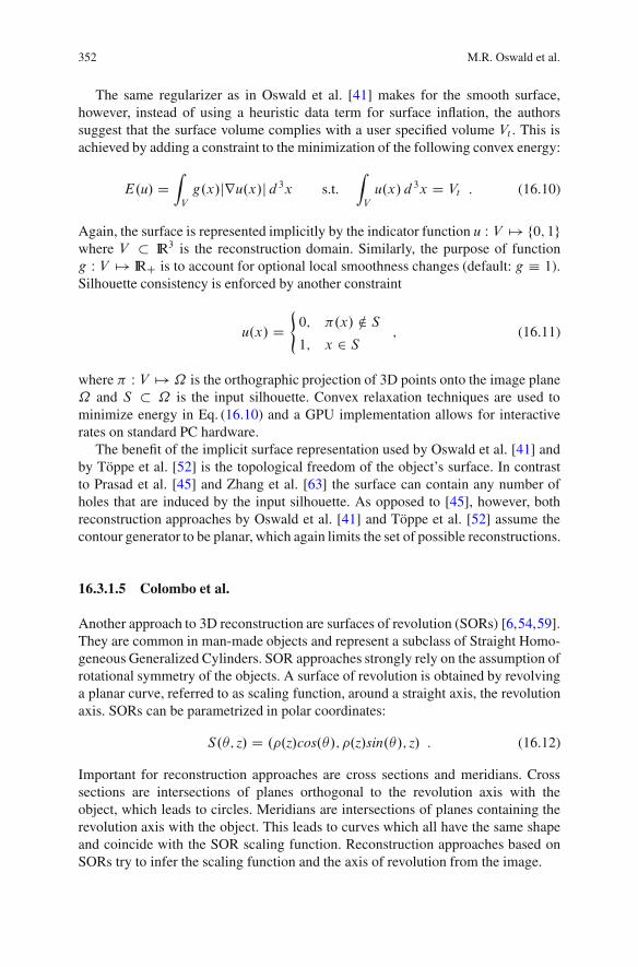
352 M.R. Oswald et al.
The same regularizer as in Oswald et al. [41] makes for the smooth surface,however, instead of using a heuristic data term for surface inflation, the authorssuggest that the surface volume complies with a user specified volume Vt . This isachieved by adding a constraint to the minimization of the following convex energy:
E.u/ DZ
V
g.x/jru.x/j d3x s.t.Z
V
u.x/ d3x D Vt : (16.10)
Again, the surface is represented implicitly by the indicator function u W V 7! f0; 1gwhere V ! IR3 is the reconstruction domain. Similarly, the purpose of functiong W V 7! IRC is to account for optional local smoothness changes (default: g " 1).Silhouette consistency is enforced by another constraint
u.x/ D(0; #.x/ … S1; x 2 S
; (16.11)
where # W V 7! ˝ is the orthographic projection of 3D points onto the image plane˝ and S ! ˝ is the input silhouette. Convex relaxation techniques are used tominimize energy in Eq. (16.10) and a GPU implementation allows for interactiverates on standard PC hardware.
The benefit of the implicit surface representation used by Oswald et al. [41] andby Toppe et al. [52] is the topological freedom of the object’s surface. In contrastto Prasad et al. [45] and Zhang et al. [63] the surface can contain any number ofholes that are induced by the input silhouette. As opposed to [45], however, bothreconstruction approaches by Oswald et al. [41] and Toppe et al. [52] assume thecontour generator to be planar, which again limits the set of possible reconstructions.
16.3.1.5 Colombo et al.
Another approach to 3D reconstruction are surfaces of revolution (SORs) [6,54,59].They are common in man-made objects and represent a subclass of Straight Homo-geneous Generalized Cylinders. SOR approaches strongly rely on the assumption ofrotational symmetry of the objects. A surface of revolution is obtained by revolvinga planar curve, referred to as scaling function, around a straight axis, the revolutionaxis. SORs can be parametrized in polar coordinates:
S.'; z/ D .(.z/cos.'/; (.z/sin.'/; z/ : (16.12)
Important for reconstruction approaches are cross sections and meridians. Crosssections are intersections of planes orthogonal to the revolution axis with theobject, which leads to circles. Meridians are intersections of planes containing therevolution axis with the object. This leads to curves which all have the same shapeand coincide with the SOR scaling function. Reconstruction approaches based onSORs try to infer the scaling function and the axis of revolution from the image.
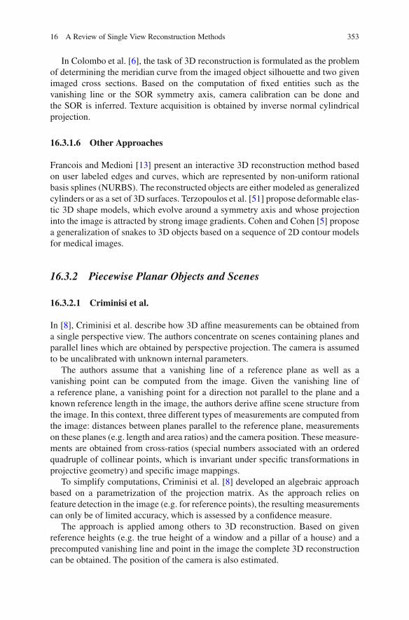
16 A Review of Single View Reconstruction Methods 353
In Colombo et al. [6], the task of 3D reconstruction is formulated as the problemof determining the meridian curve from the imaged object silhouette and two givenimaged cross sections. Based on the computation of fixed entities such as thevanishing line or the SOR symmetry axis, camera calibration can be done andthe SOR is inferred. Texture acquisition is obtained by inverse normal cylindricalprojection.
16.3.1.6 Other Approaches
Francois and Medioni [13] present an interactive 3D reconstruction method basedon user labeled edges and curves, which are represented by non-uniform rationalbasis splines (NURBS). The reconstructed objects are either modeled as generalizedcylinders or as a set of 3D surfaces. Terzopoulos et al. [51] propose deformable elas-tic 3D shape models, which evolve around a symmetry axis and whose projectioninto the image is attracted by strong image gradients. Cohen and Cohen [5] proposea generalization of snakes to 3D objects based on a sequence of 2D contour modelsfor medical images.
16.3.2 Piecewise Planar Objects and Scenes
16.3.2.1 Criminisi et al.
In [8], Criminisi et al. describe how 3D affine measurements can be obtained froma single perspective view. The authors concentrate on scenes containing planes andparallel lines which are obtained by perspective projection. The camera is assumedto be uncalibrated with unknown internal parameters.
The authors assume that a vanishing line of a reference plane as well as avanishing point can be computed from the image. Given the vanishing line ofa reference plane, a vanishing point for a direction not parallel to the plane and aknown reference length in the image, the authors derive affine scene structure fromthe image. In this context, three different types of measurements are computed fromthe image: distances between planes parallel to the reference plane, measurementson these planes (e.g. length and area ratios) and the camera position. These measure-ments are obtained from cross-ratios (special numbers associated with an orderedquadruple of collinear points, which is invariant under specific transformations inprojective geometry) and specific image mappings.
To simplify computations, Criminisi et al. [8] developed an algebraic approachbased on a parametrization of the projection matrix. As the approach relies onfeature detection in the image (e.g. for reference points), the resulting measurementscan only be of limited accuracy, which is assessed by a confidence measure.
The approach is applied among others to 3D reconstruction. Based on givenreference heights (e.g. the true height of a window and a pillar of a house) and aprecomputed vanishing line and point in the image the complete 3D reconstructioncan be obtained. The position of the camera is also estimated.

354 M.R. Oswald et al.
16.3.2.2 Delage et al.
Delage et al. [10] describe an approach for the automatic reconstruction of 3Dindoor scenes, which mainly consist of orthogonal planes. The following assump-tions are made: (1) The image is obtained by perspective projection with knowncamera calibration. (2) The objects in the scene are composed of planes and edgeswith only three mutually orthogonal orientations (‘Manhattan world assumption’).(3) The camera’s axis is vertical to the floor with known height.
To distinguish planes from edges with their orientations, the authors devise aMarkov Random Field (MRF) consisting of vertices V and edges E with six labelsyv D fp1; p2; p3; e1; e2; e3g for v 2 V . fp1; p2; p3g encodes plane orientationand fe1; e2; e3g encodes edge orientation. Let xv and xu;v denote the feature vectorat node v and at node pair .u; v/ respectively. The following joint probabilitydistribution is defined over all labels yv:
P' .yjx/ D1
Z' .x/exp
0
@$X
v2V 1.yv; xv; '1/$
X
.u;v/2E 2.yu; yv; xu;v; '2/
1
A :
(16.13)
Here, Z' .x/ stands for the partition function and ' D Œ'1; '2! indicates the modelparameters. The unary term 1.yv; xv; '1/ D 'T1 $.yv; xv/ is a linear combinationof image features $.yv; xv/ such as edge orientation or floor affiliation, whereas thepairwise term 2.yu; yv; xu;v; '2/ D 'T2 $.yu; yv; xu;v/ encodes features indicatinglabel consistency or if two pixels were members of the same partition after asegmentation of the image.
To obtain a 3D reconstruction from the MRF labeling, a constrained iterativeoptimization problem is formulated to obtain the location and orientation of planesand edges in 3D space. The constraints yielding 3D points for each image pixelcan be formulated from the Manhattan world assumption which ensures a uniquesolution. To obtain a correct result, occlusion vs. non-occlusion of edges is inferred.Delage et al. [10] can be viewed as a modification and generalization of Sturm andMaybank [49].
16.3.2.3 Koutsourakis et al.
In [30], Koutsourakis et al. generate urban 3D reconstructions from images byestimating the parameters of a 3D shape grammar in a MRF approach, so that thegenerated building best matches the image.
A shape grammar describes how basic shapes interact together through a setof replacement rules to produce complex structured geometries. It contains basicor atomic shapes, which are modified by operators. The operators either transformthe object by means of translation, rotation or scaling, or they perform structuraloperations such as splitting or mirroring. The main advantages of using a shapegrammar are that it always produces well-defined buildings and that the complexityof the optimization as well as the dimensionality of the problem is strongly reduced.
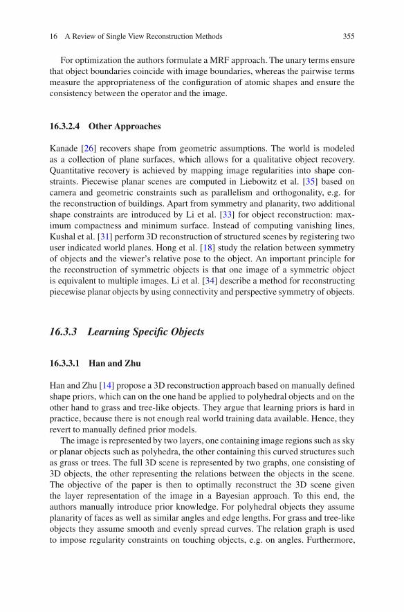
16 A Review of Single View Reconstruction Methods 355
For optimization the authors formulate a MRF approach. The unary terms ensurethat object boundaries coincide with image boundaries, whereas the pairwise termsmeasure the appropriateness of the configuration of atomic shapes and ensure theconsistency between the operator and the image.
16.3.2.4 Other Approaches
Kanade [26] recovers shape from geometric assumptions. The world is modeledas a collection of plane surfaces, which allows for a qualitative object recovery.Quantitative recovery is achieved by mapping image regularities into shape con-straints. Piecewise planar scenes are computed in Liebowitz et al. [35] based oncamera and geometric constraints such as parallelism and orthogonality, e.g. forthe reconstruction of buildings. Apart from symmetry and planarity, two additionalshape constraints are introduced by Li et al. [33] for object reconstruction: max-imum compactness and minimum surface. Instead of computing vanishing lines,Kushal et al. [31] perform 3D reconstruction of structured scenes by registering twouser indicated world planes. Hong et al. [18] study the relation between symmetryof objects and the viewer’s relative pose to the object. An important principle forthe reconstruction of symmetric objects is that one image of a symmetric objectis equivalent to multiple images. Li et al. [34] describe a method for reconstructingpiecewise planar objects by using connectivity and perspective symmetry of objects.
16.3.3 Learning Specific Objects
16.3.3.1 Han and Zhu
Han and Zhu [14] propose a 3D reconstruction approach based on manually definedshape priors, which can on the one hand be applied to polyhedral objects and on theother hand to grass and tree-like objects. They argue that learning priors is hard inpractice, because there is not enough real world training data available. Hence, theyrevert to manually defined prior models.
The image is represented by two layers, one containing image regions such as skyor planar objects such as polyhedra, the other containing this curved structures suchas grass or trees. The full 3D scene is represented by two graphs, one consisting of3D objects, the other representing the relations between the objects in the scene.The objective of the paper is then to optimally reconstruct the 3D scene giventhe layer representation of the image in a Bayesian approach. To this end, theauthors manually introduce prior knowledge. For polyhedral objects they assumeplanarity of faces as well as similar angles and edge lengths. For grass and tree-likeobjects they assume smooth and evenly spread curves. The relation graph is usedto impose regularity constraints on touching objects, e.g. on angles. Furthermore,
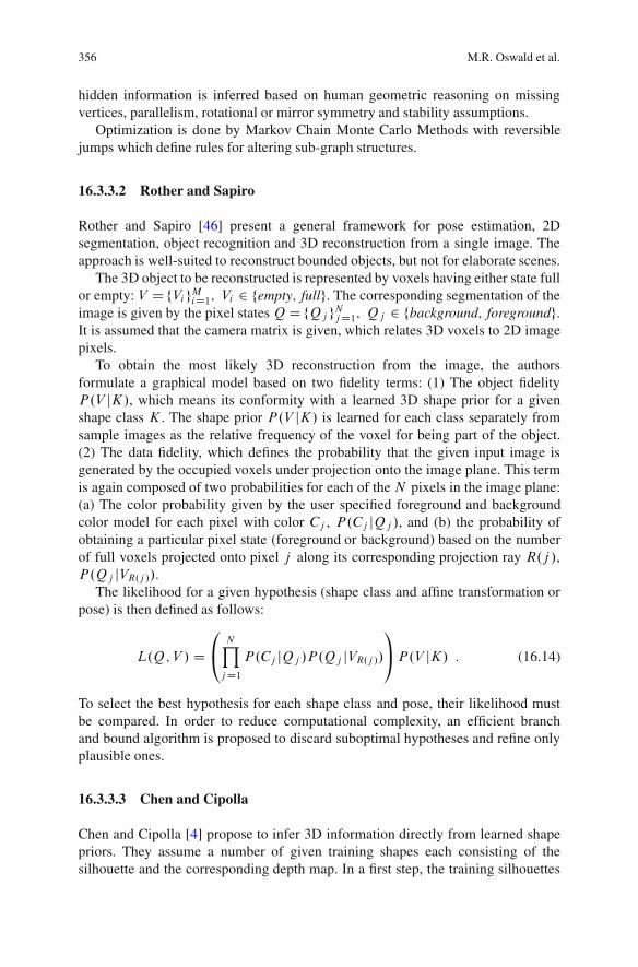
356 M.R. Oswald et al.
hidden information is inferred based on human geometric reasoning on missingvertices, parallelism, rotational or mirror symmetry and stability assumptions.
Optimization is done by Markov Chain Monte Carlo Methods with reversiblejumps which define rules for altering sub-graph structures.
16.3.3.2 Rother and Sapiro
Rother and Sapiro [46] present a general framework for pose estimation, 2Dsegmentation, object recognition and 3D reconstruction from a single image. Theapproach is well-suited to reconstruct bounded objects, but not for elaborate scenes.
The 3D object to be reconstructed is represented by voxels having either state fullor empty: V DfVi gMiD1; Vi 2 fempty; fullg. The corresponding segmentation of theimage is given by the pixel states QDfQj gNjD1; Qj 2 fbackground; foregroundg.It is assumed that the camera matrix is given, which relates 3D voxels to 2D imagepixels.
To obtain the most likely 3D reconstruction from the image, the authorsformulate a graphical model based on two fidelity terms: (1) The object fidelityP.V jK/, which means its conformity with a learned 3D shape prior for a givenshape class K . The shape prior P.V jK/ is learned for each class separately fromsample images as the relative frequency of the voxel for being part of the object.(2) The data fidelity, which defines the probability that the given input image isgenerated by the occupied voxels under projection onto the image plane. This termis again composed of two probabilities for each of the N pixels in the image plane:(a) The color probability given by the user specified foreground and backgroundcolor model for each pixel with color Cj , P.Cj jQj /, and (b) the probability ofobtaining a particular pixel state (foreground or background) based on the numberof full voxels projected onto pixel j along its corresponding projection ray R.j /,P.Qj jVR.j //.
The likelihood for a given hypothesis (shape class and affine transformation orpose) is then defined as follows:
L.Q; V / D
0
@NY
jD1P.Cj jQj /P.Qj jVR.j //
1
AP.V jK/ : (16.14)
To select the best hypothesis for each shape class and pose, their likelihood mustbe compared. In order to reduce computational complexity, an efficient branchand bound algorithm is proposed to discard suboptimal hypotheses and refine onlyplausible ones.
16.3.3.3 Chen and Cipolla
Chen and Cipolla [4] propose to infer 3D information directly from learned shapepriors. They assume a number of given training shapes each consisting of thesilhouette and the corresponding depth map. In a first step, the training silhouettes

16 A Review of Single View Reconstruction Methods 357
are registered. To ensure the independence of different data dimensions and toreduce the complexity of the approach, Principal Component Analysis is appliedto the silhouettes and the depth maps separately in order to find lower-dimensionalsubspaces of the training shapes. In this way, the authors obtain 2D lower-dimensional training feature pairs consisting of position and depth information.To model the low-dimensional sub-manifold structure underlying the feature pairspace, Gaussian Process Latent Variable Models (GPLVM) are used. They assumeGaussian processes for the position and depth information as well as for the latentvariables (the PCA coefficients). Then they estimate the underlying parameters inan optimization problem, which leads to a shape model learned from sample data.
Given an unknown silhouette, 3D information can now be inferred from thelearned shape model. First, the silhouette is registered and projected into the lower-dimensional PCA subspace yielding a position feature vector. Given this featurevector and the shape model, we ask for the most likely depth estimate at each point.Since there is no closed-form solution to this problem, the authors revert to a two-stage approach: (1) They find the most likely latent variables generating the givensilhouette feature. (2) From these latent variables the most likely depth estimate isinferred as the mean value of a Gaussian distribution. The final 3D reconstruction ateach point is the sum of the most likely depth value and the linear combination ofthe PCA eigenvectors determined by the latent variables.
16.3.3.4 Hassner and Basri
Hassner and Basri [15] aim at depth reconstruction from a single image based onexamples. The samples are given in a database S containing mappings of images totheir corresponding depth maps S D fMigniD1 D f.Ii ;Di /gniD1. For a given imagepatch Wp centered on p its depth is inferred from known depth values of the mostsimilar patches V in the database by maximizing its plausibility: Plaus.DjI; S/ DP
p2I maxSim.Wp; V /. Similarity Sim between patches is measured in the leastsquares sense. The image patches overlap leading to several depth estimates foreach pixel. These are combined by averaging. To ensure consistency of neighboringpatches a global optimization procedure is proposed which iteratively refines depthestimates.
16.3.3.5 Other Approaches
Vetter [55] learned a parametric model for the reconstruction of faces by applyingPCA to a database of registered 3D faces. Then the model parameters can be found,which best explain the given image of a face. In Nagai et al. [38], objects arelearned from a sample database. A Hidden Markov Model is used to model thecorrespondence between intensity and depth.
358 M.R. Oswald et al.
16.3.4 3D Impression from Scenes
16.3.4.1 Hoiem et al.
In [17], Hoiem et al. propose a fully automatic approach for creating 3D modelsfrom single photographs, which is similar to the creating of pop-up illustrations inchildren’s books. They divide the world into ground, sky and vertical objects, whichthey call geometric classes. The appearance of these classes is described by imagecues, which are learned from sample images.
In a first step the image is automatically segmented into superpixels, which aregrouped to constellations. Constellations consist of superpixels, which are likely tohave the same label. This probability is expressed by
S.C / DNcX
kD1
1
nk.1 $ nk/X
i;j2CklogP.yi D yj j jzi $ zj j/ ; (16.15)
where Nc is the number of constellations, nk the number of superpixels inconstellation k and P.yi D yj j jzi $ zj j/ is the estimated probability that twosuperpixels have the same label y given the absolute difference of their featurevectors z.
The likelihood of a superpixel label given its feature vector x is estimated bymarginalizing over the constellation likelihoods
P.yi D t jx/ DX
kWsi2CkP.yk D t jxk; Ck/P.Ckjxk/ ; (16.16)
where both probabilities are learned from training data. By means of a machinelearning approach the constellations are labeled as ground, sky or vertical objects.To reconstruct a 3D model from the data, the boundary of the bottom of the verticalregions is fit with the ground, the sky is removed from the model, and vertical pixelsare assumed to belong to objects sticking out of the ground. Line segments are thenfit to the ground-vertical label boundary and the segments are formed into poly-lines.The image is finally ‘folded’ along the poly-lines and ‘cut’ upward at the endpointsof these lines as well as at ground-sky and vertical-sky boundaries. A reasonablyscaled camera model can be obtained by estimating the horizon line and setting theremaining parameters to constants.
16.3.4.2 Saxena et al.
In [48], Saxena et al. propose another approach for obtaining 3D structure from asingle image of an unstructured environment. The only assumption the authors makeis that the world consists of small planes, whose 3D position and orientation is to
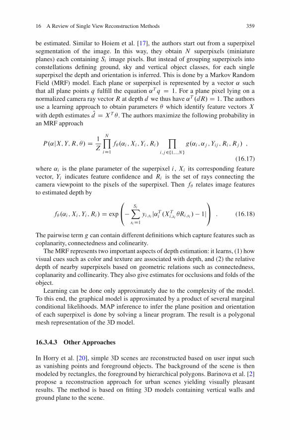
16 A Review of Single View Reconstruction Methods 359
be estimated. Similar to Hoiem et al. [17], the authors start out from a superpixelsegmentation of the image. In this way, they obtain N superpixels (miniatureplanes) each containing Si image pixels. But instead of grouping superpixels intoconstellations defining ground, sky and vertical object classes, for each singlesuperpixel the depth and orientation is inferred. This is done by a Markov RandomField (MRF) model. Each plane or superpixel is represented by a vector ˛ suchthat all plane points q fulfill the equation ˛T q D 1. For a plane pixel lying on anormalized camera ray vectorR at depth d we thus have ˛T .dR/ D 1. The authorsuse a learning approach to obtain parameters ' which identify feature vectors Xwith depth estimates Od D XT ' . The authors maximize the following probability inan MRF approach
P.˛jX; Y;R; '/ D 1
Z
NY
iD1f' .˛i ; Xi ; Yi ; Ri /
Y
i;j2f1;::;N gg.˛i ; ˛j ; Yij ; Ri ; Rj / ;
(16.17)
where ˛i is the plane parameter of the superpixel i , Xi its corresponding featurevector, Yi indicates feature confidence and Ri is the set of rays connecting thecamera viewpoint to the pixels of the superpixel. Then f' relates image featuresto estimated depth by
f' .˛i ; Xi ; Yi ; Ri / D exp
0
@$SiX
siD1yi;si j˛Ti .XT
i;si'Ri;si /$ 1j
1
A : (16.18)
The pairwise term g can contain different definitions which capture features such ascoplanarity, connectedness and colinearity.
The MRF represents two important aspects of depth estimation: it learns, (1) howvisual cues such as color and texture are associated with depth, and (2) the relativedepth of nearby superpixels based on geometric relations such as connectedness,coplanarity and collinearity. They also give estimates for occlusions and folds of theobject.
Learning can be done only approximately due to the complexity of the model.To this end, the graphical model is approximated by a product of several marginalconditional likelihoods. MAP inference to infer the plane position and orientationof each superpixel is done by solving a linear program. The result is a polygonalmesh representation of the 3D model.
16.3.4.3 Other Approaches
In Horry et al. [20], simple 3D scenes are reconstructed based on user input suchas vanishing points and foreground objects. The background of the scene is thenmodeled by rectangles, the foreground by hierarchical polygons. Barinova et al. [2]propose a reconstruction approach for urban scenes yielding visually pleasantresults. The method is based on fitting 3D models containing vertical walls andground plane to the scene.
360 M.R. Oswald et al.
16.4 General Comparison of High-Level Approaches
In the previous section we have presented important high-level single viewreconstruction approaches. In this section, these approaches will be comparedwith respect to several categories, which we find important for their successfulapplication. Table 16.1 compares the presented approaches with respect to thesecategories. It also indicates related image cues and shape priors for each approach,which were described in the previous section.
Applicability The applicability of a reconstruction approach depends on severalaspects. First, methods are usually limited to some reconstruction domain whichrefers to the set of objects or scenes which can be reconstructed “successfully”.These domains range from architectural such as buildings over man-made objectsand piecewise planar environments to natural scenes. The examined single viewapproaches are therefore listed with respect to the categories introduced in Sect. 16.3(first column of Table 16.1).
The applicability of an approach is also characterized by the assumptions madeby the method. If specific assumptions are not met, the reconstruction process easilyfails. Assumptions for each method are given in column five of Table 16.1. Typicalassumptions are a calibrated camera [10], a simplified scene composition [10, 17],an object database containing samples for learning shape priors [4, 46], a specificviewpoint [41, 45, 52] or given geometric properties such as vanishing lines ofreference planes [8].
Another aspect which determines the applicability of an approach to a specialproblem is its envisaged reconstruction precision. The precision of a methoddescribes the consistency of the reconstructed 3D model with the actual real-worldscene. There is a trade-off between precision and reconstruction feasibility. One canwitness a correlation between reconstruction precision and requirements: the higherthe envisaged reconstruction precision, the more assumptions and priors have to bemade on the reconstruction domain.
Reconstructions can be exact, if the computed lengths and orientations of theinferred 3D objects accurately correspond to the true object. This is usually onlypossible from a single image if strong assumptions are made, e.g. piecewise pla-narity with only three orientations (Manhattan assumption) [10] or known referenceheights and a calibrated camera [8]. Since such strict assumptions strongly limit theapplicability of the approach, most approaches revert to computing the most likelysolution to the ill-posed reconstruction problem without guaranteeing accuracy. Theprobability of a solution is usually measured by means of manually defined [14]or learned shape priors [4, 46]. We call this a plausible precision. Finally, thereare approaches, which do not aim at reconstructing the real object. Instead, theyfind solutions which look good to the viewer when animated [17, 20, 48] or can beused to synthesize approximate new views of a scene. We call these reconstructionspleasing. The reconstruction precision is indicated in the third column of Table 16.1.

16 A Review of Single View Reconstruction Methods 361
Table 16.1 Detailed overview of single view methods: for each approach the most importantcharacteristics are indicated: Precision of the method (exact ’D’, plausible ’'’, pleasing ’"’),the representation of the 3D object, important assumptions made by the approach, the necessaryuser input and image cues as well as priors which are used in the reconstruction process. The ’L’indicates a prior which is not assumed but learned by the approach. Terms in brackets are optional.
Image Cues Priors
Method Pre
cision
Surf
ace
Rep
rese
ntat
ion
Assumptions User Input Silh
ouet
te
Edg
es
Loc
atio
n
Tex
ture
Smoo
thne
ss
Vol
ume
/Are
a
Sem
antic
Rel
atio
n
Geo
m.R
elat
ion
Shap
e
Cur
ved
Obj
ects
! x x xPrasadet al. [45]
[closed]parametric
contours,[creases]
charateristicsideview,
max. genus 2
! depth map none constraints xZhanget al. [63]
! x xOswaldet al. [41]
closedimplicit
sideview,symmetry
silhouette,[creases],
[data term]! x x xToppe
et al. [52]closedimplicit
sideview,symmetry
silhouette,[creases],[volume]
! x xColomboet al. [6]
closedparametric
rotationalsymmetry
silhouette,cross sec.
Pie
cew
ise
Pla
nar = x xCriminisi
et al. [8]non-closedpolygonal
vanishing line,refer. height,ground plane
all edgesto be
measured! none x x x x x xDelage
et al. [10]non-closedpolygonal
calibration,Manhattan
= none x x xKoutsourakiset al. [30]
closedpolygonal
rectified image,buildings
shapegrammar
Lea
rnin
gSp
ecifi
cO
bjec
ts
! none x x x LHan &Zhu [14]
closedpolygonal
polyhedra,plants
proba-bilistic
! none xRother &Sapiro [46]
closedimplicit
calibration,color models,
database
learnedvoxelmodel
! depth map database silhouette xChen &Cipolla [4]
learnedPCAmodel
! depth map none x xHassner &Basri [15]
fixed view,spec. objectdatabase
learnedexamplebased
Scen
es
" none x x x L xHoiemet al. [17]
pw. planardepth map
simple scene:sky, vertical
walls&ground" none x x x L xSaxena
et al. [48]pw. planardepth map
worldconsistsof planes
362 M.R. Oswald et al.
‘D’ indicates exact precision, ‘'’ plausible precision and ‘&’ a pleasing approach.Surely there are smooth transitions between these classes.
Representation The form of representation is closely connected to the recon-struction algorithm. Firstly, only those objects are reconstructable that can beadequately represented. Seen the other way, the representation has to reflect thereconstruction domain well. And secondly, the representation model has to conformto the reconstruction process.
Different representations have been used for single view reconstructionapproaches. We distinguish between parametric and implicit representations. Eachpoint on a parametric surface can be uniquely described by a coordinate. Findinga good parametrization for an object is not straightforward and generally does notallow for arbitrary topology. Implicit surfaces are a remedy to this problem. In thiscase, the surface is a level set of a function defined on R3. In contrast to parametricsurfaces, single points on the surface are not easily addressed. Polygonal surfacerepresentations are neither parametric nor implicit and can be described as a planargraph with nodes, edges and faces. Note that polygonal surfaces often describepiecewise planar objects but are also used for approximating curved parametricsurfaces. Finally, representations can describe closed and non-closed 3D surfaces.As a special case we also regard depth maps, which assign a depth to each pixel.
User Input and Runtime Completely automatic reconstruction on a single inputimage is often not feasible. Therefore, the user may be required to give cues onimportant image features. Most single view approaches aim to keep user inputsimple. User input can convey low-level and high-level information. High-levelinput is of semantic quality which helps to dissolve ambiguities, e.g. the objectsilhouette.
This stands in contrast to tools, where the user models the reconstruction withthe help of low-level operations, e.g. by specifying surface normals or cuttingaway object parts. Many of these modeling tools [3, 25, 58] are not image-basedand therefore only remotely related to single view reconstruction. In Sketch-basedmodeling tools [23,27,40,61] such modeling operations are driven by user indicatedlines. The Teddy tool will be examined in more detail in Sect. 16.5. A pioneeringwork on free-form modeling was done by Welch and Witkin [57].
There is 2D and 3D user input. Most approaches use 2D input which in mostcases is directly applied to the input image [52]. This involves tracing contour edgessuch as creases or vanishing lines. 3D input is directly applied to the reconstructionsurface and is often more involved for the user as he needs to navigate in 3D space(e.g. specifying normals).
For some approaches the user input stage is separate from the reconstructionstage [4, 8]. Other methods compute a first reconstruction, then the user can addfurther input and the process is continued [41, 45, 52, 63]. For approaches of thelatter kind, runtime is obviously an important factor of the reconstruction approach.
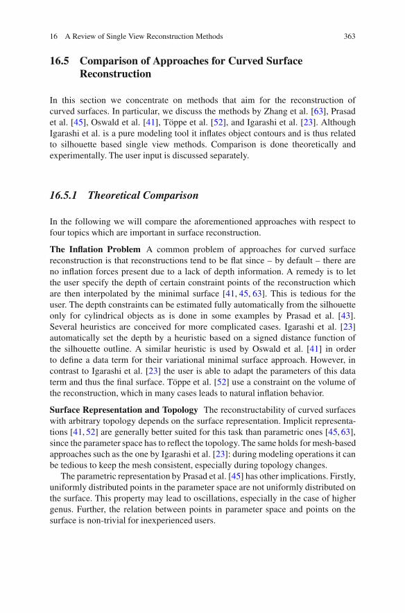
16 A Review of Single View Reconstruction Methods 363
16.5 Comparison of Approaches for Curved SurfaceReconstruction
In this section we concentrate on methods that aim for the reconstruction ofcurved surfaces. In particular, we discuss the methods by Zhang et al. [63], Prasadet al. [45], Oswald et al. [41], Toppe et al. [52], and Igarashi et al. [23]. AlthoughIgarashi et al. is a pure modeling tool it inflates object contours and is thus relatedto silhouette based single view methods. Comparison is done theoretically andexperimentally. The user input is discussed separately.
16.5.1 Theoretical Comparison
In the following we will compare the aforementioned approaches with respect tofour topics which are important in surface reconstruction.
The Inflation Problem A common problem of approaches for curved surfacereconstruction is that reconstructions tend to be flat since – by default – there areno inflation forces present due to a lack of depth information. A remedy is to letthe user specify the depth of certain constraint points of the reconstruction whichare then interpolated by the minimal surface [41, 45, 63]. This is tedious for theuser. The depth constraints can be estimated fully automatically from the silhouetteonly for cylindrical objects as is done in some examples by Prasad et al. [43].Several heuristics are conceived for more complicated cases. Igarashi et al. [23]automatically set the depth by a heuristic based on a signed distance function ofthe silhouette outline. A similar heuristic is used by Oswald et al. [41] in orderto define a data term for their variational minimal surface approach. However, incontrast to Igarashi et al. [23] the user is able to adapt the parameters of this dataterm and thus the final surface. Toppe et al. [52] use a constraint on the volume ofthe reconstruction, which in many cases leads to natural inflation behavior.
Surface Representation and Topology The reconstructability of curved surfaceswith arbitrary topology depends on the surface representation. Implicit representa-tions [41, 52] are generally better suited for this task than parametric ones [45, 63],since the parameter space has to reflect the topology. The same holds for mesh-basedapproaches such as the one by Igarashi et al. [23]: during modeling operations it canbe tedious to keep the mesh consistent, especially during topology changes.
The parametric representation by Prasad et al. [45] has other implications. Firstly,uniformly distributed points in the parameter space are not uniformly distributed onthe surface. This property may lead to oscillations, especially in the case of highergenus. Further, the relation between points in parameter space and points on thesurface is non-trivial for inexperienced users.
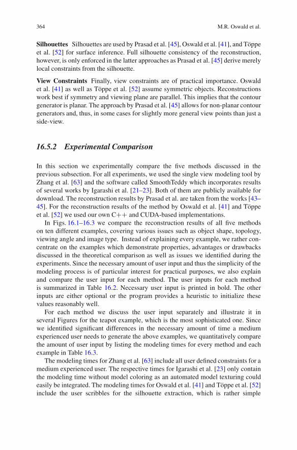
364 M.R. Oswald et al.
Silhouettes Silhouettes are used by Prasad et al. [45], Oswald et al. [41], and Toppeet al. [52] for surface inference. Full silhouette consistency of the reconstruction,however, is only enforced in the latter approaches as Prasad et al. [45] derive merelylocal constraints from the silhouette.
View Constraints Finally, view constraints are of practical importance. Oswaldet al. [41] as well as Toppe et al. [52] assume symmetric objects. Reconstructionswork best if symmetry and viewing plane are parallel. This implies that the contourgenerator is planar. The approach by Prasad et al. [45] allows for non-planar contourgenerators and, thus, in some cases for slightly more general view points than just aside-view.
16.5.2 Experimental Comparison
In this section we experimentally compare the five methods discussed in theprevious subsection. For all experiments, we used the single view modeling tool byZhang et al. [63] and the software called SmoothTeddy which incorporates resultsof several works by Igarashi et al. [21–23]. Both of them are publicly available fordownload. The reconstruction results by Prasad et al. are taken from the works [43–45]. For the reconstruction results of the method by Oswald et al. [41] and Toppeet al. [52] we used our own CCC and CUDA-based implementations.
In Figs. 16.1–16.3 we compare the reconstruction results of all five methodson ten different examples, covering various issues such as object shape, topology,viewing angle and image type. Instead of explaining every example, we rather con-centrate on the examples which demonstrate properties, advantages or drawbacksdiscussed in the theoretical comparison as well as issues we identified during theexperiments. Since the necessary amount of user input and thus the simplicity of themodeling process is of particular interest for practical purposes, we also explainand compare the user input for each method. The user inputs for each methodis summarized in Table 16.2. Necessary user input is printed in bold. The otherinputs are either optional or the program provides a heuristic to initialize thesevalues reasonably well.
For each method we discuss the user input separately and illustrate it inseveral Figures for the teapot example, which is the most sophisticated one. Sincewe identified significant differences in the necessary amount of time a mediumexperienced user needs to generate the above examples, we quantitatively comparethe amount of user input by listing the modeling times for every method and eachexample in Table 16.3.
The modeling times for Zhang et al. [63] include all user defined constraints for amedium experienced user. The respective times for Igarashi et al. [23] only containthe modeling time without model coloring as an automated model texturing couldeasily be integrated. The modeling times for Oswald et al. [41] and Toppe et al. [52]include the user scribbles for the silhouette extraction, which is rather simple
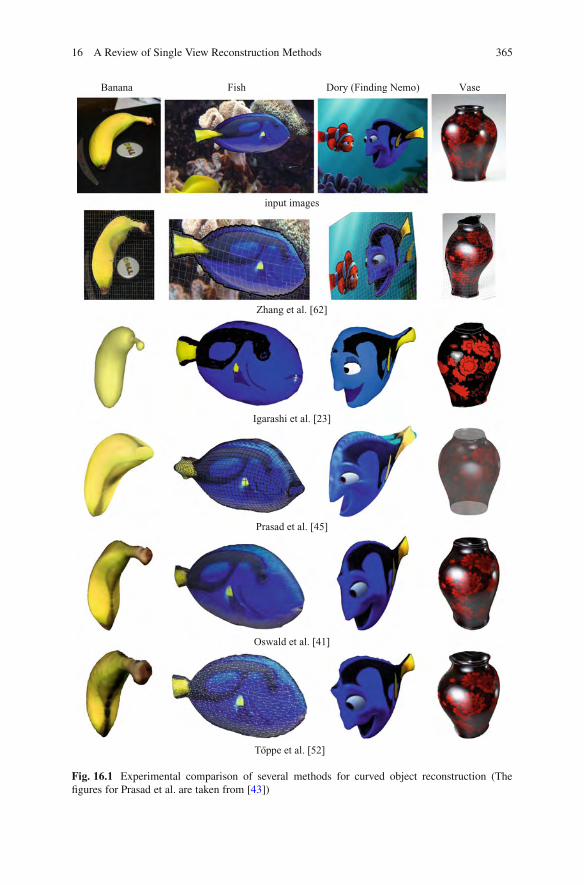
16 A Review of Single View Reconstruction Methods 365
Banana Fish Dory (Finding Nemo) Vase
input images
Zhang et al. [62]
Igarashi et al. [23]
Prasad et al. [45]
Oswald et al. [41]
Toppe et al. [52]
Fig. 16.1 Experimental comparison of several methods for curved object reconstruction (Thefigures for Prasad et al. are taken from [43])

366 M.R. Oswald et al.
Squash Orange Ostrich Donut
input images
Zhang et al. [62]
Igarashi et al. [23]
Prasad et al. [45]
Oswald et al. [41]
Toppe et al. [52]
Fig. 16.2 Continuation of Fig. 16.1: experimental comparison of several methods for curvedobject reconstruction (The figures for Prasad et al. are taken from [43])

16 A Review of Single View Reconstruction Methods 367
Jelly Bean Teapot Teapot Geometry
input images
Zhang et al. [62]
Igarashi et al. [23]
Prasad et al. [45]
Oswald et al. [41]
Toppe et al. [52]
Fig. 16.3 Continuation of Fig. 16.2: experimental comparison of several methods for curvedobject reconstruction (The figures for Prasad et al. are taken from [43])

368 M.R. Oswald et al.
Table 16.2 Necessary (bold) and optional user inputs and modeling steps for several methods incomparison. Optional user inputs are still required algorithm inputs but they can be predefined bydefault values or simple heuristics and later on changed by the user if desired. Note that the varietyof user input shown in this table does not reflect the amount or complexity of the input that isnecessary for a reconstruction
Method User input (optional and required)Zhanget al. [63]
• Depth map dimensions• Normal/position constraints• Discontinuity lines (position/normal discontinuity)• Planar region constraint• Curvature/torsion minimizing fairing curve constraints• Manual mesh-subdivision
Igarashiet al. [23]
• Rough contour lines• Union or cut operations between objects• Object coloring
Prasadet al. [45]
• Mesh resolution• Silhouette extraction• Define corresponding parameter space boundaries (defines topology)• Assign parts of the contour to lines in the parameter space• Choose inflation heuristic (cylindrical, cylindrical by parts, distance transform,
approximation constraints) C further inflation input• Spillage correction (correct silhouette consistency violated through optimization)• Surface creases
Oswaldet al. [41]
• Volume dimensions• Silhouette extraction• Define data term shape interactively (4 parameters)• Surface creases
Toppeet al. [52]
• Volume dimensions• Silhouette extraction• Define target volume interactively• Surface creases
Table 16.3 Approximate modeling times for all five methods and all examples in Figs. 16.1–16.3 for a medium experienced user. Considering the very similar reconstruction results, this tablereveals significant differences for the time of their modeling
Zhang Igarashi Prasad Oswald ToppeExample et al. [63] et al. [23] et al. [45] et al. [41] et al. [52]Banana 20 min <1 min 10 min 5 min <1 minFish 15 min <1 min 2 min 8 min 1 minDory 40 min <1 min 5 min 7 min 1 minVase 20 min <1 min 2 min 13 min 4 minSquash 12 min <1 min 2 min 2 min 1 minOrange 14 min <1 min <1 min 3 min <1 minOstrich 30 min <1 min 15 min 7 min 2 minDonut 55 min <1 min 10 min 3 min 1 minJelly Bean 15 min <1 min 2 min 4 min 1 minTeapot 35 min <1 min 20 min 15 min 4 min
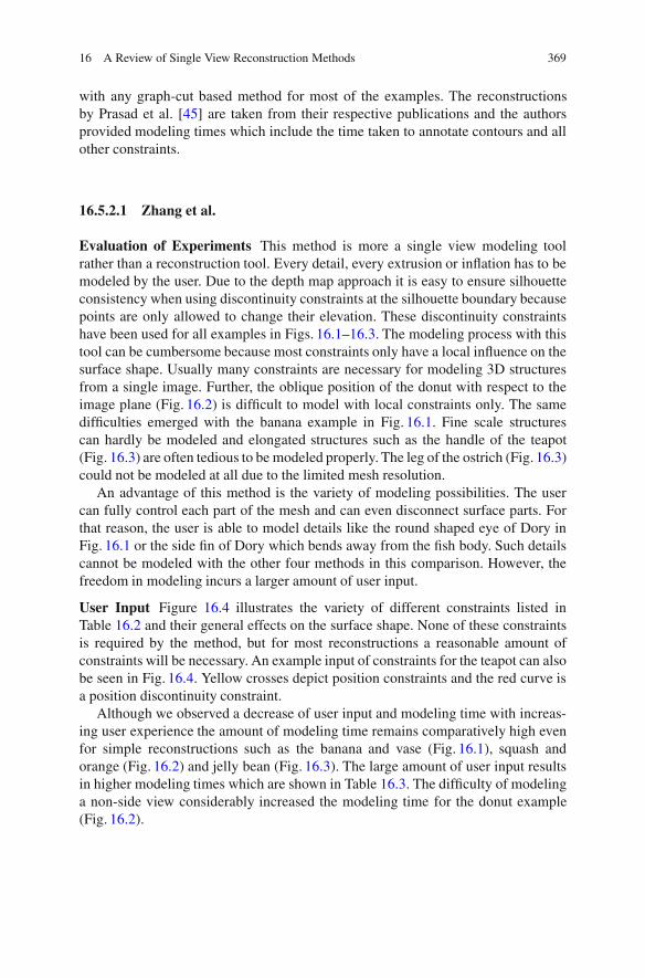
16 A Review of Single View Reconstruction Methods 369
with any graph-cut based method for most of the examples. The reconstructionsby Prasad et al. [45] are taken from their respective publications and the authorsprovided modeling times which include the time taken to annotate contours and allother constraints.
16.5.2.1 Zhang et al.
Evaluation of Experiments This method is more a single view modeling toolrather than a reconstruction tool. Every detail, every extrusion or inflation has to bemodeled by the user. Due to the depth map approach it is easy to ensure silhouetteconsistency when using discontinuity constraints at the silhouette boundary becausepoints are only allowed to change their elevation. These discontinuity constraintshave been used for all examples in Figs. 16.1–16.3. The modeling process with thistool can be cumbersome because most constraints only have a local influence on thesurface shape. Usually many constraints are necessary for modeling 3D structuresfrom a single image. Further, the oblique position of the donut with respect to theimage plane (Fig. 16.2) is difficult to model with local constraints only. The samedifficulties emerged with the banana example in Fig. 16.1. Fine scale structurescan hardly be modeled and elongated structures such as the handle of the teapot(Fig. 16.3) are often tedious to be modeled properly. The leg of the ostrich (Fig. 16.3)could not be modeled at all due to the limited mesh resolution.
An advantage of this method is the variety of modeling possibilities. The usercan fully control each part of the mesh and can even disconnect surface parts. Forthat reason, the user is able to model details like the round shaped eye of Dory inFig. 16.1 or the side fin of Dory which bends away from the fish body. Such detailscannot be modeled with the other four methods in this comparison. However, thefreedom in modeling incurs a larger amount of user input.
User Input Figure 16.4 illustrates the variety of different constraints listed inTable 16.2 and their general effects on the surface shape. None of these constraintsis required by the method, but for most reconstructions a reasonable amount ofconstraints will be necessary. An example input of constraints for the teapot can alsobe seen in Fig. 16.4. Yellow crosses depict position constraints and the red curve isa position discontinuity constraint.
Although we observed a decrease of user input and modeling time with increas-ing user experience the amount of modeling time remains comparatively high evenfor simple reconstructions such as the banana and vase (Fig. 16.1), squash andorange (Fig. 16.2) and jelly bean (Fig. 16.3). The large amount of user input resultsin higher modeling times which are shown in Table 16.3. The difficulty of modelinga non-side view considerably increased the modeling time for the donut example(Fig. 16.2).

370 M.R. Oswald et al.
general effect of constraints constraints for teapot
Zhang et al. [62]
contour outline
model coloring
Igarashi et al. [23]
a b c
f
ed
Fig. 16.4 User input for the methods of Zhang et al. [63] and Igarashi et al. [23]. The first imageshows general effects of different constraints and is taken from [63]. In particular, the constraintsare: (a) position (blue) and normal (red) constraints, (b) depth discontinuity constraint, (c) creaseconstraint, (d) planar region constraint, (e) curvature minimizing fairing curve and (f) torsionminimizing fairing curve (see [63] for further details)
16.5.2.2 Igarashi et al.
Evaluation of Experiments This method generally over-smoothes the input sil-houette which can be seen in many examples but especially at the peak of thebird in the ostrich example in Fig. 16.2. Although part of the input silhouette theleg of the ostrich is totally missing. Similarly, the grip of teapot lid in Fig. 16.3is not reconstructed although it is part of the input silhouette which is shown inFig. 16.4 (top right). Consequently, the reconstructions resulting from this methodare not silhouette consistent. Further, the mesh generation in this approach is notstraightforward and may lead to mesh inconsistencies which can be observed in thereconstruction of the ostrich example in the lower neck area (Fig. 16.2).
The main advantage of this approach is the fast and intuitive modeling ofgeometrically simple objects. One of the drawbacks is the restricted topology,the hole in the donut example in Fig. 16.2 cannot be reconstructed. A furtherdisadvantage is the limited influence of the user during the modeling process. Thefact that surface discontinuities like sharp edges are not allowed largely decreasesthe class of reconstructable objects. For instance, the tail fin of Dory in Fig. 16.1cannot be modeled to end with a sharp edge. The same holds for the top andbottom parts of the vase example in the same figure and for the bottom part of theteapot in Fig. 16.3. Only very simple roundish objects like the banana (Fig. 16.1),squash and orange (Fig. 16.2) or the jelly bean (Fig. 16.3) can be easily and reliablyreconstructed.
User Input None of the user input in Table 16.2 needs much experience or evenexpert knowledge: From a given closed contour line the method instantly inflates a3D mesh. For better user experience the user interface of the tool provides simple

16 A Review of Single View Reconstruction Methods 371
paint operations to color the model. See Fig. 16.4 for the exemplary user inputof the teapot example. In all experiments this method needed the least user input(cf. Table 16.3) at the price of producing the least accurate reconstructions withrespect to the given input silhouette (see Figs. 16.1–16.3).
16.5.2.3 Prasad et al.
Evaluation of Experiments The main benefit of this method stems from a fewextensions over the method by Zhang et al. [63] which facilitate the object inflationand allow the reconstruction of closed surfaces. Apart from the silhouette outlinethe user can assign any contour line to a line in the parameter space. For instance,this has been used to relate a contour edge of the banana (Fig. 16.1) to a crease inthe reconstructed geometry (see [45] for further details).
For closed surfaces a correspondence of parameter space boundaries has to bedefined. One the one hand, this facilitates the reconstruction of objects with a simplegeometry such as the orange example in Fig. 16.2 or the jelly bean in Fig. 16.3.The orange and the jelly bean get naturally inflated only be defining the silhouettecontour and the correspondence of parameter space boundaries. On the other hand,the definition of the parametrization can be sophisticated for objects of higher genussuch as in the teapot example (Fig. 16.3) which has genus 2. However, not only theobject topology limits the applicability of this method: it is also difficult to definea proper parametrization for objects which have many elongated structures such aslegs, arms, tails or spikes. A limiting example may be the ostrich in Fig. 16.2 whichis parametrized as a cylinder starting from the peak, going through the neck down tothe leg. The body of the ostrich is modeled as a ‘bump’ in this cylinder which alreadyleads to very sparsely sampled regions at the back of the ostrich. A further modelingof the tail feathers is done with the other methods would need an enormous increaseof the mesh resolution in the tail part of the ostrich in order to have enough quadsthat can align to the silhouette. Thus, finding a good parametrization is a demandingtask despite a simple object genus of 0 as for example when modeling a cow with4 legs and a tail. Moreover, an undesired effect of such a parametrization is the non-uniform distribution of points in the parameter space on the surface as shown in theostrich (Fig. 16.2) and teapot (Fig. 16.3) examples. Together with further constraintsthis may lead to non-controllable surface oscillations of the object surface. This canbe observed in the top part of the teapot which is connected to the teapot handle(Fig. 16.3).
Another disadvantage is the fact that silhouette consistency is only incorporatedwith boundary conditions which may get violated during the optimization process.The user may need to add further constraints to ensure a silhouette consistent recon-struction. This process is called spillage correction in Table 16.2 and Fig. 16.5f.Nonetheless, this method generated the most accurate results for the non-side-viewexamples (banana and teapot).
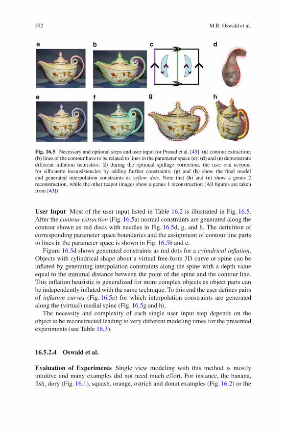
372 M.R. Oswald et al.
a b c d
e f g h
Fig. 16.5 Necessary and optional steps and user input for Prasad et al. [45]: (a) contour extraction;(b) lines of the contour have to be related to lines in the parameter space (c); (d) and (e) demonstratedifferent inflation heuristics; (f) during the optional spillage correction, the user can accountfor silhouette inconsistencies by adding further constraints; (g) and (h) show the final modeland generated interpolation constraints as yellow dots. Note that (b) and (c) show a genus 2reconstruction, while the other teapot images show a genus 1 reconstruction (All figures are takenfrom [43])
User Input Most of the user input listed in Table 16.2 is illustrated in Fig. 16.5.After the contour extraction (Fig. 16.5a) normal constraints are generated along thecontour shown as red discs with needles in Fig. 16.5d, g, and h. The definition ofcorresponding parameter space boundaries and the assignment of contour line partsto lines in the parameter space is shown in Fig. 16.5b and c.
Figure 16.5d shows generated constraints as red dots for a cylindrical inflation.Objects with cylindrical shape about a virtual free-form 3D curve or spine can beinflated by generating interpolation constraints along the spine with a depth valueequal to the minimal distance between the point of the spine and the contour line.This inflation heuristic is generalized for more complex objects as object parts canbe independently inflated with the same technique. To this end the user defines pairsof inflation curves (Fig. 16.5e) for which interpolation constraints are generatedalong the (virtual) medial spine (Fig. 16.5g and h).
The necessity and complexity of each single user input step depends on theobject to be reconstructed leading to very different modeling times for the presentedexperiments (see Table 16.3).
16.5.2.4 Oswald et al.
Evaluation of Experiments Single view modeling with this method is mostlyintuitive and many examples did not need much effort. For instance, the banana,fish, dory (Fig. 16.1), squash, orange, ostrich and donut examples (Fig. 16.2) or the
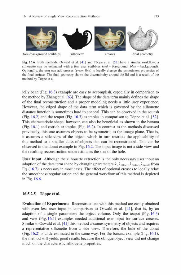
16 A Review of Single View Reconstruction Methods 373
fore-/background scribbles silhouette creases final geometry
Fig. 16.6 Both methods, Oswald et al. [41] and Toppe et al. [52] have a similar workflow: asilhouette can be estimated with a few user scribbles (redD foreground, blueD background).Optionally, the user can add creases (green line) to locally change the smoothness properties ofthe final surface. The final geometry shows the discontinuity around the lid and is a result of themethod by Toppe et al.
jelly bean (Fig. 16.3) example are easy to accomplish, especially in comparison tothe method by Zhang et al. [63]. The shape of the data term mainly defines the shapeof the final reconstruction and a proper modeling needs a little user experience.However, the edged shape of the data term which is governed by the silhouettedistance function is sometimes hard to conceal. This can be observed in the squash(Fig. 16.2) and the teapot (Fig. 16.3) examples in comparison to Toppe et al. [52].This characteristic shape, however, can also be beneficial as shown in the banana(Fig. 16.1) and ostrich examples (Fig. 16.2). In contrast to the methods discussedpreviously, this one assumes objects to be symmetric to the image plane. That is,it assumes a side view of the object, which in turn restricts the applicability ofthis method to a smaller class of objects that can be reconstructed. This can beobserved in the donut example in Fig. 16.2. The input image is not a side view andthe resulting reconstruction underestimates the size of the hole.
User Input Although the silhouette extraction is the only necessary user input anadaption of the data term shape by changing parameters k;%offset;%factor;%cutoff fromEq. (16.7) is necessary in most cases. The effect of optional creases to locally relaxthe smoothness regularization and the general workflow of this method is depictedin Fig. 16.6.
16.5.2.5 Toppe et al.
Evaluation of Experiments Reconstructions with this method are easily obtainedwith even less user input in comparison to Oswald et al. [41], that is, by anadaption of a single parameter: the object volume. Only the teapot (Fig. 16.3)and vase (Fig. 16.1) examples needed additional user input for surface creases.Similar to Oswald et al. [41] this method assumes symmetry of objects and requiresa representative silhouette from a side view. Therefore, the hole of the donut(Fig. 16.2) is underestimated in the same way. For the banana example (Fig. 16.1),the method still yields good results because the oblique object view did not changemuch on the characteristic silhouette properties.

374 M.R. Oswald et al.
Table 16.4 Overview of advantages and disadvantages for each method. Note that the number ofadvantages and disadvantages is not important in this listing since each point weights differentlydepending on the desired application of each method
Method Advantages (C) and disadvantages (#)Zhang C Large variety of constraints allows for flexible user modelinget al. [63] C User has full control of every surface detail
# Reconstructions are restricted to a depth map# Occluded object parts cannot be modeled,
synthesized views from different angles will reveal those areas# Large amount of user input is often necessary
Igarashi C Very easy to use and fast interactive modelinget al. [23] # Over-smoothes the input silhouette
# Smoothness properties cannot be changed by the user# Not silhouette consistent# Topology is limited to genus 0
Prasad C Objects can also be modeled from oblique view pointset al. [45] C Apart from the silhouette the user can also use contour edges for modeling
# Parametric surface representation limits topology andobject shape (many long elongated structures are difficult to model)# Higher complexity of user input (requires expert knowledge)# Silhouette consistency is not guaranteed and may require additional user input
Oswald CModerately fast modelinget al. [41] C Reconstructions are silhouette consistent
# Objects need to be symmetric, a side view is required
Toppe C Fast modelinget al. [52] C Very little user input
C Reconstructions are silhouette consistent# Objects need to be symmetric, a side view is required# User can barely influence the surface shape# Limited possibilities to add surface creases
User Input Similar to Oswald et al. [41] the object silhouette is the only necessaryuser input (see also Fig. 16.6). Apart from the silhouette the object shape is mainlydefined by the adapting the object volume. Also similar to Oswald et al. [41] surfacecreases can be added to create non-smooth surface parts. However, changing thesmoothness locally may behave differently at different locations within the objectsilhouette, because there is no data term that governs the object shape in non-smoothsurface areas. In these areas the surface shape is more defined by the distribution ofvolume which minimizes the overall surface area for given smoothness properties.
16.5.2.6 Summary
The theoretical and experimental comparison of the five methods for curved objectreconstruction identified several advantages and disadvantages of the presentedapproaches which are listed in Table 16.4. In general, the performance of a method
16 A Review of Single View Reconstruction Methods 375
highly depends on the application. Each method has its strengths and weaknesseswhen applied to a specific class of single view reconstruction problems.
The results of our experiments support the hypothesis that generality andflexibility of a reconstruction method is traded for the amount of user input orexpert knowledge. Expert knowledge refers to the variety or complexity of the userinput. The flexibility of modeling fine details with the method by Zhang et al. [63]either requires the user to know and understand a variety of modeling constraintsor it needs a large amount of user input. On the other hand, the method by Prasadet al. [45] needs less user input, but increases its complexity such as the definitionof a suitable surface parametrization. The comparatively simple and small amountof user input for the methods by Igarashi et al. [23], Oswald et al. [41], and Toppeet al. [52] comes along with the limited generality and flexibility of these methods.
16.6 Conclusion
Single view reconstruction approaches infer the structure of 3D objects from 2Dimages. In this chapter, we discussed a representative set of existing algorithms andgrouped them into four classes: curved objects, piecewise planar objects, learningspecific objects and 3D impression from scenes. These groupings are based on thedifferent reconstruction objectives of the algorithms. We identified several importantcategories for comparing the approaches: the reconstruction precision, the 3D objectrepresentation, the assumptions made by the algorithm, the required user interaction,as well as image cues and priors used by the algorithms. Moreover, we haveconcentrated on five methods aiming for curved object reconstruction and providedan extensive experimental comparison of established and recent methods.
Acknowledgements We thank Li Zhang and Steve Seitz for sharing their data and providing theirsingle view modeling tool. Further, we are grateful to Mukta Prasad and co-authors for providingtest data and results of their single view reconstruction method.
References
1. Bae, S., Durand, F.: Defocus magnification. In: Proceedings of the Eurographics. Blackwell,Oxford (2007)
2. Barinova, O., Konushin, V., Yakubenko, A., Lee, K., Lim, H., Konushin, A.: Fast automaticsingle-view 3-d reconstruction of urban scenes. In: Proceedings of the European Conferenceon Computer Vision, pp. 100–113. Springer, Berlin/Heidelberg (2008)
3. Botsch, M., Kobbelt, L.: An intuitive framework for real-time freeform modeling. In: ACMTransactions on Graphics (Proc. SIGGRAPH), vol. 23, pp. 630–634. ACM/Addison-WesleyPublishing Co., New York (2004)
4. Chen, Y., Cipolla, R.: Single and sparse view 3d reconstruction by learning shape priors.Comput. Vis. Image Underst. 115, 586–602 (2011)
376 M.R. Oswald et al.
5. Cohen, L.D., Cohen, I.: Finite-element methods for active contour models and balloons for 2-dand 3-d images. IEEE Trans. Pattern Anal. Mach. Intell. 15(11), 1131–1147 (1993)
6. Colombo, C., Del Bimbo, A., Pernici, F.: Metric 3d reconstruction and texture acquisition ofsurfaces of revolution from a single uncalibrated view. IEEE Trans. Pattern Anal. Mach. Intell.27, 99–114 (2005)
7. Courteille, F., Crouzil, A., Durou, J.-D., Gurdjos, P.: Towards shape from shading underrealistic photographic conditions. pp. 277–280 (2004)
8. Criminisi, A., Reid, I., Zisserman, A.: Single view metrology. Int. J. Comput. Vis. 40(2),123–148 (2000)
9. Daum, M., Dudek, G.: On 3-d surface reconstruction using shape from shadows. In: Pro-ceedings of the International Conference on Computer Vision and Pattern Recognition, SantaBarbara, CA, USA, pp. 461–468 (1998)
10. Delage, E., Lee, H., Ng, A.Y.: Automatic single-image 3d reconstructions of indoor Manhattanworld scenes (2005)
11. Duchon, J.: Splines Minimizing Rotation-Invariant Semi-norms in Sobolev Spaces. In:Schempp, W., Zeller, K. (eds.) Constructive Theory of Functions of Several Variables,vol. 571/1977, pp. 85–100. Springer, Berlin (1977)
12. Durou, J.-D., Falcone, M., Sagona, M.: Numerical methods for shape-from-shading: a newsurvey with benchmarks. Comput. Vis. Image Underst. 109, 22–43 (2008)
13. Francois, A.R.J., Medioni, G.G.: Interactive 3d model extraction from a single image. ImageVis. Comput. 19(6), 317–328 (2001)
14. Han, F., Zhu, S.-C.: Bayesian reconstruction of 3d shapes and scenes from a single image.In: Proceedings of the Higher-Level Knowledge in 3D Modeling and Motion Analysis, Nice,France, pp. 12–20. (2003)
15. Hassner, T., Basri, R.: Example based 3d reconstruction from single 2d images. In: BeyondPatches Workshop at IEEE Conference on Computer Vision and Pattern Recognition, NewYork, NY, USA, p. 15. (2006)
16. Hatzitheodorou, M.: The derivation of 3-d surface shape from shadows. In: Proceedingsof a Workshop on Image Understanding Workshop, pp. 1012–1020. Morgan Kaufmann, SanFrancisco (1989)
17. Hoiem, D., Efros, A.A., Hebert, M.: Automatic photo pop-up. ACM Trans. Graph. 24(3),577–584 (2005)
18. Hong, W., Yang, A.-Y., Huang, K., Ma, Y.: On symmetry and multiple-view geometry:structure, pose, and calibration from a single image. Int. J. Comput. Vis. 60, 241–265 (2004).doi:10.1023/B:VISI.0000036837.76476.10
19. Horaud, R.P., Brady, M.: On the geometric interpretation of image contours. Artif. Intell.37(1–3), 333–353 (1988). Special Issue on Geometric Reasoning
20. Horry, Y., Anjyo, K.-I., Arai, K.: Tour into the picture: using a spidery mesh interface tomake animation from a single image. In: SIGGRAPH ’97: Proceedings of the 24th AnnualConference on Computer Graphics and Interactive Techniques, pp. 225–232. ACM/Addison-Wesley, New York (1997)
21. Igarashi, T.: Adaptive unwrapping for interactive texture painting. In: Proceedings of the ACMSymposium on Interactive 3D Graphics, pp. 209–216. ACM, New York (2001)
22. Igarashi, T.: Smooth meshes for sketch-based freeform modeling. In: Proceedings of the 2003Symposium on Interactive 3D Graphics, pp. 139–142. ACM, New York (2003)
23. Igarashi, T., Matsuoka, S., Tanaka, H.: Teddy: a sketching interface for 3d freeformdesign. In: ACM Transactions on Graphics (Proceedings of the SIGGRAPH), pp. 409–416.ACM/Addison-Wesley, New York (1999)
24. Ikeuchi, K., Horn, B.K.P.: Numerical shape from shading and occluding boundaries. Artif.Intell. 17, 141–185 (1981)
25. Joshi, P., Carr, N.: Repousse: automatic inflation of 2d art. In: Proceedings of the EurographicsWorkshop on Sketch-Based Modeling, Annecy, France (2008)
26. Kanade, T.: Recovery of the three-dimensional shape of an object from a single view. Artif.Intell. 17, 409–460 (1981)

16 A Review of Single View Reconstruction Methods 377
27. Karpenko, O.A., Hughes, J.F.: Smoothsketch: 3d free-form shapes from complex sketches.ACM Trans. Graph. 25(3), 589–598 (2006)
28. Karpenko, O., Hughes, J.F., Raskar, R.: Free-form sketching with variational implicit surfaces.Comput. Graph. Forum 21(3), 585–594 (2002)
29. Kender, J., Smith, E.: Shape from darkness. In: Proceedings of the International Conferenceon Computer Vision, London, pp. 539–546 (1987)
30. Koutsourakis, P., Simon, L., Teboul, O., Tziritas, G., Paragios, N.: Single view reconstructionusing shape grammars for urban environments. In: Proceedings of the International Conferenceon Computer Vision, Kyoto. IEEE (2009)
31. Kushal, A.M., Sanyal, S., Bansal, V., Banerjee, S.: A simple method for interactive 3dreconstruction and camera calibration from a single view. In: Proceedings Indian Conferencein Computer Vision, Graphics and Image Processing, Ahmedabad, India (2002)
32. Levin, A.: Analyzing depth from coded aperture sets. In: Proceedings of the EuropeanConference on Computer Vision, pp. 214–227. Springer, Berlin (2010)
33. Li, Y., Pizlo, Z., Steinman, R.M.: A computational model that recovers the 3d shape of anobject from a single 2d retinal representation. Vis. Res. 49, 979–991 (2009)
34. Li, Z., Liu, J., Tang, X.: A closed-form solution to 3d reconstruction of piecewise planar objectsfrom single images. In: Proceedings of the International Conference on Computer Vision andPattern Recognition, Minneapolis, MN, USA, pp. 1–6 (2007)
35. Liebowitz, D., Criminisi, A., Zisserman, A.: Creating architectural models from images. In:Proceedings of the EuroGraphics, vol. 18, pp. 39–50 (1999)
36. Lowe, D.G.: Three-dimensional object recognition from single two-dimensional images. Artif.Intell. 31, 355–395 (1987)
37. Malik, J., Rosenholtz, R.: Computing local surface orientation and shape from texture forcurved surfaces. Int. J. Comput. Vis. 23(2), 149–168 (1997)
38. Nagai, T., Naruse, T., Ikehara, M., Kurematsu, A.: Hmm-based surface reconstructionfrom single images. In: Proceedings of the International Conference on Image Processing,Rochester, NY, USA, vol. 2, pp. II–561–II–564 (2002)
39. Nayar, S.K., Ikeuchi, K., Kanade, T.: Shape from interreflections. In: Proceedings of theInternational Conference on Computer Vision, Osaka, Japan, pp. 2–11 (1990)
40. Nealen, A., Igarashi, T., Sorkine, O., Alexa, M.: Fibermesh: designing freeform surfaces with3d curves. ACM Trans. Graph. 26(3), 41 (2007)
41. Oswald, M.R., Toppe, E., Kolev, K., Cremers, D.: Non-parametric single view reconstructionof curved objects using convex optimization. In: Pattern Recognition (Proceedings of theDAGM), Jena (2009)
42. Prados, E., Faugeras, O.: Shape from shading: a well-posed problem? In: Proceedings of theInternational Conference on Computer Vision and Pattern Recognition, vol. 2, pp. 870–877.IEEE, San Diego/Etats-Unis (2005)
43. Prasad, M.: Class-based single view reconstruction. Ph.D. thesis, University of Oxford (2009)44. Prasad, M., Zisserman, A., Fitzgibbon, A.W.: Fast and controllable 3D modelling from
silhouettes. In: Eurographics, Short Papers, pp. 9–12 (2005)45. Prasad, M., Zisserman, A., Fitzgibbon, A.W.: Single view reconstruction of curved surfaces.
In: Proceedings of the International Conference on Computer Vision and Pattern Recognition,New York, pp. 1345–1354 (2006)
46. Rother, D., Sapiro, G.: Seeing 3d objects in a single 2d image. In: Proceedings of theInternational Conference on Computer Vision, Kyoto, pp. 1819–1826 (2009)
47. Saxena, A., Chung, S.H., Ng, A.Y.: 3-d depth reconstruction from a single still image. Int. J.Comput. Vis. 76, 53–69 (2007)
48. Saxena, A., Sun, M., Ng, A.Y.: Make3d: learning 3d scene structure from a single still image.IEEE Trans. Pattern Anal. Mach. Intell. 31(5), 824–840 (2009)
49. Sturm, P.F., Maybank, S.J.: A method for interactive 3d reconstruction of piecewise planarobjects from single images. In: Proceedings of the BMVC, pp. 265–274. British MachineVision Association, England (1999)
378 M.R. Oswald et al.
50. Super, B.J., Bovik, A.C.: Shape from texture using local spectral moments. IEEE Trans. PatternAnal. Mach. Intell. 17, 333–343 (1995)
51. Terzopoulos, D., Witkin, A., Kass, M.: Symmetry-seeking models and 3d object reconstruc-tion. Int. J. Comput. Vis. 1, 211–221 (1987)
52. Toppe, E., Oswald, M.R., Cremers, D., Rother, C.: Image-based 3d modeling via cheeger sets.In: Proceedings of the Asian Conference on Computer Vision, Queenstown (2010)
53. Ulupinar, F., Nevatia, R.: Shape from contour: straight homogeneous generalized cylindersand constant cross section generalized cylinders. IEEE Trans. Pattern Anal. Mach. Intell. 17,120–135 (1995)
54. Utcke, S., Zisserman, A.: Projective reconstruction of surfaces of revolution. In: PatternRecognition (Proceedings of the DAGM), pp. 93–102. Springer, Berlin/New York (2003)
55. Vetter, T.: Synthesis of novel views from a single face image. Int. J. Comput. Vis. 28, 103(1998)
56. Wang, G., Su, W., Song, Y.: A new shape from shading approach for specular surfaces. In:Proceedings of the Third International Conference on Artificial Intelligence and ComputationalIntelligence – Volume Part III. Lecture Notes in Computer Science, pp. 71–78. Springer,Berlin/Heidelberg (2011)
57. Welch, W., Witkin, A.P.: Free-form shape design using triangulated surfaces. In: ACMTransactions on Graphics (Proceedings of the SIGGRAPH), pp. 247–256 (1994)
58. Williams, L.: 3d paint. In: Proceedings of the 1990 Symposium on Interactive 3D Graphics,Snowbird, pp. 225–233 (1990)
59. Wong, K.-Y.K., Mendonca, P.R.S., Cipolla, R.: Reconstruction of surfaces of revolution fromsingle uncalibrated views. In: Proceedings of the British Machine Vision Conference, Cardiff,pp. 265–272 (2002)
60. Yu, Y., Chang, J.: Shadow graphs and surface reconstruction. In: Proceedings of the EuropeanConference on Computer Vision, Copenhagen, pp. 31–45 (2002)
61. Zeleznik, R.C., Herndon, K.P., Hughes, J.F.: Sketch: an interface for sketching 3d scenes.In: ACM Transactions on Graphics (Proceedings of the SIGGRAPH), pp. 163–170. ACM,New York (1996)
62. Zhang, R., Tsai, P.-S., Cryer, J.E., Shah, M.: Shape from shading: a survey. IEEE Trans. PatternAnal. Mach. Intell. 21(8), 690–706 (1999)
63. Zhang, L., Dugas-Phocion, G., Samson, J.-S., Seitz, S.M.: Single view modeling of free-form scenes. In: Proceedings of the International Conference on Computer Vision and PatternRecognition, Kauai, HI USA, pp. 990–997 (2001)
Chapter 17On Globally Optimal Local Modeling: FromMoving Least Squares to Over-parametrization
Shachar Shem-Tov, Guy Rosman, Gilad Adiv, Ron Kimmel,and Alfred M. Bruckstein
Abstract This paper discusses a variational methodology, which involves locallymodeling of data from noisy samples, combined with global model parameterregularization. We show that this methodology encompasses many previouslyproposed algorithms, from the celebrated moving least squares methods to theglobally optimal over-parametrization methods recently published for smoothingand optic flow estimation. However, the unified look at the range of problems andmethods previously considered also suggests a wealth of novel global functionalsand local modeling possibilities. Specifically, we show that a new non-localvariational functional provided by this methodology greatly improves robustnessand accuracy in local model recovery compared to previous methods. The proposedmethodology may be viewed as a basis for a general framework for addressing avariety of common problem domains in signal and image processing and analysis,such as denoising, adaptive smoothing, reconstruction and segmentation.
17.1 Introduction
A fundamental problem in both image and signal processing is that of recovering afunction, a curve or a surface (i.e., a signal or an image) from its noisy and distortedsamples. Significant research effort was invested in this problem and the resultsobtained so far are quite remarkable. The most important ingredient in the success ofany method that extracts signals from noise is, of course, the set of assumptions that
S. Shem-Tov (!) ! G. Rosman ! R. Kimmel ! A.M. BrucksteinTechnion - Israel Institute of Technology, 2000, Haifa, Israele-mail: [email protected]; [email protected]; [email protected];[email protected]
G. AdivRafael, Haifa, Israele-mail: [email protected]
M. Breuß et al. (eds.), Innovations for Shape Analysis, Mathematics and Visualization,DOI 10.1007/978-3-642-34141-0 17, © Springer-Verlag Berlin Heidelberg 2013
379
380 S. Shem-Tov et al.
summarizes our prior knowledge about the properties of the signal that effectivelydifferentiates it from the noise. These assumptions range from some vague generalrequirements of smoothness on the signals, to quite detailed information on thestructure or functional form of the signals that might be available due to priorknowledge on their sources.
The prior information on signal/image is often expressed in the form of aparameterized model. For instance, in speech recognition [25] slowly varyingcoefficients of the short-time Fourier transform (STFT) are used to locally describeand model highly fluctuating spectral characteristics over time. In object recognitionthe choice of the correct spatial support for objects i.e., the segmentation, is afundamental issue [19], hence, in general scene understanding, support maps areused to represent segmentation of images into homogeneous chunks, enablingthe representation of objects as disjoint regions with different local modelingparameters [9]. This concept of spatial support selection for estimation problemsis closely related to layered models of scenes which offer significant benefits formotion estimation producing state of the art results [33]. In geometric modeling,B-splines (which are essentially a continuous set of piecewise polynomials), areused for local curve and surface approximation, interpolation and fitting fromnoisy samples [8]. In model-based texture segmentation [13], the selection of anappropriate support set for the local model, is important to obtain a good localtexture representation, which then serves as a basis for the segmentation process.In sparse coding [1, 23], the main goal is to model data vectors (signals) as a linearcombination of a few elements (support set) from a known dictionary. Sparse codinghas proven to be very effective for many signal or image processing tasks, as wellas advances in computer vision tasks such as object recognition.
One of the widespread and successful methods for local signal modeling, isthe celebrated moving least squares local fitting method (MLS), which in recentyears has evolved to become an important tool in both image and signal processingand in computational graphics. In [17], Levin explored the moving least-squaresmethod and applied it to scattered-data interpolation, smoothing and gradientapproximation. In [2, 4, 18] the moving least squares technique was employed formodeling surfaces from point-sampled data, and proved to be a powerful approach.This was followed by the work of Fleishman et al. [2, 11], incorporating robuststatistics mechanisms for outlier removal. Common to these works is the locality ofthe fitting procedure and the lack of global assumptions expressing prior knowledgeon the variations of local parameters.
The aim of this paper is to show how one can design variational functionals thatexploit local fitting of models and global smoothness assumptions on the variationsof model parameters, that are natural for various types of signals. A first attempt,at such a variational methodology, was made by Nir et al. [21, 22]. This work wassubsequently broadened and generalized by Bruckstein in [6], by the realizationthat over-parametrization methods naturally follow from combining moving leastsquares, or other local fitting methods, with global priors on parameter variations.The local modeling relates to a wealth of classical methods, such as Haralick’sand Watson’s facet model for images [14] and extends them in many ways.
17 On Globally Optimal Local Modeling 381
More importantly, the discussion and experimental results reported in this paperpoint at a rather general methodology for designing functionals for variationalmodel estimation and signal reconstruction and focusing on the denoising problemis merely an illustrative test case.
The importance of the proposed variational framework, lies in the fact thatit allows for directly incorporating knowledge of the problem domain, henceit is easily extendable to address numerous problem areas, such as denoising,deconvolution and optical flow in image and signal processing and various otherfields of research. Moreover, due to the structure of the proposed functionals, ourvariational framework is able, unlike many common methods, to accurately recoverthe underlying model of a signal while addressing its main aim.
17.2 The Local Modeling of Data
For the sake of simplicity, we shall here limit our discussion to one dimensionalsignals and address the generic problem of denoising. Let f .x/ be a one dimensionalsignal and fnoisy.x/ D f .x/ C n.x/ be it’s noisy counterpart. Also, denote by˚fj D f .xj /C n.xj /
!the set of samples of the noisy signal. Suppose that f can
be (locally) described by a parameterized model of the form
f .x/ DnX
iD1Ai!i .x/ (17.1)
where A D fAi gniD1 is a set of parameters, and ! D f!i gniD1 is a set of ‘basis’signals. Local modeling is the process of estimating A D fAi g from the noisysignal fnoisy or it’s samples
˚fj!, in the neighborhood of a point x. As a simple
example, we can consider the Taylor approximation as a parameterized model withpolynomial basis functions !i D xi"1.
Suppose we would like to use this local modeling for denoising our noisy datafnoisy.x/ or
˚fj!. Then, around x D x0, we want to estimate Ai.x0/, i.e., the
parameters of the model (17.1), by solving:
arg minŒA1;A2;:::;An"
"""""fnoisy.x0/!nX
iD1Ai!i .x0/
""""" ; (17.2)
in some local neighborhood of x0 and a distance norm k"k. This minimization givesus the best local estimate of Of .x0/
Of .x0/ DnX
iD1Ai .x0/!i .x0/: (17.3)
Repeating this process for every location x give us the “moving” best estimate of f .

382 S. Shem-Tov et al.
The choice of the distance or measure of error is of a great importance. Onecommon choice is the weighted least squares distance, as considered, for example,by Farneback [10], as a generalization to the facet model:
"""""fnoisy.x/!nX
iD1Ai .x/!i .x/
"""""w
DZ
fnoisy .y/!nX
iD1Ai .x/!i .y/
!2w .y ! x/ dy:
(17.4)
This is essentially a weighted L2 norm, where w."/ is a weight function whichlocalizes the estimation of the parameters Ai.x0/ (This error measure can also beapplied to a sampled signal). Both the continuous and the discrete cases, describedabove, yield a process to compute the local model parameters Ai.x/ and thereforefor estimating the signal Of .x/, not only at x0 but at all x. This process is the well-known moving least squares estimation process.
We wish to emphasize that although our proposed methodology, discussed in thenext section, focuses on the L2 norm, this is by no means the only choice of errormeasure. The choice of the error measure may be adapted to each particular problemof interest. Other measures, such as the least sum of absolute values distance [34]or L1 norm, can readily be substituted into the cost functionals.
17.3 Global Priors on Local Model Parameter Variations
In the previous discussion we did not impose any conditions on the modelparameters Ai , and in the definition of the neighborhood around x0, via the weightfunctions, we did not use any idea of adaptation to the data.
Suppose now that we are given some structural knowledge of the signal f .x/. Wewould like to use this knowledge to improve the estimation process. For example,suppose we a priori know that f .x/ is a piecewise polynomial signal over a set ofintervals, i.e., we know that:
f .x/ DnX
iD1Ari x
i"1 for x 2 Œxr ; xrC1" (17.5)
but we do not know the sequence of breakpoints fxr g. Using polynomial basisfunctions
#1; x; x2; : : : ; xn"1
$, we know a priori that a good estimate for f .x/ may
be provided by piecewise constant sets of parameters fAg, over Œxr ; xrC1" segments,and changes in the parameters occur only at the breakpoints fxrg. Such knowledgeprovides us the incentive to impose some global prior on the parameters, suchthat the minimum achieved by the optimization process, will indeed favor themto be piecewise constant. This may be achieved by supplementing the moving leastsquares local fitting process with constraints on the variations of the parameters inthe minimization process. Thus, we shall force the estimated parameters not only to

17 On Globally Optimal Local Modeling 383
provide the best weighted local fit to the data, but also to be consistent with the localfitting over adjacent neighborhoods. This is where we diverge and extend the facetmodel, which assigns the basis function’s parameters at each point, using solely alocal least square fit process.
In this paper, the assumed structural knowledge of the signal implies that goodestimates can be achieved by a piecewise constant model i.e., a model whoseparameters are piecewise constant. Therefore the focus of this work will be to designfunctionals which also impose global priors on the model parameters. We shalldemonstrate that one can design a functional that does indeed fulfil this requirement.
The mix of local fitting and global regularity is the main idea and power behindover-parameterized variational methods and is what makes them a versatile problemsolving tool. By adapting the local fitting process and incorporating the global prior(in a way that will be described in the following sections), this methodology can bereadily applied to address problems in various domains.
17.4 The Over-parameterized Functional
In [21] Nir and Bruckstein presented a first attempt at noise removal based on anover-parameterized functional. This functional was, similarly to many well knownfunctionals, a combination of two terms, as follows:
E .f;A/ D ED .f;A/C ˛ES .A/ : (17.6)
Here ˛, is some fixed relative weight parameter, ED is a data or fidelity term, andES is a regularization term. The data term ED was chosen to:
ED.f;A/ DZ
fnoisy.x/ !nX
iD1Ai .x/!i .x/
!2dx: (17.7)
Note that this functional implies a neighborhood of size 0 in the distance mea-sure (17.4), which means that this data term only penalizes for point-wise deviations
of the estimated signal vianPiD1
Ai.x/!i .x/ from fnoisy.
The smoothness or regularization term,ES , was defined to penalize variations ofthe parameters Ai as follows
ES.A/ DZ#
nX
iD1A0i .x/
2
!dx (17.8)
where #%s2&Dps2 C $2.

384 S. Shem-Tov et al.
The resulting functional yields a channel-coupled total variation (TV) regular-ization process for the estimation of the model parameters. Note that (17.8) is anapproximated L1 type of regularizer (sometimes referred to as the Charbonnierpenalty function). This regularizer causes the functional to be more robust tooutliers, and allows for smaller penalties for high data differences (compared toa quadratic regularizer), while maintaining convexity and continuity [5, 20]. Theregularization term was designed to impose the global prior on the parameters. Itis channel-coupled to “encourage” the parameters to change simultaneously, thuspreferring a piecewise constant solution as described in Sect. 17.3.
In our experiments (which are discussed in Sect. 17.7), as well as in [21] , thisfunctional displayed good performance for noise removal compared with RudinOsher and Fatemi’s [28] classical total variation noise removal functional. A similarfunctional, with data term modifications, was used by Nir et al. in [22] for opticalflow estimation, producing state of the art results.
17.4.1 The Over-parameterized Functional Weaknesses
Despite the good performance displayed by the over-parameterized functional,it still lacks with regard to the following shortcomings, that were clear in ourexperiments:
Discontinuities smearing: As mentioned, the regularization term is an approxi-mate L1 regularizer. A precise L1 regularizer is indifferent to the way signaldiscontinuities appear, i.e. the same penalty is given to a smooth gradual signalchange, and to sharp discontinuities (as long as the total signal difference isthe same). See for example Pock’s Ph.D. work [24] for a detailed example. Weconsider this property as a shortcoming, because we expect the reconstructedparameters to be piecewise constant, where discontinuities appear as relativelyfew and sharp changes, hence this regularizer does not convey the intended globalprior on the parameters, and does not prefer a “truly” piecewise constant solution.In practice the problem is even more severe: first the selection of $ constant, inthe Charbonnier penalty function, proves to be problematic. Choosing a bigger $value causes the functional to lose the ability to preserve sharp discontinuitiesand actually prefers to smooth out discontinuities. On the other hand, choosinga smaller $ value degenerates the penalty function. In fact, for any choiceof $, this penalty function will tend to smooth sharp discontinuities. Second,as discussed above the TV-L1 model suffers from the so called staircasingeffect, where smooth regions are recovered as piecewise constant staircases inthe reconstruction. See the work of Savage et al. [29] and references therein, fora detailed review of such effects.
Origin biasing: The over-parameterized functional’s global minimum maydepend on the selected origin of the model. In the over-parameterized
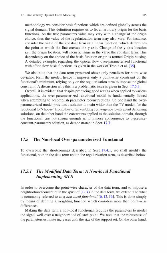
17 On Globally Optimal Local Modeling 385
methodology we consider basis functions which are defined globally across thesignal domain. This definition requires us to fix an arbitrary origin for the basisfunctions. As the true parameters value may vary with a change of the originchoice, thus the value of the regularization term may also vary. For instance,consider the value of the constant term in a linear function, which determinesthe point at which the line crosses the y-axis. Change of the y-axis locationi.e., the origin location, will incur achange in the value the constant term. Thisdependency on the choice of the basis function origin is termed Origin biasing.A detailed example, regarding the optical flow over-parameterized functionalwith affine flow basis functions, is given in the work of Trobin et al. [35].
We also note that the data term presented above only penalizes for point-wisedeviation form the model, hence it imposes only a point-wise constraint on thefunctional’s minimum, relying only on the regularization term to impose the globalconstraint. A discussion why this is a problematic issue is given in Sect. 17.5.3.
Overall, it is evident, that despite producing good results when applied to variousapplications, the over-parameterized functional model is fundamentally flawedwhen attempting to accomplish parameter reconstructions. On one hand the over-parameterized model provides a solution domain wider than the TV model, for thefunctional to “choose” from, thus often enabling convergence to excellent denoisingsolutions, on the other hand the constraints applied to the solution domain, throughthe functional, are not strong enough as to impose convergence to piecewise-constant-parameters solution, as demonstrated in Sect. 17.7.
17.5 The Non-local Over-parameterized Functional
To overcome the shortcomings described in Sect. 17.4.1, we shall modify thefunctional, both in the data term and in the regularization term, as described below
17.5.1 The Modified Data Term: A Non-local FunctionalImplementing MLS
In order to overcome the point-wise character of the data term, and to impose aneighborhood constraint in the spirit of (17.4) in the data term, we extend it to whatis commonly referred to as a non-local functional [6, 12, 16]. This is done simplyby means of defining a weighting function which considers more then point-wisedifferences.
Making the data term a non-local functional, requires the parameters to modelthe signal well over a neighborhood of each point. We note that the robustness ofthe parameters estimate increases with the size of the support set. On the other hand,

386 S. Shem-Tov et al.
increasing the size of the support set too much, may reduce the functional’s abilityto detect discontinuities and to preserve them.
The non-local data term functional is
ED DZ
x
Z
y
fnoisy.y/!
nX
iD1Ai .x/!i .y/
!2w .x; y/ dydx (17.9)
and it conforms to the functional form of the weighted least squares fit distancedefined in Sect. 17.2. Note that there is yet no restriction on the size or shape of thesupport set around each point that is induced by the weighting function w .x; y/.
For the 1D case, which is thoroughly explored in this work, we defined a simpleyet powerful sliding window weighting function, as described in Sect. 17.5.1.1. Thegeneralization of the functional to the 2D case may require a more sophisticatedoptimal data dependent weighting function, which will be the subject of futureresearch.
17.5.1.1 Weighting Scheme
The choice of the weighting scheme is of great importance. For each location x0,the weighting scheme expresses the support set from which the parameters are to bereconstructed from i.e. the set of samples which are used for the implicit MLS fittingprocess calculated in the minimization process. Thus the weighting scheme shouldbe designed in such a manner which, at points near a discontinuity, will preventthe combination of samples from different sides of the discontinuity, thus enablesthe preservation of signal discontinuities in the reconstruction process. This impliesthat a simple box or gaussian window around each location x0 will not suffice, as itmay spread a discontinuity across several samples around the actual location of thediscontinuity (which was evident in various experiments we performed).
In order to avoid this behavior, we defined an adaptive sliding window weightingfunction, which is closely related to concepts of ENO schemes used for theapproximation of hyperbolic conservation laws first introduced in the fundamentalwork of Harten et al. [15] (a detailed description was presented by Shu in [32]). Foreach point x of the signal, we choose a windowW of lengthN such that, x 2 W and
r .x/ DNPjD1
r%x; yj
&is minimal, where yj 2 W and r
%x; yj
&is the non-weighted
least squares fit distance at x:
r%x; yj
&D fnoisy.yj / !
nX
iD1Ai .x/ !i .yj /
!2: (17.10)
Specifically, we chose a successive set of points of size N which include x andalso minimizes r .x/. For example, for a window of size 5, there are 5 window

17 On Globally Optimal Local Modeling 387
x-5 x-4
W1W2W3
W5W4
x-3 x-2 x-1 x x+1 x+2 x+3 x+4 x+5
possibilities as described below: We mark the chosen window by wx , and theselected weight function will then be:
w.y ! x/ D
8<
:
1N
if y 2 wx
0 otherwise(17.11)
By no means do we claim that this is the best choice of the weightingfunction. This is but one possible, adaptive weighting function selection process,that enhances the data term to impose a non point-wise constraint, while allowingfor the preservation and sharpening of discontinuities in the signal and that wasfound to yield good results. Note that the choice of the window is sensitive tonoise, therefore for achieving better results we updated the selected window at eachlocation throughout the minimization process as described in Sect. 17.6.
17.5.2 The Modified Regularization Term
We extend the over-parameterized regularization term using the Ambrosio-Tortorelli(AT) scheme [3] in a similar manner as done in [7] for the TV functional, whileretaining the L1 penalty function as proposed by Shah [30, 31], and applied to theover-parameterization functional by Rosman et al. [26]. This functional transformsthe regularization into an implicit segmentation process, each segment with it’sown set of parameters. In effect, the AT scheme allows the regularization term toprefer few parameter discontinuities and to prevent discontinuities from smearinginto neighboring pixels via the diffusion process, thus allowing piecewise smoothsolution. This directly addresses the discontinuities smearing effect described inSect. 17.4.1. The choice of L1 regularizer, as opposed to the L2 regularizer inoriginal AT scheme, is due to the fact that a L1 regularizer better encourages apiecewise constant solution, which is the intended global prior we wish to imposeon the solution. Exploration of different sub-L1 regularizer functions, is beyond thescope of this paper.
The chosen AT regularization term is:
ES;AT DZ.1 ! vAT /
2 #
nX
iD1jjA0i jj2
!C %1.vAT /2 C %2
""v0AT""2 (17.12)
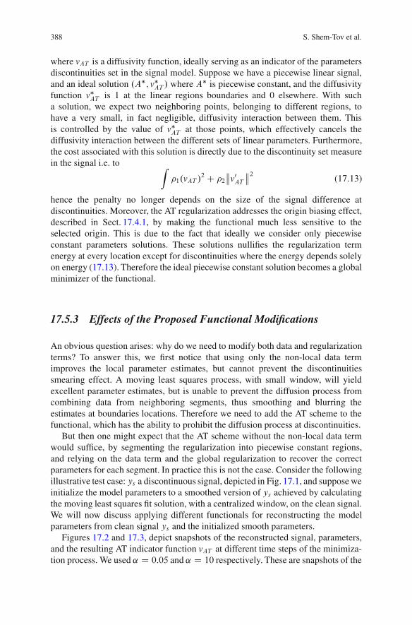
388 S. Shem-Tov et al.
where vAT is a diffusivity function, ideally serving as an indicator of the parametersdiscontinuities set in the signal model. Suppose we have a piecewise linear signal,and an ideal solution .A#; v#AT / where A# is piecewise constant, and the diffusivityfunction v#AT is 1 at the linear regions boundaries and 0 elsewhere. With sucha solution, we expect two neighboring points, belonging to different regions, tohave a very small, in fact negligible, diffusivity interaction between them. Thisis controlled by the value of v#AT at those points, which effectively cancels thediffusivity interaction between the different sets of linear parameters. Furthermore,the cost associated with this solution is directly due to the discontinuity set measurein the signal i.e. to Z
%1.vAT /2 C %2
""v0AT""2 (17.13)
hence the penalty no longer depends on the size of the signal difference atdiscontinuities. Moreover, the AT regularization addresses the origin biasing effect,described in Sect. 17.4.1, by making the functional much less sensitive to theselected origin. This is due to the fact that ideally we consider only piecewiseconstant parameters solutions. These solutions nullifies the regularization termenergy at every location except for discontinuities where the energy depends solelyon energy (17.13). Therefore the ideal piecewise constant solution becomes a globalminimizer of the functional.
17.5.3 Effects of the Proposed Functional Modifications
An obvious question arises: why do we need to modify both data and regularizationterms? To answer this, we first notice that using only the non-local data termimproves the local parameter estimates, but cannot prevent the discontinuitiessmearing effect. A moving least squares process, with small window, will yieldexcellent parameter estimates, but is unable to prevent the diffusion process fromcombining data from neighboring segments, thus smoothing and blurring theestimates at boundaries locations. Therefore we need to add the AT scheme to thefunctional, which has the ability to prohibit the diffusion process at discontinuities.
But then one might expect that the AT scheme without the non-local data termwould suffice, by segmenting the regularization into piecewise constant regions,and relying on the data term and the global regularization to recover the correctparameters for each segment. In practice this is not the case. Consider the followingillustrative test case: ys a discontinuous signal, depicted in Fig. 17.1, and suppose weinitialize the model parameters to a smoothed version of ys achieved by calculatingthe moving least squares fit solution, with a centralized window, on the clean signal.We will now discuss applying different functionals for reconstructing the modelparameters from clean signal ys and the initialized smooth parameters.
Figures 17.2 and 17.3, depict snapshots of the reconstructed signal, parameters,and the resulting AT indicator function vAT at different time steps of the minimiza-tion process. We used ˛ D 0:05 and ˛ D 10 respectively. These are snapshots of the
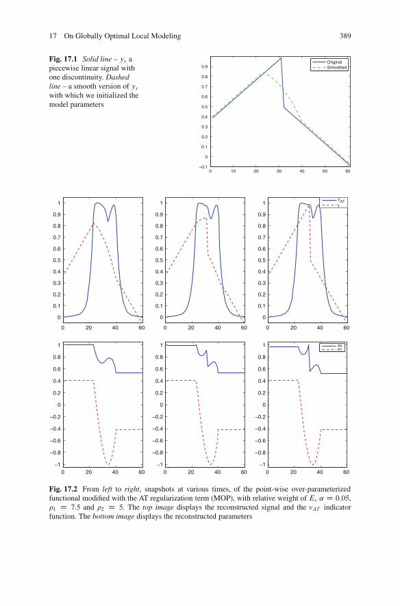
17 On Globally Optimal Local Modeling 389
0 10 20 30 40 50 60!0.1
0
0.1
0.2
0.3
0.4
0.5
0.6
0.7
0.8
0.9OriginalSmoothed
Fig. 17.1 Solid line – ys apiecewise linear signal withone discontinuity. Dashedline – a smooth version of yswith which we initialized themodel parameters
0 20 40 60
0
0.1
0.2
0.3
0.4
0.5
0.6
0.7
0.8
0.9
1
0 20 40 60
0
0.1
0.2
0.3
0.4
0.5
0.6
0.7
0.8
0.9
1
0 20 40 60
0
0.1
0.2
0.3
0.4
0.5
0.6
0.7
0.8
0.9
1VATy
0 20 40 60!1
!0.8
!0.6
!0.4
!0.2
0
0.2
0.4
0.6
0.8
1
0 20 40 60!1
!0.8
!0.6
!0.4
!0.2
0
0.2
0.4
0.6
0.8
1
0 20 40 60!1
!0.8
!0.6
!0.4
!0.2
0
0.2
0.4
0.6
0.8
1 A0A1
Fig. 17.2 From left to right, snapshots at various times, of the point-wise over-parameterizedfunctional modified with the AT regularization term (MOP), with relative weight of Es � D 0:05,%1 D 7:5 and %2 D 5. The top image displays the reconstructed signal and the vAT indicatorfunction. The bottom image displays the reconstructed parameters

390 S. Shem-Tov et al.
0 20 40 60
0
0.1
0.2
0.3
0.4
0.5
0.6
0.7
0.8
0.9
1
0 20 40 60
0
0.1
0.2
0.3
0.4
0.5
0.6
0.7
0.8
0.9
1
0 20 40 60
0
0.1
0.2
0.3
0.4
0.5
0.6
0.7
0.8
0.9
1
VATy
0 20 40 60!1
!0.8
!0.6
!0.4
!0.2
0
0.2
0.4
0.6
0.8
1
0 20 40 60!1
!0.8
!0.6
!0.4
!0.2
0
0.2
0.4
0.6
0.8
1
0 20 40 60!1
!0.8
!0.6
!0.4
!0.2
0
0.2
0.4
0.6
0.8
1
A0A1
Fig. 17.3 From left to right, snapshots at various times, of the Mpoint-wise over-parameterizedfunctional modified with the AT regularization term (MOP), with relative weight of Es � D 10,%1 D 7:5 and %2 D 5. The top image displays the reconstructed signal and the vAT indicatorfunction. The bottom image displays the reconstructed parameters
minimization process of the point-wise over-parameterized functional, modifiedwith the AT regularization term (MOP). Both minimizations were carried outuntil convergence. It is evident that the reconstructed parameters are not piecewiseconstant, as we would like to have from our prior information on the signal.Also, it is important to note that in the first series (Fig. 17.2) the signal isperfectly reconstructed, effectively nullifying the data term, and in the second series(Fig. 17.3) the signal is smoothed, however the data term energy is still very low.
In contrast, Fig. 17.4 depicts a series of snapshots of the minimization process ofthe non-local over-parameterized functional (NLOP). Note that here the parametersare perfectly reconstructed, the AT indicator function vAT receives a value closeto one only in the vicinity of the discontinuity and also the signal is perfectlyreconstructed.
We wanted to try and understand why did the MOP functional converged to sucha solution, is this solution a local/global minimum of the functional? We addressed
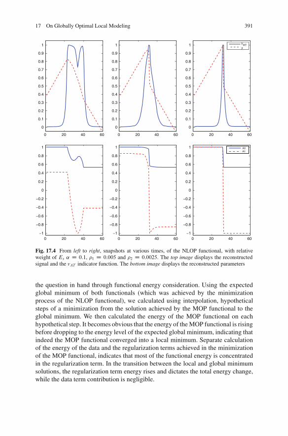
17 On Globally Optimal Local Modeling 391
0 20 40 60
0
0.1
0.2
0.3
0.4
0.5
0.6
0.7
0.8
0.9
1
0 20 40 60
0
0.1
0.2
0.3
0.4
0.5
0.6
0.7
0.8
0.9
1
0 20 40 60
0
0.1
0.2
0.3
0.4
0.5
0.6
0.7
0.8
0.9
1 VATy
0 20 40 60!1
!0.8
!0.6
!0.4
!0.2
0
0.2
0.4
0.6
0.8
1
0 20 40 60!1
!0.8
!0.6
!0.4
!0.2
0
0.2
0.4
0.6
0.8
1
0 20 40 60!1
!0.8
!0.6
!0.4
!0.2
0
0.2
0.4
0.6
0.8
1 A0A1
Fig. 17.4 From left to right, snapshots at various times, of the NLOP functional, with relativeweight of Es � D 0:1, %1 D 0:005 and %2 D 0:0025. The top image displays the reconstructedsignal and the vAT indicator function. The bottom image displays the reconstructed parameters
the question in hand through functional energy consideration. Using the expectedglobal minimum of both functionals (which was achieved by the minimizationprocess of the NLOP functional), we calculated using interpolation, hypotheticalsteps of a minimization from the solution achieved by the MOP functional to theglobal minimum. We then calculated the energy of the MOP functional on eachhypothetical step. It becomes obvious that the energy of the MOP functional is risingbefore dropping to the energy level of the expected global minimum, indicating thatindeed the MOP functional converged into a local minimum. Separate calculationof the energy of the data and the regularization terms achieved in the minimizationof the MOP functional, indicates that most of the functional energy is concentratedin the regularization term. In the transition between the local and global minimumsolutions, the regularization term energy rises and dictates the total energy change,while the data term contribution is negligible.
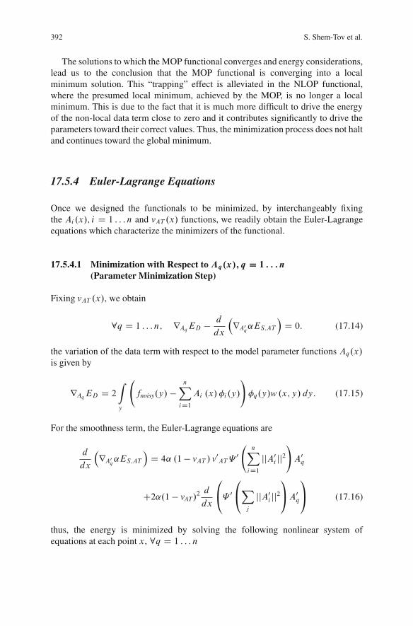
392 S. Shem-Tov et al.
The solutions to which the MOP functional converges and energy considerations,lead us to the conclusion that the MOP functional is converging into a localminimum solution. This “trapping” effect is alleviated in the NLOP functional,where the presumed local minimum, achieved by the MOP, is no longer a localminimum. This is due to the fact that it is much more difficult to drive the energyof the non-local data term close to zero and it contributes significantly to drive theparameters toward their correct values. Thus, the minimization process does not haltand continues toward the global minimum.
17.5.4 Euler-Lagrange Equations
Once we designed the functionals to be minimized, by interchangeably fixingthe Ai.x/; i D 1 : : : n and vAT .x/ functions, we readily obtain the Euler-Lagrangeequations which characterize the minimizers of the functional.
17.5.4.1 Minimization with Respect to Aq.x/; q D 1 : : : n(Parameter Minimization Step)
Fixing vAT .x/, we obtain
8q D 1 : : : n; rAqED !d
dx
'rA0
q˛ES;AT
(D 0: (17.14)
the variation of the data term with respect to the model parameter functions Aq.x/is given by
rAqED D 2Z
y
fnoisy.y/ !
nX
iD1Ai .x/ !i .y/
!!q.y/w .x; y/ dy: (17.15)
For the smoothness term, the Euler-Lagrange equations are
d
dx
'rA0
q˛ES;AT
(D 4˛ .1 ! vAT / v0AT# 0
nX
iD1jjA0i jj2
!A0q
C2˛.1 ! vAT/2 d
dx
0
@# 00
@X
j
jjA0i jj21
AA0q
1
A (17.16)
thus, the energy is minimized by solving the following nonlinear system ofequations at each point x, 8q D 1 : : : n

17 On Globally Optimal Local Modeling 393
2
Z
y
fnoisy.y/!
nX
iD1Ai .x/!i .y/
!!q.y/w .x; y/ dy
! 4˛ .1! vAT / v0AT# 0
nX
iD1jjA0i jj2
!A0q
! 2˛.1 ! vAT /2 d
dx
0
@# 00
@X
j
jjA0i jj21
AA0q
1
A D 0: (17.17)
17.5.4.2 Minimization with Respect to vAT .x/ (AT Minimization Step)
Fixing the functionsAi.x/; i D 1 : : : n, we obtain
! 2˛ .1 ! vAT /Es C 2%1 .vAT /! %2.v00AT / D 0: (17.18)
17.6 Implementation
We used central first and second derivatives and reflecting boundary conditions.In all the methods, we used various ˛; %1 and %2 constants, depending on thenoise level, as is common in noise reduction methods (this was done for all theconsidered algorithms, with the appropriate parameters). In all the examples, weassumed a sampling interval of dx D 1. For the minimization process we usedgradient descent with 200,000 iterations. This minimization method is a notoriouslyslowly converging method, but it is fast enough for our 1D example, and we intendto pursue a faster implementations in future work.
We performed anAT minimization step every 100 parameter minimization steps,and updated the weighting function every 1,000 parameter minimization steps. Weused a window size of ten sample points both for the NLOP functional, and forthe weighted least square fit method (used for initialization and reconstruction). Wenote that using a bigger window size resulted in significantly superior results on alltests, but this may not be the case in other signals. Choosing too big a window maycause an overlap between adjacent discontinuities and prevent the functional fromcorrectly recovering them.
17.6.1 Initialization
In order to prevent trapping into local minima, we initialize the model param-eters from the noisy data by means of a robust MLS fitting i.e. we computeeach point’s parameters by choosing the best least square fitting approximation

394 S. Shem-Tov et al.
via a sliding window least square calculation. This was done in exactly the samemanner as the sliding window weighting function described in Sect. 17.5.1.1. Theparameters chosen are those which generated the minimal reconstruction error.This computation provided a robust initialization, which already preserves, to someextent, discontinuities in the signal. This claim is strengthened by experiments weperformed comparing with a regular moving least square fitting initialization. Wefound that with the robust initialization, the functional converges to a better solution,and nicely exposes the true discontinuities in the signal models.
17.7 Experiments and Results
We conducted various experiments in order to verify the performance of theproposed functional. In this paper we focus mainly on 1D examples leaving 2Dextensions to images for future publications, nevertheless we exhibit some initialexperiments conducted on 2D synthetic images which yield a good idea of theperformance to be expected in the 2D case.
17.7.1 1D Experiments
We begin with the selection of the basis functions. We consider linear basis functionsof the form: )
!1 D 1!2 D x
(17.19)
This seemingly simple choice of functions, enables us to make comprehensive testsof the functional performance. Under this choice, the functional is expected to havethe best performance on piecewise linear signals. We note that this is an arbitrarychoice of basis functions, and one should choose other basis functions appropriatefor the signal domain.
To perform the tests we devised a set of synthetic 1D signals, and added whiteGaussian noise with standard deviation ranging from STD D 0:01 up to STD D0:25. These signals can be separated to two main groups:
• The first group is comprised of noisy piecewise linear signals. This group isinteresting because it enables us to test the parameter reconstruction performanceas well as noise reduction capabilities, under the optimal basis functions. Thepiecewise linear signals are depicted in Fig. 17.5.
• The second group is comprised of noisy nonlinear signals, such as higher degreepolynomials. This group is interesting only with regard to the noise removalperformance, because generating the ground truth parameters for linear basis
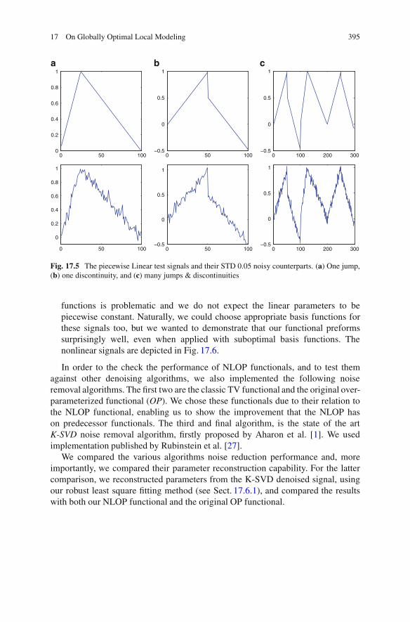
17 On Globally Optimal Local Modeling 395
0 50 1000
0.2
0.4
0.6
0.8
1a b c
0 50 100
0
0.2
0.4
0.6
0.8
1
0 50 100!0.5
0
0.5
1
0 50 100!0.5
0
0.5
1
0 100 200 300!0.5
0
0.5
1
0 100 200 300!0.5
0
0.5
1
Fig. 17.5 The piecewise Linear test signals and their STD 0.05 noisy counterparts. (a) One jump,(b) one discontinuity, and (c) many jumps & discontinuities
functions is problematic and we do not expect the linear parameters to bepiecewise constant. Naturally, we could choose appropriate basis functions forthese signals too, but we wanted to demonstrate that our functional preformssurprisingly well, even when applied with suboptimal basis functions. Thenonlinear signals are depicted in Fig. 17.6.
In order to the check the performance of NLOP functionals, and to test themagainst other denoising algorithms, we also implemented the following noiseremoval algorithms. The first two are the classic TV functional and the original over-parameterized functional (OP). We chose these functionals due to their relation tothe NLOP functional, enabling us to show the improvement that the NLOP hason predecessor functionals. The third and final algorithm, is the state of the artK-SVD noise removal algorithm, firstly proposed by Aharon et al. [1]. We usedimplementation published by Rubinstein et al. [27].
We compared the various algorithms noise reduction performance and, moreimportantly, we compared their parameter reconstruction capability. For the lattercomparison, we reconstructed parameters from the K-SVD denoised signal, usingour robust least square fitting method (see Sect. 17.6.1), and compared the resultswith both our NLOP functional and the original OP functional.

396 S. Shem-Tov et al.
0 50 1000.2
0.4
0.6
0.8
1
0 50 100
0.2
0.4
0.6
0.8
1
0 100 200
0
0.5
1
0 100 200
0
0.5
1
Polynomial Trig
a b
Fig. 17.6 The nonlinear test signals and their STD 0.05 noisy counterparts. Left: a polynomialssignal of degree 2. Right: a signal of combined sine and cosine functions
17.7.2 1D Results
Noise removal performance testing, was done by comparing the L2 norm of theresidual noise, that is the difference between the cleaned reconstructed signal andthe original signal:
EL2 D"""""f .x/ !
nX
iD1Ai.x/!i .x/
"""""2
: (17.20)
Parameters reconstruction performance testing (which with the linear basisfunction, is only relevant on the piecewise linear signals), was done by calculatingtheL2 norm of the difference between the reconstructed parameters and the originalparameters, with whom we generated the signal. Figure 17.7 depicts an exampleof the recovered parameters and the vAT indicator function obtained for the “Manyjumps & discontinuities” signal.
Figure 17.8, displays graphs comparing performance of the various algorithmson piecewise linear signals. The left graphs display the noise removal error norms,while the right graphs display parameters reconstruction error norms.
On various noise removal performance graphs we can see the excellent perfor-mance of both OP and NLOP functionals, reinforcing the claims of outstandingnoise removal performance obtained by the OP functional and maintained by ournew functional. Also, we can see that when the signal contains a discontinuity, suchas in the “One discontinuity” signal (as apposed to a continuous signal with onlyparameters discontinuity such as the “One jump” signal), the NLOP functional hasgreater ability to cope with the discontinuity, thus generating better results than
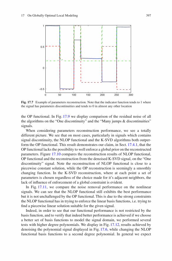
17 On Globally Optimal Local Modeling 397
0 50 100 150 200 250 300
!0.5
0
0.5
1
Fig. 17.7 Example of parameters reconstruction. Note that the indicator function tends to 1 wherethe signal has parameters discontinuities and tends to 0 in almost any other location
the OP functional. In Fig. 17.9 we display comparison of the residual noise of allthe algorithms on the “One discontinuity” and the “Many jumps & discontinuities”signals.
When considering parameters reconstruction performance, we see a totallydifferent picture. We see that on most cases, particularly in signals which containssignal discontinuity, the NLOP functional and the K-SVD algorithms both outper-form the OP functional. This result demonstrates our claim, in Sect. 17.4.1, that theOP functional lacks the possibility to well enforce a global prior on the reconstructedparameters. Figure 17.10 compares the reconstruction results of NLOP functional,OP functional and the reconstruction from the denoised K-SVD signal, on the “Onediscontinuity” signal. Note the reconstruction of NLOP functional is close to apiecewise constant solution, while the OP reconstruction is seemingly a smoothlychanging function. In the K-SVD reconstruction, where at each point a set ofparameters is chosen regardless of the choice made for it’s adjacent neighbors, thelack of influence of enforcement of a global constraint is evident.
In Fig. 17.11, we compare the noise removal performance on the nonlinearsignals. We can see that the NLOP functional still exhibits the best performancebut it is not unchallenged by the OP functional. This is due to the strong constraintsthe NLOP functional has in trying to enforce the linear basis functions, i.e. trying tofind a piecewise linear solution suitable for the given signal.
Indeed, in order to see that our functional performance is not restricted by thebasis function, and to verify that indeed better performance is achieved if we choosea better set of basis functions to model the signal domain, we performed severaltests with higher degree polynomials. We display in Fig. 17.12, results achieved bydenoising the polynomial signal displayed in Fig. 17.6, while changing the NLOPfunctional basis functions to a second degree polynomial. In general we expect

398 S. Shem-Tov et al.
0.000 0.100 0.200 0.3000.00
1.00
2.00
3.00non-localopksvdtv
Noise level
erro
r no
rm
One jump signal
0.000 0.100 0.200 0.3000.00
5.00
10.00
15.00non-localopksvd
Noise level
erro
r no
rm
One jump parameters
0.0 0.1 0.2 0.30.00
1.00
2.00
3.00non-localopksvdtv
Noise level
erro
r no
rm
One discontinuity signal
0.000 0.100 0.200 0.3000.00
5.00
10.00
15.00
20.00non-local opksvd
Noise level
erro
r no
rm
One discontinuity parameters
0.000 0.100 0.200 0.3000.00
1.00
2.00
3.00
4.00non-local opksvdtv
Noise level
erro
r no
rm
Many jumps & discontinuities signal
0.000 0.100 0.200 0.3000.00
20.00
40.00
60.00
80.00
100.00non-localopksvd
Noise level
erro
r no
rm
Many jumps & discontinuities parameters
a b
c d
e f
Fig. 17.8 Signal noise removal and parameters reconstruction comparison for the various piece-wise Linear signals. On the left column depicted are graphs compering the L2 norm of the residualnoise of the various algorithms. On the right column depicted are graphs compering the L2 normof the various algorithms reconstructed parameters compared to the expected parameters
a polynomial signal to be best recovered by polynomial basis functions of the samedegree. This is clearly depicted in the graph displayed in Fig. 17.12, where we seebetter performance by NLOP with polynomial basis function compared to NLOPwith linear basis functions.
Another test we performed with polynomial basis functions, was on a C1continuous second degree polynomial displayed in Fig. 17.13. This is an interestingcase, as both this signal and it’s first derivative are continuous, and only thesecond derivative is discontinuous. We found that this signal proved challengingfor the MLS initialization method, causing it to misplace the point of discontinuity
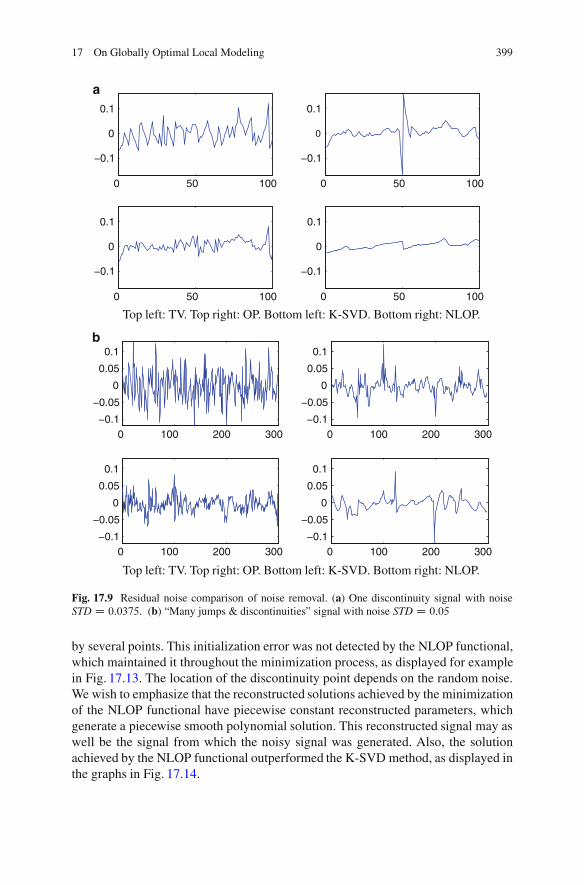
17 On Globally Optimal Local Modeling 399
0 50 100
!0.1
0
0.1
0 50 100
!0.1
0
0.1
0 50 100
!0.1
0
0.1
0 50 100
!0.1
0
0.1
Top left: TV. Top right: OP. Bottom left: K-SVD. Bottom right: NLOP.
0 100 200 300!0.1
!0.05
0
0.05
0.1
0 100 200 300!0.1
!0.05
0
0.05
0.1
0 100 200 300!0.1
!0.05
0
0.05
0.1
0 100 200 300!0.1
!0.05
0
0.05
0.1
Top left: TV. Top right: OP. Bottom left: K-SVD. Bottom right: NLOP.
a
b
Fig. 17.9 Residual noise comparison of noise removal. (a) One discontinuity signal with noiseSTD D 0:0375. (b) “Many jumps & discontinuities” signal with noise STD D 0:05
by several points. This initialization error was not detected by the NLOP functional,which maintained it throughout the minimization process, as displayed for examplein Fig. 17.13. The location of the discontinuity point depends on the random noise.We wish to emphasize that the reconstructed solutions achieved by the minimizationof the NLOP functional have piecewise constant reconstructed parameters, whichgenerate a piecewise smooth polynomial solution. This reconstructed signal may aswell be the signal from which the noisy signal was generated. Also, the solutionachieved by the NLOP functional outperformed the K-SVD method, as displayed inthe graphs in Fig. 17.14.
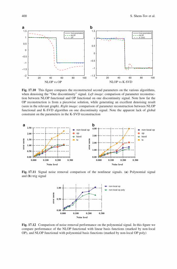
400 S. Shem-Tov et al.
0 20 40 60 80 100!2
!1.5
!1
!0.5
0
0.5
1
1.5true parametersNLOPOP
NLOP vs OP0 20 40 60 80 100
!1.5
!1
!0.5
0
0.5
1
1.5true parametersNLOPK!SVD
NLOP vs K-SVD
a b
Fig. 17.10 This figure compares the reconstructed second parameters on the various algorithms,when denoising the “One discontinuity” signal. Left image: comparison of parameter reconstruc-tion between NLOP functional and OP functional on one discontinuity signal. Note how far theOP reconstruction is from a piecewise solution, while generating an excellent denoising result(seen in the relevant graph). Right image: comparison of parameter reconstruction between NLOPfunctional and K-SVD algorithm on one discontinuity signal. Note the apparent lack of globalconstraint on the parameters in the K-SVD reconstruction
0.000 0.100 0.200 0.3000.00
0.50
1.00
1.50
2.00
2.50non-local opopksvdtv
Noise level
erro
r no
rm
0.000 0.100 0.200 0.3000.00
1.00
2.00
3.00
4.00 non-local opopksvdtv
Noise level
erro
r no
rm
a b
Fig. 17.11 Signal noise removal comparison of the nonlinear signals. (a) Polynomial signaland (b) trig signal
0.000 0.100 0.200 0.3000.00
0.50
1.00non-local op
non-local op poly
Noise level
erro
r no
rm
Fig. 17.12 Comparison of noise removal performance on the polynomial signal. In this figure wecompare performance of the NLOP functional with linear basis functions (marked by non-localOP), and NLOP functional with polynomial basis functions (marked by non-local OP poly)
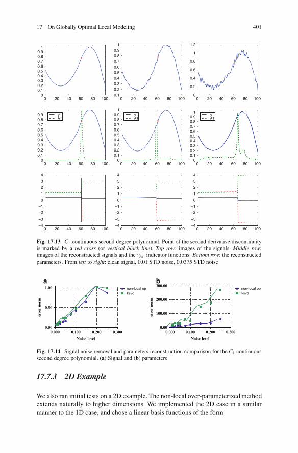
17 On Globally Optimal Local Modeling 401
0 20 40 60 80 1000
0.10.20.30.40.50.60.70.80.9
1
0 20 40 60 80 1000.10.20.30.40.50.60.70.80.9
1
0 20 40 60 80 1000
0.2
0.4
0.6
0.8
1
1.2
0 20 40 60 80 1000
0.10.20.30.40.50.60.70.80.9
1yAT
yAT
yAT
0 20 40 60 80 1000
0.10.20.30.40.50.60.70.80.9
1
0 20 40 60 80 1000
0.10.20.30.40.50.60.70.80.9
1
0 20 40 60 80 100!4
!3
!2
!1
0
1
2
3
4
0 20 40 60 80 100!4
!3
!2
!1
0
1
2
3
4
0 20 40 60 80 100!4
!3
!2
!1
0
1
2
3
4
Fig. 17.13 C1 continuous second degree polynomial. Point of the second derivative discontinuityis marked by a red cross (or vertical black line). Top row: images of the signals. Middle row:images of the reconstructed signals and the vAT indicator functions. Bottom row: the reconstructedparameters. From left to right: clean signal, 0.01 STD noise, 0.0375 STD noise
0.000 0.100 0.200 0.3000.00
0.50
1.00 non-local opksvd
Noise level
erro
r no
rm
0.000 0.100 0.200 0.3000.00
100.00
200.00
300.00non-local opksvd
Noise level
erro
r no
rm
a b
Fig. 17.14 Signal noise removal and parameters reconstruction comparison for the C1 continuoussecond degree polynomial. (a) Signal and (b) parameters
17.7.3 2D Example
We also ran initial tests on a 2D example. The non-local over-parameterized methodextends naturally to higher dimensions. We implemented the 2D case in a similarmanner to the 1D case, and chose a linear basis functions of the form
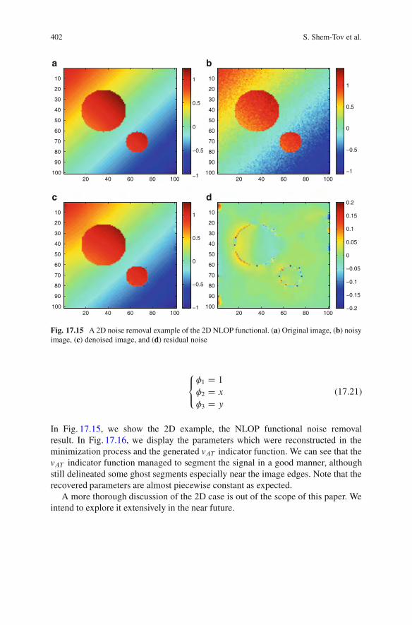
402 S. Shem-Tov et al.
20 40 60 80 100
10
20
30
40
50
60
70
80
90
100 !1
!0.5
0
0.5
1
20 40 60 80 100
10
20
30
40
50
60
70
80
90
100 !1
!0.5
0
0.5
1
20 40 60 80 100
10
20
30
40
50
60
70
80
90
100 !1
!0.5
0
0.5
1
20 40 60 80 100
10
20
30
40
50
60
70
80
90
100 !0.2
!0.15
!0.1
!0.05
0
0.05
0.1
0.15
0.2
a b
c d
Fig. 17.15 A 2D noise removal example of the 2D NLOP functional. (a) Original image, (b) noisyimage, (c) denoised image, and (d) residual noise
8<
:
!1 D 1!2 D x!3 D y
(17.21)
In Fig. 17.15, we show the 2D example, the NLOP functional noise removalresult. In Fig. 17.16, we display the parameters which were reconstructed in theminimization process and the generated vAT indicator function. We can see that thevAT indicator function managed to segment the signal in a good manner, althoughstill delineated some ghost segments especially near the image edges. Note that therecovered parameters are almost piecewise constant as expected.
A more thorough discussion of the 2D case is out of the scope of this paper. Weintend to explore it extensively in the near future.
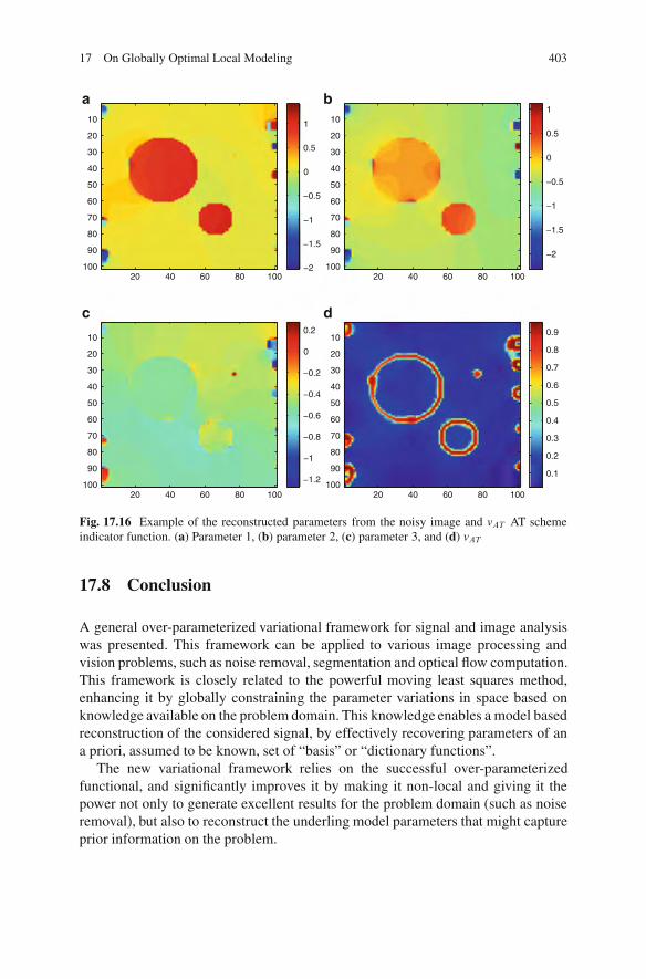
17 On Globally Optimal Local Modeling 403
20 40 60 80 100
10
20
30
40
50
60
70
80
90
100 !2
!1.5
!1
!0.5
0
0.5
1
20 40 60 80 100
10
20
30
40
50
60
70
80
90
100!2
!1.5
!1
!0.5
0
0.5
1
20 40 60 80 100
10
20
30
40
50
60
70
80
90
100 !1.2
!1
!0.8
!0.6
!0.4
!0.2
0
0.2
20 40 60 80 100
10
20
30
40
50
60
70
80
90
1000.1
0.2
0.3
0.4
0.5
0.6
0.7
0.8
0.9
a b
c d
Fig. 17.16 Example of the reconstructed parameters from the noisy image and vAT AT schemeindicator function. (a) Parameter 1, (b) parameter 2, (c) parameter 3, and (d) vAT
17.8 Conclusion
A general over-parameterized variational framework for signal and image analysiswas presented. This framework can be applied to various image processing andvision problems, such as noise removal, segmentation and optical flow computation.This framework is closely related to the powerful moving least squares method,enhancing it by globally constraining the parameter variations in space based onknowledge available on the problem domain. This knowledge enables a model basedreconstruction of the considered signal, by effectively recovering parameters of ana priori, assumed to be known, set of “basis” or “dictionary functions”.
The new variational framework relies on the successful over-parameterizedfunctional, and significantly improves it by making it non-local and giving it thepower not only to generate excellent results for the problem domain (such as noiseremoval), but also to reconstruct the underling model parameters that might captureprior information on the problem.
404 S. Shem-Tov et al.
This paper may be viewed as the basis of extensive future research on thesubject of over-parametrization. In future work we intend to thoroughly explorethe extension of the non-local over-parametrization denoising functional into 2Dsettings, where the choice of the support set, expressed by the weighting function,becomes a challenging matter. Also we intend to explore a variety of different basisfunctions, such has higher degree polynomials and non-polynomial basis functions,which may be relevent for other applications. Finally we would like to extend theproposed framework and to apply it to various other problem domains in computervision.
Acknowledgements This research was supported by the Israel Science foundation (ISF) grant no.1551/09.
References
1. Aharon, M., Elad, M., Bruckstein, A.: K-SVD: design of dictionaries for sparse representation.In: Proceedings of SPARS’05, Rennes, pp. 9–12 (2005)
2. Alexa, M., Behr, J., Cohen-Or, D., Fleishman, S., Levin, D., Silva, C.T.: Point set surfaces.In: IEEE Visualization 2001, pp. 21–28. IEEE Computer Society, Piscataway (2001)
3. Ambrosio, L., Tortorelli, V.M.: Approximation of functional depending on jumps by ellipticfunctional via & -convergence. Commun. Pure Appl. Math. 43(8), 999–1036 (1990)
4. Amenta, N., Kil, Y.J.: Defining point-set surfaces. ACM Trans. Graph. 23, 264–270 (2004)5. Black, M.J., Anandan, P.: The robust estimation of multiple motions: parametric and piecewise-
smooth flow fields. Comput. Vis. Image Underst. 63, 75–104 (1996)6. Bruckstein, A.M.: On globally optimal local modeling: from moving least squares to over-
parametrization. In: Workshop on Sparse Representation of Multiscale Data and Images:Theory and Applications. Institute of Advanced Study, Nanyang, Technological University,Singapore (2009)
7. Chan, T.F., Shen, J.: On the role of the bv image model in image restoration. AMS Contemp.Math. 330, 25–41 (2003). accepted (by two referees)
8. Cohen, E., Riesenfeld, R.F., Elber, G.: Geometric Modeling with Splines: an Introduction. AKPeters, Natick (2001)
9. Darrell, T.J., Pentland, A.P.: Cooperative robust estimation using layers of support. IEEETrans. Pattern Anal. Mach. Intell. 17, 474–487 (1991)
10. Farneback, G.: Spatial domain methods for orientation and velocity estimation. Lic. ThesisLiU-Tek-Lic-1999:13, Dept. EE, Linkoping University, SE-581 83 Linkoping, (1999). ThesisNo. 755, ISBN 91-7219-441-3
11. Fleishman, S., Cohen-Or, D., Silva, C.T.: Robust moving least-squares fitting with sharpfeatures. ACM Trans. Graph. 24, 544–552 (2005)
12. Gilboa, G., Osher, S.: Nonlocal operators with applications to image processing. MultiscaleModel. Simul. 7(3), 1005–1028 (2008)
13. Haindl, M., Mikes, S.: Model-based texture segmentation. In: Proceedings of the InternationalConference on Image Analysis and Recognition, pp. 306–313. Springer, Berlin (2004)
14. Haralick, R.M., Watson, L.: A facet model for image data. Comput. Graph. Image Process.15(2), 113–129 (1981)
15. Harten, A., Osher, S.: Uniformly high-order accurate nonoscillatory schemes. SIAM J. Numer.Anal. 24, 279–309 (1987)
16. Kindermann, S., Osher, S., Jones, P.W.: Deblurring and denoising of images by nonlocalfunctionals. Multiscale Model. Simul. 4(4), 1091–1115 (2005)
17 On Globally Optimal Local Modeling 405
17. Levin, D.: The approximation power of moving least-squares. Math. Comput. 67, 1517–1531(1998)
18. Levin, D.: Mesh-independent surface interpolation. In: Brunnett, G. et al. (eds.) GeometricModeling for Scientific Visualization, pp. 37–49. Springer, Berlin/London (2003)
19. Malisiewicz, T., Efros, A.A.: Improving spatial support for objects via multiple segmentations.In: Proceedings of the British Machine Vision Conference (BMVC), Warwich (2007)
20. Memin, E., Perez, P.: A multigrid approach for hierarchical motion estimation. In: Proceedingsof the Sixth International Conference on Computer Vision, 1998, Bombay, pp. 933–938 (1998)
21. Nir, T., Bruckstein, A.M.: On over-parameterized model based TV-denoising. In: InternationalSymposium on Signals, Circuits and Systems (ISSCS 2007), Iasi (2007)
22. Nir, T., Bruckstein, A.M., Kimmel, R.: Over-parameterized variational optical flow. Int. J.Comput. Vis. 76(2), 205–216 (2008)
23. Olshausen, B.A., Fieldt, D.J.: Sparse coding with an overcomplete basis set: a strategyemployed by v1. Vis. Res. 37, 3311–3325 (1997)
24. Pock, T.: Fast total variation for computer vision. Ph.D. thesis, Graz University of Technology(2008)
25. Quatieri, T.: Discrete-Time Speech Signal Processing: Principles and Practice, 1st edn. PrenticeHall, Upper Saddle River (2001)
26. Rosman, G., Shem-Tov, S., Bitton, D., Nir, T., Adiv, G., Kimmel, R., Feuer, A., Bruckstein,A.M.: Over-parameterized optical flow using a stereoscopic constraint. In: Proceedings of theScale Space and Variational Methods in Computer Vision. Springer, Berlin/London (2011)
27. Rubinstein, R., Zibulevsky, M., Elad, M.: Efficient implementation of the k-svd algorithm usingbatch orthogonal matching pursuit. Technical report, Technion – Israel Institute of Technology(2008)
28. Rudin, L.I., Osher, S., Fatemi, E.: Nonlinear total variation based noise removal algorithms.Phys. D 60, 259–268 (1992)
29. Savage, J., Chen, K.: On multigrids for solving a class of improved total variation basedstaircasing reduction models. In: Tai, X.-C., Lie, K.-A., Chan, T.F., Osher, S. (eds.) Proceedingsof the International Conference on PDE-Based Image Processing and Related Inverse Prob-lems, CMA, Oslo, 8–12 Aug 2005. Mathematics and Visualization, Image Processing Basedon Partial Differential Equations, pp. 69–94 (2006)
30. Shah, J.: A common framework for curve evolution, segmentation and anisotropic diffusion.In: Proceedings of the 1996 Conference on Computer Vision and Pattern Recognition (CVPR’96), p. 136. IEEE Computer Society, Washington, DC (1996)
31. Shah, J.: Curve evolution and segmentation functionals: application to color images. In: Pro-ceedings of the IEEE ICIP’96, Lausanne, pp. 461–464 (1996)
32. Shu, C.W.: Essentially non-oscillatory and weighted essentially non-oscillatory schemes forhyperbolic conservation laws. In: Cockburn, B., Shu, C.-W., Johnson, C., Tadmor, E. (eds.)Advanced Numerical Approximation of Nonlinear Hyperbolic Equations. Lecture Notes inMathematics, vol. 1697, pp. 325–432. Springer (1997)
33. Sun, D., Sudderth, E., Black, M.: Layered image motion with explicit occlusions, temporalconsistency, and depth ordering. In: Lafferty, J., Williams, C.K.I., Shawe-Taylor, J., Zemel,R.S., Culotta, A. (eds.) Proceedings of the Advances in Neural Information ProcessingSystems, Vancouver, vol. 23, pp. 2226–2234 (2010)
34. Tarantola, A.: Inverse Problem Theory and Methods for Model Parameter Estimation. Societyfor Industrial and Applied Mathematics, Philadelphia (2004)
35. Trobin, W., Pock, T., Cremers, D., Bischof, H.: An unbiased second-order prior for high-accuracy motion estimation. In: Proceedings of the DAGM Symposium, pp. 396–405. Springer,Berlin/New York (2008)
Chapter 18Incremental Level Set Tracking
Shay Dekel, Nir Sochen, and Shai Avidan
Abstract We consider the problem of contour tracking in the level set framework.Level set methods rely on low level image features, and very mild assumptionson the shape of the object to be tracked. To improve their robustness to noise andocclusion, one might consider adding shape priors that give additional weight tocontours that are more likely than others. This works well in practice, but assumesthat the class of object to be tracked is known in advance so that the proper shapeprior is learned. In this work we propose to learn the shape priors on the fly. Thatis, during tracking we learn an eigenspace of the shape contour and use it to detectand handle occlusions and noise. Experiments on a number of sequences reveal theadvantages of our method.
18.1 Introduction
Contour tracking is a task in which the contour of the object(s) of interest has to beextracted for each frame in a video in a way which is robust to noise and clutter.This task is different from object tracing in which a bounding box that contains theobject is sought or segmentation in which the contour in a given image is extracted.The main issues that we address in this paper is the robustness to noise, clutterand occlusions on one hand and the ability to deal with shape/behavior change.Accordingly, this paper introduces a way to achieve such a robustness as a matterof principle without paying too much attention to the quality of segmentation. Theway it is done is via variational and level-set methods.
S. Dekel (!) ! S. AvidanDepartment of Electrical Engineering, Tel Aviv University, Tel Aviv, Israel
N. SochenDepartment of Applied Mathematics, Tel Aviv University, Tel Aviv, Israele-mail: [email protected]
M. Breuß et al. (eds.), Innovations for Shape Analysis, Mathematics and Visualization,DOI 10.1007/978-3-642-34141-0 18, © Springer-Verlag Berlin Heidelberg 2013
407
408 S. Dekel et al.
Level set methods are a convenient way to parameterize and track objectcontours. They work by evolving a contour which tightly encloses the deformableobject to be tracked. However this method cannot handle missing or misleadinginformation due to noise, clutter or occlusions in the input images. In order to over-come these problems one can derive a parametric model for implicit representationof the segmentation curve by applying low dimensional subspace representation,such as Principle Component Analysis (PCA) to a specific collection of trainingset images before the tracking begins. In this case the evolving curve has limiteddegrees of freedom since the curve lies on the PCA subspace. This property enablesthe segmentation to be robust to noise and partial occlusions. However this modelrelies on a fixed training set and assumes that the object class to be tracked is knownin advance.
We present an extension that deals with these shortcomings. Our approach learns,on line, a shape prior that is then used during tracking. This enables our tracker toovercome occlusions and, unlike previous algorithms, it does not demand a specificpredefined training set.
We formulate the tracking process as a mixture of two major models: In theOn-line Learning Model, we perform region-based segmentation on each frameusing the Chan-Vese approach [3] together with the edge-based approach which isbased on the Geodesic Active Contour [2]. The segmentation results are then usedto incrementally learn an on-line low dimensional subspace representation of theobjects’ contour, efficiently adapting to changes in the appearance of the target.
In case of occlusion, the eigencoordinates of the segmented shape will differconsiderably from those obtained so far and, in that case, we switch to thePCA Representation Model that tracks the object using the currently availablePCA space. This PCA eigenbase representation together with the temporal priorrepresentation allows us to limit the degree of freedom of the evolving contourwhich enables it to cope with missing or misleading information due to occlusions,partial occlusions and noise. Once the object reappears we switch back to the onlinelearning model and keep updating our representation model. Hence, we can properlytrack deformable objects through occlusion and noise.
We provide experimental results that present several properties of our method:We show that our method can cope with partial or total occlusions, as well as exam-ples in which the images are severely contaminated with strong Gaussian noise.In addition, we show that our algorithm can adapt to considerable deformations inshape.
18.2 Background
Contour tracking via variational methods and level-sets is based on the seminalworks [1, 3, 18] and many more; see [6] for a very nice overview and for furtherreferences on level-set based tracking.
18 Incremental Level Set Tracking 409
Several authors combined prior shape information into level-set-based segmenta-tion. Leventon et al. [11] incorporated a training set information as a prior model torestrict the flow of the geodesic active contour using Principle Component Analysis(PCA). Tsai et al. [25] used only the first few eigenmodes by performing optimiza-tion. Rousson et al. [20, 21] introduced shape information on the variational level.Chen et al. [4] imposed shape constraints directly on the contour. However theseauthors ignored the temporal coherence of the shapes which leads to degredation inperformance when dealing with occlusions.
Cremers [5] proposes to model the embedding functions by a Principle Com-ponent Analysis (PCA) and to use dynamical shape prior. He learns a specificset of training shapes before the tracking begins and also exploits the temporalcorrelations between consecutive shapes. This enables him to handle occlusionsand large amounts of noise. His method is well-suited for specific tracking missionswhere a pre-defined training set can be performed off-line.
Another approach is presented in the work of Fussenegger et al. [7]. In that worka level-set method is combined with PCA decomposition of shape space. This isvery similar and relevant to this paper. The difference is in the aim and type of videotreated. In Fussengger et al. there are many, mainly rigid, objects to segment suchthat each individual shape doesn’t change too much from frame to frame. Our paperdeals with mainly one object with changing shape and the main focus is on the wayto deal with occlusions and changes of shape along the video.
Our work is motivated in part by the power of subspace representation andexploits the temporal correlations between consecutive shapes following the workof Cremers [5]. But in contrast to eigentracking algorithms, our algorithm does notrequire a specific training set before tracking begins. It learns the eigenbase on-lineduring the object tracking process, thus eliminating the need to collect the trainingimages prior to tracking.
18.2.1 Integrated Active Contours
We start with a generic algorithm for data-based segmentation. The model isformulated in variational way and we use the Integrated Active Contour model[19, 22] that combines region-based and edge-based segmentation via the level-setformulation. In order to perform region-based segmentation in each frame we usethe Chan-Vese algorithm which attempts to partition the image into two regionsaccording to common image properties. Then we add to the functional an edge-based term which is based on the Geodesic Active Contour (GAC).
Let It W ˝ ! IR be the image at time t that assigns for each pixel x 2 ˝ ! IR2
a real value grey level. A contour that separates the object (or objects) from thebackground is encoded as a zero level-set of a function !t W ˝ ! IR. The contourat frame t is Ct D f.x; y/j!t .x; y/ D 0g. We denote the region inside the zero-level set by ˝C D f.x; y/j!t .x; y/ > 0g and similarly the region outside the zero

410 S. Dekel et al.
level-set ˝" D f.x; y/j!t .x; y/ < 0g . The probability of the contour !t , given theprevious contours and all the measurements ŒI0.x/ : : : It .x/" using the Bayes rule is:
P.!t jI0Wt ;!0Wt"1/ /PC.It j!t /„ ƒ‚ …Target
"P".It j!t /„ ƒ‚ …Background
"P.!0Wt"1j!t /„ ƒ‚ …Shape
" P.!t /„ƒ‚…Smoothness
(18.1)
Here P˙ are the probability distributions of the grey value intensities inside andoutside of the zero level-set of !t .
While P˙ can be quite involved in real-life applications we choose here to stickto the simple Gaussian model in order to concentrate on the tracking part. Thischoice leads to the Chan-Vese model. In this approach we find a contour, representedby !.x/, that partitions the image into two regions ˝C and ˝", that describean optimal piecewise constant approximation of the image. We also assume thatthe intensities of the shape and the background are independent samples from twoGaussian probabilities, therefore:
P˙.It j!t / DY
x2˝˙
1q2˘#2˙
exp" .It!C˙/2
2#2˙ (18.2)
Thereby C˙ and #˙ are the mean and standard deviation of the intensities insideand outside of the zero level-set of !t .
The region-based energy is defined as
ERB.!t ; CC; C"/ D # logfPC.It j!t / "P".It j!t /g (18.3)
The contour with the highest probability is the one that minimizes the followingregion-based energy functional:
ERB.!t ; CC; C"/ DZ
˝
f 12#2C
.It .x/ # CC/2 C1
2log.2$#2C/gH.!t .x//dx
CZ
˝
f 12#2"
.It .x/ # C"/2 C1
2log.2$#2"/gf1#H.!t .x//gdx (18.4)
whereH.!t .x// is the Heaviside step function:
H.!t .x// D!1 if !t .x/ > 00 if !t .x/ 0 0
(18.5)
The smoothness prior is taken to be the Geodesic Active Contour (GAC) term [2].This term defines the object boundaries as a (locally) minimal length weighted bythe local gradients. In other words it is a geodesic over a Riemannian manifoldwhose metric is defined via the gradients of the image. It leads to the followingfunctional:

18 Incremental Level Set Tracking 411
EGAC.!t / DZ
˝
gGAC .jrI j/jrH.!t .x//jdx (18.6)
where gGAC D 1=.1C jrI j2/.Finally, the Integrated Active Contour functional EIAC is obtained by the
summation of the region-based energy ERB (18.4) and the edge-based geodesicactive contour energyEGAC (18.6) as:
EIAC.!t ; CC; C"/ D ERB.!t ; CC; C"/C %EGAC .!t / (18.7)
with the Euler-Lagrange equation:
ıEIAC
ı!tDhlog.
#C#"/C 1
2#2C.It .x/ # CC/2
# 1
2#2".It .x/ # C"/2 # %div.gGAC .jrI j/
r!t .x/jr!t .x/j
/iı.!t .x// (18.8)
18.2.2 Building the PCA Eigenbase
The shape term, as explained earlier, is an on-line learning model that producesand updates an eigenbase representation during tracking. We work here witha PCA decomposition, where we first build a PCA eigenbase from the first nframes of the sequence and then incrementally update it as new m observationsarrive. For efficiency we use an incremental PCA algorithm and only keep thetop k eigenvalues. The corresponding eigenvectors are denoted by i . This PCAeigenbase, i , will help us cope with occlusions in the PCA representation model.Each shape is represented as:
!i .x/ D N!0.x/CkX
jD1˛ij j (18.9)
where !i .x/ represents the i -th shape from the PCA subspace model, N!0.x/ is themean shape and ˛ij is the PCA coefficient of the i -th shape.
18.2.2.1 First PCA Eigenbase
We produce the first PCA eigenbase from the previous n segmentation results of theOn-Line Learning model. Let A D f!1.x/;!2.x/ : : : !n.x/g be the previous n levelset function segmentations. Each data element, !i .x/, is a d $1 vector that containsthe level set function of the i -th shape. We calculate the mean shape !A.x/ as:
412 S. Dekel et al.
N!A.x/ D1
n
nX
iD1!i .x/ (18.10)
Then we apply singular value decomposition (SVD) on the centered n previous levelset functions
UA˙AVTA D SVDf!1 # N!A;!2 # N!A; : : : ;!n # N!Ag (18.11)
Here UA and ˙A contain the eigenvectors and the eigenvalues, respectively. Thenthe first PCA eigenbase denoted as A.x/ D U
.1Wk/A contains the eigenvectors cor-
responding to the k largest eigenvalues, i.e. vectors of UA. These terms A.x/ and˙A will serve as initialization to the incremental PCA algorithm.
18.2.2.2 Updating the Eigenspace
Incremental PCA combines the current eigenbase with new observations without re-calculating the entire SVD. Numerous algorithms have been developed to efficientlyupdate an eigenbase as more data arrive [8, 9]. However, most methods assumea fixed mean when updating the eigenbase. We use the Sequential Karhunen-Loeve (SKL) algorithm of Levy and Lindenbaum [12]. They present an efficientmethod that incrementally updates the eigenbase as well as the mean when newobservations arrive. They also add a forgetting factor f 2 Œ0; 1" that down-weightsthe contribution of the earlier observations. This property plays an important rolein the on-line learning. As time progresses the observation history can become verylarge and the object may change its appearance, and the forgetting factor allows us tostrengthen the contribution of the current data such that the updated PCA eigenbasewill be able to cope with that change. This algorithm allows us to update the PCAeigenbase online while tracking using the segmentation results during the on-linelearning model.
18.2.2.3 Detection of Occlusion
In the on-line learning model we performed region-based segmentation in eachframe and incrementally updated the PCA eigenbase. We want to know when thecurrent contour encounters an occlusion in order to switch to the PCA representationmodel. Then, after the occlusion ends we switch back to the on-line learning modelto keep updating our representation model.
For this purpose, we rely on the PCA coefficients that represent the current shapeand observe that under occlusions these coefficients are farther away from the meanPCA coefficients.
18 Incremental Level Set Tracking 413
During the on-line learning model we project each contour segmentation !t onthe current PCA subspace & .x/ to obtain its current PCA coefficient ˛t . Then wemeasure the Mahalanobis distance between the current PCA coefficient ˛t and themean PCA coefficient N :
Dt.˛t / Dp.˛t # N /T S"1.˛t # N / (18.12)
Here N is the mean PCA coefficient and S is the covariance matrix. These twoterms were obtained by collecting only the good PCA coefficients every frameduring the on-line learning model. From (18.12), if Dt.˛t / > Th our methodswitches to the PCA representation model and when Dt.˛t / < Th we return backto the on-line learning model.
Experimental results show that if the scene is free of occlusions, the Mahalanobisdistance is usually Dt.˛t / < Th. Figure 18.1 shows the Mahalanobis distance ineach frame during the two models. We can see that during the on-line learning modelthe contour encounters an occlusion and its appropriate Mahalanobis distance isabove Th (the peaks in the blue bars in the middle), in that moment we switch to thePCA representation model and see the improvement in the Mahalanobis distancesduring the occlusion (the red bars in the middle). Then we switch back to the on-linelearning model when the coefficients are below Th.
18.2.3 Dynamical Statistical Shape Model
Once the algorithm detects an occlusion, it switches to the PCA representationmodel with the updated PCA eigenbase. But before we switch to the PCArepresentation model, we want to exploit the temporal correlations between theshapes. As explained in Eq. (18.9) we can represent each shape using the PCAeigenbase and the mean shape. Therefore the segmentation in the current frame!t .x/ can be represented by the PCA coefficient vector ˛t . This will lead usto write the probability of the shape prior from (18.1) as: P.˛t j˛0Wt"1/ insteadof P.!t j!0Wt"1/. In addition during the on-line learning model, we ignored thecorrelation between the frames since we assumed that the object wasn’t occludedand therefore no temporal prior information was needed. In the PCA representationmodel, where the deformable object may be occluded, we have to obtain morepowerful prior which relies on the correlation between consecutive frames. For thisreason we can represent each shape by a Markov chain of order q in a manner similarto Cremers [5]. More formally, the current shape at time t can be represented by theprevious shapes using an Auto Regressive (AR) model as follows:
˛t D # C A1˛t"1 C A2˛t"2 : : :C Aq˛t"q C ' (18.13)

414 S. Dekel et al.
Fig. 18.1 The Mahalanobis distance between the current PCA coefficient ˛t and the mean PCAcoefficient N in each frame during the two models on-line learning model (blue) and PCArepresentation model (red)
Here ' is Gaussian noise with zero mean and covariance matrix (, Ai are thetransition matrices of the AR model. and # is the mean of the process. With thisAR model we can determine the probability P.˛t j˛0Wt"1/ for observing a particularshape ˛t at time t given the shapes estimated on the previous frames as follows:
P.˛t j˛0Wt"1/ / exp.#12!T("1!/ (18.14)
Where:! D ˛t # # #A1˛t"1 #A2˛t"2 : : : #Aq˛t"q (18.15)
Various methods have been proposed in the literature to estimate the modelparameters: ', ( and Ai . We applied a Stepwise Least Squares algorithm as pro-posed in [16]. The order q determines the accuracy of the AR model approximationand its value depends on the input sequence. In order to estimate its value we usethe Schwarz Bayesian Criterion [23].
18.3 PCA Representation Model
The algorithm switches to that model only if it detects an occlusion. Once detectingan occlusion, it continually tracks the same target using the PCA eigenbase and theAR parameters which were obtained in the on-line learning model. As explained

18 Incremental Level Set Tracking 415
in Sect. 18.2.2, according to (18.9) the segmentation in the current frame !t .x/ canbe represented by the PCA coefficient vector ˛t . Therefore we actually exchange in(18.1) each level set function ! by the appropriate shape vector representation ˛:
P.˛t jI0Wt ; ˛0Wt"1/ /PC.It j˛t /„ ƒ‚ …Target
"P".It j˛t /„ ƒ‚ …Background
"P.˛t j˛0Wt"1/„ ƒ‚ …Shape Prior
(18.16)
This will lead us in this model to focus on estimating the shape vectorrepresentation ˛t by minimizing the following energy functional:
EPCA.˛t ; CC; C"/ D #log.P.˛t jI0Wt ; ˛0Wt"1//D # log PC.It j˛t / "P".It j˛t /„ ƒ‚ …
Data
# log P.˛t j˛0Wt"1/„ ƒ‚ …Shape Prior
(18.17)
Thereby the probabilities P˙.It j˛t / are similar to the Chan-Vese probabilities(18.2), except that !t .x/ is determined by ˛t as (18.9).
Applying these probabilities and (18.14)–(18.17) leads to the following energyfunctional:
EPCA.˛t ; CC; C!/ D 1
2#2C
Z
˝.It .x/" CC/2H.!.˛t //dxC
1
2log.2$#2C/
Z
˝H.!.˛t //dx
C 1
2#2!
Z
˝.It .x/" C!/2.1"H.!.˛t ///dxC 1
2log.2$#2!/
Z
˝.1"H.!.˛t ///dxC )1
2!T(!1!
(18.18)
Here ) is an additional parameter that allows relative weighting between dataand prior and !.˛t / is the level set estimation which is determined by ˛t . Thesegmentation in each frame requires the estimation of the shape vector ˛t , whichis done by minimizing (18.18) with respect to ˛t using gradient descent strategy.
18.4 Motion Estimation
In each frame we estimate the translation positions .u; v/t and use this to translatethe previous contour !t"1 as initialization to estimate the current contour. In theOn-Line Learning model the segmentations aren’t sensitive to the initial contoursince we assume that the object isn’t occluded. Therefore we use Lucas-Kanadeapproach [13] to estimate the translation position .u; v/t by minimizing
ELK.u; v/t D KW % .IxuC IyvC It /2 (18.19)
where KW % ."/ denotes the convolution with an integration window of size W .Ix; Iy are the x; y derivatives of the image in each axis and It is the derivative
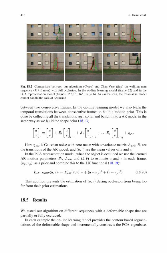
416 S. Dekel et al.
Fig. 18.2 Comparison between our algorithm (Green) and Chan-Vese (Red) on walking mansequence (319 frames) with full occlusion. In the on-line learning model (frame 22) and in thePCA representation model (frames: 153,161,165,176,266). As can be seen, the Chan-Vese modelcannot handle the case of occlusion
between two consecutive frames. In the on-line learning model we also learn thetemporal translations between consecutive frames to build a motion prior. This isdone by collecting all the translations seen so far and build it into a AR model in thesame way as we build the shape prior (18.13)
"uv
#
t
D"NuNv
#C B1
"uv
#
t"1C B2
"uv
#
t"2C : : : Bq
"uv
#
t"qC 'pos
Here 'pos is Gaussian noise with zero mean with covariance matrix(pos , Bi arethe transitions of the AR model, and .Nu; Nv/ are the mean values of u and v.
In the PCA representation model, when the object is occluded we use the learnedAR motion parameters Bi , (pos and .Nu; Nv/ to estimate u and v in each frame,.up; vp/, as a prior and combine this to the LK functional (18.19):
ELK"PRIOR.u; v/t D ELK.u; v/C *..u # up/2 C .v # vp/2/ (18.20)
This addition prevents the estimation of .u; v/ during occlusion from being toofar from their prior estimations.
18.5 Results
We tested our algorithm on different sequences with a deformable shape that arepartially or fully occluded.
In each example the on-line learning model provides the contour based segmen-tations of the deformable shape and incrementally constructs the PCA eigenbase.

18 Incremental Level Set Tracking 417
Fig. 18.3 Results of our algorithm on walking man sequence (200 frames) with partial trafficocclusions (yellow and silver car). The algorithm automatically switches from on-line learning(frame 60) to PCA representation as soon as occlusion is detected (frames: 11,66,68,70,77,84)
Fig. 18.4 Results of our algorithm on walking man sequence (173 frames) with full occlusion(walking woman hides the target). The algorithm automatically switches from on-line learn-ing (frame 95) to PCA representation as soon as occlusion is detected (frames: 35,100,101,103,104,109)
When it detects an occlusion, it estimates the AR parameters that capture thetemporal dynamics of the shapes evolution seen so far and switches to the PCArepresentation model. The PCA model uses the current PCA eigenbase and theestimated AR prior parameters to keep segmenting the deformable shape duringocclusion. Finally, when the target reappears it switches back to the on-line learningmodel and keeps tracking the target and updating the PCA eigenbase. We can seethat it maintains the appropriate contours when the shape is totally or partiallyoccluded.

418 S. Dekel et al.
Fig. 18.5 Results of our algorithm on jumping man sequence (225 frames) with full occlusion(walking man hides the target). Frames: 103,120,121,122,124,125
Fig. 18.6 Results of our algorithm on running horse sequence (290 frames) with one partially longperiod (synthetic) occlusion (20 frames with white label hides partially the target). We showedthat our method was able to remain locked onto the target and illustrate the appropriate contours.Frames: 10,89,115,119,120,124
First, we compared our method to a stand-alone Chan-Vese algorithm on asequence of walking man with one occlusion (left column). As can be seen inFig. 18.2, the Chan-Vese model could not handle the occlusion properly, whileour method kept tracking the person through the entire sequence and was able toillustrate the appropriate shapes when the man was totally occluded by the leftcolumn (Figs. 18.3–18.6).
Finally, in Fig. 18.7 we examined our method on a noisy sequence of a jumpingman with additive Gaussian noise (SNRD15), and, as can be seen, our algorithm isable to cope with Gaussian noise and occlusion as well.
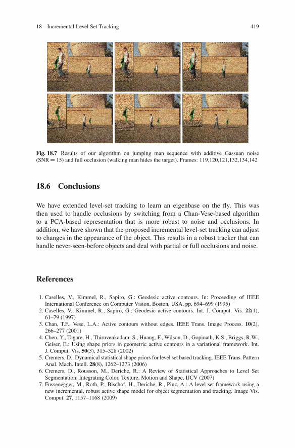
18 Incremental Level Set Tracking 419
Fig. 18.7 Results of our algorithm on jumping man sequence with additive Gassuan noise(SNRD 15) and full occlusion (walking man hides the target). Frames: 119,120,121,132,134,142
18.6 Conclusions
We have extended level-set tracking to learn an eigenbase on the fly. This wasthen used to handle occlusions by switching from a Chan-Vese-based algorithmto a PCA-based representation that is more robust to noise and occlusions. Inaddition, we have shown that the proposed incremental level-set tracking can adjustto changes in the appearance of the object. This results in a robust tracker that canhandle never-seen-before objects and deal with partial or full occlusions and noise.
References
1. Caselles, V., Kimmel, R., Sapiro, G.: Geodesic active contours. In: Proceeding of IEEEInternational Conference on Computer Vision, Boston, USA, pp. 694–699 (1995)
2. Caselles, V., Kimmel, R., Sapiro, G.: Geodesic active contours. Int. J. Comput. Vis. 22(1),61–79 (1997)
3. Chan, T.F., Vese, L.A.: Active contours without edges. IEEE Trans. Image Process. 10(2),266–277 (2001)
4. Chen, Y., Tagare, H., Thiruvenkadam, S., Huang, F., Wilson, D., Gopinath, K.S., Briggs, R.W.,Geiser, E.: Using shape priors in geometric active contours in a variational framework. Int.J. Comput. Vis. 50(3), 315–328 (2002)
5. Cremers, D.: Dynamical statistical shape priors for level set based tracking. IEEE Trans. PatternAnal. Mach. Intell. 28(8), 1262–1273 (2006)
6. Cremers, D., Rousson, M., Deriche, R.: A Review of Statistical Approaches to Level SetSegmentation: Integrating Color, Texture, Motion and Shape, IJCV (2007)
7. Fussenegger, M., Roth, P., Bischof, H., Deriche, R., Pinz, A.: A level set framework using anew incremental, robust active shape model for object segmentation and tracking. Image Vis.Comput. 27, 1157–1168 (2009)
420 S. Dekel et al.
8. Golub, G.H., Van Loan, C.F.: Matrix Computations. The Johns Hopkins University Press,Baltimore (1996)
9. Hall, P., Marshall, D., Martin, R.: Incremental eigenanalysis for classification. In: Proceedingsof British Machine Vision Conference, pp. 286–295 (1998)
10. Kichenassamy, S., Kunar, A., Olver, P.J., Tannenbaum, A., Yezzi, A.J.: Gradient flows andgeometric active contour model. In: IEEE International Conference on Computer Vision,pp. 810–815 (1995)
11. Leventon, M., Grimson, W., Faugeras, O.: Statistical shape influence in geodesic activecontours. In: CVPR, vol. 1, Hilton Head Island, SC, pp. 316–323 (2000)
12. Levy, A., Lindenbaum, M.: Sequential Karhunen-Loeve basis extraction and its application toimages. IEEE Trans. Image Process. 9(8), 1371–1374 (2000)
13. Lucas, B.D., Kanade, T.: An iterative image registration technique with an application to stereovision. In: Proceedings of the 7th International Joint Conference on Artificial Intelligence,pp. 674–679 (1981)
14. Malladi, R., Sethian, J.A., Vemuri, B.C.: Shape modeling with front propagation: a level setapproach. IEEE Trans. Pattern Anal. Mach. Intell. 17(2), 158–175 (1995)
15. Mumford, D., Shah, J.: Optimal approximations by piecewise smooth functions and associatedvariational problems. Commun. Pure Appl. Math. 42, 577–685 (1989)
16. Neumaier, A., Schneider, T.: Estimation of parameters and eigenmodes of multivariateautoregressive models. ACM Trans. Math. Softw. 27(1), 27–57 (2001)
17. Osher, S.J., Sethian, J.A.: Fronts propagation with curvature dependent speed: algorithms basedon Hamilton-Jacobi formulations. J. Comput. Phys. 79, 12–49 (1988)
18. Paragios, N., Derichle, R.: Geodestic active regions and level set methods for supervised texturesegmentation. Int. J. Comput. Vis. 46(3), 223–247 (2002)
19. Paragios, N., Deriche, R.: Geodesic active regions and level set methods for motion estimationand tracking. Comput. Vis. Image Underst. 97(3), 259–282 (2005)
20. Rousson, M., Paragios, N.: Shape priors for level set representations. In: Heyden, A. et al.(eds.) European Conference on Computer Vision. Volume 2351 of Lecture Notes in ComputerScience, pp. 78–92. Springer, Berlin (2002)
21. Rousson, M., Paragios, N., Deriche, R.: Implicit active shape models for 3d segmentation inMRI imaging. In: MICCAI, pp. 209–216 (2004)
22. Sagiv, C., Sochen, N., Zeevi, Y.Y.: Integrated active contours for texture segmentation. IEEETrans. Image Process. 1(1), 1–19 (2006)
23. Schwarz, G.: Estimating the dimension of a model. Ann. Stat. 6, 461–464 (1978)24. Tsai, A., Yezzi, A., Wells, W., Tempany, C., Tucker, D., Fan, A., Grimson, E., Willsky, A.:
Model-based curve evolution technique for image segmentation. In: Computer Vision andPattern Recognition, Kauai, Hawaii, pp. 463–468 (2001)
25. Tsai, A., Yezzi, A.J., Willsky, A.S.: Curve evolution implementation of the Mumford-Shahfunctional for image segmentation, denoising, interpolation, and magnification. IEEE Trans.Image Process. 10(8), 1169–1186 (2001)

Chapter 19Simultaneous Convex Optimization of Regionsand Region Parameters in Image SegmentationModels
Egil Bae, Jing Yuan, and Xue-Cheng Tai
Abstract This work develops a convex optimization framework for image segmen-tation models, where both the unknown regions and parameters describing eachregion are part of the optimization process. Convex relaxations and optimizationalgorithms are proposed, which produce results that are independent from theinitializations and closely approximate global minima. We focus especially onproblems where the data fitting term depends on the mean or median image intensitywithin each region. We also develop a convex relaxation for the piecewise constantMumford-Shah model, where additionally the number of regions is unknown. Theapproach is based on optimizing a convex energy potential over functions definedover a space of one higher dimension than the image domain.
19.1 Introduction
Image segmentation is one of the most important problems in image processingand computer vision. The task is to group the image pixels into several regionsor objects based on their intensity values. Energy minimization has becomean established paradigm to formulate such problem mathematically, where bothdata/scene consistency and the regularity of the segmentation regions are encoded in
E. Bae (!)Department of Mathematics, University of California, Los Angeles, CA, USAe-mail: [email protected]
J. YuanComputer Science Department, University of Western Ontario, London, ON, Canadae-mail: [email protected]
X.-C. TaiDepartment of Mathematics, University of Bergen, Bergen, Norwaye-mail: [email protected]
M. Breuß et al. (eds.), Innovations for Shape Analysis, Mathematics and Visualization,DOI 10.1007/978-3-642-34141-0 19, © Springer-Verlag Berlin Heidelberg 2013
421
422 E. Bae et al.
an energy potential. A major challenge is to solve the resulting NP-hard optimizationproblems numerically.
Variational Models for Image Segmentation
In this work, we focus on image segmentation with Potts regularity [16], whichenforces region boundaries of minimal total length. We wish to partition the imagedomain˝ into n regions f˝igniD1. The image domain is usually a rectangular subsetof R2 or R3. For each point x 2 ˝ and each i D 1; : : : ; n, define the data costfunction fi .x/ of assigning x to the region˝i . Image segmentation with Potts priorand predefined data cost functions can then be formulated as
minf˝i gniD1
nX
iD1
Z
˝i
fi .x/ dx C ˛
nX
iD1
Z
@˝i
ds (19.1)
s.t. [niD1 ˝i D ˝ ; ˝k \˝l D ; ; 8k ¤ l ; (19.2)
where ˛ is a parameter which controls the impact of the boundary regularization.The model (19.1) will be referred to as Potts model in this work. When n > 2 theoptimization problem (19.1) in a discrete setting is NP-hard, therefore it is generallytoo difficult to find a global optimum. Algorithms exist that can compute goodapproximations [3] and in some cases exact solutions for level set representationsof the problem [1]. In a continuous setting, several convex methods have recentlyappeared that may often lead to global solutions, or otherwise produce goodapproximations of global solutions [2, 4, 10, 14, 22].
An important example of the data costs in (19.1) is
fi .x/ D jI 0.x/ ! !i jˇ; (19.3)
where I 0.x/ is the input image function and !i 2 R, i D 1; : : : ; n are predefinedregion parameters and ˇ " 1. An intuitive explanation of !i is the mean of theimage intensity I 0 within region˝i in case ˇ D 2, or the median value within˝i ifˇ D 1. They are, however, unknown in advance. Therefore, the function fi dependson the unknown segmentation region ˝i and does not fit into the framework of(19.1). The most ideal model should not rely on a post-processing step to determinethe parameters, instead the values !i should be part of the optimization process. In[6] and [13] such an image segmentation model was formulated as follows
minf˝i gniD1
minf!i gniD12X
nX
iD1
Z
˝i
jI 0.x/ ! !i jˇdx C ˛
nX
iD1
Z
@˝i
ds (19.4)
subject to (19.2). The set X is typically the set of feasible gray values, which maybe the real line X D R or a discrete quantization X D f`1; : : : ; `Lg. In contrast to
19 Simultaneous Optimization of Regions and Region Parameters in Image . . . 423
(19.1) along with (19.3), the energy is minimized over both f˝igniD1 and the regionparameters f!i gniD1. The model (19.4) is often called the Chan-Vese model. If thereis no regularization, i.e. ˛ D 0, (19.4) can be recognized as the “k-means” model,which is also an NP-hard problem. To solve (19.4), one possibility is alternatingminimization with respect to ˝i and !i until convergence as follows:Find initialization f!0i gniD1. For k D 0; : : : until convergence
1: f˝kC1i gniD1 D arg minf˝igniD1
nX
iD1
Z
˝i
jI 0.x/! !ki jˇdx C ˛
nX
iD1
Z
@˝i
ds subject to (19.2)
(19.5)
2: f!kC1i gniD1 D arg minf!igniD12X
nX
iD1
Z
˝kC1i
jI 0.x/! !i jˇdx C ˛
nX
iD1
Z
@˝kC1i
ds (19.6)
Since (19.4) is not jointly convex, such a procedure does not in general produce aglobal minimum, but converges to a local optimum depending on the initializationof !. Furthermore, there is no easy way to measure the quality of the convergedresult.
Closely related is the piecewise constant Mumford-Shah model [13], which canbe expressed as a slight variation of (19.4) as (see Sect. 19.2.2)
minn
minf˝i gniD1
minf!i gniD12X
nX
iD1
Z
˝i
jI 0.x/ ! !i jˇdx C ˛
nX
iD1
Z
@˝i
ds (19.7)
subject to (19.2). The energy potential (19.7) is also optimized over the number ofregions n. In spite of the seemingly higher complexity, we show the problem (19.7)is easier to tackle than (19.4) in the following sections.
The optimization problem (19.4) can also be extended to more general data costfunctions fi ."i ; x/, where "i is some unknown parameter associated with region˝i .
minf˝i gniD1
minf"i gniD1
nX
iD1
Z
˝i
f ."i ; x/ dx C ˛
nX
iD1
Z
@˝i
ds (19.8)
s.t. [niD1 ˝i D ˝ ; ˝k \˝l D ; ; 8k ¤ l ;
One example is "i D .!i ; #i /, where !i is the mean and #i is the standard deviationof intensities in˝i . The data term can then be formulated as the log of the Gaussiandistribution fi .!i ; #i ; x/ D log. 1p
2$#iexp.! .I 0.x/!!i /2
2#2i//.
An image segmentation model based on the minimum description rule (MDL)was proposed [23] which places a direct penalty to the number of appearing regionsof the Potts model (19.1). Recently, various algorithms have been proposed forcomputing global or good approximations of global minima [9, 18, 21] of the
424 E. Bae et al.
resulting optimization problems. We will also see that there is a close relationshipbetween such a MDL based segmentation model and (19.4) or (19.8) if fi and thepenalty parameter are chosen in a particular way, as discussed in Sect. 19.4.
Instead of optimizing over the continuous setX D R, the parameters!i in (19.4)or (19.7) can be optimized over a finite set of real numbersX D f`1; : : : ; `Lg, whereL is the number of elements in X . This is the case for digital images, where theimage intensity is quantized and the set X consists of a finite number of grayvalues, for instance 256. When the L1 data fitting term is applied (that is, ˇ D 1in (19.3)), we show there exists globally optimal f!igniD1 that are also present inthe input image. Therefore, optimizing over the finite set will produce an exactglobal optimum. This extends the result of [8] from 2 to any number of regions.A similar result can also be found in [20] for denoising problems with total variationregularization.
Contributions and Previous Work
Little work has been devoted to global optimization over the regions and parameterssimultaneously in the image segmentation models (19.4) or (19.7). In order tooptimize (19.4) or (19.7) over the finite set X , one simple, but very slow approach,is to minimize the energy in the Potts model (19.1) for every combination off!i gniD1 2 X , and finally select the combination of f!i gniD1 2 X which yieldsthe lowest energy. Since there are a total of Ln such combinations when X containsL elements, a total number of Ln problems of the form (19.1) need to be solved. Incase of two regions, it is known each subproblem can be solved exactly and globally[7], butL2 subproblems need to be solved which would be rather slow asL becomeslarge.
Restricted to two regions and a finite set X , Darbon [8] developed an algorithmwhich solved a sequence of two region problems with fixed parameters !1 and !2,but avoided to check all L2 combinations. The number of two region subproblemsto be solved is still O.L2/. In [5], Brown et al. cast a relaxation of the problemwith two regions and quantized parameters as an optimization problem over ahigher dimensional space. The size of the convex problem is O.j˝jL2/, wherej˝j is the number of pixels, therefore the complexity of their algorithm is alsoO.j˝jL2/. An approach based on the branch and bound method was proposedfor two region problems in [12]. In worst case its complexity is O.j˝jL2/, butthe method appears to converge linearly in the number of parameter values inpractice. An algorithm was proposed in [17] for segmentation problems with tworegions, where a sequence ofL total variation regularized problems could be solved,followed byL simple thresholding operations each step. The complexity is thereforeeffectivelyO.j˝jL/.Contributions: This work presents a jointly convex optimization framework forminimizing energy potentials of the form (19.4) over the regions and the parameters
19 Simultaneous Optimization of Regions and Region Parameters in Image . . . 425
associated with each region (such as mean intensities). We also derive a convexrelaxation of the piecewise constant Mumford-Shah model (19.7), where addition-ally the number of regions are unknown. The convex relaxation of (19.4) can beapplied for problems with any number of regions, not just n D 2. Furthermore, thesize of the convex relaxed problems grow at most linearly in the number of potentialparameter values L, i.e. as O.j˝jL/.
The problems are first reformulated as minimization problems over binaryfunctions defined in a space of one higher dimension than the image domain. Convexrelaxations are then derived based on the reformulated problems. The methodis not guaranteed to always produce an exact solution, but some conditions areidentified for when this is possible. We begin by treating the piecewise constantMumford Shah model in Sect. 19.2.2. Next, we present convex relaxations for theproblems (19.4) and (19.8), where the number of regions are upper bounded. Fastalgorithms are derived in Sect. 19.4.
19.2 Convex Relaxation Models
In this section the problems (19.4) and (19.7) are first reformulated as optimizationproblems in terms of a binary function in a space of one higher dimension thanthe image domain. Convex relaxations are then derived based on the reformulatedproblems. The new relaxations build on recently proposed convex relaxations forPotts model (19.1) which are briefly reviewed next.
19.2.1 Convex Relaxation for Potts Model
Several convex relaxations for Potts model (19.1) have recently been proposed[2, 10, 14, 22]. Any such convex relaxation can be used as building block for thenew relaxations of the more complicated models (19.4) and (19.7) proposed inthis work. However, we focus particularly on a simple relaxation for Potts model[2, 10, 22], which has demonstrated to work well for practical problems. Let ui .x/be the characteristic function of the region˝i , defined as
ui .x/ WD!1; x 2 ˝i
0; x … ˝i; i D 1; : : : ; n :
Then, the Potts model (19.1) can be written in terms of ui as:
minfui gniD12B
nX
iD1
Z
˝
ui .x/fi .x/ dx C ˛
nX
iD1
Z
˝
jrui j dx (19.9)
426 E. Bae et al.
subject tonX
iD1ui .x/ D 1 ; 8x 2 ˝ (19.10)
where B is the set
B D fu 2 BV.˝/ W u.x/ 2 f0; 1g; 8x 2 ˝g (19.11)
and the total-variation of the characteristic function ui .x/ encodes the length of theboundary of the region˝i .
A convex relaxation of (19.9), was proposed and studied in [2, 10, 19, 22] byinstead minimizing over the convex set
ui 2 B 0 D fu 2 BV.˝/ W u.x/ 2 Œ0; 1%; 8x 2 ˝g (19.12)
for i D 1; : : : ; n. If the solution of the relaxed problem is binary at all x 2 ˝ ,it is also a global minimum of (19.1). Otherwise different schemes were proposed[2, 10, 22] to generate a binary solution Qu, which may either be a global minimumor close approximation to a global minimum of (19.1). The simplest such roundingscheme is just:
Qu.x/ D e`.x/; where ` D arg maxiui .x/; (19.13)
where e` is the indicator vector which is 1 at the `-th component and 0 elsewhere.
19.2.2 Convex Relaxation for Piecewise-ConstantMumford-Shah Model
In this section, we show that the piecewise constant Mumford-Shah model (19.7)can be expressed as a special case of (19.9). In its most general form, the Mumford-Shah model seeks an approximation image I and a set of curves & which minimizes
inf&;IE'.&; I / D
Z
˝
jI 0.x/ ! I.x/jˇdx C 'Z
˝n&jrI j2dx C ˛
Z
&
ds: (19.14)
Its piecewise constant variant can be regarded as the limit model as the penaltyparameter ' goes to infinity i.e.
inf&;IE1.&; I / (19.15)
Due to infinite weight on the termR˝n& jrI j2, (19.15) enforces solutions I.x/
that are constant everywhere except for the discontinuity set & , i.e. the functionI.x/ is piecewise constant. The discontinuity set & therefore splits the domain ˝into a set of subdomains, say n in number: f˝igniD1. The number n is unknown in
19 Simultaneous Optimization of Regions and Region Parameters in Image . . . 427
advance, and is part of the optimization process. The piecewise constant Mumford-Shah model can therefore equivalently be formulated as (19.7), which is optimizedover the regions˝i for i D 1; : : : ; n, the mean values !i of I.x/ within each region˝i for i D 1; : : : ; n and the number of regions n.
Alternatively, (19.7) can be formulated in terms of the characteristic functionsui .x/ as:
minn
minfuigniD12B
minf!igniD12X
E.u;!; n/DnX
iD1
Z
˝ui .x/jI 0.x/! !i jˇ dx C ˛
nX
iD1
Z
˝jrui j dx
(19.16)
subject tonX
iD1ui .x/ D 1 ; 8x 2 ˝:
Assume now that the set of feasible values !i is finite, i.e. X D f`1; : : : ; `Lg.For instance X may consist of the set of quantized gray values: X D f1; : : : ; Lg.For each element `i 2 X define the corresponding characteristic function ui .x/2B .We will show the piecewise constant Mumford-Shah model (19.7) can be writtenas a minimization problem over such a set fuigLiD1. More specifically, we showthat the following minimization problem is equivalent to the piecewise constantMumford-Shah model (19.16) if the feasible intensity values are restricted to X Df`1; : : : ; `Lg:
minfui gLiD12B
Eext.fuigLiD1/ DLX
iD1
Z
˝
ui .x/jI 0.x/ ! `i jˇdx C ˛LX
iD1
Z
˝
jrui jdx
(19.17)subject to
LX
iD1ui .x/ D 1; ui .x/ " 0; 8x 2 ˝; i D 1; : : : ; L: (19.18)
The above energy has the same form as (19.9).
Proposition 19.1. Given an optimum u" of (19.17). Let n" be the number ofindices i for which u"i 6# 0. Define the set of indices fij gn
!jD1 $ f1; : : : ; Lg where
u"ij 6# 0. Then .f`ij gn!jD1; fu"ij gn
!jD1; n
"/ is a global optimum of the piecewise constantMumford-Shah model (19.16) with X D f`1; : : : ; `Lg.
The proof is given in the appendix.In view of Proposition 19.1, a convex relaxation of the piecewise constant
Mumford-Shah model can be defined as the minimization of (19.17) over B 0 Dfu 2 BV.˝/ W u.x/ 2 Œ0; 1% 8x 2 ˝g. It has the same form as the convex relaxedPotts model, which has already been studied in [2, 10, 19, 22].

428 E. Bae et al.
The piecewise constant Mumford-Shah model (19.16) will naturally result ina sparse solution, where the number of ‘active’ regions n is relatively low incomparison to L. The regularization parameter ˛ controls both regularity of theregion boundaries and the number of regions. If ˛ D 0, the solution is just I D I 0
and the pixels are not grouped in any way, instead each pixel is regarded as a distinctregion. Therefore, the Mumford-Shah model may result in more regions than desiredunless ˛ is set sufficiently high.
19.2.3 Jointly Convex Relaxation over Regions and RegionParameters
In this section we propose a convex relaxation for image segmentation models wherethe number of regions are fixed, e.g. (19.4) or (19.8). In many applications, thenumber of regions is known in advance, but the region parameters are unknown.This is for instance the case for segmentation problems with two regions where onewishes to distinguish foreground and background.
We start by writing out (19.4) in terms of the characteristic functions ui of eachregion˝i as follows
minfui gniD12B
minf!i gniD12X
nX
iD1
Z
˝
ui .x/jI 0.x/!!i jˇ dxC ˛nX
iD1
Z
˝
jrui j dx : (19.19)
s.t.Pn
iD1 ui .x/ D 1 for all x 2 ˝ . In order to optimize (19.4) over the set !i 2X D f`1; : : : ; `Lg, i D 1; : : : ; n, we start by proposing two equivalent alternativereformulations of (19.4):
Alternative 1: For each binary-valued function ui , i D 1; : : : ; L, define a binaryvariable vi 2 f0; 1g, with the interpretation vi D 1 if ui .x/ ¤ 0 for some x 2 ˝ andvi D 0 else. Then (19.4) can be formulated as
minu;v
Eext.fuigLiD1/ DLX
iD1
Z
˝
ui .x/jI 0.x/ ! `i jˇ C ˛ jrui j dx (19.20)
subject to
LX
iD1ui .x/ D 1 ; 8x 2 ˝; (19.21)
LX
iD1vi % n ; (19.22)
19 Simultaneous Optimization of Regions and Region Parameters in Image . . . 429
ui .x/ % vi ; 8x 2 ˝; i D 1; : : : ; L (19.23)
ui .x/ 2 f0; 1g ; 8x 2 ˝; i D 1; : : : ; L (19.24)
vi 2 f0; 1g ; i D 1; : : : ; L (19.25)
Alternative 2: The problem can also be formulated without the artificial variable v.Observe that by definition, supx2˝ ui .x/ % vi , therefore the constraints (19.22)and (19.23) can be shortened by
PLiD1 supx2˝ ui .x/ % n, which is also convex.
Therefore the problem can equivalently be formulated as
minu
Eext.fuigLiD1/ DLX
iD1
Z
˝
ui .x/jI 0.x/ ! `i jˇ C ˛ jrui j dx (19.26)
subject to
LX
iD1ui .x/ D 1 ; 8x 2 ˝; (19.27)
LX
iD1supx2˝
ui .x/ % n ; (19.28)
ui .x/ 2 f0; 1g ; 8x 2 ˝; i D 1; : : : ; L (19.29)
The constraint (19.28) forces the solution to satisfy ui # 0 for all but at mostn indices i 2 f1; : : : ; Lg. The next result shows that an optimum of (19.19), orequivalently of (19.4), can be obtained by finding an optimal solution u" to either ofthe two above problems, (19.20) or (19.26), through the following proposition.
Proposition 19.2. Given an optimum u" of (19.20) or (19.26). Let n" be thenumber of indices i for which u"i 6# 0. Define the set of indices fij gn
!jD1 $ f1; : : : ; Lg
such that u"ij 6# 0. Then f`ij gn!jD1; fu"ij gn
!jD1 is a global optimum to (19.19) with
X D f`1; : : : ; `Lg.Clearly, n" % n, otherwise the constraints (19.28) or (19.23) would be violated. Therest follows by an identical proof to that of Proposition 19.1.
Both formulations (19.20) and (19.26) are nonconvex due to the binary con-straints on u and v. Convex relaxations can instead be derived by replacing the binaryconstraints (19.24), (19.25) by
ui .x/ 2 Œ0; 1%; 8x 2 ˝; i D 1; : : : ; L (19.30)
vi 2 Œ0; 1%; i D 1; : : : ; L : (19.31)
430 E. Bae et al.
The convex relaxations resulting from the two alternatives (19.20) and (19.26) areequivalent as they share the same set of minimizers u. If the computed solution ofthe relaxed problem is binary for all x 2 ˝ , it is also globally optimal to the originalproblem. If not, a close approximation can be obtained by the binarization scheme(19.13).
19.3 Some Optimality Results
In general, the convex relaxations are not guaranteed to produce an exact globalminimum, but will provide close approximations. In this section we derive someconditions under which an exact solution can be obtained. First, we show thatunder L1 data fidelity, the optimal gray values belong to the set of gray valueswhich are already contained in the image. Second, we show that in case of tworegions (n D 2) a thresholding scheme for producing exact solutions can appliedunder some conditions.
19.3.1 L1 Data Fidelity
Consider the models (19.1) and (19.7) with fi , i D 1; : : : ; n, given by (19.3) andˇ D 1, i.e. the L1 fidelity term. Assume further the input image I 0.x/ is quantizedand takes values in the set f`1; : : : ; `Lg. The next result shows that there exists opti-mal parameters !i , i D 1; : : : ; n, that also take values in the same set f`1; : : : ; `Lg.Hence it suffices to optimize ! over the set X D f`1; : : : ; `Lg. This result haspreviously been shown by the two-region problems (n D 2) in [8].
Proposition 19.3. Given I 0 W ˝ 7! f`1; : : : ; `Lg, and consider the data term(19.3) with ˇ D 1 and X D R. There exists globally optimal .f˝igniD1; f!"i gniD1; n/to the Mumford-Shah model (19.7) or f˝igniD1; f!"i gniD1 to (19.4), where !"i 2f`1; : : : ; `Lg for i D 1; : : : ; n.
Proof. The proof is by induction. When restricted to two regions, n D 2, the resultwas proved in [8], Theorem 1. Assume the result holds for n D k, then there existsa globally optimal solution f˝igkC1iD1 ; f!i gkC1iD1 ; k C 1 to the Mumford-Shah model(19.7), or f˝igkC1iD1 ; f!i gkC1iD1 to (19.4), where f!igkC1iD1;i¤j 2 f1; : : : ; Lg. We willshow the result also holds for n D kC 1. Pick any j 2 f1; : : : ; kC 1g, and considerthe image domain ˝n˝j . Clearly, f˝igkC1iD1;i¤j ; f!i g
kC1iD1;i¤j ; k is globally optimal
to the Mumford Shah model in the domain ˝n˝j . It remains to show that also!j 2 f1; : : : ; Lg. Pick any ` ¤ j 2 f1; : : : ; Lg. Then f˝igkC1iD1;i¤`; f!i g
kC1iD1;i¤`; k is
globally optimal to the Mumford Shah model in the domain˝n˝`. By the inductionhypotheses it is possible that f!i gkC1iD1;i¤` 2 f1; : : : ; Lg, which implies there existsoptimal !j 2 f1; : : : ; Lg.
19 Simultaneous Optimization of Regions and Region Parameters in Image . . . 431
19.3.2 Optimality of Relaxation for n D 2
The relaxations are not in general exact, but will produce solutions that areoptimal or nearly optimal. In case n D 2, exact solutions can be generated undersome conditions. It suffices that for two indices k; j , the boundary uk.x/ D 1 anduj .y/ D 1 is attained for some x; y 2 ˝ .
Proposition 19.4. Let u" be a solution of (19.26), or alternatively u"; v" a solutionof (19.20) with n D 2, where the binary constraints B are replaced by the convexconstraint B 0. Assume the variable v is binary, or equivalently, assume there existsk; j 2 f1; : : : ; Lg such that uk.x/ D 1 for some x 2 ˝ and uk.y/ D 1 for somey 2 ˝ For any threshold level t 2 .0; 1/ define the function Qu such that
Quk.x/ WD
8<
:
1 ; if u"i .x/ " t
0 ; if u"i .x/ < t; Quj .x/ WD
8<
:
1 ; if u"i .x/ > 1 ! t
0 ; if u"i .x/ % 1 ! t:
and Qui D ui for all i ¤ k; j 2 f1; : : : ; Lg. Then .Qu; v"/ is a binary global optimumof (19.20) subject to (19.21)–(19.23) and the binary constraints (19.24) and (19.25).
Proof. Since uk.x/ D 1 for some x 2 ˝ and uk.y/ D 1 for some y 2 ˝ , it followsby constraint (19.28) that ui .x/ D 0 for all i ¤ k; j 2 f1; : : : ; Lg. Define ( D uk ,then since uk C uj D 1, ( D 1 ! uj . Define
Q(.x/ WD
8<
:
1 ; (.x/ " t
0 ; (.x/ < t
:
and observe that Q( D Quk and Q( D 1 ! Quj . Then
Eext.u/ DZ
˝
uk.x/jI 0.x/ ! kjˇ C uj .x/jI 0.x/ ! j jˇ C ˛Z
˝
jrukj C jruj j dx
DZ
˝
(.x/jI 0.x/ ! kjˇ C .1 ! (.x//jI 0.x/ ! j jˇ C 2˛Z
˝
jr(j dx
DZ
˝
Q(.x/jI 0.x/ ! kjˇ C .1 ! Q(.x//jI 0.x/ ! j jˇ C 2˛Z
˝
jr Q(j dx
DZ
˝
Quk.x/jI 0.x/!kjˇC Quj .x/jI 0.x/! j jˇC˛Z
˝
jr QukjC jr Quj j dx D Eext.Qu/:
The third equality follows by the thresholding theorem of [7] for relaxed binarysegmentation problems.
432 E. Bae et al.
19.4 Algorithms
The convex relaxation for the piecewise constant Mumford-Shah model (19.17)has the form of the convex relaxed Potts model [11, 22], and can be optimizedby established algorithms. In [19] a very efficient algorithm was proposed basedon the dual formulation, which can also be parallelized over each characteristicfunction. This algorithm is therefore well suited for optimizing (19.17), whichusually contains a large number of characteristic functions.
The convex relaxation of (19.4) is a little more complicated due the extraconstraints. As stated in Sect. 19.2.3, there are two equivalent formulations of therelaxation. We will build up an algorithm based on alternative 2, i.e. solve (19.26)with constraints (19.27), (19.28) and (19.30). We assume the optimal number ofregions n is attained (i.e. equality in (19.28)). If the optimal number of regions isless than n, exactly the same solution would be produced by the convex relaxationof the piecewise constant Mumford-Shah model, which is simpler to optimize andcould be checked by a separate calculation. Let ) be a Lagrange multiplier for theconstraint
LX
iD1supx2˝
ui .x/ ! n D 0: (19.32)
The problem can then be stated as the saddle point problem
max)
minu
L .u; )/ DLX
iD1
Z
˝
ui .x/jI 0.x/ ! `i jˇ C ˛ jrui j dx C ).LX
iD1
maxx2˝
ui .x/ ! n/
(19.33)
s.t.LX
iD1
ui .x/ D 1; ui .x/ " 0 8x 2 ˝; i D 1; : : : ; L; ) " 0
In order to optimize (19.33), the Lagrangian method can be applied as follows: fork D 1; : : : until convergence
1. ukC1 D arg minuL .u; )k/; s.t.PL
iD1 ui .x/ D 1; ui .x/ " 0 8x 2 ˝; i D1; : : : ; L
2. )kC1 D max.0; )k C c.PLiD1 maxx˝ ukC1i .x/ ! n//.
Observe that subproblem 1. has the same form as the label cost prior problem studiedin [18, 21]. A fast algorithm for solving such problems was proposed in [21]. Inparticular, it was shown 1. could be written as the primal-dual problem
minu2B 0;
PLiD1 ui .x/D1; 8x2˝
L .u; )k/ D minu
maxps ;pt ;q;r
Z
˝ps dx C
nX
iD1
Z
˝ui .divqi ! ps C pi ! ri /
(19.34)
s.t. pi .x/ # jI 0.x/! `i jˇ ; jqi .x/j # ˛;
Z
˝jri .x/j dx # )k I i D 1 : : : n :

19 Simultaneous Optimization of Regions and Region Parameters in Image . . . 433
Fig. 19.1 (a) Input image. (b) and (c) Convex relaxation of (19.4) with n D 2 and ˛ D 0:15: (b)ˇ D 2, estimated parameters !1 D 0:09;!2 D 0:59 , energy D 1:25 " 103; (c) ˇ D 1 estimatedparameters !1 D 0:06;!2 D 0:62 , energy D 5:39 " 103. (d) Convex relaxation of piecewiseconstant Mumford-Shah model (19.7) with ˇ D 1 and ˛ D 0:15, energyD 3:31 " 103
Fig. 19.2 (a) Input image. (b) Convex relaxation of (19.4) with n D 2, ˇ D 1 and ˛ D 0:15:estimated parameters !1 D 0:23;!2 D 0:93 , energy 9:23"103 . (c) Convex relaxation of piecewiseconstant Mumford-Shah model (19.7) with ˇ D 1, energyD 7:13 " 103
where ui works as a Lagrange multiplier. The above energy functional can beoptimized separately for ps; pi ; qi and ri in closed form. Therefore the augmentedLagrangian method could be applied to efficiently solve the overall problem. Inpractice, only a few iterations are necessary before ) is updated.
19.5 Numerical Experiments
In this section we demonstrate numerically the new convex relaxation for optimizingthe energy in the image segmentation model (19.4) jointly over the regions andregions parameters, and the new convex relaxation of the piecewise constantMumford-Shah model (19.7). In Figs. 19.1, 19.2 and 19.4, we have used 100 quan-tization levels for the unknown parameters, i.e. X D f0:01; 0:02; : : : ; 1:00g and inFig. 19.3, 255 levels have been used. In order to visualize results, we depict thefunction u.x/ D `i if x 2 ˝i , i D 1; : : : ; n.
Observe that the piecewise constant Mumford-Shah model may result in moreregions than desired, as shown in the last subfigures. This is especially visiblein Figs. 19.1 and 19.2, whereas it leads to more reasonable results in Figs. 19.3
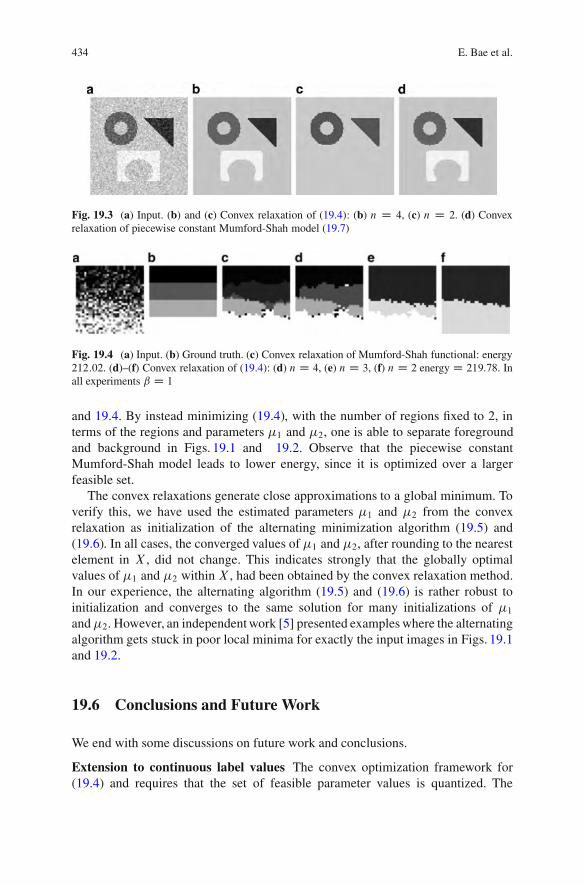
434 E. Bae et al.
Fig. 19.3 (a) Input. (b) and (c) Convex relaxation of (19.4): (b) n D 4, (c) n D 2. (d) Convexrelaxation of piecewise constant Mumford-Shah model (19.7)
Fig. 19.4 (a) Input. (b) Ground truth. (c) Convex relaxation of Mumford-Shah functional: energy212:02. (d)–(f) Convex relaxation of (19.4): (d) n D 4, (e) n D 3, (f) n D 2 energy D 219:78. Inall experiments ˇ D 1
and 19.4. By instead minimizing (19.4), with the number of regions fixed to 2, interms of the regions and parameters !1 and !2, one is able to separate foregroundand background in Figs. 19.1 and 19.2. Observe that the piecewise constantMumford-Shah model leads to lower energy, since it is optimized over a largerfeasible set.
The convex relaxations generate close approximations to a global minimum. Toverify this, we have used the estimated parameters !1 and !2 from the convexrelaxation as initialization of the alternating minimization algorithm (19.5) and(19.6). In all cases, the converged values of !1 and !2, after rounding to the nearestelement in X , did not change. This indicates strongly that the globally optimalvalues of !1 and !2 within X , had been obtained by the convex relaxation method.In our experience, the alternating algorithm (19.5) and (19.6) is rather robust toinitialization and converges to the same solution for many initializations of !1and!2. However, an independent work [5] presented examples where the alternatingalgorithm gets stuck in poor local minima for exactly the input images in Figs. 19.1and 19.2.
19.6 Conclusions and Future Work
We end with some discussions on future work and conclusions.
Extension to continuous label values The convex optimization framework for(19.4) and requires that the set of feasible parameter values is quantized. The
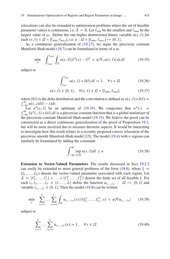
19 Simultaneous Optimization of Regions and Region Parameters in Image . . . 435
relaxations can also be extended to optimization problems where the set of feasibleparameter values is continuous, i.e. X D R. Let `min be the smallest and `max be thelargest value of !i . Define the one-higher dimensional binary variable u.x; `/ foreach .x; `/ 2 ˝ & Œ`min; `max %, i.e. u W ˝ & Œ`min; `max % 7! f0; 1g.
As a continuous generalization of (19.17), we argue the piecewise constantMumford-Shah model (19.7) can be formulated in terms of u as
minu
Z `max
`min
Z
˝
u.x; `/jI 0.x/ ! `jˇ C ˛jrxu.x; `/j dx d` (19.35)
subject toZ `max
`min
u.x; `/ ' ı.`/ d` D 1; 8x 2 ˝ (19.36)
u.x; `/ 2 f0; 1g; 8.x; `/ 2 ˝ & Œ`min; `max%: (19.37)
where ı.`/ is the delta distribution and the convolution is defined as u.x; `/'ı.`/ DR1!1 u.x; s/ı.` ! s/ds.
Let u".x; `/ be an optimum of (19.35). We conjecture that w".:/ DR1!1 `u
".:; `/' ı.`/ d` is a piecewise constant function that is a global minimizer ofthe piecewise constant Mumford-Shah model (19.15). We believe the proof can beconstructed as a direct continuous generalization of the proof of Proposition 19.1,but will be more involved due to measure theoretic aspects. It would be interestingto investigate how this result relates to a recently proposed convex relaxation of thepiecewise smooth Mumford-Shah model [15]. The model (19.4) with n regions cansimilarly be formulated by adding the constraint
Z 1
!1supx2˝
u.x; `/d` % n (19.38)
Extension to Vector-Valued Parameters The results discussed in Sect. 19.2.3can easily be extended to more general problems of the form (19.8), where " D."1; : : : ; "N / denote the vector-valued parameter associated with each region. LetX D f`11; : : : ; `1Lg & : : : & f`N1 ; : : : ; `NL g denote the finite set of all feasible ". Foreach i1; i2; : : : ; iN 2 f1; : : : ; Lg define the function ui1;:::;iN W ˝ 7! f0; 1g andvariable vi1;:::;iN 2 f0; 1g. Then the model (19.8) can be written
minu
LX
i1D1: : :
LX
iND1
Z
˝
ui1;:::;iN .x/f ."1i1; : : : ; "NiN ; x/ C ˛jrui1;:::;iN j (19.39)
subject to
LX
i1D1: : :
LX
iND1ui1;:::;iN .x/ D 1 ; 8x 2 ˝ (19.40)
436 E. Bae et al.
LX
i1D1: : :
LX
iND1maxx2˝
ui1;:::;iN .x/ % n; (19.41)
ui1;:::;iN .x/ 2 f0; 1g ; 8x 2 ˝; i1; : : : ; iN 2 X : (19.42)
The equivalence between (19.8) and (19.39) follows by a straight forward general-ization of Proposition 19.2.
19.6.1 Conclusions
Image segmentation problems can successfully be modeled as the minimization ofan energy potential with respect to regions and parameters associated with eachregion. In this work, we have reformulated such problems as the optimization ofbinary functions in a space of one higher dimension than the image domain. Convexrelaxations and optimization algorithms have been proposed which does not dependon initializations and produce close approximations to global minima. In contrastto previous work, the complexity of our algorithm grows at most linearly with thenumber of potential parameter values, and can be applied for segmentation problemswith any number of regions.
19.7 Proofs
Proof of Proposition 19.1
Proof. Let .fQuj gQnjD1; f`Qij gQnjD1; Qn/ be any other solution of (19.16). Define the vectorfunction
Nuj D 0; for j 2 f1; : : : ; LgnfQi1; : : : ; QiQngNuQij D Quj for j D 1; : : : ; Qn:
Then Nu belongs to the feasible set (19.18) of the problem (19.17).
Eext.Nu/DLX
iD1
Z
˝Nui jI 0.x/!`i j2 dxC
LX
iD1
˛
Z
˝jr Nui jdx D
QnX
jD1
Z
˝NuQij jI 0.x/!`i j2dxC
QnX
jD1
˛
Z
˝jr NuQij jdx
DQnX
iD1
Z
˝Qui jI 0.x/! `Qij j2 dxC
QnX
iD1
˛
Z
˝jrQui jdx D E.fQuj gQnjD1; f`Qij gQnjD1; Qn/:
But since u" is a global minimizer of Eext
Eext.u"/ % Eext.Nu/ D E.fQuj gQnjD1; f`Qij gQnjD1; Qn/; (19.43)
19 Simultaneous Optimization of Regions and Region Parameters in Image . . . 437
and since
Eext.u"/ DLX
iD1
Z
˝
u"i jI 0.x/ ! `i j2 dx CLX
iD1˛
Z
˝
jru"i j dx
DnX
jD1
Z
˝
u"ij jI0.x/ ! `ij j2dx C
nX
jD1˛
Z
˝
jru"ij jdx D E.fu"ijgnjD1; fij gnjD1; n/:
(19.44)
Combining (19.43) and (19.44) it follows that
E.fu"ij gnjD1; fij gnjD1; n/ % E.fQuj gQnjD1; f`Qij g
QnjD1; Qn/:
Hence fu"ij gnjD1; fij gnjD1; n must be a solution to (19.16).
References
1. Bae, E., Tai, X.-C.: Efficient global minimization for the multiphase Chan-Vese model ofimage segmentation. In: Cremers, D., Boykov, Y., Blake, A., Schmidt, F.R. (eds.) EnergyMinimization Methods in Computer Vision and Pattern Recognition 2009. Volume 5681 ofLecture Notes in Computer Science, pp. 28–41. Springer, Berlin/Heidelberg (2009)
2. Bae, E., Yuan, J., Tai, X.-C.: Global minimization for continuous multiphase partitioningproblems using a dual approach. Int. J. Comput. Vis. 92, 112–129 (2011)
3. Boykov, Y., Veksler, O., Zabih, R.: Fast approximate energy minimization via graph cuts. IEEETrans. Pattern Anal. Mach. Intell. 23, 1222–1239 (2001)
4. Brown, E.S., Chan, T.F., Bresson, X.: A convex relaxation method for a class of vector-valuedminimization problems with applications to mumford-shah segmentation. UCLA, AppliedMathematics, CAM-report-10-43, Department of Mathematics, UCLA, July 2010
5. Brown, E.S., Chan, T.F., Bresson, X.: Completely convex formulation of the chan-vese imagesegmentation model. Int. J. Comput. Vis. (2011). doi:10.1007/s11263-011-0499-y
6. Chan, T., Vese, L.A.: Active contours without edges. IEEE Image Proc. 10, 266–277 (2001)7. Chan, T.F., Esedoglu, S., Nikolova, M.: Algorithms for finding global minimizers of image
segmentation and denoising models. SIAM J. Appl. Math. 66(5), 1632–1648 (electronic)(2006)
8. Darbon, J.: A note on the discrete binary mumford-shah model. In: Proceedings of Com-puter Vision/Computer Graphics Collaboration Techniques, (MIRAGE 2007). LNCS Series,vol. 4418, pp. 283–294, March 2007
9. Delong, A., Osokin, A., Isack, H., Boykov, Y.: Fast approximate energy minimization withlabel costs. In: IEEE Conference on Computer Vision and Pattern Recognition (CVPR),pp. 2173–2180 (2010)
10. Lellmann, J., Kappes, J., Yuan, J., Becker, F., Schnorr, C.: Convex multi-class image labelingby simplex-constrained total variation. In: Tai, X.-C., Morken, K., Lysaker, M., Lie, K.-A.(eds.) Scale Space and Variational Methods in Computer Vision (SSVM 2009). Volume 5567of LNCS, pp. 150–162. Springer, Berlin/Heidelberg (2009)
438 E. Bae et al.
11. Lellmann, J., Breitenreicher, D., Schnorr, C.: Fast and exact primal-dual iterations for varia-tional problems in computer vision. In: European Conference on Computer Vision (ECCV).LNCS vol. 6312, pp. 494–505 (2010)
12. Lempitsky, V., Blake, A., Rother, C.: Image segmentation by branch-and-mincut. In: Proceed-ings of the 10th European Conference on Computer Vision: Part IV, pp. 15–29. Springer,Berlin, Heidelberg (2008)
13. Mumford, D., Shah, J.: Optimal approximation by piecewise smooth functions and associatedvariational problems. Commun. Pure Appl. Math. 42, 577–685 (1989)
14. Pock, T., Chambolle, A., Bischof, H., Cremers, D.: A convex relaxation approach for com-puting minimal partitions. In: IEEE Conference on Computer Vision and Pattern Recognition(CVPR), Miami, Florida (2009)
15. Pock, T., Cremers, D., Bischof, H., Chambolle, A.: An algorithm for minimizing the piecewisesmooth mumford-shah functional. In: IEEE International Conference on Computer Vision(ICCV), Kyoto, Japan (2009)
16. Potts, R.B.: Some generalized order-disorder transformations. In: Proceedings of the Cam-bridge Philosophical Society, vol. 48, pp. 106–109 (1952)
17. Strandmark, P., Kahl, F., Overgaard, N.C.: Optimizing parametric total variation models. In:IEEE 12th International Conference on Computer Vision, pp. 2240–2247, pp. 26–33 (2009)
18. Yuan, J., Boykov, Y.: Tv-based image segmentation with label cost prior. In: BMVC, Articleno 101, pp. 101:1–101:12. BMVA Press, Sept 2010
19. Yuan, J., Bae, E., Tai, X.-C., Boykov, Y.: A continuous max-flow approach to potts model. In:ECCV. Lecture Notes in Computer Science, vol. 6316, pp. 379–392 (2010)
20. Yuan, J., Shi, J., Tai, X.-C.: A convex and exact approach to discrete constrained tv-l1 imageapproximation. Technical report CAM-10–51, UCLA, CAM, UCLA (2010)
21. Yuan, J., Bae, E., Boykov, Y., Tai, X.C.: A continuous max-flow approach to minimal partitionswith label cost prior. In: Bruckstein, A.M., ter Haar Romeny, B.M., Bronstein, A.M., Bronstein,M.M. (eds.) Scale Space and Variational Methods in Computer Vision. Lecture Notes inComputer Science, vol. 6667, pp. 279–290 (2012)
22. Zach, C., Gallup, D., Frahm, J.-M., Niethammer, M.: Fast global labeling for real-time stereousing multiple plane sweeps. In: Deussen, O., Keim, D.A., Saupe, D. (eds.) Proceedings of theVision, Modeling and Visualization Conference (VMV), pp. 243–252 (2008)
23. Zhu, S.C., Yuille, A.: Region competition: Unifying snakes, region growing, and bayes/mdl formulti-band image segmentation. IEEE Trans. Pattern Anal. Mach. Intell. 18, 884–900 (1996)

Chapter 20Fluctuating Distance Fields, Parts, Three-PartiteSkeletons
Sibel Tari
So the nature of a visual experience can not be described interms of inches of size and distance.Rudolf Arnheim
Abstract Shapes are continuous objects, even when they are drawn on digitalmedia or composed using finite number of elements. As such, they defy analyticapproach; explicitization of their parts, hierarchies, skeletons, or even centroids isill-posed. I describe a novel approach to perceptually organize shapes and explicatetheir features without being negligent of their continuous nature. The basic constructis an unusual phase field that can be conceived in a number of varying ways usingvarying mathematical machinery, so highlighting the field itself rather than how it isbeing computed. Connections among the field, Mumford-Shah and Tari-Shah-Pienmodels, and reaction-diffusion equation suggest that the field may bridge low-leveland high-level visual processing.
20.1 Shapes Are Continuous
Shapes are continuous objects, even when they are drawn on digital media orcomposed using finite number of elements. In favor of the argument, Gestalt schoolproduced numerous illustrations, e.g., (1) a finite set of isolated dots placed at afixed distance from a fixed location creates a circle percept; (2) a peanut shapeprevailingly reveals two discrete blobs or approaches to a blob, as its neck thinsor thickens; (3) two squares juxtaposed to form an eight-pointed star gives way tonew parts, namely eight triangles and an octagon.
S. Tari (!)Middle East Technical University, 06531, Ankara, Turkeye-mail: [email protected]
M. Breuß et al. (eds.), Innovations for Shape Analysis, Mathematics and Visualization,DOI 10.1007/978-3-642-34141-0 20, © Springer-Verlag Berlin Heidelberg 2013
439
440 S. Tari
In a similar vein but surpassing Gestalt, Stiny [50] speaks for ambiguity(i.e. multiple interpretations) in part perception, convincing the reader to placepart boundaries wherever and whenever desired. Such a liberal view of shapetopology certainly stands in strong contrast to prevalent theories on part perceptionexemplified by seminal works of Biederman [9] (imposing regularity on parts) andHoffman and Richards [23] (imposing regularity on break points); nevertheless,contemporary work in neuroscience support the continuity of the process, too [37].
Additionally, shapes live in continua as opposed to standing in isolation. Thebasis of this argument is two-fold: (1) perception of a shape is influenced bynearby shapes (underlying category structures); indeed, several papers, e.g. [17,34],draw parallels between this contextual effect and experimentally observed non-metric characteristics (asymmetry and violation of triangle inequality) of pairwisedissimilarities; (2) shapes naturally deform into other shapes, say, a peanut changesto a blob-like shape or a pair of disjoint blobs as its neck thickens or thins,respectively.
To a great extent, it is the continuous nature of shapes that hinders theircomprehension and description using analytic methods; thus, it is only natural thatseveral chapters from this book present state of the art techniques for situatingshapes in continua by constructing shape dynamics, shape spaces etc.
In pursuit of the goal, the presented approach is an attempt to perceptuallyorganize shapes and explicate their features in the form of skeletons withoutbeing negligent of their continuous nature. At the core of constructions is anunusual distance-like, scalar field, !, that implicitly codes interactions among shapeelements, both over the region and along the boundary and both local and non-local.
Overview of the New Distance Field The most distinct feature of the new fieldis that it fluctuates, i.e., unlike previous ones [4, 22, 28, 42, 54], the new one is anon-monotone function of the distance to a set of input points. It is non-monotonebecause the value of the field at each point mimics the distance (a diffuse one [54,55]) from the point to the union of (1) a set of input points and (2) a yet to bedetermined curve.
The set of input points specifies the shape boundary either incompletely (in casesof open contours, illusory contours or outcomes of edge detectors) or completelyas the bounding curve of a connected bounded open set, say ˝ ! R2. In eithercase, the shape boundary is indicated by the set of input points, denoted by @˝ andsubjected to homogeneous Dirichlet type boundary condition.
The construction of the! is valid regardless of the form the boundary is specified.If it is completely specified with a clear distinction between interior and exterior, thefield can be computed only on the interior. If, however, the boundary is incompletelyspecified, the field needs to be computed on a wider scope R which is a simplyconnected subset of R2 containing the input set. Of course, a suitable boundarycondition is needed on @R.
The new field has interesting emergent features; for example, it attains value zeronot only on the shape boundary (which is due to homogeneous Dirichlet boundarycondition on @˝) but also on a curve bounding a central cut. The latter locusis an emergent feature and divides the shape into central and peripheral regions.

20 Fluctuating Distance Fields 441
Fig. 20.1 The values of the new field fluctuate between positive and negative. The iso-level curvesreflect the minimum distance to the union of the shape boundary and an emergent curve (shown ingreen)
Roughly speaking, the central region is the least deformable and coarse structureof the shape; moreover, the field inside it is a flexible indicator of the topology andcentrality, not necessarily bound to a unique interpretation.
A sample field is depicted in Fig. 20.1. The leftmost figure displays some iso-level curves of the field and the top right one displays its absolute value. Finally, thebottom right figure is the plot of the values at the cross-section marked by the red linein the top right. Observe that the field exhibits interesting features in addition to theemergent zero-level curve: lower level sets in the peripheral region code appendages,the level curves neighboring the boundary resemble erosions of the shape, and thelevel curves neighboring the zero-level curve resemble erosions and dilations of thecentral region. All create a dynamic view of the shape.
What’s more, the geometry of the level curves is intricately related to that ofa well studied diffuse distance field [3, 4, 47, 54, 55] which is the solution of thescreened Poisson PDE and has close connection to the Ambrosio-Tortorelli approx-imation [1] of the Mumford-Shah functional [35] (more on this in Sect. 20.2.3).
The intricate relation between the two fields facilitates an unorthodox skeletonabstraction that I call Three-Partite, due to its being composed of three distinctgroups providing a separation into (1) gross structure; (2) limbs and (3) boundarytexture or noise. Two examples are shown in Fig. 20.2 where the three skeletongroups are respectively shown in red, blue and green. The first group (red) consistsof nested closed curves and abstracts the topology as well as the centrality of thecoarse structure. It has two distinct layers: the inner (dark red) and the outer (lightred). Both layers are coarser forms of the boundary. The outer layer, which is finerthan the inner one, can be considered as the coarsest and least articulable structurestill indicating the appendages. The inner layer is the emergent zero-level curve,bounding the central region. The second group (blue) consists of disjoint branches
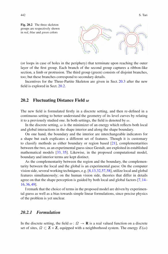
442 S. Tari
Fig. 20.2 The three skeletongroups are respectively shownin red, blue and green colors
(or loops in case of holes in the periphery) that terminate upon reaching the outerlayer of the first group. Each branch of the second group captures a ribbon-likesection, a limb or protrusion. The third group (green) consists of disjoint branches,too; but these branches correspond to secondary details.
Incentives for the Three-Partite Skeleton are given in Sect. 20.3 after the newfield is explored in Sect. 20.2.
20.2 Fluctuating Distance Field !
The new field is formulated firstly in a discrete setting, and then re-defined in acontinuous setting to better understand the geometry of its level curves by relatingit to a previously studied one. In both settings, the field is denoted by !.
In the discrete setting, ! is the minimizer of an energy which reflects both localand global interactions in the shape interior and along the shape boundary.
On one hand, the boundary and the interior are interchangeable indicators fora shape but each explicates a different set of features. Though it is customaryto classify methods as either boundary or region based [21], complementaritiesbetween the two, as an experimental guess since Gestalt, are exploited in establishedmathematical models [33, 35]. Likewise, in the proposed computational model,boundary and interior terms are kept distinct.
As the complementarity between the region and the boundary, the complemen-tarity between the local and the global is an experimental guess: On the computervision side, several working techniques, e.g. [8,13,32,57,58], utilize local and globalfeatures simultaneously; on the human vision side, theories that differ in detailsagree on that the shape perception is guided by both local and global factors [7,14–16, 36, 49].
I remark that the choice of terms in the proposed model are driven by experimen-tal guess as well as a bias towards simple linear formulations, since precise physicsof the problem is yet unclear.
20.2.1 Formulation
In the discrete setting, the field ! W ˝ ! R is a real valued function on a discreteset of sites, ˝ ! Z " Z, equipped with a neighborhood system. The energy E.!/
20 Fluctuating Distance Fields 443
is taken as a linear combination of a region based energy EReg.!/ defined on ˝and a boundary based energy EBdy.!/ defined on @˝ , both of which is a sum ofpixel-wise terms:
E.!/ DX
.i;j /2˝EReg.!i;j / C !
X
.i;j /2@˝EBdy.!i;j / (20.1)
where ! > 0 is a constant. The additive form is for computational simplicity.
Region Energy The region energy composed of both local and global terms isexpressed as a linear combination, too:
EReg DX
.i;j /2˝EGReg.!i;j /
„ ƒ‚ …EGReg : global
C ˇX
.i;j /2˝ELReg.!i;j /
„ ƒ‚ …ELReg : local
(20.2)
where ˇ > 0 is a constant. In the absence of a specific bias towards local or global,a natural choice may be ˇ D 1.
Global Component Consider the squared average, the simplest quadratic expres-sion linking all the nodes, as the global energy:
EGReg.!i;j / WD
0
@ 1
j˝jX
.k;l/2˝!k;l
1
A2
Differentiating its sum over˝ w.r.t. !i;j :
@
@!i;jEGReg D
@
@!i;j
X
.i;j /2˝
0
@ 1
j˝jX
.k;l/2˝!k;l
1
A2
D 2
j˝jX
.k;l/2˝!k;l (20.3)
Notice that the considered energy is minimized by either the zero function or afluctuating function of which positive and negative values cancel each other.
Local Component The simplest local interaction model appears to be the sum ofpairwise products of ! value at a site with ! values at the site’s nearest neighbors.Such a component in the energy imposes regularity by favoring configurations inwhich each node agrees with its immediate neighbors. Assuming the usual four-connectivity, such that f.iC1; j /; .i#1; j /; .i; jC1/; .i; j#1/g defines the nearestneighbors of site .i; j /, local interaction energy takes the form:
ELReg.!i;j / WD #
!!i;j $ !iC1;j C !i;j $ !i!1;j C !i;j $ !i;jC1 C !i;j $ !i;j!1
"
444 S. Tari
Differentiating w.r.t. !i;j :
@ELReg
@ !i;jD @
@!i;j
X
.i;j /2˝#!!i;j $ !iC1;j C !i;j $ !i!1;j C !i;j $ !i;jC1 C !i;j $ !i;j!1
"
D #2#!iC1;j C !i!1;j C !i;jC1 C !i;j!1
$(20.4a)
D #2hL!!i;j
"C 4!i;j
i(20.4b)
where L denotes the usual five-point discretization of the Laplace operator 4 WD@2
@x2C @2
@y2, using step size one. Notice that (20.4a) is nothing but the sum of the
four neighbors, and (20.4b) is obtained by re-arranging the terms after adding andsubtracting 4 !i;j .
The scope of the regularity induced by the local energy can be extended byconsidering pairwise interactions in a larger neighborhood Nij :
ELReg.!i;j / WD #
X
.k;l/2Nij
ai;j Ik;l $ !i;j $ !k;l (20.5)
where ai;j Ik;l D ak;lIi;j are suitably chosen positive weights, say, inversely propor-tional to the squared distances between the pairs as defined by the neighborhoodsystem. Then the derivative of EL
Reg w.r.t. !i;j is nothing but a weighted sum of theneighbors:
@ELReg
@!i;jD @
@!i;j
X
.i;j /2˝#
0
@X
.k;l/2Nij
ai;j Ik;l $ !i;j $ !k;l
1
A
D #2X
.k;l/2Nij
ai;j Ik;l $ !k;l (20.6)
As a result, similar to (20.4b), it can be be re-written as
# 2 $hLG!!i;j
"C "G !i;j
i(20.7)
where LG!:"
denotes the graph Laplacian and "G > 0 a constant that depends onthe neighborhood system.
Of course, the scope of the local regularity may be further extended by includingall of the pairwise interactions among the elements in Nij :
X
.k;l/2Nij.m;n/2Nij
.k;l/¤.m;n/
ak;lIm;n $ !k;l $ !m;n (20.8)

20 Fluctuating Distance Fields 445
Fig. 20.3 The distancebetween a pair of nodesjoined by a blue arrow iseither 2 (the Manhattan) orp2 (the Euclidean)
with the weights reflecting the distances (Fig. 20.3). Then the derivative w.r.t. !i;jis either of the following nine-point weighted averages in a 5 " 5 window centeredat .i; j /:
1
4
2
66664
" " 1 " "" 2 " 2 "1 " " " 1" 2 " 2 "" " 1 " "
3
777751
4
2
66664
" " 1 " "" 4 " 4 "1 " " " 1" 4 " 4 "" " 1 " "
3
77775
The one the left is obtained if the weights are calculated according to the Manhattan,the natural metric for the 4-connected grid, and the one on the left according tothe Euclidean. Upon subtracting a suitable multiple of !i;j , both stencils becomea realization of the nine-point discrete Laplacian on a redefined grid. That is, aslong as local interactions are restricted to pairwise products (linear combinations of(20.5) and (20.8)), the derivative of the local energy w.r.t. !i;j is of the form:
@ELReg
@!i;jD #2"1
hL#!!i;j
"C "2!i;j
i(20.9)
where L# is some approximation to the discrete Laplacian.
Adding Local and Global Components Combining (20.9) and (20.3) according tothe additive model (20.2) yields
@EReg
@!i;jD #2
hL#!!i;j
"C N"!i;j #
1
O!j˝j
"X
.k;l/2˝!k;l
i(20.10)
where O!j˝j
"denotes a positive constant on the order of the domain size and
N" > 0 depends on assumed local connectivities as well as the parameter ˇ in (20.2).Later on, we will see that the choice of N" has no bearing on the result.
Boundary Energy Formulating interactions along a contour is not as simple asformulating them over a region. The task gets further complicated in the case oflong-range interactions because critical ones occur among specific pairs of boundarypoints, e.g., two opposing indentation points on a neck region.
446 S. Tari
Fortunately, the usual distance transform provides a way out. At the outset, it isa transform that assigns to each point on a domain the minimum distance from thepoint to the domain boundary, yet it is at the same time a compact representationfor boundary interactions. Indeed, its construction can be imagined as a dynamicprocess, a time-dependent evolution of the shape boundary such that each point onit moves with a unit speed in the direction of the unit normal; so the distance fieldt as a function over the digital plane is defined by setting ti;j D the time when theevolving curve passes through the point .i; j /. Through the course of the evolution,singularities form as opposing pairs of boundary points meet and characterize theshape as its parts and symmetries are revealed [10].
The key point is that once a bridge between boundary interactions and thedistance transform is established, EBdy is easily defined as a quadratic expressionover the region˝:
X
.i;j /2@˝EBdy.!i;j / WD
X
.i;j /2˝
!!i;j # ti;j
"2 (20.11)
As a result,
@EBdy
@!i;jD @
@!i;j
X
.i;j /2@˝EBdy.!i;j /
D 2!!i;j # ti;j
"(20.12)
That is, ! D t .Complete Energy Combining (20.12) and (20.10) according to the additive model(20.1):
@E
@!i;jD #L#
!!i;j
"C 1
O!j˝j
"X
.k;l/2˝!k;l C .! # N"/ !i;j # !ti;j (20.13)
Then the condition satisfied by the minimizer is obtained by setting the expressionin (20.13) to zero, which is in matrix notation given by
%#L C 1
O .j˝j/J C .! # N"/ I&
w D ! t (20.14)
where
• w and t are vector representations for the field ! and the distance transform t ;• L is the j˝j " j˝j matrix representation for a discrete Dirichlet Laplacian;• J is the j˝j " j˝j matrix of ones;• I is the j˝j " j˝j identity matrix.

20 Fluctuating Distance Fields 447
Firstly, notice that the uniform scaling of the right hand side term with ! has noeffect on the geometry of !; it only scales the values, leaving the shape of the levelcurves intact. As a result, the geometric features of ! depends only on the choice of.! # N"/. Secondly, notice that
##LC 1
O.j˝j/ $ JC .! # N"/ $ I$
is a positive definitematrix if .! # N"/ % 0. The difference between the strict positivity and zero, from thelinear algebraic point of view, is that the former one has a better condition numberso strict positivity of .! # N"/ may be preferable. But if .! # N"/ exceeds 1
O.j˝j/ ,the non-spatial term dominates over the spatial ones. Such intuition suggest that.! # N"/, the only parameter, should be approximately 1
j˝j . Later on this choice issupported in the continuous domain model as well.
Implementation Based on the above discussion the parameters N" # ! and ! areeliminated: Firstly, N" # ! is selected as inversely proportional to the domain size.Secondly, t is replaced by Nt denoting an arbitrary scaling of the distance transformbecause the right hand side scaling by ! does not affect the geometry of the solution.
Using the method of gradient descent, computing ! is cast as computing thesteady state solution of the following differential-difference equation:
d!i;j .#/d#
D # @E
@!i;j(20.15)
D L#!!i;j
"# 1
O!j˝j
"X
.k;l/2˝!k;l #
1
O!j˝j
"!i;j C Nti;j
Discretizing # as
!nC1i;j # !ni;j$#
D!!ni;jC1 C !ni;j!1 C !niC1;j C !ni!1j; # 4!ni;j
"(20.16)
# 1
j˝jX
.k;l/2˝!nk;l #
1
j˝j!nC1k;l C Nti;j
where n D 0; 1; 2; $ $ $ is the iteration variable yields an iterative scheme once theterms in (20.16) are re-arranged. Note that L# is simply replaced with the usual fivepoint discrete Laplacian, and O
!j˝j
"with j˝j.
Behavior of ! The solution satisfies three competing criteria:
# having low expected value (20.17a)
# being smooth (20.17b)
# staying close to the usual distance transform (20.17c)
At a first glance, the first criterion seems to favor flatness by forcing the minimizerto attain values close to zero; yet this criterion is also satisfied when the values of
448 S. Tari
! fluctuate between positive and negative. The other two criteria impose additionalregularities so the fluctuations form a certain spatial pattern as opposed to beingrandom localization of positive and negative values. Firstly, the locations of identicalsign tend to form spatial proximity groups as defined by the graph neighborhoodsystem. Secondly, the positive clusters tend to occur in the central region. This isdue to the third criterion: Whenever ! is negative at a point .i; j /, a penalty largerthan t2i;j is incurred; therefore, ! has a stronger tendency to be positive at locationswhere the value of distance transform is higher in order to minimize the total costof deviating from the distance transform. Consequently, ! attains positive values incentral locations where the value of the distance transform is higher and negativevalues at peripheral locations where the value of the distance transform is lower.
20.2.2 Illustrative Results
Few illustrative results are depicted in Figs. 20.4–20.6. In color illustrations, !values are normalized to Œ0; 1% within regions of identical sign for convenience ofvisualization and the zero-level is depicted in dark blue.
Central and Peripheral Separation In each case, the zero-level set partitionsthe shape domain into upper and lower zero level sets, ˝C and ˝!, denotingrespectively central and peripheral regions.˝! contains all the detail: limbs, protrusions, and boundary texture or noise.
In contrast, ˝C is coarse blob-like form, which can even be considered as aninterval estimate of the center; most commonly, it is a simply connected set.Of course, it may also be either disconnected or multiply connected. For instance, itis disconnected for a dumbbell-like shape (two blobs of comparable radii combinedthrough a thin neck) whereas it is multiply connected for an annulus formed by twoconcentric circles. Indeed, the annulus gets split into three concentric rings. Whereasthe middle ring is the ˝C, the union of the outermost and the innermost rings forma multiply-connected set corresponding to the ˝!, separated by the ˝C.
For quite a many shapes, however,˝C is a simply connected set. Firstly, shapesobtained by protruding a blob as well as shapes whose peripheral parts are smaller orthinner than their main parts always have a simply connected˝C. This is expected:When the width of a part is small, the highest value of the distance transform tinside the part is small. That is, the local contribution to .! # t/2 incurring due tonegative values is less significant for such a part as compared to locations withhigher positive values of t . Consequently, ! tends to attain negative values onnarrow or small parts as well as on protrusions. Shapes with holes also have asimply connected ˝C as long as the holes are far from the center. Secondly, evena dumbbell-like shape may have a simply connected ˝C. This happens if the joinarea, namely the neck, is wide enough, e.g., the top right in Fig. 20.4. Nevertheless,this does not cause any representational instability: Whereas the ˝C for a blob-like shape has a unique maximum located roughly at its centroid, the ˝C for a
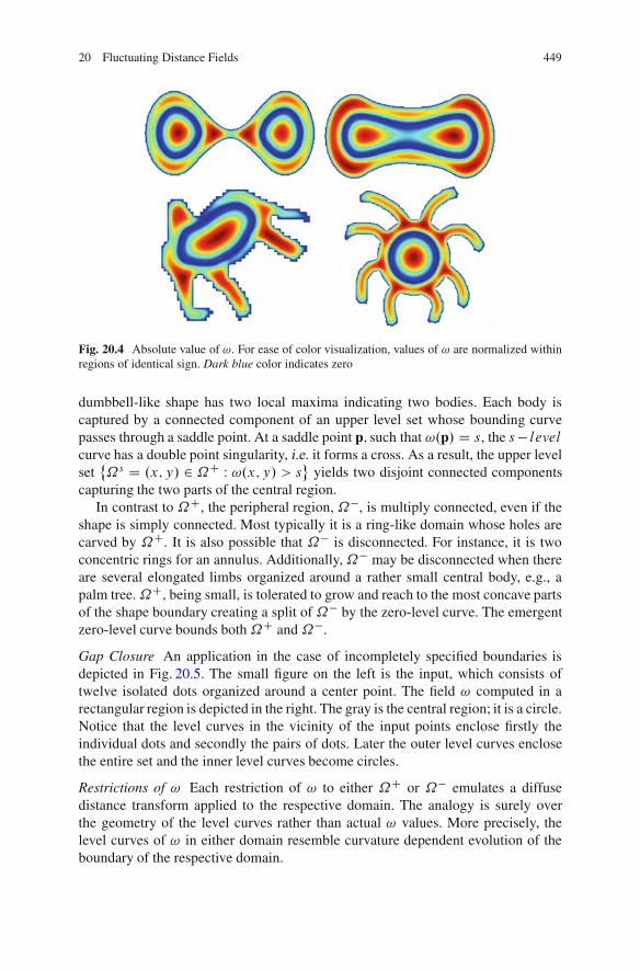
20 Fluctuating Distance Fields 449
Fig. 20.4 Absolute value of !. For ease of color visualization, values of ! are normalized withinregions of identical sign. Dark blue color indicates zero
dumbbell-like shape has two local maxima indicating two bodies. Each body iscaptured by a connected component of an upper level set whose bounding curvepasses through a saddle point. At a saddle point p; such that !.p/ D s, the s# levelcurve has a double point singularity, i.e. it forms a cross. As a result, the upper levelset
˚˝s D .x; y/ 2 ˝C W !.x; y/ > s
'yields two disjoint connected components
capturing the two parts of the central region.In contrast to ˝C, the peripheral region, ˝!, is multiply connected, even if the
shape is simply connected. Most typically it is a ring-like domain whose holes arecarved by ˝C. It is also possible that ˝! is disconnected. For instance, it is twoconcentric rings for an annulus. Additionally,˝! may be disconnected when thereare several elongated limbs organized around a rather small central body, e.g., apalm tree.˝C, being small, is tolerated to grow and reach to the most concave partsof the shape boundary creating a split of ˝! by the zero-level curve. The emergentzero-level curve bounds both˝C and ˝!.
Gap Closure An application in the case of incompletely specified boundaries isdepicted in Fig. 20.5. The small figure on the left is the input, which consists oftwelve isolated dots organized around a center point. The field ! computed in arectangular region is depicted in the right. The gray is the central region; it is a circle.Notice that the level curves in the vicinity of the input points enclose firstly theindividual dots and secondly the pairs of dots. Later the outer level curves enclosethe entire set and the inner level curves become circles.
Restrictions of ! Each restriction of ! to either ˝C or ˝! emulates a diffusedistance transform applied to the respective domain. The analogy is surely overthe geometry of the level curves rather than actual ! values. More precisely, thelevel curves of ! in either domain resemble curvature dependent evolution of theboundary of the respective domain.
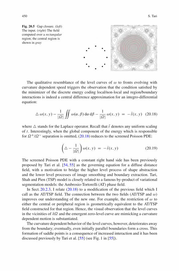
450 S. Tari
Fig. 20.5 Gap closure. (left)The input. (right) The fieldcomputed over a rectangularregion; the central region isshown in gray
The qualitative resemblance of the level curves of ! to fronts evolving withcurvature dependent speed triggers the observation that the condition satisfied bythe minimizer of the discrete energy coding local/non-local and region/boundaryinteractions is indeed a central difference approximation for an integro-differentialequation:
4 !.x; y/ # 1
j˝j
“!.˛; ˇ/ d˛ dˇ # 1
j˝j !.x; y/ D #Nt.x; y/ (20.18)
where4 stands for the Laplace operator. Recall that Nt denotes any uniform scalingof t . Interestingly, when the global component of the energy which is responsiblefor˝C/˝! separation is omitted, (20.18) reduces to the screened Poisson PDE:
%4 # 1
j˝j
&!.x; y/ D # Nt.x; y/ (20.19)
The screened Poisson PDE with a constant right hand side has been previouslyproposed by Tari et al. [54, 55] as the governing equation for a diffuse distancefield, with a motivation to bridge the higher level process of shape abstractionand the lower level processes of image smoothing and boundary extraction. Tari,Shah and Pien (TSP) model is closely related to a famous by-product of variationalsegmentation models: the Ambrosio-Tortorelli (AT) phase field.
In Sect. 20.2.3, I relate (20.18) to a modification of the previous field which Icall as the AT/TSP field. The connection between the two fields (AT/TSP and !)improves our understanding of the new one. For example, the restriction of ! toeither the central or peripheral region is geometrically equivalent to the AT/TSPfield constructed for that region. Hence, the visual observation that the level curvesin the vicinities of @˝ and the emergent zero-level curve are mimicking a curvaturedependent motion is substantiated.
The curvature dependent behavior of the level curves, however, deteriorates awayfrom the boundary; eventually, even initially parallel boundaries form a cross. Thisformation of saddle points is a consequence of increased interaction and it has beendiscussed previously by Tari et al. [55] (see Fig. 1 in [55]).

20 Fluctuating Distance Fields 451
Fig. 20.6 Level curves of !.For visualization purposes,the values are normalizedwithin central and peripheralregions; the zero level isdepicted in dark blue
Fig. 20.7 Formation of watershed zones in the peripheral region is a consequence of the relationof the new field to the AT/TSP field
Fortunately, in the new framework, this behavioral deviation provides consider-able convenience by assuring that the peripheral region is always partitioned, unlessit is a perfect annulus. Figure 20.6 depicts level curves of ! for the octopus. Noticethe formation of eight saddle points separating the arms of the octopus. Indeed thezones separated by the saddle points are easily extracted as watershed zones [31] ofthe peripheral region (Fig. 20.7). Of course, raw watershed partitions are subject totopologic instabilities. Obtaining topologically stable partitions is a separate issuewhich is tackled in a recent work by Tari and Genctav [51] by constructing aprobabilistic part tree; nevertheless, watershed zones surrounding the central regionare perfectly sufficient as rough part estimates.
20.2.3 ! and the AT/TSP Field
In vision applications, the AT (Ambrosio-Tortorelli) phase field appeared first as atechnical device to apply gradient descent to the Mumford-Shah functional [35],where it served as a continuous indicator for boundary/not-boundary phases ateach domain point [44]. The field is the minimizer of an energy composed oftwo competing terms: One term favors configurations that take values close toeither 0 or 1 (separation into boundary/not-boundary phases) and the other term
452 S. Tari
encourages local interaction in the domain by penalizing spatial inhomogeneity. Aparameter controls the relative influence of these two terms hence the interaction. Asthis “interaction” parameter tends to 0, the separation term is strongly emphasized;consequently, the field tends to the characteristic function 1#&S of the boundary setS and the respective energy tends (following the ' convergence framework [11]) tothe boundary length.
Over the years, the AT field has been used in numerous applications addressinga rich variety of visual problems, cf. Shah and colleagues [39, 44, 45, 48], Marchand Dozio [29], Proesman et al. [41], Teboul et al. [56], Bar et al. [6], Droskeand Rumpf [40], Erdem and Tari [18], Patz and Preusser [38], and Jung andVese [24]. In all these applications, because the field serves as an auxiliaryvariable to facilitate discontinuity-preserving smoothing and boundary detection,the interaction parameter ( is chosen sufficiently small, i.e., ( ! 0, to localizeboundaries accurately.
Increased Interaction: the AT/TSP Field In the late 1990s, Tari, Shah andPien (TSP) re-casted the AT field as a compact representation of the morphologyof regions implied by putative edges [54, 55]. To such end, they weakenedboundary/not-boundary separation by letting the interaction parameter be suffi-ciently large, in contrast to the prevalent applications of the AT field exemplified bythe above referenced works. Furthermore, they examined the geometry of the levelcurves and then devised robust schemes that explicate curvature related criticalitiessuch as skeletons.
On the technical side, they used standard coupled equations obtained by applyinggradient descent to the AT approximations of available segmentation energies [44,45]. For example, given an image g.x; y/ defined on a region R ! R2, theycomputed a de-noised image u.x; y/ and the AT field v.x; y/ by solving
@u@#D r $ .v2ru/# ˇ
˛.u # g/ (20.20)
@v@#D 4v# 2˛jruj2v
(# .v!1/
(2(20.21)
subject to homogeneous Neumann conditions on the image boundary:
@u@n
ˇˇ@R
D 0; @v@n
ˇˇ@R
D 0 (20.22)
where @R is the image boundary and n is the outer unit normal vector to @R, while˛ and ˇ are Mumford-Shah related parameters determining contrast and scale [45,55], ( is the interaction parameter. The key trick is to choose ( sufficiently large,typically at the order of the radius of the maximal circle that can be fit inside putativeshapes – regions implied by putative boundaries.
That is, in the TSP approach, boundary localization is traded with shapeabstraction, thus, the role of AT field changed from being a fixed property detector
20 Fluctuating Distance Fields 453
(boundary/no-boundary) to being an implicit shape coder. From now on, I referto the v function as AT/TSP field if local interactions are emphasized during itscomputation.
When the computation of the AT/TSP field is restricted to shape interior(indicated by ˝ ! R2, a connected bounded open set with a boundary @˝), thefield satisfies on ˝ a screened Poisson PDE with a constant source term:
%4 # 1
(2
&v.x; y/ D # 1
(2(20.23)
subject to homogenous Dirichlet condition. The solution to (20.23) is the uniqueminimizer of the AT energy:
“
˝
1
(
hv.x; y/ # &˝.x; y/
i2
„ ƒ‚ …boundary/interior
separation
C(ˇrv.x; y/
ˇ2„ ƒ‚ …local interaction
dx dy
with v.x; y/ D 0 for .x; y/ 2 @˝ (20.24)
where &˝.x; y/ is the shape indicator that attains 1 in ˝ and 0 on @˝ .There are two important practical implications of the AT/TSP model:
1. v is a smooth distance transform of which gradient at a point exponentiallydepends on the medialness of the point; this leads to a robust procedure forextracting curvature based criticalities [53, 55];
2. The level curves of v approximate evolution of the shape boundary such thateach point on it moves with a curvature-dependent speed in the direction of theunit normal; that is, a nonlinear wave-like phenomena can be modeled using alinear diffusion operator; as a result, the reaction-diffusion scale space of Kimiaet al. [25] can be easily constructed [54].
The right hand side of (20.23) may be scaled if the interest is purely on the geometryof the level curves. Then infinite interaction limit (!1 can be considered, givingthe Poisson PDE [22] or approximating the Aslan-Tari model [3, 4]; but then theexponential dependence on medialness [55] is lost. In the original paper by Tari,Shah and Pien, there are several experiments illustrating the role of (. In whatfollows, ( is assumed to be at least on the order of the radius of the maximal circlethat can be fit inside the shape for the diffusive effect of jr:j2 to influence the entireshape.
Now I modify (20.24) in a way that its minimizer is geometrically equivalent tothe ! function defined earlier in Sect. 20.2.1 as a balance among different types ofinteractions. Take a note that the AT/TSP field which is the solution of the screenedPoisson equation with a constant source term (20.23) is geometrically equivalent tothe solution of a screened Poisson equation for which the source term is a monotonicfunction of the distance (20.19); the change of the source term affects the actualvalues while leaving the geometry of the level curves almost intact.
454 S. Tari
Fluctuating AT/TSP The key idea is to break down the monotone behavior of theAT/TSP to partition the shape into central and peripheral regions within which thefield remains qualitatively similar to the AT/TSP. This can be achieved by additivelyaugmenting the energy in (20.24) with a term minimized by a fluctuating function,e.g. a multiple of
!’!.x; y/ dx dy
"2, but one has to make sure that locations
of identical sign form meaningful spatial proximity groups. The termˇrv.x; y/
ˇ2
prevents wild fluctuations and ensures that nearby locations have similar values, butit can not influence where these groups form. An obvious way of obtaining central
versus peripheral separation is to increase the residualhv.x; y/ # &˝.x; y/
i2at
central regions to penalize discrepancies more, hence, forcing the function to bepositive in a central area while attaining the opposite sign in remaining locations to
minimize penalty incurring due to the new termh’
!.x; y/ dx dyi2
.There are two possible strategies: Either making the phase separation term
space variant by multiplying it with a medialness dependent coefficient or using amedialness dependent indicator function. In both cases, medialness dependence canbe modeled via any monotonic function of the distance. Using the second strategyand letting the distance transform t.x; y/ serve as the weighted indicator yields
“
˝
1
(
(!.x; y/ # t .x; y/
)2 C (
2
64ˇr!.x; y/
ˇ2 C
0
@ 1
j˝j
“
˝
!.˛; ˇ/ d˛ dˇ
1
A23
75 dx dy;
with !.x; y/ D 0 for x; y D .x; y/ 2 @˝:(20.25)
Similar to the AT/TSP field, the minimizer of (20.25) is a compromise betweeninhomogeneity and homogeneity though the inhomogeneity is forced both exter-nally (by t) and internally (by the third term). Unlike the phases defined by theAT/TSP field (its level curves), those defined by! do not necessarily mimic erosionsof the shape boundary but they have a richer meaning that facilitates extraction of anovel skeleton as detailed in the next section.
To find the minimizer of (20.25), let us consider the Gateaux variation
ıE.!; )/ WD lim*!0
E.! C *)/# E.!/*
D @
@*E.! C *)/
ˇˇ*D0
(20.26)
for all test functions ) properly prescribed on the boundary. Setting ıE.!; )/ D 0yields
“
˝
(1
(2
#! # t
$#4!
)) C E
(!)E())D 0 (20.27)
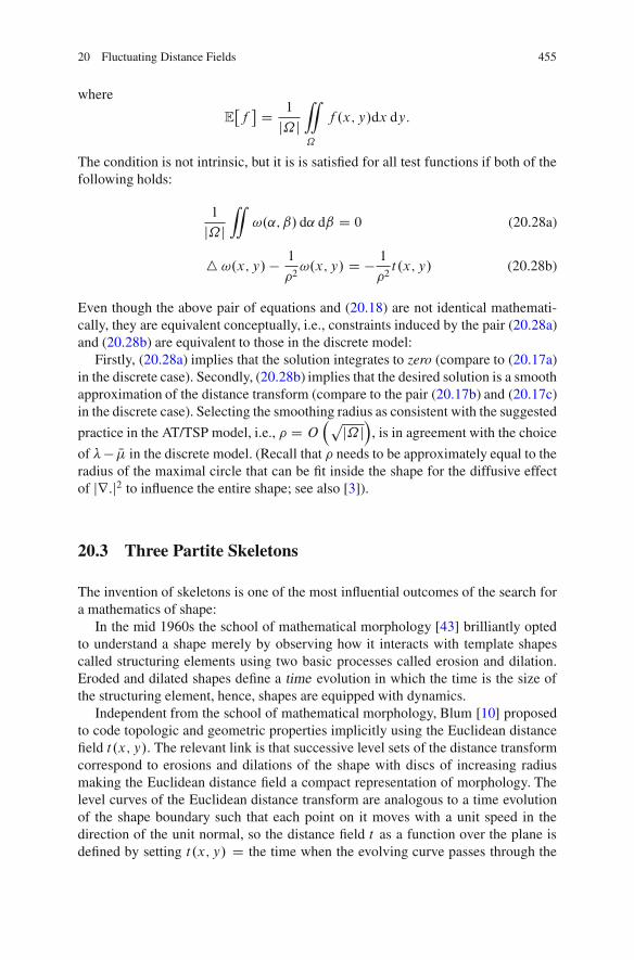
20 Fluctuating Distance Fields 455
where
E(f)D 1
j˝j
“
˝
f .x; y/dx dy:
The condition is not intrinsic, but it is is satisfied for all test functions if both of thefollowing holds:
1
j˝j
“!.˛; ˇ/ d˛ dˇ D 0 (20.28a)
4 !.x; y/ # 1
(2!.x; y/ D # 1
(2t.x; y/ (20.28b)
Even though the above pair of equations and (20.18) are not identical mathemati-cally, they are equivalent conceptually, i.e., constraints induced by the pair (20.28a)and (20.28b) are equivalent to those in the discrete model:
Firstly, (20.28a) implies that the solution integrates to zero (compare to (20.17a)in the discrete case). Secondly, (20.28b) implies that the desired solution is a smoothapproximation of the distance transform (compare to the pair (20.17b) and (20.17c)in the discrete case). Selecting the smoothing radius as consistent with the suggestedpractice in the AT/TSP model, i.e., ( D O
#pj˝j
$, is in agreement with the choice
of !# N" in the discrete model. (Recall that ( needs to be approximately equal to theradius of the maximal circle that can be fit inside the shape for the diffusive effectof jr:j2 to influence the entire shape; see also [3]).
20.3 Three Partite Skeletons
The invention of skeletons is one of the most influential outcomes of the search fora mathematics of shape:
In the mid 1960s the school of mathematical morphology [43] brilliantly optedto understand a shape merely by observing how it interacts with template shapescalled structuring elements using two basic processes called erosion and dilation.Eroded and dilated shapes define a time evolution in which the time is the size ofthe structuring element, hence, shapes are equipped with dynamics.
Independent from the school of mathematical morphology, Blum [10] proposedto code topologic and geometric properties implicitly using the Euclidean distancefield t.x; y/. The relevant link is that successive level sets of the distance transformcorrespond to erosions and dilations of the shape with discs of increasing radiusmaking the Euclidean distance field a compact representation of morphology. Thelevel curves of the Euclidean distance transform are analogous to a time evolutionof the shape boundary such that each point on it moves with a unit speed in thedirection of the unit normal, so the distance field t as a function over the plane isdefined by setting t.x; y/ D the time when the evolving curve passes through the
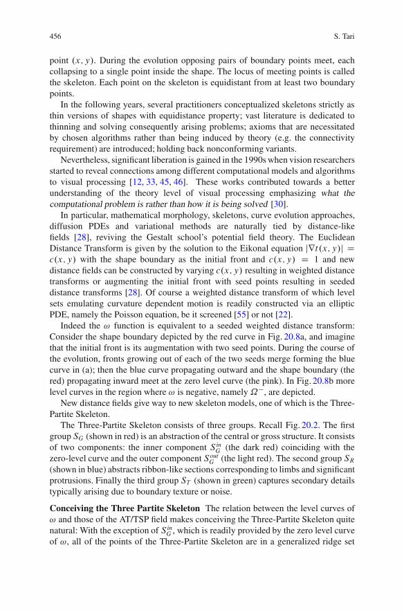
456 S. Tari
point .x; y/. During the evolution opposing pairs of boundary points meet, eachcollapsing to a single point inside the shape. The locus of meeting points is calledthe skeleton. Each point on the skeleton is equidistant from at least two boundarypoints.
In the following years, several practitioners conceptualized skeletons strictly asthin versions of shapes with equidistance property; vast literature is dedicated tothinning and solving consequently arising problems; axioms that are necessitatedby chosen algorithms rather than being induced by theory (e.g. the connectivityrequirement) are introduced; holding back nonconforming variants.
Nevertheless, significant liberation is gained in the 1990s when vision researchersstarted to reveal connections among different computational models and algorithmsto visual processing [12, 33, 45, 46]. These works contributed towards a betterunderstanding of the theory level of visual processing emphasizing what thecomputational problem is rather than how it is being solved [30].
In particular, mathematical morphology, skeletons, curve evolution approaches,diffusion PDEs and variational methods are naturally tied by distance-likefields [28], reviving the Gestalt school’s potential field theory. The EuclideanDistance Transform is given by the solution to the Eikonal equation jrt.x; y/j Dc.x; y/ with the shape boundary as the initial front and c.x; y/ D 1 and newdistance fields can be constructed by varying c.x; y/ resulting in weighted distancetransforms or augmenting the initial front with seed points resulting in seededdistance transforms [28]. Of course a weighted distance transform of which levelsets emulating curvature dependent motion is readily constructed via an ellipticPDE, namely the Poisson equation, be it screened [55] or not [22].
Indeed the ! function is equivalent to a seeded weighted distance transform:Consider the shape boundary depicted by the red curve in Fig. 20.8a, and imaginethat the initial front is its augmentation with two seed points. During the course ofthe evolution, fronts growing out of each of the two seeds merge forming the bluecurve in (a); then the blue curve propagating outward and the shape boundary (thered) propagating inward meet at the zero level curve (the pink). In Fig. 20.8b morelevel curves in the region where ! is negative, namely˝!, are depicted.
New distance fields give way to new skeleton models, one of which is the Three-Partite Skeleton.
The Three-Partite Skeleton consists of three groups. Recall Fig. 20.2. The firstgroup SG (shown in red) is an abstraction of the central or gross structure. It consistsof two components: the inner component S in
G (the dark red) coinciding with thezero-level curve and the outer component Sout
G (the light red). The second group SR(shown in blue) abstracts ribbon-like sections corresponding to limbs and significantprotrusions. Finally the third group ST (shown in green) captures secondary detailstypically arising due to boundary texture or noise.
Conceiving the Three Partite Skeleton The relation between the level curves of! and those of the AT/TSP field makes conceiving the Three-Partite Skeleton quitenatural: With the exception of S in
G , which is readily provided by the zero level curveof !, all of the points of the Three-Partite Skeleton are in a generalized ridge set
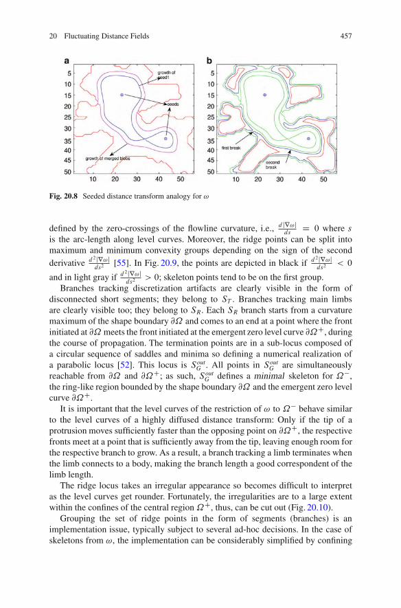
20 Fluctuating Distance Fields 457
Fig. 20.8 Seeded distance transform analogy for !
defined by the zero-crossings of the flowline curvature, i.e., d jr!jdsD 0 where s
is the arc-length along level curves. Moreover, the ridge points can be split intomaximum and minimum convexity groups depending on the sign of the secondderivative d2jr!j
ds2[55]. In Fig. 20.9, the points are depicted in black if d2jr!j
ds2< 0
and in light gray if d2jr!jds2
> 0; skeleton points tend to be on the first group.Branches tracking discretization artifacts are clearly visible in the form of
disconnected short segments; they belong to ST . Branches tracking main limbsare clearly visible too; they belong to SR. Each SR branch starts from a curvaturemaximum of the shape boundary @˝ and comes to an end at a point where the frontinitiated at @˝ meets the front initiated at the emergent zero level curve @˝C, duringthe course of propagation. The termination points are in a sub-locus composed ofa circular sequence of saddles and minima so defining a numerical realization ofa parabolic locus [52]. This locus is Sout
G . All points in SoutG are simultaneously
reachable from @˝ and @˝C; as such, SoutG defines a minimal skeleton for ˝!,
the ring-like region bounded by the shape boundary @˝ and the emergent zero levelcurve @˝C.
It is important that the level curves of the restriction of ! to ˝! behave similarto the level curves of a highly diffused distance transform: Only if the tip of aprotrusion moves sufficiently faster than the opposing point on @˝C, the respectivefronts meet at a point that is sufficiently away from the tip, leaving enough room forthe respective branch to grow. As a result, a branch tracking a limb terminates whenthe limb connects to a body, making the branch length a good correspondent of thelimb length.
The ridge locus takes an irregular appearance so becomes difficult to interpretas the level curves get rounder. Fortunately, the irregularities are to a large extentwithin the confines of the central region˝C, thus, can be cut out (Fig. 20.10).
Grouping the set of ridge points in the form of segments (branches) is animplementation issue, typically subject to several ad-hoc decisions. In the case ofskeletons from !, the implementation can be considerably simplified by confining
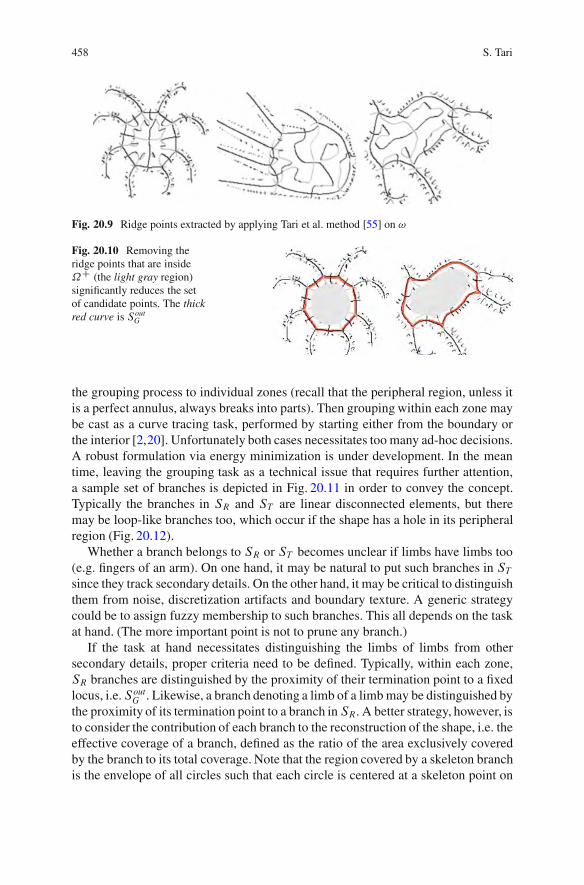
458 S. Tari
Fig. 20.9 Ridge points extracted by applying Tari et al. method [55] on !
Fig. 20.10 Removing theridge points that are inside˝C (the light gray region)significantly reduces the setof candidate points. The thickred curve is Sout
G
the grouping process to individual zones (recall that the peripheral region, unless itis a perfect annulus, always breaks into parts). Then grouping within each zone maybe cast as a curve tracing task, performed by starting either from the boundary orthe interior [2,20]. Unfortunately both cases necessitates too many ad-hoc decisions.A robust formulation via energy minimization is under development. In the meantime, leaving the grouping task as a technical issue that requires further attention,a sample set of branches is depicted in Fig. 20.11 in order to convey the concept.Typically the branches in SR and ST are linear disconnected elements, but theremay be loop-like branches too, which occur if the shape has a hole in its peripheralregion (Fig. 20.12).
Whether a branch belongs to SR or ST becomes unclear if limbs have limbs too(e.g. fingers of an arm). On one hand, it may be natural to put such branches in STsince they track secondary details. On the other hand, it may be critical to distinguishthem from noise, discretization artifacts and boundary texture. A generic strategycould be to assign fuzzy membership to such branches. This all depends on the taskat hand. (The more important point is not to prune any branch.)
If the task at hand necessitates distinguishing the limbs of limbs from othersecondary details, proper criteria need to be defined. Typically, within each zone,SR branches are distinguished by the proximity of their termination point to a fixedlocus, i.e. Sout
G . Likewise, a branch denoting a limb of a limb may be distinguished bythe proximity of its termination point to a branch in SR. A better strategy, however, isto consider the contribution of each branch to the reconstruction of the shape, i.e. theeffective coverage of a branch, defined as the ratio of the area exclusively coveredby the branch to its total coverage. Note that the region covered by a skeleton branchis the envelope of all circles such that each circle is centered at a skeleton point on

20 Fluctuating Distance Fields 459
Fig. 20.11 Sample branches
Fig. 20.12 Shape with a hole
the branch, and has a radius given by the value of the distance transform at thatpoint [10].
In general, computing the effective coverage is difficult [19] but becomes easy inour case because the branches can be put into a priority order, at least within a zone.This order is based on the branch length and proximity to a fixed locus, be it Sout
G ormembers of SR.
Effective coverages of the branches for the elephant shape are depicted inFig. 20.13. The gray toning of the covered regions (left) reflects the magnitudesof the effective coverage ratios of the corresponding branches. On the right, the fivebranches forming SR covers almost the entire peripheral region.
20.3.1 Why Three Partite Skeletons?
I make four arguments in favor of the new skeleton model:
Boundary Details The most frequently reported problem of the classical skeletonis its sensitivity to boundary perturbations: small indentations or protrusionsintroduce spurious branches. A classical connectivity-preserving skeleton for the
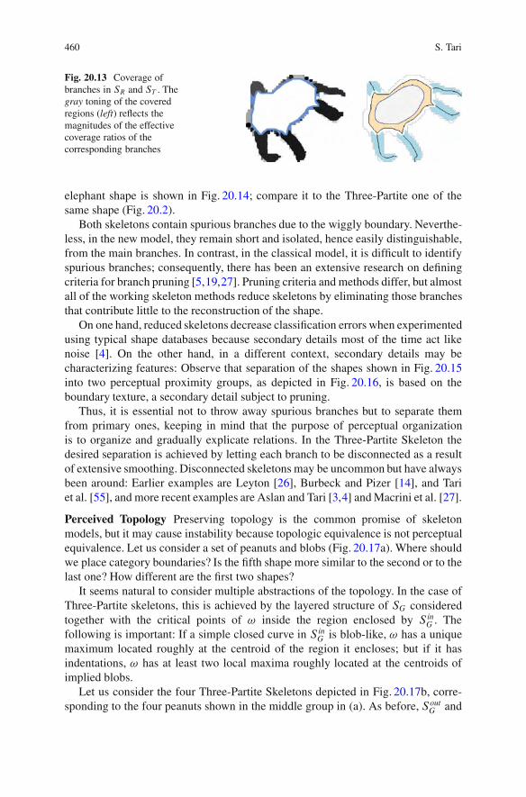
460 S. Tari
Fig. 20.13 Coverage ofbranches in SR and ST . Thegray toning of the coveredregions (left) reflects themagnitudes of the effectivecoverage ratios of thecorresponding branches
elephant shape is shown in Fig. 20.14; compare it to the Three-Partite one of thesame shape (Fig. 20.2).
Both skeletons contain spurious branches due to the wiggly boundary. Neverthe-less, in the new model, they remain short and isolated, hence easily distinguishable,from the main branches. In contrast, in the classical model, it is difficult to identifyspurious branches; consequently, there has been an extensive research on definingcriteria for branch pruning [5,19,27]. Pruning criteria and methods differ, but almostall of the working skeleton methods reduce skeletons by eliminating those branchesthat contribute little to the reconstruction of the shape.
On one hand, reduced skeletons decrease classification errors when experimentedusing typical shape databases because secondary details most of the time act likenoise [4]. On the other hand, in a different context, secondary details may becharacterizing features: Observe that separation of the shapes shown in Fig. 20.15into two perceptual proximity groups, as depicted in Fig. 20.16, is based on theboundary texture, a secondary detail subject to pruning.
Thus, it is essential not to throw away spurious branches but to separate themfrom primary ones, keeping in mind that the purpose of perceptual organizationis to organize and gradually explicate relations. In the Three-Partite Skeleton thedesired separation is achieved by letting each branch to be disconnected as a resultof extensive smoothing. Disconnected skeletons may be uncommon but have alwaysbeen around: Earlier examples are Leyton [26], Burbeck and Pizer [14], and Tariet al. [55], and more recent examples are Aslan and Tari [3,4] and Macrini et al. [27].
Perceived Topology Preserving topology is the common promise of skeletonmodels, but it may cause instability because topologic equivalence is not perceptualequivalence. Let us consider a set of peanuts and blobs (Fig. 20.17a). Where shouldwe place category boundaries? Is the fifth shape more similar to the second or to thelast one? How different are the first two shapes?
It seems natural to consider multiple abstractions of the topology. In the case ofThree-Partite skeletons, this is achieved by the layered structure of SG consideredtogether with the critical points of ! inside the region enclosed by S in
G . Thefollowing is important: If a simple closed curve in S in
G is blob-like, ! has a uniquemaximum located roughly at the centroid of the region it encloses; but if it hasindentations, ! has at least two local maxima roughly located at the centroids ofimplied blobs.
Let us consider the four Three-Partite Skeletons depicted in Fig. 20.17b, corre-sponding to the four peanuts shown in the middle group in (a). As before, Sout
G and
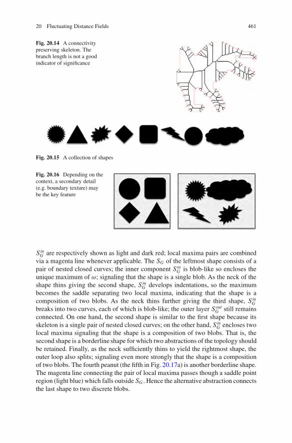
20 Fluctuating Distance Fields 461
Fig. 20.14 A connectivitypreserving skeleton. Thebranch length is not a goodindicator of significance
Fig. 20.15 A collection of shapes
Fig. 20.16 Depending on thecontext, a secondary detail(e.g. boundary texture) maybe the key feature
S inG are respectively shown as light and dark red; local maxima pairs are combined
via a magenta line whenever applicable. The SG of the leftmost shape consists of apair of nested closed curves; the inner component S in
G is blob-like so encloses theunique maximum of !; signaling that the shape is a single blob. As the neck of theshape thins giving the second shape, S in
G develops indentations, so the maximumbecomes the saddle separating two local maxima, indicating that the shape is acomposition of two blobs. As the neck thins further giving the third shape, S in
G
breaks into two curves, each of which is blob-like; the outer layer SoutG still remains
connected. On one hand, the second shape is similar to the first shape because itsskeleton is a single pair of nested closed curves; on the other hand, S in
G encloses twolocal maxima signaling that the shape is a composition of two blobs. That is, thesecond shape is a borderline shape for which two abstractions of the topology shouldbe retained. Finally, as the neck sufficiently thins to yield the rightmost shape, theouter loop also splits; signaling even more strongly that the shape is a compositionof two blobs. The fourth peanut (the fifth in Fig. 20.17a) is another borderline shape.The magenta line connecting the pair of local maxima passes though a saddle pointregion (light blue) which falls outside SG . Hence the alternative abstraction connectsthe last shape to two discrete blobs.
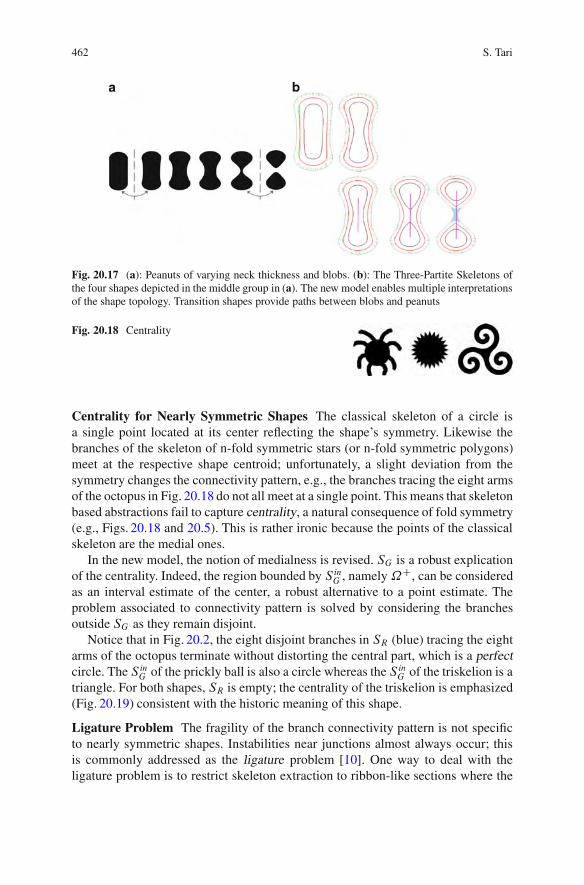
462 S. Tari
Fig. 20.17 (a): Peanuts of varying neck thickness and blobs. (b): The Three-Partite Skeletons ofthe four shapes depicted in the middle group in (a). The new model enables multiple interpretationsof the shape topology. Transition shapes provide paths between blobs and peanuts
Fig. 20.18 Centrality
Centrality for Nearly Symmetric Shapes The classical skeleton of a circle isa single point located at its center reflecting the shape’s symmetry. Likewise thebranches of the skeleton of n-fold symmetric stars (or n-fold symmetric polygons)meet at the respective shape centroid; unfortunately, a slight deviation from thesymmetry changes the connectivity pattern, e.g., the branches tracing the eight armsof the octopus in Fig. 20.18 do not all meet at a single point. This means that skeletonbased abstractions fail to capture centrality, a natural consequence of fold symmetry(e.g., Figs. 20.18 and 20.5). This is rather ironic because the points of the classicalskeleton are the medial ones.
In the new model, the notion of medialness is revised. SG is a robust explicationof the centrality. Indeed, the region bounded by S in
G , namely˝C, can be consideredas an interval estimate of the center, a robust alternative to a point estimate. Theproblem associated to connectivity pattern is solved by considering the branchesoutside SG as they remain disjoint.
Notice that in Fig. 20.2, the eight disjoint branches in SR (blue) tracing the eightarms of the octopus terminate without distorting the central part, which is a perfectcircle. The S in
G of the prickly ball is also a circle whereas the S inG of the triskelion is a
triangle. For both shapes, SR is empty; the centrality of the triskelion is emphasized(Fig. 20.19) consistent with the historic meaning of this shape.
Ligature Problem The fragility of the branch connectivity pattern is not specificto nearly symmetric shapes. Instabilities near junctions almost always occur; thisis commonly addressed as the ligature problem [10]. One way to deal with theligature problem is to restrict skeleton extraction to ribbon-like sections where the
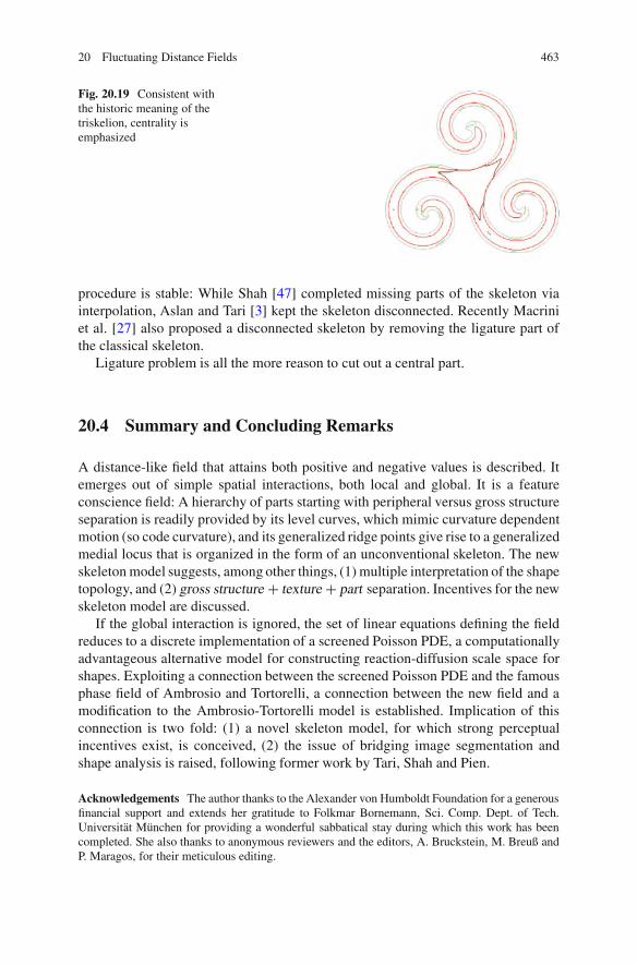
20 Fluctuating Distance Fields 463
Fig. 20.19 Consistent withthe historic meaning of thetriskelion, centrality isemphasized
procedure is stable: While Shah [47] completed missing parts of the skeleton viainterpolation, Aslan and Tari [3] kept the skeleton disconnected. Recently Macriniet al. [27] also proposed a disconnected skeleton by removing the ligature part ofthe classical skeleton.
Ligature problem is all the more reason to cut out a central part.
20.4 Summary and Concluding Remarks
A distance-like field that attains both positive and negative values is described. Itemerges out of simple spatial interactions, both local and global. It is a featureconscience field: A hierarchy of parts starting with peripheral versus gross structureseparation is readily provided by its level curves, which mimic curvature dependentmotion (so code curvature), and its generalized ridge points give rise to a generalizedmedial locus that is organized in the form of an unconventional skeleton. The newskeleton model suggests, among other things, (1) multiple interpretation of the shapetopology, and (2) gross structureC textureC part separation. Incentives for the newskeleton model are discussed.
If the global interaction is ignored, the set of linear equations defining the fieldreduces to a discrete implementation of a screened Poisson PDE, a computationallyadvantageous alternative model for constructing reaction-diffusion scale space forshapes. Exploiting a connection between the screened Poisson PDE and the famousphase field of Ambrosio and Tortorelli, a connection between the new field and amodification to the Ambrosio-Tortorelli model is established. Implication of thisconnection is two fold: (1) a novel skeleton model, for which strong perceptualincentives exist, is conceived, (2) the issue of bridging image segmentation andshape analysis is raised, following former work by Tari, Shah and Pien.
Acknowledgements The author thanks to the Alexander von Humboldt Foundation for a generousfinancial support and extends her gratitude to Folkmar Bornemann, Sci. Comp. Dept. of Tech.Universitat Munchen for providing a wonderful sabbatical stay during which this work has beencompleted. She also thanks to anonymous reviewers and the editors, A. Bruckstein, M. Breuß andP. Maragos, for their meticulous editing.
464 S. Tari
References
1. Ambrosio, L., Tortorelli, V.: On the approximation of functionals depending on jumps byelliptic functionals via ' -convergence. Commun. Pure Appl. Math. 43(8), 999–1036 (1990)
2. Aslan, C.: Disconnected skeletons for shape recognition. Master’s thesis, Department ofComputer Engineering, Middle East Technical University (2005)
3. Aslan, C., Tari, S.: An axis-based representation for recognition. In: Proceedings of the ICCV,pp. 1339–1346. Springer, Berlin/New York (2005)
4. Aslan, C., Erdem, A., Erdem, E., Tari, S.: Disconnected skeleton: shape at its absolute scale.IEEE Trans. Pattern Anal. Mach. Intell. 30(12), 2188–2203 (2008)
5. Bai, X., Latecki, L., Liu, W.Y.: Skeleton pruning by contour partitioning with discrete curveevolution. IEEE Trans. Pattern Anal. Mach. Intell. 29, 449–462 (2007)
6. Bar, L., Sochen, N., Kiryati, N.: Image deblurring in the presence of impulsive noise. Int. J.Comput. Vis. 70(3), 279–298 (2006)
7. Barenholtz, E., Feldman, J.: Visual comparisons within and between object-parts: evidence fora single- part superiority effect. Vis. Res. 43, 1655–1666 (2003)
8. Belongie, S., Malik, J., Puzicha, J.: Shape matching and object recognition using shapecontexts. IEEE Trans. Pattern Anal. Mach. Intell. 24, 509–522 (2002)
9. Biederman, I.: Recognition-by-components: a theory of human image understanding. Psychol.Rev. 94(2), 115–117 (1987)
10. Blum, H.: Biological shape and visual science. J. Theor. Biol. 38, 205–287 (1973)11. Braides, A.: Approximation of Free-Discontinuity Problems. Lecture Notes in Mathematics,
vol. 1694. Springer, Berlin/New York (1998)12. Brockett, R., Maragos, P.: Evolution equations for continuous–scale morphology. In: Proceed-
ings of the ICASSP, vol. 3, pp. 125–128. IEEE, Piscataway (1992)13. Buades, A., Coll, B., Morel, J.M.: A non-local algorithm for image denoising. In: Proceedings
of the CVPR, pp. 60–65. IEEE Computer Society, Los Alamitos (2005)14. Burbeck, C.A., Pizer, S.M.: Object representation by cores: identifying and representing
primitive spatial regions. Vis. Res. 35, 1917–1930 (1995)15. Cohen, E.H., Singh, M.: Geometric determinants of shape segmentation: tests using segment
identification. Vis. Res. 47, 2825–2840 (2007)16. de Winter, J., Wagemans, J.: Segmentation of object outlines into parts: a large-scale integrative
study. Cognition 99, 275–325 (1999)17. Edelman, S., Cutzu, F., Duvdevani-Bar, S.: Similarity to reference shapes as a basis for shape
representation. In: Proceedings of the COGSCI, San Diego (1996)18. Erdem, E., Tari, S.: Mumford-Shah regularizer with contextual feedback. JMIV 33, 67–84
(2009)19. Feldman, J., Singh, M.: Bayesian estimation of the shape skeleton. PNAS 103(47), 18014–
18019 (2006)20. Genctav, M.: Matching global skeleton. Master’s thesis, Department of Computer Engineering,
Middle East Technical University (2010)21. Gonzalez, R., Woods, R.: Digital Image Processing, 2nd edn. Addison-Wesley Longman
Publishing Co., Inc., Boston (2001)22. Gorelick, L., Galun, M., Sharon, E., Basri, R., Brandt, A.: Shape representation and
classification using the poisson equation. IEEE Trans. Pattern Anal. Mach. Intell. 28(12),1991–2005 (2006)
23. Hofmann, D., Richards, W.: Parts of recognition. Cognition 18, 65–96 (1984)24. Jung, M., Vese, L.: Nonlocal variational image deblurring models in the presence of gaussian
or impulse noise. In: Proceedings of the SSVM, pp. 401–412. Springer, Berlin/New York(2009)
25. Kimia, B., Tannenbaum, A., Zucker, S.: Shapes, shocks, and deformations I: the componentsof two-dimensional shape and the reaction-diffusion space. Int. J. Comput. Vis. 15(3), 189–224(1995)

20 Fluctuating Distance Fields 465
26. Leyton, M.: A process-grammar for shape. Art. Intell. 34(2), 213–247 (1988)27. Macrini, D., Dickinson, S., Fleet, D., Siddiqi, K.: Bone graphs: medial shape parsing and
abstraction. Comput. Vis. Image Underst. 115, 1044–1061 (2011)28. Maragos, P., Butt, M.A.: Curve evolution, differential morphology and distance transforms as
applied to multiscale and eikonal problems. Fundam. Inf. 41, 91–129 (2000)29. March, R., Dozio, M.: A variational method for the recovery of smooth boundaries. Image
Vis. Comput. 15(9), 705–712 (1997)30. Marr, D.: Vision: A Computational Investigation into the Human Representation and
Processing of Visual Information. W.H. Freeman, San Francisco (1982)31. Meyer, F.: Topographic distance and watershed lines. Signal Process. 38, 113–125 (1994)32. Mi, X., DeCarlo, D.: Separating parts from 2d shapes using relatability. In: Proceedings of the
ICCV, pp. 1–8. IEEE Computer Society, Los Alamitos (2007)33. Morel, J.-M., Solimini, S.: Variational Methods in Image Segmentation. Birkhauser, Boston
(1995)34. Mumford, D.: Mathematical theories of shape: do they model perception? In: Proceedings of
the SPIE, vol. 1570. SPIE, Bellingham (1991)35. Mumford, D., Shah, J.: Optimal approximations by piecewise smooth functions and associated
variational problems. Commun. Pure Appl. Math. 42, 577–685 (1989)36. Navon, D.: Forest before trees: the precedence of global features in visual perception. Cogn.
Psychol. 9, 355–383 (1977)37. Pasupathy, A., Connor, C.: Population coding of shape in area V4. Nat. Neurosci. 5(2), 1332–
1338 (2002)38. Patz, T., Preusser, T.: Ambrosio-Tortorelli segmentation of stochastic images. In: Proceedings
of the ECCV, pp. 254–267. Springer, Berlin (2010)39. Pien, H.H., Desai, M., Shah, J.: Segmentation of mr images using curve evolution and prior
information. IJPRAI 11(8), 1233–1245 (1997)40. Preußer, T., Droske, M., Garbe, C., Rumpf, M., Telea, A.: A phase field method for joint
denoising, edge detection and motion estimation. SIAM J. Appl. Math. 68(3), 599–618 (2007)41. Proesman, M., Pauwels, E., van Gool, L.: Coupled geometry-driven diffusion equations for
low-level vision. In: Romeny, B. (ed.) Geometry Driven Diffusion in Computer Vision. LectureNotes in Computer Science. Kluwer, Dordrecht/Boston (1994)
42. Rosenfeld, A., Pfaltz, J.L.: Distance functions on digital pictures. Pattern Recognit. 1, 33–61(1968)
43. Serra, J.: Image Analysis and Mathematical Morphology. London Academic, Orlando (1982)44. Shah, J.: Segmentation by nonlinear diffusion. In: Proceedings of the CVPR, pp. 202–207.
IEEE Computer Society, Los Alamitos (1991)45. Shah, J.: A common framework for curve evolution, segmentation and anisotropic diffusion.
In: Proceedings of the CVPR, pp. 136–142 (1996)46. Shah, J.: Riemannian drums, anisotropic curve evolution and segmentation. In: Proceedings
of the Scale-Space, pp. 129–140. Springer, Berlin/New York (1999)47. Shah, J.: Skeletons and segmentation of shapes. Technical report, Northeastern University.
http://www.math.neu.edu/!shah/publications.html (2005)48. Shah, J., Pien, H.H., Gauch, J.: Recovery of shapes of surfaces with discontinuities by fusion
of shading and range data within a variational framework. IEEE Trans. Image Process. 5(8),1243–1251 (1996)
49. Siddiqi, K., Tresness, K.J., Kimia, B.: Parts of visual form: ecological and psychophysicalaspects. Perception 25, 399–424 (1996)
50. Stiny, G.: Shape: Talking about Seeing and Doing. MIT, Cambridge (2006)51. Tari, S., Genctav, M.: From a modified Ambrosio-Tortorelli to a randomized part hierarchy
tree. In: Bruckstein, A.M., ter Haar Romeny, B.M., Bronstein, A.M., Bronstein, M.M.(eds.) Scale Space and Variational Methods. Lecture Notes in Computer Science, vol. 6667,pp. 267–278. Springer, Berlin/Heidelberg (2011)
52. Tari, S., Shah, J.: Simultaneous segmentation of images and shapes. In: Proceedings of theSPIE, San Diego, vol. 3168, San Diego pp. 88–94 (1997)

466 S. Tari
53. Tari, S., Shah, J.: Local symmetries of shapes in arbitrary dimension. In: Proceedings of theICCV, pp. 1123–1128. Narosa, New Delhi (1998)
54. Tari, S., Shah, J., Pien, H.: A computationally efficient shape analysis via level sets. In:Proceedings of the MMBIA, pp. 234–243. IEEE Computer Society, Los Alamitos (1996)
55. Tari, S., Shah, J., Pien, H.: Extraction of shape skeletons from grayscale images. CVIU 66(2),133–146 (1997)
56. Teboul, S., Blanc-Feraud, L., Aubert, G., Barlaud, M.: Variational approach for edge preservingregularization using coupled PDE’s. IEEE Trans. Image. Process. 7, 387–397 (1998)
57. Xu, C., Liu, J., Tang, X.: 2d shape matching by contour flexibility. IEEE Trans. Pattern Anal.Mach. Intell. 31(1), 180–186 (2009)
58. Zeng, J.T., Lakaemper, R., Wei, X., Li, X.: 2d shape decomposition based on combinedskeleton-boundary features. In: Proceedings of the Advances in Visual Computing, 4thInternational Symposium, ISVC, pp. 682–691. Springer, Berlin/New York (2008)

Chapter 21Integrated DEM Construction and Calibrationof Hyperspectral Imagery: A Remote SensingPerspective
Christian Wohler and Arne Grumpe
Abstract In this study, we present from a remote sensing perspective a methodfor the combination of surface gradient information obtained by photoclinometryand shape from shading with absolute depth data (here: light detection and ranging(LIDAR) data) by exploiting their respective advantages, regarding distinctly non-Lambertian surfaces with non-uniform albedos. While photometry-based 3D recon-struction methods yield reliable small-scale surface gradient information for eachimage pixel, absolute depth data which are typically noisy on small scales butreliable on large scales are provided by LIDAR techniques. The first step of theproposed algorithm consists of an extended photoclinometry approach which takesinto account both image and LIDAR data. In a second step the reconstructed surfaceis refined based on an iterative scheme relying on the minimisation of a global errorfunctional, thus compensating the inaccuracies of the measured surface gradientsand the LIDAR data on the respective scales. The surface shape and non-uniformalbedo map represent the best fit to the observed image radiances and LIDAR data.We apply our framework to the construction of digital elevation models (DEM) oflunar surface regions. We use hyperspectral imagery in order to employ the DEM tonormalise the wavelength-dependent surface reflectance to a standard illuminationand viewing geometry. Although we employ a highly realistic, physically motivatedreflectance model (the Hapke model), systematic topography-dependent distortionsof the pixel spectra occur, which lead to errors in the extracted spectral parameters(e.g. the absorption wavelength, depth, and width of prominent absorption troughs)and for which we propose an empirical, PCA-based correction approach. Basedon the correspondingly corrected surface reflectances we obtain a refined DEMalong with spectral parameter maps in which (except for the hydroxyl absorption)topographic effects are nearly completely removed.
C. Wohler (!) ! A. GrumpeImage Analysis Group, Dortmund University of Technology, Otto-Hahn-Str. 4,44227 Dortmund, Germanye-mail: [email protected]; [email protected]
M. Breuß et al. (eds.), Innovations for Shape Analysis, Mathematics and Visualization,DOI 10.1007/978-3-642-34141-0 21, © Springer-Verlag Berlin Heidelberg 2013
467
468 C. Wohler and A. Grumpe
21.1 Introduction
The concept of photoclinometry is introduced by Wilhelms [52] for the image-basedmeasurement of lunar surface slopes. The concepts of shape from shading andphotometric stereo are introduced by Horn [20] and Woodham [54], respectively.The method of characteristic strip expansion by Horn [21] and also the method byKozera [29] directly yield a depth map of the surface. In contrast, other methodsby Horn [20, 22] estimate the gradient field of the surface and infer the depth mapby integration. The computational efficiency of such gradient-based approaches isincreased e.g. by Simchony et al. [47] by an analytical approach. An extensivesurvey is provided in [1].
Improved results can be achieved by combining photometrically determinedsurface gradient data with independently measured absolute depth data. Generalsolutions for this problem are proposed e.g. in [7] and [40], where a highly detailed3D surface reconstruction is obtained by a combination of the low-frequency part ofthe absolute depth data with the high-frequency component of the photometricallydetermined surface gradients. Non-Lambertian metallic surfaces are reconstructede.g. in [53], multiple views are taken into account in [25,32,55], and moving objectsare analysed in [46].
In the context of lunar remote sensing, a global digital elevation model (DEM)of the Moon of 100m nominal lateral resolution with a typical vertical accuracyof 23m is described in [44], which is termed “GLD100” and has been constructedbased on the stereoscopic evaluation of images acquired by the LROC WAC (LunarReconnaissance Orbiter Wide Angle Camera). LROC NAC (Narrow Angle Camera)based stereo images analysis has led to the construction of local lunar DEMs of veryhigh lateral resolution [31, 36]. Detailed information about the LROC WAC andNAC instruments can be found in [43]. A nearly global lunar hyperspectral imagemosaic of typically 140m resolution has been acquired by the Moon MineralogyMapper (M3) instrument on board the Indian spacecraft Chandrayaan-1 [42] (http://m3.jpl.nasa.gov/m3data.html).
A combination of stereo image analysis and shape from shading is used in [28]to construct DEMs of high lateral resolution of the surface of Mars. Lunar DEMsare generated in [33] based on images acquired by the Clementine spacecraft using atechnique termed “multi-image shape from shading”, where the elevation values andthe parameters of the surface reflectance function are adapted to the image radianceinformation, assuming a uniform surface albedo. A photometric stereo methodis used for DEM construction in [10] based on overlapping images of the lunarsouthern polar region acquired by the SMART-1 Advanced Moon micro-ImagerExperiment (AMIE) camera. Detailed information about the AMIE instrument canbe found in [26]. The properties of the recently acquired lunar orbital image datasets are summarised in Table 21.1.
The global DEMs obtained by the LIDAR instrument LALT on board theJapanese Kaguya spacecraft and the Lunar Orbiter Laser Altimeter (LOLA) instru-ment on board the LRO spacecraft have vertical accuracies of a few metres (cf. [4]and [31] for a short description of LALT and LOLA data, respectively). The nominal
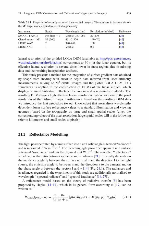
21 Integrated DEM Construction and Calibration of Hyperspectral Imagery 469
Table 21.1 Properties of recently acquired lunar orbital imagery. The numbers in brackets denotethe M3 target mode applied to selected regions only
Instrument Bands Wavelength (nm) Resolution (m/pixel) Reference
SMART-1 AMIE No filterC 3 Visible, 750–960 27–270 [26]Chandrayaan-1 M3 85 (260) 461–2;976 140 (70) [42]LROC WAC 7 320–690 100 [43]LROC NAC 1 Visible 0:5 [43]
lateral resolution of the gridded LOLA DEM (available at http://pds-geosciences.wustl.edu/missions/lro/lola.htm) corresponds to 30m at the lunar equator, but itseffective lateral resolution is several times lower in most regions due to missingdata and the resulting interpolation artifacts.
This study presents a method for the integration of surface gradient data obtainedby shape from shading with absolute depth data inferred from laser altimetrymeasurements, relying on M3 orbital images and the global LOLA DEM. Thisframework is applied to the construction of DEMs of the lunar surface, whichdisplays a non-Lambertian reflectance behaviour and a non-uniform albedo. Theresulting DEMs have a high effective lateral resolution that comes close to the pixelresolution of the utilised images. Furthermore, based on the resulting DEM datawe introduce the first procedure (to our knowledge) that normalises wavelength-dependent lunar surface reflectance values to a standard illumination and viewinggeometry based on the topography on large and small spatial scales (given thecorresponding values of the pixel resolution, large spatial scales will in the followingrefer to kilometres and small scales to pixels).
21.2 Reflectance Modelling
The light power emitted by a unit surface into a unit solid angle is termed “radiance”and is measured in W m"2 sr"1. The incoming light power per apparent unit surfaceis termed “irradiance” and has the physical unit W m"2. The so-called “reflectance”is defined as the ratio between radiance and irradiance [21]. It usually depends onthe incidence angle !i between the surface normal n and the direction l to the lightsource, the emission angle !e between n and the direction v to the camera, and onthe phase angle ˛ between the vectors l and v [14] (Fig. 21.1). The radiances andirradiances regarded in the experiments of this study are additionally normalised towavelength (“spectral radiance” and “spectral irradiance” [14, 27]).
A reflectance model based on the theory of radiative transfer [5] has beenproposed by Hapke [14–17], which in its general form according to [17] can bewritten as
RAMSA."0;"; ˛/ Dw4#
"0
"0 C "Œp.˛/BSH.˛/CM."0;"/$BCB.˛/ (21.1)
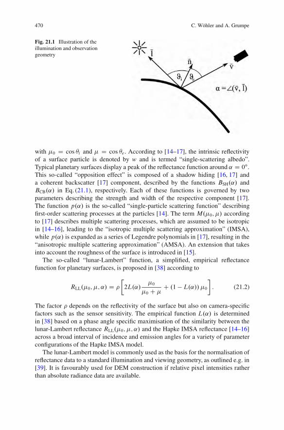
470 C. Wohler and A. Grumpe
Fig. 21.1 Illustration of theillumination and observationgeometry
with "0 D cos !i and " D cos !e. According to [14–17], the intrinsic reflectivityof a surface particle is denoted by w and is termed “single-scattering albedo”.Typical planetary surfaces display a peak of the reflectance function around ˛ D 0ı.This so-called “opposition effect” is composed of a shadow hiding [16, 17] anda coherent backscatter [17] component, described by the functions BSH.˛/ andBCB.˛/ in Eq. (21.1), respectively. Each of these functions is governed by twoparameters describing the strength and width of the respective component [17].The function p.˛/ is the so-called “single-particle scattering function” describingfirst-order scattering processes at the particles [14]. The term M."0;"/ accordingto [17] describes multiple scattering processes, which are assumed to be isotropicin [14–16], leading to the “isotropic multiple scattering approximation” (IMSA),while p.˛/ is expanded as a series of Legendre polynomials in [17], resulting in the“anisotropic multiple scattering approximation” (AMSA). An extension that takesinto account the roughness of the surface is introduced in [15].
The so-called “lunar-Lambert” function, a simplified, empirical reflectancefunction for planetary surfaces, is proposed in [38] according to
RLL."0;"; ˛/ D %!2L.˛/
"0
"0 C "C .1 !L.˛//"0
": (21.2)
The factor % depends on the reflectivity of the surface but also on camera-specificfactors such as the sensor sensitivity. The empirical function L.˛/ is determinedin [38] based on a phase angle specific maximisation of the similarity between thelunar-Lambert reflectance RLL."0;"; ˛/ and the Hapke IMSA reflectance [14–16]across a broad interval of incidence and emission angles for a variety of parameterconfigurations of the Hapke IMSA model.
The lunar-Lambert model is commonly used as the basis for the normalisation ofreflectance data to a standard illumination and viewing geometry, as outlined e.g. in[39]. It is favourably used for DEM construction if relative pixel intensities ratherthan absolute radiance data are available.
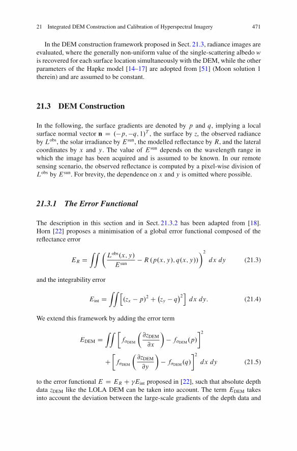
21 Integrated DEM Construction and Calibration of Hyperspectral Imagery 471
In the DEM construction framework proposed in Sect. 21.3, radiance images areevaluated, where the generally non-uniform value of the single-scattering albedo wis recovered for each surface location simultaneously with the DEM, while the otherparameters of the Hapke model [14–17] are adopted from [51] (Moon solution 1therein) and are assumed to be constant.
21.3 DEM Construction
In the following, the surface gradients are denoted by p and q, implying a localsurface normal vector n D .!p;!q; 1/T , the surface by z, the observed radianceby Lobs, the solar irradiance by Esun, the modelled reflectance by R, and the lateralcoordinates by x and y. The value of Esun depends on the wavelength range inwhich the image has been acquired and is assumed to be known. In our remotesensing scenario, the observed reflectance is computed by a pixel-wise division ofLobs by Esun. For brevity, the dependence on x and y is omitted where possible.
21.3.1 The Error Functional
The description in this section and in Sect. 21.3.2 has been adapted from [18].Horn [22] proposes a minimisation of a global error functional composed of thereflectance error
ER DZZ #
Lobs.x; y/
Esun! R .p.x; y/; q.x; y//
$2dx dy (21.3)
and the integrability error
Eint DZZ h
.zx ! p/2 C%zy ! q
&2idx dy: (21.4)
We extend this framework by adding the error term
EDEM DZZ !
f&DEM
#@zDEM
@x
$! f&DEM.p/
"2
C!f&DEM
#@zDEM
@y
$! f&DEM.q/
"2dx dy (21.5)
to the error functional E D ER C 'Eint proposed in [22], such that absolute depthdata zDEM like the LOLA DEM can be taken into account. The term EDEM takesinto account the deviation between the large-scale gradients of the depth data and
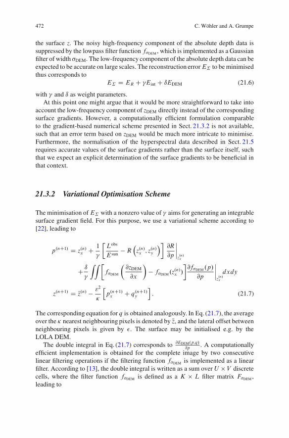
472 C. Wohler and A. Grumpe
the surface z. The noisy high-frequency component of the absolute depth data issuppressed by the lowpass filter function f&DEM , which is implemented as a Gaussianfilter of width &DEM. The low-frequency component of the absolute depth data can beexpected to be accurate on large scales. The reconstruction errorE˙ to be minimisedthus corresponds to
E˙ D ER C 'Eint C ıEDEM (21.6)
with ' and ı as weight parameters.At this point one might argue that it would be more straightforward to take into
account the low-frequency component of zDEM directly instead of the correspondingsurface gradients. However, a computationally efficient formulation comparableto the gradient-based numerical scheme presented in Sect. 21.3.2 is not available,such that an error term based on zDEM would be much more intricate to minimise.Furthermore, the normalisation of the hyperspectral data described in Sect. 21.5requires accurate values of the surface gradients rather than the surface itself, suchthat we expect an explicit determination of the surface gradients to be beneficial inthat context.
21.3.2 Variational Optimisation Scheme
The minimisation ofE˙ with a nonzero value of ' aims for generating an integrablesurface gradient field. For this purpose, we use a variational scheme according to[22], leading to
p.nC1/ D z.n/x C1
'
!Lobs
Esun!R
'z.n/x ; z
.n/y
(" @R@p
ˇˇz.n/x
C ı'
ZZ !f&DEM
#@zDEM
@x
$! f&DEM.z
.n/x /
"@f&DEM .p/
@p
ˇˇz.n/x
dxdy
z.nC1/ D Nz.n/ ! "2
(
hp.nC1/x C q.nC1/y
i: (21.7)
The corresponding equation for q is obtained analogously. In Eq. (21.7), the averageover the ( nearest neighbouring pixels is denoted by Nz, and the lateral offset betweenneighbouring pixels is given by ). The surface may be initialised e.g. by theLOLA DEM.
The double integral in Eq. (21.7) corresponds to @EDEM.p;q/@p
. A computationallyefficient implementation is obtained for the complete image by two consecutivelinear filtering operations if the filtering function f&DEM is implemented as a linearfilter. According to [13], the double integral is written as a sum over U " V discretecells, where the filter function f&DEM is defined as a K " L filter matrix F&DEM ,leading to
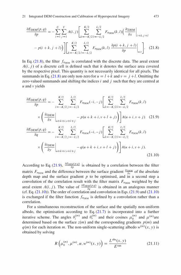
21 Integrated DEM Construction and Calibration of Hyperspectral Imagery 473
@EDEM.p; q/
@pD !
UX
iD1
VX
jD1A.i; j /
" K=2X
kD"K=2
L=2X
lD"L=2F&DEM .k; l/
' @zDEM
@x
ˇˇiCk;jCl
! p.i C k; j C l/(#" K=2X
kD"K=2
L=2X
lD"L=2F&DEM.k; l/
@p.i C k; j C l/@p
ˇˇu;v
#: (21.8)
In Eq. (21.8), the filter f&DEM is correlated with the discrete data. The areal extentA.i; j / of a discrete cell is defined such that it denotes the surface area coveredby the respective pixel. This quantity is not necessarily identical for all pixels. Thesummands in Eq. (21.8) are only non-zero for u D lCk and v D jCl . Omitting thezero-valued summands and shifting the indices i and j such that they are centred atu and v yields
@EDEM.p; q/
@pD !
K=2X
iD"K=2
L=2X
jD"L=2F&DEM.!i;!j /
" K=2X
kD"K=2
L=2X
lD"L=2F&DEM.k; l/
" @zDEM
@x
ˇˇuCkCi;vClCj
! p.uC k C i; vC l C j /!#A.uC i; vC j / (21.9)
@EDEM.p; q/
@qD !
K=2X
iD"K=2
L=2X
jD"L=2F&DEM.!i;!j /
" K=2X
kD"K=2
L=2X
lD"L=2F&DEM.k; l/
" @zDEM
@y
ˇˇuCkCi;vClCj
! q.uC k C i; vC l C j /!#A.uC i; vC j /:
(21.10)
According to Eq. (21.9), @EDEM.p;q/@p
is obtained by a correlation between the filter
matrix F&DEM and the difference between the surface gradient @zDEM@x
of the absolutedepth map and the surface gradient p to be optimised, and in a second step aconvolution of the correlation result with the filter matrix F&DEM weighted by theareal extent A.i; j /. The value of @EDEM.p;q/
@qis obtained in an analogous manner
(cf. Eq. (21.10)). The order of correlation and convolution in Eqs. (21.9) and (21.10)is exchanged if the filter function f&DEM is defined by a convolution rather than acorrelation.
For a simultaneous reconstruction of the surface and the spatially non-uniformalbedo, the optimisation according to Eq. (21.7) is incorporated into a furtheriterative scheme. The angles ! .m/i and ! .m/e and their cosines ".m/0 and ".m/aredetermined based on the surface z.m/ and the corresponding gradients p.m/ andq.m/ for each iteration m. The non-uniform single-scattering albedo w.m/.x; y/ isobtained by solving
R'".m/0 ;".m/; ˛;w.m/.x; y/
(D Lobs.x; y/
Esun(21.11)
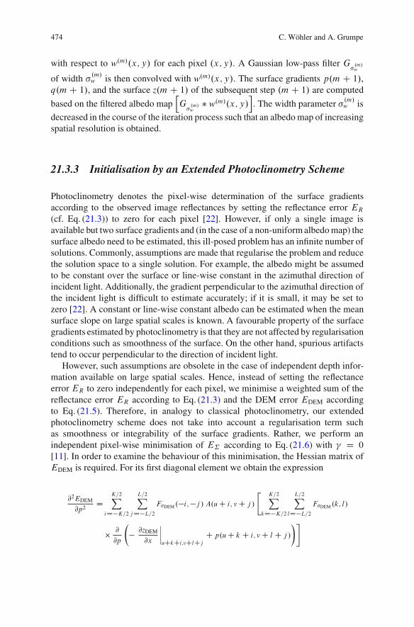
474 C. Wohler and A. Grumpe
with respect to w.m/.x; y/ for each pixel .x; y/. A Gaussian low-pass filter G&.m/w
of width & .m/w is then convolved with w.m/.x; y/. The surface gradients p.m C 1/,q.mC 1/, and the surface z.m C 1/ of the subsequent step .mC 1/ are computedbased on the filtered albedo map
hG&.m/w# w.m/.x; y/
i. The width parameter & .m/w is
decreased in the course of the iteration process such that an albedo map of increasingspatial resolution is obtained.
21.3.3 Initialisation by an Extended Photoclinometry Scheme
Photoclinometry denotes the pixel-wise determination of the surface gradientsaccording to the observed image reflectances by setting the reflectance error ER(cf. Eq. (21.3)) to zero for each pixel [22]. However, if only a single image isavailable but two surface gradients and (in the case of a non-uniform albedo map) thesurface albedo need to be estimated, this ill-posed problem has an infinite number ofsolutions. Commonly, assumptions are made that regularise the problem and reducethe solution space to a single solution. For example, the albedo might be assumedto be constant over the surface or line-wise constant in the azimuthal direction ofincident light. Additionally, the gradient perpendicular to the azimuthal direction ofthe incident light is difficult to estimate accurately; if it is small, it may be set tozero [22]. A constant or line-wise constant albedo can be estimated when the meansurface slope on large spatial scales is known. A favourable property of the surfacegradients estimated by photoclinometry is that they are not affected by regularisationconditions such as smoothness of the surface. On the other hand, spurious artifactstend to occur perpendicular to the direction of incident light.
However, such assumptions are obsolete in the case of independent depth infor-mation available on large spatial scales. Hence, instead of setting the reflectanceerror ER to zero independently for each pixel, we minimise a weighted sum of thereflectance error ER according to Eq. (21.3) and the DEM error EDEM accordingto Eq. (21.5). Therefore, in analogy to classical photoclinometry, our extendedphotoclinometry scheme does not take into account a regularisation term suchas smoothness or integrability of the surface gradients. Rather, we perform anindependent pixel-wise minimisation of E˙ according to Eq. (21.6) with ' D 0[11]. In order to examine the behaviour of this minimisation, the Hessian matrix ofEDEM is required. For its first diagonal element we obtain the expression
@2EDEM
@p2D
K=2X
iD!K=2
L=2X
jD!L=2F&DEM ."i;"j / A.uC i; vC j /
"K=2X
kD!K=2
L=2X
lD!L=2F&DEM .k; l/
# @
@p
" @zDEM
@x
ˇˇuCkCi;vClCj
C p.uC k C i; vC l C j /!#

21 Integrated DEM Construction and Calibration of Hyperspectral Imagery 475
DK=2X
iD!K=2
L=2X
jD!L=2F&DEM ."i;"j / A.uC i; vC j /
"K=2X
kD!K=2
L=2X
lD!L=2F&DEM .k; l/
# @
@p.p.uC kC i; vC l C j //
#
: (21.12)
In Eq. (21.12), kC i D 0 and l C j D 0 must hold for all non-zero summands, andthe equation reduces to
@2EDEM
@p2D
K=2X
iD"K=2
L=2X
jD"L=2F 2&DEM
.!i;!j / $ A.uC i; vC j /: (21.13)
The second derivative with respect to q has the same value. Since neither Eq. (21.9)depends on q nor Eq. (21.10) depends on p, the mixed derivatives are given by
@2EDEM
@p@qD @2EDEM
@q@pD 0: (21.14)
Therefore, the Hessian matrix of EDEM reduces to a diagonal matrix. Due to thefact that not all filter coefficients of F&DEM are zero and the pixel area A is positiveby definition, all eigenvalues of the Hessian matrix are positive for all pixels. Thisimplies thatEDEM possesses only one global minimum. Assuming a minimisation ofEDEM with the soft constraint ER weighted by 1=ı, convergence is thus guaranteedfor sufficiently large ı.
The resulting surface gradients p and q may be quite far from being integrable,such that we determine the “nearest” surface z based on the approach introduced in[21]. As an alternative to the LOLA DEM, the resulting surface can be used as aninitialisation of the variational optimisation scheme described in Sect. 21.3.2. It willbe shown in Sect. 21.4 that this initialisation results in a significantly higher absolutereconstruction accuracy.
The albedo map is computed pixel-wise using the initial surface and is thenlow-pass filtered as explained in Sect. 21.3.2. Since the method by Horn [21] ofestimating the surface z from the gradients p and q does not allow large variationsof z on large spatial scales, we apply a pyramidal approach, where both the imageand the LOLA DEM are downscaled npyr times by a factor of 2. Starting from thelowest resolution level, the surface and the albedo map are computed and passed onto the next pyramid level until the full image resolution is reached.
21.4 Results of DEM Construction
For DEM construction, we utilise imagery acquired with the Moon MineralogyMapper (M3) on board the Indian Chandrayaan-1 spacecraft. The M3 instrumentis a hyperspectral pushbroom sensor with (in global mode) 85 pixel-synchronous

476 C. Wohler and A. Grumpe
spectral channels with 20–40nm per channel with centre wavelengths between461 and 2,976 nm, where the image resolution typically corresponds to 140mper pixel [42] (cf. also Table 21.1). The M3 data archive accessible at http://m3.jpl.nasa.gov/m3data.html comprises radiance images for each wavelength channeland provides for each image pixel the selenographic longitude and latitude aswell as the incidence angle ! .0/i , the emission angle ! .0/e , and the phase angle ˛,where topography is neglected and a smooth spherical surface is assumed for thegiven values of ! .0/i and ! .0/e . We compute the reflectance error ER as the sum ofsquared channel-wise errors according to Eq. (21.3) for channels 50–60, coveringthe wavelength range from 1; 579 to 1;978 nm. As the lunar surface temperaturemay reach up to 396K [50], we do not use channels with centre wavelengthsbeyond 2;000 nm in order to avoid the resulting thermal radiance component. TheDEM error according to Eq. (21.5) is computed based on the gridded DEM derivedfrom LOLA data (http://pds-geosciences.wustl.edu/missions/lro/lola.htm), whichprovides absolute elevation values relative to the mean lunar radius of 1;738 kmand is georeferenced to the same coordinate system as the M3 images.
Our first example DEM covers the eastern half of the lunar crater Alphonsus,which shows a distinctly non-uniform surface albedo due to the presence ofpyroclastic deposits on the crater floor which consist of dark volcanic ash [9].Bright highland material appears as high-albedo regions. This crater is well suitedfor demonstrating the capability of the DEM construction algorithm proposed inSect. 21.3 to separate radiance variations due to topography from those due to non-uniform albedo. The M3 image of Alphonsus, the corresponding LOLA DEM, therefined DEM and the albedo map are shown in Fig. 21.2. Another lunar regiondisplaying distinct albedo variations is the crater Bullialdus (cf. Fig. 21.3). Ourrefined DEM reveals the terraced structure of the inner crater walls and a multitudeof small craters which are invisible in the LOLA DEM. Similarly, we found thatdespite the high nominal lateral resolution of the GLD100 according to [44], ourconstructed DEMs reveal much finer details than the GLD100 (cf. also [12]).
No topographic map of sufficiently high lateral resolution is available for theexamined regions as ground truth. In order to nevertheless obtain an estimate of theabsolute accuracy, a synthetic image of Bullialdus crater was created by illuminatingthe constructed DEM using the inferred albedo map. The illumination and viewingdirection were adopted from the original M3 image. This synthetic image wasused as an input image for our DEM construction algorithm. When the variationaloptimisation scheme is initialised with the LOLA DEM, the reconstruction error(RMSE) corresponds to 54m, while it becomes as low as 9m when the resultof the extended photoclinometry scheme is used for initialisation. The RMSE ofthe inferred albedo map at 1;978 nm wavelength amounts to 0:007 and 0:005,corresponding to 1:8 and 1:3% of the mean albedo of 0:391, respectively.
These results were obtained by performing 8 iterations of the variationalapproach (cf. Sect. 21.3.2) with &w decreasing from 11 to 7 pixels, &DEM D 7 pixels,' D 9 " 10"4, and ı D 2:5 " 10"5. The values of ' and ı have been chosen assmall as possible for the optimisation scheme to converge in order to maximise
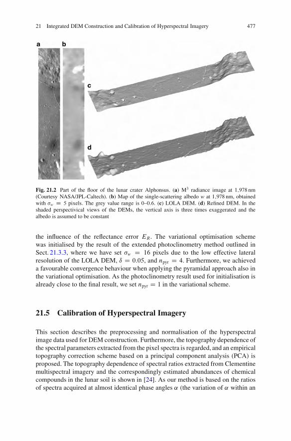
21 Integrated DEM Construction and Calibration of Hyperspectral Imagery 477
Fig. 21.2 Part of the floor of the lunar crater Alphonsus. (a) M3 radiance image at 1;978 nm(Courtesy NASA/JPL-Caltech). (b) Map of the single-scattering albedo w at 1;978 nm, obtainedwith &w D 5 pixels. The grey value range is 0–0:6. (c) LOLA DEM. (d) Refined DEM. In theshaded perspectivical views of the DEMs, the vertical axis is three times exaggerated and thealbedo is assumed to be constant
the influence of the reflectance error ER. The variational optimisation schemewas initialised by the result of the extended photoclinometry method outlined inSect. 21.3.3, where we have set &w D 16 pixels due to the low effective lateralresolution of the LOLA DEM, ı D 0:05, and npyr D 4. Furthermore, we achieveda favourable convergence behaviour when applying the pyramidal approach also inthe variational optimisation. As the photoclinometry result used for initialisation isalready close to the final result, we set npyr D 1 in the variational scheme.
21.5 Calibration of Hyperspectral Imagery
This section describes the preprocessing and normalisation of the hyperspectralimage data used for DEM construction. Furthermore, the topography dependence ofthe spectral parameters extracted from the pixel spectra is regarded, and an empiricaltopography correction scheme based on a principal component analysis (PCA) isproposed. The topography dependence of spectral ratios extracted from Clementinemultispectral imagery and the correspondingly estimated abundances of chemicalcompounds in the lunar soil is shown in [24]. As our method is based on the ratiosof spectra acquired at almost identical phase angles ˛ (the variation of ˛ within an
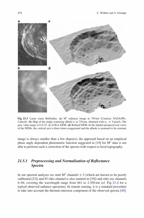
478 C. Wohler and A. Grumpe
Fig. 21.3 Lunar crater Bullialdus. (a) M3 radiance image at 750 nm (Courtesy NASA/JPL-Caltech). (b) Map of the single-scattering albedo w at 750 nm, obtained with &w D 9 pixels. Thegrey value range is 0–0:35. (c) LOLA DEM. (d) Refined DEM. In the shaded perspectivical viewsof the DEMs, the vertical axis is three times exaggerated and the albedo is assumed to be constant
image is always smaller than a few degrees), the approach based on an empiricalphase angle dependent photometric function suggested in [19] for M3 data is notable to perform such a correction of the spectra with respect to local topography.
21.5.1 Preprocessing and Normalisation of ReflectanceSpectra
In our spectral analyses we omit M3 channels 1–5 (which are known to be poorlycalibrated [23]) and 85 (this channel is also omitted in [19]) and only use channels6–84, covering the wavelength range from 661 to 2;936 nm (cf. Fig. 21.4 for atypical observed radiance spectrum). In remote sensing, it is a standard procedureto take into account the thermal emission component of the observed spectra [45].
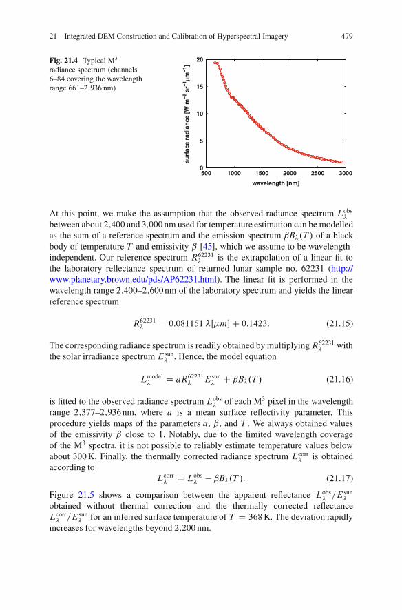
21 Integrated DEM Construction and Calibration of Hyperspectral Imagery 479
500 1000 1500 2000 2500 30000
5
10
15
20
wavelength [nm]su
rfac
e ra
dian
ce [W
m!2
sr!1
mm!1
]
Fig. 21.4 Typical M3
radiance spectrum (channels6–84 covering the wavelengthrange 661–2;936 nm)
At this point, we make the assumption that the observed radiance spectrum Lobs*
between about 2;400 and 3;000 nm used for temperature estimation can be modelledas the sum of a reference spectrum and the emission spectrum � B*.T / of a blackbody of temperature T and emissivity � [45], which we assume to be wavelength-independent. Our reference spectrum R62231* is the extrapolation of a linear fit tothe laboratory reflectance spectrum of returned lunar sample no. 62231 (http://www.planetary.brown.edu/pds/AP62231.html). The linear fit is performed in thewavelength range 2;400–2;600nm of the laboratory spectrum and yields the linearreference spectrum
R62231* D 0:081151 * å "m$C 0:1423: (21.15)
The corresponding radiance spectrum is readily obtained by multiplyingR62231* withthe solar irradiance spectrum Esun
* . Hence, the model equation
Lmodel* D aR62231* Esun
* C � B*.T / (21.16)
is fitted to the observed radiance spectrum Lobs* of each M3 pixel in the wavelength
range 2;377–2;936nm, where a is a mean surface reflectivity parameter. Thisprocedure yields maps of the parameters a, � , and T . We always obtained valuesof the emissivity � close to 1. Notably, due to the limited wavelength coverageof the M3 spectra, it is not possible to reliably estimate temperature values belowabout 300K. Finally, the thermally corrected radiance spectrum Lcorr
* is obtainedaccording to
Lcorr* D Lobs
* ! � B*.T /: (21.17)
Figure 21.5 shows a comparison between the apparent reflectance Lobs* =Esun
*
obtained without thermal correction and the thermally corrected reflectanceLcorr* =Esun
* for an inferred surface temperature of T D 368K. The deviation rapidlyincreases for wavelengths beyond 2;200 nm.
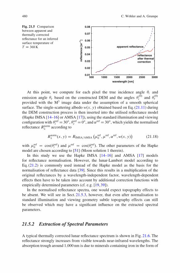
480 C. Wohler and A. Grumpe
500 1000 1500 2000 2500 30000.01
0.02
0.03
0.04
0.05
0.06
0.07
0.08
wavelength [nm]re
flect
ance
[sr!1
]
apparent reflectance
reflectanceafter thermalcorrection
Fig. 21.5 Comparisonbetween apparent andthermally correctedreflectance for an inferredsurface temperature ofT D 368K
At this point, we compute for each pixel the true incidence angle !i andemission angle !e based on the constructed DEM and the angles ! .0/i and ! .0/eprovided with the M3 image data under the assumption of a smooth sphericalsurface. The single-scattering albedo w.x; y/ obtained based on Eq. (21.11) duringthe DEM construction process is then inserted into the utilised reflectance model(Hapke IMSA [14–16] or AMSA [17]), using the standard illumination and viewingconfiguration with ! ref
i D 30 � , ! refe D 0 � , and � refD 30 � , which yields the normalised
reflectance Rnorm* according to
Rnorm* .x; y/ D RIMSA=AMSA
%"ref0 ;"
ref; � ref;w.x; y/&
(21.18)
with "ref0 D cos.! ref
i / and "ref D cos.! refe /. The other parameters of the Hapke
model are chosen according to [51] (Moon solution 1 therein).In this study we use the Hapke IMSA [14–16] and AMSA [17] models
for reflectance normalisation. However, the lunar-Lambert model according toEq. (21.2) is commonly used instead of the Hapke model as the basis for thenormalisation of reflectance data [39]. Since this results in a multiplication of theoriginal reflectances by a wavelength-independent factor, wavelength-dependenteffects then have to be taken into account by additional correction functions withempirically determined parameters (cf. e.g. [19, 39]).
In the normalised reflectance spectra, one would expect topography effects tobe absent. We will see in Sect. 21.5.3, however, that even after normalisation tostandard illumination and viewing geometry subtle topography effects can stillbe observed which may have a significant influence on the extracted spectralparameters.
21.5.2 Extraction of Spectral Parameters
A typical thermally corrected lunar reflectance spectrum is shown in Fig. 21.6. Thereflectance strongly increases from visible towards near-infrared wavelengths. Theabsorption trough around 1;000 nm is due to minerals containing iron in the form of

21 Integrated DEM Construction and Calibration of Hyperspectral Imagery 481
Fig. 21.6 Typical thermally corrected lunar reflectance spectrum, illustrating the primary absorp-tion troughs
Fe2C ions [3,35,48]. A second absorption trough around 2;000 nm can be attributedto the mineral pyroxene [3]. The absorption trough around 2;800 nm is describede.g. in [6], where it is attributed to the presence of water molecules and OH" ions inthe lunar soil. According to [37], they originate from chemical reactions of oxygencontained in the minerals of the lunar surface with protons of the solar wind.
Easily obtainable quantities to characterise the depths of the ferrous absorptiontrough around 1;000 nm and the hydrous absorption trough around 2;800 nm are thediagnostic spectral ratios Rnorm
950 =Rnorm750 (cf. e.g. [9]) and Rnorm
2817 =Rnorm2657 , respectively.
Additionally, the detailed composition of lunar iron-bearing minerals causes subtlevariations of the shape of the ferrous absorption trough, which can be examinedbased on the continuum-removed spectrum [35, 48].
To compute the continuum-removed reflectance spectrum, the normalisedreflectance spectrum is smoothed by adapting a curve for which the mean squareddeviation from the measured reflectance values and the mean squared secondderivative are minimised simultaneously [34]. The spectral continuum is thenapproximated by a straight line between the smoothed reflectances at 701 and1;249 nm (cf. [30]). Division of the smoothed reflectance spectrum by the linearcontinuum then yields the continuum-removed reflectance spectrum [30], to whichan interpolation based on the Akima method [2] is applied (cf. Fig. 21.7).
The extracted spectral parameters of the absorption trough around 1;000 nm are(as illustrated in Fig. 21.7) the absorption wavelength *abs, the full width at halfmaximum (FWHM), the absorption depth ı (cf. [30]), and the integrated band depth(IBD) [8], corresponding to the area under the trough in Fig. 21.7. The absorptionwavelength e.g. allows to differentiate between pyroxenes containing high and lowabundances of calcium [35, 48]. The absorption depth depends on the amount of

482 C. Wohler and A. Grumpe
Fig. 21.7 Typical smoothed and continuum-removed reflectance spectrum showing the ferrousabsorption trough around 1;000 nm
Fig. 21.8 (a) M3 750 nm radiance image of the crater Bullialdus (Courtesy NASA/JPL-Caltech).(b) Single-scattering albedo w at 750 nm. (c) and (d) Integrated band depth (IBD) of the ferrousabsorption trough around 1;000 nm inferred based on the lunar-Lambert and on the Hapke AMSAreflectance function, respectively (grey value range 0–50). (e) Relative difference of the IBD values(grey value range 0–0:15)
mafic minerals [48] and also on the so-called “optical maturity” of the soil [41],i.e. the period of time the surface has been exposed to high-energy solar radiation.A broad absorption, i.e. a large FWHM value, indicates that olivine occurs in the soil[35, 48]. The IBD of the ferrous absorption trough is correlated with the abundanceof pyroxene [8].
Figure 21.8 illustrates the difference between the values of the IBD of theferrous absorption trough inferred based on the wavelength-independent lunar-Lambert reflectance function [38] according to Eq. (21.2) and on the Hapke AMSAreflectance function [17] according to Eq. (21.1), respectively.
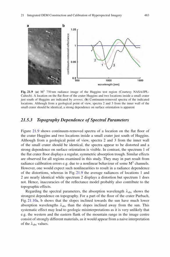
21 Integrated DEM Construction and Calibration of Hyperspectral Imagery 483
Fig. 21.9 (a) M3 750 nm radiance image of the Huggins test region (Courtesy NASA/JPL-Caltech). A location on the flat floor of the crater Huggins and two locations inside a small craterjust south of Huggins are indicated by arrows. (b) Continuum-removed spectra of the indicatedlocations. Although from a geological point of view, spectra 2 and 3 from the inner wall of thesmall crater should be identical, a strong dependence on surface orientation is apparent
21.5.3 Topography Dependence of Spectral Parameters
Figure 21.9 shows continuum-removed spectra of a location on the flat floor ofthe crater Huggins and two locations inside a small crater just south of Huggins.Although from a geological point of view, spectra 2 and 3 from the inner wallof the small crater should be identical, the spectra appear to be distorted and astrong dependence on surface orientation is visible. In contrast, the spectrum 1 ofthe flat crater floor displays a regular, symmetric absorption trough. Similar effectsare observed for all regions examined in this study. They may in part result fromradiance calibration errors e.g. due to a nonlinear behaviour of some M3 channels.However, one would expect such nonlinearities to result in a radiance dependenceof the distortions, whereas in Fig. 21.9 the average radiances of locations 1 and2 are nearly identical while spectrum 2 displays a distortion but spectrum 1 doesnot. Hence, inaccuracies of the reflectance model probably also contribute to thetopographic effects.
Regarding the spectral parameters, the absorption wavelength *abs shows thestrongest dependence on topography. For a part of the floor of the crater Purbach,Fig. 21.10a, b shows that the slopes inclined towards the sun have much lowerabsorption wavelengths *abs than the slopes inclined away from the sun. Thissystematic effect may lead to geologic misinterpretations as it is very unlikely thate.g. the western and the eastern flank of the mountain range in the image centreconsist of strongly different materials, as it would appear from a naive interpretationof the *abs values.
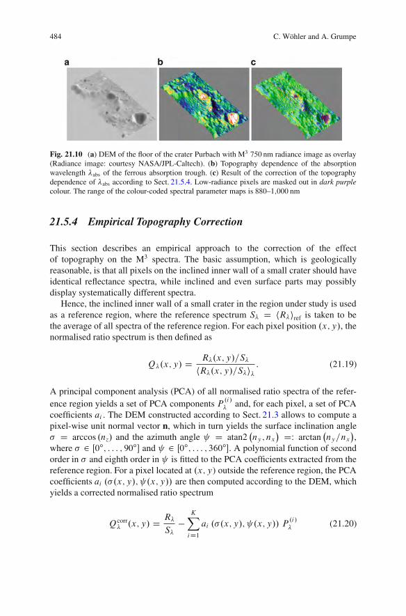
484 C. Wohler and A. Grumpe
Fig. 21.10 (a) DEM of the floor of the crater Purbach with M3 750 nm radiance image as overlay(Radiance image: courtesy NASA/JPL-Caltech). (b) Topography dependence of the absorptionwavelength *abs of the ferrous absorption trough. (c) Result of the correction of the topographydependence of *abs according to Sect. 21.5.4. Low-radiance pixels are masked out in dark purplecolour. The range of the colour-coded spectral parameter maps is 880–1;000 nm
21.5.4 Empirical Topography Correction
This section describes an empirical approach to the correction of the effectof topography on the M3 spectra. The basic assumption, which is geologicallyreasonable, is that all pixels on the inclined inner wall of a small crater should haveidentical reflectance spectra, while inclined and even surface parts may possiblydisplay systematically different spectra.
Hence, the inclined inner wall of a small crater in the region under study is usedas a reference region, where the reference spectrum S* D hR*iref is taken to bethe average of all spectra of the reference region. For each pixel position .x; y/, thenormalised ratio spectrum is then defined as
Q*.x; y/ DR*.x; y/=S*
hR*.x; y/=S*i*: (21.19)
A principal component analysis (PCA) of all normalised ratio spectra of the refer-ence region yields a set of PCA components P .i/
* and, for each pixel, a set of PCAcoefficients ai . The DEM constructed according to Sect. 21.3 allows to compute apixel-wise unit normal vector n, which in turn yields the surface inclination angle& D arccos .nz/ and the azimuth angle D atan2
%ny; nx
&DW arctan
%ny=nx
&,
where & 2 Œ0ı; : : : ; 90ı$ and 2 Œ0ı; : : : ; 360ı$. A polynomial function of secondorder in & and eighth order in is fitted to the PCA coefficients extracted from thereference region. For a pixel located at .x; y) outside the reference region, the PCAcoefficients ai .&.x; y/; .x; y// are then computed according to the DEM, whichyields a corrected normalised ratio spectrum
Qcorr* .x; y/ D R*
S*!
KX
iD1ai .&.x; y/; .x; y// P
.i/* (21.20)

21 Integrated DEM Construction and Calibration of Hyperspectral Imagery 485
500 1000 1500 2000 2500 3000
!0.25
!0.2
!0.15
!0.1
!0.05
0
0.05
0.1
0.15
wavelength [nm]
Mea
n, p
rinc
ipal
com
pone
nts
of Q
!
Mea
n, p
rinc
ipal
com
pone
nts
of Q
!
PC1
PC2
<Q!>
ref ! 1
500 1000 1500 2000 2500 3000!0.3
!0.2
!0.1
0
0.1
0.2
wavelength [nm]
<Q!>
ref ! 1
PC1
PC2
a b
Fig. 21.11 Average value of Q*.x; y/ according to Eq. (21.19) and the first two principalcomponents (denoted by PC1 and PC2), extracted from the pixels belonging (a) to the innerwalls of two small craters just south of Huggins and (b) to those of the small crater Purbach A,respectively
and a corrected reflectance spectrum
Rcorr* .x; y/ D Qcorr
* .x; y/S*: (21.21)
For our two test regions, the first four principal components comprise 98% of theinformation, such that we always set K D 4 in Eq. (21.20). The average value ofQ*.x; y/ is shown along with the first two PCA components for the Huggins andPurbach test regions in Fig. 21.11. The differences between the test regions are dueto the higher southern selenographic latitude of the Huggins region, resulting in amore oblique solar illumination angle.
Based on the corrected reflectances, a refined DEM is constructed according toSect. 21.3.2, where the Hapke IMSA reflectance model is used due to convergenceproblems with the AMSA model. Finally, the reflectance normalisation and PCA-based topography correction is repeated using the Hapke AMSA model, where itis favourable to neglect low-radiance pixels (e.g. shaded crater walls or mountainflanks) in the analysis due to their very low signal-to-noise ratio.
21.6 Results of Topography Correction and Final DEMConstruction
The final DEMs of the Huggins and Purbach test regions are shown in Fig. 21.12,showing a high amount of small-scale surface detail. The spectral parametersextracted from the uncorrected and the final corrected reflectance spectra of theseregions are shown in Figs. 21.13 and 21.14, respectively, where dark pixels with750nm radiances below 7W m"2 +m"1 sr"1 are masked out. Figure 21.10c shows
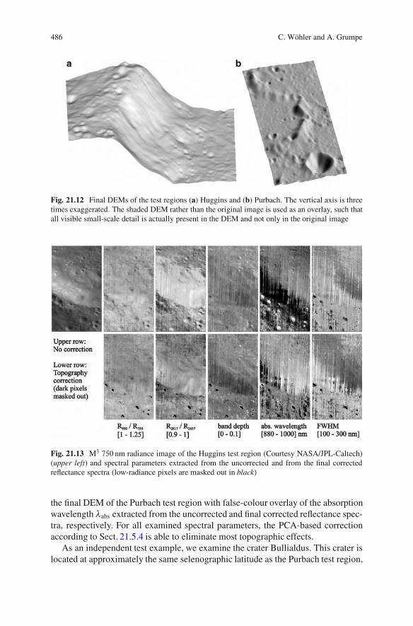
486 C. Wohler and A. Grumpe
Fig. 21.12 Final DEMs of the test regions (a) Huggins and (b) Purbach. The vertical axis is threetimes exaggerated. The shaded DEM rather than the original image is used as an overlay, such thatall visible small-scale detail is actually present in the DEM and not only in the original image
Fig. 21.13 M3 750 nm radiance image of the Huggins test region (Courtesy NASA/JPL-Caltech)(upper left) and spectral parameters extracted from the uncorrected and from the final correctedreflectance spectra (low-radiance pixels are masked out in black)
the final DEM of the Purbach test region with false-colour overlay of the absorptionwavelength *abs extracted from the uncorrected and final corrected reflectance spec-tra, respectively. For all examined spectral parameters, the PCA-based correctionaccording to Sect. 21.5.4 is able to eliminate most topographic effects.
As an independent test example, we examine the crater Bullialdus. This crater islocated at approximately the same selenographic latitude as the Purbach test region,

21 Integrated DEM Construction and Calibration of Hyperspectral Imagery 487
Fig. 21.14 M3 750 nm radiance image of the Purbach test region (Courtesy NASA/JPL-Caltech)(upper left) and spectral parameters extracted from the uncorrected and from the final correctedreflectance spectra (low-radiance pixels are masked out in black)
resulting in similar illumination conditions in the corresponding M3 data. Hence,we use the PCA components P .i/
* and the coefficient functions ai .&; / inferredfrom the Purbach region in order to compute corrected reflectances accordingto Eq. (21.21) and extract the corresponding corrected spectral parameters. Thespectral parameters extracted from the uncorrected and corrected reflectances areshown in Fig. 21.15 (cf. Fig. 21.3 for the final DEM). Again, the topographycorrection is most obvious in the map of the absorption wavelength *abs, whichis used as an overlay of the final DEM of Bullialdus in Fig. 21.16. After correction,the crater walls, most of the crater floor, and the even surface outside the craterdisplay similar values of *abs, only the central peaks still display excessively lowabsorption wavelengths. These low *abs values are much more clearly confined tothe central peaks than without correction. In [49], the spectral characteristics of thecentral peaks of Bullialdus are attributed to the occurrence of the mineral norite.
Figure 21.15 shows that the cold, shaded flanks of the central peak of Bullialdusdisplay a stronger hydroxyl absorption (i.e. lower R2817=R2657 ratio) than thewarmer crater floor. This effect is not eliminated by the empirical correctionapproach. Temperatures below 250–300K cannot be estimated reliably due to the
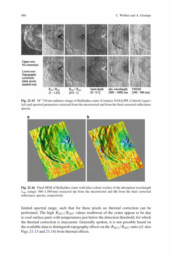
488 C. Wohler and A. Grumpe
Fig. 21.15 M3 750 nm radiance image of Bullialdus crater (Courtesy NASA/JPL-Caltech) (upperleft) and spectral parameters extracted from the uncorrected and from the final corrected reflectancespectra
Fig. 21.16 Final DEM of Bullialdus crater with false-colour overlay of the absorption wavelength*abs (range: 880–1;000 nm) extracted (a) from the uncorrected and (b) from the final correctedreflectance spectra, respectively
limited spectral range, such that for these pixels no thermal correction can beperformed. The high R2817=R2657 values southwest of the crater appear to be dueto cool surface parts with temperatures just below the detection threshold, for whichthe thermal correction is inaccurate. Generally spoken, it is not possible based onthe available data to distinguish topography effects on the R2817=R2657 ratio (cf. alsoFigs. 21.13 and 21.14) from thermal effects.

21 Integrated DEM Construction and Calibration of Hyperspectral Imagery 489
21.7 Summary and Conclusion
A method for the construction of lunar DEMs which combines surface gradientsobtained by photoclinometry and shape from shading with absolute depth data(here: lunar orbital LIDAR data) by exploiting their respective advantages hasbeen presented. The lunar surface has a non-Lambertian reflectance behaviour anda non-uniform albedo. In a first step, the surface gradients are estimated basedon an extended photoclinometry approach which takes into account both imageand LIDAR data, and the surface is reconstructed by integration. The second stepconsists of the minimisation of a global error functional based on a variationalapproach in order to combine the surface gradient information on small spatialscales and the LIDAR data on large spatial scales, where the result of the firststep is used for initialisation. This framework has been applied to the constructionof DEMs of lunar surface regions. Based on the available hyperspectral imagery,the obtained DEMs have been used to normalise the wavelength-dependent surfacereflectance to a standard illumination and viewing geometry. In this context, anempirical, PCA-based correction approach has been proposed to compensate thedetected systematic topography-dependent distortions of the pixel spectra whichaffect the extracted spectral parameters. Relying on the corrected surface reflectancedata, refined DEMs have been constructed and spectral parameter maps have beenobtained in which (except for the hydroxyl absorption) topographic effects arenearly completely removed.
References
1. Agrawal, A., Raskar, R., Chellappa, R.: What is the range of surface reconstructions froma gradient field? In: Leonardis, A., Bischof, H., Pinz, A. (eds.) Proceedings of EuropeanConference on Computer Vision. Lecture Notes in Computer Science, vol. 3951, pp. 578–591.Springer (2006)
2. Akima, H.: A new method of interpolation and smooth curve fitting based on local procedures.J. Assoc. Comput. Mach. 17(4), 589–602 (1970)
3. Burns, R.G., Abu-Eid, R.M., Huggins, F.E.: Crystal field spectra of lunar pyroxenes. In:Proceedings of Lunar Science Conference, vol. 2, pp. 533–543. Lunar and Planetary Institute,Houston (1972)
4. Bussey, D.B.J., McGovern, J.A., Spudis, P.D., Neish, C.D., Sorensen, S.A.: Lunar polarillumination conditions derived using Kaguya laser data. In: Proceedings of Annual Meetingof LEAG. Lunar and Planetary Institute, Houston (2009)
5. Chandrasekhar, S.: Radiative Transfer. Dover, New York (1960)6. Clark R., Pieters, C.M., Green, R.O., Boardman, J., Buratti, B.J., Head, J.W., Isaacson, P.J.,
Livo, K.E., McCord, T.B., Nettles, J.W., Petro, N.E., Sunshine, J.M., Taylor, L.A.: Waterand Hydroxyl on the Moon as seen by the Moon Mineralogy Mapper (M3). In: Proceedingsof Lunar Planetary Science XXXXI, abstract #2302. Lunar and Planetary Institute, Houston(2010)
7. Cryer, J.E., Tsai, P.-S., Shah, M.: Integration of shape from shading and stereo. PatternRecognit. 28(7), 1033–1043 (1995)

490 C. Wohler and A. Grumpe
8. Dhingra, D., Pieters, C.M., Isaacson, P., Staid, M., Mustard, J., Klima, R., Taylor, L.A.,Kramer, G., Nettles, J., M3 team: Spectroscopic signature of the high titanium basalts atmare tranquillitatis from Moon Mineralogy Mapper (M3). In: Proceedings of Lunar PlanetaryScience XXXXI, abstract #2494. Lunar and Planetary Institute, Houston (2010)
9. Gaddis, L.R., Staid, M.I., Tyburczy, J.A., Hawke, B.R., Petro, N.E.: Compositional analyses oflunar pyroclastic deposits. Icarus 161, 262–280 (2003)
10. Grieger, B., Beauvivre, S., Despan, D., Erard, S., Josset, J.-L., Koschny, D.: Investigating apeak of (almost) eternal light close to the lunar south pole with SMART-1/AMIE images.In: Proceedings of European Planetary Science Congress, EPSC2008-A-00205, Munster,Germany (2008)
11. Grumpe, A., Wohler, C.: DEM construction and calibration of hyperspectral image data usingpairs of radiance images. In: Proceedings of IEEE International Symposium on Image andSignal Processing and Analysis, Dubrovnik, Croatia, pp. 609–614 (2011)
12. Grumpe, A., Wohler, C.: Image-based construction of lunar digital elevation models of veryhigh lateral resolution. In: Proceedings of Lunar Planetary Science XXXXIII, abstract #2597.Lunar and Planetary Institute, Houston (2012)
13. Grumpe, A., Herbort, S., Wohler, C.: 3D reconstruction of non-Lambertian surfaces with non-uniform reflectance parameters by fusion of photometrically estimated surface normal datawith active range scanner data. In: Proceedings of Oldenburger 3D-Tage, Oldenburg, Germany,pp. 54–61 (2011)
14. Hapke, B.W.: Bidirectional reflectance spectroscopy 1: theory. J. Geophys. Res. 86, 3039–3054(1981)
15. Hapke, B.W.: Bidirectional reflectance spectroscopy 3: correction for macroscopic roughness.Icarus 59, 41–59 (1984)
16. Hapke, B.W.: Bidirectional reflectance spectroscopy 4: the extinction coefficient and theopposition effect. Icarus 67, 264–280 (1986)
17. Hapke, B.W.: Bidirectional reflectance spectroscopy 5: the coherent backscatter oppositioneffect and anisotropic scattering. Icarus 157, 523–534 (2002)
18. Herbort, S., Grumpe, A., Wohler, C.: Reconstruction of non-Lambertian surfaces by fusionof shape from shading and active range scanning. In: Proceedings of IEEE InternationalConferences on Image Processing, Brussels, Belgium, pp. 17–20 (2011)
19. Hicks, M.D., Buratti, B.J., Nettles, J., Staid, M., Sunshine, J., Pieters, C.M., Besse, S.,Boardman, J.: A photometric function for analysis of lunar images in the visual and infraredbased on Moon Mineralogy Mapper observations. J. Geophys. Res. 116, E00G15 (2011).doi:10.1029/2010JE003733
20. Horn, B.K.P.: Shape from shading: a method for obtaining the shape of a smooth opaque objectfrom one view. MIT Technical Report 232, Massachusetts Institute of Technology (1970)
21. Horn, B.K.P.: Robot Vision. MIT Press, Cambridge, MA (1986)22. Horn, B.K.P.: Height and gradient from shading. AI Memo 1105A, MIT AI Lab (1989)23. Isaacson, P.: M3 overview and working with M3 data. M3 Data Tutorial at Lunar Planetary Sci-
ence XXXXII. http://m3.jpl.nasa.gov/pubs/Isaacson M3DataWorkshop LPSC2011.pdf (2011)24. Jolliff, B.L.: Clementine UVVIS multispectral data and the Apollo 17 landing site: what can
we tell and how well? J. Geophys. Res. 104(E6), 14123–14148 (1999)25. Joshi, N., Kriegman, D.J.: Shape from varying illumination and viewpoint. In: Proceedings of
the International Conference on Computer Vision. IEEE, New York (2007)26. Josset, J.-L., et al.: Science objectives and first results from the SMART-1/AMIE multicolour
micro-camera. Adv. Space Res. 37, 14–20 (2006)27. Kieffer, H.H., Stone, T.C.: The spectral irradiance of the Moon. Astron. J. 129, 2887–2901
(2005)28. Kirk, R.L., Soderblom, L.A., Howington-Kraus, E., Archinal, B.: USGS high-resolution
topomapping of Mars with Mars orbiter camera narrow-angle images. In: Proceedings ofISPRS Symposium on Geospatial Theory, Processing and Applications. International Societyfor Photogrammetry and Remote Sensing (2002)
21 Integrated DEM Construction and Calibration of Hyperspectral Imagery 491
29. Kozera, R.:. Existence and uniqueness in photometric stereo. Appl. Math. Comput. 44(1),1–103 (1991)
30. Le Mouelic, S., Lucey, P.G., Langevin, Y., Hawke, B.R.: Calculating iron contents of lunarhighland materials surrounding Tycho crater from integrated Clementine UV-visible and near-infrared data. J. Geophys. Res. 107(E10), 5074 (2002). doi:10.1029/2000JE001484
31. Li, R., Wang, W., He, S., Yan, L., Meng, X., Crawford, J., Robinson, M.S., Tran, T., Archinal,B.A., the LROC Team: Latest results of 3D topographic mapping using lunar reconnaissanceorbiter narrow-angle camera data. In: Proceedings of Lunar Planetary Science XXXXII,abstract #2010. Lunar and Planetary Institute, Houston (2011)
32. Lim, J., Ho, J., Yang, M.-H., Kriegman, D.: Passive photometric stereo from motion. In:Proceedings of International Conference on Computer Vision, vol. 2, pp. 1635–1642. IEEE,New York (2005)
33. Lohse, V., Heipke, C., Kirk, R.L.: Derivation of planetary topography using multi-image shape-from-shading. Planet. Space Sci. 54, 661–674 (2006)
34. Marsland, S.: Machine Learning: An Algorithmic Perspective. Chapman & Hall/CRC MachineLearning and Pattern Recognition Series. CRC, Boca Raton (2009)
35. Matsunaga, T., et al.: Discoveries on the lithology of lunar crater central peaks by SELENESpectral Profiler. Geophys. Res. Lett. 35, L23201 (2008). doi:10.1029/2008GL035868
36. Mattson, S., Ojha, A., Ortiz, A., McEwen, A.S., Burns, K.: Regional digital terrain modelproduction with LROC-NAC. In: Proceedings Lunar Planetary Science XXXXIII, abstract#2630. Lunar and Planetary Institute, Houston (2012)
37. McCord, T.B., Taylor, L.A., Orlando, T.M., Pieters, C.M., Combe, J.-Ph., Kramer, G.,Sunshine, J.M., Head, J.W., Mustard, J.F.: Origin of OH/Water on the lunar surface detected bythe Moon Mineralogy Mapper. In: Proceedings of Lunar Planetary Science XXXXI, abstract#1860. Lunar and Planetary Institute, Houston (2010)
38. McEwen, A.S.: Photometric functions for photoclinometry and other applications. Icarus 92,298–311 (1991)
39. McEwen, A.S., Eliason, E., Lucey, P., Malaret, E., Pieters, C., Robinson, M., Sucharski, T.:Summary of radiometric calibration and photometric normalization steps for the ClementineUVVIS images. In: Proceedings Lunar Planetary Science XXIX, abstract #1466. Lunar andPlanetary Institute, Houston (1998)
40. Nehab, D., Rusinkiewicz, S., Davis, J., Ramamoorthi, R.: Efficiently combining positions andnormals for precise 3D geometry. ACM Trans. Graph. (Proc. SIGGRAPH) 24(3), 536–543(2005)
41. Nettles, J.W., Besse, S., Boardman, J., Combe, J.-P., Clark, R., Dhingra, D., Isaacson, P., Klima,R., Kramer, G., Petro, N.E., Pieters, C.M., Staid, M., Taylor, L.A.: Progress toward a newlunar optical maturity measure based on Moon Mineralogy Mapper (M3) data. In: Proceedingsof Lunar Planetary Science XXXXI, abstract #2217. Lunar and Planetary Institute, Houston(2010)
42. Pieters, C.M., et al.: The Moon Mineralogy Mapper (M3) on Chandrayaan-1. Curr. Sci. 96(4),500–505 (2009)
43. Robinson, M.S., et al.: Lunar reconnaissance orbiter camera (LROC) instrument overview.Space Sci. Rev. 150, 81–124 (2010)
44. Scholten, F., Oberst, J., Matz, K.-D., Roatsch, T., Wahlisch, M., Robinson, M.S., the LROCTeam: GLD100 – the global lunar 100 meter raster DTM from LROC WAC Stereo models.In: Proceedings of Lunar Planetary Science XXXXII, abstract #2046. Lunar and PlanetaryInstitute, Houston (2011)
45. Schowengerdt, R.A.: Remote Sensing: Models and Methods for Image Processing. AcademicPress, Burlington (2006)
46. Simakov, D., Frolova, D., Basri, R.: Dense shape reconstruction of a moving object underarbitrary, unknown lighting. In: Proceedings of International Conferences on Computer Vision,vol. 2, pp. 1202–1209. IEEE, New York (2003)
47. Simchony, T., Chellappa, R., Shao, M.: Direct analytical methods for solving poisson equationsin computer vision problems. IEEE Trans. Pattern Anal. Mach. Intell. 12(5), 435–446 (1990)
492 C. Wohler and A. Grumpe
48. Smrekar, S., Pieters, C.M.: Near-infrared spectroscopy of probable impact melt from threelarge lunar highland craters. Icarus 63, 442–452 (1985)
49. Tompkins, S., Pieters, C.M., Mustard, J.F., Pinet, P., Chevrel, S.D.: Distribution of materialsexcavated by the lunar crater Bullialdus and implications for the geologic history of the Nubiumregion. Icarus 110(2), 261–274 (1994)
50. Vaniman, D., Reedy, R., Heiken, G., Olhoeft, G., Mendell, W.: The lunar environment. In:Heiken, G., Vaniman, D., French, B.M. (eds.) Lunar Sourcebook. Cambridge University Press,Cambridge, UK (1991)
51. Warell, J.: Properties of the Hermean regolith: IV. Photometric parameters of Mercury and theMoon contrasted with Hapke modelling. Icarus 167(2), 271–286 (2004)
52. Wilhelms, D.E.: A photometric technique for measurement of lunar slopes. In: AstrogeologicStudies, Annual Progress Report, Part D: Studies for Space Flight Program, USGS preliminaryreport, United States Geological Survey, pp. 1–12 (1964)
53. Wohler, C., d’Angelo, P.: Stereo image analysis of non-Lambertian surfaces. Int. J. Comput.Vis. 81(2), 172–190 (2009)
54. Woodham, R.J.: Photometric method for determining surface orientation from multiple images.Opt. Eng. 19(1), 139–144 (1980)
55. Zhang, L., Curless, B., Hertzmann, A., Seitz, S.M.: Shape and motion under varyingillumination: unifying structure from motion, photometric stereo, and multi-view stereo. In:Proceedings of International Conference on Computer Vision, vol. 1, pp. 618–626. IEEE,New York (2003)

Index
Active contour(s), 52, 59, 61energy functional, 409geodesic, 409on graphs, 59, 67level set method, 409
Affine morphological scale space (AMSS), 202Ambrosio-Tortorelli, regularization term, 261,
268, 308, 387, 441
Centers of maximal balls (CMB), 117, 122Composite principal nested spheres, 105Computational anatomy, 33Computational neuroscience, 299Computational topology, 3Convolution on graphs, 66Curvature on graphs, 65Curve skeleton, 123
3Dimages, 3reconstruction, 217scalar fields, 3shapes, 325
Descriptorheat kernel signature, 169informativity, 180region descriptor, 170scale-invariant, 169volumetric, 164
Diffusion geometry, 161, 332Digital elevation map (DEM)
construction, 467local topography, 478remote sensing, 467topography correction, 484
Discrete mean curvature, 246Discrete s-Reps, 102Distance images, border-ownership, 299, 300Distance map, 77Distance transform, Euclidean distance maps,
77, 117, 120, 122, 306, 456
Enclosure field, border-ownership, 300Energy functional, 60
Fast marching method, 332Feature(s)
bags of features, 160descriptor, 162detection, 169semi-local, 159volumetric, 164
Feature-based methods, 160Fluctuating distance fields, 439Forman theory, 8, 16, 21Functional
active contour, 410Ambrosio-Tortorelli, 443global, 383, 443for integrability error, 471non-local, 383, 443over parameterized, 383
Gaussian curvature, 247Geodesic active contours on graphs, 59–68Geodesic regression, 33Geometric evolution, 247Geometric modeling, 243Geometry recovery, 341
M. Breuß et al. (eds.), Innovations for Shape Analysis, Mathematics and Visualization,DOI 10.1007/978-3-642-34141-0, © Springer-Verlag Berlin Heidelberg 2013
493
494 Index
Geometry, regularization, 243Global optimization variational methods, 349Graph
component trees, 166maximally stable components, 165maximally stable extremal regions, 165representation, 11, 166
Hamilton-Jacobi equations, 196and weak solution, 220
Heat equation, 162Heat kernel, 332, 333Heat kernel signature (HKS), 162, 333Hyperspectral imagery, 467
Intermediate-level vision, 299, 302Intrinsic
geometry, 331gradient, 251, 268metric, 332symmetry, 333
Jacobi fields, 37
Karhunen-Loeve (SKL) algorithm, 412Kendall’s shape space, 45Kernel regression, 41, 42
Laplace-Beltrami operator, 162, 164, 246, 269,325, 331
Laplacian, 444Laplacian operator, 163
Least squares, 386, 414constrained nonlinear, 281, 285least squares regression, 36moving, 385
Level set (LS) method, for contour tracking,190, 207, 407
Level sets, 60, 61, 407, 441Lie-groups, 261, 266Local field potentials, 317Local modeling, 221, 381Local model parameter variations, 379, 382Lucas-Kanade, 415
Manifold statistics, 34Markov Random Field (MRF), 352Matching, 327
hierarchical, 329
Mathematical morphology, 51, 455Mean curvature, discrete, 246Mean curvature motion (MCM), 190,
202Medial axis transform (MAT), 76, 80,
116medial axis representation, 94
Meshregularization, 243, 245triangle meshes, 243unstructured, 243
Models, over parameterized, 379Morphology on graphs, 51, 55Morse complexes, 3, 11
construction, 11, 15representation, 11simplification, 23
Morse incidence graph, 11, 14, 16Morse-Smale complexes, 3, 14
construction, 14, 15representation, 14simplification, 23
Morse theory, 3Motion estimation, 415Motion segmentation, 261, 264Moving least squares, 385Muller-Lyer illusion, 306Multiscale morphology, 51, 53
on graphs, 53, 58Mumford-Shah, 261, 268, 426, 441
Nonlinear differential models, 190Nonlinear filtering, 190, 192, 202Non-rigid shapes, 325
Object decomposition, 126, 131On-line learning model, 408Optical flow, 210Optimization, 142
combinatorial, 427convex, 421convex relaxation, 421, 425global, 424global local, 379globally optimal, 379Karush-Kuhn-Tucker (KKT) conditions,
284Levenberg-Marquardt method, 288primal-dual problem, 432quadratic programming, 328, 329variational methods, 472
Index 495
Parameter estimation, 421Partial differential equations (PDEs), 54, 162,
189, 220, 243, 269, 308, 331, 392,411, 450
on graphs, 62Perceptual organization, 460Photoclinometry, 474Photometric stereo, 217, 468
coplanar light sources, 220uniqueness, 230
Point cloud, denoising, 281, 286Principal component analysis (PCA), 92, 102,
281, 344, 408, 409, 477Principal geodesic analysis (PGA), 100, 104Principal nested spheres (PNS), 105Pruning, 131Pseudo surface skeleton (PSS), 118
Quaternions, 43
Reactiondiffusion, 439, 453scale space, 453
Reflectance modelspectra, 478surface albedo, 468, 469
Region-growing approach, 21Regression, 33
on manifolds, 33, 34, 42in shape spaces, 44
Remeshing, 243adaptive, 249
Riemannian geometry, 34, 161, 269Riemannian metric, 331Robust statistics, 288
Sampling, anisotropic, 243Scale space, 202, 304, 310
reaction diffusion, 453Segmentation, 4, 51, 191, 207, 210, 261, 290,
421active contour, 409on graphs, 67motion-based, 210, 261of surfaces, 261
Semi-Lagrangian schemes, 189, 193, 238Shape(s)
anisotropy, 135, 150articulated, 261, 264
correspondence, 325deformable, 159dynamic, 439dynamical statistical method, 413metric structure, 333models, 159multi-component, 135, 140, 148non-rigid, 159orientability measure, 151orientation, 135, 136, 139, 147priors, 345, 407recovery, 217, 236, 342representation, 166, 243symmetry, 462
Shape from shading (SfS), 190, 196, 217, 342,468
Similarity, 326Single view reconstruction, 341
for curved surfaces, 341inflation problem, 363survey, 341
Skeletal modelsnested sphere statistics, 91of non-branching objects, 93s-rep, 93, 94
Skeleton, 91comparative graph matching, 77, 82complexity, 823D, 115disconnected, 460exactness of reconstruction, 81homotopy, 81minimality, 81partition, 127, 128pruning, 80, 124three-partite, 439, 459
Skeletonization, 51, 130comparative skeleton graph matching, 77discrete, 115flux-ordered adaptive thinning, 77, 78flux-ordered thinning, 78Hamilton-Jacobi method, 76Hamilton-Jacobi skeletons, 78homotopic thinning, 75–77maximal disc thinning, 77, 79medial axis transform, 75, 115quality criteria, 75, 77, 81thinning order, 77, 124
Spectral parameters, 477s-Rep
discrete, 96fitting, 97, 99probabilistic analysis, 96, 105
Statistical shape analysis, 33

496 Index
Structuring graph, 56Support set, 385Surface skeleton, 115Symmetry, intrinsic, 115, 219, 228, 326, 333,
345, 462
Tari, Shah and Pien (TSP), 450, 453Top-down and bottom-up, 299Total variation, 384Total variation (TV) regularization,
267
Variationalfunctional, 211, 379methods, 379, 422, 442segmentation, 263, 422
Viscosity solutions, 189
Watershed, 16Weighting scheme, 386
Zone of influence, 119