manual on foreign trade and trade policy - cepal
TRANSCRIPT
MANUAL ON FOREIGN TRADE AND TRADE POLICY
BASICS, CL ASSIFICATIONS AND INDICATORS
OF TRADE PAT TERNS AND TRADE DYNAMICS
José E. Durán LimaMariano AlvarezDaniel Cracau
Project Document
Manual on foreign trade and trade policy
Basics, classifications and indicators of trade patterns and trade dynamics
José E. Durán Lima Mariano Alvarez Daniel Cracau
Economic Commission for Latin America and the Caribbean (ECLAC)
This document was prepared by José E. Durán Lima, Mariano Alvarez and Daniel Cracau, staff of the International Tradeand Integration Division of the Economic Commission for Latin America and the Caribbean (ECLAC). The preparation ofthe document was funded by the Spanish Agency for International Development Cooperation (AECID) within theframework of the project “Integration, Trade and Investment” (AEC/10/003). The revision, updating and translation of thisdocument received financial support from the United Nations Development Account Project 1415AL on enhancing thecontribution of preferential trade agreements to inclusive and equitable trade.
The authors thank Gastón Rigollet for substantive inputs. His contributions and comments were very useful in thecompletion of this work.
The opinions expressed in this document, which has not yet undergone editorial review, are the sole responsibility of theauthors and do not necessarily reflect those of the Organization.
LC/W.430Copyright © United Nations, December 2016. All rights reservedPrinted at the United Nations, SantiagoS.16-01136
ECLAC Manual on foreign trade and trade policy…
3
Index
Summary ......................................................................................................................................... 7
Introduction ...................................................................................................................................... 9
I. Overview about the basic statistical analysis of foreign trade ............................................... 11A. Proportions ..................................................................................................................... 11B. Rates of change ............................................................................................................. 12C. Index numbers................................................................................................................ 13D. Deflators ......................................................................................................................... 13E. Changing bases and splicing series............................................................................... 14F. Weightings...................................................................................................................... 15G. Structural changes ......................................................................................................... 16
II. Price and quantity indicators, price ratios, and terms of trade............................................... 19A. Price indices ................................................................................................................... 19B. Volume indices ............................................................................................................... 20C. Terms of trade................................................................................................................ 21D. Real exchange rate ........................................................................................................ 21E. Real effective exchange rate.......................................................................................... 22F. Trade-weighted exchange rate ...................................................................................... 22G. Real trade exchange rate............................................................................................... 23H. Tradable and non-tradable prices .................................................................................. 23
III. The link between trade and production.................................................................................. 25A. Added-value of production ............................................................................................. 25B. The maquiladora activities ............................................................................................. 26C. Decomposition of maquila.............................................................................................. 27D. Different denominations of the maquiladora activity ...................................................... 29E. Decomposition of trade data by grade of processing..................................................... 30
IV. Tariffs and non-tariff barriers ................................................................................................. 31A. Most favored nation tariff................................................................................................ 32B. The effective tariff........................................................................................................... 32C. Tariff peaks..................................................................................................................... 33D. Tariff escalation .............................................................................................................. 34E. Tariff quotas and contingents......................................................................................... 34F. Ad valorem tariff and equivalents................................................................................... 36
ECLAC Manual on foreign trade and trade policy…
4
G. Tariff binding................................................................................................................... 38H. Non-tariff measures........................................................................................................ 38I. Method of calculating the effective protection................................................................ 40J. Cost of transportation..................................................................................................... 41
V. Main trade classifications and their different analytical usage............................................... 43A. Customs and tariff classifications of trade flows ............................................................ 44
1. Brussels Tariff Nomenclature (BTN) ...................................................................... 442. Customs Cooperation Council Nomenclature (CCCN) .......................................... 443. Harmonized commodity description and coding system (HS)................................ 45
B. Statistical classifications of trade flows .......................................................................... 461. Standardized International Trade Classification (SITC) ......................................... 462. International Standard Industrial Classification of
all economic activities (ISIC) .................................................................................. 483. Classification by economic use or destination ....................................................... 504. Classification by Broad Economic Categories (BEC)............................................. 515. Central Product Classification (CPC) ..................................................................... 53
C. Concordance between the described classifications ..................................................... 54D. Some specific classifications.......................................................................................... 55
1. The classification by Pavitt (1984).......................................................................... 552. Classification by technological intensity ................................................................. 573. Classification of information and communication technologies.............................. 594. Classification for environmentally sensitive industries ........................................... 595. Classification of Environmental Goods (EG).......................................................... 60
VI. Basic indicators of trade pattern ............................................................................................ 63A. Export value of goods and services ............................................................................... 63B. Import value of goods and services ............................................................................... 64C. Statistics of trade in services.......................................................................................... 64D. Trade balance ................................................................................................................ 66E. Relative indicators of foreign trade................................................................................. 67F. Shares in world trade ..................................................................................................... 69G. Basic indicators of trade concentration at the product level .......................................... 71H. Number of main destinations/origins.............................................................................. 72
VII. Indicators related to trade dynamism..................................................................................... 73A. Revealed comparative advantages................................................................................ 73B. Concentration/diversification index ................................................................................ 75C. Trade overlap index ....................................................................................................... 76D. Theil index ...................................................................................................................... 77E. Grubel-Lloyd index ......................................................................................................... 78F. Lafay index ..................................................................................................................... 80G. Economic environment index ......................................................................................... 80H. Similarity index ............................................................................................................... 81I. Krugman index ............................................................................................................... 82
VIII. Indicators of relative dynamics in intra-regional trade ........................................................... 83A. Intra-regional trade index ............................................................................................... 83B. Trade Intensity Index...................................................................................................... 84C. Potential intra-regional trade .......................................................................................... 85D. Effects of a customs union ............................................................................................. 87
Bibliography................................................................................................................................... 89
ECLAC Manual on foreign trade and trade policy…
5
Tables
Table 1 Argentina: foreign trade in current and constant pricesof 2010, 2005 - 2014............................................................................................ 14
Table 2 Central American Common Market: calculation ofthe weighted average for exports per capita, 2014 ............................................. 15
Table 3 Sources of information and institutions that follow maquiladora activities........... 27Table 4 Some indicators for analysising maquiladora activities ....................................... 28Table 5 Central American Common Market: examples of analytical indicators of
the maquiladora activity, 1990, 2000, 2010 and 2014......................................... 28Table 6 Latin America and the Caribbean: different denomination
of maquila activity ................................................................................................ 29Table 7 Stages of processing: examples.......................................................................... 30Table 8 Colombia: MFN tariffs and proxy of effective tariffs, 1990 - 2014........................ 33Table 9 Non-ad valorem tariffs.......................................................................................... 36Table 10 Conversion factors of unit quantities.................................................................... 38Table 11 Classification of some non-tariff measures.......................................................... 39Table 12 Selected countries: coverage ratio of non-tariff measures
(technical barriers to trade) for product groups, 2008 - 2010 .............................. 40Table 13 Rate of effective protection and ressource allocation decisions.......................... 41Table 14 Structure of the harmonized commodity description and coding system ............ 46Table 15 Evolution of the number of levels by classification .............................................. 46Table 16 Summary of the SITC .......................................................................................... 47Table 17 Structure of the SITC ........................................................................................... 48Table 18 Structure of the ISIC ............................................................................................ 49Table 19 Initial structure of the CUODE ............................................................................. 50Table 20 New structure of the CUODE............................................................................... 51Table 21 Structure of the BEC ............................................................................................ 52Table 22 Structure of the CPC............................................................................................ 54Table 23 Classification of trade by consumption destination.............................................. 56Table 24 Structure of the classification by technological intensity...................................... 57Table 25 Classification of trade by incorporated technological intensity ............................ 58Table 26 Classification of information and communication technologies ........................... 59Table 27 Environmentally sensivitve industries .................................................................. 60Table 28 Proposals for environmental goods and impact on trade, 2009 .......................... 61Table 29 Some relative indicators of foreign trade ............................................................. 67Table 30 Latin America and the Caribbean: level of trade openness,
2000 and 2014 ..................................................................................................... 67Table 31 Some relative indicators on the participation of national trade
in world trade ....................................................................................................... 69Table 32 Latin America: concentration at the product level with highest
impact on the exports, 2014................................................................................. 71Table 33 Panama and DR-CAFTA countries: normalized IRCA for the
US market products with IRCA > 0.33), 2014...................................................... 74Table 34 Plurinational State of Bolivia: degree of technological intensity
in the intra-industry trade in the Andean countries, 2014 .................................... 80Table 35 Andean Community: calculation of Similarity index, 2014................................... 82Table 36 Andean Community: calculation of Krugman index, 2014................................... 82Table 37 Selected regions: development of the intra-regional trade coefficient
measured by exports: 1990, 2000, 2010, and 2014 ............................................ 84Table 38 Selected regions: estimation of potential intra-regional trade
and its impact on total exports, 2014 ................................................................... 86
ECLAC Manual on foreign trade and trade policy…
6
Figures
Figure 1 Mexico: structural change in the export basket by technologicalintensity, 1986 - 2014........................................................................................... 16
Figure 2 Mexico: main export destinations, 1990, 2000, 2010, and 2014 ......................... 17Figure 3 Latin America and the Caribbean: participation in the global
value-added, 2014 ............................................................................................... 25Figure 4 Central American Common Market: maquila and non-maquila
exports, 1990 - 2014 ............................................................................................ 26Figure 5 Central American Common Market: some indicators of
maquiladora activities, 1990 - 2014 ..................................................................... 29Figure 6 China: MFN tariffs applied to the world, 2014...................................................... 33Figure 7 Selected countries: tariff escalation of soy, 2014 ................................................ 34Figure 8 Germany: breakdown of applied tariffs to Argentina on some
selected products, 2013....................................................................................... 37Figure 9 Latin America: exports of recorded services in the balance
of payments, 1990 - 2014 .................................................................................... 65Figure 10 Argentina: trade balance with China by technological intensity,
average 2012 - 2014............................................................................................ 66Figure 11 Latin America and the Caribbean: coefficient of openness
measured by exports of goods, 2014 .................................................................. 69Figure 12 Argentina, Brazil and the United States: relative participation
in global export of soy, average 2012 - 2014....................................................... 70Figure 13 Global distribution of trade in services, 2013....................................................... 70Figure 14 Intraregional trade in Latin America: degree of concentration
at the product level, 2014..................................................................................... 72Figure 15 Latin America and benchmark countries: concentration
of exports, 2000 - 2001 and 2013 - 2014............................................................. 76Figure 16 Mexico and Central America: diversification, 1990, 2000, and 2014 .................. 78Figure 17 Plurinational State of Bolivia: economic environment index, 2000 - 2015........... 81Figure 18 MERCOSUR: development of the trade intensity index, 1990 - 2014................. 85Figure 19 MERCOSUR: historical and potential intra-regional trade, 1998 - 2014 ............. 87
Schemes
Scheme 1 Derivation of a ratio.............................................................................................. 12Scheme 2 Stages of the production process with international trade................................... 31Scheme 3 Introduction of a tariff and import demand........................................................... 35Scheme 4 Introduction of a quota and import demand......................................................... 35Scheme 5 Evolution of the main international trade classifications ...................................... 43Scheme 6 Correlations of trade classifications ..................................................................... 55
ECLAC Manual on foreign trade and trade policy…
7
Summary
This manual systematizes the basics of a set of methodologies, analytical variables and indicators fora better understanding of international trade dynamics. For the systematic development of thatdocument, the first part includes basic knowledge like definitions of proportions, percentages, annualgrowth rates, and structural analysis. Based upon that, the second part introduces morecomprehensive concepts for a profound analysis of trade. Furthermore, concepts of tariff and non-tariff protection, the link between production and trade as well as the main classifications ofinternational trade and their different analytical uses are discussed in detail.
The manual focuses on providing the largest number of possible indicators for a betterunderstanding of a country’s trade pattern and its trade dynamics, taking into account the differenttypes of firms and sectors involved in international trade. Among the developed and analyzedindicators are: simple diversification/concentration indices and the Herfindahl-Hirschman index,similarity indices, revealed comparative advantage, the Balassa index, and the index of intra-industrytrade (Grubel-Lloyd index). To illustrate the concepts, an important part is dedicated to practicalexamples from the regional environment.
The main purpose of this work is to provide technical support for government officials,negotiators and/or decision-makers in both political and business sectors. However, it is expected thatthe work will also be used in academia and for the dissemination of the analysis of international tradepatterns in Latin America and the Caribbean.

ECLAC Manual on foreign trade and trade policy…
9
Introduction
During the last decade, the International Trade and Integration Division of the Economic Commissionfor Latin America and the Caribbean (ECLAC) has been developing technical assistance activities inthe field of strengthening technical and analytical capacities for the development of foreign tradeindicators and trade policy. Different groups of government officials from various countries in theregion have been contributing their experiences in many ways and have thereby allowed thecomprehensive development of the present manual.
Countless discussions, a variety of approaches as well as the potential uses of primarysources of statistical information on foreign trade allowed us to gain practical experience that we nowprovide to technicians of the region.
The main purpose of this manual is providing officials in the area of foreign trade with aneasy-to-use toolkit for the development of their daily work including the assessment of internationaltrade dynamics, the analysis of the nature of national and regional export patterns, and assistingnegotiators and/or decision-makers in both political and business environments. At the same time, itis expected that the present work will stimulate a homogenous and elaborated compilation of tradestatistics for academic use, dissemination, and economic diagnosis.
We hope that the regional reports developed by the countries can build upon that effort of amethodological compilation while at the same time this is a starting point for a critical look on theavailable information and materials analyzed for their own audience.
This document consolidates, updates, and expands two technical reports of the InternationalTrade and Integration Division of ECLAC from the period 2008-2010, as part of the program oftechnical cooperation in the countries of the region. It is a revised and updated translation of theSpanish original version “Manual de comercio exterior y política comercial” from 2011.
Among the topics covered in this outlet are basic methodological notions in key topics suchas rates of change, annual growth, index numbers, deflation, change of base and weighting along witha review of the applied practices for calculating the index numbers relevant to the subsequent trackingof prices and the volume of foreign trade and the real exchange rate. Moreover, the basics of the linkbetween trade and production are presented together with a detailed review of tariff and non-tarifftrade barriers. Comprehensive related references for the main classifications of trade and its differentanalytical uses are also included.
ECLAC Manual on foreign trade and trade policy…
10
Additionally, a number of selected indicators for a better understanding of a country’s tradepattern are analyzed, as well as its trade dynamics, taking into account the different types of firms andsectors involved in international trade. Among the developed and analyzed indicators are: indicatorsper capita, relative indices of foreign trade, proportions of domestic trade relative to world trade,simple diversification/concentration indices and the Herfindahl-Hirschman index, similarity indices,revealed comparative advantage, the Balassa index, and the index of intra-industry trade (Grubel-Lloyd index).
Finally, the review and calculation of a set of designed indicators is included to understandthe dynamics and relative weight of intraregional trade in the subregions of Latin America and theCaribbean: the Andean Community, the Caribbean Community, the Central American CommonMarket, and the Southern Common Market.
We hope that this manual, together with the “Indicators of Foreign Trade and Trade Policy:Analysis and derivations of balance of payments” (Span.: Indicadores de comercio exterior y políticacomercial: análisis y derivaciones de la balanza de pagos) and the “Manual on Micro, Small, andMedium Enterprises. A contribution to the improvement of information systems and the developmentof public policies” (Span.: Manual de la Micro, Pequeña y Mediana Empresa. Una contribución a lamejora de los sistemas de información y el desarrollo de las políticas públicas) becomes a primarysource of reference.
ECLAC Manual on foreign trade and trade policy…
11
I. Overview about the basic statisticalanalysis of foreign trade
This first section is dedicated to the basic, but fundamental notions of the foreign economic sector.Some definitions apply across a wide range of economic studies while others belong morespecifically within the scope of foreign trade. Most of them provide useful tools on their own, butthey will also be necessary elements within the remaining sections of that manual.
A. Proportions
Before conducting any analysis it is important to point out a basic indicator for quantitative analysesthat is easily calculated but essential to the conjecture of wide parts of those indicators that we willlook at later. A proportion is simply the ratio between two measurable figures (e.g. prices, quantities);it is one part of a population or a sample disaggregated in parts.
A simple way to understand the concept is starting from a fraction with the maximum (total)in the denominator (this number we will call N) and the relevant part in the numerator (this numberwe will call n). Mathematically, the proportion is an integer value or a decimal between zero and one,which can then be expressed in percentages when multiplied by one hundred.
If the possible values obtained for different homogeneous individuals (n) of a sub-sample aresummed up, it is possible to calculate the total value for the sample (N), which in relative terms isalways 100. Because of that, one commonly speaks of a “certain of hundred” instead of a proportion,or alternatively of “percentages”.
ECLAC Manual on foreign trade and trade policy…
12
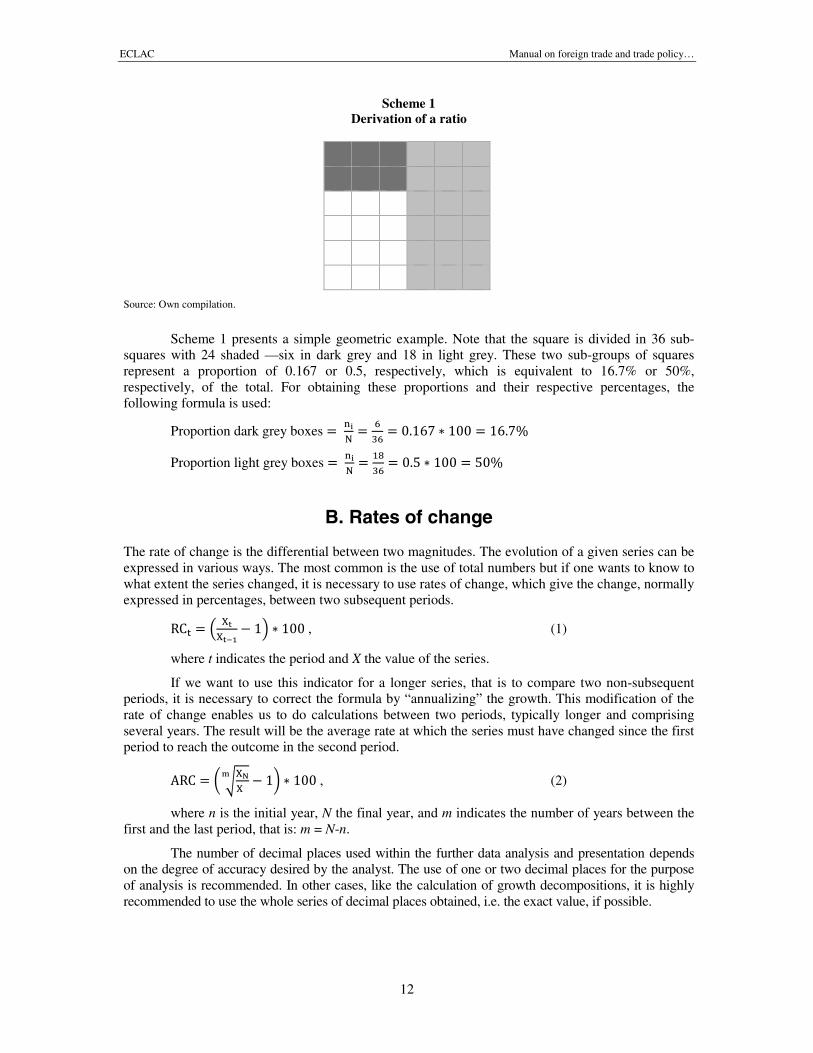
Scheme 1Derivation of a ratio
Source: Own compilation.
Scheme 1 presents a simple geometric example. Note that the square is divided in 36 sub-squares with 24 shaded —six in dark grey and 18 in light grey. These two sub-groups of squaresrepresent a proportion of 0.167 or 0.5, respectively, which is equivalent to 16.7% or 50%,respectively, of the total. For obtaining these proportions and their respective percentages, thefollowing formula is used:
Proportion dark grey boxes = = = 0.167 ∗ 100 = 16.7%
Proportion light grey boxes = = = 0.5 ∗ 100 = 50%
B. Rates of change
The rate of change is the differential between two magnitudes. The evolution of a given series can beexpressed in various ways. The most common is the use of total numbers but if one wants to know towhat extent the series changed, it is necessary to use rates of change, which give the change, normallyexpressed in percentages, between two subsequent periods.
RC = − 1 ∗ 100 , (1)
where t indicates the period and X the value of the series.
If we want to use this indicator for a longer series, that is to compare two non-subsequentperiods, it is necessary to correct the formula by “annualizing” the growth. This modification of therate of change enables us to do calculations between two periods, typically longer and comprisingseveral years. The result will be the average rate at which the series must have changed since the firstperiod to reach the outcome in the second period.
ARC = − 1 ∗ 100 , (2)
where n is the initial year, N the final year, and m indicates the number of years between thefirst and the last period, that is: m = N-n.
The number of decimal places used within the further data analysis and presentation dependson the degree of accuracy desired by the analyst. The use of one or two decimal places for the purposeof analysis is recommended. In other cases, like the calculation of growth decompositions, it is highlyrecommended to use the whole series of decimal places obtained, i.e. the exact value, if possible.
ECLAC Manual on foreign trade and trade policy…
13
C. Index numbers
This is an indicator that has the power to capture the central tendency of a dataset. In general, indexnumbers are expressed in percentages, where the center of the series is referred to as the “base year”,for which the indicator value is 100.
In foreign trade, it is essential to have series that show the evolution of exports and imports,as well as its decomposition. Here, the number indices are of great importance because they allowcomparing the trend in the levels of two distinct series, which originally had been difficult todetermine, for example, due to different scales.
Due to their intrinsic characteristics, index numbers must fulfill a set of ideal properties, butas simple indices —those that condense information of solely one variable— they meet most of these.The more complex ones —those that combine the value of different variables through a system ofweights that determine their interrelation— do not fulfill some of the properties.
Identity: indicates that if the actual period is equal to the base period, the result must be 100.In case of complex indices, this has to be realized following the sum of the weightings.
Proportionality: if all quantities of the index are increased by the same proportion, the indexitself must exactly increase in the same way.
Inversion: implies that if the base (t0) and the actual period (t1) are inverted in the fraction,and one divides 1 by that term, the result must be equal to the initial index. Formally: t/t =1/(t ⁄ t).
Circularity: implies that the multiplication of two index numbers from subsequent periods t1
with base t0 and t2 with base t1, is equal to an index derived from taking t2 as the actual and t0 as thebase value. Formally:
∗ =
.Example: Given the indices t0 = 100, t1 = 110, and t2 = 111. For circularity, it must hold that
∗ = ∗ = 1.11 =
= (which is true in that case).
Existence: the values of the index must always be real and finite.
D. Deflators
The procedure of deflation appears to be very useful. It is done by taking a dataset at a base year anddiscounting the price effect between that year and the succeeding years. As a result, we obtain theeffect of prices on the quantity effect (also called quantum), which indicates the evolution of thevolume of a certain measured variable or indicator, such as the Gross Domestic Product (GDP),exports, or another statistical series.
The main tool used for this process is a series of deflators centered on a base year. Often anindex number is used that well represents the characteristics of a given year. If different conventionsare available for the base years, one often uses those ending on a zero or a five, e.g. 1990 or 2015.
The deflation procedure is formally defined as the division of the variable in nominal termsby the value of the deflator. This means, for example, for calculating the value of exports/imports inconstant prices we apply the following formulas:
X = ∗ 100 , (3)
M = ∗ 100 , (4)
ECLAC Manual on foreign trade and trade policy…
14
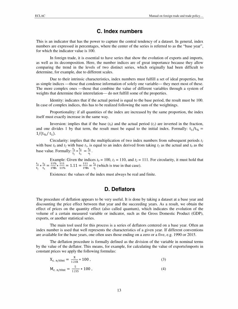
where X and M are the imports and exports of goods in current prices, and UVIX and UVIMare the corresponding indices of the unit value of exports and imports, respectively. Table 1 presentsan example with practical results.
Table 1Argentina: foreign trade in current and constant
prices of 2010, 2005 - 2014($ million and indices)
2005 2006 2007 2008 2009 2010 2011 2012 2013 2014
Current exports 40 106 46 546 55 780 70 019 55 672 68 187 84 051 80 927 76 634 68 335
UVIX 67.0 72.7 82.5 104.3 92.9 100.0 119.2 121.9 119.7 117.2
Constant exports 59 885 64 026 67 583 67 140 59 943 68 187 70 532 66 400 64 003 58 300
Current imports 28 689 34 154 44 707 57 462 38 786 56 792 74 319 68 507 73 655 65 323
UVIM 87.7 89.7 96.0 108.2 95.5 100.0 107.1 105.3 111.0 111.2
Constant imports 32 721 38 055 46 581 53 106 40 612 56 792 69 394 65 069 66 332 58 745
Source: Own compilation based on figures from CEPALSTAT and Comtrade of the United Nations Statistics Division(UNSD).
E. Changing bases and splicing series
With each year that we move away from the base year, the structure of the weighting coefficients getsless representative for reality —especially with complex indices. Therefore it can become necessaryto determine a new base year or period by establishing a weighting structure to better reflect the newprice structure.
To avoid having different, unconnected series, there exists a process that can be defined as“rebasing”. In the jargon of researchers this process is also known as the “splicing” of different seriesor statistical indices. Usually this is necessary for long-term series and the analysis of historicalperformance. In this case, the researcher might be interested in taking an old series with a new baseor, vice versa and trough a process of retrograde extrapolation, consider the trend of an old series withits growth rates or annual variation in consecutive periods with available data.
Given the value of the initial year of a new series and the growth rates of the old series fromits beginning to the common year, it is possible to calculate the new values by retrogradeextrapolation using the following methodology:
G = α
; … G = α
; …G = α
, (5)
where Gt is the value in the initial year of the given series, at is the annual variationexpressed in percentage of the index for the year t (the last year of the old series and the start of theseries that is to be spliced).
Example: Given in the year 2015, the total value of exports of a country yields $103 millionand the growth rate from 2015 is known to be 3%. Then the total value of export in 2014 is $100
million, because X = α
= = 100.
ECLAC Manual on foreign trade and trade policy…
15
F. Weightings
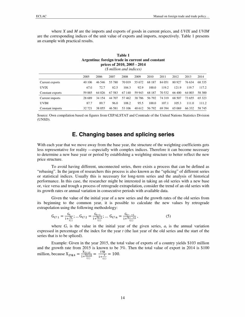
When calculating the averages for various economic indicators one must be careful with not beingprone to an error that often occurs. For example, if the values of export per capita for each CentralAmerican country are given and we want to calculate the average value of exports per capita for theentire subregion, it is recommended not to use the arithmetic mean of the data for its derivation;otherwise the researcher must clarify that this is the simple average that not considers the relative sizeor the scale of the different economies involved. This problem can be serious if the group of countriesshows considerable differences and asymmetries, as it is the case with the Member States ofMERCOSUR (Southern Common Market), where Argentina and Brazil are large-scale producerswhile the other three members are of much smaller scale.
Table 2, column 2, shows the exports per capita of the five member countries of the CentralAmerican Common Market (CACM). The simple arithmetic average of the exports per capita for thecountries in the named subregion can be calculated as $946. However, this value is different to thatobtained by taking the weighted average according to column 5. In this case, the weighted average of$821 yields the more accurate value representing the joint population of the CACM. Note that thefocus of this analysis is directly related to the weightings applied in column 4.
The weighted average in the mentioned example considers the internal differences of thesample. The result is equivalent to taking all joint exports and the joint population and thenperforming the calculation of the average value.
Table 2Central American Common Market: calculation of the weighted
average for exports per capita, 2014
CountriesExports per capita
($)
Population(million people)
Weights(rounded)
Weighted exports percapita ($)
Costa Rica 2,307 4.9 0.12 272
El Salvador 824 6.4 0.15 127
Guatemala 686 15.8 0.38 261
Honduras 496 8.2 0.20 98
Nicaragua 419 6.2 0.15 63
Sum 41.5 1.00 821
Simple average 946
Weighted average 821
Source: Own compilation based on figures from Comtrade and the World Bank.
Formally, the weights are defined as the proportion of a specific variable of the population.In this case the countries’ population was chosen, however, the chosen variable may also be adifferent one, such as GDP. The choice of the variable solely depends on the researcher. Generallyspeaking, the weight αi of each observation i is equal to:
α = ∑ , (6)
where fi is the respective value of observation i.
Using all αi, the weighted average can be derived in the following way:
X = ∑ X = ∑ α ∗ f , (7)
where Xi are the weighted values of each observation i.
ECLAC Manual on foreign trade and trade policy…
16
G. Structural changes
In general, production, trade, and consumption undergo structural changes of various kinds andorigins over time. These changes can be explained using different factors: changes in relative prices,technical progress, the expansion of services in production and consumption, the emergence ofinternational production sharing systems (typically known as outsourcing), among others.
A simple way to capture these changes is analyzing the different sectors over time or indifferent points of time. In this case, it is very useful to remember what we have learned aboutpercentages and proportions.
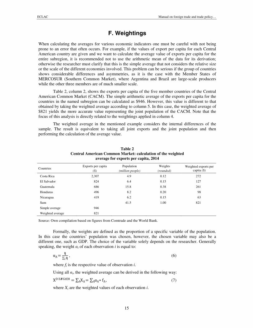
As an example, let us take the change in the structure of Mexico’s exports to the world. In theearly 90’s, one of the principal products exported was oil, which can be seen in the fact that primaryproducts accounted for more than 40% of total exports. Over time, and with the development ofmaquilas (manufacturing plants in free-trade zones mostly in the north of Mexico, see also ChapterIV.B), the weight of primary materials dropped as can be seen in figure 1. The development ofproduction and exports towards more elaborated products is typical for developing countries(Akamatsu, 1962).
Figure 1Mexico: structural change in the export basket by
technological intensity, 1986 - 2014(% of total exports)
Source: Own compilation based on figures from Comtrade.
0
10
20
30
40
50
60
70
80
90
100
1986
1987
1988
1989
1990
1991
1992
1993
1994
1995
1996
1997
1998
1999
2000
2001
2002
2003
2004
2005
2006
2007
2008
2009
2010
2011
2012
2013
2014
Primary products Manufacturing based on natural resources
Low tech manufacturing Medium tech manufacturing
High tech manufacturing
ECLAC Manual on foreign trade and trade policy…
17
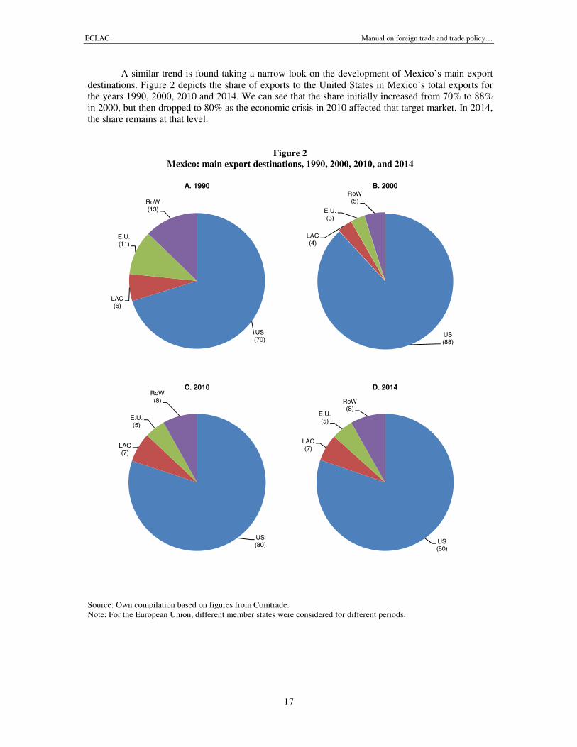
A similar trend is found taking a narrow look on the development of Mexico’s main exportdestinations. Figure 2 depicts the share of exports to the United States in Mexico’s total exports forthe years 1990, 2000, 2010 and 2014. We can see that the share initially increased from 70% to 88%in 2000, but then dropped to 80% as the economic crisis in 2010 affected that target market. In 2014,the share remains at that level.
Figure 2Mexico: main export destinations, 1990, 2000, 2010, and 2014
US(70)
LAC(6)
E.U.(11)
RoW(13)
A. 1990
US(88)
LAC(4)
E.U.(3)
RoW(5)
B. 2000
US(80)
LAC(7)
E.U.(5)
RoW(8)
C. 2010
US(80)
LAC(7)
E.U.(5)
RoW(8)
D. 2014
Source: Own compilation based on figures from Comtrade.Note: For the European Union, different member states were considered for different periods.

ECLAC Manual on foreign trade and trade policy…
19
II. Price and quantity indicators,price ratios, and terms of trade
A. Price indices
The development of exports or imports in absolute values does not tell us too much about a long-termseries, as its increase or decrease may be due to variations in prices, the exchange rate or thecountry’s inflation (next to other causes).1 It is therefore necessary to analyze the development of thetrade basket, for which a price index is calculated. This index is the same as the unit cost of theproducts, but in a more general expression.
These indicators can be calculated for both exports as well as imports and are usually obtainedfollowing the methodology of price indices of either Laspeyres (1871) or Paasche (1874). The choicebetween the two indices depends on the needs and/or restrictions the researcher faces. In the case of theLaspeyres price index (LPI), the calculation is done according to the following formula:
LPI = ∑∗
∑ ∗ 100 ≡ ∑∑ ∗ 100 , (8)
where pn is the price in a given period, p0 is the price in the period considered as the base, q0
is the quantity in the base period, and subindex k represents the type of the considered good.
The index should be interpreted as the level that the prices achieve in a given year, whentheir value in the base year is set to 100 and the same quantities of the base year are considered inboth periods. Thus, the change in prices is calculated for an identical basket of export/import goods,i.e. that of the base year. The result then corresponds to the change in prices over time.
It is important to note that in the Laspeyres index the value of the quantities should not varyover time, so that it is not distorted. When that occurs, it s recommended to use the alternativePaasche price index (PPI). It is calculated as:
1 We will mainly discuss countries as representatives of an economy. Note, however, that all presented conceptsapply not only to countries but also to any other kind of economies (if correponding data are available).
ECLAC Manual on foreign trade and trade policy…
20
PPI = ∑∗
∑ ∗ 100 ≡ ∑∑ ∗ 100 , (9)
where the notation is the same as for the LPI and qn is the quantity in a given period.
The methodological change within the PPI is that quantities are not kept constant, since thePPI considers the quantities of the basket in a given year as measurement unit. Related to that, it issaid that the PPI underestimates the ideal cost of living, as it assumes the same basket of goods in thebase year as is observed in the given year. Thereby it ignores the possibility that consumers haveadjusted their consumption pattern over time.
Strictly speaking, the price index shows the development of prices over time, being a priceindex of foreign trade as well. The technical description of the unit value reflects that fact that inpractice there exist different varieties of the same good and the index of a product is typically anaverage of the prices of its different varieties.
In this manual, we refer to unit value indices of exports (UVIX) and unit value indices ofimports (UVIM) as indicators to measure the development of export and import prices, respectively,over time.
B. Volume indices
A volume index (quantum) is an indicator that is used to measure the development of quantities. Thisis very helpful in identifying the price effect in exports or imports and to observe its real trend. To saythat a country is exporting more than before can have two (not exclusive) meanings: one in absoluteterms, where only the value is analyzed, and the other one in relative terms, where also the change inquantities is analyzed.
The calculation of volume indices follows the same logic and criteria as that of price indices.Thus, a Laspeyres volume index (LVI) will be:
LVI = ∑∗
∑ ∗ 100 ≡ ∑∑ ∗ 100 . (10)
Similarly, a Paasche volume index (PVI) is:
PVI = ∑∗
∑ ∗ 100 ≡ ∑∑ ∗ 100 . (11)
When calculating such indices for foreign trade, ECLAC follows the methodology of factorreversal according to Fisher (1922, p. 75), which is based on an analogy criterion: “[…] no reason canbe given for employing a given formula for one of the two factors which does not apply to the other,and, […] such reversibility already applies to each pair of individual price and quantity ratios, andshould, in all logic, apply to the index numbers which aim to represent them in the mass.” Thus, if fora certain product it holds that
Value = p ∗ q , (12)
i.e. the multiplication of price indices with quantities yields a value index of total trade, it ispossible to estimate the respective volume indices (VI) from the actual export or import value indices,with the following formulas:
VIX = ∗ 100 , (13)
VIM = ∗ 100 . (14)
ECLAC Manual on foreign trade and trade policy…
21
What has been done by dividing the value index of trade (exports or imports) by itsrespective price index is a deflation that isolates the price effect on the trade. If the price and the valueindex are expressed on a base 100, the result will be a volume index also with a base 100. If the priceindex was not previously based on 100, the deflation process will approximate the series from unitsexpressed in current prices to units expressed in constant prices on the basis of the used index.
C. Terms of trade
This expression measures the exchange ratio between the basket of goods that a country exports withthat the same country imports, considering the price effect adjusted on a base year. Statistically, it isdefined as the ratio between the price index of exports and the price index of imports. Both indicesmust be related to the same base. Following the previously used notation, the terms of trade (TOT) inyear t are calculated as:
TOT = ∗ 100 . (15)
The result of this indicator is a measure for the development of the exchange rate between theexports of a given country and its imports. In other terms, it represents the change in the purchasingpower of a given export volume, i.e. the extent to which such an export volume allows the country toaccess a similar volume of imported products, taking the base year as a reference. Thus take as anexample a hypothetical country that exports a natural resource like wood and needs to export 5 tonsof wood to import one tractor in the base year. Five years later, it needed to export 20 tons of wood toimport the same tractor. Then, the TOT index has decreased by 75%, reflecting the development ofprices in that period.
In economic jargon, we usually speak about an improvement or a deterioration of the termsof trade, depending on the development of this indicator. If the base is 100 and the index reaches 115,we would speak of improved TOT while we would call a subsequent decline to 100 a deterioration ofthe TOT.
This analysis is very important to study a country’s dependence on its trade partners and itsrelation towards them as regards its ability to buy or sell. For further details see Furtado (1961).
D. Real exchange rate
This expression measures the ratio of a country’s export basket (domestic) with respect to the exportsof another country (foreign). In other words, it indicates the relative price of the foreign country’sgoods expressed in terms of local goods. Technically, it is defined as a bilateral exchange rate andcalculated as follows:
RER = ∗
, (16)
where E is the type of the nominal exchange rate, D is the GDP deflator, subindices iindicates the local country, and j the foreign country.
This indicator measures the position of the prices of domestic tradables relative to the changein the prices of foreign goods, considering the nominal exchange rate, which itself can experiencechanges that result in changes in the relative prices of a country’s export basket. Likewise, we cancalculate real exchange rates for imports.
The correct way of interpreting this indicator is taking a base year as a reference. From there,a reduction of the RER is equivalent to a real appreciation of local goods, which makes them moreexpensive compared to the prices of the foreign goods. Vice versa, an increase in the RER indicates a
ECLAC Manual on foreign trade and trade policy…
22
real depreciation, with which the local goods become less expensive relative to the neighboringcountry’s goods. Following that approach, we can derive the formulas for calculating the realexchange rates for exports (RERX) and imports (RERM) for a given country as:
RERX = ∗ ≡ E ∗ , (17)
RERM = ∗ ≡ E ∗ , (18)
where E is the nominal exchange rate, PIX is the price index of exports, PIM is the priceindex of imports, and PIC is the price index of consumption.
The difficulty of the bilateral RER is that it cannot be compared between countries, becauseof the different baskets of goods traded between. While it is possible to conduct an analysis as regardsthe same indicator over time, it is not adequate to compare the bilateral exchange rates betweencountries. To circumvent this difficulty in the analytical field, the calculation of a relative RER, ormultilateral RER, is applied where the RER is weighted according to the trade with each country.
E. Real effective exchange rate
The effective exchange rate is an indicator that gives information about a country’s internationalcompetitiveness shown in the terms of trade with the countries it trades with.
The nominal effective exchange rate (NEER) is obtained using a weighted average of thelocal currency with respect to the exchange rates of the trade partners, where the weighting representsthe relative importance in the country’s foreign trade. It can be calculated for exports, imports or totaltrade by varying the weights appropriately.
NEER = ∏ E ∗ P , (19)
where Eij is the nominal exchange rate of the local country (i) with its trade partner (j), Pj isthe relative weight that this trade partner has in the total exports (or imports) of the domestic country(i), and n is the total number of trading partners of country i.
When the nominal effective exchange rate is adjusted so that it incorporates the differences inthe inflation rates, we obtain the real effective exchange rate (REER). That way, the nominalexchange rate is deflated by the price index of the country and those of the corresponding tradepartners. As in the case of the NEER, it can be calculated for the exports as well as for the imports orthe total trade by applying the corresponding price index.
REER = ∗ PI , (20)
where PI is the corresponding price index (e.g. of exports or imports) and D is a deflator ofthe economy, which could be the consumer price index or the GDP deflator.
F. Trade-weighted exchange rate
In the previous section, we have described the REER, which cannot be compared across countriesbecause the export/import basket varies among prospective destinations. To solve that problem, it ispossible to take all the goods baskets and weight them according to the share they represent within thetotal exports/imports of the country of interest. The result is the trade-weighted exchange rate (TWER).This indicator is thus calculated on the basis of bilateral exchange rates that are weighted according tothe importance of each trading partner within the exports and/or imports of the local country.
TWER = ∑ BER ∗ P , (21)
ECLAC Manualonforeigntradeandtradepolicy…
23
whereBERisthebilateralexchangeratebetweenthedomesticcountry(i)andtheforeigncountry(j),nisthenumberoftradepartners,andPjistheshareofcountryjinthetotalexportsofthedomesticcountry.
Thisindicatorhasthepropertythatwecancompareitbetweendifferentcountries,therebyyieldinganapproximately homogenous measure ofthe development ofthe macroeconomiccompetitivenessderivedfromtherelativepricesandtheexchangerate.Thecalculationsareusuallyconductedwithrespecttoaninternationallyaccepted,ratherhardcurrency,traditionallyin$orinrecentyearsalsoinEuro(€).
G.Realtradeexchangerate
Ifweperformadoubledeflationoftheexchangerate,thefirsttocoverthechangeinexportpricesandthesecondtocovernationalinflation, weobtaintherealtradeexchangerate(RTER).Thisindicatormeasuresthechangeofacountry’sbasketofgoodsthatitexportstoanothercountryortothe world,takingintoaccountthechangeinexportvaluetothatdestination.Likewise,onecancalculateanindicatorfortheimportside.
RTER=∗
, (22)
whereERisthenominalexchangerateindollars,UVIXistheunitvalueindexofexports(orUVIMforimports),andDisapricedeflatorofthenationaleconomy(whichmightbetheconsumerpriceindexortheGDPdeflator).
Thepracticaltoreadthisindicatoriscreatingaseriescomposedofindexnumbersbuildonabaseyearwithvalue100.Areductionisthenequivalenttoarealappreciationoflocalgoodsandviceversa.
H.Tradableandnon-tradableprices
Thetradablesectorsofaneconomyareallthosethatareproducinginthenationaleconomyandaresubjecttotradingwithothercountries,whilenon-tradablesarethosesolelyconsumedintheeconomywheretheyareproduced.
Byitsverynature,tradableandnon-tradablegoodsinaneconomyoftenexperiencedifferentchangesintheirpricelevels,whichfinallydeterminevariationsintheinflationwithinaneconomy.Therelativepricesoftradablesandnon-tradablesprovideinformationaboutthegoodsandserviceswhosevaluesareprimarilydeterminedbyinternationalpricesas wellasaboutthosegoodsandserviceswhosepricesare mainlydeterminedbysuchfactorsasdomesticsupplyanddemand(andindirectlybythetradablesectors).
Thedistinctionbetweentradableandnon-tradablepricesisquitedifficultandtheacademicdiscourseisnotyetcompleted.Themostcommonwaytodifferentiatebetweenbothisdistinguishingbetweentradableandnon-tradablesectorsinaneconomy,toseparatetheminimportandexportsectorslateron.
Followingthe methodologydevelopedby Dwyer(1992)forthecaseof Australia,thefollowingstepsaredefined:
(i) Measuretheproduction(output)ofeachindustryintheeconomy;
(ii)identifytowhichextentthedomesticproductionofeachsectorisexportedanddefineathresholdvaluefromwhichitcanbeclassifiedasexport-oriented;
(iii)identifytheextenttowhichthedomesticproductionisreplaceablewithimportsanddefineathresholdvaluefromwhichthisproductioncanbeclassifiedascompetingwithimports;
ECLAC Manual on foreign trade and trade policy…
24
(iv) sum up the production (output) of all sectors defined as export-oriented and competingwith imports to obtain a measure for the tradable sectors;
(v) sum up the production (output) of all remaining industries to obtain a measure for non-tradable goods sectors.
As you can see from the steps outlined above, important, subjective considerations persist indefining the threshold values for classifying an industry as export-oriented or competing withimports. However, this problem can be partially resolved by analyzing the changes in size and thecomposition of each of the sectors for different thresholds. This can help us to determine thresholdsthat are considerably robust.
Knight and Johnson (1997) present two criteria for defining thresholds in the most adequatemanner. On the one hand, the threshold should reflect to which extent the participation in imports orexports affects the behavior of the sector to be more exposed to the influences of international trade.On the other hand, the classification resulting from the thresholds should maintain certain stabilityover time, so that the representativity of the tradable sectors is given also through the economic cycle.
It is important to understand that this methodology defines a measure of production (output)at a single moment and does not incorporate the possibility that a product will be tradedinternationally in the future. For that reason, the same authors define two general ways for classifyingthe tradable products. The first definition considers the products and services that are actually tradedinternationally as tradables and those that are absorbed domestically as non-tradables. This approachobviously depends on the availability of international trade statistics.
The second approach is more sophisticated and more difficult to implement in practicebecause it considers the change in relative prices when defining products as tradables or non-tradables. A more strict approach should consider both definitions.
Indices of tradable and non-tradable prices that are adjusted reflections of inflation behaviorcan yield essential information for the analysis of foreign trade and exchange rates. They thus providea tool for decision-making on type and intensity of trade policies.
In the same way, it has been found that the tradable goods in economies that are internationalprice takers can create an effect on the local inflation that escapes from the macroeconomic controlwhich the central banks may have on that phenomenon. That point is not trivial within the developmentof practices related to the degree of monetary policy and other instruments to control inflation.
ECLAC Manual on foreign trade and trade policy…
25
III. The link between trade and production
A. Added-value of production
The value-added corresponds to that part of a country’s total production that is related to the processingindustry. It is defined as the differential between the costs (inputs and fixed capital) and the incomeobtained from the sale of the final product. The sum of the value-added for the whole country is its GDP.
The value-added can be consumed domestically or exported to residents of other economies.The share exported from the value-added is also known as “export propensity” and provides ameasure that is often used as an indicator for an “economy’s internationalization”. A higher value ofthis measure thus hints on the fact that the economy at hand is more internationalized.
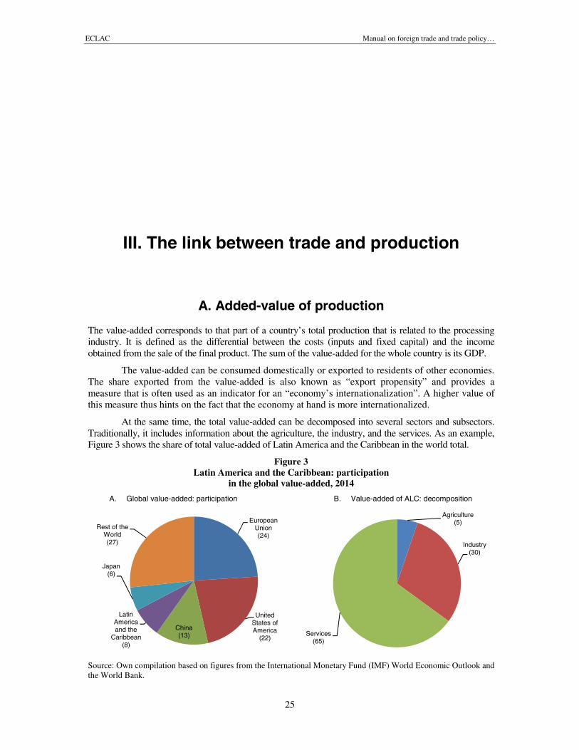
At the same time, the total value-added can be decomposed into several sectors and subsectors.Traditionally, it includes information about the agriculture, the industry, and the services. As an example,Figure 3 shows the share of total value-added of Latin America and the Caribbean in the world total.
Figure 3Latin America and the Caribbean: participation
in the global value-added, 2014
A. Global value-added: participation B. Value-added of ALC: decomposition
Source: Own compilation based on figures from the International Monetary Fund (IMF) World Economic Outlook andthe World Bank.
EuropeanUnion(24)
UnitedStates ofAmerica
(22)
China(13)
LatinAmericaand the
Caribbean(8)
Japan(6)
Rest of theWorld(27)
Agriculture(5)
Industry(30)
Services(65)
ECLAC
B. The maquiladora activities
There are indications that the use of the word “maquila” dates back to the yearused to describe the portion of the ground that belonged to the miller. The root of the word comesfrom the Arabic word “makila” whose root kthe actual use of the word to describe thatparties. These are then in charge of assembling elaborated pieces, with the particularity that the inputsto assemble are brought from abroad with the commitment that the final product made thisbe resold abroad or internalized into the local economy. It is this principal connotation that describesthe actual maquilas in the region. Moreover, their activity has been enhanced to a large degree bytransnational corporations (Durán Lima and
Given the greater integration of the firm, the production and the trade of technology, as wellas the components and their subsequent assembly, globalized industries have become more importantin the 90s, replacing the old pattern thastrategic access to raw materials needed for production.
In this context, the maquiladora activities have considerably developed in Latin America,especially in Mexico and Central America. In thefrom a value less than $ 1,000 million in 1990 to overcome the barrier of $13,000 million in 2008.Due to the financial crisis, their value decreased slightly in 2009 and reached more than $16,000million in 2014 (see Figure 4).
Central American
A. $ million
Source: Own compilation based on figures from the countries’ central banks.
In the process of valueintermediate goods has increased over time, yielding a vertiginous wave of shared production atindustry level. However, this process occurs with greater intensity in some types of industriethose that assemble computers, electronic equipment, aircrafts, vehicles, and textile manufacturing(OECD, 1996).
According to the Organisation for Economic Comain intra-firm operations in the midon areas related to technology, research and development, as well as on the cooperation duringdifferent stages of the production. To some extent, this process has also occurred in Latin America,especially in Mexico, Central America and the Dominican Republic. Maquila activities also havecontributed to local technological development (Buitelaar, Padilla and Urrutia, 1999).
0
10 000
20 000
30 000
40 000
1990
1992
1994
1996
1998
2000
2002
2004
Non-Maquila Exports
Manual on foreign trade and trade policy
26
B. The maquiladora activities
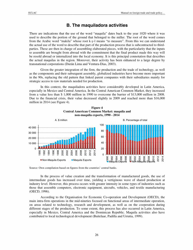
There are indications that the use of the word “maquila” dates back to the year 1020 where it wasused to describe the portion of the ground that belonged to the miller. The root of the word comesfrom the Arabic word “makila” whose root k-y-l means “to measure”. From this we can understandthe actual use of the word to describe that part of the production process that is subcontracted to thirdparties. These are then in charge of assembling elaborated pieces, with the particularity that the inputsto assemble are brought from abroad with the commitment that the final product made thisbe resold abroad or internalized into the local economy. It is this principal connotation that describesthe actual maquilas in the region. Moreover, their activity has been enhanced to a large degree bytransnational corporations (Durán Lima and Ventura-Dias, 2003).
Given the greater integration of the firm, the production and the trade of technology, as wellas the components and their subsequent assembly, globalized industries have become more importantin the 90s, replacing the old pattern that linked parent companies with their subsidiaries mainly forstrategic access to raw materials needed for production.
In this context, the maquiladora activities have considerably developed in Latin America,especially in Mexico and Central America. In the Central American Common Market, they increasedfrom a value less than $ 1,000 million in 1990 to overcome the barrier of $13,000 million in 2008.Due to the financial crisis, their value decreased slightly in 2009 and reached more than $16,000
Figure 4Central American Common Market: maquila and
non-maquila exports, 1990 - 2014
B. Percentage of total
wn compilation based on figures from the countries’ central banks.
In the process of value creation and the transformation of manufactured goods, the use ofintermediate goods has increased over time, yielding a vertiginous wave of shared production atindustry level. However, this process occurs with greater intensity in some types of industriethose that assemble computers, electronic equipment, aircrafts, vehicles, and textile manufacturing
According to the Organisation for Economic Co-operation and Development (OECD), thefirm operations in the mid-nineties focused on functional areas of intermediate operation,
on areas related to technology, research and development, as well as on the cooperation duringdifferent stages of the production. To some extent, this process has also occurred in Latin America,
ally in Mexico, Central America and the Dominican Republic. Maquila activities also havecontributed to local technological development (Buitelaar, Padilla and Urrutia, 1999).
2004
2006
2008
2010
2012
2014
Maquila Exports
0
20
40
60
80
100
1990
1992
1994
1996
1998
2000
2002
2004
2006
Maquila Exports Non-Maquila Exports
oreign trade and trade policy…
1020 where it wasused to describe the portion of the ground that belonged to the miller. The root of the word comes
l means “to measure”. From this we can understandpart of the production process that is subcontracted to third-
parties. These are then in charge of assembling elaborated pieces, with the particularity that the inputsto assemble are brought from abroad with the commitment that the final product made this way willbe resold abroad or internalized into the local economy. It is this principal connotation that describesthe actual maquilas in the region. Moreover, their activity has been enhanced to a large degree by
Given the greater integration of the firm, the production and the trade of technology, as wellas the components and their subsequent assembly, globalized industries have become more important
t linked parent companies with their subsidiaries mainly for
In this context, the maquiladora activities have considerably developed in Latin America,Central American Common Market, they increased
from a value less than $ 1,000 million in 1990 to overcome the barrier of $13,000 million in 2008.Due to the financial crisis, their value decreased slightly in 2009 and reached more than $16,000
Percentage of total
creation and the transformation of manufactured goods, the use ofintermediate goods has increased over time, yielding a vertiginous wave of shared production atindustry level. However, this process occurs with greater intensity in some types of industries such asthose that assemble computers, electronic equipment, aircrafts, vehicles, and textile manufacturing
operation and Development (OECD), theocused on functional areas of intermediate operation,
on areas related to technology, research and development, as well as on the cooperation duringdifferent stages of the production. To some extent, this process has also occurred in Latin America,
ally in Mexico, Central America and the Dominican Republic. Maquila activities also have
2006
2008
2010
2012
2014
Maquila Exports
ECLAC Manual on foreign trade and trade policy…
27
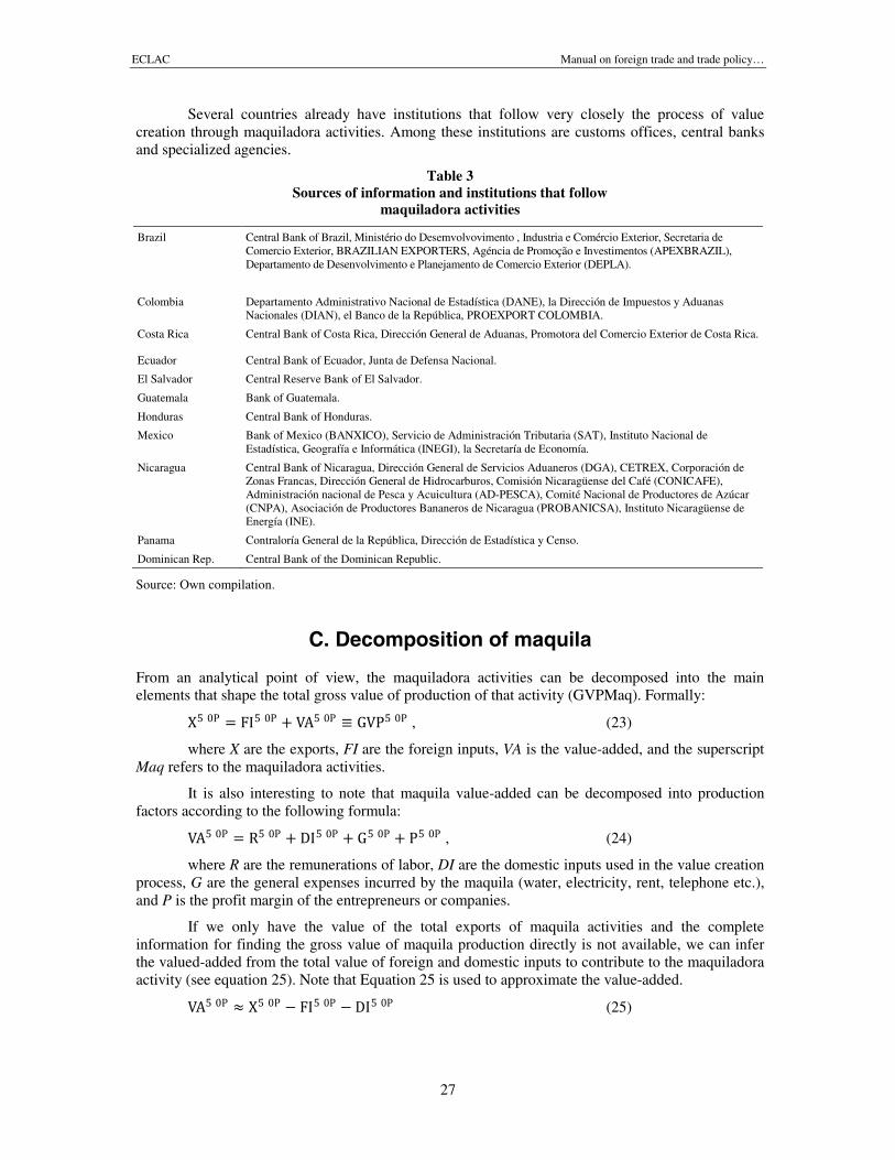
Several countries already have institutions that follow very closely the process of valuecreation through maquiladora activities. Among these institutions are customs offices, central banksand specialized agencies.
Table 3Sources of information and institutions that follow
maquiladora activities
Brazil Central Bank of Brazil, Ministério do Desemvolvovimento , Industria e Comércio Exterior, Secretaria deComercio Exterior, BRAZILIAN EXPORTERS, Agéncia de Promoção e Investimentos (APEXBRAZIL),Departamento de Desenvolvimento e Planejamento de Comercio Exterior (DEPLA).
Colombia Departamento Administrativo Nacional de Estadística (DANE), la Dirección de Impuestos y AduanasNacionales (DIAN), el Banco de la República, PROEXPORT COLOMBIA.
Costa Rica Central Bank of Costa Rica, Dirección General de Aduanas, Promotora del Comercio Exterior de Costa Rica.
Ecuador Central Bank of Ecuador, Junta de Defensa Nacional.
El Salvador Central Reserve Bank of El Salvador.
Guatemala Bank of Guatemala.
Honduras Central Bank of Honduras.
Mexico Bank of Mexico (BANXICO), Servicio de Administración Tributaria (SAT), Instituto Nacional deEstadística, Geografía e Informática (INEGI), la Secretaría de Economía.
Nicaragua Central Bank of Nicaragua, Dirección General de Servicios Aduaneros (DGA), CETREX, Corporación deZonas Francas, Dirección General de Hidrocarburos, Comisión Nicaragüense del Café (CONICAFE),Administración nacional de Pesca y Acuicultura (AD-PESCA), Comité Nacional de Productores de Azúcar(CNPA), Asociación de Productores Bananeros de Nicaragua (PROBANICSA), Instituto Nicaragüense deEnergía (INE).
Panama Contraloría General de la República, Dirección de Estadística y Censo.
Dominican Rep. Central Bank of the Dominican Republic.
Source: Own compilation.
C. Decomposition of maquila
From an analytical point of view, the maquiladora activities can be decomposed into the mainelements that shape the total gross value of production of that activity (GVPMaq). Formally:
X = FI + VA ≡ GVP , (23)
where X are the exports, FI are the foreign inputs, VA is the value-added, and the superscriptMaq refers to the maquiladora activities.
It is also interesting to note that maquila value-added can be decomposed into productionfactors according to the following formula:
VA = R + DI + G + P , (24)
where R are the remunerations of labor, DI are the domestic inputs used in the value creationprocess, G are the general expenses incurred by the maquila (water, electricity, rent, telephone etc.),and P is the profit margin of the entrepreneurs or companies.
If we only have the value of the total exports of maquila activities and the completeinformation for finding the gross value of maquila production directly is not available, we can inferthe valued-added from the total value of foreign and domestic inputs to contribute to the maquiladoraactivity (see equation 25). Note that Equation 25 is used to approximate the value-added.
VA ≈ X − FI−DI (25)
ECLAC Manual on foreign trade and trade policy…
28
If the sectoral information for different product groups and/or single products is available indetail, we can derive the information about the whole maquiladora activities from the analysis of thevalue-added and its components. It is not the same to know the share of the value-added in the totalmaquiladora activities, compared to having an idea of the difference of the same indicator for thecases of the gross production in the different industries, e.g. textile industry, electronics, and cars.
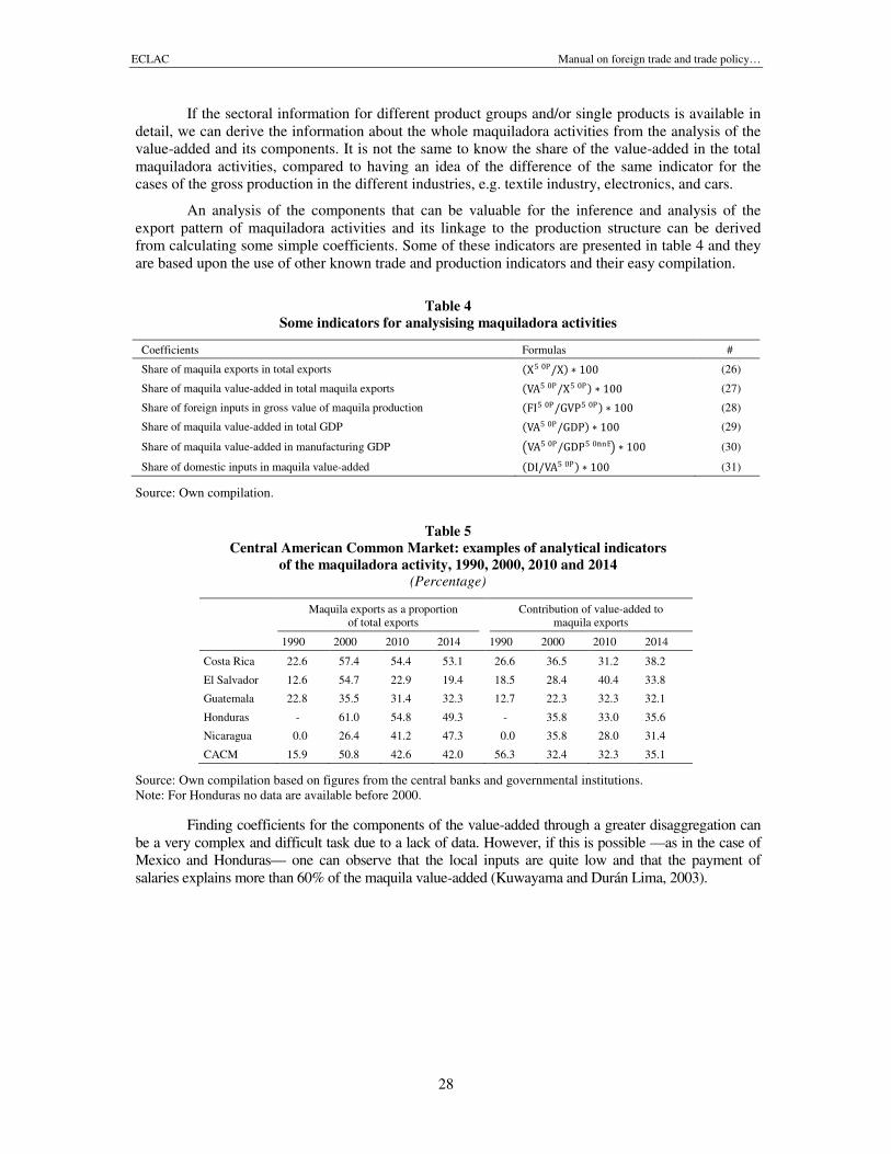
An analysis of the components that can be valuable for the inference and analysis of theexport pattern of maquiladora activities and its linkage to the production structure can be derivedfrom calculating some simple coefficients. Some of these indicators are presented in table 4 and theyare based upon the use of other known trade and production indicators and their easy compilation.
Table 4Some indicators for analysising maquiladora activities
Coefficients Formulas #
Share of maquila exports in total exports (X/X) ∗ 100 (26)
Share of maquila value-added in total maquila exports (VA/X) ∗ 100 (27)
Share of foreign inputs in gross value of maquila production (FI/GVP) ∗ 100 (28)
Share of maquila value-added in total GDP (VA/GDP) ∗ 100 (29)
Share of maquila value-added in manufacturing GDP VA/GDP ∗ 100 (30)
Share of domestic inputs in maquila value-added (DI/VA) ∗ 100 (31)
Source: Own compilation.
Table 5Central American Common Market: examples of analytical indicators
of the maquiladora activity, 1990, 2000, 2010 and 2014(Percentage)
Maquila exports as a proportionof total exports
Contribution of value-added tomaquila exports
1990 2000 2010 2014 1990 2000 2010 2014
Costa Rica 22.6 57.4 54.4 53.1 26.6 36.5 31.2 38.2
El Salvador 12.6 54.7 22.9 19.4 18.5 28.4 40.4 33.8
Guatemala 22.8 35.5 31.4 32.3 12.7 22.3 32.3 32.1
Honduras - 61.0 54.8 49.3 - 35.8 33.0 35.6
Nicaragua 0.0 26.4 41.2 47.3 0.0 35.8 28.0 31.4
CACM 15.9 50.8 42.6 42.0 56.3 32.4 32.3 35.1
Source: Own compilation based on figures from the central banks and governmental institutions.Note: For Honduras no data are available before 2000.
Finding coefficients for the components of the value-added through a greater disaggregation canbe a very complex and difficult task due to a lack of data. However, if this is possible —as in the case ofMexico and Honduras— one can observe that the local inputs are quite low and that the payment ofsalaries explains more than 60% of the maquila value-added (Kuwayama and Durán Lima, 2003).
ECLAC
Central Americanof
A. Decomposition of maquila exports
Source: Own compilation based on figures from CEPALSTAT, and the countries’ central banks and governmentalinstitutions.Note: Honduras is not included until 2000.
D. Different denominations of the maquiladora activity
For some countries in the region, the proportion of exports realized through the use of mechanisms oftemporary admission or special custom regimes is relatively high. The more familiar name in theliterature for the definition of this activity is “maquilathe countries vary its name, it is strictly speaking a definition comparable to the unique concept of themaquiladora activities.
Needless to say that the existence of a free zone does not necessarily imply tactivity develops itself in this area. A free zone with temporal admission of goods becomes a generatorof maquila if it allows the installation of industries and processing of production using foreign inputsunder the free zone regime, i.e. without paying taxes, provided that these products are exported.
Among the different possible names are: “freeperfeccionamiento activo), “Goods for processing” (Span.:more specified terms with tax implication as in the case of “Vallejos Plan” (named after its inventorJoaquín Vallejo Arbelaéz) or “Special Free Zones” (Span.:(see table 6). Other countries outside that region also appin China. In Jordan, Madagascar and the Syrian Arab Republic these are known as free industrialzones, in Togo as tax-free factories, and in Thailand as free points.
Latin America and the Caribbean: diff
Denominations (original in spanish)
Z. Franca, Z. Libre Comercio, Polo Industrial
Maquila
Bienes para transformación
Perfeccionamiento activo
Valor bruto de producción
Decreto 29-89
Plan Vallejos, 2006 (ZZ. FF. Especial, 2007)
Source: Own compilation.
0
5 000
10 000
15 000
20 000
1990
1992
1994
1996
1998
2000
2002
2004
Imported Inputs Value
Manual on foreign trade and trade policy
29
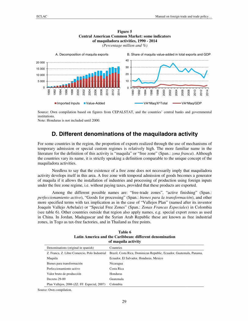
Figure 5Central American Common Market: some indicators
of maquiladora activities, 1990 - 2014(Percentage million and %)
Decomposition of maquila exports B. Share of maquila value-added in total exports and GDP
wn compilation based on figures from CEPALSTAT, and the countries’ central banks and governmental
Note: Honduras is not included until 2000.
D. Different denominations of the maquiladora activity
For some countries in the region, the proportion of exports realized through the use of mechanisms oftemporary admission or special custom regimes is relatively high. The more familiar name in theliterature for the definition of this activity is “maquila” or “free zone” (Span.: zona francathe countries vary its name, it is strictly speaking a definition comparable to the unique concept of the
Needless to say that the existence of a free zone does not necessarily imply that maquiladoraactivity develops itself in this area. A free zone with temporal admission of goods becomes a generatorof maquila if it allows the installation of industries and processing of production using foreign inputs
. without paying taxes, provided that these products are exported.
Among the different possible names are: “free-trade zones”, “active finishing” (Span.:), “Goods for processing” (Span.: bienes para la transformación
ore specified terms with tax implication as in the case of “Vallejos Plan” (named after its inventorJoaquín Vallejo Arbelaéz) or “Special Free Zones” (Span.: Zonas Francas Especiales
able 6). Other countries outside that region also apply names, e.g. special export zones as usedin China. In Jordan, Madagascar and the Syrian Arab Republic these are known as free industrial
free factories, and in Thailand as free points.
Table 6Latin America and the Caribbean: different denomination
of maquila activity
panish) Countries
Franca, Z. Libre Comercio, Polo Industrial Brazil, Costa Rica, Dominican Republic, Ecuador, Guatemala, Panama,
Ecuador, El Salvador, Honduras, Mexico
Nicaragua
Costa Rica
Honduras
Guatemala
Plan Vallejos, 2006 (ZZ. FF. Especial, 2007) Colombia
2006
2008
2010
2012
2014
Value-Added
0
10
20
30
40
1990
1992
1994
1996
1998
2000
2002
2004
2006
VA^Maq/X^Total VA^Maq/GDP
oreign trade and trade policy…
added in total exports and GDP
wn compilation based on figures from CEPALSTAT, and the countries’ central banks and governmental
D. Different denominations of the maquiladora activity
For some countries in the region, the proportion of exports realized through the use of mechanisms oftemporary admission or special custom regimes is relatively high. The more familiar name in the
zona franca). Althoughthe countries vary its name, it is strictly speaking a definition comparable to the unique concept of the
hat maquiladoraactivity develops itself in this area. A free zone with temporal admission of goods becomes a generatorof maquila if it allows the installation of industries and processing of production using foreign inputs
. without paying taxes, provided that these products are exported.
trade zones”, “active finishing” (Span.:bienes para la transformación), and other
ore specified terms with tax implication as in the case of “Vallejos Plan” (named after its inventorZonas Francas Especiales) in Colombia
ly names, e.g. special export zones as usedin China. In Jordan, Madagascar and the Syrian Arab Republic these are known as free industrial
, Ecuador, Guatemala, Panama,
2008
2010
2012
2014
VA^Maq/GDP
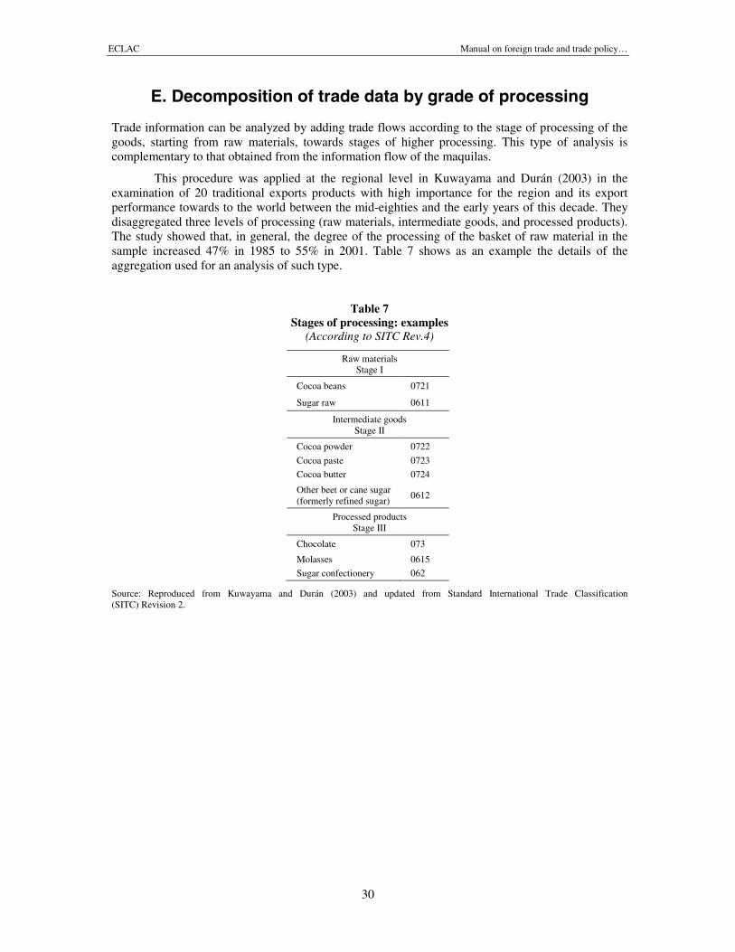
ECLAC Manual on foreign trade and trade policy…
30
E. Decomposition of trade data by grade of processing
Trade information can be analyzed by adding trade flows according to the stage of processing of thegoods, starting from raw materials, towards stages of higher processing. This type of analysis iscomplementary to that obtained from the information flow of the maquilas.
This procedure was applied at the regional level in Kuwayama and Durán (2003) in theexamination of 20 traditional exports products with high importance for the region and its exportperformance towards to the world between the mid-eighties and the early years of this decade. Theydisaggregated three levels of processing (raw materials, intermediate goods, and processed products).The study showed that, in general, the degree of the processing of the basket of raw material in thesample increased 47% in 1985 to 55% in 2001. Table 7 shows as an example the details of theaggregation used for an analysis of such type.
Table 7Stages of processing: examples
(According to SITC Rev.4)
Raw materialsStage I
Cocoa beans 0721
Sugar raw 0611
Intermediate goodsStage II
Cocoa powder
Cocoa paste
Cocoa butter
0722
0723
0724
Other beet or cane sugar(formerly refined sugar)
0612
Processed productsStage III
Chocolate 073
Molasses
Sugar confectionery
0615
062
Source: Reproduced from Kuwayama and Durán (2003) and updated from Standard International Trade Classification(SITC) Revision 2.
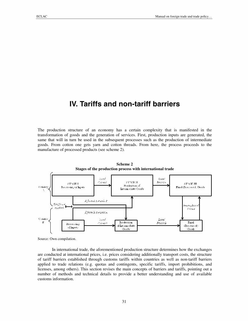
ECLAC Manual on foreign trade and trade policy…
31
IV. Tariffs and non-tariff barriers
The production structure of an economy has a certain complexity that is manifested in thetransformation of goods and the generation of services. First, production inputs are generated, thesame that will in turn be used in the subsequent processes such as the production of intermediategoods. From cotton one gets yarn and cotton threads. From here, the process proceeds to themanufacture of processed products (see scheme 2).
Scheme 2Stages of the production process with international trade
Source: Own compilation.
In international trade, the aforementioned production structure determines how the exchangesare conducted at international prices, i.e. prices considering additionally transport costs, the structureof tariff barriers established through customs tariffs within countries as well as non-tariff barriersapplied to trade relations (e.g. quotas and contingents, specific tariffs, import prohibitions, andlicenses, among others). This section revises the main concepts of barriers and tariffs, pointing out anumber of methods and technical details to provide a better understanding and use of availablecustoms information.
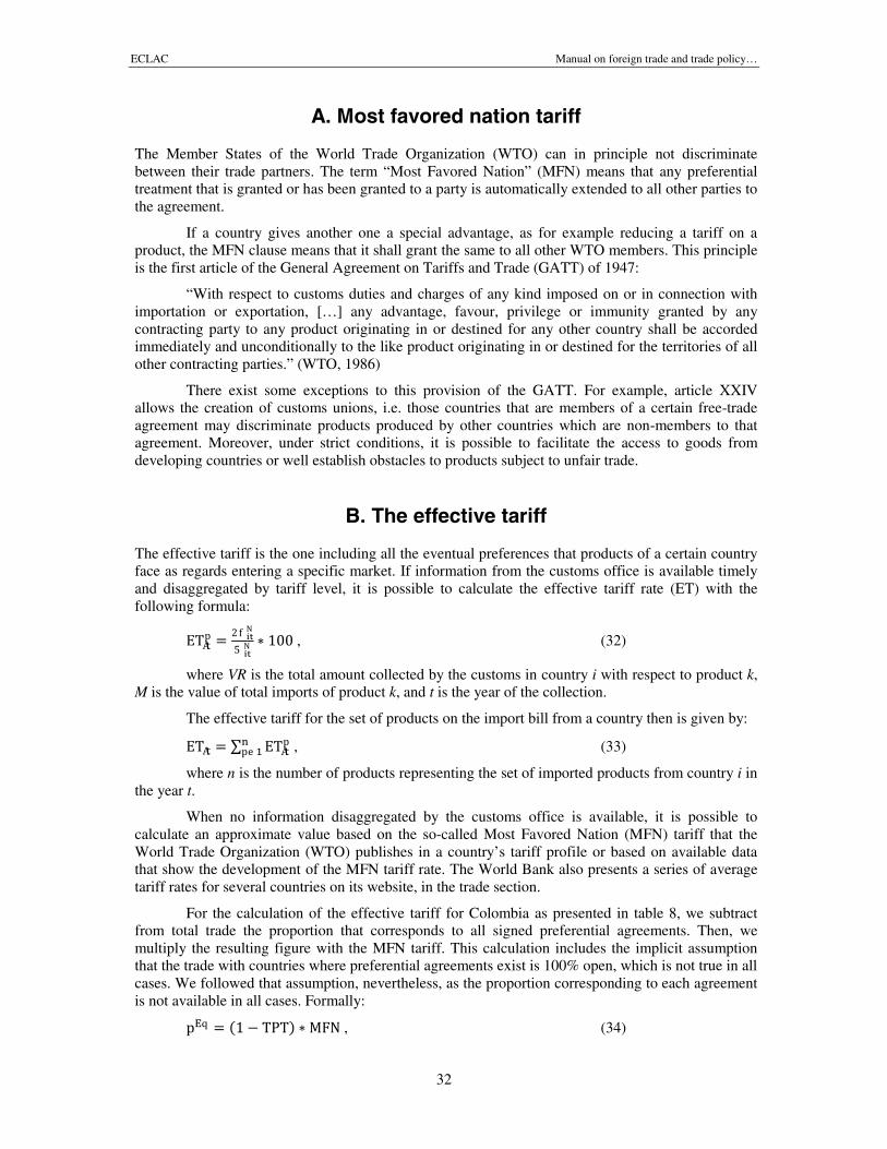
ECLAC Manual on foreign trade and trade policy…
32
A. Most favored nation tariff
The Member States of the World Trade Organization (WTO) can in principle not discriminatebetween their trade partners. The term “Most Favored Nation” (MFN) means that any preferentialtreatment that is granted or has been granted to a party is automatically extended to all other parties tothe agreement.
If a country gives another one a special advantage, as for example reducing a tariff on aproduct, the MFN clause means that it shall grant the same to all other WTO members. This principleis the first article of the General Agreement on Tariffs and Trade (GATT) of 1947:
“With respect to customs duties and charges of any kind imposed on or in connection withimportation or exportation, […] any advantage, favour, privilege or immunity granted by anycontracting party to any product originating in or destined for any other country shall be accordedimmediately and unconditionally to the like product originating in or destined for the territories of allother contracting parties.” (WTO, 1986)
There exist some exceptions to this provision of the GATT. For example, article XXIVallows the creation of customs unions, i.e. those countries that are members of a certain free-tradeagreement may discriminate products produced by other countries which are non-members to thatagreement. Moreover, under strict conditions, it is possible to facilitate the access to goods fromdeveloping countries or well establish obstacles to products subject to unfair trade.
B. The effective tariff
The effective tariff is the one including all the eventual preferences that products of a certain countryface as regards entering a specific market. If information from the customs office is available timelyand disaggregated by tariff level, it is possible to calculate the effective tariff rate (ET) with thefollowing formula:
ET = ∗ 100 , (32)
where VR is the total amount collected by the customs in country i with respect to product k,M is the value of total imports of product k, and t is the year of the collection.
The effective tariff for the set of products on the import bill from a country then is given by:
ET = ∑ ET , (33)
where n is the number of products representing the set of imported products from country i inthe year t.
When no information disaggregated by the customs office is available, it is possible tocalculate an approximate value based on the so-called Most Favored Nation (MFN) tariff that theWorld Trade Organization (WTO) publishes in a country’s tariff profile or based on available datathat show the development of the MFN tariff rate. The World Bank also presents a series of averagetariff rates for several countries on its website, in the trade section.
For the calculation of the effective tariff for Colombia as presented in table 8, we subtractfrom total trade the proportion that corresponds to all signed preferential agreements. Then, wemultiply the resulting figure with the MFN tariff. This calculation includes the implicit assumptionthat the trade with countries where preferential agreements exist is 100% open, which is not true in allcases. We followed that assumption, nevertheless, as the proportion corresponding to each agreementis not available in all cases. Formally:
p = (1 − TPT) ∗ MFN , (34)
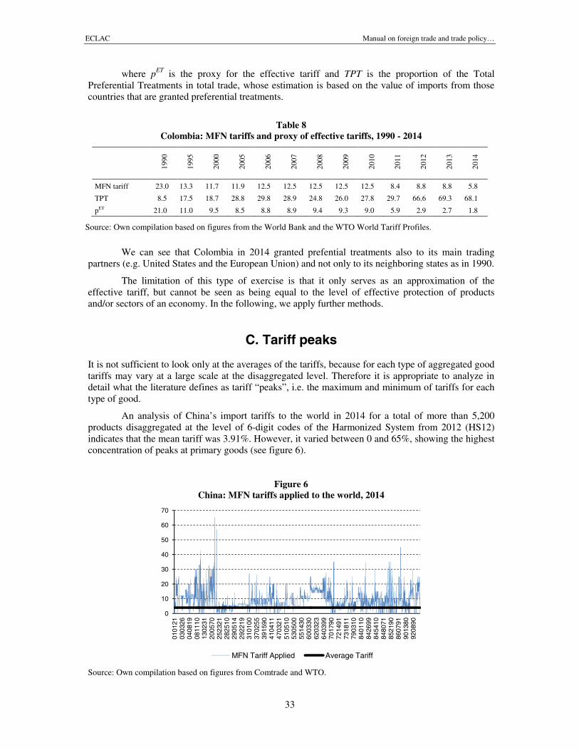
ECLAC Manual on foreign trade and trade policy…
33
where pET is the proxy for the effective tariff and TPT is the proportion of the TotalPreferential Treatments in total trade, whose estimation is based on the value of imports from thosecountries that are granted preferential treatments.
Table 8Colombia: MFN tariffs and proxy of effective tariffs, 1990 - 2014
1990
1995
2000
2005
2006
2007
2008
2009
2010
2011
2012
2013
2014
MFN tariff 23.0 13.3 11.7 11.9 12.5 12.5 12.5 12.5 12.5 8.4 8.8 8.8 5.8
TPT 8.5 17.5 18.7 28.8 29.8 28.9 24.8 26.0 27.8 29.7 66.6 69.3 68.1
pET 21.0 11.0 9.5 8.5 8.8 8.9 9.4 9.3 9.0 5.9 2.9 2.7 1.8
Source: Own compilation based on figures from the World Bank and the WTO World Tariff Profiles.
We can see that Colombia in 2014 granted prefential treatments also to its main tradingpartners (e.g. United States and the European Union) and not only to its neighboring states as in 1990.
The limitation of this type of exercise is that it only serves as an approximation of theeffective tariff, but cannot be seen as being equal to the level of effective protection of productsand/or sectors of an economy. In the following, we apply further methods.
C. Tariff peaks
It is not sufficient to look only at the averages of the tariffs, because for each type of aggregated goodtariffs may vary at a large scale at the disaggregated level. Therefore it is appropriate to analyze indetail what the literature defines as tariff “peaks”, i.e. the maximum and minimum of tariffs for eachtype of good.
An analysis of China’s import tariffs to the world in 2014 for a total of more than 5,200products disaggregated at the level of 6-digit codes of the Harmonized System from 2012 (HS12)indicates that the mean tariff was 3.91%. However, it varied between 0 and 65%, showing the highestconcentration of peaks at primary goods (see figure 6).
Figure 6China: MFN tariffs applied to the world, 2014
Source: Own compilation based on figures from Comtrade and WTO.
0
10
20
30
40
50
60
70
0101
2103
0326
0408
1908
1110
1302
3120
0570
2523
2128
2510
2905
1429
2219
3101
0037
0255
3915
9041
0411
4703
2151
0510
5305
0055
1430
6003
3062
0323
6403
9970
1790
7214
9173
1811
7903
1084
0110
8426
9984
5410
8480
7185
2190
8607
9190
1380
9208
90
MFN Tariff Applied Average Tariff
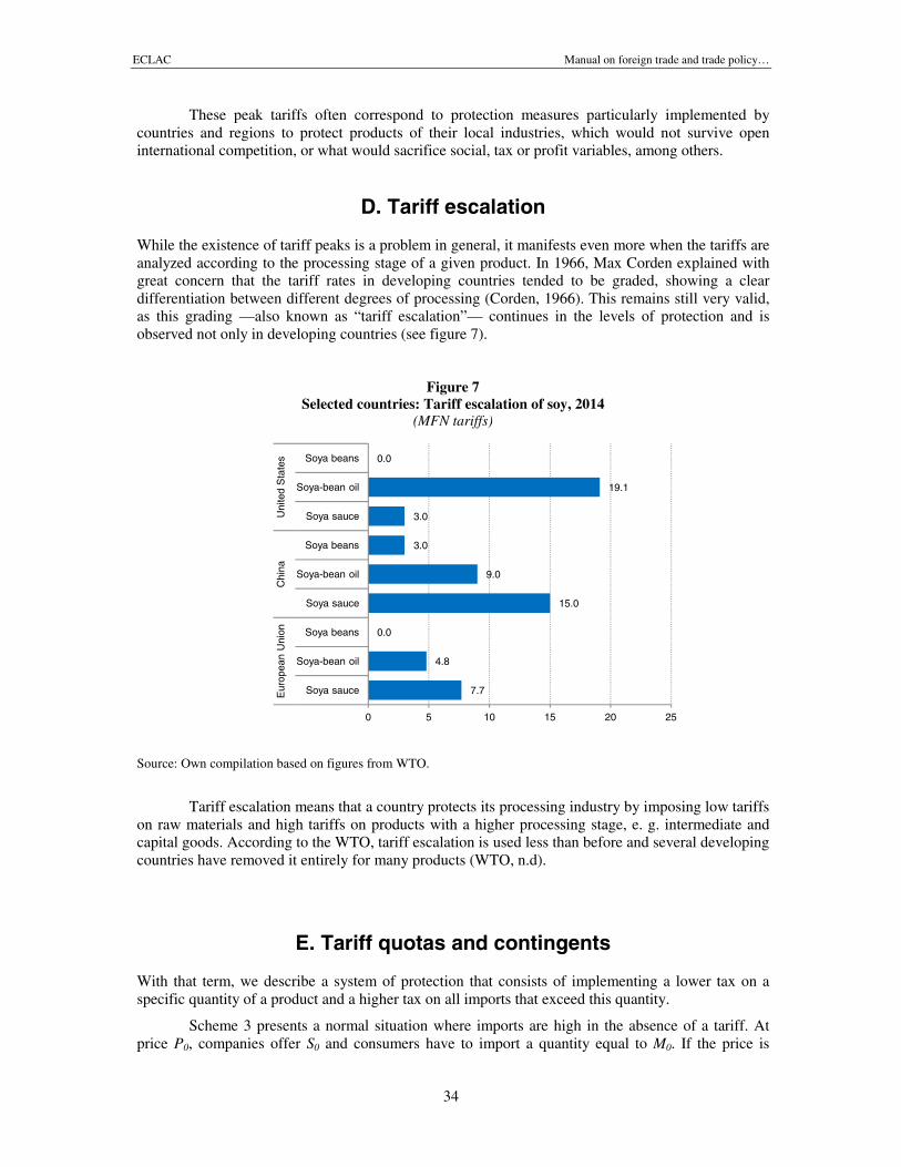
ECLAC Manual on foreign trade and trade policy…
34
These peak tariffs often correspond to protection measures particularly implemented bycountries and regions to protect products of their local industries, which would not survive openinternational competition, or what would sacrifice social, tax or profit variables, among others.
D. Tariff escalation
While the existence of tariff peaks is a problem in general, it manifests even more when the tariffs areanalyzed according to the processing stage of a given product. In 1966, Max Corden explained withgreat concern that the tariff rates in developing countries tended to be graded, showing a cleardifferentiation between different degrees of processing (Corden, 1966). This remains still very valid,as this grading —also known as “tariff escalation”— continues in the levels of protection and isobserved not only in developing countries (see figure 7).
Figure 7Selected countries: Tariff escalation of soy, 2014
(MFN tariffs)
Source: Own compilation based on figures from WTO.
Tariff escalation means that a country protects its processing industry by imposing low tariffson raw materials and high tariffs on products with a higher processing stage, e. g. intermediate andcapital goods. According to the WTO, tariff escalation is used less than before and several developingcountries have removed it entirely for many products (WTO, n.d).
E. Tariff quotas and contingents
With that term, we describe a system of protection that consists of implementing a lower tax on aspecific quantity of a product and a higher tax on all imports that exceed this quantity.
Scheme 3 presents a normal situation where imports are high in the absence of a tariff. Atprice P0, companies offer S0 and consumers have to import a quantity equal to M0. If the price is
7.7
4.8
0.0
15.0
9.0
3.0
3.0
19.1
0.0
0 5 10 15 20 25
Soya sauce
Soya-bean oil
Soya beans
Soya sauce
Soya-bean oil
Soya beans
Soya sauce
Soya-bean oil
Soya beans
Eur
opea
nU
nion
Chi
naU
nite
dS
tate
s
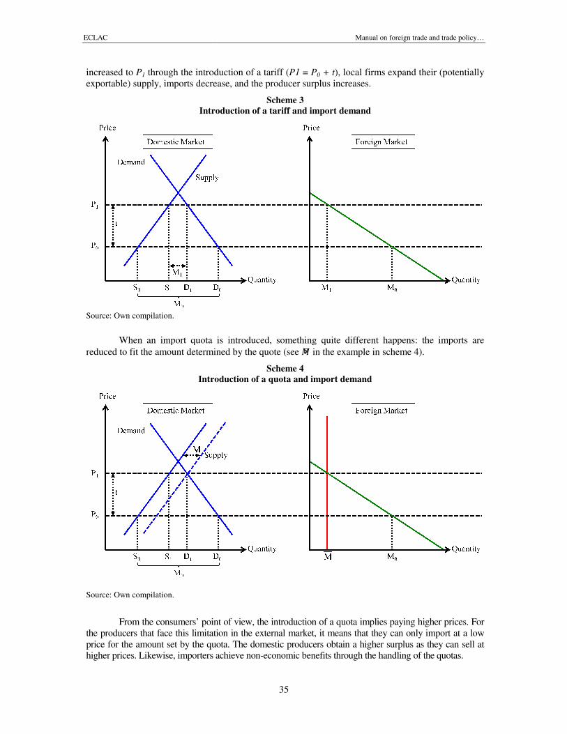
ECLAC
increased to P1 through the introduction of a tariff (exportable) supply, imports decrease, and the producer surplus increases.
Introduction of a tariff and import demand
Source: Own compilation.
When an import quota is introduced, something quite different happens: the imports arereduced to fit the amount determined by the quote (see
Introduction
Source: Own compilation.
From the consumers’ point of view, the introduction of a quota implies paying higher prices. Forthe producers that face this limitation in the external market, it means that they can only import at a lowprice for the amount set by the quotahigher prices. Likewise, importers achieve non
Manual on foreign trade and trade policy
35
through the introduction of a tariff (P1 = P0 + t), local firms expand their (potentiallyexportable) supply, imports decrease, and the producer surplus increases.
Scheme 3ntroduction of a tariff and import demand
When an import quota is introduced, something quite different happens: the imports arereduced to fit the amount determined by the quote (see in the example in scheme 4).
Scheme 4ntroduction of a quota and import demand
From the consumers’ point of view, the introduction of a quota implies paying higher prices. Forthe producers that face this limitation in the external market, it means that they can only import at a lowprice for the amount set by the quota. The domestic producers obtain a higher surplus as they can sell athigher prices. Likewise, importers achieve non-economic benefits through the handling of the quotas.
oreign trade and trade policy…
local firms expand their (potentially
When an import quota is introduced, something quite different happens: the imports arecheme 4).
From the consumers’ point of view, the introduction of a quota implies paying higher prices. Forthe producers that face this limitation in the external market, it means that they can only import at a low
. The domestic producers obtain a higher surplus as they can sell ateconomic benefits through the handling of the quotas.
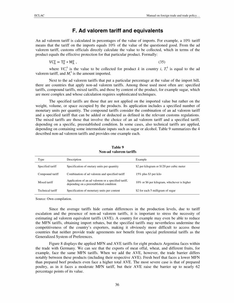
ECLAC Manual on foreign trade and trade policy…
36
F. Ad valorem tariff and equivalents
An ad valorem tariff is calculated in percentages of the value of imports. For example, a 10% tariffmeans that the tariff on the imports equals 10% of the value of the questioned good. From the advalorem tariff, customs officials directly calculate the value to be collected, which in terms of theproduct equals the effective protection for that particular product. Formally:
VC = T ∗ M , (35)
where VCik is the value to be collected for product k in country i, Ti
k is equal to the advalorem tariff, and Mi
k is the amount imported.
Next to the ad valorem tariffs that put a particular percentage at the value of the import bill,there are countries that apply non-ad valorem tariffs. Among those used most often are: specifiedtariffs, compound tariffs, mixed tariffs, and those by content of the product, for example sugar, whichare more complex and whose calculation requires sophisticated techniques.
The specified tariffs are those that are not applied on the imported value but rather on theweight, volume, or space occupied by the products. Its application includes a specified number ofmonetary units per quantity. The compound tariffs consider the combination of an ad valorem tariffand a specified tariff that can be added or deducted as defined in the relevant customs regulations.The mixed tariffs are those that involve the choice of an ad valorem tariff and a specified tariff,depending on a specific, preestablished condition. In some cases, also technical tariffs are applied,depending on containing some intermediate inputs such as sugar or alcohol. Table 9 summarizes the 4described non-ad valorem tariffs and provides one example each.
Table 9Non-ad valorem tariffs
Type Description Example
Specified tariff Specification of onetary units per quantity $2 per kilogram or $120 per cubic meter
Compound tariff Combination of ad valorem and specified tariff 15% plus $3 per kilo
Mixed tariffApplication of an ad valorem or a specified tariff,depending on a preestablished condition
10% or $6 per kilogram, whichever is higher
Technical tariff Specification of monetary units per content $2 for each 5 milligram of sugar
Source: Own compilation.
Since the average tariffs hide certain differences in the production levels, due to tariffescalation and the presence of non-ad valorem tariffs, it is important to stress the necessity ofestimating ad valorem equivalent tariffs (AVE). A country for example may even be able to reducethe MFN tariffs, obtaining import rebates, but the specified tariffs may nevertheless undermine thecompetitiveness of the country’s exporters, making it obviously more difficult to access thosecountries that neither provide trade agreements nor benefit from special preferential tariffs as theGeneralized System of Preferences.
Figure 8 displays the applied MFN and AVE tariffs for eight products Argentina faces withinthe trade with Germany. We can see that the exports of meat offal, wheat, and different fruits, forexample, face the same MFN tariffs. When we add the AVE, however, the trade barrier differsnotably between these products (including their respective AVE). Fresh beef that faces a lower MFNthan prepared beef products even face a higher total AVE. The most severe case is that of preparedpoultry, as in it faces a moderate MFN tariff, but their AVE raise the barrier up to nearly 62percentage points of its value.
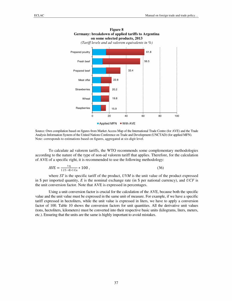
ECLAC Manual on foreign trade and trade policy…
37
Figure 8Germany: breakdown of applied tariffs to Argentina
on some selected products, 2013(Tariff levels and ad valorem equivalents in %)
Source: Own compilation based on figures from Market Access Map of the International Trade Centre (for AVE) and the TradeAnalysis Information System of the United Nations Conference on Trade and Development (UNCTAD) (for applied MFN).Note: corresponds to estimations based on figures, aggregated at six-digit level.
To calculate ad valorem tariffs, the WTO recommends some complementary methodologiesaccording to the nature of the type of non-ad valorem tariff that applies. Therefore, for the calculationof AVE of a specific right, it is recommended to use the following methodology:
AVE = ∗∗ ∗ 100 , (36)
where ST is the specific tariff of the product, UVM is the unit value of the product expressedin $ per imported quantity, E is the nominal exchange rate (in $ per national currency), and UCF isthe unit conversion factor. Note that AVE is expressed in percentages.
Using a unit conversion factor is crucial for the calculation of the AVE, because both the specificvalue and the unit value must be expressed in the same unit of measure. For example, if we have a specifictariff expressed in hectoliters, while the unit value is expressed in liters, we have to apply a conversionfactor of 100. Table 10 shows the conversion factors for unit quantities. All the derivative unit values(tons, hectoliters, kilometers) must be converted into their respective basic units (kilograms, liters, meters,etc.). Ensuring that the units are the same is highly important to avoid mistakes.
15.9
19.8
20.2
22.8
33.4
56.5
61.8
0 20 40 60 80 100
Raspberries
Wheat
Strawberries
Meat offal
Prepared beef
Fresh beef
Prepared poultry
Applied MFN With AVE
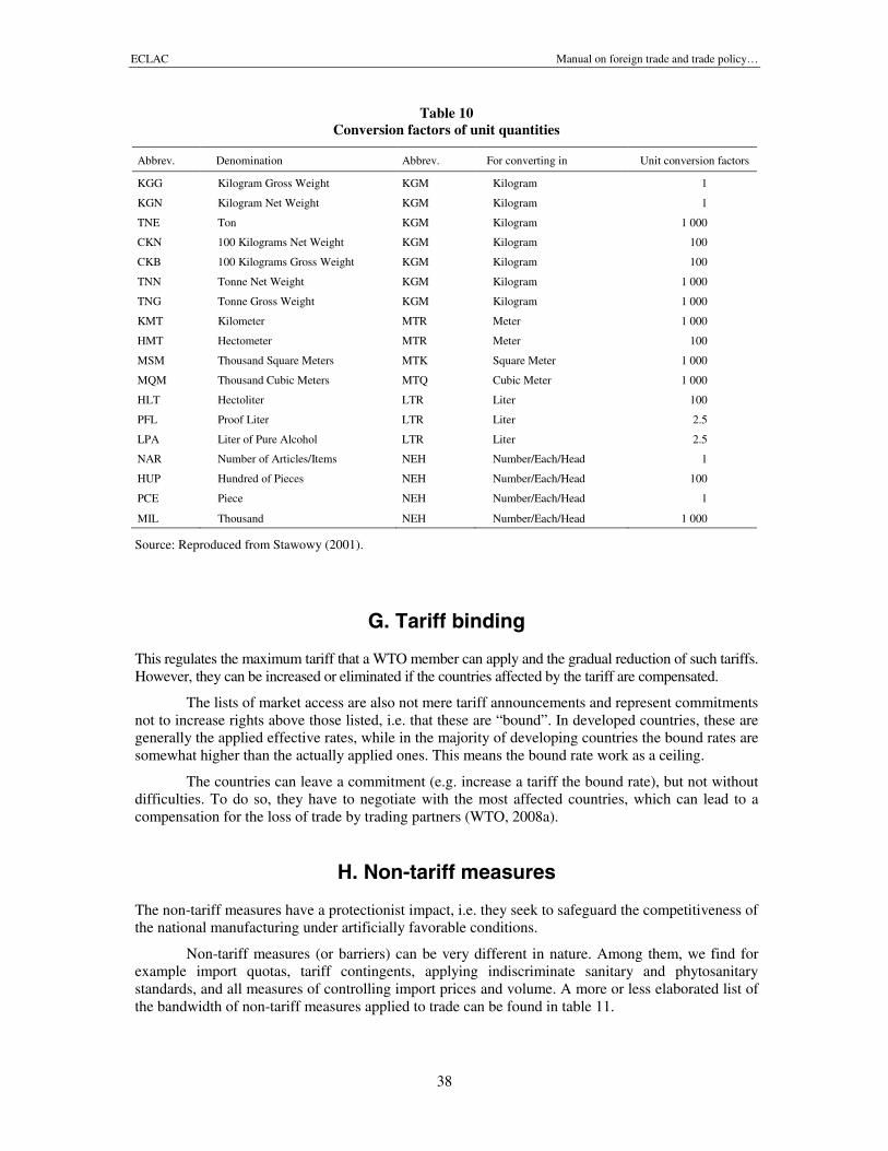
ECLAC Manual on foreign trade and trade policy…
38
Table 10Conversion factors of unit quantities
Abbrev. Denomination Abbrev. For converting in Unit conversion factors
KGG Kilogram Gross Weight KGM Kilogram 1
KGN Kilogram Net Weight KGM Kilogram 1
TNE Ton KGM Kilogram 1 000
CKN 100 Kilograms Net Weight KGM Kilogram 100
CKB 100 Kilograms Gross Weight KGM Kilogram 100
TNN Tonne Net Weight KGM Kilogram 1 000
TNG Tonne Gross Weight KGM Kilogram 1 000
KMT Kilometer MTR Meter 1 000
HMT Hectometer MTR Meter 100
MSM Thousand Square Meters MTK Square Meter 1 000
MQM Thousand Cubic Meters MTQ Cubic Meter 1 000
HLT Hectoliter LTR Liter 100
PFL Proof Liter LTR Liter 2.5
LPA Liter of Pure Alcohol LTR Liter 2.5
NAR Number of Articles/Items NEH Number/Each/Head 1
HUP Hundred of Pieces NEH Number/Each/Head 100
PCE Piece NEH Number/Each/Head 1
MIL Thousand NEH Number/Each/Head 1 000
Source: Reproduced from Stawowy (2001).
G. Tariff binding
This regulates the maximum tariff that a WTO member can apply and the gradual reduction of such tariffs.However, they can be increased or eliminated if the countries affected by the tariff are compensated.
The lists of market access are also not mere tariff announcements and represent commitmentsnot to increase rights above those listed, i.e. that these are “bound”. In developed countries, these aregenerally the applied effective rates, while in the majority of developing countries the bound rates aresomewhat higher than the actually applied ones. This means the bound rate work as a ceiling.
The countries can leave a commitment (e.g. increase a tariff the bound rate), but not withoutdifficulties. To do so, they have to negotiate with the most affected countries, which can lead to acompensation for the loss of trade by trading partners (WTO, 2008a).
H. Non-tariff measures
The non-tariff measures have a protectionist impact, i.e. they seek to safeguard the competitiveness ofthe national manufacturing under artificially favorable conditions.
Non-tariff measures (or barriers) can be very different in nature. Among them, we find forexample import quotas, tariff contingents, applying indiscriminate sanitary and phytosanitarystandards, and all measures of controlling import prices and volume. A more or less elaborated list ofthe bandwidth of non-tariff measures applied to trade can be found in table 11.
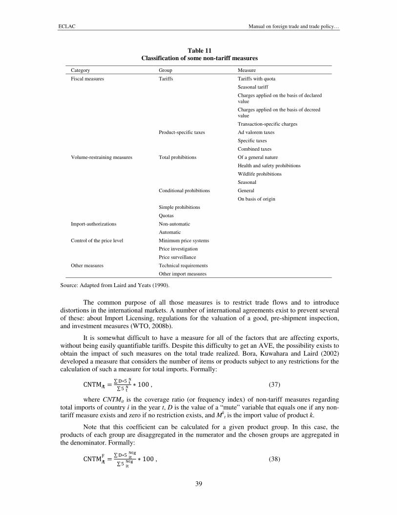
ECLAC Manual on foreign trade and trade policy…
39
Table 11Classification of some non-tariff measures
Category Group Measure
Fiscal measures Tariffs Tariffs with quota
Seasonal tariff
Charges applied on the basis of declaredvalue
Charges applied on the basis of decreedvalue
Transaction-specific charges
Product-specific taxes Ad valorem taxes
Specific taxes
Combined taxes
Volume-restraining measures Total prohibitions Of a general nature
Health and safety prohibitions
Wildlife prohibitions
Seasonal
Conditional prohibitions General
On basis of origin
Simple prohibitions
Quotas
Import-authorizations Non-automatic
Automatic
Control of the price level Minimum price systems
Price investigation
Price surveillance
Other measures Technical requirements
Other import measures
Source: Adapted from Laird and Yeats (1990).
The common purpose of all those measures is to restrict trade flows and to introducedistortions in the international markets. A number of international agreements exist to prevent severalof these: about Import Licensing, regulations for the valuation of a good, pre-shipment inspection,and investment measures (WTO, 2008b).
It is somewhat difficult to have a measure for all of the factors that are affecting exports,without being easily quantifiable tariffs. Despite this difficulty to get an AVE, the possibility exists toobtain the impact of such measures on the total trade realized. Bora, Kuwahara and Laird (2002)developed a measure that considers the number of items or products subject to any restrictions for thecalculation of such a measure for total imports. Formally:
CNTM = ∑∗∑ ∗ 100 , (37)
where CNTMit is the coverage ratio (or frequency index) of non-tariff measures regardingtotal imports of country i in the year t, D is the value of a “mute” variable that equals one if any non-tariff measure exists and zero if no restriction exists, and Mk
t is the import value of product k.
Note that this coefficient can be calculated for a given product group. In this case, theproducts of each group are disaggregated in the numerator and the chosen groups are aggregated inthe denominator. Formally:
CNTM = ∑∗∈∑∈
∗ 100 , (38)
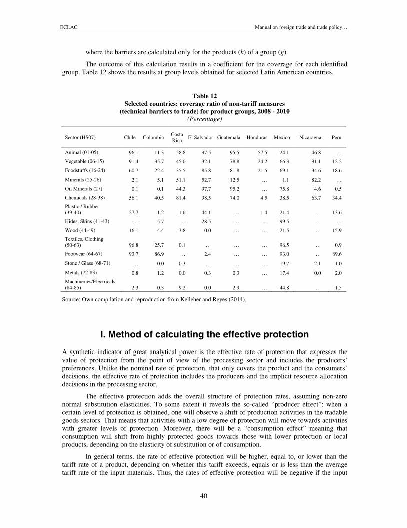
ECLAC Manual on foreign trade and trade policy…
40
where the barriers are calculated only for the products (k) of a group (g).
The outcome of this calculation results in a coefficient for the coverage for each identifiedgroup. Table 12 shows the results at group levels obtained for selected Latin American countries.
Table 12Selected countries: coverage ratio of non-tariff measures
(technical barriers to trade) for product groups, 2008 - 2010(Percentage)
Sector (HS07) Chile ColombiaCostaRica
El Salvador Guatemala Honduras Mexico Nicaragua Peru
Animal (01-05) 96.1 11.3 58.8 97.5 95.5 57.5 24.1 46.8 …
Vegetable (06-15) 91.4 35.7 45.0 32.1 78.8 24.2 66.3 91.1 12.2
Foodstuffs (16-24) 60.7 22.4 35.5 85.8 81.8 21.5 69.1 34.6 18.6
Minerals (25-26) 2.1 5.1 51.1 52.7 12.5 … 1.1 82.2 …
Oil Minerals (27) 0.1 0.1 44.3 97.7 95.2 … 75.8 4.6 0.5
Chemicals (28-38) 56.1 40.5 81.4 98.5 74.0 4.5 38.5 63.7 34.4
Plastic / Rubber(39-40) 27.7 1.2 1.6 44.1 … 1.4 21.4 … 13.6
Hides, Skins (41-43) … 5.7 … 28.5 … … 99.5 … …
Wood (44-49) 16.1 4.4 3.8 0.0 … … 21.5 … 15.9
Textiles, Clothing(50-63) 96.8 25.7 0.1 … … … 96.5 … 0.9
Footwear (64-67) 93.7 86.9 … 2.4 … … 93.0 … 89.6
Stone / Glass (68-71) … 0.0 0.3 … … … 19.7 2.1 1.0
Metals (72-83) 0.8 1.2 0.0 0.3 0.3 … 17.4 0.0 2.0
Machineries/Electricals(84-85) 2.3 0.3 9.2 0.0 2.9 … 44.8 … 1.5
Source: Own compilation and reproduction from Kelleher and Reyes (2014).
I. Method of calculating the effective protection
A synthetic indicator of great analytical power is the effective rate of protection that expresses thevalue of protection from the point of view of the processing sector and includes the producers’preferences. Unlike the nominal rate of protection, that only covers the product and the consumers’decisions, the effective rate of protection includes the producers and the implicit resource allocationdecisions in the processing sector.
The effective protection adds the overall structure of protection rates, assuming non-zeronormal substitution elasticities. To some extent it reveals the so-called “producer effect”: when acertain level of protection is obtained, one will observe a shift of production activities in the tradablegoods sectors. That means that activities with a low degree of protection will move towards activitieswith greater levels of protection. Moreover, there will be a “consumption effect” meaning thatconsumption will shift from highly protected goods towards those with lower protection or localproducts, depending on the elasticity of substitution or of consumption.
In general terms, the rate of effective protection will be higher, equal to, or lower than thetariff rate of a product, depending on whether this tariff exceeds, equals or is less than the averagetariff rate of the input materials. Thus, the rates of effective protection will be negative if the input
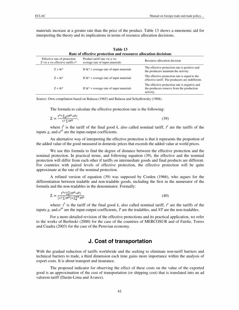
ECLAC Manual on foreign trade and trade policy…
41
materials increase at a greater rate than the price of the product. Table 13 shows a mnemonic aid forinterpreting the theory and its implications in terms of resource allocation decisions.
Table 13Rate of effective protection and ressource allocation decisions
Effective rate of protectionZ vis a vis effective tariffs t*
Product tariff rate vis a visaverage rate of input materials
Resource allocation decision
Z > tk* If tk* > average rate of input materialsThe effective protection rate is positive andthe producers maintain the activity.
Z = tk* If tk* = average rate of input materialsThe effective protection rate is equal to theeffective tariff. The producers are indifferent.
Z < tk* If tk* < average rate of input materialsThe effective protection rate is negative andthe producers remove from the productionactivity.
Source: Own compilation based on Balassa (1965) and Balassa and Schydlowsky (1968).
The formula to calculate the effective protection rate is the following:
Z = ∑ (∗)∑ , (39)
where tk is the tariff of the final good k, also called nominal tariff, tg are the tariffs of theinputs g, and agk are the input-output coefficients.
An alternative way of interpreting the effective protection is that it represents the proportion ofthe added value of the good measured in domestic prices that exceeds the added value at world prices.
We use this formula to find the degree of distance between the effective protection and thenominal protection. In practical terms, and following equation (39), the effective and the nominalprotection will differ from each other if tariffs on intermediate goods and final products are different.For countries with paired levels of effective protection, the effective protection will be quiteapproximate at the rate of the nominal protection.
A refined version of equation (39) was supposed by Corden (1966), who argues for thedifferentiation between tradable and non-tradable goods, including the first in the numerator of theformula and the non-tradables in the denominator. Formally:
Z = ∑ (∗)∑∑ (40)
where: tk is the tariff of the final good k, also called nominal tariff, tg are the tariffs of theinputs g, and agk are the input-output coefficients, T are the tradables, and NT are the non-tradables.
For a more-detailed revision of the effective protections and its practical application, we referto the works of Berlinski (2000) for the case of the countries of MERCOSUR and of Fairlie, Torresand Cuadra (2003) for the case of the Peruvian economy.
J. Cost of transportation
With the gradual reduction of tariffs worldwide and the seeking to eliminate non-tariff barriers andtechnical barriers to trade, a third dimension each time gains more importance within the analysis ofexport costs. It is about transport and insurance.
The proposed indicator for observing the effect of these costs on the value of the exportedgood is an approximation of the cost of transportation (or shipping cost) that is translated into an advalorem tariff (Durán-Lima and Avarez).
ECLAC Manual on foreign trade and trade policy…
42
It uses the methodology of Cost of Insurance and Freight (CIF) versus Free on Board (FOB),but from an approximation of unit values, which allows to solve several drawbacks of reporting. Thisis due to the traditional methodology that consists of deducting from the CIF reported by the countryof destination the FOB cost reported by the country of origin. Several limitations appear hereby,starting from the loss of goods on the way, rejected products, registry errors, and finally shipping thatbegins in one year and arrives the following year. The result is a calculation of the product’s unitvalue in the port of origin and destination. On this basis, a calculation of the inference is performed.Formally, the cost of transportation CT is given by:
CT = − 1 ∗ 100, (41)
where M and X are the imports and exports, respectively, Q are the quantities, i is the countryof origin, j is the destination and k is the product.
It is important that the calculation is conducted at the highest disaggregated level possible toobtain the best data available regarding the unit value.
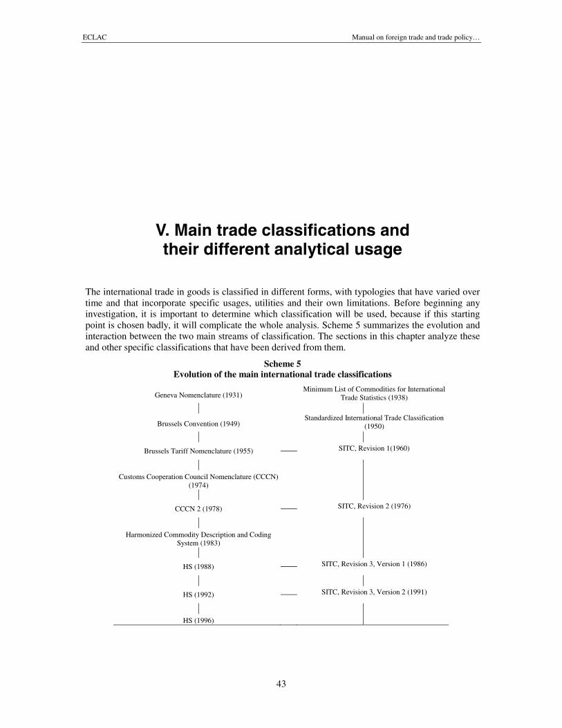
ECLAC Manual on foreign trade and trade policy…
43
V. Main trade classifications andtheir different analytical usage
The international trade in goods is classified in different forms, with typologies that have varied overtime and that incorporate specific usages, utilities and their own limitations. Before beginning anyinvestigation, it is important to determine which classification will be used, because if this startingpoint is chosen badly, it will complicate the whole analysis. Scheme 5 summarizes the evolution andinteraction between the two main streams of classification. The sections in this chapter analyze theseand other specific classifications that have been derived from them.
Scheme 5Evolution of the main international trade classifications
Geneva Nomenclature (1931)Minimum List of Commodities for International
Trade Statistics (1938)
Brussels Convention (1949)Standardized International Trade Classification
(1950)
Brussels Tariff Nomenclature (1955) SITC, Revision 1(1960)
Customs Cooperation Council Nomenclature (CCCN)(1974)
CCCN 2 (1978) SITC, Revision 2 (1976)
Harmonized Commodity Description and CodingSystem (1983)
HS (1988) SITC, Revision 3, Version 1 (1986)
HS (1992) SITC, Revision 3, Version 2 (1991)
HS (1996)
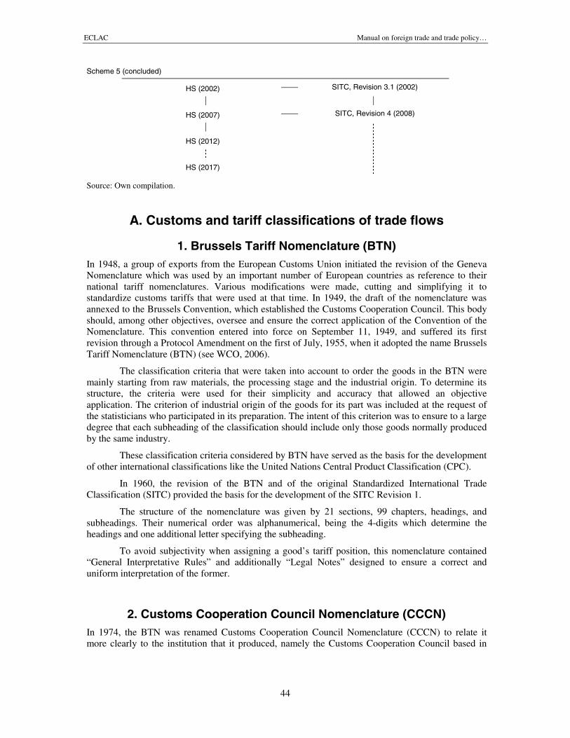
ECLAC Manual on foreign trade and trade policy…
44
Scheme 5 (concluded)
HS (2002) SITC, Revision 3.1 (2002)
HS (2007) SITC, Revision 4 (2008)
HS (2012)
HS (2017)
Source: Own compilation.
A. Customs and tariff classifications of trade flows
1. Brussels Tariff Nomenclature (BTN)In 1948, a group of exports from the European Customs Union initiated the revision of the GenevaNomenclature which was used by an important number of European countries as reference to theirnational tariff nomenclatures. Various modifications were made, cutting and simplifying it tostandardize customs tariffs that were used at that time. In 1949, the draft of the nomenclature wasannexed to the Brussels Convention, which established the Customs Cooperation Council. This bodyshould, among other objectives, oversee and ensure the correct application of the Convention of theNomenclature. This convention entered into force on September 11, 1949, and suffered its firstrevision through a Protocol Amendment on the first of July, 1955, when it adopted the name BrusselsTariff Nomenclature (BTN) (see WCO, 2006).
The classification criteria that were taken into account to order the goods in the BTN weremainly starting from raw materials, the processing stage and the industrial origin. To determine itsstructure, the criteria were used for their simplicity and accuracy that allowed an objectiveapplication. The criterion of industrial origin of the goods for its part was included at the request ofthe statisticians who participated in its preparation. The intent of this criterion was to ensure to a largedegree that each subheading of the classification should include only those goods normally producedby the same industry.
These classification criteria considered by BTN have served as the basis for the developmentof other international classifications like the United Nations Central Product Classification (CPC).
In 1960, the revision of the BTN and of the original Standardized International TradeClassification (SITC) provided the basis for the development of the SITC Revision 1.
The structure of the nomenclature was given by 21 sections, 99 chapters, headings, andsubheadings. Their numerical order was alphanumerical, being the 4-digits which determine theheadings and one additional letter specifying the subheading.
To avoid subjectivity when assigning a good’s tariff position, this nomenclature contained“General Interpretative Rules” and additionally “Legal Notes” designed to ensure a correct anduniform interpretation of the former.
2. Customs Cooperation Council Nomenclature (CCCN)In 1974, the BTN was renamed Customs Cooperation Council Nomenclature (CCCN) to relate itmore clearly to the institution that it produced, namely the Customs Cooperation Council based in
ECLAC Manual on foreign trade and trade policy…
45
Brussels (WCO, 2006). Later, in 1978, to achieve a full correspondence with the SITC Rev.2, 1083statistical subheadings were incorporated into the CCCN, derived from 262 of its 1011 headings.
3. Harmonized commodity description and coding system (HS)In 1983, the name of the CCCN was changed into Harmonized Commodity Description and CodingSystem (HS), see CCC (1985). On the first of January 1988, the HS88 entered into force, delivering anew classification with multiple purposes (WCO, 2006). The most important ones were: providing abase for the development of tariffs, the collection of statistics on international trade, the rules oforigin, the collection of excise tax, the trade of goods, the transport tariffs and statistics, and themonitoring and control of goods. Moreover, as a vital element of customs controls and procedures,they included the assessment of risk, information technologies, and compliance.
In contrast to its predecessor CCCN, the HS88, broadened the categories from four to sixdigits to maintain a nearly full correspondence to the new SITC Rev.3. The only exception betweenthat version of the HS and the SITC is given for heading HS88 2710 which is not divided insubheadings as occurring in SITC Rev.3 (8 subheadings).2
The HS88 shows a structure of 21 sections, 96 chapters (plus one Chapter 77 for potentialfuture use), and 1241 headings of four digits. Of this total, 930 of the headings are divided intosubheadings giving origin to a total of 5019 groups of goods identified by a six-digit code. Later on,the HS88 was revised in the years 1992, 1996, 2002, 2007, and 2012. A further revision is alreadyannounced to take part in 2017 (WCO, 2015).
The most recent version HS12 maintains the structure of the 21 sections (of 1 digit) from1988, but not the number of the following categories: chapters 96 (two digits, plus chapter 77 forfuture use and chapter 98 and 99 for national use), 1225 headings (four digits), and subheadings (sixdigits). In total, the HS12 counts 5299 subheadings of which 4996 directly correspond to HS88. Thesituation of the heading 2710 in the HS88 was resolved through incorporating five subheadings HS12(2710.12, 2710.19, 2710.20, 2710.91, and 2710.99) that correspond now with the new structure of theheading 334 of the SITC Rev.4. To sum up, the HS88 has undergone several modifications since itsimplementation that have also affected the SITC.
As it would be too extensive to describe the various aggregation levels of that classification,we list the 21 sections that build the base for its structure below in table 14.
Like the BTN and the CCCN, the HS also has General Interpretative Notes on the system andExplanatory Notes for the sections, chapters, and subheadings as well as an Alphabetical Index ofheadings and subheadings if appropriate.
According to accessible data, the development of the number of levels of these customsclassifications in each version is as presented in table 15.
2 HS88 2710: “Petroleum oils and oils obtained from bituminous minerals, other than crude; preparations notelsewhere specified or included, containing by weight 70% or more of petroleum oils or of oils obtained frombituminous minerals, these oils being the basic constituents of the preparations; waste oils” (WCO, 2002).
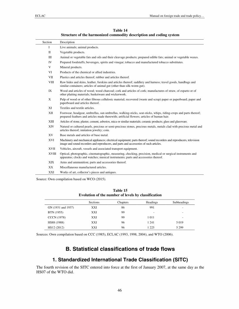
ECLAC Manual on foreign trade and trade policy…
46
Table 14Structure of the harmonized commodity description and coding system
Section Description
I Live animals; animal products.
II Vegetable products.
III Animal or vegetable fats and oils and their cleavage products; prepared edible fats; animal or vegetable waxes.
IV Prepared foodstuffs; beverages, spirits and vinegar; tobacco and manufactured tobacco substitutes.
V Mineral products.
VI Products of the chemical or allied industries.
VII Plastics and articles thereof; rubber and articles thereof.
VIII Raw hides and skins, leather, furskins and articles thereof; saddlery and harness; travel goods, handbags andsimilar containers; articles of animal gut (other than silk-worm gut).
IX Wood and articles of wood; wood charcoal; cork and articles of cork; manufactures of straw, of esparto or ofother plaiting materials; basketware and wickerwork.
X Pulp of wood or of other fibrous cellulosic material; recovered (waste and scrap) paper or paperboard; paper andpaperboard and articles thereof.
XI Textiles and textile articles.
XII Footwear, headgear, umbrellas, sun umbrellas, walking-sticks, seat-sticks, whips, riding-crops and parts thereof;prepared feathers and articles made therewith; artificial flowers; articles of human hair.
XIII Articles of stone, plaster, cement, asbestos, mica or similar materials; ceramic products; glass and glassware.
XIV Natural or cultured pearls, precious or semi-precious stones, precious metals, metals clad with precious metal andarticles thereof; imitation jewelry; coin.
XV Base metals and articles of base metal.
XVI Machinery and mechanical appliances; electrical equipment; parts thereof; sound recorders and reproducers, televisionimage and sound recorders and reproducers, and parts and accessories of such articles.
XVII Vehicles, aircraft, vessels and associated transport equipment.
XVIII Optical, photographic, cinematographic, measuring, checking, precision, medical or surgical instruments andapparatus; clocks and watches; musical instruments; parts and accessories thereof.
XIX Arms and ammunition; parts and accessories thereof.
XX Miscellaneous manufactured articles.
XXI Works of art, collector’s pieces and antiques.
Source: Own compilation based on WCO (2015).
Table 15Evolution of the number of levels by classification
Sections Chapters Headings Subheadings
GN (1931 and 1937) XXI 86 991 -
BTN (1955) XXI 99 - -
CCCN (1978) XXI 99 1 011 -
HS88 (1988) XXI 96 1 241 5 019
HS12 (2012) XXI 96 1 225 5 299
Sources: Own compilation based on CCC (1985), ECLAC (1993, 1998, 2004), and WTO (2006).
B. Statistical classifications of trade flows
1. Standardized International Trade Classification (SITC)The fourth revision of the SITC entered into force at the first of January 2007, at the same day as theHS07 of the WTO did.
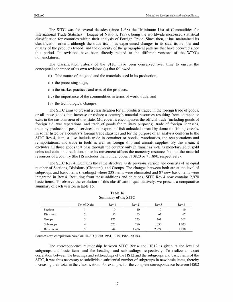
ECLAC Manual on foreign trade and trade policy…
47
The SITC was for several decades (since 1938) the “Minimum List of Commodities forInternational Trade Statistics” (League of Nations, 1938), being the worldwide most-used statisticalclassification for countries within their analysis of Foreign Trade. Since then, it has maintained itsclassification criteria although the trade itself has experienced changes in its size, its number andquality of the products traded, and the diversity of the geographical patterns that have occurred sincethis period. Its revisions have been directly related to the different versions of the WTO’snomenclatures.
The classification criteria of the SITC have been conserved over time to ensure theconceptual coherence of its own revisions (4) that followed:
(i) Tthe nature of the good and the materials used in its production,
(ii) the processing stage,
(iii) the market practices and uses of the products,
(iv) the importance of the commodities in terms of world trade, and
(v) the technological changes.
The SITC aims to present a classification for all products traded in the foreign trade of goods,or all those goods that increase or reduce a country’s material resources resulting from entrance orexits in the customs area of that state. Moreover, it encompasses the official trade (including goods offoreign aid, war reparations, and trade of goods for military purposes), trade of foreign licensees,trade by products of postal services, and exports of fish unloaded abroad by domestic fishing vessels.In so far listed by a country’s foreign trade statistics and for the purpose of an analysis conform to theSITC Rev.4, it must also include trade in container or bonded warehouses, the reexportations andreimportations, and trade in fuels as well as foreign ship and aircraft supplies. By this mean, itexcludes all those goods that pass through the country only in transit as well as monetary gold, goldcoins and coins in circulation, since its movement affects the monetary resources but not the materialresources of a country (the HS includes them under codes 710820 or 711890, respectively).
The SITC Rev.4 maintains the same structure as its previous version and consists of an equalnumber of Sections, Divisions (Chapters), and Groups. The changes between both are at the level ofsubgroups and basic items (headings) where 238 items were eliminated and 87 new basic items wereintegrated in Rev.4. Resulting from these additions and deletions, SITC Rev.4 now contains 2,970basic items. To observe the evolution of this classification quantitatively, we present a comparativesummary of each version in table 16.
Table 16Summary of the SITC
No. of Digits Rev.1 Rev.2 Rev.3 Rev.4
Sections 1 10 10 10 10
Divisions 2 56 63 67 67
Groups 3 177 233 261 262
Subgroups 4 625 786 1 033 1 023
Basic items 5 944 1 466 2 824 2 970
Source: Own compilation based on UNSD (1950, 1961, 1975, 1986, 2006a).
The correspondence relationship between SITC Rev.4 and HS12 is given at the level ofsubgroups and basic items and the headings and subheadings, respectively. To realize an exactcorrelation between the headings and subheadings of the HS12 and the subgroups and basic items of theSITC, it was thus necessary to subdivide a substantial number of subgroups in new basic items, therebyincreasing their total in the classification. For example, for the complete correspondence between HS02
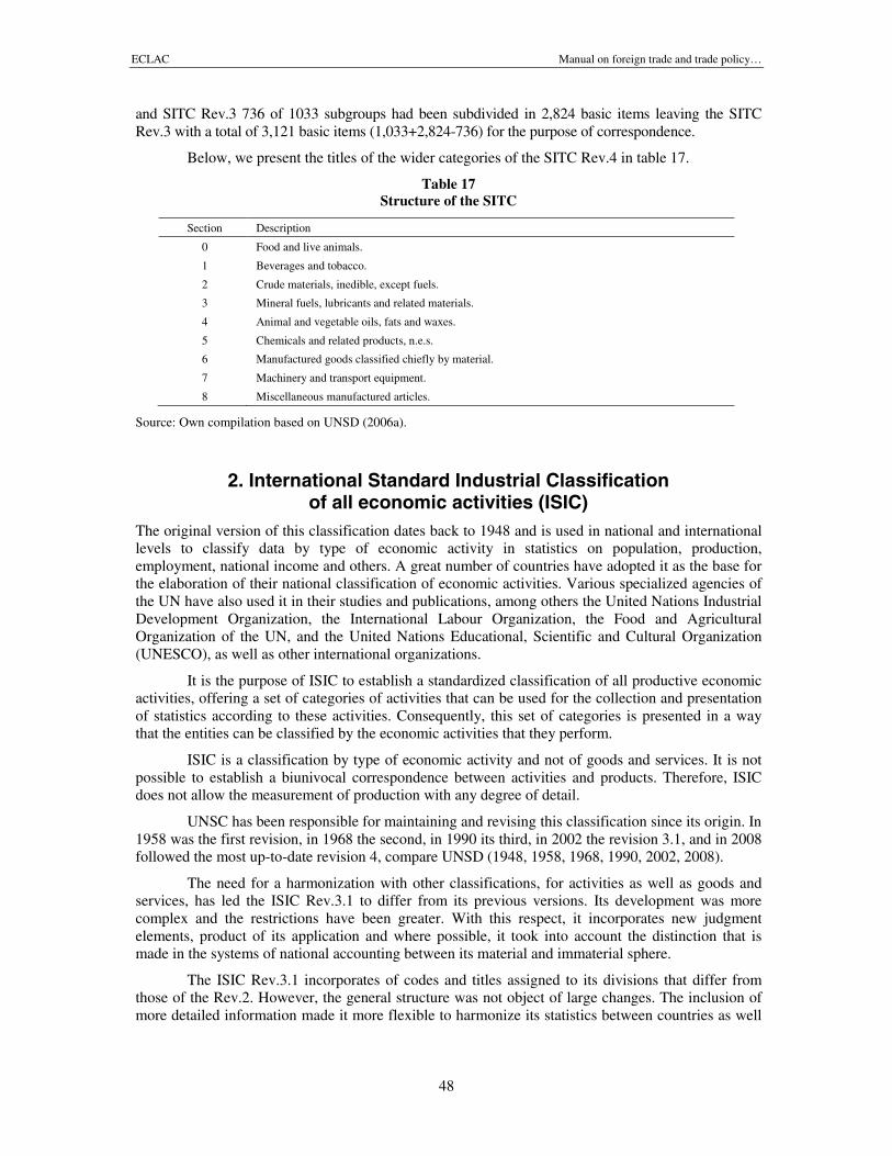
ECLAC Manual on foreign trade and trade policy…
48
and SITC Rev.3 736 of 1033 subgroups had been subdivided in 2,824 basic items leaving the SITCRev.3 with a total of 3,121 basic items (1,033+2,824-736) for the purpose of correspondence.
Below, we present the titles of the wider categories of the SITC Rev.4 in table 17.
Table 17Structure of the SITC
Section Description
0 Food and live animals.
1 Beverages and tobacco.
2 Crude materials, inedible, except fuels.
3 Mineral fuels, lubricants and related materials.
4 Animal and vegetable oils, fats and waxes.
5 Chemicals and related products, n.e.s.
6 Manufactured goods classified chiefly by material.
7 Machinery and transport equipment.
8 Miscellaneous manufactured articles.
Source: Own compilation based on UNSD (2006a).
2. International Standard Industrial Classificationof all economic activities (ISIC)
The original version of this classification dates back to 1948 and is used in national and internationallevels to classify data by type of economic activity in statistics on population, production,employment, national income and others. A great number of countries have adopted it as the base forthe elaboration of their national classification of economic activities. Various specialized agencies ofthe UN have also used it in their studies and publications, among others the United Nations IndustrialDevelopment Organization, the International Labour Organization, the Food and AgriculturalOrganization of the UN, and the United Nations Educational, Scientific and Cultural Organization(UNESCO), as well as other international organizations.
It is the purpose of ISIC to establish a standardized classification of all productive economicactivities, offering a set of categories of activities that can be used for the collection and presentationof statistics according to these activities. Consequently, this set of categories is presented in a waythat the entities can be classified by the economic activities that they perform.
ISIC is a classification by type of economic activity and not of goods and services. It is notpossible to establish a biunivocal correspondence between activities and products. Therefore, ISICdoes not allow the measurement of production with any degree of detail.
UNSC has been responsible for maintaining and revising this classification since its origin. In1958 was the first revision, in 1968 the second, in 1990 its third, in 2002 the revision 3.1, and in 2008followed the most up-to-date revision 4, compare UNSD (1948, 1958, 1968, 1990, 2002, 2008).
The need for a harmonization with other classifications, for activities as well as goods andservices, has led the ISIC Rev.3.1 to differ from its previous versions. Its development was morecomplex and the restrictions have been greater. With this respect, it incorporates new judgmentelements, product of its application and where possible, it took into account the distinction that ismade in the systems of national accounting between its material and immaterial sphere.
The ISIC Rev.3.1 incorporates of codes and titles assigned to its divisions that differ fromthose of the Rev.2. However, the general structure was not object of large changes. The inclusion ofmore detailed information made it more flexible to harmonize its statistics between countries as well
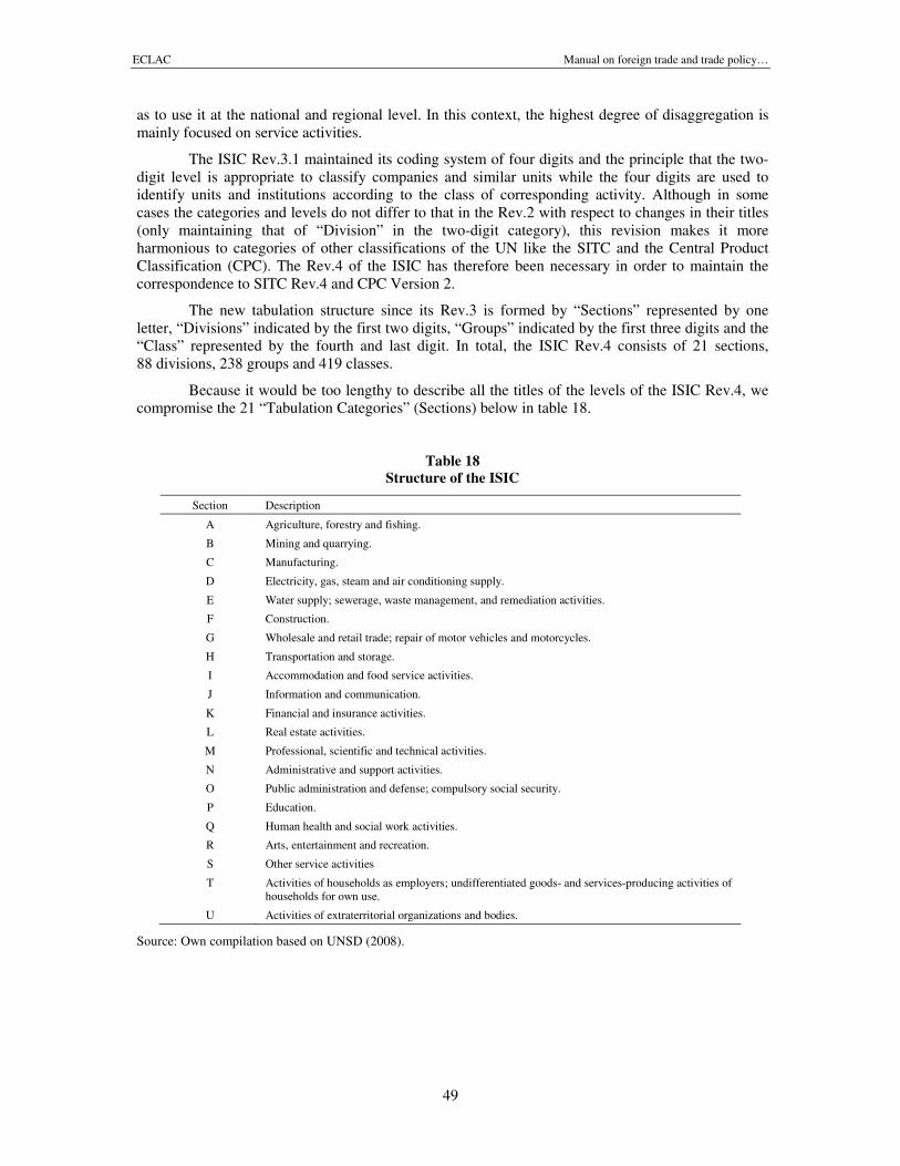
ECLAC Manual on foreign trade and trade policy…
49
as to use it at the national and regional level. In this context, the highest degree of disaggregation ismainly focused on service activities.
The ISIC Rev.3.1 maintained its coding system of four digits and the principle that the two-digit level is appropriate to classify companies and similar units while the four digits are used toidentify units and institutions according to the class of corresponding activity. Although in somecases the categories and levels do not differ to that in the Rev.2 with respect to changes in their titles(only maintaining that of “Division” in the two-digit category), this revision makes it moreharmonious to categories of other classifications of the UN like the SITC and the Central ProductClassification (CPC). The Rev.4 of the ISIC has therefore been necessary in order to maintain thecorrespondence to SITC Rev.4 and CPC Version 2.
The new tabulation structure since its Rev.3 is formed by “Sections” represented by oneletter, “Divisions” indicated by the first two digits, “Groups” indicated by the first three digits and the“Class” represented by the fourth and last digit. In total, the ISIC Rev.4 consists of 21 sections,88 divisions, 238 groups and 419 classes.
Because it would be too lengthy to describe all the titles of the levels of the ISIC Rev.4, wecompromise the 21 “Tabulation Categories” (Sections) below in table 18.
Table 18Structure of the ISIC
Section Description
A Agriculture, forestry and fishing.
B Mining and quarrying.
C Manufacturing.
D Electricity, gas, steam and air conditioning supply.
E Water supply; sewerage, waste management, and remediation activities.
F Construction.
G Wholesale and retail trade; repair of motor vehicles and motorcycles.
H Transportation and storage.
I Accommodation and food service activities.
J Information and communication.
K Financial and insurance activities.
L Real estate activities.
M Professional, scientific and technical activities.
N Administrative and support activities.
O Public administration and defense; compulsory social security.
P Education.
Q Human health and social work activities.
R Arts, entertainment and recreation.
S Other service activities
T Activities of households as employers; undifferentiated goods- and services-producing activities ofhouseholds for own use.
U Activities of extraterritorial organizations and bodies.
Source: Own compilation based on UNSD (2008).
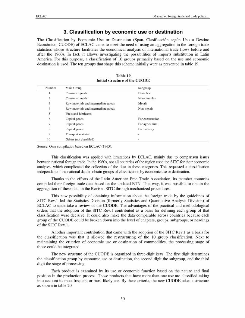
ECLAC Manual on foreign trade and trade policy…
50
3. Classification by economic use or destinationThe Classification by Economic Use or Destination (Span. Clasificación según Uso o DestinoEconómico, CUODE) of ECLAC came to meet the need of using an aggregation in the foreign tradestatistics whose structure facilitates the economical analysis of international trade flows before andafter the 1960s. In fact, it allows investigating the possibilities of imports substitution in LatinAmerica. For this purpose, a classification of 10 groups primarily based on the use and economicdestination is used. The ten groups that shape this scheme initially were as presented in table 19.
Table 19Initial structure of the CUODE
Number Main Group Subgroup
1 Consumer goods Durables
2 Consumer goods Non-durables
3 Raw materials and intermediate goods Metals
4 Raw materials and intermediate goods Non-metals
5 Fuels and lubricants -
6 Capital goods For construction
7 Capital goods For agriculture
8 Capital goods For industry
9 Transport material -
10 Others (not classified) -
Source: Own compilation based on ECLAC (1965).
This classification was applied with limitations by ECLAC, mainly due to comparison issuesbetween national foreign trade. In the 1960s, not all countries of the region used the SITC for their economicanalyses, which complicated the collection of the data in these categories. This requested a classificationindependent of the national data to obtain groups of classification by economic use or destination.
Thanks to the efforts of the Latin American Free Trade Association, its member countriescompiled their foreign trade data based on the updated BTN. That way, it was possible to obtain theaggregation of these data in the Revised SITC through mechanized procedures.
This new possibility of obtaining information about the foreign trade by the guidelines ofSITC Rev.1 led the Statistics Division (formerly Statistics and Quantitative Analysis Division) ofECLAC to undertake a review of the CUODE. The advantages of the practical and methodologicalorders that the adoption of the SITC Rev.1 contributed as a basis for defining each group of thatclassification were decisive. It could also make the data comparable across countries because eachgroup of the CUODE could be broken down into the level of chapters, groups, subgroups, or headingsof the SITC Rev.1.
Another important contribution that came with the adoption of the SITC Rev.1 as a basis forthe classification was that it allowed the restructuring of the 10 group classification. Next tomaintaining the criterion of economic use or destination of commodities, the processing stage ofthose could be integrated.
The new structure of the CUODE is organized in three-digit keys. The first digit determinesthe classification group by economic use or destination, the second digit the subgroup, and the thirddigit the stage of processing.
Each product is examined by its use or economic function based on the nature and finalposition in the production process. Those products that have more than one use are classified takinginto account its most frequent or most likely use. By these criteria, the new CUODE takes a structureas shown in table 20.
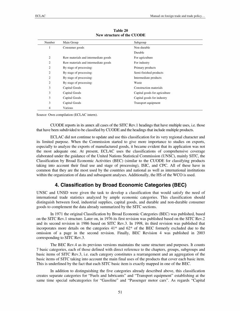
ECLAC Manual on foreign trade and trade policy…
51
Table 20New structure of the CUODE
Number Main Group Subgroup
1 Consumer goods Non-durable
Durable
2 Raw materials and intermediate goods For agriculture
2 Raw materials and intermediate goods For industry
2 By stage of processing: Primary products
2 By stage of processing: Semi-finished products
2 By stage of processing: Intermediate products
2 By stage of processing: Waste
3 Capital Goods Construction materials
3 Capital Goods Capital goods for agriculture
3 Capital Goods Capital goods for industry
3 Capital Goods Transport equipment
4 Various
Source: Own compilation (ECLAC intern).
CUODE reports in its annex all cases of the SITC Rev.1 headings that have multiple uses, i.e. thosethat have been subdivided to be classified by CUODE and the headings that include multiple products.
ECLAC did not continue to update and use this classification for its very regional character andits limited purpose. When the Commission started to give more importance to studies on exports,especially to analyze the exports of manufactured goods, it became evident that its application was notthe most adequate one. At present, ECLAC uses the classifications of comprehensive coverageelaborated under the guidance of the United Nations Statistical Commission (UNSC), mainly SITC, theClassification by Broad Economic Activities (BEC) (similar to the CUODE for classifying productstaking into account their final use and stage of processing), ISIC, and CPC. All of these have incommon that they are the most used by the countries and national as well as international institutionswithin the organization of data and subsequent analyses. Additionally, the HS of the WCO is used.
4. Classification by Broad Economic Categories (BEC)UNSC and UNSD were given the task to develop a classification that would satisfy the need ofinternational trade statistics analyzed by ample economic categories. This classification shoulddistinguish between food, industrial supplies, capital goods, and durable and non-durable consumergoods to complement the data already summarized by the SITC sections.
In 1971 the original Classification by Broad Economic Categories (BEC) was published, basedon the SITC Rev.1 structure. Later on, in 1976 its first revision was published based on the SITC Rev.2and its second revision in 1986 based on SITC Rev.3. In 1998, its third revision was published thatincorporates more details on the categories 41* and 62* of the BEC formerly excluded due to theomission of a page in the second revision. Finally, BEC Revision 4 was published in 2003corresponding to SITC Rev.3.
The BEC Rev.4 as its previous versions maintains the same structure and purposes. It counts7 basic categories, each of those defined with direct reference to the chapters, groups, subgroups andbasic items of SITC Rev.3, i.e. each category constitutes a rearrangement and an aggregation of thebasic items of SITC taking into account the main final uses of the products that cover each basic item.This is underlined by the fact that each SITC basic item is exactly mapped in one of the BEC.
In addition to distinguishing the five categories already described above, this classificationcreates separate categories for “Fuels and lubricants” and “Transport equipment” establishing at thesame time special subcategories for “Gasoline” and “Passenger motor cars”. As regards “Capital
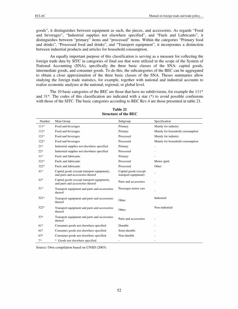
ECLAC Manual on foreign trade and trade policy…
52
goods”, it distinguishes between equipment as such, the pieces, and accessories. As regards “Foodand beverages”, “Industrial supplies not elsewhere specified”, and “Fuels and Lubricants”, itdistinguishes between “primary” items and “processed” items. Within the categories “Primary foodand drinks”, “Processed food and drinks”, and “Transport equipment”, it incorporates a distinctionbetween industrial products and articles for household consumption.
An equally important purpose of this classification is serving as a measure for collecting theforeign trade data by SITC in categories of final use that were utilized in the scope of the System ofNational Accounting (SNA), specifically the three basic classes of the SNA: capital goods,intermediate goods, and consumer goods. To do this, the subcategories of the BEC can be aggregatedto obtain a close approximation of the three basic classes of the SNA. Theses summaries allowstudying the foreign trade statistics, for example, together with national and industrial accounts torealize economic analyses at the national, regional, or global level.
The 10 basic categories of the BEC are those that have no subdivisions, for example the 111*and 31*. The codes of this classification are indicated with a star (*) to avoid possible confusionswith those of the SITC. The basic categories according to BEC Rev.4 are those presented in table 21.
Table 21Structure of the BEC
Number Main Group Subgroup Specification
111* Food and beverages Primary Mainly for industry
112* Food and beverages Primary Mainly for household consumption
121* Food and beverages Processed Mainly for industry
122* Food and beverages Processed Mainly for household consumption
21* Industrial supplies not elsewhere specified Primary -
22* Industrial supplies not elsewhere specified Processed -
31* Fuels and lubricants Primary -
321* Fuels and lubricants Processed Motor spirit
322* Fuels and lubricants Processed Other
41* Capital goods (except transport equipment),and parts and accessories thereof
Capital goods (excepttransport equipment)
-
42* Capital goods (except transport equipment),and parts and accessories thereof
Parts and accessories -
51* Transport equipment and parts and accessoriesthereof
Passenger motor cars-
521* Transport equipment and parts and accessoriesthereof
OtherIndustrial
522* Transport equipment and parts and accessoriesthereof
OtherNon-industrial
53* Transport equipment and parts and accessoriesthereof
Parts and accessories -
61* Consumer goods not elsewhere specified Durable -
62* Consumer goods not elsewhere specified Semi-durable -
63* Consumer goods not elsewhere specified Non-durable -
7* * Goods not elsewhere specified - -
Source: Own compilation based on UNSD (2003).
ECLAC Manual on foreign trade and trade policy…
53
5. Central Product Classification (CPC)The CPC was provisionally approved by the UNSC in 1989. With its provisional character, it wassought to gain experience and gather comments through its application, all which should provide thebase for any subsequent revision.
In 1991 the provisional CPC was published where the experience of the national andinternational users provided an appropriate basis for its revision. The experience acquired within thedevelopment of the Statistical Classification of Products by Activity of the European Union was alsotaken into account (EEC, 1993).
In 1998, the provisional CPC was revised, updated, and completed and submitted forapproval through the UNSD under the name CPC Version 1.0. In this version, particular attentionwas paid to the part corresponding to the services. The result guaranteed that the structure of the CPCcorresponded adequately to the new technologies and the rise of the service sector in the economy.The transportable goods in the provisional CPC and in the SITC Rev.3 were revised in accordancewith the 1996 version of the HS.
In 2002, the CPC Ver.1.0 was actualized giving origin to the Ver.1.1 that was published to beused in 2006 (UNSD, 2006b). This new revision took into account the work of a technical groupcreated by the Expert Group on International Economic and Social Classifications of the UNSC andthe collaboration of a large number of international countries and organizations. In this sense, itincorporated all changes that appeared since its official application in 1998 until the modificationsdone in SITC Rev.3 in accordance with the 2002 edition of the HS. These changes and the necessarychanges to correspond with the SITC Rev.3.1 have been integrated in the Ver.1.1 in its sections 0 to4. In 2008, the Version 2 of the CPC was published and presents a correspondence to the new HS2007 and the SITC Rev.4. Finally, CPC Ver.2.1 has been released in 2015.
The purpose of CPC is very broad although it is treated as a central standardized productclassification. It satisfies needs of detailed information referring to statistics about production,consumption, prices, foreign trade, flows of goods, inventories or balances, accumulation of capital,and others. Moreover, it contains information needed to prepare input-output tables and the balanceof payments (BOP). It was also designed to achieve an improved harmonization between thesubsectors of economic statistics and those related and, additionally, to increase the usefulness of thenational accounts and balances as instruments of coordinating economic statistics.
The CPC includes categories corresponding to all the articles that can be traded on a national orinternational level or can be stored. It covers not only the goods and services derived from an economicactivity, but also buying and selling of land or analogous transactions as well as those that stem fromjuristic contracts (patents, licenses, copyrights, among others). Consequently, it encompasses transportableand non-transportable goods, services as well as tangible and intangible assets. Although these assets areneither considered as goods nor as services in the SNA, they are included as they are object to numeroustrade activities, at national and international level and are of great interest to many users.
In short, the CPC provides a framework for the comparison of statistics on goods, services,and assets across countries. It also works as a reference for the countries that develop a productclassification for the first time or decide to review their current information system to becomecompatible with international norms.
The CPC that contains all the goods and services is a comprehensive system of categoriesand also mutually exclusive. In most of the case, the CPC classifies products in categories based ontheir physical properties, their inherent nature and their industrial source.
The relationship between the CPC and the HS is very narrow, because it completely utilizesthe HS to form its first five sections (0 to 4). In other words, each subclass of the sections 0 to 4 of theCPC —which correspond to the transportable goods— has as unit elements the headings andsubheadings of the HS, i.e. each subclass is an aggregate of one or more headings of the HS.
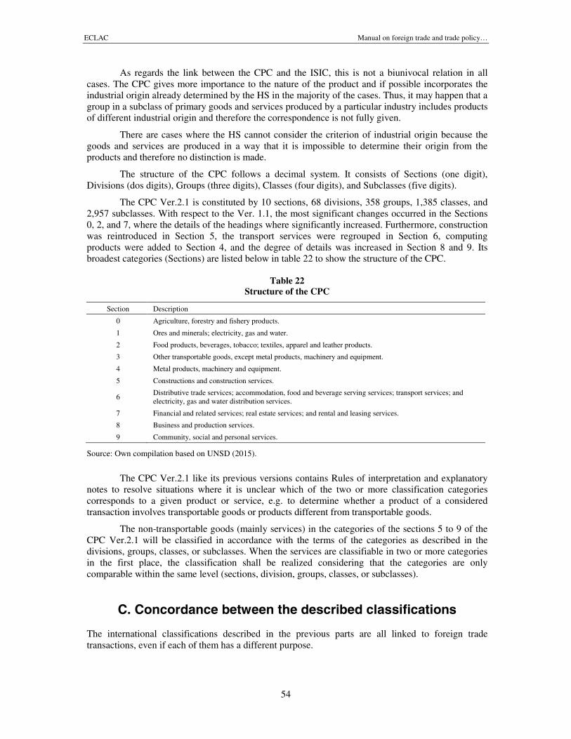
ECLAC Manual on foreign trade and trade policy…
54
As regards the link between the CPC and the ISIC, this is not a biunivocal relation in allcases. The CPC gives more importance to the nature of the product and if possible incorporates theindustrial origin already determined by the HS in the majority of the cases. Thus, it may happen that agroup in a subclass of primary goods and services produced by a particular industry includes productsof different industrial origin and therefore the correspondence is not fully given.
There are cases where the HS cannot consider the criterion of industrial origin because thegoods and services are produced in a way that it is impossible to determine their origin from theproducts and therefore no distinction is made.
The structure of the CPC follows a decimal system. It consists of Sections (one digit),Divisions (dos digits), Groups (three digits), Classes (four digits), and Subclasses (five digits).
The CPC Ver.2.1 is constituted by 10 sections, 68 divisions, 358 groups, 1,385 classes, and2,957 subclasses. With respect to the Ver. 1.1, the most significant changes occurred in the Sections0, 2, and 7, where the details of the headings where significantly increased. Furthermore, constructionwas reintroduced in Section 5, the transport services were regrouped in Section 6, computingproducts were added to Section 4, and the degree of details was increased in Section 8 and 9. Itsbroadest categories (Sections) are listed below in table 22 to show the structure of the CPC.
Table 22Structure of the CPC
Section Description
0 Agriculture, forestry and fishery products.
1 Ores and minerals; electricity, gas and water.
2 Food products, beverages, tobacco; textiles, apparel and leather products.
3 Other transportable goods, except metal products, machinery and equipment.
4 Metal products, machinery and equipment.
5 Constructions and construction services.
6Distributive trade services; accommodation, food and beverage serving services; transport services; andelectricity, gas and water distribution services.
7 Financial and related services; real estate services; and rental and leasing services.
8 Business and production services.
9 Community, social and personal services.
Source: Own compilation based on UNSD (2015).
The CPC Ver.2.1 like its previous versions contains Rules of interpretation and explanatorynotes to resolve situations where it is unclear which of the two or more classification categoriescorresponds to a given product or service, e.g. to determine whether a product of a consideredtransaction involves transportable goods or products different from transportable goods.
The non-transportable goods (mainly services) in the categories of the sections 5 to 9 of theCPC Ver.2.1 will be classified in accordance with the terms of the categories as described in thedivisions, groups, classes, or subclasses. When the services are classifiable in two or more categoriesin the first place, the classification shall be realized considering that the categories are onlycomparable within the same level (sections, division, groups, classes, or subclasses).
C. Concordance between the described classifications
The international classifications described in the previous parts are all linked to foreign tradetransactions, even if each of them has a different purpose.
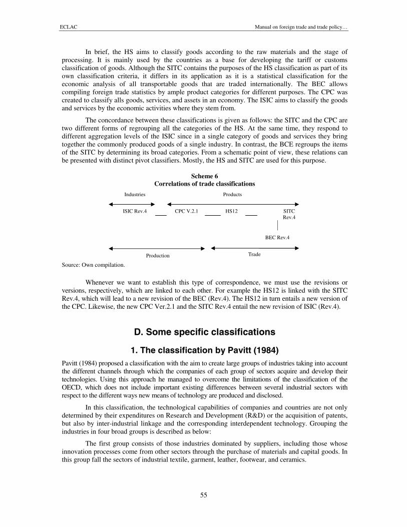
ECLAC Manual on foreign trade and trade policy…
55
In brief, the HS aims to classify goods according to the raw materials and the stage ofprocessing. It is mainly used by the countries as a base for developing the tariff or customsclassification of goods. Although the SITC contains the purposes of the HS classification as part of itsown classification criteria, it differs in its application as it is a statistical classification for theeconomic analysis of all transportable goods that are traded internationally. The BEC allowscompiling foreign trade statistics by ample product categories for different purposes. The CPC wascreated to classify alls goods, services, and assets in an economy. The ISIC aims to classify the goodsand services by the economic activities where they stem from.
The concordance between these classifications is given as follows: the SITC and the CPC aretwo different forms of regrouping all the categories of the HS. At the same time, they respond todifferent aggregation levels of the ISIC since in a single category of goods and services they bringtogether the commonly produced goods of a single industry. In contrast, the BCE regroups the itemsof the SITC by determining its broad categories. From a schematic point of view, these relations canbe presented with distinct pivot classifiers. Mostly, the HS and SITC are used for this purpose.
Scheme 6Correlations of trade classifications
Industries Products
ISIC Rev.4 CPC V.2.1 HS12 SITCRev.4
BEC Rev.4
Production Trade
Source: Own compilation.
Whenever we want to establish this type of correspondence, we must use the revisions orversions, respectively, which are linked to each other. For example the HS12 is linked with the SITCRev.4, which will lead to a new revision of the BEC (Rev.4). The HS12 in turn entails a new version ofthe CPC. Likewise, the new CPC Ver.2.1 and the SITC Rev.4 entail the new revision of ISIC (Rev.4).
D. Some specific classifications
1. The classification by Pavitt (1984)Pavitt (1984) proposed a classification with the aim to create large groups of industries taking into accountthe different channels through which the companies of each group of sectors acquire and develop theirtechnologies. Using this approach he managed to overcome the limitations of the classification of theOECD, which does not include important existing differences between several industrial sectors withrespect to the different ways new means of technology are produced and disclosed.
In this classification, the technological capabilities of companies and countries are not onlydetermined by their expenditures on Research and Development (R&D) or the acquisition of patents,but also by inter-industrial linkage and the corresponding interdependent technology. Grouping theindustries in four broad groups is described as below:
The first group consists of those industries dominated by suppliers, including those whoseinnovation processes come from other sectors through the purchase of materials and capital goods. Inthis group fall the sectors of industrial textile, garment, leather, footwear, and ceramics.
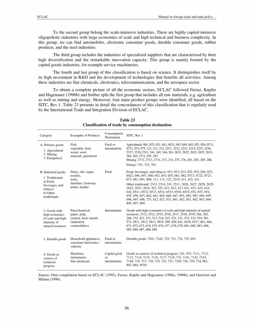
ECLAC Manual on foreign trade and trade policy…
56
To the second group belong the scale-intensive industries. These are highly capital-intensiveoligopolistic industries with large economies of scale and high technical and business complexity. Inthis group, we can find automobiles, electronic consumer goods, durable consumer goods, rubberproducts, and the steel industries.
The third group includes the industries of specialized suppliers that are characterized by theirhigh diversification and the remarkable innovation capacity. This group is mainly formed by thecapital goods industries, for example service machineries.
The fourth and last group of this classification is based on science. It distinguishes itself byits high investment in R&D and the development of technologies that benefits all activities. Amongthese industries are fine chemicals, electronics, telecommunication, and the aerospace sector.
To obtain a complete picture of all the economic sectors, ECLAC followed Ferraz, Kupferand Hagenauer (1996b) and further split the first group that includes all raw materials, e.g. agricultureas well as mining and energy. Moreover, four main product groups were identified, all based on theSITC, Rev.1. Table 23 presents in detail the concordances of this classification that is regularly usedby the International Trade and Integration Division of ECLAC.
Table 23Classification of trade by consumption destination
Category Examples of ProductsConsumptionDestination
SITC, Rev.1
A. Primary goods
1. Agricultural2. Mining3. Energetical
Fish,vegetable, fruit,wood, wool,minerals, petroleum
Final orintermediate
Agricultural: 001, 025, 031, 041, 0421, 043, 044, 045, 051, 054, 0711,0721, 074, 075, 121, 211, 212, 2211, 2212, 2213, 2214, 2215, 2216,2217, 2218, 2311, 241, 242, 244, 261, 2621, 2622, 2623, 2625, 2631,264, 265, 2711, 291, 292.Mining: 2712, 2713, 2714, 273, 274, 275, 276, 281, 283, 285, 286.
Energy: 321, 331, 341.
B. Industrial goods
1. Traditionalsa) Food,beverages, andtobaccob) Othertraditionals
Dairy, oils, sugar,textiles,tools,furniture, footwear,prints, leather
Final Food, beverages, and tobacco: 011, 012, 013, 022, 023, 024, 032,0422, 046, 047, 048, 052, 053, 055, 061, 062, 0713, 0722, 0723,073, 081, 091, 099, 111, 112, 122, 2219, 411, 422, 431.
Other traditional: 2313, 2314, 243, 2511, 2626, 2627, 2628, 2629,2632, 2633, 2634, 267, 551, 611, 612, 613, 621, 631, 632, 633,642, 6511, 6512, 6513, 6514, 6515, 6518, 6519, 652, 653, 654,655, 656, 657, 662, 663, 665, 666, 667, 691, 692, 693, 694, 695,696, 697, 698, 733, 812, 821, 831, 841, 842, 851, 892, 893, 894,895, 897, 899.
2. Goods withhigh economicsof scale and highintensity ofnatural resources
Petrochemical,paper, pulp,cement, basic metals(industrialcommodities)
Intermediate Goods with high economies of scale and high intensity of naturalresources: 2312, 2512, 2515, 2516, 2517, 2518, 2519, 266, 282,284, 332, 421, 512, 513, 514, 515, 521, 531, 532, 533, 554, 561,571, 5811, 5812, 5813, 5819, 599, 629, 641, 6516, 6517, 661, 664,671, 672, 673, 674, 675, 676, 677, 678, 679, 681, 682, 683, 684,685, 686, 687, 688, 689.
3. Durable goods Household appliances,consumer electronics,vehicles
Final orintermediate
Durable goods: 7241, 7242, 725, 731, 732, 735, 891.
4. Goods assources oftechnicalprogress
Machines,instruments,fine chemicals
Capital goodorintermediate
Goods as sources of technical progress: 541, 553, 7111, 7112,7113, 7114, 7115, 7116, 7117, 7118, 712, 7141, 7142, 7143,7149, 715, 717, 718, 719, 722, 723, 7249, 726, 729, 734, 861,862, 864, 9510.
Source: Own compilation based on ECLAC (1992), Ferraz, Kupfer and Hagenauer (1996a, 1996b), and Guerrieri andMilana (1990).
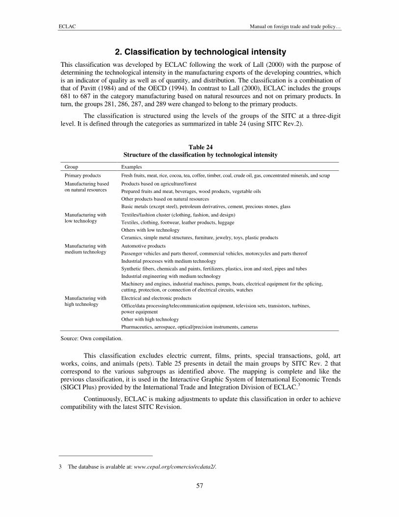
ECLAC Manual on foreign trade and trade policy…
57
2. Classification by technological intensityThis classification was developed by ECLAC following the work of Lall (2000) with the purpose ofdetermining the technological intensity in the manufacturing exports of the developing countries, whichis an indicator of quality as well as of quantity, and distribution. The classification is a combination ofthat of Pavitt (1984) and of the OECD (1994). In contrast to Lall (2000), ECLAC includes the groups681 to 687 in the category manufacturing based on natural resources and not on primary products. Inturn, the groups 281, 286, 287, and 289 were changed to belong to the primary products.
The classification is structured using the levels of the groups of the SITC at a three-digitlevel. It is defined through the categories as summarized in table 24 (using SITC Rev.2).
Table 24Structure of the classification by technological intensity
Group Examples
Primary products Fresh fruits, meat, rice, cocoa, tea, coffee, timber, coal, crude oil, gas, concentrated minerals, and scrap
Manufacturing basedon natural resources
Products based on agriculture/forest
Prepared fruits and meat, beverages, wood products, vegetable oils
Other products based on natural resources
Basic metals (except steel), petroleum derivatives, cement, precious stones, glass
Manufacturing withlow technology
Textiles/fashion cluster (clothing, fashion, and design)
Textiles, clothing, footwear, leather products, luggage
Others with low technology
Ceramics, simple metal structures, furniture, jewelry, toys, plastic products
Manufacturing withmedium technology
Automotive products
Passenger vehicles and parts thereof, commercial vehicles, motorcycles and parts thereof
Industrial processes with medium technology
Synthetic fibers, chemicals and paints, fertilizers, plastics, iron and steel, pipes and tubes
Industrial engineering with medium technology
Machinery and engines, industrial machines, pumps, boats, electrical equipment for the splicing,cutting, protection, or connection of electrical circuits, watches
Manufacturing withhigh technology
Electrical and electronic products
Office/data processing/telecommunication equipment, television sets, transistors, turbines,power equipment
Other with high technology
Pharmaceutics, aerospace, optical/precision instruments, cameras
Source: Own compilation.
This classification excludes electric current, films, prints, special transactions, gold, artworks, coins, and animals (pets). Table 25 presents in detail the main groups by SITC Rev. 2 thatcorrespond to the various subgroups as identified above. The mapping is complete and like theprevious classification, it is used in the Interactive Graphic System of International Economic Trends(SIGCI Plus) provided by the International Trade and Integration Division of ECLAC.3
Continuously, ECLAC is making adjustments to update this classification in order to achievecompatibility with the latest SITC Revision.
3 The database is avalable at: www.cepal.org/comercio/ecdata2/.
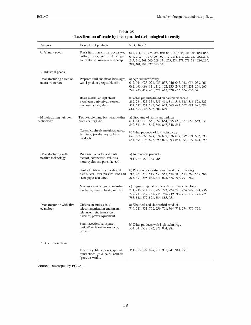
ECLAC Manual on foreign trade and trade policy…
58
Table 25Classification of trade by incorporated technological intensity
Category Examples of products SITC, Rev.2
A. Primary goods Fresh fruits, meat, rice, cocoa, tea,coffee, timber, coal, crude oil, gas,concentrated minerals, and scrap.
001, 011, 022, 025, 034, 036, 041, 042, 043, 044, 045, 054, 057,071, 072, 074, 075, 081, 091, 121, 211, 212, 222, 223, 232, 244,245, 246, 261, 263, 268, 271, 273, 274, 277, 278, 281, 286, 287,289, 291, 292, 322, 333, 341.
B. Industrial goods
- Manufacturing based onnatural resources
Prepared fruit and meat, beverages,wood products, vegetable oils.
Basic metals (except steel),petroleum derivatives, cement,precious stones, glass
a) Agriculture/forestry012, 014, 023, 024, 035, 037, 046, 047, 048, 056, 058, 061,062, 073, 098, 111, 112, 122, 233, 247, 248, 251, 264, 265,269, 423, 424, 431, 621, 625, 628, 633, 634, 635, 641.
b) Other products based on natural resources282, 288, 323, 334, 335, 411, 511, 514, 515, 516, 522, 523,531, 532, 551, 592, 661, 662, 663, 664, 667, 681, 682, 683,684, 685, 686, 687, 688, 689.
- Manufacturing with lowtechnology
Textiles, clothing, footwear, leatherproducts, luggage
Ceramics, simple metal structures,furniture, jewelry, toys, plasticproducts
a) Grouping of textile and fashion611, 612, 613, 651, 652, 654, 655, 656, 657, 658, 659, 831,842, 843, 844, 845, 846, 847, 848, 851.
b) Other products of low technology642, 665, 666, 673, 674, 675, 676, 677, 679, 691, 692, 693,694, 695, 696, 697, 699, 821, 893, 894, 895, 897, 898, 899.
- Manufacturing withmedium technology
Passenger vehicles and partsthereof, commercial vehicles,motorcycles and parts thereof
Synthetic fibers, chemicals andpaints, fertilizers, plastics, iron andsteel, pipes and tubes
Machinery and engines, industrialmachines, pumps, boats, watches
a) Automotive products
781, 782, 783, 784, 785.
b) Processing industries with medium technology266, 267, 512, 513, 533, 553, 554, 562, 572, 582, 583, 584,585, 591, 598, 653, 671, 672, 678, 786, 791, 882.
c) Engineering industries with medium technology711, 713, 714, 721, 722, 723, 724, 725, 726, 727, 728, 736,737, 741, 742, 743, 744, 745, 749, 762, 763, 772, 773, 775,793, 812, 872, 873, 884, 885, 951.
- Manufacturing with hightechnology
Office/data processing/telecommunication equipment,television sets, transistors,turbines, power equipment
Pharmaceutics, aerospace,optical/precision instruments,cameras
a) Electrical and electronical products716, 718, 751, 752, 759, 761, 764, 771, 774, 776, 778.
b) Other products with high technology524, 541, 712, 792, 871, 874, 881.
C. Other transactions
Electricity, films, prints, specialtransactions, gold, coins, animals(pets, art works.
351, 883, 892, 896, 911, 931, 941, 961, 971.
Source: Developed by ECLAC.
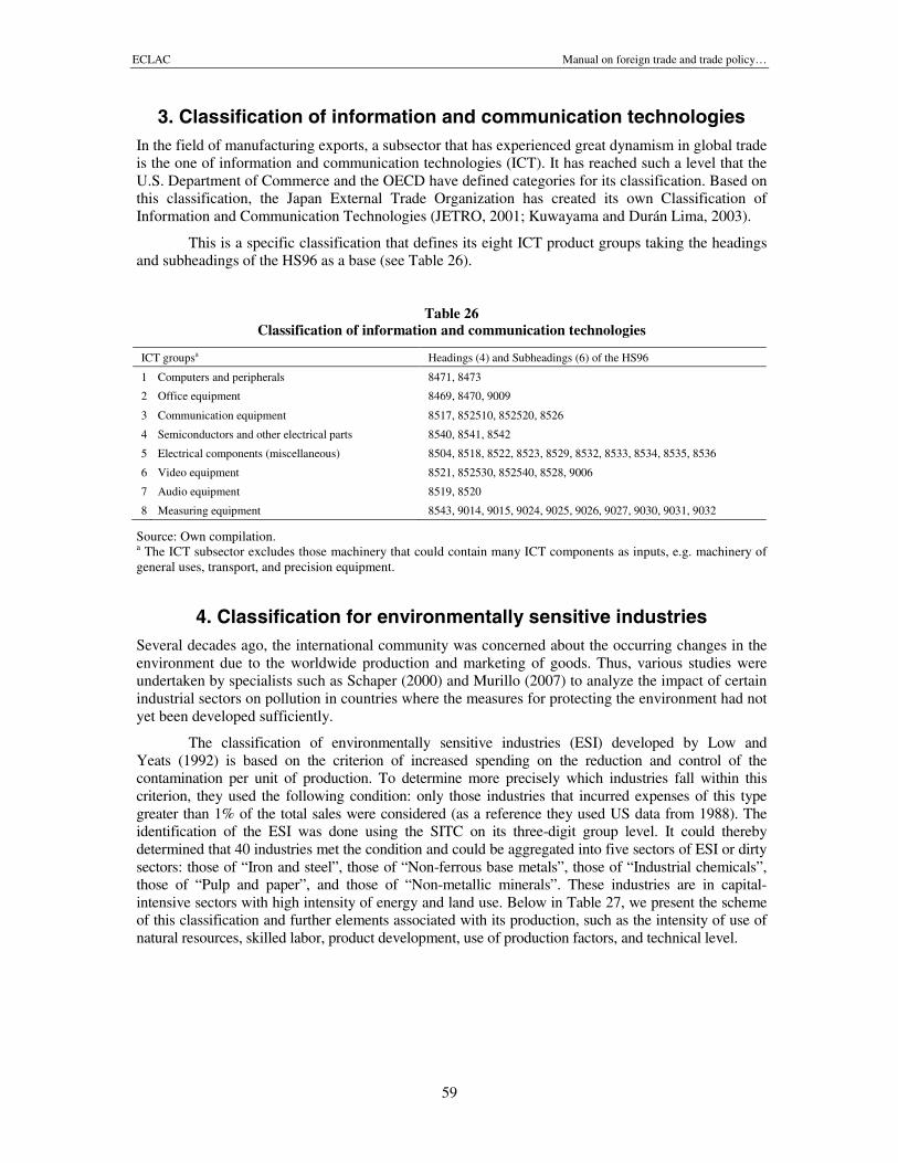
ECLAC Manual on foreign trade and trade policy…
59
3. Classification of information and communication technologiesIn the field of manufacturing exports, a subsector that has experienced great dynamism in global tradeis the one of information and communication technologies (ICT). It has reached such a level that theU.S. Department of Commerce and the OECD have defined categories for its classification. Based onthis classification, the Japan External Trade Organization has created its own Classification ofInformation and Communication Technologies (JETRO, 2001; Kuwayama and Durán Lima, 2003).
This is a specific classification that defines its eight ICT product groups taking the headingsand subheadings of the HS96 as a base (see Table 26).
Table 26Classification of information and communication technologies
ICT groupsa Headings (4) and Subheadings (6) of the HS96
1 Computers and peripherals 8471, 8473
2 Office equipment 8469, 8470, 9009
3 Communication equipment 8517, 852510, 852520, 8526
4 Semiconductors and other electrical parts 8540, 8541, 8542
5 Electrical components (miscellaneous) 8504, 8518, 8522, 8523, 8529, 8532, 8533, 8534, 8535, 8536
6 Video equipment 8521, 852530, 852540, 8528, 9006
7 Audio equipment 8519, 8520
8 Measuring equipment 8543, 9014, 9015, 9024, 9025, 9026, 9027, 9030, 9031, 9032
Source: Own compilation.a The ICT subsector excludes those machinery that could contain many ICT components as inputs, e.g. machinery ofgeneral uses, transport, and precision equipment.
4. Classification for environmentally sensitive industriesSeveral decades ago, the international community was concerned about the occurring changes in theenvironment due to the worldwide production and marketing of goods. Thus, various studies wereundertaken by specialists such as Schaper (2000) and Murillo (2007) to analyze the impact of certainindustrial sectors on pollution in countries where the measures for protecting the environment had notyet been developed sufficiently.
The classification of environmentally sensitive industries (ESI) developed by Low andYeats (1992) is based on the criterion of increased spending on the reduction and control of thecontamination per unit of production. To determine more precisely which industries fall within thiscriterion, they used the following condition: only those industries that incurred expenses of this typegreater than 1% of the total sales were considered (as a reference they used US data from 1988). Theidentification of the ESI was done using the SITC on its three-digit group level. It could therebydetermined that 40 industries met the condition and could be aggregated into five sectors of ESI or dirtysectors: those of “Iron and steel”, those of “Non-ferrous base metals”, those of “Industrial chemicals”,those of “Pulp and paper”, and those of “Non-metallic minerals”. These industries are in capital-intensive sectors with high intensity of energy and land use. Below in Table 27, we present the schemeof this classification and further elements associated with its production, such as the intensity of use ofnatural resources, skilled labor, product development, use of production factors, and technical level.
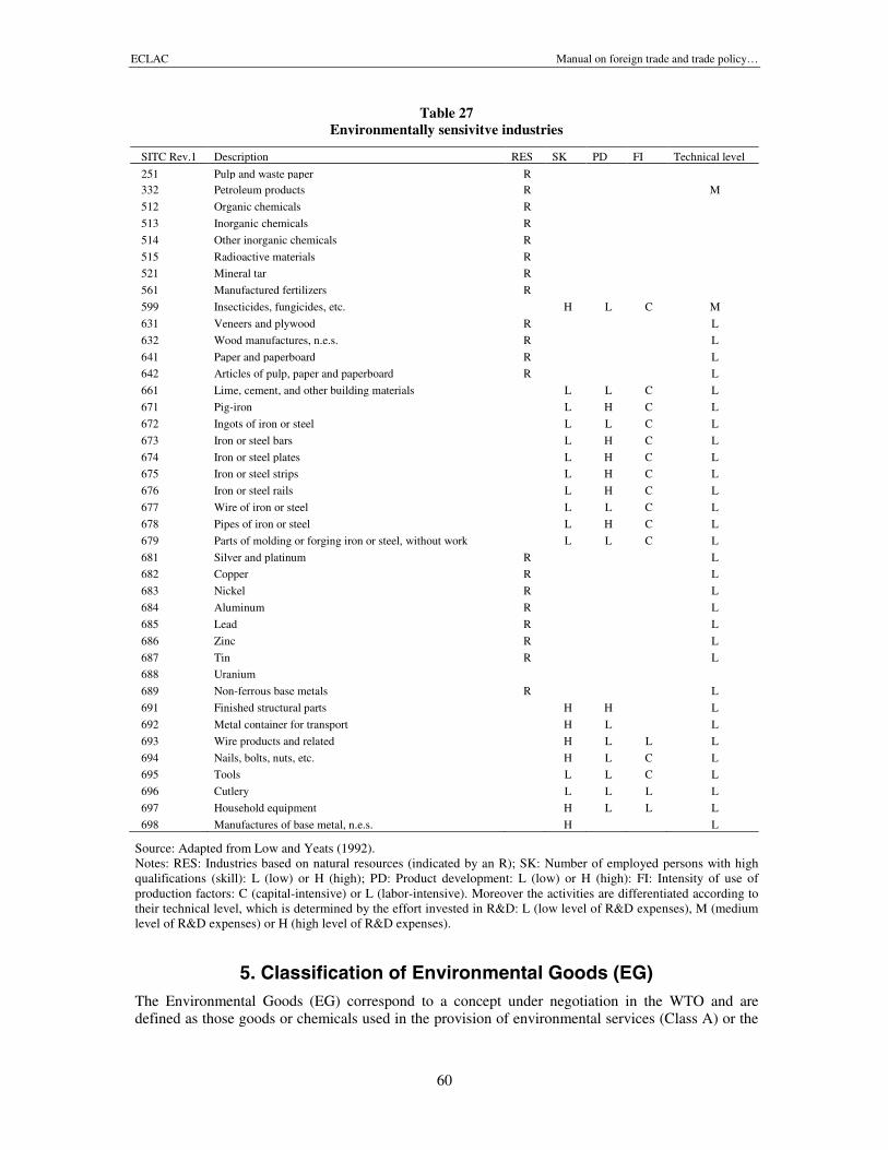
ECLAC Manual on foreign trade and trade policy…
60
Table 27Environmentally sensivitve industries
SITC Rev.1 Description RES SK PD FI Technical level
251 Pulp and waste paper R332 Petroleum products R M
512 Organic chemicals R
513 Inorganic chemicals R
514 Other inorganic chemicals R
515 Radioactive materials R
521 Mineral tar R
561 Manufactured fertilizers R
599 Insecticides, fungicides, etc. H L C M
631 Veneers and plywood R L
632 Wood manufactures, n.e.s. R L
641 Paper and paperboard R L
642 Articles of pulp, paper and paperboard R L
661 Lime, cement, and other building materials L L C L
671 Pig-iron L H C L
672 Ingots of iron or steel L L C L
673 Iron or steel bars L H C L
674 Iron or steel plates L H C L
675 Iron or steel strips L H C L
676 Iron or steel rails L H C L
677 Wire of iron or steel L L C L
678 Pipes of iron or steel L H C L
679 Parts of molding or forging iron or steel, without work L L C L
681 Silver and platinum R L
682 Copper R L
683 Nickel R L
684 Aluminum R L
685 Lead R L
686 Zinc R L
687 Tin R L
688 Uranium
689 Non-ferrous base metals R L
691 Finished structural parts H H L
692 Metal container for transport H L L
693 Wire products and related H L L L
694 Nails, bolts, nuts, etc. H L C L
695 Tools L L C L
696 Cutlery L L L L
697 Household equipment H L L L
698 Manufactures of base metal, n.e.s. H L
Source: Adapted from Low and Yeats (1992).Notes: RES: Industries based on natural resources (indicated by an R); SK: Number of employed persons with highqualifications (skill): L (low) or H (high); PD: Product development: L (low) or H (high): FI: Intensity of use ofproduction factors: C (capital-intensive) or L (labor-intensive). Moreover the activities are differentiated according totheir technical level, which is determined by the effort invested in R&D: L (low level of R&D expenses), M (mediumlevel of R&D expenses) or H (high level of R&D expenses).
5. Classification of Environmental Goods (EG)The Environmental Goods (EG) correspond to a concept under negotiation in the WTO and aredefined as those goods or chemicals used in the provision of environmental services (Class A) or the
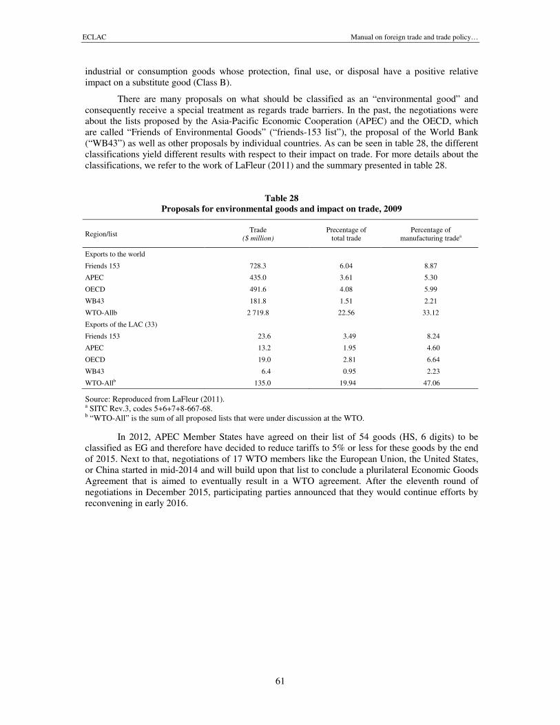
ECLAC Manual on foreign trade and trade policy…
61
industrial or consumption goods whose protection, final use, or disposal have a positive relativeimpact on a substitute good (Class B).
There are many proposals on what should be classified as an “environmental good” andconsequently receive a special treatment as regards trade barriers. In the past, the negotiations wereabout the lists proposed by the Asia-Pacific Economic Cooperation (APEC) and the OECD, whichare called “Friends of Environmental Goods” (“friends-153 list”), the proposal of the World Bank(“WB43”) as well as other proposals by individual countries. As can be seen in table 28, the differentclassifications yield different results with respect to their impact on trade. For more details about theclassifications, we refer to the work of LaFleur (2011) and the summary presented in table 28.
Table 28Proposals for environmental goods and impact on trade, 2009
Region/listTrade
($ million)Precentage of
total tradePercentage of
manufacturing tradea
Exports to the world
Friends 153 728.3 6.04 8.87
APEC 435.0 3.61 5.30
OECD 491.6 4.08 5.99
WB43 181.8 1.51 2.21
WTO-Allb 2 719.8 22.56 33.12
Exports of the LAC (33)
Friends 153 23.6 3.49 8.24
APEC 13.2 1.95 4.60
OECD 19.0 2.81 6.64
WB43 6.4 0.95 2.23
WTO-Allb 135.0 19.94 47.06
Source: Reproduced from LaFleur (2011).a SITC Rev.3, codes 5+6+7+8-667-68.b “WTO-All” is the sum of all proposed lists that were under discussion at the WTO.
In 2012, APEC Member States have agreed on their list of 54 goods (HS, 6 digits) to beclassified as EG and therefore have decided to reduce tariffs to 5% or less for these goods by the endof 2015. Next to that, negotiations of 17 WTO members like the European Union, the United States,or China started in mid-2014 and will build upon that list to conclude a plurilateral Economic GoodsAgreement that is aimed to eventually result in a WTO agreement. After the eleventh round ofnegotiations in December 2015, participating parties announced that they would continue efforts byreconvening in early 2016.

ECLAC Manual on foreign trade and trade policy…
63
VI. Basic indicators of trade pattern
The main data of foreign trade correspond to the components of the current account, namely the exportsand imports of goods and services. The basic indicators are widely known and define a profound measureof a country’s (or more generally speaking an economy’s) level of internationalization. In this section, wewill analyze the definitions and use of these key trade indicators.
A. Export value of goods and services
The exports correspond to the set of goods and services that are sold from residents of one economyto residents of another economy. In other words, they correspond to the proportion of domesticproduction that is not consumed within the economy or stored, but sold abroad. The analysis ofexport is important at least in three dimensions (i) the structure, (ii) the evolution (or dynamics), and(iii) its record and measurement.
Regarding the composition of exports, it is necessary to note that the type of productsincluded in the majority of the export structure of goods will determine the trade pattern of thatcountry. Thus, the prevalence of natural resources in the total exports of goods hints on largeadvantages in that category. The same holds for the trade in services, which are more or lesscomplementary indicators to the trade in goods and allow a broad view on the real effect ofglobalization on production patterns in a more and more intertwined world.
Moreover, the evolution of exports in goods and services identified by the annual variationor the average rate of growth in a given period is indicative for the contribution of exports to GDPgrowth. Recently, we observe that more studies try to analyze the determinants of the evolution ofglobal trade in services.
As regards the record and measurement export activities, it can be noted that for the case ofgoods, the customs prepare a list of products and their individual characteristics. In the case of services,one can follow the guidelines defined in the Balance of Payments Manual (most recent version BPM6of 2013) and/or Quarterly National Accounts Manual, both drafted by the IMF, as well as in theManual on Statistics of International Trade in Services (most recent version MSITS 2010, revisedin 2013) which is a joint publication of UNSD, the Statistical Office of the European Union, IMF,OECD, UNCTAD, World Tourism Organization, and WTO; see also Durán Lima and Alvarez (2013).
ECLAC Manual on foreign trade and trade policy…
64
Additionally, a combination of all of these three dimensions in the long term can help tounderstand to a certain degree the evolution of the development strategy of the country at hand.Obviously, this comes along with the utilization of other indicators that require the disaggregation ofbasic export data at the product and destination level. This in turn will be discussed in the secondsection of this chapter.
Although it has already been pointed out, the reader is reminded that exports may be goodsand/or services with the goods being tangible items that occupy physical space in an internationalmean of transport (truck, train, ship, or plane) passing through the customs. The services are by theirnature “intangible” and so their tradability is not discussed. Thus, the MSITS adds to the definitionof international trade in services the value of those services provided through subsidiaries abroad.Moreover, it includes the services provided by persons staying abroad, either as service providers oras employees of suppliers.
Section C presents some considerations about the statistics in services which are a bit morecomplicated to systematize and to measure according to its special treatment, compared to the tradein goods that is easier to record as the objects pass the customs.
B. Import value of goods and services
The concept of imports is exactly opposite to that of exports, i.e. it is the set of all goods andservices bought by the residents of an economy from residents of another. If exports measure theshare of domestic production that is consumed outside of a country, the imports evaluate theproportion of domestic consumption of goods that is not produced inside the country. Again, westress here the importance of all dimensions of such an indicator like structure and dynamics.
Considering the components, the imports can also be goods and services. Due to its highcomplementarity, we observe a steadily increasing number of international service activities that areinvolved in the structural transformation of transnational companies. In 2014, services generatedmore than 80% of the valued-added in Luxembourg and Greece and 60% or more in the rest of theOECD countries (World Bank, n.d.). Lately, companies have become more internationalized than inthe past and the production is distributed in numerous geographical regions within or outsidenational borders (Durán Lima and Ventura-Dias, 2003).
In case of the goods, the recording and measurement is normally undertaken usingclassification criteria based on comprehensive product lists that in turn are related to the level ofcustoms protection.
C. Statistics of trade in services
The trade in services in Latin America has experienced continuing growth in more than the lasttwenty-five years with remarkable acceleration in the 2000s, especially in the category “Otherservices”. It also showed a higher rate than that of exports in goods and services in general (seefigure 9). This leads to an increased need of improving the statistics with which the calculations aremade, in order to be able to derive better trade promotion policies or to raise more beneficial clausesin trade agreements based on a profound understanding of the sector.
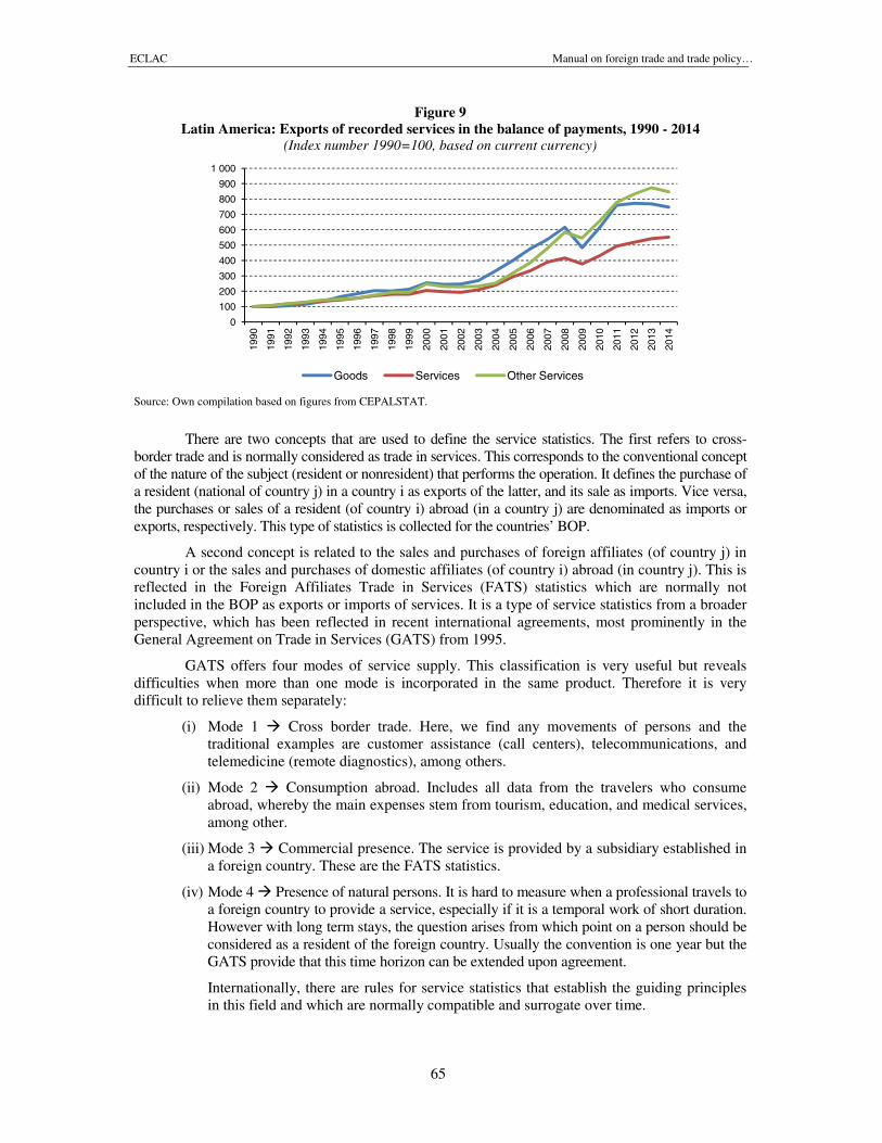
ECLAC Manual on foreign trade and trade policy…
65
Figure 9Latin America: Exports of recorded services in the balance of payments, 1990 - 2014
(Index number 1990=100, based on current currency)
Source: Own compilation based on figures from CEPALSTAT.
There are two concepts that are used to define the service statistics. The first refers to cross-border trade and is normally considered as trade in services. This corresponds to the conventional conceptof the nature of the subject (resident or nonresident) that performs the operation. It defines the purchase ofa resident (national of country j) in a country i as exports of the latter, and its sale as imports. Vice versa,the purchases or sales of a resident (of country i) abroad (in a country j) are denominated as imports orexports, respectively. This type of statistics is collected for the countries’ BOP.
A second concept is related to the sales and purchases of foreign affiliates (of country j) incountry i or the sales and purchases of domestic affiliates (of country i) abroad (in country j). This isreflected in the Foreign Affiliates Trade in Services (FATS) statistics which are normally notincluded in the BOP as exports or imports of services. It is a type of service statistics from a broaderperspective, which has been reflected in recent international agreements, most prominently in theGeneral Agreement on Trade in Services (GATS) from 1995.
GATS offers four modes of service supply. This classification is very useful but revealsdifficulties when more than one mode is incorporated in the same product. Therefore it is verydifficult to relieve them separately:
(i) Mode 1 Cross border trade. Here, we find any movements of persons and thetraditional examples are customer assistance (call centers), telecommunications, andtelemedicine (remote diagnostics), among others.
(ii) Mode 2 Consumption abroad. Includes all data from the travelers who consumeabroad, whereby the main expenses stem from tourism, education, and medical services,among other.
(iii) Mode 3 Commercial presence. The service is provided by a subsidiary established ina foreign country. These are the FATS statistics.
(iv) Mode 4 Presence of natural persons. It is hard to measure when a professional travels toa foreign country to provide a service, especially if it is a temporal work of short duration.However with long term stays, the question arises from which point on a person should beconsidered as a resident of the foreign country. Usually the convention is one year but theGATS provide that this time horizon can be extended upon agreement.
Internationally, there are rules for service statistics that establish the guiding principlesin this field and which are normally compatible and surrogate over time.
0
100
200
300
400
500
600
700
800
900
1 000
1990
1991
1992
1993
1994
1995
1996
1997
1998
1999
2000
2001
2002
2003
2004
2005
2006
2007
2008
2009
2010
2011
2012
2013
2014
Goods Services Other Services
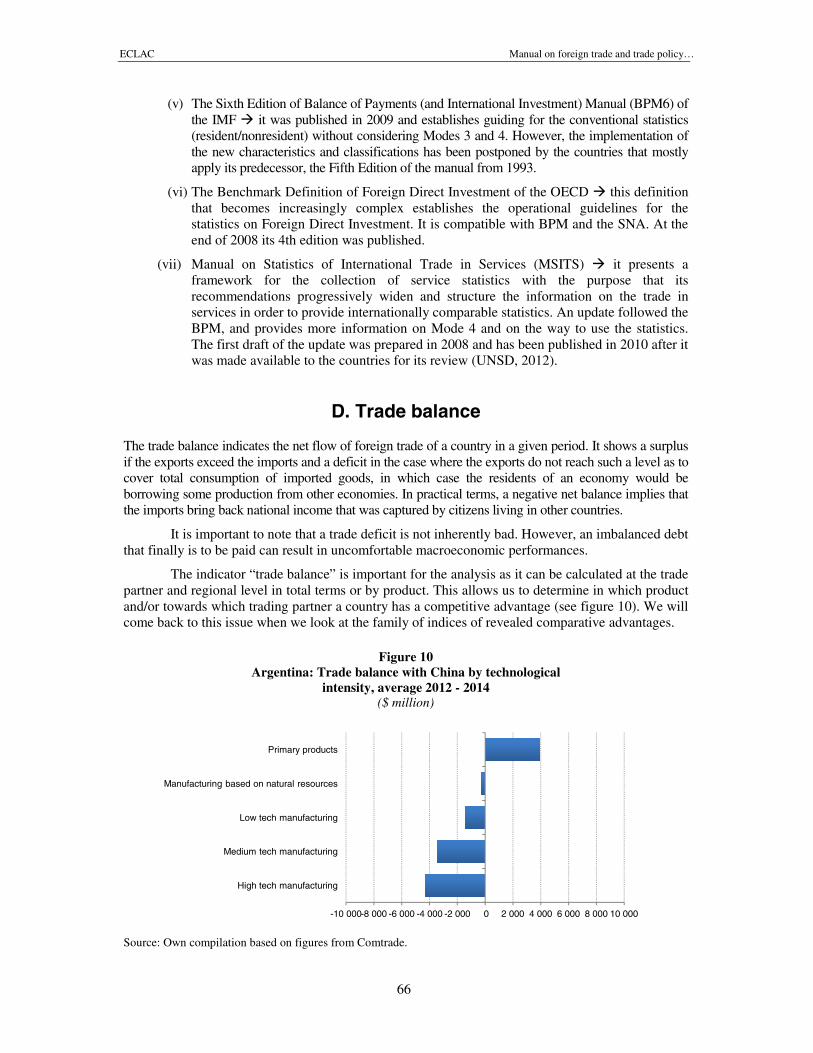
ECLAC Manual on foreign trade and trade policy…
66
(v) The Sixth Edition of Balance of Payments (and International Investment) Manual (BPM6) ofthe IMF it was published in 2009 and establishes guiding for the conventional statistics(resident/nonresident) without considering Modes 3 and 4. However, the implementation ofthe new characteristics and classifications has been postponed by the countries that mostlyapply its predecessor, the Fifth Edition of the manual from 1993.
(vi) The Benchmark Definition of Foreign Direct Investment of the OECD this definitionthat becomes increasingly complex establishes the operational guidelines for thestatistics on Foreign Direct Investment. It is compatible with BPM and the SNA. At theend of 2008 its 4th edition was published.
(vii) Manual on Statistics of International Trade in Services (MSITS) it presents aframework for the collection of service statistics with the purpose that itsrecommendations progressively widen and structure the information on the trade inservices in order to provide internationally comparable statistics. An update followed theBPM, and provides more information on Mode 4 and on the way to use the statistics.The first draft of the update was prepared in 2008 and has been published in 2010 after itwas made available to the countries for its review (UNSD, 2012).
D. Trade balance
The trade balance indicates the net flow of foreign trade of a country in a given period. It shows a surplusif the exports exceed the imports and a deficit in the case where the exports do not reach such a level as tocover total consumption of imported goods, in which case the residents of an economy would beborrowing some production from other economies. In practical terms, a negative net balance implies thatthe imports bring back national income that was captured by citizens living in other countries.
It is important to note that a trade deficit is not inherently bad. However, an imbalanced debtthat finally is to be paid can result in uncomfortable macroeconomic performances.
The indicator “trade balance” is important for the analysis as it can be calculated at the tradepartner and regional level in total terms or by product. This allows us to determine in which productand/or towards which trading partner a country has a competitive advantage (see figure 10). We willcome back to this issue when we look at the family of indices of revealed comparative advantages.
Figure 10Argentina: Trade balance with China by technological
intensity, average 2012 - 2014($ million)
Source: Own compilation based on figures from Comtrade.
-10 000-8 000 -6 000 -4 000 -2 000 0 2 000 4 000 6 000 8 000 10 000
High tech manufacturing
Medium tech manufacturing
Low tech manufacturing
Manufacturing based on natural resources
Primary products
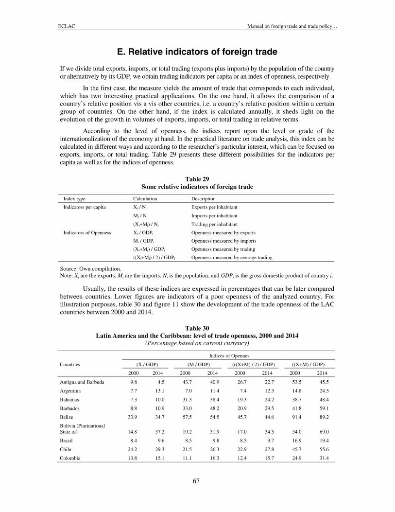
ECLAC Manual on foreign trade and trade policy…
67
E. Relative indicators of foreign trade
If we divide total exports, imports, or total trading (exports plus imports) by the population of the countryor alternatively by its GDP, we obtain trading indicators per capita or an index of openness, respectively.
In the first case, the measure yields the amount of trade that corresponds to each individual,which has two interesting practical applications. On the one hand, it allows the comparison of acountry’s relative position vis a vis other countries, i.e. a country’s relative position within a certaingroup of countries. On the other hand, if the index is calculated annually, it sheds light on theevolution of the growth in volumes of exports, imports, or total trading in relative terms.
According to the level of openness, the indices report upon the level or grade of theinternationalization of the economy at hand. In the practical literature on trade analysis, this index can becalculated in different ways and according to the researcher’s particular interest, which can be focused onexports, imports, or total trading. Table 29 presents these different possibilities for the indicators percapita as well as for the indices of openness.
Table 29Some relative indicators of foreign trade
Index type Calculation Description
Indicators per capita Xi / Ni Exports per inhabitant
Mi / Ni Imports per inhabitant
(Xi+Mi) / Ni Trading per inhabitant
Indicators of Openness Xi / GDPi Openness measured by exports
Mi / GDPi Openness measured by imports
(Xi+Mi) / GDPi Openness measured by trading
((Xi+Mi) / 2) / GDPi Openness measured by average trading
Source: Own compilation.Note: Xi are the exports, Mi are the imports, Ni is the population, and GDPi is the gross domestic product of country i.
Usually, the results of these indices are expressed in percentages that can be later comparedbetween countries. Lower figures are indicators of a poor openness of the analyzed country. Forillustration purposes, table 30 and figure 11 show the development of the trade openness of the LACcountries between 2000 and 2014.
Table 30Latin America and the Caribbean: level of trade openness, 2000 and 2014
(Percentage based on current currency)
Indices of Opennes
Countries (X / GDP) (M / GDP) (((X+M) / 2) / GDP) ((X+M) / GDP)
2000 2014 2000 2014 2000 2014 2000 2014
Antigua and Barbuda 9.8 4.5 43.7 40.9 26.7 22.7 53.5 45.5
Argentina 7.7 13.1 7.0 11.4 7.4 12.3 14.8 24.5
Bahamas 7.3 10.0 31.3 38.4 19.3 24.2 38.7 48.4
Barbados 8.8 10.9 33.0 48.2 20.9 29.5 41.8 59.1
Belize 33.9 34.7 57.5 54.5 45.7 44.6 91.4 89.2
Bolivia (PlurinationalState of) 14.8 37.2 19.2 31.9 17.0 34.5 34.0 69.0
Brazil 8.4 9.6 8.5 9.8 8.5 9.7 16.9 19.4
Chile 24.2 29.3 21.5 26.3 22.9 27.8 45.7 55.6
Colombia 13.8 15.1 11.1 16.3 12.4 15.7 24.9 31.4
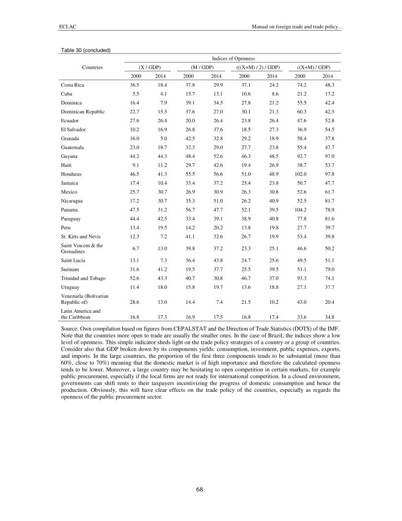
ECLAC Manual on foreign trade and trade policy…
68
Table 30 (concluded)
Indices of Openness
Countries (X / GDP) (M / GDP) (((X+M) / 2) / GDP) ((X+M) / GDP)
2000 2014 2000 2014 2000 2014 2000 2014
Costa Rica 36.5 18.4 37.8 29.9 37.1 24.2 74.2 48.3
Cuba 5.5 4.1 15.7 13.1 10.6 8.6 21.2 17.2
Dominica 16.4 7.9 39.1 34.5 27.8 21.2 55.5 42.4
Dominican Republic 22.7 15.5 37.6 27.0 30.1 21.3 60.3 42.5
Ecuador 27.6 26.4 20.0 26.4 23.8 26.4 47.6 52.8
El Salvador 10.2 16.9 26.8 37.6 18.5 27.3 36.9 54.5
Granada 16.0 5.0 42.5 32.8 29.2 18.9 58.4 37.8
Guatemala 23.0 18.7 32.3 29.0 27.7 23.8 55.4 47.7
Guyana 44.2 44.3 48.4 52.6 46.3 48.5 92.7 97.0
Haiti 9.1 11.2 29.7 42.6 19.4 26.9 38.7 53.7
Honduras 46.5 41.3 55.5 56.6 51.0 48.9 102.0 97.8
Jamaica 17.4 10.4 33.4 37.2 25.4 23.8 50.7 47.7
Mexico 25.7 30.7 26.9 30.9 26.3 30.8 52.6 61.7
Nicaragua 17.2 30.7 35.3 51.0 26.2 40.9 52.5 81.7
Panama 47.5 31.2 56.7 47.7 52.1 39.5 104.2 78.9
Paraguay 44.4 42.5 33.4 39.1 38.9 40.8 77.8 81.6
Peru 13.4 19.5 14.2 20.2 13.8 19.8 27.7 39.7
St. Kitts and Nevis 12.3 7.2 41.1 32.6 26.7 19.9 53.4 39.8
Saint Vincent & theGrenadines
6.7 13.0 39.8 37.2 23.3 25.1 46.6 50.2
Saint Lucia 13.1 7.3 36.4 43.8 24.7 25.6 49.5 51.1
Surinam 31.6 41.2 19.5 37.7 25.5 39.5 51.1 79.0
Trinidad and Tobago 52.6 43.3 40.7 30.8 46.7 37.0 93.3 74.1
Uruguay 11.4 18.0 15.8 19.7 13.6 18.8 27.1 37.7
Venezuela (BolivarianRepublic of) 28.6 13.0 14.4 7.4 21.5 10.2 43.0 20.4
Latin America andthe Caribbean 16.8 17.3 16.9 17.5 16.8 17.4 33.6 34.8
Source: Own compilation based on figures from CEPALSTAT and the Direction of Trade Statistics (DOTS) of the IMF.Note that the countries more open to trade are usually the smaller ones. In the case of Brazil, the indices show a lowlevel of openness. This simple indicator sheds light on the trade policy strategies of a country or a group of countries.Consider also that GDP broken down by its components yields: consumption, investment, public expenses, exports,and imports. In the large countries, the proportion of the first three components tends to be substantial (more than60%, close to 70%) meaning that the domestic market is of high importance and therefore the calculated opennesstends to be lower. Moreover, a large country may be hesitating to open competition in certain markets, for examplepublic procurement, especially if the local firms are not ready for international competition. In a closed environment,governments can shift rents to their taxpayers incentivizing the progress of domestic consumption and hence theproduction. Obviously, this will have clear effects on the trade policy of the countries, especially as regards theopenness of the public procurement sector.
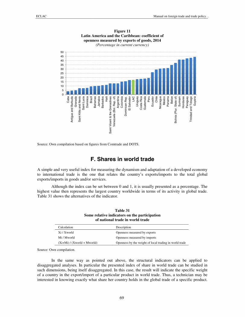
ECLAC
Latin America and theopenness measured by exports of goods
Source: Own compilation based on figures from Comtrade and DOTS.
F. Shares in
A simple and very useful index for measuring the dynamism and adaptation of a developed economyto international trade is the one that relates the country’s exports/imports to the total globalexports/imports in goods and/or services.
Although the index can be set between 0 and 1, it is usually presented as a percentage. Thehighest value then represents the largest country worldwide in terms of its activity in global trade.Table 31 shows the alternatives of the indicator.
Some
Calculation
Xi / Xworld
Mi / Mworld
(Xi+Mi) / (Xworld + Mworld)
Source: Own compilation.
In the same way as pointed out above, the structural indicators can be applied todisaggregated analyses. In particular the presented index of share in world trade can be studied insuch dimensions, being itself disaggregated. In this case, the result will indicate the specific weightof a country in the export/import of a particular product in world trade. Thus, a technician may beinterested in knowing exactly what share her country holds in the global trade of
0
5
10
15
20
25
30
35
40
45
50
Cub
aA
ntig
uaan
dB
arbu
daG
rana
daS
aint
Kitt
san
dN
evis
Sai
ntLu
cia
Dom
inic
aB
razi
l
Manual on foreign trade and trade policy
69
Figure 11Latin America and the Caribbean: coefficient of
openness measured by exports of goods, 2014(Percentage in current currency)
wn compilation based on figures from Comtrade and DOTS.
F. Shares in world trade
A simple and very useful index for measuring the dynamism and adaptation of a developed economyto international trade is the one that relates the country’s exports/imports to the total globalexports/imports in goods and/or services.
the index can be set between 0 and 1, it is usually presented as a percentage. Thehighest value then represents the largest country worldwide in terms of its activity in global trade.Table 31 shows the alternatives of the indicator.
Table 31ome relative indicators on the participation
of national trade in world trade
Description
Openness measured by exports
Openness measured by imports
(Xi+Mi) / (Xworld + Mworld) Openness by the weight of local trading in world trade
In the same way as pointed out above, the structural indicators can be applied todisaggregated analyses. In particular the presented index of share in world trade can be studied in
disaggregated. In this case, the result will indicate the specific weightof a country in the export/import of a particular product in world trade. Thus, a technician may beinterested in knowing exactly what share her country holds in the global trade of a specific product.
Bra
zil
Bah
amas
Jam
aica
Bar
bado
sH
aiti
Sai
ntV
icen
t&
the
Gre
nadi
nes
Ven
ezue
la(B
ol.R
ep.
of)
Arg
entin
aC
olom
bia
Dom
inic
anR
ep.
ElS
alva
dor
LAC
Uru
guay
Cos
taR
ica
Gua
tem
ala
Per
uE
cuad
orC
hile
Nic
arag
uaM
exic
oP
anam
aB
eliz
eB
oliv
ia(P
lur.
Sta
teof
)S
urin
amH
ondu
ras
oreign trade and trade policy…
A simple and very useful index for measuring the dynamism and adaptation of a developed economyto international trade is the one that relates the country’s exports/imports to the total global
the index can be set between 0 and 1, it is usually presented as a percentage. Thehighest value then represents the largest country worldwide in terms of its activity in global trade.
trade
In the same way as pointed out above, the structural indicators can be applied todisaggregated analyses. In particular the presented index of share in world trade can be studied in
disaggregated. In this case, the result will indicate the specific weightof a country in the export/import of a particular product in world trade. Thus, a technician may be
a specific product.
Hon
dura
sP
arag
uay
Trin
idad
and
Tob
ago
Guy
ana
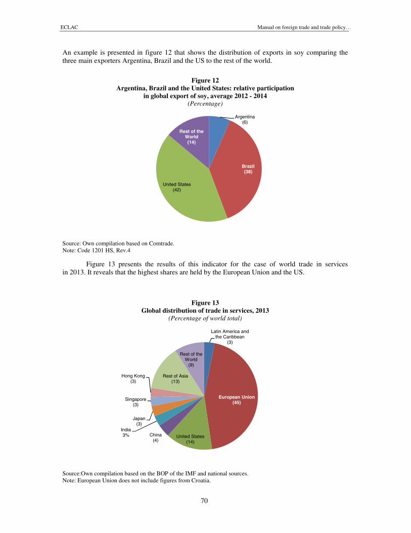
ECLAC Manual on foreign trade and trade policy…
70
An example is presented in figure 12 that shows the distribution of exports in soy comparing thethree main exporters Argentina, Brazil and the US to the rest of the world.
Figure 12Argentina, Brazil and the United States: relative participation
in global export of soy, average 2012 - 2014(Percentage)
Source: Own compilation based on Comtrade.Note: Code 1201 HS, Rev.4
Figure 13 presents the results of this indicator for the case of world trade in servicesin 2013. It reveals that the highest shares are held by the European Union and the US.
Figure 13Global distribution of trade in services, 2013
(Percentage of world total)
Source:Own compilation based on the BOP of the IMF and national sources.Note: European Union does not include figures from Croatia.
Argentina(6)
Brazil(38)
United States(42)
Rest of theWorld(14)
Latin America andthe Caribbean
(3)
European Union(45)
United States(14)
China(4)
India3%
Japan(3)
Singapore(3)
Hong Kong(3)
Rest of Asia(13)
Rest of theWorld
(9)
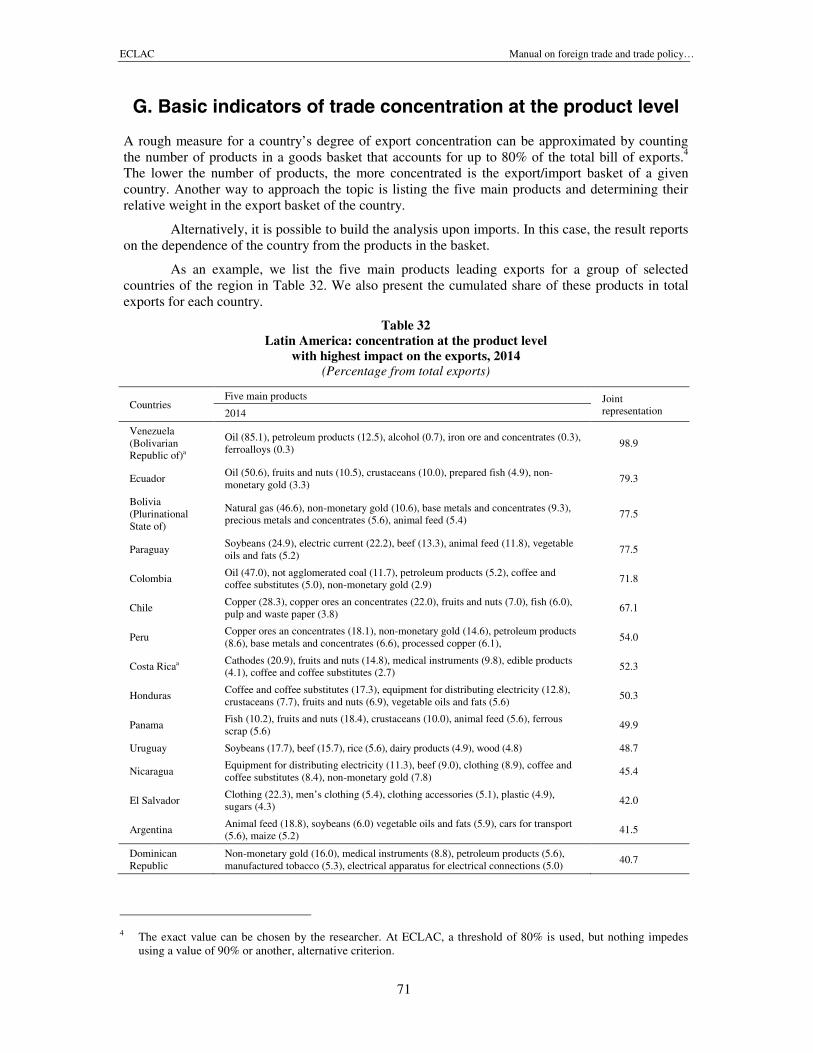
ECLAC Manual on foreign trade and trade policy…
71
G. Basic indicators of trade concentration at the product level
A rough measure for a country’s degree of export concentration can be approximated by countingthe number of products in a goods basket that accounts for up to 80% of the total bill of exports.4
The lower the number of products, the more concentrated is the export/import basket of a givencountry. Another way to approach the topic is listing the five main products and determining theirrelative weight in the export basket of the country.
Alternatively, it is possible to build the analysis upon imports. In this case, the result reportson the dependence of the country from the products in the basket.
As an example, we list the five main products leading exports for a group of selectedcountries of the region in Table 32. We also present the cumulated share of these products in totalexports for each country.
Table 32Latin America: concentration at the product level
with highest impact on the exports, 2014(Percentage from total exports)
CountriesFive main products Joint
representation2014
Venezuela(BolivarianRepublic of)a
Oil (85.1), petroleum products (12.5), alcohol (0.7), iron ore and concentrates (0.3),ferroalloys (0.3)
98.9
EcuadorOil (50.6), fruits and nuts (10.5), crustaceans (10.0), prepared fish (4.9), non-monetary gold (3.3)
79.3
Bolivia(PlurinationalState of)
Natural gas (46.6), non-monetary gold (10.6), base metals and concentrates (9.3),precious metals and concentrates (5.6), animal feed (5.4)
77.5
ParaguaySoybeans (24.9), electric current (22.2), beef (13.3), animal feed (11.8), vegetableoils and fats (5.2)
77.5
ColombiaOil (47.0), not agglomerated coal (11.7), petroleum products (5.2), coffee andcoffee substitutes (5.0), non-monetary gold (2.9)
71.8
ChileCopper (28.3), copper ores an concentrates (22.0), fruits and nuts (7.0), fish (6.0),pulp and waste paper (3.8)
67.1
PeruCopper ores an concentrates (18.1), non-monetary gold (14.6), petroleum products(8.6), base metals and concentrates (6.6), processed copper (6.1),
54.0
Costa Ricaa Cathodes (20.9), fruits and nuts (14.8), medical instruments (9.8), edible products(4.1), coffee and coffee substitutes (2.7)
52.3
HondurasCoffee and coffee substitutes (17.3), equipment for distributing electricity (12.8),crustaceans (7.7), fruits and nuts (6.9), vegetable oils and fats (5.6)
50.3
PanamaFish (10.2), fruits and nuts (18.4), crustaceans (10.0), animal feed (5.6), ferrousscrap (5.6)
49.9
Uruguay Soybeans (17.7), beef (15.7), rice (5.6), dairy products (4.9), wood (4.8) 48.7
NicaraguaEquipment for distributing electricity (11.3), beef (9.0), clothing (8.9), coffee andcoffee substitutes (8.4), non-monetary gold (7.8)
45.4
El SalvadorClothing (22.3), men’s clothing (5.4), clothing accessories (5.1), plastic (4.9),sugars (4.3)
42.0
ArgentinaAnimal feed (18.8), soybeans (6.0) vegetable oils and fats (5.9), cars for transport(5.6), maize (5.2)
41.5
DominicanRepublic
Non-monetary gold (16.0), medical instruments (8.8), petroleum products (5.6),manufactured tobacco (5.3), electrical apparatus for electrical connections (5.0)
40.7
4 The exact value can be chosen by the researcher. At ECLAC, a threshold of 80% is used, but nothing impedesusing a value of 90% or another, alternative criterion.
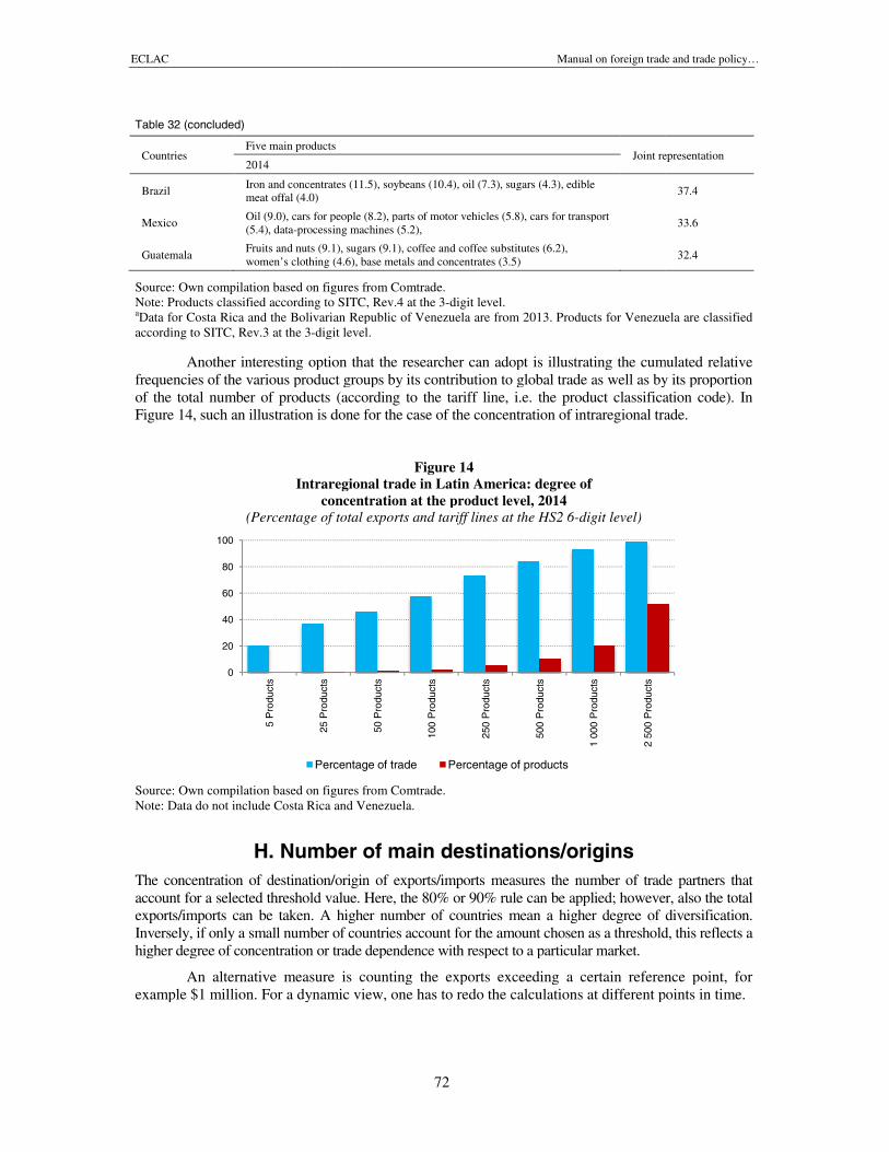
ECLAC
Table 32 (concluded)
CountriesFive main products
2014
BrazilIron and concentrates (11.5), soybeans (10.4), oil (7.3), sugars (4.3), ediblemeat offal (4.0)
MexicoOil (9.0), cars for people (8.2), parts of motor vehicles (5.8), cars for transport(5.4), data-processing machines (5.2),
GuatemalaFruits and nuts (9.1), sugars (9.1), coffee and coffee substitutes (6.2),women’s clothing (4.6), base metals and co
Source: Own compilation based on figures from Comtrade.Note: Products classified according to SITC, Rev.4 at the 3aData for Costa Rica and the Bolivarian Republic of Venezuela are from 2013. Products for Venezuela are classifiedaccording to SITC, Rev.3 at the 3-digit level.
Another interesting option that the researcher can adopt is illustrating the cumulated relativefrequencies of the various product groups by its contribution to global trade as well as by its proportionof the total number of products (according to the tariff line, i.e. the product classification code). InFigure 14, such an illustration is done for th
Intraregional trade in Latin Americaconcentration at the product level
(Percentage of total exports and tariff lines at the HS2 6
Source: Own compilation based on figures from Comtrade.Note: Data do not include Costa Rica and Venezuela.
H. Number of main destinations/originsThe concentration of destination/origin of exports/imports measures the number of trade partners thataccount for a selected threshold valexports/imports can be taken. A higher number of countries mean a higher degree of diversification.Inversely, if only a small number of countries account for the amount chosen as a threhigher degree of concentration or trade dependence with respect to a particular market.
An alternative measure is counting the exports exceeding a certain reference point, forexample $1 million. For a dynamic view, one has to redo t
0
20
40
60
80
100
5P
rodu
cts
25P
rodu
cts
Percentage of trade
Manual on foreign trade and trade policy
72
Five main productsJoint representation
Iron and concentrates (11.5), soybeans (10.4), oil (7.3), sugars (4.3), edible
Oil (9.0), cars for people (8.2), parts of motor vehicles (5.8), cars for transportprocessing machines (5.2),
Fruits and nuts (9.1), sugars (9.1), coffee and coffee substitutes (6.2),women’s clothing (4.6), base metals and concentrates (3.5)
wn compilation based on figures from Comtrade.roducts classified according to SITC, Rev.4 at the 3-digit level.
for Costa Rica and the Bolivarian Republic of Venezuela are from 2013. Products for Venezuela are classifieddigit level.
Another interesting option that the researcher can adopt is illustrating the cumulated relativeequencies of the various product groups by its contribution to global trade as well as by its proportion
of the total number of products (according to the tariff line, i.e. the product classification code). InFigure 14, such an illustration is done for the case of the concentration of intraregional trade.
Figure 14ntraregional trade in Latin America: degree of
concentration at the product level, 2014(Percentage of total exports and tariff lines at the HS2 6-digit level)
on figures from Comtrade.ata do not include Costa Rica and Venezuela.
H. Number of main destinations/originsThe concentration of destination/origin of exports/imports measures the number of trade partners thataccount for a selected threshold value. Here, the 80% or 90% rule can be applied; however, also the totalexports/imports can be taken. A higher number of countries mean a higher degree of diversification.Inversely, if only a small number of countries account for the amount chosen as a threshold, this reflects ahigher degree of concentration or trade dependence with respect to a particular market.
An alternative measure is counting the exports exceeding a certain reference point, forexample $1 million. For a dynamic view, one has to redo the calculations at different points in time.
50P
rodu
cts
100
Pro
duct
s
250
Pro
duct
s
500
Pro
duct
s
100
0P
rodu
cts
250
0P
rodu
cts
Percentage of trade Percentage of products
oreign trade and trade policy…
Joint representation
37.4
33.6
32.4
for Costa Rica and the Bolivarian Republic of Venezuela are from 2013. Products for Venezuela are classified
Another interesting option that the researcher can adopt is illustrating the cumulated relativeequencies of the various product groups by its contribution to global trade as well as by its proportion
of the total number of products (according to the tariff line, i.e. the product classification code). Ine case of the concentration of intraregional trade.
The concentration of destination/origin of exports/imports measures the number of trade partners thatue. Here, the 80% or 90% rule can be applied; however, also the total
exports/imports can be taken. A higher number of countries mean a higher degree of diversification.shold, this reflects a
An alternative measure is counting the exports exceeding a certain reference point, forhe calculations at different points in time.
ECLAC Manual on foreign trade and trade policy…
73
VII. Indicators related to trade dynamism
A. Revealed comparative advantages
These indicators are used to analyze a country’s comparative advantages or disadvantages in tradingwith its partners or certain groups of countries. Its most simple form is the Relative Trade Balance(RTB), formally:
RTB = , (42)
where X are the exports, M are the imports, subindex k corresponds to the products, i to thecountry of origin, j to the country of destination, w to the world, and t to the year.
The index can take positive and negative values. A negative (positive) index will indicate adeficit (surplus) in total trade, thereby expressing a disadvantage/advantage in trading. In otherwords, an RTB index greater than zero indicates that the sector is competitive with potential, while anegative index hints on a net import sector that lacks competitiveness with other markets.
The calculation of the same index for both various subregions and/or countries allowsidentifying where the main advantages for each country or region lie. Moreover, it helps to observein which sectors structural coincidences can be found. The calculation of the index can be performedusing time series.
The Balassa index (BI) and its variants also belong to this family of indicators (Balassa, 1963b).It measures the degree of importance of a product within the exports of one market to another relative tothe importance of the same country’s exports in the exports of that product to the world. Formally:
BI = , (43)
where X are the exports, TX are total exports, subindex k corresponds to the products, i tothe country of origin, j to the country of destination, and w to the world.
This index can be calculated in particular cases with information in reference to the analyzedtarget market. Equation 44 presents the calculation of the Balassa index for a specific market, i.e. from theperspective of the country receiving the exports. In the literature, this index is also known as the index ofrevealed comparative advantage (IRCA) of the exports and is derived by the following formula:
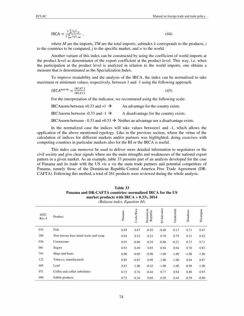
ECLAC Manual on foreign trade and trade policy…
74
IRCA = , (44)
where M are the imports, TM are the total imports; subindex k corresponds to the products, ito the countries to be compared, j to the specific market, and w to the world.
Another variant of this index can be constructed by using the coefficient of world imports atthe product level as denominator of the export coefficient at the product level. This way, i.e. whenthe participation at the product level is analyzed in relation to the world imports, one obtains ameasure that is denominated as the Specialization Index.
To improve treatability and the analysis of the IRCA, the index can be normalized to takemaximum or minimum values, respectively, between 1 and -1 using the following approach:
= (45)
For the interpretation of the indicator, we recommend using the following scale:
IRCAnorm between +0.33 and +1 An advantage for the country exists.
IRCAnorm between -0.33 and -1 A disadvantage for the country exists.
IRCAnorm between - 0.33 and +0.33 Neither an advantage nor a disadvantage exists.
In the normalized case the indices will take values between1 and -1, which allows theapplication of the above mentioned typology. Like in the previous section, where the virtue of thecalculation of indices for different markets and/or partners was highlighted, doing exercises withcompeting countries in particular markets also for the BI or the IRCA is useful.
This index can moreover be used to deliver more detailed information to negotiators or thecivil society and give clear signals where are the main strengths and weaknesses of the national exportpattern in a given market. As an example, table 33 presents part of an analysis developed for the caseof Panama and its trade with the US vis a vis the main trade partners and potential competitors ofPanama, namely those of the Dominican Republic-Central America Free Trade Agreement (DR-CAFTA). Following this method, a total of 261 products were reviewed during the whole analysis.
Table 33Panama and DR-CAFTA countries: normalized IRCA for the US
market products with IRCA > 0.33), 2014(Balassa index, Equation 44)
SITCRev.4
Product
Pana
ma
Cos
taR
ica
Dom
inic
anR
epub
lic
ElS
alva
dor
Gua
tem
ala
Hon
dura
s
Nic
arag
ua
034 Fish 0.95 0.47 -0.93 -0.46 -0.17 0.71 0.47
288 Non-ferrous base metal waste and scrap 0.94 0.32 0.23 0.70 0.79 0.31 0.42
036 Crustaceans 0.93 -0.86 -0.54 -0.88 -0.21 0.73 0.71
061 Sugars 0.93 0.49 0.85 0.94 0.94 0.70 0.83
793 Ships and boats 0.90 -0.69 -0.98 -1.00 -1.00 -1.00 -1.00
122 Tobacco, manufactured 0.85 -0.87 0.99 -1.00 -1.00 0.94 0.97
685 Lead 0.83 -1.00 -0.42 -1.00 -1.00 -0.99 -1.00
071 Coffee and coffee substitutes 0.72 0.76 -0.44 0.77 0.94 0.88 0.93
098 Edible products 0.72 -0.24 0.69 0.50 0.44 -0.59 -0.90
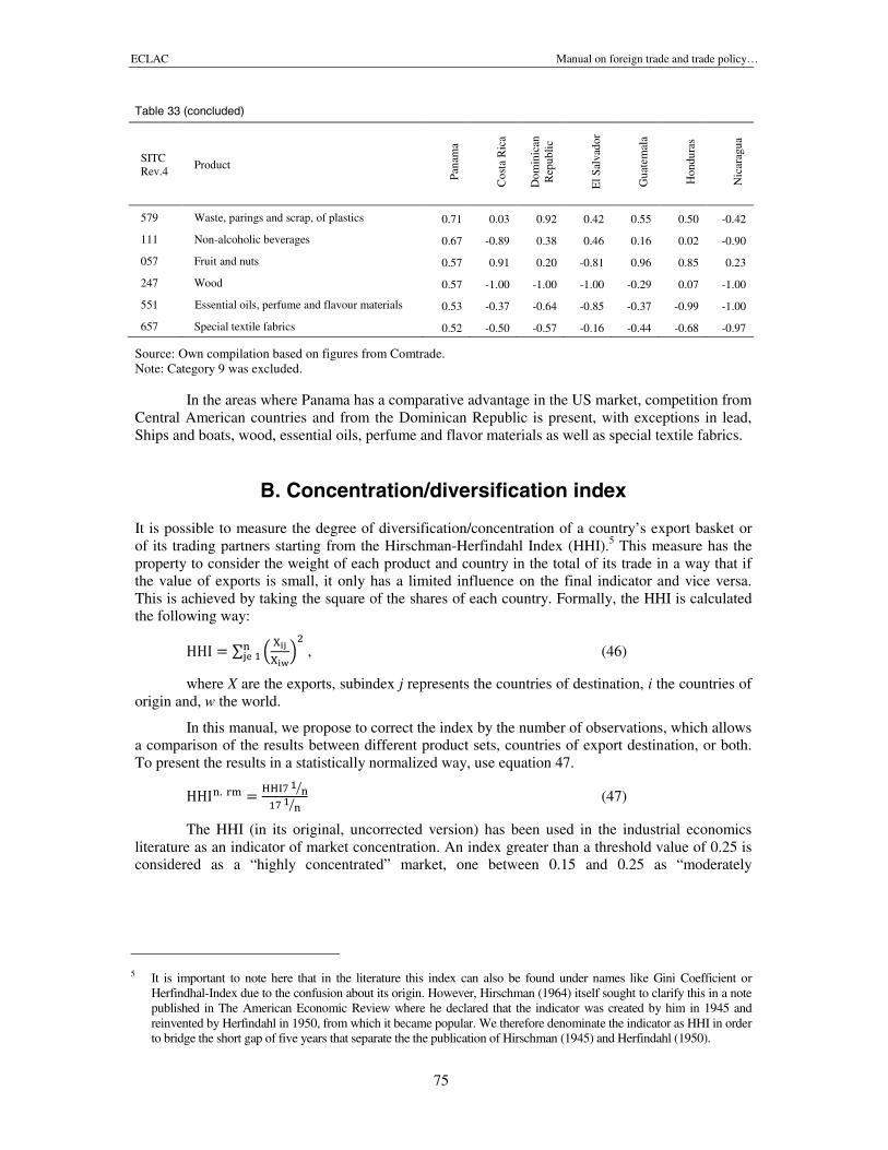
ECLAC Manual on foreign trade and trade policy…
75
Table 33 (concluded)
SITCRev.4
Product
Pana
ma
Cos
taR
ica
Dom
inic
anR
epub
lic
ElS
alva
dor
Gua
tem
ala
Hon
dura
s
Nic
arag
ua
579 Waste, parings and scrap, of plastics 0.71 0.03 0.92 0.42 0.55 0.50 -0.42
111 Non-alcoholic beverages 0.67 -0.89 0.38 0.46 0.16 0.02 -0.90
057 Fruit and nuts 0.57 0.91 0.20 -0.81 0.96 0.85 0.23
247 Wood 0.57 -1.00 -1.00 -1.00 -0.29 0.07 -1.00
551 Essential oils, perfume and flavour materials 0.53 -0.37 -0.64 -0.85 -0.37 -0.99 -1.00
657 Special textile fabrics 0.52 -0.50 -0.57 -0.16 -0.44 -0.68 -0.97
Source: Own compilation based on figures from Comtrade.Note: Category 9 was excluded.
In the areas where Panama has a comparative advantage in the US market, competition fromCentral American countries and from the Dominican Republic is present, with exceptions in lead,Ships and boats, wood, essential oils, perfume and flavor materials as well as special textile fabrics.
B. Concentration/diversification index
It is possible to measure the degree of diversification/concentration of a country’s export basket orof its trading partners starting from the Hirschman-Herfindahl Index (HHI).5 This measure has theproperty to consider the weight of each product and country in the total of its trade in a way that ifthe value of exports is small, it only has a limited influence on the final indicator and vice versa.This is achieved by taking the square of the shares of each country. Formally, the HHI is calculatedthe following way:
HHI = ∑ , (46)
where X are the exports, subindex j represents the countries of destination, i the countries oforigin and, w the world.
In this manual, we propose to correct the index by the number of observations, which allowsa comparison of the results between different product sets, countries of export destination, or both.To present the results in a statistically normalized way, use equation 47.
HHI = (47)
The HHI (in its original, uncorrected version) has been used in the industrial economicsliterature as an indicator of market concentration. An index greater than a threshold value of 0.25 isconsidered as a “highly concentrated” market, one between 0.15 and 0.25 as “moderately
5 It is important to note here that in the literature this index can also be found under names like Gini Coefficient orHerfindhal-Index due to the confusion about its origin. However, Hirschman (1964) itself sought to clarify this in a notepublished in The American Economic Review where he declared that the indicator was created by him in 1945 andreinvented by Herfindahl in 1950, from which it became popular. We therefore denominate the indicator as HHI in orderto bridge the short gap of five years that separate the the publication of Hirschman (1945) and Herfindahl (1950).
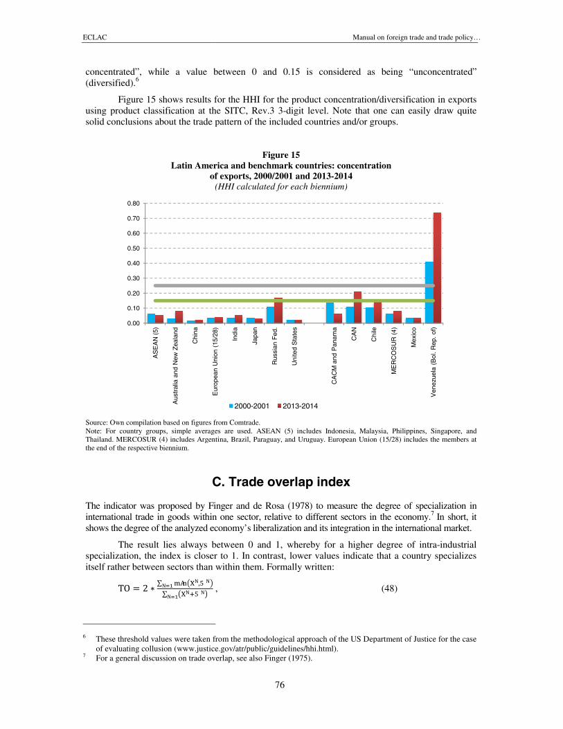
ECLAC
concentrated”, while a value between 0 and 0.(diversified).6
Figure 15 shows results for the HHI for the product concentration/diversification in exportsusing product classification at the SITC, Rev.3 3solid conclusions about the trade pattern of the included countries and/or groups.
Latin America and benchmark countries: concentrationof exports, 2000/2001 and 2013
Source: Own compilation based on figuresNote: For country groups, simple averages are used. ASEAN (5) includes Indonesia, Malaysia, Philippines, Singapore, andThailand. MERCOSUR (4) includes Argentina, Brazil, Paraguay, and Uruguay. European Union (15/28) includes the members atthe end of the respective biennium.
The indicator was proposed by Finger and de Rosa (1978) to measure the degree of specialization ininternational trade in goods within one sector, relative to different sectors in the economy.shows the degree of the analyzed economy’s liberalization and its integration in the international market.
The result lies always between 0 and 1, whereby for a higher degree of intraspecialization, the index is closer to 1. In contritself rather between sectors than within them. Formally written:
TO = 2 ∗ ∑ ,∑
6 These threshold values were taken from the methodological approach of the US Department of Justice for the caseof evaluating collusion (www.justice.gov/atr/public/guidelines/hhi.html).
7 For a general discussion on trade overlap, see also Finger (1975).
0.00
0.10
0.20
0.30
0.40
0.50
0.60
0.70
0.80
AS
EA
N(5
)
Aus
tral
iaan
dN
ewZ
eala
nd
Chi
na
Manual on foreign trade and trade policy
76
concentrated”, while a value between 0 and 0.15 is considered as being “unconcentrated”
Figure 15 shows results for the HHI for the product concentration/diversification in exportsusing product classification at the SITC, Rev.3 3-digit level. Note that one can easily draw quite
conclusions about the trade pattern of the included countries and/or groups.
Figure 15Latin America and benchmark countries: concentration
of exports, 2000/2001 and 2013-2014(HHI calculated for each biennium)
wn compilation based on figures from Comtrade.Note: For country groups, simple averages are used. ASEAN (5) includes Indonesia, Malaysia, Philippines, Singapore, andThailand. MERCOSUR (4) includes Argentina, Brazil, Paraguay, and Uruguay. European Union (15/28) includes the members at
C. Trade overlap index
The indicator was proposed by Finger and de Rosa (1978) to measure the degree of specialization ininternational trade in goods within one sector, relative to different sectors in the economy.shows the degree of the analyzed economy’s liberalization and its integration in the international market.
The result lies always between 0 and 1, whereby for a higher degree of intraspecialization, the index is closer to 1. In contrast, lower values indicate that a country specializesitself rather between sectors than within them. Formally written:
, (48)
These threshold values were taken from the methodological approach of the US Department of Justice for the caseon (www.justice.gov/atr/public/guidelines/hhi.html).
For a general discussion on trade overlap, see also Finger (1975).
Eur
opea
nU
nion
(15/
28)
Indi
a
Japa
n
Rus
sian
Fed
.
Uni
ted
Sta
tes
CA
CM
and
Pan
ama
CA
N
Chi
le
ME
RC
OS
UR
(4)
Mex
ico
2000-2001 2013-2014
oreign trade and trade policy…
15 is considered as being “unconcentrated”
Figure 15 shows results for the HHI for the product concentration/diversification in exportsdigit level. Note that one can easily draw quite
Note: For country groups, simple averages are used. ASEAN (5) includes Indonesia, Malaysia, Philippines, Singapore, andThailand. MERCOSUR (4) includes Argentina, Brazil, Paraguay, and Uruguay. European Union (15/28) includes the members at
The indicator was proposed by Finger and de Rosa (1978) to measure the degree of specialization ininternational trade in goods within one sector, relative to different sectors in the economy.7 In short, itshows the degree of the analyzed economy’s liberalization and its integration in the international market.
The result lies always between 0 and 1, whereby for a higher degree of intra-industrialast, lower values indicate that a country specializes
These threshold values were taken from the methodological approach of the US Department of Justice for the case
Ven
ezue
la(B
ol.R
ep.
of)
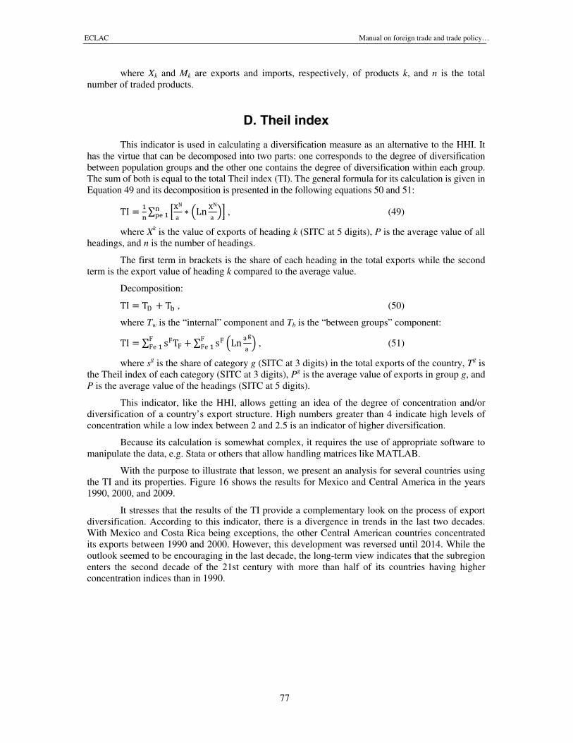
ECLAC Manual on foreign trade and trade policy…
77
where Xk and Mk are exports and imports, respectively, of products k, and n is the totalnumber of traded products.
D. Theil index
This indicator is used in calculating a diversification measure as an alternative to the HHI. Ithas the virtue that can be decomposed into two parts: one corresponds to the degree of diversificationbetween population groups and the other one contains the degree of diversification within each group.The sum of both is equal to the total Theil index (TI). The general formula for its calculation is given inEquation 49 and its decomposition is presented in the following equations 50 and 51:
TI = ∑ ∗ Ln
, (49)
where Xk is the value of exports of heading k (SITC at 5 digits), P is the average value of allheadings, and n is the number of headings.
The first term in brackets is the share of each heading in the total exports while the secondterm is the export value of heading k compared to the average value.
Decomposition:
TI = T + T , (50)
where Tw is the “internal” component and Tb is the “between groups” component:
TI = ∑ sT + ∑ s Ln , (51)
where sg is the share of category g (SITC at 3 digits) in the total exports of the country, Tg isthe Theil index of each category (SITC at 3 digits), Pg is the average value of exports in group g, andP is the average value of the headings (SITC at 5 digits).
This indicator, like the HHI, allows getting an idea of the degree of concentration and/ordiversification of a country’s export structure. High numbers greater than 4 indicate high levels ofconcentration while a low index between 2 and 2.5 is an indicator of higher diversification.
Because its calculation is somewhat complex, it requires the use of appropriate software tomanipulate the data, e.g. Stata or others that allow handling matrices like MATLAB.
With the purpose to illustrate that lesson, we present an analysis for several countries usingthe TI and its properties. Figure 16 shows the results for Mexico and Central America in the years1990, 2000, and 2009.
It stresses that the results of the TI provide a complementary look on the process of exportdiversification. According to this indicator, there is a divergence in trends in the last two decades.With Mexico and Costa Rica being exceptions, the other Central American countries concentratedits exports between 1990 and 2000. However, this development was reversed until 2014. While theoutlook seemed to be encouraging in the last decade, the long-term view indicates that the subregionenters the second decade of the 21st century with more than half of its countries having higherconcentration indices than in 1990.
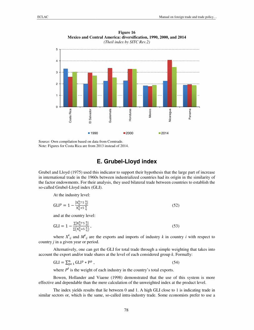
ECLAC
Mexico and Central America
Source: Own compilation based on data from Comtrade.Note: Figures for Costa Rica are from 2013 instead of 2014.
Grubel and Lloyd (1975) used this indicator to support their hypothesis that the large part of increasein international trade in the 1960s between industrialized countries had its origin in the similarity ofthe factor endowments. For their analysis, they used bilateral trade between countries to establish theso-called Grubel-Lloyd index (GLI).
At the industry level:
GLI = 1 −
and at the country level:
GLI = 1 − ∑ ∑ ,
where Xkij and Mk
ij are the exports and imports of industrycountry j in a given year or period.
Alternatively, one can get the GLI for total trade through a simple weighting that takes intoaccount the export and/or trade shares at the level o
GLI = ∑ GLI ∗ P ,
where Pk is the weight of each industry in the country’s total exports.
Bowen, Hollander and Viaene (1998) demonstrated that the use of this system is moreeffective and dependable than the m
The index yields results that lie between 0 and 1. A high GLI close to 1 is indicating trade insimilar sectors or, which is the same, so
0
1
2
3
4
5
Cos
taR
ica
ElS
alva
dor
1990
Manual on foreign trade and trade policy
78
Figure 16Central America: diversification, 1990, 2000, and 2014
(Theil index by SITC Rev.2)
wn compilation based on data from Comtrade.igures for Costa Rica are from 2013 instead of 2014.
E. Grubel-Lloyd index
Grubel and Lloyd (1975) used this indicator to support their hypothesis that the large part of increasein international trade in the 1960s between industrialized countries had its origin in the similarity of
r their analysis, they used bilateral trade between countries to establish theLloyd index (GLI).
(52)
and at the country level:
(53)
are the exports and imports of industry k in country i with respect toin a given year or period.
Alternatively, one can get the GLI for total trade through a simple weighting that takes intoaccount the export and/or trade shares at the level of each considered group k. Formally:
(54)
is the weight of each industry in the country’s total exports.
Bowen, Hollander and Viaene (1998) demonstrated that the use of this system is moreeffective and dependable than the mere calculation of the unweighted index at the product level.
The index yields results that lie between 0 and 1. A high GLI close to 1 is indicating trade insimilar sectors or, which is the same, so-called intra-industry trade. Some economists prefer to u
Gua
tem
ala
Hon
dura
s
Mex
ico
Nic
arag
ua
Pan
ama
1990 2000 2014
oreign trade and trade policy…
Grubel and Lloyd (1975) used this indicator to support their hypothesis that the large part of increasein international trade in the 1960s between industrialized countries had its origin in the similarity of
r their analysis, they used bilateral trade between countries to establish the
with respect to
Alternatively, one can get the GLI for total trade through a simple weighting that takes into. Formally:
Bowen, Hollander and Viaene (1998) demonstrated that the use of this system is moreere calculation of the unweighted index at the product level.
The index yields results that lie between 0 and 1. A high GLI close to 1 is indicating trade inindustry trade. Some economists prefer to use a
Pan
ama
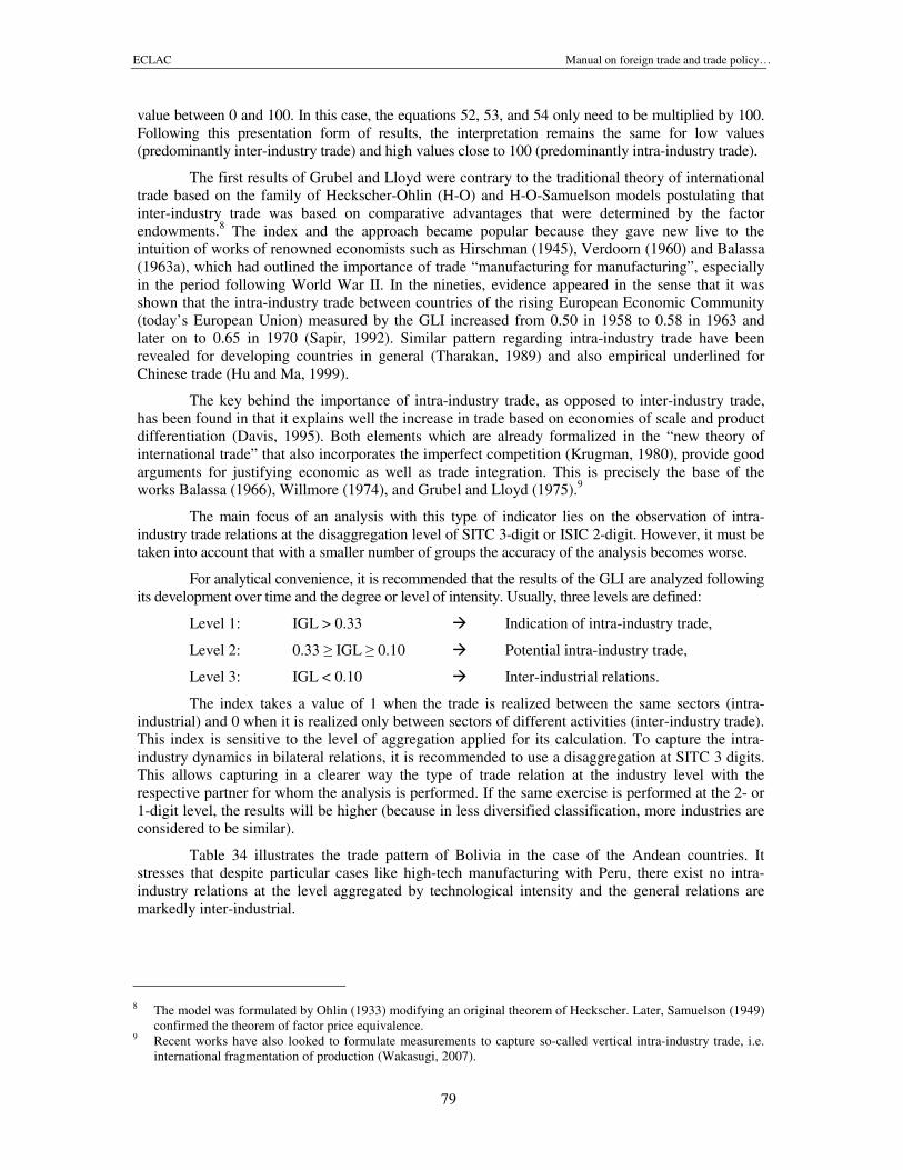
ECLAC Manual on foreign trade and trade policy…
79
value between 0 and 100. In this case, the equations 52, 53, and 54 only need to be multiplied by 100.Following this presentation form of results, the interpretation remains the same for low values(predominantly inter-industry trade) and high values close to 100 (predominantly intra-industry trade).
The first results of Grubel and Lloyd were contrary to the traditional theory of internationaltrade based on the family of Heckscher-Ohlin (H-O) and H-O-Samuelson models postulating thatinter-industry trade was based on comparative advantages that were determined by the factorendowments.8 The index and the approach became popular because they gave new live to theintuition of works of renowned economists such as Hirschman (1945), Verdoorn (1960) and Balassa(1963a), which had outlined the importance of trade “manufacturing for manufacturing”, especiallyin the period following World War II. In the nineties, evidence appeared in the sense that it wasshown that the intra-industry trade between countries of the rising European Economic Community(today’s European Union) measured by the GLI increased from 0.50 in 1958 to 0.58 in 1963 andlater on to 0.65 in 1970 (Sapir, 1992). Similar pattern regarding intra-industry trade have beenrevealed for developing countries in general (Tharakan, 1989) and also empirical underlined forChinese trade (Hu and Ma, 1999).
The key behind the importance of intra-industry trade, as opposed to inter-industry trade,has been found in that it explains well the increase in trade based on economies of scale and productdifferentiation (Davis, 1995). Both elements which are already formalized in the “new theory ofinternational trade” that also incorporates the imperfect competition (Krugman, 1980), provide goodarguments for justifying economic as well as trade integration. This is precisely the base of theworks Balassa (1966), Willmore (1974), and Grubel and Lloyd (1975).9
The main focus of an analysis with this type of indicator lies on the observation of intra-industry trade relations at the disaggregation level of SITC 3-digit or ISIC 2-digit. However, it must betaken into account that with a smaller number of groups the accuracy of the analysis becomes worse.
For analytical convenience, it is recommended that the results of the GLI are analyzed followingits development over time and the degree or level of intensity. Usually, three levels are defined:
Level 1: IGL > 0.33 Indication of intra-industry trade,
Level 2: 0.33 ≥ IGL ≥ 0.10 Potential intra-industry trade,
Level 3: IGL < 0.10 Inter-industrial relations.
The index takes a value of 1 when the trade is realized between the same sectors (intra-industrial) and 0 when it is realized only between sectors of different activities (inter-industry trade).This index is sensitive to the level of aggregation applied for its calculation. To capture the intra-industry dynamics in bilateral relations, it is recommended to use a disaggregation at SITC 3 digits.This allows capturing in a clearer way the type of trade relation at the industry level with therespective partner for whom the analysis is performed. If the same exercise is performed at the 2- or1-digit level, the results will be higher (because in less diversified classification, more industries areconsidered to be similar).
Table 34 illustrates the trade pattern of Bolivia in the case of the Andean countries. Itstresses that despite particular cases like high-tech manufacturing with Peru, there exist no intra-industry relations at the level aggregated by technological intensity and the general relations aremarkedly inter-industrial.
8 The model was formulated by Ohlin (1933) modifying an original theorem of Heckscher. Later, Samuelson (1949)confirmed the theorem of factor price equivalence.
9 Recent works have also looked to formulate measurements to capture so-called vertical intra-industry trade, i.e.international fragmentation of production (Wakasugi, 2007).
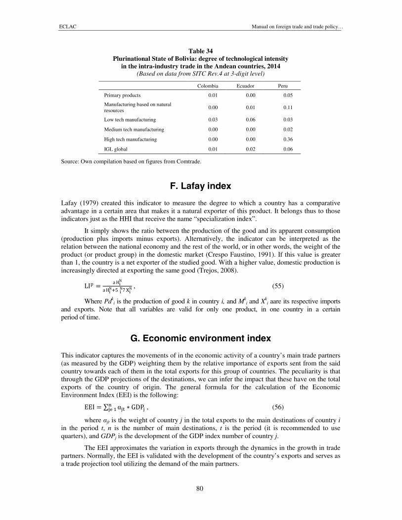
ECLAC Manual on foreign trade and trade policy…
80
Table 34Plurinational State of Bolivia: degree of technological intensity
in the intra-industry trade in the Andean countries, 2014(Based on data from SITC Rev.4 at 3-digit level)
Colombia Ecuador Peru
Primary products 0.01 0.00 0.05
Manufacturing based on naturalresources
0.00 0.01 0.11
Low tech manufacturing 0.03 0.06 0.03
Medium tech manufacturing 0.00 0.00 0.02
High tech manufacturing 0.00 0.00 0.36
IGL global 0.01 0.02 0.06
Source: Own compilation based on figures from Comtrade.
F. Lafay index
Lafay (1979) created this indicator to measure the degree to which a country has a comparativeadvantage in a certain area that makes it a natural exporter of this product. It belongs thus to thoseindicators just as the HHI that receive the name “specialization index”.
It simply shows the ratio between the production of the good and its apparent consumption(production plus imports minus exports). Alternatively, the indicator can be interpreted as therelation between the national economy and the rest of the world, or in other words, the weight of theproduct (or product group) in the domestic market (Crespo Faustino, 1991). If this value is greaterthan 1, the country is a net exporter of the studied good. With a higher value, domestic production isincreasingly directed at exporting the same good (Trejos, 2008).
LI = , (55)
Where Pdki is the production of good k in country i, and Mk
i and Xki aare its respective imports
and exports. Note that all variables are valid for only one product, in one country in a certainperiod of time.
G. Economic environment index
This indicator captures the movements of in the economic activity of a country’s main trade partners(as measured by the GDP) weighting them by the relative importance of exports sent from the saidcountry towards each of them in the total exports for this group of countries. The peculiarity is thatthrough the GDP projections of the destinations, we can infer the impact that these have on the totalexports of the country of origin. The general formula for the calculation of the EconomicEnvironment Index (EEI) is the following:
EEI = ∑ α ∗ GDP , (56)
where αjt is the weight of country j in the total exports to the main destinations of country iin the period t, n is the number of main destinations, t is the period (it is recommended to usequarters), and GDPj is the development of the GDP index number of country j.
The EEI approximates the variation in exports through the dynamics in the growth in tradepartners. Normally, the EEI is validated with the development of the country’s exports and serves asa trade projection tool utilizing the demand of the main partners.
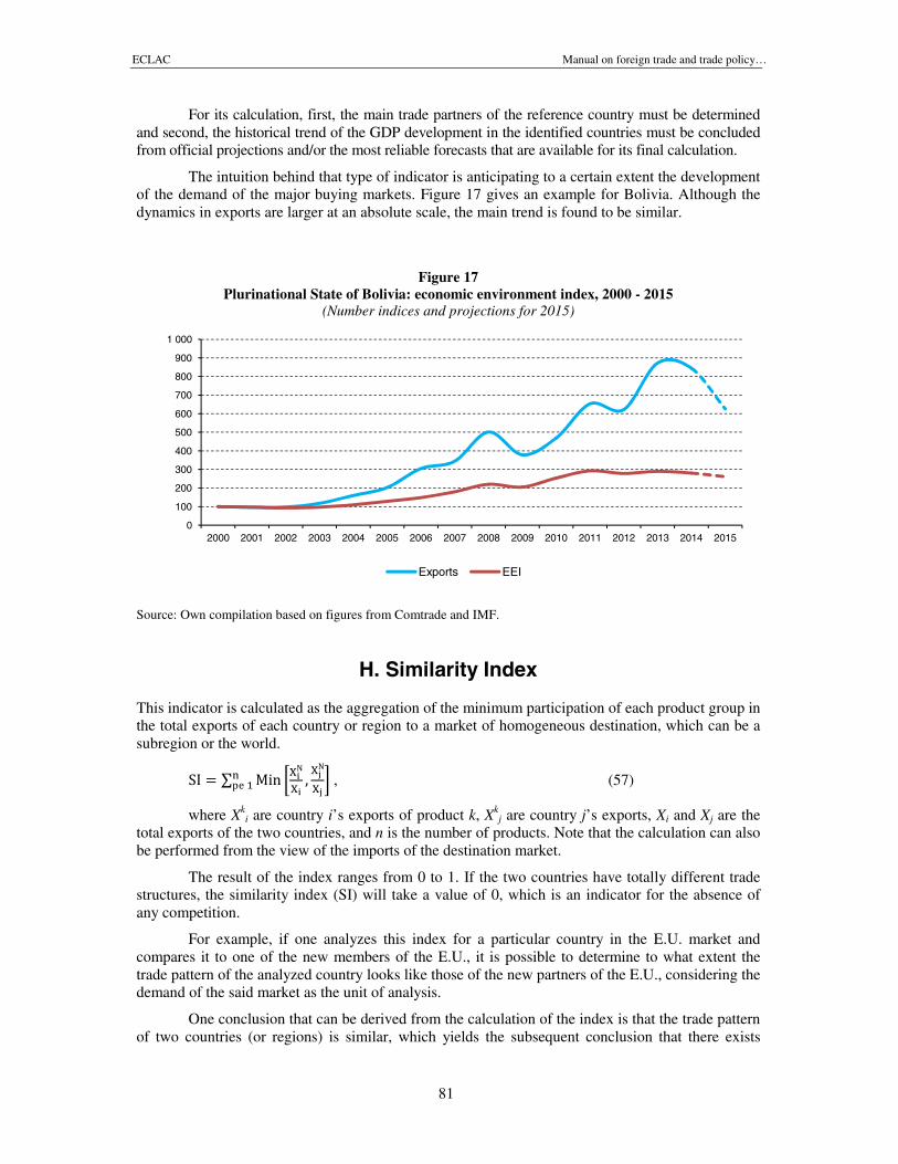
ECLAC Manual on foreign trade and trade policy…
81
For its calculation, first, the main trade partners of the reference country must be determinedand second, the historical trend of the GDP development in the identified countries must be concludedfrom official projections and/or the most reliable forecasts that are available for its final calculation.
The intuition behind that type of indicator is anticipating to a certain extent the developmentof the demand of the major buying markets. Figure 17 gives an example for Bolivia. Although thedynamics in exports are larger at an absolute scale, the main trend is found to be similar.
Figure 17Plurinational State of Bolivia: economic environment index, 2000 - 2015
(Number indices and projections for 2015)
Source: Own compilation based on figures from Comtrade and IMF.
H. Similarity Index
This indicator is calculated as the aggregation of the minimum participation of each product group inthe total exports of each country or region to a market of homogeneous destination, which can be asubregion or the world.
SI = ∑ Min , , (57)
where Xki are country i’s exports of product k, Xk
j are country j’s exports, Xi and Xj are thetotal exports of the two countries, and n is the number of products. Note that the calculation can alsobe performed from the view of the imports of the destination market.
The result of the index ranges from 0 to 1. If the two countries have totally different tradestructures, the similarity index (SI) will take a value of 0, which is an indicator for the absence ofany competition.
For example, if one analyzes this index for a particular country in the E.U. market andcompares it to one of the new members of the E.U., it is possible to determine to what extent thetrade pattern of the analyzed country looks like those of the new partners of the E.U., considering thedemand of the said market as the unit of analysis.
One conclusion that can be derived from the calculation of the index is that the trade patternof two countries (or regions) is similar, which yields the subsequent conclusion that there exists
0
100
200
300
400
500
600
700
800
900
1 000
2000 2001 2002 2003 2004 2005 2006 2007 2008 2009 2010 2011 2012 2013 2014 2015
Exports EEI
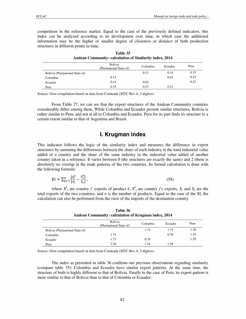
ECLAC Manual on foreign trade and trade policy…
82
competition in the reference market. Equal to the case of the previously defined indicators, thisindex can be analyzed according to its development over time, in which case the additionalinformation may be the higher or smaller degree of closeness or distance of both productionstructures in different points in time.
Table 35Andean Community: calculation of Similarity index, 2014
Bolivia(Plurinational State of)
Colombia Ecuador Peru
Bolivia (Plurinational State of) 0.13 0.14 0.35
Colombia 0.13 0.62 0.23
Ecuador 0.14 0.62 0.21
Peru 0.35 0.23 0.21
Source: Own compilation based on data from Comtrade (SITC Rev.4, 3-digitos).
From Table 27, we can see that the export structures of the Andean Community countriesconsiderably differ among them. While Colombia and Ecuador present similar structures, Bolivia israther similar to Peru, and not at all to Colombia and Ecuador. Peru for its part finds its structure to acertain extent similar to that of Argentina and Brazil.
I. Krugman index
This indicator follows the logic of the similarity index and measures the difference in exportstructures by summing the differences between the share of each industry in the total industrial valueadded of a country and the share of the same industry in the industrial value added of anothercountry taken as a reference. It varies between 0 (the structures are exactly the same) and 2 (there isabsolutely no overlap in the trade patterns of the two countries. Its formal calculation is done withthe following formula:
KI = ∑ − , (58)
where Xki are country i’ exports of product k, Xk
j are country j’s exports, Xi and Xj are thetotal exports of the two countries, and n is the number of products. Equal to the case of the SI, thecalculation can also be performed from the view of the imports of the destination country.
Table 36Andean Community: calculation of Krugman index, 2014
Bolivia(Plurinational State of)
Colombia Ecuador Peru
Bolivia (Plurinational State of) 1.74 1.73 1.30
Colombia 1.74 0.76 1.54
Ecuador 1.73 0.76 1.58
Peru 1.30 1.54 1.58
Source: Own compilation based on data from Comtrade (SITC Rev.4, 3-digitos).
The index as presented in table 36 confirms our previous observations regarding similarity(compare table 35): Colombia and Ecuador have similar export patterns. At the same time, thestructure of both is highly different to that of Bolivia. Finally in the case of Peru, its export pattern ismore similar to that of Bolivia than to that of Colombia or Ecuador.
ECLAC Manual on foreign trade and trade policy…
83
VIII. Indicators of relative dynamicsin intra-regional trade
In the international trade literature, a field of increasing importance is referred to as the analysis ofthe trade dynamics in regional integration schemes or countries participating in customs unionsprojects. In Latin America and the Caribbean, for example, exist four: the Andean Community, theSouthern Common Market (MERCOSUR), the Central American Common Market, and theCaribbean Community. This section summarizes some key indicators that have the power tomeasure and explain the intensity of intra-regional trade.
A. Intra-regional trade index
This is the best-known and simplest indicator to measure the importance of intra-regionaltrade flows. It is calculated by relating the total mutual trade between the members of a customsunion or a trade agreement (may be exports, imports, or both) to the total exports that the group ofcountries trades to the world. Formally:
IRTI = ∑ ∑
, (59)
where Xij are country i’s exports to partner j, and XTi are the total exports of country i. Notethat the indicator can be calculated for the case of imports or total trade as well.
The index shows directly the share representing the trade between members of a regionalgrouping and is a quick measure of the relationship of the countries in a trade group. Nevertheless,there are economists that question its usefulness given the bias that a measure like this can cause forgroups of countries that maintain high participation levels in world trade, e.g. the countries of theE.U. In contrast, the small countries forming integration groups do not reach high levels at such anindicator because the effect of their small scale reduces the size of the index. This is the case of theindex for the integration schemes of Latin America and the Caribbean, which is still small comparedto that in the E.U. (compare table 37).
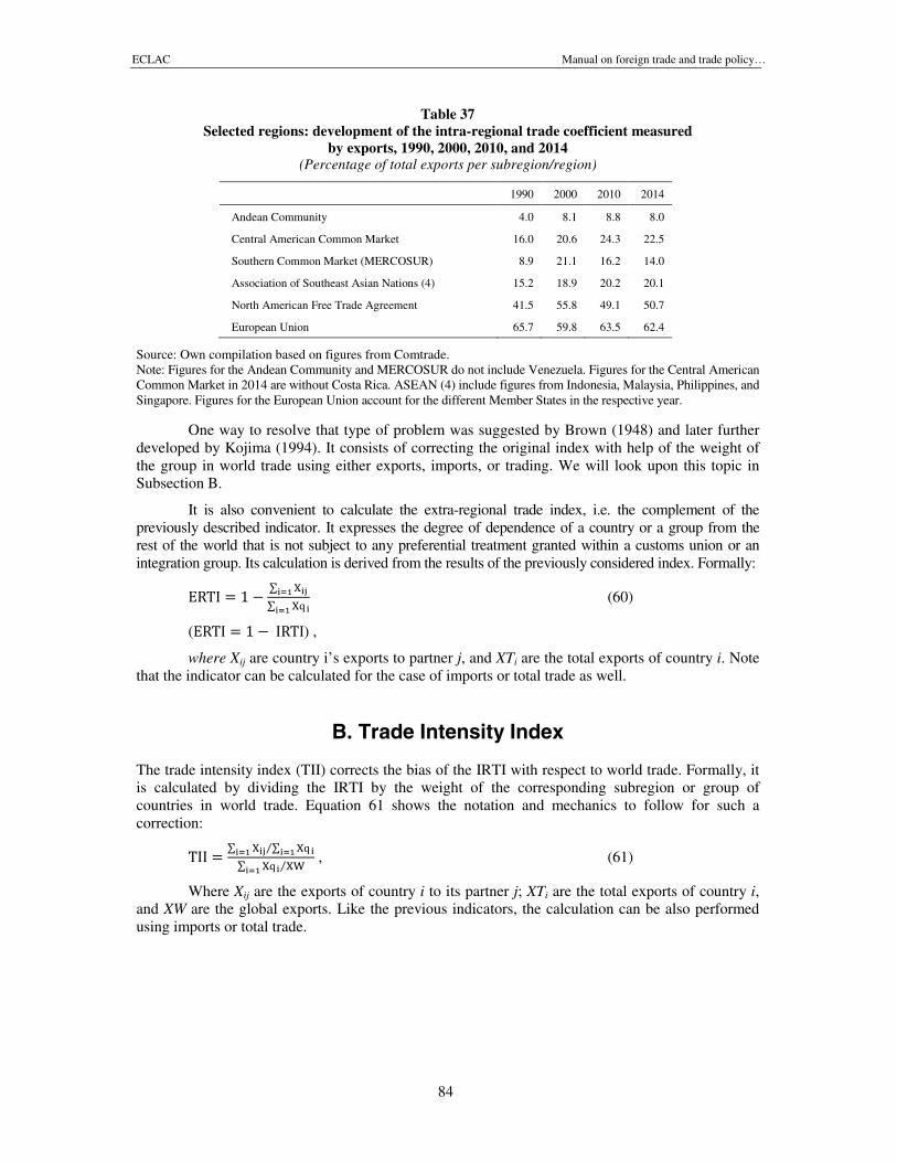
ECLAC Manual on foreign trade and trade policy…
84
Table 37Selected regions: development of the intra-regional trade coefficient measured
by exports, 1990, 2000, 2010, and 2014(Percentage of total exports per subregion/region)
1990 2000 2010 2014
Andean Community 4.0 8.1 8.8 8.0
Central American Common Market 16.0 20.6 24.3 22.5
Southern Common Market (MERCOSUR) 8.9 21.1 16.2 14.0
Association of Southeast Asian Nations (4) 15.2 18.9 20.2 20.1
North American Free Trade Agreement 41.5 55.8 49.1 50.7
European Union 65.7 59.8 63.5 62.4
Source: Own compilation based on figures from Comtrade.Note: Figures for the Andean Community and MERCOSUR do not include Venezuela. Figures for the Central AmericanCommon Market in 2014 are without Costa Rica. ASEAN (4) include figures from Indonesia, Malaysia, Philippines, andSingapore. Figures for the European Union account for the different Member States in the respective year.
One way to resolve that type of problem was suggested by Brown (1948) and later furtherdeveloped by Kojima (1994). It consists of correcting the original index with help of the weight ofthe group in world trade using either exports, imports, or trading. We will look upon this topic inSubsection B.
It is also convenient to calculate the extra-regional trade index, i.e. the complement of thepreviously described indicator. It expresses the degree of dependence of a country or a group from therest of the world that is not subject to any preferential treatment granted within a customs union or anintegration group. Its calculation is derived from the results of the previously considered index. Formally:
ERTI = 1 − ∑ ∑
(60)
(ERTI = 1 − IRTI) ,
where Xij are country i’s exports to partner j, and XTi are the total exports of country i. Notethat the indicator can be calculated for the case of imports or total trade as well.
B. Trade Intensity Index
The trade intensity index (TII) corrects the bias of the IRTI with respect to world trade. Formally, itis calculated by dividing the IRTI by the weight of the corresponding subregion or group ofcountries in world trade. Equation 61 shows the notation and mechanics to follow for such acorrection:
TII = ∑ ∑ ⁄∑ ⁄ , (61)
Where Xij are the exports of country i to its partner j; XTi are the total exports of country i,and XW are the global exports. Like the previous indicators, the calculation can be also performedusing imports or total trade.
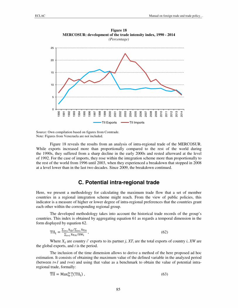
ECLAC Manual on foreign trade and trade policy…
85
Figure 18MERCOSUR: development of the trade intensity index, 1990 - 2014
(Percentage)
Source: Own compilation based on figures from Comtrade.Note: Figures from Venezuela are not included.
Figure 18 reveals the results from an analysis of intra-regional trade of the MERCOSUR.While exports increased more than proportionally compared to the rest of the world duringthe 1990s, they suffered from a sharp decline in the early 2000s and rested afterward at the levelof 1992. For the case of imports, they rose within the integration scheme more than proportionally tothe rest of the world from 1996 until 2003, when they experienced a breakdown that stopped in 2008at a level lower than in the last two decades. Since 2009, the breakdown continued.
C. Potential intra-regional trade
Here, we present a methodology for calculating the maximum trade flow that a set of membercountries in a regional integration scheme might reach. From the view of public policies, thisindicator is a measure of higher or lower degree of intra-regional preferences that the countries granteach other within the corresponding regional group.
The developed methodology takes into account the historical trade records of the group’scountries. This index is obtained by aggregating equation 61 as regards a temporal dimension in theform displayed by equation 62.
TII = ∑ ∑ ⁄∑ ⁄ , (62)
Where Xij are country i’ exports to its partner j, XTi are the total exports of country i, XW arethe global exports, and t is the period.
The inclusion of the time dimension allows to derive a method of the here proposed ad hocestimation. It consists of obtaining the maximum value of the defined variable in the analyzed period(between t=1 and t=n) and using that value as a benchmark to obtain the value of potential intra-regional trade, formally:
TII = Max(TII) , (63)
0
5
10
15
20
25
1990
1991
1992
1993
1994
1995
1996
1997
1998
1999
2000
2001
2002
2003
2004
2005
2006
2007
2008
2009
2010
2011
2012
2013
2014
TII Exports TII Imports
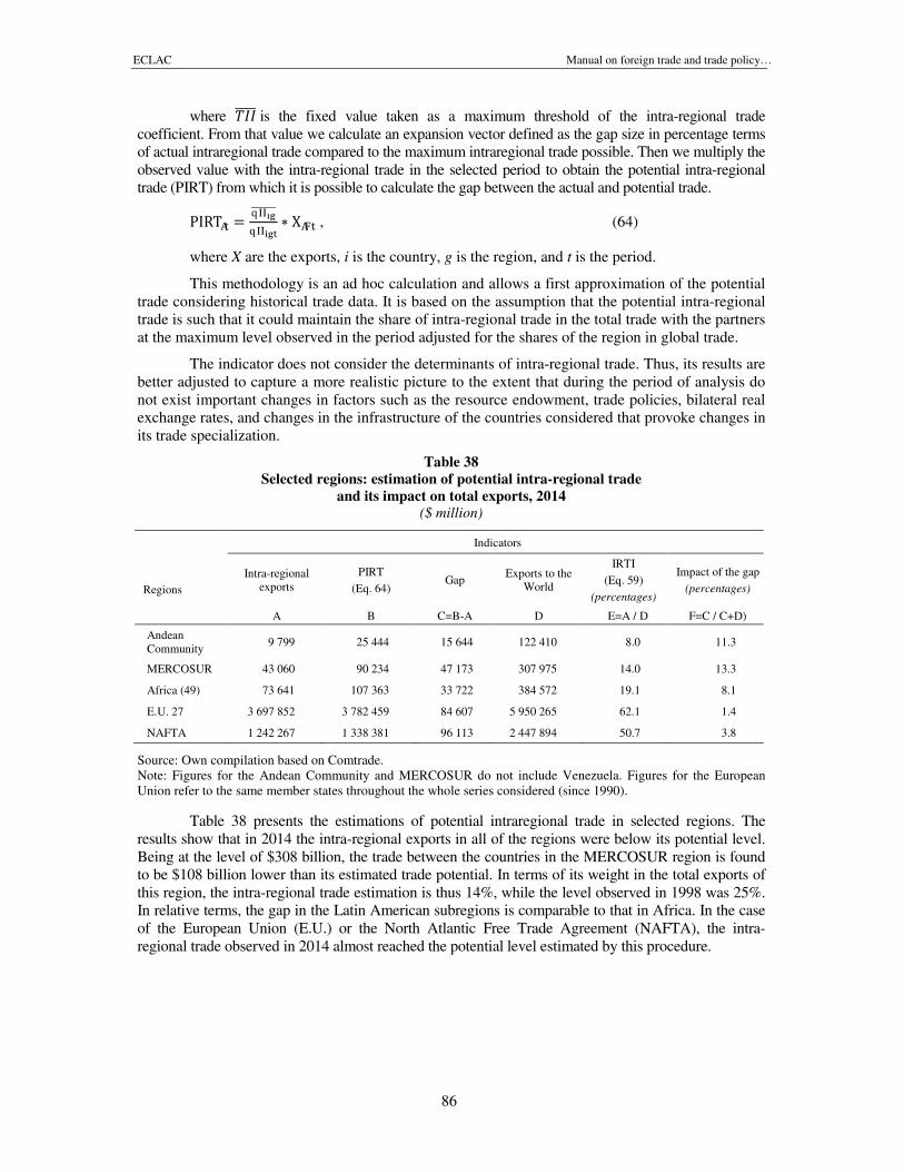
ECLAC Manual on foreign trade and trade policy…
86
where is the fixed value taken as a maximum threshold of the intra-regional tradecoefficient. From that value we calculate an expansion vector defined as the gap size in percentage termsof actual intraregional trade compared to the maximum intraregional trade possible. Then we multiply theobserved value with the intra-regional trade in the selected period to obtain the potential intra-regionaltrade (PIRT) from which it is possible to calculate the gap between the actual and potential trade.
PIRT = ∗ X , (64)
where X are the exports, i is the country, g is the region, and t is the period.
This methodology is an ad hoc calculation and allows a first approximation of the potentialtrade considering historical trade data. It is based on the assumption that the potential intra-regionaltrade is such that it could maintain the share of intra-regional trade in the total trade with the partnersat the maximum level observed in the period adjusted for the shares of the region in global trade.
The indicator does not consider the determinants of intra-regional trade. Thus, its results arebetter adjusted to capture a more realistic picture to the extent that during the period of analysis donot exist important changes in factors such as the resource endowment, trade policies, bilateral realexchange rates, and changes in the infrastructure of the countries considered that provoke changes inits trade specialization.
Table 38Selected regions: estimation of potential intra-regional trade
and its impact on total exports, 2014($ million)
Indicators
RegionsIntra-regional
exportsPIRT
(Eq. 64)Gap
Exports to theWorld
IRTI
(Eq. 59)(percentages)
Impact of the gap(percentages)
A B C=B-A D E=A / D F=C / C+D)
AndeanCommunity
9 799 25 444 15 644 122 410 8.0 11.3
MERCOSUR 43 060 90 234 47 173 307 975 14.0 13.3
Africa (49) 73 641 107 363 33 722 384 572 19.1 8.1
E.U. 27 3 697 852 3 782 459 84 607 5 950 265 62.1 1.4
NAFTA 1 242 267 1 338 381 96 113 2 447 894 50.7 3.8
Source: Own compilation based on Comtrade.Note: Figures for the Andean Community and MERCOSUR do not include Venezuela. Figures for the EuropeanUnion refer to the same member states throughout the whole series considered (since 1990).
Table 38 presents the estimations of potential intraregional trade in selected regions. Theresults show that in 2014 the intra-regional exports in all of the regions were below its potential level.Being at the level of $308 billion, the trade between the countries in the MERCOSUR region is foundto be $108 billion lower than its estimated trade potential. In terms of its weight in the total exports ofthis region, the intra-regional trade estimation is thus 14%, while the level observed in 1998 was 25%.In relative terms, the gap in the Latin American subregions is comparable to that in Africa. In the caseof the European Union (E.U.) or the North Atlantic Free Trade Agreement (NAFTA), the intra-regional trade observed in 2014 almost reached the potential level estimated by this procedure.
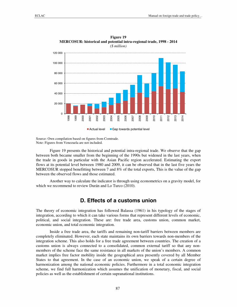
ECLAC Manual on foreign trade and trade policy…
87
Figure 19MERCOSUR: historical and potential intra-regional trade, 1998 - 2014
($ million)
Source: Own compilation based on figures from Comtrade.Note: Figures from Venezuela are not included.
Figure 19 presents the historical and potential intra-regional trade. We observe that the gapbetween both became smaller from the beginning of the 1990s but widened in the last years, whenthe trade in goods in particular with the Asian Pacific region accelerated. Estimating the exportflows at its potential level between 1980 and 2009, it can be observed that in the last five years theMERCOSUR stopped benefitting between 7 and 8% of the total exports, This is the value of the gapbetween the observed flows and those estimated.
Another way to calculate the indicator is through using econometrics on a gravity model, forwhich we recommend to review Durán and Lo Turco (2010).
D. Effects of a customs union
The theory of economic integration has followed Balassa (1961) in his typology of the stages ofintegration, according to which it can take various forms that represent different levels of economic,political, and social integration. These are: free trade area, customs union, common market,economic union, and total economic integration.
Inside a free trade area, the tariffs and remaining non-tariff barriers between members arecompletely eliminated. However, each state maintains its own barriers towards non-members of theintegration scheme. This also holds for a free trade agreement between countries. The creation of acustoms union is always connected to a consolidated, common external tariff so that any non-members of the scheme face the same resistance in all markets of the union’s members. A commonmarket implies free factor mobility inside the geographical area presently covered by all MemberStates to that agreement. In the case of an economic union, we speak of a certain degree ofharmonization among the national economic policies. Furthermore in a total economic integrationscheme, we find full harmonization which assumes the unification of monetary, fiscal, and socialpolicies as well as the establishment of certain supranational institutions.
0
20 000
40 000
60 000
80 000
100 000
120 000
1998
1999
2000
2001
2002
2003
2004
2005
2006
2007
2008
2009
2010
2011
2012
2013
2014
Actual level Gap towards potential level
ECLAC Manual on foreign trade and trade policy…
88
From the second stage of the economic theory, the risk of trade diversion raises, i.e. the newimports that a country A receives from the partner B which is member of the scheme, or the new exportsthat it sends to the latter do not create (new) trade. This is because trade with another partner C (outsidethe preference scheme) is now shifted towards a partner B because of the newly assigned preferences.
While trade creation implies a change from one supplier with high cost to one with lowercosts, trade diversion acts in the opposite direction by producing a change in purchases from aproducer with low costs to one with higher costs but higher preferences. That is why the benefits ofa customs union predominate if the trade creation exceeds trade diversion.
However, these benefits will depend on the differences of the unit costs between theproducts subject to created and diverted trade. Therefore, if the differences in the unit costs areconsiderably higher for the goods that have been creating trade than for those goods that have beendiverting trade, it is possible that the customs union yields benefits in global efficiency, even whentrade diversion is greater than trade creation.
Following the intuition of Viner (1950), this is why we propose the use of an artificialindicator —whose information is difficult to collect— that would allow identifying the CustomsUnion Effect (CUE). Formally:
CUE = ∑
∑
, (65)
where CT is the created trade, DT is the diverted trade, V is the value, Q is the quantity, t isthe period, and k is the product.
This type of analysis can lead to the conclusion that the trade creation and diversion onlycover an aspect of productive effects and that if one looks for a greater accuracy it is necessary todistinguish between negative and positive effects of the products’ unit costs.
To that it should be added that “[…] the consumption effects of a union may be positive ornegative, depending primarily on the extent of trade relations between the member countries, thecomplementarity and competitiveness of the participating economies, and the height of tariff levels”(Balassa, 1961, p. 62). Everything that claims to provide a general theory about the integrationeffects should be taken only with great caution.
ECLAC Manual on foreign trade and trade policy…
89
Bibliography
Akamatsu, K. (1962). A Historical Pattern of Economic Growth in Developing Countries. The DevelopingEconomies, Vol. 1, pp. 3-25.
Balassa, B. (1961). The Theory of Economic Integration. Homewood: Richard D. Irwin.Balassa, B. (1963a). European Integration: Problems and Issues. The American Economic Review, Vol. 53 (2),
pp. 175-184.Balassa, B. (1963b). An Empirical Demonstration of Classical Comparative Cost Theory. The Review of
Economics and Statistics, Vol. 45 (3), pp. 231-238.Balassa, B. (1965). Tariff Protection in Industrial Countries: An Evaluation. Journal of Political Economy,
Vol. 73 (6), pp. 573-594.Balassa, B. (1966). Tariff Reductions and Trade in Manufactures among the Industrial Countries. The
American Economic Review, Vol. 56 (3), pp. 466-473.Balassa, B. and Schydlowsky, D. M. (1968). Effective Tariffs, Domestic Cost of Foreign Exchange and the
Equilibrium Exchange Rate. Journal of Political Economy, Vol. 76 (3), pp. 348-360.Berlinski, J. (2000). Sobre el beneficio de la integración plena en el MERCOSUR: una evaluación
económica de las restricciones al comercio interno y su impacto regional. Red MERCOSUR deinvestigaciones económicas, Serie BRIEF, Nº 3.
Bora, B., Kuwahara, A. and Laird, S. (2002). Quantification of Non-Tariff Measures. UNCTAD Policy Issues inInternational Trade and Commodities, Study Series No. 18. New York and Geneva: United Nations.
Bowen, H., Hollander, A. and Viaene, J.-M. (1998). Applied International Trade Analysis. Ann Arbor:University of Michigan Press.
Brown, A. J. (1948). Applied Economics: Aspects of the World Economy in War and Peace. New York:Rinehart and Company.
Buitelaar, R. M., Padilla, R. and Urrutia, R. (1999). The in-bond Assembly Industry and Technical Change.CEPAL Review, Vol. 67, pp. 137-156.
CCC (1985). The Harmonized Commodity Description and Coding System. Brussels: CustomsCooperation Council.
Corden, W. M. (1966). The Structure of a Tariff System and the Effective Protective Rate. Journal ofPolitical Economy, Vol. 74 (3), pp. 221-237.
Crespo Faustino, H. (1991). On the Controversy between Ballance-Forstner-Murray and Bowen aboutMeasuring Comparative Advantage. Estudos de Economia, Vol. 11 (2), pp. 203-212.
Davis, D. R. (1995). Intra-Industry Trade: A Heckscher-Ohlin-Ricardo Approach. Journal of InternationalEconomics, Vol. 39 (3-4), pp. 201-226.
Durán Lima, J. E. and Alvarez, M. (2007). Shipping Costs: A Rising Challenge to the Region’sCompetitive Development. FAL Bulletin, Nº 256.
ECLAC Manual on foreign trade and trade policy…
90
Durán Lima, J. E. and Alvarez, M. (2013). Indicadores de comercio exterior y política comercial: análisis yderivaciones de la balanza de pagos. Documento de proyecto CEPAL, LC/W.259.Rev.2, Santiagode Chile: Naciones Unidas.
Durán Lima, J.E. and Lo Turco, A. (2010). El comercio intrarregional en América Latina: Patrón deespecialización y patrón exportador. In: M. I. Terra, and J. Durán Lima (Eds.), Los impactos de lacrisis internacional en América Latina: ¿hay margen para el diseño de políticas regionales?, RedMERCOSUR de investigaciones económicas, Serie Red MERCOSUR, Nº 18, pp. 91-148.
Durán Lima, J.E. and Ventura-Dias, V. (2003). Comercio intrafirma: concepto, alcance y magnitud.CEPAL, Serie Comercio Internacional, Nº 44. Santiago de Chile: Naciones Unidas.
Dwyer, J. A. (1992). The Tradeable non-Tradeable Dichotomy: A Practical Approach. AustralianEconomic Papers, Vol. 31 (59), pp. 443-458.
ECLAC (1965). Clasificación del comercio exterior según uso o destino económico. Estudios e informes dela CEPAL, Nº 88. Santiago de Chile: Naciones Unidas.
ECLAC (1992). El comercio de manufacturas de América Latina: evolución y estructura 1962-1989.Estudios e informes de la CEPAL, Nº 88. Santiago de Chile: Naciones Unidas.
ECLAC (1993). Clasificaciones estadísticas internacionales incorporadas en el banco de datos del comercioexterior de América Latina y el Caribe de la CEPAL. Cuadernos Estadísticos N º 18. Santiago deChile: Naciones Unidas.
ECLAC (1998). Clasificaciones estadísticas internacionales incorporadas en el banco de datos del comercioexterior de América Latina y el Caribe de la CEPAL: Revisión I. Cuadernos Estadísticos Nº 25.Santiago de Chile: Naciones Unidas.
ECLAC (2004). Clasificaciones estadísticas internacionales incorporadas en el banco de datos del comercioexterior de América Latina y el Caribe de la CEPAL: Revisión 2. Cuadernos Estadísticos Nº 30.Santiago de Chile: Naciones Unidas.
EEC (1993). Statistical Classification of Products by Activity (CPA). Council Regulation (EEC), No 3696/93.Fairlie, A., Torres, J. and Cuadra, G. (2003). Apertura comercial y protecciones efectivas en el Perú.
Economía y Sociedad, CIES, Vol. 50.Ferraz, J. C., Kupfer, D. and Hagenauer, L. (1996a). Made in Brazil: desafios competitivos para a indústria.
Río de Janeiro: Editora Campus.Ferraz, J. C., Kupfer, D. and Hagenauer, L. (1996b). The Competitive Challenge for Brazilian Industry.
CEPAL Review, Vol. 58, pp. 145-173.Finger, J. M. (1975). Trade Overlap and Intra-Industry Trade. Economic Inquiry, Vol. 13 (4), pp. 581-589.Finger, J. M. and de Rosa, D. A. (1978). Trade Overlap, Comparative Advantage and Protection. In: H.
Giersch (Ed.), On the Economics of Intra-Industry Trade, Tübingen: J.C.B. Mohr, pp. 213-240.Fisher, I. (1922). The Making of Index Numbers. A Study of their Varieties, Tests, and Reliability. Boston
and New York: Houghton Mifflin Company.Furtado, C. (1961). Desenvolvimento e subdesenvolvimento. Rio de Janeiro: Editôra Fundo de Cultura.Grubel, H. G. and Lloyd, P. J. (1975). Intra-Industry Trade: The Theory and Measurement of International
Trade in Differentiated Products. London: Macmillan.Guerrieri, P. and Milana, C. (1990). L’Italia e il commercio mondiale: mutamenti e tendenze nella
divisione internazionale del lavoro. Bologna: Il Mulino.Herfindahl, O. C. (1950). Concentration in the US Steel Industry. New York: Colombia University Press.Hirschman, A. O. (1945). National Power and the Structure of Foreign Trade. Publications of the Bureau of
Business and Economic Research. Berkeley and Los Angeles: University of California Press.Hirschman, A. O. (1964). The Paternity of an Index. The American Economic Review, Vol. 54 (5), pp. 761-762.Hu, X. and Ma, Y. (1999). International Intra-Industry Trade of China. Weltwirtschaftliches Archiv, Vol.
(135 (1), pp. 82-101.JETRO (2001). White Paper on International Trade 2001: World Trade Expands Broadly and China Rises
to Prominence. Tokyo: Japan External Trade Organization.Kelleher, S. and Reyes, J.-D. (2014). Technical Measures to Trade in Central America: Incidence, Price
Effects, and Consumer Welfare. The World Bank, Policy Research Working Paper WPS6857.Knight, G. and Johnson, L. (1997). Tradables: Developing Output and Price Measures for Australia's
Tradable and Non-Tradable Sectors. Australian Bureau of Statistics, Working Paper, No. 97/1.Kojima, K. (1994). Australia's Trade with Asia: Some Policy Issues. Hitotsubashi Journal of Economics,
Vol. 21 (1), pp. 1-14.
ECLAC Manual on foreign trade and trade policy…
91
Krugman, P. (1980). Scale Economies, Product Differentiation, and the Pattern of Trade. The AmericanEconomic Review, Vol. 70 (5), pp. 950-959.
Kuwayama, M. and Durán Lima, J. E. (2003). La calidad de la inserción internacional de América Latina yel Caribe en el comercio mundial. CEPAL, Serie de Comercio Internacional, Nº 26. Santiago deChile: Naciones Unidas.
Lafay, G. (1979). Dynamique de la spécialisation internationale. Paris: Economica.LaFleur, M. (2011). The Liberalization of Environmental Goods and Services: Overview and Implications
for Latin America and the Caribbean. CEPAL, Serie Comercio Internacional Nº 111. Santiago deChile: United Nations.
Laird, S. and Yeats, A. (1990). Quantitative Methods for Trade-Barrier Analysis. New York: New YorkUniversity Press.
Lall, S. (2000). The Technological Structure and Performance of Developing Country ManufacturedExports, 1985-1998. Oxford Development Studies, Vol. 28 (3), pp. 337-369.
Laspeyres, É. (1871). Die Berechnung einer mittleren Waarenpreissteigerung. Jahrbücher fürNationalökonomie und Statistik, Vol. 16, 296-314.
League of Nations. (1938). Minimum List of Commodities for International Trade Statistics. Geneva:League of Nations.
Low, P. and Yeats, A. (1992). Do “Dirty” Industries Migrate? In: P. Low (Ed.), International Trade and theEnvironment, World Bank Discussion Papers, No. 159, pp. 89-103.
Murillo, D. R. (2007). La competitividad exportadora de los sectores ambientales sensibles y laconstrucción de un patrón exportador sostenible en América Latina y el Caribe. Documento deproyecto CEPAL, LC/W.148, Santiago de Chile: Naciones Unidas.
OECD (1994). The Measurement of Scientific and Technological Activities Using Patent Dated as Scienceand Technology Indicators. Paris: OECD Publishing.
OECD (1996). Globalization of Industry: Overview and Sector Reports. Paris: OECD.Ohlin, B. (1933). Interregional and International Trade. Cambridge: Harvard University Press.Paasche, H. (1874). Über die Preisentwicklung der letzten Jahre nach den Hamburger Borsennotirungen.
Jahrbücher für Nationalökonomie und Statistik, Vol. 23, pp. 168-178.Pavitt, K. (1984). Sectoral Patterns of Technical Change: Towards a Taxonomy and a Theory. Research
Policy, Vol. 13 (6), pp. 343-373.Samuelson, P. A. (1949). Market Mechanisms and Maximization. Santa Monica, California: The RAND
Corporation.Sapir, A. (1992). Regional integration in Europe. Economic Journal, Vol. 102 (415), pp. 1491-1506.Schaper, M. (2000). Impactos ambientales de los cambios en la estructura exportadora en nueve países de
América Latina y el Caribe: 1980 - 1995. CEPAL, Serie Medio Ambiente y Desarrollo, Nº 19.Santiago de Chile: Naciones Unidas.
Stawowy, W. (2001). Calculation of Ad Valorem Equivalents of Non-Ad Valorem Tariffs - MethodologyNotes. Geneva: UNCTAD.
Tharakan, P. K . M. (1989). Bilateral Intra-Industry Trade between Countries with Different FactorEndowment Patterns. In: P. K. M. Tharakan and J. Kol (Eds.), Intra-Industry Trade. Theory,Evidence and Extensions), London: Palgrave Macmillan, pp. 69-91.
Trejos, A. (2008). Instrumentos para la evaluación del impacto de acuerdos comerciales internacionales:aplicaciones para países pequeños en América Latina. CEPAL, Serie Estudios y Perspectivas,Nº 110. Mexico DF.: Naciones Unidas.
UNSD (1948). International Standard Industrial Trade Classification of All Economic Activities. StatisticalPapers, No. 4, New York: United Nations.
UNSD (1950). Standard International Trade Classification Statistical Papers, Series M No. 10, New York:United Nations.
UNSD (1958). International Standard Industrial Trade Classification of All Economic Activities. StatisticalPapers, Series M No. 4, Rev.1, New York: United Nations.
UNSD (1961). Standard International Trade Classification: Revision 1. Statistical Papers, Series M, No. 34,New York: United Nations.
UNSD (1968). International Standard Industrial Trade Classification of All Economic Activities, Revision 2.Statistical Papers, Series M No. 4, Rev.2, New York: United Nations.
UNSD (1975). Standard International Trade Classification: Revision 2. Statistical Papers, Series M,No. 34/Rev.2, New York: United Nations.
ECLAC Manual on foreign trade and trade policy…
92
UNSD (1986). Standard International Trade Classification: Revision 3. Statistical Papers, Series M,No. 34/Rev.3, New York: United Nations.
UNSD (1990). International Standard Industrial Trade Classification of All Economic Activities, ThirdRevision. Statistical Papers, Series M No. 4, Rev.3, New York: United Nations.
UNSD (2002). International Standard Industrial Trade Classification of All Economic Activities (ISIC),Revision 3.1. Statistical Papers, Series M No. 4, Rev.3.1, New York: United Nations.
UNSD (2003). Classification by Broad Economic Categories. Statistical Papers, Series M No. 53, Rev.4,New York: United Nations.
UNSD (2006a). Standard International Trade Classification: Revision 4. Statistical Papers, Series M,No. 34/Rev. 4, New York: United Nations.
UNSD (2006b). Central Product Classification (CPC): Version 1.1. Statistical Papers, Series M, No. 77,Ver. 1.1, New York: United Nations.
UNSD (2008). International Standard Industrial Trade Classification of All Economic Activities (ISIC),Rev.4. Statistical Papers, Series M No. 4, Rev.4, New York: United Nations.
UNSD (2012). Manual on Statistics of International Trade in Services 2010 (MSITS2010). Geneva,Luxembourg, Madrid, New York, Paris and Washington D.C.: United Nations.
UNSD (2015). Central Product Classification (CPC): Version 2.1. Statistical Papers, Series M, No. 77,Ver. 2.1, New York: United Nations.
UNSD (n.d.). Detailed Structure and Explanatory Notes: ‘Standard International Trade Classification”,URL: http://unstats.un.org/unsd/cr/registry/regcst.asp?Cl=28 (04. January 2016).
Verdoorn, P. J. (1960). The Intra-Block Trade of Benelux. In: E. A. G. Robinson (Ed.), EconomicConsequence of the Size of Nations, London: Palgrave Macmillan, pp. 291-321.
Viner, J. (1950). The Customs Union Issue. New York: Carnegie Endowment for International Peace.Wakasugi, R. (2007). Vertical Intra-Industry and Economic Integration in East Asia. Asian Economic
Papers, Vol. 6 (1), pp. 24-45.WCO (2006). The Harmonized System: A Universal Language for International Trade. Brussels: World
Customs Organization.WCO (2002). HS Nomenclature 2002 Edition: ‘2710E’. Official Website of the World Customs Organization,
URL: http://www.wcoomd.org/en/topics/nomenclature/instrument-and-tools/hs_nomenclature_older_edition/~/media/E775D35300BA46FE9063114781C3E131.ashx (04. January 2016).
WCO (2015). ‘HS Nomenclature 2017’. Official Website of the World Customs Organization, URL:http://www.wcoomd.org/en/topics/nomenclature/instrument-and-tools/hs-nomenclature-2017-edition.aspx (04. January 2016).
Willmore, L. (1974). The Pattern of Trade and Specialisation in the Central American Common Market.Journal of Economic Studies, Vol. 1 (2), pp. 113-134.
World Bank (n.d.). ‘World DataBank’. Official Website of The World Bank, URL:http://databank.worldbank.org/ddp/home.do (05. January, 2016).
WTO (1986). ‘The Text of The General Agreement on Tariffs and Trade GATT’. Official Website of theWorld Trade Organization, URL: https://www.wto.org/english/docs_e/legal_e/gatt47_e.pdf (04.January 2016).
WTO (n.d.a). Understanding the WTO: Developing Countries, ‘Some Issues Raised’. Official Website of theWorld Trade Organization, URL: https://www.wto.org/english/thewto_e/whatis_e/tif_e/dev4_e.htm(04. January 2016).
WTO (n.d.b). Understanding the WTO: The Agreements, ‘Tariffs: more binding and closer to zero’. OfficialWebsite of the World Trade Organization, URL: https://www.wto.org/english/thewto_e/whatis_e/tif_e/agrm2_e.htm (04. January 2016).
WTO (n.d.c). Understanding the WTO: The Agreements, ‘Non-tariff barriers: red tape, etc’. Official Website ofthe World Trade Organization, URL: https://www.wto.org/english/thewto_e/whatis_e/tif_e/agrm9_e.htm (04. January 2016).