machine learning for financial products recommendation

HAL Id: tel-02974918https://tel.archives-ouvertes.fr/tel-02974918

Submitted on 22 Oct 2020

HAL is a multi-disciplinary open accessarchive for the deposit and dissemination of sci-entific research documents, whether they are pub-lished or not. The documents may come fromteaching and research institutions in France orabroad, or from public or private research centers.

L’archive ouverte pluridisciplinaire HAL, estdestinée au dépôt et à la diffusion de documentsscientifiques de niveau recherche, publiés ou non,émanant des établissements d’enseignement et derecherche français ou étrangers, des laboratoirespublics ou privés.

Machine Learning for Financial ProductsRecommendation

Baptiste Barreau

To cite this version:Baptiste Barreau. Machine Learning for Financial Products Recommendation. Computational Engi-neering, Finance, and Science [cs.CE]. Université Paris-Saclay, 2020. English. �NNT : 2020UPAST010�.�tel-02974918�

https://tel.archives-ouvertes.fr/tel-02974918

https://hal.archives-ouvertes.fr

Machine Learning for Financial Products Recommendation

Apprentissage Statistique pour la Recommandation

de Produits Financiers

Thèse de doctorat de l'université Paris-Saclay

École doctorale n°573 Interfaces : Approches interdisciplinaires, fondements, applications et

innovation Spécialité de doctorat : Mathématiques appliquées

Unité de recherche : Université Paris-Saclay, CentraleSupélec, Mathématiques et Informatique pour la Complexité et les Systèmes, 91190, Gif-sur-Yvette, France.

Référent : CentraleSupélec

Thèse présentée et soutenue à Gif-sur-Yvette, le 15 septembre 2020, par

Baptiste BARREAU

Composition du Jury

Michael BENZAQUEN Professeur, École Polytechnique Président

Charles-Albert LEHALLE Head of Data analytics, Capital Fund Management, HDR Rapporteur & Examinateur

Elsa NEGRE Maître de conférences, Université Paris-Dauphine, HDR Rapporteur & Examinatrice

Eduardo ABI JABER Maître de conférences, Université Paris 1 Examinateur

Sylvain ARLOT Professeur, Université Paris-Sud Examinateur

Damien CHALLET Professeur, CentraleSupélec Directeur de thèse

Sarah LEMLER Maître de conférences, CentraleSupélec Co-Directrice de thèse

Frédéric ABERGEL Professeur, BNP Paribas Asset Management Invité

Laurent CARLIER Head of Data & AI Lab, BNPP CIB Global Markets Invité

Thès

e de

doc

tora

t N

NT

: 202

0UPA

ST01

0

Résumé

L’anticipation des besoins des clients est cruciale pour toute entreprise — c’est particulièrementvrai des banques d’investissement telles que BNP Paribas Corporate and Institutional Bankingau vu de leur rôle dans les marchés financiers. Cette thèse s’intéresse au problème de la pré-diction des intérêts futurs des clients sur les marchés financiers, et met plus particulièrementl’accent sur le développement d’algorithmes ad hoc conçus pour résoudre des problématiquesspécifiques au monde financier.

Ce manuscrit se compose de cinq chapitres, répartis comme suit:

- Le chapitre 1 expose le problème de la prédiction des intérêts futurs des clients sur lesmarchés financiers. Le but de ce chapitre est de fournir aux lecteurs toutes les clés néces-saires à la bonne compréhension du reste de cette thèse. Ces clés sont divisées en troisparties: une mise en lumière des jeux de données à notre disposition pour la résolution duproblème de prédiction des intérêts futurs et de leurs caractéristiques, une vue d’ensemble,non exhaustive, des algorithmes pouvant être utilisés pour la résolution de ce problème,et la mise au point de métriques permettant d’évaluer la performance de ces algorithmessur nos jeux de données. Ce chapitre se clôt sur les défis que l’on peut rencontrer lorsde la conception d’algorithmes permettant de résoudre le problème de la prédiction desintérêts futurs en finance, défis qui seront, en partie, résolus dans les chapitres suivants;

- Le chapitre 2 compare une partie des algorithmes introduits dans le chapitre 1 sur un jeude données provenant de BNP Paribas CIB, et met en avant les di�cultés rencontrées pourla comparaison d’algorithmes de nature di�érente sur un même jeu de données, ainsi quequelques pistes permettant de surmonter ces di�cultés. Ce comparatif met en pratiquedes algorithmes de recommandation classiques uniquement envisagés d’un point de vuethéorique au chapitre précédent, et permet d’acquérir une compréhension plus fine desdi�érentes métriques introduites au chapitre 1 au travers de l’analyse des résultats de cesalgorithmes;

- Le chapitre 3 introduit un nouvel algorithme, Experts Network, i.e., réseau d’experts,conçu pour résoudre le problème de l’hétérogénéité de comportement des investisseursd’un marché donné au travers d’une architecture de réseau de neurones originale, inspiréede la recherche sur les mélanges d’experts. Dans ce chapitre, cette nouvelle méthodologieest utilisée sur trois jeux de données distincts: un jeu de données synthétique, un jeu dedonnées en libre accès, et un jeu de données provenant de BNP Paribas CIB. Ce chapitreprésente aussi en plus grand détail la genèse de l’algorithme et fournit des pistes pourl’améliorer;

- Le chapitre 4 introduit lui aussi un nouvel algorithme, appelé History-augmented collabora-tive filtering, i.e., filtrage collaboratif augmenté par historiques, qui proposes d’augmenterles approches de factorisation matricielle classiques à l’aide des historiques d’interaction

i

des clients et produits considérés. Ce chapitre poursuit l’étude du jeu de données étudiéau chapitre 2 et étend l’algorithme introduit avec de nombreuses idées. Plus précisément,ce chapitre adapte l’algorithme de façon à permettre de résoudre le problème du coldstart, i.e., l’incapacité d’un système de recommandation à fournir des prédictions pour denouveaux utilisateurs, ainsi qu’un nouveau cas d’application sur lequel cette adaptationest essayée;

- Le chapitre 5 met en lumière une collection d’idées et d’algorithmes, fructueux ou non,qui ont été essayés au cours de cette thèse. Ce chapitre se clôt sur un nouvel algorithmemariant les idées des algorithmes introduits aux chapitres 3 et 4.

La recherche présentée dans cette thèse a été conduite via le programme de thèses CIFRE, en col-laboration entre le laboratoire MICS de CentraleSupélec et la division Global Markets de BNPParibas CIB. Elle a été conduite dans le cadre du mandat de l’équipe Data & AI Lab, une équipede science des données faisant partie de la recherche quantitative et dévouée à l’application desméthodes d’apprentissage statistique aux problématiques des di�érentes équipes de Global Mar-kets.

Mots-clés. Apprentissage statistique, finance, systèmes de recommandation, clustering su-pervisé, systèmes de recommandation dépendants du contexte, systèmes de recommandationdépendants du temps, apprentissage profond, réseaux de neurones.

ii

Abstract

Anticipating clients’ needs is crucial to any business — this is particularly true for corporateand institutional banks such as BNP Paribas Corporate and Institutional Banking due to theirrole in the financial markets. This thesis addresses the problem of future interests prediction inthe financial context and focuses on the development of ad hoc algorithms designed for solvingspecific financial challenges.

This manuscript is composed of five chapters:

- Chapter 1 introduces the problem of future interests prediction in the financial world. Thegoal of this chapter is to provide the reader with all the keys necessary to understand theremainder of this thesis. These keys are divided into three parts: a presentation of thedatasets we have at our disposal to solve the future interests prediction problem and theircharacteristics, an overview of the candidate algorithms to solve this problem, and thedevelopment of metrics to monitor the performance of these algorithms on our datasets.This chapter finishes with some of the challenges that we face when designing algorithmsto solve the future interests problem in finance, challenges that will be partly addressedin the following chapters;

- Chapter 2 proposes a benchmark of some of the algorithms introduced in Chapter 1 ona real-word dataset from BNP Paribas CIB, along with a development on the di�cultiesencountered for comparing di�erent algorithmic approaches on a same dataset and onways to tackle them. This benchmark puts in practice classic recommendation algorithmsthat were considered on a theoretical point of view in the preceding chapter, and providesfurther intuition on the analysis of the metrics introduced in Chapter 1;

- Chapter 3 introduces a new algorithm, called Experts Network, that is designed to solvethe problem of behavioral heterogeneity of investors on a given financial market using acustom-built neural network architecture inspired from mixture-of-experts research. Inthis chapter, the introduced methodology is experimented on three datasets: a syntheticdataset, an open-source one and a real-world dataset from BNP Paribas CIB. The chapterprovides further insights into the development of the methodology and ways to extend it;

- Chapter 4 also introduces a new algorithm, called History-augmented Collaborative Filter-ing, that proposes to augment classic matrix factorization approaches with the informationof users and items’ interaction histories. This chapter provides further experiments on thedataset used in Chapter 2, and extends the presented methodology with various ideas.Notably, this chapter exposes an adaptation of the methodology to solve the cold-startproblem and applies it to a new dataset;

- Chapter 5 brings to light a collection of ideas and algorithms, successful or not, thatwere experimented during the development of this thesis. This chapter finishes on a new

iii

algorithm that blends the methodologies introduced in Chapters 3 and 4.

The research presented in this thesis has been conducted under the French CIFRE Ph.D. pro-gram, in collaboration between the MICS Laboratory at CentraleSupélec and the Global Mar-kets division of BNP Paribas CIB. It has been conducted as part of the Data & AI Lab mandate,a data science team within Quantitative Research devoted to the applications of machine learn-ing for the support of Global Markets’ business lines.

Keywords. Machine learning, finance, recommender systems, supervised clustering, context-aware recommender systems, time-aware recommender systems, deep learning, neural net-works.

iv

Contents

Résumé i

Abstract iii

Acknowledgements 5

1 Recommendations in the financial world 71.1 Predicting future interests . . . . . . . . . . . . . . . . . . . . . . . . . . . . . . . 7

1.1.1 Enhancing sales with recommender systems . . . . . . . . . . . . . . . . . 71.1.2 An overview of bonds and options . . . . . . . . . . . . . . . . . . . . . . 9

1.2 Understanding data . . . . . . . . . . . . . . . . . . . . . . . . . . . . . . . . . . 121.2.1 Data sources . . . . . . . . . . . . . . . . . . . . . . . . . . . . . . . . . . 121.2.2 Exploring the heterogeneity of clients and assets . . . . . . . . . . . . . . 13

1.3 A non-exhaustive overview of recommender systems . . . . . . . . . . . . . . . . 141.3.1 Benchmarking algorithms . . . . . . . . . . . . . . . . . . . . . . . . . . . 161.3.2 Content-filtering strategies . . . . . . . . . . . . . . . . . . . . . . . . . . 171.3.3 Collaborative filtering strategies . . . . . . . . . . . . . . . . . . . . . . . 191.3.4 Other approaches . . . . . . . . . . . . . . . . . . . . . . . . . . . . . . . . 261.3.5 The cold-start problem . . . . . . . . . . . . . . . . . . . . . . . . . . . . 27

1.4 Evaluating financial recommender systems . . . . . . . . . . . . . . . . . . . . . . 271.4.1 Deriving symmetrized mean average precision . . . . . . . . . . . . . . . . 271.4.2 A closer look at area under curve metrics . . . . . . . . . . . . . . . . . . 301.4.3 Monitoring diversity . . . . . . . . . . . . . . . . . . . . . . . . . . . . . . 31

1.5 The challenges of the financial world . . . . . . . . . . . . . . . . . . . . . . . . . 32

2 First results on real-world RFQ data 352.1 From binary to oriented interests . . . . . . . . . . . . . . . . . . . . . . . . . . . 352.2 A benchmark of classic algorithms . . . . . . . . . . . . . . . . . . . . . . . . . . 36

2.2.1 Historical models . . . . . . . . . . . . . . . . . . . . . . . . . . . . . . . . 362.2.2 Resource redistribution models . . . . . . . . . . . . . . . . . . . . . . . . 372.2.3 Matrix factorization models . . . . . . . . . . . . . . . . . . . . . . . . . . 392.2.4 Gradient tree-boosting models . . . . . . . . . . . . . . . . . . . . . . . . 402.2.5 Overall benchmark . . . . . . . . . . . . . . . . . . . . . . . . . . . . . . . 41

2.3 Concluding remarks . . . . . . . . . . . . . . . . . . . . . . . . . . . . . . . . . . 42

3 A supervised clustering approach to future interests prediction 433.1 Heterogeneous clusters of investors . . . . . . . . . . . . . . . . . . . . . . . . . . 44

3.1.1 Translating heterogeneity . . . . . . . . . . . . . . . . . . . . . . . . . . . 443.1.2 Non-universality of investors . . . . . . . . . . . . . . . . . . . . . . . . . 453.1.3 Related work . . . . . . . . . . . . . . . . . . . . . . . . . . . . . . . . . . 46

1

3.2 Introducing Experts Network . . . . . . . . . . . . . . . . . . . . . . . . . . . . . 473.2.1 Architecture of the network . . . . . . . . . . . . . . . . . . . . . . . . . . 473.2.2 Disambiguation of investors’ experts mapping . . . . . . . . . . . . . . . . 483.2.3 Helping experts specialize . . . . . . . . . . . . . . . . . . . . . . . . . . . 493.2.4 From gating to classification . . . . . . . . . . . . . . . . . . . . . . . . . . 493.2.5 Limitations of the approach . . . . . . . . . . . . . . . . . . . . . . . . . . 50

3.3 Experiments . . . . . . . . . . . . . . . . . . . . . . . . . . . . . . . . . . . . . . . 503.3.1 Synthetic data . . . . . . . . . . . . . . . . . . . . . . . . . . . . . . . . . 503.3.2 IBEX data . . . . . . . . . . . . . . . . . . . . . . . . . . . . . . . . . . . 553.3.3 BNPP CIB data . . . . . . . . . . . . . . . . . . . . . . . . . . . . . . . . 58

3.4 A collection of unfortunate ideas . . . . . . . . . . . . . . . . . . . . . . . . . . . 593.4.1 About architecture . . . . . . . . . . . . . . . . . . . . . . . . . . . . . . . 593.4.2 About regularization . . . . . . . . . . . . . . . . . . . . . . . . . . . . . . 613.4.3 About training . . . . . . . . . . . . . . . . . . . . . . . . . . . . . . . . . 62

3.5 Further topics in Experts Networks . . . . . . . . . . . . . . . . . . . . . . . . . . 633.5.1 Boosting ExNets . . . . . . . . . . . . . . . . . . . . . . . . . . . . . . . . 633.5.2 Towards a new gating strategy . . . . . . . . . . . . . . . . . . . . . . . . 64


4 Towards time-dependent recommendations 674.1 Tackling financial challenges . . . . . . . . . . . . . . . . . . . . . . . . . . . . . . 67

4.1.1 Context and objectives . . . . . . . . . . . . . . . . . . . . . . . . . . . . . 674.1.2 Related work . . . . . . . . . . . . . . . . . . . . . . . . . . . . . . . . . . 68

4.2 Enhancing recommendations with histories . . . . . . . . . . . . . . . . . . . . . 694.2.1 Some definitions . . . . . . . . . . . . . . . . . . . . . . . . . . . . . . . . 694.2.2 Architecture of the network . . . . . . . . . . . . . . . . . . . . . . . . . . 704.2.3 Optimizing HCF . . . . . . . . . . . . . . . . . . . . . . . . . . . . . . . . 704.2.4 Going further . . . . . . . . . . . . . . . . . . . . . . . . . . . . . . . . . . 71

4.3 Experiments . . . . . . . . . . . . . . . . . . . . . . . . . . . . . . . . . . . . . . . 714.3.1 Evolution of forward performance with training window size . . . . . . . . 724.3.2 Evolution of forward performance with time . . . . . . . . . . . . . . . . . 744.3.3 Evolution of forward performance with history size . . . . . . . . . . . . . 75

4.4 Further topics in history-augmented collaborative filtering . . . . . . . . . . . . . 754.4.1 Sampling strategies . . . . . . . . . . . . . . . . . . . . . . . . . . . . . . . 764.4.2 Evolution of scores with time . . . . . . . . . . . . . . . . . . . . . . . . . 774.4.3 Solving cold-start . . . . . . . . . . . . . . . . . . . . . . . . . . . . . . . . 784.4.4 Application to primary markets of structured products . . . . . . . . . . . 81


5 Further topics in financial recommender systems 855.1 Mapping investors’ behaviors with statistically validated networks . . . . . . . . 855.2 A collection of small enhancements . . . . . . . . . . . . . . . . . . . . . . . . . . 89

5.2.1 A focal version of Bayesian Personalized Ranking . . . . . . . . . . . . . . 895.2.2 Validation strategies in non-stationary settings . . . . . . . . . . . . . . . 905.2.3 Ensembling with an entropic stacking strategy . . . . . . . . . . . . . . . 91

5.3 First steps towards lead-lag detection . . . . . . . . . . . . . . . . . . . . . . . . . 935.3.1 Simulating lead-lag . . . . . . . . . . . . . . . . . . . . . . . . . . . . . . . 945.3.2 A trial architecture using attention . . . . . . . . . . . . . . . . . . . . . . 955.3.3 First experimental results . . . . . . . . . . . . . . . . . . . . . . . . . . . 96

5.4 Towards history-augmented experts . . . . . . . . . . . . . . . . . . . . . . . . . . 98

2

Conclusions and perspectives 101

Conclusions et perspectives 103

Bibliography 105

List of Figures 115

List of Tables 117

Glossary 119

A Basics of deep learning 121A.1 General principles of neural networks . . . . . . . . . . . . . . . . . . . . . . . . . 121

A.1.1 Perceptrons . . . . . . . . . . . . . . . . . . . . . . . . . . . . . . . . . . . 121A.1.2 Multi-layer perceptrons . . . . . . . . . . . . . . . . . . . . . . . . . . . . 123A.1.3 Designing deep neural networks . . . . . . . . . . . . . . . . . . . . . . . . 124

A.2 Stochastic gradient descent . . . . . . . . . . . . . . . . . . . . . . . . . . . . . . 125A.2.1 Defining the optimization problem . . . . . . . . . . . . . . . . . . . . . . 125A.2.2 Deriving the SGD algorithm . . . . . . . . . . . . . . . . . . . . . . . . . 126A.2.3 A couple variations of SGD . . . . . . . . . . . . . . . . . . . . . . . . . . 127

A.3 Backpropagation algorithm . . . . . . . . . . . . . . . . . . . . . . . . . . . . . . 128A.4 Convolutional neural networks . . . . . . . . . . . . . . . . . . . . . . . . . . . . 130

3

Acknowledgements

I would like to express my gratitude to Frédéric Abergel and Laurent Carlier for providingme with the opportunity to conduct this Ph.D. thesis within BNP Paribas Corporate andInstitutional Banking. Thanks to Frédéric Abergel for accepting to be my academic Ph.D.supervisor, and for his initial and precious guidance on my research. Many thanks to DamienChallet, who took over the supervision of my thesis for the last two years and who, thanks tohis academic support and his deep and thoughtful questions, fueled me with the inspiration Irequired to pursue this work. Thanks also to Sarah Lemler for following my work, even remotely,and for her help when I needed it.

I would also like to thank the fantastic Global Markets Data & AI Lab team as a whole and, moreparticularly, its Parisian division for their welcome and all the good times we spent togetherduring these past three years. Many thanks to Laurent Carlier for being my industrial Ph.D.supervisor and our countless and fruitful discussions on our research ideas. Thanks to JulienDinh for following my work and examining it with his knowledgeable scrutiny. Special thanksto William Benhaim, François-Hubert Dupuy, Amine Amiroune, the more recent Jeremi Assaeland Alexandre Philbert, and our two graduate program rotations, Victor Geo�roy and Jean-Charles Nigretto, for our fruitful discussions and our pub crawls that, without doubt, fueledthe creativity required for this work. Many thanks also to the interns Lola Moisset, Dan Sfedj,Camille Garcin, and Yassine Lahna, with whom I had the chance to work on topics related to theresearch presented in this manuscript and deepen my knowledge of the presented subjects.

I am sincerely grateful to my family as a whole and more particularly to my parents, Annickand Bruno Barreau, for their love and support during my entire academic journey, which endswith this work. My deepest thanks go to the one who shares my life, Camille Ra�n, for herunconditional support and her heartwarming love, in both good and bad times.

5

Chapter 1

Recommendations in the financialworld

Mathematics have made their appearance in corporate and institutional banks in the 90s withthe development of quantitative research teams. Quantitative researchers, a.k.a. quants, aredevoted to applying all tools of mathematics to help the traders and salespeople, a.k.a. sales,of the bank. Quants have historically focused on developing tools and innovations for the use oftraders — the recent advances of machine learning, however, have allowed them to provide newkinds of solutions for the previously overlooked salespeople. Notably, deep learning methodolo-gies allow assisting sales with their daily tasks in many ways, from automating repetitive tasksby leveraging natural language processing tools to providing decision-support algorithms suchas recommender systems. This thesis provides an in-depth exploration of recommender systems,their application to the context of a corporate and investment bank, and how we can improvemodels from literature to better suit the characteristics of the financial world.

This chapter introduces the context and research question examined in this thesis (Section 1.1),elaborates on and explores the data we use (Section 1.2), gives an overview of recommendersystems (Section 1.3), sets the evaluation strategy that we use in all further experiments (Section1.4) and provides insights into the challenges we face in a financial context (Section 1.5).

1.1 Predicting future interestsThis section introduces the financial context, defines the recommendation problem that we wantto solve, and provides first insights into the datasets we study.

1.1.1 Enhancing sales with recommender systemsBNP Paribas CIB is a market maker. The second Markets in Financial Instruments Directive,MiFID II, a directive of the European Commission for the regulation of financial markets, definesa market maker as "a person who holds himself out on the financial markets on a continuous basisas being willing to deal on own account by buying and selling financial instruments against thatperson’s proprietary capital at prices defined by that person," see (The European Commission,2014, Article 4-7).

Market makers play the role of liquidity providers in the financial markets by quoting both buyand sell prices for many di�erent financial assets. From the perspective of a market maker, a.k.a.the sell side, we call bid the buy price and ask the sell price, with pbid < pask. Consequently, onthe buy side, a client has to pay the ask price to buy a given product. The business of a market

7

maker is driven by the bid-ask spread, i.e., the di�erence between bid and ask prices — therole of a market maker is therefore not to invest in the financial markets but to o�er investorsthe opportunity to do so. The perfect situation happens when the market maker directly findsbuyers and sellers for the same financial product at the same time. However, this ideal case isnot common, and the bank has to su�er risk from holding products before they are bought byan investor or from stocking products to cope with demand. These assets, called axes, need tobe carefully managed to minimize the risk to which the bank is exposed. This management ispart of the role of traders and sales, and has notably been studied in Guéant et al. (2013).

Sales teams are the interface between the bank and its clients. When a client wants to buy or sella financial asset, she may call a sales from a given bank, or directly interact with market makerson an electronic platform such as the Bloomberg Dealer-to-Client (D2C) one (Bloomberg, 2020).It can happen that a client does not want to buy/sell a given product at the moment of thesales’ call, but shows interest in it. Sales can then register an indication of interest (IOI) inBNPP CIB systems, a piece of valuable information for further commercial discussions, and forthe prediction of future interests. On D2C platforms, clients can request prices from marketmakers in two distinct processes called request for quotation (RFQ) and request for market(RFM). RFQs are directed, meaning that these requests are specifically made for either a buyor sell direction, whereas RFMs are not. RFMs can be seen as more advantageous to the client,as she provides less information about her intent in this process. However, for less liquid assetssuch as bonds, the common practice is to perform RFQs. Market makers continuously streambid and ask prices for many assets on D2C platforms. When a client is interested in a givenproduct, she can select n providers and send them an RFQ — providers then respond withtheir final price, and the client chooses to buy or sell the requested product with either one ofthese n providers, or do nothing. Only market makers among these n receive information aboutthe client’s final decision. A typical value of n is 6, such as for the Bloomberg D2C platform.Fermanian et al. (2016) provide an extensive study along with a modeling of the RFQ process.Responding to calls and requests is the core of a sales’ work. But sales can also directly contactclients and suggest relevant trade ideas to them, e.g., assets on which the bank is axed and forwhich it might o�er a better price than its competitors. This proactive behavior is particularlyimportant for the bank as it helps manage financial inventories and better serve the bank’sclients when their needs are correctly anticipated.

Correctly anticipating clients’ needs and interests, materialized by the requests they perform, istherefore of particular interest to the bank. Recommender systems, defined as "an information-filtering technique used to present the items of information (video, music, books, images, Web-sites, etc.) that may be of interest to the user" (Negre, 2015), could help us better anticipatethese requests and support the proactive behavior of sales by allowing them to navigate thecomplexity of markets more easily. Consequently, the research problem that we try to solve inthis thesis is the following:

At a given date, which investor is interested in buying and/or selling a givenfinancial asset?

This thesis aims at designing algorithms that try to solve this open question while being well-suited to the specificities of the financial world, further examined in Section 1.5.

8

1.1.2 An overview of bonds and optionsThe mandate of the Data & AI Lab covers multiple asset classes, from bonds to options onequity or foreign exchange market, as known as FX. In-depth knowledge of these financialproducts is not required to understand the algorithms that are developed in this thesis. However,it is essential to know what these products and their characteristics are to design relevantmethodologies. This section consequently provides an overview of the financial assets that willbe covered in this thesis. It does not require prior knowledge of mathematical finance, andonly aims at providing insights into the main characteristics and properties of these assets. Anin-depth study of financial assets can be found in Hull (2014).

Bonds

It is possible to leverage financial markets to issue debt in the form of bonds. Fabozzi (2012,Chapter 1) defines a bond as "a debt instrument requiring the issuer to repay to the lender theamount borrowed plus interest over a specified period of time." There are three main types ofbonds, defined by their issuer — municipal bonds, government bonds, and corporate bonds.The definitions and examples provided in this section are freely inspired by Hull (2014, Chap-ter 4).

Bonds, as other financial assets, are issued on primary markets, where investors can buy themfor a limited period of time. In the context of equities, initial public o�erings (IPO) are anexample of a primary market. The issuance date of a bond corresponds to its entry on thesecondary market. On the secondary market, investors can freely trade bonds before theirmaturity date, .i.e., their expiry date. Consequently, bonds have a market price determined bybid and ask, and usual features related to its evolution can be computed.

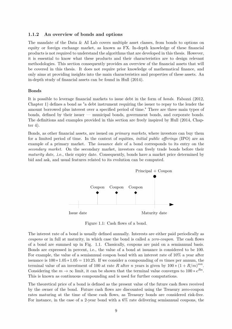
Figure 1.1: Cash flows of a bond.

The interest rate of a bond is usually defined annually. Interests are either paid periodically ascoupons or in full at maturity, in which case the bond is called a zero-coupon. The cash flowsof a bond are summed up in Fig. 1.1. Classically, coupons are paid on a semiannual basis.Bonds are expressed in percent, i.e., the value of a bond at issuance is considered to be 100.For example, the value of a semiannual coupon bond with an interest rate of 10% a year afterissuance is 100 ú 1.05 ú 1.05 = 110.25. If we consider a compounding of m times per annum, theterminal value of an investment of 100 at rate R after n years is given by 100 ú (1 + R/m)mn.Considering the m æ Œ limit, it can be shown that the terminal value converges to 100 ú e

Rn.This is known as continuous compounding and is used for further computations.

The theoretical price of a bond is defined as the present value of the future cash flows receivedby the owner of the bond. Future cash flows are discounted using the Treasury zero-couponrates maturing at the time of these cash flows, as Treasury bonds are considered risk-free.For instance, in the case of a 2-year bond with a 6% rate delivering semiannual coupons, the

9

theoretical price of the bond pt, expressed in basis points, is defined as pt = 3e≠T0.5ú0.5 +

3e≠T1.ú1. +3e

≠T1.5ú1.5 +103e≠T2.ú2., where Tn is the n-year Treasury zero-coupon rate. The yield

y of a bond is defined as the single discount rate that equals the theoretical bond price, i.e., inbasis points, pt = 3e

≠yú0.5 +3e≠yú1. +3e

≠yú1.5 +103e≠yú2.. The yield can be found using iterative

methods such as Newton-Raphson. High yields can come from either high coupons or a lowtheoretical bond value — its interpretation is consequently subject to caution. It is, however,a useful quantity to understand bonds, and yield curves representing yield as a function ofmaturity for zero-coupon government bonds are often used to analyze rates markets. The bondspread corresponds to the di�erence, expressed in basis points, between the bond yield and thezero-coupon rate of a risk-free bond of the same maturity.

Another useful quantity is the duration of a bond. Noting ci, i œ [[1; n]] the cash flow at timeti, the theoretical bond price can be written pt =

qn

i=1 cie≠yti , where y denotes the yield. The

duration of the bond is then defined as

Dt =q

n

i=1 ticie≠yti

pt

=nÿ

i=1ti

Ccie

≠yti

pt

D

. (1.1)

Duration can be understood as a weighted average of payment times with a weight correspondingto the proportion of the bond’s total present value provided by the i-th cash flow. It consequentlymeasures how long on average an investor has to wait before receiving payments.

Finally, bonds also receive a credit rating representing the credit worthiness of their issuer.Credit rating agencies such as Moody’s or Standard & Poors publish them regularly for bothcorporate and governmental bonds. As they are meant to indicate the likelihood that the debtwill be fully repaid, investors use such ratings to guide their investment choices.

More information about interest rates in general and bonds in particular can be found in Hull(2014, Chapter 4). In this work, we cover corporate and G10 bonds, i.e., governmental bondsfrom countries of the G10 group (Germany, Belgium, Canada, United States, France, Italy,Japan, Netherlands, United Kingdom, Sweden, Switzerland).

Options

Hull (2014, Chapter 10) defines options as financial contracts giving holders the right to buyor sell an underlying asset by (or at) a certain date for a specific price. The right to buy anunderlying asset is named a call option, and the right to sell is named a put option. The priceat which the underlying asset can be bought/sold is called the strike price. The date at whichthe underlying asset can be bought/sold is called the maturity date, as in bonds. If the optionallows exercising this right at any time before maturity, it is said to be American. If the rightcan only be exercised at maturity, the option is said to be European. American options are themost popular ones, but we consider here European options for ease of analysis. Investors haveto pay a price to acquire an option, regardless of the exercise of the provided right.

Options can be bought or sold, and can even be traded. Buyers of options are said to have longpositions, and sellers are said to have short positions. Sellers are also said to write the option.Figure 1.2 shows the four di�erent cases possible and their associated payo�s.

To understand the interest of options, let us take the example of an investor buying a Europeancall option for 100 shares of a given stock with a strike price of 50Ä at a price of 5Ä per share.Assume the price at the moment of the contract was 48Ä. If at maturity, the price of the stockis 57Ä, the investor exercises its right to buy 100 shares of the stock at 50Ä and directly sellsthem. She makes a net profit of 700-500=200Ä. If the investor would have invested the sameamount in the stock directly, she would have made a profit of 9Ä per share and could have

10

Figure 1.2: The four di�erent options payo� structures. (·)+ denotes here max (·, 0).

bought only 4 of them, making a net profit of 36Ä. Options are leverage instruments: for thesame amount of money invested, they provide the opportunity to obtain far better returns atthe cost of higher risk. We see in this example that at prices below 55Ä, the options investorwould start losing money, whereas the buyer of the shares would still make a profit.

In the case of equity options, Hull (2014, Chapter 11) enumerates six factors a�ecting the priceof an option:

- the current price of the equity, noted S0;- the strike price K;- the time to maturity T ;- the volatility of the underlying ‡;- the risk-free interest rate r;- the dividends D expected to be paid, if any.

Using the no-arbitrage principle stating that there are no risk-free investments insuring strictlypositive returns, an analysis of these factors allows deriving lower and upper bounds on theoption price (Hull, 2014, Chapter 11). The arbitrage analysis allows as well to uncover thecall-put parity. This property links call and put prices by the formula:

Ccall + Ke≠rT + D = Cput + S0, (1.2)

considering that stocks with no dividends have D = 0.

The price of an option can be derived analytically using stochastic calculus. If we assume,among other hypotheses that one can find in Hull (2014, Chapter 15), that stock prices followa geometric Brownian motion dSt = St (µdt + ‡dBt) where µ is the drift and ‡ the volatility,we can derive the Black-Scholes equation (Black and Scholes, 1973):

ˆC

ˆt+ rS

ˆC

ˆS+ 1

2‡2S

2 ˆ2C

ˆS2 ≠ rC = 0, (1.3)

11

where C is the price of the (European) option, S the price of the underlying, ‡ the volatility ofthe underlying and r the risk-free rate. Notably, this equation links the price of the option tothe volatility of the underlying. Using the bounds found in the arbitrage analysis, the equationcan be used both to derive the price of an option using the historical volatility computed frompast prices of its underlying and to determine the implied volatility from the option currentprice. Implied volatility is an indicator that is used for markets analysis, and can serve as inputin more complex models.

Moreover, calls and puts can be combined in option strategies to form new payo� structures.Classic combinations include the following:

- Call spread. A call spread is the combination of a long call at a given strike and a shortcall at a higher strike. The payo� corresponds to the one of a call, with a cap on themaximum profit possible. Call spreads allow benefiting from a moderate increase in price,at a lower cost than a classic call option.

- Put spread. A put spread is the combination of a short put at a given strike and a longput at a higher strike. The payo� corresponds to the one of a put, with a cap on themaximum profit possible. Put spreads allow benefiting from a moderate decrease in price,at a lower cost than a classic put option.

- Straddle. Buying a straddle corresponds to buying a call and a put with the same strikeprices and maturities on the same underlying. This position is used in high volatilitysituations when an investor reckons that the underlying price might evolve a lot in eitherdirection.

- Strangle. Buying a strangle corresponds to buying a call and a put with the maturitieson the same underlying, but with di�erent strike prices. This position is used in the samesituation as a straddle, but can be bought at a lower price.

1.2 Understanding dataWe introduced the global characteristics of the RFQ datasets that are studied in this thesis inSection 1.1. However, an in-depth exploration of the data is required to understand the chal-lenges that lie within data: from this exploration follow insights that can guide the constructionof an algorithm tailored to face these challenges. Consequently, this section explains the datasources at hand and provides an exploratory analysis of a particularly important characteristicof the datasets we study in this thesis.

1.2.1 Data sourcesTo solve the problem exposed in Section 1.1, we have various sources of data at our disposal.For all the asset classes that we may consider, we count three data categories.

- Client-related data. When an investor becomes a BNPP CIB client, she fills KnowYour Customer (KYC) information that can be used in our models, such as her sectorof activity, her region, . . . , i.e., a set of categorical features. Due to their size and/or thenature of their business, some clients may also have to periodically report the content oftheir portfolio. This data is particularly valuable, as an investor cannot sell an asset shedoes not have. Consequently, knowing their portfolio allows for more accurate predictions— in particular, in the sell direction.

- Asset-related data. Financial products are all uniquely identified in the markets by theirInternational Securities Identification Number (ISIN, 2020). Depending on the nature ofthe asset, categorical features can be derived to describe it. For instance, bonds canbe described through their issuer, also known as the ticker of the bond, the sector of

12

activity of the latter, the currency in which it was issued, its issuance and maturity dates,. . . Market data of the assets can also be extracted, i.e., numerical features such as theprice, the volatility or other useful financial indicators. Usually, these features are recordedon a daily basis at their close value, i.e., their value at the end of the trading day. Foroptions, both market data for the option and its underlying can be extracted.

- Trade-related data. The most important data for recommender systems is the trade-related one. This data corresponds to all RFQs, RFMs, and IOIs that were gathered bysales teams (see Section 1.1.1). These requests and indications of interest provide us withthe raw interest signal of a client for a given product. As the final decision following arequest is not always known, we use the fact that a client made a request on a particularproduct as a positive event of interest for that product.

These di�erent sources are brought together in various ways depending on the algorithms thatwe use, as exposed in Section 1.3 and in the next chapters of this thesis.

1.2.2 Exploring the heterogeneity of clients and assetsAn essential characteristic of our RFQ datasets, common to many fields of application, is hetero-geneity. Heterogeneity of activity is deeply embedded in our financial datasets and appears onboth the client and asset sides. We explore here the case of the corporate bonds RFQ database,studying a portion ranging from 07/01/2017 to 03/01/2020. In this period, we count roughly4000 clients and 30000 bonds. Of these 4000 clients, about 23% regularly disclose the content oftheir bond portfolios — this information is consequently di�cult to use in a model performingpredictions for all clients.

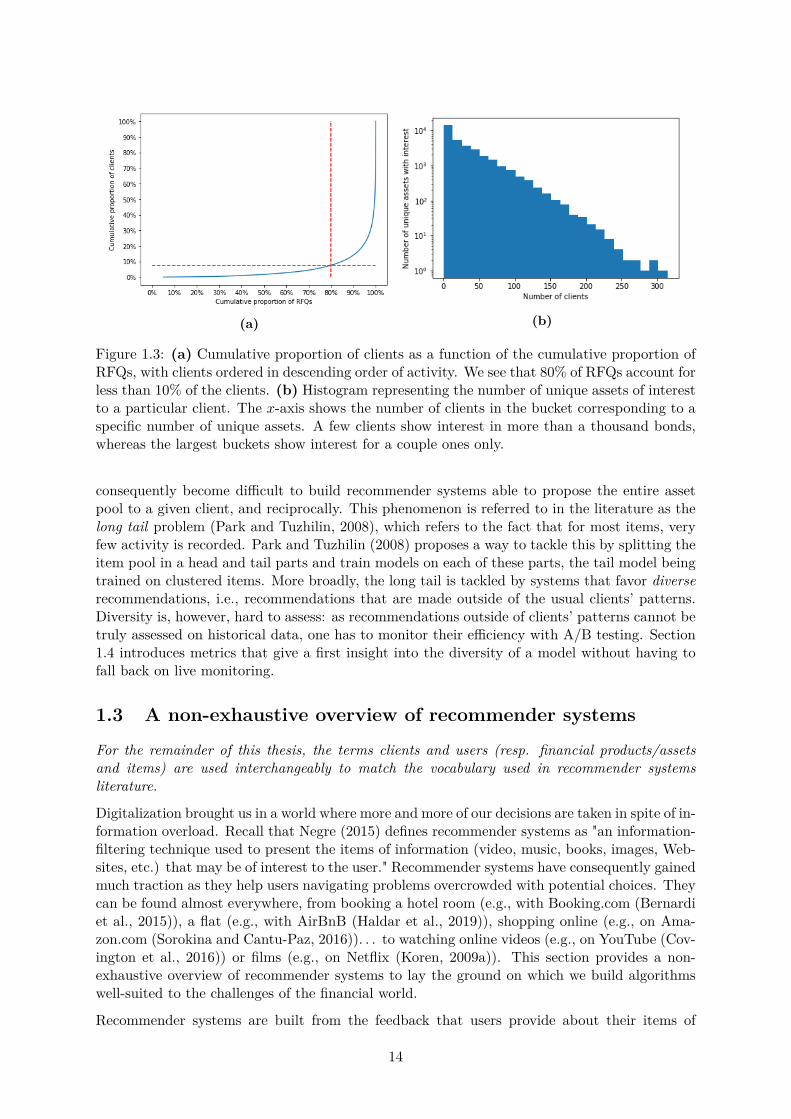
Let us begin with the heterogeneity of clients. A glimpse at heterogeneity can be taken bylooking at a single client: the most active client accounted for 5% of all performed RFQs alone,and up to 6.4% when taking into account all its subsidiaries. The heterogeneity of clients canbe further explored with Fig. 1.3. In Fig. 1.3a, we see that 80% of the accounted RFQs weremade by less than 10% of the client pool. Most of BNPP CIB business is consequently donewith a small portion of its client reach: a recommender system could help better serve thisportion of BNPP clients by providing sales with o�ers tailored to their needs. The histogramshown in Fig. 1.3b provides another visualization of this result. We see here that a few clientsrequest prices for thousands of unique bonds, whereas over the same period, some clients onlyrequest prices for a handful of bonds. Clients are consequently profoundly heterogeneous. Notehowever that this heterogeneity, to some extent, might only be perceived as such as we do notobserve the complete activity of our clients and only what they do on platforms on which BNPPCIB is active.

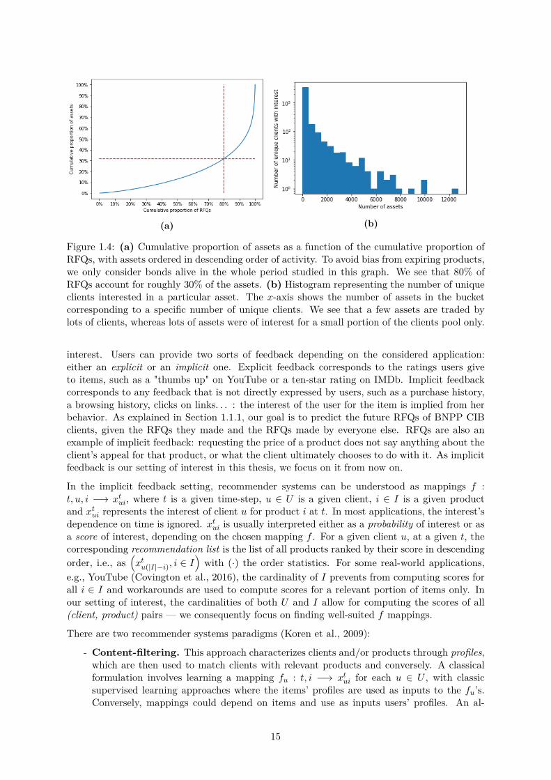
We now give a closer look at the heterogeneity of bonds. In particular, here, the most activebond accounted for 0.3% of all RFQs, and up to 1% when aggregating all bonds emitted bythe same issuer. A global look at these statistics is presented in Fig. 1.4a. To avoid biasfrom expiring products, we only account in this graph for bonds with issue and maturity datesstrictly outside of the considered period. We see here that 80% of the RFQs were done on morethan 30% of the considered assets. The heterogeneity of bonds is consequently less pronouncedthat the heterogeneity of clients. There are however more pronounced popularity e�ects, ascan be seen in Fig. 1.4b. Here, we see that only a small portion of bonds are shared amongthe client pool. Most bonds can be considered as niche, and are only traded by a handfulof clients. Consequently, even though bonds are, on average, more active than clients, theirrelative popularities reveal their heterogeneity.

In Fig. 1.3 and 1.4, (b) graphs both show the sparsity of this dataset. Most clients onlytrade a handful of bonds, and most bonds are only traded by a handful of clients. It can

13

(a) (b)

Figure 1.3: (a) Cumulative proportion of clients as a function of the cumulative proportion ofRFQs, with clients ordered in descending order of activity. We see that 80% of RFQs account forless than 10% of the clients. (b) Histogram representing the number of unique assets of interestto a particular client. The x-axis shows the number of clients in the bucket corresponding to aspecific number of unique assets. A few clients show interest in more than a thousand bonds,whereas the largest buckets show interest for a couple ones only.

consequently become di�cult to build recommender systems able to propose the entire assetpool to a given client, and reciprocally. This phenomenon is referred to in the literature as thelong tail problem (Park and Tuzhilin, 2008), which refers to the fact that for most items, veryfew activity is recorded. Park and Tuzhilin (2008) proposes a way to tackle this by splitting theitem pool in a head and tail parts and train models on each of these parts, the tail model beingtrained on clustered items. More broadly, the long tail is tackled by systems that favor diverserecommendations, i.e., recommendations that are made outside of the usual clients’ patterns.Diversity is, however, hard to assess: as recommendations outside of clients’ patterns cannot betruly assessed on historical data, one has to monitor their e�ciency with A/B testing. Section1.4 introduces metrics that give a first insight into the diversity of a model without having tofall back on live monitoring.

1.3 A non-exhaustive overview of recommender systems

For the remainder of this thesis, the terms clients and users (resp. financial products/assetsand items) are used interchangeably to match the vocabulary used in recommender systemsliterature.

Digitalization brought us in a world where more and more of our decisions are taken in spite of in-formation overload. Recall that Negre (2015) defines recommender systems as "an information-filtering technique used to present the items of information (video, music, books, images, Web-sites, etc.) that may be of interest to the user." Recommender systems have consequently gainedmuch traction as they help users navigating problems overcrowded with potential choices. Theycan be found almost everywhere, from booking a hotel room (e.g., with Booking.com (Bernardiet al., 2015)), a flat (e.g., with AirBnB (Haldar et al., 2019)), shopping online (e.g., on Ama-zon.com (Sorokina and Cantu-Paz, 2016)). . . to watching online videos (e.g., on YouTube (Cov-ington et al., 2016)) or films (e.g., on Netflix (Koren, 2009a)). This section provides a non-exhaustive overview of recommender systems to lay the ground on which we build algorithmswell-suited to the challenges of the financial world.

Recommender systems are built from the feedback that users provide about their items of

14

(a) (b)

Figure 1.4: (a) Cumulative proportion of assets as a function of the cumulative proportion ofRFQs, with assets ordered in descending order of activity. To avoid bias from expiring products,we only consider bonds alive in the whole period studied in this graph. We see that 80% ofRFQs account for roughly 30% of the assets. (b) Histogram representing the number of uniqueclients interested in a particular asset. The x-axis shows the number of assets in the bucketcorresponding to a specific number of unique clients. We see that a few assets are traded bylots of clients, whereas lots of assets were of interest for a small portion of the clients pool only.

interest. Users can provide two sorts of feedback depending on the considered application:either an explicit or an implicit one. Explicit feedback corresponds to the ratings users giveto items, such as a "thumbs up" on YouTube or a ten-star rating on IMDb. Implicit feedbackcorresponds to any feedback that is not directly expressed by users, such as a purchase history,a browsing history, clicks on links. . . : the interest of the user for the item is implied from herbehavior. As explained in Section 1.1.1, our goal is to predict the future RFQs of BNPP CIBclients, given the RFQs they made and the RFQs made by everyone else. RFQs are also anexample of implicit feedback: requesting the price of a product does not say anything about theclient’s appeal for that product, or what the client ultimately chooses to do with it. As implicitfeedback is our setting of interest in this thesis, we focus on it from now on.

In the implicit feedback setting, recommender systems can be understood as mappings f :t, u, i ≠æ x

t

ui, where t is a given time-step, u œ U is a given client, i œ I is a given product

and xt

uirepresents the interest of client u for product i at t. In most applications, the interest’s

dependence on time is ignored. xt

uiis usually interpreted either as a probability of interest or as

a score of interest, depending on the chosen mapping f . For a given client u, at a given t, thecorresponding recommendation list is the list of all products ranked by their score in descendingorder, i.e., as

1x

t

u(|I|≠i), i œ I

2with (·) the order statistics. For some real-world applications,

e.g., YouTube (Covington et al., 2016), the cardinality of I prevents from computing scores forall i œ I and workarounds are used to compute scores for a relevant portion of items only. Inour setting of interest, the cardinalities of both U and I allow for computing the scores of all(client, product) pairs — we consequently focus on finding well-suited f mappings.

There are two recommender systems paradigms (Koren et al., 2009):

- Content-filtering. This approach characterizes clients and/or products through profiles,which are then used to match clients with relevant products and conversely. A classicalformulation involves learning a mapping fu : t, i ≠æ x

t

uifor each u œ U , with classic

supervised learning approaches where the items’ profiles are used as inputs to the fu’s.Conversely, mappings could depend on items and use as inputs users’ profiles. An al-

15

ternative approach is to use a global mapping f : t, u, i ≠æ xt

uiusing as input, e.g., a

concatenation of u and i profiles at t, and features depending on both u and i.- Collaborative filtering. The term, coined by Goldberg et al. (1992) for Tapestry, the

first recommender system, refers to algorithms making predictions about a given clientusing the knowledge of what all other clients have been doing. According to Koren et al.(2009), the two main areas of collaborative filtering are neighborhood methods and latentfactor models. Neighborhood methods compute weighted averages of the rating vectorsof users (resp. items) to find missing (user, item) ratings, e.g., using user-user (resp.item-item) similarities as weights. Latent factor models characterize users and items withvector representations of given dimension d inferred from observed ratings and use thesevectors to compute missing (user, item) ratings. These two approaches can be broughttogether, e.g., as in (Koren, 2008).

Content- and collaborative filtering are not contradictory and can be brought together, e.g., asin Basilico and Hofmann (2004). Learning latent representations of users and items, as is done inlatent factor models, has advantages beyond inferring missing ratings. These representations canbe used a posteriori for clustering, visualization of user-user, item-item or user-item relationshipsand their evolution with time,. . . These applications of latent factors are particularly useful forbusiness, e.g., to understand how BNP Paribas CIB clients relate to each other and consequentlyreorganize the way sales operate. For that reason, the collaborative filtering algorithms we studyhere are mainly latent factor models.

We now examine how baseline recommender systems can be obtained, develop on the contentfiltering approach with a specific formulation of the problem as a classification one, expand onsome collaborative filtering algorithms and provide insights into other approaches for recom-mender systems.

1.3.1 Benchmarking algorithmsBaselines are algorithms that serve as reference for determining the performance of a proposalalgorithm. Consequently, baselines are crucial for understanding how well an algorithm is doingon a given problem. In computer vision problems such as the ImageNet challenge (Russakovskyet al., 2015), the baseline is a human performance score. However, obtaining a human per-formance baseline is more complicated in recommender systems as the goal is to automate atask that is inherently not doable by any human: it would require at the very least an in-depthknowledge of the full corpus of users and items for a human to solve this recommendationtask.

A simple recommender system baseline is the historical one. Using a classical train/test splitof the observed events, a first baseline is given by the mapping fhist : (u, i) ≠æ rui with rui œ Nthe number of observed events for the (u, i) couple on the train split. The score can also beexpressed as a frequency of interest, either on the user- or item-side; i.e., on the user-sideas rui/

qiœI

rui. The historical model can also be improved using the temporal information,considering that at a given t, closer interests should weigh more in the score. An example ofsuch mapping is

fhist : (t, u, i) ≠æt≠1ÿ

tÕ=1e

≠⁄(t+1≠tÕ)

rtÕ

ui (1.4)

where rtÕ

uidenotes the number of observed events for the (u, i) couple at t

Õ, and ⁄ is a decayfactor. Note that the sum stops at t ≠ 1 for prediction at t since observed events at t cannot betaken into account for predicting that time-step. In the following, we mainly use the most simpleinstance of baseline where the score of a (u, i) couple is given by their number of interactionsobserved in the training split.

16

1.3.2 Content-filtering strategiesWe previously defined content filtering algorithms as mapping profiles of users, items, or bothof them to the interest x

t

ui. The di�culty of this approach lies in the construction of users and

items’ profiles, as they require data sources other than the observation of interactions betweenthe two. As exposed in Section 1.2, we have at our disposal multiple data sources from whichto build such profiles. Concretely, each of the three sources outlined in Section 1.2.1 leads to aprofile — one can consequently build a user profile, an item profile, and an interaction profilefrom the available data.

The profile of a user (resp. item) is built from the numerical and categorical informationavailable describing her (resp. its) state. Numerical features such as the buy/sell frequencyof a user or the price of an item can be directly used. However, categorical features, e.g.,the user’s country or the company producing the item, require an encoding for an algorithmto make use of them. Categories can be encoded in various ways, the most popular ones inmachine learning being one-hot encoding, frequency encoding and target encoding. One-hotencoding converts a category c œ [[1; K]] to the c-th element ec of the canonical basis of RK ,ec = (0, . . . , 1, . . . , 0) œ RK , i.e., a zero vector with a 1 in the c-th position. Frequency encodingconverts a category c œ [[1; K]] to its frequency of appearance in the training set. Target encodingconverts a category c œ [[1; K]] to the mean of targets y observed for particular instances of thatcategory. One-hot encoding is a simple and widespread methodology for dealing with categoricalvariables; frequency and target encoding, to the best of our knowledge, could be more qualifiedof "tricks of the trade" used by data science competitors on platforms such as Kaggle (KaggleInc., 2020). One-hot encodings are, by essence, sparse and grow the number of features usedby a model by as many categories there are per categorical feature. Deep learning modelsusually handle categorical features through embeddings, i.e., trainable latent representations ofa size specifically chosen for each feature. These embeddings are trained along with all otherparameters of the neural networks.

Provided with embeddings of categorical features describing the state of a particular user (resp.item), a profile of this user (resp. item) can be obtained by the concatenation of the numericalfeatures and embeddings related to her. These profiles are then used to learn mappings fi

for all i œ I (resp. fu for all u œ U), or can be concatenated to learn a global mappingf : (t, u, i) ≠æ x

t

ui. One can also add cross-features depending on both u and i, such as the

frequency at which u buys or sells i. Indeed, in the financial context, it is usual for investorsto re-buy or re-sell in the future products they bought or sold previously — cross-featuresdescribing the activity of a user u on an item i are consequently meaningful. A good practicefor numerical features is to transform them using standard scores, as known as z-scores. Afeature x is turned into a z-score z with z = x≠µ

‡, where µ and ‡ are the mean and standard

deviation of x, computed using the training split of the data. Z-scores can also be computed oncategories of a given categorical feature, using µc and ‡c for all c œ [[1; K]], provided that we haveenough data for each category to get meaningful means and variances. The distribution of afeature can vary much with categories: for instance, the buying frequency of a hedge fund is notthe same as the one of a central bank. Using z-scores modulated per category of a categoricalfeature consequently helps to make these categories comparable.

In the implicit feedback setting, the recommendation problem can be understood as a classi-fication task. Provided with a profile, i.e., a set of features x describing a particular (t, u, i)triplet, we want to predict whether u is interested in i or not at t, i.e., predict a binary targety œ {0, 1}. If, as mentioned in Section 1.1.1, we want to predict whether u is interested inbuying and/or selling i, the target y can consequently take up to four values corresponding to alack of interest, an interest in buying, in selling or in doing both, the last case happening onlywhen the time-step is large enough to allow for it — the size of the time-step usually depends

17

on the liquidity of the considered asset class, as mentioned in Section 2.2.4. Classification is asupervised learning problem for which many classic machine learning algorithms can be used.A classic way to train a classifier is to optimize its cross-entropy loss, defined for a sample x

as

l(x) = ≠Cÿ

i=1yi(x) log yi(x) ,

a term derived from maximum likelihood where C is the total number of classification classes,yi(x) = y(x)=i and yi(x) the probability of class i outputted by the model for sample x. Avariation of cross-entropy, the focal loss (Lin et al., 2017), can help in cases of severe classimbalance. Focal loss performs an adaptive, per-sample reweighing of the loss, defined for asample x as

lfocal(x) = ≠Cÿ

i=1(1 ≠ yi(x))“

yi(x) log yi(x) , (1.5)

with “ an hyperparameter, usually chosen in the ]0; 4] range and depending on the imbalanceratio, defined in the binary case as the ratio of the number of instances in the majority classand the ones in the minority class. In imbalance settings, the majority class is easily learntby the algorithm and accounts for most of the algorithm loss performance. The (1 ≠ yi(x))“

term counterbalances this by disregarding confidently classified samples, and focuses the sumon "harder-to-learn" ones. Consequently, when the imbalance ratio is high, higher values of “

are favored.

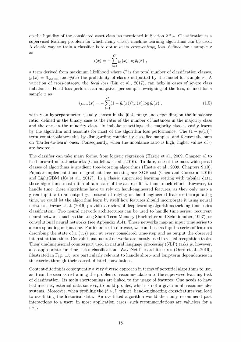
The classifier can take many forms, from logistic regression (Hastie et al., 2009, Chapter 4) tofeed-forward neural networks (Goodfellow et al., 2016). To date, one of the most widespreadclasses of algorithms is gradient tree-boosting algorithms (Hastie et al., 2009, Chapters 9,10).Popular implementations of gradient tree-boosting are XGBoost (Chen and Guestrin, 2016)and LightGBM (Ke et al., 2017). In a classic supervised learning setting with tabular data,these algorithms most often obtain state-of-the-art results without much e�ort. However, tohandle time, these algorithms have to rely on hand-engineered features, as they only map agiven input x to an output y. Instead of relying on hand-engineered features incorporatingtime, we could let the algorithm learn by itself how features should incorporate it using neuralnetworks. Fawaz et al. (2019) provides a review of deep learning algorithms tackling time seriesclassification. Two neural network architectures can be used to handle time series: recurrentneural networks, such as the Long Short-Term Memory (Hochreiter and Schmidhuber, 1997), orconvolutional neural networks (see Appendix A.4). These networks map an input time series toa corresponding output one. For instance, in our case, we could use as input a series of featuresdescribing the state of a (u, i) pair at every considered time-step and as output the observedinterest at that time. Convolutional neural networks are mostly used in visual recognition tasks.Their unidimensional counterpart used in natural language processing (NLP) tasks is, however,also appropriate for time series classification. WaveNet-like architectures (Oord et al., 2016),illustrated in Fig. 1.5, are particularly relevant to handle short- and long-term dependencies intime series through their causal, dilated convolutions.

Content-filtering is consequently a very diverse approach in terms of potential algorithms to use,as it can be seen as re-framing the problem of recommendation to the supervised learning taskof classification. Its main shortcomings are linked to the usage of features. One needs to havefeatures, i.e., external data sources, to build profiles, which is not a given in all recommendersystems. Moreover, when profiling the (t, u, i) triplet, hand-engineering cross-features can leadto overfitting the historical data. An overfitted algorithm would then only recommend pastinteractions to a user: in most application cases, such recommendations are valueless for auser.

18

Because models with causal convolutions do not have recurrent connections, they are typically fasterto train than RNNs, especially when applied to very long sequences. One of the problems of causalconvolutions is that they require many layers, or large filters to increase the receptive field. Forexample, in Fig. 2 the receptive field is only 5 (= #layers + filter length - 1). In this paper we usedilated convolutions to increase the receptive field by orders of magnitude, without greatly increasingcomputational cost.

A dilated convolution (also called a trous, or convolution with holes) is a convolution where thefilter is applied over an area larger than its length by skipping input values with a certain step. It isequivalent to a convolution with a larger filter derived from the original filter by dilating it with zeros,but is significantly more efficient. A dilated convolution effectively allows the network to operate ona coarser scale than with a normal convolution. This is similar to pooling or strided convolutions, buthere the output has the same size as the input. As a special case, dilated convolution with dilation1 yields the standard convolution. Fig. 3 depicts dilated causal convolutions for dilations 1, 2, 4,and 8. Dilated convolutions have previously been used in various contexts, e.g. signal processing(Holschneider et al., 1989; Dutilleux, 1989), and image segmentation (Chen et al., 2015; Yu &Koltun, 2016).

Input

Hidden LayerDilation = 1



OutputDilation = 8

Figure 3: Visualization of a stack of dilated causal convolutional layers.

Stacked dilated convolutions enable networks to have very large receptive fields with just a few lay-ers, while preserving the input resolution throughout the network as well as computational efficiency.In this paper, the dilation is doubled for every layer up to a limit and then repeated: e.g.

1, 2, 4, . . . , 512, 1, 2, 4, . . . , 512, 1, 2, 4, . . . , 512.

The intuition behind this configuration is two-fold. First, exponentially increasing the dilation factorresults in exponential receptive field growth with depth (Yu & Koltun, 2016). For example each1, 2, 4, . . . , 512 block has receptive field of size 1024, and can be seen as a more efficient and dis-criminative (non-linear) counterpart of a 1�1024 convolution. Second, stacking these blocks furtherincreases the model capacity and the receptive field size.

2.2 SOFTMAX DISTRIBUTIONS

One approach to modeling the conditional distributions p (xt | x1, . . . , xt�1) over the individualaudio samples would be to use a mixture model such as a mixture density network (Bishop, 1994)or mixture of conditional Gaussian scale mixtures (MCGSM) (Theis & Bethge, 2015). However,van den Oord et al. (2016a) showed that a softmax distribution tends to work better, even when thedata is implicitly continuous (as is the case for image pixel intensities or audio sample values). Oneof the reasons is that a categorical distribution is more flexible and can more easily model arbitrarydistributions because it makes no assumptions about their shape.

Because raw audio is typically stored as a sequence of 16-bit integer values (one per timestep), asoftmax layer would need to output 65,536 probabilities per timestep to model all possible values.To make this more tractable, we first apply a µ-law companding transformation (ITU-T, 1988) tothe data, and then quantize it to 256 possible values:

f (xt) = sign(xt)ln (1 + µ |xt|)

ln (1 + µ),

3

Figure 1.5: The WaveNet architecture, using causal and dilated convolutions. Causal convolu-tions relate their output at t to inputs at t

Õ Æ t only. Dilated convolutions, as known as à trousconvolutions, only consider as inputs to a particular output index the multiples of the dilationfactor at that index. Dilated convolutions extend the receptive field of the network, i.e., theperiod of time taken into account for the computation of a particular output. WaveNets usedstacked dilated convolutions, with a dilation factor doubled up to a limit and repeated, e.g., 1,2, 4, 16, 32, 1, 2, 4, 16, 32, . . . to get the widest receptive field possible. Illustration taken fromOord et al. (2016).

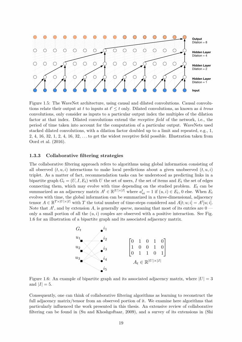
1.3.3 Collaborative filtering strategiesThe collaborative filtering approach refers to algorithms using global information consisting ofall observed (t, u, i) interactions to make local predictions about a given unobserved (t, u, i)triplet. As a matter of fact, recommendation tasks can be understood as predicting links in abipartite graph Gt = (U, I, Et) with U the set of users, I the set of items and Et the set of edgesconnecting them, which may evolve with time depending on the studied problem. Et can besummarized as an adjacency matrix A

t œ R|U |◊|I| where at

ui= 1 if (u, i) œ Et, 0 else. When Et

evolves with time, the global information can be summarized in a three-dimensional, adjacencytensor A œ RT ◊|U |◊|I| with T the total number of time-steps considered and A[t; u; i] = A

t[u; i].Note that A

t, and by extension A, is generally sparse, meaning that most of its entries are 0 —only a small portion of all the (u, i) couples are observed with a positive interaction. See Fig.1.6 for an illustration of a bipartite graph and its associated adjacency matrix.

Figure 1.6: An example of bipartite graph and its associated adjacency matrix, where |U | = 3and |I| = 5.

Consequently, one can think of collaborative filtering algorithms as learning to reconstruct thefull adjacency matrix/tensor from an observed portion of it. We examine here algorithms thatparticularly influenced the work presented in this thesis. An extensive review of collaborativefiltering can be found in (Su and Khoshgoftaar, 2009), and a survey of its extensions in (Shi

19

et al., 2014).

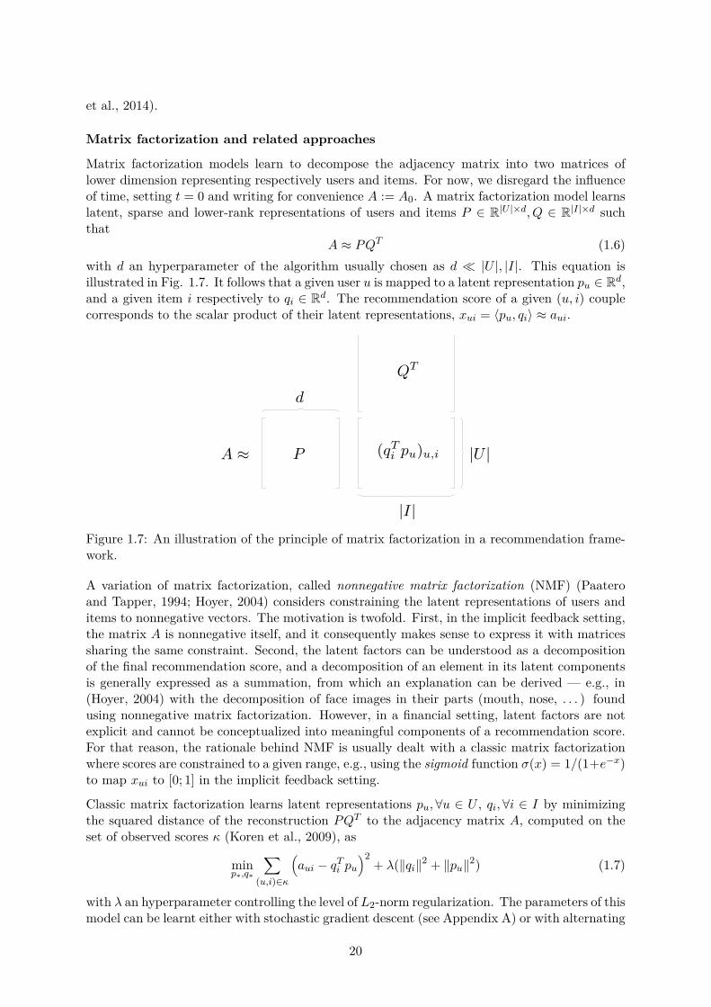
Matrix factorization and related approaches

Matrix factorization models learn to decompose the adjacency matrix into two matrices oflower dimension representing respectively users and items. For now, we disregard the influenceof time, setting t = 0 and writing for convenience A := A0. A matrix factorization model learnslatent, sparse and lower-rank representations of users and items P œ R|U |◊d

, Q œ R|I|◊d suchthat

A ¥ PQT (1.6)

with d an hyperparameter of the algorithm usually chosen as d π |U |, |I|. This equation isillustrated in Fig. 1.7. It follows that a given user u is mapped to a latent representation pu œ Rd,and a given item i respectively to qi œ Rd. The recommendation score of a given (u, i) couplecorresponds to the scalar product of their latent representations, xui = Èpu, qiÍ ¥ aui.

Figure 1.7: An illustration of the principle of matrix factorization in a recommendation frame-work.

A variation of matrix factorization, called nonnegative matrix factorization (NMF) (Paateroand Tapper, 1994; Hoyer, 2004) considers constraining the latent representations of users anditems to nonnegative vectors. The motivation is twofold. First, in the implicit feedback setting,the matrix A is nonnegative itself, and it consequently makes sense to express it with matricessharing the same constraint. Second, the latent factors can be understood as a decompositionof the final recommendation score, and a decomposition of an element in its latent componentsis generally expressed as a summation, from which an explanation can be derived — e.g., in(Hoyer, 2004) with the decomposition of face images in their parts (mouth, nose, . . . ) foundusing nonnegative matrix factorization. However, in a financial setting, latent factors are notexplicit and cannot be conceptualized into meaningful components of a recommendation score.For that reason, the rationale behind NMF is usually dealt with a classic matrix factorizationwhere scores are constrained to a given range, e.g., using the sigmoid function ‡(x) = 1/(1+e

≠x)to map xui to [0; 1] in the implicit feedback setting.

Classic matrix factorization learns latent representations pu, ’u œ U , qi, ’i œ I by minimizingthe squared distance of the reconstruction PQ

T to the adjacency matrix A, computed on theset of observed scores Ÿ (Koren et al., 2009), as

minpú,qú

ÿ

(u,i)œŸ

1aui ≠ q

T

i pu

22+ ⁄(ÎqiÎ2 + ÎpuÎ2) (1.7)

with ⁄ an hyperparameter controlling the level of L2-norm regularization. The parameters of thismodel can be learnt either with stochastic gradient descent (see Appendix A) or with alternating

20

least squares (Hu et al., 2008; Pilászy et al., 2010; Takács and Tikk, 2012). A probabilisticinterpretation of this model (Mnih and Salakhutdinov, 2008) shows that this objective functionis equivalent to a Gaussian prior assumption on the latent factors.

This formulation of matrix factorization is particularly relevant for explicit feedback. In implicitfeedback however, all unobserved events are considered negative, and positive ones are implied— a (u, i) pair considered positive does not assuredly correspond to a true positive event, asexplained in the incipit of this section. To counter these assumptions, Hu et al. (2008) introducea notion of confidence weighing in the above equation. Keeping rui as the number of observedinteractions of the (u, i) pair in the considered dataset, the authors introduce two definitions ofconfidence:

- Linear: cui = 1 + –rui

- Logarithmic: cui = 1 + – log(1 + rui/‘)

where –, ‘ are hyperparameters of the algorithm. We empirically found logarithmic confidencesto provide better results, a performance that we attribute to logarithms flattening the highlyheterogeneous users’ and items’ activity we observe in our datasets (see Section 1.2.2). Definingpui := rui>0 = aui, the implicit feedback objective is written

minpú,qú

ÿ

u,i

cui

1pui ≠ q

T

i pu

22+ ⁄(ÎqiÎ2 + ÎpuÎ2). (1.8)

Note that the summation is now performed on all possible (u, i) pairs. Most often, the total num-ber of pairs makes stochastic gradient descent impractical, and these objectives are optimizedusing alternating least squares. In our case, however, the total number of pairs of a few millions— tens of millions, in the worst case — still allows for gradient descent optimizations.

A related approach is Bayesian Personalized Ranking (BPR) (Rendle et al., 2009), an optimiza-tion method specifically designed for implicit feedback datasets. The goal, as initially exposed,is to provide users with a ranked list of items. BPR abandons the probability approach for xui

used in the above algorithms to focus on a scoring approach. The underlying idea of BPR isto give a higher score to observed (u, i) couples than unobserved ones. To do so, the authorsformalize a dataset D = {(u, i, j)|i œ I

+u · j œ I\I

+u } where I

+u is the set of items which have

a positive event with user u in the considered data. D is consequently formed of all possibletriplets containing a positive (u, i) pair and an associated negative item j. The BPR objectiveis then defined as maximizing the quantity

LBP R =ÿ

(u,i,j)œD

ln ‡(xuij) ≠ ⁄ Î�Î2 (1.9)

where xuij is the score associated to the (u, i, j) triplet, defined such that p(i >u j|�) := xuij(�)with >u the total ranking associated to u — i.e., the ranking corresponding to the preferencesof u in terms of items, see Rendle et al. (2009, Section 3.1)—, and ⁄ is an hyperparametercontrolling the level of regularization. As D grows exponentially with the number of users anditems, this objective is approximated using negative sampling (Mikolov et al., 2013). Followingmatrix factorization ideas, we define xuij = xui ≠ xuj , with xui = q

T

ipu where pu, qi are latent

factors defined as previously. The BPR objective is a relaxation of the ROC AUC score (seeSection 1.4), a ranking metric also used in the context of binary classification. BPR combinedwith latent factors is, at the time of writing this thesis, one of the most successful and widespreadalgorithms to solve implicit feedback recommendation.

In specific contexts, Average Precision (AP) and the related mean Average Precision (mAP) aremore reliable metrics than ROC AUC to score recommender systems — see Section 1.4 for anin-depth explanation of AP, mAP and a comparison of AP and AUC. Optimizing a relaxation

21

of mAP is proposed in (Eban et al., 2017; Henderson and Ferrari, 2016). Extending the work ofChapelle and Wu (2010), Shi et al. (2012) propose a relaxation of mAP trained in a way similarto BPR. They derive a smoothed approximation of user-side mAP as

LmAP = 1|U |

|U |ÿ

u=1

1|I|q

i=1aui

|I|ÿ

i=1aui‡(xui)

|I|ÿ

j=1auj‡(xuij) (1.10)

with ‡, xui, xuij defined as previously. This term corresponds to a smoothed approximationof the interpretation of mAP as an average of precisions at L, detailed in Section 1.4. Usingproperties of average precision, Shi et al. (2012) also derive a sampling technique to approximatethe summations in a fast way. Still, as appealing as it seems to directly optimize mAP, thisappears too computation-intensive to be of practical use.

Neural network-based models

In recent years, neural networks have made their appearance in the field of recommender sys-tems. We cover here some interesting neural architectures and approaches that extend the abovealgorithms.

20"/�3" 1,/

3&!",�3" 1,/0

�3"/�$"�3"/�$"

4�1 %�3" 1,/ 0"�/ %�3" 1,/

"*�"!!"!�0"�/ %�1,("+0"*�"!!"!�3&!",�4�1 %"0

"5�*-)"��$"$"+!"/

$",$/�-%& "*�"!!&+$

1/�&+&+$0"/3&+$

�"��

�"��

�"��

�--/,5ă�1,-��

0,#1*�5

)�00�-/,��&)&1&"0

+"�/"01�+"&$%�,/&+!"5

Figure 3: Deep candidate generation model architecture showing embedded sparse features concatenated withdense features. Embeddings are averaged before concatenation to transform variable sized bags of sparse IDsinto fixed-width vectors suitable for input to the hidden layers. All hidden layers are fully connected. Intraining, a cross-entropy loss is minimized with gradient descent on the output of the sampled softmax.At serving, an approximate nearest neighbor lookup is performed to generate hundreds of candidate videorecommendations.

case in which the user has just issued a search query for“tay-lor swift”. Since our problem is posed as predicting the nextwatched video, a classifier given this information will predictthat the most likely videos to be watched are those whichappear on the corresponding search results page for “tay-lor swift”. Unsurpisingly, reproducing the user’s last searchpage as homepage recommendations performs very poorly.By discarding sequence information and representing searchqueries with an unordered bag of tokens, the classifier is nolonger directly aware of the origin of the label.

Natural consumption patterns of videos typically lead tovery asymmetric co-watch probabilities. Episodic series areusually watched sequentially and users often discover artistsin a genre beginning with the most broadly popular beforefocusing on smaller niches. We therefore found much betterperformance predicting the user’s next watch, rather thanpredicting a randomly held-out watch (Figure 5). Many col-laborative filtering systems implicitly choose the labels andcontext by holding out a random item and predicting it fromother items in the user’s history (5a). This leaks future infor-

mation and ignores any asymmetric consumption patterns.In contrast, we “rollback” a user’s history by choosing a ran-dom watch and only input actions the user took before theheld-out label watch (5b).

3.5 Experiments with Features and DepthAdding features and depth significantly improves preci-

sion on holdout data as shown in Figure 6. In these exper-iments, a vocabulary of 1M videos and 1M search tokenswere embedded with 256 floats each in a maximum bag sizeof 50 recent watches and 50 recent searches. The softmaxlayer outputs a multinomial distribution over the same 1Mvideo classes with a dimension of 256 (which can be thoughtof as a separate output video embedding). These modelswere trained until convergence over all YouTube users, corre-sponding to several epochs over the data. Network structurefollowed a common “tower” pattern in which the bottom ofthe network is widest and each successive hidden layer halvesthe number of units (similar to Figure 3). The depth zeronetwork is e�ectively a linear factorization scheme which

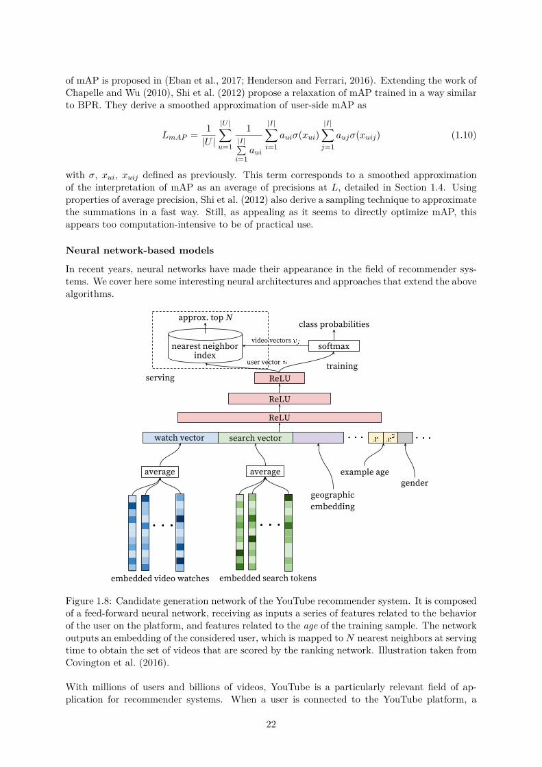
Figure 1.8: Candidate generation network of the YouTube recommender system. It is composedof a feed-forward neural network, receiving as inputs a series of features related to the behaviorof the user on the platform, and features related to the age of the training sample. The networkoutputs an embedding of the considered user, which is mapped to N nearest neighbors at servingtime to obtain the set of videos that are scored by the ranking network. Illustration taken fromCovington et al. (2016).

With millions of users and billions of videos, YouTube is a particularly relevant field of ap-plication for recommender systems. When a user is connected to the YouTube platform, a

22

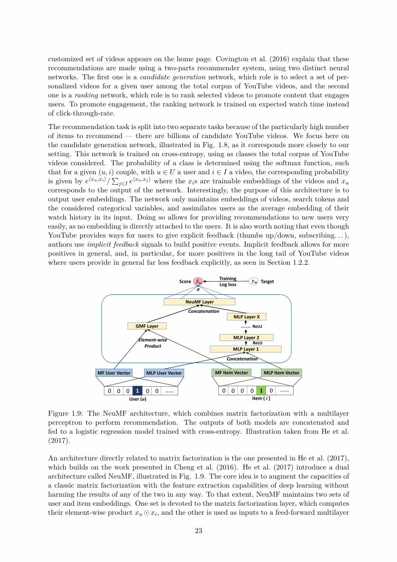
customized set of videos appears on the home page. Covington et al. (2016) explain that theserecommendations are made using a two-parts recommender system, using two distinct neuralnetworks. The first one is a candidate generation network, which role is to select a set of per-sonalized videos for a given user among the total corpus of YouTube videos, and the secondone is a ranking network, which role is to rank selected videos to promote content that engagesusers. To promote engagement, the ranking network is trained on expected watch time insteadof click-through-rate.

The recommendation task is split into two separate tasks because of the particularly high numberof items to recommend — there are billions of candidate YouTube videos. We focus here onthe candidate generation network, illustrated in Fig. 1.8, as it corresponds more closely to oursetting. This network is trained on cross-entropy, using as classes the total corpus of YouTubevideos considered. The probability of a class is determined using the softmax function, suchthat for a given (u, i) couple, with u œ U a user and i œ I a video, the corresponding probabilityis given by e

Èxu,xiÍ/q

jœIe

Èxu,xjÍ where the xis are trainable embeddings of the videos and xu

corresponds to the output of the network. Interestingly, the purpose of this architecture is tooutput user embeddings. The network only maintains embeddings of videos, search tokens andthe considered categorical variables, and assimilates users as the average embedding of theirwatch history in its input. Doing so allows for providing recommendations to new users veryeasily, as no embedding is directly attached to the users. It is also worth noting that even thoughYouTube provides ways for users to give explicit feedback (thumbs up/down, subscribing. . . ),authors use implicit feedback signals to build positive events. Implicit feedback allows for morepositives in general, and, in particular, for more positives in the long tail of YouTube videoswhere users provide in general far less feedback explicitly, as seen in Section 1.2.2.

1000 0 0 ……User (u)

0000 1 0 ……Item ( i )

MF User Vector MF Item Vector

GMF Layer ……

Score TargetTrainingŷui yui

MLP Layer 1

MLP User Vector MLP Item Vector

Element-wise Product

Concatenation

MLP Layer 2

MLP Layer X

NeuMF Layer

Log loss𝝈

ReLU

ReLU

Concatenation

Figure 3: Neural matrix factorization model

so that they can mutually reinforce each other to bettermodel the complex user-iterm interactions?

A straightforward solution is to let GMF and MLP sharethe same embedding layer, and then combine the outputs oftheir interaction functions. This way shares a similar spiritwith the well-known Neural Tensor Network (NTN) [33].Specifically, the model for combining GMF with a one-layerMLP can be formulated as

yui = �(hT a(pu � qi + W

�pu

qi

�+ b)). (11)

However, sharing embeddings of GMF and MLP mightlimit the performance of the fused model. For example,it implies that GMF and MLP must use the same size ofembeddings; for datasets where the optimal embedding sizeof the two models varies a lot, this solution may fail to obtainthe optimal ensemble.

To provide more flexibility to the fused model, we allowGMF and MLP to learn separate embeddings, and combinethe two models by concatenating their last hidden layer.Figure 3 illustrates our proposal, the formulation of whichis given as follows

�GMF = pGu � qG

i ,

�MLP = aL(WTL(aL�1(...a2(W

T2

�pM

u

qMi

�+ b2)...)) + bL),

yui = �(hT

��GMF

�MLP

�),

(12)where pG

u and pMu denote the user embedding for GMF

and MLP parts, respectively; and similar notations of qGi

and qMi for item embeddings. As discussed before, we use

ReLU as the activation function of MLP layers. This modelcombines the linearity of MF and non-linearity of DNNs formodelling user–item latent structures. We dub this model“NeuMF”, short for Neural Matrix Factorization. The deriva-tive of the model w.r.t. each model parameter can be cal-culated with standard back-propagation, which is omittedhere due to space limitation.

3.4.1 Pre-trainingDue to the non-convexity of the objective function of NeuMF,

gradient-based optimization methods only find locally-optimalsolutions. It is reported that the initialization plays an im-portant role for the convergence and performance of deeplearning models [7]. Since NeuMF is an ensemble of GMF

and MLP, we propose to initialize NeuMF using the pre-trained models of GMF and MLP.

We first train GMF and MLP with random initializationsuntil convergence. We then use their model parameters asthe initialization for the corresponding parts of NeuMF’sparameters. The only tweak is on the output layer, wherewe concatenate weights of the two models with

h ��

�hGMF

(1 � �)hMLP

�, (13)

where hGMF and hMLP denote the h vector of the pre-trained GMF and MLP model, respectively; and � is ahyper-parameter determining the trade-o� between the twopre-trained models.

For training GMF and MLP from scratch, we adopt theAdaptive Moment Estimation (Adam) [20], which adaptsthe learning rate for each parameter by performing smallerupdates for frequent and larger updates for infrequent pa-rameters. The Adam method yields faster convergence forboth models than the vanilla SGD and relieves the pain oftuning the learning rate. After feeding pre-trained parame-ters into NeuMF, we optimize it with the vanilla SGD, ratherthan Adam. This is because Adam needs to save momentuminformation for updating parameters properly. As we ini-tialize NeuMF with pre-trained model parameters only andforgo saving the momentum information, it is unsuitable tofurther optimize NeuMF with momentum-based methods.

4. EXPERIMENTSIn this section, we conduct experiments with the aim of

answering the following research questions:

RQ1 Do our proposed NCF methods outperform the state-of-the-art implicit collaborative filtering methods?

RQ2 How does our proposed optimization framework (logloss with negative sampling) work for the recommen-dation task?

RQ3 Are deeper layers of hidden units helpful for learningfrom user–item interaction data?

In what follows, we first present the experimental settings,followed by answering the above three research questions.

4.1 Experimental SettingsDatasets. We experimented with two publicly accessibledatasets: MovieLens4 and Pinterest5. The characteristics ofthe two datasets are summarized in Table 1.

1. MovieLens. This movie rating dataset has beenwidely used to evaluate collaborative filtering algorithms.We used the version containing one million ratings, whereeach user has at least 20 ratings. While it is an explicitfeedback data, we have intentionally chosen it to investigatethe performance of learning from the implicit signal [21] ofexplicit feedback. To this end, we transformed it into im-plicit data, where each entry is marked as 0 or 1 indicatingwhether the user has rated the item.

2. Pinterest. This implicit feedback data is constructedby [8] for evaluating content-based image recommendation.

4http://grouplens.org/datasets/movielens/1m/5https://sites.google.com/site/xueatalphabeta/academic-projects

Figure 1.9: The NeuMF architecture, which combines matrix factorization with a multilayerperceptron to perform recommendation. The outputs of both models are concatenated andfed to a logistic regression model trained with cross-entropy. Illustration taken from He et al.(2017).

An architecture directly related to matrix factorization is the one presented in He et al. (2017),which builds on the work presented in Cheng et al. (2016). He et al. (2017) introduce a dualarchitecture called NeuMF, illustrated in Fig. 1.9. The core idea is to augment the capacities ofa classic matrix factorization with the feature extraction capabilities of deep learning withoutharming the results of any of the two in any way. To that extent, NeuMF maintains two sets ofuser and item embeddings. One set is devoted to the matrix factorization layer, which computestheir element-wise product xu § xi, and the other is used as inputs to a feed-forward multilayer

23

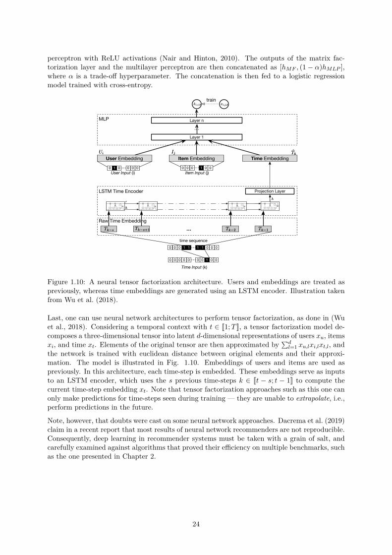
perceptron with ReLU activations (Nair and Hinton, 2010). The outputs of the matrix fac-torization layer and the multilayer perceptron are then concatenated as [hMF , (1 ≠ –)hMLP ],where – is a trade-o� hyperparameter. The concatenation is then fed to a logistic regressionmodel trained with cross-entropy.

Neural Tensor Factorization KDD’18, Aug 2018, London, UK

Item Embedding Time Embedding

Layer 1

Layer nMLP

…

IjIj TkTk

Tk�sTk�s

Projection Layer

Tk�s+1Tk�s+1 Tk�2Tk�2 Tk�1Tk�1

train

LSTM Time Encoder

Raw Time Embedding

sigmoid sigmoid tanh sigmoid

X +

XX

tanh


X +

XX

tanh


X +

XX

tanh


X +

XX

tanh

hh

cchh

xi,j,kxi,j,k xi,j,kxi,j,k

0 0 0 … 1 0 0

User EmbeddingUiUi

0 1 0 … 0 0 0User Input (i) Item Input (j)

0 0 0 … 0 10

0 1 … 1 0 00 0

0 00 0

Time Input (k)

1 0

time sequence

…

1

Figure 1: The Neural network based Tensor Factorization(NTF) Framework.

general compared to others [38]. As a general tensor factoriza-tion framework, NTF is also flexible to integrate other variants ofrecurrent neural networks.

• To model the non-linearity of multi-dimensional interactions, wedecide to use a Multi-layer Perceptron (MLP) on top of the firsttwo layers. Let us consider the generated tensor with user-item-time dimensions as an example. The projected temporal embed-ding vectors will be fed into a multi-layer neural architecturetogether with the embedding vectors of users and items. This en-ables NTF to incorporate the learned complex dependencies in thetemporal dimension into the factorization process as constrains.By doing so, we can detect the implicit patterns of user-item-timeinteractions through each layer in the MLP framework and modelthe non-linear combinations of latent factors to make better pre-dictions. Finally, the latent vectors will be mapped to quantitativevalues (i.e., xi, j,k ) which represents future interactions acrossdifferent dimensions.

3.2 Modeling Temporal Dynamics via LSTMRecurrent Neural Network (RNN) has been widely used to addressvarious challenges in time series analysis. However, two key lim-itations exist in the basic RNN. First, it is difficult to train due tothe problem of gradient vanishing and exploding, since the gradientmight approach zero (vanish) or diverge (explode) as it is propagatedback through time steps during the training process. Second, it isincapable to model long-distance dependencies in sequence data. Toobviate the above problems and make the architecture more effective,LSTM is introduced as a special kind of RNN to model long-termdependencies and addresses the vanishing gradient problem by devel-oping a more complicated hidden unit. In particular, LSTM proposesto derive the vector representations of hidden states ht and ct for

Algorithm 1: Training the NTF model.Input: Tensor X � RI��K , observed interaction set X, sequence

length s , and batch size bsize.Paras :Embedding matrices U � RI�L , I � R��L , T � RK�L , and

other hidden parameters � .1 Initialize all parameters;// Sample a minibatch of size bsize.

2 foreach Tbatch = sample(X, bsize) do3 foreach �i, j, k � � Tbatch do

/* Gather embeddings for all dimensions.

*/4 Ui = U[i, :], Ij = I[j, :];5 c = c0, h = h0; // init. hidden states6 for t � (k � s) to (k � 1) do7 c, h = LSTM(T[t, :], c, h); // according to Eq.38 end9 Tk = Projection(h); // encoded time

embedding

10 xi, j,k = MLP([Ui ; Ij ; Tk ]); // according to Eq.611 xi, j,k = X[i, j, k ];12 update loss L w.r.t 1

2 (xi, j,k � xi, j,k )2;13 end14 update all parameters w.r.t L;15 end

each time step t as follows:

it =� (Wiht�1 +Vixt + bi )ot =� (Woht�1 +Voxt + bo )ft =� (Wf ht�1 +Vf xt + bf )�ct =�(Wcht�1 +Vcxt + bc )ct =ft � ct�1 + it � �ct

ht =ot � �(ct ) (3)

whereW� � Rds�ds represents the transformation matrix from theprevious state (i.e., ct�1 and ht�1) to LSTM cell and V� � Rdx�ds

are the transformation matrices from input to LSTM cell, where dxand ds denotes the dimension of input vectors and hidden states, re-spectively. Furthermore, b� � Rds is defined as a vector of bias term.� (·) and �(·) represents the sigmoid and tanh function, respectively.The � operator denotes the element-wise product. In Eq. 3, it , ot ,and ft represents input gate, output gate and forget gate, respectively.For simplicity, we denote Eq. 3 as [ct ,ht ] = LSTM(�, ct�1,ht�1) inthe following subsections.

3.3 Fusion of LSTM and TFIn this subsection, we present how we fuse LSTM and TF underthe NTF framework to model the time-evolving interactions acrossthree dimensions RI , R� and RK . In relational data, dynamic char-acteristics are observed across different time slots. In this work,we consider temporal factors affecting the interactions over timebased on a global trend by assuming that the interactions betweenmulti-dimensions evolve in a smooth way. In particular, to capturethe temporal smoothness, we further assume that the embeddingvectors of the temporal dimension depends on embedding vectors

Figure 1.10: A neural tensor factorization architecture. Users and embeddings are treated aspreviously, whereas time embeddings are generated using an LSTM encoder. Illustration takenfrom Wu et al. (2018).

Last, one can use neural network architectures to perform tensor factorization, as done in (Wuet al., 2018). Considering a temporal context with t œ [[1; T ]], a tensor factorization model de-composes a three-dimensional tensor into latent d-dimensional representations of users xu, itemsxi, and time xt. Elements of the original tensor are then approximated by

qd

l=1 xu,lxi,lxt,l, andthe network is trained with euclidean distance between original elements and their approxi-mation. The model is illustrated in Fig. 1.10. Embeddings of users and items are used aspreviously. In this architecture, each time-step is embedded. These embeddings serve as inputsto an LSTM encoder, which uses the s previous time-steps k œ [[t ≠ s; t ≠ 1]] to compute thecurrent time-step embedding xt. Note that tensor factorization approaches such as this one canonly make predictions for time-steps seen during training — they are unable to extrapolate, i.e.,perform predictions in the future.

Note, however, that doubts were cast on some neural network approaches. Dacrema et al. (2019)claim in a recent report that most results of neural network recommenders are not reproducible.Consequently, deep learning in recommender systems must be taken with a grain of salt, andcarefully examined against algorithms that proved their e�ciency on multiple benchmarks, suchas the one presented in Chapter 2.

24

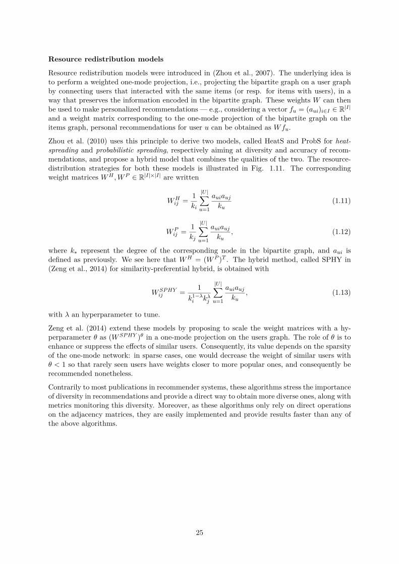
Resource redistribution models

Resource redistribution models were introduced in (Zhou et al., 2007). The underlying idea isto perform a weighted one-mode projection, i.e., projecting the bipartite graph on a user graphby connecting users that interacted with the same items (or resp. for items with users), in away that preserves the information encoded in the bipartite graph. These weights W can thenbe used to make personalized recommendations — e.g., considering a vector fu = (aui)iœI œ R|I|

and a weight matrix corresponding to the one-mode projection of the bipartite graph on theitems graph, personal recommendations for user u can be obtained as Wfu.

Zhou et al. (2010) uses this principle to derive two models, called HeatS and ProbS for heat-spreading and probabilistic spreading, respectively aiming at diversity and accuracy of recom-mendations, and propose a hybrid model that combines the qualities of the two. The resource-distribution strategies for both these models is illustrated in Fig. 1.11. The correspondingweight matrices W

H, W

P œ R|I|◊|I| are written

WH

ij = 1ki

|U |ÿ

u=1

auiauj

ku

(1.11)

WP

ij = 1kj

|U |ÿ

u=1

auiauj

ku

, (1.12)

where kú represent the degree of the corresponding node in the bipartite graph, and aui isdefined as previously. We see here that W

H = (W P )T . The hybrid method, called SPHY in(Zeng et al., 2014) for similarity-preferential hybrid, is obtained with

WSP HY

ij = 1k

1≠⁄

ik

⁄

j

|U |ÿ

u=1

auiauj

ku

, (1.13)

with ⁄ an hyperparameter to tune.

Zeng et al. (2014) extend these models by proposing to scale the weight matrices with a hy-perparameter ◊ as (W SP HY )◊ in a one-mode projection on the users graph. The role of ◊ is toenhance or suppress the e�ects of similar users. Consequently, its value depends on the sparsityof the one-mode network: in sparse cases, one would decrease the weight of similar users with◊ < 1 so that rarely seen users have weights closer to more popular ones, and consequently berecommended nonetheless.

Contrarily to most publications in recommender systems, these algorithms stress the importanceof diversity in recommendations and provide a direct way to obtain more diverse ones, along withmetrics monitoring this diversity. Moreover, as these algorithms only rely on direct operationson the adjacency matrices, they are easily implemented and provide results faster than any ofthe above algorithms.

25

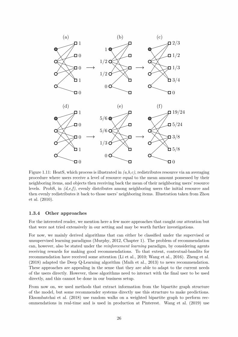
0

1

0

0

1(a)

��

0

1/2

1/2

1

(b)

��

0

3/4

1/3

1/2

2/3(c)

0

1

0

0

1(d)

��

0

1/3

5/6

5/6

(e)

��

0

5/8

3/8

5/24

19/24(f)

Fig. 1. The HeatS (a,b,c) and ProbS (d,e,f) algorithms (Eqs. 1 and 2) at work on thebipartite user-object network. Objects are shown as squares, users as circles, with the targetuser indicated by the shaded circle. While the HeatS algorithm redistributes resource via anearest-neighbour averaging process, the ProbS algorithm works by an equal distribution ofresource among nearest neighbours.

Table 1. Properties of the tested datasets.

dataset users objects links sparsityNetflix 10 000 6 000 701 947 1.17 · 10�2

RYM 33 786 5 381 613 387 3.37 · 10�3

Delicious 10 000 232 657 1 233 997 5.30 · 10�4

Table 2. Performance of the recommendation algorithms according to each of the four metrics: recovery of deleted links,precision enhancement, personalization, and surprisal.

Netflix RYM Deliciousmethod r eP (20) h(20) I(20) r eP (20) h(20) I(20) r eP (20) h(20) I(20)GRank 0.057 58.7 0.450 1.79 0.119 57.3 0.178 4.64 0.314 147 0.097 4.23USim 0.051 68.5 0.516 1.82 0.087 150 0.721 5.17 0.223 249 0.522 4.49ProbS 0.045 70.4 0.557 1.85 0.071 185 0.758 5.32 0.210 254 0.783 5.81HeatS 0.102 0.11 0.821 12.9 0.085 121 0.939 10.1 0.271 30.8 0.975 12.6

Table 3. Performance of individual rec-ommendation algorithms for a probe setconsisting of only low-degree (k < 100)objects.

method r eP (20) h(20) I(20)GRank 0.327 0.000 0.525 1.68USim 0.308 0.000 0.579 1.72ProbS 0.279 0.014 0.610 1.74HeatS 0.262 0.679 0.848 13.1

Table 4. Tuning the HeatS+ProbS hybridization pa-rameter � to optimize for r produces simultaneousimprovements in other metrics. The relative changesare given in percentage terms against the pure ProbSalgorithm.

dataset � �r �eP (20) �h(20) �I(20)Netflix 0.23 10.6% 16.5% 28.5% 28.8%RYM 0.41 6.8% 10.8% 20.1% 17.2%Delicious 0.66 1.2% -6.0% 22.5% 61.7%

6 www.pnas.org — — Footline Author

Figure 1.11: HeatS, which process is illustrated in (a,b,c), redistributes resource via an averagingprocedure where users receive a level of resource equal to the mean amount possessed by theirneighboring items, and objects then receiving back the mean of their neighboring users’ resourcelevels. ProbS, in (d,e,f), evenly distributes among neighboring users the initial resource andthen evenly redistributes it back to those users’ neighboring items. Illustration taken from Zhouet al. (2010).

1.3.4 Other approachesFor the interested reader, we mention here a few more approaches that caught our attention butthat were not tried extensively in our setting and may be worth further investigations.

For now, we mainly derived algorithms that can either be classified under the supervised orunsupervised learning paradigms (Murphy, 2012, Chapter 1). The problem of recommendationcan, however, also be stated under the reinforcement learning paradigm, by considering agentsreceiving rewards for making good recommendations. To that extent, contextual-bandits forrecommendation have received some attention (Li et al., 2010; Wang et al., 2016). Zheng et al.(2018) adapted the Deep Q-Learning algorithm (Mnih et al., 2013) to news recommendation.These approaches are appealing in the sense that they are able to adapt to the current needsof the users directly. However, these algorithms need to interact with the final user to be useddirectly, and this cannot be done in our business setup.

From now on, we used methods that extract information from the bipartite graph structureof the model, but some recommender systems directly use this structure to make predictions.Eksombatchai et al. (2018) use random walks on a weighted bipartite graph to perform rec-ommendations in real-time and is used in production at Pinterest. Wang et al. (2019) use

26

graph neural networks to enhance classic matrix factorization strategies with the informationof higher-order connectivity from the bipartite graph.

1.3.5 The cold-start problemCold-start refers to the fact that one needs to gather enough information about a new user oritem to include it in the predictions of a recommender system (Bobadilla et al., 2013). Notably,in matrix factorization-related approaches, the set of users and items on which predictions canbe made is determined by the sets on which the adjacency matrix was built, and cannot bechanged unless retraining the algorithm.

In most cases, recommender systems su�er from the user cold-start — an e-commerce website isnot able to onboard a new client in its recommender system before gathering enough informationabout its shopping patterns. In the CIB business, however, onboarding new clients is not thatcommon — the financial setting su�ers more from item cold-start. As a matter of fact, financialproducts such as bonds and options have a limited lifespan: new products are constantly emittedto replace expiring ones. For a matrix factorization-like algorithm, however, these two productsare distinct and could not be assimilated. Bobadilla et al. (2013) provide multiple ways in whichuser and item cold-start can be tackled. We also provide in the next chapters ways to battle itin general, and more especially in the case of item cold-start.

1.4 Evaluating financial recommender systemsEvaluating recommender systems can be done in many ways, depending on how the problem isframed. We describe below the set of metrics we use for the remainder of this thesis.

1.4.1 Deriving symmetrized mean average precisionThe problem of retrieving probabilities of interest p introduced in Section 1.3.2 can be under-stood as a classification task - our target is a discrete value in {0, . . . , C ≠1} with C the numberof classes that we consider. If we are only interested in the binary interest of our clients, C = 2;if we want to introduce buy and/or sell interests, we use C = 4 to represent no interest, buyinterest, sell interest and interest into buying and selling the considered asset in the consideredwindow of time.

In such a classification setting, metrics based on the confusion matrix, see Fig. 1.12, are usedto assess the performance of algorithms. In a binary setting, denoting the prediction of themonitored algorithm for a particular sample y, the confusion matrix compares the predicted y

with the true labels y, distinguishing between four di�erent cases.

Figure 1.12: The confusion matrix outline.

27

This confusion matrix can then be summed up through a collection of metrics such as precision,which corresponds to the proportion of correct predictions that were made, recall, also calledtrue positive rate, which corresponds to the proportion of the real targets that were retrieved,false positive rate, which corresponds to the proportion of negative events predicted as positive,i.e., the proportion of "false alarms"... Formulas for these quantities are given in Table 1.1.

Table 1.1: Examples of metrics describing the confusion matrix.

Precision (P) T P

T P +F P

Recall (R or TPR) T P

T P +F N

False Positive Rate (FPR) F P

F P +T N

True Negative Rate (TNR) T N

F P +T N

False Discovery Rate (FDR) F P

F P +T P

However, a comparison criterion must be unique: one algorithm could beat its competitors on agiven metric but not on the others, leading to an ambiguous choice of preferred algorithm. Aswe would like to compare our algorithms with a combination of confusion matrix-based metricsnonetheless, we have to rely on summary metrics. The most common ones are F -scores, definedas

F— = (1 + —2) · P · R

(—2 · P ) + R. (1.14)

F1 score is the most common one and corresponds to the harmonic mean between precision andrecall. Less classic options include F2 scores, which weigh more recall than precision, and F0.5score which weigh more precision than recall. Consequently, the choice of — entirely dependson the use case we want to assess.

We examined here the case of binary classification tasks. In a multiclass setting, it is usual toderive scores for each class in a one-versus-all setup, identical to a binary one, and average foundscores using a given strategy. The most common averaging strategies are micro- and macro-averaging. For classes c œ {0, . . . , C ≠ 1}, macro-averaging is defined as, with the example ofprecision P ,

Pmacro = 1C

ÿ

c

Pc, (1.15)

where Pc is the precision of class c obtained considering the one-versus-all setup. Micro-averaging is defined as, with the example of precision,

Pmicro =q

cTPcq

cTPc +

qcFPc

. (1.16)

As appears in these formulas, macro-averaging treats all classes equally, whereas micro-averagingtakes into consideration the relative weight of all classes. In the financial setup, it is often thecase that the considered classes are ill-balanced, i.e., that the distribution of classes amongsamples is not uniform at all. In our future interest prediction setting, it appears that a clientwill most of the time not be interested in a given product, leading to an over-representationof the "no interest" class, i.e., to severe imbalance. The "positive interest" class is the one thattruly matters: its performance must consequently not be drowned under the performance ofthe "no interest" one. For that reason, when required, we choose macro-averaging proceduresto give equal weights to all considered classes.

However, most algorithms do not directly lead to the class prediction y. In a binary setting,classification algorithms learn the probability of the positive class p = p◊(y = 1|x), and wehave to introduce a threshold · such that y = 1 if p > · and 0 else: the above metrics are

28

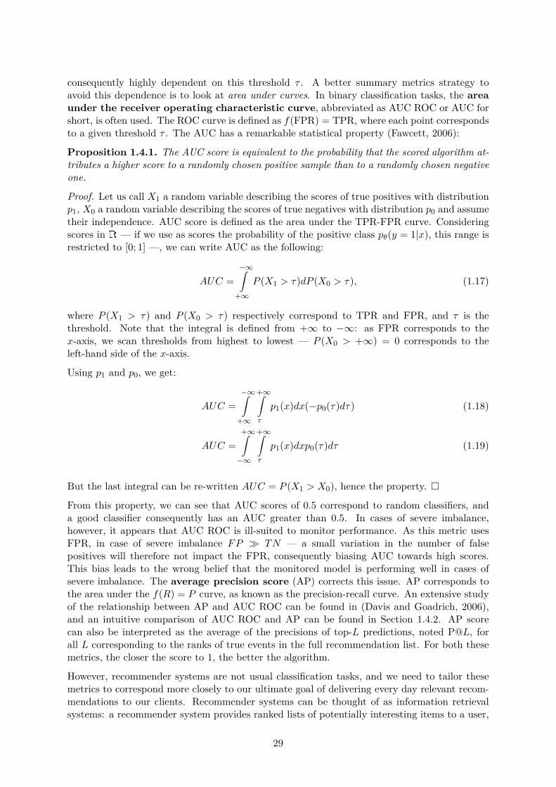
consequently highly dependent on this threshold · . A better summary metrics strategy toavoid this dependence is to look at area under curves. In binary classification tasks, the areaunder the receiver operating characteristic curve, abbreviated as AUC ROC or AUC forshort, is often used. The ROC curve is defined as f(FPR) = TPR, where each point correspondsto a given threshold · . The AUC has a remarkable statistical property (Fawcett, 2006):

Proposition 1.4.1. The AUC score is equivalent to the probability that the scored algorithm at-tributes a higher score to a randomly chosen positive sample than to a randomly chosen negativeone.

Proof. Let us call X1 a random variable describing the scores of true positives with distributionp1, X0 a random variable describing the scores of true negatives with distribution p0 and assumetheir independence. AUC score is defined as the area under the TPR-FPR curve. Consideringscores in — if we use as scores the probability of the positive class p◊(y = 1|x), this range isrestricted to [0; 1] —, we can write AUC as the following:

AUC =≠Œ⁄

+Œ

P (X1 > ·)dP (X0 > ·), (1.17)

where P (X1 > ·) and P (X0 > ·) respectively correspond to TPR and FPR, and · is thethreshold. Note that the integral is defined from +Œ to ≠Œ: as FPR corresponds to thex-axis, we scan thresholds from highest to lowest — P (X0 > +Œ) = 0 corresponds to theleft-hand side of the x-axis.

Using p1 and p0, we get:

AUC =≠Œ⁄

+Œ

+Œ⁄

·

p1(x)dx(≠p0(·)d·) (1.18)

AUC =+Œ⁄

≠Œ

+Œ⁄

·

p1(x)dxp0(·)d· (1.19)

But the last integral can be re-written AUC = P (X1 > X0), hence the property. ⇤From this property, we can see that AUC scores of 0.5 correspond to random classifiers, anda good classifier consequently has an AUC greater than 0.5. In cases of severe imbalance,however, it appears that AUC ROC is ill-suited to monitor performance. As this metric usesFPR, in case of severe imbalance FP ∫ TN — a small variation in the number of falsepositives will therefore not impact the FPR, consequently biasing AUC towards high scores.This bias leads to the wrong belief that the monitored model is performing well in cases ofsevere imbalance. The average precision score (AP) corrects this issue. AP corresponds tothe area under the f(R) = P curve, as known as the precision-recall curve. An extensive studyof the relationship between AP and AUC ROC can be found in (Davis and Goadrich, 2006),and an intuitive comparison of AUC ROC and AP can be found in Section 1.4.2. AP scorecan also be interpreted as the average of the precisions of top-L predictions, noted P@L, forall L corresponding to the ranks of true events in the full recommendation list. For both thesemetrics, the closer the score to 1, the better the algorithm.

However, recommender systems are not usual classification tasks, and we need to tailor thesemetrics to correspond more closely to our ultimate goal of delivering every day relevant recom-mendations to our clients. Recommender systems can be thought of as information retrievalsystems: a recommender system provides ranked lists of potentially interesting items to a user,

29

who willingly — or not — queried it. An overview of useful metrics for information retrievalcan be found in (Manning et al., 2010). We stick here with AP for its above-cited properties,using a slight variation of it. Instead of AP, we monitor the performance of our models usingmean average precision (mAP), defined as

mAP = 1|Q|

ÿ

qœQ

AP (q), (1.20)

where q is a query. We define queries in two ways:

- User-side. A query corresponds to the recommendation list of a given user at a givendate.

- Item-side. A query corresponds to the recommendation list of a given item at a givendate.

The item-side query is introduced to obtain the item perspective usually not monitored inrecommender systems. This perspective is particularly relevant for corporate banks — to controlher risk, a market maker needs to control her positions, i.e., make sure she does not hold agiven position for too long. It is consequently of strategic interest to find relevant clients for agiven asset, and item queries allow for monitoring the corresponding performance. Moreover,salespeople usually monitor the provided recommendations by looking at the predicted scoresfor a particular client or asset — we consequently need our models to provide useful rankingsat the client and asset scales, and that is what user- and item-side mAP scores evaluate. Notethat mean AUC scores can be defined in the same way, as

mAUC = 1|Q|

ÿ

qœQ

AUC(q). (1.21)

Finally, as we want to describe the performance of our algorithms with one score only, weintroduce the symmetrized mAP, defined as the harmonic mean between the user- and item-side mAP. From now on, this score is used to monitor the performance of our algorithms — whenapplicable. As seen in Section 1.3.2, content-filtering approaches may rely on cross-features forwhich we might lack data, preventing us from computing them at any time for all couples. Insuch cases, we favor using AP on the overall task instead.

1.4.2 A closer look at area under curve metricsTo understand the behavioral di�erences between AUC and AP, we study a couple of examplesto get a better intuition at how they score particular recommendations. We consider hererecommendation lists of size 10000 to mimic our actual user-side setting, that we score withboth AUC and AP.

Consider a user having two interests at a given date, and first examine a case where theseinterests were ranked 10-th and 100-th.

- Following the probabilistic interpretation of AUC, in that case we can compute an AUCof 0.5 ú ((1 ≠ 9

9999) + (1 ≠ 989998)) ¥ 0.995. The score consequently highlights what would

be an excellent recommendation.- Using the P@L interpretation of AP, we compute a score of 0.5 ú (1/10 + 2/100) ¥ 0.06.

The score consequently highlights what would be a very poor recommendation.

Now, consider the extreme case where the two interests are ranked first and last. We get thefollowing:

30

- With the probabilistic interpretation, we compute an AUC of 0.5 ú (1 + (1 ≠ 1)) = 0.5. Itcorresponds to the score of a random recommendation.

- With the P@L interpretation, we compute an AP of 0.5 ú (1 + 2/10000) = 0.5001, thescore of a quite good recommendation.

From these examples, we see that AUC scores do not di�erentiate predictions relatively totheir position in the recommendation list. This behavior leads to a good score in the firstexample, and a bad one in the second. A recommender system with good AUC is consequentlya recommender that is good on a broad scale. Contrarily, AP weighs heavier the top of therecommendation list due to its usage of P@L. It follows that in the first example, the AP scoreis quite low due to the first true event appearing in the 10-th position only. But in the secondexample, the relatively good AP score is entirely driven by the fact that the first prediction wasindeed correct.

Consequently, AP is more adapted in cases where we matter most about the first recommenda-tions that the system does. In our business case, that is the reason why we favor AP: consideringthat recommendation lists are sales’ calls plannings, a salesperson needs to get good returns onher calls fast, as their time (and patience) is limited. There are no correct metrics to use in theabsolute — there are metrics more adapted to a given situation.

1.4.3 Monitoring diversityQualitative metrics can also be used to monitor our recommender systems. The precision ofrecommender systems is, of course, of great importance. Still, a system only targeting precisionmight fall into the trap of always recommending the same items, thereby a self-sustained loop— a client who is only recommended already seen items keeps treating them with us, and maybefinds another counterparty for other items that may be of interest for her. Moreover, we alsowant to recommend items in the long tail (see Section 1.2.2). For these reasons, monitoring thediversity of our systems following the ideas introduced in Zhou et al. (2010) and continued inZeng et al. (2014) is also helpful.

We introduce two qualitative metrics called diversity and similarity. Diversity D(L) is definedas

D(L) = 1L

ÿ

iœI

ÿ

uœU

ki iœR1:L,u (1.22)

with R1:L,u the top-L ranked items for user u and ki the degree of item i as computed on thetraining dataset, the degree corresponding to the number of unique users connected to item i

in the bipartite graph corresponding to the training dataset. D(L) corresponds to the averagedegree of an item present in the top-L recommendation lists of all our users at a given date —the lower the metric, the more diverse the recommendations. Similarity S(L) is defined as

S(L) = 2|U |(|U | ≠ 1)

ÿ

u>v

Cuv(L)L

(1.23)

with Cuv(L) the number of identical items in top-L recommendation lists of users u and v.S(L) corresponds to the average number of identical items in the top-L recommendation listsfor all pairs of users, at a given date. The lower the metric, the less similar the recommendationlists. L depends here on the asset class and has to be chosen in accordance with the users ofthe recommender system. Both of these metrics are introduced on the user-side and could becomputed on the item-side as well. As the purpose of these metrics is only qualitative, it is heremore relevant to stick with un-symmetrized values to keep their interpretation intact.

31

These metrics are monitored along with symmetrized mAP in our further experiments, when ap-plicable. In cases of approximately equal symmetrized mAP performances, we favor algorithmsobtaining better diversity and similarity scores.

1.5 The challenges of the financial worldIn this chapter, we gave a relatively broad overview of the problem we want to solve, whatdata we have at our disposal to solve it and algorithms that can solve it. In doing so, we metchallenges among which the heterogeneity of clients and assets (Section 1.2.2) and the itemcold-start problem (Section 1.3.5). We explore here, haphazardly, additional challenges that weface in future financial interest prediction and that we will, partly, tackle in the remainder ofthis work.

We already mentioned in Section 1.1 that the RFQ information is imperfect. We only know apart of clients’ interests, either the ones expressed on a platform where BNPP CIB operatesor the ones told to salespeople. The final decision of the client is not always known, due tothe rules of D2C platforms seen in Section 1.1.1. We have to keep this fact in mind whenconstructing our algorithms — what appears to us as no interest events could be real intereststhat we did not monitor. Moreover, the financial setup brings about two challenges: the buy-sell asymmetry, and the potentially cyclic interests. The asymmetry corresponds to the factthat a client can only sell a product she already possesses — such a piece of information canbe obtained for some of BNP Paribas CIB clients from their portfolio snapshots, but does notconcern the majority of them. The second challenge di�erentiates the financial setup froma classic e-commerce recommendation problem. In finance, buying a given product does notprevent at all from re-buying it in the future, a behavior that would be far rarer, e.g., for anAmazon customer. We consequently have to keep all of the past interests of a client in herpotential future interests. There is even a tendency for a client to trade what she has alreadytraded in the past: studying the corporate bonds RFQ database, in 2019, on average 28% ofclients’ RFQs are made on products they already traded before. If we restrict to the 500 mostactive clients of 2019, this figure rises to 58%, meaning that active clients have a high tendencyto replicate their past behaviors.

Another challenge comes from the specificities of asset classes: there cannot be a single, cross-asset model. Each asset class has its own characteristics and features, as exposed in Section1.1.2. We also observe di�erent behaviors depending on the asset class — professional investorsdo not trade equity, options, and bonds in the same ways and have proper strategies for each ofthese asset classes. Moreover, in the same asset class, investors might even react di�erently tothe same input signal: in equity, for instance, a price decrease does not mean the same for trendfollowers and mean-reverting traders. A global, cross-asset model is consequently not a goodoption, and we also need ways to adapt to the potentially many di�erent trading strategies thatinvestors have in each asset class, i.e., their behavioral heterogeneity.

Yet another challenge, usually disregarded in the recommender systems literature, is the impor-tance of time, omnipresent in finance. Financial indicators continuously evolve, and with themthe interests of clients: consequently, time must be taken into account to provide relevant rec-ommendations. This evolution of interests with time is related to what is known as concept driftin the recommender systems literature. Tsymbal (2004) identifies concept drift as coming eitherfrom a change in the underlying data distribution or a change in the target concept. Drift canalso be sudden or gradual. Financial time series are highly non-stationary — consequently, theprimary source of concept drift we have to face is a gradual or abrupt change in the underlyingdata distribution. This challenge is, to the best of our knowledge, not addressed su�ciently byliterature as it conceptually di�ers from the usual trends or seasonalities.

32

Additional challenges come from the way our future interest prediction problem is framed. Astandard assumption in the recommender systems literature is that we can directly interact withthe final users of the system. However, as seen in Section 1.1, the recipients of the providedrecommendations are not directly the clients of the bank, but the salespeople with whom clientsare engaged in business discussions. We consequently cannot resort to A/B testing strategiesor bandit algorithms: sales take a risk when calling a client on behalf of the bank, and needto be able to trust the system. For a sales to follow a recommendation, predictions must beunderstandable. Giving insights into why recommendations are made helps sales gain confidencein the system, and provides them with ways to introduce the trade idea to their clients. Thisfalls in the field of interpretability, where many di�erent proposals have been made to try andunderstand the predictions made by black-box algorithms such as neural networks or gradienttree boosting algorithms. A popular method is LIME (Ribeiro et al., 2016), which learnsan interpretable, linear model around the prediction to be interpreted. For neural networks,methods such as DeepLIFT (Shrikumar et al., 2017), which backpropagates the output to beinterpreted to the input features, have been proposed. Lundberg and Lee (2017) propose tounify the field of interpretability using the game theory notion of Shapley values (Shapley, 1953).Finally, Kim et al. (2017) propose to interpret outputs using user-defined concepts instead ofinput features, which may not always be meaningful to a non-specialist.

On a more practical note, our predictions must also be reliable and user-friendly. Scores mustbe good indicators of the confidence we have that the interest might happen so as not to losetime on unlikely interests. Moreover, scores must also be easily readable by our users: forinstance, if we take as score the probability of interest in a given product, it will most often bevery low — a more meaningful score here could be the daily variation of predicted probability.A scoring scale, e.g., between 0 and 5, could also be instituted following sales’ wishes and needs.Consequently, we see that sales have to be fully integrated into the design of the recommendersystem’s specifications to provide them with meaningful help and enhance their proactivity.Among these technical considerations, we also find legal aspects: as in most businesses, thereare compliance challenges related to the design of such an algorithm. Thus, great care must betaken into the data sources we use, and the results we disclose to our clients.

33

Chapter 2

First results on real-world RFQ data

Chapter 1 introduces the future interest prediction task to a great extent and provides insightsinto suitable algorithms for solving this task. The goal of Chapter 2 is to further these insightsthrough the application of classic recommender systems to the future interest prediction problemusing a real-world RFQ dataset from BNP Paribas CIB. In this chapter, Section 2.1 reviewsstrategies allowing to handle multi-class outputs with models designed for binary ones andconsequently bridge the gap between content-filtering and collaborative filtering algorithms,and Section 2.2 presents a benchmark of classic, seminal algorithms introduced in Section 1.3.

2.1 From binary to oriented interestsIn Section 1.1, we introduced the problem of future interest prediction as predicting whether aclient is interested in buying and/or selling a given financial asset at a given time. However,most collaborative filtering algorithms cannot handle per se a multi-class classification settingsuch as this one and only deal with binary interests. However, collaborative filtering and,more particularly, matrix factorization-like algorithms are particularly interesting in that theyallow for a posteriori analysis of latent representations of users and items, a feature we donot retrieve in content-filtering strategies. Consequently, this section explores two ideas thatallow bridging the gap between binary and multi-class prediction settings, enabling the usageof matrix factorization-like algorithms for the future interest prediction task.

A simple strategy for dealing with multi-class prediction is, when applicable, to split the predic-tion task into multiple tasks. As a matter of fact, our future interest prediction task is composedof two nested prediction tasks. The first one aims to find whether a client has an interest in agiven product, and the second one seeks to retrieve the nature of this interest, i.e., whether it isan interest in buying and/or selling the considered product. Consequently, in such a setting, it ispossible to use two algorithms to solve each of these tasks: a matrix factorization-like algorithmwould deal with the interest/no interest prediction task, and a second algorithm with the inter-est’s nature retrieval. A natural choice for this second algorithm would be a content-filteringone using appropriate, handcrafted features, trained on a cross-entropy objective. Another sim-ple idea that deals with any multi-class prediction setting is to split the prediction task into asmany tasks as there are classes, each task being a "one-versus-all" retrieval of a given class. Amatrix factorization-like algorithm can then be used for each of these tasks.

However, the "one-versus-all" strategy does not exploit the potential correlations between thedi�erent classes of the prediction task. Exploiting these correlations can only be done with algo-rithms that directly address the multi-class framing of the prediction problem. We introducedin Section 1.3.3 the tensor factorization idea for tackling temporal contexts. The same idea

35

can be applied to multi-class classification, by considering three-dimensional adjacency tensorsA œ R|U |◊|I|◊C , with C the number of classes. Using a tensor factorization model using latentrepresentations of users, items and classes respectively denoted P œ R|U |◊d, Q œ R|I|◊d andK œ RC◊d with d the latent dimension, the score of the c class of a given (u, i) couple is givenby

xc

ui =dÿ

l=1pu,lqi,lkc,l. (2.1)

This algorithm can then be trained using a cross-entropy entropy objective, as

l =ÿ

c

yc

ui log ‡ (xc

ui) , (2.2)

with yc

ui:= au,i,c and ‡ the sigmoid function.

In this thesis, we focus on the development of ad hoc algorithmic designs aimed at solvingspecific challenges of the financial sector, as will be seen in Chapters 3 and 4. Consequently, thebinary-to-multi-class problem considered in this section appears as a technicality, and will notbe evoked further. From now on, we use the most natural setting for the considered algorithms,be it binary or multi-class.

2.2 A benchmark of classic algorithmsThis section presents a benchmark of algorithms presented in Section 1.3 on a G10 bondsRFQ dataset from BNP Paribas CIB which is more extensively studied in Chapter 4. Ourdataset comprises hundreds of clients and thousands of bonds and ranges from 01/08/2018 to30/09/2019. We consider as training set the events from 01/08/2018 to 31/07/2019, as valida-tion set the events from 01/08/2019 to 31/08/2019 and as test set the events from 01/09/2019to 30/09/2019. First, we examine the methodology and hyperparameters considered for algo-rithms of four di�erent model classes. Second, we present, compare, and analyze the resultsobtained with these algorithms on all the metrics introduced in Section 1.4. All models arescored on a perimeter composed of all the couples U ◊ I = {(u, i)|u œ U, i œ I}, with U (resp.I) the set of all users (resp. items) observed in the training set, for all the dates of the scoredsplit of data. Qualitative metrics were all computed using L = 20, where L corresponds to thenumber of top recommended items or users, depending on the chosen side (see Section 1.4.3).

2.2.1 Historical modelsWe first consider historical models, as introduced in Section 1.3.1. In this benchmark, we usetwo historical models: a naive one that we note "Histo", and a temporal one that we note"⁄-Histo". ⁄-Histo di�ers from the Histo model in that events are penalized according to theirobservation date: the further away in the past the observation of a (u, i) couple, the lower itsweight in the score of the (u, i) couple.

The scores are computed using the training set only, using for ⁄-Histo a temporal penaltyinspired from the one introduced in Section 1.3.1, defined as e

≠⁄(T ≠t), where T is the final dayof the training set and t is the observation day of the event. These scores are then re-used toperform recommendations on all dates of the validation and test sets.

Figure 2.1 shows the evolution of the validation performance, defined by the symmetrized mAPscore, with the ⁄ parameter. This parameter can be interpreted in terms of half-life — therange of values considered corresponds to half-lives ranging from roughly two years to a day.The best validation performance is obtained for a value of ⁄ ¥ 0.02, corresponding to a half-life

36

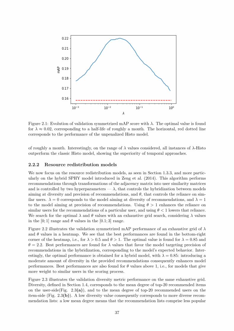
Figure 2.1: Evolution of validation symmetrized mAP score with ⁄. The optimal value is foundfor ⁄ ¥ 0.02, corresponding to a half-life of roughly a month. The horizontal, red dotted linecorresponds to the performance of the unpenalized Histo model.

of roughly a month. Interestingly, on the range of ⁄ values considered, all instances of ⁄-Histooutperform the classic Histo model, showing the superiority of temporal approaches.

2.2.2 Resource redistribution modelsWe now focus on the resource redistribution models, as seen in Section 1.3.3, and more partic-ularly on the hybrid SPHY model introduced in Zeng et al. (2014). This algorithm performsrecommendations through transformations of the adjacency matrix into user similarity matricesand is controlled by two hyperparameters — ⁄, that controls the hybridization between modelsaiming at diversity and precision of recommendations, and ◊, that controls the reliance on sim-ilar users. ⁄ = 0 corresponds to the model aiming at diversity of recommendations, and ⁄ = 1to the model aiming at precision of recommendations. Using ◊ > 1 enhances the reliance onsimilar users for the recommendations of a particular user, and using ◊ < 1 lowers that reliance.We search for the optimal ⁄ and ◊ values with an exhaustive grid search, considering ⁄ valuesin the [0; 1] range and ◊ values in the [0.1; 3] range.

Figure 2.2 illustrates the validation symmetrized mAP performance of an exhaustive grid of ⁄

and ◊ values in a heatmap. We see that the best performances are found in the bottom-rightcorner of the heatmap, i.e., for ⁄ > 0.5 and ◊ > 1. The optimal value is found for ⁄ = 0.85 and◊ = 2.2. Best performances are found for ⁄ values that favor the model targeting precision ofrecommendations in the hybridization, corresponding to the model’s expected behavior. Inter-estingly, the optimal performance is obtained for a hybrid model, with ⁄ = 0.85: introducing amoderate amount of diversity in the provided recommendations consequently enhances modelperformances. Best performances are also found for ◊ values above 1, i.e., for models that givemore weight to similar users in the scoring process.

Figure 2.3 illustrates the validation diversity metric performance on the same exhaustive grid.Diversity, defined in Section 1.4, corresponds to the mean degree of top-20 recommended itemson the user-side(Fig. 2.3(a)), and to the mean degree of top-20 recommended users on theitem-side (Fig. 2.3(b)). A low diversity value consequently corresponds to more diverse recom-mendation lists: a low mean degree means that the recommendation lists comprise less popular

37

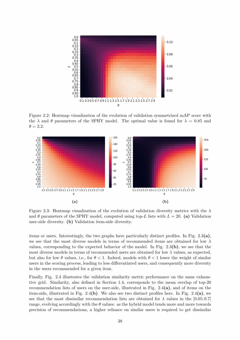
Figure 2.2: Heatmap visualization of the evolution of validation symmetrized mAP score withthe ⁄ and ◊ parameters of the SPHY model. The optimal value is found for ⁄ = 0.85 and◊ = 2.2.

(a) (b)

Figure 2.3: Heatmap visualization of the evolution of validation diversity metrics with the ⁄

and ◊ parameters of the SPHY model, computed using top-L lists with L = 20. (a) Validationuser-side diversity. (b) Validation item-side diversity.

items or users. Interestingly, the two graphs have particularly distinct profiles. In Fig. 2.3(a),we see that the most diverse models in terms of recommended items are obtained for low ⁄

values, corresponding to the expected behavior of the model. In Fig. 2.3(b), we see that themost diverse models in terms of recommended users are obtained for low ⁄ values, as expected,but also for low ◊ values, i.e., for ◊ < 1. Indeed, models with ◊ < 1 lower the weight of similarusers in the scoring process, leading to less di�erentiated users, and consequently more diversityin the users recommended for a given item.

Finally, Fig. 2.4 illustrates the validation similarity metric performance on the same exhaus-tive grid. Similarity, also defined in Section 1.4, corresponds to the mean overlap of top-20recommendation lists of users on the user-side, illustrated in Fig. 2.4(a), and of items on theitem-side, illustrated in Fig. 2.4(b). We also see two distinct profiles here. In Fig. 2.4(a), wesee that the most dissimilar recommendation lists are obtained for ⁄ values in the [0.05; 0.7]range, evolving accordingly with the ◊ values: as the hybrid model tends more and more towardsprecision of recommendations, a higher reliance on similar users is required to get dissimilar

38

(a) (b)

Figure 2.4: Heatmap visualization of the evolution of validation similarity metrics with the ⁄

and ◊ parameters of the SPHY model, computed using top-L lists with L = 20. (a) Validationuser-side similarity. (b) Validation item-side similarity.

recommendation lists for all users. Indeed, polarizing users around their most similar peers ap-pear to specialize their recommendation lists, and consequently lead to dissimilar lists overall.In Fig. 2.4(b), we see that the most dissimilar items’ recommendation lists are obtained eitherfor low values of ⁄ and ◊ or, more interestingly — and counterintuitively —, for values of ◊ ¥ 1and ⁄ > 0.5. Slightly less dissimilar lists are also obtained with values of ⁄ ¥ 0.2 and ◊ > 2, abehavior already encountered on the user-side in Fig. 2.4(a).

2.2.3 Matrix factorization modelsWe examine in this benchmark two matrix factorization approaches based on the implicit feed-back and BPR objectives, introduced in Section 1.3.3, that we respectively call MF - Implicitand MF - BPR. For both models, hyperparameters are found using a combination of a hundredtrials of random search and hand fine-tuning. The MF - Implicit algorithm with best validationsymmetrized mAP performance used an embedding size d = 512, batches of size 256, a L2penalty weight of 4e

≠7, a learning rate of 7e≠4 and a logarithmic confidence with parameters

– = 4 and ‘ = 10. The confidence weights are illustrated in Fig. 2.5, which shows the evolutionof weights with the number of occurrences r — in the considered dataset, the maximal value ofr is 223, and confidence weights are consequently found in the [1; 14] range.

The MF - BPR algorithm with best validation symmetrized mAP performance used embeddingsof size d = 1024, batches of size 256, a L2 penalty weight of 2e

≠7 and a learning rate of 9e≠5.

Both algorithms were trained with the Adam optimizer (Kingma and Ba, 2015), with earlystopping and a patience of 50.

39

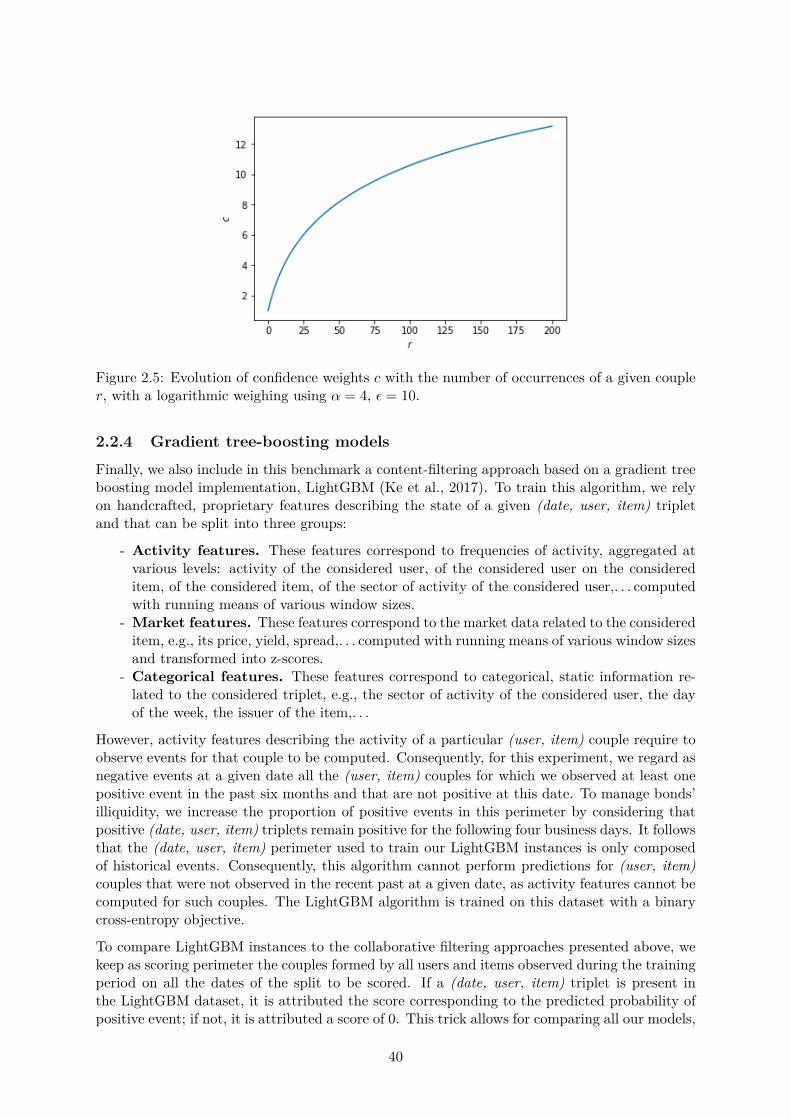
Figure 2.5: Evolution of confidence weights c with the number of occurrences of a given coupler, with a logarithmic weighing using – = 4, ‘ = 10.

2.2.4 Gradient tree-boosting modelsFinally, we also include in this benchmark a content-filtering approach based on a gradient treeboosting model implementation, LightGBM (Ke et al., 2017). To train this algorithm, we relyon handcrafted, proprietary features describing the state of a given (date, user, item) tripletand that can be split into three groups:

- Activity features. These features correspond to frequencies of activity, aggregated atvarious levels: activity of the considered user, of the considered user on the considereditem, of the considered item, of the sector of activity of the considered user,. . . computedwith running means of various window sizes.

- Market features. These features correspond to the market data related to the considereditem, e.g., its price, yield, spread,. . . computed with running means of various window sizesand transformed into z-scores.

- Categorical features. These features correspond to categorical, static information re-lated to the considered triplet, e.g., the sector of activity of the considered user, the dayof the week, the issuer of the item,. . .

However, activity features describing the activity of a particular (user, item) couple require toobserve events for that couple to be computed. Consequently, for this experiment, we regard asnegative events at a given date all the (user, item) couples for which we observed at least onepositive event in the past six months and that are not positive at this date. To manage bonds’illiquidity, we increase the proportion of positive events in this perimeter by considering thatpositive (date, user, item) triplets remain positive for the following four business days. It followsthat the (date, user, item) perimeter used to train our LightGBM instances is only composedof historical events. Consequently, this algorithm cannot perform predictions for (user, item)couples that were not observed in the recent past at a given date, as activity features cannot becomputed for such couples. The LightGBM algorithm is trained on this dataset with a binarycross-entropy objective.

To compare LightGBM instances to the collaborative filtering approaches presented above, wekeep as scoring perimeter the couples formed by all users and items observed during the trainingperiod on all the dates of the split to be scored. If a (date, user, item) triplet is present inthe LightGBM dataset, it is attributed the score corresponding to the predicted probability ofpositive event; if not, it is attributed a score of 0. This trick allows for comparing all our models,

40

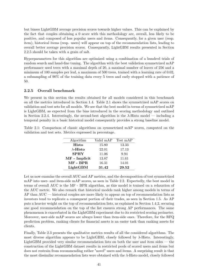
but biases LightGBM average precision scores towards higher values. This can be explained bythe fact that couples obtaining a 0 score with this methodology are, overall, less likely to bepositive, and composed of less popular users and items. Consequently, for a given user (resp.item), historical items (resp. users) will appear on top of the recommendation lists, leading tooverall better average precision scores. Consequently, LightGBM results presented in Section2.2.5 should be taken with a grain of salt.

Hyperparameters for this algorithm are optimized using a combination of a hundred trials ofrandom search and hand-fine tuning. The algorithm with the best validation symmetrized mAPperformance used trees with a maximal depth of 20, a maximal number of leaves of 256 and aminimum of 100 samples per leaf, a maximum of 500 trees, trained with a learning rate of 0.02,a subsampling of 90% of the training data every 5 trees and early stopped with a patience of50.

2.2.5 Overall benchmarkWe present in this section the results obtained for all models considered in this benchmarkon all the metrics introduced in Section 1.4. Table 2.1 shows the symmetrized mAP scores onvalidation and test sets for all models. We see that the best model in terms of symmetrized mAPis LightGBM, as expected from the bias introduced in the scoring methodology and outlinedin Section 2.2.4. Interestingly, the second-best algorithm is the ⁄-Histo model — including atemporal penalty in a basic historical model consequently provides a strong baseline model.

Table 2.1: Comparison of classic algorithms on symmetrized mAP scores, computed on thevalidation and test sets. Metrics expressed in percentage.

Algorithm Valid mAP Test mAPHisto 15.80 13.33

⁄-Histo 22.01 17.13SPHY 11.06 9.94

MF - Implicit 13.87 11.61MF - BPR 16.31 14.01LightGBM 31.42 29.52

Let us now examine the overall AUC and AP metrics, and the decomposition of test symmetrizedmAP into user- and item-side mAP scores, as seen in Table 2.2. Expectedly, the best model interms of overall AUC is the MF - BPR algorithm, as this model is trained on a relaxation ofthe AUC metric. We also remark that historical models rank higher among models in terms ofAP than AUC — historical couples are more likely to appear on top of recommendation lists asinvestors tend to replicate a consequent portion of their trades, as seen in Section 1.5. As APputs a heavier weight on the top of recommendation lists, as explained in Section 1.4.2, securingone good recommendation on the top of the list ensures strong AP performances. The samephenomenon is exacerbated in the LightGBM experiment due to its restricted scoring perimeter.Moreover, user-side mAP scores are always lower than item-side ones. Therefore, for the RFQprediction problem, ranking clients for financial assets is an easier task than ranking assets forclients.

Finally, Table 2.3 presents the qualitative metrics results of all the considered algorithms. Themost diverse algorithm appears to be LightGBM, closely followed by ⁄-Histo. Interestingly,LightGBM provided very similar recommendation lists on both the user and item sides — theconstruction of the LightGBM dataset results in restricted pools of scored users and items butdoes not restrain from recommending rather "novel" users and items. A surprising result is thatthe most dissimilar recommendation lists were obtained with the ⁄-Histo model, closely followed

41

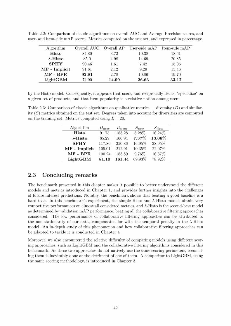
Table 2.2: Comparison of classic algorithms on overall AUC and Average Precision scores, anduser- and item-side mAP scores. Metrics computed on the test set, and expressed in percentage.

Algorithm Overall AUC Overall AP User-side mAP Item-side mAPHisto 84.80 3.72 10.38 18.61

⁄-Histo 85.0 4.98 14.69 20.85SPHY 90.46 1.61 7.42 15.06

MF - Implicit 91.61 2.12 9.29 15.46MF - BPR 92.81 2.78 10.86 19.70LightGBM 74.90 14.99 26.63 33.12

by the Histo model. Consequently, it appears that users, and reciprocally items, "specialize" ona given set of products, and that item popularity is a relative notion among users.

Table 2.3: Comparison of classic algorithms on qualitative metrics — diversity (D) and similar-ity (S) metrics obtained on the test set. Degrees taken into account for diversities are computedon the training set. Metrics computed using L = 20.

Algorithm Duser Ditem Suser Sitem

Histo 91.75 183.28 8.28% 16.24%⁄-Histo 85.29 166.94 7.37% 13.06%SPHY 117.86 250.86 16.95% 38.95%

MF - Implicit 105.01 212.91 10.35% 22.07%MF - BPR 100.24 183.89 9.76% 16.37%LightGBM 81.10 161.44 69.93% 78.92%

2.3 Concluding remarksThe benchmark presented in this chapter makes it possible to better understand the di�erentmodels and metrics introduced in Chapter 1, and provides further insights into the challengesof future interest predictions. Notably, the benchmark shows that beating a good baseline is ahard task. In this benchmark’s experiment, the simple Histo and ⁄-Histo models obtain verycompetitive performances on almost all considered metrics, and ⁄-Histo is the second-best modelas determined by validation mAP performance, beating all the collaborative filtering approachesconsidered. The low performance of collaborative filtering approaches can be attributed tothe non-stationarity of our data, compensated for with the temporal penalty in the ⁄-Histomodel. An in-depth study of this phenomenon and how collaborative filtering approaches canbe adapted to tackle it is conducted in Chapter 4.

Moreover, we also encountered the relative di�culty of comparing models using di�erent scor-ing approaches, such as LightGBM and the collaborative filtering algorithms considered in thisbenchmark. As these two approaches do not natively use the same scoring perimeters, reconcil-ing them is inevitably done at the detriment of one of them. A competitor to LightGBM, usingthe same scoring methodology, is introduced in Chapter 3.

42

Chapter 3

A supervised clustering approach tofuture interests prediction

The work exposed in this chapter has been orally presented at the 24th Workshop of Economicswith Heterogeneous Interacting Agents and was selected for an oral presentation at the 13th

Financial Risks International Forum organized by the Institut Louis Bachelier. It has beenselected for publication in the Algorithmic Finance journal under the title "Deep Prediction ofInvestor Interest: a Supervised Clustering Approach".

This chapter proposes a neural network architecture for the future interest prediction problemthat performs both investor clustering and modeling at the same time, thereby introducinga supervised clustering approach. The relevance of this architecture for the clustering andmodeling tasks is controlled in an experiment on a synthetic scenario, and the performance ofthe algorithm is monitored on two real-world databases, a publicly available dataset about theposition of investors in the Spanish stock market and a proprietary RFQ dataset from BNPParibas Corporate and Institutional Banking already presented in Section 1.2.

In this chapter, we examine the heterogeneity of investors and introduce a mathematical mod-eling of this heterogeneity (see Section 3.1), we introduce the above-mentioned neural networkarchitecture designed to tackle heterogeneous clusters of investors (see Section 3.2), we exper-iment this architecture on the synthetic and real-world datasets (see Section 3.3), we presentthe path of ideas that led to the introduced design (see Section 3.4) and we elaborate on waysto extend the current version (see Section 3.5).

43

3.1 Heterogeneous clusters of investorsPredicting future investor activity is a challenging problem in finance, as already stressed inChapter 1. Two of the challenges that make this problem particularly di�cult are the substantialheterogeneity of both investors and assets (see Section 1.2), compounded by the non-stationarynature of markets and investors and the limited time over which predictions are relevant. Thischapter explicitly tackles the first di�culty; the second one will be further explored in Chapter4.

3.1.1 Translating heterogeneityThe heterogeneity of investors translates into a heterogeneity of investment strategies (Tum-minello et al., 2012; Musciotto et al., 2018): for the same set of information, e.g., financialand past activity indicators, investors can take totally di�erent actions. Take for instance thecase of an asset whose price has just decreased: some investors will buy it because they havepositive long-term price increase expectations and thus are happy to be able to buy this asset ata discount; reversely, some other investors will interpret the recent price decrease as indicativeof the future trend or risk and refrain from buying it. We consequently expect a collection ofheterogeneous behaviors to emerge in our RFQ datasets.

It has been shown that ad hoc methods are surprisingly e�cient at clustering investors accordingto their trades in a single asset (Tumminello et al., 2012). Besides, clusters of investors deter-mined for several assets separately have a substantial overlap (Baltakys et al., 2018), whichshows that one may be able to cluster investors for more than a few assets at a time. Theactivity of a given cluster may also systematically depend on some clusters’ previous activity,which can then be used to predict the investment flow of investors (Challet et al., 2018). Here,we leverage deep learning to train a single neural network on all the investors and all the assetsof a given market and give temporal predictions for each investor, following the content filteringstrategy exposed in Chapter 1, Section 1.3.2. Our goal is to leverage these clusters of investors,expected to follow distinct investment strategies, to enhance predictions of single investors.

Formally, in our setting, we call strategy a mapping f from current information x to the expres-sion of interest to buy and/or sell a given asset, encoded by a categorical variable y: f : x ‘æ y.We call here

D = {fk : x ‘æ y}k (3.1)

the set of all the investment strategies that an investor may follow. Unsupervised clusteringmethods suggest that the number of di�erent strategies that describe investors’ decisions isfinite (Musciotto et al., 2018). We therefore expect our dataset to have a finite number K ofclusters of investors, each following a given investment strategy fk. Consequently, we expect Dto be such that |D| = K, i.e.

D = {fk : x ‘æ y}k=1,··· ,K . (3.2)

Alternatively, D can be thought of as the set of distinguishable strategies, which may be smallerthan the total number of strategies and, therefore, be considered an e�ective set of strategies.Consequently, a suitable algorithm to meet our goal needs to infer the set of investment strategiesD.

44

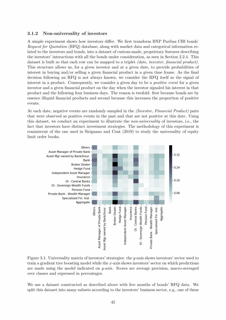
3.1.2 Non-universality of investorsA simple experiment shows how investors di�er. We first transform BNP Paribas CIB bonds’Request for Quotation (RFQ) database, along with market data and categorical information re-lated to the investors and bonds, into a dataset of custom-made, proprietary features describingthe investors’ interactions with all the bonds under consideration, as seen in Section 2.2.4. Thisdataset is built so that each row can be mapped to a triplet (date, investor, financial product).This structure allows us, for a given investor and at a given date, to provide probabilities ofinterest in buying and/or selling a given financial product in a given time frame. As the finaldecision following an RFQ is not always known, we consider the RFQ itself as the signal ofinterest in a product. Consequently, we consider a given day to be a positive event for a giveninvestor and a given financial product on the day when the investor signaled his interest in thatproduct and the following four business days. The reason is twofold: first because bonds are byessence illiquid financial products and second because this increases the proportion of positiveevents.

At each date, negative events are randomly sampled in the (Investor, Financial Product) pairsthat were observed as positive events in the past and that are not positive at this date. Usingthis dataset, we conduct an experiment to illustrate the non-universality of investors, i.e., thefact that investors have distinct investment strategies. The methodology of this experiment isreminiscent of the one used in Sirignano and Cont (2019) to study the universality of equitylimit order books.

Figure 3.1: Universality matrix of investors’ strategies: the y-axis shows investors’ sector used totrain a gradient tree boosting model while the x-axis shows investors’ sector on which predictionsare made using the model indicated on y-axis. Scores are average precision, macro-averagedover classes and expressed in percentages.

We use a dataset constructed as described above with five months of bonds’ RFQ data. Wesplit this dataset into many subsets according to the investors’ business sector, e.g., one of these

45

subsets contains investors coming from the Insurance sector only. We consider here only thesectors with a su�cient amount of data samples to train and test a model. The remainingsectors are grouped under the Others flag. Note that this flag is mainly composed of Corporatesectors, such as car industry, media, technology, telecommunications. . . For each sector, some ofthe latest data is held out, and a LightGBM model (Ke et al., 2017) is trained on the remainingdata. This model is then used for prediction on the held-out data of the model’s underlyingsector, and for all the other sectors as well. For comparison purposes, an aggregated modelusing all sectors at once is also trained and tested in the same way.

Because classes are unbalanced, we compute the average precision score of the obtained results,as advised by Davis and Goadrich (2006), macro-averaged over all the classes (see Section 1.4.1),which yields the universality matrix shown in Fig. 3.1. The y-axis labels the sector used fortraining, and the x-axis is the section on which the predictions are made.

We observe that some sectors are inherently di�cult to predict, even when calibrated on theirdata only — this is the case for Asset Managers of Private Banks and Pension Funds. On thecontrary, some sectors seem to be relatively easy to predict, e.g., Broker Dealers and, to someextent, Central Banks. Overall, we note that there is always some degree of variability of thescores obtained by a given model — no universal model gives good predictions for all the sectorsof activity. Thus follows the non-universality of clients. In addition, it is worth noting thatthe aggregated model obtained better performance in some sectors than the models trainedon these sectors’ data only. As a consequence, a suitable grouping of sectors would improvepredictions for some sectors. This observation is in agreement with the above K-investmentstrategies hypothesis.

Following on these hypotheses, the algorithm introduced in this chapter leverages deep learningboth to uncover the structure of similarity between investors, namely the K clusters, or strate-gies, and to make relevant predictions on each inferred cluster. The advantage of deep learninglies in that it allows solving both tasks at once and thereby unveils the structure of investorsthat most closely corresponds to their trading behavior in a self-consistent way.

3.1.3 Related workThe work conducted in this chapter finds its roots in mixture-of-experts research, which beganwith Jacobs et al. (1991), from which we keep the essential elements that drive the structure pre-sented in Section 3.2, and more particularly the gating and expert blocks. A rather exhaustivehistory of the research performed on this subject can be found in Yuksel et al. (2012).

The main inspiration for our work is Shazeer et al. (2017), which, although falling within theconditional computation framework, presented the first adaptation of mixture of experts for deeplearning models. We build on this work to come up with a novel structure designed to solvethe particular problem presented in Section 3.1. As far as we know, the approach we proposeis new. We use an additional loss term to improve the learning of the strategies, reminiscent ofthe one introduced in Liu and Yao (1999).

46

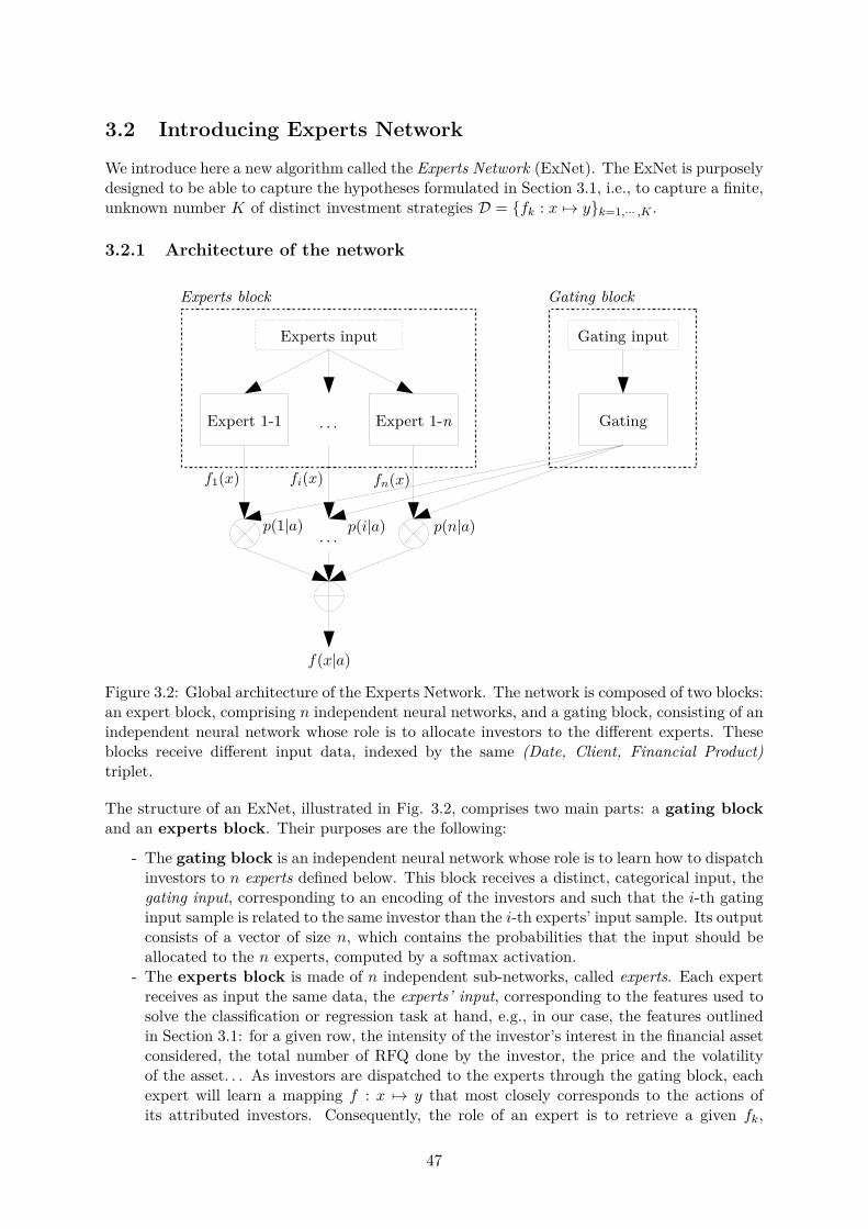
3.2 Introducing Experts Network

We introduce here a new algorithm called the Experts Network (ExNet). The ExNet is purposelydesigned to be able to capture the hypotheses formulated in Section 3.1, i.e., to capture a finite,unknown number K of distinct investment strategies D = {fk : x ‘æ y}k=1,··· ,K .

3.2.1 Architecture of the network

Figure 3.2: Global architecture of the Experts Network. The network is composed of two blocks:an expert block, comprising n independent neural networks, and a gating block, consisting of anindependent neural network whose role is to allocate investors to the di�erent experts. Theseblocks receive di�erent input data, indexed by the same (Date, Client, Financial Product)triplet.

The structure of an ExNet, illustrated in Fig. 3.2, comprises two main parts: a gating blockand an experts block. Their purposes are the following:

- The gating block is an independent neural network whose role is to learn how to dispatchinvestors to n experts defined below. This block receives a distinct, categorical input, thegating input, corresponding to an encoding of the investors and such that the i-th gatinginput sample is related to the same investor than the i-th experts’ input sample. Its outputconsists of a vector of size n, which contains the probabilities that the input should beallocated to the n experts, computed by a softmax activation.

- The experts block is made of n independent sub-networks, called experts. Each expertreceives as input the same data, the experts’ input, corresponding to the features used tosolve the classification or regression task at hand, e.g., in our case, the features outlinedin Section 3.1: for a given row, the intensity of the investor’s interest in the financial assetconsidered, the total number of RFQ done by the investor, the price and the volatilityof the asset. . . As investors are dispatched to the experts through the gating block, eachexpert will learn a mapping f : x ‘æ y that most closely corresponds to the actions ofits attributed investors. Consequently, the role of an expert is to retrieve a given fk,

47

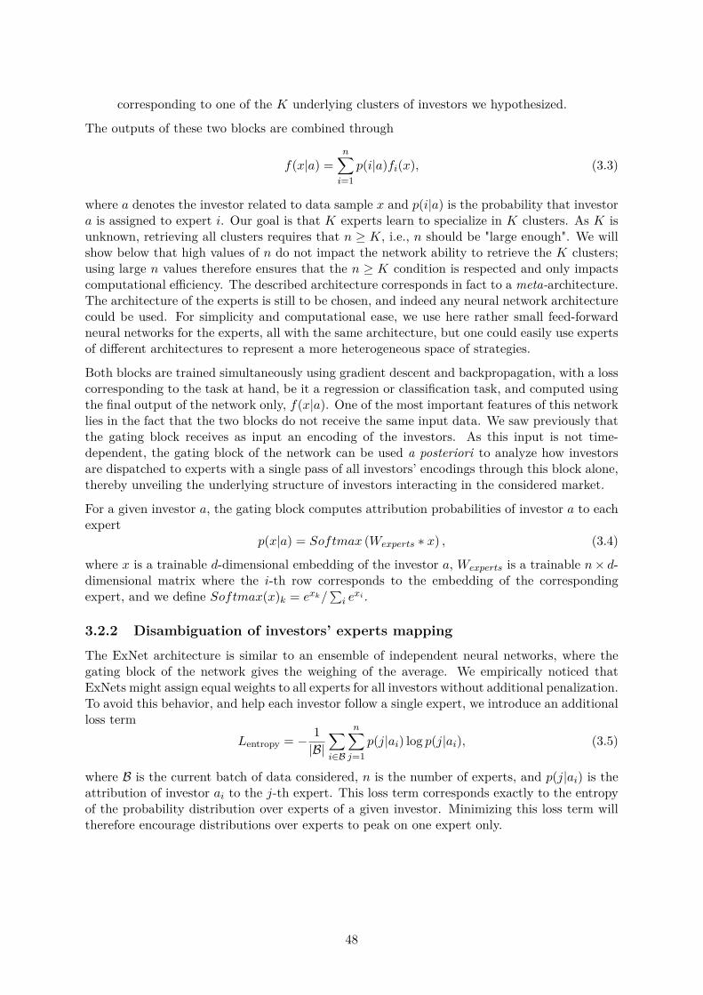
corresponding to one of the K underlying clusters of investors we hypothesized.

The outputs of these two blocks are combined through

f(x|a) =nÿ

i=1p(i|a)fi(x), (3.3)

where a denotes the investor related to data sample x and p(i|a) is the probability that investora is assigned to expert i. Our goal is that K experts learn to specialize in K clusters. As K isunknown, retrieving all clusters requires that n Ø K, i.e., n should be "large enough". We willshow below that high values of n do not impact the network ability to retrieve the K clusters;using large n values therefore ensures that the n Ø K condition is respected and only impactscomputational e�ciency. The described architecture corresponds in fact to a meta-architecture.The architecture of the experts is still to be chosen, and indeed any neural network architecturecould be used. For simplicity and computational ease, we use here rather small feed-forwardneural networks for the experts, all with the same architecture, but one could easily use expertsof di�erent architectures to represent a more heterogeneous space of strategies.

Both blocks are trained simultaneously using gradient descent and backpropagation, with a losscorresponding to the task at hand, be it a regression or classification task, and computed usingthe final output of the network only, f(x|a). One of the most important features of this networklies in the fact that the two blocks do not receive the same input data. We saw previously thatthe gating block receives as input an encoding of the investors. As this input is not time-dependent, the gating block of the network can be used a posteriori to analyze how investorsare dispatched to experts with a single pass of all investors’ encodings through this block alone,thereby unveiling the underlying structure of investors interacting in the considered market.

For a given investor a, the gating block computes attribution probabilities of investor a to eachexpert

p(x|a) = Softmax (Wexperts ú x) , (3.4)

where x is a trainable d-dimensional embedding of the investor a, Wexperts is a trainable n ◊ d-dimensional matrix where the i-th row corresponds to the embedding of the correspondingexpert, and we define Softmax(x)k = e

xk/q

ie

xi .

3.2.2 Disambiguation of investors’ experts mappingThe ExNet architecture is similar to an ensemble of independent neural networks, where thegating block of the network gives the weighing of the average. We empirically noticed thatExNets might assign equal weights to all experts for all investors without additional penalization.To avoid this behavior, and help each investor follow a single expert, we introduce an additionalloss term

Lentropy = ≠ 1|B|

ÿ

iœB

nÿ

j=1p(j|ai) log p(j|ai), (3.5)

where B is the current batch of data considered, n is the number of experts, and p(j|ai) is theattribution of investor ai to the j-th expert. This loss term corresponds exactly to the entropyof the probability distribution over experts of a given investor. Minimizing this loss term willtherefore encourage distributions over experts to peak on one expert only.

48

3.2.3 Helping experts specializeWithout a suitable additional loss term, the network has a tendency to let a few experts learnthe same investment strategy, which also leads to more ambiguous mappings from investorsto experts. Thus, to help the network finding di�erent investment strategies and to increaseits discrimination power regarding investors, we add a specialization loss term, which involvescross-experts correlations, weighted accordingly to their relative attribution probabilities. It iswritten as:

Lspec =nÿ

i=1

nÿ

j=1,j ”=i

wi,jfli,j (3.6)

with wi,j =pipjq

n

i=1q

n

j=1,j ”=ipipj

if i ”= j, 0 else, (3.7)

and pi =q

aœAp

a

iqaœA p

ai >0

. (3.8)

Here, i, j œ {1, . . . , n}, fli,j is the batch-wise correlation between experts i and j outputs,averaged over the output dimension, and pi is the batch-wise mean attribution probability toexpert i, with p

a

ithe attribution probability of investor a to expert i, computed on the current

batch of investors that counted this expert in their top L only. The intuition behind this weightis that we want to avoid correlation between experts that were confidently selected by investors,i.e., to make sure that the experts that matter do not replicate the same investment strategy. Asthe number of the investors clustered around a given expert should not matter in this weighing,we only account for the nonnegative probabilities for all the considered investors in the weights,computed using relative mean probabilities pi. In some experiments, it was found useful torescale Lspec from [≠1; 1] to [0; 1].

This additional loss term is reminiscent of Liu and Yao (1999). As a matter of fact, in ensemblesof machine learning models, negatively correlated models are expected to perform better thanpositively correlated ones. A better performance can also be expected from the experts of anExNet, as negatively correlated experts better span the space of investment strategies. As thenumber of very distinct strategies grow, we can expect to find strategies that more closely matchthe ones investors follow in the considered market, or the basis functions on which investmentstrategies can be decomposed.

3.2.4 From gating to classificationUp to this point, we only discussed gating inputs related to investors. However, as seen above,being able to retrieve the structure of attribution of inputs to experts only requires to usecategorical data as input to the gating part of the network. In fact, gating can be performed onwhatever is thought to be suitable — for instance, it is reasonable to think that bond investorshave di�erent investment strategies depending on the bonds’ grades or on the sector of activityof the bond issuers. Higher-level details about investors could also be considered, e.g., becauseinvestment strategies may depend on factors such as the sector of activity of the investor, i.e.,whether it is a hedge fund, a central bank, or an asset manager, or the region of the investor.The investor dimension could even be totally forgotten, and the gating performed on asset-related categories only. Gating allows one to retrieve the underlying structure of interactions ofa given category or set of categories. Consequently, one can purposely set categories to studyhow they relate to the problem one wants to study. However, this may impact the model’sperformance, as chosen categories do not necessarily have distinct decision rules.

Note also that the initialization of weights in the gating network has a major impact on thealgorithm’s future performance. To find relevant clusters, i.e., clusters that are composed of

49

unequivocally attributed categories and that correspond to the original clusters expected in thedataset, categories need to be able to explore many di�erent clusters’ configurations before theexploitation of one relevant configuration. Consequently, the gating block must be initializedso that all the expert weights are fairly evenly initially distributed to allow for this exploration.In our implementation, we use a random normal initialization scheme for the d-dimensionalembeddings of the categories and of the experts.

3.2.5 Limitations of the approachOur approach allows us to treat well a known, fixed base of investors. However, it cannote�ciently deal with new investors or, at a higher level, new categories, as seen in Section 3.2.4,as embeddings for these new types of elements would need to be trained from scratch. To copewith such situations, we recommend using sets of fixed categories to describe the evolving ones.For instance, instead of performing gating on investors directly, one can use investors’ categoriessuch as sector, region,. . . that are already present in the dataset and on which we can trainembeddings. Doing so improves the robustness of our approach to unseen categories. Note thatthis limitation corresponds to the cold-start problem, already encountered in Section 1.3.5 andfurther explored in Section 4.4.3.

3.3 ExperimentsBefore testing the ExNet architecture on real data, we first check its ability to recover a knownstrategy set, to attribute investors correctly to strategies, and finally to classify the interest ofinvestors on synthetic data. We then show how our methodology compares with other algorithmson two di�erent datasets: a dataset open-sourced1 as part of the experiments presented inGutiérrez-Roig et al. (2019), and a BNP Paribas CIB dataset. Source code for the experimentson synthetic data and the open-source dataset is provided and can be found at https://github.com/BptBrr/deep_prediction.

3.3.1 Synthetic data

Generating the dataset

Taking a cue from BNP Paribas CIB bonds’ RFQ database (cf. Section 1.2.2), we definethree clusters of investors, each having a distinct investment strategy, which we label as "high-activity", "low-activity" and "medium-activity". Each cluster contains a di�erent proportion ofinvestors, and each investor within a cluster has the same activity frequency: the "high-activity"cluster accounts for roughly 70% of the dataset samples while containing roughly 10% of thetotal number of investors. The "low-activity" cluster accounts for roughly 10% of the sampleswhile containing roughly 50% of the total number of investors. The "medium-activity" clusteraccounts for the remaining number of samples and investors. In all the clusters, we assume thatinvestors are equally active.

We model the state of investors as a binary classification task, with a set of p features, denotedby X œ Rp, and a binary output Y representing the fact that an investor is interested or not inthe considered asset. Investor a belonging to cluster c follows the decision rule given by

Ya = (‡(wT

a X) > U) œ {0, 1} (3.9)

, wherewa = wc + ba œ Rp

, (3.10)1Data available at https://zenodo.org/record/2573031

50

wc œ Rp being the cluster weights and ba ≥ N (0, –) œ R an investor-specific bias, Xi ≥ N (0, 1)for i = 1, · · · , p, U is distributed according to the uniform distribution on [0, 1], and ‡ is thelogistic function.

The experiment is conducted using a generated dataset of 100, 000 samples, 500 investors andp = 5 features. This dataset is split into train/validation/test sets, corresponding to 70/20/10%of the whole dataset. – is set to 0.5, and the cluster weights are taken as follows:

- High-activity cluster: whigh = (5, 5, 0, 0, ≠5)- Low-activity cluster: wlow = (≠5, 0, 5, 0, 5)- Medium-activity cluster: wmedium = (≠5, 0, 5, 5, 0)

These weights are chosen so that the correlation between the low- and medium-activity clustersis positive, but both are negatively correlated with the high-activity cluster. In this way, webuild a structure of clusters, core decision rules, and correlation patterns that are su�cientlychallenging to demonstrate the usefulness of our approach.

Results

We examine the performance of our proposed algorithm, ExNet, against a benchmark algorithm,LightGBM (Ke et al., 2017). LightGBM is a widespread implementation of gradient boosting, asshown, for example, by the percentage of top Kaggle submissions that use it. The LightGBM isfed with the experts’ input and an encoding of the corresponding investors, used as a categoricalfeature in the LightGBM algorithm. For comparison purposes, experiments are also performedon a LightGBM model fed with experts’ input and an encoding of the investors’ underlyingclusters, i.e., whether the investor belongs to the high-, low- or medium-activity cluster, calledLGBM-Cluster.

ExNets are trained using the cross-entropy loss since we want to solve a classification prob-lem. The network is optimized using Nadam (Dozat, 2016), a variation of the Adam optimizer(Kingma and Ba, 2015) using Nesterov’s Accelerated Gradient (Nesterov, 1983), reintroducedin the deep learning framework by Sutskever et al. (2013), and Lookahead (Zhang et al., 2019).For comparison purposes, experiments are also performed on a multi-layer perceptron modelfed with the experts’ inputs concatenated with a trainable embedding of the investors, calledEmbed-MLP — consequently, this model di�ers from a one-expert ExNet in that such an ExNetwould not use an embedding of the investor to perform its predictions. All neural network mod-els presented here used the rectified linear unit, ReLU(x) = max(x, 0), as activation function(Nair and Hinton, 2010).

LightGBM, ExNet and Embed-MLP results are shown in Table 3.1. They were obtained using acombination of random search (Bergstra and Bengio, 2012) and manual fine-tuning. LightGBM-Cluster results used the hyperparameters found for LightGBM. These results correspond to themodel achieving the best validation accuracy over all our tests. The LightGBM and LightGBM-Cluster shown had 64 leaves, a minimum of 32 samples per leaf, a maximum depth of 10, alearning rate of 0.005, and a subsample ratio of 25% with a frequency of 2. ExNet-Opt, theExNet which achieved the best validation accuracy, used 16 experts with three hidden layers ofsizes 64, 128 and 64, a dropout rate (Srivastava et al., 2014) of 40%, loss weights ⁄spec = 7e

≠3

and ⁄entropy = 1e≠3, a batch size of 1024, and a learning rate of 7e≠3. The Embed-MLP model

shown used two hidden layers of size 128 and 64, a dropout rate of 15%, an embedding sized = 64, a batch size of 64, and a learning rate of 4.2e

≠5.

To study the influence of the number of experts on the performance of ExNets, we call ExNet-nan ExNet algorithm with n experts and vary n. These ExNets used experts with no hiddenlayers, batch-normalized inputs (Io�e and Szegedy, 2015), and an investor embedding of size

51

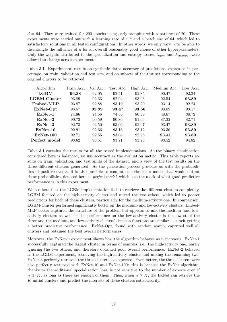
d = 64. They were trained for 200 epochs using early stopping with a patience of 20. Theseexperiments were carried out with a learning rate of e

≠3 and a batch size of 64, which led tosatisfactory solutions in all tested configurations. In other words, we only vary n to be able todisentangle the influence of n for an overall reasonably good choice of other hyperparameters.Only the weights attributed to the specialization and entropy losses, ⁄spec and ⁄entropy, wereallowed to change across experiments.

Table 3.1: Experimental results on synthetic data: accuracy of predictions, expressed in per-centage, on train, validation and test sets, and on subsets of the test set corresponding to theoriginal clusters to be retrieved.

Algorithm Train Acc. Val Acc. Test Acc. High Acc. Medium Acc. Low Acc.LGBM 96.38 92.05 92.41 92.85 90.47 92.34

LGBM-Cluster 93.89 92.33 92.94 93.03 92.54 93.89Embed-MLP 93.87 92.88 93.19 93.20 93.14 92.24ExNet-Opt 93.57 92.99 93.47 93.56 93.09 93.17

ExNet-1 74.86 74.56 74.56 80.39 48.67 38.72ExNet-2 90.73 90.59 90.86 91.66 87.32 82.71ExNet-3 92.73 92.50 93.06 92.97 93.47 93.89

ExNet-10 92.91 92.66 93.16 93.12 93.36 93.89ExNet-100 92.71 92.55 93.04 92.96 93.41 93.89

Perfect model 93.62 93.51 93.71 93.75 93.52 94.82

Table 3.1 contains the results for all the tested implementations. As the binary classificationconsidered here is balanced, we use accuracy as the evaluation metric. This table reports re-sults on train, validation, and test splits of the dataset, and a view of the test results on thethree di�erent clusters generated. As the generation process provides us with the probabili-ties of positive events, it is also possible to compute metrics for a model that would outputthese probabilities, denoted here as perfect model, which sets the mark of what good predictiveperformance is in this experiment.

We see here that the LGBM implementation fails to retrieve the di�erent clusters completely.LGBM focused on the high-activity cluster and mixed the two others, which led to poorerpredictions for both of these clusters, particularly for the medium-activity one. In comparison,LGBM-Cluster performed significantly better on the medium- and low-activity clusters. Embed-MLP better captured the structure of the problem but appears to mix the medium- and low-activity clusters as well — the performance on the low-activity cluster is the lowest of thethree and the medium- and low-activity clusters’ decision functions are similar —,albeit gettinga better predictive performance. ExNet-Opt, found with random search, captured well allclusters and obtained the best overall performances.

Moreover, the ExNet-n experiment shows how the algorithm behaves as n increases. ExNet-1successfully captured the largest cluster in terms of samples, i.e., the high-activity one, partlyignoring the two others, and therefore obtained poor overall performance. ExNet-2 behavedas the LGBM experiment, retrieving the high-activity cluster and mixing the remaining two.ExNet-3 perfectly retrieved the three clusters, as expected. Even better, the three clusters werealso perfectly retrieved with ExNet-10 and ExNet-100: this is because the ExNet algorithm,thanks to the additional specialization loss, is not sensitive to the number of experts even ifn ∫ K, as long as there are enough of them. Thus, when n Ø K, the ExNet can retrieve theK initial clusters and predict the interests of these clusters satisfactorily.

52

Further analysis of specialization

The previous results show that as long as n Ø K, the ExNet algorithm can e�ciently capture theinvestment strategies corresponding to the underlying investor clusters. One still needs to checkthat the attribution to experts is working well, i.e., that the investors are mapped to a single,unique expert. To this end, we retrieved from the gating block the attribution probabilities tothe n experts of all the investors a posteriori. For comparison, we also analyze the investors’embeddings of Embed-MLP. The comparison of the final embeddings of ExNet-Opt and theones trained in the Embed-MLP algorithm is shown in Fig. 3.3.

Figure 3.3: UMAP visualization of investors embeddings for both Embed-MLP (left) and ExNet(right) algorithms. Colors correspond to investors’ original clusters: high-activity is shown inblue, medium-activity in green and low-activity in red.

To visualize embeddings, we use here the UMAP algorithm (McInnes et al., 2018), which is par-ticularly relevant as it seeks to preserve the topological structure of the embeddings’ data man-ifold in a lower-dimensional space, thus keeping vectors that are close in the original space closein the embedding space, and making inter-cluster distances meaningful in the two-dimensionalplot.

Consequently, the two-dimensional map given by UMAP is a helpful tool for understandinghow investors relate to each other according to the deep learning method considered. In theseplots, high-activity investors are shown in blue, low-activity investors in red and medium-activity investors in green. We can see in Fig. 3.3 that the Embed-MLP algorithm did notmake an apparent distinction between the low- and medium-activity clusters, contrarily to theExNet, which separated these two categories except for a few low-activity investors mixed inthe medium-activity cluster. The ExNet algorithm was, therefore, completely able to retrievethe original clusters.

The attribution probabilities to the di�erent experts of ExNet-Opt are shown in Fig. 3.4. Wesee in this figure that the attribution structure of this ExNet instance is quite noisy, with threedi�erent behaviors discernable. The first group of investors corresponds to the low-activitycluster, the second group to the medium-activity cluster, and the last one to the high-activitycluster. Here, attributions are very noisy and investors of a same cluster are not uniquelymapped to an expert.

However, it is possible to achieve a more satisfactory experts attribution, as one can see in Fig.3.5 with the plots of ExNet-100. The more precise attribution comes from the fact that theExNet-100 instance used a higher level of ⁄entropy than ExNet-Opt — at the expense of someperformance, we can obtain far cleaner attributions to the experts. We see here on the left

53

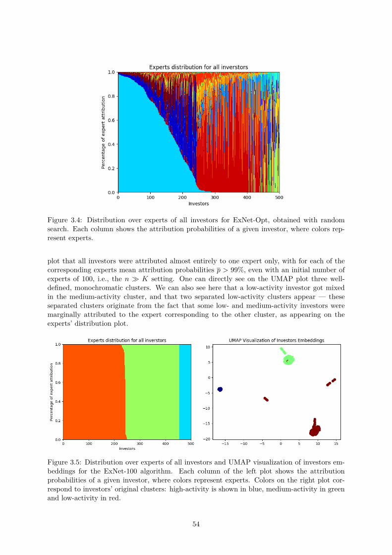
Figure 3.4: Distribution over experts of all investors for ExNet-Opt, obtained with randomsearch. Each column shows the attribution probabilities of a given investor, where colors rep-resent experts.

plot that all investors were attributed almost entirely to one expert only, with for each of thecorresponding experts mean attribution probabilities p > 99%, even with an initial number ofexperts of 100, i.e., the n ∫ K setting. One can directly see on the UMAP plot three well-defined, monochromatic clusters. We can also see here that a low-activity investor got mixedin the medium-activity cluster, and that two separated low-activity clusters appear — theseseparated clusters originate from the fact that some low- and medium-activity investors weremarginally attributed to the expert corresponding to the other cluster, as appearing on theexperts’ distribution plot.

Figure 3.5: Distribution over experts of all investors and UMAP visualization of investors em-beddings for the ExNet-100 algorithm. Each column of the left plot shows the attributionprobabilities of a given investor, where colors represent experts. Colors on the right plot cor-respond to investors’ original clusters: high-activity is shown in blue, medium-activity in greenand low-activity in red.

54

The ExNet-100 therefore solved the problem that we originally defined, obtaining excellentpredictive performance on the three original clusters and uniquely mapping investors to oneexpert only, thereby explicitly uncovering the initial structure of the investors, a feature thatan algorithm such as Embed-MLP is unable to perform.

3.3.2 IBEX data

Constructing the dataset

This experiment uses a real-world, publicly available dataset published as part of Gutiérrez-Roig et al. (2019) (https://zenodo.org/record/2573031) which contains data about a fewhundred private investors trading 8 Spanish equities from the IBEX index, from January 2000to October 2007. For a given stock and each day and each investor, the dataset gives the end-of-the-day position, the open, close, maximum, and minimum prices of the stock as well as thetraded volume.

We focus here on the stock of the Spanish telecommunication company Telefónica, TEF, as itis the stock with the largest number of trades. Using this data, we try to predict, at each date,whether an investor will be interested in buying TEF or not. An investor is considered to havean interest into buying TEF when

�pa

t = pa

t ≠ pa

t≠1 > 0, (3.11)

where pat is the position of investor a at time t. We only consider here the buy interest, as the

sell interest of private investors can be driven by exogenous factors that cannot be modeled,such as a liquidity shortage of an investor, whereas the buy interest of an investor depends,to some extent, on market conditions. Thus, we face a binary classification problem which ishighly unbalanced: on average, a buy event occurs with a frequency of 2.7%.

We consider a temporal split of our data in three parts: training data is taken from January2000 to December 2005, validation data from January 2006 to December 2006, and test datafrom January 2007 to October 2007. We restrict our investor perimeter to investors that boughtTEF more than 20 times during the training period. We build two kinds of features:

- Position features. Position is shifted such that at date t corresponds pt≠1, and is nor-malized for each investor using statistics computed on the training set. This normalized,shifted position is used as a feature, along with moving averages of it with windows of 1month, 3 months, 6 months and 1 year.

- Technical analysis features. We compute all the features available in the ta package(Padial, 2018), which are grouped under five categories: Volume, Volatility, Trend, Mo-mentum, and Others features. As most of these features use close price information, weshift them such that features at a date t only use the information available up to t ≠ 1.

We are left with 308 rather active investors and 63 features composing six di�erent groups.

55

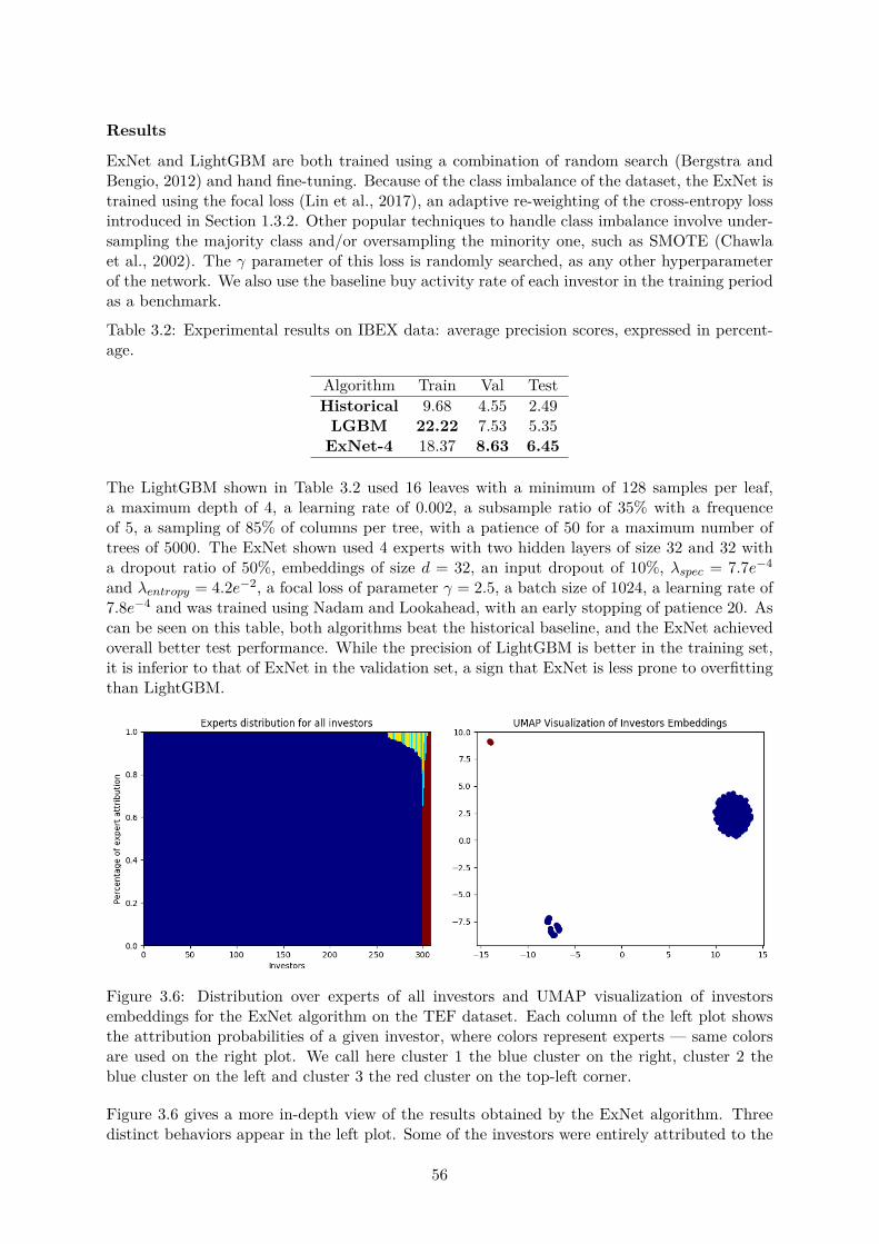
Results

ExNet and LightGBM are both trained using a combination of random search (Bergstra andBengio, 2012) and hand fine-tuning. Because of the class imbalance of the dataset, the ExNet istrained using the focal loss (Lin et al., 2017), an adaptive re-weighting of the cross-entropy lossintroduced in Section 1.3.2. Other popular techniques to handle class imbalance involve under-sampling the majority class and/or oversampling the minority one, such as SMOTE (Chawlaet al., 2002). The “ parameter of this loss is randomly searched, as any other hyperparameterof the network. We also use the baseline buy activity rate of each investor in the training periodas a benchmark.

Table 3.2: Experimental results on IBEX data: average precision scores, expressed in percent-age.

Algorithm Train Val TestHistorical 9.68 4.55 2.49

LGBM 22.22 7.53 5.35ExNet-4 18.37 8.63 6.45

The LightGBM shown in Table 3.2 used 16 leaves with a minimum of 128 samples per leaf,a maximum depth of 4, a learning rate of 0.002, a subsample ratio of 35% with a frequenceof 5, a sampling of 85% of columns per tree, with a patience of 50 for a maximum number oftrees of 5000. The ExNet shown used 4 experts with two hidden layers of size 32 and 32 witha dropout ratio of 50%, embeddings of size d = 32, an input dropout of 10%, ⁄spec = 7.7e

≠4

and ⁄entropy = 4.2e≠2, a focal loss of parameter “ = 2.5, a batch size of 1024, a learning rate of

7.8e≠4 and was trained using Nadam and Lookahead, with an early stopping of patience 20. As

can be seen on this table, both algorithms beat the historical baseline, and the ExNet achievedoverall better test performance. While the precision of LightGBM is better in the training set,it is inferior to that of ExNet in the validation set, a sign that ExNet is less prone to overfittingthan LightGBM.

Figure 3.6: Distribution over experts of all investors and UMAP visualization of investorsembeddings for the ExNet algorithm on the TEF dataset. Each column of the left plot showsthe attribution probabilities of a given investor, where colors represent experts — same colorsare used on the right plot. We call here cluster 1 the blue cluster on the right, cluster 2 theblue cluster on the left and cluster 3 the red cluster on the top-left corner.

Figure 3.6 gives a more in-depth view of the results obtained by the ExNet algorithm. Threedistinct behaviors appear in the left plot. Some of the investors were entirely attributed to the

56

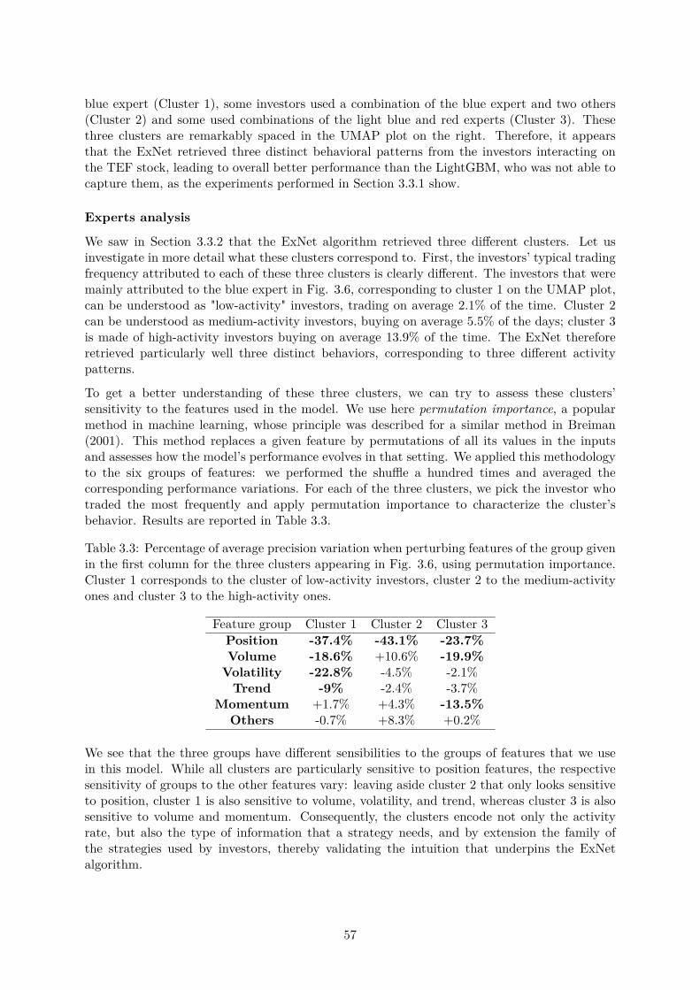
blue expert (Cluster 1), some investors used a combination of the blue expert and two others(Cluster 2) and some used combinations of the light blue and red experts (Cluster 3). Thesethree clusters are remarkably spaced in the UMAP plot on the right. Therefore, it appearsthat the ExNet retrieved three distinct behavioral patterns from the investors interacting onthe TEF stock, leading to overall better performance than the LightGBM, who was not able tocapture them, as the experiments performed in Section 3.3.1 show.

Experts analysis

We saw in Section 3.3.2 that the ExNet algorithm retrieved three di�erent clusters. Let usinvestigate in more detail what these clusters correspond to. First, the investors’ typical tradingfrequency attributed to each of these three clusters is clearly di�erent. The investors that weremainly attributed to the blue expert in Fig. 3.6, corresponding to cluster 1 on the UMAP plot,can be understood as "low-activity" investors, trading on average 2.1% of the time. Cluster 2can be understood as medium-activity investors, buying on average 5.5% of the days; cluster 3is made of high-activity investors buying on average 13.9% of the time. The ExNet thereforeretrieved particularly well three distinct behaviors, corresponding to three di�erent activitypatterns.

To get a better understanding of these three clusters, we can try to assess these clusters’sensitivity to the features used in the model. We use here permutation importance, a popularmethod in machine learning, whose principle was described for a similar method in Breiman(2001). This method replaces a given feature by permutations of all its values in the inputsand assesses how the model’s performance evolves in that setting. We applied this methodologyto the six groups of features: we performed the shu�e a hundred times and averaged thecorresponding performance variations. For each of the three clusters, we pick the investor whotraded the most frequently and apply permutation importance to characterize the cluster’sbehavior. Results are reported in Table 3.3.

Table 3.3: Percentage of average precision variation when perturbing features of the group givenin the first column for the three clusters appearing in Fig. 3.6, using permutation importance.Cluster 1 corresponds to the cluster of low-activity investors, cluster 2 to the medium-activityones and cluster 3 to the high-activity ones.

Feature group Cluster 1 Cluster 2 Cluster 3Position -37.4% -43.1% -23.7%Volume -18.6% +10.6% -19.9%

Volatility -22.8% -4.5% -2.1%Trend -9% -2.4% -3.7%

Momentum +1.7% +4.3% -13.5%Others -0.7% +8.3% +0.2%

We see that the three groups have di�erent sensibilities to the groups of features that we usein this model. While all clusters are particularly sensitive to position features, the respectivesensitivity of groups to the other features vary: leaving aside cluster 2 that only looks sensitiveto position, cluster 1 is also sensitive to volume, volatility, and trend, whereas cluster 3 is alsosensitive to volume and momentum. Consequently, the clusters encode not only the activityrate, but also the type of information that a strategy needs, and by extension the family ofthe strategies used by investors, thereby validating the intuition that underpins the ExNetalgorithm.

57

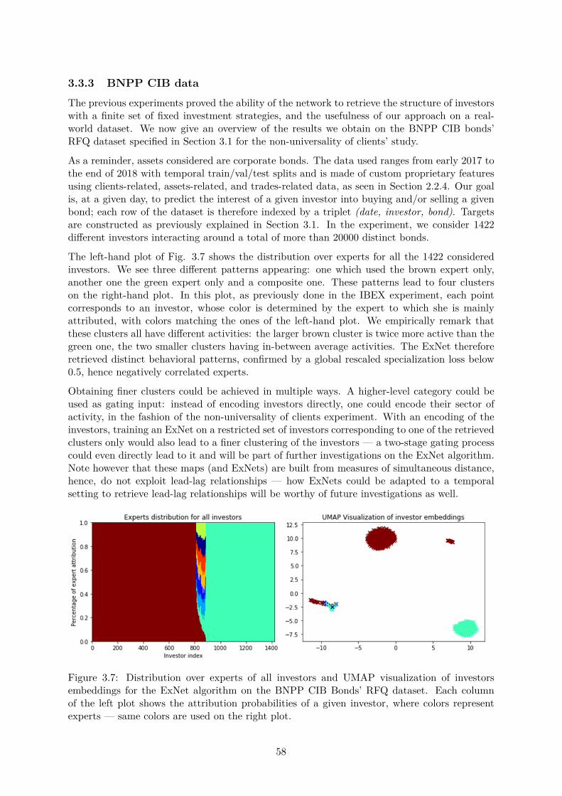
3.3.3 BNPP CIB dataThe previous experiments proved the ability of the network to retrieve the structure of investorswith a finite set of fixed investment strategies, and the usefulness of our approach on a real-world dataset. We now give an overview of the results we obtain on the BNPP CIB bonds’RFQ dataset specified in Section 3.1 for the non-universality of clients’ study.

As a reminder, assets considered are corporate bonds. The data used ranges from early 2017 tothe end of 2018 with temporal train/val/test splits and is made of custom proprietary featuresusing clients-related, assets-related, and trades-related data, as seen in Section 2.2.4. Our goalis, at a given day, to predict the interest of a given investor into buying and/or selling a givenbond; each row of the dataset is therefore indexed by a triplet (date, investor, bond). Targetsare constructed as previously explained in Section 3.1. In the experiment, we consider 1422di�erent investors interacting around a total of more than 20000 distinct bonds.

The left-hand plot of Fig. 3.7 shows the distribution over experts for all the 1422 consideredinvestors. We see three di�erent patterns appearing: one which used the brown expert only,another one the green expert only and a composite one. These patterns lead to four clusterson the right-hand plot. In this plot, as previously done in the IBEX experiment, each pointcorresponds to an investor, whose color is determined by the expert to which she is mainlyattributed, with colors matching the ones of the left-hand plot. We empirically remark thatthese clusters all have di�erent activities: the larger brown cluster is twice more active than thegreen one, the two smaller clusters having in-between average activities. The ExNet thereforeretrieved distinct behavioral patterns, confirmed by a global rescaled specialization loss below0.5, hence negatively correlated experts.

Obtaining finer clusters could be achieved in multiple ways. A higher-level category could beused as gating input: instead of encoding investors directly, one could encode their sector ofactivity, in the fashion of the non-universality of clients experiment. With an encoding of theinvestors, training an ExNet on a restricted set of investors corresponding to one of the retrievedclusters only would also lead to a finer clustering of the investors — a two-stage gating processcould even directly lead to it and will be part of further investigations on the ExNet algorithm.Note however that these maps (and ExNets) are built from measures of simultaneous distance,hence, do not exploit lead-lag relationships — how ExNets could be adapted to a temporalsetting to retrieve lead-lag relationships will be worthy of future investigations as well.

Figure 3.7: Distribution over experts of all investors and UMAP visualization of investorsembeddings for the ExNet algorithm on the BNPP CIB Bonds’ RFQ dataset. Each columnof the left plot shows the attribution probabilities of a given investor, where colors representexperts — same colors are used on the right plot.

58

On a global scale, these plots help us understand how investors relate to each other. Therefore,one can use them to obtain a better understanding of BNP Paribas CIB business and howBNP Paribas CIB clients’ behave on a given market through a thorough analysis of the learnedexperts.

3.4 A collection of unfortunate ideasDesigning the ExNet architecture presented above took time, e�orts, and a consequent numberof dead ends. Throughout the development of this algorithm, and more generally, for all thework presented in this thesis, Occam’s razor served as a guiding principle: when competingalgorithms led to similar results, we always favored the simpler one. This section presents,along with milestone designs that led to the actual one, a compendium of potentially promisingideas that led to mild disappointments, and consequently su�ered the razor blade.

3.4.1 About architectureAlthough the network presented in Section 3.2 is inspired to a great extent by the work ofShazeer et al. (2017), a lot of architectural variations were tried to obtain more satisfactoryresults. We examine here two of the most promising ideas we tested.

Representing the shared features of investment strategies

The ExNet design corresponds to the intuition that on a given market, investors tend toform clusters corresponding to particular investment strategies. Investment strategies, how-ever, might share features — at the very least, their shared goal of making money. This corebehavior underpinning all potential investment strategies can be explicitly represented as an-other independent neural network, receiving as input the same features experts do.

The corresponding architecture is depicted in Fig. 3.8. We see that an "average" block, usingthe same input as experts, is systematically added to the recombination of experts, leading toan output

f(x|a) = favg(x) +nÿ

i=1fi(x)p(i|a). (3.12)

In such a setting, experts fi(x) learn what amounts to residuals of the final output, in a mannerclose to the first step of a boosting algorithm (Hastie et al., 2009, Chapter 10), or more recentlyto a residual block (He et al., 2016).

This architecture was proven successful in learning the output but failed to cluster investors toexperts correctly, and was consequently abandoned to designs that succeeded at both tasks.

A gating strategy built for exploration

The initial design of the ExNet’s gating block was a lot closer to the architecture presented in(Shazeer et al., 2017). The idea is that, for a given investor a, the gating block performs thefollowing computation :

p(x|a) = Softmax

3KeepTopL

3Wgatingx + ‘ ú

ÒSoftplus(Wnoisex)

44(3.13)

where x is a trainable d-dimensional embedding of the investor a, Wnoise, Wgating are trainableweights of the network, ‘ ≥ N (0, 1), the softmax function defined as before and with thesoftplus function defined as Softplus(x) = log(1 + exp x). The KeepTopL function, introduced

59

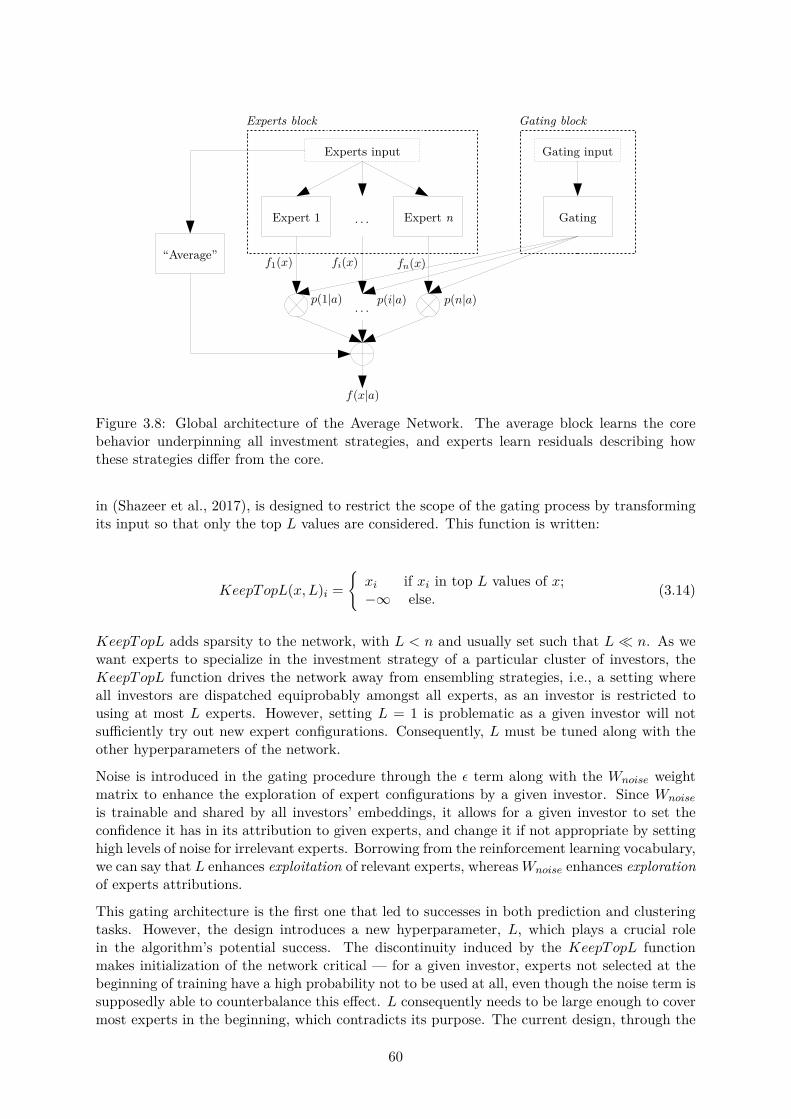
Figure 3.8: Global architecture of the Average Network. The average block learns the corebehavior underpinning all investment strategies, and experts learn residuals describing howthese strategies di�er from the core.

in (Shazeer et al., 2017), is designed to restrict the scope of the gating process by transformingits input so that only the top L values are considered. This function is written:

KeepTopL(x, L)i =I

xi if xi in top L values of x;≠Œ else. (3.14)

KeepTopL adds sparsity to the network, with L < n and usually set such that L π n. As wewant experts to specialize in the investment strategy of a particular cluster of investors, theKeepTopL function drives the network away from ensembling strategies, i.e., a setting whereall investors are dispatched equiprobably amongst all experts, as an investor is restricted tousing at most L experts. However, setting L = 1 is problematic as a given investor will notsu�ciently try out new expert configurations. Consequently, L must be tuned along with theother hyperparameters of the network.

Noise is introduced in the gating procedure through the ‘ term along with the Wnoise weightmatrix to enhance the exploration of expert configurations by a given investor. Since Wnoise

is trainable and shared by all investors’ embeddings, it allows for a given investor to set theconfidence it has in its attribution to given experts, and change it if not appropriate by settinghigh levels of noise for irrelevant experts. Borrowing from the reinforcement learning vocabulary,we can say that L enhances exploitation of relevant experts, whereas Wnoise enhances explorationof experts attributions.

This gating architecture is the first one that led to successes in both prediction and clusteringtasks. However, the design introduces a new hyperparameter, L, which plays a crucial rolein the algorithm’s potential success. The discontinuity induced by the KeepTopL functionmakes initialization of the network critical — for a given investor, experts not selected at thebeginning of training have a high probability not to be used at all, even though the noise term issupposedly able to counterbalance this e�ect. L consequently needs to be large enough to covermost experts in the beginning, which contradicts its purpose. The current design, through the

60

entropy loss, induces sparsity without enforcing it: it is a smoother, more straightforward wayto perform the same task that we consequently favored.

3.4.2 About regularizationThe regularization terms presented in Sections 3.2.2 and 3.2.3 have known a series of evolutionsfollowing the architectural ones seen above. We explore here the evolution of the specializationand sparsity terms that led to their current versions.

Evolution of specialization term

The first version of the specialization term was inspired from the total variation measure(Berestycki, 2016, Section 1.2). Total variation measures the distance between two probabilitydistributions. In a setting where experts output class probabilities, as is the case in the futureinterests prediction setting, total variation can enforce the di�erentiation of experts outputsby ensuring large distances between probability distributions. As we want to maximize totalvariation and as it is bounded by 1, the corresponding loss term we first used was written

Lspec = 1 ≠ 1n2|B|

nÿ

i=1

nÿ

j=1

ÿ

xœB

Cÿ

c=1|f c

i (x) ≠ fc

j (x)|, (3.15)

where n is the number of experts, B a batch of data, C the number of output classes and fc

i(x)

the output of expert i for class c œ [[1; C]]. This term did not lead to satisfactory results: theL1 penalization of the di�erence of the outputs here drives them such that one gets close to 1and the other close to 0. We deemed that such a penalty term harmed the optimization of theprediction loss, and moved towards smoother versions of this penalty.

A smoother way to enforce di�erentiation of experts is to penalize their correlations, as exposedin Section 3.2.3. As we want to avoid similar experts, the idea is to penalize correlated ones —the corresponding term was written

Lspec = 2n(n ≠ 1)

nÿ

i=1

nÿ

j=1,j ”=i

max1fli,j , 0

2, (3.16)

where all parameters are defined as in Section 3.2.3. We see that this term di�ers from thecurrent one in two ways: the maximum function and the weighing of the individual terms.The maximum served as a way only to penalize positively correlated experts. Although thisperfectly avoids replication, it misses the fact that slightly correlated experts are expected tospan the space of investment strategies better. The averaging here is also problematic: a goodspecialization loss could be obtained by driving unused experts to be negatively correlated.The weights used in the current version correct this by only accounting for used experts, whichallows for small clusters to still matter in the specialization penalty.

61

Evolution of parsimony term

The parsimony term currently used is an entropy loss, as seen in Section 3.2.2. Before usingentropy, we tried to enforce sparsity by acting on the variance of the probability distributionsoutputted by the gating block — the highest possible variance of a probability distribution isattained with a probability of 1 for a class, and 0 everywhere, which is the sparse result we wishto obtain. The corresponding penalty was written:

Lparsimony = 1|B|

ÿ

xœB

3 1n‡2

x

4, (3.17)

where B is a batch of data, n the number of experts and ‡x the standard deviation of thegating output of the investor corresponding to sample x. However, the inverse used in this lossterm is problematic as the incurred penalty is not linear with regard to the underlying sparsity:distributions far from being sparse would incur a high penalty, whereas distributions closer toit would not matter much anymore in the term. Consequently, distributions trained with sucha penalty would not attain the level of sparsity we wished for.

The parsimony term then disappeared with the introduction of the KeepTopL function seen inSection 3.4.1: sparsity was then a direct result of the L hyperparameter, and we consequentlyabandoned the idea of enforcing it through a penalty term. The term finally reappeared in itscurrent entropic form, which allowed dispensing with the noised gating architecture.

3.4.3 About trainingA few tricks were also tried to enhance the training of the network, as it was particularly di�cultin the first iterations of the methodology to converge to an ExNet that would be both goodat prediction and clustering. Although these tricks disappeared in the current version of thenetwork, we mention them here for the record.

Using pre-computed embeddings

Training a relevant clustering of investors from scratch is a di�cult task. A reasonable idea isto initialize these embeddings with meaningful values to help the network learning embeddingsleading to clusters that serve the prediction task. We tried using the embeddings of a matrixfactorization algorithm trained on the same predictive task, in the fashion of the implicit versionof matrix factorization introduced in (Hu et al., 2008) and explained in Section 1.3.3. However,this initialization did not prove useful in helping either the prediction or the clustering tasksand led to similar final results for both.

Alternating tasks training

ExNets solve two distinct tasks at once: a clustering task and a prediction task, both potentiallysubject to overfitting the training data. Classic regularization techniques will prevent overfittingfor the prediction task, but might not be su�cient for the clustering one.

For this reason, we introduce an alternating training schedule. The idea is to split the trainingdata into two parts, both respecting investors’ proportions, i.e., an x% split of the datasetshould contain x% of each investor’s data. This ensures that both splits use the same set ofinvestors and that their relative appearance proportions are maintained in both splits. Trainingis then done according to the following schedule:

1. Train the whole network for an epoch of a given split to warm the network up.

2. Loop until convergence:

62

- Train the gating block of the network only on a given split;- Train the experts block of the network only on the other split.

The goal of this schedule was to improve the generalization of expert repartitions we obtainfrom the network. Training the network in such a way, however, did not prove useful whatsoeverfor improving out-of-sample performance on either task.

3.5 Further topics in Experts NetworksAlthough the ExNet algorithm proved its usefulness, as seen in Section 3.3, there is alwaysroom for improvement. We introduce here a couple of enhancements of the algorithm that haveshown promise.

3.5.1 Boosting ExNetsBefore introducing ExNets in the BNPP CIB RFQ prediction framework, leading algorithmswere all gradient tree-boosting models such as XGBoost (Chen and Guestrin, 2016) or Light-GBM (Ke et al., 2017). The idea behind gradient boosting is to enhance the capacity of a simple,basis function by adding an ensemble of such functions (Hastie et al., 2009, Chapter 10). Neuralnetworks are consequently not the perfect candidate for boosting, as these models are designedto capture complexity through depth.

Instead of directly plugging a neural network as basis function of a gradient boosting model, it is,however, possible to translate the core ideas behind boosting to a neural network architecture.We consequently designed such an architecture to boost the performance of an ExNet — theglobal architecture is depicted in Fig. 3.9. Experts blocks can here be thought of as the basisfunction of the boosting strategy. A single gating network is shared across all boosting stagesto allow for a posteriori analysis of the obtained clustering. The output of stage k is written

fk(x|a) = ÷fk≠1(x|a) +ÿ

i

fk,i(x) + p(i|a), (3.18)

and all stages incur a loss lk on their outputs. The whole network is trained in an end-to-endfashion using stochastic gradient descent and backpropagation.

This network has the expected behavior: during training, each boosting stage has lower lossvalues than its direct predecessor. However, the overall gain of performance over a classic ExNetof this approach is marginal at the expense of far higher computation time. We consequentlystill favor the original ExNet architecture.

The approach taken for this network is reminiscent of residual networks (He et al., 2016). Aresidual network is made of residual blocks performing the computation y = F(x, {Wi}) + x,where x is the block input, y the block output, F an operator and Wi, bi the parameters of theoperator — He et al. (2016) use F = W2f(W1x), with f an activation function. The initial goalof residual networks is to allow for network growth by tackling the vanishing gradient problemsthrough skip-connections using the identity function. These connections allow for a better flowof the gradient throughout the network. Huang et al. (2018) explore the connection betweenresidual networks and gradient boosting theory, through a BoostResNet model that boosts overfeatures, instead of the classical boosting over outputs. Instead of using boosting for the neuralnetwork, a way to enhance the results of the ExNet could be to use residual networks as expertsin the network. As residual networks can be interpreted as ensembles of relatively shallownetworks (Veit et al., 2016), such a network would be an ensemble. . . of ensembles.

63

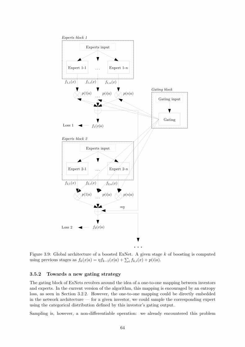
Figure 3.9: Global architecture of a boosted ExNet. A given stage k of boosting is computedusing previous stages as fk(x|a) = ÷fk≠1(x|a) +

qifk,i(x) + p(i|a).

3.5.2 Towards a new gating strategyThe gating block of ExNets revolves around the idea of a one-to-one mapping between investorsand experts. In the current version of the algorithm, this mapping is encouraged by an entropyloss, as seen in Section 3.2.2. However, the one-to-one mapping could be directly embeddedin the network architecture — for a given investor, we could sample the corresponding expertusing the categorical distribution defined by this investor’s gating output.

Sampling is, however, a non-di�erentiable operation: we already encountered this problem

64

with the KeepTopL function in Section 3.4.1. The Gumbel-Softmax distribution, introducedsimultaneously by Jang et al. (2017) and Maddison et al. (2017), solves this issue by replacingthe non-di�erentiable sample with a di�erentiable one. The trick is to draw samples y œ �n≠1,with �n≠1 the n ≠ 1-simplex and n the number of experts, with yi defined as

yi = exp((log(fii) + gi)/·)q

n

j=1 exp((log(fij) + gj)/·) . (3.19)

Here, g1, . . . , gn are i.i.d. samples drawn from a Gumbel(0,1) distribution — Gumbel(0,1) areeasily drawn with g = ≠ log(≠ log(u)) where u ≥ U([0, 1]) —, fi1, . . . , fin are the allocationprobabilities for the considered investors as obtained with the gating block of the ExNet, and ·

is a parameter controlling the temperature of the softmax distribution. The Gumbel-Softmaxhas the nice property that when · ≠æ 0, the distribution converges to a categorical one.Consequently, smoothly annealing · during training allows for a quasi-categorical distributionwith di�erentiable samples all along, solving the issues raised in Section 3.4.1. Guo et al. (2019)present an adaptation of this trick in the context of transfer learning.

Gumbel-Softmax has been adapted to ExNets but is still in its infancy for now. It has shown firstpromising results, leading to relevant yet imperfect one-to-one mappings between investors andexperts, but it appears to be very sensitive to the annealing schedule of the · parameter. Thedevelopment of a schedule leading to satisfying results will be the subject of further research.

3.6 Concluding remarksIn this chapter, we introduced a novel algorithm, ExNet, based on the financial intuition that ina given market, investors may act di�erently when exposed to the same signals and form clustersaround a finite number of investment strategies. This algorithm performs both prediction, beit regression or classification, and clustering at the same time. The fact that these operationsare trained simultaneously leads to a clustering that most closely serves the prediction task anda prediction improved by the clustering. Moreover, one can use this clustering a posteriori,independently, to examine how individual agents behave and interact with each other. To helpthe clustering process, we introduced two additional loss terms that penalize the correlation be-tween the inferred investment strategies and the entropy of the investors’ allocations to experts.Thanks to an experiment with simulated data, we proved the usefulness of our approach, andwe discussed how the ExNet algorithm performs on an open-source dataset of Spanish stockmarket data and data from BNP Paribas CIB.

This chapter extended the original article by providing insights into the development of thealgorithm, including the di�culties encountered, the failed attempts, and potential leads forfurther improvements. Further research on ExNets will include how such architectures could beextended and staged and how they could be adapted to retrieve lead-lag relationships in a givenmarket. Finally, it is worth noting that the ExNet architecture can be applied wherever oneexpects agents to use a finite number of decision patterns, e.g., in e-shopping or movie opiniondatabases (Bennett et al., 2007).

65

Chapter 4

Towards time-dependentrecommendations

The work exposed in this chapter has been selected as a short paper to the 14th ACM Confer-ence on Recommender Systems, RecSys2020, under the title "History-Augmented CollaborativeFiltering for Financial Recommendations".

Chapter 3 tackled the challenge of investors’ behavioral heterogeneity. In this chapter, we pro-pose a novel collaborative filtering algorithm that captures the temporal context of a user-iteminteraction through the user and item recent histories, thereby tackling the non-stationarity ofinvestors’ interests with a custom neural network architecture. The performance and propertiesof the algorithm are monitored in a series of experiments on a G10 bond request for quotationproprietary database from BNP Paribas CIB.

This chapter introduces the context and reach of this work (see Section 4.1), explains in greatextent the neural network architecture proposed to meet the targeted goals (see Section 4.2),presents experiments proving the usefulness of the said architecture (see Section 4.3) and elab-orates on ways to further the proposed work, along with details about its development and anew use case (see Section 4.4).

4.1 Tackling financial challengesIn this section, we briefly review some of the notions introduced in Chapter 1, expose thechallenges we want to tackle with our recommender systems and present recommender systemsresearch related to these challenges.

4.1.1 Context and objectivesWhen a client wants to trade a financial product, she either requests prices on an electronicplatform where many di�erent market makers operate in a process called a request for quotation(RFQ), or contact a salesperson of a bank. Reciprocally, salespeople can also directly contactclients and suggest relevant trade ideas to them, e.g., financial products held by the bank and onwhich it might o�er a better price than its competitors. Section 1.1.1 already elaborated on thecrucial importance of proactive salespeople for the bank. To support salespeople’s proactivity,we can provide them with an RFQ recommender system purposefully designed to assist themin their daily tasks. Consequently, our goal is to design a recommender system that suitsthe particularities of the financial world. The RFQ recommendation problem is an imperfectinformation and an implicit feedback problem: we only observe the electronic RFQs performed

67

on the platforms on which BNP Paribas provides services, and we do not explicitly observeclients’ opinions about the products they request. Implicit feedback is a classic recommendersystem setup already addressed by the research community, e.g., in (Hu et al., 2008). Thefinancial environment, however, brings about specific issues that require attention. To thatend, the algorithm we introduce here has three main aims:

- To incorporate time. In a classic e-commerce environment, leaving aside popularityand seasonal e�ects, recommendations provided at a given date may remain relevant fora couple of months, since users’ shopping tastes do not markedly evolve with time. Inthe financial world, a user is interested in a financial product at a given date not onlybecause of the product’s intrinsic characteristics but also because of the current marketconditions. Time is consequently crucial for RFQ prediction and should be taken intoaccount in a manner that allows for future predictions.

- To obtain dynamic embeddings. Being able to capture how clients (resp. financialproducts) relate to each other and how this relationship evolves with time is of greatinterest for business, as it allows getting a deeper understanding of the market. One ofour goals is consequently to keep the global architecture of matrix factorization algorithmswhere the recommendation score of a (client, product) couple is given by the scalar productof their latent representations.

- To symmetrize users and items. Classic recommender systems focus on the client-side. However, the product-side is also of interest in the context of a corporate bank.To control her risk, a market maker needs to control her positions, i.e., make sure shedoes not hold a given position for too long. Consequently, coming up with the relevantclient for a given asset is also important, and the symmetry of clients and assets will beintegrated here in both our algorithms and evaluation strategies.

We tackle these goals with a context-aware recommender system that only uses client-productinteractions as its signal source. Notably, the context considered here is temporal and will beinferred from clients’ and products’ past behaviors. The terms clients and users (resp. financialproducts/assets and items) will be used interchangeably to match the vocabulary used in therecommender systems literature.

4.1.2 Related workTime-dependent collaborative filtering is an active area of research that has known many devel-opments over the years (Shi et al., 2014). Introducing time in matrix factorization was done inKoren (2009b) with the timeSVD++ algorithm. Ding and Li (2005) propose to downweigh pastsamples in a memory-based collaborative filtering algorithm. Tensor factorization algorithmscan also handle time by considering the user-item co-occurrence matrix as a three-dimensionaltensor, where the additional dimension corresponds to time, e.g., in Xiong et al. (2010) and Wuet al. (2018), the latter using neural network architectures. However, algorithms relying on ma-trix or tensor factorization do not allow for making predictions in the future. Enhancing latentfactor models with Kalman filters as in Sarkar et al. (2007) or with LSTM cells (Hochreiter andSchmidhuber, 1997) to capture the dynamics of rating vectors as in Wu et al. (2017) alleviatesthis issue. Using historical data to introduce dynamics in a neural network recommender sys-tem was done in Covington et al. (2016), where the authors assimilate YouTube users to theirviewing histories.

The algorithm introduced in this paper is, to some extent, reminiscent of graph neural networks(Hamilton et al., 2017) and their adaptation to recommendation (Wang et al., 2019), where onewould stop at first-order connectivity. Using time to enhance recommendations with randomwalks on bipartite graphs was explored in Xiang et al. (2010). How graph neural networksbehave with dynamic bipartite graphs is to the best of our knowledge yet to be discovered and

68

could lead to an extension of this work. A first attempt at financial products recommendationwas made in Wright et al. (2018), with the particular example of corporate bonds.

4.2 Enhancing recommendations with historiesWe introduce a neural network architecture that aims at producing recommendations throughdynamic embeddings of users and items, that we call History-augmented Collaborative Filtering(HCF).

4.2.1 Some definitions

Let U be the set of all users and I the set of all items. Let us note xu œ Rd for u œ U , xi œ Rd

for i œ I the d-dimensional embeddings of all the users and items we consider. Let t œ [[0 ; Œ]]be a discrete timestep, taken as days in this work. For a given u, at a given t, we define ht

uas the items’ history of u, i.e. the set of items found to be of interest to u in the past — werespectively define ht

i as item i users’ history. We use here as histories the last n events thathappened strictly before t to either user u or item i. If at a given t we observe 0 Æ n

Õ< n

previous events, histories are only formed of those nÕ events. By doing so, we place users on the

same event scale — high-activity users will have histories spanning a couple of days, whereaslow-activity ones will span a couple of months (resp. for items). Histories formed of items/usersof interest in a past window of fixed size were also tried but led to inferior performance thanthe previous history definition.

Figure 4.1: a. Global architecture of the HCF network, composed of two symmetric user anditem blocks. b. Illustration of the application of a one-dimensional convolution of kernel size 1along the embedding dimension axis of our inputs xu and h

tu for a user u œ U , where –, —, “ are

the parameters of the convolution filter and l œ [[1; d]]. The same computation holds for itemsi œ I respectively.

69

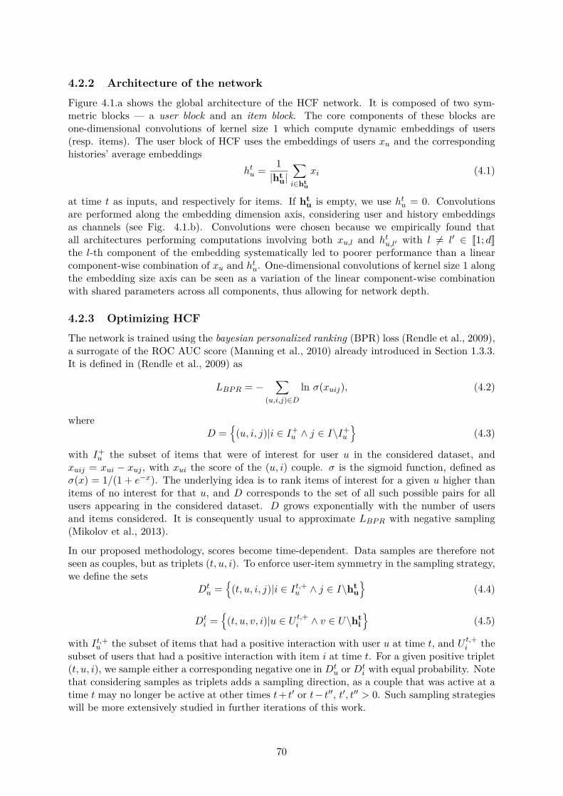
4.2.2 Architecture of the networkFigure 4.1.a shows the global architecture of the HCF network. It is composed of two sym-metric blocks — a user block and an item block. The core components of these blocks areone-dimensional convolutions of kernel size 1 which compute dynamic embeddings of users(resp. items). The user block of HCF uses the embeddings of users xu and the correspondinghistories’ average embeddings

ht

u = 1|htu|

ÿ

iœhtu

xi (4.1)

at time t as inputs, and respectively for items. If htu is empty, we use h

tu = 0. Convolutions

are performed along the embedding dimension axis, considering user and history embeddingsas channels (see Fig. 4.1.b). Convolutions were chosen because we empirically found thatall architectures performing computations involving both xu,l and h

t

u,lÕ with l ”= lÕ œ [[1; d]]

the l-th component of the embedding systematically led to poorer performance than a linearcomponent-wise combination of xu and h

tu. One-dimensional convolutions of kernel size 1 along

the embedding size axis can be seen as a variation of the linear component-wise combinationwith shared parameters across all components, thus allowing for network depth.

4.2.3 Optimizing HCFThe network is trained using the bayesian personalized ranking (BPR) loss (Rendle et al., 2009),a surrogate of the ROC AUC score (Manning et al., 2010) already introduced in Section 1.3.3.It is defined in (Rendle et al., 2009) as

LBP R = ≠ÿ

(u,i,j)œD

ln ‡(xuij), (4.2)

whereD =

Ó(u, i, j)|i œ I

+u · j œ I\I

+u

Ô(4.3)

with I+u the subset of items that were of interest for user u in the considered dataset, and

xuij = xui ≠ xuj , with xui the score of the (u, i) couple. ‡ is the sigmoid function, defined as‡(x) = 1/(1 + e

≠x). The underlying idea is to rank items of interest for a given u higher thanitems of no interest for that u, and D corresponds to the set of all such possible pairs for allusers appearing in the considered dataset. D grows exponentially with the number of usersand items considered. It is consequently usual to approximate LBP R with negative sampling(Mikolov et al., 2013).

In our proposed methodology, scores become time-dependent. Data samples are therefore notseen as couples, but as triplets (t, u, i). To enforce user-item symmetry in the sampling strategy,we define the sets

Dt

u =Ó

(t, u, i, j)|i œ It,+u · j œ I\ht

uÔ

(4.4)

Dt

i =Ó

(t, u, v, i)|u œ Ut,+i

· v œ U\htiÔ

(4.5)

with It,+u the subset of items that had a positive interaction with user u at time t, and U

t,+i

thesubset of users that had a positive interaction with item i at time t. For a given positive triplet(t, u, i), we sample either a corresponding negative one in D

tu or D

t

iwith equal probability. Note

that considering samples as triplets adds a sampling direction, as a couple that was active at atime t may no longer be active at other times t + t

Õ or t ≠ tÕÕ, t

Õ, t

ÕÕ> 0. Such sampling strategies

will be more extensively studied in further iterations of this work.

70

4.2.4 Going furtherHCF retains a matrix factorization-like architecture to allow for using dynamic embeddingsof users and items a posteriori, e.g., for clustering, visualization, analysis of the evolution ofrelationships with time,. . . Note that the network outlined in this article only uses the user-iteminteractions signal. More complex features could be used in the user (resp. item) block, as longas they only depend on users (resp. items). Both blocks would then require encoders to mapuser and item embeddings to the same space.

Using features could also alleviate the well-known cold-start problem (see (Koren et al., 2009), orSection 1.3.5). This problem can arise for both users and items and is mainly targeted at usersin the literature. However, new clients are not frequent in the CIB business. The item cold-start problem is a more important challenge to address in a financial recommender system, asnew financial products constantly appear in the markets. With the outlined methodology, suchproducts could not be scored directly. Nevertheless, some financial assets, and more particularlybonds, can be defined by the collection of their characteristics: embedding these characteristicsinstead of the bonds themselves would allow for forming scores for any bond at any time. Thisapproach is explored further in Section 4.4.3.

4.3 ExperimentsWe conduct a series of experiments to understand the behavior of the proposed HCF algorithmon a proprietary database of RFQs on governmental bonds from the G10 countries. Thisdatabase accounts for hundreds of clients and thousands of bonds and ranges from 08/01/2018to 09/30/2019. We examine here the performance of our proposal in comparison to benchmarkalgorithms in two experiments. Benchmark algorithms, chosen for their relative respect of theaims outlined in Section 4.1, are a historical baseline and two matrix factorization algorithmstrained with objectives corresponding to (Hu et al., 2008) and (Rendle et al., 2009), that werespectively call MF - implicit and MF - BPR. Further details about these models can be foundin Section 1.3 and in Section 2.2. We adopt for MF - BPR the symmetrical sampling strategyoutlined in Section 4.2. The historical baseline scores a (user, item) couple with their observednumber of interactions during the training period considered.

In this section, the performance of our models is evaluated using mean average precision (mAP)(Manning et al., 2010), defined as

mAP = 1/|Q| úÿ

qœQ

AP(q) (4.6)

where Q is the set of queries to the recommender system, and AP(q) is the average precisionscore of a given query q. To monitor the performance of our algorithms on both the user- anditem-sides, we define two sets of queries over which averaging:

- User-side queries. Queries correspond to the recommendation list formulated everyday for all users;

- Item-side queries. Queries correspond to the recommendation list formulated everyday for all items.

These two query sets lead to user- and item-side mAPs that we summarize with a harmonicmean in a symmetrized mAP score used to monitor all the following experiments, as

mAPsym = 2 ú mAPu ú mAPi

mAPu + mAPi

. (4.7)

71

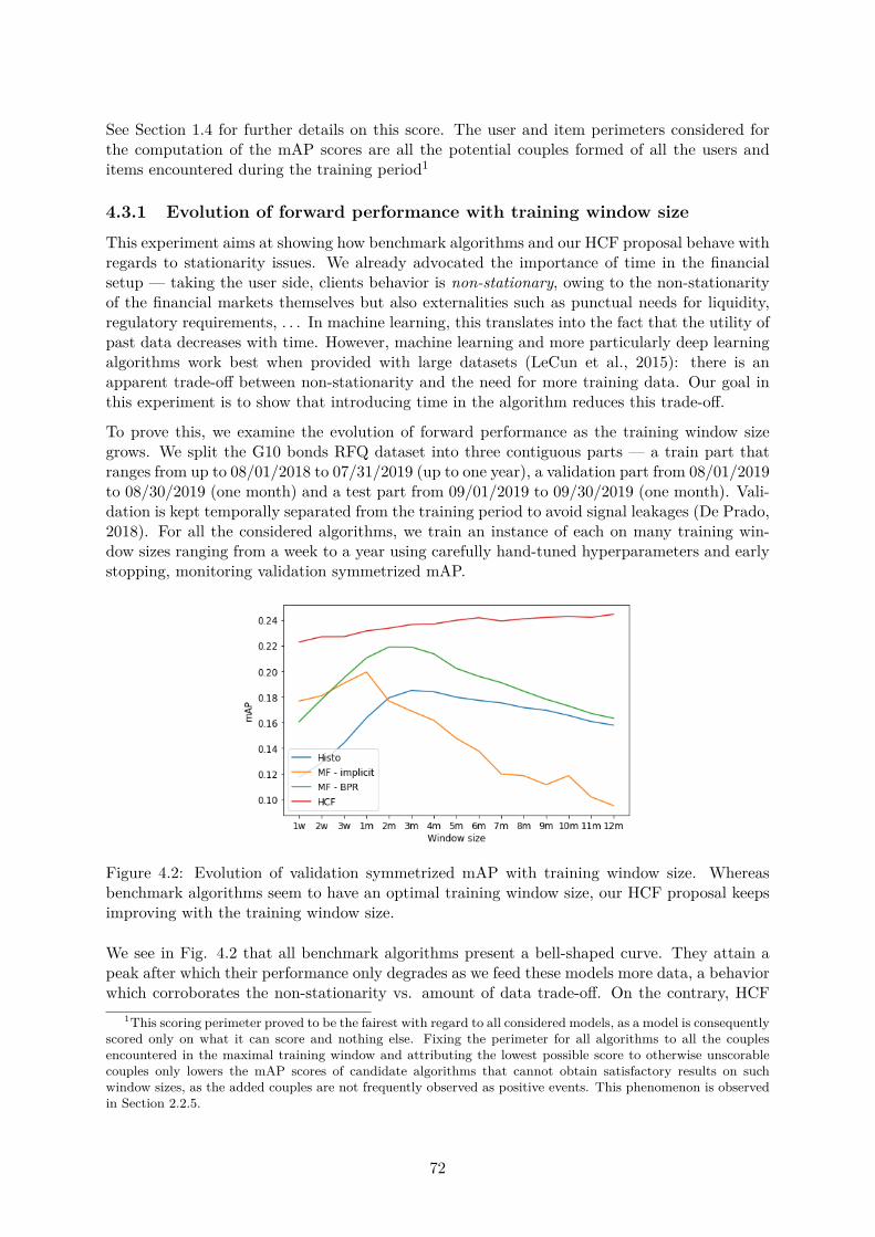
See Section 1.4 for further details on this score. The user and item perimeters considered forthe computation of the mAP scores are all the potential couples formed of all the users anditems encountered during the training period1

4.3.1 Evolution of forward performance with training window sizeThis experiment aims at showing how benchmark algorithms and our HCF proposal behave withregards to stationarity issues. We already advocated the importance of time in the financialsetup — taking the user side, clients behavior is non-stationary, owing to the non-stationarityof the financial markets themselves but also externalities such as punctual needs for liquidity,regulatory requirements, . . . In machine learning, this translates into the fact that the utility ofpast data decreases with time. However, machine learning and more particularly deep learningalgorithms work best when provided with large datasets (LeCun et al., 2015): there is anapparent trade-o� between non-stationarity and the need for more training data. Our goal inthis experiment is to show that introducing time in the algorithm reduces this trade-o�.

To prove this, we examine the evolution of forward performance as the training window sizegrows. We split the G10 bonds RFQ dataset into three contiguous parts — a train part thatranges from up to 08/01/2018 to 07/31/2019 (up to one year), a validation part from 08/01/2019to 08/30/2019 (one month) and a test part from 09/01/2019 to 09/30/2019 (one month). Vali-dation is kept temporally separated from the training period to avoid signal leakages (De Prado,2018). For all the considered algorithms, we train an instance of each on many training win-dow sizes ranging from a week to a year using carefully hand-tuned hyperparameters and earlystopping, monitoring validation symmetrized mAP.

Figure 4.2: Evolution of validation symmetrized mAP with training window size. Whereasbenchmark algorithms seem to have an optimal training window size, our HCF proposal keepsimproving with the training window size.

We see in Fig. 4.2 that all benchmark algorithms present a bell-shaped curve. They attain apeak after which their performance only degrades as we feed these models more data, a behaviorwhich corroborates the non-stationarity vs. amount of data trade-o�. On the contrary, HCF

1This scoring perimeter proved to be the fairest with regard to all considered models, as a model is consequentlyscored only on what it can score and nothing else. Fixing the perimeter for all algorithms to all the couplesencountered in the maximal training window and attributing the lowest possible score to otherwise unscorablecouples only lowers the mAP scores of candidate algorithms that cannot obtain satisfactory results on suchwindow sizes, as the added couples are not frequently observed as positive events. This phenomenon is observedin Section 2.2.5.

72

only gets better with training data size. Notably, HCF 12m, which obtained best validationperformance, used n = 20 and blocks with two hidden layers and ReLU activations.

To show that these bell-shaped curves are not an artifact of the hyperparameters chosen inthe previous experiment, we conduct a systematic hyperparameter search for multiple trainingwindow sizes using a combination of a hundred trials of random search (Bergstra and Bengio,2012) and hand-tuning. The optimal sets of hyperparameters for each considered window sizeare then used as in the previous experiment to obtain graphs of their validation mAP scoresagainst the training window size. Results are shown in Figure 4.3. MF - BPR 6m and 12moptimal hyperparameters happened to coincide, and their results are consequently shown onthe same graph.

Figure 4.3: Evolution of validation symmetrized mAP with training window size. Left: OptimalMF - implicit for the 1m, 3m, 6m and 12m windows. A consensus arises around the 1m window.Right: Optimal MF - BPR for the 1m, 2m, 3m, 6m and 12m windows. A consensus arises aroundthe 2m-3m windows, slightly favoring the 2m window.

We see here that for both MF - implicit and MF - BPR, hyperparameters optimized for manydi�erent window sizes seem to agree on optimal window size, respectively around one month andtwo months, with slight variations around these peaks. Consequently, bell shapes are inherentto these algorithms, which proves their non-stationarity vs. data size trade-o�.

To obtain test performances that are not penalized by the discontinuity of the training and testwindows, we retrain all these algorithms with the best hyperparameters and window size foundfor the validation period on dates directly preceding the test period, using the same number oftraining epochs as before. The performances of all the considered algorithms are reported inTable 4.1.

Table 4.1: Window size study — symmetrized mAP scores, in percentage.

Algorithm Window Valid mAP Test mAPHistorical 3m 18.51 16.86

MF - implicit 1m 19.94 19.24MF - BPR 2m 21.89 20.05

HCF 12m 24.43 25.02

We see here that our HCF algorithm, augmented with the temporal context, obtained bet-ter performances on both validation and test periods than the static BPR and implicit MFalgorithms. Consequently, introducing time is essential to obtain better performances in thefinancial setup that we consider.

73

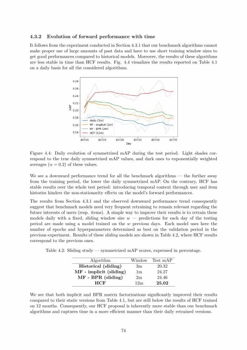
4.3.2 Evolution of forward performance with timeIt follows from the experiment conducted in Section 4.3.1 that our benchmark algorithms cannotmake proper use of large amounts of past data and have to use short training window sizes toget good performances compared to historical models. Moreover, the results of these algorithmsare less stable in time than HCF results. Fig. 4.4 visualizes the results reported on Table 4.1on a daily basis for all the considered algorithms.

Figure 4.4: Daily evolution of symmetrized mAP during the test period. Light shades cor-respond to the true daily symmetrized mAP values, and dark ones to exponentially weightedaverages (– = 0.2) of these values.

We see a downward performance trend for all the benchmark algorithms — the further awayfrom the training period, the lower the daily symmetrized mAP. On the contrary, HCF hasstable results over the whole test period: introducing temporal context through user and itemhistories hinders the non-stationarity e�ects on the model’s forward performances.

The results from Section 4.3.1 and the observed downward performance trend consequentlysuggest that benchmark models need very frequent retraining to remain relevant regarding thefuture interests of users (resp. items). A simple way to improve their results is to retrain thesemodels daily with a fixed, sliding window size w — predictions for each day of the testingperiod are made using a model trained on the w previous days. Each model uses here thenumber of epochs and hyperparameters determined as best on the validation period in theprevious experiment. Results of these sliding models are shown in Table 4.2, where HCF resultscorrespond to the previous ones.

Table 4.2: Sliding study — symmetrized mAP scores, expressed in percentage.

Algorithm Window Test mAPHistorical (sliding) 3m 20.32

MF - implicit (sliding) 1m 24.27MF - BPR (sliding) 2m 24.46

HCF 12m 25.02

We see that both implicit and BPR matrix factorizations significantly improved their resultscompared to their static versions from Table 4.1, but are still below the results of HCF trainedon 12 months. Consequently, our HCF proposal is inherently more stable than our benchmarkalgorithms and captures time in a more e�cient manner than their daily retrained versions.

74

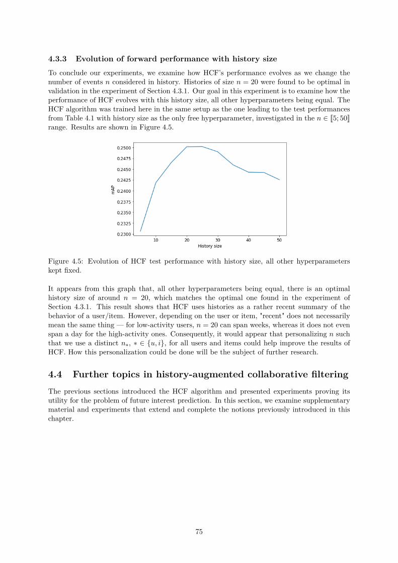
4.3.3 Evolution of forward performance with history sizeTo conclude our experiments, we examine how HCF’s performance evolves as we change thenumber of events n considered in history. Histories of size n = 20 were found to be optimal invalidation in the experiment of Section 4.3.1. Our goal in this experiment is to examine how theperformance of HCF evolves with this history size, all other hyperparameters being equal. TheHCF algorithm was trained here in the same setup as the one leading to the test performancesfrom Table 4.1 with history size as the only free hyperparameter, investigated in the n œ [[5; 50]]range. Results are shown in Figure 4.5.

Figure 4.5: Evolution of HCF test performance with history size, all other hyperparameterskept fixed.

It appears from this graph that, all other hyperparameters being equal, there is an optimalhistory size of around n = 20, which matches the optimal one found in the experiment ofSection 4.3.1. This result shows that HCF uses histories as a rather recent summary of thebehavior of a user/item. However, depending on the user or item, "recent" does not necessarilymean the same thing — for low-activity users, n = 20 can span weeks, whereas it does not evenspan a day for the high-activity ones. Consequently, it would appear that personalizing n suchthat we use a distinct nú, ú œ {u, i}, for all users and items could help improve the results ofHCF. How this personalization could be done will be the subject of further research.

4.4 Further topics in history-augmented collaborative filteringThe previous sections introduced the HCF algorithm and presented experiments proving itsutility for the problem of future interest prediction. In this section, we examine supplementarymaterial and experiments that extend and complete the notions previously introduced in thischapter.

75

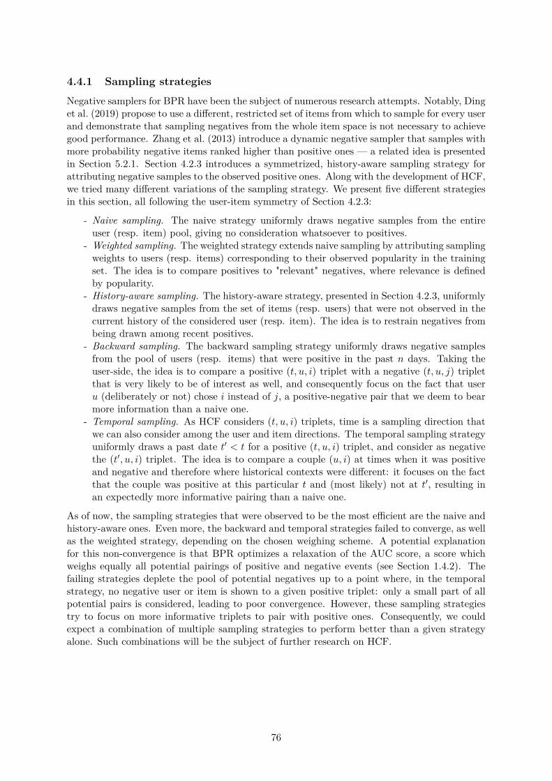
4.4.1 Sampling strategiesNegative samplers for BPR have been the subject of numerous research attempts. Notably, Dinget al. (2019) propose to use a di�erent, restricted set of items from which to sample for every userand demonstrate that sampling negatives from the whole item space is not necessary to achievegood performance. Zhang et al. (2013) introduce a dynamic negative sampler that samples withmore probability negative items ranked higher than positive ones — a related idea is presentedin Section 5.2.1. Section 4.2.3 introduces a symmetrized, history-aware sampling strategy forattributing negative samples to the observed positive ones. Along with the development of HCF,we tried many di�erent variations of the sampling strategy. We present five di�erent strategiesin this section, all following the user-item symmetry of Section 4.2.3:

- Naive sampling. The naive strategy uniformly draws negative samples from the entireuser (resp. item) pool, giving no consideration whatsoever to positives.

- Weighted sampling. The weighted strategy extends naive sampling by attributing samplingweights to users (resp. items) corresponding to their observed popularity in the trainingset. The idea is to compare positives to "relevant" negatives, where relevance is definedby popularity.

- History-aware sampling. The history-aware strategy, presented in Section 4.2.3, uniformlydraws negative samples from the set of items (resp. users) that were not observed in thecurrent history of the considered user (resp. item). The idea is to restrain negatives frombeing drawn among recent positives.

- Backward sampling. The backward sampling strategy uniformly draws negative samplesfrom the pool of users (resp. items) that were positive in the past n days. Taking theuser-side, the idea is to compare a positive (t, u, i) triplet with a negative (t, u, j) tripletthat is very likely to be of interest as well, and consequently focus on the fact that useru (deliberately or not) chose i instead of j, a positive-negative pair that we deem to bearmore information than a naive one.

- Temporal sampling. As HCF considers (t, u, i) triplets, time is a sampling direction thatwe can also consider among the user and item directions. The temporal sampling strategyuniformly draws a past date t

Õ< t for a positive (t, u, i) triplet, and consider as negative

the (tÕ, u, i) triplet. The idea is to compare a couple (u, i) at times when it was positive

and negative and therefore where historical contexts were di�erent: it focuses on the factthat the couple was positive at this particular t and (most likely) not at t

Õ, resulting inan expectedly more informative pairing than a naive one.

As of now, the sampling strategies that were observed to be the most e�cient are the naive andhistory-aware ones. Even more, the backward and temporal strategies failed to converge, as wellas the weighted strategy, depending on the chosen weighing scheme. A potential explanationfor this non-convergence is that BPR optimizes a relaxation of the AUC score, a score whichweighs equally all potential pairings of positive and negative events (see Section 1.4.2). Thefailing strategies deplete the pool of potential negatives up to a point where, in the temporalstrategy, no negative user or item is shown to a given positive triplet: only a small part of allpotential pairs is considered, leading to poor convergence. However, these sampling strategiestry to focus on more informative triplets to pair with positive ones. Consequently, we couldexpect a combination of multiple sampling strategies to perform better than a given strategyalone. Such combinations will be the subject of further research on HCF.

76

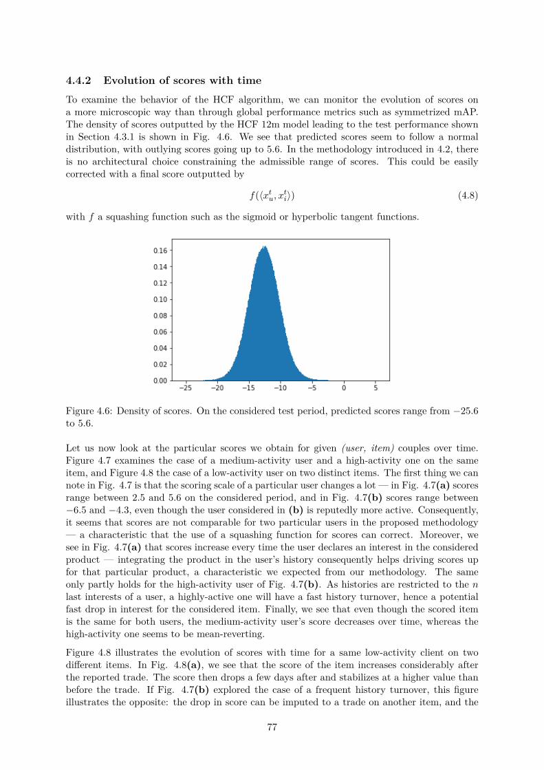
4.4.2 Evolution of scores with timeTo examine the behavior of the HCF algorithm, we can monitor the evolution of scores ona more microscopic way than through global performance metrics such as symmetrized mAP.The density of scores outputted by the HCF 12m model leading to the test performance shownin Section 4.3.1 is shown in Fig. 4.6. We see that predicted scores seem to follow a normaldistribution, with outlying scores going up to 5.6. In the methodology introduced in 4.2, thereis no architectural choice constraining the admissible range of scores. This could be easilycorrected with a final score outputted by

f(Èxt

u, xt

iÍ) (4.8)

with f a squashing function such as the sigmoid or hyperbolic tangent functions.

Figure 4.6: Density of scores. On the considered test period, predicted scores range from ≠25.6to 5.6.

Let us now look at the particular scores we obtain for given (user, item) couples over time.Figure 4.7 examines the case of a medium-activity user and a high-activity one on the sameitem, and Figure 4.8 the case of a low-activity user on two distinct items. The first thing we cannote in Fig. 4.7 is that the scoring scale of a particular user changes a lot — in Fig. 4.7(a) scoresrange between 2.5 and 5.6 on the considered period, and in Fig. 4.7(b) scores range between≠6.5 and ≠4.3, even though the user considered in (b) is reputedly more active. Consequently,it seems that scores are not comparable for two particular users in the proposed methodology— a characteristic that the use of a squashing function for scores can correct. Moreover, wesee in Fig. 4.7(a) that scores increase every time the user declares an interest in the consideredproduct — integrating the product in the user’s history consequently helps driving scores upfor that particular product, a characteristic we expected from our methodology. The sameonly partly holds for the high-activity user of Fig. 4.7(b). As histories are restricted to the n

last interests of a user, a highly-active one will have a fast history turnover, hence a potentialfast drop in interest for the considered item. Finally, we see that even though the scored itemis the same for both users, the medium-activity user’s score decreases over time, whereas thehigh-activity one seems to be mean-reverting.

Figure 4.8 illustrates the evolution of scores with time for a same low-activity client on twodi�erent items. In Fig. 4.8(a), we see that the score of the item increases considerably afterthe reported trade. The score then drops a few days after and stabilizes at a higher value thanbefore the trade. If Fig. 4.7(b) explored the case of a frequent history turnover, this figureillustrates the opposite: the drop in score can be imputed to a trade on another item, and the

77

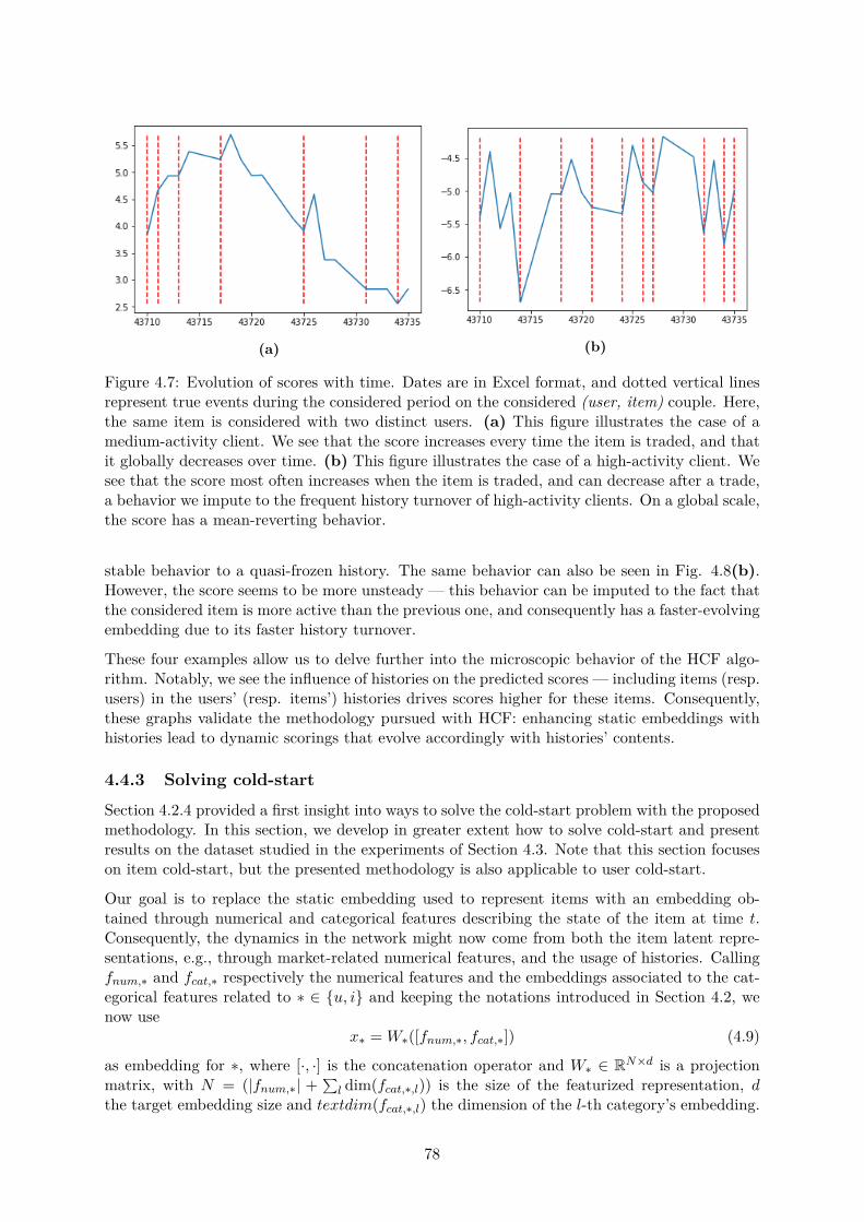
(a) (b)

Figure 4.7: Evolution of scores with time. Dates are in Excel format, and dotted vertical linesrepresent true events during the considered period on the considered (user, item) couple. Here,the same item is considered with two distinct users. (a) This figure illustrates the case of amedium-activity client. We see that the score increases every time the item is traded, and thatit globally decreases over time. (b) This figure illustrates the case of a high-activity client. Wesee that the score most often increases when the item is traded, and can decrease after a trade,a behavior we impute to the frequent history turnover of high-activity clients. On a global scale,the score has a mean-reverting behavior.

stable behavior to a quasi-frozen history. The same behavior can also be seen in Fig. 4.8(b).However, the score seems to be more unsteady — this behavior can be imputed to the fact thatthe considered item is more active than the previous one, and consequently has a faster-evolvingembedding due to its faster history turnover.

These four examples allow us to delve further into the microscopic behavior of the HCF algo-rithm. Notably, we see the influence of histories on the predicted scores — including items (resp.users) in the users’ (resp. items’) histories drives scores higher for these items. Consequently,these graphs validate the methodology pursued with HCF: enhancing static embeddings withhistories lead to dynamic scorings that evolve accordingly with histories’ contents.

4.4.3 Solving cold-startSection 4.2.4 provided a first insight into ways to solve the cold-start problem with the proposedmethodology. In this section, we develop in greater extent how to solve cold-start and presentresults on the dataset studied in the experiments of Section 4.3. Note that this section focuseson item cold-start, but the presented methodology is also applicable to user cold-start.

Our goal is to replace the static embedding used to represent items with an embedding ob-tained through numerical and categorical features describing the state of the item at time t.Consequently, the dynamics in the network might now come from both the item latent repre-sentations, e.g., through market-related numerical features, and the usage of histories. Callingfnum,ú and fcat,ú respectively the numerical features and the embeddings associated to the cat-egorical features related to ú œ {u, i} and keeping the notations introduced in Section 4.2, wenow use

xú = Wú([fnum,ú, fcat,ú]) (4.9)

as embedding for ú, where [·, ·] is the concatenation operator and Wú œ RN◊d is a projectionmatrix, with N = (|fnum,ú| +

qldim(fcat,ú,l)) is the size of the featurized representation, d

the target embedding size and textdim(fcat,ú,l) the dimension of the l-th category’s embedding.

78

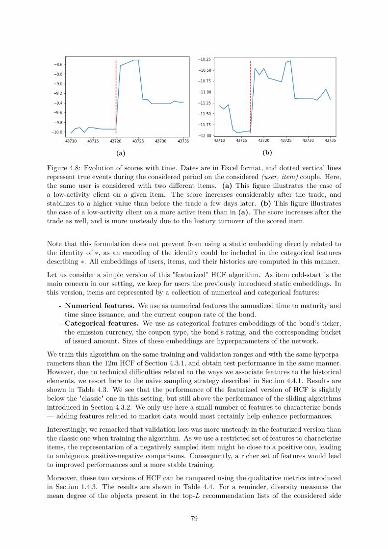
(a) (b)

Figure 4.8: Evolution of scores with time. Dates are in Excel format, and dotted vertical linesrepresent true events during the considered period on the considered (user, item) couple. Here,the same user is considered with two di�erent items. (a) This figure illustrates the case ofa low-activity client on a given item. The score increases considerably after the trade, andstabilizes to a higher value than before the trade a few days later. (b) This figure illustratesthe case of a low-activity client on a more active item than in (a). The score increases after thetrade as well, and is more unsteady due to the history turnover of the scored item.

Note that this formulation does not prevent from using a static embedding directly related tothe identity of ú, as an encoding of the identity could be included in the categorical featuresdescribing ú. All embeddings of users, items, and their histories are computed in this manner.

Let us consider a simple version of this "featurized" HCF algorithm. As item cold-start is themain concern in our setting, we keep for users the previously introduced static embeddings. Inthis version, items are represented by a collection of numerical and categorical features:

- Numerical features. We use as numerical features the annualized time to maturity andtime since issuance, and the current coupon rate of the bond.

- Categorical features. We use as categorical features embeddings of the bond’s ticker,the emission currency, the coupon type, the bond’s rating, and the corresponding bucketof issued amount. Sizes of these embeddings are hyperparameters of the network.

We train this algorithm on the same training and validation ranges and with the same hyperpa-rameters than the 12m HCF of Section 4.3.1, and obtain test performance in the same manner.However, due to technical di�culties related to the ways we associate features to the historicalelements, we resort here to the naive sampling strategy described in Section 4.4.1. Results areshown in Table 4.3. We see that the performance of the featurized version of HCF is slightlybelow the "classic" one in this setting, but still above the performance of the sliding algorithmsintroduced in Section 4.3.2. We only use here a small number of features to characterize bonds— adding features related to market data would most certainly help enhance performances.

Interestingly, we remarked that validation loss was more unsteady in the featurized version thanthe classic one when training the algorithm. As we use a restricted set of features to characterizeitems, the representation of a negatively sampled item might be close to a positive one, leadingto ambiguous positive-negative comparisons. Consequently, a richer set of features would leadto improved performances and a more stable training.

Moreover, these two versions of HCF can be compared using the qualitative metrics introducedin Section 1.4.3. The results are shown in Table 4.4. For a reminder, diversity measures themean degree of the objects present in the top-L recommendation lists of the considered side

79

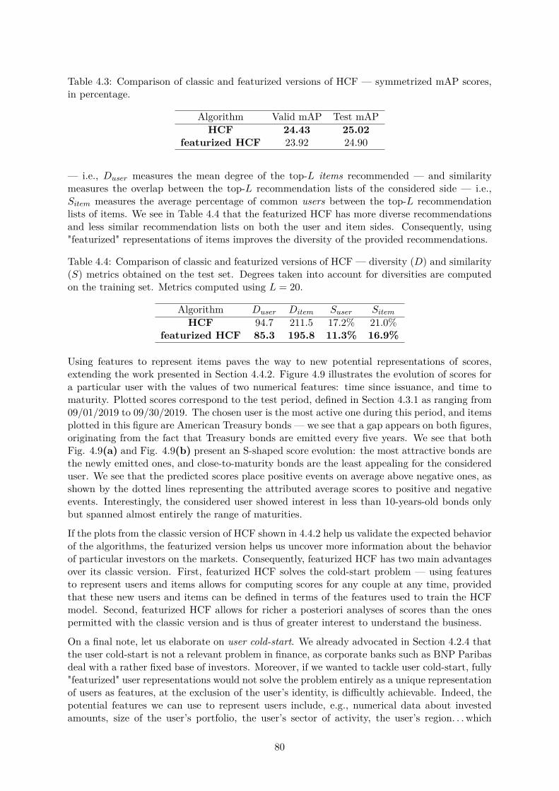
Table 4.3: Comparison of classic and featurized versions of HCF — symmetrized mAP scores,in percentage.

Algorithm Valid mAP Test mAPHCF 24.43 25.02

featurized HCF 23.92 24.90

— i.e., Duser measures the mean degree of the top-L items recommended — and similaritymeasures the overlap between the top-L recommendation lists of the considered side — i.e.,Sitem measures the average percentage of common users between the top-L recommendationlists of items. We see in Table 4.4 that the featurized HCF has more diverse recommendationsand less similar recommendation lists on both the user and item sides. Consequently, using"featurized" representations of items improves the diversity of the provided recommendations.

Table 4.4: Comparison of classic and featurized versions of HCF — diversity (D) and similarity(S) metrics obtained on the test set. Degrees taken into account for diversities are computedon the training set. Metrics computed using L = 20.

Algorithm Duser Ditem Suser Sitem

HCF 94.7 211.5 17.2% 21.0%featurized HCF 85.3 195.8 11.3% 16.9%

Using features to represent items paves the way to new potential representations of scores,extending the work presented in Section 4.4.2. Figure 4.9 illustrates the evolution of scores fora particular user with the values of two numerical features: time since issuance, and time tomaturity. Plotted scores correspond to the test period, defined in Section 4.3.1 as ranging from09/01/2019 to 09/30/2019. The chosen user is the most active one during this period, and itemsplotted in this figure are American Treasury bonds — we see that a gap appears on both figures,originating from the fact that Treasury bonds are emitted every five years. We see that bothFig. 4.9(a) and Fig. 4.9(b) present an S-shaped score evolution: the most attractive bonds arethe newly emitted ones, and close-to-maturity bonds are the least appealing for the considereduser. We see that the predicted scores place positive events on average above negative ones, asshown by the dotted lines representing the attributed average scores to positive and negativeevents. Interestingly, the considered user showed interest in less than 10-years-old bonds onlybut spanned almost entirely the range of maturities.

If the plots from the classic version of HCF shown in 4.4.2 help us validate the expected behaviorof the algorithms, the featurized version helps us uncover more information about the behaviorof particular investors on the markets. Consequently, featurized HCF has two main advantagesover its classic version. First, featurized HCF solves the cold-start problem — using featuresto represent users and items allows for computing scores for any couple at any time, providedthat these new users and items can be defined in terms of the features used to train the HCFmodel. Second, featurized HCF allows for richer a posteriori analyses of scores than the onespermitted with the classic version and is thus of greater interest to understand the business.

On a final note, let us elaborate on user cold-start. We already advocated in Section 4.2.4 thatthe user cold-start is not a relevant problem in finance, as corporate banks such as BNP Paribasdeal with a rather fixed base of investors. Moreover, if we wanted to tackle user cold-start, fully"featurized" user representations would not solve the problem entirely as a unique representationof users as features, at the exclusion of the user’s identity, is di�cultly achievable. Indeed, thepotential features we can use to represent users include, e.g., numerical data about investedamounts, size of the user’s portfolio, the user’s sector of activity, the user’s region. . . which

80

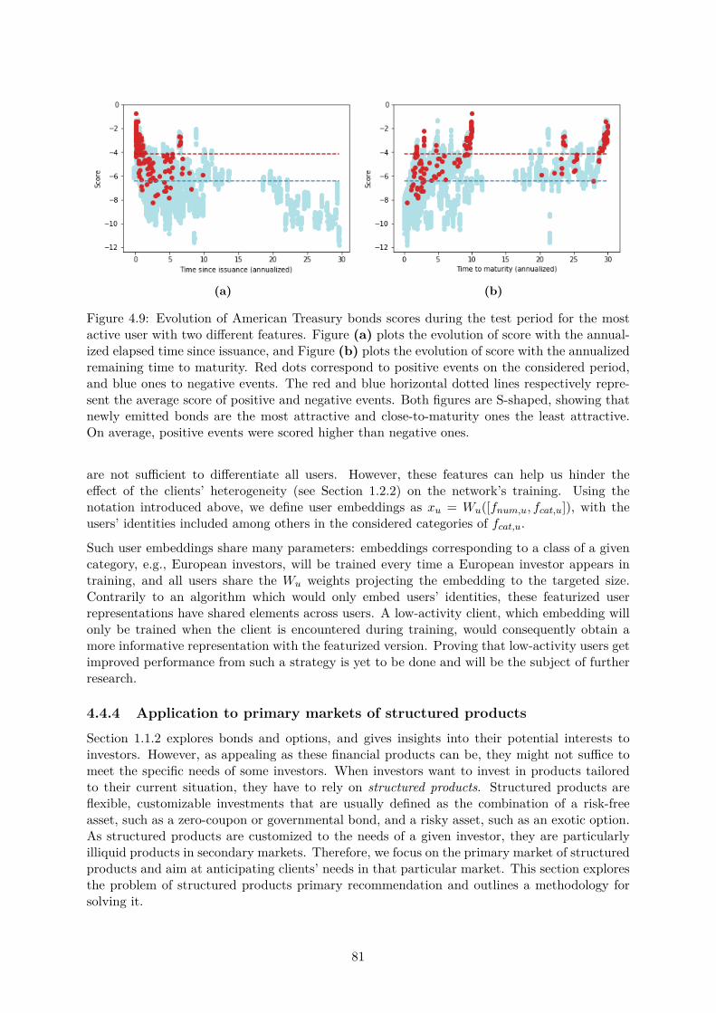
(a) (b)

Figure 4.9: Evolution of American Treasury bonds scores during the test period for the mostactive user with two di�erent features. Figure (a) plots the evolution of score with the annual-ized elapsed time since issuance, and Figure (b) plots the evolution of score with the annualizedremaining time to maturity. Red dots correspond to positive events on the considered period,and blue ones to negative events. The red and blue horizontal dotted lines respectively repre-sent the average score of positive and negative events. Both figures are S-shaped, showing thatnewly emitted bonds are the most attractive and close-to-maturity ones the least attractive.On average, positive events were scored higher than negative ones.

are not su�cient to di�erentiate all users. However, these features can help us hinder thee�ect of the clients’ heterogeneity (see Section 1.2.2) on the network’s training. Using thenotation introduced above, we define user embeddings as xu = Wu([fnum,u, fcat,u]), with theusers’ identities included among others in the considered categories of fcat,u.

Such user embeddings share many parameters: embeddings corresponding to a class of a givencategory, e.g., European investors, will be trained every time a European investor appears intraining, and all users share the Wu weights projecting the embedding to the targeted size.Contrarily to an algorithm which would only embed users’ identities, these featurized userrepresentations have shared elements across users. A low-activity client, which embedding willonly be trained when the client is encountered during training, would consequently obtain amore informative representation with the featurized version. Proving that low-activity users getimproved performance from such a strategy is yet to be done and will be the subject of furtherresearch.

4.4.4 Application to primary markets of structured productsSection 1.1.2 explores bonds and options, and gives insights into their potential interests toinvestors. However, as appealing as these financial products can be, they might not su�ce tomeet the specific needs of some investors. When investors want to invest in products tailoredto their current situation, they have to rely on structured products. Structured products areflexible, customizable investments that are usually defined as the combination of a risk-freeasset, such as a zero-coupon or governmental bond, and a risky asset, such as an exotic option.As structured products are customized to the needs of a given investor, they are particularlyilliquid products in secondary markets. Therefore, we focus on the primary market of structuredproducts and aim at anticipating clients’ needs in that particular market. This section exploresthe problem of structured products primary recommendation and outlines a methodology forsolving it.

81

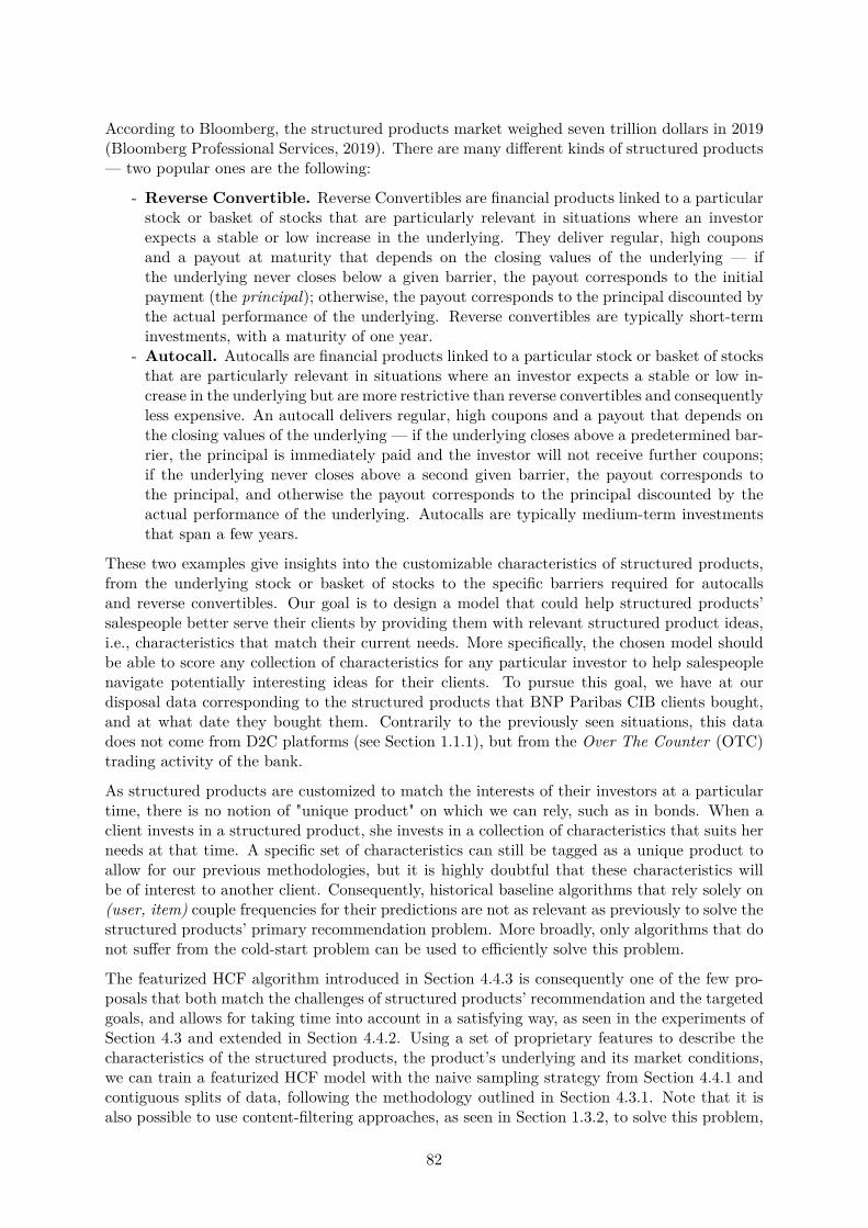
According to Bloomberg, the structured products market weighed seven trillion dollars in 2019(Bloomberg Professional Services, 2019). There are many di�erent kinds of structured products— two popular ones are the following:

- Reverse Convertible. Reverse Convertibles are financial products linked to a particularstock or basket of stocks that are particularly relevant in situations where an investorexpects a stable or low increase in the underlying. They deliver regular, high couponsand a payout at maturity that depends on the closing values of the underlying — ifthe underlying never closes below a given barrier, the payout corresponds to the initialpayment (the principal); otherwise, the payout corresponds to the principal discounted bythe actual performance of the underlying. Reverse convertibles are typically short-terminvestments, with a maturity of one year.

- Autocall. Autocalls are financial products linked to a particular stock or basket of stocksthat are particularly relevant in situations where an investor expects a stable or low in-crease in the underlying but are more restrictive than reverse convertibles and consequentlyless expensive. An autocall delivers regular, high coupons and a payout that depends onthe closing values of the underlying — if the underlying closes above a predetermined bar-rier, the principal is immediately paid and the investor will not receive further coupons;if the underlying never closes above a second given barrier, the payout corresponds tothe principal, and otherwise the payout corresponds to the principal discounted by theactual performance of the underlying. Autocalls are typically medium-term investmentsthat span a few years.

These two examples give insights into the customizable characteristics of structured products,from the underlying stock or basket of stocks to the specific barriers required for autocallsand reverse convertibles. Our goal is to design a model that could help structured products’salespeople better serve their clients by providing them with relevant structured product ideas,i.e., characteristics that match their current needs. More specifically, the chosen model shouldbe able to score any collection of characteristics for any particular investor to help salespeoplenavigate potentially interesting ideas for their clients. To pursue this goal, we have at ourdisposal data corresponding to the structured products that BNP Paribas CIB clients bought,and at what date they bought them. Contrarily to the previously seen situations, this datadoes not come from D2C platforms (see Section 1.1.1), but from the Over The Counter (OTC)trading activity of the bank.

As structured products are customized to match the interests of their investors at a particulartime, there is no notion of "unique product" on which we can rely, such as in bonds. When aclient invests in a structured product, she invests in a collection of characteristics that suits herneeds at that time. A specific set of characteristics can still be tagged as a unique product toallow for our previous methodologies, but it is highly doubtful that these characteristics willbe of interest to another client. Consequently, historical baseline algorithms that rely solely on(user, item) couple frequencies for their predictions are not as relevant as previously to solve thestructured products’ primary recommendation problem. More broadly, only algorithms that donot su�er from the cold-start problem can be used to e�ciently solve this problem.

The featurized HCF algorithm introduced in Section 4.4.3 is consequently one of the few pro-posals that both match the challenges of structured products’ recommendation and the targetedgoals, and allows for taking time into account in a satisfying way, as seen in the experiments ofSection 4.3 and extended in Section 4.4.2. Using a set of proprietary features to describe thecharacteristics of the structured products, the product’s underlying and its market conditions,we can train a featurized HCF model with the naive sampling strategy from Section 4.4.1 andcontiguous splits of data, following the methodology outlined in Section 4.3.1. Note that it isalso possible to use content-filtering approaches, as seen in Section 1.3.2, to solve this problem,

82

using the same kind of features as the ones outlined above for HCF. Such algorithms could betrained on a cross-entropy objective, with negative events sampled as in the HCF methodology— the imbalance ratio should be controlled to obtain relevant probabilities.

As a given structured product will only appear a couple of times in our data, scoring thealgorithms becomes particularly tricky: the methodologies explained in Section 1.4 and 4.3 arenot applicable anymore, as restraining the scoring perimeter to the users and items observedduring training would not capture the actual trades that happened during the testing period.Consequently, we change the scoring perimeter previously defined as all potential (user, item)couples formed of users and items appearing in the training period to a perimeter defined bythe couples formed of all users seen during the training period and all the products that weretraded during the past month. This provides a perimeter of relevant items to which comparethe scores predicted for the positive ones. As previously, we can use the symmetrized mAPscore for evaluation. Table 4.5 shows first results of three algorithms on the primary structuredproducts prediction problems: a historical baseline obtained as suggested above by consideringsets of characteristics as our unique products, a "featurized" MF trained with the BPR loss,and a "featurized" HCF model — see Section 4.4.3 for more details. These algorithms use atraining set that can range from 02/01/2019 to 12/31/2019, a validation set that ranges from01/01/2020 to 01/31/2020 and a test set that ranges from 02/01/2020 to 29/02/2020. We usefor these algorithms the window sizes the closest possible to the optimal ones found in Section4.3.1, and the MF and HCF algorithms use the same values for their common hyperparameters.

Table 4.5: Comparison of historical, featurized MF and HCF algorithms on the primary struc-tured products prediction problem. Symmetrized mAP scores, expressed in percentages.

Algorithm Valid mAP Test mAPHisto - 3m 10.96 8.75

featurized MF (BPR) - 2m 13.67 11.93featurized HCF - 11m 34.33 32.75

We see that the featurized HCF obtained, by far, the best validation and test performances.Note that the featurized HCF algorithm only di�ers from featurized MF by its usage of histories.Consequently, it appears that the introduction of time in the primary prediction problem iscrucial, validating again the approach taken for HCF. Further research e�ort will be devoted toimproving our models for the primary structured product prediction problem.

4.5 Concluding remarksThis chapter introduces a novel HCF algorithm, a time-aware recommender system that usesuser and item histories to capture the dynamics of the user-item interactions, and that providesdynamic recommendations that can be used for future predictions. In the context of financialG10 bonds RFQ recommendations, we show that for classic matrix factorization algorithms, atrade-o� exists between the non-stationarity of users’ and items’ behaviors and the size of thedatasets that we use for training. This trade-o� is overcome with history-augmented embed-dings. Moreover, such embeddings outperform sliding versions of classic matrix factorizationalgorithms and prove to be more stable predictors of the future interests of the users and items.

This chapter also supplements the HCF algorithm with its featurized extension, provides insightsinto potential sampling strategies, studies predicted scores, and presents a use-case for whichthe featurized version of HCF is particularly relevant. Further research on the HCF subject willinclude how history sizes could be personalized, how sampling strategies could be combined andhow we could tackle clients’ heterogeneity more e�ciently with featurized user representations.

83

Chapter 5

Further topics in financialrecommender systems

Developing the two algorithms presented in chapters 3 and 4 required countless experiments, ascan be seen in both chapters from the many iterations these algorithms have known. However,iterating on the models introduced in the previous chapters is not the only work that has beendone during the elaboration of this thesis. Consequently, this chapter collects, haphazardly,the other experiments we conducted and ideas we developed and that do not deserve their ownchapter.

This chapter introduces statistically validated networks and their application to BNP ParibasCIB datasets (see Section 5.1), elaborates on minor improvements that help previously intro-duced algorithms achieve better performance (see Section 5.2), presents an experiment tryingto capture lead-lag relationships using neural networks (see 5.3) and paves the way for a modelbridging the ideas introduced in chapters 3 and 4 (see Section 5.4).

5.1 Mapping investors’ behaviors with statistically validatednetworks

Clustering clients can be done in many ways. Provided with user profiles, a wide range ofclustering algorithms can be used to group lookalike clients — classic ways include K-means(Hastie et al., 2009, Chapter 13) and DBSCAN (Ester et al., 1996). In this section, we considera rather unusual graph mining method that detects regular, common patterns among clientsand that leads to a behavioral-based clustering of clients, reminiscent of the work presentedin Chapter 3, and apply it to the corporate bonds RFQ datasets of BNP Paribas CIB. Themethod, called statistically validated networks, is described in Tumminello et al. (2011) and hasbeen successfully applied to a financial dataset in Tumminello et al. (2012).

The financial dataset studied in Tumminello et al. (2012) corresponds to the trading behaviorof individual investors on the Nokia stock. As bonds are less liquid products than stocks,the data related to a given bond is far sparser than it is the case for a given stock such asNokia. Consequently, the methodology outlined in Tumminello et al. (2012) cannot be directlytransposed to our bonds RFQ dataset. To use this methodology, we consider the interactionsclients have with the bond market as a whole by considering all bonds as one.

The idea behind statistically validated networks is to connect clients according to their RFQpatterns. Let us consider a bipartite graph G = (C, T, E) with C the set of clients, T the setof considered trading days, and E the set of edges connecting them. Clients can be connected

85

to a trading day by three di�erent kinds of links, corresponding to their observed behavior onthat day — a "buy" link if the client mostly requests bonds’ prices for the buy direction on thatday, a "sell" link if the client mostly requests bonds’ prices for the sell direction on that day, ora "buy-sell" link if the client requests prices for both directions on that day in a balanced way.Links are determined using

r(i, t) = Vb(i, t) ≠ Vs(i, t)Vb(i, t) + Vs(i, t) , (5.1)

where i œ C represents a client, t œ T a trading day, and Vb and Vs are the aggregated requestedamount of buy and sell movements for client i on day t. We consider that the link between i

and t is a buy link if r(i, t) > fl, a sell link if r(i, t) < ≠fl and a buy-sell link if ≠fl < r(i, t) < fl

with Vb(i, t) > 0 and Vs(i, t) > 0. If client i is linked to day t with a buy link, we say that i inin a buy state during that day, and respectively for all other link types. Following Tumminelloet al. (2012), the threshold value is taken to be fl = 0.01. Note that taking fl = 0 is equivalentto considering buy and sell links only.

We now want to project this bipartite graph into a one-mode graph that connects clients ac-cording to their RFQ patterns. A first idea is to consider a graph G

Õ = (C, EÕ) where (i, j) œ E

Õ

if i and j both made a move on the same day, e.g., if for a given day t, client i is in a buystate and client j in a sell state, i and j are connected in G

Õ with a buy-sell link. However, thisapproach rapidly fails: as co-occurrence of states might happen for totally unrelated reasons,the corresponding graph would be fully connected with a high probability. Consequently, wehave to correct for potentially random co-occurrences of states. To do so, the idea introducedin Tumminello et al. (2011) is to use a statistical test to check whether co-occurrence of statesbetween two given clients is random. We note GSV N = (C, ESV N ) the corresponding graph.

The statistical test is the following. We consider as null hypothesis that co-occurrence of statesP and Q for clients i and j is random, and want to test whether this hypothesis holds. LetNP be the number of days client i spent in state P , NQ the number of days client j spent instate Q, NP,Q the number of days when we observe the co-occurrence of state P for client i andstate Q for client j and T the total number of trading days we consider — for ease of notation,we assimilate the set of trading days to its number of elements. Under the null hypothesis,the probability of observing X co-occurrences of the given states for the two clients is givenby the hypergeometric distribution, that we note H(X|T, NP , NQ). Consequently, the p-valuecorresponding to the described statistical test is given by

p(NP,Q) = 1 ≠NP,Q≠1ÿ

X=0H(X|T, NP , NQ) (5.2)

As this test is performed for all possible client pairs and all possible combinations of states, werely on multiple hypotheses testing to conclude on rejections of the null. Classic methods toaccount for multiple hypotheses are the Bonferroni correction (Bland and Altman, 1995) andthe Benjamini-Hochberg procedure (Benjamini and Hochberg, 1995). The Bonferroni correctionaims at controlling the family-wise error rate (FWER), defined as FWER = P(FP Ø 1), withFP the number of false positives. Bonferroni ensures that FWER Æ –, with – the chosensignificance level of the test, by rejecting an hypothesis Hi if its corresponding p-value pi is suchthat pi Æ –

m, with m the total number of hypotheses considered.

We focus here on the Benjamini-Hochberg procedure, which is a more conservative way toaccount for multiple hypotheses. This procedure aims at controlling the false discovery rate(FDR), defined as the expectation of the false discovery proportion (FDP), written FDP =FN/ max(R, 1), with FN the number of false negatives and R the total number of rejections.The Benjamini-Hochberg procedure attempts to control the FDR at level –. The procedureworks as the following:

86

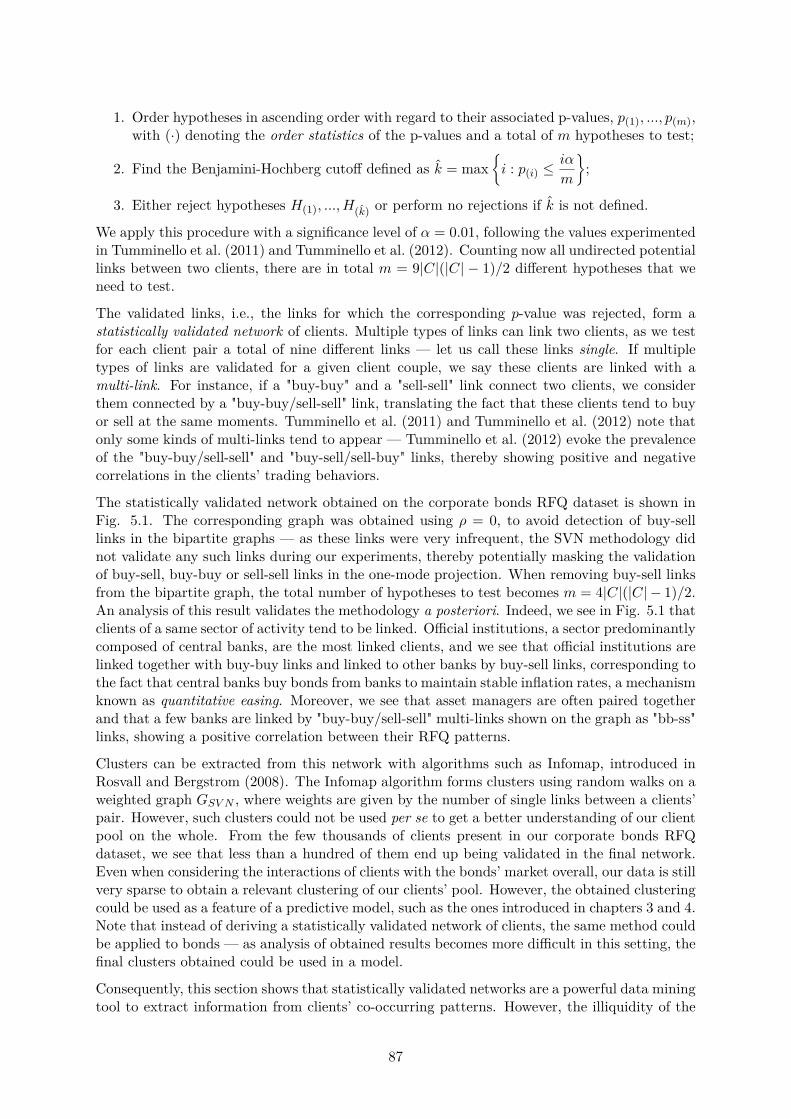
1. Order hypotheses in ascending order with regard to their associated p-values, p(1), ..., p(m),with (·) denoting the order statistics of the p-values and a total of m hypotheses to test;

2. Find the Benjamini-Hochberg cuto� defined as k = max;

i : p(i) Æ i–

m

<;

3. Either reject hypotheses H(1), ..., H(k) or perform no rejections if k is not defined.

We apply this procedure with a significance level of – = 0.01, following the values experimentedin Tumminello et al. (2011) and Tumminello et al. (2012). Counting now all undirected potentiallinks between two clients, there are in total m = 9|C|(|C| ≠ 1)/2 di�erent hypotheses that weneed to test.

The validated links, i.e., the links for which the corresponding p-value was rejected, form astatistically validated network of clients. Multiple types of links can link two clients, as we testfor each client pair a total of nine di�erent links — let us call these links single. If multipletypes of links are validated for a given client couple, we say these clients are linked with amulti-link. For instance, if a "buy-buy" and a "sell-sell" link connect two clients, we considerthem connected by a "buy-buy/sell-sell" link, translating the fact that these clients tend to buyor sell at the same moments. Tumminello et al. (2011) and Tumminello et al. (2012) note thatonly some kinds of multi-links tend to appear — Tumminello et al. (2012) evoke the prevalenceof the "buy-buy/sell-sell" and "buy-sell/sell-buy" links, thereby showing positive and negativecorrelations in the clients’ trading behaviors.

The statistically validated network obtained on the corporate bonds RFQ dataset is shown inFig. 5.1. The corresponding graph was obtained using fl = 0, to avoid detection of buy-selllinks in the bipartite graphs — as these links were very infrequent, the SVN methodology didnot validate any such links during our experiments, thereby potentially masking the validationof buy-sell, buy-buy or sell-sell links in the one-mode projection. When removing buy-sell linksfrom the bipartite graph, the total number of hypotheses to test becomes m = 4|C|(|C| ≠ 1)/2.An analysis of this result validates the methodology a posteriori. Indeed, we see in Fig. 5.1 thatclients of a same sector of activity tend to be linked. O�cial institutions, a sector predominantlycomposed of central banks, are the most linked clients, and we see that o�cial institutions arelinked together with buy-buy links and linked to other banks by buy-sell links, corresponding tothe fact that central banks buy bonds from banks to maintain stable inflation rates, a mechanismknown as quantitative easing. Moreover, we see that asset managers are often paired togetherand that a few banks are linked by "buy-buy/sell-sell" multi-links shown on the graph as "bb-ss"links, showing a positive correlation between their RFQ patterns.

Clusters can be extracted from this network with algorithms such as Infomap, introduced inRosvall and Bergstrom (2008). The Infomap algorithm forms clusters using random walks on aweighted graph GSV N , where weights are given by the number of single links between a clients’pair. However, such clusters could not be used per se to get a better understanding of our clientpool on the whole. From the few thousands of clients present in our corporate bonds RFQdataset, we see that less than a hundred of them end up being validated in the final network.Even when considering the interactions of clients with the bonds’ market overall, our data is stillvery sparse to obtain a relevant clustering of our clients’ pool. However, the obtained clusteringcould be used as a feature of a predictive model, such as the ones introduced in chapters 3 and 4.Note that instead of deriving a statistically validated network of clients, the same method couldbe applied to bonds — as analysis of obtained results becomes more di�cult in this setting, thefinal clusters obtained could be used in a model.

Consequently, this section shows that statistically validated networks are a powerful data miningtool to extract information from clients’ co-occurring patterns. However, the illiquidity of the

87

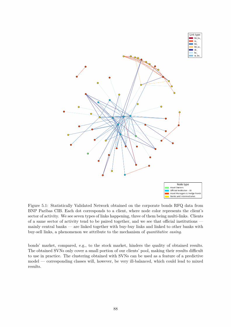
Figure 5.1: Statistically Validated Network obtained on the corporate bonds RFQ data fromBNP Paribas CIB. Each dot corresponds to a client, where node color represents the client’ssector of activity. We see seven types of links happening, three of them being multi-links. Clientsof a same sector of activity tend to be paired together, and we see that o�cial institutions —mainly central banks — are linked together with buy-buy links and linked to other banks withbuy-sell links, a phenomenon we attribute to the mechanism of quantitative easing.

bonds’ market, compared, e.g., to the stock market, hinders the quality of obtained results.The obtained SVNs only cover a small portion of our clients’ pool, making their results di�cultto use in practice. The clustering obtained with SVNs can be used as a feature of a predictivemodel — corresponding classes will, however, be very ill-balanced, which could lead to mixedresults.

88

5.2 A collection of small enhancementsDuring the development of the algorithms presented in chapters 3 and 4, a lot of small improve-ments have been tried to enhance the performance of our predictive models. In this section,we present three of these most successful variations that we deem not worth their own researchstudies.

5.2.1 A focal version of Bayesian Personalized RankingChapter 4 extensively studied and applied the BPR objective function of Rendle et al. (2009). Inthis chapter, we proposed ways to augment BPR through di�erent sampling strategies, namelywith a symmetrized, history-aware sampling (see Sections 4.2.3, 4.4.1). The BPR objectivecould also be enhanced with the ideas underpinning the focal loss (Lin et al., 2017) (see Section1.3.2).

The focal loss is a variation of cross-entropy that weighs hard-to-classify samples more, as

lfocal(x) = ≠Cÿ

i=1(1 ≠ yi(x))“

yi(x) log yi(x) , (5.3)

with C the number of classes considered in the classification problem, (x, y) a given sample wherey is a C-dimensional one-hot encoding of the class corresponding to sample x, y a predictor and“ a hyperparameter controlling the adaptive weighing. The term (1 ≠ yi(x))“ emphasizes theloss on the wrongly classified samples, or classified with low confidence. This idea can be easilyadapted to the BPR objective, as

lBP R,focal = (1 ≠ ‡(xuij))“ ln ‡(xuij), (5.4)

where ‡ denotes the sigmoid function, xuij is the score associated to the (u, i, j) triplet where(u, i) is a positive couple and j a negative item, and “ is an hyperparameter controlling theadaptive weighing. The BPR objective is constructed such that ‡(xuij) represents P(i >u j)(Rendle et al., 2009), with >u the total ranking defined by user u, i.e., the order defined by theinterests of u. Consequently, the (1 ≠ ‡(xuij))“ term focuses the loss on samples for which themodel puts negative items higher than positive ones in its ranking. Note that setting “ = 0leads to the classic BPR objective.

We experiment this new loss on the HCF model, using the hyperparameters and window sizes ofthe HCF 12m model of Section 4.3.1 and the same experimental setup for obtaining validationand test performances. Results are shown in Table 5.1.

Table 5.1: Comparison of classic and focal versions of HCF — symmetrized mAP scores, inpercentage.

Algorithm Valid mAP Test mAPHCF 24.43 25.02

focal HCF - “ = 1 24.68 25.44focal HCF - “ = 2 24.53 25.31focal HCF - “ = 3 24.39 25.16

We see that the best model with regards to validation performance is an HCF model trainedwith the focal BPR objective using “ = 1. Note here that a more thorough search for “ inthe ]0; 2] range would be necessary to find the optimal “ value. We see that the validation

89

performance falls below the classic version for “ = 3 — with too high “ values, the low weightof triplets (u, i, j) such that P(i >u j) ¥ 0.5, i.e., triplets for which the network is indecisive,hinders the network performance. The “ = 1 model achieved a test performance marginallyabove classic HCF, with a +1.7% increase in symmetrized mAP score. Consequently, our focalBPR objective proposal helps achieve overall better performances by focusing the BPR objectiveon hard-to-rank positive-negative pairs.

5.2.2 Validation strategies in non-stationary settingsK-fold cross-validation is a widespread technique for estimating the prediction error of a machinelearning model (Hastie et al., 2009, Chapter 7.10). The idea is to split available data into K

equally-sized parts, to train a model on K ≠1 of these parts and test it on the held-out last one.Noting Ÿ : {1, . . . , n} ≠æ {1, . . . , K} the partition function splitting the samples {(xi, yi)}i=1,...,n

into K folds, the cross-validation estimate of the prediction error is given by

CV(f) = 1n

nÿ

i=1L(yi, f

≠Ÿ(i)(xi)), (5.5)

with f the predictor, L the considered evaluation function, and f≠Ÿ(i) a predictor trained on all

K folds except for the one where sample i lies. K-fold cross validation allows for obtaining goodestimates of the prediction error when there is not su�cient data to use a separate, held-outvalidation set.

However, in the financial context, De Prado (2018, Chapter 7) advocates that K-fold validationis prone to signal leakages. Indeed, in non-stationary settings samples cannot be consideredi.i.d. anymore: when using temporal folds of data, on the boundaries between train and valida-tion splits, it is often the case that (xt, yt) ¥ (xtÕ , ytÕ) for t

Õ close enough to t. De Prado (2018,Chapter 7) consequently proposes a "purged" K-fold cross-validation procedure, illustrated inFig. 5.2. The procedure, similar to what is known in the literature as h‹-block cross-validation(Racine, 2000), follows the idea of classic K-fold cross-validation but avoids leakages by dis-carding samples "close" to the validation block, i.e., in a h-sized window around the validationblock. A complete overview of cross-validation strategies suitable for time series prediction canbe found in Bergmeir and Benítez (2012).

However, when plenty of data is at our disposal, there is no need to use such cross-validationstrategies: using a held-out, large validation set is su�cient to monitor the generalizationperformance of a model. In such cases, the common practice is to use contiguous splits ofdata ordered as training, validation, and test splits, as was done in the experiments of Chapter3 and 4. Such a validation strategy emulates the real-world environment of the model, which willbe used for predicting events after the training period. There are, however, two observationswe can consider when choosing a validation strategy:

- We expect the performance of a model on the validation set to be a good predictor of themodel’s generalization performance. Consequently, the most important characteristic weshould aim at when searching for an appropriate validation set is the correlation betweenthe validation and test performances.

- In non-stationary environments, the further away from the training period the predictions,the worse their performance. Consequently, an appropriate validation strategy wouldideally let samples temporally close to the testing period in the training set.

Following these observations, we try a validation strategy that uses contiguous splits of dataordered as validation, training, and test splits. Using the G10 bonds RFQ dataset (see Section4.3 for more details), we train 200 instances of a LightGBM (Ke et al., 2017) with randomly

90

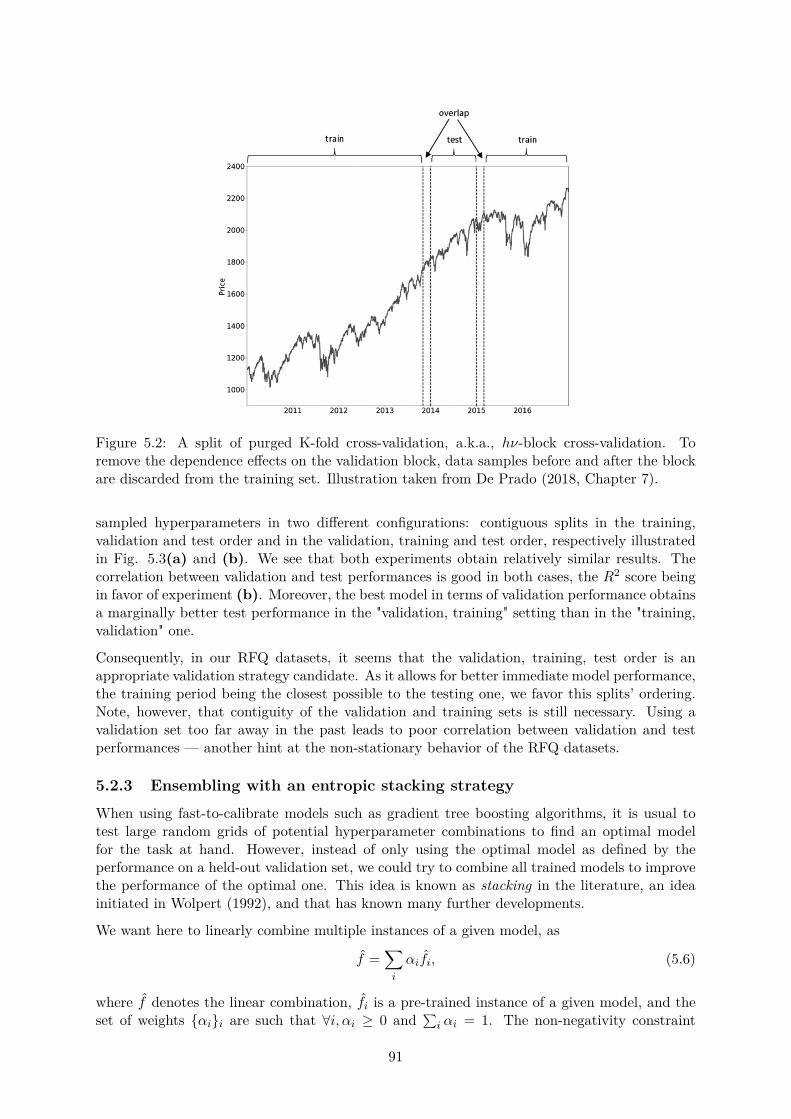
A SOLUTION: PURGED K-FOLD CV 107

FIGURE 7.2 Purging overlap in the training set

k�, performance will not improve, indicating that the backtest is not pro!ting fromleaks. Figure 7.2 plots one partition of the k-fold CV. The test set is surrounded bytwo train sets, generating two overlaps that must be purged to prevent leakage.

7.4.2 Embargo

For those cases where purging is not able to prevent all leakage, we can imposean embargo on training observations after every test set. The embargo does notneed to affect training observations prior to a test set, because training labels Yi =f [[ti,0, ti,1]], where ti,1 < tj,0 (training ends before testing begins), contain informa-tion that was available at the testing time tj,0. In other words, we are only con-cerned with training labels Yi = f [[ti,0, ti,1]] that take place immediately after thetest, tj,1 � ti,0 � tj,1 + h. We can implement this embargo period h by setting Yj =f [[tj,0, tj,1 + h]] before purging. A small value h � .01T often suf!ces to preventall leakage, as can be con!rmed by testing that performance does not improveinde!nitely by increasing k � T . Figure 7.3 illustrates the embargoing of trainobservations immediately after the testing set. Snippet 7.2 implements the embargologic.

Figure 5.2: A split of purged K-fold cross-validation, a.k.a., h‹-block cross-validation. Toremove the dependence e�ects on the validation block, data samples before and after the blockare discarded from the training set. Illustration taken from De Prado (2018, Chapter 7).

sampled hyperparameters in two di�erent configurations: contiguous splits in the training,validation and test order and in the validation, training and test order, respectively illustratedin Fig. 5.3(a) and (b). We see that both experiments obtain relatively similar results. Thecorrelation between validation and test performances is good in both cases, the R

2 score beingin favor of experiment (b). Moreover, the best model in terms of validation performance obtainsa marginally better test performance in the "validation, training" setting than in the "training,validation" one.

Consequently, in our RFQ datasets, it seems that the validation, training, test order is anappropriate validation strategy candidate. As it allows for better immediate model performance,the training period being the closest possible to the testing one, we favor this splits’ ordering.Note, however, that contiguity of the validation and training sets is still necessary. Using avalidation set too far away in the past leads to poor correlation between validation and testperformances — another hint at the non-stationary behavior of the RFQ datasets.

5.2.3 Ensembling with an entropic stacking strategyWhen using fast-to-calibrate models such as gradient tree boosting algorithms, it is usual totest large random grids of potential hyperparameter combinations to find an optimal modelfor the task at hand. However, instead of only using the optimal model as defined by theperformance on a held-out validation set, we could try to combine all trained models to improvethe performance of the optimal one. This idea is known as stacking in the literature, an ideainitiated in Wolpert (1992), and that has known many further developments.

We want here to linearly combine multiple instances of a given model, as

f =ÿ

i

–ifi, (5.6)

where f denotes the linear combination, fi is a pre-trained instance of a given model, and theset of weights {–i}i are such that ’i, –i Ø 0 and

qi–i = 1. The non-negativity constraint

91

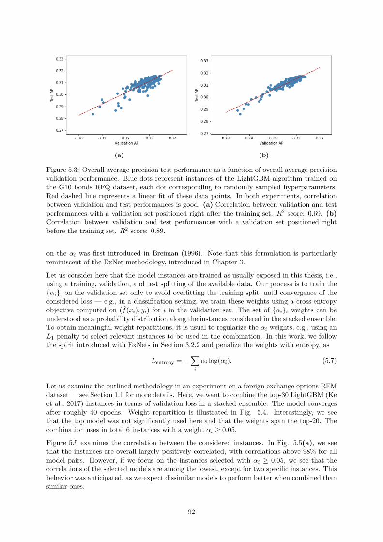
(a) (b)

Figure 5.3: Overall average precision test performance as a function of overall average precisionvalidation performance. Blue dots represent instances of the LightGBM algorithm trained onthe G10 bonds RFQ dataset, each dot corresponding to randomly sampled hyperparameters.Red dashed line represents a linear fit of these data points. In both experiments, correlationbetween validation and test performances is good. (a) Correlation between validation and testperformances with a validation set positioned right after the training set. R

2 score: 0.69. (b)Correlation between validation and test performances with a validation set positioned rightbefore the training set. R

2 score: 0.89.

on the –i was first introduced in Breiman (1996). Note that this formulation is particularlyreminiscent of the ExNet methodology, introduced in Chapter 3.

Let us consider here that the model instances are trained as usually exposed in this thesis, i.e.,using a training, validation, and test splitting of the available data. Our process is to train the{–i}i on the validation set only to avoid overfitting the training split, until convergence of theconsidered loss — e.g., in a classification setting, we train these weights using a cross-entropyobjective computed on (f(xi), yi) for i in the validation set. The set of {–i}i weights can beunderstood as a probability distribution along the instances considered in the stacked ensemble.To obtain meaningful weight repartitions, it is usual to regularize the –i weights, e.g., using anL1 penalty to select relevant instances to be used in the combination. In this work, we followthe spirit introduced with ExNets in Section 3.2.2 and penalize the weights with entropy, as

Lentropy = ≠ÿ

i

–i log(–i). (5.7)

Let us examine the outlined methodology in an experiment on a foreign exchange options RFMdataset — see Section 1.1 for more details. Here, we want to combine the top-30 LightGBM (Keet al., 2017) instances in terms of validation loss in a stacked ensemble. The model convergesafter roughly 40 epochs. Weight repartition is illustrated in Fig. 5.4. Interestingly, we seethat the top model was not significantly used here and that the weights span the top-20. Thecombination uses in total 6 instances with a weight –i Ø 0.05.

Figure 5.5 examines the correlation between the considered instances. In Fig. 5.5(a), we seethat the instances are overall largely positively correlated, with correlations above 98% for allmodel pairs. However, if we focus on the instances selected with –i Ø 0.05, we see that thecorrelations of the selected models are among the lowest, except for two specific instances. Thisbehavior was anticipated, as we expect dissimilar models to perform better when combined thansimilar ones.

92

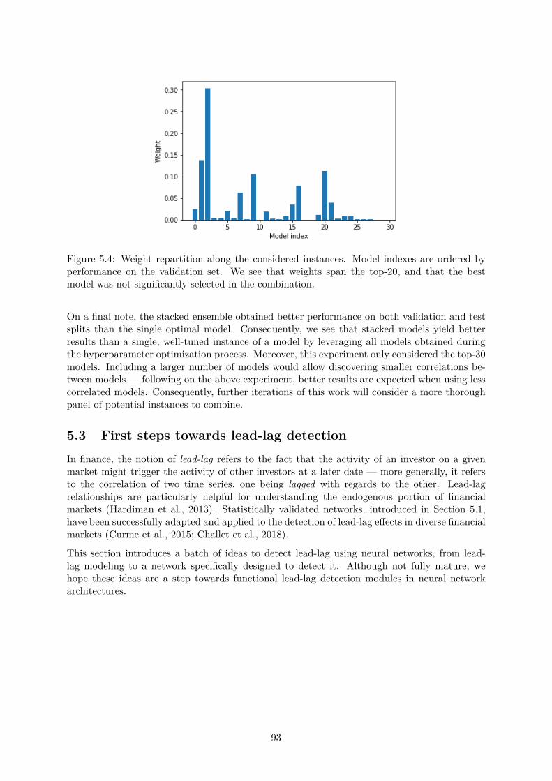
Figure 5.4: Weight repartition along the considered instances. Model indexes are ordered byperformance on the validation set. We see that weights span the top-20, and that the bestmodel was not significantly selected in the combination.

On a final note, the stacked ensemble obtained better performance on both validation and testsplits than the single optimal model. Consequently, we see that stacked models yield betterresults than a single, well-tuned instance of a model by leveraging all models obtained duringthe hyperparameter optimization process. Moreover, this experiment only considered the top-30models. Including a larger number of models would allow discovering smaller correlations be-tween models — following on the above experiment, better results are expected when using lesscorrelated models. Consequently, further iterations of this work will consider a more thoroughpanel of potential instances to combine.

5.3 First steps towards lead-lag detectionIn finance, the notion of lead-lag refers to the fact that the activity of an investor on a givenmarket might trigger the activity of other investors at a later date — more generally, it refersto the correlation of two time series, one being lagged with regards to the other. Lead-lagrelationships are particularly helpful for understanding the endogenous portion of financialmarkets (Hardiman et al., 2013). Statistically validated networks, introduced in Section 5.1,have been successfully adapted and applied to the detection of lead-lag e�ects in diverse financialmarkets (Curme et al., 2015; Challet et al., 2018).

This section introduces a batch of ideas to detect lead-lag using neural networks, from lead-lag modeling to a network specifically designed to detect it. Although not fully mature, wehope these ideas are a step towards functional lead-lag detection modules in neural networkarchitectures.

93

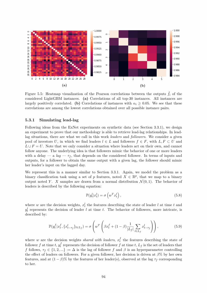
(a) (b)

Figure 5.5: Heatmap visualization of the Pearson correlations between the outputs fi of theconsidered LightGBM instances. (a) Correlations of all top-30 instances. All instances arelargely positively correlated. (b) Correlations of instances with –i Ø 0.05. We see that thesecorrelations are among the lowest correlations obtained over all possible instance pairs.

5.3.1 Simulating lead-lagFollowing ideas from the ExNet experiments on synthetic data (see Section 3.3.1), we designan experiment to prove that our methodology is able to retrieve lead-lag relationships. In lead-lag situations, there are what we call in this work leaders and followers. We consider a givenpool of investors U , in which we find leaders l œ L and followers f œ F , with L, F µ U andL fi F = U . Note that we only consider a situation where leaders act on their own, and cannotfollow anyone. The underlying idea is that followers mimic the behavior of one or more leaderswith a delay — a lag — ·f , that depends on the considered follower. In terms of inputs andoutputs, for a follower to obtain the same output with a given lag, the follower should mimicher leader’s input on the lagged day.

We represent this in a manner similar to Section 3.3.1. Again, we model the problem as abinary classification task using a set of p features, noted X œ Rp, that we map to a binaryoutput noted Y . X samples are drawn from a normal distribution N (0, 1). The behavior ofleaders is described by the following equation:

P(yl

t|xl

t) = ‡

1w

Tx

l

t

2, (5.8)

where w are the decision weights, xlt the features describing the state of leader l at time t and

ylt represents the decision of leader l at time t. The behavior of followers, more intricate, is

described by:

P(yf

t|xf

t, {x

l

t≠·f}lœLf

) = ‡

Q

awT

Q

a—xf

t+ (1 ≠ —) 1

|Lf |ÿ

lœLf

xl

t≠·f

R

b

R

b , (5.9)

where w are the decision weights shared with leaders, xf

tthe features describing the state of

follower f at time t, yf

trepresents the decision of follower f at time t, Lf is the set of leaders that

f follows, ·f œ {1, 2, ...} := � is the lag of follower f and — is an hyperparameter controllingthe e�ect of leaders on followers. For a given follower, her decision is driven at —% by her ownfeatures, and at (1 ≠ —)% by the features of her leader(s), observed at the lag ·f correspondingto her.

94

The final decision of a given investor is then determined with

Yú

t = (P(yút ) > U) œ {0, 1}, ú œ {l, f}, (5.10)

where U is uniformly drawn in [0; 1]. As our interest is in retrieving who follows who, weuse a common decision rule for all investors not to add more complexity on top of an alreadydi�cult problem. The number of leaders followed Lf and the lags ·f are randomly drawn for allfollowers. In this section, we consider a simple case where p = 5 features are used, ’f, |Lf | = 1and ·f = 1, and we vary the value of — to determine our ability to retrieve leaders and followersin a pool of 100 clients examined during 1000 time-steps. As in Section 3.3.1, decision weightsare given by w = (5, 5, 0, 0, ≠5). With such weights, binary outputs are balanced.

5.3.2 A trial architecture using attentionWe introduce here an architecture that mostly relies on the attention mechanism. Attention,popularized by Transformer networks (Vaswani et al., 2017), is a deep learning concept par-ticularly important in natural language processing. As of now, Transformer networks are thecore component of all state-of-the-art language models, from GPT-2 (Radford et al., 2019) toBERT (Devlin et al., 2019) and their numerous improvements and variations (Dai et al., 2019;Yang et al., 2019; Liu et al., 2019; Clark et al., 2020). In NLP, the idea of attention is to enrichthe representation of a given word using the words that surrounds it in a particular sentence,thereby contextualizing words’ representations. To detect lead-lag relationships, we try here toadapt this idea to enrich the features of a given investor with the features — lagged or not —of other investors.

To do so, we introduce two sets of attention weights, {–cl,u œ R|U |}uœU and {–lag,u œ R|�|+1}uœU ,respectively the attention weights of investors to investors, i.e., potential leaders, and investorsto lags — the +1 refers to the attention given to the current time-step. For a given investor,at a given time-step t, the idea is to visualize data as a "cube" xt œ R|U |◊p◊(|�|+1) and reducethis volume, identical for all investors at a given time-step, into a personalized sample usingthe attention weights corresponding to the considered investor, as illustrated in Fig. 5.6. Doingthis for all investors, we obtain a design matrix Xt that can be used as the input of a basicfeed-forward neural network, trained with cross-entropy to retrieve targets yt. Due to thecomputational requirements of this volume reduction, a batch of data is composed of the featuresof all investors for a given date.

Figure 5.6: Example of data volume reduction for a particular investor using investor and lagattentions. The original three-dimensional tensor is reduced to a sample xt œ Rp through twoweighted averages, where weights are given by the investor and lag attentions of the consideredinvestor.

Taking inspiration from Vaswani et al. (2017), we define attention weights using three sets ofembeddings, all sharing the same dimension d:

95

- Investor query embeddings. These embeddings are used to query the attention weightscorresponding to a particular investor, be it investor-investor or investor-lag attentions.

- Investor key embeddings. These embeddings, used in conjunction with investor queryembeddings, give the queried investor compatibility to the considered key investor. In-vestor query and key embeddings introduce asymmetry: lead-lag relationships are ori-ented, and the corresponding attention weights matrix consequently cannot be symmetric.

- Lag key embeddings. These embeddings, used in conjunction with investor queryembeddings, give the queried investor compatibility to the considered key lag.

The compatibility between the query and key embeddings is determined using

{–ú,u}uœU =)‡

1ÈquK

T

ú Í2 *

uœU, (5.11)

with ú œ {cl, lag}, ‡ the sigmoid function, qu œ Rd the query embedding of investor u andKú œ Rdú◊d the dú considered key embeddings. Note that di�erent query embeddings could beused to match lag keys: we use the same query embeddings for both attention modules to shareparameters across two intricately linked attention-retrieval tasks, as the attention an investorhas to pay to another investor is only valid for a given lag.

All attention weights are modulated by the sigmoid function, so that –ú,u œ [0; 1], ’ú œ {cl, lag},’u œ U — a given investor either has to pay attention to a particular investor (resp. lag), ornot. As we want investors to focus on a few leaders at most only, we enforce sparsity of theinvestor-investor attention weights with an entropic penalty similar to the one introduced inSection 3.2.2 that drives attention weights to either 0 or 1.

5.3.3 First experimental resultsWe experiment the methodology outlined in Section 5.3.2 on two synthetic datasets, createdaccording to 5.3.1 with respectively — = 0 and — = 0.2, — corresponding to the reliance of afollower, in percentage, on her own features. The two datasets contain 1000 dates, 800 of thembeing used for training and 200 as a validation set used for early stopping.

Let us first examine the — = 0 case, illustrated in Fig. 5.7. In this setting, a follower’s decisionfunction is entirely given by her leader’s features. We see in Fig. 5.7(a) that the network wasable to retrieve the leaders of almost all followers, but failed to learn that leaders only followthemselves, except for one. Interestingly, the attribution patterns of the two followers that didnot retrieve their leader is the same: these two followers have the same original leader andmanaged to retrieve the leader’s features using the features of other followers. The investor-lagattention weights shown in Fig. 5.7(b) confirm this. On the leader side, we see that the leaderthat learned to follow herself also learned to pay attention to a lag of 0, i.e., the current time-step. Most leaders have 0 attention weights on both lags — the network completely failed tolearn the behavior of these leaders, and only provided them with 0 features. On the followerside, we see that almost all followers learned to pay attention to the lag of 1. The two followersthat did not are the ones that recomposed the features of their leader with followers — we seehere that they pay attention to a lag of 0, with a weight we can interpret as a scaling factorwhich counters the summation of many investors.

Let us now examine the — = 0.2 experiment, illustrated in Fig. 5.8. In this setting, the decisionfunction of followers depends on both their features and the features of their leader. We see inFig. 5.8(a) that with a few exceptions, almost all investors learnt to pay attention to themselves.However, no follower learned to pay attention to a leader — the network completely failed toretrieve lead-lag relationships in this setting. This behavior is confirmed in Fig. 5.8(b), wherewe see that no weight was given for anyone to lags of 1.

96

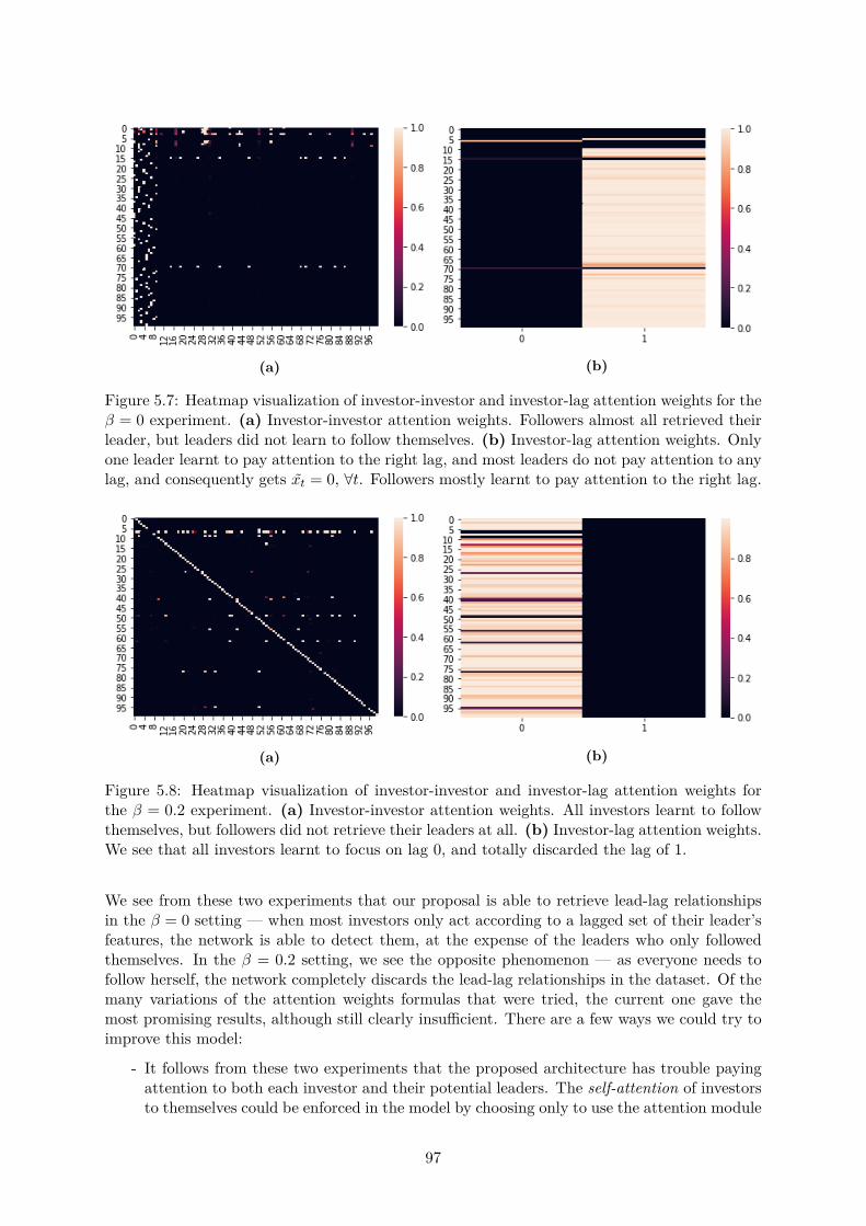
(a) (b)

Figure 5.7: Heatmap visualization of investor-investor and investor-lag attention weights for the— = 0 experiment. (a) Investor-investor attention weights. Followers almost all retrieved theirleader, but leaders did not learn to follow themselves. (b) Investor-lag attention weights. Onlyone leader learnt to pay attention to the right lag, and most leaders do not pay attention to anylag, and consequently gets xt = 0, ’t. Followers mostly learnt to pay attention to the right lag.

(a) (b)

Figure 5.8: Heatmap visualization of investor-investor and investor-lag attention weights forthe — = 0.2 experiment. (a) Investor-investor attention weights. All investors learnt to followthemselves, but followers did not retrieve their leaders at all. (b) Investor-lag attention weights.We see that all investors learnt to focus on lag 0, and totally discarded the lag of 1.

We see from these two experiments that our proposal is able to retrieve lead-lag relationshipsin the — = 0 setting — when most investors only act according to a lagged set of their leader’sfeatures, the network is able to detect them, at the expense of the leaders who only followedthemselves. In the — = 0.2 setting, we see the opposite phenomenon — as everyone needs tofollow herself, the network completely discards the lead-lag relationships in the dataset. Of themany variations of the attention weights formulas that were tried, the current one gave themost promising results, although still clearly insu�cient. There are a few ways we could try toimprove this model:

- It follows from these two experiments that the proposed architecture has trouble payingattention to both each investor and their potential leaders. The self-attention of investorsto themselves could be enforced in the model by choosing only to use the attention module

97

to detect lead-lag and not self-oriented relationships, i.e., by adding the features of a giveninvestor at a given time-step to the result of the attention module depicted in Fig. 5.6.However, such a model would be entirely designed to mimic the mathematical formulationof the problem, consequently introducing bias in the process.

- In the current methodology, we enforce sparsity by penalizing the entropy of the attentionweights in the same way as in Section 3.2.2. However, this penalty enforces to get either0 or 1 but does not prevent many 1 from happening. This penalty term could, therefore,be coupled to a L0 penalty, as is done in Guo et al. (2019) with a term

lú = 1|U |

ÿ

uœU

A

maxA

ÿ

i

–ú,u,i ≠ kú, 0BB2

, (5.12)

with ú œ {cl, lag}, –ú,u,i the i-th term of the attention weight vector –ú,u and kú themaximal number of admissible weights used for ú. Such a penalty would help correct thebehavior shown for the two outlying followers of the — = 0 experiment shown in Fig. 5.7.

- A problem of the current methodology could be that the network cannot really exploredi�erent lag or leaders’ configurations before having to exploit its findings. Exploration ofdi�erent configurations could be enhanced with the Gumbel-Softmax sampling strategyoutlined in Section 3.5.2.

These three ideas could improve the current results and hopefully lead to satisfactory lead-lagrelationships retrieval on synthetic data. If the first results of this attempt at lead-lag detectionusing neural network architectures are promising, further research is required to get a fullyfunctional model that could work on both synthetic and real-world data.

5.4 Towards history-augmented expertsChapters 3 and 4 introduced algorithms respectively aiming at taking into account the het-erogeneity of investment strategies and at introducing time in future interests’ prediction usingclients’ and assets’ trading histories. These two goals are not orthogonal, and could both partic-ipate in the success of a financial recommender system. In this section, we explore to a greaterextent how the ideas underpinning the ExNet and HCF algorithms could be merged into a newhistory-augmented experts network algorithm.

The ExNet algorithm revolves around the idea that not all investors follow the same decisionfunction, and that the set of potential decision functions should be made explicit in the networkarchitecture to uncover post-training the structure of relationships between investors’ behav-iors. In classic matrix factorization algorithms such as the ones introduced in Section 1.3.3, thedecision function corresponds to the scalar product between user and item latent representa-tions. Consequently, the user and item embeddings encode features deemed useful by the modelduring training for interests’ prediction. As all users (resp. items) have their own embeddings,the model can learn to encode di�erent features for each. Consequently, matrix factorizationalgorithms, to a certain extent, already personalize decision functions — the structure explicitlyuncovered in ExNets with the gating block is tantamount to the result we would obtain by usingclustering methods directly on the users’ embeddings of a matrix factorization algorithm.

However, the history-enhancement step of the HCF algorithm introduces a level of complexitythat might not be relevant to share between all users or items. Taking the user-side, thecomposition of a user’s embedding and the embedding of her recent item history should, e.g.,be di�erent for users in search of novelty and users that rely heavily on their past behavior.Consequently, the convolution module, which takes care of the transformation of a static userembedding into a time-aware user embedding, could be considered as an expert of the HCF user

98

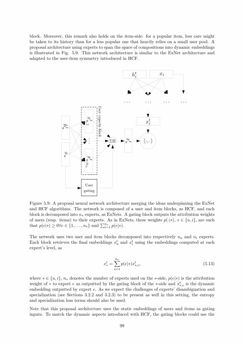
block. Moreover, this remark also holds on the item-side: for a popular item, less care mightbe taken to its history than for a less popular one that heavily relies on a small user pool. Aproposal architecture using experts to span the space of compositions into dynamic embeddingsis illustrated in Fig. 5.9. This network architecture is similar to the ExNet architecture andadapted to the user-item symmetry introduced in HCF.

Figure 5.9: A proposal neural network architecture merging the ideas underpinning the ExNetand HCF algorithms. The network is composed of a user and item blocks, as HCF, and eachblock is decomposed into nú experts, as ExNets. A gating block outputs the attribution weightsof users (resp. items) to their experts. As in ExNets, these weights p(·|ú), ú œ {u, i}, are suchthat p(e|ú) Ø 0’e œ {1, . . . , nú} and

qnúe=1 p(e|ú).

The network uses two user and item blocks decomposed into respectively nu and ni experts.Each block retrieves the final embeddings x

tu and x

t

iusing the embeddings computed at each

expert’s level, as

xt

ú =núÿ

e=1p(e|ú)xt

ú,e, (5.13)

where ú œ {u, i}, nú denotes the number of experts used on the ú-side, p(e|ú) is the attributionweight of ú to expert e as outputted by the gating block of the ú-side and x

tú,e is the dynamic

embedding outputted by expert e. As we expect the challenges of experts’ disambiguation andspecialization (see Sections 3.2.2 and 3.2.3) to be present as well in this setting, the entropyand specialization loss terms should also be used.

Note that this proposal architecture uses the static embeddings of users and items as gatinginputs. To match the dynamic aspects introduced with HCF, the gating blocks could use the

99

same convolution modules as the experts of this network and become time-dependent. Thisarchitecture is also fully compatible with the "featurized" version of HCF introduced in Section4.4.3. Whether this proposal architecture and its featurized variation are superior to both theExNet and HCF architectures or not is yet to be proven, and will be the subject of furtherresearch.

100

Conclusions and perspectives

Recommender systems must be adapted to the context of a corporate and institutional bank toprovide relevant predictions. In this thesis, we prove the benefits of deep learning methodologiesfor the future interest prediction problem with ad hoc algorithms specifically designed to tacklechallenges of the financial world.

With the Experts Network (ExNet) algorithm, we address the heterogeneity of investors’ behav-iors in financial markets. This custom neural network architecture obtains competitive resultswith respect to gradient tree boosting algorithms, which are particularly successful approachesin tabular data contexts. We demonstrate that the ExNet algorithm is able to retrieve clus-ters of investors showing di�erent trading frequencies, and, more interestingly, di�erent tradingstrategies. Moreover, the network outputs an a posteriori map of investors explicitly unveilingtheir behavioral similarities in the considered market. The History-augmented CollaborativeFiltering (HCF) algorithm solves the problem of the non-stationarity of investors’ behaviors.We show that this bespoke architecture obtains overall better results than competitor matrixfactorization-based algorithms, but also that the results of HCF remain stable in time withouthaving to regularly re-train the algorithm.

The ExNet and HCF algorithms used to solve these challenges are novel neural network archi-tectures that respectively define and improve the state-of-the-art for these specific tasks. Theperformance of these algorithms can even be further enhanced using overall improvements suchas the focal BPR loss or our temporal validation strategy in a non-stationary context.

Still, various research directions can be pursued to continue and extend the work of this thesis.ExNets can be robustified by using the Gumbel-Softmax strategy in their gating block. ExNetscould also be staged — the presented architecture is only composed of one gating stage, butmore complex gating structures could be tried to find finer-grained clusterings of investors.Moreover, ExNets detect correlations between investors’ behaviors: they could consequently beleveraged in the lead-lag detection research. The approach taken for the HCF algorithm canalso be further improved. Mainly, what appears to be the most relevant lead is to personalizethe history sizes for users and items. Indeed, a more accurate representation of the users’and items’ underlying dynamics could be obtained with a customized history size, depending,for instance, on users’ and items’ activity. Moreover, the introduction of time leads to a newsampling direction for BPR optimization that is not fully leveraged yet.

The algorithm introduced in Chapter 5, blending the underlying ideas of the ExNet and HCFalgorithms, is also yet to be implemented and duly experimented. The architecture, conceptuallysimple, is however computationally very demanding — the following years will most certainlyprovide us with the appropriate tools for training such architectures in a reasonable amount oftime. Finally, the future interest predictions provided by our deep learning algorithms shouldbe made more directly interpretable to help salespeople better present the recommendations weprovide to the clients of the bank.

101

I sincerely hope that the research presented in this thesis will be helpful to both academicresearchers wanting to know more about the application of recommender systems to the financialworld, and to industrial researchers aiming at improving the results of their future interestprediction algorithms.

102

Conclusions et perspectives

Les systèmes de recommandation doivent être adaptés au contexte d’une banque d’investissementpour fournir des prédictions pertinentes. Dans cette thèse, nous faisons la preuve de l’utilitédes méthodologies d’apprentissage profond pour le problème de prédiction des intérêts futurs àl’aide d’algorithmes ad hoc spécifiquement conçus pour faire face aux défis du monde financier.

Avec l’algorithme de réseau d’experts (ExNet), nous adressons le problème de l’hétérogénéitéde comportement des investisseurs sur les marchés financiers. Cette architecture de réseau deneurones nouvelle obtient des résultats compétitifs vis-à-vis d’approches de gradient boostingutilisant des arbres de classification, approches particulièrement fructueuses dans le contextede données tabulaires. Nous démontrons que l’algorithme ExNet est à même de retrouver desgroupes d’investisseurs suivant leurs fréquences d’investissement, mais aussi suivant leurs straté-gies d’investissement. De plus, le réseau fournit un graphe a posteriori d’investisseurs dévoilantde façon explicite leurs similarités comportementales sur le marché considéré. L’algorithme defiltrage collaboratif augmenté par historiques (HCF) résout le problème de la non-stationnaritédes comportements des investisseurs. Nous montrons que cette architecture, conçue pour ceproblème, obtient de meilleures performances que des approches concurrentes aux spécifica-tions proches, mais également que les résultats obtenus avec HCF sont stables dans le temps,évitant ainsi d’avoir à ré-entraîner l’algorithme de façon régulière.

Les algorithmes ExNet et HCF utilisés pour résoudre ces défis sont des architectures de réseaude neurones nouvelles qui respectivement définissent et améliorent l’état de l’art pour ces tâchesspécifiques. Par ailleurs, les résultats obtenus avec ces algorithmes peuvent encore être améliorésà l’aide de modifications globales telles que la version focale de la fonction de coût de BayesianPersonalized Ranking (BPR), i.e., classement bayésien personnalisé, ou notre stratégie de vali-dation temporelle pour contextes non-stationnaires.

De nombreuses directions de recherche peuvent cependant encore être poursuivies pour con-tinuer et étendre le travail présenté dans cette thèse. Les ExNets peuvent être rendus plusrobustes par l’utilisation de la distribution Gumbel-Softmax dans le bloc de gating, i.e., derépartition des investisseurs considérés. La répartition faite par les ExNets peut également sefaire sur plusieurs niveaux — l’architecture présentée ne comporte qu’un niveau de répartition,mais des structures plus complexes, à plusieurs niveaux de granularité, pourraient mener à despartitionnements plus fins des investisseurs. Par ailleurs, les ExNets détectent les corrélationsentre les comportements des investisseurs: ils pourraient donc être exploités dans une approchede détection de comportements meneur-suiveur sur les marchés. L’approche considérée pourl’algorithme HCF peut également être améliorée de plusieurs façons. En particulier, la per-sonnalisation des tailles d’historique utilisées pour les clients et produits apparaît comme l’unedes meilleures pistes d’amélioration potentielles. En e�et, une représentation plus précise desdynamiques des clients et produits pourrait être obtenue via une taille d’historique adaptée àchaque, et dépendant, par exemple, de leur activité. De plus, l’introduction du temps dansl’algorithme ajoute une direction potentielle de tirage aléatoire pour l’optimisation via BPR qui

103

n’a jusqu’ici pas été pleinement prise en compte.

L’algorithme introduit au chapitre 5 mariant les idées des algorithmes ExNet et HCF est égale-ment encore à implémenter et tester comme il se doit. L’architecture, conceptuellement simple,demande cependant de grandes ressources de calcul — les prochaines années fourniront assuré-ment des outils plus appropriés pour entraîner de telles architectures en un temps raisonnable.Enfin, les prédictions d’intérêts futurs fournies par nos algorithmes d’apprentissage profonddevraient être rendues plus directement interprétables pour faciliter la présentation de nosrecommandations par les vendeurs aux clients de la banque.

J’espère sincèrement que la recherche présentée dans cette thèse pourra être utile à la foisaux chercheurs académiques souhaitant en connaître davantage sur l’application des systèmesde recommandation au monde financier ainsi qu’aux chercheurs du secteur privé cherchant àaméliorer les résultats de leurs algorithmes de prédiction des intérêts futurs.

104

Bibliography

K. Baltakys, J. Kanniainen, and F. Emmert-Streib. Multilayer aggregation with statisticalvalidation: Application to investor networks. Scientific Reports, 8(1):8198, 2018.

J. Basilico and T. Hofmann. Unifying collaborative and content-based filtering. In Proceedingsof the twenty-first International Conference on Machine Learning, page 9, 2004.

Y. Bengio. Practical recommendations for gradient-based training of deep architectures. InNeural Networks: Tricks of the Trade, pages 437–478. Springer, 2012.

Y. Benjamini and Y. Hochberg. Controlling the false discovery rate: A practical and powerfulapproach to multiple testing. Journal of the Royal Statistical Society: Series B (Methodolog-ical), 57(1):289–300, 1995.

J. Bennett, S. Lanning, et al. The Netflix Prize. In Proceedings of KDD Cup and Workshop,volume 2007, page 35. New York, NY, USA., 2007.

N. Berestycki. Mixing times of markov chains: Techniques and examples. Latin AmericanJournal of Probability and Mathematical Statistics (ALEA), 2016.

C. Bergmeir and J. M. Benítez. On the use of cross-validation for time series predictor evalua-tion. Information Sciences, 191:192–213, 2012.

J. Bergstra and Y. Bengio. Random search for hyper-parameter optimization. Journal ofMachine Learning Research, 13(Feb):281–305, 2012.

L. Bernardi, J. Kamps, J. Kiseleva, and M. J. Müller. The continuous cold start problem ine-commerce recommender systems. 2015.

F. Black and M. Scholes. The pricing of options and corporate liabilities. Journal of PoliticalEconomy, 81(3):637–654, 1973.

M. J. Bland and D. G. Altman. Multiple significance tests: the Bonferroni method. BritishMedical Journal, 310(6973):170, 1995.

Bloomberg. Bloomberg Professional Services. https://www.bloomberg.com/professional/,2020. Last accessed on 04/01/2020.

Bloomberg Professional Services. Sure time to grasp the potential ofstructured products. https://www.bloomberg.com/professional/blog/sure-time-to-grasp-the-potential-of-structured-products/, 2019. Last accessed on06/01/2020.

J. Bobadilla, F. Ortega, A. Hernando, and A. Gutiérrez. Recommender systems survey.Knowledge-based Systems, 46:109–132, 2013.

L. Breiman. Stacked regressions. Machine Learning, 24(1):49–64, 1996.

105

L. Breiman. Random forests. Machine Learning, 45(1):5–32, 2001.

D. Challet, R. Chicheportiche, M. Lallouache, and S. Kassibrakis. Statistically validated lead-lag networks and inventory prediction in the foreign exchange market. Advances in ComplexSystems, 21(08):1850019, 2018.

O. Chapelle and M. Wu. Gradient descent optimization of smoothed information retrievalmetrics. Information Retrieval, 13(3):216–235, 2010.

N. V. Chawla, K. W. Bowyer, L. O. Hall, and P. W. Kegelmeyer. SMOTE: synthetic minorityover-sampling technique. Journal of Artificial Intelligence Research, 16:321–357, 2002.

T. Chen and C. Guestrin. XGBoost: A scalable tree boosting system. In Proceedings of thetwenty-second ACM SIGKDD International Conference on Knowledge Discovery and DataMining, pages 785–794, 2016.

H.-T. Cheng, L. Koc, J. Harmsen, T. Shaked, T. Chandra, H. Aradhye, G. Anderson, G. Cor-rado, W. Chai, M. Ispir, et al. Wide & deep learning for recommender systems. In Proceedingsof the first Workshop on Deep Learning for Recommender Systems, pages 7–10, 2016.

K. Clark, M.-T. Luong, Q. V. Le, and C. D. Manning. ELECTRA: Pre-training text encoders asdiscriminators rather than generators. International Conference on Learning Representations,2020.

P. Covington, J. Adams, and E. Sargin. Deep neural networks for YouTube recommendations.In Proceedings of the tenth ACM Conference on Recommender Systems, pages 191–198. ACM,2016.

C. Curme, M. Tumminello, R. N. Mantegna, E. H. Stanley, and D. Y. Kenett. Emergence ofstatistically validated financial intraday lead-lag relationships. Quantitative Finance, 15(8):1375–1386, 2015.

M. F. Dacrema, P. Cremonesi, and D. Jannach. Are we really making much progress? a worryinganalysis of recent neural recommendation approaches. In Proceedings of the thirteenth ACMConference on Recommender Systems, pages 101–109, 2019.

Z. Dai, Z. Yang, Y. Yang, J. G. Carbonell, Q. V. Le, and R. Salakhutdinov. Transformer-XL:Attentive language models beyond a fixed-length context. In Proceedings of the fifty-seventhAnnual Meeting of the Association for Computational Linguistics, pages 2978–2988, 2019.

J. Davis and M. Goadrich. The relationship between Precision-Recall and ROC curves. InProceedings of the twenty-third International Conference on Machine Learning, pages 233–240. ACM, 2006.

M. L. De Prado. Advances in financial machine learning, chapter 7. John Wiley & Sons, 2018.

J. Devlin, M.-W. Chang, K. Lee, and K. Toutanova. BERT: Pre-training of deep bidirectionaltransformers for language understanding. In Proceedings of the 2019 Conference of the NorthAmerican Chapter of the Association for Computational Linguistics: Human Language Tech-nologies, Volume 1 (Long and Short Papers), pages 4171–4186. Association for ComputationalLinguistics, 2019.

J. Ding, G. Yu, X. He, F. Feng, Y. Li, and D. Jin. Sampler design for bayesian personalizedranking by leveraging view data. IEEE Transactions on Knowledge and Data Engineering,2019.

Y. Ding and X. Li. Time weight collaborative filtering. In Proceedings of the fourteenth ACMInternational Conference on Information and Knowledge Management, pages 485–492, 2005.

106

P. Domingos. A few useful things to know about machine learning. Communications of theACM, 55(10):78–87, 2012.

T. Dozat. Incorporating Nesterov momentum into Adam. 2016.

E. Eban, M. Schain, A. Mackey, A. Gordon, R. Rifkin, and G. Elidan. Scalable learning ofnon-decomposable objectives. In Artificial Intelligence and Statistics, pages 832–840, 2017.

C. Eksombatchai, P. Jindal, J. Z. Liu, Y. Liu, R. Sharma, C. Sugnet, M. Ulrich, and J. Leskovec.Pixie: A system for recommending 3+ billion items to 200+ million users in real-time. InProceedings of the 2018 World Wide Web Conference, pages 1775–1784, 2018.

M. Ester, H.-P. Kriegel, J. Sander, X. Xu, et al. A density-based algorithm for discoveringclusters in large spatial databases with noise. In KDD, volume 96, pages 226–231, 1996.

F. J. Fabozzi. Bond Markets, Analysis and Strategies — 8th Edition. Prentice Hall, 2012.

H. I. Fawaz, G. Forestier, J. Weber, L. Idoumghar, and P.-A. Muller. Deep learning for timeseries classification: a review. Data Mining and Knowledge Discovery, 33(4):917–963, 2019.

T. Fawcett. An introduction to ROC analysis. Pattern Recognition Letters, 27(8):861–874, 2006.

J.-D. Fermanian, O. Guéant, and J. Pu. The behavior of dealers and clients on the europeancorporate bond market: the case of multi-dealer-to-client platforms. Market Microstructureand Liquidity, 2, 2016.

P. I. Frazier. A tutorial on Bayesian optimization. arXiv preprint arXiv:1807.02811, 2018.

T. Galanti, L. Wolf, and T. Hazan. A theoretical framework for deep transfer learning. Infor-mation and Inference: A Journal of the IMA, 5(2):159–209, 2016.

D. Goldberg, D. Nichols, B. M. Oki, and D. Terry. Using collaborative filtering to weave aninformation tapestry. Communications of the ACM, 35(12):61–70, 1992.

I. Goodfellow, Y. Bengio, and A. Courville. Deep Learning. MIT Press, 2016.

O. Guéant, C.-A. Lehalle, and J. Fernandez-Tapia. Dealing with the inventory risk: a solutionto the market making problem. Mathematics and Financial Economics, 7(4):477–507, 2013.

Y. Guo, H. Shi, A. Kumar, K. Grauman, T. Rosing, and R. Feris. SpotTune: transfer learningthrough adaptive fine-tuning. In Proceedings of the IEEE Conference on Computer Visionand Pattern Recognition, pages 4805–4814, 2019.

M. Gutiérrez-Roig, J. Borge-Holthoefer, A. Arenas, and J. Perelló. Mapping individual behaviorin financial markets: synchronization and anticipation. EPJ Data Science, 8(1):10, 2019.

M. Haldar, M. Abdool, P. Ramanathan, T. Xu, S. Yang, H. Duan, Q. Zhang, N. Barrow-Williams, B. C. Turnbull, B. M. Collins, et al. Applying deep learning to AirBnB search.In Proceedings of the twenty-fifth ACM SIGKDD International Conference on KnowledgeDiscovery & Data Mining, pages 1927–1935, 2019.

W. Hamilton, Z. Ying, and J. Leskovec. Inductive representation learning on large graphs. InAdvances in Neural Information Processing Systems, pages 1024–1034, 2017.

S. J. Hardiman, N. Bercot, and J.-P. Bouchaud. Critical reflexivity in financial markets: aHawkes process analysis. The European Physical Journal B, 86(10):442, 2013.

T. Hastie, R. Tibshirani, and J. Friedman. The Elements of Statistical Learning: Data Mining,Inference, and Prediction. Springer Science & Business Media, 2009.

107

K. He, X. Zhang, S. Ren, and J. Sun. Deep residual learning for image recognition. In Proceedingsof the IEEE Conference on Computer Vision and Pattern Recognition, pages 770–778, 2016.

X. He, L. Liao, H. Zhang, L. Nie, X. Hu, and T.-S. Chua. Neural collaborative filtering. InProceedings of the 26th International Conference on World Wide Web, pages 173–182, 2017.

X. He, Z. He, X. Du, and T.-S. Chua. Adversarial personalized ranking for recommendation.In The forty-first International ACM SIGIR Conference on Research & Development in In-formation Retrieval, pages 355–364, 2018.

P. Henderson and V. Ferrari. End-to-end training of object class detectors for mean averageprecision. In Asian Conference on Computer Vision, pages 198–213. Springer, 2016.

S. Hochreiter and J. Schmidhuber. Long short-term memory. Neural Computation, 9(8):1735–1780, 1997.

K. Hornik, M. Stinchcombe, H. White, et al. Multilayer feedforward networks are universalapproximators. Neural Networks, 2(5):359–366, 1989.

P. O. Hoyer. Non-negative matrix factorization with sparseness constraints. Journal of MachineLearning Research, 5(Nov):1457–1469, 2004.

Y. Hu, Y. Koren, and C. Volinsky. Collaborative filtering for implicit feedback datasets. In2008 Eighth IEEE International Conference on Data Mining, pages 263–272. IEEE, 2008.

F. Huang, J. Ash, J. Langford, and R. Schapire. Learning deep ResNet blocks sequentiallyusing boosting theory. In Proceedings of the thirty-fifth International Conference on MachineLearning, 2018.

J. C. Hull. Options, futures and other derivatives — 9th Edition. Pearson Education, 2014.

S. Io�e and C. Szegedy. Batch Normalization: Accelerating deep network training by reducinginternal covariate shift. In International Conference on Machine Learning, pages 448–456,2015.

ISIN. ISIN Organization. https://www.isin.org/, 2020. Last accessed on 04/03/2020.

R. A. Jacobs, M. I. Jordan, S. J. Nowlan, and G. E. Hinton. Adaptive mixtures of local experts.Neural Computation, 3(1):79–87, 1991.

E. Jang, S. Gu, and B. Poole. Categorical reparameterization with Gumbel-Softmax. Interna-tional Conference on Learning Representations, 2017.

Kaggle Inc. Kaggle. https://www.kaggle.com/, 2020. Last accessed on 04/23/2020.

A. Karpathy. Stanford CS231n Convolutional Neural Networks for Visual Recognition. http://cs231n.github.io/convolutional-networks/, 2016. Accessed: 2020-05-11.

G. Ke, Q. Meng, T. Finley, T. Wang, W. Chen, W. Ma, Q. Ye, and T.-Y. Liu. LightGBM: Ahighly e�cient gradient boosting decision tree. In Advances in Neural Information ProcessingSystems, pages 3146–3154, 2017.

B. Kim, M. Wattenberg, J. Gilmer, C. Cai, J. Wexler, F. Viegas, and R. Sayres. Interpretabilitybeyond feature attribution: Quantitative testing with concept activation vectors (TCAV).arXiv preprint arXiv:1711.11279, 2017.

D. P. Kingma and J. Ba. Adam: A method for stochastic optimization. International Conferenceon Learning Representations, 2015.

108

Y. Koren. Factorization meets the neighborhood: a multifaceted collaborative filtering model.In Proceedings of the fourteenth ACM SIGKDD International Conference on Knowledge Dis-covery and Data Mining, pages 426–434, 2008.

Y. Koren. The BellKor solution to the Netflix grand prize. Netflix Prize Documentation, 81(2009):1–10, 2009a.

Y. Koren. Collaborative filtering with temporal dynamics. In Proceedings of the fifteenth ACMSIGKDD International Conference on Knowledge Discovery and Data Mining, pages 447–456,2009b.

Y. Koren, R. Bell, and C. Volinsky. Matrix factorization techniques for recommender systems.Computer, 42(8):30–37, 2009.

Y. LeCun, Y. Bengio, and G. Hinton. Deep learning. Nature, 521(7553):436–444, 2015.

L. Li, W. Chu, J. Langford, and R. E. Schapire. A contextual-bandit approach to personalizednews article recommendation. In Proceedings of the nineteenth International Conference onWorld Wide Web, pages 661–670, 2010.

T.-Y. Lin, P. Goyal, R. Girshick, K. He, and P. Dollár. Focal loss for dense object detection.In Proceedings of the IEEE International Conference on Computer Vision, pages 2980–2988,2017.

Y. Liu and X. Yao. Simultaneous training of negatively correlated neural networks in an en-semble. IEEE Transactions on Systems, Man, and Cybernetics, Part B (Cybernetics), 29(6):716–725, 1999.

Y. Liu, M. Ott, N. Goyal, J. Du, M. Joshi, D. Chen, O. Levy, M. Lewis, L. Zettlemoyer, andV. Stoyanov. RoBERTa: A robustly optimized BERT pretraining approach. arXiv preprintarXiv:1907.11692, 2019.

S. M. Lundberg and S.-I. Lee. A unified approach to interpreting model predictions. In Advancesin Neural Information Processing Systems, pages 4765–4774, 2017.

L. v. d. Maaten and G. Hinton. Visualizing data using t-SNE. Journal of Machine LearningResearch, 9(Nov):2579–2605, 2008.

C. J. Maddison, A. Mnih, and Y. W. Teh. The concrete distribution: A continuous relaxationof discrete random variables. International Conference on Learning Representations, 2017.

C. Manning, P. Raghavan, and H. Schütze. Introduction to information retrieval, volume 16,chapter 8.4, pages 100–103. Cambridge University Press, 2010.

L. McInnes, J. Healy, and J. Melville. UMAP: Uniform manifold approximation and projectionfor dimension reduction. arXiv preprint arXiv:1802.03426, 2018.

T. Mikolov, I. Sutskever, K. Chen, G. S. Corrado, and J. Dean. Distributed representations ofwords and phrases and their compositionality. In Advances in Neural Information ProcessingSystems, pages 3111–3119, 2013.

A. Mnih and R. R. Salakhutdinov. Probabilistic matrix factorization. In Advances in NeuralInformation Processing Systems, pages 1257–1264, 2008.

V. Mnih, K. Kavukcuoglu, D. Silver, A. Graves, I. Antonoglou, D. Wierstra, and M. Riedmiller.Playing Atari with deep reinforcement learning. In Advances in Neural Information ProcessingSystems, 2013.

109

V. Mnih, A. P. Badia, M. Mirza, A. Graves, T. Lillicrap, T. Harley, D. Silver, andK. Kavukcuoglu. Asynchronous methods for deep reinforcement learning. In InternationalConference on Machine Learning, pages 1928–1937, 2016.

K. P. Murphy. Machine learning: a probabilistic perspective. MIT Press, 2012.

F. Musciotto, L. Marotta, J. Piilo, and R. N. Mantegna. Long-term ecology of investors in afinancial market. Palgrave Communications, 4(1):92, 2018.

V. Nair and G. E. Hinton. Rectified linear units improve restricted Boltzmann machines. InProceedings of the twenty-seventh International Conference on Machine Learning (ICML-10),pages 807–814, 2010.

E. Negre. Information and Recommender Systems. John Wiley & Sons, 2015.

Y. E. Nesterov. A method for solving the convex programming problem with convergence rateo(1/k

2). In Dokl. Akad. Nauk SSSR, volume 269, pages 543–547, 1983.

M. Nielsen. Neural Networks and Deep Learning. Determination Press, 2015.

A. v. d. Oord, S. Dieleman, H. Zen, K. Simonyan, O. Vinyals, A. Graves, N. Kalchbrenner,A. Senior, and K. Kavukcuoglu. WaveNet: A generative model for raw audio. arXiv preprintarXiv:1609.03499, 2016.

P. Paatero and U. Tapper. Positive matrix factorization: A non-negative factor model withoptimal utilization of error estimates of data values. Environmetrics, 5(2):111–126, 1994.

D. L. Padial. Technical Analysis Library using Pandas. https://github.com/bukosabino/ta,2018.

Y.-J. Park and A. Tuzhilin. The long tail of recommender systems and how to leverage it. InProceedings of the 2008 ACM Conference on Recommender Systems, pages 11–18, 2008.

I. Pilászy, D. Zibriczky, and D. Tikk. Fast ALS-based matrix factorization for explicit andimplicit feedback datasets. In Proceedings of the fourth ACM Conference on RecommenderSystems, pages 71–78, 2010.

J. Racine. Consistent cross-validatory model-selection for dependent data: hv-block cross-validation. Journal of Econometrics, 99(1):39–61, 2000.

A. Radford, J. Wu, R. Child, D. Luan, D. Amodei, and I. Sutskever. Language models areunsupervised multitask learners. OpenAI Blog, 1(8):9, 2019.

S. Rendle, C. Freudenthaler, Z. Gantner, and L. Schmidt-Thieme. BPR: Bayesian personalizedranking from implicit feedback. In Proceedings of the twenty-fifth Conference on Uncertaintyin Artificial Intelligence, pages 452–461. AUAI Press, 2009.

M. T. Ribeiro, S. Singh, and C. Guestrin. "Why should I trust you?" Explaining the predictionsof any classifier. In Proceedings of the twenty-second ACM SIGKDD International Conferenceon Knowledge Discovery and Data Mining, pages 1135–1144, 2016.

M. Rosvall and C. T. Bergstrom. Maps of random walks on complex networks reveal communitystructure. Proceedings of the National Academy of Sciences, 105(4):1118–1123, 2008.

D. E. Rumelhart, G. E. Hinton, and R. J. Williams. Learning representations by back-propagating errors. Nature, 323(6088):533–536, 1986.

O. Russakovsky, J. Deng, H. Su, J. Krause, S. Satheesh, S. Ma, Z. Huang, A. Karpathy,A. Khosla, M. Bernstein, et al. ImageNet large scale visual recognition challenge. Inter-national Journal of Computer Vision, 115(3):211–252, 2015.

110

P. Sarkar, S. M. Siddiqi, and G. J. Gordon. A latent space approach to dynamic embedding ofco-occurrence data. In Artificial Intelligence and Statistics, pages 420–427, 2007.

L. S. Shapley. A value for n-person games. Contributions to the Theory of Games, 2(28):307–317, 1953.

N. Shazeer, A. Mirhoseini, K. Maziarz, A. Davis, Q. Le, G. Hinton, and J. Dean. Outrageouslylarge neural networks: The sparsely-gated mixture-of-experts layer. International Conferenceon Learning Representations, 2017.

Y. Shi, A. Karatzoglou, L. Baltrunas, M. Larson, A. Hanjalic, and N. Oliver. TFMAP: opti-mizing MAP for top-n context-aware recommendation. In Proceedings of the thiry-fifth In-ternational ACM SIGIR Conference on Research and Development in Information Retrieval,pages 155–164, 2012.

Y. Shi, M. Larson, and A. Hanjalic. Collaborative filtering beyond the user-item matrix: Asurvey of the state of the art and future challenges. ACM Computing Surveys (CSUR), 47(1):1–45, 2014.

A. Shrikumar, P. Greenside, and A. Kundaje. Learning important features through propagatingactivation di�erences. In Proceedings of the thirty-fourth International Conference on MachineLearning, pages 3145–3153. JMLR. org, 2017.

J. Sirignano and R. Cont. Universal features of price formation in financial markets: Perspectivesfrom deep learning. Quantitative Finance, 19(9):1449–1459, 2019.

D. Sorokina and E. Cantu-Paz. Amazon search: The joy of ranking products. In Proceedingsof the thiry-ninth International ACM SIGIR Conference on Research and Development inInformation Retrieval, pages 459–460, 2016.

N. Srivastava, G. Hinton, A. Krizhevsky, I. Sutskever, and R. Salakhutdinov. Dropout: A simpleway to prevent neural networks from overfitting. Journal of Machine Learning Research, 15(1):1929–1958, 2014.

X. Su and T. M. Khoshgoftaar. A survey of collaborative filtering techniques. Advances inArtificial Intelligence, 2009, 2009.

I. Sutskever, J. Martens, G. Dahl, and G. Hinton. On the importance of initialization andmomentum in deep learning. In International Conference on Machine Learning, pages 1139–1147, 2013.

G. Takács and D. Tikk. Alternating least squares for personalized ranking. In Proceedings ofthe sixth ACM Conference on Recommender Systems, pages 83–90, 2012.

The European Commission. Markets in Financial Instruments Directive, II — Scopes andDefinitions. 2014.

A. Tsymbal. The problem of concept drift: definitions and related work. Computer ScienceDepartment, Trinity College Dublin, 106(2):58, 2004.

M. Tumminello, S. Micciche, F. Lillo, J. Piilo, and R. N. Mantegna. Statistically validatednetworks in bipartite complex systems. PloS one, 6(3), 2011.

M. Tumminello, F. Lillo, J. Piilo, and R. N. Mantegna. Identification of clusters of investorsfrom their real trading activity in a financial market. New Journal of Physics, 14(1):013041,2012.

111

A. Vaswani, N. Shazeer, N. Parmar, J. Uszkoreit, L. Jones, A. N. Gomez, £. Kaiser, andI. Polosukhin. Attention is all you need. In Advances in Neural Information ProcessingSystems, pages 5998–6008, 2017.

A. Veit, M. J. Wilber, and S. Belongie. Residual networks behave like ensembles of relativelyshallow networks. In Advances in Neural Information Processing Systems, pages 550–558,2016.

H. Wang, Q. Wu, and H. Wang. Learning hidden features for contextual bandits. In Pro-ceedings of the twenty-fifth ACM International Conference on Information and KnowledgeManagement, pages 1633–1642, 2016.

X. Wang, X. He, M. Wang, F. Feng, and T.-S. Chua. Neural graph collaborative filtering.In Proceedings of the fourty-second International ACM SIGIR Conference on Research andDevelopment in Information Retrieval, pages 165–174, 2019.

D. H. Wolpert. Stacked generalization. Neural Networks, 5(2):241–259, 1992.

D. Wright, L. Capriotti, and J. Lee. Machine learning and corporate bond trading. AlgorithmicFinance, 7(3-4):105–110, 2018.

C.-Y. Wu, A. Ahmed, A. Beutel, A. J. Smola, and H. Jing. Recurrent recommender networks.In Proceedings of the tenth ACM International Conference on Web Search and Data Mining,pages 495–503, 2017.

X. Wu, B. Shi, Y. Dong, C. Huang, and N. Chawla. Neural tensor factorization. arXiv preprintarXiv:1802.04416, 2018.

L. Xiang, Q. Yuan, S. Zhao, L. Chen, X. Zhang, Q. Yang, and J. Sun. Temporal recommendationon graphs via long- and short-term preference fusion. In Proceedings of the sixteenth ACMSIGKDD International Conference on Knowledge Discovery and Data Mining, pages 723–732,2010.

L. Xiong, X. Chen, T.-K. Huang, J. Schneider, and J. G. Carbonell. Temporal collaborativefiltering with bayesian probabilistic tensor factorization. In Proceedings of the 2010 SIAMInternational Conference on Data Mining, pages 211–222. SIAM, 2010.

Z. Yang, Z. Dai, Y. Yang, J. Carbonell, R. R. Salakhutdinov, and Q. V. Le. XLNet: Generalizedautoregressive pretraining for language understanding. In Advances in Neural InformationProcessing Systems, pages 5754–5764, 2019.

S. E. Yuksel, J. N. Wilson, and P. D. Gader. Twenty years of mixture of experts. IEEETransactions on Neural Networks and Learning Systems, 23(8):1177–1193, 2012.

A. Zeng, A. Vidmer, M. Medo, and Y.-C. Zhang. Information filtering by similarity-preferentialdi�usion processes. EPL (Europhysics Letters), 105(5):58002, 2014.

M. R. Zhang, J. Lucas, G. Hinton, and J. Ba. Lookahead Optimizer: k steps forward, 1 stepback. arXiv preprint arXiv:1907.08610, 2019.

W. Zhang, T. Chen, J. Wang, and Y. Yu. Optimizing top-n collaborative filtering via dy-namic negative item sampling. In Proceedings of the thirty-sixth International ACM SIGIRConference on Research and Development in Information Retrieval, pages 785–788, 2013.

G. Zheng, F. Zhang, Z. Zheng, Y. Xiang, N. J. Yuan, X. Xie, and Z. Li. Drn: A deep reinforce-ment learning framework for news recommendation. In Proceedings of the 2018 World WideWeb Conference, pages 167–176, 2018.

112

T. Zhou, J. Ren, M. Medo, and Y.-C. Zhang. Bipartite network projection and personal rec-ommendation. Physical Review E, 76(4):046115, 2007.

T. Zhou, Z. Kuscsik, J.-G. Liu, M. Medo, J. R. Wakeling, and Y.-C. Zhang. Solving the apparentdiversity-accuracy dilemma of recommender systems. Proceedings of the National Academyof Sciences, 107(10):4511–4515, 2010.

113

List of Figures

1.1 Cash flows of a bond . . . . . . . . . . . . . . . . . . . . . . . . . . . . . . . . . . 91.2 The four di�erent options payo� structures . . . . . . . . . . . . . . . . . . . . . 111.3 Study of the heterogeneity of clients . . . . . . . . . . . . . . . . . . . . . . . . . 141.4 Study of the heterogeneity of corporate bonds . . . . . . . . . . . . . . . . . . . . 151.5 The WaveNet architecture . . . . . . . . . . . . . . . . . . . . . . . . . . . . . . . 191.6 An example of bipartite graph and its associated adjacency matrix . . . . . . . . 191.7 The principle of matrix factorization . . . . . . . . . . . . . . . . . . . . . . . . . 201.8 Candidate generation network of the YouTube recommender system . . . . . . . 221.9 The NeuMF architecture . . . . . . . . . . . . . . . . . . . . . . . . . . . . . . . . 231.10 A neural tensor factorization architecture . . . . . . . . . . . . . . . . . . . . . . 241.11 Illustration of HeatS and ProbS . . . . . . . . . . . . . . . . . . . . . . . . . . . . 261.12 The confusion matrix outline . . . . . . . . . . . . . . . . . . . . . . . . . . . . . 27

2.1 Evolution of validation symmetrized mAP score with ⁄ . . . . . . . . . . . . . . . 372.2 Heatmap visualization of SPHY performance . . . . . . . . . . . . . . . . . . . . 382.3 Heatmap visualization of SPHY diversity performance . . . . . . . . . . . . . . . 382.4 Heatmap visualization of SPHY similarity performance . . . . . . . . . . . . . . . 392.5 Evolution of confidence weights . . . . . . . . . . . . . . . . . . . . . . . . . . . . 40

3.1 Universality matrix of investors’ strategies . . . . . . . . . . . . . . . . . . . . . . 453.2 Global architecture of the Experts Network . . . . . . . . . . . . . . . . . . . . . 473.3 UMAP visualization of investors embeddings for Embed-MLP and ExNet . . . . 533.4 Distribution over experts of all investors for ExNet-Opt . . . . . . . . . . . . . . 543.5 Distribution over experts of all investors and UMAP visualization of investors

embeddings for ExNet-100 . . . . . . . . . . . . . . . . . . . . . . . . . . . . . . . 543.6 Distribution over experts of all investors and UMAP visualization of investors

embeddings for ExNet on the TEF dataset . . . . . . . . . . . . . . . . . . . . . 563.7 Distribution over experts of all investors and UMAP visualization of investors

embeddings for ExNet on the BNPP CIB Bonds’ RFQ dataset . . . . . . . . . . 583.8 Global architecture of the Average Network . . . . . . . . . . . . . . . . . . . . . 603.9 Global architecture of a boosted ExNet . . . . . . . . . . . . . . . . . . . . . . . 64

4.1 Architecture of the HCF network and details on used convolutions . . . . . . . . 694.2 Evolution of validation symmetrized mAP with training window size . . . . . . . 724.3 Evolution of validation symmetrized mAP with training window size with bench-

mark optimized for various windows . . . . . . . . . . . . . . . . . . . . . . . . . 734.4 Daily evolution of symmetrized mAP during the test period . . . . . . . . . . . . 744.5 Evolution of HCF test performance with history size . . . . . . . . . . . . . . . . 754.6 Density of scores . . . . . . . . . . . . . . . . . . . . . . . . . . . . . . . . . . . . 774.7 Evolution of scores with time for a medium- and high-activity user on a same item 78

115

4.8 Evolution of scores with time for a low-activity user on two di�erent items . . . . 794.9 Evolution of American Treasury bonds scores during the test period for the most

active user with two di�erent features . . . . . . . . . . . . . . . . . . . . . . . . 81

5.1 Statistically Validated Network obtained on corporate bonds RFQ data . . . . . 885.2 A split of purged K-fold cross-validation . . . . . . . . . . . . . . . . . . . . . . . 915.3 Overall average precision test performance as a function of overall average preci-

sion validation performance . . . . . . . . . . . . . . . . . . . . . . . . . . . . . . 925.4 Weight repartition of the entropic stacking strategy . . . . . . . . . . . . . . . . . 935.5 Heatmap visualization of the Pearson correlations between the stacked models . . 945.6 Example of data volume reduction for a particular investor using investor and

lag attentions . . . . . . . . . . . . . . . . . . . . . . . . . . . . . . . . . . . . . . 955.7 Heatmap visualization of investor-investor and investor-lag attention weights for

the — = 0 experiment . . . . . . . . . . . . . . . . . . . . . . . . . . . . . . . . . . 975.8 Heatmap visualization of investor-investor and investor-lag attention weights for

the — = 0.2 experiment . . . . . . . . . . . . . . . . . . . . . . . . . . . . . . . . . 975.9 A proposal neural network architecture merging the ideas underpinning the ExNet

and HCF algorithms . . . . . . . . . . . . . . . . . . . . . . . . . . . . . . . . . . 99

A.1 Global outline of the perceptron model . . . . . . . . . . . . . . . . . . . . . . . . 121A.2 A simple perceptron and its R2 representation . . . . . . . . . . . . . . . . . . . . 122A.3 The NAND perceptron . . . . . . . . . . . . . . . . . . . . . . . . . . . . . . . . . 122A.4 An example of multi-layer perceptron . . . . . . . . . . . . . . . . . . . . . . . . 124A.5 An example of convolutional layer . . . . . . . . . . . . . . . . . . . . . . . . . . 131A.6 An example of convolutional neural network . . . . . . . . . . . . . . . . . . . . . 133

116

List of Tables

1.1 Some confusion matrix metrics . . . . . . . . . . . . . . . . . . . . . . . . . . . . 28

2.1 Comparison of classic algorithms on mAP . . . . . . . . . . . . . . . . . . . . . . 412.2 Comparison of classic algorithms on AUC and AP . . . . . . . . . . . . . . . . . 422.3 Comparison of classic algorithms on qualitative metrics . . . . . . . . . . . . . . 42

3.1 Experimental results on synthetic data . . . . . . . . . . . . . . . . . . . . . . . . 523.2 Experimental results on IBEX data . . . . . . . . . . . . . . . . . . . . . . . . . . 563.3 Permutation importance results on IBEX experiment . . . . . . . . . . . . . . . . 57

4.1 Window size study . . . . . . . . . . . . . . . . . . . . . . . . . . . . . . . . . . . 734.2 Sliding study . . . . . . . . . . . . . . . . . . . . . . . . . . . . . . . . . . . . . . 744.3 Comparison of classic and featurized versions of HCF . . . . . . . . . . . . . . . . 804.4 Qualitative comparison of classic and featurized versions of HCF . . . . . . . . . 804.5 Comparison of historical, featurized MF and HCF algorithms on the primary

structured products prediction problem . . . . . . . . . . . . . . . . . . . . . . . 83

5.1 Comparison of classic and focal versions of HCF . . . . . . . . . . . . . . . . . . 89

117

Glossary

CIB. Corporate and Institutional Bank.Sales. Financial lingo referring to salespeople.D2C. Dealer-to-Client. Refers to electronic platforms where clients can stream prices for manyfinancial assets as given by market makers.RFQ. Request For Quotation. A process in which a client declares her interest into buy-ing/selling a given amount of a given financial asset.RFM. Request For Market. A process in which a client declares her interest in a given financialasset.IOI. Indication of Interest. Indication recorded by sales that a given client might have aninterest for a given financial asset.G10. Refers to the G10 group of countries, composed of Germany, Belgium, Canada, UnitedStates of America, France, Italy, Japan, Netherlands, United Kingdom, Sweden, and Switzer-land.NLP. Natural Language Processing. Refers to a subfield of machine learning interested intothe understanding of human language.MLP. Multi-Layer Perceptron. Refers to a feed-forward, fully-connected neural network. SeeAppendix A for more information.LGBM. Refers to the LightGBM algorithm (Ke et al., 2017).LSTM. Long-Short Term Memory. A specific type of recurrent neural networks introduced inHochreiter and Schmidhuber (1997).ExNet. Experts Network. Refers to a novel neural network architecture introduced in thismanuscript in Chapter 3.HCF. History-augmented Collaborative Filtering. Refers to a novel neural network architec-ture introduced in this manuscript in Chapter 4.MF. Matrix Factorization. A collaborative filtering algorithm outlined in Section 1.3.3.NMF. Nonnegative Matrix Factorization. A collaborative filtering algorithm outlined in Sec-tion 1.3.3.BPR. Bayesian Personalized Ranking. A loss function used in collaborative filtering, and in-troduced in Section 1.3.3.UMAP. Uniform Manifold Approximation and Projection. A dimension reduction algorithmintroduced in McInnes et al. (2018).AUC ROC. Area Under the Receiver Operating Characteristic Curve. Also encountered asAUC, or ROC AUC. A binary classification metric.AP. Average Precision. A binary classification metric.mAP. Mean Average Precision. In this work, used for short of symmetrized mean averageprecision, a metric introduced in Section 1.4.

119

Appendix A

Basics of deep learning

The purpose of this appendix is to delve into the mathematics onto which deep learning lies.The structure of this appendix is as follows:

- Introducing the general principles on which the field of deep learning relies;- Providing the reader with the mathematical tools required for training neural networks,

i.e., the gradient descent and backpropagation algorithms;- Thoroughly presenting the concepts behind the two classic neural network architectures

of multi-layer perceptrons and convolutional neural networks.

For ease of understanding, we focus on a supervised learning framework throughout this ap-pendix.

A.1 General principles of neural networksThis section introduces general principles of neural networks, from the historical perceptronmodel to multi-layer perceptrons and presents heuristics and ideas to guide the design of neuralnetwork architectures.

A.1.1 PerceptronsNeural networks are a very popular toolbox to tackle supervised learning problems, from naturallanguage processing tasks to computer vision ones. To understand their popularity, we traceback their history, relying mainly on the outline given by Nielsen (2015). In 1957, FrankRosenblatt introduced the perceptron, a model broadly mimicking the functioning of a biologicalneuron: a perceptron receives inputs and then makes the decision to fire or not fire based onthese inputs. The model of the perceptron is illustrated in Fig. A.1.

∈ {0,1}Output

'(

')

…Inputs

Figure A.1: Global outline of the perceptron model. A perceptron takes inputs x1, ..., xn andoutputs either 0 or 1, mimicking the behavior of a biological neuron.

The perceptron takes inputs x1, ..., xn and outputs either 0 or 1, corresponding to the firing of

121

a biological neuron. Firing is determined using a set of weights {w1, ..., wn} and a bias denotedb, according to

output =I

0 if w · x + b 6 01 if w · x + b > 0 (A.1)

By carefully tuning the weights and bias, the perceptron attributes to a given set of inputsa value of either 0 or 1. Fig. A.2 illustrates a simple perceptron based on the decision rule3x ≠ 2y + 1 > 0.

!

"

3

-2

1 -4,8 -4 -3,2 -2,4 -1,6 -0,8 0 0,8 1,6 2,4 3,2 4 4,8

-2,4

-1,6

-0,8

0,8

1,6

2,4

#$%&$% = 0

#$%&$% = 1

Decision boundary

Figure A.2: A simple perceptron and its R2 representation. This perceptron corresponds to thedecision rule 3x ≠ 2y + 1 > 0.

This example highlights the fact that a perceptron can be seen as a linear classifier, and thatthe corresponding decision boundary is given by the equation

Èw, xÍ + b = 0. (A.2)

On one side of this boundary, the output of the perceptron is 1; on the other side, includingthe boundary itself, the output is 0. In Rn, the decision boundary corresponds to a hyperplane.Following on this, we see that perceptrons are able to solve linearly separable problems. Butperceptrons can be easily connected together by considering the outputs of some as the inputsof others, thereby creating a network of perceptrons — a neural network. The hope is then thatsuch a network is able to solve more di�cult problems than linearly separable ones.

Ler us consider the NAND perceptron to go further on this idea. Recall that the NANDgate, which takes as input two binary variables x1 and x2 and outputs x1 NAND x2, i.e.,the not and logic operation, is a universal logic gate. This means that from the NAND gate,we are able to construct any other boolean function, and thereby performing any calculation.Consequently, if we are capable of mimicking the NAND gate with a perceptron, a neuralnetwork can theoretically compute any function.

!"

!#

-2

-2

3

Figure A.3: The NAND perceptron, defined by the equation ≠2x1 ≠ 2x2 + 3 > 0. The only pair(x1, x2) which gives 0 as output is the pair (1, 1), corresponding to the not and logic operation.

122

The perceptron depicted in Fig. A.3 is equivalent to the NAND logic operator. The onlypair (x1, x2) which gives 0 as output is the pair (1, 1). Perceptrons have thus the computationaluniversality property of the NAND gate, provided that all weights and biases are set in advance.

However, perceptrons are neither a simple ersatz of NAND gates nor another way to designlogic circuits. The main interest of perceptrons and neural networks is their learning property.Instead of manually designing a network to solve a given problem, a neural network can learnby itself how to adjust and tune its weights and biases for the problem at hand. Learning ispermitted by the gradient descent and backpropagation algorithms, that will be further exploredin this appendix.

A.1.2 Multi-layer perceptronsThe properties of perceptrons outlined in Section A.1.1 can be seen as a first motivation to "godeep" and design large neural networks, although we lack theoretical guarantees for now. Letus focus first on a prerequisite for the learning property to be valid.

Perceptrons have binary outputs, as previously seen. However, it is very doubtful that anylearning can happen in such a setting. Assume that we have a learning process able to carefullytune the weights and biases of a neural network — if the weights and biases of a given perceptronin the network are such that w · x + b ¥ 0, even a small change in either w or b is very likelyto make the perceptron reverse its decision, and thereby completely change the decision of thewhole network. Consequently, we need to introduce the concept of activation functions.Instead of binary outputs, consider now that neuron outputs are computed as f(w · x + b),where f is a given non-linear function. f needs to be non-linear, otherwise a neural network ofsuch units would reduce to a single layer of neurons, since the set of linear functions is closedunder composition. The di�erential of the activation function shows us that this new output issuch that

df =ÿ

j

ˆf

ˆwj

dwj + ˆf

ˆbdb. (A.3)

Consequently, a small change in weights or bias causes a small change in the output, pro-portionally to the partial derivative of the changed quantity. Historically, the first activationfunction considered was the sigmoid function ‡(x) := (1 + e

≠x)≠1. Since a perceptron is aneuron which activation function is the Heaviside step function, a sigmoid neuron performs asmooth, continuous approximation of the perceptron. Classic activation functions include func-tions with a shape approximating the Heaviside function such as the sigmoid and hyperbolictangent functions, or functions with interesting derivatives, such as the ReLU function definedby f(x) = max(0, x) which gradient is 1 for all positive inputs.

We will henceforth focus our study on neural networks composed of such neurons. Thesenetworks are called, by extension, multi-layer perceptrons. Fig. A.4 illustrates this conceptwith the example of a four-layer perceptron. Each neuron composing the network is linked tothe others, such that each layer takes as inputs the outputs of the previous layer.

In fact, a theoretical guarantee ensures that multi-layer perceptrons are universal approxima-tors. This guarantee can be stated as the following:

Theorem A.1.1. For any measurable function mapping a finite-dimensional space to anotherfinite-dimensional space, there exists a neural network with one hidden layer which can approx-imate this function to any desired degree of accuracy. This holds regardless of the activation

123

Input layer Hidden layers Output layer

Figure A.4: An example of multi-layer perceptron. This multi-layer perceptron is composed offour layers. Intermediary layers are called hidden.

function used.

This theorem guarantees that neural networks with one hidden layer are universal functionapproximators. Proofs of such results are quite technical, and can be found for instance inHornik et al. (1989) for the case of continuous activation functions and squashing functions,which are functions respectively tending to 0 and 1 as their input tends towards ≠Œ and +Œ.As reassuring as this result can be, it only concerns relatively shallow neural networks. In thatsense, the need to go deep does not rely on theory, but merely on practice and experimentation.

A.1.3 Designing deep neural networksLet us now derive a mathematical formulation of neural networks, following a framework used,among others, in Galanti et al. (2016). A neural network architecture is a set (V, E, f), whereV denotes the set of neurons, E the set of directed edges, and f the activation function. Werepresent the weights and biaises of the network with a weight function w : E æ R — the biasesare included with the assumption that each layer includes a "bias" neuron, linked to all theneurons of the following layer only. Following on this, we can classify neural networks accordingto their architecture (V, E, f), defining the class C(V,E,f) as the set of all neural networks whicharchitecture is (V, E, f).

Neurons are organized in disjoint layers L0, ..., LN , such that V = fiN

i=0Li. The number ofneurons in a given layer, |Li|, is called the size of the layer Li. Using the graph terminology, wetalk about fully-connected layers when, ’i œ {0, ...N ≠ 1}, all neurons in layer Li are connectedto all neurons in layer Li+1. A feed-forward neural network is a neural network which graphcontains no directed cycles. Using these notations, we can therefore state that the class of multi-layer perceptrons is the set of all classes C(V,E,f) such that the resulting network is feed-forward,with fully-connected layers.

We call a neural network deep when it has more than one hidden layer, i.e. when N > 2.Otherwise, we call it shallow. One of the main problems of deep learning is the design ofsuch networks, i.e., choosing the appropriate neural network class C(V,E,f) to solve a givenproblem. The sizes of the input and output layers depend entirely on the problem at hand, andare consequently easily found. For instance, let us consider that we want to build a networkdetecting the presence of cars and planes in an image. The input layer would take images —

124

assuming that we are working with 128*128 RGB images, the size of the input, i.e., of the L0layer, would be of 128 ú 128 ú 3 = 49152. The output layer would consist of two neurons, eachgiving the probability that there is, say, a car for the first one, and a plane for the second one.

What is however more problematic is the design of the hidden layers. How many layers shouldwe use, and with how many neurons in each? There is, as of now, no mathematical theory thatcan guide us towards what would be considered a "good" or "e�cient" design. We have to relyon heuristics, which are often only useful for given sets of problems. The number of hiddenlayers and neurons in them are a part of the hyperparameters of the network, parameters thatwe have to tune and engineer carefully in order to get the network to solve the problem wewant.

A classic heuristic is to adopt a diamond shape in the design of hidden layers. Starting withthe input layer, we use several hidden layers with a growing number of neurons, and then wedecrease this number so that it comes back to the size of the output layer. When doing so, weimmerse the problem we want to solve in a higher-dimensional space, where it is supposedlymore easily solved, and we then go back smoothly to the output space dimension. A commonidea is also to use powers of 2 as hidden layer sizes. Doing this allows ones to see more clearlyhow the network reacts when we increase or reduce the number of neurons in a given layer: itis doubtful that adding a few neurons only would have an e�ect on the e�ciency of a network,and this rule consequently guides the choice of layer sizes. Such ideas and heuristics, commonlyused by practitioners, can be found for instance in Bengio (2012).

A.2 Stochastic gradient descentIn deep learning, learning is usually performed using two algorithms, one of which being thestochastic gradient descent (SGD) or one of its numerous variations. In this section, we introducethe gradient descent algorithm from which SGD is derived, and then briefly mention a coupleuseful variations of SGD.

A.2.1 Defining the optimization problemAn optimization problem is composed of three distinct parts, as stated in Domingos (2012).These three parts are the following:

- The model. The model part of the problem consists of the class of neural networks weconsider and the data at our disposal. For example, a given class C(V,E,f) in the class ofmulti-layer perceptrons. We suppose that the training data consists of i.i.d. samples ofan unknown probability distribution, e.g., (xi, yi)i=1...n ≥i.i.d. µ. A

- The loss function. The loss function is the function that we need to optimize using ourmodel. It is a function of the weights and biases of the network that we write L(w, b). Aclassic example of loss function is the mean squared error (MSE), which in our case hasthe following form, writing ai the output of the network for an input xi:

L(w, b) =nÿ

i=1Îyi ≠ aiÎ2

2. (A.4)

For ease of notation, we introduce v = (w, b) such that L is now a function of v, denotedL(v).

- The optimization method. Also denoted the optimizer in literature, the optimizationmethod is the algorithm we use to search in the considered class of neural networks theone whose weights minimize the loss function using training data. Gradient descent andits variations are examples of such methods, and are the ones we focus on in this appendix.

125

A.2.2 Deriving the SGD algorithmLet us now consider optimization methods, and more particularly gradient descent. The gradi-ent descent algorithm is based on the following functional analysis fact.

Proposition A.2.1. Assume that L(v) is defined and di�erentiable in the neighbourhood of apoint z. L decreases fastest in the opposite direction of its gradient ÒL(z).

Using this idea, starting from a given point z0 and supposing that the loss function has allrequired regularity, we can construct a series of points z1, ...zn such that

zi+1 = zi ≠ ÷ÒL(zi) ’i œ N, (A.5)

with, for ÷ small enough, the fact that

L(z0) > L(z1) > ... > L(zn). (A.6)

We stop when the di�erence in loss between two steps becomes very small, typically smallerthan an ‘ > 0 fixed beforehand. We therefore have an algorithm allowing us to compute a seriesof point which converges towards a minimum of the loss function. Note that the minimum wefind using this algorithm may only be a local minimum of the loss. ÷ is called the learningrate, and can be changed at every step of our algorithm.

Assume now that the loss function is separable, i.e. that it can be broken down into piecesthat only depend on one sample of the training set {(xi, yi)}i=1...n. The loss can then be written

L(v) = 1n

nÿ

i=1Li(v). (A.7)

Following on this, the gradient ÒL(v) can be decomposed in the same manner. But whenwe compute the sequence of points in the gradient descent algorithm, we would then have tocalculate, at each step, 1

n

qn

i=1 ÒLi(v), which can be computationally very expensive when thetraining set is large, as is typically required for training deep neural networks.

To overcome this issue, we introduce the idea of stochastic gradient descent. At every step,instead of using all the available training data to calculate the gradient, we only calculateit using a small subset of the training examples picked uniformly at random, that we call amini-batch. The gradient computed on that mini-batch of data approximates the true gradient,

dfrac1m

ÿ

iœB

ÒLi(zj) ¥ ÒL(zj), (A.8)

where B is a subset of {1, ..., n} picked uniformly at random and such that |B| = m. Notethat this approximator is unbiased. We then update z using this approximated gradient anditerate this process, picking subsets of the remaining training examples until all are used. Whenthe pool of training examples if depleted, we say that we completed an epoch. Algorithm 1

126

summarizes these steps.

Algorithm 1: The stochastic gradient descent algorithm.Data: Training set {(xi, yi)}i=1...n ≥i.i.d.

µ

Result: A local minimum of the loss function LInitialize v = (w, b), set the learning rate ÷;for l = 1, ...epochs do

Set the training set to be the whole data;for i = 1...n/m do

Pick uniformly at random m training examples from the training set;

Calculate the approximate gradient 1m

qjœB

ÒLj(v);

Update v following v := v ≠ ÷1m

qjœB

ÒLj(vi);Subtract chosen examples from the training set;

The mini-batch size m, the number of epochs and the learning rate ÷ are all hyperparameters ofthe optimization problem, along with the hyperparameters of the neural network architecture.

A.2.3 A couple variations of SGDThe previous section introduced the classic SGD algorithm, but there exist also many otherextensions and variants of the underlying idea. We briefly discuss in this section two of its mostclassic extensions, the momentum method and RMSProp. A recap of these two methods canalso be found in the supplements of Mnih et al. (2016).

The momentum method was first introduced in Rumelhart et al. (1986). This method uses aslightly di�erent updating step, remembering at each step the di�erence between the previousvalue of z, zi≠1, and the current value zi; denoting �iz = zi ≠ zi≠1, the momentum update ruleis defined as the following, where the gradient is approximated using a mini-batch :

zi+1 = zi ≠ ÷ÒL(zi) + –�iz. (A.9)

This update rule is designed following basic physics principles. If we consider that our point z

represents a ball on the "hilly space" that is our loss function L, the momentum update has asimple physics analogy. The gradient part of the update corresponds to the force applied to theball, and the delta part to a viscous force governed by the – coe�cient, a new hyperparameterof the problem. A typical value of – is – = 0.9. We observe that when using this rule, z isupdated along its previous direction, thereby preventing the oscillations one can observe withclassic SGD and that are due to the mini-batch approximation.

RMSProp, which stands for Root Mean Square Propagation, relies on a di�erent idea. RMSPropuses an adaptative learning rate, which is found at each step using the previous gradients of theloss.

At each step, RMSProp keeps a moving mean of the squared gradients,

v(zi) := ‹v(zi≠1) + (1 ≠ ‹)(ÒL(zi))2, (A.10)

where ‹ is called the forgetting factor. We then use this mean to adapt the learning rate to the

127

current step through the update rule defined by

zi+1 = zi ≠ ÷

v(zi)ÒL(zi). (A.11)

All gradients used here are mini-batches approximations. This method, unpublished, was pro-posed by G. Hinton and T. Tieleman in 2012. Hinton suggests to take ‹ = 0.9. This methodwas experimentally shown to adapt the learning rate in an e�cient way, thereby acceleratingconvergence of stochastic gradient descent. At the time of writing this appendix, the mostwidespread optimizer is Adam (Kingma and Ba, 2015), which e�ciently combines the ideas ofmomentum and RMSProp optimizers.

A.3 Backpropagation algorithmSGD provides a way to update the weights and biases of a neural network using gradients,but assumes that we can e�ectively compute these gradients. In deep learning, gradients arecomputed using the backpropagation algorithm.

Let us first define the notations we use to refer to a neural network. Assuming a neural networkof a given class C(V,E,f) with L layers, for l = 1, ..., L, we denote as w

l

j,kthe weight for the

connection of neuron k in layer (l ≠ 1) to neuron j in layer l, and bl

jfor the bias for neuron j

in layer l. For each layer, we can therefore define a weight matrix Wl and a bias vector bl. We

also introduce al, the activation vector of layer l, which components are defined such that

al

j = f

Aÿ

k

wl

jkal≠1k

+ bl

j

B

. (A.12)

Using these notations, the computations performed by a neural network can be summarized inthe following vectorized form:

al = f

1W

lal≠1 + bl2

. (A.13)

Let us finally introduce the weighted input zl, such that

zl := Wlal≠1 + bl

, (A.14)

therefore verifying al = f(zl).

Backpropagation provides us with a way to compute the partial derivatives of the loss functionwith regard to any weight w

l

j,k, i.e., ˆL

ˆwlj,k

, and any bias bl

j, i.e., ˆL

ˆblj, of our network. Back-

propagation relies on two assumptions on the loss function L. The first one is the separabilityhypothesis that was already required for SGD. The second one is that the partial losses obtainedthrough separability can be written as functions of the outputs of the neural network only, i.e.,such that Li = Li(aL) — MSE, introduced in Section A.2.1, is an example of such a loss. Forease of notation, working from now on on such losses Li, we drop the subscript i.

Let us note”

l

j := ˆLˆz

l

j

(A.15)

the error of neuron j in layer l, and ”l the associated vector. The backpropagation algorithm

gives us a way to calculate these errors, and to relate them to the partial derivatives of interestˆL

ˆwlj,k

and ˆLˆb

lj

that we need for SGD. The algorithm relies on four equations, stated in the fol-lowing proposition.

128

Proposition A.3.1. Using the framework defined above, we have the following equations:

”L = ÒaLL § f

Õ(zL), (A.16)

”l = ((W l+1)T

”l+1) § f

Õ(zl) (A.17)

ˆLˆb

l

j

= ”l

j (A.18)

ˆLˆw

l

j,k

= al≠1k

”l

j (A.19)

where § designates the Hadamard product, i.e. the component-wise vector product.

Proof. All these equations rely on the chain rule of derivation.

A.16 : Recall that ”L

j= ˆL

ˆzLj

. Applying the chain rule, this equation becomes ”L

j=

qk

ˆLâ

L

k

âL

k

ˆzL

j

.

But, recalling the definition of aL, â

L

k

ˆzL

j

is nil for all k ”= j, and thus we get ”L

j= ˆL

âL

j

âL

j

ˆzL

j

.

Hence, using that aL

j= f(zL

j), we obtain that

”L

j = ˆLâ

L

j

fÕ(zL

j ),

and hereby the result.

A.17 : We have that ”l

j= ˆL

ˆzlj. Using the chain rule, we obtain

”l

j =ÿ

k

ˆLˆz

l+1k

ˆzl+1k

ˆzl

j

=ÿ

k

ˆzl+1k

ˆzl

j

”l+1k

,

plugging in the definition of ”. We also know that zl+1k

=q

jw

l+1k,j

al

j+b

l+1k

=q

jw

l+1k,j

f(zl

j)+b

l+1k

.

We thus obtain, di�erentiating this expression by zl

j,

ˆzl+1k

ˆzl

j

= wl+1k,j

fÕ(zl

j).

Plugging this expression in the previous sum, we find that

”l

j =ÿ

k

wl+1k,j

”l+1k

fÕ(zl

j)

= ((W l+1)T”

l+1)jfÕ(zl

j),

thus the result.

A.18 : Starting again from the fact that ”l

j= ˆL

ˆzlj

and using the chain rule, we obtain

”l

j =ÿ

k

ˆLˆb

l

k

ˆbl

k

ˆzl

j

=ÿ

k

ˆLˆb

l

k

{j = k}

129

since bl

j= z

l

j≠

qk

wl

j,ka

l≠1k

, hence the result.

A.19 : Starting now from ˆLˆw

lj,k

and using the chain rule, we obtain

ˆLˆw

l

j,k

= ˆLˆz

l

j

ˆzl

j

ˆwl

j,k

= ”l

jal≠1k

,

since zl

j=

qk

wl

j,ka

l≠1k

+ bl

j. We therefore have proven all the equations. ⇤

These four equations provide us with a way to compute the output error ”L, and then propagate

it in our network in a backwards motion to find the gradients we need to update the weightsand biases. We can therefore write the learning procedure, our optimizer, as the following,combining backpropagation and stochastic gradient descent. This pseudocode is inspired by(Nielsen, 2015).

1. Input a set of i.i.d. training examples {(xi, yi)}i=1...n.

2. For each training example i, set the activation input ai,1, and execute the following steps:

- a. Feedforward : for each layer l = 2, . . . , L, compute the weighted input zi,l =

Wla

i,l≠1 + bl and the corresponding activation a

i,l = f(zi,l).- b. Output error : Compute the output error ”

i,L, using equation A.16.- c. Backpropagation of the errors: for each layer l = L ≠ 1, ..., 2, compute the errors

”i,l using equation A.17.

3. Stochastic Gradient Descent : for each layer l = L, ..., 2, update the weights and biasesusing mini-batches B, following the (classic) SGD defined in the previous section where at eachstep the update rule becomes

- a. Wl = W

l ≠ ÷

m

qiœB

”i,l(ai,l≠1)T (Equation A.19)

- b. bl = b

l ≠ ÷

m

qiœB

”i,l (Equation A.18)

Using this optimizer, we can find in the network class C(V,E,f) the set of weights and biasesminimizing the loss function L on the training dataset. We now have all the required elementsof our optimization problem, and can therefore learn from the training data an e�cient networksolving the problem at hand.

A.4 Convolutional neural networksLet us close this appendix with the broad principles and functioning of convolutional neuralnetworks (CNN), also encountered in this thesis in Chapter 4. This section is inspired fromLeCun et al. (2015) and Karpathy (2016).

Convolutional neural networks can be understood as a kind of feed-forward neural networksspecifically designed to process data in the form of multiple arrays, according to LeCun et al.(2015). For instance, a color image is composed of three two-dimensional arrays — one foreach RGB channel —, language and time series can be seen as one-dimensional arrays, or audiospectrograms as two-dimensional arrays — one dimension for time, and one for frequency. CNNsare state-of-the-art algorithms in the fields of computer vision and speech recognition, theirpopularity having constantly grown since their massive success in the ImageNet competition(Russakovsky et al., 2015).

130

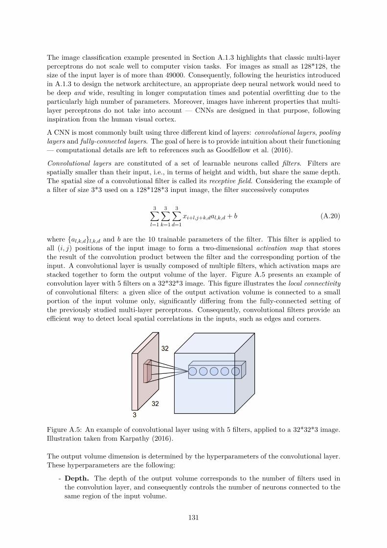
The image classification example presented in Section A.1.3 highlights that classic multi-layerperceptrons do not scale well to computer vision tasks. For images as small as 128*128, thesize of the input layer is of more than 49000. Consequently, following the heuristics introducedin A.1.3 to design the network architecture, an appropriate deep neural network would need tobe deep and wide, resulting in longer computation times and potential overfitting due to theparticularly high number of parameters. Moreover, images have inherent properties that multi-layer perceptrons do not take into account — CNNs are designed in that purpose, followinginspiration from the human visual cortex.

A CNN is most commonly built using three di�erent kind of layers: convolutional layers, poolinglayers and fully-connected layers. The goal of here is to provide intuition about their functioning— computational details are left to references such as Goodfellow et al. (2016).

Convolutional layers are constituted of a set of learnable neurons called filters. Filters arespatially smaller than their input, i.e., in terms of height and width, but share the same depth.The spatial size of a convolutional filter is called its receptive field. Considering the example ofa filter of size 3*3 used on a 128*128*3 input image, the filter successively computes

3ÿ

l=1

3ÿ

k=1

3ÿ

d=1xi+l,j+k,dal,k,d + b (A.20)

where {al,k,d}l,k,d and b are the 10 trainable parameters of the filter. This filter is applied toall (i, j) positions of the input image to form a two-dimensional activation map that storesthe result of the convolution product between the filter and the corresponding portion of theinput. A convolutional layer is usually composed of multiple filters, which activation maps arestacked together to form the output volume of the layer. Figure A.5 presents an example ofconvolution layer with 5 filters on a 32*32*3 image. This figure illustrates the local connectivityof convolutional filters: a given slice of the output activation volume is connected to a smallportion of the input volume only, significantly di�ering from the fully-connected setting ofthe previously studied multi-layer perceptrons. Consequently, convolutional filters provide ane�cient way to detect local spatial correlations in the inputs, such as edges and corners.

Figure A.5: An example of convolutional layer using with 5 filters, applied to a 32*32*3 image.Illustration taken from Karpathy (2016).

The output volume dimension is determined by the hyperparameters of the convolutional layer.These hyperparameters are the following:

- Depth. The depth of the output volume corresponds to the number of filters used inthe convolution layer, and consequently controls the number of neurons connected to thesame region of the input volume.

131

- Stride. The stride of the layer controls the way filters are applied over the input. Applyingfilters to all (i, j) positions of the input correspond to a stride of 1, but depending on filtersizes, practitioners can choose to apply filters every s pixels — that s corresponds to thestride hyperparamter.

- Padding. The padding controls the output volume spatial size by adding zeros to theborders of the input image. In literature, a valid padding corresponds to not adding zeroson the borders, and a same padding to adding zeros such that the output volume has thesame spatial size than its input. Concretely, by applying 3*3 filters on a 128*128 image,for the 127-th and 128-th positions of the x- and y-axis there is not enough pixels tocompute the convolution product — in this situation, padding the input image using two"borders" of zeros allows to retrieve 128*128 activation maps in output.

In a convolution layer, the number of weights and biases is given by f ◊ n2 ◊ d, with f the

number of filters, n the filter size and d the input depth. A depth slice of the output volume ofa convolution layer has been obtained using the same parameters — this is called the parametersharing scheme. This scheme is related to the property of translation invariance — as a givenfilter searches for a specific pattern in its input, constraining a slice depth to the same filtermakes it search for the feature in the exact same way in the whole input.

Pooling layers reduce the size of their input following a non-linear pooling function. The mostcommon pooling layer is the max-pooling. The max-pooling layer partitions each depth slice ofthe input into non-overlapping rectangles, and outputs the maximum of each of these regions.Pooling layers allow to gradually reduce the spatial size of the input, thereby reducing thenumber of parameters needed for computations and hence preventing overfitting.

Fully-connected layers correspond to the classic layers introduced in Section A.1.2. These layersare usually found at the end of computer vision networks and perform the classification orregression task at hand using the features extracted by the convolution layers of the network.

These types of layers are usually interwoven with ReLU activations, defined as f(x) = max(0, x),and all together form what we call (deep) convolutional neural networks. An example of suchnetwork is shown in Fig. A.6. In this figure, information flows bottom-up, from the picture of aSamoyed dog to its decomposition into features learnt by the network and a classification taskperformed by a last fully-connected layer. Among all 1000 classes of the ImageNet classificationtask, the right class is attributed 16% of probability.

In this thesis, we make use of one-dimensional convolution layers in Chapter 4. The com-putations performed with one-dimensional convolution layers follow the same idea than two-dimensional ones: for a given time series {xt}t and a filter of size n, a one-dimensional convo-lution computes

nÿ

l=1

mÿ

d=1xt+l,dal,d + b, (A.21)

with m the number of features per time-step t comprised in xt.

132

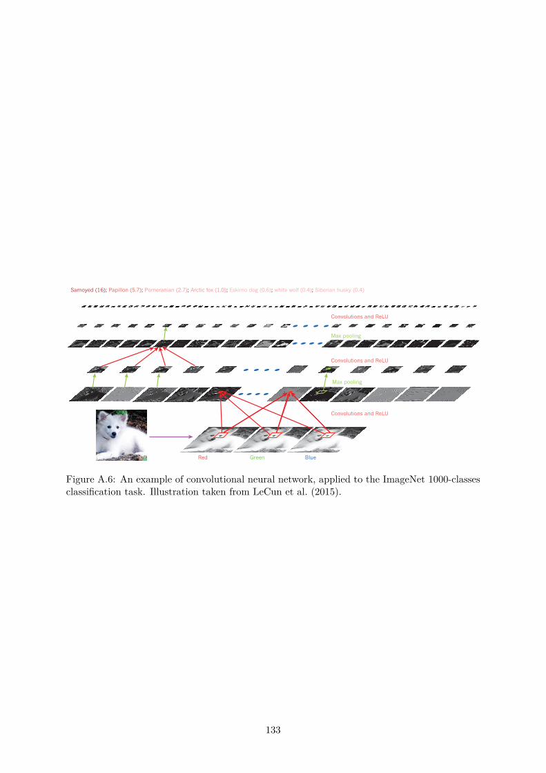
raw pixels could not possibly distinguish the latter two, while putting the former two in the same category. This is why shallow classifiers require a good feature extractor that solves the selectivity–invariance dilemma — one that produces representations that are selective to the aspects of the image that are important for discrimination, but that are invariant to irrelevant aspects such as the pose of the animal. To make classifiers more powerful, one can use generic non-linear features, as with kernel methods20, but generic features such as those arising with the Gaussian kernel do not allow the learner to general-ize well far from the training examples21. The conventional option is to hand design good feature extractors, which requires a consider-able amount of engineering skill and domain expertise. But this can all be avoided if good features can be learned automatically using a general-purpose learning procedure. This is the key advantage of deep learning.

A deep-learning architecture is a multilayer stack of simple mod-ules, all (or most) of which are subject to learning, and many of which compute non-linear input–output mappings. Each module in the stack transforms its input to increase both the selectivity and the invariance of the representation. With multiple non-linear layers, say a depth of 5 to 20, a system can implement extremely intricate func-tions of its inputs that are simultaneously sensitive to minute details — distinguishing Samoyeds from white wolves — and insensitive to large irrelevant variations such as the background, pose, lighting and surrounding objects.

Backpropagation to train multilayer architectures From the earliest days of pattern recognition22,23, the aim of research-ers has been to replace hand-engineered features with trainable multilayer networks, but despite its simplicity, the solution was not widely understood until the mid 1980s. As it turns out, multilayer architectures can be trained by simple stochastic gradient descent. As long as the modules are relatively smooth functions of their inputs and of their internal weights, one can compute gradients using the backpropagation procedure. The idea that this could be done, and that it worked, was discovered independently by several different groups during the 1970s and 1980s24–27.

The backpropagation procedure to compute the gradient of an objective function with respect to the weights of a multilayer stack of modules is nothing more than a practical application of the chain

rule for derivatives. The key insight is that the derivative (or gradi-ent) of the objective with respect to the input of a module can be computed by working backwards from the gradient with respect to the output of that module (or the input of the subsequent module) (Fig.!1). The backpropagation equation can be applied repeatedly to propagate gradients through all modules, starting from the output at the top (where the network produces its prediction) all the way to the bottom (where the external input is fed). Once these gradients have been computed, it is straightforward to compute the gradients with respect to the weights of each module.

Many applications of deep learning use feedforward neural net-work architectures (Fig. 1), which learn to map a fixed-size input (for example, an image) to a fixed-size output (for example, a prob-ability for each of several categories). To go from one layer to the next, a set of units compute a weighted sum of their inputs from the previous layer and pass the result through a non-linear function. At present, the most popular non-linear function is the rectified linear unit (ReLU), which is simply the half-wave rectifier f(z) = max(z, 0). In past decades, neural nets used smoother non-linearities, such as tanh(z) or 1/(1 + exp("z)), but the ReLU typically learns much faster in networks with many layers, allowing training of a deep supervised network without unsupervised pre-training28. Units that are not in the input or output layer are conventionally called hidden units. The hidden layers can be seen as distorting the input in a non-linear way so that categories become linearly separable by the last layer (Fig.!1).

In the late 1990s, neural nets and backpropagation were largely forsaken by the machine-learning community and ignored by the computer-vision and speech-recognition communities. It was widely thought that learning useful, multistage, feature extractors with lit-tle prior knowledge was infeasible. In particular, it was commonly thought that simple gradient descent would get trapped in poor local minima — weight configurations for which no small change would reduce the average error.

In practice, poor local minima are rarely a problem with large net-works. Regardless of the initial conditions, the system nearly always reaches solutions of very similar quality. Recent theoretical and empirical results strongly suggest that local minima are not a serious issue in general. Instead, the landscape is packed with a combinato-rially large number of saddle points where the gradient is zero, and the surface curves up in most dimensions and curves down in the

Figure 2 | Inside a convolutional network. The outputs (not the filters) of each layer (horizontally) of a typical convolutional network architecture applied to the image of a Samoyed dog (bottom left; and RGB (red, green, blue) inputs, bottom right). Each rectangular image is a feature map

corresponding to the output for one of the learned features, detected at each of the image positions. Information flows bottom up, with lower-level features acting as oriented edge detectors, and a score is computed for each image class in output. ReLU, rectified linear unit.

Red Green Blue

Samoyed (16); Papillon (5.7); Pomeranian (2.7); Arctic fox (1.0); Eskimo dog (0.6); white wolf (0.4); Siberian husky (0.4)

Convolutions and ReLU

Max pooling

Max pooling



4 3 8 | N A T U R E | V O L 5 2 1 | 2 8 M A Y 2 0 1 5

REVIEWINSIGHT

© 2015 Macmillan Publishers Limited. All rights reserved

Figure A.6: An example of convolutional neural network, applied to the ImageNet 1000-classesclassification task. Illustration taken from LeCun et al. (2015).

133

Université Paris-Saclay Espace Technologique / Immeuble Discovery

Route de l’Orme aux Merisiers RD 128 / 91190 Saint-Aubin, France

Titre : Apprentissage statistique pour la recommandation de produits financiers

Mots clés : apprentissage statistique, finance, systèmes de recommandation, clustering supervisé, systèmes de recommandation dépendants du temps, apprentissage profond

Résumé : L’anticipation des besoins des clients est cruciale pour toute entreprise — c’est particulièrement vrai des banques d’investissement telles que BNP Paribas Corporate and Institutional Banking au vu de leur rôle dans les marchés financiers. Cette thèse s’intéresse au problème de la prédiction des intérêts futurs des clients sur les marchés financiers, et met plus particulièrement l’accent sur le développement d’algorithmes ad hoc conçus pour résoudre des problématiques spécifiques au monde financier. Ce manuscrit se compose de cinq chapitres, répartis comme suit : - Le chapitre 1 expose le problème de la prédiction des intérêts futurs des clients sur les marchés financiers. Le but de ce chapitre est de fournir aux lecteurs toutes les clés nécessaires à la bonne compréhension du reste de cette thèse. Ces clés sont divisées en trois parties : une mise en lumière des jeux de données à notre disposition pour la résolution du problème de prédiction des intérêts futurs et de leurs caractéristiques, une vue d’ensemble, non exhaustive, des algorithmes pouvant être utilisés pour la résolution de ce problème, et la mise au point de métriques permettant d’évaluer la performance de ces algorithmes sur nos jeux de données. Ce chapitre se clôt sur les défis que l’on peut rencontrer lors de la conception d’algorithmes permettant de résoudre le problème de la prédiction des intérêts futurs en finance, défis qui seront, en partie, résolus dans les chapitres suivants ; - Le chapitre 2 compare une partie des algorithmes introduits dans le chapitre 1 sur un jeu de données provenant de BNP Paribas CIB, et met en avant les difficultés rencontrées pour la comparaison d’algorithmes de nature différente sur un même jeu de données, ainsi que quelques pistes permettant de surmonter ces difficultés. Ce comparatif met en pratique des algorithmes de recommandation classiques uniquement envisagés d’un point de vue

théorique au chapitre précédent, et permet d’acquérir une compréhension plus fine des différentes métriques introduites au chapitre 1 au travers de l’analyse des résultats de ces algorithmes ; - Le chapitre 3 introduit un nouvel algorithme, Experts Network, i.e., réseau d’experts, conçu pour résoudre le problème de l’hétérogénéité de comportement des investisseurs d’un marché donné au travers d’une architecture de réseau de neurones originale, inspirée de la recherche sur les mélanges d’experts. Dans ce chapitre, cette nouvelle méthodologie est utilisée sur trois jeux de données distincts : un jeu de données synthétique, un jeu de données en libre accès, et un jeu de données provenant de BNP Paribas CIB. Ce chapitre présente aussi en plus grand détail la genèse de l’algorithme et fournit des pistes pour l’améliorer ; - Le chapitre 4 introduit lui aussi un nouvel algorithme, appelé History-augmented collaborative filtering, i.e., filtrage collaboratif augmenté par historiques, qui proposes d’augmenter les approches de factorisation matricielle classiques à l’aide des historiques d’interaction des clients et produits considérés. Ce chapitre poursuit l’étude du jeu de données étudié au chapitre 2 et étend l’algorithme introduit avec de nombreuses idées. Plus précisément, ce chapitre adapte l’algorithme de façon à permettre de résoudre le problème du cold start, i.e., l’incapacité d’un système de recommandation à fournir des prédictions pour de nouveaux utilisateurs, ainsi qu’un nouveau cas d’application sur lequel cette adaptation est essayée ; - Le chapitre 5 met en lumière une collection d’idées et d’algorithmes, fructueux ou non, qui ont été essayés au cours de cette thèse. Ce chapitre se clôt sur un nouvel algorithme mariant les idées des algorithmes introduits aux chapitres 3 et 4.

Université Paris-Saclay Espace Technologique / Immeuble Discovery

Route de l’Orme aux Merisiers RD 128 / 91190 Saint-Aubin, France

Title : Machine learning for financial products recommendation

Keywords : machine learning, finance, recommender systems, supervised clustering, time-aware

recommender systems, deep learning

Abstract : Anticipating clients’ needs is crucial to any

business — this is particularly true for corporate and

institutional banks such as BNP Paribas Corporate

and Institutional Banking due to their role in the

financial markets. This thesis addresses the problem

of future interests prediction in the financial context

and focuses on the development of ad hoc

algorithms designed for solving specific financial

challenges.

This manuscript is composed of five chapters:

- Chapter 1 introduces the problem of future interests

prediction in the financial world. The goal of this

chapter is to provide the reader with all the keys

necessary to understand the remainder of this thesis.

These keys are divided into three parts: a

presentation of the datasets we have at our disposal

to solve the future interests prediction problem and

their characteristics, an overview of the candidate

algorithms to solve this problem, and the

development of metrics to monitor the performance

of these algorithms on our datasets. This chapter

finishes with some of the challenges that we face

when designing algorithms to solve the future

interests problem in finance, challenges that will be

partly addressed in the following chapters;

- Chapter 2 proposes a benchmark of some of the

algorithms introduced in Chapter 1 on a real-word

dataset from BNP Paribas CIB, along with a

development on the difficulties encountered for

comparing different algorithmic approaches on a

same dataset and on ways to tackle them. This

benchmark puts in practice classic recommendation

algorithms that were considered on a theoretical

point of view in the preceding chapter, and provides

further intuition on the analysis of the metrics

introduced in Chapter 1;

- Chapter 3 introduces a new algorithm, called

Experts Network, that is designed to solve the

problem of behavioral heterogeneity of investors

on a given financial market using a custom-built

neural network architecture inspired from mixture-

of-experts research. In this chapter, the introduced

methodology is experimented on three datasets: a

synthetic dataset, an open-source one and a real-

world dataset from BNP Paribas CIB. The chapter

provides further insights into the development of

the methodology and ways to extend it;

- Chapter 4 also introduces a new algorithm, called

History-augmented Collaborative Filtering, that

proposes to augment classic matrix factorization

approaches with the information of users and

items’ interaction histories. This chapter provides

further experiments on the dataset used in Chapter

2, and extends the presented methodology with

various ideas. Notably, this chapter exposes an

adaptation of the methodology to solve the cold-

start problem and applies it to a new dataset;

- Chapter 5 brings to light a collection of ideas and

algorithms, successful or not, that were

experimented during the development of this

thesis. This chapter finishes on a new algorithm that

blends the methodologies introduced in Chapters

3 and 4.

machine learning for financial products recommendation

Documents