' ,,

• j /~ev :l'.:~v c

I ~

I

ti

PROPOSED T.EX::HNICAL NOI'E

Statistical r-Ethcxis

•

-i-

Statistical Methods

I. Introduction

A. What Is Statistics? B. Purpose Of This Teclmical Note C. SAS: A 'Ibol For Statistics

II. Uses for Statistics in the SCS

III.

A. Dat:.a Collection (Sanpling) B~ Data Analysis C. Decision Making and Predictions

Basic;. ~taM:stics a:-V..t1vrr..., .)--<.. ..

A. t.,Mean B. Standard Deviation and Variance c. Coefficient Of Variation D. Standard Error Of The Mean E. Correlation Coefficient F. Using SAS

rJ. Sanpling Teclmiques

A. Sinple ~ Sanpling B. Semple Size

V. Confidence Limits (Reliability of The Semple)

VI. Hypothesis Testing

A. Testing ~ Mean B. Catparing Two Groups Of Data

(Test Of Difference)

VII. Linear Regression Analysis And Prediction

A. Sinple Regression B. Multiple Regression

• f ~.. -

.t

I

I

• -ii-

VIII. Appendix of Formulas

IX. Glossary

X. References

•

•

What Is Statistics?

W:mster defines statistics as: "the mathematics of the collection, organization, and interpretation of mmerical data1 especially the analysis of population characteristics by inference frc:ln sanpling." (It is inp::>rtant to note that statistics includes o~ization and interpretation of data.) 'Ibis definition has been "watered " in the past because people have confused the science of statistics with the plural fonn of statistic, the latter being defined as the nunerical data itself. Even though both are spelled the sane, their neanings are quite different. To minimize confusion, a statistic or a group of statistics will be referred to as data in this paper. '!be science of statistics deals with: · --

1. Designing surveys

2. Collecting and sumnarizing data

3. Measuring the variation in survey data

4. Measuring the accuracy of estimates

5. Testing hypotheses about the population

6. Studying relationships arrong two or nore variables

Statistics, then, boils down to the techniques used to obtain analytical rreasures, the methods for estimating their reliability, and the drawing of inferences f ran than.

Purpose of 'Ibis Technical lt>te

'!he purrose of this technical note is to facilitate in the understanding .of a variety of statistical techniques, their limitations, the asSUirptions behind than, and the\ interpretations that can be made fran than. It is written under the asSUirption that SCS personnel will at sare tine be involved in a prd::>lem solving situation in which a working knowledge of basic statistical rcethods would be useful. '!be purpose is not to pracote statistics as a panacea for all data prd:>lems, but to develop a guide for those wh::> have an opportunity to apply statistical analysis in their work •

•

I

•

• -2-

•

•

SAS: A Tool For Statistics

'!he Statistical Analysis System (SAS) is a cxmputer software system originally developed for statistical needs. SAS is not a carputer "language" in conventional terms as is FORI'RAN or a:>EOL. SAS is a collection of prewritten programs which cxrcpute statistical measures and can be accessed by a few relatively s~le carmands. ·

Ckle problem in writing a traditional statistical users guide is the ever-present mass of fornulas needed throughout to develop analytical measures. Their presence often leaves the ~rer frustrated, discouraged, and ultimately QJ;PJsed to any further use or study of statistics. But, by incorporating SAS into this paper, the pages of fornulas can be replaced by a few SAS programs. Ultimately, the statistical calculations can be done easily on a cxrcputer without the need for rrerorizing fornulas. The fornulas are, however, included in an Appendix so that the user is able to study the carplete derivations. ·

-3-

II. USES FOR SI'ATISTICS IN 'niE SCS

N:> matter what activities are underway in the SCS, it's very likely they involve problem-solving in scree fonn. The SCS technical specialist is often called into this process to interject his/her expertise whether it be in project work, conservation operations, or other SCS endeavors. The specialist uses the tools that he/she has learned in either fonnal or infonnal training as a means to answer questions and solve problems. Ci'le tool that can be useful in certain situations is statistics. '!here are basically three areas that the user of statistical metl'vxls is equipped to deal with:

1. Data collection (sarrpling)

2. Data analysis

3. Decision41laking and predictions

Data Collection (Sa111?ling)

•

Q1e of the ITOst fundarrental steps in ans-wering questions and solving I problems is the collection of relevant data about the problem. People are constantly in pursuit of the "correct" infonnation upon which to make day to day decisions. For nost, the accuracy of infonnation is only as inportant as the decision to be made. For exarrple, in collecting facts to detennine which brand of laundry detergent to purchase, one might ask a neighbor or a friend. lt>st, l'lo.Never, usually are content to learn by trial and error. And why not? The nost risked if the choice is incorrect is a few dollars. But, when one sets out to purchase a new autacobile, usually a nurrber of o.-Jners are questioned, many dealers are consulted, and consurrer periodicals are scoured to obtain data for the decision of whether or not to buy. After all, a new car is not a minor investrrent.

\

'llle use of infonnation gathering in SCS is not tmlike that of daily life. SCS personnel are constantly weighing whether or not additional infonnation (obtained at scree cost) will yield results which justify the effort and expense. Sate problems encamted are too minor to justify a large expenditure for detailed data collection. Q1 the other hand, scree decisions involve thousands of dollars and years of devel~t. It's only camon sense to appropriate nore effort to tl'x>se types of decisions. But, where is the line drawn? HON far should one go to insure the accuracy of data collection efforts? In ITOst situations, it is inp:>ssible to oollect infonnation fran every data source. For exarrple, the SCS may need to find out the extent conservation tillage is being used in the United States. It \tJOUld be inpossible to contact and interview every fann operator. So a sanple is taken fran the total of all famers. But, is the sanple large enough to reflect the "true" infonnation about all fa.mers? Conver5ely, • funds been wasted by taking a larger sarrple than necessary? Statistical

. '

•

•

•

-4-

netixxls can be used to help ans-wer these questions. With the aid of statistics during data collection, sarrple size which will meet specific precision criteria for each individual situation can be detennined. Olapter r.v deals specifically with the use of statistics in data collection.

Data Analysis

When data is received fran a sarrple, whether fran a pd.nary or a secondary source, confidence in that data is always a question. Using the conservation tillage exarrple, it is irrportant to know that the farrrers surveyed are representative of all farrrers. It is possible, through the use of statistical nethods, to quantify "confidence" in the reliability of the sanple data characterizing the total data. In fact, many of the basic statistical.treasures in Ciapter III can be tested for the degree of reliability they possess •. That is a unique characteristic of nodern statistical nethods.

Why is the ability to quantify confidence in statistical neasurenents so irrportant? Imagine assigning two people to independently carry out the study of a particular problem. 'lb make an intelligent decision, both people separately survey the problem, analyze the data, and report their results. Unfortunately, their results are very different. Person A subjectively decided to take a 10% sanple. He averaged the data and reported the average (nean) • Person B used statistics to determine the rcost econanical sample size. When his sample was collected he, again using statistics, was able to report hoN well his sarrple represented the total. His average (nean) was reported as well but he also included the limits of confidence that should be assuned for his s~le nean representing the actual nean.

'Ihe only thing that Person B did differently was to use statistical nethods to determine sample size and to quantify confidence in his results. NJw, which persons' analysis would be accepted? In rcost cases, a sanple estimate which includes an indication of reliability is intuitively rcore acceptable than one which does not.

Decision Making and Predictions

'Ihe main purpose of ItDst SCS studies is eventually to make sare decision or to predict a future trend or event. It is possible to use statistics in both cases. Hypothesis testing is a nethod that can be used to carpare an estimate or intelligent guess, to actual sanpled data. For exarrple, if infonnation was obtained that the average soybean yield in Iowa was 33 bushels per acre, and the figure seated low, a quick sample could developed fran Ag census data or sare other obtainable source. Using this sanple and the techniques of hypothesis testing, a statistical test oould be perfonred to see if the average yield was indeed 33 bushels per acre. (Nurcerical exanples of hypothesis testing are given in Ciapter VI •

-5-

Predicting the future is a job rost SCS technical specialists are expected to perfonn to sace extent. Statistics provides a nethod called regression which enables the user to predict future trends based on past data. For exanple, it is possible to est:imate future yields based on past yields and associated, levels of fertilizer, herbicide, etc. 'Ibis type of relationship be'bleen inputs in agriculture and associated yields is cxxmonl y knoWn as a production function. Why is it called a function? Because the end result of regression analysis is a mathenatical equation (function) which can be used for prediction. 'Ibis is one of the nnst powerful tools in statistics and probably the nost widely used. P.egression analysis is covered in Chapter VII.

'lb sumrarize, statistics carbined with SAS gives the user:

1. A nurrber of ways to sanple and analyze data, (Chapters III, rv, VI, and VII).

2. Sinple, tine-saving nearu; to quantify the reliability of the sanple (Chapter V) •

3. Techniques to carpare estimates and data (Chapters III and VI).

4. A way to predict future trends based on past events (Chapter VII).

•

•

•

•

•

•

-6-

III. BAsIC STATISTICS

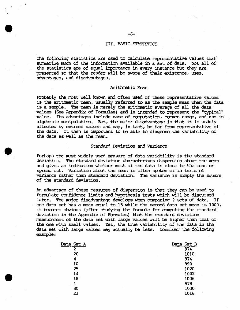
'!he following statistics are used to calculate representative values that surmarize much of the information available in a set of data. lt>t all of the statistics are of equal inp:>rtance in ever:y instance but they are presented so that the reader will be aware of their existence, uses, advantages, and disadvantages.

Arithrretic M3a.n

Probably the rrost \\1ell known and often used of these representative values is the aritimetic rcean, usually referred to as the sample rcean when the data is a sarcple. '!he rcean is rerely the arithrcetic average of all the data· values (See ~ of Fonrn.llas) and is intended to represent the "typical" value. Its advantages include ease of catpltation, cumon usage, and use in algebraic manipulation. But, the major disadvantage is that it is unduly affected by extrene values and may, in fact, be far fran representative of the data. It then is inp:>rtant to be able to diagnose the variability of the data as \\1ell as the rcean.

Standard Deviation and Variance

Perhaps the rrost widely used reasure of data variability is the standard deviation. The standard deviation characterizes dispersion arout the rcean and gives an indication whether nost of the data is close to the rcean or spread out. Variation arout the rcean is often spoken of in terms of variance rather than standard deviation. '!be variance is sinpl y the square of the standard deviation.

An advantage of these reasures of dispersion is that they can be used to fonm.ilate confidence limits and hypothesis tests which will be discussed later. The major disadvantage develops when ccrrparing 2 sets of data. If one data set has a rcean equal to 15 while the second data set nean is 1000, it becares obvious (flfter studying the fonm.ila for ccrrputing the standard deviation in the ~ of Fonmllas) that the standard deviation reasurenent of the data set with large values.will be higher than that of the one with small values. Yet, the true variability of the data in the data set with large values may actual! y be less. Consider the following exanple:

Data Set A 2 20 4 10 25 14 18 4 30 23

Data Set B 974 1010 974 990 1020 1002 1006 978 1030 1016

-7-

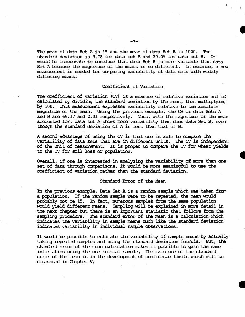
'!he mean of data Set A is 15 and the mean of data Set B is 1000. The standard deviation is 9.78 for data set A and 20.09 for data set B. It would be inaccurate to conclude that data Set B is rrore variable than data Set A because the magnitude of the means is so different. In essence, a new neasurercent is needed for ccrrparing variability of data sets with widely differing means.

Coefficient of Variation

'!he coefficient of variation (CV) is a measure of relative variation and is calculated by dividing the standard deviation by the mean, then nultiplying by 100. '!his measurercent expresses variability relative to the absolute magnitude of the mean. Using the previous exaJtt>le, the CV of data Sets A and Bare 65.17 and 2.01 respectively. Thus, with the magnitude of the mean accounted for, data set A shows nore variability than does data Set B, even though the standard deviation of A is less than that of B.

A second advantage of using the CV is that one is able to ccrrpare the variability of data sets that are in different units. '!he CV is independent of the unit of measurercent. It is proper to ccrrpare the CV for wheat yields to the CV for soil loss or population.

Overall, if one i's interested in analyzing the variability of rrore than one set of data through ccrrparisons, it would be nore meaningful to use the coefficient of variation rather than the standard deviation.

Standard Error of the Mean

In the previous exarrple, Data Set A is a randan sarrple which was taken fran a population. If the randan sanple were to be repeated, the mean would probably not be 15. In fact, nunerous sarrples fran the sarre population would yield different means. Sarcpling will be explained in rrore detail in the next chapter but there is an inportant statistic that follCMS fran the sarcpling procedure. '!he standard error of the mean is a calculation which indicates the variability in salll>le means much like the standard deviation indicates variability in individual sanple ooservations.

It would be possible to estimate the variability of sanple means by actually taking repeated sanples and using the standard deviation forrrula. But, the standard error of the mean calculation makes it possible to gain the same infonnation using the one initial sanple. The main use of the standard error of the mean is in the develq:m:mt of oonfidence limits which will be discussed in Chapter v.

•

•

•

•

•

•

-8-

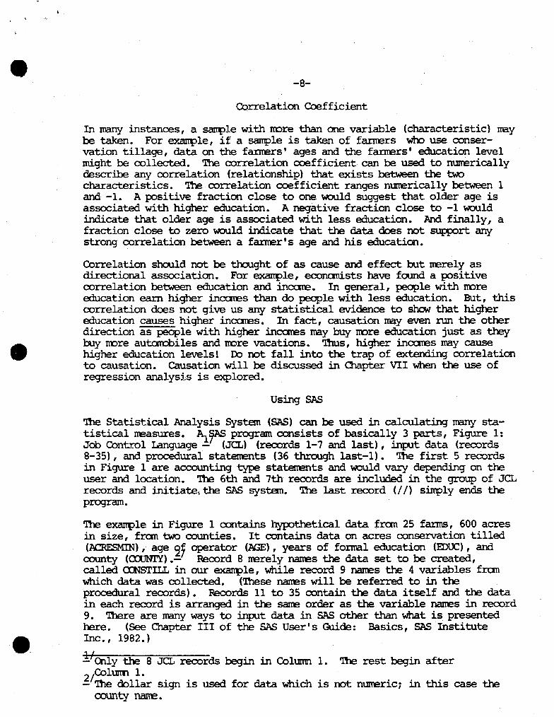
Correlation Coefficient

In many instances, a satl1?le with nore than one variable (characteristic) may be taken. For exarrple, if a satl1?le is taken of fancers who use conser­vation tillage, data on the fancers' ages and the fancers' education level might be collected. The correlation coefficient can be used to mmerically describe any correlation (relationship) that exists between the two characteristics. The correlation coefficient ranges numerically between 1 and -1. A positive fraction close to one would suggest that older age is associated with higher education. A negative fraction close to -1 wuuld indicate that older age is associated with less education. And finally, a fraction close to zero \\Ullld indicate that the data does not support any strong correlation between a fancer's age and his education.

Correlation should not be thought of as cause and effect but merely as directional association. For exanple, econanists have found a positive correlation between education and incare. In general, people with nore education eam higher incC.rces than do people with less education. But, this correlation does not give us any statistical evidence to show that higher education causes higher incares. In fact, causation may even nm the other direction as people with higher incares may buy nore education just as they buy nore autarobiles and nore vacations. '1hus, higher inc::cmas may cause higher education levels! Ib not fall into the trap of extending correlation to causation. Causation will be discussed in Chapter VII when the use of regression analysis is explored.

Using SAS

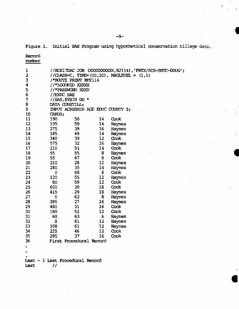
'!be Statistical Analysis Systan (SAS) can be used in calculating many sta­tistical measures. ~~ program consists of basically 3 parts, Figure 1: Job Control Language - (JCL) (records 1-7 and last), input data (records 8-35), and procedural statercents (36 through last-1). The first 5 reeords in Figure 1 are accounting type statenents and 'WOUld vary depending on the user and location. The 6th and 7th records are included in the group of JCL records and initiate\ the SAS systan. The last record (I I) sinpl y ends the program.

The exanple in Figure 1 contains hypothetical data fran 25 fanns, 600 acres in size, fran two counties. It contains data on acres conservation tilled (ACRF.SMIN), age <21 operator (J>iGE), years of fo:rmal education (EDUC), and county (cnJNI'Y).- Pecord 8 merely nanes the data set to be created, called a:NSTILL in our exarrple, while record 9 nanes the 4 variables fran which data was collected. (These nanes will be referred to in the procedural records). Pecords 11 to 35 contain the data itself and the data in each record is arranged in the sarre order as the variable nanes in record 9. There are many ways to input data in SAS other than what is presented here. (See Chapter III of the SAS User's Guide: Basics, SAS Institute Inc., 1982.)

ll Only the 8 JCL records begin in Colurm 1. The rest begin after

21eo1urm 1. - '!be dollar sign is used for data which is not numeric; in this case the

county nane.

• -9-

Figure 1. Initial SAS Program using hypothetical oonservation_tillage data.

Record m.ri:>er

1 I /SCSl 7DN:. JOB (XXXXXXXXXX, PJ114) ' 'FWrX/SCS-SNOC-IXXJG I ;

2 //CI..ASS=C, TIME=(00,20), MSGI..EVEL = (1,1) 3 I *RCXJTE PRINT RMI'l14 4 //*~ID XXXXX 5 //*P~RD XXXX 6 //FXFC SAS 7 //SAS.SYSIN DD * 9· DATA CONSTILL; Q INPUT N:.RESMIN AGE EDUC CCXJNrY $; J

10 CARDS; 11 190 50 14 Cook 12 135 59 14 Haynes 13 275 39 16 Haynes 14 185 49 14 Haynes 15 340 39 12 Cook 16 575 32 16 Haynes 17 210 51 14 Cook • 18 95 55 8 Haynes 19 55 67 8 Cook 20 210 28 12 Haynes 21 280 35 14 Haynes 22 0 68 8 Cook 23 120 55 12 Haynes 24 80 59 12 Cook 25 600 30 18 Cook 26 415 . 29 18 Haynes 27 0 62 8 Haynes 28 395 27 16 Haynes 29 480 31 16 Cook 30 180 52 12 Cook 31 60 63 6 Haynes 32 0 61 12 Haynes 33 108 61 12 Haynes 34 225 46 12 Cook 35 295 37 16 Cook 36 First Procedural Pecord

. last - 1 last Procedural Fecord last //

•

•

•

•

-10-

'll1e procedural records are tOOse which are used to initiate.the prewritten programs of SAS. These programs include a nurrber of applications for statistics as will becare evident through use of the conservation tillage ex.ample. Because the procedural records vary depending upon the specific program desired, Figure 1 displays only space·for the records (records 36 ••• Last-1). Specific procedural records will be supplied in conjunction with the specific program as each chapter warrants.

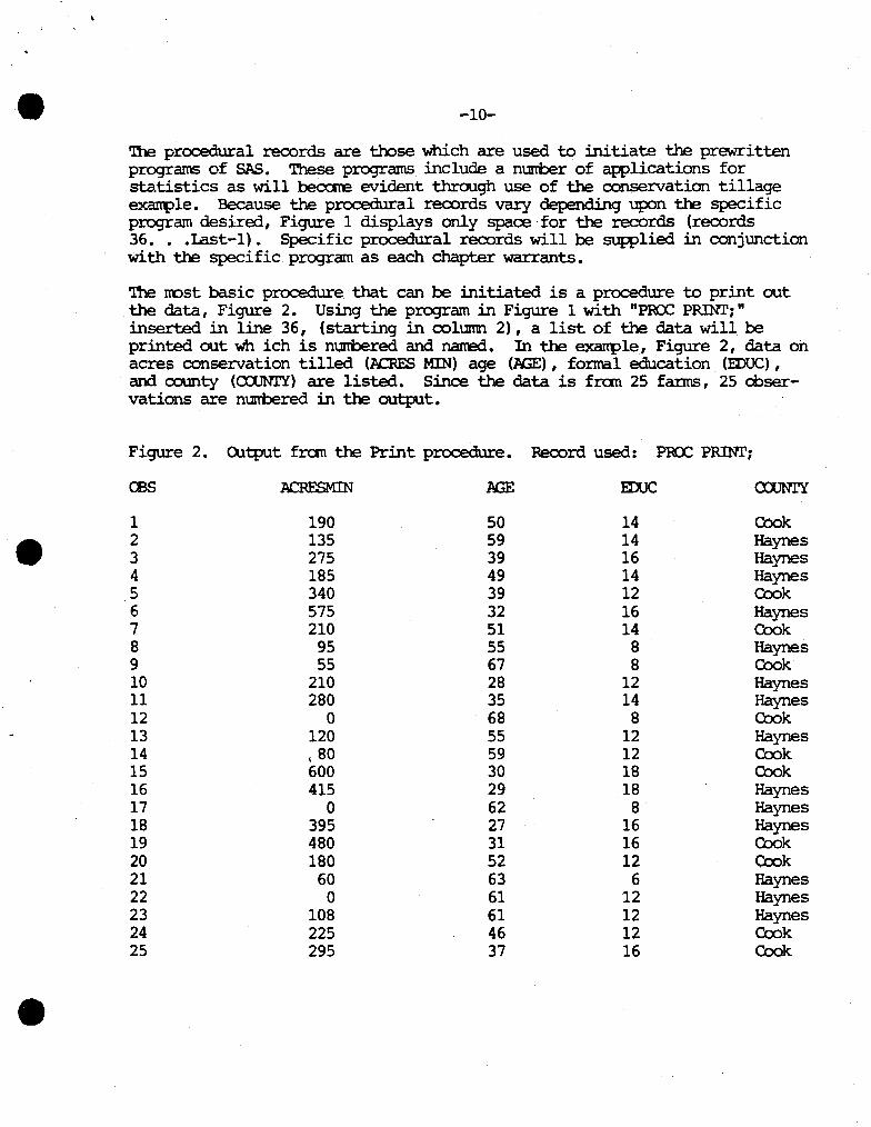
The rcost basic procedure that can be initiated is a procedure to print out the data, Figure 2. Using the program in Figure 1 with "PRO: PRINT;" inserted in line 36, (starting in column 2), a list of the data will be printed out wh ich is nurrbered and narred. . In the exanple, Figure 2, data oh acres conservation tilled (.ACRES MIN) age {.AGE) , fonnal education (EDUC) , and county (ca.JNI'Y) are listed. Since the data is fran 25 fanns, 25 obser­vations are nurrbered in the output.

Figure 2. Q.itput fran the Print procedure. Record used: PRO: PRINr;

CBS .ACRFSMIN .AGE ID.JC caJNI'Y

1 190 50 14 Cook 2 135 59 14 Haynes 3 275 39 16 Haynes 4 185 49 14 Haynes 5 340 39 12 Cook 6 575 32 16 Haynes 7 210 51 14 Cook 8 95 55 8 Haynes 9 55 67 8 Cook 10 210 28 12 Haynes 11 280 35 14 Haynes 12 0 68 8 Cook 13 120 55 12 Haynes 14 \ 80 59 12 Cook 15 600 30 18 Cook 16 415 29 18 Haynes 17 0 62 8 Haynes 18 395 27 16 Haynes 19 480 31 16 Cook 20 180 52 12 Cook 21 60 63 6 Haynes 22 0 61 12 Haynes 23 108 61 12 Haynes 24 225 46 12 Cook 25 295 37 16 Cook

-11-

Cbservation one represents a 50 year old famer fran Cook County with two years post high school education who conservation tills 190 of his 600 acres. Cbservation two represents a 59 year old farner fran Haynes County with two years post high school education who conservation tills 135 of his 600 acres, and so on.

There are two major uses for this procedure. The first is to supply the user with a hard copy of his/her data. '!he second is to allCM the user to easily check his/her data for keypunching errors •

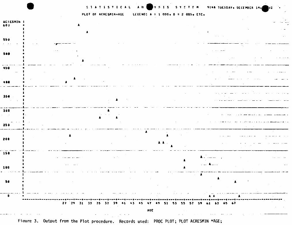
.Another way to view the data is by plotting it on a graph. SAS has a procedure called Plot which can provide a two dirrensional graph with very little user effort. 1}gures 3 and 4 sh::M that two records inserted into the program of Figure 1 - produce a two variable graph which.is scaled and labeled. In Figlire 3, acres conservation tilled l1'.CRFSMJN) is plotted against the farr-~rs' age (AGE) • · ACRESMIN is designated to the. vertical axis because it is listed first in the record "PIDI' ACRESMIN *.AGE;". If AGE was . first, it would be on the vertical axis. Acres conservation tilled and age are considered inversely related because the two sets of data nove in q>posi te directions. '!hat is, lower levels of conservation tillage . are . associated with higher ages while higher levels of conservation tillage are associated with lower ages. This inverse relationship between the two sets of data can be recognized in a graph by a general downward slope of the points.

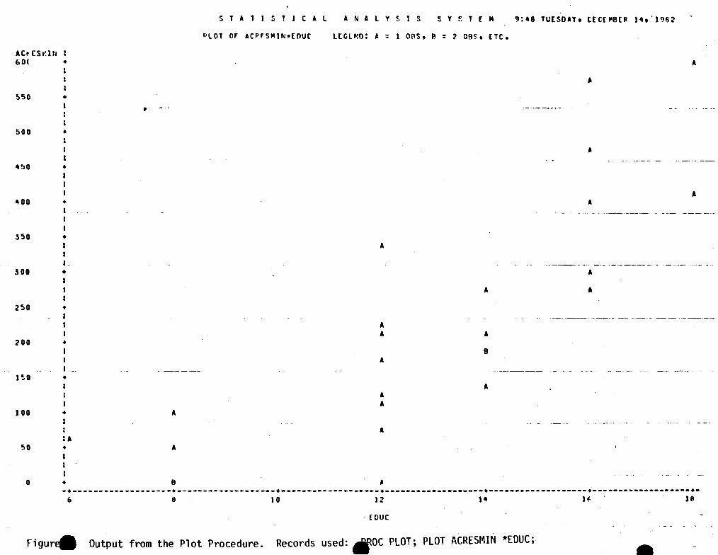
Figure 4 is a graph of ACRESMIN and EDUC. These two sets of data indicate graphically that conservation tilled acres and fanrers' education are directly related because higher levels of conservation tillage are associated with higher levels of education anong the farners sanpled. This direct relationship is characterized by an upward slope of the data points.

!tbst of this chapter has been devoted to defining a few basic statistics which are useful in problem solving professions. Difficulties arise in the use of many of these neasures because the calculations are time-consuming and saretirces cx:mplex, especially if the data sets being studied are vecy large (see Appendix of Formulas). But, fran the develop- nent of SAS cane a procedure called Means which calculates these rreasures for the user. With one procedural record, Figure 5, a rnmber of useful treasures are produced for each variable (characteristic) of the data set.

Using the conservation tillage exanple, Figure 5, the average faI."Iter (out of 25 sw:veyed) was 47 years old with alnost a year of post high school education who conservation tilled 220 of his 600 acres. 'lhe m:inimJm and maxim.mt values of the 3 variables give a feel for the rarKJe of values in the data. Acres which were conservation tilled ranged frcm O to 600; age ranged fran 27 to 68; and education ranged fran 6th grade to Masters Degree.

! 1'1hese records should be inserted in spaces designated "Procedural records" in Figure 1.

•

•

•

~C:lESMJ~ 60 JI +

551» •

511 • I I

•

··- -- ·---. ···-··. -- --- .

... •

S T A T I S T I C A L A H • Y ~ I S S Y ~ T r M CJ:-8 1UlSDAh l>CCC li'BCR H 9.32

PLOT OF lCRE~lN•lGl L[G[NO: A : l oas. 8 = 2 oe~. Etc.

A

l

-r-·--·-·

A

A

• · -·---- ·- .... -· .. ----· I I

351 • I I

--·- - ----1.--3 g,g •

L I I

250 • ---··-··----•- -- --·· - .

I

• 200 • I

• . .J. ___ . ___ .

15il •

lH • - - - ... - - - . '-· •· -----

1 I

50 •

0 •

.. --··· ·-·····. -·- -·· .. _ .. -------------------

A l

l

A l l

-·-· -··-·· ------l

A. - . -·

• l

. ' --------------------·---·---·---·---·---·---·---·---·---·---·---·---·---·---·---·---·---·---·---·---·--------------------~- .

AGE

Fiaure 3. Output from the Plot procedure. Records used: PROC PLOT; PLOT ACRESMIN *AGE;

ACt ESt'.lU &Ol •

550 •

500 •

4~0 •

•

l50 •

300

& I L_

•

250 •

200 •

I

I --1 !.O •

100

50

0

•

: A

•

•

..

S T A t I S T l C A l

0 LOT OF ACPrSMIN•EOUC

A

A

8

A~ALY~lS S Y ~ T £ M

ltGUJO: A : oos, ~ = 2 oes. rrc.

A

A A

A

A A

A

A

A

8

A

A

A A

A

-·-------------------·-------------------·-------------------·------------~---.---·-------------------·-~-----------------·-6 8 10 12 14 lf 18

£0UC

Figur. Output from the Plot Procedure. Records used: .QC PLOT; PLOT ACRESMIN *EDUC;

• -14-

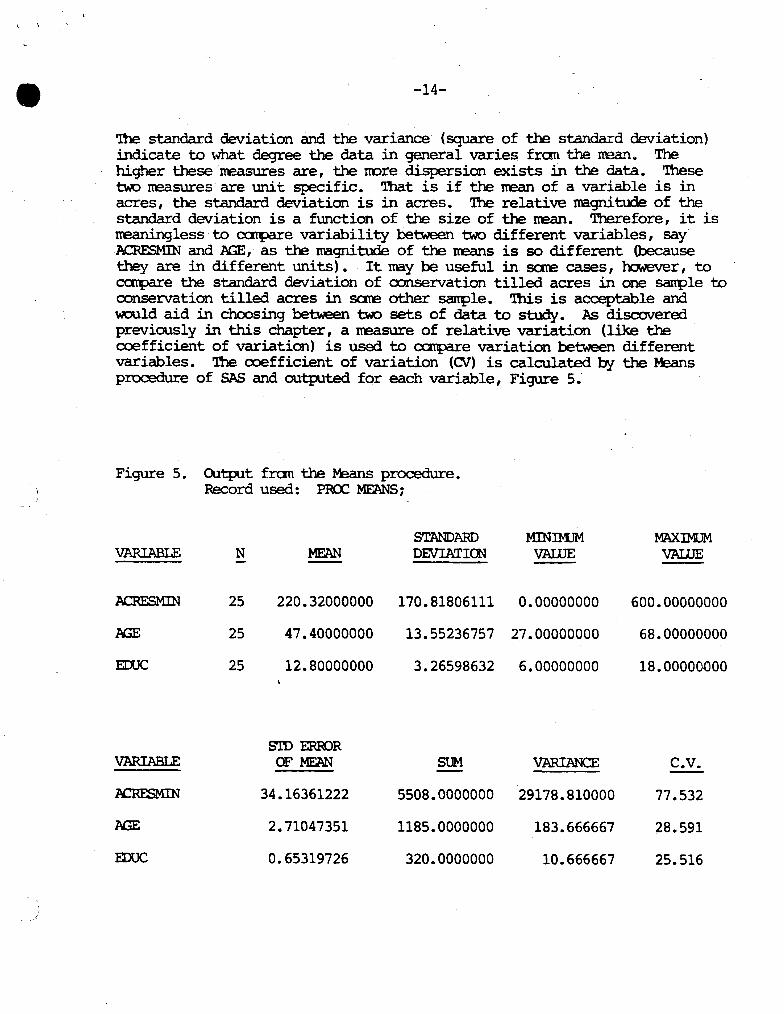
'!he standard deviation and the variance (square of the standard deviation) indicate to what degree the data in general varies fran the xrean. The higher these ·It'F'...asures are, the nore dispersion exists in the data. 'lhese two measures are unit specific. That is if the mean of a variable is in acres, the standard deviation is in acres. The relative magnitude of the . standard deviation is a function of the size of the mean. Therefore, it is rreaningless to canpare variability between two different variables, say ACRF.sMIN and AGE, as the magnitude of the neans is so different (because they are in different units). It may be useful in scree cases, however, to canpare the standard deviation of oonservation tilled acres in one sarcple to oonservation tilled acres in scree other sanple. '!his is acceptable and would aid in choosing between two sets of data to study. As discovered previously in this chapter, a measure of relative variation (like the coefficient of variation) is used to canpare variation between different variables. The coefficient of variation (CV) is calculated by the Means procedure of SAS and outputed for each variable, Figure 5.

Figure 5.

VARIABLE

ACRF.sMIN

AGE

EOOC

VARIABLE

EDUC

CAltput fran the Means procedure. Record used: PRO: MEANS;

N

25

25

25

MEAN

220.32000000

47.40000000

12.80000000

STD ERROR OF MEAN

34.16361222

2.71047351

0.65319726

STANDARD MINIKJM DEVIATIOO VAilJE

170.81806111 0.00000000

13.55236757 27.00000000

3.26598632 6.00000000

SUM VARIANCE

5508.0000000 29178.810000

1185.0000000 183.666667

320.0000000 10.666667

MAXIMUM VAilJE

600.00000000

68.00000000

18.00000000

c.v.

77.532

28.591

25.516

-15-

'!he standard error, which can be thought of as the standard deviation of sant>le means, is also supplied in the ~ prcx::edure. This treasure is used extensively in the developrent of confidence intervals which will be discussed in Cl1apter V.

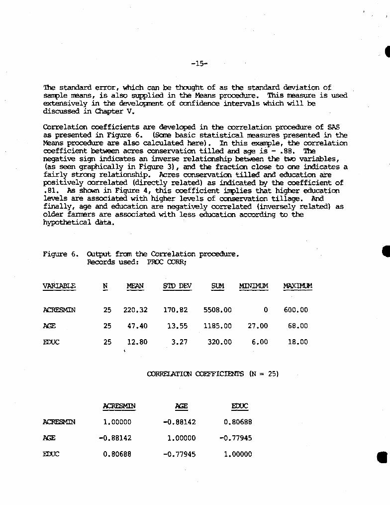
Correlation coefficients are developed in the oorrelation procedure of SAS as presented in Figure 6. (Sate basic statistical neasures presented in the Means procedure are also calculated here). In this exanple, the oorrelation ooefficient between acres oonservation tilled and age is - • 88. The negative sign indicates an inverse relationship between the two variables, (as seen graphically in Figure 3), and the fraction close to one indicates a fairly strong relationship. Acres oonservation tilled and education are positively oorrelated (directly related) as indicated by the coefficient of .81. As shOllll in Figure 4, this coefficient ~lies that higher education levels are associated with higher· levels of conservation tillage. And finally, age and education are negatively oorrelated (inversely related) as older farners are associated with less education according to the hypothetical data.

Figure 6.

VARIABLE

N:RESMIN

AGE

EDUC

ID.JC

Q.itput fran the Correlation procedure. Records used: PRCC CORR;

N MEAN S'ID DEV SUM MINIMUM

25 220.32 170.82 5508.00 0

25 47.40 13.55 1185.00 27.00

25 12.80 3.27 320.00 6.00

CORREI.ATIOO COEFFICIENI'S (N = 25)

1.00000

-0.88142

0.80688

-0.88142

1.00000

-0.77945

0.80688

-0.77945

1.00000

MAXIMUM

600.00

68.00

18.00

•

•

•

•

•

•

rv.

-16-

SAMPLING TOCHNICUES

Alnost everyone in today's society is affected by sanpling in one way or. another. Polls are taken for public opinion, manufactured products are sanpled for quality control, and consurrers are surveyed to disclose their wants in market analyses. A car load of coal or grain is accepted or rejected based on analysis of a few pounds. Physicians make decisions about health based on a few drops of blood. Politicians are projected to win or lose based on results fran a few precincts. '!be use of sarrpling is very widespread, yet the inp:>rtance of sarrpling sareti.nes goes unnoticed. In SCS, day to day duties, are often fulfilled with studies or raw data that originated as a survey or 5a1I1?le of sare kind.

A sanple is basically a small oollection of infonnation fran sare larger aggregate, the population. '!be 5a1I1?le is collected and analyzed to make inferences about the total population. What makes this process nore difficult is the presence of variation. If every farmer on earth was alike, a sanple of 1 farmer would represent all farmers. Since this is not the case and rcerrbers of a population are usually different, successive sanples are usually different. '!bus, the major task is to reach appropriate conclusions about the population in spite of sarrpling variation.

There are a nurrber of different sarcples that are used. They are distinguished by the manner in which the sanple is obtained, the nurrber of variables recorded, and the purpose for drawing the sanple. When considering the net.hod of collection, ~ broad cl.asses of sanpling are possible; oollection by judgerrent and collection by chance. Collection by chance, called randan sanpling, is preferred over judgerrental oollection because with randan sanpling infonnation fran the observed sarrple can be mathematically deduced based on the laws of prd:>ability. The purpose of randanness is to make certain these laws apply. There are no such laws which can apply to personal judgem:mt.

SIMPLE RANrQ1 SAMPLING

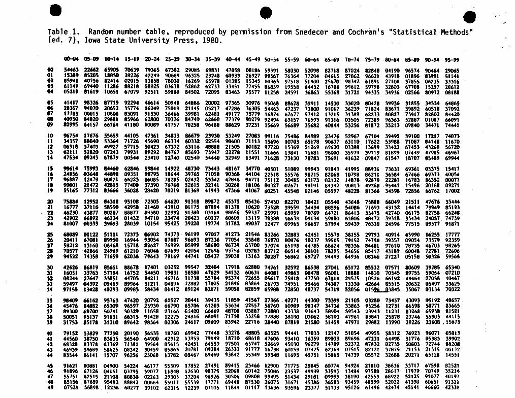
If a sarrple is chosen so that each value in the population has an equal and independent chance of being oollected, it is ~ sinple randan sanple. A sanple of this type can be obtained in a nurrber of ways. Drawing marbles fran an urn, tossing ooins, and throwing dice are classical nethods of cbtaining randarness. '!be nore nodem net.hod is to use a table of randan nurrbers, Table· 1. This table contains 10,000 digits jUllbled in randan fashion with 5 x 5 blocks to facilitate reading. There are 100 rcMS and 100 oolumns nunbered fran 00 to 99.

'lb illustrate the use of a table of randan nunbers, assurre a list of 700 farmers in the~ oounty area (Cook and Haynes), nurrbered fran 1-700. SuFJEX'511a sarrple of 25 farmers fran the population of 700 is to be drawn.-

~(

-17-

Refer to a table of randan nurcbers such as Table 1 to draw a randan sarcple and proceed through the following steps:

1. Flip a coin (or any other nethcxl) to choose which page of the table to begin with. ·

2. Without direction, bring a pencil point dONn on the page so as to hit a digit.

3. Read this digit and the next three to the right, e.g. 3478.

4. re~ ~he first two digits (34) signify a rCM and the last two digits colunn.

5. the point in the table (row 34, colunn 78) and read that digit '· :.md the next two on the right. '!his nunber is 960.

6. Starting at this point, run down the colunn and reoord the nurct>ers between 001 and 700. 'nle nurrbers observed are 960, 807, 561, 431, 412, 821, etc. Record 561, 431, and 412, etc. because they are between 001 and 700, which is within the range of nurcbers assigned to the ?JpUlation of fanrers. When the bottan of the page is reached, nurct>er 964, nove to the next 3 columns to the right and start back up. Continue this process until 25 nurci:>ers between 001 and 700 are collected. '1'he fanters that correspond to these 25 nurrbers constitute a randan sarrple.

The net.hod presented here is not sacred. It makes no difference whether nuvernent is up or down, left or right. As long as the digits are collected in this general fashion of randanness, any oontrived technique is

· permissible.

Sanple Size

Before the randan nurrber table is of any use, it llU.lSt be decided OC,.., large a Sar£l>le is needed. As discussed earlier, too snail a sarrple may lead to inaccurate assumptions about the population. C!:>serving one fanter' s conservation tillage net.hods does not tell nuch about the other 699 fanters in the area. Yet, it is not necessary to survey all 700 fanners either. This involves undue expense and tine. ·

One nethod for determining adequate sar£1?le size uses the following equation:

tV n=--E2

I

•

• • • r

Table 1. Random number table, reproduced by pennission from Snedecor and Cochran's "Statistical Methods" (ed. 7), Iowa State University Press, 1980.

G0-04 05-09 10-14 15-19 20-24 25-29 30-34 35-39 *-44 45-49 50-54 55-59 60-64 65~9 70-74 75-79 80-84 85-89 90-94 95-99

00 54463 22662 65905 70639 79365 67382 290115 69831 47058 08186 59191 58030 52098 82718 87024 82848 04190 96574 90464 29065 01 15389 15205 18850 39226 42249 90669 96325 23248 60933 26927 99567 76164 77204 04615 27062 96621 43918 01896 83991 51141 02 15941 40756 82414 02015 13858 78030 16269 65978 01385 15345 10363 97518 51400 25670 98342 61891 27101 37855 06235 33316 03 61149 69440 11286 88218 58925 03638 52862 62733 33451 77455 86859 19558 64432 16706 99612 59798 32803 67708 15297 28612 04 05219 11619 10651 67079 92511 59888 84502 72095 83463 75577 11258 24591 36863 55368 31721 94335 34936 02566 80972 08188

05 41417 98326 87719 92294 46614 50948 64886 20002 97365 30976 95068 88628 35911 14530 33020 80428 39936 31855 34334 64865 06 28357 94070 20652 35774 16249 75019 21145 05217 47286 76305 54463 47237 73800 91017 36239 71824 83671 39892 60518 37092 07 17783 00015 10806 83091 91530 36466 39981 62481 49177 75779 16874 62677 57412 13215 31389 62233 80827 .73917 82802 84420 08 40950 14820 29881 85966 62800 70326 84740 62660 77379 90279 92494 63157 76593 91316 03505 72389 96363 52887 01087 66091 09 12995 64157 66164 41180 10089 41757 78258 96488 88629 37231 15669 56689 35682 40844 53256 81872 35213 09840 34471 74441

10 96754 17676 55659 44105 47361 34833 86679 23930 53249 27083 99116 75486 14989 23476 52967 67104 39495 39100 17217 74073 11 34357 88040 53364 71726 45690 66334 60332 22554 90600 71113 15696 10703 65178 90637 63110 17622 53988 71087 84148 11670 12 06311 37403 49927 57715 50423 67372 63116 48888 21505 80182 97720 15369 51269 69620 03388 13699 33423 67453 43269 56720 u 62111 52820 07243 79931 89292 84767 85693 73947 22278 11551 11666 13841 71681 98000 35979 39719 81899 07449 47985 46967 14 47534 09243 67879 00544 23410 12740 02540 54440 32949 13491 71628 73130 78783 75691 41632 09847 61547 18707 85489 69944

15 91614 75993 84460 62846 59844 14922 48730 73443 48167 34770 40501 51089 99943 91843 41995 88931 73631 69361 05375 15417

" 24856 03648 44898 09351 98795 18644 39765 71058 90368 44104 22518 55576 98215 82068 10798 86211 36584 67466 69373 40054 17 96887 12479 80621 66223 86085 78285 02432 53342 42846 94771 75112 30485 62173 02132 14878 92879 22281 16783 86352 00077 .. 90801 21472 42815 77408 37390 76766 52615 32141 30268 18106 80327 02671 98191 84342 90813 49268 95441 15496 20168 09271 19 55165 77312 83666 36028 28420 70219 81369. 41943 47366 41067 60251 45548 02146 05597 48228 81366 34598 72856 66762 17002

• 75814 12952 14318 95108 72305 64620 91318 89872 45375 85436 57430 82270 10421 05540 43648 75888 66049 21511 47676 33444 21 16777 37116 58550 42958 21460 43910 01175 87894 81378 10620 73528 39559 34434 88596 54086 71693 43132 14414 79949 85193 22 46230 43877 80207 88877 89380 32992 91380 03164 98656 59337 25991 65959 70769 64721 86413 33475 42740 06175 82758 66248 23 42902 66892 46134 01432 94710 23474 20423 60137 60609 13119 78388 16638 09134 59880 63806 48472 39318 35434 24057 74739 24 11007 00333 39693 28039 10154 95425 39220 19774 31782 49037 12477 09965 96657 57994 59439 76330 24596 77515 09577 91871

25 68089 01122 51111 72373 06902 74373 96199 97017 41273 21546 83266 32883 42451 15579 38155 29793 40914 65990 16255 177T1 26 20411 67081 89950 16944 93054 87687 96693 87236 77054 33848 76970 80876 10237 39515 79152 74798 39357 09054 73579 92359 27 58212 13160 06468 15718 82627 76999 05999 58680 96739 63700 37074 65198 44795. 68624 98336 84481 97610 78735 46703 98265 21 70577 42866 24969 61210 76046 67699 42054 12696 93758 03283 83712 06514 30101 78295 54656 85417 43189 60048 72781 72606 29 94522 74358 71659 62038 79643 79169 44741 05437 39038 13163 20287 56862 69727 94443 64936 08366 27227 05158 50326 59566

30 42626 86819 85651 88678 17401 03252 99547 32404 17918 62880 74261 32592 86538 27041 65172 85532 07571 80609 39285 65340 ,. 16051 33763 57194 16752 54450 19031 58580 47629 54132 60631 64081 49863 08478 96001 18888 14810 70545 89755 59064 07210 J2 08244 27647 33851 44705 94211 46716 11738 55784 95374 72655 05617 75818 47750 67814 29575 10526 66192 44464 27058 40467 33 59497 04392 09419 89964 51211 04894 72882 17805 21896 83864 26793 74951 95466 74307 13330 42664 85515 20632 05497 33625 S4 97155 13428 40293 09985 58434 01412 69124 82171 59058 82859 65988 72850 48737 54719 52056 015L.J23845 35067 03134 70322

35 98409 66162 95763 47420 20792 61527 20441 39435 11859 41567 273'6 42271 44300 73399 21105 03280 73457 43093 05192 48657 36 45476 84882 65109 96597 25931) 66790 65706 61203 53634 22557 56760 10909 98147 34736 33863 95256 12731 66598 50771 83665 l7 89300 69700 50741 30329 11658 23166 G5400 66669 48708 03887 72880 43338 9360 58904 59543 2390 11231 83268 65938 81581 31 50051 95137 91631 66315 91428 12275 24816 68091 71710 33258 77888 38100 03062 58103 47961 83841 25878 23746 55903 4411S 39 31753 85171 31310 89642 98364 02306 24617 09609 83942 22716 28440 07819 21580 51459 47971 29882 13990 29226 23608 t 15873

40 79152 53829 77250 20190 56535 18760 69942 77448 33278 48805 63525 94441 77033 12141 51054 49955 58312 76923 96071 05813 41 44560 38750 83635 56540 64900 42912 13953 79149 18710 68618 47606 93410 16359 89033 89696 47231 64498 31776 05383 39902 42 68328 83378 63369 71381 39564 05615 42451 64559 97501 65747 52669 45030 96279 14709 52372 87832 02735 50803 72744 88208 43 46939 38689 58625 08342 30459 85863 20781 09284 26333 91777 16738 60159 07425 62369 07515 82721 37875 71153 21315 00132 44 83544 86141 15707 96256 23068 13782 08467 89469 93842 55349 59348 11695 45751 15865 74739 05572 32688 20271 65128 14551

45 91621 00881 04900 54224 46177 55309 17852 27491 89415 23466 12900 71775 29845 60774 94924 21810 38636 33717 67598 82521 46 91896 67126 04151 03795 59077 11848 12630 98375 52068 60142 75086 23537 49939 33595 13484 97588 28617 17979 70749 35234 47 55751 62515 21108 80830 02263 29303 37204 96926 30506 09808 99495 514}4 29181 09993 38190 42553 68922 52125 91077 40197 48 85156. 87689 95493 88842 00664 55017 55539 17771 69448 87530 26075 31671 45386 36583 93459 48599 52022 41330 60651 91321 49 07521 56898 12236 60277 39102 62315 12239 07105 1\844 01117 13636 93596 23377 51133 95126 61496 42474 45141 46660 4231@

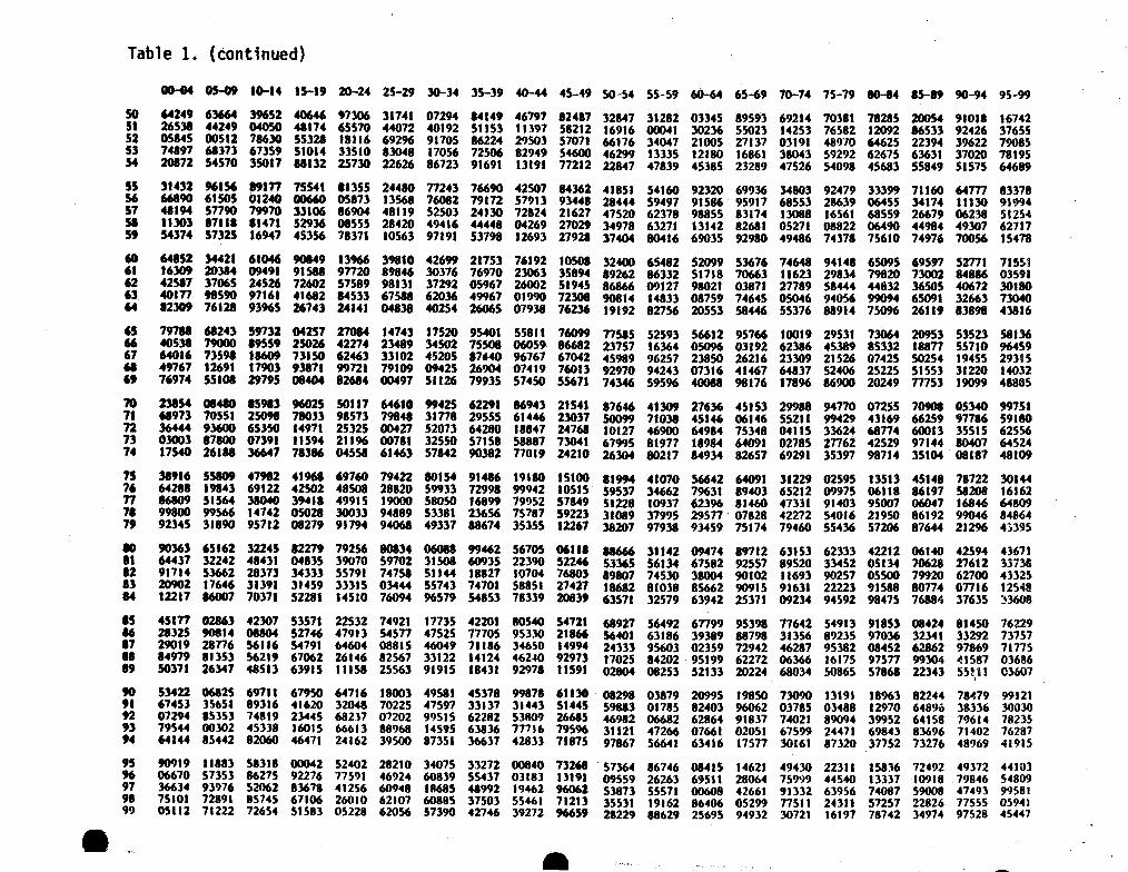
Table 1. (continued)

OO-o4 ~ 10-14 IS-19 20-24 25-29 30-34 35-39 40-44 45-49 50-54 55-59 60-64 65-69 70-74 75-79 86-84 85-89 90-94 95-99

50 64249 63664 39652 40646 97306 31741 07294 84149 46797 82487 32847 31282 03345 89593 69214 70381 78285 20054 91018 16742 51 26531 44249 04050 48174 65570 44072 40192 51153 11197 58212 16916 00041 30216 55023 14253 76582 12092 86533 92426 37655 52 05845 00512 78610 55128 18116 69296 91705 86224 29503 57071 66176 34047 21005 27117 03191 489"/0 64625 22394 39622 79085 53 74897 68373 67359 51014 33510 83048 17056 72506 82949 54600 46299 13335 12180 16861 38043 59292 62675 61631 37020 78195 54 20872 54570 35017 88132 25730 22626 86723 91691 13191 77212 22847 47839 45385 23289 47526 54098 45683 55849 51575 64689

55 31432 96156 19177 75541 11355 24480 77243 76690 42507 84162 41851 54160 92320 69936 34803 92479 33399 71160 64777 83378 56 66890 61505 01240 00660 05873 13568 76082 79172 57913 93448 28444 59497 91586 95917 68553 28639 06455 34174 11130 91994 57 48194 57790 79970 33106 86904 48119 52501 24130 72824 21627 47520 62378 98855 83174 13088 16561 68559 26679 06238 51254 51 11103 17118 11471 52916 08555 28420 49416 44448 04269 27029 34978 63271 13142 82681 05271 08822 06490 44984 49307 62717 59 54374 57325 16947 45356 78l7t 10563 97191 53798 12693 27928 37404 80416 69035 92980 49486 74378 75610 74976 70056 15478

'° 64152 34421 61046 90849 13966 39810 -42699 21753 76192 10508 32400 65482 52099 53676 74648 94148 65095 69597 52771 71551 61 16109 20384 09491 91588 97720 89846 30376 76970 23061 35894 89262 86332 51718 70663 11623 29834 79820 73002 84886 03591 62 42587 37065 24526 72602 57589 98131 37292 05967 26002 51945 86866 09127 98021 03871 27789 58444 44832 36505 40672 30180 63 401n 98590 97161 41682 84513 67588 62036 49967 01990 72308 90814 14833 08759 74645 05046 94056 99094 65091 32663 73040 64 12309 76128 93965 26743 24141 04838 40254 26065 07938 76236 19192 82756 20553 58446 55376 88914 75096 26119 83898 43816

6S 79781 68243 59732 04257 27084 14143 17520 95401 55811 76099 77585 52593 56612 95766 10019 29531 73064 20953 53523 58136 66 40538 79000 19559 25026 42274 23489 34502 75508 06059 86682 23757 16364 05096 03192 62386 45389 85332 18877 55710 96459 67 64016 73598 18609 73150 62463 33102 45205 874140 96767 67042 45989 96257 23850 26216 23309 21526 07425 50254 19455 29315 68 49767 12691 17903 93171 99721 79109 09425 26904 07419 76013 92970 9420 07316 41467 64837 52406 25225 51553 31220 14032

" 76974 55108 29795 08404 82684 00497 51126 79935 57450 55671 74346 59596 40088 98176 17896 86900 20249 77753 19099 48885

70 23154 08480 15983 96025 50117 64610 99425 62291 86943 21541 87646 41309 27636 45153 29988 94770 07255 70908 05340 99751 71 61973 70551 25091 7803) 98573 79848 31778 29555 61446 23037 50099 71038 45146 06146 55211 99429 43169 66259 97786 59180 72 36444 93600 65350 14971 25325 00427 52073 64280 18847 24768 10127 46900 64984 75348 04115 33624 68774 60013 35515 625S6 7l 03003 17800 07391 11594 21196 00781 32550 57158 58887 73041 67995 81977 18984 64091 02785 27762 42529 97144 80407 64524 74 17540 26188 36647 78186 04558 61463 57842 90382 77019 24210 26304 80217 84934 82657 69291 35397 98714 35104 08187 48109

75 31916 55809 47912 41968 69760 79422 80154 91486 19180 15100 81994 41070 56642 64091 31229 02595 13513 45148 78722 30144 76 64288 19843 69122 42502 48508 28820 59933 72998 99942 10515 59537 34662 79631 89403 65212 09975 06118 86197 58208 16162 77 86809 51564 38040 39418 49915 19000 58050 16899 79952 57849 51228 10937 62396 81460 47331 91403 95007 06047 16846 64809 71 99800 99566 14742 05028 30033 94889 53381 23656 75787 5922] 31089 37995 29571 07828 42272 54016 21950 86192 99046 84864 79 92345 31890 95712 08279 91794 94068 49337 88674 35355 12267 38207 97938 93459 75174 79460 55436 57206 87644 21296 43395

80 90363 65162 32245 82279 79256 80834 06088 99462 56705 06111 88666 31142 09474 89712 63153 62333 42212 06140 42594 0671 11 64437 32242 48431 04835 39070 59702 31508 60935 22390 52246 53365 56134 67582 92557 89520 33452 05134 70628 27612 33738 12 91714 53662 28373 3433) 55791 747S8 51144 18827 10704 76803 89807 74510 38004 90102 11693 90257 05500 79920 62700 4332S 13 20902 17646 31391 31459 33315 03444 55743 74701 58851 27427 18682 81038 85662 90915 91631 22223 91588 80774 cm16 12548 14 12217 86007 70371 52281 14510 76094 96579 54853 78339 20839 63571 32579 63942 25371 09234 94592 98475 768H 37635 33608

IS 45177 02863 42107 53571 22532 74921 17735 42201 80540 54721 68927 56492 67799 95398 77642 54913 91853 08424 81450 76229 86 28125 90814 08804 52746 4791) 54577 47525 77705 95330 21866 56401 63186 39389 88798 31356 89235 97036 32341 33292 73757 17 29019 28776 56116 54791 64604 08815 46049 71186 34650 14994 24333 95603 02359 72942 46287 95382 08452 62862 97869 71775 .. 84979 81l53 S6219 67062 26146 82567 33122 14124 46240 92973 17025 84202 95199 62272 06366 16175 97577 99304 ~1587 03686 19 50371 26347 48513 63915 11158 25563 91915 18431 92978 11591 02804 08253 52133 20224 68034 50865 57868 22343 5511! 03[,07

I

90 53422 06825 69711 67950 64716 18003 49581 45378 99878 61130 08298 03879 20995 19850 73090 13191 18961 82244 78479 99121 91 6745) 35651 89316 41620 32048 70225 47597 33137 31443 51445 59883 01785 82403 96062 03785 03488 12970 64890 38336 30030 92 07294 85153 74819 23445 68217 07202 99515 62282 51809 26685 .46982 06682 62864 91837 74021 89094 39952 64158 79614 78215 9l 79544 00302 45338 16015 66613 88968 ••595 63836 77716 79596 31121 47266 07661 02051 67599 24471 69843 83696 71402 76287 94 64144 85442 82060 46471 24162 39500 87351 36637 42833 71875 97867 56641 63416 17577 30161 87320 37752 73276 48969 41915

95 90919 11883 58318 00042 52402 28210 34075 33272 00840 73268 . 57364 86746 08415 14621 49430 22111 15836 72492 49372 44103 96 06670 57353 86275 92276 77591 46924 60819 55437 0}18] 13191 09559 26263 69511 28064 75999 44540 13337 10918 79846 54809 97 36634 93976 52062 83678 41256 60948 18685 48992 19462 96062 53873 55571 00608 42661 91332 63956 74087 59008 47493 99581 98 75101 72891 85745 67106 26010 62107 60885 37503 55461 7120 35531 19162 86406 05299 77511 2011 57257 22826 77555 05941 99 05112 71222 72654 51583 05228 62056 57390 42746 39272 96659 28229 88629 25695 94932 30721 16197 78742 )4974 97528 45447 - • •

. \

•

•

•

-20-

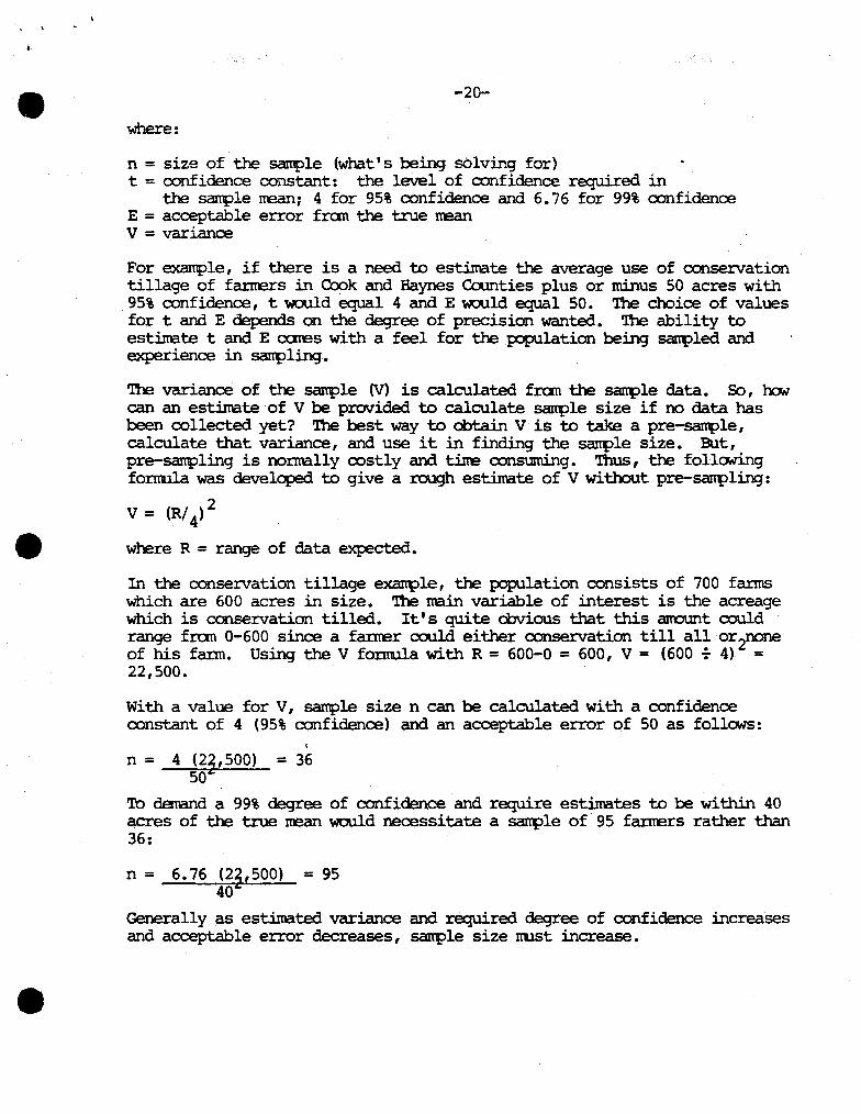
where:

n = size of the sanple (what' s being sbl ving for) t = confidence constant: the le'1el of confidence required in

the sanple mean: 4 for 95% confidence and 6.76 for 99% confidence E = acceptable error fran the true nean V = variance

For exarrple, if there is a need to estimate the average use of conservation tillage of farners in Cook and Haynes Counties plus or minus 50 acres with 95% confidence, t would equal 4 and E would equal SO. The choice of values for t and E depends on the degree of precision wanted. The ability to estimate t and E ccrres with a feel for the population being sanpled and experience in sanpling.

The variance of the sanple (V) is calculated fran the sanple data. So, how can an estimate·of V be provided to calculate sanple size if no data has been collected yet? The best way to obtain V is to take a pre-sanple, calculate that variance, and use it in finding the sarcple size. But, pre-sanpling is nonnally costly and tine consuming. Thus, the follCMing fonru.la was developed to give a rough estimate of V without pre-sanpling:

2 V = (R/ 4)

where R = range of data expected.

In the conservation tillage exanple, the population consists of 700 fanns which are 600 acres in size. The main variable of interest is the acreage which is conservation tilled. It's quite obvious that this arrount could range fran 0-600 since a farner could either conservation till all or2none of his fann. Using the V foncula with R = 600-0 = 600, V = (600 f 4) = 22,500.

With a value for V, sanple size n can be calculated with a confidence constant of 4 (95% confidence) and an acceptable error of 50 as fella-ls:

n = 4 (2~,500) = 36 so

'lb demand a 99% degree of confidence and require estimates to be within 40 acres of the true mean would necessitate a sarcple of 95 fanrers rather than 36:

n = 6.76 (2~,500) = 95 40

Generally as estimated variance and required degree of confidence increases and acceptable error decreases, sanple size nust increase •

-21-

V. CXNFIDENCE LIMITS

(P.eliability of the Semple)

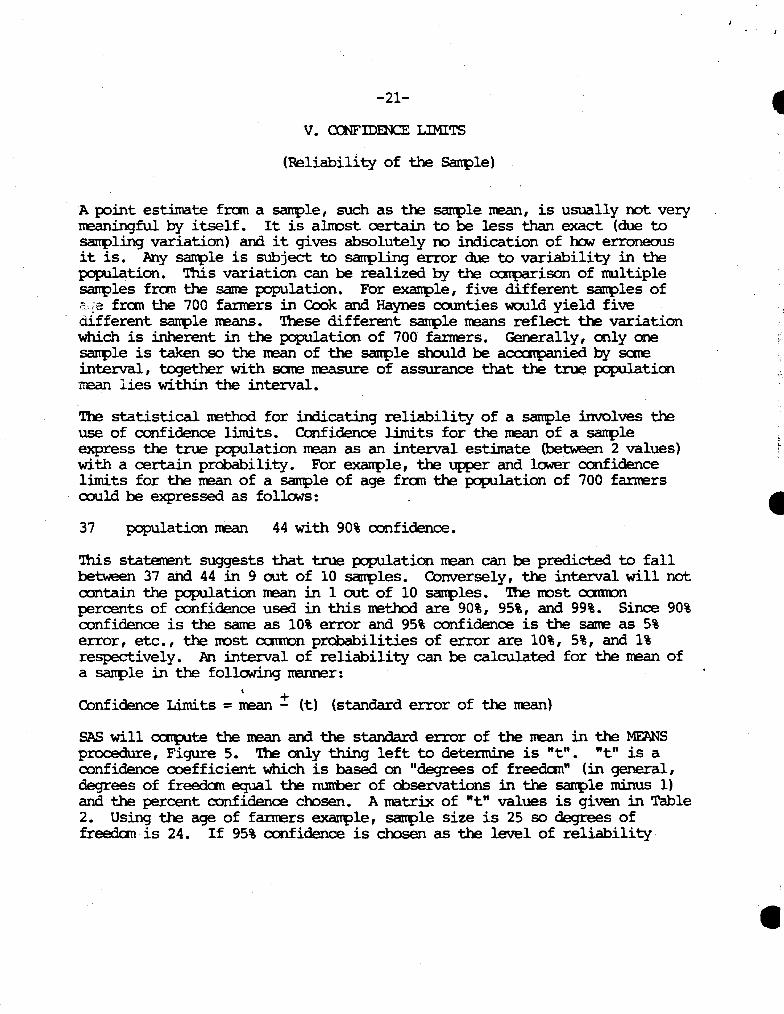
A point estirrate fran a sarcple, such as the sant>le mean, is usually not very meaningful by itself. It is alnost certain to be less than exact (due to sampling variation) and it gives absolutely no indication of hoN erroneous it is. 1my sanple is subject to sanpling error due to variability in the population. This variation can be realized by the cc::q:>arison of multiple sant>les fran the same population. For exanple, five different sanples of ;;: :e fran the 700 fanrers in Cook and Haynes counties would yield five different sanple means. These different sanple means reflect the variation which is inherent in the population of 700 fanrers. Generally, only one sanple is taken so· the mean of the sarcple should be acccrcpanied by scree interval, together with sare neasure of assurance that the true p::JpUlation rrean lies within the interval.

The statistical mathod for indicating reliability of a sarrple involves the use of confidence limits. Confidence limits for the mean of a sarrple express the true population mean as an interval estimate (between 2 values) with a certain probability. For exanple, the upper and lc:Mer confidence limits for the mean of a sarcple of age fran the population of 700 fanrers could be expressed as follows:

37 population mean 44 with 90% confidence.

'Ibis staten:ent suggests that true population mean can be predicted to fall between 37 and 44 in 9 out of 10 sanples. Conversely, the interval will not oontain the population mean in 1 out of 10 salll>les. '!he nost cumon percents of confidence used in this mathod are 90%, 95%, and 99%. Since 90% oonf idence is the sane as 10% error and 95% confidence is the sane as 5% error, etc., the nost cxmron probabilities of error are 10%, 5%, and 1% respectively. An interval of reliability can be calculated for the mean of a sarcple in the following manner:

Confidence Limits=~ ± (t) (standard error of the mean)

SAS will cacplte the mean and the standard error of the mean in the MEANS procedure, Figure 5. The only thing left to determine is "t". "t" is a confidence coefficient which is based on "degrees of freedan" (in general, degrees of freedan equal the nurcber of observations in the sanple minus 1) and the percent confidence chosen. A matrix of "t" values is given in Table 2. Using the age of fanrers exarrple, sarcple size is 25 so degrees of freedan is 24. If 95% confidence is chosen as the level of reliability

I

•

. \

• -22-

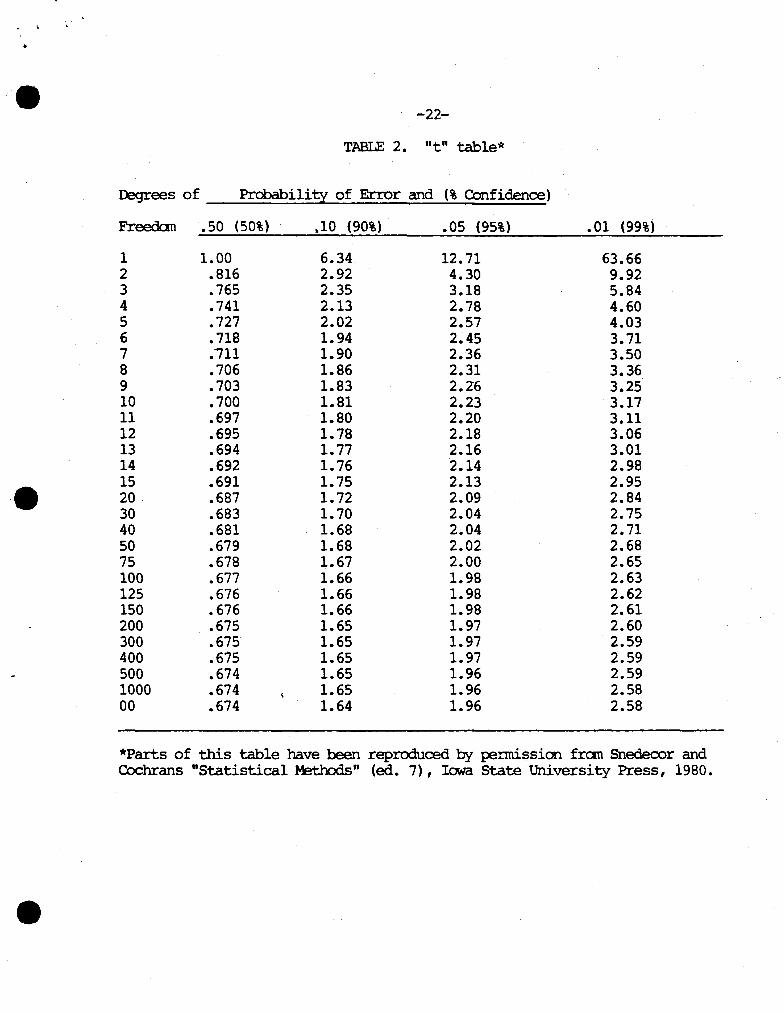
TABLE 2. "t" table*

Degrees of Probability of Error and (% Confidence)

Freedan .so (50%) ,10 (90%) • 05 (95%) • 01 (99%)

1 1.00 6.34. 12.71 63.66 2 .816 2.92 4.30 9.92 3 .765 2.35 3.18 5.84 4 .741 2.13 2.78 4.60 5 .727 2.02 2.57 4.03 6 .718 1.94 2.45 3.71 7 .-111 1.90 2.36 3.50 8 .706 1.86 2.31 3.36 9 .703 1.83 2.26 3.25 10 .700 1.81 2.23 3.17 11 .697 1.80 2.20 3.11 12 .695 1.78 2.18 3.06 13 .694 1.77 2.16 3.01 14 .692 1.76 2.14 2.98 .

• 15 .691 1.75 2.13 2.95 20 .687 1. 72 2.09 2.84 30 .683 1. 70 2.04 2.75 40 .681 1.68 2.04 2. 71 50 .679 1.68 2.02 2.68 75 .678 1.67 2.00 2.65 100 .677 1.66 1.98 2.63 125 .676 1.66 1.98 2.62 150 .676 1.66 1.98 2.61 200 .675 1.65 1.97 2.60 300 .675' 1.65 1.97 2.59 400 .675 1.65 1.97 2.59 500 .674 1.65 1.96 2.59 1000 .674 1.65 1.96 2.58 00 .674 1.64 1.96 2.58

*Parts of this table have been reprcx:1uced by pennission f ran Snedecor and C.OChrans "Statistical Methods" (ed. 7), Iowa State University Press, 1980 •

•

-23-

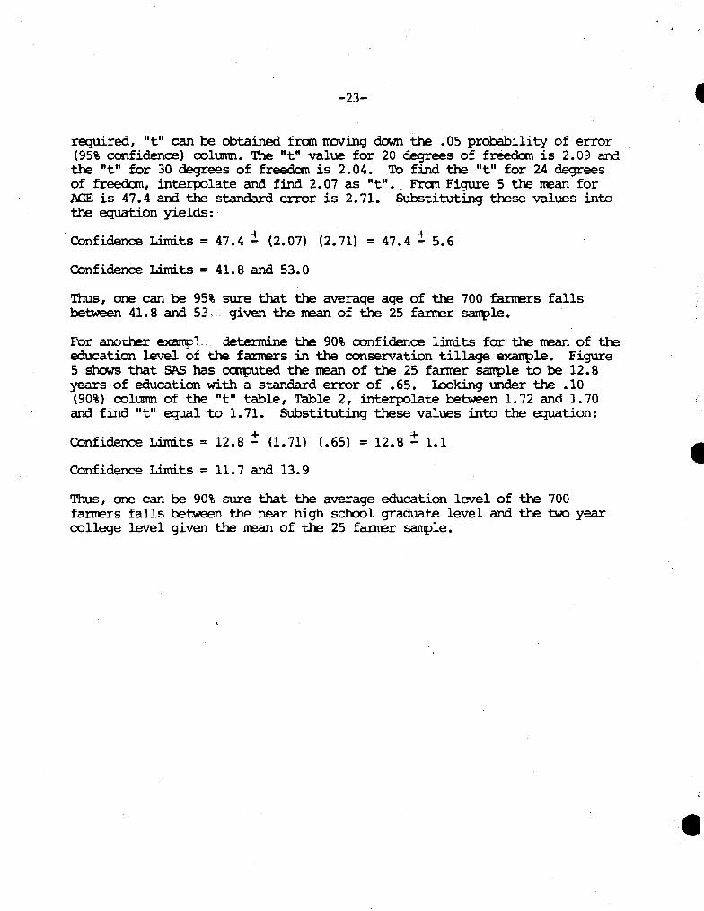
required, "t" can be obtained fran noving down the .05 probability of error (95% confidence) oolUlm. '!be "t" value for 20 degrees of freedan is 2.09 and the "t" for 30 degrees of freedan is 2.04. To find the "t" for 24 degrees of freedan, interpolate and find 2.07 as "t" •. Fran Figure 5 the rrean for AGE is 47.4 and the standard error is 2.71. Substituting these values into the equation yields:

Confidence Limits= 47.4 ± (2.07) (2.71) = 47.4 ± 5.6

Confidence Limits = 41.8 and 53.0

Thus, one can be 95% sure that the average age of the 700 farners falls between 41. 8 and 53 given the rrean of the 25 farmar sarcple.

E'er anocller examo'.. detennine the 90% confidence limits for the rrean of the education level of the fanrers in the conservation tillage exanple. Figure 5 shows that SAS has carputed the rrean of the 25 farmar sarcple to be 12.8 years of education ·with a standard error of .65. Looking under the .10 (90%) oolUlm of the "t" table, Table 2, interpolate between 1. 72 and 1. 70 and find "t" equal to 1.71. Substituting these values into the equation:

+ + Confidence Limits= 12.8 - (1.71) (.65) = 12.8 - 1.1

Confidence Limits= 11.7 and 13.9

Thus, one can be 90% sure that the average education level of the 700 fariters falls between the near high school graduate level and the two year oollege level given the rrean of the 25 farner sanple.

I

•

. . '

•

•

•

-24-

VI. HYPOI'HESIS TESTING

A hypothesis can be defined as tentative theory or supposition. Everyone hypothesizes fran tine to tine observations are made. For exanple, the following could be taken as hypotheses: ( 1) the average height of American adult males is 5 feet, 9 inches (2) the soybean yield in watershed x is 35. bushels per acre (3) the average rCM crop farmer in the Micl\.Jest conservation tills half his cropland. These three hypotheses are statistical hypotheses because they are staterrents about a statistical population: specifically they are staterrents about a certain variable (characteristic) in a statistical population.

It is often desirable to test if such hypotheses are valid. 'lb do this, an cq::propriate saI'll>le is taken and the hypothesis is accepted or rejected based on the results of statistical tests. This chapter deals with two such statistical tests.

TESTING 'lHE MEAN

'!he average 600 acre farner in Cook and Haynes Counties is 55 years old, has an eight grade education, and conservation tills 200 of his 600. acres. This is a hypothesis. In fact, it is actually three separate hypotheses about the sane 700 farrrer population. HcM ~ld one go about testing whether these estimates are accurate? One way would be to interview all 700 farrrers. Although very thorough, this nethod involves extensive tine and noney. Too extensive for the resourees of nest governrrent agencies. 'ltlere is another option. It involves: (1) interviewing an appropriate sized randan sarrple of the 700 farners; (2) gathering information about age, education, and degree of conservation tillage; (3) calculating the sarrple nean for each of the 3 variables; and ( 4) using hypothesis testing nethods to carpare the sarrpled neans to the original hypotheses.

Steps 1, 2, and 3 have already been carpleted (using hypothetical data). The results of these steps are recorded in Figure 5 where SAS has helped calculate the sarct>le neans. Step 4 involves the use and carparison of two "t" statistics; the "table t" found in Table 2 (just as was done for confidence intervals\ in Chapter V); and the "calculated t" which is calculated using information fran the sanple.

As was done to calculate confidence intervals, the percent confidence r~red of the test nust be determined. Using this value, plus the degrees of freedan, the correct table t can be found in Table 2. In this case the sanple size is 25 so degrees of freedan are one less than that or 24. If 90% confidence is required in the hypothesis test, the next step is to interpolate between 20 and 30 degrees of freedan in Table 2 under the .10 (90%) colurm and find that the table t is equal to~·

J, '7 /

-25-

'!he equation used to find the calculated t is: calculated t = I (sanple rcean - hypothesized rrean I .:. standard error of the sanple mean •

In the MEANS procedure, SAS calculates the saill>le rrean and the standard error of the sanple rrean as seen in Figure 5. 'lb calculate the calculated t for age subtract the hypothesized rrean (55) fran the sanple rrean (47) which gives - 8. '!he absolute value ( 8) is then divided by the standard error of the rrean (2.71) to yield a calculated t of 3.86:

calculated t for age= /47-55/ f 2.71=3.86

'!he carparison rule for table t and calculated t is as follows: If calculated t exceeds table t reject the hypothesis; if not, accept t:Pe hypothesis. )

. ~(J,'11 The age hypothesis stated that the 700 fa.nrers' average age is -55. The calculated t (3.86) is greater than the table t ~ so this hypothesis is rejected. ('Ihe sarrple tends to show the average age is less than 55.) The test is done with the understanding that the decision to reject is done so with 90% confidence, thus a 10% margin of error is accepted.

'lb test the second hypothesis that the farners' average education level is an eighth grade education, the sane steps are followed using data fran the education information in the sanple, Figure 5. If the 90% level of confidence is satisfactory, the table t would be the saire as in the age exanple, ~ '!be calculated t in this exan:ple would be:

I. '71 calculated t for education= /(12.8-8)/ f .65 = 7.38

In the equation, 12.8 is the sarrple rcean fran SAS (Figure 5), 8 is the hypothesized rcean, and • 65 is the standard error of the nean fran SAS--- I. 7 / (Figure 5). The calculated t (7 .38) is larger than the table t {2...-0'7') so the hypothesis that the average fa.mer in the population of 700 nas an eighth grade education is rejected. ('llle sarrple would tend to show they have higher than an eighth grade education on the average.)

The third test is on the hypothesis that the average f arner conservation ~f his 600 acre fann. h;suming a 90% confidence level again, the

\ :'\ \ table t is ~ The calculated t is • 59 using the output fran SAS in

Figure 5 under the conservation till variable, ACRES MIN:

calculated t for conservation tilled acres= /(220-200)/ f 34.16 = .59. 1.7 I

The calculated t (.59) does not exceed the table t ~ so the hypothesis that the average fa.mer conservation tills 200 acres is accepted.

'lb sumnarize, statistical procedures lNere used to test 3 different hypotheses about 700 fanrers in Cook and Haynes Counties. 'llle procedure involved carparison of a value (calculated t) which cares fran the carbined • results of the sarcple and the hypothesis to a value which incorporates saI'l1?le size and an acceptable level of precision (tablet).

•

•

•

-26-.

'll1e acceptance of a hypothesis reveals that the sanple mean itself is no rore accurate than the hypothesized value. (Alt.hough the nethods used to d:>tain the sanple mean may be rore defendable. ) 'lbe rejection of a hypothesis shaNs that the sarcple mean is statistically rore accurate than the hypothesized nean although confidence in this decision is only as high as the level of confidence used to obtain the table t.

Carparing Two groups of Data (Test of Difference)

O'le of the rrost often used statistical hypothesis tests is the Test of Difference. The differences being investigated are those between 2 means, and the hypothesis being tested states that the two means are ~l. Uses for this test could include carparing the rate of gain of hogs on 2 dif­ferent rations, carparing math scores of males vs. ferrales, or testing to see if the 300 f arners in Cook Co\ll'lty vary fran the 400 in Haynes County in tenns of age, education, and use of conservation tillage. '!be actual hypothesis \<JOUld state that there are no differences in rate of gain between rations; that there are no differences in average scores between males and ferrales; and that there are no differences bebJeen average age, education, or use of conservation tillage between the 2 counties, respectively •

'lb test the 3 hypotheses that there is no difference between average use of conservation tillage, age, and education bebJeen farmers sarcpled in Cook and Haynes Counties, a "calculated t" and a "table t" are carpared to detennine whether each of the 3 hypotheses are accepted or rejected just as was done for the "Testing the Mean" procedure. ~r, the calculated t formula for the test of difference is nuch rore cacplicated than the one for testing the nean (see Appendix of Formulas) • Thus a SAS procedure T1'EST has been developed to arrive at the calculated t for the Test of Difference.

'lb use the T1'EST procedure the initial program, Figure 1, is rl.ll'l with 2 procedural records inserted in lines 36 and 37. "P:RCX: Tl'FST;" initiates the prewritten SAS program which develops a calculated t for the variable in each hypothesis (acres conservation tilled, age and education). "CIA5S CXXJNI'Y;" indicates the variable (CXXJNI'Y) upon which carparisons will be made.

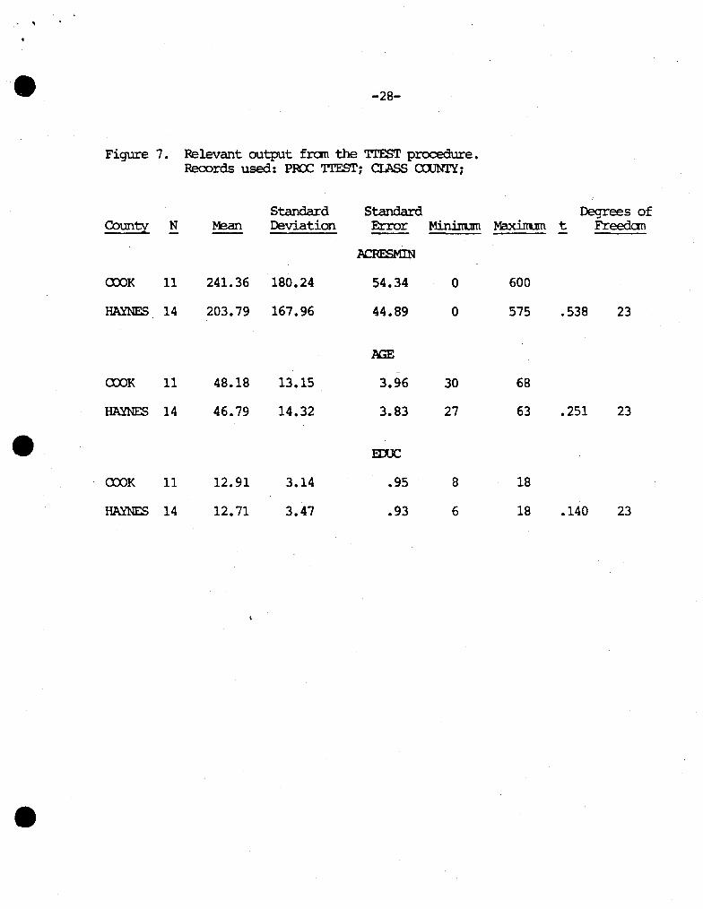
Figure 7 illustrates the output fran the T1'EST procedure. The basic statistical neasures are supplied for each variable and divided into the 2 counties. calculated t and degrees of freedan are also supplied for use in the Test of Difference. 'lbe decision rule for the Test of Difference is: If the calculated t is larger than the table t, reject the hypothesis. ('lhl.s is the identical rule used in Testing the Mean. )

-27-

For the hypothesis that the average use of conservation tillage is the sarre in Cook and Haynes Counties the calcuiated t is • 538, Figure 7. Figure 7 also shc:Ms there are 23 degrees of freedan in this exarcple. If 95% confidence is required in the test, the .05(95%) column of Table 2 supplies the table t. .fvbv'ing down the .05 (95%) column to 23 degrees of freedan an interpolation nust be made between 2.04 and 2.09 yielding 2.06 as the table t. 'n1e calculated t is not larger than the table t so the hypothesis is calculated. Using the sanple of 11 fa:rners fran Cook County and 14 farmers fran Haynes County plus the Test of Difference it can be concluded that the population of 300 farmers in Cook County conservation till, on average, the sane proportions of their farms as do the 400 fai:ners in Haynes County.

The hypothesis which states that the average age of the 300 farmers in Cook County does not differ fran the average age of the 400 fanrers in Haynes County can be tested as well. The calculated t is • 251, Figure 7, and if a 95% confidence was assuned again, the table t would again be 2.06. Since the calculated t is not larger than the table t the original hypothesis al:x>ut the average age of the fanrers is accepted. Using the sane procedure it \\10\.lld also be concluded that the average education level between counties does not differ statistically for the total PoP'Itations since the calcuiated t (.140) is less than the tabled t (2.06). -

The Test of Difference is a useful technique in statistics. Many carparisons of large populations can be made using this test along with sanpling techniques. This particular hypothesis testing procedure is enhanced since the calculations can be done easily using SAS.

1/ It is just by chance that all 3 exalll?le hypotheses were accepted, since the conservation tillage exanple used throughout this publication cares fran hypothetical data. In real life it is probable that m:>st counties are nore diverse than th:>se in this exanple.

I

'

•

. "

• -28-

Figure 7. Felevant output fran the 'ITFSI' procedure. Records used: P:R:X: 'ITFSI'; CI.ASS roMl'Y;

Standard Standard Degrees of Cotmty N Mean Deviation Error Mininum Maxinum t Freedan -

.ACRESMIN

CXX)K 11 241.36 180.24 54.34 0 600

HAYNES 14 203.79 167.96 44.89 0 575 .538 23

.AGE

CXX)K 11 48.18 13.15 3.96 30 68

HAYNES 14 46.79 14.32 3.83 27 63 .251 23

• EIXJC

CXX)K 11 12.91 3.14 .95 8 18

HAYNES 14 12.71 3.47 .93 6 18 .140 23

•

-29-

VII. Linear F.egression Analysis and Prediction

In the previous chapters the problems considered involved only a single variable of a population at one tine. Confidence limits were constructed around the nean of one variable. Hypothesis tests were developed for a single variable. 'Ille c:i>servation in a sarrple may have been cxnpared in groups but generally this cxnparison was based on only one neasurerrent or variable per carparison. In this chapter attention is turned to statistical influences based on two or rrore variables of each rrerber of the sanple. For exanple, nore adequate judgerrents about a farrcers' use of oonservation tillage can be made if characteristics that may affect this use, like his age or education level can be studied sirrultaneously.

Linear regression analysis is concerned with the·relationship of 2 or nore variables. !t:>re specifically, it enables a user to determine to what degree one variable is affected by the others. In the conservation tillage exanple, fanrers' use of conservation tillage may depend to sate degree on their age and their education level. Linear regression analysis can be ett>loyed to mathematically and statistically describe the relationship of age and education to farners' use of conservation tillage.

'1be major CCJip:>nent of linear regression analysis is the linear regression · I nodel. This nodel may vary fran application to application, but it can be expressed in general as: Y = B

0 + B1 x1 + B2 ~ + • • • + Bn Xn

where: Y= variable to be explained called the dependent variable, eg. use of conservation tillage. (data fran a sanple)

B = intercept (solved for using SAS) >f. = variable or variables, used to explain Y, called the

1 independent variables, eg. age, education. (data fran a sanple) B. = ~ parameters (solved for using SAS) n1 = mmber of independent variables

'!he term linear regression stems directly fran the use of the linear regression nodel presented here. cne fonn of the ~tion, if plotted on a graph, wuld constitute points in a straight line.- The tenns sinple regression and nultiple regression refer to the nunber of independent variables used in the analysis. A sinple regression analysis relates only 1 independent variable to the dependent variable. Multiple regression analysis relates 2 or nore independent variables to the dependent variable.

1/ 'n"lere are a nultitude of nan-linear m:xlels used in non-linear regression - analysis but these netl:x:rls are beyond the scope of this publication.

•

•

•

•

-30-

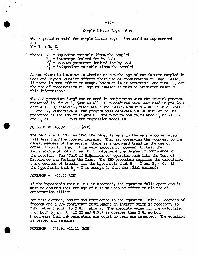
Sinple Linear Pegression

'll:e regression rrodel for sinple .linear regression would be represented as: Y =Bo+ Bl xl

Where: Y = dependent variable (fran the sanple)

:~ : ~ ~== ~'!1~ s:~ by SAS) x1 = independent variable (fran the sarrple)

Ass.me there is interest in whether or not the age of the fanrers sarrpled in Cook and Haynes Counties affects their use of conservation tillage. Also, · if there is sare effect on usage, how much is it affected? And finally, can the use of conservation tillage by similar fanrers be predicted based on this infonnation?

'll:e SAS procedure "Reg" can be used in conjunction with the initial program presented in Figure 1, just as all SAS procedures have been used in previous chapters. By inserting "PRCX: REX;;" and "M:DEL .ACRESMIN = JGE;" into lines 36 and 37, respectively, the program will generate output similar to that presented at the top of Figure 8. The program has calculated B1 as 7 46. 92 and B1 as -11.11. Thus the regression nodel is:

.ACRESMIN = 746.92 - 11.ll(PiGE)

The negative B1 irrplies that the older fanrers in the sarrple conservation till less than the younger fanrers. That is, observing the youngest to the oldest nerbers of the sanple, there is a downward trend in the use of conservation tillage. It is very ilrportant, however, to test the significance of both B . and B1 to detenni.ne the degree of confidence in the results. The "Tes~ of Significance" operates much like the Test of Difference and Testing the Mean. The Rm procedure supplies the calculated t and degrees of freedan for the hypothesis that B = O and B1 = O. If the hypothesis that B = O is accepted, then the n8ae1 becares:

0 \

.ACRESMIN = -11.ll(PiGE)

If the hypothesis that B1 = O is accepted, the equation falls apart and it nust be assuired that the age of a farner has no effect on his use of conservation tillage.

For this exarrple, assune 99% confidence in the equation. With 23 degrees of freedan and a 99% confidence requirerent an interpolation is necessary to find table t equal to 2.81, Table 2. The absolute value for the calculated t of 1:x:rl:h B and ~1 (12. 22 and 8. 95) is greater than 2. 81 so both hypothesis ~t the pararreters are equal to zero are rejected. The equation is tested and remains:

.ACRESMIN = 746.92 -11.11 (]GE)

-31-

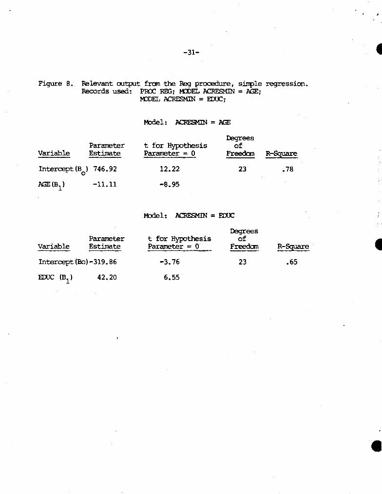
Figure 8. Pelevant output fran the Peg procedure, sinple regression. Records used: PRO: Rm; MDEL ACRF.sMIN = AGE;

MJDEL ACRESMIN = EDUC;

ftbdel: ACRF.sMIN = .AGE

Degrees of

Variable Pararceter Estimate

t for Hypothesis Pararceter = O Freedan R-Square

Intercept(B ) 746.92 0

AGE(B1) -11.11

Variable Pararceter Estimate

Intercept(Bo)-319.86

42.20

12.22

-8.95

23

ftbdel: ACRF.SMIN = EDUC

t for Hypothesis Pararceter = o·

-3.76

6.55

Degrees of

Freedan

23

.78

R-Square

.65

,

'•

t

•

•

•

•

-32-

'Ihus, the relationship described previously between AGE·and.ACRF.S MIN also stands. ~t does this equation~? Given the age of a fanrer with similar characteristics as those sarrpled, the equation can predict the anount of conservation tillage he is practicing. Thus, a 48 year old fa.mer could be expected to conservation till 214 acres, (214=746.92-11.11(48)). A 24 year old fanrer could be expected to conservation till 480 acres,. (480 = 746.92~11.11(24))

For a second exanple, assune there is interest in whether or not the education level of farrcers affect their use of conservation tillage. The bottan of Figure 8 is the result of using the initial program, Figure 1, with "PRO: Rm;" and "MDEL ACRF.SMIN = EDUC;" inserted in lines 36 and 37 1

re~ctively. The regression noded becares:

.ACRES MIN= -319.86 + 42.20(EDUC)

The absolute value of calculated t's for B and B (3.76 and 6.55) are each larger than the tablet (2.81). '!bus~ the ortginal equation remains since the hyp:)theses that B = O and B = O are rejected. A farrcer with similar characteristics as ~se sarcplM with a high school education would be predicted to oonservation till 187 acres, (187= -319.86 + 42.20(12)) •

The R-square is the estimated coefficient of determination. It is the fraction of total variation in the dependent variable that is aCCO\IDted for by the independent variable. In the two exanples, OOth age and education were seperately tested significant (using the test of significance) in explaining the variation of acres conservation tilled. hje did a better job because the R-square of AGE is higher than that for EDUC, Figure 8. Why? The closer the R-square is to 1, the better jd:> the nodel does of explaining the dependent variable, thus the nore useful it is in prediction. (Studying the R-Square f onrula in the Appendix of Fonrulas will aid understanding the inplications of· the actual neasure itself).

Multiple Linear P.egression \

The regression nodel for ItUltiple linear regression is represented as:

Where: Y = dependent variable (fran the sarrple)

:~: ~~~~~ (=~ for by SAS) x1 - ~ = independent variables (fran the sarcple)

Using the conservation tillage exanple, the effects of OOth age and education on conservation tillage use could be found by substituting these variables into the regression nodel as:

1CRESMIN = B0

+ Bl (AGE) + B2 (EDUC)

-33-

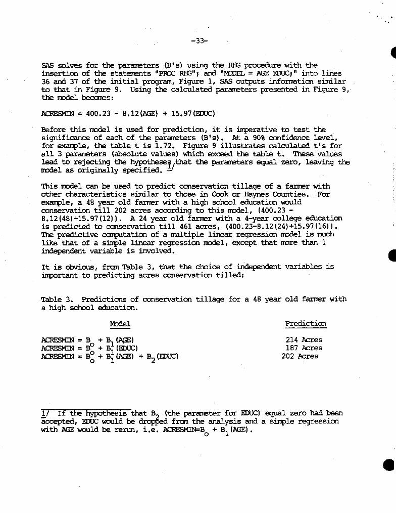
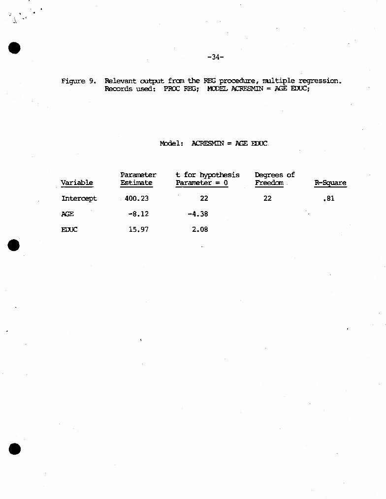
SAS solves for the paraneters (B's) using the Rm procedure with the insertion of the statercents "PRX: REX;"1 ·ana "MDEL =AGE IDJC1" into lines 36 and 37 of the initial program, Figure 1, SAS outputs infonnation similar to that in Figure 9. Using the calculated para:rreters presented in Figure 9, · the ncdel becares:

ACRESMIN = 400.23 - 8.12(.AGE) + 15.97(EDUC)

Before this nodel is used for prediction, it is imperative to test the significance of each of the paraneters (B's). At a 90% confidence level, for exanple# the table t is 1. 72. Figure 9 illustrates calculated t' s for all 3 paraneters (absolute values) which exceed the table t. These values lead to rejecting the hypothesel!that the paraneters equal zero, leaving the m:xlel as originally specified. - .

This ncdel can be used to predict conservation tillage of a farrrer with other characteristics similar to those in Cook or Haynes Cot.mties. For exanple, a 48 year old fanrer with a high school education tNOU.ld conservation till 202 acres according to this ncdel, (400.23 -8.12(48)+15.97(12)). A 24 year old fanrer with a 4-year college education is predicted to conservation till 461 acres, (400.23-8.12(24)+15.97(16)). The predictive catpUtation of a multiple linear regression nodel is rruch like that of a sinple linear regression ncdel, except that nore than 1 independent variable is involved.

It is obvious, fran Table 3, that the choice of independent variables is .inp::>rtant to predicting acres conservation tilled:

Table 3. Predictions of conservation tillage for a 48 year old farner with a high school education.

ltrlel

ACRESMIN = B + B (A(;E) ACRESMIN = Bo + Bl (EDUC) ACRESMIN = B~ + Bi (AGE) + B2 (EDUC)

Prediction

214 Acres 187 Acres

202 kres

lf If the hypothesis that B2 (the pararreter for EDUC) equal zero had been accepted, EDUC would be dropped fran the analysis and a si.nple regression with .AGE \\10\lld be renm, i.e. 1'.CRESMIN==B

0 + B1 (.AGE).

'•

•

• -34-

Figure 9. P.elevant output fran the mx; procedure, rcul tip le regression. Records used: PROC REG; MDEL N:RESMIN = .AGE ID.JC;

Paraneter t for hypothesis Degrees of Variable Estimate Paraneter = 0 Freedan. R-Square

Intercept 400.23 22 22 .81

1GE -8.12 -4.38

EOOC 15.97 2.08

•

•

-35-

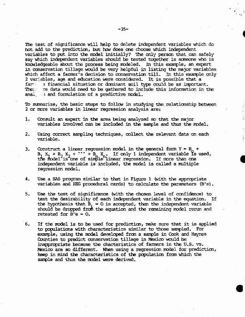
'Ihe test of significance will help to delete independent variables which do not add to the prediction, but how does one choose which independent variables to ?It into the rrodel initially? 'n1e only person that can safely say which independent variables should be tested together is sata::>ne who is knoNledgeable about the process being rcodeled. In this exarrt>le, an expert in conservation tillage tNOUld be very helpful in listing the major variables which affect a farner's decision to conservation till. In this exart1?le only 2 variables, age and education were considered. It is possible that a fa.r- s financial situation or dani.nant soil type could be as inlx:>rtant. The1 :-e data would need to be gathered to include this infonnation in the anal. 3 and fonrulation of a predictive nodel.

'lb surmarize, the basic steps to follCM in studying the relationship between 2 or nore variables in linear regression analysis are:

1.

2.

3.

4.

5.

6.

Consult an expert in the area being analyzed so that the rnajor variables involved can be included in the sant>le and thus the nodel.

Using correct sarrpling teclmiques, collect the relevant data on each variable.

Construct a linear regression nodel in the general fonn Y = B0

+ B1 x, ~ B2 X2 + • • • + B x . If only 1 independent variable 1.S used, tne ITodel is one of sinthenlinear regression. If nore than one independent variable is included, the m:xlel is called a multiple regression nodel. -

Use a SAS program similar to that in Figure 1 (with the appropriate variables and REXi procedural cards) to calculate the pararreters (B's).

Use the test of significance (with the chosen level of confidence) to test the desirability of each independent variable in the equation. If the hypothesis that B. = O is accepted, then the independent variable should be dropped f ~ the equation and the remaining rcodel rerun and retested for B's = o.

If the ItDdel is to be used for prediction, make sure that it is applied to populations with characteristics similar to those sarrpled. For ex.arrple, using the m:x3el developed fran a sarcple in Cook and Haynes Colmties to predict conservation tillage in ?4:!xico would be inappropriate because the chacteristics of fanrers in the U.S. vs. Mexico are so different. When using a regression nodel for prediction, keep in mind the characteristics of the population fran which the san:ple and thus the nodel were derived.

..

•

•

•

•

•

-36-

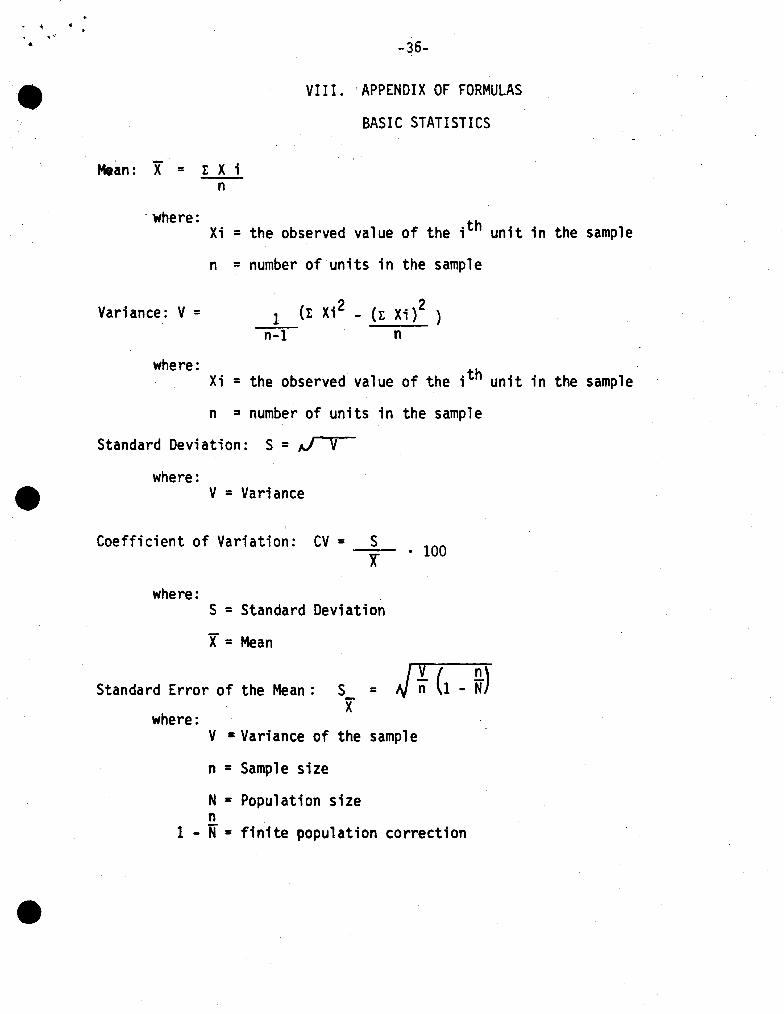
VIII. APPENDIX OF FORMULAS

BASIC STATISTICS

Mean : X = I: X i n

·where:

Variance: V =

where:

Xi = the observed value of the ;th unit in the sample

n = number of units in the sample

1 n-1

(I: Xi 2 - (I: Xi)2 ) n

Xi = the observed value of the ;th unit in the sample

n ~ number of units in the sample

Standard Deviation: S = ~ V

where: V = Variance

Coefficient of Variation: CV = S r

where: S = Standard Deviation

X = Mean

• 100

s = J ~ (1 - ~) x Standard Error of the Mean :

where: V =Variance of the sample

n = Sample size

N = Population size n

1 - N = finite population correction

-37-

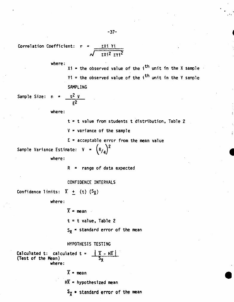
Correlation Coefficient: r = IXi Yi

,J IXi2 IYi2

where: Xi = the observed value of the ;th unit in the X sample

Yi = the observed value of the ;th unit in the Y sample

SAMPLING

Sample Size: n = t2 V

where:

f 2

t = t value from students t distribution, Table 2

V = variance of the sample

E = acceptable error from the mean value

Sample Variance Estimate: V = (R;4)2

where:

R = range of data expected

CONFIDENCE INTERVALS

Confidence limits: X :!:_ (t) (Sx)

where:

X = mean

t = t value, Table 2

s~ = standard error of the mean

HYPOTHESIS TESTING

Calculated t: calculated t = (Test of the Mean)

Ix - Hfl s~

where:

X = mean

HX = hypothesized mean

Sx • standard error of the mean

·""•

•

•

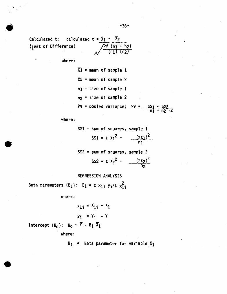
• -38-

Calculated t: calculated t = Xl - X2 (lest of Difference) ~2)

ti -rnr>-rn2' & where:

where:

Xl = mean of sample 1

X2 = mean of sample 2

n1 = size of sample 1

n2 = size of sample 2

PV = pooled variance; PV =

SSl = sum of squares, sample 1

ss1 + ss2 n1 + n2 ~2

SSl = I X12 - (IX1)2 n1

SS2 = sum of squares, sample 2

SS2 = I X22 - (IX2)2

REGRESSION ANALYSIS

Beta parameters (B1): Bi= I Xli Yi/I xj;

where:

Xli = X1; - X1

Yi = Yi - V Intercept (B0 ): Bo = V - Bi Xi

where:

n2

81 = Beta parameter for variable X1

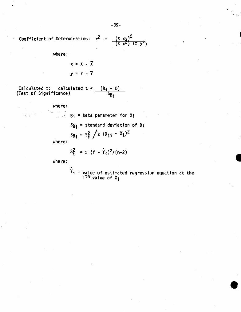
-39-

Coefficient of Detennination: r2 =

where:

x = x - x y = y - v

1: x ) (t y2)

Calculated t: calculated t = (Test of Significance)

(B; - 0) Ss.

1

where:

where:

where:

Bi = beta parameter for X;

Ss; = standard deviation of Bi

Ss; = s~ /r. {Xii - I1)2

s~ = r (Y - Yi)2/(n-2)

,.

Y; = value of estimated regression equation at the ;th value of X1

.. '

•

•

•

•

•

•

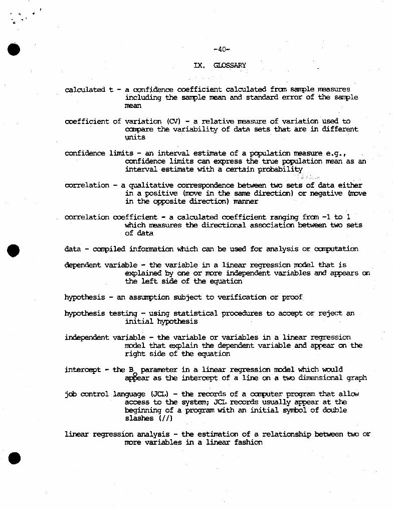
.;..40-

IX. GI.DSSARY

calculated t - a confidence coefficient calculated fran sample rceasures including the ~le rrean and standard error of the sanple trean

coefficient of variation (CV) - a relative measure of variation used to carpare the variability of data sets that are in different units ·

confidence lllni.ts - an interval estimate of a pqJUlation measure e.g., confidence lllnits can express the true population rrean as an interval estimate with a certain probability

oorrelation - a qualitative oorrespondence between two sets of data either in a positive (ncve in the same direction) or negative (nove in the opp:>site direction) manner

oorrelation coefficient - a calculated coefficient ranging fran -1 to 1 which measures the directional association between two sets of data

data - carpiled information which can be used for analysis or carputation

dependent variable - the variable in a linear regression rrodel that is explained by one or nore independent variables and appears an the left side of the equation

hypothesis - an assurtption subject to verification or proof

hypothesis testing - using statistical procedures to accept or reject an initial hypothesis

independent variable - the variable or variables in a linear regression rrodel that explain the dependent variable and a~ on the right side of the equation

intercept - the B paraneter in a linear regression rccdel which would ~ as the intercept of a line on a two dircensional graph

job control language (JCL) - the records of a catpUter program that allow access to the system: JCL records usually appear at the beginning of a program with an initial syntx>l of double slashes (//)

linear regression analysis - the estimation of a relationship between two or nore variables in a linear fashion

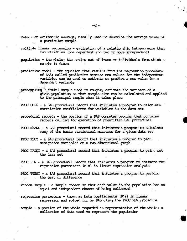
-41-

nean - an arithmetic average, usually used to describe 'the average value of a particular sant>le

nultiple linear regression - estimation of a relatiooship between trore than two variables (one dependent and two or nore independent)

population - the wh:>le; tr.e entire set of items or individuals fran which a sanple is drawn

predictive rcodel - the equation that results fran the regression procedure of SAS; called predictive because new values for the independent variables can be used to estimate or predict a new value for a dependent variable

.~e~lillg·i:. .. a-r..m:ini sample used to roughly estirrate the variance of a '•·, . ' given population so that sant>le size can be calculated and applied

to the principal sant=>le when it takes place

PROC CDRR - a SAS procedural record that initiates a program to calculate correlation coefficients for variables in the data set

procedural records - the portion of a SAS a::rrplt:er program that contains records calling for execution.of prewritten SAS procedures

PROC MEANS - a SAS procedural record that initiatesl.·.a program to calculate many of the basic statistical treasures for a given data set

PROC Pim - a SAS procedural record that initiates a program to plot designated variables on a two dinensional graph

PROC PRm,T ·- a SAS procedural record that initiates a program to print out the data set

PRO: Rm - a SAS procedural record that initiates a program to estinate the regression parameters (B's) in linear regression analysis

PR:X: 'l'rE'Sl' - a SAS procedural record that initiates a program to perform the test of difference

randan sarrple - a sanple chosen so that each value in the population has an equal and independent chance of being collected

regression parameters - known as beta coefficients (B's) in linear regression and solved for by SAS using the PROC REX; procedure

sarrple - a portion of the whole regarded as representative of the wh:>le; a collecticn of data used to represent the population

•

•

, "' ·4'· .

-t

•

•

•

-42-

s:ilrple linear regression - estimation of a relationship betweeri two variables (ooe dependent and one independent)

standard deviation - dispersion of values about the nean, indicating the variation· in.the data set

standard error of the mean - a measure that indicates the variability of sanple means. llUch like the standard deviation indicates . variability in individual sanple observations

Statistical Analysis System (SAS) - a cx::rrplter software system originally developed for statistical needs; it contains a oollection of prewritten programs that can be accessed by a few sinple carmands :~.t:.v :.tr~ .. ~~.,; .. . 5,,::rs1:

statistics - the science that deals with b;dmiques ·used .tQ. <;btain . ·' ~~"''' analytical neasures, the nethods for estimating tPeir reliability, and the drawing of inferences fran them ,.

t or table t - a CXl'lfidence constant usually found in a "t" table and originally developed fran a probability distribution called "students t"; t is used in many statistical calculations including sarcple size, confidence limits, hyp:>thesis testing, and regression analysis

table of randan nurrbers - table with a large quantity of single digits arranged ina randan fashion; used to facilitate the design of a randan sarcple

test of difference - a·· test that checks for differences in twO populations by statistically cnrparing sarcple ~ .,

test of the.mean - a test that uses the rrean fran a sarrple and probability theory to accept or reject a hyp:>thesis about the sanple

test of significance - a test of the desirability of each independent variable in regression analysis based on the hypothesis that the beta paraneters (B's) equal zero

variable - a characteristic of a population that can be coosen for study

variance - the square of the standard deviation used to measure data variability

AndeJ:son, Richard -L.; Allen, David M.>and Cady, z-F8ster B .. , 1972. "Selection of predictor variables in linear nultiple regression" In St,atj.stical Papers in Honor of George W. Snedecor. . .Ames., .. IcMa: The Icwa State University Press.

Bapcroft, ·,"T. A. , l%S. : Topics in intenrediate statistical rrethods. Ml=s, Iowa: '!be ·Iowa. State lJni versi ty Press.

Iarson, Harold J;,1974. Introduction to probability theory and statistical inference. (New York: John Wiley and Sons, 1974).

~rinell, ~11 R., 1981. F.conanics, 8th ed. (New York: ~~lt~kCotpanyQ 1981).

Ostle, Bemard and· ~sing, Richard w., 1975. Statistics in research, 3rd ed. Anes, Ic::Ma: 'Ule.:·-Iowa State University Press.

Snedecor, George W., 1980. Statistical rre~, 8th ed. Fires, Iowa: 'lbe-ICMa State College Press.

SAS Institute Inc., 1982. SAS user's guide: Basics, 1982 Edition, . cary, NC: SAS Institute Inc., 923 pp.

SAS Institute Inc. 1982. SAS user's guide: Statistics, 1982 Faition. cary, NC: SAS Institute Inc., 584 pp.

•

•