looking for adaptive footprints in the hsp90aa1 ovine gene

Salces-Ortiz et al. BMC Evolutionary Biology (2015) 15:7 DOI 10.1186/s12862-015-0280-x

RESEARCH ARTICLE Open Access

Looking for adaptive footprints in the HSP90AA1ovine geneJudit Salces-Ortiz1, Carmen González1, Marta Martínez2, Tomás Mayoral2, Jorge H Calvo3 and M Magdalena Serrano1*

Abstract

Background: Climatic factors play an important role in determining species distributions and phenotypic variationof populations over geographic space. Since domestic sheep is managed under low intensive systems animalscould have retained some genome adaptive footprints. The gene encoding the Hsp90α has been extensivelystudied in sheep and some polymorphisms located at its promoter have been associates with differences in thetranscription rate of the gene depending on climatic conditions. In this work the relationships among thedistribution and frequencies of 11 polymorphisms of the ovine HSP90AA1 gene promoter in 31 sheep breeds andthe climatic and geographic variables prevailing in their regions of origin have been studied. Also the promotersequence has been characterized in 9 species of the Caprinae subfamily.

Results: Correlations among several climatic variables and allele frequencies of the polymorphisms of the HSP90AA1gene promoter linked with differences in the transcription activity of the gene under heat stress conditions havebeen assessed. A group of breeds reared in semi dry climates have high frequencies of the insertion allele of theg.667-668insC associated with the heat stress response. Other group of breeds native to semi arid conditionsshowed very low frequencies of this same allele. However, in some cases, this previous correlation has not beenachieved, revealing the high levels of gene flow among populations occurred following domestication. TheBayesian Test of Beaumont and Balding identified two outlier loci, the g.522A > G and g.703_704del(2)A candidatesto balancing and directional selection, respectively. Polymorphisms detected in O. aries are also present in severalspecies of the Caprinae subfamily being C. hircus, O. musimon and O. moschatus those sharing the highest numberof them with O. aries.

Conclusions: Despite domestication, sheep breeds showed some genetic footprints related to climatic variables.Adaptation of breeds to heat climates can suppose a selective advantage to cope with global warming caused byclimatic change. Polymorphisms of the HSP90AA1 gene detected in the Ovis aries species are also present in wildspecies from the Caprinae subfamily, indicating a great antiquity of these mutations and its importance in theadaptation of species to past climatic conditions existing in its native environments.

Keywords: Sheep breeds, Climatic variables, HSP90AA1 polymorphisms, Bayesian test, Caprinae species

BackgroundThe Subfamily Caprinae includes a widespread and di-verse group of ungulates (hoofed mammals) that aremost extending from the arctic to the equator. WildCaprinae were the ancestors of two of the most import-ant species of domestic livestock - domestic sheep (Ovisaries) and goats (Capra hircus). Present day populationsof wild Caprinae represent a potential source of know-ledge of adaptation genetics which can be used to improve

* Correspondence: [email protected], Carretera de La Coruña Km. 7,5. 280040, Madrid, SpainFull list of author information is available at the end of the article

© 2015 Salces-Ortiz et al.; licensee BioMed CenCommons Attribution License (http://creativecreproduction in any medium, provided the orDedication waiver (http://creativecommons.orunless otherwise stated.

or adapt current domestic breeds to less productive con-ditions [1].Sheep was one of the first species to be domesticated,

approximately 11,000 years before the present in theFertile Crescent [2], due to its small size, docile behaviorand high adaptability to very different environments.This domestication process must have involved a genetic-ally broad sampling of wild stock and also the persistenceof cross-breeding with wild populations [3]. Domesticationpressure over animal’s life had as consequence that naturalselection loosed impact over their biological fitness givingup the turn to artificial selection imposed by humans over

tral. This is an Open Access article distributed under the terms of the Creativeommons.org/licenses/by/4.0), which permits unrestricted use, distribution, andiginal work is properly credited. The Creative Commons Public Domaing/publicdomain/zero/1.0/) applies to the data made available in this article,

mailto:[email protected]

http://creativecommons.org/licenses/by/4.0

http://creativecommons.org/publicdomain/zero/1.0/

Salces-Ortiz et al. BMC Evolutionary Biology (2015) 15:7 of 24

productive traits (wool, meat, milk). However, sheep isone of the livestock species managed under low intensivesystems and therefore could have retained from its wildancestors some genome footprints in genes related to en-vironmental adaptation.Climatic factors like temperature and humidity play an

important role in determining species distributions andthey likely influence phenotypic variation of populationsover geographic space [4]. Correlations between phenotypeand environment may be revealed by genetic polymor-phisms which allele frequencies strongly differentiate pop-ulations that live in different environments [5] and suchdifferences can be maintained in the face of gene flow [6].Several studies have examined the distributions of gen-

etic variants in candidate genes for traits that vary withclimate. For example, in humans, candidate gene studieshave yielded evidence that variants involved in sodiumhomeostasis and energy metabolism [4] and those re-lated with type 2 diabetes and obesity [7] are stronglycorrelated with climate variables. Also a decrease in thefrequency of variants implicated in salt sensitive hyper-tension had been correlated with increasing distancefrom the equator [8]. In Drosophila melanogaster, variantsinvolved in circadian rhythms, aging and energy metabolismwere correlated with climate [9], in Arabidopsis thaliana,variants associated with flowering time were correlatedwith latitude [10], and in pines several genes contain vari-ation have been correlated with temperature [11].The heat shock response is among the most important

and ubiquitous fact in nature. Heat, both quantitativelyand qualitatively is one of the best inducers of HeatStress Proteins (Hsp). They act as molecular chaperones,helping to maintain the metabolic and structural integ-rity of the cell, as a protective response to externalstresses. The chaperone Hsp90 is one of the most abun-dant, highly conserved and usually heat-induced proteinsfound in all eukaryotes studied so far. HSP90 genepresents two isoforms, HSP90-α (inducible form) andHSP90- β (constitutive form). There are only few publi-cations on the role of Hsp90 function in species adapta-tion and survival under extreme conditions [12-14]. Thegene encoding the Hsp90α heat-shock protein (HSP90AA1)has been extensively studied in sheep [15-18]. Differencesin the HSP90AA1 transcription rate [18-20] depending ongenotype combination of some polymorphisms located atits promoter and the environmental conditions existingwhen sample collections have been shown. Also an effectof these polymorphisms over ram’s sperm DNA fragmen-tation depending on environmental temperatures has beenassessed [20,21].This work has the aim to study the relationships be-

tween the frequencies of 11 polymorphisms located inthe HSP90AA1 gene promoter in 31 sheep breeds fromdifferent locations of the European, Asian and Africa

continents and the climatic and geographic variablesprevailing in the regions where these breeds are reared;and to characterize the HSP90AA1 promoter sequencein 9 species of the Caprinae and in 2 species of the Bovinaesubfamilies to determine polymorphisms history and con-tribute to elucidate the phylogeny of one of the most con-troversial subfamily of the sub order Ruminantia.

ResultsPolymorphism variability and test for linkagedisequilibrium in sheep breedsGenotype and allele frequencies of the 11 polymor-phisms studied in each of the 31 sheep breeds areshowed in Tables 1 and 2. Levels of polymorphism weregenerally high in all breeds. There were no private allelesin any of the breeds studied. The less polymorphicmarker was the SNP g.522 > G for which the G allelewas fixed in 18 breeds. For the INDELs g.666_667insCand g.516_517insG, the D allele was fixed in nine andsix breeds, respectively.It is outstanding that seven polymorphisms had the

MAF for the same allele in all breeds (I-668, I-667, A-601,G-524, A-522, I-516, G-468 and A-444). However, the MAFfor g.703_704del(2)A, g.660G > C and g.528G > A poly-morphisms were the AA-704, C-660, and A-528 alleles infive Asian (DGL, EDIL, KAR, KRB and KRC) and oneEuropean (KARM) breeds, while for the remaining breedswere the D-704, G-660 and G-528 alleles (Tables 1 and 2).The Hardy Weinberg equilibrium test for all breeds

joined (Additional file 1, AF1) shows all polymorphismsin HW equilibrium except for the INDELs g.666_667insCand g.703_704del(2)A. The average expected (Ehet) andobserved (Ohet) heterozygosis were 0.273 and 0.258, re-spectively, for all breeds joined.Linkage disequilibrium (LD) was estimated to obtain

polymorphism linked blocks across and within breeds.Additional file 2 (AF2) shows the LD matrix for all pop-ulations and for each breed separately and also a figureof LD blocks and haplotypes. In most breeds, similar LDthan those previously observed in Manchega Spanishbreed (MNCH) [19] were obtained. Thus, three LD blocksof polymorphisms can be established: g.666_667insC_g.444A >G; g.703_704del(2)A_g.660G >C_g.528A >G andg.601A > C_g.524G > T_g.468G > T.

Phylogenetic relationships between sheep breedsAdditional file 3 (AF3) shows population pairwise FSTs,p values and significances and the Reynolds’s distancematrix among the 31 sheep breeds studied. Average, me-dian, maximum and minimum distances across popula-tions were 0.0952, 0.0628, 0.6159 and 0.0000, respectively.Among AW, SZ, AS, Cl, LX, KAR, DGL, KARM andEDIL breeds distances higher than 0.25 were observed.Breeds with distance values lower than 0.01 (even 0.00)

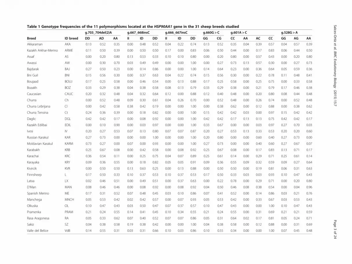
Table 1 Genotype frequencies of the 11 polymorphisms located at the HSP90AA1 gene in the 31 sheep breeds studied

g.703_704del(2)A g.667_668insC g.666_667insC g.660G > C g.601A > C g.528G > A

Breed ID breed DD AD AA II ID DD II ID DD GG CG CC AA AC CC GG AG AA

Akkaraman AKA 0.13 0.52 0.35 0.00 0.48 0.52 0.04 0.22 0.74 0.13 0.52 0.35 0.04 0.39 0.57 0.04 0.57 0.39

Kazakh Arkhar-Merino ARME 0.11 0.50 0.39 0.00 0.50 0.50 0.17 0.00 0.83 0.06 0.50 0.44 0.00 0.17 0.83 0.06 0.44 0.50

Assaf AS 0.00 0.20 0.80 0.13 0.53 0.33 0.10 0.10 0.80 0.00 0.20 0.80 0.00 0.57 0.43 0.00 0.20 0.80

Awassi AW 0.00 0.30 0.70 0.03 0.49 0.49 0.00 0.00 1.00 0.00 0.27 0.73 0.13 0.57 0.30 0.00 0.27 0.73

Bajdarak BAJ 0.27 0.50 0.23 0.00 0.14 0.86 0.00 0.00 1.00 0.14 0.64 0.23 0.00 0.36 0.64 0.05 0.59 0.36

Bni Guil BNI 0.15 0.56 0.30 0.00 0.37 0.63 0.04 0.22 0.74 0.15 0.56 0.30 0.00 0.22 0.78 0.11 0.48 0.41

Boujaad BOUJ 0.17 0.25 0.58 0.00 0.46 0.54 0.00 0.13 0.88 0.17 0.25 0.58 0.00 0.25 0.75 0.00 0.33 0.58

Bozakh BOZ 0.33 0.29 0.38 0.04 0.38 0.58 0.08 0.13 0.79 0.33 0.29 0.38 0.00 0.21 0.79 0.17 0.46 0.38

Caucasian CAUC 0.20 0.32 0.48 0.04 0.32 0.64 0.12 0.00 0.88 0.12 0.40 0.48 0.00 0.20 0.80 0.08 0.44 0.48

Churra Ch 0.00 0.52 0.48 0.09 0.30 0.61 0.04 0.26 0.70 0.00 0.52 0.48 0.00 0.26 0.74 0.00 0.52 0.48

Churra Lebrijana Cl 0.00 0.42 0.58 0.38 0.42 0.19 0.00 0.00 1.00 0.00 0.38 0.62 0.00 0.12 0.88 0.00 0.38 0.62

Churra Tensina Ct 0.24 0.36 0.39 0.00 0.18 0.82 0.00 0.00 1.00 0.15 0.42 0.42 0.03 0.00 0.97 0.15 0.42 0.42

Daglic DGL 0.42 0.42 0.17 0.00 0.08 0.92 0.00 0.00 1.00 0.42 0.42 0.17 0.13 0.13 0.75 0.42 0.42 0.17

Kazakh Edilbai EDIL 0.00 0.10 0.90 0.00 0.03 0.97 0.00 0.00 1.00 0.33 0.67 0.00 0.00 0.03 0.97 0.27 0.70 0.03

Ivesi IV 0.20 0.27 0.53 0.07 0.13 0.80 0.07 0.07 0.87 0.20 0.27 0.53 0.13 0.33 0.53 0.20 0.20 0.60

Russian Karakul KAR 0.27 0.73 0.00 0.00 0.00 1.00 0.00 0.00 1.00 0.20 0.80 0.00 0.00 0.60 0.40 0.27 0.73 0.00

Moldavian Karakul KARM 0.73 0.27 0.00 0.07 0.00 0.93 0.00 0.00 1.00 0.27 0.73 0.00 0.00 0.40 0.60 0.27 0.67 0.07

Karabakh KRB 0.25 0.67 0.08 0.00 0.42 0.58 0.00 0.08 0.92 0.25 0.67 0.08 0.00 0.17 0.83 0.13 0.71 0.17

Karachai KRC 0.36 0.54 0.11 0.00 0.25 0.75 0.04 0.07 0.89 0.25 0.61 0.14 0.00 0.29 0.71 0.25 0.61 0.14

Karayaka KRY 0.09 0.36 0.55 0.00 0.18 0.82 0.05 0.05 0.91 0.09 0.36 0.55 0.09 0.32 0.59 0.09 0.27 0.64

Kivircik KVR 0.00 0.50 0.50 0.13 0.63 0.25 0.00 0.13 0.88 0.00 0.50 0.50 0.00 0.19 0.81 0.06 0.31 0.63

Finnsheep L 0.17 0.50 0.33 0.10 0.37 0.53 0.10 0.37 0.53 0.17 0.50 0.33 0.03 0.03 0.93 0.10 0.47 0.43

Latxa LX 0.02 0.46 0.51 0.00 0.49 0.51 0.00 0.37 0.63 0.00 0.22 0.78 0.00 0.29 0.71 0.00 0.20 0.80

D’Man MAN 0.08 0.46 0.46 0.00 0.08 0.92 0.00 0.08 0.92 0.04 0.50 0.46 0.08 0.38 0.54 0.00 0.04 0.96

Spanish Merino ME 0.17 0.31 0.52 0.07 0.48 0.45 0.03 0.10 0.86 0.07 0.41 0.52 0.00 0.14 0.86 0.03 0.21 0.76

Manchega MNCH 0.05 0.53 0.42 0.02 0.42 0.57 0.00 0.07 0.93 0.05 0.53 0.42 0.00 0.33 0.67 0.03 0.53 0.43

Olkuska OL 0.10 0.47 0.43 0.03 0.50 0.47 0.07 0.37 0.57 0.10 0.47 0.43 0.00 0.00 1.00 0.10 0.47 0.43

Pramenka PRAM 0.21 0.24 0.55 0.14 0.41 0.45 0.10 0.34 0.55 0.21 0.24 0.55 0.00 0.31 0.69 0.21 0.21 0.59

Rasa Aragonesa RA 0.05 0.33 0.62 0.07 0.40 0.52 0.07 0.07 0.86 0.05 0.31 0.64 0.02 0.17 0.81 0.05 0.24 0.71

Sakiz SZ 0.04 0.38 0.58 0.19 0.38 0.42 0.00 0.00 1.00 0.04 0.38 0.58 0.00 0.12 0.88 0.00 0.31 0.69

Valle del Belice VdB 0.14 0.55 0.31 0.03 0.31 0.66 0.10 0.03 0.86 0.10 0.55 0.34 0.00 0.00 1.00 0.07 0.45 0.48

Salces-Ortiz

etal.BM

CEvolutionary

Biology (2015) 15:7

Page3of

24

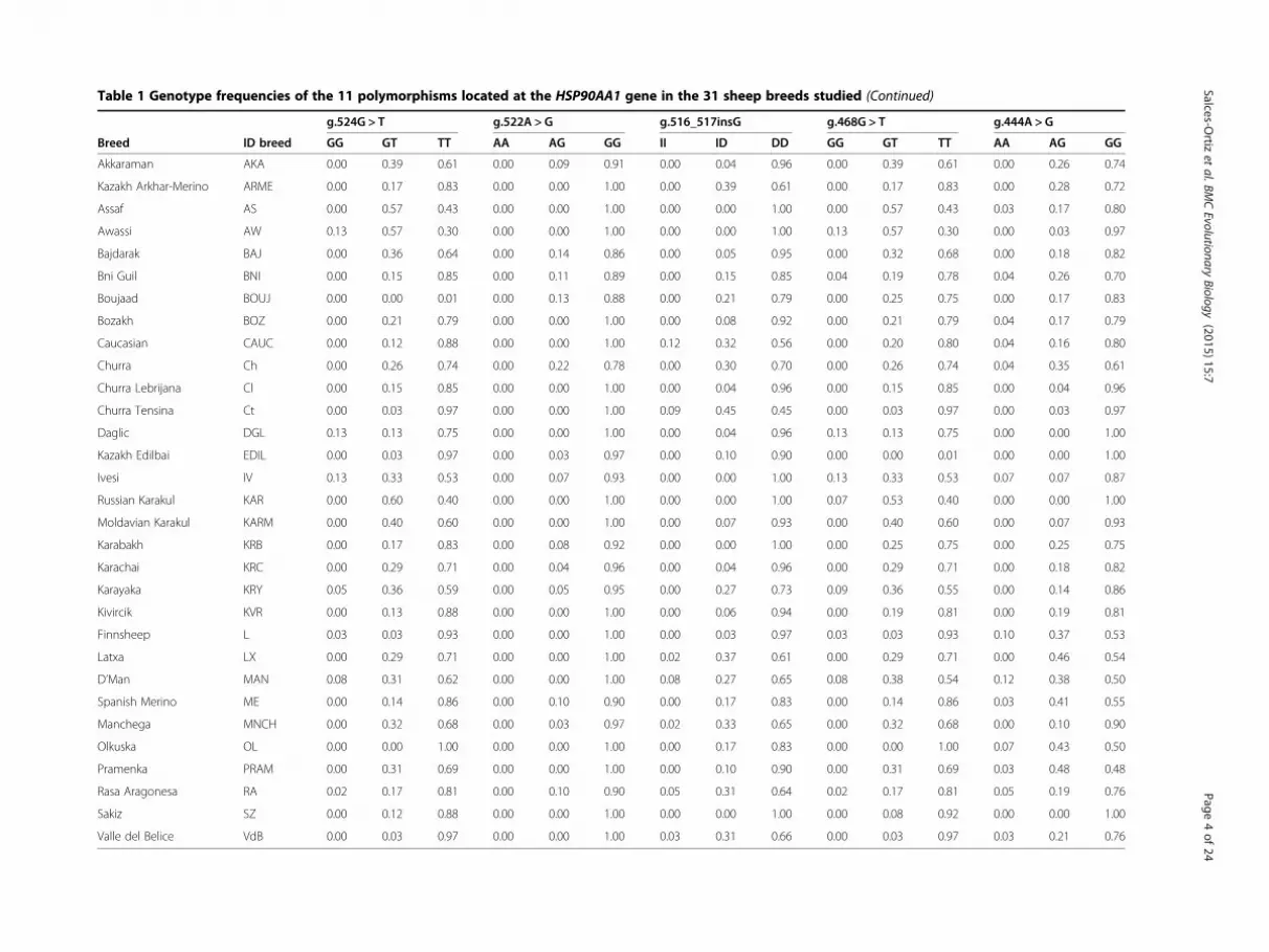
Table 1 Genotype frequencies of the 11 polymorphisms located at the HSP90AA1 gene in the 31 sheep breeds studied (Continued)

g.524G > T g.522A > G g.516_517insG g.468G > T g.444A > G

Breed ID breed GG GT TT AA AG GG II ID DD GG GT TT AA AG GG

Akkaraman AKA 0.00 0.39 0.61 0.00 0.09 0.91 0.00 0.04 0.96 0.00 0.39 0.61 0.00 0.26 0.74

Kazakh Arkhar-Merino ARME 0.00 0.17 0.83 0.00 0.00 1.00 0.00 0.39 0.61 0.00 0.17 0.83 0.00 0.28 0.72

Assaf AS 0.00 0.57 0.43 0.00 0.00 1.00 0.00 0.00 1.00 0.00 0.57 0.43 0.03 0.17 0.80

Awassi AW 0.13 0.57 0.30 0.00 0.00 1.00 0.00 0.00 1.00 0.13 0.57 0.30 0.00 0.03 0.97

Bajdarak BAJ 0.00 0.36 0.64 0.00 0.14 0.86 0.00 0.05 0.95 0.00 0.32 0.68 0.00 0.18 0.82

Bni Guil BNI 0.00 0.15 0.85 0.00 0.11 0.89 0.00 0.15 0.85 0.04 0.19 0.78 0.04 0.26 0.70

Boujaad BOUJ 0.00 0.00 0.01 0.00 0.13 0.88 0.00 0.21 0.79 0.00 0.25 0.75 0.00 0.17 0.83

Bozakh BOZ 0.00 0.21 0.79 0.00 0.00 1.00 0.00 0.08 0.92 0.00 0.21 0.79 0.04 0.17 0.79

Caucasian CAUC 0.00 0.12 0.88 0.00 0.00 1.00 0.12 0.32 0.56 0.00 0.20 0.80 0.04 0.16 0.80

Churra Ch 0.00 0.26 0.74 0.00 0.22 0.78 0.00 0.30 0.70 0.00 0.26 0.74 0.04 0.35 0.61

Churra Lebrijana Cl 0.00 0.15 0.85 0.00 0.00 1.00 0.00 0.04 0.96 0.00 0.15 0.85 0.00 0.04 0.96

Churra Tensina Ct 0.00 0.03 0.97 0.00 0.00 1.00 0.09 0.45 0.45 0.00 0.03 0.97 0.00 0.03 0.97

Daglic DGL 0.13 0.13 0.75 0.00 0.00 1.00 0.00 0.04 0.96 0.13 0.13 0.75 0.00 0.00 1.00

Kazakh Edilbai EDIL 0.00 0.03 0.97 0.00 0.03 0.97 0.00 0.10 0.90 0.00 0.00 0.01 0.00 0.00 1.00

Ivesi IV 0.13 0.33 0.53 0.00 0.07 0.93 0.00 0.00 1.00 0.13 0.33 0.53 0.07 0.07 0.87

Russian Karakul KAR 0.00 0.60 0.40 0.00 0.00 1.00 0.00 0.00 1.00 0.07 0.53 0.40 0.00 0.00 1.00

Moldavian Karakul KARM 0.00 0.40 0.60 0.00 0.00 1.00 0.00 0.07 0.93 0.00 0.40 0.60 0.00 0.07 0.93

Karabakh KRB 0.00 0.17 0.83 0.00 0.08 0.92 0.00 0.00 1.00 0.00 0.25 0.75 0.00 0.25 0.75

Karachai KRC 0.00 0.29 0.71 0.00 0.04 0.96 0.00 0.04 0.96 0.00 0.29 0.71 0.00 0.18 0.82

Karayaka KRY 0.05 0.36 0.59 0.00 0.05 0.95 0.00 0.27 0.73 0.09 0.36 0.55 0.00 0.14 0.86

Kivircik KVR 0.00 0.13 0.88 0.00 0.00 1.00 0.00 0.06 0.94 0.00 0.19 0.81 0.00 0.19 0.81

Finnsheep L 0.03 0.03 0.93 0.00 0.00 1.00 0.00 0.03 0.97 0.03 0.03 0.93 0.10 0.37 0.53

Latxa LX 0.00 0.29 0.71 0.00 0.00 1.00 0.02 0.37 0.61 0.00 0.29 0.71 0.00 0.46 0.54

D’Man MAN 0.08 0.31 0.62 0.00 0.00 1.00 0.08 0.27 0.65 0.08 0.38 0.54 0.12 0.38 0.50

Spanish Merino ME 0.00 0.14 0.86 0.00 0.10 0.90 0.00 0.17 0.83 0.00 0.14 0.86 0.03 0.41 0.55

Manchega MNCH 0.00 0.32 0.68 0.00 0.03 0.97 0.02 0.33 0.65 0.00 0.32 0.68 0.00 0.10 0.90

Olkuska OL 0.00 0.00 1.00 0.00 0.00 1.00 0.00 0.17 0.83 0.00 0.00 1.00 0.07 0.43 0.50

Pramenka PRAM 0.00 0.31 0.69 0.00 0.00 1.00 0.00 0.10 0.90 0.00 0.31 0.69 0.03 0.48 0.48

Rasa Aragonesa RA 0.02 0.17 0.81 0.00 0.10 0.90 0.05 0.31 0.64 0.02 0.17 0.81 0.05 0.19 0.76

Sakiz SZ 0.00 0.12 0.88 0.00 0.00 1.00 0.00 0.00 1.00 0.00 0.08 0.92 0.00 0.00 1.00

Valle del Belice VdB 0.00 0.03 0.97 0.00 0.00 1.00 0.03 0.31 0.66 0.00 0.03 0.97 0.03 0.21 0.76

Salces-Ortiz

etal.BM

CEvolutionary

Biology (2015) 15:7

Page4of

24

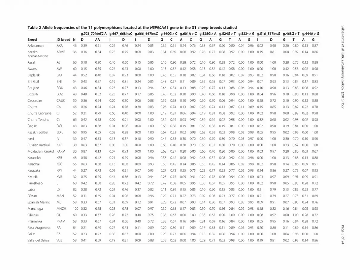
Table 2 Allele frequencies of the 11 polymorphisms located at the HSP90AA1 gene in the 31 sheep breeds studied

g.703_704del(2)A g.667_668insC g.666_667insC g.660G > C g.601A > C g.528G > A g.524G > T g.522ª > G g.516_517insG g.468G > T g.444A > G

Breed ID breed N D AA I D I D G C A C G A G T A G I D G T A G

Akkaraman AKA 46 0.39 0.61 0.24 0.76 0.24 0.85 0.39 0.61 0.24 0.76 0.33 0.67 0.20 0.80 0.04 0.96 0.02 0.98 0.20 0.80 0.13 0.87

KazakhArkhar-Merino

ARME 36 0.36 0.64 0.25 0.75 0.08 0.83 0.31 0.69 0.08 0.92 0.28 0.72 0.08 0.92 0.00 1.00 0.19 0.81 0.08 0.92 0.14 0.86

Assaf AS 60 0.10 0.90 0.40 0.60 0.15 0.85 0.10 0.90 0.28 0.72 0.10 0.90 0.28 0.72 0.00 1.00 0.00 1.00 0.28 0.72 0.12 0.88

Awassi AW 60 0.15 0.85 0.27 0.73 0.00 1.00 0.13 0.87 0.42 0.58 0.13 0.87 0.42 0.58 0.00 1.00 0.00 1.00 0.42 0.58 0.02 0.98

Bajdarak BAJ 44 0.52 0.48 0.07 0.93 0.00 1.00 0.45 0.55 0.18 0.82 0.34 0.66 0.18 0.82 0.07 0.93 0.02 0.98 0.16 0.84 0.09 0.91

Bni Guil BNI 54 0.43 0.57 0.19 0.81 0.24 0.85 0.43 0.57 0.11 0.89 0.35 0.65 0.07 0.93 0.06 0.94 0.07 0.93 0.13 0.87 0.17 0.83

Boujaad BOUJ 48 0.46 0.54 0.23 0.77 0.13 0.94 0.46 0.54 0.13 0.88 0.25 0.75 0.13 0.88 0.06 0.94 0.10 0.90 0.13 0.88 0.08 0.92

Bozakh BOZ 48 0.48 0.52 0.23 0.77 0.17 0.85 0.48 0.52 0.10 0.90 0.40 0.60 0.10 0.90 0.00 1.00 0.04 0.96 0.10 0.90 0.13 0.88

Caucasian CAUC 50 0.36 0.64 0.20 0.80 0.06 0.88 0.32 0.68 0.10 0.90 0.30 0.70 0.06 0.94 0.00 1.00 0.28 0.72 0.10 0.90 0.12 0.88

Churra Ch 46 0.26 0.74 0.24 0.76 0.28 0.83 0.26 0.74 0.13 0.87 0.26 0.74 0.13 0.87 0.11 0.89 0.15 0.85 0.13 0.87 0.22 0.78

Churra Lebrijana Cl 52 0.21 0.79 0.60 0.40 0.00 1.00 0.19 0.81 0.06 0.94 0.19 0.81 0.08 0.92 0.00 1.00 0.02 0.98 0.08 0.92 0.02 0.98

Churra Tensina Ct 66 0.42 0.58 0.09 0.91 0.00 1.00 0.36 0.64 0.03 0.97 0.36 0.64 0.02 0.98 0.00 1.00 0.32 0.68 0.02 0.98 0.02 0.98

Daglic DGL 48 0.63 0.38 0.04 0.96 0.00 1.00 0.63 0.38 0.19 0.81 0.63 0.38 0.19 0.81 0.00 1.00 0.02 0.98 0.19 0.81 0.00 1.00

Kazakh Edilbai EDIL 60 0.95 0.05 0.02 0.98 0.00 1.00 0.67 0.33 0.02 0.98 0.62 0.38 0.02 0.98 0.02 0.98 0.05 0.95 0.02 0.98 0.00 1.00

Ivesi IV 30 0.47 0.53 0.13 0.87 0.10 0.90 0.47 0.53 0.30 0.70 0.30 0.70 0.30 0.70 0.03 0.97 0.00 1.00 0.30 0.70 0.10 0.90

Russian Karakul KAR 30 0.63 0.37 0.00 1.00 0.00 1.00 0.60 0.40 0.30 0.70 0.63 0.37 0.30 0.70 0.00 1.00 0.00 1.00 0.33 0.67 0.00 1.00

Moldavian Karakul KARM 30 0.87 0.13 0.07 0.93 0.00 1.00 0.63 0.37 0.20 0.80 0.60 0.40 0.20 0.80 0.00 1.00 0.03 0.97 0.20 0.80 0.03 0.67

Karabakh KRB 48 0.58 0.42 0.21 0.79 0.08 0.96 0.58 0.42 0.08 0.92 0.48 0.52 0.08 0.92 0.04 0.96 0.00 1.00 0.13 0.88 0.13 0.88

Karachai KRC 56 0.63 0.38 0.13 0.88 0.09 0.93 0.55 0.45 0.14 0.86 0.55 0.45 0.14 0.86 0.02 0.98 0.02 0.98 0.14 0.86 0.09 0.91

Karayaka KRY 44 0.27 0.73 0.09 0.91 0.07 0.93 0.27 0.73 0.25 0.75 0.23 0.77 0.23 0.77 0.02 0.98 0.14 0.86 0.27 0.73 0.07 0.93

Kivircik KVR 32 0.25 0.75 0.44 0.56 0.13 0.94 0.25 0.75 0.09 0.91 0.22 0.78 0.06 0.94 0.00 1.00 0.03 0.97 0.09 0.91 0.09 0.91

Finnsheep L 60 0.42 0.58 0.28 0.72 0.42 0.72 0.42 0.58 0.05 0.95 0.33 0.67 0.05 0.95 0.00 1.00 0.02 0.98 0.05 0.95 0.28 0.72

Latxa LX 82 0.28 0.72 0.24 0.76 0.37 0.82 0.11 0.89 0.15 0.85 0.10 0.90 0.15 0.85 0.00 1.00 0.21 0.79 0.15 0.85 0.23 0.77

D’Man MAN 52 0.31 0.69 0.04 0.96 0.08 0.96 0.29 0.71 0.27 0.73 0.02 0.98 0.23 0.77 0.00 1.00 0.21 0.79 0.27 0.73 0.31 0.69

Spanish Merino ME 58 0.33 0.67 0.31 0.69 0.12 0.91 0.28 0.72 0.07 0.93 0.14 0.86 0.07 0.93 0.05 0.95 0.09 0.91 0.07 0.93 0.24 0.76

Manchega MNCH 120 0.32 0.68 0.23 0.78 0.07 0.97 0.32 0.68 0.17 0.83 0.30 0.70 0.16 0.84 0.02 0.98 0.18 0.82 0.16 0.84 0.05 0.95

Olkuska OL 60 0.33 0.67 0.28 0.72 0.40 0.75 0.33 0.67 0.00 1.00 0.33 0.67 0.00 1.00 0.00 1.00 0.08 0.92 0.00 1.00 0.28 0.72

Pramenka PRAM 58 0.33 0.67 0.34 0.66 0.40 0.72 0.33 0.67 0.16 0.84 0.31 0.69 0.16 0.84 0.00 1.00 0.05 0.95 0.16 0.84 0.28 0.72

Rasa Aragonesa RA 84 0.21 0.79 0.27 0.73 0.11 0.89 0.20 0.80 0.11 0.89 0.17 0.83 0.11 0.89 0.05 0.95 0.20 0.80 0.11 0.89 0.14 0.86

Sakiz SZ 52 0.23 0.77 0.38 0.62 0.00 1.00 0.23 0.77 0.06 0.94 0.15 0.85 0.06 0.94 0.00 1.00 0.00 1.00 0.04 0.96 0.00 1.00

Valle del Belice VdB 58 0.41 0.59 0.19 0.81 0.09 0.88 0.38 0.62 0.00 1.00 0.29 0.71 0.02 0.98 0.00 1.00 0.19 0.81 0.02 0.98 0.14 0.86

Salces-Ortiz

etal.BM

CEvolutionary

Biology (2015) 15:7

Page5of

24


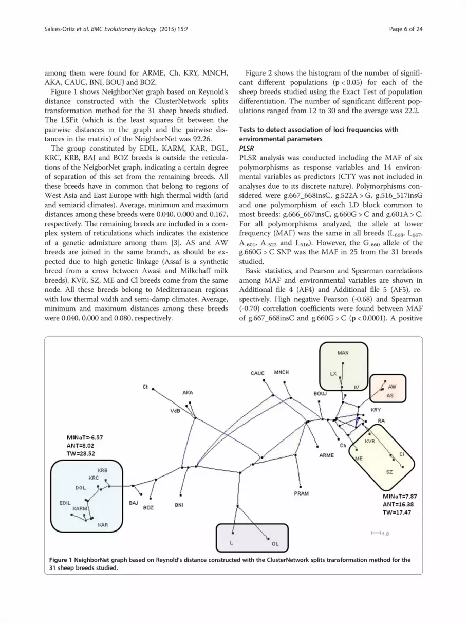
among them were found for ARME, Ch, KRY, MNCH,AKA, CAUC, BNI, BOUJ and BOZ.Figure 1 shows NeighborNet graph based on Reynold’s

distance constructed with the ClusterNetwork splitstransformation method for the 31 sheep breeds studied.The LSFit (which is the least squares fit between thepairwise distances in the graph and the pairwise dis-tances in the matrix) of the NeighborNet was 92.26.The group constituted by EDIL, KARM, KAR, DGL,

KRC, KRB, BAJ and BOZ breeds is outside the reticula-tions of the NeigborNet graph, indicating a certain degreeof separation of this set from the remaining breeds. Allthese breeds have in common that belong to regions ofWest Asia and East Europe with high thermal width (aridand semiarid climates). Average, minimum and maximumdistances among these breeds were 0.040, 0.000 and 0.167,respectively. The remaining breeds are included in a com-plex system of reticulations which indicates the existenceof a genetic admixture among them [3]. AS and AWbreeds are joined in the same branch, as should be ex-pected due to high genetic linkage (Assaf is a syntheticbreed from a cross between Awasi and Milkchaff milkbreeds). KVR, SZ, ME and Cl breeds come from the samenode. All these breeds belong to Mediterranean regionswith low thermal width and semi-damp climates. Average,minimum and maximum distances among these breedswere 0.040, 0.000 and 0.080, respectively.

Figure 1 NeighborNet graph based on Reynold’s distance constructed31 sheep breeds studied.

Figure 2 shows the histogram of the number of signifi-cant different populations (p < 0.05) for each of thesheep breeds studied using the Exact Test of populationdifferentiation. The number of significant different pop-ulations ranged from 12 to 30 and the average was 22.2.

Tests to detect association of loci frequencies withenvironmental parametersPLSRPLSR analysis was conducted including the MAF of sixpolymorphisms as response variables and 14 environ-mental variables as predictors (CTY was not included inanalyses due to its discrete nature). Polymorphisms con-sidered were g.667_668insC, g.522A > G, g.516_517insGand one polymorphism of each LD block common tomost breeds: g.666_667insC, g.660G > C and g.601A > C.For all polymorphisms analyzed, the allele at lowerfrequency (MAF) was the same in all breeds (I-668, I-667,A-601, A-522 and I-516). However, the G-660 allele of theg.660G > C SNP was the MAF in 25 from the 31 breedsstudied.Basic statistics, and Pearson and Spearman correlations

among MAF and environmental variables are shown inAdditional file 4 (AF4) and Additional file 5 (AF5), re-spectively. High negative Pearson (-0.68) and Spearman(-0.70) correlation coefficients were found between MAFof g.667_668insC and g.660G >C (p < 0.0001). A positive

with the ClusterNetwork splits transformation method for the

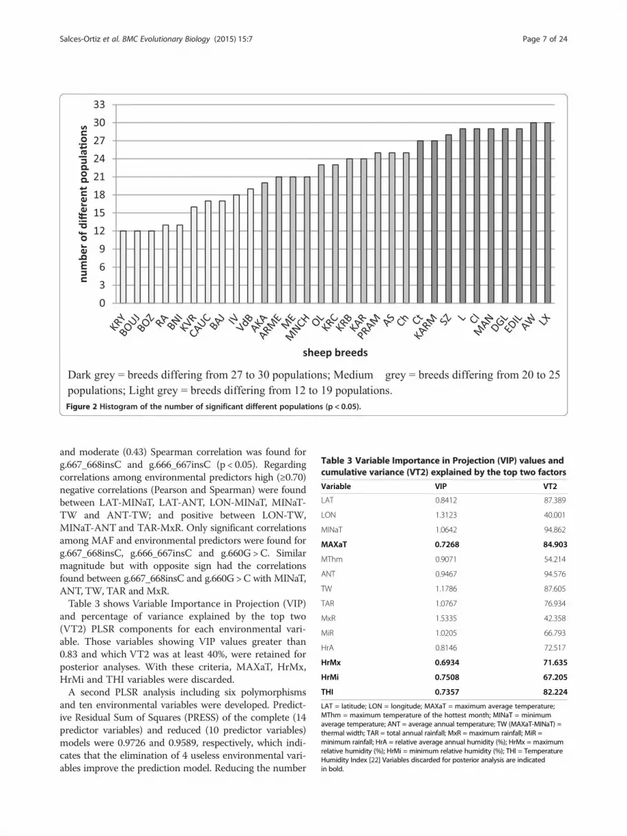
Figure 2 Histogram of the number of significant different populations (p < 0.05).

Table 3 Variable Importance in Projection (VIP) values andcumulative variance (VT2) explained by the top two factors

Variable VIP VT2

LAT 0.8412 87.389

LON 1.3123 40.001

MINaT 1.0642 94.862

MAXaT 0.7268 84.903

MThm 0.9071 54.214

ANT 0.9467 94.576

TW 1.1786 87.605

TAR 1.0767 76.934

MxR 1.5335 42.358

MiR 1.0205 66.793

HrA 0.8146 72.517

HrMx 0.6934 71.635

HrMi 0.7508 67.205

THI 0.7357 82.224

LAT = latitude; LON = longitude; MAXaT = maximum average temperature;MThm = maximum temperature of the hottest month; MINaT = minimumaverage temperature; ANT = average annual temperature; TW (MAXaT-MINaT) =thermal width; TAR = total annual rainfall; MxR = maximum rainfall; MiR =minimum rainfall; HrA = relative average annual humidity (%); HrMx = maximumrelative humidity (%); HrMi = minimum relative humidity (%); THI = TemperatureHumidity Index [22] Variables discarded for posterior analysis are indicatedin bold.


and moderate (0.43) Spearman correlation was found forg.667_668insC and g.666_667insC (p < 0.05). Regardingcorrelations among environmental predictors high (≥0.70)negative correlations (Pearson and Spearman) were foundbetween LAT-MINaT, LAT-ANT, LON-MINaT, MINaT-TW and ANT-TW; and positive between LON-TW,MINaT-ANT and TAR-MxR. Only significant correlationsamong MAF and environmental predictors were found forg.667_668insC, g.666_667insC and g.660G >C. Similarmagnitude but with opposite sign had the correlationsfound between g.667_668insC and g.660G >C with MINaT,ANT, TW, TAR and MxR.Table 3 shows Variable Importance in Projection (VIP)

and percentage of variance explained by the top two(VT2) PLSR components for each environmental vari-able. Those variables showing VIP values greater than0.83 and which VT2 was at least 40%, were retained forposterior analyses. With these criteria, MAXaT, HrMx,HrMi and THI variables were discarded.A second PLSR analysis including six polymorphisms

and ten environmental variables were developed. Predict-ive Residual Sum of Squares (PRESS) of the complete (14predictor variables) and reduced (10 predictor variables)models were 0.9726 and 0.9589, respectively, which indi-cates that the elimination of 4 useless environmental vari-ables improve the prediction model. Reducing the number


of predictors, R2 (value of explained variation) was alsoimproved from 0.82 (14 predictors) to 0.85 (10 predictors).Three components were retained using the optimal

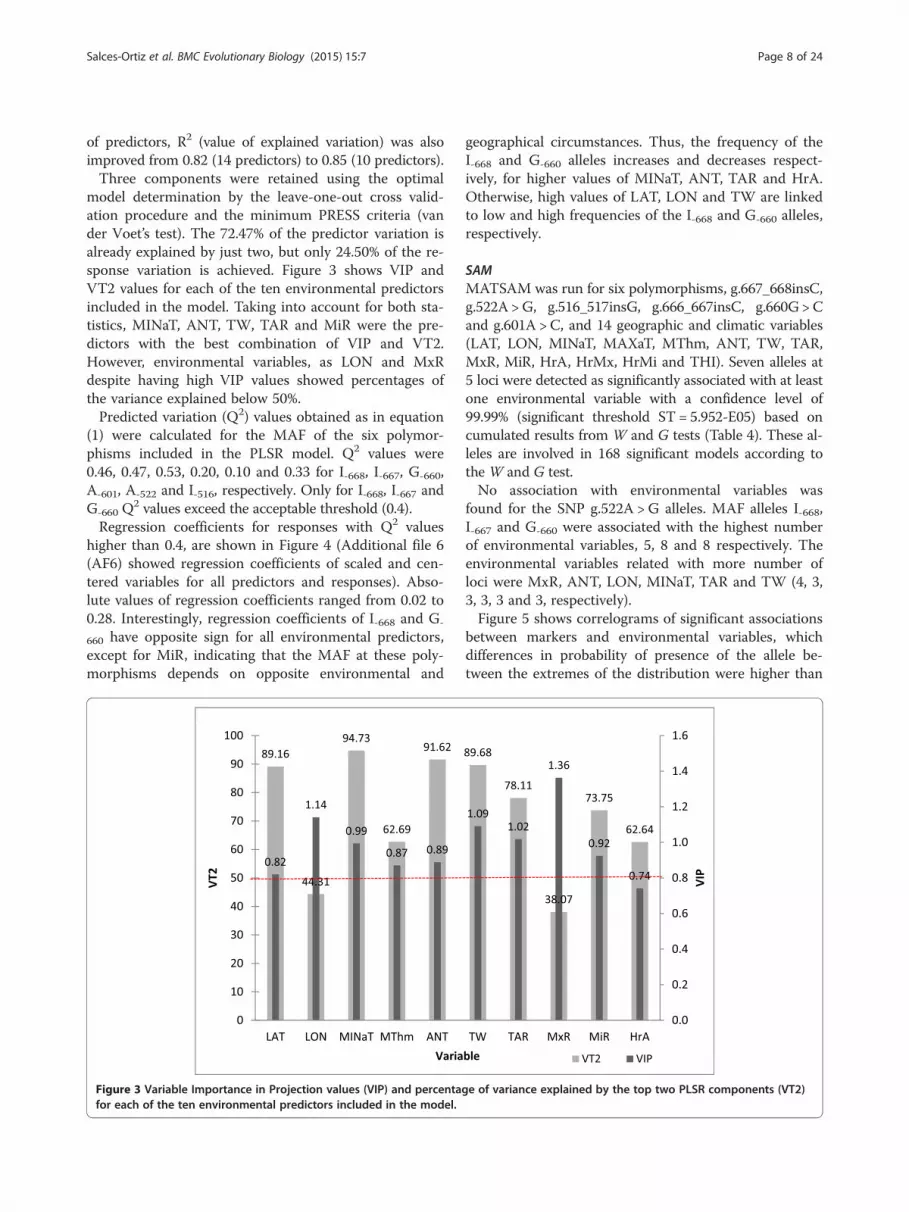
model determination by the leave-one-out cross valid-ation procedure and the minimum PRESS criteria (vander Voet’s test). The 72.47% of the predictor variation isalready explained by just two, but only 24.50% of the re-sponse variation is achieved. Figure 3 shows VIP andVT2 values for each of the ten environmental predictorsincluded in the model. Taking into account for both sta-tistics, MINaT, ANT, TW, TAR and MiR were the pre-dictors with the best combination of VIP and VT2.However, environmental variables, as LON and MxRdespite having high VIP values showed percentages ofthe variance explained below 50%.Predicted variation (Q2) values obtained as in equation

(1) were calculated for the MAF of the six polymor-phisms included in the PLSR model. Q2 values were0.46, 0.47, 0.53, 0.20, 0.10 and 0.33 for I-668, I-667, G-660,A-601, A-522 and I-516, respectively. Only for I-668, I-667 andG-660 Q

2 values exceed the acceptable threshold (0.4).Regression coefficients for responses with Q2 values

higher than 0.4, are shown in Figure 4 (Additional file 6(AF6) showed regression coefficients of scaled and cen-tered variables for all predictors and responses). Abso-lute values of regression coefficients ranged from 0.02 to0.28. Interestingly, regression coefficients of I-668 and G-

660 have opposite sign for all environmental predictors,except for MiR, indicating that the MAF at these poly-morphisms depends on opposite environmental and

Figure 3 Variable Importance in Projection values (VIP) and percentafor each of the ten environmental predictors included in the model.

geographical circumstances. Thus, the frequency of theI-668 and G-660 alleles increases and decreases respect-ively, for higher values of MINaT, ANT, TAR and HrA.Otherwise, high values of LAT, LON and TW are linkedto low and high frequencies of the I-668 and G-660 alleles,respectively.

SAMMATSAM was run for six polymorphisms, g.667_668insC,g.522A >G, g.516_517insG, g.666_667insC, g.660G > Cand g.601A > C, and 14 geographic and climatic variables(LAT, LON, MINaT, MAXaT, MThm, ANT, TW, TAR,MxR, MiR, HrA, HrMx, HrMi and THI). Seven alleles at5 loci were detected as significantly associated with at leastone environmental variable with a confidence level of99.99% (significant threshold ST = 5.952-E05) based oncumulated results from W and G tests (Table 4). These al-leles are involved in 168 significant models according tothe W and G test.No association with environmental variables was

found for the SNP g.522A > G alleles. MAF alleles I-668,I-667 and G-660 were associated with the highest numberof environmental variables, 5, 8 and 8 respectively. Theenvironmental variables related with more number ofloci were MxR, ANT, LON, MINaT, TAR and TW (4, 3,3, 3, 3 and 3, respectively).Figure 5 shows correlograms of significant associations

between markers and environmental variables, whichdifferences in probability of presence of the allele be-tween the extremes of the distribution were higher than

ge of variance explained by the top two PLSR components (VT2)

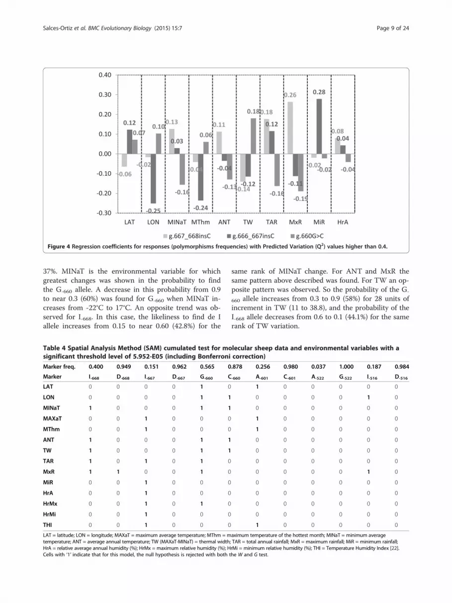
Figure 4 Regression coefficients for responses (polymorphisms frequencies) with Predicted Variation (Q2) values higher than 0.4.


37%. MINaT is the environmental variable for whichgreatest changes was shown in the probability to findthe G-660 allele. A decrease in this probability from 0.9to near 0.3 (60%) was found for G-660 when MINaT in-creases from -22°C to 17°C. An opposite trend was ob-served for I-668. In this case, the likeliness to find de Iallele increases from 0.15 to near 0.60 (42.8%) for the

Table 4 Spatial Analysis Method (SAM) cumulated test for mosignificant threshold level of 5.952-E05 (including Bonferroni

Marker freq. 0.400 0.949 0.151 0.962 0.565 0

Marker I-668 D-668 I-667 D-667 G-660 C

LAT 0 0 0 0 1 0

LON 0 0 0 0 1 1

MINaT 1 0 0 0 1 1

MAXaT 0 0 1 0 0 0

MThm 0 0 1 0 0 0

ANT 1 0 0 0 1 1

TW 1 0 0 0 1 1

TAR 1 0 1 0 1 0

MxR 1 1 0 0 1 0

MiR 0 0 1 0 0 0

HrA 0 0 1 0 0 0

HrMx 0 0 1 0 1 0

HrMi 0 0 1 0 0 0

THI 0 0 1 0 0 0

LAT = latitude; LON = longitude; MAXaT = maximum average temperature; MThm = mtemperature; ANT = average annual temperature; TW (MAXaT-MINaT) = thermal widthHrA = relative average annual humidity (%); HrMx = maximum relative humidity (%); HCells with ‘1’ indicate that for this model, the null hypothesis is rejected with both t

same rank of MINaT change. For ANT and MxR thesame pattern above described was found. For TW an op-posite pattern was observed. So the probability of the G-

660 allele increases from 0.3 to 0.9 (58%) for 28 units ofincrement in TW (11 to 38.8), and the probability of theI-668 allele decreases from 0.6 to 0.1 (44.1%) for the samerank of TW variation.

lecular sheep data and environmental variables with acorrection)

.878 0.256 0.980 0.037 1.000 0.187 0.984

-660 A-601 C-601 A-522 G-522 I-516 D-516

1 0 0 0 0 0

0 0 0 0 1 0

0 0 0 0 0 0

1 0 0 0 0 0

1 0 0 0 0 0

0 0 0 0 0 0

0 0 0 0 0 0

0 0 0 0 0 0

0 0 0 0 1 0

0 0 0 0 0 0

0 0 0 0 0 0

0 0 0 0 0 0

0 0 0 0 0 0

1 0 0 0 0 0

aximum temperature of the hottest month; MINaT = minimum average; TAR = total annual rainfall; MxR = maximum rainfall; MiR = minimum rainfall;rMi = minimum relative humidity (%); THI = Temperature Humidity Index [22].he W and G test.

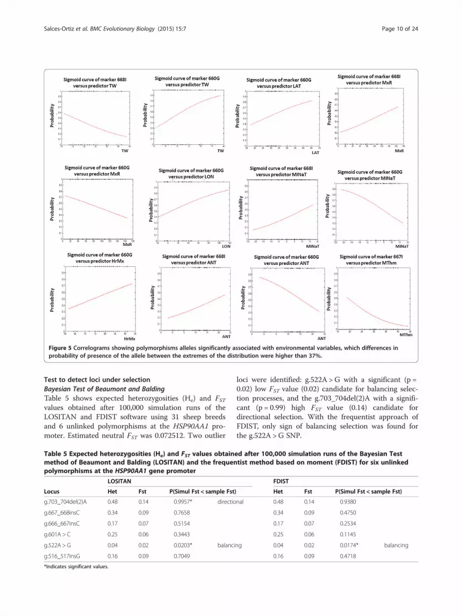
Figure 5 Correlograms showing polymorphisms alleles significantly associated with environmental variables, which differences inprobability of presence of the allele between the extremes of the distribution were higher than 37%.


Test to detect loci under selectionBayesian Test of Beaumont and BaldingTable 5 shows expected heterozygosities (He) and FSTvalues obtained after 100,000 simulation runs of theLOSITAN and FDIST software using 31 sheep breedsand 6 unlinked polymorphisms at the HSP90AA1 pro-moter. Estimated neutral FST was 0.072512. Two outlier

Table 5 Expected heterozygosities (He) and FST values obtainemethod of Beaumont and Balding (LOSITAN) and the frequenpolymorphisms at the HSP90AA1 gene promoter

LOSITAN

Locus Het Fst P(Simul Fst < sample Fst)

g.703_704del(2)A 0.48 0.14 0.9957* directio

g.667_668insC 0.34 0.09 0.7658

g.666_667insC 0.17 0.07 0.5154

g.601A > C 0.25 0.06 0.3443

g.522A > G 0.04 0.02 0.0203* balanci

g.516_517insG 0.16 0.09 0.7049

*Indicates significant values.

loci were identified: g.522A > G with a significant (p =0.02) low FST value (0.02) candidate for balancing selec-tion processes, and the g.703_704del(2)A with a signifi-cant (p = 0.99) high FST value (0.14) candidate fordirectional selection. With the frequentist approach ofFDIST, only sign of balancing selection was found forthe g.522A > G SNP.

d after 100,000 simulation runs of the Bayesian Testtist method based on moment (FDIST) for six unlinked

FDIST

Het Fst P(Simul Fst < sample Fst)

nal 0.48 0.14 0.9380

0.34 0.09 0.4750

0.17 0.07 0.2534

0.25 0.06 0.1145

ng 0.04 0.02 0.0174* balancing

0.16 0.09 0.4718


Characterization of the HSP90AA1 promoter in species ofthe Caprinae and Bovinae subfamiliesAligned sequences of a410 bp amplicon from theHSP90AA1 gene promoter of a total of 12 species be-longing to the Caprinae and Bovinae subfamilies areshown in Additional file 7 (AF7). Species from the Ovisgenus show 99% similarity with Ovis aries, followed byCapra hircus and Ovibos moschatus both with a similar-ity of 98%. The least similar species to Ovis aries wereBos mutus (92%) and Bos Taurus (93%). Additional file 8(AF8) shows haplotypes frequencies in each speciesstudied. In O. aries 36 different haplotypes were found.From them only the first four (H1 to H4) had a fre-quency higher than 10%. In O. musimon all the haplo-types found were shared with O. aries. O. canadiensishad not polymorphisms in the sequence analyzed. C. hir-cus showed 24 different haplotypes but only one wasfound in C. pyrenaica.The Tamura 3-parameter model (T92) with evolution-

ary rates among sites modeled by using a discreteGamma distribution (+G) with 5 rate categories had thehighest fit (lowest BIC value) among the 24 different nu-cleotide substitution models tested by maximum likeli-hood. This model was fitted to estimate EvolutionaryDivergence between species sequences, to conduct theTajima’s Neutrality Test and to construct the ML tree.Table 6 shows estimates of evolutionary divergence

over sequence pairs between species. Within the Caprinaesubfamily, the R. pyrenaica showed the highest percentageof sequence divergence with the remaining species (4.4%with species from the Ovis and Ovibos genus, 7% with spe-cies from the Capra genus and 7.6% with A. lervia. Inter-estingly O. moschatus was much closer to species of theOvis genus (0.8 to 1%) than to those of Capra, Ammotra-gus and Rupicapra. As expected, very low evolutionary di-vergences among species of the Ovis genus and among thespecies of the Capra genus were observed.Table 7 shows polymorphisms detected and its fre-

quencies in the species studied. Within the Caprinaesubfamily, the species with more number of polymor-phisms, SNPs or INDELs, were C. hircus and O. aries,with 13 and 11 polymorphic sites, respectively, fromwhich only 6 were shared between them. Also O.moschatus and O. musimon showed high number ofpolymorphism, 8 and 7, respectively. The species whichshared more number of polymorphisms with O. aries(reference species in our work) were O. musimon (7), Omoschatus (7) and C hircus (5). In general, within thissubfamily, polymorphisms shared among the differentspecies had the same pattern of allele frequency, exceptfor g.528A >G in O. moschatus where the A allele showedthe highest frequency (0.93) and for g.703_704del(2)A inR. pyrenaica where the double A deletion allele was themost frequent (0.75). Exclusive polymorphisms were

found in C. hircus (8), A. lervia (3), O aries (2) and O.moschatus (1). The two out group species from the Bovisgenus (B. mutus and B. taurus) showed very few polymor-phisms and did not share any mutations with the reamingspecies.The three INDELs g.703_704del(2)A, g.667_668insC

and g.666_667insC existed simultaneously only in O.moschatus, O. musimon and O. aries. C hircus had thetwo contiguous g.667_668insC and g.666_667insC, andO. ammon and R pyrenaica the g.703_704del(2)A. Thehighest frequency of the I-668 allele, related with heatstress tolerance, was found in O. musimon (0.47) and O.moschatus (0.43) followed by O. aries (0.28) and C. hir-cus (0.18). The SNP g.660G > C seems to be exclusive ofthe Caprinae subfamily. Unfortunately, this region is asequence of several consecutive cytosines and thereforeis difficult to know if there is not mutation at -660 pos-ition or if the C-660 allele is fixed in Bos. Anyway, C ap-pears to be the wild allele of the g.660G > C SNP.Tajima’s Neutrality Test [23] conducted for the se-

quences of the HSP90AA1 promoter was -2.56 (p_value <0.05 [24]) which reveals an excess of low frequencypolymorphisms relative to expectation (DL = -1.78). Thisfact could indicate a purifying selection removing allelesthat diminish animal’s biological fitness but also thepresence of “young” beneficial mutations going tohigher frequencies.Figure 6 shows Maximum Likelihood bootstrap ori-

ginal and condensed trees based on the Tamura 3-parameter model and inferred from 5000 replicates. Thetree was constructed considering only haplotypes withfrequencies higher than 0.05. Branches corresponding topartitions reproduced in less than 50% bootstrap repli-cates are collapsed. The analysis involved 33 nucleotidesequences. There were a total of 410 positions in thefinal dataset. Out-group species (B. taurus and B.mutus)were located in a separate branch with a high bootstrappercentage (99). One branch were constituted by speciesof the Capra and Ammotragus genus (97) and otherbranch by those of the Ovis, Rupicapra and Ovibos ones(86). In the ML consensus tree, O. moschatus was lo-cated as a sister species of R. pyrenaica. Species fromthe Ovis genus (O. aries; O. musimon, O. vignei, O.ammon and O. canadiensis) appear mixed since manyhaplotypes are shared among them and promoter se-quences showed a high degree of similarity.

DiscussionPrevious studies from our group pointed out the exist-ence of different expression profiles in sheep carrying al-ternative genotypes of some polymorphisms located atthe HSP90AA1 gene promoter depending on environ-mental temperatures [18-20]. The join genotype of theg.667_668insC and the g.660G > C polymorphisms had

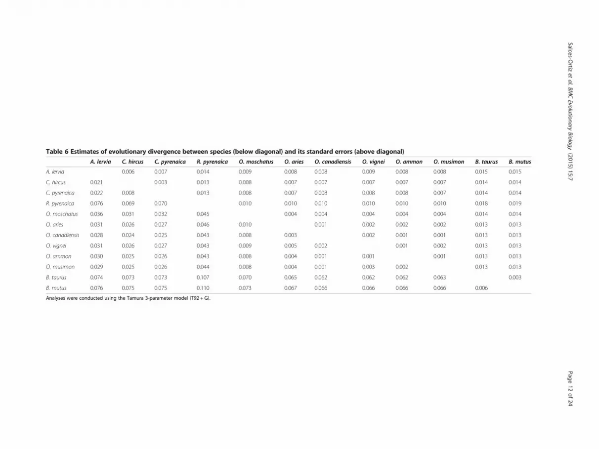
Table 6 Estimates of evolutionary divergence between species (below diagonal) and its standard errors (above diagonal)

A. lervia C. hircus C. pyrenaica R. pyrenaica O. moschatus O. aries O. canadiensis O. vignei O. ammon O. musimon B. taurus B. mutus

A. lervia 0.006 0.007 0.014 0.009 0.008 0.008 0.009 0.008 0.008 0.015 0.015

C. hircus 0.021 0.003 0.013 0.008 0.007 0.007 0.007 0.007 0.007 0.014 0.014

C. pyrenaica 0.022 0.008 0.013 0.008 0.007 0.008 0.008 0.008 0.007 0.014 0.014

R. pyrenaica 0.076 0.069 0.070 0.010 0.010 0.010 0.010 0.010 0.010 0.018 0.019

O. moschatus 0.036 0.031 0.032 0.045 0.004 0.004 0.004 0.004 0.004 0.014 0.014

O. aries 0.031 0.026 0.027 0.046 0.010 0.001 0.002 0.002 0.002 0.013 0.013

O. canadiensis 0.028 0.024 0.025 0.043 0.008 0.003 0.002 0.001 0.001 0.013 0.013

O. vignei 0.031 0.026 0.027 0.043 0.009 0.005 0.002 0.001 0.002 0.013 0.013

O. ammon 0.030 0.025 0.026 0.043 0.008 0.004 0.001 0.001 0.001 0.013 0.013

O. musimon 0.029 0.025 0.026 0.044 0.008 0.004 0.001 0.003 0.002 0.013 0.013

B. taurus 0.074 0.073 0.073 0.107 0.070 0.065 0.062 0.062 0.062 0.063 0.003

B. mutus 0.076 0.075 0.075 0.110 0.073 0.067 0.066 0.066 0.066 0.066 0.006

Analyses were conducted using the Tamura 3-parameter model (T92 + G).

Salces-Ortiz

etal.BM

CEvolutionary

Biology (2015) 15:7

Page12

of24

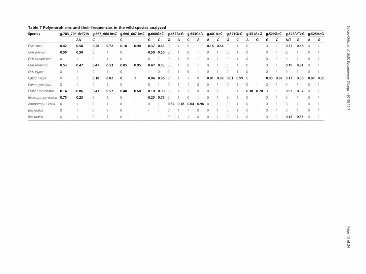
Table 7 Polymorphisms and their frequencies in the wild species analyzed

Species g.703_704 del(2)A g.667_668 insC g.666_667 insC g.660G>C g.657A>G g.653C>A g.601A>C g.571G>C g.551A>G g.529G>C g.528A/T>G g.525A>G

- AA C - C - G C G A C A A C G C A G G C A/T G A G

Ovis aries 0.42 0.58 0.28 0.72 0.10 0.90 0.37 0.63 0 1 0 1 0.16 0.84 0 1 0 1 0 1 0.32 0.68 0 1

Ovis ammon 0.50 0.50 0 1 0 1 0.50 0.50 0 1 0 1 0 1 0 1 0 1 0 1 0 1 0 1

Ovis canadiensis 0 1 0 1 0 1 0 1 0 1 0 1 0 1 0 1 0 1 0 1 0 1 0 1

Ovis musimon 0.53 0.47 0.47 0.53 0.05 0.95 0.47 0.53 0 1 0 1 0 1 0 1 0 1 0 1 0.19 0.81 0 1

Ovis vignei 0 1 0 1 0 1 1 0 0 1 0 1 0 1 0 1 0 1 0 1 0 1 0 1

Capra hircus 0 1 0.18 0.82 0 1 0.04 0.96 0 1 1 0 0.01 0.99 0.01 0.99 0 1 0.03 0.97 0.13 0.88 0.07 0.93

Capra pyrenaica 0 1 0 1 0 1 0 1 0 1 1 0 0 1 0 1 0 1 0 1 0 1 0 1

Ovibos moschatus 0.14 0.86 0.43 0.57 0.40 0.60 0.10 0.90 0 1 1 0 0 1 0 1 0.30 0.70 0 1 0.93 0.07 0 1

Rupicapra pyrenaica 0.75 0.25 0 1 0 1 0.25 0.75 0 1 0 1 0 1 0 1 0 1 0 1 0 1 0 1

Ammotragus lervia 0 1 0 1 0 1 0 1 0.82 0.18 0.04 0.96 0 1 0 1 0 1 0 1 0 1 0 1

Bos mutus 0 1 0 1 0 1 - - 0 1 1 0 0 1 0 1 0 1 0 1 0 1 0 1

Bos taurus 0 1 0 1 0 1 - - 0 1 1 0 0 1 0 1 0 1 0 1 0.15 0.85 0 1

Salces-Ortiz

etal.BM

CEvolutionary

Biology (2015) 15:7

Page13

of24

Table 7 Polymorphisms and their frequencies in the wild species analyzed (Continued)

Species g.524G>T g.522A>G g.516_517 insG g.498G>C g.482T>C g.468G>T g.463G>A g.456A>G g.444A>G g.406A>G g.395A>G g.384T>G g.320c>G

G T A G G - G C T C G T G A A G A G A G G A G T C

Ovis aries 0.15 0.85 0.02 0.98 0.12 0.88 0 1 0 1 0.17 0.83 0 1 0 1 0.15 0.85 0 1 0 1 0 1 0

Ovis ammon 0 1 0 1 0 1 0 1 0 1 0 1 0 1 0 1 0 1 0 1 0 1 0 1 0

Ovis canadiensis 0 1 0 1 0 1 0 1 0 1 0 1 0 1 0 1 0 1 0 1 0 1 0 1 0

Ovis musimon 0 1 0 1 0.13 0.87 0 1 0 1 0 1 0 1 0 1 0.05 0.95 0 1 0 1 0 1 0

Ovis vignei 0 1 0 1 0 1 0 1 0 1 0 1 0 1 0 1 0 1 0 1 0 1 0 1 0

Capra hircus 0 1 0 1 0 1 0 1 0 1 0 1 0 1 0.05 0.95 0.01 0.99 0.23 0.77 0.16 0.84 0.64 0.36 0.08

Capra pyrenaica 0 1 0.13 0.87 0 1 0 1 0 1 0 1 0 1 0 1 0 1 1 0 0 1 0 1 0

Ovibos moschatus 0 1 0.03 0.97 0 1 0 1 0 1 0 1 0 1 0 1 0.47 0.53 0 1 0 1 0 1 0

Rupicapra pyrenaica 0 1 0 1 0 1 0 1 0 1 0 1 0 1 0 1 0 1 0 1 0 1 0 1 0

Ammotragus lervia 0 1 0 1 0 1 0.18 0.82 0 1 0 1 0 1 0 1 0 1 0 1 0 1 0 1 0

Bos mutus 0 1 T T 0 1 0 1 0.92 0.08 0 1 0 1 0 1 0 1 0 1 0 1 0 1 0

Bos taurus 0 1 T T 0 1 0 1 0 1 0 1 0.85 0.15 0 1 0 1 0 1 0 1 0 1 0

In bold are polymorphic positions.

Salces-Ortiz

etal.BM

CEvolutionary

Biology (2015) 15:7

Page14

of24

ML Original Tree ML Condensed Tree

Figure 6 Molecular Phylogenetic analysis by Maximum Likelihood method developed with MEGA6. Original and condensed ML trees.


the highest effect on the expression rate of the gene andon the sperm DNA fragmentation levels [20,21]. Animalscarrying the II-668-CC-660 genotype showed higher expres-sion rate (Fold Change = 3.1 to 3.5) of the HSP90AA1 genethan those with DD-668-CC-660, DD-668-CG-660 and DD-668-GG-660 under heat stress environmental conditions (27°Caverage daily temperature and 34°C maximum dailytemperature) [19,20]. At the phenotypic level the II-668-CC-660 combined genotype had the lowest values of spermDNA fragmentation (up to 3.5 times less) compared withthe remaining genotypes, when heat stress events occursalong the spermatogenesis process [20,21].The results above described may contribute to clarify

the phylogeographic relationship for some sheep breedsand the opposite correlations observed between the fre-quency of the I-668 and G-660 alleles and some climaticand geographic variables from the locations where theyare reared. Since the I-668 allele is responsible of the up-regulation of the gene under heat stress conditions, highfrequency of this allele is expected to be found in cli-mates with high minimum (MINaT) and average annual

(ANT) temperatures (positive regression coefficients, 0.11and 0.13) and therefore with low thermal width (TW)(negative regression coefficient, -0.14). Despite no signifi-cant correlation was found among Total Annual Rainfall(TAR) and Maximum Rainfall (MxR) with MINaT andANT, the frequency of the I-668 allele seems to be also as-sociated with changes in these last variables. Thus the I-668allele frequency is high in climates with high MINaT,ANT, TAR and MxR values and low TW values.Looking at climatic variables of countries where those

breeds are reared (Table 8) we can observe that SemiArid (SA) regions showed greater average TW (24.87)and average ANT (13.70) and lower average MINaT(-1.15) than Semi Damp (SD) locations (average TW=18.69, ANT = 11.04 and MINaT = 4.47). Also in SD loca-tions TAR and MxR values (626 and 103, respectively)are much higher than those of SA regions (372 and 58,respectively). Therefore, as SD are heater than SA re-gions, it is possible to hypothesize that heat events ac-companied with high rainfall in SD regions could bemore stressful since thermal stress increases when high

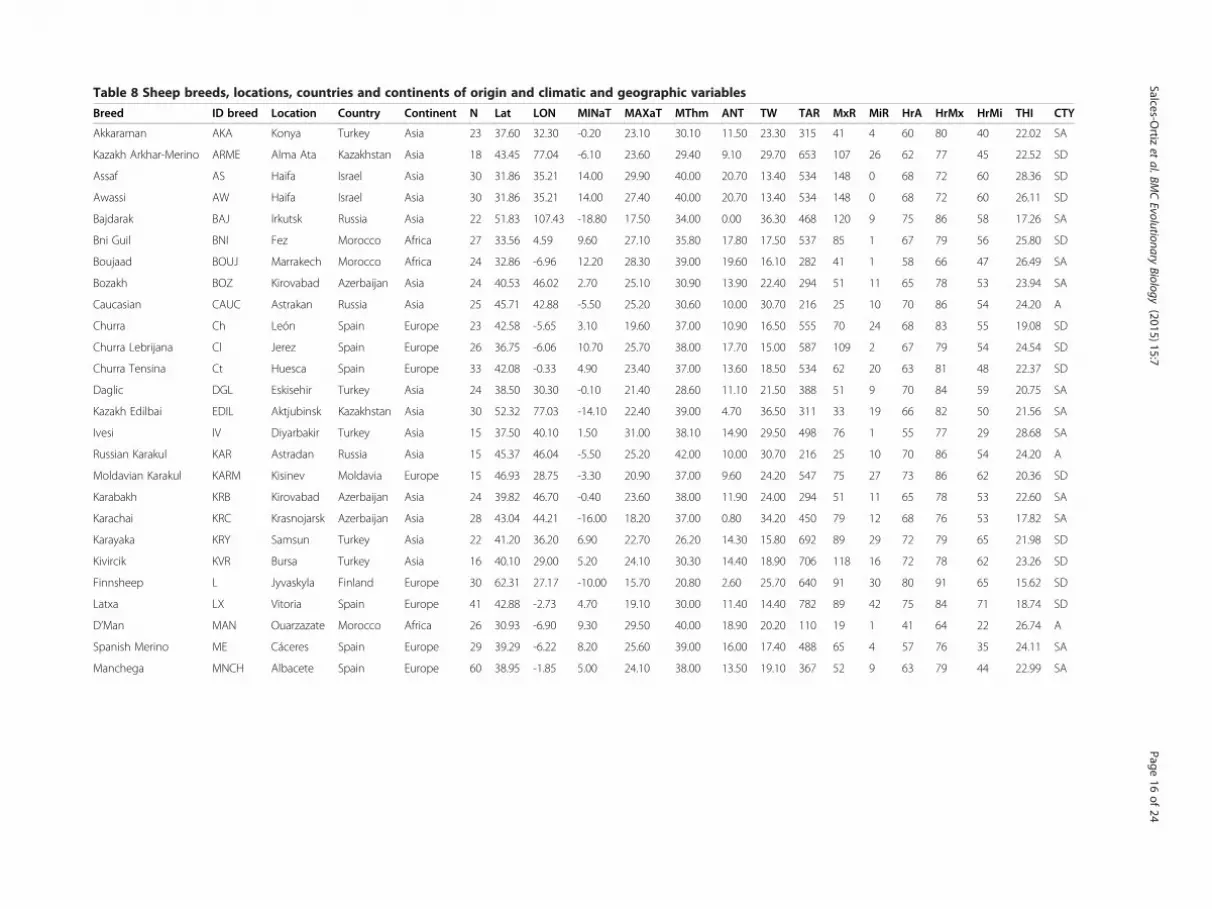
Table 8 Sheep breeds, locations, countries and continents of origin and climatic and geographic variables

Breed ID breed Location Country Continent N Lat LON MINaT MAXaT MThm ANT TW TAR MxR MiR HrA HrMx HrMi THI CTY

Akkaraman AKA Konya Turkey Asia 23 37.60 32.30 -0.20 23.10 30.10 11.50 23.30 315 41 4 60 80 40 22.02 SA

Kazakh Arkhar-Merino ARME Alma Ata Kazakhstan Asia 18 43.45 77.04 -6.10 23.60 29.40 9.10 29.70 653 107 26 62 77 45 22.52 SD

Assaf AS Haifa Israel Asia 30 31.86 35.21 14.00 29.90 40.00 20.70 13.40 534 148 0 68 72 60 28.36 SD

Awassi AW Haifa Israel Asia 30 31.86 35.21 14.00 27.40 40.00 20.70 13.40 534 148 0 68 72 60 26.11 SD

Bajdarak BAJ Irkutsk Russia Asia 22 51.83 107.43 -18.80 17.50 34.00 0.00 36.30 468 120 9 75 86 58 17.26 SA

Bni Guil BNI Fez Morocco Africa 27 33.56 4.59 9.60 27.10 35.80 17.80 17.50 537 85 1 67 79 56 25.80 SD

Boujaad BOUJ Marrakech Morocco Africa 24 32.86 -6.96 12.20 28.30 39.00 19.60 16.10 282 41 1 58 66 47 26.49 SA

Bozakh BOZ Kirovabad Azerbaijan Asia 24 40.53 46.02 2.70 25.10 30.90 13.90 22.40 294 51 11 65 78 53 23.94 SA

Caucasian CAUC Astrakan Russia Asia 25 45.71 42.88 -5.50 25.20 30.60 10.00 30.70 216 25 10 70 86 54 24.20 A

Churra Ch León Spain Europe 23 42.58 -5.65 3.10 19.60 37.00 10.90 16.50 555 70 24 68 83 55 19.08 SD

Churra Lebrijana Cl Jerez Spain Europe 26 36.75 -6.06 10.70 25.70 38.00 17.70 15.00 587 109 2 67 79 54 24.54 SD

Churra Tensina Ct Huesca Spain Europe 33 42.08 -0.33 4.90 23.40 37.00 13.60 18.50 534 62 20 63 81 48 22.37 SD

Daglic DGL Eskisehir Turkey Asia 24 38.50 30.30 -0.10 21.40 28.60 11.10 21.50 388 51 9 70 84 59 20.75 SA

Kazakh Edilbai EDIL Aktjubinsk Kazakhstan Asia 30 52.32 77.03 -14.10 22.40 39.00 4.70 36.50 311 33 19 66 82 50 21.56 SA

Ivesi IV Diyarbakir Turkey Asia 15 37.50 40.10 1.50 31.00 38.10 14.90 29.50 498 76 1 55 77 29 28.68 SA

Russian Karakul KAR Astradan Russia Asia 15 45.37 46.04 -5.50 25.20 42.00 10.00 30.70 216 25 10 70 86 54 24.20 A

Moldavian Karakul KARM Kisinev Moldavia Europe 15 46.93 28.75 -3.30 20.90 37.00 9.60 24.20 547 75 27 73 86 62 20.36 SD

Karabakh KRB Kirovabad Azerbaijan Asia 24 39.82 46.70 -0.40 23.60 38.00 11.90 24.00 294 51 11 65 78 53 22.60 SA

Karachai KRC Krasnojarsk Azerbaijan Asia 28 43.04 44.21 -16.00 18.20 37.00 0.80 34.20 450 79 12 68 76 53 17.82 SA

Karayaka KRY Samsun Turkey Asia 22 41.20 36.20 6.90 22.70 26.20 14.30 15.80 692 89 29 72 79 65 21.98 SD

Kivircik KVR Bursa Turkey Asia 16 40.10 29.00 5.20 24.10 30.30 14.40 18.90 706 118 16 72 78 62 23.26 SD

Finnsheep L Jyvaskyla Finland Europe 30 62.31 27.17 -10.00 15.70 20.80 2.60 25.70 640 91 30 80 91 65 15.62 SD

Latxa LX Vitoria Spain Europe 41 42.88 -2.73 4.70 19.10 30.00 11.40 14.40 782 89 42 75 84 71 18.74 SD

D’Man MAN Ouarzazate Morocco Africa 26 30.93 -6.90 9.30 29.50 40.00 18.90 20.20 110 19 1 41 64 22 26.74 A

Spanish Merino ME Cáceres Spain Europe 29 39.29 -6.22 8.20 25.60 39.00 16.00 17.40 488 65 4 57 76 35 24.11 SA

Manchega MNCH Albacete Spain Europe 60 38.95 -1.85 5.00 24.10 38.00 13.50 19.10 367 52 9 63 79 44 22.99 SA

Salces-Ortiz

etal.BM

CEvolutionary

Biology (2015) 15:7

Page16

of24

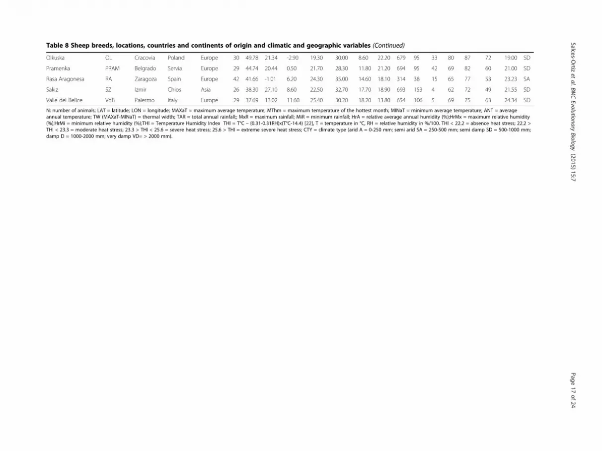
Table 8 Sheep breeds, locations, countries and continents of origin and climatic and geographic variables (Continued)

Olkuska OL Cracovia Poland Europe 30 49.78 21.34 -2.90 19.30 30.00 8.60 22.20 679 95 33 80 87 72 19.00 SD

Pramenka PRAM Belgrado Servia Europe 29 44.74 20.44 0.50 21.70 28.30 11.80 21.20 694 95 42 69 82 60 21.00 SD

Rasa Aragonesa RA Zaragoza Spain Europe 42 41.66 -1.01 6.20 24.30 35.00 14.60 18.10 314 38 15 65 77 53 23.23 SA

Sakiz SZ Izmir Chios Asia 26 38.30 27.10 8.60 22.50 32.70 17.70 18.90 693 153 4 62 72 49 21.55 SD

Valle del Belice VdB Palermo Italy Europe 29 37.69 13.02 11.60 25.40 30.20 18.20 13.80 654 106 5 69 75 63 24.34 SD

N: number of animals; LAT = latitude; LON = longitude; MAXaT = maximum average temperature; MThm = maximum temperature of the hottest month; MINaT = minimum average temperature; ANT = averageannual temperature; TW (MAXaT-MINaT) = thermal width; TAR = total annual rainfall;; MxR = maximum rainfall; MiR = minimum rainfall; HrA = relative average annual humidity (%);HrMx = maximum relative humidity(%);HrMi = minimum relative humidity (%);THI = Temperature Humidity Index THI = T°C – (0.31-0.31RH)x(T°C-14.4) [22], T = temperature in °C, RH = relative humidity in %/100. THI < 22.2 = absence heat stress; 22.2 >THI < 23.3 = moderate heat stress; 23.3 > THI < 25.6 = severe heat stress; 25.6 > THI = extreme severe heat stress; CTY = climate type (arid A = 0-250 mm; semi arid SA = 250-500 mm; semi damp SD = 500-1000 mm;damp D = 1000-2000 mm; very damp VD= > 2000 mm).

Salces-Ortiz

etal.BM

CEvolutionary

Biology (2015) 15:7

Page17

of24


temperatures and high relative air humidity go together[25]. In this sense, Paim and colleagues [26] describedthat THI (an index that combines air temperature andrelative air humidity) had a great influence on animalsuperficial temperatures, demonstrating that this is ableto characterize the animal response to environment.However in this work any association was found be-tween this variable and polymorphisms frequencies.Regarding the G-660 allele in the gene promoter, op-

posite results than those of the I-668 were observed,which agree with the transcription results above men-tioned. The G-660 allele is linked to the lowest expressionrates of the HSP90AA1 gene under both heat stress andmild temperature conditions. Therefore high frequenciesof such allele are only expected in breeds reared in re-gions with low MINaT and ANT temperatures and highTW, in which heat is not a critical source of stress. Thenegative association of the G-660 frequency with MINaT(-0.16) and ANT (-0.13) and positive with TW (0.18)agree with such expectations. However, high frequenciesof the C-660 allele were found in all kind of locations butpredominating in breeds reared in hot climates. Thiscould be due to the genetic exchange that occurred dur-ing the development of modern breeds more than toadaptation processes. Linkage disequilibrium (LD) be-tween g.667_668insC and g.660G > C is little than 0.20in the whole breeds and range between 0.001 and 0.540across breeds, however D-668 and G-660 alleles are com-pletely linked in the 836 animals genotyped, constitutingthe most thermo sensible haplotype [20].On the basis of Reynold’s distances, two groups of

breeds showing the minimum distances between breedswithin group and maximum distances with breeds of theother group can be established. The first group was consti-tuted by KRC, KRB, KAR, DGL, KARM and EDIL breedsand the second group by ME, PRAM, SZ, AS, KVR and Clbreeds. Among breeds of these two groups, average, mini-mum and maximum distances were 0.267, 0.064 and0.604, respectively. In these two groups of breeds, oppositefrequencies of the two polymorphism most related withgene expression differences (g.667_668insC and g.660G >C)were observed. Thus, in the first group of breeds the aver-age frequencies of the I-668 and G-660 alleles were 0.08 and0.61, respectively. In all these breeds the G-660 allele wasthat with the maximum frequency and the I-668 allele hada frequency <13%. In the second group of breeds averagefrequencies of I-668 and G-660 alleles were 0.41 and 0.23,respectively. In all these breeds the I-668 allele frequencywas >30% and the G-660 allele had a frequency <33%.Interestingly, all breeds from group 1, except KARM, arereared in SA or A climates, mainly from Asian regions.On the contrary, all breeds from group 2, except ME, arereared in SD Mediterranean climates. Average MINaT,ANT, TW, TAR and MxR were -6.57, 8.02, 28.52, 367.63

and 52.30, respectively, in group 1 and 7.87, 16.38, 17.47,617 and 114.67, respectively, in group 2. Q2 values higherthan 0.4 were only found for I-668, I-667 and G-660 suggest-ing the action of natural selection in driving the differen-tial allele frequency distribution of these polymorphismsamong sheep populations. Therefore, a correlation be-tween genetic (allele frequencies) and environmental (cli-matic parameters) variables among some sheep breedshave been established which demonstrates that despite ofthe great admixture existing among them and its domesti-cation status, some footprints of the natural selection ac-tion can be glimpsed. This fact may be due to the generallow artificial selection exerted over breeds of this speciesand their semi-extensive or extensive management condi-tions which may have retained some genes related withadaptation to environmental conditions existing in nature.Thus, breeds reared in SD climates, in which high temper-atures and humidity are sources of physiological stress,have high frequency of alleles (I-668 and C-660) related tohigher expression rates of the HSP90AA1 gene as responseto heat stress. However, low frequencies of these alleleswere only found in those breeds reared in climates inwhich heat and humidity levels are not enough to inducea heat stress response. The frequencies of A-601, A-522 andI-516 alleles (Q

2 values < 0.4) are not influenced by climaticconditions and therefore its presence in the HS90AA1gene promoter seem to have no impact in the adaptationto environment of the ovine species. This finding wasalready suggested by [19] by notice that these polymor-phisms did not produce expression differences among ge-notypes when comparing RNA samples obtained underheat stress and thermo-neutral conditions.In a large study where 49,034 SNPs were genotyped in

74 sheep breeds, [3] some signs of directional selection intwo candidate genes located at chromosome 18 (FST =0.428), in which also the HSP90AA1 gene is located, werefound. One of them was ABHD2 (abhydrolase domaincontaining 2) which has, among other functions, a role inthe response to wounding. This protein that interacts withUBC (polyubiquitin C) has a high expression rate in tes-ticle (BioGPS. biogps.org) and correlates with HSPA1L(Heat shock protein 70 kD like). Hsp70 is a well knownprotein involved in the heat shock response which is partof the Hsp90 complex. Therefore, although authors [3]recognize that the identification of adaptive alleles has notbeen achieved, some footprints of directional selectionover genes more or less directly related with adaptive traitscan be found.When assessing evidence for an ecocline, it is crucial

to control for population history and structure, for ac-curately assessing whether a correlation between a gen-etic variant and geographic or climate variables is due tonatural selection [27]. For example, if migration patternscorrespond closely with variation in a particular climate


variable, the correlations between neutral alleles and thatclimate variable may be high even if selection has notacted on the locus. Conversely, if selection effects arelower to that of population structure on allele frequen-cies, correlations may be underestimated if populationhistory is not taken into account [4].This is the reasonwhy PLSR and SAM approaches cannot be used inde-pendently, without comparing results with specializedstatistic methods based on population genetics theories,and focus on the analysis of genetic data as the BayesianTest of Beaumont and Balding (LOSITAN). Thus,among all loci-environment associations detected byPLSR and SAM methods, only the frequency of twopolymorphisms, the g.703_704del(2)A and the g.522A >G,seems to be under the action of some selective process.The g.703_704del(2)A showed a high FST outlier whichmakes it a candidate to directional selective processes.The low FST outlier of the g.522A >G SNP reveals thepossibility of balancing selection acting over its frequency.The g.703_704del(2)A is highly linked with the g.660G > CSNP (r2 = 0.86 in the whole data) ranging r2 values in mostbreeds from 0.84 to 1. Thus, directional selection pre-dicted for the g.703_704del(2)A could be extended to theSNP g.660G > C for which differential expression of theHSP90AA1 gene has been assessed depending on geno-type [19,20], but not with the g.667_668insC. The high de-gree of conservation in LD phase found in this sortsequence in almost breeds, independently of their geo-graphic origin, could indicate that high levels of gene flowhave occurred between populations following domestica-tion, as is suggested by Kijas and coworkers [3], but also, aselection pressure exerted over this DNA region [28].The Bovidae family includes more species than any

other extant family of large mammals, but their phylo-genetic relationships remain largely unresolved in partbecause it appears to represent a rapid, early radiationinto many forms without clear connections among them[29]. Furthermore, certain morphological traits haveevolved several times within the family to create evolu-tive convergences that obscures true relationships [30].The subfamily Caprinae includes bovids adapted to ex-treme climates and difficult terrains. Fossil records arepoorly documented but the group first appeared duringthe upper Miocene [31]. In a recent work, a completeestimate of the phylogenetic relationships in Ruminantiahas been proposed combining morphological, ethologicaland molecular information [29]. The resolution of thesupertree varies among groups and some componentclades, particularly Caprinae (67.7%), are much less wellresolved than others (e.g. Bovinae, 95.7%). In particular,the position of the genera Budorcas and Ovibos has beencontroversial, having at times constituted the tribeOvibovini, and at others been separated and located indifferent tribes. In general, the genus Ovis is split into a

“New World” clade represented by O. dalli and O. cana-densis and an “Old World” clade including the two sisterspecies O. vignei and O. aries, on the one hand, and O.ammon, on the other hand [29,32]. In our work, haplo-types from O. vignei, O canadiensis and O. musimon ap-peared mixed with those from O. aries. O. aries and O.musimon share many polymorphic sites (7) as expectedfrom the past hybridization between both species.Ropiquet and Hassanin [33] using mitochondrial and

nuclear DNA sequences located A. lervia closer to goats(Capra) and O. moschatus closer to R. pyrenaica. How-ever, in recent works [34,35] A. lervia was closer to Rupi-capra genus within the Caprina tribe and O. moschatuswas distant from them within the Ovibovina tribe. Ourtree located A. lervia as a sister species of C. hircus and C.pyrenaica (boosttrap proportion = 97) and R. pyrenaicacloser to O moschatus (bootstrap proportion = 60). In thework of Matthee and Davis [36] using data from nuclearDNA a politomy for C. hircus, O. moschatus and O. arieswas found. However, when analyzing nuclear DNA joinedto mtDNA data, C. hircus and O. aries appear as sisterspecies separated from O. moschatus. In our work we haveobserved a relative high similarity between O. moschatus,O. aries and O. musimon species regarding polymorphismshared among them.Although O. moschatus is currently restricted to

Greenland and the Arctic Archipelago [37], a higherfrequency of alleles related with the heat stress response(I-668 = 0.43; C-660 = 0.90) were found in this species. Fos-sils of this species have occasionally found in southwestEurope, so that’s why it seems that Ovibos did not in-habit exclusively cold tundra during the Pleistocene [37].Praeovibos, an older morphotype of O moschatus, doesnot appear to have been restricted to inhabiting coldclimates as its remains have also been identified in tem-perate and Mediterranean forest [38,39]. In contrast tomodern Ovibos, Praeovibos was distributed over muchmore southern latitudes, samples have been found as farsouth as France and Spain [38-40], which indicates thatPraeovibos is an early more cosmopolitan form ofmuskox [37]. Could these high frequencies of alleles re-lated with the heat stress response found in O moschatuscame from its Praeovibos ancestor? Lent [41] indicatesthat muskox is sensitive to both climate warming andfluctuations, that is why Campos and colleagues [37]hold these factors responsible of the actual confinementof the muskox to Greenland and the Arctic Archipelagobut not a human impact. Our results regarding the poly-morphisms of the HSP90AA1 gene in this species seemsto indicate that the actual muskox is genetically well pre-pared to tolerate warm climates. Therefore, which couldbe the reasons to its actual geographic limitations? Cli-mate change is known to affect not only animal’s thermosensitivity but also by triggering vegetation change [39,42].


Increasing temperature pushed the adaptive vegetationbalance firmly towards bogs, shrub tundra, forest and low-nutrient acidic soils, which resulted in communities ofconservative plants highly defended against herbivore andsupporting a small biomass of large mammals [43].Palmqvist and coworkers [44] in an ecomorphologicalanalysis of the early Pleistocene fauna of Venta Micena(Orce, Guadix-Baza basin, SE Spain), provide interestingclues on the physiology, dietary regimes, habitat prefer-ences and ecological interactions of large mammals.Unexpectedly, A. lervia which colonizes arid and hot

areas of the rocky mountains of north Africa (Saharaand Magreb) is not polymorphic for the mutation mostassociated to the upregulation of the HSP90AA1 geneinduced by heat stress events. It is probably that inthis species, as in the Bos genus, other genetic mecha-nisms exist to cope with stress imposed by climaticconditions.Regarding those polymorphisms for which our group

has detected some relation with hot climates adapta-tion by its association with the expression rate of theHSP90AA1 gene under heat stress conditions (g-.667_668insC and g.660G > C), it’s noteworthy that they wereonly segregating in C. hircus, O. moschatus, O.musimonand O. aries. Because there were only one sample of O.vignei and two of O ammon, any conclusion from thesetwo species can be extracted. It seems reasonable tohypothesize that these polymorphisms could come froman ancestral species common to the Ovis, Ovibos andCapra genera but not to Ammotragus. However also it ispossible that the evolvability of this gene may be due to itsphysical susceptibility to mutagenesis and therefore thatthe similitudes/differences found in the species analyzeddoes not be related with their phylogenetic relations.

ConclusionWe have assessed that despite the domestication processoccurred 11,000 years BP, sheep breeds showed somegenetic footprints related to climatic variables existing inthe regions where they are reared. Thus artificial selec-tion carried out by humans to improve productive traitsin this species seems to be occurred concurrently withnatural selective forces for traits related with the adapta-tion to environmental conditions. Adaptation of breedsto heat climates can suppose a selective advantage tocope with global warming caused by climatic change.Polymorphisms of the HSP90AA1 gene detected in theOvis aries species can be used in selection programs toimprove animals resistance to heat environments. Muta-tions of the ovine HSP90AA1 gene promoter are alsobeen found in wild species from the Caprinae subfamily,indicating a great antiquity of these mutations which canhelp us to elucidate how climatic conditions have evolvedin the past.

MethodsEthics statementThe current study was carried out under a Project Li-cense from the INIA Scientific Ethic Committee. Animalmanipulations were performed according to the SpanishPolicy for Animal Protection RD 53/2013, which meetsthe European Union Directive 86/609 about the protec-tion of animals used in experimentation. We hereby con-firm that the INIA Scientific Ethic Committee (IACUC)has approved this study.

Animal material, nucleic acid isolation, DNA amplificationand SNPs genotypingAnimals from 31 sheep breeds from Europe, Asia andAfrica and from 11 species of the Caprinae (9) and theBovinae (2) subfamilies constitute the biological materialof this work. Tables 8 and 9 shows breeds, species, num-ber of animals from each breed and species, location,country, continent and climatic and geographic vari-ables. Additional file 9 (AF9) contains the genotypes ofall animals analyzed for each polimorphisms existent ineach species.Peripheral whole blood samples were collected in order

to analyse 11 polymorphisms of interest located at theHSP90AA1 promoter [20]. Polymorphisms genotyped were:g.703_704del(2)A; g.667_668insC (rs397514115); g.666_667insC; g.660G > C (rs397514116); g.601A > C (rs397514117); g.528A >G (rs397514269); g.524G > T (rs397514270); g.522A >G (rs397514271); g.516_517insG (rs397514268); g.468G > T (rs397514272); g.444A >G (rs397514273). HSP90AA1 promoter sequencing was done in allanimals according to Salces-Ortiz and coworkers [19].

Polymorphisms characterization and linkagedisequilibrium estimationPLINK software [45] was used to estimate linkage dis-equilibrium among all pairs of the 11 SNPs measured asr2 in the whole sheep data and in each breed separately.Hardy-Weinberg equilibrium exact test, observed andexpected heterozygosis for each breed were also calcu-lated using PLINK.

Phylogenetic relationship between sheep breedsThe relationship between breeds was examined usingthe Reynold’s distance metric [46]. Reynold’s distance(D = -ln(1-FST) matrix was estimated performing 90,000permutations and a significance level of 0.05 was estab-lished. An Exact Test of population differentiation with asignificance level of 0.05 was performed to test the hy-pothesis of a random distribution of individuals betweenpairs of populations [47,48], running 100,000 Markovchain and 10,000 dememorization steps. The histogramof the number of populations which are significantly dif-ferent (p < 0.05) from a given population was generated.

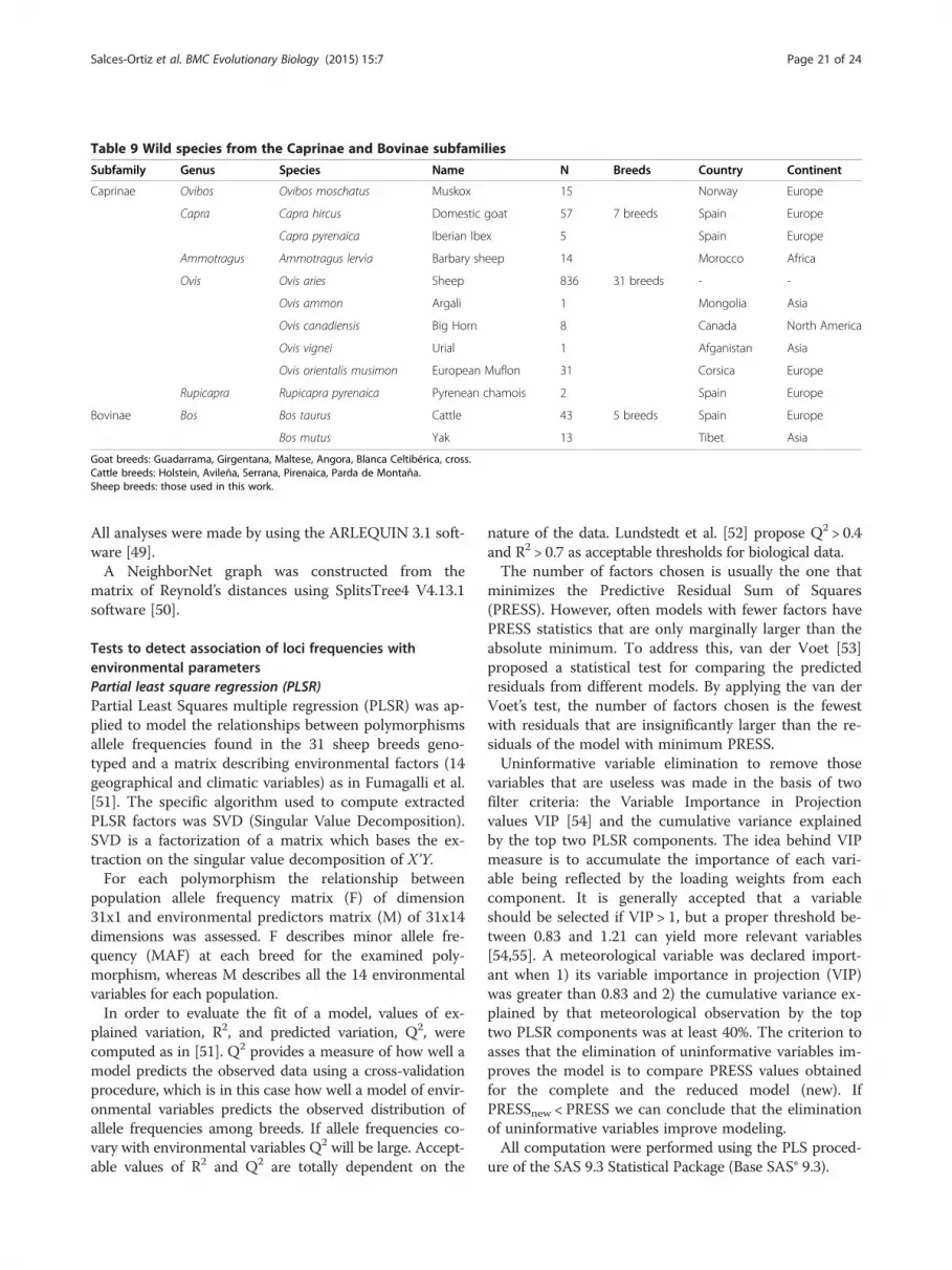
Table 9 Wild species from the Caprinae and Bovinae subfamilies

Subfamily Genus Species Name N Breeds Country Continent

Caprinae Ovibos Ovibos moschatus Muskox 15 Norway Europe

Capra Capra hircus Domestic goat 57 7 breeds Spain Europe

Capra pyrenaica Iberian Ibex 5 Spain Europe

Ammotragus Ammotragus lervia Barbary sheep 14 Morocco Africa

Ovis Ovis aries Sheep 836 31 breeds - -

Ovis ammon Argali 1 Mongolia Asia

Ovis canadiensis Big Horn 8 Canada North America

Ovis vignei Urial 1 Afganistan Asia

Ovis orientalis musimon European Muflon 31 Corsica Europe

Rupicapra Rupicapra pyrenaica Pyrenean chamois 2 Spain Europe

Bovinae Bos Bos taurus Cattle 43 5 breeds Spain Europe

Bos mutus Yak 13 Tibet Asia

Goat breeds: Guadarrama, Girgentana, Maltese, Angora, Blanca Celtibérica, cross.Cattle breeds: Holstein, Avileña, Serrana, Pirenaica, Parda de Montaña.Sheep breeds: those used in this work.


All analyses were made by using the ARLEQUIN 3.1 soft-ware [49].A NeighborNet graph was constructed from the

matrix of Reynold’s distances using SplitsTree4 V4.13.1software [50].

Tests to detect association of loci frequencies withenvironmental parametersPartial least square regression (PLSR)Partial Least Squares multiple regression (PLSR) was ap-plied to model the relationships between polymorphismsallele frequencies found in the 31 sheep breeds geno-typed and a matrix describing environmental factors (14geographical and climatic variables) as in Fumagalli et al.[51]. The specific algorithm used to compute extractedPLSR factors was SVD (Singular Value Decomposition).SVD is a factorization of a matrix which bases the ex-traction on the singular value decomposition of X’Y.For each polymorphism the relationship between

population allele frequency matrix (F) of dimension31x1 and environmental predictors matrix (M) of 31x14dimensions was assessed. F describes minor allele fre-quency (MAF) at each breed for the examined poly-morphism, whereas M describes all the 14 environmentalvariables for each population.In order to evaluate the fit of a model, values of ex-

plained variation, R2, and predicted variation, Q2, werecomputed as in [51]. Q2 provides a measure of how well amodel predicts the observed data using a cross-validationprocedure, which is in this case how well a model of envir-onmental variables predicts the observed distribution ofallele frequencies among breeds. If allele frequencies co-vary with environmental variables Q2 will be large. Accept-able values of R2 and Q2 are totally dependent on the

nature of the data. Lundstedt et al. [52] propose Q2 > 0.4and R2 > 0.7 as acceptable thresholds for biological data.The number of factors chosen is usually the one that

minimizes the Predictive Residual Sum of Squares(PRESS). However, often models with fewer factors havePRESS statistics that are only marginally larger than theabsolute minimum. To address this, van der Voet [53]proposed a statistical test for comparing the predictedresiduals from different models. By applying the van derVoet’s test, the number of factors chosen is the fewestwith residuals that are insignificantly larger than the re-siduals of the model with minimum PRESS.Uninformative variable elimination to remove those

variables that are useless was made in the basis of twofilter criteria: the Variable Importance in Projectionvalues VIP [54] and the cumulative variance explainedby the top two PLSR components. The idea behind VIPmeasure is to accumulate the importance of each vari-able being reflected by the loading weights from eachcomponent. It is generally accepted that a variableshould be selected if VIP > 1, but a proper threshold be-tween 0.83 and 1.21 can yield more relevant variables[54,55]. A meteorological variable was declared import-ant when 1) its variable importance in projection (VIP)was greater than 0.83 and 2) the cumulative variance ex-plained by that meteorological observation by the toptwo PLSR components was at least 40%. The criterion toasses that the elimination of uninformative variables im-proves the model is to compare PRESS values obtainedfor the complete and the reduced model (new). IfPRESSnew < PRESS we can conclude that the eliminationof uninformative variables improve modeling.All computation were performed using the PLS proced-

ure of the SAS 9.3 Statistical Package (Base SAS® 9.3).


Spatial analysis method (SAM)Other approach to assess the effect of any selection onpolymorphisms across populations is the Spatial AnalysisMethod (SAM) developed by [56,57]. SAM is based onthe spatial coincidence analysis to connect genetic infor-mation with geo-environmental data. The logistic regres-sion uses random binomial variables as response for themodel, thus, each allele is set to ‘1’ if it occurs in a givenindividual, and to ‘0’ if not. Logistic regression is used toassess the significance of the models constituted by allpossible marker-environmental variable pairs. The com-parison of observed with predicted values is based onthe likelihood ratio (G) and Wald (W) tests [58] to deter-mine the significance of the models. For both tests, thenull hypothesis is that the model with the examinedvariable does not explain the observed distributionbetter than a model with a constant only. A model isconsidered significant only if both tests reject the corre-sponding null hypothesis. To restrict the analysis to ro-bust candidate associations the Bonferroni correctionwas applied and only cumulated tests in which both Wand G tests were significant were used to identify associ-ated loci [56]. Computations were performed using theMatSAM v2Beta software [57].

Statistical analysis to detect loci under selection acrosspopulationsBayesian Test of Beaumont and BaldingThe Bayesian test of Beaumont and Balding [59] evaluatethe relationship between FST and He (expected heterozy-gosity) describing the expected distribution of Wright’sinbreeding coefficient FST vs. He under an island modelof migration with neutral markers. This distribution isused to identify outlier loci that have excessively high orlow FST compared to neutral expectations. Such outlierloci are candidates for being subject to selection [60].Low FST outliers indicate loci subject to balancing selec-tion, whereas high outliers suggest adaptative (directional)selection [59]. The Bayesian Test method of Beaumontand Balding was assessed using the LOSITAN (Lookingfor Selection In a Tangled dataset) package [60]. Initially100,000 simulations under the infinite allele mutationmodel were run using all populations and all unlinked locito determine a first candidate subset of selected loci inorder to remove them from the computation of the neu-tral FST. After the first run, all loci outside the desiredconfidence interval (99%) are removed. Subsequently anew 100,000 simulations run was developed to computethe mean neutral FST. A final run of LOSITAN using allloci is then conducted using the last computed mean.Also, a frequentist method based on moment-based esti-mates of FST, using the FDIST option of the LOSITANpackage, was tested to compare results with the Bayesianapproach.

Phylogenetic Relationship between species from theCaprinae subfamilyHaplotype sequences from the different species analyzedwere inferred by using PLINK software [45]. Promotersequences were aligned by CLUSTAL. MEGA 6 software[61] was used to estimate nucleotide substitution models,evolutionary divergence and Tajima’s Neutrality Test andto construct the ML tree. Initial tree(s) for the heuristicsearch were obtained by applying the BioNJ method to amatrix of pairwise distances estimated using the Max-imum Composite Likelihood (MCL) approach. A discreteGamma distribution was used to model evolutionary ratedifferences among sites (5 categories (+G, parameter =5.6803)).

Availability of supporting dataThe data sets supporting the results of this article are in-cluded as an additional file (AF9).

Additional files

Additional file 1: Hardy Weinberg equilibrium test for all sheepbreeds and for each breed separately.

Additional file 2: Linkage disequilibrium of the 11 polymorphismsin all sheep breeds studied.

Additional file 3: Population pairwise FSTs.

Additional file 4: Basic statistics for polymorphisms MAF andenvironmental variables considered.

Additional file 5: Pearson (above diagonal) and Spearman (belowdiagonal) correlations and significance for MAF of polymorphismsand environmental variables. In bold and shading significant values atα = 0.05.

Additional file 6: Regression coefficients of scaled and centeredvariables for predictors and responses.

Additional file 7: Alignment of the 12 different species studied andtheir identity with the reference sequence (Ovis aries) based ontheir most frequent haplotype. Also accession numbers of eachsequence are shown.

Additional file 8: Haplotypes inferred by PLINK for sheep breedsand wild species studied.

Additional file 9: Genotypes of all animals used in this study for allthe polymorphic sites detected in each species.

Competing interestsThe authors declare that they have no competing interests.

Authors’ contributionsJSO participated in the development of the statistical analyses, DNAextraction, PCR reactions and writing the manuscript. CGV participated in thedesign of the study, DNA extraction and PCR reactions. MAM and TOMmade the sequence of the DNA fragments. JHC participated in writing themanuscript and PCR reactions design. MMS, participated in the design of thestudy, develop of the statistical analyses and writing the manuscript. Allauthors read and approved the final manuscript.

AcknowledgementsThe authors gratefully acknowledge financial support by RTA2009-00098 INIA(Spain) project. Also authors express their gratitude to the National VeterinaryLaboratory from the Spanish Department of Agriculture, Food andEnvironmental Affairs for sample genotyping and Juan López Cantalapiedra

http://www.biomedcentral.com/content/supplementary/s12862-015-0280-x-s1.docx

http://www.biomedcentral.com/content/supplementary/s12862-015-0280-x-s2.xlsx

http://www.biomedcentral.com/content/supplementary/s12862-015-0280-x-s3.txt






http://www.biomedcentral.com/content/supplementary/s12862-015-0280-x-s9.xlsx


from the Paleobiology Department of the Natural Sciences Museum ofMadrid (Spain) for his scientific support.Finally, authors want to thanks all persons and institutions providing DNAsamples for this work: Juha Kantanen from the Biotechnology and FoodResearch MTT Agrifood Research Finland (Finland) for samples of severalovine breeds from Asia and Europe and for Yak samples; Yasemin Öner fromthe Animal Science Department, Faculty of Agriculture, Uludag University,Bursa (Turkey) for samples of Turkish sheep breeds; Inmaculada Martín Burrielfrom the Genetic Biochemistry Laboratory (LAGENBIO) of the Veterinaryfaculty of Zaragoza University (Spain) for samples of African sheep breeds;Tengs Torstein from the Norwegian Veterinary Institute (Norway) for Muskoxsamples; Mª José Gens Abujas from the Biodiversity, hunting and river fishingService (Spain) for Barbary Sheep samples; Julian Santiago from theReproduction Department of INIA Madrid (Spain) for samples of EuropeanMouflon, Pyrenean Chamois and Iberian ibex; AGRAMA and CERSYRAValdepeñas (Spain) for samples of Manchega sheep breed and BlancaCeltibérica goat; Julian Garde from the Albacete University (Spain) forsamples of European Mouflon; Juan Delibes for samples of Argali and Urial;Eva Ugarte from NEIKER-Tecnalia (Spain) for samples of Latxa sheep breed;Mercedes Izquierdo from the Agrarian Investigation Centre of Extremadura(Spain) for samples of Merino sheep breed; Jorge Calvo from CITA Zaragoza(Spain) for samples of Rasa Aragonesa, Churra Tensina, Churra Lebrijana andChurra sheep breeds, several goat breeds and Spanish cattle breeds; Angel RuizMantecon from CSIC León (Spain) for samples of Assaf and Awasi sheep breeds;Salvatore Mastrangelo from the University of Palermo for samples of Valle delBelice sheep breed and Girgentana and Maltese goat breeds; James Kijas fromCSIRO Brisbane (Australia) for samples of Big Horn; Asociación de Avileña (Spain)for samples of Avileña cattle and CONAFE (Spain) for samples of Holstein cattle.

Author details1INIA, Carretera de La Coruña Km. 7,5. 280040, Madrid, Spain. 2LaboratorioCentral de Veterinaria, MAGRAMA, Ctra. M-106 km1.4 28110, Madrid, Spain.3CITA, Avda, Montañana, 930, 50059, Zaragoza, Spain.

Received: 7 October 2014 Accepted: 5 January 2015

References1. Shackleton DM. Wild Sheep and Goats and Their Relatives: Status Survey

and Conservation Action Plan for Caprinae, vol. 33. 1997.2. Zeder MA. Domestication and early agriculture in the Mediterranean Basin:

Origins, diffusion, and impact. Proc Natl Acad Sci U S A. 2008;105(33):11597–604.3. Kijas JW, Lenstra JA, Hayes B, Boitard S, Porto Neto LR, San Cristobal M, et al.

Genome-wide analysis of the world’s sheep breeds reveals high levels ofhistoric mixture and strong recent selection. PLoS Biol. 2012;10(2):e1001258.

4. Hancock AM, Witonsky DB, Alkorta-Aranburu G, Beall CM, Gebremedhin A,Sukernik R, et al. Adaptations to climate-mediated selective pressures inhumans. PLoS Genet. 2011;7(4):e1001375.

5. Coop G, Witonsky D, Di Rienzo A, Pritchard JK. Using environmental correlationsto identify loci underlying local adaptation. Genetics. 2010;185(4):1411–23.

6. Lenormand T. Gene flow and the limits to natural selection. Trends EcolEvol. 2002;17(4):183–9.

7. Hancock AM, Witonsky DB, Gordon AS, Eshel G, Pritchard JK, Coop G, et al.Adaptations to climate in candidate genes for common metabolicdisorders. PLoS Genet. 2008;4(2):e32.

8. Thompson EE, Kuttab-Boulos H, Witonsky D, Yang L, Roe BA, Di Rienzo A.CYP3A variation and the evolution of salt-sensitivity variants. Am J HumGenet. 2004;75(6):1059–69.

9. Sezgin E, Duvernell DD, Matzkin LM, Duan Y, Zhu CT, Verrelli BC, et al.Single-locus latitudinal clines and their relationship to temperate adaptationin metabolic genes and derived alleles in Drosophila melanogaster. Genetics.2004;168(2):923–31.

10. Stinchcombe JR, Weinig C, Ungerer M, Olsen KM, Mays C, Halldorsdottir SS, et al.A latitudinal cline in flowering time in Arabidopsis thaliana modulated by theflowering time gene FRIGIDA. Proc Natl Acad Sci U S A. 2004;101(13):4712–7.

11. Grivet D, Sebastiani F, Alia R, Bataillon T, Torre S, Zabal-Aguirre M, et al.Molecular footprints of local adaptation in two Mediterranean conifers.Mol Biol Evol. 2011;28(1):101–16.

12. Arad Z, Mizrahi T, Goldenberg S, Heller J. Natural annual cycle of heat shockprotein expression in land snails: desert versus Mediterranean species ofSphincterochila. J Exp Biol. 2010;213(Pt 20):3487–95.

13. Jarosz DF, Lindquist S. Hsp90 and environmental stress transform theadaptive value of natural genetic variation. Science. 2010;330(6012):1820–4.

14. Reddy PS, Thirulogachandar V, Vaishnavi CS, Aakrati A, Sopory SK, Reddy MK.Molecular characterization and expression of a gene encoding cytosolicHsp90 from Pennisetum glaucum and its role in abiotic stress adaptation.Gene. 2011;474(1–2):29–38.

15. Oner Y, Calvo JH, Serrano M, Elmaci C. Polymorphisms at the 5′ flankingregion of the HSP90AA1 gene in native Turkish sheep breeds. Livest Sci.2012;150(1–3):381–5.

16. Marcos-Carcavilla A, Calvo JH, Gonzalez C, Moazami-Goudarzi K, Laurent P,Bertaud M, et al. Structural and functional analysis of the HSP90AA1 gene:distribution of polymorphisms among sheep with different responses toscrapie. Cell Stress Chaperones. 2008;13(1):19–29.

17. Marcos-Carcavilla A, Moreno C, Serrano M, Laurent P, Cribiu EP, AndreolettiO, et al. Polymorphisms in the HSP90AA1 5’ flanking region are associatedwith scrapie incubation period in sheep. Cell Stress Chaperones.2010;15(4):343–9.

18. Marcos-Carcavilla A, Mutikainen M, Gonzalez C, Calvo JH, Kantanen J, SanzA, et al. A SNP in the HSP90AA1 gene 5’ flanking region is associated withthe adaptation to differential thermal conditions in the ovine species. CellStress Chaperones. 2010;15(1):67–81.

19. Salces-Ortiz J, Gonzalez C, Moreno-Sanchez N, Calvo JH, Perez-Guzman MD,Serrano MM. Ovine HSP90AA1 expression rate is affected by several SNPs atthe promoter under both basal and heat stress conditions. PLoS One.2013;8(6):e66641.

20. Salces-Ortiz J, Ramón M, Gonzalez C, Perez-Guzman MD, Garde JJ, Calvo JH,et al. Differences in the ovine HSP90AA1 gene expression rates caused bytwo linked polymorphisms at its promoter affect rams sperm DNAfragmentation under environmental heat stress conditions. PLoS One. 2014.(Accepted)

21. Ramon M, Salces-Ortiz J, Gonzalez C, Perez-Guzman MD, Garde JJ,Garcia-Alvarez O, et al. Influence of the temperature and the genotype ofthe HSP90AA1 gene over sperm chromatin stability in manchega Rams.PLoS One. 2014;9(1):e86107.

22. Marai IFM, El-Darawany AA, Fadiel A, Abdel-Hafez MAM. Physiological traitsas affected by heat stress in sheep - a review. Small Rum Res. 2007;71:1–12.

23. Tajima F. Statistical method for testing the neutral mutation hypothesis byDNA polymorphism. Genetics. 1989;123(3):585–95.

24. Simonsen KL, Churchill GA, Aquadro CF. Properties of statistical tests ofneutrality for DNA polymorphism data. Genetics. 1995;141(1):413–29.

25. Lally VE, Watson BF. Humiture revisited. Weatherwise. 1960;13:254–6.26. Paim BOB TP, Lima PMT, Dallago BSL, Louvandini H, McManus C. Relation

between thermographic temperatures of lambs and thermal comfortindices. Int J Appl Animal Sci. 2012;1(4):108–15.

27. Endler JA. Geographic Variation, Speciation and Clines. Princeton, Newjersey: Princeton University Press; 1977.

28. Nielsen R, Williamson S, Kim Y, Hubisz MJ, Clark AG, Bustamante C. Genomicscans for selective sweeps using SNP data. Genome Res. 2005;15(11):1566–75.

29. Hernandez Fernandez M, Vrba ES. A complete estimate of the phylogeneticrelationships in Ruminantia: a dated species-level supertree of the extantruminants. Biol Rev Camb Philos Soc. 2005;80(2):269–302.

30. Gentry AW. The subfamilies and tribes of the family Bovidae. Mammal Rev.1992;22(1):1–32.

31. Gentry AW. The Miocene differentiation of old world Pecora (Mammalia).Hist Biol. 1994;7(2):115–58.

32. Hassanin A, Lecointre G, Tillier S. The ‘evolutionary signal’ of homoplasy inprotein-coding gene sequences and its consequences for a priori weightingin phylogeny. Comptes rendus de l’Academie des sciences Serie III, Sciencesde la vie. 1998;321(7):611–20.

33. Hassanin A, Ropiquet A. Molecular phylogeny of the tribe Bovini (Bovidae,Bovinae) and the taxonomic status of the Kouprey, Bos sauveli Urbain 1937.Mol Phylogenet Evol. 2004;33(3):896–907.

34. Hassanin A, An J, Ropiquet A, Nguyen TT, Couloux A. Combining multipleautosomal introns for studying shallow phylogeny and taxonomy ofLaurasiatherian mammals: Application to the tribe Bovini (Cetartiodactyla,Bovidae). Mol Phylogenet Evol. 2013;66(3):766–75.

35. Bibi F. A multi-calibrated mitochondrial phylogeny of extant Bovidae(Artiodactyla, Ruminantia) and the importance of the fossil record tosystematics. BMC Evol Biol. 2013;13:166.

36. Matthee CA, Davis SK. Molecular insights into the evolution of the familyBovidae: a nuclear DNA perspective. Mol Biol Evol. 2001;18(7):1220–30.


37. Campos PF, Sher A, Mead JI, Tikhonov A, Buckley M, Collins M, et al.Clarification of the taxonomic relationship of the extant and extinctovibovids, Ovibos, Praeovibos, Euceratherium and Bootherium. QuaternarySci Rev. 2010;29(17–18):2123–30.

38. Cregut-Bonnoure E. The Pleistocene Ovibovinae of Western Europe:Temporo-spatial Expansion and Paleoecological Implications. In: BiologicalPapers of the University of Alaska. 1984.

39. Rivals F, Schulz E, Kaiser TM. A new application of dental wear analyses:estimation of duration of hominid occupations in archaeological localities.J Hum Evol. 2009;56(4):329–39.

40. McDonald JN, Ray CE, Harington CR. Taxonomy and zoogeography of themusk ox genus Praeovibos Staudinger, 1908. In: llinois State MuseumScientific Papers, vol. 23. 1991. p. 285–314.

41. Lent PC. Ovibos moschatus. Mammalian Species. 1988;302:1–9.42. Barnosky AD, Koch PL, Feranec RS, Wing SL, Shabel AB. Assessing the causes of

late Pleistocene extinctions on the continents. Science. 2004;306(5693):70–5.43. Guthrie RD. New carbon dates link climatic change with human

colonization and Pleistocene extinctions. Nature. 2006;441(7090):207–9.44. Paul Palmqvist JAP-C, Janis CM, Borja F, Vanessa T, Gröcke DR. Tracing the

ecophysiology of ungulates and predator–prey relationships in an earlyPleistocene large mammal community. Palaeogeography, Palaeoclimatology,Palaeoecology. 2008;266(1–2):95–111.

45. Purcell S, Neale B, Todd-Brown K, Thomas L, Ferreira MA, Bender D, et al.PLINK: a tool set for whole-genome association and population-basedlinkage analyses. Am J Hum Genet. 2007;81(3):559–75.

46. Reynolds J, Weir BS, Cockerham CC. Estimation of the coancestry coefficient:basis for a short-term genetic distance. Genetics. 1983;105(3):767–79.

47. Rousset RMF. An exact test for population differentiation. Evolution.1995;49(6):1280–3.

48. Goudet J, Raymond M, de Meeus T, Rousset F. Testing differentiation indiploid populations. Genetics. 1996;144(4):1933–40.

49. Excoffier L, Laval G, Schneider S. Arlequin (version 3.0): an integratedsoftware package for population genetics data analysis. Evol Bioinformaticsonline. 2005;1:47–50.

50. Huson DH, Bryant D. Application of phylogenetic networks in evolutionarystudies. Mol Biol Evol. 2006;23(2):254–67.

51. Fumagalli M, Sironi M, Pozzoli U, Ferrer-Admetlla A, Pattini L, Nielsen R.Signatures of environmental genetic adaptation pinpoint pathogens as themain selective pressure through human evolution. PLoS Genet.2011;7(11):e1002355.

52. Torbjörn Lundstedt ES, Lisbeth A, Bernt T, Asa N, Jarle P, Rolf B. Experimentaldesign and optimization. Chemometr Intell Lab Syst. 1998;42:3–40.

53. van der Voet H. Comparing the predictive accuracy of models using asimple randomization test. Chemometr Intell Lab Syst. 1994;25(2):313–23.

54. Chong I-G, Jun C-H. Performance of some variable selection methods whenmulticollinearity is present. Chemometr Intell Lab Syst. 2005;78(1–2):103–12.

55. Svante Wold MS, Lennart E. PLS-regression: a basic tool of chemometrics.Chemometr Intell Lab Syst. 2001;58:109–30.

56. Joost S, Bonin A, Bruford MW, Despres L, Conord C, Erhardt G, et al. Aspatial analysis method (SAM) to detect candidate loci for selection:towards a landscape genomics approach to adaptation. Mol Ecol.2007;16(18):3955–69.

57. Joost S, Kalbermatten M, Bonin A. Spatial analysis method (sam): a softwaretool combining molecular and environmental data to identify candidateloci for selection. Mol Ecol Resour. 2008;8(5):957–60.

58. David W, Hosmer SL. Applied Logistic Regression. Columbus, Ohio: JohnWiley & Sons, Inc.The Ohio State University; 2000.

59. Beaumont MA, Balding DJ. Identifying adaptive genetic divergence amongpopulations from genome scans. Mol Ecol. 2004;13(4):969–80.

60. Antao T, Lopes A, Lopes RJ, Beja-Pereira A, Luikart G. LOSITAN: a workbenchto detect molecular adaptation based on a Fst-outlier method. BMCBioinformatics. 2008;9:323.

61. Tamura K, Stecher G, Peterson D, Filipski A, Kumar S. MEGA6: MolecularEvolutionary Genetics Analysis version 6.0. Mol Biol Evol. 2013;30(12):2725–9.

Submit your next manuscript to BioMed Centraland take full advantage of:

• Convenient online submission

• Thorough peer review

• No space constraints or color figure charges

• Immediate publication on acceptance

• Inclusion in PubMed, CAS, Scopus and Google Scholar

• Research which is freely available for redistribution

Submit your manuscript at www.biomedcentral.com/submit

looking for adaptive footprints in the hsp90aa1 ovine gene

Documents