long-term ranging patterns of wild gelada

LONG-TERM RANGING PATTERNS OF WILD GELADA MONKEYS

(THEROPITHECUS GELADA) ON AN INTACT AFRO-ALPINE

GRASSLAND AT GUASSA, ETHIOPIA

____________________________________

A Thesis

Presented to the

Faculty of

California State University, Fullerton

____________________________________

In Partial Fulfillment

of the Requirements for the Degree

Master of Arts

in

Anthropology

____________________________________

By

Cha Moua

Thesis Committee Approval:

Associate Professor Peter J. Fashing, Chair

Associate Professor Nga Nguyen, Department of Anthropology

Associate Professor Elizabeth G. Pillsworth, Department of Anthropology

Fall, 2015

ii

ABSTRACT

Long-term studies of animal ranging ecology are critical to understanding how

animals utilize their habitat across space and time. Although gelada monkeys

(Theropithecus gelada) inhabit an unusual, high altitude habitat that presents unique

ecological challenges, no long-term studies of their ranging behavior have been

conducted. To close this gap, I investigated the daily path length (DPL), annual home

ranges (95%), and annual core areas (50%) of a band of ~220 wild gelada monkeys at

Guassa, Ethiopia, from January 2007 to December 2011 (for total of n = 785 full-day

follows). I estimated annual home ranges and core area using the fixed kernel reference

(FK REF) and smoothed cross-validation (FK SCV) bandwidths, and the minimum

convex polygon (MCP) method. Both annual home range (MCP - 2007: 5.9 km2; 2008:

8.6 km2; 2009: 9.2 km2; 2010: 11.5 km2; 2011: 11.6 km2) and core area increased over

the 5-year study period. The MCP and FK REF generated broadly consistent, though

slightly larger estimates that contained areas in which the geladas were never observed.

All three methods omitted one to 19 sleeping sites from the home range depending on the

year. Thus, neither the MCP nor fixed kernel estimators were more accurate than the

other. Similarly, mean annual DPL (± SE m) increased over the study period (2007:

2,848±57 m; 2008: 3,339±65 m; 2009: 3,272±72 m; 2010: 3,835±80 m; 2011: 4,100±86

m). In general, the geladas showed remarkable variation in daily, monthly, and annual

iii

DPL. I also investigated the effects of movement across uneven topography on DPL, and

I discuss the ecological implications of these findings. I compare the ranging behavior of

geladas at Guassa to (a) geladas at other study sites, (b) to Papio (baboon) species, (c) to

both terrestrial and arboreal primates, and (d) to grazing ungulates. The extensive inter-

annual variability in ranging patterns in this study demonstrates the importance of long-

term monitoring for wild nonhuman primates and its implications for conservation policy.

iv

TABLE OF CONTENTS

ABSTRACT ................................................................................................................... ii

LIST OF TABLES ......................................................................................................... vi

LIST OF FIGURES ....................................................................................................... vii

ACKNOWLEDGMENTS ............................................................................................. viii

Chapter

1. INTRODUCTION ................................................................................................ 1

Research in Animal Ranging Ecology .................................................................. 1

The Importance of Long-Term Ranging Studies ........................................... 4

Gelada Monkeys as a Model System ............................................................. 6

Gelada Monkeys Study Site, Guassa, Ethiopia .............................................. 8

Objectives of the Study .................................................................................. 9

2. METHODS ........................................................................................................... 11

Study site............................................................................................................... 11

The Qero System and its Future .................................................................... 12

Study Subjects ................................................................................................ 13

Data Collection and Analysis ............................................................................... 14

Daily Ranging Data ....................................................................................... 15

Ranging Analysis: Calculation of Daily Path Lengths .................................. 17

Ranging Analysis: Amending Daily Path Lengths to Account for Changes

in Altitude ................................................................................................. 18

Home Range Analysis .......................................................................................... 19

Home Range Estimator: Minimum Convex Polygon .................................... 20

Home Range Estimator: Fixed kernel ............................................................ 23

Autocorrelation: Implications on Home Range Analysis .............................. 27

Statistical Analysis ................................................................................................ 30

3. RESULTS ............................................................................................................. 32

Annual Home Range Estimates: MCP.................................................................. 32

Annual Home Range Estimates: FK REF ...................................................... 33

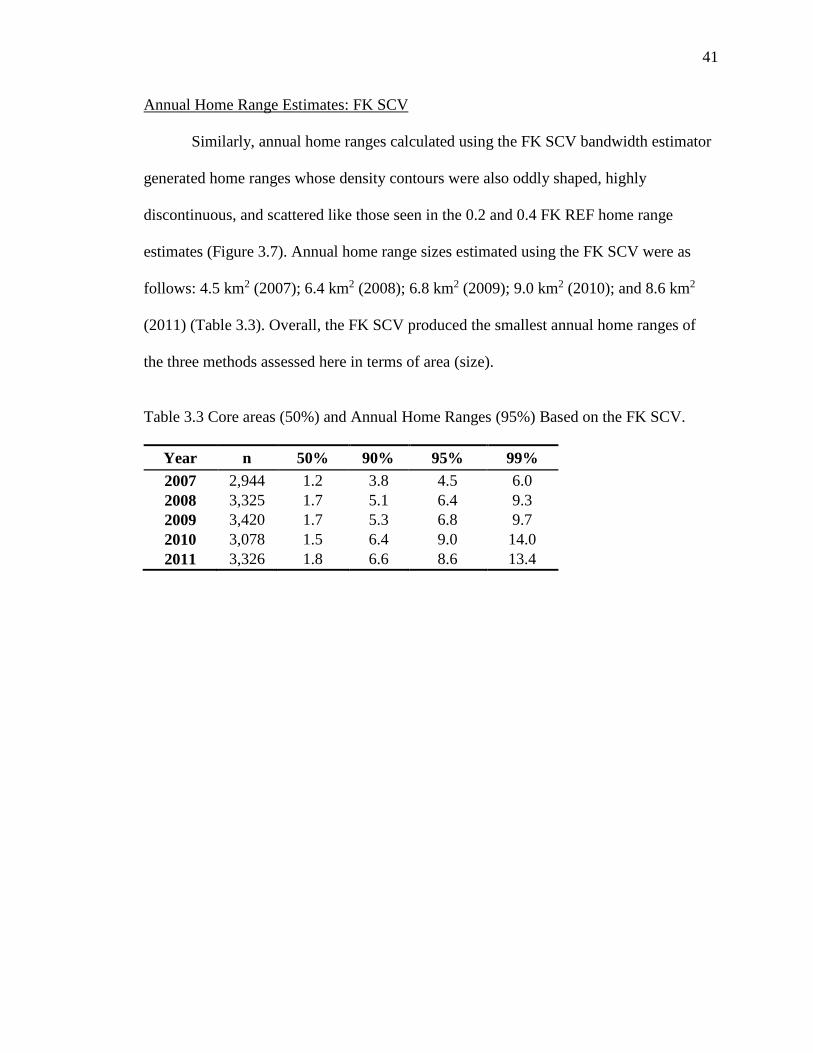
Annual Home Range Estimates: FK SCV ..................................................... 41

v

Comparison of Annual Home Range Across Methods ......................................... 43

Trends in Annual Home Range ..................................................................... 43

Annual Core Area: Use and Trends ............................................................... 46

Ranging Patterns: Daily, Monthly, and annual trends in DPL ............................. 49

Monthly Mean DPL ....................................................................................... 51

Annual Mean DPL ......................................................................................... 53

4. DISCUSSION ....................................................................................................... 56

Summary of Findings............................................................................................ 56

Evaluation of the MCP Method ..................................................................... 57

Evaluation of the Kernel Estimators .............................................................. 60

Implications and Suggestions for Future Research ........................................ 63

Comparison of Gelada Monkey Ranging Behavior Across Sites ......................... 67

How do the Annual Home Range Estimates of Geladas at Guassa Compare

to Those for Geladas at Other Sites?......................................................... 68

How do Geladas Utilize Their Home Range at Guassa and How Does it

Compare to That of Geladas at Other Sites? ............................................. 70

How do the DPL of Geladas at Guassa Compare to Those of Geladas at

Other Sites? .............................................................................................. 71

Comparison of Gelada Monkey Ranging Behavior Across Taxa......................... 71

Comparison of Gelada Ranging Behavior to Papio Species ......................... 72

Comparison of Gelada Ranging Behavior to Terrestrial Nonhuman Primate

Species ...................................................................................................... 77

Comparison of Gelada Ranging Behavior to Arboreal Nonhuman Primate

Species ...................................................................................................... 83

Comparison of Gelada Ranging Behavior to Terrestrial Ungulate Species .. 89

Implications of Inhabiting in a Topographically Variable Environment on

Calculations of Distance Traveled ..................................................................... 91

Ecological Implications of Movement Across Uneven Topography............. 92

Critiques of the Altitudinal Change Formula ................................................ 96

Conclusions ........................................................................................................... 97

APPENDIX: ADDING ERROR TO USER IDENTIFIED DUPLICATE PAIRS ...... 100

BIBLIOGRAPHY .......................................................................................................... 105

vi

LIST OF TABLES

Table Page

2.1 Results of Autocorrelation Analysis ....................................................................... 30

3.1 Comparison of Annual Home Range Estimates for MCP ...................................... 33

3.2 Core Areas (50%) and Annual Home Ranges (95%) Based on the FK

0.6*REF .................................................................................................................. 34

3.3 Core Areas (50%) and Annual Home Ranges (95%) Based on the FK SCV ......... 41

3.4 Monthly Mean DPL ± SE (m), Number of Full-days, and Range of DPL

for Each and all Years. ............................................................................................ 52

4.1 Comparison of Gelada Monkey Ranging Patterns Across Sites ............................. 69

4.2 DPL, Home Range, and Core Area of Papio Species............................................. 75

4.3 DPL, Home Range, and Core Area of Terrestrial and Arboreal Nonhuman

Primates................................................................................................................... 78

4.4 DPL, Home Range, and Core Area of Terrestrial Ungulate Species ...................... 86

vii

LIST OF FIGURES

Figure Page

2.1 Monthly Mean Rainfall at Guassa, Ethiopia .......................................................... 12

2.2 Monthly Mean Temperature at Guassa, Ehiopia ................................................... 13

2.3 Diagram Showing the Corrected DPL Based on a2 + b2 = c2. ................................ 19

3.1 Comparison of Annual Home Ranges From 2007 to 2008 Using the MCP

Method .................................................................................................................... 35

3.2 Comparison of Annual Home Ranges for 2007 Based on Scaling the FK REF..... 36





3.7 Comparison of Annual Home Ranges From 2007 to 2011 Using the FK SCV ..... 42

3.8 Cumulative 10-day Home Range Size Calculated Using the MCP Method

(95% Solid and 100% Dotted) .............................................................................. 45

3.9 Cumulative Annual Home Range Estimates Calculated Using the MCP

Method .................................................................................................................. 48

3.10 Comparison of the Relationship Between Time and DPL for Each and all

Range Years ......................................................................................................... 50

3.11 Comparison of Monthly Mean DPL and for all Range Years .............................. 51

3.12 Plot of Monthly Mean DPL on a Continuous Time Scale ................................... 54

3.13 Comparison of Annual Mean DPL + SE (m)........................................................ 55

viii

ACKNOWLEDGMENTS

I owe thanks and am indebted to many people who helped made this thesis

possible.

First and foremost, I would like to thank my life-long partner, the love of my life,

and my only best friend, Judy N. Vang, for her unconditional and unwavering support

and love these last five long and arduous years. Her presence and comfort were

instrumental in keeping me on the right path, and her happiness and health push me to

always do better and attain great things for the betterment of our lives. My daughter,

Julianne Dej Ntshiab Moua, though she is too young to realize, has been a constant bright

spot in my life, uplifting my spirit and resparking my resolve.

Next, I owe thanks to my parents, Vang Moua and Mai Lor, for giving me the

opportunity to receive an education, and in essence, experience the wonders of education

in their place. It is without doubt my parents’ struggles working in the fields to this day

and their individual and collective strengths to stay strong and unrelenting have changed

my siblings’ and my life for the better. I cannot appreciate them enough for all that they

have done for my siblings and me. I would like to thank my grandparents, Wa Lee Moua

and Xiong Thao, who were instrumental in raising my siblings and me during our

childhood years. I only wish they could be here still to share this moment with me.

ix

Life in Fullerton was made easier thanks to my brother, Sher, who was also

working on his Master’s at the time, spent some of his time in my car driving back and

forth between Fullerton and Long Beach just so that I could be closer to my school. I also

would like to thank my younger brother, Tao, and his girlfriend, Jennifer Lee, who

opened their home up to me every time I visited them in San Diego. Furthermore, I thank

my youngest brother, Yen Kong, and my younger sisters, Panglee, Gao Nou, Chamee, for

helping take care of our parents while we were away home for college.

Moreover, I thank Dr. John V.H. Constable, my undergraduate advisor and

mentor at Fresno State who continued to give me life lessons and guidance about

graduate school.

Last but not least, I thank the wonderful people I met during my time here at CSU

Fullerton, from my peers to my professors to the office staff, in particular Tannise

Collymore, and to my Thesis Committee advisors, Drs. Elizabeth Pillsworth, Nga

Nguyen, and Peter J. Fashing. I am especially indebted to Drs. Nguyen and Fashing, two

of the hardest working, devoted, and generous people I know. I will always remember

and be thankful for the patience, support, friendliness, and hospitality they have given me

and my family these past five years. They remained by me and were there for me

whenever I needed them. I cannot thank them enough for giving me the opportunity to

explore and expand my mind and develop as a scientist and a scholar. Thank you.

1

CHAPTER 1

INTRODUCTION

Research in Animal Ranging Ecology

Over the last half century, studies of animal ranging ecology have played an

integral role in expanding our knowledge of the behavior and ecology of numerous

species of animals, from ungulates (pronghorn antelope Antilocapra americana:

Buechner 1950; elk Cervus canadensis: Craighead et al. 1975), to birds (breeding,

feeding, and ranging ecology reviewed in Sutherland et al. 2004 and Wiens 1989), and

land mammals (giraffe Girafa camelopardalis: Dagg and Foster 1976, Leuthold and

Leuthold 1978; leopard Panthera onca: Rabinowitz and Nottingham 1986; African

elephant Loxodonta africana: Sikes 1971) including nonhuman primates (chimpanzees

Pan troglodytes: Boesch and Achermann 2000; L’Hoest’s monkeys Cercopithecus

lhoesti: Kaplin 2001; Bale monkey Chlorocebus djamdjamensis: Mekonnen et al. 2010;

mountain gorilla Gorilla beringei beringei: Vedder 1984; Watts 1998).

Being able to monitor and document an animal’s behavior and ecology over time

can clarify or reveal the role some animals have on the biological integrity of their

ecosystem. African elephants (Loxodonta africana), for example, consume or destroy

woody vegetation, which allows light to penetrate into the forest floor thereby facilitating

light-dependent plant species to establish and diversify (Field 1971; Western 1989).

Further, organisms like bumble bees, birds (Avian spp.), and (arguably) nonhuman

2

primates engage in pollination or seed dispersal, which facilitates reproductive success

and genetic diversity of plant species (Chapman et al. 1994; Dew and Wright 1998;

Howe 1977; Wallace and Trueman 1995). Lastly, predators consume prey to regulate

prey population densities (Berger et al. 2001; Bergerud et al. 1983; Mills 1984).

While these studies demonstrate that animals can play an integral part in the

success and health of their ecosystems, they also show that the relationship between

organisms and their environment is a highly complex and deeply interconnected one.

This suggests that as resources, such as food, water, and shelter, and ecological variables,

such as weather patterns, predation pressure, habitat loss, and group size vary across

space and time, we can expect animals to adjust their behaviors and movements in

accordance to these changes in order to maintain continued acquisition of the resources

required for survival and reproduction.

In response to ecological variability, for example, terrestrial ungulates (Albon and

Langvatn 1992; Lesage et al. 2000; Luccarini et al. 2006; Marra et al. 2005) and

nonhuman primates (Li et al. 2008) have been shown to migrate to or occupy temporary

(or seasonal) home ranges. Furthermore, animals may make minor or major shifts within

or outside their normal home range (Asensio et al. 2012; Donaldson and Echternacht

2005; Edwards et al. 2009; Fashing et al. 2007; Ferguson et al. 1999; Li et al. 2010), or

exploit alternative or fall back resources (Doran-Sheehy et al. 2009; Dunbar 1977; Li and

Rogers 2005; Pavelka et al. 2003) when primary resources become scarce. Alternatively,

large groups may fission into smaller factions to mitigate the effects of within-group

feeding competition while simultaneously reducing travel distance needed to search for

(more) food (Chapman and Chapman 2000; Chapman and Pavelka 2005; Dias and Strier

3

2003; Oluput et al. 1994). Indeed, studies of animal ranging ecology have provided

researchers with a valuable tool for documenting the behavioral responses animals make

in relation to changes in their surrounding environment.

In addition to information about space use and movement patterns, studies of

animal ranging ecology can also provide valuable data or uncover aspects of an animal’s

ranging ecology essential to making informed conservation decisions (e.g., Covert et al.

2008; Hervert et al. 2005; Heymann and Aquino 2010; Hillman 1988; Kaplin 2001;

Mekonnen et al. 2010; Laliberte and Ripple 2004; Rabinowitz and Nottingham 1986).

Recently, Mekonnen et al. (2010) completed the first study on the ranging and feeding

behavior of the Bale monkey (Chlorocebus djamdjamensis). They were able to

document, among other things, the monkey’s immense reliance on bamboo leaves,

despite inhabiting an area where the resource is heavily exploited by the local human

population (Mekonnen et al. 2010). Alternatively, information about an animal’s

behavioral or ranging ecology may be lacking or unclear. In these instances, researchers

may reinvestigate to gather additional data (e.g., Georgii 1980) or reevaluate the existing

literature in order to arrive at more robust conclusions about an animal’s ranging

behavior or habitat use preferences (e.g., Heymann and Aquino 2010). The Peruvian red

uakari monkey (Cacajao calvus ucayalii), for example, was once widely considered to be

apt to flooded-forest habitats. A recent review of all available data on its sightings and

whereabouts by Heymann and Aquino (2010), however, left the authors to reject this

notion and instead conclude that the monkeys show a preference for habitats mixed with

flooded-forest, terra firme (comprised of differently sized vegetation and terrain), or palm

swamps.

4

Indeed, the types of information obtained from studies of animal ranging, such as

the types of resources an animal relies on for survival (or the foods it substitutes when

conditions worsen), its habitat use patterns (over time), or its ecological role in its

environment, not only represent valuable assets concerned individuals need in order to

make informed conservation and management-related decisions, but also demonstrates

the importance of monitoring in animal populations.

The Importance of Long-Term Ranging Studies

Despite the significance of studies of animal ranging ecology, most ranging

studies (in nonhuman primates in particular) have only been carried out over several

months (e.g., Baoping et al. 2009; Doran 1997; Dunbar and Dunbar 1975; Mekonnen et

al. 2010; Zinner et al. 2002) or a single annual cycle (e.g., Albernaz and Magnusson

1999; Barton et al. 1992; Fashing 2001; Hunter 2001; Poulsen et al. 2001; Schreier 2010;

Willems et al. 2009). Though informative, some social activities, such as mating or births

(Carnegie et al. 2011; Janson and Verdolin 2005) and group size (Dias and Strier 2003;

Wieczkowski 2005), and ecological factors, such as food resources (Li and Walker 1986)

and climatic patterns (Haile 2005; Malhi and Wright 2004), may vary seasonally or occur

only during certain years, but not others. Therefore, the ability to acquire data over a long

stretch of time is important because it may lend researchers the opportunity to identify

behavior or movement trends that would otherwise be imperceptible with studies shorter

in duration.

For example, in their investigation of the longitudinal ranging patterns of muriqui

(Brachyteles arachnoides hypoxanthus) at Estação Biolόgica de Caratinga, Minas Gerais,

Brazil, across two temporally distinct study periods 15 years apart, Dias and Strier (2003)

5

reported an increase in the home range size (from 1.68 km2 to 3.09 km2) of their group of

muriquis between the study periods, which they attributed to a concomitant increase in

group size (from 23-27 to 57-63 individuals) over this same period. Similarly,

Wieczkowski (2005), in her re-examination of the ranging behavior of a group of Tana

River mangabeys in Kenya, first studied by Homewood (1976) and then later by Kinnaird

(1990), spanning more than two decades, found that home range size in their group of

mangabeys had increased over time (0.17 km2 to 0.19 km2 to 0.47 km2 in 1974, 1988-

1989, and 2000-2001, respectively). This pattern of increasing range use coincided with,

and was likely explained by the large group sizes found during each study period (36 to

17 to 50 members in 1974, 1988-1989, and 2000-2001, respectively) (Wieczkowski

2005). (In the 1960s, habitat disturbance led to a reduction in available habitat, which is

argued to explain the high density of mangabeys and their smaller range sizes in the 1970

study by Homewood [Wieczkowski 2005].) Lastly, Li et al. (2010), studying the long-

term ranging patterns of the Yunnan snub-nosed monkey (Rhinopithecus bieti) at Samage

Forest in the Baimaxueshan Nature Reserve, Yunnan, China, from 1998 to 2007, found

that annual home range size increased each year until it reached an asymptote after the

seventh year of observation, where it decreased slightly thereafter (7.67 km2 in 1998 to

18.77 km2 in 2004 to 17.14 km2 in 2007). These findings are important because they

capture the adaptive responses animals make as resources and conditions vary across

space and time, and further demonstrate the value of longitudinal monitoring in wild

nonhuman primate populations—and animals in general.

6

Gelada Monkeys as a Model System

Gelada monkeys (Theropithecus gelada) are an ideal model system with which to

employ home range estimators to investigate and uncover how these animals utilize their

home range across space and time. First and foremost, gelada monkeys live in a complex

fission-fusion social system (Kawai et al. 1983). Multiple one-male units can come

together and form a unit called the band which consists of units that are typically seen

ranging together and share a common home range (Kawai et al. 1983; Snyder-Mackler et

al. 2012). Units from different bands sometimes aggregate to form a larger unit called the

herd, or all the individuals seen traveling together at a particular time (Dunbar and

Dunbar 1975; Kawai et al. 1983; Ohsawa 1979; Snyder-Mackler et al. 2012). Not all of

the one-male units belonging to a single band are necessarily present at any given time

(Dunbar 1980; Dunbar and Dunbar 1975; Ohsawa 1979; Snyder-Mackler et al. 2012).

Therefore, herd size can fluctuate considerably across time. Secondly, gelada monkeys

live in an environment characterized by high altitude (range: 1700 – 4200 m: Dunbar

1998), cold temperatures, and rugged and mountainous topography (Ashenafi 2001;

Dunbar and Dunbar 1974, 1975; Fashing et al. 2014; Hunter 2001; Kawai 1979; Mori and

Belay 1990). We can therefore expect the physical constraints imposed by their

environment, coupled with the instability of their herd sizes, to shape the decisions these

monkeys make in terms of movement and habitat selection in both the short- and long-

term.

Despite the wealth of literature on the social system and behavior of gelada

monkeys, relatively little is known about how gelada monkeys utilize their unusual

habitat, especially in regard to home range size and daily movement patterns (e.g., Hunter

7

2001) over an extended and continuous period of time. Prior research has indicated that

gelada monkeys exhibit marked variations in both the distance they travel on a daily basis

and in their use of certain parts of the home range relative to other areas over time (Crook

1966; Dunbar and Dunbar 1974, 1975; Hunter 2001; Kawai 1979), and that such

movement patterns may be related to variations in resource availability and distribution,

band (herd) size, and weather conditions, e.g., fog, rainfall, and hail (Dunbar and Dunbar

1975; Hunter 2001; Iwamoto and Dunbar 1983; Kawai and Iwamoto 1979). Though

intriguing and informative, these findings only describe the ranging behavior of gelada

monkeys over the short-term (i.e., no more than one year of continuous observation:

Hunter 2001), and more pertinent to the objectives of this study, lack detailed

investigations into the home range size and use patterns of geladas in the long-term and

the specific analytical tools used to estimate home range (Dunbar and Dunbar 1974,

1975; Kawai 1979).

The scarcity of reports on the ranging ecology of geladas is alarming given the

number of potential challenges the species faces in the following years, including rising

global temperatures (Dunbar 1998), human encroachment and hunting pressures at

Sankaber, Gich, and Bole (Dunbar 1977; but see Beehner et al. 2008), and the potentially

tenuous status of long-standing traditional conservation bylaws at Guassa, the most

pristine of all established gelada study sites (Ashenafi 2001; Ashanfi and Leader-

Williams 2005). In combination, these challenges threaten the integrity of the remaining

gelada habitat and ultimately their long-term existence. Therefore, the need to quantify

how gelada monkeys utilize their unusual habitat, including their movement patterns and

spatial requirements, is at an all-time high. Critical questions include: (i) How large of an

8

area do gelada monkeys utilize on a year-to-year basis?; (ii) How do gelada monkeys use

their home range and how do their home range use patterns change over time?; (iii) How

far do gelada monkeys travel on a daily basis, how do their daily movements vary month-

to-month and year-to-year, and how does living in an uneven and hilly habitat influence

total daily distance traveled? Obtaining answers to these questions will undoubtedly

expand our knowledge about their short-term and long-term ranging patterns, and more

importantly, provide information essential for making informed conservation-related

decisions (Beehner et al. 2008; Cowlishaw and Dunbar 2000; Dunbar 1998).

Furthermore, the information obtained as a result of these questions can facilitate

comparisons of gelada ranging patterns to other species of nonhuman primates and

ungulates, and possibly help evaluate their utility in hypotheses about human and

nonhuman primate evolution (Jolly 1970; Jablonski 1993; Wrangham 1980; Fashing et al.

2014).

Gelada Monkey Study Site, Guassa, Ethiopia

In December 2005, Nguyen and Fashing (2009) established a new gelada monkey

study site at Guassa, an ecologically intact afro-alpine grassland in the Ethiopian

Highlands (Ashenafi 2001; Ashenafi and Leader-Williams 2005). Before this research

commenced at Guassa, the only sites where gelada monkeys had been studied were at

three more disturbed sites in the northern Ethiopian Highlands—Sankaber and Gich, both

located in the Simen Mountains, and Bole (Crook 1966; Dunbar and Dunbar 1974, 1975;

Kawai 1979)—and at one location, Arsi, in central Ethiopia south of the Rift Valley

(Mori and Belay 1990). Recently, reports by Fashing, Nguyen, and colleagues (Fashing et

al. 2010, 2011, 2014; Lee 2011; Moua et al. 2012; Nguyen and Fashing 2012; Nguyen et

9

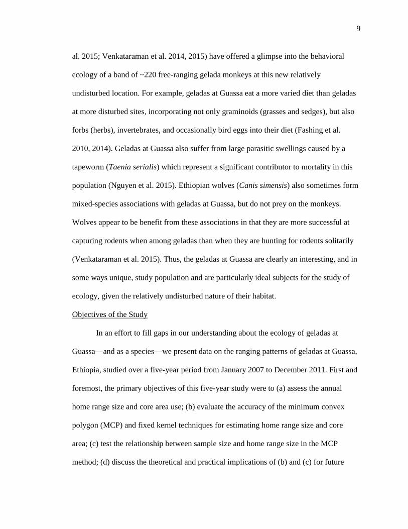
al. 2015; Venkataraman et al. 2014, 2015) have offered a glimpse into the behavioral

ecology of a band of ~220 free-ranging gelada monkeys at this new relatively

undisturbed location. For example, geladas at Guassa eat a more varied diet than geladas

at more disturbed sites, incorporating not only graminoids (grasses and sedges), but also

forbs (herbs), invertebrates, and occasionally bird eggs into their diet (Fashing et al.

2010, 2014). Geladas at Guassa also suffer from large parasitic swellings caused by a

tapeworm (Taenia serialis) which represent a significant contributor to mortality in this

population (Nguyen et al. 2015). Ethiopian wolves (Canis simensis) also sometimes form

mixed-species associations with geladas at Guassa, but do not prey on the monkeys.

Wolves appear to be benefit from these associations in that they are more successful at

capturing rodents when among geladas than when they are hunting for rodents solitarily

(Venkataraman et al. 2015). Thus, the geladas at Guassa are clearly an interesting, and in

some ways unique, study population and are particularly ideal subjects for the study of

ecology, given the relatively undisturbed nature of their habitat.

Objectives of the Study

In an effort to fill gaps in our understanding about the ecology of geladas at

Guassa—and as a species—we present data on the ranging patterns of geladas at Guassa,

Ethiopia, studied over a five-year period from January 2007 to December 2011. First and

foremost, the primary objectives of this five-year study were to (a) assess the annual

home range size and core area use; (b) evaluate the accuracy of the minimum convex

polygon (MCP) and fixed kernel techniques for estimating home range size and core

area; (c) test the relationship between sample size and home range size in the MCP

method; (d) discuss the theoretical and practical implications of (b) and (c) for future

10

research; and (e) determine the total distance traveled daily and explore the effects of

living in an environment with uneven topography on estimates of distance traveled. Our

secondary objectives were to compare the ranging behavior of gelada monkeys at Guassa

to (f) gelada monkeys at other study sites where similar data are available; (g) to Papio

spp., terrestrial nonhuman primates (e.g., chimpanzees, patas monkeys, etc.), and both

arboreal frugivorous and folivorous nonhuman primates; and (h) to terrestrial ungulate

species (because of their similar gramnivorous diet to gelada monkeys). Lastly, we

provide a discussion the importance of longitudinal monitoring for conservation and

management purposes and suggestions for future research.

The objectives of this study will afford us the opportunity to evaluate the

effectiveness of the MCP and fixed kernel methods in estimating the home range and

core area use patterns in this band of gelada monkeys, and also provide us with the

valuable information we have been missing about the long-term ranging behavior of

gelada monkeys.

11

CHAPTER 2

METHODS

Study Site

The Guassa study area, ~111 km2 in area (Lat 10 15’ - 10 - 27’ N and Lon 39

45’ - 39 48’ E), is an unusually intact afro-alpine grassland located in the Central

Highlands of Ethiopia (Ashenafi 2001; Ashenafi and Leader-Williams 2005). The study

site rests between 3200-3600 m above sea level on the western border of the Greater Rift

Valley (Ashenafi 2001; Fashing et al. 2010). Guassa’s unique geographic location makes

the study site extremely hilly and mountainous, with steep drop offs of greater than 1 km

along the eastern edge of the study area (Ashenafi 2001). Moreover, Guassa experiences

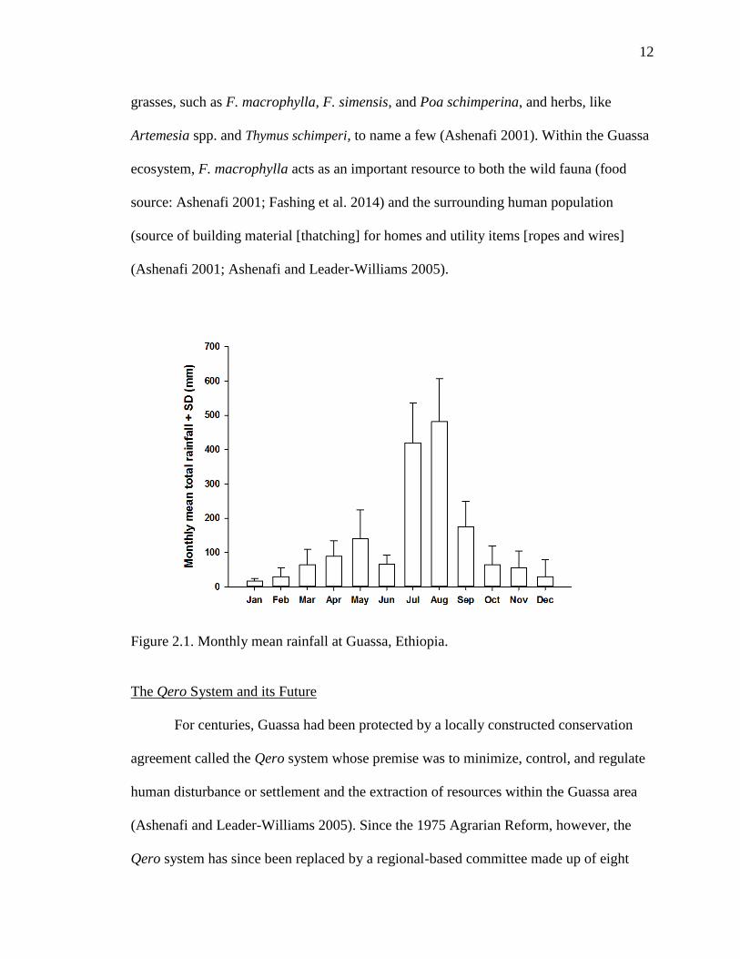
highly seasonal weather patterns. Rainfall occurs throughout the year (range of monthly

mean rainfall: 17 mm to 482 mm), but is mostly concentrated between July and August

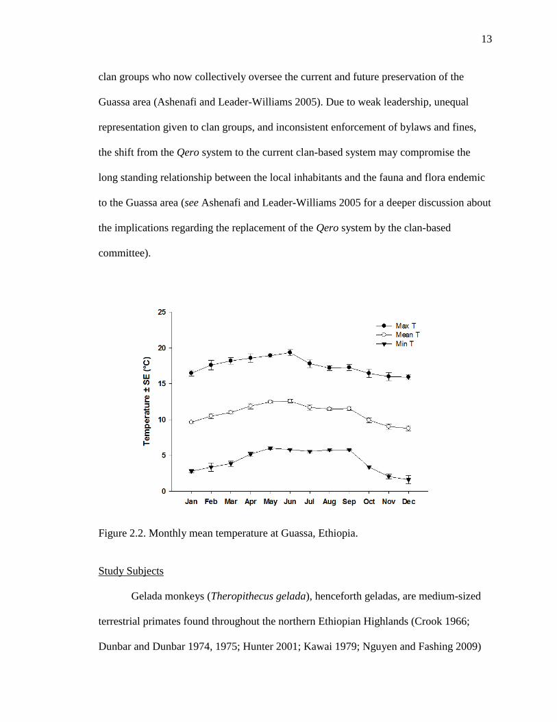
(Figure 2.1). Monthly mean maximum temperatures typically range from 16 to 19 C,

whereas monthly mean minimum temperatures generally range from 1 to 6 C; the

overall monthly mean daily temperature ranges from 9 to 12.5 C (Figure 2.2) (Fashing

et al. 2014).

Guassa’s pristine afro-alpine grassland can be categorized into distinctive

vegetation zones depending on the composition of the plants in each area (Ashenafi

2001). The Festuca grassland (also known locally as guassa), the second largest

vegetation zone which covers ~19.9% of Guassa, is composed of various species of

12

grasses, such as F. macrophylla, F. simensis, and Poa schimperina, and herbs, like

Artemesia spp. and Thymus schimperi, to name a few (Ashenafi 2001). Within the Guassa

ecosystem, F. macrophylla acts as an important resource to both the wild fauna (food

source: Ashenafi 2001; Fashing et al. 2014) and the surrounding human population

(source of building material [thatching] for homes and utility items [ropes and wires]

(Ashenafi 2001; Ashenafi and Leader-Williams 2005).

Figure 2.1. Monthly mean rainfall at Guassa, Ethiopia.

The Qero System and its Future

For centuries, Guassa had been protected by a locally constructed conservation

agreement called the Qero system whose premise was to minimize, control, and regulate

human disturbance or settlement and the extraction of resources within the Guassa area

(Ashenafi and Leader-Williams 2005). Since the 1975 Agrarian Reform, however, the

Qero system has since been replaced by a regional-based committee made up of eight

13

clan groups who now collectively oversee the current and future preservation of the

Guassa area (Ashenafi and Leader-Williams 2005). Due to weak leadership, unequal

representation given to clan groups, and inconsistent enforcement of bylaws and fines,

the shift from the Qero system to the current clan-based system may compromise the

long standing relationship between the local inhabitants and the fauna and flora endemic

to the Guassa area (see Ashenafi and Leader-Williams 2005 for a deeper discussion about

the implications regarding the replacement of the Qero system by the clan-based

committee).

Figure 2.2. Monthly mean temperature at Guassa, Ethiopia.

Study Subjects

Gelada monkeys (Theropithecus gelada), henceforth geladas, are medium-sized

terrestrial primates found throughout the northern Ethiopian Highlands (Crook 1966;

Dunbar and Dunbar 1974, 1975; Hunter 2001; Kawai 1979; Nguyen and Fashing 2009)

14

and at one location, Arsi, in central Ethiopia south of the Rift Valley (Mori and Belay

1990; Mori et al. 1999). Geladas sleep alongside cliff edges, but conduct their daily

activities on the plateau above (Dunbar and Dunbar 1974, 1975; Kawai and Iwamoto

1979). Their diet consists mostly of grasses (Crook 1966; Dunbar and Dunbar 1975;

Iwamoto 1979; Fashing et al. 2014), however, geladas have also been observed to

consume herbs, roots, and insects (Dunbar 1977; Iwamoto 1993), especially at Guassa

where these items play an important role in the gelada diet (Fashing et al. 2010, 2014).

The foundation of the gelada monkey multi-level social system is the one-male

unit (OMU), which consists of 1-3 males, 1-9 females, juveniles, and dependent young

(Dunbar 1980; Kawai 1979; Kawai et al. 1983; Nguyen and Fashing 2009, 2012).

Alternatively, males without any alliance to an OMU may group together to form an all-

male unit (Kawai et al. 1983). Multiple OMUs that tend to range within the same

geographic location is called a band (Dunbar 1980; Kawai et al. 1983). A temporary mass

of OMUs or bands without a social or reproductive connection is called a herd (Kawai et

al. 1983). Prior research has indicated that though OMUs (with the occasional cycling of

the alpha male due to male-to-male competition) and bands may remain stable over time,

herds have been shown to be much more fluid and unpredictable in duration and number

(Dunbar and Dunbar 1975; Hunter 2001; Ohsawa 1979; P. Fashing, unpub.data).

Data Collection and Analysis

The data used for this study were collected by members of the Guassa Gelada

Research Project, headed by Peter Fashing and Nga Nguyen, and span a five-year period

from January 2007 to December 2011.

15

Daily Ranging Data

Ranging data were collected on a band of approximately 220 geladas, known as

Steelers band, grouped into 16 OMUs (Nguyen et al. 2015). Fashing and Nguyen first

started habituating Steelers band in December 2005 and, along with field assistants and

student researchers, have continued to monitor the animals’ behaviors and movements on

a near-daily basis since November 2006 (Fashing et al. 2010). Follows started at 0700-

0800 in the morning before the geladas departed their sleeping cliffs and concluded at

1730-1800 in the evening, depending on the geladas’ distance from the camp and weather

conditions. The location of the Steelers band OMU currently followed was recorded

every half-hour with a handheld GPS device (Garmin GPSMAP 62). During instances

when the researchers had to switch to a different OMU of Steelers band during the daily

follow, e.g., to carry out behavior sampling on a different OMU, the researchers selected

the next OMU of Steelers band within five to 10 meters to the OMU being followed

currently as the new follow unit. This was done to minimize the distance between the old

and new OMU and to ensure an accurate depiction of the band’s (or herd’s) movement.

All half-hour readings were recorded with an error of less than 10 meters (m), unless

striving to obtain a reading with an error of less than 10 m placed the researcher in a

precarious situation, e.g., the band was at the edge of a cliff.

Data Analysis: To be considered a valid ranging day, henceforth full-day, each

full-day had to have both a morning and an evening sleeping cliff reading and at least a

1600 (i.e., 4:00 PM) reading. There was no minimum number of half-hour readings so as

long as the aforementioned criteria were met. Based on the criteria above, I identified a

total of n = 785 full-day follows (mean = 157, range = 145 – 168) from January 2007

16

through December 2011, with an average of 20 ± 1.4 (SD) number of readings per day

(range = 14 – 24).

Sometimes the researchers were unable to remain with the herd until an evening

sleeping cliff site was chosen. In these cases, the researchers returned the next morning

before the geladas departed from their morning sleeping cliff and recorded the exact

location of the current sleeping cliff and used this sleeping cliff reading as the evening

sleeping cliff for the previous ranging day. Since the geladas had yet to venture from this

sleeping cliff, the researchers were confident that the gelada monkeys slept on this

sleeping cliff the entire night. Under this circumstance, the researchers assumed the

geladas took the shortest possible route from their last known location the prior day to

their sleeping cliff site that night. It is therefore likely that the animals’ path lengths and

daily path length (for such days) may have been slightly underestimated for some full-

day follows (e.g., Swedell 2006), though this is not expected to present any major

problems to the analysis conducted here. All GPS locations were recorded in Latitude and

Longitude (Lat and Lon), Geographic World Coordinate System WGS 84 and

subsequently uploaded to MapSource® (Garmin 2011) at the end of each month.

Data Analysis: Preparing the Data for ArcMap 10 I used Microsoft Excel 2010 to

organize and prepare the data for ranging analysis. First, I matched each GPS location

data point, identified by its waypoint number (i.e., the unique ID number indicating the

order in which the GPS point was taken) and Lat and Lon coordinate, to their respective

researcher notes. The researcher notes were entered into a palm device (Palm m500) in

the field at the time of each reading, and describe the number and sequence of the

reading, the time and date of the reading, whether the reading was a sleeping cliff or

17

regular half-hour reading, and any relevant information that may be used to assess the

validity of that particular reading. Then, I uploaded the organized Excel documents into

ArcMap 10 (ESRI 2012) under the coordinate system Geographic World Coordinate

System, WGS 84. Thereafter, I changed the Layers Data Frame properties to the

Projected Coordinate System, UTM (i.e., Universal Trans Mercator), WGS 84, Northern

Hemisphere, WGS 84 UTM Zone 37N, the coordinate zone to which Ethiopia belongs.

This series of changes transforms the Lat and Lon decimal degree coordinates into UTM

meter coordinates, making it possible to calculate the distance between consecutive half-

hour readings (for daily path length) and to estimate fixed kernel home ranges. Since the

coordinate transformation is not permanent using this procedure, I exported the data as a

shapefile, and then implemented the addxy command in Geospatial Modeling

Environment 0.7.2 (GME; Beyer 2012) to replace the original Lat and Lon coordinates

with the newly defined UTM coordinates.

Ranging Analysis: Calculation of Daily Path Lengths

I calculated all half-hour path lengths and daily path length (henceforth DPL)

using GME 0.7.2 (Beyer 2012). I define DPL as the sum of all consecutive half-hour

readings belonging to each unique full-day follow.

I identified two approaches in GME that can be used to calculate DPL, and I

utilized both approaches to validate my estimates. The first approach utilizes the

convert.pointstolines and addlength commands. The former command uses a line to

connect all of the consecutive half-hour readings belonging to a unique full-day follow

while the latter then calculates the total distance of that line (in a unit of distance

specified by the user, such as m [meters] in this case); the final value represents the DPL.

18

Alternatively, the second approach utilizes the movement.pathmetrics command. Because

this command calculates the distance of each half-hour reading, I first re-organized all

half-hour readings that belong to the same full-day, and then I obtained the sum of all the

half-hour readings to determine the DPL. Lastly, I compared the DPL estimates produced

via both of these methods and verified that both techniques produced identical estimates

(Moua unpub. data).

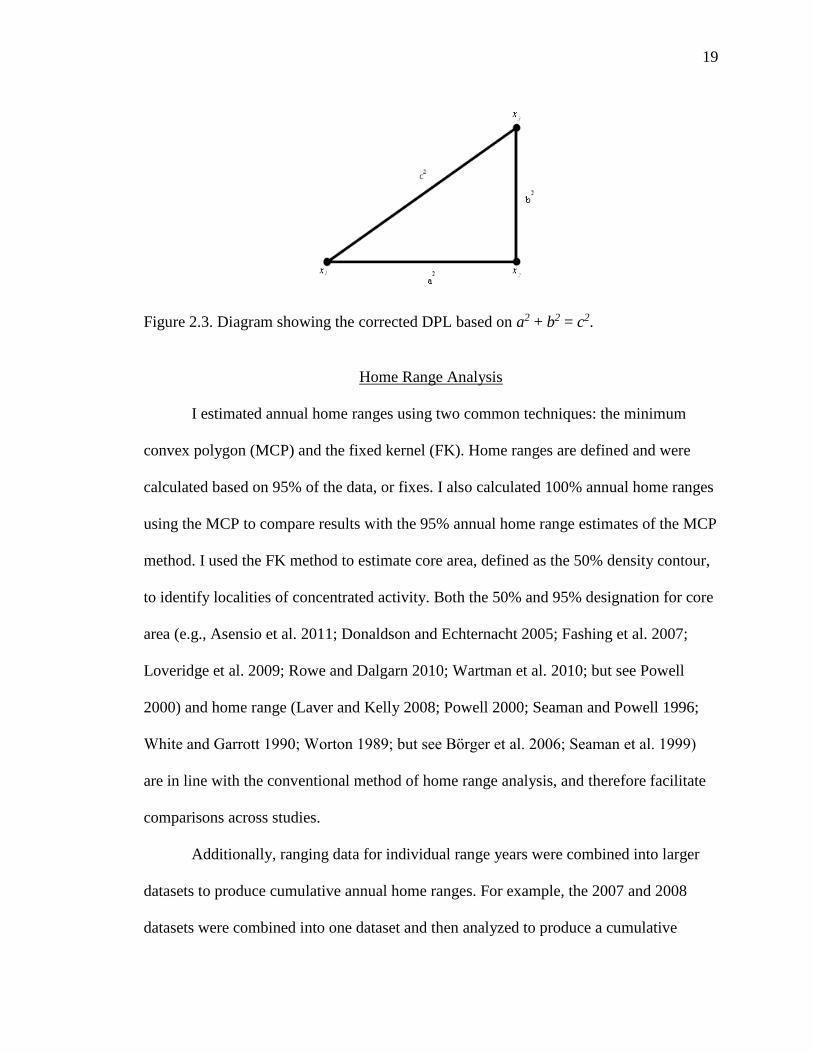
Ranging Analysis: Amending Daily Path Lengths to Cccount for Changes in Altitude

Once I confirmed the validity of the DPL estimates, I manually reanalyzed each

half-hour path length reading to account for the influence of changing altitude on distance

traveled. I reasoned that the extremely rugged and mountainous topography of Guassa

will cause the geladas to travel longer distances than traditionally calculated (e.g.,

Sprague 2000). To test the influence of changing altitude on distance traveled in this band

of geladas, I adapted Pythagora’s theorem for the three sides of a right triangle (i.e., a2 +

b2 = c2) (Figure 2.3). Specifically, I assumed that: (i) x1 and x2 denotes the location of

subsequent half-hour readings and a2 represents the distance, in meters, between these

two readings, squared; (ii) line segment x2x3, denoted as b2, represents the change in

altitude, in meters, squared, between half-hour readings x1 and x2; and (iii) lastly, c2 is the

sum of a2 and b2, where after solving for c2, I obtain c, the corrected path length after

taking into account change in altitude. I implemented this formula to calculate the

corrected path length for all half-hour readings. Then, I summed all corrected half-hour

path length readings belonging to each unique full-day follow to obtain the overall

corrected DPL, henceforth referred to as simply DPL (i.e., all reports of DPL henceforth

refer to the corrected estimate described here, unless otherwise stated).

19

Figure 2.3. Diagram showing the corrected DPL based on a2 + b2 = c2.

Home Range Analysis

I estimated annual home ranges using two common techniques: the minimum

convex polygon (MCP) and the fixed kernel (FK). Home ranges are defined and were

calculated based on 95% of the data, or fixes. I also calculated 100% annual home ranges

using the MCP to compare results with the 95% annual home range estimates of the MCP

method. I used the FK method to estimate core area, defined as the 50% density contour,

to identify localities of concentrated activity. Both the 50% and 95% designation for core

area (e.g., Asensio et al. 2011; Donaldson and Echternacht 2005; Fashing et al. 2007;

Loveridge et al. 2009; Rowe and Dalgarn 2010; Wartman et al. 2010; but see Powell

2000) and home range (Laver and Kelly 2008; Powell 2000; Seaman and Powell 1996;

White and Garrott 1990; Worton 1989; but see Bӧrger et al. 2006; Seaman et al. 1999)

are in line with the conventional method of home range analysis, and therefore facilitate

comparisons across studies.

Additionally, ranging data for individual range years were combined into larger

datasets to produce cumulative annual home ranges. For example, the 2007 and 2008

datasets were combined into one dataset and then analyzed to produce a cumulative

20

annual home range for 2007-2008. I repeated this process of adding subsequent datasets

for the remaining range years. In the end, I obtained a total of five datasets, four of which

contained data from subsequent years (i.e., 2007-2008, 2007-2009, 2007-2010, and 2007-

2011, except for 2007). All cumulative annual home ranges were estimated using the

MCP method only.

Lastly, I calculated cumulative home ranges at every 10 full-days. For example,

the first dataset started at full-days 1-10, then full-days 1-20, then full-days 1-30, until

full-days 1-785. As with the cumulative annual home ranges, all cumulative 10-day home

ranges were estimated using the MCP method only.

Home Range Estimator: Minimum Convex Polygon

The MCP (Mohr 1947) is a relatively old method researchers have utilized to

extrapolate home range. The MCP method uses straight lines and convex angles of less

than 180 degrees to connect the outermost points in a distribution of “fixes” (i.e.,

telemetry or geographic location data) to produce a home range in the shape of a polygon

(Anderson 1982a; Mohr 1947). Mechanically and conceptually the MCP is simple to

understand and implement, but the practical applicability of a polygon-shaped home

range has engendered a variety of issues that have severely hampered its long-standing

use as a home range tool (e.g., Borger et al. 2006; Laver and Kelly 2008; Powell 2000). A

commonly cited drawback associated with the MCP method is its tendency to

erroneously include areas the focal subject has never visited or been observed in within

the home range estimate (Andreka et al. 1999; Pebsworth et al. 2012; Powell 2000). This

leads to two additional problems: first, it does not accurately reflect the focal subject’s

movement and home range use patterns, and second, it overestimates the actual extent of

21

the focal subject’s home range (e.g., Andreka et al. 1999; Pebsworth et al. 2012).

Furthermore, outliers or unusual movements, due to their location generally being on the

periphery of the home range, will exacerbate the issues above. This is because the MCP

connects the farthest points together, and since outliers are usually farther away from

more common movements near the center of the home range, areas of space that lie

between adjacent data will be inadvertently included in the home range, inflating the

home range estimate. Moreover, the accuracy of the MCP has been tied to sample size

such that the larger the sample size, the larger (and more accurate) the home range

estimate (Bekoff and Mech 1984; Boyle et al. 2009; Girard et al. 2002; Jennrich and

Turner 1969; Schoener 1981; Seaman and Powell 1996). Lastly, the MCP fails to

produce any meaningful conclusions about trends in the focal subject’s activity inside the

home range. This inability to assess space use patterns within the home range is

significant considering the question of how an animal utilizes its home range is equally, if

not arguably more, important to how large the home range is.

Despite the aforementioned limitations of the MCP method, I constructed MCP

home ranges using both 95% and 100% of the data points in Home Range Tools, version

1.1 for ArcGIS 9.3 (Rodgers et al. 2007). I calculated 95% MCP home ranges using the

“Fixed Mean” default option in HRT. I note sample size where appropriate. The scientific

community has generally chosen to construct MCP home ranges using only a percentage

of the data points, usually 95% (Anderson 1982; Powell 2000; Powell et al. 1997),

because the MC method is highly susceptible to outliers (Andreka et al. 1982; Bekoff and

Mech 1984; Börger et al. 2006; Pebsworth et al. 2012; Powell 2000). However, several

authors (e.g., Kernohan et al. 2001; White and Garrott 1990) have argued there is no

22

biological support for the removal of the top 5% of the data, because it can result in the

loss of valuable data, e.g., removal of sleeping cliff sites from the (95%) home range

estimate (Pebsworth et al. 2012). Rodgers et al. (2007) advise that researchers should use

the “Remove X/Y Duplicates" command to remove all duplicate data points prior to

home range analysis because calculating the distances between duplicate data can result

in a “division by zero” error that can lead to a software crash. I was reluctant to

implement this command to remove duplicate data for several reasons: geladas at Guassa

routinely reuse sleeping cliffs, and they often remain immobile during periods of extreme

weather conditions, such as hail, rainfall, and thick fog (Dunbar 1977; Dunbar and

Dunbar 1975; Hunter 2001; Kawai and Iwamoto 1979; this study). Indeed, both of these

behaviors often result in duplicate or clumping of data points because the geladas are in

the same location for an extended period of time. Third, I was unsure of the ramifications

that removing duplicate data would have on the overall home range, both in terms of the

home range area estimate and possible biological interpretations (e.g., Blundell et al.

2001; de Solla et al. 1999). To determine whether or not removing the duplicate data

would have any effect on the home range estimate, I calculated home ranges with (i.e.,

the original datasets) and without duplicate data points using the “Remove X/Y

Duplicates” command in HRT. I compared the results and found that 95% MCP home

ranges constructed without duplicate points were (1-3%) larger than those constructed

with duplicate points for four of the five years (Moua, unpub. data). Further, ArcGIS 9.3

did not force quit or malfunction when the MCP command was used to calculate annual

home ranges with duplicate points in the dataset. Based on the findings above, I decided

to estimate all home ranges using data from the original datasets.

23

Though the MCP command successfully calculated all the annual and cumulative

annual home ranges from the original datasets, I later discovered that the MCP command

failed to produce any cumulative 10-day home range estimates for the first 100 full-days

(i.e., full-days 1-10, 1-20, 1-30, . . . 1-100) with the original datasets. In some cases,

ArcGIS 9.3 unexpectedly shut down without warning. This experience is indicative of the

software crash Rodgers et al. (2007) warned that can occur because of duplicate data in

the dataset. It appears that the effects of duplicate data on the home range analysis of the

MCP method in HRT is much more pronounced in smaller sample sizes than larger (since

no similar issues occurred with the larger datasets). Since I was unable to calculate 10-

day cumulative home ranges for the first 100 days of the study using the original data, I

re-analyzed all annual, cumulative annual, and cumulative 10-day home range estimates

without any duplicate data (to ensure all estimates of home range were calculated from

the same data using the MCP method). Therefore, all reports of MCP annual home range,

cumulative annual home range, and cumulative 10-day home range estimates have been

derived from the datasets containing no duplicate data. Lastly, as I previously determined

that 95% home ranges calculated without duplicate data were slightly larger than those

calculated from the original data, I acknowledge that the 95% home range estimates

reported in this study could be slightly overestimated, though a negligible difference.

Further, I acknowledge that MCP and fixed kernel annual home ranges will be calculated

using different sample sizes, however, I anticipate the results to be negligible (above).

Home Range Estimator: Fixed Kernel

Unlike the MCP method, kernel estimators can provide information about how an

animal utilizes its home range, in addition to several other features that make kernel

24

estimators currently the most preferred home range tool (Borger et al. 2006; Gitzen et al.

2006; Laver and Kelly 2008; Nilsen et al. 2009; Powell 2000; Seaman and Powell 1996).

Kernel estimators construct a home range, called a kernel or density estimate, based on

the relative density of points in a utilization distribution (UD)—a juxtaposition of fixes

(Silverman 1986; Worton 1989). It accomplishes this placing a fixed or an adaptive

kernel around each data point. A fixed kernel applies a constant smoothing factor (or

bandwidth), h, to the data, whereas an adaptive kernel adjusts its bandwidth relative to

the concentration of points in the regions such that more concentrated areas receive less

smoothing and vice versa (Silverman 1986; Worton 1989). Seaman and Powell (1996)

have demonstrated that the fixed kernel produces home range estimates that more closely

reflect the UD than the adaptive kernel.

Currently, the fixed kernel is the preferred home range estimator due to its ability

to generate density estimates of animal ranging behavior and produce a home range

estimate that may fit the shape of the focal subject’s distribution (as opposed to the MCP

which is confined to a polygon) (Laver and Kelly 2008; Powell 2000; Seaman and Powell

1999; Worton 1989). A density estimate, or density contour, represents the probability

value of the focal subject being in that location relative to other areas in the home range

(Worton 1989). The density estimate is extrapolated to identify areas within the home

range that are of relative importance to the focal subject, such as a core area, information

critical to uncovering how animals use their home range and for conservation-related

purposes. Lastly, kernels, unlike other home range estimators, such as the MCP, grid cell,

and ellipse, are free from issues that constrain the home range to a rigid and fixed shape,

and this characteristic allows kernels to produce a home range estimate that may captures

25

the focal subject’s fluid movements and dynamic home range use patterns (reviewed in

Powell 2000).

Effects of Bandwidth Estimator on Kernel Home Range Estimates Despite

possessing features that are ideal to any home range estimator, the accuracy and

performance of kernel estimators have been shown to be highly dependent on the

bandwidth used to assess the data (Borger et al. 2006; Gitzen et al. 2006; Powell 2000;

Seaman and Powell 1996; Worton 1989). Currently, the least-squares cross validation

bandwidth (LSCV) is the bandwidth of choice (Borger et al. 2006; Gitzen et al. 2006;

Powell 2000; Seaman and Powell 1999); the LSCV bandwidth, however, is limited in

application and prone to errors (Blundell et al. 2001; Gitzen et al. 2006; Horne and

Garton 2006).

Recently, research by Gitzen et al. (2006) and Horne and Garton (2006) found

that bandwidths such as the plug-in and solve-the-equation, and the likelihood cross-

validated bandwidths, respectively, performed similarly or better than the widely

considered LSCV bandwidth under identical experimental conditions. Horne and Garton

(2006) demonstrated, for example, that the likelihood cross-validated bandwidth

generated density contours that were relatively more accurate and indicative of the focal

subject’s home range use patterns than those estimated using the LSCV bandwidth when

sample size was ≤50. (Both the LSCV and likelihood cross-validated bandwidths

produced similar density estimates as sample size increased, indicating that sample size

has a relatively larger impact on density estimates than the choice of smoothing

parameter [Horne and Garton 2006; Seaman et al. 1999].) Indeed, these findings

corroborate the push by many researchers who advocate using multiple bandwidth

26

estimators in an effort to gauge the performance capabilities of each relative to the other

(Börger et al. 2006; Boyle et al. 2009; Powell 2000; Seaman and Powell 1996; White and

Garron 1990; Worton 1989). Based on these suggestions, I implemented FK analysis

using the reference, or ad hoc (REF); the LSCV; plug-in; and smoothed cross-validation

(SCV) bandwidth estimators. I used Home Range Tools (HRT) (Rodgers et al. 2007) to

conduct fixed kernel REF and LSCV home range analyses, whereas I used GME to

calculate fixed kernel LSCV, plug-in, and SCV home ranges (Beyer 2012). (GME does

not possess the REF option, whereas calculating the LSCV in both HRT and GME

provides comparability of results across programs.) Following the recommendation of

many researchers (Gitzen et al. 2006; Pebsworth et al. 2012; Rodgers et al. 2007; Seaman

and Powell 1996; Worton 1989), I multiplied the REF by a fixed proportion (e.g., 0.2,

0.4, 0.6, 0.8, and 1.0), also known as scaling the REF, which may circumvent its

tendency to underestimate or overestimate the home range.

Results of Preliminary Analyses of FK Kernel Estimators I conducted a series of

preliminary analyses to evaluate the performance capabilities of each bandwidth

estimator.

During the preliminary analysis phase, I discovered that HRT was unable to

produce any home range estimates using the LSCV bandwidth estimator, in which the

following error message appeared: “Warning: the LSCV function failed to minimize

between 0.5*HREF and 2.00*HREF. The bandwidth defaulted to HREF.” It appears that

when the LSCV bandwidth fails to reduce the mean integrated square error to an

appreciable level, it reverts to the REF bandwidth (Gitzen et al. 2006; Rodgers et al.

2007). Conversely, I found that GME successfully generated LSCV home ranges. I

27

compared the LSCV home ranges obtained in GME to the 1.0*REF home ranges

calculated in HRT, and found that the density contours of each were remarkably similar

(Moua unpub. data). I suspect GME was also unable to process the LSCV and

automatically reverted to the REF bandwidth, though without notifying the user about the

underlying reasons for the change. Following the unraveling of these findings, I omitted

the LSCV bandwidth estimator from this study altogether.

Both the SCV and plug-in bandwidth estimators produced home range estimates

with highly disconnected and scattered density contours (Moua unpub. data). Given the

similarity in the estimates produced by these two bandwidths, I report the findings for the

SCV bandwidth only. In sum, I report home range estimates for only the FK REF and

SCV bandwidths.

Autocorrelation: Implications on Ranging Analysis

Autocorrelation is defined as the aggregation of (location) data points that are

spaced too close in time that their association is no longer the result of random movement

(Legendre 1983; Swihart and Slade 1985a). It is generally assumed that data are

independent of one another, i.e., not autocorrelated (Legendre 1993; Swihart and Slade

1985b), because data that are autocorrelated may lead researchers to support or reject a

hypothesis without a statistically significant finding (Legendre 1993). The purported

impacts of autocorrelated data on estimates of animal ranging ecology are mixed at best.

Studies have shown, for example, that autocorrelated data generate MCP home ranges

that underestimated and did not correctly portray the focal subject’s space use patterns,

and also reduced the detail and length of travel paths (Swihart and Slade 1985b).

Conversely, numerous studies have demonstrated that eliminating autocorrelation may

28

actually diminish the quality and interpretational power of the findings (e.g., Blundell et

al. 2001; de Solla et al. 1999; Hansteen et al. 1997; Legendre 1993; Otis and White

1990). de Solla et al. (1999) found, for instance, that measurements of movement patterns

of both antler files (Protopiophila litigata) and snapping turtles (Chelydra serpentina)

were negatively affected at the expense of increasing the sampling time interval (to reach

independence of observations), such that a longer sampling interval resulted in a

reduction in the detail of the animal’s whereabouts and thus underestimated total distance

traveled. It appears that deleting data or increasing the time interval between subsequent

readings to reach independence of observations (as suggested by Swihart and Slade

1985a, b) may actually do more harm to the data analysis than intended (de Solla et al.

1999; Legendre 1993), and others have shown that autocorrelated data may actually help

interpret results (Hansteen et al. 1997). For example, in their examination of root vole

(Microtus oeconomus) ranging behavior, Hansteen et al. (1997) found that male root

voles tended to exhibit autocorrelated movement at short sampling intervals (i.e., at 30

and 60 mins). The authors posit this phenomenon may be explained by the animals

having large home ranges but not moving far enough between consecutive time intervals

to reach independence of observations (Hansteen et al. 1997) (an animal with a large

home range needs relatively more time between consecutive time intervals to distance

itself from its previous location if independence of observations is to be met: Schoener

1981). Indeed, these results suggest that, in some cases, autocorrelation may provide

researchers with added analytical and interpretational power about the behavior and

ecology of the focal subject.

29

I have described the disadvantages and advantages of autocorrelation on estimates

of animal ranging parameters, and the possible solutions to remedy autocorrelated data

(e.g., increase time interval or delete data points: Swihart and Slade 1985a, b). However,

I feel that increasing the time interval between consecutive observations or deleting data

until independence of observations is met (Swihart and Slade 1985a,b) would result in the

loss of crucial data and possibly inferential power about the movement patterns of the

geladas at Guassa. Ranging data in this study were collected at regular 30-minute

intervals throughout each full study day to insure a complete record was obtained of

gelada monkey movement patterns at Guassa. Furthermore, geladas are known to remain

immobile or inactive during periods of extreme weather and they frequently re-use

sleeping sites (Dunbar and Dunbar 1975; Hunter 2001; Kawai and Iwamoto 1979; this

study), behaviors that are likely to lead to autocorrelation (clumping of data points).

Indeed, eliminating data from the analysis for the sole purpose of reaching independence

of observations could potentially diminish the quality of the estimates (e.g., de Solla et al.

1999; Hansteen et al. 1997). I feel that this was something I did not want to risk.

Prior to fixed kernel analysis, I subjected the data to both Schoener’s Index (Schoener

1981) and Swihart and Slade’s Index (Swihart and Slade 1985b) to test for serial

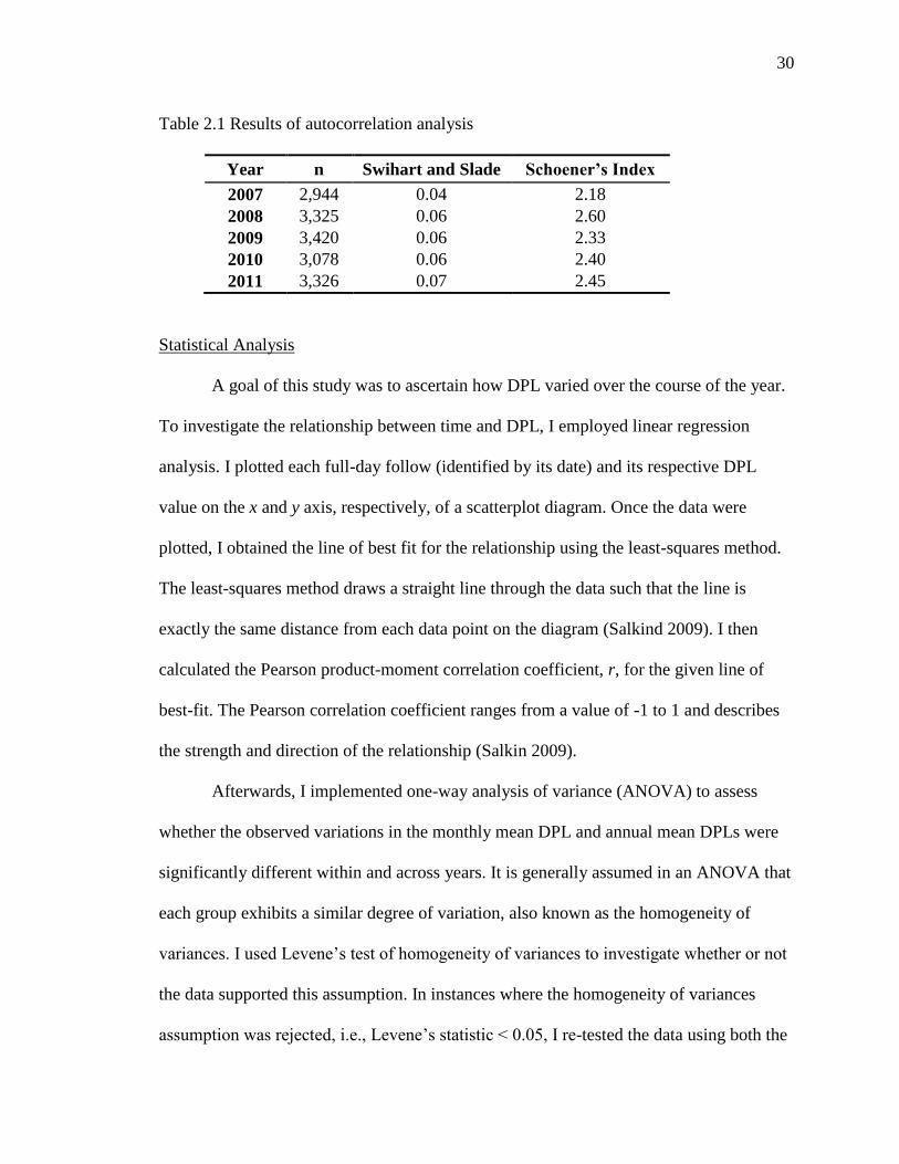
autocorrelation with the option provided in HRT. The results (Table 2.1) of the

autocorrelation analysis indicate that the data are autocorrelated. Values of <1.6 or >2.4

for Schoener’s Index or >0.6 for Swihart and Slade’s Index indicate autocorrelation.

Given the discussion on the issue of autocorrelation (above), and in spite of the

autocorrelation test results (below), I opted to analyze the data without amending them to

reach independence of observations.

30

Table 2.1 Results of autocorrelation analysis

Year n Swihart and Slade Schoener’s Index

2007 2,944 0.04 2.18

2008 3,325 0.06 2.60

2009 3,420 0.06 2.33

2010 3,078 0.06 2.40

2011 3,326 0.07 2.45

Statistical Analysis

A goal of this study was to ascertain how DPL varied over the course of the year.

To investigate the relationship between time and DPL, I employed linear regression

analysis. I plotted each full-day follow (identified by its date) and its respective DPL

value on the x and y axis, respectively, of a scatterplot diagram. Once the data were

plotted, I obtained the line of best fit for the relationship using the least-squares method.

The least-squares method draws a straight line through the data such that the line is

exactly the same distance from each data point on the diagram (Salkind 2009). I then

calculated the Pearson product-moment correlation coefficient, r, for the given line of

best-fit. The Pearson correlation coefficient ranges from a value of -1 to 1 and describes

the strength and direction of the relationship (Salkin 2009).

Afterwards, I implemented one-way analysis of variance (ANOVA) to assess

whether the observed variations in the monthly mean DPL and annual mean DPLs were

significantly different within and across years. It is generally assumed in an ANOVA that

each group exhibits a similar degree of variation, also known as the homogeneity of

variances. I used Levene’s test of homogeneity of variances to investigate whether or not

the data supported this assumption. In instances where the homogeneity of variances

assumption was rejected, i.e., Levene’s statistic < 0.05, I re-tested the data using both the

31

Welch and Brown-Forsythe tests, ideal in cases in which the homogeneity of variances

assumption has been rejected (Pallant 2010).

All statistical tests were implemented using SPSS 20 (IBM 2012) and tested with

a significance level of α = 0.05, unless otherwise stated.

All figures were created using SigmaPlot 12.5.

32

CHAPTER 3

RESULTS

Annual Home Range Estimates: MCP

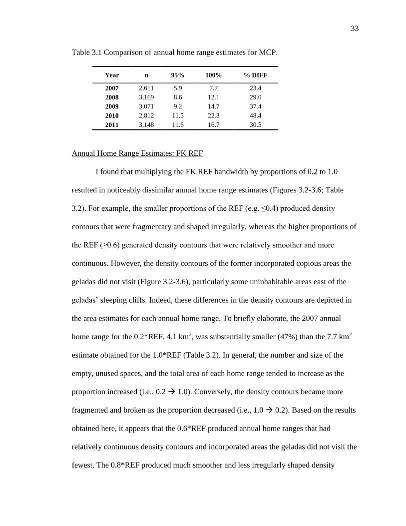
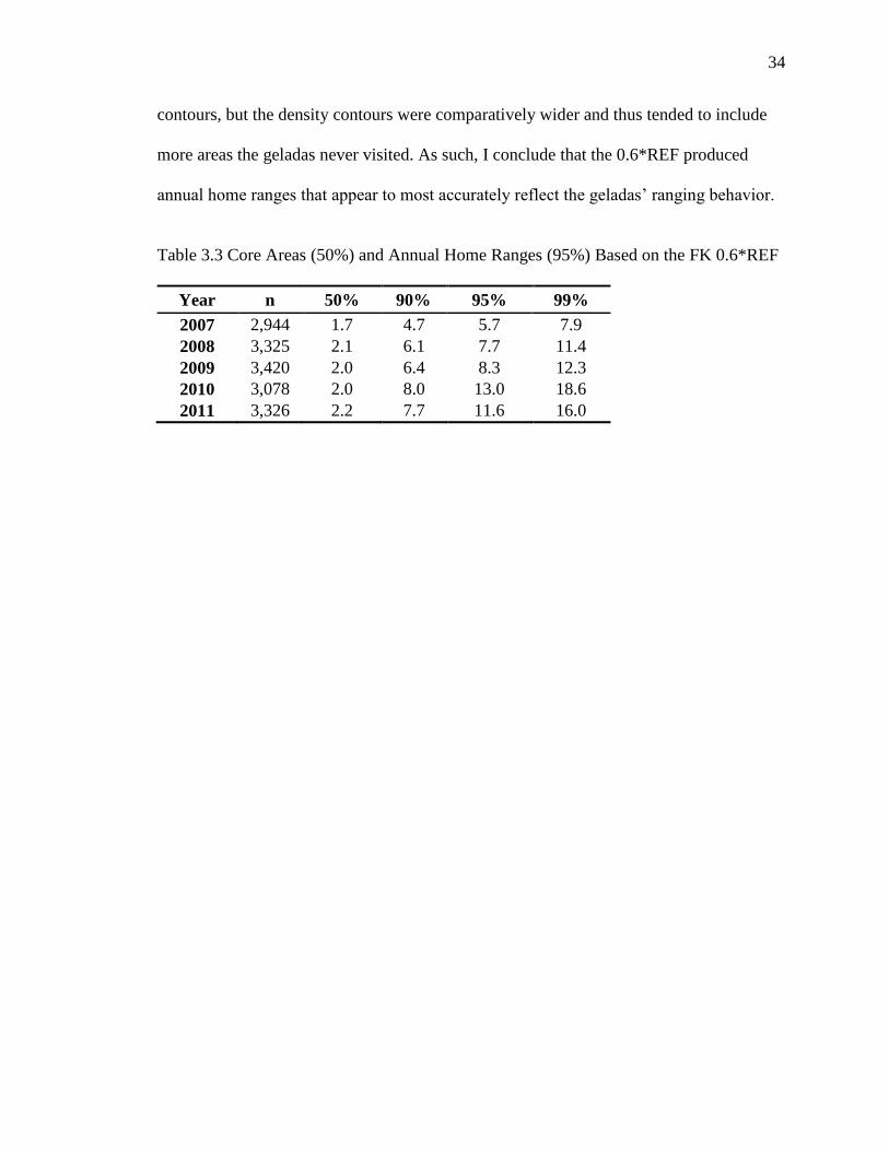
Annual home range (95%) increased in size over the five-year study period

(Figure 3.1), being smallest in 2007 (5.7 km2) and largest in 2011 (11.6 km2). The 95%

and 100% annual home range and the percentage difference between them are shown in

Table 3.1. Overall, this difference in increase in home range area from 2007 to 2011

amounts to a percent of increase of more than 50% over this time period.

All annual home range estimates from 2007 to 2011 contained areas the geladas

were not observed in (Figure 3.1). However, these areas of empty and unused areas were

relatively fewer and reduced in the 95% estimates compared to the 100% estimates,

which resulted in home ranges that were 23.4% (2007) to 48.4% (2010) smaller than their

respective 100% home range estimates (Table 3.1). Despite these findings of reduced

home range size, numerous sleeping sites (2007: 2; 2008: 1; 2009: 10; 2010: 9; 2011: 19),

which are all located along the cliff edges that border the eastern edge of the study area,

were erroneously excluded from the 95% home range estimates.

33

Table 3.1 Comparison of annual home range estimates for MCP.

Year n 95% 100% % DIFF

2007 2,611 5.9 7.7 23.4

2008 3,169 8.6 12.1 29.0

2009 3,071 9.2 14.7 37.4

2010 2,812 11.5 22.3 48.4

2011 3,148 11.6 16.7 30.5

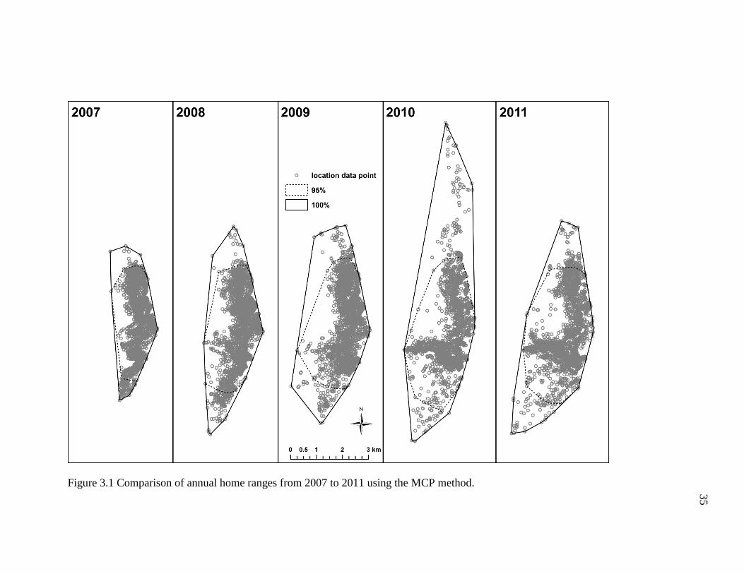
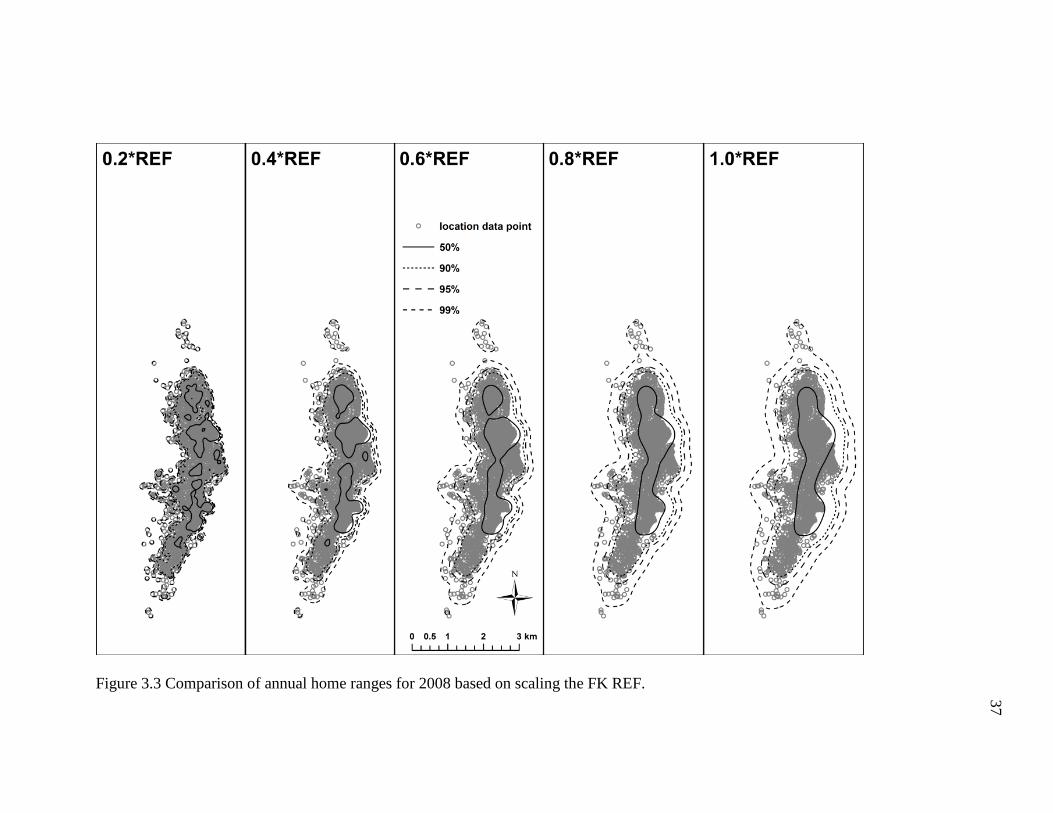
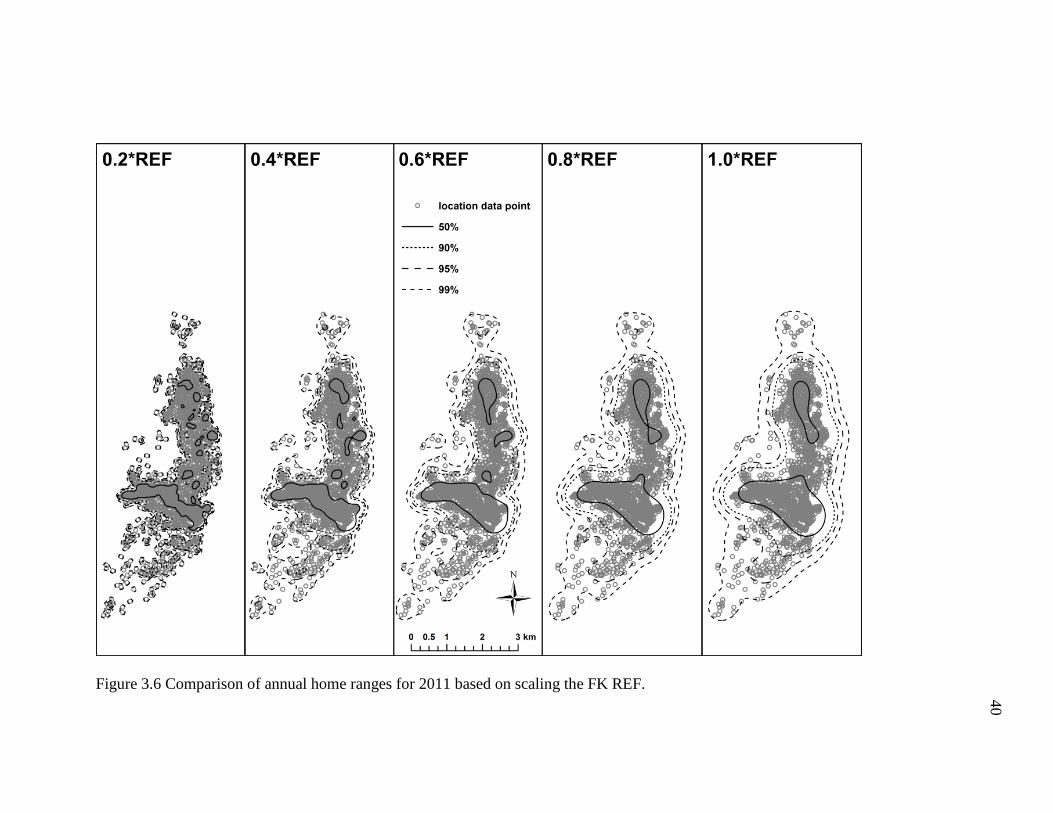
Annual Home Range Estimates: FK REF

I found that multiplying the FK REF bandwidth by proportions of 0.2 to 1.0

resulted in noticeably dissimilar annual home range estimates (Figures 3.2-3.6; Table

3.2). For example, the smaller proportions of the REF (e.g. ≤0.4) produced density

contours that were fragmentary and shaped irregularly, whereas the higher proportions of

the REF (≥0.6) generated density contours that were relatively smoother and more

continuous. However, the density contours of the former incorporated copious areas the

geladas did not visit (Figure 3.2-3.6), particularly some uninhabitable areas east of the

geladas’ sleeping cliffs. Indeed, these differences in the density contours are depicted in

the area estimates for each annual home range. To briefly elaborate, the 2007 annual

home range for the 0.2*REF, 4.1 km2, was substantially smaller (47%) than the 7.7 km2

estimate obtained for the 1.0*REF (Table 3.2). In general, the number and size of the

empty, unused spaces, and the total area of each home range tended to increase as the

proportion increased (i.e., 0.2 1.0). Conversely, the density contours became more

fragmented and broken as the proportion decreased (i.e., 1.0 0.2). Based on the results

obtained here, it appears that the 0.6*REF produced annual home ranges that had

relatively continuous density contours and incorporated areas the geladas did not visit the

fewest. The 0.8*REF produced much smoother and less irregularly shaped density

34

contours, but the density contours were comparatively wider and thus tended to include

more areas the geladas never visited. As such, I conclude that the 0.6*REF produced

annual home ranges that appear to most accurately reflect the geladas’ ranging behavior.

Table 3.3 Core Areas (50%) and Annual Home Ranges (95%) Based on the FK 0.6*REF

Year n 50% 90% 95% 99%

2007 2,944 1.7 4.7 5.7 7.9

2008 3,325 2.1 6.1 7.7 11.4

2009 3,420 2.0 6.4 8.3 12.3

2010 3,078 2.0 8.0 13.0 18.6

2011 3,326 2.2 7.7 11.6 16.0

35

Figure 3.1 Comparison of annual home ranges from 2007 to 2011 using the MCP method.

36

Figure 3.2 Comparison of annual home ranges for 2007 based on scaling the FK REF.

37


38


39

Figure 3.5 Comparison of annual home range for 2010 based on scaling the FK REF.

40


41

Annual Home Range Estimates: FK SCV

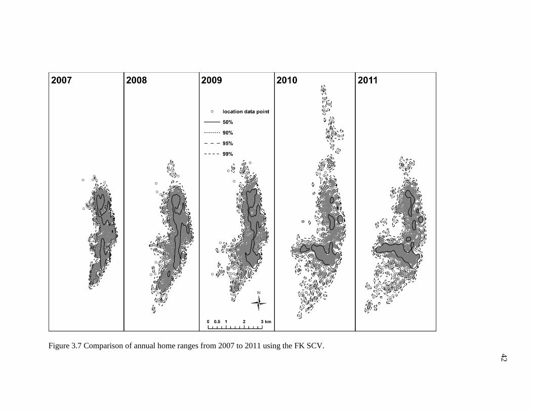
Similarly, annual home ranges calculated using the FK SCV bandwidth estimator

generated home ranges whose density contours were also oddly shaped, highly

discontinuous, and scattered like those seen in the 0.2 and 0.4 FK REF home range

estimates (Figure 3.7). Annual home range sizes estimated using the FK SCV were as

follows: 4.5 km2 (2007); 6.4 km2 (2008); 6.8 km2 (2009); 9.0 km2 (2010); and 8.6 km2

(2011) (Table 3.3). Overall, the FK SCV produced the smallest annual home ranges of

the three methods assessed here in terms of area (size).

Table 3.3 Core areas (50%) and Annual Home Ranges (95%) Based on the FK SCV.

Year n 50% 90% 95% 99%

2007 2,944 1.2 3.8 4.5 6.0

2008 3,325 1.7 5.1 6.4 9.3

2009 3,420 1.7 5.3 6.8 9.7

2010 3,078 1.5 6.4 9.0 14.0

2011 3,326 1.8 6.6 8.6 13.4

42

Figure 3.7 Comparison of annual home ranges from 2007 to 2011 using the FK SCV.

43

Comparison of Annual Home Ranges Across Methods

Despite the considerable variation in the home range estimates produced by each

method, there is evidence that illustrates some degree of commonality in the home ranges

among the MCP and both fixed kernel REF and SCV methods. To being with, the FK

SCV and some proportions of the REF method (e.g., 0.2 and 0.4) generally produced

small, disconnected, and incongruous density contours that resulted in small range size

estimates. Conversely, the ≥0.6 FK REF generated mostly contiguous and smooth density

contours, particularly at the higher density contours (e.g., >90%). Further, like the MCP

method, the ≥0.6 FK REF tended to incorporate areas never used by the animals, which

consequently resulted in inflated area estimates (Table 3.1 and 3.2). Additionally, each

home range method omitted one to 19 sleeping sites from the 95% estimates. Lastly,

despite the observed differences in the appearance of the annual home ranges estimated

by these methods, the trend of increasing annual home range size over time was evident

across all three home range estimate methods.

Trends in Annual Home Range

In general, annual home range size increased gradually over the five-year study

period: it was smallest in 2007, largest in 2010, and dropped slightly in 2011 (except for

the MCP in 2010 and 2011 where we found the reverse to be true). A closer examination

of the relationship between number of study days and home range size found that growth

in the home range was greatest during the first two to three years of the study period

(study days 460-470), but has since slowed down and appears to have reached an

asymptote after the 2010 and 2011 range years, with an occasional peak in home range

44

(e.g., study days 550-560, 660-670, and 780-785) (Figure 3.8). These findings imply an

underlying relationship between the number of study days and the size of the home range.

45

Figure 3.8 Cumulative 10-day home range size calculated using the MCP method (95% solid and 100% dotted).

Number of study days

0 50 100 150 200 250 300 350 400 450 500 550 600 650 700 750

Ho

me

ra

ng

e s

ize

(k

m2)

0

5

10

15

20

25

30

46

Cumulative Annual Home Range Estimates In general, annual home range size

increased with the addition of ranging data from subsequent years (Table 3.4). Using the

MCP method, the cumulative annual home range for 2007-2011 was slightly smaller

(11.2 km2) than the annual home range for 2011 (11.6 km2). One possible explanation for

this observation is that I calculated 95% MCP home ranges using the “Fixed Mean”

option in HRT, which obtains the mean of all the Lat and Lon coordinate pairs, then

removes the top 5% coordinate pairs from the dataset that are farthest from this mean.

Since the cumulative annual home range for 2007-2011 contained the largest sample size

and therefore most data near the center of the home range, the mean for the 2007-2011

dataset was likely smaller than the mean for the 2011 dataset, which meant that more data

were considered “farther” away and thus removed.

Annual Core Area: Use and Trends

Core area use during the five-year study indicates the geladas concentrated the

majority of their activities in roughly two to five regions within the home range (Figures

3.2-3.7): one to four in the northern and one in the southern region. The geladas’ space

use patterns did not remain static over time. According to both the FK REF and SCV, in

2010 and 2011 the core area in the southern region of the home range underwent a

westward expansion after having remained relatively stable (in size) the three years prior.

Core area size estimates varied considerably among the various proportions of the

FK REF bandwidth (Table 3.2). Roughly, annual core area for the FK REF increased in

size from 2007 to 2008, and depending on the particular proportion examined, it either

increased again or reduced in size until it finally increased to its largest size in 2011.

Similarly, annual core area for the FK SCV increased from 2007 (1.2 km2) to 2008 (1.7

47

km2), where it remained unchanged in 2009, but then it dipped back down in 2010 (1.5

km2), before it increased to its largest (combined) size in 2011 (1.8 km2). Overall, core

area use can be characterized as being smallest in the first year of study and largest in the

last year, though the number and size of the core areas changed year to year as estimated

using the FK SCV method.

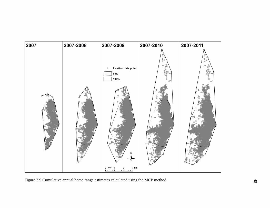
48

Figure 3.9 Cumulative annual home range estimates calculated using the MCP method.

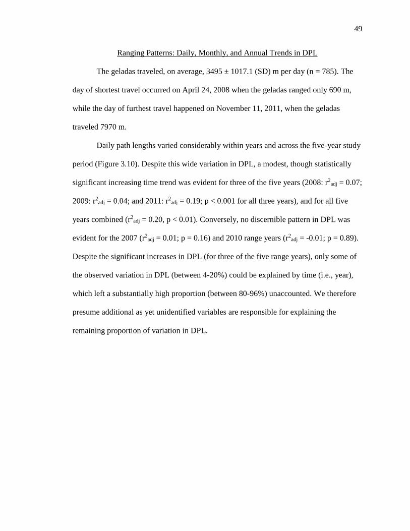
49

Ranging Patterns: Daily, Monthly, and Annual Trends in DPL

The geladas traveled, on average, 3495 ± 1017.1 (SD) m per day (n = 785). The

day of shortest travel occurred on April 24, 2008 when the geladas ranged only 690 m,

while the day of furthest travel happened on November 11, 2011, when the geladas

traveled 7970 m.

Daily path lengths varied considerably within years and across the five-year study

period (Figure 3.10). Despite this wide variation in DPL, a modest, though statistically

significant increasing time trend was evident for three of the five years (2008: r2adj = 0.07;

2009: r2adj = 0.04; and 2011: r2

adj = 0.19; p < 0.001 for all three years), and for all five

years combined (r2adj = 0.20, p < 0.01). Conversely, no discernible pattern in DPL was

evident for the 2007 (r2adj = 0.01; p = 0.16) and 2010 range years (r2

adj = -0.01; p = 0.89).

Despite the significant increases in DPL (for three of the five range years), only some of

the observed variation in DPL (between 4-20%) could be explained by time (i.e., year),

which left a substantially high proportion (between 80-96%) unaccounted. We therefore

presume additional as yet unidentified variables are responsible for explaining the

remaining proportion of variation in DPL.

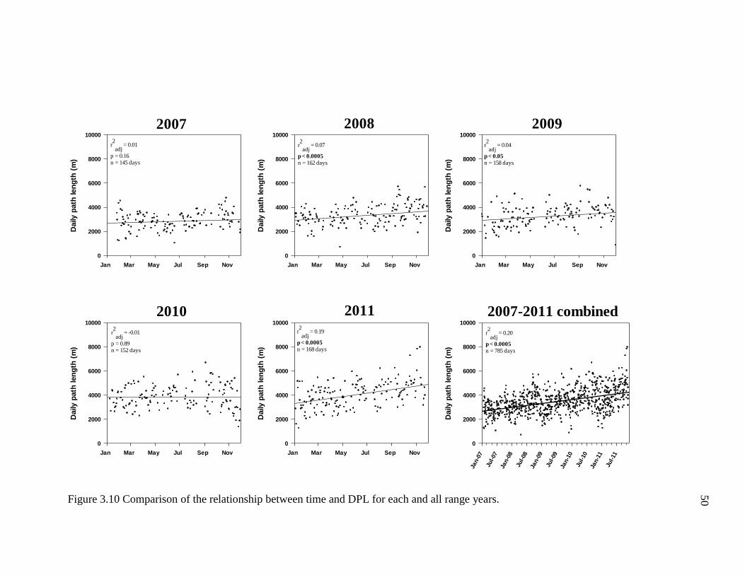
50

Figure 3.10 Comparison of the relationship between time and DPL for each and all range years.

Jan-0

7

Jul-07

Ja

n-0

8

Jul-08

Ja

n-0

9

Jul-09

Ja

n-1

0

Jul-10

Ja

n-1

1

Jul-11

Daily p

ath

len

gth

(m

)0

2000

4000

6000

8000

10000

r2

adj = 0.20

p < 0.0005

2007-2011 combined

Jan Mar May Jul Sep Nov

Daily p

ath

len

gth

(m

)

0

2000

4000

6000

8000

10000

Jan Mar May Jul Sep Nov D

aily p

ath

len

gth

(m

)0

2000

4000

6000

8000

10000


Daily p

ath

len

gth

(m

)

0

2000

4000

6000

8000

10000


Daily p

ath

len

gth

(m

)

0

2000

4000

6000

8000

10000


Daily p

ath

len

gth

(m

)

0

2000

4000

6000

8000

10000

2007 2008 2009

2010 2011

r2

adj = 0.20

p < 0.0005

n = 785 days

r2

adj = 0.19

p < 0.0005

n = 168 days

r2

adj = -0.01

p = 0.89n = 152 days

r2

adj = 0.04

p < 0.05

n = 158 days

r2

adj = 0.07

p < 0.0005

n = 162 days

r2

adj = 0.01

p = 0.16n = 145 days

51

Jan Feb Mar Apr May Jun Jul Aug Sep Oct Nov Dec

Mo

nth

ly m

ean

DP

L (

m)

0

1000

2000

3000

4000

5000

6000

2007

2008

2009

2010

2011

Mean 2007-2011

Figure 3.11 Comparison of monthly mean DPL and for all range years.

Monthly Mean DPL

The monthly average distance the geladas traveled each day (i.e., monthly mean

DPL ± SE (m)) varied considerably within and across years (Figure 3.11 and Table 3.4).

The monthly minimum and maximum values also illustrate and further bolster the widely

variable daily movement patterns of the geladas at Guassa (Table 3.4). Despite these

observations, plotting the monthly mean DPL data on a continuous time scale show a

peak in monthly mean DPL during the latter period of each year between September and

November (Figure 3.12). We found that the observed variation in monthly mean DPLs

within years was significantly different from each other for all range years (one-way

ANOVA, 2007: F(11,133) = 2.94, p < 0.01; 2008: F(11,150) = 4.10, p < 0.001; 2009: F(11,146)

= 2.75, p < 0.01; 2010: F(11,140) = 1.89, p < 0.05; 2011: F(11,156) = 5.94, p < 0.001).

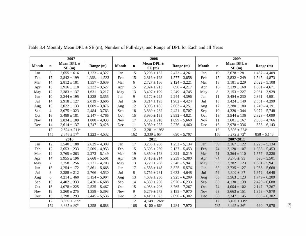
52

Table 3.4 Monthly Mean DPL ± SE (m), Number of Full-days, and Range of DPL for Each and all Years

2007 2008 2009

Month n Mean DPL ±

SE (m) Range (m) Month n

Mean DPL ±

SE (m) Range (m) Month n

Mean DPL ±

SE (m) Range (m)

Jan 5 2,655 ± 616 1,223 – 4,327 Jan 15 3,293 ± 132 2,473 – 4,261 Jan 10 2,678 ± 281 1,437 – 4,409

Feb 17 2,842 ± 199 1,368, – 4,532 Feb 15 2,816 ± 193 1,577 – 3,858 Feb 15 2,832 ± 249 1,545 – 4,873

Mar 14 2,812 ± 181 1,557 – 3,639 Mar 6 2,727 ± 166 2,124 – 3,221 Mar 18 3,181 ± 229 2,022 – 5,108

Apr 13 2,916 ± 118 2,222 – 3,527 Apr 15 2,924 ± 213 690 – 4,217 Apr 16 3,139 ± 168 1,891 – 4,671

May 12 2,383 ± 137 1,631 – 3,217 May 13 3,497 ± 199 2,249 – 4,745 May 8 3,153 ± 227 2,031 – 3,929

Jun 10 2,344 ± 195 1,328 – 3,355 Jun 9 3,172 ± 225 2,244 – 4,396 Jun 11 3,454 ± 230 2,361 – 4,981

Jul 14 2,918 ± 127 2,019 – 3,606 Jul 16 3,214 ± 193 1,982 – 4,424 Jul 13 3,424 ± 140 2,551 – 4,299

Aug 15 3,022 ± 133 1,609 – 3,876 Aug 12 3,093 ± 185 2,063 – 4,251 Aug 17 3,280 ± 180 1,749 – 4,191

Sep 4 3,075 ± 323 2,484 – 3,763 Sep 18 3,889 ± 232 2,421 – 5,707 Sep 10 4,320 ± 344 3,072 – 5,748

Oct 16 3,489 ± 181 2,147 – 4,766 Oct 15 3,930 ± 155 2,952 – 4,821 Oct 13 3,544 ± 136 2,328 – 4,099

Nov 11 2,834 ± 189 1,888 – 4,033 Nov 17 3,782 ± 218 1,899 – 5,668 Nov 11 3,681 ± 167 2,803 – 4,766

Dec 14 2,614 ± 137 1,747 – 3,428 Dec 11 3,030 ± 225 2,276 – 4,460 Dec 16 2,978 ± 336 858 – 6,143

12 2,824 ± 211a 12 3,281 ± 195a 12 3,305 ± 224a

145 2,848 ± 57b 1,223 – 4,532 162 3,339 ± 65b 690 – 5,707 158 3,272 ± 72b 858 – 6,143

2010 2011 2007-2011

Jan 12 3,540 ± 188 2,629 – 4,399 Jan 17 3,233 ± 288 1,252 – 5,134 Jan 59 3,167 ± 122 1,223 – 5,134

Feb 12 3,653 ± 233 2,509 – 4,953 Feb 15 3,603 ± 239 2,137 – 5,453 Feb 74 3,120 ± 107 1,368 – 5,453

Mar 14 3,765 ± 263 2,273 – 5,149 Mar 19 3,850 ± 178 2,324 – 5,219 Mar 71 3,364 ± 110 1,557 – 5,220

Apr 14 3,955 ± 196 2,668 – 5,501 Apr 16 3,416 ± 214 2,239 – 5,380 Apr 74 3,270 ± 93 690 – 5,501

May 7 3,758 ± 256 2,721 – 4,703 May 13 3,720 ± 288 2,546 – 5,941 May 53 3,282 ± 123 1,631 – 5,941

Jun 15 4,254 ± 172 2,861 – 5,668 Jun 17 4,536 ± 148 3,525 – 5,576 Jun 62 3,735 ± 127 1,033 – 5,668

Jul 8 3,388 ± 212 2,766 – 4,530 Jul 8 3,756 ± 281 2,632 – 4,648 Jul 59 3,302 ± 87 1,972 – 4,648

Aug 6 4,214 ± 460 3,154 – 5,904 Aug 13 4,689 ± 230 2,925 – 6,209 Aug 63 3,563 ± 123 1,749 – 6,209

Sep 15 4,402 ± 333 2,420 – 6,688 Sep 14 4,330 ± 250 2,970 – 6,233 Sep 60 4,130 ± 139 2,420 – 6,688

Oct 15 4,078 ± 225 2,525 – 5,467 Oct 15 4,953 ± 206 3,765 – 7,267 Oct 74 4,004 ± 102 2,147 – 7,267

Nov 19 3,260 ± 275 1,358 – 5,393 Nov 9 5,279 ± 573 3,155 – 7,970 Nov 68 3,663 ± 151 1,358 – 7,970

Dec 15 3,798 ± 293 2,445 – 5,536 Dec 12 4,419 ± 323 2,090 – 6,302 Dec 68 3,347 ± 145 858 – 6,302

12 3,839 ± 259a 12 4,149 ± 268a 12 3,496 ± 119a

152 3,835 ± 80b 1,358 – 6,688 168 4,100 ± 86b 1,284 – 7,970 785 3,495 ± 36b 690 – 7,970

53

Annual Mean DPL

Annual mean DPL increased significantly over the course of the five-year period

(Figure 3.13; one way ANOVA: F(4,780) = 44.1, p < 0.001). Results from Scheffe’s post-

hoc test reveal the annual mean DPL for 2007 was significantly different from the annual

mean DPL for 2008-2011 (p < 0.001 for all cases); the annual mean DPL for both 2008

and 2009 were significantly different from 2007 and 2010-2011 (p < 0.01 for all cases);

and the annual mean DPL for both 2010 and 2011 were significantly different from 2007-

2009 (p < 0.001 for all cases) (in Figure 3.6, letters that are shared among years indicate

where years are not significantly different from each other, whereas letters that differ

among years indicate where years are significantly different from each other). Despite the

significant increases in annual mean DPL, approximately only 18% of the variation in

annual mean DPL can be explained by time (i.e., year). We therefore suspect the

remaining 82% of the variation in annual mean DPL to be explained by additional though

currently unidentifiable variables (shaping DPL at the annual time scale).

Effect of Change in Altitude on Calculations of Distance Traveled

We found that accounting for changes in altitude on half-hourly distance traveled

resulted in a 0.15% (8 August 2011) to 12.2% (1 December 2009) increase in DPL (n =

785, mean = 1.67 ± 0.9% (SD)). In terms of actual additional distance traveled, these

percentages amount to an increase in DPL by 8 to 278 m (mean = 53 ± 22.4 m (SD)).

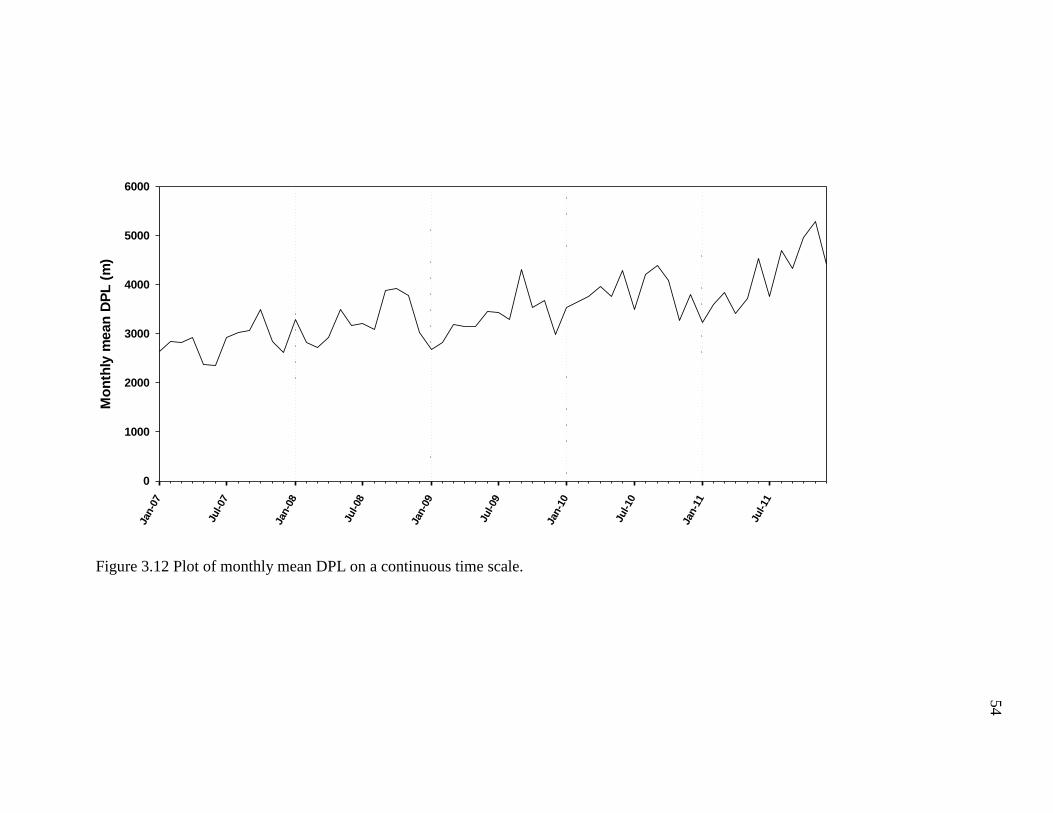
54

Jan-0

7

Jul-07

Jan-0

8

Jul-08

Jan-0

9

Jul-09

Jan-1

0

Jul-10

Jan-1

1

Jul-11

Mo

nth

ly m

ean

DP

L (

m)

0

1000

2000

3000

4000

5000

6000

Figure 3.12 Plot of monthly mean DPL on a continuous time scale.

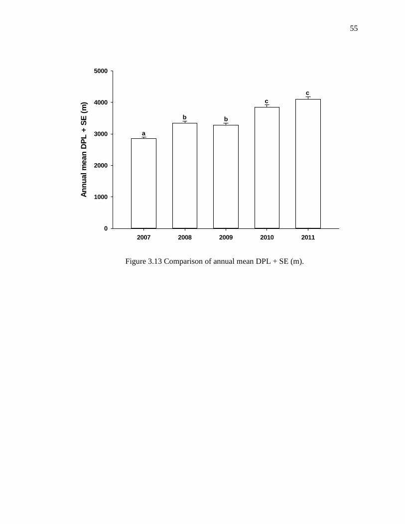
55

2007 2008 2009 2010 2011

An

nu

al m

ean

DP

L +

SE

(m

)

0

1000

2000

3000

4000

5000

a

b b

c

c

Figure 3.13 Comparison of annual mean DPL + SE (m).

56

CHAPTER 4

DISCUSSION

Summary of Findings

Annual home ranges estimated using the MCP method included spacious areas

the geladas never used, which were exacerbated by outliers and ultimately inflated home

range area estimates. Additionally, several sleeping sites were omitted from the 95%

home range estimates.

Like the MCP, both the fixed kernel SCV and REF bandwidths omitted several

sleeping sites from the 95% estimate. Both the SCV and (0.2 and 0.4) REF bandwidths

constructed annual home ranges with discontinuous and broken density contours.

Conversely, the >0.6*REF bandwidth produced continuous density contours, though

these density contours included areas the geladas did not and could not use.

In general, home range estimates estimated with the MPC were larger in area than

those estimated using both the REF and SCV bandwidths.

Gelada monkey annual home range and core area use increased in size from year

to year and were generally larger at the end of the study than at the beginning of the

study, patterns evident across all home range estimation techniques.

Daily path length (DPL), on the other hand, varied considerably within years,

though the total distance the geladas covered on any given day tended to increase from

January through to December. Monthly mean DPLs also varied extensively within and

57

between years, though it can be said that monthly mean DPLs generally increased over

the five-year study period. Overall, annual mean DPL increased significantly between

years, being shortest in 2007 and longest in 2011.

Evaluation of the MCP Method

Annual home ranges calculated using the MCP method were generally larger in

size than those estimated using both fixed kernel methods (Pimley et al. 2005; but see

Boyle et al. 2009), and tended to include areas the geladas never visited (Andreka et al.

1999; Fashing et al. 2007; Pebsworth et al. 2012; Powell 2000), trends that are evident

across the literature. A likely explanation for these observations is that the MCP method

uses straight lines and convex angles to connect the outermost data points to create a

home range whose shape is confined to a rigid and static figure that is unable to capture

the fluid and dynamic movements and space use patterns of animals. All annual home

ranges, for instance, contained a sizeable pocket of empty space in the western region of

the home range, despite the lack of evidence suggesting the geladas were observed in this

area over the five-year study period.

The decision to exclude a small portion of data from home range analysis,

typically the top 5%, has become common practice among studies of animal ranging

ecology (e.g., Andreka et al. 1999; Fashing et al. 2007; Pebsworth et al. 2012; Pimley et

al. 2005; Powell 2000; but see Borger et al. 2006), since this technique has demonstrated

consistently the ability to remove outliers or unusual movements that can have

detrimental impacts on the home range estimate, or at least mitigate their effects. Indeed,

removal of the top 5% from home range analysis reduced the size of the 95% annual

home ranges by 23.4% to 48.4% relative to their respective 100% estimates. The largest

58

reduction occurred between the annual home ranges for the 2010 range year, which saw

the 100% MCP drop from 22.3 km2 to 11.5 km2 in the 95% MCP, a decrease of 48.4%.

Comparisons of the 95% and 100% annual home ranges for all five years show a

decrease in the inclusion of data located on the periphery of the home range, which in

turn reduced the size and prevalence of empty, unused areas within the home range. This

was most evident for the 2010 range year when the geladas made two separate and

uncharacteristically long excursions to the far north of the Guassa study area. The

removal of these extreme data points explains the significant reduction in the home range

area for the 95% annual home range for 2010, and further highlights the susceptibility of

home range estimators such as the MCP to outliers.

Several authors have questioned the decision to exclude data from the home range

analysis (Kernohan et al. 2001; Powell 2000; White and Garrott 1990), and though the

findings reported here appear to show that this strategy of excluding the top 5% is

effective at eliminating unusual data points and producing smaller and relatively more

accurate home ranges, there is evidence that supports the concerns raised by these

authors. Specifically, several sleeping sites, from one to 19 depending on the range year,

were omitted from the 95% annual home range estimates (e.g., Pebsworth et al. 2012).

Recently, Pebsworth et al. (2012), in their investigation of the ranging ecology of chacma

baboons (Papio hamadryas ursinus) at Wildcliff Nature Reserve in Western Cape, South

Africa, reported the loss of two of seven sleeping sites from their 95% MCP estimates. It

is difficult to assess how often biologically important data such as sleeping sites get

removed from the 95% home range estimate, but it appears to be related to the practice of

excluding some portion of the top data from the home range analysis. Presumably, the top

59

5% generally represent the data located on the boundary or fringes of the home range,

movements considered to have relatively little biological significance. The findings here

show, however, that data on the fringes of the home range, such as sleeping sites, can

present critical challenges on the MCP method because such data may not only be

considered an outlier and therefore are more likely to excluded from the home range

analysis, but they can also represent areas essential to the focal subject’s ecology, in this

case sleeping sites (Powell 2000). Indeed, the findings of loss of sleeping sites reported

here and in Pebsworth et al. (2012) question the merit behind the removal of data from

the home range analysis and stress the need for researchers to consider the advantages

and disadvantages of their analytical decisions (e.g., Kernohan et al. 2001; Powell 2000;

White and Garrott 1990).

Home ranges estimated using the MCP method tend to increase as sample size

increases (Bekoff and Mech 1984; Boulander and White 1990; Boyle et al. 2009;

Jennrich and Turner 1969; Schoener 1981). The home ranges estimated at 10-day

intervals—a proxy measure of sample size—demonstrated that the geladas’ home range

increased in size as the number of study days increased, until home range size reached an

asymptote after approximately 570 days of study, a sample size of n = 12,244. Studies

using simulation data (Bekoff and Mech 1984) and telemetry data (Girard et al. 2002)

found 100-200 and 100-300 data points, respectively, could be enough to produce reliable

and accurate home range estimates. The finding that the geladas’ home range continued

to increase well beyond the 200-300 data point threshold suggests that the relationship

between home range size and sample size is much more complex and most likely

involves research-related components, such as sampling regime and analytical methods,

60

and species-specific variables, such as behavior and ecology (Bekoff and Mech 1984;

Boyle et al. 2009). The current study, however, did not categorically attempt to test the

relationship between home range size and sample size in the MCP method (e.g., Boyle et

al. 2009), and thus the conclusions reached here are derived from the analysis of the

home range size at 10-day intervals. Nonetheless, this finding of increasing home range

size with increasing study days is important for two reasons: firstly, it appears to support

the conclusion that home range size is directly correlated with sample size in the MCP

method; and secondly, but more importantly, it demonstrates the value of long-term

studies in discovering and illuminating the nuances in animal ranging behavior attainable

only through extended and continuous research. Lastly, this finding of increasing home

range size with increasing sample days invokes the need to investigate the determinants

of this phenomena in geladas at Guassa, Ethiopia.

Evaluation of the Kernel Estimators

Both fixed kernel estimators produced widely disparate results. The fixed kernel

SCV, for example, generated annual home ranges whose density contours were relatively

more disconnected, fragmented (i.e., islands), and shaped irregularly. As this is the first

study to utilize the fixed kernel SCV bandwidth in a practical setting (see Duong and

Hazelton 2005 for multivariate SCV; see Hall et al. 1992 for univariate SCV for full

descriptions of the bandwidth; see Dobrovidov and Rud’ko 2009 for the SCV bandwidth

applied in statistical and theoretical settings), it is difficult to explain the observed density

contours. Similar findings of fragmented and disconnected density contours have been

reported for the LSCV bandwidth (Amstrup et al. 2004; Blundell et al. 2001; Gitzen et al.

2006), which occur when the LSCV fails to find an appropriate smoothing value for the

61

given dataset (Gitzen et al. 2006; Rodgers et al. 2007; Seaman and Powell 1996). Perhaps

a similar issue may explain the fragmentary contours observed in the SCV estimates,

though additional research is required to confirm whether or not this is the case.

Whereas the MCP incorporated empty, unused areas predominantly in the western

region of home range, the fixed kernel REF, and to a certain extent the fixed kernel SCV,

included inhospitable areas east of the geladas’ sleeping sites that line the eastern border

of the Guassa study site. This finding suggests that data such as sleeping sites that are

located near the periphery of the home range pose an issue to all three home range

estimators as each included areas the animals were never observed in, and thus produced

annual home range values that were overestimates. One possible explanation for these

results is that the REF bandwidth has been reported to produce wide and expansive

density contours—that is, it tends to overestimate the boundaries of the home range—

when used to analyze utilization distributions with more than one center of activity (i.e.,

core area) (Gitzen et al. 2006; Seaman and Powell 1996; Seaman et al. 1999). The

findings reported here suggest that the geladas utilized more than one core area (based on

the 50% density contour), which supports the conclusion that the REF bandwidth is not

an appropriate bandwidth estimator for distributions with multiple centers of activity

(Gitzen et al. 2006; Seaman and Powell 1996; Seaman et al 1999).

Not all annual home ranges estimated using the REF bandwidth included areas the

geladas neither used nor visited. Rather, we found that scaling—i.e., multiplying—the

REF bandwidth by a fixed proportion (i.e., 0.2, 0.4, 0.6, 0.8, and 1.0) (e.g., Gitzen et al.

2006; Pebsworth et al. 2012; Seaman and Powell 1996; Worton 1989) produced annual

home ranges with density contours that varied in degree of continuity and

62

disconnectivity. To determine which proportion produced the most accurate and reliable

home range, Pebsworth et al. (2012) assessed each home range on its ability to include all

sleeping sites and major centers of activity, and the least amount of empty, unused areas.

Based on these criteria, Pebsworth et al. (2012) concluded that a proportion of 0.65 of the

REF generated the most reliable and accurate home range estimate for their study group

of chacma baboons. Using these criteria to assess the results reported here, I conclude

that a proportion of 0.6 of the REF produced a home range that had a combination of

smooth and continuous density contours and density contours that incorporated relatively

smaller degree of areas the geladas were never observed in. Unfortunately, none of the

proportions I analyzed produced an annual home range that contained all sleeping sites

for all five study years while meeting the two criteria above. The findings reported here

and in Pebsworth et al. (2012) demonstrate that the practice of scaling the REF

bandwidth by a fixed proportion affords the user the ability to decide the appropriate

bandwidth value for the given utilization distribution.

Kernel estimators are widely purported to be superior to the MCP method in

home range estimation (Borger et al. 2006; Laver and Kelly 2008), but the findings here

do not definitively support this popular supposition. The results show that both kernel

estimators, like the MCP, incorporated areas the geladas did not utilize and omitted

sleeping sites from the annual home range estimates. In turn, these results demonstrate

the value of utilizing multiple home range tools to estimate home range as results may

not conform to previous findings (Boyle et al. 2009).

63

Implications and Suggestions for Future Research

Studies of animal ranging ecology are imperative for conservation-related

purposes, and the analytical techniques and tools researchers utilize to investigate and

understand aspects of animal movement and home range use patterns are equally critical

for developing sound and effective conservation plans. The results reported here have

wide implications for future research. I therefore propose the following recommendations

based on the observations reported here.

For the choice of home range estimators, I strongly agree the MCP should be still

utilized as a home range estimator despite its widely documented drawbacks and the

growing consensus against its continued use (Borger et al. 2006; Gitzen et al. 2006; Laver

and Kelly 2008). I contend that using the MCP to estimate home range affords

researchers the invaluable ability of making comparisons between methods (Boyle et al.

2009; Pimley et al. 2005; Pebsworth et al. 2012) and within the same study or across

studies and taxa (Biebouw et al. 2009; Fashing et al. 2007; Grueter et al. 2009; Robbins

and McNeilage 2003; Strier 2003; Wartman et al. 2010; Wieczkowski 2005). Moreover, I

recommend using the fixed kernel method to supplement the MCP method (Borger et al.

2006; Boyle et al. 2009; Gitzen et al. 2006; Laver and Kelly 2008; Powell 2000; Seaman

and Powell 1999). The choice of bandwidth will likely vary depending on the nature of

the data being analyzed (Gitzen et al. 2006; Powell 2000), though I recommend using the

LSCV and REF bandwidth estimators. The LSCV, despite its drawbacks (Blundell et al.

2001; Boyle et al. 2009; Gitzen et al. 2006; Pebsworth et al. 2012), is the bandwidth of

choice among researchers (e.g., Powell 2000) and its use is worth attempting. The REF

bandwidth should be implemented with the scaling option at consistent intervals of 0.05,

64

or an interval the researcher finds suitable for the given dataset (e.g., 0.1). Though the

results reported here regarding the home range estimating power of the SCV bandwidth is

inconclusive at best, additional research is needed to ascertain whether or not the SCV

bandwidth will have a place as a reliable home range estimator. Indeed, this sentiment

applies to many bandwidth estimators that have seen little application in home range

studies, e.g., the plug-in methods and cross-validation bandwidths (Beyer 2012; Gitzen et

al. 2006), and thus I recommend researchers test various bandwidth estimators to assess

its efficacy as a home range estimator.

On the topic of data analysis, the decision to subject the entire dataset (i.e., 100%)

or a majority of the data (e.g., 90% or 95%) to home range analysis should be driven

largely by the research question(s) being asked and the behavioral ecology of the focal

subject. As I have demonstrated, in focal subjects, like the geladas at Guassa, where the

periphery of the home range is the location of critical data essential to understanding the

behavioral ecology of the species, the researcher must select a data analysis procedure

that is line with the research question but will simultaneously produce results that are

reliable and accurate. Nonetheless, I strongly advise researchers to conduct home range

analysis using both 95% and 100% of the dataset, since doing so will allow for

comparisons across techniques and the assurance of making informed and sound

decisions supported by quantitative analysis and field notes.

Additional components to consider include sample size and sampling regime.

With regard to sample size, the number of data points needed to produce a reliable and

accurate home range estimate is contingent upon a variety of factors, such as home range

estimator (e.g., Anderson 1982; Bekoff and Mech 1984; Boyle et al. 2009; Seaman and

65

Powell 1999), behavior and ecology of the focal subject (see Bekoff and Mech 1984 for

examples; Girard et al. 2002), and body size (mass) (Clutton-Brock and Harvey 1977).

Research has shown, for example, that the MCP method can underestimate (Girard et al.

2002) and overestimate home range at small sample sizes (Glessener and Britt 2004),

whereas the fixed kernel method can produce a home range that provides a general, but

accurate account of the focal subject’s space use patterns with a small sample size

(sample size of 10 in Borger et al. 2006; sample size of 30-50 in Seaman and Powell

1999; but see Boyle et al. 2009). Whether or not the focal subject lives independently or

in a group can possibly have an effect on the number of data points required to reproduce

an accurate depiction of its home range. Group living may invoke greater instances of

intra-specific competition for resources, which in turn will force the group to make

additional or further movements in search of food (Chapman and Chapman 2000; Dunbar

and Dunbar 1975; Dunbar and Iwamoto 1983; Fashing et al. 2007). Similarly, diet, such

as fruigivory, insectivory, and gummivory, has been shown to influence home range size

(Clutton-Brock and Harvey 1977; Isbell 1998). In light of these variables, the ability to

find the “optimal” sample size may be difficult given the number of factors that influence

the relationship between sample size and home range estimation. I therefore recommend

a sample size that falls within the means of the research goal(s), taking into account each

of the variables described above, including the likelihood and practicality of gathering

such data and the associated costs (i.e., time and money). Finally, it may be more

strategic to gather a plethora of data at the onset and then sub-sample or condense the

data later whenever needs change.

66

The sampling regime, defined as the time interval between subsequent data

points, the length of the study, and which locations should be recorded, is arguably

influenced by the same factors that affect sample size as discussed above. For instance, a

short time between subsequent data points, such as 15 to 30 minutes, may be ideal for

focal subjects that cover long distances in short periods of time. Conversely, a longer

time between subsequent data points of one hour or greater may be more appropriate for

focal subjects that remain immobile in a general area over an extended period of time or

do not travel far enough between sampling intervals (e.g., Hansteen et al. 1997). If the

time interval between subsequent data points is too short, this may lead to data being

autocorrelated, which has been argued to undermine the integrity of the results (Swihart

and Slade 1985a,b; but see Fieberg 2007; de Solla et al. 1999). Depending on the focal

subject, some locations may be more critical than others, e.g., sleeping sites, water holes,

territorial zones, etc., and thus their acquisition should take precedence over other

location data, particularly in the event that time or cost may prevent ample data

acquisition. Where sufficient time and funding are available, researchers beginning

detailed studies of animal ranging ecology should plan to undertake several years of

continuous observation as this will result in (a) more complete estimations of overall

home range size and (b) the identification of any inter-annual differences in movement

and home range use patterns.

In sum, the recommendations described above provide the researcher with the

greatest degree of comparability of results across studies and confidence in research

method supported by extensive research (e.g., Borger et al. 2006; Pimley et al. 2009;

Pebsworth et al. 2012; Powell 2000).

67

Comparison of Gelada Monkey Ranging Behavior Across Sites

One purpose of this study was to compare the DPL, home range size, core area,

and furthest distance traveled from a sleeping cliff site (edge) for geladas at Guassa,

Ethiopia, to those at Sankaber, Gich, and Bole (no ranging data exist for geladas

inhabiting the study area at Arsi, Ethiopia: Mori and Belay 1990; Mori et al. 1999). Both

Sankaber and Gich are located within 15 km of each other in the Simien Mountains

National Park in central Ethiopia (Dunbar and Dunbar 1975; Iwamoto and Dunbar 1983;

Kawai 1979). They are approximately ~305 km and ~320 km northwest of Guassa,

respectively. The study site of Bole, on the other hand, lies ~ 100-200 (south)west of

Guassa, near Addis Ababa, the capital of Ethiopia (Dunbar and Dunbar 1974; Iwamoto

and Dunbar 1983).

One obstacle to comparing home range estimates across sites or species (here and

below) concerns the types of method(s) used to estimate the home range. For example, I

estimated home range size using both the MCP and fixed kernel methods, whereas

Hunter (2001) utilized the grid-cell method with 200 x 200 m quadrats (Dunbar and

Dunbar 1975 and Kawai 1979 did not specify which methods they used). Because each

method employs different assumptions or criteria to construct a home range, the use of

different techniques makes it problematic to make direct and robust comparisons about

space use patterns. In addition to using different methods to calculate home range size,

the time scale in which the ranging data are collected is another obstacle to consider.

Home ranges estimated from data gathered over only a few weeks or several months, for

example, are not the same as home ranges estimated using data obtained from an entire

year or more, because each estimate reflects the habitat and space use patterns of the

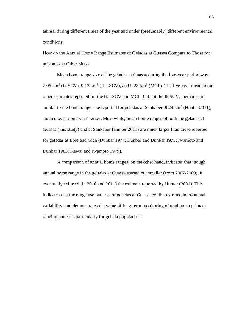
68

animal during different times of the year and under (presumably) different environmental

conditions.

How do the Annual Home Range Estimates of Geladas at Guassa Compare to Those for

gGeladas at Other Sites?

Mean home range size of the geladas at Guassa during the five-year period was

7.06 km2 (fk SCV), 9.12 km2 (fk LSCV), and 9.28 km2 (MCP). The five-year mean home

range estimates reported for the fk LSCV and MCP, but not the fk SCV, methods are

similar to the home range size reported for geladas at Sankaber, 9.28 km2 (Hunter 2011),

studied over a one-year period. Meanwhile, mean home ranges of both the geladas at

Guassa (this study) and at Sankaber (Hunter 2011) are much larger than those reported

for geladas at Bole and Gich (Dunbar 1977; Dunbar and Dunbar 1975; Iwamoto and

Dunbar 1983; Kawai and Iwamoto 1979).

A comparison of annual home ranges, on the other hand, indicates that though

annual home range in the geladas at Guassa started out smaller (from 2007-2009), it

eventually eclipsed (in 2010 and 2011) the estimate reported by Hunter (2001). This

indicates that the range use patterns of geladas at Guassa exhibit extreme inter-annual

variability, and demonstrates the value of long-term monitoring of nonhuman primate

ranging patterns, particularly for gelada populations.

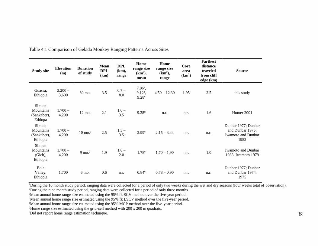
69

Table 4.1 Comparison of Gelada Monkey Ranging Patterns Across Sites

Study site Elevation

(m)

Duration

of study

Mean

DPL

(km)

DPL

(km),

range

Home

range size

(km2),

mean

Home

range size

(km2),

range

Core

area

(km2)

Farthest

distance

traveled

from cliff

edge (km)

Source

Guassa,

Ethiopia

3,200 –

3,600 60 mo. 3.5

0.7 –

8.0

7.06a,

9.12b,

9.28c

4.50 – 12.30 1.95 2.5 this study

Simien

Mountains

(Sankaber),

Ethiopa

1,700 –

4,200 12 mo. 2.1

1.0 –

3.5 9.28d n.r. n.r. 1.6 Hunter 2001

Simien

Mountains

(Sankaber),

Ethiopia

1,700 –

4,200 10 mo.1 2.5

1.5 –

3.5 2.99e 2.15 – 3.44 n.r. n.r.

Dunbar 1977; Dunbar

and Dunbar 1975;

Iwamoto and Dunbar

1983

Simien

Mountains

(Gich),

Ethiopia

1,700 –

4,200 9 mo.2 1.9

1.8 –

2.0 1.78e 1.70 – 1.90 n.r. 1.0

Iwamoto and Dunbar

1983, Iwamoto 1979

Bole

Valley,

Ethiopia

1,700 6 mo. 0.6 n.r. 0.84e 0.78 – 0.90 n.r. n.r.

Dunbar 1977; Dunbar

and Dunbar 1974,

1975

1During the 10 month study period, ranging data were collected for a period of only two weeks during the wet and dry seasons (four weeks total of observation). 2During the nine month study period, ranging data were collected for a period of only three months. aMean annual home range size estimated using the 95% fk SCV method over the five-year period. bMean annual home range size estimated using the 95% fk LSCV method over the five-year period. cMean annual home range size estimated using the 95% MCP method over the five-year period. dHome range size estimated using the grid-cell method with 200 x 200 m quadrats. eDid not report home range estimation technique.

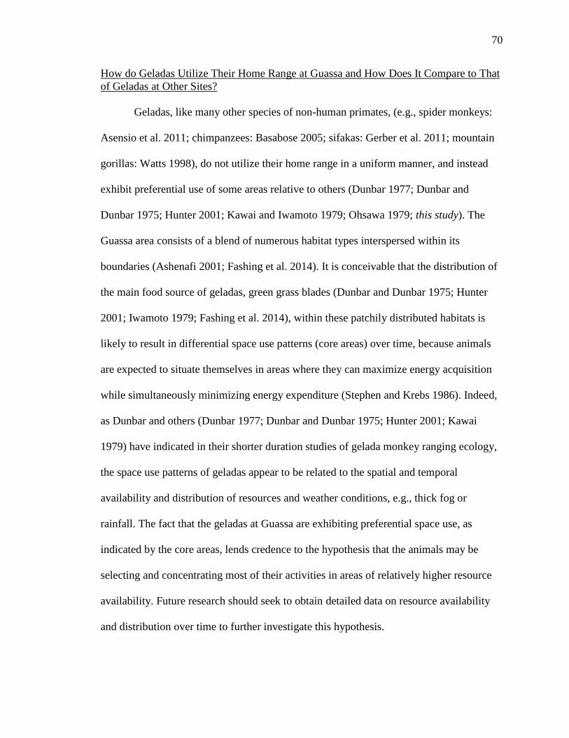
70

How do Geladas Utilize Their Home Range at Guassa and How Does It Compare to That

of Geladas at Other Sites?

Geladas, like many other species of non-human primates, (e.g., spider monkeys:

Asensio et al. 2011; chimpanzees: Basabose 2005; sifakas: Gerber et al. 2011; mountain

gorillas: Watts 1998), do not utilize their home range in a uniform manner, and instead

exhibit preferential use of some areas relative to others (Dunbar 1977; Dunbar and

Dunbar 1975; Hunter 2001; Kawai and Iwamoto 1979; Ohsawa 1979; this study). The

Guassa area consists of a blend of numerous habitat types interspersed within its

boundaries (Ashenafi 2001; Fashing et al. 2014). It is conceivable that the distribution of

the main food source of geladas, green grass blades (Dunbar and Dunbar 1975; Hunter

2001; Iwamoto 1979; Fashing et al. 2014), within these patchily distributed habitats is

likely to result in differential space use patterns (core areas) over time, because animals

are expected to situate themselves in areas where they can maximize energy acquisition

while simultaneously minimizing energy expenditure (Stephen and Krebs 1986). Indeed,

as Dunbar and others (Dunbar 1977; Dunbar and Dunbar 1975; Hunter 2001; Kawai

1979) have indicated in their shorter duration studies of gelada monkey ranging ecology,

the space use patterns of geladas appear to be related to the spatial and temporal

availability and distribution of resources and weather conditions, e.g., thick fog or

rainfall. The fact that the geladas at Guassa are exhibiting preferential space use, as

indicated by the core areas, lends credence to the hypothesis that the animals may be

selecting and concentrating most of their activities in areas of relatively higher resource

availability. Future research should seek to obtain detailed data on resource availability

and distribution over time to further investigate this hypothesis.

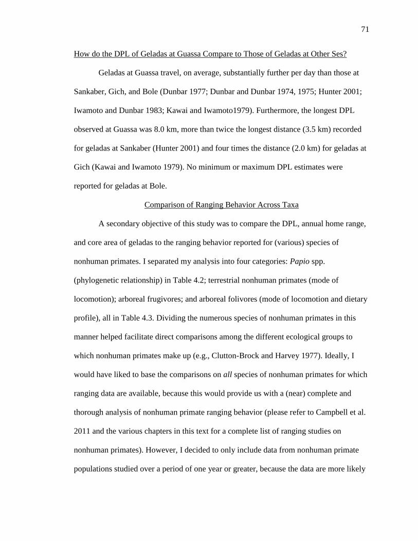
71

How do the DPL of Geladas at Guassa Compare to Those of Geladas at Other Ses?

Geladas at Guassa travel, on average, substantially further per day than those at

Sankaber, Gich, and Bole (Dunbar 1977; Dunbar and Dunbar 1974, 1975; Hunter 2001;

Iwamoto and Dunbar 1983; Kawai and Iwamoto1979). Furthermore, the longest DPL

observed at Guassa was 8.0 km, more than twice the longest distance (3.5 km) recorded

for geladas at Sankaber (Hunter 2001) and four times the distance (2.0 km) for geladas at

Gich (Kawai and Iwamoto 1979). No minimum or maximum DPL estimates were

reported for geladas at Bole.

Comparison of Ranging Behavior Across Taxa

A secondary objective of this study was to compare the DPL, annual home range,

and core area of geladas to the ranging behavior reported for (various) species of

nonhuman primates. I separated my analysis into four categories: Papio spp.

(phylogenetic relationship) in Table 4.2; terrestrial nonhuman primates (mode of

locomotion); arboreal frugivores; and arboreal folivores (mode of locomotion and dietary

profile), all in Table 4.3. Dividing the numerous species of nonhuman primates in this

manner helped facilitate direct comparisons among the different ecological groups to

which nonhuman primates make up (e.g., Clutton-Brock and Harvey 1977). Ideally, I

would have liked to base the comparisons on all species of nonhuman primates for which

ranging data are available, because this would provide us with a (near) complete and

thorough analysis of nonhuman primate ranging behavior (please refer to Campbell et al.

2011 and the various chapters in this text for a complete list of ranging studies on

nonhuman primates). However, I decided to only include data from nonhuman primate

populations studied over a period of one year or greater, because the data are more likely

72

to depict the animals’ ranging patterns over the course of (at least) an entire annual cycle

(which also corresponds with the data presented in our study). Lastly, as I have discussed

above, making comparisons across species is problematic due to the differential use of

methods to estimate home range in each study. Therefore, I focus my attention only on

the value(s) reported and do not make any assumptions beyond that.

Comparison of Gelada Ranging Behavior to Papio Species

Baboons (Papio spp.), travel, on average, further per day and occupy home ranges

larger in size than geladas (see Table 4.2). If I compare the ranging behavior of gelada

monkeys to individual species of Papio, however, different relationships emerge.

Geladas, particularly the Guassa geladas (mean DPL = 3.5 km), exhibit a mean

DPL comparable to, though slightly shorter than chacma baboons (P. cyncephalus

ursinus) studied at the Drakensberg Mountains, Natal Province, South Africa (4.1 km:

Henzi et al. 1992; Whiten et al. 1987) and at the Suikerbosrand Nature Reserve,

Transvaal, South Africa (4.1 km: Anderson 1981, 1982). No study populations of

geladas, however, travel as far per day as those chacma baboons at Tshipise, Transvaal,

South Africa (8.5 km: Stoltz and Saayman 1970). Despite their fairly similar DPLs, home

range size in chacma baboons (17.2 – 24.6 km2) are several times larger than those

reported for geladas (0.84 – 12.3 km2).

The mean DPL reported for yellow (P. cynacephalus) (5.6 km: Barton et al.

1992), olive (P. anubis) (5.0 km: Bronikowski and Altmann 1996), and hamadyras (P.

hamadryas) (7.5 – 13.2 km) baboons are longer than those observed for all studied

groups of geladas. Similarly, home range sizes for olive (4.1 – 43.8 km2) and hamadyras

73

(28 – 30 km2) baboons are (considerably) larger than those reported for geladas in

general.

What can explain the observed differences and similarities in the ranging behavior

of geladas and Papio spp.? Research has indicated that variations in group (herd) size,

temperature, food availability and distribution, access to water, weather patterns, and

proximity or access to sleeping cliff sites have been suggested to influence both the

movement and space use patterns among Papio (Barton et al. 1992; Bronikowski and

Altmann 1996; Henzi et al. 1992; Kunz and Lisenmair 2008; Stoltz and Saayman 1970;

Schreier 2010; Smuts 1985; Swedell 2006, 2011; Whiten et al. 1987) and geladas

(Dunbar and Dunbar 1975; Hunter 2001; Kawai 1979). Here, I elaborate on two of these

factors and their effects on ranging behavior in baboons and geladas: access to sleeping

sites and waterholes.

Whiten et al. (1987) have postulated that access to multiple sleeping cliff sites and

the differential use of sleeping cliff sites on a nightly basis may explain the shorter day

ranges observed in their population of chacma baboons at the Drakensberg Mountains,

Natal Province, South Africa, than compared to other species of baboons (e.g.,

hamadryas and olive baboons: Kunz and Lisenmair 2008; Sigg and Stolba 1981; Smuts

1985; Swedell 2006). Having access to multiple (and suitable) sleeping sites reduces the

amount of travel an animal has to invest in when searching for a place to sleep (Whiten et

al. 1987). Like chacma baboons, geladas have access to multiple sleeping sites and also

tend to use different sleeping sites on a nightly basis, though repeated use of a sleeping

cliff site on consecutive days has been observed many times in this band of geladas as

well (Moua unpubl. data). Conversely, hamadryas baboons regularly use the same

74

sleeping cliff site for numerous days on end (Sigg and Stolba 1981; Swedell 2006), and

coupled with the lack of potential sleeping cliff sites (at Filoha: Swedell 2006; and

Comoé National Park, Ivory Coast: Kunz and Linsenmair 2008), this may explain the

longer day ranges in these animals relative to chacma baboons and geladas.

In addition to the impact access to sleeping sites can have on the movement and

space use patterns, access to water has also been considered a factor in determining how

far baboons travel on a daily basis, which areas of their habitat are used, and the size of

the home range (Barton et al. 1992; Hamilton et al. 1976; Kunz and Linsenair 2008;

Smuts 1985; Stoltz and Saayman 1970; Swedell 2011). For example, chacma baboons

inhabiting the study site at Tshipise, Transvaal, South Africa, traveled long distances to

waterholes widely dispersed throughout their home range (Stoltz and Saayman 1970).

Furthermore, limited access to water can result in larger home ranges (olive baboons:

Kunz and Linsenmair 2008), because the animals would have to incorporate a home

range of relatively larger area to compensate for the lack of available waterholes. In

geladas, such as those at Gich (Kawai and Iwamoto 1979), the high availability of water

sources within the home range facilitates minimal movement to and from waterholes;

however, this implies that where access to water is (becomes) limited, it is conceivable

geladas, like baboons, are likely to increase movement or expand their home range in

search for additional sources of water. Future research should aim to obtain more

information about the geographic distribution of waterholes within the home range of the

geladas at Guassa, and record the behavior of the Guassa geladas in relation to drinking

water to better understand the relationship between access to water and movement and

space use patterns.

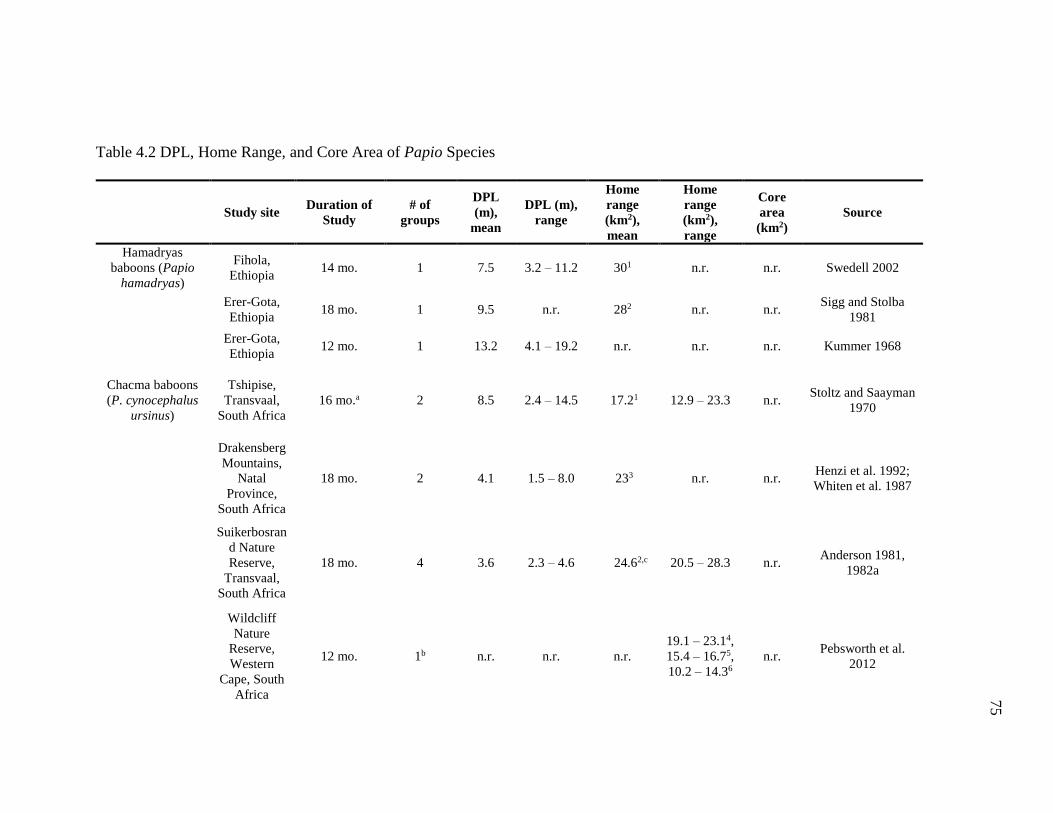
75

Table 4.2 DPL, Home Range, and Core Area of Papio Species

Study site Duration of

Study

# of

groups

DPL

(m),

mean

DPL (m),

range

Home

range

(km2),

mean

Home

range

(km2),

range

Core

area

(km2)

Source

Hamadryas

baboons (Papio

hamadryas)

Fihola,

Ethiopia 14 mo. 1 7.5 3.2 – 11.2 301 n.r. n.r. Swedell 2002

Erer-Gota,

Ethiopia 18 mo. 1 9.5 n.r. 282 n.r. n.r.

Sigg and Stolba

1981

Erer-Gota,

Ethiopia 12 mo. 1 13.2 4.1 – 19.2 n.r. n.r. n.r. Kummer 1968

Chacma baboons

(P. cynocephalus

ursinus)

Tshipise,

Transvaal,

South Africa

16 mo.a 2 8.5 2.4 – 14.5 17.21 12.9 – 23.3 n.r. Stoltz and Saayman

1970

Drakensberg

Mountains,

Natal

Province,

South Africa

18 mo. 2 4.1 1.5 – 8.0 233 n.r. n.r. Henzi et al. 1992;

Whiten et al. 1987

Suikerbosran

d Nature

Reserve,

Transvaal,

South Africa

18 mo. 4 3.6 2.3 – 4.6 24.62,c 20.5 – 28.3 n.r. Anderson 1981,

1982a

Wildcliff

Nature

Reserve,

Western

Cape, South

Africa

12 mo. 1b n.r. n.r. n.r.

19.1 – 23.14,

15.4 – 16.75,

10.2 – 14.36

n.r. Pebsworth et al.

2012

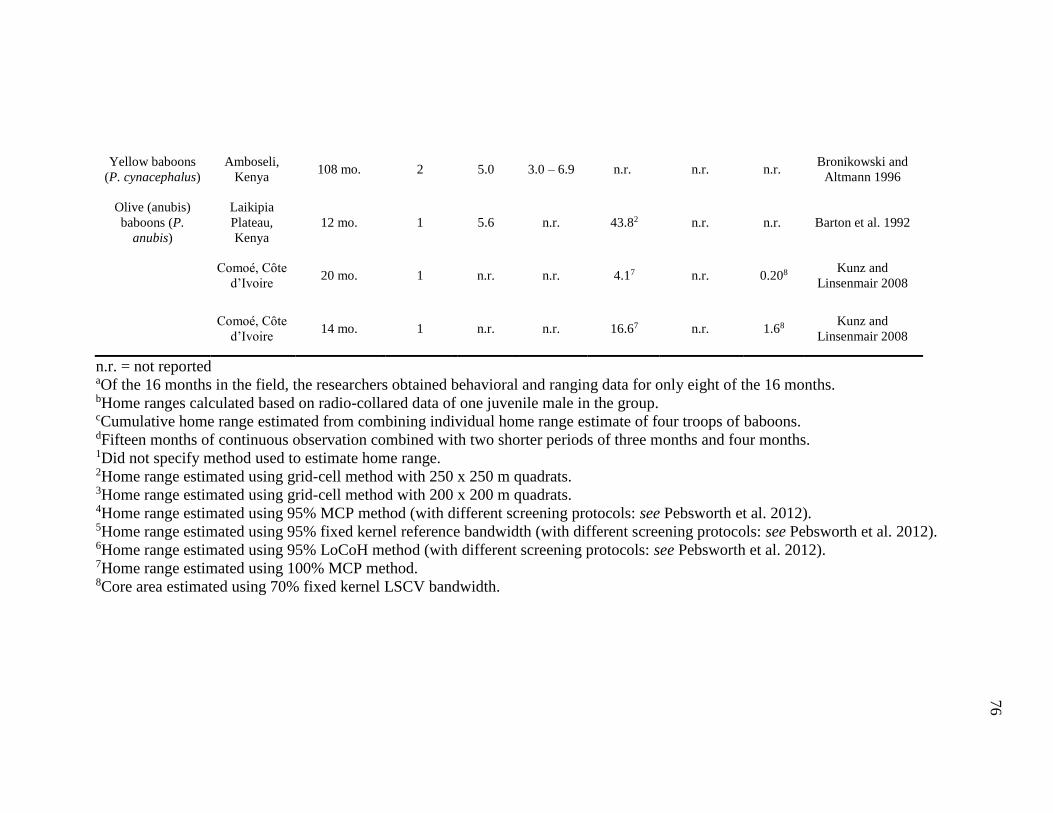
76

Yellow baboons

(P. cynacephalus)

Amboseli,

Kenya 108 mo. 2 5.0 3.0 – 6.9 n.r. n.r. n.r.

Bronikowski and

Altmann 1996

Olive (anubis)

baboons (P.

anubis)

Laikipia

Plateau,

Kenya

12 mo. 1 5.6 n.r. 43.82 n.r. n.r. Barton et al. 1992

Comoé, Cȏte

d’Ivoire 20 mo. 1 n.r. n.r. 4.17 n.r. 0.208 Kunz and

Linsenmair 2008

Comoé, Cȏte

d’Ivoire 14 mo. 1 n.r. n.r. 16.67 n.r. 1.68 Kunz and

Linsenmair 2008

n.r. = not reported aOf the 16 months in the field, the researchers obtained behavioral and ranging data for only eight of the 16 months. bHome ranges calculated based on radio-collared data of one juvenile male in the group. cCumulative home range estimated from combining individual home range estimate of four troops of baboons. dFifteen months of continuous observation combined with two shorter periods of three months and four months. 1Did not specify method used to estimate home range. 2Home range estimated using grid-cell method with 250 x 250 m quadrats. 3Home range estimated using grid-cell method with 200 x 200 m quadrats. 4Home range estimated using 95% MCP method (with different screening protocols: see Pebsworth et al. 2012). 5Home range estimated using 95% fixed kernel reference bandwidth (with different screening protocols: see Pebsworth et al. 2012). 6Home range estimated using 95% LoCoH method (with different screening protocols: see Pebsworth et al. 2012). 7Home range estimated using 100% MCP method. 8Core area estimated using 70% fixed kernel LSCV bandwidth.

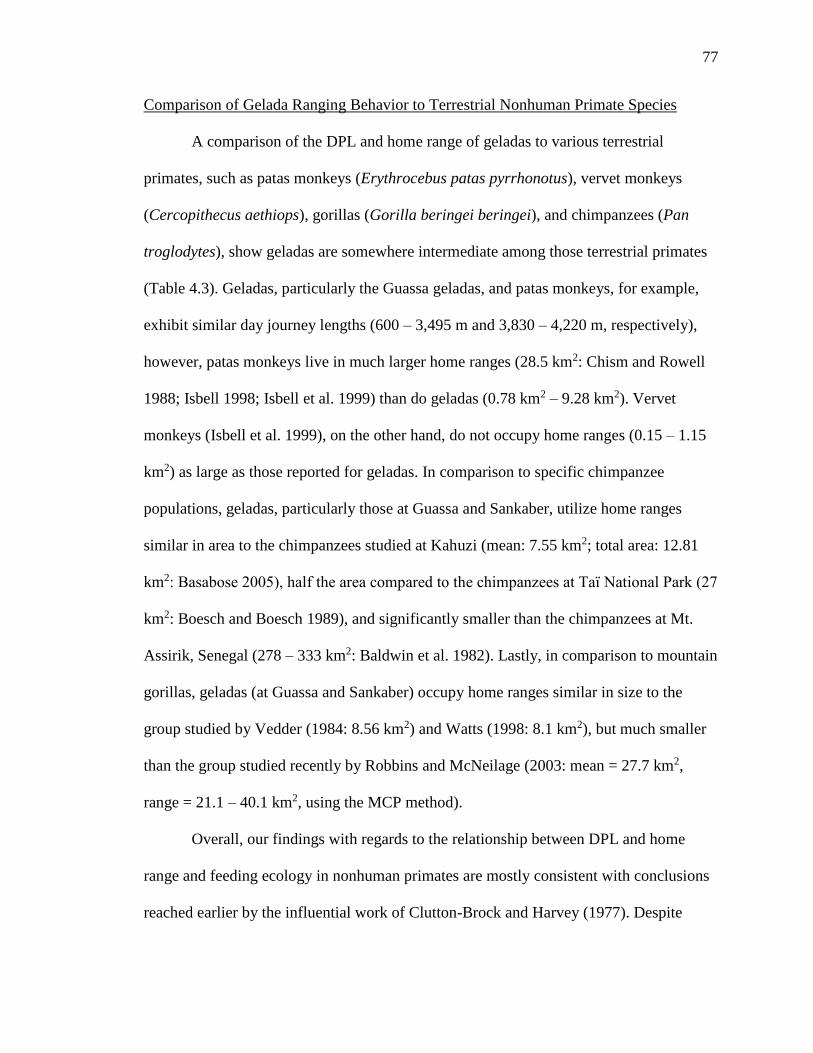
77

Comparison of Gelada Ranging Behavior to Terrestrial Nonhuman Primate Species

A comparison of the DPL and home range of geladas to various terrestrial

primates, such as patas monkeys (Erythrocebus patas pyrrhonotus), vervet monkeys

(Cercopithecus aethiops), gorillas (Gorilla beringei beringei), and chimpanzees (Pan

troglodytes), show geladas are somewhere intermediate among those terrestrial primates

(Table 4.3). Geladas, particularly the Guassa geladas, and patas monkeys, for example,

exhibit similar day journey lengths (600 – 3,495 m and 3,830 – 4,220 m, respectively),

however, patas monkeys live in much larger home ranges (28.5 km2: Chism and Rowell

1988; Isbell 1998; Isbell et al. 1999) than do geladas (0.78 km2 – 9.28 km2). Vervet

monkeys (Isbell et al. 1999), on the other hand, do not occupy home ranges (0.15 – 1.15

km2) as large as those reported for geladas. In comparison to specific chimpanzee

populations, geladas, particularly those at Guassa and Sankaber, utilize home ranges

similar in area to the chimpanzees studied at Kahuzi (mean: 7.55 km2; total area: 12.81

km2: Basabose 2005), half the area compared to the chimpanzees at Taї National Park (27

km2: Boesch and Boesch 1989), and significantly smaller than the chimpanzees at Mt.

Assirik, Senegal (278 – 333 km2: Baldwin et al. 1982). Lastly, in comparison to mountain

gorillas, geladas (at Guassa and Sankaber) occupy home ranges similar in size to the

group studied by Vedder (1984: 8.56 km2) and Watts (1998: 8.1 km2), but much smaller

than the group studied recently by Robbins and McNeilage (2003: mean = 27.7 km2,

range = 21.1 – 40.1 km2, using the MCP method).

Overall, our findings with regards to the relationship between DPL and home

range and feeding ecology in nonhuman primates are mostly consistent with conclusions

reached earlier by the influential work of Clutton-Brock and Harvey (1977). Despite

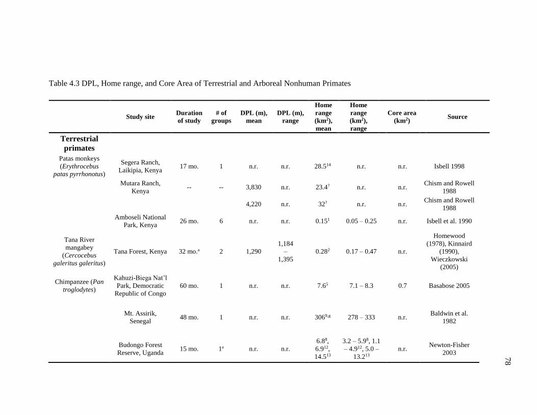
78

Table 4.3 DPL, Home range, and Core Area of Terrestrial and Arboreal Nonhuman Primates

Study site Duration

of study

# of

groups

DPL (m),

mean

DPL (m),

range

Home

range

(km2),

mean

Home

range

(km2),

range

Core area

(km2) Source

Terrestrial

primates

Patas monkeys

(Erythrocebus

patas pyrrhonotus)

Segera Ranch,

Laikipia, Kenya 17 mo. 1 n.r. n.r. 28.514 n.r. n.r. Isbell 1998

Mutara Ranch,

Kenya -- -- 3,830 n.r. 23.4? n.r. n.r.

Chism and Rowell

1988

4,220 n.r. 32? n.r. n.r. Chism and Rowell

1988

Amboseli National

Park, Kenya 26 mo. 6 n.r. n.r. 0.151 0.05 – 0.25 n.r. Isbell et al. 1990

Tana River

mangabey

(Cercocebus

galeritus galeritus)

Tana Forest, Kenya 32 mo.a 2 1,290

1,184

–

1,395

0.282 0.17 – 0.47 n.r.

Homewood

(1978), Kinnaird

(1990),

Wieczkowski

(2005)

Chimpanzee (Pan

troglodytes)

Kahuzi-Biega Nat’l

Park, Democratic

Republic of Congo

60 mo. 1 n.r. n.r. 7.65 7.1 – 8.3 0.7 Basabose 2005

Mt. Assirik,

Senegal 48 mo. 1 n.r. n.r. 3069,g 278 – 333 n.r.

Baldwin et al.

1982

Budongo Forest

Reserve, Uganda 15 mo. 1e n.r. n.r.

6.88,

6.912,

14.513

3.2 – 5.98, 1.1

– 4.912, 5.0 –

13.213

n.r. Newton-Fisher

2003

79

Mountain gorilla

(Gorilla beringei

beringei)

Bwindi

Impenetrable

National Park,

Uganda

36 mo. 1 n.r. n.r. 206, 289 16.3 – 286,

21.1 – 40.19 9.5b-c Robbins and

McNeilage 2003

Bwindi

Impenetrable

National Park,

Rwanda

84 mo. 3 – 5 n.r. n.r. 8.15 3.1 – 15.6 2.9 Watts 1998

Bwindi

Impenetrable

National Park,

Rwanda

18 mo. 1 n.r. n.r. 8.565 n.r. n.r. Vedder 1984

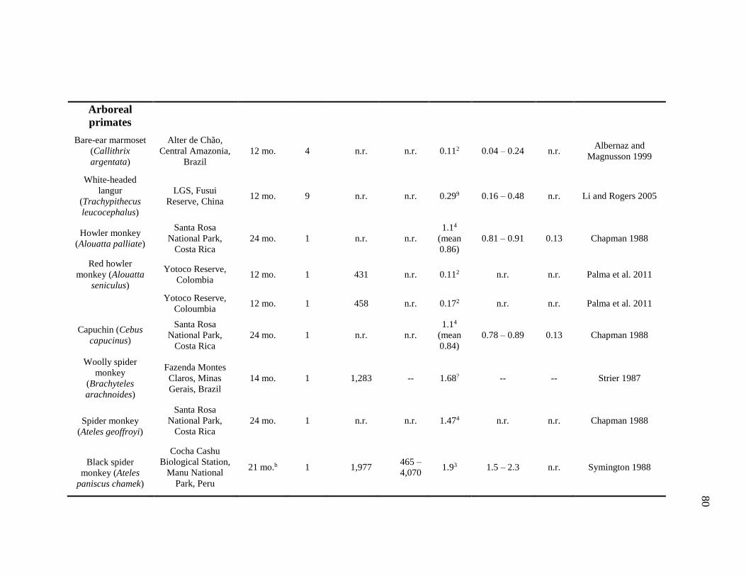
80

Arboreal

primates

Bare-ear marmoset

(Callithrix

argentata)

Alter de Chão,

Central Amazonia,

Brazil

12 mo. 4 n.r. n.r. 0.112 0.04 – 0.24 n.r. Albernaz and

Magnusson 1999

White-headed

langur

(Trachypithecus

leucocephalus)

LGS, Fusui

Reserve, China 12 mo. 9 n.r. n.r. 0.299 0.16 – 0.48 n.r. Li and Rogers 2005

Howler monkey

(Alouatta palliate)

Santa Rosa

National Park,

Costa Rica

24 mo. 1 n.r. n.r.

1.14

(mean

0.86)

0.81 – 0.91 0.13 Chapman 1988

Red howler

monkey (Alouatta

seniculus)

Yotoco Reserve,

Colombia 12 mo. 1 431 n.r. 0.112 n.r. n.r. Palma et al. 2011

Yotoco Reserve,

Coloumbia 12 mo. 1 458 n.r. 0.172 n.r. n.r. Palma et al. 2011

Capuchin (Cebus

capucinus)

Santa Rosa

National Park,

Costa Rica

24 mo. 1 n.r. n.r.

1.14

(mean

0.84)

0.78 – 0.89 0.13 Chapman 1988

Woolly spider

monkey

(Brachyteles

arachnoides)

Fazenda Montes

Claros, Minas

Gerais, Brazil

14 mo. 1 1,283 -- 1.68? -- -- Strier 1987

Spider monkey

(Ateles geoffroyi)

Santa Rosa

National Park,

Costa Rica

24 mo. 1 n.r. n.r. 1.474 n.r. n.r. Chapman 1988

Black spider

monkey (Ateles

paniscus chamek)

Cocha Cashu

Biological Station,

Manu National

Park, Peru

21 mo.b 1 1,977 465 –

4,070 1.93 1.5 – 2.3 n.r. Symington 1988

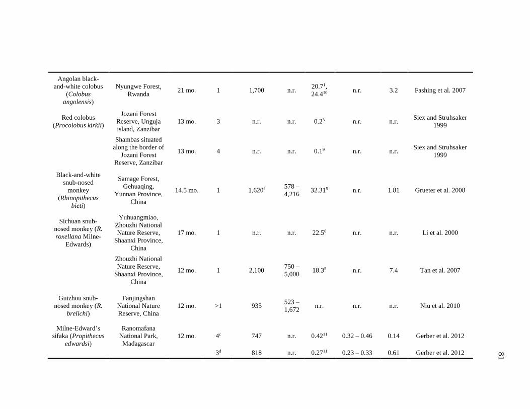
81

Angolan black-

and-white colobus

(Colobus

angolensis)

Nyungwe Forest,

Rwanda 21 mo. 1 1,700 n.r.

20.71,

24.410 n.r. 3.2 Fashing et al. 2007

Red colobus

(Procolobus kirkii)

Jozani Forest

Reserve, Unguja

island, Zanzibar

13 mo. 3 n.r. n.r. 0.23 n.r. n.r. Siex and Struhsaker

1999

Shambas situated

along the border of

Jozani Forest

Reserve, Zanzibar

13 mo. 4 n.r. n.r. 0.19 n.r. n.r. Siex and Struhsaker

1999

Black-and-white

snub-nosed

monkey

(Rhinopithecus

bieti)

Samage Forest,

Gehuaqing,

Yunnan Province,

China

14.5 mo. 1 1,620f 578 –

4,216 32.315 n.r. 1.81 Grueter et al. 2008

Sichuan snub-

nosed monkey (R.

roxellana Milne-

Edwards)

Yuhuangmiao,

Zhouzhi National

Nature Reserve,

Shaanxi Province,

China

17 mo. 1 n.r. n.r. 22.56 n.r. n.r. Li et al. 2000

Zhouzhi National

Nature Reserve,

Shaanxi Province,

China

12 mo. 1 2,100 750 –

5,000 18.35 n.r. 7.4 Tan et al. 2007

Guizhou snub-

nosed monkey (R.

brelichi)

Fanjingshan

National Nature

Reserve, China

12 mo. >1 935 523 –

1,672 n.r. n.r. n.r. Niu et al. 2010

Milne-Edward’s

sifaka (Propithecus

edwardsi)

Ranomafana

National Park,

Madagascar

12 mo. 4c 747 n.r. 0.4211 0.32 – 0.46 0.14 Gerber et al. 2012

3d 818 n.r. 0.2711 0.23 – 0.33 0.61 Gerber et al. 2012

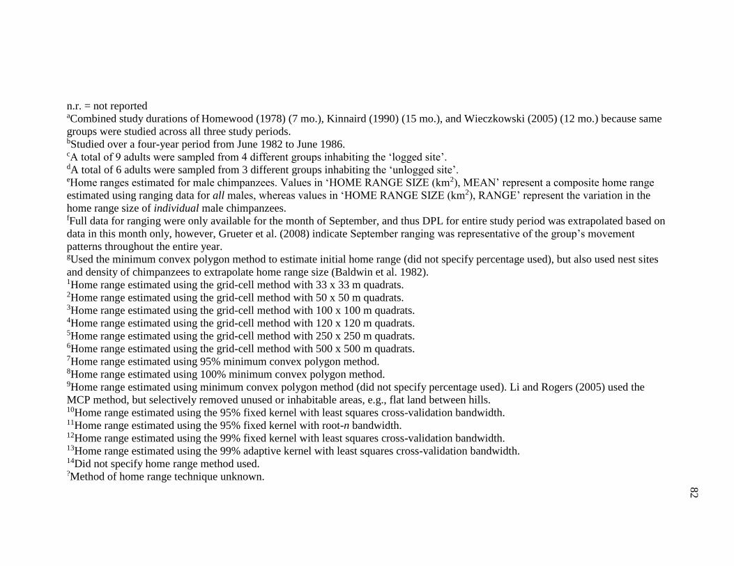
82

n.r. = not reported aCombined study durations of Homewood (1978) (7 mo.), Kinnaird (1990) (15 mo.), and Wieczkowski (2005) (12 mo.) because same

groups were studied across all three study periods. bStudied over a four-year period from June 1982 to June 1986. cA total of 9 adults were sampled from 4 different groups inhabiting the ‘logged site’. dA total of 6 adults were sampled from 3 different groups inhabiting the ‘unlogged site’. eHome ranges estimated for male chimpanzees. Values in ‘HOME RANGE SIZE (km2), MEAN’ represent a composite home range

estimated using ranging data for all males, whereas values in ‘HOME RANGE SIZE (km2), RANGE’ represent the variation in the

home range size of individual male chimpanzees. fFull data for ranging were only available for the month of September, and thus DPL for entire study period was extrapolated based on

data in this month only, however, Grueter et al. (2008) indicate September ranging was representative of the group’s movement

patterns throughout the entire year. gUsed the minimum convex polygon method to estimate initial home range (did not specify percentage used), but also used nest sites

and density of chimpanzees to extrapolate home range size (Baldwin et al. 1982). 1Home range estimated using the grid-cell method with 33 x 33 m quadrats. 2Home range estimated using the grid-cell method with 50 x 50 m quadrats. 3Home range estimated using the grid-cell method with 100 x 100 m quadrats. 4Home range estimated using the grid-cell method with 120 x 120 m quadrats. 5Home range estimated using the grid-cell method with 250 x 250 m quadrats. 6Home range estimated using the grid-cell method with 500 x 500 m quadrats. 7Home range estimated using 95% minimum convex polygon method. 8Home range estimated using 100% minimum convex polygon method. 9Home range estimated using minimum convex polygon method (did not specify percentage used). Li and Rogers (2005) used the

MCP method, but selectively removed unused or inhabitable areas, e.g., flat land between hills. 10Home range estimated using the 95% fixed kernel with least squares cross-validation bandwidth. 11Home range estimated using the 95% fixed kernel with root-n bandwidth. 12Home range estimated using the 99% fixed kernel with least squares cross-validation bandwidth. 13Home range estimated using the 99% adaptive kernel with least squares cross-validation bandwidth. 14Did not specify home range method used. ?Method of home range technique unknown.

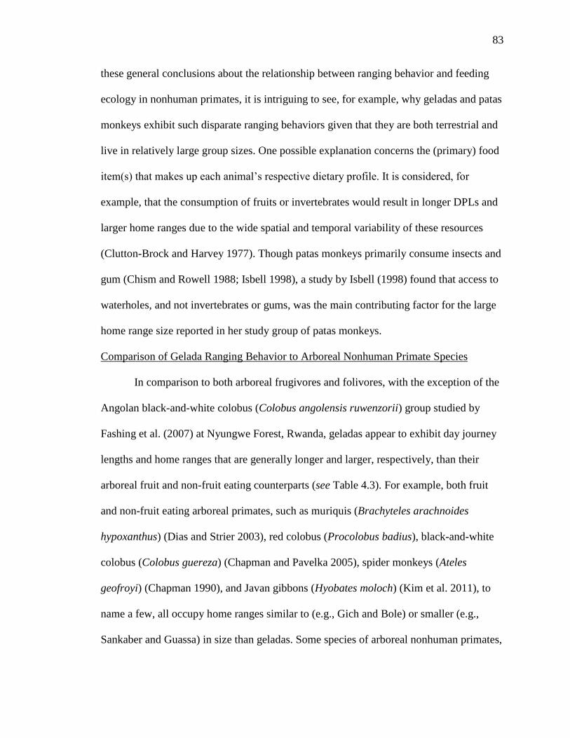
83

these general conclusions about the relationship between ranging behavior and feeding

ecology in nonhuman primates, it is intriguing to see, for example, why geladas and patas

monkeys exhibit such disparate ranging behaviors given that they are both terrestrial and

live in relatively large group sizes. One possible explanation concerns the (primary) food

item(s) that makes up each animal’s respective dietary profile. It is considered, for

example, that the consumption of fruits or invertebrates would result in longer DPLs and

larger home ranges due to the wide spatial and temporal variability of these resources

(Clutton-Brock and Harvey 1977). Though patas monkeys primarily consume insects and

gum (Chism and Rowell 1988; Isbell 1998), a study by Isbell (1998) found that access to

waterholes, and not invertebrates or gums, was the main contributing factor for the large

home range size reported in her study group of patas monkeys.

Comparison of Gelada Ranging Behavior to Arboreal Nonhuman Primate Species

In comparison to both arboreal frugivores and folivores, with the exception of the

Angolan black-and-white colobus (Colobus angolensis ruwenzorii) group studied by

Fashing et al. (2007) at Nyungwe Forest, Rwanda, geladas appear to exhibit day journey

lengths and home ranges that are generally longer and larger, respectively, than their

arboreal fruit and non-fruit eating counterparts (see Table 4.3). For example, both fruit

and non-fruit eating arboreal primates, such as muriquis (Brachyteles arachnoides

hypoxanthus) (Dias and Strier 2003), red colobus (Procolobus badius), black-and-white

colobus (Colobus guereza) (Chapman and Pavelka 2005), spider monkeys (Ateles

geofroyi) (Chapman 1990), and Javan gibbons (Hyobates moloch) (Kim et al. 2011), to

name a few, all occupy home ranges similar to (e.g., Gich and Bole) or smaller (e.g.,

Sankaber and Guassa) in size than geladas. Some species of arboreal nonhuman primates,

84

however, do appear to exhibit mean DPLs similar to or longer than the populations of

geladas at Gich, Bole, and Sankaber, but not those at Guassa: black spider monkey

(Ateles geoffroyi, 1,977 m: Chapman 1988; Angolan black-and-white colobus (Colobus

angolensis, 1,700 m: Fashing et al. 2007); black-and-white snub-nosed monkey

(Rhinopithecus bieti, 1,620 m: Grueter et al. 2008; and the Sichuan snub-nosed monkeys

(R. roxellana Milne-Edwards, 2,100 m: Tan et al. 2007).

Furthermore, as mentioned above, in their investigation of the ranging behavior of

Angolan black-and-white colobus (Colobus angolensis ruwenzorii) at Nyungwe, Fashing

et al. (2007) found these monkeys occupied a home range size of 20.7 to 24.4 km2

(estimated using the 95% fixed kernel with LSCV and MCP methods, respectively),

considerably larger than the home range reported for any other species of colobus

(Fashing et al. 2007) and numerous species of nonhuman primates reported here,

including geladas (see Tables 4.1-4.3). Despite being primarily leaf consumers and living

in a habitat shown to have high resource availability, the authors suggest that the

monkeys’ uncharacteristically large group size (> 300 individuals) may be creating a

situation in which even the abundant supply of resources is insufficient to support a group

size of that magnitude (Fashing et al. 2007). Therefore, to compensate for such a large

group size, the study group invested more time in moving and feeding at the expense of

resting time, while simultaneously increasing their DPL and home range (Fashing et al.

2007). Dunbar and Dunbar (1975) and Iwamoto and Dunbar (1983) have indicated gelada

monkeys travel further when there are more animals present in the herd. A similar

argument has been made for various species of nonhuman primates (Barton et al. 1992;

85

Chapman and Pavelka 2005; Schreier 2010). Future research should investigate the

relationship between herd size and DPL and home range in this band of gelada monkeys.

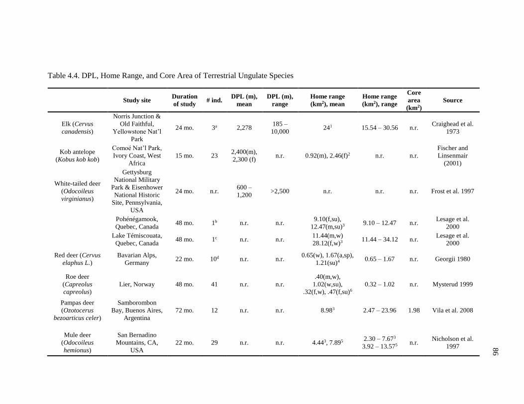
86

Table 4.4. DPL, Home Range, and Core Area of Terrestrial Ungulate Species

Study site Duration

of study # ind.

DPL (m),

mean

DPL (m),

range

Home range

(km2), mean

Home range

(km2), range

Core

area

(km2)

Source

Elk (Cervus

canadensis)

Norris Junction &

Old Faithful,

Yellowstone Nat’l

Park

24 mo. 3a 2,278 185 –

10,000 241 15.54 – 30.56 n.r.

Craighead et al.

1973

Kob antelope

(Kobus kob kob)

Comoé Nat’l Park,

Ivory Coast, West

Africa

15 mo. 23 2,400(m),

2,300 (f) n.r. 0.92(m), 2.46(f)2 n.r. n.r.

Fischer and

Linsenmair

(2001)

White-tailed deer

(Odocoileus

virginianus)

Gettysburg

National Military

Park & Eisenhower

National Historic

Site, Pennsylvania,

USA

24 mo. n.r. 600 –

1,200 >2,500 n.r. n.r. n.r. Frost et al. 1997

Pohénégamook,

Quebec, Canada 48 mo. 1b n.r. n.r.

9.10(f,su),

12.47(m,su)3 9.10 – 12.47 n.r. Lesage et al.

2000

Lake Témiscouata,

Quebec, Canada 48 mo. 1c n.r. n.r.

11.44(m,w)

28.12(f,w)3 11.44 – 34.12 n.r. Lesage et al.

2000

Red deer (Cervus

elaphus L.)

Bavarian Alps,

Germany 22 mo. 10d n.r. n.r.

0.65(w), 1.67(a,sp),

1.21(su)4 0.65 – 1.67 n.r. Georgii 1980

Roe deer

(Capreolus

capreolus)

Lier, Norway 48 mo. 41 n.r. n.r.

.40(m,w),

1.02(w,su),

.32(f,w), .47(f,su)6

0.32 – 1.02 n.r. Mysterud 1999

Pampas deer

(Ozotocerus

bezoarticus celer)

Samborombon

Bay, Buenos Aires,

Argentina

72 mo. 12 n.r. n.r. 8.983 2.47 – 23.96 1.98 Vila et al. 2008

Mule deer

(Odocoileus

hemionus)

San Bernadino

Mountains, CA,

USA

22 mo. 29 n.r. n.r. 4.443, 7.895 2.30 – 7.673

3.92 – 13.575 n.r.

Nicholson et al.

1997

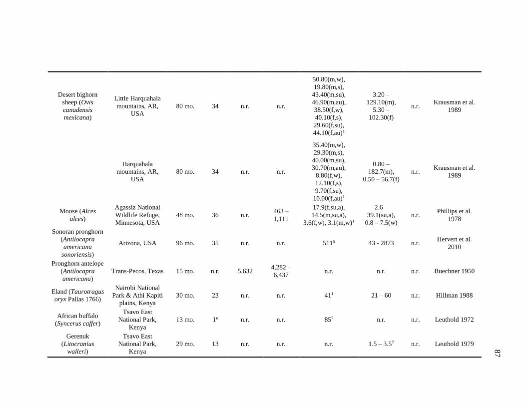
87

Desert bighorn

sheep (Ovis

canadensis

mexicana)

Little Harquahala

mountains, AR,

USA

80 mo. 34 n.r. n.r.

50.80(m,w),

19.80(m,s),

43.40(m,su),

46.90(m,au),

38.50(f,w),

40.10(f,s),

29.60(f,su),

44.10(f,au)1

3.20 –

129.10(m),

5.30 –

102.30(f)

n.r. Krausman et al.

1989

Harquahala

mountains, AR,

USA

80 mo. 34 n.r. n.r.

35.40(m,w),

29.30(m,s),

40.00(m,su),

30.70(m,au),

8.80(f,w),

12.10(f,s),

9.70(f,su),

10.00(f,au)1

0.80 –

182.7(m),

0.50 – 56.7(f)

n.r. Krausman et al.

1989

Moose (Alces

alces)

Agassiz National

Wildlife Refuge,

Minnesota, USA

48 mo. 36 n.r. 463 –

1,111

17.9(f,su,a),

14.5(m,su,a),

3.6(f,w), 3.1(m,w)1

2.6 –

39.1(su,a),

0.8 – 7.5(w)

n.r. Phillips et al.

1978

Sonoran pronghorn

(Antilocapra

americana

sonoriensis)

Arizona, USA 96 mo. 35 n.r. n.r. 5115 43 - 2873 n.r. Hervert et al.

2010

Pronghorn antelope

(Antilocapra

americana)

Trans-Pecos, Texas 15 mo. n.r. 5,632 4,282 –

6,437 n.r. n.r. n.r. Buechner 1950

Eland (Taurotragus

oryx Pallas 1766)

Nairobi National

Park & Athi Kapiti

plains, Kenya

30 mo. 23 n.r. n.r. 411 21 – 60 n.r. Hillman 1988

African buffalo

(Syncerus caffer)

Tsavo East

National Park,

Kenya

13 mo. 1e n.r. n.r. 857 n.r. n.r. Leuthold 1972

Gerenuk

(Litocranius

walleri)

Tsavo East

National Park,

Kenya

29 mo. 13 n.r. n.r. n.r. 1.5 – 3.57 n.r. Leuthold 1979

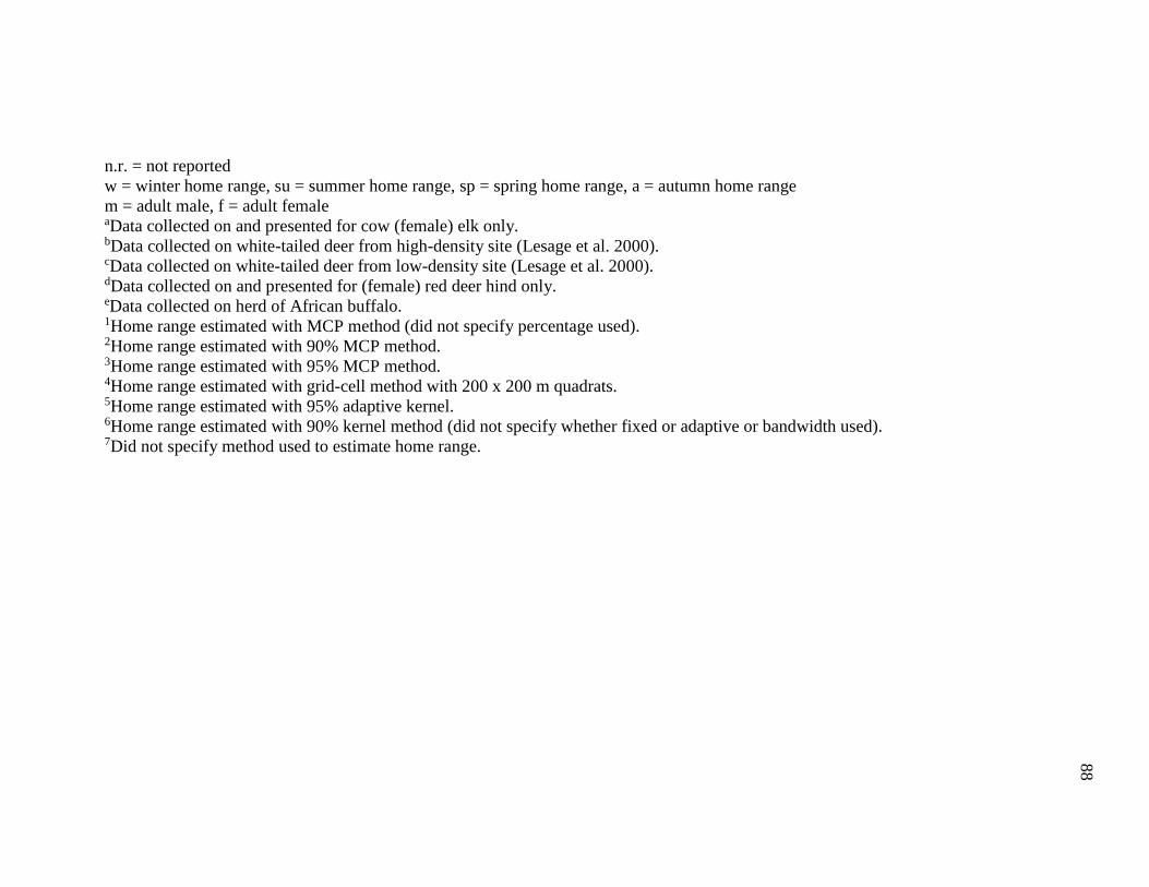
88

n.r. = not reported

w = winter home range, su = summer home range, sp = spring home range, a = autumn home range

m = adult male, f = adult female aData collected on and presented for cow (female) elk only. bData collected on white-tailed deer from high-density site (Lesage et al. 2000). cData collected on white-tailed deer from low-density site (Lesage et al. 2000). dData collected on and presented for (female) red deer hind only. eData collected on herd of African buffalo. 1Home range estimated with MCP method (did not specify percentage used). 2Home range estimated with 90% MCP method. 3Home range estimated with 95% MCP method. 4Home range estimated with grid-cell method with 200 x 200 m quadrats. 5Home range estimated with 95% adaptive kernel. 6Home range estimated with 90% kernel method (did not specify whether fixed or adaptive or bandwidth used). 7Did not specify method used to estimate home range.

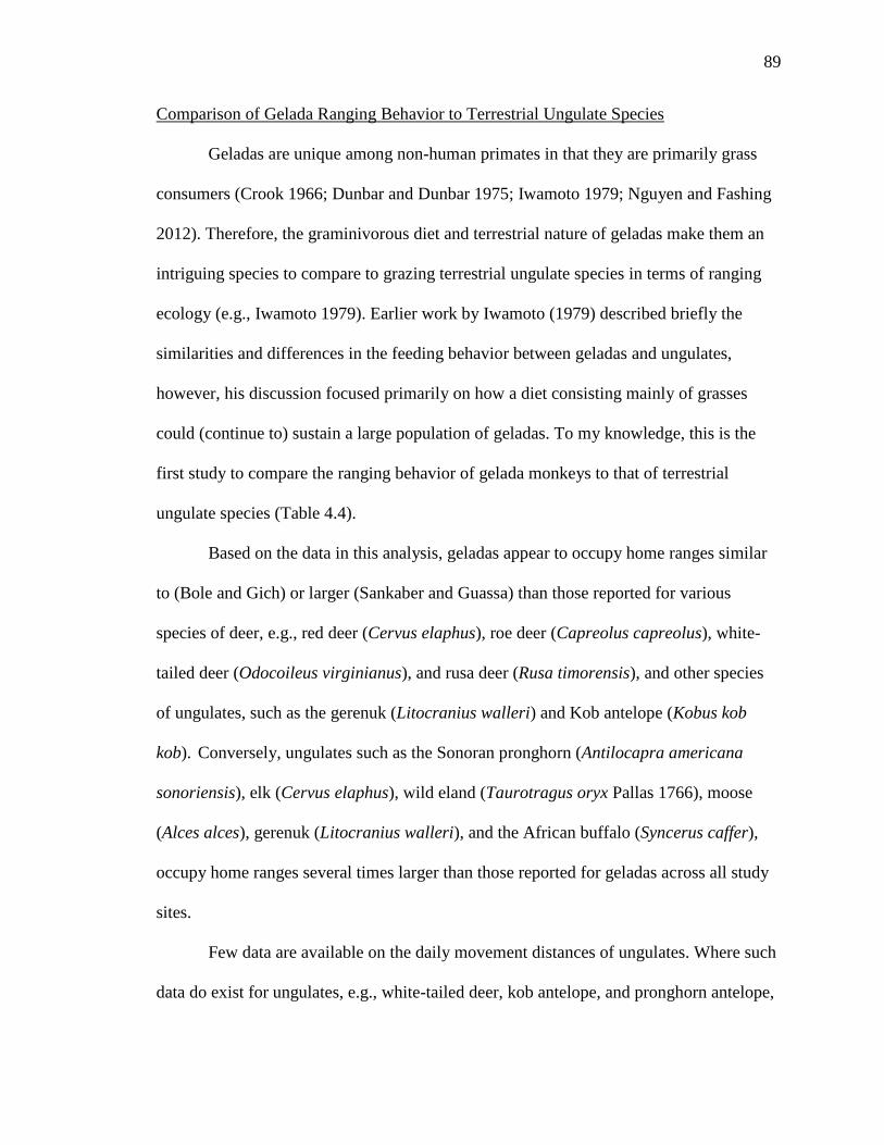
89

Comparison of Gelada Ranging Behavior to Terrestrial Ungulate Species

Geladas are unique among non-human primates in that they are primarily grass

consumers (Crook 1966; Dunbar and Dunbar 1975; Iwamoto 1979; Nguyen and Fashing

2012). Therefore, the graminivorous diet and terrestrial nature of geladas make them an

intriguing species to compare to grazing terrestrial ungulate species in terms of ranging

ecology (e.g., Iwamoto 1979). Earlier work by Iwamoto (1979) described briefly the

similarities and differences in the feeding behavior between geladas and ungulates,

however, his discussion focused primarily on how a diet consisting mainly of grasses

could (continue to) sustain a large population of geladas. To my knowledge, this is the

first study to compare the ranging behavior of gelada monkeys to that of terrestrial

ungulate species (Table 4.4).

Based on the data in this analysis, geladas appear to occupy home ranges similar

to (Bole and Gich) or larger (Sankaber and Guassa) than those reported for various

species of deer, e.g., red deer (Cervus elaphus), roe deer (Capreolus capreolus), white-

tailed deer (Odocoileus virginianus), and rusa deer (Rusa timorensis), and other species

of ungulates, such as the gerenuk (Litocranius walleri) and Kob antelope (Kobus kob

kob). Conversely, ungulates such as the Sonoran pronghorn (Antilocapra americana

sonoriensis), elk (Cervus elaphus), wild eland (Taurotragus oryx Pallas 1766), moose

(Alces alces), gerenuk (Litocranius walleri), and the African buffalo (Syncerus caffer),

occupy home ranges several times larger than those reported for geladas across all study

sites.

Few data are available on the daily movement distances of ungulates. Where such

data do exist for ungulates, e.g., white-tailed deer, kob antelope, and pronghorn antelope,

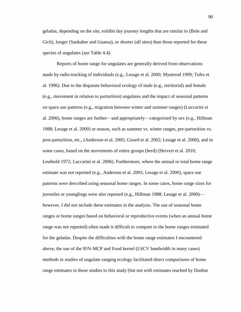
90

geladas, depending on the site, exhibit day journey lengths that are similar to (Bole and

Gich), longer (Sankaber and Guassa), or shorter (all sites) than those reported for these

species of ungulates (see Table 4.4).

Reports of home range for ungulates are generally derived from observations

made by radio-tracking of individuals (e.g., Lesage et al. 2000; Mysterud 1999; Tufto et

al. 1996). Due to the disparate behavioral ecology of male (e.g., territorial) and female

(e.g., movement in relation to parturition) ungulates and the impact of seasonal patterns

on space use patterns (e.g., migration between winter and summer ranges) (Luccarini et

al. 2006), home ranges are further—and appropriately—categorized by sex (e.g., Hillman

1988; Lesage et al. 2000) or season, such as summer vs. winter ranges, pre-parturition vs.

post-parturition, etc., (Anderson et al. 2005; Girard et al. 2002; Lesage et al. 2000), and in

some cases, based on the movements of entire groups (herd) (Hervert et al. 2010;

Leuthold 1972; Luccarini et al. 2006). Furthermore, where the annual or total home range

estimate was not reported (e.g., Anderson et al. 2005; Lesage et al. 2000), space use

patterns were described using seasonal home ranges. In some cases, home range sizes for

juveniles or younglings were also reported (e.g., Hillman 1988; Lesage et al. 2000)—

however, I did not include these estimates in the analysis. The use of seasonal home

ranges or home ranges based on behavioral or reproductive events (when an annual home

range was not reported) often made it difficult to compare to the home ranges estimated

for the geladas. Despite the difficulties with the home range estimates I encountered

above, the use of the 95% MCP and fixed kernel (LSCV bandwidth in many cases)

methods in studies of ungulate ranging ecology facilitated direct comparisons of home

range estimates in those studies to this study (but not with estimates reached by Dunbar

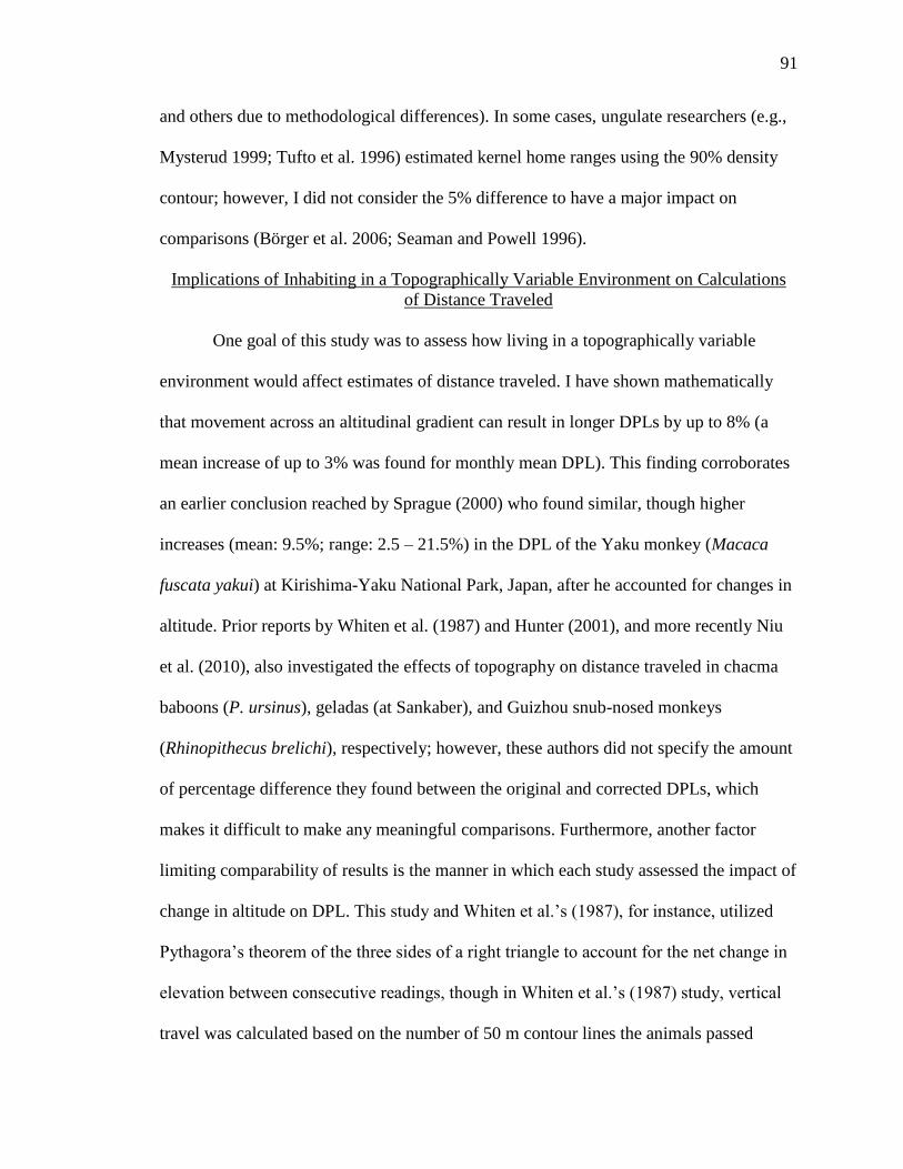
91

and others due to methodological differences). In some cases, ungulate researchers (e.g.,

Mysterud 1999; Tufto et al. 1996) estimated kernel home ranges using the 90% density

contour; however, I did not consider the 5% difference to have a major impact on

comparisons (Börger et al. 2006; Seaman and Powell 1996).

Implications of Inhabiting in a Topographically Variable Environment on Calculations

of Distance Traveled

One goal of this study was to assess how living in a topographically variable

environment would affect estimates of distance traveled. I have shown mathematically

that movement across an altitudinal gradient can result in longer DPLs by up to 8% (a

mean increase of up to 3% was found for monthly mean DPL). This finding corroborates

an earlier conclusion reached by Sprague (2000) who found similar, though higher

increases (mean: 9.5%; range: 2.5 – 21.5%) in the DPL of the Yaku monkey (Macaca

fuscata yakui) at Kirishima-Yaku National Park, Japan, after he accounted for changes in

altitude. Prior reports by Whiten et al. (1987) and Hunter (2001), and more recently Niu

et al. (2010), also investigated the effects of topography on distance traveled in chacma

baboons (P. ursinus), geladas (at Sankaber), and Guizhou snub-nosed monkeys

(Rhinopithecus brelichi), respectively; however, these authors did not specify the amount

of percentage difference they found between the original and corrected DPLs, which

makes it difficult to make any meaningful comparisons. Furthermore, another factor

limiting comparability of results is the manner in which each study assessed the impact of

change in altitude on DPL. This study and Whiten et al.’s (1987), for instance, utilized

Pythagora’s theorem of the three sides of a right triangle to account for the net change in

elevation between consecutive readings, though in Whiten et al.’s (1987) study, vertical

travel was calculated based on the number of 50 m contour lines the animals passed

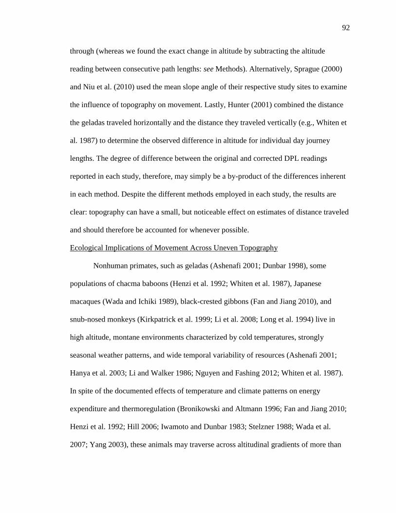
92

through (whereas we found the exact change in altitude by subtracting the altitude

reading between consecutive path lengths: see Methods). Alternatively, Sprague (2000)

and Niu et al. (2010) used the mean slope angle of their respective study sites to examine

the influence of topography on movement. Lastly, Hunter (2001) combined the distance

the geladas traveled horizontally and the distance they traveled vertically (e.g., Whiten et

al. 1987) to determine the observed difference in altitude for individual day journey

lengths. The degree of difference between the original and corrected DPL readings

reported in each study, therefore, may simply be a by-product of the differences inherent

in each method. Despite the different methods employed in each study, the results are

clear: topography can have a small, but noticeable effect on estimates of distance traveled

and should therefore be accounted for whenever possible.

Ecological Implications of Movement Across Uneven Topography

Nonhuman primates, such as geladas (Ashenafi 2001; Dunbar 1998), some

populations of chacma baboons (Henzi et al. 1992; Whiten et al. 1987), Japanese

macaques (Wada and Ichiki 1989), black-crested gibbons (Fan and Jiang 2010), and

snub-nosed monkeys (Kirkpatrick et al. 1999; Li et al. 2008; Long et al. 1994) live in

high altitude, montane environments characterized by cold temperatures, strongly

seasonal weather patterns, and wide temporal variability of resources (Ashenafi 2001;

Hanya et al. 2003; Li and Walker 1986; Nguyen and Fashing 2012; Whiten et al. 1987).

In spite of the documented effects of temperature and climate patterns on energy

expenditure and thermoregulation (Bronikowski and Altmann 1996; Fan and Jiang 2010;

Henzi et al. 1992; Hill 2006; Iwamoto and Dunbar 1983; Stelzner 1988; Wada et al.

2007; Yang 2003), these animals may traverse across altitudinal gradients of more than

93

30 m on a daily basis to satisfy their basic biological needs, e.g., acquire food, return to

sleeping sites, etc. (Dunbar and Dunbar 1975; Fan and Jiang 2010; Hanya et al. 2003;

Kawai and Iwamoto 1979; Niu et al. 2010; Whiten et al. 1987; Yang 2003; Moua unpubl.

data). Furthermore, not only does upslope movement result in longer (than expected)

DPLs (Sprague 2000; this study), but an animal moving across uneven topography

expends relatively more energy (related to locomotion) than it would if moving across

horizontal or downslope landscape (researched in small ruminants and grazing mammals:

Dailey and Hobbs 1989; Lachica and Aguilera 2000; Lachica et al. 1997; reviewed by

Lachica and Aguilera 2005). It is therefore conceivable that the cumulative effects of

upslope travel, longer travel distances, and thermoregulatory responses in relation to

existing temperature and weather conditions can be expected to impose (considerable)

energetic constraints on an animal’s overall energy expenditure and behavioral ecology.

In their investigation of the altitudinal ranging patterns of Guizhou snub-nosed

monkeys at Fanjinshan National Nature Reserve, China, Niu et al. (2010) uncovered that

the monkeys would travel from lower to higher elevations to feed and then return to

lower elevations to sleep at night. This type of ‘oscillatory’ (Niu et al. 2010: 241)

behavior in movement is similar to the ranging behavior reported for geladas (Dunbar

and Dunbar 1975; Kawai and Iwamoto 1979; Moua unpubl. data) and possibly chacma

baboons (Henzi et al. 1992; Stoltz and Saayman 1970), where the animals sleep alongside

cliff edges down on the slopes below but conduct the rest of their daily activities on

higher elevation above the sleeping sites. Fittingly, Niu et al. (2010) have questioned why

nonhuman primates instead simply adopt a routine where the animals ‘sleep where they

eat’ (Niu et al. 2010: 241) to minimize traveling up and down slopes and therefore

94

conserve energy. Niu et al. (2010) have suggested that such altitudinal movement patterns

in the Guizhou snub-nosed monkey mark a trade-off between acquiring resources (in the

higher elevations where food is more abundant) and avoiding predators (in the lower

elevations where the animals can hide in the dense foliage and where snowfall and

temperatures are thwarted by the canopy cover). Perhaps this trade-off of increased

energy costs related to movement across an altitudinal gradient and reduced predation

risk may also explain the similar up and down movement patterns and use of sleeping

cliffs in geladas (and maybe chacma baboons).

Though the trade-off between resource acquisition and anti-predatory defense

may potentially explain why nonhuman primates such as geladas and Guizhou snub-

nosed monkeys exhibit such energy costly movement patterns over the course of a day,

the trade-off explanation does not explain the energetic costs the monkeys experience at

the time of their of upslope travels, or the impact of current environmental conditions on

their energy budget (i.e., thermoregulatory responses). For example, black-crested

gibbons studied at Mt. Wuliang, central Yunnan, China, tended to range at lower

elevations in the morning when it was cold but moved to higher elevations in the

afternoon when temperatures got warmer (Fan and Jiang 2010). Alternatively, during

snow storms, for example, Japanese macaques (Macaca fuscata) in the Shiga Heights,

Japan, huddled closely to one another in order to conserve energy and create heat (Wada

et al. 2007). Lastly, laboratory experiments using rats showed that the animals increased

energy intake and metabolic activity (e.g., become more active or mobile) during low

temperatures in order to provide the body with (additional) energy to create heat to

reduce hypothermia (Brobeck 1948). These findings indicate that animals may adopt or

95

develop a variety of responses to conserve energy or maintain optimal body temperature

under energetically costly situations. It is in this regard that I discuss the ecological

implications of the ‘shuffle’ technique in gelada monkeys (Wrangham 1980).

In his study of gelada monkey ranging behavior, Wrangham (1980) noted that

geladas often shuffle while feeding and that shuffling accounted for between 14-30% of

actual distance traveled per day (cited in Iwamoto and Dunbar 1983). During a ‘shuffle’,

geladas slide their hind legs back and forth with the legs maintaining continuous contact

with the ground (Hunter 2001). It therefore appears that geladas should ‘shuffle’ in

situations where they only wish to move a short distance, e.g., within a food patch,

whereas quadruped locomotion should be used in circumstances where long(er) distance

movement is required or where speed is a factor (e.g., running away from a predator). If

this assumption is correct, it implies that a ‘shuffle’ would be energetically more efficient

than quadruped locomotion, otherwise it would be impractical from an evolutionary and

energetic perspective to ‘shuffle’ when moving on all four limbs covers more ground for

the same amount of energy used. Therefore, I hypothesize that the ‘shuffle’ technique in

geladas could have evolved as a more (energetically) efficient form of short movement

bout in an environment characterized by cold temperatures and low nutrient quality

resources. However, further more detailed data on the movement behavior of geladas,

such as when geladas shuffle and when they use quadruped location and the ecological

context in which each behavior was observed, are required in order to fully test this

hypothesis.

96

Critiques of Altitudinal Change Formula

There are a couple shortcomings associated with the altitudinal change formula

applied here that warrant mention. First, the exact geographic location of the herd was

recorded only once every half-hour. Since it is conceivable the geladas could have

traveled multiple times upslope or downslope between subsequent half-hour readings, I

cannot know for certain the exact change in elevation that occurred between subsequent

readings, and it is therefore possible that the estimates of half-hour path lengths (and

ultimately DPL) may have been underestimated. Moreover, the monkeys could have

moved exactly the same distance upslope and downslope between consecutive half-hour

readings, thereby resulting in a net change in altitude of 0 m when in fact movement

across an altitudinal cline had occurred. In fact, the mean net change in altitude between

the very first and last readings (the difference in elevation between the morning and

evening sleeping site locations, respectively) on the same full-day was only +5 m, but I

was able to demonstrate the high degree of movement across uneven topography in our

study group of geladas (Moua unpub. data). The finding that the mean net change in

elevation on a daily basis was +5 m suggests it may be important to record the animals’

whereabouts in a time frame capable of capturing their movement across uneven

landscape, because of the possibility that such (small) changes in elevation may be lost in

consecutive readings with longer time intervals. Despite the simplicity of the formula, the

corrected path length values obtained as a result of altitudinal effects nonetheless provide

an estimate that reflects the influence of change in altitude on distance traveled. The

findings presented here suggest that the conventional method of calculating DPL may be

unsuitable for study sites where the topography is heterogeneous or when a percentage of

97

the animals’ movement involves upslope or downslope travel, because of the likelihood

that path lengths and DPL will be underestimated (Sprague 2000). Thus, I advise that

future studies of primates and other terrestrial animals that range over rugged terrain

consider the influence of elevation and topographic variation when calculating movement

parameters.

Conclusions

The continual expansion of the annual home range reported in this study has

considerable implications for the conservation and management of the geladas and their

natural habitat at Guassa (and for geladas elsewhere), and further demonstrates the

importance of long-term monitoring in wild animal populations. The increasing trend in

annual home range suggests that one or two years of observation would not have

provided sufficient data to make an accurate conclusion about the geographic extent of

the geladas’ range at Guassa. Moreover, this pattern also indicates that the home range

estimates reported for the gelada populations at Sankaber, Gich, and Bole (Dunbar and

Dunbar 1974, 1975; Hunter 2001; Kawai and Iwamoto 1979), which reflect data gathered

from a few weeks to a single annual cycle, may not be entirely representative of the

animals’ space use patterns over a longer period of time (i.e., it is possible that home

range size may be larger than what was reported at these sites had the animals been

observed for a longer period of time).

Furthermore, most, if not all, of the expansions in the annual range over the five-

year period have occurred primarily in the southern and western regions of the Guassa

area. Though the geladas are understandably unable to expand any further east because of

the cliff edges that are situated along this side of their range, movement into the northern

98

region of the range, though plausible, has been rare (except for two unusually far

excursions in May and August of 2010). Why the geladas seldom range in this region

remains unknown, though a likely explanation may have to do with the local inhabitants

who reside in this area. During both trips to this region in 2010, for example, researchers

were unable to remain with the geladas because it was part of a different administrative

unit in which the study team did not have permission to work. Therefore, it is presently

unknown the type of relationship that exists between the locals in this region and the

geladas. Similarly, recent studies by Li et al. (2008, 2010) on the ranging ecology of the

Yunnan snub-nosed monkeys (R. bieti) and the black-and-white snub nosed monkeys (R.

bieti) at Samage Forest, Baimaxue-shan National Nature Reserve, Yunnan, China, found

evidence to suggest that human encroachment and disturbance into the surrounding

habitat may be limiting the monkeys’ ability to expand their home range and completely

avoiding ranging in areas disturbed by humans.

For geladas and animals in general, the restriction of range expansion or space use

related to human activity may present a serious (and compounding) issue for the integrity

of the species and their natural habitat going into the future. Computer simulations

developed by Dunbar (1998), for example, demonstrate the potential implications of

rising world temperatures on the distribution and viability of grasslands throughout the

geladas’ home ranges in the northern Ethiopian Highlands. Human encroachment and

agricultural cultivation have already penetrated other gelada monkey study sites (e.g.,

Sankaber, Gich, and Bole: Dunbar and Dunbar 1974, 1975; Hunter 2001; Kawai 1979),

while Guassa remains relatively intact ecologically in large part because of the (Qero)

conservation system put in place there hundreds of years ago (Ashenafi 2001; but see

99

Ashenafi and Leader-Williams 2005 for the implications of the recent change in

management regime for the Guassa area). Should rising world temperatures result in the

demise of the gelada monkeys’ grassland ecosystem as Dunbar (1998) projected, and

coupled with continuing human encroachment, the monkeys can be expected to be

pushed to higher elevations with far reduced available habitat (Dunbar 1998). I advise

researchers to continue monitoring the ranging behavior and habitat quality of gelada

monkeys at these study sites and at other locations where such observations are possible.

Doing so should provide valuable data about the monkeys’ space use patterns (over an

extended period) in an environment that is likely to change due to global climate change

and human activity.

In sum, I advise that ongoing and future studies of animal ranging ecology

attempt to invest several years of continuous observation for the highest possibility of

acquiring sufficient data about the space use patterns of animals in relation to ecological

variability across space and time. The information obtained from these studies can prove

crucial in helping us make informed conservation and management-related decisions.

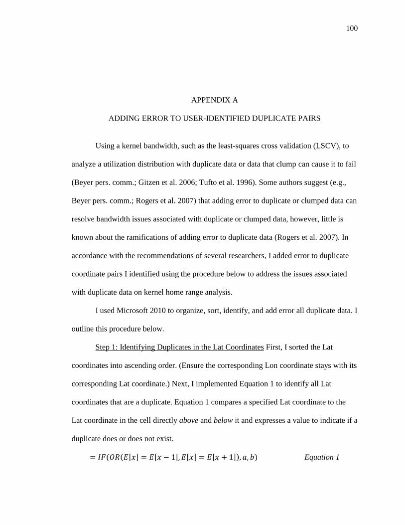
100

APPENDIX A

ADDING ERROR TO USER-IDENTIFIED DUPLICATE PAIRS

Using a kernel bandwidth, such as the least-squares cross validation (LSCV), to

analyze a utilization distribution with duplicate data or data that clump can cause it to fail

(Beyer pers. comm.; Gitzen et al. 2006; Tufto et al. 1996). Some authors suggest (e.g.,

Beyer pers. comm.; Rogers et al. 2007) that adding error to duplicate or clumped data can

resolve bandwidth issues associated with duplicate or clumped data, however, little is

known about the ramifications of adding error to duplicate data (Rogers et al. 2007). In

accordance with the recommendations of several researchers, I added error to duplicate

coordinate pairs I identified using the procedure below to address the issues associated

with duplicate data on kernel home range analysis.

I used Microsoft 2010 to organize, sort, identify, and add error all duplicate data. I

outline this procedure below.

Step 1: Identifying Duplicates in the Lat Coordinates First, I sorted the Lat

coordinates into ascending order. (Ensure the corresponding Lon coordinate stays with its

corresponding Lat coordinate.) Next, I implemented Equation 1 to identify all Lat

coordinates that are a duplicate. Equation 1 compares a specified Lat coordinate to the

Lat coordinate in the cell directly above and below it and expresses a value to indicate if a

duplicate does or does not exist.

= 𝐼𝐹(𝑂𝑅(𝐸[𝑥] = 𝐸[𝑥 − 1], 𝐸[𝑥] = 𝐸[𝑥 + 1]), 𝑎, 𝑏) Equation 1

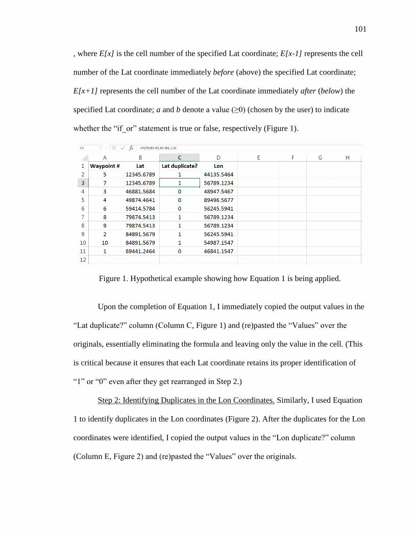
101

, where E[x] is the cell number of the specified Lat coordinate; E[x-1] represents the cell

number of the Lat coordinate immediately before (above) the specified Lat coordinate;

E[x+1] represents the cell number of the Lat coordinate immediately after (below) the

specified Lat coordinate; a and b denote a value (≥0) (chosen by the user) to indicate

whether the “if_or” statement is true or false, respectively (Figure 1).

Figure 1. Hypothetical example showing how Equation 1 is being applied.

Upon the completion of Equation 1, I immediately copied the output values in the

“Lat duplicate?” column (Column C, Figure 1) and (re)pasted the “Values” over the

originals, essentially eliminating the formula and leaving only the value in the cell. (This

is critical because it ensures that each Lat coordinate retains its proper identification of

“1” or “0” even after they get rearranged in Step 2.)

Step 2: Identifying Duplicates in the Lon Coordinates. Similarly, I used Equation

1 to identify duplicates in the Lon coordinates (Figure 2). After the duplicates for the Lon

coordinates were identified, I copied the output values in the “Lon duplicate?” column

(Column E, Figure 2) and (re)pasted the “Values” over the originals.

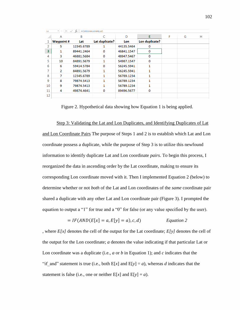
102

Figure 2. Hypothetical data showing how Equation 1 is being applied.

Step 3: Validating the Lat and Lon Duplicates, and Identifying Duplicates of Lat

and Lon Coordinate Pairs The purpose of Steps 1 and 2 is to establish which Lat and Lon

coordinate possess a duplicate, while the purpose of Step 3 is to utilize this newfound

information to identify duplicate Lat and Lon coordinate pairs. To begin this process, I

reorganized the data in ascending order by the Lat coordinate, making to ensure its

corresponding Lon coordinate moved with it. Then I implemented Equation 2 (below) to

determine whether or not both of the Lat and Lon coordinates of the same coordinate pair

shared a duplicate with any other Lat and Lon coordinate pair (Figure 3). I prompted the

equation to output a “1” for true and a “0” for false (or any value specified by the user).

= 𝐼𝐹(𝐴𝑁𝐷(𝐸[𝑥] = 𝑎, 𝐸[𝑦] = 𝑎), 𝑐, 𝑑) Equation 2

, where E[x] denotes the cell of the output for the Lat coordinate; E[y] denotes the cell of

the output for the Lon coordinate; a denotes the value indicating if that particular Lat or

Lon coordinate was a duplicate (i.e., a or b in Equation 1); and c indicates that the

“if_and” statement is true (i.e., both E[x] and E[y] = a), whereas d indicates that the

statement is false (i.e., one or neither E[x] and E[y] = a).

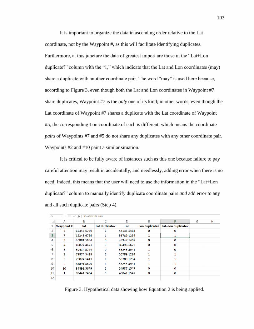
103

It is important to organize the data in ascending order relative to the Lat

coordinate, not by the Waypoint #, as this will facilitate identifying duplicates.

Furthermore, at this juncture the data of greatest import are those in the “Lat+Lon

duplicate?” column with the “1,” which indicate that the Lat and Lon coordinates (may)

share a duplicate with another coordinate pair. The word “may” is used here because,

according to Figure 3, even though both the Lat and Lon coordinates in Waypoint #7

share duplicates, Waypoint #7 is the only one of its kind; in other words, even though the

Lat coordinate of Waypoint #7 shares a duplicate with the Lat coordinate of Waypoint

#5, the corresponding Lon coordinate of each is different, which means the coordinate

pairs of Waypoints #7 and #5 do not share any duplicates with any other coordinate pair.

Waypoints #2 and #10 paint a similar situation.

It is critical to be fully aware of instances such as this one because failure to pay

careful attention may result in accidentally, and needlessly, adding error when there is no

need. Indeed, this means that the user will need to use the information in the “Lat+Lon

duplicate?” column to manually identify duplicate coordinate pairs and add error to any

and all such duplicate pairs (Step 4).

Figure 3. Hypothetical data showing how Equation 2 is being applied.

104

Step 4: Adding Error to User-Identified Duplicate Coordinate Pairs I added error

in increments of two meters) to both the Lat and Lon coordinates of each duplicate

coordinate pair, beginning with the second duplicate coordinate pair. (I always left one

duplicate coordinate pair in its original state.) To elaborate, if a Lat and Lon coordinate

pair had a total of three duplicates, I (i) left one of the three duplicates in its original state;

(ii) then added two m of error to the Lat and Lon coordinate of the second of three

duplicates; and (iii) lastly added four m of error to the Lat and Lon coordinate of the

remaining duplicate pair. (Similarly, I added six m of error would be added to the fourth

duplicate pair, eight m of error would added to the fifth duplicate pair, etc.) I continued

this process of adding error to each of the remaining duplicate coordinate pairs until error

had been added to all user-identified duplicate coordinate pairs. The most random error

added this way was 20 m (most likely to a sleeping cliff coordinate value as the geladas

regularly re-used sleeping cliff sites throughout the five-year study). The new coordinate

pairs will then replace the original coordinate pairs.

Step 5: Re-analysis of data for (inadvertent) duplicate data It is quite conceivable

that coordinate data may be inadvertently duplicated during the error adding phase of

Step 4. This is plausible because the user, by adding error in the form of a distance,

changes the makeup of each coordinate pair, creating a new Lat and Lon that may in turn

share the same value as another Lat and Lon coordinate pair. To ensure this phenomenon

of creating inadvertent duplicate data does not happen, I repeated Steps 1 through 3 to

identify any duplicate data, and where there were duplicate pairs, I added error to them. I

continued this process (of rearranging and adding random error) until there were no

longer any duplicate pairs in the dataset.

105

BIBLIOGRAPHY

Albernaz A, and Magnusson W. 1999. Home-range size of the bare-ear marmoset

(Callithrix argentata) at Alter do Chão, Central Amazonia, Brazil. International

Journal of Primatology 20(5):665-677.

Albon SD, and Langvatn R. 1992. Plant phenology and the benefits of migration in a

temperate ungulate. Oikos 65(3):502-513.

Amstrup SC, McDonald TL, and Durner GM. 2004. Using satellite radiotelemetry data to

delineate and manage wildlife populations. Wildlife Society Bulletin

32(3)(Autumn 2004):661-679.

Anderson C. 1981. Intertroop relations of chacma baboon (Papio ursinus). International


Anderson CM. 1982. Baboons below the tropic of capricorn. Journal of Human Evolution

11(3):205-217.

Anderson D. 1982b. The home range: A new nonparametric estimation technique.

Ecology 63(1):103-112.

Anderson DP, Forester JD, Turner MG, Frair JL, Merrill EH, Fortin D, Mao JS, and

Boyce MS. 2005. Factors influencing female home range sizes in elk (Cervus

elaphus) in North American landscapes. Landscape Ecology 20(3):257-271.

Andreka G, Linn I, Perrine M, and Maddock A. 1999. Range use by the wild dog in the

Hluhluwe-Umfolozi Park, South Africa. South African Journal of Wildlife

Research 29(1):1-9.

Asensio N, Schaffner CM, and Aureli F. 2012. Variability in core areas of spider

monkeys (Ateles geoffroyi) in a tropical dry forest in Costa Rica. Primates

53(2):147-156.

Ashenafi ZT. 2001. Common Property Resource Management of an Afro-Alpine Habitat

Supporting a Population of the Critically Endangered Ethiopian Wolf (Canis

simensis). Ph.D. Thesis. University of Kent, Canterbury, UK.

106

Ashenafi ZT, and Leader-Williams N. 2005. Indigenous common property resource

management in the Central Highlands of Ethiopia. Human Ecology 33(4):539-

563.

Baldwin PJ, McGrew WC, and Tutin CEG. 1982. Wide-ranging chimpanzees at Mt.

Assirik, Senegal. International Journal of Primatology 3(4):367-385.

Baoping R, Ming L, Yongcheng L, and Fuwen W. 2009. Influence of day length, ambient

temperature, and seasonality on daily travel distance in the Yunnan snub-nosed

monkey at Jinsichang, Yunnan, China. American Journal of Primatology

71(3):233-241.

Barton R, Whiten A, Strum S, Byrne R, and Simpson A. 1992. Habitat use and resource

availability in baboons. Animal Behaviour 43(5):831-844.

Basabose AK. 2005. Ranging patterns of chimpanzees in a montane forest of Kahuzi,

Democratic Republic of Congo. International Journal of Primatology 26(1):33-54.

Beehner J, Berhanu G, and McCann C. 2008. Population estimate for geladas

(Theropithecus gelada) living in and around the Simien Mountains National Park,

Ethiopia. SINET 30:149-154.

Bekoff M, and Mech LD. 1984. Simulation analyses of space use: Home range estimates,

variability, and sample size. Behavior Research Methods, Instruments, &

Computers 16(1):32-37.

Berger J, Stacey PB, Bellis L, and Johnson MP. 2001. A mammalian predator-prey

imbalance: Grizzly bear and wolf extinction affect Avian neotropical migrants.

Ecological Applications 11(4):947-960.

Bergerud A, Wyett W, and Snider B. 1983. The role of wolf predation in limiting a

moose population. The Journal of Wildlife Management:977-988.

Beyer HL. 2012a. Geospatial Modelling Environment. 0.7.2.0 ed.

Beyer HL. 2012b. Geospatial Modelling Environment Help PDF.

Biebouw K. 2009. Home range size and use in Allocebus trichotis in Analamazaotra

special reserve, central eastern Madagascar. International Journal of Primatology

30(2):367-386.

Blundell G, Maier J, and Debevec E. 2001. Linear home ranges: effects of smoothing,

sample size, and autocorrelation on kernel estimates. Ecological Monographs

71(3):469-489.

107

Boesch C, and Achermann HB. 2000. The chimpanzees of the Taï forest: behavioural

ecology and evolution: New York, Oxford University Press, USA.

Boesch C, and Boesch H. 1989. Hunting behavior of wild chimpanzees in the Tai

National Park. American journal of physical anthropology 78(4):547-573.

Börger L, Franconi N, De Michele G, Gantz A, Meschi F, Manica A, Lovari S, and

Coulson T. 2006. Effects of sampling regime on the mean and variance of home

range size estimates. The Journal of Animal Ecology 75(6):1393-1405.

Boulanger J, and White G. 1990. A comparison of home-range estimators using Monte

Carlo simulation. The Journal of Wildlife Management 54(2):310-315.

Bowman A, and Azzalini A. 1997. Applied Smoothing Techniques for Data Analysis:

The Kernel Approach with S-Plus Illustrations. Oxford: Clarendon Press.

Boyle SA, Lourenço WC, Da Silva LR, and Smith AT. 2009. Home range estimates vary

with sample size and methods. Folia Primatologica 80(1):33-42.

Brobeck JR. 1948. Food intake as a mechanism of temperature regulation. The Yale

Journal of Biology and Medicine 20(6):545.

Bronikowski AM, and Altmann J. 1996. Foraging in a variable environment: weather

patterns and the behavioral ecology of baboons. Behavioral Ecology and

Sociobiology 39(1):11-25.

Buechner HK. 1950. Life history, ecology, and range use of the pronghorn antelope in

Trans-Pecos Texas. American Midland Naturalist: 257-354.

Burgman M, and Fox J. 2003. Bias in species range estimates from minimum convex

polygons: implications for conservation and options for improved planning.

Animal Conservation 6:19-28.

Carnegie S, Fedigan L, and Melin A. 2011. Reproductive seasonality in female capuchins

(Cebus capucinus) in Santa Rosa (Area de Conservación Guanacaste), Costa Rica.

International Journal of Primatology 32(5):1076-1090.

Chapman CA. 1988. Patterns of foraging and range use by three species of neotropical

primates. Primates 29(2):177-194.

Chapman CA, and Chapman L. 2000. Determinants of group size in primates: the

importance of travel costs. In: Boinski S, and Garber P, editors. On the Move:

How and Why Animals Travel in Groups. Chicago and London: The University

of Chicago Press. p 24-41.

108

Chapman CA, and Pavelka MM. 2005. Group size in folivorous primates: ecological

constraints and the possible influence of social factors. Primates 46(1):1-9.

Chism J, and Rowell T. 1988. The natural history of patas monkeys. In: Gautier-Hion A,

Bourliére F, Gautier J, and Kingdon J, editors. Primate Radiation: Evolutionary

Biology of the African Guenons. Cambridge: Cambridge University Press. p 412-

438.

Clutton-Brock TH, and Harvey PH. 1977. Primate ecology and social organization.

Journal of Zoology 183(1):1-39.

Cohen J. 1988. Statistical power analysis for the behavioral sciences. Hillsdale, New

Jersey. Lawrence Erlbaum Associates, Publishers.

Covert H, Quyet L, and Wright B. 2008. On the brink of extinction: Research for the

conservation on the Tonkin snub-nosed monkey (Rhinopithecus avunculus). In:

Fleagle J, and Gilbert C, editors. Ewyln Simons: A Search for Origins: Springer-

Verlag New York. p 409-427.

Cowlishaw G, and Dunbar RI. 2000. Primate Conservation Biology: University of

Chicago Press. Chicago, USA.

Craighead JJ, Craighead FC, Ruff RL, and O'Gara BW. 1973. Home ranges and activity

patterns of nonmigratory elk of the Madison drainage herd as determined by

biotelemetry. Wildlife Monographs (33):3-50.

Crook JH. 1966. Gelada baboon herd structure and movement: a comparative report.

Symp Zool Soc Lond. p 237-258.

Crook JH, and Aldrich-Blake P. 1968. Ecological and behavioural contrasts between

sympatric ground dwelling primates in Ethiopia. Folia Primatologica 8(3-4):192-

227.

Dagg AI, and Foster JB. 1976. The giraffe: its biology, behavior, and ecology: Van

Nostrand Reinhold Company. New York.

de Solla SR, Bonduriansky R, and Brooks RJ. 1999. Eliminating autocorrelation reduces

biological relevance of home range estimates. Journal of Animal Ecology

68(2):221-234.

Dew JL, and Wright P. 1998. Frugivory and seed dispersal by four species of primates in

Madagascar's eastern rain forest. Biotropica 30(3):425-437.

Dias L, and Strier K. 2003. Effects of group size on ranging patterns in Brachyteles

arachnoides hypoxanthus. International Journal of Primatology 24(2):209-221.

109

Dobrovidov AV, and Ruds’ko IM. 2010. Bandwidth selection in nonparametric estimator

of density derivative by smoothed cross-validation method. Autom Remote

Control 71(2):209-224.

Donaldson BM, and Echternacht AC. 2005. Aquatic habitat use relative to home range

and seasonal movement of eastern box turtles (Terrapene carolina carolina:

Emydidae) in eastern Tennessee. Journal of Herpetology 39(2):278-284.

Doran D. 1997. Influence of Seasonality on Activity Patterns, Feeding Behavior,

Ranging, and Grouping Patterns in Taï Chimpanzees. International Journal of

Primatology 18(2):183-206.

Doran-Sheehy D, Mongo P, Lodwick J, and Conklin-Brittain NL. 2009. Male and female

western gorilla diet: Preferred foods, use of fallback resources, and implications

for ape versus old world monkey foraging strategies. American Journal Physical

Anthropology 140(4):727-738.

Dunbar R. 1977. Feeding ecology of gelada baboons: a preliminary report. In: Clutton-

Brock T, editor. Primate Ecology: Studies of feeding and ranging behaviour in

lemurs, monkeys and apes. London, New York, San Francisco: Academic Press. p

251-273.

Dunbar R. 1980. Demographic and life history variables of a population of gelada

baboons (Theropithecus gelada). The Journal of animal ecology:485-506.

Dunbar R, and Dunbar P. 1974. Ecological relations and niche separation between

sympatric terrestrial primates in Ethiopia. Folia Primatologica 21(1):36-60.

Dunbar RIM. 1998. Impact of global warming on the distribution and survival of the

gelada baboon: a modelling approach. Global Change Biology 4(3):293-304.

Dunbar RIM, and Dunbar P. 1975. Social Dynamics of Gelada Baboons: S. Karger.

Duong T, and Hazelton ML. 2005. Cross-validation bandwidth matrices for multivariate

kernel density estimation. Scandinavian Journal of Statistics 32(3):485-506.

Edwards MA, Nagy JA, and Derocher AE. 2009. Low site fidelity and home range drift

in a wide-ranging, large Arctic omnivore. Animal Behaviour 77(1):23-28.

ESRI. 2011. ArcGIS Desktop: Release 10.1. Redlands, CA: Environmental Systems

Research Insititute.

Fashing P. 2001. Activity and ranging patterns of guerezas in the Kakamega Forest:

Intergroup variation and implications for intragroup feeding competition.


110

Fashing P, Nguyen N, and Fashing N. 2010. Behavior of geladas and other endemic

wildlife during a desert locust outbreak at Guassa, Ethiopia: ecological and

conservation implications. Primates 51(3):193-197.

Fashing PJ, Mulindahabi F, Gakima J-B, Masozera M, Mununura I, Plumptre AJ, and

Nguyen N. 2007. Activity and ranging patterns of Colobus angolensis ruwenzorii

in Nyungwe Forest, Rwanda: possible costs of large group size. International


Fashing PJ, Nguyen N, Barry TS, Goodale CB, Burke RJ, Jones SCZ, Kerby JT, Lee LM,

Nurmi NO, and Venkataraman VV. 2011. Death among geladas (Theropithecus

gelada): a broader perspective on mummified infants and primate thanatology.

American Journal of Primatology 73(5):405-409.

Fashing PJ, Nguyen N, Venkataraman VV, and Kerby JT. 2014. Gelada feeding ecology

in an intact ecosystem at Guassa, Ethiopia: variability over time and implications

for theropith and hominin dietary evolution. American journal of physical

anthropology 155(1):1-16.

Ferguson SH, Taylor MK, Born EW, Rosing-Asvid A, and Messier F. 1999.

Determinants of home range size for polar bears (Ursus maritimus). Ecology

Letters 2(5):311-318.

Fieberg J. 2007. Kernel density estimators of home range: smoothing and the

autocorrelation red herring. Ecology 88(4):1059-1066.

Field CR. 1971. Elephant ecology in the Queen Elizabeth National Park, Uganda. African

Journal of Ecology 9(1):99-123.

Fischer F, and Linsenmair KE. 2001. Spatial and temporal habitat use of kob antelopes

(Kobus kob kob, Erxleben 1777) in the Comoé National Park, Ivory Coast as

revealed by radio tracking. African Journal of Ecology 39(3):249-256.

Frost HC, Storm GL, Batcheller MJ, and Lovallo MJ. 1997. White-tailed deer

management at Gettysburg National Military Park and Eisenhower National

Historic Site. Wildlife Society Bulletin:462-469.

Garber P. 1980. Locomotor behavior and feeding ecology of the Panamanian tamarin

(Saguinus oedipus geoffroyi, Callitrichidae, Primates). International Journal of


Georgii B. 1980. Home range patterns of female red deer (Cervus elaphus L.) in the Alps.

Oecologia 47(2):278-285.

111

Gerber BD, Arrigo-Nelson S, Karpanty SM, Kotschwar M, and Wright PC. 2012. Spatial

ecology of the endangered Milne-Edwards’ sifaka (Propithecus edwardsi): Do

logging and season affect home range and daily ranging patterns? International

Journal of Primatology: 1-17.

Girard I, Ouellet J-P, Courtois R, Dussault C, and Breton L. 2002. Effects of sampling

effort based on GPS telemetry on home-range size estimations. The Journal of

Wildlife Management 66(4):1290-1300.

Gitzen RA, Millspaugh JJ, and Kernohan BJ. 2006. Bandwidth selection for fixed-kernel

analysis of animal utilization distributions. Journal of Wildlife Management

70(5):1334-1344.

Glessner KD, and Britt A. 2005. Population density and home range size of Indri indri in

a protected low altitude rain forest. International Journal of Primatology

26(4):855-872.

Gravetter FJ, and Wallnau LB. 2008. Essentials of statistics for the behavioral sciences:

Wadsworth Publishing Company. Belmont, CA, USA.

Grueter C, Li D, Ren B, and Wei F. 2009. Choice of analytical method can have dramatic

effects on primate home range estimates. Primates 50(1):81-84.

Grueter CC, Li D, van Schaik CP, Ren B, Long Y, and Wei F. 2008. Ranging of

Rhinopithecus bieti in the Samage Forest, China. I. Characteristics of range use.


Haile M. 2005. Weather patterns, food security and humanitarian response in sub-

Saharan Africa. Philosophical transactions of the Royal Society of London Series

B, Biological sciences 360:2169-2182.

Hall P, Marron JS, and Park B. 1992. Smoothed cross-validation. Probability Theory and

Related Fields 92(1):1-20.

Hansteen TL, Andreassen HP, and Ims RA. 1997. Effects of spatiotemporal scale on

autocorrelation and home range estimators. The Journal of Wildlife Management:

280-290.

Hanya G, Noma N, and Agetsuma N. 2003. Altitudinal and seasonal variations in the diet

of Japanese macaques in Yakushima. Primates 44(1):51-59.

Hemson G, Johnson P, South A, Kenward R, Ripley R, and McDonald D. 2005. Are

kernels the mustard? Data from global positioning system (GPS) collars suggests

problems for kernel home-range analyses with least-squares cross-validation.

Journal of Animal Ecology 74(3):455-463.

112

Henzi SP, Byrne RW, and Whiten A. 1992. Patterns of movement by baboons in the

Drakensberg mountains: Primary responses to the environment. International


Hervert JJ, Bright JL, Henry RS, Piest LA, and Brown MT. 2005. Home-range and

habitat-use patterns of Sonoran pronghorn in Arizona. Wildlife Society Bulletin

33(1):8-15.

Heymann EW, and Aquino R. 2010. Peruvian red uakaris (Cacajao calvus ucayalii) are

not flooded-forest specialists. International Journal Primatology 31(5):751-758.

Hillman J. 1988. Home range and movement of the common eland (Taurotragus oryx

Pallas 1766) in Kenya. African Journal of Ecology 26(2):135-148.

Homewood KM. 1978. Feeding strategy of the Tana mangabey (Cercocebus galeritus

galeritus) (Mammalia: Primates). Journal of Zoology 186(3):375-391.

Horne JS, and Garton EO. 2006. Likelihood cross-validation versus least squares cross-

validation for choosing the smoothing parameter in kernel home-range analysis.

Journal of Wildlife Management 70(3):641-648.

Hunter CP. 2001. Ecological Determinants of Gelada Ranging Patterns (Theropithecus

gelada). PhD Thesis. The British Library: University of Liverpool. 208 p.

IBM Corp. Released 2012. IBM SPSS Statistics for Windows, Version 20.0. Armonk,

NY: IBM Corp.

Isbell LA. 1998. Diet for a small primate: Insectivory and gummivory in the (large) patas

monkey (Erythrocebus patas pyrrhonotus). American Journal of Primatology

45(4):381-398.

Isbell LA, Cheney DL, and Seyfarth RM. 1990. Costs and benefits of home range shifts

among vervet monkeys (Cercopithecus aethiops) in Amboseli National Park,

Kenya. Behavioral Ecology and Sociobiology 27(5):351-358.

Iwamoto T. 1979. Feeding Ecology. In: Kawai M, editor. Ecological and Sociological

Studies of Gelada Baboons: S. Karger. p 279-330.

Iwamoto T. 1993. The ecology of Theropithecus gelada. In: Jablonski NG, editor.

Theropithecus: The Rise and Fall of a Primate Genus. Great Britain: Cambridge

University Press. p 441-452.

Iwamoto T, and Dunbar RIM. 1983. Thermoregulation, habitat quality and the

behavioural ecology of gelada baboons. Journal of Animal Ecology 52(2):357-

366.

113

Jablonski NG. 1993. Theropithecus: the rise and fall of a primate genus: Cambridge

University Press.

Janson C, and Verdolin J. 2005. Seasonality of primate births in relation to climate. In:

Brockman D, and van Schaik C, editors. Seasonality in Primates: Studies of

Living and Extinct Human and Non-human Primate. New York: Cambridge

University Press. p 307-350.

Jennrich R, and Turner F. 1969. Measurement of non-circular home range. Journal of

Theoretical Biology 22(2):227-237.

Jolly CJ. 1970. The seed-eaters: a new model of hominid differentiation based on a

baboon analogy. [Indianapolis]: [Bobbs-Merrill].

Kaplin BA. 2001. Ranging behavior of two species of guenons (Cercopithecus lhoesti

and C. mitis doggetti) in the Nyungwe Forest Reserve, Rwanda. International


Kawai M, editor. 1979. Ecological and Sociological Studies of Gelada Baboons: S.

Karger.

Kawai M, Ohsawa H, Mori U, and Dunbar R. 1983. Social organization of gelada

baboons: Social units and definitions. Primates 24(1):13-24.

Kernohan B, Gitzen R, and Millspaugh J. 2001. Analysis of animal space use and

movements. In: Millspaugh J, and Marzluff J, editors. Radio tracking and animal

populations. San Diego: Academic Press. p 125-166.

Kinnaird MF. 1990. Behavioral and demographic responses to habitat change by the Tana

River crested mangabey (Cercocebus galeritus galeritus). Ph.D. Dissertation.

Gainesville, FL: University of Florida.

Krausman PR, Leopold BD, Seegmiller RF, and Torres SG. 1989. Relationships between

desert bighorn sheep and habitat in western Arizona. Wildlife Monographs

(102):3-66.

Kummer H. 1968. Social Organization of Hamadryas Baboons: A Field Study. Chicago:

University of Chicago.

Kunz BK, and Linsenmair KE. 2008. The disregarded West: diet and behavioural

ecology of olive baboons in the Ivory Coast. Folia Primatologica 79(1):31-51.

Lachica M, and Aguilera J. 2000. Estimation of the energy costs of locomotion in the

Iberian pig (Sus mediterraneus). British Journal of Nutrition 83(01):35-41.

114

Lachica M, and Aguilera J. 2005. Energy expenditure of walk in grassland for small

ruminants. Small Ruminant Research 59(2):105-121.

Lachica M, Prieto C & Aguilera JF (1997) The energy cost of walking on the level and

on negative and positive slopes in the Granadina goat (Capra hircus). British

Journal of Nutrition 77, 73–81.

Laliberte AS, and Ripple WJ. 2004. Range contractions of North American carnivores

and ungulates. BioScience 54(2):123-138.

Laver PN, and Kelly MJ. 2008. A critical review of home range studies. Journal of

Wildlife Management 72(1):290-298.

Lee, LM. 2011. Parturition among gelada monkeys (Theropithecus gelada) at Guassa,

Ethiopia [M.A. thesis]. Fullerton: California State University Fullerton.

Legendre P. 1983. Spatial autocorrelation: Trouble or new paradigm? Ecology

74(6):1659-1673.

Lesage L, Crête M, Huot J, Dumont A, and Ouellet J-P. 2000. Seasonal home range size

and philopatry in two northern white-tailed deer populations. Canadian Journal of

Zoology 78(11):1930-1940.

Lesage L, Crête M, Huot J, Dumont A, and Ouellet J-P. 2000. Seasonal home range size

and philopatry in two northern white-tailed deer populations. Canadian Journal of

Zoology 78(11):1930-1940.

Leuthold W. 1972. Home range, movements and food of a buffalo herd in Tsavo National

Park. African Journal of Ecology 10(3):237-243.

Leuthold W. 1978. On the ecology of the gerenuk Litocranius walleri. Journal of Animal

Ecology 47(2):561-580.

Leuthold B, and Leuthold W. 1978. Ecology of the giraffe in Tsavo East National Park,

Kenya. African Journal of Ecology 16(1):1-20.

Li B, Chen C, Ji W, and Ren B. 2000. Seasonal home range changes of the Sichuan snub-

nosed monkey (Rhinopithecus roxellana) in the Qinling Mountains of China.

Folia Primatologica 71(6):375-386.

Li D, Grueter CC, Ren B, Long Y, Li M, Peng Z, and Wei F. 2008. Ranging of

Rhinopithecus bieti in the Samage Forest, China. II. Use of land cover types and

altitudes. International Journal of Primatology 29(5):1147-1173.

Li D, Ren B, Li B, and Li M. 2010. Range expansion as a response to increasing group

size in the Yunnan snub-nosed monkey. Folia Primatologica 81(6):315-329.

115

Li X, and Walker D. 1986. The plant geography of Yunnan Province, southwest China.

Journal of Biogeography:367-397.

Li Z, and Rogers ME. 2005. Habitat quality and range use of white-headed langurs in

Fusui, China. Folia Primatologica 76(4):185-195.

Loveridge AJ, Valeix M, Davidson Z, Murindagomo F, Fritz H, and Macdonald DW.

2009. Changes in home range size of African lions in relation to pride size and

prey biomass in a semi-arid savanna. Ecography 32(6):953-962.

Luccarini S, Mauri L, Ciuti S, Lamberti P, and Apollonio M. 2006. Red deer (Cervus

elaphus) spatial use in the Italian Alps: home range patterns, seasonal migrations,

and effects of snow and winter feeding. Ethology Ecology & Evolution

18(2):127-145.

Mahli Y, and Wright J. 2004. Spatial patterns and recent trends in the climate of tropical

rainforest regions. Philosophical transactions of the Royal Society of London

Series B, Biological sciences 359(1443):311-329.

Marra PP, Francis CM, Mulvihill RS, and Moore FR. 2005. The Influence of climate on

the timing and rate of spring bird migration. Oecologia 142(2):307-315.

Mekonnen A, Bekele A, Fashing PJ, Hemson G, and Atickem A. 2010. Diet, activity

patterns, and ranging ecology of the Bale monkey (Chlorocebus djamdjamensis)

in Odobullu Forest, Ethiopia. International Journal of Primatology 31(3):339-362.

Mitchell MS, and Powell RA. 2007. Optimal use of resources structures home ranges and

spatial distribution of black bears. Animal Behaviour 74(2):219-230.

Mori A, and Belay G. 1990. The distribution of baboon species and a new population of

gelada baboons along the Wabi-Shebeli river, Ethiopia. Primates 31(4):495-508.

Mori A, Iwamoto T, Mori U, and Bekele A. 1999. Sociological and demographic

characteristics of a recently found Arsi gelada population in Ethiopia. Primates

40(2):365-381.

Moua C, Fashing PJ, and Nguyen N. 2012. Inter-annual variability in the ranging ecology

of wild geladas (Theropithecus gelada) at Guassa, Ethiopia, from 2007-2011

[Abstract]. American Society of Primatology, 2012.

Mysterud A. 1999. Seasonal migration pattern and home range of roe deer (Capreolus

capreolus) in an altitudinal gradient in southern Norway. Journal of Zoology

247(4):479-486.

Nicholson MC, Bowyer RT, and Kie JG. 1997. Habitat selection and survival of mule

deer: Tradeoffs associated with migration. Journal of Mammalogy 78(2):483-504.

116

Newton‐Fisher NE. 2003. The home range of the Sonso community of chimpanzees from

the Budongo Forest, Uganda. African Journal of Ecology 41(2):150-156.

Nguyen N, and Fashing PJ. 2009. Guassa gelada research project: A guide to working on

the Guassa gelada monkey project for prospective field research assistants.

Unpublished manuscript.

Nguyen N, and Fashing PJ. 2012. Birth seasonality in relation to rainfall and food in wild

geladas (Theropithecus gelada) at Guassa, Ethiopia: Variation within and between

one-male units. American Journal Physical Anthropology 147:223-223.

Nguyen N, Fashing PJ, Boyd DA, Barry TS, Burke RJ, Goodale CB, Jones SC, Kerby JT,

Kellogg BS, and Lee LM. 2015. Fitness impacts of tapeworm parasitism on wild

gelada monkeys at Guassa, Ethiopia. American journal of primatology 77(5):579-

594.

Nilsen EB, Pedersen S, and Linnell JD. 2008. Can minimum convex polygon home

ranges be used to draw biologically meaningful conclusions? Ecological Research

23(3):635-639.

Niu K, Tan CL, and Yang Y. 2010. Altitudinal movements of Guizhou snub-nosed

monkeys (Rhinopithecus brelichi) in Fanjingshan National Nature Reserve,

China: implications for conservation management of a flagship species. Folia

Primatologica 81(4):233-244.

Ohsawa H. 1979. Herd Dynamics. In: Kawai M, editor. Ecological and Sociological

Studies of Gelada Baboons: S. Karger. p 48-80.

Olupot W, Chapman CA, Brown CH, and Waser PM. 1994. Mangabey (Cercocebus

albigena) population density, group size, and ranging: A twenty‐year comparison.


Otis DL, and White GC. 1999. Autocorrelation of location estimates and the analysis of

radiotracking data. The Journal of Wildlife Management:1039-1044.

Pallant J. 2010. SPSS survival manual: A step by step guide to data analysis using SPSS:

Open University Press.

Palma AC, Vélez A, Gómez‐Posada C, López H, Zárate DA, and Stevenson PR. 2011.

Use of space, activity patterns, and foraging behavior of red howler monkeys

(Alouatta seniculus) in an Andean forest fragment in Colombia. American journal

of primatology 73(10):1062-1071.

117

Pavelka MM, Brusselers O, Nowak D, and Behie A. 2003. Population reduction and

social disorganization in Alouatta pigra following a hurricane. International


Pebsworth PA, Morgan HR, and Huffman MA. 2012. Evaluating home range techniques:

use of Global Positioning System (GPS) collar data from chacma baboons.

Primates 53(4):345-355.

Pimley ER, Bearder SK, and Dixson AF. 2005. Home range analysis of Perodicticus

potto edwardsi and Sciurocheirus cameronensis. International Journal of


Phillips R, Berg W, and Siniff D. 1973. Moose movement patterns and range use in

northwestern Minnesota. The Journal of Wildlife Management:266-278.

Poulsen JR, Clark CJ, and Smith TB. 2001. Seasonal variation in the feeding ecology of

the grey-cheeked mangabey (Lophocebus albigena) in Cameroon. American


Powell R. 2000. Animal Home Ranges and Territories and Home Range Estimators. In:

Boitani L, and Fuller T, editors. Research Techniques in Animal Ecology:

Controversies and Consequences. New York: Columbia University Press. p 65-

110.

Rabinowitz AR, and Nottingham BG, Jr. 1986. Ecology and behaviour of the Jaguar

(Panthera onca) in Belize, Central America. Journal of Zoology 210(1):149-159.

Robbins MM, and McNeilage A. 2003. Home range and frugivory patterns of mountain

gorillas in Bwindi Impenetrable National Park, Uganda. International Journal of


Rodgers AR, Carr A, Beyer H, Smith L, and Kie J. 2007. HRT: home range tools for

ArcGIS. Ontario Ministry of Natural Resources, Centre for Northern Forest

Ecosystem Research, Thunder Bay, Ontario, Canada.

Rowe J, and Dalgarn S. 2010. Home range size and daily movements of midland painted

turtles (Chrysemys picta marginata) in relation to body size, sex, and weather

patterns. Herpetological Conservation and Biology 5(3):461-473.

Rueness EK, Asmyhr MG, Sillero-Zubiri C, Macdonald DW, Bekele A, Atickem A, and

Stenseth NC. 2011. The cryptic African wolf: Canis aureus lupaster is not a

golden jackal and is not endemic to Egypt. PLoS ONE 6(1):e16385.

Salkind NJ. 2009. Statistics for people who (think they) hate statistics: EXCEL 2007

Edition: Sage Publications, Incorporated. Los Angeles, CA, USA.

118

Schaller GB. 2000. The Mountain Gorilla: Ecology and Behavior. Chicago: University of

Chicago Press. 450 p.

Schoener T. 1981. An empirically based estimate of home range. Theoretical Population

Biology 20:281-325.

Schreier AL. 2010. Feeding ecology, food availability and ranging patterns of wild

hamadryas baboons at Filoha. Folia Primatologica 81(3):129-145.

Silverman, BW. 1986. Density Estimation for Statistics and Data Analysis. London:

Chapman and Hall.

Seaman D, and Powell R. 1996. An evaluation of the accuracy of kernel density

estimators for home range analysis. Ecology 77(7):2075-2085.

Seaman DE, Millspaugh JJ, Kernohan BJ, Brundige GC, Raedeke KJ, and Gitzen RA.

1999. Effects of sample size on kernel home range estimates. The Journal of

Wildlife Management: 739-747.

Siex KS, and Struhsaker TT. 1999. Ecology of the Zanzibar red colobus monkey:

Demographic variability and habitat stability. International Journal of


Sigg H, and Stolba A. 1981. Home range and daily march in a hamadryas baboon troop.

Folia Primatologica 36(1-2):40-75.

Sikes SK. 1971. The Natural History of the African Elephant. London: Weidenfeld &

Nicolson. 397 p.

Smuts BB. 1985. Sex and friendship in baboons: New York, Aldine Publishing Co.

Sprague D. 2000. Topographic effects on spatial data at a Japanese macaque study site.


Stephen DW, and Krebs JR. 1986. Foraging Theory. USA: Princeton University Press.

Stelzner JK. 1988. Thermal effects on movement patterns of yellow baboons. Primates

29(1):91-105.

Stoltz L, and Saayman G. 1970. Ecology and behaviour of baboons in the northern

Transvaal. Annals of the Transvaal Museum 26(99):143.

Strier K. 1987. Ranging behavior of woolly spider monkeys, or muriquis, Brachyteles

arachnoides. International Journal of Primatology 8(6):575-591.

119

Sutherland WJ, Newton I, and Green R. 2004. Bird Ecology and Conservation: A

Handbook of Techniques. Oxford, New York: Oxford University Press.

Swedell L. 2006. Strategies of Sex and Survival in Hamadryas Baboons: Through a

Female Lens. Upper Saddle River, New Jersey: Pearson Prentice Hall.

Swedell L. 2011. African Papionins: Diversity of social organization and ecological

flexibility. In: Campbell C, Fuentes A, MacKinnon K, and Panger M, editors.

Primates in Perspective. New York and Oxford: Oxford University Press. p 241-

277.

Swihart RK, and Slade NA. 1985a. Influence of sampling interval on estimates of home-

range size. The Journal of Wildlife Management:1019-1025.

Swihart RK, and Slade NA. 1985b. Testing for independence of observations in animal

movements. Ecology:1176-1184.

Symington MM. 1988. Demography, ranging patterns, and activity budgets of black

spider monkeys (Ateles paniscus chamek) in the Manu National Park, Peru.


Snyder-Mackler N, Beehner J, and Bergman T. 2012. Defining Higher Levels in the

Multilevel Societies of Geladas (Theropithecus gelada). International Journal of

Primatology 33(5):1054-1068.

Tan CL, Guo S, and Li B. 2007. Population structure and ranging patterns of

Rhinopithecus roxellana in Zhouzhi National Nature Reserve, Shaanxi, China.


Tufto J, Andersen R, and Linnell J. 1996. Habitat use and ecological correlates of home

range size in a small cervid: the roe deer. Journal of Animal Ecology:715-724.

Vedder AL. 1984. Movement patterns of a group of free‐ranging mountain gorillas

(Gorilla gorilla beringei) and their relation to food availability. American Journal

of Primatology 7(2):73-88.

Venkataraman VV, Glowacka H, Fritz J, Clauss M, Seyoum C, Nguyen N, and Fashing

PJ. 2014. Effects of dietary fracture toughness and dental wear on chewing

efficiency in geladas (Theropithecus gelada). American journal of physical

anthropology 155(1):17-32.

Venkataraman VV, Kerby JT, Nguyen N, Ashenafi ZT, and Fashing PJ. 2015. Solitary

Ethiopian wolves increase predation success on rodents when among grazing

gelada monkey herds. Journal of Mammalogy 96(1):129-137.

120

Vila AR, Beade MS, and Barrios Lamunière D. 2008. Home range and habitat selection

of pampas deer. Journal of Zoology 276(1):95-102.

Wada K, Tokida E, and Ogawa H. 2007. The influence of snowfall, temperature and

social relationships on sleeping clusters of Japanese monkeys during winter in

Shiga Heights. Primates 48(2):130-139.

Wallace HM, and Trueman SJ. 1995. Dispersal of Eucalyptus torelliana seeds by the

resin-collecting stingless bee, Trigona carbonaria. Oecologia 104(1):12-16.

Wartmann FM, Purves RS, and van Schaik CP. 2010. Modelling ranging behaviour of

female orang-utans: a case study in Tuanan, Central Kalimantan, Indonesia.

Primates 51(2):119-130.

Watts D. 1998. Long-Term Habitat Use by Mountain Gorillas (Gorilla gorilla beringei).

1. Consistency, Variation, and Home Range Size and Stability. International


Western D. 1989. The Ecological Role of Elephants in Africa. In: Gakahu C, Western O,

Martin E, Goode B, and Vigne L, editors. Pachyderm: A Publication of the

African Elephant and Rhino Specialist Group: Wildlife Conservation

International. p 42-45.

White G, and Garrott R. 1990. Analysis of wildlife radio-tracking data. University of

Michigan: Academic Press.

Whiten A, Byrne RW, and Henzi SP. 1987. The behavioral ecology of mountain

baboons. International Journal of Primatology 8(4):367-388.

Wieczkowski J. 2005. Examination of increased annual range of a Tana mangabey

(Cercocebus galeritus) group. American Journal Physical Anthropology

128(2):381-388.

Wiens JA. 1989. The Ecology of Bird Communities. Cambridge, UK: Cambridge

University Press.

Willems EP, Barton RA, and Hill RA. 2009. Remotely sensed productivity, regional

home range selection, and local range use by an omnivorous primate. Behavioral

Ecology 20(5):985-992.

Worton BJ. 1989. Kernel methods for estimating the utilization distribution in home-

range studies. Ecology 70(1):164-168.

Wrangham R. 1980. Bipedal locomotion as a feeding adaptation in gelada baboons, and

its implications for hominid evolution. Journal of Human Evolution 9(4):329-331.

121

Wrangham RW, Chapman CA, and Chapman LJ. 1994. Seed dispersal by forest

chimpanzees in Uganda. Journal of Tropical Ecology 10(03):355-368.

Zinner D, Peláez F, and Torkler F. 2002. Distribution and habitat of grivet monkeys

(Cercopithecus aethiops aethiops) in eastern and central Eritrea. African Journal

of Ecology 40(2):151-158.

long-term ranging patterns of wild gelada

Documents