local‐scaling transformations and the direct determination of kohnsham orbitals and potentials for...

Local-scaling transformations and the direct determination of Kohn–Shamorbitals and potentials for beryllium

Eduardo V. Ludena,a) Jorge Maldonado, and Roberto Lopez-BoadaCentro de Quı´mica, Instituto Venezolano de Investigaciones Cientı´ficas, IVIC, Apartado 21827, Caracas1020-A, Venezuela

Toshikatsu KogaDepartment of Applied Chemistry, Muroran Institute of Technology, Muroran, Hokkaido 50, Japan

Eugene S. KryachkoBogoliubov Institute for Theoretical Physics, 252130 Kiev-130, Ukraine

~Received 19 May 1993; accepted 15 September 1994!

Local-scaling transformations are used in the present work to obtain accurate Kohn–Sham 1s and2s orbitals for the beryllium atom by means of a density-constrained variation of thesingle-determinant kinetic energy functional. An analytic representation of these Kohn–Shamorbitals is given and the quality of the different types of orbitals generated is discussed withparticular reference to their kinetic energy and momenta mean values. In addition, we determine theeffective Kohn–Sham potential and analyze it in terms of its exchange-only and correlationcontributions. ©1995 American Institute of Physics.

na

r

u

o

e

hh

emnkto

f

nn

etsthen

ornt-fx--

s--

ri-eto

I. INTRODUCTION

One of the basic tenets of the Kohn–Sham theory1–4 isthe existence ofN single-particle orbitals~whereN is thenumber of electrons in the system! such that the one-particledensity obtained from the determinantal wave function costructed from these orbitals is equal to the exact ground-stone-particle density. The former density is related to a nointeracting system whereas the latter corresponds to the tinteractingN-particle system.

A direct way to obtain theseN single-particle orbitals isto solve the Kohn–Sham equations. However, these eqtions contain an effective local potential whose exchangcorrelation part corresponds to the functional derivativethe exactKohn–Sham exchange-correlation functional. Athis functional is unknown, this approach cannot be realizin practice.

It is possible, nevertheless, to obtain quite accurate aproximations to the Kohn–Sham orbitals by means of procdures that do not require the exchange-correlation functionbut just the more accessible ‘‘exact’’ one-particle density.This quantity can be obtained from accurate wave functionfrom Monte Carlo simulations or from experiment. Thus, foexample, in the case of the beryllium atom, Almbladh anPedroza5 have solved the Kohn–Sham equations by fittingparametric expression for the effective potential such that tensuing one-particle orbitals reproduce the density of t650-term configuration interaction wave function of Esquiveand Bunge.6 This approach has also been used for treatinother atoms.7,8

Several approaches to this ‘‘inverse’’ problem where onmust obtain the effective potential and hence the KohnSham one-particle orbitals and energies from the sole knowedge of the one-particle density, have been advanced inlast few years. Let us mention here the pioneer work of Ta

a!Author to whom all correspondence should be addressed.

318 J. Chem. Phys. 102 (1), 1 January 1995 0021-9606/Downloaded¬30¬Dec¬2004¬to¬139.165.204.76.¬Redistribution¬subject

-ten-ue

a-e-fsd

p-e-al

s,rdaeelg

e–l-thel-

man and Shadwick,9 which, although devoted to finding thelocal-potential equivalent to the exchange potential for thHartree–Fock case, is quite relevant to the Kohn–Shaproblem. Another interesting development is that of Werdeand Davidson10 where linear response theory is used to linthe effective potential to the charge density; closely relatedthis work are those of Wang and Parr11 and Gorling.12

In the approach advanced by Aryasetiawan and Stott,13,14

the inverse problem is dealt with in terms of a system oN21 nonlinear differential equations which involve thegiven density directly. For completeness, let us also mentiothe treatment to this problem given in the work of Dawsoand March15 and its sequels.16–18

In addition to the methods mentioned above, there is yan alternative way for obtaining the Kohn–Sham orbitalwhere one takes advantage of the connection betweenKohn–Sham formalism and the density-constrained variatioof the kinetic energy of a noninteracting system.19–21 In thiscontext, the implementation of a procedure for calculatingNanalytic or numerical orbitals, which can be used as basis fthe expansion of the exact one-particle density, is equivaleto the problem of solving the Kohn–Sham equations, provided that these orbitals also minimize the kinetic energy othe corresponding single Slater determinant. Thus, for eample, in the case of the beryllium atom, the problem reduces to that of finding 1s and 2s orbitals that both minimizethe kinetic energy for the corresponding noninteracting sytem and yield at the same time the ‘‘exact’’ one-particle density. Some particular methods for dealing with this problemhave been developed by Zhao and Parr.22,23

In a previous work24 we have advanced a procedurewhere explicit use is made of local-scalingtransformations25–31 for the purpose of carrying out thedensity-constrained kinetic energy minimization. Particulaemphasis was placed in the determination of the defect knetic energy in Kohn–Sham theory. In the present work, waddress the question of how this method can be applied

95/102(1)/318/9/$6.00 © 1995 American Institute of Physics¬to¬AIP¬license¬or¬copyright,¬see¬http://jcp.aip.org/jcp/copyright.jsp

hh

l

tho

iot

d

r

g

’e

he

n

.e

-

I

-

nty-

sd

s

319Ludena et al.: Kohn–Sham orbitals for Be

calculate numerical and analytic Kohn–Sham orbitals for tberyllium atom plus their one-particle eigenvalues and tKohn–Sham effective potential.

In Sec. II, we briefly review local-scaling transformations, in particular, as applied to the construction of locascaled orbitals basis. In Sec. III we discuss the use of locscaling transformations in the density-constrained minimiztion of the kinetic energy functional and indicate the connetion between this procedure and the Kohn–Sham equatioIn Sec. IV we describe the procedure followed in orderobtain both canonical Kohn–Sham orbitals and texchange-correlation potential and discuss the decomption of this potential into its exchange-only and correlatiocontributions. We also discuss in this section the constructof analytic approximations to the numerical Kohn–Shambitals. In Sec. V we analyze some results obtained inpresent work and make some comments regarding the uslocal-scaling transformations.

II. LOCAL-SCALING TRANSFORMATIONS

Local-scaling transformations25–31 correspond to gener-alizations of the well-known scaling transformations and agiven byrPR3→l~r !r[f~r !PR3 wherel is not just a sca-lar but a function. Starting from an arbitraryN-particle wavefunction F and a given vector functionf~r ! for the local-scaling transformation, one can obtain a ‘‘locally scaletransformed wave functionFT by applying these local-scaling transformations to each spatial coordinate ofF; ex-plicitly this new wave function is26,28

FT~r1 ,...,rN!5)i51

N

@J~ f~r i !;r i !#1/2F~ f~r1!,...,f~rN!!,

~1!

whereJ~f~r i!;r i! is the Jacobian of the local-scaling transfomation for the coordinater i .

The densityrFT(r ) of the transformed wave function isrelated to the densityrF~r ! of the initial one by

rFT~r !5J~ f~r !;r !rF~ f~r !!. ~2!

Using spherical polar coordinatesr5~r ,V! and f5~f ~r !,V!this relationship can be explicitly rewritten as the followinfirst-order partial differential equation:28

d f~r ,V!

dr5

r 2

f ~r ,V!2rFT~r ,V!

rF~ f ~r ,V!,V!. ~3!

Equation~3! is important with respect to the ‘‘inverse’problem leading from densities to wave functions. Considfor example, the case when we start from two known denties: an initial densityri~r ![rF~r ! and a final oner f(r )[ rFT(r ). By solving Eq.~3! it is then possible to obtain thelocal-scaling transformation functionf ~r ! that carriesri~r !into rf~r !. In turn, introducing this transformation functioninto Eq. ~1!, one can generate from an arbitraryN-particlewave functionF [ Fr i

associated with the initial densityri~r !, a locally-scaled wave functionF

T [ Fr f. Clearly, this

transformed wave function yields the densityrf~r !. Notefrom Eq. ~2! that the Jacobian of the transformation is

J. Chem. Phys., Vol. 102Downloaded¬30¬Dec¬2004¬to¬139.165.204.76.¬Redistribution¬subjec

ee

-lyal-a-c-ns.oesi-nonr-hee of

re

’’

-

r,si-

J~ f~r !;r !5rFT~r !

rF~ f~r !!~4!

so that oncef ~r ! is known, all terms of Eq.~1! are defined.The fact that in Hilbert space there are infiniteN-particle

wave functionsFr i@1# , Fr i

@2# •••Fr i@`# that yield the same one-

particle densityri~r ! allows us to decompose Hilbert spaceinto an infinite number of orbits.28 Each orbitO [k] is formedby the distinct wave functions$Fr

T[k]% @wherer~r ! is any oneof the topologically admissible densities for theN-particleproblem at hand# generated fromFr i

@k# by means of local-

scaling transformations. Because of the uniqueness of ttransformation function connecting two densities,27 there ex-ists within an orbit a one to one correspondence betweewave functions and one-particle densities.27,28 This fact willprove useful for the constrained variation discussed below

In the present work we are interested in obtaining thlocal-scaling transformation functionf (r ) that relates an ini-tial spherically symmetric densityri(r ) with a final densityrf(r )5rCI(r ). The former is assumed to come from an arbitrary single Slater determinantFr i

@constructed from the ra-dial orbitalsR1s(r ) andR2s(r )# for the [1s22s2] configura-tion of the 1S state of the beryllium atom. The latter is the‘‘exact’’ one-particle density associated with the 650-term Cwave function of Esquivel and Bunge.6 Once the transforma-tion function is obtained, we use it in order to produce alocally scaled single Slater determinantFrCI

T .

In the present case theR1s(r ) andR2s(r ) orbitals are ofthe Raffenetti type,32 i.e., they are expanded as

Rns~r !5(j51

M

Cns jx j~r ! ~5!

in terms of the simplified Slater-type orbitals

x j~r !5~2a j !3/2/~2! !1/2 exp~2a j r !, ~6!

whose exponents area j5ab j . These functions, particularlywhenM512 have proven to be sufficiently accurate to describe the Hartree–Fock wave function for the berylliumatom.

The transformed radial orbitals are given by

RnsT ~r !5AJ~ f ~r !;r !Rns~ f ~r !![A rCI~r !

r i~ f ~r !!Rns~ f ~r !!.

~7!

We have investigated in this work both the situation whenthe parameters of the initialR1s(r ) andR2s(r ) orbitals arethose of the Hartree–Fock functions as well as the situatiowhen these parameters are optimized by means of a densiconstrained variation of the kinetic energy.

III. LOCAL-SCALING TRANSFORMATIONS ANDKINETIC ENERGY MINIMIZATION

The determination of noncanonical Kohn–Sham orbitalis carried out in the present work by a density-constraineminimization of the kinetic energy of a noninteractingN-particle system. The use of local-scaling transformationis crucial in this minimization procedure.

, No. 1, 1 January 1995t¬to¬AIP¬license¬or¬copyright,¬see¬http://jcp.aip.org/jcp/copyright.jsp

gt

dr

s

z

gt

sed

t

a

i-e

-

-

-

ity

-

320 Ludena et al.: Kohn–Sham orbitals for Be

Consider the constrained variation of the kinetic enerexpectation value of a noninteracting system subject tocondition of fixed one-particle densityr 5 rC0

:

Ts@r5rC0#5 inf $^FruTuFr&%,

FrPS N ~8!

Fr→r5rC0

where we denote byS N the subclass of Hilbert space formeby single Slater determinants and where the kinetic eneoperator isT 5 ( i51

N ( 2 1/2)¹ r i2 . Lieb21 has shown that the

infimum occurs at a minimum and thus, that there existwave function Fr

minPS N , such that Ts@rC0#

5 ^Fr(min)uTuFr

(min)& for r(r ) 5 rC0.

Let us now indicate how local-scaling transformationcan be used in order to carry out the constrained minimition of the kinetic energy functional. The strategy that whave adopted is first to select a Slater determinantFr i

@k# as the

trial wave function from which by means of local-scalintransformations we generate the transformed wave funcFr0

T@k# in orbit O [k],S N @here, we taker0(r ) [ rC0(r )#.

We assume thatFr i@k# depends upon some set of paramete

$vi[k]%. Since the final density is fixed, any change in the

parameters gives rise to a transformed wave function diffent fromFr0

T@k# but which, however, yields the same fixe

densityr0~r !. This wave function must necessarily belongan orbit different fromO [k] in view of the one to one cor-respondence~within an orbit! between wave functions anddensities.28 Thus, the variational problem of Eq.~8! can berewritten as

Ts@r0#5 inf $^Fr0

T@k#uTuFr0

T@k#&%

over all orbits O @k#,S N

Fr0

T@k#PO @k#, Fr0

T@k#→rC0. ~9!

The extremum of the kinetic energy functional in Eq.~9! isattained at the transformed single-Slater determinFr0

T@kopt# in orbit O @kopt#.

As mentioned above, we deal in the present work wRaffenetti-type orbitals32 which only depend upon the exponentsa[k] andb[k] . We take as the initial wave function thsingle Slater determinant

Fr i@k#~ @a@k#,b@k##;r 1 ,s1 ,...,r 4 ,s4!

51

A4!det@R1s~@a@k#,b@k##;r 1!a~s1!•••

3R2s~@a@k#,b@k##;r 4!b~s4!#. ~10!

This orbit-generating wave function yields the one-particdensityr i([a

[k] ,b [k] ] ; r ) which is the starting point for theapplication of the local-scaling transformation. As a reasoable approximation to the final densityr0~r !, we take theEsquivel–Bunge6 densityrCI(r ). For each orbit, i.e., for eachchoice of parametersa[k] andb[k] we can obtain the trans-


yhe

gy

a

sa-e

ion

rs

er-

o

nt

th

le

n-

formation function f (r ) in numerical form and hence thenumerical locally scaled transformed orbitals$Rns

T (r )%through Eq.~7!.

The locally scaled single-Slater determinantFrCI

T@k# is ex-

plicitly given by

FrCI

T@k#~ @a@k#,b0@k##;r 1 ,s1 ,...,r 4 ,s4!

51

A4!det@R1s

T ~@a@k#,b@k##;r 1!a~s1!•••

3R2sT ~@a@k#,b@k##;r 4!b~s4!#, ~11!

wherea[k] andb[k] are the variational parameters. However,as introduction of arbitrary values fora[k] andb[k] into theoriginal Raffenetti 1sHF and 2sHF orbitals renders them non-orthonormal, and since there is not a unique way of constructing a new set of orthonormal orbitals from the modifiedRaffenetti orbitals, we have introduced as an additional condition the requirement that the new orthonormal orbitalsR1s([a

[k] ,b [k] ] ; r ) andR2s([a[k] ,b [k] ] ; r ) have a maximum

overlap with the original Raffenetti Hartree–Fock orbitalsR1s~@a

@HF#,b@HF##;r ! andR2s~@a@HF#,b@HF##;r !, respectively.

For the purpose of attaining the extremum of the kineticenergy functional in Eq.~9!, we vary the parametersa[k] andb[k] in ^FrCI

T@k#(@a@k#,b@k##)uTuFrCI

T@k#(@a@k#,b@k##)&. This is

equivalent to the orbit scanning indicated in Eq.~9!. In thisway, we obtain the optimal single Slater determinantFrCI

T@kopt#(@a@kopt#,b@kopt##) constructed from the transformed

orthonormal set$RnsT (@a@kopt#,b@kopt##;r )%n51

2 .

IV. DETERMINATION OF CANONICAL KOHN–SHAMORBITALS AND POTENTIALS

When the variational problem of Eq.~8! @or of Eq.~9!# isexplicitly expressed in terms of an orbital set of noncanonical Kohn–Sham orbitals$c i

KS(r )%, we obtain

d

dc iKS* ~r ! F(

i51

N E d3r c iKS* ~r !S 2

1

2¹2D c i

KS~r !

2E d3rv~r !S (i51

N

c iKS* ~r !c i

KS~r !2rC0~r !D

1(i51

N

(j51

N

« i j S E d3r c iKS* ~r !c j

KS~r !2d i j D G1c.c.50.

~12!

Here, the Lagrange multiplier functionv~r ! is associatedwith the condition that the one-particle density for the non-interacting system be equal to the exact ground-state densrC0

(r ) of the interacting system. Similarly, the Lagrangemultipliers$« i j % incorporate the orthonormality conditions onthe noncanonical Kohn–Sham orbitals. As a result of carrying out the variation in Eq.~12!, we obtain the noncanonicalKohn–Sham equations


a-se

-le

to

-

-

gce-


S 21

2¹21v~r ! D c i

KS~r !5(j51

« i j c jKS~r !. ~13!

The transformed orbitals$RnsT (@a@kopt#,b@kopt##;r )%n51

2 thatyield the exact one-particle density and minimize the singlSlater determinant kinetic energy are accurate approximtions to the radial part of the solutions to the noncanonicKohn–Sham equations.

The canonical Kohn–Sham equations, on the other haare obtained by performing a unitary transformatioCKS5UcKS that diagonalizes the Lagrange multiplier matrix: «5U «U21. It follows, therefore, that the canonicalKohn–Sham equations are19

S 21

2¹21v~r ! Dc i

KS~r !

5S 21

2¹21veff

KS~@rC0~r !#;r ! Dc i

KS~r !5« iKSc i

KS~r !,

~14!

where the equivalence between the Lagrange multiplierv~r !and the effective Kohn–Sham potentialveff

KS(@rC0(r )#;r ) is

established.


e-a-al

nd,n-

The canonical Kohn–Sham orbitals are linear combintions of the noncanonical transformed functions. In the caat hand, sincec i

KS(r ) 5 Rni ,l iKS (r )/A4p, we can write, for

the beryllium atom, the following expressions, where we emphasize the dependence of the rotated orbitals on the angu

R1su ~r !5cosu R1s

T ~@a@kopt#,b@kopt##;r !

1sinu R2sT ~@a@kopt#,b@kopt##;r !,

R2su ~r !52sinu R1s

T ~@a@kopt#,b@kopt##;r !

1cosu R2sT ~@a@kopt#,b@kopt##;r !. ~15!

Notice that the canonical Kohn–Sham orbitals correspondthe particular value of theta, namely,u5uKS and henceforth,they are denoted byRns

KS [ RnsuKS.

Besides the angleuKS, we must determine the eigenvalues «1s

KS and «2sKS and the effective potential

veffKS(@rC0

(r )#;r ). In order to reduce the number of un

knowns we take the value of«2sKS from experiment, as it is

the ionization energy for Be. For the purpose of calculatinthe above quantities, we have resorted to an iterative produre where at thekth iteration step the effective potential isapproximated by

veff~k!~u!5

«1s~k21!~u!~R1s

u ~r !!21«2sexp~R2s

u ~r !!21R1su ~r !~¹2/2!R1s

u ~r !1R2su ~r !~¹2/2!R2s

u ~r !

~R1su ~r !!21~R2s

u ~r !!2. ~16!

n-

eoicve

re

The zeroth-order approximation is obtained directly from thKohn–Sham equation:

veff~0!~u!5«2s

exp1¹2R2s

u ~r !

2R2su ~r !

. ~17!

The eigenvalue«1s(k)(u) is given by

«1s~k!~u!5^R1s

u ~r !u2¹2/21veff~k21!~u!uR1s

u ~r !&. ~18!

The convergence criterion is set by the value ofe satisfying* dr r 2R1s

u (r )(veff(k)(u) 2 veff

(k21)(u))R1su (r)< e.

The Kohn–Sham effective potentialveffKS~@r0~r !#;r ! is the

sum of the external potentialv~r !, the Coulomb potentialvCoulomb~@r0~r !#;r ! and the Kohn–Sham exchange-correlatiopotentialvXC

KS(@r0(r )#;r ):

veffKS~@r0~r !#;r !5v~r !1vCoulomb~@r0~r !#;r !

1vXCKS~@r0~r !#;r !. ~19!

Moreover, the exchange-correlation potential may be decoposed into the correlation and exchange-only potentials:

vXCKS~@r0~r !#;r !5vX

KS~@r0~r !#;r !1vCKS~@r0~r !#;r !.

~20!

Hence, the correlation potentialvCKS(@r0(r )#;r ), can be com-

puted as the difference between the exchange-correlationtential calculated by means of the above iterative proceduand the exchange-only potentialvX

KS(@r0(r )#;r ). For theevaluation of the latter, we have used the same densi

e

n

m-

po-re

ty-

constrained variation of the kinetic energy but with the dif-ference that the fixed final density was assumed to be Raffeetti Hartree–Fock one-particle density.

As the canonical Kohn–Sham orbitals calculated by thabove procedure are of the numerical type, we have alsconsidered the problem of constructing approximate analytrepresentations of these orbitals. For this purpose, we hastarted from the orthonormal set$C is(R12;r )% i51

12 expandedin terms of the Raffenetti 12-term primitive basis set:

C is~R12;r !5(j51

12

bi jx j~r !. ~21!

The first two orbitalsC1s andC2s have been taken to be the1sHF and 2sHF Raffenetti orbitals, respectively. The approxi-mate analytic representations of the Kohn–Sham orbitals agiven by

nsKS[RnsKS~K !~ @a@kopt#,b@kopt##;r !/A4p

5(i51

K

ansi~K !C is~R12;r !, ~22!

whereK indicates the number of orthonormal functionsCis

employed in the expansion. The expansion coefficientsansi(K)

have been evaluated minimizing the accuracy parameterDns(K)

defined by


s

.

m

eb-e,

-ee

k


Dns~K !5E dr r 2uRns

KS~@a@kopt#,b@kopt##;r !

2RnsKS~K !~ @a@kopt#,b@kopt##;r !u2. ~23!

Introducing Eq.~21! into Eq. ~22! we obtain

nsKS~K !5(

j51

12 F(i51

K

ansi~K !bi j Gx j~r !5(

j51

12

dns j~K !x j~r !. ~24!

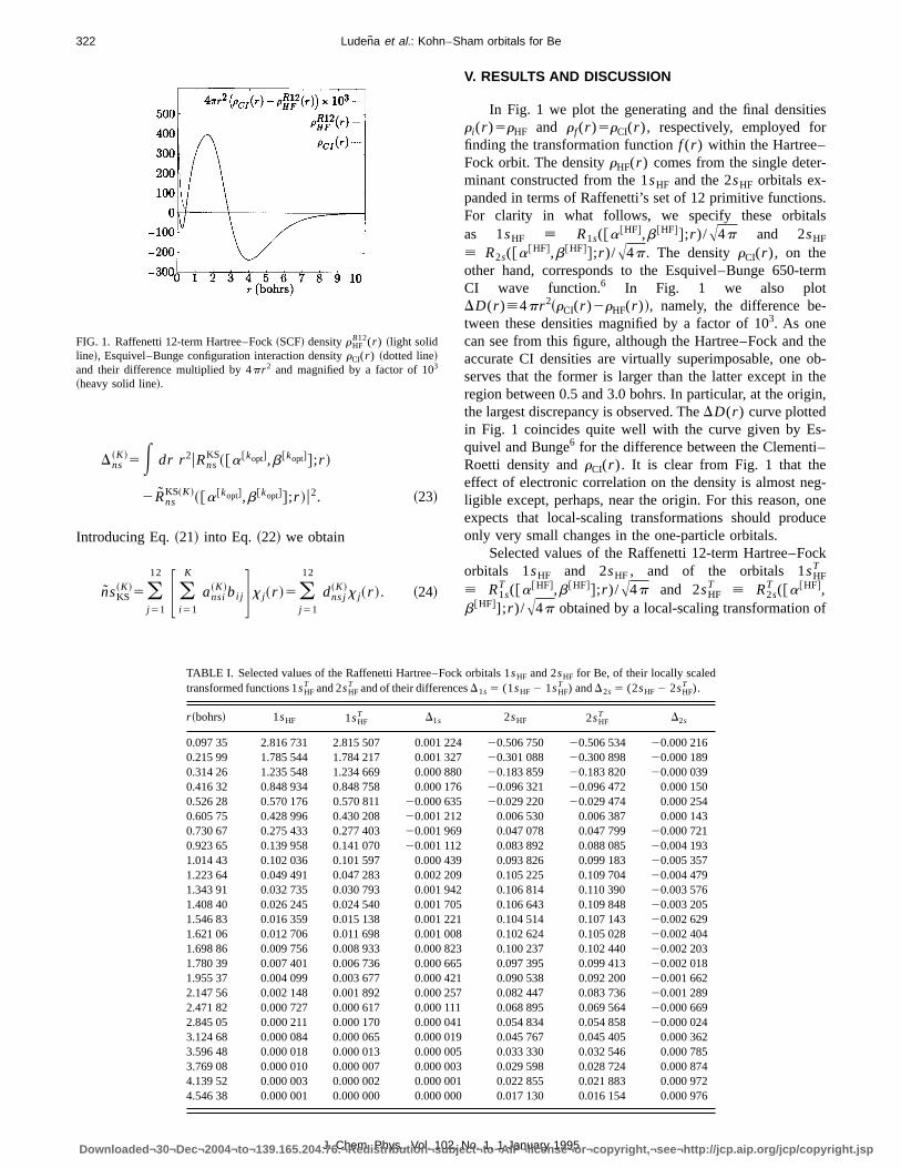
FIG. 1. Raffenetti 12-term Hartree–Fock~SCF! densityrHFB12(r ) ~light solid

line!, Esquivel–Bunge configuration interaction densityrCI(r ) ~dotted line!and their difference multiplied by 4pr 2 and magnified by a factor of 103

~heavy solid line!.

J. Chem. Phys., Vol. 10Downloaded¬30¬Dec¬2004¬to¬139.165.204.76.¬Redistribution¬subje

V. RESULTS AND DISCUSSION

In Fig. 1 we plot the generating and the final densitieri(r )5rHF and rf(r )5rCI(r ), respectively, employed forfinding the transformation functionf (r ) within the Hartree–Fock orbit. The densityrHF(r ) comes from the single deter-minant constructed from the 1sHF and the 2sHF orbitals ex-panded in terms of Raffenetti’s set of 12 primitive functionsFor clarity in what follows, we specify these orbitalsas 1sHF [ R1s(@a@HF#,b@HF##;r )/A4p and 2sHF[ R2s(@a@HF#,b@HF##;r )/A4p. The densityrCI(r ), on theother hand, corresponds to the Esquivel–Bunge 650-terCI wave function.6 In Fig. 1 we also plotDD(r )[4pr 2~rCI(r )2rHF(r )!, namely, the difference be-tween these densities magnified by a factor of 103. As onecan see from this figure, although the Hartree–Fock and thaccurate CI densities are virtually superimposable, one oserves that the former is larger than the latter except in thregion between 0.5 and 3.0 bohrs. In particular, at the originthe largest discrepancy is observed. TheDD(r ) curve plottedin Fig. 1 coincides quite well with the curve given by Es-quivel and Bunge6 for the difference between the Clementi–Roetti density andrCI(r ). It is clear from Fig. 1 that theeffect of electronic correlation on the density is almost negligible except, perhaps, near the origin. For this reason, onexpects that local-scaling transformations should produconly very small changes in the one-particle orbitals.

Selected values of the Raffenetti 12-term Hartree–Focorbitals 1sHF and 2sHF, and of the orbitals 1sHF

T

[ R1sT (@a@HF#,b@HF##;r )/A4p and 2sHF

T [ R2sT (@a@HF#,

b@HF#]; r )/A4p obtained by a local-scaling transformation of

TABLE I. Selected values of the Raffenetti Hartree–Fock orbitals 1sHF and 2sHF for Be, of their locally scaledtransformed functions 1sHF

T and 2sHFT and of their differencesD1s 5 (1sHF2 1sHF

T ) andD2s 5 (2sHF2 2sHFT ).

r ~bohrs! 1sHF 1sHFT D1s 2sHF 2sHF

T D2s

0.097 35 2.816 731 2.815 507 0.001 224 20.506 750 20.506 534 20.000 2160.215 99 1.785 544 1.784 217 0.001 327 20.301 088 20.300 898 20.000 1890.314 26 1.235 548 1.234 669 0.000 880 20.183 859 20.183 820 20.000 0390.416 32 0.848 934 0.848 758 0.000 176 20.096 321 20.096 472 0.000 1500.526 28 0.570 176 0.570 811 20.000 635 20.029 220 20.029 474 0.000 2540.605 75 0.428 996 0.430 208 20.001 212 0.006 530 0.006 387 0.000 1430.730 67 0.275 433 0.277 403 20.001 969 0.047 078 0.047 799 20.000 7210.923 65 0.139 958 0.141 070 20.001 112 0.083 892 0.088 085 20.004 1931.014 43 0.102 036 0.101 597 0.000 439 0.093 826 0.099 18320.005 3571.223 64 0.049 491 0.047 283 0.002 209 0.105 225 0.109 70420.004 4791.343 91 0.032 735 0.030 793 0.001 942 0.106 814 0.110 39020.003 5761.408 40 0.026 245 0.024 540 0.001 705 0.106 643 0.109 84820.003 2051.546 83 0.016 359 0.015 138 0.001 221 0.104 514 0.107 14320.002 6291.621 06 0.012 706 0.011 698 0.001 008 0.102 624 0.105 02820.002 4041.698 86 0.009 756 0.008 933 0.000 823 0.100 237 0.102 44020.002 2031.780 39 0.007 401 0.006 736 0.000 665 0.097 395 0.099 41320.002 0181.955 37 0.004 099 0.003 677 0.000 421 0.090 538 0.092 20020.001 6622.147 56 0.002 148 0.001 892 0.000 257 0.082 447 0.083 73620.001 2892.471 82 0.000 727 0.000 617 0.000 111 0.068 895 0.069 56420.000 6692.845 05 0.000 211 0.000 170 0.000 041 0.054 834 0.054 85820.000 0243.124 68 0.000 084 0.000 065 0.000 019 0.045 767 0.045 405 0.000 3623.596 48 0.000 018 0.000 013 0.000 005 0.033 330 0.032 546 0.000 7853.769 08 0.000 010 0.000 007 0.000 003 0.029 598 0.028 724 0.000 8744.139 52 0.000 003 0.000 002 0.000 001 0.022 855 0.021 883 0.000 9724.546 38 0.000 001 0.000 000 0.000 000 0.017 130 0.016 154 0.000 976

2, No. 1, 1 January 1995ct¬to¬AIP¬license¬or¬copyright,¬see¬http://jcp.aip.org/jcp/copyright.jsp

q.


the former according to Eq.~7!, are given in Table I. Forcompleteness, we have also listed values of the differenbetween the Hartree–Fock and the transformed orbitnamely,D1s[1sHF21sHF

T andD2s[ 2sHF2 2sHFT . The rather

small values of these differences are in line with our expetation based on the similarity betweenrHF(r ) andrCI(r ).

The kinetic energy functional T[F]5^FuTuF&evaluated whenF is the single Slater determinanFrCI

T@HF#(@a@HF#,b@HF##) ~constructed from the transformed—

numerical—Raffenetti 12-term Hartree–Fock orbitals!, has avalue of 14.596 94 hartrees fora@HF#50.582 434 andb@HF#51.318 837. Clearly, this number does not correspoto the one-determinantal kinetic-energy minimumTs@r0# ofEq. ~9! which is quite accurately described by its uppbound value of 14.593 13 hartrees.24 The reason for thisdifference stems from the fact that althougFrCI

T@HF#(@a@HF#,b@HF##) is exactly associated with the

Esquivel–Bunge one-particle density, it does not belongthe optimal orbitO @kopt#,S N . A fairly close approximationto this optimal orbit is reached by varying the orbital parametersa[k] andb[k] appearing in the Raffenetti primitive basiset. The optimal parameters determined in the present warea@kopt# 5 0.582 472 andb@kopt# 5 1.309 112;they yielda kinetic energy value of 14.593 18 hartrees.

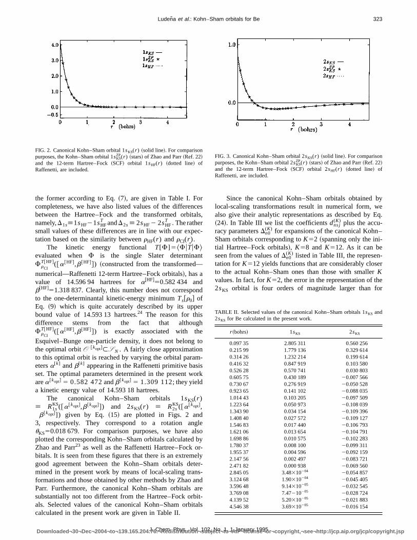
The canonical Kohn–Sham orbitals 1sKS(r )[ R1s

KS(@a@kopt#,b@kopt##) and 2sKS(r ) [ R2sKS(@a@kopt#,

b@kopt#]) given by Eq. ~15! are plotted in Figs. 2 and3, respectively. They correspond to a rotation anguKS50.018 679. For comparison purposes, we have aplotted the corresponding Kohn–Sham orbitals calculatedZhao and Parr23 as well as the Raffenetti Hartree–Fock obitals. It is seen from these figures that there is an extremgood agreement between the Kohn–Sham orbitals demined in the present work by means of local-scaling tranformations and those obtained by other methods by ZhaoParr. Furthermore, the canonical Kohn–Sham orbitalssubstantially not too different from the Hartree–Fock orbals. Selected values of the canonical Kohn–Sham orbicalculated in the present work are given in Table II.

FIG. 2. Canonical Kohn–Sham orbital 1sKS(r ) ~solid line!. For comparisonpurposes, the Kohn–Sham orbital 1sKS

ZP(r ) ~stars! of Zhao and Parr~Ref. 22!and the 12-term Hartree–Fock~SCF! orbital 1sHF(r ) ~dotted line! ofRaffenetti, are included.

J. Chem. Phys., Vol. 102Downloaded¬30¬Dec¬2004¬to¬139.165.204.76.¬Redistribution¬subje

cesals,

c-

t

nd

er

h

to

-sork

lelsobyr-elyter-s-andareit-tals

Since the canonical Kohn–Sham orbitals obtained bylocal-scaling transformations result in numerical form, wealso give their analytic representations as described by E~24!. In Table III we list the coefficientsdns j

(K) plus the accu-racy parametersDn0

(K) for expansions of the canonical Kohn–Sham orbitals corresponding toK52 ~spanning only the ini-tial Hartree–Fock orbitals!, K58 andK512. As it can beseen from the values ofDn0

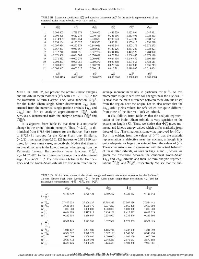
(K) listed in Table III, the represen-tation forK512 yields functions that are considerably closerto the actual Kohn–Sham ones than those with smallerKvalues. In fact, forK52, the error in the representation of the2sKS orbital is four orders of magnitude larger than for

FIG. 3. Canonical Kohn–Sham orbital 2sKS(r ) ~solid line!. For comparisonpurposes, the Kohn–Sham orbital 2sKS

ZP(r ) ~stars! of Zhao and Parr~Ref. 22!and the 12-term Hartree–Fock~SCF! orbital 2sHF(r ) ~dotted line! ofRaffenetti, are included.

TABLE II. Selected values of the canonical Kohn–Sham orbitals 1sKS and2sKS for Be calculated in the present work.

r ~bohrs! 1sKS 2sKS

0.097 35 2.805 311 0.560 2560.215 99 1.779 136 0.329 6140.314 26 1.232 214 0.199 6140.416 32 0.847 919 0.103 5800.526 28 0.570 741 0.030 8030.605 75 0.430 189 20.007 5660.730 67 0.276 919 20.050 5280.923 65 0.141 102 20.088 0351.014 43 0.103 205 20.097 5091.223 64 0.050 973 20.108 0391.343 90 0.034 154 20.109 3961.408 40 0.027 572 20.109 1271.546 83 0.017 440 20.106 7931.621 06 0.013 654 20.104 7911.698 86 0.010 575 20.102 2831.780 37 0.008 100 20.099 3111.955 37 0.004 596 20.092 1592.147 56 0.002 497 20.083 7212.471 82 0.000 938 20.069 5602.845 05 3.48310204 20.054 8573.124 68 1.90310204 20.045 4053.596 48 9.14310205 20.032 5453.769 08 7.47210205 20.028 7244.139 52 5.20310205 20.021 8834.546 38 3.69310205 20.016 154

, No. 1, 1 January 1995ct¬to¬AIP¬license¬or¬copyright,¬see¬http://jcp.aip.org/jcp/copyright.jsp


TABLE III. Expansion coefficientsdn0 j(K) and accuracy parametersDn0

(K) for the analytic representations of thecanonical Kohn–Sham orbitals, forK52, 8, and 12.

j d10j(2) d20j

(2) d10j(8) d20j

(8) d10j(12) d20j

(12)

1 0.008 803 1.789 878 0.009 902 1.442 539 0.032 004 1.047 4912 0.000 895 20.612 210 20.010 718 20.245 506 20.183 496 1.728 8333 20.014 939 0.030 154 20.030 689 0.783 073 0.573 399 23.834 7224 0.039 164 20.198 627 0.109 350 1.858 201 21.155 415 4.753 2285 20.097 984 20.260 879 20.148 021 0.906 244 1.603 178 25.371 2736 0.567 837 20.043 667 0.568 629 20.149 226 21.057 249 3.723 8217 0.512 740 0.011 531 0.522 772 20.294 466 1.443 925 21.484 9708 20.071 968 20.034 505 20.076 099 0.073 704 20.230 465 20.279 1909 0.071 882 20.002 270 0.069 987 0.024 408 20.146 450 0.699 81010 20.000 253 20.001 051 20.000 272 20.000 418 0.197 553 20.434 51111 20.000 893 0.000 508 20.000 731 20.025 546 20.072 832 0.136 71312 20.000 347 0.000 017 0.000 117 0.010 761 0.010 00520.019 034

D10~2! D20

~2! D10~8! D20

~8! D10~12! D20

~12!

0.000 0195 0.001 2088 0.000 0009 0.000 0165 0.000 0002 0.000 0008

e

la

t

s, itisesthe

n-he

m

it is

viorweamn-a-

K512. In Table IV, we present the orbital kinetic energieand the orbital mean moments^r k& with k522,21,0,1,2 forthe Raffenetti 12-term Hartree–Fock wave function,FHF

R12,for the Kohn–Sham single Slater determinantFKS ~con-structed from the numerical single-particle orbitals 1sKS and2sKS! and for its analytic approximationsFKS

(K) , withK52,8,12,~constructed from the analytic orbitals 1sKS

(K) and2sKS

(K)!.It is apparent from Table IV that there is a noticeabl

change in the orbital kinetic energies. Thus,^2D/2&1s is di-minished from 6.785 410 hartrees for the Hartree–Fock cato 6.725 431 hartrees for the Kohn–Sham one. Similar^2D/2&2s increases from 0.501 125 hartrees to 0.571 160 htrees, for these same cases, respectively. Notice that theran overall increase in the kinetic energy when going from thRaffenetti 12-term Hartree–Fock wave function,FHF

R12,Ts514.573 070 to the Kohn–Sham single Slater determinaFKS, Ts514.593 182. The differences between the HartreeFock and the Kohn–Sham orbitals are also manifested in

J. Chem. Phys., Vol. 102,Downloaded¬30¬Dec¬2004¬to¬139.165.204.76.¬Redistribution¬subject

s

sey,r-e ise

nt–he

average momentum values, in particular for^r22&. As thismomentum is quite sensitive for changes near the nucleuis clear that the main difference between these orbitals arfrom the region near the origin. Let us also notice that2sKS orbit yields values for r 2& which are quite differentfrom those of the Hartree–Fock 2s orbital.

It also follows from Table IV that the analytic represetation of the Kohn–Sham orbitals is very sensitive to texpansion length (K). Thus, we notice thatFKS

~2! gives mo-menta and kinetic energy values which differ markedly frothose ofFKS. The situation is somewhat improved forFKS

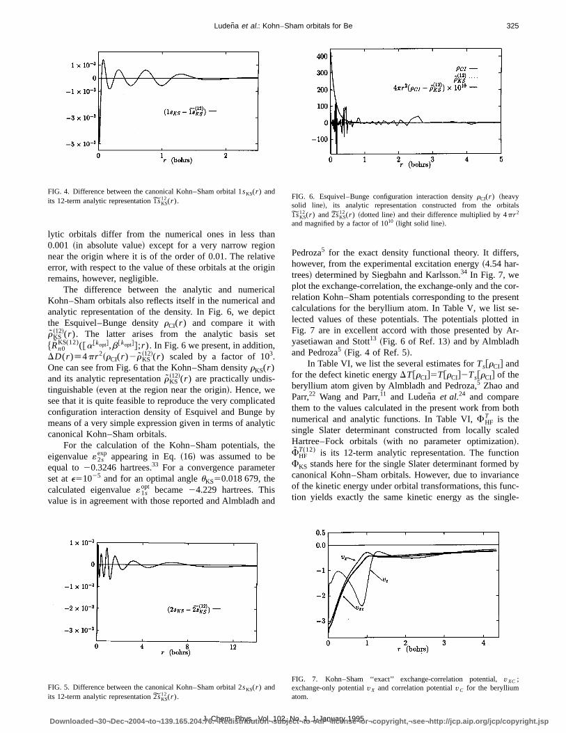
~12! .But it is evident from the values ofr22& that the analyticrepresentation is defective near the nucleus, althoughquite adequate for larger , as evinced from the values of^r 2&.These conclusions are in agreement with the actual behaof these fitted orbitals, as seen in Figs. 4 and 5, wheregraph the difference between the canonical Kohn–Sh1sKS and 2sKS orbitals and their 12-term analytic represetations 1sKS

(12) and 2sKS(12) , respectively. We see that the an

TABLE IV. Orbital mean values of the kinetic energy and several momentum operators for the Raffenetti12-term Hartree–Fock wave functionFHF

R12, for the Kohn–Sham single-Slater determinantFKS and forits analytic representationsFKS

~2! , FKS~8! , and FKS

~12! .

FHFR12 FKS FKS

~2! FKS~8! FKS

~12!

K2D

2 L1s

6.785 410 6.725 431 6.769 302 6.726 062 6.726 342

^r22&1s 27.407 633 27.209 127 27.704 323 27.567 086 27.584 442^r21&1s 3.681 884 3.665 175 3.677 299 3.665 339 3.665 398^r 0&1s 1.000 000 1.000 000 1.000 000 1.000 000 1.000 000^r 1&1s 0.414 993 0.417 819 0.416 101 0.417 822 0.417 819^r 2&1s 0.232 954 0.236 867 0.234 900 0.236 870 0.236 866

K2D

2 L2s

0.501 125 0.571 160 0.517 537 0.570 853 0.571 025

^r22&2s 1.044 147 1.231 980 1.105 714 1.237 030 1.241 890^r21&2s 0.522 522 0.548 323 0.527 193 0.548 242 0.548 290^r 0&2s 1.000 000 1.000 000 1.000 000 1.000 000 1.000 000^r 1&2s 2.649 412 2.570 101 2.648 283 2.570 583 2.570 103^r 2&2s 8.426 426 7.900 428 8.424 439 7.909 390 7.900 581

No. 1, 1 January 1995¬to¬AIP¬license¬or¬copyright,¬see¬http://jcp.aip.org/jcp/copyright.jsp

vg

ni

e,

tb

h

r-t


lytic orbitals differ from the numerical ones in less tha0.001 ~in absolute value! except for a very narrow regionnear the origin where it is of the order of 0.01. The relatierror, with respect to the value of these orbitals at the oriremains, however, negligible.

The difference between the analytic and numericKohn–Sham orbitals also reflects itself in the numerical aanalytic representation of the density. In Fig. 6, we depthe Esquivel–Bunge densityrCI(r ) and compare it withrKS

~12!(r ). The latter arises from the analytic basis s$Rn0

KS(12)(@a@kopt#,b@kopt##;r ). In Fig. 6 we present, in additionDD(r )[4pr 2~rCI(r )2rKS

~12!(r ) scaled by a factor of 103.One can see from Fig. 6 that the Kohn–Sham densityrKS(r )and its analytic representationrKS

~12!(r ) are practically undis-tinguishable~even at the region near the origin!. Hence, wesee that it is quite feasible to reproduce the very complicaconfiguration interaction density of Esquivel and Bungemeans of a very simple expression given in terms of analycanonical Kohn–Sham orbitals.

For the calculation of the Kohn–Sham potentials, teigenvalue«2s

exp appearing in Eq.~16! was assumed to beequal to20.3246 hartrees.33 For a convergence parameteset ate51025 and for an optimal angleuKS50.018 679, thecalculated eigenvalue«1s

opt became24.229 hartrees. Thisvalue is in agreement with those reported and Almbladh a

FIG. 5. Difference between the canonical Kohn–Sham orbital 2sKS(r ) andits 12-term analytic representation 2sKS

12(r ).

FIG. 4. Difference between the canonical Kohn–Sham orbital 1sKS(r ) andits 12-term analytic representation 1sKS

12(r ).


n

ein

aldct

t

edytic

e

r

nd

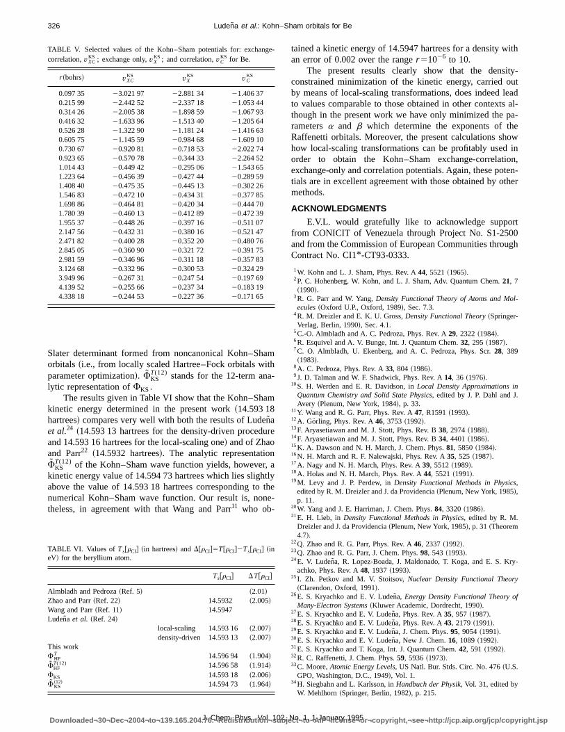
Pedroza5 for the exact density functional theory. It differs,however, from the experimental excitation energy~4.54 har-trees! determined by Siegbahn and Karlsson.34 In Fig. 7, weplot the exchange-correlation, the exchange-only and the corelation Kohn–Sham potentials corresponding to the presencalculations for the beryllium atom. In Table V, we list se-lected values of these potentials. The potentials plotted inFig. 7 are in excellent accord with those presented by Ar-yasetiawan and Stott13 ~Fig. 6 of Ref. 13! and by Almbladhand Pedroza5 ~Fig. 4 of Ref. 5!.

In Table VI, we list the several estimates forTs@rCI# andfor the defect kinetic energyDT@rCI#5T@rCI#2Ts@rCI# of theberyllium atom given by Almbladh and Pedroza,5 Zhao andParr,22 Wang and Parr,11 and Luden˜a et al.24 and comparethem to the values calculated in the present work from bothnumerical and analytic functions. In Table VI,FHF

T is thesingle Slater determinant constructed from locally scaledHartree–Fock orbitals~with no parameter optimization!.FHFT(12) is its 12-term analytic representation. The function

FKS stands here for the single Slater determinant formed bycanonical Kohn–Sham orbitals. However, due to invarianceof the kinetic energy under orbital transformations, this func-tion yields exactly the same kinetic energy as the single-

FIG. 6. Esquivel–Bunge configuration interaction densityrCI(r ) ~heavysolid line!, its analytic representation constructed from the orbitals1sKS

12(r ) and 2sKS12(r ) ~dotted line! and their difference multiplied by 4pr 2

and magnified by a factor of 1010 ~light solid line!.

FIG. 7. Kohn–Sham ‘‘exact’’ exchange-correlation potential,vXC ;exchange-only potentialvX and correlation potentialvC for the berylliumatom.


-

dl--

,-r

h


Slater determinant formed from noncanonical Kohn–Shaorbitals~i.e., from locally scaled Hartree–Fock orbitals withparameter optimization!. FKS

T(12) stands for the 12-term ana-lytic representation ofFKS.

The results given in Table VI show that the Kohn–Shakinetic energy determined in the present work~14.593 18hartrees! compares very well with both the results of Ludenãet al.24 ~14.593 13 hartrees for the density-driven proceduand 14.593 16 hartrees for the local-scaling one! and of Zhaoand Parr22 ~14.5932 hartrees!. The analytic representationFKST(12) of the Kohn–Sham wave function yields, however,

kinetic energy value of 14.594 73 hartrees which lies slightabove the value of 14.593 18 hartrees corresponding tonumerical Kohn–Sham wave function. Our result is, nontheless, in agreement with that Wang and Parr11 who ob-

TABLE V. Selected values of the Kohn–Sham potentials for: exchangcorrelation,vXC

KS ; exchange only,vXKS ; and correlation,vC

KS for Be.

r ~bohrs! vXCKS vX

KS vCKS

0.097 35 23.021 97 22.881 34 21.406 370.215 99 22.442 52 22.337 18 21.053 440.314 26 22.005 38 21.898 59 21.067 930.416 32 21.633 96 21.513 40 21.205 640.526 28 21.322 90 21.181 24 21.416 630.605 75 21.145 59 20.984 68 21.609 100.730 67 20.920 81 20.718 53 22.022 740.923 65 20.570 78 20.344 33 22.264 521.014 43 20.449 42 20.295 06 21.543 651.223 64 20.456 39 20.427 44 20.289 591.408 40 20.475 35 20.445 13 20.302 261.546 83 20.472 10 20.434 31 20.377 851.698 86 20.464 81 20.420 34 20.444 701.780 39 20.460 13 20.412 89 20.472 391.955 37 20.448 26 20.397 16 20.511 072.147 56 20.432 31 20.380 16 20.521 472.471 82 20.400 28 20.352 20 20.480 762.845 05 20.360 90 20.321 72 20.391 752.981 59 20.346 96 20.311 18 20.357 833.124 68 20.332 96 20.300 53 20.324 293.949 96 20.267 31 20.247 54 20.197 694.139 52 20.255 66 20.237 34 20.183 194.338 18 20.244 53 20.227 36 20.171 65

TABLE VI. Values of Ts@rCI# ~in hartrees! andD@rCI#5T@rCI#2Ts@rCI# ~ineV! for the beryllium atom.

Ts@rCI# DT@rCI#

Almbladh and Pedroza~Ref. 5! ~2.01!Zhao and Parr~Ref. 22! 14.5932 ~2.005!Wang and Parr~Ref. 11! 14.5947Ludena et al. ~Ref. 24!

local-scaling 14.593 16 ~2.007!density-driven 14.593 13 ~2.007!

This workFHF

T 14.596 94 ~1.904!FHFT(12) 14.596 58 ~1.914!

FKS 14.593 18 ~2.006!FKS

~12! 14.594 73 ~1.964!


m

m

re

alythee-

tained a kinetic energy of 14.5947 hartrees for a density withan error of 0.002 over the ranger51026 to 10.

The present results clearly show that the densityconstrained minimization of the kinetic energy, carried outby means of local-scaling transformations, does indeed leato values comparable to those obtained in other contexts athough in the present work we have only minimized the parametersa and b which determine the exponents of theRaffenetti orbitals. Moreover, the present calculations showhow local-scaling transformations can be profitably used inorder to obtain the Kohn–Sham exchange-correlationexchange-only and correlation potentials. Again, these potentials are in excellent agreement with those obtained by othemethods.

ACKNOWLEDGMENTS

E.V.L. would gratefully like to acknowledge supportfrom CONICIT of Venezuela through Project No. S1-2500and from the Commission of European Communities througContract No. CI1*-CT93-0333.

1W. Kohn and L. J. Sham, Phys. Rev. A44, 5521~1965!.2P. C. Hohenberg, W. Kohn, and L. J. Sham, Adv. Quantum Chem.21, 7~1990!.

3R. G. Parr and W. Yang,Density Functional Theory of Atoms and Mol-ecules~Oxford U.P., Oxford, 1989!, Sec. 7.3.

4R. M. Dreizler and E. K. U. Gross,Density Functional Theory~Springer-Verlag, Berlin, 1990!, Sec. 4.1.

5C.-O. Almbladh and A. C. Pedroza, Phys. Rev. A29, 2322~1984!.6R. Esquivel and A. V. Bunge, Int. J. Quantum Chem.32, 295 ~1987!.7C. O. Almbladh, U. Ekenberg, and A. C. Pedroza, Phys. Scr.28, 389~1983!.

8A. C. Pedroza, Phys. Rev. A33, 804 ~1986!.9J. D. Talman and W. F. Shadwick, Phys. Rev. A14, 36 ~1976!.10S. H. Werden and E. R. Davidson, inLocal Density Approximations inQuantum Chemistry and Solid State Physics, edited by J. P. Dahl and J.Avery ~Plenum, New York, 1984!, p. 33.

11Y. Wang and R. G. Parr, Phys. Rev. A47, R1591~1993!.12A. Gorling, Phys. Rev. A46, 3753~1992!.13F. Aryasetiawan and M. J. Stott, Phys. Rev. B38, 2974~1988!.14F. Aryasetiawan and M. J. Stott, Phys. Rev. B34, 4401~1986!.15K. A. Dawson and N. H. March, J. Chem. Phys.81, 5850~1984!.16N. H. March and R. F. Nalewajski, Phys. Rev. A35, 525 ~1987!.17A. Nagy and N. H. March, Phys. Rev. A39, 5512~1989!.18A. Holas and N. H. March, Phys. Rev. A44, 5521~1991!.19M. Levy and J. P. Perdew, inDensity Functional Methods in Physics,edited by R. M. Dreizler and J. da Providencia~Plenum, New York, 1985!,p. 11.

20W. Yang and J. E. Harriman, J. Chem. Phys.84, 3320~1986!.21E. H. Lieb, inDensity Functional Methods in Physics, edited by R. M.Dreizler and J. da Providencia~Plenum, New York, 1985!, p. 31~Theorem4.7!.

22Q. Zhao and R. G. Parr, Phys. Rev. A46, 2337~1992!.23Q. Zhao and R. G. Parr, J. Chem. Phys.98, 543 ~1993!.24E. V. Ludena, R. Lopez-Boada, J. Maldonado, T. Koga, and E. S. Kry-achko, Phys. Rev. A48, 1937~1993!.

25I. Zh. Petkov and M. V. Stoitsov,Nuclear Density Functional Theory~Clarendon, Oxford, 1991!.

26E. S. Kryachko and E. V. Ludenã, Energy Density Functional Theory ofMany-Electron Systems~Kluwer Academic, Dordrecht, 1990!.

27E. S. Kryachko and E. V. Ludenã, Phys. Rev. A35, 957 ~1987!.28E. S. Kryachko and E. V. Ludenã, Phys. Rev. A43, 2179~1991!.29E. S. Kryachko and E. V. Ludenã, J. Chem. Phys.95, 9054~1991!.30E. S. Kryachko and E. V. Ludenã, New J. Chem.16, 1089~1992!.31E. S. Kryachko and T. Koga, Int. J. Quantum Chem.42, 591 ~1992!.32R. C. Raffenetti, J. Chem. Phys.59, 5936~1973!.33C. Moore,Atomic Energy Levels, US Natl. Bur. Stds. Circ. No. 476~U.S.GPO, Washington, D.C., 1949!, Vol. 1.

34H. Siegbahn and L. Karlsson, inHandbuch der Physik, Vol. 31, edited byW. Mehlhorn~Springer, Berlin, 1982!, p. 215.

e-


local‐scaling transformations and the direct determination of kohnsham orbitals and potentials for...

Documents